/


Текст
Contents
Strange • Electronic Music: Systems, Techniques, and Controls
Front Matter 1
Foreword 1
Preface 2
1. Preliminary Statements About the Subject Matter
Text
2. Considerations of the Basic Parameters of Sound
Text
3. Electronic Sound Sources and Their Characteristics
Text
4. Basic Signal Processing: Amplifiers and Filters
Text
5. Concepts of Voltage Control
Text
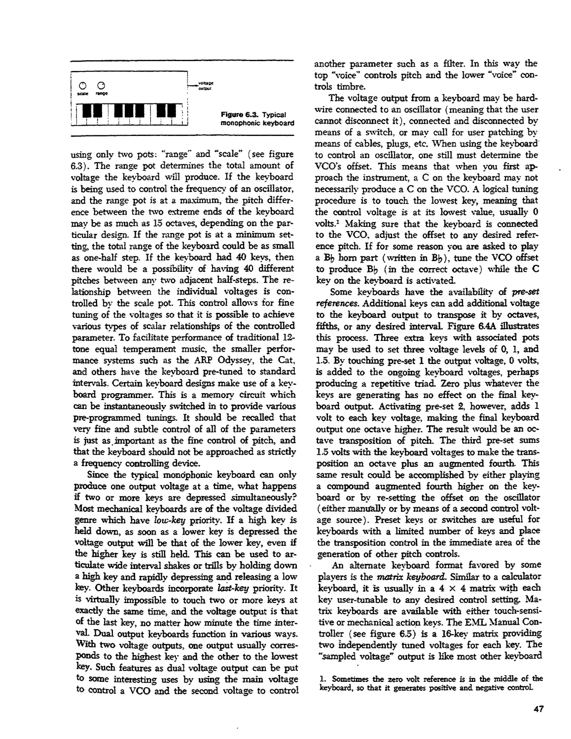
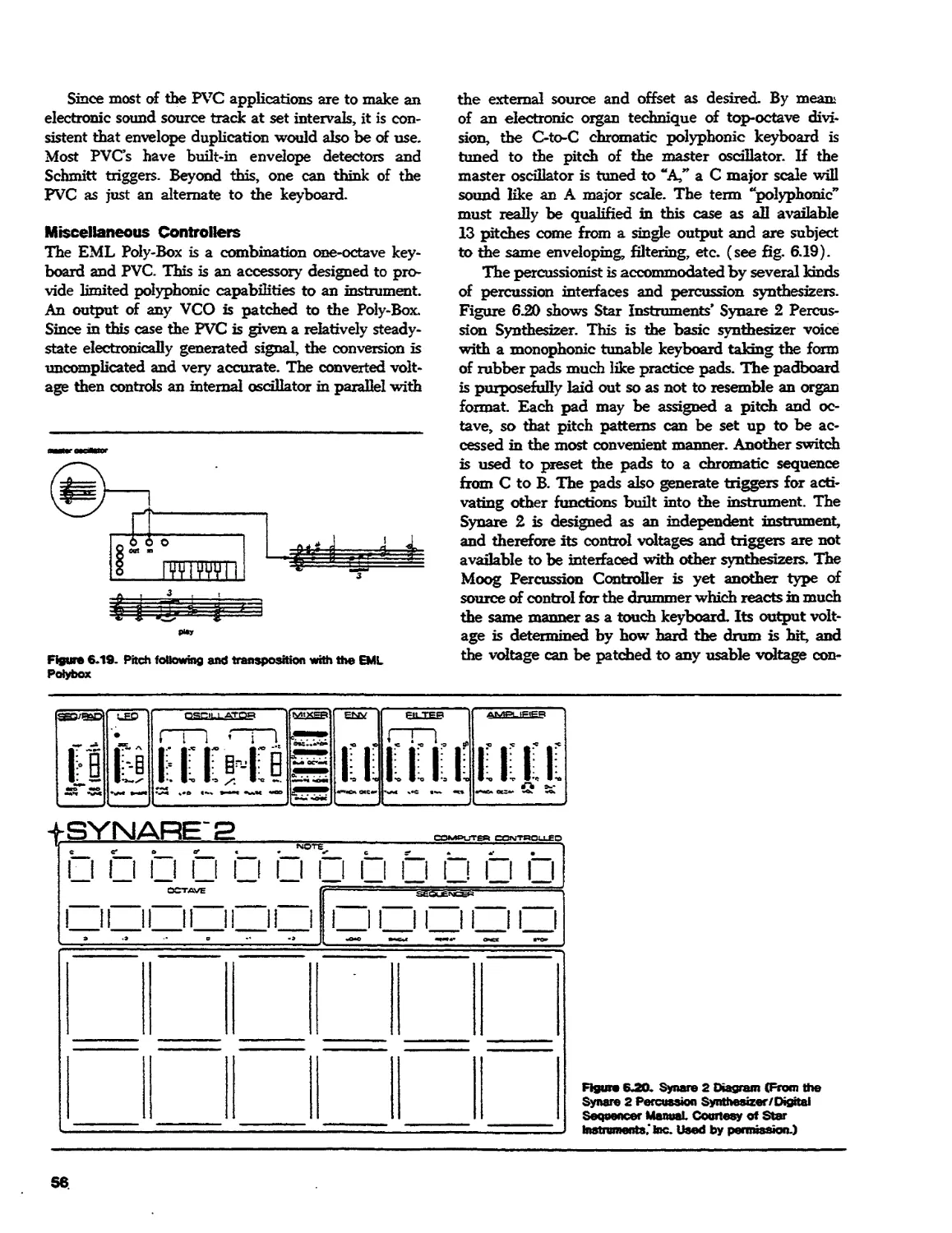
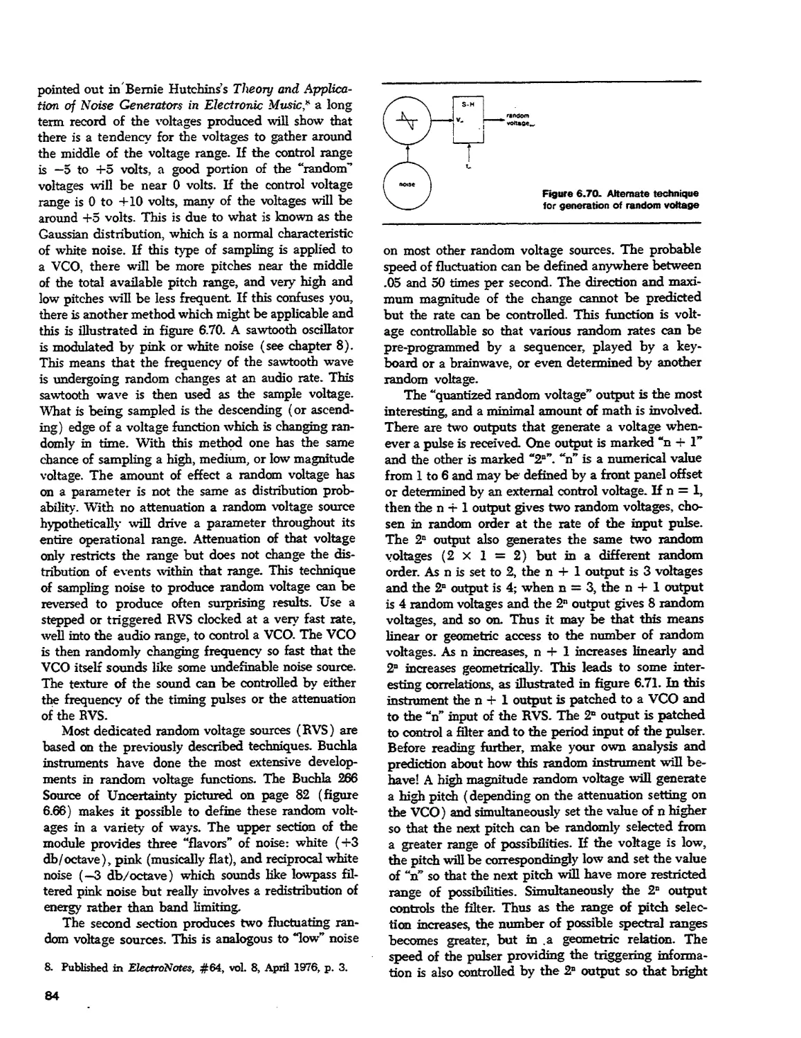
6. Control Voltage Sources
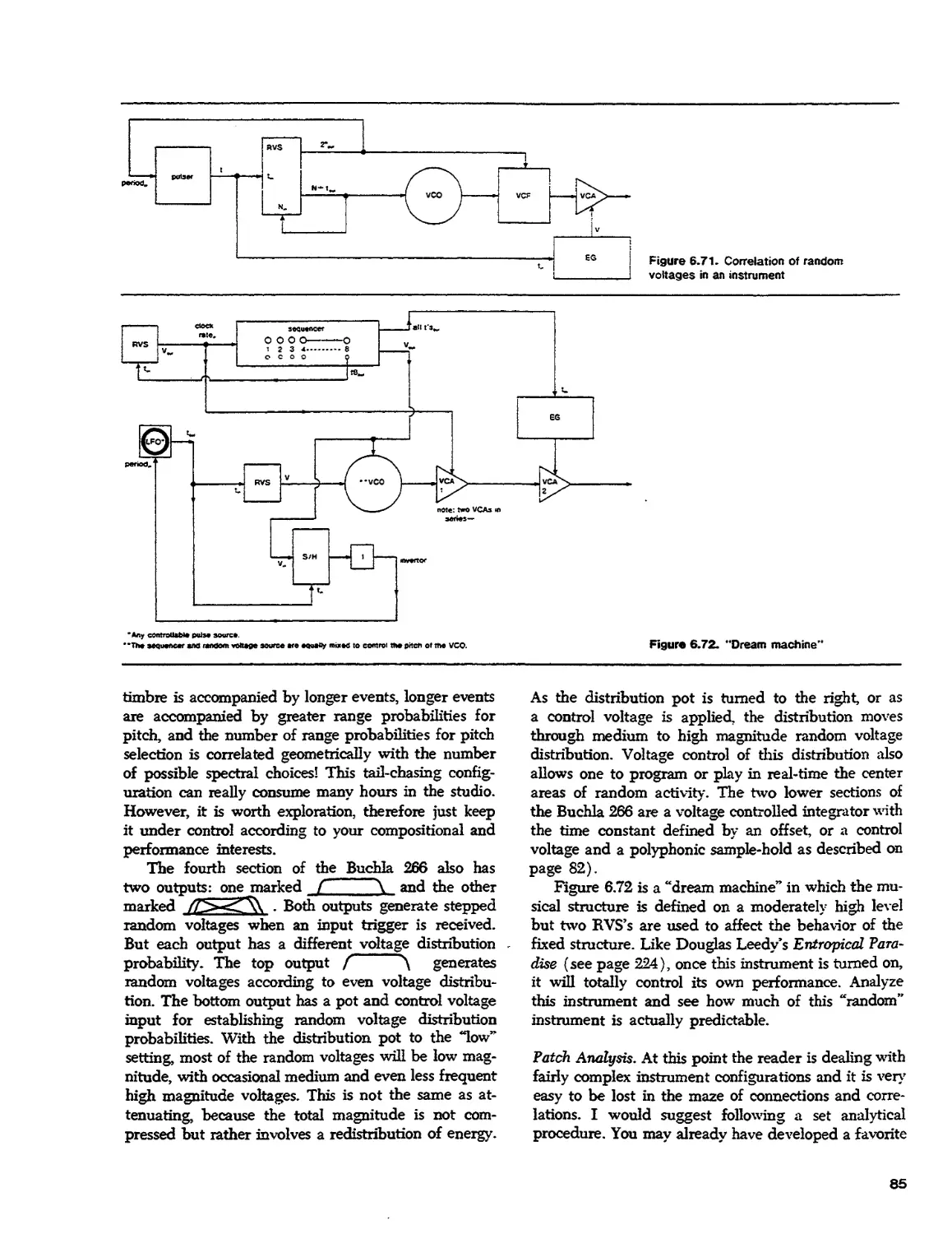
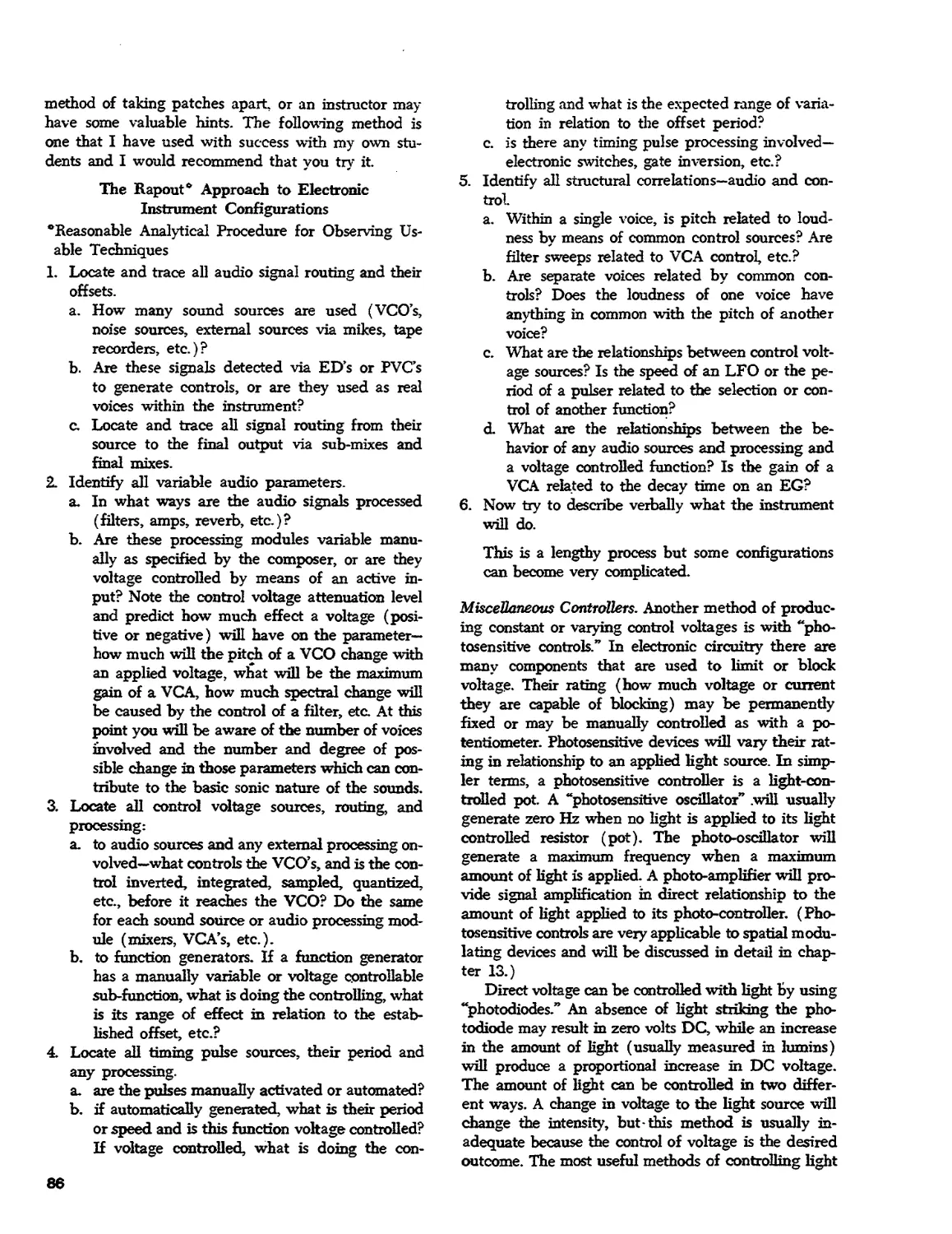
Text
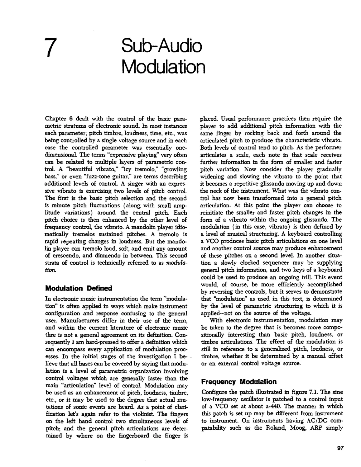
7. Sub-Audio Modulation
Text
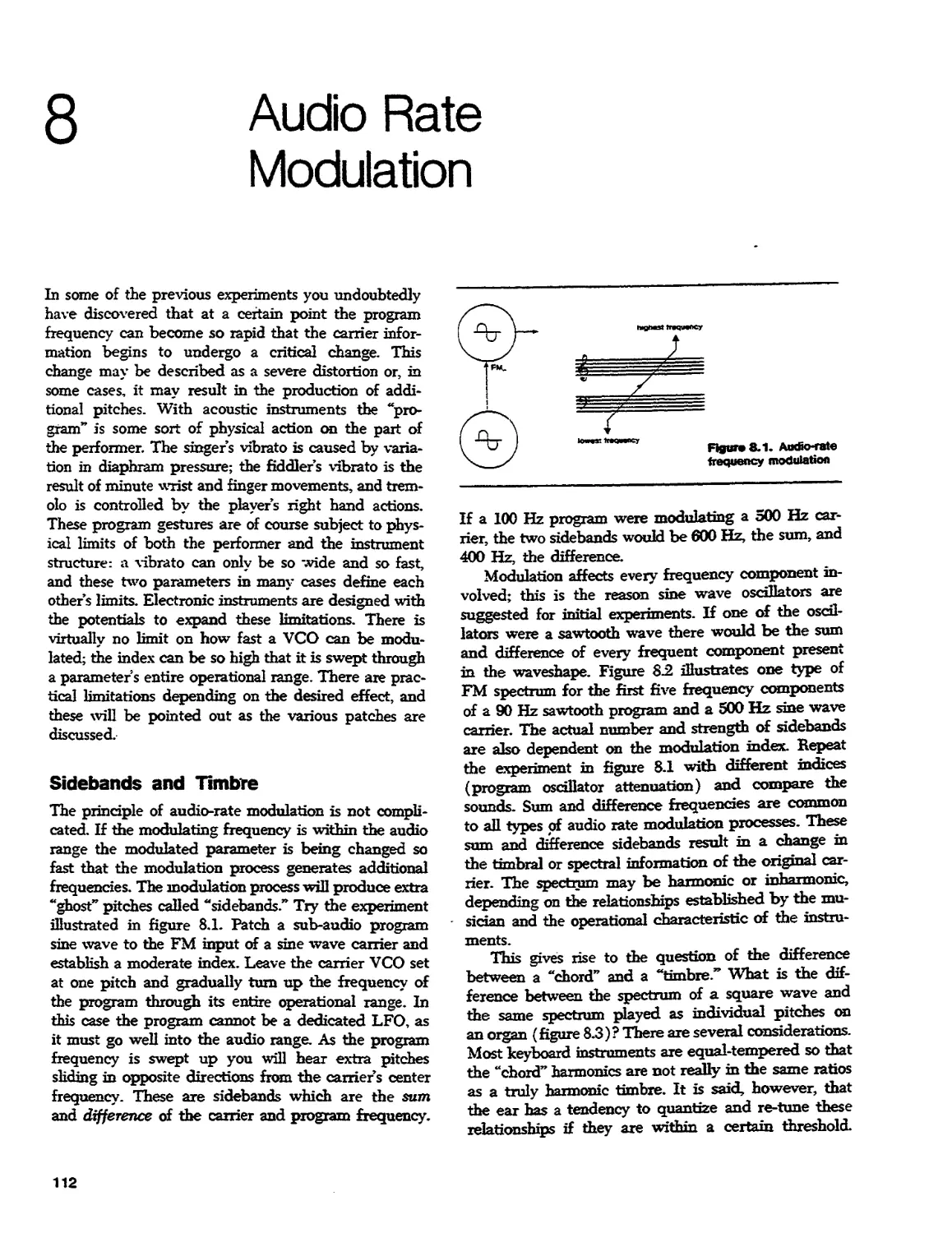
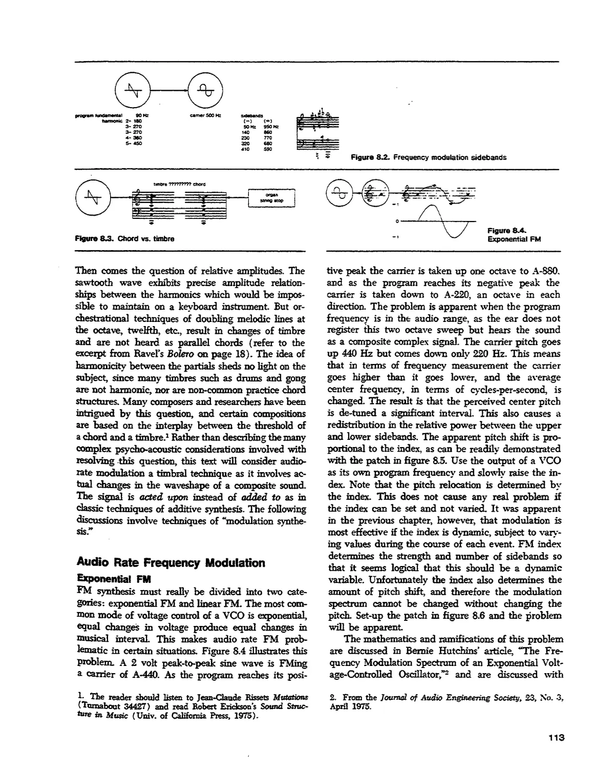
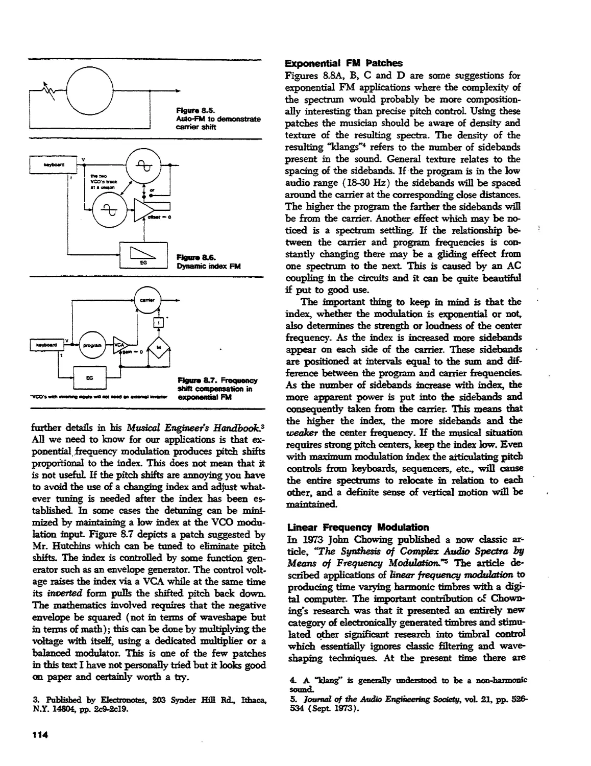
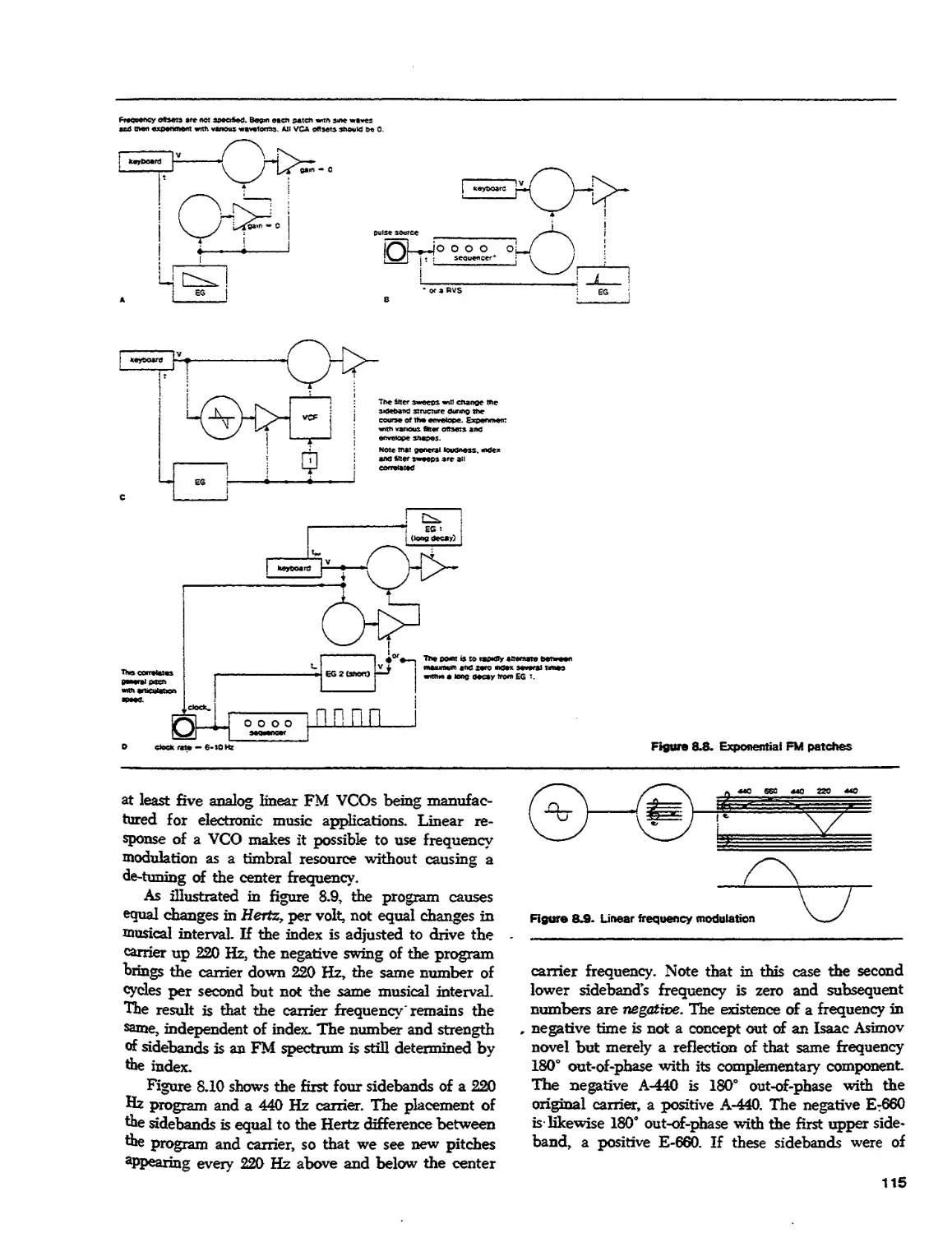
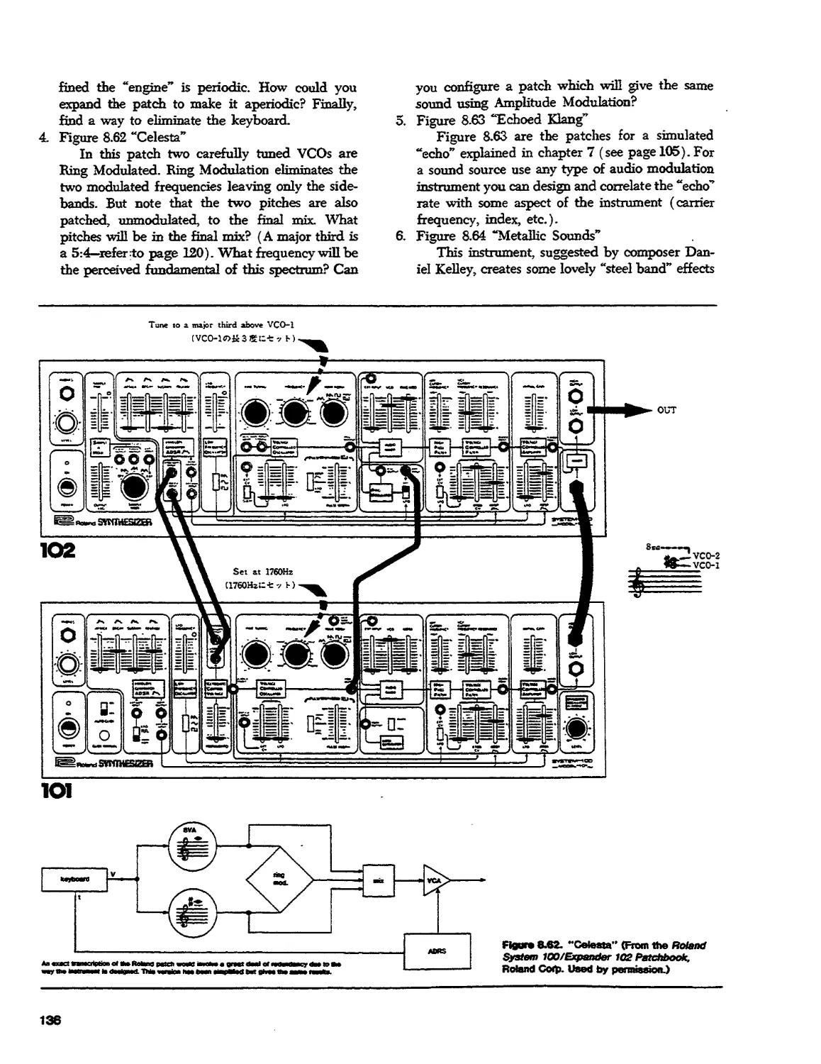
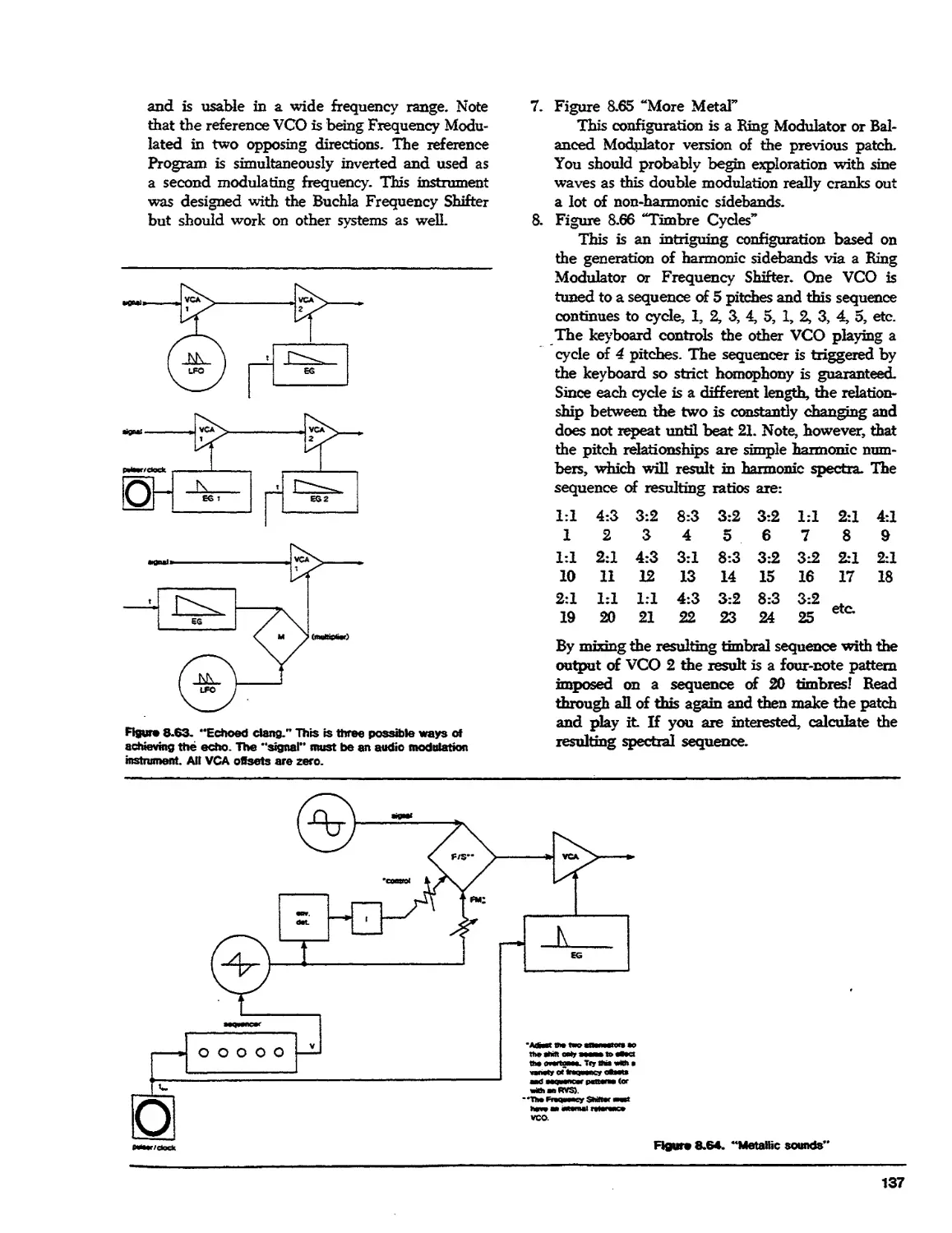
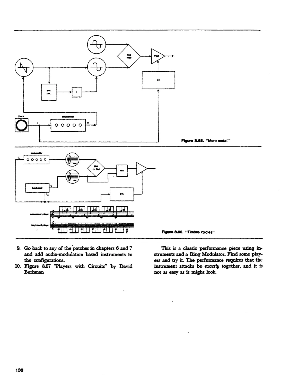
8. Audio Rate Modulation
Text
9. Equalization and Filtering
Text
10. Magnetic Tape Recording
Text
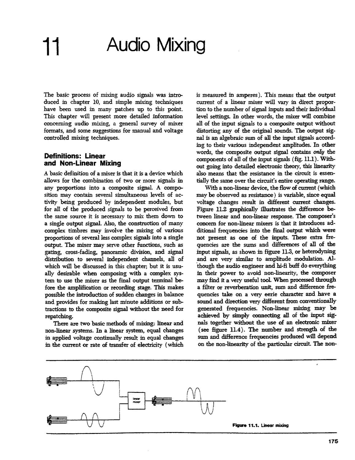
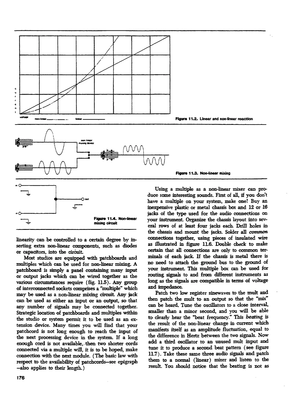
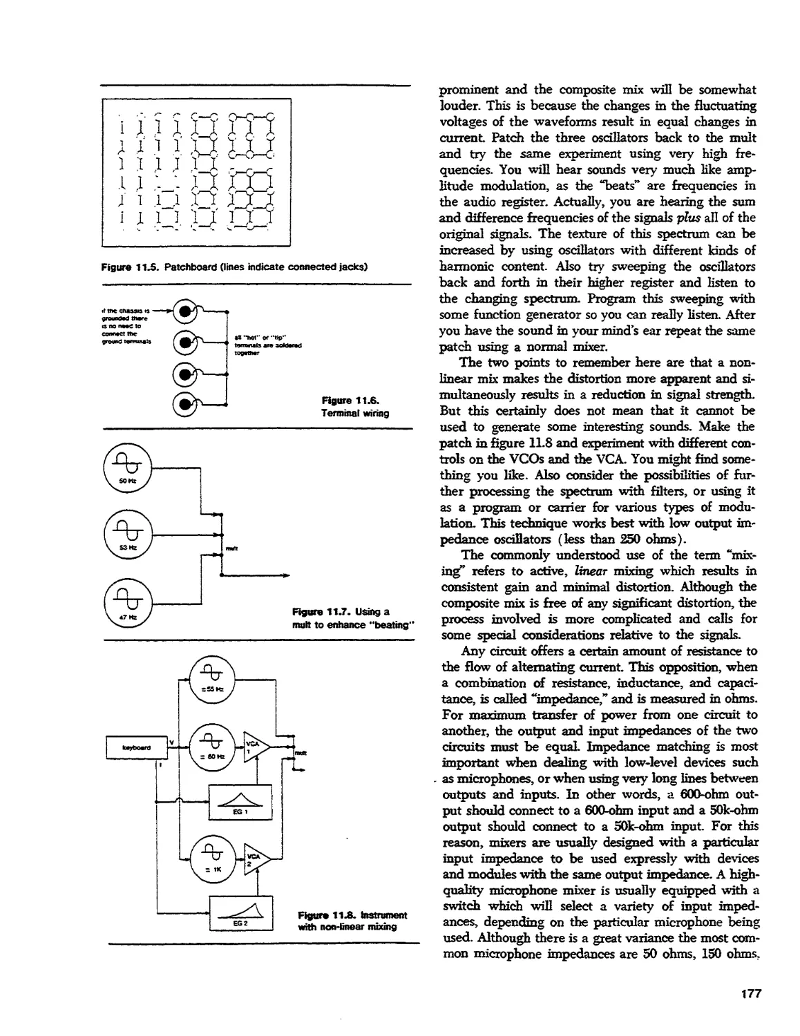
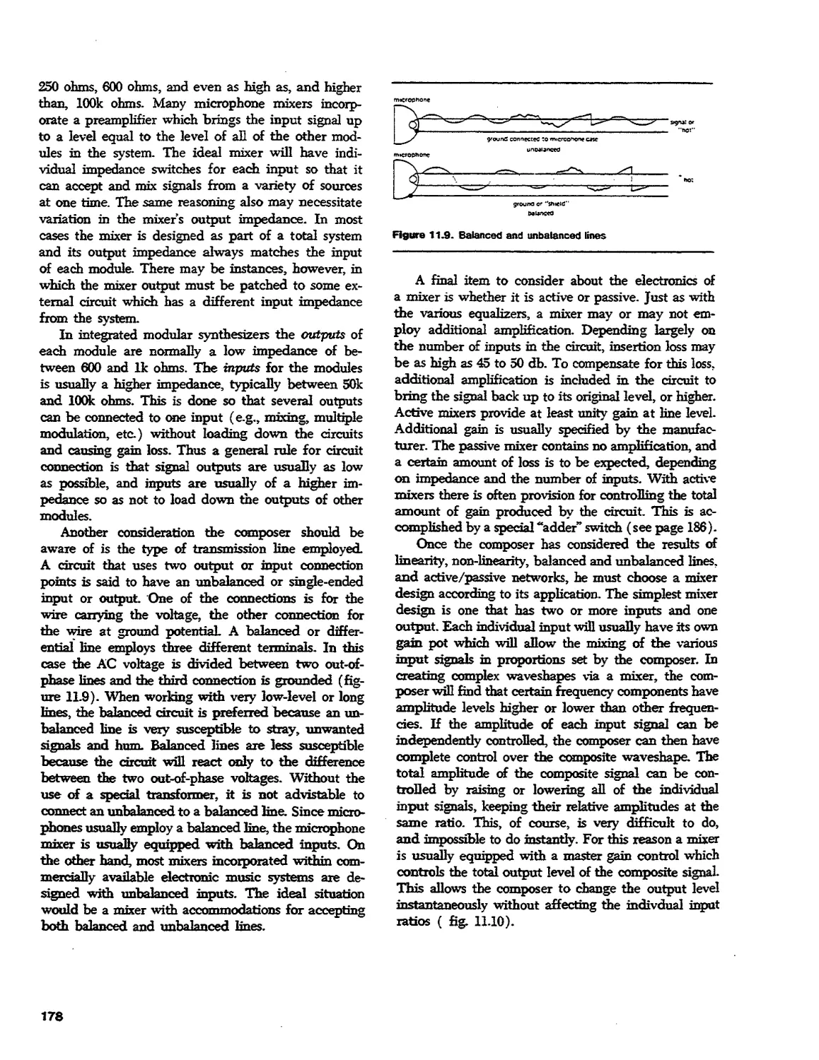
11. Audio Mixing
5
5
11
11
15
15
26
26
36
36
49
49
101
101
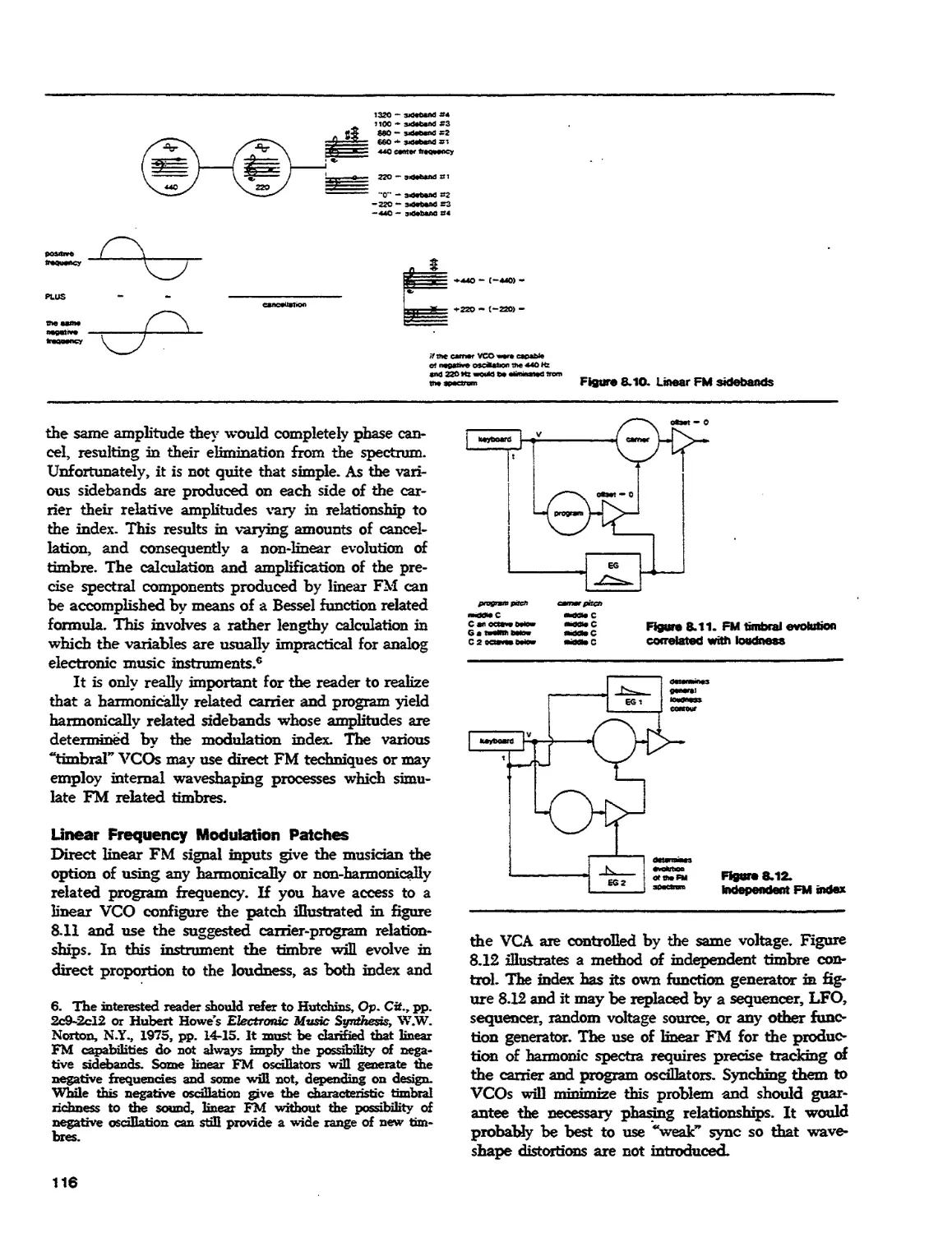
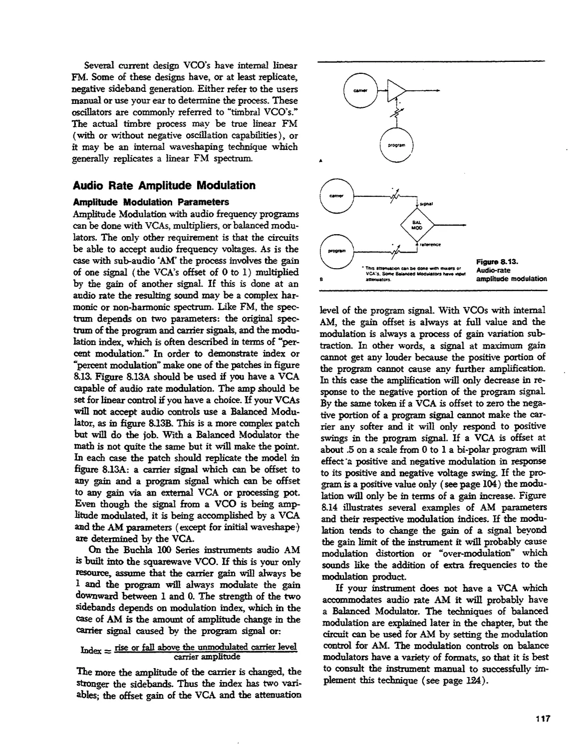
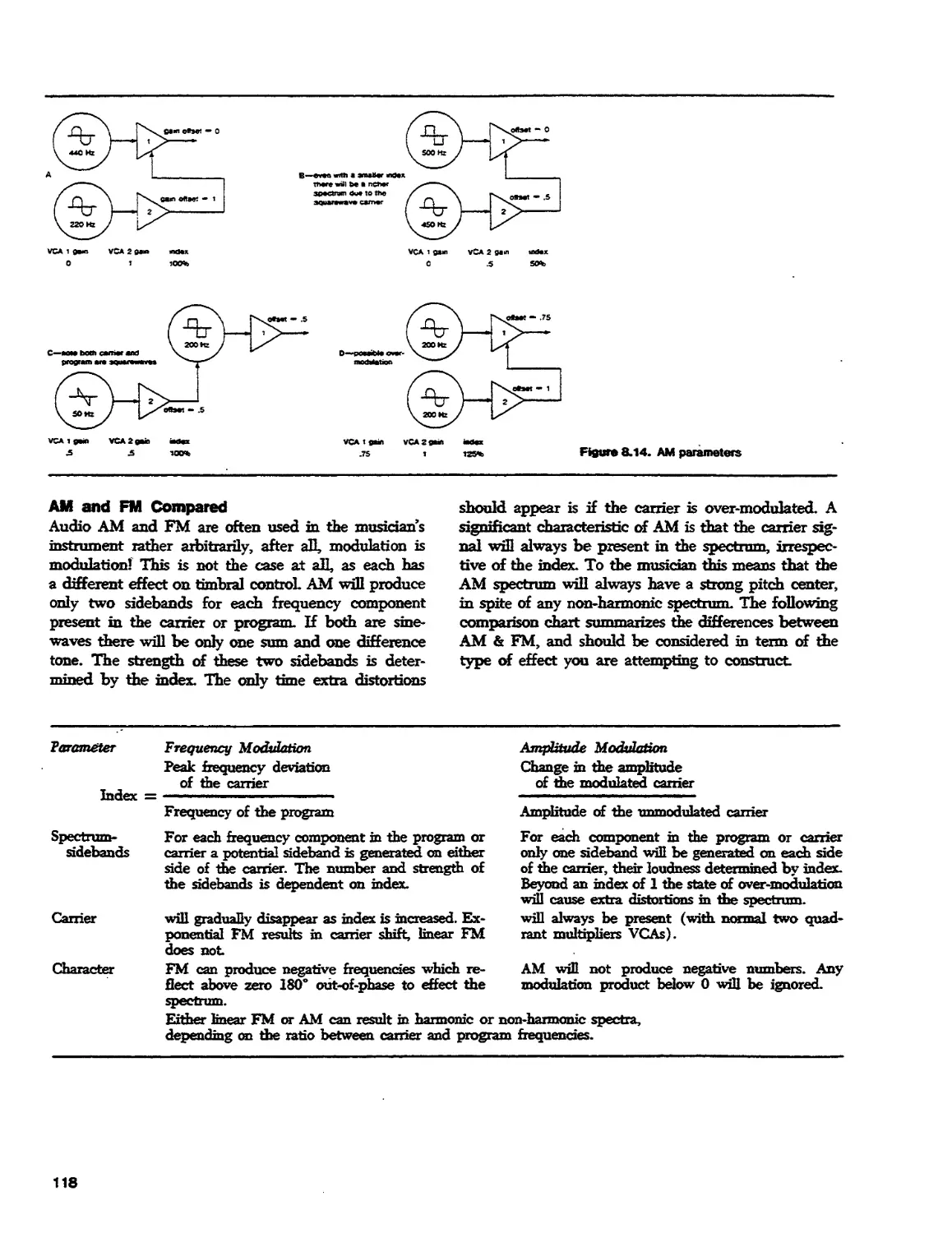
116
116
146
146
168
168
179
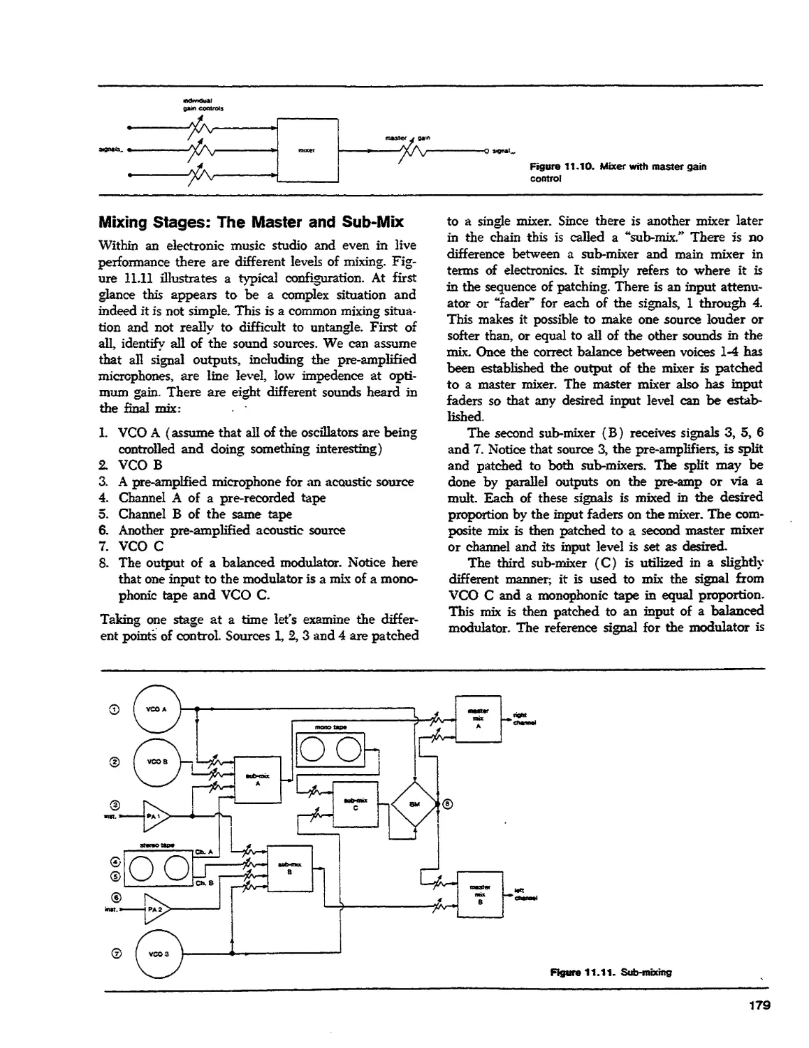
Text 179
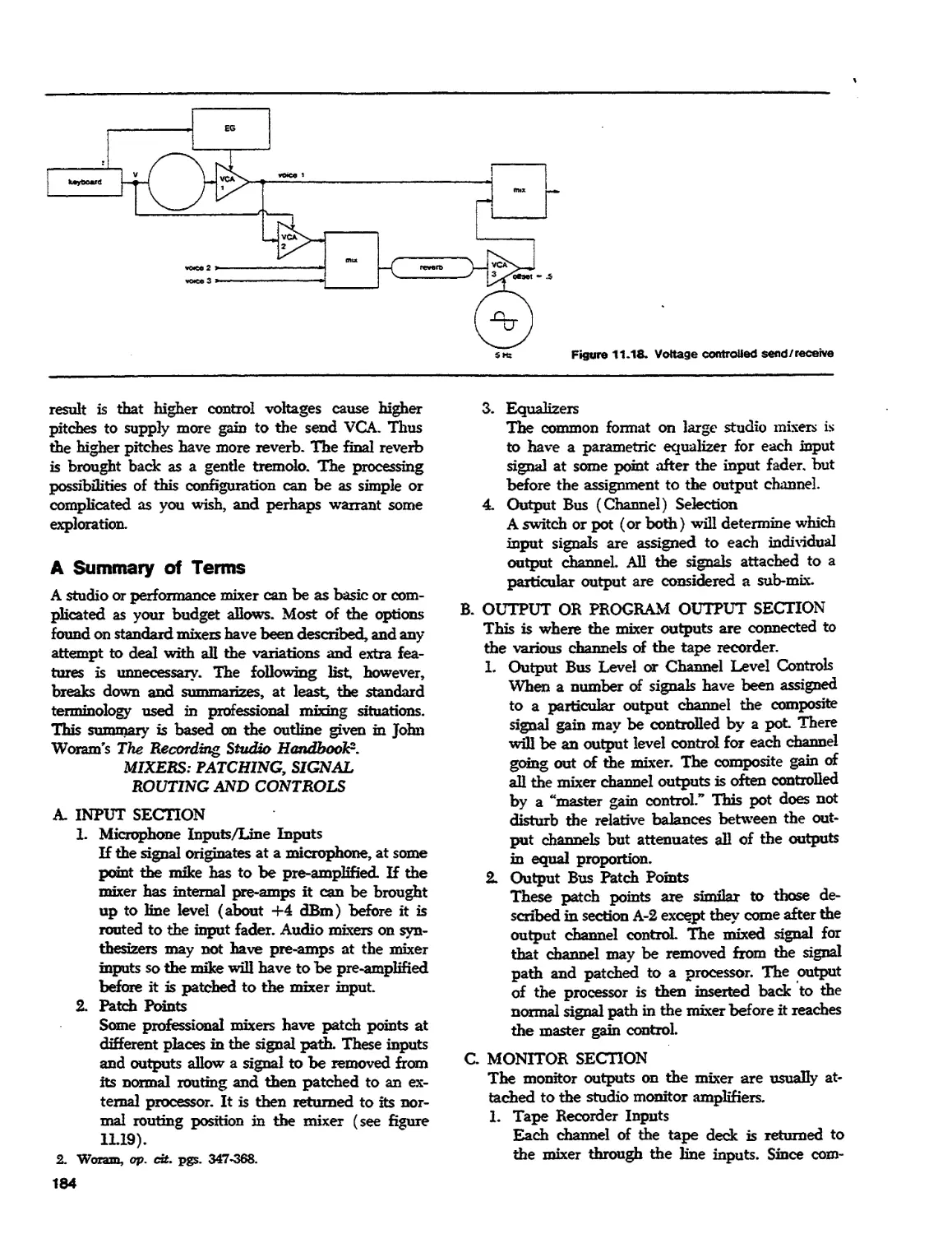
in
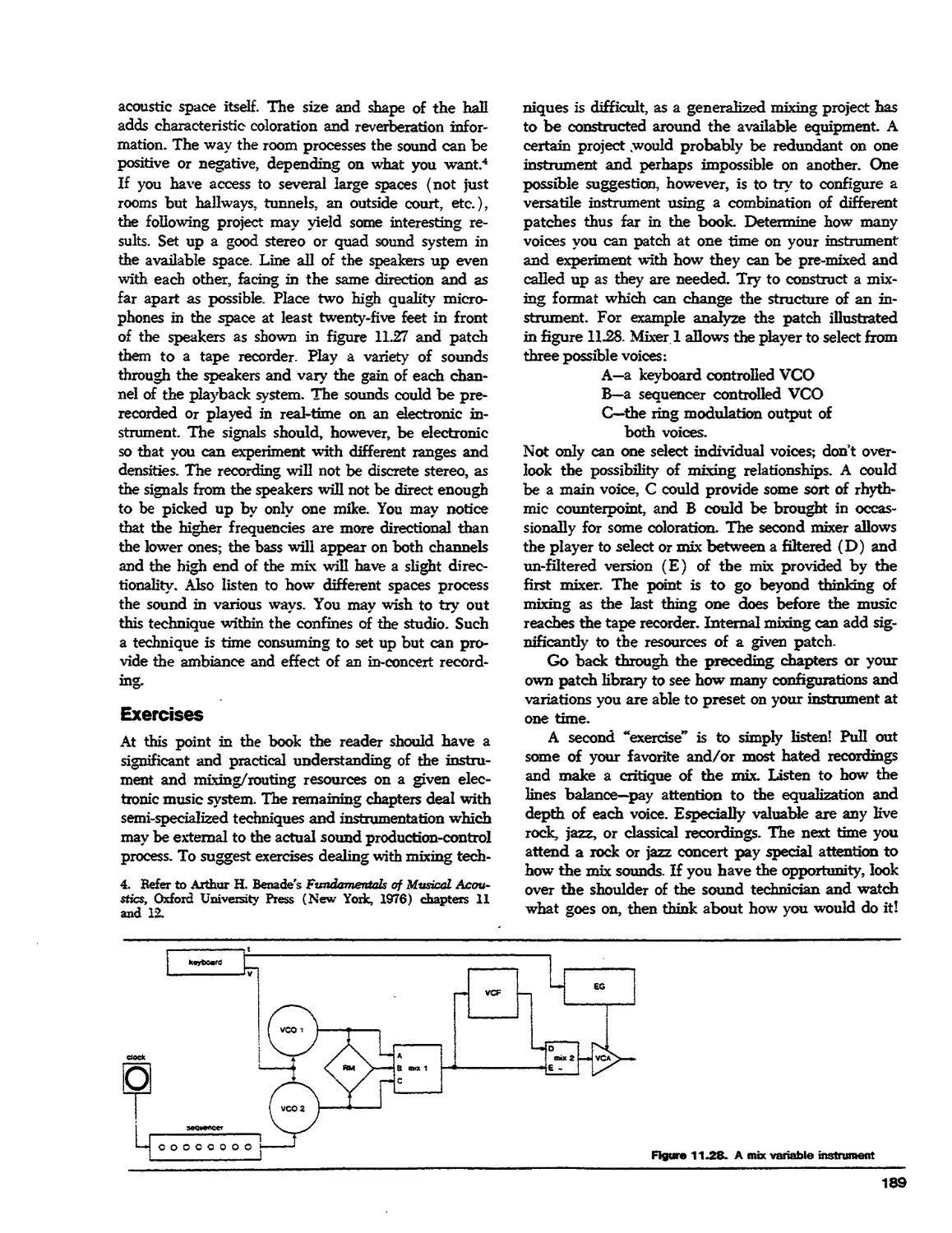
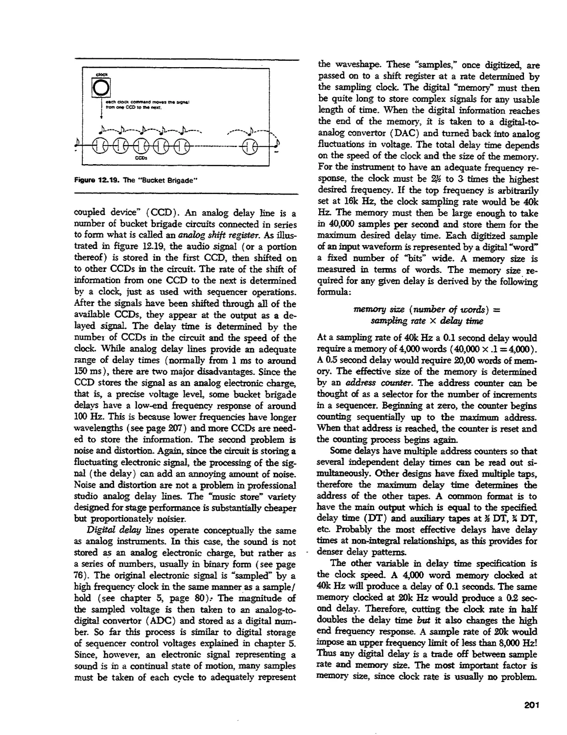
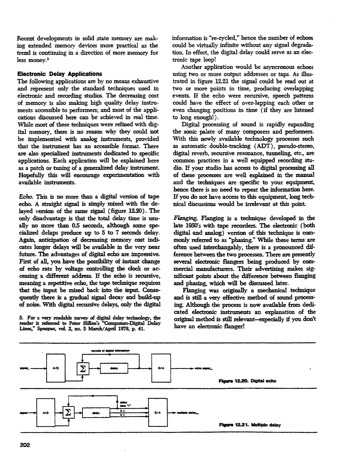
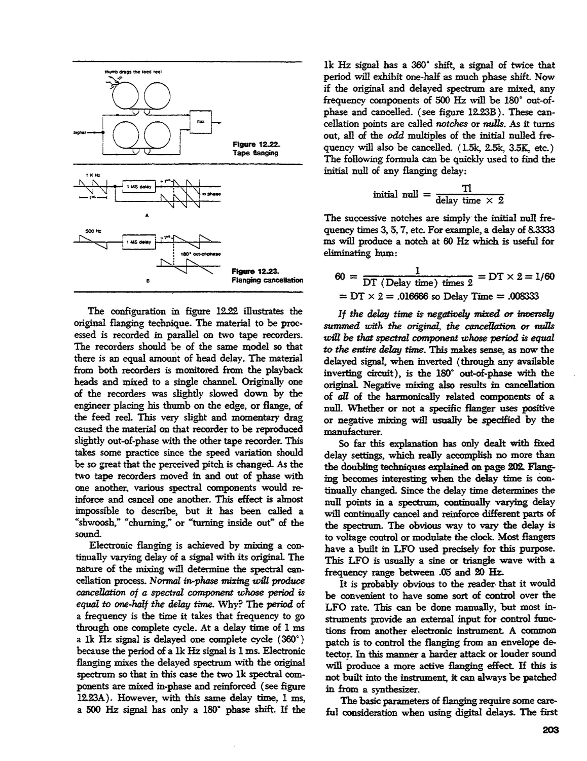
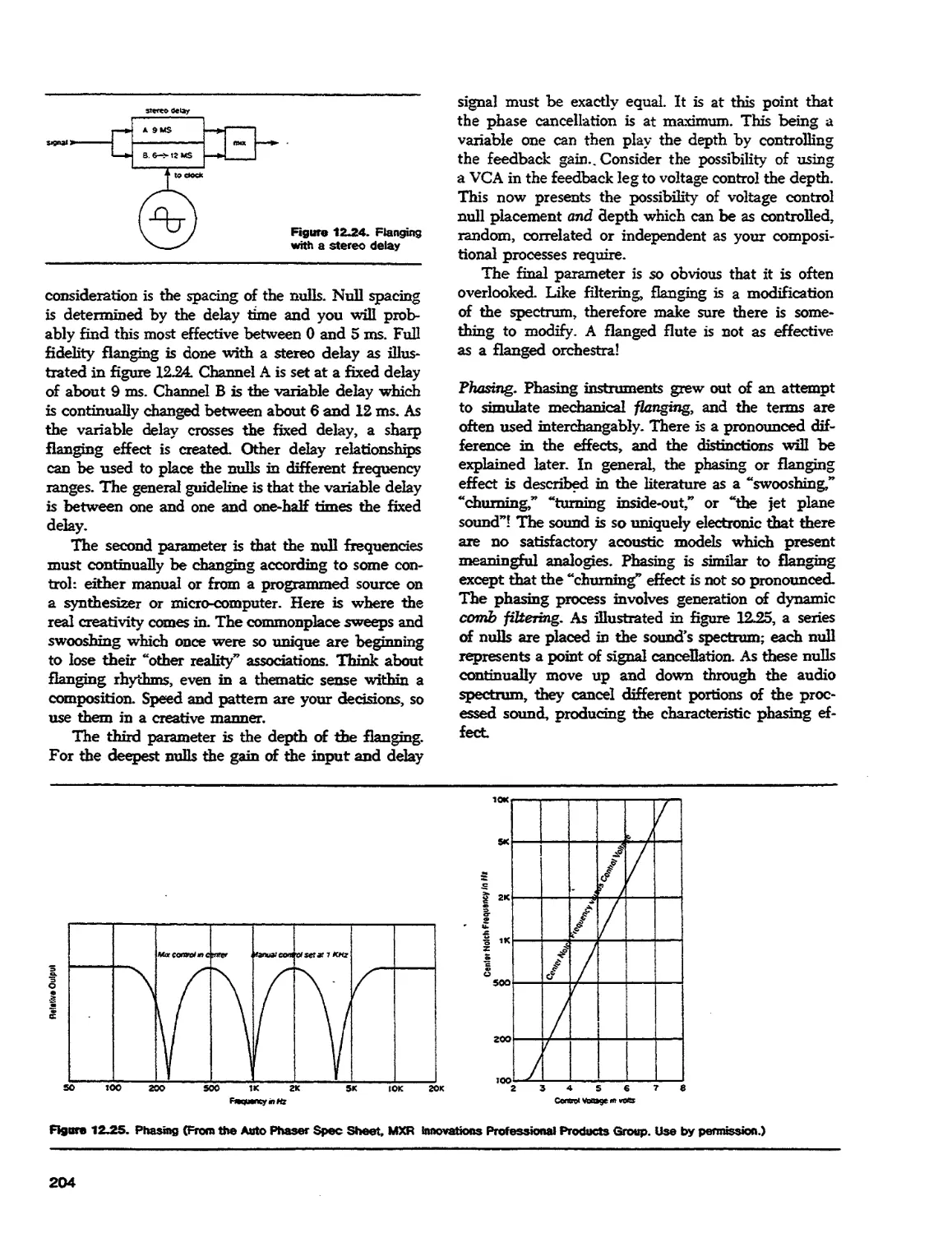
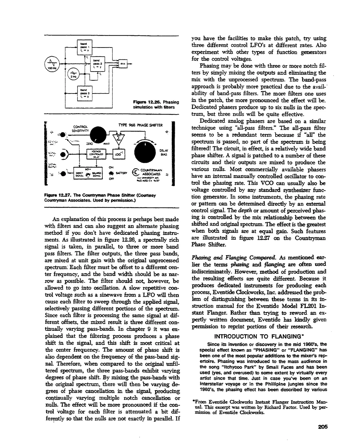
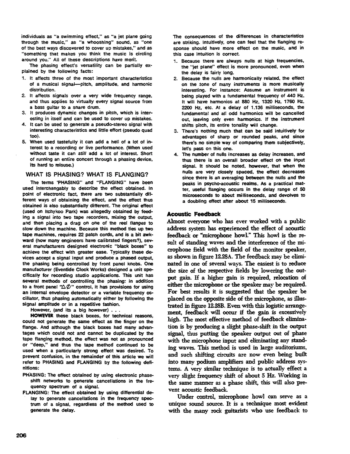
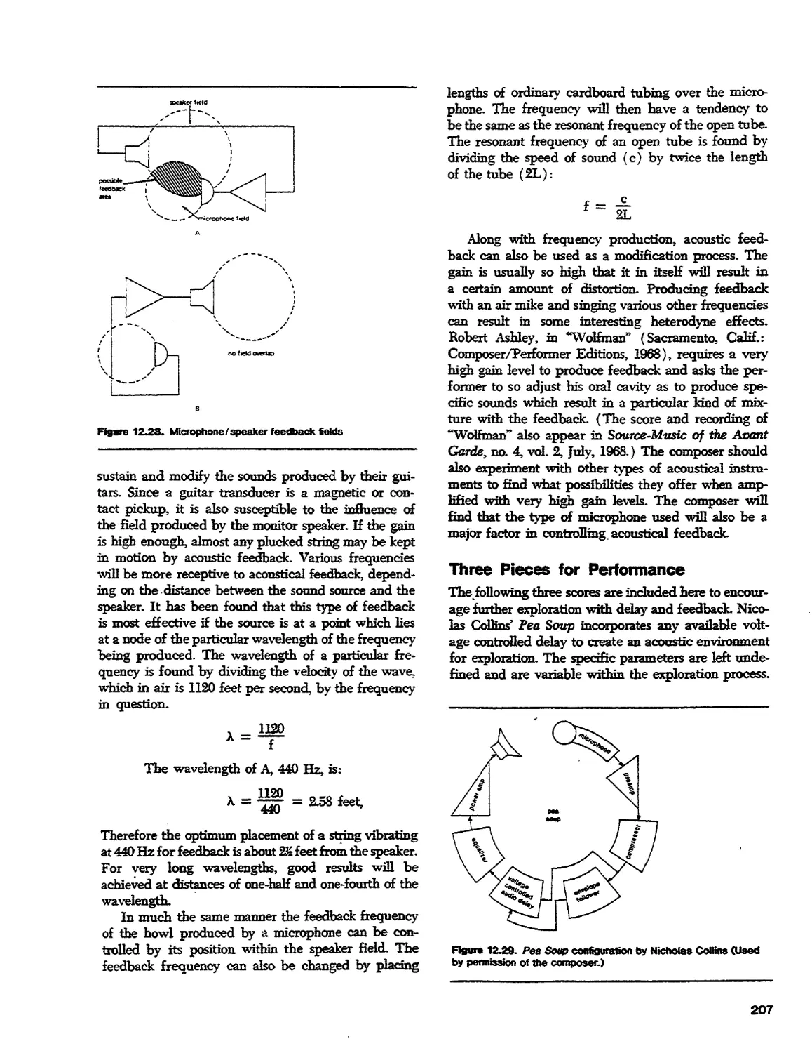
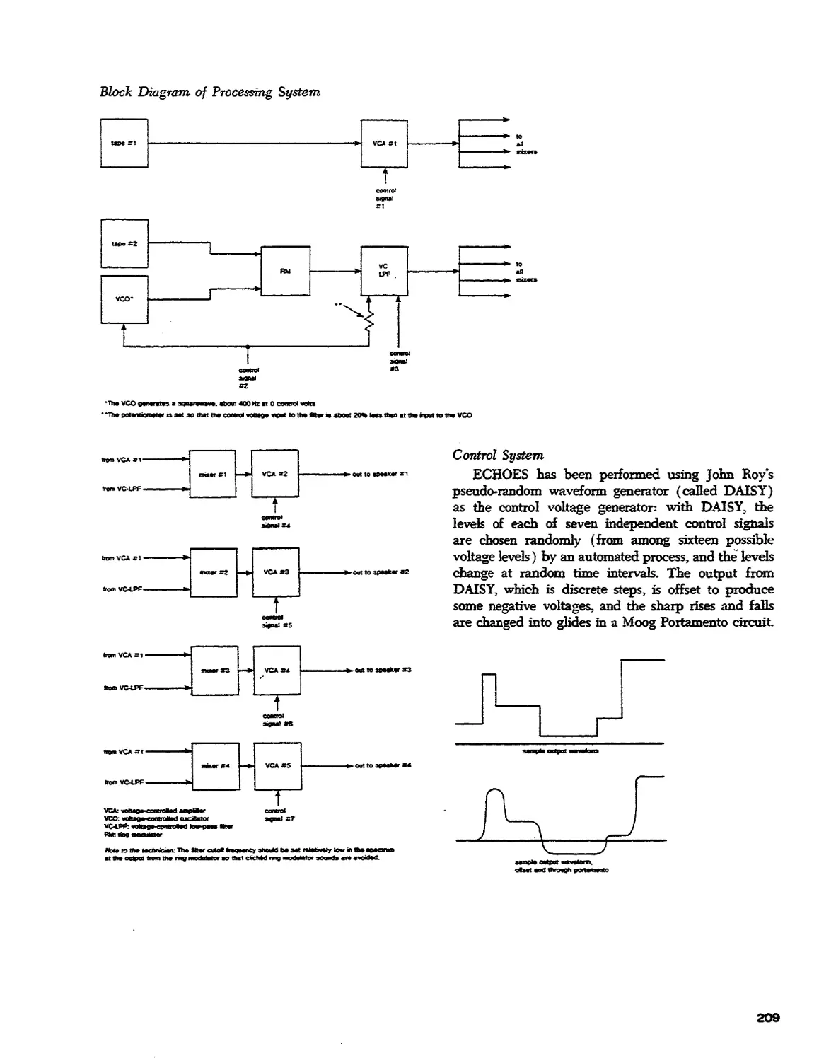
12. Reverberation, Echo and Feedback
194
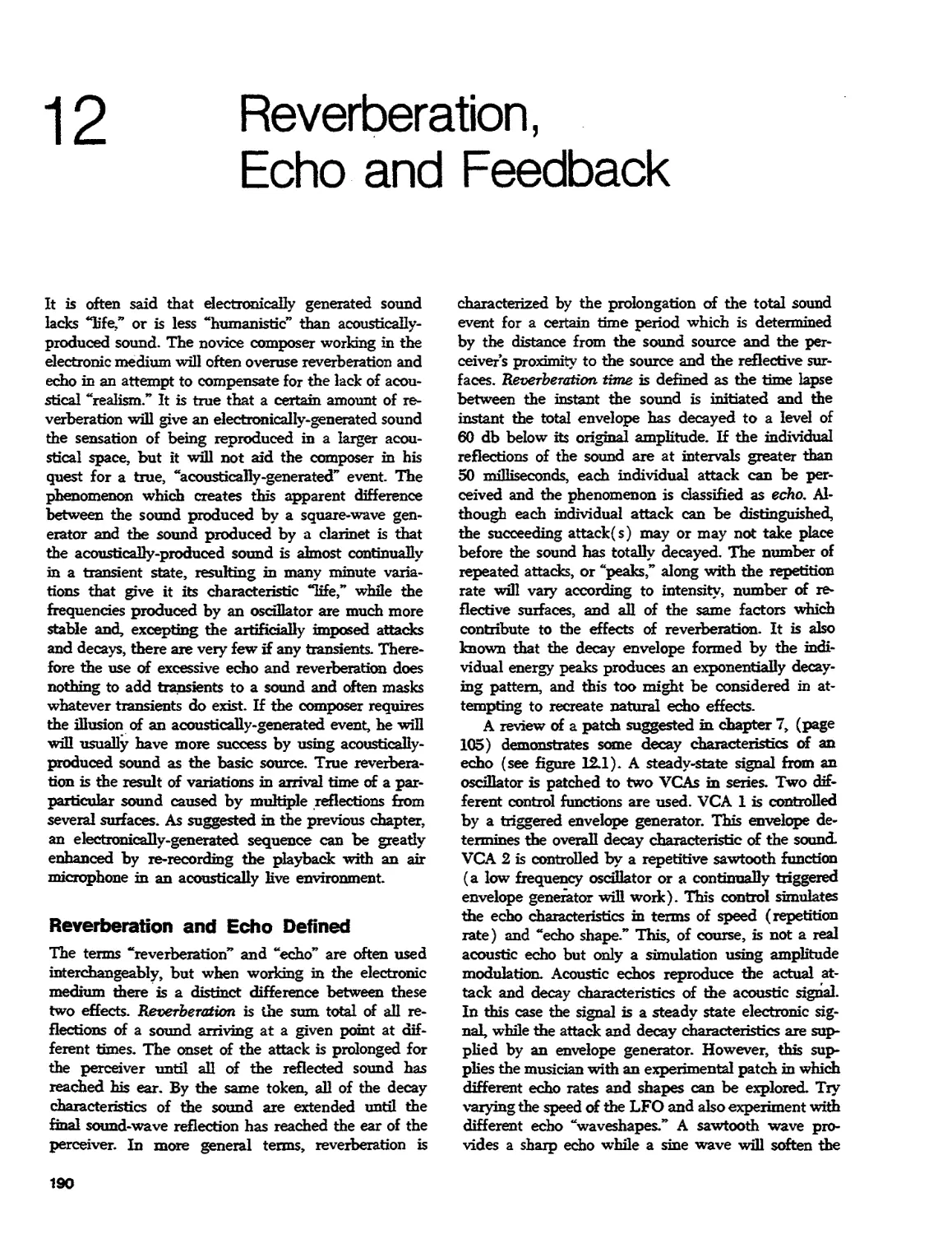
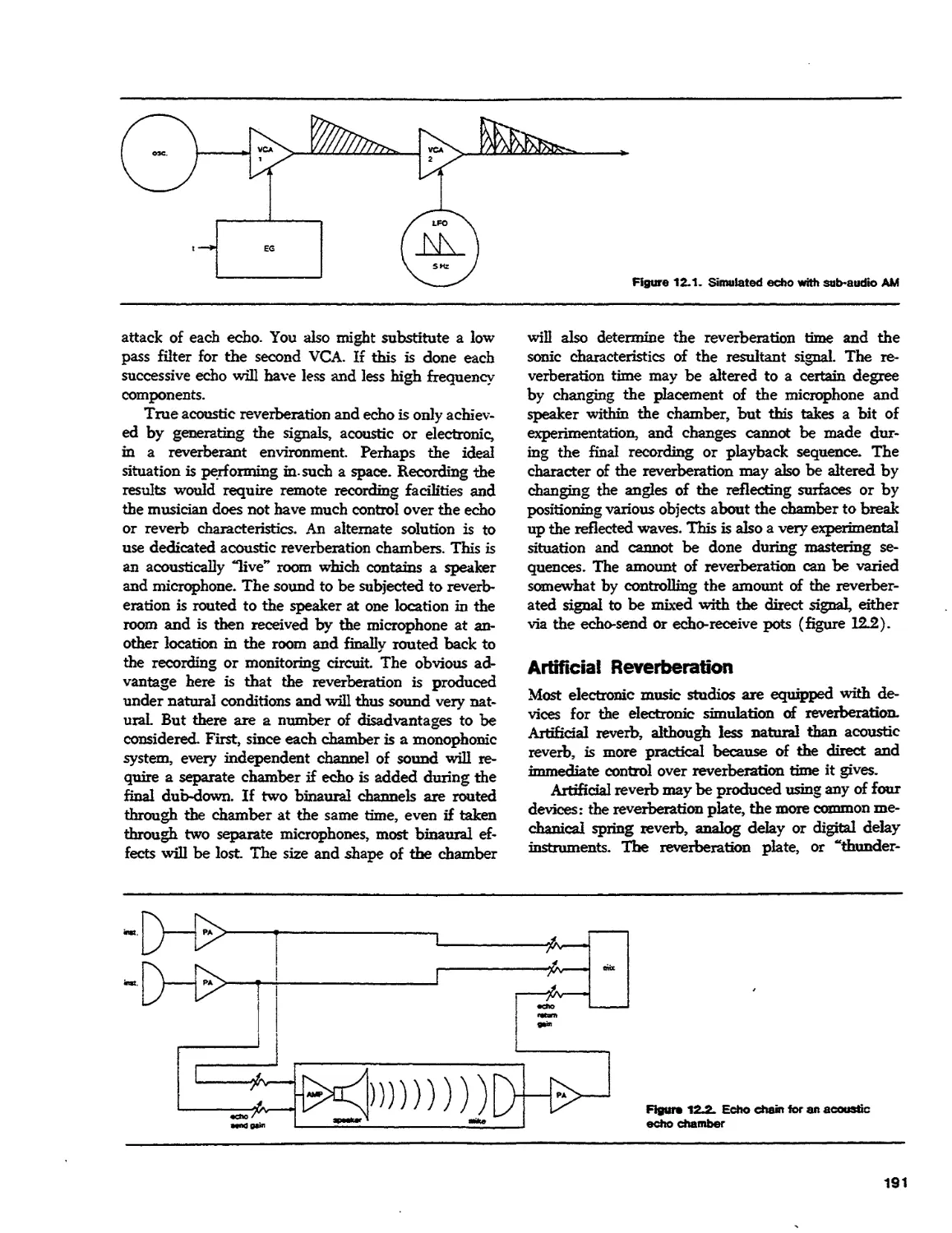
Text
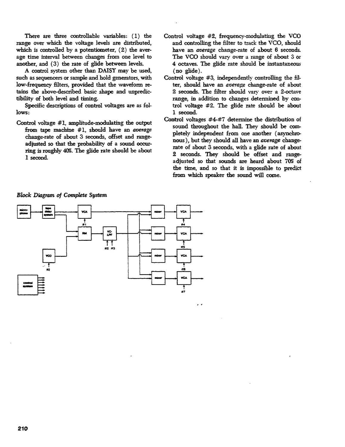
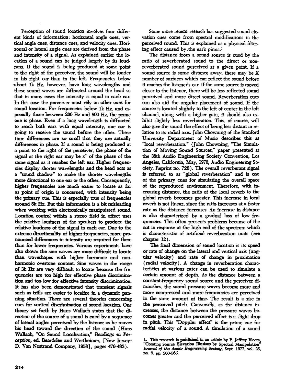
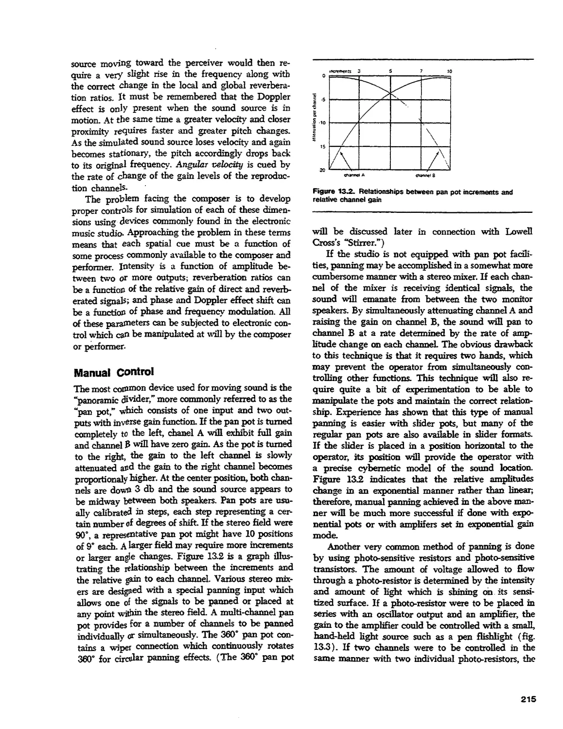
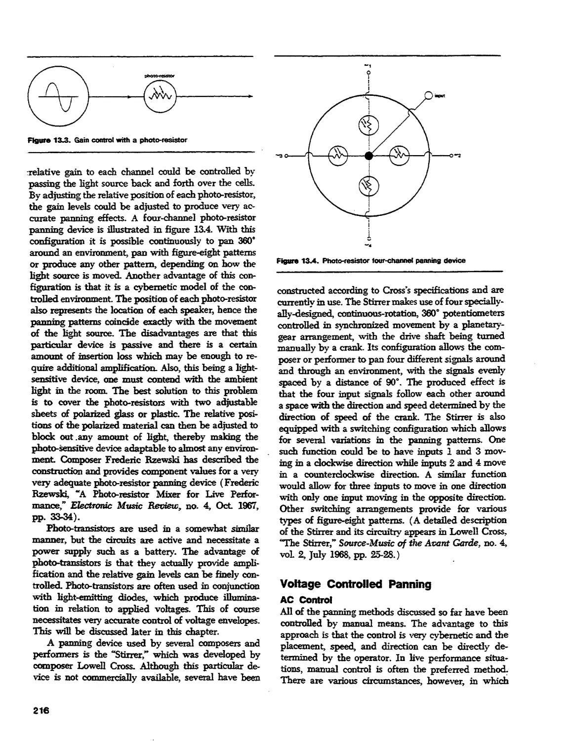
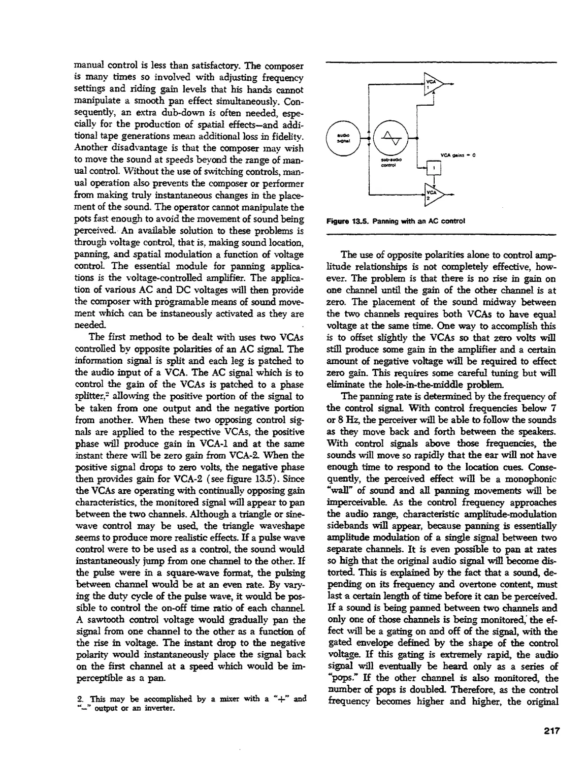
13. Panning and Sound Location Control
Text
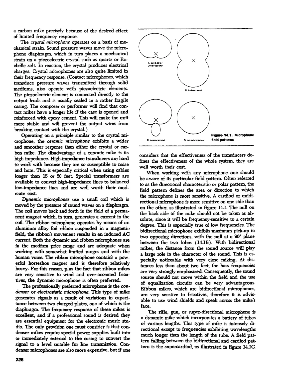
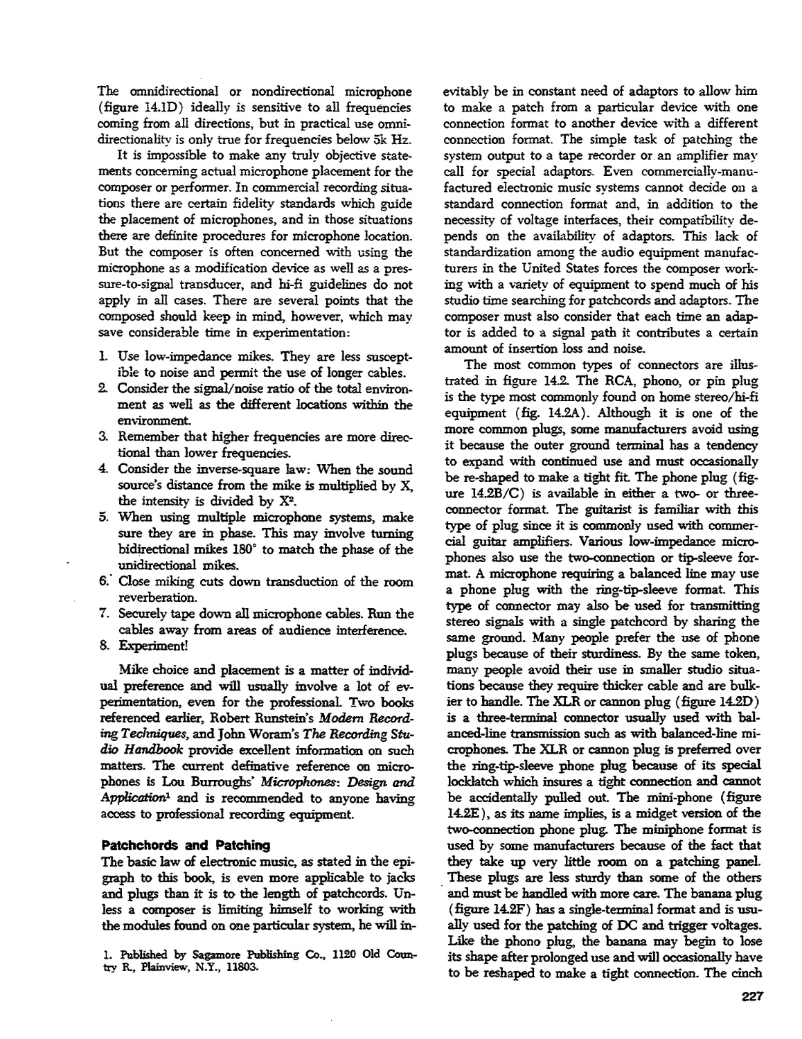
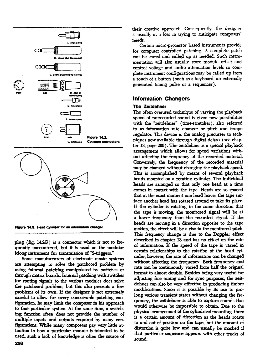
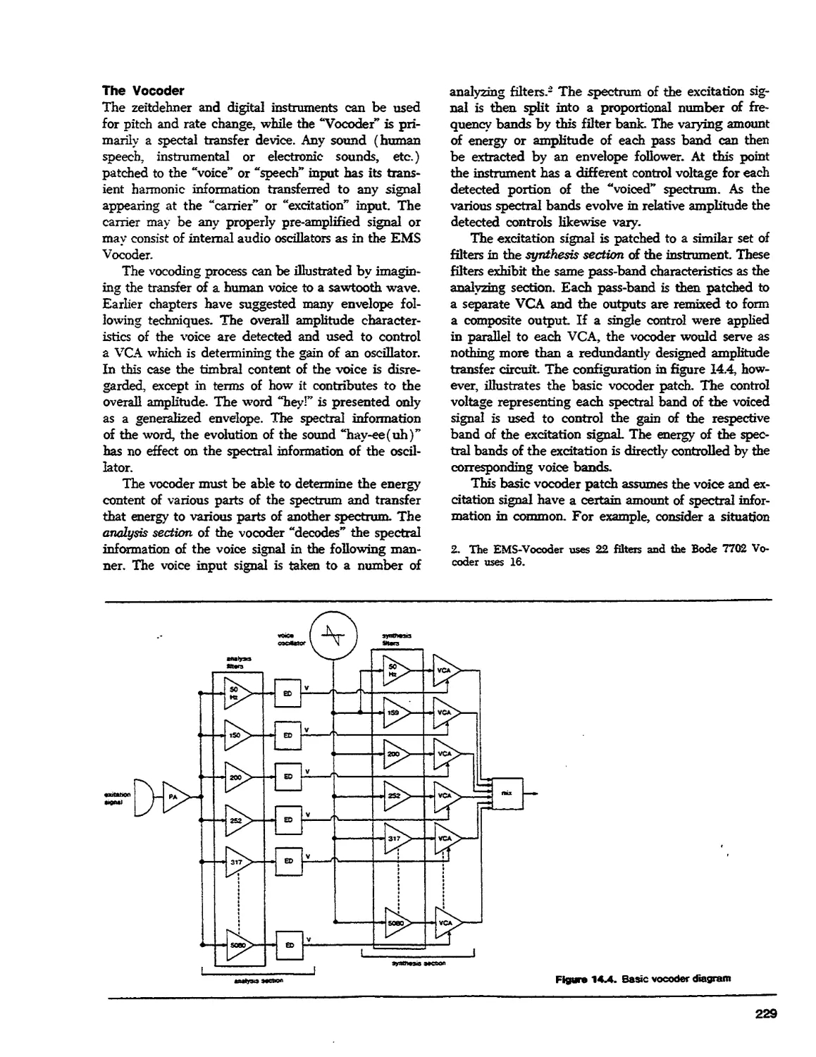
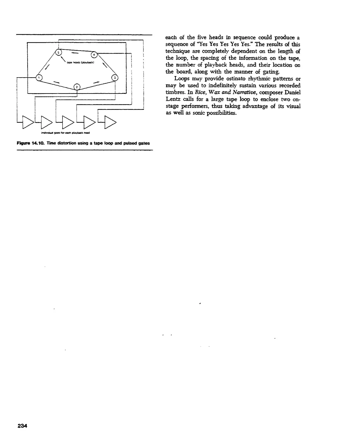
14. Miscellaneous Equipment
Text
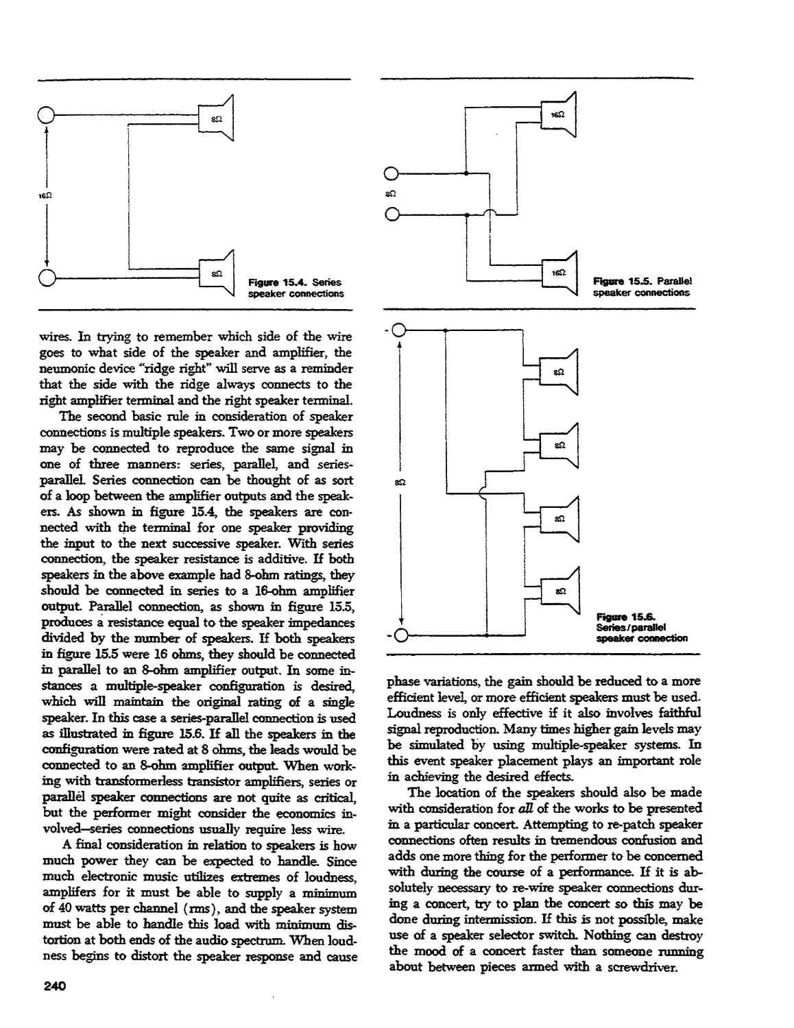
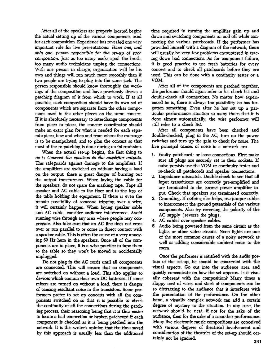
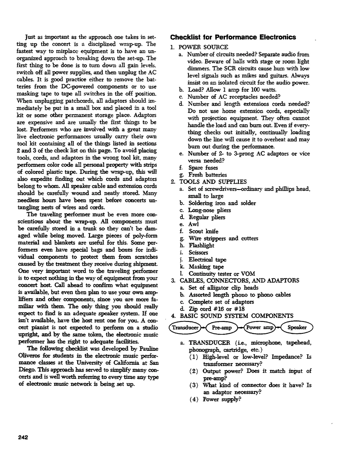
15. Performance Electronics
Text
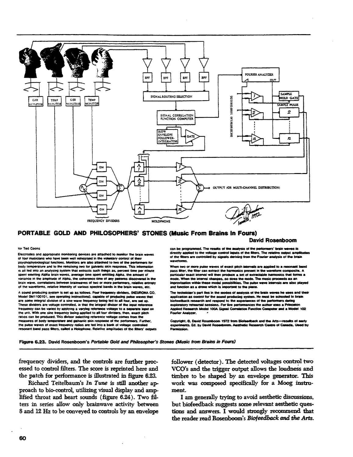
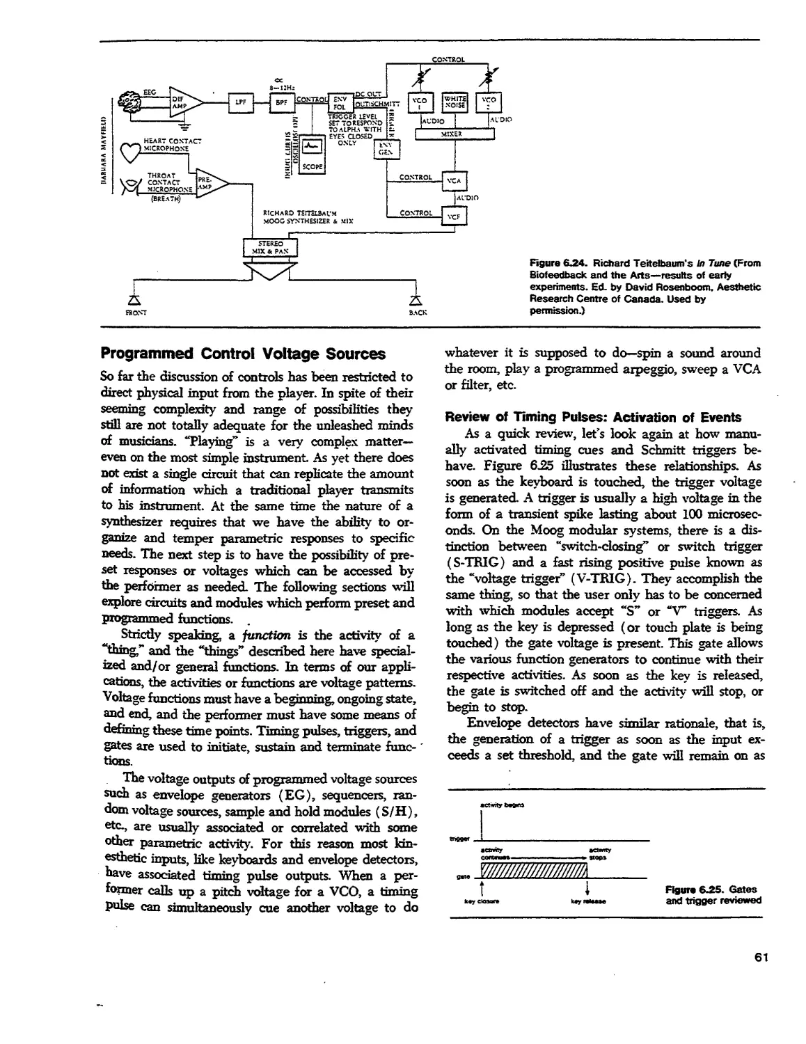
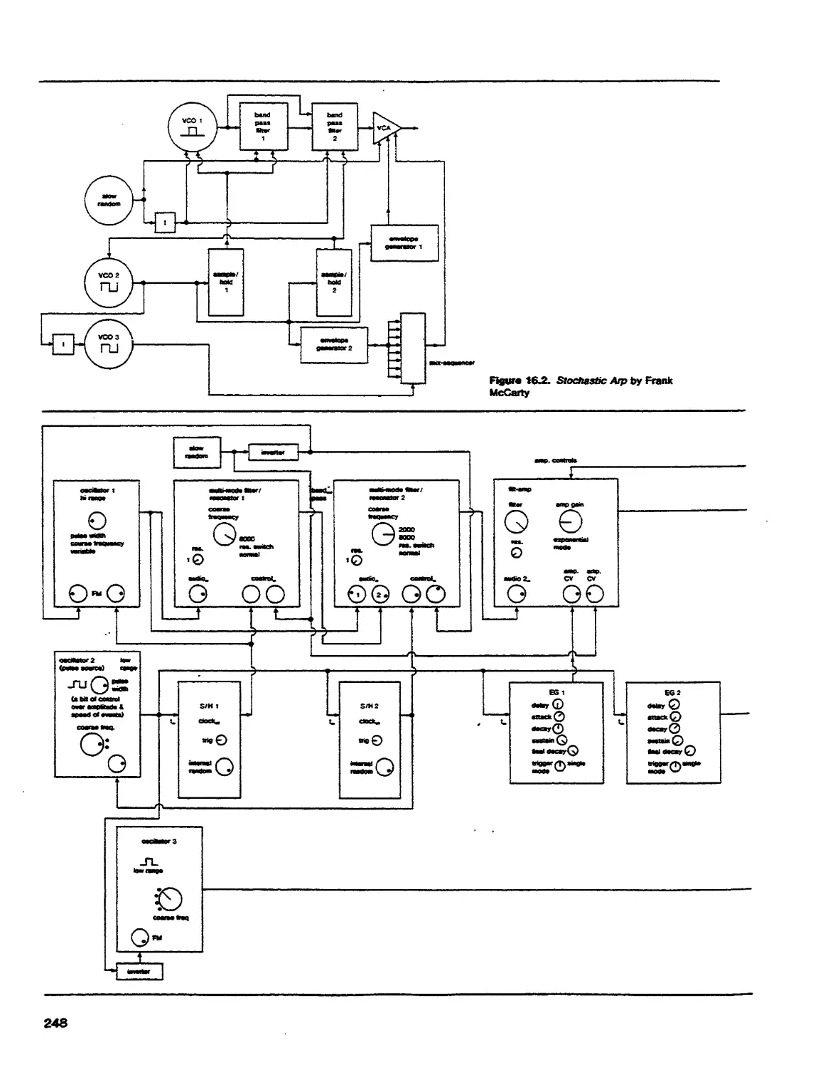
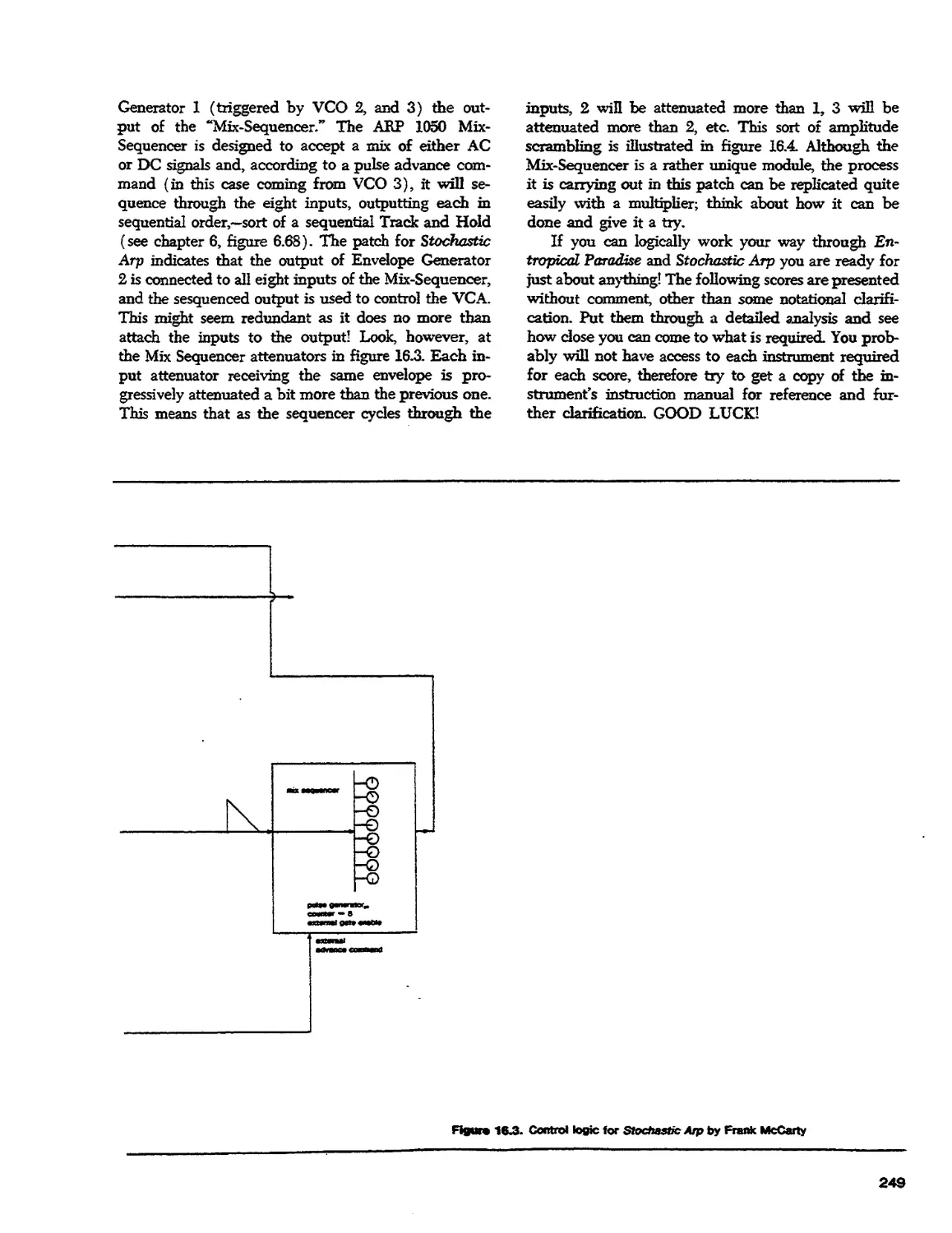
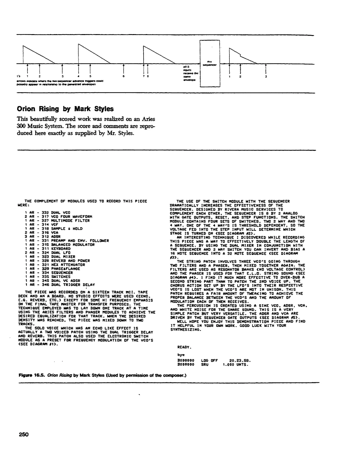
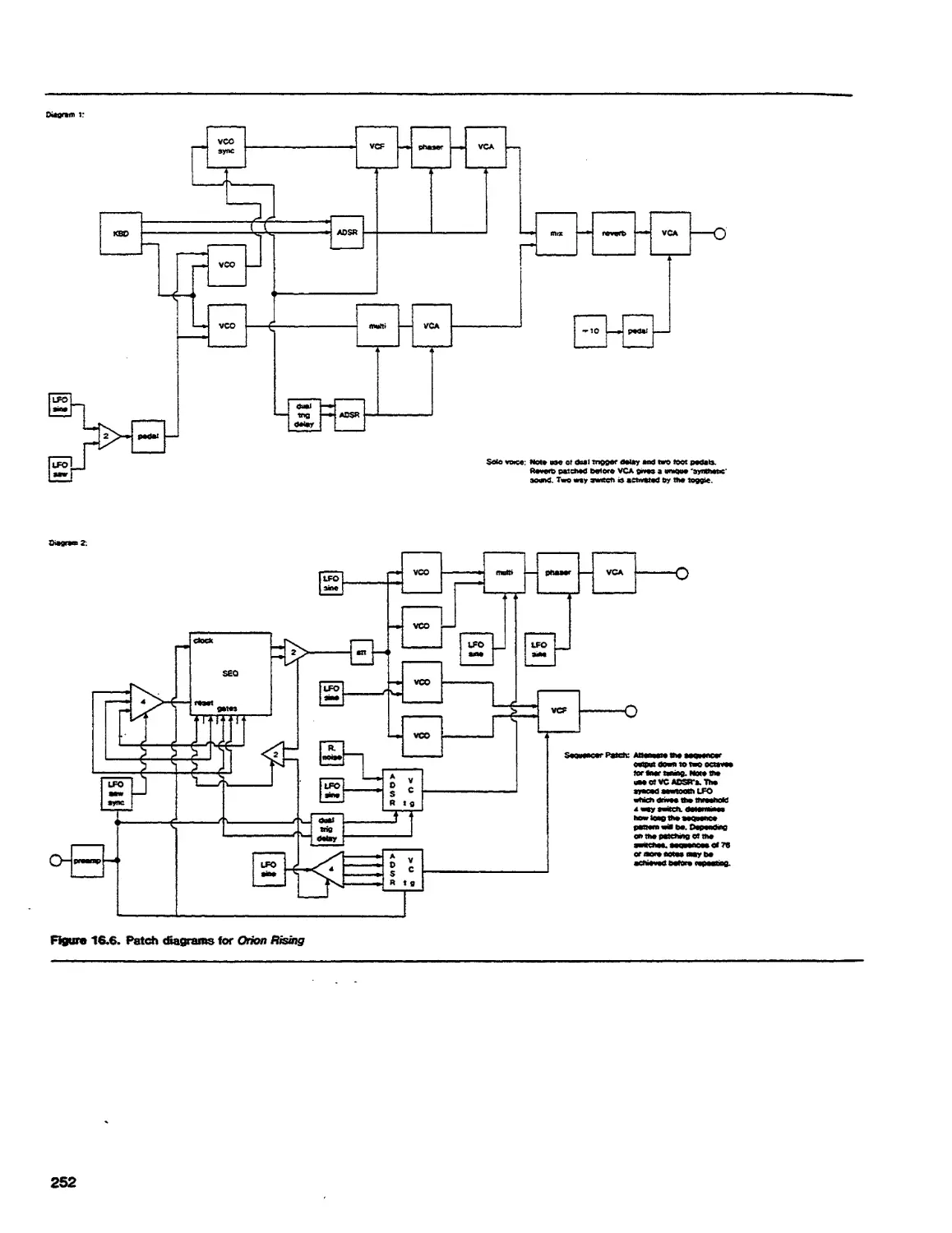
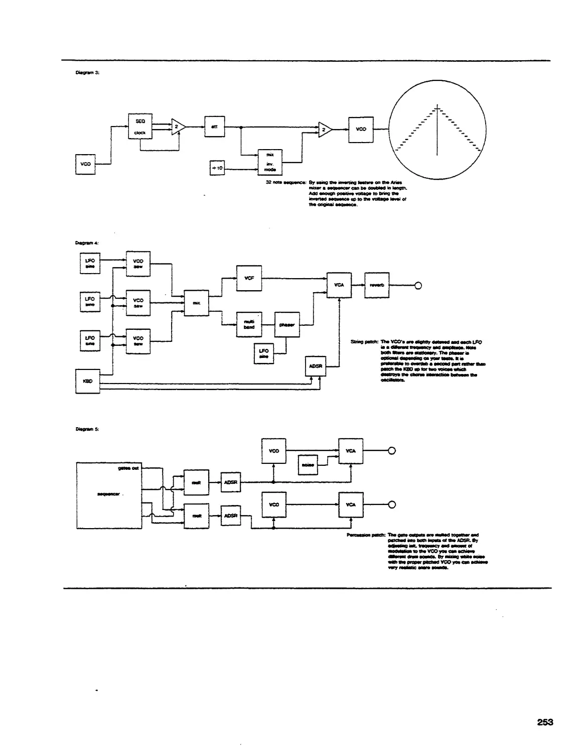
16. Scores for Analysis and Performance
Text
Back Matter
194
216
216
229
229
239
239
248
248
267
Afterword 267
Annotated Bibliography 268
Index 277
iv
Foreword
by Gordon Mumma
When in 1972 the first edition of Allen Strange's Electronic Music: Systems, Tech-
niques and Controls was published, the magenta, blue and white covered book
rapidly became ubiquitous. It was the first comprehensive and useful guide to the
subject, and was relatively easy to obtain. It had occasional errors of detail, and was
involved in the technological tumult before general standards were agreed upon, so
that some of the illustrative graphic symbols became relics. Nonetheless, that edition
proved quite robust.
At least two factors explain the first edition's survival for nearly a decade. Firstly,
Allen Strange organized the relatively new and complex material so that it evolved
with pedigogical sensibility. Secondly, his explanations of conceptual matters were
lucid. This lucidity may be due to a balance in the authors own world. He is an
experienced performer of electronic and acoustical instruments, a versatile
composer, a historian-theorist of diverse cultural background, and a very effective
teacher.
In the ensuing years several other books on the subject appeared. Some
contributed updated material, and others devoted more attention to certain areas, though
often at the expense of others. In spite of the example set by Allen Strange's book,
none of the others seems to have achieved his balanced presentation. And few
matched his marvelous attitude towards the subject, an attitude which induced the
reader to be alert to the many possibilities of a rapidly developing creative
medium.
This second edition, as the author notes in his preface, is in many respects a
new book. But it repeats that most important achievement of the earlier edition: it
is a comprehensive, detailed, and clearly organized guide to working with the
instruments and technical procedures of electronic music. Besides the expected updating
which includes many devices and procedures developed during the 1970s, the author
continues his method of explaining details within the context of general operating
principles. This makes the book applicable to virtually any analog electronic music
apparatus.
In its relatively short history—a bit more than half a century—music made with
electronic and electro-acoustic means is'well on its way to becoming as pluralistic as
that produced during many centuries with purely acoustic resources. It already has
both "cultivated" and "vernacular" traditions, which are widely disseminated by
broadcasting and recording throughout every part of the world. A major part of
recent popular and commercial music would not exist without synthesizers and the
creative use of multi-track recording. The recording studio, whether the relatively
simple home-variety or a multi-million dollar commercial facility, has itself become
a musical instrument—in Brian Eno's words, "a compositional tool." Electronic
music has even developed "foUdoric" aspects. Electronic sensors originally designed to
detonate anti-personnel weapons are now used as components of public-access
electronic-music environments in shopping centers and galleries. This is certainly
analogous to the use of cast-off oil drums in the making of steel-band music.
As with Allen Strange's earlier book, this new edition will continue to be an
important text for schools and universities. But perhaps more important, in a time of
declining support for arts innovation in educational institutions, this book will be
vital to creative people who develop their work independently.
ix
Preface
The original edition of this text was completed over
ten years ago. Compared to this new edition the
original writing was a very simple task. In 1970 there were
only three or four commercially available instruments
—today the number has increased to over thirty. What
was in 1970 a basic instrument format has expanded
in many directions as there are available instruments.
Each manufacturer has a different design format and
different implications in terms of the application of the
instrument. To cover such a subject area called for a
complete rewriting of the text. Due to the incredible
growth in the field of electronic music
instrumentation the subject matter covered in this present text has
nearly doubled that of the first edition. In a sense it
is inaccurate to refer to this as a second edition; it
is really a second book created out of the ever
expanding field. At the same time this new version makes
no claim to cover every possible resource and
technique available to today's musician. This text does,
however, deal with all of the generally accepted
designs and techniques common to today's electronic
instruments. The instructor and reader will find that
it provides a firm and basic foundation of
understanding which allows the user to develop the techniques
and processes specific to an individual instrument or
studio situation.
Regarding pedagogic technique.. I know of no two
people who approach this extensive subject in exactly
the same manner. The organizational approach to
teaching electronic music is greatly dependent on the
resources of the instrument and the resources of the
studio. Instrument X may be very keyboard oriented,
implying one approach, while instrument Y is based
on pre-programming and suggests a completely
different orientation and approach. Some studios are
designed around xnultitrack recording fadlties, while
others exist strictly as real-time performance spaces
with little or no recording equipment. Some electronic
music programs are compositionally oriented, while
other programs deal only with techniques and
problems of instrument performance. This book is
organized in a manner which is adaptable to any approach.
Each chapter is a progressive overview of the wluzt
and how of electronic instrumentation. Beginning with
a discussion of what "electronic music" means in this
decade, each chapter progresses from the basic
considerations of electronic sound through basic
techniques of control to advanced process of instrument
patching and sound modification.
The reader should not consider this to be a text on
electronic music composition. Composition texts can
do more than explain either general or specific
techniques of organization and structural manipulation.
When it comes to the "composing," this must be dealt
with on a personal, one-to-one relationship between
student, instructor, and the specific composition at
hand. This book is simply a text on "technique": how
to operate the instruments with various insights on
developing a consistent working method. Specific
composition assignments or "etudes" have to be designed
by the instructor, as appropriate to the given resources
of a studio. There are certainly compositional
implications of many of the patches and techniques explored
in this book. A particular mode of control or routing
of the signal patch through various modules
determines the variables of a musical situation. The
performer's manipulation of these variables is up to the
individual, and he/she should be able to explore the
possibilities outside of any aesthetic I might be prone
to dictate. I have my own set of assignments specific
to my studio's resources, and I would expect that
every other teacher has his or her own set of specifics..
While every instrument has its own unique
characteristics, the general operational principles remain
the same. With every instrument the performer must
deal with basic problems of routing signals through
various shaping and modification devices,
establishing operational norms and configuring ongoing
controls to produce the desired event The signal flow
through any instrument begins with the sound source,
goes through selected modification circuits, and each
circuit is assigned some form of control, be it manual
manipulation or different kinds of pre-programming.
This text is organized in the same way the instrument
is organized. The initial chapters deal with, the basic
sonic resources available to the musician. After the
introductory considerations each chapter is profusely
illustrated with patch diagrams and examples of
extant equipment Several of the unique features
available on certain instruments are described in a general
manner, with the explanation that in many instances
these features can be replicated on other instruments.
Chapters 4 through 13 are dedicated to various
techniques of control and sound processing. In these
chapters the initial "basic patches" are logically expanded
and notated in a unified format At the end of the
appropriate chapters there are projects and exercises
x
intended to enhance the reader's understanding of
various techniques. These projects and exercises have
been suggested by colleagues, and range from
conceptual problem solving to the realization of compositions
by different composers. The last third of the text deals
with techniques and devices usually external to the
actual performance instrument. Basic techniques of
mixing, tape recording, stereo and quadraphonic
considerations, as well as performance electronics are
covered in sufficient detail to give the reader a substantial
point of departure for advanced development.
This book is not meant to be a substitute for an
instrument's operation manual or a general handbook
for a given studio; rather, it is a basic organizational
guide for learning. While many detailed techniques are
discussed, the specific patching format and specific
techniques have to be left to the individual instructor
and the manufacturer's own documentation. Every
studio has a different design which is applicable to
itself; and this text makes no attempt to describe a
specific studio format. Such information must be left
to the instructor, and most of the initial class
discussions deal with the layout and general operation of a
given studio. Because we present as many of the
resources as are generally available, we realize that the
reader may find some of the material redundant or too
technical, depending on the goals of the class. The
instructor should design the reading assigments in
consideration of this fact. Certain material may be
irrelevant to some situations and can easily be excluded.
Each chapter does, however, begin with the bare
essentials of a subject area or technique and will be
applicable to every instrument. The teacher will also
find it necessary to augment certain portions of this
text, discussing devices and techniques specific to a
studio's own resources.
This present text contains over 400 illustrations
designed to clarify, to demonstrate, and to expand the
reader's understanding of the techniques of electronic
music. At the same time it is recommended that the
reader keep a notebook of patches developed in class
or on his/her own studio time. Such patch libraries
prove invaluable as references while developing new
skills and techniques. At the end of each course I have
found it useful to make a class project out of
compiling all of the most useful student-generated patches
into a single document for future reference. Another
activiity I have found very useful to students is to
have certain patches and techniques documented on
tape. Any patch can potentially generate a wide range
of sounds, depending on the fine adjustment of the
various controls, and sonic models can be very useful
as guides for the beginning student Each student may
also wish to keep a personal library of recorded patches.
Various patch assignments can be recorded on a
cassette tape by the students and indexed to a specific
diagram in a patchbook.
The reader^ who are first beginning the study of
electronic music outside a controlled class situation
are encouraged to deal with the subjects as they appear
in sequence in this text. This will insure continuity
of subject matter and avoid encountering undefined
terms. The class instructor undoubtedly has his or her
own approach to which my approach may be
perfectly applicable. Or the instructor may wish to
rearrange the sequence of the middle chapters to
accommodate his own methods. This is certainly- to be
encouraged, as each chapter attempts to be as
independent as possible. The problem of undefined terms
due to re-sequencing is solved by cross-references and
an extensive index. Certain definitions and
clarifications can also be presented by in-class lectures.
During recent years low cost technology and the
development of the micro-processor have generated
much interest in digital applications to the analog
electronic music system. At the present time there are
several operational systems which make computer
control of electronic instruments very attractive. It would
be redundant to attempt to rewrite the
documentation of these systems for this text since such
information is available from more direct sources. The
reader, however, will be introduced to some of these
approaches, and certain instruments specifically
designed for local and/or computer control will be
covered. Digital control, at this point at least, is providing
for more accessible and accurate performance
techniques in terms of establishing and recalling complex
situations. It is also providing for the expansion of a
particular instrument's capabilities in terms of more
complex functions. This means that the computer is
increasing the efficiency of what these instruments
can usually do. The concepts of voltage control and
parametric design are the same with or without
computer aid, and at the present time a separate chapter
dealing with digital control is not warranted. The
number of digitally controlled studios is limited and
their operational procedures are usually unique. Until
some common ground for digital control has been
established in commercially available instruments, in-
depth documentation is best left to the manufacturer.
At the present time certain companies offer instruments
specifically intended for digital control. These devices
will be dealt with in a context established by their
musical function. For example, a digitally controlled
amplifier is still an amplifier and serves the same
parametric function irrelevant of manner of control.
Modern digital technology has provided the
musician with some exciting new handles on musical
structure, especially in the area of time manipulation.
These instruments, with their basic operational
methods and musical applications, have opened up some
xi
possibilities for the musician which ten years ago were
considered impossible. In spite of these instruments'
dependence on digital sound reconstruction, their
operational modes are compatible with modem analog
equipment and will be discussed with basically the
same vocabulary.
On the other side of the coin this book does not
concern itself exclusively with lii-tech' electronic
musical instruments. Today's state-of-the-art had its
beginnings with non-musical devices forced into a music-
making chore. This is a healthy attitude for the arts
and is not to be discouraged; Techniques involving
extant equipment other than commercially available
instruments will be dealt with if those techniques
provide a workable music-making situation, and any sup-
portative literature for these applications will be
documented. In certain situations a mailing tube and a
microphone may make a very suitable oscillator (see
page 207), and bits of editing tape can be used to
articulate complex rhythmic sequences. Some may find
these types of jury-rigged techniques far from so-
phisicated but if they work, then they work! After all,
there must be some reason that the muscians'
activities are often called 'playing.'
The last chapter of this book is concerned with the
final task of the musician—the making of music.
Several composers have been kind enough to make then-
scores available specifically for the purpose of analysis
and performance. These works appear in their original
format as designed by the composers. Each score is
given in its complete form and is intended to be
realized by those users with the proper resources. Even if
performance is not practical a detailed analysis of each
work will be time well spent. Since a score can never
completely represent the musical event, four of the
five works are available on Dolby cassettes specifically
as performance models. For information concerning
these tapes please write to Ocean Records, #4 Euclid
Avenue, Los Gatos, Calif., 95030.
Acknowledgments
To acknowledge every person who contributed to the
development of this book would be impossible. This
is a standard first line for acknowledgment statement
and it is unfortunately true. Perhaps the greatest help
came from my students. Their feedback and never
ending questions helped me clarify in my own mind just
what needs to be said about the subject of electronic
music. Of no less importance was the help of Robin
and Pat Strange who tolerated my hours of isolation
in the studio preparing this manuscript. Special thanks
go to the many instrument designers who willingly
provided me with documentation, photographs and
hours of telephone conversation answering my
questions. Of these, special mention must be made of Har-
ald Bode of Bode Sound Company, Scott Wedge, Ed
Rudnig and Marco Alpert at Eu Instruments, Robert
Moog of Moog Music, and Donald Buchla of Buchla
and Associates. Last but certainly not least special
thanks go to all of the composers and performers who
suggested techniques and supplied scores. Without
these artists there would be very little need for the
instruments and certainly no need at all for this book
Allen Strange
xii
"1 Preliminary
Statements about
the Subject Matter
The term "electronic music," a common post-1950 term,
has been the source of a certain amount of
misunderstanding among musicians and audiences. Prior to the
1960s it usually referred to a type of music
characterized by presentation on pre-recorded tapes. The phrase
itself often called to mind a music based on discordant
sounds and angular structures. I certainly do not wish
to imply any negative value judgments about early
electronic music but am attempting to identify some
generalized characteristics in order to explain a
generalized aesthetic comment. To the non-practitioner,
there was little or no distinction between the various
schools of musique concrete and 'pure' electronic
music. While pre-1960 electronic music resulted in many
significant compositions and was the catalyst of the
research that led to present day electronic instruments,
there is some basis to this generalized electronic music
aesthetic that still lingers in the minds of many people.
Even today one might attend a concert of new
'acoustic' music concerned with new timbres and
unusual structural relationships and hear the comment
that it "sounded like electronic music"! What is the
reason for this association? The early history of
electronic media in music was a period of experimentation
with very little prior history to provide direction.
Schaeffer and the musique concrete group made music
with whatever sound they could capture on disc, wire
or tape. Eimert and Stockhausen, representing German
elektronische musik, heralded the use of the electric
oscillator as the source of 'pure' electronic music; the
Columbia-Princeton school was coaxing music out of
a $250,000 computer and capturing it on tape. What
expressions in that decade had in common has had a
significant role in formation of the layman's concept
of electronic music today.
Looking back on the years between 1950 and 1960
one's first observation is that the practitioners were
making music with devices designed for other
purposes. The tape recorder, the oscillator and early
computers were designed as tools of science and not tools
of art Prior to that time our musical traditions told
us that musical instruments were plucked, bowed,
blown into, or struck, and these actions enabled us
to reproduce a history of musical thought. When the
computer, oscillator, and tape recorder were given the
role of a musical instrument, pluck, bow, blow and
strike were joined by a plug in, punch, turn and splice!
The musician was busy making music on
instrumentation not designed for conventional musical use. Since
the generation and control of sound on these devices
were generally foreign to our traditions at that time, it
was only logical that the resulting music would be
proportionately removed from the norm. The results
brought to light some forgotten basic ideas about
music, specifically about musical instruments.
To discuss musical instruments in a manner
relevant to electronic media calls for a re-orientation
relative to what we may assume to be a simple subject
We all know what musical instruments are—they are
things we play and make music with! This
straightforward definition implies some rather far reaching
concepts which may appear to be simultaneously quite
simple and somewhat technical- However, I think that
the patient reader will benefit by considering the
following ideas. Any musical instrument requires at least
three things: a method of playing (input or perhaps
stimulus), structural organization of the object being
played, and a resulting sound (output or response).
A violin is bowed or plucked, it is made of wood with
strings attached and tuned in a prescribed manner and
it produces a sound that we identify with that input
and structure. A laboratory oscillator has a dial which
is turned (input), it is made of a specific collection
and organization of electronic parts (structure) and it
behaves like a laboratory test oscillator. A violin
possesses the structure and inputting capabilities which
make the production of virtually any specific pitch
within a four octave range a simple matter for the
trained player. A laboratory test oscillator, while
capable of a far greater range, cannot readily produce the
specific pitch patterns found in pre-1950 musical
literature. One can imagine trying to play a Bach Tar-
tita" by manually turning the dial on the front of
an oscillator. At the same time, however, it would be
1
verv difficult to coax a smooth ten octave glissando
with a consistent timbre out of a violin. Thus the
nature of a musical instrument,—its input, structure and
output,—defines the musical characteristics of that
instrument. What really makes an instrument musical
is that a musidan decides to make use of it.
This may all seem rather obvious, but may serve
to answer some basic questions and provide us with
guidelines to the functions of electronic media in the
sonic arts. During the decade between 1950 and 1960
composers and performers were making music on
instruments not designed for conventional performance.
The task of inputting or playing was difficult, and
performance of any kind of pre-existing musical literature
was almost impossible. Even simple sequential event
structures were difficult to achieve. In this situation
one can readily understand that one reason for the
seemingly radical sounds of early electronic music was
partly due to the fact that the musicians could
generate such sounds with relative ease. Music exists in
a continuum of time and time will not wait for one
to find the next pitch on an oscillator or program a
new set of instructions for a computer. There were
two obvious solutions to the problem. One was to
build a new land of music to accommodate the type
of instruments used. If precise pitch at specific times
was difficult to attain, then make a music that took
advantage of the things these instruments could do-
such as extreme glides, non-fluxuating timbres,
expanded dynamic ranges and so on. Hence—our first
models for the "electronic music" The alternate
solution to the problem was, in essence, to stop time
in order for the performer or composer to rearrange
his collection of instruments, making ready for the next
event In the field of electronic music the tape
recorder is an instrument which provides for this need.
To produce a precise sequence of pitches on a
laboratory test oscillator one finds the starting note,
records it, turns off the tape recorder; finds the second
note, records that, turns off the tape recorder; finds
the third note and repeats this process until tile
sequence of desired notes are on the tape. He then cuts
the tape into lengths which produce the desired
rhythmic pattern and puts it all back together again with
splicing tape. The tape recorder then reproduces a
five second stream of pitches the composer needed
thirty minutes to construct. The reason for this out-
of-time performance was that the generating
instrument, in this case an oscillator, did not have the
inputting capabilities needed to produce the desired
event in real-time. The two obvious solutions to this
problem were to evolve the literature to suit the
instruments or to develop the instruments to suit the
literature. The evolution of technology and consdous-
ness provided both. The development of new musical
instruments has continued to remind us that we can
make music out of anything from which we choose
to make music. There is more to the art of sound than
twelve pitches, bowing, blowing, plucking and
striking. Many of what seemed like definitely unmusical
events in 1950 are now quite acceptable, even to the
conservative ear. The revolutionary music from the
Columbia-Princeton studios during the early and
middle 1950s is very tame compared to today's orchestral
music by composers such as Iannis Xenakis. Along
with the evolution of our aesthetic, the instrumentation
itself underwent significant development. Alterations
in oscillators were made, which allowed the performer
to control precise pitch change in real-time. We learned
that workable performance modes could be devdoped
for the musidan. Oscillators and other artifacts once
designed for the communication studio were
redesigned to accommodate a wide variety of musical
thought. By the early 1960s electronic devices
dedicated exdusively to the production of music were
available. The composer in tine dectronic medium no
longer had to work within narrowly defined limits,
nor was it necessary to manipulate the flow of time
with a tape recorder. Contemporary electronic musical
instruments are devices capable of a wide range of
inputs, structures and resulting sounds—all of which
are decided and implemented by the
composer/performer.
A trip to the local record store provides
substantial insight into the current state-of-the-art. In the bin
marked "Electronic Music" one can find works by
John Cage, Milton Babbitt, reorchestrations of
masterpieces ranging from Monteverdi to Stravinsky, a
variety of popular artists ranging from Herbie
Hancock to Klaus Schulze, contemporary masterworks by
Morton Subotnick, the Sonic Arts Union, and Karlheinz
Stockhausen; and I am sure this bin has grown
significantly since this text went to the printer. If such a
wide variety of music is listed as "electronic music,"
then the term cannot possibly refer to any single
aesthetic production. What am I talking about when I
say this is a book about dectronic music? What is it
that all of those records have in common? The answer
I provide and one which is the basic premise of this
text is instrumentation and orchestration.
The purpose of this book is to guide one in the
technique of playing electronic instruments. Beware
of the simplification of that statement. The subject
matter is a bit more complicated than might be
imagined at this point, and the complication is due to the
nature of these instruments. A woodwind, string, brass
or percussion instrument is structurally constant.
Performance modes have been established which
accommodate their structure and their sounds can be pre-
cisdy predicted. The reason a clarinet, trumpet, viola,
whatever, exists as a workable musical tool is because
it has a fixed structure which is based on a given set
of performance modes to provide a consistent response.
Whenever the composer, through whatever suitable
notation, instructs a performer to produce a certain
pitch by bowing a string, he is calling for a known
event to be produced. If he tells the performer to
change the nature of his input, perhaps to pluck the
string, he is still operating within a set of known
performance modes and resulting sounds. This is
possible because the instrument is a fixed instrument—its
structure being the result of its technical evolution
tempered by the demands of its evolving literature.
Most electronic instruments, specifically the ones
to be dealt with in this book, are not fixed
instruments. The contemporary electronic music system has
no pre-defined structure, but is initially a collection of
possibilities—a set of musical variables or parameters
such as pitch, loudness, space, timbre, etc., that exist
in an undedicated state. The contemporary electronic
music system offers several potential means for pitch
control; it has capabilities of shaping articulation and
loudness; it provides many methods for the control
of timbre and density, and so on. All of these
possible sources and controls are components of a yet to
be produced musical event. The art of electronic
music involves organizing these parameters into desired
structural relationships, coming to some decision about
performance modes suited to the situation, and finally,
dealing with the task of actually playing the
instrument to produce the musical experience. For example,
a composer or performer may require a two octave
ascending glissando from an instrument that has a
very harsh, metallic sound. In one situation it may be
convenient for the musician to produce that event by
turning a knob. In another situation it may be more
convenient to produce the same event by touching a
key, illumination of a light, or even by slamming a
door! Or perhaps he wishes for that door slam to set
off a 16 note sequence of pitches, while playing a
keyboard causes the sound to spin around the room
in various patterns. In another situation the harshness
of the sound may be determined by some internal
biological function such as the performers brainwave
activity or perhaps by an external natural function
such as the air temperature in the room. The real task
at hand is the conception of the musical structure and
event and then deciding what sort of stimulus or
action will call forth and/or alter those events. To the
reader not familiar with current electronic music
literature or instrumentation these examples may appear
to be far fetched. As unlikely as they may seem, they
are viable methods of controlling electronic sound and
serve to illustrate the range of performance modes
open to the musician today.
In the earlier edition of this book I reacted against
the use of the word '"synthesizer" as applied to
contemporary electronic musical instruments. Too often
that term has led to such phrases as '.synthetic music"
and 'synthetic sound.' Although I hold with my initial
viewpoint, the term is meaningful but in a different
sense than was originally implied. If synthesis refers
to building up from component parts, what is being
synthesized are musical instruments. (Perhaps the
instruments should be called "synthetics" and the players
could then be called the "synthesizers!")
There are some final observations which should be
made in defining the scope of the subject matter in
this book. This is not a text on music theory,
composition, or detailed recording techniques. Thus it is
assumed that the reader possesses the basic academic
skills such as note reading. This work is written for
the musician from a practical musical viewpoint. It
explains how to approach, structure and play very
idiomatic instruments. An experienced composer knows
that it is difficult to compose for idiomatic instruments
unless he has some working knowledge about them.
The guitar and harp are good examples of this. If one
wishes to compose for an instrument he should have
a basic knowledge about what that instrument is
capable of doing and how it is done.
Dealing with the concepts of parametric
organization, voltage control, and tracing patch connections is
certainly enough for the beginner, without having to
be concerned with the graces of compositional
gesture, at least in the initial stages. This is not meant
to remove composition from the realm of this study,
but rather to point out that dealing successfully with
composing for an idiomatic situation requires
adequate working knowledge of that idiom. The approach
to be used here is to deal primarily with the task of
learning the sonic vocabulary of the electronic
medium and developing the intellectual and performance
skills needed to bring those sounds to life. The act of
composition involves primary decisions about 'when*
and 'how long' an event is to occur. The 'when* and
'how long' are aesthetic decisions borne out of
compositional attitudes. This book can instruct one about
how to make sure things happen 'when' they are
supposed to and offers techniques for controlling 'how
long.'
Although certain compositionally based etudes and
tutorially valuable scores will be suggested as a means
for exploring a specific technique available on the
instruments, large scale compositional assignments are
best left to the discretion of the instnictor where they
can be tailored to meet individual situations. This is
also not to say that electronic instruments have not
contributed new ideas to the discipline of composing.
Since the art of electronic music involves structural
design it brings with it some new methods and slants
on traditional manners of organization. Electronic
instrumentation has also given us a new handle on the
3
parameters of time and space, actually offering us
some new things to compose with. These areas will
be covered, and their suggested applications
hopefully will lead to some new ideas for the composer.
But it should be recalled that the purpose of this book
is to teach the user to play the instrument. Not
everyone involved with electronic music is especially
interested in composing. And I am quite sure that the
more competent performers of electronic instruments
there are, the happier the composers of electronic
music will be.
Parametric Design
A teacher of any subject matter has a two-fold
responsibility; to be proficient and knowledgeable about the
subject matter; and to be familiar with the pedagogy of
the subject. As of this writing I know of no generally
accepted pedagogic method in the area of electronic
music. How does one go about learning and teaching
in this field? Perhaps the very nature of the subject
as it has been expounded in the previous pages makes
a single teaching approach impossible. A consistent
approach is only possible when one has become aware
of the consistencies in the subject matter. •
In the previous paragraphs I have gone to some
length to illustrate what I believe to be a consistent
concept in this area. This is the instruments' ability to
be structured according to an immediate musical need.
A successful practitioner in the field of electronic
music is one who can: 1) envision a musical event
(either of his own or others' invention); 2)
demonstrate the musical knowledge and technical skills to
set up the instrument to produce the required events;
and 3) finally possess the artistic sensitivities to bring
die event to life—independent of whether he is in a
compositional studio environment or a real-time
performance situation. This book is designed to deal with
two of these three areas.
The reader will be exposed to certain operational
principles which are common to all current electronic
musical instrumentation. These principles are based
on two concepts: -parametric design and voltage
control. The study of brass instruments teaches one to
deal with the production and control of sound in terms
of resonating tubes. Likewise, the early chapters will
show the reader how to view a musical event as a
set of electrical analogs. The pitch, loudness and
timbre of a vibrating string can be described in terms
of that string's activity. In the same manner, the
produced pitch of an electronic instrument is described
as electricity behaving in a certain manner. Electronic
instruments provide a collection of circuits (in some
cases called "modules") which provide control over
one or more elements of a musical situation.
Structuring a musical event is a process of isolating those
4
elements needed for the particular situation at hand,
and then prescribing a set of controls that will enable
those elements to work together in the most efficient
manner possible.
Parametric design is an analytical process in which
one envisions the individual and corporeal influences
of all of the parameters of an existing or imagined
sound. One will learn that parametric activities are
not isolated from one another. Pitch influences
loudness, loudness influences timbre, timbre, in turn,
influences pitch, and around the circle goes. Thus, in
deciding how to obtain the desired results from an
electronic instrument one must be familiar with the
roles and limitations of each part of the instrument,
as well as possess a basic understanding of the
psycho-acoustic nature of what he is going after. As these
electrical analogs of sound are explained, they will be
accompanied by whatever psyche-acoustic information
is needed to make the behavior of the instrument
meaningful in a musically perceived situation. Once
one is able to describe an event parametrically that
description has to be transferred to the instrument.
This is a physical or kinesthetic process of
interconnecting various parts of the instrument through
switches, patchcords or whatever, and turning knobs.
The mathematics used here will not go beyond
elementary multiplication; and discussion of internal
circuitry will be almost non-existent Those interested in
the more detailed and technical aspects of this field
are referred to the annotated bibliography at the end
of this book.
Voltage Control involves the physical assignment
of various types of electronic activities to specific parts
of the instrument, and the production and routing
of those controls comprises the actual performance
techniques. Such controls are in the form of steady
and fluctuating voltages. Some voltages are
pre-programmed to come into play by the touch of a switch,
others are more efficiently handled by manual means
in real-time. Voltage control techniques are given
prime attention in this course of study, since this is
the basic operational principle behind current
electronic music instruments. The subject matter of this
book ends at this point.
It is within the scope of the text to prescribe
methods of electronic sound production, to provide
illustrative models by means of exploratory etudes, and
to suggest supportive literature in the form of
recordings and scores to stimulate creative thinking. It
is not within the scope of this text to dictate
musicianship or aesthetic direction. Musicality is something the
student or teacher must bring into the situation on
his own. Aesthetic applications are so numerous that I
would not attempt to represent any others but my
own, and since my own are those only I am expected
to agree with I prefer to avoid the subject as much
as possible. Any references to literature will be in
terms of successful models of specific techniques; and
the student is urged to expand on these models. The
student is urged to not be limited by such references,
this text included, or by the front panel graphics of
an instrument. Try everything! Never wonder "should
I do this?". Instead an attitude of "I wonder what will
happen when I do this?" may lead to an expansion or
development of a unique technique. A designer may
manufacture a device to satisfy a specific musical need,
and an innovative musician may discover that the
device suits many other needs which never entered the
mind of the designer. For the most part current
electronic instruments are "student proof," so that
anything one has access to through the front panel
cannot cause any damage. In the case of a blown circuit
one can be comforted by the fact that electronic
instruments are usually easier to repair than acoustic
ones. Please don't interpret these remarks as though
the instruments are indestructible. Realize that they
are musical instruments and require the same care as
any fine instrument. But still, if you have an idea-
give it a try.
After the basic concepts described above have been
dealt with, the subsequent chapters will be
individually dedicated to the exploration of techniques and
processes relevant to specific parameters and
situations. At this point there arises an organizational
situation which only the user can solve for himself. A
composite musical event treats all of the parameters
collectively. Pitch, loudness, tone color, space, etc.,
all happen at the same time. But a successful approach
to the electronic media demands individual attention
to these parameters, at least in the initial stages. We
have to consider pitch, loudness, etc., as independent
variables in the learning stage, but we all know that
music does not occur as a set of individual variables.
If I were trying to describe how to imitate the music
of a particular composer it would be a relatively easy
task to approach and organize all the parameters in
a manner that would articulate a particular style. The
same can be said of a situation in which one was also
concerned with teaching the basics of music through
electronic instruments. Nevertheless, in dealing with
the "how to" of highly idiomatic instruments the
teaching reference should be as variable or "modular" as
the instruments it represents. To some situations it
may be more useful to deal with the chapter on tape
recording as an introduction to the subject area. Those
interested in live performance may find that tape
techniques have little to do with their anticipated
applications. Those with limited instrument facilities may
find the chapters on modulation techniques go into
much more detail than the instrument can
accommodate, while persons with access to larger instruments
will find these chapters essential.
Whatever the case, if you continue to develop your
techniques and instruments, all of the information here
will be applicable at some point, therefore, don't sell
the book when you finish it!
Patching and Notation
Since the synthesizer is not a "fixed" instrument the
musician working with electronic instruments has a
two-fold notational responsibility; 1) the notation of
the musical events and 2) the notation of how the
instrument is configured. In spite of many national
and international attempts to codify a notational
system each artist still continues to use whatever method
suits his or her own needs (this actually depends on
the templates and press-on letters the artist has
available at the time!). This text will be as consistent as
possible, but it should not be taken as an attempt at
universal codification. The evolution of music itself
resulted in and is still causing changes to the notational
system. As new instruments and new processes are
developed the various patching notations will change.
At the present time, however, the system used in this
text is clear and easily understood. The prime
concern of this system is that the notation be relevant
to practically any electronic instrument. Each
instrument provides sound sources and means of
modifying the sounds. Each system requires the performer
to establish certain norms—to what pitch or frequency
are the oscillators tuned? Where in the spectrum is the
filter set? What is the initial setting of the amplifier?
All of these variables are referred to as offsets. Such
indications will be notated, when needed, directly next
to the module to which the notation refers. As you
will learn later in the text, all of the variables on an
instrument are usually controlled in some manner by
different functions on the instrument. A given
control may affect a great change in a parameter (a four
octave jump in pitch), or a minute change in a
parameter (a % tone change in pitch). The magnitude of
the change is determined by how much a control is
"attenuated," meaning literally to lower or reduce. In
other words a given control may be "attenuated" or
"processed" before it reaches the part of the
instrument it will actually control. Thus the various
"attenuation" or "processing" indications have to be notated,
along with the offsets." Where attenuation
specifications are critical the levels will be indicated next to
the affected module. If the attenuation is variable the
standard electronic attenuator symbol will be used as
illustrated in fig. 1.1.
Figure 1.1. Attenuator
5
GENERAL SIGNAL FLOW:
CONTROL VOLTAGE SOURCES
•D
all signals will ftow in a general
lefMo-ngm direction
indicates mat m« wires
•re not connected
together
mo>eatea i switch or
alternate signal
eomectton
indicates out • signal a
patched to one or more
« • paten toe last arrow
out to trie right mdieates
m»t the instrument a to
be connected to the
monitor system so A may
be heard.
SOUND SOURCES:
All sUcuonicalty generated sources are
mdreated as aretes. Tne exact module a
idontiied ay its symbol or term. Oscillator
waveform ts radicated inside tne cirele
Q_0
tape recorder
AUWO SIGNAL PROCESSBtG DEVICES:
4VCA>— VoBage Controlled Amplifier
AM Mters win be idoritmed
by rfte appropriate t
Ring Modulator. Balanced Modulator
and Frewency SMier
^^1"
<
>
Reverberation Device
All other audio faoamcation devices «n» be dearly labelad as they appearinthe patches.
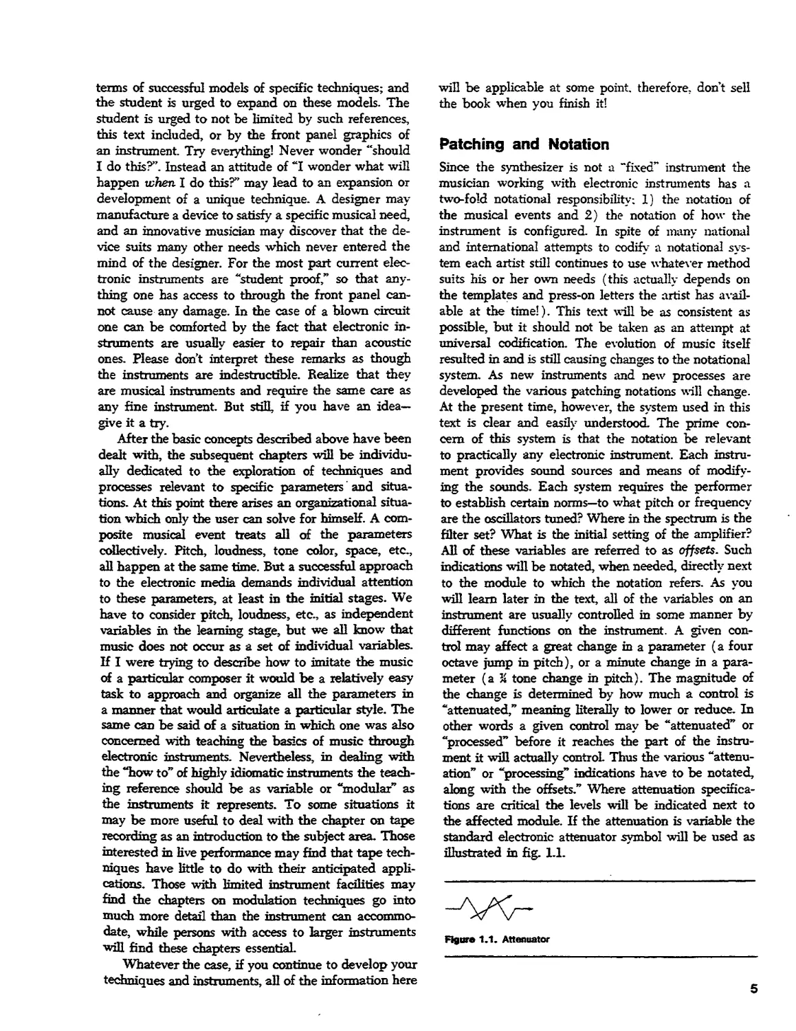
Hgw* 1.2. Notations! symbols
Many central devices generate botn
voltages and various types Of timing pulses
(triggers iM gates} Tne function 01 eacn
voltage will be indicated by "V" tor
voltage, "t" <or trigger and "pate"
keyboard
«-L_
Keyboard. Specialized keyboard produced
voltages will be indicated as "P" tot
portamento and "Pf tor pressure
I V t Envelope Generator. SpeoaKied AR.AOSR
EG I tunetioos will be mdieated where neeaed.
OOOOO
\*.
o
Clock. The one symbol win be used to identify any device capable of
generating Mng pulses (tnggers and/or gates). The dene* may be
a dedicated dock, timing parse generator OTPG) or low-treqoeney
oscillator OFO). Where a specne device is ruaaad it wig ee ao
S/H i— Sample and Mow or Track and mow (T/M)
CONTROL VOLTAGE PROCESSORS:
m some cases an ampBair a, eaea to
| VCA^> control the strengrri at a cemtci voltage.
The normal VCA symbol win be used,
s h-
Voltage Summer or rawer. On a
> same oreart as
the audo signal meter.
Figure 1.2 illustrates the symbology for the basic
devices found on electronic instruments. Although some
of these terms may mean absolutely nothing at this
point they are illustrated here because you •will
encounter them all very soon. Any specialized or unusual
device encountered in a patch will be clearly
identified in the diagram. Throughout this text there are
several patch charts which are designed by the
manufacturer for specific commercial instruments. Where
needed a patch diagram of the chart indications is
given so configurations may be transferred from
instrument to instrument
6
2 Considerations of
the Basic Parameters
of Sound
The purpose of this chapter is to give the reader a
basic understanding of the technical side of the
subject matter and to provide a point of departure for
those who wish to rearrange the chapter order to suit
their particular situation. Basic musical parameters are
understood by all musicians; we relate to the basic
variables of pitch, rhythm, loudness, timbre, etc.,
inasmuch as they are constantly under our control in
conventional performance practices on acoustic
instruments. Simultaneous control of relevant parameters is
a skill developed through dedicated practice, and such
control is a learned tactile response to some stimulus-
be it a notated phrase, a conductor's direction, or one's
own internal musical sense. Terms such as "more
legato," "more articulate," "richer," "funkier," "straigh-
ter," etc. are adjectives or adverbs that call for
alterations in almost all the ongoing parameters. To play
"dirtier" or "cleaner" calls for alterations in pitch,
loudness, articulation, and so on. This sort of response is
a skill learned as a single performance variable through
long term training that deals with simultaneous
attention to many individual variables. We are
traditionally taught to alter our playing response (i.e., style,
techniques . . . whatever word is applicable) in
reaction to a single stimulus. If the playing is not
correct it usually means that many variables have to be
altered m various degrees. When adjusting to a
"baroque" manner of playing, a trained performer almost
instinctively makes the proper adjustments without
really thinking about all of the variables be is
dealing with; his prime stimulus is die total musical sound.
As pointed out in the previous chapter, the one
function that really characterizes electronic media for
the musician is parametric thinking. We are
consciously and separately attending to many different
parameters. One must individually, yet simultaneously, be
aware of and in control of pitch, (an oscillator),
dynamics and rhythm (an amplifier), timbre (usually
a filter), and a host of other variables still to be
introduced. Taking care of all of these things at one time
is a sizable chore, both mentally and physically. One
aid in this task is the ability to view all the variables
as a single concept. For example, a certain situation
may call for a fuller, louder sound. Loudness is a
parameter which has several contributing factors (as do
all the parameters), but in terms of the physics
involved it means ending up with more acoustic energy
reaching the ear. In one case an increase in loudness
may require turning up an amplifier. In another case
it may involve decreasing the amount of mechanical
reverberation, and in still another situation it may
require a change in the timbral quality of the sound.
All of these operations in turn involve a change in
how the instrument is behaving, the end result being
an increase in the energy that reaches the ear. Thus
the musician is ultimately concerned with different
manners of vibration.
Vibrations and Musical Sound
The production of any kind of sound, musical or
otherwise, is due to rapid vibration of some object. With
acoustic instruments a string, reed, membrane, etc.,
is forced into vibration and this causes its immediate
surrounding air space to similarly vibrate. When these
vibrations ultimately reach our ear they are perceived
as sound. The characteristics of a particular sound are
largely, but not exclusively, dependent on the
manner in which the vibrating object is behaving. The
object's physical structure, how fast it vibrates, how
forcefully it vibrates, and several other factors,
determine the final sonic characteristics that object is
responsible for. Musical performance techniques can be
thought of as actions applied to an instrument
(inputs) which affect how that instrument vibrates. A
trumpet player may press a valve to change the
vibration rate of air in a metal tube; the same player blows
harder to increase the force or amplitude of those
vibrations. A string player changes finger placement on
a string to change that string's vibration rate and
simultaneously may press harder or softer with the bow
to affect the amplitude of that vibrating string (its
loudness). A mute placed across the bridge of a violin
or in the bell of a trumpet is another performance
7
input that changes the way the instrument responds,
and tins has various effects on tone quality. Many
musical parameters involve the generation and alteration
of vibrations.
Anything that vibrates within a certain frequency
range and with enough force has the potential of
being a sonic event If you happen to be sitting in a
room with fluorescent lighting at this moment you
will probably be able to hear a faint pitch around the
area of Bj>. Florescent lights actually turn on and off
at a rate of 120 times each second; this vibration rate
is fast and strong enough to be perceived as a
definite pitch. The device which helps produce the image
on a home television screen scans back and forth on
the picture tube at a rate of 15,730 times each
second, producing a very high pitch. This fast frequency
can be very annoying to persons with sensitive hearing.
Musical pitches we refer to with letter names such as
BJ>, F, Cf, etc. actually describe different rates of
vibration. The standard tuning reference for
instruments in America assigns to middle"A" a vibration rate
of 440 times each second. Every musical pitch refers
to a specific rate of a vibrating string, tube,
membrane, electronic circuit, etc.
Sound is multi-dimensional One cannot perceive
pitch without perceiving a sensation of loudness, tone
quality, duration, and apparent source. Pitch is fairly
easy to deal with because we have some well defined
references; consequently it has been the most
accessible musical parameter for the composer. Loudness
is less clear, since there are not as many well defined
limits and references. Loudness is perceived primarily
as the result of how much or how forcefully something
is vibrating. Stated a little differently, loudness is the
result of how much air is displaced by the vibrating
object Blowing softly into a clarinet will produce a
soft sound. Blowing harder into the instrument causes
die reed to vibrate with more energy, resulting in a
greater amount of air being displaced in the immediate
environment, and hence a louder sound. Loudness
does have a specific unit of measurement called the
decibel; this will be discussed in chapter 9.
Timbre, or tone quality, is partly determined by
the pattern of vibration. A string, when bowed,
vibrates in a particular way producing the sound of a
bowed string. A plucked string has a markedly
different sound. It may be vibrating at the same rate and
with the same energy as the bowed string, but its
manner or pattern of vibration is different Fitch,
loudness, and timbre are terms we assign to different
aspects of a vibrating object Pitch refers to rate,
loudness to perceived energy, and timbre, in part, refers
to the pattern of vibration.
AH of the foregoing analogies have been in terms of
familiar acoustic instruments, and transferring these
ideas to electronic instruments is a simple matter.
Electricity is a source of energy that can be specified
and controlled. Through various types of circuit
designs and controls, electricity can cause objects,
usually speaker cones, to vibrate in specified ways. One
can design a circuit to produce energy fluctuations at
certain rates, amplitudes, and patterns. When these
fluctuations are transmitted to a speaker cone the
speaker transfers these vibrations into the air, and
from that point the sound takes essentially the same
path to our ear as any other sound. Once the
electrically generated signals have become translated into
airborne vibrations their behavior is independent of
the sound source. Electronic sound is only "electronic"
in terms of generation and control. The generation
and control of sound on electronic and acoustic
instruments have conceptual similarities—a sensitive
cellist is continually concerned with how fast, how hard,
and in what pattern the strings are vibrating. The
musician relates to electronic instruments in precisely the
same manner; he is concerned with telling the
electronic circuits how fast to produce energy changes,
the amount of energy to be transmitted, as well as
the various shapes and patterns of energy changes
produced by the electronic circuitry.
Musical Structure and
Temporal Measurements
AH musical processes can ultimately be defined as
temporal pressure variations perceived by the ear. The
mind's ear is continually making measurements and
comparisons of information on multi-dimensional
levels. On one level we may observe the length of a
composition, movements, or phrases. Such long term
measurements are usually spoken of as form. On
another level we measure the durations of and intervals
between individual notes and call that rhythm. On
still another level we measure the number of air fronts
moving past our ear in order to establish the identity
of a single pitch or composite sound. On another
dimension a stronger or more forceful vibration will
usually be perceived as a louder sound than a weaker
vibration. The parameter of timbre is indeed
enigmatic and eludes precise definition. As mentioned
before, timbre is related to the maimer in which an
object vibrates, but this is only one of several
contributing factors in timbral identities. Such
complications are subsequently elaborated in cited
references.1 For the present we may accept the statement
that timbre is a dynamic parameter subject to an
infinitude of changes or variations in time.
1. For further reading in the area of musical timbre refer to
Robert Eridkson's Sound Structure in Music, University of
California Press, 1975.
8
Although perhaps premature at the time in terms
of available technology, the theories of Karlheinz
Stockhausen during the middle 1950s, merit
consideration by the practitioners of electronic music, if not
for all media. Stockhausen's writings detail the
previously mentioned idea that long durations of time
(macro-time) contain musical forms; shorter temporal
variations contain phrases or motifs, while still smaller
temporal divisions enter the realm of rhythm. A
rhythm, if increased to about 18 times a second,
begins to be perceived as a pitch (micro-time).
Continuing with this same manner of thinking, a higher pitch
(faster rhythm?) enters a perceptual domain
providing some, but not a!, information about timbre. Stock-
hausen's theories imply that form, phrase, rhythm,
pitch, and timbre are all the workings of a single
system—vibrations or variations.
"The musical organization is carried into the
vibrational structures of the sound phenomena. The sound
phenomena of a composition are an integral part of this
organization and are derived from the laws of structure:
namely, that the texture of the material and the
structure of the work should form a unity; and the microtonal
and macrotonal form of the work have to be brought into
a conformity that accords with the basic formal idea
which every singie composition has."2
The amount of energy or force behind any of the
vibrating domains influences loudness. It is notable
that this energy affects each of these perceptual
domains in the same manner. We will learn that
increased energy in the higher frequencies will alter the
parameter of timbre; increased relative energy between
18 and about 17,000 times a second results in louder
pitches; energy variations below 10 or 15 times a
second affect the dynamics of rhythm (accents), phrases,
and formal contrasts.
All musical instruments-are dedicated to file
production of variations in air pressure at various rates,
with forces, and in differing patterns. A vibrating
string, reed, lip, or membrane ultimately results in a
sensation we hope will be of musical interest.
Assuming that the listener is perceiving sound in an acoustic
space we know that the air is conveying the
vibrations to our ears from some vibrating source like a
string, reed, lip, or membrane (such as a speaker cone
as is the case with most electronic instruments).
2. Quoted by Sejppo Heikialjeimo in The Electronic Music of
Karlheinz Stockhausen (Studies on the Esthetical and Formal
Problems of its First Phase). (Bryn Mawr, Penna., Acta Mus-
icologia Fennica, Theodore Presser Co., 1972) p. 15 from
Teste zur elektronischen tend instrumentdlen Musik (Volume I)
by Stockhausen.
Non-Linear Perception
Most human sensory perception is non-linear. A
physiological response such as hearing or sight is not
directly proportional to the stimulus (sound or light)
causing that response. Non-linearity means that equal
changes in some stimulus (vibration rate, intensity.
etc.) do not result in equal changes in perception
(pitch, loudness, etc.).
Pitch is the result of a given rate of change or
vibration of some physical object—in this context a
speaker cone. A vibration of 65.4 vibrations per
second, or Hertz (abbreviated Hz) registers the pitch
sensation of low C. By doubling that frequency to 130.8
Hz the C an octave above will be heard The next
octave C, middle C is 261.6 Hz, or four times the
original low C. Note that between CL> and C3 there
is a difference of 65.4 Hz (130.8 - 65.4 = 65.4), but
between C and middle C there is a difference of 130.8
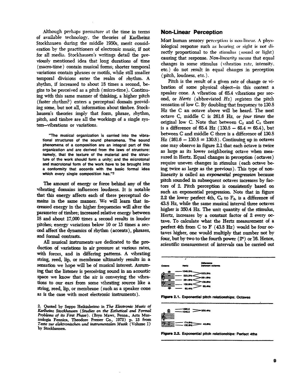
Hz (261.6 - 130.8 = 130.8). Continuing up in octaves
one may observe in figure 2.1 that each octave is twice
as large as its lower neighboring octave when
measured in Hertz. Equal changes in perception (octaves)
require uneven changes in stimulus (each octave
being twice as large as the previous). This type of non-
linearity is called an exponential progression because
pitch sounded in subsequent octaves increases by
factors of 2. Pitch perception is consistently based on
such an exponential progression. Note that in figure
2J2 the lower perfect 4th, C3 to F3, is a difference of
43.8 Hz, while the same musical interval three octaves
higher is 350.4 Hz. The unit quantity of the stimulus,
Hertz, increases by a constant factor of 2 every
octave. To calculate what the Hertz measurement of a
perfect 4th from C to F (43.8 Hz) would be four
octaves higher, one would multiply that number not by
four, but by two to the fourth power (2*) or 16. Hence,
scientific measurement of intervals can be carried out
Wiwhi
Figure 2.1. Exponential pitch relationships: Octaves
Figure 22. Exponential pitch relationships: Perfect 4ths
in Hertz, but in terms of our ears' response, higher
intervals contain more Hertz than identical musical
intervals in lower octaves.
Changes in loudness are due to perceptions of the
change of physical strength or amplitude of vibration.
The more energy contained in the air fronts moving
past our ears, the louder the perceived sound. Like
pitch, the perception of loudness is also non-linear.
Loudness is measured in units called decibels
(abbreviated db); this is the smallest unit of noticeable
loudness difference the ear can detect. The decibel is
usually used as a measurement of relative loudness
between two events. If 1 db is assumed to be the softest
possible sound, then 60 db would represent the
loudness level of a normal conversation at a distance of
about three feet However, a db level of twice that
figure, 120 db, is not twice that loud, but 1,000 times
as loud!5 For the mathematically minded the decibel
equals 20 log™ P1/P2. PI and P2 are the two
difference levels being compared. At this point it is only
necessary to realize that the decibel is a non-linear unit
of loudness measurement- perceived equal changes in
loudness taking more energy at louder levels.4
Subjective and Objective Measurement
The perception of vibrations may be dealt with either
subjectively or objectively. An objective measurement
would be the observation of such vibrations against
a precisely calibrated measuring device, and under
every condition that same rate of vibration would al-
3. Some common decibel relationships to keep in mind are
6 db = 2:1, 10 db = 3d, 20 db = 10:1, 40 db = 100:1,
60 db = 1,000:1. See Appendix II for a decibel chart.
4. Burke, A. Oscar, "The Decibel: Basics" DBS, No. 3 (March
1974) pg. 24. The reader is referred to this article for a good
layman's study of the decibel.
ways measure the same. For example, speaking of
pitch in terms of Hertz is an objective measurement
A = 440 Hz is an objective statement because the
reference, a period of 1 second, is not variable. When,
however, these vibrations are forced through a variety
of media (around comers, through walls) under a
variety of conditions (different loudnesses, timbres,
etc.) the subjective measurement, what we actually
perceive and register, may not agree with the
objective measurement. It is not the intent of this book
to dealve into a detailed study of psycho-acoustics, but
it is important for die musician to realize that there
is a difference between objective and subjective
measurements.5 Objective appraisement involves
measurements against a consistent norm: subjective
appraisement is a perceptual measurement which can be
influenced by many variables. Frequency is an
objective measurement, but pitch is a subjective
measurement Frequency is objectively measured in Hertz, and
pitch is subjectively measured in musical intervals
such as thirds, fifths, octaves, etc., or in specific pitch
references such as Bfc and C%. Amplitude is an
objective measurement of the subjective phenomenon we
call loudness. Amplitude may be measured as voltage
levels, and loudness may be measured hi terms of
decibels or traditional musical dynamics such as piano
and forte. In some cases decibels may be objectively
measured with various types of meters, but speaking
practically, the db is a measurement of what we hear.
The various conditions that alter our subjective
perceptions will be discussed in situations where those
variables can be put under some sort of controL
5. For further reading in the area of psycho-acoustic musical
phenomena the reader is referred to Joan G. Roederer's
Introduction to the Physics and Psychophysics of Music (New York,
Springer-Vedag), 1973.
10
3
Electronic Sound
Sources and Their
Characteristics
Logically, the production of a musical event begins
with the generation of an initial sound. The performer
provides certain information to the instrument, and
the instrument responds by producing a characteristic
and often musically raw sound. This can be
demonstrated by listening to a beginning player on any
instrument. The basic sound is modified by the
physical properties of instrument and also by additional
performance nuances supplied by the player. This
process applies with equal accuracy to botfi electronic
and acoustic instruments.
Although any sound can be modified and disguised
almost beyond recognition, its initial characteristics
will suggest applicable modifications in terms of the
desired result. If an orchestrator or arranger wants a
delicate, shimmering effect more than likely he will
not begin with a tuba! A major skill required of
electronic instrument composers and performers is
orchestration. Obtaining the desired result is dependent on
beginning with the most effective source. Professional
electronic instrument programmers1 must be aware of
the physical and sonic characteristics of the basic
electronic sounds before- beginning to add the subtle
nuances and processing called for by the producer or
performer.
Voltage and Sound
As the fiddler s bow hairs force the violin string and
sounding board to vibrate and cause die air pressure
in that string's environment to fluctuate, electrical
voltage causes the paper or metal cone of a loudspeaker
to vibrate—again resulting in variations in air pressure.
Electric current is a measurement of the flow of
electric energy. Voltage is the force that causes the
current to flow through a wire. Although voltage and
current are measurements of two different electric
activities they are mutually related. At this point it is
1. A programmer is a musician responsible for "making the
patch" on the instrument for a performer. People such as Mike
Boddicker and Ian Underwood are highly respected
programmers and are successful due to their ability to work quickly
and efficiently in the studio.
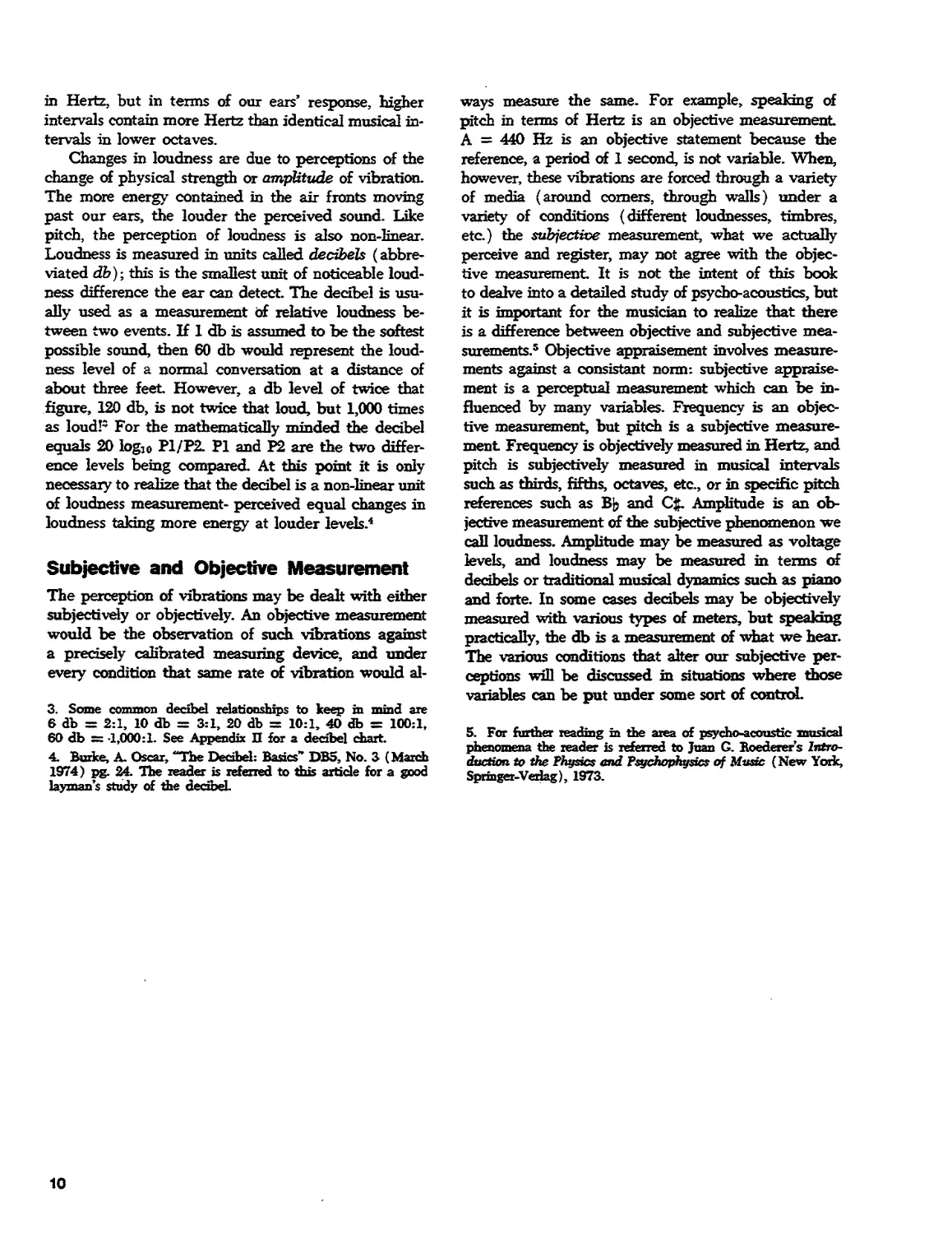
Figure 3.1. Speaker cone movement
not really necessary to distinguish between the two.
If a speaker cone is connected to an alternating
current, certain physical changes take place. When no
voltage is applied to the speaker, the speaker cone is
in a neutral position (fig. 3.1A). When a "positive"
voltage is applied to the speaker, the cone is pushed
outward (fig. 3.1B) and then, as the positive voltage
decreases, returns toward its original position. As a
"negative" voltage is applied to the speaker, the cone
is pulled back to a point opposite the positive voltage
position of the speaker (fig. 3.1C).
Every time the speaker cone is moved by the
alternating current—AC (positive, passing through a
neutral position, negative, and again passing through a
neutral position) masses of air or pressure waves are
moved past our ear, producing the sensation of pitch.
If die speaker cone is moved back and forth 440 times
in one second, for example, we hear a sound which
is commonly referred to as "tuning A." If the cone
moves back and form at a rate of 261.6 times a
second, we perceive a pitch of "middle C Each back-
and-forth movement caused by the application of a
positive voltage followed by a negative voltage is
referred to as a "cycle,** or a "Hertz." Therefore, 440
Hertz (Hz) produce "tuning A."
The volume, loudness, or amplitude of a sound is
determined basically by how far the speaker cone is
moved back and forth on its neutral axis, which is
a result of the voltage level of the AC. If an
alternating current hypothetically displaces a speaker cone
1/4 inch in each direction from its neutral position
11
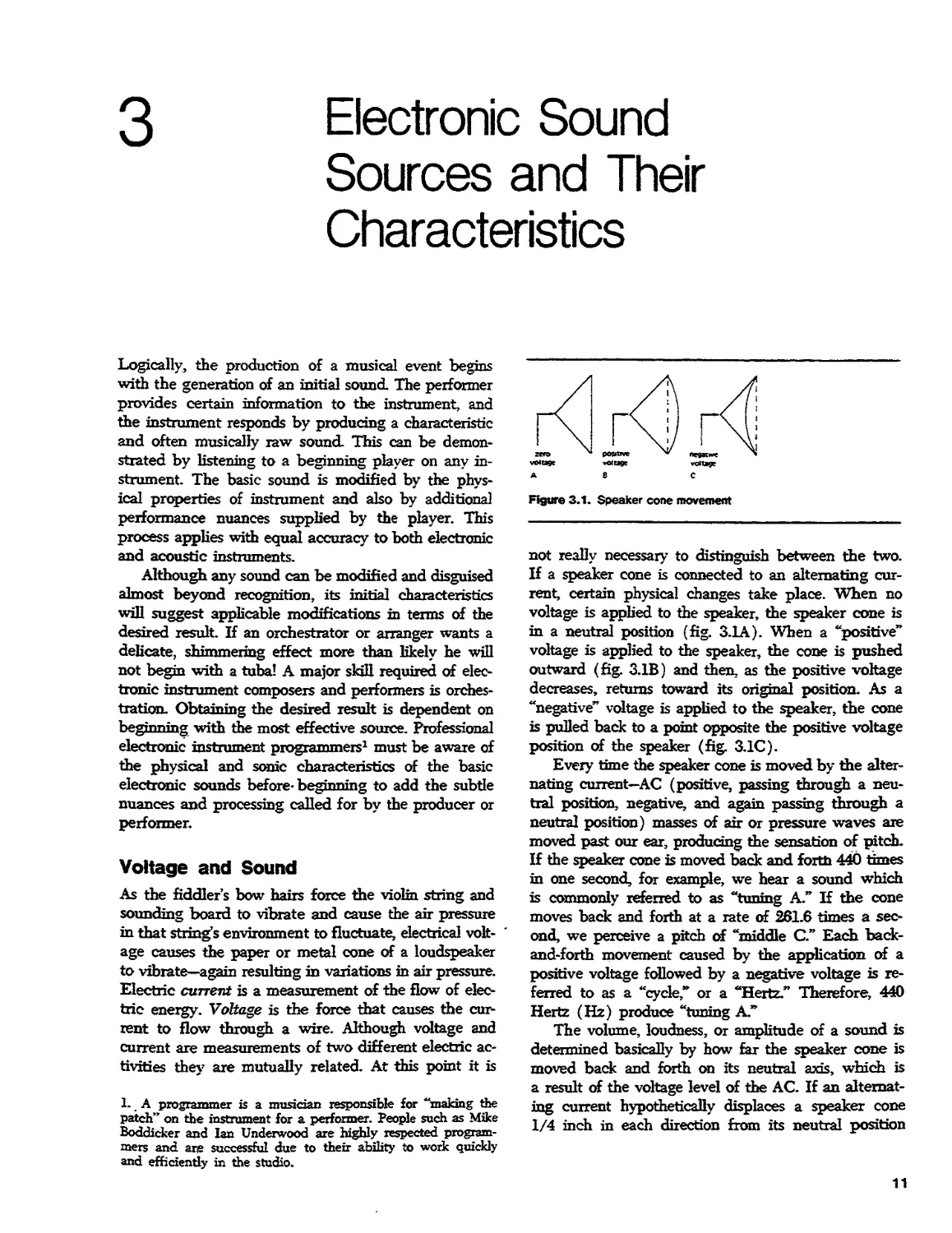
v^-inc* cone di»!3cer>enT 1-2 -»ncr* cone aisDt»«ine«i
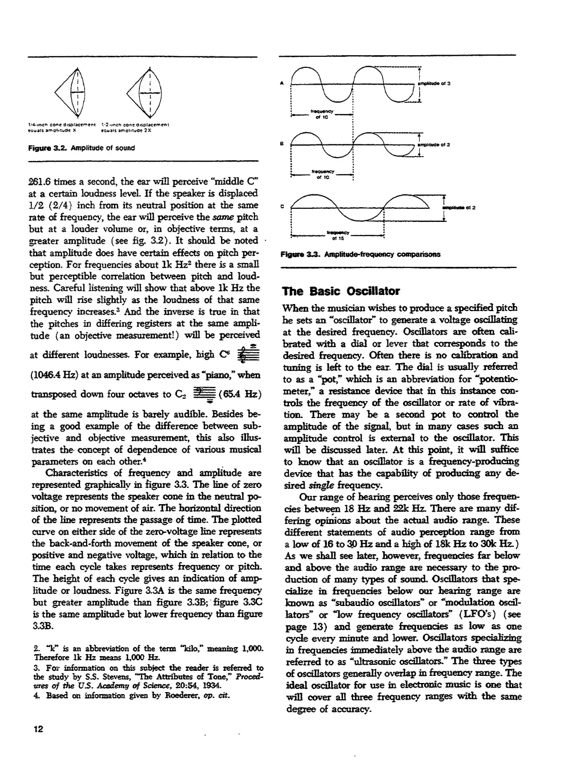
Figure 3.2. Amplitude of sound
261.6 times a second, the ear will perceive "middle C
at a certain loudness level. If the speaker is displaced
1/2 (2/4) inch from its neutral position at the same
rate of frequency, the ear will perceive the same pitch
but at a louder volume or, in objective terms, at a
greater amplitude (see fig. 3.2). It should be noted
that amplitude does have certain effects on pitch
perception. For frequencies about Ik Hz2 there is a small
but perceptible correlation between pitch and
loudness. Careful listening will show that above Ik Hz the
pitch will rise slightly as the loudness of that same
frequency increases.3 And the inverse is true in that
the pitches in differing registers at the same
amplitude (an objective measurement!) will be perceived
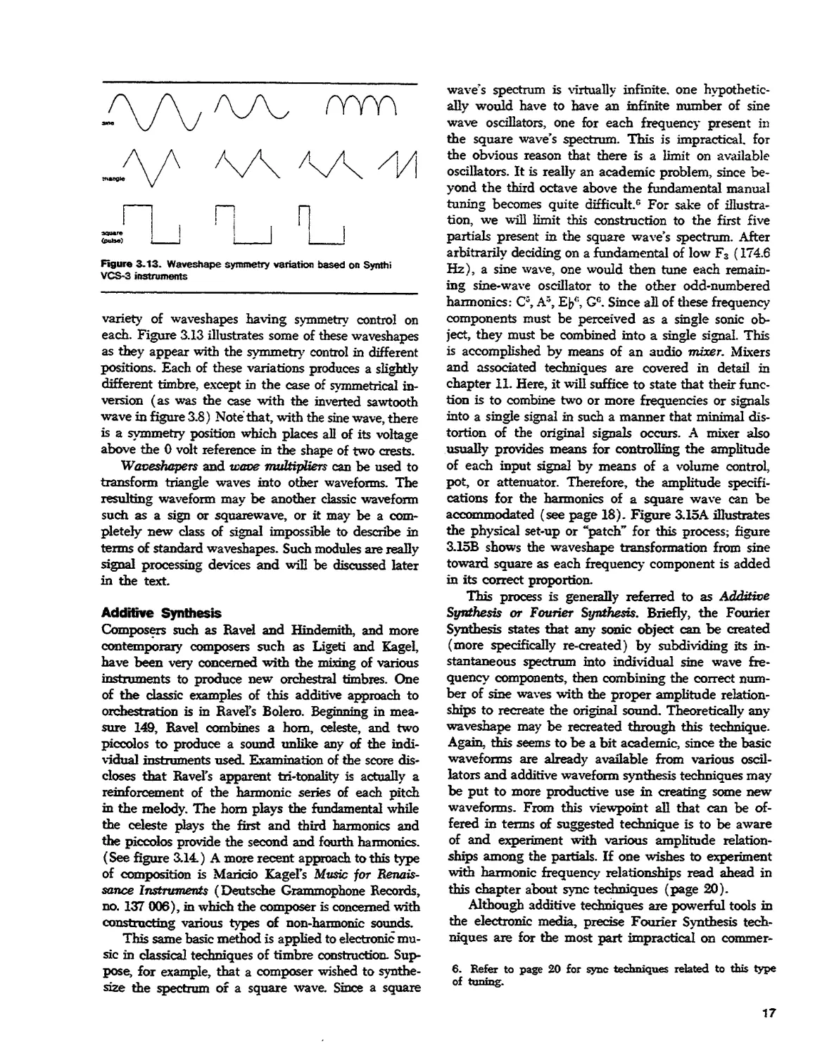
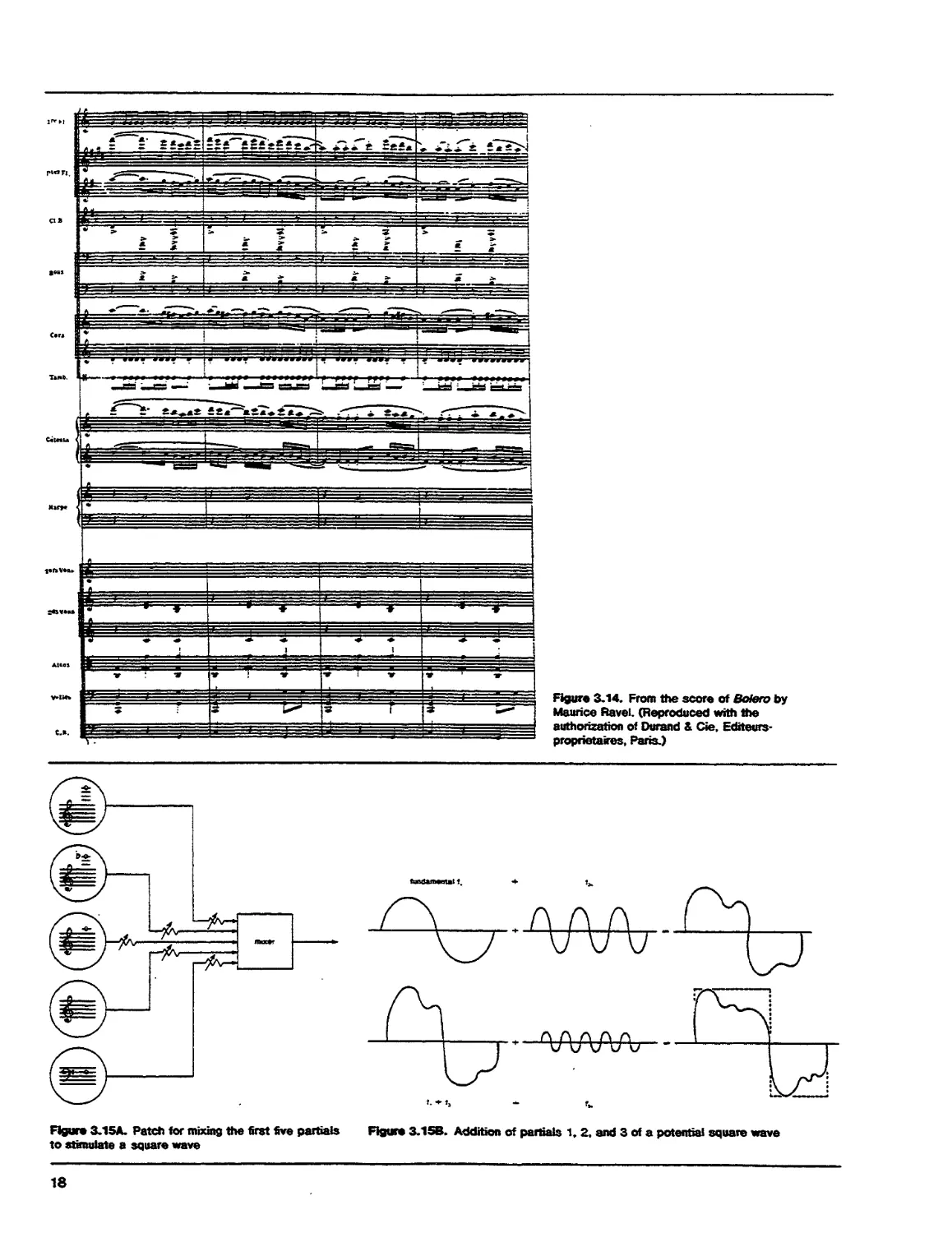
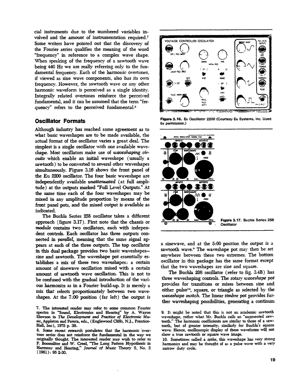
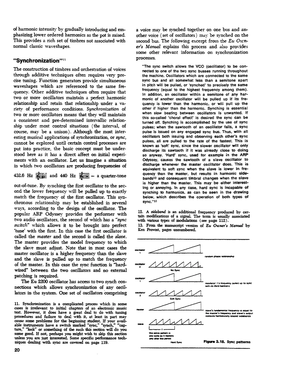
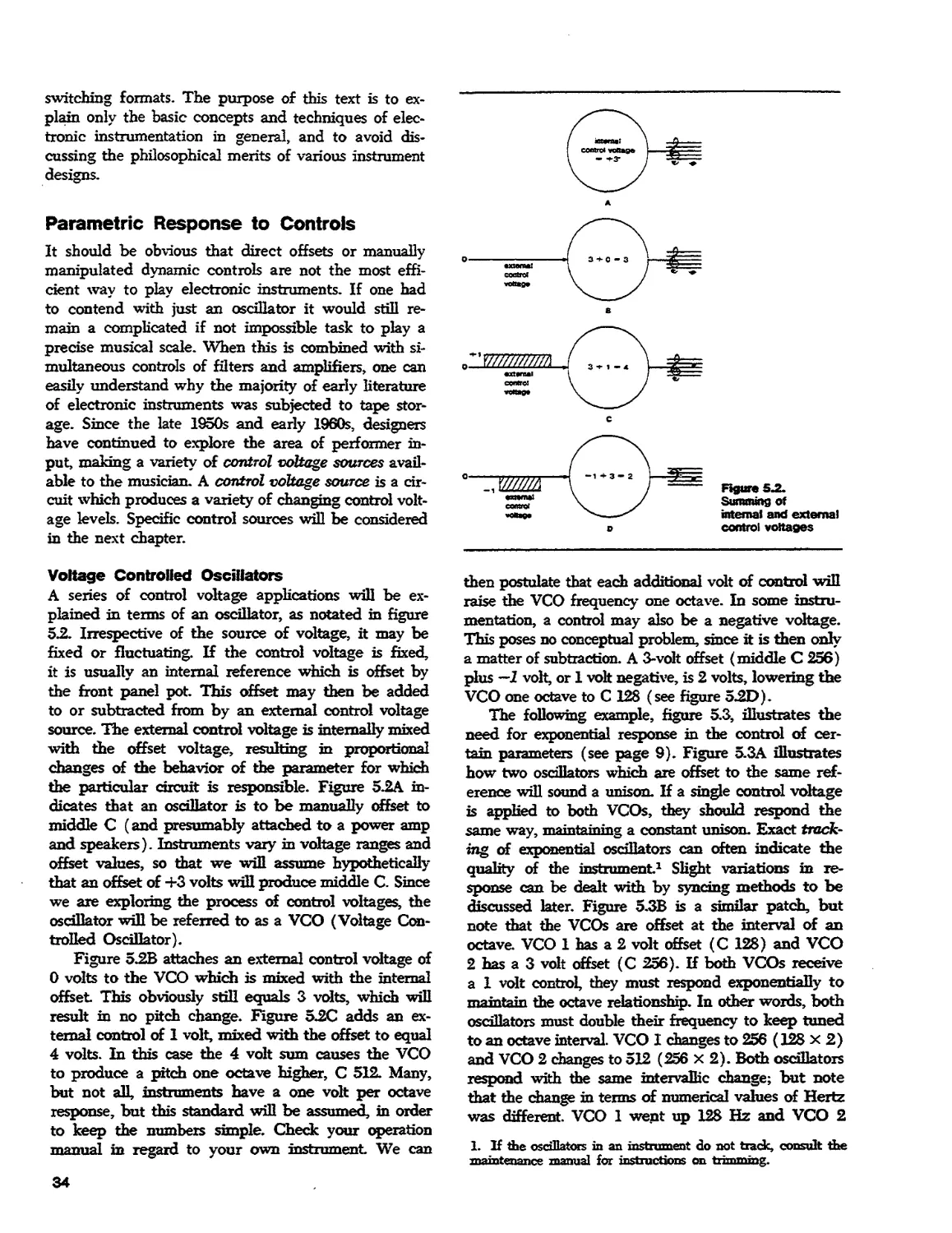
at different loudnesses. For example, high C5
(1046.4 Hz) at an amplitude perceived as "piano," when
transposed down four octaves to C2 ?" _ (65.4 Hz)
at the same amplitude is barely audible. Besides
being a good example of the difference between
subjective and objective measurement, this also
illustrates the concept of dependence of various musical
parameters on each other.4
Characteristics of frequency and amplitude are
represented graphically in figure 3.3. The line of zero
voltage represents the speaker cone in the neutral
position, or no movement of air. The horizontal direction
of the line represents the passage of time. The plotted
curve on either side of die zero-voltage line represents
the back-and-forth movement of the speaker cone, or
positive and negative voltage, which in relation to the
time each cycle takes represents frequency or pitch.
The height of each cycle gives an indication of
amplitude or loudness. Figure 3.3A is the same frequency
but greater amplitude than figure 3.3B; figure 3.3C
is the same amplitude but lower frequency than figure
3.3B.
2. "k" is an abbreviation of the term "kilo," meaning 1,000.
Therefore Ik Hz means 1,000 Hz.
3. For information on this subject the reader is referred to
the study by S.S. Stevens, "The Attributes of Tone,"
Procedures of the VS. Academy of Science, 20:54, 1934.
4. Based on information given by Roederer, op. cit.
of 15
Figure &3. Amplitude-frequency comparisons
The Basic Oscillator
When the musician wishes to produce a specified pitch
he sets an "oscillator' to generate a voltage oscillating
at the desired frequency. Oscillators are often
calibrated with a dial or lever that corresponds to the
desired frequency. Often there is no calibration and
tuning is left to the ear. The dial is usually referred
to as a "pot," which is an abbreviation for
"potentiometer,'' a resistance device that in this instance
controls the frequency of the oscillator or rate of
vibration. There may be a second pot to control the
amplitude of the signal, but in many cases such an
amplitude control is external to the oscillator. This
will be discussed later. At this point, it will suffice
to know that an oscillator is a frequency-producing
device that has the capability of producing any
desired single frequency.
Our range of hearing perceives only those
frequencies between 18 Hz and 22k Hz. There are many
differing opinions about the actual audio range. These
different statements of audio perception range from
a low of 16 to 30 Hz and a high of 18k Hz to 30k Hz.)
As we shall see later, however, frequencies far below
and above the audio range are necessary to the
production of many types of sound. Oscillators that
specialize in frequencies below our hearing range are
known as "subaudio oscillators*' or "modulation
oscillators" or low frequency oscillators'' (LFO's) (see
page 13) and generate frequencies as low as one
cycle every minute and lower. Oscillators specializing
in frequencies immediately above the audio range are
referred to as "ultrasonic oscillators.'' The three types
of oscillators generally overlap in frequency range. The
ideal oscillator for use in electronic music is one that
wiD cover all three frequency ranges with the same
degree of accuracy.
12
Figure 3.4A. Moog 921 Oscillator (Courtesy of Root. A. Moog.
Moog Music'. Used by permission.)
Figure 3.4A is the front panel of the Moog 921
oscillator with rotary pots and 3.4B is the Buchla 208
oscillator with linear or slide pots. Some performers
prefer the slide pots as they give a more graphic
indication of the produced pitches—the higher the knob
the higher the pitch; rotary pots have the advantage
of higher "setability."
With the first and second generation electronic
music oscillators there was often a trade-off between
sweep range and stability. An oscillator with a single
continuous range from 5 to 20k Hz might suffer from
lack of accuracy and drift (uncontrollable pitch
variations). To minimize this problem some oscillators are
designed to have their total range divided into octaves
by a calibrated switch, such as the Moog 921 in figure
3.4A. In this case, the octaves are indicated in "feet,"
taking a cue from standard organ terminology. The
exact pitch within each octave can then be
manually determined by the frequency control. This
particular oscillator has the additional capability of serv-
Figure 3.4B. Buchla 208 Oscillator
ing as a sub-audio oscillator by setting the "coarse
range" switch to "sub-audio." "Coarse-range" refers to
a very broad operational range. In the case of the Moog
921 the two course ranges available are .01 Hz (one
cycle every 100 seconds) to 400 Hz and 1 Hz to 40k
Hz. Other oscillators may have ranges calibrated in
Hertz. The Electro-Comp EML-200 has six switchable
ranges: .01 Hz, .1 Hz, 1 Hz, 10 Hz, 100 Hz and Ik
Hz. The Buchla 258 oscillator is a single sweep
oscillator with a range from about 2 Hz to 20k Hz (this
range is extended through the application of external
controls). Fine tuning may be accomplished by means
of a small pot known as a trimmer. The Synthi VCS-3
provides a single sweep oscillator with a range from
1 Hz to 10k Hz, calibrated with numbers from 1 to
10. In this case fine tuning is done by means of a
ten-turn rotary pot. This means that the pot can be
completely rotated 10 times—one complete rotation
covering only 1/10 of its total range. This is
advantageous in the sense that it provides more .manual
precision when trying to pin-point exact pitches. One
possible disadvantage is that the ten-turn format takes
slightly longer to offset manually to a different
register.
While on the subject of pitch precision a word
about oscillator drift may be in order. In the "Ice Age"
of electronic music systems (the early 1960s) there
5. Offset is a tenn refening to the establishment of the initial
state or reference of a particular parameter. This will be
covered in detail in chapter 5.
13
was a great deal of criticism of voltage controlled
oscillators for not holding a set pitch accurately for
extended periods of time. Formerly musicians either used
a different oscillator or composed around the problem.
In newer instruments drift has been minimized to an
almost insignificant degree. It is my own opinion that
electronic musical instruments are still musical
instruments, and any musical instrument requires tuning.
One should not really expect an oscillator to hold its
reference pitch in a performing situation to any greater
degree than one would expect a violin, flute, or
trumpet to hold a pitch in the same situation (although
many of the available electronic instruments do have
great stability and will stay exactly in tune for long
periods of time). At the same time we realize that with
any instrument, including electronic ones, pitch will
not be stable until it is sufficiently warmed up. Leave
ample time for the instrument to be turned on and
left in the environment in which it will be used. Some
studios make a practice of leaving the instruments on
continually. Unless there is tube circuitry in the
instrument this should not cause any problems with
over-heating and the practice will add to the stability
of the system.
Basic Waveshape and Spectra
Before exploring some specific oscillator formats it is
necessary to learn the relationship between various
patterns of generated audio voltages or tcavesliapes,
sound spectrum, and the aural experience.
Manufacturers have come to some agreement as to the basic
"orchestra1* of commercial electronic music instruments,
and the-waveshapes to be discussed here are common
to most instruments. If we trunk of vcaveshape as the
graphic representation of the rise and fall of voltage
from zero to a maximum positive and/or negative and
back again, it is possible to identify basic
electronically generated sounds by their shape. There is a direct
relationship between the visual and sonic quality of
a sound. Nearly all sounds exhibit a spectrum or a
collection of many individual frequencies which
combine to make a single aural event. In striking a gong
it is possible, by careful listening, to isolate aurally
the multitude of pitches which make up the total
complex sound of this instrument. Most instruments
produce sounds which consist of many combined
frequencies called overtones or partials.
Gongs, bells and other percussive instruments
display unusual spectra where apparently there is no
consistent relationship between the frequency components
or partials. Most strings, brasses, reeds, and certain
electronically generated sounds, however, display a
predictable spectrum based on a rather simple
concept Any vibrating source is capable of the excitation
of generation of additional frequencies. The standard
14
classroom method of observing this is to silently
depress middle C4 on the piano and strike C3 an octave
below. One will hear middle C ring out as it has been
forced into vibration by the lower octave C3. This
type of forced vibrtion is called sympathetic vibration
and demonstrates that one vibrating system has the
potential of generating other vibrations.
It is an observed fact that nature accomplishes
things in the easiest and most efficient manner. The
easiest way we have of expressing simple
relationships is in terms of integers, or whole numbers (1,
2, 3, etc.) The most common type of excitation in
vibrating systems also occurs at whole-number
intervals. A low C» of 65.4 Hz is capable of generating
twice that frequency, 130.8 Hz (the octave Qor2x
65.4 Hz), the multiplier "2" being the first integer
above 1 (the unison). The same vibration of 65.4 Hz
is also capable of generating 196.2 Hz (3 x 65.4),
which is the pitch G3, a perfect 12th above the original
frequency. The process of multiplying a basic
frequency by whole numbers could continue ad
infinitum. Most sounds made by what we call "traditional''
musical instruments exhibit a spectrum containing
frequencies related by whole numbers. This type of
spectrum is called the harmonic overtone series and is
illustrated in part in figure 3.5. The lowest frequency of
this spectrum is called the fundamental and is the
generator of the series—each overtone being an integral or
whole number multiples of the fundamental The
overtones are, in this case, harmonic, referring to the fact
that each is an integral multiple of a single
fundamental frequency, forming a consistent system of
relationships one with another. The term "harmonic,"
for my purposes, does not refer to the obvious
progression of whole numbers, but rather to the fact that
there is a consistent relationship between the
numbers, irrespective of the nature of the consistency or
simplicity. They are "in harmony" with each other
due to a consistent relationship. By this definition
there can be other harmonic relationships built on
systems other than whole number multiples; this idea
will be further .explored in chapter 8 (see page 114).
In the meantime we will retain the tradition of
"harmonic" referring to whole number relationships.
There is often confusion as to the precise
definition of the terms overtone, partial and harmonic. For
die purposes of this text overtone will refer to any
frequency component in a spectrum above a given
fundamental. If the overtone bears an integral
relationship to the fundamental it will be called a
harmonic overtone, or just a harmonic. There is also
occasional confusion about the term harmonic, and the
confusion arises from differentiation between harmonic
and harmonic number. If one uses or assumes the
term harmonic number, the series begins with the
fundamental as harmonic #1, the octave then being
harmonic #2 and so on. On the other hand, the term 1st
Figure 3.5. Hannonic series
harmonic usually refers to the first integral multiple
above the fundamental or the octave. The 2nd
harmonic is the second integral multiple (the perfect 12th)
above the fundamental, etc. This text will use the
former practice of harmonic numbers, the fundamental
being 1, the octave being hannonic #2, the 12th being
harmonic #3, and so on. This is perhaps the more
logical, since the harmonic number then agrees with
its integral multiple (harmonic #1 is fundamental
times 1; harmonic #2 is the fundamental x 2,
harmonic #3 is the fundamental X 3, etc.). The term
partial refers to specific spectral content irrespective
of harmonic or non-harmonic relationships. And as
will be seen, certain sounds contain only selected
overtones. A clarinet, for example, has a spectrum
containing only odd-numbered harmonics (the fundamental,
3rd, 5th, 7th, etc.). In this case, the fundamental is the
first partial, and due to the lack of a scoend harmonic,
the 3rd harmonic is actually the second partial, the
5th is the third partial and so on. This garble of terms
is clarified by figure 3.6.
To a certain extent the overtone content of a sound,
be it harmonic or non-harmonic, provides us with its
aural signature or timbre. There are other factors
which contribute significantly to tunbral perception.
The loudness of a sound, the manner in which the
sound is activated and the manner in which it stops
vibrating, the relative amplitude of the overtones, etc.,
all play an important part in timbral recognition and
these factors will be explained as their control
techniques are introduced.
Perceptually, or perhaps even aesthetically die most
noncomplex type of sound is the sine wave. This
particular waveshape contains no overtones. The closest
sound to a pure sine wave in a symphony orchestra is
that of a flute. As is shown in figure 3.7 the voltage
is in a particular state of motion. Starting at zero, it
gradually increases to maximum positive, then decays
through zero to maximum negative, then returns to the
original starting place.
A sine wave exhibits this same pattern
independently of frequency or amplitude. Figure 3.7B shows
the same frequency as figure 3.7A but with an
increased amplitude. The device that electronically
produces sine waves is referred to as a sine-wave oscillator.
Sine waves, like any other waveshapes, can exist in
any frequency range. Due to distortions caused by
various components of the oscillator and/or distortions
in the reproduction equipment, however, a precise sine
(rondtflWAtftt)
Figure 3.6. Harmonics vs. partiais
X7
Figure 3.7. Sine waves
wave is very difficult to generate, and the composer
usually has to settle for something less. It is the
observation of this writer that a pure sine wave used
as an audio signal is not an especially monumental
musical sound and a bit of hannonic distortion (very
small traces of additional harmonic content) may add
to the incipient musicallity. Various manufacturers
publish the amount of harmonic distortion of their
sine wave oscillators along with other instrument
specifications. An imperfect waveshape used as an audio
signal can be accepted, and may often prove to be
more musically interesting than the textbook model.
Figure 3.8 is an oscilloscopic (graphic)
representation of a sawtooth or ramp wave. In contrast to die
pure sine wave, a sawtooth wave contains all
harmonic overtones of the fundamental frequency. These
harmonic overtones have relative amplitudes that
decrease exponentially as they exist higher up in the
harmonic series. A sawtooth oscillator will produce this
basic waveshape in any frequency range. Note that
figure 3.8A is symmetrically inverse of 3.8B and is
often referred to as an inverted sawtooth. Both are
legitimate sawtooth waves and, in spite of the reverse
position of the leading edge, will sound the same. The
sawtooth wave is very bright and piercing, somewhat
like the sound of an oboe or violin.
B*tfWfTOti SaWtOOth
Figure 3*8. Sawtooth waves
15
A third basic waveshape is the triangle or delta
wave (fig. 3.9). This waveshape consists of a
fundamental frequency and all of the odd-number
harmonics, with amplitudes falling off in ratios of 1/9,
1/25, 1/49. etc. By using a classic studio technique of
"additive synthesis," it is possible to construct a
triangle wave (or any other waveshape) by using a
specific collection of different sine waves. Starting
with a fundamental of C (65.4 Hz) with a hypothetical
amplitude of x, a second sine wave tuned to 65.4 Hz
times 3 (for the second overtone) is added (196.2 Hz)
with an ampiltude of 1/9 X. Then a third sine wave
which is the fifth multiple of the fundamental (327
Hz) is added with an amplitude of 1/25 X. The
composer continues this process until all of the necessary
harmonics with the correct amplitudes are present If
the amplitudes of the harmonics are thought of in
ratios, it is easy to understand how the perceived
harmonic content of any given wave is dependent on the
amplitude of the fundamental.
Perhaps the waveshape that is most commonly used
by the composer is the pulse or rectangular wave. As
shown in figure 3.10, the positive and negative
voltages of a pulse wave are never in a transient state.
They are instantaneously positive, then
instantaneously negative, whereas the sine, sawtooth and triangle
waves all exhibit various types of gradual rise and fall
between positive and/or negative states. If a pulse
generator is programmed to osculate anywhere below 7
to 10 Hz, the speaker cone can be heard snapping
back and forth.
Figure 3.10 shows a particular type of pulse wave
known as a square wave. A square wave is related to
a triangle wave in that it also contains odd-numbered
harmonics, but with quite different amplitude
relationships. The amplitude relationships of the harmonics of
a square wave are 1/3, 1/5, 1/7, 1/9. etc. A clarinet
in the chalumeau register produces a sound that is
very close to that of a square wave. Figure 3.11
illustrates in standard musical notation the harmonic
content of the four basic waveshapes. The relative
amplitudes are indicated by the size of the note. Note that
there are no even numbered harmonics in any of the
symmetrical waveforms.
Due to the many uses of the square wave, it is
thought of as a basic waveshape, even though it is
a variety of a pulse wave There are many other types
of pulse waves, and they are defined by what is known
as their "duty cycle." The duty cycle of a pulse wave
is the positive or "on" portion of the entire cycle.
Figure 3.12 shows the duty cycle of two different pulse
waves.
The duty cycle determines the harmonic content
of the waveshape. In the case of the square wave, the
duty cycle is one-half of the total wave, or a ratio of
1:2 (as in fig. 3.12A). Expressed as a fraction, the
16
Figure 3.9. Triangle wave
Figure 3.10. Pulse or rectangular (square) wave
Bwwe swtootftwive irofiglew**
Figure 3.11. The four basic waveshapes and their harmonic
content (up to the 9th multiple)
1:2dutveveit
l:3*rtyeyel«
! B
Figure 3.12. Pulse-wave duty cycles
duty cycle of a square wave is one-half of the total
wave, and it is the denominator of this fraction that
tells us its harmonic content The denominator "2"
indicates that every second harmonic is absent from its
harmonic overtone series, confirming die earlier
statement that the square wave consists only of a
fundamental and the odd-numbered harmonics. A pulse
wave with, a duty cycle of 1:3 (as in fig. 3.12B)
contains the fundamental and the first, second, fourth,
fifth, seventh* eighth, tenth, etc., harmonics. In other
words, the denominator is an indicator of what order
harmonics are absent from the spectrum. Oscillators
designed for use in electronic music systems may have
controls or pots marked pulse width, duty cycle,
symmetry or tcaveform adjustment. Pulse width and duty
cycle refer specifically to pulse waves and may vary
the "on" portion of the wave from 10% to 90S or more
of the total cycle.
Waveform adjustment or symmetry are variations
which are possible with any waveshape. For example
the Synthi VCS-3 provides three oscillators with a
aqove |
<pube) ( I i I ' '
Figure 3.13. Waveshape symmetry variation based on Synthi
VCS-3 instruments
variety of waveshapes having symmetry control on
each. Figure 3.13 illustrates some of these waveshapes
as they appear with the symmetry control in different
positions. Each of these variations produces a slightly
different timbre, except in the case of symmetrical
inversion (as was the case with the inverted sawtooth
wave in figure 3.8) Note that, with the sine wave, there
is a symmetry position which places all of its voltage
above the 0 volt reference in the shape of two crests.
Waveshapers and wave multipliers can be used to
transform triangle waves into other waveforms. The
resulting wavefonn may be another classic wavefonn
such as a sign or squarewave, or it may be a
completely new class of signal impossible to describe in
terms of standard waveshapes. Such modules are really
signal processing devices and will be discussed later
in die text.
Additive Synthesis
Composers such as Ravel and Hindemith, and more
contemporary composers such as Ligeti and Kagel,
have been very concerned with the mixing of various
instruments to produce new orchestral timbres. One
of the classic examples of this additive approach to
orchestration is in Ravel's Bolero. Beginning in
measure 149, Ravel combines a hom, celeste, and two
piccolos to produce a sound unlike any of die
individual instruments used. Examination of the score
discloses that Ravel's apparent tri-tonality is actually a
reinforcement of the harmonic series of each pitch
in the melody. The hom plays the fundamental while
the celeste plays the first and third harmonics and
the piccolos provide the second and fourth harmonics.
(See figure 3.14) A more recent approach to this type
of composition is Maricio Kagel's Music for
Renaissance Instruments (Deutsche Grammophone Records,
no. 137 006), in which the composer is concerned with
constructing various types of non-harmonic sounds.
This same basic method is applied to electronic
music in classical techniques of timbre construction.
Suppose, for example, that a composer wished to
synthesize the spectrum of a square wave. Since a square
wave's spectrum is virtually infinite, one hypothetic-
ally would have to have an infinite number of sine
wave oscillators, one for each frequency present in
the square wave's spectrum. This is impractical, for
the obvious reason that there is a limit on available
oscillators. It is really an academic problem, since
beyond the third octave above the fundamental manual
tuning becomes quite difficult/' For sake of
illustration, we will limit this construction to the first five
partials present in the square wave's spectrum. After
arbitrarily deciding on a fundamental of low F3 (174.6
Hz), a sine wave, one would then tune each
remaining sine-wave oscillator to the other odd-numbered
harmonics: C5, A5, Ej>fl, Gc. Since all of these frequency-
components must be perceived as a single sonic
object, they must be combined into a single signal. This
is accomplished by means of an audio mixer. Mixers
and associated techniques are covered in detail in
chapter 11. Here, it will suffice to state that their
function is to combine two or more frequencies or signals
into a single signal in such a manner that minimal
distortion of the original signals occurs. A mixer also
usually provides means for controlling the amplitude
of each input signal by means of a volume control,
pot, or attenuator. Therefore, the amplitude
specifications for the harmonics of a square wave can be
accommodated (see page 18). Figure 3.15A illustrates
the physical set-up or "patch" for this process; figure
3.15B shows the waveshape transformation from sine
toward square as each frequency component is added
in its correct proportion.
This process is generally referred to as Additive
Synthesis or Fourier Synthesis. Briefly, the Fourier
Synthesis states that any sonic object can be created
(more specifically re-created) by subdividing its
instantaneous spectrum into individual sine wave
frequency components, then combining the correct
number of sine waves with the proper amplitude
relationships to recreate the original sound. Theoretically any
waveshape may be recreated through this technique-
Again, this seems to be a bit academic, since the basic
waveforms are already available from various
oscillators and additive waveform synthesis techniques may
be put to more productive use in creating some new
waveforms. From this viewpoint all that can be
offered in terms of suggested technique is to be aware
of and experiment with various amplitude
relationships among the partials. If one wishes to experiment
with harmonic frequency relationships read ahead in
this chapter about sync techniques (page 20).
Although additive techniques are powerful tools in
the electronic media, precise Fourier Synthesis
techniques are for the most part impractical on commer-
6. Refer to page 20 for sync techniques related to this type
of tuning.
17
i«c»vm»
Figure 3.14. From the score of Bolero by
Maurice Ravel. (Reproduced with the
authorization of Durand & Cie, Editeurs-
proprietaires, Paris.)
fandanwoul 1.
- r\AN\f\j -
I.* t,
Figure 3.15A. Patch for mixing the first five partials
to stimulate a square wave
Figure 3.15B. Addition of partials 1.2. and 3 of a potential square wave
18
cial instruments due to the numbered variables
involved and the amount of instrumentation required.7
Some writers have pointed out that the discovery of
the Fourier series qualifies the meaning of the word
"frequency" in reference to a complex wave shape.
When speaking of the frequency of a sawtooth wave
being 440 Hz we are really referring only to the
fundamental frequency. Each of the harmonic overtones,
if viewed as sine wave components, also has its own
frequency. However, the sawtooth wave or any other
harmonic waveform is perceived as a single identity.
Integrally related overtones reinforce the perceived
fundamental, and it can be assumed that the term
"frequency" refers to the perceived fundamental.*
Oscillator Formats
Although industry has reached some agreement as to
what basic waveshapes are to be made available, the
actual format of the oscillator varies a great deal. The
simplest is a single oscillator with one available
waveshape. Most oscillators make use of waveshaping
circuits which enable an initial waveshape (usually a
sawtooth) to be converted to several other waveshapes
simultaneously. Figure 3.16 shows the front panel of
the Eu 2200 oscillator. The four basic waveshape are
independently available unattenuated (at full
amplitude) at the outputs marked "Full Level Outputs." At
the same time each of the four waveshapes may be
mixed in any amplitude proportion by means of the
front panel pots, and the mixed output is available as
indicated.
The Buchla Series 258 oscillator takes a different
approach (figure 3.17). First note that the chassis or
module contains two oscillators, each with
independent controls. Each oscillator has three outputs
connected in parallel, meaning that the same signal
appears at each of the three outputs. The top oscillator
in this dual package provides two basic waveshapes-
sine and sawtooth. The waveshape pot essentially
establishes a mix of these two waveshapes: a certain
amount of sinewave oscillation mixed with a certain
amount of sawtooth wave oscillation. This is not to
be confused with the gradual introduction of the
various harmonics as in a Fourier build-up. It is merely a
mix that selects proportionately between two
waveshapes. At the 7:00 position (far left) the output is
7. The interested reader may refer to some common Fourier
spectra in "Sound, Electronics and Hearing" by A. Wayne
Slawson in The Development and Practice of Electronic
Music, Appleton and Perera, eds., (Englewood Cliffs, N.J., Prentice-
Hall, Inc), 1975 p. 38.
8. Some recent research postulates that the harmonic
overtone series does not reinforce the fundamental in the way we
originally thought. The interested reader may wish to refer to
P- Boomsliter and W. Creel, "The Long Pattern Hypothesis in
Harmony and Hearing," Journal of Music Theory 5, No. 2
(1961): 95 2-30.
VOLTAGE CONTROLLED OSCILLATOR
o o
BUS
»
in;
^T^W'A^-g^^-A'WBWWWW^**1^1
Figure 3.16. Eu Oscillator 2200 (Courtesy Eu Systems. Inc. Used
by permission.)
SUM OKULATO* «OOM >U
6>7^e> e^^e fcJ^p^" Figure 3.17. Buchla Series 258
® « - Oscillator
a sinewave, and at the 5:00 position the output is a
sawtooth wave." The waveshape pot may then be set
anywhere between these two extremes. The bottom
oscillator in this package has the same format except
that the two waveshapes are sine and square.
The Buchla 208 oscillator (refer to fig. 3.4B) has
three waveshaping controls. The rotary icavesliape pot
provides for transitions or mixes between sine and
either pulse10, square, or triangle as selected by the
tcaveshape switch. The linear timbre pot provides
further waveshaping possibilities, generating a continum
9. It might be noted that this is not an academic sawtooth
waveshape, rather what Mr. Buchla calls an "augmented
sawtooth." The harmonic coefficients are similar to those of a
sawtooth, but of greater intensity; similarly for Buchla's square
wave. Hence, osdlloscopic display of these waveforms will not
show a true sawtooth or square wave image.
10. Sometimes called a spike, this waveshape has very strong
harmonics and may be thought of as a pulse wave with a very
narrow duty cycle.
19
of harmonic intensity by gradually introducing and
emphasizing lower ordered harmonics as the pot is raised.
This provides a rich set of timbres not associated with
normal classic waveshapes.
"Synchronization"1 '
The construction of timbres and orchestration of voices
through additive techniques often requires very
precise tuning. Function generators provide simultaneous
waveshapes which are referenced to the same
frequency. Other additive techniques often require that
two or more oscillators maintain a perfect harmonic
relationship and retain that relationship under a
variety of performance conditions. Synchronization of
two or more oscillators means that they will maintain
a consistent and pre-determined intervallic
relationship under most control situations (the interval, of
course, may be a unison). Although the most
interesting musical applications of synchronization, or sync,
cannot be explored until certain control processes are
put into practicer the basic concept must be
understood here as it has a direct affect on initial
experiments with an oscillator. Let us imagine a situation
in which two oscillators are producing frequencies of
432.6 Hz jfhjjr and 440 Hz ^y=57 — a quarter-tone
out-of-tune. By synching the first oscillator to the
second the lower frequency will be pulled up to exactly
match the frequency of the first oscillator. This
synchronous relationship may be established in several
ways, according to the design of the oscillator. The
popular ARP Odyssey provides the performer with
two audio oscillators, the second of which has a "sync
switch" which allows it to be brought into perfect
'tune' with the first. In this case the first oscillator is
called the master and the second is called the slave.
The master provides the model frequency to which
the slave must adjust. Note that in most cases the
master oscillator is a higher frequency than the slave
and the slave is pulled up to match the frequency
of the master. In this case the sync function is
"hardwired" between the two oscillators and no external
patching is required.
The Eu 2200 oscillator has access to two synch
connections which allows synchronization of any
oscillators in the system. One set of oscillators comprising
11. Synchronization is a complicated process which in some
cases is irrelevant to initial chapters of an electronic music
text. However, it does have a great deal to do -with tuning
procedures and failure to deal with it, at least in part may
cause some problems for the beginning student. If your
available instruments have a switch marked "sync," "synch,"'
"capture," "lock" or something of the such mis section will do you
some good. If not, perhaps you might wish to skip this section
unless you are just interested. Some specific performance
techniques dealing with sync are covered on page 119.
a voice may be synched together on one bus and
another voice (set of oscillators) may be synched on the
second bus. The following excerpt from the Eu
Owner's Manual explains this process and also provides
some other relevant information on synchronization
processes.
"The sync switch allows the VCO (oscillator) to be
connected to one of the two sync busses running throughout
the machine. Oscillators which are connected to the same
sync bus and all somewhat less than a semitone apart
in pitch will be pulled, or 'synched' to precisely the same
frequency (equal to the highest frequency among them).
In addition, an oscillator within a semitone of any
harmonic of another oscillator will be pulled up if its
frequency is lower than the harmonic, or will pull up the
other if higher than the harmonic. Synching is essential
when slow beating between oscillators is unwanted. If
this so-called 'choral effect' is desired the sync can be
turned off. Synching is accomplished by the use of sync
pulses; when the sawtooth of an oscillator falls, a sync
puise is issued on any engaged sync bus. Thus, with all
oscillators both issuing and observing each other's sync
pulses, all are pulled to the rate of the fastest. This is
known as 'soft' sync, since the slower oscillator will only
discharge its sawtooth if it was already close to doing
so anyway. 'Hard' sync, used for example in the ARP
Odyssey, causes the sawtooth of a slave oscillator to
discharge whenever the master oscillator does. This is
equivalent to soft sync when the slave is lower in
frequency than the master, but results in harmonic
sidebands1- and consequent timbral changes when the slave
is higher than the master. This may be either
interesting or annoying. In any case, hard sync is incapable of
synching to harmonics, as can be seen in the drawing
below, which describes the operation of both types of
sync."i-"
12. A sideband is an additional frequency produced by
certain modifications of a signal. The term is usually associated
with various types of modulations (see page 112).
13. From the manuscript version of Eu Owner's Manual by
Ken Provost, pages unnumbered.
random phase muHioasnip
SvASv^A/W
NO Sync
osaaeior Is frequency puued up to syne
with its tntrd harmonic
•IXlXlXIXlXl
Sen Sync
,/I^XUxlXl^U
slave's fundamental frequency a coital to
the master's frequency and slave's output
contains harmonically related sioeeends
-1 •
this enftro pattern is
one cycle as it repasts
ooty after tfw penod
Hard Sync
Figure 3.18. Sync patterns
20
It is not the purpose of this text to give a detailed
description of every instrument A glance at the front
panel of any oscillator will usually reveal its format;
and specific questions are usually answered in the
owner's manual or spec sheet. This brief exposure to
oscillators and some common formats should provide the
reader with enough information to approach any
oscillator with at least some meaningful questions, and
may also serve as a guide for some applications of
whatever format oscillator is available at the time.
White Sound
The last electronic sound (as differentiated from many
other sounds available through transducers such as
microphones, prerecorded tapes and discs, etc.) to be
considered is white sound, or white noise (also
sometimes referred to as Gaussian or thermal noise).
Perhaps the most descriptive term is "white sound."
Analogous to a color wheel that produces the color white
as the wheel is rapidly rotated, white sound is a
mixture of all the audible frequencies at random
instantaneous amplitudes. Therefore, the term "white" is
preferred over "Gaussian"—and rJbe present writer
prefers the use of "sound" because of the negative
implications of the term "noise." White sound is heard as
a hiss or as the sound of a jet engine. White sound
is defined as having equal energy per unit frequency.
This means that there is the same amount of energy
between 500 Hz and 501 Hz as there is between 1500
Hz and 1501 Hz. Equal energy per unit frequency
means that the noise is spectrally flat. Another type
of sound common to most electronic music instruments
is "pink sound." Just as with white sound, pink sound
contains all the frequencies of the audio spectrum,
but its energy distribution or amplitude curve is
different. Pink sound contains equal energy per octave
and is often represented as -7- and referred to as
being musically flat. It may be obvious to the reader that
tihe term 'pink sound' is a logical color analogy as it
refers to the lower end of the light spectrum; in terms
of perception pink sound simply has more bass or
rumble (see figure 3.19). Taking a cue from these
color analogies one could easily construct color
representations for any number of noise bands. "For
example, boosting the higher end of the spectrum may
produce what one could call blue or azure sound, while
a spectrum with a boosted mid-range might even be
green! These terms are by no means representative of
spectral standards but may serve as convenient
terminology for describing different types or bands of sound.
Electronic instruments provide noise coloration in
various ways. The Synthi VCS-3 instruments control
noise spectra by means of a pot marked "colour" with
r
white sound
pink sound
J "--'
1HS 16Mr
frequency
Figure 3.19. White and pink sound
the far left and right positions appropriately marked
"low" and "high," and the middle straight up position
assuming to be spectrally flat white sound. The Buchla
Source of Uncertainty Model 265, among other things,
provides three independent noise outputs. The output
labeled "HI" is what has been defined as white sound.
The middle unmarked output provides pink sound and
the output labeled "LOW" is a type of noise which
is the musical inverse of the frequency distribution
found in white sound. As explained, white sound has
equal energy per unit frequency, while pink sound has
equal energy per octave. If the white sound spectrum
is measured in octaves one will see that there is
actually an increase of 3 db per octave. Buchla's noise
resources establish musically flat pink sound as the
norm with "HT having a 3 db increase per octave
and "LOW* having a 3 db decrease per octave. Some
manufacturers refer to white sound, pink sound, etc.,
simply as random signal generators (such as the Moog
903A Random Signal Generator). The term 'random*
is used because the amplitudes of the various
frequencies at any given instant are random and must
be measured over a certain time period in order to
calculate an average measurement. In other cases the
term 'random noise' refers to extremely low random
frequencies (around 15 Hz and lower); it is not
audible but rather is used as a control for random musical
events (see page 83).
Thus far, only the basic types of sound sources and
some typical formats have been discussed. It is
essential that the reader understand how sound can be
thought of as AC voltage, and that these voltages can
be shown graphically on an oscilloscope (as they are
represented in the various figures used in this book).
Since the scope of this writing does not permit the
discussion of every type of sound available to the
composer, we have given the four basic waveshapes—sine,
sawtooth, triangle, and pulse—and the concept of white
sound. An understanding of these is all that is needed
for a basic understanding of electronic music system
operation.
21
4 Basic Signal Processing:
Amplifiers and Filters
It is now time to return to music as set of dynamics—
not merely dynamics in terms of loudness, but rather
a more general view of simultaneous variability of
co-existing parameters. Most musical events involve
fluctuation, on many different levels of frequency,
amplitude, and timbre. Other parameters such as
space, rhythm, etc., can really be conceived of in terms
of these basic three parameters and will be discussed
as various forms of control are introduced.
Composition and performance with electronic instruments
demand that one make decisions and enforce controls
(which may range from totally determinant or
completely random) on these parameters. Failure to do
so, at least in the initial stages of learning, can lead
to frustrations, the most serious of which is the dread
of every electronic music novice, silence! As one will
discover, the production and control of electronic
sound is usually an evolutionary process. One module
generates the sound, one module imposes controls on
frequency, another controls amplitude, still another
controls spectral content, etc. Failure to understand
any one of these generation and control processes in
the chain, will ultimately result in a discrepancy
between the original musical concept and the final
musical result
The shaping of musical events involves various
processes dealing initially with frequency, amplitude,
and timbre. The realm of frequency variation and
waveform should be basically understood by this point.
Before embarking on a study of precise control
procedures one should understand the basic processes of
amplitude and timbral variation in terms of voltage
and waveform variation. An electronic circuit operates
only in terms of voltages (shapes and amplitudes). The
musician must be able to think in these same terms
to communicate his musical needs to his instrument.
Conceiving of a musical event or structure is only
the beginning. The musician working in the electronic
medium then must translate his concept to a language
understood by his instrument This chapter deals with
the parameters of loudness control through amplifiers
and various aspects of timbre through filtering. Again
the emphasis is placed on what each circuit is doing
to the electronic signal
Amplification and Gain
With the existence of a multi-million dollar home hi-
fi/stereo industry the term amplifier and its concept
is familiar, at least in part, to almost everyone. An
amplifier, of course, amplifies! Technically this means
that it is a device which increases some externally
generated voltage. Earlier, it was explained that voltage
levels, or the degree of excursion that a waveshape
exhibits, determines the loudness of a signal. This
degree of excursion, or amplitude, is a musical variable
that is usually spoken of as loudness (loudness being
a subjective measurement of amplitude). The
musician working in the electronic media deals with
amplification on several different levels. Sounds—more
specifically, signals produced by electronic
instruments—are quite low in magnitude. The exact strength
of an audio signal from an oscillator varies with each
manufacturer. Systems on the market today have
output voltages anywhere from 1 to 10 volts.1 These
voltages carry with them a variable called impedance,
which is a measurement of electrical resistance,
measured in units called ohms (ft). It would be unneces-
sairly confusing to attempt a detailed discussion of
impedance at this point. For those interested, the
output impedance in most electronic instruments and
studios is usually between 600 and Ik ohms. If this
is meaningless to you, either forget about it for now
or ask a technician. The point is that these signal
levels coming out of most electronic instruments are
not strong enough to drive a speaker cone- Hooking
an oscillator directly to a speaker will produce little,
if any, sound—certainly not enough to be of any real
musical use. Therefore, one must raise the voltage
level, or waveshape excursion, to such a magnitude
that it can efficiently drive a speaker cone And this
must be done without changing the original frequency
or waveshape. The device used to accomplish this is
a power amplifier. The power amp is not an integral
part of the electronic instrument but certainly is a
major factor when it comes to the final sounds. The use
1. This information is usually gives on the instrument's
specification sheet Because of voltage variations It is not
advisable to interconnect instruments made by different companies
without first checking the voltage and impedance levels.
22
•itiplited
sagnai
Figure 4.1. Amplification and gain
of power amps will be discussed in the consideration
of live performances (chapter 15); but, for the present,
it will suffice to say that their function is to take a
line-level signal (about 1.4 volts) from an electronic
instrument and boost it to a level that has enough
energy to efficiently move a speaker cone (see figure
4.1). '
Voltage Controlled Amplifiers
It is certainly redundant to say that loudness is a
dynamic variable for the musician. However, the
effective use of loudness variations requires a bit more
detailed understanding of what is involved with
amplification in electronic instruments. The amplifier of
most concern to the musician is called a voltage
controlled amplifier (VCA), sometimes referred to as a
gate. At this point we need not be concerned with the
"voltage controlled" aspect of this module, and
therefore this discussion will be limited to manual or hands-
on front panel control. The VCA provides gain. This
is a word which has been used before and refers to
the amount of voltage an amp provides. If a signal
goes in to a circuit at a peak-to-peak reading of 1
volt (see figure 4.1B) and comes out at a peak-to-pealc
reading of 2 voks the amp is said to have a gain of 2.
If the signal comes out at 0 volts (silence) the gain
is 0. The amount of gain, under manual control,
depends on the setting of the gain pot, gain offset or
volume control. When you raise the gain offset the
output voltage is increased and you hear a stronger
signal from the speaker. In electronic musical
instruments it is common for the VCAs to have a gain of 1,
or unity gain. This tends to be a bit confusing because
with unity gain there is no voltage increase. The
signal goes in. and if the gain offset is at maximum, the
output signal has the same magnitude as the input
signal. An amplifier with unity gain is really an
attenuator. It can produce variations in gain or
loudness not exceeding the strength of the original
signal before it was patched into the amp. The reason
for this is explained by the basic design philosophy
of electronic instruments. Each module, oscillator, amp-
plifier, etc., is a parametric building block. In some
situations certain building blocks may not be
necessary for the generation of a musical event, so that
the modules must be designed, in such a way that they
can function with or without any other module. For
example, there may be a situation where loudness is
not a variable and the signal is needed at full gain
directly from the oscillator. Therefore the amp
maybe by-passed, (see figure 4.2, oscillator A). This
"voice" may be joined by another voice that does
require loudness variations (figure 4.2 oscillator B).
Oscillator A has a constant loudness, while the
loudness of oscillator B is controlled by a VCA. If the amp
has more than unity gain, great care has to be taken
to insure that it will not overpower oscillator A which
has no gain increase. But since the amp has only unity
gain, at full output (the gain offset all the way up)
it will perfectly match the amplitude of oscillator A.
Sometimes gain is specified in decibels. Unity gain is
the same as a gain of 0 db.
If an amp is used for setting final manual levels
which do not require continuous variation, a mixer
might perform the same function with a little more
versatility. As explained previously, a mixer allows the
combination of many signals down to a single line
without any distortion of the original sounds. Adjusting the
balances on a mixer is the same as adjusting the gain
on an amplifier or set of amplifiers. It is not unusual
for mixers (and amps) to have gain, a common figure
being 6 db or a gain of 2. On a mixer the amount of
gain is initially established by the input pots. These
pots are attenuators which determine the incoming
strength of the various signals. Figure 4.3 illustrates
a mixing situation with two different input settings.
Figure 4.2- Gain variation
•■" (w^
^(w^
Figure 4.3. Gain controi in mixing2
Figure 4.3A shows two sine waves two octaves apart
mixed down to a single signal with equal gain for both
signals. Figure 4.3B illustrates a similar situation but
the lower octave C4 is attenuated. The final mix has
the same frequency components but the lower octave
is softer.
Amps used in electronic music instruments
sometimes have mixing capabilities built into the circuits.
Such is the case with the Moog 902. This module,
considering only manual control capabilities, will accept
two incoming signals and provide an eqtud mix of both
at the output The gain of the mix is 0 with the fixed
control voltage pot at 0 and unity gain with the same
pot at 10. There are also two outputs marked *+" and
"—". These two outputs are 180° out-of-phase with
each other. The Eu 2000 amplifier is of similar design
except that it has three inputs; "full level," "+" and
"—" (see figure 4.4). All three inputs are mixed
internally before the final amplification stage, which,
in this case, has a gain of 2 (6db). The inputs marked
2. ■*?$■ is an electronic symbol for a variable resistor, or pot,
which is used to affect the attenuation.
"+" and "—" have input attenuators to allow various
mix levels to be established before amplification. The
"—" input is an inverting input, as opposed to the Moog
902 inverting output. The real applications of these
inverting features will be described when dealing with
voltage control (see page 37).
Note that in figure 44 die amp has a switch marked
linear and exponential. In this case linear means that
the gain increases in exact proportion to the pot setting.
Exponential indicates that the gain increases
exponentially to the pot position; the higher pot positions give
greater gain variances. Expressed in another way,
linear means equal changes in output voltage in response
to the manual control (electrically smooth), and
exponential means equal changes in output decibels in
response to me control (perceptually smooth).
Linear control provides a consistent response throughout
the range of the amp. Exponential control means that
the amp is very sensitive to gain increases at low pot
settings, and the sensitivity decreases as the pot
setting is higher. Therefore, if one needs very delicate
balances at soft levels, he has better control in the
exponential mode. On some amps the linear/exponential
switch will make a difference where the 0 db gain
or silence occurs, in accordance with the pot position.
If no signal is passed through the amp in exponential
mode with the pot a certain setting, switching to linear
mode will result in a slight signal gain at the output
A comparison of exponential and linear response is
given in figure 45. The exponential curve is really
a decibel response, reinforcing the statement that
linear control results in equal change in voltage, and
exponential control produces equal changes in decibels.
Some instruments with linear/exponential options may
attach this function only to incoming external control
sources, and the manual control may be only linear.
If there is any question, refer to the instrument
specification sheet or instruction manual If your
instrument does,not have linear/exponential options don't
feel that you have an inferior device- Many of these
VOUAGE CONTSOUS> AMHJRER
urn
smmm.mm a
Figure 4.4- Eu 2000
Ampfifier (Courtesy of
Eu Systems, inc. Used
fay permission.}
Figure 4.5. Linear
<o and exponential
response
24
design decisions are made to increase the
compatibility with other modules in the system and are not
necessarily an indication of the instrument's quality
or potential usefulness.
If your studio or instrument facility is equipped
with Buchla 100 Series instruments you will find that
the 110 Dual Voltage Controlled Gate (another term
often used for VCAs) does not provide for manually
applied front panel gain or offset. The initial
amplification is provided by external control voltages and
the output gain is then attenuated to the desired level
by the front panel pot. If this is the case the
exercises suggested in this chapter can be done using a
Buchla 106 mixer (which has a gain of 2). The Buchla
292 Quad Gates have the manual offset control (see
page 28).
Pre-Ampiifiers
Another type of amplifier of concern to the musician
is a pre-amplifier or pre-amp. Many audio signals,
usually those generated by mechanical means such as
a phonograph or a microphone, produce signals too
weak even for the power amp. These signals are so
small that they are measured in millivolts. If one
plugged a mike directly into a power amp the
output signal would be so weak that it would not be
useful. Power amps are designed to amplify what is
referred to as a high level or line level signal. Such
signals are on the order of 1 volt at 600 ft. To get a
mike's signal up to mat level an intermediate
preamplifier is used. The low level signal is plugged into
the pre-amp, the pre-amp boosts the low level signal
up to line level, and at this point the electronic signal
can be treated as if it were the same as an oscillator
signal subject to any kind of amplitude shaping by
means of the VCA. The pre-amp will usually have
an impedance or gain control on the front panel
Various types of mikes have different strengths of
signals referenced in terms of impedance. A low
impedance, or low Z, mike has a rating of between 50
to 250 ft. A high Z mike will have a typical rating of
25k ft. Check the impedance specs for your available
mikes and see that the impedance switch on the pre-
amp is in the correct position. If the sound is muddy
or distorted this is an indication that the impedance
match is not correct Some pre-amps may have gain
switches. Such is the case with the Eu 2420 Dual Pre-
Amp (see figure 4.6). The gain positions for this
instrument are marked 20 db, 40 db, and 60 db, and
provide a gain of 10, 100, and 1000 respectively. After
the signal has been boosted by one of these factors,
the final signal is then attenuated by a level control.
Readers familiar with rock amplifiers will know
that they can plug a mike or guitar (which is also a
low level signal) directly into the amp, apparently
without the use of a pre-amp. This type of amp is
# fi
■m
UK
•■Sao* ^^
«* •
# *S
tWEi
Figure 4.6. Eu Dual Pre-Amp (Courtesy
Eu Systems, Inc. Used by permission.)
known as an integrated amplifier, and the pre-amp is
built into the general circuit and wired directly to
the power amp stage. The volume and tone controls
are part of the pre-amp stage, and the power amp
stage men amplifies the final signal. Most keyboard
oriented electronic instruments such as the popular
ABP Odyssey and Mini-Moog have two different
output signals. The high level output or line level output
is ready to be patched into a power amplifier. If this
high level signal was fed to an integrated amp one
would then be attempting to pre-amplify a signal that
is already pre-amplified. In this case the low level
output of the instrument should be used, since it can
be taken to the integrated amp and used with other
low level signals such as electric guitars, mikes, etc
Much more will be said about pre-amps and mikes;
the information given here is intended only to avoid
some possible distorted sounds during the initial stages
of exploring the instrument.
Filtering: Subtractive Synthesis and
Basic Filtering Concepts
Earlier in this chapter mention was made of additive
synthesis whereby the musician builds up waveshapes
and sound complexes by methods of mixing together
of less complex components. Another method which
takes the opposite approach is called subtractive
synthesis. As the name implies, this method involves using
a complex sound as the initial material.and removing
those frequency components that are not desired. Just
as additive synthesis can, at least hypothetically, build
up any complex from its individual sine wave
components, subtractive synthesis can, again
hypothetically, remove any number and combination of
components from a complex structure. For example, it is
possible to begin with a sawtooth wave and remove
all of the overtones, leaving only the fundamental, a
sine wave (figure 4.7A). Similarly removing all of
the even numbered harmonics would produce a
reasonable square wave (figure 4.7B). Removing only
25
\
\
\j
#=~ &== fe=
\T J^ _ 7*. JT" _ : «
C ■ «• S-
Figure 4.7.
Subtractive waveshaping
the fundamental, leaving all of the overtones, would
produce an unusual waveshape with transposed
harmonics or "half harmonics," that is, all of the
harmonic overtones are present but one octave lower
than usual (figure 4.7C). If this is confusing, think
of the 1st harmonic overtone, which is usually the
octave, being transposed down to the unison, the 12th
is now a fifth above the new fundamental, and so on.
This is an academic example and not as sonically
striking as it might seem.
Low Pass Filtering
The module that accomplishes these kinds of
transformations is called a filter. Just as an amplifier
provides control in loudness in the amplitude domain,
so also the filter provides for control in the spectral
domain. In fact one may hear a filter referred to as
a frequency selective attenuator or frequency selective
amplifier. In other words, a filter is a device that
provides gain for only selected portions of a composite
signal or spectrum. The portion of the signal which
is affected is determined by the function of the filter.
A loic pass filter, perhaps the most common of the
filters built for electronic music instrumentation, will
amplify or "pass" only those frequencies below a
specified frequency setting or cut-off (f,.).* Referring to
figure 3.11 (page 16) the original spectrum is a
sawtooth wave with a fundamental frequency of 65.4 Hz,
C3. If this signal is patched into a low pass filter with
a cut-off of somewhere between 65.4 Hz and 130.8
Hz (the octave harmonic) the filter would suppress
those frequencies above the cut-off. ideally leaving
only the fundamental frequency. If the cut-off
frequency were raised to slightly above 130.8 Hz, the
3. Sometimes called the "break" frequency.
filter output would be a structure with only the
fundamental and 2nd harmonic. Starting at the other end
of the spectnim may be more in keeping with the idea
of subtractive methods. If the fc (cut-off frequency)
of a low pass filter was set at maximum any
waveshape would theoretically pass unaltered. This is
usually not the case, since a sawtooth wave in theory has
an infinity of harmonic overtones, and the cut-off of
a filter should go infinitely high. The reality is that
these two "infinities'* may not be the same. A filter
has a limit to its high end, and an oscillator will not
produce an unlimited number of overtones. This is
easy to test. Just listen to a signal straight from the
oscillator and compare it with the same signal patched
into a low pass filter with the f«. at maximum. In
addition to some slight high frequency loss there will
probably be some coloration. Coloration refers to slight
attenuation or amplification of various parts of the
spectrum caused by the circuit. Keeping this patch,
gradually lower the fc and the upper harmonics will
be sequentially removed. Figure 4.8 illustrates this
process. Also note that as fc is lowered the edge of
the waveshape begins to round off, eventually
resulting in a smooth sine wave. The lesson to "be learned
here is that waveshapes with more crests and edges
usually indicate the presence of more frequency
components.
Details about filter response such as roU-off and
Q are best deferred to the chapter dealing
specifically with filtering, but brief mention will be made
here to introduce this concept. The below figure is
a useful example, but things usually don't happen that
efficiently. A filter cannot abruptly cut off at the
specified f<~ The fc is a selected spot where die filter has
caused a 3 db attenuation in the spectrum. The
attenuation continues from that point at a given rate, slope
or roll-off. A common figure for roll-off in a low pass
filter is 24 db per octave. This means that if our 64.5
Hz sawtooth wave was patched into a 24 db/octave
filter with a fc of 196.2 Hz (65.4 x 3), the output
would be a spectrum with the 3rd harmonic down
3 db, with the loudness decreasing as one goes higher
in the overtone series. The octave above this cut-off,
fX
K - maxmam CIO) fc - 7
le-S
le-3 ic«th»«
Figure 4.8. Low pass Uttering
26
Figure 4.9. 24 db/octave low pass fitter slope
the fifth harmonic is down 24 db and the next octave,
the 12 harmonic, would be down 48 db (see figure
4.9). Filter designs will vary with the manufacturer
and such roll-off figures are usually given on the
specifications sheet These figures will usually be
-multiples of 6 (12, 18, 24, etc.).
Q is a circuit modification that alters the effect of
a filter. The mechanics, applications, and tricks made
available with Q are covered in chapter 9. Here Q
can be explained as an additional amplification
process within the filter. If a low pass filter is set with
a cut-off of Ik Hz, any signal or spectral component
just below cut-off frequency will be amplified as the
Q is increased. Most low pass filters, such as the
Moog 904A pictured in figure 410A have a Q pot on
the front panel (in this case called regeneration). With
the Q set high, manually sweeping through a
harmonically rich waveform will make the filtering
process more obvious. Figure 4.10B illustrates what
happens to the cut-off frequency as the Q is raised.
Notice that as Q is raised the part of the spectrum just
below fc becomes proportionately louder and stronger.
At the same time the rest of the spectrum passed
through the filter becomes slightly attenuated.4 The
overall effect is the fc becomes more and more
prominent. Much more will be said about Q in chapter 9,
but for the present all we need to know is that Q
emphasizes fe and has a numerical value related to
the increase in gain at the cut-off; the higher the Q,
the higher the gain. Gain can be increased to the point
at which the filter begins to distort or "break up" the
cut-off frequency. Q can also be increased to die point
where the filter will begin to "howl" or oscillate. This
type of oscillation is a sine wave and can be useful
for certain techniques (covered in chapter 9). This
application is only mentioned here because it is an in-
4. This band-pass attenuation is not always the case and
depends on individual circuit design.
Figure 4.10A.
Moog 904A Low Pass FHter
KigriO
Figure 4.10B. Q comparisons in low pass filtering
strument variable and can result in some phantom
pitches and distortions if one is not aware of the
process. Other names for Q in addition to "regeneration"
are "resonance," "response," "emphasis" and
"feedback."
27
Other Filter Functions
Another common filter format is the High Pass Filter.
As the name implies, it accomplishes the inverse of
the low pass filter, attenuating all of the frequencies
belotc {,. and passing all of the spectral components
above ft~ Other filter formats include band pass, band
reject or notch, and the fixed filter banks, which is
a collection of band pass filters mixed to a single
output. The functions of these filters are indicated by
their descriptive names. Universal filters are single
modules which combine the four basic filter functions,
—high pass, low pass, band pass, and band reject,—
into a single instrument. Another filter variation which
may be available to the musician is what AKP
Instruments call the Filtamp. It is a very common
practice simultaneously to control the amplitude and
timbre of a signal by patching it through an
amplifier and then through a filter (see the "basic patch"
on page 29).
The Buchla 292 Quad Low Fass Gate (figure 4.11)
has similar functions. This module consists of four
independent gates, each of which has three possible
operational modes. The mode switch in the upper
position turns the gate into a low pass filter; the lower
position turns the gate into an amplifier; the middle
position, "combination,'' combines the amp and low
pass functions to provide "spectral gating"—a process
similar to simultaneous spectral and amplitude
control. In this mode, as the amplitude is lowered there
is a simultaneous loss of high frequencies. Both of
these functions occur at the same time as they share
the same offset control The audible result of this
process is a slight emphasis of the lower partials as
the gain is lowered. This is most striking when
accomplished by fast external controls (see page 35). When
doing the experiments at the end of this chapter,
notice especially what mode the gate is in. The output
of each gate is independently available, or an equal
mix of all four is available from the output marked
"all." The Buchla 200 Series instruments do not
provide a variable low pass filter as a separate module.
A common experience for the novice is to find that
the filter is blocking the sound. A signal is present at
the input but nothing comes out If this happens at
least one of three common errors is being made. First,
if the filter has mixing capabilities, as with the ARP
1006, the input attenuator may be turned down.
Second, the fc may be so high or so low that it is beyond
any spectral content present in the sound. The third,
and most common error is that one is trying to filter
a sine wave. Remember that a sine wave has only one
spectral component and therefore it is the only thing
that can be removed. This is not so obvious as it may
appear. If a filter is a frequency selective attenuator
all it can do with a sine wave is to attenuate the whole
Figure 4.11. Buchla Series
292 Quad Low Pass Gate
thing.. In this case the filter is being used as an
amplifier! This is a good thing to keep in mind when you
run out of amps, but for the present, avoid filtering
sine waves!
Just as with amps and oscillators, there are as many
filter modules as there are manufacturers. And this
portion of the present chapter is only meant as an
introduction to the low pass process and how it
affects the waveshapes, both sonicaHy and graphically.
It is important to realize that the spectral
characteristics of a signal are generally described in terms of
waveshape,—the patterns an audio electrical voltage
produces. The basic waveshapes introduced at the
beginning of this chapter are by no means models of a
"correct" or automatically desirable musical sound.
They are only starting points which are usually
further shaped by various processes.
Pitch, loudness, and timbre are three of many
variables at work in all music, and this chapter has only
skimmed the surface of the musician's concern with
these obvious parameters. This chapter does not
supply definitive information about oscillators, amplifiers,
and filters, but gives the reader enough information
to proceed with his studies of electronic instruments.
To aid in the task this chapter has explained pitch,
loudness, and timbre as a single concept-voltage
fluctuation. As one becomes involved with finer means of
control and is introduced to new structural situations,
he will find that he is still dealing with the same
process,—the shaping of voltages. As musical events are
imagined in the mind's ear, the composer, and more
often the performer, will have to adjust his battery
of modules to accommodate input, structure, and
output. If he can visualize what is happening to the
electrical gestures at each point in the instrument he wiD
be more effective and proficient at his job.
28
The Basic Patch
An example of this process is illustrated with an
instrument configuration that has become known as the
basic patch (figure 4.12). This is a three-parameter
instrument consisting of an oscillator, a filter, and an
amp connected in series. Let's assume that the
oscillator only provides a sawtooth waveshape and has no
output attenuation; the filter is a low pass with only
a moderate amount of Q, and the amplifier has unity
gain. Looking at things quite graphically, let's quickly
review each function in this chain of parameters. The
oscillator's only variable is speed or frequency
(assuming a single waveshape). The low pass filter,
assuming it receives a spectrally rich signal, has the
ability generally to re-shape with original signal by
removing overtones. Since the amplifier will probably
have unity gain its only variable is to attenuate or
compress the signal it receives from the filter. The
nature of the final musical sound is dependent on the
status of these three variables. Each may be static (non-
varying) or dynamic, (undergoing change as the event
is being perceived). The first set of exercises are
several simple sonic events described verbally, then no-
tated with the normal musical conventions and then
re-notated in terms of how each module affects the
voltage. For this exercise timbre will be notated on
a scale of 0 to 10, 0 being a sine wave with all of
the overtones filtered out, and 10 being an ideally
€H
to tjrJtvnt
output or
POW 9fB0
Figure 4.12.
The "basic patch"
unaffected sawtooth wave with f0 at maximum. Thus
timbral crescendi and diminuendi can be notated as in
figure 4.13. This notation is convenient, as the
numbers can stand for analogous filter settings. Likewise
.the amplifier offset can be notated on a scale from
0 to 10, 0 being complete attenuation and 10 being
unity gain. Pitch will be notated in Hertz for the
oscillator. The important point here is not the numbers
but rather the nature of the sound as these
parameters are varied.
Exercises and Projects
1. Study and discuss the examples in figure 4.13. Try
them out on available instruments and observe
whether the sonic result is as described. If you
have access to an oscilloscope, invent some
similar examples. Take these patches apart and
listen to how the signal sounds as it comes out of
each module. A convenient way to do this is to
make the patch shown in figure 4.14. The
unprocessed oscillator can be heard by turning up pot
A on the mixer, the signal from the filter before
it reaches the amp can be heard by turning up
pot B, and the whole series of processes is
available at pot C.
2. If possible set the oscillator to a sub-audio
frequency (you may have to use a special sub-audio
oscillator), using the same patch as in figure 4.12.
You will hear a series of clicks or pops that occur
at the frequency of the oscillator. How does the
fe of the filter affect these pops?
3. If you have the available instruments configure
three or more of the "basic patches'' with sub-
to»PMt«l«
A. A nigh, complex, lend
8. A tow prtcii vitti
nraonica
C. Agios, tram low w
Kg*.
■ mt» ft
•i jft « —~
5232 — 13M S-fi
3-10
m>m,
o-s
«xe.ste
10-3
Figure 4.13- Parametric patterns
29
» to aystwn ouput
Figure 4.14. Processing comparisons
n your ttton or amos tuvo nwneo
OMSUitm mo matt m»y M
4M1MIU04 ttont tins poicA,
Figure 4.15. A simple rhythm machine
audio oscillators. Vary the frequency of each
rhythm and also vary its prominence with the
filter and the amp. If there are not enough amps
and filters substitute the patch shown in figure
4.25.
4. At what point in the above exercise does a rhythm
become a pitch?
5. Substitute a microphone for the oscillator in the
basic patch. Be sure to check the mike impedance
and make die needed adjustments on the pre-
amp. How do the filter and amp affect acoustic
signals such as your voice. If possible observe this
process on an oscilloscope.
6. Build some interesting drone chords. Then using
the patch in figure 4.15 sweep the fc of a low
pass filter around to highlight different spectral
areas of the drones.
7. Try "coloring" some timbres or chords with bits
of filtered noise, as in figure 4.16. How much
noise can be added until the sense of pitch is
lost? This is called masking. Is there a
relationship between the filter's fc (filtering the noise)
and the oscillator's frequency when this masking
threshold is reached?
syAlofli
' output
Figure 4.16.
Coloring with noise
8. What do input, structure, and output have to do
with these exercises?
9. Keeping in mind the idea of input, structure, and
output, combine two or more of these exercises
and make some music.
10. Make up a set of shapes or gestures. Assign a
player to control a single parameter each; one
player for the oscillator, one player for the
filter, and one player for the amplifier. Each player
is then given a series of gestures with indications
of how long each gesture should take, and then
on cue those shapes are applied manually to each
parameter. For example the "score for the
oscillator player may be jgy^f^^r\
which would indicate a steady glissando followed
by some high frequency variations, a sudden
drop to a medium register, and then a long
downward glissando to the sub-audio register.
Likewise the filter and amp player should have their
own gestural score. If the oscillator has
waveform symmetry or waveform mixing functions,
apply the same type of gestural scoring. If filter
Q and linear/exponential amplification are
possible, include diem as variables. Instead of
inventing gestures look around your environment to see
what shapes are already available (e.g., the
horizon, temperature variations through the day, the
movement of a "dancer" in a given space).
Composer Charles Dodge uses a similar technique for
determining parametric design in his work Earth's
Magnetic Field (Nonesuch H-71250). Some scores
by John Cage may be applicable for this type of
etude. Generalize some gestures and attempt to
apply diem to die individual waveforms outputted
from die filter or amp (micro-structure), as well
as to die over-all macro-structure.
11. Widi an ensemble of patches like in figure 415
make a realization of Frank Mccarty's score
shown in figure 417. Use only sub-audio clicks
and pops, varying waveshape, fc, Q and
amplification. A recording of one realization of diis work
is available on Ocean Record?, Composer's
Cassettes, Series I, Issue L
30
FRANK L. MCCARTY
PRESENTS
IA«ffl flKVVf
a soniroj.i2c
sprcvis&tiesai prsiess
IN WIICI
o
at least five
VISUAL-*
pulse-producers
AND
iGH M
a: least five
*■ AUDIO
oulse-Droducers
si ide projectors OPERATING percussion
overhead projectors INDEPENDENTLY electronic systems
lasers OR woodwinds, brass, strings
film projectors SOMEWHAT voices and bodies
lights and mirrors UNITED found sounds
A Pulse-Train
Performers individually following the DENSITY-INTENSITY CURVE, will make
widely-seperated PULSES which gradually (and according to the plan found below)
increase in DENSITY AND INTENSITY and then return to their original state.
*i|l|i »■!!
THE DENSITY-INTENSITY CURVE
t
INTENSITY
DENSITY
4.
4—PERCENTAGE OF TIME-
Perforaers shoald agree apon the duration of 532 PEEFOHMASCE (being the
ainimua or fifteen minutes ir. length) and the total range of DESSHY-mTSUSITr
(being possibly fr«a one pvlse every twenty seconds i» and iato the doaains cf
PITCH and VISUAL CCtfOTTuTTY).
«
tge nm
99
Performers will set a personal TACTUS (c.d*50) to be used throughout the
performance. Within that TACTUS, produce one single PULSE followed by a number
of beats of rest. REPEAT THIS PATTERN POUR TIMES. Produce that original pulse
again and add AHOIBER PULSE during the original beats of rest. SOW REPEAT THIS
PATTERN FOUR TIMES. Continue this process of pulse-addition (conforming to the
DEHSm-lNTENSITY CURVE), until reaching the top of the range. Then (indicated
by the CURVE) REVERSE THE PROCESS.
IHTEZPOLATIONS nay be added to the basic process indicated by the CURVE,
through brief anticipations of or returns to other sections of the CURVE.
TIMBRE (that is, visual and auditory color) should be varied throughout,
conforming to some pre-deterained plan, but such changes should not reflect the
contour of the DENSITX-IHTENSITY CURVE.
FREE IhfTERPRETATIONS OF THIS PLAN
A IE
©ffW.F.rKartvj.
Ftgur* 4.17. Tactus-Tempus by Frank McCarty
31
5
Concepts of
Voltage Control
The preceding chapters have stressed the idea that
electronic instruments require the player to think para-
metrically. A musical event consists of several
parameters shaped and combined to result in a final sonic
event, however simple or complex. Chapter 1
introduced the notion that any musical instrument demands
some manner of input, a determined physical
structure, and a "musical" response. Chapters 2 through 4
limited themselves to direct manual input or control,
a basic parametric structure dealing with pitch, timbre,
and loudness,—basically simple musical events. By this
time it is certainly evident to the musician that more
complex structures will require more involved
parametric organization and more intricate methods of
playing the instrument. At this point it is again
necessary to examine the philosophy of what we understand
by "playing" and apply that concept to electronic
instrumentation. The following lists categorize several
musical variables under the basic parameters of
frequency, spectrum, and amplitude:
Frequency
pitch (discrete
and gliss)
vibrato
timbre
Spectrum
timbre
loudness
vibrato/tremolo
Amplitut
loudness
rhythm
tremolo
The appearance of a particular parameter under more
than one category reminds one that perceptually these
categories have definite effects on each other. This
list is by no means all inclusive, but is sufficiently
complete to make the point.
Learning an acoustic instrument is, in die early
stages, primarily the development of kinesthetic skills.
Depending on the instrument, one must master all
of the dynamic parameters which the instrument
provides, and initially this is a matter of coordination.
Controlling pitch on a violin is quite a different
matter from controlling pitch on a piano; the control of
timbre on a trumpet requires a different manner of
input than controlling timbre on a clarinet. The
mastery of these skills is made more difficult by the fact
that on each instrument several parameters may be
linked to or associated with one input. The fiddler's
left hand is responsible for pitch, vibrato, note
duration, and varying degrees of articulation, while right
32
hand activity controls loudness, rhythm (durations),
timbre, and articulations. On many instruments a single
parameter is directly determined by two independent
inputs: a trumpet derives its pitch from both the
depression of valves and embouchure variation. This
suggests that musical events involve two types of
parametric organization: the first is a matter of
perception, the second is a matter of performance mode. And
just as with any other instrument, both are of concern
to the performer of electronic instruments.
Offsets: Fixed Control Voltages
As stated earlier in this text, contemporary electronic,
instruments are a collection of possibilities.
Depending on the desired events, the musician must
physically organize his available resources—the basic patch
offered in chapter 4 being only one simple approach—
and then decide on some means to initiate and
control the resulting sound(s). As integrated electronic
music systems were being developed, it became
evident that the complexity of dealing with many
differentiated and ongoing parameters could be
simplified by making each parameter controllable in a
conceptually unified manner. The previous chapter
explained the basic dimensions of sound in terms of
voltage changes. A change in some aspect of the sound
was accomplished by changing the way voltage was
behaving in a particular circuit Turning up a pot on
an oscillator made the voltage fluctuations increase in
speed, resulting in higher pitches; raising the pot on
an amplifier increased the strength of the voltage
fluctuations, resulting in louder sounds.
The behavior of an audio voltage in a circuit is
controlled by the application of another structural
level of voltage. These controls are usually lower in
frequency as they impart information concerning
actual musical structure such as individual note shapes,
articulations, phrasing, and overall formal design. The
reader might again consider the various frequency
ranges of musical organization and response discussed
in chapter 2, page 9. When one turns up the pot on
an oscillator, that pot applies a fixed amount of
positive voltage to the circuit, which causes it to oscillate
faster. As the pot is turned down, the amount of fixed
control voltage decreases, causing the circuit to osdl-
Figure 5.1. Parametric responses with manually
fixed control voltages
late more slowly. By the same token, the direct
manual control of a low-pass filter involves manually
determining the amount of fixed control voltage, which
has been referred to as offset. A low control voltage
results in a spectrally low cut-off frequency; raising
the front panel pot increases the amount of control
voltage applied to the filter control circuit, thereby
raising the cut-off frequency.
Figure 5.1 illustrates a version of the basic patch
with two different sets of manually fixed control
voltage levels. Not all electronic instrumentation operates
within the same control voltage range. This is a
hypothetical example with a control voltage range of 0
to +10 volts.
Figure 5.IA has a fixed control voltage of 1 volt
applied to the oscillator, which results in a frequency
of 645 Hz (low C). In figure 5.1B this control
voltage has been raised to 2 volts, which raises the pitch
one octave. In figure 5.1A the fixed control voltage
has set the filter s cut-off frequency at 512 Hz,
attenuating the spectrum above die 8th harmonic, in
figure 5. IB the fixed control voltage was lowered one
volt, lowering the cut-off one octave to 256 Hz. Since
the pitch was raised an octave and the cut-off was
lowered an octave, die resulting spectrum is hypo-
thetically limited to just the fundamental.
In figure 5.1A the amplifiers fixed control voltage
was at maximum, allowing the signal to pass at unity
gain. Assuming a linear mode of operation (see page
24), cutting the amount of fixed control voltage in
half will cut the gain in half. The dynamic marking
in this case is purely subjective, and "mp" is not
necessarily half x>i "ff."
Offsets establish the nature of the other strata of
voltage activity in electronic instruments, and the
fluctuating audio voltages are eventually heard as
sound. It has been this writers experience that the
newcomer to the techniques of playing electronic
instruments is often confused by these two levels of
voltage activity. Whether the difference is
philosophical or electrical, it must be clear in the musician's
mind at what point he is working with the source of
the sound or with the control of that source. Terms
that will be used consistently throughout this book
are signal and control A signal is a voltage
fluctuating at an audio rate that will eventually be heard as
a sound. A control is a voltage that causes some cliange
in the signal.
Dynamic Controls
A control source may simply be a manually established
offset. If one stops here the delineation is simple.
However, if one sweeps the frequency offset pot of an
oscillator up and down, causing various rates of glis-
sandi, isn't that still voltage control? The only
difference is that the control voltage itself is fluctuating.
A control may indeed be a fixed offset or it may be
continually varied. A varying control is referred to as
a dynamic voltage. This and succeeding chapters will
cover a variety of control voltage sources which
produce static and preset controls, as well as control
voltages that fluctuate at speeds from sub-audio to audio
rates.
It is still essential that the musician understand the
difference between the signals and controls—signal is
sound and control is structure. Both are voltage
activities, and what is musician A's sound may be
musician B's structure. For musicians A and B to perform
efficiently, however, each must be very certain in his
own mind about the flow of these two lands of
information. On some instruments this differentiation is
entirely user-determined, while on others the levels
are physically separated by types of patch- cords or
33
switching formats. The purpose of this text is to
explain only the basic concepts and techniques of
electronic instrumentation in general, and to avoid
discussing the philosophical merits of various instrument
designs.
Parametric Response to Controls
It should be obvious that direct offsets or manually
manipulated dynamic controls are not the most
efficient way to play electronic instruments. If one had
to contend with just an oscillator it would still
remain a complicated if not impossible task to play a
precise musical scale. When this is combined with
simultaneous controls of filters and amplifiers, one can
easily understand why the majority of early literature
of electronic instruments was subjected to tape
storage. Since the late 1950s and early 1960s, designers
have continued to explore the area of performer
input, making a variety of control voltage sources
available to the musician. A control voltage source is a
circuit which produces a variety of changing control
voltage levels. Specific control sources will be considered
in the next chapter.
Voltage Controlled Oscillators
A series of control voltage applications will be
explained in terms of an oscillator, as notated in figure
5.2. Irrespective of the source of voltage, it may be
fixed or fluctuating. If the control voltage is fixed,
it is usually an internal reference which is offset by
the front panel pot. This offset may then be added
to or subtracted from by an external control voltage
source. The external control voltage is internally mixed
with the offset voltage, resulting in proportional
changes of the behavior of the parameter for which
the particular circuit is responsible. Figure 5.2A
indicates that an oscillator is to be manually offset to
middle C (and presumably attached to a power amp
and speakers). Instruments vary in voltage ranges and
offset values, so that we will assume hypothetically
that an offset of +3 volts will produce middle C. Since
we are exploring the process of control voltages, the
oscillator will be referred to as a VCO (Voltage
Controlled Oscillator).
Figure 5.2B attaches an external control voltage of
0 volts to the VCO which is mixed with the internal
offset This obviously still equals 3 volts, which will
result in no pitch change. Figure 5.2C adds an
external control of 1 volt, mixed with the offset to equal
4 volts. In this case the 4 volt sum causes the VCO
to produce a pitch one octave higher, C 512. Many,
but not all, instruments have a one volt per octave
response, but tins standard will be assumed, in order
to keep the numbers simple. Check your operation
manual in regard to your own instrument We can
34
control
"W///////M .
exttrnai
control
external
control
Figure 5.2.
Summing of
internal and externa!
control voltages
then postulate that each additional volt of control will
raise the VCO frequency one octave. In some
instrumentation, a control may also be a negative voltage.
This poses no conceptual problem, since it is then only
a matter of subtraction. A 3-volt offset (middle C 256)
plus —I volt, or 1 volt negative, is 2 volts, lowering the
VCO one octave to C 128 (see figure 5.2D).
The following example, figure 5.3, illustrates the
need for exponential response in the control of
certain parameters (see page 9). Figure 5.3A illustrates
how two oscillators which are offset to the same
reference will sound a unison. If a single control voltage
is applied to both VCOs, they should respond the
same way, maintaining a constant unison. Exact
tracking of exponential oscillators can often indicate the
quality of the instrument1 Slight variations in
response can be dealt with by syncing methods to be
discussed later. Figure 5-3B is a similar patch, but
note that the VCOs are offset at the interval of an
octave. VCO 1 has a 2 volt offset (C 128) and VCO
2 has a 3 volt offset (C 256). If both VCOs receive
a 1 volt control, they must respond exponentially to
maintain the octave relationship. In other words, both
oscillators must double their frequency to keep tuned
to an octave interval. VCO I changes to 256 (128 x 2)
and VCO 2 changes to 512 (256 x 2). Both oscillators
respond with the same intervallic change; but note
that the change in terms of numerical values of Hertz
was different. VCO 1 went up 128 Hz and VCO 2
1. If the oscillators in an instrument do not track, consult the
maintenance manual for instructions on trimming.
V1
control vottaoe
Figure 5.3. Voltage controlled oscillator
tracking
went up 256 Hz. Equal changes in musical interval,
regardless of offset values, require exponential
response. If the response were linear, for each volt of
control there would then be equal changes in the
number of Hertz, not equal changes in musical
interval. As in figure 5.3C, VCO 1 would perhaps change
to 256, a numerical change of 128 Hz and an intervallic
change of one octave; VCO 2, however, would only
go up to G, an intervallic change of a fifth. To
reiterate an important principle, exponential response
means equal musical interval changes per applied
control value, and linear response means equal Hertz
change per applied control value. This is not to say
that linear response is of no value to the muscian.
Certain musical responses at other levels of organization
require linear change, and this will be dealt with when
the subject demands. If the composer/performer is in
need of octave relationships and traditional orchestra-
tional devices, then exponential response is required.2
^" j^006 iBtrurnents, such as the PAIA, have linear oscillators
apd maintain exponential relationships by generating exponen-
wal controls.
Voltage Controlled Amplifiers
The control voltage examples thus far have been
discrete values (2 volts, 3 volts, 4 volts), all causing
instant changes in the VCO's frequency. It is rather
evident that not all musical states change instantly or
remain fixed for long periods of time- A crescendo,
glissando, vibrato, and vowel shifts in a song are all
examples of continuously variable parameters. To
accommodate this operation the musician must have
devices that produce transitional or dynamic control
voltages. Loudness is a parameter which usually requires
some sort of evolutionary or continuously variable
control. Figure 5.4 illustrates a VCO offset to middle C
patched to a Voltage Controlled Amplifier, or VCA.
The gain of the VCA is controlled by the sum of the
internal offset voltage and the applied external
control voltage. Figure 5.4A indicates that the VCA is
offset to produce a loudness perceived as
"mpw—perhaps 4 volts. Some dynamic external control voltage
begins at 0 volts and increases over a two-second
period to 10 volts, then decays once more to 0 volts.
35
Figure 5.4. VCA response to a dynamic control
When applied to the VCA, the loudness will increase
from its initial "mp" offset to a full "forte," then fall
back to "mp." in proportion to the activity of the
external control. As the external control voltage rises,
it is added to the internal offset. Note that at the
highest external control value, the VCA is actually
receiving a total sum of 14 volts, but the circuit may
be designed for a 10 volt maximum. Usually if a
module receives a control which exceeds its response
capability, it will respond only to its peak value and the
excess control (or saturation) will not harm the
circuit. This does not mean one should plug 110 volts
into the control input of a module or even attempt
some type of interaction between instruments. Check
the operations manual before doing something that is
not obvious on the instrument
If the VCA's offset is at maximum and one attempts
to use an external positive control, nothing will
happen. The VCA is already at maximum gain and
another control cannot make it any louder (usually!).
In figure 5.4B the VCA is offset to 0, and no audio
signal is passed. The signal will not be audible until
some external control raises the gain to a perceptible
level. Application of the same control as in figure
5.4A will result in a crescendo from silence to "ff
and back to silence (the offset). It should be clear
that negative controls cannot lower the gain past 0,
but can lower any positive offset value. More will be
said about this in chapter 7.
Coexisting Controls
Dealing with two ongoing controls is proportionally
complicated and is illustrated in figure 5.5A. A VCO,
over a particular tune period, receives a series of three
discrete control voltage changes—1, 2, and 3 volts
respectively. Assuming an offset of 128 Hz, the three
36
Figor* 5.5. Co-existing controls
voltage changes will produce three one-octave shifts
to 256 Hz, 512 Hz, and 1024 Hz. Simultaneous with
these voltage changes is a dynamic voltage beginning
at 0 and ascending to 10 volts. This dynamic voltage
is applied to a VCA with an offset of 0. The resulting
sound would be three octave Cs, each beginning with
silence and crescendoing to "ft" If the controls were
reversed as in figure 5.5B, the sonic result would be
an upward glissando at three increasing loudness
steps. Since the dynamic voltage, goes from 0 to 10
volts, this would produce a 10 octave glissando. To
insure that the oscillator does not go out of audible
range, the VCO should be offset to some lower
frequency so that a 10 octave range can be
accommodated. It should be mentioned that these control
voltage contours are really no different than the manual
shapes suggested for the exercises at the end of
chapter 4. The only difference is that the external controls
can be very precise, both in level and timing, because
they are generated by instrumentation dedicated to
their production and control. The coexistence and
relationship between a multitude of control voltages
defines 50% of an instrument's structure. The other 50%
of the structure is determined by the routing or
patching of die audio signals.
Control Voltage Processing
Just as an initial signal from a VCO is not the final
sonic image in practical music making, most control
voltages must be tailored and processed for certain
applications. Once a control has been generated, it
may be processed in much, the same manner as an
audio signal, and a single control may be given a
variety of identities or transformations. A control
format for an instrument may then consist of a number
of unrelated controls or a number of voltage
transformations derived from a single source. A control
may be transformed by means of attenuation,
multiplication, integration, interpolation, or inoersison.
Detailed explanation of the processes will be covered as
the various applications are discussed. The following
definitions will provide sufficient information to make
basic control voltage generation meaningful.
Attenuation
Just as an amplifier can attenuate a signal (see
page 23), a control voltage may also be lessened in
strength. For example, three one-volt steps usually
result in three one-octave skips when applied to an un-
attenuated VCO. Most voltage controlled circuits have
front panel control voltage attenuators, attenuating
input or processing inputs. By applying a voltage to
an attenuating input, the incoming control can be
compressed to any desired voltage range. In figure
5.6 the original three one-volt steps are attenuated
by 30% to produce three £-volt steps, each in turn
producing a skip of an augmented fourth. Note that the
voltage ratios do not change, only their composite
range. It should also be emphasized that input
attenuation has no effect on the source of the control The
voltages are produced at full value, and- the
attenuation takes place beyond this point of generation.
The majority of die EMS instruments, such as the
Synthi AKS, are based on control voltage output
attenuation. The magnitude of a control voltage is
determined at the source of the voltage; and it is not
possible to attenuate controls separately for every
parameter. This imposes limits on instrument
structuring but, as with any instrument, if the user is aware
of the design, he can use it successfully.
Some instrumentation has two lands of control
inputs, "fixed" and "attenuated." In the case of VCOs,
the fixed input is usually referenced to one volt per
octave and cannot easily be changed. This obviously
is convenient for standard tenting. Other inputs may
have variable front panel attenuators so that the
control voltage can be tailored to other needs. Some
manufacturers have designed instrumentation so that when
the attenuator or processing pot is at maximum, the
VCO, filter or whatever will respond to one volt per
octave.
Control voltage attenuation can also be
accomplished by separate control voltage processors, and in
some instruments by AC/DC coupled mixers or
amplifiers. Unlike a dedicated audio mixer, this type of
mixer can accept and mix control voltages as well
as audio signals. The Moog 984 Mixer is an example
of such an instrument. A control may be taken into
any available input, then freely attenuated and mixed
with other incoming controls. The final composite
signal then appears at the output If only a single con-
Figure 5.6. Control voltage attenuation
trol is taken, the module can be used just for
attenuation as determined by the input pot. This is basically
the same sort of circuit used within a module to mix
manually the internal offset with an incoming
control. Both the manual offset and the external control
have to be mixed or summed before being applied to
the controlled parameter. Coupled mixers such as the
Moog 984 Mixer and the Eu 2010 Amplifier make this
process possible by means of external modules.
Unless such a mixer provides some gain, expansion of
a control voltage will be impossible. A gain of 2 would
mean that an incoming 2 volts would possibly be
expanded to 4 volts, 3 volts to 6, and so on.
Putting these concepts into acoustic instrument
analogies is a bit challenging, but it may be pedagogic-
ally useful. Consider a guitar string in analogy to a
VCO. The tension of a string could be considered the
offset, tuned to a specific pitch. The player's fingers,
as they are placed on the strings, are analogous to
control voltages. Beginning with the index finger, each
successively higher finger produces a higher pitch.
Changing the tuning of the string would constitute a
change in offset, with the controls still having the
same effect. Modification of the fret placement—for
example, placing them closer together—would
represent the process of control attenuation, resulting in the
production of smaller intervals.
Inversion
Investigating the process of inversion, one has to
understand the nature of the control voltages for each
instrument Some instrument designs use a control
range operating on both sides of 0 volts—positive and
negative control. Other instruments restrict the
control to the positive side of 0 only. In each case the
process of inversion is slightly different. In the case
of positive and negative control, inversison would be
an inverse value around 0 (figure 5.7A). A positive
voltage inverted is simply a similar negative value.
In terms of application, suppose that a control raises
die pitch of an oscillator one octave; if that voltage
were inverted it would then lower the pitch one
octave (figure 5.7B).
37
I [ mvvrtor a
i
Figure 5.7. Inversion of positive/negative controls
If the instrument's control range is only positive
voltage, inversion must be thought of in a different
way. If the controls are only positive it would be
impossible to take a parameter below its offset value.
The lowest value a control could have is 0 volts, which
will have no effect on the controlled parameter. How
then does one invert a control that never goes below
0? Figure 5.8 illustrates inversion in relation to 0,
as in the earlier example: +5 becomes —5, +7
becomes —7, and so on. Instead of looking at this as a
—10 to +10 volt range, consider it to be simply a
total range of 20 volts. Now by moving the 0 volt
reference line to the point of lowest voltage (figure
5.8B), we observe that what was +5 is still +5, +7
is +3, etc. What has happened is that 0 volts has
been established as the lowest value, and all controls
are on the positive side of 0. Inversion now becomes
a process of reciprocal values within the total control
range. The inversion of a value is arrived at by
subtracting that value from die total available range.
Within a 10-volt operating range, the inversion of 5
is still 5, the inversion of 7 is 3, the inversion of
9 is 1, etc. Reciprocal inversion could possibly be
explained more simply; but showing its relationship to
positive-negative inversion as merely a
re-establishment of the lowest voltage value will be important
to a conceptual understanding of all electronic
instruments.
Now comes the question—why invert? Why would
someone wish to control something upside down?
Consider a left-handed guitarist having to learn from
scratch on a right-handed guitar. While there is no
38
norewt mwnun napncu *mnMon
A 8
O-IO 1
) - 9 J
a- a /
3-«f
«„„ <I S V «»e*™eiii<*»s
""*"■" ' * / anthn • 0 to 10 wit ration
7 - 3 I
8-2 1
9-11
10 - 0 '
Figure S.8. Voltage inversion of one side of zero (reciprocal
inversion)
real problem with the coordination, all the books are
upside down. Admittedly a simple example, but it
makes the point about accommodating various inputs
to an instrument. There is no acoustic law which states
that highest notes on a keyboard have to be on the
right. After all, on an accordian the highest notes are
down! This problem also relates to more complex
instrument structuring. Consider a case in which two
oscillators are to produce mirror scales of each other.
For one VCO you would need an ascending series of
voltages and for the other VCO a descending series
of voltages. Instead of using two separate control
sources, why not use one source driving VCO 1
directly and at the same time invert another leg of the
same voltage to drive VCO 2 (see figure 5.9A)?
Assuming that the controls regulate fixed voltage inputs,
the only tuning required is the offset The complexity
of control is simplified and performance deals with
only one control source, not two.
Another example of the use of inverted control is
illustrated in Figure 5.9B. This deals with more
complex parametric correlation, but is certainly worth
thinking about at this point. The task is to generate a
specific pitch-timbre relationship in which all high
pitches have simple timbres and lower pitches have
proportionally richer timbres. Simply use the inverted
form of die voltages driving the oscillator to control a
low-pass filter. A high voltage produces a high pitch,
and simultaneously, its inverted form, a low voltage,
establishes a low filter cut-off frequency, removing the
desired amount of harmonics.
Integration
Certain control devices such as keyboards and
sequencers (see pages 45 and 70} can produce either
manually activated or pre-programmed voltage steps, as
in figure 5.10. If applied to a VCO, the result is a
%,, ^ 1,1 — ■>- *-,.. i», i i r T
8 S 4 2 4 S 8
nomeer o< nannofucs pfeMm tor mcb p«en Figure 5.9. inversion applications
JI9PPC0 control
voluoe
Figure 5.10. Integration
comtot voitaoe
Figure 5.11. Positive and negative slew
series of discrete pitches. The process of integration
is comparable to a portamento or glissando between
and through the pitches. The time it takes to integrate
two voltage levels is called the "time constant." A tc
of .2 means that it would take 3. seconds for a voltage
to integrate or slope from its previous value to a new
value. The portamento control on an electronic
keyboard is a time constant pot which sets the
portamento rate. Some other control sources have
integration possibilities built into the instruments, while other
instrumentation provides integration possibilities by-
means of a separate module.
Other terms for integration are lag and slew. These
terms actually describe specialized integration
functions. A "slew" can be either positive or negative.
Serge System instruments provide modules dedicated
to either positive or negative integration and are called
&e Dual Negative Slew and Dual Positive Slew (dual
meaning that it can process two independent voltages).
The negative slew will integrate between descending
voltage levels only (see figure 5.11).
A Lag Processor, as on the ARP 2600, is usually
associated with a device called an envelope detector
(see page 53), which is used to convert an incoming
audio signal into a control voltage. Acoustically
generated sounds have very complex waveshapes and are
usually too transient, with very rapid fluctuations, to
be used as controls. The lag is essentially a negative
slew that slopes off the descending portions of the
waveshape. More will be said about integration
functions associated with envelope detectors on page 53.
Some integration slopes are linear and some are
logarithmic,—linear meaning that the rate of voltage
change is constant, and exponential meaning that the
closer the voltage gets to the next value the slower
39
it changes. If your available instrument provides both
possibilities, use your ear to determine your
preference for each controlled parameter. If the instrument
has only one slope, don't worry about it—the
difference is usually very subtle. It may, however, be
useful to realize that with exponential curves the final
value is never reached within the slope. At some point
the slope is broken and the final value is latched onto,
actually breaking the integration function as the slope
approaches the final value. However, this latching is
almost inaudible. I suppose someone could make a
case for linear integration, with the full transition heard
since the rate change is constant, but . . .!
Examples of acoustic counterparts of integration
are evident, but some thought might be given to
conventional music terms for various integrated
parameters:
Integrated pitch = glissando or portamento
Integrated dynamics = crescendo and diminuendo
Integrated tempo = accelerando and ritardando
Quantization
Quantization is the opposite of integration: it takes a
continuously variable voltage and divides it into
ongoing discrete steps or values. Modules such" as
envelope generators or random voltage sources (low
frequency noise) produce continuously variable voltages.
Figure 5.12 illustrates a voltage sloping from 0 to 10
volts. If one quantized this slope into five equidistant
values, it would produce a sequence of 0, 2.5, 5, 7.5,
and 10 volts. Slopes always quantize to the nearest
predetermined quantization value. If the 10 volt range
is to be quantized into 5 equal steps, it would first
produce 0 volts (step 1); then as the slope rises past
L25 volts, halfway to the next quantized value, the
output would switch to 2.5 volts. The output would
remain at 25 volts until the slope reached 3.75 volts
(halfway between 25 and the next value, 5) and at
that point switch to 5 volts, and so on. This process
is not to be confused with sample/hold techniques
(see page 80), since quantized values are usually
fixed by the instrument or pre-determined by the
performer.
The string bass and bass guitar provide excellent
analogies of continuous and quantized functions. The
string of a standard concert bass is capable of infinite
pitch selection, and the performer can slide or
glissando between any interval within the range of a
single string. The standard electric bass guitar,
however, is quantized into equal tempered half-steps, so
that all the performer must do is come close, making
sure he places a finger behind each fret or integration
value. Harry Partch's Adapted Guitar relocates the
frets so that the guitar integrates at different values,
with the player generating his own intonation
requirements.
40
sloeM •sRag*
10 ~~w
Qw8g»d ttnoa wia> ryumawion *"HJUt* 9.1Z.
VMM cm o. z.s. s. 7.s aao io mb* Quantization
Each interval quantization is often built into
programmable voltage sources such as the EML 400
Sequencer and the Bucbla 248 Multiple Arbitrary
Function Generator. With the increasing use of digital
control of analog instruments, user-determined
quantization can be of immense value in the exploration
of non-tempered scales.
Multiplication
This is not easy to describe, since it is difficult to find
a simple acoustic analogy. Voltage multiplication is
a process whereby one value (a voltage level) is
determined by another value (a second voltage level).
If a series of voltages—0, 2, 4, 6, 8, 10—were applied
to one input of a multiplier, the output voltage would
be dependent on the voltage level at the other input.
For example, assume that the multiplier is 5 volts.
Since the total voltage range of the system is 10 volts,
5 represents a multiplicand of 5, one-half the total
range. In this case the output series would be 0, 1, 2,
3, 4, 5 volts (figure 5.13A). If the multiplicand were
7 volts (figure 5.13B). Things get a bit more
complex if the multiplicand is dynamic. For instance,
suppose the multiplicand switched from 1 to 5 to 10 volts.
This would represent values of .L, 5, and 1. If the
multiplicand changed each time the series began at 0,
the output would be 0, £, .4, .6, .8,1, 0, 1, 1,2, 3, 4, 5,
0, 2, 4, 6, 8, 10 (figure 5.13C).
As mentioned earlier, such product functions are
not so apparent in acoustic devices, especially where
both variables are performer determined. One such
example might be the "Jaw's Harp." The loudness is
a product of the amplitude of the vibrating metal
strip and the resonance of the performer's mouth. In
the open air the instrument is barely audible, and a
resonant space is useless without a vibrating source.
When combined, however, they produce loudness
functions which can be controlled by either variable,
one determining the other.
\ / 0 1 2 3 4 S
\X volts
lvoB SvottS 10«00S
<*M>nc«A«i*f Rgur*5.13. Mnttipiication
Control voltage multiplication is also possible with
an AC/DC coupled VCA,—one which can attenuate
a control voltage by means of another incoming
control. With the offset at 0, the value of the VCA
output voltage is the product of the input voltage (in
this case a control) and the applied control voltage.
The Moog 902 Voltage Controlled Amplifier is
capable of this process, with the added capability of
inverted or normal outputs (see figure 5.14). There are
some other techniques which may be used to
simulate multiplication, and these will be pointed out in
applicable situations.
Now, what does a musician do with this plethora
of information? It is through the processing of controls
that the performer or composer determines the
complexity of responses from his instrument. Consider a
situation in which some traditional performance
controls could be sensed and transformed into analogous
control voltages. These controls could be processed in
various ways, then redistributed to different
parameters of an electronic instrument. Suppose, for
example, a string player producing the event notated in
figure 5.15A, a repetitive D major scale with a
crescendo and diminuendo; with suitable instrumentation
the pitch and loudness activity could be turned into
usable voltages. A Pitch-to-Vokage Converter (see
page 55) would transform the strings' frequencies into
^ ^
W
macgW2
Flgur» 5.14. Moog 902 VCA
41
o Figure 5.15. Parametric transfer
a series of voltages. Assuming a 1 volt/octave
conversion with the lowest voltage being 0, the output would
be a series as shown in figure 5.15B. The loudness
variation could be sensed by an envelope detector
(see page 53) and its output voltage would be as
illustrated in figure 5.15C. Two obvious inputs have
been extracted from the performer and transformed
into independent controls. Now let's put the instrument
back together in a new way. We could simply reverse
the controls: the rising and falling voltage originated
by bow pressure would cause a rising and falling
pitch, and the discrete voltage steps caused by finger
placement would produce sudden changes in loudness
(figure 5.15D).
Now let's complicate things and add some control
processing. In figure 5.16 the original pitch is
multiplied by .5 (5 volts, assuming a 10 volt range) and
the loudness contour is inverted Redistributed to the
instrument, the voltage sequence for the pitches
would be one half the original values, producing a
8-note quarter-tone scale, and the loudness contour
would be a diminuendo followed by a crescendo.
Needless to say, one could incorporate quantizers,
attenuators, more multipliers, and other elements to
complicate the examples. If you want to attempt it, try
the exercises 1 and 3 at the end of chapter 6, and let
your imagination run free. This is the heart of dealing
with electronic instruments, and if you can come up
with the ideas, they can probably be implemented.
Applications
This chapter has been largely conceptual and
mentions a very limited number of specific instruments.
Consequently, it would not be practical to suggest any
hardware-oriented projects at this point Nevertheless,
due to the importance of voltage control concepts to
the electronic media it is strongly urged that the reader
spend a day or two considering some ideas before
going on to chapter 6. The next chapter contains what
are perhaps the most important pages in this text, and
it is based on the reader's grasp on voltage control
concepts.
rauaek*ro*.5
Figure 5.16. Parametric transfer and processing
42
It is suggested that one use the following
situation as a basis for some self-constructed exercises,
considerations, and possible group or class discussions.
Theorom 1: Anything which can be measured can be
translated into an analogous voltage.
Theorom 2: Voltages may be changed or processed by.
A. Addition to another voltager
B. Subtraction by another voltage
C. Inversion
D. Integration
E. Quantization
F. Multiplication by another voltage
Theorom 3: In an ideal situation within the electronic
media, any desired musical parameter may be
determined and controlled by any voltage.
Theorom 4: Given theoroms 1, 2 and 3, you are free to
create as you wish!
This is, of course, what every composer or
performer dreams of doing. However, used as a basis for
various hypothetical constructions, this goes to the
heart of the subject at hand: conceptualizing the
relationships between control and resulting sound.
This exercise is to take any imaginable situation
and isolate some variables within that situation. Once
the variables have been defined, assign their units of
measurement to a voltage range. It is suggested that
you check your instrument manual and work within
those voltage boundaries. In this way you can begin
to think in terms of a specific instrument (the example
given below will be based on a ^ 10 volt range). Since
measurements can be translated into precise voltages
one can have any measured action control various
modules.of an electronic instrument. The best place
to begin is in terms of the "basic patch" explained in
chapter 4.
Example: A Sonic Weather Machine
The measurable variables .-
A—air temperature
B—wind speed
C—humidity
Corresponding voltages: (subjective assignments)
A—temperature: each 10 degrees Fahrenheit will
equal 1/2 of a volt.
B—speed: each 1 mile-per-hour measurement will
equal .1 volt.
C—humidity: every 5% humidity will equal 1 volt.
Voltage assignments: I It is here that one decides what
voltage activity will control each part of the basic
patch.
A—air temperature controls the VCO. Each 10° F.
equal 1/12 volt. Assuming that the VCO
operates on a 1 volt/octave range, each degree will
change the VCO by % step.
B—air speed controls the VCF (Voltage Controlled
Low Pass Filter). Assuming a 1 volt/octave
range, each mph change will move the filter
cut-off one octave.
C—humidity controls the VCA. Every 5% humidity
will change the gain 10%.
Take special note of the offsets; they should be
indicated in each patch.
The VCO is a sawtooth wave so there is a rich
spectrum to filter. The frequency is offset to 128 Hz
(C).
The VCF is offset to the fundamental pitch of the
VCO.
The VCA is offset to a gain of .5 (control of 5085) so
the humidity variations can potentially create cres-
cendi and diminuendi.
••••• GO BACK AND READ THIS EXERCISE
AGAIN SO IT IS WELL UNDERSTOOD UP TO
THIS POINT ooooc
Conditions: It is a calm and stable day.
Temperature = 70e F = .7 volts
Air Speed = 2 mph = 2 volts
Humidity = 5% = 1 volt
Results:
Pitch would be a perfect 5th higher (7 half-steps)
Filter cut-off would be 2 octaves higher (512 Hz)
Amplitude would be increased slightly
-10
Tha amp must tx tamad an tha way opiotM nanatim «
it tha ntiat oain ta xaco ttta naoatwa vottaoa cannot pomftt/1
namainttar tnat tha signal out o» tha oaciBator o at tut»
ampMar can go to it ia to turn it down!
haa aoioauMo to auotract fiwri.
i aad Tha only thing tha
VCO
Ic - 128Hz
A 9*G
[*■ •» •
VCF
Figure 5.17. Sonic wind machine
Figure 5.18. Some weather machine with appBed
controls
Problem 1: What happens is the temperature
suddenly drops 20° and, air speed increases 1 mph and,
humidity increases 202?
Problem 2: What sonic result would take place if
the above changes took place steadily over a one
minute period?
Problem 3: How could you cause the pitch to rise
in response to a falling temperature?
Problem 4: What would be the result if the VCA and
VCO controls were interchanged?
Problem 5: After the change described in problem 4,
how would you get a smoothly changing humidity
to result in discreet pitch changes?
Problem 6: Using only the basic patch, invent some
new situations for controls and assign them to the
instrument in various ways. Be sure to consider
relationships and offsets for each control If this seems
too easy, try processing the voltages and dealing
with two or three basic patches at one time.
44
6 Control
Voltage :
Control voltage sources are the basic organs of
contemporary instruments. The possibilities of control
processing were introduced before discussing
individual control voltage generators, so that here it will
be possible to discuss control sources in a more
contextual relationship to their applications. This chapter
will introduce a variety of control generators and make
some suggestions concerning obvious and perhaps not
so obvious applications by the musician.
In most instances of recorded electronic music, the
composer fills a dual role of creator and performer. In
the older studios of Europe, it was a common
practice for the composer to realize his work through the
aid of an engineer; he would seldom come in direct
contact with the equipment. But due to simplified
methods and design, along with the contemporary
composer's increasing knowledge of electronic methods and
an instinctive curiosity about the internal workings of
his art, the electronic music composer today holds a
tighter rein on die compositional processes. One of
the major appeals of electronic music is that if offers
the composer an opportunity to come into direct
contact with the various parameters in which he is
interested. Some composers appreciate this because of
the unrestricted control it affords; others value it
because of the actual kinesthetic sensations involved,
much as in the act of painting or sculpting.
There is an endless number of lands of voltage
sources which the composer may use; and every studio
may have its own particular version of a basic type
that has been built or modified to meet a specific
need. This chapter will discuss the basic resources
of control sources and some of the more common
refinements and modifications found on much of the
equipment which is commercially available. There will
be no attempt to present any particular design in its
entirety, and all of the discussed refinements and
modifications are usually not found on any one system.
There are so many individual variations in design that
complete coverage would amount to a detailed
description of every electronic studio in die world.
For purposes of lucid and coherent discussion, this
overview will be divided into two sections. The first
"will deal with kinesthetic sources, that is, those in
which the generated voltage is the result of some di-
•ect and discrete action by the performer, such as with
various types of keyboards, pitch-to-voltage converters,
joysticks, and such. The second section will
concentrate on programmed controllers; in this case a voltage
function is pre-set by the instrument or by the
performer and called into action as needed. In some
instances this categorization is not clear because of a
complexity of inputting possibilities. In these
situations the modules will be dealt with at a point that
seems most logical.
Kinesthetic Control Voltage Sources
Keyboards
The most popular, but not necessarily most useful,
source of control voltage is the voltage keyboard or
keyboard controller. This is essentially a multiple
voltage source that will produce a different instantaneous
voltage for each key activated. The keyboard may be
similar to an organ keyboard, or it may be a series of
metal plates (commonly known as capacitance plates
or a "touch keyboard'*) which are touched by the
performer. The similarity to an organ or piano keyboard
is often confusing because the voltage keyboard need
not necessarily change pitch. It produces voltages
which may be used to control pitch as well as
amplitude, timbre, or any other desired parameter. Ideally,
each individual key would have the capability of
producing its own voltage independent of the other keys.
This maybe achieved by each key having its own
voltage pot which could be manually set. Because it
has individual controls, the keyboard is not limited to
having any particular voltage sequence; going from
left to right would not necessarily mean higher
voltages. By depressing die individual keys, the performer
would effect a change to the preset voltage of that
particular key.
Note tibat in figure 6.1 there is only one main
output for the voltage. The basic voltage keyboards are
"monophonic," since they will produce only one
voltage at a time, that is, if controlling an oscillator with
diem, die player would produce only one pitch at a
time. The output may be divided to control any
number of modules, but each module would receive the
same voltage. Some keyboards will produce the
preset voltage only while tibat particular key is depressed.
45
key 3
key 1
key?
t 1 t
J i—L
"HOLD" Keyboard—once ■ key is touched me resulting voftege romtflu at me output. This u trie
most common design.
1
i
i
LL_
i
i
i
i i
key i
A
1
press
MM
1
use
it«y2
1
keys
etc.
♦ * *
! I 1
p p p
? t
f r
etc.
-NO-HOLD" Keyboard—once ■ key is louened Hie appropriate voltage appears at me oimwt.
When nie key is released n* voltage output turn to 0 acta.
Figure 6.1. Basic voltage keyboard
This is often referred to as a "hold-no hold" function;
certain designs of keyboards will function in either
mode, selected either by a "hold-no hold" switch or by
separate "hold-no hold" outputs.
Over the years there has been much discussion,
arguments, and design variations relating to
polyphonic systems. My own opinion is that the
synthesizer is, at least as of this writing, essentially not a
polyphonic device. There are indeed many types of
"polyphonic" keyboards and dedicated "polyphonic"
electronic instruments. What die performer gains in
polyphonic capabilities from a single control source,
one usually loses in user-implemented design
possibilities. I find great difficulty in trying to remember which
type of polyphonic keyboard has low or high note
priority, which portions of the keyboard go to what
module, -and become quite confused amid the
"sometimes, always, never, continuous, reset, reassign"
operations. Manufacturers of polyphonic keyboards
supply the user with all necessary operation information,
and therefore I will leave such descriptions to the
user manuals. It would hopelessly confuse the reader
if in a single text one attempted to cover all possible
keyboard operations. I will deal only with the mono-
phonic voltage keyboard; a thorough knowledge of this
type of controller will facilitate the understanding of
polyphonic systems, and all of the information will be
readily transferable.
Computer-aided polyphonic performance is really
a different situation. In this case the performer can
program a series of parallel functions. But now we
are talking about computers and micro-processors,
rather than manually operated keyboards. The state-
of-the-art system is a mtdtrphomc instrument capable
of a myriad of interesting sounds and structures. Our
own physical resources of ten fingers would place a
severe limitation on the control and implementation
of these structures if they were only accessible through
direct control of a keyboard. Perhaps this statement
46
*OOOOOOOG
bOOGOOOOO
J_
I
■"oHapa*.
Figure 6J2. Two voltage
homophone keyboard
may offend some manufacturers and a sufficient
number of musicians. This, of course, is not my intent I
am only saying that the concept of polyphony
cannot be limited to what is available from pianos and
organs. An orchestra is also a polyphonic instrument,
we know how many hands it uses. A seasoned
performer with access to a large studio system still could
not create that same level of structural complexity in
real time if he were limited to a keyboard, no matter
how polyphonic it may be. He can, however,
preprogram functions and timbres to react to a keyboard,
a computer or the cycling of die moon; and I prefer
this concept of polyphony to my limitations with a
keyboard.
Figure 6.2 is a type of "homophonic" keyboard.
With this particular design, each key is able to
produce two independent preset voltages. The top row
of pots are preset and the voltage is taken from
output A. The lower row of pots are also preset and their
output voltage is taken from output B. It is thus
possible to have any single key produce two independent
voltages which may be used to control two
independent modules.
In certain instances it may be very useful to have
a third independent output with its own set of
control pots. Each output would also have a set of
corresponding pots for the presetting of each key, and
each separate voltage output could then be used to
control any voltage-controlled module in the system.
A more common keyboard design is the voltage
divider fonnat which divides a control voltage range into
equal steps, resulting in fixed equal division of pitches.
This keyboard design achieves voltage regulation by
! o o H^r
! II I III II i Figure 6.3. Typical
: ! I i i ! i ! ; l ; I monophonic keyboard
using only two pots: "range" and "scale" (see figure
6.3). The range pot determines the total amount of
voltage the keyboard will produce. If the keyboard
is being used to control the frequency of an oscillator,
and the range pot is at a maximum, die pitch
difference between the two extreme ends of the keyboard
may be as much as 15 octaves, depending on the
particular design. If the range pot is at a rninimum
setting, the total range of the keyboard could be as small
as one-half step. If the keyboard had 40 keys, then
there would be a possibility of having 40 different
pitches between any two adjacent half-steps. The
relationship between the individual voltages is
controlled by the scale pot. This control allows for fine
tuning of the voltages so that it is possible to achieve
various types of scalar relationships of the controlled
parameter. To facilitate performance of traditional 12-
tone equal temperament music, the smaller
performance systems such as the ARP Odyssey, the Cat,
and others have the keyboard pre-tuned to standard
intervals. Certain keyboard designs make use of a
keyboard programmer. This is a memory circuit which
can be instantaneously switched in to provide various
pre-programmed tunings. It should be recalled that
very fine and subtle control of all of the parameters
is just as.important as the fine control of pitch, and
that the keyboard should not be approached as strictly
a frequency controlling device.
Since the typical monophonic keyboard can only
produce one output voltage at a time, what happens
if two or more keys are depressed simultaneously?
Most mechanical keyboards are of the voltage divided
genre which have low-key priority. If a high key is
held down, as soon as a lower key is depressed the
voltage output will be that of the lower key, even if
the higher key is still held. This can be used to
articulate wide interval shakes or trills by holding down
a high key and rapidly depressing and releasing a low
key. Other keyboards incorporate last-key priority. It
is virtually impossible to touch two or more keys at
exactly the same time, and the voltage output is that
of the last key, no matter how minute the time
interval. Dual output keyboards function in various ways.
With two voltage outputs, one output usually
corresponds to the highest key and the other to the lowest
key. Such features as dual voltage output can be put
to some interesting uses by using the main voltage
to control a VCO and the second voltage to control
another parameter such as a filter. In this way the
top "voice" controls pitch and the lower "voice"
controls timbre.
The voltage output from a keyboard may be
hardwire connected to an oscillator (meaning that the user
cannot disconnect it), connected and disconnected by
means of a switch, or may call for user patching by
means of cables, plugs, etc. When using the keyboard
to control an oscillator, one still must determine the
VCO's offset. This means that when you first
approach the instrument, a C on the keyboard may not
necessarily produce a C on the VCO. A logical tuning
procedure is to touch the lowest key, meaning that
the control voltage is at its lowest value, usually 0
volts.1 Making sure that the keyboard is connected
to the VCO, adjust the offset to any desired
reference pitch. If for some reason you are asked to play
a B(? hom part (written in B|>), tune the VCO offset
to produce Bj? (in the correct octave) while the C
key on the keyboard is activated.
Some keyboards have the availability of preset
references. Additional keys can add additional voltage
to the keyboard output to transpose it by octaves,
fifths, or any desired interval Figure 6.4A illustrates
this process. Three extra keys with associated pots
may be used to set three voltage levels of 0, 1, and
1.5. By touching pre-set 1 the output voltage, 0 volts,
is added to the ongoing keyboard voltages, perhaps
producing a repetitive triad. Zero plus whatever the
keys are generating has no effect on the final
keyboard output. Activating pre-set 2, however, adds 1
volt to each key voltage, making the final keyboard
output one octave higher. The result would be an
octave transposition of pitch. The third pre-set sums
1.5 volts with the keyboard voltages to make the
transposition an octave plus an augmented fourth. This
same result could be accomplished by either playing
a compound augmented fourth higher on the
keyboard or by re-setting the offset on the oscillator
(either manually or by means of a second control
voltage source). Preset keys or switches are useful for
kevboards with a limited number of keys and place
the transposition control in the immediate area of the
generation of other pitch controls.
An alternate keyboard format favored by some
players is the matrix keyboard. Similar to a calculator
keyboard, it is usually in a 4 x 4 matrix with each
key user-tunable to any desired control setting.
Matrix keyboards are available with either
touch-sensitive or mechanical action keys. The EML Manual
Controller (see figure 6.5) is a 16-key matrix providing
two independently tuned voltages for each key. The
"sampled voltage" output is like most other keyboard
1. Sometimes the zero volt reference is in the middle of the
keyboard, so that it generates positive and negative control.
47
u3tf>0 presets lor transpositions
Sresets
C 115
ooo
bob id
~
tc«y vottiges proa*** i Axed ftrpeQgio
pr««l3
preset : v*"*Z i.Svobs
Figure 6-4. Keyboard presets
Figure &5. EML Manual
Controfier
control voltage outputs in that each key depression
is memorized by the circuit and the output voltage
will remain at that level until a new key is depressed.
The "voltage" output, however, is a no-hold process
in which the control instantly drops to zero as soon
as the key is released. Some applications of homo-
phonic keyboards were given earlier, but this no-hold
function provides additional possibilities. The
"sampled" output could be used to control a VCO, and
the "voltage" output then could be used to control
the amplitude of a VCA. Since each key has separate
tunable voltage outputs, each pitch could be
preprogrammed to a specific loudness. A possible
advantage here is that as soon as the key is released,
the "voltage" returns to zero, thus instantly turning
down the VCA. In effect this produces rather crude
"envelopes" but still is useful when you run out of
envelope generators (see page 64). The real
advantage of the matrix keyboard is in the relationships one
can establish between performance gestures and
tunings.
Tracking and Tuning,. A format common to many
instruments is to have the keyboard patched to a VCO
and simultaneously to a Voltage Controlled Filter
(VCF). With this patch one can offset pitch and filter
cut-offs, and both will track in parallel (see figure
6.6A). Why do this? If, for example, a low pass filter
is offset to 512 Hz, the frequency component above
that cut-off will be attenuated. That means as the VCO
produces pitches closer and closer to that cut-off they
will contain less and less spectral components and lie
higher notes will have proportionally simpler timbres
(figure 6.6B). If this is the desired effect, fine. If
consistent timbres are desired, the filter cut-off must move
higher as the pitch moves higher so that the filter
attenuates at the same point relative to any given pitch
fundamental. Figure 6.6C shows the VCO and VCF
offset to where the filter cut-off is at the fourth
harmonic. As a keyboard voltage is applied the pitch and
filter cut-off move up in "unison" so that the cut-off
is still at the fourth harmonic of any pitch. More likely
than not the filter s control voltage attenuator will have
to be adjusted in order to track with the oscillator. If
you have tried this (and it works), don't stop with
the obvious. Try different attenuation levels and see
what you get. If you have the resources, invert or
multiply the control to the filter.
Controlling two or more VCO's from the keyboard
is also possible. The oscillators can be offset to any
desired interval and, if correctly tuned in terms of the
control, they will track at that interval. With fixed
voltage inputs or hardwired keyboard connections the VCO
tracking is no problem. If the control voltage attenua-
48
VCF
tc-512
Tiottre i» constant ainca htflhw;
rumioAte rs always tha tnoto
OCIava.
Figure 6.6. Tracking an oscillator and filter
tors are continuously variable, tuning the correct
response with more than one VCO can be difficult. Let
me suggest a method that may make it easier.
a. Patch all the VCO's into a mixer so they may all
be heard together or individually. It will help if
they all come out of the same speaker.
b. Connect the keyboard or any other control to each
VCO in parallel (the same control going to each
VCO simultaneously).
c. On the mixer, turn down all but one VCO and
adjust its control voltage attenuator so that an octave
on the keyboard sounds like an octave. When doing
this, begin with the lowest available octave on the
keyboard; then when satisfied, check the upper
octaves. It will also help if the VCO's are all set to
a harmonically rich waveshape such, as square or
sawtooth. Do this for all other VCO's, listening to
each one individually.
d. Touch the lowest key on the keyboard (or the key
corresponding to 0 volts) and turn up the gain for
the second VCO.
e. You will now hear both VCO's, probably set at
some absurd interval, so tune them to a unison.
The rich waveshape will make it easier to hear the
beats.
f- Touch the octave key and adjust the processing
pot on VCO 2 so that it is in tune with the
reference. Do not touch the reference VCO unless you
are sure it has drifted or been changed. After the
processing pot has been adjusted to produce a
unison, touch the 0 volt key and readjust the offset
of VCO 2, as it probably will have changed a bit.
g. Repeat this process for each oscillator. Now the
VCO's can be offset to any intervals and should
track exactly in tune.
Some VCO's have phase locking capabilities which
will insure precise tracking. It has been my experience
that the use of phase locking to correct intonation really
makes a bank of oscillators sound like one VCO as you
lose much of the phasing information inherent in so
many interesting timbres. However, if this is what you
want, by all means use it Uses of phasing can be very
effective with other techniques and if you have to
waste phasing by keeping the VCO's in tune,
something is probably out of adjustment on the VCO or
the keyboard (See figure 6.7a.)
Keep in mind that VCO's do not have to track in
parallel. Try taking one leg of the control voltage
through some various process such as inversion or
slewing (see figure 6.7b).
Portamento. At times it may be desirable to have a
gradual voltage change, as in figure 6.8. This gradual
voltage change may be achieved on certain keyboards
by using a "portamento'" control. The word
"portamento" must be understood in its literal sense (Italian—
"to carry"), since the gradual change of voltage need
not be applied to frequency. The portamento control
setting will determine the time it takes for the voltage
to change from one level to another. This rate may be
49
fcey&otra
-H
vco
krytxmn) —-+
r
in
-\
V
Figure 6.8. Keyboard portamento
any avnlsU*
votuge processor
Figure 6.7. Tracking two VCOs
Figure 6.9. Pressure control
a few milliseconds or sometimes as long as 10 seconds.
If two adjacent keys produced the voltages of 3 and
4 volts respectively, and the portamento control was
set at 1 second, the utilization of the keys would
produce a 1-second rate change from one voltage to the
other. If the voltages were controlling an amplifier,
the effect would be a 1 second crescendo or
diminuendo.
If your keyboard does not have portamento
capabilities, you might invest in an integrator. Just route
the keyboard voltage through the integrator before
attaching it to an oscillator and you have controllable
portamento. If the integration rate is voltage
controllable, you have all the added features.
Fluctuating Controls from a Keyboard. Another
operating characteristic of many voltage keyboards is
that the output voltage may be a function of the
manual force applied to any individual key. Keyboards
consisting of capacitance plates will produce voltages
proportional to the applied finger pressure. This would
be very useful if the keyboard has a separate output
for the preset voltages and for voltages produced by
finger pressure, since it would be possible to create
various phrasings and accents by using the preset
voltage to control frequency and using the finger-pressure
voltage to control the amplitude of each frequency
(figure 6.9). With this patching, the individual
amplitudes, along with possible cresendi and diminuendi,
would be a function of finger pressure, and pitch
would be a function of keyboard voltages.
The use of pressure as a viable control requires a
bit of practice but it is worth die time spent. Although
the input is called pressure on touch keyboards, it is
50
really a result of amount of skin contact. This is a
correlative of finger pressure, but accurate
performance requires that we really know what is going on.
First, the standard "thumb under" keyboard usually
doesn't work. This technique brings the thumbnail in
contact with the touch plate and no voltage will be
produced Attach the pressure output to a VCF or
VCO and try just rocking back and forth on a key.
The key doesn't matter, as the voltage is not produced
by key selection. Wira a VCO, see how accurate you
can become in playing specific intervals. Process the
voltage by attenuating it to workable levels. Some
keyboards allow keyboard adjustment of pressure
response so that it can really be tailored to your own
touch. If you have the capability of voltage-controlled
portamento, control the portamento rate with pressure.
In this way, if a higher voltage decreases the
portamento time (you may have to invert the voltage to get
this correlation), the firmer you press a new key the
faster you arrive at a new pitch. In this manner
portamento rate can vary from pitch to pitch.
The Buchla 219 Kinesthetic Input Port is designed
as an interfacing instrument for use between the
performer and a microprocessor, or is able to control
appropriate analog modules by direct front panel
patching. Designed in a touch sensitive keyboard format,
it offers still another dynamic input. In addition to the
previously described touch sensitivity, it provides
positive and negative controls proportional to lateral
movement of tibe entire keyboard. It is so mounted that there
is about 1/20 of an inch movement of the keyboard on
its lateral axis. One can use these voltages, summed
with the regular key voltages, to control the pitch of
a VCO. In this way each key would produce a
discrete pitch but it could be bent flat or sharp with kt-
era! pressure. The pressure voltage could then be used
to control some other dynamic parameter such as a
filter.
Additional dynamic inputs provided by various
keyboard designs include velocity and depth
sensitivity. In the first case a control is produced
proportional to how fast a key is depressed, and the latter
capability produces a voltage proportional to how far
a key is depressed. All of this implies an important
point which the musician should always bear in mind.
Acoustic events which have been useful as artistic
tools are usually complex structures with several
ongoing variables. If one approves of this direction (and
some relevant composers often do not), the more
inputting or interfacing capabilities one has with the
instrument the better.
A device usually associated with the keyboard is
the "ribbon controller"' or the "linear controller." This
is a tight band about 2 feet long that will produce a
voltage proportional to where it is touched by the
performer. The linear controller is usually equipped with
a pot which will determine the total output voltage,
similar to the range control on the keyboard. If the
total output is 5 volts, and it is controlling an
oscillator, it would be possible to produce a 5 octave glis-
sando by sliding one's finger from one end of the
ribbon to the other. An ascending glissando would be
achieved by sliding from left to right, while the
opposite action would produce a descending glissando. If
the total output of the ribbon was set at 1 volt, the
same physical action would produce only a 1 octave
glissando. This device will produce the same effects as
the portamento control on the keyboard. The basic
differences are that the ribbon often has a smaller
range, but the individual characteristics of the voltage
sweeps can be more immediately controlled by the
performer. An extended voltage range with the same
length ribbon could result in a loss of performance
accuracy. Some ribbon controllers are hardwired to
add to the keyboard output, limiting it to association
with whatever the keyboard happens to be controlling.
Other ribbon controllers have undedicated outputs,
and they may be used to control whatever the
performer decides.
Timing fvises. Still another application of the
keyboard, independent of format, is the production of
triggers and gates (both referred to as "timing pulses").
These terms often differ from manufacturer to
manufacturer. As discussed earlier in this text, performing
on an instrument often requires a single input to
control a variety of activities. Assuming the keyboard is
being used for pitch selection, you might also want
other things to happen simultaneously. For example,
the timbre and loudness might change according to
some pre-programmed design, and at the same time
tbe sound might spin around the room in various
patterns. These are preprogrammed functions which the
performer usually determines previously and accesses
in various ways in modules like envelope generators
(see page 64). sequencers (page 70), random voltage
sources (page 83), etc. These functions then have to
be called forth by some command. And it is usually
desirable to call forth these commands simultaneously
with other parametric changes which might be
controlled by a keyboard.
These commands are called timing pulses. The
terms "trigger" and "gate" are often used
interchangeably but there is a distinction in what they do. First
of all we should understand that a trigger and gate
have manufacturer determined levels and that the
same voltage level for each is produced for every key.
Key 1 produces the same trigger and gate voltage as
key 30. A trigger is a transient voltage that has a very
fast rise and fall (see figure 6.13A). A trigger is used
to cause something to happen, such as incrementing
a sequencer (page 64), calling up a random voltage,
or triggering an envelope generator to begin its attack
(see page 70). Trigger voltages will vary from
manufacturer to manufacturer, but they are usually high
magnitude voltages. A gate always accompanies a
trigger and is a sustaining voltage which allows something
to continue to happen. The gate voltage may be the
same magnitude as the trigger or may be a bit lower
(see figure 6.13B). Each time a key is depressed it
produces a trigger and a gate at the appropriate
outputs. The trigger is transient and its length cannot be
varied. The gate, however, will stay "on" or "high"
for as long as the key is depressed. Upon release of
the key the gate will immediately turn "off or "low."
This means that the trigger will activate some
function and the gate will allow this function to continue
until the key is released.
In some cases an instrument is so designed that a
clear user distinction between trigger and gate is
necessary. These systems will usually have separate trigger
and gate outputs and inputs. Other systems tie triggers
and gates together internally, and the responding
module must distinguish between the two types of
information and use them accordingly. More will be said
about triggers and gates when discussing programmed
control sources and other types of timing pulse sources.
A ' triggers
—- mm m w///////m wa
Figure 6.10. Triggers and gates
51
At this point the reader should realize that most lands
of timing pulses are not controls in the sense that they
can be adjusted in voltage to cause different
magnitudes of response. This does not mean that you should
indiscriminately plug triggers and gates into just any
input. If there is a danger in confusing timing pulses
with controls, it will so state in the user's manual,
or there will be a clear distinction with the type or
color of plug used.
Joysticks
One of the cybernetic means of voltage production is
the "joystick." A joystick consists of two or more
potential voltage sources which are simultaneously
controlled by a vertically-positioned lever. The two
voltages are physically controlled at an angle of 90° to
each other on an X-Y axis. Movements of the
joystick from right to left would produce a relative change
in voltage X, while movements of the stick toward or
away from the body would produce relative changes
in voltage Y. The advantage of the joystick is that it
provides simultaneous but independent control of any
two voltage-controllable parameters. If voltage X is
being used to control amplitude and voltage Y is being
used to control frequency, an endless number of
amplitude-frequency relationships can be realized.
Movement of the stick at a 90s angle in relation to the body
will vary the frequency independent of amplitude, and
a right-left movement of the stick will vary the
amplitude independent of frequency. Moving the stick at
an ascending angle would result in an abrupt change
in frequency with a relatively slow change in
amplitude (figure 6.11A). The opposite effect (abrupt
change in amplitude with a relatively slow change in
frequency) could be produced by moving the stick
at a right angle (figure 6.11B). A circular rotation of
the joystick would produce a continually varying
change in the two parameters in constant opposite
relationships (figure 6.11C).
Some joystick shafts are mounted on a vertically
positioned pot to provide a Z axis voltage. The voltage
is then proportional to the up-down movement of the
stick. This 2 axis voltage, of course, can be attached
to any desired parameter. This may be combined with
the previous patch to control a filter cut-off as
illustrated in figure 6.11D.
^^r
•fa-VcjFapx^xtfrx ate
Flflur»6.11. Joysticks
52
Even more useful, and more expensive, joystick
designs provide a fourth voltage produced by a rotary
handle. As the stick is being turned, the handle or
entire stick is capable of independent rotation, thereby
producing a fourth dynamically variable control. Such
a four-axis joystick can provide control of four
independent parameters with a single hand. Keep in mind
that this is not easy and requires practice—but what
instrument capable of significant structures doesn't?
Envelope Detectors
Many performance situations are enhanced and often
simplified by interfacing external acoustic or
electronic signals with electronic instruments. The circuits
which provide for direct control from external
instruments are generally known as Envelope Detectors (or
Envelope Followers) and Pitch-to-VoUage converters
(FVC). Basically, the envelope detector produces a
control voltage proportional to the amplitude or
incipient loudness of a sound, and the PVC produces a
control voltage proportional to the fundamental
frequency or pitch of a sound. The following section will
discuss both instruments in some detail.
An "envelope" is commonly known as the loudness
curve of a sound. Figure 6.12 illustrates some
generalized envelopes from various familiar acoustic
events. It must be pointed out that envelopes from
acoustic sound sources are much more complex than
these illustrations represent If you have access to an
oscilloscope, observe the voltage behavior of various
kinds of acoustic waveshapes. It must also be stressed
that these envelopes are a function of the loudness
of the instrument, not the pitch. There is a certain
amount of correlation between loudness and pitch,
but in order to keep things understandable, don't be
concerned with the correlation at this time. Most
envelope detectors are designed to accept a line or high
level signal. Details of this are given in chapter 14. In
this present discussion it means that most acoustic
sources such as electric guitars, microphones, some
electronic pianos, etc., will have to be pre-amplified,
as their signal is too low to be effectively detected by
the circuit Therefore, in trying out some of the
suggested patches, have your studio technician adjust
your instrument up to line level (if you don't know
how to do it), or turn ahead and read chapter 14,
page 225).
Working from a simple patch will facilitate the
understanding of an envelope detector. If you have
the resources, patch together the instrument
illustrated in figure 6.13. After the audio signal is brought
up to the correct level with a pre-amp, it is patched
to the input of the ED. Its output is then patched to
the control input of a VCO. It will be easier to hear
what is happening if the waveshape has minimal
harmonic content (sine or triangle). The ED will usu-
gurtir (rtftQtno)
gwl«f (pluck)
the word "you"
ocevnwsve
Figure 6.12.
Generalized
envelopes
Figure 6.13. Envelope
detector patch
ally have a control marked "sensitivity" or "response."
It may be a pot or switch which determines the
proportion of output control voltage to the amplitude of
the input signal. With this control at minimum, a "mP
sound will produce little or no control voltage. Play
some different articulations on the instrument and
experiment with how this control affects the VCO. If
the sensitivity is at maximum, a moderately loud sound
will produce a control that drives up the pitch- of
the VCO a proportional amount As the sensitivity is
lowered, the same sound will not have as much effect
on the pitch of the VCO, since the output voltage has
been reduced. The sensitivity control is, in fact, an
attenuator which allows you to tailor the ED's response
to your own needs. This same thing can be
accomplished by lowering the control voltage attenuator on
the VCO, but leave it at maximum for now so the
various effects of the ED can be heard.
Now patch up the instrument as in figure 6.14. In
this case the output of the ED is patched to the
control input of a VGA Trying the same experiments, you
will find that the loudness and articulation of the
input signal determines the loudness and articulation of
the signal from the VCA. Most ED's will have a
second control marked "decay," "lag," or even "slew."
Figure 6.14. Gain control
with an envelope detector
53
—►HI}
0*c*y
->
ED
MnHMMiy
nmhata
A
mmm
sm
E.
Figure 6.15- Envelope decay time
Figure 6.16. Triggers and gates from an envelope detector
The control determines how closely the circuit will
follow or reconstruct the input signal as shown in
figure 6.15. With this control at maximum, a staccato
sound produces a control envelope with a somewhat
longer decay. If the ED has a pot specifically marked
"decay," this will usually refer to a downward slew,
and sharp attacks will be" maintained. If other terms
are used, it may mean that the entire envelope is
generally smoothed out Listen to die response of the patch
and the function will be evident
An ED may respond linearly or exponentially, and
some have switch or jack selection between the two
types of detector slopes. In the linear mode, the ED
will produce control voltage changes in direct
proportion to the voltage level of the input signal. If the
VGA being controlled by the ED is in exponential
mode, the signal going through the VCA will have
the same envelope as the signal going into the ED. If
the ED is responding exponentially, dynamic changes
toward the upper end of a loudness scale will produce
greater output voltage changes from the ED than at
softer input levels. The difference between these two
modes of response is easily heard by driving a VCO
with the ED.
A second output produced by most ED's is a
trigger and/or gate voltage. Most ED's contain a circuit
called a Schmxtt Trigger. The Schmitt trigger examines
the input or output envelope and creates a tzigger or
gate (a timing pulse) when it reaches a pre-set level
known as the threshold. The threshold is determined
by a comparator circuit and in some designs this term
may be used: Figure 6.16 illustrates trigger and gate
generation with different threshold values. The timing
pulse output may respond either of two ways. In one
mode of operation the gate will stay high for as long
as the envelope is above the threshold level; this is
the case with a true comparator. In certain instances
the gate length may be determined by front panel
controls. Some circuits will not generate a timing pulse
until the envelope falls below the threshold level and
a new attack is initiated. Other designs make it pos-
54
sible to generate new timing pulses with any amount
of transient activity above the established threshold.
Different instruments solve this problem in various
ways ranging from simple to complex—check your
instrument manual.
The patches in figure 6.17 suggests some initial
applications of envelope detectors. Except in one case,
the use of externally generated triggers will be left
until later when they can be discussed in terms of
devices that can effectively make use of them. In each
case the patches can be used with any properly pre-
amplified instrument—voice, guitars, barking dogs, etc.
Figure 6.17A illustrates envelope transfer between two
instruments. Each instrument is taken in parallel to a
VCA and an ED. With the VCA offsets at zero, the
signal of the respective instrument will not be audible
(through the VCA) until it is opened up by a
control voltage. The control used to drive the VCA is the
control voltage produced by the other instrument
Instrument 1 wul not be heard unless instrument 2 is
playing, and vice versa. If 1 is playing sustained notes
and 2 is playing a series of staccato notes, the sustained
note of 1 will actually be heard as a series of staccato
articulations. If the instruments can be directly heard,
such as with voice, this type of patch is made more
effective by removing the instruments from the
immediate environment, or by tape recording the events.
You may wish either to tape record the instruments
before they are processed or to tape the final
processed result In this way only the processed events will
be heard. Previous taping has the advantage of
eliminating the pre-amplifiers, as tape outputs are already
up to line level
Figure 6.176 is a variation on the previous patch;
in this case the loudness of instrument 2 controls tie
final timbre of instrument 1 by using a detected
envelope to control a filter. Figure 6.17C uses an
external envelope to control the loudness of an electronic
signal. The oscillator may be generating a series of
events from a keyboard or any other controller but
is not heard unless the acoustic instrument is
generating a control for the VCA. Figure 6.17D uses the
opposite logic, in that the control envelope is inverted.
If the instrument is not playing, the processed control
is at maximum. As the instrument produces an
envelope, the control voltage is proportionally
attenuated. Hence the VCO is heard only while the acoustic
instrument is not playing. As soon as the instrument
begins to play, the inverted envelope turns down the
VCA gain proportionally. If this sort of "if," "and,"
-Both VCA* ©tfeet - c
Th» VCA gain most M UP
»th# M0ttT*« vo&ao* few
Vto nvtvtsr W twv th#
gwDOm
"neither," "nor" logic interests the reader, turn to the
score for Robert Ashley's String Quartet Describing
the Motions of Large Real Bodies at the end of this
chapter (page 92).
Pitch-to-Voltage Converters
If the process of envelope detection is understood, the
process of pitch-to-voltage conversion will be relatively
simple to grasp but not always so easy to accomplish.
A pitch-to-voltage converter (PVC) is exactly what the
term implies: it detects the fundamental of a note
being played and converts it to an analogous control
voltage. For example, suppose a flute were to play a
series of arpeggios, as in example 6.18. The PVC would
extract the fundamental of each note and convert it
to corresponding control voltages. Assuming the 1 volt
per octave standard, the control voltages could then
be patched to a VCO and, if offset to the correct pitch,
would reproduce the pitches played by the flute. The
VCO could also be offset at a different pitch and
would track with the flute at that interval. With
certain instruments, PVCs present some problems. Most
acoustic signals have a transient harmonic state,
especially on the attack What this amounts to is that
the fundamental of a pitch is not always the strongest
or most apparent component of a sound's spectrum.
When this is the case, it can be very difficult for the
PVC to perceive what the fundamental frequency
actually is. Depending on the nature of the transients,
the PVC may switch back and forth between
harmonics, or even noise, until the waveshape has settled
down enough to present clearly the fundamental for
conversion. This, of course, takes too much time for
adequate musical applications. There are several
methods a manufacturer may use to solve these problems,
but this also takes time for die circuitry to do the job.
Current surveys of PVC users indicate various degrees
of satisfaction and dissatisfaction, most of them
relating to this type of problem. We can assume, however,
that technology will perfect the PVC, and the
following discussion will be based upon this assumption.
PHwre 6.17. Envelope detector applications
• "tha two VCOS track in paraitot
S0K ttaoaaa thvy W ©aaaf
Figure 6.18. Pitch-to-voltage conversion
55
Since most of the PVC applications are to make an
electronic sound source track at set intervals, it is
consistent that envelope duplication would also be of use.
Most PVCs have built-in envelope detectors and
Schmitt triggers. Beyond tins, one can think of the
PVC as just an alternate to the keyboard.
Miscellaneous Controllers
The EML Poly-Box is a combination one-octave
keyboard and PVC. This is an accessory designed to
provide limited polyphonic capabilities to an instrument.
An output of any VCO is patched to the Poly-Box.
Since in this case the PVC is given a relatively steady-
state electronically generated signal, the conversion is
uncomplicated and very accurate. The converted
voltage then controls an internal oscillator in parallel with
V*t
Figure 6.19. Pitch following and transposition with the EML
Potybox
the external source and offset as desired- By mean*
of an electronic organ technique of top-octave
division, the C-to-C chromatic polyphonic keyboard is
tuned to the pitch of the master oscillator. If the
master oscillator is tuned to "A," a C major scale will
sound like an A major scale. The term "polyphonic"
must really be qualified in this case as all available
13 pitches come from a single output and are subject
to the same enveloping, filtering, etc. (see fig. 6.19).
The percussionist is accommodated by several kinds
of percussion interfaces and percussion synthesizers.
Figure 6.20 shows Star Instruments' Synare 2
Percussion Synthesizer. This is the basic synthesizer voice
with a monophonic tunable keyboard taking the form
of rubber pads much like practice pads. The padboard
is purposefully laid out so as not to resemble an organ
format. Each pad may be assigned a pitch and
octave, so that pitch patterns can be set up to be
accessed in the most convenient manner. Another switch
is used to preset the pads to a chromatic sequence
from C to B. The pads also generate triggers for
activating other functions built into the instrument. The
Synare £ is designed as an independent instrument,
and therefore its control voltages and triggers are not
available to be interfaced with other synthesizers. The
Moog Percussion Controller is yet another type of
source of control for the drummer which reacts in much
the same manner as a touch keyboard. Its output
voltage is determined by how hard the drum is hit, and
the voltage can be patched to any usable voltage con-
SB3/Q3D
H
LEO
rr~i
ii
IF Mb
EC&
II
BLXES
liiiiir
AMU* tglFR
ii ii t i
O *■■
e C ft ef c
MINIM!
NOTH
Mil
OCTAVE
1 II II 1
» .» o
* ■»
COMPUTER CONTROLLED
II 1 II II II 1 1
seqlcimceS"
1 II II II 1
*ox> ancr ■»*•*» occ a*^
Figure 6J20. Synare 2 Diagram (From the
Synare 2 Percussion Synthesizer/Digital
Sequencer Manual. Courtesy of Star
Instruments. Inc. Used by permission-)
56
Lyricon Instrument
Up Transducer WlndTrentduoer
■v >
x<8><?
CD <p ®ff
' 1" ' \ •■■ ■ ,„.,..,■, .. ■ ;\^i,y-ifvr.(m!T.,.vr:--<-.,w. ■" •
'" -~jiwroiilUli>WM«ft«^W»WtWUMMIWIUWM^
Wind Gate
Low Octave and Thumb Rest
Thumb Rast
Computer Console
key I range \\ mouthpiece control I] wind dynamics |
basic overtones
RttS
wind overtones
1 mi
mixer
Bb v Ob
fillers %Mniuivii» w [ I n 0|t
•rmcj h, , > ' ' ,
O rO -®r O
tuning
o
Mill a (IIwk «**<♦ a ttlxk
o o
"TTT
Vf i, ,
o o o o
O
"»
loudness
»
s
s
depth
.up- (
o o o o o
piOf»;l>on ■ 1
«?.) I "4 t I
o o o o
I on CD on power
' lone color * *^-«
o o - o
«%
• i*** ovIUOflH •tuttiinw
\i**6 timtit HcoillMnlo
• limki*
Ifcfmtit
output
o
computone Incorporated in™.» mtti
v>l conlinl Ihiolhold conltnl °"
4>
iniliument
Key switch
converts or "flans-
poses" basic key
ol inslrument
IromG through
Bb Instants-
neousty.
Tuning conlrol
enables
continuous control oi
pilch thiough
Wi lull tones
Irom any baste
key sotting.
Range section Mouthpiece Contiot section en-
varies the live ables Initial sel-up of gtissando,
octave range timbre, and overtones alt to be
ol the Lyricon. controlled by the rood Iransduc-
Instrument er. Variations Irom these initial
controls 3 oc- settings are then under the com-
faves by mend ol the player through
thumb shirt. changes tnhtsembouchuie. The
Piters varies section may be turned on or oil
filter overtone without alfectlng settings. Brit-
pilch tit eocor- fiance Increases the overall pre-
dancewilh senceol strident or bright lones.
flange setting. Portamento enables the player to
Range and slowdown note changes or
fillers are "glide" Irom note lo note. Timbre
used normally changes the main character ol
on coinciding the sound Irom "brassy"
positions. through "woody". Sensitivity
adjusts resistance of blowing ellori
as compared lo loudness.
The Wind Dynamics section adds
. colorful qualities to the sound by
varying the overtones and Umbra as
the player varies his wind attack.
The speed at which the timbre and
overtones change is continuously
conltoltable by the filter attack and
Vmbie attack controls. The depth ol
contribution ol each Is controlled
separately by their respective depth
controls.
The Loudness control enables five
player to select a suitable loudness
range as dictated by room
acoustics, number ol Instruments In
group, etc.
The Baste Overtones section Is compitsed ot Irva distinct and Independently controllable
tones lixed at piescribed musical Intervals and designated It. 12. (3.14, and 15. The
Individual proportion controls vary tho extent to which each tone contributes to the overall
sound. The sustain controls provide a method for coloring Iho contribution ol each
overtone Independently. The Baste Overtones section Is at the command ol the player
continuously as he plays as determined by his inillal adjustments ol the Wind Dynamics and
Mouthpiece ConUot sections.
The Wind Overtones section is n
separately controllable tone
generating section that varies its
tonal structure with changes in
wind pressure enabling the
player to select and reinforce
desirable overtones while playing.
The Tone Coloi controls add a
"reody" quality to the sound at
the discretion ot the player as lie
varies his wind pressure.
The Mixer control
balances the Initial
contribution to the overall sound
ol the Wind Overtones
and Basic Overtones
sections. With wind
variation atone, the player Is
(hen able to vary and mix
the sound character
produced by each section
The Output jack may be
used to drive
headphones, an external am-
ptilier, or other electronic
devices.
Figure 6.21. The Lyricon Inslrument and Computer Console (Courtesy of Computone, Ino. Used by permission.)
trolled parameter. The percussionist may control the
pitch of a VCO, loudness by means of a VCA, etc.
Two manually set controls determine the drum's
sensitivity (how hard one has to hit to get a response)
and scale or output voltage range. These voltages, of
course, may then be further altered by whatever
processing modules are needed and available.
Wind players cannot be neglected; they are
accommodated by instruments like the Lyricon (figure 6.21).
Designed in much the same manner as a claiinet with
fingerings based on the classic Boehm system, the
instrument gives direct control over pitch, loudness,
articulation, and timbre.
Biological Controls
One of the more interesting areas of performer input
is the sensing and transduction of direct biological
functions and reactions. Keep in mind that anything which
can be measured can be turned into a voltage, and if
a voltage is compatible with an instrument,
practically anything is fair game. Various types of brainwave
activity, skin temperature, muscle tension, periods
between different modes of physical activities, etc., can
be used and have been used as real-time performance
input for electronic instruments.
One of the earliest works of this nature is Alvin
Lucier's Music for Solo Performer. Here the
performer's alpha activity- is sensed through special
amplifiers and amplified to be used as sub-audio and low
frequency activators for various resonating objects.
Since this is such a landmark work in the development
of input concepts, the score is reproduced here as a
matter of documentation. A newer version of Music
for Solo Performer was developed in 1973 with the
assistance of Nicholas Collins (figure 6.22). In this
version the "comparator" and "retriggerable mono-
stable" generate timing pulses when the alpha voltage
2. An alpha wave is a very low magnitude voltage of from
9 to 13 Hz generated by certain brain activity.
Figure 6.22. Alvin Lucier's Music far Soto
Performer (Used by permission of the
composer.)
58
exceeds a preset threshold—really an envelope
detector and Schmitt trigger. The pulses are then used to
mix and route the low frequencies to the resonating
objects. This version was performed at the Paula
Cooper gallery in May of 1975—the tenth anniversary
of the piece. It should be interesting to be at its Silver
anniversary in 1990 to hear/see what new
orchestrations technology will contribute!
Music for Soto Performer (1965)
The idea for Music for Soio Performer (1965) came
out of a series of conversations ! had in 1964 with
physicist Edmond Dewan of the Air Force Cambridge
Research Laboratory in Bedford, Massachusetts. At that
time. Oewan was engaged in brainwave research
particularly as it pertained to frying: it was believed that
certain periodic visual rhythms of slow propellor speeds
were locking onto corresponding brainwave frequencies
of aircraft pilots, causing dizziness, blackouts, and
epileptic fits. Dewan, an accomplished amateur organist,
was eager to share his ideas and equipment with any
composer interested in exploring this hitherto uncharted
region. Inspired by the imagery and technology of
electroencephalography, I immediately set to work to
discover all I could about alpha.
Working long hours alone in the Brandeis University
Electronic Music Studio with Dewan's equipment (two
Tektronix Type 122 preamplifiers in series, one Model
330M Kronhite Bandpass Filter, which had been set for
a range of from 9 to 15 Hz, one integrating threshold
switch, electrodes, appropriate connectors, etc.) plus the
studio's conventional equipment, I learned to produce
alpha fairly consistently. I found that success could be
attained by setting the gain on the audio amplifier to a
point just below oscillation so that even a relatively weak
alpha signal would come through. Often, I could
produce alpha only in short bursts; it took precisely the
right physical and psychological conditions to sustain it
in longer phrases. I did not attempt any experiments in
bio-feedback as such but was aware of the
reinforcement of my own alpha-producing ability while monitoring
in real-time the sounds that came out of the studio
loudspeakers. I observed that over long periods of time, for
example while recording alpha for storage material for
use in performances, or when tired, relaxed or slightly
bored, the alpha would tend to driift somewhat
downward and settle.
From the beginning, I was determined to make a live
performance work despite the delicate uncertainty of the
equipment, difficult to handle even under controlled
laboratory conditions. I realized the value of the EEG
situation as a theatre element and knew from experience that
live sounds are more interesting than taped ones. I was
also touched by the image of the immobile if not
paralyzed human being who, by merely changing states of
visual attention, can activate a large configuration of com-
muncation equipment with what appears to be power
from a spiritual realm. I found the alpha's quiet thunder
extremely beautiful and, instead of spoiling it by proc-
essing, chose to use it as an active force in the same way
one uses the power of a river.
I used the alpha to resonate a large battery of
percussion instruments including cymbals, gongs, bass drums,
timpani, and other resonant found objects. In most cases,
»t was necessary physically to couple the loudspeaker to
the instrument, although in the case of highly resonant
bass drums and timpani, the loudspeaker could be an
inch or so away. Placing loudspeakers in trash cans or
cardboard boxes worked extremely well, as did using
cheap small speakers face down on snare drums or taped
against windows. I learned that by varying both short
bursts and longer sustained phrases of alpha plus
making musical decisions as to placement of loudspeakers,
choice of resonant instruments or objects, volume
control, channelling and mixing, I was able to get a wide
variety of sonorities as well as retain the natural
physical quality that seemed asked for by the sound source
itself.
in conjunction with the threshold switch, I used the
alpha as a control signal to operate a stereo tape
recorder upon which was stored transposed versions of
pre-recorded alpha accelerated up to five times. These
higher phantoms relieved the sameness of the fow-
frequency originals and were used both by themselves
and to impart contrasting resonances to whatever
instruments they were coupled to. My original intention was to
develop the idea of control to include more sophisticated
systems of lights, alarms, television sets, radios, whole
environments.
Although an assistant is usually needed to operate the
preamplifier controls, I did perform Music for Solo
Performer (1965) by mysetf on the "Visions of the Present"
festival in Stockholm in 1966. I succeeded in producing
alpha by letting my hands operate the amplifier controls
as randomly as possible to avoid visualization caused by
decision-making with reference to channeling and
placement of loudspeakers. I have always wanted to have a
situation in which the alpha could perform all the
control functions by means of a code; for example, a certain
number of bursts of certain durations could trigger
certain mixtures of channels.
I have not pursued further development of brainwaves
as a musical resource in order to let myself move on
to other works involving other ideas including echoic-
cation, underwater sound, resonant characteristics of
rooms, and the alteration of vocal identities. I am happy
to see that many other composers are using alpha in
creative and imaginative ways.
Music for Solo Performer (1965) is dedicated to John
Cage who assisted me in the first performance on May 5,
1965 at the Rose Art Museum, Brandeis University and
to whom I am grateful for encouragement greatly
appreciated at that time as well as now.
Alvin Lucter
September 8, 1971
Middletown, Connecticut
More technically complex and differing
applications of bio-control were pioneered and continue to
be developed by composer/performer David Rosen-
boom. Much of his early work is documented in
Biofeedback and the Arts: Results of Early Experiments.3
Rosenboom's Portable Gold and Philosophers' Stones
{Music from Brains in Fours) uses control voltages
derived from galvanic skin response and body
temperature. These voltages are used to control a bank of
3. Published by A.E.C. Publications, P.O. Box 3044,
Vancouver, B.C, Canada, V6B 3X5.
59
cfcct *
BPF SPF BPF BPF
•* ■• * »
4 FOURIER ANA1K2ER
>^1 OUT
I "-^1
I
SAMPLE
HOLD CATC
SAMPLE PULSE
2
IT"
OtTTUT (OH MULTI-CHANNEL DISTRIBUTION-)
FREQUENCY DIVIDERS
HOIOPHONE
PORTABLE GOLD AND PHILOSOPHERS' STONES (Music From Brains In Fours)
David Rosenboom
for Tea Coons
Electrodes and appropriate reonitormg devices are attached to monitor the brain waves
o) four musicians who have been wet) rehearsed in the voluntary control of their
psychophysiological functions. Monitors are abo attached to two of the performers for
body temperature and to the remaining two for galvanic stun response. This information
is an ted into an analyzing system that extracts such things as. percent time per minute
spent emitting MSna brain waves, average time spent emitting Alpha, the amount of
variance in the amplitude of Alpha, the coherence time of any panelm discovered in the
brain wave, correlations between brainwaves of two or more pertormert. relative entropy
of the waveforms, relative intensity of various spectral bands in the brain waves, etc.
A sound producing system is set up as follows. Four frequency dmders. (NEUROMA CO.
Model OM1100101. see operating instructions), capable of producing pulse waves that
are some integral division of a sine wave frequency being ted to an four, are sat op.
These dividers are voltage controlled, in that the integral divisor of the input relerence
frequency can be varied by applying a varying reference voltage to a separate input on
the unit. With one sine frequency being applied to an four dividers, then, exact pitch
ratios can be produced. This dhrisor selecting reference voltage comes from the
measures of body temperature and galvanic skin response of the performers. Further,
the pulse waves of exact frequency rates are fed into a bank of voltage controlled
resonant band pass there, caned a Hotophone. Relative amplitudes of the tutors' outputs
analysis of the performers brain waves is
of the filers. The relative output amplitudes
from the Fourier analysis of the brain
can be programmed. The results of the
directly applied to the voltage control
of the fitters are controlled by signals
waveforms.
When two or more pulse waves of exact pitch intervals are applied to a resonant band
pass flier, the fitter can extract the harmonics present in the waveform composite. A
particular exact interval wis then produce a set of eiiiaruwn harmonics that forms a
mode. When the mtervat changes, so does the mode. The music proceeds ass an
improvisation within these modal possmifities. The pulse wave intervals are also pteved
and function as a drone which is unpen ant to the piece.
The technician s part fies m the modes of analysis of the bram waves he eaes end thee*
application as control for the sound producmg system.
biofeedback research and respond to the experiences of the
exploratory rehearsal sessions. For five performances the author
Applied Research Model 10QA Signal Correlatioo Function
Fourier Analyzer. '
uses a Prmceton
and a Model 102
Copyright, fit. David Rosenboom 1972 from
experiments. Ed. by David Rosoaboofn.
Biofeedback and the Arts—results of early
Research Centre of Canada. Uied by
Figure 6.23. David Rosenboom's Portable Gold and Philosopher's Stones (Music Irom Brains in Fours)
frequency dividers, and the controls are further
processed to control filters. The score is reprinted here and
the patch for performance is illustrated in figure 6J23.
Richard Teitelbaum's In Tune is still another
approach to bio-control, utilizing visual display and
amplified throat and heart sounds (figure 6.24). Two
filters in series allow only brainwave activity between
8 and 12 Hz to be conveyed to controls by an envelope
follower (detector). The detected voltages control two
VCO's and the trigger output allows the loudness and
timbre to be shaped by an envelope generator. This
work was composed specifically for a. Moog
instrument.
I am generally trying to avoid aesthetic discussions,
but biofeedback suggests some relevant aesthetic
questions and answers. I would strongly recommend that
the reader read Rosenboom's Biofeedback and the Arts.
60
CONTROL
EEC
D1F
AMP
wr
n
HEART CONTACT
MICROPHONE
THROAT
CONTACT
MICROPHONE
(BREATH)
PRE-
AMP
4-i:H:
BPF
CONTROL! ENV
FOL
OUT.SCHMITT
SCOPE
TRIGGER L£V£l
SET TO RESPOND
TO ALPHA UMTH
EYES CLOSED
ONLY
ZZ£
vco
I
WHITE
NOISE
AUDIO
kNV
CE.N
RICHARD TEITELBAl-M
MOOG SYNTHESIZER & MIX
CONTROL
CONTROL
STEREO
MIX & PAN
k
FRONT
JZsL
k
BACK
VCO
AVOIO
MIXER
VCA
AL-DIO
VCF
Figure 6JM- Richard TeitelbaunVs In Tune (From
Biofeedback and the Arts—results of early
experiments. Ed. by David Rosenboom. Aesthetic
Research Centre of Canada. Used by
permission.)
Programmed Control Voltage Sources
So far the discussion of controls has been restricted to
direct physical input from the player. In spite of their
seeming complexity and range of possibilities they
still are not totally adequate for the unleashed minds
of musicians. "Playing" is a very complex matter~
even on the most simple instrument As yet there does
not exist a single circuit that can replicate the amount
of information which a traditional player transmits
to his instrument. At die same rime the nature of a
synthesizer requires that we have the ability to
organize and temper parametric responses to specific
needs. The next step is to have the possibility of
preset responses or voltages which can be accessed by
the performer as needed. The following sections will
explore circuits and modules which perform preset and
programmed functions.
Strictly speaking, a function is the activity of a
"thing,'* and the "things" described here have
specialized and/or general functions. In terms of our
applications, the activities or functions are voltage patterns.
Voltage functions must have a beginning, ongoing state,
and end, and the performer must have some means of
defining these time points. Timing pulses, triggers, and
gates are used to initiate, sustain and terminate
functions.
The voltage outputs of programmed voltage sources
such as envelope generators (EG), sequencers,
random voltage sources, sample and hold modules (S/H),
etc, are usually associated or correlated with some
other parametric activity. For this reason most
kinesthetic inputs, like keyboards and envelope detectors,
nave associated timing pulse outputs. When a
performer calls up a pitch voltage for a VCO, a timing
pulse can simultaneously cue another voltage to do
whatever it is supposed to do—spin a sound around
the room, play a programmed arpeggio, sweep a VCA
or filter, etc.
Review of Timing Pulses: Activation of Events
As a quick review, let's look again at how
manually activated timing cues and Schmitt triggers
behave. Figure 6.25 illustrates these relationships. As
soon as the keyboard is touched, the trigger voltage
is generated. A trigger is usually a high voltage in the
form of a transient spike lasting about 100
microseconds. On the Moog modular systems, there is a
distinction between "switch-closing" or switch trigger
(S-TRIG) and a fast rising positive pulse known as
the "voltage trigger" (V-TRIG). They accomplish the
same thing, so that the user only has to be concerned
with which modules accept "S" or "V" triggers. As
long as the key is depressed (or touch plate is being
touched) the gate voltage is present. This gate allows
the various function generators to continue with their
respective activities. As soon as the key is released,
the gate is switched off and the activity will stop, or
begin to stop.
Envelope detectors have similar rationale, that is,
the generation of a trigger as soon as the input
exceeds a set threshold, and the gate will remain on as
trigger ,
*«y
k»)r
Figure 6-25. Gates
and trigger reviewed
61
mtmiMtittiiimwmmm
S*M—ctopm» ■no' fio4d key X
sec-
-n
j£L
Zk3
mgg*f—1» * now oettag* Mnu wx:
r»w*» K*y Y Wo not r«to»» K«y X)
9ftt*3
EMfl K3 R F/////7/W/I
'For oifomuoon on MQMOcars <soc> «M «ndora voBM* <oofC«s »•• pagw 70 •«» 83.
1
Figure 6.26. Gate and trigger functions
Figure tL27. Gate and trigger on one line
long as the input voltage is above the threshold. As
soon as the input voltage is below the threshold, the
gate will go off. The reason for the distinction between
gate and trigger information is that it allows one
input device such as a key closure to separately activate
and sustain different events. A key closure may
activate a repetitive pattern of voltages and
simultaneously call up a random voltage pattern. If the voltage
partem is to continue while a new random voltage is
called up, the gate information would maintain the
pattern's activity and the trigger would call up the
random voltage—all by just touching another key. It could
even be done by very rapidly releasing or touching
the same key, as long as it is done fast enough so that
the interruption in the gate voltage is not apparent
(figure 6.26).
Some systems such as the Buchla instruments
eliminate the necessity of separate trigger and gate outputs
and inputs. The gate and trigger information are set
at two different voltage levels and may be transmitted
simultaneously with a single patchcord as illustrated
in figure 6.27. With this approach the function
generators can be told, usually by means of switching,
whether or not to respond to the gate information.
Timing Pulse Generators
In many cases, ongoing timing pulses may be called
for which are independent of any manual or detecting
input. This would be the case when using timing pulses
for generating different levels of tempo and various
repetitive rhythmic activities. Modules called Pulsers
and/or Low Frequency Oscillators (LFO) are
generally used for this task. Most smaller performance
instruments such as the ARP Odyssey, Roland System
100, etc., will contain an oscillator dedicated to a
frequency range of about .2 to 20 Hz. These sub-audio
waveshapes are usually used for different types of
modulation (see chapter 7), but also may be used for
the generation of triggers. The way this is
accomplished is that the squarewave output is fed to a
Schmitt trigger and corresponding triggers are
generated. Some function generators will not require a
trigger as such and will trigger with the leading edge of
the squarewave. Unless the oscillator has some means
of duty-cycle control or pulse-width modulation, there
will be no way to vary the gate time. With the Schmitt
trigger technique, any sub-audio waveform can be
turned into a trigger, and non-switching waveshapes
such as sine, triangle, etc., can produce variable gate
times by adjusting die threshold. On smaller
performance instruments, the LFO is usually not voltage
controllable. On larger instruments, oscillators with sub-
audio ranges can be fed to Schmitt triggers, and
voltage control of the VCO results in voltage controlled
trigger rates.
LFO's dedicated to the generation of timing pulses
are referred to as Pulsers or Timing Pulse Generators
(TPG). Although no longer in production, the Buchla
Series Timing Pulse Generator is a useful approach
to timing pulse production and is still in operation in
studios. The Buchla 100 Series instruments did not sum
internal offsets with controls, so that the period of
pulse generation had to be voltage controlled or
manually varied, not both at the same time—although this
could be accomplished by summing external controls
through a control voltage processor before being
patched to the "period" input. Timing pulse rate is
often measured in terms of "period." It is important
to understand that the term "period" means the time
between pulses. Higher voltages applied to a period
input will result in longer periods or less frequent
pulses.4 The "pulse length" or pulse width determines
gate or sustain information and can be manually or
voltage controlled. At a pulse period of 1 second, 100%
pulse width indicates that the pulse voltage will be
high for the entire period. A 50% pulse width (see
4. This is not the case with the Pulser on the 208 Programmed
Sound Source. Information on this instrument is covered in
Programming and Meta-Frogrammmg ike Electro-Organism by
Allen Strange, published by Buchla and Associates, Berkeley,
California.
62
so*
7S%
—1"^
pcnoct
Figure 6.28. Pulse length
figure 6.28) indicates that the pulse is high for only
one half a second. Pulse width in no way affects the
rate at which pulses are being generated. Using voltage
control of pulse width can offer some interesting
correlations. These applications will be covered when
discussing envelope generators (see page64). The Buchla
100 Series Timing Pulse Generator has two
alternating outputs, and these output pulses are altemately
assigned to each output, allowing pulse division by 2
or alternate triggering of functions. With the mode
switch in the "repetitive" position, die TPG will
produce timing pulses at a period proportional to the
manual offset or an external control voltage.
Certain oscillators can be used to perform most of
the above tasks. What is needed is a low frequency
squarewave oscillator with pulse width modulation
VOLTAGE CONIROUEO OSCILLATOR
an ncc
> 0
uKomamcr
e o
cut
Hast mm jBt
• 0
t <m 2
*
mo
MRU.
■em
wnmflKs
in u
m
tOW
i m 2
%
CTC
#
Haw* 629. Eu 2200 VCO (Courtesy Eu Systems, Inc. Used by
PWitssion.)
and gate inputs. The Eu 2200 has these specifications
and is pictured in figure 6.29. The Eu 2200 VCO
oscillates as slow as .03 Hz. That means an incipient pulse
period of 33 seconds—certainly long enough for most
applications. When the "gate" input receives a
voltage of about 2.5 volts or more (from another gate or
any other controller), the oscillation will stop, and
as soon as the gate voltage drops below this threshold,
the oscillator will start again. This is close enough to
a start-stop mode to be workable for the
knowledgeable user. The pulse width offset and pulse width
modulation input determine the duty-cycle from 0 to
100%. This is comparable to width or gate time. On
some oscillators the pulse width can virtually be 0 or
100%. With 0% pulse width all you have is 0 volts, and
100% pulse width means non-fluctuating DC—hence no
oscillation in either case. If a pulse width variable
oscillator appears not to be working, check out the pulse
width controls. Whether the oscillator has to be
patched through an ED to give the correct voltage
levels will vary from instrument to instrument.
Usually, as long as an incipient trigger and gate voltage
are above the required levels, everything should work.
Of course not all VCO's have all these features; but
a little thought and investigation of the specs will
usually bring latent possibilities to light
Electronic Switches
Electronic, Analogue or Sequential Switches are not
limited to timing pulse information, but they will be
discussed briefly so that various function generators
can be presented in a variety of applications. Figure
6.30 illustrates a logic module capable of processing
in
^\/\Sk/\
Figure 6^0. Analogue
L. switch
63
both analogue (control) and digital (timing) voltages.
For example, imagine that three different keyboard
players were producing independent controls for a
VCO, and the three keyboard voltages were taken to
the three "signal" inputs of the switch. The voltage
which is present at the output depends on the condition
of the input pulse information. If a pulse input is
activated, the associated control voltage input is
connected to the output. Thus a player may select which
of the ongoing controls will be sent to the VCO by
routing pulses to the desired input or by manually
activating a front panel switch. The switch also has
corresponding trigger outputs which are activated
whenever a corresponding input signal is selected.
Instruments such as the Moog 962 Sequential Switch
can switch control or audio voltages, and the
switching may be pulse or manually activated in any chosen
order. They may* be sequentially switched (1-2-3-1-2-
3 or 1-2-1-2, etc.) by applying timing voltages to the
"switching input."
Timing Pulse Delays
A timing pulse is binary information—it is either there
or not there—and just about all one can do is to
define conditions in which they will or will not be
generated or allowed to have some effect. There is.
however, one other possible timing pulse process, and this
is to delay it. Some function generators have built-in
trigger delays. With a pot or control voltage, the user
may define a delay time. Once this delay time has been
defined, a pulse can be applied and die function will
not begin until after that delay time has been
completed. Figure 6.31 shows the Moog 911-A Dual
Trigger Delay. In this design a "coupling mode" switch
determines the routing of the input and output pulses.
In the "parallel" position the trigger inputs of both
delays are connected. A' single pulse at either input
will activate both delay circuits, each still having the
possibility of independent delay time for each circuit
When each circuit's delay time is complete, a pulse
will be generated at its respective output. When the
switch is in the "series" position, the trigger output
of the upper circuit is connected to the input of the
lower circuit. When the delay cycle of the upper
circuit is complete, it will automatically trigger the lower
circuit In the "off" position both circuits are
completely independent. In addition to dedicated trigger
delay modules, there are a few "tricks" that one may
use to make other function generators delay and
divide timing pulses. These techniques will be described
in connection with the appropriate module.
The preceding paragraphs by no means present
extensive information on timing pulse logic. But there
is enough information to "trigger* the question, "so
what?" The rest of this chapter will be dedicated to
a survey of most types of function generators. Having
mzcg 915*
Figure 6.31. Moog 911A Trigger Delay
a basic understanding of timing pulse logic at this
point makes it possible to explore the many
applications of control voltage generation without confusing
the role of a timing voltage and a control voltage. A
timing pulse can initiate, sustain, or terminate a
function; a function is a control that defines a parametric
response.
Voltage Sources
Envelope Generators. The most common function
generator is known under various names, such as
Envelope Generator (EG), Attack Generator (AG),
Transient Generator (TG), Contour Generator (CG),
Function Generator (FG), AR, ADSR, and probably
some more I have omitted. Such a divergence in terms
has to do with their assumed application by the
manufacturer or with attempts to describe circuit
operation. Each term has come under semantic attack by
the competitors with both significant and insignificant
arguments. Rather than contribute to the situation of
a confused terminology, I will arbitrarily use the
general term Envelope Generator (EG), simply because
this is universally understood.
64
Figure 6.32. Attack-decay envelope generator
Figure 6J33. Basic envelope generator patch
The EG, upon receiving a timing pulse, generates
multi-staged evolutionary voltage. The most simple EG
is the "attack-decay" genre (figure 6.32). Upon
receipt of a trigger, the module will produce a voltage
which, rises to its maximum voltage output (the attack),
then falls back to 0 volts (the decay mode). The
amount of time the voltage spends in the attack and
decay is determined by front panel offsets, and may
range from a few milliseconds to 30 seconds or longer,
depending on the manufacturer (although the range
of attack time on an EG is usually shorter than
available decay time).
The most common application of EGs is illustrated
in figure 6.33. A keyboard is controlling a VCO which
is patched through a VCA. With the VCA offset at 0.
some control is required to raise the gain so the
oscillator may be heard. This may be an unnecessary
statement, but it would be convenient if the gain was
turned up and down simultaneous with pitch choice
by the keyboard! (This, however, also may not be the
case.) Assuming that this is what is to happen, simply
take a pulse issued by the keyboard to the EG and
patch the EG control to the VCA. Now every time
a key is depressed for pitch selection, a simultaneous
trigger tells the EG to produce its voltage function,
and we hear the loudness of the sound evolve in
proportion to the control voltage. Keep in mind that the
envelope voltage is summed with the VCA's internal
offset voltage, so for the signal to decay to silence the
offset must be at 0.
Referring to figure 6.32, it was shown that these
envelopes may have exponential or linear slopes—
either set be the designer or user selectable. If the
VCA has a linear response, it may be best to use
exponential slope, and vice versa. If there are no switches
or specs about this on your instrument, don't worry
about it.
Figure 6.34A shows a patch variation that reverses
the control routing. Here the keyboard determines the
loudness and the EG causes the pitch of the VCO to
Mybowa oeteon
Mm 100%
Figure 6.34. Envelope applications
rise and fall with each trigger. Figure 6.34B is a
further variation which inverts the control envelope. In
this case the VCO is sonic until a trigger is received.
The rising and falling envelope is then inverted to a
falling and rising envelope to effect a diminuendo and
crescendo. In figure 6.34C an envelope is quantized
before being patched to a VCO and also patched in
its normal state to a VCA. The result is a correlation
between a scale or arpeggio (depending on
quantization points) and loudness. Most AD envelope
generators will have a "duration" control. The setting of a
pot will determine how long the envelope will remain
at its peak level before the decay cycle begins. This
setting would define the sustain qualities of a sound
but is not to be confused with the "sustain" level of
an ADSR (see page 67).
Figure 6.35 shows the "Attack-Release" or "AR"
type of EG. The difference between this and the "AD"
is that the AR is not allowed to complete its attack if
die gate is not present, or to begin its decay cycle
until the gate voltage is low. If the timing pulses come
from a keyboard, this means that the envelope will
sustain at its maximum voltage until the key is released,
at which point the programmed decay cycle begins.
The Buchla 100 and 200 Series Attack Generators and
the 200 Series Quad Function Generator have front
panel switches which tell the circuit whether or not
to respond to the gate or sustain information, although
with this module the attack will not be interrupted.
Figure 6^5.
"Attack-release"
envelope generator
In the "sustained" mode, the envelope will not decay
until the gate is released. In the "transient" mode, the
sustain time is preprogrammed and will not depend
on gate duration. On most designs the sustain time
will continue to evolve even if the AR is being held
in sustain by a gate. When the gate is released and
the sustain time has gone past its setting, the envelope
will begin to decay. Extremely short duration sounds
and interesting "dicks" are almost impossible to
achieve if an EG is reading the gate
information—especially if from a keyboard.
Examine the patch diagram in figure 6.36. A
keyboard is controlling a VCO whose output is split into
two parallel VCA's. Each controlling EG is triggered
by the keyboard pulse. EG 1 is in the transient mode
with a rapid attack and decay (about .02
milliseconds). EG 2 is in the sustain mode, so that its output
voltage will stay high as long as a key is depressed
The signal from VCA 1 will be short clicks of sounds
with the pitch identity depending on the frequency.
Low frequencies have to be sonic longer than high
frequencies, as it takes a crtain number of "cycles"
before our ear registers a definite pitch. This will
probably be more effective with a rich waveshape.
Since EG 1 does not register gate information, the
envelope will always be the same length, independent
of gate time or how long the key is depressed. EG 2,
however, will sustain until the gate is released by
releasing the key. The final mixed result is a "click" at
the beginning of the sound, accompanied by a
sustained sound of the same pitch. You should be able
to hold down any key and effect the clicks by
touching other keys (without releasing the depressed key).
Remember that the pitch will either be the lowest or
last key depressed, depending on keyboard design. On
some instruments, gate and trigger information are
carried by the same patchcord, and with other
instruments will have to be separately patched in.
Figure &36. Parallel envelopes
66
Remember that any suggestion appearing at any
point in this text can usually be combined with other
information provided previously. For a text to
document and notate every possible patch would be
impossible. It is recommended here that the reader begin
a catalogue of cross-referenced patches. Whenever
new information pertaining to your resources is
presented, add it to the patch book and turn back through
the older patches to see how it can be incorporated.
The most common type of EG is the ADSR, such
as the Eu 2350 Transient Generator pictured in figure
6.37A. With acoustically produced events, the inertia
required initially to get a string, reed, lips, etc.,
moving contains much more energy than what is required
to sustain the event. When driving a car the gas pedal
is held down until the desired speed is reached and,
at least on flat land, tie pedal can he released a bit
and the speed will be maintained. This "attack"
transient results in a lot of helter-skelter with fluctuating
harmonic and non-harmonic content and noise. The
ADSR is an attempt to' simulate some of this activity
with a high magnitude attack transient When
triggered by an external pulse, the envelope generator
will produce a voltage which rises to a maximum DC
level with a rise time as fast as 1 millisecond or as
slow as 10 seconds, depending on the design. This is
the "A" or Attack stage. As soon as the voltage level
has reached maximum, it begins an "initial decay'*
which is also manually set to last between 1 millisecond
and 10 seconds. During this time the initial decay
voltage approaches a manually set "sustain" level that may
range from zero DC to die system's maximum level
This sustain level will be maintained until the gate
voltage is released. The sustain control is not a
temporal device like the rise time and initial decay pots,
but is used to determine the amount or magnitude of
the sustain voltage. The time period of the sustain
voltage is dependent on the length of the applied
trigger pulse. After the trigger voltage is released, there
is a "final decay" or "release," "R," which is also
manually preset for any time period between 1 millisecond
and 10 seconds. All four events automatically take
place in sequence upon receiving a single timing pulse.
Figure 6.37B is a graphic representation of a generated
ADSR envelope.
Getting the right kind of responses from various
keyboard timing pulses takes some thought and
practice. The music in figure 6.38 requires a series of
envelopes with differing decays. It is, of course, usually
aot practical to play the release pot manually while
playing the keyboard. The solution here is to know
that the initial decay in most ADSR's is terminated
with the release of the gate voltage. By holding down
a key, the attack and initial decay will cycle as
programmed. If die key is just tapped, the initial decay
voltage will immediately fall to the sustain level, no
DUAL TRANSIENT GENERATOR
J*"*. /V
«
§ 9 a as
,^Cx nc ne tat irk nc /^^
una cut name on
too «us mm ajar mm- nutinr
■UMUL WE TBJCCEtMC fflp
Figure 6.37A. Transient generator (Courtesy Eu Systems, inc.
Used by permission.)
W/////M/////MWA
ol gat* wRaoe
A- «t*ekwne
O- ma* Oecsy erne
S- statin wttage |*»M <dur«iion mm a
(MWrrmmea by me e»'« owitien)
B- rettase » *ui oacar
Figure 6.37B. The ADSR
Figure 6.38.
Envelope articulations
matter where it is in its cycle. To produce the
articulations notated in the example, set the functions as
follows-, attack = minimum; initial decay = the longest
required note value; sustain level = 0 volts; release =
minimum. As shown in figure 6.39, a sustained key
will let the initial decay evolve through its entire cycle,
in effect simulating an AD function. If the key (gate
voltage) is released at any time before the cycle is
complete, the voltage will immediately drop to zero.
In this way one can approximate piano-like
articulations. Remember, this technique only works if the
initial decay can be interrupted by the release of the
gate.
More real-time variation in envelope shapes can be
accomplishd by voltage control of all the functions.
These manipulations are usually only possible on larger
instruments, but they certainly are worth the extra
expense for the meticulous composer or performer.
Eu Instruments manufacture an adjunct to their
envelope generator, called the 2355-Voltage Controlled
Transient Generator Input Unit. It is connected to the
67
3umam and
rillm — 0
ft J I
9ml*.
■^s
N
.JZL
■0-' ■»■■
tv ".ST
Figure 639. Various
gate durations used
to vary articulations
JS
KB
X
"
y
t
p
1v
S
t
A
^
Figure 6.40. ADSR
voltage controlled
parameters
envelope generator by internal connectors. Input
voltages to the module may be front panel attenuated as
needed and then summed with the envelope
generator's offsets. Thus any or all of the voltage functions
may be controlled dynamically. One very common
application is to set the EC for short envelopes and
use an inverted form of the voltage going to the VCO
(see figure 6.40A). Since low notes require relatively
longer envelopes, the low voltage producing low
pitches is inverted to a high voltage and produces
proportionally longer decays. Other voltages could be
used to control other parameters as in figure 6.40B.
Here the X axis of a joystick is patched to the initial
decay input, the Y axis is patched to sustain level
input, and some kmesthetically generated keyboard
voltage (velocity, pressure, eta) is inverted to
control the attack. This is probably a hypothetical patch
for the resources of most players, but it does point
out the possibilities. A sharp keyboard attack produces
a short attack, low notes have corresponding longer
final decays, and the overall loudness and initial decay
can be controlled simultaneously by the joystick.
The applications of trigger delay will come up in
future patches but should be briefly discussed here
in terms of delayed onset times. All of the above
examples involve relatively slow time patterns. In
actual usage, envelope generators are usually
programmed to function at very rapid speeds. The
onset behavior or attack of most acoustical events has
different effects on the various components of a wave.
Figure 6.41 shows the amplitude characteristics of the
fundamental and first four overtones in the first 130
milliseconds of a violin attack (at a frequency of 435
Hz). It can be seen that the fundamental has a
comparatively slow rise rime when compared to the third
overtone. The third overtone also has a very rapid
initial decay time. In the electronic creation of attacks,
the individual control of these various characteristics
can be readily directed with an envelope generator
reacting on a voltage controlled amplifier. Observing
the many amplitude changes in figure 6.41, one can
imagine how an envelope generator with an unlimited
number of programmable voltage levels can be of great
use in the control of transients. The various voltage
levels of the initial rise times are achieved with the
use of a voltage attenuator or a control voltage
processor (see page 37). By controlling a bank of envelope
generators from a single trigger pulse, all of the
components in figure 6.41 can be controlled. The delayed
onset of the fifth overtone is accomplished by using
a ^trigger delay." A pulse would directly trigger four
envelope generators and a trigger delay would initiate
the fifth overtone about 22 milliseconds later (figure
6.42). Each envelope generator would be programmed
to produce the various rise, duration, and decay times
for the particular wave component it is controlling.
The trigger delay may be a function of the envlope
generator, as with Eu Instruments, or may be
accomplished through a delay module as on the Moog studio
instruments.
The Buchla 281 Quad Function Generator (figure
6.43A) has a feature which would be quite difficult
to patch externally (see figure 6.43B). By means of
a switch, the top and/or bottom two function
generators are put in "quadrature." In essence this means
that the two functions are 90* out-of-phase with each
other, independent of individual time constants. When
a timing pulse is received, FG1 begins its attack. When
the attack peak is reached, FG 2 begins its attack.
FG 2 is then not allowed to begin its decay until FG 1
has ended its decay. The two envelopes are available
as separate outputs or they may be mixed internally.
The Buchla 281 also issues an output trigger when the
decay reaches 0 volts. This trigger may be patched
to any external module and/or patched by means of
a switch back to the trigger input for cyclical firing.
With a patch cord one can also attach the output
trigger to the input of the next FG. All four FG's can be
68
J2L
OOftB HmCTtOX OtMOATO* MUM ill
A.
0 10 20 30 40 SO 60 70 80 90 100110120 1301«0
ms
Figure 6.41. Violin attack at 435 Hz (Amplitude characteristics of
a violin attack from Music, Sound and Sensation: A Modem
Exposition by Fritz Winckel, Dover Publications. Inc., New York,
1967. Reprinted through permission of the publisher.)
Figure 6-42. Transient waveform synthesis with trigger delay
patched to cycle and sequence so as to produce a
multitude of envelope relationships. These patterns can
be set up with any number of envelope generators with
output triggers.
The following are some ideas for envelope patches,
including some function processing possibilities:
A. A single EG to control timbre and amplitude
simultaneously.
B. Independent control of timbre and amplitude with
two EG's. In this patch be sure the attack time
for the VCA is faster than the attack time for the
VCF, or the initial filtering effect will not be heard.
Figure 6.43A. Buchla
„ Series 281 Quad
*";£ Function Generator
tuneiion
gwiafator A
function
gctwator B
Figure 6.43B.
Quadrature
relationships
In these patches use an inverter on the output of any
of the envelopes patched to the filter.
C. The filter and VCA are put in parallel and
remixed. In this way the final gain is not entirely
dependent on the filter or VCA, but is a
combination of both spectrum and amplitude.
The following are examples of multiplication patches
(if the reader does not have AC/DC coupled VCAs
for multiplication, it may help to turn to page 37 and
read about specialized processors). If a control
voltage multiplier is not available, put the audio signal
through two VCA's in series (compare figures D and
E).
D. This is a diminuendoing echo effect. The LFO
sawtooth or a recycling short envelope is
multiplied by a longer envelope. The same effect can
be producd with two VCA's in series, one with
the repetitive function and the other with the
primary envelope. (See figure E.)
69
_Zj^ O—^f ^
E6
EG*
hk>-
EG 8
hNN
1.-1—» EG1
EG 2
VCf
f^Zl-,
E
-^^
VCF
EG
A^r7]>A^
y*
EG
G
Q
c
.ifcfe
^
y1
fm
1
•
Figure 6.44. Envelope generator applications
F.
G.
H.
An envelope's overall magnitude can be controlled
by multiplying it with another voltage. Here a
pressure or velocity voltage from the keyboard is
used, so hard or fast key depressions determine
the total magnitude of the envelope—thus harder
key articulations produce louder sounds.
The attack and decay of an AB. function is extended
by integration. Take care here that integration
time is not so slow that it prevents the voltage
peak from being reached.
A variation on patches A, B, or C, in which the
spectral sweep can be quantized into harmonic
"steps."
Sequencers. The sequencer, sequential voltage source,
sequential controller, etc., is a programmable memory
of non-fluctuating control voltages which can be taught
to handle a variety of tasks. Since the sequencer
has a multitude of applications, it is probably the
most complex of all voltage sources. The main
function of the sequencer is to supply the composer with
pots lor satting votes* <■*•> 'or aaeh mag**
i
4-
OOOOOOO t~
o o o o o o o
v-
status light to Mieat* which stag* is bsing
a4dt*sa*d at *ach nocnant
Figure 6.45.
sequencer
a repetitious stage of preset voltages. The various
designs may allow for as few as 2 or as many as 256
individual DC voltages to be produced in sequence
at varying speeds. The basic design for a sequencer
is illustrated in figure 6.45. Each individual voltage
may be manually set by using the individual voltage
pots. By controlling the speed of the sequencer with
trigger pulses, it is possible to produce the voltages
at a constant rate, or the rate may be changed by
varying the speed of the control trigger. The most
commonly used source of trigger pulses with the
sequencer is the timing pulse generator or a clock
oscillator, because the rate of the pulses can be
controlled manually or by voltage control. Some
sequencers are equipped with an internal speed control
70
Otoe* or pulse source <msy be internal to the sequencer)
Figure 6.46. Sequencer ostinato
voltage cat
resufong trom
ramng the sot
tram bottom to top*
svaspsttor
>ol
1 vottraflge
QtteottKeo
voltage steps
caused by raising
the pot trom bottom
to top*
l octave gbssendo
ti/12
S'6
8'1
213
Tl IS
Mi
SM8
1/3
! IA
ue
1/12
0
g ■'-«$♦'•»?»-*=
•aegratea 12 note cinematic scale
"Tho example assumes en anemuKM 1 volt range ot the voltage sweep.
The Qitauliior may be internal to the Seqeancar so enemaI medntoi are not
neeced, AB Qeaetizers do not automat K eay miintflo 12-tone equal temperament.
Cheek yoari
Figure 6.47. Quantized sequences
and do not necessarily have to depend on external
trigger pulses.
An ostinato passage, as in figure 6.46 would very
easily lend itself to sequencer applications. The
sequencer would be patched to a voltage controlled os-
cuTator and each increment of the sequencer would
then be set to produce the desired frequency of the
ostinato passage. If the tempo is J = 180, the 32nd
notes must be at a speed of 24 per second. The
sequencer can be programmed to fire at this rate by
supplying it with trigger pulses with a period of .4. The
sequencer may continue to produce this pattern for
any number of repetitions, or it may be programmed
to stop after the first repetition. Sequencers with
internal speed controls will produce the same tempo by
manual setting of the pot.
The voltage offset for each increment is usually
an analog pot It is continuously variable throughout
its entire voltage range. There are several models
available which feature quantization, such as the EML 400
Series Sequencer and the Buchla 248 Multiple
Arbitrary Function Generator. The quantizer will divide
the infinitely variable pot voltage into discrete
voltage levels, usually linear voltage divisions to be used
in various lands of equal interval tuning. By
quantizing a bank of controls, equal temperament tuning can
be accomplished faster and more accurately (see
figures 6.47A and B).
The programmed voltages in a sequencer bank are
non-fluctuating. If controlling a VCO, it would
normally be impossible to glissando between pitches.
Voltage slides can be produced by using an integrator.
The sequencer voltages are processed through the in-
71
ij-ffesy-y JJ—^ ^ -i- > J :H
Figure 6-48. integrated sequencer patterns
Figure 6.49. Mutti-bank or matrix
tegrator and the appropriate time constants are set
(see figure 6.48). The Buchla 248 provides the option
of individual increment selection for integration. In
this way some pitches can have accompanying glis-
sandi and others can be non-glissandi. If appHed to
a VCF, certain increments would cause timbral sweeps
while others would produce abrupt timbre changes.
Just as with tie voltage keyboards, the sequencer
may have from one to three (or more) banks of
individually controlled outputs. This is sometimes called
a matrix sequencer. Each bank can have a different
sequence of preset voltages, but the firing speed for
all three banks will remain constant When the first
increment for the first bank fires, so does the first
increment for all of the other banks. Whether or not
the composer chooses to utilize the other banks is his
own decision. With multiple banks it is possible to
program any sequence of frequencies with, one set of
pots and control the individual amplitudes with
another set (figure 6.49A). By using a third output, it
is possible to program very complex rhythmic
patterns. Patching an output to a sequencer's speed
control, via a timing pulse generator or its own internal
firing control, the player will change each progression
to the next increment, with the speed proportional to
the voltage of that particular increment (figure 6.49B).
As an example, the relatively simple pattern below
could be programmed in the following manner:
J': «0
xu in
72
The first increment on the sequencer would be set
to produce a voltage which, when applied to the
sequencer's speed control, would advance to the next
increment at a rate of once every 2 seconds. The
second and third increments would have to produce a
higher voltage which would advance the sequencer at
a rate of twice in 1 second, and the fourth increment
would have to advance the sequencer at a rate of every
1& seconds, continuing in the same manner for the
time value of each note. If this process were being
controlled by the third bank of voltages, with
frequency controlled by the first bank and amplitude by
the second, the three basic parameters of musical
composition could be subjected to sequential
programming.
Sequencers are particularly, but not exclusively,
applicable to serial techniques because of die possibility
of transforming any parameter to a voltage and
controlling it with a sequential (serial) source.
The standard design of sequencers today consists
of either 8, 12, or 16 increments. These are only
arbitrary numbers decided upon by the manufacturers
and axe of no special benefit to the composer. By
using an "increment switch," it is possible to fire any
number of successive increments in the bank. If a
composed wishes to have only five increments in a
particular pattern, he can set the increment switch
to "5* and only the first five voltages would fire as
a repetitive pattern. Another method of increment
selection is with individual switches that allow for any
number of individual voltages to be eliminated from
the sequence. By switching out the unwanted
increments, the composer is not always forced to use the
preset successive voltages. In certain designed
sequencers, this switching may be manual or controlled
with triggers.
Two other techniques of incrementation available
on some instruments are pulse address and analog
address. With pulse address, each increment will have
an accompanying pulse input When a trigger is set
to an increment's pulse address input, the sequencer
will switch to that increment The composer may then
program a series of sub-sequences and call them up
as needed. Figure 6.50 illustrates one possible
application. A 16-stage sequencer is programmed for four
different arpeggio patterns to control a VCO. The
individual pulse outputs from another sequencer are used
to define which sub-sequence is addressed. The
addressing sequencer can then be set for the desired
clocking rate or may be clocked manually.
Analog address allows a control voltage level from
any source to select a sequencer increment For
example, a low voltage from a keyboard would select a
low increment, and a higher voltage would select a
proportionately higher increment In this manner a
series of sub-sequences could be programmed and
addressed in any order. Analog address can be a
useful method of re-toning an equal-tempered keyboard.
Patch the keyboard voltage output to the analog
address input and see what keys address what sequencer
increments. Ideally key #1 should address increment
#1, key #2 address increment #2, and so on. Now use
the sequencer output to control a VCO. Each
increment can then be tuned to any desired frequency and
twelve-tone equal-^tamperment"5 can be defeated.
Another application of sequencer incrementation is
random, address. Some designs such as the ARP 400
have this option built into the circuit. By switching
from "sequential" to "random," the sequencer will
switch from increment to increment in random order.
This can be very useful when the composer wishes to
establish a file of specific voltages and then have the
instrument randomly pick from that file. The sequencer
could be tuned to a diatonic octave scale and then
randomly access diatonically related pitches from that
scale—a possibility for "random pandiatonic music'?
The selection of increments will be at the rate
determined by the clock. This parameter could be given a
correlating randomness by using the output of the
randomly selected increments to control the clock speed.
5. A lovely term coined by composer Lou Harrison.
»1 C2 S3 3t*
oooooooooooooooo
oooooooooooooooo
'■ * ♦ +
'~X
00600000
OOOOOOOO
Figure 6.50. Sequencer pulse address
The term "correlated" random is used because it is
assumed that the sequencer will also control another
parameter such as pitch. If a voltage controls both
pitch and duration of that pitch, there is an
established and predictable relationship. If die clock is an
LFO, a high random voltage will produce a high pitch
and a correspondingly shorter duration (higher clock
speed). If the clock is of the "pulser" genre, a higher
voltage will produce a longer duration as a high
voltage will result in a long period. To adjust an LFO to
behave like a pulser, invert the incoming control
voltage,—and vice versa. Other methods of random address
will be discussed in connection with their application
of random voltage sources (see page 83).
The number of increments in a bank can be
extended if there are multiple banks and if there is the
availability of an electronic switch. A 16 x 3 matrix
sequencer can be turned into a 45-increment sequencer
by using the patch in figure 6.52. The output voltages
from the three banks are taken to the inputs of an
electronic switch. The trigger output of the last
increment is taken into the "sequential switching input"
of the switch. Every time the sequencer fires trigger
#16, the switch will sequentially route the next
control voltage bank to its output
The sequencer may be turned on and off by two
different methods, depending on its manner of control
If it is being triggered by pulses from an external
source, it may be stopped simply by stopping the
source. Start-stop control of the timing pulse
generator is extremely useful in this way. If the TPG is in
the single pulse mode, the sequencer may be fired at
will by the manual depression of the firing button.
Sequencers with internal firing and control have self-
contained trigger inputs for starting and stopping. The
individual increments may also have a switch which
will stop the firing action when that particular
increment in the series is reached. One application would
be to have one sequencer start and stop another. In
figure 6.53 both sequencers' controls are taken to a
VCO (other parameters are also dealt with in the
patch—analyze them!). Sequencer "AT is set for 8 stages
and supplies control logic for an arbitrary series of
pitches. The trigger output from increment 8 starts
sequencer "B", which is clocked at a faster rate and
t
A O
eO
cO
0
2
o
o
o
o
3
0
0
0
0
4
o
o
o
0
SAQvQOCW
S 6 7
o o o
o o o
o o o
o o o
o—
—c
6
:>
<-.-.,
V.
v.
v
analog wtten
2
3
saqv
tmaal
1.
programmed to output a pentatonic scale function.
The first increment of sequencer A sends a trigger to
stop sequencer B. The function is as follows: A
produces a sequence of pitches. At the eighth event, a
trigger is sent to start B (clocking at its own rate),
thus imposing a pentatonic scale on the last pitch.
When A recycles back to increment #1, a pulse is
issued to stop sequencer B.
Sequencers with digital memories are often
designed to "read" externally generated voltages and
store them for future recall Manufacturers are
reluctant to call such instruments "'sequencers,', since
they usually are capable of wider applications than
the initial sequencer concept One such instrument is
the Koland MC-8 MicroComposer; the EMS AKS and
100, Sequential Systems Instruments, Eu 2500
modules are other examples. With read-in capabilities,
external voltages, their durations and timing pulses are
turned into numerical information by what is called
an ADC or analog-to-digital converter. Once in
numerical form, they are stored in a digital memory.
Application of timing pulses from a clocking device
then reads out the numbers to a DAC or digital-to-
analog converter which converts the information into
the original control voltages. Since the voltage levels
are stored as numbers, various types of information
processing, such as multiplication and division, can
be applied. As the voltages are stored as numbers,
they can be accessed or read out at different rates
without changing their value. Manipulation or voltage
control of the clock will only affect the rhythm or
speed of retrieval and will not alter the value of the
outputted voltage.
Digital memories are as varied and offer as many
specialized features as there are manufacturers, and
stag*
stag*
stag*
stag*
stag*
ataea
stag*
stag*
stag*
stag*
stag*
stag*
SMS*
2 1
» a
« 3
» «
s S
S 6
* 7
* 8
B 3
a 10
» ti
* 12
* 13
tamdtoa
BM0 tO«
Mad toa
tvaadtoa
taaadtoa
tmotoi
taaad toa
tome to*
tuasdtoa
taaadto a
twaad toa
taaad toa
twwdto*
l/i ratio
21/20 ratio
9/8 moo
32/27 raw.
14/u ratio
4/3 ratio
10/7 ratio
3/2 ratio
11/7 ratio
27/18 ratio
18/9 ratio
40/21 ratio
2/t ratio
C
c*
0
D*
E
F
FJ
6
61
A
AS
8
C
12-Ton* pjttngofian Toning. This ■» only an
acasSmc mod*!. To acctmtaty ton* 8
troaW two* to ratar to a twang cfaKt *ao •*• •
Figure 651. Sequencer analog address for "re-tuning" a keyboard
74
switches to next bank
(art,.
8 C A
A 1 2 3 4 5 6 7 8 9 10 11 12 13 14 15 I 2 3 4 5 6 7 6 9 10 11 12 13 14 15 1 2 3 4 5 6 7 8 9 10 11 12 13 14 tS 1 2 3 4 S etc.
V123456789
til 11222222 2
S67S90t 234 S 6
3333333333
0 123456783
12 3 4 5
2 3
Figure 6.52. Sequencer increment extension with an analog switcrl
sequencer A
1 2 3 4.,
A 0 O O O
e o o o o
c o o o o
9000
"«
.8
0
0
0
W„
sequencer B
OOOOO
00000
v_
Note that seooencer B must be docked eve timea taster man
it's Ave voltages can be anpoaee on the one voKage of
sequencer A so when it is t
8 or sequencer A.
Figure 6.53. Sequencer "start-stop" patch
therefore it would be impossible to cover every
option in this context. There are, however, some basic
capabilities which should be understood by the
prospective purchaser and user. Most digital memories are
volatile. This means that when the power is shut off,
the information stored in memory is erased.
Microprocessor-based instruments have the possibility of
"dumping" the stored information into a long-term
storage device such as regular audio tape, floppy discs,
etc. With the increasing accessibility of digital
storage, many home-built instruments and a few
commercial instruments are employing PROM storage
(Programmable Read Only Memory). A PROM is a small
integrated circuit on which the user or design can
permanently store a sequence of information that is
commonly used. This can be non-traditional tuning for
keyboards, envelope functions, functions for panning
sound (see chapter 13), or whatever. Digital memories
and many analog memories do not have to be read in
sequential order, so that the information may be read
out in any order (see analog and pulse address, page
73). A great advantage to PROM storage is that they
are non-volatile, and thus the information is not lost
when the instrument is turned off. Erasable PROM's
(EPROM) can be used for long-term storage and re-
programmed as desired.
One problem with digital storage can be the tempo
and rhythm. Memories are not infinite. The number of
events which can be stored is usually some binary
number such as 256, 512,1024, etc. Rhythm and rests
are stored events, and depending on design, can use
up. a significant amount of that memory. What we
shall call design "A" presents the problems. In this
fonnat a clock rate is set, for example, at 10 Hz. Every
tenth of a second the memory looks at whatever
voltage is present at its input and stores it. Everything is
satisfactory until information is given faster than every
tenth of a second, such as rapid trills (see figure 6.54).
The memory will only be able to store those portions
of the trill coinciding with tie tenth of a second read
command. The seemingly logical solution is to speed
up the clock so it can get all of die information. So
we now set the clock for perhaps 30 Hz. We do get
the trill but the memory is being clocked through its
total capacity at a faster rate so the total time is
significantly shorter. Using this type of memory then calls
for a balanced compromise of information rate and
clock speed. Simple measured sequences use less
memory and provide longer storage times, while more
complex rhythms at faster tempi result in shorter storage
times.
With design TT, rhythm and tempo do not impose
restrictions on sequence length. In this method two
separate words of information are stored for each
event. The ADC stores the voltage information and
the number of clock counts associated with each
voltage. The clock is free running at a high .frequency and
external to the actual memory. This is exemplified in
figure 6.55. Clock speeds usually run at higher rates,
but let's hypothetically assume that the reference is
sending out clock pulses at a frequency of 600 Hz, or
expressed another way, the memory can make 600
observations each second. At a tempo of J = 60, a
quarter note is equivalent to 600 counts, an eighth note
equal 300 counts, a sixteenth note equals 150, each
division of a quarter note triplet receives 200 counts,
etc. As the player reads in the information, the pitch
information is put in one register (a place where digi-
75
r«aq».
3 3
mii'iiiiniiiii
MmpUng
Mints
Figure 634. Digital memory
J>,
fej^^fe^
R
■J
MEMORY
ft&3t9f A
B'% rtprwuttrtg
pitch vottaoH
'F'~
A"
■8>-
■C"
■A"
•B.-
•G-
•C"
-E"
«p..
f90t$ttf B
s°i npr*Mm<ng
P<tcf>*otog»
3ut»t<oo»
800
300
300
150
ISO
ISO'
ISO
200
200
200
eoo
*rtsmiMnb#r ttitt ttw memory nom numbwi which
fQpftNftt ■ <#Ott%Q% ™tn*y 0OH*t JrtOft th* VCtVJftt
pitch!
fMfcttf "©*" OOWt
Figur* 635. Digital memory
tal information is stashed), and the duration or
number of counts that the voltage is to be present is put
in a separate but parallel counting register. Register
A now contains a series of digital words to be used
as pitch information without using that memory for
any rhythmic information. Register B has a string of
associated numbers that will be translated back into
durations for each voltage. In reading the
information back, the first pulse of the clock calls out the
T" voltage and that voltage will be present at the
output for 600 clock counts. On clock count 601, the
memory switches to the second address, putting out
the "A" voltage and will hold that voltage for 300
counts, etc. The clock is only putting out pulses so
that it has an unlimited number; the counting is being
done by the memory, and hence the durations can be
of virtually any length and the number of possible
stored events is not eaten into. These types of
memories are finite (again usually a binary number), but
the possible number of storable events is not changed
by tempo or durations. The articulation of a note is
controlled by a VGA and an envelope generator, as
is usually done with analog sequencers. Consequently
the digital memory must produce timing pulses whose
period is equal to the period of each voltage change—
again the same as analog sequencers.
Timing pulse accessibility on a sequencer greatly
defines its range of applications, and an openly
designed sequencer may be looked at as a programmable
timing pulse source. The way sequencer pulse
outputs are accessed varies from instrument to instrument
but can be put in three general categories: individual
pulse outputs, bus outputs, and multiple bus outputs.
These three access methods are illustrated in figure
swgwbis #.
Prtm tQ2Q30
■ •- ♦ ♦ ' ■■ ■♦' # 1. *. s. a. e
«6 so ep 7O sp
-e s
-• «
-• 3
-O 2
P 3p <p 5p »p 7p8-p
S S ,,—1> Si fj 1. «. 5. T
■■»■ -S • I ►—I > ■# 2. «. S. 6
• 1 < > • 3. S. 6
"Now that onto* *8 i* not mian»a to an output
Figure 636. Sequencer pulse outputs
6.56. Figure 6.57 illustrates how two sequencers can
be used to structure polyphonic events. Sequencer 1
produces controls to generate an eight note ascending
scale (VCO. 1). On increments 1, 3, 6 and 8 a trigger
is taken to start sequencer 2. This sequencer is clocked
at a much faster speed and generates a four note
embellishment figure. All of sequencer 2*s triggers are
used to fire an envelope generator so that the pitches
are heard only when the sequencer is running. The
trigger from increment 4 is taken to the stop input,
therefore the sequencer will stop on the last stage.
The bus output can be set up in two ways. The
pulses may be hardwired to the output as in figure
6.58A, or may be user-switched as in figure 6.58B. In
76
A—PtOamo Panning. This *3 a vtwefly comptax patch. Analyze
aw audio triQoof and cofflioi route? carefully.
oooooooo
12 3*56 7
• ••••• *<l
D ■pOypftone mm wati two stqimmn
Figure 6.57. Sequencer pulse output applications
OOOOOOOO
V
«nrs»-
«MCtMI'V,
Figure 6.58.
Hardwired "all" bus
and "switched" bus
the "A" format, a pulse is issued to a single output
with each incrementation so that other functions can
he initiated with each sequencer event. In format "B,"
the performer can attach whichever pulses he chooses
to the output This is useful in creating irregular pulse
division of the clock rate to generate mixed time
structures as illustrated in the accompanying patch (figure
6-59). Here the clock is set to a period of .25 (% of
a second) which we can consider to be a sixteenth-note
at a tempo of J = 60. With the sequencer set for 16
stages, pulse outputs 1, 5, 10, and 13 are taken to
*G 2. The clock pulses (or a hardwired "all" bus
output from the sequencer) fires EG 1 which
produces the generalized envelope. The output signal is
taken to a second VCA which is offset about 75%. The
switched bus output fires EG 2 on the "downbeats"
of each measure, generating a shorter envelope that
opens VCA 2 to full gain, creating a louder sound at
those points. This patch can be simplified by using
a control voltage mixer VCA with summing control
inputs so that both envelopes can be patched to a
single module.
A switchable bus may be simulated by attaching
the selected pulse outputs together. Depending on the
patching format, the pulse patchcords may be stacked
together (as with the Pomona plugs used on the
Buchla instruments), or they may be attached to a
"multiple,"6 as illustrated in figure 6.60.
Multiple buses or a "bus matrix"' offers more
possibilities. With this format any pulse may be attached
to any available outputs. The number of individual
buses differs with each instrument, but a common
number is three. With most multiple buses, a pulse
is switchable only to one of the available number of
outputs. However a few designs make it possible to
attach a pulse to any number of the available outputs.
The decision to do this is usually conditioned by cost
6. A multiple or "mult" is simply a collection of jacks all
wired together. This is an essential item for any studio; if you
don't have one, have one made (or do it yourself).
77
Sain- .75
switcrtetiri
Figure 6.59. Selected sequencer
triggers used for dynamic accents
311 tip contacts are
<wM tegetnar
a» grouncs are nred
together
Figure 6.60. Multiple
and/or front panel space. One can always replicate
multiple bus attachment by the use of cord stacking
or multiples.
An application of multiple pulse buses is an
expansion of the previous patch and is illustrated in figure
6.61. With the availability of three buses, each can
be programmed for different metric accents. Bus one
carries pulses 1, 4, 8, 14, and 19, creating a 3/4, 4/4,
6/4, 3/4, 2/4 pattern; bus two carries pulses 1, 5, 9,
13, and 17, creating a continuous 4/4 pattern; bus three
articulates a 5/4 pattern with pulses 1, 6, 13, and 16.
Sequencer pulse outputs can be used to generate
higher level structures by being used to stop and start
other sequencers, fire envelope generators, route
voltages via electronic switches, etc. The range of
applications is limited only by the imagination of the
musician. The Coordinated Electronic Music Studio
(CEMS System) at the State University of New York
in Albany, designed by Joel Chadabe and Robert
Moog, makes extensive use of this type of
programming. An excellent discussion of automation with
sequencers and Chadabe's own DAISY instrument is
contained in The Voltage-Controlled Synthesizer" by Joel
Chadabe.7
7. The Development and Practice of "Electronic Music, Apple-
ton and Perera, eds. (Enjdewood Cliffs, N.J.: Prentice-Hall,
1975), pp. 168-177.
A control voltage bank itself may be used as a series
of timing pulses if you find yourself in need of extra
switchable buses. Remember that a gate or trigger is
usually just a medium or high level voltage with a
sharp leading edge. Patch the control voltage from a
sequencer bank to the timing pulse input of a
function generator. Turn all the increment voltage pots to
0 and clock die sequencer at a moderate rate. Turn
one of the voltage pots up until you get a reaction
from the function generator. Although the voltage may
not be called a timing pulse, it is of so high a
magnitude with a sharp leading edge that it accomplishes
the same thing. Each increment can then be tuned to
a timing pulse level and the sequencer bank can be
used as a switchable bus. If using this "trickery" with
Moog instrumentation, the voltage must be used as a
"Voltage Trigger" or "V-trig," One case in which this
may not work is if two adjacent increments are set at
the same voltage magnitude. The difficulty here is
that when the sequencer switches from one stage to
the next, there is no differentiate leading edge. This
can usually be taken care of by having the first of the
two increments just above the gating threshold and
the next increment slightly above the first Then when
the sequencer switches to the second of the two stages,
a leading edge is still produced. This technique is a
typical "defeat the system" approach, hence it is
important to keep track of the reasoning in terms of
instrument structure.
Sequencer designs probably vary more than any
other standard electronic music module and
application notes accommodating every possibility would be
a wasted effort and probably useless to most readers.
It is important to be aware of the possible options in
design and then try to invent methods to simulate on
your own instrument what might not be apparent. The
following is a summary of current commercial analog
sequencer features which could be considered as bases
for experiment.
78
oooooooooooooooooooo
1 2 3 * S 6 ? 8 9 10 11 12 13 1« IS l€ 17 18 19 20
2<>
LUUi
* T T * T *
—r~T"
?-*
O0>
£6i
EG 2
3%HSj—*&"*$• *
EG 3
>
Figure 6.61. Trigger bus used for porymetric patterns
J/.jJj.ji j-jJ j-|J j.
fJ-
L^ OOOOOOOOOOOO
1 234 s f m 9 io in:
bus 2 • i * i • ♦
Figure 6.62. Complex sequencer-based instrument
B.
C.
Clock control
1. Available speed or period
2. Voltage control possibilities
3. Dedicated or external clocks
4. Stop/Start/Hold/Enable options
5. Associated functions
a. Variable gate time (manual or voltage
controlled)
b. Associated function outputs (reference or
delta for simultaneous envelope functions)
Storage
1. Number of increments
2. Number of banks
3. Series/Parallel outputs
Internal storage processing
1- Quantization
2. Integration
3. Input ports
Pulse output routing
1. Individual outputs
2. Non-switchable bus
3. Switchable bus
4. Multiple switchable buses
Access
1. Sequential only
Increment skip
Sub-increments
a. Analog address
b. Pulse address
Random access
2.
3.
4.
The following instrument (figure 6.62) is based on
a general hypothetical sequencer with the minimum
features of two twelve-increment banks in parallel,
individual timing pulse outputs for each increment, a
voltage controlled pulser or clock with stop, start, and
79
umpie
It t T t t
A ' aywchtuwum wmpbOQ of *n #B*otopt
A
V
tttttttttttll
B ■■■ synctwodom wmpbOQ o( ft witnQto n
t tt 11
k wnpMQ of • Wtft001
Flow* 6.63. Sample/hold
syne it4:i
S/H
t t t f t
9VSIpl# COHWmflS (taQQVS Of pdMS}
«ne tt 8:1
S'H
£h
HP
111111111
syne at 16:>
sm
Z\
mttmttmtttt
S7
Figure 6-64. Syncsampfing
gate length controls. First analyze the patch and try
to imagine what sort of structuring will be generated.
After it all makes sense, try to design both hypothetical
instruments and instruments fitted to your own
resources.
Sample/Hold. A Sample/Hold (S/H) is a single event
memory. It has the capability of remembering a
control voltage level but must not be confused with a
sequencer, as it can only remember one voltage at a
time. The S/H has two inputs: a voltage input and a
sample command input which will be some sort of
timing pulse. By means of the voltage input, the S/H
can look" at a continually changing voltage such as
the output of an audio oscillator or LFO, noise, an
envelope, keyboards, sequencers, etc. Upon receiving
a sample command, the circuit will remember the level
of that voltage at the precise moment it received the
command and hold that voltage at its output until a
new sample command is received.
80
Figure 6.63 illustrates sampling commands and the
sampled outputs, using a variety of different input
voltages. Note that in figures 6.63 A and B there is a
repetitve "staircase'' pattern produced. This will be the
case whenever the period of the sampled voltage is the
same as, or "harmonic'' with, the period of the sample
command. In this sense the term "harmonic" means
that there is an integral or synchronous relationship
between the two functions, the sampling command
usually being the faster of the two. The voltage
output pattern will repeat at the same point that die
sample command and input voltage are back in phase
with one another. This is not really difficult to tune
if you have some way of monitoring the input voltage
and the sampling rate. Some instruments have LED's
on both functions which are very useful for this
purpose. Another method for achieving synchrony is to
phase lock or sync the sampled function and the sample
command. This is readily accomplished on some
instruments by using two synched LFO's (refer back
to page 12, chapter 3). One LFO will generate the
sample command and the other will be the sampled
voltage. Figure 6.64 illustrates different integral
voltage/sample relationships. With some S/H formats the
sampling clock and generator for the sampled voltage
(usually a multi-waveshape LFO) are packaged
together as a single module. It is common in this case
to have integral relationships built in so that synchrony
is automatic. This is convenient for generating
staircase functions but usually eliminates the possibility of
non-synchronous patterns. A few minutes of
experimentation will make all of these voltage patterns
obvious.
Figure 6.65 is a series of related patches which use
the S/H as a dynamic memory to store information
and articulate a definite structural or compositional
o o o
o o o
v.
t>3
S/H
m ■■■ ; i r r,J.d ■ ■ ,i
v" :_
EG
*Bf»
oooooooo
c
o o o o o o
12 3*56
o o o o o
l 2 3 « 5
ts_
-M VCO l
V, S/H
—U VC02 j-
Fi9tir* &65. Sample/hold applications
technique. Figure 6.65A uses S/H to memorize every
third keyboard voltage, independent of rhythm. The
keyboard timing pulse is taken to any device that can
be divided by three; this may be a three-input
sequential switch, a sequencer using only every third
pulse output, etc. The keyboard directly controls a
VCO and by pulse division the S/H outputs only every
third keyboard voltage. VCO 1 is routed through a
VCA for articulation and VCO 2 is at a constant level,
therefore every third pitch is sustained under the other
pitch activity. If this patch is possible with your
resources, try offsetting the oscillators at different
intervals.
Figure 6.65B can be described as an ongoing pitch
sequence with one voice (VCO 1), the S/H being used
as a manually activated "window" to catch any of the
pitch voltages for voice 2 (VCO 2). The sampled
voltage is also used to control a LPF for voice 1. Thus
there is a one-to-one relationship between the umbre
of voice 1 and the held pitch of voice 2. This is really
just an extension of figure 6.65A, as the sample
command is given manually by a keyboard gate instead
of automated by a pulse divider.
A further development of this same kind of logic
is illustrated in figure 6.65C. Here the S/H is used
to create a retrograde canon in augmentation. This is
probably beyond tbe resources of many readers; but
an analysis of the patch is interesting. This
instrument is an example of how overall compositional
structure can be totally defined by the module
configuration, and the performer can insert and define the
sonic details. Here two sequencers, A and B, are used
in two different ways. Sequencer A generates a
cycling pitch pattern and sequencer B is used as a non-
synchronous pulse divider. The pulse output of
sequencer A triggers sequencer B, but the important
relationship is that sequencer B has one stage less than
A. In this case A is set for six stages and B is set for
five stages. Looking at the resulting pitches, it is
observed that sequencer B receives its pulse from
sequencer A but will then send a pulse to the command
input of the S/H only on its fifth increment
Assuming that both VCO's are offset and tuned to track
in unison, on the first event both VCO's sound B}>.
VCO 1 continues with the sequence and VCO 2
sustains die Bj? as it has not yet received a sample
command to change. On the fifth increment of sequencer
A, sequencer B sends a sample command to the S/H,
which then picks up the fifth increment of sequencer
B, an Ejj pitch voltage. Sequencer A continues to cycle
while sequencer B sustains the EJ>. Since sequencer B
will send a sample command every fifth pulse, the
next change for the S/H is simultaneous with the B|>,
which it holds until the next fifth pulse. In ibis way
the S/H is allowing VCO 2 to move backward through
the pitch sequence and one-fifth the rate,—complicated
but a lot of fun if you can make it work. Don't forget
the possibility of inverting the S/H output for
inversions or adding glissandi with an integrator.
Many S/H circuits have integrators built in before
the output. These are usually described as slew or
lag but merely adds a portamento function to die
output voltages as the portamento on a keyboard does.
If die musician approaches this S/H as a "window"
for ongoing voltage patterns, very complex
compositional logic can be articulated widi a relatively small
number of modules. The Buchla 266 Source of
Uncertainty (see figure 6.66) contains a simultaneous
polyphonic sample and hold. When a trigger is
received, the voltage appearing at die output is also
stored in alternate output #1. When a new trigger
is received, the new voltage appears at alternate
output #2 while the first voltage remains at output #1.
Processing a ramp function into an arpeggio could
produce three different patterns, the "all" output
generating die ongoing arpeggio and die alternating
outputs giving alternating and sustaining pitches of die
arpeggio. This is not die same as switching a voltage
source between two VCO's as die pitches of one voice
are sustained while die odier voice changes. The
Buchla 266 has alternate pulse outputs, and dierefore
each voice can be independently enveloped as shown
in die patch. This polyphonic capability can be
replicated widi two S/H's and alternating sample
commands.
SOtttCC Of UMCftUUNTY MOCHt. 1«
J8L
*WSf
9 $ 9® $$
-Ubioetm*
fttt
*m>hca*t
Hjscmtme wumtm mrucs
® s-^ts
• •
so
trokthlt *»te <f dm>
MCUTCEED
tum minces illi I H
..tun..'
b*1 ttttes
fatrtkmtke mtptts
STM£P
unit nats&
Figure 6.66. BucMa Series 266 source of uncertainty
82
Figure 6.67. Aries AR-318 Sample/Hold
(Photograph Courtesy of Aries Music Inc.
Used by permission.)
age is processed through a T/H. The voltage of the
triangle function will appear unaltered at the output
until a gate is present, perhaps from a keyboard. As
soon as the T/H receives the gate, the output voltage
will hold at the level present on the input at that time.
The result is that the "tempo" of the clock will also
hold at a proportional speed. As soon as the gate is
released, the fluctuating input voltage will be out-
putted and the clock speed will immediately switch
to the proportional speed and continue to follow the
voltage function. This patch allows the player to grab
and hold a fluctuating tempo. The clock can be used
to trigger sequences, envelope generators, switches,
etc. The T/H gives the player the ability to "freeze"
an ongoing voltage at any point in its evolution, apply
that voltage to any parameter, then to return to the
ongoing voltage at will. This process can be applied
to any transient voltage—sequencers, envelope
generators, etc.
Track-and-Hold. The Track-and-Hold (T/H) is a
variation often accompanying the Sample-Hold and will
usually be built into the same module, such as the
Eu 2410 or the Aries AR-318 Sample and Hold (see
figure 6.67). A track-and-hold operation relies on a
gate input. When a gate voltage is present, it will
exactly follow or duplicate the incoming voltage and
as soon as the gate is released the output will hold
at the last voltage level tracked. Consider the patch
in figure 6.68. A triangle LFO or repetitive envelope
is determining the period of a pulse source. Normally
the period of the clock would vary with the rise and
fall of the programming voltage. In this case the volt-
Random Voltage Sources. The most common
application of the S/H is in the generation of random
voltages. Most S/H circuits can sample an AC or DC
voltage, independent of its frequency range. White
or pink noise, when viewed on an oscilloscope, can
be seen as rapid and random fluctuations in
amplitude or voltage level. The S/H can grab one of these
random voltages at any time so that the output is
a stepped random voltage. The unattenuated
output ideally is a random selection of control voltages
throughout the control voltage range of the instrument
(see figure 6.69). I say "ideally" because there is
a probability factor involved with this method. As
keytxMfd 0*to
Figure 6.68. Track /hold application
Aj /^
ame" I II 1 I | | I I I ! | I ! i
ccmmante I I : ! 1 I I I I I t I • I I
S'H
^tJ
Figure 6.69. Sampling noise to produce random voltages
83
pointed out in Bemie Hutchins's Theory and
Application of Noise Generators in Electronic Music* a long
term record of the voltages produced will show that
there is a tendency for the voltages to gather around
the middle of the voltage range. If the control range
is —5 to 4-5 volts, a good portion of the "random"
voltages will be near 0 volts. If the control voltage
range is 0 to +10 volts, many of the voltages will be
around +5 volts. This is due to what is known as the
Gaussian distribution, which is a normal characteristic
of white noise. If this type of sampling is applied to
a VCO, there will be more pitches near the middle
of the total available pitch range, and very high and
low pitches will be less frequent If this confuses you,
there is another method which might be applicable and
this is illustrated in figure 6.70. A sawtooth oscillator
is modulated by pink or white noise (see chapter 8).
This means that the frequency of the sawtooth wave
is undergoing random changes at an audio rate. This
sawtooth wave is then used as the sample voltage.
What is being sampled is the descending (or
ascending) edge of a voltage function which is changing
randomly in time. With this method one has die same
chance of sampling a high, medium, or low magnitude
voltage. The amount of effect a random voltage has
on a parameter is not the same as distribution
probability. With no attenuation a random voltage source
hypothetically will drive a parameter throughout its
entire operational range. Attenuation of that voltage
only restricts the range but does not change the
distribution of events within that range. This technique
of sampling noise to produce random voltage can be
reversed to produce often surprising results. Use a
stepped or triggered RVS clocked at a very fast rate,
well into the audio range, to control a VCO. The VCO
is then randomly changing frequency so fast that the
VCO itself sounds like some undefinable noise source.
The texture of the sound can be controlled by either
the frequency of the timing pulses or the attenuation
of the RVS. '
Most dedicated random voltage sources (RVS) are
based on the previously described techniques. Buchla
instruments have done the most extensive
developments in random voltage functions. The Buchla 266
Source of Uncertainty pictured on page 82 (figure
6.66) makes it possible to define these random
voltages in a variety of ways. The upper section of the
module provides three "flavors" of noise: white (+3
db/octave), pink (musically flat), and reciprocal white
noise (—3 db/octave) which sounds like lowpass
filtered pink noise but really involves a redistribution of
energy rather than band limiting.
The second section produces two fluctuating
random voltage sources. This is analogous to low" noise
8. Published in ElectroNotes, #64, vol. 8, April 1976, p. 3.
random
Figure 6.70- Alternate technique
for generation of random voltage
on most other random voltage sources. The probable
speed of fluctuation can be defined anywhere between
.05 and 50 times per second. The direction and
maximum magnitude of the change cannot be predicted
but the rate can be controlled. This function is
voltage controllable so that various random rates can be
pre-programmed by a sequencer, played by a
keyboard or a brainwave, or even determined by another
random voltage.
The "quantized random voltage" output is the most
interesting, and a minimal amount of math is involved.
There are two outputs that generate a voltage
whenever a pulse is received. One output is marked "n 4- 1"
and the other is marked "2n". "n" is a numerical value
from 1 to 6 and may be defined by a front panel offset
or determined by an external control voltage. If n = 1,
then the n 4-1 output gives two random voltages,
chosen in random order at the rate of the input pulse.
The 2n output also generates the same two random
voltages (2x1 = 2) but in a different random
order. As n is set to 2, the n + 1 output is 3 voltages
and the 2° output is 4; when n = 3, the n + 1 output
is 4 random voltages and the 2n output gives 8 random
voltages, and so on. Thus it may be that this means
linear or geometric access to the number of random
voltages. As n increases, n 4- 1 increases linearly and
2° increases geometrically. This leads to some
interesting correlations, as illustrated in figure 6.71. In this
instrument the n 4- 1 output is patched to a VCO and
to the "n" input of the RVS. The 2n output is patched
to control a filter and to the period input of the pulser.
Before reading further, make your own analysis and
prediction about how this random instrument will
behave! A high magnitude random voltage will generate
a high pitch (depending on the attenuation setting on
the VCO) and simultaneously set the value of n higher
so that the next pitch can be randomly selected from
a greater range of possibilities. If the voltage is low,
the pitch will be correspondingly low and set the value
of "n" so that the next pitch will have more restricted
range of possibilities. Simultaneously the 2° output
controls the filter. Thus as the range of pitch
selection increases, the number of possible spectral ranges
becomes greater, but in .a geometric relation. The
speed of the pulser providing the triggering
information is also controlled by the 2° output so that bright
84
portotf.
Figure 6.71. Correlation of random
voltages in an instrument
deck
r»te.
soQveflcer
ooo o o
1 2 3 4 8
o c o o
fc
v«.
perioa.
note: two VCAi»
'Any comroUiol* pals* source.
"The sequencer iM random voltage sours* (re toomOf mixed to control too pilcfi ol the VCO.
,,«.
EG
vca\_
Figure 6.72. "Dream machine"
timbre is accompanied by longer events, longer events
are accompanied by greater range probabilities for
pitch, and the number of range probabilities for pitch
selection is correlated geometrically with the number
of possible spectral choices! This tail-chasing
configuration can really consume many hours in the studio.
However, it is worth exploration, therefore just keep
it under control according to your compositional and
performance interests.
The fourth section of the Buchla 266 also has
two outputs: one marked f~
y and the other
marked /£>-£t^ . Both outputs generate stepped
random voltages when an input trigger is received.
But each output has a different voltage distribution
probability. The top output f "\ generates
random voltages according to even voltage
distribution. The bottom output has a pot and control voltage
input for establishing random voltage distribution
probabilities. With the distribution pot to the "low"
setting, most of the random voltages will be low
magnitude, with occasional medium and even less frequent
high magnitude voltages. This is not the same as
attenuating, because the total magnitude is not
compressed but rather involves a redistribution of energy.
As the distribution pot is turned to the right, or as
a control voltage is applied, the distribution moves
through medium to high magnitude random voltage
distribution. Voltage control of this distribution also
allows one to program or play in real-time the center
areas of random activity. The two lower sections of
the Buchla 266 are a voltage controlled integrator with
the time constant defined by an offset, or a control
voltage and a polyphonic sample-hold as described on
page 82).
Figure 6.72 is a "dream machine" in which the
musical structure is defined on a moderately high level
but two RVS's are used to affect the behavior of the
fixed structure. Like Douglas Leedy's Entropical
Paradise (see page 224), once this instrument is turned on,
it will totally control its own performance. Analyze
this instrument and see how much of this "random"
instrument is actually predictable.
Patch Analysis. At this point the reader is dealing with
fairly complex instrument configurations and it is very
easy to be lost in the maze of connections and
correlations. I would suggest following a set analytical
procedure. You may already have developed a favorite
85
method of taking patches apart, or an instructor may-
have some valuable hints. The following method is
one that I have used with success with my own
students and I would recommend that you try it.
The Rapout* Approach to Electronic
Instrument Configurations
"Reasonable Analytical Procedure for Observing
Usable Techniques
1. Locate and trace all audio signal routing and their
offsets.
a. How many sound sources are used (VCO's,
noise sources, external sources via mikes, tape
recorders, etc.)?
b. Are these signals detected via ED's or PVC's
to generate controls, or are they used as real
voices within the instrument?
c. Locate and trace all signal routing from their
source to the final output via sub-mixes and
final mixes.
2. Identify all variable audio parameters.
a. In what ways are the audio signals processed
(filters, amps, reverb, etc.)?
b. Are these processing modules variable
manually as specified by the composer, or are they
voltage controlled by means of an active
input? Note the control voltage attenuation level
and predict how much effect a voltage
(positive or negative) will have on the parameter-
how much will the pitch of a VCO change with
an applied voltage, what will be die maximum
gain of a VCA, how much spectral change will
be caused by the control of a filter, etc At this
point you will be aware of the number of voices
involved and the number and degree of
possible change in those parameters which can
contribute to the basic sonic nature of the sounds.
3. Locate all control voltage sources, routing, and
processing:
a. to audio sources and any external processing on-
volved—what controls the VCO's, and is the
control inverted, integrated, sampled, quantized,
etc., before it reaches the VCO? Do the same
for each sound source or audio processing
module (mixers, VCA's, etc.).
b. to function generators. If a function generator
has a manually variable or voltage controllable
sub-function, what is doing die controlling, what
is its range of effect in relation to the
established offset, etc.?
4. Locate all timing pulse sources, their period and
any processing.
a. are the pulses manually activated or automated?
b. if automatically generated, what is their period
or speed and is this function voltage controlled?
If voltage controlled, what is doing the con-
86
trolling and what is the expected range of
variation in relation to the offset period?
c. is there any timing pulse processing involved-
electronic switches, gate inversion, etc.?
5. Identify all structural correlations—audio and
control
a. Within a single voice, is pitch related to
loudness by means of common control sources? Are
filter sweeps related to VCA control, etc.?
b. Are separate voices related by common
controls? Does the loudness of one voice have
anything in common with the pitch of another
voice?
c. What are the relationships between control
voltage sources? Is the speed of an LFO or the
period of a pulser related to the selection or
control of another function?
d. What are the relationships between the
behavior of any audio sources and processing and
a voltage controlled function? Is the gain of a
VCA related to the decay time on an EG?
6. Now try to describe verbally what the instrument
will do.
This is a lengthy process but some configurations
can become very complicated.
Miscellaneous Controllers. Another method of
producing constant or varying control voltages is with
"photosensitive controls." In electronic circuitry there are
many components that are used to limit or block
voltage. Their rating (how much voltage or current
they are capable of blocking) may be permanently
fixed or may be manually controlled as with a
potentiometer. Photosensitive devices will vary their
rating in relationship to an applied light source. In
simpler terms, a photosensitive controller is a
light-controlled pot. A "photosensitive oscillator" .will usually
generate zero Hz when no light is applied to its light
controlled resistor (pot). The photo-oscillator will
generate a maximum frequency when a maximum
amount of light is applied. A photo-amplifier will
provide signal amplification in direct relationship to the
amount of light applied to its photo-controller.
(Photosensitive controls are very applicable to spatial
modulating devices and will be discussed in detail in
chapter 13.)
Direct voltage can be controlled with light by using
"photodiodes." An absence of light striking the pho-
todiode may result in zero volts DC, while an increase
in the amount of light (usually measured in lumins)
will produce a proportional increase in DC voltage.
The amount of light can be controlled in two
different ways. A change in voltage to the light source will
change the intensity, but this method is usually
inadequate because the control of voltage is the desired
outcome. The most useful methods of controlling light
intensity is with the use of film. By placing film with
varying levels of translucency between the light source
and the photocell, it is possible to produce many
voltage levels. By making lengths of film with various
translucent patterns and driving it in front of the
photocell with a motorized transport system, it is possible
to create practically any type of fluctuating DC (or
AC) voltage pattern. If a film consisted of a series of
transparent frames in alternation with opaque frames,
the produced voltage would be a partem of voltage
pulses. The pulse speed could be varied by altering the
speed of the transport system, and the pulse
magnitude would be a function of the translucency of the
frames. Any voltage envelope could be produced in
the same manner.
Punched tape control also uses a transport system.
A strip of paper containing a series of perforations is
passed over a switch by a transport system. The
perforations are detected in one of several ways which
either triggers a voltage on or off, usually by means
of light-sensitive switches or relays. These voltages axe
usually preset and can be used to control any voltage-
sensitive device. The "reader" usually has eight or
twelve lateral switches which will accommodate a
lateral series of perforations in the paper. Each series of
punches can be used to control a differnt parameter.
The Coordinome, developed by Emmanuel Ghent
at the Columbia-Princeton Electronic Music Center,
is essentially a punched tape reader which can be
programmed to control aU of the parameters of sound as
well as distributing cue signals to the performers for
the coordination of live and prerecorded music. (See
Emmanuel Ghent, "The Coordinome in Relation to
Electronic Music," Electronic Music Review, no. 1,
January 1967, pp. 33-38, for a detailed discussion of
punched paper programming.)
The advantages of film and punched paper
programming are that the program is a physical entity
which can be saved to be used at any future time;
punched paper can control as many simultaneous
sequences as there are switches on the reader, an
entire composition may be programmed on film or paper
and played in much the same manner as player pianos
play rolls of music. The major disadvantage is the
preparation of the film on paper. Using control pots,
the composer can allow for a certain amount of
experimentation in his compositional process and his
only loss is the time it takes to turn a dial and listen
to the results. With film and paper programming,
however, there is a great deal of time involved in the
actual physical preparation of the sequences; and if
the composer wishes to recompose some particular
event, this involves a complete physical reprogram-
ming of that portion of the film or tape. This method
of programming is practically superseded by current
digital techniques but it is still in operation in several
studios.
This chapter has presented an overview of typical
control voltage sources, methods of processing, with
both common and uncommon applications. Every
manufacturer will have a different design format,
features and occasional varying terminology. At the same
time, various instruments may have control voltage
options not specifically cited but they will usually fall
into some category of sources described here, or they
may be an integrated combination of typical sources
and processing options. It is essential that the
musician have a firm grasp of what a specific control
voltage source can do and understand how to control
it in a structured musical environment.
Any audio or temporal art can never be fairly
represented with words, and the only real representation
of voltage control is in the actual practice of its
application to a real time situation. A graphic explanation
of voltage control may leave the reader with the
opinion that the time spent on preparing the desired
voltage is not justified by the end results. In acoustically
produced music, after the conceptual problems have
been solved, the final task is to make the appropriate
designs on the score and parts to serve as a cue for
the performer to produce the desired event It must
be remembered that the "standard notation" has been
in use for centuries and some people take its
comprehension for granted. But would a person first
embarking on the study of controlled sound production
(music performance) find the standard music notation any
less time consuming to comprehend and utilize than
voltage envelopes? In the same manner, the composer
working in the field of electronic music very quickly
learns to use voltage programming in the same way
that standard notation is used as a form of visual
programming. And as the composer becomes more and
more familiar with the music and acoustical
counterpart of electronic manipulations, the production of the
desired control voltage is no more a task than the
copying of a score and parts.
By now the reader should try to practice away
from the instrument Once the nature of the sound(s)
and basic performance logic is determined, patches
can be designed in any quiet comer. The patches can
then be taken back to the instrument for verification
and refinement. And, as with any kind of practiced
skill, the more one does it the more efficient he
becomes. The following projects and exercises are
related to the general techniques and instruments
described in this chapter and are usually intended to
making the user aware of the workings and limits of
whatever instrumentation is available. As you work
through a project, take notes about the lands of
responses you get, the kinds of sounds produced, and
add any newly invented configurations to your patch-
book.
87
Exercises and Projects
These suggestions summarize some of the basic points
of control concepts and should not be attempted until
the entire chapter has been read. Each of these
projects may be approached on three levels: (1) If you
don't have the available resources to carry out the
suggestions, at least read through all of them and give
them some thought; you may be able to come up with
a way. (2) If you have the required resources, go
through each project as it is laid out (3) If you have
access to a thoroughly equipped studio, most projects
can readily be expanded into larger and more
complex research projects.
L Take any acoustical instrument you are familiar
with and analyze its input gestures, structure, and
output—what actions control pitch, loudness,
timbre, etc., and how are they all interrelated to
produce a characteristic sound? Try to defeat its
structure by experimenting with, new inputs (e.g.,
press the sustain pedal on a piano and sing or
play into it, put a speaker under the soundboard
and play electronic sounds into it, bow a guitar,
put a reed on a trumpet, etc.).
2. If it were possible to re-define the input of an
acoustic instrument in terms of function
generators, what functions would be of interest to you?
Design and draw up your concepts—it might be
possible!
3. Conceptually invent a completely new
instrument Don't be concerned with any technical
problems—assume an engineer can take care of that
Decide what convenient physical, mental, or
environmental actions would control each parameter
and how they would correlate each other.
4. Any module providing a choice of linear or
exponential function generation or control should*be
experimented with. A suggested approach is to
apply a level-varying voltage from a keyboard or
EG to a control voltage input and do an A/B
comparison by switching back and forth between
linear and exponential modes.
5. This text assumes a control voltage range of from
—10 to +10 volts. Check out your operation or
studio manual to see whether or not this is the
case with your resources. If the instruments are
0 to +5, 10, 12 volts, there is no problem, as they
can be normalized to ±10 by reading the text
voltages in terms of percent. +5 is 50% of the
total range, +7 is 70%, etc. If die operational range
is bi-directional, a percentile transfer is still quite
simple. A common bi-directional control voltage
range is —5 to +5 volts. In this case a 0 volt text
voltage would still be 0, a +5 text voltage would
be 100% of its potential. If the operation manual
does not provide this information, ask the studio
technician or instructor to help you look at the
control voltage on an oscilloscope.
6. Set up a bank or set of three or more VCO's to
track in parallel. If you have problems, use the
techniques on page 49. Set the patch up as in
figure 6.73A Set the VCO's to track at different
intervallic relationships and use other function
generators instead of the keyboard. Now
independently process each control voltage leg as in
figure 6.73B. Predict the response before you set
things in motion.
r^Oi^
Figure 6.73. ParaBei
processing exercise
7. If you have access to integrators, quantizers, and
multipliers (coupled VGA's), turn discrete
control voltages from keyboards, sequencers, etc.,
into continually varying functions. A fixed voltage
may also be made into a fluctuating voltage by
multiplying it with a sloped voltage such as an
EG, LFO, fluctuating random, etc. Now reverse
die process and turn varying functions into
discrete levels. Invent an instrument based on this
process.
8. Figure 6.74 is an excerpt from Robert C. Ehle's
Prelude in 19 Tone Equal Temperament. This
tuning requires 19 equal divisions of the octave.
The procedure for tuning an electronic instrument
for this response is to patch the keyboard voltage
into an attenuatable control input on a VCO. Tune
the correct intervallic response by turning down
the control voltage attenuator (or processing
level) until a keyboard span of a perfect 12th
(Cj to Ga—20 pitches, 19 intervals) sounds like
a perfect octave There will then be 19 equally
spaced intervals in a -sounding octave. Mr. Ehle
has then notated the keys to be played, as our
88
4tmc
Figure 6.74. Prelude in 19 tone Equal Temperment OP. 21
(excerpt) (By Robert C. Ehte. Used by permission of the
composer.)
traditional notation cannot accommodate this
tuning. The Aft to E diminished fifth in measure four
will actually sound more like a flat major third.
Make this tuning and play through the excerpt,
listening carefully.
9. Try the Asian 7 tone equal-temperament tuning.
Here seven equally spaced intervals are divided
into the octave. Remember that seven intervals
makes eight notes, so that the required response
is a played perfect fifth (C-G) sounds an octave.
On some systems a seven note span will not
generate enough voltage swing to produce an octave
on a VCO since this involves amplification of the
control voltage on a 1 volt per octave system. If
the processing input will not expand the voltage
sufficiently, try the options given in figure 6.75A
and B. Either mix a control voltage with itself
through two control voltage inputs (one of which
must be an attenuating input), or mix it with
itself via an external DC mixer.
Figure 6.75.
Voltage expansion
for macro-tunings
10. If you have some type of control voltage
multiplier or coupled VCA, use it in conjunction with
some form of pre-set (on a keyboard or a
manually triggered sequence) to store some newly
invented tunings. A suggestion for doing this is
illustrated in figure 6.76. The equal-voltage
keyboard output is patched to the input of the
multiplier and the pre-set voltages are taken to the
multiplier or control input. Remember that the
value of the input voltage (the keyboard) will
be determined by the control (the pre-sets or
sequencer). If using a coupled VCA for a
multiplier, offset it to zero. Now the value of the
preset voltage will determine the amount of
attenuation of the keyboard voltage. The 19 tone equal-
temperament voltage will be recovered if the
pre-set is a bit below 6 volts—5.833 volts to be
exact. Don't be concerned about exact numbers
at this point—just use them to get in the right
area and then use your ear. 25 tone
equal-temperament would be tuned by making a 26 interval
span (d to C#3) sound like an octave. Fokker's
popular 31 tone equal-temperament would call for
a 32 key span to sound as an octave. Any of these
multipliers can be stored as control voltages and
accessed as needed. In this way it is possible to
switch tunings on command.
p>*-*»t YOtttgw
o o o o
ODOO
MjiSeart
V
V
A
\ x
V
vco
Figure 6.76.
Timing storage
11. Take a single control voltage function and apply
it to every controllable parameter in your
instrument (or at least to the ones discussed so far).
Try various attenuations and processing
possibilities on each parameter. Repeat this exercise
using only two control voltage sources, then three
and so on. As you find things of interest along
the way, add them to your patchbook.
89
12. The entire score for Daniel Goode's Faust Crosses
the Raritan Somewliere in East Africa and Finds
Himself Back Home, A Little South of the Reich
is reprinted here. It is an excellent piece for
initial work with a sequencer and a lot of fun to
play. The use of quantizers is not allowed in a
performance!
"Faust crosses the Raritan somewhere in East Africa and finds himself back home, a
little sooth of the Reich . . ."
—performance piece for Synthesizer
Daniel Goode © 197S
Take a familiar tune, an anthem or march, tor example. "Yankee Doodle." Sub-divide it
into eighth-notes as shown.
Tune a tO increment sequencer to the first ten eighth-notes. (To aid the tuning use the
fixed frequency of the keyboard and a second VCO as a pitch model).
While the sequence is repeating (live) re-tune the first note (first sequencer increment)
to the pitch of the eleventh note of the tune. Take your time ... let the stages of tuning
provide variations on that one note. Perhaps make use of microtonai and sliding efects
with that pot while arriving at the new pilch.
In a like manner tune the second pot to the twelfth eighth-note of the tone. Then the
third to the thirteenth . . . and so on to the end of the tune. (When one tunes the tenth
pot. continue with the first pot and so on).
The series of changes should be pot in a matrix which serves as a score for the
performer
Pot st— G
2— G
3— A
4— B
S— G
6— B
7— A
8— D
9— G
10— G
A
B
G
G
Ft
F*
G
G
A
B
C
B
A
6
F»
D
E
Fl
6
6
The piece ends when all ten increments of the sequencer have been tuned to the last
note of the tune.
Some microtonai discrepancies are part of the sound of the piece.
A suitable waveshape (timbre) should be chosen. Farther elaboration of timbre by
means of voltage control is possible, but it must be considered decorative to the
structure of the piece.
4Sfe~J*^l2sr*to^
?/f/&
*r
Figure 6.77. Daniel Goode's "Faust crosses the Raritan
somewhere in East Africa ana" ends himself back home, a little
south of the Reich. . ." performance piece for synthesizer
(Daniel Goode © 1975) (Used by permission of the composer.)
13. Figure 6.78 is a "random access sequencer"
configuration for the Buchla 100 instruments used
by Frank McCarty. An analysis of the logic is as
follows: Timing Pulse Generator 1 is used to
produce a sequence of alternating high and low
voltages. These voltages are taken into one input of
a Control Voltage Processor, in this case used as
a voltage multiplier. A keyboard is taken into the
other CVP input. Thus the value or magnitude of
the pulse voltages are determined by the
magnitude of the keyboard voltage. Low keyboard
voltages result in low voltage pulses, while higher
keyboard voltages produce proportionally higher
magnitude pulses. The period or rate of these
pulses can be varied by controlling the period of
TPG 1. The pulses then are used to determine the
period of TPG 2 which is firing a sequencer. As
the controlling pulses switch back and forth
between their set magnitude and zero, they will vary
the period of TPG 2. Realize that TPG 1 is not
directly triggering the sequencer. It is only
supplying controls which determine the period of
TPG 2. If TPG l's pulse is in its "off state (0
volts), TPG 2 will clock very fast. As the
controlling pulse turns on to its value determined by
the keyboard, TPG 2 will respond with a longer
period or slower speed. If TPG 2 is offset fast
enough, the sequencer will appear to be randomly
skipping about in the sequence, picking out
patterns which are dependent on both the period of
TPG 1 and the pulse magnitude as defined by the
keyboard voltage. The noise between the random
patterns is the result of the sequencer scanning
very fast, responding to the 0 voltage control of
the controlling pulse (remember that if a timing
pulse source uses the term "period," a control will
increase the period, not the speed). This noise
can be eliminated by using TPG l's unprocessed
pulses to trigger a VCA, so that only the slower
"random" sequences are in effect (when the con-
"On tha Buehli Timing Pal** Generator dm om of the aftermt* pul** outputs. A"
LFO may also be eted it it can be uaed a* a trigger *wee.
•it th» woiieiieer h*» an Mental clock the Meond TPG can M eliminated.
Figure 6.78. Random access sequencing
90
trol pulse is high). This is a complex patch but
can be made to work on any instrument if the
processes are clear. An analysis of the patch will
clarify in general terms what is taking place.
General analysis: the task is to control the
scanning rate of a sequencer so that is passes over
certain stages fast enough that pitch recognition is
not possible but slows down to last on certain
increments to form random patterns. This is done
by alternately turning the sequencers clock up and
down. When the clock is slowed down, it must
be slow enough that it will not generate another
output pulse for a second or so. The clock is then
turned up and down by applying a variable
magnitude sub-audio square wave. The magnitude of
this clock control must be controlled in some
convenient manner. If the noise generated by the fast
scanning is not wanted, the controlled VCO can
be taken through a VCA which is turned on only
when the sequencer slows down to grab an
increment. This configuration works for every
sequencer I have used; try it out!
14. The score to John Cage's Williams Mix (1951)
tells the performer to collect on tape eight
different kinds of environmental sounds, some with
electronic processing. Each of these tapes is to be
cut into different shapes, such as those illustrated
in figure 6.79, and then spliced back onto leader
tape. The shape of each cut is actually an
amplitude function for that sound as it is played back.
The shape of each segment is itself analogous to
the shape of an envelope controlling a VCA. How
could you perform an automated version of
Williams Mix using mikes and pre-amps to collect the
sounds (in real-time if possible) and eight VCA's
to simulate the splices? The task is to program
the envelope functions and play them to control
tape t
oo
oo
UpeZ
.
EG I
«. •
.
env.
det.
t
env.
det.
2
t«
.
vca\
■ ^-i
,
.
U-
I- ,■ ■ »
Is*
*— /
E>
Figure 6.80. Information transfer with envelope detectors
\
V.
5 .
t_
VCF )
t
■p S'H
VCF.2
tv
EG 2
Figure 6.79.
Simulation of Cage's
Williams Mix
the VCA's. The obvious answer is digital storage
of the envelope functions. There are at least two
other viable methods. Think about it!
15. Figure 6.80 is an instrument to be used for
information transfer between two compositions. Each
composition, perhaps some recorded electronic
music, is put on a mono tape and various kinds
of information is extracted from one piece and
imposed on the other. What kind of information
is being transferred and what parameters are
being affected? Try this yourself, using two tape
recorders or a record with true stereophonic
separation between the channels.
16. Robert Ashley's String Quartet Describing the
Motions of Large Real Bodies (figure 6.81) is a
matrix of AND gates. The pulses are generated by
the string quartet using "son file" techniques
described in the score. Here the AND gates are any
voltage-controlled modules where the strength of
the output signal depends on an incoming
control (VCA, VCF, multipliers, various types of
modulators). Both the signals and the controls
are generated by the string quartet, and a
player's "pulse" will only get through, if it is coin-
91
STRING QUARTET DESCRIBING THE MOTIONS OF LARCE REAL BODIES
AUOIO MIXING fcUSSES (0
k
/TMX BOW IS DRAWM COMT1MUOUSW BUT So SUOWW AMb WITH SUCH GREAT PRK.A*SUPJt OM IMC SYRlNC TMATTHC fTRINQ
RCSPOtt»ft IM tUHOprtt.V OCCUOAIMQ CIMGLB "PULSES." IM Tut* H AMHBV flgW-tymC THKRfc IS fMRB SMLENCCtMAM SOUND.
TRU««***» SHPUUO ■fruHS© «*«»OHHl*f l-«W.
or imc tHSTOuftMeMTS.
■nrPlCAUUT, AStNQk.E OIIVCTtON OF TWE ^OWMrTAKC IO MINUTES. MStltMNIH'
USC DlPJECTIONAW MICROPHONES IXTRCMSLX CUOSE (wiTWIN 3 INCHu) TO
THE PEWAY MATMX SHOULD PA0VIOK DtrrKPXKT «IC»4Ahr-OCLAY TIMES US( A RAMCC •KTmCKXC S M1U4SSCOMOS AMD *f©
MlkUSSC<M<4»S FOR EACH OP TME SEVEN CROUPS OF OUTPUTS. DELAY TIMS IS THE SAME FOR AU. OUTPUTS W4 A CROUP.
WITHIN BACH VotXACE-CONTSjpUI-SP-MODIFIER MET AMY VC DEVICES H«r QK UCKD (wiTMOuT REGARD TO SYMMETRY.)
USC AT LEAST ONE .« A* MAHY AS WVSN.VCM NETS , ALTERNATING. A-TYPE AMD R-TTPt IN SERIES. AUMWS
o»invi; the symmetry or c*hmtoL.-si<s*/Ai_ and procram-siCmaIl. itourtNOf.
IDEALLY, TME SUM OF THE EU.NALS AT THE LOUOSPSAKEKS SHOULD
OF THE CTftlfclCKO 1M5TRUMENTS.
NO LOUBS-^TIIAH THE, UMAMPblFIKO MUMD
VOLTAGE-CONTROLLED -MODIFIER NETS
audio nnctMo musses (»)
C«C0MTftOLSICMAL INPUT P» PHPCRAW StOWAt-IWPWT
S-lEEl
ROBERT ASHLEY R72
Figure 6.81. Robert Ashley's String Quartet Describing the Motions of Large Real Bodies (Courtesy Robert Ashley. Used by permission of
Visibility Music Publishers.)
92
cidental with another player's pulse. Analyze the
patch and see how the players relate. It will help
to refer to chapter 12 and look over the process
of tape delay or have someone explain it to you.
17. Below is a collection of patches from
commercially available patch books. These books are
excellent tutors, even if they don't relate directly
to your own instrument. If you are aware of the
basic set-up of each instrument, this knowledge
can be translated into a generalized patch chart
and applied to whatever resources are available
to you. Most smaller keyboard "performance"
synthesizers are set up around the basic patch
described on page 29. By means of slide pots or
switches, the sound sources, VCO's, modulators,
and noise are taken to a mixer, through one or
more filters, then to a VCA. In most cases the
keyboard is patched directly to the oscillators for
12 tone equal-temperament response and the
keyboard timing pulses are patched directly to the
envelope generators. The common envelope
generators are an ADSR and often a second AR. With
this assumption, any patch can be re-notated,
using the guidelines suggested by the patch
analysis procedure on page 86. The patch in figure
6.82 is from the ARP AXXE Patch Book and will
serve as a guide to the transcription method,
a. Locate and notate aU audio signal routing from
their source through all signal processors to the
output (see figure 6.82A). The AXXE VCO
has two available waveshapes, both of which
are used here. If your instrument does not have
this possibility, use a separate sawtooth and
squarewave VCO tuned and tracking in
unison. From the mixer the signal goes to a VCF,
in this case a low-pass filter, and the filter is
patched to a VCA. Note the offsets for each
audio parameter. The square wave is not really
square, since the pulse-width has been offset
to about 25%. Both waveshapes are mixed with
equal gain into the mixer. The VCF is offset
with its cut-off frequency at ininimum, and the
offset for the VCA is also zero. It may be
helpful to mark the audio, control voltages,
and timing pulses in different colors to keep
them from being confused with each other. As
you become more familiar with the technique
this probably won't be necessary.
b. Identify alt variable audio parameters (see
figure 6.82B). The keyboard is pre-patched to
the VCO, therefore be sure to notate that
connection. In this case the keyboard
transposition switch, an offset, is in the low octave.
The other variable parameters are the filter
cut-off and the VCA gain, both of which are
controlled by the envelope generator, in this
case an ADSR. For the filter control, the ADSR
is attenuated about 30£, and for the VCA the
ADSR is unattenuated. Notate these levels in
the patch. Note the shape of the envelope: a
very sharp attack with moderate initial decay
falling to a lower sustain level. This will
simulate the "picked" attack of a bass guitar.
c. Locate all timing pulses, their period and proc-
cessing (see figure 6.82C). The only function
requiring a timing pulse here is the ADSR.
The AXXE has triggers patched directly from
the keyboard to the ADSR. The period, of
course, is determined by the player
depressing a key.
d. Identify the structural correlations. Since the
ADSR controls both the filter and the VCA,
the spectrum or timbre will become richer as
the sound grows louder. The keyboard
provides pitch and timing logic, and when a pitch
choice is made we will hear the sound.
e. Verbally describe the instrument. As a key is
depressed, there will be a correspondingly low
pitch. The sound is relatively rich in harmonics
due to the waveshapes used. As a key is
pressed, the envelope generator sweeps the
filter and opens the VCA. When the key is
released, the sound decays to silence.
As most of these patchbooks frankly point
out, each instrument, even those of the same
brand and model, have variations, and the
patches should be understood as 100%
accurate in terms of fine tuning. Each patch takes
experimentation to tune your instrument to
your ear. Now try to apply this complete patch
to your own instrument and when you get it
to work, stash it in your patch book.
Try the following patches; - even if they
will not transfer to your instrument, do the
analysis.
93
t
w
AMMO
wrur
H04H
OtNMATM
*/H
VQLTAM COMTBOUtO
OSCILLATOR
• Jin.
LOW
FMOUINCV
OSCILLATOR
rtrt
AUDIO
MIXfR
VOLTAOI COHTROLLI0 FIITIR
VOLTAOI
contnoluo
amplifier
nrcHMM)
TRANSMSI
t OCTAVM
y
"«* ??*vt*
r width —•
•OftTAMtMTO
;J
c&
ICt MIO-
fMO HANCt
KTtO
MMAT
'I
AUTO
RlftAI
aosr
' INVILOFI OtNIRATOR '
ATTACK MCA* IWTAW MUAM
I
i!
I/O LW> t/H ABM
(W /vn. .A>.
tre asm
WON! VCO VCO
wntc v i/o am*
t/H AA) y^>-
MOAt
Electric Bass
VCF
-V
lunod In
(mFflon
-tr
VCF
VCA
1 »
VCF*
t
-——«
VCA
l A3DR
•Low paw Mlai—oHasI—minimum
ADSR pioctaalng—30<Ki allenuallon.
' 'VCA—gain " O ADSR pioceaalag—
lull.
'' 'Low octave
c
kayboatd
V
I
-J\?\
vjy
—*
i.
VCF
t
-■— ■ ■
vc
Figure 6.82, ARP Axxe patch (From Axxe Patohbook ARP Instruments. Used by permission.)
/S /S /V Is*-
AMACK OICAV SUtlWH MM«t
n
Roland SYNTHESIZER
SYSTEM- 1DO
MDDEL-10*
8
Try tapping different keys to get the effect of different guns shooting,
(»|) < * -1: * -> T ♦ « o fclftjH & fH * i t *f C ft * to)
For a machine gun effect, try this '.
(
bN?k*i'o
)
Ax /V. A* f-«.
AllAf.« Oil*' SU<»« Hll Ail
1
^ij—• —Hi
IHVIIOM
GIMBMCM
*osn A\
r
tiu
mi oui nc i
I noise I—
low pass Mist
oftset " 40*
»• VGF
oeln oKael*'0
—»lvcX>
no ettonuAlton
koybOA'd
eMenuoilon
equal mis
kbd/fO
voltages
"I ■¥~Hsl3
1 '—I ••' voltage
■ J /»D3n J—' •—
_£L_
\
foi "mschlne gun efface* subiiilule a LFO
ae lire Envelops Qenetaloi lilggei loufce
Figure 6.03. Roland 100 Patch (From the Roland System-100/
Synthesizer 101 Patchbook. Roland Corporations. Used by
permission.)
smumeoRUBaueHTOua)caE&wsH»>OR?
\0(t
JK5C
^
)*_(iDSR
vtM :
J*U>v vl ubn - t-«vu,-tM.m
a - ^;
It - rtioif <w"
■"Hi N » "<ini:*i»ir*.
*VC-> frvqucmto -it*:*: "«* iwhs; !♦•? whr^w^r '.uurmI *>uu«anL High lreqw»c\ for
:«ru?, ti^cwf.i J»»r &C* ****v.' '*'*■'" ■«* turner hyena- Ai?»o>: an> u&nloc of vCO*s
pr-tfiiMv* *«iir* mm* <4 ;«ui^I wni»iA; _ :o» boi,- ..pan. net. Kcybpare can be uscC
u-v&aacvf»Khuf Virk", : mt «vcpcq>:«; um* rcpcatim: &»*■• (especially •wctu.'}.
Figure 6.84. PAIA patch (From The Source, Book of Patching and
Programming from Polyphony Magazifie. Used by permission.)
96
7 Sub-Audio
Modulation
Chapter 6 dealt with the control of the basic
parametric stratums of electronic sound. In most instances
each parameter; pitch timbre, loudness, time, etc., was
being controlled by a single voltage source and in each
case the controlled parameter was essentially one-
dimensional. The terms "expressive playing" very often
can be related to multiple layers of parametric
control. A "beautiful vibrato," "icy tremolo," "growling
bass," or even "fuzz-tone guitar," are terms describing
additional levels of control. A singer with an
expressive vibrato is exercising two levels of pitch control.
The first is the basic pitch selection and the second
is minute pitch fluctuations (along with small
amplitude variations) around the central pitch. Each
pitch choice is then enhanced by the other level of
frequency control, the vibrato. A mandolin player
idiomatically tremelos sustained pitches. A tremolo is
rapid repeating changes in loudness. But the
mandolin player can tremolo loud, soft, and emit any amount
of crescendo, and dimuendo in between. This second
strata of control is technically referred to as
modulation.
Modulation Defined
In electronic music instrumentation the term
"modulation'' is often applied in ways which make instrument
configuration and response confusing to the general
user. Manufacturers differ in their use of the term,
and within the current literature of electronic music
thre is not a general agreement on its definition.
Consequently I am hard-pressed to offer a definition which
can encompass every application of modulation
processes. In the initial stages of the investigation I be- .
lieve that all bases can be covered by saying that
modulation is a level of parametric organization involving
control voltages which are generally faster than the
main "articulation'' level of control. Modulation may
be used as an enhancement of pitch, loudness, timbre,
etc., or it may be used to the degree that actual
mutations of sonic events are heard. As a point of
clarification let's again refer to the violinist. The fingers
on the left hand control two simultaneous levels of
pitch; and the general pitch articulations are
determined by where on the fingerboard the finger is
placed. Usual performance practices then require the
player to add additional pitch information with the
same finger by rocking back and forth around the
articulated pitch to produce the characteristic vibrato.
Both levels of control tend to pitch. As the performer
articulates a scale, each note in that scale receives
further information in the form of smaller and faster
pitch variation. Now consider the player gradually
widening and slowing the vibrato to the point that
it becomes a repetitive glissando moving up and down
the neck of the instrument. What was the vibrato
control has now been transformed into a general pitch
articulation. At this point the player can choose to
reinitiate the smaller and faster pitch changes in the
form of a vibrato within the ongoing glissando. The
modulation (in this case, vibrato) is then defined by
a level of musical structuring. A keyboard controlling
a VCO produces basic pitch articulations on one level
and another control source may produce enhancement
of these pitches on a second level. In another
situation a slowly clocked sequencer may be supplying
general pitch information, and two keys of a keyboard
could be used to produce an ongoing trill. This event
would, of course, be more efficiently accomplished
by reversing the controls, but it serves to demonstrate
that "modulation" as used in this text, is determined
by the level of parametric structuring to which it is
applied—not on the source of the voltage.
With electronic instrumentation, modulation may
be taken to the degree that is becomes more compo-
sitionally interesting than basic pitch, loudness, or
timbre articulations. The effect of the modulation is
still in reference to a generalized pitch, loudness, or
timbre, whether it be determined by a manual offset
or an external control voltage source.
Frequency Modulation
Configure the patch illustrated in figure 7.1. The sine
low-frequency oscillator is patched to a control input
of a VCO set at about a-440. The manner in which
this patch is set up may be different from instrument
to instrument. On instruments having AC/DC com-
patability such as the Roland, Moog, ARP simply
97
( -^b- ) "(p^) "
Figure 7.1. Sub-audio frequency modification
patch from the output of one oscillator to any
attenuated input of another oscillator, observing the
specified frequency offsets. For the present, turn the
attenuator to minimum. On systems designed with
AC/DC distinction, such as Buchla instruments, there
are specified modulation inputs which accept only
AC signals. In this case the input may be marked
"FM" or "frequency modulation.'' At this point there
arises a problem in terminology inherent in
producing a general text covering a variety of instrument
designs. Control inputs on modules, especially VCOs,
will vary both in terminology and manner of control.
Any player familiar with a variety of instruments is
barraged with terms like "AC input," "DC input,"
"keyboard input," "FM" or "frequency modulation" input,
"exponential" and/or "linear input," "attenuating
input," "fixed voltage" input, etc. Approaching die
subject of modulation with any sanity requires at least
a cursory understanding of what all this means.
The term modulation literally means "change," and
any control voltage will, of course, cause a change
in the controlled parameter. On smaller ARP
keyboard oriented instruments all of the VCO control
inputs are generalized as "frequency modulation."
Typical keyboard control is not what is generally
understood as frequency modulation, although a keyboard
might be patched in through any of the inputs. The
Moog 921A VCO has inputs marked "A.C. Modulate"
and "D.C. Modulate." These inputs provide "linear"
response to control voltages (see page 35), and
therefore traditional keyboard octave relationships will not
be possible. Eu and Roland instruments, among others,
have dedicated 1 volt/octave inputs, often marked
"keyboard." Buchla instruments have control inputs
which are distinguished by the type of jack used,—
mini-phone and banana,—as well as a fixed sensitivity
"keyboard" input on the 259 signal source. What we
shall use for modulation inputs is any attenuating
input which can accept a signal from another oscillator.
If you have the choice of linear or exponential inputs,
use the exponential. If there is an AC/DC
discrimination, use the AC input which is usually marked
"FM" or "frequency modulation." On Moog
instruments use a frequency control input on die 921
Oscillator Driver. On the small keyboard performance
instruments a modulating source is often accessed by
a switch or pre-patched to an associated attenuator.
Thus, by any means available get a low frequency
waveform, preferably sine, into an attenuatable
control input of another VCO.
Modulation Parameters:
Index, Program and Carrier
By gradually raising the attenuator for this input, you
will hear the frequency of the audio oscillator begin
to change in accordance with the speed and shape
of the low frequency oscillator (see figure 7.2). The
intervallic displacement of the pitch will be in direct
proportion to the amount of attenuation; this is
referred to as "modulation index," or depth of
modulation. This is no different than attenuation of any other
control voltage, but use of the term "index"
immediately tells the musician what level of structuring is
being dealt with.
We must further distinguish between what is doing
the modulating and what is being modulated. The
terms which will be used consistently in this text are
program and carrier. Again there are varying
preferences for these distinctions. The "program" signal is
the source of the modulation. Other terms in use are
"modulating signal," "modulation source," "modulator,"
etc. "Carrier" will always refer to the parameter being
affected, in the case of FM, the frequency of a VCO.
The musician may encounter terms such as "modulated
signal" and even "other."1 The terms "program" and
"carrier" are taken from broadcast terminology (AM
and FM radio), easy to enunciate, and they accurately
delineate the relationship between the two signal
sources. The program in fact "programs" the carrier
as to how to behave, and the carrier "carries" the
program information in the same way vibrato
information is carried by the musician's central pitch.
1. A tongue-in-cheek suggestion from the people at Eu
instruments.
500* S0<fe 00b
(§y-^-Om^A/\l\f\
Figure 7.2. FM with increasing index and different waveforms
98
Now alter the patch in figure 7.1 by using a square
wave as the program or modulating signal. Again vary
the index and listen to how the pitch variation is
affected (figure 7.2b). Try this for all available
waveshapes. Note that the shape of the program signal is
imposed on the carrier and can actually be heard as
a modulation characteristic. Try the same patch, this
time using noise as the program signal. In this case a
repetitious fluctuation will not be heard, but rather
will result in a harsh distortion of the carrier signal,
depending on the index. Remember that noise is all
possible frequencies at random amplitudes. Thus the
logical modulation result would be very rapid pitch
fluctuations with different magnitudes of pitch
displacement. The noise is producing noise components of
frequency centered around the carrier signal Compare
a white noise program with a characteristic pink noise
program. This is a technique for producing various
"flavors" or colors of noise and is covered in detail on
page 123.
Program Signal Parameters
Efficient use of modulation requires more detailed
information about oscillator voltages. Figure 7.3
compares the oscillator output signals of a Moog 921B
VCO, ARP 1004p VCO, and an Eu 2200 VCO. The
Moog signals have a nominal 1.3 volt peak-to-peak
value, the ARP has a 10 volt magnitude: the sine and
triangle exhibiting a 5 volt swing on each side of
zero volts (+ and —5), and the others being 10 volts
on the positive side of zero. The Eu outputs have a
bi-polar (positive and negative) 10 volts swing,
except for the sawtooth which is only five volts positive.
These different magnitudes and references to zero
will each result in a different carrier behavior. A
bipolar program voltage will cause carrier modulation
above and below the center frequency, proportional
to the magnitude of the program signal's voltage. If
the program signal is only on one side of zero, as the
Eu sawtooth, the carrier's pitch will only be driven
up and will not go below the carrier offset frequency.
This admittedly causes problems in consistent
approaches to structuring, but this can be handled if
the musician keeps the general principles in mind. THE
CARRIER WILL RESPOND TO THE SHAPE,
MAGNITUDE, AND FREQUENCY OF THE
PROGRAM. The program's shape is simply the waveshape.
The magnitude is the product of the magnitude of the
program oscillator output and the index. The
frequency of the program signal determines how fast
the carrier will change frequency. A bi-polar program
signal will cause the program to fluctuate above and
below its center frequency, and a program on one side
of zero will result in frequency changes on one side
of the carrier frequency only. It is essential to spend
MOOG ARP
Eu
J=fa-
%
■£Wtr
J^, k-r-
-6-^-
Figure 7.3.
Waveform magnitudes
some time experimenting with your instrument, using
the patch in figure 7.1 with all available waveshapes.2
If you listen carefully you may notice that a bi-polar
program, if symmetrical, drives the carrier [the same
interval] above and below the center pitch. This can
be experimented with, using a bi-polar squarewave.
Set the program for a very low frequency so that when
it reaches its positive peak you can actually discern
the pitch of the carrier. Adjust the index so that the
carrier is modulated up a major third. If the program
is symmetrical when it reaches its negative peak, the
carrier will fall a major third below the carrier's
center frequency. Experiment with the index in tuning
the carrier frequency excursion to precisely tuned
intervals as if you were tuning trills.
Applications
Now let's turn to some of the applications and
controls of specific instrument configuration. The
following patches are just a few suggestions for basic
design which can readily be expanded by using
different kinds of controllers and control functions. Set
up the patch illustrated in figure 7.4. A keyboard and
a sub-audio oscillator (LFO) are patched to a VCO.
Tune the keyboard to 12 tone-equal-temperment and
set the modulation index for a suitable vibrato. The
discrete keyboard voltages determine the VCO's
center frequency, and the vibrato is supplied by the
program oscillator. If the index is not changed, note that
the amount of modulation is the same for every pitch.
By keeping one hand on the index pot (the
attenuator) it is possible to vary dynamically the amount of
modulation. Try various kinds of articulations: begin
a note with zero index and gradually raise and lower
2. Some oscillators produce waveforms with a certain amount
of "DC offset." Simply explained, this is a measure of
unbalance between the voltage magnitudes of a waveshape or
extra DC voltage accompanying a waveshape. This offset will
cause a shift in the offset frequency of the carrier oscillator,
and you may wish to retune after the program has been
connected. This can be either trivial or critical, depending on the
design of your instrument
manually vary the input
attenuator to central FM
index
' n you have to use an axramat mixer it must be
coupled to accept both AC (Program
escalator) and OC (Keyboard) voltages. Check
your manual.
Figure 7.4.
Dynamic index
fcvytmvnJ
/ 3UD-
V
>
.*
audio
VC»
r
voltage
"X"
■The index 13 dependant
on born the output sain o>
the VCA and me
attenuation level ol the
program signal at the
earner oscillator.
voltage "X" can be any available changng voltage
Figure 7.5. Voltaged
controlled FM index
the attenuator so that the vibrato has a dynamic shape
within each different pitch. Listen to how a concert
violinist, concert guitarist, or even electric guitarist
controls the vibrato parameter.
The amount of vibrato or index is an important
variable in the shaping of individual notes and phrases.
It would then be useful for electronic instruments to
have this option when needed. Modulation index is
merely a measurement of the magnitude or amplitude
of the program signal. Since amplifiers control
amplitude, a VCA may be incorporated in the patch to
provide voltage control over index. Some instruments
have voltage controlled index as an integral part of
a module. Even if this is the case an explanation of
this technique will facilitate the understanding of what
is involved. The configuration in figure 7.5 is
commonly used for voltage controlled index. The program
signal is patched through a VCA before it is
connected to a control input of the carrier VCO.
Modulation index is now dependent on two variables; the
attenuation level at the carrier input and the gain of
the program VCO. The normal procedure is to raise
the program oscillator's gain to maximum, set the
maximum desired index on the carrier with the
attenuation pot, and then rum the VCA gain back to
zero. Now modulation index can be controlled by
applying different control functions to the VCA.
Correlation of Modulation Index
with Other Parameters
Several common techniques are illustrated in figures
7.6A-D. Figure 7.6A uses a keyboard triggered EG to
control modulation index and the loudness of the
carrier. When a key is depressed the EG initiates its
function: a sharp attack followed by a long decay.
This same voltage is used for VCA 2 which is, in
effect, control of the modulation index, the program
signal having the same attack and decay as the
carrier. On the attack the program gain, or index, is at
maximum and will decrease in direct proportion to
the envelope decay. Expressed in other terms, there
is maximum vibrato on the attack, becoming less
apparent as the sound decays. The function can be
reversed by using a long attack and a sharp decay. With
the envelope generator in a sustain mode, both the
carrier's loudness and the modulation index will hold
in proportion to the sustained voltage magnitude.
Figure 7.6B utilizes an inverse relationship. Here
the envelope voltage is inverted before being applied
to the index controller (VCA). In this case the
sustained sound (the VCA being at full gain due to
inverted control) will have minimum index, and the
index will increase as the sound decays. Keep in mind
that the maximum index will be determined by the
attenuating input on the carrier VCO. Figure 7.6C
adds further refinement by controlling index with
keyboard pressure. With this configuration the index
can be "played" and precisely varied within the
context of any note. Consider the use of other kinesthetic
controls as a direct control of index. Figure 7.6D uses
just the opposite approach, since the index is
determined by a random voltage source. If this were a
triggered RVS a keyboard could supply the timing
pulse so that every pitch would have a new random
index.
Figure 7.7 takes this patch a step further by
subjecting index control to an unassociated control One
player is determining pitch control with a keyboard.
The program oscillator is patched through a VCA for
index control In this configuration the index is
controlled by a detected signal from a second player. The
louder the musician plays, the higher the detected
voltage and the greater the index. This patch goes
beyond the traditional method of vibrato control, but
that is one good reason we have electronic instruments!
Delayed Modulation Index
Figure 7.8 shows another configuration which is built-
in to many performance systems such as the Roland
SH-5, CAT-SRM and others. Again taking a model
from acoustic traditions, some vibratos are
characterized by a delay in the index, the vibrato not taking
effect until sometime after the sound has been initi-
100
IWllfeMftj
c
\^-T\
[ r
y
X.
EG
Ps,^
VOA
U"
Figure 7.6. Voltage controlled FM index
applications
t»
kfty&owd
V,
«.
■odie I—»
d*t«y tw» - i"
Figure 7.7. Index control with an envelope
detector
Figure 7.8. FM index delay
ated. This effect can be rephcated by using a trigger
delay (refer to page 64). A timing pulse initiates an
envelope, and the unmodulated signal is heard. The
same timing pulse is patched to a trigger delay which
is set for an appropriate delay period, perhaps one
second. After one second EG 2 is triggered and its
voltage determines the modulation index via VCA 2.
Once EG 2 is triggered the index may take on the
various evolutionary shapes previously described.
Programmed Pitch Ornamentation
Another way to describe sub-audio FM is as pitch
ornamentation. A series of trills as notated in figure
7.9 could be produced by FM with a sub-audio square-
wave. Assuming that the trill would have to be to or
from an upper auxilliary pitch, the program waveshape
would have to be a positive value only. If the square
wave were positive and negative the effect would be
instant FM through the center pitch which would
never be heard. Different performance practices
require that trills begin either on the pitch or on the
upper auxilliary. If the program square wave is a
free running oscillator it will be impossible to
maintain the notated rhythm and articulate every pitch
coincidental with the zero voltage level or positive
peak phase of the program signal. There are several
solutions to this problem, one of which is possible
with a waveform clamping oscillator such as the Moog
921 VCO. This design allows the performer to select
any point on the waveshape, and then, upon
application of a timing pulse, the waveform will reset to
the specified position and continue to evolve from that
101
>w
kayboard
^
■"N
H
proeram aional
md«x muat be **t so
m« "trio" a i
major lacond tatervat
Figure 7.9. FM trills
WAVEFORM CLAMPING AT 25*.
MTHAMS-TRIGGER:
OUTPUT WAVEFORM
CLAMPING TRIGGER
WAVEFORM CLAMPING AT SOX.
MTHAV-TRIG6ER:
%NJ\JV\>
OUTPUT NAVE FORM
CLAMPIK TRIGGER
VWUAav
Figure 7.10. Moog 921 waveform clamping
point. On the Moog 921 the damping point is spe-
dfied by a pot calibrated from GS> to 100% of a
waveform's cycle. Figure 7.10 illustrates a sine wave
damped at 25% and 50%.
The patch in figure 7.11 can then be used to
guarantee that each FM trill begins on its upper auxilliary.
The keyboard supplies pitch information to the
carrier VCO and produces timing pulses for two EGs
and damping commands. As a key is depressed EG 1
determines the loudness and articulation of the signal,
and EG 2 controls the index evolution. VCO B, the
program signal, is a square wave clamped at 0% (or
slightly above) so that it will initiate an upper trill
every time a key is depressed.
Further dynamics could be added to the trills by
dynamically varying the program pulse width.
However, this is possibly an academic example as the
keyboard player could certainly execute the needed
embellishments directly from the keyboard. Consider,
however, the passage notated in figure 7.12. Out of
a sequence of eight events only three sdected pitches
have FM trills, each of which must begin on the
upper auxiliary. We will assume that this has to be
a programmed pattern, as the performer is handling
some other aspects of the music. One solution is to
use a sequencer's individual timing pulse outputs as
cueing information to initiate the FM and to control
the clamping. Pulse outputs 2, 4 and 8 correspond to
the pitches to be modulated. These pulses are used
to trigger an envdope generator which in turn opens
up the VCA. The EG's 'on' time should correspond
to the note duration, therefore the function should
probably be controlled by gating information. The
index could abruptly be gated on to generate the
correct interval or could be controlled by various
envelope contours. A sequencer timing pulse
simultaneously clamps the program oscillator to the desired
point in the waveform.
Figure 7.11. Controlled trills with damping
102
** *
12 3*5678
OOOGOOOO
• ♦ • •••••
1:2 4
> clamp.
-®w
EGi
VCA
"Now: il the damp coranuri r» a gale me triB will only
occur lor tt>« duration of that particular sequencer increment.
II mg clamp command is only a trigger me "triir will nave
to Be turned on and o* 6y controlling trie index with an
abrupt envelope.
EG 2
Figure 7.12. Selected FM trills with
sequencer commands
Ift/WY.^WW
Figure 7.13. Double FM
Double Frequency Modulation
Figure 7.13 illustrates some techniques of double FM;
the frequency of the carrier itself is being modulated.
In figure 7.13A a 1 Hz sine wave is modulating the
frequency of a 5 Hz square wave which in turn is
modulating an audio VCO. The best thing to do is
patch it up and listen to it, keeping the index of
oscillator 2 moderately low. Since two oscillators are
responsible for program information, oscillator 2 might
be referred to as "program" and oscillator 3 as
"subprogram." In this instrument the vibrato rate will
change in accordance with the waveshape of the
subprogram, becoming faster as it goes positive and
slower as it goes negative. Figure 7.13B is a form of
double modulation, but now in the "sub-program" is
a function generator, in this case an EG (EG2) with
a long attack. The resulting sound will be a gradual
increase in vibrato rate as EG 2 produces a slowing
rising voltage. The EG might well be replaced by
a falling edge sub-audio sawtooth, but we would lose
the advantage of triggering the function when to start,
unless clamping is possible. I think that the reader
may now begin to realize the difficulty of trying to
formulate an all encompassing definition of
modulation. Any changing voltage source, be it repetitive,
non-repetitive, AC or DC, audio or sub-audio, can
serve as a modulation source. The only way to
distinguish modulation from the other controls covered
in chapter 6 is in terms of the structure itself.
Perceived modulation is carried by a slower change in
structural decisions. In the case of FM the center
frequency of the carrier is either manually offset or
played by a voltage function. The FM information is
then added by the voltage of the program signal.
The initial applications of modulation have been
put in terms of FM, simply because it is easy to hear.
Once the basic concepts of program and carrier
relationships and index are understood, the modulation
of any other parameter can be readily comprehended.
103
Figure 7.14. Sub-audio amplitude
modulation
Sub-Audio Amplitude Modulation
Amplitude Modulation Parameters
The basic AM patch is illustrated in figure 7.14. Any
carrier sound source is taken to a VCA and the
program signal is used as a control. As the voltage of the
program signal rises, it proportionately raises the gain
of the VCA, resulting in what is traditionally called
tremolo. There are two factors which must be
considered when using an AC signal as the program: first,
the VCA must be offset at some point above zero
gain so that the negative phase of a program signal
can have a positive and negative effect (if the VCA is
offset at zero there would be no sound during the
negative phase and the positive phase would sound
like gain control with a cycling EG.); the second
consideration is whether or not your instrument has
AC/DC compatability. If the VCA will not accept an
AC signal there are two options. The first is to turn
the AC signal into a DC control using an envelope
detector (refer to page 53); this can consume many
of EDs and patchchords when the patches get
complicated, and the ED may not react fast enough for
many -applications. The other option is to use a
balanced modulator or ring modulator for a VCA
whenever AC control is required. A VCA is typically a two-
quadrant multiplier, and a balanced or ring modulator
is a four-quadrant multiplier. A four-quadrant
multiplier can produce an effect known as "negative gain"
or "gain inversion." A silence, of course, cannot
become any softer, but the result is a typical phase-
cancellation which has a quite different audible
effect when modulating at audible program frequencies.
With sub-audio AC program signals or DC program
the balanced modulator and VCA will do almost the
same thing and may be inter-changed in exploring the
following patches. The typical applications of ring and
balanced modulators are discussed in chapter 8. Most
VCAs will accept AC control so that the patches for
this section will be notated as such.
Patches
Most of the instrument configurations given for FM
can be transferred for AM applications. The only
additional variable which must be considered is whether
104
or not the VCA has linear or exponential response.
Reviewing chapter 4 page 24, linear response means
equal changes in gain (output voltage), and
exponential means equal changes in loudness. What this
means in terms of AM is that in linear mode the
affects will be more drastic than in exponential mode.
If you have a choice use the linear mode for the
following patches. If you don't have a choice, don't worry
about it.
Like FM, some instruments have built-in voltage
control of AM index. As with the FM patches this
is the same as taking the program signal through
another VCA or multiplier before it reaches the
modulating circuit, in this case another VCA. The Buchla
100 Series Squarewave VCOs have an AM input on
the front panel, and therefore an external VCA may
not be needed for many of these patches.
Figure 7.15A provides for tremolo within the
context of generalized loudness control from an EG. VCA
1 (offset above zero gain) affects the AM
parameters, and VCA 2 controls the general loudness. Note
that in figure 7.15B the program voltage and the
envelope control can be summed as is done with some
FM patches. With this patch the program, signal will
continually open the VCA and never decay to silence,
defeating the effect of the EG.3 Remember that a
voltage multiplier can be substituted for the series VCA
since it accomplishes the same effect (see figure
7.15C). Figure 7.15D involves a minor variation of
7.15A which can be useful in producing echoing
effects. Here the program VCA is offset to zero,
therefore the carrier signal only gets through on the
positive voltage swing of the carrier. This will be more
effective if the program signal is a descending
sawtooth wave. Now even if VCA 2 is open the sound
will be gated on and off in accordance with the
program waveshape, assuming that the waveshape is
bipolar. As the EG voltage decays the signals, general
loudness decays proportionately, but the reiterated
3. With careful tuning this can be done by summing if the
program signal is attenuated to the point mat it doesn't
result in an audible output signal. The Eu 2000 VCA has a mode
switch that turns the summing inputs into multiplying inputs
so that this patch is greatly simplified. The PAIA 2720-1 VCA
uses algebraic C.V. summing, and this effect can be simulated
by the use of an applied "bias voltage" or external offset.
positw* Nwtooth
pfOQrwn
d Figure 7.15. Sub-audio AM patches
echos are still articulated within the shape of the EG
control.
Figure 7.16 illustrates a general patch for
controlling AM index. The AM process itself is accomplished
by the two VCA in series as in patch 7.15A. Here the
index itself becomes a controlled parameter by
patching the program through a VGA for gain processing.
Now any voltage, an envelope, random voltage, the
output of a joystick, etc., can determine the amplitude
modulation index.
The patch in figure 7.17 correlates tremolo speed
with general loudness. As the EG voltage increases
die gain for VCA 2, it simultaneously causes the
program frequency (VCO 2) to speed up. With this patch
die program VCO should be offset to the lowest
desired tremolo rate and the EG control processed so
that the oscillator is never taken above 13 to 15 Hz.
The precise range of desired tremolo variation can
be tuned by the offset and index pot Figure 7.18 is
the patch for delayed AM. Compare this patch with
the delayed FM patch (figure 7.8, page 101). A word
of caution is to be sure that the delay time is not
longer than the total envelope function time, or the
resulting modulation will not be heard!
The number of modules used for dynamic AM is
significantly reduced if the parameters (AM signal
input and voltage controlled index) are built into a
VCO. Not many commercially available VCOs have
these features, therefore, make the most out of the
patches documented in this section. Try all possible
EG
or* 1 . VC*N „ VCA\
( program \—. vcK>
vca i.»Mwcts tp# afBQbtsOa ttodMta&on
VCA 2—me game*! lenaniii i»«lom
VCA 3—eoeeota Max <Jha gaia o» faa program
VOagaX turning yo» wan to—I
Figure 7.16. Voltage
control AM index
Havre 7.17. Correlation between general loudness and tremelo
rate
105
<«. <>-«-
J »{ eirnw
EG t
VCA>
( pr09««> V- V^*> '
EG 2
Figure 7.18. AM index delay
waveshapes from sine to a narrow pulse. Experiment
with various program frequency offsets to see how
fast each waveshape can be used until the carrier
pitch begins to be distorted. At this point don't spend
too much time with audio rate AM as there are a
sufficient amount of variations possible with sub-audio
program frequencies. The musician need not limit tie
explorations to electronic sound sources. Most of the
patches can just as well use any properly pre-amplified
acoustic sound. A solid-body electric guitar or direct
signal out of an electric piano will be ideal,.as the
acoustic signal will not be loud enough to mask the
modulation effects.
Timbre Modulation
Dynamic timbre control can be approached several
different ways. Timbre Modulation (TM) can be die
result of filter modulation, pulse width modulation,
synching techniques, carefully tuned audio FM & AM,
balanced modulation techniques, tricks with voltage
controlled reverb and time delay, etc. Many of these
techniques require specialized instrumentation; the
various operation manuals supply ample information
about these processes. The most viable techniques
applicable to electronic music instruments in general
are filter modulation, pulse width modulation (PWM),
and synching. Some instruments also provide the
player with possibilities of direct waveshape modulation.
Fitter Modulation
The techniques of AM are readily transferred to filter
modulation, simply substitute a voltage controlled
filter (VCF) in place of a VGA. A voltage controlled
filter may be of the low-pass, band-pass, high-pass,
or band reject variety; and techniques specific to
each of these covered in chapter 9. The most
common VCF is the low-pass filter, and the following
filter modulation patches will be done in terms of
low-pass applications. All of the patches can be readily
applied to any filter format once the technique is
PfOQl'Affl •$ now 3 tnsnQto WW witH
» po»i»o-n«B»w* wcaae mn»o.
Figure 7.19. Fitter modulation (filter sweeps)
understood (see exercise 4, page 110). Figure 7.19A-B
illustrates the basic low-pass filter modulation, the
carrier being a C-256 Hz sawtooth and the program
being a 1 Hz signal. The illustration shows a variety
of program waveshapes. With filter modulation
special attention must be given to the filter's offset and
the index (control voltage attenuation level). As the
program sine wave voltage rises and falls it
continually and correspondingly changes the filter cut-off.
In figure 7.19A the filter is offset so that its
cutoff is precisely at the fundamental pitch of the
sawtooth carrier, C-256. The program voltage of the
filter's cut-off frequency is modulated upward, letting
more and more harmonics through. This will be more
evident if the filter Q is at about 50% * The modulation
index can be adjusted so that the program sweeps
through a specific number of harmonics. Figure 7.19A
specifies that die index is set so that the peak voltage
of the program drives die filter only up to the 4th
harmonic. Experiment with this patch and tune
specific index values. Since there is no timbral
information below the fundamental of the carrier, the
negative swing of the program voltage has no audible
effect with low pass filters. Figure 7.19B re-establishes
the filter cut-off somewhere in die middle of die
spectrum. As die negative portion of die program sweeps
die cut-off below die offset diere is some spectral
information to affect
A final consideration comes into play if die carrier
pitch is changing. If die carrier is relocated, say by
4. For these patches leave the Q at a moderate level
Specific applications of Q variations is covered in chapter 9.
106
Figure 7.20. Filter tracking for
constant Star modulation spectra
I aS6«r j—
128 Hi
Of
-AA
AA
HXHz
AA
54 XHz
AA
XHz
Figure 7.21. Drone patches with filter
modulation and tuned square waves
a keyboard voltage, its relationship to the filter
cutoff will change and the spectral modulation will not
have the same effect. A similar problem is dealt with
in figure 6.6 in the proceeding chapter, and the
solution is the same. Use the keyboard voltage to relocate
the cut-off frequency in direct relation to the VCO
pitch, as illustrated in figure 7.20. With this
configuration the program voltage will modulate the filter
cutoff through the same part of the carriers spectrum
regardless of pitch choice. The techniques used for
AM are directly applicable to filter modulation.
Voltage controlled index, program frequency, simultaneous
FM, eta, can all be accomplished by referring to die
AM patches (figures 7.13 through 7.18) substituting a
filter for a VCA.
Low program frequency filter modulation is very
effective for creating drone environments. Figure 7.21
illustrates such a technique. Figure 7.21A uses three
square wave oscillators tuned in octaves, each being
filter modulated with a different program frequency.
The tuning and program relationships may be of
interest for structural considerations. Octaves . of the
fundamental frequency are not present in a square
wave, thus octave relationships between die oscillators
provide a rich spectrum to play with. The program
frequency for each oscillator is in inverse proportion
to the ration of the pitches. Oscillator 2 is twice as
high as oscillator 1 and its filter modulation is twice
as slow. Oscillator 3 is 4 times as high (in terms of
Hz—remember exponentiaBity!) as oscillator 1 and its
107
-You <ngm attenuate me keyboard vonmge so yow instninwra doasn't "apeaic" 12 tone eouai-
tafnperafnent
"Use ■ «n*8»« BOftamemo keyboard votage ao Pie "voice" «rffl glide and net "apeak" in
OOCreOt SteP3
"*"U» «fly dynamic voltage available msMM o» keyboard pressure
Figure 7.22. Voice simulation with filter
modulation
corresponding program is four times as slow. If there
is just one filter available,- try the patch in 7.21B. Here
all three carrier pitches are subject to one program.
If you have three low frequency oscillators available,
try mixing them together to produce a composite
complex modulation signal.
Figure 7.22 is a rather complex filter modulation
patch which can produce some interesting "voice-like''
sounds if carefully tuned. A sawtooth wave VCO
offset at 100 Hz or lower is taken in parallel to two
filters. Band-pass filters with a moderate "Q" will give
the best results, but low-pass filters or a combination
of both will work. If you only have one filter the
results are not as effective but are worm a trial. A
triangle wave LFO is used as a program for the
oscillator frequency (FM) and both filters. If possible
invert the program before going into one of the
filters. The LFO is then controlled by some dynamic
voltage such as keyboard pressure, a joystick, or even
your hand. Tuning the filters to various relative
cutoff frequencies will determine the "voicing." Use an
AR envelope with various sustain and decay times and
see what you get. This instrument involves
simultaneous FM and filter modulation and works best if the
indices are kept at a moderate level.
Pulse Width Modulation
Pulse Width Modulation (PWM) is another approach
to timbre modulation. Chapter 3 (page 16, figure 3.12)
explained how the duty cycle of a pulse wave could
be varied to produce different harmonic spectra. If
there is a control voltage input on a VCO for pulse-
width or waveshape symmetry, the following patches
will be of interest. It is necessary to be aware of the
difference between spectral changes with filtering and
spectral changes with pulse-width variation. Filtering
provides linear access to overtone content As a low-
dety
cycle
1/4 t/3 1/4 1/3 1/4
UUUUU
0
•Trw eaarnplo goes onty to fha 9rft miHohi to
Figure 7.23. Putse-width-modulation (PWM)
pass filter is swept by a program voltage it emphasizes
each adjacent harmonic. Pulse-width variation
determines what order harmonics are missing from the
spectrum so the modulation of this parameter may
affect more than one non-adjacent harmonic at a time
(see figure 7.23). PWM with a sub-audio sine or
triangle program sounds very much like the phasing or
flanging techniques described in chapter 12 page 202.
This effect can be emphasized by mixing the pulse-
width modulated VCO with another harmonically rich
VCO tuned at a unison. With this patch the various
transient harmonics will be emphasized and
de-emphasized as they move in and out of phase with each
other. It will probably be noted that high index PWM
above 7 or 8 Hz creates a slight pitch shift. PWM is,
in fact, very low index frequency modulation. As the
position of the duty cycle varies back and forth within
one cycle there is an actual displacement of time
reference, and frequency is a measurement of time. As
with filter modulation, PWM can be applied in a
variety of situations by duplicating the previous patches
and patching the program to the PWM input
108
etectne ggnar
tins paten eao«
the owier"* toudness
m be tepfceaiecl
Note: tins and win net be possible unless year mstruawm allows
eat* vottages act me matne as audio pulse waves.
Figure 7.24. Simulated PWM using a voltage control
threshold of an envelope detector
maoua&y vary the frequency
Figure 7.25. Timbre modulation using VCO
sync
If an envelope detector or Schmitt trigger has an
external comparator input and voltage controllable
threshold it can be used to produce some interesting
PWM effects with an acoustic instrument Suitably
pre-amplify the instrument, an electric guitar works
well, and patch it to the comparator input as
illustrated in figure 7JJ4. When the comparator input
voltage is above the established threshold it will produce
a gate voltage which will remain high for as long as
the input is above the threshold. A low frequency sine
wave is used to modulate that threshold so that the
comparator generates a gate at changing points each
time the comparator voltage goes through a cycle.
The gate output is a pulse modulated voltage which
may be used as an audio signal In this case the
comparator voltage is generating the carrier, and threshold
voltage is generating the program. If the sound is too
raspy for your taste, patch it through a low pass filter
to remove some of the edges. I have seen this
technique used with Eu and Serge instruments, and it
should be possible with any instrument with external
comparator inputs.
Timbre Modulation Using VCO Sync
VCO synchronization can be used with sub-audio FM
to achieve effects sounding similar to resonant filter
modulation. With "strong sync" (see chapter 3, figure
3.18) the slave VCO will try to lock on to the closest
harmonic of the master VCO. If your instrument
provides sync possibilities, set up the patch illustrated in
figure 7.25A. Switch or patch the sync output
(usually a square wave) from a VCO set at a low pitch
to the sync input of another VCO and listen only to
the slave oscillator. In "strong" sync mode, manually
turn the slave's frequency up and down. You should
hear, not a continuous glissando, but rather something
more like high Q filtering or blowing through the
harmonic series on a pipe. As the slave's frequency is
changed it will try to grab the closest hannonic
multiple of the master VCO frequency. If the slave VCO
is frequency modulated the program voltage will drive
the slave carrier up and down, replicating the
harmonic series of the master. The slave's frequency
offset will establish a reference point in the harmonic
series, and the index will determine the extent of the
harmonic sweep. Further color may be added by
mixing the master and slave VCOs together as shown
109
in figure 7.25B. This technique is especially effective
if the slave's sweep is controlled by various modulation
or voltage control techniques as illustrated in figure
7.25C.
Patterned movement of sound m a stereo or
quadraphonic space involves specialized techniques with
VCAs, balanced modulators, and frequency shifters.
Due to the complexity of these techniques, location
modulation is treated as a separate subject in chapter
13. Most of the aforementioned techniques may be
applied to any voltage controllable parameter. If one
understands the implications of variable index and the
results of differing program frequencies and
waveshapes, sub-audio modulation can add significant
richness and expressiveness to a performance.
Exercises
1. Using sub-audio FM practice the following etude.
By manually controlling index, progress through a
series of tuned FM trills. Begin by adjusting index
to a minor second, then major second, and so on
up to an octave and back down to a unison. If the
program square wave is positive polarity only, the
exercise will function as in figure 7.26A. If the
program square wave is bi-polar it will be more
difficult, as illustrated in 7.26B. This is an
exercise for both the hand and- the ear.
2. Use a twelve stage sequencer to automate the
previous exercise as illustrated in figure 7.27.
3. Analyze the instrument configuration in figure 7.28.
What parameters are at work and what parameters
are correlated with each other? This involves both
FM and AM.
4. Using filter modulation, devise a patch which will
produce the event notated in figure 7.29.
5. Invent an instrument in which you have voltage
control access to all the parameters of sub-audio
modulation of pitch, loudness, and timbre. The
following listing can act as a guide.
Program Oscillator Rate
Index (Program gain and attenuation)
Program Waveform (If you do not have
voltage controlled waveform perhaps it might
be possible to switch between different
program oscillators in some manner)
Carrier offsets (VCO, VCA and VCF)
Also consider die possibilities of double
modulation.
This patch will probably go beyond the resources
of many instruments. However, it will be good
conceptual practice to draw the patch out in
several versions.
Figure 7.26. Interval expansion
Figure 7J27. Trill piogramining
110
*«yeo»«
Figure 7-28. Parametric correlation in a modaiation
instrument
Figure 7.29. Programmed spectra! trills
111
8 Audio Rate
Modulation
In some of the previous experiments you undoubtedly
have discovered that at a certain point the program
frequency can become so rapid that the carrier
information begins to undergo a critical change. This
change may be described as a severe distortion or, in
some cases, it may result in the production of
additional pitches. With acoustic instruments the
"program" is some sort of physical action on the part of
the performer. The singer s vibrato is caused by
variation in diaphram pressure; the fiddlers vibrato is the
result of minute wrist and finger movements, and
tremolo is controlled by the players right hand actions.
These program gestures are of course subject to
physical limits of both the performer and the instrument
structure: a vibrato can only be so wide and so fast,
and these two parameters in many cases define each
other s limits. Electronic instruments are designed with
the potentials to expand these limitations. There is
virtually no limit on how fast a VCO can be
modulated; the index can be so high that it is swept through
a parameter s entire operational range. There are
practical limitations depending on the desired effect, and
these will be pointed out as the various patches are
discussed.
Sidebands and Timbre
The principle of audio-rate modulation is not
complicated. If the modulating frequency is within the audio
range the modulated parameter is being changed so
fast that the modulation process generates additional
frequencies. The modulation process will produce extra
"ghost" pitches called "sidebands." Try the experiment
illustrated in figure 8.1. Patch a sub-audio program
sine wave to the FM input of a sine wave carrier and
establish a moderate index. Leave the carrier VCO set
at one pitch and gradually turn up the frequency of
the program through its entire operational range. In
this case the program cannot be a dedicated LFO, as
it must go well into the audio range. As the program
frequency is swept up you will hear extra pitches
sliding in opposite directions from the carriers center
frequency. These are sidebands which are the sum
and difference of the carrier and program frequency.
If a 100 Hz program were modulating a 500 Hz
carrier, the two sidebands would be 600 Hz, the sum, and
400 Hz, the difference.
Modulation affects every frequency component
involved; this is the reason sine wave oscillators are
suggested for initial experiments. If one of the
oscillators were a sawtooth wave there would be the sum
and difference of every frequent component present
in the waveshape. Figure 82 illustrates one type of
FM spectrum for the first five frequency components
of a 90 Hz sawtooth program and a 500 Hz sine wave
carrier. The actual number and strength of sidebands
are also dependent on the modulation index. Repeat
the experiment in figure 8.1 with different indices
(program oscillator attenuation) and compare the
sounds. Sum and difference frequencies are common
to all types of audio rate modulation processes. These
sum and difference sidebands result in a change in
the timbral or spectral information of the original
carrier. The spectrum may be harmonic or inharmonic,
depending on the relationships established by the
musician and the operational characteristic of the
instruments.
This gives rise to the question of the difference
between a "chord" and a "timbre." What is the
difference between the spectrum of a square wave and
the same spectrum played as individual pitches on
an organ (figure 8.3)? There are several considerations.
Most keyboard instruments are equal-tempered so that
the "chord" harmonics are not really in the same ratios
as a truly harmonic timbre. It is said, however, that
the ear has a tendency to quantize and re-tune these
relationships if they are within a certain threshold.
112
pragma twidaowoui 90 Kt
harmonic 2- ISO
3-270
3-270
4-360
S-4S0
owner SOOH:
aoounfis
C->
50 Hx
1*0
230
320
410
<*)
950 HZ
«eo
770
680
530
Figure 8.2. Frequency modulation sidebands
tnn&re TTTTTfTt? chord
Figure &3. Chord vs. timbre
Figure 8.4.
Exponential FM
Then comes the question of relative amplitudes. The
sawtooth wave exhibits precise amplitude
relationships between the harmonics which would be
impossible to maintain on a keyboard instrument. But or-
chestrational techniques of doubling melodic lines at
the octave, twelfth, etc., result in changes of timbre
and are not heard as parallel chords (refer to the
excerpt from Ravel's Bolero on page 18). The idea of
harmonicity between the partials sheds no light on the
subject, since many timbres such as drums and gong
are not harmonic, nor are non-common practice chord
structures. Many composers and researchers have been
intrigued by this question, and certain compositions
are based on the interplay between die threshold of
a chord and a timbre.1 Bather than describing the many
complex psycho-acoustic considerations involved with
resolving this question, this text will consider audio-
rate modulation a timbral technique as it involves
actual changes in the waveshape of a composite sound.
The signal is acted upon instead of added to as in
classic techniques of additive synthesis. The following
discussions involve techniques of "modulation
synthesis."
Audio Rate Frequency Modulation
Exponential FM
FM synthesis must really be divided into two
categories: exponential FM and linear FM. The most
common mode of voltage control of a VCO is exponential,
equal changes in voltage produce equal changes in
musical interval This makes audio rate FM
problematic in certain situations. Figure 8.4 illustrates this
problem, A 2 volt peak-to-peak sine wave is FMing
a carrier of A-440. As the program reaches its posi-
1- The reader should listen to Jean-Claude Rissets Mutations
(Turnabout 34427) and read Robert Erickson's Sound
Structure in. Music (Univ. of California Press, 1975).
tive peak the carrier is taken up one octave to A-880.
and as the program reaches its negative peak the
carrier is taken down to A-220, an octave in each
direction. The problem is apparent when the program
frequency is in the audio range, as the ear does not
register this two octave sweep but hears the sound
as a composite complex signal. The carrier pitch goes
up 440 Hz but comes down only 220 Hz. This means
that in terms of frequency measurement the carrier
goes higher than it goes lower, and the average
center frequency, in terms of cycles-per-second, is
changed. The result is that the perceived center pitch
is de-tuned a significant interval. This also causes a
redistribution in the relative power between the upper
and lower sidebands. The apparent pitch shift is
proportional to the index, as can be readily demonstrated
with the patch in figure 8.5. Use the output of a VCO
as its own program frequency and slowly raise the
index. Note that the pitch relocation is determined by
the index. This does not cause any real problem if
the index can be set and not varied. It was apparent
in the previous chapter, however, that modulation is
most effective if the index is dynamic, subject to
varying values during the course of each event. FM index
determines the strength and number of sidebands so
that it seems logical that this should be a dynamic
variable. Unfortunately the index also determines the
amount of pitch shift, and therefore the modulation
spectrum cannot be changed without changing the
pitch. Set-up the patch in figure 8.6 and the problem
will be apparent
The mathematics and ramifications of this problem
are discussed in Beroie Hutchins' article, The
Frequency Modulation Spectrum of an Exponential
Voltage-Controlled Oscillator,"2 and are discussed with
2. From the Journal of Audio Engineering Society, 23, No. 3,
April 1975.
113
Figure 8.5.
Auto-FM to demonstrate
carrier shift
Myfcoanl
ttmrmo
VCO'atnek
X^j
jo a tnot / . —
Figure 8.6.
Dynamic index FM
•vCO» mitti «i.»njng «p»t» »a «ot —d t> va*nu> inline
Figure 8.7. Frequency
shift compensation in
exponential FM
further details in his Musical Engineers Handbook.3
All we need to know for our applications is that
exponential frequency modulation produces pitch shifts
proportional to the index. This does not mean that it
is not useful. If the pitch shifts are annoying you have
to avoid the use of a changing index and adjust
whatever tuning is needed after the index has been
established. In some cases the detuning can be
minimized by maintaining a low index at the VCO
modulation input Figure 8.7 depicts a patch suggested by
Mr. Hutchins which can be tuned to eliminate pitch
shifts. The index is controlled by some function
generator such as an envelope generator. The control
voltage raises the index via a VCA while at the same time
its inverted form pulls the shifted pitch back down.
The mathematics involved requires that the negative
envelope be squared (not in terms of waveshape but
in terms of math); this can be done by multiplying the
voltage with itself, using a dedicated multiplier or a
balanced modulator. This is one of the few patches
in this text I have not personally tried but it looks good
on paper and certainly worth a try.
3. Published by Ekctronotes, 203 Synder Hill RcL, Ithaca,
N.Y. 14804, pp. 2c9-2cl9.
Exponential FM Patches
Figures 8.8A, B, C and D are some suggestions for
exponential FM applications where the complexity of
the spectrum would probably be more composition-
ally interesting than precise pitch control. Using these
patches the musician should be aware of density and
texture of die resulting spectra. The density of the
resulting "klangs"4 refers to the number of sidebands
present in the sound. General texture relates to the
spacing of the sidebands. If the program is in the low
audio range (18-30 Hz) the sidebands will be spaced
around the carrier at the corresponding close distances.
The higher the program the farther the sidebands will
be from the carrier. Another effect which may be
noticed is a spectrum settling. If the relationship
between the carrier and program frequencies is
constantly changing there may be a gliding effect from
one spectrum to the next. This is caused by an AC
coupling in the circuits and it can be quite beautiful
if put to good use.
The important thing to keep in mind is that the
index, whether the modulation is exponential or not,
also determines the strength or loudness of the center
frequency. As the index is increased more sidebands
appear on each side of the carrier. These sidebands
are positioned at intervals equal to the sum and
difference between the program and carrier frequencies.
As the number of sidebands increase with index, die
more apparent power is put into the sidebands and
consequently taken from the carrier. This means that
the higher the index, the more sidebands and the
weaker the center frequency. If the musical situation
requires strong pitch centers, keep the index low. Even
with maximum modulation index the articulating pitch
controls from keyboards, sequencers, etc, will cause
the entire spectrums to relocate in relation to each
other, and a definite sense of vertical motion will be
maintained.
linear Frequency Modulation
In 1973 John Chowing published a now classic
article, "The Synthesis of Complex Audio Spectra by
Means of Frequency Modulation."* The article
described applications of linear frequency modulation to
producing time varying harmonic timbres with a
digital computer. The important contribution of
Crowning's research was that it presented an entirely new
category of electronically generated timbres and
stimulated other significant research into timbral control
which essentially ignores classic filtering and wave-
shaping techniques. At the present time there are
4. A "Hang" is generally understood to be a non-harmonic
sound.
5. Journal of the Audio Engineering Society, voL 21, pp. 526-
534 (Sept 1973).
114
Frequency offsets are net seeeiSed. Been eaei satcfl wiri» sme waves
and men experiment with venous wavetorras. All VCA offsets sftould M 0.
keypeerd
gain — 0
i r
4^
EG
Dulse source
The filter sweeps wts eftanoe Ae
sideband structure durmo trie
course ef the envelope. Experiment
with various fitter offsets and
envelope stupes.
Note met oenerai loudness, index
and titer sweeps are an
corretaiea
The porst is to rapidly attemare
rnaxmwfn and zero **dex several
witfim • long decay trom EG t.
dock rate — 6-to Hz
Figure 8-8. Exponential FM patches
at least five analog linear FM VCOs being
manufactured for electronic music applications. Linear
response of a VCO makes it possible to use frequency
modulation as a timbral resource without causing a
de-tuning of the center frequency.
As illustrated in figure 8.9, the program causes
equal changes in Hertz, per volt, not equal changes in
musical interval. If the index is adjusted to drive the
carrier up 220 Hz, the negative swing of the program
brings the carrier down 220 Hz, the same number of
cycles per second but not the same musical interval.
The result is that the carrier frequency" remains the
same, independent of index. The number and strength
of sidebands is an FM spectrum is still determined by
the index.
Figure 8.10 shows the first four sidebands of a 220
Hz program and a 440 Hz carrier. The placement of
&e sidebands is equal to the Hertz difference between
*be program and carrier, so that we see new pitches
aPpearing every 220 Hz above and below the center
440 220 440
Figure &9. Linear frequency modulation
carrier frequency. Note that in this case the second
lower sideband's frequency is zero and subsequent
numbers are negative. The existence of a frequency in
negative time is not a concept out of an Isaac Asimov
novel but merely a reflection of that same frequency
180° out-of-phase with its complementary component
The negative A-440 is 180° out-of-phase with the
original carrier, a positive A-440. The negative Er660
is likewise 180° out-of-phase with the first upper
sideband, a positive E-660. If these sidebands were of
115
1320 - siMtaM at
1100 - wSabaftd S3
860- »dabandc2
660 •*■ jieaband si
440 etnter (ngMOCy
220 - sideband st
"0" - adaband »2
-220- iMtMft
-440 - sidebaad S4
PLUS
mmt
Aaoative
4-440 - C-440) ■
+220 - (-220) -
it mt eamar VCO ware capable
o> n«g«ii>« oscaamn aw 440 Hi
and 220 tte *n«M be elimiaaied tree*
tries
Figure 8.10. Linear FM sidebands
the same amplitude they would completely phase
cancel, resulting in their elimination from the spectrum.
Unfortunately, it is not quite that simple. As the
various sidebands are produced on each side of the
carrier their relative amplitudes vary in relationship to
the index. This results in varying amounts of
cancellation, and consequently a non-linear evolution of
timbre. The calculation and amplification of the
precise spectral components produced by linear FM can
be accomplished by means of a Bessel function related
formula. This involves a rather lengthy calculation in
which the variables are usually impractical for analog
electronic music instruments.6
It is only really important for the reader to realize
that a harmonically related carrier and program yield
harmonically related sidebands whose amplitudes are
determined by the modulation index. The various
"timbral" VCOs may use direct FM techniques or may
employ internal waveshaping processes which
simulate FM related timbres.
Linear Frequency Modulation Patches
Direct linear FM signal inputs give the musician the
option of using any harmonically or non-hannonically
related program frequency. If you have access to a
linear VCO configure the patch illustrated in figure
8.11 and use the suggested carrier-program
relationships. In this instrument the timbre wiU evolve in
direct proportion to the loudness, as both index and
6. The interested reader should refer to Hutchins, Op. CU., pp.
2c9-2cl2 or Hubert Howe's Electronic Music Synthesis, W.W.
Norton, NX, 1975, pp. 14-15. It must be clarified that linear
FM capabilities do not always imply the possibility of
negative sidebands. Some linear FM oscillators will generate the
negative frequencies and some will not, depending on design.
While this negative oscillation give the characteristic timbral
richness to the sound, linear FM without the possibility of
negative oscillation can still provide a wide range of new
timbres.
keyboard
X"~">v oiaet- 0
Kry£f
EG
fifOfffM/B pitch
mddttC
C an octave below
6 a tvaMti below
C2(
Figure 8-11. FM timbral evolution
correlated with loudness
keyboard
wd m J >
Figure 8.12.
Independent FM index
the VCA are controlled by the same voltage. Figure
8.12 illustrates a method of independent timbre
control. The index has its own function generator in
figure 8.12 and it may be replaced by a sequencer, LFO,
sequencer, random voltage source, or any other
function generator. The use of linear FM for the
production of harmonic spectra requires precise tracking of
the carrier and program oscillators. Synching them to
VCOs will minimize this problem and should
guarantee the necessary phasing relationships. It would
probably be best to use "weak" sync so that
waveshape distortions are not introduced.
116
Several current design VCO's have internal linear
FM. Some of these designs have, or at least replicate,
negative sideband generation. Either refer to the users
manual or use your ear to determine the process. These
oscillators are commonly referred to "timbral VCO's."
The actual timbre process may be true linear FM
(with or without negative oscillation capabilities), or
it may be an internal waveshaping technique which
generally replicates a linear FM spectrum.
Audio Rate Amplitude Modulation
Amplitude Modulation Parameters
Amplitude Modulation with audio frequency programs
can be done with VCAs, multipliers, or balanced
modulators. The only other requirement is that the circuits
be able to accept audio frequency voltages. As is the
case with sub-audio 'AM' the process involves the gain
of one signal (the VCA's offset of 0 to 1) multiplied
by the gain of another signal. If this is done at an
audio rate the resulting sound may be a complex
harmonic or non-harmonic spectrum. Like FM, the
spectrum depends on two parameters: the original
spectrum of the program and carrier signals, and the
modulation index, which is often described in terms of
"percent modulation." In order to demonstrate index or
"percent modulation" make one of the patches in figure
8.13. Figure 8.13A should be used if you have a VCA
capable of audio rate modulation. The amp should be
set for linear control if you have a choice. If your VCAs
will not accept audio controls use a Balanced
Modulator, as in figure 8.13B. This is a more complex patch
but will do the job. With a Balanced Modulator the
math is not quite the same but it will make the point.
In each case the patch should replicate the model in
figure 8.13A: a carrier signal which can be offset to
any gain and a program signal which can be offset
to any gain via an external VCA or processing pot.
Even though the signal from a VCO is being
amplitude modulated, it is being accomplished by a VCA
and the AM parameters (except for initial waveshape)
are detennined by tie VCA.
On the Buchla 100 Series instruments audio AM
is built into the squarewave VCO. If this is your only
resource, assume that the carrier gain will always be
1 and the program will always modulate the gain
downward between 1 and 0. The strength of the two
sidebands depends on modulation index, which in the
case of AM is the amount of amplitude change in the
carrier signal caused by the program signal or:
Index = rise or fall above the unmodulated carrier level
carrier amplitude
The more the amplitude of the carrier is changed, the
stronger the sidebands. Thus the index has two
variables; the offset gain of the VCA and the attenuation
' This ittvnoaiiofi can &e done with nhxers or
VCA's. Seme Balanced Mooulaiorj have mptit
atxanmors-
Figure 8.13.
Audio-rate
amplitude modulation
level of the program signal. With VCOs with internal
AM, the gain offset is always at full value and the
modulation is always a process of gain variation
subtraction. In other words, a signal at maximum gain
cannot get any louder because the positive portion of
the program cannot cause any further amplification.
In this case the amplification will only decrease in
response to the negative portion of the program signal.
By the same token if a VCA is offset to zero the
negative portion of a program signal cannot make the
carrier any softer and it will only respond to positive
swings in the program signal. If a VCA is offset at
about .5 on a scale from 0 to 1 a bi-polar program will
effect's positive and negative modulation in response
to its positive and negative voltage swing. If the
program is a positive value only (see page 104) die
modulation will only be in terms of a gain increase. Figure
8.14 illustrates several examples of AM parameters
and their respective modulation indices. If die
modulation tends to change the gain of a signal beyond
the gain limit of die instrument it will probably cause
modulation distortion or "over-modulation" which
sounds like the addition of extra frequencies to the
modulation product.
If your instrument does not have a VCA which
accommodates audio rate AM it will probably have
a Balanced Modulator. The techniques of balanced
modulation are explained later in the chapter, but the
circuit can be used for AM by setting the modulation
control for AM. The modulation controls on balance
modulators have a variety of fonnats, so that it is best
to consult the instrument manual to successfully
implement this technique (see page 124).
117
B—eveo writ* a smaller aidex
tnarewtti be ■ rtcrier
spectrum due to the
aouarewave earner
TOO*
«s»
Figure 8.14. AM parameters
AM and FM Compared
Audio AM and FM are often used in the musician's
instrument rather arbitrarily, after all, modulation is
modulation! This is not the case at all, as each has
a different effect on timbral control AM will produce
only two sidebands for each frequency component
present in the carrier or program. If both are sine*
waves there will be only one sum and one difference
tone. The strength of these two sidebands is
determined by the index. The only time extra distortions
should, appear is if the carrier is over-modulated. A
significant characteristic of AM is that the carrier
signal will always be present in the spectrum,
irrespective of the index. To the musician this means that the
AM spectrum will always have a strong pitch center,
in spite of any non-harmonic spectrum. The following
comparison chart summarizes the differences between
AM & FM, and should be considered in term of the
type of effect you are attempting to construct
Parameter
Index
Spectrum-
sidebands
Canier
Character
Frequency Modulation
Peak frequency deviation
of the carrier
Frequency of the program
For each frequency component in the progzam or
carrier a potential sideband is generated on either
side of the carrier. The number and strength of
the sidebands is dependent on index.
will gradually disappear as index is increased.
Exponential FM results in carrier shift, linear FM
does not
FM can produce negative frequencies which
reflect above zero 180° out-of-phase to effect the
spectrum.
Either linear FM or AM can result in harmonic or non-harmonic spectra,
depending on the ratio between carrier and program frequencies.
Amplitude Modulation
Change in the amplitude
of the modulated carrier
Amplitude of the unmodulated canier
For each component in the program or carrier
only one sideband will be generated on each side
of the carrier, their loudness determined by index.
Beyond an index of 1 the state of over-modulation
will cause extra distortions in the spectrum,
will always be present (with normal two
quadrant multipliers VCAs).
AM will not produce negative numbers. Any
modulation product below 0 will be i;
118
AM Spectrum Control
Since AM does not introduce any center pitch
displacement it can be used as a powerful timbral
resource, especially if the index is dynamic. If your
instrument does not have a direct voltage controlled
index, configure the patch in figure 8.15. The index
value is now controlled by the function generator
controlling VCA T." As an initial experiment, offset VCA
to about .5 and manually change the gain on VCA
"C As the program gain is raised the sidebands will
be introduced into the spectrum. Now try some
discrete tuning. Check to make certain that both VCOs
are tracking in parallel, and tune them to the various
intervals indicated. Note that with these non-harmonic
relationships the resulting sidebands are also non-
harmonic to each other and to the carrier. Even though
this is a non-harmonic timbre, the spectrum will be
consistent if the two VCOs track at the established
interval. Due to the existence of the carrier pitch all
the events will have a strong sense of pitch center
with some non-harmonic coloring. The degree of this
coloration is determined by the index. Set the
program VCA offset to zero so it will only let the signal
through in proportion to the magnitude of the
envelope generator. If the EG has a sharp attack and
long decay, the carrier frequency will begin with a
high modulation index, and the index will decrease
as the control envelope decays. You will hear the
attack of the pitch with its sidebands at full strength,
and the sidebands will fade out in proportion to the
envelope decay.
An expansion of this patch is to control both
modulation index and gain of the total event with the same
EG as illustrated in figure 8.16A. The effect here is
that as the tone becomes more pure the whole event
becomes softer. The final un-modulated pitch will
never be heard because the index reaches zero at the
same time the total gain reaches zero. If you wish the
unmodulated pitch to be heard before the sound
decays there are at least two solutions. One is to lower
the index so that it gets close enough to zero to be
ineffective before the sound decays. The other
solution is to use a different EG for each function as in
figure 8.16B. This is the recommended approach, since
the index and gain can have completely different
shapes. Figure 8.16C is an alternate version of 8.16B
if your VCA has control voltage summing inputs.
The power of AM as a timbral resource becomes
more apparent if the program and carrier are in a
harmonic relationship to each other. Explorations of
this technique can be greatly facilitated by thinking
of harmonic intervals in terms of ratios as they appear
in that natural overtone series. This is demonstrated
in figure 8.17. Simply locate the interval you wish
VCO i
c
c
c
c
c
c
VC02
uroon C
t oa»wic«nf
t oaaw higher
p*rt«ct Sth torn
mnor 7th bigfwr
» 3fn»B tt at*p bigfwr
"Th» vCO"3 must tnek m *xaet Molto),
Figure 8.15.
AM spectral control
to work with and note the corresponding harmonic
numbers: a unison is a 1/1 (C/C); an octave is a 2/1
(C/C), a fifth is a 3/2 (G/C), a major sixth is a
5/3 (G/E) etc. If the VCOs are tuned and track at
set harmonic ratios, the resulting sidebands are simple
sums and differences of the numbers in the ratio,
including the original carrier pitch.
As shown in figure 8.18 if the VCOs are tuned
to a unison, 1/1, the sidebands are the octave, a 2,
and the lower sideband is zero (1+1=2, 1—1=0). If
the VCOs are tuned to a perfect fifth, 3/2, the
sidebands are at the 5th harmonic (the major third) and
the fundamental of the AM spectrum. If you think
in terms of simple ratios the calculations are the same
for any pitch references and the mathematics is simple
enough to do in your head in real-time performances.
Tune these various ratios, making sure the VCOs
track, and experiment with various index envelope
shapes. The following patches suggest some basic
points of departure for the exploration of harmonic
dynamic AM. These configurations are equally
useful with non-harmonic AM. Keep in mind the use of
a balanced modulator if your VCA's do not accept
audio-rate controls.
Figure 8.19 uses a sequencer to store carrier,
program, and index information. Bank A determines
carrier pitch, bank B determines program pitch, and bank
C determines index. Since each parameter is
controlled with its own voltage there need not be any
fixed correlations involved. Note also that the index
is not dynamic within an event. It is set by a non-
fluctuating voltage so that each event will have a static
spectrum. The patch can be expanded in many ways.
The spectrum could be made dynamic by
integrating the voltage output of bank C or by substituting
another envelope generator for index control. Some
parametric correlations could be explored by using the
bank A carrier control voltage to determine also the
119
—t _L
EG t
koyOovd —*-. N S
nrr. 1 /""N r^ i
o^
J^ -1
EG 2
a OMittipaiar can b# ittWtiluWtf Iop VCA 1.
C"Son# oMign vw btvt control vottBQ# mpuf tfostomd so tfiss th# two comioJ onvolooot ess ©•
iCMiidte»»imt«VCA.W«ii»i«tfc»c«—VCA3ciifiiniM«»d.CH«Awri—i—H
Figure 8.16. Dynamic index AM patches
Figure 8.17. Interval ratio identification
rO
o o o a.—o
O O O O....JO
o o o 0.....0
3/2 SO
1
0C1»i ■■ ««a « ttmi. 3rd?
2/t 3
1
5/» SO
Itwi
Figure 8.18. AM
Figure 8.19. Sequencer storage of carrier and program pitch and
index
120
Figure &20. AM instrument using inverted random control
clock speed or period. In this manner there would be
a direct relationship between pitch and duration.
The patch in figure 8.20 uses an inverse random re-
lationshrp. A stepped RVS is used to determine index
and simultaneously inverted to generate parallel
carrier and program frequencies. With this
configuration the lower pitches will have stronger sidebands.
The instrument illustrated in figure 8.21 produces
a unique sound. The index is non-dynamic and the
VCOs are tuned at some harmonic relationship. The
pitch voltages, in this case from a keyboard, are taken
directly to the carrier. The same voltage is processed
through an integrator before being applied to the
program VCO. Each time a new pitch is selected the
carrier will instantly respond but the program will
glissando into the new pitch, creating a evolutionary
non-harmonic spectrum until it reaches the new
harmonically related pitch. This patch is especially suited
to keyboards with parallel portamento and direct
voltage outputs. If the keyboard is replaced by some other
function generator such as a sequencer, take care that
the integration time is not longer than the clock or
timing pulse period, or the -correct pitch relationships
will never be reached.
Figure 8.22 illustrates a technique of double
modulation. The index is dynamic and controlled by a sub-
audio waveshape; any waveshape will work but try
a sawtooth first. The modulation index is itself
modulated by the LFO creating a pulsing spectral vibrato.
This effect can be carefully tuned if the clamping VCO
is used for the program frequency.
The instrument illustrated in figure 8.23 sounds
similar to strong phase locking (see page 109) but is
accomplished in an entirely different manner. A
sequencer is used to supply the pitch logic to the
program VCO. A keyboard or any other suitable
controller tracks the carrier and program VCO in unison.
The sequencer adds further pitch control to the
program VCO. Tune the sequencer so that each
increment produces a harmonic pitch relationship with the
carrier. As an example, increment 1 sets the two VCOs
at a unison, increment 2 sets them at an octave, in-
y
-Um and inwgmtet or
Figure &21. AM with
integrated program control
Fignra BJOL Double AM—
audio and sub-audio programs
crement 3 produces a relationship of a perfect twelfth,
and 4 re-establishes the octave. As the sequencer
switches from increment to increment the harmonic
modulation spectra changes. At the same time the
keyboard is determining the pitches of this cycling timbre
set. A stepped timbral evolution can be implemented
by starting the sequencer clock with a keyboard pulse.
The last programmed stage of the sequencer sends out
a pulse to stop the clock. In this manner each pitch
selection will begin on the first increment of the
sequencer (if the sequencer is running fast enough to
clock through all the increments during the
articulation of each pitch; for this reason you many wish to
voltage control the clock speed with another dynamic
voltage such as finger pressure or a joystick).
Alternatives to the patch might be to use an EG output pulse
121
Figure &23. Timbral AM sequences
*2 - IMS
&3-84M2
S*- 7<M3
Figure &24. Multiple amplitude modulation
(if available) for the clock's stop command, or to
use the keyboard pulse for a reset command. This
instrument can be readily combined with the patch
in figure 8.21 to produce a non-harmonic glissando
into each new timbre.
The use of two program signals can be approached
two ways, each with a slightly different result. Multiple
AM involves the mixing of two program frequencies
as illustrated in figure 8.24. The phase relationships
between the mixed signals can cancel and/or reinforce
each other and the composite waveform may have a
slightly different gain characteristic At the same time
the AM spectrum will contain the sum and
differences of the two program signals. Figure 8.24B
illustrates this process. In this case the two program
signals and the carrier are related according to the ratios
5:3:2. The resulting spectrum contains a dense set of
harmonics up to harmonic number nine.
Double AM involves series multiplication as
illustrated in figure 8.25. What will be the program
amplitude is first multiplied (amplitude modulated) by
another sub-program. Assuming full index, the 3:2
ratio between the two frequencies produces a
spectrum of pitches related 5:2:1. This entire spectrum is
then used as the program to amplitude modulate the
carrier. The resulting spectrum is a complex harmonic
structure ranging up to the eleventh harmonic. Since
some of the components are duplicated in the
spectrum, the phase relationships of the programs and
carrier can result in amplification or attenuation of
certain frequencies. Due to die complexities of the
spectrum such an effect would probably be insignifi-
122
Figaro &25. Double AM
cant If it causes audible problems, phase lock the
oscillators. This instrument can produce even more
shimmering timbres if the various indices are voltage
controlled.
All of the previous instruments were based on the
use of sinewave frequencies so that basic concepts
could be discussed with a minimum of mathematics.
These techniques will work for any waveshape, but (in
terms of timbre calculations) unless you depend on
your ear, doe addition and subtraction can become
quite involved. The fact to consider is that each
additional part of the program or carrier signal's spectrum
will result in an additional set of sidebands. Consider a
case in which two square waves are used. Even if we
calculate the resulting AM spectrum using just the first
5 partials of each signal, it would result in 20
sidebands. At this point I suggest you throw away the
pencil and experiment until it sounds good to you.
I am not suggesting that only sinewaves axe usable for
modulation,—merely being honest about avoiding the
mathematics! Kich waveforms can be used in very
artistic manners to brighten any modulation spectrum.
mm *£:
IK Hx
200 Hi dotaoce
* 1KHI
t
I 200 Hs flounce
800 Hi
600 Ht
whfa\
f Mtte j-»
bind*
pass
•nor
m
200 400
Hi m
"H you don't nava aeesu to
a mm pass uMiowpus
Figure 8.26. Selected
noise bands with AM
A—Basic paten
any control
I MM i— «tt*r >
B' -control of caniaf
C—coarai of Wat
( ooia* \-m Star -» VCA^v-J
EG
Figure 8£7. Evolution
of AM noise patch
It would be of benefit to review chapter 3 and
memorize the spectrum of each basic waveshape as well as
the general amplitude relationships of the overtones.
This will give you some idea of what to expect from
each waveshape in die modulation process.
Amplitude modulation with filtered noise will
produce some whistle and sliding sounds which have no
acoustic analogy. The principles is not complicated.
The bandwidth of the filtered noise is duplicated on
each side of the carrier pitch. Figure 856 illustrates
an approach in which white sound is patched to a
bandpass filter. Hypothetically, let's limit the
bandwidth to 1 octave, say between 200 and 400 Hz. The
sum of this bandwidth and a IK Hz carrier is noise
spectrum from 1.2K to 1.4K Hz, and the difference is
a noise spectrum from 600 to 800 Hz. The modulation
spectrum will include these two noise bands and die
original carrier. Note that the noise spectrums are
placed on either side of die side band at a Hertz
interval equal to the lowest frequency component of the
filtered noise. These seemingly sharp edges are only
hypothetical, as the filter slopes are not abrupt (see
chapter 9, page 149). This gives a greater pitch
center to colored noise than similar FM techniques, since
only one set of sidebands is produced and the carrier
pitch is exacdy in the middle of die spectrum. Figure
8.27A also provides a suggestion for stepwise
expansion of this instrument. Figure 8.27B suggests voltage
control of the carrier (keyboard, S/H, sequencer, etc.);
C adds voltage control of the filter's center frequency
(perhaps correlated with carrier pitch), and D adds
the possibility of a dynamic modulation index.
AM of Acoustic Sources
The musician might now consider AM of acoustic
instruments. The principles are exacdy die same, diere-
fore rather than take up space and time repeating
myself I will offer a few patches for considerarioa
Figure 858—Basic patch for amplitude modulating
an acoustic instrument. Appropriately pre-amplify die
instrument and patch it to a VCA. Now die
instrument sound is die same as any other carrier and can
be modulated using the same techniques used with any
VCO carrier.
Figure 8.29—The modulation index is determined
by an EG or any other function generator. Since it
requires a timing pulse, die pre-amp is patched in
parallel to an envelope detector so diat when die
instrument plays the EG will produce the appropriate index
control.
Figure 8.30. A basic AM patch is set up, but the
index is controlled by another acoustic instrument
This can be structurally interesting since we dien hear
Figure 8JS. AM of
external instruments
123
/ -■: -
i
tflv
oet
^
t?~
j
|
vi-jiV^
H
Figure 8J29. Envelope control of index
'ftSVUflWOT
Figure 8-30. External modulation parameter controls
Figure 8.31. Auto-AM
Figure 8^2. Cross modulation between two instruments
modulation characteristics of one instrument as a
function of the articulations of another, perhaps
unrelated, instrument.
Figure 8.31. One instrument is simultaneously the
carrier and program. This will have interesting
spectral results if the instrument generates a relatively
simple waveform, like a flute. Academically this is the
patch for octave doubling, but it only works
effectively for sine waves. If you know the harmonic
spectrum of the acoustic instrument you are working with
you may be interested in calculating what happens
when you multiply one instrument by itself.
Figure 8.32. An expansion of the previous patch in
which one acoustic instrument modulates the other.
If the VCA is offset to zero an "AND GATE" logic is
created. There will be no sound unless both
instruments are playing at the same time. This is the basis
for Robert Ashley's String Quartet Describing the
Motions of Large Real Bodies discussed in chapter 6
(page 92).
Balanced Modulation
and Ring Modulation
The Balanced or Ring Modulator has always been an
essential instrument in electronic music due to its
capability of producing the desired interaction between
the signals.7 The process of balanced or ring
modulation can be described as nothing more than a
specialized case of amplitude modulation. The VCA, as
explained on page 104, is a two quadrant multiplier which
does not produce negative or inverted gain, and
therefore the carrier is always present in the modulation
spectrum. The balanced or ring modulator is a four
quadrant multiplier, meaning that it will generate
negative gain. The relevance mis has to spectral
control is that balanced modulation rejects die carrier
signal from the modulation product as illustrated in
figure 8.33. The result of balanced modulation is that
non-harmonic spectra will not have a real pitch
center. Timbres produced by two harmonically related
signals will have at least a virtual pitch center
because all of the sidebands are an integral multiple of
some audio frequency. Even if that frequency is not
present in the spectrum, the feeling of a
"fundamental" will still exist.
The Balanced Modulator
All of the patches documented in the previous section
on audio rate AM can be accommodated by simply
substituting a balanced modulator for a VCA. At this
point a distinction must be made between what is, in
7. Some piactitionezs still prefer the older diode ring circuits
due to their characteristic distortion which adds a certain
coloration to the sound.
124
practice, called a "balanced modulator" and what is
called a "ring modulator." Most balanced modulators
designed for electronic music applications must have
a manual and/or voltage controlled "modulation"
index. If the modulator is designated as completely
balanced, the term "index" is irrelevant, as index is always
at maximum. As was discovered with AM, the index
controls the magnitude of the sidebands. A completely
balanced modulated signal (maximum carrier
rejection) is commonly know as "ring modulation," and
"index" has no meaning in this mode. Most balanced
modulator circuits, however, can be varied from
different degrees of an unbalanced state to a completely
unbalanced state.
The PAIA 4710 Balanced Modulator (see figure
8.34A) allows the circuit to be used as a VCA (no
carrier rejection) or a completely balanced modulator
(about 50 db. carrier rejection). With the pot to the
extreme counter-clockwise position, the carrier signal
will be present in the output spectrum and the control
inputs are the same as a CV input in any VCA. As
the control is turned more to the right there will be
proportionately more carrier suppression. In tie full
clockwise position there is maximum carrier
suppression. In this fully balanced mode there will be no
output signal until a program signal is applied. This, of
course, is to be expected, because sums and differences
require two input signals. With the modulation pot in
the VCA position the "control" inputs determine the
gain of the "audio" signal (the program), thus
providing the musician with voltage controlled index. The
control voltage is in effect turning up and down the
modulation pot. To simulate true AM the voltage
should be attenuated so as not to drive the circuit to
a completely balanced mode. The degree of carrier
rejection can be varied by turning the modulation pot
to any desired point and the index will be controlled
from that reference.
The balanced modulator section of the Buchla 285
Frequency Shifter/Balanced Modulator (see figure
8.34B) has a similar format, except that the
modulation mode can be continually variable from no modu-
compve tho»« two processes.
Figure 8.33. Balance modulation and
amplitude modulation spectra
dtfftrteee s*m
uatnl rtf. strait mod.
A B
Figure 8.34. PAIA 4710 balanced modulator and Buchla Series
285 frequency shifter/balanced modulator (Left, photo used by
permission.)
lation (zero) to full balanced (ring), as determined
by the modulation pot. The incoming control voltage
is processed either positively or negatively (inverse
attenuation—see page 37) and summed with the
voltage of the modulation pot. Besides providing the
possibility of continuous voltage controlled transitions
from unmodified to amplitude modulated and ring
modulated signals, another set of signal outputs
provide access to only ring modulated signals,
independent of the modulation index. Therefore-an instrument
labeled "Balanced Modulator" will provide different
degrees of carrier suppression. If this process is
voltage controllable it may be used as a voltage controlled
index audio rate amplitude modulator.
An instrument labeled strictly "ring modulator"
usually will not have carrier rejection controls.8 With
corns'. Some ling modulators have manual front panel "balance"
controls which may be used to tune the circuit to accommodate
different level signals. These controls do not offer the same
range of flexibility as true voltage controlled carrier
suppression.
125
! B6
A—VCA vwion
8—Miancad noeulttien vtnon
Figure 8.35. Spectral control with a balanced modulator
plete balanced modulation there is no need to
distinguish between "carrier'' and "program," and
interchanging die inputs will not change the output
spectrum. It has, however, been demonstrated that with
voltage controlled modulation produces a continuum
of carrier rejection, so that these terms will continue
to be used. Various terms in current use for signal
distortion are "signal" (carrier) and "audio" (PAIA),
"signal" and "reference" (Buchla), "A" and "B" (ABP),
X and Y, etc. Some practitioners refer to the
"carrier" as the higher of die two signals, but this is often
confusing because there is no reason that the program
has to be a lower frequency. Whatever terms are used
ft is important to realize which input signal can be
potentially transferred to the output spectrum by
adjusting the modulator's balance. Due to the balanced
modulator's capability of virtually total carrier
rejection, it can completely transform timbre; thus most of
the applications are in terms of processing acoustically
originated signals such as voice, pianos, pre-recorded
tapes, etc. But this instrument's range of applications
should not be limited by common practice. Any of the
audio rate AM patches can be expanded, and in most
cases, made easier with balanced modulators. Figure
8.35A is a duplication of a dynamic index AM patch
shown in figure 8.15 (page 119). Figure 8.35B is the
same configuration using a balanced modulator. The
two VCAs originally used to provide voltage controlled
index are now replaced by a single balanced
modulator. With this technique we have a wider range of
possible timbres, as the EG voltage may be attenuated
(either externally or by the modulation index pot on
the modulator) to provide any degree of carrier
suppression.
The Ring Modulator
A "Ring Modulator" is a completely balanced
modulator. Some ring modulators have front panel balance
controls or switches which allow the musician to
adjust the circuit for maximum carrier and program
rejection. The reason for this requires explanation, but
once understood it can expand the range of timbral
control significantly. As was discussed on page 99,
some waveforms consist of only positive or negative
voltage. This means that if a waveform like the Eu
sawtooth has a magnitude of 0 to +5 volts, it actually
contains a +2& volt offset. Most ring modulators are
"AC coupled, meaning that it will re-locate that
waveform symmetrically about zero volts so that it can
generate the negative gain in the modulation process, (see
figure 8.36A). If one of the inputs is DC coupled (by
means of a balance pot or switch), the sawtooth wave
applied to this input is left "unbalanced," with its
2& volt offset interracting in the modulation process.
This DC offset is essentially a frequency of zero Hz
and it becomes a real number so far as the sum and
difference process is concerned. Therefore, the 50 Hz
sinewave plus zero adds a 50 Hz frequency component
to the modulation spectrum (see figure 8.36B). If both
modulation inputs were 0 to +5 volt "sawteeth," the
spectrum would be further enriched by having all of
both of the original frequencies appear in the
modulation spectrum. AC/DC coupled ring modulators then
SOm
lKMz
0 + SOKr-SOKs
Figure &36. AC and DC coupled ring modulation
126
usually provide the possibility of "unbalancing" one
or both of the inputs, allowing its original spectrum
to become part of the final modulation product. DC
coupling also allows a ring modulator to be used as
a VGA by applying the control voltage to a DC
coupled input.
Modulation of Acoustic Sources
The standard ring modulator is an AC coupled fully
balanced circuit and therefore the following
applications will be in terms of this design. The fact that there
is maximum carrier rejection makes the ring
modulator an ideal device for transformation of acoustic
sounds. Figure 8.37 involves ring modulating a pre-
amplified signal (voice, piano, saxophone, etc.) with
an audio sine wave. The output spectrum will consist
of the sum and difference of the sinewave frequency
and all of the spectral components of the pre-amplified
signal. It is recommended that all of these patches first
be tried with sine waves so that the spectrum can be
observed under the simplest conditions.
Using this patch play with various frequency ranges
and all available acoustic resources. In the event that
there are no sympathetic musicians available to help
with your experiments, try using signals from radios,
tape recorders, phonographs, etc. This also eliminates
any acoustic interference, and the modulation
products are clearly heard. Apply a steady oscillator
frequency, then hold a sustained pitch on the acoustic
instrument and manually turn the oscillator pot up and
down. You will hear simultaneous upward and
downward slides which are the respective upper and lower
sidebands constantly changing positions.
With-some ring modulators you may hear a
leakage of one of the input signals through the circuit if
the other input is not receiving a signal. In reference
to the above patch you might hear the oscillator sine-
wave when the acoustic instrument is not playing. This
means that the circuit is not completely balanced. This
does not necessarily indicate an inferior instrument as
this rejection is seldom more than 60 to 65 db and
usually between 40 and 50 db on most instruments.
Leakage is a characteristic which can either be composi-
tionaHy accommodated (see the score to Behrman's
Players With Circuits, exercise 20, page 139), or it may
be eliminated by a squelch patch. The "squelch." is
an analog AND gate patch configured by patching
the ring modulator output to a VCA offset at zero. The
pre-amp for the acoustic instrument is simultaneously
patched to an envelope follower so that a control
voltage is produced proportional to the gain of the
instrument's signal. Since the VCA is offset to zero the
leakage from the ring modulator is not heard As soon
as the instrument plays, the ED's control voltage
determines the gain of the VCA, making the signal aud-
Figure 8.37. Ring modulation
of acoustic instruments
Figure 8.38 Modulator squelch patch
ible. The added advantage of this patch is that the
loudness of the ring modulation spectrum is directly
controlled by the performer. This patch is illustrated
in figure 8.38 and may be used whenever leakage
becomes a problem. Some ring modulators such as the
Bode instruments have a similar squelching option
within the circuit, and may be switched in and out as
needed.
This series of patches illustrates a few of the many
techniques used for processing one or more acoustic
sound sources. These patches may be easily expanded
by using any of the coordinated control techniques
discussed in chapter 6. Once these patches have been
explored, try further sub-audio AM or timbre
modulation techniques on the ring modulated spectrum. It
is also possible to apply any FM (audio or sub-audio)
techniques to the VCO. Figure 8.39 correlates the
frequency of the VCO with the dynamics of the acoustic
input A "forte" attack will drive the VCO up (or
down) and its frequency will fall (or rise) with the
decay of die acoustic instrument. This can be made
more obvious by slewing or integrating the decay of
the ED output. The use of a quantizer would change
the glissandoing sidebands into discreet stepped
spectra.
Figure 8.40 uses the pulse output of an ED to fire
a sequencer which in turn determines the frequency
of a VCO. In this manner pre-programmed timbres can
be stepped through or addressed at will with various
analog address techniques (see page 73). Substituting
a random voltage source for the sequencer would
produce pulse selected random timbres.
127
rtjt I •—-»i PA
env
Rgure 8.39. Correlation of instrument dynamics and program
frequency
Figure 840. Program frequency storage
©
2>-
Figure 8.41. Multiple modulation
Figure 8.42. Combining two mstntments m a ring modulation
configuration
'Eapcnowot with wious flutti snd
cororet mtn« rowwtion i-nta.
Try CO-IUMttH) the MMr dinctly *otn
the wioiBpe <MMetor or ow •
Figure 8.43. Fntering the modulation spectrum with correlated
controls
tar Ujwii. DC «o»»o»
(Joyttclt* EfMr. Dtt..
K4yfeOV0 POAMMBtO
Figure 844. "Bowing" a ring modulator
—' lL
• » vcv>
ru^_
9 tfW3 !• * (BOW ###CthK# (MfflOlS but f
fBfltfJfS Mid VCA Mi pOOltMl 4¥I0 MQBtMre)
<lpm> •BCh 0 OB ttM MOQQ WCtraMMBtt.
X *ny OtwtC* th« w* «0*tt ttw tignal phCM or
Figure &4S. Ring modulation simulation
128
Figure 8.41 is a multiple modulation patch which
forms the basis of Berhmans Flayers With Circuits. In
this configuration one of the acoustic sources is mixed
with a sub-audio waveshape (try a squarewave). This
adds a rhythmic pulsing to the output spectrum. One
possible expansion is to control the frequency of this
LFO with an associated control, perhaps by an ED
driven by one of the instruments.
In figure 8.42 one of the instruments is mixed with
the other and the mix is applied to one input of the
ring modulator. We know from previous experiments
that a signal modulated with itself conceptually
produces an octave. This really is true only for sine waves,
as each of the overtones in a spectrum are not
transformed by a 2:1 ratio, although they will still bear a
harmonic relationship to each other. The result of doing
this with acoustic instruments is a general clouding of
the spectrum by modulating one source with itself and
another simultaneous signal.
The patch in figure 8.43 can be used when die
timbres get a bit out of hand. The spectrum can be
limited by various types of filtering, either manually
offset or voltage controlled. The filter control may be
correlated with one instrument's dynamics via an ED
or it may be programmed by any type of-function
generator triggered by the instrument.
The instrument in figure 8.44 is an intriguing patch
referred as "the bowed ring modulator." This requires
an AC coupled modulator and takes advantage of the
fact that it will not react to die level of a DC control
voltage but only to changes in the level of the
control. Time a couple of VCOs to a harmonic
relationship and patch them both to a mixer. The reason for
two VGOs is simply that it makes the sound more
interesting. The mixer is patched to one side of the ring
modulator. The other input is from some dynamic
control voltage source such as a joystick, as illustrated, but
it might be pressure from a keyboard, the output of
an ED driven by a violin, a ribbon controller, etc
Each time the control voltage changes it will activate
the output of die ring modulator. In tins illustration
one axis of a joystick "bows" the modulator and the
other axis controls the pitches of die VCOs.
If your system does not have a dedicated balanced
or ring modulator the effect may be replicated by
using the patch shown in figure 8.45 A or B. Patch
A uses a traditional AM patch but the carrier signal
is eliminated from die modulation spectrum by phase
cancellation. The carrier signal is taken in parallel to
an inverter (a second VGA. with negative outputs, an
inverting mixer, etc.) and shifted 180°. It is dien
remixed with the modulation spectrum and with some
careful tuning die carrier pitch can be completely
phase cancelled to simulate ring modulation.
Frequency Shifters
Spectrum Shifting
Frequency shifters are not normally referred to as
modulators, but the process is also a form of balanced
modulation. The frequency shifter is exacdy like a ring
modulator except that die sum and difference tones
are isolated from each other and independently
available, usually from different outputs or by switch
selection. The upper sideband is often referred to as
die "up-shift," whereas die lower sideband is referred
to as the "down-shift." Also known as a KlanguTmcand-
ler, die frequency shifter can be put to best use if it
is thought of as an "additive or linear transposes" A
transposition of any chord or spectrum is a process of
multiplying each component by a fixed number. A
transposition of an octave (up) is multiplication of
everything by 2. The transposition of die overtone
spectrum up a fourth is multiplication by about 1.335.
Figure 8.46A shows multiplication of part of die
harmonic overtone series by 1.335, thus transposing all
of its components upward an equal musical interval
of a fourth. If die distance between die C and F is
considered in Hertz terms, die fundamental has moved
up 21.89 Hz. But if 21.89 Hz were added to every
component in die spectrum the harmonic relationships
would no longer be maintained, and this is exacdy
what a frequency shifter does: it shifts a signal by
adding or subtracting fixed number of Hertz to or from
every frequency component present in die signal's
spectrum.9
Figure 8.47 illustrates a "C fundamental harmonic
spectrum shifted by different reference frequencies.
Two features are significant in these examples; first,
9. In the case of frequency shifters, the terms "carrier" and
"program" 'will not be used, as they do not adequately
describe the process for the musician. Bode instruments use the
terms "signal" and "carrier," the carrier being the frequency
determining the amount of shift This text will use the terms
"signal," meaning the sound to be shifted, and "reference,"
meaning the signal determining the amount of shift.
diipl«c«n—totth*
tuna—mml by 21-B8 Ht)
Figure &46. Spectrum transposition and shifting
129
U . i - , ,, i i .. i in .
M. ,.1 —fa 1 y. ,..{;_»
Oenve Sm
6S.4 32.S8
Hz Hz
»«■
lOlh min 3rd m*i 8th
327 12.37 7«.ze
HZ Hz HZ
Figure 8.47. Resulting
spectra from various
frequency shifts
if the reference is harmonic with the original signal,
the shifted spectrum will also be harmonic. Example
C may be misleading but upon examination you will
find that the spectrum shifted up a perfect fifth
replicates the third, fifth, seventh, ninth, and eleventh
harmonics of very low C (21.8 Hz). Although this
fundamental is at the very lower limit of pitch
perception the spectrum will still sound harmonic. If the
reference is not a simple harmonic ratio with the
signal the resulting spectrum will be a non-harmonic
clang. The second point to note is that an up-shift
compresses the spectrum. Likewise, if you calculated the
spectra for down-shifts you would find that the
frequency relationships would be expanded. The
frequency shifter can then be used as a powerful
instrument for transforming timbre in a very precise
manner. These examples have all involved a single pitch
with a simple harmonic spectrum. If multi-note chords
are shifted keep in mind that each fundamental in the
chord and the spectrum of each fundamental will be
shifted, and the resulting shifted signals will be that
much more complex.
Frequency Shifter Formats
Frequency shifters come in a variety of designs and
formats! The Bode 735 (figure 8.48) is a
sophisticated frequency shifter containing all the usual
features of interest to the musician. Since all of these
features may not be available on all frequency
shifters tie following discussion will suggest alternate ways
of patching to obtain similar results.
A frequency shifter's reference or amount of shift
is usually accomplished by an internal sinewave VCO.
The oscillator may be manually offset or voltage
controlled by any external control voltage. If the
reference VCO has exponential response it can be driven
in parallel with another exponential VCO. With this
option you may use any other VCO on the instrument
so that precise signal/reference ratios may be
maintained. The use of electronic signals or acoustic sounds
as a reference.
The advantage of most internal reference oscillators
is that they are quadrature VCOs. This provides the
possibility of shifting a signal through zero. With the
internal quadrature VCO tuned to zero, an incoming
AC control signal will shift the signal up an amount
proportional to the positive swing of the voltage, their
back through zero to a down-shift proportional to the
magnitude of the negative swing of the control
voltage. This is illustrated in figure 8.49, as two pitches
tuned to a perfect fifth are shifted up and down a
fixed internal above and below zero. The internal VCO
is offset to zero Hz and an incoming sinewave is
processed to modulate this VCO up and down a minor
third. If we assume that the internal VCO is
exponential, this means an upshift of 83.2 Hz and a
downshift of 62.08 Hz. Note that after the upshift the
spectrum passes through zero and continues to the
downshift. This means that both the positive and negative
shift will come from the same output on the
instrument. If the internal reference VCO is linear the up
and down shift would be the same number of Hz and
the resulting spectral slide is notated in figure 8.50.
A popular effect is to shift a filtered noise band
through zero and this patch is illustrated in figure
8.51A. Simply select a noise band via any available
filter and apply it to the processing described in the
previous patch.
The Bode 735 frequency shifter provides a
mixture pot which gives the musician the possibilities of
mixing the up-shift and the down-shift in any
proportions. This may also be accomplished by taking
both outputs to an external mixer (see figure 8.51B).
If both signals are mixed in equal proportions the
spectrum is exactly like that of a ring modulator, a
spectrum containing both the sum and difference
frequencies. By varying the proportions of the mix the
Figure 8.48. Bode 735 frequency shifter
130
Figure 8.49.
Exponential shifting
through zero
Since linear control results in •sue*
chine** in terms of Hz. the oownshrrt
ceases e wider interval (compere with
Fig. 8.49).
Figure 8.50. Linear
shifting through zero
ij . t.:
octave norse
A noise shifts through zero
upshift
F/S
expenmerit mixing in
varyrns. proportions
8—mixing of upshift and downshift
Figure 8.51. Frequency shifter patches
up-shift or down-shift can be given various degrees of
ptominance, thus providing even further coloring
possibilities.
like the ring modulator, a frequency shifter will
probably have some minimal referency frequency leak
if the signal output is not active. If the instrument does
not have a squelch it may be patched up by
replicating the patch in figure 8.38-
Applications
The following frequency shifter application
suggestions were taken from an Audio Engineering
Convention report given in 1972 by Harold Bode and Robert
*• right channel
signal >-
5-7 Kl
Figure 8.52. Frequency shifter programming with periodic and
aperiodic voltage functions
Moog,30 and from some application notes kindly
provided by Harold Bode. In each case the original
commentary has been preserved but the patches have been
notated in a manner consistent with this text.
Programming with Periodic and Aperiodic Voltage
Functions—Figure 8.52.
a. By setting the main tuning control to zero and
applying a low-frequency square wave to the
control voltage input in the linear mode, the up and
down detuned outputs will switch places,
resulting in a new stereo-type effect when heard over
two stereo channels. The character of this effect
is dependent upon the square-wave frequency
typically, for instance, 5-6 Hz) and its amplitude.
Entirely different effects are achieved when raising
this frequency above 20 Hz. The amplitude of the
square wave will determine the amount of
detuning for both sidebands, which will become
attractive when the detuning frequency is in some
harmonic relationship to the fundamental of a simple
program material.
10. Published in the Audio Engineering, Society Journal, "A
High-Accurate Frequency Shifter for Professional Audio
Applications," Bode and Mood, July/August 1972, vol. 20, no. 6,
p. 453.
131
b. By setting the main tuning control to zero beat and
applying a vibrato-type sine wave to the control
voltage input in the linear mode, a vibrato-type
effect is created, displaying the widest frequency
shift at low program frequencies, and decreasing
toward higher frequencies.
c. With the main tuning control in the zero beat
position, the application of a sawtooth wave to the
control voltage input in the linear mode produces
a dramatic effect when the sawtooth frequency is
at about 1-2 Hz and when the main tuning knob is
slowly turned out of its center position.
d. By setting the main tuning control to zero and
applying a pink noise with limited voltage to the
control voltage input in the linear mode, the
program material assumes a hoarse quality which can
be remixed with the original sound.
Multichannel Effects—Figure 8.53. A four-channel
stereo effect can be achieved by feeding the direct
program material to channel 1, the voltages of the
output OUTi to (differences) channel 2, the voltages
of the output OUT;, (sums) to channel 3, and the
ring modulator product to channel 4. In this
instrument a sub-audio sine wave (1 Hz or lower) is used
as the reference. This low of a shift will not be heard
as a pitch change but rather as a slight vibrato with
some phase shift. Each signal, the original, the sum,
the difference, and the mixed "ring modulator" signal,
will all have an opposing minute amplitude and phase
shifts. When all four signals are put into an
environment they create an interesting spatial effect. Note
that if your instrument does not have a mixed output
you may use an external mixer.
Detuning and glissandoing percussion—Figure 8.54.
When the input signal is a quasi-pitched sound, such
as that produced by a drum, the frequency shifter will
alter the apparent pitch. In the case of a drum sound,
varying the amount of frequency shift will appear to
change the "size" of the drum. In conjunction with a
envelope follower and envelope generator, a trigger
occurring at the beginning of each drum sound may
result in a rapidly varying "amount of shift" contour,
which gives a whole new class of percussion sounds
which glide or swoop each time they begin. A
drummer may also use a pedal controller, or modulating
oscillator, to vary the amount of shift, thus creating
radical changes in the processed sound while he is
playing.
A pitched sound which is rich in harmonics
becomes clangorous when passed through the Frequency
Shifter. When the Frequency Shifter is used with
controlled oscillators, it is convenient to control the
amount of shift and the frequency of the input signal
with the same control voltage. This arrangement
produces a clangorous sound whose relationships between
overtones, and therefore its perceived timbre, remain
constant as the pitch of the sound is varied.
Furthermore, exciting new timbres are created when the
oscillator tones are dynamically filtered before or after
being shifted.
Simultaneous Shift and Reference FM—Figure 8.55.
Using two sine oscillators, one fed to the signal input
and the other to a control input, a wide range of
frequency modulation is possible. If the amplitude of the
control signal is dynamically varied, a class of
clangorous tones is produced whose overtone strengths
constantly vary with time.
Iteration Effects-Fig. 8.56.
a. The output of a tape three-head tape recorder may
be mixed with its input to produce well known
tape echo effects. If you are not yet familiar with
tape echo you should wait until chapter 12 has
been covered before you try this technique.11 For
those who are following so far here is what
happens: a "basic patch, voice, instrument, etc., is
11. If you don't know how to do tape echo have the studio
technician set it up for you or read chapter 12.
Figure 8.53. Multichannel effects
132
Figure 8.54. Detuning and glissandoing percussion
Figure &S5. Dynamic control of Wang spectra
patched to a mixer. The mixer is patched to a
Frequency Shifter with a fixed reference. The
Frequency Shifter output is taken in parallel to your
output amp and the input of a three head tape
recorder. Monitor the tape output in the "Output"
mode so that there is a delay between the tape
input and the output. The tape output (delayed by
the distance between the record and playback
head) is taken back to the input of the mixer. This
delayed shifted signal is then put back into the
Frequency Shifter, the original shifted signal is
shifted again, delayed via the tape recorder, and
back through the entire patch again, and again, and
again. . . . This is a tricky configuration but can
produce some amazing results if tuned correctly.
Audio Rate Modulation of
Other Parameters
Most of the patches used for audio AM can be
applied to audio rate modulation of any other signal
processor, provided that it can accept audio frequency
control voltages. The spectrum of the modulation
product will depend on the relationship between the
carrier frequency and the program frequency; if the
relationship is hannonic the spectrum will be harmonic
and if the relationship is non-harmonic the spectrum
will be non-harmonic. The basic process of sum and
difference in tone generation is common to most types
of audio modulation.
Audio rate timbral modulation via filters, PWM,
etc., still follow the basic process of sum and
difference in tone generation. Precise calculation of
sideband amplitude is complicated by the fact that there
are changes in phase information. As stated by Bemie
Hutchins, the analysis closely parallels phase
modulation results and "the bookkeeping become
excessive."12 My own experience has shown me that the
majority of music students share my own limitations
and my ear is a far superior musical tool than my
mathematics.
In figure 8.57 the signal being filtered is also
modulating the cut-off frequency of a lowpass filter. Here
the carrier/program relationship is 1:1, and this will
result in an apparent emphasis of die cut-off
frequency of the filter, very similar to a high Q. This
is very effective with low audio range squarewaves as
it is related to a filter "ringing" technique described
in chapter 9, page 152. The program VCO may be set
to harmonic relationships other than a 1:1 and the
result will sound like a double Q filter—emphasis of
more than one frequency in the spectrum. I have found
this patch to be most striking if the program frequency
is lower than the filtered carrier. The two VCOs may,
of course, be tracked at non-harmonic intervals and
12. Hutchins, op. cit., p. 2c(22).
Figure 8-56. "Spiral echo" with a frequency shifter
133
*Th» iiiiMt wy to got ■ i:i ratio * to *
tho program 400" cstriw. Ottw ratios wiB
OKdtetof*
*lf tho Kt*f dots not how two so
and program fraqaoacy will ham to b* mixod
control tfipwts trio EG
Figure 8^7- Audio
rate filter modulation
the result is a non-harmonic "growl." Also experiment
with various program and carrier waveforms.
A final modulation technique which may serve as
food for thought is audio rate waveshape "time
sampling." This patch is difficult to place in any of the
previous categories but can be best thought of as
waveshaping technique. The instrument illustrated in
figure 8.58 is the basic sample/hold patch shown in
chapter 6, figure 6.63, page 80. The only difference is
mat sampled voltage and the sampling command are
audio frequencies. The sample command should be
several times higher than the sampled signal and thus
it may be best to use a squarewave VCO for the time
commands. The S/H thus samples the sinewave and
turns it into a staircase wave. The number of steps
and resulting timbre is dependent on the ratio of the
sinewave frequency and the frequency of the sample
command. Both VCOs could be tracked at a set ratio
or may use two different controls to systematically
(or randomly) vary the relationships to make the
timbre dynamic.
Exercises
The next four examples are patch transcriptions from
commercially available patch books dealing with
various forms of audio-rate modulation. Look over the
original notation and then, in terms of the general
notation, transfer them to your own resources. If they
do something nice, add them to your patch library.
At this point you probably realize the importance.of
very precise tuning which most notation cannot
accommodate. It might be a good idea to notate your
"usable" patches in two ways: first write them down,
and second, make the instrument and record the
correct results on a cassette with appropriate reference
numbers.
1. Figure 8.59 "Night Sounds"
This instrument involves a nice combination of
audio and sub-audio FM along with Ring
Modulation. The Source's notational format is very close
to the one used in this book, therefore I have
taken the liberty of making minor format changes.
2. Figure 8.60 "Chimes I and II"
Again from PAIA's The Source, these are two
classic "chime" or "gong" patches, depending on
the VCO offsets—and here also they have been
renotated. Chimes 1 may be most interesting as
the ADSR, greatly attenuated, causes a slight
pitch shift in one of the VCO's, simulating the
pitch bend resulting from the strike force of the
gong mallet
3. Figure 8.61 "Gasoline Engine"
This instrument explores the realm between
audio and sub-audio filter modulation. Noise is
patched to a low pass filter which is being
controlled by a low pulse wave. This is simple enough
until you start approaching the audio range with
the program LFO. Try controlling the program
VCO with the keyboard and take note of the
results—especially when the VCO begins to
approach an audio rate. As the instrument is de-
®
^
SZ
L£Klte
Figure 8.58. Audio-rate waveform sampling
134
pUy in 0» high nag*
Tons: VC01—loniimiiri mimmi
VCOS«Kj3
vco2«*i3-.-«»o«th. Rgur* &S»- "Night sound" (From 77» Source-Book of
™"9* Patching and Programming from Polyphony)
CHUKS I
r©=^h
lk
vco'*.- avow, m* «an > tank or
4jaoVCT: U»imotvi>,<l«lll nfcKft"»«™' »"&•
T»»»«ir>miiTtic»»i»o»a
CMBESII
kOcttw. JtoCttk
MA-OS
i ii tmr iin m jiim m>n m
-Urn paw I
■fcWCMtkwofawnvfcoartf
cfc ki Htwaad 40l in* caa
►WW
Figure 8.60. "Chimes I and 0" (From The
Source-Book of Patching and Programming
from Polyphony. Used by permission.)
OSOOMOR-t
I we
CONTROLLERS
so o
■ OSOUAttW-2
-OO O
B ©?•)©•
OSCILLATOR BAMK
WW
OWmtlKi laMK aaouMWC
noi mm our »vr
-31 0 © © ©■
(9)i(Lj •nantnc ato>>M( SBMxiwt I
O-^ ~ B«pQO Q
©-™
MIXER
mad n«t KCnnaC »«"■«« | wi
© -e ©■ o •
OUTPUT
Figure &81. "Gasoline engine" from Sam* Charts-Msntmoog
by Tom Rhea, Norlin Music. Used by permission.
135
fined the "engine" is periodic. How could you
expand the patch to make it aperiodic? Finally,
find a way to eliminate the keyboard.
4. Figure 8.62 "Celesta"
In this patch two carefully tuned VCOs are
King Modulated. Ring Modulation eliminates the
two modulated frequencies leaving only the
sidebands. But note that the two pitches are also
patched, unmodulated, to the final mix. What
pitches will be in the final mix? (A major third is
a 5:4—refer to page 120). What frequency will be
the perceived fundamental of this spectrum? Can
6.
you configure a patch which will give the same
sound using Amplitude Modulation?
Figure 8-63 "Echoed Klang"
Figure 8.63 are the patches for a simulated
"echo" explained in chapter 7 (see page 105). For
a sound source use any type of audio modulation
instrument you can design and correlate the "echo'
rate with some aspect of the instrument (carrier
frequency, index, etc.).
Figure 8.64 "Metallic Sounds"
This instrument, suggested by composer
Daniel Kelley, creates some lovely "steel band" effects
Tune to a major third above VCO-1
{VC0-lOikZfS.lZ*z-y b)
-2VC0-2
VCO-1
IHfto^SWITHBEffi
lOI
Figure 8.62. "Celesta" (From the Roland
System 100/Exptmder 102 Patchbook,
Roland Corp- Used by permission.)
136
and is usable in a wide frequency range. Note
that the reference VCO is being Frequency
Modulated in two opposing directions. The reference
Program is simultaneously inverted and used as
a second modulating frequency. This instrument
was designed with the Buchla Frequency Shifter
but should work on other systems as well.
7. Figure 8.65 "More Metal"
This configuration is a Ring Modulator or
Balanced Modulator version of the previous patch.
You should probably begin exploration with sine
waves as this double modulation really cranks out
a lot of non-harmonic sidebands.
8. Figure 8.66 Timbre Cycles"
This is an intriguing configuration based on
the generation of harmonic sidebands via a Ring
Modulator or Frequency Shifter. One VCO is
tuned to a sequence of 5 pitches and this sequence
continues to cycle, 1, 2, 3, 4, 5, 1, 2, 3, 4, 5, etc.
The keyboard controls the other VCO playing a
cycle of 4 pitches. The sequencer is triggered by
the keyboard so strict homophony is guaranteed.
Since each cycle is a different length, the
relationship between the two is constantly changing and
does not repeat until beat 21. Note, however, that
the pitch relationships are simple harmonic
numbers, which will result in harmonic spectra. The
sequence of resulting ratios are:
1:1
1
1:1
10
2:1
19
4:3
2
2:1
11
1:1
20
3:2
3
4:3
12
1:1
21
8:3
4
3:1
13
4:3
22
3:2
5
8:3
14
3:2
23
3:2
6
3:2
15
8:3
24
1:1
7
3:2
16
3:2
25
2:1
8
2:1
17
etc.
4:1
9
2:1
18
Figure 8.63. "Echoed dang." This is three possible ways of
achieving the echo. The "stgnal" must be an audio modulation
instrument. All VCA offsets are zero.
By mixing the resulting timbral sequence with the
output of VCO 2 the result is a four-note pattern
imposed on a sequence of 20 timbres! Read
through all of this again and then make the patch
and play it If you are interested, calculate the
resulting spectral sequence.
ttw ttvft only wmw to flVtct
th9 ovwtomt. Tcy ttiit w¥tt n
witty ot wtojMvncy ousts
(or
triOiaaRMS).
Figure 8.64. "Metallic sounds"
137
Figure 8.65. "More metal"
Figure 8*66. "Timbre cycles"
9. Go back to any of the patches in chapters 6 and 7
and add audio-modulation based instruments to
the configurations.
10. Figure 8.67 "Players with Circuits'' by David
Berhman
This is a classic performance piece using
instruments and a Ring Modulator. Find some
players and try it The performance requires that the
instrument attacks be exactly together, and it is
not as easy as it might look.
138
Players with Circuits
4—performer version
Performer 1 plays the part marked "sound source #1"
Performer 2 plays the part marked "sound source #2"
Performers 3 and 4 play the part marked "output
control," 3 handling the oscillator, 4 handling
preamplifier volume and tone controls.
A stopwatch is required for each performer (3 and 4
may share a watch).
Several instrumental realizations of sound sources
#1 and #2 are provided, which may be used in any
combination. If available, use electric guitars and/or
zithers rather than pianos.
Equipment required for performers 3 and 4: a sine-
square wave oscillator with a frequency range of 2 cps
to 20,000 cps, a ring modulator, and a preamplifier
with separate bass and treble tone controls.
Also required: additional preamplifier between
microphones and signal input of modulator, mixers,
and microphones, as shown in diagram. Guitar or
contact microphones should be used to amplify the sounds
of instruments used as sound sources #1 and #2. For
piano, at least four microphones should be distributed
throughout the bass-treble range of instrument, each
one resting directly on strings but not attached, so that
it is free to vibrate. Two or more microphones, if
available, should be used to amplify the sounds of each
guitar or zither.
To be arranged before performance:
There must be enough gain available after the ring
modulator so that sound can be maintained
indefinitely by performer 4 after the attacks by performers
1 and 2 have died out. (The strings of instruments
used as sound sources should resonate in response to
the loudspeakers, so that their microphones will
continue to feed an audio signal into the modulator
during the intervals between attacks). The moduktor
should 'if possible' have an internal preamplifier, with
volume control, at its output, which in turn can be fed
into a high level input of the external preamplifier.
(Otherwise, moduktor should be fed into a low level
input of external preamp).
The amplitude control setting of the oscilktor
should be adjusted before performance for optimum
effect on moduktor (maximum output with minimum
leakage); it should not be necessary to change it
during performance.
To perform:
To begin, the four performers meet in order to
start their stopwatches together. During the first
minute, performers 1 and 2 return to their instruments
and performer 4 very slowly opens his preamplifier
volume control. A very slowly growing soft sound
(made up of microphone feedback and leakage of the
control signal through the moduktor) should come
from the speakers during the 30 seconds before the
first attack at 1:00. Thereafter, the attacks themselves
(at stopwatch intervals marked) should create an
extremely loud speaker sound. Enough speakers and
amplification should be used to fill the room with
sound. Note (in diagram) that the sound system is
monophonic.
All performers: make all attacks and switch
position changes as precisely as possible with regard to
stopwatch time.
Note to performer 4: once or twice during
performance, especially after louder attacks, quickly reduce
sound level to zero (must be within one second after
any attack) and immediately restore it (somewhat
more slowly) to usual high post-attack level (within
two and a half seconds after the attack):
<r xaro
These should be die only silences in the piece: don't
permit sound to die out gradually when longer
intervals follow attacks. Keep volume moderate to full by
raising volume control(s) when necessary to maintain
the feedback-leakage equiUbrium described above.
o©
©
u)
cootpoi input
s>
®
S
4>
«wro*s2
=4
-»-i»p«t»
Figure 8.67. "Players with circwte"
by David Behrman
139
t control
tjHtftormcf? 3 and <0
waveform switch
band
selector
U\,
luntng diet
!/
f ;
(I treble <
controls ^ j
\ output woiuff>e control
f x 100 *
I x t
f x 0.1
fwehwt freq.-—*f
_L
| maxunum boost-
Bat——.
maximum boost-
basa < Bat
aatwr
1 *fyin/)n'm777777777fftuim»i/i>.'rmiirim
—~ %/m>im >))»mm»/ui/>>)/>>y>)>nrrrrr. 7.
IMS
I
_l_
ms
I
22Z3a»
Q-.27}
%40
f x 100
tx 10
lx 1 (,
tx 0.1
2*5
IT)
320
«00
«3S
^\.
W////M/////////MM
tone «7
control _
9:
Z2Z
ZZZZZZZZZ222
~MlMi!/m/m^
«2S
ftSO
7*S
7:40
*To.
fxlOO
tx 10
tx 1
1 x 0.1
LP *A,
73»
8:13
833
■ill))))))!
ilfiEbL
IS.
-»-
~ZaEL\-±
rrrr7
^l«M»f^//f////MMipi^
(j.)
«3S>
8*5
*1S
*40
fx 100 £}
fx 10
Ix 1
fx 0.1
tUBiAQ
^
-H-
<>){l)»)J)/\/»>»,))>)> 7777777777?: 77777
VIIIIHI777777777777,
»/v
'l/lllllll/lt Tit II l\ll I Ml VIIII III III
2.
>))))))>))))»»>)))>»)/»
Figw»a£7—Continaed
140
IS —
IS-
f&
IS--
? *
PP
rp
m
I
a—
PP
• ■* tin £y
@
3SJSS
ir
b'«,»-
vatt
PP
Muna source t—pitno vwsen
6:20
IS---
650
7:*}
8:45
£
8S5
9: IS
/*•-•
i
«—-,
/s
*:■—i
Pi*.
n>
I
n
p=
§g
//
#&*■
«5S"
PP
Tip*
SB-
1#F=
!i#=
/3-.-T
p*
o
«p
*
*r?
—=—
" >* '
■<
lV*
» /Xm* '
ft/s
*..--,
*
•n»
,.Ji, „—i
S— n
Iiii
**
b"^
jfir**
*[■—i
V/
/* '
fh
\^\
fe
«20
ft
rr>
- "^ —
«2S
75 — ,
_p*_
ftSO
xf
>■ „
7SS
/>*
7:40
ff>
>
7S»
S*
j>'»if»'
4^
83S
7>
8:45
W>
*
*ss
5ff
*1S
-P
**n
WO
»*?j
Mll O .,
■wear
/<*
Figure 8.67—Conti/M/ed
141
9
Equalization
and Filtering
Equalizers and filters are best understood as
frequency selective amplifiers and/or attenuators. A
signal patched through an equalizer or filter can have
any part of its spectrum amplified or attenuated in
order to emphasize various frequency areas. At the
same time these instruments can be used to attenuate
and sometimes virtually eliminate unwanted
colorations or noise. Both instruments, the equalizer and
filter, share the common process of amplifying or
attenuating certain parts of a sound's spectrum. There
is, however, a difference between the two when it
comes to actual applications. The equalizer is
generally used to make adjustments in the entire spectrum
by "fine tuning" various frequency areas. This type
of processing may be used to compensate for unwanted
colorations caused by a tape recorder, reverberation
device, amplifier and speaker system, or the
performance space itself. Other applications involve a
complimentary approach of using the equalizer to
introduce colorations in order to redefine a sound, such as
giving a more nasal quality to a singer's voice or
creating the effect of a miniature orchestra playing in
a tin can. The filter more closely approaches the
latter applications, as it has die task of extracting
various spectral components from a sound. What is taken
out and what is left depends on the filter format which
will be discussed later in this chapter. The filter can
generally be considered more of a major structural
device for the musician, since it can constitute a major
parameter in patch and instrument design.
Before a more detailed discussion of equalization
techniques can take place, a standard unit of
attenuation and amplification measurement must be
established. Since loudness is a very subjective
phenomenon, acousticians and engineers have decided on a
more objective type of measurement of intensity which
is called the decibel (abbreviated db). In the early
days of cable telephone transmission, the unit of
measurement was "miles-of-loss," which referred to the
amount of intensity lost by resistance in a loop-mile"
(which was actually two miles—one in each direction).
Some time later this rather ambiguous term was
replaced by a logarithmic ratio called the "transmission
unit" and was later re-named die "bel" in honor of
142
dbcn
60
SO
•40
•30
•20
♦10
0
-10
-20
-30
manage-
1000 watts
100 wans
lOwatxs
1 "Ott
100 nwv
10 mw
1 mw
.1 mw
.01 mw
.001 mw
voltage
rns
2*3.8
77.46
24A9
7.746
2:449
.7746
3449
.07746
.02449
Figure 9.1. Decibel
scale with 1mW/600
ohm reference
Alexander Graham Bell. For the sake of practicality, a
smaller unit, l/10th of a bel, or "decibel," has been
established as the standard unit of amplitude
measurement. The decibel is not a fixed value like an ohm
or volt, but rather an expression of the notable
difference of intensity between two sounds or signals.
Consequently, db levels must be specified, in relation
to some fixed reference. In the past years many
different power levels have been used, such as 6, 10,125
and 30 milliwatts.* In 1939 the electronics industries
adopted a 1 milliwatt reference power in a 600-ohm
line as the standard for zero db. When this .001 watt
reference is used it is often expressed as dbm. The
zero dbm rating also represents a level of 0.7746 volts.
Figure 9.1 indicates the voltage-wattage and dbm
levels for a 600-ohm line; —20 dbm indicates a level
of -20 db referred to .001 watt, and +40 dbm indicates
a level of +40 db also referred to .001 watt. As an
objective measurement of loudness, a Ik Hz tone at
10-16 watts/cm2 has been accepted as a standard. The
reason for this is that that particular frequency at that
particular level is very close to the threshold of
audibility. Using these figures a very accurate measure of
intensity can be made:
db = 10 log I/Io
I = 10*6 watts/cm2 and I* = the intensity to be
compared
therefore: db = 10 log I/10-" watts/cm2
The reason for tins logarithmic scale to the base 10
is the tremendous sensitivity of the ear. The human
*The watt (w) is a specified unit of electric power which is
required to do work at a fixed rate, and 1 milliwatt of course
is l/1000th of a watt.
•120 ai>-P*n mmeid
- 90 oe-"<e>«v traffic
- 75 Ob-OclWitral br«s insifumena slaving PF
- 60 Ob-Orcfttstral string and wooOv^n* eOvir>S FF
- "5 <to—Normal convcrtanon at 10 <«:
* 30 so-Normal ttfwt irart«. reisentiai rjamei Figure 9.2.
♦ io taj-Normai -isoer a, io««; Average decibel ratings
I of normal environments
Figure 9.3. VU meter
ear is sensitive to pressure changes on a scale of
1,000,(X)0,000,000 to 1. By using a log to the base 10,
it is possible to express this on a scale of approximately
14 to 1, each unit representing a bel. By dividing this
scale into units of 10, a decibel range of 0 to 140 is
derived. A sound of 1 db is almost inaudible and a
difference of 1 db is barely noticeable. Figure 9.2 lists
various environmental conditions with their intensities
rated in decibels.
Most professional recording and reproduction
equipment such as mixers, recording and playback
amplifiers, etc., are equipped with a meter which allows the
decibel rating of the program to be visually indicated.
These devices are referred to as VU meters, an
abbreviation for "volume unit." VU meters are calibrated
to a certain number of decibels expressing the ratio of
the intensity of the signal being measured to the
intensity of a .001 watt power signal in a 600-ohm line.
A "line level" signal means that it requires no pre-
amplification and may be a direct wire-to-wire or
"line" connection to a power amp. All audio signals
within a synthesizer are usually line level
The novice is often confused by die calibration of
VU meters. The "0" level does not indicate zero db,
but rather is an indication that when the needle
reaches that point the signal is at the maximum level
at which it can be recorded or reproduced without
a certain amount of distortion.
With this basic understanding of decibel ratings,
a more detailed discussion of equalization is possible.
Just as the conductor of an orchestra must balance
the various sonorities of the sections to achieve the
desired sound, the electronic music composer learns
to attenuate and balance various frequencies to achieve
the desired timbre. Even the simple tone controls on
the average hi-fi amplifier can be an invaluable tool
Figure 9.4. Standard equalization curves for tape recording
(curves are for playback). (From Norman H. Crowhurst, Audio
Systems Handbook, Blue Ridge Summit, Pennsylvania, Tab Books.
1969. p. 33. Used by permission of the publisher.)
for the composer.1 Although the concept of
equalization originates from a desire for accurate sound
reproduction, the composer often uses it for very
opposite effects. One of the simplest and most frequently
used techniques in musique concrete and electronic
music is the reproduction of sounds and speeds
different from the original recording speed. The major
difficulty with this technique is that the end result
usually has a certain identifying quality about it in effect,
which reveals what has been done. A 7& ips recording
played back at 15 ips sounds just like a 7g ips recording
played back at 15 ips, and the same is true of the
reverse process. The basic reason for this is that by
changing the playback speed, higher and lower frequencies
are affected which were not inversely treated in the
recording stage. By observing the American (the
European curve begins with about a 34 db response at 20
Hz) Standard Equalization Curve used in tape
recording playback, it can be seen that a Ik Hz signal
has a flat response while a 2k Hz signal is attenuated
about 3 db. (The recording equalization would be the
exact inverse of the playback graph.) Therefore, when
a Ik Hz signal is played back at twice the intended
speed, it is equalized as a 2k Hz signal, This seems
redundant, because a Ik Hz signal played at twice the
speed would be a 2k Hz signal. The problems lie in
the fact that this shift in the pre-equalization and post-
equalization curves causes a noticeable loss in the high-
frequency components of the recorded sounds. By
using the tone controls on the pre-amplifier, this shift
can be compensated for by boosting the high frequen-
1. The Nonesuch H-71224 recording of John Cage's HPSCHD
comes with a pezfonnanee score (KNOBS) so that the listener
may "play" the equalization (treble and bass controls) and
loudness for each channel.
143
ticated recording and electronic music studios. A
parametric equalizer is usually understood to be an
instrument consisting of at least two or three filters.
Each filter section is dedicated to a general frequency
area within the audio spectrum. Parametric equalizers
may be built into a studio mixing consol or may exist
as a separate instrument like the Moog Three Band
Parametric Equalizer pictured in figure 9.5. Each of
the filter sections are a general "band-pass" format,
which means they may boost or attenuate all of the
spectral components within specified ranges. These
limits or "bandwidths" will vary from manufacturer to
manufacturer and are also dependent on the number
of filter sections within the instrument A typical three
band parametric equalizer will have center
frequencies variable between 20 Hz and Ik Hz (low range),
75 Hz and 7.5k Hz (mid-range) and 400 Hz to 20k
Hz (high range). Once a center frequency has been
specified its effective range may be specified by a
control marked "bandwidth" or "Q".2 On the Moog
Parametric Equalizer each of the three bands may be
as wide as four octaves or as narrow as & octave. As
an example of a general application, suppose a
recording or performance sounded too bass. The
musician could then use the equalizer, and with the
center frequency controls he/she could find the general
area of the spectrum causing die problems. There is
no magic formula regarding the amount of
attenuation required, therefore the musician must just
experiment until it suits his ear. The amount of attenuation
available will vary with design but it is usually
somewhere between 12 and 20 db. Many of the commonly
used lead voidngs" used in commercial electronic
music can often be enhanced by using the mid-range
section of the equalizer to give a spectral boost
between Ik and 5k.
2. **Q" is a term referring to the efficiency of a filter and will
be discussed in detail kter in the chapter. Is many egualizeis
Q is understood to mean bandwidth.
Figure 9.5. Moog three band parametric equalizer
cies. A half-speed playback can also be greatly
improved by boosting the lower frequencies. It would
be possible to make these adjustments in pre-equali-
zation, but this usually involves a bit of
experimentation and could result in a great deal of recording
time. Many recorders are equipped with an
equalization switch for recording at various speeds. If one is
recording at 15 ips and planning to play back at 7)2
ips, it might be possible to achieve better results by
setting the equalization switch to record using 73* ips
equalization. Equalization may also be used to
eliminate a certain amount of tape "hiss." The hiss is
strongest at die higher end of the spectrum, so high-
frequency attenuation will reduce it considerably. The
problem here, however, is that this will also result in
considerable attenuation of other high frequencies.
Artificial reverberation also attenuates many of the
higher frequencies, consequently a certain amount of
equalization is needed to restore the sound to its
original balance. It should be said again that the
composer uses the controls to achieve whatever sound is
desired. There is no right or wrong way to use
equalization—it depends entirely on what you wish to hear.
Another type of equalizer sometimes found in
preamplifier circuits is called a "presence equalizer" or
"presence control." Frequently a recording or other
reproduction sounds very dull, lifeless. A presence
equalizer provides a mid-range boost centered at about
3k Hz and sloping to about 15k Hz and 6k Hz on
each side. Most presence equalizers provide for a 6 db
maximum boost, but usually even a smaller amount of
gain will result in a very noticeable change in the
sound.
Equalizers
Parametric Equalizers
Equalizer formats range from the common "bass" and
"treble" controls found on hi-fi systems to professional
"parametric" and "graphic" equalizers used in sophis-
144
Graphic Equalizers
While the parametric equalizer provides a great deal
of control over the audio spectrum, the rotary
controls for center frequency and bandwidth give the
musician little visual feedback in terms of frequency
response. This does not cause problems for the
experienced musician, as most electronic instruments are
not precisely calibrated. The "graphic equalizer"
consists of a number of bandpass filters with fixed
center frequencies spaced throughout the spectrum. The
number of filters used in a graphic equalizer will vary
with design,—between as few as nine or ten and as
many as twenty-seven. Consequently the fewer the
filter sections the wider the bandwidth, as illustrated
in figure 9-6. The placement of each frequency is
usually arranged by equally spaced musical intervals. An
"octave equalizer" has a center frequency every
octave, a "half-octave" filter has a center frequency
every half octave, etc.
Figure 9.7 compares three graphic equalizers in
terms of center frequency. The Soundcraftman TG
2209-600 is a ten-channel octave equalizer effective
between 30 and 16k Hz. The Klark-Teknic DN-22 has
eleven bands between 30 and 16k Hz, but here the
center frequencies are placed roughly at intervals
between a major and minor seventh, so that the octave
equalization overlaps slightly. The Holland 186 has
four sections which may be switched between a low,
mid and high range. Note here that the center
frequency spacing more closely corresponds to equal
spacing of frequency rather than to equal musical
interval. This center frequency distribution is based on
a Bark scale corresponding to "critical bandwidths" of
the human ear. The critical bandwidths are divisions
of the audio spectrum which are relevant to
subjective loudness and, to a certain extent, pitch and
timbre. If noise is passed through a bandpass filter and
the bandwidth is gradually widened, the subjective
loudness will remain constant until a critical
bandwidth has been exceeded. The precise relationship
between critical bandwidth and timbre has been the
subject of a considerable amount of research; and many
audio practitioners prefer this type of center frequency
distribution. Figure 9.8 illustrates the placement of
these 24 '"Barks" in comparison to actual frequency.
The real advantage of a graphic equalizer is that
it provides instant visual feedback of the equalization
curve. The amount of boost or attenuation for each
filter section is accomplished by a slider pot, therefore
the level of each section of the spectrum is
proportional to the position of the pot. Graphic equalizers
typically have a maximum boost or attenuation range
between 10 and 15 db, although this will vary with
design. The Moog Graphic Equalizer pictured in fig-
*9»l.a-
20
\ s>oo
f\^ S *oe««v»
S^T^ »oe«»v»
O320
\^-"l<h
"Kc- <h
H> <Ha
—«*9««1.
Figure 9.6. Octave and half octave'EQ
<0»k-T«(n»c 0W-S2: 30 60 12S 2S0 500
SO 90 ISO 300 500
IK 3K 4K m
X 1.SK 3K SK SK
IMC
MK
16220*400
Hnlwa Icnrraoet: SO 100 200 300 400
■or 400 ago -i.sk 3k sk
MoroaAS*: SK 7K 10K 12S 1SK
Figure 9.7. Graphic equalizers with
compared bandwidths
145
l-SOHr
2-ISO
3-250
4-350
5-450
6-570
7-700
8-840
9-1000
10-1170
11-1370
12-1600
i3-ieso
14-2150
15-3500
le-asoo
17-3400
18-4000
19-4800
20-5800
21-7000
22-8500
23-10500
34-13500
100Mt^_^
200 <^
300 -<^
400 <^
510 <^"
•30 <^
770 <P
920 <^
1080 <^
1270 <^
1480 <^
1720 <^
2000 <^
2320 «^
2700 «^
31S0 «^
3700 «^^
4400 <P
5300 «^
8400 <^
7700 ^^
9500 <£"
12000 <^
15500 •*•"*
—- 100 US
100
— 100
110
—— 120
— 140
150
—— 160
— ISO
—— 210
—— 240
>— 280
—— 320
——- 380
—— 450
«—— 550
— 700
p—- 900
.— 1100
.— 1300
*— 1800
^2S0° Figure 9.8. Bark scale
"~~3M0 (critical bandwktths)
ure 9.9 is a 10-band center frequency design with a
± 15 db range on each band. Graphic equalizers are
commonly used to really fine tune and tighten up a
sound for final recording or a live performance.
Because of the mutlitude of filters in die instrument it
can be used to suppress troublesome resonances at a
variety of points in the spectrum, boost low
frequencies, and to a certain extent remove noise from the
high end of the spectrum.
Whether you use a parametric or graphic equalizer,
you should realize that the loudness of a sound is
determined by the total spectrum. If a sound is
already at an amplitude level just below a point of
distortion, boosting any part of the spectrum will raise
the overall amplitude and may cause problems in
recording or reproduction overload. In mis case the
overall sound level may have to be attenuated to
keep things within safe limits. By the same token,
attenuation of critical areas of a spectrum will cause
an overall gain or loss, so that the sound may have
to be boosted to re-establish a suitable loudness. The
reactive components of an equalizer's circuit will cause
a certain amount of phase shift to the signal. If this
causes problems there is little that can be done about
it, as phase corrective networks can be both expensive
and complicated. The best adjustment is to use a
minimal of eq (equalization) to minimize the phase shift,
or just learn to live with it!
EQ Applications
The most efficient use of equalization only comes
through experience, and effectiveness depends upon
individual sound preferences. The following summary,
however, may be of some help in at least getting in
the right area of the spectrum before any fine tuning
is attempted. This categorization is based on general
equalization practices and is discussed in many
recording technique references. These generalities have
been slightly modified here to be more applicable to
electronic sound.
16-60 Hz: This is the real power range of sound. A
moderate boost to this register can provide a
bottom end that is usually felt more than heard. Two
words of caution here: 1) be careful that too much
boost does not overload the speakers. Electronic
instruments can generate high magnitude sine
waves and too much power in this range can
possibly do some speaker damage. Excess boost in this
range can also clutter or muddy the sound.
Annoying hum from pre-amps or ungrounded
equipment might be cleaned up by selective
attenuation around 60 Hz (see page 151).
60-400 Hz: This range usually contains the
fundamental of most events, especially acoustic instruments.
One must be careful in changing the balance on
fundamentals. This can upset the balance of the
entire spectrum by making the sound too thin or
bottomless with excessive attenuation. Too much
Figure 9A, Moog graphic equafizer
146
emphasis will make the bottom heavy and dull
sounding.
400-2K Hz: This is the normal mid-range for acoustic
instruments, although it can be extended in both
directions for electronic instruments. This range
contains the clearly audible parts of a sound's
spectrum and should be treated with care. Proper
emphasis can add clarity to a voice, but too much
of the upper end of this register will make the sound
somewhat "tinny." Since this range contains a great
deal of information, too much boost can often cause
what is known as "listener fatigue." As the
expression implies, the ear actually becomes overworked
and could result in an ineffective listening
experience.
2K-8K Hz: This is the general "presence" register for
the wide spectrum range of electronic sounds.
Boosting the middle of this range can bring the
sound more to the "front" of a mix. A standard
recording practice is to boost the area appriximately
5K, which makes the recording or performance
sound brighter and louder. High energy square
waves around 3 or 4K can be very piercing,
therefore these events may call for a bit of attenuation.
Around 4 to 6K is the "clarity" area for
instruments, but too much boost here can also cause
listener fatigue. At the higher end of this range there
is apt to be a certain amount of noise introduced
by the recording process or by noisy equipment.
Careful attenuation here can reduce the noise, but
take care that the spectrum is not significantly
changed.
6K and up: This range will determine the general
brilliance of acoustic sounds. Some electronic sounds
have their presence in this area. Tape hiss is very
audible at this end of the spectrum, hence some
slight attenuation can usually clean up the
recording. Many modulation spectra can be brightened
up by boosting the range, which in effect adds
gain to the high end of the summation frequencies.
Filters
High-Pass Fitters
While one function of an equazier is to attenuate
various parts of the frequency spectrum, it is a filters fob
to totally eliminate various frequencies and frequency
bands. In general, a filter is a circuit or network of
circuits for the transmission and elimination of
selected frequencies. In working with white sound
sources, the use of filters makes it possible to divide
the white sound into smaller bands of colored sound,
hi figure 9.10A, the white sound spectrum is
represented with an overall amplitude of 60 db. With a
nigh pass" filter, it would be possible to eliminate
16 k:
white sound sDCcfvre
24k Mj
SET lS"M*~"«
16 Ht Wgh-D«s filtering
witn ">a«3i" eut-ojf
cftanctenoies (90 Hope)
J4HHJ
Figure 9.10. High-pass
fitter applications to
white sound
the lower portion of this spectrum. The frequencies
which are attenuated by 60 db are referred to as the
"stop-band" or "reject band." The remaining
frequencies are referred to as the "pass-band." In general
terms, the point at which the attenuation begins is
called the "cut-off frequency," and with variable
filters this cut-off can be set at almost any point in the
spectrum. In figure 9.10B, the cut-off frequency is 13k
Hz. In more specific terms, the cut-off frequency is
actually the point at which the filter causes 3 db
attenuation in the spectrum.
It is much easier to observe the effectiveness of a
filter in graphic terms. The ideal filter would provide
an abrupt blockage of all frequencies, beginning with
the cut-off frequency as shown in figure 9.10C. This
90° "slope" is almost impossible to achieve, however,
due to the characteristics of the filter s components.
In very simple filters the slope is about a 6 db per
octave "roll-off." This means that the efficiency of the
filter is now measured in terms of rate of attenuation
per octave. A more efficient filter may have a 24 db
per octave rolloff (see figure 9.11). As will be
explained later in this chapter, a high-Q or sharp cut-off
filter may be the most desirable for work in electronic
music. On the other hand, a gradual-slope filter has
the advantage of being used as an equalizer.
♦60 as—
♦30 «b —
16 Hz MkHzcuiott
Figure 9.11. Low-pass filter with a 16k Hz cut-off
24kK:
147
Low-Pass Fitters
In addition to the high-pass, there are several other
filter designs. The low-pass filter achieves the exact
inverse effect of the high-pass filter. As with the high-
pass design, the cut-off frequency of the low-pass
filter can usually be set at any point in the audio
spectrum. In using a low-pass filter, it would be possible
to affect either end of the spectrum shown in figure
9.12, or to have a cut-off frequency at any point
between these two extremes.
The most valuable application of high- and low-
pass filters is in shaping various timbres by removing
overtones. As a hypothetical situation, suppose a
composer had produced a very complex timbre as notated
in figure 9.13A. In this case the composer felt the
sound was too "bright" ar had too much "bite" for his
preference. One process he might apply to reduce this
is low-pass filtering. By passing the timbre through a
low-pass 40 db/octave filter with a cut-off frequency
of 1.1k Hz, the top partials would be attenuated,
thereby taking some of the "edge" off the sound
(figure 9.13B). An even sharper roll-off would remove
these partials completely, without affecting the
intensities of the lower partials (fig. 7.13C). Another
method of eliminating the top partials is to set the
cut-off frequency at some point lower than the lowest
partials to be eliminated, perhaps 950 Hz. This will
add more attenuation to the top partials but, due to
roll-off, it would be at the expense of some of the
lower partials (fig. 9.13D).
All of the above treatments can also be applied in
working with a high-pass filter. Beginning with the
same timbre as in figure 9.13A, suppose that the
composer wished to attenuate or eliminate some of the
lower frequencies. Again the cut-off frequency must
be adjusted to produce the desired timbre (fig. 9.14).
oab wfrrrrrrSTt
16 Hx ZOcHz
16 HI 24k Hi
Figure 9.12. Low-pass filtering of white sound
U TT U TT
Figure 9.13. Notation of low-pass filtering of a complex timbre.
Relative amplitudes of individual frequencies are indicated by the
size of the note
Figure 9.14. Notation of high-pass filtering of a complex timbre
Band-Pass Filters
A third filter design to be considered is the
"bandpass." The high- and low-pass filters were limited to
attenuating either the relative low or high ends of the
spectrum. The band-pass filter has the function of
attenuating or eliminating both ends of the spectrum
at the same time. Referring again to white sound, the
ideal band-pass filter could eliminate any amount of
sound from each end of the spectrum. But of course
this instantaneous transition from band-pass to band-
stop exhibits less accurate slopes, such as those shown
in figure 9.15. The frequency midway between the
high and low cut-off frequencies is referred to as the
"center frequency." In some designs the band-pass
frequencies are determined by two pots; one for the lower
cut-off frequency (high-pass), and one for the upper
cut-off frequency (low-pass). By adjusting these two
cut-off frequencies, it is possible to produce various
band-pass patterns ranging from a very wide "shelf
pattern to a very narrow "bell curve" (figure 9.16).
Bandpass'filters have various formats for the
determination of the center frequency and for setting
the band-width. The band-width is the spectrum of
frequencies to be passed. There are several ways to
indicate this. The first is by using a separate pot for
the high and low cut-off frequencies; the second is
to have a single pot with "maximum"—and "minimum"
settings. The latter, of course, tells the composer
nothing about what the maximum and mmiTr^n" settings
represent The minimum may be a 200 Hz band-width
and the maximum may be a 300 Hz band-width—which
isn't a great deal of variation especially at higher
frequencies. Some pots are calibrated with arbitrary
numbers -1, -, -3, 0, +1, +2, +3, etc. Again, this gives
no information as to the exact band-width, and the
148
16 Hi SOO Mi center frequency
2«kMl
16 HI
:'*HJcen»r 2*kHi
frequency
16 Hi '00 mi center
frequency
24k HI
Figure 9.15. Band-pass
filtering of white sound
Sell curve
Figure 9.16. Shelf and
bell pass bands
Figure 9.17. Ttmbre modification
with a band-pass filter
composer would have to refer to the manufacturer's
specifications for information and would probably end
up calibrating the pot himself. The fourth and most
standard (in scientific terms) method of
determining band-width is "percent band width." This is
defined as (f„-fi x 100%)/Vfhfu where fh is the cut-off
frequency, the —3 db point, and fi is the standard total
attenuation point, —60 db. This involves considerable
mathematics, and a discriminating ear works just as
welL
With the band-pass filter it is possible to "center
in" on any partial or group of partials of any existing
or constructed timbre. By beginning with a saw-tooth
wave (figure 9.17A) and subjecting it to band-pass
filtering, it is possible to produce a timbre as
illustrated in figure 9.17B.
Minute inspection of timbres can be achieved by
scanning a particular timbre with a very narrow
bandwidth band-pass filter. This technique would be
analogous to the musician producing the natural harmonic
series on a string instrument by lightly running his
finger up and down the string from node to node.
More will be said about this when discussing Q.
If a studio or system is not equipped with a
bandpass filter, it is possible to create band-pass results
by using a low-pass and a high-pass filter in
conjunction with each other. To achieve the bell curve shown
in figure 9.16, the signal would first have to be
processed through a high-pass filter with a 900 Hz cut-off
and then through a low-pass filter with an 1,100 Hz
cut-off. A precaution to observe here is that both
filters should have the same roll-off characteristics or
the curve will be uneven and the center frequency
will not be in the center (see figure 9.18).
Filter Q
Most low-pass and band-pass filters allow further
modification by a provision called "Q". Also known
as "regeneration," "resonance," "response," "feedback,"
etc., Q is a measure of the efficiency or sharpness of
a filter. For a band-pass filter, Q is calculated by
dividing the center frequency by the bandwidth. In
figure 9.19A the center frequency is 500 Hz and the
bandwidth is 100 Hz (450-550 Hz). The Q factor is
then 500:100 = 5. If the bandwidth were narrowed
to 50 Hz (475-525 Hz as in figure 9.19B), then the
Q would be 10. This narrowing of the passband
audibly isolates die individual spectral components as
they are examined by the filters center frequency. In
graphic equalizers the term Q is often substituted for
bandwidth. It should be understood that a Q factor
is only meaningful when both the center frequency
and bandwidth are known. A 100 Hz bandwidth at
500 Hz yields a Q of 5, but the same bandwidth at
a Ik Hz center frequency (950-1050 Hz) produces a
Q of 10.
Try patching a sawtooth wave through a
bandpass filter with a moderately high Q setting.
Manually sweep the filter through the sawtooth's spectrum
and count the individual overtones as they come into
the passband range. Each harmonic should be fairly
obvious, at least up to the eleventh or twelfth. Beyond
this point the individual frequencies are very close
together and a higher Q may be needed to isolate
them. This experiment points out two phenomena. If
die center frequency is tuned to the fundamental of
the waveshape, a high Q filter may tend to distort and
the distortion decreases with higher center
frequencies. With classic waveforms the fundamental contains
more energy than any other harmonic Since Q can
16 Hi
24* HI
16 hi 900 hi 24k hi
low ms
1.1k Hi
cutoff
I6HI J \ 24k HI
900 Hi 1.1k hi
Figure 9.18. Series connection for band-pass
filtering
149
Q-5
soohz ssom
m
«7SHz 525 HI
SOOHt
Figure 9.19. Band-pass Q
Figure 9.20. Low-pass filter Q
be thought of as increased energy of the center
frequency, increasing the energy of an already high
energy sound may lead to circuit overload and
distortion. If you have this problem simply turn down the
Q as the center frequency approaches the
fundamental. This logic can be built into an instrument with
a voltage controlled compression patch as discussed
later in the chapter (see page 160). Another problem
you may encounter with a high Q filter is circuit
oscillation. A filter circuit is somewhat similar to that
of an oscillator. If the Q goes beyond some critical
point the filter will in fact oscillate and can often be
used as an effective sine wave oscillator. This is more
frequently the case with low-pass filters, and because
of mis the maximum position of the Q pot is often
marked as "oscillation.''
Low-pass filter Q can be described as an increase
in gain or amplitude at the cut-off frequency. As
illustrated in figure 9.20 this resonant peak is usually
accomplished by simultaneously raising the gain of the
cut-off frequency and lowering the gain of the rest of
the spectrum. High Q low-pass filtering can produce
the same distortion problems as bandpass filter. Here
also the solution is to keep the Q factor under control
by careful tuning.
Q may be added to a band-pass or low-pass filter
even if it does not have a Q control. The solution is
to use the filter to regenerate or reinforce the cut-off
or center frequency. As illustrated in figure 9.21, the
filter output is split and one leg is fed back to the
input of the filter. One must consider, however, that
there is a critical phase shift in the pass-band at the
cut-off or center frequency. If this shift is 180° and
150
Figure 9Jtt. "Q" technique by external signal regeneration
the output is mixed with the input, the result will be
cancellation of the signal. The solution is to patch the
feedback leg through a phase inversion circuit so that
it comes back "in-phase" with the original signal. The
in-phase mix will result in a boost in gain of the
center or cut-off frequency and produce a higher Q. The
circuit used for the phase shift can usually be a mixer
with positive and negative outputs, the negative
output being the inverted form of the input If the mixer
does not have a dedicated negative output, the circuit
will still usually introduce a certain amount of phase
shift dependent on the gain. In this case some
experimentation will be needed to find the correct phase
relationship by tuning the gain but is nevertheless an
effective patch.
Notch Fitters
The inverse of a band-pass function is the band-reject,
band-stop, or notch filter (also sometimes referred to
as "band-elimination" or "exclusion filters"). As the
name implies, the function of mis filter is to notch out
a selected band of frequencies from the spectrum.
Figure 9.22 illustrates a few of the many band-reject
spectra. Figure 9.23 shows, in musical notation, the
effect of the above curves on a single timbre. As with
>6Ht
241c Mt
16 Hi
24k Mi
Figure 9.22.
Band-reject filtering of
I6KI
24* hi white sound
ci^n*! timbre 209 Hz center 3SS hi center S7S H2 center
treouenCY freauercv (recueney
238 Hi cane). 560 Hi mm!- 5S3 Hi can*
kvtctn w*tft* width
Figure 9.23. Notation of the effects of band-reject
the band-pass filter, the center frequency and
bandwidth of the band-reject filter may be controlled by
using two different pots. The difference is that the
lower cut-off point determines the low-pass
frequencies and the higher cut-off point determines the high-
pass frequencies,—thus producing a rejection of all
frequencies between those two points. In the case of the
band-reject filter, the center frequency refers to the
frequency.in the center of the rejected band. In the
same manner, band-width refers to the rejected band
of frequencies.
Just as a high- and low-pass filter may be connected
in series to produce band-pass functions, they may
also be connected in "parallel" to produce band-reject
functions. A parallel circuit is one in which the signal
is divided between two or more components. In this
case the signal is split with a "Y" network* parallel
*A "Y" network or "Y" plugs have three branches usually
used as 1 input and 2 outputs. Using "Y" plugs as mixers,
2 inputs and 1 output is usually unsatisfactory, see chap. 8.
outputs or a multiple and then passed simultaneously
through both filters and then mixed back together to
produce a band-rejected signal (fig. 9.24).
In several commercial electronic music systems, the
band-pass and band-reject functions are produced by
series and parallel wiring. This can be achieved
instantaneously by a "filter selector" or "filter coupler"
switch. If the switch is off or in the "independent"
position, both the high- and low-pass filters operate
independently of each other. With the switch in
"bandpass" position, the two filters are internally hooked
in series, and in the "band-reject" position the filters
are hooked in parallel. If a coupling switch is not
available, the external patching is still relatively easy to
accomplish.
All of the filter designs discussed thus far have been
variable in terms of band-width and center frequency.
A non-variable filter is usually a band-pass network
designed to attenuate a particular fixed band-width
in the same manner as a graphic equalizer. As the
name implies, these fixed filters cannot be varied
except by internal component substitution, and this
involves a great deal of time, both in computations and
in soldering. Many studios are equipped with 60 Hz
and 120 Hz fixed filters which are usually used to
reduce the 60 Hz and 120 Hz hum often caused by
unshielded wiring or poor ground connections. (In .the
United States alternating electrical current is based
on a 60 Hz supply frequency which is often audible
as 60 Hz or 120 Hz hum—the 120 Hz hum being a
result of the 2nd harmonic) By passing the signal
through a 60 Hz and 120 Hz filter, this annoying hum
can be reduced and often eliminated. In this
particular case, the filter's Q is critical, since a wide
bandwidth would attenuate other frequencies around the
60 Hz and 120 Hz center frequencies.
Filter Banks
One of the most valuable tools for the composer
is the fixed-filter bank—several fixed filters housed
within a single chassis. One basic filter-bank design
consists of one input which is bussed to several
individual filters, each with its own output. The filter bank
shown in figure 9.25 consists of a low-pass (400 Hz
cut-off), two band-pass (400 Hz to Ik Hz and Ik Hz
to 3k Hz), and one high-pass filter (3k Hz cut-off).
filter
low-pas
filter
Figure 9.24. Parallel connection for band-reiect
filtering
151
input *—
UMVE8SAI ACTIVE FH.TCR
Figure 9.25.
Fixed filter bank
or comb filter
There is no standard band-width or number of
frequency bands employed in filter-bank design; this will
vary greatly according to the individual manufacturer.
This filter format resembles a graphic equalizer
except for die fact that filter banks usually only provide
unity gain of each part of the spectrum. Each pass-
band may be attenuated by its corresponding pot but
very seldom does it provide gain increase. Graphic
equalizers usually provide boost to each pass-band.
This, of course, does not prevent the filter bank from
being used to equalize a spectrum, and this is often
its prime application.
Universal Filters
The Universal or Multimode filter is simultaneously a
high-pass, low-pass, band-pass and notch filter, all
with independent outputs. The high, low, and
bandpass frequencies are shared by setting a single
control, and the notch center frequency can usually be
adjusted by a sesparate control, but will be within a
step or two of the center frequency of die specified
band-pass. The Eu Universal Active Filter is pictured
in figure 9.26. In addition to the obvious filtering
curves available from such an instrument, it can be
used to create a striking quadraphonic space using
the patch shown in figure 9.27. Each of the passband
outputs is taken to a different output channel and
distributed in the four corners of a performance space.
Each speaker will then produce a particular pass-band
so that the spectrum is distributed according to
spectral range throughout the room. Unlike dedicated high-
pass filters, the high-pass output of the multimode
filter can have an effective Q. Also, with this design
the rest of the spectrum is not attenuated in relation
to higher Q values.
One of the more interesting applications of this
type of filter is called "filter ringing." By patching a
sharp transient, such as a keyboard trigger, to the
filter input, the circuit will ring at the specified
cutoff frequency. You can try this by patching the
trigger output of the keyboard to the signal input of the
Figure 9.26. The Eu Universal Active Filter. (Photo courtesy of Eu
Systems. Inc. Used by permission.)
«gn*l.
Figure 9.27. Spectral
distribution in a quad
space
filter. Increase me Q so that an activated trigger
produces a decaying sound from the filter. Note that the
decay time can be adjusted by raising and lowering
the Q value. This patch is usually built into a multi-
mode filter, often referred to as "keyboard percussion.''
A switch will connect the keyboard trigger to the
filter input, therefore the need for external patching is
eliminated. Instruments with this option will probably
have two Q controls-"Q" and "final Q." These two
Q controls are used to control the envelope of the rung
filter. The produced sound is an exponentially
decaying sinewave. A single Q control determines the length
of the decay. Two Q controls make it possible to
replicate the "initial'* and "final" decay (or "release") of
the envelope, as with the ADSR. The process is a bit
complicated but should be understood in order to
maximize the possible applications of the patch. The
keyboard trigger supplies the filter with a sharp tran-
152
sient to cause the ringing, and the keyboard gate, also
.patched in with the same "percussion" switch,
determines which Q control is in effect. If the gate is high
(key depressed) the "Q" pot controls what will be
the initial decay. As the gate goes low (key released)
the Q control is given to the "final Q" pot, and this
setting determines the degree of the final decay. This
process is illustrated in figure 9.28. If the "keyboard
percussion" switch is off, the final Q control is
ineffective. This patch need not be limited to simple
decaying sinewaves. Try simultaneously filtering a sound
and imposing the filter ringing effect over it.
The multimode filter can also be useful in
producing "formants." A formant can be described as a
favorite frequency or spectral area of an instrument,
acoustic space or circuit. Whenever any signal's spectrum
contains a space or circuit's formant frequency, that
part of the spectrum will be boosted. Equalizers axe
usually used to compensate for a room's formant (s)
by attenuating that particular part of the spectrum.
A formant filter, or a multimode filter used the right
way, can simulate these formats to provide a more
lively sound—if that's what you want. The technique
is as follows: mix the high, low, and band-pass
outputs of the filter in equal proportions. The result so
far will seem redundant because high-pass plus low-
pass plus band-pass equal the original signal But now
Q can be added and the various output passbands can
be attenuated to produce some rather unique response
curves.
kaybrotf
V
1
t
ftttWA
otoOt
,
kaybotM
|,
gat*
foal
Oacay
J^
H^
"The tiaqnancy o» the "nog" is u»e«rm««a by
*• *tar» **s»aacy e*Mt *o it veatd ba
loflieu to control it witfi ttta keyboard voNao*.
Figure 9J2B. Fitter ringing. This is not possible with all fitters. If
your system is capable of this technique it will probably be
explained in your manual.
Aspects of Voltage Controlled Filters
The applications of filters in electronic music are so
vast and varied that they could almost comprise a
methodology separate from the other techniques of
electronic music. Filter techniques, however, share a
common structuring technique with other parameters
of electronic in terms of voltage control. Just as
control voltages can be used to structure the pitch,
loudness, and timing of electronic instruments, timbre and
voicing can be structured with voltage control of a
filter's center or cut-off frequency, bandwidth, and
where applicable, Q. The process of voltage control
is well understood at this point, and various voltage
control filter (VCF) applications have been previously
dealt with as needed. VCF control with keyboards,
sequencers, sample/holds, envelope generators, etc.,
can easily be experimented with by keeping in mind
which parameter is being controlled. In the event that
your resources do not provide voltage controlled Q, you
can use the patch illustrated in figure 9.30. This is
an expansion on die Q patch illustrated in figure 9.21.
To voltage control the Q all that is needed is to
voltage control the gain of the feedback leg by insertion
of a VCA in the signal patch. This makes it possible
to correlate Q with any other voltage controlled
parameter such as center frequency, the pitch of the
filtered signal, envelope shape, note duration, rhythm,
etc.
Once the cut-off frequency has been established,
either by manual setting or by application of a DC
voltage, an AC control voltage may be applied to
modulate the cut-off frequency in accordance with the
applied waveshape. The ratio of the control voltage
to the cut-off frequency displacement varies with
different systems. As a hypothetical example, suppose
that an arbitrary ratio of 1 volt of applied voltage will
produce 1 octave displacement of the center frequency.
(This is in an exponential mode.) Therefore, a square
wave control voltage with an amplitude of 1 volt, as
applied to a low-pass filter with a 440 Hz cut-off
frequency, would abruptly shift the cut-off frequency
one octave in each direction once every cycle, as shown
in figure 9.31A. If the control voltage was dropped to
1/2 volt the rate of modulation would be the same
but the displacement about the center frequency would
agnai
•A nt Mmuffl star via nam On mxjaa stag* bain Me tlw circuit. Figure 9.29. Formant filtering
■■»
(wbhIopd. RVS. etc)
n—wnBw th»> the l»»ab»ck l*g nx»i
be "«vpn*»e" wilfi tlw *nxrt signal.
Rgura 9.30. Simulation of voltage controlled Q
Figure 9.31. Voltage control of a later with a square wave
basic rectrum
\T T- rr
'ft'is* rimr*-? * H
s
~1
Figure 9.32. Voltage
control of a filter with
a sine wave
Figure 9^3. Voltage
control of a filter with
a ramp wave
only be 1/2 octave (figure 9.31B). By using a sine wave
program signal, the effect would be a glissando back
and forth about the center frequency (figure 9.32). A
ramp wave program would produce an upward
glissando to a point determined by its voltage, an abrupt
shift to a point opposite the center frequency,
followed by a glissando back up to the center frequency
(figure 9.33). If the control voltages were below the
audio range, the ear could possibly distinguish between
each of the spectral components as the cut-off
frequency moves higher and lower according to the
program signal. An approximation of musical notation of
this effect is given with each example. As the program
frequency approaches the audio range, the ear will
begin to hear sidebands produced by the rapid
modulation. As explained before, this is a combination of
phase modulation caused by ike modulation of the
cutoff frequency and amplitude modulation caused by the
fact that the slope of the filter is continually moving,
causing crescendi and diminuendi as it affects various
parts of die spectrum.
Voltage control of a high-pass filter works the same
way, except that the inverse patterns would be
produced, as shown in figure 9.34.
Band-pass and band-reject filters are also subject
to voltage control, but in this case there are usually
two voltage controllable parameters—center frequency
and band-width. If a band-pass filter is thought of as
a high- and low-pass filter connected in series, it is
very easy to understand how both center frequency
and band-width can be subjected to voltage control.
By applying the same program voltage to both filters
simultaneously, the cut-off frequencies will be shifted
in an exponential manner, keeping the band-width
between them the same. As a hypothetical example,
suppose that the center frequency was 24 Hz with a half-
octave slope on each side. This means that the cut-off
for the high-pass filter would be 16 Hz and the
cutoff for the low-pass filter would be 32 Hz. The ratio
represented by this band-width is 16:32, or 1:2. By
keeping this 1:2 ratio constant, there will always be
a half-octave slope on either side of the center fre-
Figure 9.34. Voltage control of a high-pass filter
quency. If the center frequency is 440 Hz, the high-
pass cut-off would be 330 Hz and the low-pass
cut-off would be 660 Hz (330:660 = 1:2). Since a
band-reject filter is essentially a high- and low-pass
filter connected in parallel, the treatment is the same
except that the center frequency now refers to the
point of maximum attenuation. In both cases the
application of a control voltage is the same—a higher
voltage will result in a wider shift in the center
frequency, while the waveshape determines in what
manner the frequency will move.
By routing white sound through a voltage-
controlled, band-pass filter, it would be possible to
"play" various sound bands by varying the control
voltage with a keyboard or sequencer (figure 9.35).
Even more of a pitch effect could be produced if the
filter were resonant. The same treatment with a band-
reject filter would allow the composer to play "holes"
in white sound or in a complex spectrum (figure 9.36).
By voltage-controlling the center frequency, it is
also possible to track any portion of another voltage-
controlled sound. If the following sequence of timbres
were being produced by ring modulating (or any other
type of modulation) two constant-ratio frequencies,
any constant portion of each successive timbre could
be continually passed or rejected in the following
manner. (See figure 9.37.) Set the band-pass or band-
reject filter to affect whatever portion of the first
timbre is desired, and then use the same voltage being
used to control the oscillators, which in this case is a
sequence of nonfluctuating DC voltages, to control
also the center frequency of the filter. As the DC
control voltage shifts the oscillators, it will also shift the
center frequency of the filter, resulting in similar
timbres no matter what range of frequencies are being
produced by the modulation (figure 9.37).
The band-width of a band-pass or band reject
filter can be controlled by varying the ratio between the
high and low cut-off frequencies of series and
parallel high- and low-pass filters. In die earlier example,
a center frequency of 440 Hz with a half-octave slope
on each side represented a 1:2 ratio. If the high-pass
cut-off is raised from 330 Hz to 395 Hz, and the low-
pass is lowered from 660 Hz to 550 Hz, the center
frequency would remain the same but the band-width
would have narowed to a ratio of approximately 3:2.
This process can be voltage-controlled by
exponentially moving each cut-off frequency for the high- and
low-pass filters die same interval toward or away from
the center frequency, depending on whether it is
desired to narrow or widen the band-width. An
application of a DC voltage would change the ratio according
to the preset voltage. If the preset ratio is established
with an X volt DC level, an application of a negative
DC»otuge
sourer
Figure 9J3S. Voltage control of a band-pass fitter
Figure 9-36. Voltage control of a band-reject fitter
Figure 0^7. Constant timbre production
with voltage-controBed filters
155
(&
L-J 1--- 4-^5=
Figure 9.38. Modulation of band width
X DC voltage would make the ratio larger, thereby
widening the band-width. Conversely, an application
of a positive X DC voltage would make the band-width
narrower. By using an AC program voltage, the
bandwidth would change in accordance with the positive
and negative changes in the program voltage (figure
9.38).
Following the principles of voltage control, the
amount of band-width modulation depends on the
intensity of the program signal, with the modulation
rate a function of the program frequency. It should
also be pointed out that band-width and center
frequency are independent functions and can be
controlled by two separate control voltages. This means
that it is possible to raise or lower the center frequency
while widening or narrowing the band-width. By
applying the same control voltage to both functions, it
is possible to raise or lower the center frequency in
direct proportion to the modulation of die band-width.
By routing one of the control-voltage lines through a
voltage inverter it would be possible to vary the
center frequency and band-width in inverse proportions.
Since the initial musique concrete experiments of
Pierre Schaeffer, the filter has become one of the most
widely utilized devices of the electronic music
composer. As new methods of sound modification were
developed, more effective methods of design enabled
the filter to hold its place as one of the composer's
most useful tools. The whole concept of subtractive
synthesis makes it irreplaceable in the electronic
music studio. More recent voltage-control designs have
opened an entire new realm for filter applications.
Techniques of formant and timbre modulation are still
in their infant stages and their full potentials in terms
of sound modification have yet to be realized. In
conjunction with various other modules and voltage
sources, the filter affords die composer an endless
number of sound-modification techniques.
Patches and Projects
The following patches are only beginning points for
further exploration of filtering techniques. Some
patches exemplify how various filter parameters can
be correlated with other ongoing controls in an
instrument, and other configurations suggest filter
applications outside of the normal spectral control. Work
through each patch as your resources allow, then try
to incorporate various filters in the patches suggested
in previous chapters.
Figure 9.39 Dynamic Bandwidth. A rich non-harmonic
spectrum is produced by a ring or balanced
modulator and patched through a bandpass filter. The
VCO controller, a keyboard, sequencer, random
voltage source, etc, simultaneously drives the filter so
that the center frequency is at the same relative spot
in the spectrum and this can be adjusted as desired.
The patch will be most effective if the filter's center
frequency corresponds to the center of the modulation
spectrum. Offset the filter for a minimum bandwidth
and control it with an envelope generator. When the
EG is triggered the bandwidth will open to maximum
(if the EG voltage is not attenuated) and return to
minimum as the envelope decays. This is most
effective when the transient bandwidth occurs simultaneous
with a change of spectrum so that a keyboard
controller might be best to start with. If a VGA is used
for final amplitude control, make sure that its cos-
trolling envelope is longer than the envelope
controlling the bandwidth.
Figure 9.40 Inverted Spectral Sweeps. This is an
interesting patch to use with a pre-amplified acoustic
sound such as a piano. The signal is split and taken
to two low-pass filters. An envelope detector is used
to generate a timing pulse to fire an envelope
generator. The EG's voltage is patched directly to the
center frequency control of one filter and simultaneously
patched through an invertor before being connected
to the cut-off control of the other filter. With an
attack from die instrument the trigger fires the EG,
driving the center frequency of filter 1 up and
simultaneously driving the cut-off of filter 2 down. The
two opposing spectral sweeps are mixed to a single
output channel. This simulates band-reject filtering,
but by playing with different Q relationships some
interesting phasing effects can be done due to the
phase shift in each filter. If you don't have two
bandpass filters use whatever filters are available and see
what you can do with the patch.
156
Figure 9.39. Dynamic band width
PA
VCF
EG
VCF
1
"I.
Figure 9.40. Inverted spectral sweeps
Figure 9.41. Spectral gfissandi
k#ytnwd
V
h.
Knr put
«Mr
f, -2-3 Mr
tfttQfttvd fctytoov^ wyno
*
Figure 9.42. Low-pass flter as an
integrator
Figure 9.41—Spectral Gtissandi. This patch involves
tracking a VCO and any type of available filter in
parallel. Discrete pitch choices are made by keyboard
control, and a separate portamento output is used to
drive the filter. If tie keyboard does not have a
separate portamento output, patch a leg of the keyboard
voltage through an integrator.
Figure 9.42—A Low-pass Fitter as an Integrator. If
your instrument does not have a dedicated integrator
an integration process can be accomplished with a
low-pass filter if it will accept a sub-audio DC
voltage as an input signal. Filters are, of course, designed
to process audio frequencies, but the typical circuits
used in low-pass filters affect a slew on sub-audio
frequencies. Patch a keyboard voltage through a low-
pass filter and set the center frequency around 3 to
5 Hz. Now patch the filter output to a VCO, and the
keyboard voltage will have an exponential portamento.
The portamento rate can be varied by changing the
cut-off frequency. By voltage controlling the cut-off
frequency you have the added feature of voltage
controlled integration. Using this technique requires that
157
■%
6S.«M5
^)
htgh
t - 3O0M2
lOwplU
I - 3O0M;
y\
-\y
tnxx
Figure 9.43. Selective spectral shifts
J^p
,, *
? *
oooooooooo
oooooooooo
oooooooooo
f\—f\ f\
VCA
EG
••
270 H!
1990 W!
3010 Mi
t
390
1640
2SSC
«
530
1720
2490
M
«eo
1090
a«io
•h •» u
730 S70 440
1840 1020 870
2440 2410 2240
OO
300
1190
2240
A
640
1350
2390
•r
490
1690
*Mcfi 9#qmoot bmfc is ontd to product thvss owtsr twooMicMn
Figure 9.44. Simulated vowel formants
Q be kept at minimum, since a high Q may de-tune
the keyboard. But of course such de-tuning may be
just what the musician ordered!
Figure 9.43—Selective Spectral Shifts. A filter and a
frequency shifter may be used to de-tune only
selected portions of a spectrum. In this patch a low C
squarewave is patched to a highpass filter which hy-
pothetically passes everything above the fifth partial.
The filter output is then patched to a frequency shifter
which up-shifts that part of the spectrum. It may then
be re-mixed with the original spectrum so that the
shifted harmonics (which are no longer "ha^nonic',)
clash with the up-shifted part of the original
spectrum. A more subtle approach is to use a parallel low-
pass filter set at the same cut-off frequency before
mis mixer to remove the part of the spectrum
processed by the frequency shifter. The final mix will have
the harmonic/ enharmonic clash but will be a slight
shift of just the upper partxals, much like a steel drum.
This patch can be used successfully with acoustic
signals and may be adapted to practically any filter
process.
Figure 9.44—Simulated Vowel Formants. The vowel
sounds used in human speech are produced by a buzz
source (the vocal chords) being processed by five
different formant areas in the vocal tract. As explained
earlier a f ormant is a resident resonance area, and in.
the speech process these formants are controlled by
the various throat, mouth, and tongue positions. If a
complex waveshape is passed through these resonance
areas each corresponding area of the spectrum will be
boosted. This process may be simulated with moderate
success by using a sawtooth VCO and three bandpass
or formant filters. Each filter is tuned to one of the
three formant areas for each sound. For example, the
"ee" is produced by tuning the first filter to 270 Hz,
the second to 1990 Hz and the third to 3010 Hz. The
most effective settings would be a moderately wide
bandwidth and a high Q to simulate the formant Do
158
not, however, get the Q so high that the filter goes
•into oscillation. When a rich sound is passed through
these filters in parallel and remixed to a single line
the "ee" should sound, independent of the pitch of
the VCO. These vowel sounds will be even more
realistic as they pass from one set of formants to another,
as in pronouncing "ae"- T- "ah"- "oo" and so on.
At this point we have to consider control. We know
what we have to do but now must figure out a way
to do it. The problem is to get access to three parallel
controls, one for each filter (note that the formant
regions do not move in parallel). The obvious answer
is a three bank sequencer. This will work
satisfactorily as long as we are satisfied with sequential
address, that is, calling up each set of formant in a
specific repetitive order. In order to skip around from
vowel to vowel we might try to create some sort of
artificial speech. For this we may consider a sequencer
with analog address (see page 73). Then a keyboard
could be used to select whatever vowel is desired at
any time. Another control possibility would be a
keyboard with three independent tunable voltages for
each key, which would, of course, relicates a key
addressed sequencer. Perhaps the most efficient method
would be a micro-processor based analog synthesizer
in which the formant voltages could be stored in
digital form and called up as needed. Control of the pitch
source is still another matter. People do not usually
speak in discrete pitches, but rather each sound has
a slight glissando within and around it. This can be
done with a portamento keyboard or a joystick. My
own preference for this patch is a joystick so I am
not locked into 12-tone equal temperament speaking!
A further expansion is to integrate the formants so
that the vowels slide into and out of each other. At
some point this instrument becomes rather academic
for the resources of most instruments, but is worth
experimenting with. If you have only two filters, use
the first two formants. The effect will not be as
"human" but the instruments are not human either. If
analog address is not possible tune up an interesting
sequence and clock through it with the trigger from
the keyboard used to control the VCO. Try some
random formant by controlling a couple of filters with
random voltage sources. Instead of using a single VCO,
try formant filter of some complex non-harmonic
modulation spectra. An entire composition could be
based around some artificial language created by such
a patch. More will be said about spectral replication
when discussing vocoders in chapter 14.
Figure 9.45—Whistle Fatch. This patch was kindly
supplied by Japanese composer Isao Tomita and was
originally designed for a Moog instrument The
instrument has been re-notated here as flow-chart fonnat
for the convenience of die general reader. The basis
of the patch is a white noise source passed through a
high Q low-pass filter. The various levels of control
are quite interesting and deserve a detailed analysis.
The filter is offset in the middle of its low range and
this offset defines the lowest "whistle pitch." Pitch
center is achieved by having die filter at maximum
Q without going into osculation. The filter is then
voltage controlled by two voltage sources: a keyboard
determines discrete pitch reference, and a mixed 5 Hz
LFO and envelope generator (ADSR format) provide
low raagc/Q — •
ESI
EG 2
EG 3
SOm
V
7S«t*
2m»
2m
50 a»
«0
to
4
30
3
r
Figure 9.45.
Isao Tomita
"Whistle patch" designed by
159
a transient sweep of the whistle pitch. EG 1, trigger
by the keyboard, generates the defined envelope and
a second EG controls the gain of a VCA, which in
turn shapes the amplitude of the LFO triangle wave.
Note in figure 9.45 that the mixer has a gain offset of
.2 (on a scale of 0 to 1 but the mixed triangle wave
and EG 2 contour will not affect the filter until both
EGs are triggered. When this happens the filter will
change to a new cut-off frequency as determined by
the keyboard and will also have a transient sweep as
pictured by the voltage function at the mixer output
The overall gain is determined by VCA 1, which is
controlled by a third EG, also triggered by the
keyboard.
Figure 9.46—Cut-off/Filter Q Correlation. A common
problem with high Q filtering is that the filter may
distort if there is too much energy in the part of
the spectrum being filtered. This is most annoying
when the cut-off or center frequency sweeps through
the fundamental of a waveshape. The technique for
having the most efficient Q without distortion for all
cut-off frequencies is to have voltage controlled Q,
which is available on some filters. Offset the Q to
minimum and control it with the same voltage which
is controlling the filters center frequency. Set the
cutoff or center frequency at the fundamental frequency
of the VCO and adjust die Q offset to a point where
you obtain maximum Q without distortion. Then use
the voltage which controls the filter's center frequency
and use it also to control Q. As die center frequency
gets higher the Q factor will increase. As the center
frequency comes back down and approaches the fun-
Figure 9.46. Cut-off/filter Q correlation
damental, the Q correspondingly moves lower and
distortion is avoided. If your instrument does not provide
voltage controlled Q it may be externally patched, as
was suggested in figure 9.30. The gain of the VCA
controlling the feedback signal can be controlled by
the same function controlling the filter frequency as
illustrated in figure 9.46A Perhaps a simpler approach
with a bandpass filter is to correlate bandwidth with
center frequency (figure 9.46B). In band-pass filters Q
and bandwidth are essentially the same thing so that
if they can be inversely related, higher center
frequencies having a smaller bandwidth, the distortion
problem can be avoided. Even if your filter is designed
not to distort, voltage controlled Q can be used as
an expressive variable in many filter patches. The next
three instruments are taken from ARP 2600, PAIA and
Roland 100 System patch books. Each uses filter(s)
in various ways; each patch has been reproduced here
both in its original form and in flowchart format for
adaption to other instruments.
Figure 9.47-"Steel Drum Corp$"-ABF 2600 Patch
Book Patch #49. This instrument combines low-pass
filter oscillation and audio rate filter modulation. A
stepped random voltage is produced by sampling low
noise; and this may be replaced by a triggered RVS
if needed. This random voltage and a 16 Hz square-
wave are mixed to frequency modulate a 900 Hz sine-
wave. The VCO is given discrete pitch information
from a keyboard. This rather complex signal is then
patched to a voltage controlled low-pass filter which
has its Q at maximum so that the circuit will oscillate.
The pitch of the oscillation will be somewhere above
100 Hz (the offset of the VCF), as determined by the
various voltage levels" of the program VCO. To
clarify this, think of the oscillating filter as a voltage
controlled oscillator, which is precisely its purpose in
this patch. Reviewing FM, the displacement from the
center carrier frequency depends on the magnitude
of the program voltage and the index, which in this
case is the attenuate level of VCO 2 where it is patched
into the filter control. It should be stressed that this
VCO is not an audio source being filtered, but rattier
is acting as a control for the fitter cut-off. The final
gain of the sound is determined by the VCA which
involves some nice control correlations. The envelope
for the sound is being provided by which is triggered
by the Sample/Hold Clock. Therefore the rhythm is
determined by this clock and it is performer variable
(perhaps consider voltage controlling it with
something!). Each time a new random voltage is generated
it is summed with the ADSR voltage to control the
VCA. Therefore this continually changing voltage is
in effect, causing random offsets; but the ADSR
supplies a constant envelope. The reverb is added for a
"touch of class," but may be eliminated if desired.
160
®1
e-l
ooooooooooooo
cooocoooooooo
ooooooooooooo
coooooooooooc
ooooooooooooo
ooooooooooooo
ooooooooooooo
ooooooooo
ooooooooooooo
L. ooooooooooooo
AtfiustS/H fUtetat wnpo.
I>i»y up <M doom kcytewd let aifttrent mollie effccs.
1 PATCHCORD
Steel Drum Corps
dock/IPO'
Figure 9.47. "Steel Drum Corps" from Arp
2600 Patch Book. Used by permission.
The complexity of the patch can be clarified by
distinguishing between the two modulated parameters.
The VCA is being frequency modulated at a constant
rate of 16 Hz. If you listened to the VCO output
directly it would sound as a rapid trill due to the
waveshape of the program oscillator, a squarewave. The
discrete reference pitch for the trill is being supplied
by the stepped random voltage from the S/H. So far
we have a 16 Hz trill at random pitches, and the pitch
changes every time the S/H clock supplies a trigger.
This trilled sinewave from the VCO is in essence
frequency modulating another sinewave VCO, which is
really an oscillating filter so that the filter generates
complex frequency/phase modulation spectra. The
same trigger fires an ADSR, therefore each new
envelope has a new spectrum. Why go to all the trouble
of frequency modulating an oscillating filter when you
161
could FM another VCO? The ARP 2600 has only one
sinewave VCO, and the patch requires two (the
oscillating filter being the second). The musician must
then call on his "defeat-the-system" talents and
improvise something else to do the oscillating. A second
and less major aspect of the patch is that filter
incorporates phase modulation which adds a slightly
different coloration to the sound.
Figure 9.48—"Heavy Metal Pogo Sticks" by Bruce
Goren from Polyphony Magazine designed for PAIA
instruments. This patch uses a low-pass filter and
reverb to shape the spectrum of one input to a ring
modulator. The patch is self explanatory, but the
important feature is the dual effect the filter has on the
final modulation spectrum. The filter input is a
squarewave being frequency modulated at about 3 Hz,
therefore the spectrum is not especially complex. The
filter then removes the upper harmonics of the
waveshape in accordance with the decay functions of the
ADSR. The upper partials of a squarewave are quite
strong in relation to other classic waveforms, and hence
this transient filtering process affects both spectrum
and gain, which in turn contribute to the final ring
modulation product
Figure 9.49--GONGn->R6land 101/102 Patch Book.
This instrument uses parallel low-pass filters, one of
which processes a ring modulation spectrum, while
the other processes a triangle wave, which is also one
of the RM inputs. The Roland 101/102 is in essence
a keyboard instrument with a pre-packaged set of
additional modules. The flowchart version of this patch
has been slightly re-designed, eliminating one VCA
and one ADSR. The original patch also contains a
printing error which indicates patching the keyboard
voltage to a gate input and visa versa. The VCOs are
tracked in parallel by the keyboard and are tuned
to a perfect fourth, a 4:3 ratio. The ring modulator
then produces a 1:7 (a fundamental and compound
seventh: 4 + 3 = 7 and 4 — 3 = 1) for every frequency
component in die waveshapes. More enharmonicity is
added by the low index FM on the top VCO as it
brings it in and out of tune with the other VCO. This
roughly replicates the "beating" effect we hear in large
gongs. This complex sound is patch to a low-pass
filter which is also modulated by the same low frequency
sine wave. The gong's strike tone is supplied by
mixing a filtered version of the lower triangle wave with
the modulation spectrum. A unaltered triangle wave
would be too rich in harmonics, hence it is filtered
at a constant cut-off frequency by tracking the filter
in parallel with the VCO from the keyboard. Note
also that a homogeneous timbre is achieved by
having minimum Q. Even a moderately high Q would
amplify various partials and disturb the mellowness
of the desired sound.
i aw taow uaae *> at kh^i
Timiiinimi >OB6» BQaaootriaroarty
Ct> 4720 Sua—TaaaMLp«ChtO<aax.Or
we LFO » mx. traqj. <aoogt 2S Ht).
4730 Fatar ml Iraq.—50%. Partem in .
ojack atonal prooraaaion*.
For opaaaiQ toaaa fconi TcaflaiafioQ / or
iaMntcaona to Modify tha patch to prodoca
aoaaaa fJMt vara aaatf oy aoiaa of ttia
IdSffsaad iBWa.
Saanara»*»OfirmbySctia*arorC»jar*
Lit* tlSSe):
Sat LFO var. aaar but dot at iaro. 4740
awacli tofaaxjatara. Patfona low aaataiaad
tonoa. cttda aiay pa aaafttf. aaaaoa to taata.
Md to low aad pach faaoa.
Figure 9.48. "Heavy Metal Pogo Sticks"
(From Polyphony Magazine. Vol 3. No. 2.
Polyphony Publishing. Designed by Bruce
Goren.)
162
Tutu* :^ jH*rfoct fiusr::: above \*C<W
102
101
Si-t It l<X)i:/
Umil-/.:;-*: - r
*«k /»v /V
m
E
L
Br b
HB«o»«>SWffH£S2£ft
ft
■si
4=i> L--y-
our
Figure 9.49. "Gong" (From the Roland
System 100/Expattder 102 Patehbook.
Roland Corp. Used by permission.)
163
10
Magnetic Tape
Recording
The creation of any music is a process by which an
idea goes through many stages of energy exchange
before becoming the final aesthetic object The
composer of an acoustic work begins with an idea, changes
that idea into a sonic concept, and subjects that
concept to notation (usually). The performer works
backward through that process by reading the notation and
translating the symbols into physical actions. The
instrument responds to the actions, some instruments
responding better or worse than others, generating
what the composer envisions as the sonic concept, and
the audience finally hears the music in the hope of
comprehending the composer's idea. Each of these
stages takes its toll of the original idea, as any
exchange of energy involves a loss of something.
Composing, at least in terms of our traditions, involves two
skills or talents: the first is the ability to conceive
fresh ideas, and the second is to have the technique
to move these ideas through each stage with
maximum efficiency. A proficient performer is one who
possesses the technical and intellectual ability to put
back into the music any of the aesthetic information
which may have been lost during the chain of creation.
Music composed especially for the recorded medium
offers at least two advantages to the composer: first,
it can eliminate some of the stages so that the
composer can go from idea to sonic design to instrument
to the audience, here the score stage is sometimes
eliminated, depending on how you wish to work; the
second and most significant advantage of tape
composition is that it places the composer "out of time" in
producing what will be the performance. The live
performer cannot go back in time and make corrections
but the composer in the tape medium can. He has
the opportunity to preview his "performance," he can
rework the aesthetic and sonic concepts, then he can
record and/or edit as many versions as are needed
to satisfy him. Besides the basic ability to get the
ideas, the major skill of the composer of tape music
is adequate performance techniques in the studio, both
with the electronic instruments and with the tape
recorder. Many unique ideas and good musical
performances have been lost in poor recordings. Many times
we are at the mercy of the equipment; it could be a
poorly maintained recording system or even an inade-
164
quate monitor system. A bad monitor system will add
its own colorations to the sound. In this case a better
sound system in a good performance space will
reproduce the music in a manner quite different than was
heard in the studio. A studio system should be as
flat or transparent as possible. This means the entire
audio range is produced and reproduced with the same
accuracy. Studio equalizers can tune up a studio, and
a good set of equalizers for concert reproduction will
make for a happier composer.
It is beyond the scope of this text to deal with all
the techniques of studio and concert acoustics, tape
and studio maintenance, or all of the details of the
art of recording. This chapter will provide the basics
of magnetic tape recording in the studio, with some
suggestions on the craft of tape editing. It is a good
idea to approach the tape recorder in the same
manner as any other instrument; it can be a means of
expression but its use takes practice.
Equalizing Standards
Any recorded or electronically reproduced sound is
subjected to a certain amount of high and low
frequency loss. While higher frequencies are usually the
most readily audible, they also have shorter
wavelengths and die least amount of energy content Both
high and low frequency loss can be compensated for
with special equalizing circuits. In order to better
reproduce higher frequencies, they must be recorded
at a higher level than the lower frequencies. The
easiest way to do this is to attenuate the lower frequencies,
then adjust the overall gain of the amplifier to bring
these low frequencies back up to their original level
The overall effect is then an amplification or boost of
the higher frequencies, while the lower ones are
reproduced at their original level When equalization is
used in a recording circuit it is referred to as "pre-
equalization." If the equalization circuit is utilized in
the playback stage, it is called "post-equalization."
Effective reproduction is usually a combination of pre-
and post-equalization. If certain frequencies are
recorded at a higher than usual level, transmitted by
disc, tape, broadcasting, etc., and then attenuated
during the reproduction stage, the result would
presumably be a faithful copy of the original This approach
♦20 L
•MO .
-.1
O i-
S t-
i
I
.10
-IS
-20
-H-.
K&T.tQu*ki2*7iO'i
T
J-
Wgg^™
•*£ COuAfcirATlO*
-^
^'
s:
i
,^r
2oh: som; iooh; 300h.- ik Hi % Hz iokh; 20k Hi Figure 10.1- Pre- and post-equalization curves
to equalization will only be effective, however, if there
is some sort of standard by which signals can be
recorded and reproduced. By using a standard pre-
equalization curve and an inverse post-equalization
curve, the two curves would balance each other out
and the result would be "flat" or accurate
reproduction.
At the present time there are three different
equalization standards in use: those of the Record Industry
Association of America (RIAA), the National
Association of Broadcasters (NAB), and the Audio
Engineering Society (AES). In dealing with tape recording and
reproduction, the NAB curve is the most widely used.
A professional-quality pre-amplifier should have the
capability of being switched to any one of these
standards, depending on the curve used in recording.
Magnetic Tape
Magnetic recording tape is a ribbon of acetate,
polyester, mylar, or polyvinyl chloride (PVC) on which
is bonded a very thin and even coating of minute
magnetic particles or "domains." During the
recording process these domains are aligned and realigned
in various manners in response to the input to the tape
recorder. During playback these imposed domain
patterns induce an almost identical current, via the
playback head, which is eventually perceived as a
reproduction of the original input signal. Since there is a
transfer of power from the sound source to the
recording circuit to the tape, and from the tape to the
playback circuit, the tape must be considered as one
of the prime factors in the transduction/transformation
process of creating an electronic composition. Thus,
the choice of high-quality tape is just as important as
the choice of high-quality equipment. In choosing tape
there are several factors to consider. With most
professional recording tape, one has the choice of either
acetate or polyester backing. Professional tape must
be resistant to physical changes under a variety of
temperature and humidity conditions and it must also
be able to withstand the stress of a great deal of
handling. Tests conducted by 3M, Magnetic Products
Division, have shown that temperature and humidity
have far less of an effect on the expansion and
contraction of polyestor tape than on acetate tape (see
"Polyester and Acetate for Magnetic Recording Tape
Backings," Sound Talk, vol. 2, no. 1, 1969). Tests also
reveal that polyester withstands breakage under
temperature and humidity variations better than acetate,
but this is a bit misleading. Polyester, due to its ability
to stretch almost 100 percent, can absorb sudden
stress and is less likely to break. One of the major
causes of tape breakage is sudden stops and starts of
the tape deck with the feed and the take-up wheel
and brakes out of adjustment. It is important to
always use the same size feed and take-up reel and if
there is a reel size switch for large and small reels be
sure to use it. With polyester tape these suddent
stresses stretch the tape a great deal before breakage.
Once a tape has stretched beyond 5 percent, however,
it is useless and very little can be done to salvage the
signal which happens to be imprinted on the distorted
portion. Acetate tape will break under much less stress
and the elongation of the tape is usually not quite so
critical. In many cases the break is very abrupt and
a clean splice can be made without excessive
distortion to the recorded signal. It is to be hoped that tape
decks are always in good adjustment and the
composer is always very careful in handling the tapes.
Under these circumstances polyester is usually the
preferred backing because of its ability better to
withstand environmental changes during storage.
A second and very important consideration is tape
thickness. Measured in mils, tape is available in 1/2-
mil, 1-mil and 11/2-mil thicknesses. The advantage of
thinner tape is that it is possible to store more tape
on a reel, hence more recording time in the same
amount of storage space. The disadvanages of thinner
tape are (1) it is very difficult to handle and makes
editing more of a major process than it already is,
and (2) it contributes to the problem of "print-through"
or "signal transfer." Print-through occurs when the
magnetic flux on one layer of tape transfers its signal
165
to the adjoining layers, resulting in the pre- and post-
echo heard so often on commercial recordings.
Although heat and long periods of storage contribute to
this problem, a thinner tape will be more susceptible
to print-through than a tape with a thicker backing.
A preventative measure which can be taken against
the effects of print-through is to keep the tapes stored
in "tail-out" position—that is, with the beginning or
"head" of the tape closest to the hub. (The tape must
be re-wound before it is played.) This does not
prevent print-through but any transfer that takes place
will appear as a post-echo and will often be masked
by the sound already on the tape. Another advantage
of tail-out storage is that a more even and tighter
winding is achieved if the tape is wound slowly, as it is
when being played. Getting into the habit of storing
tapes in this manner is no problem. It is just a choice
of when you wish to rewind the tape, before or after
playing. (Another good practice in tape preservation
is to store master tapes in aluminum tins in a place
of constant room temperature. This protects the tape
from stray magnetic fields and excess humidity.)
A second processing device to be considered is the
recording and playback head itself. With extended use
a tape head will build up a collection of magnetic
fields and a certain amount of dirt will be collected
on it. For the best possible head performance, the
composer should periodically de-magnetize and clean the
record and playback heads, following the directions
supplied by the manufacturer. Low-quality tape is also
a consideration in head wear. A rough coating not only
causes undue wear but also prevents consistent
contact with the heads, resulting in a certain amount of
distortion.
General Tape Recorder Operation
Recording at higher speeds passes more tape by the
record head in the same amount of time as recording
at a lower speed. Consequently, there is a higher signal-
to-noise ratio and a higher frequency response. (Signal-
to-noise ratio is an indication of level of the inherent
tape noise in relation to the recorded signal.
Professional recordings should have a SNR of between 56
and 60 db.) Most professional recording is done at a
speed of 15 inches per second and almost never at
speeds less than TA ips, unless it is intended to
reproduce the recorded material at higher speeds. This, of
course, means that greater amounts of tape must be
sacrificed for purposes of quality and fidelity. Tape is
available on reels ranging from 3 inches to 16 inches
in diameter. Because of the need for longer recording
time, along with high recording speeds, the studio
machine should be able to accept at least a 102*-inch
reel of tape. The 14-inch reel, although less common,
166
is available if longer playing time is needed. In order
to provide adustrnent in the tension arms for
constant tape/ head contact, a professional machine is
usually equipped with a switch for varying tension
according to reel size.
There are usually two different inputs to the tape
recorder. A high-level 600-ohm line input and a low-
level input usually used for microphones. Depending
on the type of microphone being used, low-level
inputs should be able to accommodate both high
impedance (5k- to 50k-ohm) and low-impedance (50-
250-ohm) microphones. Professional machines usually
have separate gain controls for the line and microphone
input. Referred to as "mike-line mixing," this allows
mixing and simultaneous recording from both an
electronic music system (providing that its output level
is 600-ohm) and from a live acoustical source. The
individual or combined input levels are monitored via
VU meters, as described in chapter 9. A standard VU
meter has two different calibration scales for the
indication of gain levels. The "A" scale is a decibel
rating from —20 to +3 db; the "B" scale reads from
zero to 100 percent, with the 100 percent mark
coinciding with zero on the "A" scale. Both "A" and "B"
VU scales are illustrated in figure 10.2. The zero db
or 100 percent mark is actually 4 db above 1 milliwatt,
indicating the optimum level the signal can be recorded
without the possibility of causing distortion. Extreme
care should be taken not to allow the VU meter's
needle to suddenly pin against the right edge of the
scale. This causes inaccuracies in calibration and could
result in permanent meter damage.
Recording the music at a maximum efficiency level
with a minimum of trial runs and experimentation
largely depends on the muscian's understanding of
what information the VU meter is actually
providing. The meter indicates the effective loudness of the
signal on the tape, or the volume readings which will
make a difference in loudness to the ear. There may
be many transient voltage peaks in the signal ranging
from 8 to 14 db higher than what the meter indicates.
These transients usually occur in the attack of the
signal. The VU meter indicates the "rms" (root-mean-
square) value of a signal which is .707 times the peak
voltages of the sound. The difference between the
maximum level at which a signal can be recorded and
the average operating level of the recorder (0 db). is
called me "headroom." On the tape recorder the
headroom is usually 6 db above 0 db which is not enough
for even an 8 db transient peak. In recording acoustic
instruments the peak values can be anticipated by an
an experienced engineer. Various instruments are
recorded at points below 0 db in order to leave enough
headroom for distortion. In recording electronic music
in the studio these peak transients may cause
significant problems. The attack time and general envelope
OutDut «n OB
"A" se»te
PQWC3I 6>e'- .OO02S" j ^J_^
" Ma^icttc Gw '* "0O02S" ; ~~
"B" seal*
Figure 10.2. VU meter
scales
time of electronically generated and processed sound
can be much faster than most acoustic events. This
problem is compounded by the fact that the musician
is often working with unfamiliar sounds so that the
peaks cannot be anticipated. In the studio the
recording chain is usually directly from the instrument to the
line input of the tape recorder, with no microphones
or speakers to smooth out the transients. Certain kinds
of professional recording studio processing equipment
such as limiters and compressors can reduce these
problems, but such equipment is often not available
to electronic music studios.
So how does one get a clean recording with a
maximum signal-to-noise ratio and a minimum of
distortion? The first answer is a well maintained studio with
periodic cleaning and servicing of the instruments. The
second answer goes back to the perennial task of
"practice." Leam the tape recorder just as you would learn
to use any other instrument. You soon discover just
how far the instrument can be pushed before it begins
to give unwanted responses. The meter readings mean
different things with different kinds of sounds, and this
is only learned through practice and familiarity. A
good beginning point is to record as close to 0 db as
possible. This means above the 0 db meter reading
as well as below it. Realize that there is some
headroom on the tape and don't be afraid of going "into
the red" with various passages, especially those with
smooth, simple harmonic character. As stated
previously, do not record at such a level that the meter
suddenly pins against the right hand edge. This will
definitely cause distortion problems and will probably
result in damage to the instrument.
Some general knowledge about record/playback
EQ can help in making efficient recordings.
Figure 10.3 shows the unequalized record-playback
response of a professional quality tape recorder
operating at TA and 15 ips. A comparison of the response
curves shows that each recording speed requires a
different equalization pattern. Generally speaking, the
required treble or high-frequency boost varies inversely
with the tape speed. On most machines the change
in equalization is accomplished with a simple switch
with speed indications. The actual location of the
equalization circuits within the total record/playback
circuitry is very important The guiding principle is
0 20
Figure 10.3. Record/playback response, unequalized. (From
Herman Burstein and Henry Poliak, Elements of Tape Recorder
Circuits, Blue Ridge Summit. Pennsylvania. Tab Books. 1957,
p. 94. Used by permission of the publishers.)
to get as much undistorted signal on the tape as
possible. The recording process, although it affects both
the high and the low frequencies, most sharply
attenuates the high end of the spectrum. If the high-
frequency boost were located in the playback circuit,
there would be a marked increase in audible tape hiss
and the signal-to-noise ratio would also be adversely
affected. Therefore, the high-frequency boost is a
function of the recording circuit. In figure 10.3 it can
be observed that up to 30 db boost is required at the
lower end of the spectrum. This amount of boost in
the recording process would produce a tremendous
amount of distortion on the tape, therefore bass
equalization is usually a function of the playback process.
At times the composer may be concerned with
producing deliberate distortion in the recorded signal,
therefore an ideal studio situation would be the
possibility of bass and treble equalization both during
record and playback, along with provisions for the
standard NAB equalization curves for the various
recording speeds.
It is essential that studio machines have separate
record and playback heads. The average home
machine may have dual purpose heads which are used
for the combined function of recording and playback.
The major disadvantage of these is that the playback
output function is not as efficient as it could be with
separate record and playback heads. Consequently,
most professional machines are designed with three
separate heads: erase, record, and playback as shown
in figure 10.4 Besides presenting possibilities for tape
echo (see chapter 12, page 194), the separate heads
allow for monitoring of the signal either before it
enters the recording circuit or after it has been
recorded on the tape via die playback head. This
comparison between the input and output signal is
referred to as "A-B" comparison. It is accomplished by
means of a switch that allows for monitoring before
the signal is recorded, or from the playback head. For
optimum recording quality, there should be very little
difference in the signal levels with an A-B comparison.
167
^TJU
erase record playback
t>ea« heae neae
Figure 10.4.
Head format for
three-head decks
TR 1
ou:
i
L
i
l
1
TR2
mix
v. ,
Figure 10.5. Sync recording with two tape recorders and a mixer
Stereo and Multi-track Recording
In constructing a composition, the process many times
involves recording several different channels for sound
and then mixing them down to one single channel;
this is the dub-down. The recording process involves
recording on one channel, rewinding the tape, and
recording the next channel while monitoring the
previously recorded channel, and then repeating this
procedure for as many channels as are needed or allowed.
Because the playback head is usually located an inch
or two beyond the record head, exact synchronization
between the input and playback signals is almost
impossible. If the machine is equipped with only dual
purpose heads, and if it is possible to record and
playback on each channel independently, exact
synchronization is possible in the following manner. After
recording on one channel, the tape is rewound and
information monitored by having the first channel in
playback mode, the second in record. The output of
the first channel and the input to the second will be
in sync since the heads are stacked in line with each
other. If the recording is being done with an air mike,
then the monitoring should be done through earphones
to prevent any first-channel sounds from being picked
up by the second channel microphones.
Synchronous recording on a machine with
separate record and playback heads must be done on a
deck with special circuitry called "selective
synchronization,'* or "sel-sync." "Sel-sync" is the trade name of
the original process developed by Ampex and only
appears on Ampex products. The same process will
appear in various guises such as "multi-sync," "simul-
sync," eta, on other instruments. Sel-sync allows the
record head to function temporarily as a playback head
when put in operation by a special switch. By doing
this, one can monitor the signal on any channel(s)
while recording a signal at the same temporal place
on any other channel While monitoring from sel-sync,
the fidelity isn't as high as it would be from the normal
playback head, but it is quite adequate for sync
purposes. (Be sure to switch the monitor back to the
playback head for the final dub-down.)
Culpa: 01 cnannei A
monitored xnrougn earptiones
Cnarmd A in ouvMck mode
Cnannei B m record moot
Figure 10.6. Sync recording with a sterophonic tape recorder
Material may be synced together with two tape
recorders and a mixer. The process involves recording
information on one tape recorder and then rewinding
the tape and patching the output to a mixer input
The new source of information is then patched to
another input of the same mixer and the mixer output
is patched to the input of a second recorder. Now
tape one can be monitored as part of the total input
signal to recorder two. All of the information ends up
on a single channel A block diagram of this technique
is shown in figure 10.5. This same method may be
simplified with die use of a stereo tape recorder. By
patching the output of tape recorder one directly into
one channel of tape recorder two and adding the new
information on the other channel, the need for a mixer
is eliminated. Of course, if tape recorder two has
independent record and playback for the separate
channels, the necessity of the first tape recorder is
eliminated.
Some home stereo machines have independent
record playback switches for each channel. These
machines usually have the record/playback functions in
a single head Material may be recorded on one
channel and men the channel may be set for playback only.
Material may then be recorded on the second channel
while listening to the simultaneous playback of the
first. The two channels will be in-sync due to the
combined record/playback operation of the head (see
figure 10.6).
The procedure illustrated in figure 10J5 is built into
some tape recorders and is referred to as "sound-on-
sound." The simultaneous recording with switchable
168
record/play operation illustrated in figure 10.6 is
commonly called "sound-with-sound." With "sound-on-
sound" the information is recorded on one channel and
the tape is rewound and set to record on channel two.
If the sound-on-sound circuit is activated, the
information on channel one will automatically be mixed
with the input signal to channel two, resulting in both
signals being on the same channel. The same process
can then be repeated with three sequences, ending up
on channel one. This procedure can be repeated up
to about five takes. After that there is a great deal of
loss in the previously recorded tracks. On some
machines the "sound-on-sound" process may be done only
on one channel.
Sound-on-sound may also be accomplished using
two other approaches. On some professional machines
it is possible to switch out or unplug the erase head.
This allows the composer to record sequence one, then
rewind the tape and record sequence two over the
original sequence without erasing it. This can be done
by placing some non-inductive material, such as
celluloid film, over the erase head to defeat its function.
A major drawback to this technique is that there is
a great amount of high-frequency loss with each
successive overlay. There may be a total gain loss of up
to 18 db or more in the original takes. Therefore, if
one uses an erase head defeat method, it is advisable
to record the sequences made up of the lower
frequencies first and also record the first takes at a
slightly higher level Sound-on-sound may also be
achieved by the placement of the playback head
preceding the erase head. This configuration allows the
recorded signal to be added to the input signal before
it is erased. As illustrated in figure 10.7 this method
is a single-channel version of the sound-on-sound
technique described previously. The addition of the extra
playback head provides sound-on-sound possibilities
without the gain or high frequency loss encountered
with the erase head defeat method.
Due to the various electromagnetic characteristics
involved in the recording process, the more tape
surface available for a signal the greater the signal-to-
noise ratio. Therefore, everything else being equal, the
best quality recording will be obtained by utilizing a
full-track system. As shown in figure 10.8, this means
that the recording track covers almost the entire width
of the tape. According to the figures given in Modern
"Recording Techniques by Robert Runstem,1 the exact
track size is JJ40 inch, or .01 inch narrower than the
Ji-inch recording tape. If the composer plans to make
several source tapes to be mixed and dubbed down
to one or two channels, it would be a good procedure
to try to have all of the source tapes recorded full-
track. Full-track recording also makes many more edi-
1. Published by Howard W. Sams & Co., N.Y., 1974.
DUvbxktwae
Figure 10.7. Additional playback head for sound-on-sound
recording
ting possibilities available, as will be discussed later
in this chapter. Half-track heads cover .080 inch of
tape area and are available in monophonic or
stereophonic configurations. The half-track mono system has
only a single record head, making it possible to
record on the upper half of the tape, then turn the tape
over and record independent information in the other
direction on its lower half. A stereophonic half-track
format involves two in-line half-track heads stacked
one above the other mounted in the same housing.
There is approximately a .07-inch separation between
the two tracks, which prevents excessive signal
leakage or "crosstalk** between the two channels. (A
certain amount of crosstalk is to be expected, but this
should occur at a level of about 60 db below the
information on the track being monitored.) With mis
configuration, two simultaneous channels of
information can be recorded and played back together in
perfect synchronization. Because of the availability of
more recording time, the average home machine
utilizes a quarter-track head configuration. The quarter-
track format has two in-line heads with individual gaps
of .043 inch stacked together in one housing. The
measurement from the center of head one to the
center of head two is .134 inch, which means two other
tracks can be placed alongside the original tracks. With
four tracks on the tape, one stereo system may be
recorded in one direction and a second in the other. The
usual format for this is tracks one and three comprise
one system and tracks two and four comprise the other
(see fig. 10.8). The advantage of quarter-track stereo
is the availability of twice the recording time by using
both- directions of the tape. The numerous
disadvantages include (1) less recording area per channel,
resulting in a lower signal-to-noise ratio and less
fidelity, (2) less separation between adjacent tracks
resulting in more crosstalk, and (3) the fact that if both
169
fun v track * trie* u men 4 Ctuanet
<t»cn stereo axttto (oocdraetiOMC)
= rMUtD
.13* 2
n
I 1 Figure 10.8. Tape
____^__^___ recorder head fonnats
directions of the tape were used, splicing would be
impossible without cutting into the other track. For
these reasons most studios incorporate half-track stereo
systems. If for some reason a source tape were to be
recorded with a quarter-track format, it should not be
played on a half-track machine. The half-track head
will also cover the adjacent track on the quarter-track
format and, assuming that that particular channel is
blank, will result in excessive tape hiss during
playback. For this reason some tape decks, although they
employ exclusive half-track recording, have provisions
for both half- and quarter-track playback. This is
usually accomplished by having two sets of playback
heads and switching in whichever format is needed,
or by using only quarter-track playback heads and, by
means of a lever, shifting them down so that they are
placed right in the center of the half-track playback
path.
By careful planning it is possible to use full-, half-,
and quarter-track machines together to achieve a very
unusual full-track mix. Up to five channels of
information may be reproduced on a single full-track tape by
following this procedure: record information A on a
full-track machine and, using the same tape, record
information B and C on the two respective tracks with
a half-track machine. (Usual stereo format designates
the left channel as channel 1, the right channel as
channel 2.) This of course will erase part of
information A's signal but it will still be present in the gap
which separates the two half-track heads. What is now
on the tape is, starring from the top edge,
information B, information A, and information C recorded at
approximate gaps of .09 inch, .07 inch, and .09 inch
respectively. Now, using a quarter-track stereo
machine, record information D and E on the tape's two
respective tracks. The final tape will then contain five
different tracks of information located, in order from
the top edge, B, D, A, E, C. AH five tracks may then
be monitored by play the tape on a full-track deck.
This is not the most effective way of mixing, but it
has been used very successfully many times by
composers with limited mixing equipment. One
precaution to be observed is that the individual machines
have erase heads which only affect the particular
tracks being recorded. A full-track erase head on the
half- or quarter-track machine makes this technique
impossible.
A more effective method of multi-track recording
is with regular, multi-track machines with the required
number of tracks all running in the same direction.
The most common multi-track format is the four-track
tape recorder. Utilizing &-inch tape, the head format
is four in-line record heads, each with a .080-inch track
and the same amount of separation as the half-track
stereo format. Some four-track home machines,
referred to as "quadraphonic," use 5»-inch tape and have
the same formats as quarter-track stereo, but with all
four tracks running in the same direction. The reason
for the Jt-inch tape is that it allows for wider tracking
and better separation of the individual channels.
Because the four-track machine is used primarily for
building up various layers of a composition, it is
necessary that it have sel-sync operation. Eight, twelve,
sixteen and twenty-four-track formats are available using
1, 2, 4 and 8 inch tape.
Most electronic music studios are equipped with at
least one and often two quad or four channel tape
recorders. It is less common, but not unusual, to find
eight channel decks in an electronic music studio, and
these are more common two professional recording
studios. With a bit of care and technique what might
appear as limited resources for laying down a multi-
voiced composition can be used very effectively. If
the music requires only four independent voices a
quad deck is all that is needed. As one becomes a
more experienced player there is no reason that two
voices could not be recorded at the same time on a
single track. This would leave an extra track open
for "sweetening." Sweetening is a process of adding
extra effects or voices after the recording of the basic
tracks. After the basic tracks have been recorded the
musician may decide that an extra event here and there
will enhance the_ music, or perhaps a voice should
be doubled to make it stronger. For such after-thoughts
it is always a good idea so keep an extra track open
for sweetening. When recording two parts on one
track the balance between the two voices must be
exactly the way you want it to be on the final mix.
Once both voices are on tape there is very little you
can do to change the balance. It is good practice to
choose two voices having the same function in the
music. If you record a foreground or lead voice on
the same track as a background voice it is very
difficult to anticipate the final balance. If both parts
serve as background information they can
simultaneously be boosted or attenuated as needed. If the two
170
parts are in different registers, one part can be boosted
or attenuated by using selective equalization in the
final mix.
Bouncing or ping-ponging can also be used if there
is a limited number of tracks available. This technique
involves recording information independently on two
different tracks, then mixing the two parts and
recording the mix on a third track. If the mix is acceptable
the two original tracks can be erased and used for
new information. This technique is best approached in
the following way:
1. Kecord voice one on track 1
instrument -
track 1 (record)
Rewind the tape and switch track 1 for sel sync
playback (do not record over this track!). Monitor
track 1 through headphones or over a speaker and
record voice two on track 2.
sel sync playback-—~^g}
1 ,
track 1
instrument^—«- track 2 (record)
3.
Rewind the tape and set track 1 and 2 for normal
playback and patch both tracks to a mixer.
Experiment with the mix until you are satisfied.
normal playback-
t
track 1
-^ niix I <^g
normal playback.
i
I .
track 2 I
4 Patch the mixer output to track 4 and record the
mix.
track 1
track 2
h.
mix
» track 4 (record)
You now have two voices on track 4, leaving tracks 1
and 2 open for new information. If for some reason
the mix has to be recorded from sel sync playback
do not record on an adjacent track. The proximity of
the sel-sync playback and record heads may cause a
high frequency oscillation in the mix. When laying
down these tracks do not be confused by the front
panel layout of the tracks. On semi-professional J* inch
quad decks the top two meters are for tracks one and
three and the bottom two are for tracks two and four.
The head configuration, however, orders the tracks in
vertical descending order with track one at the top.
Bouncing techniques may be used between two
different machines and provide the possibility of even
more voices. Bouncing can be used to generate 5, 6,
or 7 voices on one quad deck, then all the channels
can be mixed, in normal playback mode, and dumped
on a single track of a second machine. A number of
voices could then be recorded on the remaining
channels. Adding a second mix from tape 1 may cause
problems when trying to sync with what is already
one tape two. The problems of synchronization and
noise build-up are akin to group dynamics—the
problems increase geometrically as the number of voices
increase. The more voices that are committed to a
mix, the more likely you are to misjudge the balance.
But if you have enough patience, bouncing can greatly
increase the resources of a seemingly limited situation.
Although the composer can find a justified use for
a great number of tracks, he must keep in mind that
each channel adds to the number of mixer inputs and
equalization circuits required to make that channel
usable. Except for very special situations, the
composer will find that an eight-track machine will be
sufficient for die normal studio requirements. In most
cases the four-track machine is all that will be
required; this is the usual multi-track deck found in
the average studio. A well-equipped studio, however,
should have two four-track machines to allow for four-
track dubbing plus the availability of as many
halftrack stereo and full-track machines as possible.
Playback at speeds different from the recording
speed, if used with taste, can result in some very
intriguing sounds. The provisions for speed changes at
ratios other than 2:1 (3.34:7.5 and 7.5:15) gives the
composer even finer control and provides many other
variations in sound. In the event that two tapes must
be synced together, minute variations in speed allow
the composer to make very fine adjustments in
timing and tuning. There are several tape machines
available today with provisions for limited speed variation.
By means <Jf a manual control pot, the playback speed
may be varied within a range of from 20 to 30
percent (Some of these commercial decks provide for
speed variation both in record and playback mode,
while others operate only in playback mode.) With
more professional machines that utilize a "hysteresis
synchronis" motor, the basic record/playback speed is
determined by the voltage frequency, which in the
United States is a 60 Hz standard. With these
machines it is then possible to use other frequencies than
the standard 60 Hz and achieve speeds other than the
standard 7% ips and the 2:1 multiples and divisions
thereof. Several studio model tape recorders have a
special input jack which allows an external oscillator
to determine the speed. With this manner of control,
171
speed will vary in direct proportion to the input
frequency. The usual speed range is variable from 1-7/8
ips to 60 ips, or a 32:1 ratio. This means that a
frequency recorded at the slowest speed could be raised
five octaves during playback at the fastest speed. The
composer must also remember that this also causes a
5:1 change in the tempo of the recorded material.
With experimentation it will be found that speed
changes can also be very useful in achieving very
unique timbre changes. Some of the newer tape decks
have the control oscillator built into the deck chassis
and no external oscillator is needed. The advantage
of an external oscillator is that it would be possible
to use various frequency-modulated signals to control
the tape speed, providing the composer with an
unusual approach to sound modification. Because of the
various loop techniques used by the composers of
musique concrete, the loop machines also had
provisions for a certain amount of speed variation. Even
in the more modem studios these loop machines can
be very useful in various multi-deck set-ups and were
discussed in relationship to tape delay and feedback
techniques.
Splicing
Voltage control has several times over reduced die
task of tape editing which was once the major job
in creating electronic music. But still the composer will
find that a basic knowledge of editing procedures can
be a very useful tool. Repairing broken tape, adding
leader, adding or deleting bits of information after
the major sequences have been recorded, making loops,
etc., all require a certain amount of skill with the
splicing block. The guiding factor in making a good
splice is to create as little disturbance as possible to
the recorded signal. If possible, all cuts should be
made at an angle somewhere between 45° and 60°.
A cut above an angle of 60° will begin to cause an
excessive amount of electrical disturbance as the splice
passes the playback head, and a cut at an angle below
45° may cause the tape edges held by the splicing
tape to bend back and wear loose. In the event a 90°
splice must be made, the noise and disturbance can
be kept at a minimum by following procedures
discussed below.
A deck with an edit button frees the transport
system so the tape may be manually moved back and forth
across the playback head. (The composer might
experiment recording by manually moving the tape by
the record head while the transport is free.) This
enables the operator to pinpoint exact sounds and
silences at any point on the tape. Of course, as the tape
is moved more slowly, the pitch is proportionally lower.
Consequently, the novice editor may at first find it
very difficult to recognize a particular sound due to
speed and pitch distortions. However, he will soon
learn how various attacks, transients, decays, and
timbres sound under editing conditions. As soon as the
particular point on the tape is found, it is marked
with a wax pencil. The tape should be marked on its
shiny side at a point on the tape backing directly on
top of the playback gap. A machine specially designed
for editing locates the head at a very accessible point
just for that reason. If the head is in an inconvenient
position for marking, the common procedure is to
locate the portion to be clipped with the playback head
and then mark the tape at some other consistent and
convenient point along the tape path. The editing
block should have a cue mark located at the same
distance from the razor guide as the cue mark is from
the playback head, as shown in figure 10.9. When the
cue mark on the tape is lined up with the cue mark
on the editing block men the exact portion of the
tape which was against the playback head will line up
with the razor guide. This procedure also protects the
playback head from dirt and grease from fingers and
marking pencil. The cut should be made as close to
the beginning of the sound as the editing technique
allows. If mis is carefully done, then the disturbance
caused by the cut is masked by the attack transients
of the recorded sound and the splice will be less
noticeable. If the composer plans to edit silences into
acoustically recorded events, it is good practice to
record a minute or so of silence from the same
environment and save it for editing purposes. If a silence must
then be added to a final recording, the extra tape will
contain the same level of background noise and
apparent acoustical characteristics. When adding
silences to a recording from an electronic sound source,
it is desirable to use leader tape because of its
complete lack of a recorded signal- Most composers
prefer to use paper leader, since a plastic leader is
capable of holding a slight amount of static which is often
audible as it passes the playback head. The composer
should also take care that the razor blade used for
cutting the tape does not become magnetized. A
magnetized blade will induce stray magnetic fields onto
the tape, and this electrical disturbance will be
audible as the splice passes the playback head.
The most important factor in making a good splice
is cleanliness. A professional splicing block will hold
both pieces of tape firmly yet will allow them to be
easily butted together with a minimum of handling
and without any overlap. Any oil or dirt on the tape
will prevent the splice from holding firmly and could
result in noise. Once the two pieces of tape are in
position, they are joined by a short piece of splicing
tape. Very long pieces of splicing tape affect the
pressure pads which hold the magnetic tape flush against
the playback head and may result in a 3 to 4 db signal
172
razor guide
Figure 10.9- Set-up for "off-the-head" editing
loss. If the splicing tape is too short ft may tend to
peel back as it wraps around the heads. The splicing
tape should then be slightly longer than the
horizontal width of the largest head. The preferred
splicing tape is 7/32 inch wide, or 1/32 inch narrower than
the recording tape. The reason for this is that after
long periods of storage the adhesive may "bleed" out
from under the splicing tape and cause the adjacent
layer to stick. If the splicing tape is the same width
as the recording tape, the problem is magnified
because of the possibility of the adhesive seeping over
the edges of several layers of recording tape. (The
hourglass splice pictured in figure 10.10 really doesn't
solve the problem and the indentation could result
in momentary gain loss if it cuts into the recorded
signal.)
To avoid direct handling of the magnetic tape, the
master tape should have leaders at both ends of the
recorded portions. At the head the leader should
extend right up to the initial attack, and tail leader
should be added as soon after the final decay as
possible. This is done to eliminate any tape hiss which
may proceed or precede die recorded signal As an
added aid it is a good practice to have a minute or
so of a Ik test signal recorded at zero db according
to the VU meter preceding the head leader tape. This
allows the player of the tape to set the playback gain
at the level intended by the composer, ensuring
accurate reproduction. As mentioned earlier, the tape
should be stored in aluminum tins in a tail-out
position to prevent pre-echo. An added precaution is
to provide about 1/4 inch of bumper tape between
the center reel hub and the head leader. The guide
holes in the reel hub cause tension fluctuations in the
tape wound in the first 1/4 inch nearest the hub and
may result in periodic gain fluctuations at those points
which line up with the holes. The bumper tape acts
as a cushion between the hub and the leader to pre-
Rgore 10.10. Splicing
tape formats
vent these gain fluctuations. All extra bits of unused
tape should be salvaged for this purpose, since it is
much less expensive than leader.
For the unexperienced editor all of these
precautions and procedures may seem very time-consuming
and even unwarranted. True, tape editing is at first
a very tiring and often frustrating process. A good
editing habit to get into—one which will make edit-
tmg an easier task—is to always lay out tools and
materials in the same way. The beginning editor usually
spends more time searching for a razor blade than he
does searching for the right place to cut. As for the
necessity of careful editing, ask any composer whose
master tape has been ruined because of splicing tape
ooze, excessive print-through, or gain fluctuations due
to lack of bumper tape.
In the modern studio, splicing is usually used for
adding or deleting various parts of the tape or for
adding leader. Various splicing configurations can also be
used to create a limited number of attack and decay
patterns. The amount of playback gain, although
dependent on the strength of the recorded signal and
amount of playback amplification, can also be a
function of the amount of tape which comes in contact
with the playback head. A 90° splice into a sound
will result in a very sharp attack which is boosted by
the electrical disturbance caused by that particular
cutting angle. A more gradual attack would be achieved
if the cutting angle were only 10° or 15". As the tape
passes the playback head, more and more of the
recorded surface would come in contact with the head,
resulting in a rise in output gain. As mentioned earlier,
less than a 45° cut will eventually affect the stability
of the splice, but these artificial attacks are usually
made on source tapes and re-dubbed onto a master.
If a splice such as the one shown in figure 10.11B is
made on a stereo tape, the effect would be an attack
and crescendo on channel B followed by a later attack
and crescendo on channel A. To achieve a
simultaneous attack pattern on both channels of a stereo tape,
a splice such as the one shown in figure 10.11C would
have to be made. The editor may even carry this
technique to the very complex manner of creating
amplitude modulation, as shown in figure 10.1 ID. In the
173
Figure 10.11.
Envelope generation
with splicing patterns
same manner, decay patterns can be created using the
opposite angles. With this technique, attack and decay-
times are a function of angle and tape speed,
therefore, if fidelity permits, some of these effects are easier
to achieve at slower speeds. Another problem with
this technique is that unless die editor has an editing
block suited for these unusual cuts, the accurate
fitting of the leader and magnetic tape is very difficult.
This, along with possible gain losses due to very long
patches of splicing tape, further demonstrates the
value of voltage control. As all these envelopes are
readily available with simple function generators.
One of the most important considerations in terms
of recording and playback equipment is its location
within the studio. It can be very tune-consuming if
the composer must continually move back and forth
across the studio to press the record button and then
back to the output system to control what is being
put on the tape. If the tape machines cannot be
situated in a place convenient to both the system output
and tape input, remote control devices may be used.
Tape decks intended for studio applications are
available with provisions for remote-controlled playback,
record, fast forward, and rewind Unless manual
cueing is required, this gives the composer full control
over the tape transport system, and he still has
immediate access to the signal sources. In commercial
recording studios, the tape decks are usually built into
a large panel and their placement is quite permanent.
The obvious advantage of this situation is that there
is less chance of maladjustment or damage due to
excessive movement. In the electronic music studio many
composers prefer to have all equipment, including
turntables, tape decks, mixers, amplifiers, etc., fastened
to chassis with portable rollers. Because of the many
unusual and unpredictable uses to which a composer
may subject equipment, the added advantage of
portability is very important. This also makes the
equipment available for use in live electronic situations
which may occur away from the studio. A tape
machine which is intended for use in concert situations,
in addition to all of the other requirements discussed
thus far, should be designed in such a way that all
parts are very accessible for maintenance purposes. It
is not unusual to have to repair a machine during the
intermission of a concert where time is of the essence.
(The ideal situation would be to have a machine so
rugged and dependable that no maintenance is ever
required, but here the artist is waiting for technology
to make the required advances.)
The electronic music composed realizes that the
tape recorder is used for more than just storing
information. The tape recorder is an instrument which must
be treated with just as much care and knowledge as
a fine violin and must constantly be kept in optimum
condition. Many times the studio budget does not
provide for a full-time technician to make sure that the
machines are properly cared for. Therefore, the
composer should carefully study the operation manual,
specification sheet, and maintenance manual of all tape
recorders in the studio. Even if he does not have the
technical ability to repair a machine, he should at
least be aware when it is not operating up to the
standards set by the manufacturer, so that professional
maintenance can be summoned.
This chapter has served only as a very basic
introduction to general techniques of audio recording. The
increasing development of new recording formats such
as the four-channel cassette, digital recording, etc.,
must be considered outside the scope of this text
Recording is a highly skilled art which is not as
essential to mastering the techniques of electronic music
as in the earlier years of musique concrete. More and
more colleges and universities are offering two and
four year recording arts programs outside the area
of the electronic music.
Many of the specialized applications of the tape
recorder as a signal processing device (echo,
flanging, short term storage for gating, etc.) are covered
in subsequent chapters where the techniques can be
discussed in terms of a specified musical need.
For more detailed information on techniques
related specifically to the professional recording studio I
recommend Modern Recording Techniques by
Robert Runstein (Howard W. Sams & Co., Inc., Indiana,
1974) and The Recording Studio Handbook by John
Woram (Sagamore Publishing Co., Inc., N.Y., 1976).
174
11
Audio Mixing
The basic process of mixing audio signals was
introduced in chapter 10, and simple mixing techniques
have been used in many patches up to this point.
This chapter will present more detailed information
concerning -audio mixing, a general survey of mixer
formats, and some suggestions for manual and voltage
controlled mixing techniques.
Definitions: Linear
and Non-Linear Mixing
A basic definition of a mixer is that it is a device which
allows for the combination of two or more signals in
any proportions into a composite signal. A
composition may contain several simultaneous levels of
activity being produced by independent modules, but
for all of the produced signals to be perceived from
the same source it is necessary to mix them down to
a single output signal. Also, the construction of many
complex timbres may involve the mixing of various
proportions of several less complex signals into a single
output. The mixer may serve other functions, such as
gating, cross-fading, panoramic division, and signal
distribution to several independent channels, all of
which will be discussed in this chapter; but it is
usually desirable when composing with a complex
system to use the mixer as the final output terminal
before the amplification or recording stage. This makes
possible the introduction of sudden changes in balance
and provides for making last minute additions or
subtractions to the composite signal without the need for
repatching.
There are two basic methods of mixing: linear and
non-linear systems. In a linear system, equal changes
in applied voltage continually result in equal changes
in the current or rate of transfer of electricity (which
is measured in amperes). This means that the output
current of a linear mixer will vary in direct
proportion to the number of signal inputs and their individual
level settings. In other words, the mixer will combine
all of the input signals to a composite output without
distorting any of die original sounds. The output
signal is an algebraic sum of all the input signals
according to their various independent amplitudes. In other
words, the composite output signal contains only the
components of all of the input signals (fig. 1L1).
Without going into detailed electronic theory, this linearity
also means that the resistance in the circuit is
essentially the same over the circuit's entire operating range.
With a non-linear device, the flow of current (which
may be observed as resistance) is variable, since equal
voltage changes result in different current changes.
Figure 1L2 graphically illustrates the difference
between linear and non-linear response. The composer's
concern for non-linear mixers is that it introduces
additional frequencies into the final output which were
not present as one of the inputs. These extra
frequencies are the sums and differences of all of the
input signals, as shown in figure 11.3, or heterodyning
and are very similar to amplitude modulation.
Although the audio engineer and hi-fi buff do everything
in their power to avoid non-linearity, the composer
may find it a very useful tool When processed through
a filter or reverberation unit, sum and difference
frequencies take on a very eerie character and have a
sound and direction very different from conventionally
generated frequencies. Non-linear mixing may be
achieved by simply connecting all of the input
signals together without the use of an electronic mixer
(see figure 11.4). The number and strength of the
sum and difference frequencies produced will depend
on the non-linearity of the particular circuit. The non-
V
m
\K
Figure 11.1. Linear mixing
175
t^^^~m_^rm
s^S
^s?
s^S
/
/>
/
/
/
^
^^
vottwe
Figure 11.2. Linear and non-Knear reaction
•^WV
mix 019 device
A
'■AN]
Figaro 11.3. NoiHinear mixing
B>0-
-Qout
Figure 11.4. Non-linear
mixing evewt
linearity can be controlled to a certain degree by
inserting extra non-linear components, such as diodes
or capacitors, into the circuit
Most studios are equipped with patchboards and
multiples which can be used for non-linear mixing. A
patchboard is simply a panel containing many input
or output jacks which can be wired together as die
various circumstances require (fig. 11.5). Any group
of interconnected sockets comprises a "multiple" which
may be used as a non-linear mixing circuit Any jack
can be used as either an input or an output, so that
any number of signals may be connected together.
Strategic location of patchboards and multiples within
the studio or system permit it to be used as an
extension device. Many times you will find that your
patchcord is not long enough to reach the input of
the next processing device in the system. If a long
enough cord is not available, then two shorter cords
connected via a multiple will, it is to be hoped, make
connection with the next module. (The basic law with
respect to the availability of patchcords—see epigraph
—also applies to their length.)
Using a multiple as a non-linear mixer can
produce some interesting sounds. First of all, if you don't
have a multiple on your system, make one! Buy an
inexpensive plastic or metal chassis box and 12 or 16
jacks of the type used for the audio connections on
your instrument Organize the chassis layout into
several rows of at least four jacks each. Drill holes in
the chassis and mount the jacks. Solder all common
connections together, using pieces of insulated wire
as illustrated in figure 11.6. Double check to make
certain that all connections are only to common
terminals of each jack. If the chassis is metal there is
no need to attach the ground bus to the ground of
your instrument This multiple box can be used for
routing signals to and from different instruments as
long as the signals are compatible in terms of voltage
and impedance.
Patch two low register sinewaves to the mult and
then patch the mult to an output so that the "mix"
can be heard. Tune the oscillators to a close interval,
smaller than a minor second, and you will be able
to clearly hear the "beat frequency." This beating is
the result of the non-linear change in current which
manifests itself as an amplitude fluctuation, equal to
the difference in Hertz between the two signals. Now
add a third oscillator to an unused mult input and
tune it to produce a second beat pattem (see figure
11.7). Take these same three audio signals and patch
them to a normal (linear) mixer and listen to the
result You should notice that the beating is not as
176
i'ii'x ft TTx
x i ] i O UJ>
i 11 ,i ,ii...
11 .-.j. q ;j3
i i i i ijt i j i
Figure 11.5. Patchboard (lines indicate connected jacks)
it ttie chassis. *s
Oreuoovd tttore
anonMftto
Conn#ctthe
gro«CK3 tormtnsia
*8 -HOI" Of "tip"
Figure 11.6.
Terminal wiring
Figure 11.7. Using a
mult to enhance "beating"
Figure 11.8. instrument
with non-linear mixing
prominent and the composite mix will be somewhat
louder. This is because the changes in the fluctuating
voltages of the waveforms result in equal changes in
current Patch the three oscillators back to the mult
and try the same experiment using very high
frequencies. You will hear sounds very much like
amplitude modulation, as the "beats" are frequencies in
the audio register. Actually, you are hearing the sum
and difference frequencies of the signals plus all of the
original signals. The texture of this spectrum can be
increased by using oscillators with different lands of
harmonic content. Also try sweeping the oscillators
back and forth in their higher register and listen to
the changing spectrum. Program this sweeping with
some function generator so you can really listen. After
you have the sound in your mind's ear repeat the same
patch using a normal mixer.
The two points to remember here are that a
nonlinear mix makes the distortion more apparent and
simultaneously results in a reduction in signal strength.
But this certainly does not mean that it cannot be
used to generate some interesting sounds. Make the
patch in figure 11.8 and experiment with different
controls on die VCOs and the VCA. You might find
something you like. Also consider the possibilities of
further processing the spectrum with filters, or using it
as a program or carrier for various types of
modulation. This technique works best with low output
impedance oscillators (less than 250 ohms).
The commonly understood use of the term
"mixing" refers to active, linear mixing which results in
consistent gain and minimal distortion. Although the
composite mix is free of any significant distortion, the
process involved is more complicated and calls for
some special considerations relative to the signals.
Any circuit offers a certain amount of resistance to
the flow of alternating current. This opposition, when
a combination of resistance, inductance, and
capacitance, is called "impedance," and is measured in ohms.
For maximum transfer of power from one circuit to
another, the output and input impedances of the two
circuits must be equal. Impedance matching is most
important when dealing with low-level devices such
. as microphones, or when using very long lines between
outputs and inputs. In other words, a 600-ohm
output should connect to a 600-ohm input and a 50k-ohm
output should connect to a 50k-ohm input. For this
reason, mixers are usually designed with a particular
input impedance to be used expressly with devices
and modules with the same output impedance. A high-
quality microphone mixer is usually equipped with a
switch which will select a variety of input
impedances, depending on the particular microphone being
used. Although there is a great variance the most
common microphone impedances are 50 ohms, 150 ohms.
177
250 ohms, 600 ohms, and even as high as, and higher
than, 100k ohms. Many microphone mixers
incorporate a preamplifier which brings the input signal up
to a level equal to the level of all of the other
modules in the system. The ideal mixer will have
individual impedance switches for each input so that it
can accept and mix signals from a variety of sources
at one time. The same reasoning also may necessitate
variation in the mixers output impedance. In most
cases the mixer is designed as part of a total system
and its output impedance always matches the input
of each module. There may be instances, however, in
which the mixer output must be patched to some
external circuit which has a different input impedance
from the system.
In integrated modular synthesizers the outputs of
each module are normally a low impedance of
between 600 and Ik ohms. The inputs for the modules
is usually a higher impedance, typically between 50k
and 100k ohms. This is done so that several outputs
can be connected to one input (e.g., mixing, multiple
modulation, etc.) without loading down the circuits
and causing gain loss. Thus a general rule for circuit
connection is that signal outputs are usually as low
as possible, and inputs are usually of a higher
impedance so as not to load down the outputs of other
modules.
Another consideration the composer should be
aware of is the type of transmission line employed.
A circuit that uses two output or input connection
points is said to have an unbalanced or single-ended
input or output One of the connections is for die
wire carrying the voltage, the other connection for
the wire at ground potential. A balanced or
differential line employs three different terminals. In this
case the AC voltage is divided between two out-of-
phase lines and the third connection is grounded
(figure 11.9). When working with very low-level or long
lines, the balanced circuit is preferred because an
unbalanced line is very susceptible to stray, unwanted
signals and hum. Balanced lines are less susceptible
because the circuit will react only to the difference
between the two out-of-phase voltages. Without the
use of a special transformer, it is not advistable to
connect an unbalanced to a balanced line. Since
microphones usually employ a balanced line, the microphone
mixer is usually equipped with balanced inputs. On
the other hand, most mixers incorporated within
commercially available electronic music systems are
designed with unbalanced inputs. The ideal situation
would be a mixer with accommodations for accepting
both balanced and unbalanced lines.
grouna of "jhieie"
Otunceo
Figure 11.9. Balanced and unbalanced lines
A final item to consider about the electronics of
a mixer is whether it is active or passive. Just as with
the various equalizers, a mixer may or may not
employ additional amplification. Depending largely on
the number of inputs in the circuit, insertion loss may
be as high as 45 to 50 db. To compensate for this loss,
additional amplification is included in the circuit to
bring the signal back up to its original level, or higher.
Active mixers provide at least unity gain at line level.
Additional gain is usually specified by the
manufacturer. The passive mixer contains no amplification, and
a certain amount of loss is to be expected, depending
on impedance and the number of inputs. With active
mixers there is often provision for controlling the total
amount of gain produced by the circuit. This is
accomplished by a special "adder" switch (see page 186).
Once the composer has considered the results of
linearity, non-linearity, balanced and unbalanced lines,
and active/passive networks, he must choose a mixer
design according to its application. The simplest mixer
design is one that has two or more inputs and one
output. Each individual input will usually have its own
gain pot which will allow the mixing of the various
input signals in proportions set by the composer. In
creating complex waveshapes via a mixer, the
composer will find that certain frequency components have
amplitude levels higher or lower than other
frequencies. If the amplitude of each input signal can be
independently controlled, the composer can then have
complete control over the composite waveshape. The
total amplitude of the composite signal can be
controlled by raising or lowering all of the individual
input signals, keeping their relative amplitudes at the
same ratio. This, of course, is very difficult to do,
and impossible to do instantly. For this reason a mixer
is usually equipped with a master gain control which
controls the total output level of the composite signal.
This allows the composer to change the output level
instantaneously without affecting the indivdual input
ratios ( fig. 11.10).
178
»0n*b, •-
9ma controls
■^V-
«w** j gam
ner j gam
^>0V
-O XBMl-
Figure 11.10. Mixer with master gain
control
Mixing Stages: The Master and Sub-Mix
Within an electronic music studio and even in live
performance there are different levels of mixing.
Figure 11.11 illustrates a typical configuration. At first
glance this appears to be a complex situation and
indeed it is not simple. This is a common mixing
situation and not really to difficult to untangle. First of
all, identify all of the sound sources. We can assume
that all signal outputs, including the pre-amplified
microphones, are line level, low impedence at
optimum gain. There are eight different sounds heard in
the final mix:
1. VCO A (assume that all of the oscillators are being
controlled and doing something interesting)
2. VCOB
3. A pre-amplfied microphone for an acoustic source
4. Channel A of a pre-recorded tape
5. Channel B of the same tape
6. Another pre-amplified acoustic source
7. VCO C
8. The output of a balanced modulator. Notice here
that one input to the modulator is a mix of a mono-
phonic tape and VCO C.
Taking one stage at a time let's examine the
different points of control. Sources 1, 2, 3 and 4 are patched
to a single mixer. Since there is another mixer later
in the chain this is called a "sub-mix." There is no
difference between a sub-mixer and main mixer in
terms of electronics. It simply refers to where it is
in the sequence of patching. There is an input
attenuator or "fader" for each of the signals, 1 through 4.
This makes it possible to make one source louder or
softer than, or equal to all of the other sounds in the
mix. Once the correct balance between voices 1-4 has
been established the output of the mixer is patched
to a master mixer. The master mixer also has input
faders so that any desired input level can be
established.
The second sub-mixer (B) receives signals 3, 5, 6
and 7. Notice that source 3, the pre-amplifiers, is split
and patched to both sub-mixers. The split may be
done by parallel outputs on the pre-amp or via a
mult. Each of these signals is mixed in the desired
proportion by the input faders on the mixer. The
composite mix is then patched to a second master mixer
or channel and its input level is set as desired.
The third sub-mixer (C) is utilized in a slightly
different manner; it is used to mix the signal from
VCO C and a monophonic tape in equal proportion.
This mix is then patched to an input of a balanced
modulator. The reference signal for the modulator is
©
©
oo
CtL A
W-
oo
r-J^-
Oi. 8
©
«l«t.» 1PA2
—J&V—•
® ( VC03
■*■■ .
I—fi~*
fir~
Figure 11.11. Sub-mixing
179
shown here as a VCO A. The output of the
modulator is then patched to both of the master mixers. If
you consider the outputs of sub-mix A, sub-mix B,
and the modulator as three separate voices, this type
of patching provides for easy manual control. Voices
1 and 2 are controlled by the input faders on master
mixers A and B. Voice 3 is split between the two
master mixers and controlled by its own fader. The
only drawback here is that the level control for voice
three is on two separate faders, which will call for
two hands in playing the mix. Perhaps a more
efficient patch would be to route the output of the
balanced modulator to a VCA before being split to the
two mixers. In this way the gain to both mixers can
be controlled by a single pot
The two master mixers are connected to the tape
recorders or amplifiers in the studio, and thus it is
common for these mixers to have a pot to control
output gain. At the same time there may be one "master
gain" control for both outputs, which allows the
musician to raise or lower the level of both outputs while
still maintaining the relative gain levels.
The Monitor and Program
Most professional mixers have two different output
sections: a monitor and a program (also referred to
as "bus" or "output"). Everything coming into the
mixer is normally connected to the program outputs.
This usually means that they go directly to the
inputs of the tape recorder. The monitor outputs are
usually connected to die amplifier and speaker
system in the studio. This configuration is illustrated in
figure 11.12. This type of mixer is of great aid
because- during the mixing process you may wish to
listen to only part of the final mix without disturbing
what is being recorded on the tape. For example,
during the mixdown you suspect that one of the parts
is not quite correct but this is difficult to hear within
the context of the total mix. If you turned down all
of the other voices they of course would not be
recorded. The monitor switches could be used to listen
to an individual part without interrupting the
recording mix. What goes to the monitor amplifiers is
determined in a variety of ways, depending on design, and
which various terminology is used. A "monitor"
"preview" or "solo" switch usually disconnects the program
output from the monitor amps and reconnects it to
whatever signal is associated with the switch.
Sometimes the solo or preview signal is assigned to a
specific channel in the studio and sometimes it is
assigned to all of the channels; again this depends on
the mixer design.
At some point, either after or during die recording
process you are going to want to hear what is "on"
the tape as opposed to what is being "sent to" the tape.
Sometimes a studio patch bay is used to re-patch the
tape recorder outputs to the studio monitor system.
If this is the case it is just a matter of changing some
patchcords. More often the situation is that the
outputs of the tape recorders are patched into the main
mixer, hence it is possible to record from one tape
to die other as in figure 11.13. If this is the case
special thought has to be given to the signal routing. To
playback a tape it is just a matter of turning up the
tape output controls on the mixer. If there is no
separate monitor and program output the usual result is
that the mixer output goes simultaneously to the tape
recorder and the studio sound system and it is here
Figure 11.12. Program and monitor mix
outputs
180
tape t
-for-*
ft\ >
Figure 11.13. Tape recorder routing
through the mixer
that one can run into problems. If you are sending
a signal to a tape recorder and the output of the tape
recorder is patched back to the input of the mixer,
you can create a feedback loop. The signal is being
sent to the recorder, recorded on the tape, sent from
the output of the tape recorder back to the mixer,
the output of the mixer again goes to the input of
the tape, etc. This is a useful technique for the
production of tape echo but more than likely the final
product will be unwanted oscillation and distortion
(see page 194, chapter 12). The best solution is to have
separate program and monitor outputs on the mixer.
If you want to hear what is going onto the tape you
can punch it up on the monitor. If you want to hear
what is coming back off of the tape you can punch
the tape output up on the monitor. Since what you
send on the monitor is not being sent to the tape
recorder there is no chance of feedback. If there are
no separate monitor and program outputs, take care
that the tape output pots on the mixer are not up
during the recordng process.
During live performances a typical patch would
be to patch the monitor outputs to a monitor speaker
system just for the performers and to patch the bus
or program output to the main sound system for the
audience. Another possibility is to patch the monitor
mix to a set of headphones for a performer playing
the electronic instruments. This makes it very
convenient to determine whether all the parts in die mix
are behaving as expected before they are sent out for
audience consumption. With monitor or solo switches
you can listen to each voice before it is brought up
on the input faders.
Signal Modification with Mixers
Some studio mixers have features such as EQ,
variable output channel selection and effects lines. On
professional mixers each of the inputs will usually have
their own parametric equalizer. This makes it possible
to tune each voice independent of the other voices.
One voice may call for a mid-range boost and another
may require some high end attenuation. Some mixers
may have an "equalizer In/Out" switch. In some cases
you may not wish to use any EQ on a particular voice,
and the whole process can be bypassed. At the same
time you may wish to monitor just that particular voice.
On some mixers the monitor switch for a voice comes
before the equalizer stage, on other mixers it comes
after the equalizer stage. With the EQ in/out switch
the channel can still be monitored without any EQ,
but keep in mind that if the EQ is switched out the
signal goes to the program output un-equalized.
A studio mixer should allow any input signal to be
sent to any selected output or set of outputs. This
can be done in a variety of ways. On the synthesizer
the most common method is direct patching: take a
signal output and patch it to a sub-mix or a main
channel output. On the studio mixer this routing is
usually done with a set of switches or a "pan-pot.'* A
two-channel or stereo mixer such as the Roland 103
(figure 11.14) will usually have a two-channel pan-pot
which allows the signal to be located virtually
anywhere in die stereo field. With the pot to the full-left
the signal will appear on channel A. With the pot
at full right the signal will appear on channel B. If
the pan-pot is at the 12:00 position the signal will
appear to come equally from both channels. At the
9:00 or 10:00 position the signal will be positioned
somewhere between center and far left (channel A).
This is illustrated in figure 11.14.
The actual electronic process of signal location is
explained in chapter 13. At this point, however, the
musician may begin to think about the aesthetics of
sound location. Figure 11.15 illustrates four different
mixes, three of which are "panoramic.'*1 Each voice
has a particular musical identity: voice 1 is a high
main or lead voice, 2 is a lower range lead voice, 3 is
a subsidiary counterpoint part, and voice 4 is an on-
1. "Panoramic" refers to the fact that the sources are located
in different parts of the stereo space—hence the term "pan-pot.**
181
©
?
G
©
Caopot
©
Figura 11.14. Panpots
A
0
i i
oooo
1 2 3 «
© © © ©
I I
OOOG
1 2 3 «
<2> (Jj ©
X I
OOOG
1 2 3 «
O
© (T«) ©
OOOO
1 2 3 «
1: Mpi
2: tow
3:
4:
Figura 11.15. Stereo arrays
going non-pitched rhythmic voice. Figure 11.15A is
a simple monophozdc mix; all of the voices are evenly
balanced, between both channels and will appear to
come from the center of the sound field. Figure 11.15C
has the two main voices in the center with the
contrapuntal and rhythmic voices on opposite channels.
Here the counterpoint and on-going rhythm have been
perceptually separated, and some questions should be
considered. Does the separation of the counterpoint
from the main voice have an effect on the function of
the counterpoint? Would it be better to keeep the
counterpoint with the main voices, or is it in fact
more contrapuntal with the spatial separation? Does
die isolated rhythm have a distracting effect on the
other parts of the music? Figure 11.15D separates the
two main voices. If they are playing in unison, or
even the same rhythmic line, do you lose the blend
of the voices with this much separation? Do you really
want a blend of the two voices? Figure 11.15B is a
four voice stereo array giving the effect of the parts
spread out in a line in front of the listener. In this
case the outside voices may have too much promi-
nance. In traditional music practices a "tonic" or
"registrar accent is a note winch receives attention
because it is out of an established register. This
concept can be transferred to spatial location, as an
isolated or border location voice seems to get more
attention. Of course there are no objective answers for
these questions and the musician must decide for
himself just what effect he is after. The point is that
if a mixer provides the possibility of discreet channel
assignment or panning, use it to highlight the music.
On a four-channel output or quad mixer the
channel allocation is often done by switch assignment Each
input will have 4 output assignment switches. If you
wish to have a signal go to the channel 1 bus, punch
up switch 1. If you want the signal to go to channels
1 and 3, punch up switches 1 and 3, and so on. A
quad mixer with switchable channel assignment may
also have panning facilities. The most common format
is that die pan-pot will move the signal between any
two-channels punched up on the assignment switches.
Other formats allow panning between only the two
front or two rear channels. The ideal situation for
the composer is four channel panning in any pattern.
Sound location has become an important dynamic
parameter in electronic music. Details on specialized
panning instrumentation and techniques are covered
in chapter 13.
Effects lines are essential for live performance and
are usually an integral part of a professional mixer.
These are specialized lines or outputs from the mixer
which can be patched into a signal processing
instrument such as a reverb, modulator, etc. The output from
the processor is then patched back into the mixer, and
thus the processed sound may be mixed in any
proportion with the other sounds.
182
Figure 11.16. Echo "send"/"receive"
Figure 11.17. Effects send attenuation
The most common effects line is the echo send and
echo receive or echo return. The usual format is that
any signal coming into the mixer may be picked up
by means of a switch or pot and routed to the echo
send output. Note in figure 11.16 that this echo send
is in parallel with the mixer program output, and
attaching a signal to the echo send does not
disconnect it from the main mix. The echo send input may
have a "pre-" or "post-fader" selector switch. The
position of this switch determines just where in the
input patch the signal is picked off and sent to the echo
send. If the switch is in the "pre-fader" position the
signal is picked off before the input attenuator as
shown in figure 11.16B. This signal routing is needed
if the input signal is to be relatively soft in the final
mix, but at the same time highly reverberant By
patching it to the echo send at the level it is to appear in
the mix the signal may not be strong enough to drive
the echo device sufficiently. If the signal is picked
up "pre-fader" it is patched to the echo device at
its full input level. The reverbed signal can then be
patched back into the main mix through the echo
return and its volume adjusted by the echo return level
control. The common practice is to mix the reverbed
signal with the "dry" or non-reverbed signal to achieve
the correct proportion known as a "dry-wet" mix.
The "post-fader" position for echo send can be used
to achieve varying degrees of reverb in a composite
mix. In this case the signal(s) is sent to the reverb
after it has been attenuated by the input fader. For
example, suppose that a mix consists of four sounds,
A, B, C and D, and each sound appears to be a bit
more distant than the other. As illustrated in figure
11.17, each signal would be attenuated at a different
level and sent to the reverb. The signal with die least
attenuation will be the strongest in the reverb receive
mix.
Other send/receive lines on a mixer may be
available but not dedicated to a specific kind of signal
processor. These lines may be used any way your
imagination suggests to you. They may be patched to filters,
modulators, external VCAs, used as modulation inputs
for other mixes, or may even be used as separate
monitor lines for individual plays. When used as monitor
lines the send line will be patched to separate monitor
amps and not returned back to the main mix.
If your system does not have an effects line it may
be worth while to dedicate an extra small mixer for
this purpose. In this case the diagrams for the
previous patches would be directly appliacabie. The great
advantage of this situation is that it provides the
possibility of voltage controlling the send gain and/ or
subjecting the send or the return to other types of
processing. One possibility is illustrated in figure 11.18.
A VCA is inserted in the send path of one voice, and
its gain is correlated with the voice's pitch control. The
reverb output is patched through another VCA which
is being modulated by a sub-audio sine wave. The
183
SHJ
Figure 11.18. Vottage controlled send /receive
result is that higher control voltages cause higher
pitches to supply more gain to the send VCA. Thus
the higher pitches have more reverb- The final reverb
is brought back as a gentle tremolo. The processing
possibilities of this configuration can be as simple or
complicated as you wish, and perhaps warrant some
exploration.
A Summary off Terms
A studio or performance mixer can be as basic or
complicated as your budget allows. Most of the options
found on standard mixers have been described, and any
attempt to deal with all the variations and extra
features is unnecessary. The following list, however,
breaks down and summarizes, at least, the standard
terminology used in professional mixing situations.
This summary is based on the outline given in John
Woram's The Recording Studio Handbook?.
MIXERS: BATCHING, SIGNAL
ROUTING AND CONTROLS
A. INPUT SECTION
1. Microphone Inputs/Lone Inputs
If the signal originates at a microphone, at some
point the mike has to be pre-amplified. If the
mixer has internal pre-amps it can be brought
up to line level (about +4 dBm) before it is
routed to the input fader. Audio mixers on
synthesizers may not have pre-amps at the mixer
inputs so the mike will have to be pre-amplified
before it is patched to the mixer input.
2. Patch Points
Some professional mixers have patch points at
different places in the signal path. These inputs
and outputs allow a signal to be removed from
its normal routing and then patched to an
external processor. It is then returned to its
normal routing position in the mixer (see figure
11.19).
2. Woiam, op. at. pgs. 347-368.
3. Equalizers
The common format on large studio mixers is
to have a parametric equalizer for each input
signal at some point after the input fader, but
before the assignment to the output channel.
4. Output Bus (Channel) Selection
A switch or pot (or both) will determine which
input signals are assigned to each individual
output channel. All the signals attached to a
particular output are considered a sub-mix.
B. OUTPUT OR PROGRAM OUTPUT SECTION
This is where the mixer outputs are connected to
the various channels of the tape recorder.
1. Output Bus Level or Channel Level Controls
When a number of signals have been assigned
to a particular output channel the composite
signal gain may be controlled by a pot There
will be an output level control for each channel
going out of the mixer. The composite gain of
all the mixer channel outputs is often controlled
by a "master gain control." This pot does not
disturb the relative balances between the
output channels but attenuates all of the outputs
in equal proportion.
2. Output Bus Patch Points
These patch points are similar to those
described in section A-2 except they come after the
output channel control The mixed signal for
that channel may be removed from the signal
path and patched to a processor. The output
of the processor is then inserted back to die
normal signal path in the mixer before it reaches
the master gain control.
C. MONITOR SECTION
The monitor outputs on the mixer are usually
attached to the studio monitor amplifiers.
1. Tape Recorder Inputs
Each channel of the tape deck is returned to
the mixer through the line inputs. Since com-
184
f
it • ftv
A: pt«*<nput att«nuttor
B: poM>tftput an«fiu*tor and pre-EQ
C: pose SO
0: pr*-*ehosand
E: cost ocho »<ia
at tfteae points my typ« of siQftat motftfiuttons eoutd to don*
Figure 11.19. Patch points
mon synthesizer mixers are all line inputs there
is not real distinction between a normal mixer
input and the tape recorder return input. As
discussed earlier, make sure that during the
recording process the tape return inputs are not
up so the signal from the tape goes back out the
mixer to the tape recorder input
2. Monitor Select Switches
On a professional mixing console a switch will
enable the musician to listen to the output of
the mixer (often called the bus output) or any
of the various sub-mixes. If the switch is in
the "tape" position the bus output is
disconnected from the monitor output and replaced
with the output from the tape recorder. When
monitoring any sub-mix, effect return, or patch
point, the signal may be heard either on all of
the monitor speakers or on discrete monitor
channels, depending on design and switching
formats.
3. Monitor Control Level
This is usually a single pot that adjusts the gain
of the signal sent to the monitor amps. Since
the monitoring may be done at various points
in the mixer (pre-fader, post-fader) the
musician will wish to adjust a suitable listening
level without affecting the levels of the signals
being sent to the tape recorder.
D. EFFECTS SEND AND RECEIVE
Some mixers may only have an echo send/receive,
while other designs may have several effects lines.
If there is only and echo send/receive line, always
consider the possibility of using a patch point for
additional effects lines.
1. Effects Send Switch
A switch will be used to send a particular
signal to the effects mixer. This switch may be
used to pick up the signal pre- or post-fader.
Remember that this routing, unlike a patch
point, does not interrupt the normal signal path.
It simple switches in a mult and sends one leg
of the signal to the effects mixer and the other
leg maintains the normal signal routing in the
mixer.
2. Effects Mixer
All of the signals sent to an effects line are mixed
to a signal* line and the gain of the composite
signal is controlled by a "master echo send
level" pot.
3. Effects Return Level
The processed signal may not be required to be
mixed in to the final output at unity gain. The
return level pot makes it possible to return the
signal at any desired level.
4. Effects Return Selector
The processed signal can be assigned to the
various program or bus output channels by switches
or a pot, depending on design. A common
routing is to have the dry or unprocessed signal on
one channel and the wet or processed signal on
the opposite channel.
Monophonic Mixers
An adequate mixing format for a two-channel studio
may be set up with only three small mono mixers as
illustrated in figure 11.20. Mixers A and B are the two
main output points. The signal from each mixer is
split: one leg is sent to the line input of one channel
of a tape deck, the other leg being sent to the
"auxiliary" or "spare" input of the studio monitor amplifer.
The output of the tape deck is patched to the "tape"
input of the studio monitor amplifier. If the musician
wishes to hear the output of the mixers before the
signal reaches the tape deck, he switches the monitor
amp to "aux" or "spare." If he wishes to hear the
output-of the tape recorder the monitor amp is switched
to "tape."3 The signals going to the respective chan-
3. Commercial integrated amps will have a variety of inputs;
the point here is to get the mixer output and the tape output
on any two switc-hable inputs.
185
oo
motor
A
m
•flacts
nuxvr
C
mix«r
8
iux or apacc^l |
.0.
• •••
tape recorder
OO
?
Figure 11-20. Complex mixing with mono mixers
nels of the tape recorder and monitor amp are now
patched to either mixer A or B. In this illustration each
mixer has identical input formats. 1A and IB axe pre-
amplified signals from two different microphones. 2A
and 2B are signals from two different channels of a
second tape deck. These signals could, of course, be
processed before patched to the mixer. 3A and 3B are
signals directly from the electronic instruments. The
third mixer, C, is used for an effects line. In this case
the signals from the electronic instruments are split
with one leg going to mixer C and the other leg to
mixers A and B, respectively. The output of mixer C
is patched to a reverb unit and the output of the
reverb unit and the output of the reverb is split and
patched to 4A and 4B. The input attenuators on mixer
C are used as echo send fader, and the inputs on mixers
A and B are used as echo receive faders. This mixing
patch is commonly used within the mixing capabilities
of a large synthesizer. It is certainly not as versatile
as a professional studio mixer but can usually get the
job done.
Matrix Mixers
A mixer design found on several studio instruments is
the matrix mixer. This format provides several inputs,
usually between four and eight; and any input may be
coupled to any number of outputs (usually four
outputs are possible) by means of attenuators. The
illustration in figure 11.21 is a typical 8 by 4 matrix mixer.
Any input signal can be sent to any number of
available output channels. The coupling to an output
channel is accomplished with individual gain controls so
that a signal may be sent to each output at different
levels. This allows for the design of complex
quadraphonic arrays on tape or in live performance.
Certain mixer designs incorporate a gain function
separate from the master gain control. The "adder gain
switch" found on various mixers determines the total
amount of gain the circuit can provide and thereby be
controlled by the master gain control The number of
1 2 3 « S 6 7 8
oooooooo •*
OOOOOOOO «b
OOOOOOOO «C
OOOOOOOO «0
Outputs
inputs
1234S67A
trout pawl fonmt
fTTTTTTT
-0\,
>>>> f>>
-oe_
-oc_
kkkkkkr
"OO.
r rkkkkkk
6 6
1. 2.
6 O 6 O
3. 4. S. 6.
O
7.
o
a.
Figure 11.21- Matrix mixer
selection possibilities and amount of gain increase is
not standardized and will vary according to design.
A mixer designed and described by Robert Moog
("Construction of a Simple Mixer," Electronic Mttsic
Review, no. 4, Oct., 1967) has the possibility of zero
db, +10 db or +20 db gain. If the particular mixer
is a combination of normal mixing functions and
preamplifier for microphone mixing, the adder switch will
often not affect the preamplifier gain.
Voltage Controlled Mixing
As with most other electronic music techniques, the
range of applications of the mixer has been greatly
extended by incorporation of voltage control. Computer
controlled mix-down is common practice in most
professional recording studios but is not usually within
the financial reach of the student. The following
patches will, however, provide some automated
mixing techniques well within the resources of a modest
186
electronic music studio, and they are equally viable
for live performance.
There are several dedicated voltage controlled
mixers available with commercial electronic
instrumentation. These are essentially a collection of voltage
controlled amplifiers with a mixed output Many
manufacturers package a collection of VCAs in a single
module and provide a mixed output just for voltage
controlled mixing applications. The level of a signal
in a mix is then controlled by applying a control
voltage to the control input for a particular channel. A
voltage controlled mixer or "quad VCA" is illustrated
in figure 11.22. The techniques suggested in the
following patches will be discussed in terms of a quad
VCA and can be easily transferred to any voltage-
controlled mixer format.
One of the many advantages of a voltage-controlled
mixer is its ability to switch rapidly from one input to
another at speeds which would be impossible
manually. Figures 11.23 and 11.24 suggest two approaches
using a multiple bank sequencer with separate timing
pulse output buses. The music in figure 11.23 requires
instant switching between die input signals. This is
referred to as a "pulsed mix" and can be accomplished
with the gate outputs of a sequencer. Remember that
a gate is a rather high magnitude DC voltage and it
can usually be used to directly drive a VCA. This mix
involves three pitches which are to be combined in
different patterns. Three oscillators are tuned to the
specified notes and patched to three VCAs. If the
VCAs are not already available from a common output
simply patch them to a mixer. Turn down the offset
on the VCAs so that the signals will not get through
until a control voltage is received, in this case the gate
voltage from a bank on a sequencer. The patch r^lfc
for a switchable three bus sequencer (see chapter 6,
page 77). The "C is to be attacked on the 1st, 3rd, 4th
and 7th eighth note so gate outputs 1, 3, 4 and 7 are
patched to bus one output which is in turn patched to
VCA 1. Each of the other pitch events is likewise
programmed. As the sequencer is driven in a steady
or varying rhythm the different gates will open each
VCA in sequence. If the sequencer does not have
sustain gate outputs, then use alternating high and low
voltages from the control voltage outputs on each
sequencer bank. The advantage of using gates as
controls is that the mix is simply an on-off function and
the continuously variable sequencer control voltages
could be used for other parameters.
The patch in figure 11.24 is similar to the previous
configuration, but here the mix is dynamic rather than
switched. Each "voice" crescendos and diminuendos
in and out of the mix according to the dynamics of
an envelope generator. In this example the sequencer
supplies triggering information to each EG from a
different trigger bus. The only drawback is that one
is limited to sequential triggering which may be
hampering in an improvisatory situation. A more
versatile approach may be to manually trigger each
envelope. A keyboard wim individual triggers for each
key could perhaps be an even better solution, if you
happen to have such an instrument. Even more ideal
is to use a micro-processor for the triggering and/or
Hour* n.22. Voltage controlled mixer
gm« bm t. 2 & 3
Figure 11.23. "Pulsed nix" with a voltage controBed mixer and sequencer
187
gaMtus 1.H3
Figure 11.24.
"Dynamic mix" with
voltage controlled mixer
VCM
12 34
TTTT
RVS
2
RVS
2
tby
..STT^ «»«• 11-25-
■<iibi3iMi. Random mixing
the envelope information. Voltage controlled function
generators could also be used to van' the dynamics of
each voice.
Figure 11.25 suggests a randomly controlled mix,
with the addition of a random function for the echo
receive.
The patch illustrated in 11.26 uses the output of
several envelope detectors to control input gains to a
voltage-controlled mixer.
At this point the patches bear a strong
resemblance to configurations given earlier in the book, and
this illustrates the power and versatility of voltage
control. Rather than waste space with obvious variations
on these techniques, give some thought to different
kinds of playing logic which can be used with voltage
controlled mixing. How can you incorporate inverters,
multipliers, function generators, keyboards, etc., to
provide musical design for the final mix of your music?
And more important, be aware of the established
relationships built into each patch. Is it possible to make
a composite mix depending on the time of day or the
general noise level of an audience?
A final technique which is often overlooked is the
universal mixer—the air! The elastic air space between
a listener and the speakers can combine sounds in a way
which is virtually impossible with electronic mixers.
Think about the last time you attended an orchestral
or rock concert. More than likely the orchestra was
not amplified but the sound was presented in an array
across the auditorium which cannot be duplicated with
speakers. Even the rock concerts with elaborate
realtime mixing is dependent on the space between you
and the sound sources. The significant factor is the
2 -
3
r»». - ..
D-
y>-~
^*N »
d*t.
2
t
at.
i
V
EG
stmo t>po
c
)
o
VC
•>
1 2
Jt n
A
8
M *.
3 4
"~i
COflSfOl.
V
at. i—*
3
■
V
•n».
d«t.
4
2 3eure*3 »oore»*
o o
Figure 11.26. Envelope control of a mix
Figure 11.27. Mr mixing
188
acoustic space itself. The size and shape of the hall
adds characteristic coloration and reverberation
information. The way the room processes the sound can be
positive or negative, depending on what you want.4
If you have access to several large spaces (not just
rooms but hallways, tunnels, an outside court, etc.),
the following project may yield some interesting
results. Set up a good stereo or quad sound system in
the available space. Line all of the speakers up even
with each other, facing in the same direction and as
far apart as possible. Place two high quality
microphones in the space at least twenty-five feet in front
of the speakers as shown in figure 11.27 and patch
them to a tape recorder. Play a variety of sounds
through the speakers and vary the gain of each
channel of the playback system. The sounds could be
prerecorded or played in real-time on an electronic
instrument. The signals should, however, be electronic
so that you can experiment with different ranges and
densities. The recording will not be discrete stereo, as
the signals from the speakers will not be direct enough
to be picked up by only one mike. You may notice
that the higher frequencies are more directional than
the lower ones; the bass will appear on both channels
and the high end of the mix will have a slight
directionality. Also listen to how different spaces process
the sound in various ways. You may wish to try out
this technique within the confines of the studio. Such
a technique is time consuming to set up but can
provide the ambiance and effect of an in-concert
recording.
Exercises
At this point in the book the reader should have a
significant and practical understanding of the
instrument and mixing/routing resources on a given
electronic music system. The remaining chapters deal with
semi-specialized techniques and instrumentation which
may be external to the actual sound production-control
process. To suggest exercises dealing with mixing tech-
4. Refer to Arthur H. Benade's Fundamentals of Musical
Acoustics, Oxford University Press (New York, 1976) chapters 11
and 12.
niques is difficult, as a generalized mixing project has
to be constructed around the available equipment. A
certain project .would probably be redundant on one
instrument and perhaps impossible on another. One
possible suggestion, however, is to try to configure a
versatile instrument using a combination of different
patches thus far in the book. Determine how many
voices you can patch at one time on your instrument
and experiment with how they can be pre-mixed and
called up as they are needed. Try to construct a
mixing format which can change the structure of an
instrument. For example analyze the patch illustrated
in figure 11-28. Mixer. 1 allows the player to select from
three possible voices:
A—a keyboard controlled VCO
B—a sequencer controlled VCO
C—the ring modulation output of
both voices.
Not only can one select individual voices; don't
overlook the possibility of mixing relationships. A could
be a main voice, C could provide some sort of
rhythmic counterpoint, and B could be brought in occas-
sionally for some coloration. The second mixer allows
the player to select or mix between a filtered (D) and
un-filtered version (E) of the mix provided by the
first mixer. The point is to go beyond thinking of
mixing as the last thing one does before the music
reaches the tape recorder. Internal mixing can add
significantly to the resources of a given patch.
Go back through the preceding chapters or your
own patch library to see how many configurations and
variations you are able to preset on your instrument at
one time.
A second "exercise" is to simply listen! Pull out
some of your favorite and/or most hated recordings
and make a critique of the mix. Listen to how the
lines balance—pay attention to the equalization and
depth of each voice. Especially valuable are any live
rock, jazz, or classical recordings. The next time you
attend a rock or jazz concert pay special attention to
how the mix sounds. If you have the opportunity, look
over the shoulder of the sound technician and watch
what goes on, then think about how you would do it!
EG
mix 2 —* VCAJ>—..
Figure 11.28. A mix variable instrument
189
12 Reverberation,
Echo and Feedback
It is often said that electronically generated sound
lacks "life." or is less "humanistic*' than acoustically-
produced sound. The novice composer working in the
electronic medium will often overuse reverberation and
echo in an attempt to compensate for the lack of
acoustical "realism." It is true that a certain amount of
reverberation will give an electronically-generated sound
the sensation of being reproduced in a larger
acoustical space, but it will not aid the composer in his
quest for a true, "acoustically-generated'' event. The
phenomenon which creates this apparent difference
between the sound produced by a square-wave
generator and the sound produced by a clarinet is that
the acoustically-produced sound is almost continually
in a transient state, resulting in many minute
variations that give it its characteristic "life," while die
frequencies produced by an oscillator are much more
stable and, excepting the artificially imposed attacks
and decays, there are very few if any transients.
Therefore the use of excessive echo and reverberation does
nothing to add transients to a sound and often masks
whatever transients do exist. If the composer requires
the illusion of an acoustically-generated event, he will
will usually have more success by using acoustically-
produced sound as the basic source. True
reverberation is die result of variations in arrival time of a par-
particular sound caused by multiple reflections from
several surfaces. As suggested in the previous chapter,
an electronically-generated sequence can be greatly
enhanced by re-recording the playback with an air
microphone in an acoustically live environment.
Reverberation and Echo Defined
The terms "reve^be^ation,' and "echo" are often used
interchangeably, but when working in the electronic
medium there is a distinct difference between these
two effects. Reverberation is the sum total of all
reflections of a sound arriving at a given point at
different times. The onset of the attack is prolonged for
the perceiver until all of the reflected sound has
reached his ear. By the same token, all of the decay
characteristics of the sound are extended until the
final sound-wave reflection has reached the ear of the
perceiver. In more general terms, reverberation is
characterized by the prolongation of the total sound
event for a certain time period which is determined
by the distance from the sound source and the per-
ceiver's proximity to the source and the reflective
surfaces. Reverberation time is defined as the time lapse
between the instant die sound is initiated and the
instant the total envelope has decayed to a level of
60 db below its original amplitude. If the individual
reflections of the sound are at intervals greater than
50 milliseconds, each individual attack can be
perceived and the phenomenon is classified as echo.
Although each individual attack can be distinguished,
the succeeding attack(s) may or may not take place
before the sound has totally decayed. The number of
repeated attacks, or "peaks," along with die repetition
rate will vary according to intensity, number of
reflective surfaces, and all of the same factors which
contribute to the effects of reverberation. It is also
known that the decay envelope formed by die
individual energy peaks produces an exponentially
decaying pattern, and diis too might be considered in
attempting to recreate natural echo effects.
A review of a patch suggested in chapter 7, (page
105) demonstrates some decay characteristics of an
echo (see figure 12.1). A steady-state signal from an
oscillator is patched to two VCAs in series. Two
different control functions are used. VCA 1 is controlled
by a triggered envelope generator. This envelope
determines the overall decay characteristic of the sound.
VCA 2 is controlled by a repetitive sawtooth function
(a low frequency oscillator or a continually triggered
envelope generator will work). This control simulates
the echo characteristics in terms of speed (repetition
rate) and "echo shape." This, of course, is not a real
acoustic echo but only a simulation using amplitude
modulation. Acoustic echos reproduce the actual
attack and decay characteristics of me acoustic signal.
In this case the signal is a steady state electronic
signal, while the attack and decay characteristics are
supplied by an envelope generator. However, diis
supplies die musician with an experimental patch in which
different echo rates and shapes can be explored. Try
varying die speed of die LFO and also experiment widi
different echo "waveshapes." A sawtoodi wave
provides a sharp echo while a sine wave will soften die
190
^3)3^
Figure 12.1. Simulated echo with sub-audio AM
attack of each echo. You also might substitute a low
pass filter for the second VCA. If this is done each
successive echo will have less and less high frequency
components.
True acoustic reverberation and echo is only
achieved by generating the signals, acoustic or electronic,
in a reverberant environment. Perhaps the ideal
situation is performing in. such a space. Recording the
results would require remote recording facilities and
the musician does not have much control over the echo
or reverb characteristics. An alternate solution is to
use dedicated acoustic reverberation chambers. This is
an acoustically "live" room which contains a speaker
and microphone. The sound to be subjected to
reverberation is routed to the speaker at one location in the
room and is then received by the microphone at
another location in the room and finally routed back to
the recording or monitoring circuit. The obvious
advantage here is that the reverberation is produced
under natural conditions and will thus sound very
natural. But there are a number of disadvantages to be
considered. First, since each chamber is a xnonophonic
system, every independent channel of sound will
require a separate chamber if echo is added during the
final dub-down. If two binaural channels are routed
through die chamber at the same time, even if taken
through two separate microphones, most binaural
effects will be lost The size and shape of the chamber
will also determine the reverberation time and the
sonic characteristics of the resultant signal. The
reverberation time may be altered to a certain degree
by changing the placement of the microphone and
speaker within the chamber, but this takes a bit of
experimentation, and changes cannot be made
during the final recording or playback sequence. The
character of the reverberation may also be altered by
changing the angles of the reflecting surfaces or by
positioning various objects about the chamber to break
up the reflected waves. This is also a very experimental
situation and cannot be done during mastering
sequences. The amount of reverberation can be varied
somewhat by controlling the amount of the
reverberated signal to be mixed with the direct signal, either
via the echo-send or echo-receive pots (figure 12J2).
Artificial Reverberation
Most electronic music studios are equipped with
devices for the electronic simulation of reverberation.
Artificial reverb, although less natural than acoustic
reverb, is more practical because of the direct and
immediate control over reverberation time it gives.
Artificial reverb may be produced using any of four
devices: the reverberation plate, the more common
mechanical spring reverb, analog delay or digital delay
instruments. The reverberation plate, or "thunder-
Rgura 12A. Echo chain for an acoustic
echo chamber
191
sheet," is a large flexible metal sheet to which is
attached an output transducer which transmits the
signal from the system output to the metal sheet and an
input transducer or contact microphone which is used
to receive the signal. As the signal is transformed into
vibrations traveling in various directions along the
plate, the fluctuations of the metal simulate the
reflections in an acoustical reverberation situation and
are received as such by the output transducer. The
normal maximum reverberation time for such an echo
plate is about five seconds. This can be varied a great
deal by placing some sort of damping material
adjacent to the piate. This damping can be electrically
controlled anrd varied from a state of complete damping
to its maximum reverberation time.
The spring reverb is more common to the
electronic music studio but is also less accurate and adds
more of its own coloristic shading to the output
signal. Operating on the same principle of input and
output transducers, the signal is fed to a small spring
or series of springs which cause the characteristic
redundancies in the signal envelope. As with the echo
chain illustrated in figure 12.2, the amount of
reverberation may be controlled by the intensity of the
reverberated signal which is mixed with the direct signal.
Due to the characteristics of any particular system,
the subjection of a sound to artificial reverberation will
result in additional signal modifications. One of the
most noticeable effects of artificial reverb is die critical
loss of high frequencies. To compensate for this loss,
the more professional reverberation systems employ
equalization circuits which provide boosts at various
high frequencies. Although there are no set standards
for this type of equalization, it is most effective at
frequencies around 2k, 3k and 5k Hz. The composer will
find that in conjunction with reverberation die
boosting of these various bands will restore much of the
original timbre to the sound, as well as providing
possibilities for a minimum amount of timbre
modification. Another consequence of artificial reverb is a
definite amount of gain loss. When mixed with the direct
signal, this loss in gain is not so apparent. If the
composer is working with totally reverberated signals,
however, he may find there is as much as 10 db loss
in gain. To compensate for this loss, many
reverberation systems provide a variable gain pot to boost the
output signal. Although the amount of reverb can be
controlled by the ratio of mixture with the direct
signal, several of the professional systems also provide
control over reverberation time by switching the
signal to springs of proportionately varying lengths. These
reverb times will vary from less than .5 second to a
maximum over about 5 seconds.
As with most audio equipment, artificial
reverberation was originally designed to add more realism to
192
a reproduced signal. And as with most composers
working in the electronic medium, the concern is very often
with the production of sounds not to be found in a
real acoustical situation. Depending on the desired
effects, the composer will require different reverb
characteristics for different situations. If he wishes to
simulate the reverberant characteristics of a particular
environment, it is possible to compute the optimum
reverberation time according to the simulated room
size, nature of the produced sound, and its frequency
band. This is a very complex computation carried out
by first finding the average absorption coefficient of
the environment to be simulated at the desired
frequency. John Backus in The Acoustical Foundations
of Music (New York: W. W. Norton, 1969) provides
charts of absorption coefficients for some of the more
common environments. These figures are arrived at by
dividing the total number of absorption units by the
total surface area (measured in square feet). Once
this figure is found, the optimum reverberation time
may be computed using the formula
.05V
S log, (1-aac)
where T = the optimum reverb time in seconds, S =
the total room size measure in square feet and aac =
the average absorption coefficient. The type of music
being monitored will also determine different reverb
times. It has been found that the average reverb time
for a large symphony orchestra in a full hall may be
as long as 2J2 seconds, while the average chamber
music situation needs only a 1.4-second decay for
optimum reverberation. Unless the composer is
attempting to recreate a live acoustical situation, he may have
more success by leaving the formulas to the engineers
and acousticians, and relying on his own ear and
judgment. Reverberation can even be carried to the
extreme of routing a signal through several reverb units
in series, resulting in an almost total "smear" of the
final output signal It must be kept in mind, however,
that artificial reverberation results in a definite amount
of coloration to the sound, and unless this is the
desired result it must be compensated for by mixing with
a direct signal or by means of equalization.
A final precaution which should be observed when
working with reverb units is their handling. The metal
sheets or springs must exhibit a certain amount of
flexibility in order to produce the required redundance
in the signal If the chassis of the reverb unit is
suddenly jarred, the sheet or spring will be put in motion,
resulting in a very loud "crash." If done with care, this
effect can be used as a very unusual sound source.
(The old thundersheets used for sound effects in
theaters are very similar to the reverberation plate
described earlier.) Very fine control of the "rumbling"
can be achieved by patching only the reverb output
A—Frequency selective revemeretton
1 '
i f \
.L
E6
[V
■
VCA
Figure 12-3. Unusual reverb applications
to various types of filters, without using any signal to
the reverb input. In this manner the very harsh
output signals produced by jarring the unit can be split
into various "thunder bandwidths."0 A minimum
amount of movement will cause a great amount of
disturbance to the sheet or springs, therefore great
care must be taken not to damage the unit or
overload die output.
The filter may also be used in conjunction with a
reverb unit in another unusual manner. Instead of
subjecting the total signal to reverberation, it may be
divided into various frequency bands with a
bandpass filter or filter bank, in which case the composer
has the option of routing individual bands to the
reverb. Then, in mixing the bands back down to the
original spectrum, some of the frequencies will
exhibit reverberation while other frequencies wfll not
(fig. 12.3A). If the composite signal is the result of
an additive process, each component could be
subjected to reverb with an echo-send provision on die
mixing board."1 But if the signal is a modulation
product, there is no prior band separation, and the method
illustrated in figure 12.3A would be required. This
technique in conjunction with voltage-controlled
filters offers the composer many variations in application.
"This technique was utilized by Allen Strange in the
production of the pre-recorded tapes for Vanity Faire
(Champaign, HI.: Media Press, 1969). See Chapter 15, pg. 238.
1. Note that the term "echo-send," in most cases is a "reverb-
send."
Another unusual use of a reverb unit is illustrated
in figure 12.3B. In this configuration the reverb is
placed before a VCA. At first glance this appears to
be nonsense, as a short envelope controlling the VCA
will not permit the reverb decay to be heard. This
is another "take advantage of the inadequacies"
approaches which can produce some rather unusual
results. A spring or plate reverb, being a mechanical
device, will add its own coloration to the processed
sound. In figure 12.3B the reverb is used as a
coloration device. Control envelopes for the VCA have
shorter durations that the total reverb time will cut
off the natural decay but still allow the sound to be
colored by mechanics of the reverb device. At the same
time any transient activity within the sound envelope
will be clouded by the reverberation process. This
patch requires some experimentation with reverb time
and envelope setting but can add some life to dry
sounds without the tyical rainbarrel reverb sounds.*
Electronically produced echo and reverb is possible
through a variety of instruments. Each of the
following processes involves the same principle of storing a
sound or sequence of sounds, then reproducing them
an instant later. Independent of the technique used,
the process is referred to as "signal delay."
•Other patches for processing reverberation are discussed in
Danny Sofer's "Synthesis—Ambience: Part Two," Synapse,
vol. 2, no. 5, March/April 1978, pp. 43-44.
193
Tape Delay
The most common electronic delay technique is with
magnetic tape.2 Electronically-produced echo is
possible from a variety of sources, all of which operate
on the same principle of delayed reproduction of
recorded events. By recording an event on magnetic tape
and then subjecting it to playback via several
individual and evenly spaced playback heads, a fairly
accurate simulation of natural echo can be produced. As
the recorded event comes in contact with each
successive playback head, it is repeated and gives the
effect of being a reflection, as in acoustically-produced
echo. The speed of the echo is often a function of the
speed of the tape and the distance between die
playback heads. The number of echoes or repetitions
depends on the number of playback heads being
monitored. If the purpose is to simulate natural echo, the
output gain of each successive head will have to be set
in an exponentially decaying manner, as are the
successive reflections of natural echo. Care must also be
taken to ensure that the playback heads are spaced
at precise regular intervals so that the repetition rate
will be constant (figure 12.4). This is not to imply
that irregular echo patterns are not always effective,
only but to say that natural echo is usually
characterized by some sort of reptitive pattern. The
disadvantage to this method of multiple head echo is that the
composer may find that there are not enough playback
heads for prolonged echoes.
Another approach to the production of tape echo
is with a three-head tape recorder (one with separate
2. There is documentation of signal delay techniques using
phonograph--discs, bat this process is inferior to the current
delay processes.
record and playback heads) and feedback circuit. If
the event is recorded on a machine with separate
record and playback heads, it may be monitored an
instant later through the playback head by using the
tape-monitor provision. If it is possible to monitor both
the input and playback head at the same time, the
effect will be of a single reflection, with the
intervening time between the original event and the
repetition again dependent on the tape speed and the
placement of the playback head. On professional machines
the distance between the record and playback heads
will vary from 1.25 inches to 2 inches (approximately),
making possible a delay time of from .166 seconds to
.266 seconds at 735 ips and from .083 seconds to .133
seconds at 15 ips. The patching configuration for a
single repetition is illustrated in figure 125.
If the input signal is not monitored the effect will
only be a delay between the initiation of the signal
and the actual sound. The repetition is a result of
hearing both the initiation and the delay. Repetition
of a steady state sound is usually not very effective.
A continuously sounding "C mixed with a delayed
continuously sounding "C only produces two
continuously sounding "Cs. The patch will be more
effective if the sound is a short duration or continually
changing pitch. Some care will also have to be taken
to balance correctly the loudness of the original and
delayed signal Normal echo is characterized by a
softer delayed sound. This is readily accomplished by
adjusting the respective input gains on the mixer.
There is no reason that the original sound could not
be softer than the delay. Again, this should be
adjusted on the mixer so that the level of the input
signal to the tape recorder is not affected.
nttfb
f—?—9—*
UUUUU
•igraJ •
~n
R0«m 12A. Tape echo with multiple heads
194
record twad puytuck twaa
siontl
Figure 12^. Single
repeat tape delay
~A_
Figure 12.6. Two channel bounce
Figure 12.6 is a single repetition patch, but in this
case the echo is bounced to a different channel The
original unrecorded signal is taken to channel A of a
stereo monitoring system and delay is taken to
channel B.
Non-repeating delays are often used in series with
artificial reverberation devices (see figure 12.7). In a
reverberant space there is often an audible time delay
between the inflation of a sound and the first
reflection of the reverberant information. This can be
accomplished by inserting a tape delay in the signal path
before it reaches the reverb instrument
Naturally the composer is usually interested in more
than just a singe echo. This can be accomplished by
splitting the output signal and routing one leg back
to the input circuit. In this manner the output signal
is recorded, played back at a given instant later, and
then re-recorded to be played back again at the same
interval of time later. The speed of the repetitions
again depends on the intervening distance between
the heads and tape speed. Also, the number and
amplitude of the repetitions are a function of the
combined input and playback gain. If the feedback loop is
accomplished by using a mixer at the input to the
recording circuit, the composer can have complete
control over the amplitude relationship between the
input and echo. The mixing may be done with the use
of a Y plug, but this could lead to a certain amount
of non-linear distortion and gives the composer less
control over the amplitude levels. In order to save
tape, it is possible to use a tape loop as shown in figure
12.8. If the output is to be recorded, however,
another generation of tape would still be needed,
resulting in a minimum loss of high frequencies. This entire
mechanism/circuit is available commercially
especially for the production of artificial echo and is
usually referred to as a "repeater" or "echo loop deck."
To provide varying echo rates, these decks allows the
playback head to be positioned various distances from
the record head by sliding the head along a guide.
The composer may even choose to calibrate the echo
rate along the playback head guide. It is most useful
to have the calibration in terms of repetitions per
minute, in the same manner as conventional tempo-
marking or in fractions of a second indicating the
length of time between each repetition. If it is
possible to have more than one repeater, many very
interesting repetition patterns may be produced by
patching them in series with each set at a different
repetition rate (figure 12.9). If the playback head is
moved along its guide path while the repeater is in
operation, the result will be an exaggerated simulation
of the Doppler effect.3 Depending on the rate and
3. This is the observed effect of an apparent pitch shift when
the distance between the sound source and the listener is
continually changing. The classic example is the rising pitch of
a train whistle as the train approaches a listner. This may be
accomplished with a tape delay by either continually moving
the playback head (if such a provision is available) or by
varying the tape speed. Minimal tape speed variation is built
into several consumer tape decks, or your studio may be
equipped with a wide range variable speed tape deck. Both
head displacement and speed variation result in reproducing me
signal at a speed faster or slower than it was recorded. The
exact calculation of Doppler shifts is not really relevant to
mechanical control, but nevertheless the process of simulated
Doppler should be experimented with. Other techniques of
Doppler simulation are discussed later in this chapter.
Figure 12.7. Delayed reverb
195
wv
*gn»i
p-jJv-»
■for*
M nix *.
tMdtaOMB
-for*
-fov*
Figure 12A Patching configuration for multiple echo
Figure 12:9. Use of multiple repeaters
4XH
Rgore 12.10. Tape echo using acoustical feedback and
stmuttaneoas microphone and tine moots
amount of displacement, the composer will find a
wealth of modification possibilities which are not
possible except by means of delayed feedback.
If one is recording from an acoustic sound source
with an air mike, tape echo may be produced by simply
splitting the line input. This, of course, requires a deck
with mike/line mixing inputs. The amount of echo can
then be controlled by using the line input gain
control as shown in figure 12.10A. Another method of
working with acoustical sources is to set up an acoustic
feedback loop, with the monitor speaker providing the
delayed input to the microphone (figure 12.10B). A
necessary precaution to observe is the critical
placement of the microphone and monitor speaker. If the
microphone sound field overlaps with the speaker
sound field, an acoustically-induced howl may be
produced. (This type of acoustic feedback can be put to
very creative uses and is discussed on page 207.) Even
the electronic feedback/delay loops can result in
unwanted resonances if the gain is not carefully
controlled. In this case the build-up is so great that the
original signals may become masked in a surge of
white sound caused by too high a feedback gain. This
can be controlled to a degree by careful equalization,
but it will also have a definite effect on the frequency'
response of the output signal.
With the use of a stereo tape recorder, the tape
echo can be made to cause each successive repetition
to emit from alternate channels. The patching
configuration used to accomplish this is illustrated in
figure 12.11. This patching will pass the signal back and
forth between the two channels with the repetition
rate dependent on twice the distance between the
record and playback heads. This time can be cut in half
by simply monitoring the second channel from the
input and not from the playback head. Similar cross-
coupling of the channels can also be utilized with
multi-track tape recorders as shown in the four-track
feedback configuration in figure 12.12, a
configuration that provides the composer with many possibilities
of tape-echo patterns, depending on whether the
individual channels are monitored from the playback head
(as shown in figure 12.12) or from the input, which
would halve the repetition rate to the next channel.
The composer should also consider the possibility of
splitting the outputs of other channels and also
patching them back into the first channel or any other
channel. Remember that the feedback leg must be
combined with the original input signal by means of a
mixer. Do not use a mult for this kind of mixing as
it will cause distortion and provides no means for
feedback gain control.
The use of two or more machines with the
possibility of using varying speeds provides the composer
with an unlimited number of tape-delay configurations.
Figure 12.13 offers some other possible patchings
which may stimulate the imagination. With these
examples, keep in mind that the echo rate can be varied
by switching from input to output monitoring. More
complex patching also requires careful gain control to
avoid excessive build-up or overloading.
Patch 12.13A is a simple two-channel delay. The
delayed output of each channel is fed back and mixed
with itself. In each case the strength or number of
echos will be determined by the gain of the feedback
leg at the mixer. Remember that in all of these echo
patches the tape must be set for "tape monitor."
196
&$gn%ia
-<3 <3-
-<! <3-
Figure 12.11. Tape echo on alternating
channels
signal <
-A-r-.
*8y raisins 1*>*s
sot toe quia »uy
will regenerate
as m the promota
pttcn
—~Q'
pO
D-
[>4
t ongnat
!Set>. 2
—»*•
f\et>. 3
r"*" ha..*
Figure 12.12. Four channel echo configuration
hrQ Eh-
hB3 E>-
Lrn
E^
C^
e * ■
H-<3~.E>
DO f .»■
^3
<3 ' E>
E>-J
E o
ru^
motors loc routing thofoodoecic loos
to the moots
Figure 12.13. Various tape-echo
configurations
The delay system illustrated in figure 12.13B
involves a complex cross-channel bounce. The inputs to
both channels of the tape recorder are mixed with
their own delayed outputs to produce an initial repeat.
The delayed output of each channel is also taken back
and mixed with the input of the opposite channel so
that the second repeat will be on the other channel.
The delay patch suggested in figure 12.13C uses
two tape recorders. The delayed output of channel A
of tape one is patched directly to the input of channel
A on tape two. The delayed output of tape two is fed
back to the input of channel A, tape one. In effect
this channel has twice the normal delay as it
undergoes two record/playback processes before the
delayed signal is heard. Channel B is basically the same
patch, but note that on this channel the "tape input"
is sent to tape two. There is no delay involved with
the first recording process, and therefore the delay
time will be twice as short as channel A. A more
efficient way of making this patch is to patch channel B's
signal directly to channel B of tape two. This will
improve the signal-to-noise problem caused by series
recording with two tape decks. The advantage of the
197
lit vaCM P 9
Figure 12.14. Complex patching (Patching configuration for
Beautiful Soop by Pauline Oliveros (1967) from "Tape Delay
Techniques for Electronic Music Composition" by Pauline Oliveros.
The Composer, vol. 1. no. 3, Dec. 1969, p. 140.)
patch as notated is that the musician can immediately
switch between delay times by means of the tape
monitor switch. Long delays will use "tape"
monitoring and shorter delays will use "source" or "input"
monitoring.
The patches in figures 12.13D and £ illustrate even
more complex delay systems. If you have the facilities
patch them up and then analyze what is taking place.
The composer could utilize even more complex
configurations which also take advantage of different tape
speeds and varying distances between the heads, as
shown in figure 12.14.
Very slow repetition rates may be produced by-
using two or more tape recorders playing back a single
continuous tape. The set-up in figure 12.15A illustrates
how the tape is fed from tape recorder 1 to the take-up
reel of tape recorder 2. In using this technique, one
must make sure that the tape follows the normal
threading path on each particular machine so that the
automatic stop is not activated nor the tension arms
bypassed. The distance between the machines
determines the repetition rate, which is 1.6 seconds delay
for every foot of distance between the record head
of tape recorder 1 and the playback head of tape
recorder 2 at a speed of 73a ips and .8 second delay at
a speed of 15 ips. Therefore, the echo rate produced
by the set-up in figure 12.15A is one repetition every
4.8 seconds. Figure 12.15B illustrates one possible
configuration using a combination of multiple machine-
delay and electronic feedback. It is even possible to
utilize three or more tape recorders for delay as shown
in figure 12.15C. Composer Alvin Lucier calls for seven
or eight (or more) machines for a very complex
multiple delay/loop in his composition The Only Talking
Machine of Its Kind in the Whole World.
As the composer becomes more and more familiar
with delay and feedback loops, he will find that they
can be a valuable tool for achieving sound
modification. The mixture and superimposition of attack and
decay transients will also serve to produce a certain
amount of timbre modification if the levels are
carefully controlled. This effect is even more noticeable
* ,
" * —1—
o °
<
° o
i ■»
a
o
T7
Q
X>
Figure 12.15. Extended tape-delay using
c several playback decks.
198
on sustained tones where the feedback results in
varying amounts of phase modulation, along with the
repetition of transients. Even with the use of only two
channels, the maze of multiple attacks, decays, and
temporal distortions will seem to fill the sound field
with a cloud of sound of which the direction of origin
is not apparent. The composer should also consider
the possibilities of patching any of the feedback legs
through any type of processing module (filter, gate,
modulator, reverb, etc.) and then patching it back into
the delay configuration, or using it as an output
channel by itself. Tape-delay configurations produced by
a variable-speed tape recorder will also provide the
composer with quasi-Doppler effects, much like the
results of the technique of using a moving playback
head.
"Reverse echo" may be produced with either of two
methods, both of which require & track stereo tape
recorders. In one, first record the sequence of events to
be subjected to reverse echo in the normal manner on
tape recorder 1. Next, exchange the position of the
reel so that the tape can be played in reverse on the
same machine. Patch the output of tape recorder 1 to
the input of tape recorder 2 and re-dub the original
sequence, playing backward while adding tape echo
as shown back in figure 12.8. Then, if this generation
of tape is played in reverse, the sequence will be in
the original direction, with the echo preceding the
initial sounds. But this can be done with a single
halftrack stereo tape recorder with a bit more ease. Record
the sequence on one channel and then turn the tape
over to play it in reverse. By reversing the tape, the
recorded track will now appear on the second channel
Then patch the output of the second channel to die
input of the first and add echo in the usual manner,
as illustrated in figure 12.16. Finally, turn the tape
back over and play the dubbed sequence in its original
direction, with the echo preceding the original events.
If the half-track tape recorder is equipped with sound-
on-sound, this technique is further simplified by
letting the S-O-S switch make the connection from the
output of the second channel back to the first (figure
12.13A, page 197).
Due to the increased use of tape echo, many home
machines are manufactured with a built-in feedback
circuit which may be switched in and out as the
operator desires. Certain mixing consoles are now built
with inputs and outputs especially designed for use
with delay loops and provisions for additional extended
delay inputs. Because of the relative ease of use of
these techniques, they have come to be somewhat of
a cliche with the less innovative person. This is not
meant to imply that the use of tape echo and
feedback is an indication of a lack of creativity, because—
as described earlier—they can provide the composer
Figure 12.16. Patching configuration for reverse echo
echo device
sijoaJ
vngie d««y
pvt enamel Ain
aeHtyfte so tlw signal
■3 UlWft OH Ot DM
record »**a
Figure 12.17.
Simulated pre-echo
with many different and unusual means of sound
modification. But the composer should extend his
techniques beyond the simple configurations illustrated
in this book and become familiar with all of the
delay/feedback configurations that his particular
studio situation will allow. The reader should also refer
to Pauline Oliveros' article, Tape Delay Techniques
for Electronic Music Composition'' (The Composer,
vol. 1, no. 3, Dec. 1969) for even more ideas and
information on the subject.
A novel pre-echo effect can be produced using tie
patch illustrated in figure 12.17. This can be done in
real-time (figure 12.17A) or from a pre-recorded tape
(figure 12.17B). The procedure is to send a signal
directly to an echo device and then to mix the echo
with a non-repetitive delayed version of the original
signal. Probably the most accessible way to do this
is with a three-head tape recorder.
Figure 12.17A splits the source signal, one leg going
to any available delay instrument (another tape
recorder) and the other leg goes to a tape recorder. If
two tape decks are used, the deck employed for the
echo should have a shorter record/playback gap than
the other. This is done so that the echo effect is in
process before the delayed signal is heard. Figure
199
J -80
Figure 12.18. Canons with tape delay
12.17B produces the same effect from a pre-recorded
tape. The tape must have the same material on two
tracks. By monitoring one track from the playback
head (in sel-sync) the signal will reach the delay
device before the other track is heard from the normal
playback head.
Remember that sonic delays operate within the
musical parameter of time. Delays and echos have a
temporal or rhythmic dimension which can be used very
creatively. Set up a non-repetitive delay and try the
following exercises. Listen to the non-repetitiye delay
and use the delay time as a reference beat or any
division of a reference beat In figure 12.18 the delay
is .5 or one-half a second. The suggested exercise is
to then play into the delay at a tempo of J = 60.
The delay will then be exactly an eighth-note later.
This canonic relationship can then be used in the
formation of complex counterpoint as illustrated in the
example.
Excellent examples of live performance with tape
delay used as a conscious rhythmic parameter are
found in the music of Terry Riley. Two current
recordings which should be' studied are Rainbow in
Curved Air and Whirling Surgery Dervish.4
Specialized Delay Techniques
Analog and Digital Delay Instruments
Relatively recent developments in analog and digital
electronics have generated a class of instruments
dedicated to audio delay techniques. Such instrumentation
is standard equipment in most recording studios.
Although these instruments, at least as of this writing,
are not standard modules on all electronic music
instruments, the techniques are very relevant to
electronic and acoustic sound processing. A few
manufacturers are making delay modules available as parts
of larger systems, and in the very near future dedi-
4. SainbotD in Citmed Air is available on Colombia Records
(MS7315), and Whirling Surgery Dervish is available through
Shandar Records, 40 Rue Mazarine, Paris 6, France.
cated electronic delays will be as common as the
voltage controlled oscillator.
An electronic delay is conceptually the same as the
mechanical tape delay. A signal is stored in some form
and reproduced after a controlled time interval. After
the signal has been reproduced it may be used as a
straight delay or may be fed back to the delay input
to achieve repetitive or recursive effects. Compared to
mechanical techniques, the electronic delays afford the
musician greater control over the parameters involved.
Depending on design, the delay time (or repetition
rate) may be as short as one millisecond and as long
as five seconds or more. In most electronic delay
instruments, the delay time is continually variable
throughout its range, and this parameter is usually
controllable by any control from a synthesizer. This wider
range of control has given rise to a catalog of delay
techniques which can be of immense use to the
musician. These techniques are usually not dependent on
how the delay is produced Certain patches, however,
may lend themselves more to one delay system than
another, and these considerations will be discussed
where appropriate. What is important is an
understanding of the vocabulary. This includes the logic of
the patch used to generate the desired effect and
tuning of the relevant parameters. If the process is
understood, the effects may be modified and/or
expanded using whatever instrumentation is available.
Analog delays store and retrieve the electronic
signal without changing its format, the most common
analog delay system being the tape recorder. Using
the previously explained head delay techniques, a two-
inch distance between the record and playback head
would provide delay times of 66 milliseconds at 7.5
inches-per-second, 133 ms at 15 ips and 266 ms at 30
ips. The delay techniques to be dealt with require
time delays often as fast as 1 ms, so that such
mechanically controlled delays are usually not suitable
for these purposes.
Electronic analog delay instruments are made
possible by means of a "bucket brigade" or "charge
200
o
j eien clock command moves ttio stgnai
{ from one CCO to m« next.
Figure 12.19. The "8ucket Brigade"
coupled device" (CCD). An analog delay line is a
number of bucket brigade circuits connected in series
to form what is called an analog shift register. As
illustrated in figure 12.19, the audio signal (or a portion
thereof) is stored in the first CCD, then shifted on
to other CCDs in the circuit. The rate of the shift of
information from one CCD to the next is determined
by a clock, just as used with sequencer operations.
After the signals have been shifted through all of the
available CCDs, they appear at the output as a
delayed signal. The delay time is determined by the
number of CCDs in the circuit and the speed of the
clock. While analog delay lines provide an adequate
range of delay times (normally from lms to around
150 ms), there are two major disadvantages. Since the
CCD stores the signal as an analog electronic charge,
that is, a precise voltage level, some bucket brigade
delays have a low-end frequency response of around
100 Hz. This is because lower frequencies have longer
wavelengths (see page 207) and more CCDs are
needed to store the information. The second problem is
noise and distortion. Again, since the circuit is storing a
fluctuating electronic signal, the processing of die
signal (the delay) can add an annoying amount of noise.
Noise and distortion are not a problem in professional
studio analog delay lines. The "music store" variety
designed for stage performance is substantially cheaper
but proportionately noisier.
Digital delay lines operate conceptually the same
as analog instruments. In this case, the sound is not
stored as an analog electronic charge, but rather as
a series of numbers, usually in binary form (see page
76). The original electronic signal is "sampled" by a
high frequency clock in the same manner as a sample/
hold (see chapter 5, page 80).* The magnitude of
the sampled voltage is then taken to an analog-to-
digital convertor (ADC) and stored as a digital
number. So far this process is similar to digital storage
of sequencer control voltages explained in chapter 5.
Since, however, an electronic signal representing a
sound is in a continual state of motion, many samples
must be taken of each cycle to adequately represent
the waveshape. These "samples," once digitized, are
passed on to a shift register at a rate determined by
the sampling clock. The digital "memory" must then
be quite long to store complex signals for any usable
length of time. When the digital information reaches
the end of the memory, it is taken to a digital-to-
analog convertor (DAC) and turned back into analog
fluctuations in voltage. The total delay time depends
on the speed of the clock and the size of the memory.
For the instrument to have an adequate frequency
response, the clock must be 2# to 3 times the highest
desired frequency. If the top frequency is arbitrarily
set at 16k Hz, the clock sampling rate would be 40k
Hz. The memory must then be large enough to take
in 40,000 samples per second and store them for the
maximum desired delay time. Each digitized sample
of an input waveform is represented by a digital "word"
a fixed number of "bits" wide. A memory size is
measured in terms of words. The memory size
required for any given delay is derived by the following
formula:
memory size (number of words) =
sampling rate x delay time
At a sampling rate of 40k Hz a 0.1 second delay would
require a memory of 4,000 words (40,000 X .1 = 4,000).
A 0.5 second delay would require 20,00 words of
memory. The effective size of the memory is determined
by an address counter. The address counter can be
thought of as a selector for the number of increments
in a sequencer. Beginning at zero, the counter begins
counting sequentially up to the maximum address.
When that address is reached, the counter is reset and
the counting process begins again.
Some delays have multiple address counters so that
several independent delay times can be read out
simultaneously. Other designs have fixed multiple taps,
therefore the maximum delay time determines the
address of the other tapes. A common format is to
have the main output which is equal to the specified
delay time (DT) and auxiliary tapes at % DT, % DT,
etc. Probably the most effective delays have delay
times at non-integral relationships, as this provides for
denser delay patterns.
The other variable in delay time specification is
the clock speed. A 4,000 word memory clocked at
40k Hz will produce a delay of 0.1 seconds. The same
memory clocked at 20k Hz would produce a 0.2
second delay. Therefore, cutting the clock rate in half
doubles the delay time but it also changes the high
end frequency response. A sample rate of 20k would
impose an upper frequency limit of less than 8,000 Hz!
Thus any digital delay is a trade off between sample
rate and memory size. The most important factor is
memory size, since clock rate is usually no problem.
201
Recent developments in solid state memory are
making extended memory devices more practical as the
trend is continuing in a direction of more memory for
less money.5
Electronic Delay Applications
The following applications are by no means exhaustive
and represent only the standard techniques used in
electronic and recording studios. The decreasing cost
of memory is also making high quality delay
instruments accessible to performers; and most of the
applications discussed here can be achieved in real time.
While most of these techniques were refined with
digital memory, there is no reason why they could not
be implemented with analog instruments, provided
that the instrument has an accessible format. There
are also specialized instruments dedicated to specific
applications. Each application will be explained here
as a patch or tuning of a generalized delay instrument.
Hopefully this will encourage experimentation with
available instruments.
Echo. This is no more than a digital version of tape
echo. A straight signal is simply mixed with the
delayed version of the same signal (figure 1220). The
only disadvantage is that the total delay time is
usually no more than 0.5 seconds, although some
specialized delaps produce up to 5 to 7 seconds delay.
Again, anticipation of decreasing memory cost
indicates longer delays will be available in the very near
future. The advantages of digital echo are impressive.
First of all, you have the possibility of instant change
of echo rate by voltage controlling the clock or
accessing a -different address. If the echo is recursive,
meaning a repetitive echo, the tape technique requires
that the input be mixed back into the input
Consequently there is a gradual signal decay and build-up
of noise. With digital recursive delays, only the digital
5. For a very readable survey of digital delay technology, die
reader is referred to Peter Hiflen's "Computers-Digital Delay
Lines,'' Synapse, vol 2, no. 5 March/April 1978, p. 41.
t*c?d» of «gta!
AID
"
"S
2
i
. 1
■
s
t
« ■■ ■■ —-
i
»*
>0—ir
»i
x t
O/A
information is "re-cycled," hence the number of echoes
could be virtually infinite without any signal
degradation. In effect, the digital delay could serve as an
electronic tape loop!
Another application would be asyncronous echoes
using two or more output addresses or taps. As
illustrated in figure 12.21 the signal could be read out at
two or more points in time, producing overlapping
events. If the echo were recursive, speech patterns
could have the effect of over-lapping each other or
even changing positions in time (if they are listened
to long enough!).
Digital processing of sound is rapidly expanding
the sonic palate of many composers and performers.
With this newly available technology processes such
as automatic double-tracking (ADT), pseudo-stereo,
digital reverb, recursive resonance, tunneling, etc., are
common practices in a well equipped recording
studio. If your studio has access to digital processing all
of these processes are well explained in the manual
and the techniques are specific to your equipment,
hence there is no need to repeat the information here.
If you do not have access to this equipment, long
technical discussions would be irrelevant at this point
Flanging. Flanging is a technique developed in the
late lSoCs with tape recorders. The electronic (both
digital and analog) version of this technique is
commonly referred to as "phasing." While these terms are
often used interchangably, there is a pronounced
difference between the two processes. There are presently
several electronic flangers being produced by
commercial manufacturers. Their advertising makes
significant points about the difference between flanging
and phasing, which will be discussed later.
Flanging was originally a mechanical technique
and is still a very effective method of sound
processing. Although the process is now available from
dedicated electronic instruments an explanation of the
original method is still relevant—especially if you dont
have an electronic flanger!
Figur* 12^0. Digital echo
Figure 1Z21. Multiple delay
202
thumb dogs the feed reel
3>e>>*>
Figure 12.22.
Tape flanging
-NN-E
MSoeMy
500 Hr
1 MSMUy
ris,.
rf^^jN
j^
180* oot-ot-phaM
^
Figure 12-23.
Flanging cancellation
The configuration in figure 1SL22 illustrates the
original flanging technique. The material to be
processed is recorded in parallel on two tape recorders.
The recorders should be of the same model so that
there is an equal amount of head delay. The material
from both recorders is monitored from the playback
heads and mixed to a single channel Originally one
of the recorders was slightly slowed down by the
engineer placing his thumb on the edge, or flange, of
the feed reel. This very slight and momentary drag
caused the material on that recorder to be reproduced
slightly out-of-phase with the other tape recorder. This
takes some practice since the speed variation should
be so great that the perceived pitch is changed As the
two tape recorders moved in and out of phase with
one another, various spectral components would
reinforce and cancel one another. This effect is almost
impossible to describe, but it has been called a
"shwoosh," "churning,'' or "turning inside out" of the
sound.
Electronic flanging is achieved by mixing a
continually varying delay of a signal with its original. The
nature of the mixing will determine the spectral
cancellation process. Normal in-phase mixing teiH produce
cancellation of a spectral component whose period is
equal to one-half the delay time. Why? The period of
a frequency is the time it takes that frequency to go
through one complete cycle. At a delay time of 1 ms
a Ik Hz signal is delayed one complete cycle (360c)
because the period of a Ik Hz signal is 1 ms. Electronic
flanging mixes the delayed spectrum with the original
spectrum so that in this case the two Ik spectral
components are mixed in-phase and reinforced (see figure
12.23A). However, with this same delay time, 1 ms,
a 500 Hz signal has only a 180° phase shift. If the
Ik Hz signal has a 360° shift, a signal of twice that
period will exhibit one-half as much phase shift. Now
if the original and delayed spectrum are mixed, any
frequency components of 500 Hz will be 180° out-of-
phase and cancelled, (see figure 12L23B). These
cancellation points are called notches or nulls. As it turns
out, all of the odd multiples of the initial nulled
frequency will also be cancelled. (1.5k, 2.5k, 3.5K, etc.)
The following formula can be quickly used to find the
initial null of any flanging delay:
initial null =
Tl
delay time x 2
The successive notches are simply the initial null
frequency times 3, 5,7, etc. For example, a delay of 8.3333
ms will produce a notch at 60 Hz which is useful for
eliminating hum:
60 =
1
= DT x 2 = 1/60
DT (Delay time) times 2
=s DT x 2 = .016666 so Delay Time - .008333
If the delay time is negatively mixed or inversely
summed with the original, the cancellation or nulls
will be that spectral component whose period is equal
to the entire delay time. This makes sense, as now the
delayed signal, when inverted (through any available
inverting circuit), is the 180° out-of-phase with the
original. Negative mixing also results in cancellation
of all of the harmonically related components of a
null. Whether or not a specific flanger uses positive
or negative mixing will usually be specified by the
manufacturer.
So far this explanation has only dealt with fixed
delay settings, which really accomplish no more than
the doubling techniques explained on page 202.
Flanging becomes interesting when the delay time is
continually changed. Since the delay time determines the
null points in a spectrum, continually varying delay
will continually cancel and reinforce different parts of
the spectrum. The obvious way to vary the delay is
to voltage control or modulate the clock. Most flangers
have a built in LFO used precisely for this purpose.
This LFO is usually a sine or triangle wave with a
frequency range between .05 and 20 Hz.
It is probably obvious to the reader that it would
be convenient to have some sort of control over the
LFO rate. This can be done manually, but most
instruments provide an external input for control
functions from another electronic instrument A common
patch is to control the flanging from an envelope
detector. In this manner a harder attack or louder sound
will produce a more active flanging effect If this is
not built into the instrument, it can always be patched
in from a synthesizer.
The basic parameters of flanging require some
careful consideration when using digital delays. The first
203
stereo delay
signal)
A 9 MS
3. 6-> ti MS
mtx
Figure 12-24. Flanging
with a stereo delay
consideration is the spacing of the nulls. Null spacing
is determined by the delay time and you will
probably find this most effective between 0 and 5 ms. Full
fidelity flanging is done with a stereo delay as
illustrated in figure 12.24 Channel A is set at a fixed delay
of about 9 ms. Channel B is the variable delay which
is continually changed between about 6 and 12 ms. As
the variable delay crosses the fixed delay, a sharp
flanging effect is created. Other delay relationships
can be used to place die nulls in different frequency
ranges. The general guideline is that the variable delay
is between one and one and one-half times the fixed
delay.
The second parameter is that the null frequencies
must continually be changing according to some
control: either manual or from a programmed source on
a synthesizer or micro-computer. Here is where the
real creativity comes in. The commonplace sweeps and
swooshing which once were so unique are beginning
to lose their "other reality" associations. Think about
flanging rhythms, even in a thematic sense within a
composition. Speed and partem are your decisions, so
use them in a creative manner.
The third parameter is the depth of the flanging.
For die deepest nulls die gain of die input and delay
signal must be exactly equal. It is at this point that
the phase cancellation is at maximum. This being a
variable one can then play the depth by controlling
the feedback gain.. Consider the possibility of using
a VCA in the feedback leg to voltage control the depth.
This now presents the possibility of voltage control
null placement and depdi which can be as controlled,
random, correlated or independent as your
compositional processes require.
The final parameter is so obvious that it is often
overlooked. Like filtering, flanging is a modification
of the spectrum, therefore make sure there is
something to modify. A flanged flute is not as effective
as a flanged orchestra!
Phasing. Phasing instruments grew out of an attempt
to simulate mechanical flanging, and the terms are
often used interchangably. There is a pronounced
difference in the effects, and the distinctions will be
explained later. In general, the phasing or flanging
effect is described in the literature as a "swooshing,"
"churning," "turning inside-out," or "the jet plane
sound"! The sound is so uniquely electronic tiat there
are no satisfactory acoustic models which present
meaningful analogies. Phasing is similar to flanging
except that the "churning" effect is not so pronounced.
The phasing process involves generation of dynamic
comb filtering. As illustrated in figure 1235, a series
of nulls are placed in the sound's spectrum; each null
represents a point of signal cancellation. As these nulls
continually move up and down through die audio
spectrum, they cancel different portions of die
processed sound, producing the characteristic phasing
effect
i
5
<E
N
Maccroclnc
r
\ i
Y
HJfcr
\
\
Xanuaieofl
r
i
i
eisciatitoa
\ /
V
r
50 tOO
200
500 IK 2K
FtaqusncyinHx
5K lOK 20K
10K
r
200
100
1
4
/
/
t
J?
/
it
P
f\
& /
T
2 3 •* S 6 7 8
Control Votwj*? ift vOfts
Figure 1££5. Phasing (From the Auto Phaser Spec Sheet, MXR innovations Professional Products Group. Use by permission.)
204
Figure 12-26. Phasing
simulation with fitters
r
CONTROL ^^^
S£nS1T)V!TY ^^^^ . -jr—
W w
1 3*0 " «A* Y
TYPE 968 PHASE ShOrTER
•£?•>
i 1 .
'
!
i
VQtTASt
^
£r
■»
ON
^ 34XT3JY
OH-
€
COUNTRYMAN
ASSOCIATES 3
Figure 12^7. The Countryman Phase Shifter (Courtesy
Countryman Associates. Used by permission.)
An explanation of this process is perhaps best made
with filters and can also suggest an alternate phasing
method if you don't have dedicated phasing
instruments. As illustrated in figure 12.26, a spectrally rich
signal is taken, in parallel, to three or more band
pass filters. The filter outputs, the three pass bands,
are mixed at unit gain with the original unprocessed
spectrum. Each filter must be offset to a different
center frequency, and the band width should be as
narrow as possible. The filter should not, however, be
allowed to go into oscillation. A slow repetitive
control voltage such as a sinewave from a LFO will then
cause each filter to sweep through the applied signal,
selectively passing different portions of the spectrum.
Since each filter is processing the same signal at
different offsets, the mixed result is three different
continually varying pass-bands. In chapter 9 it was
explained that the filtering process produces a phase
shift m the signal, and this shift is most critical at
the center frequency. The amount of phase shift is
also dependent on the frequency of the pass-band
signal. Therefore, when compared to the original unfil-
tered spectrum, the three pass-bands exhibit varying
degrees of phase shift. By mixing the pass-bands with
the original spectrum, there will then be varying
degrees of phase cancellation in the signal, producing
continually varying multiple notch cancellation or
nulls. The effect will be more pronounced if the
control voltage for each filter is attenuated a bit
differently so that the nulls are not exactly in parallel. If
you have the facilities to make this patch, try using
three different control LFO's at different rates. Also
experiment with other types of function generators
for the control voltages.
Phasing may be done with three or more notch
filters by simply mixing the outputs and eliminating the
mix with the unprocessed spectrum. The band-pass
approach is probably more practical due to the
availability of band-pass filters. The more filters one uses
in the patch, the more pronounced the effect will be.
Dedicated phasers produce up to six nulls in the
spectrum, but three nulls will be quite effective.
Dedicated analog phasers are based on a similar
technique using "all-pass filters." The all-pass filter
seems to be a redundant term because if "all" the
spectrum is passed, no part of the spectrum is being
filtered! The circuit, in effect, is a relatively wide band
phase shifter. A signal is patched to a number of these
circuits and their outputs are mixed to produce the
various nulls. Most commercially available phasers
have an internal manually controlled oscillator to
control the phasing rate. This VCO can usually also be
voltage controlled by any standard synthesizer
function generator. In some instruments, the phasing rate
or pattern can be determined directly by an external
control signal. The depth or amount of perceived
phasing is controlled by the mix relationship between the
shifted and original spectrum. The effect is the greatest
when both signals are at equal gain. Such features
are illustrated in figure 12.27 on the Countryman
Phase Shifter.
Phasing and Flanging Compared. As mentioned
earlier the terms phasing and flanging are often used
mdiscriminately. However, method of production and
the resulting effects are quite different. Because it
produces dedicated instruments for producing each
process, Eventide Clockworks, Inc. addressed tie
problem of distinguishing between these terms in its
instruction manual for the Eventide Model FL201
Instant Flanger. Rather than trying to reword an
expertly written document, Eventide has kindly given
permission to reprint portions of their research.
INTRODUCTION TO FLANGING*
Since its invention or discovery in the mid 1960's, the
special effect known as "PHASING" or "FLANGING" has
been one of the most popular additions to the mixer's
repertoire. Phasing was introduced to the mass audience in
the song "Itchycoo Park" by Small Faces and has been
used (yes, and overused) to some extent by virtually every
artist since that time. Just in case you've been on an
interstellar voyage or in the Phillipine jungles since the
1960's, the phasing effect has been described by various
"From Eventide Qockwoiks Instant Flanger Instruction
Manual. This excerpt was written by Richard Factor. Used by
permission of Eventide Clockworks.
205
individuals as "a swimming effect," as "a jet plane going
through the music," as "a whooshing" sound, as "one
of the best ways discovered to cover up mistakes," and as
"something that makes you think the music is circling
around you." AH of these descriptions have merit.
The phasing effect's versatility can be partially
explained by the following facts:
1. It affects three of the most important characteristics
of a musical signal—pitch, amplitude, and harmonic
distribution.
2. It affects signals over a very wide frequency range,
and thus applies to virtually every signal source from
a bass guitar to a snare drum.
3. It produces dynamic changes in pitch, which is
interesting in itself and can be used to cover up mistakes.
4. It can be used to generate a pseudo-stereo signal with
interesting characteristics and little effort (pseudo quad
too).
5. When used tastefully it can add a hell of a lot of
interest to a recording or live performance. (When used
without taste it can still add a lot of interest. Short
of running an entire concert through a phasing device,
its hard to misuse.)
WHAT IS PHASING? WHAT IS FLANGING?
The terms 'PHASING" and "FLANGING" have been
used interchangably to describe the effect obtained. In
point of electronic fact, there are two substantially
different ways of obtaining the effect, and the effect thus
obtained is also substantially different. The original effect
(used on itchykoo Park) was allegedly obtained by
feeding a signal into two tape recorders, mixing the output,
and then placing a drag on one of the reel flanges to
slow down the machine. Because this method ties up two
tape machines, requires 22 patch cords, and is a bit
awkward (how many engineers have calibrated fingers?),
several manufacturers designed electronic "black boxes" to
achieve the effect with greater ease. Typically these
devices accept a signal input and produce a phased output,
the phasing being controlled by front panel knobs. One
manufacturer (Eventide Clock Works) designed a unit
specifically for recording studio applications. This unit has
several methods of controlling the phasing: in addition
to a front panel "A0" control, it has provisions for using
an internal envelope detector or a variable frequency
oscillator, thus phasing automatically either by following the
signal amplitude or in a repetitive fashion.
However, (and its a big however) . . .
HOWEVER these black boxes, for technical reasons,
could not generate the same effect as the finger on the
flange. And although the black boxes had many
advantages which could not and cannot be duplicated by the
tape flanging method, the effect was not as pronounced
or "deep," and thus the tape method continued to be
used when a particularly strong effect was desired. To
prevent confusion, in the remainder of this article we will
refer to PHASING and FLANGING by the following
definitions:
PHASING: The effect obtained by using electronic phase-
shift networks to generate cancellations in the
frequency spectrum of a signal.
FLANGING: The effect obtained by using differential
delay to generate cancellations in the frequency
spectrum of a signal, regardless of the method used to
generate the delay.
The consequences of the differences in characteristics
are striking. Intuitively, one can feel that the flanging
response should have more effect on the music, and in
this case intuition is correct.
1. Because there are always nulls at high frequencies,
the "jet plane" effect is more pronounced, even when
the delay is fairly long.
2. Because the nulls are harmonically related, the effect
on the .tone of many instruments is more musically
interesting. For instance: Assume an instrument is
being played with a fundamental frequency of 440 Hz.
It will have harmonics at 880 Hz, 1320 Hz, 1760 Hz,
2200 Hz, etc. At a delay of 1.136 milliseconds, the
fundamental and all odd harmonics will be cancelled
out, leaving only even harmonics. If the instrument
shifts pitch, its entire tonality will change.
3. There's nothing much that can be said intuitively for
advantages of sharp or rounded peaks, and since
there's no simple way of comparing them subjectively,
let's pass on this one.
4. The number of nulls increases as delay increases, and
thus there is an overall broader effect on the input
signal. It should be noted, however, that when the
nulls are very closely spaced, the effect decreases
since there is an averaging between the nulls and the
peaks in psycho-acoustic realms. As a practical
matter, useful flanging occurs in the delay range of 50
microseconds to about milliseconds, and devolves to
a doubling effect after about 15 milliseconds.
Acoustic Feedback
Almost everyone who has ever worked with a public
address system has experienced the effect of acoustic
feedback or "microphone howl" This howl is the
result of standing waves and the interference of the
microphone field with the field of the monitor speaker,
as shown in figure 15128A. The feedback may be
eliminated in one of several ways. The easiest is to reduce
the size of the respective fields by lowering the
output gain. If a higher gain is required, relocation of
either the microphone or tie speaker may be required.
For best results it is suggested that the speaker be
placed on the opposite side of the microphone, as
illustrated in figure 12.28B. Even with this logistic
arrangement, feedback will occur if the gain is excessively
high. The most effective method of feedback
elimination is by producing a slight phase-shift in the output
signal, thus putting the speaker output out of phase
with the microphone input and eliminating any
standing waves. This method is used in large auditoriums,
and such shifting circuits are now even being built
into many podium amplifiers and public address
systems. A very similar technique is to actually effect a
very slight frequency shift of about 5 Hz. Working in
the same manner as a phase shift, this will also
prevent acoustic feedback.
Under control, microphone howl can serve as a
unique sound source. It is a technique most evident
with tile many rock guitarists who use feedback to
206
sseakcrteia
icrooftone field
Aefiewovcrtao
Figure 1228. Microphone/speaker feedback fields
sustain and modify the sounds produced by their
guitars. Since a guitar transducer is a magnetic or
contact pickup, it is also susceptible to the influence of
the field produced by the monitor speaker. If the gain
is high enough, almost any plucked string may be kept
in motion by acoustic feedback. Various frequencies
will be more receptive to acoustical feedback,
depending on the distance between die sound source and the
speaker. It has been found that this type of feedback
is most effective if the source is at a point which lies
at a node of the particular wavelength of the frequency
being produced. The wavelength of a particular
frequency is found by dividing the velocity of the wave,
which in air is 1120 feet per second, by die frequency
in question.
A =
1120
f
The wavelength of A, 440 Hz, is:
Therefore the optimum placement of a string vibrating
at 440 Hz for feedback is about 2% feet from the speaker.
For very long wavelengths, good results will be
achieved at distances of one-half and one-fourth of the
wavelength.
In much the same manner the feedback frequency
of the howl produced by a microphone can be
controlled by its position within the speaker field. The
feedback frequency can also be changed by placing
lengths of ordinary cardboard tubing over the
microphone. The frequency will then have a tendency to
be the same as the resonant frequency of the open tube.
The resonant frequency of an open tube is found by
dividing the speed of sound (c) by twice the length
of the tube (2L):
Along with frequency production, acoustic
feedback can also be used as a modification process. The
gain is usually so high that it in itself will result in
a certain amount of distortion. Producing feedback
with an air mike and singing various other frequencies
can result in some interesting heterodyne effects.
Robert Ashley, in "Wolfman"' (Sacramento, Calif.:
Composer/Performer Editions, 1968), requires a very
high gain level to produce feedback and asks the
performer to so adjust his oral cavity as to produce
specific sounds which result in a particular kind of
mixture with the feedback. (The score and recording of
"Wolfman** also appear in Source-Music of the Avant
Garde, no. 4, vol. 2, July, 1968.) The composer should
also experiment with other types of acoustical
instruments to find what possibilities they offer when
amplified with very high gain levels. The composer will
find that the type of microphone used will also be a
major factor in controlling acoustical feedback.
Three Pieces for Performance
The following three scores are included here to
encourage further exploration with delay and feedback.
Nicolas Collins' Pea Soup incorporates any available
voltage controlled delay to create an acoustic environment
for exploration. The specific parameters are left
undefined and are variable within the exploration process.
Figure 1£2S. Pea Soup configuration by Nicholas Collins (Used
by permission of the composer.)
207
John Bischoffs Distant Morning Rendevous, which can
be performed with a minimum of equipment, explores
some possibilities of a close proximity feedback loop
with a speaker cone and a contact microphone. Joel
Chadabe's Echos is based on the random processing
of delayed sounds in a more complex score. All four
scores are self-explanatory and may be performed in
a studio or concert situation.
1. PEA SOUP by Nicolas Collins. "A self-stabilizing
feedback network, made up of two or more loops of
the below configuration, that creates an acoustic
environment and reacts subjectively to movement and
sound activity performed within it."
2. Distant Morning Rendevous by John Bischoff.
Put together three feedback circuits using die follow-
components:
The contact microphone should be a crystal, high
output type—Lafayette Radio has one for a dollar and
a hftlf called a "Harmonica Contact Microphone"
(shown at right). The speaker should be jq.
only three to four inches in diameter and £■—^
unincased.
The speaker is placed on its back, face up. The
contact mike is set on the cone of the speaker, free to
move around the cone—the vibration due to the
feedback will cause slight changes in position of the
contact mike. The amplifier gain is left at a level high
enough to generate feedback; the circuit is activated
and unactivated by plugging and unplugging the
amplifier from the wall outlet (leavmg the power switch
"ON"). The contact mike should already be on the
speaker cone whenever the amplifier is plugged in.
Locate all the A.C. wall outlets in the performance
space and place each circuit next to a different
outlet Begin by plugging in all three circuits, one right
after the other. At varying intervals (between five and
fifteen minutes), make one or a series of the
following alterations in one, two, or all of the circuits:
1. Unplug a circuit.
2. Re-plug a circuit that has been unplugged.
3. Move a circuit to an unused outlet
4. Unplug a circuit, change the position of the
contact mike on the speaker cone, and re-plug it.
Note: A wall outlet is considered "used" when one of
its plugs has been used.
Once you plug the circuit in, do not change the
position of the contact mike even if feedback does not
occur. The piece is over when all of the outlets in the
performance space have been used for at least one in-
tervaL
3. ECHOES by Joel Chadabe (1972).
208
Electronics Description
General Remarks
There are two instrumental scores for ECHOES:
one for percussion and one for violin.* However,
EVENINGS, for guitar solo, may be used in a version
for guitar and electronics. A complete score for
ECHOES consists of (1) this description, and either
(2) a score for percussion or violin, or a score for
EVENINGS, for guitar.
Instrumental sounds are picked up by microphone,
delayed for a few seconds, transformed by an
automated electronic system and selectively distributed
throughout die room as transformed echoes of the
instrumental sounds. Most, but not all. of the
instrumental sounds are heard as echoes; die appearance of
an echo is unpredictable, as is the specific nature of
the pitch and timbre transformation that is die echo.
That the electronic system be automated is vital to
die concept of the composition: die composition is
about an instrumentalist interacting with a
compositional system; it is not an improvisation between an
electronic performer and an instrumentalist
The drawing indicates die relative positions of
instrumentalist electronics and speakers. The speakers
should be high, 4 to 8 feet above the floor, depending
upon the hall. The microphone should be positioned
to avoid feedback. "With percussion, die microphone
may be hand-held by a microphonist The electronics
operators should be positioned to hear die balance
between loudspeakers in die hall
Tape Delay System
cr
i . i fc toVCAgl
Qo
HWMCMWltt lap* IMCIBM BZ
The tape is wound from die supply reel on tape
machine #1 to die take-up reel on tape machine #2.
The sounds are recorded at 1% ips (19 cps) on tape
machine #1, played back immediately from tape
machine #1 (a delay of about 2/15 second), dien played
back from tape machine #2 (a delay of about 4
seconds).
•The violin version of ECHOES is available on CF* records
(CPV2).
Block Diagram of Processing System
upe si
VCA st
** mown
control
r!
•thovco
"th*
Bofntiowwot b»i» nut m«
400 HZ at 0 control volts
control »ofl»o» I** to th» «tar ■• aooot 20* Mo thso at tho input to th* VCO
from vCAsi-
trom VC-LPF-
non VCA si •
«ronlVC-U>F-
nom VCA si
ffom VC-LPF
(torn VCA at
ffom VC-LPF
fJW«f C1
mamt&2
mam S3
mmx*r&*
VCA =2
control
signals*
VCA S3
VCftl
VOO»5:,
VCAS4
-•oat to 3pMk«r S2
«** ovl to 3pMk*r S3
Oot tO jp<»fc«r £4.
M0t# 19 010* MCftfliCNft; Th» ttMf CtfOW frsKJIMnCy 9M0VW b# Mt
st tn# owtput (row tt># tiflQ modolwtor •© Out cvCnvo nno ModvAtrtor
fwctMQly low in nvtotcnn
Control System
ECHOES has been performed using John Roy's
pseudo-random waveform generator (called DAISY)
as the control voltage generator: with DAISY, the
levels of each of seven independent control signals
are chosen randomly (from among sixteen possible
voltage levels) by an automated process, and the levels
change at random time intervals. The output from
DAISY, which is discrete steps, is offset to produce
some negative voltages, and the sharp rises and falls
are changed into glides in a Moog Portamento circuit.
nptooatpot ■a.rtonn.
4€Mt ttotf tfafQtjQfl pCftWMMO
209
There are three controllable variables: (1) the
range over which the voltage levels are distributed,
which is controlled by a potentiometer, (2) the
average time interval between changes from one level to
another, and (3) the rate of glide between levels.
A control system other than DAISY may be used,
such as sequencers or sample and hold generators, with
low-frequency filters, provided that the waveform
retains the above-described basic shape and unpredic-
tibility of both level and timing.
Specific descriptions of control voltages are as
follows:
Control voltage #1, amplitude-modulating the output
from tape machine #1, should have an average
change-rate of about 3 seconds, offset and range-
adjusted so that the probability of a sound
occurring is roughly 40%. The glide rate should be about
1 second
Block Diagram of Complete System
4*nr
■.■in
"
vco
• t
82
VCA
*1
RM
VC-
w
«2 S3
'
t
>
N
210
Control voltage #2, frequency-modulating the VCO
and controlling the filter to track the VCO, should
have an average change-rate of about 6 seconds.
The VCO should vary over a range of about 3 or
4 octaves. The glide rate should be instantaneous
(no glide).
Control voltage #3, independently controlling the
filter, should have an average change-rate of about
2 seconds. The filter should van- over a 2-octave
range, in addition to changes determined by
control voltage #2. The glide rate should be about
1 second.
Control voltages #4-#7 determine the distribution of
sound throughout the hall. They should be
completely independent from one another
(asynchronous), but they should all have an average change-
rate of about 3 seconds, with a glide rate of about
2 seconds. They should be offset and range-
adjusted so that sounds are heard about 70£ of
the time, and so that it is impossible to predict
from which speaker the sound will come.
VCA
T
VCA
SS
VCA
T
OS
• VCA
T
wAKirfiitMiur
XCSOK
t*r*1mUMmmi »l»«tn»l»«
JCELCKAOttfie
=p,s:5^
sag
p*
■J
>m
^
»»
^s^"-
<■«*
*=
^
-*—
»»
So
J*
^
♦
W
==552=
«= » '
~'-*' ' '■-==—
^m
-*—-
* ■' «-
£
t. »M
K> ' g'^
1
?»- -bl ^ ,« 'ff*
^
i h~
v ta 'k. -
211
13 Panning and
Sound Location
Control
The history and development of music have been
governed basically by what techniques the composer has
chosen to include in his compositional vocabulary. The
composers of early Church music were concerned with
pitch as manifested in single melodic lines and two-
part organum. The Renaissance composer began to
add a more complex polyphony to his vocabulary. The
music of the early Baroque began to utilize notated
dynamics and new concepts of orchestration.
Consequently, throughout the history of musical performance
the musician has been required to become more and
more concerned with finer aspects of sound
production. Much of the music since the middle of the
twentieth century has tended to isolate various parameters
and to be composed basically with those aspects,
leaving other parameters as sort of residual products. Many
times the conventional hierarchy of parameters has
been inverted—by, for example, concentrating mainly
on timbre and using pitch and rhythm only as vehicle
for timbral. development
A parameter which has been rediscovered in recent
years is that of space. Spatial considerations are by no
means new to the composer. Responsorial and anti-
phonal psalmody of the early vocal church music, the
cori spezzati (divided choirs) of the sixteenth-century
St Mark's Cathedral, Mozart's "Notturno" in D Major-
K 286 for four orchestras, Verdi's use of off-stage
trumpets in his "Requiem" are all examples of interest in
in the spatial location of sound. In many twentieth-
century scores the composers give very precise
instructions for exact placement of individual and groups of
instruments. A composer representative of this
approach is Henry Brant. Since the middle of this century
Brant has been concerned with spatial aspects of
performance, and his scores give exact seating and
placement for the instruments. He puts forth his views and
experience on spatial concepts in his article, "Space
as an Essential Aspect of Musical Composition" (in
Contemporary Composers on Contemporary Music, e&
Schwartz and Childs [New York: Holt, Rinehart and
Winston, 1967]).
The Electronic Simulation
of Sound Location
Early musique concrete and electronic music
composers were limited in their approach to spatial
considerations. With the development of multi-track
recording; tape presentations were able to allocate various
sounds according to speaker placement, and the
refinement of stereophonic recording and reproduction now
enables the composer to locate a sound source at any
point within a stereo field generated by only two
speakers. If two speakers are reproducing the same program
with identical phase and amplitude, the sound will
appear to come from a point exactly between the two
speakers. If the composer wishes the sound to appear
to be generated at a point to the right of center, he
lowers the gain to the left speaker and raises the gain
to the right speaker. With only two speakers it is
possible to simulate up to five or six individual sound
locations at one time in a stereophonic field by
adjusting the relative output gains. Figure 13.1 shows
the relative amplitude relationships for the two
channels of a stereophonic tape with five evenly-spaced
tracks across the stereo field. The spatial image
produced by these amplitude relationships would place
tracks A and E at the extreme sides, track C in the
exact center, track D right of center, and track B left
of center. This could be accomplished by using several
stereophonic tape decks and a stereo mixer to
reproduce five stereophonic tapes or, as more commonly
done, dub down a composite mixture of the tracks with
the correct amplitude relationships on each track. An
available example of a five-track stereo image is Stock-
hausen's Telemusik (Deutsche Grammophone Records
no 137012).
In addition to being able to locate sounds precisely
in a stereo field, stereophony can also be used to
create the illusion of a sound source moving back and
forth between two speakers. An excellent example of
this simulated movement is in "Her Majesty" (Lennon
and McCartney) on die Abbey Road LP by the Beat-
ties (Apple Records no. SO-383). Paul McCartney's
212
r
<s>
-s>
w
-0
^v
Figure 13.1. Amplitude relationships between channels for
stereophonic location
voice and guitar accompaniment are first heard on the
left channel and over a 22-second period the whole
track slowly moves across the stereo field to the right
channel.
The movement of a sound image across a stereo
field is called "panning," derived from the term
"panorama." The word is also used in the visual arts when
a camera "pans" across a scene. In music the technique
still implies a visual quality. As a sound moves from
one side of a room to the other a listener will have a
tendency to follow it with his eyes' as if he were
actually visualizing a sonic image. This is partly due to
patterned human response, but head movement is quite
important in localizing sound sources.
Sound movement, as a strucural parameter, can be
approached in a multitude of ways. Particular voices
may be associated with specific locations in a stereo
or quadraphonic space. A physical location may be
correlated with other parametric activity. For example,
high notes of one voice may always appear on the left
channel and low notes, from the same voice, always
appear on the right channel; slower rhythms can be
associated with one space and faster rhythms with
another; brighter timbres may be dedicated to the rear
rear channels. Dynamic sound movement or location
modulation" can be used to produce thematic panning
patterns. These patterns can be as simple as a gentle
modulation between two channels (a spatial trill?) or
they may be highly complex patterns, evolving and
changing during the entire course of the composition.
The reader is referred to Mort Subotnik's Until Spring
(Columbia 54158) as a striking example of dynamic
location control with analog instruments. Some of the
most impressive research on sound location has been
carried out by John Chowning and his colleagues at
Stanford's Artificial Intelligence Center in California
and at IRCAM in Paris. Digital sound generation
makes it possible to control the subtle parameters
involved with directionality in ways that are currently
not possible with analog instruments. Analog
techniques, however, are effective enough to add another
layer of organization and expression to the composer/
performer's craft.
But now how do you bring all this about? At this
time there is not much instumentatxon made
specifically for location control beyond the manual pan-pots
(see chapter 11, page 182) on mixing boards.
Consequently the musician is often in a situation where he
must patch together sound routing instruments from
available mixers, VCAs or switches. Sound location as
a primary parameter does not enjoy the benefit of
a history of or traditions, therefore the musician is
also required to be creative in the truest sense of
the word. Configuring the instruments, deciding what
to do and then figuring out how to do it requires
information dealing with the psycho-acoustics of sound
directionality. The following brief overview of sound
perception is by no means exhaustive but will provide
enough information to begin some initial explorations.
This will be followed by suggestions as to how to
configure programmable sound location instruments from
standard synthesizer modules. At that point the reader
will have a basic understanding of how dedicated
panning instruments work and several programming
techniques will be discussed.
The Psycho-Acoustics Involved
The composer should consider that the electronic
movement of sound is an illusion. The most effective
manner of .location modulation is to physically move
the sound source during a live performance. At the
same time, the composer should remember that a media
must be dealt with for what it is and what it can do.
He may spend a great deal of time attempting to
"synthesize" the sound of a bassoon. If that sound is
then used to do something a real bassoon could do
just as well or better, then the time was spent only
as a technical exercise. If that sound was used in a
manner which is technically impossible with the
bassoon, however, then the composer was certainly
justified in its synthesis, and any small flaws in its realism
are often masked by the produced effects. By the
same token, electronic control can go beyond what can
be done by having performers move about an
environment with sound sources. Although many of these
techniques are not 100 percent effective as a simulation
of acoustical sound movement, they still present the
composer with many new processing possibilities and
provide him with a control over an often neglected
parameter.
213
Perception of sound location involves four
different lands of information: horizontal angle cues,
vertical angle cues, distance cues, and velocity cues.
Horizontal or lateral angle cues are derived from the phase
and intensity of a signal As explained earlier the
location of a sound can be judged largely by its
loudness. If the sound is being produced at some point
to die right of the perceiver, the sound will be louder
in his right ear than in the left Frequencies below
about Ik Hz, however, have long wavelengths and
these sound waves are diffracted around the head so
that in many cases the intensity is equal in each ear.
In this case the perceiver must rely on other cues for
sound location. For frequencies below Ik Hz, and
especially those between 200 Hz and 800 Hz, the prime
cue is phase. Even if a long wavelength is diffracted
to reach both ears with equal intensity, one ear is
going to receive the sound before the other. These
time differences are so small that they are actually
differences in phase. If a sound is being produced at
a point to the right of the perceiver, the phase of the
signal at the right ear may be x° of the phase of the
same signal as it reaches the left ear. Higher
frequencies display shorter wavelengths and the head acts as
a "sound shadow" to make the shorter wavelengths
more directional to one ear or the other. Consequently,
higher frequencies are much easier to locate as far
as point of origin is concerned, with intensity being
the primary cue. This is especially true of frequencies
around 5k Hz. But this information is a bit misleading
when working with electronically manipulated sound
Location control within a stereo field in effect uses
the relative loudness of the speakers to produce the
relative loudness of the signal in each ear. Due to the
extreme directionality of higher frequencies, more
pronounced differences in intensity are required for them
than for lower frequencies. Various experiments have
also shown the sine waves are more difficult to locate
than waveshapes with higher harmonic and non-
harmonic overtone content Sine waves in the range
of 3k Hz are very difficult to locate because the
frequencies are too high for effective phase
discrimination and too low for effective intensity discrimination.
It has also been demonstrated that transient signals
such as trills axe easier to localize in a dynamic
panning situation. There are several theories concerning
cues for vertical discrimination of sound location. One
theory set forth by Hans WaHach states that the
direction of the source of a sound is cued by a sequence
of lateral angles perceived by the listener as he moves
his head toward the direction of the sound (Hans
WaHach, "On Sound Localization," Readings in
Perception, ed. Beaxdslee and Wertheimer, [New Jersey:
D. Van Nostrand Company, 1958], pages 476-483).
Some more recent reseach has suggested sound
elevation cues come from spectral modifications in the
perceived sound. This is explained as a physical
filtering effect caused by the ear's pinna.1
The distance from a sound source is cued by the
ratio of reverberated sound to the direct or non-
reverberated sound perceived at a given point. If a
sound source is some distance away, mere may be X
number of surfaces which can reflect the sound before
it reaches the listener's ear. If the same source is moved
closer to the listener, there will be less reflected sound
perceived and more direct sound. Reverberation cues
can also aid the angular placement of sound. If the
source is located slightly to the left of center in the left
channel, along with a higher gain, it should also
exhibit slightly less reverberation. This, of course, will
also give the sound the effect of being less distant in
relation to its radial axis. John Chowning of the Stanford
University Department of Music describes this as
"local reverberation." (John Chowning, The
Simulation of Moving Sound Sources," paper presented at
the 38th Audio Engineering Society Convention, Los
Angeles, California, May, 1970, Audio Engineering
Society. Reprint no. 726). The overall reverberant signal
is referred to as "global reverberation" and is one
of the primary cues for simulating the overall space
of the reproduced environment Therefore, with
increasing distance, the ratio of the local reverb to the
global reverb becomes greater. This increase in local
reverb is not linear, since the ratio increases at a faster
rate as the distance increases. An increase in distance
is also characterized by a gradual loss of low
frequencies. This often presents problems because of the
cut in response at the high end of the spectrum which
is characteristic of artificial reverberation units (see
chapter 12).
The final dimension of sound location is its speed
or rate of change on the lateral and vertical axis
(angular velocity) and rate of change in proximation
(radial velocity). A change in reverberation
characteristics at various rates can be used to simulate a
certain amount of depth. As the distance between a
constant-frequency sound source and the perceiver
diminishes, the sound pressure waves become more and
more compressed and more frequencies are perceived
in the same amount of time. The result is a rise in
the perceived pitch. Conversely, as the distance
increases, the distance between the pressure waves
becomes greater and the perceived effect is a slight drop
in pitch. This "Doppler effect" is the prime cue for
radial velocity of a sound. A simulation of a sound
1. This research is published in an article by P. Jeffrey Bloom,
"Creating Source Elevation Illusions by Spectral Manipulation''
Journal of the Audio Engineeriag Society, Sept 1977, voL 25,
no. 9, pp. 560-5®.
214
source moving toward the perceiver would then
require a very" slight rise in the frequency along with
the correct change in the local and global
reverberation ratios. It must be remembered that the Doppler
effect is only present when the sound source is in
motion. At the same time a greater velocity and closer
proximity requires faster and greater pitch changes.
As the simulated sound source loses velocity and again
becomes stationary, the pitch accordingly drops back
to its original frequency. Angular velocity is cued by
the rate of change of the gain levels of the
reproduction channels-
The problem facing the composer is to develop
proper controls for simulation of each of these
dimensions using devices commonly found in the electronic
music studio- Approaching the problem in these terms
means that £ach spatial cue must be a function of
some process commonly available to the composer and
performer. Intensity is a function of amplitude
between two or more outputs; reverberation ratios can
be a function of the relative gain of direct and
reverberated signals; and phase and Doppler effect shift can
be a function of phase and frequency modulation. All
of these parameters can be subjected to electronic
control which can be manipulated at will by the composer
or performer.
Manual Control
The most coromon device used for moving sound is the
"panoramic divider," more commonly referred to as the
"pan pot," which consists of one input and two
outputs with inverse gain function. If the pan pot is turned
completely to the left, chanel A will exhibit full gain
and channel 3 wiH have zero gain. As the pot is turned
to the right, the gain to the left channel is slowly
attenuated afld the gain to the right channel becomes
proportionaly higher. At the center position, both
channels are down 3 db and the sound source appears to
be midway between both speakers. Pan pots are
usually calibrated in steps, each step representing a
certain number of degrees of shift. If the stereo field were
90°, a representative pan pot might have 10 positions
of 9° each. A larger field may require more increments
or larger angie changes. Figure 13.2 is a graph
illustrating the relationship between the increments and
the relative fpin to each channel. Various stereo
mixers are designed with a special panning input which
allows one of the signals to be panned or placed at
any point within the stereo field. A multi-channel pan
pot provides for a number of channels to be panned
individually or simultaneously. The 360° pan pot
contains a wiper connection which continuously rotates
360° for circular panning effects. (The 360° pan pot
incrwwm 3 S 7 10
/
A
\
\
\
A
tfwnnei A channel 6
Figure 13.2. Relationships between pan pot increments and
relative channel gain
will be discussed later in connection with Lowell
Cross's "Stirrer.")
If the studio is not equipped with pan pot
facilities, panning may be accomplished in a somewhat more
cumbersome manner with a stereo mixer. If each
channel of the mixer is receiving identical signals, the
sound will emanate from between the two monitor
speakers. By simultaneously attenuating channel A and
raising the gain on channel 6, the sound will pan to
channel B at a rate determined by the rate of
amplitude change on each channel. The obvious drawback
to this technique is that it requires two hands, which
may prevent the operator from simultaneously
controlling other functions. This technique will also
require quite a bit of experimentation to be able to
manipulate the pots and maintain the correct
relationship. Experience has shown that this type of manual
panning is easier with slider pots, but many of the
regular pan pots are also available in slider formats.
If the slider is placed in a position horizontal to the
operator, its position will provide the operator with
a precise cybernetic model of the sound location.
Figure 13.2 indicates that the relative amplitudes
change in an exponential manner rather than linear;
therefore, manual panning achieved in the above
manner will be much more successful if done with
exponential pots or with amplif ers set in exponential gain
mode.
Another very common method of panning is done
by using photo-sensitive resistors and photo-sensitive
transistors. The amount of voltage allowed to flow
through a photo-resistor is determined by the intensity
and amount of light which is shining oh its
sensitized surface. If a photo-resistor were to be placed in
series with an oscillator output and an amplifier, the
gain to the amplifier could be controlled with a small,
hand-held light source such as a pen flishlight (fig.
13-3). If two channels were to be controlled in the
same manner with two individual photo-resistors, the
215
pboicroiser
Figure 1&3. Gam control with a photo-resistor
:relative gain to each channel could be controlled
bypassing the light source back and forth over the cells.
By adjusting the relative position of each photo-resistor,
the gain levels could be adjusted to produce very
accurate panning effects. A four-channel photo-resistor
panning device is illustrated in figure 13.4. With this
configuration it is possible continuously to pan 360*
around an environment, pan with figure-eight patterns
or produce any other pattern, depending on how the
light source is moved. Another advantage of this
configuration is that it is a cybernetic model of the
controlled environment. The position of each photo-resistor
also represents the location of each speaker, hence the
panning patterns coincide exactly with the movement
of the light source. The disadvantages are that this
particular device is passive and there is a certain
amount of insertion loss which may be enough to
require additional amplification. Also, this being a light-
sensitive device, one must contend with the ambient
light in the room. The best solution to this problem
is to cover the photo-resistors with two adjustable
sheets of polarized glass or plastic The relative
positions of the polarized material can then be adjusted to
block out .any amount of light, thereby making the
photo-sensitive device adaptable to almost any
environment Composer Frederic Bzewsld has described the
construction and provides component values for a very
very adequate photo-resistor panning device (Frederic
Rzewski, "A Photo-resistor Mixer for Live
Performance," Electronic Music Bedew, no. 4, Oct 1967,
pp. 33-34).
Photo-transistors are used in a somewhat similar
manner, but the circuits are active and necessitate a
power supply such as a battery. The advantage of
photo-transistors is that they actually provide
amplification and the relative gain levels can be finely
controlled. Photo-transistors are often used in conjunction
with light-emitting diodes, which produce
illumination in relation to applied voltages. This of course
necessitates very accurate control of voltage envelopes.
This will be discussed later in this chapter.
A panning device used by several composers and
performers is the "Stirrer," which was developed by
composer Lowell Cross. Although this particular
device is not commercially available, several have been
~3 0
Figure 13.4. Photo-resistor four-channel panning device
constructed according to Cross's specifications and are
currently in use. The Stirrer makes use of four specially-
ally-designed, continuous-rotation, 360° potentiometers
controlled in synchronized movement by a planetary-
gear arrangement, with the drive shaft being turned
manually by a crank. Its configuration allows the
composer or performer to pan four different signals around
and through an environment, with the signals evenly
spaced by a distance of 90°. The produced effect is
that the four input signals follow each other around
a space with the direction and speed determined by the
direction of speed of the crank. The Stirrer is also
equipped with a switching configuration which allows
for several variations in the panning patterns. One
such function could be to have inputs 1 and 3
moving in a clockwise direction while inputs 2 and 4 move
in a counterclockwise direction. A similar function
would allow for three inputs to move in one direction
with only one input moving in the opposite direction.
Other switching arrangements provide for various
types of figure-eight patterns. (A detailed description
of the Stirrer and its circuitry appears in Lowell Cross,
The Stirrer,** Source-Music of the Avant Garde, no. 4,
vol 2, July 1968, pp. 25-28.)
Voltage Controlled Panning
AC Control
All of the panning methods discussed so far have been
controlled by manual means. The advantage to this
approach is that the control is very cybernetic and the
placement, speed, and direction can be directly
determined by the operator. In live performance
situations, manual control is often the preferred method.
There are various circumstances, however, in which
216
manual control is less than satisfactory. The composer
is many times so involved with adjusting frequency
settings and riding gain levels that his hands cannot
manipulate a smooth pan effect simultaneously.
Consequently, an extra dub-down is often needed,
especially for the production of spatial effects—and
additional tape generations mean additional loss in fidelity.
Another disadvantage is that the composer may wish
to move the sound at speeds beyond the range of
manual control. Without the use of switching controls,
manual operation also prevents the composer or performer
from making truly instantaneous changes in the
placement of the sound. The operator cannot manipulate the
pots fast enough to avoid the movement of sound being
perceived. An available solution to these problems is
through voltage control, that is, making sound location,
panning, and spatial modulation a function of voltage
control. The essential module for panning
applications is the voltage-controlled amplifier. The
application of various AC and DC voltages will then provide
the composer with programable means of sound
movement which can be instaneously activated as they are
needed.
The first method to be dealt with uses two VCAs
controlled by opposite polarities of an AC signal. The
information signal is split and each leg is patched to
the audio input of a VCA. The AC signal which is to
control the gain of the VCAs is patched to a phase
splitter.2 allowing the positive portion of the signal to
be taken from one output and the negative portion
from another. When these two opposing control
signals are applied to the respective VCAs, the positive
phase will produce gain in VCA-1 and at the same
instant there will be zero gain from VCA-2. When the
positive signal drops to zero volts, the negative phase
then provides gain for VCA-2 (see figure 13.5). Since
the VCAs are operating with continually opposing gain
characteristics, the monitored signal will appear to pan
between the two channels. Although a triangle or sine-
wave control may be used, the triangle waveshape
seems to produce more realistic effects. If a pulse wave
control were to be used as a control, the sound would
instantaneously jump from one channel to the other. If
the pulse were in a square-wave format, the pulsing
between channel would be at an even rate. By
varying the duty cycle of the pulse wave, it would be
possible to control the on-off time ratio of each channel
A sawtooth control voltage would gradually pan the
signal from one channel to the other as a function of
the rise in voltage. The instant drop to the negative
polarity would instantaneously place the signal back
on the first channel at a speed which would be
imperceptible as a pan.
2. This may be accomplished by a mixer with a "+" and
"—" output or an inverter.
VCA S«ilU - 0
Figure 13.5. Panning with an AC control
The use of opposite polarities alone to control
amplitude relationships is not completely effective,
however. The problem is that there is no rise in gain on
one channel until the gain of the other channel is at
zero. The placement of the sound midway between
the two channels requires both VCAs to have equal
voltage at the same time. One way to accomplish this
is to offset slightly the VCAs so that zero volts will
still produce some gain in the amplifier and a certain
amount of negative voltage will be required to effect
zero gain. This requires some careful tuning but will
eliminate the hole-in-the-middle problem.
The panning rate is determined by the frequency of
the control signal. With control frequencies below 7
or 8 Hz, the perceiver will be able to follow the sounds
as they move back and forth between the speakers.
With control signals above those frequencies, the
sounds will move so rapidly that the ear will not have
enough time to respond to the location cues.
Consequently, the perceived effect will be a monophonic
"wall" of sound and all panning movements will be
imperceivable. As the control frequency approaches
the audio range, characteristic amplitude-modulation
sidebands will appear, because panning is essentially
amplitude modulation of a single signal between two
separate channels. It is even possible to pan at rates
so high that the original audio signal will become
distorted. This is explained by the fact that a sound,
depending on its frequency and overtone content, must
last a certain length of time before it can be perceived.
If a sound is being panned between two channels and
only one of those channels is being monitored,' the
effect will be a gating on and off of the signal, with the
gated envelope defined by the shape of the control
voltage. If this gating is extremely rapid, the audio
signal will eventually be heard only as a series of
"pops." If the other channel is also monitored, the
number of pops is doubled. Therefore, as the control
frequency becomes higher and higher, the original
217
Figure 13.6. Amplitude modulation of the
panning control
"<• yw flysMm dost not hsw 4
Voft*9* SOtfCft, Sy tttop pMc
«4h a wry low co-of,
•OMd tfMMQh • lOvpMW Vfetf
Figure 13-7. Frequency modulation of the panning control
Figure 13-8. Panning with random control
Figure 1&A. Sample/hold panning control
audio signal will tend to be dissipated into the energy
of the sidebands and the prominent signal will then
be the frequency of the control voltage. This duration
threshold is especially critical with lower-frequency
audio signals.
This technique should not be limited to control with
simple waveforms. Consider the possibilities of an
amplitude modulated low frequency sinewave as a
control. The patch illustrated in figure 13.6 would
create the effect of the signal moving back and forth at
a soft level and getting louder as the program LFO
increases in voltage.
Modifying the patch to a FM format would cause
the sound to pan at rates proportional to the rate of
the program LFO (figure 13.7).
Complementary random voltages by means of an
inverter produces a unique effect Since the gain on
one channel will constantly be the complement of the
other, the sound will appear to move randomly back
and forth in the stereo field (figure 13.8).
The previous patches involved continual motion of
the sound on the stereo axis. The patch illustrated in
figure 13.9 processes the control LFO through a
Sample/Hold before being applied to the invertor and
VCAs. The effect here is that the sound will appear
218
to jump from point to point across the field with each
new timing pulse. The sample commands could be
at a steady rate from any available timing pulse source,
or the timing pulse source could be programmed by
a sequencer, random voltage source, etc., to create
various panning rhythms. The sampling pulses might
also be generated from some external source via an
envelope detector. If a Track and Hold were used to
process the control, the sound would move only
during the "on time" (when the gate voltage is high) of
the timing command.
DC Control
The two obvious drawbacks to AC panning control is
the often annoying "hole-in-the-middle'' problem and
the limitation of only stereo panning. Control with
function generators make it possible to generate more
subtle patterns and create panning among virtually
any number of channels.
Attack-Decay format envelope generators may be
used in several ways for stereo panning. The most
straightforward method is to substitute an envelope
generator for the LFO in the previous patches (figure
13.10A). A control envelope is used to control one
VCA and an inverted form of the same control is used
to control the other VCA. The advantage this has over
LFO control are 1) a pan can be initiated on cue, and
2) there is a bit more control over the panning
pattern. As illustrated in figure 13.11B, a separate
envelope generate^ should be used for the panning
control, hence it need not be correlated with the
amplitude characteristics of the sound. If the panning
envelope had a long attack and short decay each pitch
would gradually move from channel A to channel B
and quickly snap back to channel A. A short attack
and long decay would create the opposite pattern.
Another stereo panning technique involves delayed
triggers. The patch in figure 13.11 provides the
possibility of non-symmetrical panning. This
configuration requires two envelope generators and a tuning
pulse delay module.3 A riming pulse is sent to an
envelope generator with a hypothetical one second
attack and one second decay. The same pulse is patched
to a pulse delay of one second. The delayed pulse is
then used to fire a second envelope generator which
controls a second parallel VCA. By comparing the
voltage functions you can see that the first EG causes
the sound to appear on channel A. As it begins its
decay the second EG causes the sound to appear on
channel B. The sum effect is that the sound will
effectively pan between the two channels. If the sec-
3. EGs with trigger outputs (see chapter 6, pg. 68) might also
be used but the time relationships would sot be quite the same.
It yoor inssnmwit invoiu ■round 0 volts (+5 invsnsti • "~5)
awn VCA 2 should b* otwt to ■ o*in of 1 sod VCA 1 shook) bo
otMt • 0 sain. Hi Ms notour th« rising smilopt wM oean VCA 1
with th* telling nugsiws »n»ulop» wie cIom VCA Z.
I on +DC only, botti VCA*
■Jaodinvs
»tn*VCAs.
5=:^
VCA
VCA-
04MMQ CORtTOi
Flour*) 13.10. DC control of panning
219
/ -.. \
/ audio i
1 *9B«> 1 ""
i
Wrttl 1t)t3 COt&OBCBbOl
p09)tW9 30 bOth VCAj
Figure 13.11.
1
'
■
Ootay
/\
£Gi
ri/\
EG 2
VCA
.
vet
^v
both controls •*• >/^
»wo otsot io 0 oein
Using two envelope generators for panning control
ond EG were programmed with a sharp attack, the
sound would have a one second attack and then
abruptly switch to channel B. Other envelope
functions would likewise produce different panning
patterns.
The previous patch can be expanded to
accommodate four channel or quadraphonic patterns as
illustrated in figure 13.12A. In this configuration the task
is to trigger the four voltage functions in series. This
is best done with four series pulse outputs from a
sequencer. Stage one sends a pulse to EG 1 which puts
the sound on channel 1. As die sound begins its decay
pulse two of the sequencer fires EG 2 which pans the
signal to channel 2 as in the above patch. The third
and fourth puses in turn fire EGs to pan the signal
to channel 3 and 4. If the sequencer is allowed to
recycle, the sound will continue to pan. The attack and
decay times of the four envelope generators must be
adjusted in respect to the rate of the triggers.
Changing these functions in real-time can be somewhat
clumsy and inaccurate. The modification suggested in
figure 13.12B allows the performer to change the
attack and decay functions of all four envelope
generators and the sequencer's clock from a single source.
The patch requires that the envelope generators have
voltage controlled attack and decay times.
Experimentation will show that variable panning rates require
die attack and decay times to vary in an inverse
relationship to the speed of the pulses. A rapid pan
calls for fast triggers and relatively short envelope
functions. Slower pans require slower pulse rates and
proportionately longer envelope functions. By using a
single control, perhaps a joystick, to control die clock
rate and an inverted form of the same voltage to
control the attack and decay times of all four envelope
generators one will maintain the correct time
constants. As with many complex patches this is easier
said dian done; but it is effective when once tuned
*>-"
12 3 4
o o o o
* ♦ ♦
t*~L/V/V/'N
EGt
«>>»«. 2
EG 2
Ch.3
EG 3
VCA
EG*
~KX>. - venae* coftfrot o» attack art oacay ttaws.
-V - try axon* <mKag: Thi* w* )mo Vm Btamtnrtr inn* lata pwcflrtiBnaia-to ti
Figure 13.12. Quad panning with VCAs and envelope generators
220
Figure 13.13. Speaker placement for radial panning
i^a^W, 'navci?
1— ft »*■» ?
Figure 13.14A. Buchia 227 System Interface
©uss© ena@
MM*
correctly. Also consider the use of alternative forms of
control. One possibility might be to pan a pre-amplif ied
acoustic sound*. If the signal were also patch to an
envelope follower the voltage could be used to control
the panning rate. This would correlate loudness with
the speed of the sound movement.
If you have a large space to play with, give some
thought to speaker placement. There is more than one
way to place four speakers in a performance space.
For example, you might try placing the speakers one
in front of the other so that the panning is not
circular but rather approaches the audience in a straight
line (figure 13.13). Other possibilities are elevating
certain channels above the listener, or even panning
sounds throughout several neighboring rooms.
Now after experimenting with a multitude of VCAs
and function generators the best thing to do is to get
a dedicated quad panner! Four such circuits are built
into the Buchia 227 System Interface, and single quad
and stereo panners are manufactured by Serge
Modular Music Systems (figure 13.14A and B). These
instruments offer voltage controlled panning on an X/Y
format. A voltage applied to the X input will locate a
sound on the X (left to right) axis. A voltage applied
to the Y input will locate the sound on the Y axis
(front to back). This is clarified by the series of
examples in figure 15.15A through E. Each square
represents a quad field as viewed from directly above.
The front channels are at the top of the field and
the rear channels are at the bottom of the field.
There is no universal system for numbering channels.
The system I favor is to label channel 1 as being the
left rear, 2 left front, 3 right front and 4 right rear.
w SW (jualtiaajp.
.NEaadSE lor quad
Tiay hava oaanchaaoatf
to i. 2.3 wd « «
this W9MH.
8 34UL
X — oaten points innate auxiliary aio»ah can be attackae1 to ma nix.
Figure 13.148. Diagram for the SERGE
muKt-chaimei quadraphonic mixer (QMX)
221
•
A
3
4
•
8
C
•
0
•
E
•
• +5
X: 0-
■•■10
+5
% W///Mw7wm
mmmm
X//7/TV//7A Flflure 13.1S. Control logic for X/Y quad
V/////M panning
Figure 13.16. Dynamic control logic for
quad panning
A circular panning pattern would then be 1,2,3,4,
1,2,3,4, etc. Referring to figure 13.15A it is shown that
a control of zero volts locates the sound on channel 1.
In figure B the Y voltage is increased to maximum
and the sound moves to channel 2. The sound image
is still on the left half of the space because the X
voltage is zero. If both X and Y are at maximum the
sound will come from channel 3. As Y is decreased
to zero the sound will move to channel 4 (the X
voltage still at maximum. In figure E it is illustrated that
five volts (505? of the available range) applied to each
axis locates the sound in the middle of the quad field.
Now comes the task of generating the required
controls. The most simple thing to do is to use the X
and Y axis of a joystick to determine the X/Y controls
for the panning. This give the performer a direct
physical control over image placement and motion, as does
the "Stirrer" described earlier. If you have
preconceived "composed" panning patterns in mind you
might as well get some programmed functions to do
the work for you. The patterns illustrated in figure
13.16 can be done with two envelope generators.
In example A a long attack from and EG patched
to the Y axis will pan tie sound from channel 1 to 2.
The rate of the pan is determined by the attack time.
Example B applies the same attack to both channels.
In this case the sound is moved from front to back
at the same rate it moves from left to right,
producing a diagonal pan from channels 1 to 3. It must be
explained that with this pattern the sound actually
moves through channels 2 and 4 at the same time.
222
Otherwise there would be no way to have the signal
appear to pass effectively through the center of the
field. Example C is still accomplished with one EG.
In this case one leg of the control is inverted before
being patched to the Y axis. This produces a diagonal
pan from channels 2 to 4. If the Y axis had a static
5 volts the sound would be positioned midway between
the front and rear channels. A rising and falling
envelope applied to the X axis would then pan the sound
from left to right back to left in the middle of the
field (example D). The 360° circular pan in example
E requires two EGs to be continually 90° out-of-phase
with each other. This can be accomplished by setting
the correct attack and delay times and using a delayed
pulse to fire the Y envelope. Another possibility is to
use quadrature related EGs to produce the required
functions (see-chapter 6, page 69).
Figure 13.17A through D illustrates four different
panning patterns which can be generated from one
set of controls from an integrated sequencer. Bank A
of the sequencer will control the X axis and bank B
will control the Y axis. The speed of the pan is
controlled by the sequencer clock rate. If the voltages are
to be integrated, make sure that the time constant is
no longer than the clock period. If you have a voltage
controlled integrator you might consider inversely
controlling the clock rate and time constant from the same
source. With this configuration a high control voltage
would produce a fast clock speed and a fast
integration rate. As the control voltage is lowered the clock
would slow down but the integration time would
increase, maintaining an even pan.
v to correlate
efocfc rate *nd integration tune
"VoQsqo control of tho *tmo cmihw"
Of tfttOQfBbOf) fWO.
Figure 13.17. Panning control correlation in
four source quad panning
An analysis of the patch in figure 13.17 is not as
complicated as it might appear. A four increment
sequencer is used to generate the X/Y controls for four
different quad panners. It will be assumed that each
panner has a different sound patched to its input. The
clock rate and integration time are voltage controlled
from the same source for the reasons explained above.
If integraters are not available, just eliminate them for
the present (although the voltages are illustrated as
being integrated). The voltage values for bank A (X
axis) are 0, 10, 0, 10, producing die function
illustrated for A-X on the voltage graph. The voltage values
for bank B (Y axis) are illustrated as A-Y on the graph.
This particular combination of voltages will produce
the "figure-eight" pattern illustrated in the panning
chart A. Panning chart B uses die same voltages, but
they have been reversed. What was the X axis
control is now die Y axis control, and visa-versa (see the
voltage graph for B). The panning pattern produced
by the interchange of voltages is still a figure-eight, but
a slightly different direction. Panning outputs C and
D use inverted forms of the same sequencer functions.
Note that with this inversion C is a mirror of A and
D is a rnirror of B. The Serge QMX has built-in
inverting inputs, therefore external inverting modules are
not needed.
The point of this patch is to illustrate how several
patterns can be generated from one set of controls and
to hint at some degree of "thematic" unity between the
sound motion. One could fill several pages with other
types of processing such as attenuation, sampling, or
quantization. In my opinion it is much more exciting
to discover these things for yourself.
Simulation of Other Location Cues
The techniques discussed up to this point have only
been concerned with moving sound on a single plane
laterally in front of or around the perceiver. A sound
which appears to be approaching from a distance
involves a more complex technique. The controls of local
and global reverberation and Doppler shift are not as
really complex as they are expensive or inaccessable.
We have the technology to produce a true sound
location module. The amplitude control techniques dealt
with so far could be combined with digital reverb
and Doppler in a single module to provide very
precise cues for virtually any manner of sound movement.
At the present time we are waiting patiently for
digital costs to come down enough in price so that some
clever designer will make such a black box for a
popular price. For the time being a voltage controlled
reverb can be used for the reverberant sound cues, and
a digital delay or frequency shifter can be used to
simulate the Doppler shift. These are rather complex
equations for calculation of precise reverb and
Doppler information. At this point analog control does not
justify use of such subtle specifications and it can
usually be done faster by ear.
At the beginning of this chapter it was explained
that reverberation and Doppler shifts are the prime
223
/ maC
V
■ 1
•)
v_/
s_
,
^/\
EG
—♦*
rewocb
">
2 s^
nut
VCA
1
Figure 13.18. Global planning with reverb
cues and doppter simulation
cues for radial location. The farther a sound is from
a perceiver, the more reverberation it will display. As
the sound moves closer, the local reverberation
becomes less as the intensity grows. At the same time,
depending on the speed of approach, there will be a
slight rise in pitch due to the Doppler effect. Figure
13.19 illustrates one possible configuration for
controlling the radial effects of sound. Since the amount
of reverberation is inverse to the gain, the relation of
the control voltage to the reverberation unit must be
inverted. The control signal for the Doppler simulation
must also be greatly attenuated, since the amount of
voltage used to control the VCA could result in more
of a frequency change than is needed to simulate the
Doppler effect. If the reverberation unit is not voltage-
controllable the audio signal is split and one leg is
subjected to reverberation. Before the signals are
mixed back together, the gain of the reverberated
signal is inversely controlled by the same control voltage
used to determine the final gain. If the mixer were
voltage-controllable, the first VCA could be
eliminated. A second reverberation unit could be added
after the mix to simulate global reverberation. Another
processing device which could be used is the high-
pass filter. As the sound moves closer to tie perceiver,
the lower frequencies become more and more
pronounced. As with the Doppler simulation, the control
signal would have to be considerably attenuated, since
this shift in frequency response is very slight.
By using the techniques set forth in this chapter in
various combinations, it is possible to place and pan
sound in an unlimited number of patterns. The
composer should experiment with all types of control
envelopes and different patterns of speaker placement.
Extreme care must be taken to be sure that speakers
are properly phased. Since the panning effects are
dependent on relative amplitude levels of a monophone
signal, improper phasing could result in very critical
cancellation. The more speakers and channels used, the
more precise the panning will be, and in a real-time
performance situation one is only limited by the
availability of the equipment. If die music is to be sub-
224
jected to tape storage, however, the number of
available channels is the limiting factor. The composer, in
most cases, will find that four channels are usually
sufficient for most panning requirements, since
several different panning formats may be stored on a
single tape at one time. One tape may contain
information which moves in a figure-eight pattern, another
information moving in a 360° clockwise partem, and
a third information moving in radial patterns. All
three tapes may then be dubbed-down to a single tape
without affecting any of the panning patterns. The
only limitation to the number of panning configurations
that can be produced simultaneously is their
composite effectiveness. Too many simultaneous patterns
will not be perceived individually as pans, but rather
the acoustical space will be perceived as being in an
undefinable state of flux. Of course, if this is the
composer's intent, it may be used to create some beautiful
effects. If you have a number of panning patterns
going at one time, try to keep each voice in a
different register or within the same critical bandwidth (see
page 146). Another precaution is just too much
"business" in the panning. Dynamic location takes place in
time and brings with it certain rhythmic implications.
If the durational level of the rhythm is at one tempo
and the panning "rhythm" is at a completely non-
related level, the total effect in some cases can be
distracting—unless you handle it well. The idea of
"rhythmic dissonance" can be well illustrated by setting up
a rhythmic ostinato with a VCO, VCA and the
appropriate controls. Now pan the ostinato at a slightly
different rhythm. Next, devise a way to lock the panning
rate to the durational rate of the ostsinato and
compare the different effect. Using alternate timing pulses
or electronic switches try correlating panning motion
at Vl or ?» the speed of the rhythm.
Only recently have we begun to realize the
potential of the spatial aspects of composition. Just as the
use of dynamics has been an evolutionary process of
a parameter realized in the seventeenth century, the
technology of tie twentieth century has revitalized an
aspect of sound which will continue to develop with
the composers' and performers' methods of control.
"14 Miscellaneous
Equipment
The majority of the modules and equipment discussed
in this book have been classified and dealt with in
terms of function. At the same time, most of these
devices were either incorporated as a module of a
total electronic music system or were an integral part
of the recording/playback chain. Even though
oscillators, specialized modulators, filters, etc., are now
being manufactured specifically for use by the
composer and performer in the electronic medium, they
were originally intended for use as communications
and electronic test equipment. As composers became
more and more familiar with the technology, they
found they were able to make use of this equipment
as a unique method of processing sound. The
technological age of die composer is just beginning, and as
the field of communications and electronics continues
to grow, the composer will continue to find uses for
newly developed equipment. The purpose of this
chapter is to familiarize the reader with some of the more
common equipment found in an electronic music
studio which is normally not part of present commercial
systems.
Transducers
One of the major processes of electronic music is that of
"transduction," the transfer of power from one medium
to another. A transducer is a device which reacts to
one type of wave (voltage, light, pressure, current,
etc.) by transforming that wave into an analogous wave
of another medium. Tranduction may take place
between any two mediums, such as light to voltage,
voltage to frequenecy, pressure to frequency, voltage to
pressure, etc. The ideal transducer is one that transfers
the maximum possible power from one medium to
another. Unfortunately, tie ideal transducer is a
hypothetical device; there is always a minute percentage of
non-linearity or power loss.
Microphones
The most commonly known transducer is the
microphone. In terms of function, the microphone is an
electro-acoustic transducer which reacts to pressure
waves and produces analogous electrical impulses. The
accuracy of this conversion is measured by the
microphone's sensitivity and frequency response. The
sensitivity of a microphone is a technical specification
indicating how much of the acoustical energy arriving
at a microphone's input can be converted to usable
electrical impulses. The frequency response refers to
die range of frequencies to which the microphone is
sensitive, and the deviation in sensitivity throughout
that range. The ideal microphone will exhibit a flat
response, meaning no deviation, over the entire audio
spectrum. But this ideal transducer is of course
hypothetical; microphones exhibit various combinations of
frequency ranges and areas of varying sensitivity within
those ranges. To say a microphone has a frequency
response of from 100 Hz to 10k Hz means only that
it best responds to frequencies between those
extremes. The response at 100 Hz may be "X," the
response at 600 Hz may be "2X," and the response at
5k may be "1/2X." For most purposes the flatness of
a microphone's response is more important than its
frequency range. If the microphone is used as a
transducer for flutes and violins, a smooth response at the
higher end of the spectrum is more important than
an extended lower range. Conversely, a microphone
used for the lower instruments requires a smoother
low-frequency response.
Since the quality of an amplified signal can be a
very subjective matter, the composer should become
familiar with the characteristics of all of the
microphones in the studio. It will be found that similar
microphones, even those of the same specifications
manufactured by the same manufacturer, may actually ex-
exhibit quite different characteristics. The composer
must also remember that when used in a composing
or performing situation, the microphone is the first
device to come in contact with the sound and that it will
define the quality of die rest of the system.
The least expensive type of air microphone is die
carbon, mike. (The input transducer on die normal
home telephone is essentially a carbon mike.) Its
operation is a result of varying sound pressures causing
variations in resistance between encapsulated carbon
granules. The carbon mike has a very limited frequency
response, usually about 80 Hz to 7.5k Hz. Of course,
if a carbon mike with the desired frequency range
is available, it may be used as a processing filter. Do
It by composer Robert Eiickson specifies the use of
225
a carbon mike precisely because of the desired effect
of limited frequency response.
The crystal microphone operates on a basis of
mechanical strain. Sound pressure waves move the
microphone diaphragm, which in turn places a mechanical
strain on a piezoelectric crystal such as quartz or Ro-
chelle salt. In reaction, the crystal produces electrical
charges. Crystal microphones are also quite limited in
their frequency response. (Contact microphones, which
transduce pressure waves transmitted through solid
mediums, also operate with piezoelectric elements.
The piezoelectric element is connected directly to the
output leads and is usually sealed in a rather fragile
casing. The composer or performer will find that
contact mikes have a longer life if the case is opened and
reinforced with epoxy cement This will make the unit
more stable and will prevent the output wires from
breaking contact with the crystal.)
Operating on a principle similar to the crystal
microphone, the ceramic ■microphone exhibits a wider
and smoother response than either the crystal or
carbon mike. The disadvantage of a ceramic mike is its
high impedance. High-impedance transducers are hard
to work with because they are so susceptible to noise
and hum. This is especially critical when using cables
longer than 15 or 20 feet. Special transformers are
available to convert high-impedance lines to balanced
low-impedance lines and are well worth their
moderate cost
Dynamic microphones use a small coil which is
moved by the pressure of sound waves on a diaphragm.
The coil moves back and forth in die field of a
permanent magnet which, in turn, generates a current in the
coiL The ribbon microphone operates by means of an
aluminum alloy foil ribbon suspended in a magnetic
field; the ribbon's movement results in an induced AC
current Both the dynamic and ribbon microphones are
in the medium price range and are adequate when
working with somewhat limited ranges and with the
human voice. The ribbon microphone contains a
powerful horseshoe magnet and is therefore relatively
heavy. For this reason, plus the fact that ribbon mikes
are very sensitive to wind and over-accented
fricatives, the dynamic microphone is often preferred.
The professionally preferred microphone is the
condenser or electrostatic microphone. This type of mike
generates signals as a result of variations in
capacitance between two charged plates, one of which is tie
diaphragm. The frequency response of these mikes is
excellent, and if a professional sound is desired they
are essential equipment for the electronic music
studio. The only provision one must consider is that
condenser mikes require special power supplies built into
or immediately external to the casing to convert the
signal to a level suitable for line transmission.
Condenser microphones are also more expensive, but if one
B. bidirectional
V_x Figure 14.1. Microphone
C sipcrordiee O. omntaateuonx field patterns
considers that the effectiveness of the transducers
defines the effectiveness of the whole system, they are
weB worth their cost.
When working with any microphone one should
be aware of its particular field partem. Often referred
to as the directional characteristic or polar pattern, the
field pattern defines the area or direction to which
the microphone is most sensitive. A cardiod or
unidirectional microphone is more sensitive on one side than
on the other, as illustrated in figure 14.1. The null on
the back side of the mike should not be taken as
absolute, since it will be frequency-sensitive to a certain
degree. This is especially true of low frequencies. The
bidirectional microphone exhibits maximum pick-up in
two opposing directions, with the null at a 90° plane
between the two lobes (14.1B). With bidirectional
mikes, the distance from the sound source will play
a large role in the character of the sound. This is
especially noticeable with very close miking. At
distances less than about two feet, the bass frequencies
are very strongly emphasized. Consequently, the sound
source should not move within the field and the use
of equalization circuits can be very advantageous.
Ribbon mikes, which are bidirectional microphones,
are very senstive to fricatives, therefore it is
advisable to use wind shields and speak across tie mike's
face.
The rifle, gun, or super-directional microphone is
a dynamic mike which incorporates a battery of tubes
of various lengths. This type of mike is intensely
directional except to frequencies exhibiting wavelengths
much longer than tie length of the tube. A field
pattern falling between the bidirectional and cardiod
pattern is tie supercardiod, as illustrated in figure 14.1C
226
The omnidirectional or nondirectional microphone
(figure 14.1D) ideally is sensitive to all frequencies
coming from all directions, but in practical use omni-
directionality is only true for frequencies below 5k Hz.
It is impossible to make any truly objective
statements concerning actual microphone placement for the
composer or performer. In commercial recording
situations there are certain fidelity standards which guide
the placement of microphones, and in those situations
there are definite procedures for microphone location.
But the composer is often concerned with using the
microphone as a modification device as well as a
pressure-to-signal transducer, and hi-fi guidelines do not
apply in all cases. There are several points that the
composed should keep in mind, however, which may
save considerable time in experimentation:
1. Use low-impedance mikes. They are less
susceptible to noise and permit the use of longer cables.
2. Consider the signal/noise ratio of the total
environment as well as the different locations within the
environment
3. Remember that higher frequencies are more
directional than lower frequencies.
4. Consider the inverse-square law: When the sound
source's distance from the mike is multiplied by X,
the intensity is divided by X2.
5. When using multiple microphone systems, make
sure they are in phase. This may involve turning
bidirectional mikes 180° to match the phase of the
unidirectional mikes.
6." Close miking cuts down transduction of the room
reverberation.
7. Securely tape down all microphone cables. Run the
cables away from areas of audience interference.
8. Experiment!
Mike choice and placement is a matter of
individual preference and will usually involve a lot of ev-
perimentation, even for the professional. Two books
referenced earlier, Robert Runstein's Modem
Recording Techniques, and John Woram's The Recording
Studio Handbook provide excellent information on such
matters. The current definative reference on
microphones is Lou Burroughs' Microphones: Design and
Application1 and is recommended to anyone having
access to professional recording equipment
Patchchords and Patching
The basic law of electronic music, as stated in the
epigraph to this book, is even more applicable to jacks
and plugs than it is to the length of patchcords.
Unless a composer is limiting himself to working with
the modules found on one particular system, he will in-
1. Published by Sagamore Publishing Co., 1120 Old
Country R, Plainview, N.Y., 11803-
evitably be in constant need of adaptors to allow him
to make a patch from a particular device with one
connection format to another device with a different
connection format. The simple task of patching the
system output to a tape recorder or an amplifier may
call for special adaptors. Even
commercially-manufactured electronic music systems cannot decide on a
standard connection format and, in addition to the
necessity of voltage interfaces, their compatibility
depends on the availability of adaptors. This lack of
standardization among the audio equipment
manufacturers in the United States forces the composer
working with a variety of equipment to spend much of his
studio time searching for patchcords and adaptors. The
composer must also consider that each time an
adaptor is added to a signal path it contributes a certain
amount of insertion loss and noise.
The most common types of connectors are
illustrated in figure 14.2. The RCA, phono, or pin plug
is the type most commonly found on home stereo/hi-fi
equipment (fig. 14.2A). Although it is one of the
more common plugs, some manufacturers avoid using
it because the outer ground terminal has a tendency
to expand with continued use and must occasionally
be re-shaped to make a tight fit The phone plug
(figure 14.2B/C) is available in either a two- or three-
connector format The guitarist is familiar with this
type of plug since it is commonly used with
commercial guitar amplifiers. Various low-impedance
microphones also use the two-connection or tip-sleeve
format. A microphone requiring a balanced line may use
a phone plug with the ring-tip-sleeve format This
type of connector may also be used for transmitting
stereo signals with a single patchcord by sharing the
same ground. Many people prefer the use of phone
plugs because of their sturdiness. By the same token,
many people avoid their use in smaller studio
situations because they require thicker cable and are
bulkier to handle. The XLR or cannon plug (figure 14J2D)
is a three-terminal connector usually used with
balanced-line transmission such as with balanced-line
microphones. The XLR or cannon plug is preferred over
the ring-tip-sleeve phone plug because of its special
lockktch which insures a tight connection and cannot
be accidentally pulled out The mini-phone (figure
14.2E), as its name implies, is a midget version of the
two-connection phone plug. The miniphone format is
used by some manufacturers because of the fact that
they take up very little room on a patching panel.
These plugs are less sturdy than some of the others
and must be handled with more care. The banana plug
(figure 14.2F) has a single-terminal format and is
usually used for the patching of DC and trigger voltages.
Like the phono plug, the banana may begin to lose
its shape after prolonged use and will occasionally have
to be reshaped to make a tight connection. The cinch
227
8. pAoM ptaig the MM««)
CGOC
C. ptnr» pktg (ring tip »!»»»»)
P. miwii pmg
*«• Figure 14.2.
a cacti ptog Common connectors
Figaro 14A Head cyfinder for an information changer
plug (fig. 14J2G) is a connector which is not so
frequently encountered, but it is used on the modular
Moog instrument for transmission of "S-triggers."
Some manufacturers of electronic music systems
are attempting to solve the patchcord problem by
using internal patching manipulated by switches or
through matrix boards. Internal patching with switches
for routing signals to the various modules does solve
the patchcord problem, but this also presents a few
problems of its own. If die designer is not extremely
careful to allow for every conceivable patching
configuration, he may limit the composer in his approach
to that particular system. At die same time, a
switching function often does not provide the number of
multiple inputs and outputs required by many
configurations. "While many composers pay very little
attention to how a particular module is intended to be
used, such a lack of knowledge is often die source of
228
their creative approach. Consequently, the designer
is usually at a loss in trying to anticipate composers'
needs.
Certain micro-processor based instruments provide
for computer controlled patching. A complete patch
can be stored and called up as needed. Such
instrumentation will also usually store module offset and
control voltage and audio attenuation levels so
complete instrument configurations may be called up from
a touch of a button (such as a keyboard, an externally
generated timing pulse or a sequencer).
Information Changers
The Zeitdehner
The often overused technique of varying the playback
speed of prerecorded sound is given new possibilities
with the "zertdehner" (time-stretcher), also referred
to as information rate changer or pitch and tempo
regulator. This device is the analog precurser to
techniques now available through digital delays (see
chapter 13, page 200). The zeitdehner is a special playback
arrangement which allows for speed variations
without affecting the frequency of the recorded material
Conversely, the frequency of the recorded material
may be changed without changing the playback speed.
This is accomplished by means of several playback
heads mounted on a rotating cylinder. The individual
heads are arranged so that only one head at a time
comes in contact with the tape. Heads are so spaced
that at the exact moment one head leaves the tape
surface another head has rotated around to take its place.
If the cylinder is rotating in the same direction that
the tape is moving, the monitored signal will be at
a lower frequency than the recorded signal. If the
heads are moving in a direction opposite to the tape
motion, the effect will be a rise in the monitored pitch.
This frequency change is due to the Doppler effect
described in chapter 13 and has no effect on die rate
of information. If the speed of the tape is varied in
certain relationships to the rotation of die head
cylinder, however, die rate of information can be changed
without affecting the frequency. Both frequency and
rate can be continuously varied from half die original
format to almost double. Besides being very useful for
adjusting fine tuning and for sync purposes, die
zeitdehner can also be very effective in producing timbre
modifications. Since it is possible by its use to
prolong various transient states widiout changing die
frequency, the zeitdehner is able to capture sounds that
would otherwise be impossible to obtain. Due to the
physical arrangement of the cylindrical mounting, diere
is a certain amount of distortion as the heads rotate
in and out of position on die tape, but die amount of
distortion is quite low and can usually be masked if
tibat particular sequence appears with other tracks of
sound.
The Vocoder
The zeitdehner and digital instruments can be used
for pitch and rate change, while the "Vocoder" is
primarily a spectal transfer device. Any sound (human
speech, instrumental or electronic sounds, etc.)
patched to the "voice" or "speech" input has its
transient harmonic information transferred to any signal
appearing at the "carrier" or "excitation" input. The
carrier may be any properly pre-amplified signal or
may consist of internal audio oscillators as in the EMS
Vocoder.
The vocoding process can be illustrated by
imagining the transfer of a human voice to a sawtooth wave.
Earlier chapters have suggested many envelope
following techniques. The overall amplitude
characteristics of the voice are detected and used to control
a VCA which is determining the gain of an oscillator.
In this case the timbral content of the voice is
disregarded, except in terms of how it contributes to the
overall amplitude. The word "hey!" is presented only
as a generalized envelope. The spectral information
of the word, the evolution of the sound "hay-ee(uh)"
has no effect on the spectral information of the
oscillator.
The vocoder must be able to determine the energy
content of various parts of the spectrum and transfer
that energy to various parts of another spectrum. The
analysis section of the vocoder "decodes" the spectral
information of the voice signal in the following
manner. The voice input signal is taken to a number of
analyzing filters.- The spectrum of the excitation
signal is then split into a proportional number of
frequency bands by this filter bank. The varying amount
of energy or amplitude of each pass band can then
be extracted by an envelope follower. At this point
the instrument has a different control voltage for each
detected portion of the "voiced" spectrum. As the
various spectral bands evolve in relative amplitude the
detected controls likewise vary.
The excitation signal is patched to a similar set of
filters in the synthesis section of the instrument. These
filters exhibit the same pass-band characteristics as the
analyzing section. Each pass-band is then patched to
a separate VCA and the outputs are remixed to form
a composite output If a single control were applied
in parallel to each VCA, the vocoder would serve as
nothing more than a redundantly designed amplitude
transfer circuit. The configuration in figure 14.4,
however, illustrates the basic vocoder patch. The control
voltage representing each spectral band of the voiced
signal is used to control the gain of the respective
band of the excitation signal. The energy of the
spectral bands of the excitation is directly controlled by die
corresponding voice bands.
This basic vocoder patch assumes the voice and
excitation signal have a certain amount of spectral
information in common. For example, consider a situation
2. The EMS-Vocoder uses 22 filters and the Bode 7702
Vocoder uses 16.
Figure 14.4. Basic vocoder diagram
229
Figure 145. Bode 7702 Vocoder (Courtesy Harald Bode. Bode Sound Co. Used by permission.)
tral content of the voice input would determine the
energy of the excitation signal. Other patching could
be used for other spectral transfers. One might even
experiment with processing portions of the analyzer
output (reverb; AM, delay) before the signals are
patched to the synthesizer input.
Vocoders are also equipped with "hiss" and/or
<*buzz" circuits, which are noise genertors used to
replicate the fricatives in human speech. A sample/hold
or "freeze" enables die musician to sustain a given
voice spectrum. The circuit samples the transient-
control voltages and holds them in a steady state
condition while being applied to the synthesizer VCAs.
The EMS-Vocoder has an internal pitch-to-voltage
converter so the instrument is also able to transfer pitch
information to the internal excitation VCOs or to any
other voltage-controllable parameter.
Dynamic Processors
Compressors, limiters and expanders are specialized
VCA circuits providing control over the dynamic range
of a signal If a particular sequence has a hypothetical
dynamic range of from 60 to 70 db, it will require
a fairly high gain level to make that amount of
variation in gain available. If a system begins to introduce
noise at that high a gain setting, then a compressor
may be used to compress die 60-70 db range to a
more workable range of perhaps 40-45 db.
Compression differs from overall manual gain reduction in that
while gain reduction results in equal amounts of
suppression to the total envelope, compression is a result
of applying most of the gain reduction to the higher
amplitude peaks (figure 14.7C). A Umiter is a type
of processing device which only affects the peaks of
a particular signal. Up to a specific level the output
signal is linear with the input signal. The instant the
input signal reaches a preset amplitude threshold, it is
maintained at that level and not allowed to go any
n#l
Figure 14.6. Spectral "inversion" with a vocoder
in which tie voice was a saxophone and the excitation
signal was a sinewave! The rich sax spectrum would be
decoded into a number of control voltages which would
be redundant in trying to control the non-existent
spectrum of the sinewave. A sax imposed on a square
wave or the sound of a pounding surf would be a
much more rewarding situation.
More creative games can be played with the
instalment by repatching the spectral controls. As with the
Bode 7702 illustrated in figure 145, most vocoders
provide some patching format for coupling the
analysis section to the synthesis section. An obvious
example would be to invert the respective sections as
suggested in figure 14.6. With tids patch the low spec-
230
A. cngtnai waveshape
D. iMutmo
.^\. (\
Figure 14.7.
Compression and limiting
higher. Limiting differs from compression m that it
only reduces amplitude peaks; signals below the
predetermined level are not affected (figure 14.7D). A
compressor/limiter applies the combined functions in
several different manners. The usual application is to
apply compression to the lower portion of the
dynamic range and use the limiting function as a
safeguard against sudden amplitude surges which may
exceed the top level for which the compressor is set to
function. Along with the function of noise reduction,
the compressor and limiter are used in AM
broadcasting and other situations where excessive gain levels
could result in overmodulation of the signal. In cases
where only one step of signal processing requires a
compressed or limited signal, the original gain level
may be retrieved with the use of an expander. The
expander provides a complementary function to die
compressor, since it provides automatic gain increases
to a proportionally lower level signal. A combination
compressor/expander unit is referred to as a
"compander" and is usually used to improve the signal-to-
noise ratio in communications and reproduction sys-'
terns. By understanding that these instruments are
basically VCA circuits the user is encouraged to
experiment with different control configurations.
Various attack and decay times or substituting different
control signals can replicate many of the effects
explained in chapter 6.
Noise Reduction
One of the most serious problems facing die electronic
music composer is the control of noise in the record
and playback systems. Every system has a dynamic
range which is defined by the residual noise of the
system being the low-level limit and the power
handling capacity determining the high-level limit. A noisy
system is defined as having a noise level that is
insufficiently below the highest signal level, to die
degree diat it interferes with the intelligibility of the
lowest levels of die information signal. The most
effective way to deal witib noise is to keep the systems
in top-quality condition and to exercise great care
during die recording process. Due to the unavoidable
inherent noise level in some systems, however, several
otiber methods have been devised to deal widi dris
problem.
The two most current and popular noise
reduction devices are Dolby and DBX. The Dolby Type A
is a specialized design of a compander unit which
provides a very effective type of noise reduction. The
unit divides the input signal into four separate
spectrum of frequencies below 80 Hz, 80 to 3k Hz, 3k Hz
and above, and 9k Hz and above. Frequency
components above a certain amplitude level are passed
straight through the system widiout any further
processing. Signals existing below a specific level are
boosted by 10 to 15 db, depending on their frequency.
The composite recorded signal then contains no low-
level components except for die noise introduced by
die recording process. During playback die boosed
signals are compressed back to tiaeir original low level
and the same amount of compression is applied to
the noise contributed by die recording process. The
overall result is a very specialized form of
equalization which reduces noise by 10 to 15 db. Print-
through, cross-talk, and hum are also subjected to
about 10 db suppression. Of course any signal
processed through a Dolby System must be reproduced
through a Dolby System, and any further re-dubbing
may replace die negative recording effects which were
originally suppressed. It is possible to make dubs of
die Dolbyized master on regular recording machines
and dien reproduce die dub dirough die Dolby
System. In building up several generations of tapes, die
individual source tapes should not be processed by
the Dolby. The final composite dub-down is die
generation to be processed, or there is a danger of
producing varying noise levels. Also, if odier treatment-
such as modulation, filtering, eta—are to be done, these
processes should not be manipulated while die signal
is in die Dolbyized state. Attempts to alter the
processed signal can result in low-level amplitude
modulation and distortion to die reproduced signal It is
perfecdy safe, however, to edit die processed tape
widiout danger of distorting the processed signal. Al-
diough die Dolby System is used primarily as a noise
reduction system, die processed tapes are often used
as a means for detecting low-level distortion and noise.
The composer might also consider the possibility of
231
using the processed signal reproduced on a normal
deck as a final modification means in itself.
The Dolby B unit is a simplified version of the
Dolby A. Dolby B is standard equipment on most
new cassette decks and it is also available as an
auxiliary device with several quadraphonic tape recorders.
For moderate cost studios with quad recording I have
found Dolby B to be well worth the investment. (For
a more detailed description of the function and
operation of the Dolby System see R. M. Dolby, "An Audio
Noise Reduction System," Journal of the Acoustical
Engineering Society, Vol. 15, no. 4, Oct, 1967.)
The dbx Noise Reduction System is a compressor/
expander combined with high frequency pre/post-
emphasis network. The high frequencies are boosted
well above the imposed tape noise level so on
playback the noise is reduced up to 30 db. This amount
of high frequency boost would normally distort the
tape, and therefore the compressor/expander circuit is
incorporated to prevent this from happening.
There are many such noise reduction systems on
the market, and each engineer and/or musician has
his own preferences. A summary and criticism of
Dolby, dbx and other systems is given in Woram's The
Recording Studio Handbook (pages 331-338).
Stereo Synthesizers
The true stereophonic effect is due to many different
factors, including amplitude and phase; and the
directional stereo array is created by reproducing the
exact intensity and phase characteristics as they were
in the real acoustical environment Taking advantage
of the phase phenomenon, commercial systems are now
available which can create a pseudo-stereophonic field
from a monophonic recording. This is usually
accomplished by phase-shifting various components of the
composite signal on different tracks so that one
signal reaches the listeners' ears before the other. While
they are actually much more complicated than the last
statement would imply, pseudo-stereo systems or
"stereo-synthesizers'' work very well in creating
stereophonic arrays. (A detailed explanation of one approach
to pseudo-stereo is Robert Orban, "A Rational
Technique for Synthesizing Pseudo-Stereo from Mono-
phonic Sources," Journal of the Audio Engineering
Society, vol 18, no. % April, 1970.) In addition to the
obvious application of creating stereo images from
monophonic sources, these systems can also provide
other functions. Since the effects of directionality are
largely cued by phase differences, a monophonic mix
of the pseudo-stereo channels will not result in the
"center build-up" caused by other dub-downs of stereo
channels. Another application is the use of only a
single output from the system. Since the spread and
location of the images in the stereo field are a result
of phase variation, the use of one output channel can
result in various phasing effects. Units are also
available which provide for the voltage control of the stereo
image which is very similar to voltage-controlled
panning. In this case the actual controlled parameter is
the phase.
Stereophonic playback systems require that special
care be given to speaker phasing and location. The
ambience, or characteristic acoustics, of the
environment will aslo have a great influence on the
directionality of the individual signals and the separation
between the channels. The composer will also find
that minute intensity changes are more noticeable in
a stereophonic field than with biaural reproduction.
Tape Looping
Although a now classic technique associated with, mu-
sique concrete, the continuous tape loop still holds its
own among the more automated methods of voltage
control.
The most important consideration in working with
tape loops is the splice. When subjected to several
repetitions, a noisy splice becomes even more noticeable
and can ruin whatever function the loop is to serve.
If the event on the tape is made up of several attacks
and decays, the ideal spot to make the cut is at the
very beginning of an attack. As explained in chapter
10, attack transients can be used to mask any noise
caused by the splice. If the loop consists of a single
continuous event with no attack or decay, very
special care will have to be taken with the splice, but
if the tips given in chapter 10 are followed, an
effective splice is possible.
The second consideration when using loops is the
tape tension. If a tape is not kept flush against the
playback head at a constant tension, there will be
constant fluctuations in the output gain, and speed
variations caused by the changes in tension. If the tape
decks use only pressure pads and a capstan drive,
there is usually no problem and the size of the loop
is of no consequnce; the interaction between the
pressure pads and the capstan keep the tape flush against
the head at a constant tension. A tape deck with
tension arms, however, is designed to work in
conjunction with the torque supplied by the feed and take-up
reels. Unless the tape loop is the exact size to supply
the necessary torque, the tension will not be regulated
and the playback will be very erratic. One solution to
this problem is a variable-length tape guide, as
illustrated in figure 148. The guide is adjusted to the
exact size of the loop so that the tape is under
constant tension at all tones.
232
v o i—___. i n y
0 0 0 ^3
Figure 14.8. Variable-length loop guide
An approach to providing tape tension which allows
more applications is a loop board. Illustrated in figure
14.9, the loop board is an aluminum plate with
provisions for placing tape guides or additional playback
heads at almost any point on its surface. If the board
is to be used only to provide tension for a tape loop,
then the placement of two or three tape guides
forming a triangle will suffice. The composed also has
the option of inserting playback heads in the board,
making it possible to monitor the tape at multiple
points along its path, these to be mixed with the other
playback points or taken to an individual channel. One
advantage of the board is that the tape is not
necessarily spliced end to end in a loop. Reel-to-reel
formats are applicable to loop boards.
Some studios oriented to the more classical
methods of electronic music production have a bank of
several playback decks especially intended for use with
loops. These machines differ from the normal tape
deck in several ways. They are usually full-track
formats, since most loop material is monophonic. Since
their only function is to reproduce recorded material,
they only contain a single playback head. The
playback circuits are usually external to the actual deck
chassis and it is a very simple matter to have variable-
speed playback provisions. This is especially useful
when the loops are to be used for precise rhythmic
effects, since they can be finely adjusted to exact
playback tempi
Another feature often found on a loop deck is a
provision for reversing the motors in order to play
the tapes backward without turning them over. This
is also possible on capstan drive machines which have
three separate motors for forward play and record,
rewind, and fast forward. Threading the tape on the
back side of the capstan roller will feed it backwards
past the playback head. In order to keep the tape
in constant contact with the head, it is sometimes
necessary to bypass the left-hand tension arm and thread
the tape directly to the left-hand reel. This is rather
a make-shift technique and most machines are not
intended for it. It should only be used when there is
PQ
Figure 14.9. Tape path for reversing tape play direction
no chance of damage to the machine and time does
not permit reversing the tape, such as in a live
performance situation. With a bank of loop machines,
each head should have its own separate preamplifier
with all of the output jacks located at a single patch
panel. This panel would be even more practical if it
also contained at least two mixers for combining the
loop outputs into various channels (fig. 14.9).
By using tape delay and loop boards, an effect of
time distortion can be produced. The recorded sound
is monitored at various points on a loop board and
is also monitored at the same moment that one or more
of the heads is picking up sound at another place on
the loop. Each of the playback heads is usually
equipped with some manner of gain control (in the
individual pre-amps) which permits the composer to
mix the various playback points as he wishes. By
subjecting each playback head to individual gating, an
effect of "temporal shifting" can be produced.* As an
example, suppose that the sentence, "Yes, I bet you
can," is recorded and the tape is made into a loop and
placed on a board with five different playback heads,
each with its own pulse-controlled gate (figure 14.10).
If gate 1 is pulsed at various intervals, the monitored
output would be the elimination of various words in
the sentence, depending on the length of the loop, the
temporal spacing of the words on the loop, and the
pulse speed and length. In much the same manner as
the pulsed-mixing technique, if gate 5 is- opened when
gate 1 is closed, the alternation of tie outputs of the
two heads may be something like, "Yes you you I I
can can," etc. An alternation between heads 3 and 5
could produce the following ssequence, "bet you Yes
I you can." A gating sequence of heads 2,1, and 5 may
result in "bet I you can bet Yes I can bet," etc. Gating
"Composer Steve Reich makes extensive use of a similar
technique in Come Out (Odyssey Records No. 32160160) and Ifs
Gonna Bain. (Columbia Records No. MS7265).
233
L
OM^^1^
tnoivioutf 93Kt for each ptavbJek ne>d
Figure 14.10. Time distortion using a tape loop and pulsed gates
234
each of the five heads in sequence could produce a
sequence of Tes Yes Yes Yes Yes." The results of this
technique are completely dependent on the length of
the loop, the spacing of the information on the tape,
the number of playback heads, and their location on
the board, along with the manner of gating.
Loops may provide ostinato rhythmic patterns or
may be used to indefinitely sustain various recorded
timbres. In Rice, Wax and Narrative, composer Daniel
Lentz calls for a large tape loop to enclose two
onstage performers, thus taking advantage of its visual
as well as sonic possibilities.
15 Performance
Electronics
For many years the audiences of electronic music
objected to the lack of visual activity during concerts. Up
to the middle of this century musical performance
involved the participation of a live performer. Because
of this apparent tradition, and partly due to the visual-
aural reinforcement involved, contemporary audiences
have often expressed dissatisfaction with having to
rely on speaker baffles for visual stimulation. It is true
that in some cases there may be a definite need for
visual reinforcement of sonic events, but in other
circumstances the ideal environment for listening to
music is on a soft rug in a completely darkened room.
If a work is composed purely as an audio event, the
composer should carefully examine die aesthetic
precepts of his composition before being persuaded to
add visual accompaniment The popularity of
intermedia and mixed theatre, however, has made it
possible for many composers to expand their creativities
to incorporate both sonic and visual activities into a
very successful single art form which would not be
as effective as it is without the contributions of both
disciplines. The light shows and color organs of the
discotheques of the late 1960s have now been
developed to the state that interfaces are available for
producing very complex light patterns using audio and
control signals from commercially available electronic
music systems. Many composers are also using
ordinary oscilloscopic patterns incorporated as visual
counterparts to the sound patterns controlling the scopes,
and studios are now being designed with interfaces
to provide visual patterns for every audio event
produced.
Some of die more successful expeditions into the
realm of oscilloscopic art have been carried out by
composers Lowell Cross and Jerry Hunt since the mid
1960s. Using a. television, set in a manner similar to an
oscilloscope, he creates and manipulates Lissajous
figures as a result of his composed audio tracks. Due to
the interaction of the audio and video parameters.
Cross composes in consideration of both the emotive
and visual results of the sounds being produced.
Video artists such as Nam June Paik, Erik Siegel
and Steven Beck have designed specialized video
synthesizers for exploration of this media. The interest in
video art has grown to a point that a certain amount
of commercial equipment is now available. Electronic
Music Studios (London) Limited, manufactures the
Sprectron which is a full video synthesized with
control formats compatible with their own electronic
music instruments. Many of the software packages being
developed for micro-processor based electronic
instruments contain video synthesis and computer graphics
programs.
Audio-visual art, while it does present an audience
with visually stimulating events, may or may not
involve a Uve performer. In observing a performing
musician, the audience is of course affected by the sonic
events being produced, but at the same time it is also
influenced by the theatrical consequences of an artist
displaying his craft. Although live electronic music was
not specifically created to satisfy the demands of this
particular tradition, it is certainly a result of that
tradition. There is a great amount of existing literature
for various ensambles to perform with pre-recorded
tape which requires a performer to manipulate the
playback deck on cue from a conductor or a score.
In this case the electronic processing of the sounds
has taken place at a time and place external to the
performance. In the true sense of the term, "live'*
electronic music requires sound manipulation as part of
the actual performance. This may call for one or more
performers to produce signals via acoustical or
electronic instruments and for performers to control the
real-time processing of those signals. A live electronic
situation may be as simple as the normal methods of
amplifying an acoustic instrument or as complex as
attempting to patch together a vocoder from separate
filters, envelope detectors, and VCAs. Some situations
call for purely acoustical sound sources, while other
compositions require the addition of electronic sound
sources. Still other compostions, such as Sine Screen by
David Behrman call for the exclusive use of
electronically-generated signals in a live performance. In
addition to its aesthetic consequences and technical
implications, live electronic music has also placed die audio
engineer in the role of a performing musician.
As Gordon Momma points out in his article "Live-
Electronic Music,"1 "The history of electronic music
1. In The Development and Practice of Electronic Music, Jon
Appleton and Rem Perea, eds., Prentice-Hall, Inc., Englewood
Cliffs, N.J. (1975) p. 287.
235
Figure 15.1. Patch diagram for Bert Bows.
Bells and Balls His Bass by Frank McCarty
begins with live-electronic music." It should also be
considered that live-electronic music did not begin
with the synthesizer (at least in the commercial sense
of the term). Dedicated commercial instruments grew
out of a demand from the literature. In light of this
fact it is curious to note how many commercial
electronic instruments seriously restrict the type of
literature they may accommodate. Perhaps a more positive
evaluation would be to point out that certain
instruments may be geared to a specific musical interest.
At this point the question, "what is the best
synthesizer" can only be answered in terms of the musicians'
personal needs. A night-club show band may find that
a $400 pre-patched keyboard instrument is more than
adequate for their musical requirements, while other
muscians will require a completely open modular
system in which a keyboard may be redundant In other
situations a musician may find most commercial
instruments unsuited to his needs and prefer to develop
home-made circuits for specific musical needs.
The serious student of electronic media, whether
a composer performer or historian should dedicate a
certain amount of study to die practices of
non-synthesizer electronic music performance. The "black-
box media" of the late 1950s and 1960s generated a
fascinating collection of literature performable with
just microphones and sound systems. Specialized
processing equipment was "borrowed" from the
communication media or constructed by the performer. Two
recommended references are the previously mentioned
The Development and Practice of Electronic Music
edited by Appleton and Perera and David Ernst's The
Evolution, of Electronic Music.2
A distinctive example of live electronic music
literature is Bert Bows, BeUs and Balls His Bass by Frank
McCarty. This composition, written for bassist
Bertram Turetzky, together with requiring the bassist to
perform very virtuosic passages, a running monologue,
and some very comic theatrics, utilizes a tape recorder
2. Published by Scbirmer Books, New Yoxk, 1977.
as an additional performing instrument This piece is
put together as part of the live performance. The
completed composition is a mixture of two pre-recorded
tracks along with live performance utilizing various
degrees of tape echo and feedback. The electronic
patching diagram for it is shown in figure 15.1. The
bass is transduced by an air microphone, with the gain
controlled by a foot-pedal attenuator. The output of
the attenuator is dependent on the amount of
depression applied to the pedal by the performer. The
output is then patched to a switching unit which will allow
it to be switched to microphone input A or B of a
three-head, two-channel stereophonic tape recorder.
Output channels A and B are then taken to a
stereophonic amplifier whose output is patched to monitor
speakers behind the performer.
A brief description of the performance is as
follows-. As the performance begins the microphone is
patched to channel A of the tape recorder which is
running in the record mode with the monitor output
gain level set at zero. The performer is involved with
a monologue about the history and development of,
and contemporary interest in the string bass. At
various intervals the performer interrupts his monologue
to perform -single events on the bass and at the same
time raises the output gain of the foot-pedal
attenuator so that only those events are recorded on channel
A of the tape. After each event the performer must
raise the pedal so that no sounds are recorded other
than those indicated on the score. This sequence of
monologue and isolated events is continued for about
five minutes. What now appears recorded on channel
A of the tape is a series of single events separated by
varying periods of silence. Continuing with the
monologue, the performer rewinds the tape, raises the
output gain of channel A and switches it to "tape
monitor," and switches the microphone to channel B input
Channel B is set in the "record" mode, with the
output gain level at zero, and channel A is set in the
playback mode. The performer and audience will now
hear the first recorded sequence of events from the
236
channel A monitor speaker while channel B re-records
die playback of that sequence along with the live
sounds being produced by the performer. At this
point the performer must remember to depress the
foot pedeal so that the composite signal of the
playback and the live performance reaches channel B
input. The performer continues his monologue until he
hears the playback of the first event recorded on
channel A. From this point on, each event monitored from
channel A serves as an audio cue to perform an
extended event notated in "Part: The Second" of the
score.
After this second sequence is recorded, the tape is
again rewound and channel B, containing a mixture
of the channel A sequence and the previous live
sequence, is played back over the monitor speaker for
that particular channel. At die same time, channel A
is again set to record, with the monitor switch left
in the "tape monitor" position, and the output gain is
slightly raised. The performer then plays a series of
semi-improvised events, along with the two previously
recorded sequences, which are also used as cues. At
various times during this final sequence, the foot pedal
is used to raise the input level to channel A to produce
tape echo and acoustical feedback. This is possible
because the air microphone will pick up die delayed
playback of each performed event, resulting in a
sustained repetition (as described in chapter 12). During
the performance the performer is also occupied with
attaching objects such as bells, string clamps, and ping
pong balls to his bow and bass and to his own body.
As well as serving to distort both the visual and sonic
parameters of the performance, these theatrics also
qualify the composition as being for "prepared bass."
The overall result is the construction of audio-visual
events and situations which, with the aid of a tape
recorder, is witnessed from beginning to end as part of
the total performance.
The use of electronics in Bert Bows, BeUs and Balls
His Bass seems quite simple when reading die score
or observing a performance, but there are many things
which had to be considerd in its planning and in the
organization of a performance. Perhaps the most
critical point of die entire piece is the control of volume
levels and location of the speakers. The playback level
of the first recorded sequence must match as closely
as possible the level of the live performer.
Consequently, the piece is easier to perform if a second
person is used to ride gain on die levels. The theatrics of
the piece are more effective, however, if a single
performer can manage all of the manipulation himself.
Thus, the first consideration is to experiment widi
many different tape-recorder and amplifier levels. If
possible, this should be done in die same environment
in which the performance will take place. One level
setting may work quite well for one situation and will
be completely wrong for another. The performer must
also have considerable practice with the foot pedal,
so diat the input gain to the tape recorder is neither
too high nor too low. For the first two recorded
sequences, the microphone input gain should be set so
that complete depression of the pedal results in the
desired recording level. This precaution frees the
former from concern with precise pedal positions at'
this point. The third sequence, however, requires
different pedal settings. The recorder input and output
levels must be set so diat various amounts of gain to
the recorder result in various amounts of echo and
sustained feedback as a result of interaction between
the microphone and speaker fields. Then the number
and intensity of the repetitions and amount of
feedback is completely controlled by the performer. Since
the tape echo is used only in conjunction with channel
A, only diat monitor speaker should be within the
immediate microphone field. If the speaker for
channel B is too close to the microphone, die playback
from channel B could interfere with feedback effects.
The placement of monitor speaker A is also critical
for die acoustical mixing of die first two sequences,
and obtaining die desired results will usually require
a bit of experimentation. This brings up one of die
basic considerations of live electronic music
performance: Always plan to have as much time as possible
before die concert to acquaint yourseslf witii the
performance environment. With this particular
composition, remote control provisions are unnecessary because
the performer should also have immediate access to
the deck and amplifier to control the gain levels. If
it is impossible to have a switching unit to redirect the
microphone input, this may be done manually by die
performer. A final consideration is to provide die
performer widi exacdy five minutes of recording tape
widi a great deal of leader at each end. By using a
timed reel of tape, it will be easier for the performer
to keep track of the timing—and the extended leader
will serve as insurance diat die tape doesn't
accidentally run off one of die reels during the record, rewind,
or playback process.
Anodier example of live electronic performance
which requires a more complex set-up is Vanity Faire,
composed by the present writer of this manual (Allen
Strange, Vanity Faire, Champaign, DL: Media Press,
1969). The sound sources for this composition are tihree
music boxes resonated and transduced dirough
tympani shells, a female narrator, and a pre-recorded tape.
The score for the patching of Vanity Faire is
reproduced in figure 15.2. The audio portion of the
performance is produced in die following manner: A small
contact microphone is attached to the head or shell
of each tympani, on top of which is placed a music
box. The performers dien use die tympani as
resonant filters by varying die tension of die head. The
237
contact riMices'
v»lu9
MIXER t
*-] eh*uwt2
channel 1
1200-.
tankuot
screoSiwad
^•Q.
STEREO
AMPLIFIER 1
_.._._.©
MIXER 2
-3"mm.«
STEREO
AMPLIFIER 2
input
*ptus.
pnBpWCd,
PLAYBACK
DECK 2
4Q.O
SHAKER 1
SPEAKER 2
MPWOS-2
SPEAKER 3
AUDIENCE
1 15' mift. " ■
SPEAKER*
Figure 15-2. Vanrty Fa*» audio preparation diagram {Vanity Fairs by Allen Strange. Media Press. 1969. Used by permission of the
publisher.)
three signals from the music boxes are mixed to a
composite signal and patched to channel A microphone
input of a stereo tape recorder. The monitored
output is split and one leg is monitored through one
channel of a stereophonic amplifier. The other leg is
routed back to the line input of channel B, resulting
in a delay between the two channels. The take-up
reel for the recorded tape is on a playback machine
located at least three feet from the recording deck.
This will result in about a 4- to 5-second delay
between the two monitored decks.
The output of playback channel A is taken to the
other channel of the stereo amplifier and channel B
is patched to die carrier input of a ring modulator. The
narrator is transduced with an air microphone
provided with its own separate pre-amplification. The
mike pre-amp output is split, with one leg patched to
the program input of the ring modulator, the other
leg to channel B of a stereo mixer. The output of the
ring modulator is patched to channel A of the same
stereo mixer. The prepared tape is played on a third
deck, with its respective outputs also patched to
channels A and B of the stereo mixer. Channel A of the
mixer then contains the ring-modulated product of the
narrator's voice and the delayed music box playback,
along with track A of the pre-recorded tape. Channel
B contains the unmodulated amplified voice and track
B of the pre-recorded tape. Both output channels of
this mixer are then amplified and taken to two
separate speakers. This system then provides four separate
but interrelated audio outputs. From speaker 1 is heard
the amplified music boxes; from speaker 2, a delayed
repetition of what was heard on speaker 1, giving the
impression of twice the number of music boxes; from
speaker 3, the modulated voice and track A of the
tape; and from speaker 4, the unmodified voice and
track B of the tape. During the course of the
performance, along with various rituals executed by the
music box performers, the normal amplified voice of
the narrator is slowly faded out while the level of
the modulated voice is slowly raised. The effect is a
smooth transition from intelligibihty to total
distortion, along with a simultaneous change in the
monitored location of the voice.
In this composition the prime performer is the
engineer, whose responsibility it is to keep the levels at
a constant relationship and to guard against acoustical
howl which is likely to occur when working with high
microphone levels. With this composition the
performers must be aware of the "precedence effect" That
is, in most locations in the hall the amplified voice
will take precedence over the unamplified voice. This
238
is because location is largely determined by what
sounds reach the ear first. Since signals travel along
wire faster than through air, the speaker will usually
appear to be the direct source of the sound. In this
case the precedence effect is desired and adds to the
transitory passage between the normal and modulated
voice.
The Concert Set-Up
Working with this equipment in a real-time situation
puts the performer in a very vulnerable position. In
the past the performer had to rely only on his own
technical ability to assure successful performance, but
with live electronic music performance he must also
depend on the reliability of the equipment If any part
of an electronic network should suddenly not work up
to the standard expected by the performer, the
success of the entire performance is in jeopardy. Because
of fear of suddenly being "unplugged," many
composers and performers have avoided the electronic
medium as a means of expression. Murphy's Law, "If
anything can go wrong, it will," is especially
applicable in electronic performance situations. For just this
reason, performers must have a thorough knowledge
of the equipment, an almost over-organized approach
to the concert ritual, and must anticipate problems
which could interfere with the performance.
The first consideration of any performance
situation is the performance space itself. The performer
should sit silently in the audience area and listen, in
order to acquaint himself with ambient sound levels.
Just as recording tape has a certain signal/noise ratio,
so does any environment. This consideration is very
important when setting amplification levels and
getting correct balances. The performer should next check
the liveness and reverberation of the area. Any
excessively reverberant area should be avoided when
placing speakers, since a very live hall will often destroy
the effects of amplified sounds, especially when
spatial parameters are important. Very reverberant
environments may be dealt with by placing the speakers
as close to the audience as possible. In placing the
speakers, one should also refer to any special
instructions in the scores. If the score calls for monophonic
amplification, should more than one speaker be used?
Should the audience be totally surrounded by
speakers? If the amplification is stereophonic, or
multichannel, how should the speakers be located? Should
there be more than one speaker per channel? All of
these questions involve speaker-to-space coupling and
depend on the particular environment and the
intentions of the composer. In consideration of this, the
guiding principle is that all of the sound should be
distributed equally throughout the environment so that
it is properly perceived by all of the audience. This
-J— Figure 15.3.
—[ Phasing for stereo
Si speaker systems
may involve a certain amount of experimentation be-
f or the correct combination of speakers and their
location is found. As a general rule, the best listening
area for true stereophonic amplification begins at a
distance in front of the speakers which is equal to the
distance of their separation. This ideal listening field
extends to a distance twice the distance between the
speakers. If the audience area extends back 24 feet,
the two speakers should be placed about 12 feet apart
and 12 feet from die first row of the audience. The
addition of a third middle speaker which produces a
mix of both outside channels will allow for a wider
separation of the speakers and produce a wider sound
field. With many of the contemporary
audience/performer relationslups, the seating area is not always
predictable, and again the performer is required to
rely on his judgment of the environment and the
intended results of the performance for correct speaker
formats. There are two basic rales which should be
followed in any type of speaker configuration,
however. First: Be sure aU speakers are in phase. This
means that the amplifier output terminals must all be
in the same relationship to all of the speaker terminals.
Amplifier terminals are usually labeled "ground" and
4, 8, or 16 ohms. It doesn't matter what side of the
speaker the ground is connected to as long as it is
consistent with each speaker in the system. Figure 15.3
illustrates correct and incorrect phasing for a single
stereo system. Phasing is very critical, since its
neglect could result in phase distortion or cancellation of
the signal. This is especially important when working
with monophonic sources. Many times a very long
speaker cable is required and it is difficult to keep
track of which side of the twin-conductor wire is to
be connected to which side of the speaker. Most
speaker cable, the preferred being #18 zip cord, has a
small ridge running the entire length of one of the
239
o
A
Sii
"SI
1SG
16£
o
SO.
N
Figure 15.4. Series
speaker connections
wires. In trying to remember which side of the wire
goes to what side of the speaker and amplifier, the
neumonic device "ridge right" will serve as a reminder
that the side with the ridge always connects to the
right amplifier terminal and the right speaker terminal.
The second basic rule in consideration of speaker
connections is multiple speakers. Two or more speakers
may be connected to reproduce the same signal in
one of three manners: series, parallel, and series-
parallel. Series connection can be thought of as sort
of a loop between the amplifier outputs and the
speakers. As shown in figure 15.4, the speakers are
connected with the terminal for one speaker providing
the input to the next successive speaker. With series
connection, the speaker resistance is additive. If both
speakers in the above example had 8-ohm ratings, they
should be connected in series to a 16-ohm amplifier
output Parallel connection, as shown in figure 15.5,
produces a resistance equal to the speaker impedances
divided by the number of speakers. If both speakers
in figure 15.5 were 16 ohms, they should be connected
in parallel to an 8-ohm amplifier output. In some
instances a multiple-speaker configuration is desired,
which will maintain the original rating of a single
speaker. In this case a series-parallel connection is used
as illustrated in figure 15.6. If all the speakers in the
configuration were rated at 8 ohms, the leads would be
connected to an 8-ohm amplifier output When
working with transformerless transistor amplifiers, series or
parallel speaker connections are not quite as critical,
but the perfonner might consider the economics
involved—series connections usually require less wire.
A final consideration in relation to speakers is how
much power they can be expected to handle. Since
much electronic music utilizes extremes of loudness,
amplifers for it must be able to supply a rninimum
of 40 watts per channel (rms), and the speaker system
must be able to handle this load with minimum
distortion at both ends of the audio spectrum. When
loudness begins to distort the speaker response and cause
o-
o
-m-
16&
Figure 15.5. Parallel
speaker connections
Figure 15.6.
Series/parallel
speaker connection
phase variations, the gain should be reduced to a more
efficient level, or more efficient speakers must be used.
Loudness is only effective if it also involves faithful
signal reproduction. Many times higher gain levels may
be simulated by using multiple-speaker systems. In
this event speaker placement plays an important role
in achieving the desired effects.
The location of the speakers should also be made
with consideration for all of the works to be presented
in a particular concert Attempting to re-patch speaker
connections often results in tremendous confusion and
adds one more thing for the perfonner to be concerned
with during the course of a performance. If it is
absolutely necessary to re-wire speaker connections
during a concert, try to plan the concert so mis may be
done during intermission. If this is not possible, make
use of a speaker selector switch. Nothing can destroy
the mood of a concert faster than someone running
about between pieces armed with a screwdriver.
240
After all of the speakers are properly located begins
the actual setting up of the various components used
for each composition. Experience has revealed one very
important rule for live presentations: Have one, and
only one, person responsible for the set-up of each
composition. Just as too many cooks spoil the broth,
too many audio technicians unplug the connections.
With one person in charge, organization will be his
own and things will run much more smoothly than if
two people are trying to plug into the same jack. The
person responsible should know thoroughly the
workings of the composition and have previously drawn a
patching diagram of it from which to work. If at all
possible, each composition should have its own set of
components which are separate from the other
components used in the other pieces on the same concert.
If it is absolutely necessary to interchange components
from piece to piece, the concert coordinator should
make an exact plan for what is needed for each
separate piece, hew and when and from where the exchange
is to be manipulated, and to plan the concert so that
most of the re-patching is done during an intermission.
When the actual set-up begins, the first thing to
do is Connect the speakers to the amplifier outputs.
This safeguards against damage to the amplifiers. If
the amplifiers are switched on without having a load
on the output, there is great danger of burning out
the output transformers. When laying the cable for
the speakers, do not spare the masking tape. Tape all
speaker and AC cable to the floor and to the legs of
the table holding the equipment. If there is even the
remote possibility of someone tripping over a wire,
it will certainly happen. When laying speaker cable
and AC cable, consider audience interference. Avoid
running wire through any area where people may
congregate. Also take care that an AC line does not cross
over or run parallel to or come in direct contact with
a speaker cable. This is often the cause of a very
annoying 60 Hz hum in the speakers. Once all of the
components are in place, it is a wise practice to tape them
to the table so they won't be moved or accidentally
unplugged.
Do not plug in the AC cords until all components
are connected. This will ensure that no components
are switched on without a load. This also applies to
devices which contain their own DC batteries. If some
mixers are turned on without a load, there is danger
of causing resultant noise in the transistors. Some
performers prefer to set up concerts with all die
components switched on so that it is possible to check
the continuity of all the connections during the
patching process, their reasoning being that it is thus easier
to locate a bad connection or broken patchcord if each
component is checked as it is being patched into the
network. It is this writer's opinion that the time saved
by this approach is usually less than the additional
time required in turning the amplifier gain up and
down and switching components on and off while
connecting the various patchcords. If the performer has
provided himself with a diagram of the network, there
will usually be very few problems encountered in
tracing down bad connections. As for component failure,
it is good practice to use fresh batteries for every
concert and to check all patchcords before they are
used. This can be done with a continuity tester or a
VOM.
After all of the components are patched together,
the performer should again refer to his check list and
double-check all connections. No matter how
experienced he is, there is always the possibility he has
forgotten something. Even after he has set up a
particular performance situation so many times that it is
done almost automatically, the wise performer will
still refer to a check list
After all components have been checked and
double-checked, plug in the AC, turn on the power
switches and turn up the gain to check for noise. The
five principal causes of noise in a network are—
1. Faulty patchcord: or loose connections. First make
sure all plugs are securely set in their sockets. If
noise persists use die VOM or continuity tester and
re-check all patchcords and speaker connections.
2. Impedance mismatch. Double-check to see that all
input transducers are correctly pre-amplified and
are terminated in the correct power amplifier
input Check that speakers are terminated correctly.
3. Grounding. If nothing else helps, use jumper cables
to interconnect the ground potentials of the various
components. Also try reversing the polarity of the
AC supply (reverse the plug).
4. AC cables over speaker cables.
5. Audio being powered from the same circuit as the
lights or other video circuits. Neon lights are one
of the most common causes of a noisy network as
well as adding considerable ambient noise to the
room.
Once the performer is satisfied with the audio
portion of the set-up, he should be concerned with the
visual aspects. Go out into the audience area and
quietly concentrate on how the set appears. Is it
visually coherent with the composition? Many times a
sloppy nest of wires and stack of components can be
so distracting to the audience that it interferes with
the presentation of the performance. On the other
hand, a visually complex network can add a certain
degree of mystery to the situation. In any case, the
network should be neat, if not for the sake of the
audience, then for the sake of a smoother performance.
Many live electronic music compositions are conceived
with various degrees of theatrical involvement and
consideration of the theatrics of the set-up should
certainly not be ignored.
Just as important as the approach one takes in
setting tip the concert is a disciplined wrap-up. The
fastest way to misplace equipment is to have an
unorganized approach to breaking down the set-up. The
first thing to be done is to turn down all gain levels,
switch off all power supplies, and then unplug the AC
cables. It is good practice either to remove the
batteries from the DC-powered components or to use
masking tape to tape all switches in the off position.
When unplugging patchcords, all adaptors should
immediately be put in a small box and placed in a tool
kit or some other permanent storage place. Adaptors
are expensive and are usually the first things to be
lost. Performers who are involved with a great many
live electronic performances usually carry their own
tool kit containing all of the things listed in sections
2 and 3 of the check list on this page. To avoid placing
tools, cords, and adaptors in the wrong tool kit, many
performers color code all personal property with strips
of colored plastic tape. During the wrap-up, this will
also expedite finding out which cords and adaptors
belong to whom. All speaker cable and extension cords
should be carefully wound and neatly stored. Many
needless hours have been spent before concerts
untangling nests of wires and cords.
The traveling performer must be even more
conscientious about the wrap-up. All components must
be carefully stored in a trunk so they can't be
damaged while being moved. Large pieces of poly-form
material and blankets are useful for this. Some
performers even have special bags and boxes for
individual components to protect them from scratches
caused by the treatment they receive during shipment.
One very important word to the traveling performer
is to expect nothing in the way of. equipment from your
concert host. Call ahead to confirm what equipment
is available, but even then plan to use your own
amplifiers and other components, since you are more
familiar with them. The only thing you should really
expect to find is an adequate speaker system. If one
isn't available, have the host rent one for you. A
concert pianist is not expected to perform on a studio
upright, and by the same token, the electronic music
performer has the right to adequate facilities.
The following checklist was developed by Pauline
OhVeros for students in the electronic music
performance classes at the University of California at San
Diego. This approach has served to simplify many
concerts and is well worth referring to every time any type
of electronic music network is being set up.
Checklist for Performance Electronics
1. POWER SOURCE
a. Number of circuits needed? Separate audio from
video. Beware of halls with stage or room light
dimmers. The SCR circuits cause hum with low
level signals such as mikes and guitars. Always
insist on an isolated circuit for the audio power.
b. Load? Allow 1 amp for 100 watts.
c. Number of AC receptacles needed?
d. Number and length extensions cords needed?
Do not use home extension cords, especially
with projection equipment. They often cannot
handle the load and can burn out. Even if
everything checks out initially, continually loading
down the line will cause it to overheat and may
burn out during the performance.
e. Number of 2- to 3-prong AC adaptors or vice
versa needed?
f. Spare fuses
g. Fresh batteries
2. TOOLS AND SUPPLIES
a. Set of screwdrivers—ordinary and phillips head,
small to large
b. Soldering iron and solder
c. Long-nose pliers
d. Regular pliers
e. Awl
f. Scout knife
g. Wire strippers and cutters
h. Flashlight
i. Scissors
]'. Electrical tape
k. Masking tape
1. Continuitv tester or VOM
3. CABLES, CONNECTORS, AND ADAPTORS
a. Set of alligator clip heads
b. Assorted length phono to phono cables
c. Complete set of adaptors
d. Zip cord #16 or #18
4. BASIC SOUND SYSTEM COMPONENTS
a. TRANSDUCER (ie., microphone, tapehead,
phonograph, cartridge, etc.)
(1) High-level or low-level? Impedance? Is
transformer necessary?
(2) Output power? Does it match input of
pre-amp?
(3) What kind of connector does it have? Is
an adaptor necessary?
(4) Power supply?
242
b. PRE-AMP
(1) Impedance at output?
(2) Output? Does it match input of power
amp?
(3) Input and output connectors?
(4) Power supply
(5) Gain controls?
(6) Equalization controls?
c. HIGH-LEVEL SOURCES (tape decks,
synthesizers)
(1) Final mixer—correct input impedances?
(2) Input and output connectors?
(3) Output impedance? Certain instruments
have "high'' and "low" level outputs. If
you patch directly to a power amp, use
the "high" level output If your monitor
amp is an integrated amplifier (like a
guitar amp), use the low level" output.
When using a commercial integrated amp
such as the land used for typical home
stereo systems, patch from a "high" level
output to die "spare" or "auxiliary" input
(4) Visual considerations? Remember, you are
performing in the theatrical sense of the
word. Is your set-up and staging effective
both in terms of convenience and effective
stage design?
d. POWER AMP
(1) Impedance?
(2) Output power? Will it drive speakers
efficiently?
(3) Tube or transistor? What cautions to be
observed in loading the amp?
(4) Cables and connectors needed?
(5) Power supply?
e. SPEAKERS
(1) Impedance?
(2) Efficiency?
(3) Frequency response?
f. BASIC SAFEGUARDS AGAINST MURPHY'S
LAW
The most amazing and unexplained things can
can happen before and during a concert. Even
with the most careful set-up mysterious hums,
. and buzzes will crop up! When this happens
(and it will) double check tM connections. A
common cause of hum is a ground loop
somewhere in the patching. If you cannot locate the
source of the hum and no other remedy works,
try reversing the AC plugs to the power source.
If the instrument uses a 3-prong plug
disconnect the ground plug with a 3 to 2 adaptor.
Double check that speaker and mike lines do
not cross or touch power lines.
SCR light dimmers and florescent lights can
cause problems. Make sure you have isolated
circuits for the audio. Touch-sensitive keyboards
are susceptable to SCR environments. If the
keyboard is sending out unexplained
information, try grounding yourself to your instrument.
A patchcord under your sock to any system
ground works fine!
The rituals involved with electronic performance
are still quite new, the instrumentation is still
somewhat limited, and the techniques are still very
primitive compared to what contemporary technology
suggests will come in the futre. The composers and
performers are forced to work in unfamiliar areas, often
with unfamiliar equipment and with new approaches
to the concert ritual Consequently, they should
approach the performance with as much technical
knowledge, organization, and professionalism as possible.
Performers can no longer shun electronic music
because they feel it is attempting to eliminate the
performer. Live electronic performance is a logical and
unavoidable development in the art of manipulating
sound, and performers must learn to work with it on
a professional level The tape recorder and oscillator
are real-time performance instruments in the same
tradition as the piano and flute and must be treated with
just as much artistry and understanding. The
contemporary music instrument repairman must know as
much about circuit design and troubleshooting as he
does about replacing saxophone pads or re-hairing a
violin bow. To paraphrase some statements of Marshall
McLuhan: The true artist, no matter what his field or
area of interest, is the person who can realize and
utilize the implications of his art and its relationship
to the new knowledge of his own time and
environment
243
16
Scores for
Analysis and
Performance
The purpose of this text has been to provide the
musician with enough understanding of electronic music
instruments that she/he can ultimately take part in
some music making. Performances, whether on tape
or in live concerts, call for a myriad of skills and
insights that come from practice and experience. It
seems practical therefore to present some scores for the
reader to consider. These scores have been selected
because they represent a variety of approaches to
aesthetics, notational practices, and each is designed
around a different instrument.
The scores are present here just as they have been
notated by the different composers. It will not be
possible to realize every configuration, as notated, on a
single instrument It is therefore advisable for the
reader to thoroughly analyze each patch and then re-
notate the configuration for his/her own resources. In
many instances a multi-function module may have to
be patched together from several single function
modules. In other cases a single module on one instrument
may take care of several functions another instrument
design requires two or three modules to handle. Even
if realization on your instrument is impossible, the
score/patch analysis will present some performance
and/or compositional insights which will undoubtedly
be of use in your creative development.
Entropical Paradise (with Bird Call)
by Douglas Leedy
This composition is a self-playing dream machine; the
offsets and control processing are open to a wide range
of variation. Although the work was realized on a
Buchla 100 Series instrument the score is notated in
such a way that it may easily be transferred to
practically any modular instrument. The composer notates
the patching of the various modules with simple,
written instructions, first indicating the patches which
carry the audio information and then the patches for
the control voltages. The pot settings are graphically
radicated by providing a diagram for their individual
positions. Since the performance instructions allow the
244
control setting to be varied at will, precise notations
for the pot settings are not required. The indications
on the score may be used just as a point of departure.
As an aid in tracing the interrelated functions of all
of the modules, figure 16.1 is provided as a flow-chart
or graphic representation of the score. The only
deviation from the original score is the voltage-controlled
mixers (1-5 and 6-10). They are actually not used as
mixers but rather provide a gating function.
Therefore the flow-chart does indicate them as gates
(voltage-controlled amplifiers).
Here are the numerical approximations of the
control settings indicated in the score:
Channel A output mixer
input 1—30
percent gain
input 2—60
percent gain
Channel B output mixer
input 1—50
percent gain
input 2—60
percent gain
Reverberation A and B—50 per cent
Voltage-controlled mixer (indicated as VCAs)
VCA D-100
percent gain
VCA B-100
percent gain
VCA C-100
percent gain
Voltage-controlled amplifiers*
VCA A-100
percent gain
Envelope detector
Sensitivity—60 percent
Decay Time—1 second
Sine-sawtooth oscillators (externally voltage-controlled)
VCO 1 waveshape—0 percent harmonic distortion
VCO 2 waveshape—30 percent harmonic distortion
VCD 3 waveshape—30 percent harmonic distortion
Control voltage processor—Setting "1" indicates the
proportion of combined external and internal
voltages. Setting "2T indicates the internal voltage
setting. Setting "3" indicates the mixing proportion
of the two external voltages.
•Refer to page 25 for information regarding the Buchla 100
Series VCAs.
CVP1A CVP IB
(1) 9/10 (1) 4/5
(2) 7.5 volts DC (2) 5 volts DC
(3) 1/1 (3) 3/2
CVP 2A
(1) 1/2
(2) 7 volts DC
(3) 3/2
Attack generators I and II
Attack time—0.05 seconds, decay time—2.0
seconds, sustain time—0.01 second
Timing pulse generators I and II
repeat mode pulse length—50 percent
firing rate—external control
Sequencer I:
Bank A-3/5/7/7/3/2/9/5
Bank B-15/5/.05/.05/3/7/15/5
Bank C- 05/7/15/.05/3/7/.05/S
Sequencer II: DC voltage setting for each increment-
indicated in DC voltage
Bank A-9/9/10/10/9/8/8/8/7/8/9/7/8
/8J5/&/S5
Output channel A consists of information supplied
by VCO 1 and 2. The frequency of VCO 1 is
determined by the DC envelope supplied by the envelope
detector. The particular envelope shapes will be quite
random, since they are the result of detecting "pink"
sound (low-frequency component white sound). This
is the part of the system which contributes the "bird
caH" effects. The amount of frequency activity can be
varied by manipulating the sensitivity and decay-time
controls on the envelope detector. If a pink sound
source is not available, it would be possible to use a
white sound generator in conjunction with a low-pass
filter. The amplitude of VCO 1 is continually varied
by processing the output signal through VCA C. The
control voltages for this gate are derived from die third
increment bank of sequencer 1. The firing speed of
this sequencer is controlled by the trigger output of
timing pulse generator 1 (TPG 1). In turn, the firing
speed of the trigger pulses is randomly varied by the
DC output of random voltage source B (RVS B). Since
the random voltage source will not produce an output
voltage unless cued by a trigger pulse, another
timing pulse* generator (TPG 2) is used to provide the
needed triggers. The firing rate of TPG 2 is
externally determined by another voltage which originates
with TPG 1. TPG 1 provides alternate trigger pulses
for random voltage source A, which produces random
envelopes of DC voltage. These envelopes are then
inverted and mixed with the internal voltage of control
voltage processor (CVP IB) and then patched to the
external "period" input of TPG 2, thereby determining
its firing speed.
The frequency of VCO 2 is controlled by a mixture
of DC voltages. A continuous sequence of voltages are
provided by bank A of sequencer 1. The second
voltage is a series of random envelopes produced by the
same random voltage source being used to control the
firing speed of TPG 1. These two voltages are then
mixed with the internal voltage of a voltage control
processor (CVP 1A) and used to control the frequency
of VCO 2. The amplitude of the frequencies produced
by VCO 2 is regulated into a series of attacks and
decays by an attack generator (ATG A) which has
an attack time of approximately .05 second, decay of
approximately 2 seconds, and a duration of .01 second.
Of course these settings may be varied at any time by
the performer. The trigger cues for this attack
generator are the same triggers used to fire the random
voltage source providing voltage for the VCO under
discussion. Before the output of VCO 2 reaches the
final mixing stage, it is subjected to various amounts
of artificial reverberation.
Output channel B consists of information supplied
by VCO 1 and VCO 3. VCO 1 also supplies a signal
for output channel A. In this case, the amplitude is
controlled with a separate voltage-controlled amplifier
(VCA D) which is programmed by bank C of sequencer
1. VCO 3 is controlled by a mixture of several DC
voltages in much the same manner as was VCO 2, the
difference being the point of origin of the two external
voltages. One source is sequencer 2, which has twice
the number of increments as sequencer 1. This
sequencer is triggered by pulses from timing pulse
generator 2, which also provided triggers for random
voltage source B and attack generator A. The second
voltage source is the envelope output of the controlled
voltage processor IB, which also determines the firing
speed of timing pulse generator 2. The amplitude of the
signal produced by VCO 3 is controlled by voltage-
controlled amplifier B. The program voltage for this
VCA is provided by attack generator B, whose attack
and duration times are about the same as ATG A, but
whose decay time is about 2J5 seconds. The triggers
used to fire attack generator B are supplied by timing
pulse generator 1, which is also die trigger source for
sequencer .1. The output of VCA B is then subjected
to varying amounts of reverberation as was the output
of VCA A. The final signal is mixed with the output
of VCA D to comprise output channel B.
Entropicdl Paradise with Bird Call is an excellent
example of how the various modules in a system can
be interrelated to perform a variety of functions. It
also demonstrates how output voltages can be fed back
to control the functions of the initial voltage-producing
modules. When all of die required patches are made,
245
ENTROPICAL PARADISE with bird call
for Buchla Synthesizer
AUDIO PATCHES
Mix Output to amplifier 1 -3 left channel (A)
4-6 right channel (B)
Inputs to left channel (A)—1 from Voltage Controlled Mixer 1-5 out (Gate C)
2 from Reverb A out
Inputs to right channel (B)-~1 from Reverb 6 out
2 from Voltage Controlled Mixer 6-10 out (Gate D)
Inputs A from Voltage Controlled Gate A out
B from Voltage Controlled Gate B out
Inputs 1 (C) from Sine-Sawtooth Generator 1 out
inputs 6 (O) from Sine-Sawtooth Generator 1 out
Inputs A from Sine-Sawtooth Generator 11 out
B from Sine-Sawtooth Generator III out
Envelope Detector Input A from Pink Noise Generator out
Optional: White Noise Generator to Sine-Sawtooth Generator f-m input: Pink Noise Generator
to Sine-Sawtooth Generator III f-m input. Vary percent modulation
Reverb
Voltage Controlled
Mixer (Gates C and O)
Voltage Controlled
Gates
CONTROL VOL TAGE PA TCHES
Sine-Sawtooth Generator I
Sine-Sawtooth Generator II
Sine-Sawtooth III
Control Voltage Processor <A
Control Voltage Processor IB
Control Voltage Processor 11A
Random Voltage Source
Voltage Controlled Gates
Attack Generator
Timing Pulse Generator I
Timing Pulse Generator II
Sequential Voltage Source i
Sequential Voltage Source II
Voltage Controlled Mixer
(Gate C & D)
rep
int
exr
position of
control knob
© ©
0 0
0 0
© ©
©
©
O ©
0
©
000
Input from Envelope Detector output—ext
Input from Control Voltage
Processor IA output-exr
Input from Control Voltage
Processor 11A output—exr
Input L from Random Voltage Source B out
Input R from Sequential Voltage
Source IA out
Input R (inverting) from Random
Voltage Source A out
Input L from Control Voltage
Processor IB out
input R from Sequential Voltage
Source HA out
Input A from Timing Pulse Generator I
alternate out
Input B from Timing Pulse Generator 11
all out
Input A from Attack Generator
output A
Input B from Attack Generator
output B
Trigger A from Timing Pulse Generator 11
all out
Trigger B from Timing Pulse Generator I
all out
i
Period in from Random Voltage
Source Bout
Period in from Control Voltage
Processor IB out
Pulse input from Timing Pulse Generator I
all out ©0000© 0 0
000000 0 ©
000 0 00 0 0
Pulse input from Timing Pulse Generator 11
all out 00GO000©O000©0<2>©
Input 1 (C) from Sequential Voltage
Source 1C out
Input 6 (D) from Sequential Voltage
Source 1Bout
0 ©
0 0
0 0
©
Note: Any control setting may be varied at will. The Control Voltage Processor and Sequential Voltage
Source settings given here will result in a randomly self-programming program which, once
initiated, seems to require no further attention.
Douglas Leedy
Santa Monica
March 1969
246
oenod
■noun
-* all pulses
t jitemjte Dulses
output mix A
input 1-30% 93tn
•nOuT 2-60% gjin
output mix B
•nout 1-50% jam
"HOuT 2-60"l 9»i"
rc-ttb A & B-50** mix
voltsoe-controtleO mixer
I9»te CJ—100S 9>m
i9>teD>-10O!k$wn
9K« IvCOsl
A-100%9*n
8- 10W» gun
CfiiieloDc dctecto?
Scnticmlv-SOS
Oee»v timt-i see
sme-sjwtoom oKiCUton {external voltage control)
l->«a»csn*pe WHwrmon* content
2-waveshape 30fcnamtonic content
3 nwiwet 30* harmonic content
seouencer I— 0*incfement
stauencer 11-16 menjment
Figure 16.1.
Paradise
Diagram for Entropies/
this system will be self-generating and require no
further human control. Other real-time compositions may
utilize a performer to execute patching changes or
provide necessary pot setting changes. Real-time
electronic music compositions need not be limited to the
modules found in a particular system. Very often tape
recorders are used as part of the processing network,
as described in chapter 10. Any other external device
may also be used in a .real-time performance, the only
requirement being portability to the performance area
and compatibility with die other equipment Although
one advantage of real-time networks is the elimination
of several source tapes and the dub-down process, the
actual importance of a real-time system is that it makes
the electronic music system function as a true
performance instrument.
Stochastic Arp by Frank McCarty
This is another automated dream machine which
requires little or no player input, other than making the
patch. Designed for an ARP 2500, the instrument
produces a finely correlated but highly random series of
events. The general patch is illustrated in figure 16.2.
Although three VCOs are used, the only "voice" is
VCO 1. It derives its pitch control from an inverted
random voltage source and from the output of Sample/
Hold 1. Both Sample/Holds are receiving their sample
commands from VCO 2, set for a variable pulse wave,
and its frequency is being controlled by Sample/Hold
2. In other words, VCO 2 is telling Sample/Hold 2
to pick out a random voltage which, in turn,
determines the pulse rate of VCO 2—thus determining the
sample rate of Sample/Hold 2. Note that both Sample/
Holds are essentially triggered random voltage sources.
In adapting this configuration for another instrument,
a triggered RVS could be substituted.
The spectrum of the voice (VCO 1) is being
determined by two band-pass filtered patched in series/
parallel, the signal being processed by Filter 1, then
patched to Filter 2, and the same signal patched,
unprocessed, to Filter 2. Both Filters are being
controlled by the Slow Random Voltage Source; but note
that Filter 2 gets an inverted form of the control Filter
1 is then also controlled by Sample/Hold 1 and Filter
2 by Sample/Hold 2. The most complex control is
being received by the final VCA. Here McCarty uses
the ARP 1006 Filtamp. This module is a voltage
controlled low-pass filter and VCA in series, packaged
into the same module. Since the control specifications
(see figure 16.3) indicate that the filter offset is at
maximum with no filter controls attached, one can
assume that a straight VCA can be used in its place. The
VCA is being controlled by a sum of three different
voltages: (1) the slow random voltage, (2) Envelope
247
/ W003 \
?
p?
r_r-
MM
2
Figure 162. Stochastic Am by Frank
McCarty
O
0~G
3—
o
G
G:
IM.
,©
—rtiu_
G OO
I=J
T
G
•O
00 OO
__—J _—_
S/M 1
«*©
=o
SI* 2
*0©
o
x
Q 0
O
Cv Cv
G GO
T
EG1
©
©
©
©
248
Generator 1 (triggered by VCO 2, and 3) the
output of the "Mix-Sequencer." The AKP 1050 Mix-
Sequencer is designed to accept a mix of either AC
or DC signals and, according to a pulse advance
command (in this case coming from VCO 3), it will
sequence through the eight inputs, outputting each in
sequential order,—sort of a sequential Track and Hold
(see chapter 6, figure 6.68). The patch for Stochastic
Arp indicates that the output of Envelope Generator
2 is connected to all eight inputs of the Mix-Sequencer,
and the sesquenced output is used to control the VCA.
This might seem redundant as it does no more than
attach the inputs to the output! Look, however, at
the Mix Sequencer attenuators in figure 16.3. Each
input attenuator receiving the same envelope is
progressively attenuated a bit more than the previous one.
This means that as the sequencer cycles through the
inputs, 2 will be attenuated more than 1, 3 will be
attenuated more than 2, etc. This sort of amplitude
scrambling is illustrated in figure 16.4 Although the
Mix-Sequencer is a rather unique module, the process
it is carrying out in this patch can be replicated quite
easily with a multiplier; think about how it can be
done and give it a try.
If you can logically work your way through En-
tropical Paradise and Stochastic Arp you are ready for
just about anything! The following scores are presented
without comment, other than some notational
clarification. Put them through a detailed analysis and see
how close you can come to what is required. You
probably will not have access to each instrument required
for each score, therefore try to get a copy of the
instrument's instruction manual for reference and
further clarification. GOOD LUCK!
Figure 16-3. Control logic for Stochastic Arp by Frank McCarty
249
1 t
1
f» t
.
1
.us
3 4 5 6
*now» oaeat* «twr« th« lu-wMMtr aonac* mgpws casta
POM*uy appaar in ratatianaixp to in* MwnM anvatopeJ
inputs
faCQIva tit
^ 8 same
•nwtope
seqtmncw
• .... , ._ ■
!
2
3
Orion Rising by Mark Styles
This beautifully scored work was realized on an Aries
300 Music System. The score and comments are
reproduced here exactly as supplied by Mr. Styles.
THE COMPLEMENT OF MODULES USED TO RECORD THIS PIECE
MERE:
1
2
1
1
1
2
3
1
1
1
2
1
1
1
1
1
1
1
1
AR
AR
AR
AR
AR
AR
AR
AR
AR
AR
AR
AR
AR
AR
AR
AR
AR
AR
AR
-
-
-
-
-
-
-
-
-
.
-
-
-
-
-
-
-
-
-
332
317
327
314
318
316
312
331
31S
311
324
323
328
321
329
334
33S
34S
346
DUAL VCO
VCO FOUR WAVEFORM
MULTIMODE FILTER
VCF
SAMPLE * HOLD
VCA
ADSR
PREAMP AND ENV. FOLLOWER
BALANCED MODULATOR
KEYBOARD
DUAL LFO
DUAL MIXER
REVERB AND POWER
HEX ATTENUATOR
PKASElFLANGE
SEQUENCER
SWITCHES
DUAL VC ADSR
DUAL TRIGGER DELAY
THE PIECE WAS RECORDED ON A SIXTEEN TRACK MCI. TAPE
DECK AND AN A BOARS. NO STUDIO EFFECTS WERE USES CECKO,
E.Q. REVERB, ETC.) EXCEPT FOR SOME HI FREQUENCY EMPHASIS
ON THE FINAL TAPE MASTER FOR TRANSFER PURPOSES. THE
TECHNIQUE EMPLOYED MAS TO LAY DOWN ONE TRACK AT A TIME
USING THE ARIES FILTERS AND PHASER MODULES TO ACHIEVE THE
DESIRED EQUALIZATION FOR THAT TRACK. WHEN THE DESIRED
DENSITY MAS REACHED, THE PIECE MAS NIXED DOWN TO TWO
TRACKS.
THE SOLO VOICE WHICH HAS AN ECHO LIKE EFFECT IS
ACTUALLY A TWO VOICED PATCH USING THE DUAL TRIGGER DELAY
AND REVERB. THIS PATCH ALSO USED THE ELECTRONIC SWITCH
NODULE AS A PRESET FOR FREQUENCY MODULATION OF THE VCO'S
CSEE DIAGRAM #1).
THE USE OF THE SWITCH MODULE WITH THE SEQUENCER
DRAMATICALLY INCREASES THE EFFECTIVENESS OF THE
SEQUENCER. DESIGNED BY RIVERA MUSIC SERVICES TO
COMPLEMENT EACH OTHER, THE SEQUENCER IS 8 BY 2 ANALOG
WITH GATE OUTPUTS, RESET, AND STEP FUNCTIONS. THE SWITCH
MODULE CONTAINS FOUR SETS OF SWITCHES, TWO 2 WAY AND TWO
4 WAY. ONE OF THE 4 WAY'S IS THRESHOLD DEPENDENT, SO THE
VOLTAGE FED INTO THE STEP INPUT WILL DETERMINE WHICH
STAGE IS TURNED ON CSEE DIAGRAM #2>.
AN INTERESTING TECHNIQUE I DISCOVERED WHILE RECORDING
THIS PIECE WAS A WAY TO EFFECTIVELY DOUBLE THE LENGTH OF
A SEQUENCE. BY USING THE DUAL MIXER IN CONJUNCTION WITH
THE SEQUENCER AND 2 WAY SWITCH YOU CAN INVERT AND BIAS A
16 NOTE SEQUENCE INTO A 32 NOTE SEQUENCE CSEE DIAGRAM
#3>.
THE STRING PATCH INVOLVES THREE VCO'S GOING THROUGH
TWO FILTERS AND A PHASER, THEN MIXED TOGETHER AGAIN. THE
FILTERS ARE USED AS RESONATOR BANKS CNO VOLTAGE CONTROL)
AND THE PHASER IS USED FOR THAT E.L.O. STRING SOUND CSEE
DIAGRAM #4). I FIND IT MUCH MORE EFFECTIVE TO OVER-SUB A
SECOND STRING PART THAN TO PATCH THE 2ND VOICE UP. THE
CHORUS ACTION SET UP BY THE LFO'S INTO THEIR RESPECTIVE
VCO'S IS LOST WHEN THE VCO'S ARE NOT IN UNISON. THIS
PATCH REQUIRES A FAIR AMOUNT OF TWEAKING TO ACHIEVE THE
PROPER BALANCE BETWEEN THE VCO'S AND THE AMOUNT OF
MODULATION EACH OF THEN RECEIVES.
THE PERCUSSION IS CREATED USING A SINE VCO, ADSR, VCA,
AND WHITE NOISE FOR THE SNARE SOUND. THIS IS A VERY
SIMPLE PATCH BUT VERY VERSATILE. THE ADSR AND VCA ARE
DRIVEN BY THE SEQUENCER GATE OUTPUTS CSEE DIAGRAM #5).
WELL HOPE YOU ENJOY THIS DEMONSTRATION PIECE AND FIND
IT HELPFUL IN YOUR OWN WORK. GOOD LUCK WITH YOUR
SYNTHESIZING.
READY.
bye
BX00000
BX00000
LOG OFF
SRU
20.23.SS.
1.000 UNTS.
Figure 16.5- Orion Rising by Mark Styles (Used by penmssion of the composer.)
250
7 8
arrows mOiCVt* It* fin*
■ovwiw mgotn ""ft th»
6y »•
■pproprwjtv MtmuMiOn
Figure 16.4. Amplitude scrambling
OSKNffiSDG
MHKSTCIS
SI73C 3JVEL0PES
aSSaKC SSHSKE
JUryUtli-
rscssza;
CBXCR HSDC
Five sequences in dortar. node ^UritfTrd througji tiro
VCA's for a novlng stereo field, klelc/snare wltn
assorted percussion fades in. solo voice wits sine
sad sawtooth frequency modulation Interspersed, two
phased string lines isprovise wits solo line.
Percussion and bass are sequenced.
lELffiS sKSSI&SS
251
Oitgram i:
KBO
VCO
sync
1
t
VCO
VCO
VCF
ADSR
too
o*»y
ADSR
—• phuer j—*
VCA
VCA
VCA
Solo «o<c«: Hot* m or Owl
RtwopucMd
aodnC Two wty
dM*y M4 mo loot pMais.
VCA Q(vo3 a imQuv 'jyjjUwuc'
0 cctwMvd by tho togote.
SiagnnZ:
Figure 16.6. Patch diagrams for Orion Rising
252
DtBfpwn 3;
vco
SEO
dock
■!>
1 2
"U<
32 not* ooojwneo; 9yo»«gth»
HMX4
Add
inwfting l—turo oft tti» Arioa
ess too doubted w toooth.
pooitivo fottogo to bring tho
op to tho vottooo lovol of
DtOQfOffl 4:
tK>
LFO
u=o
KBO
vco
vco
vco
VCF
LFO
ADSft
IT
Straig patch: Tho vCO'iantUgmr tilmil—g—cHlPO
i» « IfMnmt mwicj —a I
bonk ttsn ono MtloMfy* Tno (
■poMias ea yov ta«t». k i>
to m ii Uli«i
patents* IOD <P «or <■» «sieM «Ncl>
ovceoyt tho chonio inM
AOSR
AOSB
VCO
VCA
VCO
VCA
-o
Mo both Moto of tho ADSR. By
itt. trajMOcy 400 ootovBt of
»a» vcoyo«c««naii«n
253
Akarui Tsuki by John Strawn
This ""score" is detailed instructions for the realization
of a studio tape composition. The instruments were
realized on a Synthi AKS using 3 different patches.
Mr. Strawn has indicated the instrument patches using
the Synthi AKS "Dopesheets" and also indicated the
configuration in a more generalized notation. The
score, again, is just as the composer has indicated.
akarui tsuki John Strawn
in lieu of a score October 1975
i
n
was conceived and recorded over a period of several
months in the early part of 1975. I had been working
all spring on developing several instruments for my
own Synthi-AKS, and decided to fit some of these
patches together for a concert in April. Every year,
the Fulbright-Kommission in Bonn holds a conference
for the Fulbright scholars in West Germany, in the
course of which the Fulbright musicians traditonally
present a concert; I was asked to contribute a tape.
The title which I use for catalogueing this tape was
taken from a poem by Myooe (1173-1232 aj>. ) which
can be found in "Japan, the Beautiful, and Myself,"
B £ <0 % I v if. A , the Nobel Prize Essay of Yasu-
mari Kawabata. The text might be transliterated as:
aka-aka-ya aka-aka-aka-ya aka-aka-ya
aka-ya aka-aka-aka-aka tsuki
In this chain of syllables, "aka" means "bright" ("aka"
is a shortened form of 9\ % v = "akaruT = "bright"),
Y"> "ya" is a postposition meaning "&," $ = "tsuld" is
"moon." Note that the "ya" in its first occurrence joins
the first two "aka," but that it subsequently binds the
separate groups of "aka" together. Seidenstecker s
translation reads:
the bright, bright, the bright, bright, bright, the bright,
bright, the bright, the bright, bright, bright, bright
moon
However, "aka" can also mean "red" ( sfjs v> = "akaT);
according to Donald Keene (Japanese Literature;
London: John Murray, 1953), the Japanese are fond
of using such plays on words in their literature.
For those of us who have seen a crimson Midwest
harvest moon, "the red moon" also evokes a strong
image, and thus I called the first version of this tape
(see below) akai tsuki, and listed it as such on the
254
program for the Fulbright concert. Furthermore, it
would seem that this Japanese poet-mystic had used
a principle similar to that common among the serial-
ists:
2+3+2+1+4+( )
i.e. an expansion of
2 + 3 + 1+4.
Through his choice of words, Myooe was further able
to set up a "pedal-point" on the vowel "a" (pronounced
long, as in "father"), and punctuate it with "k" and
"y" the rhythm preparing for and then spanning a
big leap (4 "aka") to culminate in the totally new
"tsuki."
However, this title has nothing to do with the
composition, either as an outline of the "form," or as a
"clue" as to what "associations" I might be wanting to
"evoke" with this piece, ^^v^ ^ and "akarui tsuki"
are simply convenient ways for me to keep track of
the tape.
The concert was held in the hall of the Amerika-
Haus (a USIA institution) in West Berlin, which had
just been outfitted with a new Sony system. I had at
my disposal six speakers for two channels, the speakers
being arranged in the ceiling of the hall in the
following manner:
1
s
9
Z
6
10
3
7
tt
*
a
re
A quad system had also been installed in the hall, but
was not yet hooked up.
Fortunately, I was able to produce some test tapes
with the sound material I intended to use, and to try
them out in the hall before recording the final tape.
The hall itself is so reverberant that I avoided using
reverberation on this tape altogether. Likewise, the
speaker configuration produced an exciting effect: no
matter where I stood in the hall, I had the
impression that the sounds on the test tapes were conrng
from various distances and directions, not limited to
the two speakers directly above wherever I happened
to be standing. (After the concert, one person asked
if the tape hadn't been played over the quad system).
This I attributed to an aural deception which arose
because several sounds, each having been recorded with
its own characteristics timbre, amplitude, and
envelope, were impinging upon the ear simultaneously;
combined with the phase differences which resulted
because the same sets of sounds were coming from
several different speakers, this "deceived" the "ear"
into hearing the sounds coming from several different
locations. So I paid very little attention to motion across
the stereo field (except at the beginning and end of
the tape), and simply distributed the various signals
evenly across the stereo field in the final mix.
The recording was done in the "classical" studio
of the Institut fur Musik—und Kommunikationswissen-
schaft at the Technische Universitat Berlin (perhaps
this would be the appropriate point to thank Prof.
Fritz Winckel, Dr. Manfred Krause, and Volkmar
Hain, Tonmeister in the studio, for making the
recording sessions possible). Source tracks were recorded
Dolbyized (Dolby-A) on a 4-track Telefunken M-10
(1" tape) and 33»" stereo Telefunken M-5's, using the
BASF LGR-30 tape for which those machines are
equalized. These source tapes were mixed down on
the studio's 18-8 Telefunken mixer, de-Dolbyized after
the mix, and a master tape was recorded non-Dolby-
ized on a fourth stereo M-5. (I found that this
"cheating" with the Dolby had no audible detrimental
results when A/B-compared with a mixdown of
identical, non-DoIbyized material; however, for some still
unexplained reason, the Dolbys "breathed" during the
recording of some of the original tracks). AH
recording was done at 15 ips = 38 cm/s. A master tape was
produced in this manner in several sections, these
partial masters being spliced together to form the final
master; there are three such splices.
The original tape was recorded 2-8 April 1975 and
first performed on the evening of the 8th.
Subsequently I re-recorded the first partial master to form
the current version. Copies of the master tape were
recorded in the same studio using DNL.
As has been explained, this tape was conceived for
a reverberant hall with many speakers, and thus will
not sound its best when heard over a home stereo
system or headphones. If quad is available, patch:
13 E
II E
Attached are "Synthi Dopesheets" for each of the
three instruments. Instrument 1 was used twice: once
for the first partial master, and once for the last
Instrument 3 arose after it became apparent that 1) at
least 2 different envelopes, one for timbre and one for
amplitude, are needed to generate an interesting
electronic sound of the sort I was looking for; 2) it was
difficult to incorporate the envelope generator on the
Synthi-AKS for either parameter into a convincing
patch. Instrument 2 is a variant of Instrument 3.
Explanation of Dopesheet symbols:
x = change knob setting for each separate track
•—v ^- initial value
change setting during within limits given during
performance of a given track
Note that on the Dopesheet, the knobs have been
numbered 1-36, and are referred to in this text by number.
Instrument 1: (see figure 16.7). To tune: position
Joystick in the lower right-hand corner (as indicated
with a circle on the Dopesheet). Set 10 (Oscillator 3
Shape) at 10 or 0 (Oscillator 3 produces DC). Tune
1 and 5 so that Oscillator 1 produces a beat frequency
against Oscillator 2 of 1 Hz or less. Return 10 to
original setting; adjust 21, 35, and 36 for brightest and
loudest sound. Set 9, 33, and Realtime Pitch Spread
(on Keyboard) so that the top note of the Keyboard
just barely drives Oscillator 3 into the audio range
(ca. 20 Hz), and so that a suitable range of slower
"trills" is available across the range of the Keyboard.
Performance (by "performance," I mean the
manual changes during the recordings of a single track):
play slow "glissandT across the full range of the
Keyboard while varying Joystick and other indicated
settings. Eleven changes the "interval" of the "trilL"
For each new track: change settings marked with
"x," and retune.
Discussion (cf. attached flowchart): Oscillator 1
and Oscillator 2 beat slightly, producing a slight
phasing effect which contributes a "live" edge to each
individual track. The square wave from Oscillator 3
drives Oscillator 1 and Oscillator 2 in a trill-like
pattern. Moving the Joystick changes timbre and
amplitude; different notes on the Keyboard produce
various "trill" speeds. Changing the Shape control of
Oscillator 3 changes the relationship between the upper
and lower portions of the square wave, and thus the
temporal relationship between the higher and lower
"notes" of the "trilL" The output level of Oscillator 3
controls the frequencies of the upper and lower pitches,
and thus the "interval" heard. The Shape control of
Oscillator 2 can be changed during performance for
further variation in timbre.
Instrument 3: Variant (see figure 16.8). For the sake
of simplicity, the Variant to Instrument 3 will be
presented before Instruments 2 and 3. Instrument 2
was used for the second partial master; Instrument 3
and its Variant were both used in the third.
To tune: with "Sequencer Length" set at 5, record
% 3, or 4 pitches spaced by pauses, taking care that
the Sequencer also records the trigger for the whole
duration of the pitch, viz.:
* —^mc-j —
Performance: as the recorded sequence plays over
and over, change settings (slowly) as indicated.
For each new track: record different Sequencer
notes, and change settings marked with "x."
255
SVNIMt
EJUS. (Lemon) Ltd.
: Akanji tutu
Shtfl: msttunant t
Stan:
En<J:
Not**:
John Sumo
OMcrjpnen:
* - enmge sattog tor •k* aaparate track
f^< mbal«ala«
V i</ within given texts, change sating during
racorflma/naHui iitaoca ot a aagla track
^^
L-l-l
0°© ©
©/©, Q
©•© O
o o o o
0. O. Q Q
fta«r/o3c
rin0 mod
© 0 0 O
i«MMtO
son
TOGGER KBD SOC8
SEQ LENGTH
Q Q Q Q Q Q
pnch
ru
II
A8CDEFGMIJKLMNQP
QQ
©. Q
©..©.
Figure 16.7. Akanii Tsukt—
Instrument 1 by John Strewn
Discussion: (cf. flowchart): Oscillator 3, Oscillator
2, and the Filter form die framework of this
instrument Oscillator 2, initially producing a sub-audio
frequency, is driven into the audio range when
Oscillator 3 swings into the upper half of its square wave.
At the same time, the triangle/sawtooth from
Oscillator 3, in phase with the square wave from die same
oscillator, opens and closes the filter. Changing the
Shape control (for both the square and triangle) on
Oscillator 3 effectively changes die attack and decay
characteristics of die individual tones. The sequencer
takes care of changes in pitch and rhythm; die
envelope generator triggered by the sequencer in effect
turns the whole instrument on and off.
The Variant to instrument 3 is especially useful
for sounds which at some tunings are reminiscent of
brass instruments, but which can be modified in
performance (change 6 and 10 slowly) into other sound
qualities.
Instrument 3: (see figure 16.9). Tuning and
Performance as above. For a given tuning of the patch, 2 or
3 notes on the Sequencer will usually be especially
effective.
256
SYNTK Oopntett
E.M.S. (London} LM.
Name: Akvot Tsukt
Snoot: Huirunmt 3
Paten: Vonont
Stall:
fc>d:
JotMStreun
Oaaeription:
^^
c
s
X
fitter.'osc
s.o
nog mod
External Connections:
pftchspmrt:
roainmo
SOW 10
""W«R |sOCr[
SEO LENGTHS
2T
Q
28
oscillator 2
external
pmteh:
esc 2:
noun otnarator
o o o o
output «Mr
ru
enamel t—output—cnanaal 2
Q 0. Q Q
nog wotf
3Kk
ABCDEFGHtJKLMNOP
3*
■flpnt tvvat
QQ
^/o,
VQfeaftQS
trigger
oodtt
0,
A
ATtvn
ru
A/
j
opbocwi
ru
A/
I '
k
Mptsa
(ctt 2
out)
nog
nod
vc
liter
L_i
i
•mr
W
HI
'
t '
to
Figure 1643. Akarui TsukJ—
Instrument 3 (variant) by John
Strawn
NB: the High-Pass Filter (knob No. 16, pins C4,
F2) after Oscillator 2 is necessary to limit unwanted
leakage when Oscillator 3 drives Oscillator 2 into the
subaudio range.
Discussion: Here the signal from Oscillator 2,
already discussed above, is ring modulated against the
sine from Oscillator 1. Besides the obvious effect of
producing more complicated audio spectra, ring
modulation breaks die 1:1 relationship between the rhythm
and pitch changes produced by the sequencer as seen
above.
Instrument 2: (see figure 16.10). To tune: Touch and
hold lowest note on Keyboard. Tune 9 for time
between "strokes." The setting of 1 determines the
pitch of the "sustained note." Tune Oscillator 1, Os-
257
SYHTM Doptratoet
EM.S. (London) Ud.
Name: AkacuiTam.
ShanK tnatrMMCIf 3
Patch:
Start:
End:
Notax
JonnStraun
Oaacnptioo:
J16: piaan pn
optional: add on at K2 or M3 or H4
<^^
c
s
X
QoaeJOator 1
fi'SS
as
O O 0 ©
Qiouoj ftftoj f ex j
.7 ^ "18 ^-—^1» ^ "20
FtftQ OlOQ
Extamal Conoaetwru:
pitch spraac:
SOCR
SOCR
SEOtengtnS
Ov. 2apaakcr;
©.
©
0 © © O
27 ^ 28 29 <*
30
patch:
oat efcaa
ru
II
A8C0EFGMI J KLMMOP
ratraroaratten
QQ
O.O.
nag*
a
^y.
36
Figure 16.9 Akanii Tsukf—Instrument 3 by John Strewn
dilator 2, and Filter (including 12) = control voltage
level from Oscillator 3) for desired timbre of "stroke."
Performance: hold open Envelope Shaper with
manual trigger or Keyboard lowest note; with pin at
B5 or B6, timing of "stroke" can be monitored
visually. Change setting of 9 to vary rhythm of "stroke."
Nine can also be varied after the "attack" to obtain an
extremely long decay, for eaxmple.
For each new track: Change settings marked with
an "x." For this recording, the frequency of Oscillator
1 was left unchanged.
Transition to Instrument 3 (used only on 1 track):
add pin at K8; during performance, manually raise
setting of 9 (Oscillator 3 frequency) to e.g. 6.0, then
play (pre-determined) notes on Keyboard.
NB: J8 must be a green pin. The I8-J8 pair is
necessary for the control voltage from J5 to leak through
to Oscillator 1 slightly, and give the Tift" in "pitch"
right at the beginning of the "stroke." Here is an
example of a patch where one CV is needed at two
different levels, and where the possibility of
independently attenuating control voltages on the AKS
would make for a cleaner patch.
Discussion: This is actually a variant of, and was
developed from, Instrument 3; the same framework
is used here, without sequencer. (The Envelope
Generator/VCA combination is simply a convenient on /off
switch for use in performance). However, the period
of Oscillator 3 is quite slow (ca. 10 sec.), ie., only-
one event occurs every 10 sea, and, depending on
the tuning, the audible portion of each event lasts e.g.,
6 seconds. In the first half of each event, the filter is
slowly opened by the triangle from Oscillator 3, while
the square wave of Oscillator 3 holds the square wave
of Oscillator 2 in the subaudio range (e.g. ca. 1 Hz).
However, the Ring Modulator of the Synthi-AKS
reacts to changes in DC, so that each cycle of the square
wave from Oscillator 2 produces two distinct beats;
in other words, the sine from Oscillator 1 is gated
through the Ring Modulator at each Js-cycle of
Oscillator 2. (The purpose of the High-pass Filter in
Instrument 3 is to suppress this pulse). A sustained
tone of the same frequency as these beats is
provided by also using the sine from Oscillator 1 as a
direct input to the Filter. When Oscillator 3 swings
into the upper half of its cycle, Oscillator 2 is driven
into the audio range (cf. above, Instrument 3: Variant),
258
SYNTHI Oopeshee:
E M.S. Condon) UO.
Description:
| J8: green p«
Name: Akarui Ta<*i
Sneet: tnsusment 2
Paten.
Sun
Ene
Notes
85; optional
24: beware ot cltppug at higher settings
i ring mod
!cN!
is!
External Connections.
pitch spread
realtime 10.C
SOCR
TRIGGER
SEO length
envelope snaper
GOO
V
| external
■ patch-
ose3
nooe generator
13
output fttter
ru
Q.
channel 1— output—channel 2
18
none
rr
mows j—
<TS
i ■:
! !
"T5T
Kp
ABCDEFGHI JKtMNOP
keyboard
Vt«f1
1 !
| manual i
1 tf*
»w
ru
A/
(anvatopc
ttiapar)
:
1
anen
ru
■
*
\
sub-
audio
rp
A/
k -
.
.
rmg
mod
VC
fttter
i
VCA
(envelope
Shaper)
i
!o
Figure 16.10. Akarui Tsuki— Instrument 2 by John Strawn
and the frequent of Oscillator 1 is "lifted" slightly.
But the upper half of the square wave on the Synthi-
AKS is by no means a straight line, and this non-
linearity is magnified by the slow period and the high
level setting. Thus, the frequencies of Oscillator 1 and
Oscillator 2 sink slightly. Just enough to change the
spectrum of the Ring Modulator output while the
Filter starts to close. This combination produces the quasi-
bell timbres characteristic of Instrument 2. Once the
filter has completely closed, the square wave from
Oscillator 3 swings back to the lower half of its cycle,
and the entire process repeats itself.
259
/? SHAbau of Xrs fomBit. ssir
c'o t« iSuisi} ^'" ^nita^* *f orjtatt'maicrUl it center.
T^flV £>el«y line
Dtttteic A,&A!> Sc"d to flccj.'act (Oldo? 7-'JeJ
. &e&rc*c&*s0* Co J£«»
3.PL. aaowi. (Upco*. a^ jape egho
return H io A«.2 as ^aaf « IcAotUtocd
Increisc JeUv i««e an<i repeats
&(»*Ll»lion) 4oAm.2
ratfi /*Z»
SWy Icrtg/iUe* Attack {me or.
rW*ln(i6« «f»«elftpes W m*tk]«.
or^.rta.1 cUo.nie(J CABc.,0? . .
.*.nc*easc 90V*.©*» V.Vu*. uipui used Q.S
Control (madh'tf) on frc&utncif ^ft'dfe'-
'.*■ ■
\ Jead # to Ouipid* 2,3. . . 1.4 . . . ir
„- f Ate. /',... ^ /- Ace.2.
£.* to Oi.ipu.ti 3-4. . .
jhvdcn s££sik Lane on mtduUian. enttkoes
SVO* t° owlpaCS t.3. ...
Over-oil immtCS
htepn will, aasi modulation
iday inft - rtacrhcr-ani • Ri'Q'
■tr cnurit rinflimie selei~n a! ntdtrmt aid
feafiae* . frff rkJfat tUmuh bad Mo fetfure
heart to vo»v QivoA ooipois by channel
tt^a«<»<»e«ts o»*<* panning dtaxati.
if.
}
£o*>« eul of ori^nui /miertel
very sJoo*/u.
and i~-{h p. %ignai ce*ip~iSa( entirely
of sa»« «£/»*«■«./»»»«» ond,confoni
f>fo^iaC^/rt of th'.+ majtrtei..
Titfwt iJ^tt /«s« eJ^otdQl Jcii. ba£
rcte-ut •*" inkrvtCi of repeat-
Zcuvttt pedel speed *a*<ain«* ef Jnaduhim. cJ%v*kI
vary £hc intare e>nd .nsiwt or
a^.a^Hiy of tnHulat'OK. tci..l,3.'>
3jJC
?oint «f O tnWuUi'*^ of ■yaffle **m±Cf~L
SIX
222
£SS
faar-trsck tap*
ftwo 2"tnck
to Moos Gyataiu 55.
Uwctiofia My ba aasfly
facordar CoaV ptajibadt is
(with stands and catotaa).
RdMMS or Emu nvtnMMMs witti
(or
> digital daisy darica Ototand. feaaez, Piaaa-tina.
t(0to9wHts).
or tape actio aoit Sk» Echo-'
AMY ONE. OR ALL OF THE ABOVE SPECnCATlONS CAN BE REDUCED M NUMBER OR
COMPLEXITY. WITH A NECESSARY CHANGE W TEXTURAL MATERIALS.
PERFORatANCE AND SIMICTWUU. MTEMT
"• shadow of its tanaar aar* is dnianid to ba a fiva inetensatiea for synthatist/mizsr
tcacotdad aafriai» aad rnodulMOn. Praroeordad matari
I ot a aaantcscfc facordar* or on two atarao tapas. for tatar i
pisybaefc. Tha aynctwotualiui ot tha two starao pairs is not cnieiaL Praraeordad
mtanai anoaKi oa tsoasrai wnnn a cimuM vaniawonc.
Racord Patch n\ onto two chaonets ot a tour track tape recorder. Use Notes *J for
tanioo the 24 coflt/ol vottagas ot the soiaieocer.
White the two anal VCA's gorarn stereo placement, their associated control
oacinelcr shooVJ be varied throughout the lecordiag. Try to obtain an "arch" torn,
where the speed ot stereo pan is greatest at the center ot the tape.
Next record Patch «l onto tha Joal two tracks ot the fear track recorder, snowing
the completed tour tracks to ba asynchronous, with overall chords) separation. Notes
9Z wBbeaeedtortho asBasntiit tuuuolw on this stereo pass.
For both "pre-recordioBs." eat the envelope toHower very, very carefatly. so that it
Mitiasy prodocea a trigger no more than once every i to 3 seconds.
eaPROVISA-nON W WEWFOnMANCE
in psrtonaaaWCA. tK# wau&t vriH osa tho prweofttod BUrtwuJ. swMnsl rocofdod livo from
tbo addiancg fmsropttooM (detmyd via rfjconH>teyl>»ck dt*9ran). and motfitlatiotts of
thsao alaiMMta to caata a conplataa atmctur^..
Tba inixaf ahoukl atriva to craato co»ta<my ctoanQts tautfutas which b#Qitt mi a
complex form, move to om oaattal monunt of original matariat praaamation. and back to
a nodniatad Com of tha oriojoal (BatariaJ Kpfoducad an canon- Tha last ouaftar of tha
■mpfwlmatpoo ahoatd ba baaad aoWy upon tha daiayad tape m* ita n>oduiai»onB. Each
nodiCad iviutt of tha watariaJ wiR ba fofthar ramovad fren tha onojnal taxtura thfouoh
ffaQoaftcy ahdhno aad constaAtty chanojmo contvoi vottaoas.
Tha toOowitiB acora is an output daai0aat>on. Adataaad parforoaAca acotro can ba
obtaiWrid if daairad. by writino to tha composer through tha Bactiooie Music Studio.
Cattorni* Stata Uimarsity. San Jos* CaJiiornia, 95192.
Fltjtva) 16,11. Speciications lor A Shadow of its FoanerSeff by Dan Wymon
260
pre
recorded
zape
<
XIC.
XIC.
PATCH *3 0UTPV7 HXXXtlG SYSTEM
-*?fgfl ff r. *
ace. 1
ace. 2
SPEAKER ONE
___ SPEAKER TWO
SPEAKER THRZE
-SPEAKER rOCR
DL
PLAYBACK
PEDALS FOR VOLTAGE CONTROL
'All inputs mast be
sendabJe zo all line or
accesory outputs.
"Microphones placed in Aadience.
""Reverberation may be added if
desired, according to she
characteristics of the room or
performance area.
SO" between
the record head and playback head
Secnienzial Switch
PATCH HI
Osc. Driver
Sequencer
3 rows of c.v.
output: see
Notes HI and «2
Shifz input
Kixer
Octave
Voltage Controlled Amplifiers
TO TRACK
Oscillators
Add Pedal
Hi Pass £0 Pass
filters
Attenuator
r-ttenuat
Utoisj
Envelope Foilowef
long
responsi
Add Peda
><?
Threshold -
6
Aux. Outputs :
2 TO TRACK
'elopje Generator #Z
(set for very
long attack and decay
values- over 2 seconds
with sustain value of
7/10)
Env. Gen H2
All pots, set for
smallest values
(,002ms and Osus}
261
PATCH #2 (MODULATION SYSTEM)
Hi and Low- Pass Filters Fzecue.zcg Shift
-1
S
Sharp Attack
.Xoner decat) .
I All pots, set
'for smallest
values.
long decay
CEANSE VALUES OF ENVELOPE GENERATORS
AND FREQUENCY SBIFTER TBROVGBOVT
PERFORMANCE.
.'Sequencer clock remains on at approx.
lowest frequency. Pedal voltage
increases speed to ca. =180.
**Adjust mixer to provide foz balance
between Noise Source and Sequencer
clock oozpuz.
'"Envelope Follower responds to Noise
Source until Sequencer clock
overrides it.
NOTES ON DIAGRAMS
1. All V.c.A.'s are to be set on Linear Mode.
2. Signals proceed right from Source.
3. controls or inputs TO a module enter from left or bottom.
NOTES tl
ROW
1
2
3
1 T& ^_ "
jl ~ at
it •_£. — •s-
— * -6~ ~ — —
H >:" >i
JL 0 ^k.
« tf
\e *
NOTES #2
I
wr *z= ' *-*=-
m
<>ll I WU
0 \trt-
■e-
** zwo or aoqkmI vottAttift stnns on
S«t «n pots in raw to ~0" «ad tone aasoeiMM oscillator to dsikeiMd note. AU
Figure 16. Tl—Continued
262
Afterword
Commercial electronic instruments are often criticized
because they "sound like themselves." A musician may
form a certain attitude about a system and comment
that whatever event is executed, it still sounds like
an XXX system. It is true that due to differences in
design, each system or instrument has its own
characteristics. Even entire studios have their own
characteristics, and these can be audibly identified if one
is familiar with the literature. But this is absolutely
no different than the concert pianist who can
recognize the sound of and has a preference for a certain
make of piano. Some of the characteristics of electronic
instruments have almost become commercial cliche's,
and this is where the danger lies. A truly resourceful
musician will learn to work around the obvious patch
configurations and make the instrument work for him
and not necessarily for itself. Once the theoretical
operation of a system is understood, the composer must
go beyond its usual sounds and make the modules
produce events exactly as conceived. An analogy lies in
the use of the Western tonal system. In this system a
dominant chord has a tendency to be followed by a
tonic chord, but a deceptive cadence at the right
moment can be very refreshing. The craft of a composer
working in the tonal medium is usually measured by
how he makes the notes do what he wishes and not
by how he bends his artistic endeavors to fit the
natural tendencies of the tonal system. In like manner,
the composer working with electronically produced
and controlled sound must not stop with the
"instruction book," but go on to extend the various module
functions and manners of control- Consequently, a basic
knowledge of the various module functions is only a
point of departure. A thorough knowledge of the
medium requires the composer to have enough
understanding of electronic theory to allow him to take part
in the design, construction, and modification of
equipment This understanding will also serve as an
excellent guide to finding new methods of application.
Although this book has purposely tried to avoid
aesthetic implications, perhaps a word about
experimentation may be appropriate. No matter how
experienced a composer is with the equipment in a
studio, many events and sequences may still require hours
of work and experimentation to realize. A single
momentary sound may be the result of three or four hours
of re-patching and re-recording. When the final tape
is produced, the composer will naturally have a
tendency to be more attentive to those events which were
the most time-consuming to create. He must not
confuse this with aesthetic content, however. The per-
ceiver cannot hear the amount of time and planning
spent on the production of an event As listeners we
don't judge the aesthetic content of a composition by
the time spent on its creation, but rather by its sonic
information.
The preface to this book contained the statement
that an art so closely related to technology as electronic
music is in part dependent on the development of that
technology. This statement should be accompanied by
a final word of advice to the composer just
embarking on the field of electronic music. Beware the
temptations of super-utilization. The fact mat a studio or
system makes available a multitude of signal sources
and processing devices does not mean that each and
every module must be utilized in the creation of a
single composition. A duet can convey just as much
aesthetic information as an ensemble of symphonic
proportions. The art is not in the assemblage of sources
and control, but is rather a result of their application.
263
Annotated Bibliography
This bibliography was compiled in consideration of three
factors: practical knowledge—all listings supply
information which is applicable to practical situations;
comprehension—the more technical listings are so organized that they
may be used by persons with minimal experience in
physics and electronics; cost—most of the listings are available
at a moderate cost. Although the technical publications are
often more expensive, such listings are considered very
useful, if not essential, as basic reference material.
Due to the bibliographic material available in many of
the other writings on electronic music, this listing is not
concerned with individual articles appearing in various
periodicals. Certain periodical publication titles are,
however, listed in the appropriate sections.
This bibliography is by no means comprehensive, and
the omission of any publication is not an implication of
negligible value or lack of applicability. The listings are
a result of practical usage by the author and his colleagues
in the field of electronic music.
History, Development and Aesthetics
In this section are listed reference books with substantial
information on electronic music history, books dealing with
fields related to electronic music, sources of scores,
general references, and books of historical significance.
Appleton, Jon and Pekera, Ron, eds. The Development
and Practice of Electronic Music. New Jersey: Prentice-
HaH 1975.
A series of excellent writings about many aspects
of electronic music including its origin, the tape
studio, voltage control techniques and an outstanding
overview of live electronic music by Gordon Mumma.
Highly recommended.
Ashley, Robert. Music with Roots in Aether. New York:
Performing Artservices, Inc., 463 West Street, 10014.
Highly acclaimed video tape series with interviews
and performances by Robert Ashley, David Behrman,
Philip Glass, Alvin Lucier, Gordon Mumma, Pauline
Oliveros and Terry Riley. Available on rental. Highly
recommended.
Austin, William. Music In the 20th Century. New York:
W. W. Norton, 1966.
A general reference of contemporary music with a
chronology of the history of electronic music beginning
with the work of Tbadius Cahill (1897) to 1963 and
a chronology of pitch systems related to and used in
various aspects of electronic music.
Beauchamp, J. W., and Von Foebsteb, eds. Music By
Computers. New York: John Wiley and Sons, Inc.,
1969.
A collection of previously published articles on
computer-generated and controlled sound.
Beaver, Paul, and Kratoe, Bernard. The Nonesuch
Guide to Electronic Music. New York: Nonesuch
Records HC 73018, 1968.
Booklet and recordings describing basic studio
equipment, waveforms, voltage control, modulation,
filtering, and notational concepts. An excellent
nontechnical approach to standard system techniques with
recorded examples.
Beck, A. H. W. Words and Waves. New York: McGraw-
Hill World Universal Library, 1967.
An introduction to the history and concepts of
electronic communication. This book also covers telegraphy,
radio, telephony, and serves as a good introduction to
communications theory.
Beckwith, John, and Kasemets, Udo. The Modern
Composer and His World. Toronto: University of Toronto
Press, 1961.
Discussions with Varese, Ussachevsky, and others
on various aspects of electronic music. Also serves as
an excellent general reading on new music.
BMh The Many Worlds of Music. New York: BMI Public
Relations Department, 589 Fifth Ave., 10017, Summer
Issue, 1970.
This special issue is devoted entirely to electronic
music. It contains articles and an excellent discography
of electronic music recordings.
Borxoff, Jack, ed. Music Theatre in a Changing Society.
New York: UNESCO, 1968.
A series of writings surveying the influence of
technology and technical media on theatre, film, television,
and music. Highly recommended.
Cage, John. A Catalogue of Works. New York: Henmar
Press, Inc., 1962.
An annotated listing of all of Cage's work
(electronic, theatre pieces, etc.) up to 1962. This catalogue
also contains an excellent interview with Cage by Roger
Reynolds.
Contemporary Keyboard. Cupertino, Ca.: GPI
Publications, 20605 Lazaneo Dr.
Obviously for the keyboardist but columns on
synthesis, occasional interviews and equipment reviews.
Cope, David. New Directions in Music—1950 to 1970.
3rd edition. Dubuque, Iowa: Wm. C Brown Company
Publishers, 1981.
A survey of avant-garde music trends with chapters
on electronic and technically oriented music. This book
is very valuable as a reference to individual
compositions and contains a very good chapter-by-chapter
bibliography.
. New Music Composition. New York: Schirmer Books,
1977.
A general text on contemporary composition but
contains five chapters on electronic music and
organizational techniques. Strongly recommended.
Cross, Lowell. A Bibliography of Electronic Music.
Toronto Press, 1966.
An excellent bibliography of articles, periodicals,
books, and special publications on all aspects of
electronic music. Listening contains publications in all
languages and is current up to 1966. Highly recommended.
264
Da vies, Hugh, ed. International Electronic Music
Catalogue. Cambridge, Mass.: M.I.T. Press, 1967.
Originally published as a double issue of Electronic
Music Review this catalogue lists and annotates almost
every piece of electronic music produced prior to 1967,
including names and addresses of composers and
studios. Highly recommended.
Die Reihe. Vienna, Universal Editions: English
translations published by Theodore Presser Company, Bryn
Mawr.
Seven of the eight issues have been translated and
contain writings on and by composers active in the
avant-garde. Issue No. 5 (1961) is primarily concerned
with electronic music.
Eimert. Herbert. Electronic Music. Ottawa: National
Research Council of Canada, Technical Translation TT-
601, 1956.
Ernst, David. The Evolution of Electronic Music. New
York: Schinner Books, 1977.
An excellent "literature*' oriented overview of the
history of electronic music.
Gravesano Blatter/Gravesano Review. Switzerland.
Published semi-periodically since 1956, the
Gravesano Review contains articles by composers and
physicists on electronic music, acoustics, timbre, and
equipment. This journal serves as an historical
documentation of early work in electronic music. Highly
recommended.
Htxxer, Lejaren. Music Composed with a Computer: An
Historical Survey. Illinois Technical Report No. 18.
School of Music, University of Illinois, 1969.
Hzller, L. A., and Isaacson", L. M. Experimental Music-
Composition with an Electronic Computer. New York:
McGraw-Hill, Inc., 1959.
An historically important book touching on the
aesthetic and technical concepts of computer and
mathematically-oriented music. The book contains a
description of the processes involved with the composition of
the lUiac Suite for string quartet (since then recorded
on Heliodor Records No. H/HS 25053).
Henry, Otto. A Preliminary Checklist: Books and Articles
on Electronic Music. New Orleans, La.: 2114 Milan,
70115, 1966.
Ktrby, E. T., ed. Total Theatre-A Critical Anthology. New
York: E. P. Dutton and Company, Inc., 1969.
A collection of writings concerned with avant-garde
theatre. Some writings deal with new musical and
environmental concepts which are of interest to the
composer.
Kirby, Michael. The Art of Time—Essays On the Avant-
Garde. New York: E. P. Dutton and Company, 1969.
A collection of Kirby's writings dealing with
environmental and kinetic theatre. This book will be of
great interest to the open-minded composer.
Kostelanetz, Richard, ed. John Cage. New York: Praeger
Publishers, 1970.
A collection of writings by and about Cage and his
activities. It contains several excellent articles on his
involvement with electronic music and technology.
Highly recommended.
. Theatre of Mixed Means. New York: Dial Press,
1968.
Interviews with artists and musicians active in the
avant-garde. Of special interest to the composer are
interviews with John Cage and LaMonte Young.
Krause, Bernard. The New Nonesuch Guide to Electronic
Music. New York: Nonesuch Recrds, NB-78007, 1980.
A new edition of the original Beaver and Krause
recording with newer applications and techniques.
Lang, Paul H., and Broder, N., eds. Contemporary Music
in Europe. New York: G. Schinner, 1965.
A collection of essays written for the Fifth
Anniversary of Music Quarterly. Each article deals with the
new music of a particular European country.
Lefkoff, Gerald, ed. Computer Applications in Music.
Morgantown, W. Va.: West Virginia University Press,
1967.
Papers from the West Virginia University
Conference on Computer Applications in Music covering such
subjects as analysis, bibliography, programming, and
information processing.
Lorentzen, Bengt. An Introduction to Electronic Music.
Rockville Center, N. Y..- Belwin Mills Company, 1970.
Text, notation and recorded examples concerned
with existing electronic music literature with brief
aesthetic and methodological discussions geared at the
secondary grade levels.
Machils, Joseph. Introduction to Contemporary Music.
New York: W. W. Norton and Company, 1961.
Contains a brief introduction to electronic music
with biographical material on Stockhausen, Berio,
Boulez, Maderna, Nono and Badings with very little
material on American composers involved with
electronic music.
The Music Educator's Journal. Washington, D. C: NEA
Publication Sales, 1201 Sixteenth St., N. W., November
196S.
This reprint of the special electronic music issue
offering the educators view of the state of the art is
a bit slanted toward a single "school" but is still
valuable reading and reference material.
Oram, Daphne. An Individual Note of Music, Sound and
Electronics. New York: Galaxy Music Corp. (Galliard
Paperbacks), 1972.
This is one of the most bizaar books on the market!
An overview of electronic music technique and
technology written from a very personal viewpoint
Delightful reading.
Partch, Harry. Genesis of a Music, 2nd edition. New
York: Da Capo Press, 1974.
This book has absolutely nothing to do with
electronic music as such but is strongly recommended. The
Author's Preface is worth the price of the book.
Contains a wealth of information on tuning systems and
creative attitudes.
Perspectives of New Music. Princeton, N. J.: Princeton
University Press.
Bi-annual publication of articles by American and
European composers, theorists, performers, and critics
concerned with issues in contemporary music.
Posset, J. C. An Introductory Catalog of Computer
Synthesized Sounds. Murray Hill, N. J.: BeD Telephone
Laboratories, 1970.
Robson, Ernest. Phonetic Music (with electronic music
by Larry Wendt). Parker Ford, Penn.: 1981.
An interesting thesis on one approach to text sound
composition and the use of the voice in sound poetry.
RosENBOOM, David, ed. Bio-Feedback and the Arts.
Canada, A.R.C. Publications, P.O. Box 3044, Vancouver,
1976.
265
Early (mid-70's) writings on bio-feedback
applications to the arts. A significant documentation of
artistic approaches.
Russcol, Herbert. The Liberation of Sound. New Jersey:
Prentice-Hall, 1972.
This bears the sub-title, "An Introduction to
Electronic Music" but is actually a layman's history of
experimental music up to 1960.
Salzman, Eric. Twentieth Century Music—An
Introduction. New York: Prentice-Hall, 1967.
An authoritative survey of contemporary musical
life with excellent considerations of avant-garde
activities and activities of American composers. Very
well illustrated and documented.
Schrader, Barry. Introduction to Electro-Acoustic Music.
New Jersey: Prentice-HaH, 1982.
Chapters on basic tape manipulation. Classic and
live electronic music and interesting interviews with
composers. Highly recommended.
Schwartz, Elliot. Electronic Music: A Listener's Guide.
New York: Praeger Publishers, 1972.
An excellent book on the general why and who of
electronic music. Contains notes and comments by
various composers.
Schwartz, Elliot, and Chtlds, Barney, eds.
Contemporary Composers On Contemporary Music. New York:
Holt, Rinehart and Winston, 1967.
A collection of writings by many major twentieth-
century composers (mostly American) dealing with
many aspects of music. Of special interest are articles
by Varese, Ussachevsky, Brant, and Reich.
Source Magazine—Music of the Avant-Garde. Sacramento,
Calif., 1201 22nd St.
A bi-annual publication of avant-garde scores
(electronic, theatre, environmental) and writings by active
composers. Issue No. 3, January 1968, is devoted to
live electronic music. The series is now out-of-print but
well worth hunting for in the Kbrary.
Stuckenschmtdt,. H. H. Twentieth Century Music. New
York: McGraw-Hill, World Universal Library, trans.
Richard Deveson, 1969.
A very unique survey of musical trends in the
twentieth century with chapters on Technical Sound
Material" and "Mathematics—For and Against" Highly
recommended.
Synapse. Los Angeles: Synapse Publishing Co., 2829 Hyans
St, 90026.
Articles, interviews and instrument and literature
reviews dealing with a wide range of electronic music
applications. Recommended.
Tjepkema, Sanra L. A Bibliography of Computer Music.
Iowa: University of Iowa Press, 1981.
An extensive annotated bibliography of writings
dealing with digital applications of sound synthesis and
analysis. Recommended.
Vinton, John, ed. Dictionary of Contemporary Music. New
York: E. P. Dutton & Co., 1974.
Dictionary of terms, techniques and composers in
the field of contemporary music. Contains many of the
general terms of electronic music. Expensive but worth
having in a music Kbrary.
Zimmermann, Walter, ed. Desert Flants. Canada: A.R.C.
Publications, P.O. Box 3044, Vancouver, 1976.
A delightful series of interviews with American
composers, some of who are very active in electronic music
Highly recommended.
Electronic Theory, Schematics, and Circuits
This listing is concerned with general electronic theory for
layman, individual component theory, and sources of
circuits, all of which the composer will find useful. Most books
listed are directed toward the reader with minimal
experience in the field of electronics.
Anderton, Craig. Elctronic Projects for Musicians.
Saratoga, Ca.: Guitar Plaver Productions, P. O. Box 615,
95070.
Layman's introduction to electronic music circuitry
with projects for simple construction projects.
Audio. Philadelphia, Pa.: 134 North 13th St. 19107.
A monthly publication of equipment reviews,
general audio, and feature articles on various aspects of
audio circuit design and applications.
Brown, Robert and Mark Olsen. Experimenting with
Electronic Music. Blue Ridge, Pa.: Tab Books, 1974.
A very basic book on circuit design dealing with
electronic music modules.
Brown, Ronald. Lasers. New York: Doubleday Science
Series, Doubleday and Company, Inc., 1968-
Due to the implementation of the laser in many
aspects of contemporary art and mixed theatre, the
author feels that a general reference in this area will be
of value. This book will provide the reader with a basic
understanding of coherent light types of lasers, laser
communication, holograph techniques, and other
applications.
Buban and Schmitt. Understanding Electricity and
Electronics. New York: McGraw-Hill, 1969.
An introductory course in electrical and electronic
theory with basic information about tools, materials and
processes.
Circuit Design for Audio. Plainview, N.Y.: Sagamore
Publishing Company, Inc., 1967.
Produced by Texas Instruments, this reference
discusses audio design emphasizing practical time- and
cost-saving procedures.
Crowhorst, Norman H. Electronic Music Instruments.
Blue Ridge Summit, Pa.: TAB Books, 1971. -
An excellent coverage of the subject from simple
amplification to total electronic music considerations.
This book deals with traditional amplified instruments
to modem synthesizers. Also contains a handy section
on troubleshooting.
Electronic Circuit Design Handbook. Blue Ridge Summit,
Pa.: TAB Books, 1970.
Compiled by the editors of EEE Magazine, this is
a collection of over 600 circuits dealing with
amplification, filtering, oscillation, etc.
Field Effect Transistor Projects. Phoenix, Ariz.: Motorola
Semiconductor Products, Inc., 1966.
An introduction to FET Theory, construction
techniques, and simple, but useful, circuits.
Fiske, Kenneth A., and Harter, J. H. Direct Circuit
Analysis Through Experimentation. Seal Beach, Calif.:
The Technical Education Press, 1968.
Step-by-step exploration of DC circuit principles
and equipment usage. Contains excellent sections on
soldering and use of an electronic parts catalogue. Very
practically organized.
Fontaine, Gtry. Transistors For Audiofrequency
(Audiofrequency Amplification). New York: Hayden Book
Company, 1967.
Detailed guide of the application of transistors in
audio amplifiers illustrating now transistor
characteristics are related to the principles of design.
266
Geffe, Philip R. Simplified Modern Filter Design. New
York: Hayden Book Company, 1963.
Basic principles of filter design with extensive tables
of numerical data. Also contains chapters on
attenuation, equalization, and measurement techniques.
Gottlieb, Irving. Basic Oscillators. New York: Hayden
Book Company, 1963.
A descriptive analysis and definitions of oscillators,
components, characteristics and the theory of
oscillation. Highly recommended.
. Frequency Changers. New York: Howard W. Sams,
1965.
General principles of frequency multipliers,
translators, modulators and dividers. An excellent source of
practical schematics.
. Understanding Amplitude Modulation. New York:
Howard W. Sams, 1965.
Principles of amplitude modulation and descriptions
of various AM systems. Although intended for the radio
broadcaster, it may be used by lie electronic musician
as a basic reference.
Graf, Rudolf. Modern Dictionary of Electronics. New
York: Howard W. Sams, 1968.
Approximately 16.000 terms clearly defined for the
layman. In the opinion of the author, this is the best
dictionary of electronics for the layman. It also covers
the areas of communications, micro-electronics,
computers, and fiberoptics. Highly recommended.
Heath Digital Instrumentation. Benton Harbor, Mich.:
Heath Company.
Description- and application notes of specific Heath
equipment, but the information is very general and
introduces many concepts of digital control which may
be applied to a variety of situations.
Herrixctox, Donald E. How To Head Schematic
Diagrams. New York: Howard W. Sams, 1970.
A good reference covering schematics, block,
diagrams, chassis layout, component symbols, and wiring.
Hobermax, Stu. Understanding and Using Unijunction
Transistors. New York: Howard W. Sams, 1969.
Basic UJT circuits in regards to oscillators,
amplifiers, and power supplies. This book is also an
excellent source of various oscillator circuits. Highly
recommended.
Integrated Circuit Projects From Motorola. Phoenix, Ariz.:
Motorola Semiconductor Products, Inc., 1966.
An introduction to IC theory with several
interesting and practical audio circuits.
Lohberc, Rolf, and Lctz, Theo. Electronic Brains. New
York: Bantam Books, 1968.
One of the most interesting and comprehendible
books available on the basics of computer science,
digital control, programming, logic systems, memory
systems, and cybernetics. Highly recommended.
Malmstadt, H. V., and Enke, C. G. Digital Electronics
For Scientists. New York: W. A Benjamin, Inc., 1969.
A systematic introduction to digital systems,
circuits, and components written for the person with no
background in electronics. Highly recommended.
Markus, John. Source Book Of Electronic Circuits. New
York: McGraw-Hill, 1968.
A collection of over 3,000 various circuits
originally published in Electronics and EEE. A very valuable
source and reference book.
Mileaf, Harry. Electronics One-Seven. New York:
Hayden Book Company, 1967.
A series of seven volumes, available individually
or bound as a set, each dealing with different area of
of practical electronic theory: (1) Electronic Signals
and Modification; (2) Basic Stages of Transmission;
(3) Electronic Tubes; (4) Semi-conductors; (5) Power
Supplies and Amplifiers; (6) Oscillators, Modulators
and Mixers: (7) Auxilliary Circuits—Gates, Delays,
Limiters, etc. Highly recommended.
Reference Data for Radio Engineers—5th Edition. New
York: Howard W. Sams.
This book serves as a basic reference, in one
volume, to all fields of audio, including tables, formulas,
standards, circuit information, recording, technology,
and associated areas. Highly recommended.
Shields, John Potter. Practical Power Supply Circuits.
New York: Howard W. Sams, 1967.
Basic power supply circuits, solid state voltage
regulation, batteries and SCR operation. A very handy book
for those planning construction of a home system.
Solar Cell and Photocell Handbook. El Segundo, Calif.,
International Rectifier Corp., 1960.
Basic concepts of photocell control, performance
specifications of various types of photocells, plus many
interesting, useful, and simple circuits.
Solid State Projects From Motorola. Phoenix, Ariz.:
Motorola Semiconductor Products, Inc., 1964.
Fundamentals of semiconductor operation.
Construction hints and several useful and easy-to-construct
circuits such as oscillators, amplifiers, and mixers.
SyntheSource. Curtis Electromusic Specialties. 110
Highland Ave., Los Gatos, Calif., 93030.
A technical periodical dealing with design and chip
applications specific to synthesizers. Essential to those
involved with instrument design.
Tremaine, Howard M. Passive Audio Network Design.
New York: Howard W. Sams, 1964.
An excellent source of attenuator, equalizer, and
filter circuits including sections of circuit design,
theory, and applications. Highly recommended.
. Audio Cyclopedia—2nd Edition. New York: Howard
W. Sams, 1969.
This book is written in a question-answer format
covering every phase of audio engineering. All
information is presented in a very practical manner in terms
the layman can understand and apply. Highly
recommended.
. Passive Audio Network Design. New York: Howard
W. Sams, 1964.
A comprehensive guide to the design, construction,
and testing of all types of attenuators, equalizers, and
and filters requiring only minimal mathematical
background. Highly recommended.
Tvkseb, RtJFus P. ABC* Of Varactors. New York: Howard
W. Sams, 1966.
Basic varactor (specialized semiconductor) theory
with very useful modulator and amplifier circuits with
interesting supplementary applications.
Upton, Monroe. Inside Electronics. New York: New
American Library, A Signet Science Library Book,
1964.
Basics of electronic theory and a well-written
explanation of electronic components, amplifiers, speaker
operation, and stereophony.
Ward, Brice. Electronic Music Guidebook. Blue Ridge
Summit, Pa.: Tap Books. 1975.
A circuit guide for module design.
267
Recording and Tape Techniques
These are references dealing with tape recorders, tape care
and editing techniques, recording science, and commercial
studio techniques.
Bursteint, Herman, and Pollack, H. C. Elements of Tape
Recorder Circuits. Blue Ridge Summit, Pa.: TAB Books,
1957.
Clovers frequency response, head and tape
characteristics, and equalization. This book is a bit dated but
still serves as a good introduction to the understanding
of recorder operation.
Bubstein, Herman. Getting The Most Out Of Your Tape
Recorder. New York: Hayden Book Company, 1960.
This book discusses types of machines, availability,
pros and cons of each type and features that promote
usefulness. Also discusses types of tape, microphones,
and accessories.
Dolan, Robert Emmett. Music in Modern Media. New
York: G. Schirmer, Inc., 1967.
An introduction to recording setups, control-room
operations, recording, considerations in preparing and
producing sound tracks, and a brief introduction to
electronic music.
Haynes, N. M. Tape Editing and SpUcing. Flushing, N. Y.:
Robin industries, 1957.
This booklet is taken from Haynes' book, Elements
of Magnetic Tape Recording. Englewood Cliffs, N. J.:
Prentice-Hall, 1957. It serves as a basic explanation of
splicing techniques, types of splices, editing procedures.
This is a very practical guide for the novice editor.
Jorcensen, Finn. Handbook of Magnetic Recording. Blue
Ridge Summit, Pa.: TAB Books, 1970.
Covers all current tape recorder applications from
audio to weather surveillance data recording. Contains
basic design criteria on heads, the electronics and
transports design. Highly recommended.
Modern Recording. New York: Recording Institute
Publishing Co., Inc., 15 Columbus Circle, 10023.
Modugno, Anne, and Palmer, Charles. Tape Control in
Electronic Music. TalcottviHe, Conn.: Electronic Music
laboratories, P. O. Box H, 1970.
An introduction to recording techniques of special
value to those involved in electronic music A very
valuable guide for elementary and secondary school
programs.
NiSBETT, Alec. The Technique of the Sound Studio. New
York: Hastings House Publishers, 1971 ed.
A handbook for microphone techniques, sound
quality, editing, mixing, sound effects, echo and distortion
techniques, and sound shaping. Highly recommended.
Recording Engineer J "Producer. Hollywood, Calif., P.O. Box
2287, 90028.
A monthly publication of articles relating to
recording science and techniques. Also articles on useful
circuits and discussions of new equipment
Rukstexn, Robert. Modem Recording Techniques.
Indiana: Howard W. Sams & Co., Inc., 1974.
An excellent personably written book on all the
aspects of the art of recording. Strongly recommended.
Tcthill, C. A. How To Service Tape Recorders. New
York: Hayden Book Company, 1966.
A detailed analysis of the operation of the
mechanical and electronic systems of large number of tape
recorders giving directions for maintenance and
troubleshooting.
Westcott, Charles G., and Dubbe, Richard F. Tape
Recorders—How They Work. New York: Howard W.
Sams, 1965.
Principles of magnetic recording, mechanisms and
components, types of tape recorders, and test
procedures.
Instrument Applications, Systems
and Studio Design
This listing contains references to instrument manuals,
patchbooks, and technical information concerning studio
design. Even though a particular user's guide and/ or
patchbook is written for a specific instrument, the reader
will, nevertheless, find it valuable as a source of patch
variations and new ideas for instrument configuration. The
availability of certain materials in this section depends on
the distribution policy of the institutions and
manufacturers involved.
ARP Instruments Patchbooks; 45 Hartwell Avenue,
Lexington, Mass., 02173.
Axxe Patch Book
Odyssey Patch Book
2600 Patch Book
Devarahi. The Complete Guide to Synthesizers. New
Jersey: Prentice-Hall, 1981.
Ignore the pretentious title. This is a first rate
introduction to keyboard and small studio systems. Loads
of nifty patches. Highly recommended.
Douglas, Alan. Electronic Music Production. Blue Ridge,
Pa.: Tab Books, 1974.
Chapters on properties of acoustic instruments,
scales and tunings and electronic music. The beginning
designer may be interested in the schematics.
Chamberlin, Hal. Musical Applications of
Micro-Processors. New Jersey: Hayden Book Company, Inc., 1980.
An excellent generalized overview of analog
synthesis techniques with suggested parallel systems and
techniques with digital software and hardware. A good
introduction into the digital world. Recommended.
Clifford, Martoc. How To Use lour VOM, VTVM and
Oscilloscope. Blue Ridge Summit, Pa.: TAB Books,
1968.
Explanation of operation and servicing with the
VOM, VTVM and oscilloscope. Covers meter
movements, scales, applications, and measurements.
Coombs, C. F., Jr. Printed Circuits Handbook. New York:
McGraw-Hill, 1967.
Knowledge of printed circuit techniques will save
the builder a great deal of time in circuit construction.
This manual" covers all phases of the printed circuit
processes.
Crowhurst, Norman H. Audio Systems Handbook. Blue
Ridge Summit, Pa.: TAB Books, 1969.
General information covering amplifiers, equalizers,
mixers, stereophony, noise, suppression, reverberation,
and considerations for an integrated system. Highly
recommended.
T>.B.—The Sound Engineering Magazine. Plainview, N.Y.:
Sagamore Publishing Company.
A monthly publication of articles on acoustics,
recording techniques, circuits, and writing of general
interest to the audio engineer. Highly recommended.
268
Deutsch, Herbert A. Syntkesis—An Introduction, Theory
and Practice of Electronic Music. New York: Alfred
Publishing Co., Inc., 1976.
This is a very useful book for the reader who wishes
to get a basic and general overview of the history and
technology of the media. Not greatly detailed but good
general reading for a beginning, short-term electronic
music class.
Dezettle, L. M. ABC's Of Electrical Soldering. New York:
Howard W. Sams, 1971.
A survey of soldering theory, techniques, types of
irons, and safety considerations.
Enkel, Fritz. The Technical Facilities of the Electronic
Music Studio (of Cologne Broadcasting Station).
Ottawa: National Research Council of Canada, Technical
Translation TT-603, 1956.
Horn, Denton* T. Electronic Music Synthesis. Blue Ridge
Summit, Pa.: Tab Books, 1980.
A basic introduction to Moog, Ard. Oberheim. EML
and RM1 instruments. Includes some basic circuits.
Howe, Hubert. Buchla Manual. Fullerton, Calif.: CBS
Musical Instrument Research Department, 1300 East
Valencia Street, 92631.
This CBS Buchla owner's manual is an excellent
introduction to voltage-control concepts and a good
description of the Buchla Function Modules.
. Composer's Manual. New York: Queens College,
Department of Music, Electronic Music Studio.
Description of the Queens College Electronic
Music Studio including operation of the Moog and Buchla
100 Systems and information concerning the amplifiers,
tape recorders, speakers, and miscellaneous
equipment.
Friend, David, Alan R. Pearlman and Thomas D. Pig-
got. Learning Music with Synthesizers. Massachusetts:
Hall Leonard Publishing Corp., 1974.
A rather misleading title. This is actually a textbook
for beginning electronic music classes with the Arp
Odyssey. Recommended to beginning Odyssey owners.
Howe, Hubert S., Jr. Electronic Music Synthesis. New
York: W. W. Norton & Co., 1975.
Chapters on Acoustics and Psychoacoustics,
Electronic Music Equipment and Computers and Electronic
Music. Recommended.
Jenkins, John and Jon Smith. Electric Music—A Practical
Manual. Indiana: Indiana University Press, 1975.
A guide to electronic music concert performance.
Deals with sound sources, amps and speakers, stage
set-up, performance, recording and one chapter on
patching. This is the American edition of a British
book so it is very Synthi oriented.
Journal of the Audio Engineering Society. New York: 124
East 40th Street. 10016.
A monthly publication of articles on all aspects of •
audio, acoustics, electronic music and perception.
Judd, E. C. Electronic Music and Music Concrete.
London: Neville Spearman, Ltd., 1961.
A non-technical overview of classic studio
techniques and basic tube circuits used in electronic music.
Lewis, Robert. Electronic Construction Practices. Wilton,
Conn.: Radio Publications, Inc., 1961.
Tips and techniques on uses of tools, equipment
planning and layout, metal working, wiring and
assembly. Recommended for all involved with circuit
design.
Mathews, Max V. Technology of Computer Music.
Cambridge, Mass., MIT Press, 1969.
A very well written explanation of digital sound
production techniques. Very complete and compre-
hendible by the layman. Highly recommended.
McLachlan, N. W. Loudspeakers. New York: Dover
Publications, 1960.
A semi-technical discussion of loudspeaker designs
and problems.
Peli.tcrino, Ronald. An Electronic Studio Manual.
Columbus, O.: Ohio State University, College of the Arts,
Publication #2, 1969.
A general manual for the Moog System with
accompanying taped examples. A catalogue of 'favorite
patches' which the composer may find useful
Polyphony. Oklahoma City, OK. P.O. Box 20305, 73156.
Initial issues were very PAIA oriented but later
issues contain good information about composers,
performers and patch applications.
Rhea, Tom. Minxmoog Sound Charts. Illinois: Norlin, 7373
Cicero Ave., Lincolnwood, 60646
Rolandcorp U. S. Roland System 100/102/102 Patch Book.
Los Angeles: 2401 Saybrook, California 90230.
Sear, Walter. The New World of Electronic Music. New
York: Alfred Publishers, 1972.
Good beginning text for Moog users.
The Source-Book of Patching and Programming from
Polyphony. Oklahoma: Polyphony Publishing Co., 1978
A collection of patches collected from Polyphony
Magazine. The patches are based around the PAIA
instruments but are generally notated for other
applications. Contains some clever applications from
Polyphony subscribers.
Springer, Phujp. Switched On Synthesizer. Hollywood:
Alamo Press, 1977.
Arrangements of various pop tunes for keyboard
synthesizers. Patches are given on Arp Odyssey and
Mmimoog patch sheets plus general patch notation for
other instrument applications. Recommended for the
beginner interested in popular music applications.
Subo-tnick, Morton. The Use of the Buchla Synthesizer
in Musical Composition. New York: Audio
Engineering Society Reprint 709, 1970.
A review of the Buchla System sound sources,
modifying modules, control modules, and several
interesting patches.
Trythall, Gilbert. Principles and Practice of Electronic
Music. New York: Grosset & Dunlap, 1973.
Clearly intended for Moog instrument users. Very
clear and a good beginning text for Moog studios.
Villchur, Edgar. Reproduction of Sound. New York:
Dover Publishers.
A thorough coverage for the layman on hi-fi
systems, general reproduction systems, preamps, speakers
and simple circuit theory.
Wells, Thomas, and Eric S. Vogel. The Techniques of
Electronic Music. New York: Schirmer Books, 1981.
Very good technical reference with generally
notated patches. A real studio handbook with a
European approach to the art
Acoustics and Physics
Information on the physical behavior of sound and psycho-
acoustic considerations of music. Although some of the
books in this section may not be directly related to
electronics, any practical musician, involved in electronics or
not, will find that a basic understanding of acoustics and
the physics of sound is essential to the workings of his art.
Acoustics Handbook—Application Note 100. Palo Alto, Cal.:
Hewlett-Packard Company. 5101 Page Mill Rd.
Excellent reference on acoustics and
psycho-acoustics. Recommended.
Bachus, John. The Acoustic Foundations of Music. New
York: W. W. Norton and Company, 1969.
This is one of the best contemporary books on
musical acoustics covering basic acoustic principles,
hearing, intervals, tuning, environments and sound
production. Highly recommended.
Benade, Arthur H. Fundamentals of Musical Acoustics.
London: Oxford University Press, 1976-
An excellent new study of musical acoustic systems.
Contains a wealth of new information written in a
nontechnical language. Highly recommended.
Coker, Cecil H.,- Denes, P. B.; and Pinson, E. N. Speech
Synthesis. Bell Telephone Laboratories, Inc., 1963.
A manual designed to accompany a speech
synthesizer kit which demonstrates formant production in
human speech. The manual covers speech synthesis,
linguistic organization and the physics of sound.
Chowxing, John. The Simulation of Moving Sound
Sources. New York: Audio Engineering Society Reprint
No. 726, 1970.
A report on computerized methods of location
modulation including a discussion of location cues in
hearing and possible control envelopes. Highly
recommended.
Douglas, Alan. The Electrical Production of Music. New
York: The Philosophical Library, 1957.
Covers the physics of musical instruments, scales,
intervals, harmonic analysis of transient phenomenon,
oscillators, electrical tone production, and speakers.
Erickson, Robt. Sound Structure in Music. Berkeley:
University of California Press, 1975.
A highly documented writing dealing with the
problems of unraveling the mysteries of music timbre.
Highly recommended.
Erickson, Robert, ed. Timbre Seminar Readings," in
"Four Views of the Music Department at the
University of California at San Diego," Synthesis, Vol. 1,
Issue 2, 1971.
A bibliography of writings on general timbre,
attacks, spectrum, formant, phase, loudness, modulation,
noise, space, reverberation and timbral organization and
structure. Highly recommended.
Helmholtz, Hermann. On The Sensations of Tone. New
York: Dover Publications, trans. A. J. Ellis, 1954.
A classic reference on early acoustical studies of
resonating systems, pitch, and tuning. Highly
recommended.
Josephs, J- J. The Physics of Musical Sound. Princeton,
N. Y.: D. Van Nostrand Company, Inc., 1967.
Covers basic vibratory phenomenon, hearing and
the ear, tuning systems, musical systems, synthesized
sound, musical instruments and recording and
reproduction considerations.
The Journal of the Acoustical Society of America. New
York: American Institute of Physics, 335 East 45th
Street, 10017.
Papers on architectual and physical engineering,
underwater and musical acoustics, noise, physical
acoustics and perception. Semi-technical.
Levarie, Sigmund, and Levy, E. Tone—A Study in
Musical Acoustics. Ohio: Kent State University Press, 196S.
A very interesting and unique introduction to
musical acoustical systems beginning with an in-depth
semi-technical and philosophical discussion of intervals,
wave properties and timbre. Also sections on all
classifications of instruments and sound production. This
book also contains a lot of historical information from
a variety of sources. Highly recommended.
Moles, A. A. Information Theory and Aesthetic
Perception, trans. Joel E. Cohen. Urbana, 111.: University of
Illinois Press, 1966.
Although this book is primarily a theoretical
approach to aesthetic applications of information theory
(primarily in music), there is also a great deal of
information concerned with musical perception and
psycho-acoustics. Highly recommended.
Olson, Harry F. Music, Physics and Engineering. New
York: Dover Publications, 1967.
Originally published in 1952 under the title of
Musical Engineering, this edition deals with musical
acoustics, chapters on scales, instruments and their
characteristics, studio and room acoustics and an excellent
chapter on electronic music methods and apparatus.
Pterce, J. R., and David E. E., Jr. Man's World of Sound.
New York: Doubleday and Company, Inc., 1958.
A variety of material concerning speech, hearing,
waves, resonators, and the acoustics of speech. This
book may also serve as a layman's introduction to
communication science.
Rettinger, Michael. Acoustics-Room Design and Noise
Control. New York: Sagamore Publications, 1968.
Covers the problems and hazards of noise, physics
of sound, room acoustics and noise reduction.
Roederer, Juan G. Introduction to the Physics and Psycho-
physics of Music. New York, Heidelberg, Berlin:
Springer-Verlag, 1973.
For the musician this is probably the best book on
psycho-acoustics of music available. Very readable and
highly recommended.
Schanz, G. W. Stereo Handbook. New York: Drake
Publishers, Ltd., 1970.
Covers the fundamentals of stereo sound
perception, stereophony, transmission and reception of
stereophonic information and testing techniques. An
excellent introduction to stereophony. Highly recommended.
Taylor, C. A. the Physics of Musical Sounds. New York:
American Elsevier Publishing Company, Inc., 1965.
An analysis of musical sound production, harmonic
and Fourier analysis, amplification and sound
perception. Highly recommended.
Winckel, Fritz. Music, Sound and Sensation, trans. T.
Binkley. New York: Dover Publications, 1967.
An excellent book on the theory of sound, acoustics
and psychoacoustics. A wealth of information on the
psychoacoustics. A wealth of information on the
physical properties of sound behavior which is essential
information to the composer. Highly recommended.
Wood, Alexander. The Physics of Music. London:
University Paperbacks, 1962.
This book covers the area between physics and
music, vibration systems, musical quality,
temperament, room acoustics, recording and reproduction. A
bit dated but interesting reading.
270
Industrial References
This is a listing of companies and manufacturers
producing equipment and components used in the field of
electronics and electronic music. Although the individual
reader may not be in a position to take practical
advantage of the equipment, the catalogues and specification
sheets which are usually supplied by the companies give
many insights into new applications and circuit designs.
The reader will find that being placed on the mailing lists
is an excellent method of keeping informed of new
equipment and circuit designs.
Ampex—Professional Audio Products Division, 401
Broadway, Redwood City, Cal. 94063
Acoustic Research, 24 Thorndike Street, Cambridge. Mass.
02141
Agfa-Gevaert AG, 509 Leverkusen, Vertrieb Magneton,
West Germany
Allied/Radio Shack, Department RE-1, 2725 West 7th
Street, Fort Worth, Texas 76107
Altec-Lansing, 1515 South Manchester Avenue, Anaheim,
Calif. 92803
Automated Processes, Inc., 35 Central Drive, Fanningdale,
New York 11735
Countrvman Associates, 424 Universitv Avenue, Palo Alto,
Calif. 94302
dbx, Inc., 296 Newton St, Waltham, Mass. 02154
Dolby Laboratories, 345 Clapham Road, London SW9,
England
Dynaco Inc., 3060 Jefferson Street, Philadelphia, Pa.
19121
Edital Tape Splicing Equipment Elpha Marketing
Industries, Inc., New Hyde Park, New York
. Edmund Scientific Company, 300 Edscorp Bldg., Barring-
ton, New Jersev 08007
EICO, 283 Malta "Street, Brooklyn, New York 11207
Electro-Voice, Department 811 BU, 645 Cecil Street Bu-
chana, Mich. 49107
Fairchild Sound Equipment Corporation, 10-40 45th
Avenue, Long Island City, New York 11101
Gately Electronics, 57 West Hillcrest Avenue, Harver-
town, Pa. 19083
Gotham Audio Corporation, 2 West 46th Street New York
10036
Heathkit Benton Harbor, Mich. 49002
Hybrid Systems Corporation, 95 Terrace Hall Avenue,
Burlington, Mass. 01803
KLH Research and Development Corporation, 30 Cross
Street Cambridge, Mass. 02139
Langevin-MCA Tech, 13035 Statcoy Street Hollywood
Calif. 91605
Mcintosh Amplifiers Laboratory, Inc., 2 Chambers Street
Binghamton, New York 13903
Olson Electronics, Department LR4260, South Forge Street
Akron, Ohio
Parasound, 680 Beach Street San Francisco, Calif. 94109
Revox Corporation, 155 Michael Drive, Syosset, New York
11791
3M Company, St. Paul, Minn. 55101
Scully Recording Instruments Company, 480 Bunnell
Street, Bridgeport, Conn. 06607
Senheiser, 500 Fifth Avenue, New York 10036
Shure Brothers, Inc., 222 Hartrey Avenue, Evanston, HI.
60204
Sonv Corporation of America, 47-47 Van Dam Street Long
Island City, New York 11101
Southwest Technical Products Corporation, 219 West
Rhapsody, San Antonio, Texas 78216
Spectrum Instruments, Inc., 102 Columbus Avenue, Box
474, Tuchahoe, New York 10717
Switchcraft, Inc., 5555 North Elston Avenue, Chicago, IB.
60630
Teac Corp. of America, 7733 Telegraph Rd., Montebello,
Calif. 90640
Electronic Music Instrument
and Equipment Manufacturers
This listing was developed from a periodical list
appearing in Synapse, 2829 Hyans Street, L.A. California, 90026.
Synapse is no longer in print and the reader may wish to
double check for any address changes.
Advanced Tools for the Arts, P.O. Box 825. Tempe, Ariz.
85281
Analog/Digital Associates, 2316 Fourth St, Berkeley, Cal
94710
Aries Music Inc., P.O. Box 3065. Salem, Mass. 01970
ARP Instruments, Inc. This company is no longer in
business but ARP owners may inquire at Chicago Music
Dealers Service, 4700 W. Fullerton Ave., Chicago, HI
60639 regarding repair work.
Audio Arts, Inc*, 5615 Melrose Ave., Hollywood, CaL
90038
Blacet Music Research, 18405 Old Monte Bio Rd., Gueme-
vilk, CA 95446
Bode Sound Company, 1344 Abington Place, North Tana-
wanda, N.Y. 14120
Buchla, Box 5051, Berkeley, Calif. 94705
CFR Associates, Box F, Newton, N.H. 03858
Computone Inc/Lyricon, P.O. Box 433, Norwell, Mass.
02061
Conceit Company, 3318 Piatt Avenue, Lynwood, Calif.
90262
Dataton AB, Box 257, 2-581 02 Linkoping, Sweden
DBL Electronics, 83 Morgan Circle, Amherst Mass. 01002
Dennis (Electronic Music Components) 2130 Metcalf,
Honolulu, Hawaii 96822
Etectrax, P-O. Box 149, Tarzana, California 91356
Electron Farm/Harvest, Gregorv Kramer, 135 W.
Broadway, New York, N.Y. 10013
Electronic Music Laboratories, P.O. Box H, Vernon Conn.
06066
Electronic Music Studios, The Priority, Great Milton,
Oxford, England
Eu Instruments, 417 Broadway, Santa Cruz, Calif., 95060
Eventide'Clockworks, Inc-, 265 W. 54th Street New York,
N.Y. 10019
Farfisa, 1330 Mark St, EBcgrove Village, HL 60007
Galaxy Systems, P.O. Box 2475, Woodland Hills, CaL
91364
Gentle Electric, 140 Oxford Way, Santa Cruz, CaL 95060
Heuristics, Inc^ 900 N. San Antonio Rd., Los Altos, CaL
94022
Inner Space Electronics, Box 308, Berkeley, CaL 94701
Ionic Industries, 128 James St, Morristown, N.J. 07960
Korg/Unicord, 75 Frost Street Westbury, N.Y. 11590
Logistics, Box 9970, Marina Del Rey, CaL 90291
MCI, JbL, 7400 Imperial Dr., Box 8053, Waco, TX 76710
(817) 772-4450
Media Mix, 4060 Stanford, Dallas, Texas 75225
Micor, P.O. Box 20885, Phoena, AZ 85036 (602) 273-4111
MM Electronics, French's MilL French's Rd., Cambridge,
England CB4 3NP
Moog/Norlin, 7373 North Cicero Ave., Lincolnwood, ML
60646. Customer Service: 2500 Walden Ave., Buffalo,
N.Y. 14225
271
Musicomputer, P.O. Box 1070. Canvon Country, CA
91351
Music Technology/Crumar, 105 Fifth Ave., Garden Citv
Park, N.Y. 11040
Musitronics Corporation, Sound Lab 10, Rosemount, N.J.
08556
MXR Innovations, 277 N. Goodman Street, Rochester, New
York, 14607
New England Digital Corp., P.O. Box 305, Norwich
Vermont 05055
Oberheim Electronics, 1549 Ninth St, Santa Monica, Calif.
90401
Octave Electronics Inc., 35-73 Steinway St Long Island
City, N.Y. 11103
Octron, 1346 Bayport Avenue, San Carlos, Calif. 94070
Omnipbon, Box 166, Churchill Rd., Mason, N.H. 03048
Oznie Process Electronics, Box 7, Centerville, Perm. 16404
PAIA, Box 14359, Oklahoma City, Okla. 73114
Pollard Industries, Ind., 9014 Lindblade St. Culver City,
CaL 90230
Polyfusion Inc^ 160 Sugg Road, Buffalo, N.Y. 14225
Rhoads-Chroma, 1300 East Valencia Drive, P.O. 4137,
Fullerton, Calif. 92634.
Rocky Mount Instruments, Inc^ Macungie, Perm. 18062
Rolandcorp U.S., 2401 Saybrook, L.A., Cai 90040
SaputeBi Music Systems, P.O. Box 40267, San Francisco,
Cal. 94140
272
Scalatron/Motorola, 2130 N. Palmer Dr., Schauxnbum,
HL 60196
Sequential Circuits, 3051 North First St., San Jose, Calif.
95134
Serge Modular Music, 1107-1/2 N. Western Ave.,
Hollywood, Calif. 90029
Software Technology Corp., P.O. Box 5260, San Mateo,
CaL 94402
Solid State Music, 2102A Walsh Ave., Micro Technology
2076B Walsh, Santa Clara, Cal. 95050
Star Instruments Inc., Box 71, Stafford Springs, Conn.
06076
Sterner-Parker, 2258 South, 2700 West, Salt Lake City,
Utah 84119
Stramp, 3-2000 Hamburg 53, Bomheide 19, Germany
Strider Systems, P.O. Box 2934, Norman, Okla. 73070
Syn-Cordian, 32:73 Steinwav St, Long Island City, N.Y.
11103
Syn-Key, 114 W. Hintz Road, Wheeling, I1L 60090
THINC-Tedmical Hardware Inc^ P.O. Box 3609, Fuller-
ton, Calif. 92634
VAKO Synthesizers Inc_ 4651 62nd Avenue North, Saint
Petersburg, Florida 33565
Wavemakers, P.O. Box 27, Edmonds, Wash. 98020
Yamaha International, Box 6600, Buena Park, Calif. 90620
360 Systems, (213) 384-8447, 2825 Hyans Street, Los
Angeles, CaHf. 90026
Index
additive synthesis. 16. 17
additive transposer (see frequency
shifter)
address counter. 201
ADSR (envelope generator). 67
aipba activity. 58
alternating current (AC). 11
AM (see amplitude modulation)
AM and FM compared. 118
amplification, 22
amplifier. 7. 22 (see voltage costroUed
amplifier)
amplitude. 10.11
amplitude domain, 26
amplitude modulation (AM audio
rate), 177 ff
of acoustic sources, 123
doable AM. 121
multiple AM, 122
spectral control, 119
amplitude modulation (AM subaudio
rate). 104 ff
anafog address (see sequencer)
analog delay. 191.200 ff
analog to digital conversion (ADC).
74.75
analog shift register, 201
analog switch (see electronic switch)
analysis of instrument structure, S6
angular velocity (of sound), 214
Aries Instruments. 83.220
ARP Instruments. 25.28.39.73.94.
97.160.247
Ashley, Robert
String Quartet Describing the
Motions of Real large
Bodies. 9\S
Wolf man.-201
attack-decay (AD envelope
generator). 65
attack generator (see envelope
generator)
attack-release (AR envelope
generator). €o
attenuating inputs, 37
attenuation, 37
attenuator, 5,37
Babbitt. Milton. 2
Bachus. John. 192
balanced lines. 178
balanced modulation. 124
(see ring modulation)
balanced modulator (BM). 104.117.
124 ff
(see ring modulator)
band elimination filter (see fitters.
notch)
Bark scale. 145
basic patch, 29
beating. 176
Beck. Steven, 235
bell curve (filtering). 148
Berbman, David. 129
Players with Circuits. 139
Sine-Screen. 235
biological controls. 58
Biscboff. John
Distant Morning Rendevous. 208
Boddfcker. Mike. 11
Bode. HaraW. 131
Bode Instruments, 129.130. 230
bouncing (tape recording). 171
Brant. Henry. 212
Buchla. Donald. 19
Buchla Instruments. 13,19. 21, 24.
28.40.50.62.63.66.68.
69,71.72.82.84,85.98.
117,125.137,221,244
bucket brigade. 200
Burke. A. Oscar. 10
Cage, John, 2. 30
HPSCHD. 143
Williams Mix. 91
carrier (modulation). 98
center frequency (filtering). 148
Chadabe.Joel.78
Echoes. 208 ff
Evenings. 208
Clowning, John. 114,214
clamping (see waveform clamping)
dock (see timing pulse generator, tow
frequency oscillator)
Collins, Nick. 58
Pea Soup. 207
coloration, 26.30.142.193
Columbia-Princeton Studios. 1.87
compander. 231
comparator circuit. 54
compressor, 230
contour generator (see envelope
generator)
controls, coexisting. 36
controls defined. 33
control voltage processors (CVP). 37
Coordinome, 87
coupled mixers. 37
critical bandwidths (see Bark scale)
Cross. Lowell, 216.235
cross-talk. 169
current. 11
cut-off frequency (filtering), 26.147
cycle. 11 (see Hertz)
DAISY. 209
db (see decibel)
DBX.231
DC offset. 99
decibel. 8.10.24.142..
delta wave. 16 (see triangle wave)
digital to analog conversion (DAC).
74.201
digital delay. 200 ff
digital memory, 74
Dodge. Charles
Earth's Magnetic Fields. 30
Dolby. 231
Doppler. 195. 214. 223
drift (oscillator). 13
drones. 30,107
duty-cycle, 16 (see pulse width)
dynamic controls, 33
dynamic memory. 80
dynamic variables. 29
echo. 190 ff. 202
pre*<cttO, 199
reverse echo. 199
echo loop dfirk.» 195
echo receive (see echo return)
echo return. 183,191
echo send, 183. 191
editing (see splicing)
effects lines. 182
Eble, Robert
Prelude in 19 Tone Equal
Temperament. 88
Eimert. Herbert. 1
electricity, %
Electro-Comp instruments (EML).
13,40.47,71
electronic switch, 63
eiekronische musik. 1
EML (see Electro-Comp)
emphasis (see Q)
envelope. 53
envelope detectors (ED, envelope
followers). 53. 61
envelope followers (see envelope
detectors)
envelope generators (EG). 64 ff
EQ (see equalization)
equalization (EQ). 142 ff. 167
equalization standards. 164
equalizers. 144 ff
applications. 146
graphic 145
parametric 145
Erickson, Robert, 8
Eu Instruments, 19. 24, 25.37.63.
67.74. 152
exclusion filters (see filters, notch)
expander (amplitude). 231
exponential response 24.34
Factor. Richard. 205
fader (see attenuator)
feedback
acoustic 196,206
electronic. 197
(seeQ)
filtering (basic), 25 ff
filter ntodulatkm. 106. 133 (see
timbre modulation)
filters, 147
flail pass. 205
band pass. 148, 151
banks. 151
formant. 153
low pass. 148
non-variabie, 151
notch. 150
Q. 149
ringing. 152
universaL 152
voltage control of. 106.133,
153 ff
fixed control voltage. 32 (see offset)
fixed filter banks (see filters, banks)
fixed inputs, 37
flanging. 202
FM (see frequency modulation)
fonnants. 153 (see filters and vowel
formants)
Fourier Synthesis. 17
frequency. 10.12.19 (see pitch)
frequency modulation (FM audio
rate). 112 ff
exponential FM. 113
index. 112
linear. 114
frequency modulation (FM sub-
audio), 97 ff
as pitch ornamentation, 101 ff
double FM. 103
frequency shifter (FS). 130 ff
frequency shifting. 129 ff
function generator (see envelope
generator)
fundamental, 14. 55
gain, 22 (see amplification)
gain inversion. 104
gate (timing pulse). 51.62
Gaussian noise (see white sound)
Ghent. Emmanuel. 87
gitssando. 39
Gcode. Daniel
Faust crosses the Raritan
somewhere in East Africa
and finds himself back
home, a little sound of
the Reich. 90
Goren. Bruce. 162
graphic equalizer (see equalizer)
half harmonics. 26
harmonic distortion. 15
harmonic number. 14
harmonics. 14.119, 120
harmonic series. 15
Harrison. Lou, 73
headroom. 166
hearing range. 12
Heikinbeuno. Seppo. 9
Hertz (Hz). 9
heterodyning, 175.207
high level (see line level)
high pass filter (bask). 28 (see fibers.
high pass)
Hindemith. Paul, 17
Howe. Hubert, 116
Hunt. Jerry. 235
Hutchms. Benne. 84.113
Hz (see Hertz)
impedance. 77.25
index (modulation), 98
correlation, 100
delay. 100 ff
voltage control of, 100
integrated amplifier. 25
integration. 38, 71
with a tow pass filter, 157
in version, 37 ff
joysticks, 52.68
Kagd. Marick)
Music for Renaissance
Instruments, 17
Kelley.DanieI.136
keyboard, 45 ff
fluctuating voltages from a, 50
bold-no bold. 46
hcmophomc.46
matrix, 46
polyphonic. 46
portamento. 49
range-scale pots, 46
touch, 45. 50
tracking. 48
klang.114
khagnmwandler (see frequency
shifter)
lag. 39.82
lag processor, 39
Leedy. Douglas, 85
Entroptcal Paradise. 244 ff
273
Lentz. Daniel
Rice. Wax and Narrative. 234
LFO (see low frequency oscillator)
Ligeti. 17
limiter. 230
linear response. 24. 35
linear trassposer (see frequency
shifter)
line level. 23. 25
Lissajous figures. 235
loudness. 7. 22 (see amplitude)
low frequency oscillator. 12
as a clock. 62
as a sound. 29
tow level signals. 25 (see transducers)
low pass filter (bask). 26 (see filters.
low pass)
Lucier, Ahrin
Music for Solo Performer. 58 ff
The Only Talking Machine of Its
Kind in the Whole
World. 198
macro-time. 9
magnetic tape. 165
masking. 30
master (sync). 20.109
matrix sequencer. 72
McCartney, Paul
Her Majesty. 212
McCarty. Frank. 90
Bert Bows. Bells and Balls His
Bass. 236
StochasticArp. 247
Taaus-Tempus. 31
McLuban. Marshall 243
microphones, 25.166.177.22S ff
microprocessor. 50
micro-time. 9
mike-line mixing, 166,196
mixer (audio). 17. 24.175 ff
mixer (control voltage- see summed
controls)
mixing. 175 ff
monitor. 180
program, 180
signal modifications with, 1S1
sub-mix. 179
voltage controlled. 186
modulation oscillators (see low
frequency oscillators and
pHjgi^m oscillators)
modules, 4.19
monitor (see mixing)
Moog, Robert. 78.131,186
Moog Instruments, 13.24.25.27,37.
41,61,64,97.101.135. '
144.146.260
Monteverdi, 2
Mozart, 212
rnnltimode filter (see fibers, universal)
multiple, 77.176
mnhtphjeation, 40.69 ff
multiplier (see ring modulator)
Momma, Gordon, 235
negative gain (see gain inversion)
noise (see white sound)
noise bands, 21
notation. 5
nulls (flanging), 203
objective measurement. 10.12
offset. 5.13.32 ff
ohm, 22
Oiiveros, Pauline
Beautiful Soop. 198
orchestration, 11
oscillator, 12 ff (see voltage controlled
oscillator)
output attenuation. 37
overtones. 14 ff (see harmonic)
PAlA Instruments. 96. 125. 134. 135.
162
Paik. Nam June. 235
panning. 181.212 ff
manual control. 215
psycho-acoustics, 213
voltage controlled
AC control. 216
DC control. 219
panoramic 181
pan pot. 181.215
parallel. 19
parametric design. 4
parametric equalizer (see equalizers)
parametric processing. 42
Partch. Harry, 40
partials. 14 ff. 18 (see harmonic)
pass-band (filtering), 147
patchcords. 227
patching. 45.227
phasing, 204
photosensitive controls, 86.215
ping-ponging (see bouncing)
pink sound. 21
pitch, 7,12 (see frequency)
pitch shifts. 114 (see frequency
shifters)
pitch to voltage converters (PVC). 41.
55
portamento. 39
post-equalization. 164
potentiometer. 12
power amplifier. 22
prcampnfier. 24
[■■.JlfHlMtWI 164
presets (keyboard). 46
processing, 5
processing inputs (see attenuating
inputs)
program (see mixing)
program (modulation). 98.99
programmers, 11 .
PROM, 75
pulse address (see sequencers)
pubers.62
pulse wave, 16
pulse-width (audio). 16
pulse-width (timing pulses), 63
puke width modulation (audio
PWM). 108
pulse width modulation (gate
applications), 63
punched tape. 86
Q. 27. 106.144.149
quadrature (envelope relationships).
68
quadrature VCOs, 130
quantization. 40.71
radial velocity (of sound), 214
ramp wave (see sawtooth wave)
random address (see sequencers)
random voltage sources
fluctuating. 84
quantized. 84
stepped, 83
Ravel, Maurice, 17
Bolero. IS
rectangular wave (see pulse wave)
reference (frequency shifters). 130
regeneration (see Q)
register (digital), 75
Reich. Steve. 233
reject band (see stop band)
repeater (see echo loop deck)
resonance (see Q)
reverberation. 190 ff
artificial. 191
as coloration. 193
global. 214. 223
locaL214
plate. 191
spring. 191. 192
time. 190. 192
Rhea. Tom. 135
Riley. Terry
Rainbow in Curved Air. 200
Whirling Surgery Dervish. 200
Ring Modulation (RM see balanced
modulation). 124 ff
of acoustic sources, 127
"bowed** ring modulation, 129
Ring modulator. 126 ff
Roedeter. Juan G., 10
Roland Instruments. 74, 95, 97.136,
162
roll-off. 26.147
Rosenboon. David
Portable Gold and Philosopher's
Stones. 59
Roy. John. 209
Rzewski, Frederic 216
sample/hold (S/H), 80
sawtooth wave. 15
Schaeffer. Pierre 1.156
Schmitt trigger, 54
Sehube. Klaus. 2
sel-sync 168
sensory perception. 9 ff
sequencers. 70 ff
address modes, 73
integration. 72
quantization. 72
summary. 79
sequential switch (see electronic
switch)
Serge instruments. 71
shelf (filtering). 148
sidebands. 20.112.119
Siegd. Eric 235
signal delay. 193 (see tape delay)
signals. 33
sine wave. 15
Slawson, Wayne. 19
slew. 39.82
Sofer. Danny. 193
Sonic Arts Union. 2
sound-on-sound. 168
sound-wrta-sound, 169
speaker. 8.11
phasing, 239
spectra, 14 ff
spectral domain. 26
spectral gating. 28
spike wave, 19
spiking. 172
square wave, 16,17
squelch. 127
static variable, 29
Stirrer. 216
Stoekhausen. Karlbemz, 1,2.9
Telemusik, 212
stop-band (filtering). 147
Strange Allen
Vanity Fairc. 193.238
Stravinsky, Igor, 2
Strawn, John
Akarui Tsuki. 254
~S-Trig" (Moog instruments). 61.
228
Styles. Mark
Orion Rising. 250
sub-audio oscillator (see low
frequency oscillator)
Subotnick. Morton. 2
subtractive synthesis. 25
summed controls, 37
sweetening. 170
symmetry (waveform). 16
sympathetic vibrations. 14
synchronization (sync). 20 ff. 126
as timbral modification. 109
synchronous recording (see sel-sync)
Synthi AKS. 37. 74
SynthiVCS-3.13.16.254
tape delay. 194 ff
tape looping. 232
Teitelbaum. Richard
In Tune. 60
temporal shifting, 233
threshold. 54
timbre. 7. 8
timbre modulation (audio rate). 133
timbre pot. 19
time constant (tc), 39
time sampling. 134
time stretcher (see Zciidehncr)
timing pulse generators (TPC). 62
timing pulses, 51 ff, 61
as controls, 187
delay. 64.68
from sequencers. 76
(see triggers and gates)
Tomita. isao. 159
track and bold (T/H). 83
tracking (VCO). 34
transient generator (see envelope
generator)
tremelo. 104
triangle wave, 16
triggers. 51. 61 ff
trigger bus formats. 76 ff
trigger delay. 68
trimmer, 13
unattenuated. 19
unbalanced lines. 178
Underwood, Ian. 11
unity gain. 22
vibration. 7
vibrato. 99
vocoder, 229
voltage. 11 ff.22.132ff
voltage control. 4
voltage controlled amplifiers (VCA).
22.35
coupled VCA, 41
voltage controlled oscillators (VCO).
34ff
tracking and tuning. 48
vowel formants, 158
"V-Trig" (Moog instruments). 61.78
VU meter. 143. 166
wave form (see waveshape)
adjustment. 16
clamping, 101 ff
magnitude, 99
wave length, 207
wave multipliers. 17
waveshape, 14 ff
wave sfaapers. 17. 19
white sound, 21
Wyman,Dan
Shadow of Its Former Self. 260
Xeoakis, fomifrt. 2
Zehdehner. 228
274