Copyright © 1987 by the President and Fellows of Harvard College
All rights reserved
Pnnted in the United States of America
Sixth printing, 1997
This book is printed on acid-free paper, and its binding materials
have been chosen for strength and durability.
Library of Congress Cataloging-in-Publication Data
Sargent, Thomas J.
Dynamic macroeconomic theory.
Bibliography: p.
Includes index.
1. Macroeconomics—Mathematical models.
2. Equilibrium (Economics)—Mathematical models.
I. Title.
HB172.5.S27 1987 339'.0724 86-7601
ISBN 0-674-21877-9 (alk. paper)

For Judy, my daughter

Preface
This book originated in notes for graduate courses in
macroeconomics and monetary theory that I taught at the University of Minnesota
during the years 1977-1985. My goal has been to introduce some of the
methods and results of dynamic macroeconomics and to help the reader
apply the methods to concrete problems in macroeconomics and monetary
economics. To attain this goal, I sacrificed generality and sometimes also
rigor. I hope that the references at the end of each chapter will encourage
further and deeper study of the technical material.
This book and the ways in which I have studied and taught
macroeconomics have been heavily influenced by the work of Robert E. Lucas, Jr.,
and Neil Wallace. I have learned much from reading their papers and from
hearing their lectures. I have also learned about the subjects in this book from
a string of exceptionally able graduate students, including Robert M. Town-
send, Lars Peter Hansen, Dan Peled, Randall Wright, Richard Rogerson,
Martin Eichenbaum, Charles Whiteman, Rao Aiyagari, Rodolfo Manuelli,
and Eugene Yun (all at the University of Minnesota) and from Danny Quah
and Patrick Kehoe (both at Harvard University). For their help in reading
and criticizing the manuscript, I am grateful to Rodolfo Manuelli, Yong
Yoon, Gary Hansen, Marianne Baxter, Patrick Kehoe, and especially Baek
In Cha and Eugene Yun. For extensive assistance with typing, I thank
Wendy Williamson, Nancy Muth, Linda Dixon, and Judy Andrew. Wendy
Williamson provided extensive research assistance in finding and organizing
references and in insuring that deadlines be met. Phil Swenson, Kathy Rolfe,
and Eugene Yun prepared the graphs.

viii Preface
I also thank Harvard University and the National Bureau of Economic
Research, which I visited during the academic year 1981 - 82, for giving me
time to begin writing this book. I am indebted to the Federal Reserve Bank of
Minneapolis for its continuing support and for providing me with a perfect
place in which to think about macroeconomics. I am grateful to Marcia
Brubeck and Jodi Simpson for skillful and constructive editing. The index
was prepared by Andrew Atkeson and Jodi Simpson, for which I thank them.

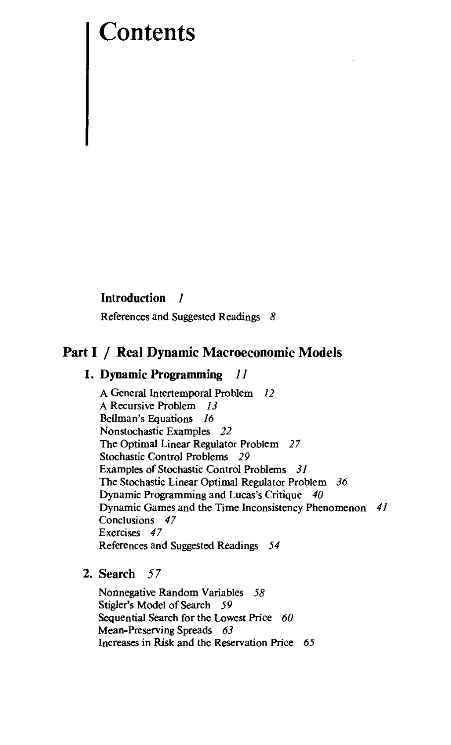
Contents
Introduction 1
References and Suggested Readings 8
Part I / Real Dynamic Macroeconomic Models
1. Dynamic Programming 11
A General Intertemporal Problem 12
A Recursive Problem 13
Bellman's Equations 16
Nonstochastic Examples 22
The Optimal Linear Regulator Problem 27
Stochastic Control Problems 29
Examples of Stochastic Control Problems 31
The Stochastic Linear Optimal Regulator Problem 36
Dynamic Programming and Lucas's Critique 40
Dynamic Games and the Time Inconsistency Phenomenon 41
Conclusions 47
Exercises 47
References and Suggested Readings 54
2. Search 57
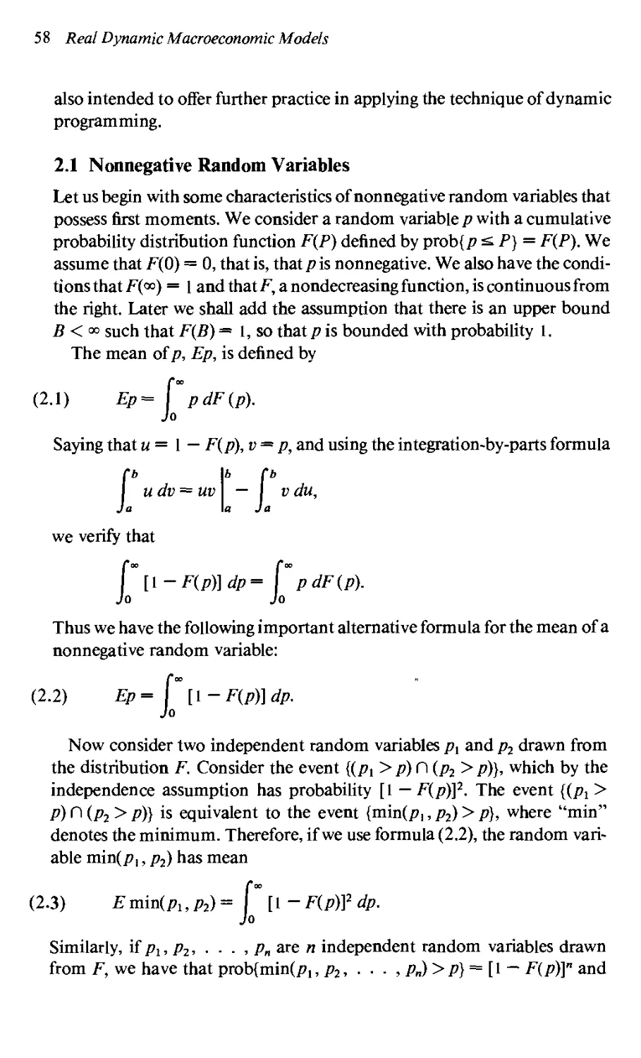
Nonnegative Random Variables 58
Stigler's Model of Search 59
Sequential Search for the Lowest Price 60
Mean-Preserving Spreads 63
Increases in Risk and the Reservation Price 65

Contents
Intertemporal Job Search 65
Waiting Times 70
Firing 70
Jovanovic's Matching Model 71
Conclusions 83
Exercises 85
References and Suggested Readings 91
3. Asset Prices and Consumption 92
Hall's Random Walk Theory of Consumption 93
The Random Walk Theory of Stock Prices 94
Lucas's Model of Asset Prices 95
Mehra and Prescott's Finite-State Version of Lucas's Model 100
Asset Pricing More Generally 101
The Modigh'ani-Miller Theorem 115
Government Debt and the Ricardian Proposition 116
Remarks on Testing and Estimation 119
Conclusions 120
Exercises 121
References and Suggested Readings 128
Part II / Monetary Economics and Government Finance
4. Currency in the Utility Function 133
The Price of Inconvertible Government Currency in Lucas's Tree Model
Issues and Models in Monetary Economics 137
Government Debt in the Utility Function 140
Government Currency in the Utility Function 142
Seignorage and the Optimum Quantity of Currency 145
A Neutrality Proposition 148
Conclusions 152
References and Suggested Readings 153
5. Cash-in-Advance Models 155
A One-Country Model 156
Fisher Equations 165
Inflation-Indexed Government Debt 166
Interactions of Monetary and Fiscal Policies 168
Interest on Reserves 177
A Two-Country Model 182
Exchange Rate Indeterminacy 188
Conclusions 192
Exercises 192
References and Suggested Readings 198
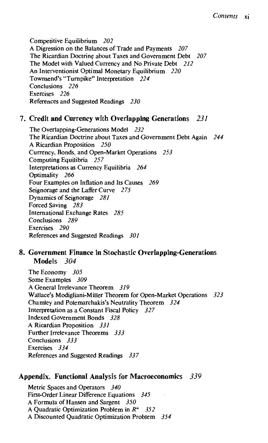
6. Credit and Currency with Long-Lived Agents 199
The Physical Setup 200
Optimal Allocations 201

Competitive Equilibrium 202
A Digression on the Balances of Trade and Payments 207
The Ricardian Doctrine about Taxes and Government Debt 207
The Model with Valued Currency and No Private Debt 212
An Interventionist Optimal Monetary Equilibrium 220
Townsend's "Turnpike" Interpretation 224
Conclusions 226
Exercises 226
References and Suggested Readings 230
7. Credit and Currency with Overlapping Generations 231
The Overlapping-Generations Model 232
The Ricardian Doctrine about Taxes and Government Debt Again 244
A Ricardian Proposition 250
Currency, Bonds, and Open-Market Operations 253
Computing Equilibria 257
Interpretations as Currency Equilibria 264
Optimality 266
Four Examples on Inflation and Its Causes 269
Seignorage and the Laffer Curve 275
Dynamics of Seignorage 281
Forced Saving 283
International Exchange Rates 285
Conclusions 289
Exercises 290
References and Suggested Readings 301
8. Government Finance in Stochastic Overlapping-Generations
Models 304
The Economy 305
Some Examples 309
A General Irrelevance Theorem 319
Wallace's Modigliani-Miller Theorem for Open-Market Operations 323
Chamley and Polemarchakis's Neutrality Theorem 324
Interpretation as a Constant Fiscal Policy 327
Indexed Government Bonds 328
A Ricardian Proposition 331
Further Irrelevance Theorems 333
Conclusions 333
Exercises 334
References and Suggested Readings 337
Appendix. Functional Analysis for Macroeconomics 339
Metric Spaces and Operators 340
First-Order Linear Difference Equations 345
A Formula of Hansen and Sargent 350
A Quadratic Optimization Problem in i?°° 352
A Discounted Quadratic Optimization Problem 354

xii Contents
Predicting a Geometric Distributed Lead of a Stochastic Process 357
Discounted Dynamic Programming 360
A Search Problem 361
Exercises 362
References and Suggested Readings 363
Index 365

Dynamic
Macroeconomic
Theory

1
Dynamic
Programming
This chapter introduces the basic ideas and methods of dynamic
programming and displays the restrictions on a dynamic system and the
objective function that must be met for dynamic programming to be
applicable. Where these restrictions are satisfied, dynamic programming provides a
powerful method for studying dynamic optimization. The required
restrictions permit the analyst to break what is in general a single exceedingly large
dimensional optimization problem into a collection of much smaller
optimization problems that can be solved sequentially. That step usually affords
computational simplicity and often provides analytical insights.
The restrictions on objective functions and the dynamic system required
for dynamic programming are satisfied in many formulations of private
agents' investment problems. There is a class of multiagent problems
(differential games), however, in which the structure of interactions among
different agents' decision problems prevents one or more agents' problems from
conforming to the restrictions required for dynamic programming. For these
agents, therefore, optimal decisions must be computed not sequentially but
simultaneously. The inapplicability of sequential methods to such decision
problems is called time inconsistency and was first studied in macroeco-
nomic contexts by Kydland and Prescott (1977) and Calvo (1978).
Although the main ideas of dynamic programming are simple, the details
can involve sophisticated mathematical arguments. In this chapter things
have been kept at a heuristic level of presentation, with the hope of
communicating the main ideas quickly and enabling the reader to use these
techniques to solve problems. More thorough presentations of the subject are

12 Real Dynamic Macroeconomic Models
listed at the end of the chapter; in particular see Bertsekas (1976); Bertsekas
and Shreve (1978); Lucas, Prescott, and Stokey (forthcoming); Bellman
(1957); and Chow (1981).
1.1 A General Intertemporal Problem
Consider the following general intertemporal optimization problem under
certainty. Let x,be an(«Xl) vector of state variables at time t, t = 0,
1, . . . , T+ 1. Let ut be a (kX 1) vector of control variables at time t,
t = 0, . . . , T. (The terms "state" and "control" are ambiguous in the
context of the problem of this section. A precise description of them will be
postponed, pending consideration of the special problem of Section 1.2, in
which they are well motivated.) The problem is to choose «<,, ux, . . . ,uT,
Xi, . . . , xT+l to maximize an objective function
(1.1) R(x0,u0,xuUi, . . . ,xT,uT,xT+l),
subject to x0 given and subject to a system of constraints connecting the
controls and the states, which we write in the implicit form
(1.2) G{xQ,u0,xl,ul, . . . ,xT,uT,xT+1)>0.
In (1.2) we imagine that G is a collection of (T+ 1 )n functions. We imagine
that R and G are sufficiently smooth and that R is sufficiently concave to
permit the method of Kuhn and Tucker to be appUed. We then have a
standard classical constrained-optimization problem, which can be solved
by forming the following Lagrangian and maximizing with respect to Uq ,
W], . . . , uTy Xj, X2, ■ . . , xT+l'.
(1.3) J^R(x0,u0>xl,ul, . . . ,xr>uT,xT+l)
-rfi G(x0, Uq, X{, Ux, . . . , XT> UT> Xr+i),
where fj. is a [(T+ \)n X 1] vector of Lagrange multipliers. The solution of
this problem can be represented as a set of functions u0 = H^x0), ut =
Hi(x0), . . . , uT= HT(x0), with the optimal controls expressed as a
function of the initial given state jc0, and a set of functions xt = Wi(x0), x2 =
^2(^0). ■ ■ ■ > *t+i =* wr+1(x0), with subsequent states expressed as a
function of the initial state x0. It is a standard feature of this problem that the
optimal controls u0, ux, . . . , wras functions of x0 must be determined
simultaneously. This feature can be verified by obtaining the first-order
necessary conditions for maximizing (1.3) and by studying the structure of
the Jacobian matrix for the system of first-order necessary conditions. The
system of first-order conditions in general fails to be recursive or block

Dynamic Programming
recursive, so that the optimal values for u, and x, are simultaneously
determined.
1.2 A Recursive Problem
For dynamic problems in which the horizon T is large, it would be
convenient if the problem could somehow be specialized to avoid the need to
compute all of the controls simultaneously. This consideration has led to the
following specialization of (1.1) and (1.2), which permits a recursive
approach to the computation of the optimal controls.
We assume that r^x,, «r) is a concave function and that the set {xl+l,
x,, ul:xt+1 <g,{x„ «r), tyGR*1} is convex and compact. We thus replace
(1.1) and (1.2) with the problem of maximizing by choice of
(«o>-*i>wi, ■ ■ ■ ,xr+1) the function
(1.4) r0(x0, u0) + rx(xls «,) + . . . + rT(xT, uT) + W0(xT+l),
subject to x0 given and the "transition" equations
(1.5) xx -g0(x0,u0)
x2 -gx{xx,ux)
The function rr(jt,, u,) is called the one-period return function at t, whereas
the function glxn «r) is called the transition function at t. The structure of
the transition equations (1.5) motivates the labeling of x, as state and ut as
control variables. The state vector x, constitutes a complete description of
the current position of the system. As far as the current and future returns
rAxs> us) for s ^ t are concerned, past values of uv and xv for v < t add no
information beyond that contained in x,. This result is a consequence of the
particular time separable structure of (1.4) and (1.5). The control vector ut
contains variables under the partial control of the problem solver that
impinge on xl+l, given x,. In general for a given problem, the appropriate
definition of the state is not unique, there being alternative ways of
completely describing the current position of the system. Many of the admissible
definitions of the state will include redundancies.
In (1.4) and (1.5) the functions r/jt,, ut), W0(xr+l), and&(xr, u,) are
assumed to be sufficiently smooth to permit the use of Lagrange's method.

14 Real Dynamic Macroeconomic Models
Forming the Lagrangian, we have
(1.6) L = r0(x0, u0) + r,(xi, m,) + . . . + rT(xT, uT) + W0(xT+1)
+ K[go(Xo> "o) - *i] + mgiixi, «i) - JfJ
+ ■ ■ ■ + A/7-[^r(^r>wr)^^r+iL
where Ar is an (n X 1) vector of Lagrange multipliers for t = 0, . . . , 7" and
the prime denotes transposition.
The first-order necessary conditions for this problem are
(1.7a) i£^iH(x u) + d^r,ut)
n7H dL _dr^u^ dgt
(i-7b) — =——— + — (xn «X- Vi^o, r= i, . . . , r
(1.7c) = W'0{xT+l) - Ar = 0
axr+i
(i.7d) jfl+i«a(jf„M,), r = o, l, . . . r.
Here drjdut is a (A; X 1) vector with drjdua in the rth row, where usi is the
element in the rth row of u,. Also, dgjdut is a (A; X n) matrix with dgsijdush in
the rth column and /rth row, where gti is the rth row of gt and uth is the /rth row
of u,. Solving (1.7b) for A,_, and shifting forward one period, we have
x __ drt+1(xt+u ui+1) + dgi+1(xl+1, ul+1)
dX1+1 dxl+i
Using this and (1.7c) recursively to eliminate Xt, t = 0, . . . , T, from
(1.7a), we obtain the following system:
(1.8a) ^,*,,„,) + te^fe + ^r^ + ^
dU, dU, loXI+i oXI+i \_dXl+2 dXl+2
t=^o, . . . ,r-1
(1.8b) xt+l =glx„ u,), t= 0, . . . , T~ 1
(1.8d) xT+i = gT(xT, uT),
where in (1.8a) it is understood that g, and rt both have arguments (x„ «,).

Dynamic Programming
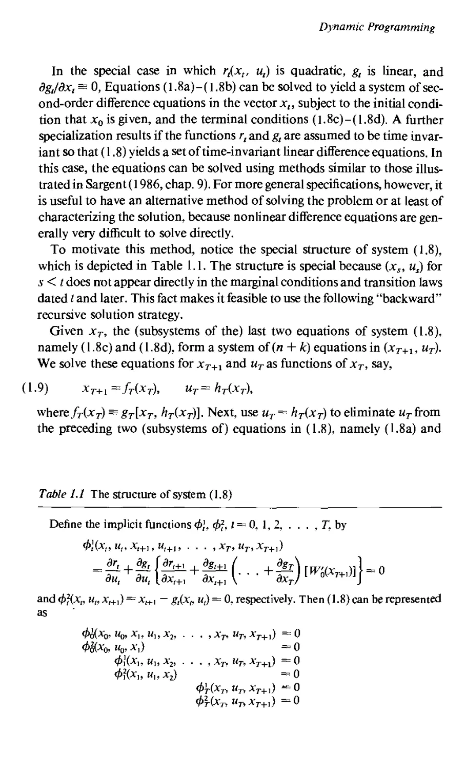
In the special case in which rt{xt, ut) is quadratic, gt is linear, and
dgjdxt 35 0, Equations (1.8a)-(l.8b) can be solved to yield a system of
second-order difference equations in the vector xt, subject to the initial
condition that x0 is given, and the terminal conditions (l.8c)-(1.8d). A further
specialization results if the functions rt and gt are assumed to be time
invariant so that (1.8) yields a set of time-invariant linear difference equations. In
this case, the equations can be solved using methods similar to those
illustrated in Sargent(1986, chap. 9). For more general specifications, however, it
is useful to have an alternative method of solving the problem or at least of
characterizing the solution, because nonlinear difference equations are
generally very difficult to solve directly.
To motivate this method, notice the special structure of system (1.8),
which is depicted in Table 1.1. The structure is special because (xs, us) for
s < t does not appear directly in the marginal conditions and transition laws
dated t and later. This fact makes it feasible to use the following ''backward"
recursive solution strategy.
Given xT, the (subsystems of the) last two equations of system (1.8),
namely (1.8c) and (1.8d), form a system of (n + k) equations in (xT+1, uT).
We solve these equations for xT+1 and «ras functions of xT, say,
(1.9) xT+l ^fT(xT), uT= hT(xT),
where fT(xT) = sAxt, hT(xT)]. Next, use uT = hT(xT) to eliminate uT from
the preceding two (subsystems of) equations in (1.8), namely (1.8a) and
Table 1.1 The structure of system (1.8)
Define the implicit functions 4>], <$, l = 0, 1, 2, . . . , T, by
<p,{x,, u,, xl+], ul+i, . . . , xT, uT,xT+1)
and 4>?(x„ u„ *,+,} = x^ — g,(x„ u,) = 0, respectively. Then (1.8) can be represented
as
Vot-Xb' Uq* X\i hD x2-> ■ ■ • > XT* UT-> XT+V == 0
<f>](xu h„ x2, . . . , xT, uT, xT+1) = 0
</>f(X„ H„X2) =0
4>t(xt, «t, *T+0 =0
4>t(xt, Ut,Xt+]) =0

16 Real Dynamic Macroeconomic Models
(1.8b) for t=T- 1,
(1 jo) SrT-i(Xr-i, uT-i) | dgT_x(xT-Xt uT-x)
duT^x duT^1
■ [j^ (xT, uT) + |g (XT, uT) ^(xr+I)j = 0
and solve these equations for «r_, and jcreach as functions ofxT^l:
(1.11) xT=fT^(xT^), uT^ = hT-x{xT-x).
One can continue recursively in this way, solving for a collection of feedback
rules of the form
(1.12) ut=hlxt), t=T, T-\,T~2, ... ,0,
where ut = h^x,), xl+1 =Mxl) solve the equations
(1.,3) ^feUr)+^(^±i+^ri^+^-
dut 8ut [dxl+l dxt+l ldxl+2 dxl+2
rt+3
dx
r+3
and xs+1 = &fo, «J for s = t, t + 1, . . . , T, given that us+1 ~ hs+1(xs+1)
for s= t,t+I, ... , T~ 1.
1.3 Bellman's Equations
The equations of system (1.13) have interpretations as the marginal
conditions from the following sequence of problems. Define the value function for
a one-period problem Wx(xT) by
(1.14) Wx(xT) =* max{/y(jcr, uT) + W0(xT+l)},
subject to xT+1 = gT(xT, uT), with xT given. We form the Lagrangian for this
problem, and the first-order conditions can be expressed, after the Lagrange
multiplier has been eliminated, as
(1.15) f^,«r) + ~^W6(*r+1) = 0,
which precisely matches the marginal condition for «rin (1.8). Equation
(1.15) and the transition law xT+1 = gj{xT, uT) are to be solved jointly for
uT= hT{xT). Now imagine substituting the solution H7- = hT{xT) of (1.15)
and (1.8d) into (1.14) to get

Dynamic Programming
(1.16) Wx(xT) = rT[xT, hT(xT)] + W0(gT[xT, hT(xT)]).
Formally, differentiating (1.16) gives
where all functions dated Tare evaluated at [xT, hT(xT)] and which by virtue
of (1.15) becomes
(1.17) W[(xT) = |^ [xT, hT(xT)]
dx
T
+ ^ [xT, hAx^W^Xr, hT(xT)]).
dx
T
Because we have not shown that dhT/dxT exists, this argument is informal or
heuristic and should be regarded as only a way of remembering the correct
answer. Correct arguments are given by Benveniste and Scheinkman (1979)
and Lucas (1977).
Now define the value function for the two-period problem W2{xT^x) as
(1.18) WAxT-x) = max{^,(^1( uT_x) + Wx{xT)\
subject to xT — ft-iOtr-i, uT-x\ with xT-x given. If we proceed as with the
problem denned by (1.14), the first-order condition for the problem on the
right side of (1.18) can be expressed as
£=! (,,._, ,„,._,) + *r-**r-u »T-,) w,{Xt) = 0.
If we use formula (1.17) for W\(xT\ this equation becomes
(1.,9) ^L(jCr_lfMr_l) + *r-,(xr-„«r-,)
dur-r *-1' ''" du
T-l
■ (|^ [xT, hT(xT)] + J^ [xT, HAxdWUgAxT, fiAxr)])) = 0.
This equation and the transition law xr= gT^x(xT-x, uT^x) are to be solved
jointly for uT-x = hT-x(xT-xX xT = fT^x(xT~x). Again proceeding as above,
we can obtain
(1.20) wXxr-J^p^ [xT-x,hT-x(xT^x)]
+ ^zl W{(gT^[xT^x,hT^(xT^)]\

18 Real Dynamic Macroeconomic Models
or, using (1.17),
aXT-l
+ 7ZTLIxt--i,!it-i(Xt-i)]
aXT-l
{
£ [xt> Ht{xt)]
+ ^ [AV, M^r)] ^[/r(^r)]},
where xT is evaluated at xT ~fr-i(xT-i) ~ gr-iixr-i» ^r-i(-*r-i)]- Notice
that Equation (1.19) is precisely the version of the marginal condition in
(1.8) for Mr_,.
The pattern for the recursion is now set. We iterate on the following
functional equation in the value functions
(1.21) WJ+1(xT^)~max{rT^xT-j, uT.j) + Wj(xT^J+1)},
subject to xT^j+1 = gT-j(xT-j, uT_j), xT_j given. The functional equation
(1.21) is a version of Bellman's equation — named after Richard Bellman
(1957). The idea is to proceed recursively and to work backward, first solving
the one-period problem with j+ 1 = 1, deducing Wx{x-j), then solving the
two-period problem withy +1 = 2, deducing the two-period value function
**2C*7-i)- The process is repeated until we obtain the(7"+ 1 )-period value
function WT+1(x0). This procedure gives the optimal value of the problem as
a function of the initial state x0. Along the way we have calculated the
optimal feedback rules uT_s — hT^j{xT-j),j= 0, 1, . . . , T. The preceding
argument suggests that this backward recursion generates the same marginal
conditions as the original problem (1.8). Indeed, the backward recursion
technique always solves the original problem if a solution exists.
The derivative of the value functions obeys the recursion
Wj+1(xT-j) = %p* [xT-j, hT-j(xT-j)]
+ |[ZW W>{gT_j[xT_p hT-j{x^j)\).
dXT-j
Comparing this equation with (1.7b) and (1.7c), we find that Wj(xT+1-j) ~
XT^j. The Lagrange multipliers AT_y in (1.6) thus give the marginal value of
the state variables for they-period problem.

Dynamic Programming
The following observations supply another perspective on the recursive
nature of our problem. Let us simply define the (T+ l)-period value
function WT+1(x0) by
(1.22) WT+1(x0) = max [r^x0t u0) + /",(*,,«,) + . . . + rT(xT, uT)
K0,K| UT
+ W<JixT+1)},
where the maximization is understood to be subject to xt+1 = g^xn wr),
i = 0, . . . , T, and x0 given. Notice that the objective function and
constraints (transition equations) have been specialized to have the key property
that controls dated t influence states xs+1 and returns rj^x,, us) for s > t but
not earlier. This key property gives the problem its recursive structure. In
particular, the property makes it legitimate to cascade the maximization
operator and to write (1.22) as
(1.23) WT+1(x0) = max{r0(x0, u0) + max{r,(x,, «,) + max{r2(x2, u2)
+ . . . + max{rT(xT,uT) + W^xT+1)} . . . }}},
where the maximization over ut is understood to be subject to xl+l =
glx,, ut) with x, given. Equation (1.23) indicates that the original large
optimization problem on the right side of (1.22) can be broken up into (T+ 1)
smaller problems. First, the problem in the innermost brackets is solved, the
optimizer being uT= hT(xT) and the optimized value being W^Xt). Then
the problem in the second innermost brackets is solved for uT-\ —
hr-xiXf-x) with optimized value W2(xT-i). This process of proceeding from
the problems in the innermost brackets outward is equivalent to iterating on
Bellman's functional equation (1.21).
The preceding argument implies that the optimal policies u, ~ h^x,), t =
0, . . . , T have a self-enforcing character in the following sense. Consider
the "remainder" of the objective function at some time s > 0, namely,
(1.24) max {rs{xs, us) + . . . + rT(xT, uT) + W0(xT+1)},
subiecttoxI+l = g^xl,ul),t = s, . . . , T, with xs given. Then the solution
of the maximum problem (1.24) is simply to use the remaining functions
us = hs{xs), s = t, . . . , T that were computed for the original problem.
Furthermore, the maximized value of (1.24) is WT_s+1(xs). Thus as time
advances, there is no incentive to depart from the original plan. This
self-enforcing character of optimal policies is known as Bellman's principle of
optimality. Optimal policies that have this property are said to be time

20 Real Dynamic Macroeconomic Models
consistent. This property is special, is a consequence of the recursive
character of the problem (1.4)—(1.5) and will not characterize the solutions of
more general problems.
It is a feature of the solution to problem (1.4)—(1.5) that in general a
different policy function u, = h^x,), mapping the state at t into the control at
t, is to be used at each date t = 0, . . . , T. This is a consequence of two
features of the problem: the fact that the horizon T is finite and the fact that
the functions r^x,, ut) and g£xt, ut) have been permitted to depend on time in
arbitrary ways. For many practical applications it is inconvenient that the
policy function varies over time. One would like to discover contexts in
which the same policy function is used for each period t. In the interests of
achieving this objective, we now specialize problem (1.4) - (1.5) with the aim
of generating conditions under which the policy functions hj converge as
j'—> — oo. We assume that
(1.25) rlxn «,) = P'r(Xl, «,), 0 <$ < 1
&(*„",) = £(*<>",)■
With this specification, Bellman's equation (1.21) becomes
WJ+1(xT.j) = max{^-HxT^, «r-;) + Wj(xT.J+1)}.
Multiplying both sides by f$j~T gives
(1.25') p-TWJ+1(xT-j) = max{r(jcr^, uT.j) + y? • p-*-TW£xT-J+l)}.
Now define the current value function
VJ+1(xT-j) = F-TWJ+1(xT^).
Notice that for j = T, we have VT+1(x0) = WV+i(*o)- Also notice that the
current value function can be directly defined as
Vj+1(xT-j) = max {r(xT-j, uT-j) + M*t-j+i , "r-y+i)
UT-j,UT-j+l,...,UT
+ . . .+pr(xT,uT) + p+1V(JixT+1)}.
In terms of the current value function, (1.25') asserts that Bellman's
equation becomes
(1.26) VJ+1(xT-j) = max{r(xT-j, uT^) + pVj(xT-j+1)},
subject to xT^J+1 = g(xT^j, uT^j) and xT^j given. More compactly, we can
write (1.26) as
(1.27) VJ+1(x) = max(r(x, u) + fiVjix)},

Dynamic Programming
subject to x = g(x, «), x given, where the tilde denotes next-period values.
Under particular conditions, iterations on (1.27) starting from any bounded
and continuous initial V0 converge asy —* °°. See Bertsekas (1976, chap. 6) or
Lucas, Prescott, and Stokey (forthcoming). The argument used to prove this
claim is outlined in Section A. 8. In this case the limit function V = lim^ V-
satisfies the following version of Bellman's equation:
(1.28) V(x) = max{r(x, u) + pv{x)},
u
where the maximization is subject to x = g(x, «), with x given. The limiting
value function Fthat solves (1.28) turns out to be the optimal value function
for the infinite horizon problem
(1.29) n*o)-maxf;£Hxt,M,),
(•dr-o r=o
where the maximization is subject toxr+i = g(xt,«,), withx0 given. Problem
(1.29) is a version of a discounted dynamic programming problem. Under
various particular regularity conditions,1 it turns out that (1) the functional
equation (1.28) has a unique strictly concave solution; (2) this solution is
approached in the limit as 7 —* °° by iterations on (1.26) starting from any
bounded and continuous initial V0; (3) there is a unique and time-invariant
optimal policy of the form u, = h(x,), where h is chosen to maximize the right
side of (1.28); (4) off corners, the limiting value function Fis differentiable
with
(1.30) V\x) = £ [x, h(x)] + ^ [x, h(x)] V'(g[x, h(x)]).
This is a version of the formula of Benveniste and Scheinkman (1979). It is a
great convenience of the specialization (1.25) of the objective function and
transition functions, and also a convenience of the specification of an
infinite horizon, that they imply a time-invariant policy function u, = h(x,\ for
it is a routine practice in economics to seek setups in which agents use
time-invariant decision rules. (Ample econometric considerations
recommend or require such setups.)
The preceding results provide two methods for solving the functional
1. Alternative sets of regularity conditions work. One set of sufficient conditions is (t) r is
concave and bounded, (2) the constraint set generated by gis convex and compact, that is, the
set of {xl+ltx„ u,:xl+l s g(x„ u,)} for admissible «, is convex and compact. See Lucas (1977),
and Bertsekas (1976) for further details of convergence results. See Benveniste and Scheinkman
(1979) and Lucas (1977) for the results on differentiability of the value function^A proof of the
uniform convergence ofiterations on (1.27) is contained in Section A.7 of the Appendix.

22 Real Dynamic Macroeconomic Models
equation (1.28). The first method is constructive and simply involves
iterating on (1.26), starting from V0 = 0t until V} has converged. The second
method involves guessing a solution Fand verifying that it is a solution to
(1.28). The second method relies on the uniqueness of the solution to (1.28),
but because it also relies on luck in making a good guess, it is not generally
available. In the examples below, the guess-and-verify method is often used.
The reader should, however, be alerted to the fact that the objective functions
and constraints of these problems have been especially rigged so that the
method will work. Essentially there are only two classes of specifications of
preferences and constraints for which the method will work, namely,
variants of specifications with linear constraints and quadratic preferences or
Cobb-Douglas constraints and logarithmic preferences.
In many problems, there is no unique way of defining states and controls,
and several alternative definitions lead to the same solution of the problem.
Sometimes the states and controls can be defined in such a way that x, does
not appear in the transition equation, so that dgjdxt = 0. In this case, the
system (1.8a)-(1.8b) simplifies to
^{x" "<>+ ST{u'] a^ °' x'+l ~ g'{u'1
The first equation is a version of what is called an Euler equation. Under
circumstances in which the second equation can be inverted to yield u( as a
function of xt+1, using the second equation to eliminate ut from the first
equation produces a second-order difference equation in x,.
Most of the dynamic programming problems that we solve in this book are
discounted dynamic programming problems.
1.4 Nonstochastic Examples
We now consider several examples of single-agent optimization problems
that can be solved using dynamic programming.
Saving under Certainty
Consider the problem of a consumer in a nonrandom environment who
seeks to maximize 2™=0/^«(Cf), 0 < fi < 1, subject to At+1 = R£A, + y, — c,),
A0gvven, where y^t^ 0, 1, . . . , is a known sequence of exponential order
less than 1//? and Rn t = 0, 1, . . . , is a known and given sequence of one-
period gross rates of return on nonlabor wealth. Here c, is consumption, A, is
nonlabor wealth at the beginning of time t, and yt is labor income at t. Labor
income is assumed to be beyond the control of the agent. For concreteness let
yt equal A#_,, and say that R, = R > 0 for all t, assuming that R > X > 0. To

Dynamic Programming
rule out a strategy of infinite consumption supported by unbounded
borrowing, we also impose the restriction that, for t ^ 0,
(i.3i) ct + i; (n xt™) ct+j^y, + i, (u *ri) y<+j + A<-
We define the state of the system as (A,, yt, R,-x) and define the control at t,
ut, as Rj1 At+1 = A, + y,-ct. Evidently the control u, is gross savings. The
transition equation for A, becomes At+1 = R,u„ which does not involve the
state at t. The function r,(xt, ut) becomes fPu(At +yt — R^1Al+1) =
plu{At + y, — ut). Bellman's equation becomes
v(A„ yt, Rt-X) = mzx{u(At + yt- ut) + 0v(utRtt yt+1, Rt)},
where ut = Rj1At+1, yl+1 — Xyt, R, = R. Benveniste and Scheinkman's for-
mula( 1.30)givesdv(At,yt, R^/dA, = u'{ct). The Euler equation for u,then
becomes
-Fu'{At + yt-R7*At+l)
+ fil+lRtu'(Al+l + yl+1 - Ry+\At+2) = 0
or
(1.32) -W(ct) + fiRtu'(ct+l) = 0.
We seek a consumption plan that satisfies (1.32) and the "isoperimetnc
condition" (1.31).
As an example, suppose that u(ct) = In ct. Then (1.32) requires that
ct+J = MuRt+k)ct.
Substituting this into the left side of (1.31) gives( 1 - p)~lct. Therefore (1.31)
and (1.32) imply that
(1.33) ct = (\ - f!)\yt+Jl(Jfi Rt+f) yt+J + At],
L j-i \k-o /
so that the agent always consumes a constant fraction of his or her total
human and nonhuman wealth. Equation (1.33) is valid for any sequences
{R^q, {#}£_„ such that the right side converges.
To specialize (1.33) to the case in which yt = Xyt~x and Rt = R, write out
(1.33) as
c, = (1 - fiKAt + yt + RT*yt+l + R7lR7Jiyt+2 + ■■■)■

24 Real Dynamic Macroeconomic Models
Repeatedly substituting Rt£x = R-1 and yt+1 = Xyt into the above equation
gives
c, = (1 - fl)(At + yt + R-Uy, + Rr2X2yt + . . .)
or ct = {\~P)\At + yt
where we require that AK_I < 1. Thatis, income is assumed to grow at a rate
less than the interest rate. In the decision rule stated above consumption
varies directly with current income y,, inversely with the currently observed
interest rate R, and directly with the rate of growth of income X.
Optimal Growth
A consumer aims to maximize
2«c,), o</?<i
subject to ct + kt+1 =f(kt), k0 > 0 given, c, ^ 0,
where h'(0) = + °°, u' > 0, u" < 0, f'(0) = + °°, /'(*>) = 0, /' > 0, and
/" < 0. Here ct is consumption and k, is the stock of capital. This is a version
of the problem that was studied by T. C. Koopmans (1963) and David Cass
(1965).
Let the state be denned as kt and the control as kt+1. Bellman's equation is
then
v(k,) = max{H[/(^) - kt+1] + Pv{kt+l)}.
The first-order condition is
(1.34) -u'[f(kt) - kt+1]+0v'(kl+1) = 0.
Benveniste and Scheinkman's equation (1.30) implies that v(k,) isdifferenti-
able with
(1.35) v'(kt) =u'[f(kt) - kt+1]f'(kt),
where kt+1 is evaluated at the optimum kt+1 = h(k,).
Because «(■) and/( ■) are strictly concave, it follows that v(k) is strictly
1
1 -XR-1

Dynamic Programming 25
concave. From this inference it follows that the optimal policy function, the
solution kl+1 — h{kt) of (1.34), is a nondecreasing function oik,.2
There is a maximum capital stock that can be sustained as a stationary
equilibrium, namely that which would eventually emerge if c, were to be zero
for all t. If c, were zero for all t, kt would evolve according to the difference
equation kt+1^f(kj). Because/'(0) = +00,/" < 0, and because/'(°°) = 0,
the equation k =f(k) has a unique positive solution. Evidently kt+l =f(k,)
converges to & as i —* °°. [To verify this point, plot f(kt) against a 45 ° line.]
Let the system begin with k0 £ (0, k]. Then for t ^ \,kt must evidently
remain in the bounded interval [0, k]. Because the optimal policy function
#(&,) = &,+! is nondecreasing in &,, it can be shown thatkQ,k1,k2, . . . ,is
a monotone, bounded sequence. On the one hand, suppose that kx > k0.
Then because /?(■) is nondecreasing, we have k2 = /?(&i) — h{k0) = kt,k3 =
h{k2) ^ h{kx) = k2, and so on. On the other hand, suppose that kt < k0.
Then k2 = hikj < h(k0) = kuk3 = h(k2) < h{kx) = k2, and so on. It
follows that kt is a monotone, bounded sequence. Inasmuch as monotone,
bounded sequences converge, it follows that k, converges to a limit point
M^o) as i —» °°.
The preceding convergence argument leaves open the possibility that the
limit point kj^k^ depends on the starting point k0. It does not do so,
however, as the following argument verifies. Let £«, be a limit point. At the limit
point, (1.34) and (1.35) hold, and kt+1 = k, = k*. The implication is that
Pf'ikJ) = 1, an equation that determines a unique optimal stationary value
km. Note that the "gross rate of return" /'(kj) = fi^1 in the stationary state
and is independent of the specifics of the current-period utility function and
the production function. Note also that the optimal stationary capital stock
depends on /(■) and fi but not on «( ■ ).
We now specialize this example by following Brock and Mirman (1972)
and considering the particular functional forms u(c) = In c and f(k) =Aka,
A > 0,0 < a < 1. We will use the guess-and-verify method for this problem.
The guess may not seem an obvious one. The inspiration for the guess can be
2. From (1.35), we have that v'(k) is continuous. This follows from the continuity of h(k),
f(k}, and f'(k). For two levels k, of k, i= 1, 2, consider the first-order condition u'[f(k,) -
^t^,)] = PV'lWkj)]. Assume that kt > k2 and that h(kt) < h(k2). By strict concavity of v( ■) and
continuity of i/( ■), it follows that (1) for all h(k,), v'[h(k,)] is well defined, and (2) h(kt) < h(k2)
implies v'[h{k^\ > v'[h(k2j\. Therefore, u'[f(kt) - h(kt)] > u'[f(k2) - h(k2j\. By strict con-
cavity ofu, the preceding inequality holds if and only ]ff(kt)- h(k}}<f(k2) - h(k2}, orequiv-
alently,0 < h(k2) - h(k}) <f(k2)—f(kt) ^0. This is a contradiction produced by the
assumption that for A:, s k2,h(k,) < h(k2). Therefore h(k) is nondecreasing in k. (The argument in this
note was constructed by Rodolfo Manuelli.)

26 Real Dynamic Macroeconomic Models
understood by working Exercise 1.1 at the end of the chapter. For this
example we make the guess
(1.36) v(k) = E+F\nk,
where E and F are undetermined coefficients. For this guess, the first-order
necessary condition (1.34) implies the following formula for the optimal
policy k = h{k), where k is next period's value and k is this period's value of
the capital stock:
Substituting (1.37) into the right side of (1.35) gives
(1.38) v'(k) = (\+pF)akr1.
Differentiating (1.36) gives
(1.39) v'{k) = Fk-\
Equating (1.38) and (1.39) permits one to solve for F, F=a/(\ - aft).
Substituting this expression for F back into (1.36) and (1.37) gives
(1.40) v(k) = E + —^—- In k
1 — ap
k = Afiaka.
The fact that expressions (1.38) and (1.39) for v'(k) have identical functional
forms both verifies the original guess (1.36) and permits one to solve for the
undetermined coefficient F. An alternative procedure for verifying the guess
involves substituting( 1.37) into Bellman's functional equation and equating
the result to the right side of (1.36). Solving the resulting equation for E and F
again gives F=a/(\ — afi) and now gives
E = {\-ji)-1 In .4(1 - aji) + fa In Afia
In Exercise 1.1, the reader is asked to construct the same solution (1.37) to
the functional equation, using the method of iterating on Bellman's
equation (1.26) starting from v0(k) = 0. For this purpose it is useful to note that
the term F=a/(\ — aft) that appears in (1.40) can be interpreted as a
geometric sum a[ 1 + afi + (afi)2 + ...].
Equation (1.40) shows that the optimal policy is to have capital
move according to the difference equation kl+1 = Afiakf, or In kl+1 =

Dynamic Programming
In Afkx. + a. In k,. Because a < 1, we know that kt converges as t —* °° for any
positive initial value kQ. The stationary point is given by the solution of
k* = AfiakZ, or kt~l — (Afht)~l. Notice that this example obeys the general
conclusion established above that k„ is determined from the solution of
1.5 The Optimal Linear Regulator Problem
We now consider a special class of dynamic programming problems in which
the return functions rt are quadratic and the transition functions & are linear.
This specification leads to the widely used optimal linear regulator problem.
We consider the special case in which the return functions rt and transition
functions & are both time invariant. The problem is to maximize over choice
of {h,}"=0 the criterion
(1.41) i{x;^+M('C4
t-o
subject to xl+1 = Axt + Bu,, x0 given. Here xt is an {n X 1) vector of state
variables, ut is a (k X 1) vector of controls, R is a negative semidefinite
symmetric matrix, Q is a negative definite symmetric matrix, A is an (n X n)
matrix, and B is an (n X k) matrix. We guess that the value function is
quadratic, V{x) — x'Px, where P is a negative semidefinite symmetric
matrix.
Using the transition law to eliminate next period's state, Bellman's
equation becomes
(1.42) x'Px = mzix{x'Rx + u'Qu + (Ax + Bu)'P(Ax + Bu)}.
u
The first-order necessary condition for the maximum problem on the right
side of (1.42) is
(1.43) (Q + B'PB)u = -B'PAx,
which implies the feedback rule for w:
(1.44) u = -(Q + B'PB)-1 B'PAx
or
(1.45) u = -Fx,
where F = (Q + B'PB)~XB'PA. Substituting the optimizer (1.45) into the

28 Real Dynamic Macroeconomic Models
right side of (1.42) and rearranging gives
(1.46) P=R + A'PA - A'PB(Q + B'PBYXB'PA.
Equation (1.46) is called the algebraic matrix Riccati equation.
Under particular conditions, Equation (1.46) has a unique negative semi-
definite solution, which is approached in the limit as 7 —»°° by iterations on
the matrix Riccati difference equation:3
(1.47) PJ+1 = R + A'PjA - A'PjB(Q + B'PjBy'B'PjA,
starting from PQ = 0. Equation (1.47) is derived much like (1.46) except that
one starts from the iterative version of Bellman's equation (1.26) rather than
from the asymptotic version (1.28).
A modified version of problem (1.41) is the discounted optimal linear
regulator problem, to maximize
(1.48) 2 FWRxt+ u\Qut\ 0<y?< 1,
t-o
subject to xt+1 = Ax, + But, xQ given. For this problem Bellman's recursive
equation (1.26) implies the following matrix Riccati difference equation
modified for discounting:
(1.49) Pj+1 = R + fiA'PjA - p2A'PjB(Q + $B'P}B)~AB'P}A.
The algebraic matrix Riccati equation is modified correspondingly. The
value function for the infinite horizon problem is simply V(x0) = x'QPx0,
where P is the limiting value of Pj resulting from iterations on (1.49)
starting from PQ — 0. The optimal policy is ut~— Fx„ where F =
%Q + PB'PB)-lB'PA.
Upon substituting the optimal control u, — — Fx, into the law of motion
xt+1 =Axt + Bu„ we obtain the optimal "closed-loop system" xt+1 =
(A — BF)x,. This difference equation governs the evolution of x, under the
optimal control. The system is said to be stable if lim,^ x, — 0 starting from
any initial x0 G R". Assume that the eigenvalues of (A — BF) are distinct,
and use the eigenvalue decomposition (A — BF) = CAC-1 where the
columns of C are the eigenvectors of (A ~ BF) and A is a diagonal matrix of
eigenvalues of (A — BF). Write the above equation as xt+1 = CAC^x,. The
solution of this difference equation for t > 0 is readily verified by repeated
substitution to be x,~ CA'C^Xq. Evidently, the system is stable for all
3. If the eigenvalues of A are bounded in modulus below unity, this result obtains, but much
weaker conditions also suffice. See Bertsekas (1976, chap. 4) and Sargent (1981).

Dynamic Programming 29
Xq G R" if and only if the eigenvalue of {A — BF) of maximum absolute
value is strictly less than unity in absolute value. When this condition is met,
(A — BF) is'said to be a "stable matrix."
A literature is devoted to characterizing the conditions on A, B, R, and Q
under which the optimal closed-loop system matrix (A — BF) is stable.
These results are described in detail in Sargent (1981) and may be briefly
described here for the undiscounted case/? — 1. Heuristically, the conditions
on Ay B, R, and Q that are required for stability are as follows. First, A and B
must be such that it is possible to pick a control law ut = — Fx, that drives x,
to zero eventually, starting from any x0 G Rn ["the pair (A, B) must be
stabilizable"]. Second, the matrix R must be such that the controller wants to
drive xt to zero as * —* °°. Notice from (1.41) that, if R is strictly negative
definite, the controller will want to drive xt to zero, because x'tRxt < 0 for
x, ¥= 0. Ifjc, does not approach zero, then the objective function is — °°. When
R is not,strictly negative definite, however, the possibility emerges that the
planner does not care whether some components of x, fail to go to zero as
t —»°°. To attain stability of (A — BF), it is necessary both for the planner to
dislike it that some components of x, threaten not to go to zero in the absence
of countervailing control actions and for (A, B) to be such that the controller
has the ability to drive those components to zero as t —* °° by an appropriate
choice of F.
These conditions are discussed under the subjects of controllability, stabi-
lizability, reconstructability, and detectability in the literature on linear
optimal control. (For continuous-time linear systems, these concepts are
described by Kwakernaak and Sivan 1972; for discrete-time systems, see
Sargent 1981.) These conditions subsume and generalize the transversality
conditions used in the discrete-time calculus of variations (see Sargent 1986).
That is, the case when (A — BF) is stable corresponds to the situation in
which it is optimal to solve "stable roots backward and unstable roots
forward." See Sargent (1986, chap. 9). Hansen and Sargent (1981) describe the
relationship between Euler equation methods and dynamic programming
for a class of linear optimal control systems. Also see Chow (1981).
The conditions under which (A — BF) is stable are also the conditions
under which x, converges to a unique stationary distribution in the stochastic
version of the linear regulator problem (see Section 1.8).
1.6 Stochastic Control Problems
We now consider a modification of problem (1.29) to permit uncertainty of
particular kinds. We modify the transition equation and consider the prob-

30 Real Dynamic Macroeconomic Models
lem, to maximize
(1.50) ^2^r(*i,Ki), 0<y?<l,
1-0
subject to
(1.51) xt+1~g(xt, h„ e/+1),
x0 known and given at t = 0, where e, is a sequence of independently and
identically distributed random variables with cumulative probability
distribution function prob{e, ^ e} = F{e) for all t; E,{y) denotes the mathematical
expectation of a random variable y, given information known at t. At time t,
xt is assumed to be known, butxt+j, j^ 1 is not known at t. That is, C/+i is
realized at (t + 1), after w, has been decided at t. In problem (1.50)—(1.51),
uncertainty is injected by assuming that x, follows a random difference
equation.
Problem (1.50-1.51) continues to have a recursive structure, stemming
jointly from the additive separability of the objective function (1.50) in pairs
(xt, u,) and from the difference equation characterization of the transition
law (1.51). In particular, controls dated t affect returns r(xs, us) tots^t but
not earlier. This feature implies that dynamic programming methods remain
appropriate.
The problem is to maximize (1.50) subject to (1.51) by choice of a "policy"
or "contingency plan" ut = h(x,). The version of Bellman's functional
equation corresponding to (1.28) becomes
(1.52) V{x) = max{r(x, u) + pE[V[g{x, h, e)]|x]},
u
where E{V[g(x, u,e)]\x} = jV[g(x,u,€)]dF(€) and where V{x) is the optimal
value of the problem starting from x at t = 0. The solution V{x) of (1.52) can
be found by iterating on
(1.53) Vj+1(x) = max{r(x, u) + PE^gix, u, e)]|x]},
u
starting from any bounded continuous initial V0. Under various particular
regularity conditions, there obtain versions of the same four properties listed
in Section 1.3. See Lucas, Prescott, and Stokey (forthcoming) or the
framework presented in the Appendix.
The first-order necessary condition for the problem on the right side of
(1.52)is
dj~ + fiE [H (x, u, e) V'(g(x, u, e))|x] = 0,

Dynamic Programming 31
which we obtained simply by differentiating the right side of (1.52), passing
the differentiation operation under the E (an integration) operator. Off
corners, the value function satisfies
V'{x) = ^ [x, h(x)] + 0E |^ [x, h{x\ e] V'(g[x, h{x\ e\)\x\.
In the special case in which dg/dx = 0, the formula for V'(x) becomes
V'(x) = ^[x,h(x)].
Substituting this formula into the first-order necessary condition for the
problem gives the stochastic Euler equation
%- (x, u) + 0E \^ (x, m, e) ^ (x, u)\x
au au dx
= 0,
where tildes over x and u denote next-period values.
1.7 Examples of Stochastic Control Problems
We now give several examples of stochastic dynamic programming
problems.
Consumption with a Random Return
A consumer seeks to maximize
3>2^M(ct), 0<y?<l,
1-0
subject to At+l = RlAt - ct), t ^ 0,^0 given, where u'(c) > 0, u"(c) < 0,and
where A, is assets at the beginning of period t, ct is consumption at t, and Rt is
the gross rate of return on assets between periods t and (t + 1). We assume
that R, becomes known at the beginning of period (t + 1), after a decision
about consumption at t, ct, must be made. Assume that Rt is governed
by a first-order Markov process, with transitions governed by prob{.K, ^
-K'l-Kf-i — R) = F(R', R). When time t decisions must be made, the
consumer knows At and Rt-ly Rt-2> .... To rule out perpetual borrowing
at the rate of return Rn we impose the requirement that At must satisfy
lim_ EoP'At = 0.
For this problem we define the state as (At, Rt_d and the control ut as
(A ~ ct). The transition equation for At is then given by At+l = Rj(At ~
ct) = Rtut, whereas the transition equation for R is implicitly defined by
F{R', R). Let v(At, Rt-i) be the value of the problem for a consumer with

32 Real Dynamic Macroeconotnic Models
initial assets A, when the last observed rate of return is Rt-1. Then Bellman's
functional equation is
v{At, Rt_x) = max{u(A, - Qt) + pEtv{utRt, R,)}.
The first-order necessary condition for the problem on the right is
- u'(ct) + pEpx(atRt, R,)Rt = 0.
Applying the Benveniste-Scheinkman formula to evaluate v£At, Rt-1) gives
vx{A,,R,-i) = u'{c^
Using this formula in the first-order necessary condition gives the Euler
equation
(1.54) u'(ct) = 0Etu'(cl+l)Rt.
A solution of the agent's optimization problem is a saving policy function
u, — h(At, R,-i), which implies a consumption policy function c, = c(At,
R,-i) mAt — h{At, R,-i). This policy function must satisfy the Euler
equation (1.54) and must imply that the boundary condition on assets lim,^.^
E0fi'At — 0 is satisfied. Substituting the function c(A„ Rt-{) into the Euler
equation and using the transition equation gives
(1.55) u'[c(A„ R^-pEyidRAA, ~ c(A„ R^l **)]**•
This is a functional equation in the optimal policy function c(At, Rt-i)-
To take a specific example, let u(c) equal lnc and let R, be an
independently and identically distributed random process such that 1 ^ERt< l//?2.
We guess that the optimal policy takes the form c,= yA„ where y is a
constant to be determined. Substituting this guess into (1.54) gives
± = BE £
yAt p yRt{At-yAtY
where E is now the unconditional expectation operator. Solving for y gives
y — 1 - /?. The optimal policy is of the form c, = (1 — fi)At. It can be verified
that this policy satisfies the boundary condition that we have imposed on
asset accumulation. The optimal policy is to consume a constant fraction of
wealth, 0 < y < 1, where y = 1 — /?.
Under the optimal policy, assets evolve according to Al+l — Rt( 1 — y)A„
which implies that
A^ii-yy'flRjAo, *>1.
J=0

Dynamic Programming 33
Consequently, we have that
t-\
c,= y(l-y)>f] RjA0, rai, c0 = yA0.
The optimal value of EQ 2™=0 /?' In ct is then given by
In yA0 + £o 2 ^ In J y( 1 - tf J] *;4> ■
/=i L _/=o
Because -Rj is independently and identically distributed, evaluating this
expression gives
v(A0,R-i) = -±-lny + ln(\-y);£fl't
1 P /-o
+ J/^'tE\nR + r^— lnA0,
t-o ' P
where £ In .K is the expectation of In Rt for all t. Still, 2JL0 #?< = p/( 1 - y?)2
(see Sargent 1979, Eq. 21, p. 88). Therefore the value function can be written
v{AQ,R-l) = ~\ny + \n{\-y)j^^ + ^^2E\nR
+ ~^A0.
The value depends directly on the mean of the logarithm of the rate of return
but is independent of the realization of the rate of return at the beginning of
the current period. This last property is special and depends on the
assumption that Rt is distributed independently and identically over time.
Dynamic Portfolio Theory
This example generalizes the preceding one to the case in which a consumer
can allocate his or her assets among a set of n assets, where the rth asset bears
gross rate of return Rit at time t. Here Ru is assumed to be a positive random
variable that is bounded from above with probability 1. The consumer
maximizes E0 S"=0 fi'u(c,) by choosing contingency plans for sit for i =
1, . . . , n and t ^ 0, subject to
n
Ct + ^sit = A„ t>0
i—i
i-l
\imE0P'A, = 0.

34 Real Dynamic Macroeconomic Models
Here sit is the amount of asset i purchased in period t, and ct is consumption
at t. At time t, At and Rit-i, i= 1, . . . , n are observed, but Rit, i =
1, . . . , n is not observed until the beginning ofperiod(r+ l).Weassume
that Rit is governed by a Markov process, with transition probabilities given
by prob{*, < R'\R,_X = R} = F(R',R\ where Rt = (RU, ■ ■ ■ ,-RJand*'
and R are both n-dimensional vectors. Shortly we will specialize the setup to
the case in which R, and Rt-l are independently distributed for all t.
We define the state for this problem as (A,, R,-i), whereas the control is
now the vector (su, . . . , sm). Bellman's functional equation is
v(A„ *,_!) = max j u{At - jj s,,) + jSEtv ( jj suRin r)\ .
Si„....Sn, { /=1 \(.= 1 /J
The first-order necessary conditions for the problem on the right are
u'Ut-^sA-pE^p^StoR^RA, i = 1 n.
The Benveniste-Scheinkman formula implies that v1 — u'(At~1,^lsit).
Substituting this equation into the above first-order conditions gives
"' U~ 2 Si)=/iEtRuu' (^ RbSh - 2 Sj,+X
V 1=1 / \k=i j-i /
/= 1, . . . ,n.
We now want to solve for optimal policy functions su ~ Sj(At, Rt-i).
Substituting the policy functions into the preceding Euler equation gives
(1.56) M'U-25'H>^-i)
L ,=1
= PEtRitW j J R,aSk(An Rt^) - J sj\j^ R^iA,, *,-i), R, },
U-i j-i L,t-i _U
*'= 1, . . . ,n.
This is a set of n functional equations in the n unknown functions s,C4,,
R,-i), /= 1, . . . ,n.
We now consider the special case in which Rit, i — 1, . . . , «, is
distributed independently and identically both over time and across /.
Furthermore, we suppose that u(c) = [1/(1 - a)]cl~a, where 0 < a < 1, so that
u'(c) = c~a. For this case we make the guess that sit — kAt, i = 1, . . . , n,
where k is a constant to be determined. Note that we are guessing that k is
independent of i, a guess inspired by the independence and identity of the
distribution of the Ru over time and across 1. Substituting this guess into

Dynamic Programming 35
(1.56), using u'(c) = c a and rearranging, gives
2**)
/-i /
v-i
Because Ru is independently and identically distributed, the above equation
can hold for all i = 1, . . . , n. This result verifies our guess and gives an
equation that can be solved for k. (Notice how this example conforms to the
preceding one.)
In the present example the household allocates the same constant fraction
of wealth to each asset in each period. This result depends on the
independence of the Rit over time and the independence and identity of the
distribution across assets i. We now explore the implications of relaxing the
assumption of identical distributions across i while retaining independence across
time and assets. Under these new assumptions we guess that the optimal
policies will be of the form sit — ktAt. Substituting this guess into the Euler
equation gives
«'[^i( 1 - 2 *,■) - PEtRttu' [£ M*r^( 1 - % *,) ,
/= 1, . . . ,n.
Further specializing this example, we take u{c) — In c. Substituting u'(c) —
c~l into the above equations and rearranging gives
j-i
This is a system of n equations in then unknowns^, . . . ,k„. For
example, when n = 2, we have the two equations
y-mki + friRz/RvT1
which are to be solved for kx and k2.
Stochastic Optimal Growth
We consider the stochastic growth example of Brock and Mirman (1972), to
maximize
£o2^Inc<> 0<fi<U
t-o

36 Real Dynamic Macroeconomic Models
subject to ct + kt+i = Ak?8,,0 <a< 1, where In 8, is an independently and
identically distributed random variable with normal distribution with mean
zero and variance a2. (The stochastic optimal growth model is a workhorse
in the literatures on capital asset pricing and business fluctuations; see Brock
1982 and Kydlandand Prescott 1982.) A planner is supposed to know(&,, 8t)
at time t but not to know future values of 8. We define the state of the system
as (kn 8,). Bellman's equation becomes
(1.57) V(k„ 8t) - max{lnC4/:?i9, - kl+l) + 0E[V(kl+i, 8l+i)\k„ 8t]).
The reader is invited to verify the guess that the solution of (1.56) is of the
form V(k, 8) — E + F In k + G In 8, where E, F, and G are undetermined
coefficients, and that the optimal policy rule is kt+1 = Aafjkf8,.
1.8 The Stochastic Linear Optimal Regulator Problem
We consider the discounted stochastic linear optimal regulator problem, to
maximize
(1.58) E0 2 Fix'.Rx, + u'tQut), 0<fi<\,
t-Q
subject to xQ given, and the law of motion
(1.59) xl+1*"Ax, + But + €t+lt r>0,
where e,+x is an (n X 1) vector of random variables that is independently and
identically distributed through time and obeys the normal distribution with
mean vector zero and contemporaneous covariance matrix
(1.60) £"e^'-X
(See Kwakernaak and Sivan 1972 for an extensive study of the continuous-
time version of this problem; also see Chow 1981.) The matrixes R, Q, A, and
B obey the assumption described in Section 1.5 above.
For this problem the value function turns out to be
(1.61) v{x)=x'Px + d,
where P is the unique negative semidefinite solution of the discounted
algebraic matrix Riccati equation corresponding to (1.49), which is the limit of
iterations on (1.49) starting from PQ = 0, and where d is given by
(1.62) d = 0(l -p)-hrPZ
where "tr" denotes the trace of a matrix. Furthermore, the optimal policy

Dynamic Programming
continues to be given by u, = —Fx,, where
(1.63) F = fi(Q + fiB'?'B)-lB'PA.
A notable feature of this solution is that the feedback rule (1.63) is identical
with the rule for the corresponding nonstochastic linear optimal regulator
problem.
To prove the preceding assertions, we substitute the guess (1.61) into
Bellman's equation to obtain
v(x) = max{xTRx +uTQu + fiE[(Ax + Bu + ef
u
■ P(Ax + Bu + e)]+fid},
where e is the realization of et+l when x, = x and where Ee\x = 0. (Both
prime ['] and superscript T denote transposition.) The above equation
implies
v(x) = max{x TRx + uTQu + fiE{x TATPAx + x TAPBu
u
+ .v TATPe + uTBTPAx + uTBTPBu + uTBTPe
+ eTPAx + eTPBu + eTPe) + fid).
Evaluating the expectations inside the braces and using Ee\x — 0 gives
v(x) - max{xTRx + uTQu + fi2xTATPBu + xTATPAx
+ PuTBTPBu + pEeTPe) + fid.
The first-order condition for u is
(Q + fiBTPB)u - -fiBTPAx,
which implies (1.63). Using EeTPe = ttEeTPe = XxPEeeT - trFX,
substituting (1.63) into the preceding expression for v(x), and using (1.61) gives
P = R+ fiA'PA - fi2A'PB{Q + fiB'PBY lB'PA,
and d = fi{\ -fi)~x trPX.
This step concludes the demonstration of the claims about the optimal value
function and the optimal decision rule.
It is a remarkable feature of this solution that, although through d the
objective function (1.60) depends on 2, the covariance matrix of the
"noises" e, the optimal decision rule u, = —Fx, is independent of 2. This is
the message of (1.63) and the discounted algebraic Riccati equation for P,
which are identical with the formulas derived earlier under certainty. In
other words, when expressed in the feedback form ut = h{xt\ the optimal

38 Real Dynamic Macroeconomic Models
policy function that solves this problem is independent of the noise statistics
of the problem. This feature is called the "certainty equivalence principle"
by economists. This is a special property of the optimal linear regulator
problem and is due to the quadratic nature of the objective function and the
linear nature of the transition equation. Certainty equivalence does not
characterize stochastic control problems generally.
For the stochastic optimal linear regulator, substituting the optimal
control u, = ~Fx, into the transition equation gives the stochastic optimal
closed-loop system xl+i = {A~ BF)xt + e/+1. Under the condition that
{A ~ BF) is a stable matrix (that is, one whose eigenvalue of maximum
absolute value is less than unity in absolute value), the system converges as
t —»°° to a unique stationary probability distribution. The spectral density of
the stationary distribution is given by
SJ,io) =[I~(A- BF)e-i<orl X[I~(A~ BF)Te+Uo]-\
CQ€[— 71, 7T].
Here SJ,co) is the Fourier transform of the covariogram of xt,
I=— 00
where Cx{z) = Ex,x,^. The covariances Cx(x) can be recovered from S^w)
by the inversion formula
Q(t) = (1/2tt) j SJia})e+i™d(D.
Spectral densities for continuous-time systems are discussed by Kwakernaak
and Sivan (1982). For an elementary discussion of discrete-time systems, see
Sargent (1986). Also see Sargent (1986, chap. 11) for definitions of the
spectral density function and methods of evaluating the above integral.
The preceding discussion shows how the stochastic optimal linear
regulator provides a complete description of the theoretical second moments of the
stationary distribution of the controlled process x,. The mapping from (A, B,
R, Q) to these theoretical moments that is implicitly described by the above
equations is the foundation of econometric methods designed to estimate a
wide class of linear rational expectations models (see Hansen and Sargent
1980, 1981). Briefly, these methods use the following procedures for
matching observations with theory. A sample of observations for some elements of
x,, t — 1, . . . , T, is assumed to be available. All possible sample second
moments of the observations are calculated. How well the theory matches
the observations is measured by choosing a metric that gives the distance

Dynamic Programming 39
between the sample moments and the theoretical moments associated with a
given (A, B, R, Q). The metric is chosen not arbitrarily but in order to deliver
good statistical properties of the estimates of (A, B, Q, R), consistency and
asymptotic efficiency. Then A, B, Q, and R are estimated by choosing them
to minimize the metric. For discussions of a good metric, see Hansen and
Sargent (1980, 1982). The theory is "tested" by measuring how far the
observations deviate from the theory, A, B, Q, and R being set at their best
values.
As a simple example of a stochastic linear regulator problem, consider a
monopolist who seeks to maximize
£o 2 nP,Yt - JtKt - (d/2)(Kl+l - K,)2], 0 < /? < 1
t-0
subject to P^Ao-AiYf + e^ ^o^X)
Yt=fKt f>0
K0 given, J,,6„ and K, known at time t. Here P, is output price, Yt is output, Jt
is the rental rate on capital, and 6, is a random shock to demand, whereas eJt
and em are white noises. The maximization is over a stochastic process for
Kl+l as a linear function of (K„ /,, 8,).
To map this problem into the stochastic linear regulator problem, we
define the state x, as the vector (K, ,Jnut,l)', whereas the control u, is simply
Kt+l - Kt. Then take A, B, Q, and R to be
A =
R =
10 0 0
0 A 0 0
0 0 fi 0
0 0 0 1
, B =
1
0
0
0
~AXP
-1/2
7/2
aju
-1/2 //2
0 0
0 0
0 0
A0f/2
0
0
0
, Q = -d/X e,=
0
0
The optimal feedback law is an investment schedule of the form u, — ~ Fxt
ot{Kt+x~Kt) = -F{Kt,J„dt> 1)'.
Problems of the kind exhibited in this example can be formulated as
stochastic discrete-time calculus-of-variations problems and can be solved as
linear difference equations (see Sargent 1986). The methods involve two
steps: (1) factoring the characteristic polynomial associated with the nonsto-

40 Real Dynamic Macroeconomic Models
chastic version of the problem in order to obtain the feedback and
feedforward parts of the solution; and (2) utilizing the Wiener-Kolmogorov linear
least-squares forecasting formula in order to express the feedforward part in
terms of information available at the decision date. Notice that the linear
regulator problem in effect accomplishes both optimization and prediction
—and does so simultaneously via iterations on the matrix Riccati difference
equation.
In Exercises 1.6 and 1.7, the readeris asked to take two problems with very
large state spaces and to map them into linear regulator problems. These
exercises are designed to show the chief advantage of the linear regulator
framework: the tractability it retains even in the face of state spaces of very
large dimension.
1.9 Dynamic Programming and Lucas's Critique
Recall the following version of the time-invariant, discounted stochastic
control problem treated in Section 1.6, namely, to choose a strategy for u,
that maximizes
£oiym*„w,), o<y?<i,
/=o
subject to jc,+i = g(x„ u,, e/+i), t ^ 0, where e/+1 is a sequence of
independently and identically distributed random variables. We have seen that the
solution is a time-invariant policy function u, = h{x,) that satisfies the
functional equation
(1.64) v(xt) « r[Xl, h(x,)] + PE(v(g[x„ h{xt), e,+1])|x,).
In general, the optimal policy h{xt) that solves the functional equation
(1.64) depends on the return function r(x,, u,), on the transition function
g(x„ u,, e/+1), on the probability distribution of e/+1, and on /?. In particular,
even with preferences [that is, fi and r(x,,«,)] fixed, the optimal decision rule
u,= h{x,) depends on the law of motion g(xn u,, e/+1). The implication is
that, in dynamic decision problems, it is in general impossible to find a single
decision rule h{x,) that will be invariant with respect to variations in the laws
of motion g{xt, u,,€l+l). This principle is illustrated in a variety of ways in
the examples that we have considered above.
Robert E. Lucas (1976) criticized a range of econometric policy evaluation
procedures because they used models that assumed private agents' decision
rules to be invariant with respect to the laws of motion that they faced. Those
models took as structural (that is, as invariant under interventions) such

Dynamic Programming
private agents' decision rules as consumption functions, investment
schedules, portfolio balance schedules, and labor supply schedules. The models
were then routinely subjected to hypothetical policy experiments that
changed the stochastic processes (or laws of motion, g) of such variables as
income flows, tax rates, wage rates, prices, and interest rates, variables that
entered private agents' constraints and decision rules. Those hypothetical
experiments violated the principle that an optimal decision rule h{xt) is a
function of the law of motion g(x,, «,,e/+1).
Lucas's criticism was a particularly telling one because it embraced two of
the fundamental ideas that underlay the enterprise of building large-scale
Keynesian econometric models. First, there was the idea that for policy
experiments it was important to isolate relationships that were structural,
that is, invariant with respect to the class of interventions to be studied.
Lucas observed that dynamic optimization theory ultimately implied that
the key structural equations in Keynesian macroeconometric models, such
as the consumption, investment, and portfolio balance schedule, should not
be regarded as structural. Second, there was the idea that it was useful to
derive the private agents' decision rules from the hypothesis of optimizing
behavior in a dynamic context, an idea reflected with increasing
sophistication by many works within the Keynesian tradition.
1.10 Dynamic Games and the Time Inconsistency Phenomenon
We now briefly describe the structure of a two-player dynamic, or
"differential," game with no randomness. (A more general treatment of the issues
described here is to be found in Hansen, Epple, and Roberds 1985; also see
Basar and Olsder 1982.) The transition equation of the system is assumed to
be
(1.65) xl+i = g(uu> u2t),
where x, is again the state vector, uu is the control vector of the first player,
and u2l is the control vector of the second player. Player i has an objective
described by
(1.66) 2^(x|f Hl/, u2l) + /iT+lV0i(xT+l), 0</?< 1, i= 1,2,
where rt(x„ uu, w2/) is the return function of the rth player. Player / is
assumed to maximize (1.66) subject to (1.65) with x0 given and also subject
to some particular assumption about player/'s choice of {«,,) orabout player
/s way of choosing it. Alternative particular assumptions about how player /

42 Real Dynamic Macroeconotnic Models
imagines player j to choose ujt determine the equilibrium concept of the
game.
We first describe a particular version of a Nash equilibrium. Assume that
player I takes player 2's actions {w^J^-o as given and as beyond player I's
control and that player 2 takes the symmetrical view with respect to player
I's actions. Then player Ps actions solve the following version of the system
(1.8) of Euler equations and transition equations
(1.67a) -^-{x,, «,„ «2/) +^t—("i„ u2t)~-{xt+x, uu+l, u2l+1) = 0,
ault auu dxt+i
t=0, 1, . . . , T- I
(1.67b) xt+1=g(ult,u2l), *=0, . . . ,7",
subject to Xq given and {«2j}£-o known, and the terminal condition
(1.67c) PTP-(XT, u1T, u2T) +/?"-' -^- (u1T, u2T) ^- (wT+1) = 0.
oU1T oU1T °XT+1
Analogously, player 2's actions solve
( l-6M TT fa* "l/, «2/)+^T- («,„ «2/) T"^- (X,+ i, Uu+l, U2t+1) = 0,
t = 0, . . . ,7"-I
(1.68b) xt+1 = g{uu, Ult), t = 0, I, . . . , T,
subject to x0 given and {uls}]-0 known, and the terminal condition
(1.68c) PT^f-(xT, ulT, u2T) +/?"-' -^- (Mir, U2T) ~~(xT+l) - 0.
OU2j- aU2f aXf+i
In a Nash equilibrium, Equations (1.67a), (1.67b), (1.67c), (1.68a), and
(I.68c) are solved jointly for {xr+1, «,„ w^}, r=0, 1, . . . , T.
We note two features of this equilibrium concept. First, each player's
problem continues to be a recursive one, because under the assumption that
the other player's actions are given, «„ affects returns r^x^ uls, u^) dated t
and later but not earlier. Thus each player's problem satisfies Bellman's
principle of optimality. Second, we note that the entire system formed by
(1.67a), (1.67b), (1.68a), and the terminal conditions is itself block recursive
and can be solved by working backward, starting from date T. Thus the Nash
equilibrium itself can be computed by recursive methods.
We now turn to a particular dominant-player game. We continue to
assume that player I regards player 2's actions as given and beyond player I's

Dynamic Programming
control. Player 2, however, is now assumed to understand that his controls
influence agent I 's simply by virtue of the fact that agent 1 's actions solve the
Euler equation (1.67a), taking «2jas given. Letusrepresent( 1.67a), (1.67c) in
the implicit form
(1.69) <f*xt, xt+u uln uu+u uz, U2,+1) = 0, * = 0, I, . . . , T- I
-^- (xT, wir, u2T) + y? -r~ (u1T, u2T) —— (xT+1) = 0.
oU1T dulT dXr+i
The decisions Mu of the follower agent 1 are determined by (1.69) and by the
relevant terminal condition, given xQ and the actions u^ of the leader. The
leader is imagined to choose {u^, wu, s ^ 0} to maximize (1.66) with i = 2,
subject to both (1.65) and (1.69). We can represent the leader's problem as
being to choose Mjo, . . . ,u2T,uw, . . . ,«ir, to maximize the Lagrangian
(1.70) L - 2 ^r2(xt, uu, u2t) + y?r+I V02(xT+l)
+ 2,P'rt[g(UmU2t)-xt+1]
1=0
T-\
+ 2 FP't[<KXnXt+l* UU, "lM-1. "2/, "2H-l)l
t=0
+ 0' J ^p-C*r, "ir, u2T) + p^{ulT, u2T)-p^(xT+1) 1,
where A,, £ — 0, . . . ,T;fin f = 0, . . . , 7" — I; and 0 are each vectors of
Lagrange multipliers. The maximization is performed with xQ taken as
given. The first-order necessary condition for the maximization of (1.70)
with respect to u2t is
(1.71) R dr^X" ""' "^ + R dg(Ul" u*> x
du2t du2t '
' P T~~ \xt-> xt+\-> u\t-> wu+i> U2t, U2t+i)fit
du2t
r = 0, I, . . . , T- I.
The reader is invited to obtain the remainder of the first-order necessary
conditions and to analyze the resulting system of difference equations for
determining {xt, ult, u2t} via the solution of the dominant player's maximum
problem. In addition, the reader is asked to verify that this system of equa-

44 Real Dynamic Macroeconomic Models
tions is simultaneous and not block recursive (make a table for the system
analogous to Table 1.1). This feature of the system and the nature of its cause
can readily be seen by comparing (1.71) with (1.68a). In (1.71) the effects of
u2t for t ^ I on values of uu for s < t and on past values of xs and r2{xs, uu>
«2j) for s < t are taken into account. Because the follower agent I's actions at
s < t depend on u^, the leader's problem fails to be recursive. Accordingly,
Bellman's principle of optimality may fail to characterize the leader's
problem. The failure of the dominant player's problem to satisfy the principle of
optimality is often called the time inconsistency of optimal plans.4
Consequently the optimal plan is not generally self-enforcing in the sense described
in Section 1.3 above.
Dynamic games occur in a variety Of contexts in dynamic
macroeconomics, industrial organization, and public finance. Early examples in
macroeconomics were given by Kydland and Prescott (1977) and by Calvo
(1978).
The following is a version of Calvo's(1978) example of a system in which
private agents' responses to the government tax strategy confront the
government with a nonrecursive problem in choosing a tax strategy. This example
departs in some details from the preceding framework but exhibits the same
essential nonrecursivity of the dominant player's (the government's)
problem. The economy is one in which a representative private agent chooses ct
and ml+1 sequences to maximize
(1.72) 2«c|f»iri.1/A), O<0<U
1-0
subject to
(1.73) c, + t, + ml+l/p, - y(Tt) + mjpn Wq > 0 given,
where u(ct,mt+1/p,) — In c,+ y^ri(mt+1/p,),y> 0. Here c, is consumption of
a single nonstorable good at time t, ml+1 is currency carried over from time t
to {t + 1), and p, is the price level at time t. The government imposes a
distorting tax (or subsidy) of t, at time t. Following Calvo, we represent the
distortion by simply positing that output at t is given by a diminishing
function of t,, y(Tt) where y' < 0. The private agent maximizes (1.72) by
choosing sequences c(, m/+1, where t ^ 0, taking as given the sequences
h*Pt-
4. For a solution to fail to satisfy the principle of optimality, it seems to be sufficient that there
exist no way of reformulating the problem (say, by redefining variables) so that it becomes
recursive. Some problems appear not to be recursive when written in one way but can be
transformed into equivalent recursive ones.

Dynamic Programming
The government seeks to maximize the utility of the representative agent
(1.72), subject to the constraints
(1.74) ct + gt = y(xt)
(1.75) g, = Tt + (mt+l - mt)/p„
where gt ^ 0, t > 0, is an exogenously given sequence of government
purchases. Equation (1.74) is the economy's resource constraint, whereas (1.75)
is the government's budget constraint. The government takes {g„ r > 0} as
given and chooses sequences of {mt+1, zt, t^ 0} to maximize (1.72). In
performing this maximization, the government is assumed to take as given
that the economy is in equilibrium and that private agents are solving their
optimum problem. Technically, this is an example of a "team" dynamic
game, because the government and the private agent share the same
objective function. Private agents are assumed to regard {p„ t,}£L0 as given
sequences.
An "equilibrium" is defined as a collection of sequences for (m1+l, r,,pt,
ct) that solve the optimum problems of both the private agent and the
government.
It can be verified that a private agent's problem is a recursive one. If we let
y(r) + m/p be the state at t, Bellman's equation for this problem can be
expressed as
v[y(r) + m/p] = max{«(c, m'/p) + pv[y(r') + m'/p']},
c.m'
c + t + m'/p ^ y(r) + m/p.
By our usual methods the Euler equation for this problem can be rearranged
to imply the difference equation
(1.76) — = 8 ! + ^—.
C,Pt Ct+lPt+l W/+1
We now use (1.76) and the equilibrium condition [ct = y(rt) — g,] to solve
for pt as a function of the (mt+l, rt) process chosen by the government.
Substituting the equilibrium condition into (1.76), regarding (1.76) as
determining pt as a function of the mt+j sequence, and solving the difference
equation (1.76) forward produce
(1.77) l/A-MTj-ft] JS^-~—■
j=o m,+j+1
Equation (1.77) gives the equilibrium price level as a function of the
sequences (t,, mt+l) chosen by the government to finance the exogenously

46 Real Dynamic Macweconomic Models
given gt expenditure sequence. Equation (1.77) embodies the results of the
Cagan effect (see Cagan 1956) by means of which expectations of future
settings of the currency stock influence the current price level.
We now consider the government's problem, which is to maximize (1.72)
subject to (1.74), (1.75), and (1.77) by choosing sequences for (t„ mt+l). In
maximizing subject to (1.77), the government is taking into account the fact
that private agents behave in a way that makes the current price level a
function of future m1+j. If we substitute (1.74) and (1.77) into (1.72), the
government's problem can be formulated as being the maximization of
(1-78) J ?u (y(zt) - g„ ymt+l[y(zt) - gt] J ? —^—\
t-0 \ j=Q mt+j+l/
subject to
(1.79) gt = t, + (mt+l - mt)/pt,
by choosing sequences for t, and mt+1, t ^ 0. This problem is evidently not a
recursive one, because future values of the control mt+J+ j influence the
government's return u(ct, mt+ i/p,) at date t. The reason is that private agents
respond to the government's choice of an mt+l+J sequence by making the
current price level respond to future settings of mt+ x .5
A consequence of the failure of the government's problem to be recursive
is that the government's problem cannot be solved sequentially using the
method of dynamic programming. As a result, the government's optimal
plan will lack the self-enforcing character of dynamic programming
solutions described above. In particular, if the government were imagined to
reopen its planning process and to consider optimizing the "remainder" of
(1,72) namely ^7^splu(ct, mt+l/pt), s > 0, by choosing {mt+l, t, for t ^ s)
subject to (1.74), (1.75), and (1.77), then in general the government would
want to depart from the original plan for {mt+x, rt, t ^ 0). This incentive
would emerge because the government would want to neglect the effect of
mt+1 for t > s on pv for 0 s v < s in setting mt+1 for t > s, an effect that was
taken into account in the original plan for (mt+l, t„ t ^ 0}. This lack of a
self-enforcement incentive is known as the time inconsistency problem.6
5. Hansen, Epple, and Roberds (1985) explicitly calculate a solution of the dominant player's
problem for a class of linear-quadratic games. Their method is applied to a simple optimal
taxation example in Sargent (1986). In these setups dynamic inconsistency of the optimal policy
for the dominant player is evident from the time-varying form of its decision rule.
6. Lucas and Stokey (1983) study two versions of an optimal taxation problem. In their
model without currency, they show that there exists a plan for restructuring the government
debt each period that, if followed, renders the optimal tax plan time consistent. This finding can
be regarded as providing a decentralization scheme between a tax authority and a
debt-management authority that is capable of supporting an optimal plan in a self-enforcing way.

Dynamic Programming 47
The time inconsistency phenomenon that is illustrated in Calvo (1978)
also surfaces in a wide variety of other dynamic optimal taxation examples.
1.11 Conclusions
Recursive dynamic optimization is a main tool of macroeconomic modeling
today. In this chapter most of the examples have been models of single agents
(Section 1.10 on dynamic games is the exception). In the next three chapters,
models will be constructed in which dynamic programming is used to
compute and study dynamic general equilibrium models. In these models the
single agent who is solving the problem is a fictitious social planner. Solving
the planner's problem will be the instrument for computing sequences of
equilibrium prices and quantities.
The reader is urged to tackle the exercises below. They provide the practice
required for comfort with the notions of states and controls and for
recognition of problems whose structure obeys the special conditions required to
apply dynamic programming.
Exercises
Exercise 1.1. Brock-Mirman (1972)
Consider the Brock-Mirman problem of maximizing
^P'lnct, O<0< 1,
/-=0
subjecttoc, + kt+l ^Akf,0 <a< 1, k0 given. Let v(k) be the optimal value
function. Use recursions on Bellman's equation (1.27), starting from
v0(k) = 0 to show that
v(k) = (1 -/T^ln^l -"/0 + y^ln^aJ + JZ^ ln *■
Exercise 1.2. Howard Policy-Improvement Algorithm
Consider the Brock-Mirman problem: to maximize
t-o
subject to c, + kt+l ^ Ak?6„ k0 given, A > 0, 1 > a > 0, where {0,} is an
i.i.d. sequence with ln 8, distributed according to a normal distribution with
mean zero and variance a2.
Consider the following algorithm. Guess at a policy of the form kt+l =

48 Real Dynamic Macroeconomic Models
h^Akfd,) for any constant h0 G (0, 1). Then form
UK, 60) - E0 2 P'HAkfd, - hoAkfdd.
t-0
Next choose a new policy hx by maximizing
]n(Akf6 -k') + pEJ^k', 6'\
where k' = hxAkfO. Then form
Mko, 60) = E0 2 f?ln(Ak?dt - hxAkfdt).
Continue iterating on this scheme until successive hj have converged.
Show that, for the present example, this algorithm converges to the
optimal policy function in one step.
Exercise 1.3. Levhari and Srinivasan (1969)
Assume that
„(c) = _L_ci-« a>o.
1 -a
Assume that Rt is independently and identically distributed and is such that
ER\~a < l/# Consider the problem
max E ^ P'u(ct), O<0< 1,
t-0
subject to At+l s R^At - ct), Aq > 0 given. It is assumed that ct must be
chosen before Rt is observed. Show that the optimal policy function takes the
form ct = XAt and give an explicit formula for X.
Hint. Consider a value function of the general form v(A) = BAl~a, for some
constant B.
Exercise 1.4 Habit Persistence: 1
Consider the problem of choosing a consumption sequence ct to maximize
2 f}'(lnct + y In c,^), 0<£< 1, y>0,
t-0
subject to ct + kt+l ^ Akf,
A>0,
0<a< 1,
k0>0, and c-x given.

Dynamic Programming 49
Here ct is consumption at t, and k, is capital stock at the beginning of period t.
The current utility function In ct+ y In c,_i is designed to represent habit
persistence in consumption.
a. Let u(k0, c_ i) be the value of 2JL0 /F(ln ct + y In c,_,) for a consumer
who begins time 0 with capital stock kQ and lagged consumption c_i and
behaves optimally. Formulate Bellman's functional equation in v(k, c_i).
b. Prove that the solution of Bellman's equation is of the form v(k,
c_i) = E + F In k + G In c_i and that the optimal policy is of the form
In £,+ i = / + H In k, where E. F, G, H, and / are constants. Give explicit
formulas for the constants £", F, G, H, and / in terms ofthe parameters A, ft,
a, and y.
Exercise 1.5 Habit Persistence: 2
Consider the more general version ofthe preceding problem, to maximize
2«c„c,_i), 0<y?<l,
subject to ct + kt+l ^f(k,), kQ > 0, c_i given, where u(ct, c,_i) is twice
continuously differentiable, bounded, increasing in both ct and ct-t, and
concave in (ct, <:,_,). and where/'(0) = +<»,/' > 0,/" < 0.
a. Formulate Bellman's functional equation for this problem.
b. Argue that in general, the optimal consumption plan is to set ct as a
function of both £,and ct_x. What features ofthe example in the preceding
problem combine to make the optimal consumption plan expressible as a
function of k( alone?
Exercise 1.6. Lucas and Prescott (1971) and Kydland and Prescott
(1982) Meet a Linear Regulator
Consider a linear quadratic version of a Lucas and Prescott (1971) model
that has been modified to incorporate a rich time-to-build structure, a la
Kydland and Prescott (1982). We first describe the model in terms of lag
operators and then show how it can be mapped into a linear regulator
problem.
The equilibrium of the model is supposed to solve the following problem:
) max F0 2 Wo " A, Y, + v,)Yt - J,i, - [d(L)K,][g(L)Kt]},
i >y?>o, ^0>0- ^i>o,

50 Real Dynamic Macroeconomic Models
subject to
(2) Yt = a{L)Kt
Kt+l = ([-a)Kt + z°, 0<<7< 1,
z\ = zl+\, 1=0, 1, . . . ,S-i
a{L)Jt = €Jt
&L)vt = ew
s~i
h = 2 TJZJ'
j-o
where
(3) a(L) = a0 + axL + . . . + aNLN
d(L) = d0 + dlL + . . . + dNLN
g(L) = g0 + glL + . . . + gNLN
a(L)= 1 -axL- . . .-apLp
Z(L)=\-£lL-. . .-£,£,*,
where A^, M, R, p, and </ are all nonnegative and finite. In (2), eJt and em are
fundamental white noises for /, and ut, respectively. At time t, variables
dated t and earlier are observed.
In (1), Yt denotes output, ct is investment expenditures, /, is the price of
new capital goods, Kt is the stock of capital, and v, is a random process
disturbing demand. The technology potentially incorporates two sorts of
time-to-build delays. First, output Yt is a distributed lag, a(L)K„ of the
capital stock Kt that is in place. As a result, given the capital stock, the one
factor of production, it requires time to produce output. Second, time
elapses between the moment when investment decisions z) are made at time
t and the moment when the machines can be used as capital, z?+J, at time
(t + s); z{ is interpreted as the number of machines in stagey available at time
t. Only machines in stage 0 can increase the capital stock.
One interpretation of the parameters t, is that they represent the fraction of
the total cost of a machine that is incurred when it is in stage j. Total
expenditures in this concept, ^.f-J Tjz{, therefore correspond to investment
at time j. It is also possible to think of the parameters t) as representing
payments to another firm that "builds" the machines. In this sense they can
reflect financing arrangements. The firm or industry also faces generalized
costs of factor adjustment, which are represented by the cost term
[d(L)Kt][g(L)Kt].
This problem can be interpreted in a variety of ways. First, it can be
interpreted as the solution of a monopoly problem, where the demand curve
facing the monopolist is p, = A0 — AtYt + vt, where p, is the output price.

Dynamic Programming 51
Second, it can be interpreted as the solution of a rational expectations
competitive equilibrium where the demand curve ispt = A0 — 2AtY, + vt. Third,
it can be interpreted as the outcome of a particular kind of Nash equilibrium
(see Hansen, Epple, and Roberds 1985).
a. Show how this general problem can be mapped into the structure of the
optimal linear regulator problem. Specify the vector of states and controls
and the matrixes R, Q, A, and B.
b. Display the solution in feedback form, and show the difference equation
that governs the state under the optimal rule.
Exercise 1.7. Interrelated Factor Demand
For another illustration of a problem that can readily be mapped into the
linear regulator framework, consider the interrelated factor demand
problem, to maximize
~E 2 P\yTFyt + [G{L)ytY\H{L)yA + Jjyt)
—=(:)' '■-(£)■
F is positive semidefinite; G(L) = G0 + GtL + . . . + GmLm, H(L) =
H0 + HXL + . . . + HmLm, where G, and //, are each (2 X 2) matrixes. It is
assumed that G$HQ is positive definite.
Here ^denotes a (2 X 1) vector of factor costs, ^denotes a (2 X l)vector
of factors of production, and [G{L)y]TH(L)yt denotes generalized costs of
adjustment. The maximization is subject to a Markov law for / of the form
Jt+\ = axJt + . . . + ap+\ Jt-P + €t+i, where e/+i is a (2 X 1) vector white
noise. At time 0, yt_}_ x and /,_;, j ^ 0, are taken as given.
a. Specify this problem as a linear regulator by defining the states and
controls xt, u, as well as the matrixes A, B, Q, and R.
Hint. It is easier to map the problem into the following more general version
of the linear regulator problem.
subject to jc/+i = Axt + Bu, + e/+i.
The following well-known argument indicates that there is no loss of
generality—when Q is nonsingular—in restricting ourselves to the case in
which W=0. Simply note that the previous problem is equivalent to the

52 Real Dynamic Macroeconomic Models
following
max E 2 ?{xT(R- W~QTxWT)xs + vjQv,},
subject to xt+l=(A~BQ~lWT)xt + Bvt + et+l, where vt = Q~lWTxt
+ ut. Therefore, denning R, Q, A, and B by
R = ][- WQ~XWT
Q = Q
A= A- BQ~XWT
B = B
gives us the standard version of the problem.
Exercise 1.8. Two-Sector Growth Models
a. Consider the following two-sector model of optimal growth. A social
planner seeks to maximize the utility of the representative agent given by
'2T=0fJ'u(ct, /,), where ct is consumption of good 1 at t, whereas /, is leisure at t.
Sector 1 produces consumption goods using capital, ku, and labor, nu,
according to the production function c, ^fx{ku, nu). Sector 2 produces the
capital good according to the production function k,+l ^f2(k2t, n2t). Total
employment, nt = nu + n2„ and leisure, l„ is constrained by the endowment
of time, /, and satisfies It + n,< 1. The sum of the amounts of capital used in
each sector cannot exceed the initial capital in the economy, that is,
^i/ + &2t — kt>k0> 0 given. Formulate this problem as a dynamic
programming problem. Display the functional equation that the value function
satisfies, and clearly specify the state and control variables.
b. Consider another economy that is similar to the previous one except for
the fact that capital is sector specific. The economy starts period t with given
amounts of capital ku and k^ that must be used in sectors 1 and 2,
respectively. During this period the capital-good sector produces capital that is
specific to each sector according to the transformation curve g^u-n,
&2t+1)^/2(^21, n2t)- Display the Bellman's equation associated with the
planner's problem. Specify which variables you choose as states and which as
controls.
Exercise 1.9. Learning to Enjoy Spare Time
A worker's instantaneous utility, «(■), depends on the amount of market-
produced goods consumed, cu, and also on the amount of home-produced
goods, c2t (for example, entertainment, leisure). In order to acquire market-
produced goods, the worker must allocate some amount of time, llt, to

Dynamic Programming 53
market activities that pay a salary of w,, measured in terms of consumption
good. The worker takes wages as given and beyond the worker's control.
There is no borrowing or lending. It is known that the market wage evolves
according to the law of motion wl+l = h(wt).
The quantity of home-produced goods depends on the stock of
"expertise" that the worker has at the beginning of the period, which we label a,.
This stock of "expertise" depreciates at the rate S and can be increased by
allocating time to nonmarket activities. To summarize the problem, the
individual agent maximizes
i«Ci„C2,), 0<y?<l,
subject to cu s w,lu [budget constraint]
c2l ^f(a,) [production function of the
home-produced good]
at+l =£ (1 — S]a{ + l2t [law of motion of the stock
of expertise]
ht + ^2/ — I [restriction on the uses of
time]
wl+l = h(Wt) [law of motion for the wage
rate]
Oq > 0 [given].
It is assumed that u{ •) and/( ■) are bounded and continuous. Formulate
this problem as a dynamic programming problem.
Exercise 1.10. Investment with Adjustment Costs
A firm maximizes present value of cash flow, with future earnings
discounted at the rate /?. Income at time t is given by sales, p, ■ q,, where pt is the
price of good, and qt is the quantity produced. The firm behaves
competitively and therefore takes prices as given. It knows that prices evolve
according to a law of motion given by pt+l =f(pt).
Total or gross production depends on the amounts of capital, k„ and
labor, nt, and on the square of the difference between current ratio of sales to
investment, xt, and the previous-period ratio. This last feature captures the
notion that changes in the ratio of sales to investment require some
reallocation of resources within the firm and consequently reduce the level of
efficiency. It is assumed that the wage rate is constant and equal to w. Capital
depreciates at the rate S. The firm's problem is
max 2 PXPAt ~ wnd, 0 < y? < 1,
/=0

54 Real Dynamic Macroeconomic Models
subject to q, + xt< g\ kt, ntt[ — ~^LJ-
L \xt xt-i
kt+i^(l -S)kt + x„ 0<S< 1
P,+i=f(P,)
kl)>0, — >0 given.
X-i
We assume that g{ •) is bounded, increasing in the first two arguments and
decreasing in the third. Formulate the firm's problem recursively, that is,
formulate Bellman's functional equation for this problem. Identify the state
and the controls, and indicate the laws of motion of the state variables.
Exercise 1.11. Investment with Signal Extraction
Consider a firm that maximizes expected present value of dividends. It is
assumed that the price of the good produced by the firm is constant and equal
to one. Production requires the use of a single input: capital that is firm
specific. Total production, f(k,), is divided between sales, qt, and investment,
xt. Revenue from sales is taxed at the rate t,. At time £, T,isknown, as isz,—a
variable that is related to xt+i by the function t/+ x ~ g(z,, e,+ i), where e,+1 is
an i.i.d. random variable that is not observed at t but whose distribution is
known to the firm. Notice that, given zt, the function ^induces a conditional
distribution of x,+1 that we denote F(xt+ {, z,). The stochastic process {z,} is
Markov with transition function//(z',z) = prob{z,+ i ^ z'|z, = zJ.Thecapi-
tal stock depreciates at the rate t. The problem faced by the firm is
max£-02^(l-^„ 0<y?<l,
1=0
subject to qt + xt ^ f(kt)
kt+l s(i -S)kt + xt, £0given, 0 < <5 < 1.
It is assumed that/(£) is increasing, concave, and bounded.
Formulate the firm's problem as a dynamic programming problem (that
is, display Bellman's equation).
References and Suggested Readings
Basar, Tamer, and Geert Jan Olsder. 1982. Dynamic Noncooperative Game Theory.
New York: Academic Press.
Bellman, Richard. 1957. Dynamic Programming. Princeton, N.J.: Princeton
University Press.
Bellman, Richard, and Stuart E. Dreyfus. 1962. Applied Dynamic Programming.
Princeton, N.J.: Princeton University Press.
)

Dynamic Programming 55
Benveniste, Lawrence, and Jose Scheinkman. 1979. On the differentiability of the
value function in dynamic models of economics. Econometrica 47(3): 727-732.
Bertsekas, Dimitri. 1976. Dynamic Programming and Stochastic Control. New
York: Academic Press. (Esp. chaps. 2, 6.)
Bertsekas, Dimitri, and Steven E. Shreve. 1978. Stochastic Optimal Control: The
Discrete Time Case. New York: Academic Press.
Brock, William A. 1982. Asset prices in a production economy. In The Economics of
Information and Uncertainty, ed. J. J. McCall, pp. 1 -43. Chicago: University of
Chicago Press.
Brock, William A., and Leonard Mirman. 1972. Optimal economic growth and
uncertainty: the discounted case. Journal of Economic Theory 4(3):479- 513.
Cagan, Phillip. 1956. The monetary dynamics of hyperinflation. In Studies in the
Quantity Theory of Money, ed. Milton Friedman, pp. 25- 117. Chicago:
University of Chicago Press.
Calvo, Guillermo A. 1978. On the time consistency of optimal policy in a monetary
economy. Econometrica 46(6): 1411 - 1428.
Cass, David. 1965. Optimum growth in an aggregative model of capital
accumulation. Review of Economic Studies 32(3):233-240.
Chow, Gregory. 1981. Econometric Analysis by Control Methods. New York: Wiley,
1981.
Hansen, Lars P., Dennis Epple, and Will Roberds. 1985. Linear-quadratic duopoly
models of resource depletion. In Energy, Foresight, and Strategy, ed. Thomas J.
Sargent, pp. 101 -142. Washington, D.C.: Resources for the Future.
Hansen, Lars P., and Thomas J. Sargent. 1980- Formulating and estimating dynamic
linear rational expectations models. Journal of Economic Dynamics and Control
2(l):7-46.
1981. Linear rational expectations models for dynamically interrelated
variables. In Rational Expectations and Econometric Practice, ed. R. E. Lucas, Jr., and
T. J. Sargent, pp. 127-156. Minneapolis: University of Minnesota Press.
1982. Instrumental variables procedures for estimating linear rational
expectations models. Journal of Monetary Economics 9(3):263 -296.
Koopmans, T. C. 1963. On the concept of optimal economic growth. Cowles
Foundation Discussion Paper. Yale University, New Haven.
Kwakeraaak, Huibert, and Raphael Sivan. 1972. Linear Optimal Control Systems.
New York: Wiley, 1972.
Kydland, Finn E., and Edward C. Prescott. 1977. Rules rather than discretion: the
inconsistency of optimal plans. Journal of Political Economy 85(3):473-491.
1982. Time to build and aggregate fluctuations. Econometrica 50(6): 1345-
1371.
Levhari, D., and T. N. Srinivasan. 1969. Optimal savings under uncertainty. Review
of Economic Studies 36(2):153- 163.
Lucas, Robert E., Jr. 1976. Econometric policy evaluation: a critique. In ThePhUUps
Curve and Labor Markets, ed. K. Brunnerand A. H. Meltzer,pp. 19-46.
Amsterdam: North-Holland, 1976.
1977. Class notes on dynamicprogramming. University of Chicago.
Unpublished.
1978. Asset prices in an exchange economy. Econometrica 46(6): 1426-
1445.

56 Real Dynamic Macroeconomic Models
Lucas, Robert E., Jr., and Edward C. Prescott. 1971. Investment under uncertainty.
Econometrica 39(5):659-681.
Lucas, Robert E., Jr., Edward C. Prescott, and Nancy L. Stokey. Recursive Methods
for Economic Dynamics. Forthcoming.
Lucas, Robert E., Jr., and Nancy Stokey. 1983. Optimal monetary and fiscal policy in
an economy without capital. Journal of Monetary Economics 12( 1 ):55 - 94.
Sargent, Thomas J. 1981. Lecture notes on filtering, control, and rational
expectations. University of Minnesota, Minneapolis. Unpublished.
1979. Macroeconomic Theory. New York: Academic Press.
1986. Macroeconomic Theory. 2nd ed. New York: Academic Press.

2
Search
This chapter applies dynamic programming in contexts in which
there is a choice between only two actions, as distinguished from the
situations studied in the previous chapter, in which the control was typically
permitted to take on a continuum of values. The two actions are whether to
accept or reject a take-it-or-leave-it offer. In particular, we shall study a
variety of search problems, including several contexts in which a buyer or
seller is confronted with a probability distribution of prices or characteristics
of a job or good from which additional offers can be drawn at a fixed cost per
offer. Given the worker's perception of the probability distribution of offers,
the worker must devise a strategy for deciding how many offers to solicit
before deciding to accept one.
The theory of search was pioneered by Stigler and McCall. It is interesting
to macroeconomists because it provides a tool for studying the phenomenon
of seemingly unemployed resources. We observe unemployed workers and
pieces of capital and variations over time in aggregates of these variables. To
explain these observations, search theory puts sellers of labor or capital in a
setting in which they rationally choose to reject available offers and to remain
unemployed in return for the opportunity to wait for better prospective
offers in the future. We want to use the theory to study how workers' choices
would respond to variations in the rate of unemployment compensation, the
perceived riskiness of wage distributions, the quality of information about
jobs, and the "technology" for sampling the wage distribution.
The present chapter aims to provide an introduction to the techniques
used in the search literature and a sampling of search models. The chapter is

58 Real Dynamic Macroeconomic Models
also intended to offer further practice in applying the technique of dynamic
programming.
2.1 N on negative Random Variables
Let us begin with some characteristics of nonnegative random variables that
possess first moments. We consider a random variable p with a cumulative
probability distribution function F(P) defined by prob{/? £f} = F{P). We
assume that F(0) = 0, that is, that p is nonnegative. We also have the
conditions that F(o=) = 1 and that F, a nondecreasing function, is continuous from
the right. Later we shall add the assumption that there is an upper bound
B < oo such that F(B) = 1, so that/? is bounded with probability 1.
The mean of/?, Ep, is defined by
(2.1) Ep= TpdFip).
Saying that u = 1 — F(p), v = /?, and using the integration-by-parts formula
J'b \b Cb
u dv = uv \ — | v du,
a \a Ja
we verify that
J [l-F(p)]dp= j pdF(p).
Thus we have the following important alternative formula for the mean of a
nonnegative random variable:
(2.2) Ep=l ^~F(P^dP-
Now consider two independent random variables pt and p2 drawn from
the distribution F. Consider the event {(pt > p) O (p2 > p)}, which by the
independence assumption has probability [1 — F(p)]2. The event {(/?! >
p) fi (p2 > p)} is equivalent to the event {min(/?,, p2) > p), where "min"
denotes the minimum. Therefore, if we use formula (2.2), the random
variable min(/?,, p2) has mean
(2.3) Emm(pup2)= \ [1 -F{p)f dp.
Similarly, if px, p2, . ■ . , P„ are n independent random variables drawn
from F, we have that prob{min(/?i, p2, . . . , P„)>P} = [1 — F(p)]n and

Search
that
(2.4) Mn^Emm(plyp2, ...,/>„)=! [1 - F(p)]n dp,
where M„ is defined as the expected value of the minimum of/?,, . . . , pn,
2.2 Stigler's Model of Search
Using formula (2.4), we can display George Stigler's (1961) model of
searching for the lowest price p drawn from known distribution F( p). Stigler
imagines that, at a constant cost of c per offer or draw, an agent can solicit
additional offers. The agent's problem is to specify the number of offers, n, to
solicit in advance of searching. The number of offers, n, is required to be a
positive integer. Stigler models the agent as selecting the number of offers to
minimize the expected minimum price plus the total costs of search:
M„ + nc= I [I - F(p)]n dp + nc.
Define the decrease in the expected minimum price of searching an nth time,
n ^ 2, as
Gn = Mn_x-Mn=\ [l-F(p)]"-ldp- j [l-F(p)]«dp
or
(2-5) Gn= f"[i -F(p)]"-iF(p)dp.
From (2.5) we have that G„ > 0, that G„ is a decreasing function of n, and that
lim,,^ G„ = 0. The rule derived by Stigler is to set n so that G„ ^ c> G„+1,
so that the cost of search is less than the decrease in the expected minimum
price resulting from the nth search but exceeds the decrease in the expected
minimum price resulting from search (n + 1). According to this model, n is a
function of c and of F. An increase in c causes n to decrease. (A
"mean-preserving increase in spread" in the sense to be defined below, can be shown to
imply that n increases, given c.)
Stigler's model has been criticized because it attributes to the agent the
objective of minimizing over the number of searches, n, the expected
minimum price over n searches plus the total costs of search. That objective is
distinct from and presumably less sensible than that of devising a strategy to
niinimize the expected value of the random variable "price plus total costs of

60 Real Dynamic Macroeconomic Models
search." These two objectives are evidently not equivalent. The second one
corresponds to searching for the lowest price. The limitation of the former
objective can be seen from the fact that it leads to a decision rule that is not
sequential. Imagine that, on the very first draw, an agent is fortunate enough
to draw the minimum price, that is, the price p for which F(p) = 0. It is
pointless to search further, yet the objective function posited by Stigier and
the decision rule derived under it require the agent to search « times.
Presumably the minimization of the alternative objective of expected price plus total
search costs will involve a sequential strategy that inspects each draw and,
depending on its value, determines whether or not to continue the search.
2.3 Sequential Search for the Lowest Price
We first solve a version of the problem in which there is no recall of past
offers. The agent searches by selecting independent drawings from the
distribution F, at a cost of c per drawing. The agent can accept the offer currently
in hand or can reject it without possibility of recall and then sample once
again. Consider the problem of an agent who has offer s in hand. Let the
function v{ s) be the minimum expected price plus the additional search costs
of an agent who has offer s in hand and who behaves optimally. The agent
can take either of two actions: (1) accept the offer s and terminate the search
or (2) reject the offer, bear an additional search cost c, and draw a new price
s'. For this problem, Bellman's equation is then
(2.6) r(s) = min{s, c+ I v(s') dF(s')}.
A graph of v(s) appears in Figure 2.1. Because c + jv(s') dF (s') is simply a
positive constant, the graph of v(s) must be as it is depicted in Figure 2.1.
Evidently there exists a critical number s = c+ f% v(s') dF(s') such that
s for s s s
(2.7) v(-s)~' s = c+ \ v(s')dF(s') torsos.
Jo
Evidently the optimal strategy is to reject offers s^s and to accept offers
s^s. The optimal strategy is thus to set a reservation price s.
To characterize Jin terms of Fand c, use (2.7) to write
s = c+ I v(s')dF(s')

Search 6
v A\
c +f'v(s')dF(s'
-Accept-
• Reject
->
Figure 2.1. The function v(s) = m'm{s, c + J%v(s')dF(s')}. The critical
number ^satisfies s = c + j%v(s')dF(s'). The optimal strategy is to
accept s < s.
or
or
s = c+ J' sdF(s) + s J dF(s)
$ l'dF(s) + s \_ dF(s) = c+ l'sdF(s) + s J dF(s).
Rearranging the above equation gives the characterization
(2.8) j\s-s)dF(s) = c.
Now define u = (s - s), dv = dF(s), and use the integration-by-parts
formula judv = uv- jvdu to get js0 (s- s) dF(s) = js0 F(s) ds. Substituting
this equation into (2.8) gives the useful characterization
<2-9) J F(s)ds = c.
Define the function
(2.10) g(s)= \F(p)dp.
Jo

62 Real Dynamic Macroeconomic Models
This function has the characteristics that #(0) = 0, g(s) > 0, g'(s) = F(s) >
0, and g"(s) = F'(s) > 0 for s > 0. Thus we can depict the determination of
the optimal reservation price s as in Figure 2.2.
We now consider search with recall. The agent sequentially makes
independent drawings from distribution F at a cost of c per draw. After each
drawing, the agent can accept it or any previous drawing or else can elect to
continue the search by making an additional drawing at a cost c. We now let s
denote the best offer that the agent has received thus far. We define J(s) as the
minimum expected price plus additional search costs of an agent who has
best price offer s in hand and who behaves optimally. The agent can accept
the offer s, in which case J(s) = s. Alternatively, the agent can elect to
reject s at this time while retaining the option to recall it and sample once
more at a cost c. The value of taking this alternative is c + J(s) J^dF (s')
+ Jo As') dF(s'), the second term reflecting the event that s' > s and the
third term reflecting the event s' < s. Thus Bellman's equation becomes
(2.11) J(s) = mm{s, c + J(s) I dF {sf) + V J(s') dF {s')).
It is natural to conjecture that the solution of the problem with recall is
identical to the solution of the problem without recall. This conjecture is
motivated by the form of the optimal rule for the problem without recall, in
9t$)^
g(s) = rF{p)dp
Figure 2.2. The optimal reservation price s, given the cost per draw c
and the distribution F(p).

Search 6
which the agent accepts the first offer less than s that comes along, a form of
rule in which the agent seems not to be constrained by the inability to recall
past offers. Thus we guess that the functional equation (2.11) has the solution
2.12) As)-\l frSZ'-
where s satisfies s = c + Si s dF (s) + s f™dF (s), the same condition that was
implied by (2.7). It is straightforward to verify that this guess is correct and
that consequently the optimal policy is to set a reservation price s that again
satisfies (2.9) and to accept the first offer that comes along that is less than s.
Under the guess (2.12), for 5^5, (2.11) becomes
J(s) = min{s, c+s J dF(s') + I s' dF(s')}
or J(s) = min{5, s) = s,
which verifies the guess for s^s. For s ^ s, (2.11) becomes
J(s) = min{s, c + s I dF (s') +1 s'dF (5')}.
Define the term c + s J^dF (s') + /0 s' dF (s') - <f>(s). Note that <f>(s) = s,
which implies that J(s) = s, as required. It remains to establish that for s < s,
J(s) = s. This point can be established if we can show that <f)(s) > s for s < s,
which follows from the facts that <f)(s) = s and that, by Leibniz's rule,
(f>'(s) = J:dF(s)<{.
Thus we have verified that our guess about J(s) solves the functional
equation. It is known that functional equations of the form of (2.11) have a
unique solution. See the Appendix for a method of proof.
2.4 Mean-Preserving Spreads
Rothschild and Stiglitz have introduced the notion of mean-preserving
spreads as a convenient way of characterizing the riskiness of two
distributions with the same mean. Consider a class of distributions with the same
mean. We index this class by a parameter r belonging to some set R. For the
rth distribution we denote prob{/? ^ P) = F(P, r). We assume that there is a
single finite B such that F(B, r) = 1 for all r in R and continue to assume as
above that F(0, r) = 0 for all r in R, so that we are considering a class of
distributions R for nonnegative, bounded random variables.

64 Real Dynamic Macroeconomic Models
From (2.2) above, we now have that Ep = /£ [ 1 — F(s, r)] ds, or
(2.13) Ep = B- J F{s,r)ds.
Therefore, two distributions with the same value of f%F(s, r) dshave
identical means. We write this as the identical means condition:
Jo
[F(8, r,)~F(i9, r2)]dd = 0
Two distributions r,, r2 are said to satisfy the single-crossing property if (ii)
there exists a 8 with 0 < 8 < B such that
(ii) F(8, r2) - F(8, r,) < 0 (^ 0) when 0 ^ (<) £
Figure 2.3 illustrates the single-crossing property. If two distributions rt and
r2 satisfy (i) and (ii), we can regard distribution r2 as having been obtained
from rj by a process that shifts probability toward the tails of the distribution
while keeping the mean constant.
Properties (i) and (ii) imply (iii), the following property:
(iii)
/:
[F(8, r2) - F(8, r,)] d8 ^ 0, 0 s y < B.
F{8, r) A
Figure 2.3. Two distributions, rx and r2, that satisfy the single-crossing
property.

Search 65
Rothschild and Stiglitz regard properties (i) and (iii) as denning the
concept of a "mean-preserving increase in spread." In particular, a distribution
indexed by r2 is said to have been obtained from a distribution indexed by rt
by a mean-preserving increase in spread if the two distributions satisfy (i) and
(iii).1
For infinitesimal changes in r, Diamond and Stiglitz use the differential
versions of (i) and (iii) to rank distributions with the same mean in order of
riskiness. An increase in r is said to represent a mean-preserving increase in
risk if
(iv) J" Fr(6,r)dd = 0
Jo
(v) | Fr(6, r) dd > 0, 0sj;<B,
Jo
where Fr(8, r) = dF(8, r)/Sr.
2.5 Increases in Risk and the Reservation Price
From Equation (2.9) or Figure 2.2, together with condition (iii) or (v), it
immediately follows that a mean-preserving increase in spread causes the
reservation price s to decrease. In other words, with a given mean, the
appropriate response to a riskier distribution is to become choosier and to
hold out for a lower price.
Given the mean, the buyer is better off with a riskier price distribution.
The reason is that the frequency of both relatively high and relatively low
prices increases when the price distribution becomes riskier. The buyer is
"censoring" the price distribution by means of a reservation price strategy.
Under such a decision rule, given the mean, a riskier price distribution is
more desirable because it gives a censored price distribution with a lower
mean net of search costs.
2.6 Intertemporal Job Search
We now consider an unemployed worker who is searching for a job in real
time under the following circumstances. Each period the worker draws one
1. Rothschild and Stiglitz (1970, 1971) use (i) and (iii) to characterize mean-preserving
spreads rather than (i) and (ii) because (i) and (ii) fail to possess transitivity. That is, if F(6, r2) is
obtained from F{6, r,) via a mean-preserving spread in the sense that the term has in (i) and (ii),
and F(d, r3) is obtained from F(d, r2) via a mean-preserving spread in the sense of (i) and (ii), it
does not follow that F(d, r3) satisfies the single crossing property (ii) vis-a-vis distribution
F{0, ft). A definition based on (i) and (iii), however, does provide a transitive ordering, which is
a desirable feature for a definition designed to order distributions according to their riskiness.

66 Real Dynamic Macroeconomic Models
offer w from the same wage distribution F{W) = prob{ws W\ with
F(0) — 0, F{B) = 1 for B < °°. The worker has the option of rejecting the
offer, in which case he or she receives c this period in unemployment
compensation and waits until next period to draw another offer from F\
alternatively, the worker can accept the offer to work at w, in which case he or
she receives a wage of w per period forever. Neither quitting nor firing is
permitted.
Let yt be the worker's income in period t. We have that yt = c if the worker
is unemployed and that yt = w if the worker has accepted an offer to work at
wage w. The unemployed worker devises a strategy to maximize E ?,'ZL0fj'yt
where 0 < /? < 1 is a discount factor.
Let v(w) be the expected value of 1%L0f?yt for a worker who has offer w in
hand, who is deciding whether to accept or to reject it, and who behaves
optimally. We assume no recall, for convenience. Bellman's functional
equation becomes
(2.14) y(w) = max jy-^-T, c + y? J v(w') dF(w')\
where the maximization is over the two actions, (1) accept the wage offer w
and work forever at wage w or (2) reject the offer, receive c this period, and
draw a new offer w' from distribution F next period. Figure 2.4 graphs the
functional equation (2.14) and reveals that its solution will be of the form
(2.15) v(w) =
W =c + p\ v(w')dF(w') ifwssiv
1-/?
if w S: w.
Using (2.15), we can convert the functional equation (2.14) into an ordinary
equation in the reservation wage w. Evaluating v(w) and using (2.15), we
have
w
or
or
J'w w P° w'
^^dF{w') + p\l^dF{w')
w j dF(w')-c = y^-g I (fiw'-w)dF(w').
1-/?
T

Search
V A
C + pfBv(W) dF(W
- Reject Offer-
0< w< w
Accept Offer ■
w < w
Figure 2.4. The function v(W) = max{tv/( 1 - #, c + pS§v{wf)dF{wfj).
The reservation wage vv= (1 — fi)[c +fi]%v(wf)dF{wfj\.
Adding w /^ dF (W) to both sides gives
(2.16) (W-c)°*-J—\ (w'-w)dF(w').
Equation (2.16) is often used to characterize the determination of the
reservation wage w. The left side is the cost of searching one more time when
an offer vv is in hand. The right side is the expected benefit of searching one
more time in terms of the expected present value associated with drawing
w' > w. Equation (2.16) instructs the agent to set w so that the cost of
searching one more time equals the benefit.
Let us define the function on the right side of (2.16) as
(2.17) h{w) = -£— [ (w'-w)dF(w').
1 P Jw
Notice that h(0) = y?/( 1 - # Ew, that ft(<») = 0, and that h(w) is differenti-
able, with derivative given by
h'(w) = -
1-/?
[1-F(w)]<0.

68 Real Dynamic Macroeconomic Models
We also have
so that h(w) is convex to the origin. Figure 2.5 graphs h{w) against (w — c),
and indicates how w is determined. From Figure 2.5 it is apparent that an
increase in c leads to an increase in w.
To get an alternative characterization of the condition determining w, we
return to (2.16) and express it as
w
-c = -J—\_ {W>-W)dF{w>) + j^\\w'-w)dF{w')
1 P Jo
B B _
Ew w
Figure 2.5. The reservation wage, tv, that satisfies tv—c =[/?/( 1
mU.wf~w)dF{wf)^h{w).

Search 69
or w-{\ -p)c^0Ew-p I (W'~ w)dF(w').
Applying integration by parts to the last integral on the right side and
rearranging, we have
18) w-c = ftEw-c) + p J F(w')dw'.
Equation (2.18) can be expressed alternatively as w — c = fi(Ew — c) +
pg{w), where g(s) is the function defined by (2.10). Recall that g'(s) = F(s),
which is between zero and one, and thatg"(s) = F'(s) > 0. In Figure 2.6 we
graph the determination of w, using Equation (2.18). Figure 2.6 can be used
to establish two propositions about w. First, given F, w increases when the
rate of unemployment compensation c increases. Second, given c, a mean-
preserving increase in risk causes w to increase. This second proposition
follows directly from Figure 2.6 and the characterization (iii) or (v) of a
mean-preserving increase in risk. From the definition of g in (2.10) and the
Figure 2.6. The reservation wage, w, that satisfies w— c —
P(Ew -c) + PJ$F(w')dw' - fi(Ew ~c)+ fig(w).

70 Real Dynamic Macroeconomic Models
characterization (iii) or (v), a mean-preserving spread causes an upward shift
in p{Ew - c) + pg(w).
2.7 Waiting Times
It is straightforward to derive the probability distribution of the waitingtime
until a job offer is accepted. Let TV be the random variable "length of time
until a successful offer is encountered," with the understanding that Ar= 1 if
the first job offeris accepted. LetA = /|frfF(H<')betheprobabilitythatajob
offer is rejected. Then we have that prob{7Y= 1} = (1 - X). The event that
N = 2 is the event that the first draw is less than w, which occurs with
probability X, and that the second draw is greater than w, which occurs with
probability (1 — X). By virtue of the independence of successive draws, we
have prob{7Y= 2} = (1 - X)X. More generally, prob{N = j) = (1 - X)XJ~',
so the waiting time is geometrically distributed. The mean waiting time is
defined as
J/j-prob{N=j) = J/j(\-X)X^i.
Using the algebra of z transforms, we say that h(z) = 2™_0 hjZJ and note that
h'{z) — 2J-, jhjZJ~l and h'(l) = 2J1, jhj. (For an introduction to z
transforms, see Gabel and Roberts 1973.) The z transform of the sequence (1 —
A^'-'isgivenbySJ.Jl -A)^'-'z> = (l -X)z/([ -Xz).Evaluatingh'{z)at
z— 1 gives, after some simplification, /^(l)^ 1/(1 — X). Therefore we have
that the mean waiting time is given by (1 — X) 2JL., jXj~' = 1/(1 —A). Asa
result, the mean waitingtime to a successful job offer equals the reciprocal of
the probability of an accepted offer on a single trial.
EXERCISE. Prove that, given F, the mean waiting time increases with increases
in the rate of unemployment compensation, c.
2.8 Firing
We now briefly consider a modification of the job search model in which
each period after the first period on the job the worker faces probability
1 > a > 0 of being fired. The probability a of being fired next period is
assumed to be independent of tenure. The worker continues to sample wage
offers from a time-invariant and known probability distribution F and to
receive unemployment compensation in the amount c. The worker receives
a time-invariant wage w on a job until he or she is fired.
We let v(w) be the expected present value of income of a previously

Search 71
unemployed worker who has offer w in hand and who behaves optimally. If
she rejects the offer, she receives c in unemployment compensation this
period and next period draws a new offer w', whose value to her now is
pjv(w') dF (wf). If she rejects the offer, v(w) = c + pfv(w') dF (w'). If she
accepts the offer, she receives w this period, with probability a that she is fired
and must draw again next period receiving f$$v{wf) dF {wf) and with
probability (1 — a) that she is not fired, in which event she receives pv{w).
Therefore, if she accepts the offer v(w) = w + fiafv(w') dF (w') + /?(1 - a)v(w).
Thus Bellman's functional equation becomes
v(w) = max{w + fiaEv + /?(1 - a)v(w), c + fiEv),
where Ev = jv(w') dF(w'). This equation has a solution of the form2
w + fiaEv
v(w) = ■
w ^ w
c + fiEv, w ^ w,
_ , w + BEv
where w solves —f = c + fi-Ey.
l-y?(l-a)
The optimal policy is of the reservation wage form. The reservation wage w
will not be characterized here as a function of c, F, and a; instead the reader is
invited to do so by pursuing the implications of the above formula.
2.9 Jovanovic's Matching Model
The preceding models invite questions about how we envision the
determination of the wage distribution F. Given F, we have seen that the worker sets
a reservation wage w and refuses all offers less than w. If homogeneous firms
were facing a homogeneous population of workers all of whom used such a
decision rule, no wages less than w would ever be recorded. Furthermore, it
would seem to be in the interest of each firm simply to offer the reservation
wage w and never to make an offer exceeding it. These considerations reveal
a force that would tend to make the wage distribution collapse to a trivial one
concentrated at w. This situation, however, would invalidate the
assumptions under which the reservation wage policy was derived. It is thus a serious
challenge to imagine an equilibrium context in which there survive both a
distribution of wage or price offers and optimal search activity by individual
2. That it takes this form can be established by guessing that v(w) is nondecreasing in w. This
guess implies the equation in the text for v(w), which is nondecreasing in w. This argument
verifies that v(w) is nondecreasing, given the uniqueness of the solution of Bellman's equation.

72 Real Dynamic Macweconomic Models
agents in the face of that distribution. A number of attempts have been made
to meet this challenge.
One interesting effort stems from matching models, in which the main
idea is to reinterpret w not as a wage but instead, more broadly, as a
parameter characterizing the entire quality of a match occurring between a pair of
agents. The parameter w is regarded as a summary measure of the
productivities or utilities jointly generated by the activities of the match. We can
consider pairs consisting of a firm and a worker, a man and a woman, a house
and an owner, or a person and a hobby. The idea is to analyze the way in
which matches form and maybe also dissolve by viewing both parties to the
match as being drawn from populations that are statistically homogeneous
to an outside observer, even though the match is idiosyncratic from the
perspective of the parties to the match.
Jovanovic has used a model of this kind supplemented by a hypothesis
that both sides of the match behave optimally but only gradually learn about
the quality of the match. Jovanovic was motivated by a desire to explain
three features of labor market data: (1) on average, wages rise with tenure on
the job, (2) quits are negatively correlated with tenure (that is, a quit has a
higher probability of occurring earlier in tenure than later), and (3) the
probability of a subsequent quit is negatively correlated with the current
wage rate. Jovanovic's insight was that each of these empirical regularities
could be interpreted as reflecting the operation of a matching process with
gradual learning about match quality. We consider a simplified version of
Jovanovic's model of matching. (Prescott and Townsend 1980 describe a
discrete-time version of Jovanovic's model, which has been simplified here.)
A market has two sides that could be variously interpreted as consisting of
firms and workers, or men and women, or owners and renters, or lakes and
fishermen. Following Jovanovic, we shall adopt the firm-worker
interpretation here. An unmatched worker and a firm form a pair and jointly draw a
random match parameter 8 from a probability distribution with cumulative
distribution function prob{0 < X) = F(X). Here the match parameter
reflects the marginal productivity of the worker in the match. In the first
period, before the worker decides whether to work at this match or to wait
and independently to draw a new match next period from the same
distribution F, the worker and the firm both observe only (6 + C), where ( is a
random noise that is uncorrected with 8. Thus in the first period, the
worker-firm pair receives only a noisy observation on 6. This situation
corresponds to that when both sides of the market form only an error-ridden
impression of the quality of the match at first. On the basis of this noisy
observation, the firm, which is imagined to operate competitively under

Search
constant returns to scale, offers to pay the worker the conditional
expectation of 0, given (8 + C), for the first period, with the understanding that in
subsequent periods it will pay the worker the expected value of 0, depending
on whatever additional information both sides of the match receive. Given
this policy of the firm, the worker decides whether to accept the match and to
work this period forE[6\{6 + Q] or to refuse the offer and drawa new match
parameter 6' and noisy observation on it, (6f + ('), nextperiod. If the worker
decides to accept the offer in the first period, then in the second period both
the firm and the worker are assumed to observe the true value of 8. This
situation corresponds to that in which both sides learn about each other and
about the quality of the match. In the second period the firm offers to pay the
worker 8 then and forever more. The worker next decides whether to accept
this offer or to quit, to be unemployed this period, and to draw a new match
parameter and a noisy observation on it next period.
We can conveniently think of this process as having three stages. Stage 1 is
the "predraw" stage, in which a previously unemployed worker has yet to
draw the one match parameter and the noisy observation on it that he is
entitled to draw after being unemployed the previous period. We let Q
denote the expected present value of wages, before drawing, of a worker who
was unemployed last period and who behaves optimally. The second stage of
the process occurs after the worker has drawn a match parameter 8, has
received the noisy observation of (8 + C) on it, and has received the firm's
wage offer of E[8\(8 + Q] for this period. At this stage, the worker decides
whether to accept this wage for this period and the prospect of receiving 8 in
all subsequent periods. The third stage occurs in the next period, when the
worker and firm discover the true value of 8 and the worker must decide
whether to work at 8 this period and in all subsequent periods that he
remains at this job (match).
We now add some more specific assumptions about the probability
distribution of 8 and (. We assume that 8 and ( are independently distributed
random variables. Both are normally distributed, 8 being normal, with mean
li and variance a\, and Cbeing normal, with mean 0 and variance 1. Thus we
write
(2.19) 8~N{(i,oh\ C-W, 1).
In the first period, after drawing a 8, the worker and firm both observe the
noise-ridden version of 8, x = 8 + C Both worker and firm are interested in
making inferences about 8, given the observation (8 + (). They are assumed
to use Bayes's law, and to calculate the "posterior" probability distribution
of 8, that is, the probability distribution of 8 conditional on (8 + 0- The

74 Real Dynamic Macweconomic Models
probability distribution of 8, given 8 + ( = x, is known to be normal, with
mean mt and variance o\ given by3
(2.20) Wl = // + ^-[ (*-//)
After drawing 8 and observing x = 8 + £ the first period, the firm is assumed
to offer the worker a wage of m | =* E[8\(8+ Q] the first period and a promise
to pay 8 for the second period and thereafter. (Jovanovic proved that this
would be an equilibrium decision rule for the firm under competitive
conditions.) The worker has the choice of accepting or rejecting the offer.
From (2,20) and the property that the random variable x — (i = 8 + ( — fi
is normal, with mean zero and variance (o£ + 1), it follows that m, is itself
normally distributed, with mean // and variance Oq/(oI + 1);
(2.21) „,,_„(„,_£_).
Note that Oq/(oI + 1) = o%/(\/crl + 1) < trg, so that m, has the same mean
but a smaller variance than 8,
The worker seeks to maximize the expected present value of wages. We
now proceed to solve the worker's problem by working backward. At stage 3,
the worker knows 8 and is confronted by the firm with an offer to work this
period and forever more at a wage of 8. We let J(8) be the expected present
value of wages of a worker at stage 3 who has a known match 8 in hand and
who behaves optimally. The worker who accepts the match this period
receives 8 this period and faces the same choice at the same 8 next period,
(The worker can quit next period, though it will turn out that the worker who
does not quit this period never will.) Therefore, if the worker accepts the
match, the value of match 8 is given by 8 + fiJ{8\ where /? is the discount
factor. The worker who rejects the match must be unemployed this period
and must draw a new match next period. The expected present value of
wages of a worker who was unemployed last period and who behaves
optimally is Q. Therefore, Bellman's functional equation is J(8) = max{0 +
fjj(8\ fJQ). This equation is graphed in Figure 2.7 and evidently has the
3. These formulas can be derived as applications of the recursive projection technique
described in Sargent (1979, chap. 10). In the special case in which random variables are jointly
rormally distributed, linear least-squares projections equal conditional expectations.

Search
Slope = 73i
-Reject Offer-
o<e<e
Accept Offer
0 <i9
Figure 2.7. The fancuon/£0)=max{0+£/(0),£g}. The reservation
wage in stage 3, 0, satisfies 0/(1 ~fi) = PQ.
solution
(2.22) J{8)
8 + £/«?) -
\-{S
forded
for 0 £ 0.
The optimal policy is a reservation wage policy: accept offers 8
reject offers 8^8, where (5 satisfies
0, and
(2.23)
1-/?
= #2-
We now turn to the worker's decision in stage 2, given the decision rule in
stage 3. In stage 2, the worker is confronted with a current wage offer mi =
E[8\(8 + Q] and a conditional probability distribution function that we
write as prob{0 ^ s\8 + Q = ^mi, <7?X (Because the distribution is
normal, it can be characterized by the two parameters m,, o\~) We let V(m i) be
the expected present value of wages of a worker at the second stage who has
offer m, in hand and who behaves optimally. The worker who rejects the

76 Real Dynamic Macroeconomic Models
offer is unemployed this period and draws a new match parameter next
period. The expected present value of this option is fiQ. The worker who
accepts the offer receives a wage of m, this period and a probability
distribution of wages of F(8f \ m,, o\) for next period. The expected present value of
this option is mi + fijJ(6f) dF(6f\m{ a]). Bellman's functional equation for
the second stage therefore becomes
(2.24) F(m,) = maxj{m, + y? I J(ff) dF{6f\m{, o\),PQ\.
Note that both m, and fijJ(6') dF(6'\mi, o\) are increasing in m{, whereas
fiQ is a constant. For this reason a reservation wage policy will be an optimal
one. The functional equation evidently has the solution
[m, + /? \ J{d')dF{d'\m{,o\) form.^m,
(2.25) F(m,)=' J
fiQ for m | =£ mt.
If we use (2.25), an implicit equation for the reservation wage mt is then
(2.26) Vim,) = m, + 0 \ J(6f) dF{6>\m{, a]) -0Q.
Using (2.26) and (2.22), we shall show that m{ < 6, so that the worker
becomes choosier over time with the firm. This force makes wages rise with
tenure.
Using (2.22) and (2.23) repeatedly in (2.26), we obtain
mi + ^j^jyF(ef\mua]) + j^refdF(ef\m1,a])
6 6 f5
-—p-—pldFie'm^
Rearranging this equation, we get
(2.27) 6 jedF(0f\ml,a])-mi = j^- I {$6* ~~6) dF{e'\m{,o\).
Now note the identity

Search
where dFis understood as dF {8f\mx, o}). Adding (2.28) to (2.27) gives
(2.29) 6- my = -J- (~ {d' - 8) dFmmy,o]).
1 ~ P Je
The right side of (2.29) is positive. The left side is therefore also positive, so
that we have established that
(2.30) 6>ml.
Equation (2.29) resembles Equation (2.16), which we encountered above,
and has a related interpretation. Given 8 and m,, the right side is the
expected benefit of a match m,, namely the expected present value of the
match in the event that the match parameter eventually turns out to exceed
the reservation match # so that the match endures. The left side is the
one-period cost of temporarily staying in a match paying less than the
eventual reservation match value 8: having remained unemployed for a period in
order to have the privilege of drawing the match parameter 0, the worker has
made an investment to acquire this opportunity and must make a similar
investment to acquire a new one. Having only the noisy observation of
(6 + O on 8, the worker is willing to stay in matches m, with m, < m, < 8
because it is worthwhile to speculate that the match is really better than it
seems now and will seem next period.
Now turning briefly to stage 1, we have defined Q as the predraw expected
present value of wages of a worker who was unemployed last period and who
is about to draw a match parameter and a noisy observation on it. Evidently
Q is given by
(2-31) Q^jV(mi)dG^mM~z
where G[m{\^, Oq/(\ + ol)] is the normal distribution with mean fi and
variance ol/{\ + o$), which, as we saw above, is the distribution of m,.
Collecting some of the equations, we see that the worker's optimal policy is
determined by
(2.22) J{8) -
0Q for 8^8

78 Real Dynamic Macroeconomic Models
(2.25) V(ni\)=-
m{+P I J{d')dF{d'\mx,o§ form, am,
fiQ for m, ^ m"i
(2.29) 0-'m{ = -J—o ['(6'-0)dF(6'\mi,o2x)
i ~ P Je
(2.31) Q= J F(m,)^^mt|//,-~~J.
To analyze formally the existence and uniqueness of a solution to these
equations, one would proceed as follows. Use (2.22), (2.25), and (2.31) to
write a single functional equation in V,
F(m1) = max|mt+y? I max \jzTg, P J V(m\) dG
m\\fi,
<
1 + oJ
The expression on the right defines an operator, T, mapping continuous
functions Finto continuous functions TV. The functional equation above
can be expressed V = TV. The operator T can be directly verified to satisfy
the following two properties'. (1) it is monotone, that is, v( m) a z(m) for all m
implies (Tv)(m) ^ (7z)(m) for all m; (2) for all positive constants c, T(v +
c)sru + fie. These are the conditions that Blackwell used to show that an
equation Tv=* v has a unique continuous solution. See the Appendix.
We now proceed to calculate probabilities and expectations of some
interesting events and variables. The probability that a previously unemployed
worker accepts an offer is given by
J mi
protym^m,}^ dG[m{\(i,o%/{\+o®\.
The probability that a previously unemployed worker accepts an offer and
then quits the second period is given by

Search
prob{(0.£0)r)(mt >mt)}» rfF(0|mt, <rf)
» 0
-II
m,-c
• rfG[wt|^o«/(l+ffS].
The probability that a previously unemployed worker accepts an offer the
first period and also elects not to quit the second period is given by
Si
m, 0
prob{(6>>0)n(mt>m)} = | | dF{6\muo\) dG {m{\(i,o2m),
where azm= c%/(\ + trg).
The mean wage of those employed the first period is given by
I m, dG{mx\ii, ozm)
(2.32) vv, = ^
Jm,
dG{mx\ti,ol)
whereas the mean wage of those workers who are in the second period of
tenure is given by
IS
6dF{e\mx,o\)dG{mx\^o2m)
(2.33) vv2 = V
II
dF{e\muo\)dG{mx\(i,o2m)
mx
We shall now prove that w2 > vv,, so that wages rise with tenure. (The
following argument is entirely due to Lars Hansen.)
We begin by evaluating (2.32), using the following formula from Johnson
and Kotz (1971) for E(x\x > x) where x is distributed #(//, a2):
o*'*'*
(2-34) E(x\x>x) = fi +
where <f> is the standardized normal density, and €> is the standardized
normal cumulative distribution function. Applying this formula to (2.32),

80 Real Dynamic Macroeconomic Models
we get
*
wx=ii + on
fi~mi
<D
fi-mx
where o*„ == 0^/(1 + o$. Use (2.34) to get
£
(2.35) _ 6dF(d\mu<j]) = m{<i>
>m,<£
+ ^(——
Also note that
where the last equality follows from the symmetry of the normal density
about its mean. Using (2.35) and the last equation, we have from (2.33) that
}\
6dF{e\muo)dG{mM,aim)
>
Jjm,o(^^)rfG(m,|M,<72J
dG{m{\fi,ol)
Because w2 > tf>2, if we can show that w2 > vv,, we will have shown that
w2 > vv,, as desired.
Define the density
(2.36) &(»!,)«'
<D
g(mt\ii,al)
K,
lo,
m{<m{,
where /:2 = / £, <£[(m, - 0)/<jt ] dG (m, |//, ct*,) and where g(m, |//, a2m) is the

Search
normal density corresponding to the normal cumulative distribution
function G(mi\ft, ait). Let G2 be the distribution function corresponding to g2.
Define the density
(2.37) ft{w,)=-
gim^ti, a2m)
Ki
m1 > m,
0, m1<m1>
where Kx = $~: dG{m^ <72m). Let Gx be the distribution function
corresponding to gt. Then evidently
(2.38) iv, = J m, ^ (m,) = ^ + J [1 - G^)] rfm,
(2.39) w2 = I m, rf<72 (mj = m, + J [1 - G2(m,)] rfm,
where the second equalities follow from integration by parts.
Now using (2.36) and (2.37), we have that
(2.40) &mi)-g*(«L^) *,(„,,).
Because €> is a monotonically increasing function of m t, given that 6 > — °°,
and because both#2 and #, are probability densities, it follows that there is an
mf such that
(2.41) Hmi)^g\(mi) form^m*,
so that the densities have a single crossing, as illustrated in Figure 2.8.
Therefore G^m^ < G(mt) for m, > m,, and 1 - G2{m{) > 1 - G(mt) for
m | > m |. It then follows from (2.38) and (2.39) that w2 > vn. Because
vv2 > w2, it also follows that w2 > wi. Therefore mean wages rise with tenure.
Notice that this argument works for any 8 > — °° and does not require that
The model thus implies that "wages rise with tenure," both in the sense
that mean wages rise with tenure and in the sense that 8>mi, which asserts
that the lower bound on second-period wages exceeds the lower bound on
first-period wages. That wages rise with tenure was observation (a) that
Jovanovic sought to explain.
Jovanovic's model also explains observation (b), that quits are negatively
correlated with tenure. The model implies that quits occur between the first
and second periods of tenure. Having decided to stay for two periods, the
worker never quits.

82 Real Dynamic Macroeconomic Models
Q{m,)^
Figure 2.8. Probability densities gi(mf) and g2(>"i) that have a single
crossing point m*.
The model also accounts for observation (c), namely that the probability
of a subsequent quit is negatively correlated with the current wage rate. The
probability of a subsequent quit is given by
-r.
prob{0'<0|m,} = rfF(^|m,,ff?),
which is evidently negatively correlated with m,, the first-period wage. Thus
the model explains each observation that Jovanovic sought to interpret. In
the version of the model that we have studied, a worker eventually becomes
permanently matched with probability 1. If we were studying a population of
such workers of fixed size, all workers would eventually be absorbed into the
state of being permanently matched. To provide a mechanism for
replenishing the stock of unmatched workers, one could combine the Jovanovic
model of Section 2.9 with the "firing" model of Section 2.8. By letting
matches 8 "go bad" with probability A each period, one could presumably
modify Jovanovic's model to get the implication that, with a fixed
population of workers, a fraction would remain unmatched each period because of
the dissolution of previously acceptable matches.

Search 83
One could enrich the model above, as Jovanovic did, by assuming that the
firm and worker never directly observe 8. Instead, for each period i that the
match endures, they acquire an additional noisy observation x,r = 8 + Q,
upon 8, where d is independently drawn from a normal distribution with
mean 0 and variance 1. At each stage of tenurey, the firm best estimates 8 by
m, = E{8\8 + Ci, 8 + C2, . . . , 8 + Q. Using the recursive projection
formula or, equivalently, Bayes's law, it can be shown that m} can be computed
recursively via
where hj = 1 ja), where cy is the conditional variance of m} around //. In this
model there is a sequence of reservation wages m, that rise monotonically
with tenure/ Jovanovic analyzed a continuous-time version of this model.
Jovanovic's work is one outstanding example of an extension to the basic
McCall model that has yielded valuable insights about labor market
phenomena. A variety of other extensions have been proposed, some of which
are described in the exercises and in the references.
2.10 Conclusions
The situations analyzed in this chapter are ones in which a currently
unemployed worker rationally chooses to refuse an offer to work, preferring to
remain unemployed today in exchange for better prospects tomorrow. The
worker is "voluntarily unemployed" in one sense, having chosen to reject the
current draw from the distribution of offers. In this model, the activity of
unemployment is an investment incurred to improve the situation faced in
the future. A theory in which unemployment is voluntary has the advantage
of permitting an analysis of the forces impinging on the choice to remain
unemployed. Thus we can study the response of the worker's decision rule to
changes in the distribution of offers, the rate of unemployment
compensation, the number of offers per period, and so on.
This chapter has aimed to provide an introduction to some of the methods
used in search theory but has not sought to provide a comprehensive survey
of the recent literature. There has recently been much creative research in
this area. Especially noteworthy are recent models of equilibrium search, in
which setups are devised for which the distribution of offers is endogenously
determined. Versions of equilibrium search models have been constructed
by Peter Diamond (1981), Mortensen (1982), Lucas and Prescott (1974),

84 Real Dynamic Macroeconomic Models
and Watanabe (1984). (Also see the papers by Albrecht and Axell 1984 and
Reinganum 1979.)
In the work of Diamond (1981) and Mortensen (1982), the distribution of
offers received by a given individual is a function of effort that the individual
and other searchers devote to search activity. There is thus an externality in
the technology for generating offers. In a Nash or competitive equilibrium,
each searcher neglects the effects that his search effort has on the constraints
faced by other searchers, generating a suboptimal equilibrium. In setups like
Diamond's or Mortensen's, there is potential scope for other mechanisms to
improve outcomes vis-a-vis the Nash or competitive outcome. Employment
agencies, for example, can potentially improve matters, as can tax-subsidy
schemes for search activity. A benefit of the explicit model of voluntary
unemployment associated with search models is that such alternative
mechanisms can be studied in a context in which individual agents purposefully
adjust their search behavior in response to the mechanism that is in place.
In the models of Lucas and Prescott (1974) and Watanabe (1984), an
equilibrium framework is devised for studying search activity over the
business cycle. These models utilize the "island model" of Phelps (1970) to
motivate an interpretation of a nontrivial offer distribution in terms of
spatial separation and costly movement over space. Watanabe (1984)
imposes a "statistical index structure" on the productivity shocks at each
location, so that productivity in a given location is the sum of a serially correlated
location-specific shock and an orthogonal economywide shock. Workers see
only the current productivity in their own location. This stochastic structure
confronts workers with a signal extraction problem that creates an
equilibrium business cycle in the sense of serially correlated movements in the
aggregate unemployment rate. Randall Wright (forthcoming) has used a
version of a closely related setup to interpret U.S. time series on the aggregate
unemployment rate.
Although this book will not pursue search theory further, two ideas
associated with search theory will recur in later chapters that deal with monetary
theory. First, in monetary theory as well as in search theory, physical
separation in time and space plays a key role. In particular, setups will eventually be
described in which spatial separation and patterns of movement of agents
create a role for government-issued currency. Second, the discussion will
focus on alternative monetary theories, including some in which
government-issued currency is voluntarily held and others in which it is
involuntarily held. The analytical advantages associated with a theory of
voluntary unemployment will also recommend theories with voluntarily held
currency.

Search 85
Exercises
Exercise 2.1. Being Unemployed with Only a Chance of an Offer
An unemployed worker samples wage offers on the following terms. Each
period, with probability cf>, 1 > <f> > 0, she receives no offer (we may regard
this as a wage offer of zero forever). With probability (1 — cf>) she receives an
offer to work for w forever, where w is drawn from a cumulative distribution
function F(w). Successive drawings across periods are independently and
identically distributed. The worker chooses a strategy to maximize
EJ?P'yt, where 0<y?< 1,
yt = w if the worker is employed, and yt = c if the worker is unemployed.
Here c is unemployment compensation, and w is the wage at which the
worker is employed. Assume that, having once accepted a job offer at wage
w, the worker stays in the job forever.
Let v( w) be the expected value of 2™_0 filyt for an unemployed worker who
has offer w in hand and who behaves optimally. Write Bellman's functional
equation for the worker's problem.
Exercise 2.2. Two Offers per Period
Consider an unemployed worker who each period can draw two
independently and identically distributed wage offers from the cumulative
probability distribution function F(w). The worker will work forever at the same
wage after having once accepted an offer. In the event of unemployment
during a period, the worker receives unemployment compensation c. The
worker derives a decision rule to maximize E 2£_0 f?yt, where yt = w or
yt = c, depending on whether she is employed or unemployed. Let v(w) be
the value of E 2^_0 ftlyt for a currently unemployed worker who has best offer
w in hand.
a. Formulate Bellman's equation for the worker's problem.
b. Prove that the worker's reservation wage is higher than it would be had
the worker faced the same c and been drawing only one offer from the same
distribution F(w) each period.
Exercise 2.3. A Random Number of Offers per Period
An unemployed worker is confronted with a random number, «, of job offers
each period. With probability nn, the worker receives « offers in a given
period, where nn > 0 for n ^ 1, and 2£_ j nn = 1 for iV < + °°. Each offer is
drawn independently from the same distribution F(w). Assume that the
number of offers n is independently distributed across time. The worker

86 Real Dynamic Macroeconomic Models
works forever at wage w after having accepted a job and receives
unemployment compensation of c during each period of unemployment. He chooses a
strategy to maximize E 2"_0 ffyt where yt = c if he is unemployed, yt= wif
he is employed.
Let v(w) be the value of the objective function of an unemployed worker
who has best offer w in hand and who proceeds optimally. Formulate
Bellman's equation for this worker.
Exercise 2.4. Cyclical Fluctuations in Number of Job Offers
Modify Exercise 2.3 as follows. Let the number of job offers « follow a
Markov process, with
prob{ number of offers next period = m | number of offers this
period = «} = n^,, m = 1,. . . ,N, n= \,. . . ,N
2 7^=1 for«=l,. . . ,N.
m-i
Here [n^] is a "stochastic matrix" generating a Markov chain. Keep all
other features of the problem as in Exercise 2.3. The worker gets n offers per
period, where n is now generated by a Markov chain so that the number of
offers is possibly correlated over time.
a. Letu(w, n) be the value of £"2^-0 f?yt for an unemployed worker who
has received n offers this period, the best of which is w. Formulate Bellman's
equation for the worker's problem.
b. Show that the optimal policy is to set a reservation wage w(n) that
depends on the number of offers received this period.
Exercise 2.5. Choosing the Number of Offers
An unemployed worker must choose the number of offers n to solicit. At a
cost of k(n) the worker receives n offers this period. Here k(n + 1) > k{n) for
hsI, The number of offers n must be chosen in advance at the beginning of
the period and cannot be revised during the period. The worker wants to
maximize E S"_0 f?yt. Here yt consists of w each period she is employed but
not searching, [w — k(n)] the first period she is employed but searches for n
offers, and [c — k(n)] each period she is unemployed but solicits and rejects n
offers. The offers are each independently drawn from F{w). The worker who
accepts an offer works forever at wage w.
Let Q be the value of the problem for an unemployed worker who has not
yet chosen the number of offers to solicit. Formulate Bellman's equation for
this worker.

Search 87
Exercise 2.6. Mortensen Externality
Two parties to a match (say, worker and firm) jointly draw a match
parameter 8 from a c.d.f. F{6). Once matched, they stay matched forever, each one
deriving a benefit of 8 per period from the match. Each unmatched pair of
agents can influence the number of offers received in a period in the
following way. The worker receives n offers per period, with n =f{c{ + c2), where
c | is the resources the worker devotes to searching and c2 is the resources the
typical firm devotes to searching. Symmetrically, the representative firm
receives n offers per period where n =f(cx + c2). (We shall define the
situation so that firms and workers have the same reservation 8 so that there is
never unrequited love.) Both Cj and c2 must be chosen at the beginning of the
period, prior to searching during the period. Firms and workers have the
same preferences, given by the expected present value of the match
parameter 8, net of search costs. The discount factor fi is the same for worker and
firm.
a. Consider a Nash equilibrium in which party / chooses ct, taking c,,
j ¥= i, as given. Let (?, be the value for an unmatched agent of type i before the
level of Cj has been chosen. Formulate Bellman's equation for agents of types
1 and 2.
b. Consider the social planning problem of choosing c, and c2
sequentially so as to maximize the criterion of A times the utility of agent 1 plus
(1 — A) times the utility of agent 2, 0 < X < 1. Let Q(X) be the value for this
problem for two unmatched agents before cx and c2 have been chosen.
Formulate Bellman's equation for this problem.
c. Comparing the results in (a) and (b), argue that, in the Nash
equilibrium, the optimal amount of resources has not been devoted to search.
Exercise 2.7. Variable Labor Supply
An unemployed worker receives each period a wage offer w drawn from the
distribution F{ w). The worker has to choose whether to accept the job — and
therefore to work forever—or to search for another offer and collect c in
unemployment compensation. The worker who decides to accept the job
must choose the number of hours to work in each period. The worker
chooses a strategy to maximize
E 2 P'u(y(, /,), where 0 < ji < 1,
and yt = c if the worker is unemployed, and yt = w( 1 — lt) if the worker is
employed and works (1 ~ It) hours; lt is leisure with 0 ^ lt •& 1.
Analyze the worker's problem. Argue that the optimal strategy has the

88 Real Dynamic Macroeconomic Models
reservation wage property. Show that the number of hours worked is the
same in every period.
Exercise 2.8. Wage Growth Rate and the Reservation Wage
An unemployed worker receives each period an offer to work for wage wt
forever, where wt = w in the first period and wt = cf>'w after t periods in the
job. Assume (f> > 1, that is, wages increase with tenure. The initial wage offer
is drawn from a distribution F(w) that is constant over time (entry-level
wages are stationary); successive drawings across periods are independently
and identically distributed.
The worker's objective function is to maximize
^2^% where 0<y?< 1,
and^,^ wt if the worker is employed and yt = cifthe worker is unemployed,
where c is unemployment compensation. Let v(w) be the optimal value of
the objective function for an unemployed worker who has offer w in hand.
Write Bellman's equation for this problem. Argue that, if two economies
differ only in the growth rate of wages of employed workers, say <f>, > <f>2, the
economy with the higher growth rate has the smaller reservation wage.
Note. Assume that </>,/? < 1, /' = 1,2.
Exercise 2.9. Search with a Finite Horizon
Consider a worker who lives two periods. In each period the worker, if
unemployed, receives an offer of lifetime work at wage w, where w is drawn
from a distribution F. Wage offers are identically and independently
distributed over time. The worker's objective is to maximize E{y{ + fiy2), where
yt= w if the worker is employed and is equal to c—unemployment
compensation — if the worker is not employed.
Analyze the worker's optimal decision rule. In particular, establish that
the optimal strategy is to choose a reservation wage in each period and to
accept any offer with a wage at least as high as the reservation wage and to
reject offers below that level. Show that the reservation wage decreases over
time.
Exercise 2.10. Finite Horizon and Mean-Preserving Spread
Consider a worker who draws every period a job offer to work forever at wage
w. Successive offers are independently and identically distributed drawings
from a distribution F,( w), i = 1,2. Assume that Fx has been obtained from F2
by a mean-preserving spread (see Section 2.4). The worker's objective is to

Search 89
maximize
E^PK, 0</?<l,
where y, = w if the worker has accepted employment at wage w and is zero
otherwise. Assume that both distributions, F, and F2, share a common
upper bound, B.
a. Show that the reservation wages of workers drawing from F, and F2
coincide at t = T and t= T— 1.
b. Argue that for t ^ T ~ 2 the reservation wage of the workers that
sample wage offers from the distribution F, is higher than the reservation wage of
the workers that sample from F2.
c. Now introduce unemployment compensation: the worker who is
unemployed collects c dollars. Prove that the result in (a) no longer holds, that
is, the reservation wage of the workers that sample from Fx is higher than the
one corresponding to workers that sample from F2 for t = T ~ 1.
Exercise 2.11. Pissarides1 Analysis of Taxation and Variable Search
Intensity
An unemployed worker receives each period a zero offer (or no offer) with
probability [1 — n(e)]. With probability n(e) the worker draws an offer w
from the distribution F. Here e stands for effort — a measure of search
intensity — and n(e) is increasing in e. A worker who accepts a job offer can
be fired with probability a, 0 < a < 1. The workerchoosesa strategy, thatis,
whether to accept an offer or not and how much effort to put into search
when unemployed, to maximize
E^f?yt, Q<0<\,
where yr= w if the worker is employed with wage w and yt= 1 — e+ zifthe
worker spends e units of leisure searching and does not accept a job. Here z is
unemployment compensation. For the worker who searched and accepted a
job, yt = w — e ~ T(w); that is, in the first period the wage is net of search
costs. Throughout, T(w) is the amount paid in taxes when the worker is
employed. We assume that w — T(w) is increasing in w. Assume that w —
T(w) = 0 for w = 0, that, if e = 0, n(e) = 0
—that is, the worker gets no offers—and that n'(e) > 0, n"(e) < 0.
a. Analyze the worker's problem. Establish that the optimal strategy is to
choose a reservation wage. Display the condition that describes the optimal
choice of e, and show that the reservation wage is independent of e.

90 Real Dynamic Macroeconomic Models
b. Assume that T{ w) = t( w~a) whereO <t< 1 and a > 0. Show that an
increase in a decreases the reservation wage and increases the level of effort,
increasing the probability of accepting employment.
c. Show under what conditions a change in t has the opposite effect.
Exercise 2.12. Search and Nonhuman Wealth
An unemployed worker receives every period an offer to work forever at
wage w, where w is drawn from the distribution F(w). Offers are
independently and identically distributed. Every agent has another source of income,
which we denote e,, and that may be regarded as nonhuman wealth. In every
period all agents get a realization of e„ which is independently and
identically distributed over time, with distribution function G(e). We also assume
that wt and e, are independent. The objective of a worker is to maximize
£2/?% 0</?<l,
where yt=* w + <£e, if the worker has accepted a job that pays w, and yt =
c + €t if the worker remains unemployed. We assume that 0 < <f> < 1 to
reflect the fact that an employed worker has less time to engage in the
collection of nonhuman wealth. Assume 1 > prob{w> c + (1 — <f>)e} > 0.
Analyze the worker's problem. Write down Bellman's equation and show
that the reservation wage increases with the level of nonhuman wealth.
Exercise 2.13. Search and Asset Accumulation
A worker receives, when unemployed, an offer to work forever at wage w,
where w is drawn from the distribution F(w). Wage offers are identically and
independently distributed over time. The worker maximizes
E^^u{ct,Q, O<0<\,
where ct is consumption and lt is leisure. Assume R, is i.i.d. with distribution
H(R). The budget constraint is given by
at+l^R£at+wfit-ct)
and lt + nt-^ 1 if the worker has a job that pays wt. If the worker is
unemployed, the budget constraint is al+i s R^a, + z — ct) and 4=1. Here z is
unemployment compensation. It is assumed that w( *) is bounded and that
at, the worker's asset position, cannot be negative. This corresponds to a
no borrowing assumption. Write down Bellman's equation for this
problem.

Search 91
References and Suggested Readings
Albrecht, James, and Bo Axell. 1984. An equilibrium model of search
unemployment. Journal of Political Economy 92(5):824- 840.
Bertsekas, Dimitri. 1976. Dynamic Programming and Stochastic Control. New
York: Academic Press.
Blackwell, David. 1965. Discounted dynamic programming. Annals of
Mathematical Statistics 36(l):226-235.
Diamond, Peter A. 1981. Mobility costs, frictional unemployment, and efficiency.
Journal of Political Economy 89(4):798 - 812.
Diamond, Peter A., and Joseph Stiglitz. 1974. Increases in risk and in risk aversion.
Journal of Economic Theory 8(3):337-360.
Gabel, R. A., and R. A. Roberts. 1973. Signals and Linear Systems. New York:
Wiley.
Johnson, Norman, and Samuel Kotz. 1971. Continuous Univariate Distributions.
New York: Wiley.
Jovanovic, Boyan. 1979. Job matching and the theory of turnover. Journal of
Political Economy 87(5):972-990.
Lippman, Steven A., and John J. McCall. 1976. The economics of job search: a
survey. Economic Inquiry l4(3):347-368.
Lucas, Robert E., Jr., and Edward C. Prescott. 1974. Equilibrium search and
unemployment. Journal of Economic Theory 7(2): 188 -209.
McCall, John J. 1970. Economics of information and job search. Quarterly Journal
of Economics 84(1): 113 —126.
Mortensen, Dale T. 1982. The matching process as a noncooperative bargaining
game. In The Economics of Information and Uncertainty, ed. John J. McCall, pp.
233-258. Chicago: University of Chicago Press for the National Bureau of
Economic Research.
Phelps, Edmund S. 1970. Introduction to Microeconomic Foundations of
Employment and Inflation Theory. New York: Norton.
Pissarides, Christopher A. 1983. Efficiency aspects of the financing of
unemployment insurance and other government expenditures. Review of Economic Studies
50(l):57-69.
Prescott, Edward C, and Robert M. Townsend. 1980. Equilibrium under
uncertainty: multiagent statistical decision theory. In Bayesian Analysis in
Econometrics and Statistics, ed. Arnold Zellner, pp. 169-194. Amsterdam: North-Holland.
Reinganum, JenniferF. 1979. A simple equilibrium model of price dispersion.
Journal of Political Economy 87(4):851 -858.
Rothschild, Micbael, and Joseph Stiglitz. 1970. Increasing risk I: a definition.
Journal of Economic Theory 2(3):225-243.
1971. Increasing risk II: its economic consequences. Journal of Economic
Theory 3(1):66- 84.
Sargent, Thomas J. 1979. Macroeconomic Theory. New York: Academic Press.
Stigler, George. 1961. The economics of information. Journal of Political Economy
69(3):213-225.
Watanabe, Shinichi. 1984. Search unemployment, the business cycle, and stochastic
growth. Ph.D. diss., University of Minnesota.
Wright, Randall. Job search and cyclical unemployment Journal of Political
Economy. Forthcoming.

Asset Prices
and Consumption
This chapter applies recursive structures to which dynamic
programming is applicable in order to construct theories of consumption and asset
prices. Versions of these theories underlie the best recent empirical work in
this area. Although the theories all use recursive structures, they differ in that
some explicitly describe complete general economic equilibria and others
are best regarded as partial analyses. Thus our first two examples, Hall's
random walk theory of consumption and the random walk theory of stock
prices, both emerge from studying marginal conditions for the consumer's
problem and from imposing restrictions directly upon them. As we shall see,
it is possible to describe simple general equilibrium setups that deliver these
restrictions.
All of our models envision a representative consumer in some version of
the following setting. The consumer maximizes
(3.1) E02fi'u(ct)> 0<P<U
t-0
subject to
(3.2) At+1 = Rt(At + yt-ct)t
with A0 given. Here c, is consumption of an agent at time t, y, is the agent's
"labor income," At is the amount of a single earning asset valued in units of
the consumption good, held at the beginning of period t, and Rt is the real
gross rate of return on the asset between dates t and (t + 1), measured in units
of time (t + 1) consumption good per time t consumption good. In general

Asset Prices and Consumption
we shall imagine that {Rt} is a random process and that .K, becomes known to
the agent only at the beginning of period (t+ 1). We also assume that {y(} is
an uncontrollable random process, with additional properties to be specified
as needed below. At the beginning of period t, when c, is chosen, we assume
that the agent knows at least values of R, dated (t — 1) and earlier, as well as
values of y, dated / and earlier. In (3.1), Et denotes the mathematical
expectation conditional on information known at the beginning of time t, MA, is
negative, it indicates that the agent is borrowing. We shall eventually assume
a limit on the amount of borrowing that can be done.
We further assume that, in (3.1), w( *) is concave, strictly increasing, and
twice continuously differentiable. Because we have assumed that labor
income yt is uncontrollable by the agent and evolves according to a stochastic
process that the agent cannot affect, the model does not incorporate
simultaneous determination of consumption and labor supply.
This problem is a version of problem (1.50) —(1.51) of Chapter 1, as the
reader may verify by defining the state at t as At and current and past y, letting
(\/Rt)Al+l be the control and Rt the random shock. The Euler equation
associated with control (i/Rt)At+l is readily verified to be
(3.3) u'(ct) = EtfiRtu'(cl+l), t-0, 1, . . .
Special cases of the Euler equation (3.3) provide the basis for several theories,
which will now be summarized.
3.1 Hall's Random Walk Theory of Consumption
First, suppose that Rt is a constant and risk-free rate of return, so that
R, = R> 1, for all t, with certainty. Then (3.3) implies that
(3.4) £tM'(cr+l)-(#*rlK'(ct),
which is Robert Hall's (1978) result that the marginal utility of consumption
follows a univariate first-order Markov process and that no other variables in
the information set help to predict (to Granger cause) u '(cl+,), once lagged
u'(ct) has been included.1
1. See Granger (1969) for his definition of causality. A random process z, is said not to causea
random process x, if E(xl+I\x„ x,_,, . . . , zr z,_,, . . . ) = E(xl+]\x,, x,_,, . . . ). The
absence of Granger causality can be tested in several ways. A direct way is to compute the two
regressions mentioned in the preceding definition and test for their equality. An alternative way
is to test the one-sidedness of the distributed lag of z, on (xs)"=^ described by Sims (1972).

94 Real Dynamic Macroeconomic Models
As an example, with the constant relative risk aversion utility function
u(ct) = cyJy, (3.4) becomes
Using aggregate data, Hall tested implication (3.4) for the special case of
quadratic utility by testing for the absence of Granger causality from other
variables toe,.
3.2 The Random Walk Theory of Stock Prices
A second special case of (3.3) is the random walk theory of stock prices. Here
we interpret the asset as a share of an enterprise that sells for price pt
measured in consumption goods at period t per share during period t and pays
nonnegative random dividends of dt consumption goods to the owner of the
share at the beginning of t. We assume that dt is governed, by a Markov
process, with time-invariant transition density f(df, d) where prob{^+J ^
df\dt= d) = $i'f{s, d)ds. Letting jt denote the number of shares owned by
the consumer at the beginning of t, and letting (pt + dt)st = At in (3.2), we
have that (3.2) can be represented as
(3.5) (pl+1 + dl+1)sl+1 = p<^ + d^ [(Pt + dt)st + yt-ct].
Pt
The gross yield on shares is Rt = (pt+i + d[+1)/pt. Substituting (pt+1 +
dt+\)/Pt= &t into (3.3) gives
For any two random variables x, y, we have the formula Etxy = EtxEty +
cov,(jc, y), where cov,(jc, y) = Et(x — Etx)(y — Ety). [This formula defines
the conditional covariance cov,(jc, y).] Applying this formula in the above
equation to evaluate
r, ,Pt+i + dt+i\ u'(ct+i)
Et
u'(ct)
gives
1 RT7 (Pj±l±^±l\ F U'(C'+^
(3.6) ^^\—jr~)Et *(ct)
H 'L u'(ct) Pt J

Asset Prices and Consumption
Xo obtain the random walk theory of stock prices, it is necessary to assume,
first, that Etu'(cl+i)/u'(ct) is a constant and, second that
Pt+i + dt+i
\u'(ct+l)
cov, — ,
= 0.
Pt
For convenience, suppose that £",«'(c,+1)/«'(c,) = 1 and that
Pr+l + 4+l
cov, — ,
Pr
= 0.
For this statement to be true, it is sufficient that u(ct) is linear in ct, so that
u'{ct) is independent of ct. In this case, Equation (3.6) implies that
(3.7) Et(Pt+i + dt+i) = P~lPf
Equation (3.7) states that, when the share price is adjusted for dividends and
discounting, it follows a first-order univariate Markov process and that no
other variables Granger cause the share price. These implications have been
tested extensively in the literature on efficient markets.2 We also note that
the stochastic difference equation (3.7) has the class of solutions (see the
Appendix)
(3.8) Pt=^pJEtdt+j + yt{^j
j-i
where yt is any random process that obeys Etyt+l = yt (that is, yt is a
"martingale"). If we set yt~ 0, Equation (3.8) becomes a commonly used formula
linking share prices with expected future dividends. Shiller (1981) studies
some of the empirical implications of this formula.
3.3 Lucas's Model of Asset Prices
The previous two special applications of (3.3) do not spell out complete
general equilibrium setups and so leave open the exact way in which the
economy is imagined to fit together, say, to yield the constant gross interest
rate assumed in Hall's example. The next example, Lucas's asset-pricing
model, does use general equilibrium reasoning in an essential way.3 Lucas
imagines an economy consisting of a large number of identical agents solving
2. Forasurveyofthisliterature,seeFama(1976a). An important early theoretical
contribution to the literature was Samuelson (1965). An important early empirical application to the
term structure of interest rates was by Roll (1970).
3. See Lucas (1978). Also see the important early work by Stephen LeRoy(1973). Breeden
(1979) was an early work on the consumption-based capital-asset-pricing model.

96 Real Dynamic Macroeconomic Models
problem (3.1)—(3.2), in which yt = 0 for all t. The only durable good in the
economy is a set of "trees," which are for convenience equal in number to the
number of people in the economy. Each period, each tree yields fruit or
dividends in the amount dt to its owner at the beginning of period t. The fruit
is nonstorable, but the tree is perfectly durable. Each agent starts life at time
zero with one tree and with its initial dividend of the consumption good,
fruit We let pt be the price of a tree in period t, measured in units of
consumption goods per tree. We again have (3.3), with Rt = (p[+l + d[+l)/
pt,ov
(3.9) Etfi!^(?*^M-l.
u'(ct) \ pt )
In this economy, however, we must have that in equilibrium, ct~ dt,
because all consumers are identical and u( •) is strictly increasing, and there is
only one source of goods, this period's dividends. Substituting c, = dt into
(3.9) and rearranging, we have
(3.10) Pt-Etp^^-(pt+l + dt+l).
Using recursions on (3.10) and the law of iterated expectations, we find that a
solution of (3.10) is
or
(3-n) '^l/^^'
which is a generalization of (3.8) in which the share price is an expected
discounted stream of dividends but with time-varying and stochastic
discount rates.
Let us study the special case of (3.11) that emerges when u(ct) = In ct.
Then (3.11) becomes
(3.12) pt = Et^pdt
or
(3.13) Pt = JL-dt.

Asset Prices and Consumption
Equation (3.13) is an example of an asset-pricing function, which maps the
state of the economy at t, dt, into the price of a capital asset at t.
In more general versions of Lucas's model, the asset-pricing function is a
key object in terms of which the equilibrium of the model is defined. In order
to make the conditional expectation in (3.9) well defined, it is necessary to
impute to the representative agent a view about the law of motion over time
ofdt and/?,. The specification of an actual law of motion for dt, which agents
are supposed to know, and a perceived pricing function that maps the history
ofdt into/?, implies that a law of motion for/?, has been perceived. Given that
Et in (3.10) is calculated using the perceived pricing function, Equation
(3.10) maps the perceived pricing function into an actual pricing function.
The notion of a rational expectations equilibrium is that the actual pricing
function equals the perceived pricing function. We will now more formally
study the nature of the mapping from perceived to actual pricing functions
that is induced by (3.10).
We reconsider the economy in Lucas's model, being careful to specify the
distributions with respect to which £",in (3.9) is taken. All agents are identical
with respect to both preferences and endowments. We can therefore work
with a representative agent. There is one tree per agent. Each tree produces
the same dividend dt at t. The dividend dt is assumed to be governed by a
Markov process with a time-invariant transition probability distribution
function given by prob{rf,+i < x'\dt = x) = F(xf, x). The conditional
expectations in (3.9) will eventually be defined with respect to this transition
probability.
The competitive equilibrium consumption allocation of this economy
can readily be computed once we have noted that the economy can be
treated as autarkic. Because preferences and endowment patterns are the
same across all individuals, there can be no gains from trade. Each household
maximizes E0 2 fL0fJ'u(ct) subject to ct<dt. Evidently the solution is to set ct
equal to dt.
We permit the existence of a competitive market in trees.4 Ownership of a
tree at the beginning of period t entitles the owner to receive the dividend in
period t and to have the right to sell the tree at price/?, in period t. If we let st be
the number of trees owned at the beginning of period t, the consumer's
consumption at t is constrained by
(3.14) ct + ptst+l^(pt + dt)st.
4. The rest of the section follows Lucas (1978) closely.

98 Real Dynamic Macroeconomic Models
We confront the household with the problem of maximizing
(3.15) E0^fl<u{ct),
subject to (3.14). In order for this problem to be well posed, we must posit a
law of motion for the stock price pt. This step is necessary so that the
constraints of the problem will be fully spelled out and so that the conditional
expectation in (3.15) will be well defined. By way of specifying this law of
motion, we posit a pricing function
(3.16) pt = h(xt\
where h is a continuous, bounded function defined on the domain of the
current state xt, where in Lucas's m odel the state xt equals current dividends
dt. Together with the transition law F(x', x) for dividends, (3.16) defines the
perceived law of motion for tree prices.
Let v(s[h(x) + x]) be the optimal value for problem (3.14), (3.15), (3.16),
when the individual initially owns s trees, when the current dividend equals
x, and when the current price of trees is h(x). Bellman's equation is
v(s[h(x) + x]) = max (u([h(x) + x]s - h(x)s')
s'
+ p I »([/*(*')+ *']■*') <#"(*',*)},
where we have substituted for consumption from c = (p + x)s — s'p and for
p from p = h(x). Here a prime denotes next-period values. The first-order
necessary condition associated with this problem is
h{x)u'{[h{x) + x]s - h(x)s')
= y? I [h{xf) + x']v'{[h{x') + xf]s')dF{xf,x)
Benveniste and Scheinkman's formula implies that v'([h(x) + x]s) = u'(c).
Using this and c(x) = [h(x) + x]s — h(x)sf in the first-order condition, we
have
-»/
h(x)u'[c(x)] = P [h(x')+x']u'[c(x')]dF(x',x)
or
(3.17) w(x) = 0 l w{x')dF{x',x) + P I x'u'[c{x')} dF{xf,x),

Asset Prices and Consumption
where we have defined w(x) as
w(x) = h(x)u'[c(x)].
Now, in equilibrium, s = s'= 1, there being one tree per person, and
c(x) = [h(x) + x]s ~ h(x)s' = x. Substituting these into (3.17) gives
(3.18) w(x) = p\ w{x')dF{x%x) + p\ x'W(x')dF(x',x).
Equation (3.18) is a functional equation in the unknown function w(x) =
h{x)u '(x). Because u(x) is known, once w(x) has been determined, h(x) can
be computed as h(x) = w(x)/u '(x). We seek to solve the functional equation
(3.18) for w(x).
Lucas assumed that w(0) = 0 and that u(c) is concave and bounded by B
where 0< B< +°°. The implication is that xu'(x) is also bounded by B. To
show that it is, note the inequalities 0 = «(0) ^ u(c) + u'(c)(—c) ^ B —
cu'{c) (from the definition of concavity). These inequalities imply that
cu'(c) < B. It follows that
-'/
g(x)=p x'u{x')dF{x',x)<pB.
The function g(x) is also continuous. The functional equation (3.18) can
thus be written as
= y? I w(x'
(3.19) w(x) = fj\ w(x')dF(x', x) + g(x).
Because g(x) is a continuous and bounded function, it can be proved that the
functional equation (3.19) has a unique continuous and bounded solution.
(See the Appendix for a proof.) Furthermore, the solution of the functional
equation is approached by iterations on wJ(x) defined by
-'/
(3.20) w^{x)=p\ wJ{x')dF{x\ x) + g(x),
starting from any initial continuous and bounded function w°(x). Once the
limiting function w(x) is known, the pricing function h(x) can be calculated
as w(x)/u'(x).
Let us write Equation (3.20) as
(3.21) fc+1(x)u'(x)=P I hi{x')W{x')dF{x',x) + g{x).

100 Real Dynamic Macroeconotnic Models
Equation (3.21) can be regarded as mapping a perceived pricing function
hj(x) into an actual pricing function hJ+1(x). A rational expectations
equilibrium is a fixed point of this mapping from perceived pricing functions to
actual pricing functions.
We have already calculated one example of an equilibrium pricing
function in (3.13). The following section will describe another example using a
discrete-state version of the model that was suggested by Mehra and Prescott
(1985).
3.4 Mehra and Prescott's Finite-State Version of Lucas's Model
Mehra and Prescott (1985) consider a discrete-state space version of Lucas's
one-kind-of-tree model. Let dividends assume the n possible distinct values
[0\,Oi, ■ ■ ■ , (Tj. Let dividends evolve through time according to a
Markov chain, with
prob{^,+1 = <7i\dt = ok) = Pkl > 0.
The (n X n) matrix P with element Pkl is called a stochastic matrix. The
matrix satisfies 2JL \Pki ~ 1 for each k. Express Equation (3.10) of Lucas's
model as
(3.22) Ptu'{dt) = 0Etpt+lu'(dl+l) + fiEtdt+1u'(dt+l).
Express the price at t as a function of the state ok at t, p, — p{ok).
Define ptu'(dt) ~p{ok)u'(ok) = wk, k = 1, . . . , n. Also define yk =
fJEtdt+iU'(dt+i) = fj?,'l=1OtU'(Oi)Pkt. Then Equation (3.22) can be
expressed as
P{ok)u'{ok) = $ 2 P(0i)u'(Oi)Pki + P 2 olu'{al)Pkl
n
or wk=yk + p^Pkiwh
or in matrix terms, w = y + fjPw, where w and y are column vectors. The
equation can be represented as (/ - fiP)w = y. This equation has a unique
solution given by5
5. Uniqueness follows by the feet that, because Pisa nonnegative matrix with row sums all
equaling unity, the eigenvalue of maximum modulus P has modulus unity. The maximum
eigenvalue of fiP then has modulus 0. (This point follows from Frobenius's theorem.) The
implication is that (/ — (JP)~] exists and that the expansion I + (JP + (J2P2 + . . . converges
and equals (/-y?P)-'.

Asset Prices and Consumption 1
(3.23) w = {I~pP)-ly.
The price of the asset in state crfc—call it pk—can then be found from
Pk = wk/[uf(ak}]. Notice that (3.23) can be represented as
(3.24) w = {I + pP + p2P2 + . . . )y
or P(ok) = Pk=,2(I + 0P + fi2P2 + . . . )w-^r,
/ u {°k)
where {I + pP + p2P2 + . . . }kl is the (&, /) element of the matrix (/ +
pP + p2P2 + . . . ). We ask the reader to interpret this formula.
3.5 Asset Pricing More Generally
Lucas's model exhibits the features shared by a variety of (representative-
agent) capital asset-pricing models. (See Brock 1982 and Altug 1985, for
example.) These all use versions of stochastic optimal growth models to
generate optimal stochastic processes for consumption that can be
reinterpreted as equilibrium consumption processes for a dynamic stochastic
competitive economy with the same preferences and technology. The
equilibrium consumption process is then used in conjunction with some version of
the Euler equation (3.3) to compute the price (or shadow price) of an asset
under analysis.
More precisely, such asset-pricing models can be constructed by the
following steps:
1. Describe the preferences, technology, and endowments of a dynamic
economy, then solve for the equilibrium intertemporal consumption
allocation. In models in which the competitive equilibrium
consumption allocation equals that of some fictitious social planning problem, it
is often easiest simply to solve this social planning problem.
2. Imagine setting up a competitive market in some particular asset that
represents a specific claim on future consumption goods. Permitting
private agents to buy and sell whatever amounts they want at
equilibrium asset prices, solve a representative agent's optimum problem. In
particular, derive the Euler equation analogous to (3.3) for this asset.
3. Set the consumption that appears in the Euler equation derived in (2)
equal to the equilibrium consumption that was derived in (1). This
procedure will give the asset price at t as a function of the state of the
economy at t.

102 Real Dynamic Macro economic Models
The Term Structure of Interest Rates
Pertinent theories have been developed by several writers.6 The economy is
identical to the one assumed by Lucas. In particular, there is a single
representative agent with preferences £"02™_0/?'w(c,). Each period, (d, > 0) units
of the consumption good become available per capita. The dividends dt
evolve according to a Markov process, with transition probabilities given by
prob{^,+1 ^ x'\dt = x) — F(x\ x). The social planning problem is to
maximize EQ 2f_0^*M(C|) subject to ct^dt. Evidently the solution of this problem
is ct = d, for all t. We now suppose that there are markets in one- and
two-period perfectly safe loans, which bear gross rates of return Ru and R2[,
respectively. At the beginning of t, the returns Ru and R2t are known with
certainty and are risk free from the viewpoint of the agents. That is, at t, R I,1
is the price of a perfectly sure claim to one unit of consumption at time
(t+ 1), and Rit is the price of a perfectly sure claim to one unit of
consumption at time (t + 2). Both of these prices are denominated in units of time t
consumption goods. If we proceed with step (2), the representative agent
solves the problem of maximizing
Eof,P'u(ct)t
1=0
subject to the condition that
c, + Llt + L2t <dt+ L„_,/?,(_! + L2t_2R2l_2,
where Ljt is the amount lent for j periods at time t. We could solve this
problem by using dynamic programming. Here, however, just for variety's
sake, we choose to solve the problem by forming the Lagrangian
J= Eo 2 fi'[u(ct) + Xt(dt + £,(-,*„-,
+ L2t_2R2l-_2 ~ ct — Lu — L2t)\,
where {Xt} is a sequence of random Lagrange multipliers. Assuming that this
problem has a solution with finite value of the objective function, we have
among the first-order necessary conditions,
[K'(ct)-AJ-0
-Xt + fiEtXt+1Rlt~Q
-Xt + p2EtXt+2R2t = Q.
6. Dynamic asset-pricing theories for the term structure of interest rates are developed by
Cox, Ingersoll, and Ross (1985a, b) and by LeRoy (1983).

Asset Prices and Consumption 1
Substituting the first into each of the second and third conditions gives
If we recall that Ru and R2t are known with certainty at the beginning of t,
Equations (3.25) and (3.26) imply
RTt-EJ
"'(<Vn)
u'(ct)
*2' Effi u'(ct) ■
(Here we are using the property of conditional expectations that, for any
variable xt included in the information set conditioning the expectation at t,
Etzxt = xtEtz for any random variable z.) To complete the model, we
perform step (3) and set dt equal to ct in (3.25) and (3.26). As an example, let us
takew(c) = In cand set </, equal toe,, in which case Equations (3.25)-(3,26)
imply that
Rtf-PEtidM+i)
R^^fi2Et(dt/dt+2).
Let us further specialize things by assuming that dividends follow the
stochastic process
dt+1=pdt8t+1, />>0,
where 81+l is a sequence of independently and identically distributed
random variables that are positive with probability 1. Then the two equations
above imply that
where we are using the independence over time of 8{. The level of interest
rates rises with the term to maturity if p/\fiE{8~1)] > 1 and falls if
p/[fiE(8'1)]< 1.

104 Real Dynamic Macroeconomic Models
Let us write Equation (3.25) as
where Et(u+l is the least-squares residual that by construction satisfies
Etht+i ~ 0- That is, we are using (3.25) and the definition of the "projection
equation"
fin^yRu~Etfi w(ct) *»+^-
Because Ruis known at time t, this equation leads to
(3.28) fiOgjg-Rji + RMM.
The variable (il+l is the least-squares one-step-ahead forecast error involved
in predicting Rufju'(c[+1)/u'(c,) from information dated t and earlier.
Because R2t is known at time t, (3.26) can be written
Substituting (3.28) into (3.29) gives
Ri/ » EtWu1 + ar/Cu+iX^rii + ^riiCi^)]
= Ru Et(Rj[+i +-^if+iCn+i +-^i(+iCif+iCi(+2
"+" Rit+iht+z)-
(3.30) /iii1 = RTftEtRTki + covt(*uU {«+,)] _
+ Ru EtRi[+1 Clt+lClt+2 ' "if -E(-*MI+1 Clf+2
Now, for the last two terms we apply the law of iterated expectations, which
states that EtEt+1 (■) = £,(■)■ We obtain
£^l(+lClH-lClH-2 ~ £'t-E'(+l^'lt+lCl(+lCll+2
— EtR^t+iEt+1Cu+iCu+2 ~ 0
and EtR^}+l(,u+2~ EtEt+lR\t+lCu+2
= EtRu1+iEt+iCu+2 ~ 0.
Substituting these two equalities into (3.30) gives
(3.31) R£ = RYftEtRTiH + covt(*rii, C»+i)],

Asset Prices and Consumption 10
where
Equation (3.31) is a generalized version of the pure expectations theory of the
term structure of interest rates, adjusted for the risk premium co\t(R^i,
Cit+i)- The pure expectations theory hypothesizes that RJ* = RT^EtR^+\.
Formula (3.31) implies that the pure expectations theory holds only in
special cases. One special case occurs when utility is linear in consumption,
so that u'(ct+i)/u'(ct) = 1. In this case, Ru, given by (3.25), is a constant,
equal to^_i,and covr(-Rr,Vi, Cu+\) = 0. A second special case occurs when
there is no uncertainty, so that {„+1*0, in which case covt(Rl*+i,
Ci(+i)«0.
Another way to obtain a version of (3.31) is to use (3.25) and (3.26) to
represent Rjtl as
R»-E'P U'(ct) fiu>(cl+ty
Using the law of iterated expectations we obtain
r-i = EE BU'{Ct+l)BU'(C'+2)
R» E<E™t u>(ct) fi u>(cM)
When we use the definition of conditional covariance, the equality becomes
n-l - F PW(Cl+l) F „-i I rm \oU'(Ct+l) n-1
** ~E'^F^rEtRu+i+cov'[^ u>{ct) -*"+i.
When we use (3.25), this becomes
3.31') RJ = Ru'EtRuii + cov, [/?^p *rt!+i
This is a restatement of (3.31) and is again a generalized version of the
expectations theory of the term structure of interest rates.

106 Real Dynamic Macroeconomic Models
An n-Tree Version of Lucas's Model
We now suppose that there are n kinds of trees, or "stocks," each person in
the economy initially being endowed with one of each kind of tree. At the
beginning of period t, the owner of one ith kind of tree receives a "dividend"
of du units of consumption good. As before, the consumption good is non-
storable, whereas trees last forever .Where dt is the n-dimensional vector (du,
d2t, . . . , d^, we assume that dt is a nonnegative Markov process with
transition density h(d\ d). Our task is to construct a theory of the prices of
different kinds of trees.
We say that dt — 2 "», du. As our first step, we calculate the solution of the
planning problem, which is ct ~ dt. Next, we imagine a market in "shares of
stock" or titles to trees, letting sit be the number of trees or shares of the ith
kind owned by the representative agent at the beginning of period t. The
representative consumer is imagined to maximize
£oi^"(c,),
subject to the constraint
n n
2 PitSit+l = 2 (Pit + dit)Sit - Cf
1-1 i-1
We ask the reader to formulate this as a dynamic programming problem and
to derive and analyze Bellman's functional equation. The Euler equation for
the ith stock can be represented as
Substituting equilibrium consumption ct — dt gives
(3.32) Pu^m\~~y(Pu+i + 4m)].
We shall now restrict (3.32) further by specializing preferences and
technology. First, we shall assume that u(c) = In c, which implies that (3.32)
becomes
(3.33) Pit = fiEt [~^ (pit+1 + du+1)\.
We now proceed to derive a collection of equilibrium pricing functions. We
shall use the method of guessing and verifying. We assume time-varying,

Asset Prices and Consumption 1
possibly stochastic price functions of the linear form
(3.34) pit = <f>itdn i= 1, . . . , n.
[Notice that, at this point, (3.34) is vacuous, because <f>it can always be chosen
to make (3.34) true. The following argument, however, will restrict <j>it.]
Substituting (3.34) into both sides of (3.33) gives
<f>itdt = fiEt</>u+l dt + fiEt (~f^) 4,
which implies
(3.35) 4>u~PEt4>M+pEt
Iterating on (3.35) implies that
(3.36) 0#-2/M?,(^).
j=\ \at+j/
Equation (3.36) gives the pricing function in terms of the conditional
distribution of the {dit, d,} stochastic process. Notice that, in the special case that
n= 1,(3.36) collapses topt~(p/(\ ~p))d„ which agrees with (3.13).
As an application of (3.36), take the special case in which n = 2,
(3.37) dlt = (\/2)(\-et)dt,
and
(3.38) d2t = (\/2)(\+€t)dt-
Assume that e, is a random variable whose distribution is concentrated in
the interval between zero and one and that et also obeys a Markov process
for which Etet+j = p>et, \p\< 1. Equation (3.37) implies that dufdt =
(1 /2)( 1 - et) and consequently that Etdll+j/dt+J = (1 /2)( 1 - p'et). By
implication,
(3.39) 4U-!(-£--J<*L-)
, _ U fi | fit** \
Note that we could have specified the state of the economy as the pair (dt, et),
in which case a pair of time-invariant but quadratic asset-pricing functions
'ii+i
h+i

108 Real Dynamic Macweconotnic Models
would have worked. We would of course find the same functions that we
found above.
Lucas (1978) and Brock (1982) provide proofs that, in similar models, the
asset-pricing functions are unique. A one-asset version of the proof strategy
is described in Section 3.3 above and in the Appendix. This uniqueness
argument, which derives from the study of an iterative process like that
induced by (3.35), gives us some peace of mind when we use the guess-and-
verify method.
Contingent Claim Markets
Following the construction of Lucas (1982), we now use optimal stochastic
growth models to price claims to virtually all imaginable assets all at once.
We do so by first pricing all one-step-ahead state-contingent securities. Later
we will show how to derive all j-step-ahead state-contingent securities prices
as functions of the prices of one-step-ahead state-contingent securities. To
start, let the state of the economy in this period be x. The state of the
economy in Lucas's model includes the current dividend dt and all
information available at t that helps predict future dividends. Let the state of the
economy evolve according to a Markov process described by density/(x', x)
defined by
[*'
prob{x,+1 ^ x'\xt ~x}= \ f(u, x) du = F(x', x).
We imagine that there is a pricing function or "pricing kernel" with the
following property. In period t, if the economy is in state x,, one can purchase
or sell a claim to one unit of a period (t + 1) consumption good contingent
on the event that xt+1 belongs to a set A in period (t+ 1), at a price in terms of
time t consumption of
I q(xt+l,xt)dxl+l.
Jx,+te.A
Letting A = Q. = the entire space of possible x, for example, one finds that
the time t price of a perfectly certain claim on period (t + 1)
consumption is
q(xl+1, x{) dxt+1,
which was earlier defined as \/Rw
We imagine that there are competitive markets in all such one-period
contingent claims. We shall imagine that agents in Lucas's one-kind-of-tree

Asset Prices and Consumption 109
economy are confronted with an opportunity to trade such one-period-
ahead state-contingent commodities. The representative household now
faces the problem of maximizing
£o 2 Fu(ct)>
subject to the sequence of constraints
ct + P,st+i + I q(xt+1, xt)y(xt+1) dxt+1 =£ {pt + dt)st + y(xt).
Here y(x1+1) is the net amount of the date (t + 1) good, contingent on the
assumption by the state ofthe economy at (t + 1) of the value xt+1, which the
consumer purchases at time t. The consumer pays g(xt+1, xt) for one unit of
consumption good in state xt+1, given that this period's state is xt. The agent
starts period t with (pt + dt)st time t worth of goods from owning trees, and
y(xt) from last period's purchase (or sale if the figure is negative) of one-
period contingent commodities.
As we know from the results of Section 3.3, for this model it is possible to
express the share price pt as a function ofthe state ofthe economy, and we use
pt = p(xt). We also express dividends as a function ofthe state ofthe
economy, dt = d(xt). Using these functions, Bellman's equation for the
optimization problem above is
v[(p + d)s + y(x),x]
= max {u{c) + p v[(p' + d')s' + y(x'), x']f(x\ x) dx%
c.s\y(x') J
where the maximization is subject to
(p + d)s + y(x)- c-ps'- I q(x\ x)y(x') dx'^0.
Here primes denote next-period values, whereas the absence of primes
denotes this-period values; s' denotes the beginning of next period's holding of
trees, whereas y(x') denotes purchases of one-period-ahead contingent
claims. The variables p% d' are next period's price of trees and dividends.
Here p and dare understood to denote functions p(x) and d(x);p' and d' are
understood to denote p(x') and d(x'). The state variables are [(p + d)s +
y(xX x], the first denoting this period's wealth ofthe individual agent and the
second indicating the overall position ofthe economy. The controls are the
scalars c, s', and the function y(x'). Note that next period's state can be

110 Real Dynamic Macroeconomic Models
expressed solely as a function of the controls and random variables
exogenous to the agent, namely, (p' + d')s' + y(x'). This observation will be
pertinent when we apply Benveniste and Scheinkman's formula for the
derivative of the value function.
To solve the constrained-maximization problem on the right side of the
functional equation, we form the Lagrangian
J=u(c) + p I v[(p' + d')s' + y(x'\x']f(x',x)dx'
+ x\(p + d)s + y—c-ps'- I q(x', x)y(x') dx' ,
where A is a nonnegative multiplier.
Consider the piece of the Lagrangian involving integration over x':
P I v{[p{x') + d{x')]s'+ y{x'),x')f{x',x)dx'
-X I q(x',x)y(x')dx'
G[y(x'\ y(x'), x', s'\ q(x', x\f(x', x)] dx',
I
where y(x') = (dfdx')y(x'). The preceding equality defines the function G.
The problem is to find the extremum of / G dx' by choice of a function y(x')
mapping the domain of x' into the real line, and a scalar s'. This is a classical
calculus-of-variations problem. The Euler equations associated with an
extremum of JG dx' with respect to the function y(x') and the scalar s' are,
respectively,
G-—~Gir = 0 for all x'
y dx' y
I
Gs. dx' = 0,
where Gy, G^, Gs,, Gs, are the derivatives of G with respect to y, y, and s',
respectively. For the above definition of G, we have Gy = fivif(x', x) —
Xq(x', x), Gy — 0, Gs. = f$V\f(x\ x)(p' + d'). Using these expressions in the
Euler equations and the definition of G above gives the first-order
conditions. With respect to c, s', and y(x'), these are, respectively,

Asset Prices and Consumption
W{c) = X
P I (p' + d')vl[(p' + d')s' + y(x'\x'\f(x\x)dx"*pX
M[(P' + d')s' + y{x'\ x']f{x\ x) = Xq{x', x).
Here vl denotes the partial derivative of v with respect to its first argument.
Using the Benveniste-Scheinkman formula for the derivative of the value
function, we have vt [(p + d)s + y(x\ x] = u '(c). Substituting this equation
into the third necessary condition and using the first necessary condition to
eliminate A, we have the formula
(3-40) «,^-,«!/(,.,*)
for contingent claims prices. Thus we have completed step (2) of our general
program for building models of asset prices, equation (3.40) being an Euler
equation.
To complete the characterization of q(x\ x), we follow step (3) of our
program and say that c = d~ x, where x is now both the level of dividends
and the state in Lucas's tree model:
(3.41) q(x%x)^p!^flf{x%x).
U (X)
Equation (3.41) is our formula for the equilibrium asset-pricing kernel.
The kernel q(x', x) can be used to find the price at t of any risky one-period
claim whose realized return at (t + 1) is a function of the realization of xt+i.
Let w(x') be any function of x'. Then the price at t of a claim that pays offthe
state-contingent amount w(xt+1) at (t + 1) when the state at (t+ l)isxr+1is
to be priced according to
(3.42) J w(x')q(x', x) dx' = f w{x')fi^^f{x\ x) dx'.
Suppose for example, that w(x ')= 1 for all x' in the sample space of
realizations of x'. The function w(x') — 1 is the payoff function for a sure claim on
one unit of consumption next period. Formula (3.42) becomes
J" w^) _
pj u'(x)jy '

112 Real Dynamic Macro economic Models
Notice that this equals (l//?lr), the price at f ofa sure claim on time (t+ 1)
consumption, which we computed earlier.
As a second example, let us price an asset with payofffunction w(x ')= 1 if
x' ^ x, 0 if x' > x. The price of such a claim is
Arbitrage Asset-Pricing Formulas
The theory of Lucas's that we have been studying imposes restrictions on
asset prices, consumption, and "production" that come from several
sources, namely, (1) the technology by which "trees'"' produce "dividends'1;
(2) the structure of preferences; (3) the distribution of endowments and
preferences across agents; and (4) an arbitrage condition that is imposed in
the course of computing equilibrium prices and requires that asset prices be
such that no sure opportunities for unbounded profits exist. Arbitrage asset-
pricing theories characterize the restrictions across asset prices that stem
from assuming only (4), also assuming that utility is strictly increasing in
consumption, which would hold in any equilibrium, regardless of the other
assumptions about (1), (2), and (3).7 Arbitrage asset-pricing theories are
formed by exhausting the implications of the notion that, in equilibrium,
asset prices must be such that individuals' budget sets remain bounded. Such
theories are formed by arguments involving manipulation only of agents'
constraint sets.
Let qu)(xj, x) be the price at t when the state of the economy is x for a unit
of the consumption good in period (t+j), contingent on the state's being xj
at time (t +j). Thus qu)(xj, x) is the pricing kernel fory-step-ahead contin-
gentclaims. Letyij)(xJ, x) be the amount of such claims purchased at timer
when the economy is in state x. Let an agent's initial wealth denominated in
units of the good at t be 0, and let the agent's wealth next period be 0'. As
above, let p(x) be the price of a share of trees entitling the owner to a
proportionate share in the future stream of dividends. Let s' be the number
of such shares purchased during the current period. Let the trees give
dividends of 4 = €(xt). The agent's budget constraint is then
c + p(x)sf + ^ I q(i\xi,x)yu\xJ,x)dxj^d.
j=\ J
7. Arbitrage pricing theory was introduced by Stephen Ross (1976). Ross presented the
theory in a different setup from the one used here, but the main idea is the same. Ross posited a
particular statistical process for asset returns, then derived the restrictions on the process that are
implied by the hypothesis that there exist no arbitrage possibilities.

Asset Prices and Consumption 1
Next period's wealth is given by
d'(x') = s'[p(x') + £'] + y(l)(x', x)
+ 2 I qij-1)(xi,x')yW(x\x)dx>.
Multiplying the second equation by g(l)(x', x), integrating with respect to x',
and using the result to eliminate jgw(x', x)yw(x', x) dx' from the first
equation, we have
■{/»(*)-[ [P(x'
c + s'\p(x)~ [p(x') + £']qw(x',x)dx'
B
+ 2 [ Vli)(x', x) - J qV-lXx>, x')qU\x', x) dx'
■ yU)(xj,x)dxi+ I 6'(x')qw(x',x)dx'^e.
We suppose that s' and y(]\x]\ x) can take on any values the agent chooses.
Unless the terms A and B multiplying s and y{i){x>, x) are zero [almost
everywhere zero in the case of y(i\x', x)\ the individual can obtain
unbounded consumption and wealth [J6'(x')q(l)(x', x) dx'] while still
satisfying the budget constraint. This situation is not feasible. Therefore, those
terms must be zero, so that we have:
(3.43) c+ \ 6'(x')q(l\x',x)dx'^6
P(x) - J [P(x') + Z'Wl\x',x) dx'
q{'\x>, x) = I qV-xXx>, x')<7(i)(*', x) dx', j ^ 2.
Equation (3.43) provides a recursive way of calculating prices of/-period
contingent claims once one-period claims have been priced.
The two preceding equations give some restrictions across asset prices that
are independent of preferences and the distribution of agents with respect to
preferences and endowments. The role of Lucas's assumption that all agents

114 Real Dynamic Macroeconomic Models
are identical in their preferences and initial endowments is to create a
framework in which the initial pricing kernel q{X){x\ x) can readily be calculated.
Then the remaining kernels can be calculated recursively. Using Equation
(3.40), we have, for example,8
q™(x', x) =/?2 j !^£^f{x', U)f(u, x) du.
Crop Insurance
We shall now use the contingent claims prices to construct a model of crop
insurance in the Lucas one-tree model. We consider a version of the Lucas
one-kind-of-tree model in which dividends follow a first-order Markov law
with transition density f(x', x), where x is now dividends. We let qa(x) be the
price in current consumption goods of a claim on one unit of consumption
next period, contingent on the event that next period's dividends fall below
a. We think of the asset being priced as "crop insurance," a claim to
consumption when next period's crops fall short of a per tree.
From the preceding section, we have
(3.44) qa{x)=p \a^^-f{x',x)dx';
Jo « \x)
we are now letting x' be dividends. Upon noting that
u'(x')f(x', x) dx' = prob{x,+ i ^ a\xt = x)
• E{u'{xt+i)\xt+i =£ a, xt = x},
we can represent the preceding equation as
(3.45) qa{x) = ~—. prob{x,+ i ^ ot\xt = x}
U (Xt)
• E{u'(xt+l)\xt+l^a,xt = x}.
Notice that, in the special case of risk neutrality [u'(x) = constant],
Equation (3.45) collapses to
Qa(x) =p prob{x,+ i ^ a\xt = *},
which is an intuitively plausible formula for the risk-neutral case. When
u" < 0 and x,^a, Equation (3.45) implies that qa(x)> fJprob(xt+l ^
8. Recall that the two-step-ahead transition function f^Kx', x) obeys fm(x\ x) = ff(x\
u)f(u, x) du, where prob(JC,+2 ^ x'\x, = jc} = J"i'„/<2)(«, jc) du.

Asset Prices and Consumption 1
a\xt = x} [becausethen E{u'(xt+l)\xl+l ^a,x, = x}> u'(xt)forx, == a]. In
other words, when the representative consumer is risk averse («" < 0), and
when x s a, the price of crop insurance ga(x) exceeds the "actuarily fair"
price of fi prob{x,+ i =£ a\x, = x).
Another way to represent (3.44) that is perhaps more convenient for
purposes of empirical testing is
<3*46) \=-J^-E[u'{xt+x)Rat]\xt
where
R =( °
ifxr+i > a
3.6 The Modigliani-Miller Theorem
Let us consider a two-kind-of-tree version of Lucas's model. Each kind of
tree yields dividends (bears fruit) according to a Markov process. We say that
dt ~ du + d2t, where du is dividends of the rth kind of tree and d, is total
dividends. The state of the economy xt = (du, d2t). We assume that xt
follows a Markov process described by the transition density/(x', x).
Suppose that the first kind of tree lives forever, throwing off the nonnega-
tive dividend stream {du}. As for the second kind of tree, we assume the
following special structure of dividends in order to represent the idea of
bankruptcy simply. The dividend stream of type 2 trees is governed by a
two-state Markov process. Dividends take either the value ol > 0 or the
value o2 — 0. Furthermore, once dividends have assumed the value zero,
they remain zero forevermore (that is, the tree has died). This specification
can be represented by stating that {d2t} follows a two-state Markov chain
with transition matrix
Lo
(1-Pn)
1
0<p11<lJ
where pi} — prob{rf,+1 = o}\dt = <7,-}. Thus pn is the probability that a living
tree of type 2 will be alive next period.
Now imagine that trees represent firms of types 1 and 2. Firms of type /
each own only one tree of type i. Consider a firm of type 2. Suppose that it
issues bonds and equities, which represent packages of state-contingent
claims of the following particular kinds. It issues a number b of bonds that
pay off r per bond per period in periods when rb =£ d2t+]- and d2t+]/b when
dit+j < rb. Here r is a constant "coupon rate."* The other security is an equity
that promises to pay {d2t+j — rb) in periods when d2t+j > rb and zero when

116 Real Dynamic Macroeconomic Models
d2l+j =£ rb. The total value of the second kind of firm's bonds, B2t, at time t is
given by
(3.47) B2t = 2 [ rbg^(xt+j, xt) dxt+j
j-l Jdto+j^rb
+ 2 ^2,+jQU)(xl+J, xt) dxt+j.
j-l Jd2t+j<rb
The total value of the firm's equities, 5*2,, at time t is
(3.48) S2t = 2 [ (d2t+j - rb)qW(xt+]-, xt) dxl+j.
j-l Jdll+j>rb
Adding (3.47) and (3.48), we find that the total value of the firm is
(3.49) B2t + S2t = J [ d2t+]g^(xt+j, xt) dxt+j,
j-i J
where d2t+j is understood as a function of xr+J. Equation (3.49) exhibits the
ModigHani-Miller proposition that the value of the firm, that is, the total
value of the firm's bonds and equities, is independent of the number of
bonds b outstanding. Total value of the firm is also independent of the
coupon rate r.9
For our example, it is reasonable to imagine that rb < ox, so that the firm
issues a small enough number of bonds and sets a small enough coupon r to
enable it to pay the promised interest as long as the tree is alive. Once
dividends drop to zero, however, they remain at zero forever. The firm is
then bankrupt, its total value dropping to zero and remaining there forever-
more.
3.7 Government Debt and the Ricardian Proposition
We now use a version of Lucas's one-kind-of-tree model to exposit the
Ricardian proposition that tax financing and bond financing of a given
stream of government expenditures are equivalent.10 This proposition may
9. See Modigliani and Miller (1958). The present treatment follows Hirshleifer (1966) and
Stiglitz(1969).
10. An article by Robert Barro (1974) promoted strong interest in the Ricardian proposition.
Barro described the proposition in a context distinct from the present one but closely related to
it. Barro used an overlapping-generations model but assumed altruistic agents who cared about
their descendants. Restricting preferences to ensure an operative bequest motive, Barro
described an overlapping-generations structure that is equivalent with a model with an infinitely
lived representative agent.

Asset Prices and Consumption 1
usefully be viewed as an application of the Modigliani-Miller theorem to
government finance and obtains under circumstances in which the
government is essentially like a firm in the constraints that it confronts with respect
to its financing decisions.
We now add to Lucas's model a government that spends current output
according to a nonnegative stochastic process {gt} that satisfies gt < d( for all
t. The variable gt denotes per capita government expenditures at t. For
analytical convenience we assume that gt is thrown away, giving no utility to
private agents. The government finances its expenditures by a stream of
lump-sum per capita taxes {t,}, a stream that we assume is a stochastic
process expressible as a function of x, at time t, and by issuing one-period
debt that is permitted to be state contingent. Letting xt be the state of the
economy at t, the government's budget constraint is
(3.50) gt = t, + I q(x1+u xt)b(x1+l) dxt+l - b{xt\
where b(x1+l) is the amount of (t + l)goodsthatthegovernmentpromisesat
t to deliver, provided the economy is in state xt+l at (t + 1), and where
q(xt+l, x,) is the current price of one-period-ahead goods at time t, provided
the next period's state is xt+1. If the government decides to issue only
one-period risk free debt, for example, we have b(xt+l) = bt+l for all xt+i, so that
jq(xt+uxt)dxt+l
= bt+l/Ru.
Equation (3.50) then becomes
(3.51) gt=rt + bt+l/Ru~bt.
Equation (3.51) is a standard form of the government's budget constraint
under conditions of certainty.
We assume that dt is given by a Markov process with transition density
f(dt+l, dt). We further assume that gn dt are jointly described by a Markov
process with transition density h(gt+l, dt+l; gt, dt), where
prob{4+i * d', gl+l =£ g'\gt = g,dt = d)
d' g-
~ I I h(z, s; g, d) ds dz.
0 0
The state of the economy is now (gt, dt) = xt.

118 Real Dynamic Macroeconomic Models
If we write the budget constraint (3.50) in the form
H*t) = M*t) ~ 8t(xt) + I Q(xt+1, Xt)b(x1+ 0 dxt+1,
and iterate upon it to eliminate future b(x1+j), we eventually find that11
(3.52) />(*,) = r,-s,+£ [ [Tt+J(xt+j)
j-l Jx,+J
~ gt+Axt+j^Q^iXt+j > xt) dx1+j,
where q(j\xt+j, xt) are the j-step-ahead contingent claims prices defined in
Equation (3.43). Equation (3.52) states that the value of government debt
maturing at time t equals the present value of the stream of government
surpluses. If all government debt is perfectly safe, (3.52) simplifies to
bt- h- gt + 2 (*t+j~gt+j)R7tl
where R/*= QU)(x1+j, xt) dxt+j.
Jxl+,
•Xl+j
We can now apply the three steps outlined above to construct equilibrium
prices. The social planning problem for this economy is to maximize
Eo 2™_0/?'«(c,) subject to ct^dt — gt, whose solution is ct = dt — gt.
Proceeding as we did in earlier sections, equilibrium state-contingent prices are
described by
(3.53) q(xt+l,xt)^^U'{^Z8g^l) ■ h{d»ug»x\dt,gt).
Equilibrium rates on perfectly safe/-period bonds, for example, are given by
(334) ^'fi%U'lfy-_'^.
For this economy, the following Ricardian proposition holds: the
equilibrium consumption stream and state-contingent prices depend only on the
stochastic process for output dt and government expenditure gt. In
particular, consumption and state-contingent prices are both independent of the
stochastic process t, for taxes. In this model, the choices of the time pattern of
11. Repeated substitution, exchange of orders of integration, and use of the definition (3.43)
of 0')-step-ahead contingent claim pricing functions are the steps used in deriving (3.52) from
the preceding equation.

Asset Prices and Consumption 1
taxes and government bond issues have no effect on any "relevant"
equilibrium price or quantity. (Some asset prices may be affected, however; see
Exercise 3.1.) The reason is that, as indicated by Equation (3.50) or (3.52),
larger deficits (gt — t,), accompanied by larger values of government debt
b(xt), now signal future government surpluses. The agents in this model
accumulate these government bond holdings and expect to use their
proceeds to pay off the very future taxes whose prospects support the value of the
bonds. Notice also that, given the stochastic process for(g,, dt\ the way in
which the government finances its deficits (or invests its surpluses) is
irrelevant. Thus it does not matter whether it borrows using short-term, long-
term, safe, or risky instruments. This irrelevance of financing is an
application of the Modigiiani-Miller theorem. Equation (3.52) may be interpreted
as stating that the present value of the government is independent of such
financing decisions.
3.8 Remarks on Testing and Estimation
All of the theories that we have described in this chapter have implications
characterized by some version of the following equation:
(3.55) ^^[iggl/^i*,], i =1,...,»,
where xt is the state of the economy at t, j is the horizon of the payoff of the
asset in question, c, is consumption at t, and R'jt is they-period realized return
from t to (t + j) of the ith asset in question. Herey'is the maturity of the ith
asset. In (3.55), E( ■ \xt) is the mathematical expectation operator condi-
tionedonXf.Itispossibletoshowthatis^lx} = 1 implies E{y\x} — 1, where
E is the linear least-squares projection operator. Thus (3.55) implies
,3.56) ,-^[i^)^(].
Suppose that time-series data are available on xu C xt, ct, R'Jt, for t =
1,. . . , T, i — 1, . . . , m, where for each asset i there is a corresponding
horizon j. Here Xi, is a subset of the information that agents are imagined to
see at time t and that is included in the state of the economy at time t.
Suppose also that one adopts a parametric form of the utility function, such
as u(c) = (cv - l)/y, y < 1. For the true value of y, Equation (3.56) then
predicts that a linear regression of w'(c,+;)-Rj,,/w'(c,) against c„ xlt and a
constant will have coefficient 1 /flJ on the constant term and zero coefficients
°n all other variables c„xu. Standard statistical hypothesis tests can be

120 Real Dynamic Macroeconomic Models
applied to test this implication of the theory. When y is not known, this
procedure can be modified slightly to permit estimating y while
simultaneously testing the theory. It is then necessary to reestimate the linear
equation (3.56) repeatedly for different assumed values of y, selecting as the
estimate of y the value of y that gives the best fit. This procedure isa version of
nonlinear least squares. The risk aversion parameter y is often estimated this
way in practice.
The same procedure could be applied to each different asset *' to get n
distinct estimates of/? and y. The theory predicts that the same estimates of/?
and y should emerge for each asset. This restrictive and powerful implication
of the theory can be tested empirically. Hansen and Singleton (1982)
describe the statistical theory required to implement such procedures and also
provide some sample applications. Versions of this test have been applied to
testing theories of consumption by Hall (1978) and Hansen and Singleton
(1982), theories of the term structure of interest rates by Fama (1976b), and
stock prices by Hansen and Singleton (198 3). The variance bounds tests used
by Shiller (1981) and by LeRoy and Porter (1981) also test some of the
implications of a special case of (3.55) or(3.56). The same procedures could
be used to test theories of insurance prices.
3.9 Conclusions
This chapter has repeatedly illustrated a method for computing equilibrium
asset prices. The method is first to compute a competitive equilibrium
consumption allocation. Next, some consumer is identified who is at an interior
solution with respect to holdings of a particular asset, so that the Euler
equation associated with that asset holds with equality for this consumer.
Finally, the consumer's Euler equation is evaluated at that consumer's
equilibrium consumption, giving a set of restrictions between the asset price and
the determinants of the process for the equilibrium consumption allocation
assigned to this particular consumer.
We have used this method in the context of a model of a representative,
infinitely lived agent. The method is more generally applicable, however,
and also works in the context of models with agents who have heterogeneous
preferences and endowments. The method is applicable, for example, in the
context of overlapping-generations models, though here it is more difficult
to apply.12 One advantage of the model in the present chapter is that it is easy
12. See Gregory Huffman (1984) and Pamela Labadie (1986). In overlapping-generations
models, the old are on corners with respect to asset purchases. One needs to use only the Euler
equation of the young to deduce asset-pricing implications.

Asset Prices and Consumption 121
to calculate the equilibrium consumption allocation of an agent who is "off
corners" with respect to potential asset purchases.13
The model with government purchases, described in Section 3.7, will form
the basis for the next two chapters. We saw in Section 3.7 that, given the
process {g,}?=0 for government purchases, it is immaterial how the
government finances its expenditures. All feasible tax-borrowing plans yield the
same present value of taxes and the same equilibrium consumption
allocation and asset prices. The portfolio, term structure, and risk structure of
government debt are irrelevant. In this model, government debt is valued
just like private assets, namely, according to the value of the state-contingent
stream of claims to subsequent consumption to which the
government-supplied asset represents a claim.
The next two chapters examine two ways in which the model of Section
3.7 can be modified to incorporate a government-supplied currency that is
inconvertible into current or future consumption goods but is valued
nevertheless. Unlike the government debt described in Section 3.7, an
inconvertible currency commits the government to no future payoffs. [In terms of the
notation of Section 3.5, w(x') = 0 for an inconvertible currency.] There is
thus no reason for such an asset to be valued in the context of the model of
Section 3.7. The next chapter pursues this matter and then considers how the
model of Section 3.7 might be modified so that an inconvertible currency has
positive value in equilibrium. Modification is required if we desire a theory
of the price level for a system with an inconvertible currency.
Exercises
Exercise 3.1. Taxation and Stock Prices
Consider a version of Lucas's one-tree model along the lines of the discussion
in Section 3.3, with u{c) — In c. Let dt follow a Markov process with
prob{rf,+J < d'\dt = d) — Jof(s, d) ds. Let a government spend or "throw
away" gt per capita in period t, where 0 < gt < dt. Let gt be given by gt =
dt€t, where et is a Markov process with prob{er+i :£e'|e, —e} =
fo'k(s, e) ds. Assume that the only assets traded are titles to trees or shares,
a. Assume that all government expenditures are financed by a lump-sum
head tax of t, per worker at time t. This tax is independent of the property
owned by the representative consumer. Calculate the equilibrium price
function for shares (that is, titles to trees).
13. Eichenbaum, Hansen, and Richard (1984) and Eichenbaum and Hansen (1985) use a
framework in which there is some heterogeneity across agents but in which a representative
a8ent construct still describes the aggregate data.

122 Real Dynamic Macroeconomic Models
b. Now assume that there is an income tax on dividends. In particular, at
time t, dividends are taxed at the rate of T,/rf,, so that rt units of time t good
are collected on dividends.
1. Assume the balanced budget rule gt = xt. Calculate the equilibrium
price function for titles to trees.
2. Assume the taxing rule rt = gt +/>( 1 — 1 /Ru), where b> 0 is a
permanent level of borrowing. Now calculate the equilibrium price function
of titles to trees.
In what sense are your results consistent with the claim that
(state-contingent) prices are independent of the tax strategy, given a stochastic process for
per capita government expenditures?
Exercise 3.2. Contingent Claims Prices in a Brock-Mirman Economy
Consider the stochastic growth model: maximize E0 2 T-0fi' In ct, subject to
c*+ kt+i ^Ak?6t,A > 0, 0 <a< 1, k0 given, where 6 is an independently
and identically distributed positive random variable with density f(8t). At
time t the planner knows {0,-,-, &,_,,7 = 0, 1,. . . }.
a. Show that the optimizing consumption and capital accumulation plans
are
ct-(l-afi)kf6t
kt+l = apAk?6t.
b. Show that, for a competitive economy with these preferences and
technology, the contingent claims prices can be expressed as
where the state of the economy is denned as (8,, kt) = x{. Show that
4®[(6t+2,kt+l,(0t,kt)]
c. Show that, in a competitive economy with these preferences and
technology, the interest rates on sure one-period and two-period loans are given
by
l/Ru = j^^kf1-^eraE(ej+\)

Asset Prices and Consumption 12 3
Exercise 3.3. Trees (Stocks) in the Utility Function
Consider the following version of Lucas's tree economy. There are two kinds
of trees. The first kind is ugly and gives no direct utility in itself but yields a
stream of fruit {du}, where du is a positive random process obeying a first-
order Markov process. The fruit is nonstorable and gives utility. The second
kind of tree is beautiful and so yields utility in itself. This tree also yields a
stream of the same kind of fruit {d2l}, where it happens that d2t m du =
(l/2)d, for all t, so that the physical yields of the two kinds of trees are equal.
There is one of each kind of tree for each of the ^individuals in the economy.
Trees last forever, but the fruit is not storable. Trees are the only source of
fruit.
Each of the N individuals in the economy has preferences described by
E0^Ptu{ct,s2t),
where u(ct, s2l) = In ct + y In s2l, y ^0, where c, is consumption of fruit in
period t and s 2, is the stock of beautiful trees owned at the beginning of period
t. The owner of a tree of either kind i at the beginning of a period receives the
fruit dit produced by the tree during that period.
Let/?,, be the price ofa tree of type i(i= 1, 2)duringperiod£.Let.K„bethe
gross rate of return on trees of type i held from t to (t + 1). Consider a rational
expectations competitive equilibrium of this economy with markets in
stocks of each kind of tree.
a. Find pricing functions mapping the state of the economy at t into p u and
Pit (give precise formulas).
b. Prove that, if y > 0, then Ru> R2t for all t (that is, beautiful trees are
dominated in rate of return).
Exercise 3.4. Government Debt in the Utility Function
Take the model of Section 3.7, but replace preferences with the alternative
where uX2 i= 0. Is the rate of return in private securities independent of the
government financing decision?
Exercise 3.5. Tobin's q
Consider a version of Lucas's one-kind-of-tree model in which "fruit" is
storable with no physical depreciation. Letting k, be the amount of fruit
stored per representative agent from time (t — 1) to time t, the social
planning problem is: maximize E01,%.0p1u(c1), subject to ct + kt+l ^ (d, + kt)

124 Real Dynamic Macroeconomic Models
and fcHlaO for all (t + 1). Notice that only nonegative amounts of fruit can
be stored. Assume that dividends follow a Markov process with transition
f(d', d). The social planner chooses sequences {ct, kt+l}.
a. Let v(k + d, d) be the value function for the social planning problem.
Show that the marginal conditions for the social planning problem imply
that
/
P vl(k' + d',d')f(d',d)dd'^u'(c),
with equality if k' > 0.
b. Now imagine a competitive equilibrium with markets in trees and
stocks of capital (stores of fruit). The representative consumer faces the
problem of maximizing £o^£-o/?'w(c,), subject to
ct + Pktkt+i + PtSt+i ^ st(pt + dt) + kt
where pkt is the price of capital, pt the price of trees, s, number of trees held at
the beginning of time t, and kt the number of units of fruit held over from
time (t— 1). Show that in equilibrium the prices of trees and capital obey the
conditions
Ph^fiE,
, \w(ct+ly
'I u'(ct) _
= iffc,+ i>0.
c.Showthat,inthismodel,giventhepair(<^, fcr),investment(fc,+i — kt)is
positively correlated with Tobin's q, that is, pk, which is the price of the
existing stock of capital relative to the cost of newly produced goods (fruit).
Exercise 3.6. A Generalization of Logarithmic Preferences
Consider an economy with a single representative consumer who maximizes
E 2 Pu(ct), 0 < ji < 1, where
t-o
u{ct) = ln(c, + a), a¥= 0.
The sole source of the single good is an everlasting tree that produces dt units
of the consumption good in period t. At the beginning of time 0, each
consumer owns one such tree. The dividend process d, is Markov, with
prob{^+i s d'\dt = d} = F(d\ d).

Asset Prices and Consumption 125
Assume that the conditional density f(d', rf)ofFexists. There are
competitive markets in titles to trees and in state-contingent claims. Let pt be the
price at t of a title to all future dividends from the tree.
a. Prove that equilibrium price pt satisfies
b. Find a formula for the risk-free one-period interest rate R u. Prove that,
in the special case in which {dt} is independently and identically distributed,
/?i,is given by/?f,! = /?fc(<^-|-a),whereA:isaconstant. Give a formula for fc.
c. Find a formula for the risk-free two-period interest rate R2t. Prove that,
in the special case in which dt is independently and identically distributed,
R2t is given by R%1 = fi2k(dt + a), where k is the same constant that you
found in part b.
Exercise 3.7. Arbitrage Pricing
At t when xt = x, an asset A promises to pay off w(x') when xt+i = x'. The
price of this asset at t, pAt, is given by the function pAt = g(xt). Construct an
argument to show that, unless g(x) = / w(x')q(x', x) dx\ there exist
arbitrage opportunities.
Exercise 3.8. Modigliani-Miller
An agent L lives in a Lucas tree economy with a very large number of other
agents. The one-step-ahead equilibrium pricing kernel in this economy is
Q{x\ x). At time t, the agent L is given a gift of a lottery ticket that has a
nonnegative function w(x') written on it. The lottery ticket entitles its owner
to receive w(x') units of consumption good at time (t + 1) contingent on
(xt+l=x').
Agent L decides to sell claims to parts of her lottery ticket in order to
increase her consumption of time t goods. She proceeds as follows. She plans
to sell B units of bonds bearing coupon rate R, a fixed number. Each bond
will pay off at (t + 1) as follows:
payoff per bond if w(x') ^ RB: R
payoff per bond if w(x') ^ RB: w{x')/B.
In addition to selling bonds, agent L sells equities in the amount of 5* shares.
Each unit of equities promises to pay off as follows:
payoff per share if w{x') ^ RB: [w(x') - RB]/S
payoff per share if w(x') ^ RB: 0.

126 Real Dynamic Macroeconomic Models
The agent chooses the coupon rate R and numbers of bonds and shares, B
and 5*, to max imize the value of the lottery ticket. If we let pB(t) be the price of
the bonds and/^(0 the price of the shares, the value of the lottery ticket in
time t goods is pB(t)B + ps(t)S.
a. Use an arbitrage argument to find formulas for pB(t) and ps(t) in terms
ofq(x',x).
b. Find the value of the lottery ticket pB{t)B + ps{t)S as a function of B, S,
R, w(x'), and q(x', x).
c. What values of R, B, and 5* does agent L choose?
Exercise 3.9. Arbitrage Pricing and the Term Structure of Interest Rates
Let R2t be the two-period sure rate of interest. Construct an arbitrage
argument to show that
^ii1- I Q{2\xt+2,xt)dxt+2.
Exercise 3.10. Pricing One-Period Options
Consider a one-tree, one-good Lucas tree model. Preferences of the
representative agent are
£oi^"to), 0</?<l,
t=o
where u(ct) — In ct. Each tree gives off a nonstorable "fruit" or dividend x,
where xt is a nonnegative random variable governed by a Markov process
with stationary one-step transition density f(x', x). We assume that, for any
x', dF(x', x)/dx < 0. The sign is implied by positive serial correlation ofxt.
The economy starts off with each household owning one tree.
a. Derive the equilibrium pricing function, mapping xt into the price of
trees/?,.
b. Derive a formula for the equilibrium kernel q(x', x) for pricing one-
step-ahead contingent claims.
c. Consider an "option" that entitles the current owner to exercise the right
to buy, but only if the owner chooses to do so, one tree one period into the
future at the fixed price p. The price ^is known at t, whereas the option to buy
is exercised at (t + 1). Let o{xt) be the function that prices this option at time
t. Find a formula for the pricing function o{xt) in terms of the parameters
describing preferences and endowments.
d. Show that, if there are two options at prices px and p2, and px > p2, then
°(xu Pi) < o(Xu Pi)- Prove that the covariance between share prices and
option prices is positive.

Asset Prices and Consumption 127
e. Consider two economies that are identical except for the discount factor
/?. Show that, in the economy with a higher degree of patience (that is, higher
/?), the price of trees is higher, and the one-period-ahead risk-free interest rate
is lower for each x.
Exercise 3.11. Pricing n-Period Options
Consider a pure exchange economy where the representative agent has
preferences over stochastic processes for consumption given by
[i
Lt-0
Fu{ct)
o<y?< 1,
where we assume that u is continuously differentiable and strictly concave.
Let the state of the economy be given by the stochastic process (jc(). We
assume that x, is a Markov process with density f(x', x) and is such that for
every continuous function h(x) the function y(x) = Jh(x')f(x', x) dx' is a
continuous function of x. We also assume that xt has compact support (that
is, the state space is compact) and that the equilibrium level of consumption,
c(x), is a continuous function of the state. Let the price of a stock be given by
Pt= p(xt), where p( ■) is assumed continuous. Let w"(x, p) be the value of an
option to buy, ex-dividend, one share at price /? either in the current period or
in one of the following n periods. The holder of this option is free not to
exercise it.
a. Show how to compute w"( ■) as a function of w"~l( ■). In particular,
show explicitly how to compute wl(-). Argue that, for any pair (x,p),
w»(x, p) a w"-l(x, p) > . . . ^ wl(x, p).
Hint. It may be helpful to price options as "bundles" of commodities and to
use the prices of contingent claims q(x', x).
b. Display the functional equation whose solution is w"(x, p): the price of
an option that can be exercised at any time.
c. (Optional.) Establish that there is only one solution wm (■) and also show
that
wCB(x,p)= lim w"(x,p).
d. Suppose we know that, in the next n periods, the stock will not pay
dividends. Letz"(jc, p) be thevalueofan option to buy one share at price/?, n
periods ahead. Notice that, although w"( ■) is the price of a contract that
allows the owner to exercise the option in any of the following n periods,
z"( ■) does so only in the nth period; that is, z"( ■) is a more constrained

128 Real Dynamic Macroeconomic Models
contract. Show, however, that, for such a dividendless stock, zn(x, p) *=
w"(x, p), provided that the risk-free interest rate, R(x), is greater than one for
almost all x—in other words, show that the option will never be exercised
until the last period.
References and Suggested Readings
Altug, Sumru. 1985. Time to build and equilibrium pricing. University of
Minnesota, Minneapolis.
Barro, Robert J. 1974. Are government bonds net weaith? Journal of Political
Economy 82(6):1095- 1117.
Benveniste, Lawrence, and Jose Scheinkman. 1979. On the differentiability of the
value function in dynamic models of economics. Econometrica 47(3):727-732.
Breeden, Douglas T. 1979. An intertemporal asset pricing model with stochastic
consumption and investment opportunities. Journal of Financial Economics
7(3):265-296.
Brock, William A. 1982. Asset pricesinaproduction economy. In The Economics of
Information and Uncertainty, ed. J. J. McCall, pp. 1-43. Chicago: University of
Chicago Press.
Brock, William A., and Leonard Mirman. 1972. Optimal economic growth and
uncertainty: the discounted case. Journal of Economic Theory 4(3):479- 513.
Cox, John C, Jonathan E. Ingersoll, Jr., and Stephen A. Ross. 1985a. An
intertemporal general equilibrium model of asset prices. Econometrica 53(2):363-384.
1985b. A theory of the term structure of interest rates. Econometrica
53(2):385-408.
Eichenbaum, Martin, and Lars P. Hansen. 1985. Estimating models with
intertemporal substitution using aggregate time series data. Carnegie-Mellon University,
Pittsburgh, Pa.
Eichenbaum, Martin, Lars P. Hansen, and S. F. Richard. 1984. The dynamic
equilibrium pricing of durable consumption goods. Carnegie Mellon University,
Pittsburgh, Pa.
Fama, Eugene F. 1976a. Foundations of Finance: Portfolio Decisions and Securities
Prices. New York: Basic Books.
1976b. Inflation uncertainty and expected returns on treasury bills. Journal
of Political Economy 84(3):427-448.
Granger, C. W. J. 1969. Investigating causal relations by econometric models and
cross-spectral methods. Econometrica 37(3):424-438.
Grossman, Sanford J., and Robert J. Shiller. 1981. The determinants of the
variability of stock market prices. American Economic Review 71(2):222-227.
Hall, Robert E. 1978. Stochastic implications of the life cycle-permanent income
hypothesis: theory and evidence. Journal of Political Economy 86(6):971 -988.
(Reprinted in Rational Expectations and Econometric Practice, ed. Thomas J.
Sargent and Robert E. Lucas, Jr., pp. 501 -520. Minneapolis: University ofMin-
nesota Press, 1981.)

Asset Prices and Consumption 129
Hansen, Lars P., and Kenneth J. Singleton. 1982. Generalized instrumental
variables estimation of nonlinear rational expectations models. Econometrica
50(5):1269-1286.
1983. Stochastic consumption, risk aversion, and the temporal behavior of
asset returns. Journal of Political Economy 91 (2):249- 265.
Hirshleifer, Jack. 1966. Investment decision under uncertainty: applications of the
state preference approach. Quarterly Journal of Economics 80{2):252-277.
Huffman, Gregory. 1984. The representative agent, overlapping generations, and
asset pricing. Working Paper 8405. University of Western Ontario, Department of
Economics. London.
Kihlstrom, Richard E., and Leonard J. Mirman. 1974. Risk aversion with many
commodities. Journal of Economic Theory 8:361 - 388.
Labadie, Pamela. 1986. Comparative dynamics and risk premia in an overlapping
generations model. Review of Economic Studies 53(1)'139-152.
LeRoy, Stephen F. 1973. Risk aversion and the Martingale property of stock prices.
International Economic Review 14(2):436-446.
1982. Risk-aversion and the term structure of interest rates. Economics
Letters lO(3-4):355-36l. (Correction in Economics Letters [1983] 12(3-
4):339-340.)
LeRoy, Stephen F., and Richard D. Porter. 1981. The present-value relation: tests
based on implied variance bounds. Econometrica 49(3):555-574.
Lucas, Robert E., Jr. 1978. Asset prices in an exchange economy. Econometrica
46(6):1426-1445.
1982. Interest rates and currency prices in a two-country world. Journal of
Monetary Economics lO(3):335-359.
Mehra, Rajnish, and Edward C. Prescott 1985. The equity premium: a puzzle.
Journal of Monetary Economics 15(2): 145 -162.
Modigliani, F., and M. H. Miller. 1958. The cost of capital, corporation finance, and
the theory of investment. American Economic Review 48(3):261 -297.
Roll, Richard. 1970. The Behavior of Interest Rates: An Application of the Efficient
Market Model to U.S. Treasury Bills. New York: Basic Books.
Ross, Stephen A. 1976. The arbitrage theory of capital asset pricing. Journal of
Economic Theory 13(3): 341 -360.
Samuelson, Paul A. 1965. Proof that properly anticipated prices fluctuate randomly.
Industrial Management Review 6(1):41 -49.
Sargent, Thomas J. 1979. Macroeconomic Theory. New York: Academic Press.
Sargent, Thomas J. 1980. Tobin's q and the rate of investment in general
equilibrium. In On the State of Macroeconomics. Carnegie-Rochester Conference Series
12, ed. K. Brunnerand A. Meltzer, pp. 107-154. Amsterdam: North-Holland.
Shiller, Robert J. 1981. Do stock prices move too much to be justified by subsequent
changes in dividends? American Economic Review 7'1(3): 421-436.
Sims, Christopher A. 1972. Money, income, and causality. American Economic
Review 62{4):540-552.
Stiglitz, Joseph E. 1969. A reexamination of the Modigliani-Miller theorem.
American Economic Review 59(5):784-793.

Monetary
Economics
and
Government
Finance
ii

Currency in the
Utility Function
This chapter introduces some issues in monetary theory, focusing on
difficulties in creating a model in which an inconvertible government
currency has value and describing the nature of these difficulties by using the
Lucas tree model to price an inconvertible government currency. In
equilibrium, an inconvertible currency is valueless; this result generally obtains in
Arrow-Debreu models.
The chapter also describes one way of altering the specification of the
model economy so that a positive value is assigned to an inconvertible
currency (namely, by altering preferences so that the real value of currency
enters the current-period utility function). The model is used to illustrate
some ideas in monetary economics.
4.1 The Price of Inconvertible Government Currency in Lucas's
Tree Model
Let us consider a version of Lucas's tree model in which the government
attempts to place an unbacked inconvertible currency into existence at time
t = 0, using it to finance government purchases at t = 0. The government
puts M units per capita of unbacked paper called dollars into circulation.
The value of this paper is wu measured in goods at t per dollar. Thus wt is the
reciprocal of the price level at t. The government sets lump-sum taxes t, — 0
for all t s 0. As for government purchases, the government selects
(4.1) g0 = Mw0
a-o, t^\.

134 Monetary Economics and Government Finance
Notice from (4.1) that g0 depends on the equilibrium value of w0. In
particular, if w0 — 0, the government purchases no goods at t — 0.
As before, we assume that the only source of the nonstorable consumption
good is trees. At time t each tree yields x, units of the consumption good. We
assume that x, ^ x > 0, so that xt is uniformly bounded away from zero from
below. We assume that there is no uncertainty, so that {jc,}<°10 is a known
sequence. There is one tree per consumer. Each consumer starts off owning
one tree at time t — 0.
We now use the steps of our asset-pricing method to determine both the
price of trees pt and the value of currency w,, < s 0. If we take gt and wt as
given to the social planner and use (4.1), the solution of the social planning
problem is c0 — x0 — A/w0, c, — x,, t a l.
We now study the representative consumer's problem when confronted
with a given nonnegative sequence for wt, (s0. The consumer maximizes
(4.2) 2^),
i-o
subject to
(4.3) ct + st+lPt + wtmt+l ^ slpt + xt) + wtmu t > 0,
m0 = 0, s0 = 1.
Here c, is consumption at t, p, is the price of trees, st is the number of trees
owned at the beginning of period t, w, is the value of currency at t, and m, is
the amount of currency owned at the beginning of period t. The
maximization of (4.2) is over sequences for (c,, mt+l, st+i) for t > 0 and is subject to
mt+l s0, m0 = 0, s0 — 1. The Lagrangian associated with this problem is
L = 2£WC*) + UsAr + JcJ + w,m,~ct~st+ip,- w,m/+1]},
where {X,} is a sequence of nonnegative multipliers. Assuming an interior
solution for ct implies that X, — u'(ct). The first-order conditions for st+l and
mt+i then are
(4.4) pt^(P1±i±x1±1\={
(4-5) ^^TT^i^^' = ifm/+1>0.
The last pair of inequalities can be expressed as
(4.6) mt
-4-^^fH-

Currency in the Utility Function l
Denning R, as the risk-free one-period gross interest rate, we have
(A+i + xt+i)/Pt= Rt- This equation together with (4.4) gives the standard
formula
Substituting the equilibrium allocations c0 — x0 — Mw0, ct = xt,t> 1, into
the above equation gives
From (4.7), Equation (4.6) can evidently be represented as
(4.9) mt+1wt (l - *,-> -^) = 0, r > 0.
There is one more equilibrium condition, namely that the demand for
currency to hold between t and (t+ 1), mt+1, must equal the supply M. Saying
that mt+1 = Min (4.9) gives
(4.10) Mwt(l- RT1 -V^±ij = 0, r > 0.
We now seek a solution of (4.10) and (4.7) or(4.8) in which wt>0 for all
t ^ 0. Evidently, if wt > 0, we require
or wt+l ^Rtw„ t>0.
Solving this difference equation gives
wta\JlRjjwo-
Using (4.8) in the above equation gives
(4.„) ^r"'"^,.
U {Xt)
Because we have assumed that xt ^ x > 0, it follows that u'{xt) ^ u'{x) <
+ °°. Therefore, u'(x0 ~ Mw0)/u'{xt) is a bounded sequence for any w0
satisfying 0 ^ Mw0 < x0. If vv0 > 0, and 0 < Afw0 ^ x0 (#0 = Mw0 ^ x0 is a re-

134 Monetary Economics and Government Finance
Notice from (4.1) that g0 depends on the equilibrium value of w0. In
particular, if w0 — 0, the government purchases no goods at t — 0.
As before, we assume that the only source of the nonstorable consumption
good is trees. At time t each tree yields xt units of the consumption good. We
assume that xt s x > 0, so that xt is uniformly bounded away from zero from
below. We assume that there is no uncertainty, so that {x,)*_0 is a known
sequence. There is one tree per consumer. Each consumer starts off owning
one tree at time t — 0.
We now use the steps of our asset-pricing method to determine both the
price of trees p, and the value of currency wt, t s 0. If we take g, and wt as
given to the social planner and use (4.1), the solution of the social planning
problem is c0 = x0 — Mw0, c, ** xt,t^ 1.
We now study the representative consumer's problem when confronted
with a given nonnegative sequence for wt, (s0. The consumer maximizes
(4.2) j^puicd,
i-o
subject to
(4.3) ct + s,+i p, + wtmt+i ^ slpt + xt) + w,mt, t > 0,
w0 = 0, 50=1.
Here c, is consumption at t, p, is the price of trees, st is the number of trees
owned at the beginning of period t, wt is the value of currency at t, and mt is
the amount of currency owned at the beginning of period t. The
maximization of (4.2) is over sequences for (ct, mt+l, st+l) for f > 0 and is subject to
mt+l > 0, m0 = 0, s0 = 1. The Lagrangian associated with this problem is
L= 2 P'iu(ct) + Us£pt + xt) + wtmt- ct- St+ipt- wtmt+i]),
t-o
where {Xt} is a sequence of nonnegative multipliers. Assuming an interior
solution for ct implies that kt = u'(ct). The first-order conditions for s,+i and
m1+l then are
u'(ct+l) (pt+l + xt+i\ _
Pt
{4A) fi^[ezL_^]„l
U \Ct)
The last pair of inequalities can be expressed as
(4-6) m,+4-^^] = 0.

Currency in the Utility Function I
Denning R, as the risk-free one-period gross interest rate, we have
(Pt+i + xt+i)/Pt ~ &f This equation together with (4.4) gives the standard
formula
<4*7) fi u'(ct) R' '■
Substituting the equilibrium allocations c0 — x0 — A/w0, c, = xt,t> 1, into
the above equation gives
From (4.7), Equation (4.6) can evidently be represented as
(4.9) mt+lwt ( 1 - RJ1 ~) = 0, ^0.
There is one more equilibrium condition, namely that the demand for
currency to hold between t and (t+ 1), mt+l, must equal the supply M. Saying
that mt+l = A/in (4.9) gives
(4.10) MwJl- R^1 ^±M = 0, f a 0.
We now seek a solution of (4.10) and (4.7) or (4.8) in which wt> 0 for all
/s0. Evidently, if wt > 0, we require
1-^1^11 = 0
or wt+i = Rtwt, t>0.
Solving this difference equation gives
wt=\JlRj)wo-
Using (4.8) in the above equation gives
(4.11) Wt = rtH^Mwo)
u'(xt)
Because we have assumed that xt > x > 0, it follows that u'{xt) < u'{x) <
+ °°. Therefore, u'(x0 — Mw0)/u'{xt) is a bounded sequence for any w0
satisfying 0 s Mw0 < x0. If w0 > 0, and 0 < A/w0 ^ x0 (#0 = Mw0 < x0 is a re-

136 Monetary Economics and Government Finance
quirement of feasibility), Equation (4.11) implies that wt grows without
bound as t -* °°. If wt were to grow without bound, however, the budget
constraint (4.3) implies that the consumer's initial wealth at t, s£p, + xt) +
wtmt — (pt + xt) + wtM would be growing without bound. If this were so,
then ct = xt for t ^ 1 would not be an optimal consumption plan for a
consumer facing the given prices for (pt, wt), t > 0. It would not be optimal
because it would be feasible to consume more in some periods without
reducing consumption in any other periods. Therefore such a path for wt
cannot be an equilibrium, and we cannot have w0 > 0. Instead, we must have
w0 = 0, wt= Oforfs: 1. Notice that if wt= 0 whenever fs 0, the consumer's
first-order condition for m1+l is satisfied wherever t ^ 0.
In summary, a unique equilibrium for this model has wt — 0 whenever
(s0 and g, = 0 whenever t s 0. An unbacked currency is valueless in this
economy. In this economy, assets are valued according to the value of the
stream of consumption that they support. An unbacked or inconvertible
currency promises to pay off nothing in the future. We have seen that
introducing an asset with such a payoff stream into Lucas's tree model leaves
the equilibrium interest rates unaltered and causes the asset to receive zero
value.
It is significant that the zero value assigned to an inconvertible currency in
this economy coexists with two other features of the economy. One feature is
that there is a unique competitive equilibrium consumption allocation in
this economy and that it is Pareto optimal. A second feature is that this is a
high-interest-rate economy in the sense that
is diverging to + °° as t —> °°. Furthermore, if the currency is to be voluntarily
held, it must bear the equilibrium rate of interest. The high interest rate that
currency must bear for it to be valued prevents it from being valued, as the
preceding argument stresses.
Models that permit an unbacked currency to be valued are typically
constructed by assuming an economy that departs from one or both of these two
features. All models of unbacked currency adopt some device to lower the
rate of return that currency must bear in order to be demanded. Currency-
in-the-utility-function models and cash-in-advance models employ devices
that drive the rate of return on currency below the rate of return on assets
with comparable risk characteristics. Currency-in-the-utility-function
models usually also eliminate the optimality of competitive equilibria.
Overlapping-generations models and Bewley-Townsend models alter the

Currency in the Utility Function 137
specification of endowments, preferences, and technologies so that the
uniqueness and optimality of competitive equilibrium no longer necessarily
obtain, and room is thereby created for an inconvertible currency to be
valued.
4.2 Issues and Models in Monetary Economics
We shall eventually study several models of economies with valued fiat
currency: models with currency in the utility function, cash-in-advance
models, Bewley-Townsend models with loan market failures, and overlap-
ping-generations models.1 Each of these models deviates from the Arrow-
Debreu model in an essential way, a necessity because there is no room for
valued unbacked currency within the Arrow-Debreu model. With the
possible exception of currency-in-the-utility-function models, each of these
models supposes an environment in which decentralized trading occurs in
contrast to the centralized trading of the Arrow-Debreu model. The different
models of fiat currency differ significantly in the ways in which they deviate
from the Arrow-Debreu structure. In models with currency in the utility
function, preferences are altered vis-a-vis an Arrow-Debreu model by the
inclusion of the stock of a particular asset—usually government-issued
currency—directly in the utility function. In cash-in-advance models, the
market structure and households* constraints are altered vis-a-vis an Arrow-
Debreu model in that at least some goods can be purchased only with
currency accumulated in advance of shopping. This constraint is motivated,
more or less implicitly, by an appeal to locational decentralization. In
models of the Bewley-Townsend type, the endowment and location patterns
are altered vis-a-vis the Arrow-Debreu model in a way that hampers loan
markets enough to leave a consumption-smoothing role for an unbacked
currency. Finally, in the overlapping-generations model, agents are arranged
intertemporally in a way that prevents markets in private loans and
insurance alone from supporting a Pareto-optimal allocation, thereby leaving a
potential social role for an unbacked currency.
We study these models to increase our understanding of a variety of
phenomena and government policy choices involving currency and its
substitutes. The things that we want such models to help us understand include
money-price correlations, free banking versus government regulation of
banks, inferior rates of return on government-supplied currencies, intema-
1. See, for example, Sidrauski (1967), Fischer (1983), and LeRoy (1984a, 1984b); Lucas
(1980, 1982); Bewley (1980) and Townsend (1980); Sargent and Wallace (1982).

138 Monetary Economics and Government Finance
tional exchange rate determination, effects of government open-market
operations, and coordination of monetary and fiscal policies.
1. Money-price correlations. We want to interpret time-series and
crosscountry correlations between aggregate stocks of various categories of
liabilities, on the one hand, and price levels and international exchange rates, on
the other hand. From the standpoint of understanding correlations between
price level and money, what are the appropriate categories of evidences of
indebtedness to include in the aggregate denned as "money"? Should the
demand for privately issued bank notes, checking accounts, money market
funds, foreign currencies and securities, and other evidences of private and
public credit be modeled in the same way as that for government currency?
Sargent and Wallace (1982) build a model in which the answer to this
question depends on the set of legal restrictions governing entry into
banking. Under free banking, a wide aggregate, being the sum of government
currency ("outside money") and intermediated private indebtedness
("inside money") is best correlated with the price level. Under a quantity theory
restriction that gives the government a monopoly in issuing
small-denomination notes (it can be interpreted as a 100 percent reserves regime) high-
powered money is best correlated with the price level.
2. Free banking versus government regulations of banks. Should the
government monopolize the issue of currency, or should there be free entry into
the business of creating small-denomination risk-free evidences of
indebtedness? What principles ought to guide the design and administration of a
system for government regulation of banks and other intermediaries that
issue liabilities in competition with government currency? Is the goal of
price-level stability sufficient to guide and rationalize regulation of those
intermediaries? Sargent and Wallace (1982) deal with these issues within the
context of an overlapping-generations model. Stanley Fischer (1983) studies
them with a currency-in-the-utility-function model.
3. Inferior rates of return on government-supplied currencies. What forces
explain the widely observed and persistent rate-of-return dominance that
other assets (for example, large-denomination government securities and
private securities) exhibit over currency? How do we explain the variation
overtime in the extent of this dominance, that is, the time-series fluctuations
in nominal rates of interest? (Models of the Fisher effect on nominal interest
rates offer one explanation.) Neil Wallace (1983) describes these issues.
4. International exchange rate determination. What determines
international exchange rates on country-specific currencies? What explains the
number of currencies that are issued throughout the world (with a few
exceptions, one currency per country)? Is there a role for currency controls
and capital controls in managing a country's currency?

Currency in the Utility Function 139
5. Effect of government open-market operations. What are the effects of
open-market operations in domestic and foreign currencies? What aspects of
the economic structure impart effectiveness to open-market operations?
6. Coordination of monetary and fiscal policies. What are the
intertemporal dimensions of the coordination problem faced by the monetary and
fiscal authorities? How much control can a central bank have over the value
of its currency? This issue was studied by Sargent and Wallace (1981).
Because they have different structures of preferences, endowments, and
technologies, models differ in their perspective on these issues. Currency-in-
the-utility-function and cash-in-advance models each have implications
about issues 1, 3,4, and 5 that stem relatively directly from the definition of
the class of assets that the analyst decides to include in the cash-in-advance
constraint or in the utility function. Typically this definition determines the
class of assets best correlated with the price level. This definition also
determines a class of assets that is dominated in rate of return by those assets not in
the utility function or not qualifying for the cash-in-advance constraint. For
multiple-country, multiple-currency versions of these models, the exchange
rate is influenced intimately by the details of the specification of the cash-in-
advance restriction or the utility function for currency-in-the-utility-func-
tion models. Altering these features of the models directly alters the
implications for exchange rate determination. Central bank exchanges of other
assets for assets in the utility function or for assets that satisfy the
cash-in-advance constraint influence equilibrium rates of return and price
levels. As for issue 2, the matter is largely decided at the point at which the
analyst specifies the class of liabilities entering the utility function or
satisfying the cash-in-advance constraint. If private agents do not have access to the
technology for issuing these liabilities, which is the usual assumption, then
there is no need to prohibit private agents from issuing such liabilities. If
private agents do have access to such technologies, then the money-in-the-
utility-function or cash-in-advance models must be regarded as relying on a
set of implicit legal restrictions that prohibit private agents from exploiting
the arbitrage profits that exist in these models and that only the central bank
is permitted to exploit. These arbitrage opportunities are symptomized by
the domination of government-issued currency in rate of return.
Overlapping-generations and Bewley-Townsend models both provide
quite a different perspective on these issues from that offered by currency-
in-the-utility-function and cash-in-advance models. In
overlapping-generations models, endowment and preference patterns exist in which fiat
currency coexists with and bears the same return as risk-free private
indebtedness. Private indebtedness and fiat currency compete for a place in
private portfolios solely on the basis of rate of return. In overlapping-genera-

140 Monetary Economics and Government Finance
tions models without legal restrictions, currency, if it is valued, is not
dominated in rate of return. The consequence is that disturbances to excess
demands for private securities impinge on the equilibrium value of
government currency. As a result, the price level-money correlations may be
strongest for wide aggregates of currency and inside indebtedness. Then, too,
the goal of price-level stability is well served by the adoption of legal
restrictions that prevent private intermediaries from issuing liabilities that compete
well with government-supplied currency; see Sargent and Wallace (1982).
The extensive substitutability of private securities for government securities
limits the government's ability to collect seignorage via an inflation tax and
means that rates of return on all private securities are in general influenced
by government attempts to extract seignorage. Again, this substitutability
can justify legal regulations designed to protect a government's currency
from competition and to facilitate collection of an inflation tax. At a positive
level, the hypothesis that legal restrictions force people to hold government-
supplied currency has been used to account for the observed patterns of
positive and time-varying nominal interest rates; see Wallace (1983).
The hypothesis of legal restrictions has also been invoked to explain
exchange rate determination in the context of overlapping-generations
models. In these models without legal restrictions on asset trading, it has
been found that equilibrium international exchange rates are indeterminate.
In these models, legal restrictions can play the role of making demands for
country-specific currencies well defined and can give different countries
scope to impose different inflation tax rates. In the overlapping-generations
model without legal restrictions, countries must coordinate their monetary
and fiscal policies, because each government is able to impose an inflation
tax on the residents of all countries. The forces for coordination are less
evident in cash-in-advance and currency-in-the-utility-function models,
shutting down at the point in the analysis when the utility functions or
cash-in-advance constraints are specified.
4.3 Government Debt in the Utility Function
We begin our discussion of models with currency in the utility function by
studying a model in which government one-period debt is in the utility
function. We begin in this way in order to stress the formal equivalence
between government debt and currency in these models and the rate-of-re-
turn dominance that characterizes the equilibrium.
We now consider a one-tree version of Lucas's model, in which a
government purchases gt goods per capita in period t. We assume that gt gives rise to

Currency in the Utility Function
no utility and that 0 < gt < dtfor all t. We assume that (gt, dt) is governed by
a first-order Markov process. The government finances its expenditures gt by
a combination of lump-sum taxes r, per capita in period t and by borrowing
in the amount b^+x/R^ per capita in sure one-period loans at t. The
government's budget constraint in per capita terms is
(4.12) & = t, + V ,/*„-&„,
where Rgt is the gross rate of return on one-period government loans from
time£to(£ + IJand^istheamountpercapitathatthe government owes in
maturing one-period loans at time t. We let Rt denote the one-period gross
interest rate on one-period private securities.
All agents are identically endowed initially with one tree, each of which
yields dividend stream {dt}. Individuals have common preferences described
by
(4.13) ^2OTncr + yln(Vi/*««)]. 0<£<1,
t-0
where y sr 0. When y > 0, government debt enters the utility function
directly. Private securities do not enter the utility function directly but only
indirectly, via the stream of consumption that they support. This
specification of preferences implies that, at equal risk-free rates of return, individuals
prefer to hold government debt rather than private debt.
The representative consumer's budget constraint at t is
Ct+it + ^ + ^ + s^a^bt + bt + sJA + dk
where bt+x is the quantity of risk-free private loans maturing at (t+ \)
purchased at t, denominated in time (t + 1) goods; Rt is the gross interest rate
on perfectly sure one-period private securities; st+1 is the number of trees
owned at the end of period t; at is the price of trees at t; and dt is dividends on
trees at t.
We assume that the government runs its fiscal policy so that b^+x > 0 for
all t sr 0. Proceeding as in Chapter 3 with our three steps to study equilibrium
asset prices and returns, we find, from the Euler equations for private
securities and government securities, respectively, that
(4.14) \=Et0Rt-*-
(4.15) 1 =EtpR8l^- + yEtRgl-^,

142 Monetary Economics and Government Finance
where in equilibrium ct= dt — gt. Because Rtand R&are known at time t,
Equations (4.14) and (4.15) imply that
(4.16) R2 = R7*+yEtl$-.
Thus if y > 0, R^ < Rt for all realizations of ct= dt — gt. In this case, risk-
free private debt dominates government debt in rate of return. Note that the
rate of return on risk-free private debt obeys R~x = ^El{(dl — gt)/(dl+i —
gt+i)}- Therefore R^1 is independent of the quantity of government bonds
bgl+1. (The independence of the rate of return on private securities from the
government's financing decision in this model is special and depends on our
having assumed that utility is separable in consumption and government
debt.) Equation (4.16) shows, however, that when y > 0, R^ varies directly
with the quantity of government bonds. As bgl+x grows without limit, R^
approaches Rt from below.
This model incorporates a limiting version of the view toward government
debt described by Tobin (1961, 1963). Government-supplied liabilities,
including currency and other forms of government debt, are assumed to be
very good or perfect substitutes for one another but are more attractive than
are private securities. In the limit, government debt and government
currency are taken to be perfect substitutes for one another, whereas private
securities are imperfect substitutes for government securities. Tobin
described the implications of such assumptions for the effectiveness of
government open-market operations. (See Chapter 8 for descendants of Tobin's
analysis.) Tobin intended to contrast such assumptions with the alternative
ones incorporated in many standard macroeconomic models, which Tobin
attributed to Keynes: namely, that private securities and government
interest-bearing securities are perfect substitutes for one another but that both are
imperfect substitutes for government-supplied currency. Let us now modify
the preceding model to accommodate this view.
4.4 Government Currency in the Utility Function
As a start, the model of the preceding section can be reinterpreted in the
following way. Let mt+1 be the amount of government-issued, non-interest-
bearing currency called dollars held by a representative agent from period t
to (t + 1). Let pt be the price level, measured in dollars per time t good. Then
dollars yield a gross rate of return from t to (/ + 1) of p,/pl+l. We can then
reinterpret the preceding model as being one in which all government debt
takes the form of dollars and in which real balances of dollars are in the utility

Currency in the Utility Function 1
function. We simply set mt+l/pt = b^+JR^, b& = mjpt, and-K^ = pjpl+x.
With this interpretation, the government budget constraint becomes
(4,v, .-, + *--*.
Preferences of the representative agent become
(4.18) E0 2 y?'[ln ct + y ln(m,+,//>,)].
The budget constraint of the representative agent is
c. + T. + ^ + ^ + s^a.^ + b. + sla.+ d,).
Pt *<t Pt
Equation (4.15) becomes
Pt+\ ct+\ Pt+l Wt+l
or
(4.19) \ipt = pEt-^-\lpt+x + yEt Ct
ct+l ™ ' 'ml+l
The stochastic difference equation (4.19) has solution
1
m,
(4.20) \/Pl = yct2PjEt
j-0 '"t+j+l
which expresses p~l as a geometric sum of expected future values of mjx.
Equations (4.19) and (4.20) can be used to describe a version of the Fisher
equation relating the nominal interest rate to the rate of inflation. Begin by
noting that in this model the kernel for pricing one-step-ahead real
state-contingent claims is given by q(x', x) = fi(c/c')f(x', x), where the state x = (d, g)
and where c= d — g. Let the sure nominal interest rate factor be denoted
<}>(xt), which is the price in dollars at t of a sure claim on one dollar at time
(t + 1). Evidently, we have
ct+\ Pt+i
Equation (4.19) asserts
mt+i

144 Monetary Economics and Government Finance
Note that, if y = 0, the above equation asserts that 1 = <f>(x,) if an
equilibrium exists. In other words, when currency is not in the utility function, the
net nominal interest must equal zero. We saw in Section 4.1, however, that
no equilibrium with valued unbacked currency exists when y = 0.
Becausep,ct/ml+, is known at time t, we can write the preceding equation
as
(4.21) 0(jf()=l-y^£L.
To derive a version of Fisher's equation, suppose that the currency process
takes the deterministic form:
— = A< — tort> 1,
m, m0
where |/?A| < 1. Here A-1 is the gross growth rate of currency. Under this
circumstance, Equation (4.20) becomes
m
t+i
p,c, 1 - A^"
Substituting this expression for m,+, /p,c, in (4.21) and solving for <f>(x,) gives
<f)(xt) = Xfi. This equation states that the nominal interest rate factor (the
reciprocal of the gross nominal interest rate) varies directly with A, the rate of
growth of the reciprocal of currency. Under the special policy of a constant
growth rate for currency for all future periods, the above equation shows that
an increase in the rate of growth of currency causes a proportional increase in
the gross nominal interest rate. The reciprocal of the gross inflation rate
under this special policy obeys
Pt -xc'+i
Pi+l C,
The preceding two equations qualify as a version of Fisher's theory of the
relation between nominal interest rates and the rate of inflation.
We now briefly consider the special case of (4.19) in which {dt — g,} is a
perfectly forecastable series, so that conditional expectations equal
subsequently realized values. Then (4.19) can be expressed as
,4m ?h±i = y£i
K } pt i-(A/A+i)*rp
where R^1 = ficjcl+l. This equation is a version of a demand schedule for

Currency in the Utility Function 1
currency. Because p,/p,+ i = R#, and we know that 0 < R^RT1 < 1, the
demand for real balances denned by this equation is nonnegative. The
demand for currency approaches satiation only when R&RT1 approaches
unity.
4.5 Seignorage and the Optimum Quantity of Currency
We now introduce another interpretation of the preceding model. We
suppose that, in addition to issuing currency, the government borrows in the
market for private loans. The government's loans in the private market do
not enter private agents' utility function. Only currency enters the utility
function. The government's budget constraint is now
(4.22) &_Tl + ^_^ + ^i-6l,
Pi Pt Kt
where bt is now government one-period interest-bearing loans due at time t.
This equation can also be expressed as
(4.23) ^^Ati-5 + ^i-^
} Pt+x Pt Pt Rt
where D, = gt— xt is the per capita government deficit when we exclude from
expenditures the interest payment on the government debt. That is, Dt is the
net-of-interest government deficit per capita.
Let us study the special case in which ct = dt — gt = c, a constant for all t.
Then we have that Rt = fl~x for all t, and (4.23) can be expressed as
(4.24) A-^+1 + fi, = ^ti-^^l.
Pt Pt-l Pt
For the purposes of discussing several issues in monetary economics, it will
suffice to focus on alternative stationary states. Suppose that Dt —
fibt+1 + bt = D + (1 — f$)b, a constant for all t. We want to study the
stationary solutions that arise when Dt — fibl+i + bt = D + (\ — fi)b, mt+l/pt= m,
and pt/pt+1 = Rm for all t in (4.24). This substitution yields
(4.25) D + (i-fi)b = m(\-Rm).
Substituting steady-state values into the demand schedule for money (4.21)
and substituting the result into (4.25), we have
(4.26) D + (\-/i)b = yc(t{~*ml Q*Rm<0-*.

146 Monetary Economics and Government Finance
Figure 4.1 plots the right side of (4.26), which gives the stationary value of
real seignorage per capita that is collected when a gross yield on currency of
Rm is sustained. Because fi~l > Rm > 0, we see that supremum of feasible
stationary values of seignorage is yc. It is not feasible to attain this supremum,
because attaining it requires that Rm = 0 and that "infinite inflation" be
sustained. At the other extreme, as Rm—> fl~l from below, stationary per
capita real balances grow without bound. Figure 4.1 and Equation (4.26),
together with the demand function (4.19'), show that, in order to increase
stationary real balances, the government must decrease D + (\— fi)b. There
is no finite value of D + (1 — fi)b that satiates the economy with holdings of
currency. This feature is a consequence of the specification of preferences
(4.18) and would be altered if (4.18) were changed to specify that the
marginal utility of(ml+1/p,) becomes zero for mt+x/pt greater than some finite
amount.
Equation (4.26) or Figure 4.1 can be used to illustrate some ideas in
monetary theory. One is the classical doctrine that, in order to support a
stable price level (Rm = 1), it is necessary and sufficient that the government
budget be in balance in the sense that the current value of government
Seignorage <f-
D + {1-0)b
Rate of Return
on Currency R,„
Figure 4.1. The seignorage raised, D + (1 -fi)b = yc(l - Rm)/(l
D °), for the rate of return on currency 0^Rm^fi~l.
RmPU

Currency In the Utility Function 1
interest-bearing indebtedness equal the present value of the net-of-interest
government surplus. If Rm = 1 in (4.26), then b = — D/( 1 — /?). This
equation states that the value of government debt equals the present value of the
prospective government net-of-interest surpluses.
Another doctrine is the "unpleasant monetarist arithmetic" of Sargent
and Wallace (1981). Equation (4.26) states that, for a given stationary value
of the net-of-interest government deficit Z>, the higher the stationary value of
interest-bearing government debt b, the lower the rate of return on currency,
that is, the higher the inflation rate. This is the foundation of Sargent and
Wallace's result that, given D > 0, a monetary authority cannot forever
forestall inflation by open-market operations that sell interest-bearing bonds
to the public. Furthermore, the largerthe stationary stock of interest-bearing
debt b that is bequeathed to the future, the larger the inflation rate must
eventually become. Such "unpleasant arithmetic" is discussed further in
Chapters 5 and 7.
We now briefly turn to consider another special case of the system formed
by (4.21) and (4.22). In (4.22), we now set gt = 0,bt = 0 for all t. Then (4.22)
becomes
(4.27) -T,-^ti—^£n.
Pt Pt-i Pt
We wish to find tax-currency creation policies that support an equilibrium in
which
(4.28) A+i=/> —A
w+i
when a constant p>/?. Substituting (4.28) and R~l = pcjcl+l into (4.21)
gives
mt+l yct
(4.29)
Pi 1 -PIP
Substituting (4.29) and (4.28) into (4.27) gives
(4.30) r, = ^fc,.
From (4.29) and (4.30), we note that it is not possible to satiate the system
with currency holdings, as can be seen by noting that if p I ft in (4.29) and
(4.30), then
lim(m,+ Jp.) = + w and lim xt = + °°.

148 Monetary Economics and Government Finance
It is not feasible (or meaningful) to send people a lump-sum tax bill reading
"+°°." Therefore, in this economy, there exists no attainable finite "optimal
quantity of money" in the sense in which Milton Friedman (1969) uses the
term. As explained above, this situation reflects the specification of
preferences in (4.18).
At the otherextreme, (4.28), (4.29), and (4.30) show that the supremum of
seignorage over classes of policies satisfying (4.29) is equal to
This limit cannot be attained, however, as (4.28) makes clear.
4.6 A Neutrality Proposition
We consider the following slight generalization of the model of the previous
two sections. We suppose that private agents have preferences that can be
represented by the function
(4.31) E0 2 l?u{ct, mt+l/pt\ 0 <$< 1,
where u(cn mt+i/Pt) is increasing in ct and mt+i/pt, twice continuously
differentiable and concave. The representative private agent's budget
constraint can be represented as
ct+ I q(xt+l, xt)bf+l(xt+l)dxt+l + mt+l/pt
^dt-xt+bf(xt) + mjptt
where 6?+1(;t,+1)istheamount of maturing one-period claims to time(f + 1)
goods in state xt+1 held by the representative private agent; q{xt+,, xt) is the
one-step-ahead kernel for pricing all private claims as well as interest-bearing
government claims; and xt is lump-sum taxes at t. The technology continues
as above, as does the stochastic process for government expenditures. The
government budget constraint is now
ml+1~
(4.32) gt=it + ~—„ £+ Q{xt+uxt)bt+i{xt+l)dxt+i- bfcd.
Pt J
Here bt+ x{xt+ x) is the quantity of one-period state-contingent debt issued by
the government at t. Equation (4.32) implies the present value form of the
government budget constraint

Currency in the Utility Function 1
(4.33) I Q(xt+l,xt)bl+l(x1+l)dxl+l
= 2 f <7° W„ xt)L+J + "Wi-""+,■ - gt+\ dxt+}.
j-i J \ Pt+j /
This equation states that the value of one-period debt issued at t equals the
present value of the future government surpluses (net of interest), where
seignorage revenues are included in government revenue. The price level/?, is
permitted to be a function of the state of the economy at t, xt, which now
includes (dt, gt) and any variables influencing prospective rates of money
creation.
As before, we have that Dt = gt — xt. As in Section 4.5, we have assumed
that government-issued currency is in the utility function (4.31), whereas
interest-bearing state-contingent government debt bt+l(xl+x) is not in the
utility function.
Given stochastic processes for dt and gn an equilibrium of this model is
defined as a collection of stochastic processes m0, b^_x0) and [ct, mt+1/pt,
bt+i(x,+ i\ Pn Tn l s 0], and a pricing function q(xt+l,xt) such that
1. ct = dt-gt.
2. The government budget constraint (4.32) is satisfied for all f > 0.
3. Given q(xt+ x,xt), the processes ct,mt+ Jpt, maximize (4.31) subject to
the consumer's budget constraint.
For this model, the marginal conditions for the consumer, which are the
basis for the asset-pricing formulas, are
"ifo (m/p)] = u2(c, m/p) +P\j, "i[C, (m/py]f(x', x)dx',
where (m/p) denotes the current value of mt+i/pt and (m/p)' denotes the
value one period ahead; p is understood to be expressed as a function of the
state of the economy x. Here/(x', x) is the transition density for the state x,
which is assumed to be Markov.
Equations (4.34) indicate that in general the prices of all assets will depend
on those elements of the model that influence the equilibrium quantity of
(mt+i/Pt), t ^ 0. In particular, the first equation of (4.34) collapses to our
Previous versions of the formula for the one-period-ahead pricing kernel
only in special cases, as when u( ■, ■) is separable.

150 Monetary Economics and Government Finance
We now state a proposition that delineates some circumstances in which
an open-market operation at time t = 0 is neutral.
PROPOSITION. Suppose that an initial equilibrium exists, and denote it {[ct,
mt+l/pt, bt+J(xt+J), pt, xt, t > 0], q(xl+l, xj) and b^xQ), m0. Hold the
stochastic process (g„ dt) fixed. Then there exists another equilibrium, denoted
by carets, such that m0 = m0, f0, = x0, b(/x0) = b0(x0), which can be
constructed as follows. Relativeto the equilibrium bearing macrons, regard the
government as conducting an open-market purchase of securities that
satisfies the equation
(4.35) ™1ZI»o + f gi^XltXo)bl(xl)dxl
Po J
= m^m,+ t qVXx^XoMx^.
Po J
Suppose that the government alters future state-contingent tax collections to
offset the altered value of its interest-bearing debt:
(4.36) [ q{Xl, Jf0)[6,(jf0 - Six,)] dxx = 2 qO\Xj, x0)[Tj(Xj) - %(Xj)]fixj.
Then the equilibrium bearing carets satisfies the equations ct = ct, q(xl+],
xj = Q~(xt+i> xt), ml+i/pt = ml+I/ptJort ^ 0. The initial price level changes
according to
Po\!^o= [
Po) Po J
l-7r)lT= ^1)(xuxo)[bl(xl)-bl(xl)]dxl.
Po/ Po J
Subsequent state-contingent government borrowings in the caret-bearing
equilibrium can be found by using (4.36) and (4.33). This statement
completes the proposition.
To prove the proposition, one simply proceeds by verifying that the
suggested caret-bearing equilibrium satisfies the government budget constraint
(4.32) at t = 0, (4.33), and the asset-pricing formulas implied by (4.34).
Essentially, all agents' budget sets are unaltered between the macron- and
the caret-bearing equilibria. Note that seignorage collected at time 0,
(mt — m0)/p0, differs across the two equilibria. In the experiment of this
proposition, the alteration in seignorage collected at t = 0 is just offset by
alterations in lump-sum state-contingent taxes xt collected for t ^ 1.
This proposition gives circumstances and a definition of an open-market
operation under which an increase in the currency stock at t = 0 accom-

Currency in the Utility Function 151
plished via an open-market operation is "neutral," leaving the consumption
stream and the stream of real interest rates unaltered while bringing about a
change in the price level proportional to the change in the stock of currency.
Notice that ml+ x/pt = ml+ i/ptfort 2= 0, a "quantity theory of money" result.
One of the key conditions used to obtain the result is condition (4.36), which
states that; when bonds are purchased from the public by the government
[bi(Xi) < &iC*i)L the present value of future taxes is reduced by just the
amount of the difference in costs of servicing this debt. This adjustment in
taxes means that the government budget constraint (4.33) will remain in
balance, with the same present value of seignorage collected for periods
as in the initial equilibrium. A change in the price-level path proportional to
the change in the initial money supply at t = 0 leaves the present value of
future seignorage unaltered and also leaves the asset-pricing formulas based
on (4.34) satisfied at the initial equilibrium value of ^(1)(a"(+i , x{).
Such an open-market operation has precisely the same effect on the
equilibrium as an increase in the money supply at time 0 accomplished via a
lump-sum transfer (a reduction in t0). Notice that the budget constraint at
zero, namely,
go = ?o 4 2+ 0(*i»*o)6it*i¥*i-&b(*o),
Po J
remains satisfied at initial equilibrium values of bi(xt), g0, b0(x0) as long as
T0^(fflr rn0)/p0 is held constant. It is straightforward to show that
variations in m, brought about in this way are neutral. We ask the reader to
demonstrate this point formally, once again using (4.33) and (4.34).
The proposition described in this section is of some interest because it
depicts open-market operations as having effects like "helicopter drops"
(that is, like once-and-for-all increases in money brought about by transfers),
or pure changes in monetary units.
The results of this proposition depend sensitively on the fact that the
alteration in currency occurs at t = 0. In general, such a neutrality
proposition cannot be stated for anticipated future open-market operations that
occur for t 2= 1. The reason is that, in response to anticipated future money
supply changes, current rates of return must change in orderto satisfy (4.34).

152 Monetary Economics and Government Finance
4.7 Conclusions
If an inconvertible currency is added to the model of Chapter 3, it turns out
to be worthless. Adding an unbacked currency does nothing to change the
equilibrium asset-pricing kernel. The unchanged asset-pricing kernel assigns
zero value to an inconvertible currency, which is after all a promise to pay
zero consumption goods in the future.
There are several ways of building a model that assigns positive value to an
inconvertible currency. One way is to alter the specification of the economy
(the preferences, endowment, technology, and location pattern) in such a
way that introduction of an inconvertible currency would alter the
equilibrium pricing kernel. This approach is taken in the Bewley-Townsend model
of Chapter 6 and the overlapping-generations model of Chapter 7. An
alternative approach is to alter the specification of the economy so that one
asset — inconvertible currency — has a source of value over and above the
value of the subsequent consumption stream that it can support. This
approach is taken by currency-in-the-utility-function models and
cash-in-advance models. In currency-in-the-utility-function models, an inconvertible
currency is valued even though other assets dominate it in rate of return. The
model imputes to agents an extra motive for holding the inconvertible
currency apart from its value in supporting subsequent consumption. This
feature is modeled by entering real balances of currency as an argument in
the utility function.
When government-issued currency is dominated in rate of return in
equilibrium, unexploited arbitrage profits are available to those agents who are
entitled to issue government currency or perfect substitutes for it. These
unexploited arbitrage profits are coincident with the presence of effects on
the price level and rates of return of government open-market exchanges of
currency for other assets. Sargent and Wallace (1983) describe the
relationship between the existence of unexploited arbitrage profits in government-
issued securities and the conditions for relevance of central bank
open-market operations. The potential arbitrage profits associated with issuing
currencylike assets can also be interpreted as reflecting an incentive to
establish banks that issue private currency (bank notes) that has the same return
stream and physical attributes as government-issued currency. The model
must be regarded as incorporating effects of some force inhibiting private
agents from exploiting these arbitrage opportunities (for example, legal
restrictions against private bank notes or an absolute refusal on the part of
private agents to regard private bank notes as comparable to government
currency notes).

Currency in the Utility Function 153
In currency-in-the-utility-function models, much is decided at the stage in
the analysis where we specify the list of assets that qualify for direct
appearance in the utility function. When we rule out private bank notes as
components of the currency stock, for example, we insulate the model of Section 4.4
against forces that, if unlocked, would cause it to collapse to the model of
Section 4.1. As another example, consider the ways in which we might
extend the currency-in-the-utility-function model to study two or more
countries, each of which issues its own inconvertible currency. How are we to
specify the argument involving currency in the utility function? One
possibility would be to enter total real balances of domestic and foreign currencies
in the utility function of a resident of each country. This specification would
lead to pervasive indeterminacy of the exchange rate along the lines that we
see occurring in the models of Chapters 5 and 7. See Sargent (1983) for
details of this argument. Alternatively, we could specify that residents of each
country derive utility only from holding real balances in the form of currency
issued by the domestic government. Mexican residents have real balances
only of pesos in their utility function, whereas U.S. residents have real
balances only in dollars in their utility function. This specification leads to
determinate demands for country-specific currencies and determinate
country-specific price levels and international exchange rates. In particular a
version of the "monetary theory of the exchange rate" emerges. In such
models, forces like those leading to "dollarization" are ruled out in
specifying the utility function.
References and Suggested Readings
Bewley, Truman. 1980. The optimum quantity of money. In Models of Monetary
Economies, ed. J. H. Kareken and N. Wallace, pp. 169-210. Minneapolis: Federal
Reserve Bank of Minneapolis.
Fischer, Stanley. 1983. A framework for monetary and banking analysis. Economic
Journal 93{supp. March):l-16.
Fisher, Irving. [1907]1930. The Theory of Interest. London: Macmillan.
Friedman, Milton. 1969. TheOptimum Quantity of Money and Other Essays.
Chicago: Aldine.
LeRoy, Stephen. 1984a. Nominal prices and interest rates in general equilibrium:
money shocks. Journal of Business 57(2):177—195.
1984b. Nominal prices and interest rates in general equilibrium: endowment
shocks. Journal of Business 57{2):197-213.
Lucas, Robert E. 1980. Equilibrium in a pure currency economy. Economic Inquiry
18{2):203-220. {Reprinted in Models of Monetary Economies, ed. J. H. Kareken
and N. Wallace, pp. 131 -145. Minneapolis: Federal Reserve Bank of
Minneapolis, 1980.)

154 Monetary Economics and Government Finance
1982. Interest rates and currency prices in a two-country world. Journal of
Monetary Economics 10{3):335-360-
Sargent, Thomas J. 1983. Comment on G. Ortiz's "DoUanzation in Mexico: Causes
and Consequences." In Financial Policies and the World Capital Market, ed. P.
Aspe-Armella, R. Dornbusch, and M. Obstfeld, pp. 95-106. Chicago: University
of Chicago Press, for the National Bureau of Economic Research.
Sargent, Thomas J., and Neil Wallace. 1981. Some unpleasant monetarist
arithmetic. Federal Reserve Bank of Minneapolis Quarterly Review 5(3): 1—17.
1982. The real bills doctrine vs. the quantity theory: a reconsideration.
Journal of Political Economy 90(6): 1212-1236.
1983. A model of commodity money. Journal of Monetary Economics
12{1):163-187.
Sidrauski, Miguel. 1967. Rational choice and patterns of growth in a monetary
economy. American Economic Review 57{2):534-544.
Tobin, James. 1961. Money, capital, and other stores of value. American Economic
Review 51(2):26-37.
1963. An essay on the principles of debt management. In Fiscal and Debt
Management Policies, ed. William Fellner et al., pp. 141-215. Englewood Cliffs,
N.J.: Prentice-Hall. (Reprinted in James Tobin, Essays in Economics, 2 vols., vol.
1, pp. 378-455. Amsterdam: North-Holland, 1971.)
Townsend, Robert. 1980. Models of money with spatially separated agents. In
Models of Monetary Economies, ed. J. H. Kareken and N. Wallace, pp. 265-303.
Minneapolis: Federal Reserve Bank of Minneapolis.
Wallace, Neil. 1983. A legal restrictions theory of the demand for "money'1 and the
role of monetary policy. Federal Reserve Bank of Minneapolis Quarterly Review
7(l):l-7.

Cash-in-Advance
Models
This chapter describes several versions of Lucas's cash-in-advance
model (1980, 1982).' A valued government-issued unbacked currency is
added to the Lucas tree model of Chapter 3. The source of currency's value is
a set of restrictions on the pattern of exchanges that requires goods to be
purchased with government-issued currency that must be acquired prior to
purchasing goods. As we saw in the previous chapter, some deviations from
the structure of Lucas's tree model are required if an unbacked currency is to
be valued. The construction of the cash-in-advance model is guided by a
concern with finding deviations from the Lucas tree model that are minimal
in the sense that they leave equilibrium consumption allocations and real
rates of interest identical to those of the Lucas tree model. The aim is to
create a model in which the real economy remains separate from forces
determining purely nominal variables. This goal is to be accomplished in a
context like that of Lucas's tree model, in which a rich array of
state-contingent prices is calculable, so that a version of classical monetary theory
consistent with a modern intertemporal capital asset-pricing model is
constructed.
As we shall see, the cash-in-advance model may be used to describe a
variety of doctrines and issues in monetary theory. We shallstudy the
following matters: (1) the relation between real and nominal interest rates, for
which Lucas's model recovers a version of Irving Fisher's theory; (2) "neu-
1. The cash-in-advance model embodies a version of the constraint on transactions
recommended by Clower (196 7).

156 Monetary Economics and Government Finance
trality" propositions, including irrelevance propositions for government
open-market exchanges of indexed government debt for nominal
government debt and for government choices of debt issues or taxation as ways of
financing government expenditures; (3) aspects of the coordination problem
facing monetary and fiscal policy; (4) ways of financing paying interest on
currency (reserves) at the market rate; (5) the "monetary theory of the
exchange rate"; and (6) the problem of "exchange rate indeterminacy" in
systems with extreme currency substitution.
The real structure of the model is identical to the Lucas tree model of
Chapter 3, Section 7. In particular, equilibrium consumption allocations
remain ct = 4 ~~ &, and the equilibrium asset-pricing kernel q{xt+,, xt)
continues to be given by Equation 3.5 3. From a mechanical point of view, there
are two main additions to the model of Chapter 3, Section 7. First, there is
appended a quantity theory equation of the form M[+, = pfct, where pt is the
price level at t and Mt+, is the per capita currency stock carried over from t to
(* + 1). Here 4 is the per capita dividend at time t, what we earlier (in Chapter
3) called xt or dt. Second, the government budget constraint is modified to
include seignorage revenues in the following way:
& = t( + I q{xt+u xt)bt+i{xt+l) dxt+l - />,{*,) + ~-i±i- -.
J Pi
Seignorage {Ml+1 — Ml)/pt will act as a lump-sum tax, leaving real asset
prices and allocations unaltered. The model will be used to determine the
implications for a host of nominal magnitudes of the quantity theory
equation Ml+l = P& and the implications for inflation and monetary and fiscal
policies of the government budget constraint.
We begin with a description of the restrictions on exchange patterns that
are used to support a positive demand for an unbacked currency in the face
of the annihilating forces described at the beginning of Chapter 4. A special
and fairly intricate combination of spatial, intertemporal, and legal
restrictions provides this support. Once the model has been set forth, the various
price level and irrelevance propositions will appear as relatively
straightforward implications of the quantity theory equation and the government
budget constraint.
5.1 A One-Country Model
The physical setup is identical with that described in Section 3.7. That is, the
economy is a one-tree version of Lucas's model in which dividends 4 are
governed by a positive stochastic process. There is also an exogenous sto-

Cash-in-Advance Models 157
chastic process for government purchases gt that satisfies 0 ^ g, < £,- Let
*t = (&, gt)- We assume that x{ is Markov with transition density/(x', x)
where prob{x,+1 ^ x'\xt = x} = $of{s', x)ds'. A representative household
maximizes E^f^^uic^. There is one tree per household, but a household
does not consume the fruit from the tree located in its own yard. Each
household consists of a worker-shopper pair. The worker stays home and
sells the fruit from the tree in its own yard, eventually paying the proceeds in
the form of dividends to the owners of the tree. The shopper leaves home and
purchases goods (fruit) from trees located in other yards. Currency is
introduced into the setup of Section 3.7 by imposing restrictions on the timing of
exchange of securities, goods, and dividends. These restrictions are
motivated partly by imagining that some exchanges must be decentralized in time
and space. In addition, some exogenous restrictions must be imposed on the
kinds of securities that private agents are permitted to issue.
The pattern of trading is summarized in Table 5.1. Each period (t ^ 0) is
divided into three distinct and successive trading sessions. In the first session,
only securities are traded. During this securities trading session, the
consumption good cannot be traded, nor can firms pay out the period t
dividends. The securities traded are shares in trees, government-issued currency,
and one-period state-contingent claims to currency at the beginning of
period (t + 1). During the second, or shopping, session, each household
conducts goods shopping and selling in the following way. A shopper leaves
home and purchases goods in exchange for currency accumulated during the
securities trading session. A worker stays home and sells in exchange for
currency the time t output from the tree that is located in the household's
yard. A household is not permitted to consume the output from its own tree.
During the third, or dividend-collecting, session, the household visits the
"yard," or tree locations, in which it owns equity and receives its share of the
currency that has been collected at that yard, or "firm." The tree yard, or
firm, pays all of its cash receipts to its shareholders each period. After
receiving these cash dividends, the household has no more opportunities to trade
during period t. It is forced to carry the currency it has received in dividends
into period (£ + 1).
The division of the period into trading sessions is used to support a role for
an unbacked government-supplied currency. As we shall see, forces present
in this model tend to drive out government currency. These forces are
assumed to be thwarted by the above-mentioned restrictions on the pattern
of trading and by restrictions that prevent private agents from issuing
currency.
All random variables dated t are assumed to be realized at the beginning of

Table 5.1 Events within a period in the cash-in-advance model
Session
Private agents
Government
Securities trading session
Initial wealth
Transaction
Equilibrium condition
Currency
Trees
State-contingent debt
Shopping session
Transaction
Dividend collection
session
Transaction
5,_! = 1 tree, worth
St-inix,) = rt(xt)
Mt/p, currency
lf(x,)/p, state-
contingent nominal
government debt
Purchases st "trees"
worth str<(xt) and
lf+i(x1+l) units of
nominal state-
contingent debt
Pays t, in lump sum
taxes
Holds currency in
amount m$>ptc,
~lt(xt)/Pt state-
contingent nominal
debt
~MJpt currency
Imposes lump-sum tax
of t, on each person
Prints additional
currency Mt+l — M,
Borrows/,+l(x,+ l) in
state-contingent form
Holds currency in
amount mf = ptgt
s,= l
lf+i(xt+l) = lt+i(xt+l) for allx,+l
"Shopper": Purchases
ct in exchange for
currency in amount
ptct subject to
mf>ptct
"Worker": Sells fruit to
private agents or
government at price
A
Total sales = pt£,t
"Shopper" collects
dividends in form of
currency from
workers who guard
trees in which it
owns shares: total
dividends =p,f(
This currency is carried
by household into
next period
Government purchases
gt from "workers" in
exchange for
mf = ptgt units of
currency
None
Government carries no
cash between periods
Note: Households consume none of the fruit produced in their own yard. Timing: at the
beginning of t, £, t,, g„ Mr+] - Mt, p, are all realized.

Cash-in-Advance Models 159
period t, prior to the securities trading session, including x, = (£ ■ gt) as well
as all endogenous variables depending on x,. Private agents and the
government are assumed to observe the same variables at the same time.
A government operates in the following way. There is a given stochastic
process {&} of government per capita purchases. The government imposes
real lump-sum taxes {t,} on the representative agent. Both gt and xt,
denominated in units of time t consumption good, are realized at the beginning of
period t, prior to the securities trading session. At the beginning of period t,
each private agent arrives carrying over Mt units of currency from period
(t — 1). At the beginning of period t, prior to securities trading, the
government announces that it will print or destroy (Ml+1 — M{) units of currency.
At the beginning of period t, prior to securities trading, the government
honors its preexisting obligation to pay lt(xt) dollars to owners of one-period
state-contingent nominal securities. Here I£xt) is the number of dollars that
the government promised at (t — 1) to pay at time t when the state of the
economy is xt. At the beginning of period t, the government also determines
the function lt+l(xl+1) giving state-contingent one-period nominal
borrowing. Let pt be the price level at t. Then the government budget constraint is
.1) & = t( + — lt+l(xl+1)n(xt+1, xt) dxl+1
Pi J
We assume that l0(x0) is given. Here n(xl+l, x,) is the kernel for pricing
one-step-ahead nominal claims. That is, at the beginning of time t, the price
in time t dollars of one dollar at the beginning of time (t + 1), given that
xt+i e A, is given by /^.^ n(x', x) dx'. The government does not purchase
shares in trees directly.
We assume that Ml+1 and zt areeach chosen to be stochastic processes that
can be expressed as functions of xt. Observing Ml+1 and xt therefore adds no
information to that contained in x,.
During the securities trading session, the government acquires currency in
the amount
mf = ptT,+ J It+i(xt+l)n(xl+1, xt) dxt+1-lt{xt) + (Mt+1-Mt).
During the shopping session, the government is subject to the
cash-in-advance constraint mf ^ ptgt, where mf is the quantity of currency held by the
government at the end of the securities trading session. We assume that the

160 Monetary Economics and Government Finance
government acts to satisfy this constraint with equality. If mf = ptgt in the
preceding equation, we have Equation (5.1).
During the securities trading session, at the beginning of period t, the
household chooses currency holdings mp, holdings of shares in trees, st, and
nominal state-contingent government debt /f+1(x(+!) subject to the wealth
constraint
mp 1 f
(5-2) --1 + zt + r(Xl)s, + — I?+i(xl+1)n(xt+1, xt) dxl+l< d£xt),
Pt Pi J
where 6, is beginning of period wealth and r(x,) is the price of trees at t.
Wealth evolves according to
(5.3) 0,+ i(xl+1) = s, + — + r(xt+l)st + — .
Pt+i Pi+i Pt+i
Here p£st is the dollar value of dividends carried over from tto(t+ 1),
whereas (mf — ptct) is excess currency that was accumulated during
securities trading in t but was not spent during the shopping session at t. During the
shopping session at t, the household is subject to the restriction mf^p,ct.
We can use (5.2) and (5.3) to derive pricing formulas via the approach of
arbitrage pricing described in Chapter 3. Multiply (5.3) by n(xt+l, x,)pt+1/p„
integrate both sides with respect to x(+l, solve for Ulp+i(xl+1)n(xt+i,
xt) dxl+1]/pt, and substitute into (5.2) to obtain
(5.4) 1- J n(xt+l,x,)dxl+l \mptp7l + t(+ ct J n(xl+l,x,) dxl+l
+J r(x() - J I r(jcr+I) ^ + Un(xt+1, xt) dxl+1\
+ 6t+ i(xt+1) -^ «(xt+ i , xt) dxl+! ^ 6t{xt).
J Pt
There is no restriction on the value of st that can be chosen by the household.
If sure unbounded wealth-generating opportunities are not to be present, the
term multiplying st in (5.4) must be zero, or
(5.5) r(Xl) = f r(xt+1) + 4-T" Rr "<*'+!»**) <*W
J L Pt+ij Pt
Denning q{xt+l, xt) = n(xt+1, x,)pl+1/ptas the kernel for pricing one-step-
ahead state-contingent inflation-indexed claims [time (t + 1) goods per unit
time / good], the above equation can be written

Cash-in-Advance Models 1
^•)=/h-')+^.
q(xl+1,xt)dxt+1.
This is a functional equation in the pricing function r(xt), which we shall
analyze more fully shortly.
Returning to (5.4), note that fn(xt+1, xt) dxt+ j is the reciprocal of the gross
nominal one-period risk-free interest rate. Evidently, if the gross risk-free
nominal interest rate exceeds unity [that is, if 1 > /n(x(+1, x,) dxl+l], the
household could earn arbitrage profits by setting mf}pt less than zero. That is,
when 1 > fn(xl+l,xt) dxl+1, the household hasan incentive to issue aclaim
that duplicates the return stream offered by currency. This force is assumed
to be blocked by means of a government legal restriction that prevents
private agents from issuing currency. When 1 > fn(xl+i, x{) dxl+1, (5.4)
shows that the household has an incentive to minimize its holdings of
currency mf. The cash-in-advance restriction mf ^ ptct will therefore be
binding when 1 > fn(xl+1, x{) dxl+1. In this case, using (5.5), (5.4) becomes
>♦/
(5.6) h + ct + 0t+l(xt+1)q(xt+uxt)dxt+l^8M.
Except where otherwise noted, we shall work with equilibria in which 1 >
fn(xt+l, xt) dxt+i, so that the cash-in-advance restriction is binding. The
condition that 1 > fn(xl+1, xt) dxt+i is an implicit restriction on /?, «, and
the {&, &}T-o and {Ml+1}T^0 processes. Equation (5.14) below displays the
restriction. Low values of /?and low values of MJM1+ x (that is, high-inflation
regimes), for example, lead to low values for fn(x', x) dx'.
The household's optimization problem can now be represented as follows.
The household chooses stochastic processes for {c„ mf, st, lf+i}T-o to
maximize
(5.7) E0 2 Pu(ct),
(-0
subject to
mP 1 f
(5.2) — + Tt + r(x,)st + - Ip+i(xl+1)n(xt+l, xt) dxt+1< 6t(xt),
Pi Pt J
(5.3) 0,+ i(**+i) = 4"T" st + r(xt+l)s, + lf+i(xt+l)/pt+l
Pt+i
+(mf-ptc,ypt+l, r^O
mf^ptct, t^O.

162 Monetary Economics and Government Finance
Here «(■) is increasing, strictly concave, and differentiable. The
maximization takes as given stochastic processes for {pt, 4, ?t}7=o and the pricing kernel
n{xt+1, xt). It is assumed that xt is a function of xt. The household starts with
given initial wealth 80(x0) = r(x0)5„, + M0/p0 + /g(x0)/A) and S-t= 1.
Given a stochastic process for {&},%, an initial stock of currency M0 > 0,
and nominal interest-bearing debt l0(x0), the government selects tax and
borrowing strategies {t(, /,+ i(x(+1)}("»0 that satisfy the government budget
constraint
(5.1) gt=Zt + -~ lt+1(xt+1)n(xl+l,xt)dxt+l
Pt J
-lt{xt)pTl + {Mt+l-MtorK
We assume that xt and Mt+ j are each chosen to be a function of xt whenever
t ^ 0. The government also chooses a stock of currency mf = ptgt that it
carries from the securities trading session at t and spends during the shopping
session at t.
Let us define an equilibrium.
definition. An equilibrium is a set of initial conditions M0 > 0, l(/x0), and
stochastic processes for (4, gt, ct, %t, Mt+I, mf, mf, st, pt, lp+I(xl+I),
l,+i(xt+i)}f=0, and pricing functions n(xt+i, xj and r(xt) such that
(i) The government budget constraint (5.1) is satisfied for all t ^0, and
mf = ptg,.
(ii) Given the pricing functions n(xtJrl, xj and r(xt), the stochastic
processes for {z{, pt, QT=o and the initial conditions M0, l(/x0), s~j = 1,
the stochastic processes {c„ mpt, st, lp+i}^o solve the household's
maximization problem.
(Hi) The markets for currency, one-period state-contingent loans, andtrees
each clear each period:
(5.8a) Mt+1 = mp + mf
(5.8b) /f+1(jt,+ i)-/r+i(*r+i)
(5.8c) s,= l, t^O.
This completes the definition of equilibrium.2
Except in Section 5.5, we will focus on equilibria in which the currency-
in-advance restriction/?,<:, ^ mf is met with equality because the risk-free net
2. Walras's law guarantees that goods market equilibrium c, + g, = £ is satisfied if
conditions (i), (ii), and (iii) are satisfied.

Cash-in-Advance Models 1
nominal interest rate is positive [1 — fn(xl+l, xt) dxt+l > 0] and because
currency pays no interest. In this case, the equilibrium allocation and pricing
functions are readily calculated. Equation (5.8a) becomes Mt+ x = plct + gt).
Because the good is nonstorable, goods market equilibrium implies that
ct + gt= 4- This can be shown to be an implication of (5.1), (5.2), (5.3),
assumptions on «(■), and the definition of equilibrium. In particular, we
argue as follows. Write the household's budget constraint as
mp 1 f
" 7 + ^ + ^ + 7 %+i(xt+i)n(xt+i,xt)dxt+1
Pt Pt J
= 6-i — St-i + r(xt)st-i + l?(xt)/pt + (mf_, -p,-id_i)/p„
Pt
t> 1.
Substitute for xt from the government budget constraint (5.1), set lp{xt) =
I£x,) and st = 1 for all t, evaluate at mp = ptct for all t, and rearrange to obtain
ct + gt=Q-l—— + ■
Pt Pt
Substitute the money market equilibrium condition Mt+l = mp + mf or
Mt+l = plct + gt) to obtain
Mt __
— w-i-
Pt-i
In turn, we have &-i = c,_! + &_!.
Thus we have Mt+1 = /?,&, or the quantity theory pricing function
(5.9) pt = Ml+l/^.
We also have the consumption allocation to the household
(5-10) c, = 4-S,
To obtain formulas for r(xt) and the pricing kernel n(xl+,, xt), we use the
procedure of Chapter 3. Associated with household's optimization problem
is the functional equation
ilu(c) + Pj v(x',
v(x, 6) = max j u(c) + 0 \ v(x', 0f)f{x', x)dx'\,
subject to c + T + r(x)5 + -— I lp(x')n(x', x) dx' < 6
e^rKs + rw + tm

164 Monetary Economics and Government Finance
where p(x) = M/£ Here a prime denotes next period's values. In
representing 6', we have usedp = Mjt, and/?' = A/'/4 to eliminate p andp' from the
expression for dividends. The first-order necessary conditions for the
problem on the right side of the functional equation can be rearranged to give
u'{c)r{x) = p
i w'(c')
r(x') + £'
M'
f(x\ x) dx'
Upon substituting the equilibrium quantities (c ~ £ — g) and (p = M/£), we
obtain the pricing formulas
Hx) = ..„/ .,- [ U'tt' - g') " M
(5.11)
u'tt-g)
r(x') + 4
M'
f(x',x)dx'
(5.12)
(x,x) Pm>z u'(Z-g) n 'x)m
Recalling that we have defined the real one-step-ahead contingent claims
pricing kernel q(x', x) = (p'/p)n(xf, x), we have from (5.12) that
(5.13) q{x',x) = p
_0u'{?-g')
Rx',x).
W(Z-g)
Note that (5.13) is exactly the same formula that we derived in Chapter 3 for
the model without currency. In particular, note that q(x', x) is independent
of the government's financing strategy.
We have established that the equilibrium consumption allocation
Ct= 4 ~~& s real balances Mt+ x/pt = 4, and the kernel q(xt+ x, xt) for pricing
real state-contingent claims do not depend on the government's financing
strategy. We summarize these findings formally in the following proposition.
proposition 5.1. Given M0, lQ(xQ), suppose that there exists an equilibrium
(4, g„ ct, st, z„ Mt+I, mf, mf, pt, Jt+1)}7=o, n(xt+1, xt), q(xt+1, xt) and
r(xt). Suppose that this macron-bearing equilibrium is one in which the net
nominal interest rate is always positive [1 — fn(xt+i, xt) dxt+1 > 0 for all xj,
so that the cash-in-advance restriction is always binding for the household.
Consider any alternative financing strategies {i„ Mt+1 > 0, lt+1(xl+1)}T^0
that satisfy
pt Pt J Pt
t^O,
St

Cash-in-Advance Models 1
with given initial conditionsM0 > 0, l(/x0), where pt = Ml+I/^. Then there
exists an equilibrium given by {&, g„ ct, st, £,, Mt+l, mpt=ptct,
mf = PSJt = Ml+1/&, lt+l(xt+1)}t=0, with n(xl+!, xt) = ptq(xtJrl, xj/pl+1,
q(xl+I, xt), andrfxj satisfying the appropriate version of (5.11).
This is a general version of a "neutrality" or "irrelevance" proposition. In
effect the proposition delineates an equivalence class of government
financial policies that support the same real allocation and real interest rates. By
exploring various dimensions of the set of policies within this equivalence
class, we shall be able to state various special neutrality propositions as
corollaries to Proposition 5.1. Before studying such corollaries, let us
examine the Fisher effect as represented in Equations (5.12) and (5.13).
5.2 Fisher Equations
The sure one-period nominal interest factor is given by fn(x', x) dx' or
(5.14) <j>{x)-p
{u'(?-8')^M_f dx,
The one-period sure real interest rate factor is given by fq(x', x) dx' or
f u'it' - £')
(5.15) y/(x) = $ I -2L—±±f{x'9 x) dx'.
Equation (5.9), (5.14), and (5.15) form a version of Irving Fisher's theory
relating the nominal interest rate to the real rate of interest. To see this point,
use the definition that, for two random variables z, and z2,£'(z1Z2 = cov,(zl3
z2) + EtzxEtz2, where cov((2i, z2) = El(zl — Etzx){z2 — Etz2). Setting z, =
"'(£' - g'W{Z - g) and z2 = ?M/£M' = p/p' and using (5.14) and (5.15),
we obtain
<j>{x) = y/{x)Et{p/p') + £ cov,
When
'u'(?-g')
L u'tt-g)
,P/p'j-
u'(t' - g')
= 0,
the nominal interest factor <f>(x) is the product of the real interest factor y^x)
and the expected inverse of the gross inflation rate, p/p'. This is Irving
Fisher's theory. We briefly mention two special cases in which cov,[«'(£' —
g')/u'(£ — g), p/p'] = 0. The first occurs when there is no uncertainty about

166 Monetary Economics and Government Finance
pt/Pt+1 at time t A second occurs when consumers are risk neutral, so that
"'(£ ~ g)is a constant for all (£ - g).
Note that the prices r (x) and </>(;t) given by (5.11) and (5.14) depend on the
government financing strategy by way of their dependence on the
distribution of M/M'. The equity price r(x) depends on the distribution ofM/M'
because ownership of equities at t entitles the owner to a claim to the dollar
value of current dividends at t and later. Only future consumption is
attainable from period t dividends because of the restrictions on trading that force
the household to collect dividends in currency at the end of the period and to
carry the currency into the next period. The time (t + 1) consumption goods
value of these dollar dividends depends on the time (t + 1) price level, which
in turn depends on the time (t + 1) currency stock M'.
5.3 Inflation-Indexed Government Debt
To make the situation here more plainly comparable to that in Chapter 3, we
may conveniently reinterpret the present model as one in which the
government issues one-period state-contingent debt that is indexed against
inflation. At time t, the government sells claims to bl+l(xl+l) worth of goods at
(t+ l)in state x,+ i orequivalently to /7,+ i6,+ i(x,+ i) dollars at time (£+ l)in
state xl+1. The value of such claims at time t in terms of time t dollars is
/
Pi+ibt+l(xt+l)n(xl+l, xt) dxl+l
Pt+ i bt+1 (xt+1) —— q(xt+1, xt) dxt+1
Pt+i
£,+ i(*r+ Mxt+ j, x,) dxl+1
Thus the value of such claims in terms of time t goods is fbt+ t(xt+ i)q(xt+1,
x^ dxt+1. These claims pay offin the securities trading session at time (t + 1)
and pay off in dollars, not in physical goods.
We can reformulate our previous results in terms of a model in which all
debt is indexed by simply replacing It+ t(xt+ {) bypt+ {bl+ .(^^ i) and replacing
n(xt+l, x,) by ptq(xt+i, xt)/pt+l. In particular, the flow government budget
constraint at t becomes
&-**+ Q(xl+i,xl)bl+l(xt)dxl+l-b^xl) + ~J±1- '-.
J Pt
In the succeeding sections, we shall work with the formulation in which all
government debt is indexed.
The preceding remarks suggest that it is in one sense irrelevant whether the

Cash-in-Advance Models 1
government issues indexed or nominal interest-bearing debt. To make this
point more concrete, we briefly consider a setup in which the government
can issue both indexed and nonindexed debt. Let the government budget
constraint be
gt=?i+ I Q(xt+i,xt)bt+l(xt+i)dxt+l
+ — n(xl+1,x^lt+1(xt+l)dxt+l-b,(x^
Pt J
_lt{xt) | Mt+l-Mt
Pt Pt
where M0 > 0, b0(x0), and l0(x0) are given.
Here bl+l(xl+l) denotes indexed state-contingent claims sold at t, whereas
h+ i(*t+1) denotes nominal claims sold at t. Let the household's budget
constraint be modified similarly, by replacing /f+iCcn-i) by /f+i(x(+i) +
Pt+ibf+i(xt+i). To the equilibrium conditions of the model we now add
bf+i(xt+i) = bl+i(xl+i). We state a theorem that asserts the irrelevance of
government open-market operations in indexed government debt. The
theorem is a simple version of ones described by Peled (1985) in settings
somewhat different from ours.
PROPOSITION S.l^ Irrelevance of government-issued indexed bonds
Given that M0 > 0, lo(x0) ~ 0, b^x0) = 0, suppose that there exists an
equilibrium without indexed debt
{&, gn ct, Tt, Mt+l, mf, mf,pt, It+i(xt+i), bt+l(xl+l) = 0}T=0,
n(xl+l, xt\ q(xl+l, xt\ and f(x().
Then for any {lt+1(xl+1), bt+I(xl+])}T=0 satisfying i+i(xt+1) +
Pt+ibt+i(xt+i) = l+i(xt+]), there is an equilibrium given by
{&,&, c» h>Ml+l, m$, mf,pn l+i(xl+i), bl+l(xt+l))T=0,
n(xl+1, xt\ q(xl+ j, xt\ and r(xt).
This proposition can be viewed as a corollary to Proposition 5.1 ■ It can be
proved directly by verifying that the asserted equilibrium satisfies all of the
equilibrium conditions. Both private agents' budget sets and the
government's budget sets are unaltered as between the macron- and caret-bearing
equilibria.
Notice how fiscal policy, in particular both {g, zt}T-o, is being held constant
in the experiment described in this proposition. The inflation tax is also
being held constant.

168 Monetary Economics and Government Finance
Relying on the result of Proposition 5.2, we shall work in the remainder of
this chapter with systems in which only indexed debt is issued by the
government.
5.4 Interactions of Monetary and Fiscal Policies
We shall use the model to study the interactions of monetary and fiscal
policies in determining the equilibrium price-level process. For this purpose
it is convenient to recall the government's sequence budget constraint at f.
(5.16) &=t,+ I q(xl+l,xt)bt+l(xt+1)dxl+l~b£xt) + t+l
The integrated form of this budget constraint at t is
Q(xt+i, xt)bt+l(xt+l) dxt+{
Pt
I
j-\ J
^\xt+j, xt)^l+j + Ml+1l+M'+i - &+>) dxt+j.
Using the above equation to eliminate fq(xt+l, Xt)bt+l(xt+l) dxl+l from
(5.16) gives the alternative form
(5-17) gt + J I Q(j)(xt+J, xt)gt+j dxt+j + bM
j-i J
Mt+l-Mt
Equation (5.17) states that the present value of government purchases
{gt+J)T-o j Plus the value in goods at t of any government debt due at t, &,(*,),
equals the present value of revenues from the explicit tax (t,+j},% and the
inflation tax {(Mt+j+i - Ml+j)ipt+])%0.
Equation (5.17) implies that monetary and fiscal policies must be
coordinated in the sense that, given a process for gt, processes for xt and Mt+1 cannot
be chosen independently if they are to satisfy (5.17). Thus even though in this
model the strict quantity theory equation (5.9) holds, statements such as
"inflation is entirely a monetary phenomenon" must be interpreted and
qualified in the light of (5.17). A correct statement would be: "Because
Pt — A*t+1/4. and because 4 is an exogenous process, insofar as government
actions are concerned, the process for inflation can be regarded as solely a
function of the process chosen by the government for Ml+l. Furthermore,

Cash-in-Advance Models 169
given a choice of a process for Mt+l, there exist choices of processes for
lump-sum tax collections t, that make the choice of Mt+1 process consistent
with (5.17)."
Two widely proposed simple alternative rules for coordinating monetary
and fiscal policies are the fixed-A/ rule and the fixed-/? rule. Under the
fixed-A/ rule, the government provides that M, = M0 for all t Under this
rule, the present value of seignorage is zero, and (5.17) collapses to
&+2 I quXxl+j,xt)gt+jdxl+j+bfat)
j-i J
= T*+2 Qu)(xt+J,xt)Tt+jdxl+J.
j-i J
This equation states that the government budget deficit net of interest
payments (gt — t,) is zero in present value, thereby restricting the class of zt
policies capable of supporting a fixed-A/ rule. Under the fixed-M rule, the
gross inflation rate is given by pt+ Jpt = 4/4+ x. In general, £"(4/4+1) |& i= 1,
and £"(4/4+ i) ^ 1 s so that the fixed-M rule need not be consistent with the
absence of expected inflation.
Under the fixed-/? rule, the government chooses an Mt+1 process to satisfy
pt = Mt+1/4 — p — Mxj£n, and Mt+ { = £,tp when t ^ 0. Using the
asset-pricing formulas (5.13) and the recursion for q(J)(xt+j, xt), the present value of
seignorage from time t onward under this policy can be calculated to be
■ £ M"'(4+> - gt+j) (4+J - 4+>-1)]|,
where Et{ -} — E{ ■ }|jct. In general, the present value of seignorage under a
fixed-/? rule is not zero in this model, as this expression shows. In an economy
with stationary & process, Kt could be expected to be small or even negative.
In an economy with expected growth in 4, Kt could be larger. In any event,
(5.17) implies that, in order to support a constant-/? rule for monetary policy,
the t, process must be chosen to satisfy
&+£ Q0)(xt+J, xt)gt+Jdxt+j + bt(xt)
>=i J
= h + 2 Q(J\x1+j, xfct+j dxl+j + Kt.
Advocates of the fixed-A/rule or the fixed-/? rule can be interpreted not as
ignoring the need to choose a conformable tax process but as considering a

170 Monetary Economics and Government Finance
permanent commitment to one of these monetary rules a way to compel the
fiscal authorities to choose a xt process that satisfies the appropriate version
of (5.17). From this perspective, the claim that inflation is entirely a
monetary phenomenon makes sense. Notice also that because (5.17) constrains
present values, the current government deficit net of interest, gt—?n has no
necessary direct connection with the price level at t. When a claim is made
that monetary policy "alone" is sufficient to manage the inflation rate
process, however, it cannot be taken to apply "regardless of fiscal policy" where
fiscal policy is regarded as a choice of strategies g£xt), z£xt), t ^ 0.
We now further explore several dimensions of the tradeoffs between
monetary and fiscal policies that are imposed by (5.17). In fact, (5.17) imposes
such intricate interconnections between "monetary" and "fiscal" policies
that it is somewhat artificial in the current context even to speak of separate
monetary and fiscal policies, especially inasmuch as our model has nothing
to say about why authority for setting Mt+ ugt, and xt might be decentralized
across distinct government agencies. We shall state and prove propositions
that are capable of representing alternative and superficially conflicting
assertions that have been made about the choice of monetary and fiscal
policies. Distinct definitions of open-market operations and government deficit
are sometimes used in describing the results of these propositions, which
explains why verbal descriptions of these propositions seem to oppose them
to one another.
We first state what can be regarded as a standard "Ricardian" proposition
for our model. The experiment involves comparing inflation processes for
economies with alternative settings of t0 ■ The proposition is simply a
corollary of Proposition 5.1.
PROPOSITION 5.3. Current government deficits financed by bond issues
are not inflationary.
Consider an economy with {gt, Q%0 processes and M0 and b^x0) given.
Let an initial equilibrium be given by q(xt+I, xt), q(J)(xl+j, xt), and
fbl+1(xl+1)q(xl+i, xj dxt+i, pt, and xt for t^O. Consider alternative tax
and borrowing strategies xt, blJrl(x,+s) that satisfy
(5.18) t0-?0- I [bl(xl)-bl(xl)]q(xux0)dxl
(5.19) I [Bl+l(xt+l)-bt+l(xl+l)]q(xt+l,xt)dxt+l

Cash-in-Advance Models 1
Tax and borrowing strategies satisfying (5.18) and (5.19) are equilibrium
strategies at a price level and at asset price functions of pt, q(xt+], xt) and
qw(xt+j, xtf
The proof of this proposition follows directly when we note that, under
conditions (5.18) and (5.19), the government budget constraints (5.16) and
(5.17) remain satisfied with the initial pricing kernel and the same process for
the stock of currency Mt+,, t s: 0, as prevails in the initial equilibrium. The
quantity theory equation (5.9) then implies that the price-level process
remains equal to the initial equilibrium process.
Adding conditions (5.18) and (5.19) gives the condition that the present
value of taxes is being held constant in the experiment described in
Proposition 5.3. Thus Proposition 5.3 states that a contemporary deficit
accompanied by prospective surpluses sufficient to leave unaltered the present value
of (zt)T-o will also leave the equilibrium price-level process unaffected.
We now state another corollary to Proposition 5.1. This corollary is
directed toward defining open-market operations in a way that makes them
neutral. A key part of any definition of an open-market operation is the sense
in which fiscal policy is being held constant. In the following proposition,
holding fiscal policy constant entails altering the stream of lump-sum taxes
t1+j, j s: 0, by just enough to offset for each j the change in government
interest payments [if fb(xt+l)q(xl+i, xt) dxt+l > 0] or government interest
earnings [if fb(xl+ i)q(xl+l,Xt) dxt+l < 0] that are consequent upon altering
the value of fb(xt+ i)q(xl+1, xt) dxl+1. Using this concept of a constant fiscal
policy and the associated concept of an open-market operation, we have the
following proposition.
proposition 5.4. Variations in Af, accomplished through open-market
operations are neutral.
Consider an economy with {gt, QT-o processes and M0 and b^x0) each
given. Let an initial equilibrium be given by q(xl+1, xt), q0)(xt+j, xj, and
fbt+1(xl+1)q(xt+I, xt) dxl+I, pt, and xtfor t ^ 0. Consider alternative tax,
currency-creation, and borrowing strategies that satisfy
(5.20) z0 = t0
(5.21) f [*,<*,) - S,C*,)]*C*.. *) *. " "^T^ + M_L^o,
J Po A)
M0 = M0, ^r+i/A+i = Mt+t/Pt for f > 0

172 Monetary Economics and Government Finance
(5.22) I [bt+l(xt+l) - bt+l(xt+l)]q(xt+1, xt) dxt+l
j-\ J
Tax, borrowing, and currency processes satisfying (5.20), (5.21), and (5.22)
are equilibrium strategies at a price level given by pt = Ml+J/^ and have
asset-pricing/unaions given by q(xl+1, xt) = q(xt+J, xj, q(j)(xt+j, xj~
q(J)(xt+jxt). Furthermore, pt+I/p, =Pt+i/Ptfor t ^ 0.
To prove this proposition, add Equation (5.21) and Equation (5.22) for
t = 0. The resulting equation verifies that the government budget constraint
is satisfied under the proposed caret-bearing equilibrium values. Note that
(5.22) implies that (Mt+ j - M,)/p, - (Mt+1 - M^/pt for t s= 1. Note also that
under the proposed caret-bearing equilibrium, the loss in seignorage at / = 0
vis-a-vis the macron-bearing equilibrium is exactly balanced by the gain in
the present value of lump-sum taxes.
Proposition 5.4 delivers a concept of open-market operations that makes
them neutral. That is, variations in the stock of currency brought about as in
Proposition 5.4 lead only to proportional variations in the price level. A key
assumption used to obtain Proposition 5.4 is the interdependence between
the public's interest-bearing bond holdings and their prospective explicit tax
liabilities, given in Equation (5.22). In Proposition 5.4, prospective taxes are
always adjusted by just enough to offset the altered debt service charges that
are incidental to the open-market exchanges brought about according to
(5.21). To invoke the conditions of Proposition 5.4, it is in effect necessary to
assume that the central bank or open-market authority possesses and
exercises the authority to alter explicit tax rates according to (5.22) whenever it
alters the public's holdings of interest-bearing debt. Under the concept of
open-market operations associated with the exercise of this power to adjust
taxes, Proposition 5.4 states that open-market policy can control the price
level and can alter the present value of the seignorage tax collected by the
government.
We now study a different definition of open-market operations that holds
fiscal policy fixed in the sense of taking the processes {gt, tJ£.0 as given. Let
{&},% and b0(x0) be given. Because (g„ Q is given, q(xt+1, xt) is determined,
as stated in Equation (5.13). Because {t,}"_0 and b0(x0) are given, Equation
(5.17) implies that the path of currency {Ml+,} must be such that the present
value of seignorage, namely,
,5.23) ^1^2 + £ [ Wj, *°{MmPL) dx>' R>
PQ j-X J \ Pj /

Cash-in-Advance Models 1
must be constant across all alternative equilibria. The term Kis the present
value of the government's net-of-interest deficit. Equation (5.23) states that
the present value of seignorage equals the present value of the net-of-interest
government deficit. If the present value of xt is less than or equal to the
present value of g„ Equation (5.17) implies that K 2= 0. From Equation (5.9)
we have that
Mt-M0_ M0
Po Po
Pi * ^ Pr 7
Substituting these into (5.23) gives
(5.24) (^ - ^) + 2 / <?0)(^ x0)(tj ~ £-. ^ dxj = K.
A B
The lower the term A, the greater the extent to which bonds are being issued
to finance g0. Across equilibria satisfying (5.24), the term A can be lowered
(p0 can be lowered by decreasing Mt) only if the term B is increased, which
requires that Pj-Jpj be lowered for some j > 1, which in turn means that
more inflation must be accepted in the future. In a positive real interest rate
economy, ^(jc,- , x0) averages to less than unity and decreases withy', which
implies that the longer into the future this inflation is postponed, the higher it
must eventually be. Thus under the assumed circumstances, a reduction in
Mx achieves a lower initial price level p0 only at the cost of higher inflation
eventually. We use these considerations to formulate the following
proposition.
proposition 5.5. Unpleasant monetarist arithmetic: government deficits
financed by bond issues are eventually more inflationary than those financed
by creating currency.
Consider an economy with processes for [gt, £„ and t,}?_0 given exoge-
nouslyfrom outside. In particular, assume that gt — g>0 and £ = £> 0,
with probability 1 for all t > 0. Let the present value ofxt be less than the
present value ofg,. Let b^x0) andM0 be given. Consider time pathsfor M, of
the form
(5.25) A/, = Afi<A/o forr^T
Mt = MT+l for/>r+l.

174 Monetary Economics and Government Finance
Assume that it is feasible to finance the present value oft he government deficit
with at least some paths of the class (5.25), which requires that the deficit not
be too large. Then the larger Sb1(x1)q(x1, x0) dxt and therefore the lower Mt
andp0, the higher the price level must eventually become.
To prove the proposition, let R~l = fq(xt+l, xt) dxt+l = fiu'(£-g)/
"'(£ _ g) = P < 1 ■ Then Equation (5.24) becomes
(5.26) U-*f\ + z<2 it-i(l -p^jp)=K> 0.
Substitute the assumed form for the currency stock path (5.25) and the
quantity theory equation (5.9) into (5.26) to obtain
Notethat(l — Mt/Mt+l)£is theamount of seignorage that is raised at time f.
Equation (5.27) states that reductions of seignorage by A at time 0 require
increases in seignorage by RTA at time T. Because R> 1, it follows that
postponing resorting to the seignorage tax requires more revenues to be
raised when it is finally levied. To restate the issue in more detail, using (5.27)
and the quantity theory equation (5.9) to solve for/?r as a function of p0, we
have
p = ^
T \+RT-RTC\K + MJp0)
Differentiating gives
(5 28) dPr - ° + RT) " (RTZ~lK + ^RTMJMX)
dp* [\+RT-RTC\K + MQlpQ)}2
Because K 2= 0 and R> 1, we have that, when M{<M0,
(5.29) ^<0.
dp0
Thus given a class of policies of the form (5.25), a lower price level for
t — 0,..., (T— 1) can be achieved only at the cost of a permanently
higher price level from t—T onward.3 This completes the proof of
Proposition 5.5.
3. It can also be shown that, within the class of policies indicated by (5.25), the later the date
T, the higher the eventual price level pT must be. We leave the demonstration as an exercise for
the reader.

Cash- in-A dvance Models 17 5
As ourdiscussion of Equation (5.24) indicates, Proposition 5.5 is a special
case of a more general class of situations in which, given a {ft, t,}£L0 process
that is in deficit in the present value sense, open-market exchanges of Ml+l
for bonds can reduce the price level only temporarily.
Proposition 5.5 exhibits the "unpleasant arithmetic" described by Sargent
and Wallace (19 81) in a related context. The proposition requires first, that ft
and xt both be exogenous processes that do not vary with the value of
interest-bearing bonds fbl+l(xl+l)q(xt+l, xt) dxt+i that are issued; second,
that the present value of government purchases exceed the present value of
explicit taxes {zt}%.0\ and third, that R exceed unity.
Proposition 5.5 states conditions under which, with fiscal policy specified
as given {gt, rt} sequences, open-market operations are not capable of
permanently lowering the price level. Here open-market operations at t are defined
as changes in Ml+l and fb(xl+ i)q(xl+1, xt) dxt+1 that satisfy the government
budget constraint (5.16), with gt and xt regarded as given processes for all t.
The idea here is that the monetary authority can conduct asset exchanges
subject to (5.16) but cannot influence the process for ft or xt. This idea leads
to a definition of an open-market operation as an asset exchange with the
public that holds fiscal policy constant, where "fiscal policy" means a
stochastic process for (ft, zt).
The loose statements in the titles of Propositions 5.4 and 5.5 raise the
"jestion of how a "government deficit" is to be defined. One definition of
„ current government deficit is simply (ft — t£). Equation (5.17) states that,
if Mt+l — Mt for all t, then the present value of the deficit defined as (ft — t£)
must equal — b£xt). In other words, if b0(x0) s= 0, only temporary deficits
(ft — t£) are feasible when Ml+l — Mt = 0 for all 12* 0.
McCallum (1984) has noted that it is common to use an alternative
definition reached by including net interest payments in the definition of the
government deficit. Following McCallum, the government budget
constraint (5.5) when Mt+i — Mt = 0 can be written
I b{xt^)q{x^x,x^dxt+x
-8t- t,+ b(xt) - I b(xt)q(xt, xt-i) dxt
+ I b(xt)q(xt, xt-x)dxt.
The term on the second line is the deficit gross of interest on the debt.
McCallum noted that it is feasible to run a permanent deficit defined as

176 Monetary Economics and Government Finance
dm(i) ~ [b(*t) ~ fb(x,)q(xt, x,_i) dxt] + g, — xt while simultaneously
keeping (Ml+1 — A/,) equal to zero for allfa 1. It is possible, for example, to set
dm{t) equal to a positive constant dm while keeping Ml+1 — Mt = 0 for all t-
When dm(t) = d>0, the value of one-period debt per capita,
fb(xl+l)q(xl+l,xt) dxt+l, is growing without bound, and so are interest
payments [b(xt) — $b(x?)q{xt, xt_t) dxt]. Therefore, with dm{t) held
constant, (t, — gt) is also growing without bound. With a given process forg,, the
government must increase xt without bound over time just enough to cover
the increased interest expenses associated with the growing stock of debt. It is
feasible for the stock of one-period debt and taxes to grow without bound in
this way while Mt+l — Mt = Q for all t ^ 0 [that is, (5.17) and (5.4) remain
satisfied].
Proposition 5.5 suggests a different and less powerful concept of open-
market operations than is associated with Proposition 5.4. In Proposition
5-5, the open-market authority is bound to take the {t,}£_0 strategy as given
and beyond its control. The open-market authority cannot alter the present
value of seignorage that the government is to collect. If the government is
running a permanent deficit, in the sense that the present value of {gt — t,}£_0
is positive, then the present value of seignorage is bound to be positive.
Under these circumstances, an open-market authority can only decide when
to invoke the inflation tax. Roughly speaking, when real interest rates are
positive, postponing the inflation tax tends to increase the inflation tax that
must eventually be imposed at a rate equal to the gross real rate of interest.
On the other hand, under Proposition 5.4, variations in Mt+1 are assumed
to be accompanied by an alteration in the stream of taxes that is sufficient to
offset the change in seignorage (Ml+1 — Mt)/pt. This change in taxes permits
open-market operations permanently to influence the price level.
Propositions 5.4 and 5.5 provide a useful background for understanding
Neil Wallace's characterization of monetary and fiscal policymakers in the
United States as having engaged in agame of "chicken" since 1981. (Wallace
offered this interpretation in remarks made orally in March 1981.) In the
United States, authority for choosing processes for Ml+ x,gt, and t, is
decentralized across three government agencies, the Federal Reserve, Congress,
and the executive. As a technical matter of legal authority, the Federal
Reserve cannot perform the powerful kind of open-market operations that
were envisioned in Proposition 5.4, in which future tax changes are
automatically triggered by open-market exchanges of currency for interest-bearing
bonds. If Congress and the President "go first" and choose plans for {gt}, {t,}
that imply that the present value of the net-of-interest budget deficit is
positive, then the situation is as described in Proposition 5.5, and it is simply

Cash-in-Advance Models 111
not feasible for the Federal Reserve forever to stick to a constant-A/ rule.
Furthermore, the longer the Fed delays in delivering to the Treasury seignor-
age revenues raised through inflation, the more inflation must eventually
occur. On the other hand, if the Federal Reserve views itself as "going first"
and as being able to sustain a constant-A/rule, then despite its lack of formal
authority to legislate tax or expenditure changes, the Fed can force the
budget into balance in the present value sense. A game of chicken seemed to
be occurring in the United States from 1981 to 1985 because the Fed
announced a policy that is feasible only if the budget swings toward balance in a
present value sense, whereas Congress and the President set in place plans for
government expenditures and taxes that imply prospective net-of-interest
deficits so large that they are feasible only if the Fed eventually creates more
inflation. In such a situation, something has to give.
5.5 Interest on Reserves
There has been a recurrent proposal to pay interest on currency (or bank
reserves) at the risk-free market rate of interest. Milton Friedman (1960)
noted that a system of legal restrictions enforcing a government monopoly
on the right to issue currency is subject to two difficulties when the
government currency bears a lower rate of return than private debt. First,
enforcement difficulties are associated with the incentive to avoid the restrictions.
Second, "bad economic results" are associated with a situation in which two
assets with similar risk characteristics offer different rates of return.
Friedman proposed paying interest on reserves at the market interest rate as a way
of overcoming both difficulties. He said that the interest payments could be
financed either by levying taxes or by having the government hold a portfolio
of private securities to back its currency, in which case the interest earnings
on that portfolio could be passed to holders of currency.
The cash-in-advance model described in this chapter exhibits the first
difficulty mentioned by Friedman but not the second. As we saw in Section
5.1, there is an arbitrage opportunity to private agents to issue currency that
is assumed to go unexploited in equilibrium. The equilibrium consumption
allocation in this model is optimal, however, despite the distortion in the
structure of rates of return associated with the presence of the
cash-in-advance restriction. This feature is special and is coincident with the fact that
things have been carefully arranged to assure that the inflation tax is nondis-
torting. If the setup were altered to render the inflation tax distorting, then
the model would also capture Friedman's second reason for paying interest
on reserves. The in flation tax would be distorting if nontrivial labor supply or

178 Monetary Economics and Government Finance
capital accumulation choices were added to the model. See Lucas and Stokey
(1983) and Y. Eugene Yun (1985) for sample analyses of cash-in-advance
models with distorting taxes.
The cash-in-advance model described above provides a convenient
context within which to analyze the consequences of different methods of
financing interest on reserves schemes. As one would expect in a general
equilibrium context, much depends on the way in which interest payments
are financed.
We consider a situation in which, beginning in period (t = 0), the
government pays interest on currency held between t and (t + 1) at the gross
nominal rate oiat = RtptJrJpt, where Rjl = jg(xl+l,xt) dxt+l. Currency thus
has the same real gross rate of return R t as risk-free interest-bearing
securities. Because currency is not dominated in rate of return, mf s: ptct will not
generally hold with equality. Instead the household's demand for real
balances of currency is indeterminate: at t consumers are content to hold any
level of real balances mptjpt exceeding c,, since they can offset these holdings
with sales of sure one-period securities and attain the same budget set.4
With the government paying interest on currency, the government's
budget constraint (5.16) needs to be altered by adding to expenditures the real
value of interest payments due at t. At this time t, the government must make
real interest payments in the total amount [Rt-i ~ (pt-i/Pt)] (MJpt-i), in
orderto equate to Rt-1 the real return on currency held from (t — 1) to t. We
assume that these payments begin at t = 1, so that for t s: 1, (5.16) must be
altered to
/ pt-x\ Mt
gt+\Rt-\-
Pt / Pt-\
= t,+ I q(xl+l,xl)bt+l(xl+l)dxl+l-bAxl) + —!±1- '-.
Rearranging this equation gives
(5.30) bM = (rt-gt)+ I bl+l(xl+l)q(xl+l,x^dxt+l
+ /M£±i_ML\+ML(1_^_i)) ral_
\ pt pt-J pt-x
4. The scheme analyzed in the text is one in which the government pays interest on currency
at the risk-free real rate of interest. Alternative schemes can be imagined in which the
government makes currency a risky asset but gives currency a return stream that makes it an asset not
dominated in rate of return. The government could, for example, make currency pay off in
nominal terms at the sure nominal rate of interest. Such modifications would still render the
demand for real balances indeterminate. Versions of our Propositions 5.6 and 5.7 would
continue to hold under such schemes.

Cash-in-Advance Models 1
For t = 0, we again have the budget constraint (5.16), since the interest
payments are assumed to commence at t = 1. We represent (5.16) for t = 0
as
(5.31) b0(x0) = (t0 - g0) + I 6,(xi)<7(x„ Jf0) <&i + A/l~A/°-
J A.
Using (5.30) and (5.31) to derive the integrated form of the government
budget constraint now leads to5
(5.32) ^ + b0(x0)
Po
= (To - So) + J£ II '" I (Ti+J-8t+jMxt+J,Xj)
• qix^Xj-i) • • • q{xux0)dxx+jdxj • • • ^.
This equation states that the value of initial government debt MJp0 + b0(x0)
equals the present value of the government net-of-interest surplus. Under
this interest-on-reserves scheme, currency is a perfect substitute for interest-
bearing government and private debt and is valued accordingly.
In (5.32) it is understood that xt is a function of xt^{xt,xt-x, . . . ,x0),
that is, the entire history of xt. At time 0, the price of a claim on one unit of
consumption at time t contingent on the history x' assuming value xl = (xt,
x,_i, . . . , x0) is given by q(xt, x,_ ,)<?(*,-1, xt-2) * * * q{xu *b)-
This claim can be established by pursuing the sort of arbitrage pricing
reasoning that we used repeatedly in Chapter 3. When a variable ^depends only
on xt, by integrating with respect to (jcr_i, . . . , xt) a term like
/.../
y(xt)q(xt, xt-Mxt-i, xt-2) • • • q(xi,x0)dxt • • • dxt
can be simplified to $y{x^q{t){xt, xQ) dxt by using the standard recursive
formula for qU)(xl+j, xt)- When a variable yt is indexed on the entire history
up to time t, x', however, the formula cannot be simplified in this way. As a
result, the present value of {tt~8t}^o m (5-32) is represented differently
from the way it is in (5.17). Note that it is useful to index xt by x* because
interest payments at t depend on R^.x, which in turn depends on xt-x.
Let <f> be the minimum value that any constant-for-all-time level of real
balances can attain and still satisfy the cash-in-advance constraint for all
t > 0. That is,
<j> = inf[</>: prob{</> > sup 4} = 1]-
5. The identity described in Exercise 5.4 is used in deriving (5.32).

180 Monetary Economics and Government Finance
We now consider a scheme in which the government levies whatever
lump-sum taxes are necessary to finance the interest payments on currency.
Under this scheme, the price level, level of taxes, and real balances are all
indeterminate. Consider potential equilibria in which real balances are
constant over time. Given b0(x0), a {gt)T~o process, and also that M0 > 0, we must
find a p0 where °° > p0 > 0 and a {t,} sequence that satisfy (5.32) and
Mq/pq > cf>. We can do so in infinitely many ways. Choose any p0 satisfying
0 < pQ ^ M0l<f>. Then choose a tax sequence satisfying (5.32). Evidently this
po and tax sequence satisfy the government budget constraint with a given
q(xl+,, xt) kernel. It can also be verified that all such choices of pQ and {t,}™_0
provide the private agent with the same budget set at a given q{x,+ i, xt)
kernel. The reason is that the increased taxes and increased Mojp0 just offset
each other as far as both the private agent's and the government's budget sets
are concerned.
The reasoning establishes
proposition 5.6. Indeterminacy of price level, real balances, and taxes
under interest on reserves with tax financing.
Let {gt}7=oi M0 > 0, b(/x0) be given. Let {T,}f_0 be chosen to satisfy (5.30) -
(5.31), thereby financing interest payments on currency at the risk-free real
rate of interest. Then for any initial price level satisfying 0<p0-£. M0/<f>,
there exists an equilibrium with constant real balances over time. The present
value of taxes varies directly with M0/p0 in the manner depicted by (5.32).
This statement completes Proposition 5.6
The present value of taxes is indeterminate under this system because the
level of real balances is indeterminate. As a result it is impossible to estimate
the level of additional taxes needed to support this scheme by observing the
levels of real balances and interest rates that prevail before the scheme is
implemented. The reason is that implementing the scheme makes currency
a good asset in terms of rate of return, thereby rendering the cash-in-advance
restriction nonbinding and the demand for currency indeterminate and
possibly much larger than it was before the scheme was introduced. The
interest payments and the taxes needed to support them then become
impossible to estimate.6
6. Robert Hall (1983) describes a system for linking payments on currency to a target price
level in a systematic way. Hall's scheme names a target price level and systematically links
interest payments on currency to the price level. Currency is dominated in rate of return when
the price level is less than the target level, causing people to abandon currency and making the
price level rise. Currency is a dominating asset when the price level exceeds the target price level,
causing people to move into currency and making the price level fall. Under tax financing,
Hall's scheme can be shown to render the price level and the present value of taxes determinate.

Cash-in-Advance Models
For each equilibrium described in Proposition 5.6, any {pt, Mt} sequence
is an equilibrium, provided that it starts from the given p0 and satisfies
Mt+ \iPt = MJp0. One example of such an equilibrium holds pt constant at
p0 and Mt+l constant at Mx for t > 1. In this equilibrium explicit interest is
being paid on currency held between t and (t + 1) at the gross interest rate Rt.
According to a second example of such an equilibrium, pt+\RJPt= 1 or
pt+l = Rj1plandMH.l = Rj-ltMtfot t > 1. In this case no explicit interest is
being paid because [Rt — (pjpt+1)] = 0. Real interest is paid on currency by
producing a deflation through taxing and using the proceeds to retire
currency. A further specialization of this example occurs when RJ1 = /?for all t,
which implies that pl+ { = fipt and Mt+1 = fiMt.
We now briefly consider the suggestion that interest payments could be
financed by having the government hold private securities to back the
currency, passing along the interest on the securities to the holders of currency.
The idea is to move to a system of paying interest on currency without raising
taxes. To study this idea, it is useful to repeat and to compare the two forms of
the intertemporal budget constraint at t = 0, the original one (5.17)
pertinent where interest is not being paid on currency and the modified one
(5.32), which holds under interest on reserves:
(5-17') M*o)=(T0-go) + i J * ■ * J (ri+J-gi+J)
•q{xx+j,x})q{Xj,Xj-x) • ■ • q{xux0) dxl+Jdxj ■ ■ ■ dxx
• g(Xj,Xj-i) • • • q(Xi,x0) dxx+jdxj • • ■ dxx
[(5.17) for t = 0: the government budget constraint without interest on
currency] and
(5-32) b0(x0) + ~ = (T0 - g0) + 2 I (T1+,- - gl+J)q(xl+Jt xj) ■ ■ •
A) y-o J
q(xl,x0)dxi+J • ■ ■ dxx
(the government budget constraint with interest paid on currency).
Consider an equilibrium in which interest is not being paid on currency,
and in which Mt = M0>0 for all f 2= 1, so that no seignorage is being raised.
Let the values of MQ > 0, Jjp(jt0), {gt}7=o> and {rt}f=Q associated with this
equilibrium be denoted by MQ, b0(x0), {gt}%-o > and {t,}™_0 . Now suppose that
we fix M0, b0(x0), {&}, {t,} at their values in the macron-bearing equilibrium
and seek an equilibrium with interest on currency at the risk-free market rate

182 Monetary Economics and Government Finance
of interest. This procedure is equivalent to requiring that both (5.17') and
(5.32) hold at the values MQ, b0(x0), {gt}7=0, ft}£-o. The only way that both
(5.17') and (5.32) can hold at these values is \^MJp0 = 0. No finite value of/?0
satisfies this equation. Therefore there exists no equilibrium with interest
payments on currency. We may summarize these findings.
proposition 5.7. Nonexistence of an equilibrium with interest payments
on currency financed solely by interest earned on the government portfolio.
Consider an initial equilibrium, denoted by macrons, with no interest
being paid on currency Let government expenditures and taxes be given by
{gt, f,}"„0. Say that M0 = MQ> 0 and b^x0) = b0(x0) are given. Let
Mt+j — Mt = 0 for all t^O so that no seignorage is being raised. Fix {gt,
Tf}r=o. M0, and b^x0) at their values for the macron-bearing economy Then
there exists no equilibrium with interest payments on reserves at the risk-free
real rate being financed by earnings on the government's portfolio.
This proposition can be generalized to dispense with the assumption that
Ml+1 — Mt = 0. We actually require that in the initial macron-bearing
equilibrium, Rt_x > Pt-j/pt for all t > 1. Under this condition, there exists no
equilibrium with {gt, t,}™=0 = {gt, t,}™„0 and with interest payments being
made on currency at the risk-free market rate.
Sargent and Wallace (1985) analyze Friedman's proposal to pay interest
on reserves in the context of an overlapping-generations model. They obtain
results related to but distinct from the present ones. With tax financing,
Sargent and Wallace find indeterminacy even more pervasive than is
indicated by Proposition 5.6: they find interest rates and consumption
allocations indeterminate as well as real balances and the price level. With interest
payments financed by government security holdings, they find that an
equilibrium may or may not exist.
5.6 A Two-Country Model
We now describe a two-country version of the cash-in-advance model. The
model is specified with the aim of representing a number of "classical"
doctrines in international monetary theory. These doctrines include (1) "the
monetary theory of the exchange rate," which is the notion that the exchange
rate is proportional to the ratio of the currency stocks in the two countries;
and (2) a two-country version of Irving Fisher's theory of interest, including
the notion that the "real interest rate" is independent of the currency supply
process, in particular, and the government's financing decision, in general,
in each country. The nature of these results hinges delicately on the
specification of the cash-in-advance constraints. Partly to highlight this delicacy, we
shall see that a consequence of altering the form of those constraints in a

Cash-in-Advance Models 1
simple way is to replace the uniquely determined exchange rate of the
monetary theory of the exchange rate with the infinite number of equilibrium
exchange rates encountered by Kareken and Wallace (1981).
There are two countries, each with its own currency. Each country has the
same number of private agents. There is one representative private agent in
each country. There is one good, which is exogenously produced by Lucas
trees, one for each agent in each country. In country 1, 4 units of the
consumption good are produced by each tree in period t, whereas in country
2, i/t units of the same consumption good are produced by the country 2 trees
in period t. We shall assume that (4, fy) are governed by a first-order Markov
process. Residents in country /' for /" = 1,2 have preferences summarized by
(5.33) EQ 2 ?u(c&
where cit is time t consumption in country i. Notice that preferences are
assumed to be identical across countries.
The government of country / purchases and uses consumption goods in
amount g\, imposes lump-sum taxes on residents of both countries in the
amounts of tJ/2 each, and issues new currency in amount (M't+l — A/j)at
the time t. Here g j and x\ are in units of the time t good, whereas M [ is in units
of dollars for /' = 1, and in units of pounds for /' = 2. The assumption that
each government taxes its own and foreign residents in equal amounts will be
seen to play an important role in setting an analytically convenient equal
initial distribution of wealth across the two countries. The state vector is now
xt = (&> tfn s\ > sh- The government of country /' is subject to the budget
constraint
(5.34) gj = Tj+ I ^ijJVife+i) dxt+\ ~ biM + t+l t £.
where bit+l(xt+i) is the amount, measured in units of time (£ + 1) good, that
the government of country / promises to pay at (t + 1) contingent on the
realization of state xt+1 at (t + 1), and p[ is the price level in country /' at t. An
integrated form of the budget constraint for government /' is
(5.35) g\ + J) J <fJ\xt+j, xdgi+j dxt+j + btM
Pt j~\ J

184 Monetary Economics and Government Finance
We assume that each government always purchases consumption goods in
the home market, using domestic currency to make the purchase.
Residents of country /' are permitted to own shares in trees in either
country as well as the currency and state-contingent debt issued by either
country. Residents of country / owe taxes to the government of both
countries. We assume that initially wealth of each kind is evenly divided between
residents of the two countries. In particular, at time 0, residents of each
country own one-half of each of the trees of country 1, the trees of country
2, the initial stocks of dollars and pounds, and the initial debt of countries
1 and 2.
The structure of trading is much as it is in the one-country model. At the
beginning of t, the random variables (&, ifc, gf> TJ> Mll+l — M\, i= 1,2) are
realized. Each period t is divided into three trading sessions. In the securities
trading session, households of each country start out with the stocks of
dollars and pounds that were paid to them as dividends by firms of countries
1 and 2, respectively, during the preceding period. Each household must pay
Tj/2 in lump-sum taxes, denominated in units of the consumption good but
payable in currency, to the government of country /' during the securities
trading session. During the securities trading session, currencies of both
countries, shares in trees of both countries, and government debt are all
traded. Residents of each country are free to hold securities and currency
issued in the other country as well as in their own.
At the conclusion of securities trading, agents disperse, and the shopping
session occurs. Each household consists of a shopper-dividend collector pair.
The shopper takes the currencies of countries 1 and 2 purchased during the
security trading period and uses them to purchase goods in the "yards" of the
people in country 1 and country 2, respectively. The goods produced in
country 1 can be purchased only with dollars, whereas the goods produced in
country 2 can be purchased only with pounds. Households are thus subject
to the following cash-in-advance constraints. Let c\t be the amount of the
good produced in countryy'thatis consumed by a resident of country/'. We
have cit = c)t + c2it, where cu is time t consumption of a resident of country /'.
Let m$ be the amount of currency of country y held by a (private) resident of
country /' at the conclusion of security trading at time t. Then we require
(5.36) m?t-3ip\c\t, wgapJcL
m?t>p)c2u, m?t-z.plcl.
The constraints on the left apply to residents of country 1, whereas those on
the right apply to residents of country 2. The constraints in the top line of
(5.36) pertain to currency of country 1, whereas those in the second line
pertain to the currency of country 2. Letting mf be the stock of ./-country

Cash-in-Advance Models 1
currency held by the government of country j at the conclusion of security
trading, we impose the following cash-in-advance constraints on the
governments:
(5.37) m*-p\g\, mf = p2g2.
We are assuming that a government does not hold currency issued by the
other country, thereby requiring the government to purchase all of its goods
domestically. During the shopping session, the worker stays home and sells
the output from her tree in exchange for domestic currency. At the end of the
shopping session, the worker has accumulated currency in an amount equal
to the value of current output. This cash must be paid out to owners of the
tree.
After shopping concludes, the third, or dividend collection, session occurs.
The shopper visits the domestic and foreign locations at which the household
owns shares in trees to collect dividends. The dividends are payable in the
currency of the country in which the tree is located. The household is forced
to carry over all of the cash into the next period. The government owns no
trees, so that households end up carrying all of the currency between periods.
We now analyze equilibrium price determination. Equilibrium
conditions in the markets for currency are
(5.38) ml} + mp2] + m?=Ml+l
mtf + m% + mf = M*+i.
Substituting (5.37) and (5.36) at equality into (5.38) gives
(5.39) p](c\l + c12l + gl) = M}+l
Equilibrium in the goods markets requires
(5.40) c;, + ci, + gj = 4
c2u + c22t + g2t=rit.
Substituting (5.40) into (5.39) gives the quantity theory equations
(5.41) pl=MUifo
P2 = M2+l/tit.
Defining the exchange rate et as p\/p] (measured in dollars per pound), we
have
(5-42> ''"^ • T
M2+l Q
This is a version of the monetary theory of the exchange rate.

186 Monetary Economics and Government Finance
We now study the decision problem of a household of country /. Let the
household begin period / with wealth of 8U, denominated in units of the
consumption good. The household chooses securities subject to the
constraint
(5.43) -s- + -s- + _ (T{ + TJ) + ri(Xyk + r2(Xl)sl
+ I Mt+\(xt+x)q{xt+ux^dxt+x^6it.
Here rx(x^ is the price in units of current consumption good of a title to
current and all future dividends 4> payable in dollars; r2(xt) is the price in
units of current consumption of the current and all future pound receipts
from selling the r\t process; s{t is the number of shares of country j tree
purchased at t by a resident of country /; and bi+ t(xl+1) is state-contingent
claims on time (t + 1) goods purchased by a resident of country i-
The household chooses {c}t, c\, m§, mff, si, si, bfl+l(xl+l)}^0 to
maximize (5.33) subject to (5.43), the cash-in-advance constraints (5.36), and the
law of motion for wealth. During the shopping period in t, the household
collects p\£,ts)t of dividends in the form of dollars, andp^rj^l of dividends in
the form of pounds. Next period's wealth, measured in units of time (t + 1)
consumption goods is then given by
+ (m& -p\c)t)lp\+x + (mg -plcD/Plx
+ rt(xt+ ,)4 + r2(xt+ t)sl + Ml+i(xt+1).
In the presence of assets bearing positive net nominal interest rates,
households will choose to make (5.36) hold with equality. Substituting these
equalities into the preceding equation then gives
(5.44) eit+l = pl&tipi+i +Plnt4/Phi
+ rt(xt+l)sla + r2(xt+l)sl + bft+l(xt+i).
Households maximize (5.33) subject to (5.36), (5.43), and (5.44).
In order to describe an equilibrium of the model, we require an initial
distribution of wealth. We have assumed that, initially, wealth of every kind
is evenly divided between the residents of the two countries. In particular, at
time 0, residents of each country own half of each and every asset, namely,
the trees of country 1, the trees of country 2, the stocks of dollars and pounds,
and the debt 6i0(-*o) and &2ot*o) of countries 1 and 2, respectively. Given this
equality of initial wealth, and the assumption that preferences are identical
in the two countries, the distribution of wealth will remain unaltered as time

Cash-in-Advance Models 1
passes. The assumption that individuals in both countries are taxed equally
by the governments of each country is made to equalize the distribution of
wealth in the two countries.
Given this equal initial distribution of wealth, the equilibrium
consumption allocation will be
(5.45) cu = c2l = [(& + 17J - {g\ + g?)]/2.
With equilibrium consumption given by (5.45), the balance of payments of
country 1, measured in dollars, is given by
P\(c ir + cL + S\) ~ (P& + etP]r\i>j2,
where p\{c \, + c\t + g\) = p\£>t is total dollar value of purchases of goods in
country 1, whereas (/?,'& + etp]r\^/2 is the dollar value of dividends received
by residents of country 1. When we use (5.45), the above expression becomes
equal to
(5-46) jp\{Zt-r}t).
Symmetrically, the balance of payments of country 2, measured in pounds,
is given by
-p^-a
With equilibrium allocations given by (5.45), equilibrium asset-pricing
formulas become
»'([(£'+ 0-(g1' + g2')]/2)
"'([(£ +*)-te'+S2)]/2)
rl(x) = u'[(^ + r1)/2-(g1+g2)/2]-i
(5-47) **',*>=r^,M !,,\vr^^
^ju'([(^ + t]')-(g1' + g2'
)]/2)
Ml
f(x', x) dx'
M1'
r2(x) = u'[(£ + ny2-(gi+giy2]-i
■fi\ *([(£'+ n')-(gv + g*)y2)
M2~\
r&c') + rt'jf?\f{x',x)dx'.

188 Monetary Economics and Government Finance
Letting <f>i(x) be the current price in dollars of a dollar tomorrow, and <f>2(x)
be the current price in pounds of a pound tomorrow, we obtain
«*» A>t>> o f »/(Ke + ^)~(g', + g2')]/2) ? Ml f( , w,
(5*48) Ux)=n -'([tf + irt-tf + rtl/a)-!^7^'^
02(x) 'J «'([(£+ >/)-(gI+g2)]/2) „^'/(*'x)^'
which are versions of Irving Fisher's decomposition of the gross nominal
interest rate into the product of a gross real rate and a gross inflation rate.
The results in this model hinge on imposing a great deal of symmetry on
agents in the two countries. In particular, the initial distribution and
composition of wealth are equal, with the two countries' currencies initially being
equally distributed among residents of both countries and with taxes being
assumed to be levied in a way consistent with this assumption. Furthermore,
agents in one country are free to trade assets and goods originating in the
other country. The exchange rate and individual country price levels,
however, are rendered determinate by prescribing that consumption goods in
each country can be purchased only with domestic country currency
accumulated in advance. In the next section, we alterthe rules to permit domestic
consumption goods to be purchased with the currency of the foreign
country.
5.7 Exchange Rate Indeterminacy
We retain all features of the preceding model except that we alter the nature
of the cash-in-advance constraint. In particular, we make currency of either
country acceptable for goods in both countries at the market exchange rate
during the shopping period. We also make dividends in each country
payable at the market exchange rate in the currency of both countries. Thus in
place of the cash-in-advance constraints (5.36), we now posit
(5.49) < + etmft>p\c\t + etP\c\t
mp2\ + etrrf*>P\c\t+etp2tci-
The first inequality restricts agents in country 1, the other restricts agents in
country 2. We retain the constraint (5.37) on the governments, for
convenience. The equilibrium condition in the money market now becomes
(wfj + < + mf) + e/m$ + wig + mf) = M)+X + e,M)+x-
Substituting (5.37), (5.40), and (5.49) at equality into the above equation

Cash-in-Advance Models 1
gives
(5.50)
Pt (U,+ 0
which relates the price level in country 1 to the world money supply
(Ml+l + etMli)-
Given the form of the cash-in-advance restraints (5.49), equilibrium will
require that neither currency dominates the other one in rate of return.
Otherwise, no private agent would hold the dominated currency. The rate of
return on currency / is p[/p|+ x. A sufficient condition for lack of dominance
is equality of these stochastic rates of return,
Pi
phi
r&o.
Pi+i
Rearranging this condition gives
= P\ = PU\ _
et
Phi
-t+\
t^Q.
which states that the exchange rate is constant over time. We shall study the
structure of the class of constant exchange rate equilibria for the model. (In
general, there may be additional equilibria outside of this class.)
We begin by repeating (5.35) and also writing a weighted sum of (5.35) for
i= 1. 2:
(5.35)
8
i + 2 I <FXxt+j, xfcUj dxt+j + b£xt)
j=i J
Mhv-M[
-Tj +
**»} +
P\
M
+ ^QU)(xt+j,xt)
t+i+j
-M
r&0
pUj
i=U2
M
dx
t+jl
(5.51)
2 (g't-'ti+f, I tFKx^xMgUj-Ti+ddXrtj + buM
_ (Mt+l + etMhi)-(M} + etM2t) + y f qU){x
j-i J
Pi
,xt)
(Ml+J+l + et+iMhi+j) -(Ml+J+ el+jMhj)~\ ^
Phj
t+j

190 Monetary Economics and Government Finance
Let us define the (worldwide) per capita quantities
gt = (gl + g2t)2-1
T =(Ti + t^)2_1
M*(e) = (M} + eM2t)2-K
These are the per capita amounts of worldwide government purchases, taxes,
state-contingent borrowings, and the world money supply, respectively.
Furthermore, define the worldwide per capita dividend process £* as £? =
(4 + >/,)2~!. Notice that with M*{e) and £* replacing Mt and 4, respectively,
and with gt, rt, and b£xt) defined as above, the two-country model of this
section becomes identical with the one-country model of Sections 5.1 and
5.2. Evidently, this is true for any value of the constant exchange rate
et = eG (0, °°). It follows that, whenever the processes (gn rn £*) are such
that an equilibrium exists for the one-country model, there will also exist an
equilibrium for the two-country model described in this section; indeed,
there will exist an equilibrium for any e £ (0, °°). We formalize and expand
upon this reasoning in the following theorem, which is a variant of one
established by Kareken and Wallace (1981) in the context of an overlapping-
generations model.
proposition 5.8 Kareken-Wallace Exchange Rate Indeterminacy
Consider an economy with [g\, TJ)£_0, i = 1, 2 and (4, fJt)T~o processes
given. Letbl0(x0), M'0 be given fori — 1,2. Let bil+}(xl+}) be given fori = 1,2,
t s 0. Let the cash-in-advance constraints be (5.49) and (5.37). Let there exist
an initial equilibrium, denoted the macron-bearing equilibrium, with a
constant exchange rate eft) =e> Ofor t^O. Suppose that in the
macron-bearing equilibrium f5.50) holds with equality. Then for any eGfO, °°), there
exists another equilibrium, denoted the caret-bearing equilibrium, in which
eft) = e for all t^O, starting from the same initial values for currency
Mi-M'o, M20 = M20. In general, Mi+]/pi¥=Mi+l/pl. The world real
money supply sequences, however, are equal: (M'l+I + eM2+])/p'l =
(M{+i + e~M2+})/pj for all t^-0. Also, the sequences of rates of return on
currency are equal in the two equilibria.
To prove the proposition, we shall show that, fora given e G (0, °°), we can
construct (pi, M[) sequences that satisfy the equilibrium conditions. Use
(5.34) for / = 1 and 2 and t = 0, to obtain

Cash-in-Advance Models 1
M
^—- ~ y. [go ~ *o ~ bti(xMXi>Xo)<bi + bto(x0)\
Po (-i J
M\ + eM\
Ph
From (5.50), however, in equilibrium (M\ + eM])/pQl = ^ + rjQ.
Substituting this formula into the above equation and solving for/?,} gives
Wir! = W + eMly 4- (4 + ifo)
+ 2 [g& - r'o - I tf(*i. x0)bn(xu x0) dxx + 6„(jc0)] \.
Choose^ =epl, and set pyp0= pyp'0 for aiit> land/ = 1,2. Use (5.34) to
solve for stocks of currency for t ^ 0:
(5.52) J&t+i^&l + fligt-Tl- J fl(x*+i,Jf*)6ft+i(Jf«+i)^«+i + *fl(Jfr)]
for / = 1,2. This equation is to be solved for stocks of currency M't+1 for t ^ 0
fon' = 1,2, subjecttotheinitialconditionsA/o = M0,i' = 1,2. It remains to
be verified that equilibrium condition (5.50) obtains for t ^ 1 with the
proposed settings of M't+ x,p\iott> 0, i = 1, 2. Use (5.34) for / = 1 and 2 to
obtain
(5.53) Mj+l + SM2+l = M} + eM2+p}A} + pjA2, t >0,
where, for j' = 1, 2,
*i-si-Ti-J
Note that the A\ process is assumed constant between the caret- and macron-
bearing equilibria. Note also that (5.53) holds because all terms M't+l have
been chosen to satisfy (5.34). Rewrite (5.53) as
(5.54) M1±1^m±1=M1^M1 . P± + A}+Ah ,al.
P\ Pit P\
Because p\-Jp\ = p}- Jp\ for t > 1, and because (M\ + eM])/pl =
(4 + ifo) = (M\ + eM])/pl0, it follows from (5.54) that (A/J + #</i)pi =
(«Si + i7i). By recursions on (5.54), it follows that (M}+i +eM2t+l)/p} =
(4 + >/*) for all £ ^ 0. We have thus constructed sequences {M\+ x, p\, i = 1,2;
£ ^ 0) that with e(t) ~ e for all f ^ 0 satisfy (5.34) and the equilibrium condi-

192 Monetary Economics and Government Finance
tion (5.50). We have constructed an equilibrium with the asserted properties,
thereby completing the proof of Proposition 5.8.
The results of Proposition 5.8 are usefully compared with the "monetary
theory of the exchange rate" embodied in Equation (5.42). Proposition 5.8
asserts that there is a continuum of equilibrium exchange rates, e, each of
them constant over time and therefore uncorrelated with the path of
A//+1/A/h-! over time. In the setup leading to Equation (5.42), exchange
rates can be expected to correlate with M}+ i/A/?+1 in a manner determined
by the dependence between M}+l/M*+l and (i/t/&)- These strikingly
different implications for exchange rate behavior stem directly from assumptions
made about the cash-in-advance restriction.
5.8 Conclusions
The cash in the models of this chapter is issued only by the government.
Evidences of private indebtedness— such as private bank notes or checks—
are assumed not to qualify as the cash needed to finance consumption
purchases. If the cash-in-advance restriction were altered to permit
evidences of private indebtedness to qualify freely as cash, government
currency would not be valued. The model would collapse to a version of the
model of Section 4.1. Theories of the price level thus hinge sensitively on the
way in which cash is defined and precisely on the way in which the cash-in-
advance constraint is set up in these models.
The cash-in-advance model is a convenient one for representing aspects of
classical monetary theory in the context of an intertemporal model. In this
model, government financial policy is irrelevant, as Proposition 5.1 states.
Government policy impinges on real interest rates and consumption
allocations only insofar as concerns a choice of a government expenditure process
(St)T~o - In this model, what the government purchases, the public must pay
for, but the form taken by the payment is irrelevant.
Exercises
Exercise 5.1. Private Wealth
Prove that in equilibrium the wealth 6lxt) that appears in Equation (5.6)
satisfies
0X*r) - (t, + & - ft) + 2 flKXt+^xfat+j + Zt+j-gt+jidx^.
j-1 J
Exercise 5.2. Unpleasant Monetarist Arithmetic
Describe what is happening to the quantity of one-period government bonds
in the example in Proposition 5.5.

Cash-in-Advance Models 193
Exercise 5.3. A Permanent (McCallum) Government Deficit
Consider McCallum's definition of the government deficit, dm(t) =
[bt(xt) - $blxt)q{xt, xt- x) dxt] + gt - xt. Let {gt, £),"_<, be a given stochastic
process. Given g„ let the government run a constant "deficit" dm(t) =dm for
alW>0.
a. Show that the equilibrium values of ct, pt, and q(xl+1, xt) are
independent of the deficit dm.
b. Calculate the present value of the constant sequence (dm).
c. Show that, taking the stochastic process {Mt) as given, the present value
of taxes at time zero is independent of dm. Argue that this is no longer true for
f>0.
Exercise 5.4. A Useful Identity under Interest on Reserves
Prove that for the model of Section 5.5
2 (Rj-t- i)q(xj,xj_l)q(Xj.uXj.2) ■ ■ ■
>=i J
q(xl,x0)dXjdxJ-i ■ ■ ■ dxt= 1.
Exercise 5.5. Defining the State Vector (Optional)
Assume that the state vector contains (Ml+1, zt) in addition to (4, &)■ Denote
(4, gt) — Xt'> W+i* Tt) = K and Zt = (Vt, Xt). Assume that Zt is Markov,
with transition density h{z'\ z). Furthermore assume that the x-component
of z is itself an independent Markov process with the same transition
function as in the text, f(x', x). We assume that P[Xt+l ^ x'\Vt= v,Xt = x] =
P[Xl+l <x'\Vt = v',Xt = x] for every (v, v').1 Then we can decompose the
transition density h{ ■) as follows:
h(z'\ z) = h(v', x'\ v, x) =f(x', x)g{v'\ x', v, x),
where g(v'; x', v, x) is interpreted as the density of Vl+l, given (Xt+i = x',
Vt = v,Xt = x), and therefore has the property that8
J g(v'\x',v,x)dv'= 1.
7. As the purpose of this exercise is to show that the neutrality Proposition 5.1 stitt holds, we
must assume that the "real" aspects of the economy, as represented by X,, are independent of
the financial decisions represented by Vt. If that were not the case, then we would be assuming
the nonneutraiity of the government financial decision, as we would be asserting that the
distribution of today's X, depends on yesterday's financial mix, Vs_,.
8. Here and below we assume that every finite dimensional distribution of the stochastic
process {Z,} possesses a density.

194 Monetary Economics and Government Finance
For this new setup, show that the following version of Proposition 5.1 holds.
Given a stochastic process for Xt = (4, gt), the equilibrium values of (ct,
Mt+ \iPn t^-0) are independent of the government's financing method. That
is, all choices of [t,, Ml+l, bt+l(zl+l), t^O] that satisfy the government
budget constraint — the relevant version of (5.16) in the text — give rise to
the same equilibrium processes for (c,, Mt+ xjpt, t s 0). Moreover, the pricing
kernel r\{z', z) can be decomposed as q{x', x) times g{v'\ x', v, x). Among
other things the implication is that
/
(1) I r\{v',x'\v,x)dv'= q{x',x).
The intertemporal prices given by the right side of (1) are independent of the
government's method of financing expenditures.
Exercise 5.6 Computing an Equilibrium
Consider a one-nonstorable-good nonstochastic Lucas cash-in-advance
economy. A single representative household maximizes 2£_o f?u{ct),
0<p< 1, where u'{c) > 0, u"{c) < 0, «'(0) - +<». The good is produced by
a tree that lasts forever and produces a constant stream of (£ > 0) units of the
consumption good each period. If a household owns st shares of the tree, it
receives p£st units of currency from the firm during the "shopping stage" of
period t Here pt is the price level at t. This cash cannot be spent at t but must
be carried over into {t+ 1). There is a securities trading period at the
beginning of t during which taxes are paid and cash and other securities are traded.
The household's budget constraints are
r,st + f + ^,8t
Pt Kt
0 =E&l+r s+h> I "t-W*
at+1 — -f rl+ iSt -f crt+ x -t-
Pt+1 Pt+1
m",
c £ —-
' p.'
where c, is consumption at t, rt is the price of a claim on the current and all
future dollar dividends from a tree (paid during the securities trading
period), mpt is the household's cash at the close of security trading at t, b?+1 is the
real value at (t + 1) of "tax anticipation" certificates purchased at t, Rtis the
rate of return on tax anticipation certificates, t, is a lump-sum tax or transfer,
and 6t is real wealth at the beginning of period t.
A government purchases a constant per capita stream of gt = g < <* for
each 12=T). These purchases give no utility to private agents. The economy

Cash-in-Advance Models 1
begins with an outstanding stock of unbacked currency of M0 = M0 at the
beginning of period zero. The government's budget constraint is
Kt Pt
and for t ~ 0
s-^ + h + Mi^k.
Ko Po
The government faces the cash-in-advance constraint
The equilibrium condition in the cash market is
M(+l = mj + mf.
When the economy begins, each household owns one tree and the
currency stock M0. In all questions below assume that
where//> 1.
a. Define an equilibrium for this economy.
b. Prove that the following prices are equilibrium ones:
' \-fi
Rt = fTl
Mt ,
c. Prove the following proposition. Consider an economy with (g.Ji) given
and with MQ given. Let an initial equilibrium be given by R, ,b,+ l, M,+ i, /?,,
t(, c,, r, for 12: 0. Consider any alternative tax, currency-creation, and
borrowing strategies that satisfy
0) t0 = t0
(2) fti-fti.-flfri-M,) | Mx-M0
Rx Po Po
(3) fyr!~fr+t = f (T^~W; for ^y > 0,
Ri Pi R\

196 Monetary Economics and Government Finance
(4) Mm = ^ ,al.
M,
Any strategies satisfying (1), (2), and (3) are also equilibria, with
pt = —-j—, R, = R,= Rt for all t, c, = c,, f, = r,.
Interpret this proposition as characterizing the neutrality of open-market
operations.
Exercise 5.7 Interest on Reserves and Stock Prices
Under the interest-on-reserves scheme described in Proposition 5.6, find a
formula for the price r(x,) of a share in trees at time t.
Exercise 5.8. Incentives for "Private Currencies"
The cash that appears in the model of this chapter is all issued by the
government, with the printing of government notes assumed to be costless.
Suppose that private agents have access to the same costless technology for
printing "notes." Show that, at equilibrium prices for the one-country model
of Section 5.1, it is feasible for a safe private bank to issue a private bank note,
that is, a piece of paper that can be converted to a specified amount of
government currency during any subsequent security trading period. Show
that, at the equilibrium prices for the model of Section 5.1, a private bank
would have an incentive to issue such notes. Given the full array of markets
in state-contingent securities that is assumed to operate in this model, to
what forces can we refer in order to interpret the absence of private bank
notes in this model?
Exercise 5.9. Other Interest-on-Re serve Schemes
Consider three different schemes for paying interest on reserves as in Section
5.5. The first guarantees a real return similar to the return on a risk-free claim
to one unit of consumption. This scheme is the one analyzed in Section 5.5
and pays interest on currency at the rate
where R(x,) = [jq(s, x,) ds]~ K The second scheme guarantees a real rate of
return similar to the rate of growth of the economy. Specifically, ot2(x,, x,+ l)
is given by
a(*"*'+l) 4 AM '

Cash-in-Advance Models 1
Finally, in the third scheme, currency earns a known nominal rate of
interest. In particular this nominal rate of interest is set equal to the nominal
risk-free rate in an equilibrium where currency does not earn interest. In
other words
a3C*,) = [J
P,+ l(X,+ i)
-1
Find formulas for the price r*(xt) of a share in trees under scheme /'. Compare
it to the prices under the scheme of Section 5.1 (no interest paid on reserves)
and to the price in the economy with no currency of Chapter 3.
Exercise 5.10. Stock Prices and Inflation
Consider a one-country version of Lucas's cash-in-advance model. The
household's preferences are
(1) E^pinc,, 0<y?<l.
(-0
Government purchases g, = 0 for all t. The endowment of the one good & is
Markov.
The stock of currency evolves according to the Markov law
where e(+i is a serially independent random process distributed
independently of M,/Mt+i and e(+i has bounded support on the interval [e, i]. The
currency changes through lump-sum transfers and taxes. Define
x = - and x =
\-p i-p'
Notice that, if M,/Ml+l is in [x, x], then Mt+j/Mt+j+l are in [x, x] for ally.
The timing of transactions remains exactly as in Lucas's model. In
particular, a share in a tree purchased during the securities trading session at t
represents a claim to the dividends payable in currency from t on.
a. Assume that M0/Mt belongs to [x, x] and that x < 1 /pp. Show that the
strong form of the quantity theory holds, that is,
P,=
_Ml+l
4 '
b. Let r, be the price of trees at time t, denominated in units of the
consumption good at /. Assume that MQ/Mt belongs to [x, x] and that

198 Monetary Economics and Government Finance
x< i/pp. Show that
' Q' \-Pp Mt+l'
c. Describe a sense in which an increase in the rate of growth of currency
increases the rate of inflation and decreases the price of trees.
d. Interpret the dependence of trees (stock prices) on the rate of currency
creation. How does an increase in the rate of growth of currency, and the
attendant effects on the price of trees and the rate of inflation, affect the
welfare of the representative consumer?
References and Suggested Readings
Qower, Robert W. 1967. A reconsideration of the micro foundations of monetary
theory. Western Economic Journal 6:1 - 9.
Friedman, Milton. 1960. A Program for Monetary Stability. Bronx: Fordham
University Press.
Hall, Robert E. 1983. Optimal fiduciary monetary systems. Journal of Monetary
Economics 12(1):33- 50.
Kareken, John H., and Neil Wallace. 1981. On the indeterminancy of equilibrium
exchange rates. Quarterly Journal of Economics 96(2):207-222.
Liviatan, Nissan. 1984. Tight money and inflation. Journal of Monetary Economics
13(1):5-15.
Lucas, Robert E., Jr. 1978. Asset prices in an exchange economy. Econometrica
42(2):1429-45.
1980. Equilibrium in a pure currency economy. Economic Inquiry
18(2):203 - 220. (Reprinted in Models of Monetary Economies, ed. J. H. Kareken
andN. Wallace, pp. 131-146. Minneapolis: Federal Reserve Bank of
Minneapolis, 1980.)
1982. Interest rates and currency prices in a two-country world. Journal of
Monetary Economics 10(3):335-359.
Lucas, Robert E., Jr., and Nancy L. Stokey. 1983. Optimal fiscal and monetary
policy in an economy without capital. Journal of Monetary Economics 12(1 ):55-
93.
1985. Money and interest in a cash-in-advance economy. Working Paper
1618. National Bureau of Economic Research, Chicago.
McCallum, Bennett T. 1984. Are bond-financed deficits inflationary? A Ricardian
analysis. Journal of Political Economy 92(1): 123- 135.
Peled, Dan. 1985. Stochastic inflation and government provision of indexed bonds.
Journal of Monetary Economics 15(3):291 - 308.
Sargent, Thomas J., and Neil Wallace. 1981. Some unpleasant monetarist
arithmetic. Federal Reserve Bank of Minneapolis Quarterly Review 5(3):1- 17.
1984. Interest on reserves. Journal of Monetary Economics 15(3):279- 290.
Yun, Y. Eugene. 1985. Business cycles in a cash-in-advance model. University of
Minnesota, Minneapolis.

6
Credit and
Currency with
Long-Lived Agents
The cash-in-advance model envisions a situation in which neither
centralized goods trading nor autarky occurs.1 The idea is that agents are
heterogeneous with regard to their preferences or endowment pattern, which
gives a motive for exchange, but that agents are locationally separated, at
least during the "shopping session," which prevents centralized exchange of
goods. Although heterogeneity of agents with respect to preferences,
endowments, and location provides the motivation for using currency, the precise
nature of this heterogeneity remains partly implicit.2 In particular, explicit
locational itineraries or traveling and search technologies are not described.
The idea in the cash-in-advance model is that the heterogeneity of
preferences, endowments, and locations can be imagined to occur in a way that
leads to an outcome for which the real side of the economy behaves like a
one-good Lucas tree model.
This chapter pursues the idea that heterogeneity of preferences,
endowments, and locations can be used to create a model of currency. The
approach of the present chapter is more primitive in the sense that much less is
left implicit than in the cash-in-advance model. The present chapter begins
1. In the Lucas tree model of Chapter 3, an equilibrium allocation occurs when each
household consumes the output of the tree in its own yard each period. In the cash-in-advance model,
preferences are assumed to be such that a household does not want to consume any of the output
from the tree in its own yard.
2. Lucas (1980) describes an interpretation of preferences over different "colors" of the same
good that rationalizes a heterogeneity of preferences consistent with maintaining preferences
for a representative household.

200 Monetary Economics and Government Finance
by precisely describing the nature of the heterogeneity across agents. The
basic idea is that when endowment patterns over time differ sufficiently
across agents, borrowing and lending occur in response to agents' desire to
smooth consumption over time. If something prevents loan markets from
operating, it is possible that an unbacked currency can play a role in helping
agents smooth their consumption over time. The present chapter will
eventually appeal to locational heterogeneity as the force that causes loan markets
to fail in this way.
The model of this chapter is a simplified version of one that was proposed
by Truman Bewley (1980) and Robert Townsend (1980). We shall use the
model to study a number of interrelated issues and theories. We use the
model to describe: (1) the "permanent income" theory of consumption, (2)
the " Ricardian doctrine" that governm ent borrowing and taxes have
equivalent economic effects, (3) the restrictions on the operation of private loan
markets needed in order that unbacked currency be valued, and (4) a theory
of the optimal inflation rate and the optimal behavior of the currency stock
over time.
6.1 The Physical Setup
Assume that there is a discrete-time, pure exchange, one-good economy
consisting of TV individuals, each of whom lives for the (T+ 1) periods
{t = 0, 1,. . ., 7"). There is no uncertainty.
All agents have identical preferences of the additively time separable form
2£=o fi'u(c?), where cf is consumption of the one good in period / by agent/?,
0 < fi < 1 is a common discount factor, and u is a utility function that obeys
u' > 0,u" < 0, «'(<*=) = 0,w'(0) = +oo. Notice thatallagents have the samey?
and u and that all agents are assumed to live lives that are identical in length.
Furthermore all agents are assumed to be born and to die in the same
periods. We will examine some versions of the model in which 7"is finite and
others in which T is infinite.
Although the agents are identical in their preferences, life spans, and times
of living, they are assumed heterogeneous with respect to the time streams of
their endowments of the one good in the model. The good is assumed to be
perishable and so cannot be stored. For simplicity, we assume that there are
two groups of agents. Let y? be the endowment of the good at time t of an
agent of type h. The first group consists of a number NA agents each of whom
is endowed as

Credit, Currency, and Long-Lived Agents 2
The second group consists of TV B agents, each of whom is endowed according
to
(6.1b)
fO, /even,
yf=\ Os;<r.
y% ll, /odd,
6.2 Optimal Allocations
We shall characterize only a subset of all optimal allocations, restricting
ourselves to those allocations that treat each of the type A agents identically
with one another and each of the type B agents identically with one another.
We define optimal allocations by imagining that there is a social planner and
solving his optimum problem. The fictitious social planner seeks to
maximize the "welfare function"
(=0 (=0
subject to the feasibility constraints
NAcA + NBcf =s NA, t even, 0</<F
NAcA + NBcB<NB, /odd, 0</<r.
Here 1 > coA > 0, coB = 1 — coA are positive weights, giving the social
planner's preferences for utility for agents of classes A and B, respectively.
Dividing the feasibility constraints by NA gives
cA + pcf =s 1, t even
cA + pcf < p, t odd, where p = NB/NA.
The reader is invited to solve this constrained-maximization problem. The
solution is to say that u'(cA+l)/u'(cA)= u'(cf+l)/u'(cf) for/ = 0, 1, . . . ,
T~ 1 and to satisfy the feasibility constraints at equality for all /. Using the
feasibility constraints in the above marginal condition, the optimality
condition can be completely expressed
«-«■) uio-cfi/p]' -"■ 'even-
We note that for p = 1 (NA = NB), these conditions are satisfied for any
constant level cA = cA for all / where Osc^ 1. Then cf = cB = 1 - cA for
all /. For/? = 1, it is thus optimal for the planner completely to smooth the
consumption paths of the agents of both types A and B. The value of cA
chosen depends on the social planner's weight coA. \fp=t 1, then in general

202 Monetary Economics and Government Finance
the optimal time path of consumption depends on the value of/?, the form of
the utility function u, and the weight coA but not on the value of the discount
factor /?.
6.3 Competitive Equilibrium
We now analyze the com petitive equilibrium of this model, assuming that all
mutually beneficial trades between members of the two groups occur. Given
the nature of preferences, and the uneven nature of endowment streams,
there is room for a loan market to emerge. We let /? be the amount of
one-period consumption loans purchased by agent h at time t, measured in
units of the ^-period consumption good. Here /? > 0 means that agent h is
lending in period t, and lh( < 0 means that he is borrowing. The one-period
net interest rate in period t is r(i), measured in units of time (t + 1) good per
unit of time t goods. If an agent lends lh( at time t, he is repaid [ 1 + r(f)]/* at
time (t+ 1). Agent h's problem is thus to maximize
(6.2) f W<*)»
(-0
subject to the sequence of budget constraints
(6.3) cf + lf^yf + lf-i [1 +r(t- 1)], 7">f> 1
where the last constraint amounts to adding the requirement that /* i = 0,
which says that individuals come into the world neither owing nor owning
any debt. The agent faces the interest rates r(t),t= 0, . . . , T~ las a price
taker.
We now define a competitive equilibrium as sequences {cf, if, h = A, B,
t=0, . . . , T) and {r{t), t = 0, . . . , T~ 1) such that (1) Agents of each
type are solving their constrained maximum problem and (2) The loan
market clears each period, which requires
NAlf + NBlf = 0, r-0, 1, . . . , T.
We find conditions for solving the agent's choice problem by forming the
Lagrangian
(6.4) /=f Wc?) + MM + It-iV + r(t- 1)] - c* ~ 11)),
(-0
subjecttoc?^ O^thnoinequalityconstrainton/^whereA?,^^ 0, . . . ,
Tis a sequence of nonnegative Lagrange multipliers, and /* i = 0 is under-

Credit, Currency, and Long-Lived Agents 2
stood as an initial condition. The first-order necessary conditions for this
problem are
(6-5) -rj = £'[m'(c?) - Af] ^ 0, =0 if c* > 0, 0 < f < 7"
(6.6) |£ = -^? + ^+U*+1[l+r(f)] = 0, f=0, 1, . . . ,T- 1
Equation (6.7) instructs the agent to set Ar— 0, which by virtue of (6.6)
implies that X, — 0 for alU= 0, . . . , T, which in turn by (6.5) implies that
u'(cf) = Oandc? = +00. Because the agent is regarded as facing the interest
rates r(t) as a price taker, the agent has an incentive to borrow unlimited
amounts and to end life with lhT = — °°. Obviously, agents of both types A and
B have the incentive to try to behave in this way. Equally obviously, in
market equilibrium they cannot all behave in this way, because this is a
closed system, with the A's and B's borrowing and lending only to one
another. No agent wants to lend in period T, regardless of the interest rate
r(T). Therefore, when we put the agents of types A and B together, the only
quantities that satisfy the loan market equilibrium condition and
constrained maximization can be
(6.8) ij. = i*=o.
An agent's consumption-lending plan can be determined by solving
Equations (6.5), (6.6), and (6.8). We note that upon imposing the boundary
conditions (6.8), the budget constraints portrayed in difference equation
(6.3) at equality have the representation
(6.9) c0*+i- ^
"lU[i + r(s~\)]
= yi + 2- , h = A,B.
'"nn+^-i)]
Equation (6.9) states that the present value of consumption equals the
present value of income. It is the "stock form" of the consumer's budget
constraint and emerges upon imposing the market equilibrium condition
Ij. = ij, = o on the agents' budget constraints in "flow form" (6.3).

204 Monetary Economics and Government Finance
We now specialize the model in order to be able to compute an
equilibrium explicitly. We assume that 7"is an odd number greater than or equal to
unity. Because the economy runs for (T + 1) periods, in other words, each of
the A's and B's has (7" + l)/2 periods in which he is endowed with zero and
(T + 1 )/2 periods in which he is endowed with one unit of the good. We also
assume that NA = NB, so that in each period there are equal numbers of
borrowers and lenders.
We now proceed to calculate an equilibrium for this version of the model.
An equilibrium of the model must satisfy (6.5), (6.6), and (6.9) for h = A,B
and also the loan market equilibrium condition NAlf + NBlf = 0 for t =
0, . . . , 7". The loan market equilibrium condition and (6.3) are readily
rearranged to yield the equivalent goods market equilibrium condition
cf + cf = 1 for all 0 ^ t < 7". Thus we seek a solution to (6.5), (6.6), (6.9),
and cf + cf = 1.
From (6.5) and (6.6) we have that
and for h = A, B. From the loan market equilibrium conditions NAlf +
NBlf = 0, (6.8), and NA = NB, we have that If = -If and cf + cf=i.
Substituting this last equation into (6.10) for h = A, B gives
,in u'{cf+x)_u'{\-cf+x)_ 1
(0'IIJ u'(cf) u'(\-cA) fi\ + r(t)]' ' ' ■"■'
Equations (6.11) are solved by
(6.12) cA = cA, t = 0, . . . , T
and 1 + r(t) = ~, t = 0, . . . , T~ 1.
The constant level of C* must satisfy the present value constraint (6.9). When
we set [ 1 + r(s)] equal to its equilibrium value of \/fi for s = 0, 1, . . . ,
T~ 1, (6.9) becomes
(6.13) c2 + 2c?/?' = ^ + i>?/?'.
For h = A, the right side is l+y?2 + y?4 + . . . +y?7""1 = (1 -£r+1)/(l -
/?2). Thus we determine the constant level of cf = cA by solving
Y-fi l-/?2
(6-14) c , a , Q2

Credit, Currency, and Long-Lived Agents 2
\-B 1
or c" —
~A _
l-y?2 1+yT
We solve for the constant level of cf = cB from (6.13) with h~Bor from
(6.15) cfl=l
1+/?'
Note that the equilibrium consumption allocation is optimal.
This special version of the model has specified the endowment patterns
and preferences of the agents in such a manner as to yield precisely a version
of the permanent income model of consumption. In spite of their having
very uneven income streams, agents of both types A and B are able to smooth
their consumption over time completely. The reason is that the endowment
patterns and relative numbers of the two types of agents are such that one
plus the interest rate ends up being a constant, equal to the reciprocal of the
common discount factor of time preference.
We now describe a somewhat modified version of the model. We keep T
odd but now have NA=tNB. The loan market equilibrium conditions now
imply that
NAcA + NBcf = NA, feven, T>t^0
NAcA + NBcf = NB, t odd, 7"> t > 0.
Dividing by NA and letting p = NB/NA, these statements can be written
(6.16) cA + pcf=\, /even, T>t>0
cf + pcf = p, todd, T> t > 0.
We shall seek a stationary equilibrium in which cA — cA for t even, cf — cA
for / odd, cf = cB for t even, cf = cB for t odd, 1 + r(t) — 1 + re for t even,
and 1 + r{t) = 1 + r0 for * odd. Conditions (6.5), (6.6), (6.8), and (6.16)
imply that
(6-17) «'(i-/*;)-«'(,;)-*! + '.) *1 + ,b)-
Notice that (6.17) implies that (1 + re)(l + r0) = 1/y?2, so that the two-period
rate of interest is pinned down by the rate of time preference.
Equations (6.17) and (6.9) for h — B provide a system that can be solved
for cB, cf, 1 + re, and 1 + r0. To specialize the model more, suppose that
u(c) = In c. Then (6.17) becomes
l-pc*_c*_ 1

206 Monetary Economics and Government Finance
The first equality implies that pc% = c(j. Then the remaining two equalities
imply
Therefore we have that
(6.18) 1+^ = |
pcBe = cB
pej = ci,
where the last equality follows from the marginal conditions for agent A. The
levels of cB, cB, ci, and ci can be computed using (6.9) and the equilibrium
interest rates in (6.18). For agents, this is easy, because the two-period gross
interest rate is l/fj2, and therefore the present value of income is (1 — fiT+l)/
(1 — ft2). At the equilibrium interest rates, we have that the present value of
consumption is
cj + c$£+cjfi2 + c$^+. . . + c$^.
Using c$ = pej from (6.18), we have that the present value of consumption is
cj(\ — fiT+1)/(\ — fi). Therefore, cj is determined from
i-/T"_l-/r"
or ci =
1
i+y?'
which implies that
1
c£ = p
1+^
The solution for cB is found from cB = (1 — \/p)Cq, which gives
,* §_
c° i+fi
«-!■ "
,B —
P l+P

Credit, Currency, and Long-Lived Agents 207
The reader can verify that these values for Cq , cf satisfy the agent's present-
value budget constraint, (6.9).
Recall that p — NB/NA. Assume that/? > 1. Then the solution of Equation
(6.18) says the interest rate is high in even periods and low in odd periods. In
even periods the aggregate endowment is NA = NB/p < NB. Even periods are
thus periods of scarcity when the demand for loans is high. The interest rate
rises to allocate the available goods. Notice that, according to (6.18), each
individual agent consumes less in even periods than in odd periods when
p>\.
This example illustrates the restrictions on the distribution and patterns of
endowments that are needed in order for individuals to be able to achieve the
kind of smoothing of consumption upon which the permanent income
theory focuses. In this model, agents would like to smooth their
consumption completely if the interest rate were 1 + r(t) = 1//? for all t. Because the
aggregate endowment fluctuates according to the sequence {NA, NB, NA,
NB, . . . ), the interest rate must adjust to reconcile individual
agents'consumption path with this fluctuating endowment stream.
6.4 A Digression on the Balances of Trade and Payments
It is possible to reinterpret our model as one describing international trade in
a pure exchange environment. Let us regard the A's all as living in one
country and the B's as living in another country. The agents are free to trade,
as before. On this interpretation, all borrowing and lending is international.
The budget constraint (6.3) can be represented as
(^*-cf) + r(r-iy{Li-(/?-/{Li)-0, h = A,B.
The first term is the trade balance of country h. The second term is the service
balance, the sum of the first two terms being the current account. The third
term is the capital account surplus, or capital movement.
6.5 The Ricardian Doctrine about Taxes and Government Debt
We shall now use our model as a vehicle for explaining the Ricardian
doctrine that, under particular circumstances, the government's decision about
whether to finance a current expenditure by taxes or borrowing is irrelevant
as far as equilibrium interest rates and individual consumption streams are
concerned.
There is assumed to be a government that taxes and borrows and uses the
proceeds to purchase the good in the economy. The government is assumed
to exist from t = 0 to t = 7"and so lives exactly as long as the private agents do

208 Monetary Economics and Government Finance
in the model and during the same periods. At time t, the government
purchases goods at the rate of g, units of good per capita. The government throws
these goods away or uses them in a way that generates no utility for
consumers. This last assumption is made only for simplicity. It could be relaxed
and is not a critical one in delivering the Ricardian results.3 At time t, each
agent of type A pays a lump-sum tax of rA, measured in time t goods, whereas
each agent of type B pays a lump-sum tax of if. The government also
borrows an amount of — If per capita at time t, where — If denotes the
amount of one-period bonds per capita, measured in time t goods, that are
issued by the government at time t. The government operates in the loan
market on an equal footing with private agents. The government's budget
constraint is
(6.19) (NA + NB)(gt + lf) = NAxf + N*zf + (NA + NB) lf_t
We will specialize the model still further by assuming that TA = rf = r, for all
t, so that the agents of types A and B are taxed equally. Substituting this
specialization into (6.19) and dividing by (NA + NB) gives
(6.20) &+/f=T, + /{L,[l+r(f-l)],
0 < f < T, /£ i = 0.
Because the government competes in the loan market on the same basis as
private agents, by the same logic that we used above to argue that in
equilibrium we must have /£=/£ = 0, we must have that lgT= 0. Neither them's
nor the B's will supply loans at any interest rate at time 7", and the
government will therefore be unable to borrow at T. Solving the difference equation
(6.20)"forward" subject to the boundary conditions/f-= 0and/£i = Ogives
the present-value constraint
(6.21) a+ifefn[i+^-D]
-To + 2Mn[l+r(s-l)]
The individual consumer of type h now faces the budget constraints
(6.22) cf + li^y{-Tt + lt-i[\+r(t- 1)], /*i-0.
3. Agents'preferences, for example, could be modified to take the form X£.0/?'«(c„g(). The
experiment in the Ricardian proposition holds the sequence (g,}£.0 fixed and proceeds by
verifying that no agent's budget set is altered by present-value-preserving changes in the time
stream of taxes. Consequently, private agents' choices are not altered by such changes in the
timing of taxes. This logic would continue to hold if preferences were altered as has been
indicated.
•

Credit, Currency, and Long-Lived Agents 2
(Eventually we will assume, as we did earlier, that [yf) is given by the
sequence {1,0, 1,0,... ) and {yf) by the sequence {0, 1, 0, 1, ...).) A
representation of (6.22) that satisfies the boundary condition lhT— 0 is
(6.23) c*+2c*(flU+r(s-[)]Y
=^ + 2^(rin + r(5-i)])!
-io-ii,([[[l + r(J-l)]) \
which is the consumer's present-value constraint in terms of after-tax
income. Substituting (6.21) into (6.23) gives
(6.24) c8 + ic?(n[l+r(s-l)]) *
(-1 \s=\ /
(-1 Vj-i /
(-1 \j=l /
The consumer's maximum problem can be formulated in the "isoperime-
tric" form: to maximize 2jL0 /?'« (c A) subject to (6.24). To solve this problem,
we form the Lagrangian
(6.25) /-2^k(c*) + 0* ■
T
2
(-=0
.^o+l+r(0) + -
'- 1)]J
[l+r(0)]. . .[l+r(r-
h „h
{
l+r(0) [l+r(0)]. . .[l+r(T- [)]
subject to cA > 0, where j?A = >-A — g,and where //A is a nonnegative Lagrange
multiplier. The first-order necessary conditions for (6.25) are
dJ_
(6.26) t^-=w'(c8)-//a^0, =0 ifcoA>0
dJ-#„>irK- **
-ir_ = B'u'ic?) — s 0
dc* PU{C,) [l+r(0)]. . .[l + r(f-l)] '
= 0 ifc?>0, f- 1,2, . . . , T.
The equilibrium condition in the goods market at t is

210 Monetary Economics and Government Finance
(6.27) NAcA + NBcf + (NA + NB)g, = (NAyA + NByf).
An equivalent equilibrium condition in terms of the loan market is NAlA +
NBlf + (NA + NB)lf = QfoTt=Q, . . . ,7". For an equilibrium to exist, it
is necessary to assume that (NA + NB )g, < (NAyA + NByf) so that the
government is not trying to purchase more goods than are available at time t.
Let us now describe an equilibrium of the model formally. We shall take
as the exogenous variables of the model {yA, yf, t = 0, . . . , 7"), and
{gt,t = Q, . . . , 7"). The endogenous variables are {1 + r(0, t = Q, . . . ,
T — 1), {cA, cf, t = 0, . . . , 7"), and a sequence of per capita tax rates
{t„ t=0, . . . , 7"). We make the following definition.
definition. A competitive equilibrium of the model is a set of sequences for
cA,cB,yA,yB,g„andTtfort=0, . . . ,T, and r(t) fort = 0, . . . ,T-1
such that
(i) Given the [1 + r(t)J sequence, cht solves the agents' maximization
problem (6.25), for h = A, B.
(ii) Given the [1 + r(t)J sequence, the r, sequence satisfies the
government's present-value constraint (6.21).
(Hi) The goods market clears every period, that is, Equation (6.27) holds.
Condition (i) is satisfied when Equations (6.26) are satisfied with equality
and (6.24) holds. Rearranging these equations and repeating (6.21) and
(6.27), we have the following set of equilibrium conditions:4
(6-28) U^=mhm '-o....,r-i.*-^
(6.24) c8 + £c*(n[l + r(s-l)]
(-1 \s~l
-a-i&fnti+^-D]
(6.27) NAcA + NBcf + (NA + NB)gt = (NAyA + NByf),
t = 0, . . . ,T.
4. The above assumptions about the shape of u may be used to deduce that (6.26) will hold at
equality.
-■

Credit, Currency, and Long-Lived Agents 2
(6.21) a + iafriti+^-i)]) *
= T0 + 2T((nn + r(5-i)])!.
These equations have a recursive structure. In particular, the (t() sequence
appears only in the last equation. Furthermore, the first three equations are
precisely those that we studied in Section 6.3 above, with the modification
that yht in Section 6.3 is to be reinterpreted as {yht — g,). As long as (NA +
NB)gt < (NAyA + NByf\ the first three equations in general produce a
solution for sequences {c^,cf,f = 0, . . . T; 1 + r(t), t = 0, . . . , T- 1).
The role of the last equation (6.21) is then simply to define a menu of tax
sequences, and implicitly a sequence of government borrowing sequences,
that are sufficient to finance the government budget. This reasoning
establishes the following proposition.
RICARDIAN PROPOSITION. Given the sequence of per capita government
expenditures {g„ t = 0, . . . , T), neither the equilibrium interest rates tf +
r(t), t= 0, . . . , T— 1) nor the equilibrium consumption allocations
depend on the particular sequence of per capita taxes {x„t= 0, . . . ,T)thatis
chosen by the government subject to (6.21). The equilibrium interest rates
and consumption allocations depend on the path of per capita government
expenditures g, but not on h ow they are financed, whether by current taxes or
borrowing.
Consider the following experiment. Start with an initial equilibrium and a
particular path of per capita taxes {f(, t = 0, . . . , 7") that satisfies (6.21).
Let the associated equilibrium path of per capita government borrowing be
given by {— If, t = 0, . . . , 7"). Now consider an alternative path in which
t0 is lowered, say, to f0 < f0, which means that— /£ must be raised, so that the
government is doing additional borrowing at t = 0 to finance its
expenditures. According to our model, this operation leaves equilibrium interest
rates and consumption allocations unaltered and via Equation (6.21) causes
2£.iT,(IIJ_i[l + r(s - l)])"1 to rise by exactly (f0 - f0). The present value
of each agent's tax liabilities is not altered by the change in taxes at time 0,
and so each agent's budget set is unaltered at the old equilibrium interest
rates. There is thus no reason to disturb the old equilibrium consumption
plans. Because the present value of per capita taxes is entirely pinned down
by (6.21) and the choice of the {g,) sequence, the choice of t, at a particular t is
irrelevant for the determination of any of the real variables of the model.
Let us compute the equilibrium ofourmodelforaparticularexample. We

212 Monetary Economics and Government Finance
take Todd, .^ = {1,0, 1,0, . . . , Q),yf- {0, 1, 0, 1, . . . ,i),NA = NB,
and a constant g, = g for all t. The reader is invited to verify that the
equilibrium ofthe model is [1 + r{t)] = p~l for alU= 0, . . . ,T-\,c? + g-l/
(1 + #, cf + g = M1 + $ for alW = 0, . . . , T. This example illustrates
the way in which the level of government expenditures g affects
consumption allocations, but the way in which they are financed does not.
Two assumptions are important for delivering the Ricardian proposition:
first, the assumption that lump-sum taxes are used rather than distorting
taxes; and second, the assumption that, when the timing of tax payments is
changed by the government, the distribution of taxes across agents is not
changed in the present value sense. In the above proposition, we assumed
that all individuals were taxed at the common rate t,, but this condition is
not necessary for the proposition to hold. If the A's and the B's can be taxed at
different rates, then the way in which those different rates are chosen will
influence equilibrium consumption allocations and interest rates. Even with
different tax rates across agents of different types, however, it will still be
possible to obtain a version ofthe Ricardian proposition, provided that the
choice between debt-financed government expenditures and tax-financed
government expenditures is not permitted to influence the present value of
the taxes paid by an agent of type A or type B.
6.6 The Model with Valued Currency and No Private Debt
We now consider a version ofthe model in which ex cathedra all private loan
markets are shut down. This device is admittedly artificial, inasmuch as our
description ofthe preferences and situations of agents leaves nothing in the
environment ofthe model to prevent loan markets from coming into being.
Later we shall consider precisely the same mathematics as describing a
different but related economy in which private loan markets simply could
not operate. For now let us simply shut down all loan markets. In so doing we
will be able to provide a potential role for unbacked or fiat money to perform
and a force that can make it valued. In the above version ofthe model with
private loan markets, markets operate "well" in the sense of delivering a
Pareto-optimal equilibrium. If an unbacked currency is introduced into that
model, it will be worthless in any competitive equilibrium, even if T= +°°.
(The skeptical reader should do Exercise 6.1.) Later we shall see in several
contexts that the existence of a Pareto-optimal equilibrium without fiat
money precludes the existence of an equilibrium in which unbacked
currency is valued.
We consider a pure exchange economy in which NA = NB = N, yj = {1,

Credit, Currency, and Long-Lived Agents 2
0,1,0, . . . ,),yf = {0,1,0,1, . . . ).Theagents of type Bare each initially
endowed with m units of unbacked, intrinsically useless, inconvertible pieces
of paper called dollars at the beginning of period 0. We let m?be the currency
that agent h chooses to hold from period t to period (t + 1). We require that
mht ^ 0, with initial endowments mdi = 0, m~\ — m. The total currency
supply is M, = mN. For now, we assume that the currency supply is constant
for all time. The price level at time t is denoted p,, measured in dollars per
unit of time t good. We begin by analyzing an economy in which T is finite.
The problem of an agent of type h is to maximize S,L0 fi'u(c?) subject to
(6.29) ptcht + mht =s pty* + mht-i, m'L t given; mht > 0.
The agent faces the sequence of nonnegative prices p, as a price taker. Notice
that (6.29) permits the agent to smooth her consumption stream only via the
holding of currency. To solve this choice problem, we form the Lagrangian
(6.30) 7=2 ?[u(ci) + XfiPtyt + mlx-ptf " w?)L
(-0
subject to cht ^ 0, mh, 2= 0, where kh, is a sequence of nonnegative Lagrange
multipliers. The first-order necessary conditions for this problem are:
(6.31a) —h = P'[u'(c*) - X*pt] < 0, =0 if c* > 0,
(6.31b) ^-A = -^? + y?'+Uf+i^0, =0 ifm?>0,
(6.31c) ^ = -f4<0, =0 ifmhT>0(OT-pTXhTmhT=0).
dJ_
dc*
t = 0, . . . , T
dJ_
dm*
t=0, . . . , T- 1
dJ_
dm'T
We use the following definition of an equilibrium with valued currency.
definition. An equilibrium with valued currency is a collection of sequences
{cf > 0, cf ^ 0, oo > pt>0, m* > 0, mf ^ 0)]L0 such that
(a) given {p,)J^0, {c,A, m?)£.0 solves agent h's constrained-maximization
problem
(b) {mf, mf)]L0 satisfies the market-clearing condition
(6.32) NAmf + NBmf = Ml, f-0, . . . , T,
where M, = Nm is the supply of currency.

214 Monetary Economics and Government Finance
We now show that there exists no equilibrium with valued currency when
7" is finite. The last condition of (6.31) states that XhT^ 0, and XhT=0 if
m% > 0. From the money market equilibrium condition (6.32), mj- > 0 or
mf > 0 or both if there is to be an equilibrium where pT < + <*>. Suppose
there is an equilibrium and/?r < + <*>. Take an agent h for which m% > 0. For
such an agent, (6.31) implies that X% = 0 and uf(chj)/pT =£ XhT = 0. Because
u' > 0 for cht < + °°, in equilibrium this inequality cannot be satisfied when
/?r < + oo. Therefore, the assum ption that pT < + °° has led us to a
contradiction. For this model, pT= +00 and /?, = +00 whenever £ < 7" is the only
equilibrium. Currency is worthless in equilibrium. With the loan markets
shut down, and no other store of value available, the equilibrium of the
model is an autarkic one, with each agent consuming her own endowment.
This outcome is readily understandable. Despite the impetus to create a
store of value because private loan markets are absent, no one wants to hold
money in period T. The budget constraint (6.29) tells the agent that, for any
finite p, path she faces, she can easily improve upon a plan that involves a
positive setting of mj- simply by disposing of currency and consuming more
in the last period. For this reason no one wants to hold currency in period T,
at any price, and so its value \/pTis bid down to zero. As a result, however,
currency is useless as a store of value in period T — 1, and so there will be no
demand for it then, either, implying that l//?r-i = 0> and so on.
To construct an economy in which unbacked currency is valued, we shall
set T= +«=. Because there is no "last period," the preceding argument no
longer prevents the existence of an equilibrium in which currency is valued.
We shall confront the individual agent with the problem of maximizing the
limit of the right side of (6.30) as /"approaches + co. Our first-order necessary
conditions are now
(6.33a) Piu'icft-tfp^O, =0ifc?>0, t = 0, 1, . . .
(6.33b) -^A? + y?,+U,A+i=£0, =0ifm?>0, f-0, 1, . . .
(6.33c) lim - fF\hT* 0, lim pTXhTmhT=0,
where (A?) is now an infinite sequence of nonnegative multipliers. The first
two equations can be rearranged to read
(6.34) u'{c1) ^ XIpt, = if c* > 0
Assuming an interior solution for consumption in all periods, these equa-

Credit, Currency, and Long-Lived Agents 2
tions imply that
(6.35) ^%} = ^%^ for all t > 0.
u'{c1) XhtPt
We begin by seeking an equilibrium with valued currency in which the
consumption allocation is optimal. We continue to assume that NA — NB.
From Section 6.1, we recall that a necessary condition for an optimal
consumption allocation is «'(c?+i)/«'(c?) = 1 for h = A, B and for t ^ 0. By
virtue of (6.35), this equality implies that
(6.36) %!**!-1, h-A,B.
A, p,
Equation (6.34), (6.36), and the equilibrium condition (6.32) imply that, in
an optimal currency equilibrium,
(6.37) ^- = fi
Pi
and % = ^ forh = A,B, f>0,
A, fi
with AS > 0. [This result follows because, in equilibrium, mht > 0 for either A
or B or for both for each t. For one h for which mht > 0, (6.34) and (6.36)
imply pl+l/p, = /?, but for the other h, (6.36) can then hold only if Xf+i/Xf =
1 //?.] In such an equilibrium, however, the boundary condition (6.33c) for an
optimum would be violated, implying that individuals are not maximizing
their utility. Heuristically, in such an equilibrium, per capita real balances
are growing without limit over time [see Equation (6.32)]. The implication is
that either the .4's or the B's or both are accumulating real balances over
time. This situation cannot be optimal, because the consumption path
associated with such a plan for real balances is easily dominated by a plan that
temporarily arrests the accumulation of real balances and consumes the
proceeds. Therefore there exists no optimal equilibrium with valued
currency and a constant stock of currency.
Although an optimal valued currency equilibrium does not exist, a non-
optimal monetary equilibrium does exist. To find it we begin by depicting
the indifference curve between cht and cf+i, holding levels of c* for s ¥= t,
t + 1 constant. From the utility function 2£.0 fi'u{c^) we have that the
indifference curve has slope dcht+xjdcht = —u'(c?)/fhi'(c?+l). The
indifference curve is convex and has slope equal to — 1 //?along a 45 ° line through the
origin (see Figure 6.1). Note that, because the indifference curve is convex,

216 Monetary Economics and Government Finance
Cf.i^
Indifference
Curve
Figure 6.1. The tradeoff between time / and time (/ + I) consumption
faced by agent h.
the slope of the indifference curve attains the value — 1 in the region in which
cf > c?+i and that, in the region in which c?+i > cf, the slope is less than
Because NA — TV*, and because the preferences of agents and their
endowments have been rigged to deliver a great deal of symmetry between
classes of agents and stationarity over time, it is natural to seek an
equilibrium of the "quantity theory" form in which p, = kM„ where k is a constant
to be determined and where M, is the aggregate stock of currency at t. We
have specified that M, is a constant M, so that we are now able to seek an
equilibrium with a constant price level p, = p. For an equilibrium in which
p, = p, the first-order necessary conditions imply
u'(cj+i) _ M+i
M'(cf) A*
1
= %i^i = ifm*>o.
Now consider the situation of agents of class A. When p, = p whenever t ^ 0,
the budget constraints of them's are equivalent to the system of constraints
c£ + ci +
c£ + c? +
s even,
5 odd.
5> 1.

Credit, Currency, and Long-Lived Agents 2
The structure of these constraints reveals that it cannot be optimal to have
mA>0 for all t, for the consumption plan associated with a currency plan
with mA>0 for all t can readily be dominated by a feasible plan with the
same consumption in all periods but one and a greater consumption in that
one period. Therefore, for at least one time subscript t, we must have mA = 0.
Heuristically, this finding corresponds to the commonsense observation that
if, in this nonstochastic economy, an agent is always holding positive
amounts of currency, then he must sometimes be holding too much
currency.
Next, by virtue of the above reasoning and the periodic structure to the
agent's endowments, it is natural to seek an optimal policy for demanding
currency and for consuming of the periodic form
mA = mA> 0, cA = c*, t even
mA = 0, cA = c**, t odd.
The agent must hold zero currency balances sometimes if he is to be
behaving optimally. The assumption of a periodic policy then means that he will
hold zero balances every other period. If we restrict him to a periodic policy,
it is sensible to guess that he will hold zero balances in odd periods, when he is
expecting to receive a unit of the good next period, and will hold positive
amou nts of currency in even periods, when he expects to receive zero u nits of
endowment the following period. If we make these guesses, adding agent A's
budget constraints for two successive periods gives.
Because our guess requires that mA = mA > 0 for t even, we have, from the
first-order necessary condition,
,6.38) 2^-1^-' reven.
Thus (c*, c**) are chosen to satisfy (6.38) and c* + c** = 1, as depicted in
Figure 6.2. We have mA = pc**, for t even. For t odd, we immediately have
(639) »^+l) = J^)_= J
( yj u'{cA) u'{c**) P F
which is consistent with mA = 0 for t odd, as required.

218 Monetary Economics and Government Finance
GIL, A
Figure 6.2. The tradeoff between time / and time (* + 1) consumption
faced by agent A (B) in equilibrium for / even (odd). For / even, cf = c*,
cf+i = c**, m? = pc**, and mf+l = 0. The slope of the indifference
cuTveaxXis—u\c^)/pu'(c^+i)=-u'(c*)/fiu'(c**)=-l,an6thesiGpQ
of the indifference curve at Y is - u'{c **)/fiu'(c*) — lffi1.
We also have that
(6.40)
^(+1
K
1
F
-A
t even
fodd.
Therefore we have that the shadow price kf oscillates periodically but is
constant on average because Xf+2 = Xf for all t. This shadow price is the
marginal utility of currency and is con stant on average. Asa consequence of
(6.40), we also have that the first-order necessary condition (6.33c) is
satisfied when ,4's planned consumption and currency holdings are:

Credit, Currency, and Long-Lived Agents 2
(6.41)
' [c**,
t even
t odd
t even
t odd.
The analysis readily suggests how the 5*s must behave if there is to be the
kind of constant price-level equilibrium that we seek. Because NA = NB, it
follows that cA + cf = 1 for all t. It then follows that
^ ,~, n fc**, feven
(6.42) c?~(c.
f odd.
Because the 5 agents each begin with an endowment of mt \ = m units of
currency, whereas the ^'s start with none, an equilibrium seems possible in
which (6.42) holds and also
r a^ a f°, feven
(6.43) >nf={c'„p (odd.
Thus, Figure 6.2 applies to the B agents with the reinterpretation that in even
periods the 5's find themselves in the situation of the ,4's in odd periods and
vice versa.
The equilibrium condition for the money market, NAmf + NBmf =
M= mN becomes, with (6.41) and (6.43), NAc**p = M, or
(6.44) p= M
c**N'
Equation (6.43) is a version of the quantity theory of money guess with which
we began the search for an equilibrium. We have now verified that such an
equilibrium exists and have characterized it.
In summary, we have constructed an equilibrium in which unbacked
currency is valued and the Afs and the B's pass currency back and forth in
order to try to smooth their consumption paths. This model captures the
heuristic story that, because incomes are not perfectly synchronized with
consumption streams, there is a motive to hold "money" to bridge the gap.
In this model, the impetus to smooth consumption is converted into a force
for valuing an unbacked currency by ruling out markets in private
consumption loans (or "inside money").
We note that this equilibrium is not an optimal one, for we have

220 Monetary Economics and Government Finance
"K.),1>"K.),. ,even
u'(cf) fi u'(cf) A' eve
u'(cf) A u'(cf) p toaa-
The marginal rates of substitution are not equal for different agents, and
Pareto-improving redistributions are therefore possible. Notice, however,
that, as fi approaches unity, the extent of suboptimality of the stationary
monetary equilibrium diminishes.
6.7 An Interventionist Optimal Monetary Equilibrium
The problem with the monetary equilibrium described above is that the gross
rate of return on money, which is p(t)/p(t + 1) = 1, is too low. A necessary
condition for optimality in this economy is that the gross rate of return on
money be P(t)/p(t + 1) = fi~l. As we saw earlier, with a fixed supply of
money over time, there does not exist such an equilibrium with the value of
currency appreciating over time. In this section, we describe a scheme by
which the government levies lump-sum taxes and transfers in a special way
on the ^4's and B's each period and uses the proceeds to vary the currency
stock. The scheme is adopted with the aim of delivering deflation at the
optimal rate of p(t+ \)/p{t)— 1 = fi — 1. We shall examine a scheme
with enough free parameters for any optimal equilibrium to be supported
under it.
Lump-sum taxes paid by agent h in period t in units of time / goods are
denoted z*. The following pattern of taxes is used:
,6.45) ^={^' 'CVen
t odd
t even
fodd,
where X and // are chosen to satisfy 0 < X < 1 + fi and also
(6-46) t^+TT/T1-
The meaning of (6.46) is as follows. The parameter X is the after-tax even-
period endowment of the .4's, while fi is the after-tax odd-period endowment
of the B's. It will turn out in equilibrium that

Credit, Currency, and Long-Lived Agents 2
(6.47)
cA = cA =
1+/T
■>B = rB = —
i+yr
* = o, . . . , t
t=o t.
Equation (6.46) is the condition that total consumption exhausts the
endowment each period.
The individual agent's budget constraint is now
(6.48) p,c1 + mt< p,y1 + m*_i - zfp,
mBt = mil.
The per capita supply of money m\ obeys
(6.49) m\ =m\.x- (zApt + zfpt),
which expresses the idea that the government is using the proceeds of the
lump-sum taxes to retire money.
We claim that an equilibrium of the model is a consumption allocation
given by (6.47) and a price-level sequence obeying
(6.50) pt+l = Pp„ t^O.
We begin verifying this guess by first guessing that the demands for money
are given by
(6.51)
A —
t
m, =
mf =
p,{X-cA) = ptXj^,
.0,
0,
pt{li-cB) = pt-^r-
/even
t odd
/even
t odd.
The money market equilibrium condition is
NBms, = NAmA + NBmB,
or, by virtue of NA = NB and Equation (6.51),
(6.52) m\ = mA,
mj= mf.
t even
todd.
Using the equilibrium condition (6.52), the law of motion (6.49) for mj, and

222 Monetary Economics and Government Finance
the tax scheme (6.45), we can express the equilibrium condition in the
money market as
(6.53) mt = mf-i-{\- X)p„ /even
mf = mj-x — (1 — fi)p„ /odd.
The first equation of (6.53) states that in equilibrium the demand for money
of the .4's in even periods equals the amount that the B's carried over last
period minus the amount that is taxed away. A symmetrical interpretation
applies to the second equation of (6.53). Substituting the second equations of
(6.51) into (6.53) and rearranging gives
TT^ + (l X) Pt T+p\
= 0, / even
= 0, t odd.
\+P v " p, i+y?J
Using (6.46), or X = 1 + /? — //, in the above equations, we find that pt-J
p, = f$~x, or p, = fipt-\ for all t. The consumption plans given by (6.46) thus
imply that p, = ftp,-1.
We have now to verify that the consumption plans (6.47) are optimal.
From (6.51) and (6.52), prices obey
(6.54) A-m?<!±2>, /even
P, = ms,{ ® fodd.
Substituting (6.54) into (6.53) and rearranging verifies that the money
supply obeys
XB
(6.55) m't — — m*t-u (even, f>0
A
with initial condition mLl = m. In particular, m% — Xfim/fi, Now the present
value of an .4's endowment is (X + fj2X + . . . ) = X/( 1 - fi2). We saw in
Section 6.3 that, when confronted with a rate of return of ft~~', it was optimal
for an agent with this present value of endowments to consume a constant
level of c? = cA = X/(\ + p).
The present value of a B's endowment is (pp + pfi3 +...) + m/p0,
because each B is initially endowed with m units of currency. Using (6.54) for

Credit, Currency, and Long-Lived Agents 2
t — 0, and ms0 = (Xfi/fi)m, we find that m/po = M1 + /?)■ Thus the present
valueofa£'sendowmentis/4?/(l -p2) + fi/(\ +J3)-fi/(\ -y?2).Itfollows
again, as in Section 6.3, that the optimal plan for an agent B confronted with
a constant rate of return on money of p~x is to consume at a constant rate of
cf = cB = (i/(l + y?). Thus we have verified the optimality of (6.47) for both
A and B. We summarize these results in the following proposition.
PROPOSITION. Given the model with NA = NB, and the loan markets
arbitrarily shut down, let the money supply process be given by
XB
(6.55) m*t — — mst-u /even, />0
m\ = ^jms(-x, /odd, t> 1,
with mtj = m, and where// + X= 1 + fi, with 0<A< 1 + fj. This money
supply process is achieved via a pattern of real lump-sum taxes (or transfers if
X> I) of (I — X) on the A's in even periods, and (1 — (i) on the B 's in the odd
periods, as indicated in (6.45), with the proceeds being used to shrink or
expand the money supply as in (6.49). A competitive equilibrium of this
model is given by
(6.47) cf = cA = -—, raO
cb=cb=—a— t > o
(6.54) />,= .
mf, (even
1+/?
rrf,, todd.
The equilibrium is an optimal one. Furthermore, by varying X suitably in the
interval (0,1 + p), any optimal equilibrium can be supported by this scheme.
According to (6.54), a quantity theory equation of the form p, = km", for
constant k holds only in the special case that// = X. When fi i= X, p, is seen to
be a time-varying function of mst in equilibrium. In this model, the nature of
the relation between the price level and the money supply depends on the
precise method that is used to alter the stock of currency over time. This
dependence occurs in (6.54), via the appearance of X and//, which represent
the distribution of taxes and transfers across agents of types A and B.

224 Monetary Economics and Government Finance
A feature of this equilibrium that Robert Townsend has emphasized is
that it requires detailed intervention by the authorities to support it. In
particular, the stream of lump-sum taxes must be chosen to depend on the
agents' endowment patterns in just the correct ways. Townsend has shown
that it will not work simply to tax all agents each period at a single common
rate z— zf = zf. Indeed, to achieve our optimal monetary equilibrium
requires precisely the same detailed knowledge about the agents and the
same order of discriminatory lump-sum taxation that would be involved in
using lump-sum taxes and subsidies to achieve an optimal allocation. In this
sense, the optimal monetary equilibrium is not achieved by a set of macroec-
onomic measures that is blind to the situation of individual agents.
6.8 Townsend's "Turnpike" Interpretation
The preceding analysis of currency is artificial in the sense that it depends
entirely on our having arbitrarily ruled out the existence of markets for
private loans. The physical setup of the model itself provided no reason for
those loan markets not to exist and indeed every incentive for them to exist.
In addition, for many questions that we want to analyze, we want a model in
which private loans and currency coexist, with currency being valued.5
Robert Townsend has proposed a model whose mathematical structure is
identical with the above model, but in which a global market in private loans
cannot emerge because agents are spatially separated. Townsend's setup can
accommodate local markets for private loans, so that it meets the objections
to the model expressed above.
In Townsend's version of the model, the economy starts at time t = 0, with
TV east-heading migrants and TV west-heading migrants physically located at
each of the integers along a "turnpike" of infinite length extending in both
directions. Each of the integers n = 0, ± 1,± 2, . . . is a trading post
number. Agents can trade the one good only with agents at the trading post at
which they find themselves at a given date. An east-heading agent at an
even-numbered trading post is endowed with one unit of the consumption
good and an odd-numbered trading post has an endowment of zero units (see
Table 6.1). A west-heading agent is endowed with zero units at an even-
numbered trading post and with one unit of the consumption good at an
odd-numbered trading post. Finally, at the end of each period, each east-
5. In the United States today, for example, M, consists of the sum of demand deposits (a part
of which is backed by commercial loans and another, smaller part of which is backed by reserves
or currency) and currency held by the public. Thus M, is not interpretable as the m in our
model.

Credit, Currency, and Long-Lived Agents 225
Table 6.1 Endowments of agents in the Townsend turnpike model
Endowment
Trading Of east-heading Of west-heading
post agent agent
-3 0 1
-2 I 0
-I 0 I
0 I 0
1 0 I
2 I 0
3 0 I
heading agent moves one trading post to the east, whereas each west-heading
agent moves one trading post to the west. The turnpike along which the
trading posts are located is of infinite length in each direction, implying that
the east-heading and west-heading agents who are paired at time t will never
meet again. This feature means that there can be no private debt between
agents moving in opposite directions. An IOU between agents moving in
opposite directions can never be collected because a potential lender never
meets the potential borrower again; nor does the lender meet anyone who
ever meets the potential borrower, and so on, ad infinitum.
Let an agent who is endowed with one unit of the good at t = 0 be called an
agent of type A and an agent who is endowed with zero units of the good at
t = 0 be called an agent of type B. Agents of type h have preferences
summarized by S"_0 fi'u(c?). Finally, start the economy at time 0 by having each
agent of type B endowed with mf = m units of unbacked currency and each
agent of type A endowed with mf = 0 units of unbacked currency.
With the symbols thus reinterpreted, this model involves precisely the
same mathematics as that which was analyzed above. Agents' spatial
separation and their movements along the turnpike have been set up to produce a
physical reason that a global market in private loans cannot exist. The
various propositions about the equilibria of the model and their optimality
that were proved above apply equally to the present turnpike version.
A version of the model could be constructed in which local private
markets for loans coexist with valued unbacked currency. To build such a model,
one would assume some heterogeneity in the time patterns of the
endowment of agents who are located at the same trading post and are headed in the
same direction. If half of the east-headed agents located at trading post i at

226 Monetary Economics and Government Finance
timet have present and future endowment pattern yf** (a,y,a,y . . . ),for
example, whereas the other half of the east-headed agents have (y, a, y,
a, . . . ) with y^cn, then there is room for local private loans among this
cohort of east-headed agents. Whether or not there exists an equilibrium
with valued currency depends on how nearly Pareto optimal the equilibrium
with local loan markets is. Exercise 6.5 involves the analysis of such a model.
In the following chapter, we shall return to the same subject in the context of
a simpler model in which "local" private loans again compete with
unbacked currency, and annihilate the value of currency if loan markets
operate too well in the sense of delivering Pareto-optimal outcomes.
In summary, Townsend's version of the model is one in which competitive
equilibria without currency fail to be Pareto optimal. The spatial separation
of agents and their endowment patterns give a setting in which private loan
markets are restricted by the requirement for agents who trade IOU's to be
linked together, if only indirectly, repeatedly over time and space. Spatial
separation is the "friction" that provides a potential social role for a valued
unbacked currency.
6.9 Conclusions
Townsend's interpretation of the model in this chapter provides an explicit
description of an economic environment in which markets in private loans
alone will not support an optimal allocation. This limitation on the
achievements of markets in private loans leaves room for a consumption-smoothing
role to be performed by a valued fiat currency.
In the next chapter, we study a model with a friction analytically related to
Townsend's. The idea will be to induce decentralized exchange and a role for
an unbacked currency by having agents separated in time rather than in
space. In order to simplify the analysis of saving behavior, households will be
assumed to live only two periods. Currency will form a vehicle for achieving
intergenerational exchanges not possible through private loan markets. In
return for the sacrifice of generality in terms of the saving decision facing
agents, we may hope to be compensated by a gain in the ease with which
heterogeneity across agents in the same generation or cohort (see Section 6.8
and Exercise 6.5) can be analyzed.
Exercises
Exercise 6.1. Value of Unbacked Currency
Prove that, in the T= +00 version of the model of Section 6.3 in which
private loan markets are permitted to operate and NA = NB, there exists no
equilibrium in which unbacked currency is valued.

Credit, Currency, and Long-Lived Agents 111
Exercise 6.2. Computing Equilibrium Interest Rates
Suppose that there are A^ agents with endowment stream (>^), t = 0, . . . ,
T, and NB agents with endowment stream {yf),t= 0, . . . , T. We require
that y? 2= 0 but otherwise leave the streams of endowments unrestricted.
Assume that the preferences of all agents are described by 1>JL.Qf¥u{c$\ where
u(c,) = «o + WiC,-(«2/2)c?, uu u2>0.
Compute the sequence of equilibrium one-period interest rates for the
consumption loans model of Section 6.2, and show that it is given by
_ (NA + NB)ux - u2(NAyf_t + NByf_t)
{ } 0[(NA + NB)ut - u2(NAyA + NByf)]
fort= 1,2, . . . , T.
Hints.
a. Formulate each agent's problem as a discrete-time calculus-of-varia-
tions problem using the methods of Sargent (1979, chap. 9) and using lht
as agent h's state variable, or as a dynamic programming problem.
Obtain the Euler equations. (See Section 1.4 on the way to derive the
Euler equations in a dynamic programming setup.)
b. Multiply agent ,4's Euler equation for lA by NA and add it to NB times
agent B's Euler equation for If.
c. Impose the equilibrium condition that NAlA + NBlf =* 0 for
t = 0, . . . , T, and solve for \+r(t~ 1).
Exercise 6.3. "Self-Insurance" and the Permanent Income Theory
Consider the following modification of the model of Section 6.3. Assume
that JV* = JV*,thatr= +00, and that >-^ for f= 0, 1, . . . is now a sequence
of independently and identically distributed random variables, each of
which is distributed uniformly on the interval [0, 1]. Assume that
yf= 1 — yA^ so that yf is also uniformly distributed on [0, 1]. Notice that
there is no aggregate risk, although there is risk for each individual. An agent
of type h seeks to maximize
(-=0
where E, is the mathematical expectation operator conditional on (yjf,
yt-i, ■ ■ ■ , yo), "(c,) = "o + UiC,-~ c], and 0<y?< 1. Let there be a
market in perfectly safe one-period consumption loans, with a one-period
gross interest rate of [1 + r(t)] between periods t and (t+ 1). The agent's

228 Monetary Economics and Government Finance
budget constraint in period ^ is c? + lht ^ yht + [1 + r(t — l)]/*-i, with
boundary conditions
lim Erf>(T, t)l1 - 0, /* i = 0, where
<f>(T,t)-({l[\+r{t+s-Y)}
Vj-i
The flow budget constraint with these terminal conditions can be solved to
give
(a) cz + EZ 2 c?+2 (n [1 + r{z+s~ 1)]
= yhz + Ez^y1+z(x\[\+r{z + S-\)}
t-\ \s-\
+ /*-,[l+r(z-l)]f
z = 0, 1,2, . . .
The equilibrium condition for the model can be expressed as either
NAtA + NAtB = 0
or cA + cf= 1 forf-0, 1, . . .
Prove that an equilibrium is given by
(b) TT^ = A ,-o,i,...
(c) ci = j + ^lLt + (\-fi){yi-j), f-0, 1, . . .,
h = A, B.
Hint. Obtain the stochastic Euler equations, using the methods of Section
1.3 or Sargent (1979, chap. 14). Notice that given (b), (c) satisfies (a) and the
stochastic Euler equations and also implies market clearing.
Notice that the interest rate is certain, despite the appearance of
randomness in the model. Notice also that (c) is a version of the "permanent
income" theory. The agent's permanent income is
\ + ^-lU = \+r{t-\)l*.u
which equals the sum of Eyht for all t plus the expected interested income
r-
r
r

Credit, Currency, and Long-Lived Agents 229
from his initial assets of l*j_x. The agent's transitory income in period t is
(y? — 1 /2). The marginal propensity to consume out of permanent income is
unity, whereas the marginal propensity to consume out of transitory income
is (1-fl.
Exercise 6.4. The Distribution of Currency
Consider the model of Section 6.6 with T = + *> and with NA = NB. Keep all
aspects of the model as in Section 6.6 except for the initial stocks of currency.
Let each type A agent begin with md.i — m/2 units of currency and each type
B agent begin with mB.l = m/2 units of currency.
a. Find equilibrium consumption allocations and a price path in which
currency is valued. How is currency redistributed over time in this
equilibrium?
b. How do this equilibrium consumption allocation and price path
compare with those computed in Section 6.6?
Exercise 6.5. Rate-of-Return Dominance
Consider a version of the turnpike model of Section 6.8 modified as follows:
two agents travel in the same direction and can therefore engage in
intertemporal trades. These agents share the same preferences but have different
endowments. East-heading agents: agents 1 and 2 have endowment streams
given by
y) = 1, t = 0, 1, . . .
2 = fO, t even
y'~\w, todd.
West-heading agents: agents 3 and 4 have endowments given by
yf = 1, f=0, 1, . . .
4= fw> ^ even
y' [0, t odd.
Preferences are given by 2 /?'«(c,A), where u(c) = (cl~p— 1)/(1 — p).
a. Assume that there is no outside debt. Compute the competitive
equilibrium of this model
b. Now endow agent 2 with m units of currency. Specify under what
conditions there exists an equilibrium in which currency is valued and the
price level is constant.
c. Compare the rates of return on different assets — currency and loans —
faced by east- and west-heading agents. What accounts for the difference?

230 Monetary Economics and Government Finance
d. Argue that neither the part (a) equilibrium nor the part (b) equilibrium
is optimal when we restrict ourselves to allocations that treat all agents of a
given type identically.
References and Suggested Readings
Bewley, Truman. 1980. The optimum quantity of money. In Models of Monetary
Economies, ed. J. H. Kareken and N. Wallace, pp. 169 -210. Minneapolis: Federal
Reserve Bank of Minneapolis.
Friedman, Milton. 1969. The optimum quantity of money. In The Optimum
Quantity of Money and Other Essays, pp. 1-50. Chicago: Aldine.
Lucas, Robert E., Jr. 1980. Equilibrium in a pure currency economy. In Models of
Monetary Economies, ed. J. H. Kareken and N. Wallace, pp. 131 -146.
Minneapolis: Federal Reserve Bank of Minneapolis.
Sargent, Thomas J. 1979. Macroeconomic Theory. New York: Academic Press.
Townsend, Robert. 1980. Models of money with spatially separated agents. In
Models of Monetary Economies, ed. J. H. Kareken and N. Wallace, pp. 265 - 304.
Minneapolis: Federal Reserve Bank of Minneapolis.

7
Credit and Currency
with Overlapping
Generations
This chapter uses the two-period-lived overlapping-generations
model introduced by Paul Samuelson to study a variety of issues in monetary
theory. This chapter uses a version of the overlapping-generations model
that has been described by Neil Wallace (1980). Like Townsend's turnpike
model, the overlapping-generations model uses a structure with missing
links among agents to inhibit the operation of loan and insurance markets
and to open up a potential role for an unbacked government-issued
currency. Like Townsend's model, the missing trading Unks create the
possibility that endowment and preferences make the economy short of borrowers.
When it is, there is a potential role for an unbacked government-issued
currency. By assuming the role of permanent borrower, the government
adds a means of reallocating goods that ameliorates the missing trading links.
The advantages of the two-period-lived overlapping-generations model are
that the missing links are structured in an analytically manageable way and
that the saving and portfolio choices faced by agents are simplified by the
assumed two-period life span. These simplifications render it possible to
analyze situations in which there is heterogeneity among agents' preferences
and endowments, which can be much more difficult to analyze in contexts
such as that of Townsend's turnpike model (see Exercise 6.5). Heterogeneity
among agents' preferences and endowments is something that we want to
study partly in order to attain a theory to help us to understand variations
over time in the volume of "inside" indebtedness and their implications for
price-level fluctuations and welfare.
In overlapping-generations models, equilibria exist in which unbacked

232 Monetary Economics and Government Finance
currency is valued and coexists with private loans. In equilibrium, private
loans neither dominate nor are dominated by currency in rate of return.
Such equilibria with no dominance in rate of return satisfy conditions
needed to deliver Modigliani-Miller theorems for government open-market
operations. The structure of these Modigliani-Miller theorems, which rely
on logic similar to that underlying the Ricardian equivalence theorem, will
be explored in this chapter and in Chapter 8. The exchange rate
indeterminacy proposition of Kareken and Wallace (1981), which we study further in
both chapters, is another version of an irrelevance proposition, one that
stems directly from equilibrium conditions requiring no dominance in rate
of return.
7.1 The Overlapping-Generations Model
The economy consists of overlapping generations of two-period-lived
agents. The economy operates in discrete time, starts at time t = 1, and ends
at time t= T+ 1. There is no uncertainty. We shall usually consider the case
in which T = + °°, which will be necessary if we want unbacked government
debt or currency to be valued. At each date t with 1 ^ t s T, there are born
N(t) young people, said to be of generation t, who are young in period t, old in
period (t + 1), and dead in period (t + 2) and beyond. Agent h of generation t
is endowed with w^(t) of a single consumption good at time t, and wfo + 1)
of the good at (t + 1). There is only one consumption good at each date t. A
government imposes a lump-sum tax of zf(t) on agent h of generation t when
he is young and z^(t + 1) when he is old. The taxes z$(t) and r?(t + 1) can be
negative, in which case they are transfers. We shall denote the after-tax
endowments as u>?(0 = wf(t)-zf(t) and ftf(t+ l)=w*(f+ 1)-t?(*+ 1).
Agent h of generation t consumes c*(t) when young and c^(t + 1) when old.
The preferences of agent h of generation t are described by a utility
function uf[cftt\ c?(t + 1)]. We assume that uht is characterized by (1)
indifference curves that are convex to the origin, (2) absence of satiation, (3) wft/
M&-»*>asc?(0/c?(f+ l)-*0, andw?j/"fe--»0asc*(OA'?(f+ l)-»°°,and
(4) positive income effects on both goods, so that both cf(t) and ch,(t + 1) are
"normal goods." Property (4) implies, in Figure 7.1, that the indifference
curves become steeper as we move northward along a line parallel to the c f(t)
axis and become less steep as we move eastward along a line parallel to the
c*}(t + 1) axis. Thus in Figure 7.1, the indifference curve is steeper at B than
at A and steeper at A than at C. These four properties are in general not
sufficient to imply that first-period saving, wf(t) — zf(t) — cf(t\ will rise
with an increase in the rate of interest. Whether saving rises with the interest

Credit, Currency, and Overlapping Generations 2 33
Figure 7.1. Indifference curves of agent h. The slope of the tangent to
the indifference curve for the utility level Ut at the point ^ =(c2, c{) is
—a. Let B be a point (c2, d + S), where <5 > 0. B is on the indifference
curve for some utility level U2 > l\. The slope of the tangent to the
indifference curve at B is —b, and -b < —a. Similarly, let C be a point
(c2 + e, c,), where e >0. Then Cison the indifference curve for some
utility level U2> Ul. The slope of the tangent to the indifference curve
at Cis — c, with—c> —a.
rate depends on whether the substitution effect of the higher interest rate is
sufficient to counterbalance the income effect, which, if the agent is
relatively well endowed in the first period of life, can cause him to increase
first-period consumption in response to a higher interest rate. We shall
sometimes want to add the following additional assumption about
preferences that is illustrated in Figure 7.2: (5) preferences are such that first-period
saving, wht(t) — xht(t) — c$(t\ always increases with an increase in the rate of
interest. This statement is equivalent to the assumption that cht(t) and
c$(t + 1) are gross substitutes (see Varian 1978). The role of this optional
assumption will be to help to reduce the number of equilibria.
In addition to the generations born at times t^ 1, at time t -= 1 there exist
N(0) old people, of whom the hth agent is endowed with w$( 1) units of the
time 1 consumption good. An old agent h at time 1 simply maximizes c§( 1).
There is a constant-returns-to-scaletechnology for storing goods between
times t and (t+ 1). If agent h stores k%(t) good at time /, then at time (t+ 1),

234 Monetary Economics and Government Finance
cm *
0 & c2 c^f+i)
Figure 7.2. Savings of agent h. Agent /i's after-tax endowment is
[w*(t+ 1), w*(t)] = (0, w). At a low interest rate ^,/i chooses [c?(/+ 1),
c*(0l = (^2. £i), and at a higher interest rate R, h chooses (c2, cx).
Savings, #?(/) — c?(0, is greater at the higher interest rate.
kht(t) [1 + p(t)] goods become available, where p(t) > -1 for t > 1. The
sequence /?(£) is exogenous and nonstochastic. All agents are imagined to
have access to this technology.
The temporal arrangement of private agents and their endowments is
depicted in Figure 7.3. A salient feature of this economy is that agents have
been placed so that private intertemporal trading can occur only between
members of the same generation. If there is heterogeneity in the endowment
patterns and/or the preferences of the agents of generation t, private
borrowing and lending between members of the same generation can occur.
Borrowing or lending cannot occur, however, between members of different
generations. On the one hand, at time t, the old will not want to lend to the
young, at any interest rate, because it is the old person's last period on earth.
On the other hand, the young will not be willing to lend to the old, because
the old have nothing of value to offer in exchange because they will be gone
from the scene in period (t + 1). To reallocate goods across generations, it is
therefore necessary to resort to some governmental or social mechanism
rather than to markets in private loans. As we shall see, there can be socially
desirable reallocations of endowments that cannot be achieved by private

Credit, Currency, and Overlapping Generations 235
Time
1 2 3 4 ... 7-1 7 7+1
wj(1)
<(1) w?(2)
wj(2) wj(3)
w^(3) w5(4)
w?.,(7-1) WJ.,(7)
w",(7) w;(7+1)
Figure 7.3. Temporal arrangement of private agents and their
endowments.
borrowing and lending arrangements. This limit on what private loan
markets can accomplish permits a role for the "social contrivance" of unbacked
currency. The intertemporal location pattern of agents serves a purpose
similar to that of Townsend's device of sending differently endowed agents
traveling along a turnpike forever in different directions.
We assume that a government transcends generations and operates as long
as the economy, namely throughout periods t-= 1, . . . , T + 1. Note that
the government lives longer than any individual if T > 1. We shall assume
that the government purchases G(t) > 0 units of goods at time t. These
purchases do not yield utility to private agents. The government consumes
all of G(t) and stores none of it. (In the next chapter, we will study the effects
of government storage.) At time t, the government imposes lump-sum taxes
of T?(r) on agent h of generation t and of t?_ x(i) on agent h of generation
(t~ 1). The government lends Lg(t) [or borrows if &(t) is negative] via
one-period loans at timer, being repaid [1 + r(t)]U(t) at time (t + 1), where
1 + r(t) is the gross rate of interest on loans at time t. The government's
budget constraint is
0 G(t) + i*(0 = 2 t*_,(0 + 2 t*(0 + [1 + r(t - l)]L'(t - 1),
h h
t > 1 with L*(0) = 0.
7-1
7

2 36 Monetary Economics and Government Finance
The national income identity or feasibility condition is
(7.2) G(t) + 2 c*(t) + 2 cU(t) + 2 *?<0
h h h
^ 2 w?(o + 2 w?-i(o + n +/>c -»)] 2 **-i(' - ])>
h h h
subject to 2A^o(0) — 0> s0 tnat we are assuming that the old at time 1 had
stored zero units when they were young at time 0 [there is no loss of
generality in making this assumption, because w&l) and [1 + p(0)]k%(0) play the
same role in the model].
Agent h of generation t maximizes uht[cht(t), cht(t + 1)], subject to the
constraints
(7.3) c{(t) + /*(*) + k*(t) ^ w*(0 - t*(0
(7.4) cht{t+ \)^wht{t+ 1)-t*(* + 1) + [1 +r(tj\lht(i)
+ [l+p(t)]k*(t),
with kht(t) > 0, cht{t) s 0, cht{t + 1) > 0, and /*(*) unconstrained. Here lht{t) is
the amount of one-period loans made by agent h in period t, whereas [ 1 +
r(t)] is the gross real rate of return on one-period loans, measured in units of
time (t + 1) good per unit of time t good. The agent is a perfect competitor
and views the sequence of market rates of return [ 1 + r (t)] and physical rates
of return 1 + p(t) as beyond his influence. The agent maximizes uht over
cht{t), cht{t + 1), kht{t), and /*(*) subject to (7.3) and (7.4), and k*(t) a 0.
Solving (7.4) for lht(t) and substituting the result into (7.3) gives the present
value form of the budget constraint:
The preceding inequality implies that, ifp(t) > r(t), then there exist arbitrage
opportunities: an individual could attain unbounded consumption by
storing an indefinitely large amount, financing the acquisition by borrowing.
Equilibrium requires the absence of any such arbitrage opportunities.
Therefore, in an equilibrium we must havep(t) s r(t). Furthermore, ifp(t) < r(t\
it is clear from the above budget constraint that an individual will want to
store a zero amount. In solving the agent's optimum problem, we shall
require that p(t) s r(t).

Credit, Currency, and Overlapping Generations 2
To solve the agent's problem, we form the Lagrangian
(7.5) / = m?[c*(0, cf(t + 1)] + rf(t)[w*(t) - t*(0 - c*(t)
-l*(t) - **(*)] + rf(* + l)[w*(t + 1) - t*(* + 1)
+ [1 + r(t)]l*(t) + [1 + p(t)]k*(t) ~ cht{t + 1)],
which is to be maximized subject to cht(t) ^ 0, cht{t + 1) > 0, k*(t) a 0, and
where//f(0, ftA(* + 1) are nonnegative multipliers. (Forconvenience, we now
drop the t subscript from m* .) The first-order necessary conditions associated
with maximizing (7.5) are
(7.6a) cht{t): u\[c?{t\ cht{t + 1)] - fiht{t) s0, =0 if cht{t) > 0
(7.6b) cht{t + 1): uh2[c?{t), cht{t + 1)] -//?(* +l)s0,
= 0 ifc*(t+l)>0
(7.6c) /f(0:-rf(0 + [l +r(t)]p&t+l) = 0
(7.6d) fc*(0: -^?(0 + [1 +P(i)]fiht(t +l)s0, =0 if kh(t) > 0.
The assumptions that we made about preferences imply that cht(t) > 0,
c*(t + 1) > 0. Conditions (7.6a)-(7.6c) can be stated as
«2[cf(t),c*ft+!)]__ 1
Mi[c*(0,c*(r+1)] 1 +r(tY
which expresses tangency between the slope of the indifference curve — «2/Wi
in the [cf(t + 1), cht{t)] plane and the slope of the budget line — 1/[1 + r(t)].
The situation is as depicted in Figure 7.4 where we have assumed that
r{t)>p(t).
We note that, if 1 + r(t) < 1 + p(t\ then every agent h has an incentive to
store an indefinitely large amount and to finance it by borrowing an
indefinitely large amount. This observation permits us to complete our description
of the supply of loans. Write the constraint (7.3) at equality as
(7-7) l*(t) = wht{t) - t?(0 - c*(0 - kf(t).
For r(t) > p(t), we have from (7.6c) and (7.6d) that kht{i) = 0. Therefore, for
r(t)>p(t), lht{t) is a continuous function of the arguments [1 + r(t),
w*(0 — t?(0, wht{t + 1) — tK1 + *)] (because excess demand functions are
continuous functions; see Varian 1978). By the normal goods assumption,
this function is increasing in wfa) — r?(t) and decreasing in wht(t + 1) —
t?(* + 1). Under assumption (5), the function is also increasing in [ 1 + r(t)].
For r(t) < p(t), the supply of loans becomes an indefinitely large negative
number. For r (t) = p(t), the supply of loans is indeterminate. Let vh(t) be the

238 Monetary Economics and Government Finance
Figure 7.4. Equilibrium consumption allocation for agent h with no
storage. The after-tax endowment of agent h, [wht(t+ 1) — rf(/+ I),
w*(t)-r'?(t)]=(w2, tv,). The dashed line with slope ~1/[I +/>(*)] is
the consumption possibility frontier when agent h can store goods at the
rate of return [1 + />(/)]. The solid line with slope -1/[1 + r(t)] > -1/
[1 +/>(0l is the consumption possibility frontier when h can lend or
borrow at the rate 1 + r(t) > 1 +p(t).
amount of saving that would be done ifp(t) = r(t), as depicted in Figure 7.6.
Then the supply of loans can be any number less than or equal to vh(t),
equaling vh(t) if kht(i) = 0 and equaKng vh(t) — kht(i) if kht{t) > 0 units are
stored. Thus the individual's supply function for loans is as depicted in
Figure 7.5 and Figure 7.7. Figure 7.5 depicts the excess supply curve of loans
for someone who is relatively well endowed in the first period of life (a
"lender"), while Figure 7.7 depicts the excess supply curve of loans for
someone who is relatively well endowed in the second period of life (a
"borrower"). We describe the excess supply curve [really a
"correspondence," because it is multiple valued at/?(£) = r(t)] by
(7.8) lt(t)=fi[r(t), w?(0-t?(0, wht{t+ 1)-t*(*+ 1)],
where /is continuous for r(t) > p(t) by the property of continuity of
demand functions (for example, Varian 1978) and increasing in r(t), under
property (5). Under the normal goods assumption (4),/* is increasing in
w*(0 - t?(0 and decreasing in w?(t + 1) — T*(r + 1), so that increases in the

Credit, Currency, and Overlapping Generations 239
1 + r(t) A
1 + Pit)
0 ."(J) ^
Figure 7.5. Supply of loans for an agent relatively well endowed in the
first period of life. Here vh{t) = tvf(/) — cf(/) > 0, where cf(/) is the
optimal first-period consumption when r(t)=p(t). For r(t)<p(t),
first-period endowment increase the supply of loans, ceteris paribus, whereas
increases in the second-period endowment decrease the supply of loans.
The government budget constraint (7.1), the national income identity
(7.2), and the budget constraints (7.3) and (7.4) can be rearranged to yield
mt) + 2 mo = [i + r(t - i)][L*(t -1) + s us -1)],
h h
t> 1.
In addition, we have the initial condition U(Q) «= 2A/o(0) = 0. The
conditions Lg(0) = 0 and 2A/o(0) = 0 amount to starting out the system at time 1
with zero maturing government debt and zero maturing private debt. The
solution of the above difference equation with this initial condition is the
loan market equilibrium condition
9) L*(t) + 2 /*(*) = 0, t = 0, . . . , 7"+ 1.
h
The variables of the model include the population size, endowment pat-

cm t
Vff) = w, - c,
1 + p(f)
cf(f+1)
Figure 7.6. Equilibrium consumption when r(t) = p(t). The after-tax
endowment of agent h, [w*(t+ 1), wf(t)] = (w2, w{). When r(t) =p(t),
agent h chooses [c?(/+ 1), c?(/)]=(c2, c{). First-period savings is
1 + r{t) 4\
0 fift)
Figure 7.7. Supply of loans for an agent relatively well endowed in the
second period of life. Here vh(t) -= #?(/) - c?(/) < 0. For r(t) <p{t),

Credit, Currency, and Overlapping Generations 24
terns, lump-sum tax rates, consumption allocations, private lending
amounts, rates of storage, net physical rates of return, interest rates, rates of
government purchases, and government borrowing sequences
W), wi(l\ Wht{t), W*(t + 1), Tg(l), T*(0, T*(* + 1), Cg(l),
c*(t), c*(t + 1), /*(*), *?(*), Pit), r(t)9 G(t), L'(t)}9
where h nans from 1 to N(t) and where t runs from 1 to T or to (7" + 1), as
indicated above. We shall adopt different partitions of these variables into
sets of endogenous and exogenous variables, depending on the example
under study. In particular, the sequences of government expenditures,
lump-sum tax rates, and government borrowing will usually contain some
exogenous and some endogenous variables, depending on the example.
Population N(t) and endowment patterns wf(s), however, will always be treated
as exogenous in this book. We now define an equilibrium.
DEFINITION. An equilibrium is a horizon T satisfying 0< T <» and a
collection of sequences
{N(t), M/fcl), w*(t), W*(t + 1), Tg(l), T*(0, T*(* + 1),
<*1), c*(t), cht{t + 1), /*(*), k*(tlp(t), r(t), G(t), L*(t))
such that
(i) Given {r(t)}J=} and {p(t)}]Lj, the consumption allocation {cht(t),
cht(t + l))J=i, lending amounts {lht(t))J=l, and storage rates {kfft)}^
solve agent Ws problem of maximizing uht[cht(t), cht(t + 1)] subject to
(7.3) and (7.4).
(it) The government budget constraint (7.1) is satisfied for t = 1, . . . ,
T+l, withL*(0) = 0.
(Hi) The loan market clears, that is, (7.9) holds for t = 1, . . - , T+ 1.
This definition is equivalent to the following more compact one.
ALTERNATIVE DEFINITION. An equilibrium is a horizon T satisfying 0 <
T & oo and a set of sequences that satisfy
(7.10) G(t) + £f(t) = 2 t*(0 + 2 T*.^) + U{t ~ 1)[1 + r(t - 1)],
h h
t= 1, . . . , T+ 1.
(7-11) /*(*) =/*[l + r(t), w*(t) - T*(f), w*(t + 1) - T*(t + 1)],
t=l, . . . , r, A«l, - • ■ ,JV(*)
(7.12) 2^) + ^) = 0' *=1, . . . , F+l

242 Monetary Economics and Government Finance
(7.13) L*(T+ 1) = 0.
Condition (7.10) assures that the government's budget constraint is
satisfied for all t. Condition (7.11) assures that private agents are choosing
amounts of lending to maximize their utility subject to their constraints.
Condition (7.12) assures that the loan market clears each period. To find an
equilibrium, it is sufficient to solve Equations (7.10), (7.11), and (7.12) for
sequences for r(t), &(t), /*(*), 4(1), r?(f), r?(f + 1), starting from the initial
condition Lg(Q) = 0.
As an example, consider an economy in which T = +00, p(t) = — 1 for all
t ^ 1. Becausep(i) = — 1, we must have k^(t) = 0 in equilibrium. We assume
that preferences are given by «?[c?(0, c*(t + 1)] = In cf(t) + In c*(t + 1).
We suppose that N(t) = A\ + N2 for all * ^ 1. For each t ^ 1, there are Nx
agents ("lenders"), each with endowment pattern [wf(£), wf(£ + 1)] = (a, 0),
where a > 0. There are N2 agents ("borrowers"), each with endowment
pattern [wht{t), w*(t + 1)] = (0, £), ji > 0. We set G{t) = 0 for alW > 1. For
taxes, we guess that one solution will be [r*(t), xht(t + 1)] = (0,0) for all h and
alW 2= 1. We restrict t£(1) to be nonpositive. The government budget
constraint (7.1) with these specifications for taxes and expenditures becomes
(7.14) Z*(1) = 2t$(1)^0
(7.15) &(t) = [l +r{t~ l)]L*(t- 1), r>2.
With the preceding specification of endowments, taxes, and preferences, the
loan supply functions of our two types of agents become a/2 for the A\
lenders, and —p/{2[ 1 + r(t)]} for the N2 borrowers. The loan market
equilibrium condition (7.12) then becomes
(7-16) N^-N*w£mi+m-0' r(t)>~1
N2B
or 1 +r(t) = — ~-—- t> 1.
w Nl(X + 2L*(t)
An equilibrium is a nonpositive setting for t§(1) and sequences for Lg(t),
1 + r{t) that satisfy (7.14), (7.15), and (7.16).
One solution of (7.14), (7.15), and (7.16) is given by 4(1) = 0 for all h,
U{t) = 0 for all t, and
If N2filNia ^ 1, this is the unique solution, as we shall soon show. This

Credit, Currency, and Overlapping Generations 243
equilibrium is just a sequence of two-period consumption loan economies of
the kind analyzed by Irving Fisher ([ 1907] 1930). There are no interactions or
reallocations across different generations, only trades between borrowers
and lenders of the same generation.
When NipjN^ot < 1, there are other solutions of (7.14), (7.15), and (7.16).
For one additional solution, set r(t) = 0 for all* 2= 1 in (7.16), implying that
*W=^-^<o, ....
where the inequality occurs because N2p/Nla< 1. Determine a set of
transfers t#( 1) to the members of the old generation that satisfies (7.14) with
U{\) = {N2p - -/Via)/2 < 0. This is a stationary equilibrium with L*(t) and
1 + r(t) unchanging for * ^ 1. In this equilibrium, goods are being
reallocated across generations, as the young of generation (t + 1) accept
government debt &(t) that is passed to them by the old of generation /. This
equilibrium is not simply a sequence of Irving Fisher's two-period equilibria.
Evidently, when N2fi/Nla < 1, there are additional nonstationary
equilibria that are associated with anyinitialinterestrate[l + r(t)] e (Nrf/fya,
1). These equilibria are constructedas follows. Select [1 +r(l)] G (N2ftjNla.,
1). Solve(7.l6)forZ/(l) < 0, and (7.14) fora set of transfers to the initial old
that support this amount of public borrowing. Then solve (7.15) for 1/(2),
where 1 + r(l) < 1 implies that 0 > U{2) > U{\). Then solve (7.16) for
1 + r(2), where L*(2) > L*(l) implies that 1 + r(2) < 1 + r(l). If we
continue in this way, one generates sequences 1 + r{t), Lg(t), each of which is
declining monotonically in absolute value.
It was asserted above that, when N2^/Nxa 2= 1, there is a unique
equilibrium with 4(1) s 0, the one associated with L*(i) = 0, 1 + r{t) = N2^/Nxa.
To show this point, note that, when N2^INxa ^ I, saying that Lg(\) < 0
implies a sequence 1 + r(t) > 1 + r(t - 1) > . . . > 1 + r(l) > 1, and
L*(t) < L*(t - 1) < . . . < L*{\) < 0. It follows that eventually L*(t) will
exceed A^a in absolute value. At that point, (7.16) cannot be satisfied by any
positive 1 + r(t)} Therefore, when N2^INxa s= I, there can be no
equilibrium with L*{\) < 0.
1 - The government is caught in a vicious circle in which, at time /, because 1 + r(t) > 1, it
must promise to pay more next period {L?(f)[\ + r(i)]} than it owes this period [lAt)l This
additional government borrowing causes interest rates to rise over time, however, which in turn
requires more borrowing. The process cannot continue indefinitely, because if it did,
government borrowing would be growing without bound. Such growth is not feasible, because there is
an upper bound of A^a/2 on the willingness of young people at t to lend to the government.
Sargent and Wallace (1981) analyze some of the dynamic implications of this vicious circle.

244 Monetary Economics and Government Finance
Eventually, we shall characterize the circumstance under wh ich there exist
multiple equilibria. We postpone doing so until we have acquired a better
understanding of the economic issues involved in interpreting a multiplicity
of equilibria.
7.2 The Ricardian Doctrine about Taxes and Government Debt
Again
We consider three example economies that will give us practice in
computing equilibria. The examples will also provide a vehicle for studying aspects
of the Ricardian doctrine.
example 7.1. Set N(t) = JVforalW; M(t), wht{t +l)] = (y-€,e) for all h and
all * = 1, . . . , T, where 0 < e < y/2; wg(l) - w0 for all h; p{t) = - 1 for
r=l, . . . , T;T< +oo;G{t) = 0for*= 1, . . . , T+ 1;t?(s) = OforalW,
s, h. Finally, we set «?[c*(0, c?(t + 1)] = In cfo) + In cht{t + 1) for all h and
t= 1, . . . ,T.
For this specification of preferences, the saving function can be computed
to be
H'?(t) - t*(*) - c*(t)
2 2[l+r(01 u
Therefore, for our example, we have
(7.17) lkt)^--f— for „,)>->.
Because we haveG(*) = 0 for t = 1, . . . , T + 1, and t*(s) = 0 for all h, t, s,
we can set H(t) = OforalU. The loan market equilibrium condition (7.12),
together with (7.17), then implies that r{t) + 1 = €/(y—e) for *= 1,
2, . . . , T. The equilibrium consumption allocation is thus the autarkic
one
c*(t)=y-e, c*(t+ l) = e, cg(l) = w0.
It is instructive to compare the present example to the example in Section
7.1. The present example contains only "lenders," each of whom has
identical endowments and preferences. There are no "borrowers" as there were in
the example of Section 7.1. The economy has a low interest rate for this
reason.

Credit, Currency, and Overlapping Generations 2
example 7.2. As our second example, we take an economy identical to the
preceding one, except that we set G(l) = N[(y/2) — e], G(t) = 0,
t = 2, . . . , T+\. We also guess that a tax scheme that will work is
Tr(7") = [OY2) — ejforall/?, with all other taxes beingzero.Thegovernment
thus purchases goods at time 1, borrows continuously during periods 1,
2, . . . , T, and eventually repays its loans at time T with taxes imposed on
members of the last generation when they are young. From the preceding
calculations and the assumed structure of taxes, we see that the supply
functions of loans are
t = i, . . . , r- i.
'*^ = >/4-2iTT^i- r(r)>~'-
With these supply functions, equilibrium is characterized by
N[(y/2) - e] + L*( 1) = 0 Equation (7.1) for t = 1 ]
L*{t) = [\+r(t- \)]L*(t - 1), [Equation (7.1) for t = 2,
3, . . . ,T-l]
(7.18) L*(T) = [1 + r(T- 1)]L*(T- 1) + N[(y/2) - e] [Equation (7.1)
for t=T]
i*(0 + 2 tf(0 = 0, r= i r+ i.
h
A solution of these equations is given by r(t) = 0, t = 1, . . . , T — 1; 1 +
r(7") = 2e/K L*(0 = -N[(y/2) -e] for r=l, . . . , T- 1; L*(7") = 0;
Examples 7.1 and 7.2 are depicted in Figures 7.8 and 7.9. Figure 7.8 shows
the time and generation structure of the endowments and the consumption
allocations of the autarkic equilibrium of Example 7.1. Figure 7.9 shows the
consumption allocation of the Example 7.2 equilibrium. This allocation is
achieved, via the intermediation of government borrowing and repayment,
by having each member of generation one hand over [(y/2) — e] units of time
1 good to the government and then each member h of generation t for
1 s t s T hand over [(y/2) — e] units of time t good to the member of
generation (t — 1) with the same h index. The government acts as an
intermediary in this process by rolling over its debt. Notice that, relative to the
Example 7.1 equilibrium, each member of each generation t for
t~\, . . . , T— 1 is better off in the Example 7.2 equilibrium, because

246 Monetary Economics and Government Finance
Time
0
1
2
3
■
■
■
T
1
w0
y-e
2
£
y-e
3
£
y-e
4
£
■
■
•
■
■
•
•
T
■
y-E
T+1
s
Figure 7.8. Equilibrium consumption allocation for Example 7.1. In
this autarkic economy, cg(I) = tvg(I) ~ wQ and [<??(/), c*(/+l)] =
[w*(*), w*(*+l)]=0>-e, e) for all /t and all / = I, 2, . . . , T.
[cht(i), cht{t + 1)] = (y/2, y/2) is preferred to the allocation (y - e,e). Only the
members of generation 7" are worse off in Example 7.2, because they
consume (y/2, e) instead of (y — e, e). The government extracts some resources
from the Example 7.2 economy but not from the Example 7.1 economy.
example 7.3. The third example is identical to the second except that we now
set t£-(7") = 0 for all h and instead set z^-j(T~j) = y/2 ~ e for some j
satisfying 1 <j<T— 1, retaining all other tax rates at zero. Thus we tax
only members of generation (T — j) and pay off the government debt at that
time. The equilibrium of this economy is directly calculated from the
counterparts of (7.17) to be r(t) = 0, t = Q, . . . , T-j~\; 1 + r(T-j) =
2e/y; r(t) + 1 = ej(y - e), t=T-j+l, • • • , T; L*(t) = -N(y/2 -e),
t=\, . . . ,T-j-l;L*(t)=Qj = T-j, . . . ,T+ 1. The equilibrium

Credit, Currency, and Overlapping Generations 247
Time
12 3 4
T T+1
Figure 7.9. Equilibrium consumption allocation for Example 7.2.
consumption allocations are c§(l) = h<5(1), [cht{i), c^(t + 1)] = (y/2, yjl) for
t= 1, . . . , T-j- l; [c*T-j(T-j), chT.j(T-j+ l)] = (y/2, e), [c*(f),
c*(r + 1)] = (y - e, e), t = T - j'+ 1, . . . , T. We invite the reader to put
the Example 7.3 consumption allocations on a graph like that shown in
Figure 7.9.
A comparison of Examples 7.2 and 7.3 reveals a couple of important
things. First, the only difference is the choice of the taxing and government
borrowing strategy that is used to finance identical paths of government
purchases G(i). The equilibrium consumption allocations and the interest
rates, however, are different across the two examples. Thus for this economy,
the Ricardian doctrine about the equivalence of government borrowing and
taxing as ways of financing expenditures fails to hold. The fundamental
reason is that the government lives longer than the individual agents and that
the choice of the timing of taxes affects the incidence of their burden and so

248 Monetary Economics and Government Finance
alters the distribution of wealth across generations. Such changes in
distribution, then, in general affect the time pattern of interest rates.
Second, although the members of generation T are better off under the
Example 7.3 equilibrium, those of generations T — j, . . . ,T— 1 are better
off under the Example 7.2 equilibrium. Under a social welfare function that
weights all generations equally, the Example 7.2 equilibrium is the better
one. The generation that pays the taxes is equally well off in each economy,
whereas the generations that are present before the government debt is
repaid are better off because government debt, being available, provides
them with a vehicle for smoothing their consumption streams over time.
Notice that, without some government intervention, private loan markets
are not able to provide such a facility in this economy (recall the Example 7.1
equilibrium). The Example 7.2 and 7.3 economies suggest a case for issuing
government debt and postponing its repayment until the last possible date.
Notice that there is no need for the government to make any purchases of
goods at t = 1. Instead, it could issue the debt at t = 1 and simply hand over
the proceeds to the old people in the form of transfers to be achieved by
setting t%{\) = - y/2 + e.
Now consider an economy in which T = + °°, and imagine counterparts to
our economies of Examples 7,1, 7.2, and 7.3. Suppose again that G(\) =
M(>72) — e] and G(t) = 0 for t > 1. The preceding argument suggests that
there is a welfare reason to attempt to refinance the government debt
indefinitely, that is, to attempt never to pay it off. Evidently when T= + °°, an
equilibrium exists in which the debt is never repaid, taxes never being levied
to repay it. Retaining the specification of preferences in our example, the
loan market equilibrium condition becomes
(7.19) N[{y/2)-e\ = -L*(t), t= 1,2, . . . ,
whereas the government budget constraint becomes
(7.20) L*(t) = [1 + r(t - \)]L*{t - 1), t = 2, 3, . . . ,
with initial condition L*(l) = - N[{y/2) - e]. A solution of (7.19) and (7.20)
is given by the interest rate sequence r(t) = 0 and by government borrowing
of— U(t) = N(y/2 — e) for all i s i. This is the counterpart to the Example
7.2 equilibrium for the case in which T = + °°. The consumption allocations
are given by cg(l) = w$(l) and [cftt), c*(t + 1)] = (y/2, y/2) for all r > 1.
When T= +«>, the allocation associated with the Example 7.2 equilibrium
evidently Pareto dominates the allocation that is associated with the autarkic
equilibrium of Example 7.1.
It is useful at this point to formulate a present-value version of the govern-

Credit, Currency, and Overlapping Generations 2
ment budget constraint. Define total lump-sum taxes collected at time t as
(7.21) 1(0=2^(0 + 2^).
h h
Recursions on the government budget constraint (7.1) imply that
(7.22) G(l) + [1 + r(l)]-1G(2) + . . . + £[ [1 + r(t)]-"G(T + 1)
= r(l) + [1 + r(l)rlT(2) + . . . + J] [1 + r(0r1r(r+ 1)
+ Uu + r(t)rl[-mT+m
In the economy with finite T, the loan market equilibrium condition for
t= T+ 1 implies that L*(T + 1) = O.Thereasonisthat2A/5-+1(7"+ 1) = 0,
because there are no young people alive in period (T + 1), only old ones, who
do not save. Therefore, for the finite T economy, L*(T+ 1) = 0 and (7.22)
imply that the present value of government expenditures equals the present
value of total tax collections.
For 1 sj< T,U{T+ l) = 0in (7.22) and (7.1) imply that
(7.23) -L*(s)=[\ +r(5)r1[T(5+ l)-G(s+ 1)]
+ . . . + l([l+r(s+j)rl[r(T+l)-G(T+l)l
7-0
which states that the value of government bonds outstanding at time s equals
the present value of prospective net-of-interest government surpluses.
In the case that T= +00, Equation (7.22) becomes
(7.24) GfO + Sntl+r^pGfO
t-i j-i
=T(i)+iri[i+r(5)riT(o
+ kmn[l+r(s)r1[-Z*(r+l)].
When T= +*>, as we have seen, there may exist equilibria in which
Urn J] [1 +r(5)]~1 [-L*(T+ 1)] > 0.
In this case, for s 2= 1, the value of government debt obeys

250 Monetary Economics and Government Finance
(7.25) ~L*{s) - £ *nl [1 + r(t)Tl[r(s +j) ~ G(s +j)]
j-\ t-s
+ um n [i + r{v)rl[-mx+ o].
T—*oo
V—S
Expression (7.24) indicates that, in an equilibrium for which
T
lim n [1 + r(s)]-l[~&(T+ 1)] > 0,
the present value of government expenditures exceeds the present value of
tax collections. In this case, the value of government debt at time s, given by
(7.25), exceeds the present value of future government surpluses. In this case,
government debt is said partly to consist of "net wealth," that is, wealth
created over and above that which represents a claim on the future net
revenues of the government. In an economy in which (7.25) holds, with
T
lim J] [1 + r{s)]-'[-U{T+ 1)] > 0,
T~"a s-1
government bonds need not be fully "backed" by prospective taxes in order
to be valued by the market
We have already encountered two examples of economies for which
equilibria exist in which limr_„ n^ [1 + r(s)]-l[-L*(T + 1)] > 0. These
examples share the properties that r(s) = 0 for all s in this equilibrium and that
there exist other equilibria in which r(s) < 0 for all s and in which Lg(t) is
either always zero or approaches zero as t grows large. Possibly government
debt can be valued without full backing in "low-interest-rate economies."
We shall see later that this characterization of the situation is essentially
correct
7.3 A Ricardian Proposition
The preceding section indicates that in one sense a Ricardian proposition
fails to characterize the overlapping-generations model. Even though we
held the sequence of government purchases G(t) fixed, alterations in the
paths of {t*(0, t*_ !(0, L*(t)} altered the budget sets of some private agents.
The paths of {xht{t), xht{t + 1), Lg(t)} were altered in a way that shifted the tax
burden across generations and across people. By affecting some private
agents' budget sets, these changed the equilibrium interest rate sequence and
consumption allocation.
In the representative-agent model of Chapters 3,4, and 5, variationsin the

Credit, Currency, and Overlapping Generations 2
stream of taxes over time were not permitted to alter the distribution of taxes
across agents. The reasons were that the representative agents have a life span
in common with one another and with the government and that all agents
were sent an identical lump-sum tax bill each period, so that redistributions
of taxes across agents were not permitted.
These observations suggest that a version of a Ricardian proposition can
be stated for the overlapping-gene rations model. Such a proposition can be
discovered by searching for an equivalence class of government tax and
borrowing strategies that leave each agent's budget set unaltered at an initial
equilibrium interest rate sequence. In order to state such a proposition, it is
convenient to summarize the equilibrium conditions of the model by the
following four equations.
(7.26) 2 *) + 2 cS-i<*) + G^ + K(-l)
h h
= [i +p(t- Dm- D + 2 w?_1(o + 2 wi(t\
h h
t>l, K(0) given
(7.27) G(t) + L*(t)
= 2 T*-i<0 + 2 *) + [! + '"<'- D]£*C ~ 1),
h h
Lg(0) = 0, t>l
(7.28) c*(t) = g{{[wt(t) ~ *)] + t( 1+y(/) -> l + '<<»
all h, all* ^ 1
(v.29) KW-^)]+^+,%;f+1)
rAf/ + 11
= c?(0 + f+7^)' all/?'alHSK
In (7.26), A(0 = 2Afc?(0- Equation (7.26) is the "national income identity"
or "goods market" equilibrium condition. Condition (7.27) is the
government's budget constraint Conditions (7.28) and (7.29) describe the optimal
consumption decisions of private agents: condition (7.29) is private agents'
budget constraint, whereas Equation (7.28) expresses first-period
consumption as a function of the present value of after-tax endowments and the real
rate of interest. The function g* is agent h's demand function forfirst-period
consumption.

252 Monetary Economics and Government Finance
An equilibrium can be denned as a set of sequences for
{c*(0, c*_i(0, G(t), K(t), r(t), p{t\ U{t), t*_i(0. Tf(*)>r-i
that satisfy (7.26), (7.27), (7.28), and (7.29).
The following version of a Ricardian proposition holds for this model.
proposition 7.1. Let there exist an initial equilibrium, called the macron-
bearing equilibrium, given by
{c*(0, c{-i(0, G(0, K(t), f{t), p{t), Lgit), t*_i(0, T?(0}Z-i.
r/ren r/rere ex/sis another equilibrium, called the caret-bearing equilibrium,
given by
[cM ctyiO, Git), Kit), Fit), pit), L'it), f*_i(t). f*(0}?.i,
T§(l) = fg(l),
/ct- any sequences H(t), it-,(t), f?(0 r/?a? sarts/y the following conditions:
(7-30) »)^-*)+g all., alH.l
(7.3i) 2 ^i<o + 2 **<*) - (2 t*-!<o + 2 ^(0)
A A \ A A /
= {Z*(0-[l+r(/-l)]Z^-l)}
- {/*(*) - [ 1 + Fit - 1 )]i>(0}, alW > 1, and
Z*(0) = Z*(0) = 0.
To prove this proposition, we proceed as follows. Note that condition
(7.30) implies that, at the original interest rate r(t\ the present value of each
private agent's after-tax endowment in the caret-bearing equilibrium is
unaltered vis-a-vis the macron-bearing equilibrium. Therefore, (7.28) and
(7.29) are satisfied with c*(0 = c*(f), cA(* + 1) = cht(t + 1) for all A and all
t >l.Evidently(7.26)issatisfiedwiththesevaluesforc?(r),c?(r+ l)for*^ 1
and all h and with £§(1) = cg(l) for all h. Finally, condition (7.31) implies
that the government's budget constraint (7.27) is satisfied for all * ^ 1. This
statement completes the proof.
Heuristically, condition (7.30) ensures that each private agent's budget set
is the same in the two equilibria, whereas condition (7.31) ensures that the
government's budget set is the same. Because no agent's budget set is
affected, equilibrium interest rates and consumption allocations are
unaffected.
It is useful to compare the structure of this theorem with that of the
Ricardian proposition described forthe Lucas tree model of Chapter 3. Each

Credit, Currency, and Overlapping Generations 2
of these theorems can be viewed as follows. An initial equilibrium is
considered. The allocation (that is, the consumption stream of the government and
each private agent) associated with this equilibrium is taken as given. Then a
class of several government tax and borrowing strategies that also supports
this allocation as an equilibrium is discovered. Choices of tax and borrowing
strategies within this equivalence class are said to be irrelevant.
In the next chapter, this logical structure will be used to study a variety of
"neutrality" or "irrelevance" theorems.
7.4 Currency, Bonds, and Open-Market Operations
We now add unbacked government currency to the model in the following
way. We set T = + °°. At the beginning of time 1, there are in the hands of the
government 7/(1) > 0 units of pieces of paper measured in dollars. (Later,
with minor adjustments to our arguments, we will start the system off with all
of the currency initially in the hands of the old people at t = 1.) Let the price
level at time t be denoted p(t), measured in dollars per time t good. The
government issues new currency or retires old currency according to the
modified version of the government budget constraint
(7.32) G(t) = 2 t^O + 2 t*(0 + [1 + r(t - \)]L*{t - 1) - L*(t)
h h
+ [H(t) ~H{t-\ )]/p(t), for all ^ 1,
where 7/(0) = 0,77(0 - 0,andall terms are asdefined previously. Wepermit
the possibility that p(t) = +«> for all t 2= 1, in which case currency is not
valued and (7.32) collapses to (7.1).
There are now four potential stores of value in this model: private loans,
storage, government loans, and, if p(t) < +«> for all t, currency. Because
there is no uncertainty in this model, if it is to be held, currency must yield
the same real gross rate of return as do private and government one-period
loans, namely [1 + r(t)]. Because the gross real rate of return on currency is
P(t)/P(t+ 1), denominated in time (t+ 1) goods per unit of time t good, we
have the arbitrage condition
(7.33) i +r(t) = p{t)ip{t+\) ifO</>(0<+°°, t^ \.
Substituting (7.33) into (7.32) and rearranging, we have
(7.34) G(0=Ji*-1{0+J*) +
»^-'«'[«-''-S^]-h-Sf].
f>l, 77(0) = 0, 7/(0) = 0.

254 Monetary Economics and Government Finance
The equilibrium condition (7.9) or (7.12) must now be modified to take
into account that there is an additional abode for savings, namely currency.
Thus (7.12) needs to be modified to become
(7.35) 2/*[l + r(t\ wHt) ~ t*(0, w*(t + 1) - t*(*+ 1)]
h
H(t)
= ~L*{t) +
Pity
which states that the excess supply of private loans equals total real
government indebtedness at time t. We define an equilibrium with valued currency,
or "currency equilibrium," in the following way.
definition. A currency equilibrium is a set of sequences for government
expenditures [G(t) aft r> ;}, tax rates {r?-i(t), xht(t), h = 1, . . . , N(t),
t > 1), government loans {U(t), t> 1), positive stocks of currency {H(t)> 0,
t > 1), finite positive price levels {0 < p(t) <+<*>, t^l), and interest rate
sequences {r(t) >-l,t> 1} that satisfy (7.33), (7.34), and (7.35).
Notice that the definition builds in market clearing, private agents'
optimization, and respect for the budget constraints of both the government and
private agents.
We state the following proposition, which is a version of one that has been
utilized by Bryant and Wallace (1979) and Wallace (198 la).
proposition 7.2. Suppose that the model possesses an equilibrium in which
currency has no value fp(t) = +<*> for all t] and in which—U(t) = -&(t) > 0
for all t ^ 1. Then the model also possesses a currency equilibrium.
Proof. [Note that the equilibrium with p(t) = +<*> is just the equilibrium of
the model studied in Sections 7.1-7.2.] Let r(t) be the equilibrium interest
rate sequence. A currency equilibrium is readily found by setting
L*(t) = 0.
[Notice that we have H(t)/p(t) > 0.] It is readily verified that (7.32) [or
(7.34)], (7.33), and (7.35) are satisfied with p(t)/p(t + 1) = r(t) + 1. The
initial price level is determined from (7.35) with r(l) = r(l):

Credit, Currency, and Overlapping Generations 2
given the initial stock of currency, H( 1), which is an arbitrary positive
number. This statement completes the proof.
Notice that the last equation and Equation (7.33) imply a special and
qualified version of the quantity theory, amounting to the statement that the
initial price level p( 1) and all subsequent price levels p(t), t> 1, are
proportional to the initial stock of currency. We state another proposition that again
stems from the work of Bryant and Wallace (1979) and Wallace (198 la).
PROPOSITION 7.3. Under the assumptions of Proposition 7.2, there exist many
currency equilibria. Let p(t) be the equilibrium price level for the Proposition
7.2 equilibrium. For a fixed value ofH(l) > 0 and fixed settings for the fiscal
policy variables {G(t), r*_,(t), xht(t), t > I), there exists a continuum of
equilibria, all with a price-level sequence identical to the price-level sequence p(t)
of the Proposition 7.2 equilibrium but with different values for H(t), t s 2, and
U(t), t sZ Fort > 2, the values ofU(t) and H(t) can be arbitrary as long as
they obey H(t) > 0 and the constraint on government open-market
operations, namely,
(7.36) ~U{t) + ^ = -U{t).
Proof. The reader is asked to verify this proposition as an exercise.
This proposition is a version of Wallace's proposition that government
open-market operations in currency and government bonds are irrelevant
for the determination of rates of return, consumption allocations, or the
price level. The proposition holds fiscal policy fixed. We shall encounter a
generalized version of this proposition in the next chapter, where we study a
stochastic model.
Consider a particular equilibrium among those described in Proposition
7.3, namely the one in which Lg(t) = 0. In this equilibrium, we have that real
balances are given by
where U(t) is the sequence of net government borrowing described in
Proposition 7.2. Let 77(0, Lg{t) be the stocks of nominal balances and real
government loans, respectively, in another of the Proposition 7.3 equilibria with
Lg(t) > 0. Proposition (7.3) implies that in the caret-bearing equilibrium

256 Monetary Economics and Government Finance
Because IJ{t) > 0, it must be true that H(t) > H(t). Equation (7.37) states
that increases in the stock of currency accomplished through government
open-market purchases of private loans have no effect on the equilibrium
price level. This is a version of the "real bills" doctrine, which states that, if
the government central bank increases the stock of currency by buying safe
private loans (real bills), the price level will not rise.2 The proposition
depends on the equal rates of return on private loans and currency in the initial
equilibrium. (For a discussion of how the proposition needs to be modified
when the initial equilibrium is one with unequal rates of return on currency
and private loans, see Sargent and Wallace 1982. Sargent and Wallace 1983
assert that the relevance of government open-market operations can be
tested by checking whether there are arbitrage profits available to a central
bank at initial equilibrium prices.)
In the equilibria described in Proposition 7.2 and 7.3 the net worth of the
government is negative. This point is highlighted by Equation (7.37), in
which the value of total liabilities of a central bank, H(t)/p(t), exceeds the
value of its assets, Lg(t\ by an amount H(t)/p(t). (See the balance sheet
depicted below.)
Assets Liabilities
Private loans held by Real value of outstanding
bank, L*(t) stock of currency, H(t)/p(t)
Net worth, -H(t)/p(t)
The variations in the stock of currency envisioned in Proposition 7.3 are
2. The real bills doctrine originated with Adam Smith (1776, bk. 2, chap. 2) and was
extensively discussed by John Stuart Mill (1848). Sargent and Wallace (1982) use an overlapping-gen-
erations model to study the real bills doctrine and to compare it with the quantity theory of
money. Sargent and Wallace's model is one in which fluctuations in the demand and supply for
private credit cause price-level fluctuations due to variations in the stock of private indebtedness
that compete with currency. In their model, the sum of currency and inside indebtedness
correlates perfectly with the price level. Sargent and Wallace describe a legal restriction
representing a prohibition against private bank notes (that is, low-denomination intermediated
private securities that compete with currency). The restriction separates the private credit
market from the currency market and permits the government to stabilize the price level by
simply stabilizing the stock of currency. Under this legal restriction, currency is dominated in
rate of return by private securities, and government open-market operations in private
securities affect equilibrium rates of return and the price-level sequence (that is. the "real bills"
conclusions of Proposition 7.3 do not obtain). Open-market operations have these effects
because they partly undo or partly strengthen the legal restriction. Sargent and Wallace describe
the welfare effects of the legal restriction, which are ambiguous on the Pareto criterion because
they shift utilities across agents. The legal restriction studied by Sargent and Wallace (1982) is a
stylized version of aspects of Peei's Bank Act of 1844, which is discussed by Mill (1844).

Credit, Currency, and Overlapping Generations 2
fully "backed" by variations in the stock of privately issued claims held by
the government. This backing prevents variation of the currency stock from
having any price-level effects. Private agents in effect "see through" the
central bank's balance sheet and realize that the increased stock of currency
leaves unaltered the government's stream of net indebtedness at the initial
equilibrium price-level sequence.
Variations in the stock of currency that are not fully backed in general
have price-level consequences. To take a simple example, return to
Proposition 7.2 and its proof. Note that there is a distinct initial price level p( 1) and a
distinct price-level path p(t) for every distinct value of the initial currency
stock H(\) > 0. The initial price level is determined from p(\) = H(l)fZ,h
fl[l + r(l), r'?(1) - t?(1), w\{2) - t?(2)], whereas subsequent price levels
are determined from p(t)/p(t + 1) = 1 + f(t). Evidently variations in H(\)
lead to proportional variations in p{t) for all* a 1 and in H(t), t > 2. Such
variations in the initial currency stock are thus consistent with the price-level
consequences associated with the quantity theory of money.
One message of these experiments is that, in the present model, the price-
level consequences associated with changes in the stock of currency depend
on how the alterations in the stock of currency are engineered. In
determining price-level consequences, it is particularly important to study the changes
in government-held assets (including prospective net tax receipts) that are
associated with alternative paths of the currency stock. Section 7.8 will
return to and expand upon this theme.3
7.5 Computing Equilibria
Let us now specialize the model in order to construct some examples for
which equilibria can be computed and for which the senses in which multiple
equilibria occur can be illustrated concretely. We assume that population
evolves according to
(7.38) N{t) = {\ + n)N{t - \) for*>l,
where n is a constant obeying n > - 1 and _/V(0) > 0 is given. We further
assume that taxes and endowments are stationary in the weak sense that the
3. In 1844, John Stuart Mill asserted: "The issues of a Government paper, even when not
permanent, will raise prices; because Governments usually issue their paper in purchases for
consumption. If issued to pay offa portion of the national debt, we believe they would have no
effect." (Miil 1844, p. 589, as quoted in Friedman and Schwartz 1982, p. 30; Friedman and
Schwartz take issue with the opinion expressed by Mill.) The assertion in Mill's second sentence
can be interpreted in terms of Proposition 7.3. The assertion in the first sentence is also
consistent with the predictions of the model of this chapter (see Section 7.10 on seignorage).

258 Monetary Economics and Government Finance
per capita aggregate savings function,
2/J[l + r{t), w*(t) - t*(0, w*(t + 1) - z*(t + 1)]
W) '
is a time-invariant function of [1 + r(t)]. Denote the per capita aggregate
saving function as/[1 + r(t)]. Let us invoke our optional assumption (5) on
preferences, which is sufficient to imply that/[(l + r(t)] is monotonically
increasing in [1 + r(t)]. Let us denote this condition as/' > 0.
Denote the per capita real government indebtedness at t zsh{t), and define
it as
-lHt) + ^\
Denote the per capita government deficit at t, net of interest on the
government debt, as d(t), and define it as
(7-40) d{t) = ^-^ .
With definitions (7.39) and (7.40), the government budget constraint (7.34)
can be expressed as
(7.41) h{t)-l+*{*~$-h{t-\) + d{t), ui,
1 + n
subject to h(0) = 0. The loan market equilibrium condition becomes
(7.42) h(t)=f[l+r(t)], lai.
Equations (7.41) and (7.42) form a system of difference equations that
potentially determine the time path of {h(t), 1 + r(t); t^l), given an exoge-
nously determined sequence for the government deficit {d(t);t s l}. Initially
think of setting H(t)/p(t) = 0 for all t, and consider per capita government
debt A (0 asconsistingentirely of loans. Section 7.6 will reinterpret some of
our results in terms of economies with currency.
We first study system (7.41)-(7.42) under the zero deficit path, d(t) = 0
for all r > 2. Because h(Q) ~ 0, (7.41) implies that h{\) = d(l). We begin by
studying stationary solutions, seeking solutions of (7.41)-(7.42) that satisfy
h{t) =• h{t— \) = h, r(t) = r for all t > 1. Evidently one such solution is
given by r = n and h~f{\ + n). Another stationary solution is given by

Credit, Currency, and Overlapping Generations 2
h = 0, 1 + r =/_1(0). When/(l + n) < 0, there does not exist a stationary
equilibrium with positive government indebtedness, because we have
assumed that f'{\ +r)>0.
Whether/(1 + n) is greater than or less than zero influences the possible
behavior of nonstationary solutions. We have assumed that/[l + r(t)] is
monotonically increasing in [1 + r(t)]. Without loss of generality, we may
saythat/[l + r(t)] is bounded from above as [1 + r(t)] approaches + *>. The
after-tax per capita endowment 2A[w?(0 — ^(t)]/N(t) is such a bound, one
that would be attained only when the entire first-period endowment was
saved by each agent. Continue to assume that d(t) = 0 for all t s 2. If
f{\ + ri) < 0, there exists no equilibrium with h{\) > 0,forif/?(l) > 0,from
the monotonicity off, we have 1 + r(l) > 1 + «, which by (7.41) implies
that h{2) > h{\). This statement in turn implies that 1 + r(2) > 1 + r(l),
which via (7.41) implies that h(3) > h(2). It follows that government
borrowing h(t) is growing without bound and would exceed per capita savings in
finite time. Such a path is not feasible and therefore cannot be an
equilibrium.
We can characterize the dynamics of the system in a single equation by
first inverting (7.42) to obtain 1 + r{t) =/" l[h(t)] and then substituting the
result into (7.41) to obtain the difference equation
h(t) = f~l[^~l)] h(t- i) + d(t)t t*X h{\) = d{\).
1 + n
To analyze this equation, we write it as
(7.43) h(t) = <j>[h{t -l)] + #),
where <f>[h(t- l)]=f~l[h(t- \)]h{t- 1)/(1 + n). We note that
(7.44) 4,Wt- I)]-™;" '" + *g^V"[*g- D]> 0
1 + n \ -r n
1 + n 1 + n
We shall temporarily assume that <f)"[h{t — 1)] > 0. The condition that
f~y'[h(t - 1)] > 0 is sufficient to guarantee that <f>"[h(t - 1)] > 0. We note
that
(7-45) ^(0)=O9.
vw 1 +n
In addition, <f)[h(t — 1)] will have an asymptote at the upper bound on per
capita savings.

260 Monetary Economics and Government Finance
We have graphed <f>[h(t ~ 1)] for the case/-1(0)/(l + n) < 1 in Figure
7.10. The graph is upward sloping and concave by (7.44) and by assumption.
If we choose initial conditions for the system by setting h{\) = d(\), the
evolution of h(t) for the deficit policy {d(t) = 0, t > 2} can be found from the
graph. There are two stationary points, where <f)[h(t — 1)] crosses the 45°
line. One is at h{t ~ 1) = 0, the other at h{t - \) = h„=f{\ +n)>0. The
graph indicates that the higher stationary point is unstable, whereas the lower
one is stable.
Forthecaseinwhich/-I(0)/(1 + n) > \,<f>[h{t+ 1)] is graphed in Figure
7.11. Once again there are two stationary points, one at zero and the other at
h«,=f{\ + n). The lower stationary point is again the stable one, which is a
reflection of the convexity of <j>[h{t - 1)].
That there are only two stationary points results from our having assumed
that (f)"[h(t — 1)] > 0 everywhere. If this assumption is abandoned, then
Figure 7.10, The function <$>[h{t- 1)] when 4>'{0)~f-\0W +
n) < 1. The function <t> has two stationary points, #<0) and 0(/i„). #<0) is
stable, and <f>(h„) is unstable. Thus when h( I) G [0, /*»), h(t) -*■ 0 as
t _* oo if n( i} G {/j^ oo^ hy) -> oo as / -* oo, which is not feasible. The
path of h(t) converging to 0 is shown for h{ 1) G {0, hj).

Credit, Currency, and Overlapping Generations 261
Figure 7.11. The function <f>[h(t-l)] when 4>'(0) = f~l(0)/(l +
n) > 1. The function 4> has two stationary points, #<0) and 4>(fL). Here
4>(Q) is unstable and #{/i») is stable. For any h( 1) > 0, h(t) -> °° as / -* °°;
therefore, /i( 1) > 0 is not feasible.
multiple stationary points can emerge, as a <f)[h(t — 1)] can then be drawn
with <f>' > 0 but with many crossings of the 45° line.
We now analyze the system when the government runs positive deficits
each period Consider an example in which the government sets d(t) = d > 0
foralU>2.If/,_1(0)/(l +n)< 1 andifrfissetatasufficiently low level, then
the situation is as in Figure 7.12, which graphs <f)[h(t — 1)] + d. There exist
two stationary points that satisfy (7.41) and (7.42) with/?„= /?(f)fbralWand
r* = r(t) for all t, or
h=f(i+U
The lower stationary point for h is the stable one. As is evident from these
equations and the graph, the stationary values of/? and r depend on the value
of d. This is another way to see that the Ricardian proposition does not hold
for this model. Note that across economies, as d increases, the lower
stationary values of h* and r„ increase but the upper stationary values decrease. In

262 Monetary Economics and Government Finance
Figure 7.12. The function 4>[h(t- 1)] + d when <f)'(0)=f-l(0)/
{1 + «) < 1. With d > 0 sufficiently low, there are two stationary points,
4>(hl) and 4>(hl). Whereas 4>(hl) is stable, 4f(hl) is unstable.
Section 7.9 below, we relate these findings to a Laffer curve that is associated
with government seignorage.
Next note that if/-!(0)/( 1 + n) > 1, then it is not feasible to run a positive
deficit forever. Also, even if/-!(0)/( 1 + n) < 1, it is not feasible to run too
large a positive deficit forever. We ask the reader to verify these claims by
studying appropriate versions of graphs of <f)[h(t — 1)] + d(t).
If the assumption that <f>" > 0 is abandoned, it is possible for the slope of
<f>[h(t — 1)] to change sign in a way that creates cyclical equilibria. Applying
the results of Sonnenschein (1973), we are free to specify any continuous
function/[l + r(t)] as the aggregate savings function and are assured that
there is an admissible specification of the endowments and preferences
m?[c?(*)> C*C + 1 )1 that generates this savings function. With such freedom to
specify the savings function, one can produce <f)[h(t — 1)] functions thatlead
to complicated cyclical dynamics, which depend delicately on initial
conditions. An example is given by the <f)[h(t — 1)] function depicted in Figure
7.13. With such a <f> function, it is possible to have many equilibrium se-

Credit, Currency, and Overlapping Generations 263
Mt)f
Figure 7.13. A <f>[h(t— 1)] function that gives rise to "chaotic
dynamics." Here we have relaxed the assumption that/' > 0, which
permits 4>' to be negative. If the system starts at the initial condition 0_<
h(Q) < h, then h(t) converges monotonically to 0. If h(Q) G (h, h\
however, then the system oscillates forever, never converging but always
remaining within the interval (h, h). Furthermore, associated with each
initial condition h(Q) G (h, h) there is a distinct equilibrium path for
{h{t)}. Each of these paths is a high-interest-rate equilibrium that is
Pareto optimal.
quences for h(t), r(t), many of which are cyclical and involve h(t) bounded
away from zero for all; s 1. Furthermore, many of these cyclical equilibria
can be "high interest rate" equilibria that satisfy the Balasko-Shell criterion
for Pareto optimality. See Section 7.7 below.
Researchers such as Benhabib and Day (1982) and Grandmont (1985)
have studied such cycles in the context of overlapping-generations models.4
4. In oral remarks at the 1984 summer meeting of the Econometric Society, Christopher
Sims pointed out that the mechanism generating these cycles requires that the cycle have a
duration that is long relative to the life span of the agents. He questioned the value of this
mechanism as a tool for understanding observed business cycles, which are short relative to
agents' life spans.

264 Monetary Economics and Government Finance
7.6 Interpretations as Currency Equilibria
We reinterpret the results of the preceding section in terms of an economy in
which U{t) = 0 for all f ^ 0, so that h{t) must be nonnegative for all /, and all
government debt must be in the form of currency. We have that (7.41) and
(7.42) of the preceding section hold with
and 1 + r(t) = p(t)/p(t + 1), f& 1, provided that 0 <p(t) < +°°.
We first reconsider a version of the scheme that we analyzed in Figure
7.10. We assume that/(l + n) > 0,thatrf(l) > 0 and that #) = Oforr > 2.
The deficit at time 1 is endogenous and is determined as follows. At time 1,
the government offers to exchange the initial stock of H( 1) units of currency
for goods at the exchange rate given by the price level p( 1). After period 1, the
government abstains from printing any more currency, so that we have
H(t) = //(1) for *^ 2 and d(t) = 0 for t ^ 2. The value of d(\) is determined
by the price level /?(1), which is endogenous. With these specifications, the
preceding analysis survives intact. In particular, one stationary equilibrium
is given by p(t) = + °° for all t. Another stationary equilibrium is given by the
solution to
or
(7-46) p^=mwTvrp*{])
and
(7.47) p(t)/p(t+l)=l+n, *ai.
Any initial price level p(l) greater than p*(l) given by (7.46) is also an
equilibrium price level, one that results in h{\) </(l +«) and
\\m^Ji{t) = 0.
There is thus a continuum of currency equilibria indexed by initial price
levels p( 1) in the interval [p*( 1), °°]. We ask the reader to verify that p( 1) <
p*(l) cannot be an equilibrium. Notice that all of the equilibria with an
initial price level greater than p*( 1) converge to situations in which currency
is valueless.
Notice that the p*(l) stationary equilibrium given by (7.46) and (7.47) is

Credit, Currency, and Overlapping Generations 265
one in which a version of the quantity theory of money holds. Doubling the
value of H(\) doubles the value of p(\) and all subsequent price levels p(t),
t ^ 2. Equivalents, changing the units in which H{ 1) is measured (for
example, from dollars to pesos) leaves real balances unaltered for every t s? 1.
It is evident from the preceding analysis that, in the situation in which
d{\) > 0, d(t) *= 0 for t a 2, and/(l + n) < 0, there will exist no equilibria
with valued currency. The reader is asked to verify this point.
To take an example, let us assume that
2 2[1+r<*)]'
with w^ > w2. Such a per capita saving function emerges from a setup in
which uht[cht{t), cht{t + l)]-=ln cht{t) + \n ch& + 1), for all* and/?, with time-
invariantpercapita endowments w^ = 1,hw$(i)/N(t), w2 = ^hw^(t + l)/N(t).
Under this specification, the equilibrium condition f[\ +r(t)] = H(t)/
p(t)N(t) becomes
H{\) _wy w2p(t+l)
p(t)N(t) 2 2 p{t)
Multiplying both sides by p(t) and rearranging, we have the linear difference
equation
wY N(t) wY
From Sargent (1979, chap. 9), we have that the general solution of this
difference equation is
for any constant c. Using N(t) = (1 + ri)N(t - 1) or N(t) = 6N(t - 1), where
0 = 1 + n, we have
«"4Llte)']f
Kc(^\, <*i.
N(t) \w2,
The infinite sum converges, provided that w2/{wY6) < 1, in which case
solutions exist and are given by

266 Monetary Economics and Government Finance
These solutions forthe price level satisfy 0 < p(t) < + °° for 1 ^ t < °° for any
constant c^O. The parameter c is arbitrary and thus serves to index a
continuum of equilibria. The stationary equilibrium emerges if c = 0.
Notice that all of the equilibria withe > Ohave\imt_^„[p(t)/p(t + 1)] = (w^w^),
which is the equilibrium gross interest rate for the economy without valued
currency.
We now move on to consider a currency equilibrium interpretation of a
version of the situation depicted in Figure 7.12 in which d(t) = d> 0 for all
t ^ 2. The first-period real government deficit can be regarded as
endogenous and determined by d{\) = h{\) = H(l)/[p(l)N(l)]. If/?(1) = + °o, the
deficit d simply cannot be financed because currency is not valued. For any
p( 1) < + °°, the deficit can be financed by creation of new currency
according to Equation (7.41). Real balances per capita will approach the lower
stationary point if the initial price level is above the value that sets initial per
capita real balances equal to its value at the upper stationary point. Along an
equilibrium path, the inflation rate is determined by
-M^-t + rv-rim
or *!±!2-{/-[*(,)]}-'.
Pit)
The inflation rate thus varies inversely with real balances per capita. The
stationary inflation rate associated with the larger stationary point value for
h(t) is therefore lower than the inflation rate sequence associated with any
other h (t) sequence that finances the government deficit. If we interpret the
inflation rate as a tax, the multiplicity of inflation rate sequences that serve to
finance the same deficit of d > 0 from time t s 2 amounts to a dynamic
version of the phenomenon described by the Laffer curve. We shall explore
this phenomenon more in Section 7.9.
7.7 Optimality
We shall briefly discuss criteria for the optimality of competitive equilibria in
over lapping-generations models. There is a close connection between the
conditions under which there fails to exist an optimal equilibrium without
valued fiat currency and under which there exists an equilibrium with valued
currency.
We begin by studying an economy consisting of agents who have identical
preferences and endowment patterns when young and for which N(t) ~
(1 + n)N(t — 1) for t s 1. Under this circumstance, the per capita savings

Credit, Currency, and Overlapping Generations 267
correspondence/I 1 + r{t)] is also the savings correspondence of the
representative agent. We begin by assuming that the net rate of return on storage
p(t) = p for ail t^ 1. We assume that G(t) = Oforalh> 1. The equilibrium
interest rate for the economy without valued currency is determined by
/[l + r(0]-0.
Because/and p do not depend on time, the solution of this equation is a
time-invariant interest rate
l + r(0=l+r, t*\.
We now establish the proposition that, if 1 + r < {1 + «), then the
equilibrium fails to be Pareto optimal. This point is established by assuming that
1 + r < 1 + n = 6 and by constructing a feasible consumption allocation
that Pareto dominates the equilibrium allocation. This superior allocation is
constructed by redistributing at least some goods from young to old for each
generation.5 Thus, in Figure 7.14, let the equilibrium consumption alloca-
tionbe [c?(t),c*(t + 1)] = (cuc2) for all Randall t> land eft 1) = Coforalih.
This allocation is feasible, which means that it satisfies the following special
case of (7.2):
N(t)ct + N(t~ \)c2 + K(t) = Y(t) + (\+p)K(t- 1),
with K(t)>0, and where Y(t) = 2Aw*(0 + l>*_i(0 = N(t)wt +
N(t - l)w2 and K(t) = 2Afc?(f). Now hold the K(t) sequence fixed at its
original value and consider the alternative allocation cftl) = c0 + OS, [c$(t),
c*C + 1)] = (^i ~ <5» ^2 + &$)■ For $ > 0, any such alternative allocation is
preferred by generation 0. It is also possible to select a S > 0 so that such an
allocation is preferred by all generations born in t s 1, because this amounts
to a southwesterly move along a straight line of slope — 1/(1 + n) = ~ 8"1
through the initial consumption allocation (ct, c2) (see Figure 7.14). Select
(q — <5, c2 + 86) as the utility-maximizing pair along this line. Furthermore,
such an allocation is feasible and also holds the K(t) sequence fixed at its
initial value, for we have that the proposed new allocation satisfies
N(t)(ci -S) + N(t - \)[c2 + (1 + n)S] + K(t)
= Y(t) + (\+p)K(t-\),
which is equivalent with the feasibility condition for the original equilib-
5. A version of this graphical argument appears in Wallace {1980b, p. 58-59). For
discussions of optimality in overlapping-generations models, see Shell (1971), Starret (1972), and
Wilson{198l).

2 68 Monetary Economics and Government Finance
0 q, c, + (1 + n)5 cftt+1)
Figure 7.14, Inefficiency when the equilibrium interest rate without
currency is less than the growth rate of the economy. With initial
endowment (w2i tv,) and the equilibrium interest rate without currency given
by 1 + r < 1 + n, the equilibrium consumption allocation is (c2, q).
The equilibrium allocation (c2, ct) is not Pareto optimal, because there
exists some S > 0 such that a feasible allocation [c2 + {1 + n)S, cx — 5\
Pareto dominates it.
rium. Thus for an equilibrium with 1 + r < (1 + n), we have constructed a
feasible allocation that Pareto dominates the equilibrium allocation.
When/' > 0 everywhere, the condition that the solution rof/(l + r) = 0
satisfies l+r<(l+n) is evidently equivalent to the condition that
/(1 + n) > 0. Subsequently, when f > 0, /(1 + n) > 0 will sometimes be
used as a characterization of the situation in which the equilibrium without
valued currency is not Pareto optimal. In the present example it is also
possible to show that, if 1 + r£ (1 + «), then the equilibrium without valued
currency is Pareto optimal. This point will not be established here.
For the case in which N(t) = N(0) andp(t) = — 1 foralUs 1, Balasko and
Shell (1980) have established a convenient general criterion for testing
whether allocations are optimal. Balasko and Shell permit diversity among
agents in terms of endowments [wh,(t), wh,(t+ 1)] and utility functions
w?[c?(0, c*(t+ 1)]. They impose several kinds of technical conditions that
serve to rule out possible pathologies. The two main categories are these.

Credit, Currency, and Overlapping Generations 2
First, they assume that indifference curves have neither flat parts nor kinks,
and they also rule out indifference curves with flat parts or kinks as limits of
sequences of indifference curves for given h as t —»°°. Second, they assume
that the aggregate endowments 2am>J_i(0 + 2Awf(f) are uniformly bounded
from above and that there exists an e > 0 such that wh,(s) > e for all t, h, s.
They consider consumption allocations uniformly bounded away from the
axes. With these conditions, Balasko and Shell consider the class of
allocations in which all young agents at t share a common marginal rate of
substitution 1 + r(t) = «?i/w?2 and in which all of the endowments are consumed.
Then Balasko and Shell show that an allocation is Pareto optimal if and only
if
(7-48) inil+r(s)] = +»,
t-l s-l
that is, if and only if the infinite sum of ^-period gross interest rates,
ni=i[! +r(s)], diverges.
The Balasko-Shell criterion for optimality succinctly summarizes the
sense in which low-interest-rate economies are not optimal. We have already
encountered repeated examples of the situation that, before an equilibrium
with valued currency can exist, the equilibrium without valued currency
must be a low-interest-rate economy in just the sense identified by Balasko-
Shell's criterion, (7.48). Furthermore, by applying the Balasko-Shell
criterion, (7.48), or by applying generalizations of it to allow for a positive net
growth rate of population «, it can be shown that, among equilibria with
valued currency, only equilibria with high rates of return on currency are
optimal. Let n = 0, for example, in the model described in Figure 7.10. Then
the Balasko-Shell criterion establishes that, among all equilibria with
h(t) > 0, only the stationary equilibrium with h(t) =f( 1 + n) is optimal. All
of the nonstationary equilibria with h(t) —» 0 have rate-of-return sequences
on currency that are too low.
Neil Wallace (1980b) discusses the connection between nonoptimality of
the equilibrium without valued currency and existence of equilibria with
valued currency. Further developments of this connection are described by
Koda (1985), Manuelli (1984), and Millan (1981).
7.8 Four Examples on Inflation and Its Causes
We study a sequence of simple examples designed partly to illustrate the
close connection between the conditions for nonoptimality of equilibria
without valued currency and the conditions for the existence of equilibria

2?0 Monetary Economics and Government Finance
with valued currency. The examples illustrate the kinds of special
assumptions that are required to yield "neutrality" of real variable with respect to
variations in the rate of expansion of currency. The examples illustrate the
"Lucas critique" in that they show that no single function expresses velocity
as a function of expected inflation and is independent of the way that that
new currency is injected into the system. Finally, the examples illustrate that
whether or not inflation is "bad" (not Pareto optimal) depends on how new
currency is injected into the system. Thus the Example 7.5 inflation leaves
the equilibrium optimal, whereas the Example 7.6 equilibrium is evidently
suboptimal.
example 7.4. Fixed Supply of Currency
Consider an economy in which H(t) = H for all t ^ 1, G(t) = 0 for all
r> 1, t?(s) = 0 for all t, h, s. Assume that N(t) = (\ +ri)N(t- 1) and that
there is a time-invariant per capita saving correspondence/[ 1 + r(t)].
Assume that the entire currency stock H is initially in the hands of the old at
t — 1. We seek a stationary equilibrium with valued currency, that is, one
with a constant real rate of return and constant per capita real balances. The
equilibrium condition is
<V.49) ^-f
H
+ 1)J p(t)N(t)
We solve this equation for a stationary equilibrium by guessing a solution for
the price level of the quantity theory form p(t) ~ kH/N(t), where k > 0 is a
constant to be determined. With this guess, we have that
kH
*') _ _*<0_ _1 + „_
p(t+\) kH
N(t+ 1)
Substituting this equation into (7.49) gives/(l + n) = H/[p(t)N(t)], which
can be solved to yield
p(0-[/(l + n)]_1 —
my
which is of the form of the quantity theory guess with k=f(l + «)_!.
Because we require that k > 0, it follows that a necessary condition for the
existence of a stationary valued-currency equilibrium is/( 1 + n) > 0. When
/' > 0, this is equivalent to the condition that the equilibrium without
valued currency fails to be Pareto optimal.

Credit. Currency, and Overlapping Generations 2
EXAMPLE 7.5. Nominal Transfers Proportional to Initial Holdings of
Currency
Consider an economy in which G( t) = 0, t ^. 1, and rf (s) — 0 for all t, s, ft.
Assume that N(t) = (1 + n)N(t — 1) for t ^ 1 and that there is a
time-invariant per capita saving correspondence/[1 + r(t)]. Assume that the currency
stock at t — 1 is H( 1) > 0 and is initially in the hands of the old at t = 1.
Assume that H(t) = zH(t-l),rs2, where z > 1. The increase in the
currency stock is neither spent by the government nor handed out via lump-sum
transfers, because G(t) = 0, and r^s) — 0 for all t, ft, s. Instead, the new
currency is handed out each period to the old in direct proportion to the
balances of currency that they chose when young. This principle is known in
advance and is taken into account by the young when they choose their
currency balances. Thus an agent ft who chooses to hold mht > 0 units when
young is given an additional (z — 1 )mf and ends up with zm J units when old.
It is as if currency paid interest at the nominal gross rate of return z. The real
gross rate of return on currency is therefore zp(t)/p(t + 1).
We seek a stationary equilibrium of the model with valued currency. The
equilibrium condition is
f[zp(t)/p(t+\)]= H(t)
p(t)N(t)
We again guess a solution of the quantity theory form p(i) = kH(t)/N(t),
k> O.Thisguessimpliesthatzp(0/P(*+ 1) = (1 +«), which in turn implies
that
*0-[/d + ")]-fg,
which verifies the guess with k —f( 1 + «)_!, provided that /(1 + n) > 0.
Notice that this is exactly the same formula for k that we encountered in the
previous example. The gross rate of inflation p{t+ \)/p(t) = 2/(1 + n),
which equals the gross rate of currency creation divided by the gross rate of
real growth. The currency is being handed out, however, in such a way that
"currency is neutral" in the sense that the equilibrium interest rate on
consumption loans, 1 + r(t) — (1 + n), is independent of z, as is velocity,
which equals/(l + «)_!.
example 7.6. Seignorage
Next we consider an economy in which the government attempts to
finance a flow of expenditures by creating currency. In particular, we assume
that N(t) = (1 + n)N(t - 1) for t > 1, and t?(s) = 0 for all t, ft, s. Let the

272 Monetary Economics and Government Finance
initial stock of currency H( 1) > 0 be in the hands of the government at the
beginning of period 1. We assume that
H(t) = zH(t- 1), z> 1, t>2.
The rate of government purchases of goods G{i) is endogenous and is
determined by the special case of (7.32):
r(t,H(t)~H(t-\)_(z-\)H(t-\)
G(t)—m m—■
We once again assume that there is a time-invariant per capita savings
function/[l + r(t)]. The equilibrium condition in the loan market is
A m
H(t)
p(t + \)j p(t)N(ty
We again seek a stationary solution and guess at the quantity theory form
p(t)=kH(t)/N(t), k> 0. This guess implies that p(t)/p(t + 1) = (1 + n)/z.
Substituting this into the loan market equilibrium condition and
rearranging gives
■<\!
Kl-"""1
-1
my
which is of the quantity theory form provided that/[( 1 + ri)/z] > 0. Because
z > 1, a necessary condition for such an equilibrium to exist is/( 1 + n) > 0,
which is the case in which the equilibrium without valued currency fails to be
Pareto optimal. For specifications of /such that/(.K) < 0 for R ^ R, there
exists a z sufficiently high that no stationary equilibrium with valued
currency exists, namely z for which z ^ (1 + n)/R.
Notice that, for this example, the equilibrium gross interest rate on
consumption loans equals [(1 + n)/z] and so depends on the rate of expansion of
currency, z. Velocity/[(l + «)/z]_! is also a function of z. The stationary
value of G(t)/N(t) is readily computed to be (z— l)y[(l + n)/z]/z. For a
given specification of/ the value of z that maximizes seignorage could be
computed.
An argument like those in Section 7.7 can be used to show that the
equilibrium of this example is not Pareto optimal because the gross rate of
return falls short of the growth rate (1 + n) when z > 1. Here Pareto
optimally refers to a comparison among alternative allocations, each of which
assigns the same consumption stream to the government.

Credit, Currency, and Overlapping Generations 2
example 7.7. Lump-Sum Currency Transfers to the Old
For our next example, we take up the case in which G(t) — 0 for all * a 1,
N(t) == (1 + n)N(t — 1) for t s 1. We now assume that all agents have
identical preferences and endowments, wht(t)= wl3wt(t+ 1) = w2, so that the per
capita saving schedule/(l + r) is the saving schedule of the representative
young agent.
We assume that H(t) = zH(t ~ 1) when t > 1 and that the increase in
currency is distributed lump sum in the equal amounts t,_i(*) to each old
agent in each period:
P\l) h
In particular the amount of the transfer received by an agent is independent
of the agent's choice of currency holdings when the agent is young. We
assume that the currency stock is initially all in the hands of the old at t — 1.
Letting h(t) be per capita real balances, we derive the following special
version of (7.34):
(7.50) h(t) = 'Y-i?'0 h{t"l)" ~nb T*-i(°-
The law of motion H(t) = zH(t- 1) implies h(t)~{z[\ + r(t~ 1)]/(1 +
ri))h{t — 1). Substituting this into (7.50) then gives
-Tt_,(0-(z-l)[l+r(*-l)]A(*-l).
The loan market equilibrium condition then becomes
,[ Pit) pjt) H(t) 1_ H(t)
J[p(t + i)'w^^f I )p(t+ [)p(t)N(t)} mp(ty
where, inconsistently, we have included the endowments explicitly as
arguments off. A stationary equilibrium with valued currency, if it exists, satisfies
/p^,*, ,* + (,-i)I±=a]-a>o,
where h = H(t)/[p(t)N(t)]. In such an equilibrium, velocity/ ! is a
complicated function of 2. For instance, with our logarithmic preference example,
w2-*iit+l)
f[\ + r(t),Wl,w2-T>;(t+i)]=^-—-2[1+vr(0] -

274 Monetary Economics and Government Finance
Then the stationary value of h is given by
m) r _ z i i
H(t)P(t) I Wl\ + n\ 1+2'
The condition that an equilibrium exists is wj > w2z/( 1 + n), which in this
special case is the condition that/[( 1 + n)/z] > 0. Notice that in the present
case of lump-sum transfers to the old, we have that velocity is given by
whereas with the same specification of preferences and the same motion of
currency H(t) = zH(t — 1) being used to finance government purchases that
we saw in Example 7.6, we would have that velocity is given by
These two examples again illustrate the general principle that velocity
depends not only on the gross rate of creation of currency z but also on the
precise way in which the new currency enters the system.
example 7.8. Lump-Sum Transfers to the Young
In the government budget constraint, we now set G(f) = 0,rf(f + l) = 0,
and
Here lump-sum transfers financed by money creation are being given to the
young. We also assume that
H(t) = zH(t- 1).
In conjunction with the previous equation, this equation implies that
M N(t)P(t) '
Consider the special case of identical logarithmic preferences and identical
endowments [w$(t), w?(t + 1)] = (w,, w2). Then the aggregate saving
function with xht{t) given as above is
JVWL2 2N(t)p(t) 2 p{t) J"

Credit, Currency, and Overlapping Generations 275
Table 7.1. Values of H(t)/[p(t)N(t)] for different sources of money creation when
H(t) *= zH(t - 1)
Source Value
Example 7.5. Second-period transfers
proportional to initial holdings
Example 7.6. Seignorage
w^ w2 1
T T 1 + n
Wi W2 Z
T T 1 + n
Example 7.7. Lump-sum transfers to the old wA I - —-—
V+VL w1 1+nJ
Example 7.8. Lump-sum transfers to the young w,\ 1 -
\z+ 1/L tv, 1 +nj
Note: Preferences for all agents are assumed to be given by In cf(t) + In cf(t + 1), and
before-tax endowments are assumed to be given by (v^, w2) = [w?(t), wf(t + 1)].
Equating aggregate saving to H(t)/p(t) and solving for H(t)/p(t)N(t) gives
p(t)N(t) \z+ 1/ \ w, 1 + n
We summarize the results of Examples 7.4-7.8 in Table 7.1, which shows
the stationary values of H(t)/[p(t)N(t)] that are associated with money
creation achieved through differing means when preferences are identical and
logarithmic and when endowment patterns are identical and given by (h^ ,
w2). The table indicates that it is impossible to find a function that can
express H(t)/[p(t)N(t)] (velocity) as a function of the expected rate of
inflation z/( 1 + ri) alone and that does not depend on precisely how new currency
is injected into the system. Instead, the relationship between velocity and
z/( 1 + n) depends precisely on the manner in which currency is injected into
the system.
7.9 Seignorage and the Laffer Curve
We now consider an economy in which N(t) = N>0 and p(t) = — 1 for all
t > l.6 We suppose that each agent born in t ^ 1 is endowed with wht{i) = w,
when young and wfrt + 1) = w2 when old, where 0 < w2 < wt. Each young
agent bom in t == 1 has identical preferences u[c$(t), cht{t + 1)]. For t ^ 1, a
young agent's saving function is given by w, — c J(f) =f[R(t)], where R(t) is
the one-period gross rate of return on saving between t and (t + 1) and where
6. This section is based on the paper by Bryant and Wallace (1984).

276 Monetary Economics and Government Finance
f > 0. The saving function /solves the equation
nsn uAwi-f(R)>w2+f(m)_R
{ ' } u2[Wl-f{R\Wl+f{K)R] '
which is the representative household's first-order necessary condition
evaluated at the boundary of its budget set.
The government is imagined to finance a constant level of purchases,
G(t) = G> 0,;s 1 ^ by printing new base money. The government's budget
constraint is
Hjt)-Hjt-Y)
G W) '
subject to H(0) given. The budget constraint can be rearranged to assume the
form
c_m) H(t-\)p(t-\)
Pit) Pit-1) Pit)
or
where Rit — 1) = p(t — l)//?(i)is the gross rate of return on holding currency
between (t — l)and t.
Substituting the equilibrium condition H(t)/p(t) =f[R(t)]/N into (7.52)
gives
(7.53) ~=f[R(t)]-f[Rit-i)]Rit~\), for^2.
We shall seek a stationary inflation rate Rit) = R for all t s 1 that finances
the deficit G. Substituting Rit) = Rfort^\ into (7.53) for t ^ 2 gives
(7.54) §=/(*Xl -*)•
For t — \, government budget constraint can be expressed as
We seek a solution of (7.54) and (7.55) for R > 0 and /?(1) > 0. Given the
resulting R and /?(1), the price level for t > 1 can be found from pit + 1) —
R-*Pit).

Credit, Currency, and Overlapping Generations 277
To characterize a solution of (7.54) and (7.55), it is helpful to study Figures
7.15-7.17. Figure 7.15 depicts a young household's offer curve through the
initial endowment point (w2, w^. The vertical distance between the points
or (w2, wi) and the point Con the offer curve equals saving,/(.K). The gross
interest rate associated with a point on the offer curve equals the negative of
the reciprocal of the slope of the straight line connecting (w2, w,) and the
point on the offer curve. If the government manages to confront the
household with a rate of return R < 1 on its savings f(R), all held in the form of
currency, the government collects revenues off(R)( 1 — R). Geometrically,
f(RX 1 - R) is found as the base AB of the triangle ABC in Figure 7.15. The
point B is found by projecting a line of slope — 1 through point C to the line
that is parallel to the cht(t) axis and that goes through point A. The
intersection of the line of slope — 1 through point Cwith the cht(t) axis is evidently at
[0,w1 + w2-f(R){\-R)].
From Figure 7.16 it follows that a gross interest rate that raises a given
amount of revenue G/N per capita can be found as follows. Draw the line of
slope— 1 connecting the points (0, w, + w2 — Gy7V)onthec?(0axis with the
cm *
w +w2-t[RYX-R\
fiR)|1-fl)
KR) I—— w,-f(Rp-R)
I — w. - W)
cflt+1)
Figure 7.15. Raising government revenue through an inflationary tax.

278 Monetary Economics and Government Finance
cMO /K
N
Figure 7.16. Two inflationary tax rates that raise the same government
revenue.
point (w, + w2 — G/N, 0) on the cht(t + 1) axis. The intersections of this line
with the offer curve through (w2, wi) are associated with [R,f(R)]
combinations that satisfy (7.54). This situation is depicted in Figure 7.16. As Figure
7.16 suggests, in general if there is one rate of return R that satisfies G/N —
f(R)( 1 ~ R), then there are at least two. Each crossing of the offer curve
through(w2, wi) with the — 45° line through the points (0, wt + w2 — G/N)
and ( m>, + m>2 - G/N, 0) determines an R that satisfies G/N =f(R)( 1 - R). If
the offer curve through (w2, wi) cuts this —45° line once from above, it must
necessarily cut it at least once more from below (why?). Following Bryant
and Wallace (1984), we let R~ be the lowest R that satisfies (7.54) and R+ the
highest R that satisfies (7.54). Figure 7.17 plots f(R)( 1 - R) against R and
depicts two values of R, namely R* and R~, that satisfy (7.54). Evidently,
f(R)(l ~ R) is zero at R = 0 and at R = 1.
From Figures 7.15,7.16, and 7.17 it is evident that many values of G/N are
simply too high to be financed on a sustained basis through currency ere-

Credit, Currency, and Overlapping Generations 2
f(RV -R) f
1^X1 -R)
Figure 7.17. The function f(R)(l — R) when/is continuous and
increasing in R, with f(0) = — °°. For 0 < G/N < G*/N, two values of
Re(0,I) satisfy G/N ~f(R)(l -R).G*/Nis the highest sustained level
of G/N that can be financed by currency creation and satisfies G*/N —
f{R*t V-R*) = max/{i?X 1 - R) with respect to R.
ation. The highest sustained level of G/N that can be financed by currency
creation is the one associated with the point on the offer curve that intersects
the line connecting (w, + w2~ G/N, 0) and (0, w1 + w2~ G/N) that is
closest to the origin.
Given an R that satisfies (7.54), (7.55) can be used to solve for p(\):
--^
or
(7.56) /,(!) =
#(0)
[fW-GN-W
From (7.56) it follows that the solution of (7.54) and (7.55) with the largest
Value of R is associated with the uniformly lowest price level p(t) for t s 1. It
follows that the solution of (7.54) and (7.55) with the largest value of R
Pareto dominates solutions with a smaller value of R. Because R < 1 for any
solution to (7.54) and (7.55) with G/N > 0, however, any such equilibrium

280 Monetary Economics and Government Finance
fails to be Pareto optimal. The symptom of failure of Pareto optimality is that
the equilibrium gross rate of return R falls short of the gross growth rate,
unity.
example. Consider the special case in which preferences are given by
In cht{t) + In cht{t + 1). We then have the saving function f(R) = h-,/2 -
w^jlR. Equation (7.54) becomes
'-<'-*(?-3).
where g ^ G/N. This equation can be rearranged to be
*.' (1+2&_V, + /J_0
w, R \ w, w,
or
j+[i~(l + b)]+R'0'
where we have defined b = w2jwl. (Here b will play a role similar to the
discount factor in the problems described by Sargent 1979, chap. 9.) To find
the stationary values of R that finance the per capita government deficit g, we
have to find the zeros of the above equation. It can be verified directly that if
R0 is a zero of this equation, then so is b/R0. Thus the stationary rates of
return on currency that finance the deficit occur in "^-reciprocal pairs." Let
X denote a zero of the above equation. Then evidently the above equation is
equivalent to
°=-'-H>H)B-K)+*-
By matching coefficients with the preceding equation, we find that X is
determined from
X Wi
For convenience, define X~l = n, where n now has an interpretation as a
gross inflation rate, because p(t+ 1) = X~1p(t) = np(t). Then the above
equation can be expressed as
(7r! + Z>7r) = — + (1+6).
The solutions of this equation are depicted in Figure 7.18, which is identical

Credit, Currency, and Overlapping Generations 2
to Figure 4 of Sargent (1979, chap. 9). The function n~l + bit attains a
minimum at a value of n of -JTJb, assuming a value of 2 V& there. For g = 0,
there are two solutions, one at 7r= 1, the other at n = l/b= w1/w2> l.The
two solutions between them capture the multiplicity of equilibria in the
model without government deficits that we described earlier. For values of g
that satisfy (1 + b) - 2g/wx >l4b or
S<y[(l + 6)-2V5],
the government deficit is small enough to be financed through inflation.
Government deficits that violate the preceding inequality are simply too
large to be financed by the inflation tax alone.
7.10 Dynamics of Seignorage
To investigate nonstationary equilibria, we now seek solutions of (7.53) and
(7.54) for p(\) and a sequence R(t). Express (7.53) and (7.55) as
(7.57) f[R(t)] = ~ +f[R(t - !)]*(* - 1),
(s2
<-> n™-h$?
1 +b
Figure 7.18. The function bx+n ' {not to scale).

282 Monetary Economics and Government Finance
Given an initial p(i), (7.57) and (7.58) describe a difference equation in
f[R(t)]. We study the evolution of this system with the aid of Figure 7.19. We
have drawn the system as having two stationary points. In general,
if there is one stationary point, then there are at least two, as we saw from
our analysis of Figures 7.15-7.17. Note from Figure 7.17 that if
R~ < R(t - 1) < R+, then f[R(t - 1)] [1 - R(t - 1)] > G/N or GfN +
R(t - \)f[R(t - 1)] <f[R(t - 1)]. Figure 7.19 is drawn to reflect this last
inequality. Evidently the stationary point with the lower value off(R), and
therefore also the lower value of R, is stable. The higher stationary value for
f(R) is not stable. The starting point for/[.K(l)] is determined via (7.58) by
selection of a p(i).
The dynamics reflected in Figure 7.19 capture what Stanley Fischer (1984)
has called the "slippery side" of the Laffer curve. There are two stationary tax
rates on real balances [ 1 — R(t)] that finance the deficit. The range of feasible
values of p(\) are given by the solutions of (7.58) that satisfy R(\) ^ R+.
Among these values for /?(1), if the system begins at a p(l) less than the
singular value of p( 1) that solves (7.58) with R( 1) at R+, the system eventually
converges to the higher and less efficient inflation tax rate (1 — R~~). Sargent
0 flfl-) f(R0)) KR*) 1 i(R(t-V)
Figure 7.19. The function G/N+f[R(t- l)]R(t- l)=f[R(t)]. For
G/7Vsufficiently small, the function G/N+f[R(t- l)]R(t- l)hastwo
stationary points,/(.R~) and/(R+). Because/ is increasing in R(t), for
any i?(l)G[0, R+), f [R(t)] ->f(R-) as t^*>. Thus/<*-) is locally
stable, whereas f(R+) is unstable.

Credit, Currency, and Overlapping Generations 283
and Wallace (1984) use a stochastic version of this model, which has a
continuum of equilibria, to study the dynamics of hyperinflation.
7.11 Forced Saving
Bryant and Wallace (1984) showed that the government can correct the
suboptimality associated with the inflation tax by issuing government bonds
with a higher yield and also by imposing a set of legal restrictions that cause
"forced saving." The heart of Bryant and Wallace's argument appears in
Figure 7.20. The government issues bonds in minimal denominations of
amount F and offers a gross rate of return of R2 > R+ on these bonds. The
government confronts the household with the all-or-none option of
remaining at (w2, h<i) or moving along the segment {w2 + [w, — c?(t)]R2, w, —
cf(t)) as long as w, — cftt) sf.A legal restriction is passed prohibiting
private agents from borrowing or lending among themselves. The force of
CM ^
wt - f[R-)
w, - F
(w. + iw.-fiRiR*, w, -f{R-))
Figure 7.20. Forced savings. Endowed with (w2, wt) and faced with an
interest rate R+t the agent chooses consumption allocation [w2 +
f(R+)R+, w, —/(&+)]. With the FJegal restriction and the interest rate
R2 > R+, the agent chooses the corner solution [w2 + FR2, tv, — F]. The
government raises per capita reVenue/(/^X 1 — R*~) without a legal
restriction and (1 — R2)F >/{/^X 1 — R+) with the F-legal restriction.

284 Monetary Economics and Government Finance
this restriction is to prevent several households from sharing a
large-denomination bond, thereby undoing the legal restriction. Notice that Fand R2 can
be chosen as in Figure 7.20, so that the household remains on the same
indifference curve as in the stationary monetary equilibrium with R(t) = R+
but with the government raising more revenue. As Figure 7.20 is drawn, the
household is maximizing at the corner [cf(t), c?(t + 1)] = (w, — F, w2 +
FR2), The government raises more revenue because evidently F( 1 — R2) >
f(R+)(\ — R+). Here F is the base of the tax, and(l — £2) is the tax rate on
savings.
Figure 7.20 indicates that the government can choose Fand R2 to satisfy
G/N = F( 1 — R2) and leave all households born in t > 1 better off than in the
inflation tax equilibrium with R(t) = R+ for t s: 1. For t sr 2, the
government's budget constraint is G/N = F — FR2(t— 1), whereat*- 1) ~• /?2 is
the gross rate of return on bonds. For t = 1, the government's budget
constraint can be construed to be
(7.59) £ "<°>
TV Np{\y
where it is understood that at t= 1, the government redeems the initial
outstanding stock of currency H(0) and issues bonds in its place. Because
F >f(R+), it follows from a comparison of (7.56) and (7.59) that the initial
price level p( 1) is lower when only bonds are issued. The initial old are thus
better off under this scheme, as is each generation born in t ^ 1.
Evidently under this scheme, given a G/JVthat is feasible to finance under a
currency-only inflation tax, it is possible to set F and R2 so that G/N is
financed and so that the resulting consumption allocation is Pareto optimal
among all those having N(wf + w2 — G/N) to allocate among consumers at
each t > 1. To establish this point, it is sufficient to invoke Balasko-Shell's
criterion, (7.48), and to show that F and R2 can be selected so that the
utility-maximizing corner in Figure 7.20 occurs at a U\(wi — F,w2 + FR2)/
"2(^1 — F, w2 + FR2) > 1. Readers should convince themselves that this can
be done.
Bryant and Wallace's analysis might be used directly to provide a defense
for the kind of forced saving program that John Maynard Keynes (1940)
advocated to finance the war. Bryant and Wallace (1984) used their analysis
to suggest why a government might want to offer different rates of return on
its debt to different lenders. They wanted to explain the widely observed
dominance in rate of return of large-denomination government debt
(interest-bearing government securities) over low-denomination government
debt (currency). They proposed that these observations be interpreted as

Credit, Currency, and Overlapping Generations 285
reflecting a set of legal restrictions designed to enforce a price discrimination
scheme that permits the government to offer different rates of return to
different lenders. In a setup with two classes of lenders, poor and rich, Bryant
and Wallace show that a scheme in which rich lenders alone are offered
higher-yielding government securities while the poor can only hold lower-
yielding currency can Pareto dominate a scheme without such price
discrimination. The equilibria with both currency and higher-yielding bonds that
Bryant and Wallace analyze are ones with imperfect price discrimination
and could in principle be Pareto dominated by a finer set of all-or-none
choices that supports an equilibrium in which all young agents at each t share
a common marginal rate of substitution of current consumption for future
consumption. Implicitly, Bryant and Wallace have in mind a setting in
which there is much heterogeneity and uncertainty and in which the
information required to support such a perfect price discrimination scheme is not
available to the government.
7.12 International Exchange Rates
In a two-country version of an overlapping-generations model with free
trade in goods, loans, and currencies, how is the exchange rate determined?
Equivalently, in this setting, how many currencies are there room for? Kare-
ken and Wallace (1981) studied these questions and found that the exchange
rate is indeterminate, or put differently, that there is room for at most one
unbacked currency in the overlapping-generations model with
heterogeneous agents. A two-country overlapping-generations model has a structure
virtually identical to that of a one-country model with heterogeneous agents.
We have seen that in many circumstances the effects of the trading "friction"
in the overlapping-generations model are cured when a single outside asset is
supplied by the government and that it is irrelevant whether this asset is
currency or bonds.7 The Kareken-Wallace exchange rate indeterminacy
results can be interpreted as another reflection of the situation that there is
room for only one outside asset in this model.8
Consider a two-country, one-nonstorable-good version of the model
described in the preceding section. In each country i= 1,2, there are overlap-
7. The sense in which the friction is cured is that the equilibrium with government
indebtedness can be an optimal one when the equilibrium without government indebtedness is not
optimal.
8. The logic of the exchange rate indeterminacy result was set forth in a note by Russell Boyer
(197i )entitled "Nickels and Dimes." Boyer pointed out that the exchange rate between nickels
and dimes is indeterminate if left to market forces. He noted that nickels and dimes are
analogous to dollars and pounds.

286 Monetary Economics and Government Finance
ping generations of two-period-lived agents. Let the aggregate net saving
function of the young at time t in country /be F i[R'(t)] where R\t) is the gross
rate of return in country / on assets held between times t and (t+ 1). At time
t > i7 the government of country / purchases Gt(t) ^ 0 units of the
consumption good, financing its purchases by issuing currency. The budget
constraint of government / is
(7.60) Gt(t) = ^(0~?f~1}, t > 1, //((0) > 0 given,
where Ht(t) is the stock of currency of government /at time t, and/?,-(?) is the
price level in country / at time t.
Consider a free-trade regime in which residents of each country are free to
hold the assets, including currency, emanating from the other country.
Because there is no uncertainty in the model, as an equilibrium condition we
require equal rates of return on all assets, R\t) = R2(t) = R(t). In particular,
we require equal rates of return on currency:
(7-6l) MfTTr^FTTy 'a1'
a condition that is necessary if px(t) and p2(t) are both to be finite for all t (that
is, if both currencies are to be voluntarily held). Rearranging this equality
gives
(7-62) P^rvrm 'atL
When we define the exchange rate e(t) = Pi(t)/p2(t), Equation (7.62) implies
that the equilibrium exchange rate is constant over time.
(7.63) e(t) = e, t> 1.
Let R{t) = Pi(t)/Pi(t + 1) = P2{t)/p2{t + 1). The equilibrium condition in
the loan (or currency) market is
(7.64) F}[R(t)] + Fj[R(t)] = ^~ + fjTp
[Notice that this is a version of Equation (7.12): 2A/f(0 + Lg(t) = 0.] Define
the worldwide saving function at time t, F,[R(t)] = F}[R(t)] + Ff[R(t)].
Then (7.64) becomes
ntx\ r\R(t*-Hl{t) i Hl{t)
(7.65) W)] " {t) + p2{t) ■

Credit, Currency, and Overlapping Generations 2
Express the government budget constraint as
(7.66) G^~Mt) Pi(t-l)R{t °' l~2
(7.67) ^O-^^-^J. -Li
Adding (7.66) for i = 1, 2 and using (7.65) gives
(7.68) Gt(t) + G2(0 = F,[R(t)] - F,^[R(t - l)]R(t ~ 1).
Adding (7.67) for i = 1,2 and using (7.63) and the definition of the exchange
rate e(t) = Pi(t)/p2(t) gives
,7.69) Gi(1) + Gl(.)-FlW.)]-m±«.
AM)
Collecting equations, we may formulate the following definition.
DEFINITION. An equilibrium is a collection of real positive and bounded
sequences for {R(t), p,(t), p2(t), H,(t), HJt), G,(t), G2(t))%j, a real number
e G (0, <*>) and given positive real numbers Hs(0), H2(0), and a saving function
F,[R(t)J that satisfy
(7.70) G1(t) + G2(t) = Ft[R(t)]-F1^[R(t- l)]R(t- 1), f*2
(7-71) ^)^l)-FM-y
(7-72) p2(t) = e-1p1(t), t^l
(7.73) R(t) = - Pi{t) , i= 1,2, f a 1
Pi(t+i)
niA\ ^,, HAt)-HAt—\)
(7-74) (7,(0 = ,v; v ^, 1-1,2, fai.
Pi\t)
The following proposition, due to Kareken and Wallace (1981),
establishes that the equilibrium exchange rate is indeterminate.
proposition 7.4. Let (R(t), p,(t), p2(t), Hft), HM G1(t), G2(t))T^ and e,
Hi(0), H2(0) be an equilibrium. Then for any e G (0, °°) there exists an
equilibrium with G/t) = G/t), R(t) = R(t), but with p/t) i= p/t), H/t) i=
Proof. Note that (7.71) is solved with 6t(t) = Gt(t), i= 1, 2, and R(t) =

288 Monetary Economics and Government Finance
R(t). Use a version of (7.71) to solve forp,(l):
^^(o) = Fi-(i)]_[gi(i) + -(i)]
Because/^(l) > 0, the right side of this equation is known to be positive.
Therefore, for any § G (0, °°), this equation has a solution for a positive, finite
price level p,(l). Solve for p2(l) using (7.72): p2{\) = £~!A(1). Then_use
(7.73) to solve for p,(t), i = 1, 2, t ^ 1. Finally, use (7.74) with Gt(t) = Gt(t)
and pt(t) = Pi(t) to solve for Ht(t), i — 1, 2; t > 1. This statement concludes
the proof.
This proposition states that the exchange rate et is indeterminate. If there is
an equilibrium in which each country is succeeding in financing its
expenditures via equations (7.66)-(7.67), and in which both currencies are valued,
then the equilibrium exchange rate must be constant over time [Equation
(7.64)]. Any constant exchange rate e G (0, °°), however, is an equilibrium
that supports the same streams of government purchases G^t) and the same
equilibrium gross rates of return R(t) for t ^ 1.
In the equilibria described in Proposition 7.4, one country may be raising
seignorage revenues from the residents of the other country. Condition
(7.62) or (7.63) states that there is a single worldwide inflation rate, which is
influenced by the G&t) streams chosen by both countries. This situation
means that there is scope for coordination of national economic policies.
Indeed, one way or another the macroeconomic policies of the two countries
must be coordinated. Sebastian (1985) and Miller and Wallace (1985)
describe various games that the authorities of the two countries may play.
One way to coordinate policies, which would be in the interest of people
who reside in a country with a small G^t) sequence and who are also lenders,
would be for there to be portfolio autarky. That is, residents of each country
would be prohibited from holding private or governmental evidences of
indebtedness emanating from the other country. These restrictions would
convert the model of this section simply to a pair of noninteracting
economies of the kind described in Section 7.10, each with its own price level and
rate-of-return process. The equilibrium exchange rate between currencies
would be determined from e(t) ~ p\{i)/p2{t) and would vary over time. In
this model, the rates of return in one country could exceed those in the other
country. This model of portfolio autarky generates a version of the
"monetary theory of the exchange rate" similar to that which we encountered in our
study of cash-in-advance models in Chapter 5.
Kareken and Wallace (1981) and Nickelsburg< 1980) describe the ways in

Credit, Currency, and Overlapping Generations 289
which legal restrictions on portfolios of various kinds would render the
exchange rate determinate.
7.13 Conclusions
The cash-in-advance models of Chapter 5 are created by grafting unbacked
government currency onto the Lucas tree model in a way that leaves intact
all of the real properties of the model. In particular, consumption allocations
and all real state-contingent future prices are left unaltered by the addition of
a monetary sector. This cash-in-advance construction is inspired by the wish
to have a theory of the price level that requires minimal alterations in the real
equilibrium associated with some version of an Arrow-Debreu economy.
Models with the Bewley-Townsend or overlapping-generations structure
embody a perspective on the dependence between "real" and "monetary"
phenomena that differs from that of the cash-in-advance model. In the
Bewley-Townsend and overlapping-generations models, when there exists
an equilibrium with valued unbacked currency, there typically also exists an
equilibrium in which currency is not valued. The allocations and real rates of
return typically differ between these equilibria with and without valued
government currency. In these models, things do not dichotomize into a
"real" and "monetary" side. Furthermore, the existence of an equilibrium
with valued unbacked government currency hinges on how well the
economy operates without valued currency. In particular, if the equilibrium
without valued currency is Pareto optimal, then no equilibrium with valued
currency will exist. The existence of an equilibrium with valued currency
thus shows that something is "wrong" with the allocation in which there is no
valued currency.
The cash-in-advance model of Chapter 5 exhibits rate-of-return
dominance of other assets over one government's currency. Such dominance does
not occur in overlapping-generations models without legal restrictions.9
The rate-of-return dominance in cash-in-advance models, however, can
also be regarded as reflecting a legal restriction. As we saw in Chapter 5, an
arbitrage opportunity in the cash-in-advance model can be interpreted in
terms of an incentive to set up private banks that issue bank notes. Some
force must be present to prevent this arbitrage opportunity from being
exploited. A costlessly enforced legal prohibition against issuing private bank
notes is one possibility and perhaps the most natural one in light of the
9. See Exercise 6.5 for an endowment pattern that delivers rate-of-return dominance in a
Townsend turnpike model.

290 Monetary Economics and Government Finance
physical description of the model.l0 There seem to be no physical or
technological impediments to issuing and using such private bank notes in the
description of the economic environment of the cash-in-advance model.11
In a variety of contexts using overlapping-generations models, Neil
Wallace has recently posited legal restrictions that render a government-issued
currency a dominated asset. Versions of his analyses were inspired by a desire
to rationalize Fisher effects, determinate exchange rates, and other
manifestations of rate-of-return dominance in the context of overlapping-genera-
tions models. Other parts of his work were aimed at providing a normative
reason that a government might want to impose legal restrictions on
portfolios in order to finance its expenditures most efficiently in a world in which
lump-sum taxation is not possible. Wallace finds that the structure of legal
restrictions influences the distribution of wealth and welfare across different
classes of agents, for example, "borrowers" and "lenders." In examples that
Wallace has studied with heterogeneous agents, it is impossible to evaluate
legal restrictions on the financial system according to macroeconomic
criteria such as price-level stability alone.12
Exercises
Exercise 7,1 Credit Controls
Consider the following overlapping-generations model. At each date t s: 1
there appear TV two- period-lived young people, said to be of generation t, who
live and consume during periods; and (t+ l).Attimer= 1 there exist TV old
10. The assertion that free banking produces bad outcomes and that legal restrictions
prohibiting free banking are a good idea has a long tradition. See Friedman (1960). At a theoretical
level, Sargent and Wallace's model (1982) can be used to represent parts of die case against free
banking (that it might cause larger price-level fluctuations and might reduce the utility attained
by some parties). That model can also be used to represent some advantages of free banking
(that it permits a Pareto-optimal equilibrium, whereasits prohibition does not). At an empirical
level, Rolnick and Weber (1983) have reexamined the actual performance of free banking in the
United States in the days before the Qvil War and have found evidence that the system was
orderly.
11. Sargent and Wallace (1983)construct an overlapping-generations models of commodity
money economies. They describe several propositions designed to shed light on the aspects of a
commodity (depreciation rate and supply conditions) that determine whether a particular
commodity is used as "money." (They have difficulty discovering a version of Gresham's law
without appealing to a structure of legal restrictions; for empirical evidence about Gresham's
law, see Rolnick and Weber 1985.) The reader is invited to consider how a commodity money
system would be modeled in a cash-in-advance structure.
12. See Wallace (1980a)andSargent and Wallace (1982). A general finding that hasemerged
from Wallace's work is that die equilibrium price level, rates of return, and consumption
allocations depend intricately on the details of the legal restrictions on the financial system.

Credit, Currency, and Overlapping Generations 291
people who are endowed with H(0) units of paper "dollars," which they offer
to supply inelastically to the young of generation 1 in exchange for goods. Let
p(t) be the price of the one good in the model, measured in dollars per time t
good. For each t ^ 1, N/2 members of generation t are endowed with y > 0
units of the good at t and 0 units at (t + 1), whereas the remaining N/2
members of generation t are endowed with 0 units of the good at t and y > 0
units when they are old. All members of all generations have the same utility
function:
u[cf(t)t c*(t + 1)] = In cf(t) + In c*(t + 1),
where cf(s) is the consumption of agent h of generationt in period s. The old
at t = 1 simply maximize c<>( 1). The consumption good is nonstorable. The
currency supply is constant through time, so H(t) = H(0), t ^ 1.
a. Define a competitive equilibrium without valued currency for this
model. Who trades what with whom?
b. Compute the n on valued-currency competitive equilibrium values of
the gross return on consumption loans, the consumption allocation of the
old at t — 1, and that of the "borrowers" and "lenders" for t > 1.
c. Define a competitive equilibrium with valued currency. Who trades
what with whom?
d. Prove that for this economy there does not exist a competitive
equilibrium with valued currency.
e. Now suppose that the government imposes the restriction that
lt{t)[\ + r(t)] ^ -y/4, where /*(*)[ 1 + r(t)] represents claims on (t + l)-pe-
riod consumption purchased (if positive) or sold (if negative) by household h
of generation t. This is a restriction on the amount of borrowing. For an
equilibrium without valued currency, compute the consumption allocation
and the gross rate of return on consumption loans.
f. In the setup of (e), show that there exists an equilibrium with valued
currency in which the price level obeys the quantity theory equation p(t) =
qH(0)/N. Find a formula for the undetermined coefficient q. Compute the
consumption allocation and the equilibrium rate of return on consumption
loans.
g. Are lenders better off in economy (b) or economy (f)? What about
borrowers? What about the old of period 1 (generation 0)?
Exercise 7.2 Inside Money and Real Bills
Consider the following overlapping-generations model of two-period-lived
people. At each date t > 1 there are born N\ individuals of type 1 who are
endowed with y > 0 units of the consumption good when they are young and

292 Monetary Economics and Government Finance
zero units when they are old; there are also born N2 individuals of type 2 who
are endowed with zero units of the consumption good when they are young
and Y > 0 units when they are old. The consumption good is nonstorable. At
time * — 1, there are TV old people, all of the same type, each endowed with
zero units of the consumption good and Hq/N units of unbacked paper called
"fiat currency." The populations of type 1 and 2 individuals, TV, and N2,
remain constant for alW ^ 1. The young of each generation are identical in
preferences and maximize the utility function In cf(t) + In cf(t + 1) where
cf(s) is consumption in the 5th period of a member h of generation t.
a. Consider the equilibrium without valued currency (that is, the
equilibrium in which there is no trade between generations). Let [ 1 + r(t)] be the
gross rate of return on consumption loans. Find a formula for [ 1 + r(t)] as a
function ofNu N2, y, and Y.
b. Suppose that NuN2,y, and Fare such that [1 + r(t)] > 1 in the
equilibrium without valued currency. Then prove that there can exist no quantity-
theory-style equilibrium where fiat currency is valued and where the price
level p(t) obeys the quantity theory equation p(t) = q • HQ, where q is a
positive constant and p(t) is measured in units of currency per unit good.
c. Suppose that TV,, N2, y, and Y are such that in the nonvalued-currency
equilibrium, 1 + r(t) < 1. Prove that there exists an equilibrium in which
fiat currency is valued and that there obtains the quantity theory equation
p(t) = q • HQ, where q is a constant. Construct an argument to show that the
equilibrium with valued currency is not Pareto superior to the non valued-
currency equilibrium.
d. Suppose that TV,, 7V2, y, and Kare such that, in the above non valued-
currency economy, [1 + r(t)] < 1, so that there exists an equilibrium in
which fiat currency is valued. Let p be the stationary equilibrium price level
in that economy. Now consider an alternative economy, identical with the
preceding one in all respects except for the following feature: a government
each peri od purchases a constant amount Lg of consumption loans and pays
for them by issuing debt on itself, called "inside money" Mu in the amount
M,(0 = Lg • p(t). The government never retires the inside money, using the
proceeds of the loans to finance new purchases of consumption loans in
subsequent periods, The quantity of outside money, or currency, remains
HQ, whereas the "total high-power money" is now HQ + Mi(t).
(i) Show that in this economy there exists a valued-currency equilibrium
in which the price level is constant over time at p(t) = p, or
equivalent^, as in the economy in (c), p(t) = qHQ.
(ii) Explain why government purchases of private debt are not
inflationary in this economy.

Credit, Currency, and Overlapping Generations 293
(iii) In standard macroeconomic models, once-and-for-all government
open-market operations in private debt normally affect real variables
and/or the price level. What accounts for the difference between those
models and the one in this problem?
Exercise 7.3 Social Security and the Price Level
Consider an economy ("economy I") that consists of overlapping
generations of two-period-lived people. At each date t s 1 there are born a constant
number TV of young people, who desire to consume both when they are
young, at t, and when they are old, at (t + 1). Each young person has the
utility function In c,(0 + lnc/f + 1), wherec/Oistime'consumPtionofan
agent born at s. For all dates f > 1, young people are endowed with y > 0
units of a single nonstorable consumption good when they are young and
zero units when they are old. In addition, at time t = 1 there are ./V old people
endowed in the aggregate with //units of unbacked fiat currency. Let p(t) be
the nominal price level at t, denominated in dollars per time t good.
a. Define and compute an equilibrium with valued fiat currency for this
economy. Argue that it exists and is unique. Now consider a second
economy ("economy II") that is identical to the above economy except that
economy II possesses a social security system. In particular, at each date
t > 1, the government taxes t > 0 units ofthe time t consumption good away
from each young person and at the same time gives x units of the time t
consumption good to each old person then alive.
b. Does economy II possess an equilibrium with valued fiat currency?
Describe the restrictions on the parameter x, if any, that are needed to ensure
the existence of such an equilibrium.
c. If an equilibrium with valued fiat currency exists, is it unique?
d. Consider the stationary equilibrium with valued fiat currency. Is it
unique? Describe how the value of currency or price level would vary across
economies with differences in the size ofthe social security system, as
measured by x.
Exercise 7.4 Seignorage
Consider an economy consisting of overlapping generations of two-period-
lived agents. At each date t > 1, there are born Nx "lenders" who are endowed
with a > 0 units of the single consumption good when they are young and
zero units when they are old. At each date t ^ 1, there are also born N2
"borrowers" who are endowed with zero units of the consumption good
when they are young and fi > 0 units when they are old. The good is
nonstorable, and ^ and N2 are constant through time. The economy starts at
time 1, at which time there are A^ old people who are in the aggregate

294 Monetary Economics and Government Finance
endowed with H(0) units of unbacked, intrinsically worthless pieces of paper
called dollars. Assume that a, /?, JVi, and N2 are such that
NiOL
Assume that everyone has preferences
u[cf(t), cf{t + 1)] - In cf(t) + In cf(t + 1),
where cf(s) is consumption of time s good of agent h born at time t.
a. Compute the equilibrium interest rate on consumption loans in the
equilibrium without valued currency.
b. Construct a 6riefargument to establish whether or not the equilibrium
without valued currency is Pareto optimal.
The economy also contains a government that purchases and destroys G,
units of the good in period t, t ^ 1. The government finances its purchases
entirely by currency creation. That is, at time t,
H{t)-H{t-\)
Gi—^r~'
where [H(t) — H(t — 1)] is the additional dollars printed by the government
at t and/?(?) is the price level at t. The government is assumed to increase H(t)
according to
H(t)=zH(t~ 1), z> 1,
where z is a constant for all time (al.
At time t, old people who carried over H(t— 1) dollars between (t— l)and
t offer these H(t — 1) dollars in exchange for time t goods. Also at t the
government offers H(t) — H(t - 1) dollars for goods, so that H(t) is the total
supply of dollars at time t, to be carried over by the young into time (t + 1).
c. Assume that 1/z > N2^/Nla. Show that under this assumption there
exists a continuum of equilibria with valued currency.
d. Display the unique stationary equilibrium with valued currency in the
form of a "quantity theory" equation. Compute the equilibrium rate of
return on currency and consumption loans.
e. Argue that if 1/z < N2p/Nia, then there exists no valued-currency
equilibrium. Interpret this result. (Hint: Look at the rate of return on
consumption loans in the equilibrium without valued currency.)
f. Find the value of z that maximizes the government's Gt in a stationary
equilibrium. Compare this with the largest value of z that is compatible with
the existence of a valued-currency equilibrium.

Credit, Currency, and Overlapping Generations 295
Exercise 7.5. Oscillating Physical Returns
Consider an overlapping-generations model with N(t) = N(Q) > 0 fort > 1.
Let the net rate of return on storage p(t) be given by the periodic sequence
M-[
/?(!)> 0, for t odd
p(2) < 0, for t even,
with [1 +/?(!)] * [1 +/?(2)] < 1. Let the per capita saving function be
/[ 1 + r(t)] for r(t) > p(t). Let the saving function satisfy/' [ 1 + r(t)] > 0 for
r(t) > p(t) and
lim /[l+r(0]>0.
m>P(2)
Let there be a fixed stock of government-supplied unbacked currency in the
amount H that is initially in the hands of the old people at t = 1. Assume that
G{t) = 0 for all t > 1 and H{t) = H for all * s 1.
a. Describe the equilibrium in which currency is valueless. Compute the
equilibrium rate of return on loans and the equilibrium amounts of storage.
b. Let p(t) be the price level and K(t) the storage amount at t. Prove that
there exists a stationary or periodic equilibrium of the form
(,) = (/>(!), 'odd
PK} \p{2), t even,
with 0 <p{2) <p{\)< °°, and with K(t) = K(\) > 0 for t odd and K(t) = 0
for t even.
c. Assume that all agents are identical, so that/[l + r(t)] is the saving
function of the representative agent. Prove that the equilibrium in (b) Pareto
dominates the equilibrium in (a).
d. (Optional.) Indicate in what sense the assumption that
lim /[l+r(0]>0
r(t)>p(2)
is necessary for the existence proof to go through. Notice that this statement
is not equivalent to saying that without that assumption an equilibrium does
not exist. It just says that without the assumption we cannot establish
existence.
e. (Optional.) Prove that no equilibrium exists with valued currency and
with zero storage at every t, that is, Kit) = 0 for all t.
f. (Optional.) Prove that there exists a continuum of equilibria with valued
currency and such that K(t) > 0 for all t. These equilibria are such that they

296 Monetary Economics and Government Finance
all "converge" to the equilibrium computed in part (a). This argument
establishes nonuniqueness of the result in (b).
g. (Optional.) Prove that there exist no equilibria such that K(t) ~ 0 and
r{t~ l) = /?(2)ifrodd.
Exercise 7.6. Indeterminacy of Exchange Rates
Consider a two-country, one-nonstorable-good, overlapping-generations
model of two-periodr lived agents. In country i there is a constant number
Nj of young people born at each t ^ 1. Agents in both countries have
the common preferences u[c?(t), c?(t + 1)] = In cf(t) + In c?(t + 1). The
per capita endowments in country /' are time invariant and are given by
[Xwf(0/A^i, Xw?(t+ 1)/Ar,] = (a,, a2) for country 1, and by &w*(t)/N2,
1w?(t + 1)/Ay = (&, #,) for country 2. At time 0, the old of country i are
endowed with Ht(0) units of inconvertible currency. The currency of
country 1 is called "pounds," whereas the currency of country 2 is called
"dollars." The government of country i makes the currency supply grow
according to Hj(t) = ZfH^t — 1) for f > 1, where z, s l. The currency is used to
finance government purchases of the good. No explicit taxes are imposed,
and the government budget constraints are Gt(t) — [Ht(t)— Ht(t— 1)]/
Pi(t), where pj(t) is the price level in country f s currency. Define the
exchange rate as e(t) = px{t)/p2{t).
Consider a free-trade, flexible-exchange-rate regime in which agents in the
two countries are permitted freely to borrow and to lend to each other and to
hold each other's currency.
a. Write down the condition for equilibrium in the world
currency-consumption loans market.
b. Prove that [(/?2 N2+ a2Nl)l{plN2 + otxNx)] < 1 is a necessary condition
for the existence of an equilibrium with valued currency if zt > landz2^ 1.
c. Find conditions on (zt ,z2,au a2, A^, A^2, /?t, fi2) such that there exists
an equilibrium in which
(i) both countries' currencies are valued
(ii) country 1 's currency is valued but there exists no equilibrium in which
country 2's currency is valued.
d. Under conditions in which an equilibrium exists, with both currencies
being valued, prove that any constant exchange rate e(t) = e, t ^ 1 in the
interval (0, °°) is an equilibrium exchange rate.
e. Give a formula for:
(i) the balance of trade
(ii) the balance of payments.

Credit, Currency, and Overlapping Generations 29
Exercise 7.7. Asset Prices and Volatility
Consider an economy with overlapping generations of two-period-lived
agents. At time t s: 1, there are born N(t) young, each of whom is endowed
with w units of the one consumption good in the model in the first period of
life and zero units in the second period of life. The consumption good can be
productively invested under the following conditions: if k(t) units of the
good are stored at t, then (1 + p)k(t) units become available at time (t + 1),
where p ^ — 1. Each agent of each generation has the utility function In
ct(t) + In c£t + l)wherec,(s)isconsumptionofthes-periodgoodofanagent
born in t.
In addition, there is a small and constant number Tof "trees," all of which
are initially in the hands of the initial old at time t= 1. These trees live
forever. At time fal, each tree drops (pays dividends) dt units of the
consumption good to its owner as of the beginning of the period. Notice that dt is
measured in units of time t consumption good per tree. Assume that {d,)^ is
a positive and bounded sequence. Let the price of trees at the vt, measured in
units of the consumption good at t per tree. Assume that the number of trees
is relatively small, in the sense that for any e > 0,
a. Assume N(t) = N and that p > 0 is constant for all time. Describe the
equilibrium of this economy. Show formally that the following formula
describes the evolution of the price of trees:
where r is the real rate of interest. Prove that r is constant over time, and give
a formula for it.
b. Assume now that p = — 1, so that the consumption good is nonstorable.
Derive a formula for vt in this economy, and compare it with (1). How is the
real rate of interest behaving in this economy? Describe an example in which
dividends are constant (dt= d>0 for all t^ 1) but in which vt varies
through time.
c. Prove that in model (b) the share price still obeys the following
generalization of (a):
■"=|ri(i+^+.-i))d-
where now the real rate r(s) varies over time. Describe the way in which r(s)
, varies over time.

298 Monetary Economics and Government Finance
Exercise 7.8. Unpleasant Monetarist Arithmetic
Consider an economy in which the aggregate demand for government
currency for t ^ 1 is given by [M(t)p(t)]d = g[Rx(t)], where Rt(t) is the gross rate
of return on currency between t and (t+ 1), M{t) is the stock of currency at t,
and p(t) is the value of currency in terms of goods at t (the reciprocal of the
price level). The function g(R) satisfies
(1) *(/*Xl--R)~A(*)>0 (orRe(R,l),
h(R)^0 forR<R, R^i, R>0.
h'(R)<0 torR>Rm
h'(R)>0 for R<Rm
h(Rm) > D, where D is a positive number to be defined shortly.
The government faces an infinitely elastic demand for its interest-bearing
bonds at a constant over time gross rate of return R2 > 1. The government
finances a budget deficit D, defined as government purchases minus explicit
taxes, that is constant over time. The government's budget constraint is
(2) D = p(t)[M(t)-M(t- I)] + B{t)'B{t~- l)R2, t>l,
subject to BiO) = 0, MiO) > 0. In equilibrium,
(3) Mit)pit) = giR.it)].
The government is free to choose paths of M(t\ Bit), subject to (2) and (3).
a. Prove that, for Bit) = 0, for all t > 0, there exist two stationary equilibria
for this model.
b. Show that there exist values of B > 0, such that there exist stationary
equilibrium with Bit) = B, Mit)pit) = Mp.
c. Prove a version of the following proposition: among stationary
equilibria, the lower the value of B, the lower the stationary rate of inflation
consistent with equilibrium. (You will have to make an assumption about LafFer
curve effects to obtain such a proposition.)
This problem displays some of the ideas used by Sargent and Wallace
(1981). Sargent and Wallace argue that, under assumptions like those
leading to the proposition stated under (c), the "looser" money is today [that is,
the higher A/( 1) and the lower B{ 1)], the lower the stationary inflation rate.
Exercise 7.9. Grandmont
Consider a nonstochastic, one-good overlapping-generations model
consisting of two-period-lived young people born in each t > 1 and an initial group
of old people at t = 1 who are endowed with //(0) > 0 units of unbacked
currency at the beginning of period 1. The one good in the model is not

Credit, Currency, and Overlapping Generations 299
storable. Let the aggregate first-period saving function of the young be time
invariant and be denoted /[ 1 + r(t)] where [ 1 + r(t)] is the gross rate of
return on consumption loans between t and (t + 1). The saving function is
assumed to satisfy/(0) = - °°,/'(1 + r) > 0, /(1) > 0.
Let the government pay interest on currency, starting in period 2 (to
holders of currency between periods 1 and 2). The government pays interest
on currency at a nominal rate of [ 1 + r(t)] p(t + 1 )/p, where [ 1 + r(t)] is the
real gross rate of return on consumption loans, p(t) is the price level at t, and
p is a target price level chosen to satisfy
p=H(0)/f(\).
The government finances its interest payments by printing new money, so
that the government's budget constraint is:
H(t+ i)~H(t)= |[1 +r(t)]?^j^- lJH(t), t^ 1,
given H( 1) = H(0) > 0. The gross rate of return on consumption loans in
this economy is 1 + r(t). In equilibrium, we have that [ 1 + r(t)] must be at
least as great as the real rate of return on currency
p p(t+\)
with equality if currency is valued,
1 + r(t) a [ 1 + r(t)]p(t)/p, 0 < p(t) < ».
The loan market-clearing condition in this economy is
f[i+r(t)] = H(t)/p(t).
a. Define an equilibrium.
b. Prove that there exists a unique monetary equilibrium in this economy
and compute it.
Exercise 7.10. Bryant-Keynes-Wallace
Consider an economy consisting of overlapping generations of two-period-
lived agents. There is a constant population of iVyoung agents born at each
date t sr 1. There is a single consumption good that is not storable. Each
agent born in t ^ 1 is endowed with wx units of the consumption good when
young and with w2 units when old, where 0 < w2<wl. Each agent born at
12: 1 has identical preferences In c^(t) + In c^(t + 1), where cfrs) is time s
consumption of agent h born at time t. In addition, at time 1, there are alive iV

300 Monetary Economics and Government Finance
old people who are endowed with H(0) units of unbacked paper currency
and who want to maximize their consumption of the time 1 good.
A government attempts to finance a constant level of government
purchases G(i) = G > 0 for t s 1 by printing new base money. The
government's budget constraint is
G=[H{t)-H{t-\)]jp{t),
where p(t) is the price level at t, and H(t) is the stock of currency carried over
from? to(t + 1) by agents born inf. Letg= G/Nbe government purchases
per young person. Assume that purchases G{f) yield no utility to private
agents.
a. Define a stationary equilibrium with valued fiat currency.
b. Prove that, for g sufficiently small, there exists a stationary equilibrium
with valued fiat currency.
c. Prove that, in general, if there exists one stationary equilibrium with
valued fiat currency, with rate of return on currency 1 + r{i) = 1 + rx, then
there exists at least one other stationary equilibrium with valued currency
with 1 + r(t) = 1 + r2 i= 1 + rx.
d. Tell whether the equilibria described in (b) and (c) are Pareto optimal,
among those allocations that allocate among private agents what is left after
the government takes G{t) = G each period. (A proof is not required here: an
informal argument will suffice.)
Now let the government institute a forced saving program of the following
form. At time 1, the government redeems the outstanding stock of currency
//(0), exchanging it for government bonds. For ^ 1, the government offers
each young consumer the option of saving at least F worth of time t goods in
the form of bonds bearing a constant rate of return (1 + r2). A legal
prohibition against private intermediation is instituted that prevents two or more
private agents from sharing one of these bonds. The government's budget
constraint for t > 2 is
G/N=B(t)-B(t-W+r2),
where B{t) s: F. Here B{t) is the saving of a young agent at t. At time t = 1,
the government's budget constraint is
wiy
where p{ 1) is the price level at which the initial currency stock is redeemed at
t = 1. The government sets F and r2.

Credit, Currency, and Overlapping Generations 30
Consider stationary equilibria with B(t) = B for t ^ 1 and r2 and F
constant.
e. Prove that ifg is small enough for an equilibrium of type(a) to exist, then
a stationary equilibrium with forced saving exists. (Either a graphic
argument or an algebraic argument is sufficient.)
f. Given g, find the values of F and r2 that maximize the utility of a
representative young agent for t sr l.
g. Is the equilibrium allocation associated with the values of Fand (1 + r2)
found in (f) optimal among those allocations that give G{t) = G to the
government for all t ^ 1? (Here an informal argument will suffice.)
References and Suggested Readings
Aiyagari, S. Rao. 1985. Deficits, interest rates, and the tax distribution. Federal
Reserve Bank of Minneapolis Quarterly Review 9(1):5-14.
Balasko, Y., and K. Shell. 1980. The overlapping-generations model I: the case of
pure exchange without money. Journal of Economic Theory 23(3 ):281-306.
Barro, Robert J. 1974. Are government bonds net wealth?yowrna/of
PoliticalEconomy 82(6):1095- 1117.
Benhabib, Jess, and Richard H. Day. 1982. A characterization of erratic dynamics in
the overlapping generations model. Journal of Economic Dynamics and Control
4(l):37-55.
Boyer, Russell. 1971. Nickels and dimes. University of Western Ontario, London,
Ontario.
Bryant, J., and N. Wallace. 1979. The inefficiency of interest-bearing national debt.
Journal of Political Economy 87(2): 365 -381.
1984. A price discrimination analysis of monetary policy. Review of
Economic Studies 51(2):279-288.
Fischer, Stanley. 1984. The economy of Israel. In Monetary and Fiscal Policies and
Their Applications, Carnegie-Rochester Conference Series 20, ed. K. Brunner and
A. H. Meltzer, pp. 7-52. Amsterdam: North-Holland.
Fisher, Irving. [1907] 1930. The Theory of Interest. London: Macmillan.
Friedman, Milton. 1960. A Program for Monetary Stability New York: Fordham
University Press.
Friedman, Milton, and Anna J. Schwartz. 1982. Monetary Trends in the United
States and the United Kingdom: Their Relation to Income, Prices, and Interest
Rates, 1867-1975. Chicago: University of Chicago Press.
Grandmont, Jean-Michel. 1985. On endogenous competitive business cycles. Econ-
ometrica 53(5):995-1046.
Kareken, J. H., and N. Wallace. 1981. On the indeterminacy of equilibrium
exchange rates. Quarterly Journal of Economics 96(2):207'-222.
Keynes, John Maynard. 1940. How to Pay for the War: A Radical Plan for the
Chancellor of the Exchequer. London: Macmillan.
Koda, Keiichi. 1984. A note on the existence of monetary equilibria in overlapping
generations models with storage. Journal of Economic Theory 34(2):388-395.

302 Monetary Economics and Government Finance
Lucas, Robert E., Jr. 1972. Expectations and the neutrality of money. Journal of
Economic Theory 4(2):103- 124.
1976. Econometric policy evaluation: a critique. In The Phillips Curve and
Labor Markets, Carnegie-Rochester Conference Series 1, ed. K. Brunner and
A. H. Meltzer, pp. 19-46. Amsterdam: North-Holland.
Manuelli, Rodolfo. 1984. A note on the relationship between existence of monetary
equilibrium and optimality of the nonmonetary equilibrium in stochastic
overlapping generations models. Northwestern University, Evanston, 111.
Mill, John Stuart. 1844. Review of books by Thomas Tooke and R. Toriens.
Westminster Review 4 l(June):593.
[1848] 1965. Principles of Political Economy. New York: A. Kelley.
Millan, Teodoro. 1981. On the existence of optimal competitive equilibria in the
overlapping-generations model. Ph.D. diss., University of Minnesota.
1982. The role of currency reserve requirements in precluding the
occurrence of inefficient equilibria. Working Paper 37. Universidad Autonoma de
Barcelona. (Forthcoming in Journal of Economic Theory.)
Miller, P.,andN. Wallace. 1985. The international coordination of macroeconomic
policies: a welfare analysis. Federal Reserve Bank of Minneapolis Quarterly
Review 9(2):14-32.
Nickelsburg, Gerald. 1980. Flexible exchange rates and uncertain government
policies: a theoretical and empirical analysis. Ph.D. diss., University of Minnesota.
Peled, Dan. 1982. Information diversity over time and the optimality of monetary
equilibria. Journal of Economic Theory 28(2):255-274.
Rolnick, A. J., and W. E. Weber. 1983. New evidence on the free banking era.
American Economic Review 73(5): 1080- 1091.
1984. The causes of free bank failures: a detailed examination. Journal of
Monetary Economics 14(3):267—291.
1985. Explaining the demand for free bank notes. Staff Report 97. Federal
Reserve Bank of Minneapolis.
Forthcoming. Gresham's law. Journal of Political Economy.
Samuelson, Paul A. 1958. An exact consumption-loan model of interest with or
without the social contrivance of money. Journal of Political Economy 66(6):467-
482.
Sargent, Thomas J. 1979. Macroeconomic Theory. New York: Academic Press.
Sargent, ThomasJ. and N. Wallace. 1981. Some unpleasant monetarist arithmetic.
Federal Reserve Bank of Minneapolis Quarterly Review 5(3):1 -17.
1982. The real bills doctrine vs. the quantity theory: a reconsideration.
Journal of Political Economy 90(6): 1212-1236.
1983. A model of commodity money. Journal of Monetary Economics
12(1):163-187,
1984. Identification and estimation of a model of hyperinflation with a
continuum of "sunspot" equilibria. Working Paper. Federal Reserve Bank of
Minneapolis.
1985. Interest on reserves. Journal of Monetary Economics 15(3):279-290.
Sebastian, Miguel. 1985. Fixed exchange rates and non-cooperative monetary
policies. University of Minnesota, Minneapolis.

Credit, Currency, and Overlapping Generations 303
Shell, Karl. 1971. Notes on the economics of infinity. Journal of Political Economy
79(5):10O2-1011.
Smith, Adam. [1776] 1937. An Inquiry into the Wealth of Nations. New York:
Modern Library.
Sonnenschein, Hugo. 1973. Do Walras'identity and continuity characterize the class
of community excess demand functions? Journal of Economic Theory 6(4):345-
354.
Starrett, David A. 1972. On golden rules, the "biological theory of interest," and
competitive inefficiency. Journal of Political Economy 80(2 ):276-291.
Varian, Hal. 1978- Microeconomic Analysis. New York: Norton.
Wallace, Neil. 1978. Models of overlapping generations: an exposition. University of
Minnesota, Minneapolis.
1980a. Integrating micro and macroeconomics: an application to credit
controls. Federal Reserve Bank of Minneapolis Quarterly Review 4{4)\{6-29.
1980b. The overlapping-generations model of fiat money. In Models of
Monetary Economies, ed. J. H. Kareken and N. Wallace, pp. 49 - 82. Minneapolis:
Federal Reserve Bank of Minneapolis.
1981a. A ModigKani-Miller theorem for open market operations. American
Economic Review 71(3):267-274.
1981b. A hybrid fiat-commodity monetary system. Journal of Economic
77Hwry25(3):421-430.
1983. A legal restrictions theory of the demand for "money" and the role
of monetary policy. Federal Reserve Bank of Minneapolis Quarterly Review
7(l):l-7.
Wilson, Charles A. 1981. Equilibrium in dynamic models with an infinity of agents.
Journal of Economic Theory 24(1 ):95- 111.

8
Government Finance
in Stochastic
Overlapping-Generations
Models
This chapter describes a stochastic version of the overlapping-genera-
tions model that Neil Wallace (1981) has used. The model is a generalization
of the one studied in the previous chapter. In the model of the present
chapter, uncertainty is introduced by making the rate of return on storage a
random process. The model can be viewed as embodying a general
equilibrium version of Tobin's "Liquidity Preference as Behavior towards Risk"
(1958) as a model of the demand for unbacked currency. We shall use the
model to discuss a variety of issues about government debt management.
The model will be used to present Wallace's Modigliani-Miller theorem for
government open-market operations as well as a related theorem of Cham-
ley and Polemarchakis (1984) that depicts a different class of "neutral"
open-market operations. We shall also use the model to study the idea of
Peled (1985) and Liviatan (1983) that introduction of government-supplied
indexed bonds by itself makes no difference. Finally, we obtain a version of
the Ricardian theorem.
These "irrelevance" theorems of Wallace, Chamley and Polemarchakis,
Peled and Liviatan, and Ricardo all have a common structure, which it is the
purpose of this chapter to study. The theorems assume an economy in which
government and private securities exist and are valued in an initial
equilibrium, with a given specification of government policy strategies. Holding the
consumption allocations associated with this initial equilibrium fixed, one
solves the equilibrium conditions for the class of government policies that
supports this same consumption allocation in equilibrium. If this class of
government policies is singular, the implication is that government policy is
relevant (at least in the vicinity of the initial equilibrium). If several distinct

Stochastic Overlapping-Generations Models 305
government policies are associated with the same equilibrium consumption
allocations, however, the implication is that choices of government policy
from among this collection of policies are irrelevant. For the economy to be
analyzed there turns out to be a wide class of government policies associated
with an initial equilibrium that satisfies some regularity conditions. The
different irrelevance theorems mentioned above correspond to movements
in alternative directions within the equivalence class of government policies
that is associated with an initial equilibrium.
For convenience, we will follow Wallace (1981) and will view the analysis
in the context of a particular class of stochastic overlapping-generations
economies. As Chamley and Polemarchakis (1984) have emphasized,
however, similar results would hold in a wide variety of economies with an initial
equilibrium that satisfies conditions like the ones that we assume. In
particular, it is sufficient for the initial equilibrium to be one in which government
and private securities of various types are voluntarily chosen by private
agents and in which enough private agents are at interior maxima. The
overlapping-generations economy is one that potentially satisfies these
requirements and has equilibrium conditions that are simple to work with.
8.1 The Economy
The economy consists of overlapping generations of two-period-lived
agents. At each date t > 1, there are born N(t) > 0 agents. An agent h born at
time t is endowed (after taxes and transfers) with w^(t) of a single date t
consumption good when young and receives (after taxes and transfers) an
endowment of w^(t + 1) units of the single date (t + 1) consumption good
when a random variable x(t + 1) = jc,.1 Thus for t > 1, each young agent's
second-period endowment is a random variable that is a function of the
realization of the random variable x(t + 1). The random variable x(t + 1)
governs the rate of return on storage of the single consumption good between
dates t and (t + 1). If an agent stores kh(t) > 0 units of the consumption good
at t, then "nature" returns x{t + \)kh{t) units of the time (t + 1) good. We
assume that for t > 1, x(t + 1) is nonnegative, is independently and
identically distributed through time, and is described by the discrete probability
distribution
pTob{x(t+ \) = Xi)=ft> /= 1, . . . ,/
I. Notice that in notation this chapter diners from the previous chapter, where w*(t) denoted
the pretax endowment.

306 Monetary Economics and Government Finance
It is assumed that x{t + 1) is observed at the beginning of time (t+ 1), before
time (t + 1) decisions are taken.
Agent h of generation t consumes cftt) when young and an x-contingent
amount c?t(t + 1) when old if x(t + 1) = Xj. Agent hatt> 1 is assumed to
maximize
Euh[cht{t), chtt{t + 1)] = 2.M<*), chS + 1)L
where M*[c*(f)» chti{t + 1)] is strictly increasing, strictly concave, and twice
difFerentiable.
An exogenous aggregate endowment of time t goods of Y(t) is available to
the economy, t sr 1. It is assumed that Y(t) is nonstochastic. If in the
aggregate Kit) ^ 0 is stored at time t, then Y{t+ \) + x{t+ \)K{t) of time (t + 1)
goods are available. We let Kp(t) s: 0 denote total private storage and
K*(t) ^ 0 denote government storage, so that Kit) = Kp(t) + K*(t).
At time 1, there are N(0) > 0 old people who are endowed in the aggregate
with M(0) units of unbacked and inconvertible fiat currency. At t = 1, old
agent h is endowed after taxes with a quantity of time 1 consumption goods
w5( 1). An old agent h at time 1 acts to maximize time 1 consumption c§( 1).
We assume that K"(0) is nonnegative and given. We also assume that Kg(0) is
nonnegative and given.
Each household can transfer goods across time and states of nature on the
following terms. First, by storing kh(t) at t, a household earns xtk\t) of time
(t+ 1) goods when x(t+ 1) = Xj, Second, at time t a household can purchase
or sell one unit of consumption in state x(t + 1) = xt at a price of s^t),
measured in units of time t consumption good per unit of time (t+ 1)
consumption good in state x(t + 1) = xt. Third, if at time t when x(t) = Xj,
the household invests m\t)pj(t) units of time t goods in currency, it receives
mh(t)pj{t + 1) of time (t + 1) goods when the state xt occurs at time (t+ 1 )■
Here pj(t) is the value of money, the reciprocal of the price level, at time t
when x{i) = Xj.2 Thus the young consumer faces the budget constraints
cfo) + k\t) + 2 st{t)dht{t) + p{t)mh{t) £ wf(t)
chtl{t + 1) < w*(t + 1) + k\t)xt + p,(t + l)m\t) + df(t),
2. Again, notice that this notation differs from that used in the previous chapter. The
notation of the present chapter is chosen to agree with that of Wallace. The currency stock M(t), tax
collections l\i\ government purchases G(l), and government investments K*(t) are each in
general permitted to be functions of (x„ *,_,,...,*,, K^O), K*(Q), 3/(0)). We will study

Stochastic Overlapping-Generations Models 3
where d?(t) is the quantity of claims on (t + 1) good contingent on state /
purchased by agent h at time t. Multiplying the second inequality by s,(r),
summing over /, and substituting the result into the first inequality gives
(8.0) cftft + ^s&yclit+Y)
* «*) + 2 sMwfct + 1) + kh(t)\ 2 xiSi{t) - 1
Notice that, if 1tfm,lxisi(t) > 1, then any household can attain unbounded
consumption by storing sufficiently high amounts kh{t) and financing this by
borrowingwhen young. Thatistosay,if[2/=iJC(5,(r)— 1] > 0, then arbitrage
opportunities exist. Accordingly, for an equilibrium without arbitrage
opportunities, it must be true that
[i>A(0-l]
<0.
Furthermore, if 2'=1 Jt,s,(0 < 1, inspection of (8.0) verifies that it is optimal
for each household to set k\t) = 0. We summarize with the condition
[x(t+ 1)5(0- 1] £0, = ifM0>0."
Here x(t + 1 )s(t) denotes the vector product 2j_i x A(0-A similar argument
demonstrates that absence of arbitrage opportunities requires
2 Pitt + iMt) - Pit) * 0, =0 if 2 m\t) > 0.
We can express this condition simply as
(-=i
equilibria in which the equilibrium price of currency at (t+ 1), p(l + 1), is a function of the
history(jif/+],j:t! . . . ,,y,) and the initial conditions K^O), AT*(0), 3/(0). Thus when we write
P(t+ t), it should be understood that we intend to connote a function p[xl+i, xt, . . . ,-x,,
K^Q), K*(0), 3/(0)]. When we want to denote this function evaluated at xl+, = x,-, we shall write
Pi(t+ \),whichmeansp[xi,x„xl_l, . . . , x,, JST^O), AT^O), M(0)]. The notation s(t) denotes
the /-element Vector whose /th component is s,{t). In equilibrium, s,{t) will turn out to be a
functionof[x,,x,_,, . . . , *,, AT"(0),^*(0), 3/(0)1, where we should recall, s,(t) is the price in
terms of the time l good of a claim on a unit of the time (t + 1) good when xl+, = x,. Let us say,
more compactly, that x'= (*„*,_,, . . . ,xt). In general, equilibrium values of both p, and
si(!) are functions of [x\ K^O), AT*(0), 3/(0)].

308 Monetary Economics and Government Finance
because if it happens that 1$t\m\t) = 0, then it must be true that currency is
valueless now and in the future, so that pf(t + 1) = 0 and p(t) = 0.
Using these results in Equation (8.0), we have that in an equilibrium each
young household maximizes
2J5k*[c?(o,c*<*+i)],
j-i
subject to cf(t) + 2 Si{t)chti{t + l) < wht{t) + 2 st{t)whS + 0
i-i t-1
or
(8.1) cfo) + s(i)cfo+ \)<wht{t) + s{t)wht{t+ 1).
The maximization is over cftt), c%(t+ 1), /'= 1, . . . , /. The first-order
necessary conditions for this problem, assuming an interior solution, are
(8.2) fM&c*(t), cUt + 1)] = 5,(0 2 fjU\[cht{t\ cfyt + 1)]
j-i
for/= 1, . . . ,/, for all/?, for all* si.
Here uf is the partial derivative of uh with respect to the7th argument. We
restate the no-arbitrage conditions as
(8.3) s{t)x{t+ 1)-1<0, = 0ifJ^p(0>0, (si
(8.4) ^+1)5(0-/^(0=0, *s=l.
Here p(t + 1)5(0 denotes the vector product 2£_!/>,-{* + 1)5,(0- This
completes the description of the behavior of private agents.
The government purchases and consumes G(t) units of the time t good. It
purchases and stores Kg(t) units of time t good. The government also
expands or contracts the supply of currency, which is set at M(t) at the
beginning of period t. In the aggregate, the government collects taxes net of
transfers in the real amount T(t), measured in units of the time t good. The
government's budget constraint is
(8.5) K*(t)+Gi(t)= T^ + K^t- l)x,{t) + M[M(t)-M(t- 1)],
for all/, f>l.
In (8.5) T(t) represents lump-sum taxes net of lump-sum subsidies, and
satisfies3
3. The variables T(t) and G(t) are permitted to depend on KH&), K«(0), M(0), and x' = (x„
*,_,, . . . , *,). We denote these functions evaluated at (*„ *,_,, . . . , *i) as 7", and G,.

Stochastic Overlapping-Generations Models 3
(8.6) nt)= no-2wKo-^wlm foralw- 'sl>
when *(f) — x, at time r. The initial conditions -K*(0), wfol), M(0) are
regarded as given.
Equilibrium requires equality between the excess demand on the part of
generation t for consumption in state x(t + 1) = x, and the excess supply on
the part of generation (t— 1) and the government. This condition can be
expressed as
(8.7) 2 [<*' + l>" w&t + ^ ~ ^O* - A<' + l)Af(0.
^ 1, /= 1, . . . ,/.
Equations (8.1)—(8.7) are the restrictions imposed by the model.
Equations (8.1)-(8.4) summarize private agents' behavior, whereas Equations
(8.5)-(8.6) restrict the government's behavior, and (8.7) is a set of
equilibrium conditions. An equilibrium is a stochastic process for {c^(t), cfa + 1),
wf(t), wftf + 1), **(*), *«*), Y(t),N(t)M(t),G(t), T(t),p(t)ands(t))^,that
satisfies equations (8.1)—(8.7). This broad definition leaves open the matter
of which variables are imagined to be exogenous (to be determined from
outside the analysis) and which are to be viewed as endogenous (to be
determined by the model). A variety of specifications of endogenous and
exogenous variables can be imagined. A couple of alternative specifications
will be used below.
Wallace (1981), for example, uses a particular definition of equilibrium,
which incorporates a particular partitioning of variables into groups of
exogenous and endogenous variables
definition. Given Kp(0), Kg(0), MfO), and w%(l) and stochastic processes for
[G(t), wfft), wht(t+ 1), Y(t),K*(t),t* 1] an equilibrium is a set of stochastic
processes [cht(t), cht(t + 1), Kp(t), p(t), s(t), M(t) and TftJ] that for allt^l
solve Equations (8.1) - (8.7).
In this definition, a given stochastic process for [G(t), w*?{t), w%(t+ 1),
K*(t\ <sl] can be regarded as reflecting the government's choice of a
policy. In this definition, M(t) and T(t) are regarded as equilibrium
outcomes that are mainly determined by the government's budget constraint.
Under alternative breakdowns into exogenous and endogenous variables,
M(t) and T(t) could themselves be exogenous.
8.2 Some Examples
It is useful to study several example economies that are special cases of the
.above economy.

310 Monetary Economics and Government Finance
example $A. A Stationary Economy with No Government Storage
We take N(t) = N for alW ^ 1, Y(t) = yN > 0, t > 1, wht{t) = y, for all h
and fa l; u^(f+ 1) = 0 for all h, t, I Say that 1 = 2, and assume that
xx < 1 <jc2 and that Ex^fiXi + f2x2 > 1 and that Ex~l > 1. For
government policy, assume that M(t) = M > 0 for all t and that G(t) = K*(t) = 0
for all t s 1. As for preferences, assume that uh[c^(t), c^(t + 1)] = In c*(t) +
lnc*(f + 1).
Given the repetitive structure of the forcing variables of this economy, it is
natural to seek a stationary equilibrium with positive private storage. In this
example, by a stationary equilibrium, we mean one in which p(t)= p and
K(t) = K for all t^ 1 and for all /and s^_t) = s,-, independent oft. Equations
(8.1) and (8.2) become
(i) cht{t) + c*(f + 1)1, + cha{t + 1 )52 = ^.
c?itf+l) 'cfto
/2 -* '
<W + 1) zc*(o"
Equations (i) and (ii) imply the demand functions
*)-|, <*(* + D = f^, <&* + 1) = ||
for all h. Equations (8.3) and (8.4) become
(iii) sxxx + s2x2 = 1
(iv) sxp + s2p = p or sx + s2=\.
These equations have the solution
Xi — x2
xx-x2
Equation (8.7) becomes
Ncft(t+ i) = Kxl+pM
Ncha(t+ \) = Kx2 + pM.
Substituting (v) and the demand functions for chti(t + 1) and cha(t + 1) into
the above equations gives

Stochastic Overlapping-Generations Models 3
(vi) N%fj^> = Kxl+PM
These two equations are to be solved for positive (pM, K). Subtracting the
second equation of (vi) from the first gives
Dividing both sides by (jct — x2) and solving for K, we have
(vii) K=Nl\f**+**2-\l
which is positive, because Ex > 1. Substituting (vii) into either equation of
(vi) and solving for pM, we have
(viii) pM = N^
y\f2Xi+fiX2-XiX2
2|_ (*i-1X1-*2)
■]■
For pM>0, we require that f2xl +fxx2 > xxx2 or Ex i=fi(xl) l +
&x2)-l>l.
This example illustrates the following property, which occurs far more
generally in models of this class: an equilibrium with valued fiat currency
exists if and only if the gross risk-free rate of interest [2S((f )1~'in the
equilibrium without valued currency is less than the gross growth rate, which in this
case is unity. See Koda (1985) and Manuelli (1984) for development of some
of the connections between conditions for existence of monetary equilibria
and optimality of nonmonetary equilibria.
We invite the reader to calculate the equilibrium without valued currency
and to verify that the condition Ex~l > 1 is equivalent to requiring that the
risk-free rate of interest in that economy is less than unity.
Example 8.2. A Stationary Economy with Government Storage and an
Equilibrium Identical to That in Example 8.1
We modify the Example 8.1 economy as follows. Let Kbe the equilibrium
value of Kgiven by (vii). For t > 1, we set K*(t) to satisfy 0 < K«{t) < K. Let
MbcXht currency stock of Example 8.1. We now assume that p(t)M(t) =
p{t)M + K*(t) for t ^ 1, where p(t) is the equilibrium value of currency.
Finally, we alter taxes for the Example 8.1 economy by taxing or subsidizing
in the second period of life in order to pay out to people the government's

312 Monetary Economics and Government Finance
earnings on its portfolio K«{t). In particular, we say that wj(f + 1) = — (1 —
x^Kg(t)/N for t ^ 1. All other features of the economy are as in Example 8.1.
We shall verify that a stationary equilibrium of this economy exists and is
identical with that of Example 8.1. In particular, we seek an equilibrium in
which p(t) = p > 0 and K(t) = K > 0 for all f a 1, and st(t) = st, s2(t) = s2
for all t s 1. As before, sx and s2 then satisfy (iii) and (iv) and are given
by (v). Note that the present value of a young agent's endowment is
given by y+sfa- l)K»(t)/N+ s2(x2 - \)Kg{t)/N=y+ [sxxx + s2x2 -
(sx + s2)]Kg{t)/N = y,by virtueof(iii)and(iv).Becausethepresentvalueofa
young agent's endowment equals its value in Example 8.1, an agent's
demand continues to be given by
*) = f *+l> = ^' i=l'2"
Now equilibrium condition (8,7) becomes
N[c*{t+ 1) + ([ " ^°] = Kp(t)xt + PM(t), /= 1,2.
or Nchti{t + 1) = [Kp(t) + KsitftXj + pM(t) - Ks{t), i = 1, 2.
Substituting the demand schedules and the government's budget constraint
on "open-market operations" [p{t)M(t) = p(t)M + K^t)] into the above
equations gives
(ix) N^= [Kp(t) + KWIx, + pM, i=[, 2.
Substituting (v) for sf into the above equations gives the same two equations
as encountered in (vi) in Example 8.1, with Kp(t) + K*{t) now playing the
role oiK. Therefore the two equations of (ix) have the same solution given by
(vii) and (viii) of Example 8.1. Thus we have proved that Kg(t) + Kp(t) = K
and p(t) = p,t > 1, are equilibrium values for Example 8.2, where (K, p) are
the equilibrium values for the Example 8.1 economy. It follows that
variations of Ks{t) and M(t) are irrelevant insofar as consumption allocations and
prices are concerned as long as they satisfy
(x) M(t) = M+ K*(t)/p(t), t > 1
and
(xi) wj(f + l)-(x(- l)K*(t)/N, t > 1.
In performing variations of M(t), Kg(t) satisfying (x) and (xi), the govern-

Stochastic Overiapping-Generations Models 3
ment is acting as an intermediary that passes on to households a pro rata
share of the net returns associated with government holdings of capital.
Households adjust to these operations by modifying their own holdings of
capital so as to leave total storage equal to its value in Example 8.1. This
example illustrates a version of Neil Wallace's irrelevance theorem, which
will be proved more generally below.
example 8.3. An Economy with Government Storage and in Which Net
Returns to Government Storage Are Used to Retire Currency
Another modification of Example 8.1 leaves its equilibrium unaltered.
The modification is designed to illustrate the irrelevance theorem of Cham-
ley and Polemarchakis (1984).
We now set K*(t) = Kg where 0 ^ K* < K, where K is given by (vii). We
continue to assume that w^(t + 1) = 0 and wht(t) = y, so taxes are identical
with thoseof Example 8.1. We continue to set G(t) = T(t) = 0 for all t. We
let p and M be the values ofp(t) and M(t) associated with the Example 8.1
equilibrium. We now set M( 1) = M and for £ > 2,
(xii) PAt)Wm -M(t-\)] = (l- xdK»,
where the caret denotes an equilibrium value for the current example.
Equation (xii) is the government's budget constraint and describes the evolution
of the stock of currency as a function of A* xt, and the equilibrium value of
currency pt{t).
We now verify that the equilibrium prices are given by s,{t) = s,- for / = 1,
2, t s l where st satisfy (iii) and (v). Also, it will be shown that the value of
currency is given by
PO)=P
Pit) \pM + K*) + X\pM + K*)'
Notice that, according to (xiii), holders of currency receive a gross rate of
return in state i,0i{t + \)/p(t), that isaweightedaverage of unity (theequilib-
rium gross rate of return on currency in the Example 8.1 economy) and jc,
(the gross rate of return on capital). The weights in (xiii) are simply the shares
of unbacked currency [pM/(p~M + K*j\ and backed currency [Kg/(pM +
K8)] in the government's total liabilities. Thus Equation (xiii) prices
government currency as though it were a mutual fund passing on its returns to its
owners.
To verify that prices given by (x iii) and (v) are equilibrium ones, we need to

314 Monetary Economics and Government Finance
show that (8.4) holds. Substituting (xiii) for /
pM+xxkg pM+x2K*
—=—^— s, H =—^— s2 — 1
pM+K* pM+ K*
or (Si + s2)pM+_ (XiSj + x2s2)K* _
pM + Kg
Evidently this equation is satisfied if (iii) and (v) hold, that is, if sxxx +
s2x2 = 1 and sx + s2 = 1. Therefore, when prices obey (xiii) and (v),
conditions (8.3) and (8.4) hold.
Each private agent's budget set is unaltered relative to the equilibrium of
Example 8.1. [Note the role of p(\) = p in leaving unaltered the budget sets
of the initial old.] Because sx and s2 are the same as in the Example 8.1
equilibrium, the allocation to private agents is unaltered relative to Example
8.1. The condition (xii) assures that the government budget constraint is
satisfied. Thus equilibrium allocations and relative prices sx and s2 equal
those of Example 8.1.
This example has very much of a "real bills" flavor. The stochastic process
for the value of currency p(t) is affected by the setting for Kg, even though
equilibrium allocations and state-contingent prices are not affected. The
reason is that K8 determines the portfolio of assets "backing" the currency.
The rate of return on currency reflects the rate of return on that portfolio.
The Example 8.3 economy serves as a counterexample to the notion that
government policies can be evaluated according to the price-level instability
or uncertainty that they produce. The consumption allocations are identical
between the economies in Example 8.1 and Example 8.3, even though the
price level is constant in the Example 8.1 equilibrium and variable in the
Example 8.3 equilibrium.
example 8.4. An Economy with Periodic Government Purchases
This example is identical to Example 8.1 except that we have
(G fort odd
[62 for t even.
These expenditures are to be financed by taxes levied on the young, so that
wf(0 = y~ GJN for t odd, wf(f) = y — G^JN for t even. Except for these
differences, the economy is identical to that studied in Example 8.1. In
particular, we have M(t) = M for all t, and K*(t) = 0 for all t.
We make the guess that an equilibrium solution can be found among the
class of periodic solutions with
= 1, 2 into (8.4) gives
= 0
= 0.

Stochastic Overlapping-Generattons Models 3
s,(0 =
Ui(2),
f odd
£ even
f odd
£ even
t odd
£ even.
With these guesses, Equations (8.3) and (8.4) assume the forms
(xiv) sl(\)xl + s2(\)x2 = 1
51(2)x1 + s2(2)x2 = 1
(xv) sl(i)p(2) + s2(i)p(2) = p(i)
sl(2)p(i) + s2(2)p(i) = p(2).
Dividing the first equation of (xv) by p(2) and the second by p( 1) gives
(xvi)
[sl(D + s2(\)] = ^)
[sl(2) + s2(2)] =
_P(2)
/>(!)'
which shows that the risk-free rate of interest [sx(t) + s2(t)]~x oscillates
periodically with period 2.
Equations (8.1) and (8.2) imply that
(xvii)
CW) N 2
cUt + 1) =
_y-G1 h
N 25,(1)
W+\) =
_y-G, f2
N 2s2(l)J
t odd
CW) N 2
cUt + 1) =
cha(t+\) =
_y-G2 A
N 2^(2)
y-G2 f2
N 2s2(2)J
t even.
We guess that K{t) = K{ 1), t odd; K{t) = K{2) for t even. With this and our
other periodic-solution guesses, Equation (8.7) becomes

316 Monetary Economtcs and Government Finance
(xviii) N chn(2) = K( 1 )x, + p(2)Afl .,
a^2) = *(1)*2 + />(2)m| roaa
Nc>2l(l) = K(2)xl + p(W} feven
Nc*22([) = K(2)x2+p([)Ml feven"
Equations (xiv), (xvi), (xvii), and (xviii) form fourteen equations in the
fourteen variables 5,(1), s2(l), 5,(2), s2(2), p{\), p(2), c*(l), chn(2), c\2{2),
ch2{2), c£,(l), c£2(l), A(l), and K{2). Under the regularity conditions that
Ex > 1 and Ex~l > 1, these equations have a unique solution with positive
values ofp(\) and/?(2).
example 8.5. An Economy with Growth
This example is identical to Example 8.1 except that it assumes that
N(t) = n'N(0), for t s 1, where n > 1, and that Ex > n, Ex~l > n~l. We
invite the reader to verify that, for this example, an equilibrium exists with
p{t) = p{\)n\
sl(t)=l~n~lX2 foralU
X, X2
*2(0 = "7- r1 f0raUf
*(0 " L~J Ld-"-1^"-^,-!)] ■
Notice that, for the claimed solution, 5,(0 + s2(t) = n_1 an(* /K* + 0/
/?(0 = n, so that the risk-free interest rate is n.
This example again illustrates the more general proposition in models of
this class that an equilibrium with valued currency exists if and only if the
gross risk-free interest rate in the equilibrium without valued currency is less
than n, the gross rate of growth in the economy. We invite the reader to verify
this proposition for this example.
EXAMPLE 8.6. An Economy with Markov Government Purchases
This example modifies Example 8.1 by permitting government
expenditures to vary stochastically. The example falls somewhat outside the domain
of the model formed by (8. l)-(8.7) because it adds an additional source of
randomness, government expenditures, but the model is easily modified to
handle this feature. In particular, we assume that G(t) is governed by a
Markov law, with
prob(G(f + 1) = Gj\G(t) = Gk) = Ylkj
where Gj>0,j= 1, . . . ,m. We continue to assume that expenditures are

Stochastic Overlapptng-Generations Models 3
entirely financed by endowment taxation on the young. We have that
wht{t) = y-^- foralU>l,
where we are assuming that N(t) = N for all f ^ 1. We assume that G(t) is
observed at the beginning of period t, before the young make theirdecisions.
We assume that the G(t) process is statistically independent of the x(s)
process for all t and s.
We now let (ij) index the state that occurs when x(t) = xt and G(t) = Gj at
the beginning of period t. In general, we would have to index endogenous
variables at t by the values of (ij) that have occurred at all dates prior to and
including date t. In this case, however, it is natural to suppose a solution in
which p(t) depends only on the j part of the state. (Example 8.4 is the
inspiration for this conjecture.) Thus we seek a solution in which p(t) = pj
for all i and all t when G(t) = Gj, s^t) = s^k) when G(t + 1) = <5,,
x(t + 1) = xh and G(t) = Gk.
In this case, Equations (8.3) and (8.4) become
(xix) 2 2 5#)*< = l for a11 L
• j
(xx) 2 2 s'j(k)Pj = Pk for a11 k-
Equations (8.1) and (8.2) now give us
(xxi) cht{t,k) = ¥^±^ when G{t) = Gk
If we use (xxi) and (8.7), equilibrium can be expressed as the requirement
that
(xxii) N
'|/ 2Hk) ]f^ = K^ + PjM foralHJ,fc
where K{t) = Kk when G{t) = Gk. Equations (xix), (xx), and (xxii) are
(m2I+ 2m) equations in the (m2/+ 2m) variables (Sy(k), p}, Kk). These
equations are to be solved simultaneously. A solution with pk > 0 exists,
provided that Ex~l > 1.
example 8.7. The End of the World
This example modifies the structure in the text by altering the source of
randomness. The consumption good is now assumed to be nonstorable so

318 Monetary Economics and Government Finance
that x{t) = 0 with probability 1 for all t. Randomness enters only because it is
not certain when the world will end. At time 1, with certainty there are born
iV( 1) > 0 young people. There are Nj people of type./, who are endowed with
w\ when young and w{ when old. We permit w'k ¥= w{ for k = 1,2, /' i= j, so
that endowments are heterogeneous across young agents. We assume that
'ZjNj = N( 1). At t = 1, there are also At 1) old people who are endowed in the
aggregate with M units of unbacked fiat currency, which they supply inelasti-
cally. There is no government activity.
For t s 2, the birth structure of the economy is as follows. If there are
young people alive at (t — 1), then with probability n, N( 1) young people are
born at times £, withA,people of type;'being born; with probability(l — n),
no people are born at t or ever thereafter. In this second event, the old simply
live out their lives at t, and the economy expires. We assume that 0 < n < 1.
We assume that young agents of each generation maximize £"[ln
cht(t) + \n cht(t + 1)], where E is the mathematical expectation operator.
Young agents are able to transfer income across time by trading claims
contingent on the state of the world next period (whether young are born
next period or not) and also perhaps by holding money. Let sx(t) be the time t
goods price of a claim on one unit of time (£ + l) good if young are born in
(f+ 1), and s2(t) the price of a unit of time (t+ 1) good if no young are born
at(f+ 1).
The reader is asked to verify the following proposition.
proposition. A stationary equilibrium with valued currency exists if and
only if n - (^NjfLjWWj) > 0.
In this case, currency is valued according to the formulas
p(2) = 0
where p(i) is the value of currency in state i; the state-contingent security
prices are
(1 - n) 2 Nj(w{ + w{)
S2= o + «)2*W '
In this equilibrium, the risk-free interest rate (on consumption loans) is

Stochastic Overlapping-Generattons Models 319
given by Rf= {sx + s2) \ or
Rf=(\-n)J/NjJl + 2'2N^l-
j J
The expected rate of return on currency is n. The preceding formula for Rf
implies that Rf< n<\.
Note that the realized rate of return on currency is unity so long as the
economy continues. Furthermore, as long as the economy continues, the
actual rate of return persistently overestimates the expected rate of return on
currency. This example is related to the phenomenon known as "the peso
problem," in which observations on the realized rate of return on a currency
(for example, the Mexican peso from 1976 to August 1982) are believed
persistently to overstate the expected return because people think that the
government's current policy actions must eventually be reversed.
Notice that '2jw{Nj/'2jW{N2 is the gross (risk-free) interest rate on
consumption loans in the (Fisherian) economy without valued fiat currency.
The preceding proposition requires that the probability of survival n exceed
the Fisher equilibrium gross interest rate. This is a version of conditions for
existence of an equilibrium with valued currency that we saw previously,
which involved comparisons of a growth rate with the Fisher interest rate. In
this regard, notice that n can be interpreted as the expected growth rate of the
economy.
8.3 A General Irrelevance Theorem
By way of generalizing Examples 8.1,8.2, and 8.3, it is useful to try to find an
equivalence class of alternative government policies in which particular
subsets of variables in equilibrium assume the same values. Following
Wallace (19 81), for example, we might ask whether there are alternative policies
that lead to the same equilibrium stochastic processes for c?(t), c^{t + 1),
K(t), s(t), andp(t). Alternatively, in the spirit of uncovering conditions for
"neutrality," we could follow Chamiey and Polemarchakis and seek to
characterize the class of all policies that lead only to the same equilibrium
stochastic process for the real allocations, real interest rates, and aggregate
investment rate [cg(l), c*(f), c{(t + l), 5(0, K(t)}.
We begin in the spirit of Chamiey and Polemarchakis. Our method is
constructive. Let us assume that an initial equilibrium exists, then use
Equations (8. l)-(8.7) to determine the class of government policies that give rise
to equilibria with the very same values of [cg(i), cht(t), cht{t+ \),K(t\ s{t)}.

320 Monetary Economics and Government Ftnance
Let a macron above variables denote the initial equilibrium, and let a caret
above variables denote an alternative equilibrium. Given an initial macron-
bearing equilibrium, we seek a caret-bearing equilibrium that satisfies:
(8.8) Ufa) = cht{t) for alW > 1, all A
(8.9) ££■(*+l) = cj(f+l) foralU>l, all h, all/'
(8.10) 5,(0 = 5,(0 for alU > 1, all /'
(8.11) g*(t) + K"(t)_= K*(t)_ + Kp[t) for alH > 1
0 < K*{t) ^ K*(t) + KP(t) for all t ^ 1
(8.12) G{t) = G{t).
In order to satisfy (8.8), (8.9), and (8.10) it is sufficient for private agents'
budget sets to remain unaltered across the macron- and caret-bearing
equilibria at the s(t) prices:
(8.13) h>*(0 + s(t)w*(t + 1) = wf(t) + s{t)wht{t + 1).
Sum (8.9) over h, then equate the market-clearing condition (8.7) for the
caret-bearing equilibrium to (8.7) for the macron-bearing equilibrium and
use (8.11) to obtain
(8.i4) 2 *Sc+l>=2 wkt+ 0 + [je*(o-**(0]*i
h h
+pi{t+\)M{t)-pi{t+\)M{t).
Next multiply both sides of (8.14) by st{t) and sum over / to obtain
2 m*i(* +1)=2 s(tw}(t +1)+[je«o - k^mt)^ + o
h h
+p(t + \)s{t)M{t) - p{t + l)s(t)M(t).
We shall require both the macron- and caret-bearing equilibria to be such
that (8.3) and (8.4) hold with equality and p(t) > 0. Under these conditions,
the preceding equation becomes
(8.i5) 2 m^ + 0 = 2 *(0W+ i) + [k*(t)-k*(t)]
h h
+p{t)M{t)-p{t)M{t).
Substituting Equation (8.13) into (8.15) gives
2 *(*)[*?('+0-w?(f+l)]
h
= [K*(t) - Kty] + P(t)M(t) - HtW{t) = 2 [w?(0 - w*(f)]-

Stochastic Overlapping-Generations Models
Rearranging the second equality gives
(8.16) p{t)M{t) = P(t)M(t) + [K*(t) - K*(t)] + 2 [w}(t) - w#)].
h
Now rewrite (8.14) as
2 *i<* +0 = 2 w<tf + 0 + [^0 - *«*)]*
Now use (8.16) in order to eliminate p(t)M(t) from the above equation,
thereby obtaining
(8.17) 2 wiit + 1) = 2 wj(r + 1) + [K*{t) - K*(t)] [*,■ - ^2±i>j
We repeat (8.16):
(8. i 6) p{t)M{t)=mm) + [je«f) - ^oi + 2 [**) - "Jwi-
Equations (8.16) and (8.17) result from our having imposed (8.8), (8.9),
(8.10), (8.11), (8.12), (8.13), (8.7), (8.3), and (8.4). That is, (8.16) and (8.17)
are implications of our having imposed identical allocations [Equations
(8.8), (8.9), (8.11), (8.12)], identical state-contingent prices [Equation
(8.10)], identical budget sets of private agents [Equation (8.13)],
state-contingent market clearing [Equation (8.7)], and no arbitrage opportunities
[Equations (8.3) and (8.4)]. Walras's law tells us that the government budget
constraint [Equations (8.5) and (8.6)] are also satisfied, because market
clearing and unaltered private agents' budget sets imply an unaltered budget
set for the government. The reader is asked to prove this point in
Exercise 8.4.
It follows that values of (w*(t), wfct + 1), K*{t\ pf{t + 1), M{t)) that satisfy
(8.13), (8.17), and (8.16) also satisfy (8.8), (8.9), (8.10), and (8.11)/Thus all
government policies M{t\ w*{t\ w*<r + 1), 0 ^ K*(t) =£ Kp[t) + Kg(t) that
satisfy (8.13), (8.17), and (8.16) are associated with equilibrium allocations
cr\0, c}(t + 1), t ^ 1 and have the same equilibrium state-contingent prices
s(t). These conditions leave open the consumption of the initial old, c§(l),

322 Monetary Economics and Government Finance
which depends on the value of currency at time 1, p( 1). In order to assure that
^oO)= eo( 1) for all h, it is sufficient that p{ 1) = p( 1). To impose this
condition, we set p(i) -«/>(i)in(8.l6)forf = 1 to obtain the following restrictions
onM(l):
(8.18) p(l)M(l) = [K^l)-K^l)]+p(l)M(l)+J/[w\(l)-w\l)].
h
We summarize the results that we have constructed in the following
theorem, special cases of which are the theorems of Wallace (l98i) and
Chamley and Polemarchakis (1984).4
THEOREM 8.1. LetK'fO), Kp(0), wh0(l), and M(0) be given. Let
[cS(0, all hi ([£*(*), £?(f + 1), all h], s(t), W) > 0,p(t) > O)^,
and the government strategy
(G(t), K*(t) [w*(t), w}(t + 1), all hi «-,
be an equilibrium. Suppose that the macron-bearing equilibrium satisfies
(8.3) and (8.4) at equality. Then
[cg(l), all hi ([<#), cht{t + l), all hi 5(0, K{t\ p{t))7-i
and the government strategy
(G(t), K*(t), [w}(t\ wht{t + 1), all hi M(t))T-i
is also an equilibrium for any Kg(t) satisfying 0 ^ Kg(t) < K(t) if the
government's strategy obeys the following conditions:
(8.13) wf(t) + s(t)wf(t + 1) = w*(t) + s(t)w*(t + 1) fs l, all A
(8.16) mm)=[K*(t)-K*(t)]+p(tW(t)
+ 2[^(0-^0L fsi
h
(8.i7) 2 *!# +Da2 *!# + i) + [*W - **)][*■ - ^p]
jM+ll-AJLtoW,
.M±l>2[*}(0-wJ(0].
ra 1, i=l, . - - ,/,
_4. In all of the theorems in this chapter, we assume that tvj5(l) = tv§(l) for all A, A>(0)!
K*(0), and ^(0) = 3/(0).

Stochastic Overiapptng-Generattons Models 3
and provided that M( 1) obeys
(8-18) pll)Ml) = P(l)-P(l)]+p(l)Ml) + 2K(l)^Jl)].
h
This statement completes Theorem 8.1.
With(8.l3) Equation (8.l6)can be rewritten as
/HOMO = [K*(t) ~ K8(t)} + p{t)M{t)
+ 2 [w*(r + 1)5(0] - 2 [** + 0^(0]-
h h
This equation states a "real bills" property, namely, that the difference in the
value of base money between the caret- and macron-bearing equilibria
reflects the difference in the value of the "backing" Kg(t) and the discounted
future taxes between the caret- and macron-bearing equilibria.
Equation (8.18) is a version of (8.16) at t = 1, combined with the side
condition p( 1) = p( 1). As was mentioned above, this condition is imposed to
assure that the initial old receive the same amount of the consumption good
in the equilibria that are being compared. If we omit (8.18), a weaker version
of the theorem evidently obtains in which the different equilibria assign
equivalent consumption allocations to the young born at t ^ 1 but not to the
initial old at t = 1.
Theorems of Wallace (1981), Chamley and Polemarchakis (1984), and
Ricardo are special cases of Theorem 8.1. The theorem of Wallace emerges
when we set p(t) = p(t) and ^,hw^(t) = ^,hw^(t) but permit the case that
K*{t) i= K*{t) and that ^hw^,{t +\)i= 2Aiv£(f + 1). In Wallace's theorem,
the government adjusts ^hwu{t + 1) as a means of paying out the earnings on
its holding Ks(t).
In the theorem of Chamley and Polemarchakis, 2AH>rV) = 2*^(0 and
^hwkt+ l) = 2AH!g(f+ 1). Still, K*(t)¥=K*(t) and p(t)¥=p(t). In Chamley
and Polemarchakis's theorem, the price- level process adjusts in order to pay
out the earnings on the government's holdings Kg(t). A version of a Ricar-
dian theorem can be obtained by setting K*(t) = K*(t), p(t) -«p(t) but
allowing the possibility that 2Aw(\f) ¥* 2Aiv?(f) and 2AwJ<f + 1) ^
^hWjt(t + l). These theorems will be described in more detail in subsequent
sections.
8.4 Wallace's Modigliani-Miller Theorem for Open-Market
Operations
Wallace's theorem is the special case that obtains when we also require that
^hwf(t) = 2Aw?(f) and that the price levels be identical across the two equi-

324 Monetary Economics and Government Finance
libria, so that p{t)=p{t) for all t ^ 1. Substituting these conditions into
(8.16) and (8.17) gives Wallace's theorem.
THEOREM 8.2 (WALLACE). Let
[cg(i), all/*],([c,A(0,^+l), anh],s(tlK(t)>0,p(t)>0)^l
and the government strategy
(G(t), K*{t), [w*(t), w*(t + 1), all h], F(0)r-i
be an equilibrium. Then
[cg(l), all*], ([^(0,^+1), all h], s(t),K(t),p(t))7-i
and the government strategy
(G(t), K*(t), [w*(t), w*(t + 1), all h], M(t)T^
is also an equilibrium for any Kg(t) satisfyingO^ Kg(t) < K(t), if the
government's strategy obeys the following conditions:
(8.13) w*(t) + s(t)wf(t + 1) = vvrA(0 + s(t)w*(t + 1), fa 1, all/?
(8.19) p{t)W(t) ~ M(t)] - [K*(t) - K*(t)], t ^ 1
(8.20) ^ **«(* +0 = 2 *&* + 0 + [^)" **(')][*," ^p]-
fa 1, i=l, . . . ,/
rAw statement completes Wallace's theorem.
Equation (8.19) for t = 1 is equivalent to (8.18) because SA w*(f) = 2a
ivrA(f). Equation (8.20) describes a scheme for distributing the net return on
the government's holdings of capital. If K*(t) >Kg(t), the government
increases it liabilities according to (8.19). It pays a gross rate of return of
pi(t + 1 )/p(t) on these liabilities and earns a gross rate of return of jc, in state /
at (t + 1). Equation (8.20) states that the government alters state-contingent
taxes vis-a-vis the macron-bearing equilibrium in order to distribute the net
return on [K*(t) — Kg(t)] to the public. By doing so and maintaining (8.13),
the government insulates private agents' budget sets from any effects
stemming from its altered holding of Kg(t).
8.5 Chamley and Polemarchakis's Neutrality Theorem
Chamley and Polemarchakis considered the case in which the government
does not perform the kind of alterations in lump-sum taxes envisioned by

Stochastic Overlapping-Generations Models 3
Wallace. Instead, Chamley and Polemarchakis rely on price-level
fluctuations to alter the return on currency relative to the macron-bearing
equilibrium, thereby distributing the net returns on the government's holdings of
capital directly to holders of currency.
To obtain the theorem of Chamley and Polemarchakis (1984) from
Theorem 8.1, we set 2Aw*(f) = 2w?(f) and also 2AwJ(r + 1) = 2AwJ(f + l),
so that no alteration in lump-sum transfers and taxes is permitted. We
permit the case that p(t) ¥= p(t) for t > 1. Substituting these conditions into
(8.17) and solving for pt{t + \)/p(t) gives
A-(i+l) _£■(*+ 1) _ PjtWjt)
Pit) Pit) Pit)Mit) + [K*(t) - K*(t)]
, v K*{t)-K*{t)
p(t)Mit) + [K*(t)-KS(t)]
or
(8.21) m (1 at) m +a,xt
. K*it)-K*(t)
where a, = —
Pit)M{t) + A*(f) - K*(t)
This equation determines pit), t^2, while A/(0,* — 1 is to be determined
from a version of (8.18) and from a version of (8.5) all t ^ 1:
(8.22) pi\)Mi\)= [K*(l)-K*(\)]+p(l)M(l)
(8.23) A(0[M0-M^- 1)] = K*{t)-xt{t)Km- 1) +GX0-W),
ra2, /=i, ...,/.
We now have the following theorem.
THEOREM 8-3 (CHAMLEY-POLEMARCHAKJS). Let
[ch0il), aHhl([cf(t),c}(t+l\ ail h], sit), K(t)>0, pit) >0)T^
and the government strategy
iGit), K*it), [w*it), w}(t + 1), all hi J/(f))r-i
be an equilibrium. Then
[<*!), all h], i[c?it), c*it + 1), all hi 5(0, Kit),Pit))t-x

326 Monetary Economics and Government Finance
and the government strategy
(G(t), K*(t), [w}(t), w}(t + 1), all h], M{t))U
isalsoan equilibrium for any Kg(t) satisfyingO ^Kg(t) ^K(t) ifpft) and the
government's strategy obey the following conditions:
^ ^r-^-^^r^ '*'• '-■■■■•'
K*(t) - K*(t)
where a, = — . -*-=—, t^\
p(t)M(t) + K*(t) - K*(t)
(8.22) p(lW(i)=[Kg(l)-K^l)]+p(l)M(\)
(8.23) Mt)[M(t) ~M(t-l)] = K*(t) - Xi(t) K*(t - 1)
These equations are to be solved recursively as follows. First, (8.22) is solved
for Mfl). Then f8.21) is solved for the vector pf2) = fp(2)/p(l)]p(l). Then
(8.23) is solved for the state-contingent vector M(2). Then(8.21) canbesolved
for the vectors p(t + l)/p(t), t ^ 2, whereas (8.23) can then be solved for the
vectors M(t), t> 2. This statement completes the theorem.
In order to interpret the behavior attributed to the government in Cham-
ley and Pole mar chakis's theorem, consider the special case in which the
government's budget on current account is always balanced so that G(t) =
f(t). In this case, (8.23) becomes
p(t)[M(t) - M(t - 1)] = [KW - K*(t - 1)]
+ [l~x(t)]K*(t-l).
The sum o£K*(t) - K*(t - 1) and [ 1 - x(t)]K*(t - 1) is the capital account
deficit. The two terms on the right side of this equation indicate that currency
is printed or retired in order both to augment the government's capital stock,
at the rate K>(t) — Kg(t — 1), and to "distribute" the net earnings on the
initial stock [1 -x(t)]K*(t- 1). The interpretation is that, if [1 ~ x(t)]
K8(t — 1) > 0, the government sells off capital in this amount and uses the
proceeds to retire currency. If [1 — x(t)]K*(t — 1) < 0, the government
prints new currency to make up its losses. This policy in the end alters the
rate of return on currency vis-a-vis the macron-bearing equilibrium, as
described in Equation (8.21), in such a way that households confront the same
opportunity sets as under the macron-bearing equilibrium. In effect, under
Equations (8.23) and (8.2l) the government is administering its holding of

Stochastic Overlapping-Generations Models 3
K*{t) and its liabilities M(t)p{t), so that its liabilities are priced as if they were
claims on a mutual fund sharing the earnings on the government's portfolio.
8.6 Interpretation as a Constant Fiscal Policy
The preceding sort of interpretation can be extended to apply to the general
setup of Theorem 8.1. In particular, Equation (8.17) can be interpreted as a
condition that calls for holding fiscal policy constant across the caret- and
macron-bearing equilibria. Following Wallace, define E(t), the earnings on
the government's portfolio held between (t — 1) and t, as
(8.24) £-(0= [x(t)~ l]K*(t- 1)- [p(t)-p(t- l)]M(t- 1), f>2,
where [p(t) — p(t — \)]M{t — 1) is the real capital gain to holders of
currency. We require that
(8.25) 2 [*t*-i(* - 0 - w*_,(f - 1)] + 2 * J-UO " 2 *}-iM
h h h
= Ei(t)-Ei(t) r>2, /=1, . . . ,/,
so that extra earnings on the government's portfolio in the caret-bearing
equilibrium are rebated to households via alterations in lump-sum taxes.
Substituting (8.24) for the caret- and macron-bearing equilibria into (8.25)
gives
h h
= [Xl(t)-l][K*(t-l)-K*(t-l)]
-[Pt(t)-p(t-l)]M(t-\) r
+ [Pi{t)-p{t- \)W{t- D- 2 *i-&- o
1 h
h -I
Substituting (8.16) into the above equation and rearranging gives
h h
= [xi(0-J~^][Kg(t- \)~K*{t- 1)]
- MtMt-i)] 2 [*f-i(t- l)-*?-,(*- i)], ra2.
h
This is simply Equation (8.17).

328 Monetary Economics and Government Finance
8.7 Indexed Government Bonds
It is straightforward to introduce "indexed government bonds" into the
preceding setup. Indexed bonds are sure claims on future goods. A number
of economists, including James Tobin (1963) and Milton Friedman (1972),
have advocated that the government issue indexed debt, arguing that this
would improve matters. Peled (1980, 1985) and Liviatan (1983) have
described models in which, in and of itself, government issues of indexed debt
are irrelevant, for reasons of a Modigliani-Miller variety. Peled's analysis can
be presented in terms of a modification of model (8.1)—(8.7).
We modify the government budget constraint (8.5) as follows. At time t,
the government now issues sure claims of F(t) units of time (t + 1) good. The
price of these claims to (t + 1) goods in terms of time t goods win be denoted
[ 1 /R(t)], where R(t) is the gross interest rate on indexed bonds between time t
and (t+ 1), measured in sure time (t + 1) good per time t good. With these
conventions, the government budget constraint (8.5) becomes amended to
(8.5') G(t) + K*(t) = Tt{t) + Xi{t)KS{t ~ 1) + p,{t)[M(t) - M{t ~ 1)]
+W)-F('-l)- 'ai-
A household's problem is now to maximize Euh[cht(t), c j(f + 1)] subject to
fh(i\
c{(t)+m + k"{t)+mh{t)p{t)+2 *<<')*o - **)
cj(f + 1) £ w}# + 1) + m\t)Pl{t + 1) + di(t)
+fh(t) + kh(t)xh alii,
where fh(t) is the number of indexed bonds purchased or sold by the
individual. Multiplying the second inequality by s,{t), summing over /', and
substituting into the first inequality gives
c*(f) + *(f)*+l)
< w*(0 + s(t)w}(t + 1) + k\t) I 2 xMt) ~ * J
+ m\t) y% Si{t)Pi{t +1) - p(o] +f(t) [2 w) - j^ j.
The absence of arbitrage opportunities now implies (8.3) and (8.4) as well as

Stochastic Overlapping-Generations Models 3
With (8.3), (8.4), and (8.26) imposed, agents' opportunity sets continue to be
parameterized as in the original model. Thus they have the same demand
functions that were given by the solution of (8.1) and (8.2). Introduction of
government indexed bonds means that the equilibrium condition (8.7) must
be modified to become
(8.7') 2 [ctit + 1) - wUt + 1)] = Pi{t + 1)M0 + xtKKt) + F{t).
h
We assume that F(0) is an initial condition. We now have the following
broad definition.
definition. An equilibrium with indexed bonds is a stochastic process for
(cift), cht(t + I), wht(t), wh%(t + I), K>(t), K'ft), Mft), T(t), Y(t), F(t),p(t), R(t),
and sft)) that satisfies (8.I), (8.2), (8.3), (8.4), (8.26), (8S), (8.6) and (8.7).
It is straightforward to obtain the following theorem, which generalizes
Theorem 8.1 in an evident way.
THEOREM 8.4. Let
[cS(l), all h], ([cf(0, c?(f+l), all hi s(t), *(0, *(0>0,
P(t)>0)T~i
and the government strategy
(G(t), K*(t), [w?(f)f w?(f + 1), all h], M{t\ F{t))U
be an equilibrium. Then
[cg(i), all hi ([c*(0, c*(t + 1), all //], 5(0, W), K{t)J{t))U
and the government strategy
(G(t), K*(t), [w?(f), w*(f +1), all hi M(t), F(0)r=i
is also an equilibrium for any Kg(t), F(t) strategy satisfying 0 ^ Kg(t) ^ K(t)
if the government's strategy obeys the following conditions
(8.13) wf(t) + sXt)$f(t + 1) = w?(t) + s(t)w*(t + 1), t* 1, all/?
(8.16') p(0M0 = P(t)M(t) + [K*t) - K*(t)] + [F(0-~F(°]
K{t)
+ 2t^(0-^(0L ^1
h

330 Monetary Economics and Government Finance
(8.170 2 *ic + o=2 *to +1) + pe*(o - A:-(o][jf,- - £^|p]
i=l, ...,/, t> l,
and provided that Af(l) obeys
(8.18') ^(l)M(i)=p(OM(i) + [^(i)-^(l)]
+ F(l)-F(l) + S[^(i)_„,(i)]
"(1) h
This statement completes the theorem.
Equations (8.16'), (8.17'), and (8.18') generalize equations (8.16), (8.17),
and (8.18), respectively.
To prove Theorem 8.4, one mimics the steps used to prove Theorem 8.1.
We shall simply display in order the equations that this process leads to,
where a prime denotes the equation corresponding to Theorem 8.4:
(8.14') 2 *S<f + 0 = 2 wj<f + 1) + [tf«f) - K*{t)]xt
+ pi(t+i)M(t)-pi(t+i)W)
+ F(t)-F(t).
(8.15') 2 *<*)*& +0=2 *<')"?(* + 1) + [K*(t)- K*(t)]
+ p(r)F(0 - p{t)M{t) + S&-&1.
w *(0 *(0
(8.16') /HOMO = /K0M0 + [**(0 - **(')]
+ F(0-~f(0 + 2 [**(0 - **<ol ^ i ■
"(0 A
(8.17') 2 *S« +l)=2wS(f+l) + \k*{t) -KHt)^xt-£i^p]
*rw±i)_M+l)W0
L P(0 A0 -T
+

Stochastic Overlapping-Generations Models 3
"^2[*)-*)L for all/.
As with Theorem 8.1, the conditions of the theorem can be interpreted as
requiring that fiscal policy be held constant in the face of an open-market
exchange by the government. In particular, the natural definition of earnings
on the government portfolio between (t — 1) and t is now
(8.24') £-(0 = [x{t) - \]K*{t - 1) - [p(t) -p(t - \)]M{t - 1)
-F(f-l)[l-l/*(f-l)].
Holding fiscal policy constant amounts to requiring that (8.25) hold.
Substituting (8.24') for the caret- and macron-bearing equilibrium into (8.25) gives
h h
= [x,(0 - l][K*(t ~ 1) - K*(t - 1)] _
-[Pi{t)-P{t- l)]M(t~ l) + [Mt)-P(t- \)W{t- 1)
-y^j]?^*-')-^*-1)]-
Substituting (8.16') to eliminate p(t— l)M(t — 1) from the preceding
equation and rearranging, wehave Equation (8.17')-
When we set K*(t) = K*{t) in Theorem 8.4, we obtain a result stating that
government open-market exchanges of currency for indexed government
debt are irrelevant for real allocations and real state-contingent prices.
8.8 A Ricardian Proposition
A Ricardian proposition emerges as a special case of Theorem 8.4 when we
set K*(t) = K*{t) and p{t) = p(t).5 We have
theorem 8.5. Ricardian Proposition
Let
[cg(lX aUAL([c?(f),cfc+l), all/?],
s(0,-K(O.*(O>0,/>(0>0)r-i
5. See Robert Barro (1974) for a discussion of a Ricardian proposition in an overlapping-gen-
erations model with bequests.

332 Monetary Economics and Government Finance
and the government strategy
(G(t), K*{t\ [wht{t), w*(t + 1), all hi M(t), F(t))T^
be an equilibrium. Then
[cg(l), all h], ([cf(0, c*(t + 1), all A], s(t), *(0. K(t), p(t))7-i
and the government strategy
(G(t), K*{t\ [w*(0, wi(t + 1), all hi M{t), F{t))%x
is also an equilibrium for anyM(t), F(t) strategy satisfying
(8.13) wi(t) + s(t)w*(t+ \) = w*(t) + s(t)w?(t + 1), t> 1, all/?.
(8.16") p(t)M(t) = p(t)M(t) + -{%^{t)
K(t)
h
(8.18") p{\)M{\)=p{\)M{\) + F{X)~F{{)
-K(l)
+ 2W<1)-"*0)]-
To verify the theorem, write (8.17') with j£*(*) = K«{t) and p(t) = p\t):
(8-17") J wj(r+ l) = 5>J(f+ l) + [F(0-^(0]("£4^ B^- ]1
-^2[-f(0-^)].
Multiplying both sides of this equation by s$) and summing over / simply
give (8.13).
To interpret the theorem, notice that (8.13) and (8.16") imply that
p(t)&(t) + 2Q = p(t)M(t) + -S^
w w *(0 w w *(f)
+ 2 *<0[w?(*+
»-*?('+Dirt
This equation asserts that the difference in the time t goods value of
one-period government debt at time t between the caret- and macron-bearing
equilibria equals the difference between the present value of time (t+ 1)
taxes on members of generation t in the caret- and macron-bearing equilib-

Stochastic Overlapping-Generathns Models 333
ria. Thus alternative paths of government debt are being compared that leave
unaltered the distribution of taxes and of wealth across agents and across
generations. Because of the overtapping-generations structure and the
resulting heterogeneity of agents with respect to time, it very much matters
when taxes are levied. For this reason the present version of the Ricardian
proposition is more restrictive in its hypotheses than some of our earlier
versions, in which it was assumed that all agents, including the government,
live over the same span of time.
8.9 Further Irrelevance Theorems
The "irrelevance theorems" studied in this chapter have all been constructed
by working backward from an assumed initial equilibrium allocation to an
equivalence class of government policies that support this same equilibrium
allocation. Without doubt, there exist many more such irrelevance
theorems. In Exercise 8.1, we ask the reader to formulate an irrelevance
theorem for government trades in a foreign currency. Using the same
structure of ideas, we also ask the reader to establish a general version of Kareken
and Wallace's result that the exchange rate is indeterminate.
8.10 Conclusions
This chapter has described a model in which there is a class of government
portfolio strategies and associated equilibrium stochastic processes for the
price level that is consistent with the same consumption allocation.
Government choices from among this class of portfolio strategies are said to be
"irrelevant."
The existence of a class of open-market operations, of the kind described
by Chamley and Polemarchakis, that affect the equilibrium stochastic
process for the price level without affecting real allocations provides a
counterexample to the notion that open-market strategies can be evaluated in terms
of the price-level uncertainty or price-level variability that they imply. In
these equilibria, price-level uncertainty simply reflects the uncertain nature
of the claims "backing" the government's currency. It is easy to construct
examples of economies in which open-market strategies exist that will
completely eliminate price level uncertainty (see Examples 8.1 and 8.3). Because
allocations are unaffected, however, there are no grounds for preferring such
open-market strategies over others that permit price-level uncertainty to
emerge.
The model of this chapter directs our attention to the backing behind a
government's currency. In more general settings than those analyzed here, a

334 Monetary Economics and Government Finance
government could be confronted with a range of alternative "investment
projects" in which to conduct open-market operations. The price-level
processes resulting from a given stochastic process for currency would in general
depend on the composition of the government's portfolio of assets. Open-
market purchases of less risky assets would generally cause the future value of
currency to be less uncertain than open-market purchases of riskier assets.
Theories such as this one have motivated informal interpretations of various
historical episodes by Bruce Smith (1985) and Thomas J, Sargent (1983).
Exercises
Exercise 8.1, A Version of Kareken-Wallace Exchange Rate
Indeterminacy
This problem concerns a two-country version of Wallace's model in his "A
Modigliani-Miller Theorem for Open Market Operations," Residents in
each country are free to hold assets issued by residents or the government of
the other country. In each country, there is the same storage technology.
If k(t) units of the single good are stored at t, then x(t + \)k{t) become avail-
ableat(£+ 1), Itis assumed thatx(f+ l)forf> 1 is a positive and
independently and identically distributed random variable. We assume that
prob(x(£+ 1) = xt) =£. The same x{t+ 1) hits both countries. Agents have
strictly increasing, strictly concave, and twice differentiable utility functions
uh[c'?(t), Ca(t + 1)]. Agents maximize
j-i
At time 1, old agents in the aggregate own M\0) units of country Ps
currency and M\Q) units of country 2's currency. Assume that there are
Nx(t) people born in country 1 and N2(t) born in country 2 at time t. Let s(t)
denote the vector of prices of one-period state-contingent commodities. Let
p\t) denote the value of country Ps currency at t (understood to be a
function of the state of the economy at t) and \etp\t) denote the value of
country 2's currency at t. Let superscripts denote country-specific values of
the quantities defined in Wallace's paper. With this convention, the
equilibrium conditions of the model can be expressed;
(1) cftf) + s(t)cf\t + 1) s w*%t) + s(t)w*%t + 1)
for all h and c= 1, 2 (c denotes country)
(2) M[c^(tl c*f(t + 1)] = 5,(0 2 J5«ttcft0» cjf(f + 1)]

Stochastic Overlapping-Generations Models 3
(3) s(t)x(t + 1) - 1 £ 0, = if KP\t) + Kp\t) > 0
(4a) p\t+\)s(t)-p\t) = 0
(4b) p2(t+l)s(t)-p2{t) = 0
(5) Kgc{t) + Gc{t)
= Tc{t) + K«Xt~ \)x{t) + p\t)[Mc{t)-M\t- 1)],
c= 1,2
(6) rf(o = r<(0-2 wttO~2 wti..-(0 cai.2
A h
0) 2 2 [<#(' +l) - «#(* +1)] - ww + ^(or-
c A
= p}{t+ X)M\t)+pt{t+ \)M\t)
subject to M\0)>0, M\0) > 0, A^O) = 0, K*\0) = 0.
a. Define an equilibrium for this economy.
b. Define an equilibrium with two valued currencies for this economy,
c. Assume that an equilibrium with two valued currencies exists, and let
this equilibrium be denoted
(G\t), G\t), wf»(_f). wftf), wf\t + 1), wf{t + 1), K<*(Q,
A*2^), K?\t) + A_f(0 > 0, 5(0, P'(0 > 0, ^0 > 0, M\t) > 0,
M\t) > 0, r1^), 7"^(0) for f ;* 1,
Furthermore, suppose that, in this equilibrium, p\t) = ep2^) for all t and
states of the world, where e > 0 is a scalar constant.
Holding A/•(O) and A/^O) fixed, prove that, for any e > 0, there exists an
equilibrium in which p(t) = ep\t), which is given by
(G'to, q\t\ ivfV). mt\ wi\t+1), wf\t+1), ^«(o,
A*2^), K?\t) + A^r) > 0, 5(0, T\t\ T\t);
p\t) > 0, p\t) > 0, A/1^) > 0, M\t) > 0) for t ^ 1.
d. Are the allocations in the caret- and macron-bearing equilibria equal to
one another? Does the answer depend on the distribution of Ml(0) and
M \Q) between old residents of countries 1 and 2?
e. State but do not prove a Modigliani-Miller-like theorem for government
open-market operations in foreign currency, [Presumably you will have to
modify (8.5) for one or both countries to state such a theorem.]
Exercise 8.2. The Term Structure of State-Contingent Claims
Consider the economy described in Wallace's "A Modigliani-Miller
Theorem for Open Market Operations." Let 5(1) (t, t + 1 J, i) denote the price

336 Monetary Economics and Government Finance
at time t when x(t) = Xj of a claim to one unit of consumption at date (t + 1)
when x(t + 1) = xt [this is Wallace's st{t)], Now suppose that there is opened
a market in two-period-ahead state-contingent claims. Let s{2) (t, t + 2; j, i)
denote the price at time t when x(t) = Xj of a claim to one unit of
consumption at date t + 2 when x(t + 2) = xit
Use an arbitrage argument to prove that
s<2\t, t + 2; 7, 0 = 2 s(1\f, f + I;;', fc)s(1>(f + Ut + 2; fc, /),
Exercise 8,3, Walras's Law: I
In the model of Section 8,2, prove that (8,2), (8,3), and (8.7) imply that
Interpret this equality.
Exercise 8,4, Walras's Law: 2
Verify that Equations (8.5) and (8.6) are satisfied for the caret-bearing
equilibrium described in Theorem 8,1.
Exercise 8,5. Constancy of Fiscal Policy
In Proposition 5,1, in what sense is fiscal policy being held constant across
equilibria?
Exercise 8,6, Altered Version of Logarithmic Preferences
Alter Example 8,1 as follows. Assume that
m*[c*(0. cfo + 1)] = ln[c?(0 + oi\ + \n[cftt + 1) + y],
Assume that all other features of the example are the same,
a. Show that there is a stationary equilibrium in which sx and s2 continue to
be given by (v) and pM and K are given by
b. In what sense are a and y parameters indexing "risk" aversion?
c. How are variations in risk aversion across economies, as indexed by a
and y, reflected in the equilibrium values of the risky asset (K) and the safe
asset (pM) that are saved?

Stochastic Overlapping-Generations Models 337
References and Suggested Readings
Barro, Robert J. 1974. Are government bonds net wealth? Journal of Political
Economy 82(6): 1095- 1117.
Chamley, Chrislophe, and Heraklis Polemarchakis. 1984. Assets, general
equilibrium, and the neutrality of money. Review of Economic Studies 51(1): 129- 138.
Friedman, Milton. 1971. Purchasing-power bonds. Newsweek, April 12. (Reprinted
inM. Friedman, An Economist's Protest, pp. 84-85, Glen Ridge, N.J,; T. Horton,
1972.)
Kareken, John, and Neil Wallace. 1981. On the indeterminacy of equilibrium
exchange rates. Quarterly Journal of Economics 96(2):207-222.
KJhlstrom, Richard E., and Leonard J. Mirman. 1981, Constant, increasing, and
decreasing risk aversion with many commodities. Review of Economic Studies
48(2):171-180.
Koda, Keiichi. 1985. A note on the existence of monetary equilibria in overlapping
generations models with storage. Journal of Economic Theory 53(5);995- 1046.
Liviatan, Nissan, 1983. On equilibrium wage indexation and neutrality of
indexation policy. In Financial Policies and the World Capital Market: The Problem of
Latin American Countries, ed, P. Aspe-Armella, R. Dornbusch, and M, Obstfeld.
Chicago: University of Chicago Press for the National Bureau of Economic
Research, 1983.
Manuelli, Rodolfo, 1984. A note on the relationship between existence of monetary
equilibrium and optimality of the nonmonetary equilibrium in stochastic
overlapping generations models. Northwestern University, Evanston, 111.
Modigliani, Franco, and Merton Miller. 1958. The cost of capital, corporation
finance, and the theory of investment American Economic Review 48(3):261-297,
Peled, Dan. 1980. Government Issued Index Bonds—Do They Improve Matters?
Ph,D,diss., University of Minnesota, Minneapolis,
1985, Stochastic inflation and government provision of indexed bonds.
Journal of Monetary Economics 15(3):291-308.
Sargent, Thomas J, 1983. The ends of four big inflations. In Inflation: Causes and
Effects, ed. Robert Hall, Chicago; University of Chicago Press, for the National
Bureau of Economic Research.
Smith, Bruce D, 1985, Some colonial evidence on two theories of money; Maryland
and the Carolinas, Working Paper 245. Federal Reserve Bank of Minneapolis,
(Reprinted in the Journal of Political Economy 93(6): 1178- 1211.)
Tobin, James. 1958. Liquidity preference as behavior towards risk. Review of
Economic Studies 25(2):65- 86,
1963, An essay on the principles of debt management. In Fiscal and Debt
Management Policies, ed. William Fellneretal., pp. 143-318. Englewood Cliffs,
N,J.: Prentice-Hall. (Reprinted in James Tobin, Essays in Economics, 2 vols., vol,
1, pp. 378-455. Amsterdam: North-Holland, 1971.)
Wallace, Neil. 1981, A Modigliani-Miller theorem for open-market operations.
American Economic Review 71(3):267-274.

APPENDIX
Functional Analysis
for Macroeconomics
The models studied in this book have solutions that are functions; for
example, the solutions of difference equations are sequences, that is,
functions mapping the integers into the real line. The solutions of dynamic
programming problems are value functions and policy functions, both
mapping elements of the state space into the real line. The equilibria of models for
pricing assets are described by pricing functions that map elements of the
state space into the nonnegative part of the real line.
The functions that solve our models are typically found by solving a set of
first-order necessary conditions (for example, Euler equations and transver-
sality and boundary conditions), together with a set of equations giving
equilibrium conditions. These conditions assume the form of functional
equations, being equalities involving unknown functions. In this book, we
encounter a variety of examples of functional equations. They include non-
stochastic difference equations (here sequences are the functions to be solved
for), stochastic difference equations (here stochastic processes are the
functions to be solved for), and Bellman's equation in dynamic programming (to
be solved for a value function and policy function).
This appendix provides an introduction to the analysis of functional
equations (functional analysis). It describes the contraction mapping
theorem, which is applied to study a variety of functional equations that are
encountered in this book. The goal is to convey the essential unity that
underlies a variety of seemingly disparate results that are used in applied
dynamic economics.

340 Appendix
A.l Metric Spaces and Operators
We begin with the definition of a metric space, which is a pair of objects, a set
Xand a function d,1
definition. A metric space is a set X and a function d called a metric, d:
XXX—* R. The metric dfx, y) satisfies the following four properties.
(Ml) (Positivity) d(x,y)> 0 for allx, yGX.
(M2) (Strict positivity) dfx, y) =* 0 if and only ifx = y
(M3) (Symmetry) dfx, y) = d(y, x) for all x, yGX.
(M4) (Triangle inequality) d(x, y) ^ dfx, z) + d(z, y) for all x, y, and
zex.
We give some examples of the metric spaces with which we will be
working,
example A.I. /p[0, «=), We say thatX = /p[0, «=) is the set of all sequences of
complex numbers (x,)"_0 for which S"_0|x,|p converges, where 1 ^p<<*>.
The function d^x, y) = (S"_0|x, — yt\p)1/p is a metric. Often we will say that
p = 2 and will work in l2[0, °°),
example A.2. U[Q, *>). The set X = /„[0, o°) is the set of bounded sequences
(Xt)?-o of real or complex numbers. The metric is dj^x, y) = sup,|x, — y,\,
example A.3. /p(— °°, «=) is the set of "two-sided" sequences (x,)"__„ such that
2JL_ „|.X(|P <+<*>, where 1 <p<<*>. The associated metric is d^x, y) =
(ZT—lx,-yt\")J/p,
example A.4. Ij^— «=, oo) is the set of bounded sequences (x()J°«-„ with metric
dj,x,y) = sup\xt- y,\,
example A.5. LetX= C[0, 7"] be the set of all continuous functions mapping
the interval [0, 7"] into R. We consider the metric
dfay) = [ l\x(t) - y(t)\p <*J *,
where the integration is in the Riemann sense,
example A.6. LetX= C[0, T] be the set of all continuous functions mapping
the interval [0, 7"] into R. We consider the metric
<U_x,y) = sup \x(t)~ y(t)\,
1. General references on the mathematics described in this appendix are Luenberger (1969)
and Naylor and Sell (1982).

Appendix 3
We now have the following important definition:
definition. A sequence (x„) in a metric space (X, d) is said to be a Cauchy
sequence if for each e > 0there exists an N(e) such that d(x„,xm) <e for any
n, m^ N(e). Thus a sequence (x„) is said to be Cauchy iflim„ m_»„ d(x„,
xj = 0.
We also have the following definition of convergence.
definition. A sequence (x„) in a metric space (X, d) is said to converge to a
limit x0GX if for every e > 0 there exists an N(e) such that d(x„, xj < efor
n a N(e).
The following lemma asserts that every convergent sequence in (X, d) is a
Cauchy sequence,
lemma. Let (x„) be a convergent sequence in a metric space (X, d). Then (x„) is
a Cauchy sequence.
Proof Fix any e > 0. Let x0 be the limit of (x„). Then for all m, n one has
d{xn, xm) ^ d(x„, x0) + d(xm, x0),
by virtue of the triangle inequality. Because x0 is the limit of (x„), there exists
an N such that d(x„, x0) < e/2 for « s N. Together with the above inequality,
this statement implies that d(x„, xm) < e for n, m ^. N. Therefore, (x„) is a
Cauchy sequence. Q.E.D.
We now consider two examples of sequences in metric spaces. The
examples are designed to illustrate aspects of the concept of a Cauchy sequence.
We first consider the metric space (C[0, 1], d2(x, y)). We let (x„) be the
sequence of continuous functions x„(t) = t". Evidently this sequence
converges pointwise to the function
_ /0, 0<t < 1
Now, in (C[0, 1 ], d2(x, y)}, the sequence xjj) is a Cauchy sequence. To verify
this point, calculate
d2(tm, tnf = j (t» - tmf dt = ^-J— + . {,t x^XT-
v J0 v ' In + 1 2m + 1 m + n + 1
Clearly, for any e > 0, it is possible to choose an N(e) that makes the square
root of the right side less than e whenever m and n both exceed N. Thus x„(t)
is a Cauchy sequence. Notice, however, that the limit point x^t) does not
belong to (C[0, 1], d2(x, y)) because it is not a continuous function.

342 Appendix
As our second example, we consider the space (C[0, 1], dj^x, y)). We
consider the sequence x„(t) = t". In (C[0, 1], d„), the sequence xjj) is not a
Cauchy sequence. To verify this point, it is sufficient to establish that, for any
fixed m > 0, there is a S > 0 such that
sup sup \t" — tm\> S,
Direct calculations show that, for fixed m,
sup sup \tn~tm\= 1,
n Os;/sl
Parenthetically we may note that
sup sup \tn — tm\= sup sup\t" — tm\= sup lim|f — tm\
= sup lim tm\tn~m- 1|= sup tm= 1.
Therefore, (*") is not a Cauchy sequence in (C[0, 1], d„).
These examples illustrate the fact that whether a given sequence is Cauchy
depends on the metric space within which it is embedded, in particular on
the metric that is being used. The sequence (t") is Cauchy in (C[0,1 ], d2), and
more generally in (C[0, 1], dp)for 1 <p < °°, The sequence (t"), however, is
not Cauchy in the metric space (C[0,1 ], rf„). The first example also illustrates
the fact that a Cauchy sequence in (X, d) need not converge to a limit point x0
belonging to the metric space. The property that Cauchy sequences converge
to points lying in the metric space is desirable in many applications. We give
this property a name.
definition. A metric space (X, d) is said to be complete if each Cauchy
sequence in (X, d) is a convergent sequence in (X, d). That is, in a complete
metric space, each Cauchy sequence converges to a point belonging to the
metric space.
The following metric spaces are complete:
(lP[0,«>),dp), lSjp<oc
(UO,«), d„)
(C[0, T], d„)
The following metric spaces are not complete:
(C[0, T],dp), \^p«».
Proofs that (/p[0, «=), dp) for 1 = p £ «> and (C[0, T], d„) are complete are
contained in Naylor and Sell (1982, chap. 3), in effect, we have already

Appendix 34
shown by counterexample that the space (C[0, 1], d2) is not complete,
because we displayed a Cauchy sequence that did not converge to a point in
the metric space. A definition may now be stated.
definition. A function fmapping a metric space (X, d) into itself is called an
operator.
Let us define continuity of an operator.
definition. Letf:X —> Xbean operator on a metric space (X, d). The
operator f is said to be continuous at a point x0GX if for every e > 0 there exists a
S>0 such that d[f(x), ffxJJ < e whenever dfx, x0) < S. The operator f is
said to be continuous if it is continuous at each point xGX.
We shall be studying a particular kind of operator, the application of
which to any two distinct points x, yGX brings them closer together,
definition. Let (X, d) be a metric space and letf;X —> X. We say that f is a
contraction or contraction mapping if there is a real number k, 0 sK /,
such that
d[f(x\f(y)]^kd(x,y) for all*, ^GX
It follows directly from the definition that a contraction mapping is a
continuous operator.
We now state the following theorem.
THEOREM. Contraction Mapping
Let (X, d) be a complete metric space and letf:X—> Xbea contraction.
Thenthereisa uniquepoint x0 G X such that f(x0) = x0. Furthermore, ifxis
any point in X and (xn) is defined inductively according to Xj =f(x), x2 =
f(Xi), , . , , x„+j =f(x„), then (x„) converges to x0.
Proof Let x be any point in X, Define x, =f(x), x2 =f(xt), , . , Express
this as x„ =f"(x). To show that the sequence x„ is Cauchy, first assume that
n>m. Then
d(x„, xm) = d[f»{x)Jm{x)] = d[fm{xn-m),fm{x)]
^kd[fm-\xn-m),f»-\x)]
By induction, we get
(*) d(x„,xm)^kmd(xn-m,x).
When we repeatedly use the triangle inequality, the above inequality implies

344 Appendix
that
d{xn, xm) < km[d(x„-m, xn_m^) + , , . + d(x2, *i) + d(xux)].
Applying (*) gives
d(xn,xm)^km(kn~m-l + , , . + k+\]d(xltx).
Because 0 ^ k < 1, we have
00 km
(t) d{xn, xm) ^km^ Ud{xx, x) = -—■ d{xx, x).
i=0 l K
The right side of (t) can be made arbitrarily small by choosing m sufficiently
large. Therefore, d(x„, xm) —> 0 as n, m —»°°. Thus (x„) is a Cauchy
sequence. Because (X, d) is complete, (x„) converges to an element of (X, d).
The limit point x0 of (x„) = (f(x)) is a fixed point of/ Because /is
continuous, lim,,.,^ /(xn) =/(lim^_M *„). Now/(limn_»„x„) =/(x0) and
limn^„/(xn) = limn^„ x„+l = x0. Therefore x0 =f(x0).
To show that the fixed point x0 is unique, assume the contrary. Assume
that x0 and y0, x0 =t y0, are two fixed points of/ But then
0 < d(x0, y0) = d[f(x0)J(y0)] < kd{x0, y0) < d{x0, y0\
which is a contradiction. Therefore/ has a unique fixed point. This
statement completes the proof of the contraction mapping theorem.
We now restrict ourselves to sets X whose elements are functions. The
spacesC[0, TJandyO^Jfor 1 </?<<*> are examples of spaces of functions.
Let us define the notion of inequality of two functions.
definition. Let X be a space of functions, and letx,yG X. Then x^y if and
only ifx(t) ^ y(t) for every t in the domain of definition of the function.
Let X be a space of functions. We use the da metric, defined as dj^x,
y) ~ supr|x(0 — y(t)\, where the supremum is over the domain of definition
of the function.
A pair of conditions that are sufficient for an operator T: (X, d*>) —> (X, d*)
to be a contraction appear in the following theorem.2
theorem A, 1, BlackwelVs Sufficient Conditions for T to Be a Contraction
Let T be an operator on a metric space (X, d*), where X is a space of
2. See Blackwetl's (1965) theorem 5. This theorem is used extenstvely by Lucas, Prescott, and
Stokey (forthcoming).

Appendix 3
functions. Assume that T has the following two properties:
(a) Monotonicity. For any x, yGX, x^y implies T(x) z> T(y).
(b) Discounting. Let c denote a function that is constant at the real value c
for all points in the domain of definition of the functions in X. For any
positiverealc and every xGX, T(x+ c) ^ T(x) + fie for some ft
satisfying 0^0 <1.
Then T is a contraction mapping with modulus /?.
Proof. Suppose that x ^ y implies that T(x) ^ T(y). We have
x = y + x — y. It follows, because x — y ^ dx(x, y), that x ^ y + d^x, y).
Then by monotonicity property (a), 7"(x) ^ T[y + da(x, y)]. Applying the
discounting property (b) to this inequality gives T(x) ^ T(y) + fida(x, y) or
T(x) - T^^pd^x, y). It follows that d„{T{x\ T{y)) spd^x, y).
Therefore T is a contraction.
We can also state the following alternative sufficient conditions for Tto be
a contraction.
THEOREM A,2, Let T be an operator on a metric space (X, d*), whereXisa
space of functions. Assume that T has the following two properties:
(a) Monotonicity. For any x, yGX,x^y implies T(x) s T(y).
(b) Discounting. Let c denote a function that is constant at the real value c
for all points in the domain of definition of the functions in X. For any
positive real c and every xGX, T(x — c) ^ T(x) + fie for some
Then T is a contraction mapping with modulus /?.
Proof Suppose x^y implies that T(x) ^ T(y). Suppose x^y. Note that
y > x — dj^x, y). Monotonicity property (a) and discounting property (b) of
T imply that T(y) ^ T[x - d„(x, y)] ^ T(x) + fid^x, y) for 0 < 0 < 1.
Therefore, 0 ^ T(y) - T(x) ^fidj,x, y). Therefore d^Tix), T(y)) ^pd„(x,
y). Therefore, T is a contraction.
A.2 First-Order Linear Difference Equations
Forward Solutions
Consider the difference equation
(A.l) yt = Xyt+l + yxt, \X\<\, t>0,
where (x,),"-o is an element of (/„[0, °°), rf„). A sequence (yt)T~o is said to solve
the difference equation (A. 1) if it satisfies (A. 1) for all f s 0. We shall apply

346 Appendix
the contraction mapping theorem to prove that there exists a unique solution
of (A. 1) in the space (/„[0, <*=), rf„).
The difference equation (A, 1) is associated with an operator on (/„[0, °°),
do). In particular, define the operator T(y) by
(A.2) [T(y)]t = Xyx+l + yxt,
where y = (yt)?-o> and [T(y)]t denotes thefth element of the sequence (T(y)),
The operator T maps (L[0, °°), d„) into itself. A solution of the difference
equation (A, 1) is evidently a fixed point of the operator, namely, a y that
satisfies y = T(y).
We have the following result.
proposition A.l. The operator T defined by (A.2) is a contraction on
(140, <»), dj.
Proof, First, suppose that X ^ 0. We verify Blackwell's sufficient conditions
for 7".
(a) T is monotone. For z, ^ yt for all £ ^ 0, we have
[T(z)]t = Xzt+l + yxt
[T{y)], = Xyl+x + yxt
[T(z)]t-[T(y)]t = X(zt+1-yl+l),
which issOinaO,
(b) Tdiscounts. For any positive constant c and any y £ (/„[0, °°), doo) we
have
[T(y + c)], = Xyt+l + Xc + yxt = [7^)], + Xc,
Because 0 ^ X < 1, we have condition (b) of Blackwell's theorem.
Now suppose that X < 0, In this case, we appeal to the alternative version
of Blackwell's conditions, Theorem A,2. We have
(a) T is monotone. For z, s y{ for all t s 0, we have
[T{z)]t-[T{y)}t = X{zt+l-yt+x),
which is ^ 0 if X ^ 0.
(b) T discounts. For any positive constant c, and any y£(L, [0, <*=), rf„),
we have
[T(y - c)l = ^J+i - Xc + 7*,+i = [roOL - Ac.
Because A ^ 0, set/? = — X, thereby establishing the fulfillment of condition
(b) of Theorem A.2,

Appendix 3
The space (/»[0, <*>), dm) is complete. Because T as defined by (A,2) is a
contraction, it follows that y = T(y) has a unique solution in (/„[0, °°), d*>).
Furthermore, this solution is approached in the limit as n —> <*> by iterations
on T, namely by y" = T"(y), where y is any point in /„[0, °°), We illustrate
such iterations by choosing as our initial point (yt)T-o = (Q)?-o> We have
y} = yxt, t>0
y? = yxt + yXxt+il t>0
yf = yxt + yXxl+l + yX2xt+2, t s o
n-i
y? = yJ/X%+i, ;>0,
i-0
Evidently, the solution lim„_™ y? is
(A.3) # = yi)A'xf+iI t*Q.
i-0
Equation (A,3) gives the unique solution of the difference equation (A,l)
that lies in the space /„[0, *>),
The difference equation (A, 1), however, has many other solutions that fail
to lie in the space /„[0, «>). In particular, it can be verified directly that, for any
constant g, a solution of (A, 1) is given by
yl = y^Xixt+i + g{\/Xy,
i-0
Only the solution for g = 0 lies in /„[0, *>), If g =t 0, gX~' fails to converge as
t —> «= because I l/X\ > 1, This example warns us that application of the
contraction mapping theorem finds a unique solution within the metric space
that we are studying. Other solutions may exist outside that space.
In many of the applications that follow, we shall restrict (xt) in (A, 1) to lie
in /2[0, «=), and we shall desire a solution for (yt) that lies in /2[0, °°). (The
economics of the problem will dictate that we seek a solution belonging to
/2[0, *>), for reasons to be described below,) We note that the space l2[0, °°) is
included in the space /„[0, *>). We have proved that (A.l) has a unique
solution (yt)T~oin U0, °°), given by (A,3), When (xt)T-0 e &[0, °°), it can be
verified directly that (yt)T-0 given by (A.3) belongs to /2[0, °°), It follows since
/2[0, *>) C /„[0, °°), that (A,3) gives the unique solution for (y()?-o of (A, 1) in
/2[0, co) when (x,) € /2[0, *>), We summarize this result in the following
'proposition.

348 Appendix
proposition A.2. lf(xt)T=0 G h[0, °°), then the difference equation (A.l) has a
unique solution {yt)7^o belonging to the space l2[0,CD). This solution is
represented by (A.3).
At this point, we introduce a metric space that is closely related to (/2[0, °°),
d2). For 0 < b < 1, we let X be the space /2[0, °°) of sequences such that
^Lob'xj < + oo. For a metric we choose d&x, y) = [2^ob%Kt - ytf]xl2, We
denote this metric space (/2[0, °°), rf2). This metric space is complete. The
space (/2[0, oo), d2) is related to (/£[0, *>), d%) in the following way. Let
(xt) G (/£[0, oo), di), Then define (xt) = (bt/zxt), It follows that (xt) is in
(/JO,«), rf2). Conversely, let (xt) G (/JO, «), rf2). Then (xr) is in (/J[0,«), rfj),
where xt = b~"2xt for all t a 0,
As an application, consider the difference equation (A, 1), where we now
assume that xt G (/£[0, *>), </*) for 0 < 6 < 1 and that |A| < 76, We can now
state the following proposition,
proposition A.3, The difference equation (A.l) with \k\ < Jb and (x,) G
l\[0, °°j hasa unique solution (y,)T=0 belonging to (lb2[0, <*>), db2). Thesolution
is given by (A.3).
Proof, Set xt = bt/2xt, and yt = bt,2yl. Then the difference equation (A. 1)
becomes
b-'^y, = Xb~«+Wy(+l + yb~l'2xt
or yt = Xb-l/zyt+l + yXt
or
(A,4) y^Aft+x + Yx,, i = Ab-"2,
Because |A| < 75, we have that \X\ = \Xb~ll2\ < 1, and because (x,)T= o is in
/2[0, °°), it follows from Proposition A,2 that the unique solution of (A,4) in
/«[0, 0°) is given by
yt = y^i%+i.
We showed that yt is in /2[0, oo), and it follows that the unique solution of
(A, 1) in (#[0, oo), d§ is given by
yl=y^JAixl+i,
1=0
Backward Solutions
Now suppose that, in (A,l), |A|> 1, In this case, the operator Tdefined in
(A.2) fails to be a contraction. Represent the difference equation (A, 1) in the

Appendix 3
form
(A.5) yl+i = Syl + axl, t>0,
where S = A-1 anda = — yX~l, We have|<5|< 1, Now define the operator
(A.6a) [T(y)]l+l = Syi + axt, t>0,
(A,6b) [T(y)]0 = y0,
where y0 is a given initial condition. Note that unless we add (A,6b) (or
something like it) to (A,6a), (A,6a) does not define an operator. The reason is
that (A,6a) maps (y})T=o sequences into sequences (pf)T-\. We begin by
supposing that (x,)"_0 belongs to (/.[0, °°), rf„). We work in the metric space
We ask the reader to verify the following proposition by directly verifying
BlackwelFs sufficient conditions as given in Theorems A, 1 and A,2.
proposition A.4, The operator T defined by (A.6) is a contraction on the
space (140, <*>), dj.
Then as an application of the contraction mapping theorem, we
immediately have the following results. The equation T(y) = y has a unique fixed
point in /„[0, °°), This fixed point is the solution of the difference equation
(A,5) or (A, 1) and is approached by iterations on T starting from any
We calculate the solution of the difference equation starting from the
initial point (#)£.0= (>b = Po. #= 0-1^\), We have
^0 = ^0
y\ = OiXQ
y}+l = axt, t>0
yl = yo
y\ = &Po + <*xo
y\ = Sax0 + axx
y?+l = dax,-x + axt, t ^ 1
yl = yo_
y\= £yo + axo
yl = <>2y~o + <x*xo + axi
yf+l = S2ax(-2 + Saxt-x + otxt, t s 2.

350 Appendix
Evidently, in the limit we will obtain
(A, 7) y0 = y0
& = #&> +a2,#Xt-i-i' *> 1-
j=0
When \S\ < 1, Equation (A. 7) represents the unique solution of the difference
equation (A,l) or (A,5) in the space (/„[0, *>), dm) that satisfies the initial
condition y0 = y0. (It also turns out to be the unique solution that satisfies
the initial condition in the larger space R", the space of infinite sequences of
real numbers (y,)"=0,)
A.3 A Formula of Hansen and Sargent
Reconsider the difference equation
(A.8) yt = Xyt+l+xn \X\< 1, faO,
where x, is a sequence that satisfies
x,= alx,-l + a2x,-2 + - • .
or x, = 2 ajxt-j,
where the (a,)jLo sequence is in /2[0, °°) and a0^ — 1. We assume that
(x,)"=_„ G l2(— °°, °°), We have already proved that there exists a unique
solution in /2[0, °°) of Equation (A,8), for Equation (A,8) is the special case of
(A. 1) with y= \, The solution in /2[0, °°) is represented by (A,3) with y = 1,
We seek an alternative representation of the solution that is of the form
(A,9) yt = f,bjXl_Jt
j=o
where the sequence (bjfiLo is in /2[0, °°). We claim that there is a unique
solution of (A.8) of the form (A.9) with {bj)J=Q in /2[0, «>).
Define the operator associated with the right side of (A.8), which maps
sequences (&")£-o int0 sequences (b"+l)jL0 as follows:
(A, 10) b%+l = (Xb%al+XbKl+ 1)
b!+i = {XbZaj+x + kb?+x\ jal,
We obtain this operator by substituting y, = ^J=0b]x,-j into (A,8) to obtain
2 brlx,-j = x(f, b?xt-J+l) + xt.
y-0 V-0 /

Appendix 3
Substituting x,+ l = 2/w1a,Jt/+1_J into the above equation gives
(b$¥lxl + bp*xt-l + bFlxl-2 +. ■ .)
= (Aft^ + Aft? + 1)jc, + {Ab%al + Aft?)*,-,
+ (Abn0anz + Aft?)*^ + - . ■
Equating coefficients on x,-j3 j^O, gives (A, 10), Thus we have defined the
operator T as
fAin m)-=lxb°ai +Xbi+{> j=0
(A. 11) I[t>h [Xboaj+i+Xbj+it ;al.
We seek the fixed point of T(b) and want to show that the fixed point is
unique. We set ft = T(b) in (A, 11) to obtain the equations
(A, 12) b0(\-Xal) = 1 + Xbx
(A, 13) bJ = Xbj+l + Xb0aj+l, jal,
From Section A, 3, we have seen that (A, 13) has a unique solution in /2[0, <»),
which is given by
(A.14) bj = b0J/Xk+lak+J+u jal
fc-0
and in particular
(A. 15) h = b0^Xk+^ak+2,
jfc-0
Our problem reduces to one of solving the two equations (A, 12) and
(A,15)for(ft0, ft,).
Define the polynomials in the lag operator L as a(L)= 1 — axL —
a2L2 — , , , , b(L) = 2£.0ftyJ/ Here the lag operator L is defined by Lx, =
*,_,, Notice that
a2X + a3X2 + a4X3 + , , . = A"1 - a, - X~xa{X),
Substituting this equation into (A, 15) gives
(A, 16) ftt = b0[X~l ~ax- X-la(X)],
Solving (A, 12) and (A, 16) for ft0 gives
(A, 17) b0 = a{XT\
Finally, substituting (A, 17) into (A, 14) gives

352 Appendix
bx = a{XTx{Xa2 + X2a3 + X3a4 + , , ,)
b2 = a(X)-\Xa2 + X2a4 + X3a5 + , , ,)
Using b(L) = 1,JL0bjlJ, we obtain the formula
(A.18) b(L) = a(X)-i[l + ft[j£ Xk-Ja^lA.
This is a generalization for infinite-order o(Z.) polynomials of a formula
derived by Hansen and Sargent (1981, formula 8, p, 99),
In summary, the unique solution of the difference equation (A,8) in the
space of square summable linear combinations of current and past terms x, is
given by
(A. 19) Vl = a(XTl J 1 + 2 ( 2 A*-^W"L
L j~\ \k~j+\ / J
where a(L)x, = 0,
These two equations display cross-equation restrictions characteristic of
rational expectations models, reflected in the appearance of the parameters
a(L) from the law of motion of xt in the formula for the parameters b(L)
depicting the dependence of y, on current and lagged x,. Hansen and Sargent
(1980, 1981) use this formula repeatedly to characterize the econometric
implications of a class of linear rational expectations models,
A.4 A Quadratic Optimization Problem in K*
Consider the problem of selecting a sequence {y,)T-0 to maximize
(A,20) J((yt}7-0) = 2 [~(f/2)y2 - (d/2)(yt - y^f + ytxt],
J-0
f>0, d>0,
subject to >-_i = y_i given. Here {jc,},"-o is a given sequence in (/2[0, °°), d2).
The maximization of (A.20) is over sequences {y,}T~o belonging to R",3
We first note that an optimum (yt}JL0, if it exists, necessarily lies in the
space (/2[0, «>), dj). For if 2f_o^f diverges, then the term -(//2) ~2?-.0y2
3- This isa version ofa problem studied in Sargent (1986, chap. 9),

Appendix 3
diverges toward — °°, making the value of the objective unbounded and
negative. With —(f/2) 2?_0^? diverging toward — «>, it can be established
directly that the term ^"^0y,x, cannot possibly diverge to + °° fast enough to
prevent the objective / in (A,20) from going to — °° as long as {xt} G /2[0, °°).
Thus, without loss of generality, we restrict our search for a solution {y,} in
(A.20) to the space (/2[0, *>), d2).4
DifferentiatingtherightsideoftA.lOJwithrespectto^forf = 0,1, , , . ,
and equating to zero, we obtain the Euler equations;
-rfCi+i + (/+ 2d)yt - dy_x = x„ f a 0
or
(A,21) (1 - XL~l)( 1 - XL)yt = ~]Xt, t*0
where
(A,22) -dlr1 + (f + 2d) - dL=({ - XL~X)(\ - XL)d/X,
Here L is the lag operator denned by Lx, = xt-x, In the factorization (A,22)
of the characteristic polynomial of the Euler equation, |A| < 1, and X is the
unique zero of the characteristic polynomial that lies inside the unit circle,
that is, X satisfies5
-dX~l + (f+2d)-dX = 0, \X\< 1,
We seek a solution {yt} G (/2[0, «>), d2) that satisfies the Euler equation (A,21)
and the initial condition y_{ = y~-t given.
We define y* = (1 - XL)y, = yt- Xyt-,, Evidently {y?}7-0 ^ (h[0,co), d2)
if and only if {yt}7-0 ^ (&[0, «>), d2). Then the Euler equation (A,21) can be
represented
(A.23) y* = Xy?+l+^xt, \X\<\,
This is the same difference equation studied above in Section A,3, From
Proposition A,2, we know that (A,23) has a unique solution in (/2[0, °°), d2)
4. The argument that the solution must lie in !2[0,«) replaces a "transversality condition."
See Sargent (1986, chap. 9) for a treatment that appeals to a transversality condition. The
condition that the solution hes in /2[0, °°) generalizes to the detectabih'ty conditions in
multivariate problems (see Sargent 1981).
5. See Sargent (1986, chap. 9) for discussion of lag operators, the characteristic polynomials
associated with Euler equations, and their factorizations.

354 Appendix
given by
(A.24) yt = ^2,XJxt+j.
"j-o
Now we get y, from
(A.25) y^Xy^+y*, raO,
starting from the initial condition y_, = jLj, As we saw in Section A,3, this
equation has a unique solution. As an alternative to the form shown in
Equation A,7, we substitute (A.24) into (A.25) and give this solution in the
"feedback-feedforward" representation
(A.26) y, = Xyt^ + ~ £ X'x^, t == 0,
" i-o
Equation (A,26) and the initial condition for y-^ set forth the unique
solution of the first-order necessary conditions (the Euler equations) that lie in
/2[0, <*>). Because the optimum necessarily lies in /2[0, «>), we have established
that (A.26) represents the unique optimizer.
We add to the specification of problem (A,20) that xt is a sequence in
h(~ °°, °°) that obeys the difference equation a(L)xt = 0, where
^jLqOJ < +co. The results of Section A,4 then become applicable. Using
formula (A, 18) of Section A,3. we can represent solution (A,26) in the form
(A.27) y^Xy^+^aiXT1
1 + 2 ( i ^a4W"L
where a(L)xt = 0, Representation (A,27) is the unique optimizer of (A,20) in
the space of square summable linear combinations of current and lagged xt.
A,5 A Discounted Quadratic Optimization Problem
Consider the problem of selecting a sequence {y,}T~0 £ ^" to maximize
(A.28) J({yt)U) = 2 b'[-(f/2)yj - (d/2)(y, - yt_xf + y,xt],
J-0
0<b< 1, d>0, f>0,
subject to y-i given. Here {xt}T~o is a given sequence in (#[0, °°)> ^2). By the
same sort of reasoning applied in Section A,4, an optimal {yt}T-o must lie in
(flO, °°), d-i). Sequences for y, not lying in this space are associated with
unbounded negative values for /,
We shall find the optimizer of (A,28) by first converting it to an undis-

Appendix 3
counted sum of some transformed variables. Note that (A,28) can be written
(A.29) 2 {'(fl1W2ylf ~ (d/2)(b«2yt
i-O
- ft'^i'-'iV,)2 + (b'/2yt)(b'/2xt)}
/-o
where
= 2 [-(/MP2~ WW* ~ blf2y,-if + MA
/-o
(A.30) pl = btf2y„xl = bt^xl.
Evidently, {yt}T~0 belongs to /2[0, °°) if and only if {yt)T-0 belongs to /^[0, °°),
Thus our strategy is to find a maximizer {y,}T-0 of (A,29) in /2[0, °°), then to
recover y, from yt by using (A,30),
The Euler equation associated with (A,29) is
(A.31) -dbl*yl+l+(f+d(l + bM-dbl<2y,-l=xl.
We use the factorization of the characteristic polynomial in L
(A,32) —^(1 -XL~X\\ -XL)
A
= {-dbl/2L~l + [/+ d{\ + b)] - db^L),
where | A | < 1, Here X is the unique root less than unity in absolute value of the
characteristic polynomial, that is, X satisfies
{-dbl/2X~l + [/+ d( 1 + b)] - dbx'2X) = 0, |X| < 1,
Substituting (A,32) into (A,31) gives the representation of the Euler equation
(i-Il-0(i-Il)a = ^*,,
We saw in Section A,4, that the unique solution of this functional equation
in /2[0, oo) satisfying y_x given can be represented as
yt = Xy,-X + -zTTp. J) X%+i, t > 0
With (A,30), this can be expressed in terms of (yt, xt) as
(A.33) yt = Xb-^yt.t + -^ f) (X^i/2)%+/, t > 0,

356 Appendix
Evidently, because {x,} belongs to l%[0, <*>), and because \A\ < 1, the right side
of (A.33) belongs to /£[0, «>), Note that, if we set X = Ib~l/2, then (A,33) can
be represented as
(A.34) # = ^I-,+A£(X&)%+i,
;>0, \X\<b-"2, \Ab\<bl/2,
which is the representation reported in Sargent (1986, chap, 9) for the
solution of a discounted problem.
Now suppose that {x,} is an element of the space /$(— °°, °°), which is
denned as the space of sequences {z,}Jl_„ such that 1%L_mb'z* < +00,
Suppose that x, satisfies the difference equation a(L)x, = 0 where J.jLoajbt < °°,
Then the results of Section A.3 can be used to show that the solution (A,34)
can be represented as
(A.35) yl = Ayl-,+^a(AbTx
j=\ \k-j+\ / j
where a(L)xt = 0, This equation represents the unique optimizer of criterion
function (A.28),
We modify problem (A,28) as follows. Suppose that
(A,36) a(L)x, = €t, f>0,
where {a})J=0 belongs to /£[0, °°), and e, is a sequence of independently and
identically distributed random variables satisfying
Ee, = 0 for all f a 0
Ee,xt_s = 0 for all t and s > 0
Ee2 = a2>0,
where E is the mathematical expectation operator. We assume that (jc_i,
JC-_2, . , .) is a given sequence satisfying 1,'^lbJX-J< °°, We replace (A.28)
with the criterion
(A.37) E0 2 b'[-fy2 - (d/2)(yt - yt.t)2 + ytxt],
which is to be maximized subject to y_t given and where £0is the conditional
expectation operator. Consider the problem of maximizing (A,37) over the
class of stochastic processes for {y,}?=0 that lies in the space of linear
combinations of current and past jc,'s, 1,jL0CjX,-j, with I.JLoCjb' < + °°, Now this
problem is a version of the stochastic optimal linear regulator problem

Appendix 3
described in Section 1,8, As an implication of the separation principle (or
certainty equivalence) that obtains for such problems, it follows that
representation (A,35) gives the solution of the problem of maximizing (A,37),
subject to (A,36) and y-t given, over the space of processes yt expressible as
6-square summable combinations of current and lagged x,, This is the result
that the optimal linear feedback rule is independent of the noise statistics,
A.6 Predicting a Geometric Distributed Lead of a Stochastic Process
Another approach may be used to derive the formula of Hansen and Sargent
that was described above. Consider the stochastic expectational difference
equation
(A.38) yl = *Eyt+l\Xt + xl, \X\<U
where xt is a covariance stationary stochastic process with Wold moving-
average representation
xt = ^Cjet-j = c{L)et,
j-o
where1,JL0cj <+<x>and€, = xt — E(xt\X,-l),UereXl = (x„xt-i, . , ,)and
E denotes the linear least-squares projection operator. We seek a solution of
difference equation (A,38) that lies in the space of square summable Unear
combinations of current and lagged e,:6
(A.39) ^ = 2^-;, i>?<+°°,
or y, = b(L)et,
Given the process for xt, and the process e, derived from xt as
e, = x, — E(xt\X,-i), the space of random processes denned in (A,39) can be
indexed by points in /2[0, oo)j the space within which {bj)]L0is restricted to lie.
We use the metric
The right side of (A.38) defines an operator from /2[0,«) into /2[0, °°). For if
yt+i = V/+i + biet + . , , , it follows that Eyt+l\Xt = Eyt+l\e„ e,-x,
, , , = bi€,+ b2€,-i + , , , , Thus if y, = b^e, + bxe,-x + , , , , then the
6. The linear space consisting of square summable linear combinations of (e„ e,_i, . , .)
equals the linear space of square summable linear combinations of (jc„jc,_i, , . ,),

358 Appendix
right side of (A,38) is
A(6ie, + 62e,_1 + , • ■) + (Co€, + c^e^ + , , ,),
We define the operator T(b) as
(A.40) [W-^, + c;-, ;a0,
The operator 7"(6) maps sequences b in /2[0, °°) into sequences T(b) in
k[0, °°). A solution of the difference equation (A,38) is evidently a fixed point
of 7^
(A,41) b = T(b),
Rather than working directly in (/2[0, °°), d2), we begin by working in the
larger space (/„[0, °°), d„\ in order to avail ourselves of BlackwelPs
conditions,
proposition A,5, The operator T defined by (A.40) has a unique fixed point
b G U[0, <*>), The fixed point is approached by iterations on T starting from
any initial b0 G l«/0, <*>).
Proof. Note that if b G/2[0,°°), then b is also an element of/„[0,«=). Consider
the operator T defined by (A,40) on the metric space (/„[0, *>), d„). With
Theorems A,l and A,2, it can be verified that T is a contraction on the
complete metric space (/„[0, °°), d„), Therefore T has a unique fixed point in
L[0, °°), which is approached starting from any initial b G /„[0, °°) by
successive iterations on T,
We note that, if the solution of b = T(b) turns out to lie in /2[0, «>), it is the
unique solution in /2[0, *>), The reason is that /2[0, «) c /„[0, <*=), we shall
show by construction that the solution b of (A,41) lies in /2[0, <*>),
We use iterations on Tto calculate the solution of (A,40) - (A.41), starting
from {bf} = {0)J°_o, We obtain the following iterates by applying Tdefinedby
(A.41):
b) = cj, y>0
bj = Xcj+l + Cj
bj = A2Cj+2 + ACj+l + Cj
bJ = Xn-'cj+n-i + Xn-1Cj+n-1 + , , , + Cj,

Appendix 3
Evidently, the limit as n —* <*> is
(A.42) bj = Cj + XcJ+l + X2cj+2, , , .
Using lag operators, we represent this solution as
b(L) = 2 (cj + cJ+lX + cJ+2X2 + . . ,)V
+ X |^L3 ^3 j + , , ,
•XL-\c0 + cxX + c2X2 + . , ,)
or
(A.43) b(L) = ,,__,
_c(L)-XL-lc(X)
I-XL-
It can be verified directly that {bj}JL0 given by (A,43) is in /2[0, <*>). Equation
(A,43) is the formula associated with predicting a geometric distributed lead
that was reported by Hansen and Sargent (1980),
Now suppose that xt = c(L)e, has an autoregressive representation. This
is equivalent to assuming that there exists an a(L) = c(L)~l where
27-oa> < +oo. In this case, (A,43) can be used to express yt as
c{L)-XL-xc{X)
y' = ~ X-XL-* €l
or
\-XL-la(X)-la(L)
\-XL~
(A,44) y,-± -_:->*>■
It can be verified using the residue calculus (see Sargent 1986, chap, 11) that
(A.45) Izigg^.atfr.[1+|(Ji^)i/].
Thus the solution (A,44) agrees with the solution (A, 18) in Section (A,3), As

360 Appendix
a result we see that the solution yt = '2j=0bjxl-J of the difference equation
yt = Ay,+ l + x,, where 2£.0&y < +°°, a(L)x, = 0, 2"_0a; < +°°, equals the
solution of the stochastic difference equation (A.38) in the space to which we
have restricted ourselves. This fact is at the heart of the certainty equivalence
principle. In Chapter 1, we saw that the decision rule that solves the
stochastic optimal linear regulator problem is independent of the variance matrix of
the noises in the system. This fact reflects the equivalence of the above
solutions of (A. 1) and (A,38), The reason is that optimal linear regulator
problems can be reformulated as stochastic calculus-of-variations problems,
whose Euler equations assume forms that resemble (A,38) in essential ways,
(See Hansen and Sargent 1981,)
A,7 Discounted Dynamic Programming
We study the functional equation associated with a discounted dynamic
programming problem;
(A,46) v(x) = max {r(x, u) + pv(x')}, x'<g(x,u), 0<y?<l,
We assume that r(x, u) is real valued, continuous, concave, and bounded and
that the set [x', x, u;x' s g(x, «), u G R*] is convex and compact.
We define the operator
Tv = max {r(x, u) + pv{x')}, x' < g(x, u), xeX,
We work with the space of continuous bounded functions mapping X into
the real line. We use the d» metric,
djy, w) = sup |v(jc) — w(x)\
This metric space is complete.
The operator 7"maps a continuous bounded function v into a continuous
bounded function Tv, (For a proof, see Lucas, Prescott, and Stokey,
forthcoming,)
We now establish that T is a contraction by verifying Blackwell's pair of
sufficient conditions. First, suppose that v(x) s w(x) for all x G X, Then
Tv = max{r(x, u) + fiv(x% x' < g(x, u)
s max{r(x, u) + Bw(x')}, x' <g(x, u)
= Tw,

Appendix 3
Thus Tis monotone. Next, notice that for any positive constant c,
T(v + c) = max (r(x, u) + $y(x') + c)}, x' ^ g(x, u)
ue.fi*
= max {r(x, u) + fiv(x') + Be}, x' ^ g(x, u)
ue/f*
= 7V + y?c
Thus 7" discounts. Therefore 7" satisfies both of Blackwell's conditions. It
follows that T is a contraction on a complete metric space. Therefore the
functional equation (A,46), which can be expressed as v = 7v, has a unique
fixed point in the space of bounded continuous functions. This fixed point is
approached in the limit in the d„ metric by iterations V = T"(v°) starting
from any bounded and continuous v°. Convergence in the dm metric implies
uniform convergence of the functions v",
Lucas, Prescott, and Stokey (forthcoming) show that T maps concave
functions into concave functions. It follows that the solution of v = Tv is a
concave function,
A.8 A Search Problem
We now study the functional equation associated with a search problem of
Chapter 2, The functional equation is
(A,47) vH = max|—^-,y? J v(w') dF {w') 1 0<y?<l,
Here the wage offer drawn at tisw,. Successive offers wt are independently
and identically distributed random variables. We assume that w, has
cumulative distribution function prob(H; ^ w} = F(w), where F(0) = 0 and
F(w) = 1 for some vv< co. In (A,47),v(w) is the optimal value function for a
currently unemployed worker who has offer w in hand. We seek a solution of
the functional equation (A,44),
We work in the space of bounded continuous functions C[0, w], and use
the d„ metric
dm{x, y)= sup \x(w)-y(w)\.
The metric space (C[0, iv], d„) is complete.
We consider the operator
(A,48) T(z) = rnaxj—-, y? J z(w') dF(w')\,
Evidently the operator Tmaps functions z in C[0, iv] into functions T(z) in

362 Appendix
C[0, w], We now assert that the operator Tdenned by (A,48) is a
contraction. To prove this assertion, we verify Blackwell's sufficient conditions.
First, assume that/(w) s g(w) for all w € [0, w]. Then note that
Tg = max \jzrjj, P J g(W) dF(w')
smaxjy^,^ J f{w')dF{W)
= Tf.
Thus T is monotone. Next, note that for any positive constant c,
r(/+c) = max|T^-J j [f(w') + c]dF(w>)
= max (7-r^ J /K) dF(w')+pc
-max {r=r^ J •A"')^F«>} +y?c
= 37+^,
Thus T satisfies the discounting property and is therefore a contraction.
Application of the contraction mapping theorem, then, establishes that
the functional equation Tv = v has a unique solution in C[0, w], which is
approached in the limit as n —* °° by 7"n(v°) = V, where v° is any point in
C[0, w]. Because the convergence in the space C[0, w] is in terms of the
metric d„, the convergence is uniform.
Exercises
Exercise A,1, Periodic Difference Equation
Consider the periodic linear difference equation
y, = Ai^+i + x,, t > 0, t odd
yi = hyt+ i+*t, t ^ 0, t even.
Suppose that x, G /„[0, <*=), Assume that |AiA2| < 1.
a. Prove that the difference equation given above has a unique solution
{yt}T=o in /-[0, «),
b. Describe an algorithm for computing this solution.
c. Find the solution for {y,}?-0 that lies in /„[0, °°),

Appendix 36
Exercise A,2, Asset Pricing
Associated with Lucas's asset-pricing model (Chapter 3) is the functional
equation
1) w(x) = p I w(x')dF(x\x) + g(x\
where g(x) is a bounded and continuous function. We assume that F( •) is
such that for every continuous and bounded function h(x') the function
f(x) = fh(x') rfF(jc',x)isacontinuous function of x. This will be thecaseif,
for example, the Markov process that xt follows is generated by an equation
of the form xt+l = g(xt, e/+i), with e, a sequence of i,i,d, random variables
and g a continuous function of x and a measurable function of e,
a,. Prove that the functional equation has a unique continuous and
bounded solution w(x),
b. Given a function g(x), describe an algorithm for computing the unique
continuous and bounded w(x) that solves (1),
References and Suggested Readings
Blackwell, David. 1965, Discounted dynamic programming. Annals of
Mathematical Statistics 36(I);226-235,
Hansen, Lars P,, and Thomas J. Sargent, 1980, Formulation and estimating dynamic
linear rational expectations models. Journal of Economic Dynamics and Control
2(I);7-46. (Reprinted in Rational Expectations and Econometric Practice, ed,
R. E. Lucas, Jr„ and T, J, Sargent pp. 91 -125, Minneapolis: University of
Minnesota Press, 1981.)
1981, Linear rational expectations models for dynamically interrelated
variables. In Rational Expectations and Econometric Practice, ed, R, E, Lucas, Jr., and
T, J, Sargent, pp, 127-156, Minneapolis; University of Minnesota Press,
Lucas, Robert E„ Jr„ Edward C, Prescott, and Nancy Stokey, Recursive methods for
economic dynamics. Forthcoming,
Luenberger, David G, 1969, Optimization by Vector Space Methods. New York;
Wiley.
Naylor, Arch, and George Sell, 1982. Linear Operator Theory in Engineering and
Science. New York; Springer.
Sargent, Thomas J. 1981. Lecture notes on filtering, control, and rational
expectations. University of Minnesota, Minneapolis. Unpublished.
1986. Macroeconomic Theory, 2nd ed. New York; Academic Press,

Index
Arbitrage asset pricing
formulas, 112-114
term structure of interest rates and,
125-126
Asset, in utility function, 123, 140- 142
Asset accumulation, search model with, 90
Asset pricing, see also Stock prices
arbitrage, 112-114
capital, consumption-based, 95n
contingent claims and, 108-112, 122
crop insurance and, 114-115
in dynamic models, 363
interest rates and, 102,125-126,335-336
intertemporal, 95n
Lucas's tree model of, 95 - 100
testing and estimation of models of,
119-121
with multiple assets, 106- 108
option pricing, 126-128, 297
with production, 108
Tobin's^and, 123-124
Asset returns, inflation uncertainty and, 95n
Balance of trade and payments in turnpike
model, 207
Balasko,Y., 268-269
Barro,R., 116n
Bellman's equations of optimization, 16-22
Benvemste, L., 21
Bertsekas, D„ 21
Blackwell, D., 344-345
Breedon, D., 95n
Brock, W., 35, 47, 108, 122
Brock-Mirman economy, 122
Bryant, J., 254-255, 275-281, 283-289,
299-301
Cagan effect, 46
Calculus of variations, 39
Calvo,G., 11,44-47
Consumption-based capital asset pricing
formula, 95 n
tests of, 100
Cash-in-advance model
Fisher equations in, 165 -166
indeterminacy of exchange rates in,
182-188
interest on reserves in, 177-182
monetary neutrality in, 164-165, 166-
168
neutrality of open-market operations,
171-173
Ricardian proposition in, 116-119
valuation of money in, 156-165
Cass, D., 24
Cauchy sequence, 341
Certainty equivalence principle, 38
Chamley, C„ 313-314, 322, 324-327
Chow, G., 29, 36

366 Index
Closed loop system of optimization, 28
Complete metric space, 342
Consumption
capital asset pricing and, 95n
with random return, 31-33
random walk theory o£, 93-94
Contingent claims, 108 -112
in Brock-Mirman economy, 122
Contraction mapping, 343
suflicient conditions for, 344-345
Cox, J„ 102n
Credit controls in overlapping generations
model, 290-291
Crop insurance, 114-115
Currency
equilibrium, optimality of, 266-269
interest on, 177-182,298-299
rate of return dominance of, 229 -230
Currency-in-utility-function model
Fisher equations in, 144
monetary neutrality in, 148-151
optimal quantity of money in, 145 -148
valuation of money in, 142-145
Deficits, fiscal, accounting for interest,
175 -176, 193, see also Ricardian
propositions
Demand, interrelated factor, 51-52
Diamond, P,, 65
Difference equations, see First-order linear
difference equations
Discounting, 354-357, 360-361
Dynamic games, 11, 41-47
Dynamic optimization and optimal control,
12-13
Bellman's equations for, 16-22
Benveniste-Scheinkman formula for, 21
closed loop system, 28
control variable, 13
with discounting, 354-357, 360-361
Euler equations for, 22
linear-quadratic method, 27-29,354-357
principle of optimality, 19
recursive specialization, 13-15
stability and, 29
state variables, 13
stochastic optimal control, 29-36
transition function, 13
Dynamic programming, 21
Epple, D., 41
Euler equations, 22
Exchange rate
determination, 190-192, 285-289
indeterminacy o£, 182-188
in cash-in-advance model, 188-192
in overlapping generations model,
285-289,296
in stochastic overlapping generations
model, 334-335
Expected value of nonnegative random
variables, 58-59
Externality, 87
Fama, E., 95n
Finite-state model, 100-101
Firing, search models with, 70-71
First-order linear difference equations
backward solutions, 348-350
forward solutions, 345-348
Fiscal policy in stochastic overlapping
generations model, 314-317
Fischer, S., 138
Fisher equations, 138, 143-144, 165-166
Forecasting of stochastic processes, 357-360
Government debt
indexed, 166-168,328-331
monetary neutrality and, 166-168
in utility function, 123, 140-142
Granger causality, 93n
Growth, see also Optimal growth; Savings
two-sector models, 52
Habit persistence, 48-49
Hall, R., 93-94, 108n
Hansen, L. P., 7, 29, 38, 41, 350-352
Howard, R., 47
Inflation
in overlapping generations model,
269-275
quantity theory and, 270- 272
social security, price level, and, 293
Inflation uncertainty and asset returns, 95n
Ingersoll, J., 102n
Interest, see also Ricardian propositions
accounting of, on fiscal deficits, 175-176,
193
on currency
in cash-in-advance model, 177-182
in overlapping generations model,
298-299

Index 36
Interest (Continued)
indexation of government debt and,
328-331
Interest rates, term structure of, 102
arbitrage pricing and, 125-126
in stochastic overlapping generations
model, 335-336
Intertemporal search, 65-70
Investment
with adjustment costs, 53
with signal extraction, 54
with time to build, 49
under uncertainty, 49- 51
Job offers, 85-86
Jovanovic's matching model, 71-83
Kareken,J., 190-192,285-289
Keynesian models, 41
Koopmans, T. C, 24
Kwakernaak, H., 29, 36
Kydland, F., 7, 11,44,49-51
Labor supply, variable, 87-88
LafFer curve, see also Equilibrium, multiple
seignorage and, 275-281, 293-294,
299-301
Leisure and learning to enjoy spare time,
52-53
LeRoy, S., 102n
Levhari, D., 48
Linear-quadratic optimization, 27-29
Lucas, R. E., Jr., 21, 30, 40-41, 49-51,
95n, 108
Lucas critique, 40- 41
Lucas's tree model of asset prices, 95 -100
finite-state version of, 100 -101
valuation of money in, 133-137
Mean-preserving spreads, 63-65
Mehra, R, 100-101
Metric space, 340, 342
Modigliani-Miller theorem, 115-116,
125-126, 254, 255, 322, see also
Open market operations
Monetarist, see Unpleasant monetarist
arithmetic
Monetary neutrality, see also Open market
operations
in cash-in-advance model, 164-165,
166-168
Chamley-Polemarchakis theorem of,
324-327
in currency-in-utility-function model,
148-151
with indexed government debt, 166-168
in stochastic overlapping generations
model, 319-323
Monetary policy, in overlapping generations
model, 275-281, 283-289, 299-301
Money
neutrality of, 313-314, 322
optimal quantity of
in currency-in-utility-function model,
145-148
in overlapping generations model,
148-151
in turnpike model, 220-224
valuation of
in cash-in-advance model, 156-165
in currency-in-utility-function model,
142-145
in Lucas's tree model, 133 -137
in overlapping generations model,
254-256
in stochastic overlapping generations
model, 309, 316, 318
in turnpike model, 212-220, 226
Mortensen, D., 87
Nash equilibrium, 42
National debt, interest-bearing, 254-255
Neutrality, see Monetary neutrality; Open
market operations
Nonnegative random variable, expected
values of, 58-59
Open market operations, neutrality of
in cash-in-advance model, 171-173
in overlapping generations model, 255,
257,291-295
in stochastic overlapping generations
model, 311-313, 323-324
Operator, 343
Optimal control, see Dynamic optimization
and optimal control
Optimal growth, 22-27, 47
stochastic, 35-36
Optimality of currency equilibrium,
266-269
Optimization, see Dynamic optimization
and optimal control
Option pricing, 126-128

368 Index
Option pricing (Continued)
in overlapping generations model, 297
Overlapping generations model, see also
Stochastic overlapping generations
model
credit controls in, 290-291
indeterminacy of exchange rates in,
285-289,296
inflation in, 269-275
interest on currency in, 298-299
monetary policy in, 275-281, 283-289,
299-301
multiple equilibria in, 259-263, 264-266
neutrality of open market operations,
255,257,291-293
optimal quantity of money in, 271
option pricing in, 297
Ricardian proposition in, 244-253
Samuelson on, 95n
valuation of money in, 254-256
Peled, D., 167
Periodic difference equation, 362
Permanent income theory, 202-207,
227-229
Pissarides, C, 89-90
Policy improvement algorithm, 47
Prescott, E. C, 7, 11, 21, 30, 44, 49-51, 72,
100-101
Price kernel, 108
Price level, social security and, 293
Polemarchakis, H., 313-314, 322, 324-327
Portfolio theory, dynamic, 33-35
Quadratic optimization, 27-29, 354-357
Quantity theory versus real bills, 138, 140
Random walk theory
consumption and, 93-94
stock prices and, 94-95
Rate of return dominance of currency,
229-230
Real bills versus quantity theory, 138 - 140
Recursive programming, 21, 30
Reservation price, risk and, 65
Reservation wage, 88
Ricardian proposition, 116-119
in cash-in-advance model, 170-171
in overlapping generations model,
244-253
in stochastic overlapping generations
model, 331-333
in turnpike model, 211
Risk and risk aversion, 63, 65
Roberds, W.,41
RoU, R., 95n
Ross,S., 102n, 112n
Rothschild, M., 63, 65
Samuelson, P., 95n
Sargent, T. J., 29, 38, 39, 138,139, 140,
147,350-352
Savings, see also Growth
optimal, 48
under certainty, 22-24
Scheinkman, J., 21
Search, 72
Search models
with asset accumulation, 90
example, 361-362
with finite horizon and mean-preserving
spread, 88
with firing, 70-71
intertemporal search, 65-70
job offers and, 85-86
Mortensen externality, 87
with nonhuman wealth, 90
Pissarides1 analysis of taxation, 89-90
sequential search, 60-63
Stigler's model, 59-60
two offers per period, 85
variable labor supply, 87-88
wage growth and reservation wage, 88
waiting times, 70
Seignorage, Lafler curve and, 275 - 281,
293-294,299-301
Sequence, convergence of, 341
Shell, K., 268-269
Shiller, R., 95
Sims, C, 93n
Sivan, R, 29, 36
Srinivasan, T. N., 48
Stigler,G., 59-60
Sliglitz,J., 63, 65
Stochastic optimal control, 29-36
Stochastic overlapping generations model,
see also Overlapping generations
model
fiscal policy in, 314-317
indeterminacy of exchange rates in,
334-335
monetary neutrality and, 319-323
neutrality of open market operations,
311-313,323-324

Index 369
Stochastic overlapping generations model
(Continued)
Ricardian proposition in, 331-333
term structure ofinterest rates and, 335-
336
valuation of money in, 309, 316, 318
Stock, in utility function, 123
Stock prices
random walk theory of, 94- 95
taxation and, 121-122
Stokey,N.,21,30
Taxation, 89-90
Time consistency, 11, 19,44-47
Time to build, 49-51
Tobin,J., 142
Tobin's?, 123-124
Townsend,R., 72, 224-226
Trade, see Balance of trade and payments
Transition function, of optimization, 13
Transversality conditions, 353n
Turnpike model, 207, 224-226
balance of trade and payments in, 207
optimal quantity of money in, 220- 224
Ricardian proposition in, 211
valuation of money in, 212-220, 226
Two-sector growth models, 52
Unpleasant monetarist arithmetic, 139, 147
in cash-in-advance model, 173-175, 192
in currency-in-utility-function model, 147
in overlapping generations model, 298
Utility function, see also Currency-in-
utility-function model
assets in, 123, 140-142
government debt in, 123, 140-142
stock in, 123
Wage growth, reservation wage and, 88
Waiting time, 70
Wallace, N., 138, 139, 140, 147, 190-192,
254-255,275-281,283-289,
299-301, 322