/


Автор: Zeidler E.
Теги: mathematics mathematical physics nonlinear functional analysis variational methods
Год: 1984
Похожие

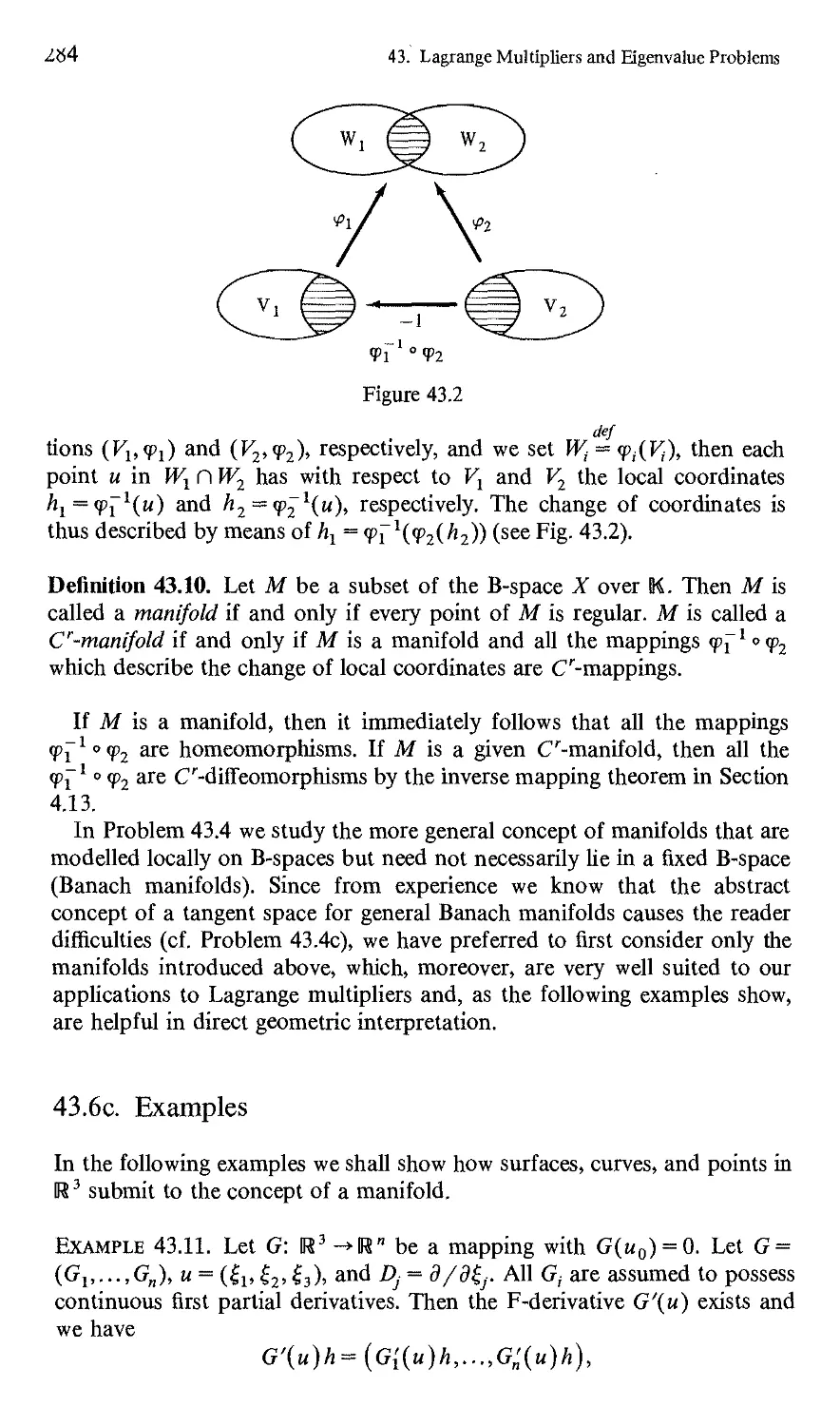
Текст
Eberhard Zeidler
Nonlinear
Functional Analysis
and its Applications
Variational Methods
and Optimization
S& BBBb'I
Leonhard Euler (1707-1783)
Eberhard Zeidler
Nonlinear
Functional ^lalys]
and its Applieatioi
III: Variational Methods
and Optimization
Translated by Leo F. Boron
With 111 Illustrations
Gl
Eberhard Zeidler
Sektion Mathematik
Karl-Marx-Platz
7010 Leipzig
German Democratic Republic
Leo F. Boron (Translator)
Department of Mathematics
and Applied Statistics
University of Idaho
Moscow, ID 83843
U.S.A.
AMS Classification: 58-01, 58-CXX, 58-EXX
Library of Congress Cataloging in Publication Data
Zeidler, Eberhard.
Nonlinear functional analysis and its applications.
Bibliography: p.
Includes index.
Contents: —pt. 3. Variational methods and
optimization.
1. Nonlinear functional analysis—Addresses, essays,
lectures. I. Title.
QA321.5.Z4513 1984 515.7 83-20455
© 1985 by Springer-Verlag New York Inc.
All rights reserved. No part of this book may be translated or reproduced in
any form without written permission from Springer-Verlag, 175 Fifth Avenue,
New York, New York 10010, U.S.A.
Typeset by Science Typographers, Inc., Medford, New York.
Printed and bound by R. R. Donnelley & Sons, Harrisonburg, Virginia.
Printed in the United States of America.
987654321
Dedicated in gratitude to my teacher
Professor Herbert Beckert
Preface
As long as a branch of knowledge offers an abundance of problems, it is full
of vitality.
David Hilbert
Over the last 15 years I have given lectures on a variety of problems in
nonUnear functional analysis and its appUcations. In doing this, I have
recommended to my students a number of excellent monographs devoted to
specialized topics, but there was no complete survey-type exposition of
nonUnear functional analysis making available a quick survey to the wide
range of readers including mathematicians, natural scientists, and engineers
who have only an elementary knowledge of linear functional analysis. I have
tried to close this gap with my five-part lecture notes, the first three parts of
which have been pubUshed in the Teubner-Texte series by Teubner-Verlag,
Leipzig, 1976, 1977, and 1978. The present EngUsh edition was translated
from a completely rewritten manuscript which is significantly longer than
the original version in the Teubner-Texte series. The material is organized in
the following way:
Part I: Fixed Point Theorems.
Part II: Monotone Operators.
Part III: Variational Methods and Optimization.
Parts IV/V: Applications to Mathematical Physics.
The exposition is guided by the following considerations:
(a) What are the supporting basic ideas and what intrinsic interrelations
exist between them?
(/6) In what relation do the basic ideas stand to the known propositions of
classical analysis and Unear functional analysis?
(•y) What typical applications are there?
Vll
Vlll
Preface
Special emphasis is placed on motivation. The reader should always have
the feeling that the theory is not developed for its own sake but rather for
the effective solution of concrete problems. At the same time I try to outline
a variegated picture of the subject matter which ranges from the
fundamental questions of set theory (the Bourbaki-Kneser fixed point theorem) to
concrete numerical methods, encompassing numerous applications to
physics, chemistry, biology, and economics. The reader should see
mathematics as a unified whole, with no separation between pure and applied
mathematics. At the same time we show how deep mathematical tools can
be used in the natural sciences, engineering, and economics. The
development of nonlinear functional analysis has been influenced in an essential
way by complicated natural scientific questions; the close contact with the
natural sciences and other sciences will also be of great significance for the
development of nonlinear functional analysis. In our exposition, the use of
analytic tools stands in the foreground, but we also seek to show
connections with algebraic and differential topology. For instance, Sections 37.27
and 37.28 contain an introduction to Morse theory as well as to singularity
and catastrophe theory. To reach the largest possible readership and to
fashion a self-contained exposition, important tools from linear functional
analysis are provided in the appendices to Parts I and II. These are
presented so that readers with a skimpy background can familiarize
themselves with this material. We forego, at the outset, the greatest possible
generality, but rather seek to expose the simple intrinsic nucleus without
trivializing it. According to the author's experience, it is easier for the
student to generalize familiar mathematical ideas to a more general situation
than to elicit the basic idea from a theorem that is formulated very generally
and burdened with many technical details. The teacher must help him in
that task. In order to make it easier for the reader to grasp the central
results, a number of propositions have been listed in a separate section
called List of Theorems to be found on page 643. It is clear that this
procedure is not entirely free of arbitrariness. However, we hope that the
lists of Theorems for Parts I-V provide an overview of the essential
substance of nonlinear functional analysis. Furthermore, since, in the
experience of the author, it is frequently difficult, because of a flood of details,
for the student to recognize the interrelationships between different
questions and the general strategies for the solution of problems, special
emphasis is placed on these interrelationships.
We have given a general overview of the content of Parts I-V and the
basic idea of nonlinear functional analysis in the Preface and in the
introduction to Part I. The present Part III consists of the following topics:
(a) Introduction to the subject.
(fi) Two fundamental existence and uniqueness principles.
(•y) Extremal problems without side conditions.
(8) Extremal problems with smooth side conditions.
(e) Extremal problems with general side conditions.
Preface
IX
(f) Saddle points and duality,
(rj) Variational inequalities.
In the introduction, and in the schematic survey in Fig. 37.1 on page 3, we
give an overview of the interrelationships between various extremal
problems. In the comprehensive introductory Chapter 37, we present many
simple, but typical, examples that are representative of those concrete
problems that have played a central role in the historical development of the
subject. In order to obtain an impression of the extraordinary variety of
problems involved, the reader should glance at the list of subjects for
Chapter 37 that appears in the Contents. In the immediately following
chapters it is our chief concern to show the reader that these problems can
be handled with the aid of a unified theory of extremal problems. The
essence of this unified theory consists of a small number of fundamental
principles of functional analysis. The title of Part III, Variational Methods
and Optimization, indicates-that we consider aspects of the classical calculus
of variations as well as modern optimization theory and their
interrelationships. By working out the supporting ideas and general fundamental
principles, we also wish to help the reader obtain an understanding of the
substance of the extraordinarily comprehensive and turbulently
accumulating literature on extremal problems, to classify these works according to
their ideas, and to note the emergence of new ideas.
Each of the 21 chapters is self-contained. Each begins with motivations,
heuristic considerations, and indications of the typical problems to be
investigated and contains the most important theorems and definitions
together with elucidating examples, figures, and typical applications. We
also do not shun citing very simple examples in the interest of the reader.
Furthermore, we always try to penetrate as quickly as possible to the heart
of the matter. We try to achieve the situation where the reader knows at
each phase of the book what concrete applications the general
considerations allow. In general, a very careful selection of the material had to be
made because one could write each chapter as a special monograph and, to
some extent, such monographs already exist. Here, we describe the
applications to nonlinear differential and integral equations, differential
inequalities, one-dimensional and multidimensional variational problems, linear and
convex optimization problems, problems in approximation theory and game
theory, continuous and discrete control problems for ordinary and partial
differential equations, and also consider important approximation methods.
In particular, in Section 37.29, we explain the basic ideas of 10 important
methods and principles for the construction of approximation methods. In
the introduction to Part I we have already pointed out that in numerical
methods the devil rides high on detail. However, general principles and
theoretical investigations of approximation methods within the setting of
numerical functional analysis are useful for recognizing the basic ideas and
for arranging the abundance of concrete numerical methods into a unified
point of view. We examine a number of more profound applications of
nonlinear functional analysis to mathematical physics in Parts IV and V.
X
Preface
At the end of each chapter the reader will find problems and references to
the literature. The problems vary considerably in their degree of difficulty:
(a) Problems without asterisks serve as drills in the material presented and
require no additional tools.
(j8) Problems with asterisks are more difficult—additional ideas are
required to solve them.
(•y) Problems with double asterisks are very difficult—one needs substantial
additional information to solve them.
Each problem contains either a solution or a precise reference to the
monograph or original work in which the solution can be found. Moreover,
we try to clarify the meaning of the results with explanatory remarks. The
problems with one or two asterisks are in part so devised that they present
targeted references to the literature on important extensions of results or
they serve to extend the reader's mathematical horizon. A number of topics
will be treated supplementarily in the problem collections. These topics are
particularly extensive in Chapter 40, where we try to sketch for the reader a
line of development from the classical calculus of variations and from
geometrical optics up to the modern theory of Fourier integral operators. In
this we let ourselves be led by the experience that the penetration of a
complicated theory is made easier for the student when she/he has an
ultimate goal from the beginning and knows the connection between the
goal and the simpler questions familiar to her/him.
The references to the literature at the end of each chapter are styled as
follows: Krasnoselskii (1956, M, B, H), etc. The year refers to the list of
literature at the end of the book. Furthermore, the capital Latin letters
mean:
M: monograph;
L: lecture notes;
S: survey;
P: proceedings;
B: the cited work contains a comprehensive bibliography;
H: the cited work contains references to the historical development of the
subject.
In this connection, the references to the literature are at the same time
supplied with clarifying captions which explain the interrelationship
between the works cited. On page 166 one finds "Recent trends". From the
abundance of available literature we have made a careful but necessarily
subjectively biased selection, which in the author's opinion will easily afford
the reader as comprehensive a picture as possible concerning the
farther-leading results. In this, the emphasis lies naturally on the surveys
and monographs. However, we also cite a number of classical works which
were of special significance for the development of the subject. We
recommend that the reader glance at several of these works in order to obtain ah
Pref.
XI
active impression of the genesis of new results and of the historical
development of mathematics. Unfortunately, in order to keep the list of literature
within tolerable bounds, we had to forego listing many important
references.
In the choice of the presentation it was taken into consideration that in
general no book is read completely from beginning to end. We hope that
even a quick skimming of the text will suffice for one to grasp the essential
contents. To this end, we recommend reading the introductions to the
individual chapters, the definitions, the theorems (without proofs), and the
examples (without proofs) as well as the comments in the text between these
definitions, theorems, etc., which point out the meaning of the individual
results. The reader who does not have time to solve the problems should,
however, briefly scrutinize the captions to the problems and the adjoining
remarks, which elucidate the meaning of the formulation of the problems
and the interrelationships." The reader who is interested in supplementary
problem material can try to prove independently all of the examples in the
text without referring to the given proof. Moreover, in the references to the
literature in Section 37.29, books are cited in which the reader will find
comprehensive collections of exercises that as a rule are not too difficult. All
hypotheses both in the theorems and in the examples are explicitly stated so
that the reader avoids a time-consuming search for the assumptions in the
antecedent text. We have taken pains to reduce the number of definitions to
a minimum in order not to burden the reader with too many concepts. On
page xii one finds a list of the most important definitions. In order to clarify
interrelationships, several assertions that belong together are at times
combined into a single theorem. In this form of exposition, we have also kept in
mind the natural scientist and the engineer who want primarily to gain
information on which mathematical tools are available for the various
nonlinear problems. We recommend Chapter 37 to the reader who wishes to
examine the class of problems which the general theory allows one to treat.
However, it suffices to glance at this comprehensive chapter, because
references will later be made at the appropriate places. The reader whose
priority is to become acquainted with the theoretical framework can
immediately begin with Chapter 38 and, on first reading, omit the sections in
the individual chapters that are devoted to applications.
Grasping the individual steps in the proofs as well as the essential ideas of
the proofs is made easier by the careful organization of the proofs. It is a
truism that only by a precise study of the proofs one can penetrate more
deeply into a mathematical theory.
Part III is to a large extent independent of the other parts. However,
where necessary, we do refer to particular results of the other parts. Note
that several auxiliary tools are made available in Parts I and II (basic
information concerning linear functional analysis, Sobolev spaces, etc.). We
formulate a number of results for locally convex spaces. The reader who is
not familiar with this material can orient himself by reading the appendix to
Part I or replace the concept of a locally convex space by that of a Banach
Xll
Preface
or Hilbert space. Dual pairs are important for duality theory. We explain
this concept in the appendix to Part III. The reference Aj (20) relates to (20)
in the appendix to the ith part. (37.20) is formula (20) in Chapter 37.
Within a particular chapter, we forego giving the chapter number of the
equation. In each chapter, theorems are distinguished by capital letters, so
that, for instance, "Theorem 57.B in Section 57.5" means the second
theorem in Chapter 57, located in Section 5 of that chapter. Propositions,
lemmas, corollaries, definitions, remarks, conventions, counterexamples,
standard examples, and examples are numbered consecutively in each
chapter—for example, in Chapter 41 one finds Definition 41.1, Proposition
41.2, Corollary 41.3, etc., in that order. The end of a proof is indicated by
the symbol □. We subdivide the chapters among the five separate parts of
this work in the following way:
Part I: Chapters 1-17.
Part II: Chapters 18-36.
Part III: Chapters 37-57.
Part IV: Chapters 58-79.
Part V: Chapters 80-100.
A list of symbols used can be found on page 637. We have taken pains to
employ the notation that is generally used. To avoid confusion, we point out
several peculiarities at the beginning of the list of symbols on page 637. A
detailed subject index can be found on page 651. As far as abbreviations are
concerned, we use only B-space (respectively, H-space) for Banach space
(respectively, Hilbert space), F-derivative (respectively, G-derivative) for
Frechet derivative (respectively Gateaux derivative) as well as M-S
sequence for Moore-Smith sequence and L-S deformation for
Ljusternik-Schnirelman deformation.
I have taken pains to write as interesting and diverse a book as possible.
Of course, whether or not I have succeeded in this only the reader can
decide.
I am indebted to numerous colleagues for interesting conversations and
letters as well as for sending me articles and books—I thank them all
heartily. I am especially grateful to my mentor Professor Herbert Beckert
for all that I learned from him as a scientist and as a human being. I should
like to dedicate the present volume to him. I cordially thank Paul H.
Rabinowitz and the Department of Mathematics of the University of
Wisconsin, Madison, for the invitation as guest resident scholar during the
fall semester 1978. The very stimulating atmosphere in Madison influenced
the final form of the exposition in an essential way. In the tasks of typing
the manuscript and of making copies, I was supported in an amiable way by
a number of colleagues, both male and female. I should like to very heartily
thank Ursula Abraham, Sonja Bruchholz, Elvira Krakowitzki, Heidi Kilhn,
Hiltraud Lehmann, Karin Quasthoff, Werner Berndt, and Rainer Schumann.
I would especially like to thank Rainer Schumann for a critical perusal of
parts of the manuscript. The understanding and extensive support shown to
Preface
xin
me by the librarian of our institute, Frau Ina Letzel, was of great value to
me. Furthermore, I thank the administrators of the Mathematics Section
of the Karl Marx University, Leipzig, and its director, Professor Horst
Schumann, for supporting this project.
I would also like to thank the translator, Professor Leo F. Boron,
University of Idaho, Moscow, for his excellent work. I am very indebted to
him for valuable suggestions and remarks. Finally, my special thanks go to
Springer-Verlag for the harmonious collaboration and the understanding
approach to all my wishes.
Eberhard Zeidler
Leipzig
Spring 1984
Contents
Introduction to the Subject 1
General Basic Ideas 4
CHAPTER 37
Introductory Typical Examples 12
§37.1. Real Functions in R1 13
§37.2. Convex Functions in R1 15
§37.3. Reai Functions in R N, Lagrange Multipliers, Saddle Points, and
Critical Points 16
§37.4. One-Dimensional Classical Variational Problems and Ordinary
Differential Equations, Legendre Transformations, the
Hamilton-Jacobi Differential Equation, and the Classical
Maximum Principle 20
§37.5. Multidimensional Classical Variational Problems and Elliptic
Partial Differential Equations 41
§37.6. Eigenvalue Problems for Elliptic Differential Equations and
Lagrange Multipliers 43
§37.7. Differential Inequalities and Variational Inequalities 44
§37.8. Game Theory and Saddle Points, Nash Equilibrium Points and
Pareto Optimization 47
§37.9. Duality between the Methods of Ritz and Trefftz, Two-Sided
Error Estimates 50
§37.10. Linear Optimization in R N, Lagrange Multipliers, and Duality 51
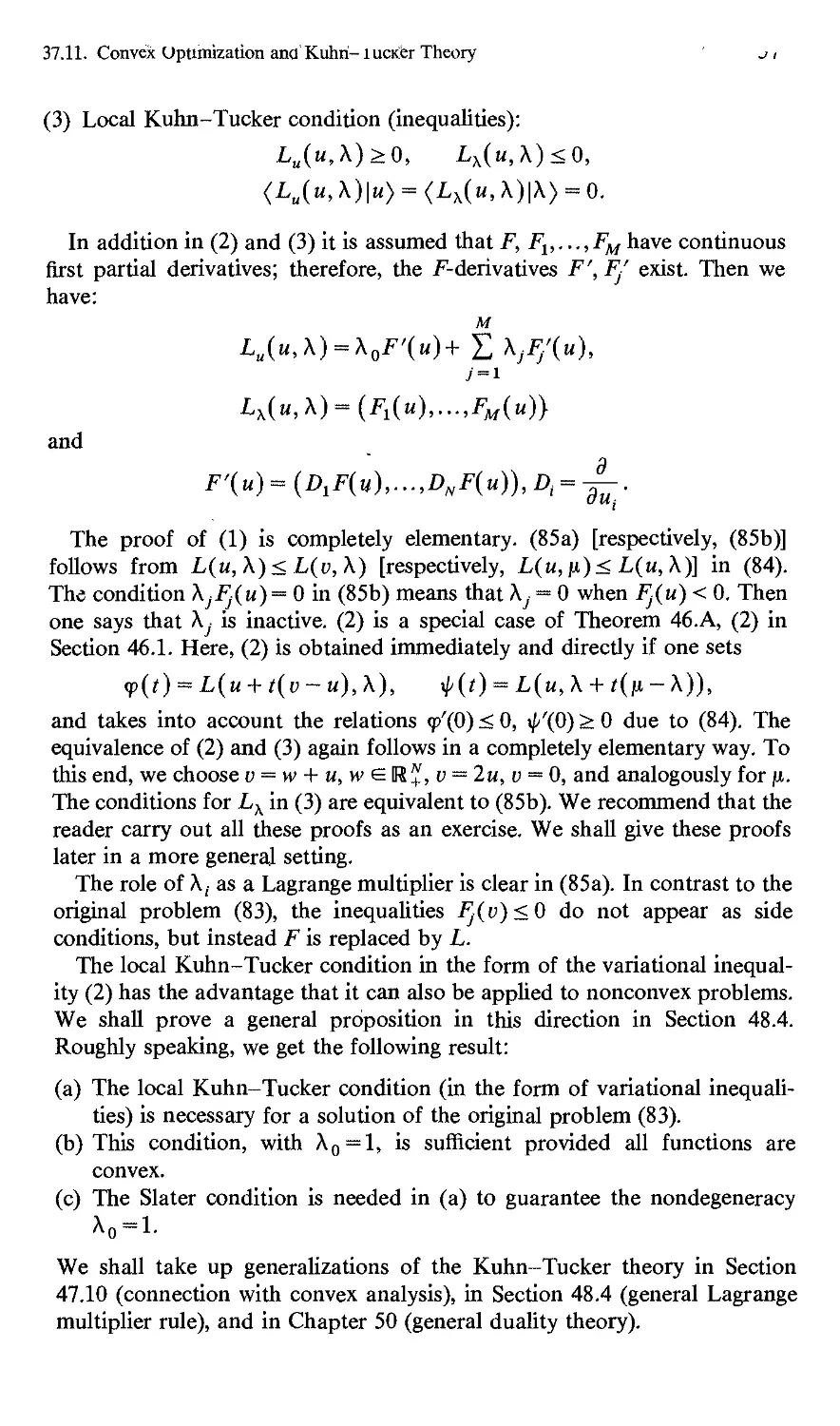
§37.11. Convex Optimization and Kuhn-Tucker Theory 55
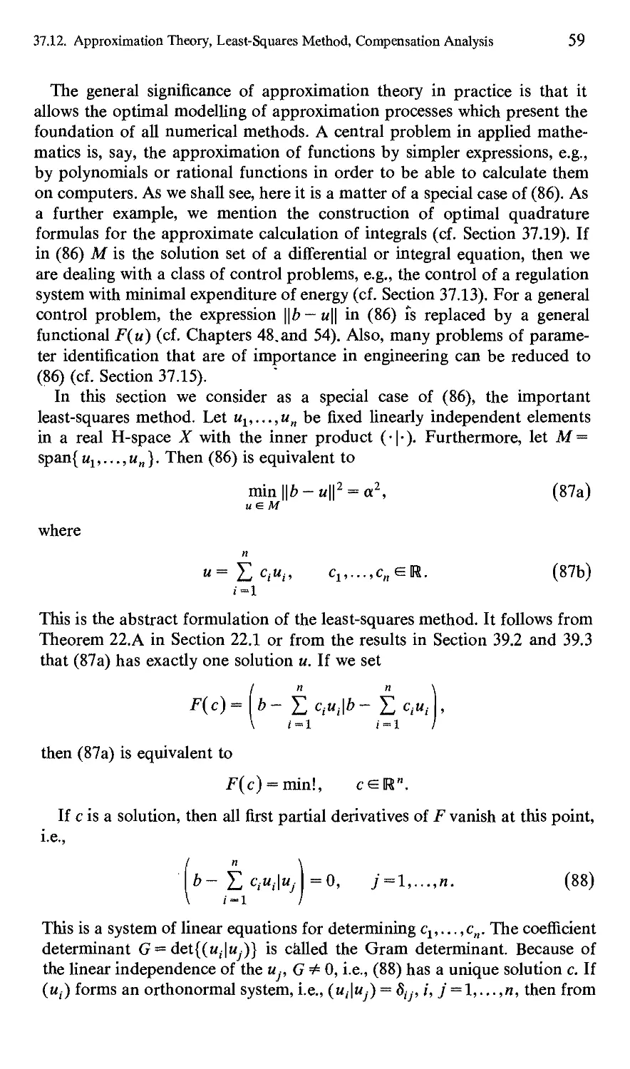
§37.12. Approximation Theory, the Least-Squares Method, Deterministic
and Stochastic Compensation Analysis 58
§37.13. Approximation Theory and Control Problems 64
xvi
Contents
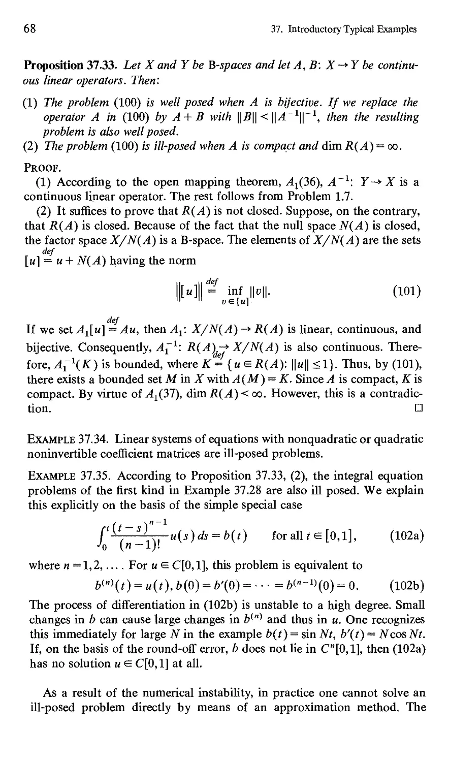
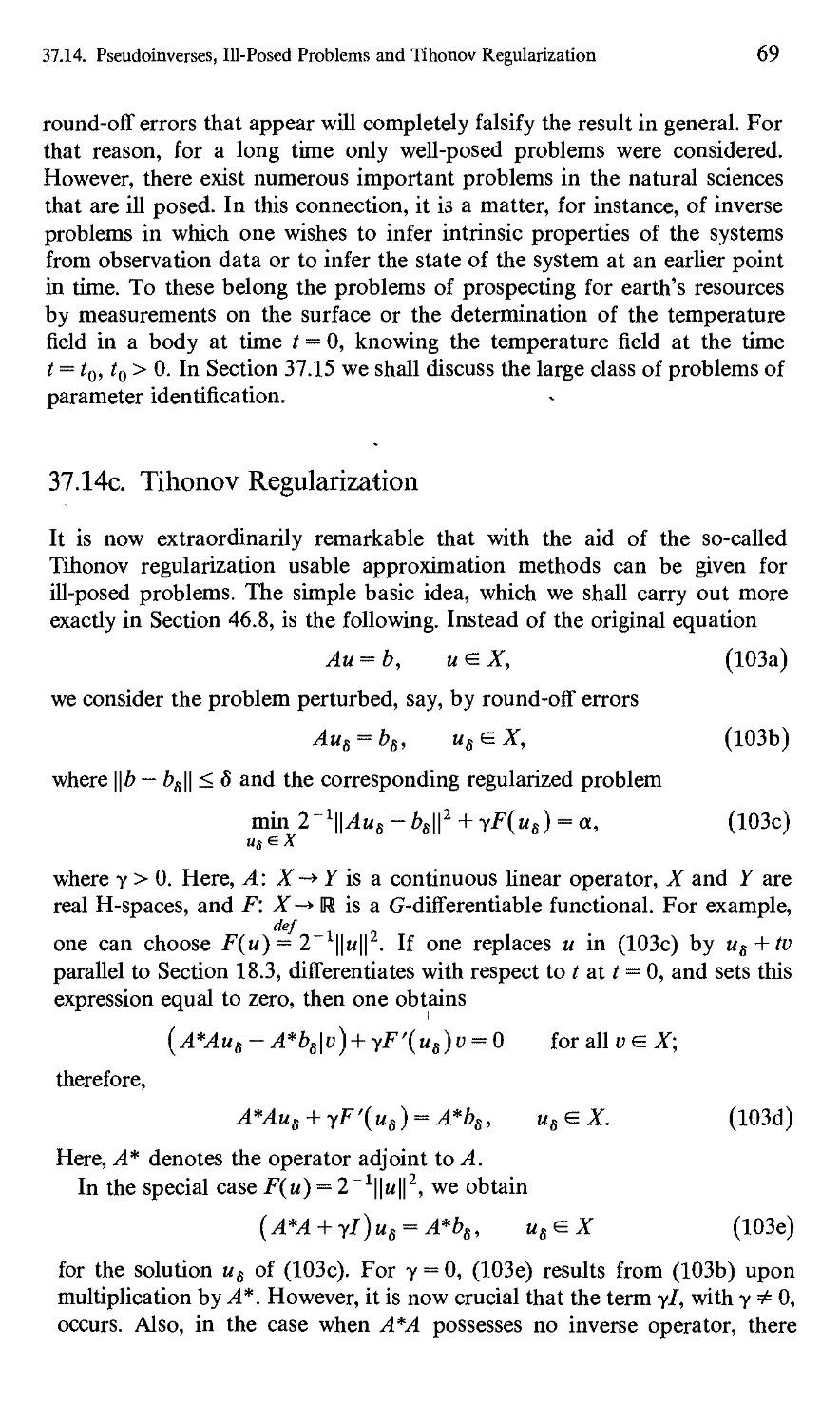
§37.14, Pseudoinverses, Ill-Posed Problems and Tihonov Regularization 65
§37,15. Parameter Identification 71
§37.16. Chebyshev Approximation and Rational Approximation 73
§37,17. Linear Optimization in Infinite-Dimensional Spaces, Chebyshev
Approximation, and Approximate Solutions for Partial
Differential Equations 76
§37.18, Splines and Finite Elements 79
§37.19. Optimal Quadrature Formulas 80
§37.20, Control Problems, Dynamic Optimization, and the Bellman
Optimization Principle 84
§37.21. Control Problems, the Pontrjagin Maximum Principle, and the
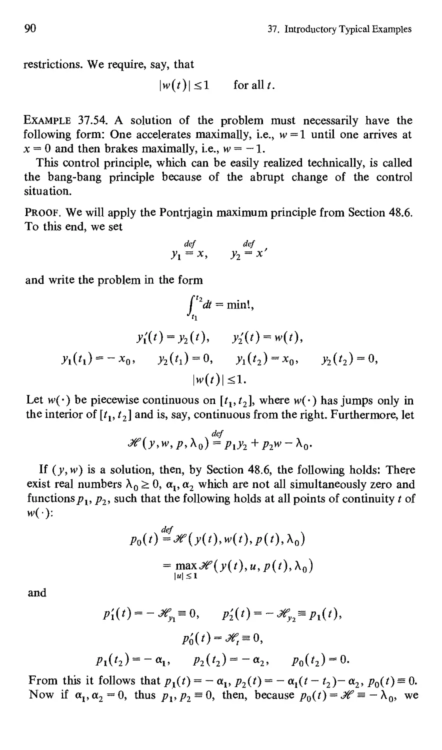
Bang-Bang Principle 89
§37.22, The Synthesis Problem for Optimal Control 92
§37.23, Elementary Provable Special Case of the Pontrjagin Maximum
Principle 93
§37.24. Control with the Aid of Partial Differential Equations 96
§37.25. Extremal Problems with Stochastic Influences 97
§37.26. The Courant Maximum-Minimum Principle, Eigenvalues,
Critical Points, and the Basic Ideas of the Ljusternik-Schnirelman
Theory 102
§37,27. Critical Points and the Basic Ideas of the Morse Theory 105
§37.28. Singularities and Catastrophe Theory 115
§37.29. Basic Ideas for the Construction of Approximate Methods for
Extremal Problems 132
TWO FUNDAMENTAL EXISTENCE AND UNIQUENESS
PRINCIPLES
CHAPTER 38
Compactness and Extremal Principles 145
§38,1, Weak Convergence and Weak* Convergence 147
§38.2. Sequential Lower Semicontinuous and Lower Semicontinuous
Functionals 149
§38.3. Main Theorem for Extremal Problems 151
§38.4. Strict Convexity and Uniqueness 152
§38.5. Variants of the Main Theorem 153
§38.6, Application to Quadratic Variational Problems 155
§38.7. Application to Linear Optimization and the Role of Extreme
Points 157
§38.8. Quasisolutions of Minimum Problems 158
§38,9. Application to a Fixed-Point Theorem 161
§38.10, The Palais-Smale Condition and a General Minimum Principle 161
§38.11. The Abstract Entropy Principle 163
Contents
XV11
CHAPTER 39
Convexity and Extremal Principles 168
§39.1. The Fundamental Principle of Geometric Functional Analysis 170
§39.2. Duality and the Role of Extreme Points in Linear Approximation
Theory 172
§39.3. Interpolation Property of Subspaces and Uniqueness 175
§39.4. Ascent Method and the Abstract Alternation Theorem 177
§39.5. AppUcation to Chebyshev Approximation 180
EXTREMAL PROBLEMS WITHOUT SIDE CONDITIONS
CHAPTER 40
Free Local Extrema of Differentiable Functionals and the Calculus
of Variations 189
§40.1. nth Variations, G-Derivative, and F-Derivative 191
§40.2. Necessary and Sufficient Conditions for Free Local Extrema 193
§40.3. Sufficient Conditions by Means of Comparison Functionals and
Abstract Field Theory 195
§40.4. AppUcation to Real Functions in RN 195
§40.5. AppUcation to Classical Multidimensional Variational Problems
in Spaces of Continuously Differentiable Functions 196
§40.6. Accessory Quadratic Variational Problems and Sufficient
Eigenvalue Criteria for Local Extrema 200
§40.7. AppUcation to Necessary and Sufficient Conditions for Local
Extrema for Classical One-Dimensional Variational Problems 203
CHAPTER 41
Potential Operators 229
§41.1. Minimal Sequences 232
§41.2. Solution of Operator Equations by Solving Extremal Problems 233
§41.3. Criteria for Potential Operators 234
§41.4. Criteria for the Weak Sequential Lower Semicontinuity of
Functionals 235
§41.5. AppUcation to Abstract Hammerstein Equations with Symmetric
Kernel Operators 237
§41,6. AppUcation to Hammerstein Integral Equations 239
CHAPTER 42
Free Minima for Convex Functionals, Ritz Method and the
Gradient Method 244
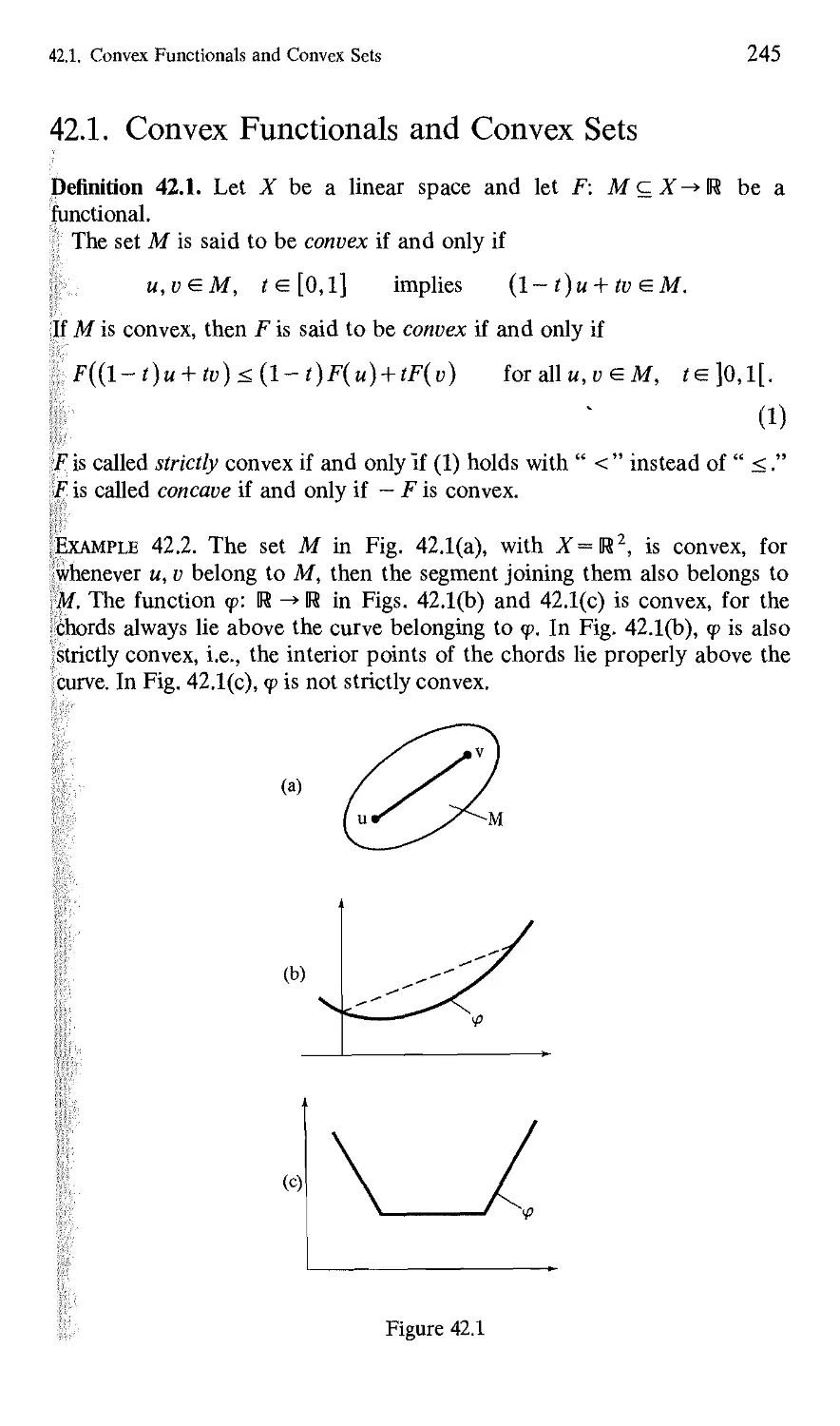
§42.1. Convex Functionals and Convex Sets 245
§42.2. Real Convex Functions 246
Contents
§42.3. Convexity of F, Monotonicity of F', and the Definiteness of the
Second Variation 247
§42.4. Monotone Potential Operators 249
§42.5. Free Convex Minimum Problems and the Ritz Method 250
§42.6. Free Convex Minimum Problems and the Gradient Method 252
§42.7. Application to Variational Problems and Quasilinear Elliptic
Differential Equations in Sobolev Spaces 255
EXTREMAL PROBLEMS WITH SMOOTH SIDE CONDITIONS
CHAPTER 43
Lagrange Multipliers and Eigenvalue Problems 273
§43.1. The Abstract Basic Idea of Lagrange Multipliers 274
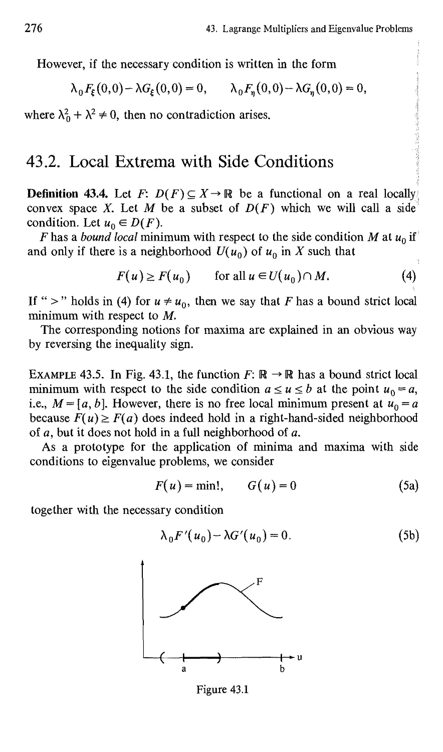
§43.2. Local Extrema with Side Conditions 276
§43.3. Existence of an Eigenvector Via a Minimum Problem 278
§43.4. Existence of a Bifurcation Point Via a Maximum Problem 279
§43.5. The Galerkin Method for Eigenvalue Problems 281
§43.6. The Generalized Implicit Function Theorem and Manifolds in
B-Spaces 282
§43.7. Proof of Theorem 43.C 288
§43.8. Lagrange Multipliers 289
§43.9. Critical Points and Lagrange Multipliers 291
§43.10. Application to Real Functions in R N 293
§43.11. Application to Information Theory 294
§43.12, Application to Statistical Physics. Temperature as a Lagrange
Multiplier 296
§43.13. Application to Variational Problems with Integral Side Conditions 299
§43.14. Application to Variational Problems with Differential Equations
as Side Conditions 300
CHAPTER 44
Ljusternik-Schnirelman Theory and the Existence of
Several Eigenvectors 313
§44.1. The Courant Maximum-Minimum Principle 314
§44.2. The Weak and the Strong Ljusternik Maximum-Minimum
Principle for the Construction of Critical Points 316
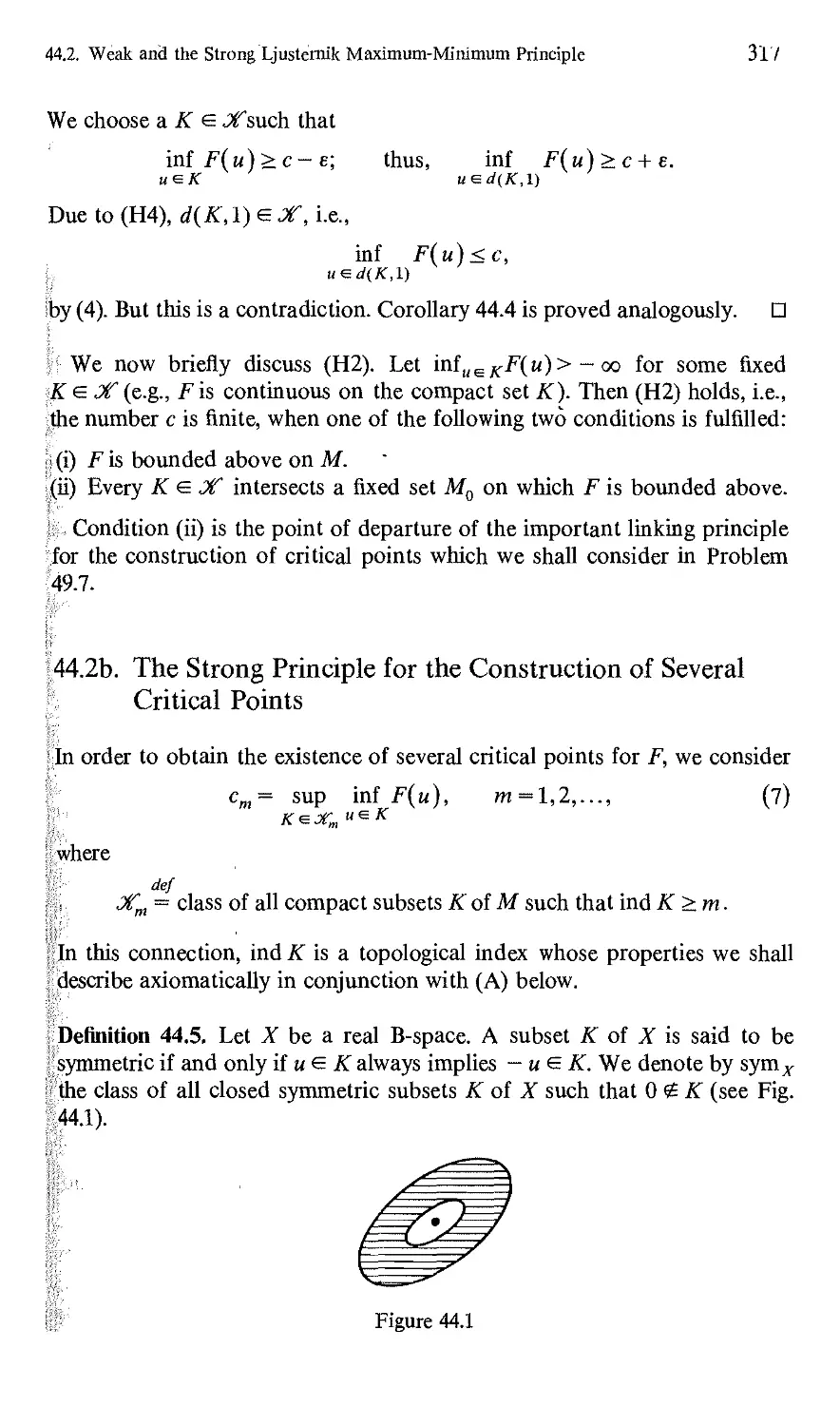
§44.3. The Genus of Symmetric Sets 319
§44.4. The Palais-Smale Condition 321
§44.5. The Main Theorem for Eigenvalue Problems in Infinite-
Dimensional B-spaces 324
§44.6. A Typical Example 328
§44.7. Proof of the Main Theorem 330
^UlllCllLS
§44.8. The Main Theorem for Eigenvalue Problems in Finite-
Dimensional B-Spaces 335
§44.9. Application to Eigenvalue Problems for Quasilinear Elliptic
Differential Equations 336
§44.10. Application to Eigenvalue Problems for Abstract Hammerstein
Equations with Symmetric Kernel Operators 337
§44.11. Application to Hammerstein Integral Equations 339
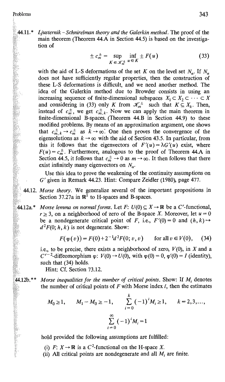
§44.12. The Mountain Pass Theorem 339
CHAPTER 45
Bifurcation for Potential Operators - 351
§45.1. Krasnoselskii's Theorem 351
§45.2. The Main Theorem • 352
§45.3. Proof of the Main Theorem 354
EXTREMAL PROBLEMS WITH GENERAL SIDE CONDITIONS
CHAPTER 46
Differentiable Functionals on Convex Sets 363
§46.1. Variational Inequalities as Necessary and Sufficient Extremal
Conditions 363
§46.2. Quadratic Variational Problems on Convex Sets and Variational
Inequalities 364
§46.3. Application to Partial Differential Inequalities 365
§46.4. Projections on Convex Sets 366
§46.5. The Ritz Method 367,
§46.6. The Projected Gradient Method 368
§46.7. The Penalty Functional Method 370
§46.8. Regularization of Linear Problems 372
§46.9. Regularization of Nonlinear Problems 375
CHAPTER 47
Convex Functionals on Convex Sets and Convex Analysis 379
§47.1. The Epigraph 380
§47.2. Continuity of Convex Functionals 383
§47.3. Subgradient and Subdifferential 385
§47.4. Subgradient and the Extremal Principle 386
§47.5. Subgradient and the G-Derivative 387
§47.6. Existence Theorem for Subgradients 387
§47.7. The Sum Rule 388
XX
Contents
§47.8. The Main Theorem of Convex Optimization 390
§47.9. The Main Theorem of Convex Approximation Theory 392
§47.10. Generalized Kuhn-Tucker Theory 392
§47.11. Maximal Monotonicity, Cyclic Monotonicity, and Subgradients 396
§47.12. Application to the Duality Mapping 399
CHAPTER 48
General Lagrange Multipliers (Dubovickii-Miljutin Theory) 407
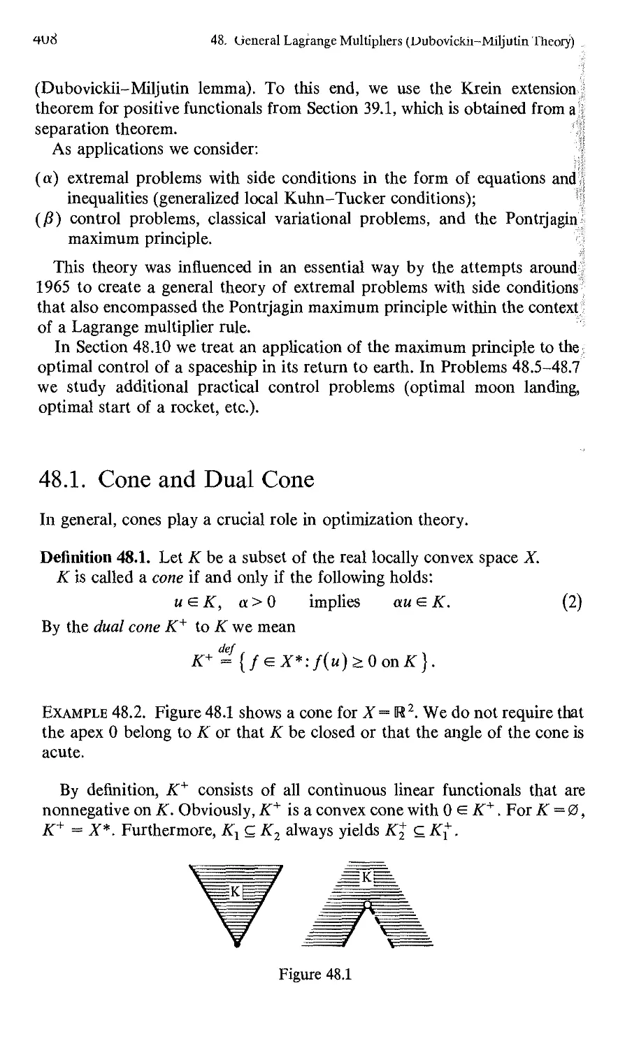
§48.1. Cone and Dual Cone 408
§48.2. The Dubovickii-Miljutin Lemma 411
§48.3. The Main Theorem on Necessary and Sufficient Extremal
Conditions for General Side Conditions 413
§48.4. Application to Minimum Problems with Side Conditions in the
Form of Equalities and Inequalities 416
§48.5. Proof of Theorem 48.B 419
§48.6. Application to Control Problems (Pontrjagin's Maximum
Principle) 422
§48.7. Proof of the Pontrjagin Maximum Principle 426
§48.8. The Maximum Principle and Classical Calculus of Variations 433
§48.9. Modifications of the Maximum Principle 435
§48.10. Return of a Spaceship to Earth 437
SADDLE POINTS AND DUALITY
CHAPTER 49
General Duality Principle by Means of Lagrange Functions
and Their Saddle Points 457
§49.1. Existence of Saddle Points 457
§49.2. Main Theorem of Duality Theory 460
§49.3. Application to Linear Optimization Problems in B-Spaces 463
CHAPTER 50
Duality and the Generalized Kuhn-Tucker Theory 479
§50.1. Side Conditions in Operator Form 479
§50.2. Side Conditions in the Form of Inequalities 482
CHAPTER 51
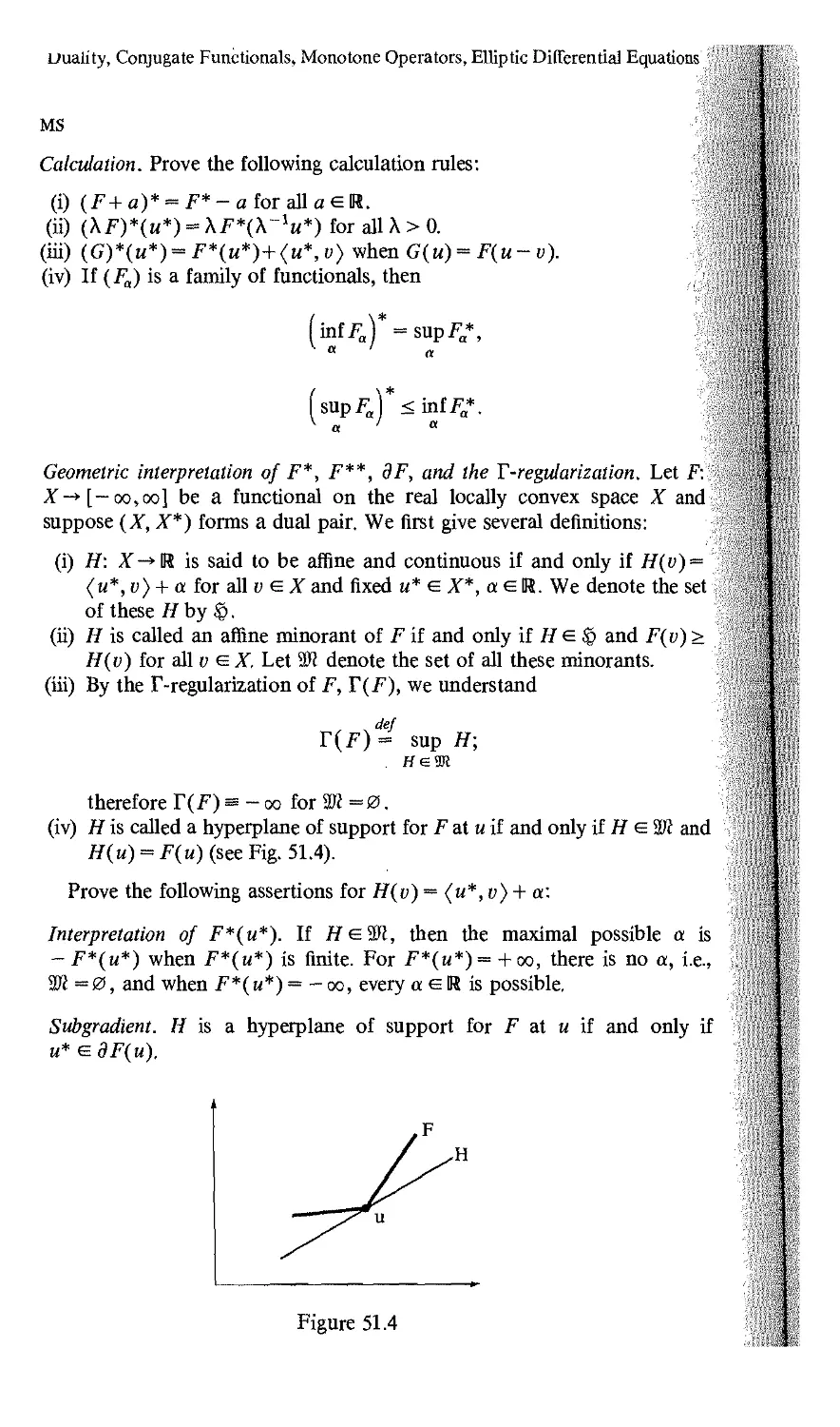
Duality, Conjugate Functionals, Monotone Operators and Elliptic
Differential Equations 487
§51.1. Conjugate Functionals 489
§51.2. Functionals Conjugate to Differentiable Convex Functionals 492
XXI
§51.3. Properties of Conjugate Functional 493
§51.4. Conjugate Functionals and the Lagrange Function 496
§51.5. Monotone Potential Operators and Duality 499
§51.6. Applications to Linear Elliptic Differential Equations, Trefftz's
Duality 502
§51.7. Application to Quasilinear Elliptic Differential Equations 506
CHAPTER 52
General Duality Principle by Means of Perturbed Problems and
Conjugate Functionals 512
§52.1. The S-Functional, Stability, and Duality . 513
§52.2. Proof of Theorem 52.A 515
§52.3. Duality Propositions of Fenchel-Rockafellar Type 517
§52.4. Application to Linear Optimization Problems in Locally Convex
Spaces 519
§52.5. The Bellman Differential Inequality and Duality for Nonconvex
Control Problems 521
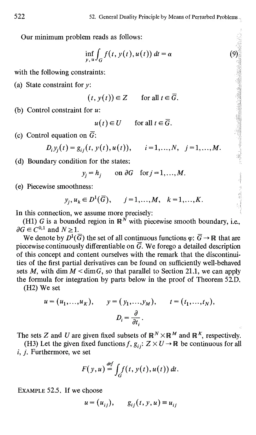
§52.6. Application to a Generalized Problem of Geometrical Optics 525
CHAPTER 53
Conjugate Functionals and Orlicz Spaces 538
§53.1. Young Functions 538
§53.2. Orlicz Spaces and Their Properties 539
§53.3. Linear Integral Operators in Orlicz Spaces 541
§53.4. The Nemyckii Operator in Orlicz Spaces 542
§53.5. Application to Hammerstein Integral Equations with Strong
Nonlinearities 542
§53.6. Sobolev-Orlicz Spaces 544
VARIATIONAL INEQUALITIES
CHAPTER 54
Elliptic Variational Inequalities 551
§54.1. The Main Theorem 551
§54.2. Application to Coercive Quadratic Variational Inequalities 552
§54.3. Semicoercive Variational Inequalities 553
§54.4. Variational Inequalities and Control Problems 556
§54.5. Application to Bilinear Forms 558
§54.6. Application to Control Problems with Elliptic Differential
Equations 559
§54.7. Semigroups and Control of Evolution Equations 560
lints
§54.8. Application to the Synthesis Problem for Linear Regulators 561
§54.9. Application to Control Problems with Parabolic Differential
Equations 562
CHAPTER 55
Evolution Variational Inequalities of First Order in H-Spaces 568
§55.1. The Resolvent of Maximal Monotone Operators 569
§55.2. The Nonlinear Yosida Approximation 570
§55.3. The Main Theorem for Inhomogeneous Problems 570
§55.4. Application to Quadratic Evolution Variational Inequalities of
First Order 572
CHAPTER 56
Evolution Variational Inequalities of Second Order in H-Spaces 577
§56.1. The Main Theorem 577
§56.2. Application to Quadratic Evolution Variational Inequalities of
Second Order 578
CHAPTER 57
Accretive Operators and Multivalued First-Order Evolution
Equations in B-Spaces 581
§57.1. Generalized Inner Products on B-Spaces 582
§57.2, Accretive Operators 583
§57.3, The Main Theorem for Inhomogeneous Problems with
m-Accretive Operators 584
§57.4. Proof of the Main Theorem 585
§57,5. Application to Nonexpansive Semigroups in B-Spaces 593
§57.6. Application to Partial Differential Equations 594
Appendix 599
References 606
List of Symbols 637
List of Theorems 643
List of the Most Important Definitions 647
Index 651
Introduction to the Subject
I love mathematics not only because it is applicable to technology but also
because it is beautiful.
Rosza Peter
Science is a first class piece of furniture for the bel etage—as long as common
sense reigns on the ground floor.
Oliver Wendell Holmes
Extremal problems play an extraordinarily large role in the application of
mathematics to practical problems, for example:
(a) in mathematical physics (mechanics and celestial mechanics,
geometrical optics, elasticity theory, hydrodynamics, rheology, relativity theory,
etc.);
(0) in geometry (geodesies, minimal surfaces, etc.);
(•y) in mathematical economics (transport problems, optimal warehouse
maintenance);
(§) in regulation technology (optimal control of general regulation systems,
e.g., industrial installations, spaceships, etc.);
(e) in chemistry, geophysics, technology, etc. (optimal determination of
unknown data from measurements);
(f) in numerical mathematics (optimal structuring of approximation
processes, etc.);
(rj) in the theory of probability (optimal control of stochastic processes,
optimal estimation of unknown parameters, optimal construction of
airplanes, water-power networks, etc.).
2
Introduction to the Subject
In this connection, we exploit the fact that many processes in nature
proceed according to extremal principles, for example:
(a) the principle of stationary action in mechanics, relativity theory,
electrodynamics, etc.;
(b) the principle of minimal potential energy in stable mechanical
equilibrium states;
(c) Fermat's principle of least time in light propagation in geometrical
optics;
(d) Einstein's principle of the motion of mass along four-dimensional
geodesies in general relativity theory.
Moreover, for economic reasons, we are interested in the optimal modelling
of production procedures and other regulation processes.
The history of extremal problems comprises four distinct stages:
(i) The solution of extremal problems for real functions with the aid of
the differential and integral calculus that was invented about 300 years ago.
(ii) Classical calculus of variations that originated about 300 years ago in
connection with mechanical problems.
(iii) Optimization that came into being because of economic and
regulation-technical questions and that has been intensively advanced during
approximately the last 30 years (linear optimization, Kuhn-Tucker theory,
Bellman dynamic optimization, Pontrjagin's maximum principle).
(iv) The theory of variational inequalities and quasivariational inequalities
with its applications to mathematical physics and the deterministic and
stochastic optimization theory that has existed for about the last 15 years.
Figure 37.1 gives a general view. In this connection, we generally
distinguish:
(a) Problems without side conditions (free problems).
(b) Problems with side conditions (bound problems).
Side conditions in the form of equations are typical for the classical calculus
of variations. For example, the shortest path joining two points on a sphere
must satisfy the equation of the sphere. On the other hand, side conditions
in the form of inequalities are typical for optimization. For example, it can
be a matter of bounds for the fuel supply under optimal control of a rocket
or the bounds for the warehouse capacity under optimal warehouse
maintenance.
In the comprehensive introductory chapter (Chapter 37), we give as an
explanation of Fig. 37.1 a survey of diverse concrete formulations of
problems, the calculus of variations, and optimization theory. In the
following chapters we show that these seemingly very disparate problems can be
treated in a unified way within the framework of a functional analytical
theory with the aid of only a few general fundamental principles.
In the following we shall go into several of these interrelationships.
NONLINEAR FUNCTIONAL ANALYSIS
stochastic optimization
EXTREMAL PROBLEMS
VARIATIONAL PROBLEMS,
Euler
differential
equations
(e.g., boundary
and boundary
eigenvalue
problems for
quasilinear elliptic
differential equations)
Variatiomal inequalities
(e.g., differential
inequalities)
..OPTIMIZATION^
/ ..game theory
Hammerstein
integral
equations
discrete
(dynamic optimization
and the discrete maximum
principle)
parameter identification
continuous
(Pontrjagin maximum
principle and the
Bellman equation)
\ I
approximation theory
I
' CONVEX OPTIMIZATION
(Kuhn-Tucker theory)
linear
optimization
Figure 37.1, Overview of extremal problems.
4
Introduction to the Subject
General Basic Ideas
By extremal problems we mean:
(i) minimum and maximum problems (extremal problems in the narrower
sense);
(ii) saddle point problems and minimax problems (game theory, duality
theory and error estimates, approximation theory);
(iii) determination of critical points (eigenvalue problems, Ljuster-
nik-Schnirelman theory, and Morse theory);
(iv) determination of noncooperative equilibrium points in the sense of
Nash, Pareto optimization, Walras equilibria (economics models);
(v) solution of variational inequalities.
Here, (iv) [respectively, (v)] is related to (ii) [respectively, (i)]. The concept of
critical point is of central significance for variational problems and their
applications. The functional F has a critical point with respect to a
neighborhood U of «0 in case, roughly speaking, the following holds: The
differenceF(u0 + h)— F(u0) is of order greater than the first with respect to
all h such that uQ + heU. For a real function F: R ->R this means that
F'(uQ) = 0 provided 1/= R. The precise definition of a critical point can be
found in Section 43.9. The intuitive meaning of a critical point is explained
in Sections 37.1. and 37.2 for real functions of one and several variables as
well as for free variational problems (respectively, variational problems with
side conditions) in 37.4b (respectively, 37.4/). In Section 43.9 we go into the
connection between critical points and Lagrange multipliers. If F has a
critical point at u0, then we also say that Fis stationary at u0. We symbolize
the problem of discovering critical points u of F with respect to U by
F(u) = stationary!, «e[/.
Many equations of mathematical physics are obtained from such
formulations of the problem (principle of stationary action). Moreover, the
symmetry properties of F lead, via the Noether theorem (cf. 37.4k), to physical
conservation quantities (energy, spin, etc.) and transformation properties of
the field equations (tensors, spinors, and gauge transformations). This is
u
Figure 37.2
General Basic Ideas
5
especially important if one wishes, for example, to obtain an overview of the
possible field equations on the basis of physical symmetry and invariance
ideas for interacting quantum fields of elementary particles.
To fix the terminology, we now recall several well-known concepts. We
designate minima and maxima as extrema. A general minimum problem has
the form
infF(«) = a. (l°)
ae(/
Here, F: U-* [ — 00,00] is a mapping that can take on the two values ± 00
besides all real values. In the introduction to Chapter 47 we explain why
taking these two improper values into consideration is very expedient.
Posing the problem in the form (1°) means that the infimum a of F is
sought on U. This infimum always exists on [—00,00]. By definition, it is
equal to the greatest lower bouqid of the values of F on U. The point uQ in U
is called a solution of (1°) or, also, a minimal point of F on U if and only if
F(u0) = a. In this case, we call a the minimal value of F on U. Moreover,
we say that F possesses a minimum on U.
If we wish to emphasize that we are seeking a minimal point, then instead
of (1°) we write
minF(«) = a. (2°)
ae(/
This way of formulating the problem thus entails the determination of the
infimum a of F on U and discovering a u0 in U such that F(u0) = a. Figure
37.2 refers to the important situation that a solution u0 of (1°) [respectively,
(2°)] need not always exist. For (1°) [respectively, (2°)] we occasionally
write
F( u) = inf., «e[/; respectively F( u) = min!, u e U.
Maximum problems of the form
sup F(u) = /3, (3°)
ae(/
maxF(tt)=)8 (4°)
ae(/
are to be understood analogously. By definition, we set the infimum
(respectively, the supremum) over the empty set U = 0 in (1°) [respectively, (3°)]
equal to a = + 00 (respectively, /3 = — 00). We shall frequently be concerned
with minimum problems only, since, because of the relation
supF(«) = - inf (-F(u)), (5°)
ae(7 ae(7
every maximum problem can be changed into a minimum problem by
switching from F to — F.
We designate problems of the type
mini sup L(x, y)) = y (6°)
6
Introduction to the Subject
as min-sup problems. The point x is a solution of (6°) if and only if, parallel
to our conventions for (1°) and (2°), we have
def / ,\
y = inf I sup L(x, y)\
x^A^y&B '
and
sup (L(x, .)0) = 7, x^A. (6a°)
yeB
If we replace the symbol "sup" by "max" in (6°), then (3c, y) is naturally
called a solution of (6°) if and only if y is a solution of (6a°). max-inf
problems, etc., are handled analogously. It is thus clear what is to be
understood by a solution (x, y) of
min sup L(x,y) = max inf L(x, y), (7°)
i€A ye B yeBxe A
namely,
del
y = inf sup L(x,y)= sup infL(x,>')
je/l jet y^BxeA
and
supL(x,>') = v, inf L(x,y) = y, (x,y)^AxB. (7a°)
One is led to (7°) when determining the saddle points (x, y) for L. If the
symbols "max" and "min" appear instead of "sup" and "inf in (7°), then
(x, y) is called a solution of the corresponding minimax problem if and only
if (7a°) holds for y = L(x,y). Problems of the form (6°) appear, for
example, in approximation theory, for one can write the problem
min||fc-x|| = -y
x e A
as
min max (y, b - x) = y,
where A C X and B= {y e X*: \\y\\ =1} in case X is a B-space. (7°) and the
corresponding minimax problems are basic to the game theory discussed in
Section 37.8 and to the duality theory in Chapter 49.
In Part III, we shall investigate the following central questions for
extremal problems:
(a) Existence and uniqueness of extremal solutions (minimal and maximal
points, saddle points, equilibrium points, critical points).
(b) Necessary and sufficient conditions for characterizing extremal
solutions.
(c) Construction of approximation methods for calculating the extremal
values a, /3, y and the extremal solutions, obtaining error estimates.
(d) Connections between various extremal problems by means of duality
theory.
(e) Estimates for the number of critical points (Morse theory and
General Basic Ideas
7
In this connection, let us elucidate several fundamental notions. In Parts I
and II we placed the fixed point theorems of Banach, Schauder, and
Bourbaki-Kneser at the pinnacle of nonlinear functional analysis. The
existence propositions for extremal solutions are based on:
(a) Compactness (generalized Weierstrass theorem).
(/?) Convexity (separation of convex sets, Hahn-Banach theorem).
We carry this out more precisely in Chapters 38 and 39. The compactness
arguments in Chapter 38 generalize the classical Weierstrass theorem: A
continuous real function on a closed bounded interval has a minimum and a
maximum. Existence propositions that are based on convexity arguments as
in Chapter 39 are frequently intimately connected with duality theory. In
this connection, together with a given minimum problem, we consider a
corresponding maximum problem. The prototype for this is shown in Fig.
37.3. The original problem reads as follows:
min||fc-w|| = a, (8a°)
u e<7
i.e., we seek the minimal Euclidean distance of the point b in R3 from the
straight line U- The corresponding dual problem reads as follows:
maxdist(b,H) = P, (8b°)
i.e., we seek the maximal Euclidean distance of the point b from all planes
H that pass through the straight line U. In the present case, a = /3. For
extremal problems in infinite-dimensional spaces, it is frequently the case
that for two given mutually dual problems one can obtain existence
propositions for one of the problems by a compactness argument and for the other
by a convexity argument. However, it is also possible that the given problem
has no solution, but that the dual problem does. This makes the
construction of generalized solutions for the original problem possible. One exploits
this situation, for instance, in the theory of minimal surfaces (Chapter 52).
Uniqueness propositions for the minimum problem
infF(«) = a (9°)
are based in general on one of the following two principles:
(a) Condition on F (strict convexity).
(/?) Condition on U (interpolation property).
bT H
0
Introduction to the Subject
/
(a)
Figure 37.4
(b)
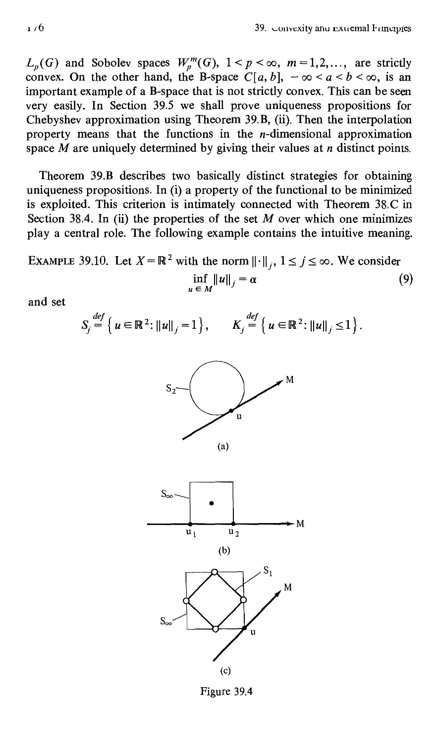
In Fig. 37.4(a), F is strictly convex and has, in contrast to Fig. 37.4(b), a
uniquely determined minimal point. In order to elucidate the prototype for
conditions on U, we consider (9°), with u = ((,if), \\u\\ = max(|£|, M), F =
\\u\\. Let U be a straight line. The set Q = {«eR2: ||h||=1} is the boundary
of the unit square. In Fig. 37.5(a), (9°) has exactly one solution, whereas in
Fig. 37.5(b) there exist infinitely many solutions. The solutions are exactly
all the points of dQ that lie on U. Moreover, a ==1. In Section 39.2 we
explain the connection with the so-called interpolation property of U. In
classical Chebyshev interpolation, the interpolation property is known as
the Haar condition.
The necessary conditions for solutions u of the minimum problem (9°)
can, to begin with, be split, roughly speaking, into two classes:
(a) the operator equation F'(u) = 0 (free minimum, u is an interior point of
U);
(fi) the Lagrange multiplier rule (minimum with side conditions).
Furthermore, there are, in addition:
(y) sub gradient condition 0 e dF(u);
(S) variational inequalities;
(e) characterization of solutions by means of dual problems.
In Parts I and II we were greatly concerned with the solution of operator
equations which one can always write in the form
Bu = 0. (10°)
The connection with extremal problems is roughly the following: If F has a
derivative F', then for an interior point u0 of U we have: If uQ is a solution
of (9°), then F'(«(,) = °-
(a)
Figure 37.5
(b)
ijeneral Basic Ideas
9
It follows from this that there is an important method for the solution of
the operator equation (10°) which, for example, can represent a differential
equation, an integral equation, or a system of real equations: We seek a
functional F such that B = F' and solve the minimum problem (9°) or a
corresponding maximum problem. However, it suffices that u0 be a critical
point—for instance, a saddle point. Then we also have F'(«0) = 0. In any
case, it must be emphasized that not all operators B can be written in the
form B = F' but rather only the so-called potential operators. In a real
Hilbert space, of the continuous linear operators it is precisely and solely
the self-adjoint operators that are also potential operators. We give general
criteria for an operator to be a potential operator in Section 41.3.
Especially strong propositions can be proved for the minimum problem
(9°) in case where Fis convex. F' is then a monotone operator. We studied
the theory of monotone operators in Part II. Not every monotone operator
is a potential operator. However, for monotone potential operators, one can
prove additional propositions— for instance, propositions for eigenvalue
and bifurcation problems. We discuss this in Chapters 43-45.
During the last 15 years, in connection with optimization problems, a
convex analysis for convex, but not necessarily differentiable, functionals
has been formulated. At the center of this theory there stands a calculus for
the subdifferential dF(u) which appears in place of the derivative F'(u).
The basic idea, which leads to the definition of dF(u), is elucidated in
Section 37.2. The necessary condition F'(«) = 0 is then replaced by 0 e
dF(u). Chapters 47 and 51-53 are devoted to convex analysis. There we
also work out the interrelationship between conjugate functionals and
duality theory.
If the minimum problem (9°) has a solution u0 which is not an interior
point of U, then more complicated necessary conditions appear for u0,
which in many cases can be summarized in a unified way under the concept
of the Lagrange multiplier rule. In general, one is led to Lagrange
multipliers if the side conditions occur in the form of equations or inequalities.
Prototypes for this are:
(a) Eigenvalue problems.
(/?) Linear or convex optimization problems.
We elucidate these prototypes in Sections 37.3, 37.6, 37.10, and 37.11.
Moreover, in Section 37.10 we also obtain the connection between the
Lagrange multiplier method and duality theory. We delve more deeply into
this interrelationship in Chapter 50. Furthermore, in Chapter 43
(respectively, Chapter 48) we justify the Lagrange multiplier method for smooth
(respectively, more general) side conditions. At this point we already note
the important situation that the Lagrange multiplier rule in the narrower
sense is tied up with certain nondegeneracy conditions. The purely formal
application of the Lagrange multiplier rule which one frequently finds in
physics textbooks can lead to false results. One finds a counterexample to
this in Section 43.1.
10
Introduction to the Subject
If U in (9°) is convex and F' exists, then the variational inequality
(F'{u0),v-u0)>0 for all ue U (11°)
holds for a solution uQ of (9°). In Section 37.1 we explain that this is a
matter of the generalization of a well-known necessary condition for the
existence of minima of real functions. A quasivariational inequality is
present when, in addition, U in (11°) depends on u0. Instead of (11°) we
shall consider more general problems, e.g.,
(Au0— b,v — u0) >h(v)— h(u0) for all v e U,
where the operator A is not necessarily a potential operator. The theory of
variational inequalities that has been developed over the last 15 years
combines the theory of extremal problems and the theory of monotone
operators under a unified viewpoint. In Chapter 9 we explained the
important connections with the theory of multivalued mappings. We concern
ourselves with variational inequalities in Chapters 46 and 54-57.
The sufficient conditions for the existence of solutions of the minimum
problem (9°) can be roughly classified as follows:
(a) Positive definiteness of the second variation.
(/?) Characterization of solutions by means of the dual problem.
(•y) Comparison functionals (abstract field theory).
(5) The method of dynamic optimization.
(e) In case of convex problems, the necessary conditions are generally
sufficient.
The criteria that use the second variation are discussed in Section 40.2 (free
local minima) and in Section 43.8 (Lagrange multiplier rule). In this
connection, this is a matter of a generalization of the known classical
criterion for real functions: F"(u0)>0 implies the existence of a local
minimum for F at u0 in the case F'(uQ) = 0. We point out the advantages of
dual problems for the characterization of solutions in Section 37.29f. In
Section 37.20b (respectively, Section 40.3), we treat the method of dynamic
optimization (respectively, the method of comparison functionals). In
Section 40.7 we elucidate the connection between the abstract results and the
field theory of classical calculus of variations.
In order to make it easier for the reader to learn the essential ideas in the
construction of approximation methods for extremal problems, we present,
in Section 37.29, the basic ideas of various important approximation
methods:
(i) The Ritz method (projection method),
(ii) The gradient method (descent method),
(iii) Ascent method,
(iv) Penalty method.
(v) Regularization.
(vi) Duality method.
General Basic Ideas
11
(vii) Dynamic optimization,
(viii) Decomposition,
(ix) Equivalence and combination principle.
These basic ideas are delved into more deeply later.
In conclusion, we summarize the advantages of duality theory:
(a) Necessary and sufficient conditions for the characterization of extremal
solutions.
(b) Existence propositions when properties of the corresponding dual
problems that are frequently easy to verify are at hand.
(c) The construction of generalized solutions for unsolvable problems with
the aid of solutions of the dual problem and the so-called extremal
relation.
(d) The construction of approximation methods with two-sided error
estimates for the extremal values and error estimates for the extremal
solutions.
(e) The side conditions of the dual problem may have a simpler structure
than that of the original problem; therefore, it is occasionally more
propitious to solve the dual problem and to obtain solutions for the
original problem by means of the extremal relation.
We explain this in Section 37.29f.
The basic ideas of duality theory can be found in Chapter 39.
Furthermore, we take up duality theory in detail in Chapters 49-53.
In Part I, the topological essence of fixed point theory concentrated on
the concept of the fixed point index (mapping degree). In the theory of
extremal problems, topological tools will be used to obtain, within the
framework of the Morse theory and the Ljusternik-Sclinirelman theory,
estimates for the smallest number of critical points and to guarantee the
existence of at least one saddle point in indefinite problems. From this we
obtain, for example, propositions concerning the number of eigensolutions
for nonlinear differential and integral equations or concerning the number
of geodesies (Chapter 44) as well as concerning the existence of solutions of
nonlinear differential equations or the existence of periodic solutions of
dynamical systems (Chapter 49).
In the preceding overview it is already apparent that the solutions
of convex minimum problems have especially propitious properties. A goal
of current research consists in making the propitious behavior of convex
problems useful also for classes of nonconvex problems by introducing
generalized concepts of a solution. We discuss this in Chapters 42 and 48.
Finally, we would like to point out that in general we follow the strategy
of reducing propositions on extremal problems for functional to that for
classical real functions. This becomes especially clear in the introduction to
Chapter 40.
CHAPTER 37
Introductory Typical Examples
When I was a student it was fashionable to give courses called "Elementary
Mathematics from the Higher Point of View" But what I needed was a
few courses called " Higher Mathematics from the Elementary Point of View."
Joel Franklin
In the occupation with mathematical problems, a more important role than
generalization is played—I believe—by specialization.
David Hubert
There are two ways to teach mathematics. One is to take real pains toward
creating understanding—visual aids, that sort of thing. The other is the old
British system of teaching until you're blue in the face.
James R. Newman, compiler of the 2,535 page The World of Mathematics,
quoted in the New York Times, Sept. 30,1956
In the following we wish to present many concrete examples, foregoing
extensive technical details, whose solutions have contributed essentially to
the development of a general theory of extremal problems. A glance at the
organization of this chapter in the Contents shows the variety of different
problems one encounters. In this connection, an especially central position
is assumed by Section 37.4, where we discuss a number of fundamental
ideas from the classical calculus of variations. The ideas of the calculus of
variations have influenced the modern theory of extremal problems in an
essential way, and knowledge of these classical ideas is indispensable for a
thorough understanding of the modern development.
In the references to the literature at the end of each section of this
chapter, we restrict ourselves to a few introductory expositions and standard
12
37.1. Real functions in R1
13
works. The later chapters are provided with detailed lists. If the reader
concentrates his attention on the works introduced in the references to the
literature in this chapter under the caption "classical works," then he can
obtain a quick survey of the historical development of the subject.
This chapter addresses itself to readers who are interested in a detailed
motivation of the general theory by means of simple but typical examples.
In the following chapters, we will show how these examples fit into a general
functional analysis theory. In this connection, the reader is often referred to
the corresponding sections of the present chapter. For this reason, a cursory
perusal of this chapter on first reading will suffice. A reader who wishes to
get acquainted immediately with the foundational principles of the theory of
extremal problems can begin with Chapters 38 and 39. There we explain the
role of compactness and convexity for existence propositions, give two
important uniqueness criteria, and treat some fundamental principles of
duality theory.
37.1. Real Functions in Ul
One can already observe numerous phenomena that are typical for extremal
problems in the study of real-valued functions of a real variable. Later we
shall often reduce the investigation of general functionals x>-+ F(x) on a
locally convex space X to the investigation of real-valued functions t >-> <p(t)
of a real variable t, where we set <p(0 = F(x(t)). Here, t >-> x(t) is a curve
inX
Let F: [a, b] -» U be a real function defined on the bounded interval
[a, b]. By definition, F has a local minimum at x0 if and only if there exists a
neighborhood U(x0) of x0 such that
F(x)>F(x0) for allx e(/(x0)n[a,fc], where x =£ x0. (12)
If F possesses a local minimum at xQ and the derivative F'(x0) exists, then
one must distinguish two cases:
(i) If x0 is an interior point of [a, b], then
*"(*„)-0. (13a)
(ii) If x0 is a boundary point of [a, b], then
F'(x0)(x-x0)>0 forallxe[a,fc]. (13b)
The condition (13b) is equivalent to F'(x0)>0 [respectively, F'(x0)<0]
for xQ = a (respectively, xQ = b) (see Fig. 37.6). Obviously, (13a) is a special
case of (13b).
If F: D(F) C X-> U is a functional, for instance, on the B-space X, then
in place of (13a) we have an operator equation (Theorem 40.B in Section
37. Introductory Typical Examples
/
/
/
\
\
\
a x0 D
Figure 37.6
40.3) and in place of (13b) we have a variational inequality (Theorem 46.A
in Section 46.1).
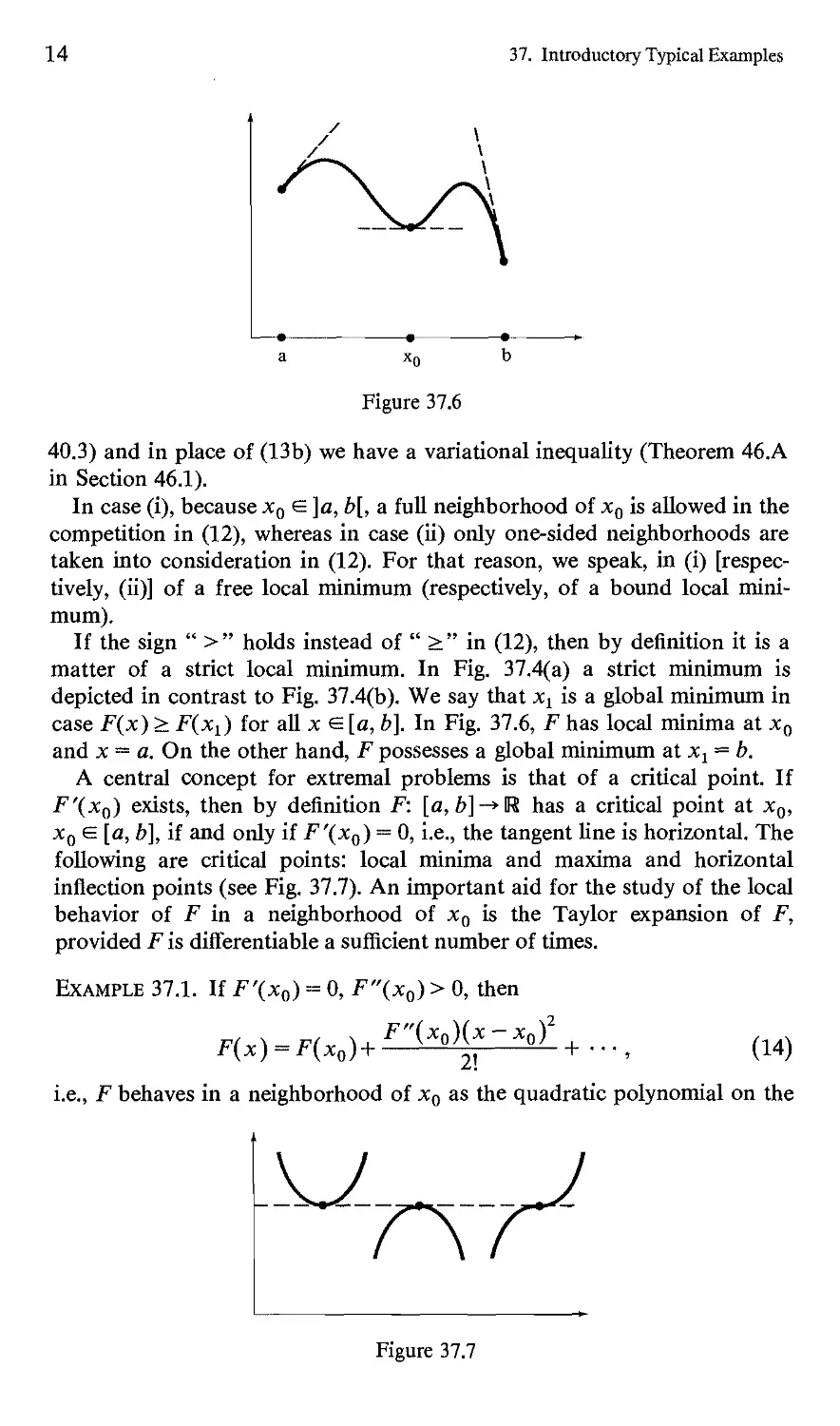
In case (i), because x0 e ]a, b[, a full neighborhood of x0 is allowed in the
competition in (12), whereas in case (ii) only one-sided neighborhoods are
taken into consideration in (12). For that reason, we speak, in (i)
[respectively, (ii)] of a free local minimum (respectively, of a bound local
minimum).
If the sign " >" holds instead of " >" in (12), then by definition it is a
matter of a strict local minimum. In Fig. 37.4(a) a strict minimum is
depicted in contrast to Fig. 37.4(b). We say that xx is a global minimum in
case F(x) > F(xt) for all x e [a, b]. In Fig. 37.6, F has local minima at x0
and x = a. On the other hand, F possesses a global minimum at xx = b.
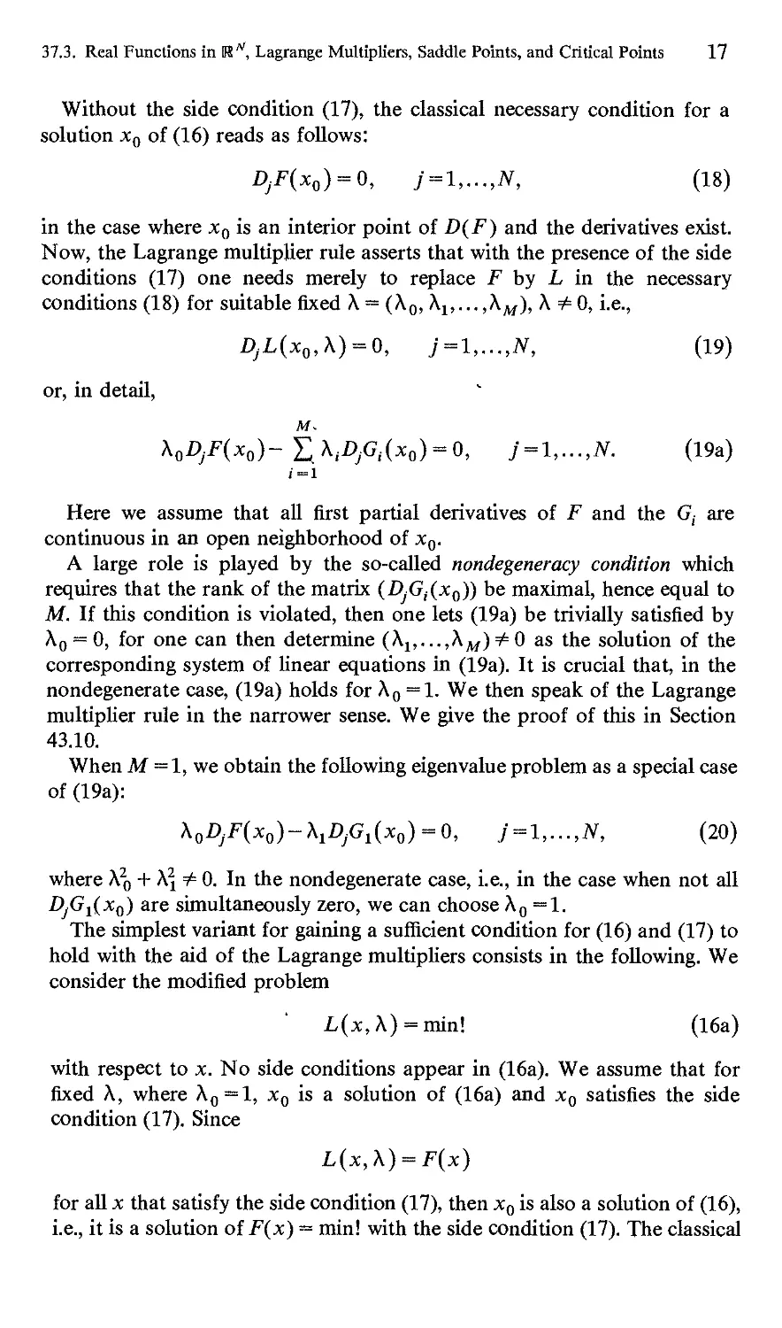
A central concept for extremal problems is that of a critical point. If
F'(x0) exists, then by definition F: [a, b]-*U has a critical point at x0,
x0 e [a, b], if and only if -F'(*o) = 0, i.e., the tangent line is horizontal. The
following are critical points: local minima and maxima and horizontal
inflection points (see Fig. 37.7). An important aid for the study of the local
behavior of F in a neighborhood of x0 is the Taylor expansion of F,
provided F is differentiable a sufficient number of times.
Example 37.1. If F'(x0) = 0, F"(x0) > 0, then
F(x) = F(x0)+F"iXo)^'Xof+---, (14)
i.e., F behaves in a neighborhood of xQ as the quadratic polynomial on the
Figure 37.7
37.2. Convex Functions in R1
15
right-hand side of (14). Consequently, F has a strict local minimum at xQ.
The precise assumptions for this are: F'(x0) = 0, F"(x0)>0, and F" is
continuous at xQ. This follows from the form of the remainder term in (14).
Example 37.2. If F(">(x0) = 0 for « =1, 2, 3, 4 and F(5>(x0) + 0, then
Therefore, x0 is a horizontal inflection point, for F behaves locally as the
fifth-degree polynomial on the right-hand side of the last equation.
The material of this section is contained in any textbook of differential
and integral calculus.
37.2. Convex Functions in U1
A function F: [a, b] -» U is said to be convex if and only if each chord lies
above the corresponding arc of the curve (see Fig. 37.8). In contrast to
arbitrary real functions, convex functions possess a number of remarkable
properties of which we list three here:
(a) If F has a local minimum at x0, then F also has a global minimum at x0.
(b) The necessary conditions (13a) [respectively, (13b)] for local minima are
also sufficient for global minima.
(c) If F' exists on [a, b], then on [a, b\. F is convex if and only if F' is
monotonely increasing.
In Chapter 42, property (c) yields the connection between convex
functional and monotone operators. A convex function possesses only minima as
critical points.
Figure 37.8
16
37. Introductory Typical Examples
Figure 37.9
If F: [a, b] -» U is a convex but not necessarily differentiable function,
then a global minimum at xQ can be characterized by
0 e dF{x0) (15)
instead of by F'(x0) = 0 or (13b). Here, the so-called subdifferential dF(x0)
equals the set of all slopes m of the straight lines through (x0, F(x0)) which
lie beneath the curve determined by F (see Fig. 37.9). (15) is the starting
point for the convex analysis that we develop in Chapter 47.
References to the Literature
Convex analysis and convex sets: Rockafellar (1970, M, H, B) and Roberts,
Varberg (1973, M, B, H) (standard works for RB); Holmes (1972, L), (1975,
M); Ekeland and Temam (1974, M); Marti (1977, M).
37.3. Real Functions in UN, Lagrange Multipliers,
Saddle Points, and Critical Points
We consider the minimum problem:
F(x) = min! (16)
subject to the side conditions
G,.(x) = 0,/=1,...,M, (17)
where x = (^,... ,£N), Dj,= d/d^j. Here, F and all the G,'s are real-valued
functions of the real variables £v...,£N, and M < N.
We denote the corresponding Lagrange function by
M
L(x,A) = A0JF(x)-£A,.G,-(*)-
i-i
All the A,'s are real numbers and are called Lagrange multipliers.
37.3. Real Functions in R^, Lagrange Multipliers, Saddle Points, and Critical Points 17
Without the side condition (17), the classical necessary condition for a
solution xQ of (16) reads as follows:
DjF{x0) = 0, j = l,...,N, (18)
in the case where xQ is an interior point of D(F) and the derivatives exist.
Now, the Lagrange multiplier rule asserts that with the presence of the side
conditions (17) one needs merely to replace F by L in the necessary
conditions (18) for suitable fixed A = (A0, A1;...,AM), A + 0, i.e.,
DjL{x0,X) = 0, j=l,...,N, (19)
or, in detail,
A0Z>yF(x0)-X;A,.Z>,.G,.(x0) = 0, j = l,...,N. (19a)
i=i
Here we assume that all first partial derivatives of F and the G, are
continuous in an open neighborhood of x0.
A large role is played by the so-called nondegeneracy condition which
requires that the rank of the matrix (Z)yG,(x0)) be maximal, hence equal to
M. If this condition is violated, then one lets (19a) be trivially satisfied by
A0 = 0, for one can then determine (A1,...,AM)#0 as the solution of the
corresponding system of linear equations in (19a). It is crucial that, in the
nondegenerate case, (19a) holds for A0 = 1. We then speak of the Lagrange
multiplier rule in the narrower sense. We give the proof of this in Section
43.10.
When M = 1, we obtain the following eigenvalue problem as a special case
of (19a):
A0^(*o)-Ai^Gi(*o)-0, j = l,.-.,N, (20)
where A20 + X\ + 0. In the nondegenerate case, i.e., in the case when not all
DjG^Xq) are simultaneously zero, we can choose A0 =1.
The simplest variant for gaining a sufficient condition for (16) and (17) to
hold with the aid of the Lagrange multipliers consists in the following. We
consider the modified problem
L(x, A) = min! (16a)
with respect to x. No side conditions appear in (16a). We assume that for
fixed A, where A0 = l, x0 is a solution of (16a) and xQ satisfies the side
condition (17). Since
L(x,X) = F(x)
for all x that satisfy the side condition (17), then x0 is also a solution of (16),
i.e., it is a solution of F(x) = min! with the side condition (17). The classical
18
37. Introductory Typical Examples
condition that xQ be a solution of (16a) reads as follows:
(a) (19) holds.
(b) The quadratic form associated with the Hessian matrix (DkDjL(x0, A))
is positive definite.
If all the Gj's are linear, then DkDjL(x0, A) = DkDjF(x0), i.e., A does not
even appear in the Hessian matrix. One must frequently deal with linear
Gj's when studying problems of the type (16) and (17) for determining
thermodynamic equilibrium states (cf. Part IV).
We will make use of this simple method in Section 37.4/ to investigate
variational problems with side conditions. In Section 43.10 we shall prove a
refined sufficiency criterion for (16) and (17).
We now explain the connection with critical points. By definition,
F possesses a critical point at xQ relative to the side condition (17) if and
only if:
(i) If we set f(t) = F(x(t)), then / has a critical point at r = 0, i.e.,
/'(0) = 0.
(ii) Here we shall consider precisely all curves t>-+x(t) which satisfy the
side condition (17) in a neighborhood of t = 0. Moreover, x'(0) must
exist. Furthermore, x(0) = xQ.
In Chapter 43 we shall show that under appropriate regularity
requirements on F and G„ the existence of a critical point for F relative to (17) in
the nondegenerate case is equivalent to (19) and A0 = 1. If no side condition
(17) is at hand, then we talk about a free critical point. If F possesses
continuous first partial derivatives at x0, then we can choose x(t) in (ii) to
have the form x0 + th and obtain from/'(0) = 0, according to the chain rule,
that 2,jDjF(x0)hj = 0 for all h e UN, and thereforeDjF(x0) = 0,/ = 1,...,N;
but this is (18). We can thus characterize a free critical point x0 as follows:
(a) Geometric condition: The tangent plane at x0 is horizontal.
(b) Analytic condition: The linear terms in the Taylor expansion vanish at
the point xQ.
(c) Degeneracy property: The linear approximation F'(*o): R"-» U of F:
U(x0)CUN-*U is not surjective. Observe that F'(x0)h = /)^(½)^
+ ■■■ + DNF(x0)hN holds.
In the theory of manifolds, the definition of a critical point is based on
(c).
Local minima and maxima and saddle points are critical points.
The use of the concept of a saddle point is not uniform in the literature.
By "saddle point" we shall mean any critical point which does not
correspond to a local minimum or a local maximum (cf. Section 43.9). In the
regular case, this means intuitively, in (i) and (ii) above, that there exist two
clef
curves r >-> xx(t) and r >-> x2(t) such that for ft{t) = F{x,{t)): /x has a local
minimum at t = 0, and /2 has a local maximum at t = 0. For example, for
37.3. Real Functions in Rw, Lagrange Multipliers, Saddle Points, and Critical Points 19
the quadratic function F: U2-*U, F(x) = ai-j + b%\, the following
assertions hold:
(a) F possesses a minimum at x = 0 when a, b>0.
(fi) F possesses a maximum at x = 0 when a, b < 0.
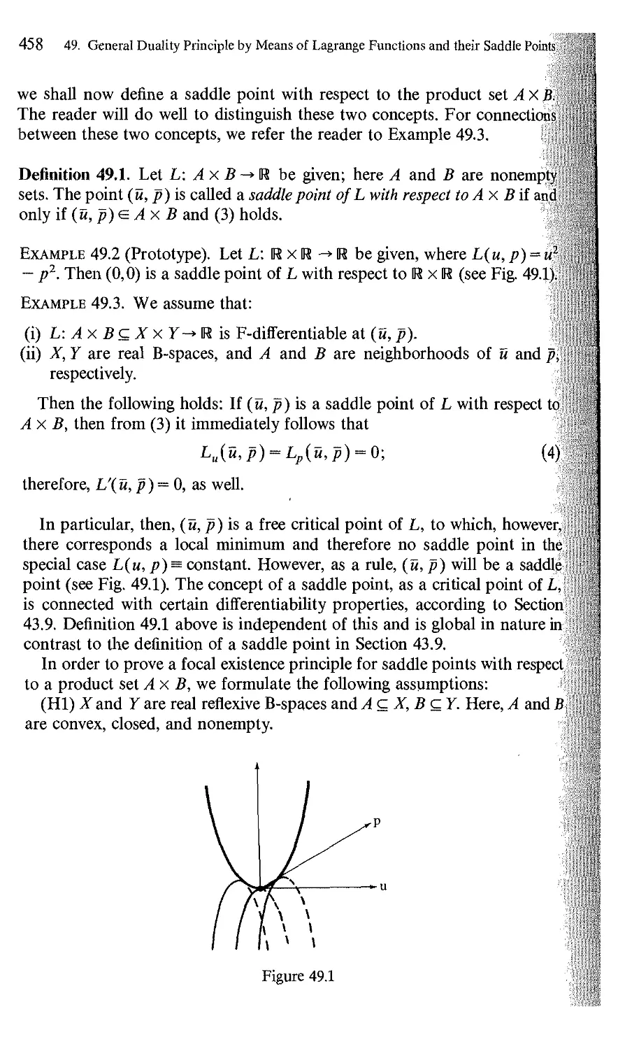
(•y) F possesses a saddle point at x = 0 when aft < 0.
For instance, if a > 0, b < 0, then £\ >-> F(£x, £2) has a minimum at £x = £2 = 0
and £2 >-> F(£1; £2) has a maximum at this point (see Fig. 49.1).
Besides, in connection with duality theory and game theory, we use the
narrower concept of a saddle point with respect to a product set. In this
connection, compare Section 49.1.
In general, one can study the local behavior in a neighborhood of a
critical point parallel to the Examples 37.1 and 37.2 with the aid of the
Taylor expansion. Morse theory provides normal forms for critical points
(cf. Section 37.26).
Saddle points are significant for game theory and duality theory.
Equation (20) shows that one obtains existence propositions for eigenvalue
problems by means of the study of the critical points of functions or, more
generally, of functionals. Existence statements for nonlinear equations of
the type (18) are obtained by constructing free critical points. In Section
44.12 we consider the so-called mountain pass theorem. This theorem
asserts the existence of a nontrivial free critical point.
Estimates for the number of critical points are obtained by using
topological tools within the framework of the Morse theory and the
Ljusternik-Schnirelman theory (cf. Sections 37.26, 37.27, and Chapter 44).
In Section 49.1 we treat a general existence theorem for saddle points with
respect to product sets. In the Problems for Chapter 49, we delve further
into existence propositions for critical points and their applications. In
particular, we deal with a general topological existence principle for saddle
points—the so-called Unking principle.
The justification of the Lagrange multiplier method for general situations
is an important concern in Part III. In this connection, compare Chapters
43, 47, 48, and 50.
The saddle point condition of the Kuhn-Tucker theory for convex
optimization problems (Sections 37.11, 47.10, 48.4, 50.1, and 50.2) and the
Pontrjagin maximum principle for control problems (Sections 37.21 and
48.6) are important contemporary extensions of the classical Lagrange
multiplier rule for problems with side conditions that are not necessarily
smooth.
References to the Literature
Sharp Lagrange multiplier rules in R": Hestenes (1966, M); Boltjanskii
(1976, M).
20
37. Introductory Typical Examples
37.4. One-Dimensional Classical Variational Problems
and Ordinary Differential Equations, Legendre
Transformations, the Hamilton-Jacobi
Differential Equation, and the Classical
Maximum Principle
This section is of central significance for a deep understanding of many
assertions here in Part III. We present the results of the classical calculus of
variations in such a way that the reader will later see the connections with
convex analysis and control theory very clearly. The Hamilton-Jacobi
formalism is the focal point—this formalism is generalized in many ways in
the later chapters.
(a) Generalization of the canonical equations and of the classical maximum
principle: Pontrjagin's maximum principle and control problems.
(fl) Generalization of the Hamilton-Jacobi differential equation: Bellman's
principle of dynamic optimization in control theory, Bellman's
differential equation, and duality theory for nonconvex problems.
(•y) Generalization of the Legendre transformation: conjugate functional
in convex analysis and duality theory.
(5) Generalization of the Hamilton-Jacobi action function S: duality by
means of the stability of perturbed problems and the ^-functional.
The Hamilton-Jacobi theory represents a general framework for the
mathematical description of the propagation of actions in nature and the
optimal modelling of control processes in economics and technology. In
the Problems in Chapter 40, we point out a number of deep physical and
mathematical connections: geometrical optics, characteristics, bicharacteris-
tics and electromagnetic waves, hyperbolic partial differential equations,
Huygens' principle, diffraction theory, asymptotic expansions and the
Maslov index, Fourier integral operators, symplectic geometry, quasiclassi-
cal asymptotic expansions in quantum mechanics, the Feynman integral in
quantum mechanics and its connection with classical mechanics, integrable
canonical systems and perturbation theory in celestial mechanics, infinite-
dimensional canonical equations and nonlinear wave equations, etc. In Part
V we delve into the connection between classical mechanics, statistical
physics, and ergodic theory and explain the derivation of the fundamental
equations of mathematical physics on the basis of variational principles as
well as the meaning of symmetry principles and Lie groups in order to
obtain conservation quantities, similarity assertions, and gauge field
theories, which have achieved a basic significance in elementary particle physics.
This presentation, which is far from complete, should nonetheless facilitate
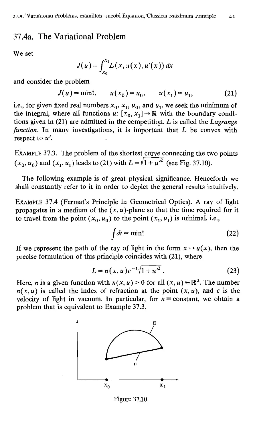
a feeling for the focal position of the Hamilton-Jacobi theory.
In the following we assume that all functions are sufficiently smooth.
j i.t.' Variauouai Problems, namiltou-jacObi Equauuu, Classical maximum rnntiiple <ii
37.4a. The Variational Problem
We set
L(x, <u(x), u'(x)) dx
and consider the problem
/(«) = min!, u(x0)=uQ, u(xl)=ul, (21)
i.e., for given fixed real numbers xQ, xlt uQ, and uv we seek the minimum of
the integral, where all functions u: [x0, xx] -» U with the boundary
conditions given in (21) are admitted in the competition. L is called the Lagrange
function. In many investigations, it is important that L be convex with
respect to u'.
Example 37.3. The problem of the shortest curve connecting the two points
(x0, u0) and (xv ut) leads to (21) with L = h+u'2 (see Fig. 37.10).
The following example is of great physical significance. Henceforth we
shall constantly refer to it in order to depict the general results intuitively.
Example 37.4 (Fermat's Principle in Geometrical Optics). A ray of light
propagates in a medium of the (x, «)-plane so that the time required for it
to travel from the point (x0, u0) to the point (xv u{) is minimal, i.e.,
jdt = min! (22)
If we represent the path of the ray of light in the form x >-> u(x), then the
precise formulation of this principle coincides with (21), where
L = n(x, u)c~ih+ u'2 . (23)
Here, n is a given function with n(x, u) > 0 for all (x, u) e U2. The number
n(x,u) is called the index of refraction at the point (x, u), and c is the
velocity of light in vacuum. In particular, for n = constant, we obtain a
problem that is equivalent to Example 37.3.
u
o
u
x0 x:
Figure 37.10
22
37. Introductory Typical Examples
In order to obtain this variational problem from (22), note that for given
«(•>•)> by definition the velocity s'(t) at the time ( of a ray of light
t >-> (x(t), u(t)) is given by
n{x{t),u{t))'
Here, s'{t)=\jx'2{t) + u'2{t); therefore,
dt = nc~lds = nc"1yl + u'2(x) dx.
37.4b. The Euler Equation as a Necessary Condition
If u is a solution of (21), then the so-called Euler equation is valid on
]x0, x^:
-£Lu.{x, u(x), «'(*)) = Lu{x, u(x), «'(*)). (24)
The simple proof makes use of methods of deduction that are typical of
all of the calculus of variations. We choose a function h such that h(xQ) =
_def
hix^)— 0. Then u = u + eh satisfies the boundary condition in (21) for all
real e (see Fig. 37.10). If we set <p(e) = J(u + eh), then the real function <p
has a minimum at e = 0, and consequently <p'(0) = 0, i.e.,
( \Lu(t, u, u')h + Lu,{t, u, u')h'\ dx - 0.
Since h(x0) = h(x1) = 0, integration by parts immediately yields
( \Lu-L'u,)hdx = 0.
This relation holds in particular for all h e Co°(x0, xt). According to the
variation lemma (Proposition 18.2), this implies (24).
def
8"J(u; h) = <p("'(0) is called the nth variation of J in u in the direction h.
By a solution of the problem
J(u) — stationary!, u(x0) = u0,u(xl) = ut (24a)
we understand any u such that 8J(u, h) = <p'(0) = 0 for all h e C™(x0, x,).
Then u is called a critical point. The above derivation shows that the critical
points are precisely the solutions of the Euler equation.
Many problems in mechanics are not of type (21) but rather of type (24a),
although this is often not mentioned in theoretical physics textbooks (cf.
Counterexample 40.9).
37.4. Variational Problems, Hamilton-Jacobi Equation, Classical Maximum Principle 23
37.4c. Legendre transformation and Canonical Equations as
Necessary Conditions
Our goal is to go from (t, u, u') to new variables (t, u, p) and to replace L
by H by means of the formulas
p = Lu,(x,u,u'), (25)
H(x,u, p) = pu'(x,u, p)~L(x,u,u'(x, u, p)). (26)
This transformation is called the Legendre transformation. In this
connection, we assume that (25) can be solved for u';i.e., u'= u'(x, u, p). Locally,
this is possible by the implicit function theorem provided Lu,u,(x, u, u') + 0.
We give global solvability conditions in Section 37.4d. From (25) and (26) it
follows that
Hu = PK - Lu + LwK = ~Lu>
Hp = u' + pu'p~Lu,u'p = u'.
Thus, if x >-> u(x) satisfies the Euler equation (24), then
p'{x) = -Hu{x,u(x),p(x)),
u'(x)) = Hp{x,u{x),p{x)). (27)
These are the so-called Hamilton canonical equations. Conversely, from (27)
and (25) it follows that (24) holds.
An advantage of (27) over (24) is that one can read off conservation
quantities directly from (27). If H does not depend on p (respectively, u),
then u(x) = constant [respectively, p(x) = constant]. If H is independent of
x, then
therefore, H(x, u(x), p(x)) = constant.
The canonical equations have been established in the complex problems
of celestial mechanics. The deeper reason lies in the fact that the integration
of (27) can be made essentially easier by means of the canonical
transformations (cf. Section 37.4n).
At the same time, the canonical formalism yields the framework for
general field theories in physics. If u and p are interpreted as operators in an
H-space with the commutator relationpu — up = h/i, then from the
canonical formalism one obtains quantum mechanics from classical mechanics.
The process of the so-called second quantization then yields quantum field
theories which describe the interaction between elementary particles.
_,. u,jroducw.j ^/picali
Example 37.5 (Geometrical Optics). If we choose L = n(x, u)c V1+ u'2
as in Example 37.4, then we obtain
p-Lu, = -
:H+u'2 '
H= pu'~L = ~\jn2{x,u)c 2 -p2 .
37.4d. Classical Maximum Principle and Necessary Conditions
We assume that
Lu,u,(x, u, u') > 0 for all (x, u, u') s R3,
L(x,u,u') , „
—- --»+00 as \u ->°°
|«'|
and define
Jf(x,u,u',p) = pu'—L(x,u,u').
As functions of u', the graphs of L, 3V, and La, have the form shown in Fig.
37.11. In particular, u'-* Lu,(x, u, u') is strictly monotonely increasing and
Lu,(x, u,u')-> ±00 asw'-»±oo.
Therefore, for fixed x, u, and p, the maximum problem
maxJfix, u,v,p)= P
always has exactly one solution u'. For this solution,
Jfu,{x,u,u',p)=0;
therefore,
p = Lu,(x,u,u'). (25a)
According to Fig. 37.11, for each p there exists exactly one u' for which
(25a) holds, i.e., we can solve the Legendre transformation (25a) globally
for u'.
■3C
Figure 37.11
j/X Variational' Problems, Hamilton-.) acbbi Equation, Classical Maximum fnriciple /J
We thus obtain the classical maximum principle: If «(•) is a solution of
the variational problem (21) and we set
p(x) = Lu,(x,u(x),u'(x)),
then for all x e [x0, xj, we have
max^f (x,u(x),v,p(x)) = 3V(x, u(x),u'(x), p(x)).
Besides,p(-) and «(•) satisfy the differential equations
p'=-JTu, u'-JTp.
These equations result from the Euler equation (24) and ,^, = — Lu,JFp = u'.
Furthermore, from (25) and (26) we obtain
H(x, u,p) = max^f (x,u, v,p). (28)
oeR
In Section 51.1 we show that this relation simply means that H is the
conjugate function to L. Thus, the Legendre transformation turns out to be
a duality transformation.
The deep Pontrjagin maximum principle in Chapter 48 is a fundamental
generalization of the above maximum principle to control problems. In
Section 48.8 we show that the following necessary conditions are obtained
by an application of the Pontrjagin maximum principle to the variational
problem (21):
(a) The Euler equation.
(P) The Legendre condition.
(Y) The Weierstrass condition.
(§) The Weierstrass-Erdmann corner condition for solutions u with corners
(jumps in the first derivatives).
Therefore, the Pontrjagin maximum principle is also of central
significance for the classical calculus of variations.
37.4e. Sufficient Conditions
The difference between weak and strong minima is important in the
variational problem (21).
(i) By definition, J has a weak local minimum at u if and only if there
exists e > 0 such that J(u) < J(u) for all u satisfying
\u(x) — u(x)\ < e, \u'(x) — u'(x)\< e on[x0,xj. (29)
Besides, all these 5's should satisfy the boundary condition u(x0) = u0,
m(x,) = ut [see Fig. 37.12(a)].
(ii) If the condition on u' is absent in (29), then we speak of a strong local
minimum [see Fig. 37.12(b)].
26
37. Introductory Typical Examples
(a) (b)
Figure 37.12
In (i) we require that not only the function values but also the derivative
values of u differ only slightly from the corresponding values of u. Here, the
u are the functions that are allowed in the competition. On the other hand,
in (ii) one foregoes the adjacency of the derivative values. Thus, every strong
local minimum is also a weak local minimum. As the derivation in Section
37.4b shows, the Euler equation is necessary for a weak local minimum.
A crucial problem reads as follows: When is a solution of the Euler
equation (24) also a solution of the variational problem (21)? Such sufficient
conditions are proved in the classical calculus of variations with the aid of:
(a) the second variation 82J (accessory variational problem, the Jacobi
condition for weak local minima);
(P) field theory (Hilbert's invariant integral, Weierstrass' criterion for strong
local minima with the aid of the E-function).
We discuss this in Section 40.7. There we also explain the connection with
general necessary and sufficient criteria for extremal problems. In particular,
we explain the role of the eigenvalue criteria in connection with the second
variation.
37.4f. Perturbed Variational Problems and the
Hamilton-Jacobi Differential Equation
We study the perturbed problem associated with (21):
L(x, u(x), u'(x)) dx = min!, u(x0) = u0, w(£) = a.
Here, perturbation means that we replace (xvul) by (£, a). We hold
(x0,u0) fixed and for variable (£, a) we set the minimum value equal to
S(£,a), i.e.,
L(x,u(x),u'(x))dx, u(x0) = u0, «(£) = a,
where the existence of a solution u of the corresponding variational problem
is assumed. In Section 37.4i we show that then, under natural assumptions,
37.4. Variational Problems, Hamilton-Jacobi Equation, Classical Maximum Principle 27
S satisfies the so-called Hamilton-Jacobi differential equation
Sx(x,u)+H(x,u,Su{x,u))=0. (30)
In Chapter 52 we use the idea of perturbed variational problems to prove
duality propositions. From (28), we can write (30) in the form
Sx(x,u)+max Jf (x,u,v,Su(x,u)) = 0. (3l)
This equation is called the Bellman differential equation. In Section 37.20
we explain the connection between a discretized form of (31) and the
Bellman optimality principle of dynamic optimization. In Chapter 52 we use
(31) to construct a duality theory for general nonconvex control problems,
which yields estimates for the minimal values and sufficient solvability
conditions.
Example 37.6 (Geometrical Optics). In the special case L =
n(x, «)c_1/l + u'2 of Example 37.4, S({, a) is the time required by a light
ray to reach the point (£, a) from (x0, u0). Here S is called eikonal. Since
H=— ]jn2c~2 — p2 , the Hamilton-Jacobi differential equation (30) is
transformed into
S2 + S2 = ^.
This equation is called the eikonal equation. The curves S(x, u) = constant
are called wave fronts. We shall explain the more exact physical meaning in
Problem 40.10.
Example 37.7 (Quadratic Variational Problem). Let L = 2~\u'2 + au2).
Then
p = Lu, = u', H^pu'-L = 2~l(p2-au2).
The Hamilton-Jacobi differential equation (30) reads as follows:
Sx+2-\S2~au2) = 0.
The substitution S = r{x)u2 leads to the Riccati differential equation r'+
2r2 — a/2 = 0. Therein lies the deeper reason why the Riccati equation
plays an important role in control problems with a quadratic objective
functional (cf. Sections 37.20 and 54.8).
In the following two subsections we show:
(a) how one can obtain solutions of the canonical equations, and thus of
the Euler equation, from solutions S of the Hamilton-Jacobi
differential equations;
(P) how, conversely, solutions of the Hamilton-Jacobi differential
equations are obtained from solutions of the canonical equations.
From the standpoint of geometrical optics, this connection is very natural.
ii. mu'oductbiy iepical Exainpifes
Light rays correspond to the solutions of the canonical equation, whereas
the solutions S of the Hamilton-Jacobi differential equation yield wave
fronts by S(x, u) = constant, to which (by Section 37.4j) the light rays are
perpendicular. One expects that there exists a mutual correspondence
between light rays and wave fronts.
37.4g. Complete Integral of the Hamilton-Jacobi Equation
and the Solution of the Canonical Equations
If we know a so-called complete integral, i.e., a solution S = S(x, u, a)+ C
of the Hamilton-Jacobi equation (30), which depends on two constants a
and C, then by means of
Sa{x,u{x),a)=P, p(x)=Su{x,u(x),ct) (32)
we obtain a solution of the canonical equations
u'=H„ p'=~Hu, (33)
provided that for fixed /6 the first equation in (32) can be solved for u and
thus x -» u(x) results. Let Sau(x, u,a)¥=0 for the corresponding (x,
u,devalues. Then «(•) andp(-) depend on the two constants a and /6 and, under
suitable regularity assumptions, represent the general solution of (33).
For the proof, we differentiate (32) with respect to x and (30) with respect
to a (respectively, u). We get
Sax + Sauu' = 0, p'~Sux + Suuu'
Sxa + HpSua^0, Sxu + Hu + HpSuu = 0.
(33) follows immediately from this.
If «(■),/?(-) Is an arbitrary solution of (33), then Sa(x, u(x), a) ~ constant,
i.e., Sa is a so-called conservation quantity, since
-~Sa(x,u(x),a) = Sax + Sauu' = Sax + SauHp-0.
Example 37.8 (Harmonic Oscillator). If u(x) is the displacement of an
oscillating spring at time x, then the Newton equation of motion
mu" = -ku (34)
holds, where m is the mass and k is the spring constant, p = mu' is the
momentum. If we choose H = p2/2m + ku2/2, then we can write (34) in the
form
u'-Hp, p'~-Hu, (35)
with the Hamilton-Jacobi differential equation
2mSx(x,u) + S2(x,u) + kmu2 = 0. (36)
^,.-,. Variational i'robleiuc, >iottiilton~jav<jdi Equauuu, Classical maximum rnnciple /.y
H is interpreted as the energy. The substitution S = — ax + T(u) yields
S = — ax + I v2ma — kmv2dv
Jo
as a solution of (36). Finally, Sa(x, u(x), a) = /6 means
— x+ I m(2ma~ kmv2) dv = P
Jo
with the solution
12a . /IT, „x
u — \ —r- sini/ — (x + p).
V k V m '
If we take into account that p — Su and Sx + H(u,Su) = 0, then we obtain
a= H(u, p), i.e., a equals the energy.
In the above example, we can also obtain the solution directly in a simple
way. The advantage of the method described above first shows up in more
complicated problems. In this connection, compare Landau and Lifsic
(1962, M), Volumes I, II.
37.4h. Solutions of Canonical Equations and the Initial Value
Problem for the Hamilton-Jacobi Differential Equation
To solve the initial value problem
Sx(x,u)+ H(x,u,Su(x,«)) = 0,
S(0,«) = 9(«) (37)
for given <p, we consider solutions of the so-called characteristic differential
equation system
u'(x) = Hp(x,u(x),p(x)), w(0) = v,
p'(x)--Hu(x,u(x),p(x)), />(0) = <p'(iO, (38)
a'(x) = p(x)u'(x) — H(x,u(x),p(x)), a(0)=<p(u).
In the following, one should take into account that the solutions of (38)
depend on x and v. We symbolize partial derivatives with respect to x by a
prime. If we set
S(x,u(x,v)) = a(x,y), (39)
then we obtain a solution S of (37) provided the following important
nondegeneracy condition is fulfilled (see Fig. 37.13):
(H) If I denotes an interval on the w-axis of the (x, «)-plane, then exactly
one solution curve x>-*u(x,v) of (38) for a corresponding u-value goes
through each point (x, u) of a suitable neighborhood of I.
30
37. Introductory Typical Examples
Figure 37.13
In the language of geometrical optics, (H) means the following: The light
rays belonging to the curves x >-> u(x, v) do not intersect, i.e., there are no
foci.
For the proof, we differentiate (39) with respect to x; therefore,
Sx + Suu' = a' = pu'~H.
Differentiation of (39) with respect to v yields
S„u„ = o„.
(40)
We obtain (37) from (40) and (H) provided we show that av = puv, because
then Su = p. In this connection, we set w = av — puv. According to (38), we
have:
w' = a„' - p'uv - pu'v
= Pvu' + P< ~ Hu«o - HpPv - P'uo - PK = 0.
From the initial conditions in (38) it follows that w(0, v) = 0. Therefore,
w(x, v) = 0; hence av = puv.
37.4L General Form of the First Variation and the
Hamilton-Jacobi Differential Equation
Our target is a general formula for the change of the integral
Ji(u)= jL(x,u(x),u'(x)) dx
when u and the interval of integration I are changed. This formula is
//(5)- J,{u) = j[Lu~L'u\{u{x)~u{x))dx
+ Lu,8u+ (L~Lu,u')8x\X^+o{P{u,u)), p->0. (41)
The arguments of L, Lu, are (x, u(x), u'(x)). The expression appearing in
the right-hand side of (41) without the remainder term o(p) is frequently
37.4. Variational Problems, Hamilton-Jacobi Equation, Classical Maximum Principle 31
denoted by SJ. We make use of the usual symbolism:
and assume that:
(i) I = [x0, xj and 7= [x0, xj are bounded intervals',
(ii) u e C\l), u e C\l). These functions will be extended linearly on U to
C'-functions.
(iii) We set fix, = xt — x,, §«, = m(x,)— u(xt), i.e., 6x, 8u are the differences
of the coordinates of the end points of the curves for u and u.
Furthermore, let
p(u,u) = max\u(x)~u(x)\
ivi
l
+ max|«'(x)-i/'(x)|+ £ |6x,.|+|6\|.
'U/ ,=0
(41) is obtained in a way parallel to Section 37.4b. The simple
calculation that uses only the Taylor theorem can be found in Gelfand and
Fomin (1961, M), page 55. In the following, the Hamilton-Jacobi
equation, the so-called transversality condition, and the Noether
theorem are obtained from (41). We recommend that the reader prove (41)
as an exercise.
In order to derive the Hamilton-Jacobi differential equation from (41),
we assume that u (respectively, m) is a solution of
Jj(u) = min!, u(x0) = u0, ^(x,)^^,
respectively,
/j(«) = min!, m(x0) = «0, ^(^)==^,
where I — [x0, xj, I = [x0, xj. We assume that
P(m,k) = 0(|Ak|+|Ax|)
holds, where Au = ul~ uv Ax = x, — xv By the definition of S in Section
37.4f, from (41) we obtain
S{xl,ul)-S{xv a,) = LU,(P) Am
+ [L(P)-Lu,(P)«'(x,)] Ax + o{\Au\+ |Ax|),
where P = (xv uv «'(xi))- One takes into account that the integral in (41)
vanishes because of the Euler equation, and x0 = x0, u0 = u0. Thus,
Su(x„«,)=MP), 5,(^,, «,)=L(P)-Lu,(P)«'(x,).
Sincep(xl) = LU,(P) and H = pu'~ L, it follows that
sx(xi> ul) + H(xv uv Su(xv «,)) = 0.
37.4j. Problems with Free End Point and Transversality
Condition
We consider the variational problem
I 1 jL(x, u(x), u'(x)) dx = min\, u(x0) = u0, u(xl{r)) = ul(r),
x0
(42)
i.e., all u( ■) are admitted to the competition which pass through a fixed left
end point (x0,u0) whereas the right end point lies on the curve t>->
(x,(t),«,(t)) (see Fig. 37.14).
If u is a solution, say, for t = t0, then the Euler equation
-j^Lu,(x, u(x), u'{x)) = Lu(x, u(x), u'(x)) (43)
holds on ]x0, x1(t0)[, and the so-called transversality condition
Lu,(P)u'l(r0)+[L(P)~Lu,(P)u'(xl)]x[(r0)=0, (44)
where P = (xv u{xv), u'ixy)) holds for the right end point xv = xx{rQ).
In order to prove this, we first consider only comparison curves u which
have the same right end point in common with u. The same argument as in
Section 37.4b yields (43). In order to prove (44), we assume that t0 = 0 and
choose admissible comparison curves that pass through (x^t), ^(t)), where
p(u, u) = O(t). Here we assume that such comparison curves exist.
Furthermore, let <p(t) = //(t)(m), I(r) = [x0, x,(t)]. We have:
8u0 = 0, §«, = ut{r)— «,(0) = «1'(0)t + o(t),
8x0 = 0, fix, = x1(t) —x,(0) =x,(0)t + o(t).
Since J has a minimum at u, <p'(0) = 0. Thus (44) follows from (41) and (43).
Example 37.9 (Geometrical Optics). In the special case L =
n(x, u)c~lyl+ u'2 of Example 37.4, (44) reads as follows:
"'(*)"i(To) + *i(To) = 0>
Figure 37.14
37.4. Variational Problems, Hamilton-Jacobi Equation, Classical Maximum Principle 33
i.e., the light ray x >-> u(x) is perpendicular to the curve r >-> (xt(r), u^r)).
This explains the designation transversality condition for (44). If one
chooses the curve in Fig. 37.14 to be in the form of a wave front S(x, u) —
constant, then by the construction of S we obtain that all the light rays that
emanate from the fixed point (x0, u0) intersect the wave front
perpendicularly.
37.4k. Noether's Theorem .
We will derive the remarkable fact that the existence of a conservation
quantity (45) below follows from an invariance property of the variational
integral.
In this connection, we use the notation of Section 37.4i and make the
following assumptions:
(i) The variational integral Jt is invariant with respect to transition from u
to m and from I to I, i.e., J,( u) = Jj(u); therefore,
/ L(x, u(x), u'(x)) dx~ I L(x,ii(x), u'{x)) dx.
(ii) This sufficiently smooth transformation depends on a parameter a such
that
x = x + ct<p(x)+ o(«), u(x) = u(x)+ ot\p(x)+ o(a).
The terms o(a) also depend on x, and o(a)/a-»0 holds as o-»0
uniformly with respect to x on I = [x0, xj.
(iii) u satisfies the Euler equation on I.
Then it follows directly from (41) that
L — Lum')cl<p\x +o(a) — 0 asa-»0.
If the assumptions are fulfilled for all a in a neighborhood of zero and for
all x0, xv then, after division by a, we obtain, as a -» 0,
Lu.{P)Hx) + (L{P)-Lu,{P)u'(x))<p(x)- constant, (45)
where P = (x, u(x), u'(x)).
Example 37.10 (Energy as a Conservation Quantity). If L does not depend
on x, then (i) holds for x~x + a, u(x) = u(x) (translation invariance).
According to (45), L{P)~Lu,{P)u'(x) = constant; therefore, H(u(x),
p(x)) = constant. In applications to mechanics, H is the energy and the
theorem on the conservation of mechanical energy is obtained.
We shall occupy ourselves with generalizations and the important
physical applications of the Norther theorem in Part V.
34
37. Introductory Typical Examples
37.4/. Variational Problems with Side Conditions and the
Lagrange Multiplier Rule
We consider the variational problem
L(x, u, u', v, v') dx = mini,
«(*o) = «o> u{xl) = ul, v(x0) = v0, v(xl) = vl (46)
for fixed xt, «,, vt, / = 0,1, subject to one of the following side conditions:
(i) Integral side condition (isoperimetric problem):
M(x, u, u', v, v') dx = constant.
(ii) Equation as a side condition:
M(x, u, v) = 0.
(iii) Differential equation as a side condition:
M(x, u,v, u',v') = 0.
Without the side conditions, the necessary conditions for a solution u, v of
(46) read as follows:
~LU,(P) = LU{P), ~LV,{P) = LV{P) on]x0,xj, (47)
where P = (x, y,u(x),u'(x),v(x),v'(x)). These Euler equations are
obtained in a way analogous to the method of Section 37.4b.
Lagrange Multiplier Rule as a Necessary Condition. This important rule
reads as follows:
If u,v^C1[x0,x1] is a solution of (46) with one of the side
conditions (i), (ii), or (iii), then (47) holds, in which connection , .
one must replace L by X0L + AM. Here, A0 is a real number and ^ •*
A is a C1 — function on [x0, xj, where A20 + A2(x) * 0.
We make the assumptions precise:
Ad (i) (L) holds with A0 = l provided M does not satisfy (47) with L
replaced by M (nondegenerate case). Otherwise, (L) is trivially fulfilled with
A0 = 0, A = l.
Ad (ii) (L) holds with A0 =1 provided the rank of the matrix
(MU(P),MV(P))
is maximal—therefore, equal to 1 for all P, i.e., M„(P)+M*(P) f= 0 for all
x e [x0, xj (nondegenerate case). For M*(P)+ M^(P) = 0, (L) is trivially
fulfilled for A0 = 0, A = 1.
37.4. Variational Problems, Hamilton-Jacobi Equation, Classical Maximum Principle 35
Ad (iii) (L) holds provided the rank of the matrix
(map), map))
is maximal, therefore, equal to 1 for all P.
The functions L and M are assumed to be sufficiently smooth. If we
denote by C the arc that belongs to the solution u = u(x), v = v(x), then it
suffices that L and M are C1-functions in a neighborhood V of C. In this
connection, to be precise, Fis the set of all (x, u, u', v, v') e Us, x e [x0, xj,
and
\u~ u(x)\, \u'~ u'(x)\, \v — v(x)\, \v'— v'(x)\<,8
for fixed 8 > 0.
Idea of the Proof. The classical proofs of (i), (ii), and (iii) can be found in
Courant and Hilbert (1953, M), Vol. I, page 216, Gelfand and Fomin (1961,
M), page 42, and Funk (1962, M), page 275, respectively. The multiplier rule
is also investigated in detail in Bolza (1949, M). We sketch the ideas of the
proof. In (i) and (ii) we make use of the multiplier rule for real functions
and make inferences analogous to those in Section 37.4b. In the more
difficult case (iii) we use an artifice of Bliss that first reduces the problem to
a Mayer problem and then applies the main theorem on underdetermined
systems of differential equations.
(i) We replace u (respectively, v) by u + elhl (respectively, v + e2h2)
where hv h2 vanish at the boundary points x0, xv We denote the left-hand
side in (46) [respectively, (i)] by F(e1; e2) [respectively, G(ev e2)]. Then F
has a minimum at (0,0) under the side condition G(ev e2) = c. From the
multiplier rule for real functions it follows that
\0Fti (0,0)+ AG,((0,0) = 0, /=1,2.
(L) follows from this in a way analogous to Section 37.4b (cf. Courant and
Hilbert (1953, M), page 216).
(ii) First we note that in this case (L) is of a purely local nature. This
follows from the fact that each solution of (46), (ii) is also a solution of the
problem that results from (46) by replacing [x0, xj by a smaller interval
[x0, xj and modifying the boundary conditions correspondingly. If, say,
MU{P*) + 0, then we can solve (ii) for u in a neighborhood of
(x*, u(x*), v(x*)), and we get u = g(x, v). This expression is substituted in
(46), possibly with [x0, xj instead of [XqjXJ, and we write the Euler
equation for this situation. Then we obtain (L) (cf. Courant, and Hilbert
(1953, M), Vol. I, page 219).
JO
j/. introductory lypicalhxampies
Exercises. Write out these proofs explicitly.
(iii) If u, v is a solution of (46), (iii) and m denotes the minimal value,
then u, v, w is a solution of
w' = L(x, u, u', v, v'), M(x, u, u', v, v') = 0
with the boundary conditions
w(x0) = 0, w(xl) = m,
u(x0) = u0, u(xl) = uv v(x0) = v0, v(xl) = vv
It is crucial that, because of the choice of m, the present problem has no
solution provided we replace m by m — b, b > 0. This means that u, v, w is a
bound arc in the sense of Problem 43.9. According to the theorem proved in
Problem 43.9, there then exist C'-functions A0, A on [x0, xj such that
A20 + A2 * 0 and
A'0 = 0,(A0L„, + AM„,)'-(A0L„ + AMJ = 0
and a corresponding relation for v instead of u. Consequently, A0 = constant
and we obtain (L).
Lagrange Multipliers and Sufficient Conditions. In a manner parallel to the
considerations for real functions in Section 37.3, simple sufficient conditions
can be formulated for variational problems with side conditions provided
one uses Lagrange multipliers. In this connection, we consider the following
problem which is a modification of (46):
[*\L + \M)dx = mini, (46*)
u(x0) = u0, u(xl) = uv v(x0) = v0, v(x1) = vv
If u, v is a solution of (46*) for fixed A and this solution satisfies the side
condition (i), then u, v is obviously also a solution of (46) with the side
condition (i). The situation behaves analogously for the side conditions (ii)
and (iii).
In Chapter 40 we prove sufficiency criteria for problems of type
(46*)—thus, for problems without side conditions. If one finds a A so that
these sufficiency criteria are applicable to (46*), then one immediately
obtains sufficient conditions for (46), with one of the side conditions (i), (ii),
or (iii).
Critical Points. The multiplier rule (L) also holds in case where "min!" is
replaced by "stationary!" in (46), i.e., in case where we are seeking critical
points u, v. Roughly speaking, in this connection, a critical point means: If
we replace u and v by u + kv v + k2, respectively, which also satisfy the side
conditions, then the change in the integral expression in (46) is of higher
than first order in kt, k2. Then, in the proofs of (L) sketched above, the real
function (ev e2) >-> F(ev e2) has a critical point at (0,0) with respect to the
37.4. Variational Problems, Hamilton-Jacobi Equation, Classical Maximum Principle 37
side conditions G(ev e2) = c, etc. However, the Lagrange multiplier rule for
real functions holds in general for critical points, not only for extrema (cf.
Corollary 43.25). We give the precise definition of a critical point in Section
43.9.
Example 37.11 (Hanging Rope). We seek the form u = u(x) of a rope of
fixed length a and constant density which hangs between two fixed points
(x0, u0) and (xv «,). The variational problem reads as follows:
I wvl+w' dx = imn\, «(x0) = «0, u(x1) = u1 (48)
with the side condition
j'Xlh+u'2dx = a. (49)
(48) comprises the requirement for minimal potential energy. In order to
motivate this, we think of the potential energy of a mass point in the
linearized gravitational field of the earth as being equal to weight times
height. If we subdivide the rope into small parts, then its potential energy is
approximately equal to u As (s = arc length), and (48) is obtained by
summation and passing to the limit as A* -» 0. The necessary condition for
a solution u reads as follows:
^(A0L + AM)„,-(A0L + AM)„ = 0,
L = uh + u'2 , m = vT+m^.
In the nondegenerate case, A0 = 1; therefore, (u + A)/Vl + u'2 = c, i.e.,
u + A = ccosh(c_1x + c,).
This is the so-called catenary. The constants A, c, and c, are determined
from the boundary conditions and the side condition.
Degeneracy occurs if a = xx — x0. Then, according to (49), we must have
u' = 0; therefore u = 0 where u0 = ut = 0. Here, we can choose A0 = 0, A = 1.
Example 37.12 (Geodesies). We seek geodesies on the surface M(x, u, v) =
0, i.e., x >-> (u(x), v(x)) must connect two fixed points and realize the
shortest distance between these two points. Then we obtain the problem:
h+u'2 + i/2dx = mini, (50)
u(x0) = u0, u{xl) = ul, v(x0) = v0, v(xl) = vl
with the side condition
M(x,u,o) = 0. (51)
The necessary solvability conditions for u, v are as follows:
38
37. Introductory Typical Examples
In the nondegenerate case, A0 =1. A simple calculation shows that we then
have: The principal normals of geodesies are normals to the surface (cf.
Smirnov (1956, M), Vol. IV, Section 70).
37.4m. The Trick of Introducing Lagrange Coordinates of the
Second Kind
Variational problems with side conditions arise very frequently in
mechanics when the principle of stationary action is applied. Concerning side
conditions in equation form, we distinguish between holonomic
(respectively, nonholonomic) side conditions when no derivatives occur
(respectively, derivatives do occur). For example, holonomic side conditions
describe the motion of mass points on surfaces. Nonholonomic conditions
occur in the motion of a ship or of a skater.
The Lagrange multiplier rule yields additional terms in the Euler
differential equations—these additional terms correspond to constraining forces in
mechanics, which, e.g., maintain the mass points on the prescribed surface.
In the case of holonomic conditions, there exists an important trick: One
introduces new coordinates so that the side conditions are automatically
fulfilled. Then, in these new coordinates (Lagrange coordinates of the
second kind), one obtains a variational problem without side conditions. In
mechanics, the Euler equations that result are called Lagrange equations of
the second kind.
Example 37.13. In Example 37.12, we introduce surface coordinates t, s on
the surface M(x, u, v) = 0. Then x = x(t, s), u = u(t,s), and v = v(t, s)
automatically satisfy (51). If we transform (50) to t, s, then we obtain
problem (51) without side conditions.
We explain the significance of geodesies on Riemannian manifolds for
general relativity theory in Part IV.
37.4n. Canonical Transformations and the Hamilton-Jacobi
Differential Equations
In order to solve the canonical equations
p'(x) = ~Hu(x,u(x),p(x)), u'(x) = Hp(x,u(x),p(x)), (52)
one can try to pass to new coordinates by means of a transformation
P = P(x,u,p), U=U(x,u,p) (53)
so that after the transformation, the solutions of (52) satisfy the new
37.4. Variational Problems, Hamilton-Jacobi Equation, Classical Maximum Principle 39
equations
P'{x) = - H*(x,U{x), P(x)), U'(x) = H*(x, U(x), P(x)).
(54)
Such transformations that preserve the form of the canonical equations are
called canonical transformations. If, e.g., H* = 0, then the solutions of (54)
are P(x) = constant, l/(x) = constant, and the solutions of (52) are easily
obtained from (53).
We show: If \p = \p(x, u, U) is a given function and
p = \pu(x,u,U), P = \f>u(x",u,U)
can be solved in the form (53), then there results a canonical transformation
with
H*(x,U, P) = H(x,u, p) + tx(x,u,U).
^ is called a generating function.
def
In order to prove this, for \j>(x) = ty{x, u(x), U(x)) we write
i'{x) = ix + i>uii'+ ^VU'=H* -H + pu' + PU' (55)
and consider
I [pu'~ H(x, u,p)\ dx = stationary!, (56a)
fl[PU'-H*{x,P,U)\ dx = stationary! (56b)
Furthermore, in (56a) and (56b) one must adjoin further fixed boundary
conditions on the functions u,p (respectively, P,U). As a result of (55), the
two integrals in (56) differ only by a constant. They thus possess the same
critical points. By Section 37.4b, these are, however, equivalent to solutions
of the corresponding Euler equations (52) [respectively, (54)] (cf. (47)).
The fact that variational integrals differ by only a constant in the case
where one adjoins a derivative in the integrand or a divergence expression in
a multiple integral is a basic trick of the calculus of variations which is
exploited, for instance, in field theory (cf. Section 40.7).
Example 37.14. As in Section 37.4g, let S(x, u, a) be a complete integral of
the Hamilton-Jacobi differential equation
Sx + H{x,u,Su) = 0. (57)
def
We choose S to be the generating function; thus, $(x, u, U) = S(x, u, U).
From (57), H* = 0; therefore, P(x) = constant, U(x) = constant. We thus
40
37. Introductory Typical Examples
obtain the solution of (52) by
p = Su{x,u,U), P = Sa(x,u,U),
where P and U are constants. This is precisely the method for the solution
of canonical equations that we have already used in Section 37.4g.
At the same time we thus obtain a new interpretation of the
Hamilton-Jacobi equation as an equation for an especially propitious
generating function of a canonical transformation.
In Problem 40.8 we treat a deep-lying application of canonical
transformations.
In celestial mechanics, in the consideration of the perturbation action of
planets in (52), perturbed Hamiltonian functions of the form H + eHl
appear instead of H. The classical method consists in carrying out a
canonical transformation with respect to the unperturbed function H
analogous to Example 37.14. Then (54) is obtained with H*(x,U,P) =
bH^x, u,p). The classical perturbation calculus for obtaining approximate
solutions for small e is now based on power series expansions for the
solutions of (54) with H * = eHv
References to the Literature
As a survey of classical works of the calculus of variations by J. Bernoulli
(1667-1748), Euler (1707-1783), Lagrange (1736-1813), Legendre
(1752-1833), Jacobi (1804-1851), Weierstrass (1815-1897), and Hilbert
(1862-1943), we recommend Funk (1962, M), Petrov (1977, M), and
Goldstine (1980, M). For the connection between the classical theory and
modern control theory, we recommend McShane (1978, M).
Introduction: Courant and Hilbert (1953, M), Volumes I, II; Gelfand and
Fomin (1961, M); Bliss (1951, M); and Funk (1962, M).
Hamilton-Jacobi theory: Rund (1966, M); Klotzler (1971, M).
Calculus of variations and first-order partial differential equations,
Lie theory of contact transformations: Caratheodory (1935, M); Frank and
von Mises (1961, M), Vol. I.
Lagrange multiplier rule: Bolza (1949, M); Funk (1962, M); Ioffe and
Tihomirov (1974, M).
Global generalized solutions of the Hamilton-Jacobi differential
equation: Lions, Jr. (1982, L).
Applications to mechanics: Sommerfeld (1962, M), Vol. I; Landau and
Lifsic (1962, M), Volumes I, II; Arnold (1974, M) (modern presentation).
Application of the canonical formalism in all branches of theoretical
physics: Landau and Lifsic (1962, M), Volumes I-IX.
(Also, cf. the references to the literature for Chapters 40 and 43.)
i /.3. lvMtidimensional Variational ProDlems
41
37.5. Multidimensional Classical Variational
Problems and Elliptic Partial Differential
Equations
As a generalization of Section 37.4, we consider the minimum problem
I L(x, y, u,ux, u)dxdy = min!, « = g on dG, (58)
where g is given. Let G be a bounded region in U2. As in Section 37.4b, we
obtain that a sufficiently smooth solution satisfies the Euler equation
±LUx{P)+^Lu(,P)-Lu{P) = Q (59)
on G, where P = (x, y, u(x, y),ux(x, y),uy(x, y)). In contrast to one-
dimensional variational problems, this is a partial differential equation. We
treat general multidimensional problems in Sections 40.5 and 40.6.
Example 37.15. In Section 18.3 of Part II we have already seen that for a
solution u e C1((?) of
JG
the relation
I \u\ + u2-2fu) dxdy = xmn\, u = g ondG, (60)
j (uxvx + uyvy-fv)dxdy = 0 for all y e C0°°(G) (61)
JG
-'I
always holds. Furthermore, in case u e C (G),
G: -uxx-uyy^f; dG:u = g. (62)
Thus, the first boundary value problem for the Poisson equation appears
here as the Euler equation for (60). The relation (61) is called a variational
equation or the generalized problem for (62) and is, as we saw in Chapter
22, the point of departure for the modern functional analysis treatment of
boundary value problems in Sobolev spaces.
In the introductory remarks before Chapter 18 we explained in detail that
for general regions G and boundary functions g, one cannot expect that
solutions u e C2(G) of (58) exist which also satisfy (59). In Section 42.7 we
treat the existence theory for (58). In this connection, the following items
are crucial:
(i) The solutions of (58) are proved to exist in Sobolev spaces and have
only generalized first derivatives,
(ii) The solutions satisfy
fc[LUx(P)vx + LU)(P)vv + Lu(P)v\ dxdy = 0
for all ye C0°° (G). (61a)
42
37. Introductory Typical Examples
This equation is called the generalized equation for the classical Euler
equation (59), and (61a) means that the first variation of (58) vanishes.
In contrast to (59), (61a) contains only first derivatives. In applications
to elasticity theory, (61a) corresponds to the principle of virtual work.
We explain this in Part IV.
(iii) Under appropriate regularity assumptions on L, dG, and g, it can be
shown with the aid of ingenious estimates that the solutions of the
generalized problem (62a) are also solutions of the Euler equation (59).
This difficult regularity theory can be found in Ladyzenskaja and
Uralceva (1964, M) and Morrey (1966, M). We also recommend
Giaquinta (1981, L) and Necas (1983, L).
(iv) A fundamental assumption of existence theory is the convexity of L
with respect to the first derivatives ux, uy. Regarding weakening this
assumption, we refer to the Problems in Chapter 42.
In Section 18.4 we pointed out the situation that is fundamental for
applications in mathematical physics that, for certain variational problems,
boundary conditions appear as necessary conditions which are not
formulated in the original variational problem. One then speaks of natural
boundary conditions.
Example 37.16. If we forego the boundary condition "u — g on dG", in
(60); i.e., we consider (60) without any boundary condition, then, from
Section 18.4, we obtain the equation (62) with the natural boundary
condition dG: du/dn = 0 instead of dG: u = g.
References to the Literature
Introduction: Courant and Hilbert (1953, M), Vol. I; Gelfand and Fomin
(1961, M); Klotzler (1971, M).
Hamilton-Jacobi theory and field theory: Rund (1966, M); Klotzler
(1971, M).
Standard works on existence and regularity theory: Ladyzenskaja and
Uralceva (1964, M); Morrey (1966, M); Gilbarg and Trudinger (1977, M).
Recent results on regularity: Giaquinta (1981, L); Frehse (1982, S); Necas
(1983, L).
Quadratic variational problems: Michlin (1962, M).
Minimal surfaces: Nitsche (1975, M); Gilbarg, and Trudinger (1977, M).
Historical survey: Ladyzenskaja and Uralceva (1964, M); Funk (1962,
M); Goldstine (1980, M).
Aleksandrov (1969, S); and Browder (1976, S). (Hilbert's 19th and 20th
problems).
37.6. Eigenvalue Problems for Elliptic Differential Equations and Lagrange Multipliers 43
37.6. Eigenvalue Problems for Elliptic Differential
Equations and Lagrange Multipliers
Instead of (58) we now consider
I L(x, y, u,ux,u ) dxdy = mini, « = g on dG (63a)
JG
with the integral side condition
I M(x, y,u,ux,uy) dxdy = constant. (63b)
JG
The Lagrange multiplier rule asserts that the necessary condition for (63)
is obtained by replacing the function L in (59) by X0L + AM, where
A2, + A2 + 0, i.e.,
^(a0L^+aMJ + ^(a0L%+aMJ-(a0L„ + aMJ = 0 (64)
on G. The argument of L and M is (x, y, u(x, y), ux(x, y), uy(x, yj). The
numbers A0 and A are real.
The degenerate case occurs provided (64) holds on G, with A0 = 0 and
A =1. In the nondegenerate case, one can choose A0 =1. We shall make this
precise in Section 43.13.
One obtains the generalized equation for (64) from (61a) by replacing L
everywhere by A0L + AM, i.e.,
f [(a0L + \M)Uxvx +(a0L + \M)UyVy +(a0L + \M)uv] dxdy = 0
(65)
for all ye C0°°(G).
If one replaces "min!" by "stationary!" in (63a), then (65) is equivalent to
(63) provided, roughly speaking, the just-mentioned nondegeneracy
condition holds. If « eC2(G), then the Euler equation (64) follows from (65).
Example 37.17. As in Section 18.5, we consider the problem
I [«2 + «21 dxdy = min!, « = 0 ondG, (66)
/ u2dxdy=l.
JG
If u^C2(G) is a solution of (66), then
G: -uxx-uyy -A« = 0; dG:u = 0 (67)
41
j/. uiu'oductoiy iepical EAtimpies
with the corresponding generalized equation
j [uxvx + uyvy - Xuv] dxdy = 0 for ally eC0°°(G). (68)
The above-mentioned nondegeneracy condition is fulfilled because u + 0.
By means of the minimum problem (66), one obtains only the smallest
eigenvalue \ = \t. But it is known that to (67) there corresponds a sequence
(\n) of eigenvalues such that 0 <\1<\2< ■ ■ ■ and \n ~* + oo as n -* oo. In
order to obtain \n for n > 2, we replace "min!" by "stationary!" in (66).
Then to the corresponding critical points u there correspond the solutions of
(68) with \ = \„ and yield the classical eigensolutions of (67) for X„ for
sufficiently smooth boundary dG.
Therefore the critical points are of fundamental significance for
discovering the eigensolutions for the higher eigenvalues. The Ljusternik-
Schnirelman theory makes available topological tools for demonstrating
the existence of critical points in connection with nonlinear eigenvalue
problems (cf. Section 37.27).
References to the Literature
Courant and Hilbert (1953, M), Vol. I; Klotzler (1971, M); Ioffe and
Tihomirov (1974, M) (functional analysis treatment of Lagrange multipliers).
Eigenvalue problems in physics and engineering: Michlin (1962, M);
Collate (1963, M).
37.7. Differential Inequalities and Variational
Inequalities
We consider the following boundary value problem:
-A« + cm = / onG, u<=C2{G), (69)
-^-g>0, «>0, (-^-g)" = 0 ondG.
Here, f ^C(G), g^C(dG) and the constant c are given, d/dn denotes the
exterior normal derivative. The boundary condition can also be written in
the form
%-geF{u), (69a)
where
({0} for u > 0,
F(u)=lu+ for« = 0,
I 0 for«<0.
37.7. Differential Inequalities and Variational Inequalities
45
In contrast to the classical boundary value problem, here there appear
inequalities (respectively, multivalued conditions). Such boundary
conditions result from a number of physical problems with one-sided bounds. As
examples we mention:
(i) sliding boundaries in elastic media (the Signorini problem in elasticity
theory);
(ii) diffusion (respectively, heat transfer) in media with semipermeable
(respectively, thermally insulated) walls.
We shall consider (i) in Part IV. In order to physically motivate problem
(69) in a simple way, we interpret u as the temperature of a medium in a
region G, The differential equation in (69) describes a stationary
temperature state with the heat source / — cu that depends on temperature. Here,
f(x)— cu(x)>0 is the heat intake at the point x. The walls dG of the
medium are to act in a thermally insulating way against the environment
which has temperature u = 0. Let, say, g = 0. Then du/dn>.Q on dG
means that there is no flow of heat to the outside (cf. Section 69.2 in Part
IV). Besides, we require that for u(x) > 0 we always have du(x)/dn = 0 at
a boundary point x, i.e., the heat at x can flow to the wall only tangentially.
Normally, because the outside temperature is u = 0, heat would flow to the
outside, but the insulated wall prevents this.
If dfi is the set of all boundary points x at which u(x) = 0, then:
dG-dfi: j^- g = 0; djG: « = 0.
Thus, the first boundary value problem applies to dfi and the second
boundary value problem applies to dG — d-fi. In fact, to begin with, dxG is
unknown and cannot be easily prescribed. One therefore speaks of a free
boundary value problem. It is characteristic of free boundary value
problems that together with the solution one must further determine a set (the
form of the boundary, part of the boundary, interior subset, etc.) which is of
special physical interest. For example, in the melting of a block of ice or of
metal, one is interested in the advance of the fusion zone (Stefan's problem).
It is hard to investigate the problem in the form (69). It is much more
convenient to consider, for «eM,an equivalent variational inequality
a(u,v — u) > b(v — u) forallyeM (70)
where
M={«eC2(6):«>0 ondG),
I N \
a(u, v) = / Yl DtuDtv + cuv dx,
b{v)= ffvdx+ f gvdO
JG JdG
46
37. Introductory Typical Examples
and the corresponding variational problem
2~la{u,u) — b(u) = min'., «eM. (7l)
Proposition 37.18. If G is a bounded region in UN, N>1, having a piecewise
smooth boundary, i.e., dG eC0,1, then the following hold:
(1) Equivalence. The problems (69), (70), and (71) are mutually equivalent.
(2) Uniqueness. Each of these problems has at most one solution.
In order to recognize the connection with variational problems, recall
that, from Section 18.2, relation (70) with the equality sign and thus the
second boundary value problem
G:-Au + cu=f, dG:^r- = g
dn
follows from (71) in case M = C2(G).
PROOF. (1) (70) «* (71). If F denotes the left-hand side in (71), then we set
<p(t) = F(u + t(v — «)) for t > 0 and fixed u, v e M. Then u is a solution of
(71) if and only if the convex function <p: [0, oo [ ■—* IR has a minimum at
t = 0, i.e., <p'(0) > 0. This is (70).
(70) <=> (72). If we set v = 2«, v = u + w for w e M in (70), then we obtain
that (70) is equivalent to
a(u, u) = b(u), a(u,w) >b(w) forallweM, (72)
where weMis sought.
(69) => (72). Multiplication of the differential equation in (69) by w e M
and subsequent integration by parts yield
/ (2,Z),«Z),w + cuw) dx— I -^-wdO = I fwdx.
JG J3C dn Jc
The boundary conditions in (69) then yield (72).
(72) => (69). By integration by parts, it follows from (72) that for all
w e M we have:
/c(-A« + c«-/Wx + /J^-g)v^0:>0,
((- Au + cu-f)udx+ f {-^-- g\ud0 = 0.
Then, for w e Co°(G), we first obtain — A« + cu = / on G. The choice of
an arbitrary w e M then yields the boundary conditions in (69).
(2) If «1; «2 are solutions of (70), then we have a(«,-, v — «,) > b(v — «,)
for all v e M. For u = «1; «2, we obtain
a{ux,u2 - Uj) >b(u2 - uj,
a(«2, «j — «2) > b(ut — u2).
Addition yields a(ut — u2, ut — u2) < 0; thus, ut = u2. D
37.8. Game Theory and Saddle Points
47
Example 37.19. Let N = l and G = ]-l,l[,/=i, g = 0. ForoO, u=l/c
is the unique solution of (69).
For c = 0, u = — 2~1x2 + Cxx + C2 is the general solution of the
differential equation in (69) and it can easily be verified that (69) possesses no other
solution. Observe that du/dn passes into ± «'(±1).
In Section 46.3 for c> 0 we shall construct a generalized solution of (70)
and hence of (69) while replacing C2(G) by the Sobolev space W2{G).
There, c>0 yields the coerciveness of a(-,-). In Chapter 54 we shall
consider semicoercive problems, to which, e.g., the Signorini problem leads.
Variational inequalities are the appropriate tool iqv handling a number of
free boundary value problems (Signorini problem, flows of ground water,
and the Stefan problem). We discuss this in Part IV. Many applications of
variational inequalities to mathematical physics can be found in Duvaut and
Lions (1972, M), and Friedman (1982, M).
References to the Literature
Classical works on variational inequalities: Fichera (1964) (solution of the
Signorini problem); Stampacchia (1965) (elliptic differential equations with
discontinuous coefficients); Hartman and Stampacchia (1966) and Browder
(1966) (variational inequalities with nonlinear monotone operators).
Introduction: Lions (1969, M), (1971, M); Kinderlehrer and Stampacchia
(1980, M)
Applications of variational inequalities: Lions (1971, M) (control
problems); Duvaut and Lions (1972, M) (mechanics); Baiocchi and Capelo
(1978, M) (free boundary value problems); Bensoussan and Lions (1978, M)
(stochastic optimization); Aubin (1979, M) (mathematical economics);
Kinderlehrer and Stampacchia (1980, M); Friedman (1982, M, B) (free
boundary value problems).
Numerical methods: Glowinski, Lions, and Tremolieres (1976, M).
37.8. Game Theory and Saddle Points, Nash
Equilibrium Points and Pareto Optimization
We have already taken up saddle points and their game-theoretical
applications in Chapter 9. In this section we consider these considerations in a
more general context.
We consider two players, Pl and P2, having the strategy sets P and Q,
respectively, i.e., each element p in P (respectively, q in Q) symbolizes a
decision of Pl (respectively, P2). Let f(p,q) [respectively, g(p,q)] denote
the winnings of Pv P2, respectively. If f(p, q)<0, then the negative win-
48
37. Introductory Typical Examples
ning of Pl means a loss for Pv At the beginning, each player Pt will first
determine his individual game value vt. By definition, this is:
v1= sup inf f(p,q), (73a)
y2= sup inf g(p,q). (73b)
For the player Pt, vt is an optimal lower bound on winnings. To see this, let
us consider, say, vt: The infimum in (73a) corresponds to the minimal gain
of Pl in case he plays p. Now he tries to make this minimal gain as large as
possible by a suitable choice of p.
The next thing that each player should ask himself is whether he can
realize the winning vt, i.e., Pl (respectively, P2) seeks a solution p
(respectively, q) of (73a) [respectively, (73b)]. These solutions are called
conservative strategies. Thus, in game theory one is led in a natural way to the
solution of max-inf problems, e.g., p is a solution of
y, = max( inf f(p,q)\,
p(EP\q(EQ I
i.e.,
i>!= inf f{p,q).
q*Q
Now we consider strategy pairs (p,q) which are propitious for both
players, (p, q) is called a Nash equilibrium point if and only if
f(p,q) = maxf(p,q), (74)
p e p
g{p,q) = maxg(p,q).
In this case, none of the players obviously has occasion to change his
strategy, provided his opponent does not vary his strategy, for each player
realizes his maximal possible payoff with the strategy chosen by his
opponent. It is, however, quite possible that there is a strategy pair (p, q) for the
players that is more advantageous than (p, q), i.e.,
f(p,q)>f(P,q), g(p,q)>g(P,q)- (75)
We call an arbitrary strategy pair (p, q) a Pareto maximum if and only if
(75) does not hold.
Naturally, both players will seek strategy pairs (p, q) which are
simultaneously equilibrium points and Pareto maxima. If this is not possible, then
one restricts oneself to strategy pairs (p,q) which have the following
properties:
(i) (p, q) is a Pareto maximum;
(ii) f(p,q)>v1,g(p,q)>v2.
By definition, all these (p, q) form the core of the game.
37.8. Game Theory and Saddle Points
49
Example 37.19. We consider the game situation presented in Table 37.1. In
the cell (pn dft) there appears (/(/>„ #/), g(fi, #,))• We can assume that this
game models economic decisions of Pl and P2 (production, sales,
purchasing, warehousing, etc.), which are related, e.g., in terms of dollars with profit
or loss. One now easily verifies the following: We have vl = — 3, v2 = — 2,
The numbers pv q2 represent conservative strategies. There exists no
equilibrium point, and the core of the game is given by (p2,1i), (Pnli)-
Thus, this strategy pair is appropriate for both players.
We will now discuss the connection with the zero-sum games discussed in
Chapter 9. In this case, / = — g. From (74) it follows immediately that
(p, q) is a Nash equilibrium point if and only if (f, q) is a saddle point of g
with respect to P X Q, i.e.,
g(?.q)£g(P>q)*g(P>q) fora\\{p,q)^PXQ. (76)
In Corollary 9.16 we showed that (p,q) satisfies (76) if and only if p, q
are conservative strategies and vl = v2. Then, in addition, vl = v2 = g(p, q).
We can express this briefly by asserting that
max inf g(p,q)= min sup g(p,q) = g{p,q). (77)
q<=Qp<=P p<=P ?<Eg
In a two-person zero-sum game, the individual game values are thus equal
to the winning of P2. Since/= — g, each strategy pair (p,q) is trivially a
Pareto maximum as well.
Therefore, an important mathematical problem consists in verifying the
existence of saddle points. In Section 9.6 we proved the fundamental
existence theorem of J. von Neumann and several of its generalizations. In
this connection, P and Q must be convex sets. This condition is not fulfilled,
e.g., for finite sets. However, in Section 9.7 we have shown that the
convexity of P and Q can be affected by having each of the players guess
their decisions only with certain probabilities. We delve into the solution of
max—inf and min—sup problems in the construction of conservative
strategies in Problem 49.14.
The concept of a Nash equilibrium point can easily be extended to n
players, parallel to (74). We shall consider this definition in Chapter 77 in
Part IV in connection with the important Nash existence theorem. In
mathematical economics there are a number of other definitions of
"equilibrium" which suit the various models, for instance, the Walras
equilibrium. In Chapter 77, we shall prove the main theorem on the existence of
Table 37.1
(/, g)
Pl
Pl
9l «2 It,
(6,-3) (-3,0) (3,-3)
(-3,2) (5,-2) (-4,-7)
50
37. Introductory Typical Examples
Walras equilibria in connection with the fundamental Ky Fan inequality. A
detailed investigation of these questions can be found in Aubin (1979, M).
In Chapter 49 we shall show that saddle points are of central importance
not only in game theory but also in duality theory.
References to the Literature
Classical works: von Neumann (1928); von Neumann and Morgenstem
(1944, M).
Introduction: Collate and Wetterling (1966, M) (connection with the
theory of linear optimization).
Burger (1959, M); Owen (1968, M); Vorobjov (1970, S); Friedman (1971,
M), (1974, M) (differential games); Friedman (1975, M) (stochastic games);
Aubin (1979, M).
Applications to mathematical economics: von Neumann and
Morgenstem (1944, M); Karlin (1959, M); Aubin (1979, M).
History of game theory: Vorobjov (1975, M).
37.9. Duality between the Methods of Ritz and
Trefftz, Two-Sided Error Estimates
As in Section 37.5, we proceed from the minimum problem
minj(u)-b(u)=*a, u = 0ondG, (78)
u
where
N
J{u)= (l-lY, (D/ufdx,
JG ,-1
b(u) = I fudx.
For a solution u e C2(G), the following holds:
G: -A«=/; dG: « = 0. (79)
According to Trefftz, we consider, parallel to (78), the maximum problem
max(- J(v))=P, -Au=/onG. (78*)
V
To begin with, there exists a formal duality between these two problems:
(i) (78) contains the boundary condition in (79) as a side condition,
(ii) (78*) contains the differential equation in (79) as a side condition.
37.10. Linear Optimization in US ", Lagrange Multipliers, and Duality 51
In Section 51.6 we shall prove the following within the context of a general
duality theory:
-J(v)<a = p<J(u)-b(u), (80)
Cf (u-u)2dx<J(u)-b(u)+J{v).
JG
This holds for all u, v with
«,yeC2(G), u = 0ondG, -Av = fonG. (80a)
u denotes the solution of (78) and (79), and it turns out that u also solves
(78*). In (80), C > 0 is a constant
From (80) we obtain practical error estimates for u and the minimal value
a by making use of test functions u and v for which (80a) holds. These error
estimates can be improved by calculating u (respectively, v) with the aid of
the Ritz method for (78) [respectively, (78*)] (cf. Chapter 18). The Ritz
method for (78*) is called the Trefftz method. The particularity of (80) and
(80a) is that one obtains lower bounds for a with the aid of (78*).
In Section 51.7 we discuss similar results for quasilinear elliptic
differential equations, which result from general duality theory.
References to the Literature
Classical works: Trefftz (1927); Friedrichs (1929).
Courant and Hilbert (1953, M), Vol. I; Michlin (1962, M), (1969, M);
Michlin and Smolizki (1969, M) (numerical methods); Velte (1976, M).
37.10. Linear Optimization in UN, Lagrange
Multipliers, and Duality
We consider the linear optimization problem
N
inf £ c,«,- = a, u<=Ul, (81)
N
bj-lLdjMKO, j = 1,..., M.
(=i
Parallel to this, for existence theory, it turns out to be basic to study the
52
37. Introductory Typical Examples
following dual problem:
M
sup E bj\j = P, XeU™, (81*)
X j-l
M
EVjr'^O. / = 1,...,2V.
>-i
Here, u = (uv...,uN), X = (X1,...,XM), and iieRj means that «,■> 0 for all
i. All c,, ft-, and djt are given real numbers, u and \ are to be found. The
manner of writing (81), (81*) is so chosen that in the next section the
connection with convex optimization becomes clear.
If we use u >: 0 for u e U+, then in matrix notation (81), (81*) read briefly
as follows:
inf(c|«) = a, «>0, b-Du<0, (81)
U
sup(b\\)=P, X^O, D*X~c<0. (81*)
\
If, after multiplying by —1, we formulate (81*) [respectively, (81)] as a
minimum problem (respectively, as a maximum problem), then, because
D** = D, one immediately recognizes that (81) is the problem dual to (81*).
As the admissible region U (respectively, A) of (81) [respectively, (81*)], we
denote all u (respectively, X) that satisfy the side conditions in (81)
[respectively, (81*)].
We will now call the reader's attention to several phenomena that will
later lead to important generalizations.
Meaning of the Vertices of U, The geometric meaning of the problem
minuj— 2«2 +4 = a(e) (81a)
u
Ui+ u2<>\ — E, IIER2+
is as follows: One determines the shortest distance of the plane E; z = «x —
2«2 +4 from the (uv «2)-plane over the admissible region U, which is a
triangle here (see Fig. 37.15).
Figure 37.15
Line, , mizat J", Li„ „;Mult, .and I „
It is intuitively clear that this minimal value is taken on at a vertex of U.
If we check all three vertices of U, then we obtain the solution
M(e) = (0,l-e), a(e) = 2 + 2e for all ee [-2^,2-1].
That the minimal value is attained at vertices of the feasible region is typical
of linear optimization problems and forms the point of departure for the
Dantzig fundamental simplicial algorithm. Here, the idea is that one
proceeds from one vertex to another so that the value of the objective
functional is always decreased. In this connection, compare the standard
work of Dantzig (1963, M).
In Section 38.7 we generalize to linear optimization problems in locally
convex spaces the observation that the minimal value is attained at vertices.
To this end we shall use extreme points of convex compact sets U.
Stability of Perturbed Problems^ Example (81a) is also remarkable in that
the minimal value a(e) depends continuously differentiably on e in a
neighborhood of e = 0. In Section 52.1 this phenomenon is the starting point
for the Rockafellar theory of stable optimization problems. Here, the role of
the S-function of the classical Hamilton-Jacobi theory in Section 37.4 is
taken over by a( •).
In order to see the connection with the general formulation in Sections
52.1 and 52.2, we set
F(u) =
clef
With S(e) = a(e), (81a) is equivalent to
min F{u) + H{\-e~u1-u2) = S{e).
u eR2
Thus, upon introducing F and H, there arises a problem over the entire
space. Later we shall use this device systematically.
Consistency, Existence, and Duality. An optimization problem is said to be
consistent if and only if the feasible region is not empty. This is a trivial
requirement for the existence of a solution. The question arises whether the
following is valid:
Consistency => Existence.
The simple example in R1,
— « = min!, «>0
shows that a consistent problem need not have a solution. However, the
«! — 2«2 +4
+ oo
forueR*
iovu<£U\
0 forueR^,
+ oo for v
*R\.
54
37. Introductory Typical Examples
following main theorem of linear optimization shows that the existence of
solutions for both problems follows from the consistency of the original
problem and of the dual problem.
Theorem 37.A. The following three assertions are equivalent:
(i) The original problem (81) has a solution.
(ii) The dual problem (81*) has a solution,
(iii) Both problems are consistent.
If any one of these conditions holds, then, moreover, a= B.
We go into a short proof that follows from a separation theorem via
Farkas' lemma in Problem 50.4.
The duality assertion in Theorem 37.A is the model for a general duality
theory that we develop in Chapters 49-52, together with numerous
applications. The assertion is not preserved in the strong form given above in
infinite-dimensional spaces and in singular finite-dimensional situations. For
example, duality gaps may occur, i.e. it may happen that a > fi or one of the
mutually dual problems has no solution. We give examples of this in
Problem 52.2. In Section 52.1 we establish the following general stability
principle:
Consistency of ( P ), ( P * ), Stability of ( P * )
=> Existence of (P) and equality of the extreme values of (P) and (P*).
Here, (P) [respectively, (P*)] denotes the original (respectively, dual)
problem.
Lagrange Multiplier Method. We construct the Lagrange function
L(u,\) = (c\u) + (\\b-Du),
i.e., we add a term to the objective functional (c\u), which takes the side
condition b — Du <, 0 into account, and instead of (81) we consider the new
minimum problem
infL(«,\) = a, «eRj!, (82)
u
in which the side condition b— Du<0 no longer appears. The components
\t of \ are called the Lagrange multipliers.
Saddle Point Theorem. The following two assertions are equivalent:
(i) u is a solution of the original problem (81), \ is a solution of the dual
problem (81*), and for the extreme values we have a — fi.
37.11. Convex Optimization and Kuhn-Tucker Theory
55
(ii) L has a saddle point («, \) with respect to R% X R +, i.e., (u, X) e R* X
Rf and
L(«,]u)<L(«,\)<L(i;,\) forall(u,fi)eR~xRf.
If either one of these conditions is fulfilled, then u is a solution of (82).
We give the proof in Section 49.3 in a more general setting. This theorem
shows that one can also apply the Lagrange multiplier method to minimum
problems with inequalities as side conditions.
Furthermore, an interesting interpretation of the dual problem results: Its
solutions are precisely the Lagrange multipliers of the original problem.
We shall place a saddle point theorem of the above form at the pinnacle
of duality theory in Chapter 49.
Linear optimization has numerous interesting applications to economics
and the natural sciences. In this connection, we recommend Dantzig (1963,
M), Collatz and Wetterling (1966, M), and Bronstein and Semendjaev
(1979, S).
References to the Literature
Classical work: Dantzig (1949) (simplex algorithm). The elements of linear
optimization theory are already contained in the book by Kantorovic (1939,
M), which has remained unnoticed for a long time.
Introduction: Collatz and Wetterling (1966, M) (emphasis on
applications); Bronstein and Semendjaev (1979, S) (handbook article).
Linear optimization and its applications: Dantzig (1963, M, B, H)
(standard work); Vogel (1967, M), Suhovickii and Avdejeva (1969, M); Glashoff
and Gustafson (1978, M); Foulds (1981, M).
37.11. Convex Optimization and Kuhn-Tucker
Theory
Parallel to the linear optimization problem (81), we consider the convex
optimization problem
infF(«) = a, «eR~, (83)
U
Fj{u)<lO, 7 = 1,....M.
We assume that all F, F^,.,.,FM~. RN —*R are convex. Motivated by Section
37.10, we construct the Lagrange function
M
L(u,\) = \0F{u)+Z\jFj{u),
7-1
oducl , _ pical I. A ,es
where \ = (\l,...,\M). All \t are real numbers; they are called Lagrange
multipliers. In the nondegenerate case, ^o = l- Therefore, we do not write
out the dependence of the function L on \Q explicitly. The point of
departure for the theory is the saddle point formula
L(u,n)<L(u,\)<L(v,\) forall(y,]u)e[R~x[|«f. (84)
Furthermore, the so-called Slater condition is of central significance:
There exists a u0 in U1 such that Fj(u0) < 0 for ally. (SC)
This condition assures the nondegenerate case \0 = 1.
Theorem 37.B (The Kuhn-Tucker Saddle Point Theorem (1951)). If (SC)
holds, then the following two assertions are equivalent:
(i) u is a solution of the original problem (83).
(ii) L, with X0 = l, has a saddle point (u,X) with respect to U^XUf, i.e.,
(84) holds and (u, X) e R~ x Rf.
Corollary 37.21. If (SC) does not hold, then, furthermore, (i) follows from
(ii). But (ii) follows from (i) only in a modified form, in that we replace X0 = 1
by
X0 > 0, X20 + X\ + ■■■ + \2„ + 0.
This means that \0 = 0 is possible, but not all the multipliers Xt are
simultaneously equal to zero.
We give the proof of this which is based on a separation theorem in
Section 47.10 in a more general context. With a view to later generalizations,
we will now give various equivalent formulations of (84). In this connection,
\0 can be chosen arbitrarily. (SC) is not assumed.
Let (u, \)eUlxU+. Then (u, X) is a saddle point of L with respect to
U+XU+if and only if any one of the following three conditions is fulfilled:
(1) Minimum problem without inequalities as side conditions: u is a
solution of
inf L(y,\) = a1; (85a)
where, in addition, the following holds:
XjFji^^O, Fj(u)<0, y' = l,...,M. (85b)
(2) Local Kuhn-Tucker condition (variational inequalities):
(Lu(u,\)\v-u)>0 forallyeR?,
(Lx(u,\)\p-\)<0 forallfteRf.
37.11. Convex Optimization ana' Kuhri-1 ucicer Theory j,
(3) Local Kuhn-Tucker condition (inequalities):
Lu(u,\)>0, Lx(u,X)<0,
<Lu(«,X)|«> = <Lx(«,X)|X> = 0.
In addition in (2) and (3) it is assumed that F, FV...,FM have continuous
first partial derivatives; therefore, the F-derivatives F', FJ exist. Then we
have:
M
Lu{u,\) = \0F'{u)+Z\jF/{u),
y'-i
Lx(u,\)=(Fl(u),...,FM(u))
and
F'{u) = {D.Fiu),...^^^)), Dt = ~.
The proof of (1) is completely elementary. (85a) [respectively, (85b)]
follows from L(u,\)< L(v,\) [respectively, L(u, fi)< L(u, X)] in (84).
The condition \jFj(u)=> 0 in (85b) means that \ = 0 when Fj(u) < 0. Then
one says that \j is inactive. (2) is a special case of Theorem 46.A, (2) in
Section 46.1. Here, (2) is obtained immediately and directly if one sets
<p(t) = L(u + t(v-u),\), ip(t) = L(u,\ + t{ii.-\)),
and takes into account the relations <p'(0) < 0, ^'(0) !> 0 due to (84). The
equivalence of (2) and (3) again follows in a completely elementary way. To
this end, we choose v = w + u, weK", v = 2u, v = 0, and analogously for ft.
The conditions for Lx in (3) are equivalent to (85b). We recommend that the
reader carry out all these proofs as an exercise. We shall give these proofs
later in a more general setting.
The role of \,- as a Lagrange multiplier is clear in (85a). In contrast to the
original problem (83), the inequalities -fj(y)^0 do not appear as side
conditions, but instead F is replaced by L.
The local Kuhn-Tucker condition in the form of the variational
inequality (2) has the advantage that it can also be applied to nonconvex problems.
We shall prove a general proposition in this direction in Section 48.4.
Roughly speaking, we get the following result:
(a) The local Kuhn-Tucker condition (in the form of variational
inequalities) is necessary for a solution of the original problem (83).
(b) This condition, with \0 = l, is sufficient provided all functions are
convex.
(c) The Slater condition is needed in (a) to guarantee the nondegeneracy
\0 = 1.
We shall take up generalizations of the Kuhn-Tucker theory in Section
47.10 (connection with convex analysis), in Section 48.4 (general Lagrange
multiplier rule), and in Chapter 50 (general duality theory).
58
37. Introductory Typical Examples
References to the Literature
Classical works: John (1948); Kuhn and Tucker (1951).
Introduction: Collate and Wetterling (1966, M); Dixon (1980, M) (state
of the art).
Arrow, Hurwicz, and Uzawa (1958, M); Hadley (1963, M); Stoer and
Witzgall (1970, M); Kreko (1974, M); Martos (1975, M); Blum and Oettli
(1975, M,B); Elster (1977, M,B).
Numerical methods: Polak (1971, M); Grossmann and Kleinmichel (1976,
L); Psenicnyi and Danilin (1979, M); Fletcher (1980, M), Vols. I, II
(standard work) (also, cf. the references to the literature in Section 37.29).
Applications to mathematical economics: Karlin (1959, M); Aubin (1979,
M).
Nonlinear optimization and nonlinear approximation theory: Collate and
Krabs (1973, M); Krabs (1975, M).
37.12. Approximation Theory, the Least-Squares
Method, Deterministic and Stochastic
Compensation Analysis
A fundamental problem of approximation theory reads as follows:
min\\b-u\\ = a, (86)
i.e., we seek an element u in the subset M of the B-space X that has minimal
distance from a given fixed element b in X (see Fig. 37.16). The following
are important problems in approximation theory:
(a) Characterization of the solution u.
(P) Determination of a.
(y) Construction of approximation methods and obtaining error estimates
for a and u.
In this connection, duality theory plays a special role (cf. Chapter 39). We
give numerous important examples of (86) in this section and in Sections
37.13-37.19.
Figure 37.16
37.12. Approximation Theory, Least-Squares Method, Compensation Analysis 59
The general significance of approximation theory in practice is that it
allows the optimal modelling of approximation processes which present the
foundation of all numerical methods. A central problem in applied
mathematics is, say, the approximation of functions by simpler expressions, e.g.,
by polynomials or rational functions in order to be able to calculate them
on computers. As we shall see, here it is a matter of a special case of (86). As
a further example, we mention the construction of optimal quadrature
formulas for the approximate calculation of integrals (cf. Section 37.19). If
in (86) M is the solution set of a differential or integral equation, then we
are dealing with a class of control problems, e.g., the control of a regulation
system with minimal expenditure of energy (cf. Section 37.13). For a general
control problem, the expression ||fc-~«|| in (86) is replaced by a general
functional F(u) (cf. Chapters 48.and 54). Also, many problems of
parameter identification that are of importance in engineering can be reduced to
(86) (cf. Section 37.15).
In this Section we consider as a special case of (86), the important
least-squares method. Let ul,...,un be fixed linearly independent elements
in a real H-space X with the inner product (-|-). Furthermore, let M =
span{ «!,...,«„}. Then (86) is equivalent to
min||fr-tt||2 = a2, (87a)
u e M
where
n
"=EC,";> clt...,c„eU. (87b)
i-l
This is the abstract formulation of the least-squares method. It follows from
Theorem 22.A in Section 22.1 or from the results in Section 39.2 and 39.3
that (87a) has exactly one solution u. If we set
\ /-i i=i I
then (87a) is equivalent to
F(c) = min!, ceR".
If c is a solution, then all first partial derivatives of F vanish at this point,
i.e.,
lb-ZciUi\u\=0, / = 1,...,«. (88)
This is a system of linear equations for determining cv...,cn. The coefficient
determinant G = det{(«,|«y)} is called the Gram determinant. Because of
the linear independence of the u,, Gt'O, i.e., (88) has a unique solution c. If
(«,) forms an orthonormal system, i.e., (u,\uj) = 5;y, i, j = 1,...,n, then from
60
37. Introductory Typical Examples
Tb
i
i
i
-i—
-»~M
Figure 37.17
(88) we obtain c- = (b\iij). Thus, for the solution of (87) we have
n
«= E (%,>,■
y-i
(89)
Equation (88) means that b — u is perpendicular to all «, and therefore is
perpendicular to M, i.e., the solution u is the orthogonal projection of b on
M (see Fig. 37.17).
We now consider four typical applications of the function analytical
results to (87).
Example 37.22 (Deterministic Compensation Analysis). The problem is
£ (b,-u{x,)) =min!,
r-l
(90)
where
u(x)= E Ci«i(x),
i = i
and has the following interpretation: Suppose k measurement data (xr, br)
are given. We seek a function y = u(x) as a Unear combination of the
functions y — ut(x), which optimally fit the measurement data in the sense
of (90) (see Fig. 37.18). Here we are dealing with a special case of (87) with
X-Uk, b={b1,...,bk), 1/, = (1/,(^),...,1/,(¾)).
y
Figure 37.18
...»_. Appi ionTL . Jy ^east-l , ; Met! . jmpen <\naly;
k
E
r-l
b,-
n
- E C,",(xr)
i = l
Equation (88) for determining cl,...,cn reads as follows:
«y(xr) = 0,y=l,...,n.
This method is very frequently applied in all areas of the natural sciences,
engineering, medicine, economics, social sciences, etc. The abundance of
empirical laws which have been discovered by the adjustment of
measurement data in astronomy is fascinating. For example, one can infer from
the period-brightness relation of periodically luminous 5-Cepheus stars
the distance of galaxies up to 106 light years away. With the aid of the
cosmological red shift that follows from general* relativity theory and the
empirically determined Hubble constant, even distances of up to 1010 light
years have been measured (recession of the galaxies). Furthermore, the
calculation of double star trajectories is based on compensation analysis.
Example 37.23 (Fourier Series). The continuous analogue of (90) reads as
follows:
f\b(x)-u{x))2dx = mini, (91a)
■'a
where
n
u{x)-Zc,u,{x), (91b)
i-i
i.e., the function b is to be optimally approximated by a linear combination
of the functions «, in the sense of (91a). This problem corresponds to (87)
for
X=L2{a,fi), («|u)=/ uvdx.
In the classical special case a = 0, /3 = 2ir, with (uv... ,u2k+l) =
^-1/2 (2-1/2,sinx,...,sinfc>c,cosx,...,cosfc>c), we have («,|«y) = dtJ, and
the solution (91b) with c, = (b\ut) corresponds to the nth partial sum of the
Fourier series for b.
Example 37.24 (Compensation Analysis for Random Variables). We now
consider (87) with
thus
X=L2(2,n), (u\v)=fuvdix;
f(b(u)-u{u))2dix = xmn\, (92)
n
«(<0)= E C,";(«).
1 = 1
62
37. Introductory Typical Examples
In order to explain the probability theoretic meaning, we remind the reader
of several fundamental concepts from probability. A probability space
(2, 3t, ft) consists of the set 2, a a-algebra 3t of subsets of 2, and a measure
ft on the sets of 3t such that 0 < n(A) < 1 for all A e 3t and ju(S2) = 1.
Elements w of £2 are called elementary events and are interpreted as
possible results of a random experiment. li(A) is the probabiUty that in the
random experiment one of the outcomes w in A occurs. The sets A in 3t are
called events. For example, if a homogeneous (fair) die is tossed, 2 =
(wx,...,w6), /*(«,-) = |. Here, w„ means that the number n appears (n =
1,..., 6). The set A = { »„ w2 } with 1>,{A) = § corresponds to the event that 1
or 2 appears. Here 3t is equal to the set of all subsets of £2. If a needle is
tossed onto a square Q, £2 = Q, the points of Q are the elementary events
(targets of the point of the needle), ft equals the Lebesgue measure, and 3t
consists of all Lebesgue-measurable subsets of Q.
The measurability of functions /: 2 -> U and the integral jafdfs, are
explained analogously to A2(4) and ^42(13), respectively. Parallel to L2(G),
L2(2, ft) consists of exactly all measurable functions /: 2 -> U such that
f f2dfx <oo.
L2(2, ft) is an H-space with the inner product
{f\g)-ffgdii,
where functions that differ on a set of fi-measure zero on 2 are identified.
The measurable functions/: 2 -* U are called probabilistic (or stochastic)
random variables./(w) is interpreted as the observed measurement value of
/ when the elementary event w occurs. For instance, in the die experiment,
the number of eyes n is a random variable, i.e., /(«n) = n. Let
A= {«eS2:a</(«)<fc}.
Then ft(^4) is the probabiUty that the measurement outcome/(w) lies in
[a, b\ We define the expected value E[f] and the dispersion D2[f] of a
random variable / to be
E[f]=ffdn, D2[f] = f(f-E[f]fdv.
The basic significance of these two information quantities of / results from
the Chebyshev inequaUty:
n(A)<l-a-2D2[f],
def
A = {o>^2:\f(o>)-E[f]\<a}
for aU a > 0. This means: The probabiUty that the measurement value/(w)
differs at most by a from the expected value E[f] is less than or equal to
37.12. Approximation Theory, Least-Squares Method, Compensation Analysis 63
1 — a~2D2[f]. The dispersion D2[f] is also designated as the variance,
Var[/]. If /, g: ti-*U are two random variables, then their covariance,
Cov(/, g), is defined to be the number
Cov{f,g)={f-E[f]\g-E[g]).
Note that Cov(/, /) s Var[/].
Problem (92) thus means that one must approximate a random variable b
by a linear combination u of random variables «, so that Var[« - b] is
minimal. In the special case n = 2, «x =1, «2 arbitrary, the solution of (92)
leads to
u = a + /•aa2~1(«2 — a2). *
Here, a (respectively, a2) [as well as a2 (respectively, a22)] is the expected
value (as well as the dispersion) of b (respectively, u2), and the number
def
r=a a2 E[(b — a)(«2—a2)] is called the correlation coefficient. This
number, r, with — l<r<l, is a basic measure for applications, to the
extent that b depends linearly on u2-
Example 37.25 (Compensation Analysis for Stochastic Processes). We
consider the basic model (87) with X= L2(ot, /?), i.e.,
P(b(t;u)-u(t;u)fdt = min! (93)
/.
u(t; «) = 22 ci(w)"/(0 forallwefi.
/-1
Here, b is a given stochastic process which is to be approximated by the
stochastic process u, and ui does not depend on randomness. We recall that
a stochastic process b: [a, /?]X 2 -> U is understood to be a mapping which
is a random variable for each fixed t. If w is kept fixed, then t >-> &(?; w) can
be interpreted as the measurement curve of a random process that depends
on time (e.g., daily temperature change). For that reason, one also
designates stochastic processes as random functions. Dependence on chance is
emphasized by the dependence on w. In conjunction with (87), the solution
of (93) reads as follows:
P
cj(a)= t,o,j[ ui(t)b(t;a)dt.
Here, all atJ- are independent of w by (88), i.e., independent of chance.
Consequently, under appropriate regularity assumptions on b, the following
holds for the expected values:
^]-Evf«,(<W(0]*-
3'/. „.,..oductc., ljricalEjk^.„.r..j
Therefore, as an approximation to b, one chooses the average measurement
curve:
«(0-E£[cik(0-
i-i
In Section 37.25 we treat additional methods for the approximation of
stochastic processes that are basic in practice.
References to the Literature
Approximation theory: Cheney (1966, M); Holmes (1972, M); Laurent
(1972, M); Collatz and Krabs (1973, M); Dreszer (1975, M) (handbook
article).
Least-squares method: Linnik (1961, M); Schmetterer (1966, M)
(statistics); Luenberger (1969, M); Rozanov (1975, M).
Compensation analysis and applications: Grossmann (1969, M); Ludwig
(1969, M).
Factor analysis and its applications in statistics: Uberla (1968, M); Focke
(1984, S).
Applications in meteorology: Bengtsson (1981, P).
(Compare, also, the references to the literature in Section 37.25.)
37.13. Approximation Theory and Control Problems
In order to explain the basic idea, we consider the problem:
(Tw2{t)dt = rmn\, (94a)
Jo
mx"(t) + ax'(t) = w(t), (94b)
x(0) = x'(0) = 0, x{T)=x0, x'{T) = 0
with the following interpretation: The function t >-* x(t) describes the
motion of a mass point (e.g., a car) of mass m under the influence of a
control force w. Here, a denotes friction. In the sense of (94a), with minimal
expenditure of force, the situation is to be achieved that a point which is at
rest at time t = 0 is to arrive at a given fixed time T at x0 with the velocity
zero. We seek a control force w with this property. For the sake of
simplification, we set a = m = T = x0 = 1.
Example 37.26. The optimal force function is
, v l + e-2e'
37.14. Pseudoinverses, Ill-Posed Problems and Tihonov Regularization
65
PROOF. Let X= L2(0,1). The solution of (94b) yields
x(\)=>( ywdt, y(t) = l-e'~l,
Jo
x'{l)~ (\wdt, z(t) = e'-1.
Jo
Thus, (94) reads as follows:
|M|2 = min!, (y\w)=l, (z|w) = 0.
In order to obtain homogeneous side conditions, we chose fcel such that
(y\b) = l, (z\b) = 0. Let N = span{ y, z } and let Nx denote the orthogonal
complement to N in X; then, with w = b — v, the problem that arises is
||fc-u||2 = min!, v^N1.
According to Section 37.12, this problem has exactly one solution v, where
w = b — v is perpendicular to N ±; therefore, it belongs to N, i.e., w = ^y +
c2z. We thus obtain a problem of the type F(cv c2) = min! Setting the first
partial derivatives equal to zero yields the assertion. □
It is left to the reader to carry out the calculations as an exercise. In
Section 37.21 we consider a more complicated control problem, where a
completely different optimal control (the bang-bang principle) arises.
References to the Literature
Luenberger (1969, M) (cf. also, Sections 37.21 and 37.24).
37.14. Pseudoinverses, Ill-Posed Problems and
Tihonov Regularization
37.14a. Pseudoinverses
We proceed from the operator equation
Au=°b. (95)
In this connection, let A'. D(A) C X-* Y be a closed linear operator. Let X
and Y be real H-spaces. We recall that every continuous linear operator A:
X-*Y is closed (cf. Ax (39)). In order to make the following general
considerations concrete, we formulate two important special cases of (95).
Example 37.27. A is a real m X n matrix and
X=W, Y=Um.
66
37. Introductory Typical Examples
Example 37.28. A: X-> Xis an integral operator of the first kind,
rk{t,s)u(s)ds = b{t) for all fe [0,1], (96)
with continuous kernel k: [0,1]X[0,1]~*U. Here, let X=L2(0,l). If the
upper limit of integration is replaced by t, then the result is a Voterra
integral equation of the first kind.
Our goal is to construct solutions and generalized solutions of (95) with
the aid of the least-squares method and to present the basic idea of a
numerically stable method for the solution of unstable problems by means
of the Tihonov regularization method. Such unstable or ill-posed problems
occur frequently when one possesses too much or too little information
about the object being investigated. For this purpose, instead of (95), we
consider
min \\Au-b\\2^a. (97)
ueD(A)
Furthermore, we designate by P: Y-*R(A) the orthogonal projection
operator of Y on W{A), and formulate the new problem
Au = Pb, u<=X. (98)
Finally, we set 0(/4+) = {b<=Y:Pb<= R(A)}.
Proposition 37.29. With the assumptions made above for A, X, and Y, (97)
and (98) are mutually equivalent for all b e /)(/4+) and possess a nonempty
convex closed solution set L. Therefore, L contains exactly one element uR with
minimal norm.
Definition 37.30. We set/1¾ = uR and call the operator A*: D(Af)cY~> X
the pseudoinverse of A. Furthermore, uR is called the normal solution of
(95).
For b e R(A), uR is obviously a solution of (95).
Proof. Instead of (97), we study
min \\v-b\\2 = a.
According to Proposition 21.28, there exists exactly one solution v and
v = Pb. Furthermore, L = { u e D(A): Au = v } and L is convex and closed.
By virtue of Proposition 38.15 and Theorem 39.B in Section 39.2, the
problem
min ||u|| = /?
u e L
has exactly one solution uR. □
37.14. Pseudoinverses, Ill-Posed Problems and Tihonov Regularization
67
The concept of a pseudoinverse plays a central role in modern numerical
mathematics. The designation is justified by the fact that, on R(A), A* is
equal to the inverse operator when the latter exists. However, A* is also
defined in more general cases, e.g., for rectangular matrices or for systems of
equations that do not have a solution at all. In this case the normal solution
uR = A'b is a generalized solution of (95).
Example 37.31. Let X = 7= U2 and
-(J ;)• ■-(;)• »-(:)•_ »-(:)•
where a # 0. Then the equation Au = b has no solution u. All solutions of
Au = Pb are obtained by u — (a — y, y) for arbitrary y. The normal solution
uR = (a/2, a/2) follows from ||«||2 = (a - y)2 + y2.
Numerous applications of pseudoinverses to integral equations of the first
kind, control problems, parameter identification, linear optimization, game
theory, networks, statistics, and compensation analysis can be found in
Nashed (1976, M, B). In Section 37.15 we will explain the connection with
parameter identification.
37.14b. Well-Posed and Ill-Posed Problems
We begin with a basic definition.
Definition 37.32. The problem Au = b, « e D(A) is well posed if and only if
the linear or nonlinear operator A: D(A)Q X-> Y is stable, i.e., there is a
number c> 0 such that
||/4h-/4i>||;>c||h-i>|| for all u, v ^D(A). (99)
In this connection, let X and Y be B-spaces. Otherwise we say that the
problem is ill posed.
Here this is a question of a central concept of numerical mathematics.
From (99) it follows directly that the equation Au = b has, for each
b e R(A), exactly one solution and the solution is stable, i.e., for each e > 0
there exists a 5(e) >0 such that 11^-^11 < *(e)> where bv b2 e R(A),
always implies that H^ — u2\\ < e for the corresponding solutions uv u2.
Furthermore, (99) shows that R(A) is closed.
First we introduce two prototypes for a well-posed and an ill-posed
problem and consider, for this purpose,
Au = b, ael
(100)
68
37. Introductory Typical Examples
Proposition 37.33. Let X and Y be B-spaces and let A, B: X-*Y be
continuous linear operators. Then:
(1) The problem (100) is well posed when A is bijective. If we replace the
operator A in (100) by A + B with \\B\\ < \\A~l\\~l, then the resulting
problem is also well posed.
(2) The problem (100) is ill-posed when A is compact and dim R(A) = oo.
Proof.
(1) According to the open mapping theorem, Al(36), A'1: Y-> X is a
continuous linear operator. The rest follows from Problem 1.7.
(2) It suffices to prove that R(A) is not closed. Suppose, on the contrary,
that R(A) is closed. Because of the fact that the null space N(A) is closed,
the factor space X/N(A) is a B-space. The elements of X/N(A) are the sets
def
[u] = u + N(A) having the norm
« = W IN- (101)
11 oe[u]-
def
If we set Aj[u] = Au, then A^. X/N(A) -* R(A) is linear, continuous, and
bijective. Consequently, /4fx: R(A)-+ X/N(A) is also continuous.
Therefore, Ai\K) is bounded, where X> {u <=R(A): \\u\\ <1}. Thus, by (101),
there exists a bounded set M in X with A(M) = K. Since A is compact, K is
compact. By virtue of /41(37), dimi?(^4)<oo. However, this is a
contradiction. D
Example 37.34. Linear systems of equations with nonquadratic or quadratic
noninvertible coefficient matrices are ill-posed problems.
Example 37.35. According to Proposition 37.33, (2), the integral equation
problems of the first kind in Example 37.28 are also ill posed. We explain
this explicitly on the basis of the simple special case
I / S\\, u{s)ds = b{t) for elite [0,1], (102a)
^o \n—l)\
where n =1,2,.... For u e C[0,1], this problem is equivalent to
ft(">(0 - «(0. b(°) = b'(°) = ■ • • = ft("_1>(0) = 0. (102b)
The process of differentiation in (102b) is unstable to a high degree. Small
changes in b can cause large changes in fc(n) and thus in u. One recognizes
this immediately for large N in the example b(t) = sin Nt, b'(t) = iVcos Nt.
If, on the basis of the round-off error, b does not lie in C"[0,1], then (102a)
has no solution u e C[0,1] at all.
/„
As a result of the numerical instability, in practice one cannot solve an
ill-posed problem directly by means of an approximation method. The
37.14. Pseudoinverses, Ill-Posed Problems and Tihonov Regularization
69
round-off errors that appear will completely falsify the result in general. For
that reason, for a long time only well-posed problems were considered.
However, there exist numerous important problems in the natural sciences
that are ill posed. In this connection, it is a matter, for instance, of inverse
problems in which one wishes to infer intrinsic properties of the systems
from observation data or to infer the state of the system at an earlier point
in time. To these belong the problems of prospecting for earth's resources
by measurements on the surface or the determination of the temperature
field in a body at time t = 0, knowing the temperature field at the time
t = t0, t0 > 0. In Section 37.15 we shall discuss the large class of problems of
parameter identification.
37.14c. Tihonov Regularization
It is now extraordinarily remarkable that with the aid of the so-called
Tihonov regularization usable approximation methods can be given for
ill-posed problems. The simple basic idea, which we shall carry out more
exactly in Section 46.8, is the following. Instead of the original equation
Au = b, ael, (103a)
we consider the problem perturbed, say, by round-off errors
Aus = bs, u8el, (103b)
where \\b — bs\\ < 8 and the corresponding regularized problem
min 2'l\\Aus-bs\\2 + yF(us) = a, (103c)
uteX
where y > 0. Here, A: X -* Y is a continuous linear operator, X and Y are
real H-spaces, and F: X -* U is a G-differentiable functional. For example,
def
one can choose F(u)=2 \\u\\ . If one replaces u in (103c) by us+tv
parallel to Section 18.3, differentiates with respect to t at t = 0, and sets this
expression equal to zero, then one obtains
(A*Aus - A*bs\v) + yF'(us)v = 0 for all uel;
therefore,
A*Aus + yF'(us) = A*bs, us^X. (103d)
Here, A* denotes the operator adjoint to A.
In the special case F(u) = 2_1||«||2, we obtain
(A*A + yl)us = A*bs, us^X (103e)
for the solution us of (103c). For 7 = 0, (103e) results from (103b) upon
multiplication by A*. However, it is now crucial that the term yl, with 7^0,
occurs. Also, in the case when A*A possesses no inverse operator, there
70
37. Introductory Typical Examples
a
a
x = a
a
X=2
exists an inverse operator for yl + A*A, 7 > 0, since 7/ + A*A is self-adjoint
and strongly positive. As a rule, one disposes of the parameter 7 so that the
defect \\Aug — bs\\ is as small as possible. To this end, one calculates us for
different values of 7.
The task of the theory consists in proving that for a suitable choice of
7 = 7(5), the sequence (us) converges as 5->+0. Moreover, one must
clarify in which sense the limiting element is a solution of the original
problem (103a). We deal with this in Chapter 46. Since, in numerical
investigations, A, also, is known only imprecisely, one has to replace A by
As, where \\A - As\\ <, d.
Here, on the basis of a simple example, we will only show which typical
effects appear in regularization.
Example 37.36. We consider the system of equations Au = b, i.e., explicitly,
x + y = a,
cy = a, (104)
with the solutions
y for c# 0 (classical solution), (104a)
for c — 0 (normal solution).
Both solutions correspond to the pseudoinverse. For c -* 0 we recognize the
instability of the construction of the pseudoinverse. The regularized
problem (103e) now reads as follows:
x + y + yx = a,
x + (1 + c2) y + yy = a + ac,
with the solutions
c2(l + 7) + 27 + 72 1 + Y V
If c = 0, then (x, y)-^ (a/2, a/2) as 7-+0, i.e., the regularized solution
tends to the normal solution. The same holds in the case where c=t 0. If we
assume that a and c are burdened with an error, i.e., if we replace a
(respectively, c) by a + d (respectively, c + 5), then one recognizes that for
the choice y = d the regularized solution in (104b) differs from (104a) for
fixed a, c only by an error of the order of magnitude 8. In contrast to (104a),
no singular behavior arises in the singular case c = 0 in (104b).
In general we thereby obtained a unified numerically stable method for
the investigation of regular, singular, and badly conditioned equations. In
Example 37.36, c = 0 indicates singular behavior, and for small c, a bad
condition arises. This general method also functions when A*A is singular,
in contrast to Example 37.36. As an example, the system of equations x = a,
37.15. Parameter Identification
71
<y = a possesses the solutions x = a, y = a/c for c # 0 and the normal
solution x = a, y = 0 for c = 0, while the solution of the regularized problem
(103e) reads as follows:
_ a _ ac
We discuss the regularization of integral equations of the first kind in the
next section.
References to the Literature
Classical works: Hadamard (1902), (1932, M) (well-posed problems); Picard
(1910) (integral equations of the first kind); Moore (1920) and Penrose
(1955), (1956) (pseudoinverse for matrices); Tihonov (1963) (regularization)
[also, cf. Tihonov and Arsenin (1977, M, B)].
Pseudoinverses: Luenberger (1969, M) (introductory); Ben-Israel and
Greville (1973, M); Marcuk and Kuznecov (1975, S,B) (iterative calculation
of pseudoinverses of matrices); Nashed (1976, P,H,B) (comprehensive
exposition with numerous applications, bibliography listing over 1700 works
with explanatory commentaries).
Ill-posed and inverse problems: Lavrentjev, Romanov, and Vasilev (1969,
M), Lattes and Lions (1969, M), and Payne (1975, M) (partial differential
equations); Tihonov and Arsenin (1977, M) (integral equations of the first
kind); Anger (1979, P) (also, cf. the references to the literature in Section
37.15).
Regularization: Lions (1969, M); Lattes and Lions (1969, M); Morozov
(1973, S, B) (linear and nonlinear deterministic or stochastic problems);
Tihonov and Arsenin (1977, M); Ivanov, Tanana, and Vasin (1978, M);
Kluge (1979, M); Anger (1979, P); Vainikko (1980) (also, cf. the references
to the literature in Section 37.29).
37.15. Parameter Identification
In order to explain the very important method of parameter identification
for numerous problems in the natural sciences and in engineering by a
simple example, we consider the problem
mx"(t) + ax'(t) = w(t), x(0) = 0, x'(0) = c. (105)
If we interpret x(t) as the coordinate of a point mass of mass m at the time
t, then (105) describes the motion of this point on the x-axis under the
influence of the external force w and the friction force — ax'. Let m—\.
72
37. Introductory Typical Examples
Example 37.37. We set w(t) = 0 and assume that we have at our disposal n
measurement data (tlt x,); from this we wish to determine the friction
constant a and the initial velocity c. The solution of (105) reads as follows:
x(t) = ca-1(l-e~at).
To determine a and c, we use the least-squares method, i.e.,
<f(a,c)= Z (x(ti)-xi)2 = min\
i = i
From this one obtains the nonlinear system of equations
<p„(a,c) = 0, <pc(a,c) = 0.
One can solve this system with the aid, say, of the Newton method, by
determining an initial approximation for (a, c) from x(^) = x,, /=1,2,3
using (105) and replacing the differential quotients by difference quotients.
Example 37.38. Now, for the sake of simplicity, let a = c=0. Then the
solution of (105) reads as follows:
x(t)= f1k(t,s)w(s)ds, (106)
where
K(t's) \ 0 if0<;<u<;l.
We assume that we know a measurement curve t >-> x(t) on the time interval
[0,1], and from this we wish to determine the force w that acts on the point
mass. Then we have to solve the integral equation (106). According to
Section 37.14, this is an ill-posed problem. Since the measurement curve
x(-) is burdened with measurement errors, we determine w by the least-
squares method:
||x8-/Hlx + YlMlx = min!> w^X, (107)
where X— L2(0,1) and ||x — xs\\x <, d. We denote the integral operator on
the right-hand side of (106) by A. Parallel to (103c), we have added a
regularizing term v||w||2 with y > 0. If x e A(X), then for y *= 8, by
Theorem 46.E in Section 46.8, (107) has exactly one solution w,el and ws -* w0
as 5 -> +0. Here, Aw0 = x. The function ws is obtained by virtue of Section
46.8 from the integral equation of the second kind:
[ kl(t,s)ws{s)ds +8ws(t)<= xs(t)
Jo
with the iterated kernel
t,((,j)= f k(T,t)k(r,s)dT.
A classical example of a parameter identification is the rediscovery of the
planetoid Ceres by Gauss in 1801, who determined the path solely from
3V.16. chebyshev Approximation and Rational Approximation
73
knowledge of 9° of the path arc. This led to an eighth-degree equation,
which Gauss solved in an ingenious way.
At present there are still very many open problems in the area of
parameter identification, e.g., in partial differential equations.
References to the Literature
Introduction: Kalaba, Spingarn (1982, M).
Parameter identification for partial differential equations: Polis and
Goodson (1974, S); Kubrusly (1977, S); Seidman (1977), (1979, S) (diffusion
equation); Kluge (1979, M, B) (abstract methods); Niirnberg (1979)
(viscosity properties of incompressible, fluids); conference volumes: IFIP-con-
ferences (1978, P), (1979, P); Kluge (1978, P); Anger (1979, P).
Numerical methods: Deuflhard and Hairer (1983, P).
Parameter identification and pseudoinverses: Nashed (1976, P).
Engineering applications: Tzafestas (1980, P).
Identification of rate constants in chemical reactions: Bock and Schloder
(1983).
37.16. Chebyshev Approximation and Rational
Approximation
In Section 37.12 we approximated functions / using the least-squares
method:
I \f(x)~ 22 £,",(*) dx—min)
i = 0
In this connection, the approximation may be very bad at a single point x.
For this reason, in practice one generally uses the principle
max
a < x<, b
1=0
min!, (108)
where — co<a <b<co. We call this uniform approximation or Chebyshev
approximation. If we use the space X— C[a, b], then (108) can be written in
the form
||/- u\\x = min!, u e M, (108a)
where M = span{u0,...,un}.
If uk(x)= xk, then it is a matter of the polynomial approximation
problem. For this, in Section 39.5 we obtain the following fundamental
classical theorem as a special case of more general results.
74
37. Introductory Typical Examples
Theorem 37.C (Alternation Theorem). For f e C[a, b], there exists exactly
one solution of (108).
u is a solution if and only if there are n +2 points x,-, a <,x0 <, ■ ■ ■ <xn+1 <
b, such that the error f(x)-~ u(x) in absolute value takes on its maximum at
all xk, and for x0, xv ... the signs of the errors alternate constantly.
Example 37.39. With the aid of the alternation theorem, one can easily
verify that x +8_1 is the best uniform approximation of -Jx by first-degree
polynomials on [0,1]. The alternate points are x0 = 0, xx = \, x2 = 1 with the
maximal error \.
We point out approximation methods, in particular the Remes algorithm,
in Section 37.29c. A crucial difficulty of Chebyshev approximation is that
one cannot apply methods of differential calculus to (108). It is a matter of a
typical convex nondifferentiable problem. For that reason, no Euler
equation appears here, but rather the condition given in the alternation theorem
in which it is extraordinarily remarkable that only finitely many points x,-
suffice for the characterization of solutions. In Chapter 39 we shall show
that such problems can be handled with the aid of geometric functional
analysis and duality theory.
The restriction to polynomial approximation is not always expedient from
the practical standpoint. For instance, one can use rational functions. Then
M in (108a) consists of all continuous rational functions on [a, b] the degree
of whose denominator and numerator are bounded by certain numbers. In
this case, M is not a linear subspace of C[a, b]. For this reason, we call the
problem a nonlinear approximation problem.
Example 37.40. For ex, the function
1.008757 + 0.854740x +0.846029x2
is the best uniform approximation with respect to all second-degree
polynomials on [0,1], with an error of (8.78)10-3. The best approximation with
respect to all rational functions whose denominator and numerator have
degree one is
0.995705+ 0.668203x
l-0.388848x
with an error of (4.32)10"3, which is only half as large as that above.
In connection with the rational approximation, we have the Pade
approximation:
/w- "^
e„w
<,constant |x|k for allx e [ — a,a].
Here, Pn and Qm are polynomials of degree n and m, respectively. If /
possesses continuous derivatives of order up to and including n + m +1 in a
37.16. Chebyshev Approximation and Rational Approximation
75
neighborhood of x = 0, then there exists a Pade approximation for / of the
above type with k^n +1. In many cases, k = n + m + 1. In Cheney (1966,
M) one finds algorithms for the calculation of the Pade approximation.
Example 37.41. In the case m =1, n = 0,1,2, Pade approximations for e~x
are the rational functions 1/(1 + x), (2 - x)/(2 + x),(6-4x + x2)/(6 + 2x).
In Varga (1962, M), these Pade approximations are used for the
construction of difference methods. In recent years, the Pade approximation has
proved to be an important auxiliary tool, e.g., in problems of quantum
physics and quantum chemistry. In this connection, the fact that one can
approximate singularities that are important in physics by means of rational
approximations plays a fundamental role, while in the polynomial
approximation no singularities appear in principle.
In the approximation of functions one frequently uses continued fractions
all al\
\°l \°2
By this we understand the iteration prescription
al ax
x0 = b0, xt = b0 + -j—, x2 = b0 -\ —,...,
1 h + —
1 b
i.e., in going over from xk to xk+v bk is replaced by bk +(ak+l/bk+l). The
continued fraction expansion for tan z stems from Gauss:
f»W~K-[3 (2^1-
While the power series for tanz converges (respectively, diverges) when
\z\<n/2 (respectively, \z\>n/2), fn(z)-*tanz as n-»oo and oi/zeC.
For example,
i/2(?)-tan(5)i^3xi(r4'
i.e., the convergence is very rapid. The application of this method to
computing is described in the article by Stoer and Bulirsch in Sauer and
Szabo (1967, M), Vol. III. There it is pointed out that the approximation of
functions by polynomials with the aid of the Taylor theorem is frequently
numerically unsuitable.
/0
"i'l. Introductory Typical Examples
References to the Literature
Classical work: Chebyshev (1859).
History of approximation theory: Cheney (1966, M), pages 224-233.
Chebyshev approximation and rational approximation: Cheney (1966,
M, B,H) (introduction); Meinardus (1964, M); Collate and Krabs (1973, M).
Pade approximation: Cheney (1966, M, B,H); Baker and Gammel (1970,
P); and Saff and Varga (1977, P) (applications to quantum physics); Baker
and Morris (1981, M).
Approximation of functions on computers: Luke (1975, M).
(Also, cf. references to the literature for Chapter 39.)
37.17. Linear Optimization in Infinite-Dimensional
Spaces, Chebyshev Approximation, and
Approximate Solutions for Partial
Differential Equations
The fundamental problem of Chebyshev approximation (108) can obviously
be written in the form
c„+1 = min!
± f(x)~ £ c,«,(x) <c„+l forallx e [a,b],
\ i-0 I
0<:c„+1. (108b)
If one compares this problem with Section 37.10, then (108b) can be
conceived of as a linear optimization problem for c— (c0,...,c„+1) with an
infinite number of side conditions in the form of inequalities. We are thus
led in a natural way to linear optimization problems in infinite-dimensional
spaces, which we shall investigate in Section 52.4 within the context of
general duality theory. A simple approximation method for (108b) consists
in considering the side conditions at only a finite number of points xv... ,xN.
Then there arises a linear optimization problem analogous to Section 37.10
to which the known simplex algorithm can be applied. Typically for this
approximation method, the minimal value of the approximation problem is
smaller than that of (108b). Adding additional points xit one approaches the
minimal value from below and we thus speak of an ascent method.
In Section 37.29f we shall treat the effective Remes algorithm for
Chebyshev approximation which is based on the alternation theorem.
We will now show by two examples how one can use the Chebyshev
approximation in connection with the maximum principle for
approximative solution of differential equations.
1..^,. linear v^Fu«iizatiou, v^n-oyshev npyidximauun, rypproximtue solutions / /
Example 37.42 (Boundary Maximum Principle). Let E be the open unit
disk. We consider the boundary value problem
E:-Au = 0; dE:u = f, (109)
where / is a given continuous function on dE. In polar coordinates our
solution can be written as
n
un{r>(p) = ao+ H (akrkcosk<p + bkrksink<p).
k = l
un satisfies the differential equation. We determine the coefficients a , bj
from
max |/(<p)-tt„(l,<p)| = min!
0<ip< 2ir
If un is a solution with the minimal value a, then from the maximum
principle for the Laplace equation one obtains the error estimate
\u(r,<p)-u„(r,<p)\<a on E
for the solution u of (109).
Example 37.43 (Problems of Monotone Type). We study the nonlinear
boundary value problem
K: -Att + /(«) = 0; dK:u-l=0. (110)
Let K be the open unit ball in U3. In order to elucidate a general important
approximation principle, we set Lu = — Aw + /(«), Mu = u — 1. The
problem is said to be of monotone type if and only if
Lu < Lw on K; Mv < Mw on OK (111)
and v, w e C2(K) always implies that v<won K. Briefly, for (111) we write
Lv < Lw, Mv < Mw. This property, which we have already investigated in
Section 7.10, has an important practical consequence: If u is a solution of
(110), then:
Lv>0, Mv>0 implies v>u,
Lw<0, Mw<,0 implies w<u.
In order to exploit this, we proceed from the substitutions
v=l + (l-r2)(a + br2), w =1 + (1- r2)(c + dr2),
where r2 = x2 + y2 + z2. Then Mv, Mw = 0, i.e., the boundary condition is
fulfilled automatically. We determine the unknown coefficients a, b, c, and d
by
| = mini, 0<Lv<£ onK,
ij = min!, -ij<Lw<0 on K. (112)
These are nonlinear optimization problems (one-sided Chebyshev
approximation). Then w < u < v, and our method minimizes the one-sided
defects.
78
37. Introductory Typical Examples
We have yet to give conditions for (110) to be of monotone type. This is
the case for/eC^R) and/'(«)>() on U. In order to show this, we set
h = w— v. Since /(w)— f(v) = f'(v^w — v), it follows immediately from
(111) that
K: -Ah+f'{v)h>0; dK:h = 0. (113)
If we take f'(v)>0 mto account, then from the maximum principle it
follows that h > 0 on K (cf. Problem 7.2).
As a numerical example, we consider (110) with /(u) = u2. Here we have
only /'(«)> 0 for u > 0. However, we can apply the same method in the
case where we know that u, v,w > 0 on K. For this, one takes into account
(113) with h = o—u,u — ve,/'(*>)- v + u, u + w, and f'(v)>0. According
to Collatz and Krabs (1973, M), page 19, we obtain
v =1- (1- /-2)(0.13545 + 0.01263/-2),
w=l-(l-/-2)(0.13691+ 0.01275/-2)
as a solution of (112). We have v,w>0 on K. Now, if (110) with/(w) = u2
has a solution u with u > 0 on K, then w < u < v on K; therefore, in
particular,
0.86309 < 1/(0,0,0) < 0.86455.
EXERCISE. Show that (110) with/(«) = u2 has exactly one solution u, u > 0, on K.
Solution. Replace u2 by u2 + eu, e > 0. We choose the subsolution ^ = 0 and the
supersolution v2 =1. Analogous to Example 7.39, one shows that (110) always has a
solution ue for all e > 0 with v1<ue< v2 on K. The a priori estimates for elliptic
equations show that the set of all ue is bounded in C2,a(K), 0 < a <1; therefore it is
relatively compact in C2(K) [cf. (6.11)]. Thus, as e->+0, a subsequence of (uc)
tends to a solution of (110) with/(«) = u2. We have introduced the regularized term
em in order to guarantee that 0 e G in Theorem 7.E in Section 7.10. The uniqueness
follows from the fact that the problem is of monotone type.
One can obviously apply this method in an analogous way to all
formulations of problems for which one has the maximum principle at his
disposal. In the problems of Chapter 7 we have formulated such maximum
principles for ordinary differential equations as well as for second-order
elliptic and parabolic partial differential equations. A number of examples
of this method can be found in the references to the literature.
References to the Literature
Collatz (1964, M); Collatz and Wetterling (1966, M); Collatz and Krabs
(1973, M); Krabs (1975, M); Collatz (1976, S).
37.18. Splines and Finite Elements
79
37.18. Splines and Finite Elements
In the Appendix of Part II we constructed finite elements. These are
piecewise polynomial functions with certain smoothness properties at the
juncture points. The crucial advantage of these finite elements is that they
represent flexible basis functions for the Ritz method and for the Galerkin
method for the approximate solution of partial differential equations in
Sobolev spaces. We discussed this in detail in the introduction to Part II and
in Chapter 22.
Definition 37.44. Let g e Cl[a, b], - oo < a < b < oo, and a partition a = xQ
< xv < • ■ ■ < xn = b be given. By a corresponding cubic spline we
understand a function Sg with the following properties:
(i)Sg(x,)=g(x,) for alii.
(ii)Sg'(a)=g'(a), £'(&)= g'(&).
(iii) On each open interval ]x,, xi+l[, Sg is a polynomial of degree at most
three and Sg eC2[a, b].
Proposition 37.45. There exists exactly one Sg with these properties.
Proof. The continuity conditions for the first and second derivatives,
together with (i) and (ii), yield a linear system of equations with the same
number of equations as unknowns for the polynomial coefficients. To the
associated homogeneous system there corresponds the case g(x,) = 0 for all
i and g'(a) = g'(b) = 0 with the unique solution Sg = 0. However, from the
uniqueness, the existence of exactly one solution follows. □
We now explain the connection with the variational problem
A/"(*)]2* = min!> /eC2[a,fr], (114)
Ja
/(x,) = g(x,),* = 0,...,«; /'(a) = g'(a),/'(ft)-g'(ft).
Proposition 37.46. For g e Cl[a, b], Sg is the only solution of (114).
The name "spline" stems from the fact that (114) can be interpreted
physically as follows: We have to determine the equilibrium position of a
thin rod which passes through given points (x,, g(x,-)) and is forced (by a
special device) to have given directions in the endpoints x — a,b. Designers
use such an instrument to draw curves through points. /(x) denotes the
displacement of the rod at x. The condition (114) means that the expression
for the potential energy (within the context of a linearized theory) is to be
minimized.
def
Proof. Let e=f—Sf, /eC [a,b]. For all piecewise linear continuous
80
37. Introductory Typical Examples
functions <p, with respect to the partition of [a, b] considered in (114),
fhe"<pdx = 0. (115)
This is easily proved using integration by parts, taking into account that
e'(a) = e\b) = 0, e(x,) = 0.
If / fulfills the side conditions in (114), then Sf = Sg because of
Proposition 37.45; thus, Sf = Sg" and
jfv *=/;[(/" - srf+s?\ dx > / v *.
One takes into account that/" = (/"-Sg")+Sg" and uses (115) with
<p = Sg. Consequently, Sg is a solution, and for each additional solution /,
we have/" = Sg'; therefore,/ = Sg by the construction of Sg. □
In approximating a function g by polynomials, one observes the following
unfavorable effect: If g behaves badly locally, then, as a rule, the global
approximation by polynomials is also bad. This disadvantage of polynomial
approximation is essentially improved by the spline approximation.
Numerical examples to demonstrate this can be found in de Boor (1978, M).
There, on page 68, it is furthermore shown that
max |g(*)-Sg(*)l<(^U4- max |g<4>(x)|
a<,x<b s \ Jo4 I a<,x<b
when g e C4[a, b]. Here h denotes the length of the largest subinterval.
References to the Literature
Classical works: Courant (1943) (finite elements); Schoenberg (1946)
(splines).
Splines: Varga (1971, S); Laurent (1972, M); Schultz (1973, M); de Boor
(1978, M) (numerical methods with computer programs).
Finite elements: Ciarlet (1977, M,B).
(Also, cf. the references to the literature in the Appendix to Part II.)
37.19. Optimal Quadrature Formulas
In this section we shall prove that the determination of optimal quadrature
formulas for function classes in (117a) below leads to an approximation
problem of the general type considered in Section 37.12. For the
approximate determination of the integral
F{f)= f f{x)dx, -oo<a<fc<oo,
one uses formulas of the form
G(f)-ic,F,(f) (116)
/-1
37.19. Optimal Quadrature Formulas
81
with Fj(f) = f(xj). In this connection, in a suitable way we can dispose of
the support points x„ a<xl<x2<- ■ ■ <x„<b and the real coefficients
cv...,c„. Let X = C[a, b] and let M be a linear subspace of X with the norm
II" II at wmch need not he equal to the max norm on X. Our goal is to choose
Xj and c, so that
\F(f)-G{f)\<a\\f\\M for all/eM (117)
and where a is the smallest possible such value. We then speak of an
optimal quadrature formula on M. We assume that H/ll^^constantll/H^
for all/ e M. Then F and G are continuous linear functional on M. If ||F||*
denotes the norm of the functional F e M*, then problem (117) is
equivalent to the approximation problem
min \\F-G\\* = a, (117a)
Gejv* .
where N * is the set of all G of the form (116).
Example 37.47. We seek an optimal quadrature formula on [0,1] with two
support points 0 < xv < x2 £ 1 for the class of continuously differentiable
functions on [0,1] with the additional property that the formula is exact for
constant functions.
We assert that this formula is
G(/)-2-»(/(i) + /($))
with the error estimate
\(lfdx-G{f)
1 max |/'(x)| (118)
0<x <1
forall/eCx[0,l].
Proof. We proceed from the starting point
G(f) = cJ(Xl)+c2f(x2).
For f =1, we should have F(f) = G(f); therefore, 1 = c, + c2. We choose
def
M={/eC>[0,l]:/(0) = 0} with ||/||M= max0s;tS1|/'(x)|. Each function
in C[0,1] differs from a function in M only by a constant. Since the
formula is to be exact for constant functions, we can restrict ourselves to M
instead of to CX[0,1]. Since c, + c2 =1, for/ e M, it easily follows from
F(f)= flf(x)dx=f\l-t)f'(t)dt, f(Xj)=fXjf'(t)dt
that
F(f)-G(f)-[lK(t)f'(t)dt,
•'n
82
37. Introductory Typical Examples
where
t ifO^<x,,
K(t)={~t + cl iixl<t<,x2
\-t ilx2<t<,\;
therefore
|F(/)-G(/)|<(/oV(Ol^
If one represents K graphically, then one recognizes without difficulty that,
for each e> 0, there exists an/ e M with ||/||M <1 and
f1K(t)f'(t)dt>f1\K(t)\dt-e
(cf. Berezin and Zidkov (1966, M), Vol. 1,3.9). Consequently,
||F-G|U=sup{|F(/)-G(/)|:/eM,||/||M<l}
= fl\K{t)\dt.
In order to minimize \\F— G||*, it suffices to note that
/i (\K{t)\dt > 4-l\lxl + {x2 - x,)2 + 2(l- x2f] > |
'0
for 0 < xl < x2 < 1 and the value | is actually assumed by J for x, = \, x2 = \,
cx = c2~\. □
Functions which, e.g., have no second derivative also belong to the class
M of the preceding example. It is to be expected that better approximations
exist for smoother functions. In (116) we have 2n parameters x-,c, to
dispose of freely. We will choose these parameters so that the formulas are
exact for all polynomials up to and including the mth degree. By (116),
there arise m +1 equations with In unknowns. Thus, we expect m = 2n — 1.
Gauss could show that this nonlinear system of equations can be solved
when the zeros of the Legendre polynomials d"(x2 — l)"/dx" are chosen as
the support points x-, with a = — 1, b = l. Linear systems of equations for
the Cj then arise.
Example 37.48. In order to have a comparison with Example 37.47, we
consider the problem of calculating the Gauss formula directly, for two
support points xx,x2 on [0,1]. After a short calculation, substituting and
equating coefficients, we have (cf. Collatz and Albrecht (1972, M), page 107)
37.19. Optimal Quadrature Formulas
83
Figure 37.19
From Berezin and Zidkov (1966, M), 3.5.2, we take the error formula
I (lfdx-G{f) £[(135)(32)] "'.max |/(4>(x)| for all/ eC4 [0,1].
I •'O 0 < x < 1
A comparison with (118) shows that the error factor is now essentially
smaller.
Multiple integrals, which appear frequently, for instance, in quantum
chemistry and quantum physics, are often calculated by the Monte Carlo
method. For one-dimensional integrals J= fofdx with 0 <,f(x)<l, the
basic idea, which can also be directly carried over to multiple integrals, is
the following: If one throws a needle perpendicularly onto a unit square N
times, then J is approximately equal to K/N, where K is the number of
trials, in which the needle point remains stuck in the hatched area in Fig.
37.19. Instead of the position of the needle, computer random numbers now
appear.
Optimal quadrature formulas for multiple integrals, i.e., so-called cuba-
ture formulas for classes of functions in Sobolev spaces, can be found in
Sobolev (1974, M) and Levin and Girsovic (1975, L, B). There are cases
where the application of these formulas is more propitious than the Monte
Carlo method.
The intimate connection between quadrature formulas and splines is
explained in Karlin (1971) and Levin and Girsovic (1979, L,B).
References to the Literature
Introduction: Levin and Girsovic (1979, L,B), Engels (1980, M) (standard
work).
Optimal quadrature formulas: Berezin and Zidkov (1966, M), Vol. 1;
Krylov (1967, M); Karlin (1971); Kiesewetter (1973, M) (the application of
algorithms of approximation theory); Sobolev (1974, M), Levin and Girsovic
(1979, L,B) (multiple integrals), Engels (1980, M).
o4
37. Introductory Typical Examples
Application to ordinary differential equations: Stroud (1974, M).
Simulation and Monte Carlo methods: Piehler and Zschiesche (1976, M)
(introduction); Sobol (1971, M); Yakowitz (1977, M).
37.20. Control Problems, Dynamic Optimization, and
the Bellman Optimization Principle
By the Bellman optimization principle, one understands the assertion that in
an optimal process all the subprocesses considered by themselves must run
their course optimally. We make this idea precise in the following for
discrete and for continuous control problems. The basic procedure of
dynamic optimization consists in studying the behavior of the minimal value
S of the control problem when the system parameters (e.g., the initial state
and initial time) are changed. The result is the so-called Bellman equation
for S. A comparison with the classical variational methods in Section 37.4
shows:
(i) Hamilton-Jacobi equation => Bellman equation.
(ii) Canonical equations => Pontrjagin's maximum principle.
Thus, one often refers to this equation as the Hamilton-Jacobi-
Bellman equation. An essential disadvantage of (i) relative to (ii) is that the
smoothness assumptions, which one needs in continuous control problems
to derive the Bellman equation, are frequently not fulfilled. However, in
Theorem 37.E in Section 37.20b, we shall give the fundamental principle of
dynamic optimization a form such that it is more general than the Bellman
equation and independent of the regularity assumptions. One advantage of
(i) is that sufficient conditions are obtained (cf. Example 37.52) and, after
discretizing continuous control problems, an effective approximation method
is at one's disposal (cf. Remark 37.50). Furthermore, an essential advantage
of (i) is that the optimal control is immediately obtained in the feedback
control form which is important in engineering (cf. Remark 37.53).
37.20a. Discrete Control Problems
As an example, we consider a production process as depicted in Fig. 37.20.
At stage 1, from the initial state x, under the influence of the control
magnitude «,, the state x2 = <pl(xv «j) arises with the cost expenditure
kl(xv «,), etc. Let x, e U N, «, e U M. Here x, means, e.g., the mass provision
of N chemical substances. If the process runs from the rth through the nth
stage with the initial state xr, then the total cost is equal to
j r n
Kr(xr; ur,...,u„) = £ M*/> ".•).
i — r
37.20. Control Problems, Dynamic Optimization, Bellman Optimization tiinciple 85
-I "2
1. I
Figure 37.20
where
inf Kr(xr;ur,...,u„) = Sr(xr),
«,,...,"„
Xj+l = <Pj(Xj,Uj), j*=r,...,n. (119)
Then the problem of the optimization of total cost reads as follows:
(120a)
Uj^Uj, , j=r,...,n. (120b)
The sets Uj in U M are given control restrictions. Furthermore, xr is given.
Through dynamic optimization, we study the minimal value Sr(xr),
defined by (120a), depending on r and xr, i.e., we also study the
perturbations of a fixed problem. The function (x, r)1-* Sr(x) is called the Bellman
function and is analogous to the 5-function in the Hamilton-Jacobi theory
in Section 37.4f. The so-called Bellman equation
Sr(xr)= inf kr(xr,ur)+Sr+l{<pr(xr,ur)) (121)
ur<BUr
def
for r = 1,...,/1 with Sn+l = 0 and
Si(xi) = ki(xi,ui)+ Si+l(xi+l), i = r,...,n,
is crucial.
(122)
Theorem 37.D. (1) The Bellman function satisfies (121).
(2) (ur,..., un), (xr,...,xn) are solutions of (120) ;/ and only if (122) holds
and the side conditions (119) and (I20fc) are fulfilled.
Corollary 37.49 (Bellman Optimality Principle). The following two assertions
are equivalent:
(/) (uv...,un), (xv...,%„) is a solution o/(l20) with /-=1.
(//) (um,...,un), (xm,...,xn) is a solution of (120) with r = m for all m =
\,...,n.
This corollary asserts that the total process is optimal if and only if all its
subprocesses are optimal.
Proof. (1) Obviously
Kr{xr;ur,...,un) = kr{xr,ur)
+ ^r+1(«Pr(^.«r);«r+l»---.«„)
37. Introductory Typical Examples
holds for the costs. Now, (121) follows immediately from (120) because
inf • • • = inf
ur, ...,«„
inf
"r L"r+1. -■•>"„
(2) For all (ur, ...,«„) with the corresponding (xr,...,xn), given by (119),
we have
Sr(xr) < k,.(xr, ur)+ Sr+l{xr+1) <kr + {kr+l + Sr+2)
<■■ <kr{xr,ur)+ ■■■ +kn{x„,u„)=Kr(xr;ur,...,un)
because of (121). For Sr = Kr, the equaUty sign must appear for each of the
subestimates, i.e., (122) holds.
Corollary 37.49 follows immediately from (2). □
Remark 37.50 (Bellman's Method). Theorem 37.D can be exploited to
calculate propitiously an optimal solution (uv...,un), (xv...,x„) of the
original problem (120) for given initial state xv
Step 1. Calculating (121) contrary to the direction of the process r = n,
n -1,...,1. For arbitrary given initial state xr of the rth stage, we calculate
the control ur(xr) and Sr(xr) as a solution of the minimum problem (121).
Step 2. Calculating (119) in the direction of the process. We set
_ dej _ _ def _ _ _ def _ _ def _ _
ux = «,(:*:,), x2 = <Pi(*i, «i), «2 = ^2(^2)1 x3 = ^2(^21 ui)i etc-
By the construction of 5,, xit (122) holds for /=1,...,/1, i.e., according to
Theorem 37.D, all u„ x, represent an optimal solution.
Continuous control problems that depend on time can be handled, by
time discretization, similarly to discrete problems.
37.20b. Continuous Control Problems
We consider problem
F(*,,z(*,)) = min!, (123)
z'(0 = /('>z(0>"(0) on]*0,*,[ (control equation), (123a)
z(t0) = z0 (initial condition), (123b)
tl^Tl, z(tl)^Zl (end condition), (123c)
w(?)el/, on]^0,^[ (control restriction). (123d)
Let Z and U be B-spaces with subsets Zx cZ, I/, C U. Furthermore, z(t)
from Z [respectively, u(t) from U] is the state (respectively, the control) of
the system at the time t. The initial time t0, the initial state z0 e Z, and the
set r, (respectively, Z,) of the possible end times and end states are given.
For r, = {T}, the end time is fixed, i.e., tx = T. We denote by C(t0, zQ) the
37.20. Control Problems, Dynamic Optimization, Bellman Optimization Principle 87
set of all admissible pairs (u, z), i.e., u: [t0, tx] -> I/ is piecewise continuous
and u, z satisfy all the side conditions (I23a)-(l23d). The end time tx
depends on (u, z). Then our problem (123) reads briefly as follows:
S(t0, z0)= inf F(*„z(*,)). (124)
(«,z)ec(r0,z0)
Here, by definition, S(t0, z0) denotes the infimum. We now vary (t0, z0) and
study the behavior of the Bellman function S. To this end, in preparation
we note that:
(a) t<-^> S(t,z(t)) is monotonically increasing on [t0, tt] for all admissible
pairs («, z).
(b) t <-* S(t, z*(0) is constant on [t0, t*] for the admissible pair («*, z*).
(c) S(tv z,) = F(tv z,) for all tx s Tv z, e Z,.
Here, (c) is only the fixing of the interpretation of the control problem in
case we start with (tv z,) e Tv X Zv
Theorem 37.E (1) Necessary condition. If («*,z*) is a solution of (123),
then (a)-(c) hold for the function S defined in (124).
(2) Sufficient condition. If there exists a function S that satisfies (a)-(c),
then («*, z*) is a solution of (123).
Proof. (1) Let t0<r1<r2< tv If («, z) is admissible on [?0, fj and [u, z] is
admissible on [t2, tt] such that z(t2)= z(t2), then there arises an admissible
pair on [t,, tt] which coincides with (u, z) on [t1(t2] and with (u, z) on
[t2, ^]. It then follows that 5(^, z(t,)) < S(r2, z(t2)); therefore (a) holds,
(b) is obtained from
S(t0,z0) = F{t*,z*{t*)) = s{t?,z*(t*))
and (a).
(2) For all admissible (u, z),
5(^0,z0)<F(^,z(^)),
and, for («*, z*),
S{t0,z0) = s{t*,z*{t*)) = F{t*,z*(t*)).
a
Remark 37.51 (The Bellman Equation). If the Bellman function S is
sufficiently regular, then from (a) by differentiation with respect to t, it
follows that
S,{t,z(t)) + S2(t,z{t))f(t,z{t),u(t))>0
for all admissible (u,z) and all t^[t0,tt]. If (u,z) is optimal, then, by
Theorem 37.E, (1), the equality sign holds. If, for fixed t and f, there exists
88
37. Introductory Typical Examples
an admissible pair (u, z) with u(t)= v, z(t) = f for each v e Uv then
inf St(t,S)+Sz(t,S)f(t,Lv) = 0.
This is the so-called Bellman equation.
Example 37.52. We consider the simplest case of the so-called linear
regulator problem:
j'\x\t)+u\t))dt- mini, (125)
'o
x'(t) = ax(t)+bu(t), x(t0) = x0 (125a)
where tQ, tv xQ, a, b are given real numbers. We assert that if c is a solution
of the Riccati equation
c'(t) -= -2ac(t)+ b2c2(t)-l, t0 < t < tu
where c(tt) = 0, and we replace u in (125a) by
u{t) = -c{t)bx{t), (126)
then we obtain the optimal state x from (125a) and the optimal control u
from (126).
Remark 37.53 (Synthesis Problem). It is extraordinarily remarkable that the
solution yields the so-called feedback control by (126). This is especially
important for the construction of regulating systems: In (126) the control
u(t) depends on the state x(t) at the same point in time and can be
constantly regulated. In contrast to this if one knows only u(t) as a function
of time, then it is difficult to realize this control technically. Say, in a lunar
landing one constantly measures the height and velocity of the landing ferry
and accordingly regulates the action of the brakes of the rocket in order to
land softly on the moon with minimal fuel consumption (cf. Problem 48.5).
The construction of optimal controls in the form of the feedback control is
designated as the solution of the synthesis problem (cf. Section 37.22).
Proof. We first write (125) in the form (123). This is a frequently used trick
and is done by introducing a new variable y. In this connection, we get
y(ty) = min!
with
,'(0 = *2(0+«2(0. >('o) = o,
x'(t) = ax(t) + bu(t), x(t0) = x0. (127)
We set S(t, x, y) = c(t)x2 + y. From (127) and the differential equation for
c, it follows that
—i ^A^L=(u{t) + c{t)bx(t)) £0,
i.e., t >-> S(t, x(t), y(t)) is monotonically increasing and constant for u(t) =
37.21. Control Problems, Pontrjagin Maximum Principle, Bang-Bang Principle 89
-c(t)bx(t). Furthermore, S(tvx(tl))y(tl))= yitj. Then Theorem 37.E,
(2) yields the assertion. □
References to the Literature
Classical works: Bellman (1953, M), (1954, S).
Fundamental monograph: Bellman (1957, M).
Elementary survey article: Bellman and Lee (1978, S, B).
Further expositions: Bellman (1961, M) (application to regulation
processes); Hadley (1963, M); Bellman (1967, M), Volumes I, II; White
(1969, M); Bellman and Angel (1972, M); and Cheung (1978, S)
(application to partial differential equations); Fleming and Rishel (1975, M)
(application to stochastic optimization); Aubin (1979, M) (connection with
quasivariational equations).
Quadratic control problems: Casti (1980, S).
Connection with the continuous Pontrjagin maximum principle:
Pontrjagin (1961, M); Fleming and Rishel (1975, M).
Connection with duality and the discrete Pontrjagin maximum principle:
Focke and Klotzler (1978).
Applications to economics: Pan-Tai-Lui (1980, P).
Hamilton-Jacobi-Bellman equation and optimal control: Lions, Jr.
(1982, L).
37.21. Control Problems, the Pontrjagin Maximum
Principle, and the Bang-Bang Principle
As a simple example for illustrating the Pontrjagin maximum principle, we
consider the following problem: At time tx = 0, suppose that a point mass of
mass m = 1, provided with a motor, is at rest at x = — x0 (Fig. 37.21). The
point is to move under the influence of the motor force w(t) in such a way
that it arrives as quickly as possible at the time t2 at x0 with velocity zero,
i.e.,
x"(0 = w(0. (128)
x(tl) = - x0, x'(t1) = 0, x(t2) = x0, x'(t2) = 0.
Here, it is decisive that we observe that the motor force is subject to
H 1 ^x
0 x0
Figure 37.21
90
37. Introductory Typical Examples
restrictions. We require, say, that
|w(0l^l for all t.
Example 37.54. A solution of the problem must necessarily have the
following form: One accelerates maximally, i.e., w — 1 until one arrives at
x = 0 and then brakes maximally, i.e., w = -1.
This control principle, which can be easily realized technically, is called
the bang-bang principle because of the abrupt change of the control
situation.
Proof. We will apply the Pontrjagin maximum principle from Section 48.6.
To this end, we set
def def
yx = x, y2 = x'
and write the problem in the form
I 2dt = mini,
yi(h) = -xo> .^(0 = 0, ^1(^2) = ½. y2(t2) = o,
Let w(-) be piecewise continuous on [^,^2]> where w(-) has jumps only in
the interior of [tv t2] and is, say, continuous from the right. Furthermore, let
def
Jtr(y,w,p,\0)=ply2+p2w-\0.
If (y, w) is a solution, then, by Section 48.6, the following holds: There
exist real numbers A0 > 0, av a2 which are not all simultaneously zero and
functions/?,, p2, such that the following holds at all points of continuity t of
w(-y.
def
Po(0=*{y{t)Mt)>p{t)>K)
= maxJf(y(t),u, p(t),\0)
l«l <i
and
^(0-^, = 0,
Pl(t2) = -aV Plih) = - «2. Poih)"0-
From this it follows that pt(t) = — otv p2(t) = — ot^t — t2)~ a2, p0(t) = 0.
Now if a,,a2 = 0, thus pvp2 — 0, then, because p0(t) = J{?= — A0, we
37.21. Control Problems, Pontrjagin Maximum Principle, Bang-Bang Principle 91
would immediately have \0 = 0, contradicting the fact that ava2,\0 are
not simultaneously equal to zero. Consequently, p2 * 0. Now the maximum
relation (15) for 3V in Section 48.6 reads as follows;
/^(0^(0-^0= maxp2(t)u-X0.
|a|<l
Thus,
w(t)=l forp2(t)>0, w(0=-l forp2(t)<0.
Since p2 is a linear function, w(-) can change its sign at most once.
Furthermore, it is intuitively clear that a braking process must occur at time
t2. Thus,
w(t)=l for0^t<tw, w(t)=>-1 * for tw£t£t2.
From (128) we obtain
x(t) = 2~lt2.-x0 forO <,t<tw,
x(t) = -2-l(t-t2)2+x0 for tw<, t£t2.
At the switching time tw, the position and velocity of both solutions must
coincide; therefore, t2 = 2tw, tw = ]j2x0, x(tw) = 0. D
In Pontrjagin (1961), Section 5 it is shown that the control found here in
fact solves the problem, i.e., the necessary condition is also sufficient.
The designation maximum principle is due to the fundamental maximum
relation for the Pontrjagin function ^f.
References to the Literature
Classical works: Boltjanskii, Gamkrelidze, Pontrjagin (1956); Gamkrelidze
(1958) (linear systems); Boltjanskii (1958) (proof of the maximum principle);
Pontrjagin (1959, S). A variant of the maximum principle was already given
by Hestenes (1950) in a paper that remained in obscurity.
Historical survey of the calculus of variations and the maximum
principle: McShane (1978, S,H).
Introduction: Macki and Strauss (1982, M).
Bronstein and Semendjaev (1979, S) (handbook article); Frank (1969, M);
Fleming and Rishel (1975, M); Petrov (1977, M); Leitmann
(1981, M).
Pontrjagin (1961, M); Lee and Markus (1967, M); Boltjanskii (1971, M);
Russell (1979, M); Cesari (1983, M) (also, cf. the comprehensive references
to the literature for Chapter 48).
Application of control theory to classical problems of the calculus of
variations: McShane (1978).
Discrete maximum principle: Boltjanskii (1976, M).
Connection of the maximum principle with dynamic optimization:
Compare the references to the literature in Section 37.20.
3/. introductory Typical Examples
37.22. The Synthesis Problem for Optimal Control
In Remark 37.53 we have already pointed out the great technical
significance of feedback control in optimal control theory and thereby the role of
the synthesis problem. To explain this further, parallel to Section 37.21, we
consider the problem
x"{t) = w{t),
x(^) = x0, x'itj-x'o, x(t2)-x'(t2)-0, (129)
|w(Ol^l for all f,
i.e., for a given initial state, we wish to attain x = 0 as rapidly as possible,
where the velocity equals zero at the arrival time. Figure 37.22 shows the
phase diagram in the (x, x')-plane. The curve OB (respectively OA) is a part
of the parabola 2x = — x'2 (respectively, 2x — x'2). We set
W(x x'\ = / ~~ * above AOB and on BO,
K ' ' \+l below AOB and on AO.
Example 37.55. The optimal solution (x, w) necessarily has the form
w{t) = W(x{t),x'{t)), x"{t) = w(t). (130)
This is a feedback control in the sense of Remark 37.53. For the form of
the optimal solution in the phase plane, in Fig. 37.22, we have: One starts at
(x0, Xq), follows the drawn-in trajectories 2x = ±x'2 + constant to AOB,
and then moves along AOB up to the origin. By w = W(x, x') the value
w = ± 1 of the optimal control depends only on the state of the system, i.e.,
on the point in the phase space. A regulating system therefore need only
measure the position x and the velocity x' in order to determine the
control w.
Figure 37.22
37.23. Elementary Provable Special Case of the Pontrjagin Maximum Principle 93
Exercise
Prove Example 37.55 parallel to Example 37.54. The solution can be found in
Pontrjagin (1961, M), Section 5. There it is also shown that (130) is not only
necessary but also sufficient, i.e., there exists exactly one optimal solution and this is
given by (130).
References to the Literature
Pontrjagin (1961, M); Lee and Markus (1967, M,B).
37.23. Elementary Provable Special Case of the
Pontrjagin Maximum Principle
We consider the abstract control problem
F(y,w) = mini, G(y,w) = 0, w^W (131)
with the control w and state y. If one writes this problem as
^(^,^) = min!, (j,w)eZ,
def
where Z = {(y,w): G(y,w)= 0, w e W), then for propitious properties of
Z (convexity, closedness) and F, one can apply the wide range of methods
to treat minimum problems (cf. Section 52.4).
An especially propitious case occurs when G(y,w) = 0 can be uniquely
solved for y for each w^W, i.e., y = y(w). If we set J(w)= F(y(w),w),
then (131) passes into
/(w) = min!, w e W. (132)
Let w0 be a solution of (132). Propositions of the type of the Pontrjagin
maximum principle can be obtained by using the following simple method;
(i) One studies the change of J in going from w0 to a suitable we (e.g.,
so-called needle variations we).
(ii) One uses [J(we)~ J(w0)]/e > 0 for e>0 and recasts the limiting value
relation as e -» +0 with the aid of the adjoint state p.
To explain this, we consider as a simple example;
F{y{T)) = mm\, (133a)
y'{t)^Ay{t)+b{t)+g(w(t)), 0<t<T (133b)
7(0) = a, w(t)eW.
Let F,g,b: R -»U be continuously differentiable. The initial state aeR,
94
37. Introductory Typical Examples
the end time T eU, and the set of control restrictions W from U are given.
Suppose the control function w: [0, T] -» U is piecewise continuous. To each
such w there belongs exactly one solution of (133b). According to a known
classical theorem, this solution has the form
y(t) = a+ f'G(t,s){b{s)+g(w(s))ds. (134)
Here, G is continuous and G(t, t) = 1 for all t e U (cf., e.g., Gunther (1972,
M), Vol. iy, page 63 for systems). We define the Pontrjagin function by
je(t,y,w,p) = p(Ay + b(t) + g(w)).
Now the maximum relation
^(r,y0(r),w0(r),p(r))=maxJf(r,y0(r),w,p(r)) (135)
we W
is crucial. Here, p is determined uniquely from the so-called adjoint state
equation p' = — 3Vy, i.e.,
p>{t)~~p{t)A for0<;<r, p(T)~-F'(y0{T)). (136)
Proposition 37.56. If(y0,w0) is a solution o/(133), then (135) and (136) hold
at all points of continuity r e [0, T[ ofw0(-).
Remark 37.57. (133) is a problem with fixed initial point .y(O) and free end
point y(T) (see Fig. 37.23). If one also fixes the end point by means of the
additional condition y(T)=c, then not every control w(-) yields a path
which ends at c. Then a more complicated case occurs, for which the proof
of the maximum principle with the aid of the Lagrange multipliers is
considerably more difficult (cf. Section 48.7).
The following proof is completely analogous for systems of equations in
(133b). Then A is a matrix. Many general nonlinear problems with a free
end point can be handled with the same idea for the proof. In this
connection, compare Ioffe and Tihomirov (1974, M), page 149. Application
of similar methods to partial differential equations and integral equations
are cited in Section 37.24.
y
_ 1 ^t
T
Figure 37.23
37.23. Elementary Provable Special Case of the Pontrjagin Maximum Principle 95
H -t
Figure 37.24
Proof. (I) Needle variations (see Fig. 37.24). Let w0(-) be continuous at
t e [0, T[. For small e > 0, we set
W'^ ' \w<=W iftf=[r,r + e].
According to (134), let the state>»„(•) belong to the control we(')- Then, for
t>T,
y,(t) = a + f'G(b + g(w0)) ds + f + 'G(t,s)[g(w)-g(w0{s))] ds
-yo(t)+eG(t,r)[g(w)-g(w0(rj)] + o(e)ase-*+0.
(II) The function z. We set
def
z(t)= lim e 1[ye('r + ^-yo('r + e)\>
■ +0
def
z(0= lim e_1[ye(t)-y0{t)] for all* >t
E-^> +0
and show that
z(r) = g(w)-g(w0(r)),
z'(t) = Az(t) for all t>r.
(137a) follows from (I) and G(r, t) = 1. Since
?.(') = ye(r + «)+ [' [Ay.{s) + *(*) + «(».(*))] ds,
y0(0 = >UT + e)+ V [Ay0(s)+ b{s) +g(w0(s))] ds,
by subtraction we have
z(t)=>z(r) + ('Az(s)ds for all t>r.
This yields (137b).
(Ill) First variation of F, From
F(ye(T))-F(y0(T))>0
(137a)
(137b)
7U
37. Introductory Typical Examples
after division by e > 0 and letting e -» + 0, by the chain rule, it follows that
F'(y0(T))z(T)>0.
(IV) Adjoint state/>. The adjoint state equation (136) yields
-p{T)z{T)>0
and
(pz)'(t) = p'z + pz'=-p(t)Az(t) + p(t)Az(t) = 0
for all t > t, according to (137b). For this reason, pz is constant on [t, T];
therefore,
-/>(t)z(t)>0.
Since z(t) = g(w)— g(w0(r)), this is (135). Observe that in the
construction of we we can choose we Wto be arbitrary. □
37.24. Control with the Aid of Partial Differential
Equations
In many technological processes, the state of the system is described by
quantities that depend on the position variables and also on time. For
instance, think of the temperature or concentration in chemical processes,
elastic vibrations, electromagnetic fields in plasma, etc. In general, one
speaks of distributed parameters. In contrast to Section 37.21, in the
optimal control of such processes there appear partial differential equations
as the control equations (optimal modelling of metallurgical tempering
processes and smelting processes, of chemical processes, etc.). Control
theory for partial differential equations is a very comprehensive area which
is developing rapidly; however, there are still many open questions.
Existence proofs for optimal controls are mathematically difficult in
complicated cases. For the engineer, however, the calculation of optimal
controls and the construction of optimal regulation systems stand in the
forefront (solution of the synthesis problem). Here, only stable regulation
systems are of practical significance. However, since stability investigations
are already very difficult for uncontrolled complicated processes, there still
remains much to do in this area.
Interesting technological examples can be found in Butkovskii (1965, M),
(1975, M) and in Lurje (1975, M). In the derivation of the Pontrjagin
maximum principle, one can use the method of needle variation that was
used in that connection in Section 37.23 (cf. Butkovskii (1965, M), Chapter
1, Section 2; Lurje (1975, M), Chapter 1, Section 7; Bittner (1975);
von Wolfersdorf (1975), (1976). In Lions (1971, M) the Hilbert space
methods for linear partial differential equations presented in Part II are
37.25. Extremal Problems with Stochastic Influences
97
applied to control problems. Control problems will play a special role in the
solution of the problem of the century—that of nuclear fusion.
References to the Literature
Butkovskii (1965, M), (1975, M); Lions (1971, M); Lurje (1975, M); Ahmed
and Teo (1981, M,B). (Also, cf. the references to the literature for Chapter
54).
37.25. Extremal Problems with Stochastic Influences
Many processes in nature, in engineering, in economics, and in medicine are
subject to influences of chance or are a priori of a purely random nature. To
model them optimally one must reckon essentially with stochastic aspects.
To this end, we give several examples.
(1) First we again consider the production process of Fig. 37.20 in Section
37.20 and now assume that the initial quantities x, are perturbed randomly.
Then one attempts to control this process so that instead of the cost it is the
expected value of the cost that turns out to be as small as possible.
(2) In order to keep the cost minimal for a large warehouse one must take
into account that the demand is subject to laws of randomness. At certain
discrete points in time, e.g., every month, the warehouse has to be filled so
that the demand will be covered, but on the other hand, the wares should
remain in the warehouse the shortest possible time.
(3) Say that a taxi enterprise has to decide each quarter which taxis
should be repaired or replaced by new ones. In this connection, the cost is
to be kept minimal but with maximal safety.
In (1)-(3), it is a matter Of the optimization of discrete stochastic decision
processes. In this connection, compare Ross (1970, M), Astrom (1970, M)
and Girlich (1973, M). In the last reference, linear optimization problems
with coefficients that are random variables are also investigated. In
continuous control processes, stochastic differential equations frequently appear as
control equations. For this, we present two examples.
(4) In Astrom (1970, M), page 188, it is described in detail how the
production process in a paper mill, which is subject to stochastic
perturbations, is controlled by a process computer in such a way that the quality of
the paper produced varies as little as possible from a prescribed correct
value.
(5) In the proceedings edited by De Giorgi (1979), on pages 339-360,
465-492, 583-662, the complicated optimal modelling of water power
networks, e.g., in France is investigated. Here, among other things, the
98
37. Introductory Typical Examples
demand for electricity and the water level in the storage reservoir are
stochastic. One can control the work of turbines. The expected value of the
cost of generating energy is to be minimized.
We will now briefly point out several mathematical aspects.
37.25a. Filtering and Prognosis of Stationary Stochastic
Processes According to N. Wiener
In order to have something concrete at hand, we consider the basic technical
problem of the optimal filtering and prognosis of signals. The point of
departure is the formula
lim -£= fT [g(t + h)-x(t)]2dt-jmn\, (138a)
where
/•00
x(0=/ K(r)f(t-r)dr (138b)
Jo
as well as the Wiener-Hopf integral equation
/•00
C/g(t + h)-J K(r)Cff(t-r)dr = 0, t>0, (139)
where
, def 1 rT
C/g(0= lim rr/ f(r)g(t + r)dr.
Schematically we consider a regulation system such as in Fig. 37.25 with
the initial signal / and the departing signal x. The quantities / and x are
related by (138b), i.e., x(t) depends linearly on the values f(s) for all earlier
times s ^t. This situation occurs, e.g., in regulation systems for which x and
/ are connected by a linear ordinary differential equation Lx = f with
constant coefficients. We now assume that the initial signal / is composed of
a signal g and the perturbation / — g. The problem (138a) reads as follows:
A regulating system is sought, i.e., we seek a function K such that the time
average value of [g(t + h)—x(t)]2, with fixed h, is minimal. The
construction of this regulation system guarantees the engineer that the departing
signal x(t) he measured optimally approximates the signal sought, g(t + h).
For h = 0 (respectively, h > 0) this is a filtering problem (respectively, a
prognosis problem).
After several calculations, one obtains the integral equation (139) as a
necessary and sufficient condition for a solution of the original problem
i K
X
Figure 37.25
37.25. Extremal Problems with Stochastic Influences
99
(138). This integral equation was solved by N. Wiener with the aid of the
Fourier transform. Details can be found in Wiener (1949, M). Technical
applications are described in Wiener (1949, M) and in Solodovnikov (1965,
M). The investigations of Wiener were made independently of the earlier
work of Kolmogorov (1941), who considered the discrete case.
In the integral equation (139) it is crucial that to determine K, the signals
/, g themselves are not required but rather only the cross correlation
function Cfg and the autocorrelation function C^. These are statistical
characteristics of the signals.
The optimal regulation systems are identical for all /, g with the same
Cfg, Cjf. In the following, by a stochastic process we understand precisely
the conceptual formulation that we defined measure theoretically in Section
37.12. No stochastic processes occur explicitly in the Wiener theory. There
one works with functions /, g and it is only required that C^, Cgg and
Cfg exist. Due to the conceptual simplicity of this notion, it is applied in
many practice-oriented expositions. However, stationary ergodic stochastic
processes lurk in the background. Stationarity means that all distribution
functions are invariant with respect to time translations—in particular, the
expected values E[f(t)], E[g(t)] are temporally constant, and the covari-
ances Co\(f(t),f(s)), Co\(f(t), g(s)), and Co\(g(t), g(s)) depend only on
the time difference t — s. Ergodicity means that the expected values can be
replaced by the time average values.
The Wiener method for stationary stochastic processes is presented within
the framework of the spectral theory of such processes in Rozanov (1975,
M), Chapter IV, 2.1. Also, compare Brillinger (1975, M).
37.25b. The Kalman-Bucy Filter for Nonstationary
Stochastic Processes
In the following we restrict ourselves to the heuristic description of a
number of basic concepts in the theory of stochastic processes. The precise
definitions together with physical motivations can be found, e.g., in the
introductory exposition by Arnold (1973, M).
The point of departure is the situation depicted in Fig. 37.26, together
with the formulas:
g'{t) + A{t)g(t) = o(t)w'(t), (140a)
f'(t) + B(t)g(t) = 0,(^(1), (140b)
g'(t) + C(t)g(t) = D(t)f'(t). (140c)
We seek the best possible approximation g for g. In this connection, g arises
in a system that is described by (140a). However, we do not know g, but can
only measure/by (140b). It is crucial that stochastic terms aw', a-^v[ appear
100
37. Introductory Typical Examples
perturbation aw'
system
(14
Da)
g
perturbation o1 wj
measurement
(140 b)
f
filter
(140 c)
Figure 37.26
in (140a) and (140b). Under suitable assumptions, it is possible to show that
the best (in a certain sense) approximation g satisfies the differential
equation (140c), where C and D can be calculated. With the aid of (140c),
one can construct a dynamic regulation system that filters out g from/. This
is the Kalman-Bucy filter. The precise formulation and proof can be found
in Fleming and Rishel (1975, M), page 136. In this connection, duality with
respect to the deterministic linear regulator problem in Example 37.52 is
exploited in a remarkable way.
We are dealing with so-called white noise in the stochastic perturbations
w',w[. Roughly speaking, these are strongly fluctuating disturbances which
are mutually independent at different times. Formally, w' and w[ are
obtained as derivatives of Wiener processes w, wt, i.e., one can intuitively
picture t >-> w(t) and t >-> w^t) to be the paths of particles in Brownian
motion under a microscope. These particles execute very strong quivering
movements. The exact interpretation of the stochastic differential equation
(140a) is obtained with the aid of
«(0 = S('o)- f'A(s)g(s) ds + f'a(s) dw(s). (140a')
Here, the second integral on the right-hand side is to be understood as the
Ito integral. It is defined by an approximation process with the aid of
suitable step functions. A rapid approach to all this is contained in Rozanov
(1975, M) and Arnold (1973, M).
If one wishes to define white noise exactly, then one must consider
generalized stochastic processes (cf. Arnold (1973, M), 3.2). These are
generalized functions (distributions) which depend on chance. Such
generalized stochastic processes play an important role in models of quantum
field theory (cf. Simon (1974, M)).
37.25c. Optimal Regulation of Stochastic Dynamic Systems
A typical example for this is
j!L(s,g(s),u(s))ds
= min!,
g'(t)+A(t,g(t),u{t))-a(t,g{t),u{t))w'(t), g(t0) = a.
37.25. Extremal Problems with Stochastic Influences
101
The stochastic differential equation for g is again to be understood in the
sense of (140a'). Here it is a question of minimizing the expected value of an
integral, where the control equation is stochastic. The term with the white
noise w' describes stochastic perturbations. An optimal control «(•) is
sought. In this connection, it is important that «(•) can be determined in
correspondence to the stochastic nature of the dynamical system in
feedback control form. The details can be found in Fleming and Rishel (1975,
M), Chapter VI.
In the consideration of discrete time states, there arise control problems
for Markov chains (cf. Astrom (1970, M); Ross (1970, M); and Girlich
(1973, M)). As an introduction to the application of dynamic optimization
to stochastic decision processes, we recommend Bellman (1957, M) and
White (1969, M). . ^f^?A~.
•N4V"7'.. '
References to the Literature
Classical works on filter theory and prognosis theory: Kolmogorov (1941);
Wiener (1949, M); Kalman and Bucy (1961).
General survey: Control theory and topics in functional analysis (1976,
M), Vol. Ill (proceedings of an international seminar in Trieste).
Introduction to stochastic control theory: Astrom (1970, M,B,H);
Fleming and Rishel (1975, M,B); Balakrishnan (1975, M).
General expositions: Bellman (1957, M) and White (1969, M) (dynamic
optimization); Bryson and Ho (1969, M); Meditch (1969, M); Girlich (1973,
M) (discrete decision models); Gihman and Skorohod (1977, M) (abstract
methods).
Prognosis and filtering: Kroschel (1973, L), Part 2 (introduction); Wiener
(1949, M); Bucy and Joseph (1968, M); Kalman, Falb, and Arbib (1969, M)
(general systems theory); Astrom (1970, M,H,B); Bensoussan (1971, M);
Arnold (1973, M); Fleming and Rishel (1975, M); Lipcer and Sirjajev (1977,
M), Kallianpur (1980, M).
Technical applications: Solodovnikov (1965, M); Schlitt (1968, M);
Kroschel (1973, L).
Time series: Jenkins and Watts (1968, M); Box and Jenkins (1970, M);
Hannan (1970, M) (multiple time series); Konig and Wolters (1972, M);
Brillinger (1975, M); Priestley (1981, M).
Stochastic optimization and variational inequalities: van Moerbeke (1974,
S), (1976); Friedman (1975, M), (1979, S); Bensoussan and Lions (1978, M);
Bensoussan (1981, M) (recommended as an introduction).
Applications: Solodovnikov (1965, M); Bucy and Joseph (1968, M);
Bryson and Ho (1969, M); Astrom (1970, M); Ross (1970, M); Girlich
(1973, M); van Moerbeke (1974, M); De Giorgi (1979, P).
102
37. Introductory Typical Examples
General References to the Literature
Probability theory and stochastic processes: Gnedenko (1962, M); Feller
(1968, M); Arnold (1973, M); and Rozanov (1975, M) (introductions);
Prohorov and Rozanov (1969, M) (handbook); Doob (1953, M); Meyer
(1966, M); Karlin (1968, M); Karlin and Taylor (1980, M); Gihman and
Skorohod (1969, M), (1971, M), Volumes I-III; Loeve (1978, M); Wentzell
(1979, M).
Generalized stochastic processes: Arnold (1973, M) (introduction);
Gelfand and Vilenkin (1964, M); Balakrishnan (1975, M); Simon (1974, M)
(applications in quantum field theory).
Stochastic differential equations: Arnold (1973, M) and Rozanov (1975,
M) (introduction); Gihman and Skorohod (1972, M); Friedman (1975, M);
Wentzell (1979, M); Ladde and Lakshmikantham (1980, M).
Handbook of queuing theory: Gnedenko and KOnig (1983).
37.26. The Courant Maximum-Minimum Principle.
Eigenvalues, Critical Points, and the Basic
Ideas of the Ljusternik-Schnirelman Theory
A fundamental problem of the theory of extremal problems consists in
finding estimates for the number of critical points of functionals using
topological tools. For this purpose, we have two different methods at our
disposal:
(i) The Ljusternik-Schnirelman theory,
(ii) Morse theory.
We treat the basic ideas in this section and the next one. Together with the
theory of the fixed point index from Part I, (i) and (ii) present the
topological heart of nonlinear functional analysis.
As a point of departure we choose the linear eigenvalue problem
Au=\u, u^UN, \eR, ||«||=1, (141)
where A: UN->UN is a symmetric N X N matrix. Let ||■ || be the Euclidean
norm. If we set/4 = (a,7), u = (^,...,iN), and
F{u) = 2~l E «,/«,-, (142)
i.e., F(u)*= 2~1(Au\u), then F' = A, and we can write (141) in the form
F'(u) = Xu, ael, \eR, ||«||=1, (143)
where X=UN. The goal of the Ljusternik-Schnirelman theory is the
37.26. Courant Max-Min Principle, Ljusternik-Schnirelman Theory
103
investigation of (143) for nonlinear operators F' in B-spaces X. In order to
get an idea of the results that one can expect, we first formulate a number of
known propositions for (141) and (142).
Proposition 37.58. The following five assertions hold for (141):
(1) There exists at least N eigenvector pairs (u, — u).
(2) If A is a k-fold eigenvalue, then the corresponding eigenvectors lie on a
(k — lydimensional sphere.
(3) The eigenvectors are exactly the critical points of F with respect to the unit
sphere S.
(4) A minimum (respectively, maximum) of F on S corresponds to the smallest
(respectively, largest) eigenvalue. All the other eigenvalues correspond to
saddle points.
(5) If the eigenvalues are ordered in the form \l<\2<- ■ ■ <\N
corresponding to their multiplicities, then
-f = sup inf F(u), m=l,...,N. (144)
1 s„, e.sem "eS™
Here,SCm is the class of all (m — lydimensional spheres, i.e., Sm = S n Xm,
where Xm is an arbitrary m-dimensional subspace of U N.
The important characterization (144) of Am was due to E. Fischer and H.
Weyl at the beginning of this century; because of the further development
of this principle by R. Courant, it is frequently referred to as the Courant
maximum-minimum principle. (144) is the starting point for the
Ljusternik-Schnirelman theory. In this connection, SCm is replaced by a
more comprehensive class Jfm.
Proof. (1) and (2) This is a classical proposition of linear algebra.
(3) Apply the Lagrange multiplier rule described in Section 37.3, first
formally to the problem
JV
F(«) = stationary!, 2-^^ = 2-1.
/-1
and then obtain (143) as a necessary condition. (3) is obtained rigorously
from Proposition 43.23.
(4) From linear algebra it is known that there exists a rotation u = Tv such
that A passes to the diagonal form and F a sum of squares
^(.) = 2-1 EM?> \<--<\N, (145)
/=i
whereF1(v)= F(Tv), v = (r)1,...,i)N). The numbers X, are the eigenvalues of
A. We get the eigenvectors on S corresponding to A, by considering the
intersection points between the T];-axis and S, i.e., y, = (0,..., 0, ± 1,0,..., 0),
1U<+
3V. iiiuodllCtOi_y i yyiCdi Examples
where ±1 occupies the ith position. Since a rotation leaves the critical
points unaltered, the assertion follows easily from (145). As an illustration,
we consider the special case
*i(o)- 2-^1,^ + \2-n22 + \371l], \1<\2<\3.
Fx has a maximum (respectively, a minimum) on S at the points ± v3 =
(0,0, ±1) [respectively, 1^ = ( + 1,0,0)]. On the other hand, ±v2 =
(0, ± 1,0) is a saddle point, for, when Tjj = 0 (respectively, tj3 = 0), then Fx
has a minimum (respectively, a maximum) on the corresponding circles
tj| + i)3 = 1 (respectively, ^ + tj| = 1) at tj2 = ± 1, tj3 = 0 (respectively, ijj = 0,
12 = ±1)-
(5) This is obtained in a manner analogous to the proof of Theorem 22.E
in Section 22.9. □
In order to generalize Proposition 37.58 to nonlinear problems within the
context of the Ljusternik-Schnirelman theory, we replace (144) by
cm= sup inf F(u), m=l,...,N. (146)
K e Xm " G K
Here, Cfm is the class of all compact symmetric sets K on the unit sphere S
with gen K >m. The number gen K denotes the so-called genus of K that we
shall consider in Section 44.3. In particular, gen Sm = m; therefore, Jt~m 2 i?m,
i.e., the spheres in (144) are replaced by more general sets. However, one
can show that cm = \m/2 in the special case (141), i.e., for F(u) =
2~\Au\u). The first main result of the Ljusternik-Schnirelman theory is
the following proposition.
Proposition 37.59 (Ljusternik (1930) and Schnirelman (1930)). If the
function F: UN-+ U is even and F possesses continuous first partial derivatives,
then the system of equations
3F
|H«) = X{„ /-1,.. -, N, (147)
where u&UN,\^U, \\u\\=l, has at least N pairs of eigenvectors (u, — u).
This proposition is a special case of Theorem 44.B in Section 44.9.
Equation (147) corresponds to F'(u) = Xu. The basic idea of the proof is
that for each cm in (146), one finds a critical point u of F with respect to S
with F(u)= cm. According to the Lagrange multiplier rule, an eigenvector of
F' corresponds to this point u. If all of the cm's are mutually distinct, then
one obtains N pairs (u, — u) of eigenvectors in this way. Otherwise, if
cm = cm+i= ''' = Cm+P ^or P — 1) l^en ^e genus of the set of all
eigenvectors of (147) on S with F(u)= cm is greater than or equal to p+1. In
particular, there then exist infinitely many eigenvectors on S. This result
generalizes the multiplicity assertion in Proposition 37.58, (2).
37.27. Critical Points and the Basic Ideas of the Morse Theory
105
The following generalization of Proposition 37.59 to infinite-dimensional
spaces is important for nonlinear functional analysis.
Proposition 37.60 (Ljusternik (1939)). The equation
F'{u) = \u, ueX, XeR, ||h||=1
possesses an infinite number of pairs («, — «) of eigenvectors in case the
following three assertions hold:
(/) X is a real separable H-space such that dim X= oo.
(//) F: X-* U is even, F e Cl(X,U) and F' is compact.
(Hi) F(0)=F'(0) = 0, and u # 0 implies that F(u)*% F'(u)¥=0.
This proposition, which was proved in weaker form by Ljusternik (1939),
is a special case of Proposition 44.17. If A: X~> X is a compact linear
operator and one sets F(u)=2~l(Au\u), then F'=A, and Proposition
37.60 is transformed into a known proposition of linear functional analysis
(cf. Theorem 22.E in Section 22.5).
References to the Literature
Ljusternik (1930) (classical work); Krasnoselskii (1956, M); Vainberg (1956,
M); Schwartz (1969, L); Rabinowitz (1974, S).
37.27. Critical Points and the Basic Ideas of the
Morse Theory
The Morse theory investigates the local and global behavior of critical
points of functions F: M -> U. In this connection, the quadratic terms in the
Taylor expansion of F and their nondegeneracy play a crucial role in the
local investigation. The global propositions connect the topological
properties of M and the number of nondegenerate critical points of F, In
particular, one obtains estimates for the number of nondegenerate local
maxima, local minima, and saddle points.
Many results can also be generalized to infinite-dimensional spaces or
manifolds M. For instance, these generalizations play an important role in
the investigation of geodesies on surfaces or on more general manifolds.
In this book we do not go into the proofs of Morse theory since a deep
knowledge of algebraic topology and differential geometry is needed for a
profound understanding of this theory and its applications, an
understanding not expected of the reader. We content ourselves with working out the
basic ideas in the most elementary way possible and giving a number of
106
37. Introductory Typical Examples
references to the literature for an effective study. In this way, we hope to
arouse the interest of the reader in this excellent mathematical theory, with
which the image of modern analysis is essentially imprinted. The connection
of Morse theory to the central modern concepts of
(a) singularity,
(/?) transversality,
(y) generic property,
(§) stable unfolding or deformation of singularities
are treated in the next section under the caption "catastrophe theory."
In order to describe the basic ideas under unified assumptions, we
assume, for the sake of simplicity, that the functions are arbitrarily often
continuously differentiable, i.e., we consider only C°°-functions. Diffeomor-
phisms, which we have defined in Section 4.13, will play a central role.
37.27a. The Simplest Situation in 0¾1
Let F: U -> U be a C°°-function. u0 is a critical point of F if and only if
F'( u0) = 0. Then the Taylor expansion of F is
F(«) = F(u0) + a(u-u0f+ o(\u- u0\2), u-+u0, (148)
where a— F"(u0)/2. The critical point u0 is said to be nondegenerate if
and only if a =/= 0. The Morse index of u0 is equal to 1 for a < 0 (local
maximum) and equal to 0 for a > 0 (local minimum). The functions F(u) =
uk, k > 3, for example, have a critical point at u = 0, which, however, is
degenerate. The following formulations are so selected that they carry over
to essentially more general situations. In (i) and (ii) below, it is assumed that
«0 is a nondegenerate critical point.
(i) Normal form. There exists a transformation of coordinates u = <p(v),
with «0 = <p(0), such that
F(<p(v))~F(u0) + (S&ia)v2. (149)
Here, <p is a C°°-diffeomorphism in a neighborhood of zero.
(ii) Stability. Each transformation of coordinates « = <p(u), with u0 =
<p(«0), which is a C°°-diffeomorphism in a neighborhood of u0, leaves the
property of u0 invariant, u0 being a nondegenerate critical point. Since
<p'("o) ^ 0> tQis ^act follows easily from the chain rule.
Furthermore, for given e > 0, each C°°-function G". U -> U also possesses
a nondegenerate critical point v0 with |«0 — v0\ < e when \F—G\, \F' — G'\,
and \F" — G"\ are sufficiently small on a suitable neighborhood of uQ.
Moreover, vQ has the same Morse index as uQ.
Degenerate critical points u0 do not have this stability property. For
example, because F0'(0) = -F0"(0) = 0, Ft(u) = w3 + tu has a degenerate criti-
37.27. Critical Points and the Basic Ideas of the Morse Theory
107
cal point at u = 0 for t = 0, whereas the perturbed function Ft has no critical
point at all for t > 0 because Ft'(u)= 3u2 + t > 0 (see Fig. 37.34).
(iii) Morse-Sard Theorem. The number c is called a critical value of F or
a critical level if and only if there exists a critical point «x such that
F(ul)=c. The following holds: The set of critical values of Fhas measure
zero in U. Intuitively, this assertion means that the critical values are rare
exceptions.
(iv) Morse Junctions. A C°°-function G: U -> U is called a Morse function
if and only if it possesses only nondegenerate critical points. These points
cannot have a finite limit point. Let F: U -> U be a C°°-function. We set
(?(«) = F(u)+au. Then G is a Morse function for almost all aeR. This
proposition intuitively asserts that the majority of all functions are Morse
functions,
(v) Level sets. We set Mc = {u e U: F(u)<c}.
Case 1: Let — oo < a < b < + do. If the set F~l[a, b] is compact and
contains no critical points, then the set Ma is C°°-diffeomorphic to Mb. In
Fig. 37.27(a), Mb arises from Ma by means of a simple deformation.
Case 2: Let uQ be a nondegenerate critical point of F such that F(u0) = c.
If F~ l[c — e, c + e] is compact for some e > 0 and u0 is the only critical point
in this set, then Mc+e is C°°-diffeomorphic to a set which arises from Mc_c
by the adjunction of an interval. In Fig. 37.27(b), Mc_e —0 while Mc+e is an
interval.
Roughly speaking, the level sets change their structure significantly only
upon passing through a critical level.
(vi) Global estimates for the number of critical points (Morse inequalities).
The function F(u)=u has no critical points on R; but if it is known that
the C2-function F: U -> U possesses only nondegenerate critical points, and
F(u)-> +oo as \u\ ->oo, then
M0>1, Mi-Mo^-l. (150)
Here, A/, denotes the number of critical points having Morse index i, i.e., M0
and Mx are the number of local minima and maxima, respectively. These
estimates are obtained easily from the fact that a maximum must lie
: between any two minima.
The estimates of the type (150) depend crucially on the topology of the
set on which F is defined. For example, let F: Sl -> U be a C2-function on
H
(a) (b)
Figure 37.27
c + e
108
37. Introductory Typical Examples
the boundary of the unit disk 51 in U 2. Critical points are defined in a way
analogous to that using local coordinates. If F has only nondegenerate
critical points, then, in contrast to (150),
M0>1, M!-M0 = 0 (151)
holds. Analogous results for closed surfaces in R3 will be given below in
Example 37.63.
In order to describe generalizations, we first need some concepts
concerning quadratic forms.
37.27b. Quadratic Forms
Let Q: X X X -> U be a symmetric bounded bilinear form, where X is a real
B-space. Then there exists a linear continuous operator A: X-> X* such
that Q(h,k) = (Ah,k) for all h,keX. By the null index of Q, we
understand dim N(A). The Morse index of Q is defined to be the maximal
dimension of all subspaces of X on which Q(h,h)<0.
Furthermore, Q is said to be nondegenerate (respectively, weakly
nondegenerate) if and only if A is bijective (respectively, injective).
Example 37.61. Let A = (a, •) be a real symmetric M XM matrix. We set
N
Q(h,k)= £ a^^j iotallh,keUN.
-../ = 1
Then the Morse index (respectively, the null index) of Q is equal to the
number of negative eigenvalues of A taking their multiplicities into account
[respectively, equal to dim N(A)]. There exists a regular linear
transformation of coordinates h=Th',k = Tk' such that Q(h,k) passes into a sum of
squares, i.e.,
JV
Q(Th',Tk')~ Z^k'i,
; = i
where e,. = ± 1,0. The Morse index (respectively, null index) of Q is equal to
the number of e, with e,- = — 1 (respectively, e, = 0). Furthermore, Q is
nondegenerate if and only if det(a,- •)# 0.
Example 37.62. Let Q: X X X -> U be a symmetric bounded bilinear form
defined on the real H-space X with dimJif=oo. Suppose there exists a
strictly positive, compact, and symmetric bilinear form b: X -> X -> U such
that
Q(h,h)>c\\h\\2x-d-b(h,h) for all A e*
and fixed constants c, d > 0. Furthermore, we consider the eigenvalue
problem
Q(h,k)=ixb(h,k) for all A: eX (152)
37.27. Critical Points and the Basic Ideas of the Morse Theory
109
Then the Morse index (respectively, null index) of Q is equal to the number
of negative eigenvalues ju taking their multiplicities into account
(respectively, equal to the multiplicity of ft = 0). Q is nondegenerate if and only if
ju = 0 is not an eigenvalue in (152).
def
Proof. The quadratic form e = Q + d- b is strongly positive and symmetric.
Therefore, Q(h,k)= (Ah,k) and A = E - d-B, where e(h,k)~ (Eh,k),
b(h,k)= (Bh,k) for all h, k e X. Here, E is strongly positive and
symmetric. B is compact and symmetric. Thus, A is a Fredholm operator of index
zero (see Section 22.7). Consequently, A is bijective if and only if dim N(A)
= 0, i.e., ft = 0 is not an eigenvalue in (152). Furthermore, dim N{A) equals
the multiplicity of ju = 0 in (152). If we write (152) in the form e(h, k)= (ju
+ d)b(h, k), then we can apply Proposition 22.31 and obtain the existence
of eigenvectors uvu2,... and eigenvalues ftj <fi2 < • • • with jun -> + oo as
n -> oo as well as b{ut, Uj)= 5,y for (152). For each h e X,
00
h= £ b(h,«,)«,;
1=1
therefore,
00
Q(h,h)= ZfiMh,u,)2.
;=i
The assertion of the example follows easily from this. D
37.27c. Generalizations
The results of Section 37.27a can be generalized to a large extent to
functions F: M -+U, where M is an open set in R" or a finite-dimensional
manifold or an infinite-dimensional manifold. For local results it suffices to
know the generalizations to open sets M of UN or of B-spaces, inasmuch as
manifolds behave locally as do those spaces. The global results, however, are
based on a detailed knowledge of the global topology of M, We give the
exact definition of the concept of a manifold in Chapter 43. The reader can
think of manifolds as sufficiently smooth curves and surfaces, on which local
coordinates can be introduced, which lie in UN or in B-spaces. The essential
strategy of the theory of manifolds is that one calculates in terms of local
coordinates, but applies only those concepts that are independent of the
local coordinate system chosen. In Problem 44.12 we point out a number of
generalizations of the Morse theory to infinite-dimensional manifolds.
First, let F: M £UN-+U be a (^-function defined on an open set M,
with 0 e M. The point u0 = 0 is a critical point of F if and only if F'(0) = 0,
i.e., all the first partial derivatives of F vanish. Then the Taylor expansion
for F reads as follows:
F(tt) = F(0) + iF"(0)tt2 + o(||tt||2) as u -> 0, (153)
110
37, Introductory Typical Examples
where
F"(0)uo= E a^vj. (154)
-../ = 1
The critical point u0 = 0 is called nondegenerate if and only if the quadratic
form in (154) is nondegenerate. By means of a regular linear transformation
of coordinates, one can then attain the situation that a,y = e,5,y- holds, where
e,-= ±1. By definition, the Morse index of u0 = 0 is equal to the Morse
index of the quadratic form in (154), i.e., it is equal to the number of the e,
with 6; = — 1. In particular, if u0 = 0 is a nondegenerate critical point in U2,
then, by means of a regular linear transformation of coordinates, one can
always attain the situation that
F(u) = ^(0) + 6^ + 62^ + 0(1142) astt-^0 (155)
holds, where the following are special cases:
ex = e2 = 1, local minimum, Morse index / = 0;
ex = e2 = — 1, local maximum, Morse index / = 2;
Ej =1, e2 = — 1, saddle point, Morse index /=1.
Analogous to (i) in Section 37.27a, the Morse lemma asserts that by means
of a suitable coordinate transformation, one can attain the situation that the
term o(||«||2) in (153) and (155) vanishes. In Theorem 73.E in Section 73.12
we shall prove a more general result in 5-spaces. An interesting application
of the Morse lemma pertains to asymptotic formulas for integrals of the
type
fa(y)eik^dy
for large k (the method of stationary phases). Such formulas, which are of
great significance in geometrical optics, can be found in Guillemin and
Sternberg (1977, M), page 16. Here, a decisive role is played by the critical
points of <p.
We give a generalization of the Morse-Sard theorem (iii) in Section
37.27a to finite-dimensional and infinite-dimensional spaces in Problem
44.12. The generalization of assertion (iv) reads as follows: If F: UN-+ U is
a Morse function, then u >-> F(u)+ au is also a Morse function for almost all
a e UN (cf. Guillemin and Pollack (1974), page 43).
The generalization of (v) in Section 37.27a concerning the structure of
level sets to infinite-dimensional Hilbert manifolds can be found in Schwartz
(1969, L), Propositions 4.67 and 4.87. Then, in Case 2, instead of intervals,
one has to adjoin balls whose dimension is connected with the index of the
associated critical points. Similar assertions are valid for the homotopy
equivalence of Mc+e and extensions of Mc_e by means of balls (cf. Milnor
(1963, M), page 14 for finite-dimensional manifolds and Skrypnik (1973,
M), Chapter 5, for infinite-dimensional Hilbert manifolds).
37.27. Critical Points and the Basic Ideas of the Morse Theory 111
General Morse inequalities are given in Milnor (1963, M), page 30 and
Kahn (1980, M) (finite-dimensional manifolds) and in Schwartz (1969, L),
Proposition 4.89 (infinite-dimensional Hilbert manifolds). These inequalities
are of the type that the alternating sum of the M, (the number of
nondegenerate critical points of Morse index i) is estimated against the alternating
sum of topological invariants (Betti numbers).
Example 37.63 (Morse Inequalities on the Torus). As an illustration, we
consider a sufficiently smooth function F: M-^Rona closed, orientable,
and sufficiently smooth surface M in three-dimensional space. Each such
well-behaved surface is homeomorphic to a sphere-with p handles (p =
0,1,2,...). The number p is called the genus of M. Figure 37.28(b) shows
the case p=l. This surface is homeomorphic to the torus in Fig. 37.28(a).
To each neighborhood of a point P belong local coordinates (uv u2). If F
has a nondegenerate critical point at P, then the Taylor expansion of F
coincides with (155) in a neighborhood of P. Now the crucial result reads as
follows: If F has only nondegenerate critical points on M, then
M0>1, M2>1, - M0 + M1~M2 = 2p-2
(M0, Mj, and M2 equal the number of minima, saddle points, and maxima,
respectively). In particular, Ml > 2p; therefore, F has at least two saddle
points on the torus with p =1.
If we consider, say, the function P >-> z(P) that assigns to each point P of
the torus in Fig. 37.28(a) the corresponding z-value, then this function has a
minimum (respectively, a maximum) at m (respectively, M) and has two
saddle points at the two points S. In Milnor (1963, M), page 1, the intuitive
form of the level sets of this function and its homotopy types are discussed.
If F is a continuously differentiable real function on the torus, then F
has at least three critical points, provided we drop the assumption that all
critical points are nondegenerate. This result does not follow from Morse
theory but from the Ljusternik-Schnirelman theory (cf. Problem 44.13d).
We shall study easily formulated special cases of Morse inequalities in
ff-spaces in Problem 44.12.
We treat additional important generalizations of Section 37.27a in Section
37.28.
m p= 1
(a) (b)
Figure 37.28
112
37. Introductory Typical Examples
37.27d. Index Theorem for Geodesies
First, as a simple example we consider the unit sphere 52 in R3 in order to
explain the intuitive meaning of the Morse index and of the null index for
geodesies. As usual, let <p (respectively, #) be the coordinates of
geographical longitude (respectively, geographical latitude), with 0 < <p < 2ir, 0<&<
it. The curve # = ir/2 corresponds to the equator. We state the variational
problem
def ra I—^ ;—
F{9)=* \ U'z+ sin2*d<p = mini, (156)
*(0) = *(a)-|
with the corresponding Euler equation
d &' sin#cos#
d(P /#'2+sin2# /#'2+sin2#
(157)
and the solution ^("P) — w/2- Furthermore, we state the second variation
of F:
82F(&0; <92) = ["Ufii - 9i&2) d<p for all &u #2 e C0°°(0, a),
Jo
(158)
as well as the eigenvalue equation
82-F(fl0; #1,^2) = /^(¾.¾) for all #2e ^/(0, a), (159)
0 . def
where &leW2(0,a) and b(ftv #2) = /0¾¾^ and the corresponding
classical eigenvalue equation
-#('-•#! = /*#!, ^(0) = ^(0) = 1. (160)
(156) describes the problem of determining the shortest curve joining two
points P0 and Pl on the equator in the form # = #(<p) (see Fig. 37.29). The
solution #0 corresponds to the shortest arc of the equator between PQ and
Pv According to (4.16), (158) arises by setting ifr(t,s) = F(&0 + t&t + s&2)
and calculating the derivative ^„(0,0). Then, (159) is the generalized prob-
Figure 37.29
37.27. Critical Points and the Basic Ideas of the Morse Theory 113
Table 37.2
0<a<ir
a = w
v < a < 2v
Null Index
of the
Geodesic #0
0
I
0
Are the Initial Point
and End Point
Conjugate?
no
yes
(multiplicity = 1)
no
Morse
Index
of #„
0
0
1
lem corresponding to (160). It arises by multiplying (160) by #2 e C<J°(0, a)
and then integrating by parts. However, it follows from regularity
considerations that (159) and (160) are equivalent. We think of 82F in (158) as a
bilinear form on X X X, where X= W^iO, a). Let the Morse index
(respectively, the null index) of #0 be by definition equal to the corresponding
index of 82F, According to Example 37.62, the null index (respectively, the
Morse index) is equal to the multiplicity of ju = 0 (respectively, the sum of
the multiplicities) of the negative eigenvalues. Moreover, the assertions in
Table 37.2 hold.
This easily results by considering the eigenfunctions sin(nir<p/a) of (160).
The points P0, Pl are called mutually conjugate if and only if the null index
of the corresponding geodesic #0 is not equal to zero (degenerate critical
point). By Table 37.2, this occurs for a = tr —therefore, it occurs for the two
antipodal points in Fig. 37.29. That the point is degenerate finds its
geometric expression in the fact that several geodesies pass through these
two antipodal points. By definition, the multiplicity of conjugate points is
equal to the null index of the corresponding geodesic. We have thus
obtained the following in our special case:
The Morse index of a geodesic is equal to the number of points in the
interior of the geodesic that are conjugate to the initial point, where
the points are counted according to their multiplicity. This proposition
(the Morse index theorem) holds in general for Riemannian manifolds
(cf. Milnor (1963, M), page 83).
37.27e. Existence of Geodesies
Morse theory and Ljusternik-Schnirelman theory present the basic tools for
proving the existence of geodesies on Riemannian manifolds M—therefore,
in particular, on surfaces in U3. Here, the idea is the following: If P0, Pl are
two points on M, then we denote by M(PQ, Pt) the space of all piecewise
continuous curves C which join PQ and Pl on M (see Fig. 37.29). Let L(C)
be the length of the curve C. By introducing a suitable metric, M(P0, Pt)
becomes an infinite-dimensional metric space. Then the critical points of L
114
37. Introductory Typical Examples
correspond to geodesies. We cite three important results:
(a) (Morse) On a Riemannian C°°-manifold that is homeomorphic to the
unit sphere in U", n > 3, there exists an infinite number of joining geodesies
between the two points P0, Pl (cf, Seifert and Threlfall (1938, M), Section
20).
(b) (Ljusternik and Schnirelman) On a closed surface in R3 that is
C°°-difFeomorphic to the unit sphere in U3 there exist three closed geodesies
that do not intersect (cf. Klingenberg (1978, M), page 214). One can specify
ellipsoids that contain exactly three such closed geodesies.
(c) (Ljusternik and Fet) There exists a closed geodesic on each compact
Riemannian C°°-manifold (cf. Klingenberg (1978, M), page 207).
Here, by a geodesic we understand not only a shortest joining curve, but
all solutions of the Euler differential equation for the shortest curve
variational problem. In Fig. 37.29, e.g., every curve which winds around the
equator several times is also a geodesic, (a) is to be understood in this sense.
The Morse index theorem in Section 37.27d holds in general for such
geodesies.
While (a) follows from Morse theory, (b) and (c) are obtained from the
Ljusternik-Schnirelman theory, (a) is based on the fact that the space
M(P0, Pj) has an infinitely high connectivity.
31.211. Comparison of the Morse Theory and the
Ljusternik-Schnirelman Theory
In contrast to Morse theory, the Ljusternik-Schnirelman theory has the
advantage that the estimates for the number of critical points are obtained
without making any assumptions whatsoever on the nondegeneracy or the
isolation of the critical points. To begin with, the Morse theory is connected
with nondegenerate critical points; but it can also be applied to degenerate
critical points with the aid of type numbers (cf. Seifert and Threlfall (1938,
M) and Berger (1977, M) as an introduction). However, in contrast to the
Ljusternik-Schnirelman theory on infinite-dimensional manifolds in the
case of degenerate critical points, the Morse estimates for the type numbers
yield no especially sharp estimates for the number of critical points. In the
case of geodesies, however, the estimates are sufficient to verify the existence
of infinitely many geodesies (cf. Seifert and Threlfall (1938, M)).
References to the Literature
Classical works; Morse (1925), (1934, M).
Introduction: Seifert and Threlfall (1938, M); Milnor (1963, M); Kahn
(1980, M); Bott (1982, S). The topological tools needed are available in an
elementary setting in the above-cited monograph by Seifert and Threlfall.
37.28. Singularities and Catastrophe Theory
115
Conjugate points, the calculus of variations and sufficient conditions for
extrema: Morse (1934, M), (1972, M).
Critical points and global analysis: Morse and Cairns (1969, M); Smale
(1977, S); Kahn (1980, M); Bott (1982, S).
Morse theory on infinite-dimensional manifolds; Berger (1977, M)
(introductory); Palais (1963), Palais and Smale (1964); Schwartz (1969, L); Rothe
(1973); Skrypnik (1973, M); Tromba (1977), (1977a); Klingenberg (1978,
M); Marsden (1981, L).
Applications to minimal surfaces: Tromba (1977), (1977a), (1977b), (1980).
Application to geodesies: Morse (1934, M); Seifert and Threlfall (1938,
M); Milnor (1963, M); Schwartz (1969, L); Klingenberg (1978, M).
Application to nonlinear elliptic differential equations: Skrypnik (1973,
M); Berger (1977, M).
Application to asymptotic integral formulas in geometrical optics: Guil-
lemin and Sternberg (1977, M).
Application to homotopy theory: Milnor (1963, M) (Freudenthal's
suspension theorem, Bott's periodicity theorem as the basis for the
Atiyah-Singer index theory for elliptic differential equations on manifolds).
Application to differential topology: Hirsch (1976, M) (classification of
closed surfaces in R3).
Degenerate critical points and their type numbers: Morse (1934, M);
Seifert and Threlfall (1938, M); Berger (1977, M).
Generalized Morse index of Conley and dynamic systems: Conley (1978,
M); Amann and Zehnder (1980) (application to differential equations);
Smoller (1983, M) (shock waves).
Infinite-dimensional Morse-Sard theorem: Fucik, Necas, and SouCek
(1973), L); Berger (1977, M); Tromba (1977b).
37.28. Singularities and Catastrophe Theory
This section supplements and generalizes parts of the Morse theory
discussed in the preceding section. The reader who wishes to become acquainted
as rapidly as possible with the fundamental ideas of catastrophe theory can
immediately begin with Section 37.28f after studying Section 37.28a. We
pursue the same aims as those described in the introduction to Section
37.27.
The purely calculational aspect of the theory which is important for
applications is explained briefly in Section 37.28k. In Chapter 73 we shall
study the following questions in a more general setting.
116
37. Introductory Typical Examples
37.28a. Singularities
Let F: U C RN -> RM be a (^-mapping defined on the open set U'mRN. By
definition, F has a singularity or a critical point at «0 if and only if the
linearization F'(u0): RN-+ RMis not surjective. This is, e.g., always the case
for N < M. The number c is called a critical value of F if and only if there
exists a critical point u0 such that F(u0)= c.
Moreover, this is obviously a matter of a generalization of the
corresponding concepts of Morse theory for functions. F is called a submersion
(respectively, an immersion) at u if and only if F\u): RN -> RM is surjective
(respectively, injective). If this property holds for all ueD(F), then we
speak simply of a submersion (respectively, immersion).
The Morse-Sard theorem asserts that critical values are rare. To be
precise, the following holds: The set of critical values of a C°°-function F:
RN-+ RM has measure zero in RM.
Example 37.64. The mapping F: R2-»R2, where F(£,tj)= (£,tj2), has a
critical point at (0,0) because
*'<«)-(J I), «-(€,!,)
anddetF'(0)=0.
Furthermore, F: R2->R2, where F(£, ?]) = (£, rf - £t]) has a critical
point at (0,0).
Example 37.65. The function F: R2 -+ R, where F(£, tj) is equal to one of
the following expressions: £2 + tj2, £2 — tj2, — £2 — tj2, has a critical point at
(0,0).
Roughly speaking, Morse theory asserts that in most cases the critical
points of functions F: R2 -* R have the structure of Example 37.65, i.e., one
can usually attain these normal forms by means of a transformation of
coordinates, which is a local diffeomorphism, and the addition of a
constant. A fundamental result due to Whitney (1955) asserts that in most cases
the mappings F: R 2 -> R 2 have only the two singularities given in Example
37.64, i.e., usually one can attain one of these two normal forms by means
of a transformation of coordinates of the dependent and independent
variables, which are local diffeomorphisms.
In singularity theory one attempts to classify the possible singularities by
producing normal forms. In this, one restricts oneself to such singularities
which, roughly speaking, occur in most cases and are stable with respect to
perturbations. As examples, we shall give the exact formulation of the
Whitney classification theorem and the Thorn classification of elementary
catastrophes, where the latter case entails stable deformations of
singularities.
37.28. Singularities and Catastrophe Theory
117
The significance of singularity theory for the natural sciences is that on
the basis of many examples one is convinced that essential phenomena in
nature are frequently connected with stable singularities. Thus, knowledge
of normal forms affords a survey of the possible wealth of structures in
nature, and one obtains hints for the mathematical modelling of natural-
scientific phenomena. However, despite the employment of deep-lying tools,
until now, we have succeeded in finding such normal forms only in simple
cases, and we know natural situations, i.e., fc-parametric deformations,
k > 6, for which an infinite number of normal forms already exists. Besides,
the simple example of gravitational potential of the sun, which has a pole at
the midpoint of the sun, already shows that the classification of singularities
of smooth mappings cannot be sufficient. The singularities in elementary
particle theory behave essentially still worse.
37.28b. Transversality
To a large extent transversality theory generalizes the following elementary
fact: For two smooth curves in the plane, there exists at a point u exactly
three possibilities:
(a) The curves contact one another (see Fig. 37.30(a)).
(b) The curves intersect each other transversally (see Fig. 37.30(b)).
(c) The curves do not intersect (see Fig. 37.30(c)).
Two curves are said to be transversal at u if and only if (b) or (c) holds.
The following observation is crucial: (b) and (c) are stable relative to small
perturbations. On the other hand, in (a) the smallest perturbations suffice in
order to attain (b) or (c) (see Fig. 37.30(d)). Therefore, it is intuitively
evident that transversality occurs in most cases. The transversality theorem
of Rene Thorn that we shall formulate in Section 37.28c makes this precise
in more general form.
First we define the concept of transversality which is of central
significance in modern differential topology.
(a) If X and Y are two C1 -manifolds in UN, then they are said to be
transversal at the point u with respect to UN if and only if one of the
following two cases occurs:
Case 1: u<£ X nY, i.e., X and Y do not intersect at u.
\J
(a) (b) (c) (d)
Figure 37.30
118
37. Introductory Typical Examples
Case 2: ue X (~)Y, and the two tangent spaces at u span UN, i.e.,
TXU + TYU = UN.
For example, one has transversality with respect to R2 (respectively, R3)
in Fig. 37.30(b) (respectively, Fig. 37.31). If two curves in R3 intersect, then
one never has transversality at the intersection point, because the tangent
spaces are one dimensional and thus cannot span R3. We explain TXU in
Definition 43.8. Intuitively, the tangent space TXU to a curve (respectively,
to a surface) is obtained by means of a translation of the tangent
(respectively, of the tangent plane) to zero.
(b) If F: R N -* R M is a (^-mapping and 7 is a (^-manifold in the image
space RM, then F is said to be transversal to Y at u with respect to RM if
and only if one of the following two cases occurs:
Casel: F(u)<£Y.
Case 2: F(u) e Y, and for the linearization F'(u) we have
R{F'(u)) + TYF(u) = UM.
If R N is replaced by a C^-manifold X in R N, then for the linearization one
has to choose the tangential mapping TF(u) instead of F'(u) (cf. Definition
43.18). We speak of transversality when it holds at each point.
First we treat two typical examples which will show how already known
nondegeneracies are to be conceived in a unified manner with the aid of the
concept of transversality.
Example 37.66 (Nondegenerate Zero). Let F: R -> R be a C00-function
such that F(u0) = 0. The zero u0 is said to be nondegenerate if and only if F
is a submersion at u, i.e., F'(u0) + 0. This can also be expressed as follows:
F is transversal to {0} at u0 with respect to the image space R.
We shall now use the concept of transversality to formulate the situation
that F has only nondegenerate zero points. To this end, we introduce the
/c-jet coordinates JkF(u) = (u, F(u), F'(u),...,F(k'>(u)) and the k-jet space
Figure 37.31
37.28. Singularities and Catastrophe Theory
119
Figure 37.32
Jk(U,i
def , „
)=11^+2. Then
JkF:U'~*Jk(U,U)
is a mapping belonging to F: U -> U. Linearization yields
(JkFy(u)h-(h,F'(u)h,...,F<k+1>(u)hk+1).
(161)
Therefore, the following holds:
(A) F: U-+U has only nondegenerate zeros if and only if J°F is
transversal to the straight line X= {(h,0) eR^lieR1} relative to U2 (see
Fig. 37.32). Intuitively, J°F is the graph of F in U 2.
Furthermore, Fig. 37.33 shows that a degenerate zero can be changed into
a nondegenerate zero by means of a small perturbation. We have already
essentially used this idea in Chapter 12 in the construction of the fixed point
index. We will give a precise formulation of this perturbation proposition in
Section 37.28c, (ii).
Example 37.67 (Nondegenerate Critical Point). The C00-function F: U -»R
possesses a critical point at u0 if and only if F'(u0) = 0. The critical point is
called nondegenerate if and only if F"(u0) + 0. According to (161), this is
equivalent to stating that JlF is transversal at u0 to the plane X= {(£, tj,0)
ee3: (£,ij)eR2} relative to Jrl(R,II«) = IR3.
(B) F possesses only nondegenerate critical points, i.e., F is a Morse
function if and only if JXF is transversal to X with respect to Z^R.IR).
Figure 37.33
no
37. Introductory Typical Examples
Exercise
Verify explicitly that (A) and (B) result from (161) and the definition of transver-
sality and visualize (B) by means of a surface in R3 that corresponds to JlF.
In order to explain the connection between JkF and the Taylor expansion
of F, we denote by j„F the function that results from the Taylor expansion
of F at the point u if one takes into account only the terms up to and
including the k th order; therefore,
jtF(v)-F{u) + F'(u)v+ -+¾^.
Then JkF results from u and the expansion coefficients without taking the
corresponding factorials into account.
As the first important application of the transversality concept, we
consider the equation
F{u) = y. (162)
Let F: UN~*UM be a C°°-mapping. We ask the question, when do the
solutions u of (162) form a C°°-manifold when y ranges over a
C°°-manifold Y in UM. The answer is: F'\Y) is a C°°-manifold when F is
transversal to Y with respect to UM (cf. Theorem 73.F in Section 73.13).
For example, if Y consists of only one pointy, then TYy = {0} holds, and
F~\y) is a C°°-manifold when R(F'(u)) = UM for all u e UN, i.e., F is a
submersion. In order to retain this proposition in 5-spaces, the concept of
submersion must be modified (cf. Section 43.6).
37.28c. Generic Properties
By such a property we shall heuristically understand that it is one that
occurs in the majority of cases and is stable relative to perturbations.
The precise definition reads as follows: A property of a C°°-mapping
F: U N -> U M is said to be generic if and only if there exists a set A that is
open and dense in CX(UN,UM) such that all mappings from A have this
property. In this connection, C^IR^,UM) is provided with the so-called
C00 -Whitney topology (cf. At (69) and Golubitsky and Guillemin (1973, M),
Chapter 2, Section 3).
As important examples, we assert that the following properties are generic
for C°°-mappings F:
(i) F: UN -> U possesses only nondegenerate critical points, i.e., F is a
Morse function,
(ii) F: UN -> UM possesses only nondegenerate zeros,
(iii) F: UN -> UM is an immersion when M^2N.
(iv) F: UN -> UM is transversal to a fixed closed C°°-manifold in UM.
37.28. Singularities and Catastrophe Theory
121
(v) For fixed k, the fc-jet mapping JkF to F: UN -> U M is transversal to a
fixed closed C°°-manifold in Jk(UN,UM)-
The genericity of (iv) and (v) is a special case of the general transversality
theorem of R. Thorn, (i)-(iii) follow from (iv) and (v). In (v), JkF{u) means
the tuple (u, F(u), DaF(u)), where Da ranges over all the partial derivatives
of Fup to and including the order k. Suppose the number of components of
this tuple is K. We set
Jk(UN,UM) = UK.
Then JkF is a mapping of R" into the A:-j'et space Jk(UN,UM)- In
connection with the Whitney theorem (iii), we give two further basic results
due to Whitney:
(a) The set of injective immersionsF: UN -> UM is dense in CX(UN,UM)
whenM^2iV + l.
(b) Every iV-dimensional manifold X, i.e., every C°°-manifold with a
countable basis that is modelled over UN can be embedded in U2N+1, i.e.,
there exists a C°°-immersion /:X-* U2N+1 which is simultaneously a
homeomorphism onto /(X) (Whitney's embedding theorem).
The proofs of all these properties can be found in Golubitsky and
Gufflemin (1973, M), Chapter 2.
37.28d. Equivalence
By the concept of equivalent mappings, we wish to think heuristically of
mappings which, by a well-behaved change of the dependent and
independent variables, go from one into the other and thus, roughly speaking,
possess the same structure.
Two C°°-mappings F, G: U N -> U M are said to be equivalent if and only if
there exist mappings <p, \p such that the following diagram commutes:
UN —^-> UM
v
where <p and \p are C°°-diffeomorphisms.
If, concerning <p and \p, this is a matter of local diffeomorphisms with
v[) = <p(u0) and F(u0) = \p(G(v0)), then F and G ate said to be locally
equivalent at u0 and v0, respectively.
122
37. Introductory Typical Examples
Example 37.68. For C°°-functions F: U ->R, the following two assertions
hold:
(i) u >-» F(u) and u -» « are locally equivalent at «0 when F'(u0) + 0.
(ii) «>->F(w) and w*-»w2 are locally equivalent at u0 and 0, respectively,
when F has a nondegenerate critical point at u0.
Exercise
Prove this and give examples of concrete functions which are mutually equivalent.
For example, u <-* u and u <-* sinh u are mutually equivalent on U, but u <-* u and
u >-> w3 are not, because the function inverse to «■-> w3 is not a C°°-function. (i)
results from considering inverse functions, whereas (ii) follows from the Morse
theory.
Example 37.69 (Normal Form of Submersions and Immersions). Let F:
U(u0) c UN-* UM be a C°°-mapping on an open neighborhood of u0. Then
the following holds:
If F is a submersion (respectively, an immersion) at u0, then, at u0, F is
locally equivalent to G: 1/(0) c U N -> U M at 0, where
def
G{^,...AN) = (^,...,^), M^iV,
(respectively,
G(^,. ..,£„) = (^,. ..,^,0,. ..,0), iV^M).
The proof follows directly from the rank theorem in Problem 4.4.
Example 37.70 (Whitney's Classification Theorem). There exists an open
and dense subset A of C°°(R2,IR2) such that each F in A is locally
equivalent at each point u to one of the following mappings at zero:
(*,i)~(*.i). (£.12). (£.i3-^)
(cf. Brocker and Lander (1975, M), Chapter 8). Generalizations can be
found in Golubitsky and Guillemin (1973, M), Chapter 7, Section 4 (Morin
singularities).
37.28e. Structural Stability
With this concept we associate the heuristic picture of functions which
preserve their essential structure under perturbations.
A function F e C°°(UN,UM) is said to be structurally stable if and only if
there is a neighborhood U(F) of Fin C°°(II«W,II«M) in which each G e U(F)
is equivalent to F
The structural stability of C°°-mappings F: X -> Y is explained in an
analogous way in the case where X, Y are finite-dimensional C°°-manifolds.
37.28. Singularities and Catastrophe Theory
123
Example 37.71. If Xis a compact C00-manifold in R", then the
(^-function F: X-> U is structurally stable if and only if F is a Morse function that
takes on distinct values at distinct critical points.
F. X-*UM is structurally stable when F is a submersion or an injective
immersion (cf. Golubitsky and Guillemin (1973, M), Chapter 3).
37.28f. The First Elementary Catastrophe
We consider the function F(u) = u3. Then Fhas a degenerate critical point
at u = 0 which is not stable, for one can consider the.family Ft{u) = u3 + tu
that depends on the parameter t having the behavior shown in Fig. 37.34.
For t + 0, the critical point of F at 0 vanishes.
However, the following question is crucial for the so-called elementary
catastrophe theory: Is the family { Ft} which describes the deformation of
the singularity above stable? The answer, which we shall make precise in
Section 37.28h is as follows: In principle; there is only one stable
deformation of u >-> u3 in a neighborhood of zero and it is given by (u, t) >-> u3 + tu.
This deformation, or unfolding, is called the first elementary catastrophe.
Example 37.72 (Isotherms of a van der Waals Gas). We consider a gas in a
container of volume V and with a temperature T. Suppose the pressure p
acts on the gas (see Fig. 37.35). We choose the state equation to be the van
der Waals equation
p^RTiV-by'-^V-2,
where a, b, and R are positive constants. The isotherms, i.e., the curves
T= constant, have the form shown in Fig. 37.36(a). For a critical
temperature rcrit, the isotherm has exactly one critical point. At this point, liquifac-
tion (condensation) occurs. Figure 37.36(a) shows the deformation, or
unfolding, of this singularity, and this deformation has the structure of the
first elementary catastrophe. The isotherms located above the critical
isotherm (T> rcrit) have no critical points. They describe the gaseous phase.
The isotherms located below the critical isotherm (T<Tcdl) have a local
minimum and a local maximum. They contain an unstable region with
t = 0
r
y
F, (u) = u3 + t u
Figure 37.34
37. lmrouuctory lypicalExainpies
Figure 37.35
dp/dV> 0, which in principle is not realizable experimentally. In fact, one
must correct the isotherms by a straight line AB as in Fig. 37.36(b). Along
this straight line the (vapor) pressure remains constant. Here, the gas and
liquid are in thermodynamic equilibrium. With the aid of the equilibrium
condition for free enthalpy, one can show that the straight line must be such
that the hatched region above and below the straight line AB in Fig.
37.36(b) have the same area. On the isotherm, only gas (respectively, only
liquid) occurs to the right of B (respectively, to the left of A). A detailed
physical discussion can be found in Sommerfeld (1962, M), Vol. V, Section
10.
T = constant
* rritic:
(a)
,, liquid
QfflJF
j&
gas
gas and
liquid
T = constant
(b)
Figure 37.36
37.2o. amgularities auu Catasiropne' Theoiy
125
t
C
3
>-s
Figure 37.37
37.28g. The Second Elementary Catastrophe or the Cusp
Catastrophe
We consider the function F(u) = u4 which has a degenerate critical point at
0. Parallel to the situation in the preceding section, to this function there
corresponds a stable deformation in a neighborhood of zero given by the
two-parameter family
Fs t(u) = u4 - su2 + tu.
This deformation, which we also call the second elementary catastrophe or
the cusp catastrophe, occurs frequently. One reason for this is that the
function u >-> u4 corresponds to the simplest form of a degenerate minimum.
We treat an application in Section 37.28J.
In order to acquire an intuitive picture of Fs t, we determine the critical
points of F t for constant (s, t) by Fs't(u) = 0, i.e.,
4u3-2su + t*=0. (163)
Multiple solutions of this equation occur for Fs"t(u) = 0, i.e., 12«2 — 2* = 0;
therefore, 8*3 = 27*2. This curve C in the (s, 0-plane is shown in Fig. 37.37.
C splits the (s, 0-plane into three parts in which the function u >-> Fs t{u)
has 3, 2, and 1 critical points (see Fig. 37.37). If we keep s fixed and
consider the changes in the family of functions u >-> F t(u) relative to the
parameter t, then we obtain the situations pictured in Fig. 37.38.
37.28h. The Seven Elementary Catastrophes of R. Thorn
Of importance for the following are the transformation formulas:
F(«) = ±F1(<p(«))-constant-e(«,«), n= (£,tj, ...) (164)
H1(u,p)^H(Hu,p),Up))+K(p), (165)
\
2^
126
37. Introductory Typical Examples
Figure 37.38
and H(u,0) = F(u). The new concepts appearing in the following theorem
will be explained in the next section.
Theorem 37.F (Classification Theorem). (1) Normal form. If F^. 1^(0) cRw
-*U is a Cx-function on the neighborhood of zero, 1^(0), which has a critical
point at u = 0 with codim Ft < 4, then one can always attain one of the normal
forms F given in Table 37.3 by means of a transformation of the form (164).
In this connection, <p is a C^-diffeomorphism on a neighborhood of zero with
<p(0) = 0, and Q is a nondegenerate quadratic form of the components of u
which do not appear in F.
Table 37.3
codim F1
1
2
3
3
3
4
4
Normal Form F
e
i4
e
e+v3
sws
i6
S2t) + t,4
Universal Stable
Deformation H (Unfolding)
of F; t, s, v, w Are Parameters
e+ta
i4-ii2+?i
e+ve+^e+tt
I3 + 7}3 + u£t? - st? - r£
|3-|T,2+t,(|2+7}2)
-sr]-t£
|27} + 7}4 + wf
+ UT)2-irj- r£
37.28. Singularities and Catastrophe Theory
127
(2) Stable deformation. To each normal form F there belongs the stable
k-parameter deformation H shown in Table 37.3.
The proof, together with graphical representations of the elementary
catastrophes, can be found in BrOcker and Lander (1975, M), Chapters 15
and 17. The stable deformations H in Table 37.3 have a universal character:
Every other stable deformation H^ of F in a neighborhood of zero cannot
contain fewer parameters and, with the aid of a coordinate and parameter
transformation according to (165), can be represented by if in a natural
way: here, ^, f, and K have the natural properties given below in (ii),
where, however, f need only be a C°°-function.
Furthermore, it is important that the expressions H given in Table 37.3
be typical for the behavior of parameter families in a neighborhood of zero
with no more than four parameters. Roughly speaking, this means that as a
rule (in the sense of a generic property) one obtains the functions H given in
Table 37.3 by means of suitable coordinate and parameter transformations.
In Chapter 73 we shall study this in greater detail.
37.28L Stable Deformations and Codimension
In the following, let U, Ut, V, and Vi be open neighborhoods of zero.
(i) Deformation. Let F: U c R N -> R be a C°°-function. By a ^-parameter
deformation, or an unfolding, of F we understand a C°°-mapping of the
form (u,p) >-> H(u, p), where H(u,0) = F(u) on V. More precisely,
H: VxV1c:UNXUk~>U.
We think of p in Uk as a parameter.
(ii) Stable deformation. In addition, H in (i) is called a stable ^-parameter
deformation of F if and only if the following holds: For each sufficiently
small neighborhood of zero, l/j XU2, in UN XUk, there exists a
neighborhood W{H) of H in C^Xl^R) such that each H^WiH) can be
obtained from H by means of a coordinate and parameter transformation
according to:
Hl(u,p)^H(t(u,p),t(p))+K(p) onU.X^.
This transformation has the following natural properties:
(a) \p(-,p). l/j -> l/j is a C°°-diffeomorphism for all/? e U2 with \p(u,0) = u
and^eC^l/iXl^.R).
(b) f: U2 -> U2 is a C°°-diffeomorphism with f (0) = 0 and K e C°°(l/2, R).
(iii) Germs. Two C00-functions .^: l/;CRw->R, /=1,2, are said to be
equivalent if and only if they coincide in a neighborhood of zero. The
corresponding equivalence classes are called germs. One can define addition,
multiplication, and differentiation of germs in a natural way by carrying out
these operations on representatives and taking into account that the result is
independent of the choice of the representatives. The germ structure plays a
128
37, Introductory Typical Examples
central role in the construction of normal forms, because one can make use
of the methods of commutative algebra (ideal theory) and algebraic
geometry. In this connection, the theory of local rings and Malgrange's
preparation theorem are especially important. The latter generalizes the Weierstrass
preparation theorem (cf. Problem 8.1).
In this connection, study Brocker and Lander (1975, M), Chapter 6.
(iv) Codimension. Let GN be the real vector space of germs of C°°-func-
tions F: U c R N -> R, and let Fx: 1^ c R N -> R be a fixed C°°-function. We
set
codim/^ = dimG7(/F1).
Here, (j1^) is the linear subspace of GN that consists of all germs
belonging to
a0+ E a,(«)-
i-1
K,
where w = (^,...,^). Furthermore, a0 eR and alia, are C°°-functions in a
neighborhood of zero. The factor space GN/(j1F1) results in the usual way
by identifying elements of GN which differ by an element in (j'1^).
Example 37.73. If Fx has no critical point or a nondegenerate critical point
at u = 0, then codim Fx = 0.
Example 37.74. If Fx: l/cR->J
G(0)it0 and m > 2, then codim
! has the form Fl(u) = umG(u) with
F1 = m-2. In this case, a basis for
GN/(j1F1) is formed by the residue classes which belong to u, u ,...,u"
Exercise. Prove Example 37.74 (cf. Golubitsky (1978, S), p. 360). One can
conceive of codim F: as the measure of degeneracy of a critical point at u = 0.
37.28J. Perturbed Bifurcation and Catastrophe Theory
As an illustration, we consider the buckling of a rod of length tr under the
influence of the external force X (see Fig. 37.39). Let y(x) be the
displacement at the point x. Here, let x denote arc length. If u denotes the maximal
37.28. Singularities and Catastrophe Theory
129
(a)
(b)
Figure 37.40
(c)
displacement, then theoretically one obtains the bifurcation diagram shown
in Fig. 37.40(a), i.e., buckling occurs only for a critical force X0. Here, u > 0
(respectively, u < 0) means that the buckling is upward (respectively,
downward). In practice, however, one obtains diagrams that correspond to Fig.
37.40 (b), (c) and which one can interpret to mean that the ideal situation is
disturbed, e.g., by an additional small weight a as in Fig. 37.41. This
situation includes the lower branch in Fig. 37.40(b).
We will now show how catastrophe theory can explain the structure of
this perturbation diagram. In order to expose the heart of the matter clearly,
we forego concrete calculations.
From the principle of stationary potential energy, we get the following
variational problem for y:
clef rT , . .
Fx= \ L(y,y',y";\)dx = stationary!, (166)
y(0) = y(n) = y"(0) = y"(n) = 0,
with the corresponding Euler equation
G(y,y',...,y^,\) = 0.
This, together with the boundary condition in (166), is a bifurcation
problem for determining y and X. We assume that with the aid of the
method from Section 8.10 we obtain a unique bifurcation branch of the
form
y(x) = uy0(x) + O(u2), X = X0 + O(u), w-»0.
We substitute y in Vx . Now suppose that we obtain
VXo(u) = au4 + 0(us), «-»0,
where a > 0, i.e., u = 0 is a critical point of codimension 2 (cf. Example
Figure 37.41
130
37. Introductory Typical Examples
37.74). According to Section 37.28h, there is a change of variable from u to £
such that
^0 = ^-
By Table 37.3, the universal stable deformation
V,tl(l)-P-se + ti (167)
corresponds to this. This means that if we are interested in stable
perturbations of the potential, then we can reduce these to (167) by means of
suitable coordinate and parameter transformations. The crucial information
that catastrophe theory provides us is that we need at least two parameters
to describe the stable deformation of the potential. Therefore, it does not
suffice to consider only the force parameter \.
The equilibrium state of the rod is now determined by the requirement
that the potential energy is stationary for fixed parameters, i.e.,
K,;,(£) = 4£3-2j£ + * = 0.
For fixed t = 0, t > 0, t < 0, we obtain the structure of the diagram in Fig.
37.40 (a), (b), (c) when we set u = £, X = X0 + s there.
Concrete calculations can be found in Golubitsky (1978, S). There,
y0(x) = sin x. For perturbed and many-parameter bifurcations, we
recommend Hale (1976, S), Chow and Hale (1982, M), Reiss (1977), and
Golubitsky and Schaeffer (1979).
37.28k. Taylor Expansion and Numerical Calculation of
Normal Forms
In the following, let F,G: l/(0)cR"-»IS be C°°-functions on a
neighborhood of zero. We denote the polynomial which consists of the terms of the
Taylor expansion of F at zero up to and including the fcth-order term by
jkF. Furthermore, let u = (^,...,^N). We call F and G locally
right-equivalent if and only if
G(u) = F(<p(u)) + constant
holds on a neighborhood of zero in UN, where <p is a local C°°-diffeomor-
phism with <p(0) = 0.
It is of great significance for practical problems that one answers the
following questions: How must one choose k so that jkF expresses the
essential behavior of F, and how can one construct such special
deformations of F that yield all deformations of F in a neighborhood of zero up to
coordinate and parameter transformations? A summary of results in this
direction together with a computer program can be found in Poston and
Stewart (1978, M), Chapter 8. In this connection, a central role is played by
fc-determinacy. The function F is called k-determined if and only if it follows
ftomjkF= jkG that F and G are locally right-equivalent.
37.28. Singularities and Catastrophe Theory
131
Example 37.75. Let F'(0)¥=0, i.e., not all the linear terms vanish in the
Taylor expansion of F at zero. Then F and H, with H(u) = £v are locally
right-equivalent. Consequently, F is one-determined.
Now let F'(0) = 0, but suppose that the critical point « = 0 is not
degenerate, i.e., all linear terms in the Taylor expansion of F vanish at zero;
however, the quadratic terms constitute a nondegenerate quadratic form.
According to Morse's lemma in Section 37.27c, F and H are locally
right-equivalent where H(u) = £x2 + ■ • ■ + £2 - £2+1 - ■ - ■ - ££. Thus, F is
two-determined.
The situation is more complicated in the investigation of degenerate
critical points u = 0 for which terms of order higher than two in the Taylor
expansion are crucial. For example, there is no number k such that
F(u) = i-1£l is ^-determined. Roughly speaking, this follows from the fact
that where G = £x£2 + £2*+1, F and G are not locally right-equivalent,
because the zeros of F lie on two straight lines, but those of G lie only on
one straight line.
As an illustration of the structure of criteria for fc-determinacy, we give
the following proposition: F is ^-determined if one obtains each
homogeneous polynomial of the (k + l)-st degree in N variables by forming
Pdk'\DlF)+---+PNjk'\DNF)
with arbitrary polynomials Pf of degree greater than or equal to two and
discards terms of order higher than k +1. Here, Z), = d/d£t.
Exercise
With the aid of this criterion show that F(u) = £i + €i€f is three-determined.
A further important criterion due to Mather reads as follows: F is
/c-determined for some k if and only if codim F is finite. In this case,
k <, codim F + 2.
In the natural sciences, one frequently uses approximations that are
obtained by truncating the Taylor expansion, i.e., one replaces F by jkF.
However, if k is chosen clumsily, then grave errors can arise. The
significance of the theory of fc-determinacy is precisely that one obtains
propositions concerning an appropriate choice of k. In Chapter 73 we shall
consider these questions in greater detail.
37.28/. Applications of Catastrophe Theory
Numerous applications in hydrodynamics, theory of elasticity,
thermodynamics, laser technology, biology, ecology, sociology, and numerical
mathematics are described in Poston and Stewart (1978, M) and Gilmore
132
37. Introductory Typical Examples
(1981, M). We recommend that the reader study these monographs. There
one also finds a detailed bibliography.
References to the Literature
Classical work on catastrophe theory: Thorn (1972, M).
Introduction: Lu (1976, L); Poston and Stewart (1978, M,B) and Gilmore
(1981, M) (elementary expositions with numerous applications); Golubitsky
(1978, S); Triebel (1981, S).
Elementary transversality theory and applications: Guillemin and Pollack
(1974, M).
General singularity theory: Golubitsky and Guillemin (1973, M), Arnold
(1981, S).
Deformations and elementary catastrophes: Brocker and Lander (1975,
M).
Classification of singularities and applications to the bifurcation theory of
dynamical systems: Arnold (1971, M), Vol. II.
Classification of critical points: Arnold (1975, S), (1983, S).
Phase integrals of geometrical optics and catastrophe theory: Duistermaat
(1974); Arnold (1975, S), (1983a, S).
Transversality and generic properties of dynamical systems: Abraham
and Robbin (1967, M).
Imperfect bifurcation and catastrophe theory: Golubitsky and Schaeffer
(1979), Chow and Hale (1982, M).
Applications to the natural sciences: Poston and Stewart (1978, M) and
Gilmore (1981, M) (comprehensive expositions); Thom (1972, M) (biology);
Zeeman (1974, S); Hilton (1974, P); Golubitsky (1978, S); Giittinger and
Eikemeier (1979, P); Ursprung (1982, L) (applications in economics);
Thompson (1982, M).
37.29. Basic Ideas for the Construction of
Approximation Methods for Extremal
Problems
In this section we shall give a summary of the basic ideas of a number of
methods for the approximate solution of extremal problems:
(a) The Ritz method.
(/6) Gradient method (descent method).
(y) Ascent method.
(5) Penalty method.
37.29. Construction of Approximation Methods for Extremal Problems
133
(e) Regularization and perturbation analysis.
(f) Duality method.
(rj) Dynamic optimization.
(#) Decomposition.
Moreover, we discuss two important principles for the construction of
further approximation methods:
(1) Equivalence principle.
(2) Combination principle.
In the following list we summarize several typical difficulties which appear
in the numerical treatment of extremal problems. In* parentheses, we give
the methods by means of which these difficulties can in principle be
overcome.
(a) Infinite-dimensional problems (the Ritz method and more general
projection methods, e.g., in the case of variational inequalities).
(/6) Side conditions (penalty method),
(y) Multiple solutions (regularization).
(§) Multivalued expressions (regularization).
(e) Instable, i.e., ill-posed problems (regularization).
(f) Large number of equations (decomposition).
If several of the above-named difficulties occur, then one must form a
combination of several of these methods. This is the combination principle.
In Chapter 25 we have, for instance, combined the projection and iteration
methods to form the projection-iteration method. Some abstract results for
combined methods can be found in Kluge (1979, M), page 204.
By the equivalence principle we understand:
(i) The reduction of extremal problems to operator equations. For
example, a necessary condition for a solution of
F(u) — min!
is the Euler equation
F'(«) = 0.
(ii) The reduction of operator equations to extremal problems. For
example,
Au = b
is equivalent to
\\Au- b\\2 = min!
In (i), for the solution of extremal problems, we also have at our disposal
the methods for the solution of operator equations, which we have already
made available in Parts I and II. We give a survey regarding this in the
references to the literature at the end of this section.
134
37. Introductory Typical Examples
37.29a. Ritz's Method
For the functional F: M c X -> R on the real B-space X, we consider the
minimum problem
minF(«) = a. (P)
ueM
The basic idea of Ritz's method consists in solving the modified problem
min F(u) = a„ (P„)
ueM n x„
instead of (P), where Xn is a finite-dimensional subspace of X. U {wv...,w„)
forms a basis in Xn, then each u e X„ can be represented as u — c^ +
■ ■ ■ + cnwn, ct e U. Consequently, (Pn) is a minimum problem for a real-
valued function of the real variables cv...,cn.
If Xl c X2 c • • • cl with U „A"„ = X, i.e., as n increases, X is
approximated better and better by Xn, then under suitable assumptions on M and
F, it can be shown that when n -» oo:
(a) The extremal values a„ converge to a.
(b) The solutions un of (/>„) converge in a certain sense to a solution of (P)
(strong or weak convergence, subsequence convergence; cf. Sections 42.5
and 46.5).
We have already explained the connection with the more general Galerkin
method (projection method) and given numerous examples in Chapters
18-22 of Part II.
37.29b. Gradient Method or the Method of Steepest Descent
If one wishes to reach the lowest point of a valley in the mountains, then
one must simply walk continually downhill, and indeed as continually as
possible, in the direction of steepest descent. Suppose that the functional
F: X -» U is given. We will use this idea to formulate an iteration method
for the minimum problem
minF(«) = a. (P)
We choose, say, X— U2, u — (£, rj), start with u0, and construct a sequence
(«„) recursively by
"n+i = "„ + *». « = 0,1,....
The direction kn is to be so chosen that F(un+1) < F(un) holds. We show
that
def , ,
k„~-t„F'(u„), t„>0
37.29. Construction of Approximation Methods for Extremal Problems
135
is a propitious choice. To this end, we set
<p(t) = F(u0 + th) forallfSR,
i.e., we consider F on the straight line t •-> uQ + th. We have
<P'(0 "F^uo + th)^ + Fv(u0 + th)h2 *F'{u0)h.
<p'(0) is smallest if, to within a normalization constant, we choose
h--F'(u0),
i.e., h = — grad F. This is the direction of steepest descent.
If the mountain landscape, i.e., the surface belonging to F, is sufficiently
well behaved, then (un) converges to a solution of (P) when the step size t„
is appropriately prescribed (cf. Sections 42.6 and 46.6).
37.29c. Ascent Methods and Remes Algorithms
In contrast to the so-called descent methods, in which the minimal value is
approached from above, in ascent methods this occurs from below. The Ritz
method and the gradient method are typical descent methods. On the other
hand, the ascent method is frequently used in approximation theory.
Prototypes are the Remes algorithms for uniform polynomial approximation. To
this end, we consider the problem of Chebyshev approximation
min [ max |/(0~«(0l) =a (p)
and, parallel to this, the discretized problem
min( max 1/(0-1/(01) = /8, (^)
where -oo<c£t1<t2<- ■ ■ <tm<,d < oo. Let M be the set of (n - l)-st
degree polynomials. Obviously, /6 <, a.
In the first Remes algorithm one successively increases the number of
subdivision points in (Pd) so that /6 constantly becomes larger: One begins
with m—\ and determines «x as a solution of (Pd). Then the point t2 is so
chosen that |/(0""i(OI assumes its maximum on [c, d] at t2. If t2 = t1,
then a<,p, i.e., a = /S, and «x is also a solution of (P). Otherwise, one
determines u2 as a solution of (Pd) with m = 2, and so forth.
EXERCISE. Prove the convergence of this algorithm (cf. Cheney (1966, M), page 96).
In using this algorithm, it is possible that m becomes very large. In the
refined second Remes algorithm, one works with a fixed m = n+l and
makes use of the equation
/(0-k(0-(-1)' + 1Y. /=1,...,»+1. (168)
136
37. Introductory Typical Examples
According to the alternation theorem in Section 37.16, u is a solution of (P)
precisely when (168) holds, with IyI = ll/~~ «11- From Corollary 39.14 it
easily follows that the unique solution of (168) is equal to the solution of
(Pdy, thus, /8 = |y|. For this reason, for each solution of (168), the error
estimate
|Yl<«<l|/-"ll
holds. Thus, the idea consists in solving (168) and increasing the number |y|
by interchanging t, until we obtain |y| = ||/ — h||.
Example 37.76. We will approximate/^) = e' uniformly in an optimal way
on [ — 1,1] by means of a first-degree polynomial u = a + bt. We set g = / — u.
According to the alternation theorem in Section 37.16, there exists exactly
one solution u, and this solution is characterized by the fact that there exist
three points -1 < tx < t2 < t3 < 1 such that
*K)--g(T2) = g(T3), |g(r,)| = ||g|| for all/.
We start with ty = -1, t2 = 0, and *3 = +1. From (168) we obtain
« = 1.272 + 1.175*, Y = 0.272.
Subdivision of [-1,1] with step size 0.1 then yields ||g||> 0.286 and
g(f) = 0.286 for I = 0.2. Due to the alternating property,
we interchange t2 and t. With the changed points tv i, and t3, we again solve
(168). This yields
« = 1.264 + 1.175*, Y = 0.278. (169)
Now, ||g|| = 0.279 and g(0.16) = 0.279. The polynomial (169) satisfies (168)
with the points -1, 0.16, and +1. For this reason, the u in (169) is the
solution within the limits of the accuracy used, and — 1, 0.16 and 1 are the
alternate points.
EXERCISE. The reader is asked to depict our calculations graphically.
The proof of the convergence of the second Remes algorithm, in which
the interchange of *, must be disposed of appropriately, can be found in
Cheney (1966, M), page 97 and, in greater generality, in Meinardus (1964,
M), page 102. This method converges linearly (respectively, quadratically
for smooth/), i.e., at the fcth step the error is of the order of magnitude qk
(respectively, q2k) for fixed <jre]0,l[. The rapid convergence for smooth/
results from the fact that in this case the algorithm can be reduced to a
Newton method.
37.29. Construction of Approximation Methods for Extremal Problems
137
s
\
\
\
/
/ -
/
/
/—
__. „ M -%
'F»
Xv
—+~
Figure 37.42
37.29d. Penalty Method
The basic idea consists in approximating minimum problems with side
conditions by such problems having no side conditions.
To explain this, for a given continuous function F: U -»R, we consider
the minimum problem with side condition,
minF(x) = a, 0<x^l (P)
and parallel to it, the minimum problem without side condition,
In addition, let
minF„(x) = a„. (S)
*eR
Fn(x) = F(x) + an(A(x)xf+bn(B(x)(l~x))2;
v ; \l ifx<0;
ayX} \l ifx>l.
Here, (an) and (b„) are monotonically increasing sequences of positive
numbers which tend to + oo as n -» oo.
Outside [0,1], for increasing n, the functions Fn are increasingly steep (see
Fig. 37.42). For this reason, it is clear that for n>n0(F), the solutions of
(S) are also solutions of (P).
We shall investigate this method in greater detail in Section 46.7. The
name "penalty" functional has its origin in the situation that one adjoins
additional terms—the so-called penalty terms—to F with Fn(x) > F(x) for
x € [0,1]. We say that violation of the side condition is penalized. This
penalty increases with increasing n.
37.29e. Regularization and Perturbation Calculus
We have already pointed out the significance of regularization methods in
Sections 37.14 and 37.15 and in the introduction to Section 37.29. The
general idea consists in replacing an equation
Au = b (P)
138
37. Introductory Typical Examples
by a regularized equation
A.u = b, (P.)
which one can treat more easily. Following this idea, one tries to construct
solutions for (P) from the solutions of (PJ. We applied this method, e.g., in
an essential way in the Yosida approximation in Chapter 31 and we will use
it in Chapter 54.
Numerous methods for regularization can be found in Lions (1969, M),
(1973, L), (1983, M), and Lions, Jr. (1982, L). A procedure for improving
the behavior of the difference method for gas dynamics problems according
to an idea of J. von Neumann by introducing artificial viscosities is
described in Richtmyer and Morton (1967, M).
In perturbation analysis one tries to represent the solutions of (PE) as
expansions in terms of the small parameter e. We shall delve into these
fundamental techniques, that are basic for theoretical physics, and their
peculiarities in Part V.
37.29L Duality Method
The basic idea of duality theory consists in considering a given minimum
problem
inf F(u) = a (P)
uGA
together with a maximum problem
sup 0(/,)=0, (P*)
peB
where ft <a. In the following, we shall explain the advantages that accrue
from this.
(i) Two-sided bounds for a. If one chooses some u^A, then F(u)>a
results from (P). However, knowing (P*), one also obtains a lower bound
for a, for it follows from (P*) that
G(p)<P<a<F(u) ioru^A, p^B. (170)
(ii) Sufficiency criterion for solvability. By (170), it follows immediately
from
F(u) = G(p) for fixed «e A, p&B (171)
that F(u) = a, i.e., u is a solution of (P), and p is a solution of (P*).
Furthermore, a = /?.
(iii) Error estimate for the solution u of (P). For all «,ce A and fixed
c, p > 0, we assume that the estimate
c\\v-u\\"<F(v)-F(u) (172)
37.29. Construction of Approximation Methods for Extremal Problems
139
holds. We give conditions for this in Section 41.3. Now, if u is a solution of
(P), then the error estimate
c\\v-uY<F{v)-G{p) for ue A, p^B (173)
follows immediately from (172) and (170).
(iv) Approximation method. If sequences («„) and (pn) with F(w„)-»a
and G(p„)-*P as n-»oo are constructed, for example, by using a Ritz
method or a gradient method for (P) and (P*), then from (173) we
immediately obtain:
c\\u„-ur<F(u„)-G(p„), (174a)
G{pn)<p<a<F{un). (174b)
(v) No duality gaps. We say that there is a duality gap when p < a. In this
case, because F(un)—G(pn)~2^a — ft, the estimate for a in (174b) and for
||w„ — u|| in (174a) cannot be arbitrarily precise for fundamental reasons. On
the other hand, for a = /3, the right-hand side of (174a) tends to zero. Thus,
one is very much interested in the condition a = /3. We shall discuss this in
Chapters 49-52.
When « = /S, by (170), one can also formulate a simple necessary and
sufficient criterion for a solution: Up is a fixed solution to the dual problem
(P*), then u is a solution to the original problem (P) if and only if
F(u)=G(p).
(vi) Extremal relations. In many cases one can give relations, say, of the
form E(u,p) = 0 between the solutions u (respectively, p) of (P)
[respectively, (P*)], which are called extremal relations. Indeed, if u = J(p), then
tlie following can be exploited: First one determines a solution/? of the dual
problem (P*) and then obtains a solution u of the original problem (P) by
u =/(/>).
This method is applied, e.g., in the case where (P*) can be solved more
easily than (P). If only the dual problem (P*) has a solution, then by
u = J(p) one can construct generalized solutions to the original problem
(P). For example, this method is applied in the theory of minimal surfaces
(cf. Problem 52.1).
37.29g. Dynamic Optimization
We have already discussed the pertinent algorithm for discrete problems in
Section 37.20a. For continuous control problems, one obtains approximate
solutions by discretizing and then applying this algorithm.
37.29h. Decomposition
Very large systems of equations occur frequently in practical problems. In
order to treat these systems effectively, one tries to break the problem up
into a number of subproblems. The idea is that in optimizing a complex of
140
37. Introductory Typical Examples
factories, an approximate solution is obtained by optimizing the individual
factories (principle of decomposition). Thus, in order to achieve a good
approximation, one must assume that the interaction between the factories,
i.e., the subsystems, is weak. A comprehensive survey of the different
methods can be found in Bensoussan, Lions and Temam (1972, S). In this
connection, not only extremal problems, but also operator equations and
evolution equations (fractional step methods) are considered.
References to the Literature
Survey of approximation methods: Courant (1943, S) (classical work);
Collate (1964, M); Cea (1971, M); Polak (1973, S,H,B); Hlavacek (1979, S);
Dixon (1980, P).
General expositions of approximation methods: Luenberger (1969, M)
and Varga (1971, L) (introductory); Collate (1964, M); KantoroviC and
Akilov (1964, M); Sauer and Szabo (1967, M) (handbook for engineers);
Kxasnoselskii (1973, M) (comprehensive exposition); Gajewski, Groger, and
Zacharias (1974, M); Langenbach (1976, M); Auslender (1976, M); Glowin-
ski, Lions and Tremolieres (1976, M) (variational inequalities); Berger
(1977, M); Kluge (1979, M); Glowinski (1980, L); Hlavacek and Necas
(1981, M).
Algorithms: Cea (1971, M); Polak (1971, M); Grossmann and Kleinmichel
(1976, L); Auslender (1976, M); Psenicnyi and Danilin (1979, M); Dixon
(1980, P); Marcuk (1980, M), (1982, M).
Rite's method: Rite (1909) (classical work); Michlin (1969, M); Ciarlet
(1977, M) (finite elements) (also, cf. the references to the literature for
Chapter 22 and to the Appendix for Part II).
Projection method and difference method: Galerkin (1915) (classical
work); Kxasnoselskii (1973, M); Richtmyer and Morton (1967, M); Birkhoff
(1971, L); Temam (1977, M) (also, cf. the comprehensive references to the
literature for Chapters 20, 21, 34, and 35).
Gradient method: Cauchy (1847) (classical work); Powell (1971) (good
algorithm); Ljubic (1970, S); Cea (1971, M); Vainberg (1972, M); Gopfert
(1973, M); Fletcher (1980, M) (also, cf. the references to the literature on
algorithms above).
Ascent methods in approximation theory: Remes (1934) (classical work);
Meinardus (1964, M); Cheney (1966, M); Laurent (1972, M).
Connection with the Newton method: Collate (1964, M); Meinardus
(1964, M) (also, cf. the references to the literature for Chapter 39).
Penalty method: Courant (1943) (classical work); Cea (1971, M);
Grossmann and Kaplan (1979, L, B).
Problems with side conditions: Poljak (1974, S,B); Glowinski, Lions, and
Tremolieres (1976, M) (numerous physical applications); Psenicnyi and
Danilin (1979, M); Fletcher (1980, M).
Regularization: Tihonov (1963) (classical work); Cea (1971, M); Morozov
(1973, S); Tihonov and Arsenin (1977, M,H,B); Ivanov, Tanana, and Vasin
(1978, M).
Regularization of monotone operators: Browder (1968/76, M, B); Lions
(1969, M); Gajewski, Groger and Zacharias (1974, M); Pascali (1974, M);
Hess (1974); Pascali and Sburlan (1978, M).
Regularization of difference methods of gas dynamics: J. von Neumann
and Richtmyer (1950) (classical work on artificial viscosity); Lax and
Wendroff (1960), (1964); Richtmyer and Morton (1967, M).
Regularization of partial differential equations: Oleinik (1957, S)
(nonlinear hyperbolic differential equations); Lions (1969, M), (1973, L), (1983, M)
(comprehensive expositions); Lions and Lattes (1969, M) (quasireversibility);
Oleinik (1971, S) (degenerate differential equations).
Regularization of the Hamilton-Jacobi equation: Lions, Jr. (1982, L).
Perturbation theory: Compare the references to the literature in Chapters
8 and 79.
Perturbed variational problems, asymptotics, homogenization: Bensous-
san, Lions and Papanicolaou (1978, M); Lions (1980, S), (1983, M).
Duality method: Ekeland and Temam (1974, M); Glowinski, Lions, and
Tremolieres (1976, M).
Minimax problems: Auslender (1972, L); Demjanov and Malozemov
(1975, M).
Decomposition: Cea (1971, M); Bensoussan, Lions and Temam (1972,
S,B).
Combination principle: Browder (1966); Kluge (1979, M).
General surveys: Jacobs (1976, P) (state of the art in numerical
mathematics); Dixon (1980, P) (state of the art in optimization); Marcuk (1980,
M), (1982, M).
Symposia on optimization problems and their applications: Bensoussan
and Lions (1975, P); Marcuk (1975, P); Cea (1976, P); IFIP Conferences
(1978, P), (1978a, P), (1979, P); Glowinski and Lions (1980, P); Tzafestas
(1980, P). Pursue the IFIP Conferences further.
Modern numerical methods: Pursue the book series, International Series
in Numerical Analysis, Birkh'auser, Basel, Volumes 1-60, and further
volumes. Furthermore, pursue the conference series Glowinski and Lions
(1980).
Complexity of numerical algorithms: Traub (1976, P); Traub and
Wozniakowski (1980, M); Smale (1981, S).
Encyclopedia of mathematics and its applications (1976/oo).
Russian mathematical encyclopedia (1977).
Handbook of applicable mathematics in 6 volumes (1980).
New directions in applied mathematics: Hilton and Young (1980, M).
Further references to the literature on approximation methods can be
found in the following:
Iteration method (Chapter 1);
Numerical method for determination of fixed points (Chapter 1);
142
37. Introductory Typical Examples
Semidiscretization, line method, and Rothe's method (Chapter 3);
Newton's method, secant method, quasilinearization, shooting methods,
and invariant embedding (Chapter 5);
Continuation by a parameter (Chapter 6);
Problems of monotone type (Chapter 7);
Approximation methods for bifurcation problems (Chapter 15);
Collocation method (Chapter 21);
Projection-iteration method (Chapter 25);
Fractional step method (Chapter 30);
Approximate solutions for control problems (Chapter 48).
The references to the literature in Chapter 1 contain a summary of
monographs on numerical mathematics.
Exercise collections and monographs with comprehensive exercise sections.
Calculus of variations: Krasnov (1975, M) (collection of exercises with
solutions); Bolza (1949, M); Gelfand and Fomin (1961, M); loffe and
Tihomirov (1974, M).
Optimal control: Oleinikov (1969, M) (collection of exercises with
solutions); Lee and Markus (1967, M); Bryson and Ho (1969, M); loffe and
Tihomirov (1974, M); Fleming and Rishel (1975, M); Leitmann (1981, M).
Dynamic optimization: Bellman (1957, M), (1967, M).
Optimization and approximation theory: Collatz and Albrecht (1972, M),
Volumes I, II (collection of exercises with solutions); Dantzig (1963, M);
Luenberger (1969, M); Holmes (1972, L), (1975, M); Foulds (1981, M).
Approximation theory: Cheney (1966, M); Collatz and Kxabs (1973, M);
de Boor (1978, M).
Stochastic optimization: Astrom (1970, M).
Game theory: Karlin (1959, M); Owen (1968, M).
Convex functions: Roberts and Varberg (1973, M).
Several optimization techniques and their applications: Foulds (1981, M)
TWO FUNDAMENTAL EXISTENCE
AND UNIQUENESS PRINCIPLES
It is a splendid feeling to realize the unity of a complex of phenomena that by
physical perception appear to be completely separated.
Albert Einstein
Having become acquainted with an abundance of concrete and very
diversified examples in the preceding chapter, we will work out, in the two
following chapters, two general principles at our disposal for existence and
uniqueness proofs. To be precise, these principles entail:
(a) compactness
(P) and convexity
in existence proofs and the significance of:
(a) strong convexity of functional
(P) and the interpolation property of subspaces
in uniqueness proofs. We have already explained the basic ideas in the
section 'Introduction to the Subject.'
In Chapter 38 we attach value to presenting the connections between
different formulations of the generalized theorem of Weierstrass, which are
available in the literature.
CHAPTER 38
Compactness and Extremal Principles
Before you generalize, formalize, and axiomatize, there must be mathematical
substance.
Hermann Weyl
Another characteristic of mathematical thought is that it can have no success
where it cannot generalize.
Charles Sanders Pierce
Of the greatest importance is the sharp distinction that Weierstrass draws
according to whether a function attains a value at a point or whether it comes
only arbitrarily close to this value.
David Hilbert 1897
In this chapter we give a far-reaching generalization of the following
classical theorem of Weierstrass using compactness arguments: A
continuous function F: [a, b] -* U, — oo < a < b < oo, has a maximum and a
minimum (see Fig. 38.1). Here, lower semicontinuous functionals and weak
sequentially lower semicontinuous functionals play a crucial role. In this
connection, we exploit, e.g., the fact that the continuity of F: [a, b] -> U is
not needed for the existence of a minimum of F, but only the lower
semicontinuity. Due to its fundamental importance, we will explain the
crucial argument in its simplest form. Let F: [a, b] -* U be a real function
defined on the closed bounded interval [a, b] with the property
F(u) <, lim F(u„) for«= lim u„,
n —» oo
n -^ oo
which we shall elucidate intuitively in Example 38.11 and Fig. 38.2(a). We
assert that Fhas a minimum on [a, b]. To prove this, let a be the inflmum of
145
146 38. Compactness and Extremal Principles
Figure 38.1
F on [a,b], and let («„) be a sequence in [a, b] such that F(u„)-*a as
n-> oo. Since [a, b] is bounded, there exists a convergent subsequence («„,)
such that «„/ -*u as n' -> oo, and because [a, b] is closed, u e [a, £]. From
F{u) <lim F(«„-) = a
it follows that F(«) = a, i.e., F has a minimum at «.
In this chapter we shall get acquainted with different variants of this
argument. The crucial point is that a bounded sequence in an infinite-
dimensional B-space does not necessarily contain a convergent subsequence;
but in a reflexive B-space there always exists a weakly convergent
subsequence. For this reason, weak convergence plays a central role in extremal
problems. In nonreflexive B-spaces one can use weak* convergence in
certain cases.
The main theorem in Section 38.3 represents a central tool for existence
propositions in extremal problems. In connection with the development of
functional analysis, a long historical development process of mathematics
was required before the abstract existence principles that are presented here
were worked out clearly in this century. In this connection, the Dirichlet
principle played a fundamental role. This principle is a method of deduction
which Dirichlet (1805-1859), inspired by an idea of Gauss, used to solve the
first boundary value problem in the plane:
G:uxx + uyy = 0; dG:u = g.
Dirichlet assumed the existence of a smooth solution u of the variational
problem
J [ux + uyj dxdy = mini, u = g ondG.
Since the first boundary value problem corresponds to the Euler equation of
this variational problem, one immediately finds that u is the solution of the
first boundary value problem. In the middle of the last century, Riemann
placed this principle at the pinnacle of complex variable theory and used it
to construct his deep theory of Abelian integrals and Riemann surfaces.
However, the Dirichlet principle was subjected to sharp criticism by
Weierstrass. He pointed out that the existence of the solution of a varia-
38.1. Weak Convergence and Weak* Convergence
147
tional problem was in no way evident. In addition, he constructed a simple
variational problem which does indeed possess an inflmum but where there
exists no function that realizes this inflmum (cf. Problem 38.5). The
justification of the Dirichlet principle thus became a famous problem of the second
half of the nineteenth century. At first, C. Neumann. H. A. Schwarz, and H.
Poincare bypassed the difficulties of the Dirichlet principle by developing
new methods which made possible the direct solution of the first boundary
value problem without going down the path of a variational problem. The
Dirichlet principle was first rigorously proved by Hilbert (1904). At the
same time, moreover, he created the so-called direct method of the calculus
of variations which works parallel to the above proof for the existence of a
minimum of a real function F, i.e., convergent minimal sequences are
constructed. On the other hand, by the indirect method one understands the
solution of a variational problem with the aid of the solution of the
corresponding Euler differential equation. The significance of lower semi-
continuity for existence questions in classical variational problems was
pointed out emphatically by Tonelli (1921, M). As we shall see, for lower
semicontinuity arguments, the concept of convexity plays a central
background role.
In this connection, we would also like to point out an important situation
which we have already discussed in the introduction to Chapter 18. If the
function F considered above is defined only on the rational numbers in
[a, b\ then it need not possess a minimum. In the proof this is expressed by
the fact that the limiting element u of the subsequence («„.) need not be a
rational number. It is only the completion of the rational numbers by the
irrational numbers that makes the above existence theorem for a minimum
possible. An analogous difficulty arose in classical variational problems. For
a general existence theory, it turned out to be necessary, parallel to the
adjunction of the irrational numbers, to adjoin certain ideal elements within
the context of a completion procedure. To these ideal elements there
correspond functions with generalized derivatives, i.e., functions from
Sobolev spaces. Formally, this comes from the fact that the spaces Ck(G) of
smooth functions are not reflexive, while the corresponding Sobolev spaces
Wp(G), 1 < p < oo, are reflexive, and thus bounded sequences always
contain weakly convergent subsequences.
38.1. Weak Convergence and Weak* Convergence
Here we repeat several frequently used definitions and propositions that are
discussed in detail in the Appendix to Part I. There the connection with
topology is also pointed out, and the difference, say, between weak
continuity and weak sequential continuity is explained to help the reader avoid
errors.
148
38. Compactness and Extremal Principles
Definition 38.1. Let Xbe a B-space. We define weak convergence as n -»oo
of a sequence (un) in Xby
u„-*u iff lim (v,u„) = (v,u) for all ue X*. (1)
« ~^> 00
We define weak* convergence as n -* oo of a sequence (¾) in X* by
*
vn-*v iff lim (vn,w) = (v,w) for all w e X. (2)
H -^> 00
Norm convergence, also called strong convergence, in X (respectively,
X*) is denoted by u„-*u (respectively, vn -> v).
Proposition 38.2. The following assertions hold in a B-space X;
(1) un-*u as n -* oo implies u^M when all un belong to M and M is a closed
convex set in X.
(2) If X is reflexive, then every bounded sequence in X has a weakly
convergent subsequence.
(3) If X is separable, then every bounded sequence in X* has a weak*
convergent subsequence.
(4) If X is reflexive, then on X*, weak* convergence and weak convergence
coincide. In particular, every H-space and every finite-dimensional B-space
are reflexive.
(5) If dim X< oo, then strong convergence, weak convergence, and weak*
convergence coincide.
(6) When n -* oo, then we have the following two limiting relations:
v„-*v in X*, un-*u in X
implies ( v„, u„ ) -> ( v, u ), (3)
and
*
v„-*v in X*, u„-*u in X
implies (v„,u„) -> (v,u). (4a)
In a reflexive B-space X, it follows by assertion (4) that:
v„-*v in X*, un-*u in X
implies (v„,un) -> (v,u). (4b)
The proofs of these standard results can be found in Dunford and Schwartz
(1958, M), Vol. I, Yosida (1965, M), and Mukherjea and Pothoven (1978,
M).
Example 38.3. According to Proposition 38.2, (4) weak* convergence plays
a special role only in the dual spaces X* of nonreflexive B-spaces X. A
prototype is the nonreflexive B-space X= L^G), where G is a bounded
38.2. Sequential Lower Semicontinuous and Lower Semicontinuous Functionals 149
region in UN. By A2(40), X* = LX(G) and weak* convergence vn -^ v in X*
means that
I vnudx -* I vudx
JG JG
as n -* oo for all u e X. The space Lt(G) is separable. Therefore,
Proposition 38.2,(3) can be applied.
38.2. Sequential Lower Semicontinuous and Lower
Semicontinuous Functionals
The point of departure is the formula
F(u)< Urn F{u„). (5)
n -^ oo
Definition 38.4. Let F: M C X-> [- oo, oo] be given. Let Ibea B-space.
The functional F is said to be sequentially lower semicontinuous at the point
u e M if and only if (5) holds for each sequence («„) in M such that u„-*u
as n -*oo.
Similarly, F is said to be weak sequentially lower semicontinuous
(respectively, weak* sequentially lower semicontinuous) at the point u e M if and
only if (5) holds for each sequence («„) in M such that «„—u (respectively,
!/„•*-«) as n -+00.
F is said to be weak sequentially continuous (respectively, weak*
sequentially continuous) at the point u e M if and only if F(u) = limn^KF(un)
holds for all sequences («„) in M such that «„ —« (respectively, «„*-«) as
H-+00.
In weak* sequential lower semicontinuity, we naturally have to assume
that X= Y * holds, where Y is a B-space. F is said to be sequentially lower
semicontinuous on M when F is sequentially lower semicontinuous for all
we M. We proceed analogously to the other concepts in Definition 38.4. In
connection with (5) we recall the known definition of limF(un). The
number h, where — oo <, h < oo, is called a limiting value of the sequence
(F(un)) if and only if there is a subsequence which converges to h. Then
limF{un) is the smallest limiting value of (F(«„)) which always exists on
[~oo,oo].
Together with Definition 38.4, we consider a parallel definition. It is
based on the properties of the set
def
Mr= {ueM:F{u)<:r}.
150
38. Compactness and Extremal Principles
Definition 38.5. Let F: M c X~* [ - oo, oo] be given.
If X is a linear space, then the functional F is said to be quasiconvex if
and only if Mr is convex for all r e R.
If Jf is a topological space, then F is said to be lower semicontinuous if and
only if Mr is closed relative to M for all r e R.
F is said to be /owe/- semicompact if and only if Mr is compact for all
reR.
F is said to be upper semicontinuous (respectively, quasiconvex) if and
only if — F is lower semicontinuous (respectively, quasiconvex).
For a closed set M, by At(9), Mr is closed relative to M if and only if Mr is
closed. In a B-space X, the closedness of Mr relative to M means that if («„)
is a sequence in Mr, then from un-*u as n -» oo and u e M, it always
follows that « e Mr.
Example 38.6. For F: M c Jf-> [ - oo, oo]:
(1) F and M are convex implies F is quasiconvex.
(2) F is continuous if and only if Fis both lower and upper semicontinuous.
The proof is obtained almost directly from the corresponding definitions
(cf. Problem 38.1). We recall the definition of convexity in Section 42.1 as
well as in Section 47.1 for functionals F: M -* [— oo, oo] with infinite values.
The continuity of F: M -* [—00,00] is explained in the usual way by the
situation that for each u e M and each neighborhood U(F(u)), there exists
a neighborhood V(u) such that F(V(u)) cU(F(u)). Here, 1/(-00)
[respectively, 1/(+00)] is a set that contains [— 00, a] (respectively, [a, + 00]) for a
fixed a eR,
In the following proposition we investigate the connection between the
following assertions in B-spaces:
(i) F is lower semicontinuous on M.
(ii) F is sequentially lower semicontinuous on M.
(iii) F is weak sequentially lower semicontinuous on M.
Proposition 38.7. For F: M C X-> [- 00,00] on the B-space X:
(1) Assertions (i) and (ii) are equivalent.
(2) If M is closed and convex and F is convex, then (i), (ii), and (iii) are
mutually equivalent.
(3) Let « e M and F(u) + ± 00. Then F is sequentially lower semicontinuous
at u if and only if, for each e > 0, there exists a 5(e) > 0 such that
\\v-u\\<8(e) implies F(u)<F(v) + e (6)
holds for all osM.
We treat the simple proofs in Problem 38.3. In particular, assertion (2)
shows that especially propitious relations occur for convex functionals. In
38.3. Main Theorem for Extremal Problems
151
(3), sequential lower semicontinuity can be replaced by lower semicontinu-
ity. If F is continuous at u, where F(u) + ± oo, then
||y-«|| <5(e) implies - e< F(u)-F(v) <e.
A comparison with (6) motivates the designation "lower semicontinuity."
38.3. Main Theorem for Extremal Problems
We study the minimum problem
minF(«) = a. (7)
u e M
The corresponding maximum problem can be reduced to (7) by passing to
— F. We are interested in existence propositions.
Theorem 38.A. For the functional F: M C X-> [- 00,00] with M + 0, (7) has
a solution in case the following hold:
(i) X is a real reflexive B-space.
(ii) M is bounded and weak sequentially closed, i.e., by definition, for each
sequence (un) in M such that un-*u as n -* 00, we always have « e M.
(Hi) F is weak sequentially lower semicontinuous on M.
Corollary 38.8. With the assumption (i), the condition (ii) holds when one of
the following two conditions holds:
(ii') M is bounded, closed, and convex.
(ii") For fixed r> 0, we set M = { « e X' G(u) = r}. Here, the functional G:
X-*U is weak sequentially continuous and
lim G(«) = +oo.
Hull-00
This corollary describes two situations which are important for
applications.
Corollary 38.9. The functional F: M c X-> [- 00,00], M¥=0, has a
minimum and a maximum on M when (i) and (ii) hold and F is weak sequentially
continuous on M.
def
Proof. Let a = miu(BMF(u). We choose a sequence («„) in M such that
F(un) -* a. Since M is bounded and X is reflexive, by Proposition 38.2, (2),
there exists a weak convergent subsequence (u„,) such that «„/—«. From (ii)
it follows that u e M; therefore,
F{u) <,limF(un,) ^ a
152
38. Compactness and Extremal Principles
according to (iii). Since a<F(u), we have F(u) = a, i.e., u is a solution of
(7). This proves Theorem 38.A.
Corollary 38.8, (ii') is identical to Proposition 38.2, (1). We now prove
Corollary 38.8, (ii"). Since G(u)-> + oo as ||u|| ->oo, M is bounded.
Furthermore, it immediately follows from G(«„) = r for all neN and «„—u
that G(u) = r.
Corollary 38.9 follows by applying Theorem 38.A to - F and taking
Example 38.6 into account. D
In Problem 38.4 we will show that Theorem 38.A is a special case of the
following more general result, which is frequently designated as the
generalized Weierstrass theorem.
Theorem 38.B (Main Theorem). Let X be a topological space. For the
functional F: M C X-> [- oo,oo], M=£0, the minimum problem (7) has a
solution in case one of the following two conditions holds:
(i) F is lower semicompact.
(ii) F is lower semicontinuous on the compact set M.
Corollary 38.10. The functional F: M-> [-00,00], M^0, has a minimum
and a maximum on M when F is continuous on the compact set M.
def
Proof, (i) By assumption, Mr= («eM: F(u)<r] is compact for all
def
rel. Let a == infu<BMF(u). For a = + 00, the assertion is trivial because
F = + 00. Therefore, let a < r0 < 00 for a fixed r0. The set MrQ is compact.
Since the intersection of a finite number of Mr's with a < r < rQ is always
nonempty, it follows from A^llg) (finite intersection property) that there is
a «0 such that
«0e p| Mr.
Obviously, F(uQ) = a, i.e., uQ is a solution of (7).
(ii) This is a special case of (i).
Corollary 38.10 follows from (ii) upon applying to - F and taking
Example 38.6 into account. □
38.4. Strict Convexity and Uniqueness
The following uniqueness criterion is used very frequently.
Theorem 38.C. The functional F: M c. X-*U has at most one minimum on
M in case the following hold:
(i) M is a convex subset of the linear space X.
38.5. v anants 01 mc Main T
15:
v/
(a) (b)
Figure 38.2
((7) F is strictly convex, i.e.,
F((l- t)u + tv) < (1- t)F(u)+ tF(v)
holds for all u,v^M,uj=v, and all t e ]0,1[.
(c)
(8)
We give another general uniqueness principle in Theorem 39.B in Section
39.2.
Proof. By (8), we arrive at a contradiction for F(u) = F(v) = min„,e MF(w)
and «=/= v when t — \. D
Example 38.11. For all u^[a,b], the real function F: [a, b]->U with
— oo < a < ft < oo in Fig. 32.8(a) is sequentially lower semicontinuous, for it
follows from un-*u that
F{u)<> Urn F(u„).
Since strong and weak convergence coincide on U, F is also weak
sequentially lower semicontinuous. Furthermore, according to Proposition 38.7,
(1), F is lower semicontinuous.
The existence of a minimum of F on [a, b] in Fig. 38.2(a) is a special case
of Theorems 38.A and 38.B in Section 38.3. In Fig. 38.2(b), F is strictly
convex, i.e., by (8), the interior points of the chord lie properly above the
curve belonging to F. In Fig. 38.2(c), F is convex, i.e., (8) holds with " <"
instead of " <." Figure 38.2(c) shows that convexity does not suffice to
assure the uniqueness of the minimum.
38.5. Variants of the Main Theorem
As a preview of later applications, we first present a summary of a number
of criteria for a minimum. After this, we explain two important tricks for
the treatment of minimum problems in unbounded and nonconvex sets.
154
38. Compactness and Extremal Principles
Proposition 38.12. The functional F: M c X-> [-00,00], M¥=0, has a
minimum on M when one of the following six conditions is fulfilled:
(a) X is a topological space and F is lower semicompact.
(a*) X is a topological space, M is compact, and F is lower semicontinuous.
(b) X=UN, N>1, M is closed and bounded, and F is lower semicontinuous.
(c) X is a reflexive B-space, M is closed, bounded, and convex, F is lower
semicontinuous and convex or, more generally, lower semicontinuous and
quasiconvex.
(d) X is a B-space, F is weak sequentially lower semicontinuous on M, and
M is weak sequentially compact, i.e., by definition:
Each sequence in M possesses a weakly convergent subsequence ,..
with limit value in M. ^ '
For example, in a reflexive B-space X, every closed, bounded, and
convex set M is also weakly sequentially compact,
(d*) X=Y*, Yis a B-space, F is weak* sequentially lower semicontinuous on
M, and M is weak* sequentially compact, i.e., by definition, (9) holds,
where "weak" is replaced by "weak*."
For example, the ball M = {v^Y*: \\v\\<,R] is weak* sequentially
compact in Y* when Y is separable.
Corollary 38.13. The functional F: M C X-> [— 00,00] possesses a maximum
and a minimum on M when in Proposition 38.12, (a*), (b), (d), (d*), we
replace "lower semicontinuous" (respectively, "sequentially lower
semicontinuous") with "continuous" (respectively, "sequentially continuous").
Proof, (a) and (a*) correspond to Theorem 38.B in Section 38.3, and (b) is
a special case of (a*). Furthermore, (c) is a special case of (a). The set Mr,
r e U, is closed, bounded, and convex (see Definition 38.5). If Xis equipped
with the weak topology, then Mr is weak compact; therefore, F is weak
lower semicompact.
(d) and (d*) are proved analogously to Theorem 38.A in Section 38.3.
Corollary 38.13 is obtained from Proposition 38.12 by passing from F
to - F. D
Trick for Unbounded Sets. The boundedness of M plays an important role
in Proposition 38.12. We now explain a frequently used trick which reduces
the minimum problem (7) on the unbounded set M of the B-space X to an
equivalent minimum problem
min F(u) = a, (10)
ui=MnU(u0,R)
_ def _
where U(u0, R)= («e X: \\u-u0\\<R}, i.e., M n U( u0, R) is bounded.
38.6. Application to Quadratic Variational Problems
155
Corollary 38.14. For the functional F: M c X-> [— oo, oo], where u0 e M,
the minimum problem over M is equivalent to (10) when
F(u)-*+oo ay||«||->oo, «eM (11)
and R is chosen sufficiently large.
Proof. Let F * + oo. By (11) there exists an R > 0 such that F(u) > F(u0)
holds for all u with ||u— u0\\ > R. □
: From Proposition 38.12, we thus obtain the following frequently used
existence proposition as a prototype.
Proposition 38.15. A functional F: McAr->[-oo,oo] on the convex, closed,
and nonempty subset M of the real reflexive B-space Xsatisfying (11) possesses
a minimum when, in addition, one of the following two conditions holds:
(a) F is convex and continuous or, more generally, convex and lower semicon-
tinuous {respectively, quasiconvex and lower semicontinuous).
(b) F is weak sequentially lower semicontinuous.
In case (a), the set of minimal points is closed, convex, and bounded.
In particular, we can choose M = X.
Proof. The solution set is equal to L = {u e M: F(u) < a), where a is the
minimal value. The boundedness of L follows from (11). Furthermore, L is
closed and convex because of the lower semicontinuity and convexity (or the
quasiconvexity) of F. O
Trick for Nonconvex Sets. The convexity of M also plays an important role
in Proposition 38.12. In the proof of Theorem 43.B in Section 43.4 we shall
use a simple trick for nonconvex sets. In place of the minimum problem on
M, one considers the corresponding problem on the closed convex hull of
M, co M, and shows that the minimum over co M is in fact taken on M. In
Theorem 43.B, M is, for instance, the boundary of a ball and thus co M is
the closed ball. In addition, we have already used this argument in the proof
of Theorem 22. E in Section 22.5.
38.6. Application to Quadratic Variational Problems
We consider the minimum problem
min 2~la{u,u)— b{u) = a. (12)
«e M
Example 38.16. Let M be a closed convex nonempty set of the real reflexive
B-space X. Let a: XX X-*U be bilinear and bounded. Furthermore, let
156
38. Compactness and Extremal Principles
b e X*. We set
def
F(u) = 2 1a(u,u)-b(u).
Then:
(1) If a is positive (respectively, strictly positive), then F is convex
(respectively, strictly convex) and continuous on M; therefore, it is lower
semicontinuous and, by Proposition 38.7, also weak sequentially lower
semicontinuous on M.
(2) If a is strongly positive, then F(u)-* + oo and f(«)/||«||-> + oo as
||«||->oo.
(3) If the bilinear form a is compact, then F is weak sequentially
continuous.
The properties of the bilinear form a{-,-) used here were defined in
Section 21.5. If A: X-> X* is a continuous linear operator and if we set
def
a(u,v) = (Au,v), for all u,v^X then, by Section 21.5, a is positive,
strictly positive, strongly positive, compact, respectively if and only if A has
the corresponding property. If Xis an H-space with the inner product (• |-),
then, by Section 21.4, we can set X— X* and (w, v) = (w\v) for all
w,v& X.
def
Proof. (1) Let <p(0 = F(u + t(v- «)) for all (eR and fixed »,ueM
Then <p is a quadratic polynomial such that the coefficient of t2 is
2~~la(v — u,v — u). If a is strictly positive, then a(v — u, v — u)> 0 for
u + v. Figure 38.3 yields
<p(0<<p(0)+f(«p(l)-<p(0)) forall*e]0,l[. (13)
This is precisely the strict convexity (8) of F. If a is positive, then (13) holds
with " < " in place of " <," i.e., F is convex.
(2) One takes into account that a(u, u)> c\\u\\2 and \b(u)\ < \\b\\ \\u\\ for
all u e Xfor fixed c> 0.
(3) «„-*« implies that a(un,un)-*a(u,u) and b(u„)-*b(u)\ therefore,
F(«„)->F(«). D
Thus, from Propositions 38.12, (c) and 38.15 and Theorem 38.B, it
immediately follows that the following existence and uniqueness proposition
holds.
0 1
Figure 38.3
38.7. Application to Linear Optimization and the Role of Extreme Points
157
Proposition 38.17. With the assumptions of Example 38.16, (12) has a
solution when one of the following two additional conditions is fulfilled:
(i) a is positive and M is bounded,
(ii) a is strongly positive.
If a is strictly positive, then (12) has at most one solution.
We treat applications in Chapter 46.
38.7. Application to Linear Optimization and the
Role of Extreme Points
Definition 38.18. Let M be a subset of the linear space X. Then u in M is
called an extreme point of M if and only if u is not an interior point of a
segment whose end points belong to M, i.e.,
u = tul + {\-t)u2, u1,u2^M, ux + u2, 0<?<1 (14)
does not hold.
Example 38.19. In Fig. 38.4, with X= U2, the vertices of M are precisely
the extreme points.
At the same time, Fig. 38.4 depicts the fundamental Krein-Milman
theorem: In a real locally convex space, a compact convex set M is the
closed convex hull of its extreme points. A proof of this theorem can be
found, for example, in Holmes (1975, M), page 74.
We apply this result to the linear optimization problem
minF(«) = a. (15)
«e M
Theorem 38.D (Main Theorem of Linear Optimization). (15) has a solution
u, where u is an extreme point of M provided one of the following two
conditions is satisfied:
(1) F: M C X-*U, M ¥=0, is a continuous linear functional on the compact
convex set M of the real locally convex space X.
(2) F: M c X-*U, M¥=0, is a continuous linear functional on the closed
bounded convex set M of the real reflexive B-space X.
jProof. (1) The existence assertion follows from Theorem 38.B in Section
:38.3. Let A be the set of solutions of (15). A is convex because F is linear. A
Figure 38.4
158
38. Compactness and Extremal Principles
is closed because, from F(up) = a, for all /6 and the MS sequential
convergence Up-*u, we obtain F(u)=a due to the continuity of F (cf.
^41(17e)). As a closed subset of M, A is compact. By the Krein-Milman
theorem, A has an extreme point u e A. We shall show that u is an extreme
point of M, too. If, on the contrary, (14) holds, then we have:
a = F(u) = tF(u1)+(l-t)F(u2)>ta + (l-t)a'=a,
i.e., Fluj) = F(u2) = a; therefore, uv «2 e A and (14) holds. Consequently,
u is an extreme point of A; but this is a contradiction.
(2) If we equip X with the weak topology, then M is weakly compact
(cf. /^(42), /^(44)). Therefore, (2) is a special case of (1). □
38.8. Quasisolutions of Minimum Problems
In the immediately following sections, we consider several general existence
principles which play an important role in numerous current investigations.
Our point of departure is the minimum problem
F(iO = min!, oel (l6)
If we can not apply the generalized Weierstrass theorem from Section 38.3
or 38.5, then the natural question arises: Can we at least prove the existence
of approximate solutions or of quasisolutions? To this end, parallel to (16),
we consider the regularized problem
F(v)+ed(u,v) = mini, oel (17)
Here, d is a metric. Obviously, because d(u, u) = 0, each solution u of (16) is
also a solution of (17) with the same minimal value. This motivates the
following definition.
Definition 38.20. We call each solution u of (17) an e-quasisolution of (16).
The following theorem guarantees the existence of quasisolutions. Our
assumptions are:
(HI) Xis a complete metric space with the metric d (e.g., Xis a B-space or a
closed set in a B-space with d(u, v) = \\u — v\\).
(H2) The functional F: X-*]— 00,00] is lower semicontinuous, bounded
below, and F ^ + 00.
Theorem 38.E (Ekeland (1974)). If (HI) and (H2) hold, then for each e > 0,
the minimum problem (16) has an e-quasisolution.
Corollary 38.21. Let X be a B-space and suppose that the functional F: X-*U
is lower semicontinuous, G-differentiable, and bounded below. Then for each
38.8. Quasisolutions of Minimum Problems
159
e > 0 there exists a « e X such that the following is valid:
F(u)£ inf F(v) + e, (18)
te X
\\F'{u)\\<e. (19)
We introduced the concepts of G-differentiability and F-differentiability
in Chapter 4. We recall these definitions again in Section 40.1. Corollary
38.21 is especially suggestive, for, as we shall see in Theorem 40.B, F'(u) = 0
is a necessary condition for the existence of a solution u of (16). According
to (18) and (19), this condition can now always be fulfilled at least
approximately. The proofs of the two assertions just given follow below as
special cases of the following general result.
Proposition 38.22. We assume that (HI) and (H2) are satisfied. For given
positive numbers e, X, we choose a u0 e X such that
F(u0)^ inf F(v)+e.
te X
Then there exists a « e X with the following three properties;
F{u)<F(u0), (20)
d(u,u0)<\ (21)
F(v)>F(u)-ed(U'V* forallv^X,v*u. (22)
One frequently chooses X = 1 or X = {t. Theorem 38. E is obviously a special
case of (22) with X = 1. In the next two sections we treat, as an application, a
general existence principle for minimum problems (Theorem 38.F) and a
fixed point theorem. Moreover, in Section 38.11 we consider a
generalization of Theorem 38.E (abstract entropy principle). Additional important
applications can be found in Ekeland (1979, S): Fixed point theorems,
Kuhn-Tucker theory, and the Pontrjagin maximum principle under weak
smoothness assumptions, geodesic curves, geometry of B-spaces, and nonex-
pansive semigroups. In addition, we also recommend a calculus for
generalized derivatives of locally Lipschitz-continuous functions, which one can
find in Clarke (1981, S), (1984, M) and Rockafellar (1981, L).
Proof of Proposition 38.22. It suffices to assume that X = 1 since we can
pass from d to d/X. We inductively define a sequence («„) for n = 0,1, —
If we know u„ e X, then we construct «„+1 in the following way:
Case 1: F(v)> F(un)—ed(un,v) for all oel Then let u„+1= un.
Case 2: F(v) <; F(un)- ed(un, v) for a ce X. Let S„ be the set of all these
def _
points v and let a„ = infs F. We then choose a «„+1 e S„ with
F{un+l)-an<2-l[F{un)-an\. (23)
10U
jo. Conipautuess anci nAticinal Principles
Our construction is so constituted that all the F(un) form a monotone
decreasing sequence, which by (H2) is bounded below and hence
convergent. We shall show that («„) also converges. By construction,
ed(u„,u„+1) <; F(u„)- F{un+1)
holds for all n. Addition yields
ed{u„,um)<F{u„)-F{um) forallm>«. (24)
Therefore («„) is a Cauchy sequence and thus a convergent sequence. Let
u„-* u as n -* oo. From the lower semicontinuity of F, it follows that
F{u)<, Urn F(u„). (25)
We shall show that u has all the desired properties.
Proof of (20). From (25) and F(u„)^F(u0) for all n, it follows that
F(u)*F(u0).
Proof of (21). For n = 0 and m -* oo in (24), we obtain
ed(u0, u) < F(u0)— in(F<e.
x
Proof of (22). On the contrary, suppose that (22) is false. Then there exists
a v, v + u, such that
F{v)<,F{u)-ed{u,v). (26)
As m -> oo, from (24) and (25) we obtain
F{u)<,F{u„)-ed{u„,u).
The triangle inequality yields
F(v)£F(u„)-ed(u„,v).
Thus v e S„ for all n. Hence, from (23) it follows that
2F(un+1)-F(un)£a„<F(v).
Let F(un) -> /3 as n -> oo. Then 0 <: F(y). From (25) it follows that F(u) < p.
Thus, F(u) £ F(v). This contradicts (26). D
Proof of Corollary 38.21. We set d(u, v) = \\u - v\\. By (22), there exists
a u e X such that
F(v)^F(u)-e\\u-v\\ forallyeX
We choose v = u + tw. Then
t~l{F{u + tw)- F{u)) ;> - e||w||.
As t -> 0, we obtain (F'(u), w)^~ e\\w\\. That is, (F'(u), z) < e||z|| for all
z(=X.Thas\\F'(u)\\<e. D
38.10. The Paiais-Smale Condition and a Cjeneral Minimum Principle
101
38.9. Application to a Fixed-Point Theorem
Concerning the following fixed-point theorem, it is remarkable that the
operator T need not be continuous. The following generalized contraction
condition is important:
d{u,Tu)<,S{u)-S{Tu) for aline X (27)
Proposition 38.23 (Caristi (1976)). Let T: X-*X be a mapping of the
complete metric space X into itself for which (27) holds. Here, let S: X -* U be
lower semicontinuous and bounded below. Then T has a fixed point.
Proof. If we apply (22) with e = \ to S, then we obtain a u e X with
S(u)^S(m)-2-V(m,i;) for ally eX
For v = Tu, it follows that
S{Tu)^.S{u)-2~ld{u,Tu).
From (27) it then follows that d{u,Tu) = 0. a
38.10. The Palais-Smale Condition and a General
Minimum Principle
Together with the minimum problem
„ ' F(«) = min!, k e X, (28)
we consider the operator equation
F'(«) = 0. (29)
The following existence assertion is based on an important compactness
property of functional s, which we shall first define.
Definition 38.24. Let the functional F: X->U be G-differentiable on the
B-space X Then F satisfies the Palais-Smale condition (PS) if and only if
the following holds:
If («„) is a sequence in X with the two properties
(i) (F(u„)) is bounded,
(ii)||f"(«B)l|-*0as«-»oo,
then («„) has a convergent subsequence.
Theorem 38.F. Let F: X-> U be an F-differentiable functional on the B-space
X which is bounded below and satisfies (PS).
Then the minimum problem (28) has a solution u which also satisfies the
operator equation (29).
162
38. Compactness and Extremal Principles
Instead of F-differentiability, it suffices to require that F is lower semicon-
tinuous and G-differentiable.
def
Proof. Let a = infXF. According to Corollary 38.21, for e = \/n, there
exists a sequence («„) with F(un)-*a and ||F'(«n)||->0 as n-*oo. The
functional F is continuous (Proposition 4.8). Due to (PS), there exists a
subsequence («„-) with un, -* u as n' -* oo. Consequently, F(u) = a. Thus, u
is a solution of (28). By Theorem 40.B in Section 40.2, u is then a solution of
(29) as well. D
The prototype for an F-differentiable functional F with (PS) is a function
F: U" -*U with continuous first partial derivatives and the weak coercive-
ness condition F(u) -* + oo as ||u|| -> oo. From the boundedness of (F(u„))
it then follows that («„) is bounded and hence that there exists a convergent
subsequence.
On the other hand, the function F: U -*U with F(u) = cos u does not
satisfy (PS). Consider («„) with un = ntr.
In B-spaces one has the following prototype for (PS).
Example 38.25. The G-differentiable functional F: X~* U with F' = A + C
on the B-space X satisfies (PS) when, in addition, the following holds:
(i) F(u)-> + oo as ||u|| ->oo.
(ii) A: X-*X* has a continuous inverse operator A~* on X*, and
C: X -> X* is compact.
In an H-space X, one can, e.g., identify X with X* and choose A to be
equal to the identity operator I.
We have already encountered such compact perturbations of the identity,
I + C, in dealing with the mapping degree in Part I and with the Fredholm
alternatives in Part II.
Proof. If (F(«„)) is bounded, then, by (i), («„) is also bounded.
Furthermore, let Aun + Cun-*0 as n->oo. Due to the compactness of C, there
exists a subsequence («„-) such that (Cu„,) converges. Consequently, (Au„,)
also converges and hence («„-) converges because of (ii). □
In Chapter 44 we shall generalize the definition of (PS) and consider
additional prototypes. There we shall also show that (PS) plays an
important role in the Ljusternik-Schnirelman theory in the proof of the
existence of critical points for functionals and for eigenvalue problems. In
Section 44.12 we shall treat the mountain pass theorem, which can be
thought of as an important supplement to Theorem 38.F. The mountain
pass theorem guarantees the existence of a critical point u of F to which
there corresponds no minimum; that is, u is a solution of (29), but not of
(28), and is therefore different from the solution whose existence was proved
38.11. The Abstract Entropy Principle
163
in Theorem 38.F. (PS) is also crucial for the mountain pass theorem. One
can frequently, but not always, verify the condition (PS) for nonlinear
partial differential equations. Then Theorem 38.F and the mountain pass
theorem yield existence assertions.
The investigation of nonlinear elliptic differential equations and the
verification of periodic solutions of nonlinear hyperbolic differential
equations and of Hamiltonian systems with such variational methods is presently
the object of intensive investigations. In this connection, study Nirenberg
(1981, S), Chow and Hale (1982, M), and the literature given in the
references to the literature in Chapter 49.
38.11. The Abstract Entropy Principle
Our goal is an assertion of the form:
u<,v implies S(u) = S(v). (30)
In this connection, we work in an ordered set, which we have defined in
Section 11.8. Roughly speaking, the set X is ordered if, for certain u, v & X,
there is defined a relation u < v with which one can calculate in the usual
way. Our assumptions read as follows:
(HI) X is an ordered set. Each monotone increasing sequence in X has an
upper bound.
(H2) S: X-*[— oo,oo[ is a monotone increasing function that is bounded
above.
It is evident that (HI) means that, for all n e N, u„ < un+1 always implies
the existence of a v e X such that u„ < v for all «eN. Furthermore, (H2)
means that u < v always implies that S(u) < S(v) and that there exists a real
number C such that S(u) < C for all u e X.
Theorem 38.G (Brezis and Browder (1976)). If (HI) and (HI) hold, then
there exists a nel such that (30) holds.
This theorem permits a simple thermodynamic interpretation. We recall
that, by the second law of thermodynamics, for each closed system the
entropy S is a monotone increasing function of time. Therefore, S tends to a
maximum as t -> + oo. The states of maximal entropy have a special
physical meaning. Roughly speaking, to these states there correspond stable
equilibrium states of the system. We now interpret u, v in X as possible
states of a system. The relation u < v means that the system in the state u
can pass into the state v at a later time. Thus, to a monotone increasing
sequence ul<u2<u3<- ■ ■, there corresponds a possible time development
of the system. (H2) models the fact that the entropy S is a monotone
164
38. Compactness and Extremal Principles
increasing function of time. Now, Theorem 38.G yields the existence of a
stable equilibrium state u. If the system is in u, then S can no longer
increase.
In Problem 57.6 we treat an important application of Theorem 38.G to
invariant sets of nonexpansive semigroups. Additional applications can be
found in Brezis and Browder (1976). There it is also shown that one can
obtain assertions concerning quasisolutions of the type considered in
Section 38.8 from Theorem 38.G.
Proof of Theorem 38.G. Our argument is analogous to that in the proof
of Proposition 38.22.
The idea of the proof is obtained directly from the physical interpretation
of the theorem.
We choose an arbitrary but fixed element »0el and inductively
construct a monotone increasing sequence («„). Let un be known. We set
M,= {ael: un < u) and fi„ = sup^S. If (30) holds for «„, then we are
finished. Otherwise, we have f}n > S(un) and we can choose a «„+1 such that
Pn-S{un+l)<2-l[pn~S{un)\. (31)
In this way we obtain a monotone increasing sequence («„) which, by (HI),
has an upper bound u, i.e.,
u„<u for all n. (32)
We shall show that u is the desired solution.
Let us assume that u does not satisfy (30). Then there exists a v such that
u<v and S(u)<S(v). The sequence (S(un)) is convergent, for it is
monotone increasing and bounded above, by (H2). From (32) and the
monotonicity of S, it follows that
lim S(u„)<S(u). (33)
Due to (32), oeM, for all n. Therefore, from (31) it follows that
2S(u„+1)~S(u„)>f}„>S(v) for all«.
As n -* oo, we now obtain the contradiction S(v) < S(u) by (33). □
Problems
38.1. Proof of Example'iS.6. Hint: Compare Example 9.12 and Dieudonne (1975,
M), Vol. II, 12.7.
38.2. Properties of lower semicontinuous functionals. Show: If F, G,Fa: M'-*[ — oo, oo]
are lower semicontinuous, then F + G, sup(F, G), inf(F,(7), and sup„F„ are
also lower semicontinuous. FG is lower semicontinuous when F, G > 0. For
F+G and FG, we require that these expressions be defined, i.e., the cases
-oo + oo and 0-oo are excluded. Hint: Compare Dieudonne (1975, M), Vol.
II, 12.7.
References
165
38.3. Proof of Proposition 38.7. Solution: Ad (1) (i) =» (ii) If F is not sequentially
lower semicontinuous at u, then there exists a sequence («„) in M such that
u„-+u and F(u)> Mmn^00F(u„). Then there exist numbers r and n0 such
that F(u) > r > F(u„) for all n > n0. Since u„-*u, this contradicts the fact
that Mr is relatively closed.
(ii) =» (i) From u„ <= Mr for all n e N and u„ -» w, it follows that F(«) <
fim F(«„) < r; therefore, « e Mr.
Ad (2) (i) <=> (iii) Follow a Une of reasoning analogous to (1). Observe that
Mr is convex and closed, and thus from u„ s Mr, for all n s n0 and u„-~u, it
always follows that « e Mr.
Ad (3) Use the definition of lim and a suitable subsequence.
38.4. Theorem 38.A is a special case of Theorem 38.B.
Solution: We equip X with the weak topology. M is weak sequentially
closed; thus, by Problem 32.3, it is also weakly closed. According to /-^(44^,
coM is a weakly compact, i.e., by /-^(12d), M is also weakly compact.
If u belongs to the weak closure Mr of Mr, then, by Problem 32.3, there
exists a sequence («„) in Mr such that u„^u; therefore, F(u) <limF(u„) < r
and hence u s Mr. Consequently, Mr is weakly closed. Furthermore, F is
weakly lower semicontinuous.
38.5. Weierstrass' classical counterexample. Show that the variational problem
inf / (xu'(x)) dx-a,
.€M'-1
del
where M = {«eC [-1,1]: «(-1) = 0, «(1) = 1}, has no solution u.
Solution: If one chooses
,, 1,1 arctanrt-1* , _
u,Ax) = - + - —, « = 1,2,...,
z z arctanrc
then u„ s M and one obtains a = 0. If « is a solution, then x«'(x) = 0 on
[ — 1,1]; therefore, u = constant, in contradiction to u( -1) = 0, «(1) = 1.
This example was given by Weierstrass to show that a minimum problem
in the calculus of variations need not always have a solution (cf. Funk (1962,
M), page 220 for historical comments).
38.6. Theorem 38.G implies Theorem 38.E. Hint: Set u<v if and only if F(u)~
d(u,v) = F(v).
References to the Literature
Classical works: Hilbert (1904) (establishing the Dirichlet principle and the
direct method of the calculus of variations); Tonelli (1921, M) (lower
semicontinuity).
Introduction: Vainberg(1956, M); Luenberger(1969, M); Girsanov(1972,
L); Holmes (1972, L); Fucik, Necas, and Soucek (1977, L), Hlavacek and
Necas (1981, M).
166
38. Compactness and Extremal Principles
Selection of monographs on the functional analysis treatment of various
aspects of the theory of extremal problems: Vainberg (1956, M), (1972, M);
Krasnosdskii (1956, M) (1975, M); Lions (1971, M), (1983, M); Klotzler
(1971, M); Cea (1971, M); Duvaut and Lions (1972, M); loffe and Tihomirov
(1974, M); Ekeland and Temam (1974, M); Holmes (1975, M); Glowinski,
Lions, and Tremolieres (1976, M); Langenbach (1976, M); Berger (1977,
M); Kluge (1979, M); Aubin (1979, M); Kinderlehrer and Stampacchia
(1980, M).
Weak convergence: Dunford and Schwartz (1958, M), Vol. I; Yosida
(1965, M); Mukherjea and Pothoven (1978, M).
Lower semicontinuous functionals: Dieudonne (1975, M), Vol. II (also,
cf. the references to the literature for Chapter 22).
Lower semicontinuity and existence theory of variational problems with
multiple integrals: Morrey (1966, M), Giaquinta (1981, L), Necas (1983, L).
Recent trends
General survey: Berkeley (1983, P).
Variational problems, (PS), and nonlinear differential equations:
Nirenberg (1981, S) (also see the references to the literature in Chapter 49).
Nonconvex problems: Ekeland (1979, S); Ekeland and Temam (1974, M);
Rockafellar (1981, L); Demjanov and Vasiljev (1981, M).
Abstract entropy principle: Brezis and Browder (1976).
Nonsmooth problems: Ekeland (1979, S); Clarke (1976a), (1981), (1984,
M); Rockafellar (1981, L); Demjanov and Vasiljev (1981, M) (see Problems
47.10 and 48.8c).
Nonconvex problems, their stochastic interpretation, and generalized
solutions: McShane (1978, S); Gamkrelidze (1978, M) (see Problem 42.14).
Duality for nonconvex problems: Kldtzler (1983, S).
Stochastic control and quasivariational differential equations: Fleming
and Rishel (1975, M); Bensoussan (1982, M).
Regularity of the solutions of variational inequalities: Kinderlehrer and
Stampacchia (1980, M), Friedman (1982, M).
Control problems governed by partial differential equations: Lions (1971,
M), (1976, S), (1977, S), (1983, M); Ahmed and Teo (1981, M).
Global generalized solutions of the Hamilton-Jacobi differential equation:
Lions, Jr. (1982, L).
Perturbed variational problems, asymptotics, homogenization:
Bensoussan, Lions, and Papanicolaou (1978, M); Lions (1980, S), (1983, M).
Global analysis and the existence of solutions in the generic case: Tromba
(1977, S) (minimal surfaces); Ekeland (1979, S) (geodesies) (see Problem
52.1h).
Minimal surfaces: Tromba (1977, S); Bohme (1980/81, S); Fomenko
(1982, M); Hildebrandt (1983, S), Almgren (1984, M).
Complexity of numerical algorithms in the generic case: Smale (1981).
Optimal algorithms: Traub and Wozniakowski (1980, M).
References
167
Global analysis and mathematical economics: Smale (1983, S).
Morse theory: Tromba (1977), (1977a); Bott (1982, S).
Shock waves, reaction-diffusion and the generalized Morse index of
Conley: Smoller (1983, M).
Global analysis, infinite-dimensional Hamiltonian systems, symplectic
geometry, and mathematical physics: Chernoff and Marsden (1974, L);
Marsden (1974, L), (1981, L).
Geometrical optics, asymptotic expansions of the solutions of partial
differential equations, symplectic geometry, geometric quantization, Maslov
index, and Fourier integral operators: Guillemin and Sternberg (1977, M);
Leray (1978, M); Homander (1983, M); Beals, Fefferman and Grossman
(1983, S).
Microlocal analysis: Kashiwara, Kawai and Sato (1973, L); Sato, Miwa
and Jimbo (1980, S) (holonomic quantum fields); Garding (1981, S);
Fefferman (1983, S).
Global analysis and control theory; Givens and Millman (1982, S).
Solitons: Bullough and Caudrey (1980, P); Zaharov (1980, M), Calogero
and Degasperis (1982, M),
Gauge field theory and elementary particles: See the references to the
literature in Chapter 40.
Modern development of general relativity: Held (1980, P); Marsden
(1981, L).
Applications of catastrophe theory to the natural sciences and
engineering: Poston and Stewart (1978, M); Gilmore (1981, M).
Classification of singularities: Arnold (1981, S), (1983, S), (1983a, S).
Optimization and operations research: Dixon (1980, M); Korte (1982,
M).
Nonlinear elasticity: Ball (1977), Necas (1983, L).
Plasticity: Temam (1983, M).
Variational inequalities and free boundary value problems: Friedman
(1982, M).
Capillarity: Finn (1984, M).
Inverse problems and parameter identification: Deuflhard and Hairer
(1983, P).
Capillarity: Finn (1984, M).
CHAPTER 39
Convexity and Extremal Principles
It seems to me that the notion of convex function is just as fundamental as
positive or increasing function. If I am not mistaken in this, the notion ought
to find its place in elementary expositions of the theory of real functions.
J. L. W. V. Jensen, 1906
The study of convex sets is a branch of geometry, analysis, and linear algebra
that has numerous connections with other areas of mathematics and serves to
unify many apparently diverse mathematical phenomena.
Victor Klee, 1950
In the preceding chapter we showed how existence propositions for extremal
problems are obtained with the aid of compactness arguments. A second
basic strategy for obtaining existence propositions consists in considering
convexity instead of compactness. Figure 39.1 shows the logical
connections. We place the Hahn-Banach theorem at the pinnacle; in the final
analysis this theorem goes back to the central fixed point theorem of
Bourbaki and Kneser, in Chapter 11, via Zorn's lemma. The separation
theorems for convex sets and the Kxein extension theorem for positive
functionals follow from the Hahn-Banach theorem. These three theorems
are standard results of functional analysis. We summarize them in Section
39.1 without proofs. The proofs can be found, e.g., in Edwards (1965, M). In
fact these three theorems, which are framed in Fig. 39.1, are mutually
equivalent if they are appropriately formulated. They represent different
conceptions of a general fundamental principle of geometric functional
analysis, which finds its most suggestive geometrical form in the separation
theorems for convex sets. These equivalences are discussed in Holmes (1975,
M), page 95 (cf. Problem 39.13). In toto, there are nine important
propositions that are equivalent to the Hahn-Banach theorem. In Problem 39.14
168
39.1. The Fundamental Principle of Geometric Functional Analysis
169
Bourbaki-Kneser fixed-point theorem
I
Zorn's lemma
Chcbyshev
approximation
saddle points
and game
theory
Kuhn-Tucker
theory
Pontrjagin
maximum
principle
Figure 39.1. Convexity and extremal problems.
we point out the interesting fact that the existence of nontrivial quantum
fields can be proved with the aid of the Hahn-Banach theorem.
In Section 39.2, as a prototype for the application of the Hahn-Banach
theorem to extremal problems, we treat the duality principle for linear
approximation theory. In this connection, we use a common proof strategy:
(a) The dual problem is solved with a convexity argument without using
compactness.
(j6) The original problem is then solved using a compactness argument.
In this chapter, as an application of general linear approximation theory,
we treat Chebyshev approximation. From the standpoint of the classical
calculus of variations, this approximation problem is difficult. To
characterize the solutions, one cannot use the methods of the differential
calculus as in the next chapter because the norm on C[a, b] is not differen-
tiable, and the simple uniqueness argument in Theorem 38.C in Section
38.4, with the aid of the strict convexity of the functional, fails because
C[a, b] is not a strictly convex B-space. In fact, it is a matter of a typical
convex optimization problem which is uniquely solvable only in certain
cases. We shall characterize the solutions in terms of extreme points of the
unit ball of the dual space. This results in a natural way from the fact that
the dual problem is a linear optimization problem on a convex set, and,
according to Section 38.7, the extreme points of convex sets are crucial.
170
39. Convexity and Extremal Principles
These extreme points also play an important role in uniqueness
propositions.
We discuss the propositions of Fig. 39.1 in later chapters of Part III.
39.1. The Fundamental Principle of Geometric
Functional Analysis
A functional p: X-> U is called sublinear if and only if p(tu) = tp(u) and
p(u + v)< p(u)+ p(v) for all u, u e Xand (eR, t>0. Furthermore, p is
called a seminorm provided that p is sublinear and in addition p{tu) =
\t\p(u) for all ael, (eR.
Proposition39.1 (General Hahn-Banach Theorem). Letf:McX-*Ubea
linear functional on the linear subspace M of the real linear space X such that
f(u)<p(u) forallu^M, (la)
where p: X-+U is sublinear. Then f can be extended to a linear functional f:
X->U such that
f(u)<p{u) for all u eX (lb)
The proof is, in principle, simple and can be found in Edwards (1965, M),
1.7.1. This fundamental theorem goes back to Hahn (1926) and Banach
(1929). The discovery of the Hahn-Banach theorem was closely related to
the famous classical momentum problem. The interesting history of this
theorem is discussed in Dieudonne (1981, M). If X is a locally convex space
and p is a continuous seminorm on X, then by passing from u to — u, it
immediately follows from (lb) that \f(u)\<>p(u) for all «eX Since
p(0) = 0 and p is continuous, / is continuous at u = 0. A translation shows
that / is also continuous on X. In particular, the following Hahn-Banach
theorem in B-spaces follows immediately.
Corollary 39.2. Let f: MC.X-+U be a linear functional on the linear
subspace M of the real B-space X such that \\f\\ < oo, i.e., \f(u)\ < \\f\\ \\u\\for
all u eM. Then f can be extended to a continuous linear functional f: X-*U
with preservation of the norm \\f\\.
Definition 39.3. Let A, B be nonempty sets in the real locally convex space
X. Then A and B can be separated if and only if there exist a continuous
linear functional/: X-» U, f + 0, and a real number a so that:
f(u)<a<f(v) for all u^A,veB. * (2)
A and B can be strictly separated if and only if " <" can be replaced
everywhere in (2) by " <."
def
If we designate the set H = {u e X: f(u) = a } for fixed / e X*, a e U,
/ =/= 0 as a closed hyperplane, then when X = U 2 we have separation in Fig.
39.1. The Fundamental Principle of Geometric Functional Analysis 171
rry fa" /rr j
(a) (b)
(«0
Figure 39.2
39.2(a) and strict separation in Figs. 39.2(b) and 39.2(c). It is extraordinarily
remarkable that the simple geometric situation that occurs in these figures
holds very generally.
Proposition 39.4 (Separation of Convex Sets). If A,B are nonempty convex
sets in the real locally convex space X, then:
(1) A and B can be separated provided
BDintA = 0, intA + 0
[see Fig. 39.2(a)]. Then, in addition to (2), above, f(u) < a for all u e int A.
(2) A and B can be strictly separated provided AC\ B = 0 and one of the
following two conditions is fulfilled:
(/) A and B are open [see Fig. 39.2(b)].
(ii) A is closed and B is compact [see Fig. 39.2(c)].
The proofs, which easily follow from the Hahn-Banach theorem, can be
found in Edwards (1965, M), 2.1. Sharper formulations, which, however, we
do not need here, are contained in Holmes (1975, M), HE. The separation
theorem will play a crucial role in Chapter 47 in the construction of convex
analysis.
By a convex cone we understand a convex set having the property, u e K,
t > 0 implies tu e K.
Proposition 39.5 (Kxein's Extension Theorem). Suppose that the following
two conditions hold:
(i) X is a real locally convex space. K is a convex cone in X and L is a linear
subspace of X such that LC\intK + <Z>.
(ii) f: L-+U is a linear functional such that /(«) > 0 for all u^Ln K.
172
39. Convexity and Extremal Principles
Then f can be extended to a continuous linear functional f: X-> U such that
f(u)>0for all u&K.
The proof, which again easily follows from the Hahn-Banach theorem,
can be found in Edwards (1965, M), 2.5.1. Proposition 39.5 is used in
Chapter 48 in an essential way to prove the Dubovickii-Miljutin lemma.
We shall base general optimality criteria on that lemma.
39.2. Duality and the Role of Extreme Points in
Linear Approximation Theory
In order to describe a typical application of the Hahn-Banach theorem, we
consider the original problem
inf \\b-u\\ = a (3)
we M
together with the dual problem corresponding to if.
sup (f,b) = P, (4)
f^K(M±)
where
def r
Mx = {f<=X*:(f,u) = 0 forallttSM},
K{Mx)={f<=Mx:\\f\\<l}.
If Y is a normed space, then in general we denote by
def
K(Y)={ueY:\\u\\<l}
(respectively,
def
S(Y)={ueY:\\u\\=l})
the closed unit ball in Y (respectively, the boundary of the unit ball in Y).
The following relation is crucial for the characterization of the solutions:
</,*-«>-||ft-«||, u^M,f&K{Mx). (5)
When ||ft - «|| + 0, H/ll = 1 must automatically hold, i.e., / e S(M x).
Theorem 39.A. Let M be a linear subspace of the real B-space X and let ft be
a fixed given element in X. Then the following hold:
(1) Dual problem. (4) has a solution f and a = /3.
(2) Original problem. (3) has a solution u provided one of the following two
conditions is fulfilled:
(i) X is reflexive and M is closed,
(ii) dimM < oo.
Then the solution set is bounded, closed, and convex.
39.2. i^uaiuy and me jvole of Jtxirenie Poirus in linear /Approximation ineory 173
(3) Characterization, u is a solution of (3) above if and only if there exists
an f such that (5) holds.
The next corollary follows directly from a = /S.
Corollary 39.6 (Error Estimate). Let u in M and fin K{M x)be arbitrary but
fixed. Then:
(f,b)<a<\\b-u\\ (6)
and
(/, b) = \\b — u\\<*uisa solution of problem (3) and f is a solution of (4).
(7)
Theorem 39.A is a prototype for the propositions of duality theory. It is
interesting that here the dual problem is always solvable, while the original
problem need not have a solution. The existence assertions for (4)
(respectively, (3)) are based on the Hahn-Banach theorem (respectively, on a
compactness argument). Corollary 39.6 is the prototype for error estimates
and solution characterizations with the aid of duality theory. The following
example contains the intuitive meaning of Theorem 39.A.
Example 39.7. Let X = U2 with the Euclidean inner product (• | •) and let M
be a straight line through the origin. We identify X with X*; therefore,
(/.") — (/I")- Then a — ft asserts that the distance between b and M equals
the maximal distance between b and all planes through M (see Fig. 39.3).
Mx corresponds to the orthogonal complement to M. The orthogonal
projection u of b on M is a solution of the approximation problem (3),
whereas, for b£M, the unit vector/ = ||fc — w||~ 1(i> — u) is a solution of the
dual problem (4). These assertions are also valid when M is a closed
subspace of a real H-space X.
Proof of Theorem 39.A. (1) For/ e K{Mx),
(/. b) = {f,b-u)< \\b - »|| for all u e M;
thus a > p. For b e M, we have a = 0, and u = b (respectively, / = 0) solve
(3) [respectively, (4)] and (5) holds. Now let b + 0. Each x in span {b, M)
can be represented in the form x = db + u, where (Jeffi,aeM are uniquely
I
i
"i ~7
-4 -/-—»-M
Figure 39.3
174
39. Convexity and Extremal Principles
determined. We set/(x ) = da. For </#0we have
1/(^)1 = 1^1«^ 1^1 II* - (— rf"1!*)!! = ||Jc||;
hence ||/|| = 1. According to the Hahn-Banach theorem (Corollary 39.2),/
can be extended to a continuous linear functional/: X-*U with ||/|| = 1. By
construction, / e M x and (/, b) = a; thus a = /S.
(2) This assertion follows directly from Proposition 38.15.
(3) This is another formulation of Corollary 39.6 taking proposition (1)
into account.
D
The dual problem (4) is a linear optimization problem on a convex set. In
Theorem 38.D in Section 38.7 we saw that essential simplifications appear in
such problems because the minimum is taken on at an extreme point. We
will now formulate the corresponding result for the approximation problem
(3) where dimM < oo.
Corollary 39.8. Let M be an n-dimensional subspace of the real B-space X
where 1 < n < oo andb *£ M. Then, for u in M, the following two assertions are
equivalent:
(i) u is a solution of the approximation problem (3).
(ii) There exist m numbers \l,...,\m>0 such that \i+ ■■■ +\m=l and
\<m<n+\ as well as m linearly independent extreme points fx,...,fm
ofK(X*)such that
</„*-«>-||ft-«||, i = l,...,m
and
m
def
Proof. (ii)=*(i) (5) holds for /= 2,A,/. Theorem 39.A, (3) yields the
assertion.
def
(i) => (ii) Let N = span{ft, M}. According to Theorem 39.A, (3), with N
instead of X, there exists an/ e S(N*)nMx such that (f,b-u) = \\b-
«||.The functional / can be represented as a convex linear combination of m
linearly independent extreme points fv...,fm of K(N*) with m<n+l, i.e.,
/ = 2,m=1\,/ (cf. Problem 39.1). Each / can be extended to an / e X* so
that / is an extreme point of K(X*) (cf. Problem 39.3). From ||/|| =1 it
follows that (/, b-u)<\\b- u\\. Since
(ll^ifi,b-u) = \\b-u\\, Xt>0 for all/
i
and Xx+ • • • +Xm=l, we have (ffib-u) = ||fc- u\\ for all/. D
39.3. Interpolation Property of Subspaces and Uniqueness 175
39.3. Interpolation Property of Subspaces and
Uniqueness
The following theorem contains an important uniqueness assertion for
approximation problems.
Tlieorem 39.B. Let M be a convex set in the real B-space X and let b be given
and fixed in X. Then the approximation problem
to/lift-«|| = a (8)
w e M
has at most one solution u when one of the following two conditions holds:
(i) X is strictly convex, i.e., for all u, v e X and r>0, we have:
\\u\\ = \\v\\ = r, u¥=v -implies \\2~l(u + v)\\ < r.
(ii) M is a linear n-dimensional subspace and possesses the interpolation
property, i.e., for arbitrary fixed ai,...,an eU, the system of equations
/;(«) = a;, i —1,..., n, «eM
has exactly one solution u when fx,...,fn are linearly independent extreme
points of K(X*).
Proof, (i) For two solutions uu u2 of (8) with ul ¥= u2 one immediately
obtains the contradiction:
II* -2~1(«1 + «2)|| - ||2~1[(* - "i) + (*- «2)] || < «,
2~l(ul + u2) eM.
def _
(ii) Let b ¢. M. If uv u2 are solutions of (8), then u = 2 l(ul + u2) is also
a solution of (8) because of the convexity of the norm. In Corollary 39.8, m
must be equal to n+l, for, if m were less than n+l, then we would
complete f\,---,fm to n linearly independent extreme points f^,...,f„ of
K(X*). Since dim X> n+l, this is always possible according to the
Krein-Milman theorem in Section 38.7. Thus, by (ii) there exists a u0 e M
such that f(u0) = l, i = \,...,n. Therefore, 'L1Li\jfj(u0)+ 0, which
contradicts 2^^,/, e M x. Furthermore, by Corollary 39.8,
f{b-u) = \\b-u\\ = a, / = 1,...,n+l;
hence
2-^-^)+2-^-^) = a, ; = 1,...,«+1.
From ||/;|| = 1 it follows that f(b - Uj) < \\b - hJ = a for j = 1,2.
Consequently, f(b — Wj) = f(b — u2), i = 1,...,n +1. The interpolation property
gives«! = «2- E
Example 39.9. According to Section 10.1, every uniformly convex B-space
X is also strictly convex. Consequently, H-spaces as well as Lebesgue spaces
1,6
39. convexity anu cxuemal Hinciples
Lp(G) and Sobolev spaces Wpm(G), l<p<oo, m = l,2,..., are strictly
convex. On the other hand, the B-space C[a, b], — oo < a < b < oo, is an
important example of a B-space that is not strictly convex. This can be seen
very easily. In Section 39.5 we shall prove uniqueness propositions for
Chebyshev approximation using Theorem 39. B, (ii). Then the interpolation
property means that the functions in the n-dimensional approximation
space M are uniquely determined by giving their values at n distinct points.
Theorem 39.B describes two basically distinct strategies for obtaining
uniqueness propositions. In (i) a property of the functional to be minimized
is exploited. This criterion is intimately connected with Theorem 38.C in
Section 38.4. In (ii) the properties of the set M over which one minimizes
play a central role. The following example contains the intuitive meaning.
Example 39.10. Let X = U2 with the norm || • ||., 1 < j < oo. We consider
inf
(9)
and set
def ,
sy-{„.
def
«||y-l}, Ky={«eR2:||„||y<l}.
u, u,
-*-M
(b)
jy.4. Ascent Method ana trie Abstract Alternation ineorem
ill
Let M be a straight line of support for Kj through a point of S-, i.e., M goes
through a boundary point and K lies entirely on one side of M. Thus, a = 1.
For/= 2, || • ||2 is the Euclidean norm, 52 is the boundary of the unit disk,
and (9) has exactly one solution u (see Fig. 39.4(a)). The space X with the
norm ||-||2 is strictly convex because S2 does not contain a straight line
segment.
For/= oo, and therefore for \\u\\K = max(|£|, |tj|), u = (£, tj), (9) need not
have a unique solution (see Fig. 39.4(b)). Here, Sx is the boundary of the
unit square and X with the norm || • H^ is not strictly convex. Then a solution
a of (9) is unique if and only if M passes through exactly one vertex of SK
(see Fig. 39.4(c)). We will show that it is precisely then that M has the
interpolation property. The norm on Jf* is ||-||l5 where ||«||i = |£|+h|- The
extreme points of Kl are (±1,0), (0, ± 1) (see Fig. 39.4(c)). As one can easily
verify, the interpolation property means that each point of M is uniquely
determined by its projection on one of the directions from the origin to
(+1,0),(0,+1).
In contrast to Theorem 39.B, here M is not a linear subspace of X, but
rather it is only parallel to a linear subspace. However, the situation in
Theorem 39.B is obtained by a translation.
39.4. Ascent Method and the Abstract Alternation
Theorem
In this section we give results that are of fundamental significance for
obtaining approximate solutions for linear approximation problems. At the
same time, we generalize the considerations in Section 37.29c. To this end,
we consider the original problem
min||fc~tt|| = a (10)
we M
together with the so-called discrete problem
min||fc-«||F = j8 (11)
we M
with the discrete seminorm
def
||fr-«||F= max \ft(b-u)\ (12)
1 ^ i <, m
and make the following assumptions:
(HI) M is an n-dimensional subspace of the real B-space X, 1 < n < oo,
and b is a fixed element in X such that b£M.
Definition 39.11. By a reference F= (f^...,/,,,), we understand a tuple of
functionals fl,...,fm e X* such that ||/j-|| = l for /( + 0. Furthermore, F is
178
39. Convexity and Extremal Principles
called regular when m = n +1, and for a choice of a fixed basis {uv...,un}
in M, we have:
ENII//ll>o. (13)
i-i
Here, ht denotes the so-called Haar determinant:
def
/i("i)
/i-i("i)
//+i("i)
/iK)
fi-l(Un)
/« + l("l) ••• /» + l("»)
which results from (fk(uj)) by eliminating the ;'th row.
Example 39.12. In the special case of Chebyshev approximation, which we
shall consider more precisely in the next section, we have X= C(T), and
one can choose f to be/)(w)= u(tt) for all u e X and fixed t, e T.
Proposition 39.13 (Error Estimate). Assume (HI) holds. Then if u is a
solution of the discrete problem (11) for a fixed reference F,
\\b-u\\F<a<\\b-u\\, (14)
and this u is a solution of the original problem (10) when
\\b-u\\F = \\b-u\\.
Proof. From ||/(||<1 it follows that ||fc-i/||F<||fc-i/|| for all aejlf;
therefore, /3 < a. D
We now give an effective method for solving (11).
Corollary 39.14. With the assumption (HI), the following two assertions hold:
(1) If F is a regular reference, then the linear system of equations
(-1)7^,)11/,11/8+ iakf(uk) = f(b), (15)
/ = 1,...,/1+1,
always has a solution (aly.. .,a„, /3). In this connection, we choose
def
p(ht) = sgn hi for ht + 0, and for ht = 0, let p(/!;) be a fixed real number with
\p(hj)\ <1. If we set u= ~L"k=lakuk, then u is a solution of (11).
(2) For each solution u = H"k=lakuk of (10) there exists a regular reference
F such that (15) holds with /3 = a.
39.4. Ascent Method and the Abstract Alternation Theorem
179
The way for an approximation method to solve the original problem (10)
is thus indicated:
(a) One determines u by (15) or, more generally, as any solution of (11).
Then the error estimate (14) holds.
(b) If ||fc - «||F = ||/b - «||, then u is already a solution of (10).
(c) Otherwise one tries to increase the discrete seminorm ||fc — n||F by
changing the reference F.
This method can be conceived of as an abstract form of the Remes
algorithm which we described in Section 37.29c for the Chebyshev
approximation. In this connection, the situation of Example 39.12 is present.
Here, changing the reference F means changing the points tt. General
algorithms for (c) are given, for instance, in Laurent (1972, M), 8.5 and in
Kiesewetter (1973, M). We refer to these as ascent methods because \\b — u\\F
approaches the value a from below.
def
Proof. (1) The determinant of coefficients of (15) is equal to - y =
- 2^1^,1||/|| < 0. From (15) it follows that
/,(&-n) = (-l)'p(A/)ll//ll/8; (16)
therefore, \\b — u\\F = /3 because of (13). We define
/(«)-Y-lBE(-l)'U(«). (17)
/ = i
According to the construction of ht and the theorem on the expansion of
determinants,/^) = 0, k = 1,..., n; thus,/(y )= 0 for ally eM. From (16)
it follows that
f{b)=f{b-u)-0.
Thus, for all v e M,
\\b-u\\F^p=f(b-v)<y~lZ\hi\\fi(b-v)\<\\b~v\\F.
i
(2) This follows from the equivalence of (16) to (15) and Theorem 39.C
below. D
In the following, p(//,) has the same meaning as in Corollary 39.14 above.
Theorem 39.C (Abstract Alternation Theorem). With the assumption (HI),
for u in M, the following two assertions are equivalent:
(/) « is a solution of the approximation problem (10).
(/7) There exists a regular reference F—(fl /„+i) such that
/.(^-^) = (-1)^(//,.)11/1111^-^11, / = 1,...,^+1. (18)
Proof. We make use of Theorem 39.A, (3) in Section 39.2 in an essential
way.
180
39. Convexity and Extremal Principles
(i) => (ii) According to Theorem 39.A, (3), there exists an / e M x such
that ||/||=1 and f(b- u) = \\b- u\\. We choose a basis {ul,...,un} in M
and, according to the Hahn-Banach theorem, we construct functional
fi,...,f„ el* such that /,(«,) = 8,, and 11./-11=1 for /,/ = 1 n. For the
reference F=-(fu...,f„,f„+l), where/„+1 = (-1)'!+1/, we have A„+1=l
and Aj = ■ • ■ = A,( = 0 since/(u) = 0 for all u e M, i.e., f is regular. If we set
def def
p(hn+l) =1 and p(/*,) =/(*>-«)/(-l)'||fc- «|| for \<i<n, then |p(/i,)|
£l and (18) holds.
(ii) =» (i) We construct/according to (17). Then/ e M x, |/(u)| <: ||u|| for
all eel, and /(£ — u) — \b — u|| because of (18). According to Theorem
39.A, (3), u is a solution of (10). D
39.5. Application to Chebyshev Approximation
We consider the problem
min||fc-M|| = a (19)
u e M
under the following assumptions:
(HI) T is a compact set in UN, T + 0 and l<iV<oo. Let X=C(T).
Here, C(T) denotes the B-space of continuous functions v. T-> U with the
max norm,
*/ . ,
||y|| = max|y(0l forallueX
Suppose ul un e X are linearly independent functions. Let
*/
M = span {«!,...,«„),
i.e., M consists of all real linear combinations qi^ + • • • + c„un.
Furthermore, b is given but fixed, b£M.
The classical special case is obtained in the following way:
(H2) T is the interval [c, d] in R1, — oo < c < d < oo, and M is the space
def
of polynomials of degree n — 1; thus, uk(t) = tk l, k —l,...,n. Finally, b:
[c, d] -* U is a given fixed continuous function, b <£ M.
It is crucial that one knows the extreme points of the unit ball in C(T)*.
According to Problem 39.5, they consist of precisely the functionals ± d,o
for arbitrary fixed t0 e T, where §,(«)= u(t0) for all u e C(T). The
interpolation property in Theorem 39.B, (ii) in Section 39.3 is equivalent to the
following condition:
(H3) For prescribed function values at n distinct points in T, there exists
exactly one function u in M that takes on these values.
39.5. Application to Chebyshev Approximation
181
The condition (H3) is always fulfilled in the classical special case (H2).
Here, the determination of the interpolating polynomial leads to a linear
system of equations whose coefficient determinant is the nonvanishing
Vandermonde determinant. According to Corollary 39.8, with/; = ± 8,, and
with the proof of Theorem 39.B, (ii), we immediately obtain the following
proposition.
Proposition 39.15. //(HI) holds, then u in M is a solution of (19) if and only
if there exist nonzero real numbers au..., am and m distinct points tl,...,tmin
T such that 1 < m < n +1 and
\b{tj)-u(tj)\~\\b-u\\, sgnaj = sgn{b{lj)-u{tj)) (20)
forj = 1,...,m as well as
m >
£ aJui(tJ) = 0, i = l,...,n.
./ = 1
If, together with (HI), (H3) is also valid, then m = n+\, and (19)possesses
exactly one solution u.
We sharpen this proposition in the classical special case of polynomial
approximation (H2) and state in addition:
|fr(*y)-«(0)l=ll&-K|l. (21)
b(tj)-u(tj) = {~iy+1(b{h)-u{tl)), y-i «+1.
Proposition 39.16 (Alternation Theorem). If (H2) holds, then u^M is a
solution of (19) if and only if there exist n+\ points tj such that a<tx<t2<
• • • <tn+l<b and (21) holds.
This classical alternation theorem for Chebyshev approximation asserts
that the error curve t <-> b(t)~ u(t) takes on in at least n +1 points values
that are largest in absolute value, and the signs of these values alternate
according to (21). We treat a simple application in Problem 39.6.
Proof. If u is a solution, then (20) holds with m = n +1; thus,
n
E «,";(',) = -a„+i",('„+i). i = l,-.-,n.
Cramer's rule yields
{-l)" + l~Ja„ + lhj
aJ = h • (22)
"n + l
However, here the Haar determinants hi in Definition 39.11 with^(«;) =
U;(tj) are Vandermonde determinants and hence are all positive. (21)
follows from this.
182
39. Convexity and Extremal Principles
clef
Conversely, if (21) holds, then (20) follows with a„ + 1 = sgn(b(tn + l)-
u(tn + i)) and the a-'s defined by (22) for j = 1,...,n. Thus, by Proposition
39.15, wis a solution of (19). D
Problems
39.1. Convex linear combinations. Show: Every x in S(R") can be represented
as a convex linear combination of at most n extreme points of K(R "), i.e.,
x lies in the convex hull of these points. For x e int K(R"), one needs at
most n +1 such points.
Hint: Use induction on the dimension. Compare Holmes (1972, L),
page 82.
39.2.* Convex sets in R", systems of inequalities, positive solutions. In this
connection, study Appendices A3(l)-A3(7), interpret these results
geometrically, and infer ideas for the proof from these interpretations.
Hint: Compare Marti (1977, M), pages 28, 208, and Vogel (1967, M),
page 49, for A3(7) (also, cf. Problem 50.4).
39.3. Extension of junctionals. Show: If iV is a linear subspace of the real
B-space X, then each f:N~*R that is an extreme point of K(N*) has an
extension /0: X~* R which is an extreme point of K(X*).
Solution: According to the Alaoglu-Bourbaki theorem (cf. A3(20)),,
K(X*) is weak* compact. We denote the set of all extensions /0 of / such
that /0eS(J*) by A. By the Hahn-Banach theorem, A*<Z>. MS
sequences immediately show that A is a weak* closed subset of K(X*), i.e.,
A is weak* compact and, by virtue of the Krein-Milman theorem, it has
an extreme point fv Indirectly by considering restrictions one now easily
shows that fl is also an extreme point of K(X*).
39.4. Continuity of functional. Let /: X-^R be a linear functional on the real
locally convex space X and let a be a fixed real number. Show:
(i) If f(u) > a on a neighborhood of a fixed point, then / is continuous,
(ii) If f(u) > 0 on a neighborhood of zero, then /= 0.
Solution: (i) By translation one obtains the boundedness of / on a
neighborhood of zero. Then the homogeneity of / yields the continuity of/
at the zero point and hence on X.
(ii) By passing from u to — u, it follows that / is equal to zero on a
neighborhood of zero.
39.5.* Extreme points in C(T)*. Let T be a compact set in R", T*0. To each
clef
point t e T one can assign the 8,-functional such that S,(F) = F(t) for all
F e C(T). Show: The set of all extreme points of the unit ball in C(T)* is
equal to {±8,: teT}.
Hint: Compare Holmes (1972, L), page 50. Use the Krein-Milman
theorem and the bipolar theorem A3(21).
39.6. Chebyshev approximation in R1. Let /eC2[c,d], with —oo<c<rf<oo
and f"(t) > 0 on [c, d\. With the aid of the alternation theorem (Proposi-
Problems
183
d
Figure 39.5
tion 39.16), determine the Chebyshev approximation of / with respect to
first-degree polynomials.
Solution: u(t) = a0 + axt, where
«i-/(<fjj?C). «o-i(/(c) + /(«2))-i(c+t2)fll.
Here, t2 is a solution of f'(t2)— u'(t2) = 0 (see Fig. 39.5). Compare
Collate and Albrecht (1972, M), page 123. There one will find numerous
additional exercises.
39.7.* The Remes algorithm. We have already described the basic idea of this
algorithm in Section 37.29c. In this connection, study the convergence
proof in Cheney (1966, M), page 95 and Meinardus (1964, M), page 98,
and especially the connection with the Newton method mentioned in
Section 37.29c, which is presented in Meinardus (1964, M), page 105.
39.8.* Chebyshev approximation in UN. We consider the problem
min ||« —Jb|| = « (23)
of Chebyshev approximation on a compact set r in R" under the
assumptions (HI) in Section 39.4. In particular, dim M= n.
39.8a. Kolmogorov's criterion, u is a solution of (23) if and only if the following
holds: For each v e M there exists a t eT such that
|ii(0-6(0l-H»-*ll. (u(t)-b(t))v(t)>0.
Hint: Compare Meinardus (1964, M), page 15 and Schonhage (1971, M).
39.8b. Haar's uniqueness theorem. (23) has a unique solution if and only if M
possesses the interpolation property, i.e., for arbitrary numbers ax a„
£1 and n distinct points t1,...,t„^T, there exists exactly one «eM
such that u(tj)—ait (=1,..., n.
Hint: Compare Laurent (1972, M), 3.4.6.
39.8c. Alternation theorem, u in M is a solution of (23) if and only if there exist
n +1 distinct points tl7..., t„+1 e T satisfying the alternation condition
6(^)-11(^)-7(-1)^(^)116-1111, y-l,...,n + l.
In this connection, t is uniformly equal to 1 or — 1 for all j. Furthermore,
39. Convexity and Extremal Principles
hj is the Haar determinant which results from the (n + 1)X n matrix (aik),
def
where alk = uk(ti), by eliminating the yth row. Here, {ux u,,} is a
def
basis in M. Furthermore, p(/i/) = sgn /i/ for /i/ =£ 0. Otherwise, p(/ij) lies
in [-1,1].
Hint: Compare Kiesewetter (1973, M), page 170.
Discrete Chebyshev approximation, compensation analysis, and linear opti-
mization.li one has n measurement values (x;>>v) and would like to
produce a linear connection y = Cx by means of compensation, then to
determine C one can also use the method of discrete Chebyshev
approximation instead of the least-squares method of Section 37.12—i.e., one
considers the minimum problem
||j-C;t|| = mini, (24)
def \
where \\y — Cx\\ = max!,;, s„|j, - Cxt\. This problem can be written as a t
linear optimization problem of the form [■
/(a,C) = min!, (25) j
j, — Cxj < a, yt — Cxt > — a for all ;', I
def l
where f(a,C) = a. The simplicial algorithm can be applied to the latter }
problem. J
Show graphically that for x = (2,4,5,6), y = (1.2,2.1,2.6,3.1), the j
solution is C = 0.54. r
Hint: Compare Cheney (1966, M), page 30. There one also finds \
algorithms and solution propositions for the case where C is a matrix. [
Then \\y — Cx\\ equals the corresponding norm \\-\\x in U", and, analo- \
gous to the pseudoinverses in Section 37.14, each solution of (24) is a [
generalized solution of y = Cx. In Section 37.17 we have already described |
the application of discrete Chebyshev approximation to the approximate I
solution of ordinary and partial differential equations. J
Iteration methods for solving linear regular and singular systems of equations. '
In this connection, study Marcuk and Kuznecov (1975, S,B). There one ♦
can find extensive material for solving Ax = y. Here, A can be a rectangu- j
lar matrix, and the solution is to be understood in the sense of \\Ax — y\\2 l
= mini, i.e., it is a matter of generalized solutions (pseudoinverses). j
General uniqueness theorem of linear approximation theory. Show: If M is •
an n-dimensional linear subspace of a normed real linear space X, then, )
for each b in X, (23) has exactly one solution provided the following %
condition is not fulfilled: i
/,(x) = ||*ll = II*-Jll, y-l,...,m, {
m
Z^ifj^S(M^).
7 = 1
Here, x€X, y e M, y # 0, \1,...,\m>Q, X1+---+Xm = l, m<n,
/i,...,/„, e X*, and all the f's are extreme points of the unit ball in X*.
References
185
•£ i »-M
0 y
Figure 39.6
Hint: Compare Holmes (1972, L), page 111. There one also finds a
number of applications, e.g., a proof of the Haar uniqueness theorem of
Problem 39.8b. Give a geometric interpretation of this result (see Fig.
39.6).
39.12.* Applications of approximation theory. Study the examples in Sections
37.12-37.19 and the literature- for these sections. Especially numerous
examples—in particular, applications to partial differential equations—can
be found in Collatz and Krabs (1973, M).
39.13.* The fundamental principle of geometric functional analysis. Study Holmes
(1975, M), page 95. There it is shown that the following propositions are
mutually equivalent: the Hahn-Banach theorem, separation theorems for
convex sets, the support theorem, Krein's extension theorem, the theorem
on subdifferentiability, Tuy's inconsistency theorem, the
Farkas-Minkowski lemma, the Hurwicz saddle point theorem, Golstein's duality theorem,
and the Dubovickil-Miljutin lemma.
39.14.** The Hahn-Banach theorem and the existence of nontrivial quantum fields.
In this connection, study Hofmann (1981). There it is shown that there are
nontrivial quantum fields that satisfy the quantum field theory axioms. The
idea consists in constructing (with the help of extension theorems for
functionals) fields whose topological properties are different from those of
known fields for free particles.
References to the Literature
Classical works: Hahn (1926); Banach (1929); Krein (1938).
History of the Hahn-Banach theorem: Dieudonne (1981, M).
Geometric functional analysis and optimization: Holmes (1975, M).
Survey of separation properties: Klee (1969, S).
Compact convex sets and their applications in functional analysis: Asimow
and Ellis (1982, M) (Krein-Milman theory, Choquet theory, etc.).
Convex cones: Fuchssteiner and Lusky (1981, M).
Geometry of Banach spaces: Beauzamy (1982, M) (cf. also the references
to the literature in the appendix).
Introduction to approximation theory and its numerical methods: Collatz
(1964, M), Sections 19, 25, and 26; Meinardus (1964, M); Cheney (1966,
M,H,B); Collatz and Kxabs (1973, M) (many examples of applications).
186
39. Convexity and Extremal Principles
Approximation of functions by computers: Sauer and Szabo (1967, M);
Vol. Ill (article by Bulirsch and Stoer); Thacher and Witzgall (1968, M);
Luke (1975, M) (handbook).
Functional analysis and approximation theory: Luenberger (1969, M);
Varga (1971, M) and Holmes (1972, L) (introductions); Singer (1970, M,B)
(standard work); Laurent (1972, M,B); Kiesewetter (1973, M); Holmes
(1975, M).
Convex analysis and approximation theory. Holmes (1972, M)
(introduction); Laurent (1972, M,B); Krabs (1975, M).
Optimal quadrature formulas: Berezin and Zidkov (1966, M), Vol. I,
Chapter 3; Isaacson and Keller (1966, M); Kiesewetter (1973, M); Sobolev
(1974, M) (multiple integrals); Engels (1980, M).
Chebyshev approximation: Meinardus (1964, M); Cheney (1966, M,H,B);
Achiezer (1967, M); Remes (1969, M); Rivlin (1969, M); Schonhage (1971,
M); Laurent (1972, M); Collatz and Krabs (1973, M); Dzjadyk (1977,
M, H, B) (references in the introduction to numerous other monographs).
Rational approximation and Pade approximation: Meinardus (1964, M);
Cheney (1966, M); Collatz and Krabs (1973, M); Baker and Gammel (1970,
P); and Saff and Varga (1977, P) (applications to quantum physics); Baker
(1975, M); Baker and Morris (1981, M).
Nonlinear approximation theory: Collatz and Krabs (1973, M); Krabs
(1975, M).
Approximation theory and splines: Varga (1971, M); Laurent (1972,
M,B); Schultz (1973, M); Prenter (1975, M); de Boor (1978, M) (methods
on computers).
Pseudoinverses in linear equations: Cheney (1966, M); Ben-Israel and
GreviUe (1973, M); Marcuk and Kuznecov (1975, S,B) (numerous iteration
methods for systems of linear equations); Nashed (1976, P,B).
Approximation of random quantities: Karlin and Studden (1966, M);
Luenberger (1969, M); Rozanov (1975, M) (also, cf. the references to the
literature on stochastic optimization in Section 37.25).
Separation of convex sets and solution of systems of inequalities:
Rockafellar (1970, M); Holmes (1975, M); Marti (1977, M); Gwinner (1981,
S); Konig (1982, S).
Systems of inequalities and approximation theory: Cheney (1966, M).
Hahn-Banach theorem and the existence of quantum fields: Hofmann
(1981).
Generalized Hahn-Banach theorem and basic concepts of geometric
functional analysis: Konig (1982, S).
Survey of the modern development of approximation theory,
optimization theory, and numerical mathematics: International Series of
Numerical Mathematics, Volumes 1-60, Birkhauser, Basel. Pursue this series.
EXTREMAL PROBLEMS WITHOUT
SIDE CONDITIONS
The shortest distance between people is a smile.
In the following three chapters we investigate how the classical condition
F'(«)«0, (N)
which is necessary for a local solution of
F(«) = min! (M)
for real functions F, carries over to more general problems.
In Chapter 40 we concern ourselves with (N). In Chapter 41 we ask the
question, what operator equations
Bu = 0 (E)
can be written in the form (N)? In combination with (M) there result
existence propositions for (E). In Chapter 42 we clarify the connection
between convex functionals F and monotone operators F'.
The applications deal with:
(a) Classical variational problems for one-dimensional and
multidimensional integrals (Chapters 40 and 42).
(B) Quasilinear elliptic differential equations (Chapter 42).
(y) Hammerstein integral equations (Chapter 41).
CHAPTER 40
Free Local Extrema of Differentiable
Functional and the Calculus of
Variations
Only he is driven to method for whom empiricism is burdensome.
Johann Wolfgang von Goethe
Besides, it is an error to believe that rigor in proof is a foe of simplicity... But
the shocking example for my assertion is the calculus of variations. The
treatment of the first and second variations of definite integrals brought with
it to some extent extremely complicated calculations, and the appropriate
development of the old mathematicians avoided rigor. Weierstrass showed us
the way to a new and secure foundation of the calculus of variations.
David Hilbert
(in his Paris lecture, 1900)
In this chapter, in an elementary way, we generalize the known classical
criteria, mentioned in Section 37.1, for free local extrema of differentiable
real functions to functionals. Theorem 40.A in Section 40.2 forms the
foundation of the classical calculus of variations.
A crucial device is this: the study of real functionals F: D(F) C X -* U on
a real locally convex space X is reduced to the study of real functions <ph of
the real variable t by setting
def
<ph{t)=F(u0 + th), t<=R. (1)
Example 40.1. Let F: U2-*U be given as in Fig. 40.1. To <ph there
corresponds the curve which lies above the straight line t>-* u0 + th on the
surface belonging to F.
One obtains information about <ph in a neighborhood of t = 0 from the
classical Taylor theorem
9*(0-9*(0)+ ttk^p- + Rn. (2)
k = l
189
190 40. Fiee Local Extrema of Differentiable Functional and the Calculus of Variations
Figure 40.1
If <ph is n-times differentiable on ]— tQ, t0[, tQ>0, then (2) holds for all
t e ] — tQ, t0[, where we have
R„ = o(t") ast~>0 (3)
for the remainder term Rn. This means that R„/t" -*0 as t -*0. The proof
can be found, e.g., in Fichtenholz (1972, M), Vol. I, pages 229, 235. To be
precise, R„ has the form
n\RH-f(tf){9t)-vW0)), (3a)
where the number #, 0 < # < 1, depends on t and h.
As an illustration of the general method, we assume that F has a local
minimum at u0, i.e., F(u)> F(u0) for all u e U(u0) (see Fig. 40.1). Then,
obviously, <ph also has a local minimum at t = 0, i.e., the known classical
condition yields
<p;(o) = o, y;(o)2:0 (4)
provided these derivatives exist. (4) follows directly from (2) and (3) with
n = 1,2. Now, (4) already contains the fundamental necessary conditions for
the existence of free local minima that we shall formulate in Theorems 40.A
and 40.B in Section 40.2, only in a somewhat different form. In Sections
40.5 and 40.7 we shall show that the functional analysis results are
generalizations of results from the classical calculus of variations.
Furthermore, in this chapter we explain two important general methods
for obtaining sufficient criteria for the existence of free local minima:
(i) Investigation of the second variation,
(ii) Construction of comparison functionals.
In connection with (i) we consider accessory quadratic variational problems
and eigenvalue criteria. In Section 40.7 we show that classical sufficient
conditions for one-dimensional variational problems [Jacobi's criterion
(respectively, the criterion of field theory)] are obtained from (i) [respectively,
(ii)]. Furthermore, we treat applications to multidimensional variational
problems. In particular, in Section 40.6 we elucidate the relationship
between eigenvalue problems and sufficient conditions for minima.
40.1. nth Variations, G-Derivative, and F-Derivative
191
In this chapter we frequently use the following assumption:
(HI) F: D(F)C X-+U is a functional on the real locally convex space X,
and u0 is a given fixed interior point of D(F).
We delve into a number of deep important applications in Problems
40.7-40.14. We handle further important physical applications in Part IV.
40.1. nth Variations, G-Derivative, and F-Derivative
The preceding considerations show that
9^(0)-
d"F(u0 + th)
dt"
(5)
r = 0
plays an important role in the study of extremal problems.
Definition 40.2. If (HI) holds, then we define the nth variation of F at the
point «0 in the direction h by
def
8»F(u0;h)-vp{0), (6)
for he. X, when the derivative appearing in the right-hand side exists. We
write 5 for 51.
If the right-sided derivative (<P/,)+(0) exists, then we define the one-sided
directional derivative of F at u0 in the direction h by
def
8+F(u0;h) = {<p'h) + (0). (7)
Here,
(vi)+(0). lim *■(". + *)-*■(".).
t —* + 0 '
In the following, for F under the assumption (HI), we recall a number of
definitions and propositions that we presented in Chapter 4 in a more
general setting. The functional F is G-differentiable at u0 if and only if there
exists a continuous linear functional ael*, that we denote by F'(u0),
such that
hmF(uo + th)-F(u0)= for all/^ ex (8)
t-* o l
F'(u0) is called the G-derivative (or Gateaux derivative) of F at u0. We also
briefly write F'(u0)h for (F'(uQ), h). The G-derivative ^'("o) exists if and
only if 8F(u0; h) exists for all h e X and h >->dF(u0; h) is a continuous
linear functional on X. Then
dF{u0;h) = (F'{u0),h) for all A eX.
192 40. Free Local Extrema of Differentiable Functional and the Calculus of Variations
Let the X in (HI) be a normed space. The functional F is F-differentiable
at «0 if and only if there exists a continuous linear functional a e X*, that
we denote by F'(u0), such that an expansion of the form
F{u0 + h) = F(u0) + (F'{u0), h) + o{\\h\\) as n ->0
holds for all h in a neighborhood of zero. F'(u0) is called the F-derivative
(or Frechet derivative) of F at u0. The F-differential of F at u0 in the
direction h is defined by dF(u0; h)= (F'(u0), h).
We again point out that we speak of the existence of the G-derivative
(respectively, of the F-derivative) of F at the point u0 only when F is defined
in a neigliborhood of u0. However, for the sake of simplicity, in the
following we will frequently forego an explicit formulation of this fact. The
assertion that F is, say, G-differentiable on M thus always tacitly includes
M Q'mt D(F).
Every F-derivative F'(u0) is also a G-derivative and
dF(u0;h) = dF(u0;h) = (F'(u0),h) for aline X (9)
Conversely, if the G-derivative F'(u) of F is defined for all u in a
neighborhood of u0, U(uQ), and if F': U(u0) C X-> X* is continuous at u0,
then F'(u0) is also the F-derivative.
If F'(u0) exists as the F-derivative, then Fis continuous at u0.
Furthermore, we recommend that the reader study Chapter 4 regarding
the definition of higher derivatives and higher differentials because we shall
frequently work with these concepts in the sequel. In particular, the nth
variation 8"F(u0; h) coincides with the nth G-differential d"F(u0; h,...,h)
of F at u0 in the direction h. For example, we recall the following
proposition. If X is a B-space, then:
thenth F-derivativeF(n)(u0) exists
<=» d"F(u0; A1,...,AB) exists for all hl,...,h„e X.
Here, d"F is the nth F-differential. If one of the conditions in (10) is
fulfilled, then d"F(u0; h) also exists for all h e X and
8"F{u0;h) = d"F{u0;h) = F<"\u0)h". (11)
Here, F(n)(u0)h" stands for F(n)(u0)h...h. In conclusion, we recall the
Taylor formula
F{u0 + th)-F{u0)+ t 8kF{"f'h)+o(\\h\\") as«->0 (12)
k-i K-
for all h in a suitable neighborhood of zero. It is assumed that F is n-times
F-differentiable in an open ball about u0 and that F("' is continuous at uQ.
In Problem 40.1 we show that (12) follows from the classical Taylor formula
(2).
(10)
40.2. Necessary and Sufficient Conditions for Free Local Extrema
193
40.2. Necessary and Sufficient Conditions for Free
Local Extrema
Definition 40.3. Assume (HI) holds. In particular, u0 e int D(F). Then the
functional F has a free local minimum at u0 if and only if there exists a
neighborhood of uQ, U(uQ), such that
F(u)>F(u0) forallnel/(n0). (13)
If " > " holds instead of " > " for u + u0, then we speak of a strict local
minimum.
The adjunct "free" points out that in (13) the neighborhood U(u0) is not
restricted by side conditions as is the case in Definition 43.1. The
corresponding definitions for local maxima are obtained in an obvious way by
replacing " > " everywhere with " <." Figure 40.2 clarifies the definition.
In the following two theorems we formulate necessary and sufficient
conditions for the existence of free local minima, first using variations and
then derivatives. In many applications it is easier to verify the existence of
variations than the existence of derivatives. The corresponding assertions for
local maxima are obtained by replacing F with — F.
Theorem 40.A. Let X be a real locally convex space. Let F: D(F)cX->R
be given and let u0 e int D(F). Then the following assertions hold:
(1) Necessary conditions. If F has a free local minimum at uQ, then:
dF(u0;h) = 0 (14)
d2F{u0;h)>0 (15)
for all lie X when these variations exist. For (14) to hold, it suffices that
SF(u0; h) exist for all h e X.
(2) Sufficient condition. Let n be an even number, n>2, and let X be a
B-space. Then F has a free strict local minimum at u0 provided the following
i i y
u0
Figure 40.2
194 40. Free Local Extrema of Diflferentiable Functionals and the Calculus of Variations
hold:
(i) For all he X and fixed c> 0,
8kF(u0;h) = 0, k = l,...,n-l, (16)
8»F(u0;h)^c\\h\\". (17)
(»") u >-* 8"F(u; h) is continuous at u0 and indeed uniformly continuous with
respect to h, i.e., to be precise, for each e> 0 there exists an tj(e)> 0 such that
\d"F(u; h)- 8"F(u0; h)\< e\\h\\n (18)
for all he X and allue X such that \\ u — u0\\ < t)(e). Here, it is assumed that
all variations that appear exist.
In concrete classical variational problems, where F(u) is an integral
expression, the Euler equation (respectively, the Legendre condition)
corresponds to (14) (respectively, (15)). In Section 40.6, within the framework of
the so-called accessory variational problem, we treat a method for verifying
(17) for n = 2.
def
Proof. (1) follows immediately from (4). To prove (2), let <ph(t) = ^(«0 +
th); therefore, ^)(t) = 8kF(ua + th; h) for all h in a neighborhood of zero.
The classical Taylor theorem (2), (3a) for t = 1 yields
F(u0 + h)-F{u0)~n(l)-n(0) = ^^-, 0<*<1.
By (17) and (18) with e= c/2, for h with ||A|| < tj(c/2) we thus have:
, , 8"F(ua + $h;h) c , „
F(u0 + h)-F(u0) = V °h1 '-^ > ^Pir-
D
Theorem 40.B. Let X be a real B-space. Let F: D(F)c. X -*U be given and
let «0eintZ)(F). Then:
(1) Necessary condition. If F has a free local minimum at uQ, then
F'(u0) = 0 (generalizedEuler equation) (19)
when F'(u0) exists as a G-derivative or as an F-derivative.
(2) Sufficient condition. Let n be an even number, n>2. Then, F has a
free strict local minimum at u0 when the following two conditions are fulfilled:
(i) For all h and fixed c> 0,
F<*>(k0) = 0, k = l,...,n-l, (20)
F^\u0)h">c\\h\\". (21)
(»") F is n-times F-differentiable in a neighborhood of u0 and F(n) is
continuous at u0.
Proof. (1) By (14) and (9), 8F(u0; h)= (F'(u0), h) = 0 for all heX;
therefore F'(u0)=0.
40.4. Application to Real Functions in R
195
(2) This is a special case of Theorem 40.A, (2) taking into consideration
that dkF(u0; h)= F<k\u0)hk by (11) and
\8"F(u; h)-8"F(u0; h)\*\\F™(u)-F™(u0)\\\\h\\\
a
40.3. Sufficient Conditions by Means of Comparison
Functional and Abstract Field Theory
Up until now we obtained sufficient conditions for local extrema by
investigating, e.g., the second variation. In the following we describe another
important method. Together with the original problem
min\F(w) = a, (22)
u<BM
we study the comparison problem
rmnK(u)=p. (23)
«e M
Tlieorem 40.C. Let F,K:M~*Ube given with F(u)>K(u) on the set M. If
(23) has a solution u0 such that F(u0)= K(u0), then u0 is also a solution of
(22).
Proof. For all «eM,wehaveF(u)>K(u)^K(u0)= F(u0). a
This simple idea is the basis for obtaining important sufficient conditions
for triinima in classical variational problems within the context of so-called
field theory. Here the crucial step is the construction of K by means of
invariant integrals. We will discuss this in Section 40.7.
40.4. Application to Real Functions in U N
Example 40.4. Suppose the function F: 1/(^(,)^11^-+11^^^1^08868868
continuous partial derivatives of order up to and including n on an open
neighborhood of uQ, U(u0).
According to Example 4.18, F then has continuous F-derivatives up to
and including order n, and for all «el/(«0), h eRw and k = l,...,n, we
have
8kF(u;h) = F<k\u)hk~ZDil...DiF(u)hil...hik.
The summation is over all (\,..., ik from 1 to N. Furthermore, u = (£x,..., i-N),
/2 = (V--,M and Dt =3/3^.
Theorem 40.A in Section 40.2 yields necessary and sufficient conditions
for the existence of a local minimum for F at u0. In particular, from (14) for
1V6 40. Free Local Extrema of Differentiate Functionals and the Calculus of Variations
n = 1 it follows that if F has a local minimum at u0, then
Z?,.F(«0) = 0, i = l,...,N. (24)
From (16) and (17) for n = 2 it follows that if (24) holds and d2F(u0; h) is
positive definite with respect to h, then F has a free strict local minimum at
"o-
By the way, the above formula for 8kF(u0; h) is also obtained directly by
a k-fold differentiation of F(«0 + th) with respect to t and an evaluation at
f = 0.
40.5. Application to Classical Multidimensional
Variational Problems in Spaces of Continuously
Differentiable Functions
We consider the classical variational problem
def r
F(u) = I L(x,Du(x)) dx = mini, ueX, (25)
Jc
where
def _
X= { h eC2m(G): Z>^ = 0 on dGfor all/?,|/?|<m-l}.
Thus, homogeneous boundary conditions are contained in the condition
u e X. Our goal is to establish the following necessary condition for (25) to
hold:
G: E (-iya]DaLD*{x,Du(x)) = 0; (26)
|o| <, m
dG:Dl>u = 0 forall/8, \P\<,m-l.
This differential equation is called the Euler equation for (25). The solutions
of (26) without the boundary conditions are called extremals of (25). In
addition, we wish to justify the following formulas for the first and second
variations for arbitrary u, h e X:
8F{u;h) = j £ LD.(x,Du(x))Dahdx,
G|o| < m
82F{u;h)=( £ LD.Di,{x,Du{x))DahDlihdx. (27)
G\a\,\P\<m
First, we explain the notation. We introduced the symbol D" for the partial
def
derivative in Section 21.1. Here, |a| is the order of Da. Let D°u = u. The
function L is to depend on x and all partial derivatives D"u up to and
40.5. Application to Classical Multidimensional Variational Problems
197
including order m. Let Du be the tuple {Dau)^&m. In particular, for
GcR1, jeR1, we have Du = («,«',...,w(m)). In order to simplify the
notation, we think of L as a function of x and D, where D = (i?a)|„|< „, and
D"eR,J)e Rrf. Furthermore, LD« is the partial derivative of L with respect
to D". One could also write LD«U for this. In particular, LDo = Lu.
In the literature oriented toward physical applications, one frequently
uses du instead of h in (27). Integrating by parts in (27), according to
Section 18.2, we obtain
8F(u;h)= (
£ {-l)]a]DaLD»{x,Du{x))
G
For this, with h = 8u, one also writes
8F
hdx. (28)
8F(u;8u)= I -r—p—rdu(x)dx.
Jg8u(x)
Therefore, the differential equation in (26) reads briefly as follows:
8F/du(x) = 0. Here 8F/du(x) is called the variational derivative and is
frequently applied to mathematical physics.
In (25), for X we introduce either the norm
IMIc""= E max\Dau{x)\
|«|<mj£5
or the norm
||tt||c=max|tt(x)|.
Definition 40.5. The function u in X is called a weak (respectively, strong)
minimal of (25) if and only if F: X -> U has a free local minimum at u with
respect to the norm \\-\\cm (respectively, ||-||c) on X.
The corresponding minimum is said to be weak (respectively, strong).
We have already given the intuitive interpretation of this definition in
Section 37.4 in connection with Fig. 37.12.
Proposition 40.6. Let G be a bounded region in UN, N>1, whose boundary is
piecewise smooth, i.e., dG e C0'1. Furthermore, let L e Cm+2(G X Ud).
Then the first and second variations exist and (27) and (28) hold for all
u,h^X.
If u is a weak minimal of (25), then
8F{u;h) = 0, d2F{u;h)>0 forallh&X (29)
and (26) holds.
We treat applications of this proposition to mechanics and elasticity
theory in Part IV. In Problem 40.3, we consider the case where L does not
depend only on one function u, but on m functions ux,...,um.
198 40. Free Local Extrema of Differential)]e Functionals and the Calculus of Variations
Proof. Observe that dkF(u;h) = <p[k)(0), where <ph{t)= F(u + th). The
differentiation can be carried out under the integral sign because of the
smoothness of all functions. (29) follows from Theorem 40.A in Section
40.2. In particular, (29) yields 8F(u;h)=0 for all AeC0K(G). Now we
obtain (26) from (28) and the lemma on variations in Section 18.1. □
Remark 40.7 (Reduction trick). If one has inhomogeneous boundary
conditions, dG: D^u= g, then one can reduce them to homogeneous ones with
respect to v by replacing u with u = v + w, where w is a fixed function
satisfying the boundary conditions. By the inverse transformation from v to
u, one obtains the differential equation (26) with the corresponding
inhomogeneous boundary conditions. One can also prove this directly in a way
parallel to Theorem 40.A in Section 40.2.
The following very simple example aims to prepare the reader for general
considerations in the next section. The use of the norm 11 -1Ij^ 2 is important.
Example 40.8. The problem of finding the shortest curve x >-* u(x) between
the two points (0,0) and (1,0) in the (x, «)-plane leads to
F(u) = [ h+u'2dx = nun\, u&X,
Jo
def
where X= {«e C2[0,1]: w(0)= w(l)= 0}. According to (25), the
corresponding Euler equation reads as follows:
d i
uX ,/-1 _j_ ,,/2
= 0, M(0) = «(1) = 0. (30)
. + i/"'
A solution of (30) is u0 = 0. The straight lines u = ex + d with arbitrary
constants c, d are extremals.
We will show that uQ is a weak minimal. To this end, we write the
following two norms on X:
\\u\\ci= max |i/(x)|+ max |i/'(x)|,
Osjtsl 0<;t<l
\l/2
J {u2 + u'2)dx\
We haveL(u') = h+ u'2 and
52F(t/;/!)= [lLu,Ju'{x))h'2dx for all u, h e X.
From the continuity of Lu.u. it follows that
\82F(u;h)-82F(u0;h)\< (leh'2dx<e\
2
1,2>
0
where ||«- uQ\\ci < t)(e). Since Lu.u,{u'0(x)) = \, we have
82F(u0;h)> Ch'2dx>c\\
II? 2
40.5. Application to Classical Multidimensional Variational Problems
199
for all liel and fixed c > 0. In this connection, we make use of the
Poincare inequality from Problem 22.1. If we choose e sufficiently small,
then
82F{u;h)^2-lc\\h\\l2 (31)
clef
for all h e X and all «el, where ||«- «0||ci < tj. Now let <P/,(0 =
F(u0 + th). Then we have <p'h(t) = 8F(u0 + th; h), <p'£(t) = 82F(u0 + th; h).
Moreover, <p'h(0) ~ 0. The classical Taylor theorem yields
^(1) = ^(0) + 2^(0), 0<#<1.
Then the desired assertion follows immediately from (31) with u=u0+ h:
F(u)> F(«0) + 4_1c||«- «olli,2" for all u such that ||«- "ollc1 < 1-
Counterexample 40.9. We consider the minimum problem
F{u) = 2_1f (u1 - u2x ~2fu)dxdt = mm\, «el, (32)
JG
def , _ def
where I={aeC2(G): « = 0 on dG}. Here, G={(x,t): 0<x<l,
0<t <t0} is a rectangle in the (x, j)-plane. The Euler equation reads as
follows:
««-««+ /-0. (33)
Furthermore,
d2F(u;h)= \(h)-h\)dxdt. (34)
JG
We can never have 82F(u; h)>0 for all /ieX For this reason (32)
possesses no local minimum. Analogously one can show that no local
inaximum exists.
If we interpret u(x, t) as the displacement of a string at the time t at the
point x, then (33) describes the equation of the vibrating string under the
influence of the exterior force /. (32) comprises the Hamilton principle of
least action, which stands at the pinnacle of mechanics. However, our
considerations show that this principle is not well posed in the form (32).
Indeed, by the principle of least action physicists do not mean (32) but the
fact that the first variation 8F(u, h) is equal to zero for all /ieX This is
/equivalent to (33). In the sense of Section 43.9, this means that F has a
critical point at u. More correctly, therefore, one must replace "min!" by
"stationary!" in (32) and speak of the principle of stationary action.
Counterexample 40.9 shows that one can solve hyperbolic partial
differential equations by seeking critical points of appropriate functionals.
However, problems for critical points are generally more difficult to solve than
minimum and maximum problems. We shall delve into this in Chap-
-.J ... rccLc... _ rcma . erentii _. nctior ,theC ,ofVi s
ters 44 and 49. In particular, for hyperbolic partial differential
equations, we recommend the works of Rabinowitz (1978a), (1978b), Benci and
Rabinowitz (1979), Brezis, Coron and Nirenberg (1980), and Amann and
Zehnder (1980), which employ deeper-lying topological methods, namely
the Fadell-Rabinowitz index, which generalizes the genus from Chapter 44
and the generalized Morse index of Conley (1978, M). In these works, from
critical points of functional, periodic solutions of the canonical Hamilton
equations also arise (cf. the Problems for Chapter 49).
Remark 40.10 (Generalized solutions). In the introductory remarks before
the first section of Chapter 18 we have already referred to the fact that
spaces of smooth functions are not appropriate for a general existence
theory for the minimum problem (25). For example, one cannot apply the
basic existence propositions from Section 38.3, since the space X in (25) is
not reflexive. In order to build up an existence theory, one must replace
C2m(G) by the Sobolev spaces W™(G). In this connection, one must ensure
that the integrals appearing above exist and that in the calculation of
8kF(u0;h) one can carry out the differentiation under the integral sign
according to A2(25). To this end, one needs restricting growth conditions on
L and Ln«. We discuss this in Section 42.7.
40.6. Accessory Quadratic Variational Problems and
Sufficient Eigenvalue Criteria for Local Extrema
We shall build up the idea used in Example 40.8 to a general functional
analytical sufficient condition and apply it to multidimensional variational
problems. In this connection, we proceed from the minimum problem
F(tt) = min!, seI (35)
with the corresponding Euler equation
dF(u;h) = 0 foralUeX (36)
Let «0 be a solution of (36). We assume that the second variation can be
written in the form d2F(u0; h)= a(h,h), where a(-,') is bilinear. We
designate the accessory variational problem by
def
mina(h,h) = y, M = {h e Y: \\h\\z = l} (37)
h eM
with the corresponding so-called Jacobi eigenvalue equation
a(h,v) = in(h\v)z forallueY. (38)
We seek h^Y, h=£0, and ft e U. In Example 40.8, we considered the
following special situation: X = { u e Cz[0,1]: «(0) = «(1) = 0}, || • || x = \\ ■ ||ci,
Y= ^/(0, i), Z= L2(0,1). We formulate the following assumptions, where
w.o. Accessory quadratic variational Problems and Sufficient Eigenvalue Criteria 201
the following so-called Garding inequality is crucial:
82F(u0;h)*c0\\h\\2Y-d0\\h\\2z (39)
for all h e Y and fixed c0 > 0, d0 > 0.
: (HI) Spaces: X cy cZ. Here, Xis a real normed space, Y and Z are real
H-spaces and the embedding Y c Z is compact. «0 e X is given and fixed.
(H2) Garding's inequality. For F: l/(«0)c X->IR, (39) holds. Here,
U(u0) is a fixed open neighborhood in X.
(H3) Uniform continuity of the second variation. For each e > 0, there exists
anij(e)> 0 such that
\82F{u;h)-82F(u0;h)\<e\\!t\\2
for all u,h&X such that ||«— ue\\x < t)(e). Here, it is naturally assumed
that 82F(u; h) exists for all u e U(u0) and all h <= X.
(H4) Bilinear form. There exists a bounded symmetric bilinear form a:
YX Y-*U such that 82F(u0; h, h)-a(h, h) for all h e Y.
Tlieorem 40.D. Assume (//1)-(//4) hold. If u0 is a solution of the Euler
equation (36), then F has a free strict local minimum on X at u0 when any one
of the following mutually equivalent conditions is fulfilled:
(i) a is strongly positive, i.e., (39) holds for d0 = 0.
(ii) a is strictly positive, i.e., 82F( u0; h) > 0 for allh^Y,h + 0.
(Hi) All eigenvalues ju in (38) are positive.
Before proving this theorem we apply it to the general multidimensional
variational problem (25) considered in the preceding section. Then:
F(u)= (L{x,Du(x))dx. (L)
JG
Furthermore, we choose
a(h,v) = j E LD„Dll{x,Du0))DtihDavdx
G\a\,\P\<m
and 7= W2m(G), Z=L2(G),
def _
X=° { u eC2m{G): Z)^«=0 on dG for all /?, |/?| < m-1}
def
with the norm ||-||;r= INIcm- Parallel to the eigenvalue problem (38), we
formulate the classical Jacobi eigenvalue equation
G: E {-\)HDa[LD,D,(x,Dua{x))Dlih}^v,h, (40)
\a\,\P\<.m
dG: /)^ = 0 for all 0, \P\<m-l.
Problem (38) is exactly the generalized problem corresponding to (40) in
the sense of Part II. Each classical solution h of (40) satisfies (38). To prove
202 40. Free Local Extrema of Diflerentiable Functionals and the Calculus of Variations
this, one has to multiply (40) by ueCo°(G) or, more generally, by ce
1¥™(G) and then integrate by parts. If the data are sufficiently smooth,
then, according to the regularity theory, (38) and (40) are mutually
equivalent. This always holds under the assumptions of the following proposition
when we are dealing with a one-dimensional variational problem, i.e.,
G = ]a,b[,x^U\
Proposition 40.11. If «0 e X is an extremal of F defined in (L), i.e., u0
satisfies the corresponding Euler equation (26), then u0 is also a strict weak
minimal of F when the following three conditions are fulfilled:
(a) The assumptions of Proposition 40.6 hold.
(b) The differential operator appearing on the left-hand side of (40) is strongly
elliptic in the sense of Section 22.14, i.e., there exists a c> 0 such that
£ LD„De(x,Du0(x))DaDl)>c £ \D"\2
|o|,|/5| = m \a\ = m
holds for all x e G. The real variables Da, D& appearing here can take on
arbitrary real values.
(c) One of the conditions (i), (ii), or (Hi) of Theorem 40.D holds.
Strong ellipticity means that the symmetric matrix (LD«Dn(x, Du0(x)) of
second partial derivatives is positive definite with a uniform constant c for
all xeG. The proof of Proposition 40.11 follows directly from Theorem
40.D if one observes that the Garding inequality follows, according to
Lemma 22.39, from the strong ellipticity. In Problem 40.4 we treat an
application of Proposition 40.11 to the minimal surface problem. One
proves the fact that u0 is a strong minimal in the sense of Definition 40.5
with the aid of field theory. We discuss this in the next section.
Proof of Theorem 40.D. Ad (i) Use the same argument as in Example
40.8.
(ii)=»(i) We define c(-,-) by a(h,v)*= c(h,v)~d0(h\v)z. According to
(39), c is strongly positive on Y. The bilinear form (h,v)<-^> (h\v)z is
compact on Y because of the compact embedding Y C Z. By Hestenes'
theorem (Problem 22.11), (i) follows from (ii).
For the sake of completeness, we give a direct proof here. According to
Example 38.16, h >-* c(h, h) is weakly sequentially lower semicontinuous on
Y and h1-* — d0(h\h)z is weakly sequentially continuous on Y, i.e., h>~*
a(h,h) is weakly sequentially lower semicontinuous on Y. If (i) does not
hold, then there exists a sequence (hn) from Y such that p„||K = l for all
«eN and a(hn, hn) -» 0. Due to the compact embedding Y c Z, hn-+h in Y
and hn-*h in Z possibly only for a subsequence—therefore, a(h„,h)-*
a(h, h) and
c0\\h„ - h\\\ - d0\\h„ - A||! < a(h„ -h,h„- h) -- a(h, h);
40.7. Application to Necessary and Sufficient Conditions for Local Extrema 203
consequently, — a(h,h) = 0, i.e., h = 0 according to (ii). However, h„ -» 0 in
7contradicts p„||K = l for all «eN.
(iii) => (ii) It suffices to show that y > 0 in (37). First we solve (37).
According to (39), a(h,h)^-dQ for all h^M. If (hn) is a minimal
sequence for (37), then by (39) it is also bounded in Y. Therefore, hn-+h in
Y, with the possible transition to a subsequence, and hence hn-*h in Z.
This yields h^M and a(h,h)< Hma(h„,h„)'=y. Consequently, h is a
solution of (37) and, according to the argument in Section 18.5 or directly
by Proposition 43.6, h is also a solution of (38). Therefore, ji = a(h, h) = y.
For an arbitrary solution lieMof (38), n = a(h,h); therefore, jn >y-
Thus, y is the smallest eigenvalue of (38), i.e., y > 0 according to (iii).
(ii) =» (iii) Now we have y > 0. For this reason, according to the preceding
considerations, the smallest eigenvalue of (38) is positive. □
40.7. Application to Necessary and Sufficient
Conditions for Local Extrema for Classical
One-Dimensional Variational Problems
Parallel to Section 40.5, we study the one-dimensional variational problem
def rb /
F(u) = / L(x, u{x),u'(x))dx*=nanl, u^X, (41)
where — oo < a < ft < oo,
def
X" {xec2[a,b]:u(a) = u(b) = 0}, LeC3(R3), (42)
and the Euler equation
-^K'(x> u{x),u'(x))-Lu(x, u(x),u'(x)) = 0. (43)
We will show how one can obtain a number of known classical criteria
from our previous considerations. In particular, we are interested in
sufficient criteria for weak and strong minima in the sense of Definition 40.5
with m — 1. In this connection, we attach no value to a derivation of the
results under the weakest possible assumptions, but rather we will work
out the simple basic ideas as clearly as possible. The essential results
that we present here are contained in Fig. 40.3. The arrows are to be
understood as implications. They indicate necessary (respectively, sufficient)
criteria for minima. In particular, we will show that with the sufficiency
criteria the convexity of L with respect to u' plays an important role. In
addition to the following considerations, we consider the Weierstrass-
Erdmann corner condition and the necessity of the Weierstrass E-condition
in Section 48.7 in connection with the Pontrjagin maximum principle. First,
zv/4 w. rree Local txtrema or Din'erentiaDle junctionals and the Calculus of Variations
free local minimum
weak *^_ _^ strong
minimum ' minimum
I
Euler equation, strong Legendre condition, field theory,
Legendre condition eigenvalue criterion Weierstrass E-function
respectively the Jacobi
conjugate points criterion
Figure 40.3
we note several important expressions. The second variation for (41) reads
as follows:
82F(u; h) = f[wAQ)h'2 +2Lu,u(Q)h'h] dx + fhLuu(Q)h2 dx
foralltt./aeX, (44)
def
where Q — (x, u(x), u'(x)) and the corresponding Jacobi eigenvalue
equation is
--^-{Rh') + Ph=t).h, h^X. (45)
Here,
def def A
R(x)~Lu,u,(Q), P(x)=Luu(Q)-j^Lu,u(Q).
If we observe that (h2)' = 2h'h, then integration by parts in (44)
immediately yields
S2F(u; h) = fb(Rh'2 + Ph2)dx for all «,/i£l (46)
Furthermore, we define the Weierstrass E-function
def
E(x,u, u',v') = L(x, u, v') — L(x, u, u')~ Lu,(x, u, u')(v'— u').
By Section 42.3, the convexity of L with respect to u' is equivalent to
E(x,u,u',v')>0 for all *,«,«', c'eK (47)
(respectively, to
Lu,u,(x,u,u')>0 for all x, «,«'e|). (48)
These two conditions will play a central role in the following.
As an illustration of our results, we use the following example.
40.7. Application to Necessary and Sufficient Conditions for Local Extrema 205
Standard Example 40.12. Let L(x, u, u') = n(x, u)n + u'2, with n > 0 on
R2. According to Section 37.4a, the solutions x •-* u(x) of (41) are the paths
of light rays in a medium with the refraction index n(x,u) at the point
{x, u) where we set the velocity of light equal to one.
Proposition 40.13 (Necessary Condition). Suppose (42) holds. If (41) has a
weak minimum at u, then the Euler equation (43) and the Legendre condition
Lu,u,(x,u(x),u'(x))>0 forallxe[a,fc] (49)
hold.
Proof. Proposition 40.6 yields the Euler equation and 82F(u; h) > 0 for all
heX. Thus, (49) follows from (46). Namely, if R(x0) < 0 for an x0 e [a, b],
then one can choose an he X having very large h'(x0) and small h(x0), so
that S2F(u; h) < 0 holds. However, this is impossible. □
(49) is always fulfilled in the Standard Example 40.12, since L is convex
with respect to u'. Explicitly, LuV = n{\ + u'2)~3/2 holds.
Proposition 40.14 (The Jacobi Sufficiency Criterion). Suppose (42) holds. If
« e X is an extremal, i.e., a solution of the Euler equation (43) with the strong
Legendre condition
Lu,u,(x,u(x),u'(x))>0 forallxe[a,b], (50)
then u is a weak minimal o/(41) when one of the following three conditions is
fulfilled:
(/) d2F(u; h) > c\\h\\h2 for all h e X and fixed c> 0.
(ii) All eigenvalues ju of the Jacobi equation (45) are greater than zero.
{Hi) If one solves the initial value problem h(a)= 0, A'(a) = l for (45) with
ja = 0, then the solution h possesses no zeros on ]a, b].
The zeros xk of h in (Hi) are called conjugate points of a. In this
connection, in (iii), one can use every initial value problem of the form
h(a) = 0, h'(a) = a, a + 0, because of the linearity of (45).
Example 40.15. If we choose n = v'l + u in the Standard Example 40.12,
then u = 4~1(l +ct2)x2 + ax is a family of extremals. From u — u(x, a),
ua(x, a)= 0, and by the elimination of a, we obtain the envelope v = 4~1x2
-1 of this family of parabolas (cf. Fig. 40.4).
If we choose a — 0 and a parabola of this family that passes through the
origin, then a short calculation shows that the first conjugate point xk is the
abscissa of the contact point of the parabola with the envelope v. For b with
a<b<xk, the segment of the parabola over [a, b] is a weak minimal by
Proposition 40.14. In geometrical optics, the envelope corresponds to the
envelope of light rays. This is the so-called caustic. In general, from the
206 40. Free Local Extrema of Diflerentiable Functional and the Calculus of Variations
\ ^K^n
Figure 40.4
standpoint of the calculus of variations, the points of the caustic are points
having singular behavior. To be more precise, the following occurs: u(-,a)
satisfies the Euler equation (43). If one differentiates this equation with
def
respect to a and sets h(x) = ua(x, a) for fixed a, then h is a solution of the
Jacobi equation (45) with ju = 0 and u(-,a) instead of «. We have h(0) = 0,
h'(0) = 1. Let a =/= 0. Then h(xk) — 0 is equivalent to ua(xk, a) = 0.
According to the theory of envelopes, «(•,«) and v are in contact at xk. These
considerations for the determination of conjugate points can obviously be
extensively generalized. Moreover, we obtain a simple interpretation of the
Jacobi equation.
Strictly speaking, the assumption made in (42) is that L e C3(!R3) is not
fulfilled since n is defined only for u> — 1. However, for a given extremal
u == 4-1(l + a2)x2 + ax, one can modify n for u<c(ot), where c(a) is a
suitable constant with c(a) > -1, and such that L e C3(R3) holds, so thatw
still remains a solution of the Euler equation and the Jacobi equation is not
changed (cf. Fig. 40.4).
Proof of Proposition 40.14. The sufficiency of (i) as well as (i) «=> (if)
follow from Proposition 40.11. The strong duplicity of (45) follows from
(50).
(iii)=»(ii) Let h0 be the solution of the initial value problem h0(a) = Q,
def
h'0(a) = l for (45) with ft = 0. We set w = - h'0R/h0. From (46) we obtain
d2F{u;h)=JbR(h'+~-) dx>0 for all A <=CZ>(a,b). (51).
In this connection, we observe that R(P + w') = w2 by (45) and
f\h2w' + 2hh'w)dx^ f\h2w)'dx = 0.
Co°(a, b) is dense in X; therefore (51) also holds for all /iel If h is a
solution of (45), then, by integration by parts, we obtain
nfbh2dx = d2F{u;h);
40.7. Application to Necessary and Sufficient Conditions for Local Extrema 207
u
I
i
I
l
\
\
\
a b
Figure 40.5
therefore ju > 0. However, because of (hi), ja = 0 cannot be an eigenvalue. □
The following basic definition comprises the situation (depicted
intuitively in Fig. 40.5) that a light ray is embedded in a family of light rays,
where there is no intersection or touching; therefore, in particular, no
caustic occurs.
Definition 40.16. Let u0 be an extremal, i.e., a solution of (43). u0 can be
embedded in afield of extremals if and only if the following three conditions
hold:
(a) There exists an open neighborhood U of the extremal u0 in the (x, u)-
plane and a family of extremals (ua), where a varies in a neighborhood
of zero.
(b) Exactly one curve ua of the family passes through each point (x, u) e JJ;
therefore, a = a(x, u).
(c) The function ^ defined on Uby $(x, u) — u'a(x), a = a(x, u), is called a
descent function of the field. We require that ^ e C\U).
In the case where U — U2, we call the field global, ^(x, u) is the value of
the derivative with respect to x of the curve ua through (x, u) at this point.
Proposition 40.17 (Sufficiency Criterion of Field Theory). Suppose (42) holds
and let «0 e X be an extremal which can be embedded in a field of extremals.
Then u is a strong minimal when L is convex with respect to u', i.e., (47) or
(48) holds.
If the field is global, then u0 yields an absolute minimum for the original
problem (41).
Example 40.18. We consider the Standard Example 40.12 with n = 1. Then
the problem is to find the shortest path in the plane connecting the points
(a,0) and (b,0). The Euler equation reads as follows:
Z.\j8 40. free Local Extrcma of Differentiable Functionals and the Calculus of Variations
therefore, t/'/vl + u'2 = constant and thus u' = constant, i.e., all nonvertical
straight lines are extremals. The boundary condition u{a) - u{b) = 0 leads
to u0(x) = 0. As the global field we choose ua{x) = a. By Proposition 40.17,
u0 yields a global minimum, as was naturally to be expected.
def
Proof of Proposition 40.17. Let UE={ueX: ||u-u0||c <e}. We
choose e > 0 so small that all curves belonging to u in UE lie in U (see Fig.
40.5). Furthermore, we define K by
F(u)~K(u)= fbE(x,u(x),^(x, u(x)),u'(x))dx. (52)
•'a
From (47) it follows that F{u) > K{u) for all u e Ue. The point is that we
can write K as a line integral:
K(u)= fib'0)Mdx + Ndu.
J(a,0)
With the aid of the Euler equation (43) for ua and because u'a(x)=*
i^(x, ua(x)), one easily verifies that
MU = NX inU (53)
holds (cf. Problem 40.5). Consequently, we obtain the crucial property that
K(u) does not depend on the path, but rather only on the boundary values;
therefore, K{u) = K(u0) for all u e. UE. According to the construction of ty
and E,
"o(*)->K*>"o(*))
and thus
£(^,^0(^),^(^,^0(^)),^0(^))-0-,
therefore, F(u0)— K(uQ) — 0 by (52). From this we obtain
F(u) ^K{u) = K(u0) = F(u0) for all u e Uc.
a
K is the comparison functional from Theorem 40.C in Section 40.3.
Problems and Supplements
40.1. Taylor's formula. Prove (12). Solution: From (2), with t = 1, and (3a), (11),
it follows that:
\n\Rn\-\rF{u0 + 9h;h)-VF(u0;h)\
<\\Fw(u^ + n)-F^(u^)\\\\hW',
therefore, Rn = o(\\h\\") as h -* 0 because 0<d<:l and because of the
continuity of F(n) at u0.
Problems and Supplements
209
40.2. Quadratic functionals. Let X be a real B-space, and let a: XxX-*U
be bilinear, symmetric, and bounded (cf. Section 21.5). We set F{u) =
2~la(u,u)-b(u), where tel*. Calculate SnF(u; h) and the F-deriva-
tive F<-"\ Solution:
8F(u;h)~a(u,h)-b(h),82F(u;h)-a(h,h), (54)
SkF(u;h)^0 for k a 3.
Let 6 = 0. According to Section 21.5, a(v) can be written as a(u,v) =
(Au,v) for all u,v^X, where A: X-* X* is linear and continuous.
Furthermore, according to Proposition 4.19,
F'(u)h = (Au,h), F"(u)hk°*(Ah,k); (55)
therefore, F'' = A, F"{u) = constant, and F("' = 0 for n > 3.
If we combine these results with Theorems 40.A and 40.B in Section
40.2, then we obtain an overview of the local minimum problems for
quadratic functionals. The definiteness condition (17) [respectively, (21)]
with n = 2 is identical to the strong positiveness of a. Then, by
Proposition 38.17, F possesses even a strict global minimum on X when X is
reflexive.
40.3. Variational problems for several sought functions. Formulate Proposition
40.6 for the case when L depends not only on a function u, but also on k
functions ux,...,uk and their derivatives up to and including the mth
order. Let D^Uj = 0 on dG for ally and all /8 such that |/J| < m -1.
Hint: Replace u and h everywhere by u = (ult...,uk) and h =
{hx,...,hk), respectively. Instead of the Euler equation (26), one obtains a
system where for each Uj,j = l,...,k, there arises a corresponding
equation which is formally obtained by ignoring Uj as well as all the other u, in
forming the derivatives; therefore,
G: £ (-l)HD"LD*Uj(x,Du(x))~0, ]-l,...,k,
|a|£m
dG: DfiUj = 0 for all /8 such that |/3| < m -1.
40.4. Minimal surface problem. We consider
j /T+yJ + v] dx dy = mini, v~g on dG, v&C2(G). (56)
We have already considered this problem and interpreted it physically in
Problem 6.5. Here it is a question of finding a surface v = v(x, y) with the
smallest area which passes through a given space curve. Let G be a
bounded region in R 2 with dG e C0,1, and let g e C2(G). Derive the Euler
equation and show that every solution of the Euler equation with v e
C2(G) and v = g on dG is a weak minimal.
def . _
Solution: We set v=u + g, X= {u gC2(G): k = 0 on dG} and
obtain
40. Free Local Extrema of Differentiable Functionals and the Calculus of Variations
According to Proposition 40.6, the Euler equation reads as follows:
and
2
S2F(u;h)=( T, DiDiUixhxdxldx1 for all/i e X,
Jc /,./-1 '' '
where
L = \jl+v2 + v2 , xx = x, x2~°y, Di = jlp'
Hence
DfiL- (l+^ + y>2)~1/2(s,;(l+yx2 + ^2)-y,i%).
The eigenvalues of the matrix {D(DjL) are greater than or equal to
(1 + y2 + y2)~1/2; thus they are greater than or equal to a for all x e G for
a suitable a > 0. For this reason,
S2F(u;h)>c(u)\\h\\l2 (57)
for all /i£l and fixed c(u)>0. Now Proposition 40.11 yields the
assertion.
The eigenvalues of (DjDjL) tend toward zero as (1 + y2 + y2) -»oo. For
this reason (57) does not hold uniformly for all ael This essentially
causes the difficulties of the existence theory for (56) within the context of
Sobolev spaces. We discuss this in Problem 52.1.
5. Proof of (53). Solution: From u'a(x)=>\j/(x, ua(x)) it follows that
<(x) = ^x{x,ua(x))+^u{x,ua(x))u'a(x).
The Euler equation (43) yields
^v(GK+weK+we)-MG)-o,
where Q = (x, ua(x), u'a(x)). Since a curve ua goes through each point
(x, u) of U, we obtain
WAP)*x(S)+ lu,x(p) = - lu,u,(p)Hs)*u(s)
-LU,U(P)HS)+LU(P),
where P = (x, u, \p(x, u)), S = (x, u). Since
N(S)-LAP), M(S)-L(P)-j,(S)LAP),
this is equivalent to Nx = Mu.
* Field theory for multidimensional integrals. For our present purpose, study
Klotzler (1971, M), Chapter V. There is is shown that an intimate
connection exists between the construction of invariant integrals that
depend only on the boundary values, the Legendre transformation, and
the Hamilton-Jacobi equation. The variegated connections between field
theory, geometrical optics, and other areas of theoretical physics can be
found in Rund (1966, M).
Problems and Supplements
211
40.7.** Canonical formalism, symplectic geometry, the Legendre transformation, Lie
algebras, and differential forms. In R2" one can generate a so-called
symplectic structure by means of the skew-symmetric inner product
n In
[x,y] = ~ L x,y„+l+ L x,y,_n.
/-1 i = n +1
If q = (qlt...,q„) and/? = (pi,...,p„) are the position coordinates and the
generalized impulse coordinates, respectively, of a mechanical system,
then by means of [x, y] with x = (p, q), there arises a symplectic structure
which is significant for a deep understanding of the canonical Hamilton
formalism, which we have described in its classical form in Section 37.4.
To this end, study Arnold (1974, M), Chapters 8, 9*and Abraham and
Marsden (1978, M).
If we denote by M the n-dimensional manifold of the position
coordinates q- (qi,...,q„) of a mechanical system, then we can first assign to
each point the corresponding tangent space with tangent space
coordinates q'=(q{ q'n), which can be interpreted as the velocity
coordinates. If one varies (q, q'), then a 2rc-dimensional manifold TM arises: the
so-called tangent bundle. If one makes all possible first-order differential
forms db> = P\dqx+ ■ ■■ + p„dq„ correspond to each point q, then one
obtains the cotangent bundle TM* with the coordinates (p,q). Here/;
can be interpreted as the generalized momentum. The Legendre
transformation signifies the transition from the tangent bundle TM to the
cotangent bundle TM*. A symplectic structure can be introduced in TM* in a
natural way, which is locally generated by the alternating differential form
dp A dq = dpi A dqx + • • • + dp„ A dqn. The apparatus of differential forms
on manifolds then permits an elegant formulation of the canonical
formalism which is important in the modern theory of linear partial
differential equations within the context of pseudodifferential operators and
Fourier integral operators (cf. Problem 40.12).
Applications of symplectic geometry to field theories in physics can be
found in Kijowski and Tulpyczew (1979, M). Furthermore, we recommend
Chernoffand Marsden (1974, L), Marsden (1974, L), (1981, L), Abraham
and Marsden (1978, M), and Guillemin and Sternberg (1977, M)
(applications of infinite-dimensional canonical systems and symplectic geometry
in mathematical physics).
40.8.** Canonical formalism and perturbation theory for mechanical systems. The
Hamilton canonical equations for i = 1,...,n read as follows:
J/'O)--ffO'O.fO)). q;(t) = ~(p(t),q(t)). (58a)
A basic method for solving these equations consists of passing to new
coordinates
Ij = Ij(p,q), <Pj = <Pj(p,q)
so that the structure of the canonical equations is preserved, i.e.,
40. Free Local Extrema of Differentiable Functionals and the Calculus of Variations
for i =1,...,n. Such transformations are called canonical transformations
when one is dealing with diffeomorphisms. In Arnold (1974, M), Chapter
10, conditions that assure that a canonical transformation exists with
H* — H*(I) (Liouville's theorem) are given. Then we obtain an especially
simple solution from (58b):
/, = constant, <p,(0 = (0,-(1)/ + <p,(0), /=1,...,/1, (59)
where w, = dH*/8I,. Moreover, all <p, are interpreted as angular
coordinates, i.e., for integer values of k, <p, and f^lirk describe the same
position of the system. Thus the paths / •-> <p,(/) are to be considered on
an //-dimensional torus which consists of all points (<p,,...,<p„), where <p,
and yj + lirk are identified for integer values of k. Figure 40.6 shows the
situation for n = 2.
Motions of the form (59) are called quasiperiodic because each
coordinate <p, executes a periodic motion with the angular frequency w,. Thus the
physical content of Liouville's theorem is that the complex motion of
numerous mechanical systems can be reduced to simple vibrations with
the choice of appropriate coordinates. Ij and <py- are called the action
variable and the angle variable, respectively. Systems for which the
reduction of (58a) to (58b) with H* = H*(I) is possible are called
integrable. The crucial sufficient condition for integrability consists in that
the following three assertions hold for (58a):
(i) There exist n integrals Fx F„ of motion with Fl — H which are in
involution, i.e., the Poisson brackets {FitFj} are identically equal to
zero for i, j = 1,..., n. In this connection, by definition,
{F,G}
£ ftp*
k=l
' FlPpk
)•
def
(ii) If we set Ma = {(//, ¢) eR2": F,(p,q)= a,, / =1,...,n) for fixed a,.
then all the F, are independent on Ma, i.e., all the differentials dFt are
linearly independent at each point of Ma.
(iii) Ma is compact and connected.
The next crucial step is to consider (58b) with H* = H0(I)+ eHx{I, <j>)
Such perturbations appear, e.g., in celestial mechanics because of the
perturbing influence of other planets on the motion of a given planet in the
gravitational field of the sun. The Kolmogorov-Arnold-Moser theon
Problems and Supplements
213
deals with this and more general perturbations. Roughly speaking, an
essential result reads as follows: In the majority of cases, quasiperiodic
motions again arise as a result of the perturbation of quasiperiodic
motions. In this connection, study Siegel and Moser (1971, M) and Arnold
(1974, M), Appendix 8 as well as Arnold (1963, S) and Sternberg (1969,
M). There one also finds important applications to the stability problem of
our planetary system, which, however, we have not yet been able to solve
in complete generality.
The abstract context for the investigation of perturbed problems is laid
out in the Moser-Nash theorem (the hard implicit function theorem). We
have already discussed this in Problem 5.9. The special difficulties in the
present perturbation problem are that resonances can appear, i.e., for the
unperturbed problem the connection between w and I is not bijective, and
formally posed perturbation series contain small divisors (cf. Problem 5.9c
and the works of Kolmogorov, Arnold, and Moser cited in Chapter 5).
Also, in Arnold (1974, M), Chapter 10, a general heuristic principle for
the treatment of perturbed problems is described. The idea, which goes
back to Gauss, is that instead of
If=egi(I,<p), ¥i = Ui{I)+eft{I,<t), i = l,...,n,
one considers the averaged equation
where
g,= (2iry"f "■■■ f *gt(J,<t)d<tv..dtf„.
One expects that J(t) and I(t) differ very little on [0, T] for T = l/e and
small e. For n =1, this can be rigorously proved under suitable
assumptions.
40.9.** Solitons, infinite-dimensional canonical systems, and nonlinear wave
equations. We have already dealt with methods for the solution of the
Korteweg-de Vries equation
u, = 6uxu-uxxx (60)
in Problem 33.7. The significance of this and similar nonlinear wave
equations is that they possess solitary waves, i.e., so-called solitons as
solutions, which exhibit stable behavior upon interaction with other
solitons (cf. Figs. 33.2 and 33.3). For this reason, one is interested in solitons
in many branches of physics (hydrodynamics, crystallography, plasma
physics, short optical impulses, elementary particle physics, general
relativity theory, etc.). The methods for the solution of (60) are based on the
following two important observations:
(i) Inverse scattering theory. If we set D = d/dx and
L(t)v(x) = (- D2+u(x,t))v(t),
A(t)v(x)= [4D3-3(uD + Du)]v(x),
40. Free Local Extrema of Differentiable Functionals and the Calculus of Variati<'ii>
then, because L'(t) = u„ one can write (60) in the form
L'=LA-AL, (CI)
where A* = - A for suitable specification of the domain of definition
of A in the H-space L2( — 00,00). Now, if u is a solution of (60), then
(61) holds. From this it follows that U~l{t)L{t)U{t) is constant villi
respect to t, where U(t) = exptA. The operator U(t) is uniting
Consequently, e.g., the eigenvalues \(t) of L(t)v = \(t)v are ni'i
dependent on t, i.e., they are conservation quantities for (60), ami
there arises the initially surprising fact that (60) possesses an infin'K1
number of conservation quantities. The application of inverse
scanning theory to the solution of the initial value problem for (60) is al-n
based on the unitary equivalence of L(0) and L(t). We have explained
the basic idea in Problem 33.7. Details can be found in Lax (1%M.
We call (L,A) a Lax pair,
(ii) Canonical equations. One can also write (60) in the form of an infir/ie-
dimensional or continuous canonical system:
where
H(u)=(X (2~lu2x+u3)dx.
•'-oo
In fact, for all h e C0°°(R), one obtains
SH(u;h) = J(uxhx + 3u2h)dx = J(-uxx + 3u2)hdx;
therefore, SH/Su= - uxx + 3u2. Zaharov and Faddeev (1971) -ik-
ceeded in verifying that (62) is integrable and in giving the action
variables and angle variables analogous to Problem 40.8. Here, oik-
finds a very natural explanation of the existence of an infinite nunilvi
of conservation quantities for (60). The formalism is built up furiliei
in Zaharov and Sabat (1974) and a perturbation formalism for a ( l.i-
of nonintegrable wave problems is developed in Zaharov (1974).
Together with the above-mentioned works, for this area of problem-,
study the monographs of Zaharov (1980, M), and Calogero (1982, M), .mil
the proceedings by Bullough and Caudrey (1980, P), where numeicii-
physical applications can be found, as well as the survey articles !n
Gelfand and Dikii (1975, S) and Miura (1976, S). As an introduction. \u'
recommend Lamb (1980, L), and Ablowitz and Sigur (1981, M).
* Wave equation, eikonal equation, canonical equations, asymptotic ex;''".-
sions, Huygens' principle, and geometrical optics. In conjunction uil'i
Section 37.4, we will explain a number of further important connect inii-
wliich have their origin in geometrical optics and which are of fundame11i.1l
significance in mathematical physics as well as in the modern theoiv i'l
partial differential equations (cf. Problem 40.12).
Problems and Supplements
215
40.10a. Variational problem and ordinary differential equations. We proceed from
I L(x,q,q') dx = mini (63)
for given fixed boundary values for q. Using the Legendre transformation,
as in Section 37.4, we obtain the canonical equations
/>'--«,, q' = Hp. (64)
40.10b. First-order partial differential equations. The Hamilton-Jacobi differential
equation corresponding to (64) reads as follows:
Sx + H{x,q,S„)-Q. ^ (65)
In Section 37.4 we have seen that there exists a very intimate relationship
between (64) and (65). The initial value problem for (65) can be solved
with the aid of (64). Conversely, from the solutions of (65), one obtains the
corresponding solutions of (64). From the standpoint of the general theory
of first-order partial differential equations, which one finds, e.g., in Courant
and Hilbert (1953, M), Vol. I or in Caratheodory (1935, M), (64) is a part
of the characteristic system for (65). The solution of the initial value
problem for (65) with the aid of the Cauchy method of characteristics also
leads naturally to (64).
In the special case of geometrical optics, L = n(x, q)c~1]jl+ q'2 and
H = -]j(n/c) - p1. Here, c/n(x, q) is interpreted as the velocity of
light at the point (x, q). Then the eikonal equation
S.H^ = (f)2 (66)
results from (65).
40.10c. Second-order wave equation. We study the wave equation
(f) "«-"«-"„ = 0 (67a)
with the corresponding Helmholtz equation
k2v + vxx + vqq = 0, k1 = (—) (67b)
and the so-called characteristic equation
(J)2tf-tf-+J-0. (67c)
If if- is a solution of (67c), then the surface \p(t, x, q) = constant in
(t, x, #)-space is called a characteristic. The curves r -* (t{r), x(r), q(r))
described by the differential equations
''(O-^)2*/, *'(t)--+,. *'(t)--*, (67d)
are called the ^characteristics associated with the characteristic \j/. If, in
particular, we seek characteristics of the form \j/(t, x,q) = t- S(x, q), then
4U. Free Local fcxtrema ol JLhlTerentiabie junctionals and the Calculus of Variation-
the eikonal equation (66) for S results from (67c). It is well known that one
is led to characteristics if one seeks surfaces ty in (r, x, o)-space thai
contain the possible discontinuities of the solutions u of the wave equation
(67a).
In order to determine the solutions of the wave equation (67a), \u-
proceed from the substitution
u(x,q,t) = e~i"'v(P),
(6M
u(P)- Zvr(P)(-i"Vret"S(n, P-(x,q).
r = 0
Then v is a solution of the Helmholtz equation (67b). Equating coefficienK
we obtain the eikonal equation (66) for S and the so-called transpoii
equations
2vSvwr+frAS = Awr_,, r = 0,l,2,...,
with y_, = 0, for the amplitudes vr. If one is seeking real solutions, then
the real and imaginary parts of (68) must be considered. Therefore, at- a
first approximation, the solution of (67a) has, for large w, the form
u=-v0e'°s-'u' +
In order to recognize the significance of (68), we set the refraction indi-\
n = \. Then
K = <r""'+2'"'x/\ r\ = 27rc/w,
and thus the real part u = cos(27r\~xx — wt) is a solution of (67a). To tkb
solution there corresponds a plane wave with wavelength X. Therefore, in
(68) we are dealing, roughly speaking, with an asymptotic expansion in
terms of small wave lengths.
If S is a solution of the eikonal equation (66), then the curve S(x, q) =
constant is called a geometric wave front. The corresponding characteristic
\j/(t,x,q) = constant, with \p(t, x, q) = t - S(x, q), describes geometric
wave fronts which move with variable time t. For the ^characteristics
which correspond according to (67d), the result is
x'(r) = Sx, q'(r)-S., t'(r)- — .
(69)
These curves stand perpendicularly to the wave front (see Fig. 40.7). We
Figure 40.7
Problems and Supplements
217
will show that these curves can be interpreted as light rays, i.e., they are
extremals of the variational problem (63). In order to arrive at symmetric
formulas, we write (63) with L = n(x, q)c'1]jl + q'2 in the parametric
form
\hnc~x{xa + qa dt = min!
for given fixed boundary values. For this variational problem, the Euler
equations read as follows (according to Problem 40.3):
d x'
dt {xirT71
d q'n
dt ptrzt
= njx'2 + q'2, (70)
= njx'2 + q'2.
ix'^q'
If we introduce the arc lengths s, with ds/dt = pc'2 + q'2 , we then obtain
Now suppose we are given a solution of (69). Then
dx _ c2Sx dq _c%
dt „2 ' dt
1 (71)
(70a) easily follows from this if one observes that S2 + S2 = n2/c2. Hence,
ds/dt = c/n and SXSXX + SgSgx = nnx/c2.
In order to motivate the expression "wave front," let S be a solution of
the eikonal equation (66), and calculate the change in S along a light ray
'""* (■*(')> <?(')) which satisfies (71). From (71) and (66), we obtain
jtS(x(t),q(t)) = Sxx'+Sgq' = l,
i.e.,
S(*('i).?('i))-S(*('o).f('o))-'i-'o-
From this it results that if light rays start from a wave front at the time t0
as in Fig. 40.7, then they arrive at time tx at a new wave front when the
family of curves has sufficiently regular behavior. This is the precise form
of Huygens' principle in geometrical optics.
" The ^characteristics play an important role in the solution of the initial
value problem of the wave equation (67a). In this connection, we seek a
solution u of (67a) for which u and the normal derivative of u take on
prescribed values on a surface Fin (x, q, f)-space. In the special case when
the plane t = 0 corresponds to F, the initial value problem reads as
follows:
u(x,q,0) = u0(x,q), u,{x,q,Q) = ux(x,q) for all (x, q) eR2
(72)
and for given fixed functions u0 and ux. Difficulties arise in the initial value
problem when one bicharacteristic contacts F. This case does not occur in
(72). In this connection, study Garding, Kotake, and Leray (1964). Here a
Riemann hypersurface is constructed for the description of the singulari-
40. Free Local Extrema of Differentiable Functionals and the Calculus of Variations
q
\ ^x
Figure 40.8
ties of the solutions of analytic hyperbolic differential equations. In this
connection, it is a matter of a far-reaching generalization of the classical
idea of conceiving of the singularities and multiple valuedness of analytic
functions, i.e., of the solutions of the Cauchy-Riemann differential
equations as Riemann surfaces.
Asymptotic series of the form (68), which play a fundamental role in
geometrical optics and quantum theory, are considered in detail in Babic
and Buldyrev (1972, M). In this connection, optical foci cause special
difficulties. These are points at which light rays x -* q(x) intersect or come
into contact (see Fig. 40.8). The envelope of light rays is called a caustic. In
Problem 40.11 we refer to a method developed by Maslov, which allows
one to extend asymptotic expansions beyond optic foci. Important
asymptotic formulas for small wave lengths for the refraction of light on a convex
body were derived by Buslaev (1964).
Electromagnetic waves and geometrical optics. The real physical background
for the asymptotic expansion (68) is the transition from electromagnetic
waves to the limiting case when the wavelength tends to zero. Geometrical
optics corresponds to this limiting case. In order to clarify this, we first
note the Maxwell equations in the international MKSA system:
curl E=-/iH,, c\ii\H = eE,, (73)
divE£ = 0, div /iH=0.
E and H are the three-dimensional vectors of the electric (and magnetic)
field strength, respectively. We consider (73) in a region in which there is a
homogeneous medium, but no charges or currents. The material constants
e and n depend on the position coordinates x,y,z and are called the
dielectric and permeability constants, respectively. An analogous
substitution for E and H as in (68), i.e.,
£= £•„(*,J'.^Oe-"'"*"'"50''''^ ••• ,
H=H0e'i-"+i-'s+ ■■■
yields the eikonal equation
S* + Sv2+ ^ = ^, 4 = EV- (74)
cL c
Here, c is the velocity of light in a vacuum. The expansions for E and H in
the form (68) are expansions in terms of small wavelengths X. By geometri-
Problems and Supplements
219
cal optics, one understands that of all the physical quantities, only the first
approximation with respect to small X or large w are considered. Now,
what is the physical definition of a light ray? In order to give a physically
motivated meaningful definition, we consider the vector P = EXH of
energy flow density. This vector describes the flow of energy. If we
designate the surfaces S = constant corresponding to E and H as wave
fronts, then, as a first approximation, the time averaged vector P stands
perpendicular to the wave front. Now, we designate as light rays the curves
which have the first approximation to P as tangent vectors, i.e., which
intersect the wave front perpendicularly. In the language of
hydrodynamics, light rays are thus the stream lines of the vector field of the energy
flow density and, indeed, in the first approximation.
In this connection, study the comprehensive standard work on
geometrical optics by Born and Wolf (1959, M) (in particular, Chapter 3). There,
within the context of the above discussion, one also finds a proof of the
Fermat principle of shortest light path that we postulated in Section 37.4.
Furthermore, study Luneburg (1964, M).
One is also led to the eikonal equation (74) if one looks for surfaces
t = S(x, y, z) on which jumps of the solutions E and H of the Maxwell
equations (73) appear. In this connection, study Courant and Hilbert
(1953, M), Vol. II, Smirnov (1956, M), Vol. IV, Section 167, and Jeffrey
and Taniuti (1964, M). There it is shown, in general, how one can
investigate the structure of wave phenomena for the equations of
mathematical physics (hydrodynamics, magnetohydrodynamics, gas dynamics,
elasticity theory, etc.) without solving the equations, by considering the
characteristics, i.e., the surfaces that can contain the discontinuities of the
solutions.
40.10e. Huygens' principle. This important heuristic physical principle, that was
developed for the qualitative description of refraction processes in light
waves and other wave phenomena, reads as follows: Every point of a wave
front is the starting point of elementary waves (spherical waves), where the
new wave front appears as the envelope of these elementary waves (see Fig.
40.9).
We have already given an exact formulation of this principle in
geometrical optics right after (71). For the wave equation
2 „,2 Li „f2 ""?' ^ '
cl dtl ,- = 1 dtf
Figure 40.9
40. Free Local Extrema of Differentiable Functionals and the Calculus of Variations
where ^ = (^,^2.^3). there results an exact formulation from the basic
Kirchhoff formula
1 \ \ [ l\\du~\ , \\du~\dr ri dr~l \ ,.
"(*o./) = t~/ - -5- +— -5- -5--[«W— Uo
+ (-^\-dV, x0eG, r>0. (76)
•'c 4wc r
In this connection, let r = \x — x0\ and let G be a bounded region in R3
with a sufficiently smooth boundary. Let [/] denote /(x, /- r/c). For
sufficiently smooth / and each sufficiently smooth solution u of (75) in G,
the formula (76) holds (cf. Smirnov (1956, M), Vol. II, Section 202). If we
set / = 0 and proceed from the substitution
u(x,t) = v(x)e"*', (77)
then v satisfies the Helmholtz equation, and from (76) we immediately
obtain
v u y 4ir Jdc r \dn \ c r J dn j K '
for x0 e G, (> 0. If we interpret r-1e_'"'/c as a spherical wave, then
according to (78), the function u(x0,t) results from the superposition of
spherical waves.
The exact formulation of Huygens' principle (78) is the starting point for
important approximation formulas of diffraction theory. In this
connection, for example, in the diffraction by passage of light through a slit,
certain physically motivated approximations concerning the exterior
normal derivative dv /dn are made in the right-hand side of (78). To this end,
study Born and Wolf (1959, M), page 377. An overview of diffraction
theory can be found in BabiC (1967, M,B). The investigation of diffraction
problems with the aid of integral equations is carried out in Kupradze
(1956, M). There, the point of departure is the substitution for v in (77) ol
the form of a single layer or double layer potential
ihir/c
p(x)~
or
v(x0)=( p(x)~^-d0, (79)
Jan r
v(x0)=°( f
-^tJtt1^
respectively. In this connection, also compare Smirnov (1956, M), Vol. IV.
Section 228 ff.
The connection with the Maxwell equations (73) results from the fad
that in a homogeneous medium without charges and flows with e = constant.
H = constant, all components of E and H satisfy the wave equation (75)
with 0 = 1/)/7/1 (where c is the velocity of light in the medium). In this
connection, compare Born and Wolf (1959, M), page 10.
Of. Weak Huygens principle and the initial value problem. By the weak Huygens j
principle, we mean the following: A sharply localized perturbation propa- •
f
Problems and Supplements
m = 3
Figure 40,10
gates wavelike in such a way that a sharp anterior and a sharp posterior
wave front are present (see Fig, 40,10 with m = 3), This is the case for
sound and light. On the other hand, if one throws a stone into water, then
no sharp wave fronts appear (see Fig. 40.10 for m = 2).
In order to alter this principle into an exact form for the wave equation,
we consider the initial value problem
C2 dt2 ,-_i dt?
(80)
u(x,0) = u0(x), ut(x,0) = Ui(x),
where x = (£j £„,). For sufficiently smooth initial data u0 and ux, (80) is
uniquely solvable, and the solution is given for all x0 <= R"', t > 0, from the
following formulas:
(i) m =1:
u(x0,t) = -z(u0(x0-ct)+u0(x0 + ct))+-=- f ul{x)dx.
(81a)
(ii) 171 = 2:
Ur,(x,t) = ^.— I , 1 d^d^2
+ ^4:( , "° d^dti- (81b)
(iii) m = 3:
Here,
l A ( 1 d(ra0) «!
•/a/f(x0,o47rr2 ^r A-nrc
(81c)
/f(x0,0= {xeRm:r^rf},r = |x-x0|,
In the formulas (81) it is immediately noticeable that the integration is
over different regions. In (81c) the value u(x0,t) depends only on the
40. Free Local Extrema of Differentiable Functional and the Calculus of Variaiifi-.
values of u and its first derivatives on dK(x0, t). This is a strict form ol ilk-
causality principle, for dK(x0, t) consists exactly of the points x with Ilk-
property that a signal which at the time / = 0 starts from x towards \.
arrives at the point x0 at exactly the time t.
In contrast to this, u(x0, t) in (81a) and (81b) depends on the values ol '/
and its first derivatives on K(x0, t). This is a weak form of the caus.ilii^
principle, for K(x0, t) consists of precisely the points x having the
puberty that a signal which starts at the time t = 0 from x towards x0 arrive .u
x0 in the time interval [0, /]. However, in this case, no sharp signal tran^lci
is possible. In U2 it would be impossible to receive radio mess.ws
meaningfully since in the receiver the signals, which are sent at diffeu-ni
times, constantly superimpose.
By the weak Huygens principle for (80), we mean that the value oi Ik-
solution u(x0, t) for x0 e U"', t> 0, depends only on the values of u .mil
its first derivatives on dK(x0, t). This is the case for all odd m, m a 3.
A geometric interpretation of the different dependence regions .1 is
shown in Fig. 40.11 with A = dK(x0, t) for m = 3 and A = K(x0, t) Iim
m=l,2. The cone C with the vertex (x0,i) is called the characten-in
conoid. C is a characteristic. Its envelope lines are ^characteristics of (Mi).
The characteristic conoid cuts the boundary of the dependency region )
out of the initial surface t — 0.
In order to elucidate the connection with the weak heuristic Hujsi-n^
principle that we formulated earlier, we assume that the initial value1- '/
and Mj are concentrated only in a small neighborhood of x. Then, at link-
t> 0, the solution u for m = 3, according to (81c), is also different limn
zero only in a small neighborhood of the surface of the ball with centi-i .n
x and radius ct, i.e., there exist sharp anterior and posterior fronts foi tlii-
perturbation propagation. In contrast to this, the solution u for m = 1 .n
time t is different from zero only outside a neighborhood of a disk uilli
center at x of radius ct, i.e., the echo effect occurs (see Fig. 40.10).
As a modern standard work for the solution of the initial value probk-in
for general linear hyperbolic differential equations, we recomnii-iul
Friedlander (1976, M). There these differential equations are conneiial
with the Riemannian geometry of a four-dimensional space-time univi-i si-
Then the characteristic conoid in Fig. 40.11 is curved. The characteriMii-
and bicharacteristics are null hypersurfaces and null geodesies, res|vi-
t t
(x0.t)
A
m=l m=2 m=3
Figure 40.11
(x0,0
(x0,t)
Problems and Supplements
'223
tively. Instead of the representation formulas (81), more complicated
expressions which contain distributions appear there. From these formulas
one can infer the criteria for the validity of the weak Huygens principle,
which refer back to the classical monograph on the initial value problem
by Hadamard (1932, M). Accordingly, the logarithmic term must vanish in
the Hadamard fundamental solution. The validity of Huygens' principle
could be verified for a number of physically important equations. In this
connection, study Gunther and Wiinsch (1974) (Maxwell's equations in
general relativity theory), Gunther (1965) (metric of plane gravitation
waves), Schimming (1977) (general tensor and spinor fields), and W'unsch
(1976) (spinor fields). A survey can be found in Schimming (1978). In the
literature, the weak Huygens principle is frequently designated briefly as
the Huygens principle.
Furthermore, concerning the initial value problems for hyperbolic
differential equations, study Courant and Hilbert (1953, M), Petrovskii (1955,
M), and Garabedian (1964, M>. More complicated questions are treated in
Leray (1952, L), Garding, Kotake, and Leray (1964) (singularities and
Riemann hypersurfaces), Lichnerowicz (1967, M) (relativistic magnetohy-
drodynamics), Atiyah, Bott, and Garding (1970) (lacunary regions),
Hawking and Ellis (1973, M) (Einstein's equations for general relativity
theory), Marsden (1974, L), (1981, L), and Smoller (1983, M) (shock
waves).
40.10g. Axiomatic construction of action propagation. In this connection, study
Gelfand and Fomin (1961, M), Appendix I. There it is shown that the
Hamilton-Jacobi differential equation and the canonical equations are
obtained from very few plausible assumptions concerning the propagation
of action.
40.10h. Global generalized solutions of the Hamilton-Jacobi equation. (Cf. Problem
52.9.)
40.11.** The Maslov WKB method. In Problem 40.10c we pointed out that the
investigation of the asymptotic series (68) encounters difficulties when, in
the language of geometrical optics, foci appear. A method for surmounting
these difficulties is due to Maslov. In this connection, there appear
additional terms in the asymptotic expansions which proceed from the foci and
are connected with the so-called Morse index of these foci. In the general
case, the index introduced by Maslov plays a crucial role.
The basic idea of Maslov's results for the Schrodinger equation can be
found in Arnold (1974, M), Appendix 11. There it is explained how
asymptotic expansions of solutions of the Schrodinger equation according
to the Planck action quantum h (quasiclassical approximations for the
motion of a quantum mechanical particle) are related to the corresponding
classical motion described by the canonical equations in phase space.
Parallel to (68), the substitution for the solution of the Schrodinger
equation has the form
u(x,t) = v(x)ets^ + 0(h), h-*0. (82)
4U. Free Local cxtrema 01 uuTerentiaDie Junctionals and the Calculus of Variations
S is the action function of the corresponding classical motion. If foci
occur, this estimate has to be modified. The physical background of this
so-called WKB-method can be found in Landau and Lifsic (1962, M), Vol.
Ill, Chapter 7. Its connection with geometrical optics is that the Schro-
dinger equation can be conceived of as an equation for electron waves
(electron optics). The passage to the limit A -+ 0 corresponds to the
transition A -+ 0, where A is the wavelength. For A = 0, the corresponding
Fermat principle yields the motion of electrons as classical particles (cf.
Born and Wolf (1959, M), page 740).
As an introduction to the Maslov theory, we recommend Eckmann,
Seneor (1976), where the harmonic and anharmonic oscillators of quantum
mechanics are treated in detail. Furthermore, we recommend Guillemin
and Sternberg (1977, M). Numerous results can be found in Maslov (1972,
M), (1977, M). In the latter monograph, nonlinear equations are also
considered.
* Fourier integral operators. This theory investigates how one can give
meaning to integral expressions of the form
( ei^x'%(x,e,oi)de (83)
within the framework of distribution theory. For example, in quantum
field theory, in the description of action propagations, there appear
expressions of the form (83), which are extremely singular and are not
functions but distributions. Under suitable restricting assumptions, the
theory of Fourier integral operators allows one to define the products of
such distributions, which are important in quantum field theory. In this
connection, study Reed and Simon (1971, M), Vol. II, Chapter IX and
Bogoljubov and Sirkov (1973, M).
One is led to integrals of the form (83) in classical optics if, over the I
caustic, an attempt is made to globally extend the asymptotic expansion,-
given locally for the wave equation with the aid of the Fresnel integrals. A,-
an introduction to this, we recommend Combet (1975, L), (1982, L)
Parallel to Problem 40.11, in the global continuation one uses method-
developed by Maslov (1972, M), which essentially are based on the Maslo\
index. In the global continuation of expressions that are given locally,
cohomology theory frequently plays a crucial role. The prototype for this i-
the construction of analytic functions of several variables with prescribed
zeros or poles (the Cousins problems). In this connection, study Maurin
(1967, M) and Hormander (1973, M). Also, in the Atiyah-Singer index ;
theorem concerning the structure of elliptic differential operators on
manifolds, jKT-theory, which is a cohomology theory for vector bundles, plays an
essential role (cf. Booss (1977, L)). Arnold could in fact show that the
Maslov index is connected with a cohomology class on a suitable manifolil
(cf. the appendix to Maslov (1972, M)).
The theory of Fourier integral operators created by Hormander (1971)
represents a powerful tool for the investigation of general linear differential
equations, where the connections given in Problems 40.7, 40.10, and 40.11 !
are extensively generalized. In particular, the concept of the wave front ol
Problems and Supplements
225
a solution in the sense of distribution theory can be introduced and the
propagation of singularities and the regularity behavior of the solutions
can be described thereby. In this connection, study the standard work on
linear partial differential equations, Hormander (1983, M), and Guillemin
and Sternberg (1977, M). In the latter monograph, one can admire the
interplay of various mathematical resources: Morse theory, symplectic
geometry on manifolds, classical mechanics, geometrical optics, cohomol-
ogy and differential forms, Lie algebras, geometric quantum theory,
asymptotic expansions for (83), pseudodifferential operators, etc.
Moreover, also study Treves (1980, M), and Taylor (1981, M)
(pseudo-differential operators).
40.13.** Connection between classical mechanics and quantum mechanics by way of
the Feynman integral and the .Wiener integral. In this connection, study
Reed and Simon (1971, M), Volume II, Section X.ll. There it is shown
how the solution of the quantum mechanical Schrodinger equation can be
represented as an integral that one can conceive of as averaging over the
paths of classical particles (Feynman integral). In the averaging for
imaginary time, the Wiener measure and the Wiener integral play an important
role which is connected with Brownian motion (the Feynman-Kac
representation formula). This formula is motivated in Reed and Simon (1971,
M) with the aid of the action function of the corresponding classical
motion, parallel to (82). Concerning the Feynman integral (respectively,
the Wiener integral), we recommend Albeverio, and Hoegh-Krohn (1976,
L) [respectively, Simon (1979, M) and Glimm and Jaffe (1981, M)]. In the
framework of the so-called Euclidean quantum field theory, the crucial
discovery was the fact that the theory becomes easier when we start with
imaginary time. Then the solutions for the real time can be obtained by
analytic continuation. From the mathematical point of view, this Euclidean
theory has the advantage that we can use the Wiener integral instead of the
Feynman integral. Up until now it was not possible to rigorously justify
the Feynman integral in the necessary generality. By the Wiener integral
we understand an integral over function spaces or spaces of distributions
with an appropriate measure (functional integral or path integral). In
recent years a number of essential connections between quantum field
theory, operator algebras, stochastic processes, and stochastic physics have
been discovered. In this connection, study Simon (1974, M), (1979, M),
Glimm and Jaffe (1981, M), and Streit (1980, P).
40.14.** Canonical equations, statistical physics, and ergodic theory. In classical
statistical physics, one considers, say, the motion of a gas which consists of
1023 molecules, as the motion of a point in a high-dimensional phase
space. This motion is described by means of the canonical equations
<l'i = Hpi, p'i = -Hqi, i=l,...,M.
Statistical average values first arise by means of time average values.
However, the crucial trick of statistical physics consists of replacing this
time average value by the so-called ensemble average value. The latter are
average values with respect to appropriate measures in the phase space.
Ergodic theory attempts to justify this procedure rigorously. In this con-
226 40. Free Local Extrema of Differentiable Functional and the Calculus of Variations
nection, as an introduction, study Reed and Simon (1971, M), Vol. I, II.5,
and Arnold and Avez (1968, M). Furthermore, we recommend Walters
(1982, M), as an introduction, and the standard work Cornfeld, Fomin,
and Sinai (1982, M).
40.15. Principle of stationary action, symmetry, Noether's theorem, conservation
quantities, and gauge field theories. We also delve into these topics in Part
V. There we show that many basic equations of mathematical physics
result from variational problems (e.g., principle of stationary action).
The Noether theorem is closely related to so-called gauge field theories
which play a fundamental role in the modern theory of elementary
particles. It seems that gauge field theories are the right tool for building
up a unified theory of elementary particles which includes all kinds of
known interactions. For example, the Weinberg-Salam theory unifies weak
and electromagnetic interaction. In the framework of strong interactions,
hypothetical particles (so-called colored quarks) and the quantums of the
related gauge fields (so-called gluons) are important.
In this connection, study Weinberg (1974, S), Faddeev and Slavnov
(1980, M), and Becher (1981, M) (physical point of view) and Eguchi et al.
(1980, S); Jaffe and Taubes (1980, M); Rund (1981, S), and Manin (1984,
M) (mathematical point of view). As an introduction, we recommend the
masterful Fermi lectures of Sir Michael Atiyah (1979, L) (Yang-Mills
equation, connections in principal fiber bundles, complex projective spaces
and Penrose twisters, holomorphic vector bundles).
Gauge field theories are a continuation of Einstein's concept of
describing physical effects mathematically in terms of differential geometry. In
general relativity, the curvature of the four-dimensional space-time
manifold is responsible for gravitation. In the gauge field theories of elementary
particle physics, curved manifolds (fiber bundles) occur, whose structure is
determined by internal symmetries of the elementary particles (the groups
SU„). In Atiyah (1979, L) it is shown how deep tools of differential
geometry and algebraic geometry can be used to obtain the exact number
of solutions of certain complex nonlinear differential equations arising
from gauge field theory (number of the so-called instantons).
40.16. History of the calculus of variations. Study the history of the Euler,
Lagrange, Jacobi, and Weierstrass necessary and sufficient conditions in
Funk (1962, M), and Goldstine (1980, M). This development is
characterized by a number of classical error deductions and their criticism. The
difficult path of the development of rigorous mathematical deductions will
then be clear.
References to the Literature
Functional analysis and classical calculus of variations; Fucik, Necas, and
Soucek (1977, L) (introduction); Klotzler (1971, M) (multiple integrals);
loffe and Tihomirov (1974, M).
References
227
Calculus of variations: Courant and Hilbert (1953, M), Vols. I, II;
Gelfand and Fomin (1961, M) (introduction); Funk (1962, M,H); Rund
(1966, M); Hestenes (1966, M); Morrey (1967, M) (standard work on
existence theory and regularity theory); Young (1969, M); Klotzler (1971,
M).
Field theory: Caratheodory (1935, M); Rund (1966, M); Klotzler (1971,
M).
Collection of exercises for the calculus of variations: Krasnov (1975, M).
Minimal surfaces: Fucik, Necas, and Soucek (1977, L) (introduction);
Nitsche (1975, M) (standard work); Ekeland and Temam (1974, M); Gilbarg
and Trudinger (1977, M); Tromba (1977, S), (1980); Hildebrandt and
Nitsche (1979), (1980/1981); Fomenko (1982, M).
Canonical formalism and perturbation theory: Arnold (1963, S), (1974,
M); Siegel and Moser (1971, M) (cf. Problem 40.8).
Solitons and infinite-dimensional canonical systems: Lamb (1980, L)
(introduction); Zaharov (1980, M); Bullough and Caudrey (1980, P);
Albowitz and Sigur (1981, M); Calogero and Degasperis (1982, M, H, B)
(cf. Problem 40.9).
Symplectic geometry, canonical systems, and mathematical physics:
Arnold (1974, M) (introduction); Guillemin and Sternberg (1977, M);
Abraham and Marsden (1978, M); Kijowski and Tulpyczew (1979, L);
Marsden (1981, L).
Infinite-dimensional canonical systems and mathematics: Chernoff and
Marsden (1974, L); Marsden (1974, L), (1981, L); Abraham and Marsden
(1978, M).
Geometrical optics: Sommerfeld (1962, M), Vol. IV; Born and Wolf
(1959, M); Luneburg (1964, M).
Geometrical optics and asymptotic expansions: Buslaev (1964); Babic
and Buldyrev (1972, M); Guillemin and Sternberg (1977, M); Babic and
Kirpicnikova (1979, M).
Maslov's WKB-method: Maslov (1972, M), (1977, M); Eckmann and
Seneor (1976) (introduction); Leray (1978, M).
Fourier integral operators and pseudodifferential operators: Hormander
(1983, M) (standard work); Reed and Simon (1971, M), Vol. II
(introduction); Guillemin and Sternberg (1977, M); Treves (1980, M); Taylor (1981,
M).
Diffraction theory: Kupradze (1956, M) (integral equations); Born and
Wolf (1959, M); Babic (1967, S, B) (survey).
Scattering theory: Lax and Philipps (1967, M); Reed and Simon (1971,
M), Vol. Ill; Amrein (1981, M); Baumgartel and Wollenberg (1983, M).
Huygens' principle: Born and Wolf (1959, M); Rund (1966, M).
Weak Huygens principle: Hadamard (1932, M); Courant and Hilbert
(1953, M), Vol. II; Friedlander (1976, M); Gunther (1965), Gunther and
Wiinsch (1974); Wunsch (1976); Ibragimov (1976); Schimming (1977),
(1978, S, B) (cf. Problem 40.10f).
228 40. Free Local Extrema of Differentiable Functional and the Calculus of Variations
Global generalized solutions of the Hamilton-Jacobi differential
equation: Benton (1977, M); Lions, Jr. (1982, L), Crandall and Lions, Jr. (1983).
Initial value problem for hyperbolic differential equations: Friedlander
(1976, M) (standard work), Courant and Hilbert (1953, M), Vol. II;
Petrovskii (1955, M); Garabedian (1964, M).
Complicated problems in hyperbolic differential equations: Leray (1952,
M); Garding, Kotake, and Leray (1964); Lichnerowicz (1967, M); Atiyah,
Bott, and Garding (1970); HSrmander (1971); Hawking and Ellis (1973,
M); Marsden (1974, L), (1981, L); Smoller (1983, M) (shock waves and
reaction-diffusion) (cf. Problem 40.10f).
Feynman integrals, Wiener integrals, stochastic processes, and quantum
field theory: Reed and Simon (1971, M), Vol. II; Albeverio, Hoegh, and
Krohn (1976, L); Simon (1974, M), (1979, M); Glimm and Jaffe (1981, M).
Statistical physics and ergodic theory: Reed and Simon (1971, M), Vol. I,
and Walters (1982, L) (introduction); Cornfield et al. (1982, M).
Principle of stationary action for obtaining fundamental equations in
mathematical physics: Sommerfeld (1962, M), Vol. I (mechanics); Landau
and Lifsic (1962, M), Volumes I-IX; Schweber (1961, M); Bogoljubov and
Sirkov (1973, M), (1980, M) (quantum field theory); Courant and Hilbert
(1953, M), Vol. I; Gelfand and Fomin (1961, M); Rund (1966, M).
Variational principles, differential geometry and gauge theory: Atiyah
(1979, L); Rund (1981, S); Eguchi et al. (1980, S); Manin (1984, M).
Applications of gauge field theory to elementary particle physics:
Weinberg (1974, S); Faddeev and Slavnov (1980, M); Bogoljubov and
Sirkov (1980, M); Jaffe and Taubes (1980, M); Becher (1981, M, B)
(introduction from the physical point of view).
CHAPTER 41
Potential Operators
To wit, since the plan of the universe is the most perfect, there can be no
doubt that all actions in the world can be determined from the observed
phenomena and the causes with the aid of the method of maxima and
minima.
Leonhard Euler (1707-1783)
He was a great scholar and a gracious human being.
(Inscription on the Euler memorial tablet in Riehen, Switzerland, near Basel,
where Euler spent bis childhood.)
Above all, I think one must study the masters rather than the disciples if one
wishes to make progress in mathematics.
Niels Henrik Abel (1802-1829)
Together with the minimum problem
inf F{u)-(b,u)x = a, (l)
ue M
we consider the Euler equation
F'(u)-b = Q (2)
and ask the following questions:
(a) How can one obtain the solutions for (2) from the solutions of (1)?
()8) Which operator equations Au - b = 0 can be written in the form (2),
i.e., when is F'= A?
(y) In what manner are the properties of F connected with those of F'l
We give the answers in this and in the next chapter. In particular, in
Chapter 42 we show that F is convex if and only if F' is monotone. This
yields the connection with the theory of monotone operators in Part II.
229
230
41. Potential Operators
The applications relate to the Hammerstein integral equations in Section
41.6 and to quasilinear elliptic partial differential equations in Section 42.7.
It has been 200 years since the death of Leonhard Euler (1707-1783), the
man who created the calculus of variations, pursuing the first works of the
Bernoulli brothers, and produced works that were crucial to the
development of mathematical physics. For this reason, at the beginning of this
chapter, in which the abstract form of the Euler equation is the focal point,
we should like to make the reader aware of this by means of some
quotations concerning his work. For the interested reader, we recommend
the Euler biographies by Juskevic (1971) and Thiele (1982, M,B). More
precisely, one would have to designate the Euler equation as the Euler-
Lagrange equation, since Lagrange was the first to derive these equations for
integrals with several variables. The original geometric methods of Euler
could not yet accomplish this. We have described Lagrange's analytic
methods of variations in a more precise form in Section 37.4b and have used
them in an essential way in Chapter 40. One can find a compilation of the
important classical works on the calculus of variations due to Johann and
Jakob Bernoulli, Euler, Lagrange, Legendre, and Jacobi in Stockel (1894,
M). One can obtain an overview of the fundamental works of Hilbert on the
calculus of variations at the beginning of this century by reading his
"Collected Works," Hilbert (1932), Vol. 3, pp. 10-54. In that volume, one
can also find Hilbert's recollections of Weierstrass and Minkowski as well as
his life history. The essential impulse and results, which for the development
of the calculus of variations in our century emanated from Hilbert's Paris
address in 1900 (Problems 19, 20, and 23), are described in the collection
volumes of Aleksandrov (1971) and Browder (1976). These volumes are
devoted to all 23 Hilbert problems. One also finds much material
concerning the history of the calculus of variations in Funk (1962, M) and
Goldstine (1980, M). Furthermore, we recommend that the reader glance at
the collected works of Euler (1911), in particular, his books on the calculus
of variations, differential and integral calculus, algebra, mechanics, and
optics. One will be astonished to see how smoothly Euler's books read even
today and surprised by the detailed presentation of very elementary things.
Mathematics knows, besides the exclusive era of the Greeks, no luckier
constellation than the one under which Leonhard Euler was born. It was up to
him to give mathematics a completely changed form and to shape it into the
powerful edifice that it is today.
Andreas Speiser (1885-1970)
The Euler "Calculus of Variations" of the year 1744 is one of the most
beautiful mathematical works that has ever been written.
Constantin Caratheodory (1873-1950)
I have recently again made a lengthier study of Euler's "Integral Calculus"
and have anew wondered how this work of over 70 years has maintained its
1. Potential Operators
231
freshness, while the contemporary d'Alembert is entirely impossible to read. It
appears to me that the reason lies in Euler"s examples.
Carl Gustav Jacob Jacobi (1804-1851)
Euler"s textbook "Complete instruction in algebra" which appeared in 1770
stems from the time of his blindness. Euler dictated the work to an
uneducated young tailor with the intention of testing the comprehensibility
directly. The pedagogical experiment was a success, according to reports of
Eulefs son, Johann Albrecht, for the tailor could solve difficult algebraic
problems without outside help. The book proceeds in small steps up to
difficult problems.
RudigerThiele(1982)
Read Euler, he is the master of us all. '
Marquis de Pierre Simon Laplace (1749-1827)
Euler truly did not sour his life with limiting value considerations,
convergence and continuity criteria and he could not and did not wish to bother
about the logical foundation of analysis, but rather he relied—only on
occasion unsuccessfully—on his astonishing certitude of instinct and
algorithmic power.
Emil Alfred Fellman (born 1927)
Seen statistically, Euler must have made a discovery every week.... About
1911, G. Enestrom published an almost complete (from today's viewpoint) list
of works with 866 titles. Of the 72 volumes of his "Collected Works" all but
three have appeared as of today. Euler's correspondence with nearly 300
colleagues is estimated to constitute 4500 to 5000 letters, of which perhaps a
third appear to have been lost. These letters are to appear in 13 volumes.
Euler was not only one of the greatest mathematicians, but also in general one
of the most creative human beings. His indefatigable scientific activity, which
could not be impaired even by his blindness, was limited however not only to
mathematics: Euler, who was indeed called the personified analysis, engaged
in a similar way in comprehensive technological application of science as also
in fundamental questions in the theory of cognition.
Rudiger Thiele (1982)
One needs to have delved but little into the principles of differential calculus
to know the method of how to determine the greatest and least ordinates of
curves. But there are maxima or minima problems of a higher order, which in
fact depend on the same method, which however can not be subjected to this
method. These are the problems where it is a matter of finding the curves
themselves.
The first problem of this type, which the geometers solved, is that of the
brachistochrone or the curve of fastest fall, which Johann Bernoulli proposed
toward the end of the preceding century. One attained this only in special
ways, and it was only some time later and on the occasion of the
investigations concerning isoperimetric problems that the great geometer of whom
we just spoke and his extraordinary brother Jacob Bernoulli gave some rules
232
41. Potential Operators
in order to solve several other problems of this type. But since these rules were
not of sufficient generality, the famous Euler undertook to refer all
investigations of this type to a general method. But even as sophisticated and fruitful
as his method is, one must nevertheless confess that it is not sufficiently
simple.... Now, here one finds a method which requires only a simple use of
the principles of differential and integral calculus; above all, I must call
attention to the fact that I have introduced in my calculations a new
characteristic S since this method requires that the same quantities vary in two
different ways.
Comte de Joseph Louis Lagrange, 1762
As I see, your analytic solution of the isoperimetric problem contains all that
one can wish for in this situation and I am very happy that this theory which I
have treated since the first attempts almost alone, has been brought precisely
by you to the highest degree of perfection. The importance of the situation
has occasioned me with the help of your new insights to myself conceive of an
analytic solution, but which I shall not make known before you have
published your deliberations, in order not to deprive you of the least part of the
fame due you.
Euler, in a letter to Lagrange
41.1. Minimal Sequences
Definition 41.1. A sequence (un) in M is called a minimal sequence for (1) if
and only if F(u„)—(b,un) ->a as n ->oo.
The following proposition is important for the existence theory for (1)
and for the construction of approximation methods.
Proposition 41.2. Suppose the functional F: M c X-+U, M¥=0 satisfies the
following four assumptions:
(i) X is a real reflexive B-space.
(ii) F is weak sequentially lower semicontinuous.
(Hi) M is weak sequentially closed (e.g., M is closed and convex),
(iv) Either M is bounded or for each sequence (un) in M such that \\un\\ -» oo
as n-+ qo, we have
lim F(un) — (b,u„) — +oo.
n -» oo
Then the following three assertions hold:
(a) For each del*,(l) possesses a solution u.
(b) For (1) there always exists a minimal sequence. Each minimal sequence
has a subsequence which converges weakly to a solution of (1).
(c) If (1) possesses exactly one solution, then every minimal sequence of (1)
converges weakly to the solution of (1).
41.2. aoiuiion oi upeiator Equuuoris by Soivmg Extremal rioblems
233
Corollary 41.3. In (b) and (c) weak convergence can be replaced by strong
convergence when one replaces the assumptions (ii) and (Hi) in Proposition
41.2 by the following two conditions (but retaining the other assumptions):
(W) F is continuous. F' exists on M as a G-derivative and satisfies the
condition (S)+, i.e., for each sequence (un) in M, as n -» oo we have:
u„-+u, lim(F'(u„),un- u) <0=> u„-* u.
(Hi') M is closed and convex.
According to Fig. 27.1 in Part II, (S)+ is fulfilled, e.g., when F'=A + V
holds for the operators A, V: X-* X*, where A is uniformly monotone and
Fis compact.
One proves Proposition 41.2 in a way analogous to Theorem 38.A in
Section 38.3. Observe that each minimal sequence is bounded, by (iv).
Assertion (c) follows from the convergence principle Proposition 10.13, (2).
We treat the proof of Corollary 41.3 in Problem 41.1.
41.2. Solution of Operator Equations by Solving
Extremal Problems
Theorem 41.A. For each del*, the operator equation (2) has a solution
when the following two conditions hold:
(i) The functional F: MC.X-+M, M¥=0, is weak sequentially lower
semicontinuous. X is a reflexive real B-space.
(ii) The G-derivative F': M c X -» X* of F exists, and one of the following
three conditions holds:
(HI) M= («61: ||«|| </?),/?> 0;
(F'(u)-b,u)>0 foralluedM.
(//2) M=X,F(u)-(b,u) -* +oo ay||K||-*oo.
(//3) M=X, <F'(tO,K>/|H-*+oo ay||K||-*oo.
Proof. Ad (HI), (H2). According to Proposition 41.2, (a), (1) possesses a
def
solution u0. For G(u) = F(u)-b, we have G'(u) = F'(u)-b. We need only
show that u0 e int M. Then it will follow that G'(u0) = 0 by Theorem 40.B,
(1) in Section 40.3. For (H2), u0 e int M is trivial. If u0 ¢. int M for (HI),
then ||«0|| = /? and G(u)>G(u0) for all ueM. However, from this we
obtain the contradiction
/^,/ \ ,. ,. G(un — tun)—G(ur,)
0><G'("0)>-"o>= lim -^-5 r~ V "' >0.
t-> +o t
Ad (H3). For large R, this is a special case of (HI). □
234
41. Potential Operators
41.3. Criteria for Potential Operators
Definition 41.4. Let X be a real B-space. The operator A: X-* X* is called
a potential operator if and only if there exists a G-differentiable functional
F: X -* U such that A = F'. Then F is called a potential of A.
If A is hemicontinuous, then we define FA: X-+H by
fa(") = C(A{tu),u)dt
and call FA a pseudopotential of A. The hemicontinuity of A guarantees the
continuity of the integrand.
Typical examples of potential operators are the Nemyckii operator in
Section 41.6 and operators which belong to the generalized boundary value
problems for quasilinear elliptic differential equations in Section 42.7. Of
the important criteria for potential operators that we shall formulate
directly, the following two equations play a crucial role:
fa(u)-fa{v)= (l(A(v + t(u-v),u-v)dt (3)"
•'o
for all u, v e X,
(A'(u)v,w) = (A'(u)w,v) ioiallu,v,w<=X. (4)
The following condition belongs to (4):
(t,s)<-+(A'(w + tu + sv)x, y) is continuous on [0,1]X[0,1] ,..
for all u, v, w, x, y e X. ^ '
Proposition 41.5. If A: X-+X* is a hemicontinuous operator on the real
B-space X, then the following two assertions hold:
(1) Integral criterion. A is a potential operator if and only if (3) holds. Then
the pseudopotential FA is a potential, and an arbitrary potential for A differs
from FA only by a constant.
(2) Derivative criterion. If A' exists on X as a G-derivative, with (5), then A
is a potential operator if and only if (4) holds.
Example 41.6. Let X=U3, u = (£,tj,0, X=X*. Then we can interpret
A = (a,b,c) to be a three-dimensional force field. If A is a potential
operator, then A = grad F holds in the sense of vector analysis, i.e., on IR3,
a = Fv b = Fv, c = Fs. (6)
It can easily be shown that (4) is equivalent to curl ,4 = 0, i.e., a„ = 6£,
a? = Cj, bf; = cv These are the known integrability conditions which follow
from (6) and F(ri = F^, etc. (cf. Problem 41.2). Furthermore, it can easily be
verified that (3) simply means that <f>Adu = Q in the sense of a classical line
41.4. Criteria for the Weak Sequential Lower Semicontinuity of Functional 235
integral when one integrates around a triangle. Furthermore,
fa{u) = / Adv>
where the integration is along the segment from 0 to u.
Consequently, Proposition 41.5 generalizes known assertions from vector
analysis.
Example 41.7. Let A: X-* X* be a continuous linear operator on the real
B-space X. We set Bu = Au-b for all ueX and fixed beX*. Then
B'{u) = A for all u e X, and from (4) it follows that:
B is a potential operator if and only if A is symmetric. Then the potential
FB is equal to
fb(u) = f\A(tu)-b,u)dt = 2-\Au,u)-(b,u).
By Theorem 41.A in Section 41.2, the equation Au — b = Q can then be
obtained only as the Euler equation of an extremal problem when A is
symmetric, i.e., (Au, v) = (Av, u) for all u,ve X. The meaning of this
assertion for partial differential equations was elucidated in Section 22.5.
In Problem 41.3 we prove Proposition 41.5 by means of the known
proposition on the integrability conditions and the independence of path for
line integrals in 0¾2.
41.4. Criteria for the Weak Sequential Lower
Semicontinuity of junctionals
In Sections 38.3, 38.5, 41.1, and 41.2, we have already learned that the
concept of the weak sequential lower semicontinuity of functional is of
fundamental significance in the existence theory in minimum problems. For
this reason it is important to know a number of criteria for this.
Proposition 41.8. The functional F: X-+H is weakly sequentially lower
semicontinuous on the real reflexive B-space X when one of the following six
conditions is fulfilled:
(//1) F is convex and lower semicontinuous.
(//2) S2F(u; h) > 0 for all u,he X, F' exists as a G-derivative.
(//3) F' is monotone.
(//4) F' is pseudomonotone and locally bounded.
(//5) F' is demicontinuous and satisfies {S)+.
^36
4i. roiential Opeiautts
(//6) F' is locally bounded and satisfies (P), i.e.,
u)l-^u=*lim(F'(ull),ull — u)>Q
as n-* oo.
In the conditions where 82F or F' appears, the existence of these expressions
on X is assumed, where F' denotes the G-derivative.
In Fig. 27.1 in Part II one finds prototypes for (H4)-(H6). Let F' = A + V
with the operators A, V: X-* X*. Then (H4) holds when A is monotone and
hemicontinuous and V is strongly continuous. (H5) occurs when A is
uniformly monotone and hemicontinuous and V is compact or strongly
continuous. From this we obtain an intimate relationship with the theory of
monotone operators.
Numerous classes of generalized boundary value problems for quasilinear
elliptic differential equations lead to (H4), (H5).
Corollary 41.9. The functional F: X-+M is weakly sequentially continuous on
the real reflexive B-space X when F' exists on X as a G-derivative and is,
strongly continuous or, more generally, only compact.
Proof. Here we shall use several results that will be proved in the next
chapter. (HI) follows from Proposition 38.7. According to Fig. 27.1, (H3),
(H4), and (H5) are special cases of (H6). In this connection, one observes
that, by Proposition 42.6, every monotone potential operator is demicon-
tinuous. By Proposition 42.6 and Corollary 42.8, (H2) is a special case of
(H3).
Therefore, it suffices to prove (H6) by contradiction. Let us assume that F
is not weakly sequentially lower semicontinuous at u. Then there exists a
number d > 0 and a sequence (un) with u„-^u such that
lim F(u„)-F(u)<-d and F(u„)-F (u) < - d forallneN.
n -» oo
(?)
def
Let <p(t) = F(u + th). The classical mean value theorem yields <p(l)-<p(0)
= <p'(&), i.e.,
F(u + h)-F(u)=*(F'(u + &h),h), 0<#<1. (8)
By (7),
[F(un)-F(u + e{ua-u))] + [F(u + e(u„-u))-F{u)]<-d. (9)
For suitable #„ e ]0,1[, depending on e, it follows from (8) that
def
A„ = F(u+e{un - u))-F(u) = e(F'(u + #„e(«„ - «)), u„ - u).
Since un-+u, (u„ — u) is bounded. The local boundedness of F' at u then
4Lj. nustract hammers teiri equations Witn symmetric js.ernel Operators 23 I
guarantees:
|A„| < eK for all n e N and e such that |e| < e0 (10)
for fixed K, e0, with e0 <^. If we choose e> 0 fixed but sufficiently small,
then, by (9) and (10), we have
I„ = F(u„)-F(u + e(un-u))<-~ forallneN. (11)
If we apply (8) to (11), we obtain
A„ = (F'(wn),(l-e)(«„-«)> = (1 -e)y-\F'(w„), wn -«>,
def _ def
where wn = u„ + #„(l-e)(«„ - u), y = l + #„(l-e\ 0<#„<1. For this
reason, wn-+u as n -» oo, and it follows from (11) that
m(F'{W„),W„ - a) =15^7(1-6)-¾ < 0.
But this contradicts (P). D
Proof of Corollary 41.9. Suppose u„-+u as n-*oo. If F{u„)^> F{u)
does not hold, then there exists an e0 > 0 and a subsequence of (u„) which
we also denote by (un) such that
0< eo^l^uj-^u)! forallneN.
For 0 < #„ < 1, (8) yields
0< e0^|<f'(« + *„(«- un),u-un)\. (12)
The sequence (u — un) is bounded. F' is compact. For this reason, there
exists a subsequence, which we again denote by («„), such that F'(u + &n(u
-«„))-> z as « -> oo. Since «„--«, the right-hand side of (12) tends to zero.
But this is a contradiction. D
41.5. Application to Abstract Hammerstein Equations
with Symmetric Kernel Operators
Here, in conjunction with Chapter 28, we deal with the operator equation
u + KF(u)=0, ueX*. (13)
Theorem 41.B. (13) has a solution when the following three conditions hold:
(f) K: X-* X* is linear, monotone, and symmetric. X is a real reflexive
B-space.
(«) F: X* -» X is a potential operator with the potential <p: X* -»IR and <p
satisfies the growth condition
<p{u) i> - a\\u\\2 - bWuf ~ c forallueX*. (14)
Here, a, b, c, and /3 are constants, a,b,c>;Q and 0 < fi < 2, 2a\\K\\ < 1.
238
41. Potential Operators
(Hi) <p is either weak sequentially lower semicontinuous on X* or K is
compact and F is continuous.
We recall that, according to Fig. 27.1 in Part II, every linear monotone
operator K is also continuous. The symmetry of the kernel operator K
means that (Ku, v)x = (Kv, u)x for all u, v e X. In (ii), we use X** = X.
Proof. By Proposition 28.1, there exists a real H-space (//,(• |-)) and a
continuous linear mapping S: X-*H, where K = S*S holds and S*:
H-* X* is injective. In this connection, we set //= H*. Moreover, \\S*\\2 <
ll*IU|S|| = l|S*ll-
Instead of (13), we consider
v + SFS*d = Q, veil. (15)
If v is a solution of (15), then u = S*v is a solution of (13). Therefore, it
suffices to solve (15). To this end, we consider the minimum problem
minh(v) = a, (16)
ueff
def ,
where h(v) = 2~~l{v\v)+<p{S*v). We shall show that:
(a) h is weak sequentially lower semicontinuous for all v e H.
(b) h{v) -» + oo as ||u|| -» oo.
(c) The G-derivative h'= I + SFS* exists.
Then Theorem 41.A in Section 41.2 yields the existence of a solution of
(16).
Case 1. <p is weak sequentially lower semicontinuous.
(a) S* is linear and continuous and, therefore, also weak sequentially
continuous according to Fig. 27.1, i.e.,
v-v„ =* S*v„-S*v =* <p(S*o) <lim<p(S*v). (17)
Furthermore, by Example 38.16, (1), v-*2~\v\v) is weak sequentially
lower semicontinuous.
(b) From (14) it follows that
h{v) > 2-^^)-a\\S*v\\2 - b\\S*o\\p - c
2:2^(1-2^111^11)110112-611^11^11^-0.
(c) For all v,we H and t -* +0, we have
h'{v)w = limrl{h{v + tw)- h(v))
= (v\w) + (<p'(S*v),S*w)
^(v + S<p'{S*v)\w).
Case 2. K is compact and F is continuous.
By assumption, <p' = F as a G-derivative. <p' is continuous and
consequently, by Section 40.1, <p is also continuous. K is linear and compact.
41.6. Application to Hammerstein Integral Equations
239
Hence, by Proposition 28.1, S is also compact. In general, from the
compactness of S, it follows that S* is also compact. Figure 27.1 shows that
S* is strongly continuous. Therefore, instead of (17), the following holds:
vn-v =* S*v„ -* S*v =» <p(S\) -* <p(S*v).
The inferences proceed now as in Case 1. □
41.6. Application to Hammerstein Integral Equations
Parallel to Section 28.4, we consider the integral equation
u(x) + lifk(x,y)f(y,u{y))dy = 0, (18)
JG
where /i e 01. We set X = Lq(G) and write (18) in the form
u+ixKFu^O, ueX*, (18')
where the Nemyckii operator F: X* -* X is generated by / and the kernel
operator K: X -* X* is generated by k by virtue of
(Fu)(x) °= f(x,u(x)), {Kv){x) = f k(x, y)v(y)dy.
Jc
In this connection, we make the following four assumptions:
(HI) G is a bounded region in UN with JV^l and l< p, q<ao,
p'1 + q~1 = l. Then as is known X* = Lp(G) holds.
(H2) The kernel operator K: X-* X* is linear, monotone, compact, and
symmetric.
If we consider
(Ku,v)x~ j \j k{x, y)u(y) dy\v{x) dx,
then by Section 28.4 these assumptions are fulfilled when:
(i) k: G X G -»Hi is measurable (e.g., continuous) and
I \k(x, y)\pdxdy <oo.
JGXG
(if) k(x, y) = k(y, x) for all x, y e G.
(iii) (Ku, u)x > 0 for all ueX.
In this connection, (i) implies the compactness of K, (ii) yields the symmetry
of K, i.e., (Ku, v) = (Kv, u) for all u,veX, and (iii) is identical to the
montonicity of K. In particular, if p = 2, then (iii) follows from (i) and (ii)
when all eigenvalues of K are nonnegative. Furthermore, with regard to
(H4) below, we mention the known fact that \\K\\ is then equal to the largest
eigenvalue of K.
x.40
41'. luiciitial Opciaturs
(H3)/: GXU -> 0¾ satisfies the Caratheodory condition (e.g.,/is
continuous), and the growth condition
\f(x,u)\<\a{x)\ + b\u\p-1 forall(jc,«)eGxlR
holds for fixed a e Lq{G) and beU + .
(H4) The Hammerstein growth condition
ff{x, v)dv>- c\u\2 - \d{x)\ M2~T- \e{x)\
holds for all {x,u)eGxU, where 0<y<2, p^2, d eL2/y(G), ee
LX{G), celR+, and
c(mesG)(^"2)//,||/s:||<l.
Proposition 41.10. (1)// (//1) and (//3) hold, then the Nemyckii operator F
is a potential operator from X* into X with the potential
def f I fu(x) \
<p(u) = f f f(x,v)dv\dx forallu^X*.
(2) If (//1)-( //4) hold, then (18) possesses a solution for n = 1.
Corollary 41.11 (Eigensolutions). //(//1)-(//3) hold and if f(x,0)^0 as
well as <p(u) =£ 0 and KFu =£ 0 for all u e X — {0}, /wen (18) te an eigensolu-
tion w£Q for every a>0, wnere (cuwdx = a for all w e K~l(u). If, in
addition, f is odd with respect to u, then for each a > 0 there exists at least m
such eigenvector pairs (u, — u) with m = dim K{X), 1 < m < oo. For
dim K(X) = oo, //iere are infinitely many characteristic numbers ji„ with
H^1 -»0 a5 n ->oo.
Proof. (1) For fixed «, w e X* and all < e [- /0, /0], we set
therefore, <p(u + /w) = /Gg(/, x) c?x, and we show that
d<p(u + /w)
g(f,x) = / f(x,v)dv; (19)
£//
= //(x, «(x))w(x) ti«. (20)
Then {^(^),^) = (^,^),- thus <p' = F. Formal calculations yield (20)
immediately. In the following we justify this with the aid of the theorem on
the differentiation of integrals with a parameter A2(25) and verify the
assumptions.
(19) exists for almost all x e G, for u >-* /(x, u) is continuous for almost
all x e G because of the Caratheodory condition. For all t e [-10, t0], from
(H3) and A2(30b) it follows that
\g(t,x)\<\a(x)\(\u(x)\+t0\w(x)\) + (constant)(\u{x)\P + tp0\w{x)\P).
(19) yields gt(t, x) = f(x, u(x)+tw(x))w(x) for all te]-t0,t0] and for
Problems
241
almost all x e G. By (H3), for these t,
\g,(t,x)\< [K^I + tconstantXH^r1 + <rV(*)l'-1)] M*)l-
Now, because u,we Lp{G) and, therefore, a, \u\p~~l, \w\p"1 e Lq(G), the
right-hand side is integrable over G by the Holder inequality A2(29).
(2) F: X* -» Zis continuous according to Proposition 26.5. By the Holder
inequality, from (H4) it follows that
v(«) :> - c||«||| - ||^||2/TIMirT-constant.
Furthermore, the Holder inequality with X* = Lp{G) yields:
I a/2 / \ 0--2)/2/.
Now Theorem 41.B in Section 41.5 yields the assertion. D
Corollary 41.11 is a special case of Theorem 44.C in Section 44.10 that we
shall prove later (Ljusternik-Schnirelman theory).
Problems
def def
41.1. Proof of Corollary 41.3. Solution: Let G(u) = F(u)-(b, «), <p(f) = G(k + t(v
- «)). Then <p'(0 = (G'(« + <(f - ")), v ~ u). The classical mean value
theorem yields <p(l)- <p(0) = <p'(ft), where 0 < # <1; therefore
G(w)-G(«) = (G'(« + #(i'-«),i'-«) forallw.yeM. (21)
Hered depends on u, v. Let (m„) be a sequence in Msuch that G(u )-> a and
a = inf„e MG(w). By (iv), («„) is bounded. Xis reflexive; consequently, m„ — u
as n -> oo, possibly after passing to a subsequence. We shall show that un -> m.
Then the continuity of G yields G(u) = a, and Proposition 41.2, (c), with
strong convergence instead of weak convergence, follows from the
convergence principle (Proposition 10.13, (1)).
Let 0 < e ^ \. From (21) we obtain
def
A„ = G(«„)-G(« + E(«„-«)) (22)
where
therefore,
■(G'(W„),(l-e)( «„-«)>,
def
w„ = »» + *»(l-e)("»-»), 0 <#„<!;
A„ = (1-6)(1+^(1-6))^(0^,).^-^-
Obviously, w„ — u as n -> oo and
Imi(G'(w„),%-«>-EHA„(l + d„(l-6))(1-6)-1.
41. Potential Operators
We shall show that
%mb„='EmG(u„)-G(u + £(u„-u))<0 (23)
as n -» oo. Then
Ern(G'(%),w„-M><0,
and (5)+ yields w„ -» u, i.e.,
«„ - «- (1 + 9n(l-e))~\wB - «)) - 0.
Proof of (23): Since u + e(un~ w)e M, we have G(u + e(u„~ u))>aloi
all n e N and G(un) -> a. For a > - oo, (23) follows. Let a = - oo. Recall that
(m„) is bounded. We choose e> 0 so small that the sequence of the G(u + e(u„
— «)) is bounded because of the continuity of G. Then (23) also holds.
Proof of Example 41.6. Solution: If, for example, we set v~ (/1,0,0), w =
(0,/i,0), /i ¥=0, then A'(u)v- {a^{u)h, b((u)h, c^(u)h) and we obtain A'(u)w
by replacing the derivative with respect to £ by the derivative with respect to ij.
Thus, (A'(u)v,w) = (A'(u)w, v) means 6j(m) = a,(«).
free/ o/ Proposition 41.5. (I) (3) is necessary. Let v4 = F'. For <p(t) — F(v +
t{u~- v)) for all t e R, we have
¢/(0-= (>4(y + f(M- y)),M- y);
therefore,
F(«)-F(i;) = <p(l)-<p(0)= (1(A(v + t(u-v),u-v)dt
and thus F( u) = F(0) + F„(«).
(II) (3) is sufficient. For * -> 0, we have
(F;(v),w)^-&ms'1{FA(v + m)-FA(v))
==lim/ (^(p + teMO.w)* = (v^.w)
•'o
according to (3), i.e., FA'=> A. Passage to the limit and integration can be
interchanged because the integrand is continuous, for A is hemicontinuous.
def
(III) (4) is necessary. Let W(t, s) = F(w + tu + sv) for all t, s e R;
therefore,
Wls{t, s) = (A'(w + tu + sv)v, u),
Wsl(t,s) = (A'(w + tu + sv)u,v).
Since, by (5), the derivatives are continuous, we have W,s(0,0) = Ws,(0,0)
according to a known classical theorem. But this is (4).
(IV) (4) is sufficient. Let
def
U(t,s) = (A(tv + su),v),
def
V(t,s) = (A(tv + su),u).
References
243
Figure 41.1
(4) means that Us(t,s) = V,(t,s) for all j,/eR. Therefore, for the classical
line integral,
&U(t, s) dt + V(t, s) ds = 0
holds. In particular, if we choose the triangle in Fig. 41.1, then we obtain (3),
i.e., A is a potential operator, by (II).
References to the Literature
Potential operators: Vainberg (1956, M), (1972, M); Gajewski, Groger and
Zacharias (1974, M); Langenbach (1976, M); Berger (1977, M).
Weak lower semicontinuity: Browder (1970b); Hess (1971); Zeidler (1976).
Weak sequential lower semicontinuity of integral expressions and
existence theory: Morrey (1966), M) (standard work); Olech (1969) and Cesari
(1983, M) (control theory); Ball (1977) (fundamental paper on nonlinear
elasticity); Dacorogna (1982, L); Giaquinta (1981, L); Necas (1983, L).
Hammerstein integral equations: Hammerstein (1930) (classical work);
Vainberg (1956, M), (1972, M); Krasnoselskii (1956, M), (1975, M), Gupta
(1970), Fucik, Necas, and Soucek (1977, L); Pascali and Sburlan (1978, M)
(also, cf. the references to the literature in Chapter 28).
CHAPTER 42
Free Minima for Convex Functional,
Ritz Method and the Gradient Method
Our science, in contrast to others, is not founded on a single period of human
history, but has accompanied the development of culture through all its
stages. Mathematics is as much interwoven with Greek culture as with the
most modern problems in engineering. It not only lends a hand to the
progressive natural sciences but participates at the same time in the abstract
investigations of logicians and philosophers.
Felix Klein (1849-1925)
In this chapter we show the intimate connection between the convexity of
the functional F and the monotonicity of the operator F', which fully
corresponds to the known connection in the case of real functions F:
U -»R. In this way we obtain an approach to the theory of monotone
operators F' by means of convex minimum problems. In contrast to general
minimum problems, convex minimum problems have a number of crucial
advantages:
(i) According to the main theorem and its variants in Sections 38.3 and
38.5, there result simple existence propositions in reflexive B-spaces.
(ii) By Theorem 38.C, it follows from the strict convexity of F that the
minimum point is unique,
(iii) Local minima are always global minima.
(iv) The Euler equation F'(u)=*Q, where ueintD(F), is not only a
necessary condition but also a sufficient condition for a free local
minimum of F at u.
(v) One has productive approximation methods at one's disposal in the
Ritz and gradient methods.
244
42.1. Convex Functionals and Convex Sets
245
42.1. Convex Functionals and Convex Sets
Definition 42.1. Let X be a linear space and let F: M c X -»IR be a
functional.
The set M is said to be convex if and only if
u,veM, re [0,1] implies (l-t)u + tveM.
If M is convex, then F is said to be convex if and only if
F((l~t)u + tv)<(l-t)F(u) + tF(v) forallu.ueM, te]0,l[.
(1)
F is called strictly convex if and only if (1) holds with " < " instead of " <."
F is called concave if and only if — F is convex.
Example 42.2. The set M in Fig. 42.1(a), with X=U2, is convex, for
whenever u, v belong to M, then the segment joining them also belongs to
M. The function <p: IR -»IR in Figs. 42.1(b) and 42.1(c) is convex, for the
chords always lie above the curve belonging to <p. In Fig. 42.1(b), <p is also
strictly convex, i.e., the interior points of the chords lie properly above the
curve. In Fig. 42.1(c), <p is not strictly convex.
Figure 42.1
246 42. Free Minima for Convex Functionals, Ritz Method and the Gradient Method
Proposition 42.3. Let F: M Q X^U be a convex functional on the convex set
M in the real locally convex space X. If F has a local minimum at u0, i.e.,
F(u)>F(u0) forallueU{u0)(~)M, (2)
where U(u0) is an appropriate neighborhood of u0, then u0 is a global
minimum, i.e.,
F(u)>F(u0) forallueM. (3)
Proof. Let «eM, where u¥=u0. Then there exists a \e]0,l] such that
u0+X(u-u0)eU(u0)DM. By (2),
F(u0) £ F(u0 + \(u- u0)) <\F(u) + (l- \)F(u0);
therefore F(u0) < F(u). 0
42.2. Real Convex Functions
Proposition 42.4 (Convexity Criterion). As in Definition 42.1, let F be given.
We set <p(t) = F(u + t(v — u)). Then:
Fis (strictly) convex <=> <p is (strictly) convex on[0,1] for all u,v e M.
We recommend that the reader give the proof as an easy exercise.
Geometrically this proposition means that a convex functional F is also
convex over every segment in M, and conversely. Proposition 42.4 allows
one to reduce the investigation of convex functionals F to the investigation
of real convex functions <p. For this reason we first summarize classical
results concerning <p and then apply these results in the next section.
Proposition 42.5. The following assertions hold for the real function <p;
[a, 6]->IR, where — oo<a<b<oo:
(a) <p is convex implies <p'_(0 < <p'+(0 for a^l e ]°> b[-
(b) <p is convex implies <p is continuous on ]a, b[.
(c) IfV exists on [a, b], then:
<p is (strictly) convex on [a, b] <=> <p' is (strictly)
monotonically increasing on [a, b].
<p is convex on[a,b] =» <p' is continuous on]a,b[
(d) If<f/' exists on [a,b] then:
<p is convex on [a, b] ** <p" > 0 on [a, b].
<p is strictly convex on [a, b] <= <p" > 0 on [a, b] ■
Assertion (a) also includes the existence of one-sided derivatives <p'±(t).
Figure 42.2 shows that <p in (b) need not be continuous on [a, b]. Moreover,
(4)
(5)
(6)
(7)
42.3. Convexity of F, Monotonicity of F' and the Definiteness of the Second Variation 247
Figure 42.2
one obtains an intuitive interpretation of (a). We treat the proof in Problem
42.3.
Let <p: [a, 6]-» IR be convex. In the proof of (4), it follows in particular
from the monotonicity relation (53) below with tx = a, t3 = b that:
<jp(ft)-<jp(a)^(ft-fl)<jp'+(fl), ' (4a)
when <p'+(a) exists. By (a) this is the case if <p is convex in a full
neighborhood of the point a. We shall often make use of relation (4a). We give an
intuitive interpretation in Example 42.9 and in Fig. 42.3.
42.3. Convexity of F, Monotonicity of F', and the
Definiteness of the Second Variation
We now generalize Proposition 42.5. In this connection, we use the
definition of monotone operators from Section 25.3.
Proposition 42.6. Let F: X -»IR be a functional on the real B-space X.
Suppose the G-derivative F'\ X^> X* exists on X, Then the following hold;
(1) The following three assertions are equivalent:
(i) F is convex on X.
(ii) F' is monotone on X.
(Hi) F(v)- F(u) > (F'(u), v-u) for all u, v e X.
(2) If F is convex on X and X is reflexive, then F' is monotone and
demicontinuous on X.
(3) The following three assertions are equivalent:
(i) F is strictly convex on X,
(ii) F' is strictly monotone on X.
(Hi) F(v)— F(u) > (F'(u), v — u) for all u,ve X such that u=f=v.
A functional F: X -»IR on the B-space X is called coercive (respectively,
weakly coercive) if and only if
-~n—»+00 as|M|->oo
/48 42. Free Minima for Convex Functionals, Ritz Method and the Gradient Method
(respectively,
.F(m)->+oo as ||k||-» oo).
Corollary 42.7. If, under the assumptions of Proposition 42.6, F' is uniformly
monotone, i.e., to be precise, if for fixed numbers p > 1, c> 0, :;
(F'(v)-F'(u),v-u)^c\\v-u\\p forallu,veX, (8);=
then
F(v)-F(u)>(F'(u),v-u) + cp-1\\v-u\\p forallu,veX. (9)
By Proposition 42.6,3 (Hi) it follows that F is strictly monotone and,
furthermore, that F is coercive.
(9) is significant for error estimates, for, if F has a minimum at u, then
F'(u) = 0 and thus
F(v)-F(u)>cp-l\\v-u\\p for all u ex (9a)
From information about F, one can thus estimate \\v — u\\. We shall discuss
this in Remark 42.13. Furthermore, for v = un, (9) allows us to immediately
infer from «„ — u and F(un) -» F(u) as n -» oo that un -» u.
In applications, the convexity of F is often obtained conveniently by
investigating the second variation. In preparation for this, we summarize as
follows:
82F(u; h) > 0 for all u, h e X. (10)
82F(u;h)>Q iora\\u,heX, h*0. (11)
82F(u;h)>c\\h\\p for all u,h e Xand fixed;? >l,c> 0, (12)
r >-» 8^(^ + t(v — u); v — u) is continuous on [0,1] for all u, v e X.
Corollary 42.8. If, in addition to the assumptions in Proposition 42.6, the
second variation 82F(u; h) exists for all u, he X, then one has the following
criteria for convexity:
(i) (10) <=> F is convex on X.
(ii) (11) =» F is strictly convex on X.
(Hi) (12) =» (8) holds and thus the assertions of Corollary 42.7 are valid.
The proofs, which follow easily from Section 42.2, will be treated in
Problem 42.4. As a special case of Corollary 42.8, we explain the application
to quadratic variational problems and thereby sharpen Example 38.16.
Example 42.9. Let X be a real B-space. We set F(u)= 2~xa(u, u)-b(u).
Here, let a: XxX^U be bilinear, bounded, and symmetric and let
42.4. Monotone Potential Operators
24S
Figure 42.3
b<BX*. According to Problem 40.2,
82F{u;h)=*a{h,h) forallK.fce*
and
(F'{u),h) = a(u,h)-b(h) for all u, h e X.
From Corollary 42.8 it follows that:
(i) a is positive <=> F convex.
(ii) a is strictly positive => F strictly convex.
(iii) a is strongly positive =» F strictly convex and coercive, and (9) holds for
The relation
F(v)- F(u)>(F'(u),v-u) for all k, us* (13)
in Proposition 42.6, (1) intuitively signifies for F: U -»01, because (a, b) =
ab, that for a differentiable convex function F, the corresponding curve lies
over the tangent through u (see Fig. 42.3).
The following proposition is obtained directly from Theorem 40.B in
Section 40.3 and (13).
Proposition 42.10. If F: X^>H is a convex G-differentiable functional on the
real B-space X, then:
Fhas a minimum at « <=> F'(u) — 0.
42.4. Monotone Potential Operators
Due to the significance of monotone operators for numerous applications,
we again present a summary of a number of important propositions for
these operators, which we obtained in Chapter 41 and in the preceding
250 42. Free Minima for Convex Functional, Ritz Method and the Gradient Method
sections. To this end, we note the following relations:
f (A(tu),u)dt- f (A(tv),v)dt
= { (A(v + t(u-v)),u-v)dt iox&\\u,v^X.
(14)
(A'{w)u,v) = (A'{w)v,u) foia\\u,v,weX, (15)
(A'(w)h,h)>Q forallw,/jeX
Proposition 42.11. Let A; X^>X* be an operator on the real reflexive
B-space X.
(1) The following assertions are equivalent:
(i) A is a monotone potential operator,
(ii) A is monotone hemicontinuous and (14) holds.
(Hi) A is a potential operator, i.e., A = F', and F is convex and weakly
sequentially lower semicontinuous on X.
(2) If the demicontinuous G-derivative A' exists on X, then the following two
assertions are equivalent:
(i) A is a monotone potential operator,
(ii) (15) holds.
(3) If A is a monotone potential operator, then A is demicontinuous.
By Proposition 38.7, one can replace the condition "F is weakly
sequentially lower semicontinuous on X" by ".Fis lower semicontinuous on X" in
(iii). In (2) the reflexivity of X is not needed.
Example 42.12. If A: X-> X* is a continuous linear operator on a real
B-space, then A'(w) = A for all weX, and it follows from Proposition
42.11, (2) that:
A is a monotone potential operator <=> A is positive and symmetric.
42.5. Free Convex Minimum Problems and the
Ritz Method
We now generalize the assertions in Theorem 22.A in Section 22.1 for
quadratic variational problems to convex variational problems. To this end,
we study the minimum problem
mmF(u)-(b,u)x-a (16)
ue x
42.5. Free Convex Minimum Problems and the Ritz Method
251
with the Euler equation
F'{u)-b*=Q. (16a)
For the construction of approximate solutions,
n
"„ = E cknwk,
we set Xn = span{ w1;..., wn } and study the Ritz approximation problem
rmn F{un)-{b,un)x = an (17)
with the corresponding Ritz equations
(F'{u„)-b,wk)x = 0, k=l,...,n. (17a)
This is a system of nonlinear equations in the real numbers cln,...,c„„, for
whose iterative solution we prepare a gradient method in the next section.
In preparation, we note further:
(F'(v)-F'(w), v - w) > c\\v - w\\p
for all u, we X and fixed;? >l,c> 0. (18)
If this condition is fulfilled, then F' is uniformly monotone.
Theorem 42.A. Suppose that the following three conditions are satisfied:
{i)X is a real separable reflexive B-space with dim X—cc and {wr,w2,...}
is a basis in X,
(ri) The convex functional F: X^>M possesses a G-derivative F'\ X-> X*
on X, which is coercive, i.e.,
<fj^U+oo a, IN-00.
{Hi) b is a fixed element in X*.
Then:
(a) Equivalence. (16) and (16a) as well as (17) and (17a) are mutually
equivalent problems. Moreover, F' is monotone and demicontinuous.
(b) Existence. (16) possesses a solution u, and for each n€N equation (17)
possesses a solution u„. If {u„) is a sequence of approximate solutions, then
there exists a subsequence which converges weakly to a solution u of (16).
(c) Uniqueness. If F' is strictly monotone, then all the solutions in (b) are
unique and u„-*u as n -> oo.
(d) Strong convergence of the Ritz method. If F' is uniformly monotone,
then (16) as well as (17) have exactly one solution for alLneN, and {un)
converges strongly to the solution u of (16).
(e) Error estimate for the solution of (16). If (18) holds, then (d) occurs,
and for all n e N we have
cp-l\\un-u\Y<an-a. (19)
lil 42. Free Minima for Convex Functional, Ritz Method and the Gradient Method
(f) Convergence of minimal values. If F is continuous, then a„-*a as
n -» oo.
Remark 42.13. If one knows a lower bound /? for the minimal value a in
(16), then a„- a<an- ji, and from (19) we obtain an estimate for \\un - u\\.':.
Such lower bounds /? are obtained with the aid of the dual maximum^
problem. We discuss this in Theorem 51.A in Section 51.3.
We treat applications of Theorem 42.A to quasilinear elliptic differential
equations in Section 42.7. Theorem 42.A is very intimately connected with
the main theorem on monotone operators in Section 26.2. In this
connection, the Ritz equations for F' are identical with the Galerkin equations.
If the F in (16) is not differentiable, then we immediately obtain the
following corollary from Proposition 38.15 and Theorem 38.C in Section
38.4.
Corollary 42.14. If F: X-* U is convex and lower semicontinuous on the real
reflexive B-space X, and if, for fixed b e X*,
F(u)-(b,u)-* + <x> ay||K||-*oo, (20)
then (16) has a solution, and the solution set is closed, bounded, and convex. If
F is strictly convex, then (16) has exactly one solution.
def
Proof of Theorem 42.A. Let G(u) = F(u)-b. Then, G'{u)= F\u)-b.
Here, F and G are convex, (a) follows directly from Propositions 42.10 and
42.11. Furthermore, (b), (c), and (d) are obtained from the main theorem on
monotone operators (Theorem 26.A in Section 26.3) and from (a). Observe
that F' is demicontinuous by Proposition 42.11, (3). Finally, (e) follows
from (9a).
We prove (f). Let nbea solution of (16). By hypothesis, {wx, w2, ■. ■} is a
basis in X. This means that Xx c X, c • • • c X and U nX„= X. Thus, there
exists a sequence of natural numbers («') and elements un, e Xn, such that
un, -» u as n' -» oo. Furthermore, X1 c X2 c - - - c X yields a„>a for all n;
(«„) decreases monotonely and thus converges. From a = G(u)<an,<
G( un,) -» G{ u), we obtain an-+ a. D
42.6. Free Convex Minimum Problems and the
Gradient Method
We elucidated the basic idea of the gradient method in Section 37.29. Here
we use this method to solve, by successive approximations, the minimum
problem
minF(u) — {b, u)x = a (21)
we A-
42.6. Free Convex Minimum Problems and the Gradient Method
253
and the corresponding Euler equation
F'{u)-b = 0 (22)
with the aid of the iteration method
un+l = un-tnU{F\un)-b), « = 0,1,.... (23)
In this connection, we make the following assumptions:
(HI) X is a real separable reflexive B-space, and b is a fixed element in
X*. The functional F: X-*U possesses the G-derivative F': X-* X*.
(H2) F' is uniformly monotone. To be precise, for all v, w e X and fixed
p > 1, c> 0, we have:
(F'{v)-F'{w)-,v-w)^c\\v-w\\''.
(H3) F' is locally Lipschitz-continuous, i.e., for each r > 0, there exists a
number M(r)>.Q such that, for all v, w e X,
|M|,|M|<r implies \\F\v)-F'{w)\\< M{r)\\v-w\\.
(H4) U: X* -> Xis a fixed operator with the property that, for all v e X*,
(v,Uv)x-\\v\\2, ||M>|| = N|.
In an H-space X, U is the duality mapping from X* into X** = X. If we
identify X with X*, then U is equal to the identity mapping I (cf. Section
21.4). If X is a strictly convex real reflexive B-space, then U is the duality
mapping from X* into X** = X. In this connection, Uv=H'{v), and
H{v) = 2-l\\v\\2 (cf. Section 47.12).
(H5) In the gradient method (23), we obtain the t„ in the following way:
We start with a fixed element u0e X and, for n = 0,1,... successively, we
choose the numbers rn, Mn, tn such that
rn = IKII+ \\F'(«„)- b\\, M„ = max(l, M{r„)),
1
Theorem 42.B. Suppose (//1)-(//5) hold. Then (21) has exactly one
solution u.
The gradient method (23) converges to u as n-* oo. For all n = 0,1,..., one
has the error estimates
¢11^-^-^11^(0-611, (24)
c2\\un-u\\^-^<2t;l[F(un)-F(un+l) + (b,un+l-un)]. (25)
Theorem 42.B is intimately connected with the generalized gradient
method of Theorem 26.B in Section 26.2.
254 42. Free Minima for Convex Functionals, Ritz Method and the Gradient Method
Proof. The existence and uniqueness assertion follows from Theorem 42.A
def
in Section 42.5. We now investigate (un) and set dn = F(un)-(b, un). The
following two relations are crucial:
(F'(".+!)-*.".~ "„+i> £d„- dn+l, (26)
c\\un-u\\P<(F'{un)-b,un-u)
<\\F'{un)-b\\\\un-u\\. (27)
(26) follows from Proposition 42.6, 1 (iii) and the monotonicity of F'. (27)
results from (H2) and F'{u) = b. (24) is a direct consequence of (27). Below
we shall prove:
2-ltn\\F>{un)-b\f<dn-dn+l, (28)
(un) is bounded. (29)
The proof follows easily from this, for, by (28), (dn) is monotonely
decreasing. dn > a for all n eN yields the convergence of (dn). Due to (29) and
(H5), inint„ > 0. Thus, (28) guarantees that .F'(«„)-&->(} as n->oo;
therefore, un -* u according to (27). Furthermore, we obtain (25) from (28) and
(24).
Proof of (28). Since t„ < 2~\ by (23) and (H4) we obtain:
\K\\<r„,
\\«„+l\\<\\un\\ + 2-l\\F'{un)-b\\,
\K-un+1\\<t„\\F'(un)-b\\,
(F'(un)-b,un-un+l) = tn(F'(u„)-b,U{F'(un)-b))
-t„\\F'{un)-b\\2.
Thus, from (26) it follows that:
d„ ~ dn+l > (F'(un)-b, un - un+l) + (F'(un+l)-F'(un),un - un+l)
>t„\\F'(un)-bf-\\F'(un+1)-F'{un)\\\\un-un+l\\
>t„\\F'("„)- b\\2 - Mn\\un- un+lf
>tn(l-t„Mj\\F'{u„)-b\\\
Proof of (29). By Corollary 42.7, .F(m)/|M| -» + oo as ||u|| -♦ oo; therefore,
F{u)-(b, «)->+oo as ||u|| —»oo. Now (29) follows from the boundedness
of (</„)■ n
Additional propositions concerning the gradient method can be found in
Problem 42.8.
42.7. Quasilinear Elliptic Differential Equations in Sobolev Spaces
255
42.7. Application to Variational Problems and
Quasilinear Elliptic Differential Equations in
Sobolev Spaces
Our goal is to give existence proofs for the classical variational problems
considered in Section 40.5. We first explain the strategy that we shall pursue
in doing this.
In Section 40.5 we considered variational problems for multidimensional
integral expressions on spaces of smooth functions. Here, for certain classes
of such problems, which correspond to perturbed convex problems, we
prove the existence of generalized solutions in Sobolev spaces. In this
connection we also obtain generalized solutions of the Euler equations that
correspond to quasilinear elliptic differential equations. The existence
propositions for these differential equations are special cases of the results that
we obtained in Chapter 26 with the aid of the theory of monotone
operators, and which resulted from Chapter 27 within the context of the
theory of pseudomonotone operators. In Chapters 26 and 27 we studied
generalized boundary value problems for quasilinear elliptic differential
equations of the form
a(u,h)-(b,h) = 0 for all A e A". (30)
There we showed that (30) is equivalent to the operator equation
Au-b = 0, ueX, (31)
where (Au, h) = a(u, h). In this section, we consider the special case
A = F', i.e., A is a potential operator. Then (31) is the Euler equation for the
minimum problem
minF(u) — (b,u) = a. (32)
we X
def
If we set G(u) = F(u)-(b,u) and take into account that 8G(u;h) =
(F'u- b, h), then (30) is identical to the vanishing of the first variation,
i.e., 8G(u; h) = 0 for all h e X. The Galerkin equations for (30),
a{un,wk)-(b,wk) = Q, k=\,...,n (33)
def
for un e Xn, where Xn = span{ wlt..., wn}, are identical to the Ritz equations
for (32) in Section 42.5. For our applications, the following situation of a
perturbed convex problem occurs;
(i) F=F1 + F2, the functional iy. X-+M is convex and continuous, F2:
X-* U is weakly sequentially continuous,
(if) F(u)-(b,u)-* + oo as ||k||-* + oo for fixed b e X*.
256 42. Free Minima for Convex Functional, Ritz Method and the Gradient Method
According to Proposition 38.7, (2), F is then weakly sequentially lower
semicontinuous. From Proposition 38.15 it follows that:
If (i) and (ii) hold and X is a real reflexive B-space, ,,...
then (32) has a solution. *• '
We fulfill condition (i) by seeing that the integrand of F1 is convex with
respect to u and all its partial derivatives and that, in comparison with Fv
F2 contains only derivatives of lower order. To these belong the growth
conditions which assure the existence of the integrals and which give the
continuity of F1 because of the continuity of the Nemyckii operator. We
guarantee (ii) by means of the coerciveness condition on the integrands.
With differentiability conditions and growth conditions for the integrands
of Fl and F2, we obtain the existence of the F-derivatives F{ and F{, where
F{ is monotone and continuous and F{ is strongly continuous, i.e., A = F{
+ F{ is pseudomonotone.
42.7a. A Second-Order Differential Equation
First we explain the preceding considerations on the basis of a simple
example:
/ \P~l El DMP + g(u)-fi* \dx = mini, u^OondG. (35)
Let G be a bounded region in IRN and let p > 2. Furthermore, let x =
(^,...,^), Dt = d/dZ/. If ueC2(G) is a solution of (35), then, by Section
40.5,
N
G:-Y,Dt(\Drtp~2Diu) + g'{u)-f, dG:u = Q. (36)
i=i
Observe that the real function <p{t) = p~1\t\p on IR has the derivative
<p'(t) = \t\r~2t. Since <p"(t) = (p-l)\t\p-2, <p"(0^0- Therefore, <p is
convex. We set
FAu)- (lP>dx
def J* def
L^ = p-lZ\D,u\", L®-g(u),
i = i
def „
and we choose X = Wp\G). Let / e Lq(G) be given, where p + q =1.
According to(22.1°), there then exists a functional be X* such that
(b,u)= f fudx for all ue X.
42.7. Quasilinear Elliptic Differential Equations in Sobolev Spaces
25?
As the generalized problem for (35), we now consider
F( u)~(b,u) = mini, ueX, (37)
def
where F=Fl + F2. For ueX, we have « = 0 on dG in the sense of
generalized boundary values. According to Section 40.5, we expect the first
variation to be
! N \
(F'u,h)=*f\ J^lDiU^-^uDth + g'i^hldx iovallheX.
(38)
To (36) there corresponds the generalized boundary value problem
(F'u,h)-(b,h) = Q for all/i eX (39)
with the corresponding Ritz equations
(F'un,wk)-(b,wlc) = 0, k=\,...,n (39a)
def
for un e Xn = span{w1,w2,...}. The wltw2,... form a basis in X. In the
appendix to Part II, we gave a number of possibilities for this (cf. A2(56)).
For g, we assume that:
geCr{U), g{u)> -(constant) u- constant f or all m e IR, (40)
|g(M)|<(constant)(l + |«|^) foralluelR, (41)
|g'(«)|< (constant) (1 + M'"1) for all ue U. (42)
For example, one can choose g(u) = \u\p.
Example 42.15. With the assumptions made above, (37) has a solution that
satisfies (39) with (38).
If g = 0, then all the assertions of Theorem 42.A in Section 42.5 hold,
including the consequences from (18). In particular, (37) has exactly one
solution u, and the uniquely determined Ritz approximations un converge
strongly to u in X as n -* oo.
In Section 51.6 we shall discuss the duality theory for (37) with g = 0 and
the error estimates that follow.
Proof. We carry out the proof so that it can immediately be carried over
to a more general situation in the next section. We set D0u = u,
D = (D0, />!,..., DN). The estimate
I N \
|L°K#")| < (constant) 1+ £ |Z);M|H, / = 1,2 (43)
\ i = o I
is essential.
258 42. Free Minima for Convex Functionals, Ritz Method and the Gradient Method
(I) Existence. Fl is continuous on X, for, according to (43) and
Proposition 26.4, it follows that the Nemyckii operator belonging to L(1) is a
continuous operator from X= Wp{G) into LY{G). Thus, from un -* u in X
it follows that Lm(Dun)-» I+l\Du) in L^G); therefore, F^uJ -* F^u),
Fr is convex because of the convexity of <p.
F2 is weakly sequentially continuous. First, as above for Fv it follows that
F2 is continuous on X. However, by virtue of (41) and Proposition 26.4, F2 is
also continuous on Lp(G). The embedding X c Lp(G) is compact. Hence,
«„ — u in X=*un-+u in Lp(G) =»
F2(un) -» F2(u) as n->oo.
Now, we shall show that F{u)— (b, «)-> + oo as ||u|| —* oo. According to
(40),
F(u) > ||M||fi;,i0 -(constant)||mHj-constant,
def
where ||K||f 0 = Fx(u) and ||-||x denotes the norm on Lr(G). By A2(53b),
II" llx jo o *s an equivalent norm on X. Due to the continuous embeddings
JfcL,(G)cL1(G),
F{u) > c\\u\\p - (constant)||«||-constant
for all u e X and positive constant c. Moreover, \(b, u)\ < \\b\\ \\u\\.
Now, the existence assertion follows from (34).
(II) Proof of (38). Let L = L(1) + L<2). For u, h e X and all t e [ - r0, f0],
j jv
-%- f L(D(u + th))dx= f Y,LDU{Du^th)Dihdx. (44)
In order to justify the differentiation under the integral sign, one has to
estimate the integrand on the right-hand side, uniformly with respect to t,
against an integrable function, according to A2(25). However, from (42)
and A 2 (30b) it follows that
ZLDlU{Du + ih)Dth
(constant)
1 + IlW
\D,h\-
By Proposition 26.4, the expression in the square brackets, [...], belongs to
Lq(G) and D,h lies in Lp(G). Consequently, by the Holder inequality,
[...]\Dth\ belongs to L^G). Now (44), with t = 0, yields 8F(u; h).
Furthermore, the Holder inequality assures that h >-* 8F(u; h)isa continuous linear
functional on X. Consequently, the G-derivative F' exists, and (38) holds.
As in the proof of Proposition 26.7, one shows the continuity of F' with
the aid of the continuity of the Nemyckii operator. Hence, F' exists even as
an F-derivative.
Theorem 40.B, (1) in Section 40.2 yields (38a).
(Ill) If g = 0, then all the assumptions of Theorem 42.A in Section 42.5
are fulfilled. In particular,
(F{(u)-F{(v), u-v)> c\\u - v\\p for all u,veX
42.7. Quasilinear Elliptic Differential Equations in Sobolev Spaces
259
follows from inequality (25.45), i.e., from
(\a\p"2a - \b\p~2b)(a -b)> cY\a - b\>> for all a, b e IR,
where cx > 0 is fixed, as well as from the fact that || - llx.^.o *s an equivalent
norm on X. □
42.7b. Differential Equations of Order 2m
We study the variational problem
(L(x, Du(x)) dx- ffudx = min!, (45)
D^u = QondG . forall/?,|/?|<m-l.
L depends on x and on all partial derivatives Dau up to and including
def
order m. In this connection, D u = u. We conceive of L as a real function
of x and D, where D = (Z>a)W;£m and D"eIR, DeUd. Furthermore, LD„
and LDaDK denote partial derivatives. \a\ is the order of the differential
operator D".
According to Section 40.5, the following boundary value problem
formally belongs to (45):
G: E (-iya]D*Aa(x,Du(x))=f(x) (46)
dG:Dpu = Q forall/8,|y8|<m-l,
with
Aa = LD« for alia, \a\ <m. (46a)
We have already dealt with problems of type (46) independently of (46a) in
Chapters 26 and 27 within the context of the theory of monotone and
pseudomonotone operators. If (46) is given, then the following question
naturally arises: When is this problem a variational problem? The first
formal answer reads as follows: (46a) must hold. In order to formulate a
handier criterion, we imagine that we always have LDaDp = LD/sD« for
smooth L. Thus, from (46a) it follows that
(Aa)D» = (Afi)D- for all a,/3 such that |a|, \P\<m. (47)
If, say, all Aa belong to C1(Gx01'') and (47) holds on GxUd, then by a
classical theorem there exists an L such that (46a) holds on G X IR d when G
is a simply connected region in IR N. Thus, in order to decide if (46) belongs
to a variational problem, one will first verify (47).
In order to treat (45) as a perturbed convex problem on a Sobolev space,
parallel to the preceding section, we set
L(x, D) = L(1)(jc, D)+ Li2){x,D)
260 42. Free Minima for Convex Functional, Ritz Method and the Gradient Method
and make the following assumptions:
(HI) G is a bounded region in IR N, N > 1, and 1 < p < oo, p'1 + q~x =1,
m >1. We set X=W^(G). Let/ e Lq(G) be given and fixed.
(H2) Growth condition. L e C(G X 0¾ d) and
\L(x,D)\<J\ai{x)\+ £ i#t)-
V |y|Sm '
To be precise, these conditions are to hold for L(1) and L(2) separately.
(H3) Coerciveness condition
L(x,D)>c2 £ IjDtV-CjZ)0-^.*;).
|y| = m .i
(H4) Convexity. D >-* L(1)(x, /)) is convex on IR'' for all x e G.
(H5) Degenerate perturbation. L(2) depends only on x and all partial
derivatives up to and including order m — 1.
(H6) Growth condition for A a. Let L e C^G XlRrf) and
\LDa(x,D)\<cJ\b(x)\+ £ IDT"1).
^ |y| < m '
To be exact, this condition is to hold for L(1) and L(2) separately.
The inequalities above are to be fulfilled for all arguments, i.e., for all,
(x, D)eGxUd and a with \a\ < m. Here, Cj denotes a positive constant.
Furthermore, let a, e L^G), b e Lq{G).
If L*1' eC^G XlRrf), then, by Problem 42.6, (H4) is equivalent to
* £ {L%l{x,D)~L%l{x,D')){Da-D'a)^Q
\a\ < m
ior&\\D,D'<aUd,x<BG.
This is the monotpnicity condition on Aa that we assumed in Section 26.5. If
L(1) e C2(G X 0¾rf), then (H4) is equivalent to
£ L<DV(x,/))/)^5:0
l«l.|/8|<m
forallD.D'elR^jceG,
i.e., the eigenvalues of the symmetric Hessian matrix
{L$D,{x,D))
are nonnegative for all (x, D) eGxUd. In generalizing the monotonicity
condition, we formulate the following.
(H7) Uniform monotonicity condition. We have
£ {L%l{x, D)- L%l(x, D')){D" -/>'«) >c5 £ |D*-Z>T
|a|sm |y| = m
for all A £>' elR**, x eG and fixed c5 > 0.
17. Qiiasilinear Elliptic Differential Equations in iobolev Spaces
2bl
Parallel to Section 42.7a, we now set
def r v ^ clef
F,(u)= Lu){x,Du{x))dx, F=F1 + F2,
Jc
def ,
(b, u)x— I fudx
JG
and consider the generalized variational problem
F(u)-(b,u) = mini, ueX (48)
instead of (45).
According to Section 40.5, we expect the first variation to be
(F'{u),h)=J £ LDa(x,Du)Dahdx, u,heX. (49)
G\a\ s m
(46) corresponds to a generalized boundary value problem
(F'{u),h)-(b,h) = 0 for all h eX (50)
with the corresponding Ritz equations
(F'{un),wk)-(b,wk) = Q, k = l,...,n (50a)
def
foruneXn, whereXn = span{wx,w2, ■ ■ ■, w„}, and w1,w2,... form a basis in
X. One can find examples for this in the Appendix to Part II (cf. A 2 (56)).
Proposition 42.16. //(//1)-(//5) hold, then the variational problem (48) has
a solution u. Furthermore, Fl is convex and continuous on X, F2 is weakly
sequentially continuous on X, and F is coercive.
If, in addition, (//6) is fulfilled, then the continuous F-derivatives F{, F{, F'
exist and (49) holds, and u satisfies the generalized boundary value problem
(50). Furthermore, F{ is monotone and F{ is strongly continuous. For L<2) = 0,
(48) and (50) are mutually equivalent.
Corollary 42.17. If (//1)-(//7) are fulfilled and L(2) = 0, then all the
assertions of Theorem 42. A in Section 42.5 are valid. In particular, (48) and (50)
have exactly one solution u and the sequence (u„) of the uniquely determined
Ritz approximations converges strongly to u e X as n ~* oo. Furthermore, F' is
uniformly monotone, i.e.,
(F'{u)- F'{v),u- v)>c\\u- v\\$
for allu,v<£ X and fixed c> 0.
The proof is obtained in a way parallel to Example 42.15, taking
Proposition 26.12 into account.
262 42. Free Minima for Convex Functionals, Ritz Method and the Gradient Method
Remark 42.18. Proposition 42.16 holds with the same proof if one weakens
the regularity assumptions on L(,) with respect to x. Instead of L(,) e C(G
xUd) for /=1,2 in (HI), it suffices that L<° satisfy a Caratheordory;
condition, i.e., x >-* L(i)(x, D) is measurable on G for all DeUd, and
D <-> L(,)(x, D) is continuous for almost all xeG. Analogously, in (H6),
instead of L(/) eC\G xUd), it suffices that L(,) and all L$ satisfy a
Caratheodory condition.
Furthermore, analogously to Section 27.4, one can weaken the growth;
conditions with the aid of the Sobolev embedding theorems. In Browder <
(1970) and Lions (1969, M), one finds general conditions on L and Lp"
which guarantee that F' is pseudomonotone (respectively, satisfies the (S)+
condition). In general, for existence theory we recommend Morrey (1966,
M). An important problem, to which many recent works have been devoted,
consists in verifying that the generalized solutions in Sobolev spaces are in
fact classical solutions. In this connection, it is a matter of a new conception
of Hilbert's nineteenth problem. Standard works on regularity theory are
Ladyzenskaja and Uralceva (1964, M) and Morrey (1966, M). For recent
results we recommend Giaquinta (1981, L), Frehse (1982, S) (capacity
methods) and Necas (1983, L). A survey of several important results can be
found in FuCik, Necas, and Soucek (1977, M), page 72. Compare also
Problem 42.13 for an important weakening of the convexity conditions.
Problems
42.1. Convex functionals. Show: If F: Wcl-»K is convex on a convex set M,
then
Flihu^zii.Fiu,) (51)
W = l I /-1
for all ^,...^,,6^,0^(,,...,(^1, 2^,=1.
Solution: (51) follows from (1) by induction.
42.2. Proof of Proposition 42.4. Solution: Simple calculations using Definition
42.1.
42.3. Proof of Proposition 42.5. Solution: (a) For a <t1<t2<t3<b, it follows
from the convexity of <p that
(t3 - t^vih) < (t3 - *2M<i)+(<2 - 'i)«P('3)- (52)
def
If we set g(r, t) = (<p(t)~<p(r))/(t - t) for t > r, then from (52) it follows
that
s(h,ti)Sg(h,h)<g(t1,t,) (53)
and thus
g(t-h,t)<g{t,t+h) lorh>0,te]a,b[. (54)
Furthermore, by (53), the right-hand side (respectively, the left-hand side) in
(54) is monotonically decreasing (respectively, monotonically increasing) as
Problems
263
h -* +0. Thus, the limits in (54) exist as h -> +0 and yield <p'_(0 < <p'+(0-
(b) The existence of y'±(t) implies the continuity of <p in t.
All the remaining assertions except (5) can be found in any textbook on
differential and integral calculus [cf., e.g., Fichtenholz (1972, M), Vol. 1].
(5) Since <p' is monotone by (4), we first have
lim <p'(r)><p'(t) loidllte]a,b[. (55)
T->(+0
By (b), qp is continuous on ]a, b[; therefore, since g(r, a) ^ y'(r),
g(t,a)= lim g(r,a)> lim <p'(r)
T->(+0 T->(+0
for t < t < a. Then, as a -> t + 0, we obtain (55) with " <," i.e., (55) holds
with " =" instead of " >." Consequently, <p' is continuous from the right.
One proves the continuity from the left analogously.
def
42.4. Proof of the assertions in Section 42.3. Let u,v*e X be fixed. For <p(t) =
F(u + t(v - «)) and all t e [0,1],
<p'(t) = (F'(u + t(v-u)),v- «),
<p"(0 = S2.F(K + f(y-K);y-K).
Ad (1) (I) F is convex on X
<=> <p is convex on [0,1] for all u, v e X (Proposition 42.4)
<=> ip' is monotonely increasing on [0,1] for all u, v e X (Proposition 42.5)
<=> F' is monotone on X (Example 25.6).
(II) F' is monotone on X
=> <p' is monotonely increasing on [0,1]
=» <p(l)- <p(0) = <p'(#) 2i ip'(0), 0 < 9 <1
=» F(y)-F(w) > (F'(u), v-u) for all u, v e X
=>F(M)-F(y)>(F'(y),M-y>
^0>(F'(u)-F'(v),v-u)
=> F' is monotone on X
Ad (2) If F is convex, then <p' is continuous on ]0,1[ by Proposition 42.5.
Since u and v are arbitrary, <p' is continuous on [0,1], i.e., F' is hemicontinu-
ous. F' is monotone by (1) and thus demicontinuous as well, according to
Fig. 27.1.
Ad (3) Use the same line of reasoning as in (1).
Proof of Corollary 42.7. <p(l)- <p(0) =
/V(0 <*- tf(0)+(\vr(t)-tf(0)) dt
:><p'(0)+ [1ctp-1\\v-u\\pdt.
Proof of Corollary 42.8. (I) Fis convex on X«> <p is convex on [0,1] for all
«,nel« <p"(0 i 0 for all t e [0,1] (Proposition 42.5).
(II) <p"(t)> 0 for all re [0,l]=>qp is strictly convex on [0,1] (Proposition
42.5) => F is strictly convex (Proposition 42.4).
h2. Free ivmmna for ^unvcx FunwuuiwiS, Ritzivitmod and u«- vjiadient mewdd
(III) Finally,
<P'(1W(°)=/V'('M
= f1S2F(u+ t(v - u);v-u) dt > (lc\\v-u\\pdt.
Proof of Proposition 42.11. Verify that this proposition follows from the
results in Sections 41.3, 41.4, and 42.3. Note that A~F', S2F(u;h) =
(F"(u)h,h).
Criteria for convex functions. Formulate necessary and sufficient conditions
for F: R N -» R to be convex.
Solution: If F e Cl(U N), then F is convex if and only if
E(Z),F(x)-Z),.F(x))(i.-|,)^0
/ = i
forallx.xeR". (56)
If F e C2 (R N), then F is convex if and only if
N
£ DiDjF(x)lij>0 forallx.xeR" (57)
(../=1
Here, x= (ZV...,ZN), Z),= d/d£,. (56) means that F' is monotone. (57)
corresponds to S2F(x;x)>0 for all x,x^UN. Take Section 42.3 and
Example 40.4 into account.
These criteria are also valid for convex functions on open convex sets of
UN. A detailed exposition of the properties of convex functions is contained
in Rockafellar (1970, M) and Roberts and Varberg (1973, M).
Strongly convex functionals. F: X-* R defined on the real H-space Xis said to
be strongly convex if and only if for all b,i;eX,(6 [0,1] and fixed m > 0,
2-»(l- t)tm\\u-vf< (l~t)F{u)+ tF(v)-F((l- t)u + tv).
F is said to be bounded convex if and only if for all u,v e X, t& [0,1] and
fixed M > 0,
{\- t) F(u)+ tF(v)- F((\- t)u + tv) <2~\\- t)tM\\u - v\\2.
Show. If F is continuous on X, then the following two assertions arc
equivalent:
(i) F is strongly convex and bounded convex.
(ii) F' exists on X as an F-derivative, and for all u,v &X and fixed m.
M>0,
m\\u - y||2 £ (F'(u)- F'(v)\u - v) £ M\\u - v\\2,
i.e., F' is strongly monotone and Lipschitz continuous.
Hint: Compare Gopfert (1973, M), page 173.
Problems
265
42.8.* Gradient method. For
min F(u) = a (58)
«e X
we consider the gradient method
uk + i = uk + tkhk, /: = 0,1,....
Here, start with u0 e X. If uk is known, then the method breaks off, by
definition, for F'(uk) = 0. If F'(uk)¥= 0, choose hk so that (F'(uk)\hk) < 0
(e.g., hk = - F'(uk)). Furthermore, determine an optimal step size tk by
F(uk + tkhk) = rcm,>0F(uk + thk).
Show: If F: X -» R is continuous, strongly convex, and bounded convex on
the real H-space X, then (58) has exactly one solution u and F'(u) = 0.
(uk) converges to u e X as & -» oo if and only if the series 2c| diverges. In
rfc/
this connection, ck = 1(-^(^-)1^)1/11-^(^)11 P/ill is a coefficient measuring
the quality of the approximation-(ck = oo when F'(uk) = 0).
For k = 1,2,... with F'(uk)i= 0 and ^(1^)^0, the following error
estimates hold:
/c-l
F(«,)-«< (F(«0)-a) EI {l-mM^cj),
/c-1
m2\\uk - u\\2 < ||F'(«o)ll2 EI {l-m2M-\:}).
m and M are taken from Problem 42.7. If hk = - F'(uk), then (¾ = 1, and the
convergence is linear (cf. Section 1.3).
Hint: Compare Gopfert (1973, M), page 180. The case of underrelaxation
is also treated there, i.e., tk is smaller than the optimal step size. Therefore, in
the general case, the zigzag path of the iteration method is smoothed.
42.9.* Gradient method and optimal positioning of factories. Study Beckert (1971).
42.10.* Convex functional and problems of elasticity and plasticity theory. Study
Langenbach (1976, M). Cf. also Part IV.
42.11. An existence theorem. Show: The minimum problem
rmnF(u) = a (59)
«e X
has a solution when F: X -> R is G-differentiable in the real reflexive B-space
X, and, for all u, h e X, S2F(u; h) exists such that
S2F(u;h)>\\h\\a(\\h\\) for all u, h e X, (60)
where a: [0, oo[ -> [0, oo[ is a continuous function with
R-1 fa(t)dt-* + oo as R -» + oo. (60a)
•'o
If a(0 > 0 for t> 0, then the solution of (59) is unique.
Hint: By (60) and (60a), F is convex and weakly sequentially lower
semicontinuous (cf. Corollary 42.8 and Proposition 41.8). Parallel to Problem
42.4, show that (60) and (60a) imply the relation F(u) -> + oo as ||u|| -> oo,
42. Free Minima for Convex Functionals, Ritz Method and the Gradient Method
and apply Theorem 41.A in Section 41.2. Compare Fucik, Necas, and Soucd,
(1977, L), page 25. The uniqueness follows from the strict convexity of F.
A variational problem. Apply the result of Problem 42.11 to the variational
problem
f L(x,Du(x))dx = mn\, u<zW{"(G) (61)
JG
and explicitly formulate the assumptions needed for L.
Solution: (61) has exactly one solution when the following two condition'-
hold:
(i) G is a bounded region in R N, N, m > 1.
(ii) LsC^GxR') and there exist a function a e C(G), where a > 0 on
G, and constants cu c2 > 0 such that for all x e G, D, D'e Ud, the following
growth conditions are satisfied:
\L(x,D)\<a(x)+Cl Z |Oy|2,
|y|<m
\Lua(x,D)\<a(x) + cx £ \Dy\ for all a, \a\ < m,
|y|<m
\LucDi>{x,D)\<a(x) for all a, /8 such that \a\, |)8| < m
as well as the definiteness condition
E LD«u,(x,D)D'"D'^c2 E \D'y\2.
|o|,l/3|5m |y|<m
Compare Fuclk, NeCas, and Soucek (1977, L), page 63. Instead of a e C(G).
it suffices to have a e LX{G). Furthermore, instead of isC2 foi
L, LD«, LDaDii, one needs only the Caratheodory conditions.
A variational problem in which the integrand is convex only with respect to tk
highest derivatives. In Section 42.7 we used a decomposition of Fol the form
Fx + Fz, where Fx is convex. However, it suffices to have F convex with
respect to the highest partial derivatives that are present. In this connection,
we consider
(L(x,D'u,D"u)dx=mn\, u<zW„m, (621
Jc y
where ZJ'« = (ZJatt)|a|sm_1 and D"u = (Dau)la]_m.
Show: (62) has a solution when the following three conditions hold:
(i) G is a bounded region in UN, N, m>\, l<p <oo,
(ii) L e Cl(G xW), and L(x, D', D") is convex with respect to D" for a I
fixed x, D'.
(iii) L satisfies the growth conditions (H2) and (H6) as well as the coerciw-
ness condition (H3) in Section 42.7b.
Instead of LgC (GxW) it suffices to require that L and all L,-
belong to C(GxR<').
Hint: Compare Berger (1977, M), page 307. The crucial point is tlw
verification of the weak sequential lower semicontinuity of the functional n
(62). To this end, use Egorov's theorem from measure theory. Importa11
Problems
267
generalizations of the above existence proposition can be found in Ekeland
and Temam (1974, M), Chapter VIII, Theorem 2.2 and Morrey (1966, M),
Theorem 1.9.1.
Ladyzenskaja and Uralceva (1964, N) and Morrey (1966, M) contain
propositions on regularity for m=l, N arbitrary.
14.** Nonconvex variational problems. Up until now, we have assumed that the
integrands have certain convexity properties with respect to the derivatives.
We now describe two methods for dealing with more general problems with
the aid of a generalized setup of the problems.
-2.14a. Generalized solutions using measures (stochastic interpretation). In order to
explain the difficulties, we consider the simple example
F(x) = f[x2(t}+(x'2(t)~l)2] dt = rmn\, (63)
x(0) = ;c(l) = 0.
Let x(') be continuous and piecewise continuously differentiable or, more
generally, absolutely continuous on [0,1]. The integrand is not convex with
respect to x'. First we show that (63) does not have a solution. The lower
bound of the integral is equal to zero. To prove this, we decompose [0,1] into
In equal subintervals and construct x„ as the polygonal path with x„(0) = 0
and x,,(t) = l (respectively, x,,(t) = -l) on adjacent subintervals (see Fig.
42.4). Then F(x„) = l/12rc2, i.e., the infimum of Fis equal to zero. However,
from F(x) = 0 it follows that x'(t) = 1, x(t) = 0; hence (63) cannot have a
solution.
In order to obtain generalized solutions which are connected with x„,
instead of (63) we consider the generalized problem
M/ {x2(t)+(v2-lf)d,i.t(v)\dt = rmn\, (63a)
*(t)-/7 jvdji.,(v)\ dt, x(l)-0.
We seek a continuous function x: [0,1] -> R and, for each <e[0,l], a
probability measure n, on R. If x(-) is a continuously differentiable function
on [0,1] and we choose n, equal to the Dirac measure Sx^,)t i.e.,
m ; \o itX'(t)eM,
Figure 42.4
ti. Free Minima for convex Funcuonais, Ritz Metnod and me uradient ivieinod
then
(f(v)d»,(v)=f(x>(t)),
and we obtain the classical expressions in (63a). Now it is easy to verify that
by
M,-2-1(« + i + «-i) (64)
we obtain a solution of (63a), with x(t) = 0. Note that the lower bound of
the functional in (63a) to be minimized equals zero, and for ju, in (64) and
x(t) = 0, because
//(1/)^,(1/)-2^(/(-1)+/(1)),
this lower bound is attained. (64) permits the interpretation that the
generalized solution takes on the derivative values x'(t)=l, or x'(t) = -1, with
probability i at any given time. If we consider the motivation for this to be
the sequence of polygonal paths (x„) constructed above, then (x„) does
indeed converge uniformly to zero as n -> oo, but x(t) = 0 is not a solution of
(63). However, the following two assertions hold:
(i) The integral value F(xn) tends to zero as n -> oo, i.e., (xn) is a minimal
sequence,
(ii) The probability that x'„(t) = +1, or x'„(t) = — 1, is equal to \.
Analogously one can explain generalized problems for more general
variational problems. The essential advantage of this theory of generalized
solutions which is due to L. C. Young and McShane is that for the measures
p.,, general existence propositions are obtained with the aid of compactness
arguments with respect to appropriate topologies. As an introduction to this
subject, we recommend McShane (1978, S,H). There, for more general
control problems as above, necessary conditions connected with the Pontrja-
gin maximum principle as well as existence propositions are given and
applied to four important classical problems of the calculus of variations.
A detailed exposition is contained in Young (1969, M) and Gamkrclidze
(1978, M).
Generalized solutions with the aid of convex regularization. Together with the
original problem
/k
L(x, u, u') dx^a, (65)
we consider the generalized problem
inf ('
hL**{x,u,u')dx-p. (65**)
U describes suitable side conditions. Here, L** relates to «'. The exact
definition of L** is given in Section 51.1. Intuitively, «'•-» L**(x,u,ur)
denotes the convex lower semicontinuous function which best approaches
«'•-> L(x, u, u') from below (cf. Fig. 42.5 and Example 51.7).
If «'•-> L(x, u, u') is not convex with respect to «', then one can instead
consider (65**), where «'■-* L**(x, u, «') is convex. Therefore, the existence
References
269
v /^s.**
«-u'
Figure 42.5
propositions of Problem 42.13 can be applied to (65.**). In Ekeland and
Temam (1974, M), Chapters IX, X it is shown in a sophisticated way that
under suitable assumptions for the multidimensional problems corresponding
to (65) and (65**), the following holds: a = /8 and the solutions of (65**) are
the limiting values of the minimal sequences for (65). In this sense, the
solutions of (65**) are generalized solutions of (65).
References to the Literature
Monotone potential operators: Vainberg (1972, M,H); Ekeland and Temam
(1974, M); Gajewski, Groger, and Zacharis (1974, M); Langenbach (1976,
M); Kluge (1979, M).
Ritz's method: Michlin (1969, M); Vainberg (1972, M); Ciarlet (1977, M)
(finite elements).
Gradient method: Ljubic (1970, S); Cea (1971, M); Vainberg (1972, M);
Gopfert (1973, M); Berger (1977, M) (cf., also, the references to the
literature on general approximation methods in Section 37.29 and in Chapter
21 as well as in the Appendix to Part II on finite elements).
Convex functions: Rockafellar (1970, M), Roberts and Varberg (1973,
M, H) (standard works).
Convex functionals: Kluge (1979, M).
Existence theory for multidimensional variational problems: Morrey
(1966, M) (standard work); Browder (1970, S), Ekeland and Temam (1974,
M); Berger (1977, M), Ball (1977), (1981) (cf., also, the references to the
literature in Chapters 26 and 27).
Regularity of generalized solutions: Ladyzenskaja and Uralceva (1964,
M,H); Morrey (1966, M); Giaquinta (1981, L); Frehse (1982, S);
Hildebrandt (1983, S); NeSas (1983, L) (cf., also, the references to the
literature in Chapter 21).
Nonconvex variational problems and generalized solutions: McShane
(1978, S,H) (introduction); Young (1969, M); Ekeland and Temam (1974,
M); Gamkrelidse (1978, M).
Hilbert problems and the calculus of variations; Aleksandrov (1971,
M,H,B); Browder (1976, M,H,B).
EXTREMAL PROBLEMS WITH
SMOOTH SIDE CONDITIONS
Everyone knows what a curve is, until he has studied enough mathematics to
become confused by the countless exceptions.
Felix Klein
In the following three chapters we consider problems of the type
min F{u) = a,
ue M
where the side condition M is given by an equation
G{u) = 0,
i.e., M= {ueD(G): G(u) = 0}. In Chapter 43 we justify the Lagrange
multiplier rule and apply these results to eigenvalue problems. In particular,
we treat:
(a) Existence of an eigenvector (Chapter 43).
(/?) Existence of bifurcation points (Chapters 43 and 45).
(y) Existence of several eigenvectors (Chapter 44).
Chapter 44 is devoted to the Ljusternik-Schnirelman theory. Chapter 45
contains a fundamental bifurcation result for potential operators. The
applications are related to:
(a) Real functions.
(/?) Information theory.
(y) Statistical physics.
(S) Variational problems with side conditions.
(e) Quasilinear elliptic differential equations.
(J) Hammerstein integral equations.
272
Extremal Problems
In Part IV we elucidate the connection with the principle of virtual
displacement in mechanics as well as with thermodynamic equilibrium, and
we treat applications to elasticity theory. Constraining forces in mechanics
and absolute temperature are examples of the physical interpretation of
Lagrange multipliers.
CHAPTER 43
Lagrange Multipliers and Eigenvalue
Problems
By generalizing Euler's method, Lagrange got the idea for his remarkable
formulas, where in a single line there is contained the solution of all problems
of analytic mechanics.
C. G. J. Jacobi
Returning to the concepts of maximum and minimum, it is a nuisance that
there reigns such confusion in the use of these words. One says that an
expression is a maximum or a minimum if one simply wishes to say that its
variation vanishes (critical point), also in the case when neither a maximum
nor a minimum occurs.
C. G. J. Jacobi, 1837
In this chapter we shall show what nondegeneracy condition is necessary to
justify the Lagrange multiplier rule in the narrower sense for smooth side
conditions. Moreover, we will interpret this condition geometrically and
explain the connection with manifolds in B-spaces. In this connection, a
generalization of the implicit function theorem is the focal point (Theorem
43.C). The central concepts are:
(a) Tangent vector, tangent space, and submersion.
(/J) Regular point of a set.
(j) Manifold.
(S) Tangential mapping.
(e) Critical point of a functional.
The desired nondegeneracy condition leads to submersions. Furthermore,
we discuss the connection between critical points, Lagrange multipliers, and
eigenvalue problems. Roughly speaking, we shall obtain the following
273
274
43. Lagrange Multipliers and Eigenvalue Problems
important result:
(L) If the smooth side condition G(u) = Q describes a manifold, then the
Lagrange multiplier rule can be applied.
43.1. The Abstract Basic Idea of Lagrange Multipliers
The basic idea of the Lagrange multiplier rule for sufficiently smooth side
conditions is based on the following proposition:
Proposition 43.1. Assume that the following two conditions hold:
(i) X and Y are B-spaces over K, where K = IR or C.
(ii) A: X-> Y and B: X->K are continuous linear operators and R(A) is
closed.
Then if
Bh = 0 for all hex such that Ah = 0 (1)
holds, there exists a AeP such that
X0Bk + A(Ak) = 0 for all k eX, (2)
with X0 = 1. For R(A) = Y, A is unique.
Corollary 43.2. If R(A)¥=Y, then, by the assumptions (i) and (ii), there
exists a AeY*, A¥=Q, such that (2) holds with X0 = Q.
In every case, X0 and A in (2) are not simultaneously zero.
Proof. We use the closed range theorem (cf. Aj^)). According to that
theorem, R(A*) = ±N(A). By assumption, B e -^(,4). Consequently, B =
— A*A; therefore,
(B,k) = -(A*A,k) = -(A,Ak) for all k el
This yields (2) with \0 =1. If R(A) = Y, then N(A*) = R(A)± = {0}, i.e.,
A* is injective. Consequently, A is determined uniquely by B.
In the case of Corollary 43.2, there exists a v e Y with v £ R{A).
According to the Hahn-Banach theorem, one can construct a A e Y* such that
A(u) = landA(w) = OforallweJR(^l). □
As a typical application, we consider the minimum problem
F(u) = imn\, G(u)=0.
Let u0 be a solution. We restrict ourselves to formal observations which we
shall make precise in Section 43.8. A curve t >-* u(t) such that u(Q) = u0 is
said to be admissible when G(u(t)) = 0 for all t in a neighborhood of zero
and u'(0) exists. Then we call u'(Q) a tangent vector. From G(u(t)) = 0 it
43.1. The Abstract Basic Idea of Lagrange Multipliers 275
follows that G'(u0)u'(0) = 0. If we set <p(t) = F(u(t)), then <p has a
minimum at t = 0; therefore <p'(0) = °> i-e-> ^"("o)"'(°)= °- Thus,
F'{u0)h = 0, G'{u0)h-0,
where h = u'(Q). The following two requirements are now crucial for the
application of Proposition 43.1:
(i) Every h such that G'{u0)h = 0, which we designate as a virtual
displacement, is a tangent vector of an admissible curve,
(ii) R(G'(u0)) is closed.
Then, according to Proposition 43.1, the following holds:
X0F'(u0)u + AG'(«0)" = 0 for all u e X, (3)
where A0 = 1. This is the Lagrange multiplier rule in the narrower sense. If
only (ii) holds, whereby, however, G'(u0) is not surjective, then we obtain
(3) with A0 = 0 and A =£ 0 according to Corollary 43.2. In this degenerate
case we need no admissible curves.
In abstract form, these considerations contain the principle of virtual
displacements of mechanics that we shall delve into in Chapter 58.
For multidimensional variational problems, (ii) can cause difficulties. For
this reason, one does not always succeed in verifying that the Lagrange
multiplier rule is a necessary condition. However, the simple method that we
described in Section 37.4/ allows us to use Lagrange multipliers to obtain
sufficient conditions.
On the basis of a simple example we shall show the meaning of condition
(0-
Counterexample 43.3. We consider
f(£,ij)=min!, G(£,ij) = 0,
where F(£, i)) = exp(£ + 7)) and G(£, tj) = £2 + tj2. The solution is u0 = (0,0),
since u0 is the only point where G(£, 17) = 0. The formal application of the
Lagrange multiplier rule in the narrower sense yields the existence of a
number X such that
F{ (0,0)- AGj (0,0) = 0, ^,(0,0)-\G, (0,0)-0.
However, this is a contradiction because Gf(0,0) = 0 and ./^(0,0) = 1. The
reason is the following: h = (hlt h2) is a virtual displacement if and only if
G'(u0)h = 0, i.e., G^O.O^ + G^O.O^-O. Hence, every h in 0¾2 is a
virtual displacement. The only admissible curve t >-* u(t) is, however, u(t) = Q
with the tangent vector ¢^(0)==0. For this reason the side condition is
designated as rigid. Thus, not every virtual displacement is the tangent
vector of an admissible curve.
276
43. Lagrange Multipliers and Eigenvalue Problems
However, if the necessary condition is written in the form
a0^(0,0)-aGj(0,0) = 0, a0jF„(0, 0)- AG, (0,0) = 0,
where \20 + \2 + 0, then no contradiction arises.
43.2. Local Extrema with Side Conditions
Definition 43.4. Let F: D(F)c X^>U be a functional on a real locally
convex space X. Let M be a subset of D{F) which we will call a side
condition. Let u0 e D(F).
F has a bound local minimum with respect to the side condition M at u0 if
and only if there is a neighborhood U(u0) of u0 in X such that
F(u)>F{u0) for all «e £/( «0)nM. (4)
If " > " holds in (4) for u¥=u0, then we say that F has a bound strict local
minimum with respect to M.
The corresponding notions for maxima are explained in an obvious way
by reversing the inequality sign.
Example 43.5. In Fig. 43.1, the function F: U -»IR has a bound strict local
minimum with respect to the side condition a<u<b at the point «0 = a,
i.e., M=>[a, b]. However, there is no free local minimum present at u0 = a
because F(u) > F(a) does indeed hold in a right-hand-sided neighborhood
of a, but it does not hold in a full neighborhood of a.
As a prototype for the application of minima and maxima with side
conditions to eigenvalue problems, we consider
f(«) = min!, G(«) = 0 (5a)
together with the necessary condition
\0F'(«o)-AG'(«0) = 0. (5b)
i—I ) h*u
a b
Figure 43.1
43.2: Local' Extrema v/iih Side vouultions
277
Proposition 43.6. There exist real numbers X0, X with X20 + X2 ¥= 0 such that
{5b) holds when the following two conditions are satisfied:
(/) F has at u0 a bound local minimum or maximum with respect to the side
def
condition M= {ueD(G): G{u) = 0}.
(/7) F, G: U(u0) c X-> IR are functional on the real B-space X, and F'(u0)
and G'(u0) exist as F-derivatives.
If the nondegeneracy condition
G'(u0) =£0, G is continuous on U(u0) (5c)
holds, then X0—l.
def
(5b) results formally from L'(u0) = 0 where L = X0F~ XG. Therefore, it
is a matter of a Lagrange multiplier rule. Without the side condition, the
necessary condition for a local extremum of F is equal to (5b) with \0 =1,
X — Q. The nondegeneracy condition (5c) is weaker than a corresponding
condition which results from the general Theorem 43.D in Section 43.8
below. For this reason we give an independent proof which is formulated in
such a way that it will later in Chapter 64 be applicable to variational
inequalities as well.
Proof. (I) Degenerate case. If G'(u0) = 0, then (5b) holds for X0 = 0, X = 1.
(II) Nondegenerate case. We choose an hx such that (G'(u0), hx) > 0. The
functional G is F-differentiable at u0. Thus, from G(u0) = 0 it follows that
G(u0 + k) = (G'(u0),k) + o(\\k\\) as k ->0. (6)
def
We set ga(S) = G(u0 + a(/?0 + S)hx + ah) and fix /80(A) by
(G'(u0), ^)^ +(G'(u0),h)-Q.
By (6),
ga{±n~l) = ± an-\G'(u0), h{) + ao(l), a-> 0.
For this reason, for each «eN, there exists an«„>0 such that an -»0 as
n->oo and ga(±n'1)^Q. According to the mean value theorem, there
thus exists a S„ e [ — n~l, n'1] such that ga (Sn) = 0; therefore,
def
G{u) = 0 ioiu = u0 + an(fi0 + dn)hl + anh.
By assumption, F has a local minimum with respect to M at u0, i.e.,
F(u0)- F(u0 + oB(A, + «„)*! + a„h) < 0.
When n -» oo, we obtain (.F'^oX AA + h) <0 analogous to (6), i.e.,
(F'(u0)-XG'(u0),h)<0 for all h (= X,
278
43. Lagrange Multipliers and Eigenvalue Problems
where X = (F'(u0), hl)/(G'(u0), hr). Consequently, (5b) holds by Problem
39.4. □
The following possibilities are available for producing existence
propositions for eigenvectors:
(a) Minimum problem (cf. Section 43.3).
(/?) Maximum problem (cf. Section 43.4).
(y) sup-min problem (cf. Section 44.5).
However, we shall see that the approach via the maximum problem even
yields a bifurcation point.
43.3. Existence of an Eigenvector Via a Minimum
Problem
We consider the minimum problem with a side condition
min F(u) = F(ua), (7a)
u e ff„
def
where Na= {ue X: G(u) = a), and the eigenvalue problem which
corresponds to it according to the Lagrange multiplier rule:
F'(ua) = XaG'{ua), \a*0, ua*0. (7b)
Theorem 43.A. Suppose that the following six conditions hold:
(i) X is a real reflexive B-space.
(ii) F: X-> IR is weakly sequentially lower semicontinuous.
(iii) G; X -* U is weakly sequentially continuous and G(0) = 0.
(iv) F',G': X-* X* exist as F-derivatives.
(v) G'(u) = 0, or F'(u) = 0, implies u — Q.
(vi) F(u)-* +oo as \\u\\ -»oo.
Then there exists a real number a, a + 0, such that Na ¥> 0. For each such a,
(7a) has a solution ua and ua is an eigensolution of (7b).
We discuss applications to quasilinear elliptic differential equations in
Section 44.9.
Proof. By (v), G & 0. Consequently, there exists slug X such that G(u) + 0.
Let a = G(u). By (iii), the level surface Na is weak sequentially
closed, for it follows from G(un) = a, un-+u that G(u) = a. According to
Proposition 41.2, (7a) possesses a solution ua. Since G(0) = 0 and G(ua) = a,
we have ua + 0 and thus G'(ua) + 0, by (v). Proposition 43.6 yields (7b). If
43.4. Existence of a Bifurcation Point Via a Maximum Problem 279
Xa were equal to zero, Xa = 0, then, by (v), F'(ua) = 0, ua + 0 would yield a
contradiction. □
43.4. Existence of a Bifurcation Point Via a Maximum
Problem
Parallel to (7), we now study the maximum problem with a side condition
maxG(«) = G(«a)> (8)
ue/V„
def
where Na = {u e X: F(u) = a}, and the corresponding eigenvalue problem
G'(«J-M"(««), *«*0, ua*0. (9)
Retaining the assumptions of Section 43.3, observe that we have
interchanged the roles of F and G. In the following, F will be assumed to be only
weak sequentially lower semicontinuous, while we assume G to have the
stronger property of weak sequential continuity. The following condition is
important for the bifurcation proposition:
(HI) (X,(-\-)) is a real H-space and G' is compact. G"(Q) exists as a
second F-derivative, and there exists a w e X such that (G"(0)w\w) > 0. We
def _
specialize F to F(u) = 2 (u\u) for all ue X.
If we identify X with X*, then F'{u) = u. By virtue of Proposition 7.33
and Problem 4.3, G"(0): X-* X is a compact symmetric operator. In this
special case, (9) reads as follows:
G'{ua) = Xaua, Xa *0, ua*0 (9a)
with the linearized eigenvalue problem
G"(Q)vl = X0vl> X0>0, v1¥^Q. (10)
Theorem 43.B (Krasnoselskii (1956)). Suppose that the following seven
conditions hold:
(/) X is a real reflexive B-space,
(r7) F: X-* U is weak sequentially lower semicontinuous.
(/(7) G: X -» U is weak sequentially continuous.
(iv) F',G': X-* X* exist as F-derivatives.
{v) F'(u) = 0 implies u = Q; G'(u) = 0 implies G(u) = 0; and G(0) = G'(0)
= F(Q) = 0.
(vi) F(u) -+ +QO as \\u\\ -» oo.
(vii) There exists a sequence (wn) in Xsuch that G(w„) > 0 for all n eN and
m>„ -»0 as n -* oo.
_iu
43, ^ufcidngelUun^jjers anu j-jgi-uvaluexiuuicms
Then:
(1) Eigensolution. For each a > 0, (8) has a solution ua and ua satisfies (9).
(2) Bifurcation point. If (HI) holds, then
(ua,\a)-*(0,\0) asa-»Q withX0>0. (11)
Here, A0 is the largest eigenvalue of G"(0).
(11) shows that (0, A0) is a bifurcation point of G'(u) = Xu. Theorem
45.A in Section 45.2 contains an important generalization of assertion (2).
Proof. (1) The crucial trick is to first consider, instead of (8), the variational
problem
def
maxG(«) = G(0. Ma= {x e X: F{u) <a], (8a)
ueMa
which is easier to solve. Let a > 0. The set Ma is bounded because F(u) ->
+ oo as ||k||-»oo. Furthermore, Ma is weak sequentially closed, for it
follows from F(un)<a, un-^u that F(u)<limF(un)<a. According to
Proposition 38.12, (d), (8a) has a solution ua.
We show that ua is also a solution of (8), i.e., F(ua) = a. To begin with, F
is continuous at u = 0. Therefore, there exists a wno e Ma. From 0 e Ma,
G(wn ) > 0 it follows that G(ua) > 0. If we had F(ua) < a, then we would
also have ua e int Ma because of the continuity of F; therefore, G'(ua) = 0
according to Theorem 40.B in Section 40.2. By (v), this yields G(ua) = 0, in
contradiction to G(ua) > 0.
We prove that F(ua) < a. Indeed, F(ua) = a and a > 0 assure that ua + 0
and F'(ua) + 0. Proposition 43.6 yields (9). Here, Aa * 0, for Aa = 0 would
yield G'(ua) = 0 and thus G(ua) = 0. This is impossible.
(2) We compare (8a) with the quadratic variational problem
max #({;)=/?, (11a)
veMa
def
where H(v) = 2 l(G"(0)v\v). If vl is a solution of (11) for a = 1, then Va vl
is a solution for a > 0.
(I) Solution of (11) for a = l. By Corollary 21.23, it follows from the
compactness of G"(Q) that H is weak sequentially continuous. An argument
analogous to that for (8a) yields the existence of a solution vr of (11) and
H'{Vl) = XoVl, 2^(^1^)=1-
Since H'(v1) = G"(0)v1, X0 = H(v1). By (11) with a = l, A0 is thus the
largest eigenvalue of G"(Q).
(II) We show:
G(u) = H(u) + o(\\u\\2) asu-»0, (12)
0(^) = 2-^0^^)1^) + 0(11^112) as«-*0. (13)
To this end, we set g{t) = G{tu)-2-lt2{G"{0)u\u). Since G'(0) = 0, the
43b. me Galeuuu method 101 i-iigenvali>v i luJems
28.
Taylor theorem immediately yields
G'{u) = G"{0)u + o{\\u\\) as«-*0. (14)
The mean value theorem implies g(l) = g'(#), 0 < # < 1. This, together with
.(14), yields (12) and (13).
(Ill) Since ua e Na, and 2_1(«a|Ma) = a, we have ua -» 0 as a -» 0. Now,
by (12) and (13), Xa -» X0 as a -» 0 is obtained from
\ji-2-l(G'{ua)\ua) = G{ua)+o{a),
X0a=H(\/avl) = G(\/avl) + o(a)<G(ua) + o(a)
= H(ua) + o(a)<H(\/avl) + o(a) .
= \0a + o(a).
Now take into consideration ua, \fa.v1 e Ma and (8a), (11). □
43.5. The Galerkin Method for Eigenvalue Problems
For an approximate solution of the eigenvalue problem
liAu = Bu, ueX, (15)
for k = 1,2,..., we consider the Galerkin equations
\ik(Auk,wi) = (Buk,wi), / = 1,...,^, (16)
def
where uk = Hf_lckiwi. We seek nk e IR and cki e IR. Here, (16) represents a
nonlinear eigenvalue problem in IR *.
Proposition 43.7. Suppose that the following three conditions hold:
(/) X is a real separable reflexive B-space with dim X = oo, and { wlt w2,. ■.}
is a basis in X,
(//) A: X-* X* is compact.
(Hi) B: X-* X* is continuous, bounded, and satisfies (S)0.
Then, if for each k e N, (16) has a solution (uk,ixk) such that sup^(||«^|| +
\l>,k\) < oo, (15) has a solution.
The convergence of the subsequence uk,-+u, i>,k>-*ii as fc'->oo implies
strong convergence uk, -* u, and (u, p) is a solution of (15).
(S)0 means that for n -» oo:
v„-*v, Bvn-+w, (Bvn,vn) -*(w, v) implies vn -» v.
According to Fig. 27.1, B satisfies, for instance, the condition (S)0 when
B = C + D, where C: X-+X* is uniformly monotone and D: X-+X* is
compact.
282
43, Lagrange Multipliers and Eigenvalue Problems
Proof. Since (uk) and (nk) are bounded and A is compact, there exist
convergent subsequences which we denote in the same way such that uk-+u,
def
pk ->;*, Auk -» z. Let Xm = span{w1,...,wm}. From (16) it follows that for
all v e Xm, m<k:
pk(Auk,v) = (Buk,v). (17)
Thus, (Buk, v) -» (pz, v) for all v e u mXm.
Since X—UmXm and (Buk) is bounded, we even have Buk-^pz (cf.
Aj(31d)). Furthermore, from (17) it follows that
(Buk,uk) = pk(Auk,uk) -* (pz, u).
Moreover, Buk-^\s,z, uk-+u. The condition (S)0 yields uk -* u, i.e., Auk -* Au.
Therefore, Au = z. Hence, Bu = pAu. O
43.6. The Generalized Implicit Function Theorem
and Manifolds in B-Spaces
We consider the equation
G(u) = Q (18)
with the known solution u0. Let G: U(u0)c X-» Y be a mapping, where X
and Y are B-spaces over K, where K =01 or C. We seek a parametric
representation of the form
w = 9(A), heVs (18a)
for all solutions of (18) in a neighborhood of u0. Here,
def ,
Vs~{heX:G'(u0)h = 0,Uh\\<8}.
Our goal is the following proposition.
If G is a submersion at u0, then there exist numbers 8,
e > 0 and a homeomorphism <p from Vs into X such that all
u from (18a) are solutions of (18). Conversely, every
solution of (18) with \\u — u0\\ < e can be represented in the
form (18a). Moreover, <p is continuously .F-differentiable
on Vs with <p(/i)= u0 + h + o(||A||) as h -* 0.
Submersions will be explained below in Definition 43.15.
(18b) is a variant of the implicit function theorem (Theorem 4.B in
Section 4.7), which is obtained as a special case of Theorem 43.C in Section
43.6. In order to interpret (18b) geometrically, we first introduce several
concepts from differential geometry in B-spaces, which are of fundamental
interest. These include tangent vectors, tangent spaces, and manifolds. In
(18b)
43.6. The Generalized Implicit Function Theorem and Manifolds in B-Spaces 283
this connection, one generalizes well-known concepts of differential
geometry in 0¾3. We explain the geometrical core in Example 43.12 and Fig. 43.3
below. In Chapter 73 we shall study Banach manifolds in greater detail.
43.6a. Tangent Vectors and Tangent Spaces
In the following one can always think of M in connection with (18) as the
set
def
M= {ueD(G):G(u) = 0}. .
Definition 43.8. Let X be a locally convex space over K (K is IR or C) and
let M be a subset of X. Let u0 be a fixed point in M.
(1) An admissible curve in M through u0 is understood to be a mapping
t >-+ u(t) with u(Q) = u0 and u(t) e M for all t in a neighborhood of zero in
R1. Moreover, the derivative u'(Q) is assumed to exist.
(2) h is called a tangent vector to M at u0 if and only if there exists an
admissible curve as in (1) such that u'(Q) = h.
(3) If the set of all tangent vectors to M at u0 form a linear space over K,
then we denote it by TMUa and call it the tangent space to M at u0.
Furthermore, u0 + TMU is called the tangent plane to M at a0.
43.6b. Manifolds
We shall now make use of the tangent space to introduce local coordinates
on Min a neighborhood of u0, with the aid of a mapping <j>. All topological
concepts for M are relative to the induced topology on M (cf. Ax(9)). In
particular, W is an open neighborhood of u0 in M if and only if W= M n
U(u0), where U(u0) is an open set in X containing u0.
Definition 43.9. A point u0 in M'is said to be regular if and only if the
following two conditions hold:
(i) The tangent space TMUa exists and is closed.
(ii) There exists an open neighborhood of zero V'm TMUa and a mapping <j>:
V c TMUa -* M which maps V homeomorphically on an open
neighborhood of u0 in M.
Each u in <p(V) can be represented as u = <p(h), where h e V. Here, h is
called a local coordinate of u, and (V, <p) is designated as a local parametri-
zation of M at a0. We now deal with change of local coordinates. If ux and
u2 are two regular points in M with the corresponding local parametriza-
Z84
43. Lagrange Multipliers and Eigenvalue Problems
Figure 43.2
def
tions (Ki,<Pi) and (F2,<p2), respectively, and we set Wt = <Pj(P,), then each
point u in Wlf) W2 has with respect to V1 and V2 the local coordinates
hx = <pf 1(u) and h2 = ff2x{u), respectively. The change of coordinates is
thus described by means of hx = <pf ^2(^2)) (see Fig- 43.2).
Definition 43.10. Let M be a subset of the B-space X over K. Then M is
called a manifold if and only if every point of M is regular. M is called a
C'-manifold if and only if M is a manifold and all the mappings <pf * °<p2
which describe the change of local coordinates are C-mappings.
If M is a manifold, then it immediately follows that all the mappings
<jpj"1o<jp2 are homeomorphisms. If M is a given Cr-manifold, then all the
<pf * 0 <p2 are C-diffeomorphisms by the inverse mapping theorem in Section
4.13.
In Problem 43.4 we study the more general concept of manifolds that are
modelled locally on B-spaces but need not necessarily lie in a fixed B-space
(Banach manifolds). Since from experience we know that the abstract
concept of a tangent space for general Banach manifolds causes the reader
difficulties (cf. Problem 43.4c), we have preferred to first consider only the
manifolds introduced above, which, moreover, are very well suited to our
applications to Lagrange multipliers and, as the following examples show,
are helpful in direct geometric interpretation.
43.6c. Examples
In the following examples we shall show how surfaces, curves, and points in
IR3 submit to the concept of a manifold.
Example 43.11. Let G: 0¾3 -*W be a mapping with G(u0) = 0. Let G =
(G1;...,G„), u = (£1( £2, £3), and D- = d/d^-. All Gt are assumed to possess
continuous first partial derivatives. Then the F-derivative G'(u) exists and
we have
G'(«)A-(Gf(«)A,...,G;(«)A),
43.6. The Generalized Implicit Function Theorem and Manifolds in B-Spaces 285
Figure 43.3
where
G,'(u)h- I, DjGMhj. *
We now consider the equation G(u) = 0, i.e.,
G1(«) = 0,...,GII(«) = 0. (20)
We denote the set of all points u that satisfy (20) by M. Then u0 lies on M.
The crucial requirement reads as follows:
R(G,{u0)) = W, (20a)
i.e., the linearization of G at u0 is surjective. Then G is a submersion at u0
(cf. Definition 43.15 below). (20a) is equivalent to
vank(DjGt(u0)) = n. (20b)
Example 43.12 (Surface). Let n=\. Then M is a surface in 0¾3. The
nondegeneracy condition (20a), (20b) now reads explicitly as follows:
£[j>/?i(«o)]2*0. (20c)
./ = 1
The following propositions are intuitively manifest (see Fig. 43.3). They
result rigorously from Theorem 43.C below.
(i) Admissible curves through u0 are curves on the surface M that pass
through u0. The normal vector (Z)1G1(«0), D2Gi(u0), Z)3G1(«0)) exists at u0,
and according to (20c) it is different from zero. The tangent vectors are
equal to the intuitive tangent vectors to the curve on the surface.
(ii) The tangent space TMUa consists precisely of all heU3 such that
G'(u0)h = 0, i.e., h is perpendicular to the normal vector. The tangent plane
u0 + TMUa coincides with the intuitive tangent plane ^{u0) in Fig. 43.3.
TMUo arises from ^{u0) by translation to the zero point. TMUo is
homeomorphic to 0¾2.
(iii) u0 is a regular point, i.e., a neighborhood of u0 in the tangent plane is
homeomorphic to a neighborhood of u0 on the surface by virtue of the
mapping u0 + h^> <p(/i). Moreover, (18b) holds.
(iv) M is a C1-manifold when (20c) holds for all u0eU3 such that
G(u0) = 0. If, in addition, all G; possess continuous partial derivatives up to
and including the rth order, then M is a C-manifold.
286
43. Lagrange Multipliers and Eigenvalue Problems
Example 43.13 (Curve, Point). For n = 2 or n = 3, M is a curve through u0
or u0 is an isolated point, respectively. As an exercise, the reader may
explicitly formulate the assertions of Theorem 43 .C below and, parallel to
Example 43.12, interpret them intuitively. We only mention that if the
nondegeneracy condition (20a), (20b) holds for all u0 e R3, where G(u0) = 0,
then M is a C1-manifold.
Example 43.14. Let U be an open set in the B-space X, and let u0 e U. All
t^>u(t) with u(t) = u0 + th are admissible curves. For this reason, each h in
X is a tangent vector. Consequently, TMu<j = X. One can choose <p(h) = u0
+ h as a local coordinate mapping. Thus, U is a C°°-manifold.
43.6d. Submersions
This concept is basic to the implicit construction of manifolds in Theorem
43.C below.
Definition 43.15. If X, Y are B-spaces over K, then a mapping G: D{G) c X
-*Y is called a submersion at u0 (respectively, an immersion at u0) if and
only if the following hold:
(i) G is continuously F-differentiable in a neighborhood of u0.
(ii) G'(u0): X-*Y is surjective, i.e., R(G'(u0)) = Y (respectively G'(u0) is
injective).
(iii) The null space N(G'(u0)) splits X, i.e., there exists a continuous
projection operator P of X on N(G'(u0)); therefore,
X-N(G'{u0))®{I-P)(X).
(respectively, R(G'{u0)) splits Y).
Example 43.16. N(G'(u0)) splits X when dimN(G'(u0))<co holds or
codim N(G'(u0)) < oo or X is an H-space. Note that N(G'(u0)) is always a
closed subspace. Then in an H-space X there even exists an orthogonal
projection operator of X on N(G'(u0)).
43.6e. Construction of Manifolds
We now formulate the main result of this section.
Theorem 43.C (Ljusternik (1934)). Suppose that the following two conditions
hold:
(i) G: D(G)c. X -» Y is a submersion at u0 with G(u0) — Q,and Xand Yare
B-spaces over K, where U =U or C.
(ii) We set M= {« e Z>(G): G(«) = 0}.
43.6. The Generalized Implicit Function Theorem and Manifolds in B-Spaces 287
Then:
(1) Tangent space, h is a tangent vector of M at u0 if and only if
G'(u0)h = 0, i.e., TMUo= N(G'(u0)).
(2) Local structure. There exists a homeomorphism ip: Fc TMUi -+ M of an
open neighborhood of zero, V, in TMUa onto an open neighborhood of u0 in M.
Furthermore, <p is continuously F-differentiable and(p(h) — u0 + h + o{\\h\\) as
h -* 0 on V.
(3) Manifold. If D(G) is open and G is a submersion for all u0 from D(G)
such that G(u0) = Q, then M is a ^-manifold. If, in addition, G is a
C-mapping on D(G), then M forms a C-manifold.
(4) Isolated solution. For N(G'(u0)) = {0}, u0 is an isolated solution of the
equation G(u) = 0.
Note that assertion (2) contains assertion (18b) above of the generalized
implicit function theorem and the fact that u0 is a regular point of M as a
particular case. The proof of Theorem 43.C will be given in Section 43.7.
43.6f. Tangential Mapping
We will now use <j> to describe the local behavior of mappings defined on a
neighborhood of u0 in M.
Corollary 43.17. Let F: U{u0) c X -* Z be F-differentiable at u0. Let X, Y, Z
be B-spaces over K and suppose that G satisfies the assumptions of Theorem
43.C. Then
F(<p{h)) = F(u0)+ F'{u0)h + o(P||) ash-*0
holds for all h in a neighborhood of zero of TMU .
This decomposition gives occasion for the following definition.
Definition 43.18. Let the mapping F: U(u0) c X-* Z be F-differentiable at
u0, where X and Z are B-spaces over K. Let M be a set in X which has a
tangent space TMUa at u0. Then we set
TF{u0)h = F'{u0)h for all h e TMUo
and we call the continuous linear operator TF(u0): TMUa~+ Z the tangent
mapping or the differential of F at u0 with respect to M.
In Section 44.4, the tangent mapping will play a focal role in the
formulation of the Palais-Smale condition. TF(u0) is nothing other than
the restriction of F'(u0) to the tangent space TMUa. Instead of TF(u0), one
also uses TF. or T. F.
^6
43. i^agimige Muiupuvi's andugtuvalue Fiuwcuis
43.7. Proof of Theorem 43.C
The intuitive content of the proof is contained in Fig. 43.3.
Let Xl~N(G'(u0)); therefore, Xx = PX, and let X2=(I-P)X. We
decompose X by X= XX®X2. Then each u in X can be uniquely
represented as
u — ux-\-u2, uleXl,u2eX2.
In this connection, ux — Pu, u2 = (I— P)u. To begin with, we assume
*i*{0}.
(Ad 2) The simple idea of the proof is to solve the equation
def
F(ux, u2) — G(u0 + ux + u2) = 0
with the aid of the implicit function theorem in the form u2 — ^(Mj) in a
neighborhood of zero in Xv To this end, we verify the assumptions of the
implicit function theorem (Theorem 4.B in Section 4.7).
(I) For F: 1/(0,0) c X1X X, -* Y, F(0,Q) = G(u0) = 0. Let [/(0,0) be an
appropriate open neighborhood of (0,0).
(II) According to the chain rule (Proposition 4.10),
FUi{u1,u2)h = G\u0 + u1+u2)h for all h e Xt (21)
holds on 1/(0,0). Here, Fu, FUj are continuous on U(0,0); consequently, F is
continuously F-differentiable on U(Q,0) (Proposition 4.14).
def
(III) We set A = FUi(0,0) and show that A: X2 -* Y is linear, continuous,
and bijective, for, according to (21), A equals the restriction of G'(u0) to X2
and
G'(u0)h = 0, h^X2=*heXl=*h = Q
as well as R(A) = R(G'(u0)) = Y.
According to Theorem 4.B in Section 4.7, there exists a number 8 > 0 and
a neighborhood of zero on Xlx X2, 1^(0,0), such that for each uY e Xl with
II**ill < * there is exactly one <H"i) e X2 with (uv <H"i)) e W(0,0) and
*•(«!,*(«!))-<). (22)
Moreover, \p is continuously F-differentiable. From (22), by partial
differentiation with respect to uu it follows that
^(0,0) + ^(0,0)^(0)-0.
(21) shows that FUi(0,0) = 0; therefore A^'(0) = 0, i-e-> t'{0) = 0- Since
^(0) = $'(0) = 0, we have <K"i) = c-dlwjl) as ux -* 0.
def
Now we set <p("i) = "o + "l + >K"i)- Then <p is a homeomorphism of a
sufficiently small neighborhood of zero in Xx onto a neighborhood of u0 in
43.8. Lagrange Multipliers 289
M. The inverse mapping of 9 is realized by the projection P. We observe
that for sufficiently small e > 0,
\\u — u0\\ <e, G(u) = Q =* u = u0 + ul + u2, ul = P(u — u0)
=> H^ll <8=>u2 = y}>(ui) =*u = <p(Ui).
If G is a C-mapping in an open neighborhood of u0, then F is a
C-mapping in a neighborhood of zero, and thus so are 1^,9, according to
Theorem 4.B in Section 4.7.
(Ad 1) If A is a tangent vector and u(-) is the corresponding admissible
curve, then from G(u(t)) = 0 and u(Q) = u0, u'(0) = A by differentiation with
respect to t at t = 0, it follows immediately that G'(u0)h = 0.
Conversely, if G'(u0)h = 0 holds, then u(t) = <p(th) is an admissible curve
according to assertion (2).
(Ad 3) Let u0 together with u0 be another point for which G(u0) = 0 and
let the corresponding mapping be ¢. If u in M possesses the two
representations
u = <p{h), h^TMUa, and k = 9(A), h^TM„a,
then by the construction of 9, the relation A = P(u — u0) = P(9(A)— u0)
follows. Since P ° 9 is continuously F-differentiable, M is a C'-manifold.
If G is a C-mapping, then so are 9 and P ° 9, i.e., M is a C-manifold.
We now assume that Xx = N(G'(u0))= {0}. According to the inverse
function theorem in Section 4.13, G is a local C'-diffeomorphism.
Consequently, u0 is an isolated solution of G(u) = Q in X. Thus, assertion (4)
holds. The only admissible curve in M through u0 is u(t) — u0; therefore,
TMU= {0} = N(G\u0)). This is (1). Assertion (2) becomes trivial with
ip(A) = u0 for all A e TMUo, i.e., A = 0. (3) is proved as above. Thus Theorem
43.C in Section 43.6 is proved.
Corollary 43.17 follows immediately from
F(u0 +k) = F{u0) + F'{uQ)k + o(\\k\\) ask->QonX
and
M0 + yc = 9(A) = «0 + A+o(||A||) asA->0.
43.8. Lagrange Multipliers
We consider the minimum problem
^(1*) = min!
with the side condition
G(k)=0
and G: D{G) cX->7. For fixed u0, let G{u0) = 0. We again set M
D{G): G(u) = 0}. Condition (24) below is crucial.
(23a)
(23b)
290
43. Lagrange Multipliers and Eigenvalue Problems
Theorem 43.D (Ljusternik (1934)). Suppose that the following two conditions
are satisfied:
(i) F: U(u0) C.X-+M is F-differentiable at u0, and X and Y are real
B-spaces.
(ii) G is a submersion at u0.
Then:
(1) Necessary condition. If F has a bound local minimum at u0 with respect
to M, then there exists a A e Y* such that
F'(u0)k-A(G'{u0)k) = Q forallk^X. (24)
(2) Sufficient condition. F has a bound strict local minimum at u0 with
respect to M when the following two conditions are fulfilled:
(a) F and G are n-times continuously F-differentiable in an open neighborhood
of u0, where n is an even integer, n>2.
(b) There exists a number c> 0 and a functional A e Y * such that
F^(u0)kr- A(G(r~>(u0)kr) = Q, r = 1,...,/1-1,
F("\u0)h" - A(G(n){u0)h") > c\\h\\"
for all k^X and all h e X such that G'(u0)h = 0.
A is called a Lagrange multiplier. Analogous assertions hold for a
maximum. Then, one has only to replace " > c||A||"" by " < — c||A||"" in (b).
Proof. (1) According to Theorem 43.C in Section 43.6, TMU= N{G'{u0)).
For this reason, for each h in N(G'(u0)) there exists an admissible curve
t <-* u(t) in M passing through u0; therefore, G(u(t)) = 0, u(Q) = u0, u'(0) =
def
h. Differentiation yields G'{u0)h = 0. Let f(t) = F(u(t)). Then/possesses a
local minimum at t = 0; therefore, /'(0) = 0, i.e., F'(u0)h = 0 for all h with
G'(u0)h = 0. Now, Proposition 43.1 yields the assertion.
(2) Let n = 2. The proof proceeds analogously for n > 2. We set
H(u) = F(u)-A{G(u)).
For r = 1,2,
/T(«„)*'= F<'>(«0)*'-A(G<"(«0)*').
By the Taylor theorem, because H'(u0)k = Q,sve have
H{u)-H{u0) = H"(u0)(u-u0)+o(\\u-u0\\)2 as«-«0. (25)
Parallel to Theorem 43.C, (2) in Section 43.6, we choose u = <p(h) for h in a
small neighborhood of zero, V, on TMUo. Then G(u) = 0; therefore H{u) =
F(u). Since <p(h) — u0 + h + o(PH), from (25) we thus obtain that for all
F(<p(h))-F{u0) = H"(u0)h2 + o(\\h\\2) > c\\h\\2 + o(\\h\\2) as h -»0.
43.9. Critical Points and Lagrange Multipliers
291
Since <p(V) is a neighborhood of u0 on M, F has a strict local minimum at
w0. □
We now generalize Theorem 43.D by weakening the assumptions on G.
The formula
X0F'(u0)k-A(G'(u0)k) = 0 for allk el (26)
is the focal point.
Proposition 43.19. Suppose that the following three conditions hold:
(i) F: U(u0)C X-+Y is F-differentiable at u0. Here, X and Y are real
B-spaces.
(ii) G: U(u0) C X -* Y is F-differentiable in an open neighborhood of u0 and
G' is continuous at u0.
(Hi) R(G'(u0)) is closed.
Then if F has a bound local minimum with respect to the side condition
M= {u e Z)(G): G(u) = 0} at u0, there exist a A0 in U and a A in Y* which
are not both equal to zero such that (26) holds.
We have A0 = 1 when the nondegeneracy condition R(G'(u0)) = Y is fulfilled.
Proof. In the degenerate case R(G'(u0)) + Y, (26) holds with A0 = 0 and
A + 0 by Corollary 43.2.
If R(G'(u0)) = Y, then the assertion follows from Theorem 43.D in the
case where G is a submersion, i.e., G is continuously differentiable in an
open neighborhood of u0 and N(G'(u0)) splits X.
Analogous to the proof of Theorem 43.D, (1), the proof of the assertion
under the present weaker assumptions follows because TMUo= N(G'(u0))
according to Problem 43.2. □
43.9. Critical Points and Lagrange Multipliers
critical points is the f<
= 0. (27)
The point of departure for the definition of critical points is the formula
d
din«{t))
/-0
Definition 43.20. Let X be a real locally convex space. The functional F:
D(F) c X-* U has a critical point with respect to M at u0 if and only if the
following two conditions hold:
(i) M is a subset of X such that u0 e Af, and D(F) contains an open
neighborhood of u0 in M.
(ii) (27) holds for all admissible curves t<-+u(t) in M that pass through u0,
i.e., u(Q) = u0, u(t) e M for all t in a neighborhood of zero of 0¾1 and
u'(0) exists.
292
43. Lagrange Multipliers and Eigenvalue Problems
If u0 e int M, i.e., M contains an open X-neighborhood of u0, then u0 is
called a free critical point of F.
For the sake of convenience, in the case of a free critical point we shall
agree that in (27) only straight lines u(t) = u0 + th for arbitrary h in X will
be considered. All of these straight lines are admissible. Then, by definition
of the first variation, the following holds: If u0 e int M, then F has a free
critical point at u0 if and only if
8F(u0;h) = Q for all A e*. (28)
A critical point which corresponds neither to a local maximum nor a local
minimum is called a saddle point. In particular, a critical point u0 of F is a
saddle point with respect to M if for each neighborhood U(u0) there exist
points v and w on M n U(u0) such that F(v) < F(u0) < F(w).
We have already explained the intuitive meaning of critical points in
Section 37.3. If F has a critical point with respect to M at u0, then we also
say that F is stationary with respect to M at u0. If X is a real B-space, the
F-derivative F'(u0) exists, and M has a tangent space TMUo at u0, then we
have the following criterion: u0 is a critical point of F with respect to M if
and only if
F'{u0)h = 0 for all h e TMu<j. (29)
This is equivalent to the assertion that the tangential mapping TF(u0):
TMUo-*M equals zero. (29) follows from (28), the chain rule, and the
definition of TM„.
We now consider the problem
F(u) = stationary!, (30)
G(u) = Q
and its connection with Lagrange multipliers. If we set M = { u e D{G):
G{u) = 0}, then (30) means that we seek critical points of F with respect to
M. Parallel to (30), we note the following crucial condition:
X0F'(u0)k-A(G'(u0)k)=0 for all k e X. (31)
Proposition 43.21. Suppose that the following two conditions hold:
(i) F: U(u0)c. X -* U is F-differentiable at u0\ X and Y are real B-spaces-
(ii) G: D(G)c. X -*Y is a submersion at u0 such that G(u0) = 0.
Then F has a critical point with respect to M at u0 if and only if (31) holds
for a fixed A e Y* and h0=l.
Corollary 43.22. If F satisfies the assumptions of Proposition 43.21 and G
satisfies the weaker (relative to Proposition 43.21) assumptions of Proposition
43.10. Application to Real Functions in R
293
43.19, then the following holds: If F has a critical point with respect to M at
u0, then there exist a A0 in U and a A in Y*, where not both are
simultaneously equal to zero, such that (31) holds. In the nondegenerate case,
R(G'(u0)) = Y, we can choose A0 == 1.
Proof. We use only the fact that TMUg= N(G'(u0)). This relation follows
from Theorem 43.C in Section 43.6.
If u0 is a critical point, then from (29) it immediately follows that
F'(u0)h = 0 for all h such that G'(u0)h = 0; therefore, (31) holds according
to Proposition 43.1.
Conversely, if (31) holds and f-*u(t) is an admissible curve in M
that passes through u0, then G{u(t)) = Q and G'(u0)u'(0) = 0; therefore,
F'(u0)u'(0) = 0 according to (31) and thus we have (27). □
Corollary 43.22 is proved analogously with the aid of TMUo = N(G'(u0))
for R(G'(u0)) = Y according to Problem 43.2. If R(G'(u0)) * Y, then we set
A0 = 0 and use Corollary 43.2.
43.10. Application to Real Functions in UN
We consider the minimum problem with side conditions:
F(u)= mini, (32a)
Gt(u)=Q, i =1,..., A"; K<N. (32b)
The following two conditions are crucial,
(i) There exist real numbers ^,...,^ and A0 =1 such that
A0Z^(k0)-£a,Z>,.G,.(k0) = 0, j = l,...,N. (33)
(ii) For all h e u N such that G({u0)h = 0, i = 1,..., K and fixed c> 0,
F"(u0)h2- ZKG"{^)h2>c\\h\\\ (34)
i-l
To be precise, we assume:
(HI) The functions F, GV...,GK: U(u0)QUN-+U, N>1, possess
continuous partial derivatives up to and including order n in the open
neighborhood U(u0). Let u = (iv...,iN) and D} = d/d^.
(H2) The rank of the K X N matrix (DjGt(u0)) is maximal, i.e., equal
to K.
294
43. Lagrange Multipliers and Eigenvalue Problems
From (HI) it immediately follows that F,GV...,GK are n-times
continuously F-differentiable on U{u0) and
F^{u0)h = ZDj,---DJF{u0)hJi---hJr
for r == 1,...,n. The summation is oveijv...,jr from 1 to N.
An analogous formula holds for the Gt. According to (H2), G is a
submersion at u0, i.e., R(G'(u0)) = UK.
Proposition 43.23. Suppose (//1) and (//2) are fulfilled and that u0 satisfies
the side condition (32b). Then the following hold:
(1) Let n=\ in (//1). If F has a bound local minimum with respect to the
side condition (32b), then (i) holds.
Condition (i) is necessary and sufficient for F to have a critical point with
respect to (32b) at u0.
(2) Let n = 2 in (//1). Then (i) and (ii) are sufficient for F to possess a
bound strict local minimum with respect to (32b) at u0.
Now we consider (32a) without the side condition (32b).
Corollary 43.24. If F satisfies the assumption (//1) for n=\, then u0is a free
critical point of F if and only if (33) holds for \0 = l,\l= ••• = XK = Q.
Proof. We set G(u)= (Gx(u),...,GK(u)) and apply Theorem 43.D in
Section 43.8 as well as Proposition 43.21 with X=UN, Y=UK, A =
(XV...,XK). Corollary 43.24 follows from(28). □
If the nondegeneracy condition (H2) is violated, then, in general, one can
formulate the Lagrange multiplier rule as follows.
Corollary 43.25. If F satisfies the assumption (//1) with n=\ and F has a
bound local minimum or a critical point with respect to the side condition (32b)
at u0, then there exist numbers X0, XV...,XK, which are not all simultaneously
equal to zero, such that (33) holds.
Proof. If (H2) is not fulfilled, then the assertion follows from Proposition
43.19 with X0 = 0 and Corollary 43.22. □
43.11. Application to Information Theory
We consider an experiment e having the possible results ev...,en. Letpt be
the probability for the occurrence of et. We define the entropy S of e by
n
S=-kZpMPi- (35)
i-i
43.11. Application to Information Theory
295
Here, we agree to set Pjln Pi = Q for pt = 0. Thus, S is continuous on
def
/c is a constant that is freely at our disposal. In statistical physics, k equals
the Boltzmann constant, i.e., k = (1.380)10^23 Ws/grd. In information
theory, we choose k so that
n
S--T,P,to&2Pf (36)
/-i
Then the unit of S is called a bit.
Before we motivate the definition (35), as an application of the Lagrange
multiplier rule, we prove the following simple assertion.
Proposition 43.26. S assumes its maximum on M at exactly the point p° —
(Pi,...,p°), where p° = ■ ■ • = p°; thus,pf = l/n for i = 1,...,n. Furthermore,
5(/) = k Inn.
Proof. The existence of a maximum point/ follows from the fact that S is
n def
continuous on the compact set M. Let p" eintK where K = [p <eU":
Q<Pi<l, i —1,...,n). From Proposition 43.23, due to the side condition
pl+ ••• +pn=l, it immediately follows that dS{p°)/dpt = \, / = 1,...,«,
i.e., -A:(lnp° +1) = \, thusp°l = ---= p°.
Now, by induction on n, one easily shows that p° e dK is impossible. □
Example 43.27. We consider the special case n = 2 and set I{Pi) =
S(Pi> 1-Pi)- Then I has the form of Fig. 43.4.
Now we motivate the definition of S. Heuristically, S is a measure of the
uncertainty of the outcome of the trial. We first consider the case n = 2 in
Fig. 43.4. For px = 1, p2 = 0 and px = 0, p2 = 1, the outcome is absolutely
certain and S equals zero. For Pi = p2^h the outcome is the most
uncertain and S is greatest. We also designate S as information. In this
connection, we take the following standpoint: If one carries out an
experiment, then the information obtained is greatest when the outcome of the
trial is most uncertain.
I
,
,1 . \ -pj
I 1
2
Figure 43.4
296
43. Lagrange Multipliers and Eigenvalue Problems
Table 43.1
Trial
Result
Probability
e
e„ i=l,...,n
Pi=l/n
f
fj, ./=1,...,m
qj = l/m
ef
ptJ = l/nm
In order to motivate the concrete form of S, we consider three
experiments e,f, and e/as given in Table 43.1.
Here, ef consists of simultaneously carrying out of e and /, where we
assume e and/to be mutually independent. For this reason the probabilities
are multiplied. We set /(//) = 5(/^,...,/7,,), where/?, = 1/« for all /'. Then
the entropy of e, /, and ef is equal to /(//), /(m), and /(nm) respectively.
We now require
J(nm) = /(//)+ /(m). (37)
This condition lies at the heart of the following intuitive idea: We can
convey the information to a remote experimenter $ty means of a channel or
even over two channels concerning e and /. In this connection we now
expect that the data add up. According to Problem 43.7a one obtains all
continuous functions /: ]0,oo[-»R such that f{xy) = f{x) + f{y) for all
x, y e ]0, oo[ by f(x) = k In x, where k e R is fixed. For this reason we set
/(«) = klnn; therefore, S(p,...,p)*= - klnp where// = 1///. This is (35).
In case of distinct probabilities /?,, S in (35) is the expected value of
- k In p.
In Problem 43.7c we give a deeper information-theoretical interpretation
of the S in (36). Roughly speaking, it turns out that NS is equal to the
average number of questions that one must ask in order to determine the
result of a trial sequence of N trials in the case where the questions are
answered solely by "yes" or "no."
43.12. Application to Statistical Physics. Temperature
as a Lagrange Multiplier
We consider the following basic model. Suppose a system has the possible
states Z1;...,Z„ with the corresponding energies Ev...,En, n > 3, where not
all of the Ej's are equal. Let//; be the probability that the system is in the
def
state Zj. We set// = (Pu---,p„) as well as
def ,
K= {/ze[R": 0 <//( <1, /=1,...,//),
def "
S{p)= -kl_lpi]xxpi
;-i
■*U I. Application to Statistical Physics. Temperature as a Lagrange Multiplier 297
and determine pt from the requirement
S(p) = max!, P^K,
tpi = h (38)
1=1
tpA = E
j==i
lm fixed E. This fundamental problem of statistical physics has the
following physical interpretation. We assume that the system 2 is part of a very
kuge system 20. Suppose 2 stands in energy exchange with 20. However,
Mippose the interaction is so weak that one can attribute an average energy
in 2. For example, one can imagine 2 to be a gas in a container and 20 to
be the Earth together with the Earth's atmosphere. (38) means that the
entropy is maximal. By the second law of thermodynamics, the entropy S
cannot decrease. The state which realizes maximal entropy is a stationary
final state. From the standpoint of information theory in Section 43.11,
mi lure seeks to realize states with maximal information.
Proposition 43.28. If (38) possesses a solution with p e int K, then there exist
iciil numbers C, X such that
j?, = Cexp\£,, i' = l,...,«.
1'roof. According to Proposition 43.23, we have
SPI(P)~ \x-M/"0;
therefore, - k(In p, +1) = X1 + X2Et. □
C and X are determined by the side conditions in (38); thus,
expXjB, ,„ .
P,= n . 1-=1,...,«• (39)
£ exp XEj
/-1
In statistical physics, one sets \= -1/kT. Then T turns out to be the
ahsolute thermodynamic temperature. The connection between T and E is
obtained from E = 2,"=1^£,.
fl: E (-l)MD"LD«u(X,D(u(X))) = 0. (42)
We now extend the model by assuming that in a state Z, of the system,
lliere belongs not only the energy Et but also a second quantity N„ where Nt,
in general, represents the number of particles. We assume that it is meaning-
lul to speak about the average number N of particles of the system 2, since
298
43. Lagrange Multipliers and Eigenvalue Problems
the exchange with the more comprehensive system 20 is rather weak. Then
we have yet to add the side condition
ipA = N (38a)
i = i
in (38) where N is fixed. Let p be a solution of (38), (38a), with p e int K. If
the nondegenerate case occurs, i.e., the rank of the matrix
1 1 --1
Ei E2 - • • En
lA N2 ••• N„J
is equal to 3, then from Proposition 43.23 it follows that there exist real
numbers X1,X2,X3 such that
Sp,{p)-K-KEi-X3N, = 0;
therefore, pt = Cexp XEt + /*iV, and consequently
^ «pXfi,+^ i = K n (4Q)
£ cxpXEj + ixNj
> = i
In statistical physics one chooses
kT' ** kT
Here, Tis the absolute temperature and f is called the chemical potential
per molecule. This plays an important role in physical chemistry. The
connection between T, f and E, N is obtained from
e-ZpA, n-Zpm
i-i i=i
and (40).
Formulas (39) and (40) are of fundamental significance in statistical
physics. The model pertaining to (39) or (40) is called the canonical
ensemble or the large canonical ensemble, respectively. We shall treat
physical applications in Chapter 68. For example, we shall consider Planck's
radiation law and the evolution of the universe after the Big-Bang. The
crucial physical problem consists in making the concepts of state Z, precise
and calculating Et, N, for a state Z,-. Here, one has various possibilities
(classical Gibbs statistics in phase space, Einstein-Bose statistics,
Fermi-Dirac statistics). In this connection, quantum theory plays a crucial
role.
In Chapter 67 it will be shown that the determination of thermodynamic
equilibrium states of physical and chemical systems leads to extremal
problems for real functions (thermodynamic potentials) with side conditions
and can be treated with the aid of Lagrange multipliers. For example, the
Gibbs phase rule and the fundamental mass action law in chemistry are
obtained in this way.
43.13. Application to Variational Problems with Integral Side Conditions
299
43.13. Application to Variational Problems with
Integral Side Conditions
We consider the minimum problem
f L(x,Du(x)) c?x = min!,
Dau = 0 on dQ for all a, \a\<m-l, (41)
I H(x,Du(x))dx = c,
where c is some constant. Here, we use the notation from Section 40.5. In
particular, Du symbolizes the function u and all its partial derivatives up to
and including order m. Let d be the number of components of Du.
According to Section 40.5, the Euler equation for L reads as follows:
Q: £ (-l)WZ>«Wx,/>(«(*)) = 0. (42)
\cc\ < m
We assume:
(HI) Q is a bounded region in 0¾N and L, H eCm+\Q xUd), N,m> 1.
By the generalized or distributional form of (42) we understand
/ E LD.u(x,Du(x))Dahdx = Q for all h e C0°°(Q). (42a)
This relation follows from (42) by multiplication by h and subsequent
integration by parts. If ueC2m(Q), then (42) follows, conversely, from
(42a) in reverse by integration by parts. In order to formulate (41)
functional analytically, we set
X= {ueCm{U): Dau = 0 on 30 for all a, \a\ < m -1},
def /■ def /■
F(u) = I L(x, Du) dx, G(u) — j H(x, Du) dx — c.
Then (41) reads as follows:
F(u) = mini, ueX, G(u) = Q. (43)
Proposition 43.29. Suppose (HI) holds. If, with respect to the side conditions
in (43), F has a bound local minimum or a critical point, then there exist real
numbers X0 and X which are not both zero such that (42) holds in the
generalized sense (42a) with £? = \0L + \H instead of L.
We have X0 = l when the side condition is not degenerate, i.e., (42) does not
hold in the generalized sense with H instead of L.
3U0
43. Lagrange Multipliers and Egenvalue Problems
Proof. We have G: X -» Y, where Y=U. If we denote the left-hand side of
(42a) by {L}, then
F'(u)h={L}, G'{u)h={H),
where R{G'{u)) = U or R{G'{u))= {0}. In both cases, R{G'{u)) is closed.
From Proposition 43.19 or Corollary 43.22 it follows that
XQF'(u)h + XG'{u)h = Q for all h e X,
where \20 + X2 + 0 and \0 = 1 for R{G'{u)) = 0¾. □
Proposition 43.29 refers to smooth solutions of the variational problem
(41). In an analogous way, one can handle nonsmooth solutions that lie in
Sobolev spaces. Parallel to 42.7, one then has to take into account that the
integrands in (41) satisfy growth conditions so that the integrals exist.
43.14. Application to Variational Problems with
Differential Equations as Side Conditions
We now replace the integral side condition (41) with differential equations,
i.e., we consider the problem
f L(x,Du(x)) dx= mini, (44)
Dau = Q on dQ for all a, \a\ < m- 1,
Gk(x,Du(x))^Q onQfork = l,...,K.
In this connection, u=(ult...,Uj), and Du symbolizes the partial
derivatives of all Uj up to and including order m. Let the number of components
of Du be /■ d. The Euler equations belonging to L read as follows:
B. £ (-l?4D"LD.Uj(x,Du(x)) = 0, /-1,...,/, (45)
|«| < m
with the corresponding generalized (or distributional) form
( E LD.u.(x,Du(x))Dtthi(x)dx = 0 for all/j, eC0°°(J2), (45a)
" |o| < m
j = 1,...,J. An important role is played by the inhomogeneous linearized
form of the side conditions
E E (Gt)B.Hy(x,zMx))z>»M*)~gt(x) (46)
j = 1 |o| s m
with k—1,..., K. We write (44) as a functional analysis problem in the form
f(«) = min!, ueX, G{u) = 0. (47)
43.14. Variational Problems with Differential Equations as Side Conditions 301
Here, F(u) is the integral in (44) and
def
G{u){x) = (Gl{x,Du{x)),...,Gk{x,Du{x))).
Let X be the B-space of all u = (ux,..., Uj) with
UjeCm(Q) and DaUj = Q on dQ
for ally = 1,...,J and all a, \a\ < m -1 equipped with the usual norm.
We now make the following assumptions, where u is a fixed solution of
(HI) Q is a bounded region in Dl" and L, G1,...,GJ(eCm+\Q)XUJd),
N, mil.
(H2) Variations with respect to u.. For each he X such that G'{u)h = 0,
i.e., (46) with gk = 0 for all k, there exists a function (x, t) •-> u(x, t) with the
following properties:
(i) u eCm(Q x[-t0,t0]) for fixed t0 > 0.
(ii) u(x,Q)= u(x), 5,(x,0) = h(x) on Q.
(iii) For each (e[-(0, r0], 5(-, t) satisfies the boundary and side
conditions in (44).
Then relative to the side condition G(v) = Q, to u there corresponds an
admissible curve in X passing through u and having h as tangent vector.
(H3) Closedness. Let
def -L .,. def JL
Z=Y\W2mW, Y= U L2{Q).
j = 1 k = 1
If h runs through the space Z, then the right-hand sides g = {gx,..-,gK) in
(47) form a closed set in Y.
Proposition 43.30. Suppose F has a bound local minimum or a critical point
relative to the side condition in (47) at u in X, and (//1)-(//3) hold for u.
Then there exist functions Xj,...,?^ in L2(Q) such that the Euler equation
(45) holds in the generalized sense (45a) in the case where L is replaced by
<e=L + z«=l\kGk.
Proof. If we replace u in (44) by u, then the derivative of the integral at
t = Q must equal zero. Since u,(x,0)= h(x), we have F\u)h = 0, G'k(u)h =
0. Moreover, the left-hand side of (45a) and (46) correspond to F\u)h and
G'k(u)h, respectively. Thus, according to (H2), the following holds:
F'(u)h = 0 for all h e Xsuch that G\u)h = 0. (48)
Since X is dense in Z, by passing to the limit in (48), we obtain
F'{u)h = 0 for all fceZ such that G'{u)h = Q. (48a)
Furthermore, the operators F'(u): X-+H and G\u): X-+Y can be
302
43. Lagrange Multipliers and Eigenvalue Problems
extended to continuous linear operators F'(u): Z-*U and G'{u): Z-*Y.
Assumption (H3) means that R(G'(u)) is closed in Y.
Now from (48a) and Proposition 43.1 we obtain the existence of a
A e Y* such that
F'(u)h + AG'{u)h = Q for all ft eZ.
Y is an H-space. By the Riesz theorem (Proposition 21.17), A = (\lt ...,XK),
where \k e L2(Q) for all k, i.e.,
F'{u)h+(Y,\kG'k(u)hdx = 0 for all h e Z.
■>a k
For ^ = (0,...,^.,0,...,0), where Ay.eC0°°(Q), (45a) follows from this
immediately with L replaced by JS?. □
In multidimensional variational problems, the closedness condition (H3)
can cause difficulties. In principle, the condition R(G'(u))=Y can be
characterized according to a general surjectivity theorem by a priori
estimates for the operator adjoint to G'(u) (cf. Problem 43.3).
If one does not succeed in verifying (H3), then one cannot apply
Proposition 43.30 in order to verify the Lagrange multiplier rule as a
necessary condition. However, independent of this, there exists the
possibility of using Lagrange multipliers in a simple way to obtain sufficient
conditions. To this end, let it be assumed that we know:
(a) a tuple of functions u = (ul,...,uJ) that satisfies the side conditions in
(44)
(b) and lagrange multipliers, i.e., functions Xl,...,XK that satisfy the Euler
equation (45) (or, more generally, (45a)) with if = L + \lGl + • • • +
XKGK instead of L.
Then instead of (44) we consider the problem
L + E KGk dx = ^111. i44*)
k-i I
Dau = 0 ondOforalla, |a|<m-l.
If we can verify, for example, with the aid of the sufficiency criteria given in
Section 40.2 with respect to the second variation, that u is a solution of
(44*), then we have obviously obtained a solution u of (44).
In Proposition 43.30, we considered a smooth solution u. These
considerations can be extended directly to solutions in the Sobolev space W™(Q)
that are not necessarily smooth, provided certain growth conditions are
placed on the functions L and Gk, parallel to Section 42.7. Then, with the
assumptions (HI) and (H3), Proposition 43.19 can be applied to F: .Z-*U,
G: Z-*Y. Here, (H3) guarantees that R(G'(u)) is closed. (H2) need not be
assumed here.
I
Problems
303
If the side conditions Gk(x, u(x)) = Q do not depend on the derivatives,
then the closedness condition (H3) cannot be fulfilled at first. However, by
differentiation with respect to x, side conditions that contain derivatives
result. For example, Gx + 2,G„ Z>« = 0 follows from G(x, u(x)) = 0.
Problems
In particular we recommend that the reader study the set of Problems 43,4 where
general Banach manifolds are considered,
43.1, The quotient theorem. Let X, Y, and Z be B-spaces over K, We consider the
diagram
B
x z
. \ A m
Y
where AeL(X,Y), BeL(X,Z), and R(A) = Y, N(A)cN(B), Show:
There exists exactly one operator Q in L(Y,Z) such that B = Q°A, i.e.,
(49) is commutative.
Hint: Compare Ioffe and Tihomirov (1974, M), 0,1,4, Use the open
mapping theorem (cf. Ax(36)). This proposition generalizes Proposition
43.1, One can think of Q as a quotient,
43,2,* General theorem on tangent vectors. Prove:
TMU= N(G'(u0))
del
for M = { u e D(G): G(u) = 0} provided:
(i) X, Y are B-spaces over K,
(ii) G; D(G) c X-* Y is F-differentiable in an open neighborhood of u0,
and G' is continuous at u0,
(iii)/J(G'(«0))-y.
These assumptions are weaker than those in Theorem 43,C in Section 43,6.
In particular, here we forego the splitting property for N(G'(u0)),
Hint: Compare Ioffe and Tihomirov (1974, M), 0,2,4, Use the Banach
fixed point theorem for multivalued mappings (Theorem 9,A in Section 9,1),
43,3, Surjectivity theorem, R(G'(u0)) closed and the condition R(G'(u0)) = Y
play an important role in the applicability of the Lagrange multiplier rule.
We give a general criterion for this. Prove: Let A: D(A)c X-+Y be a
closed linear operator with dense domain of definition D(A), Let X and Y
be B-spaces, Then R(A) = Y if and only if A* has a continuous inverse, i.e.,
there exists a number c > 0 such that
||/f*y*||:>c||.y*|| for ally* eD(A*), (50)
Use the closed range theorem (Ax (39)),
Hint: Compare Yosida (1965, M), VII, 5, Consequence 1.
In particular, every continuous linear operator A: X -» Y is also closed. If
A is the closure of a differential operator, then the a priori estimate (50)
43, Lagrange Multipliers and Eigenvalue Problems
implies the solvability of the differential equation A u = / for all / in Y. In
this connection, compare the general investigations of Browder (1959),
In order to prove that R(G'(u0)) is closed, one can appeal to Proposition
8,14: A + B is a Fredholm operator, i.e., in particular, R(A + B) is closed
provided A,B e L(X,Y), A is a Fredholm operator, and B is compact.
Generalizations can be found in Kato (1966, M), Theorems 5,22, 5,26, etc,
.4, Banach manifolds. In Definition 43,10 we considered manifolds in a fixed
B-space, For numerous applications this assumption is too restrictive. For
instance, if one considers the Riemann surface of an analytic function, then
this is a topological space on which one can calculate only locally as in the
complex plane. The general concept of a Banach manifold comprises
topological spaces on which one can calculate locally as in UN or, more
generally, as in a B-space, This concept is of central significance in the
natural sciences. It corresponds to the picture that one can describe objects
in natural science locally by parameters. Important manifolds in physics are
curves and surfaces in phase spaces (mechanics, statistical physics),
Riemannian manifolds (general relativity theory; events are described in
local coordinate systems by three space coordinates and a time coordinate),
and Lie groups for describing symmetries and conservation quantities as
well as fiber bundles (gauge field theories in elementary particle physics).
In many cases one can abstractly embed given manifolds in a single
space. According to Whitney an n-dimensional C°°-manifold with a
countable basis, which is thus described locally by W, can be embedded as a
surface in R2"+1 (cf. Section 73.21). In Part IV we shall study the theory of
Banach manifolds in greater detail.
4a. Definition. We generalize Definition 43,10 in a natural way. A topological
space M is called a C-Banach manifold if and only if the following two
conditions hold:
(i) For each point u e M there exist a B-space Xu over H, an open set Vu in
Xu, and a mapping <p„: Vu c Xu -» M which maps Vu homeomorphically
onto an open neighborhood of u in M (see Fig. 43.5).
(ii) The mappings, which describe the change of local coordinates parallel
to Definition 43.10, are C-mappings.
If all Xu are equal to the same B-space X, then one says that M is a
manifold which is modelled on the B-space X.
4b. General strateg)' of the theory of manifolds. By a change of local coordinates,
we understand that instead of the local coordinates <p,71(tt) from Vu, to the
point u we assign the local coordinates %\u) from V0, provided u lies in
<p„(Ki) (see Fig. 43.5). The general strategy is that one calculates in local
coordinates and takes into account the concepts that remain invariant
relative to change of local coordinates. In this connection, the chain rule
plays a central role. Only these concepts possess a general coordinate-free
meaning for the manifold, i.e., they represent geometrical properties of the
manifold.
For example, on a C-manifold M, one can easily define a mapping F:
M-+ R when F is a C-mapping. For this it suffices that F be a Cr-map-
I'M'blems
305
Figure 43,5
ping relative to Vu for all weM—to be precise, F°yu eC(Fu,IR) must
hold, This property is preserved for a change of local coordinates, One can
convince oneself of this explicitly with the help of the chain rule.
Analogously, one can define C-maps F: M -> N between two C-Banach
manifolds M and N.
As our next example, we consider tangent vectors.
4J.4c. Tangent space, In Definition 43.8 tangent vectors appeared in a simple
intuitive way because M was situated in a B-space X. We will now define
tangent vectors at u and the tangent space TMU at u in an invariant way so
that TMU s Xu holds (isomorphism of linear spaces).
(i) Let M be a C^manifold. By definition, a differentiable curve C on M
that passes through the point u e M is a C'-map y: U(0) cR^M with
/(0) = u. Now consider local coordinates in Vu. Then u has the local
coordinate ii = y~l{u). Furthermore, the curve C corresponds to the
curve Cu on Vu with the tangent vector tu at u. To be more precise, Cu is
given by x(r) = q>u\y(r)) and tu = x'(0) (see Fig. 43.5).
(ii) By definition, two differentiable curves C in (i) are in contact at u if and
only if they have the same tangent vector tu with respect to Vu.
(iii) By definition, a tangent vector t of M at m is the collection of all
differentiable curves passing through u which are in contact at u.
We designate tu as the representative of t with respect to Vu.
Sometimes one calls the representative tu of t a concrete tangent vector
and t an abstract tangent vector of the manifold. Obviously, tu lies in
the B-space Xu (see Fig. 43.5). With the aid of the chain rule, show that
the concepts of a differentiable curve, of contact, and of a tangent
vector introduced in (i)-(iii) are invariant relative to a change of local
coordinate systems. Observe that the curve r*-*x(j) in Xu passes to
t i-> <Kx(t)) in the space Xv.
(iv) The set of all tangent vectors t at u forms a linear space TMU which is
linearly isomorphic to Xu. In this connection, the linear operations on
tangent vectors are defined by the corresponding operations on the
representatives in Xu.
43. Lagrange Multipliers and Kgenvalue Problems
Write the transformation rule for the representatives of the tangent
vectors and derive that the linear operations for tangent vectors are
independent of the local coordinate system. Solution: \j/(x(t))' =
4>'(x(t))x'(t); therefore, tv = $\u)tu and atf1 + Ptf> = ^'(u)(at^ +
M2))-
The tangential mapping TF(u). Let M, N be C'-manifolds and let
F:M-*N
be a C'-mapping. The tangential mapping
def
TF{u):TMu^TNF{u), TF(u)t~s (51)
assigned to F is a linear mapping between the corresponding tangent spaces
which results in a natural way when one refers F to local coordinates and
linearizes (forming the F-derivative). This linearization acts on the
representatives tu of the tangent vectors t. Using the chain rule, one can easily
convince oneself that the assignment of Mo s = TF{u)t is independent of
the choice of the representatives of t and s (also, cf. Section 72.6).
u is called a critical point of F when TF(u) is not surjective. For
C'-functionals F: M-*U, this coincides with a definition parallel to
Definition 43.20. However, Definition 43.20 can also be applied to functional
which are not of the type C1.
The tangent bundle TM. Let M be a Cr-manifold modelled on the B-space X
with r>l. Show that the collection TM of all pairs (u,t), where ue M,
teTMu, forms a C~'-manifold which is modelled on XXI (tangent
bundle). TM plays a central role in modern differential geometry.
Intuitively, TM results when one attaches the tangent plane TMU at each point
«e M(see Fig. 43.6).
Solution: One assigns the set Vu X X to (u, t). The local coordinates of
(u, t) are (<p„_1(")>'u)- Here, (p„_1(«) is the local coordinate of u and tu is
the representative of t with respect to Vu. In the transition to Vv X X, one
chooses the corresponding coordinates with respect to Vv, i.e., (<p„-1(«),/„)
(see Fig. 43.5).
In a natural way, the tangential mappings TF(u) for u e M in Problem
43.4d yield a mapping TF: TM -»TN of the tangent bundles.
As an introduction to the theory of Banach manifolds and their
applications, we recommend Marsden (1974, L). An excellent introduction to the
theory of manifolds in U" that is conceptually very intuitive is Guillemin
and Pollack (1974, M).
Generalizations to Sobolev spaces. Use the hints given in Sections 43.12 and
43.13 to generalize the results of Propositions 43.29 and 43.30 to Sobolev
...
/£U £ZJ/
Figure 43.6
Problems
307
spaces. Furthermore, study the applications to the Zermelo navigation
problem and the form of the surface of a fluid under the influence of surface
tension considered in Klotzler (1971, M), page 102.
43.6. Lagrange multipliers for one-dimensional variational problems. Explicitly carry
out the proofs sketched in Section 37.4/. Numerous physically interesting
applications can be found in Bolza (1949, M) and Krasnov (1975, M)
(collection of exercises).
43.7. Information theory. In conjunction with Section 43.10 the following
exercises should enable one to obtain a deeper understanding of information
theory.
43.7a. A functional equation. Prove: If/: ]0, oo[ -» R is a continuous function such
that/(xy) = /(*)+/(/) for all x,y <e]0,oo[, then/(x) = - klax for fixed
keU.
Hint: Compare Fichtenholz,(1972, M), Vol. I, Section 75.
43.7b. Number of trial results. Suppose that an experiment e yields the outcomes
elt...,e„ with the corresponding probabilities px,...,pn. We perform the
experiment N times. By a possible outcome of the experiment we mean
e, e, • • • e, , (52)
where each ej in (52) appears according to its probability, i.e., pjN times.
The number A(N) of all possible outcomes of the experiment is
AM
A(N)~~(Pi*y----(p,N)\ ■
Show that N'1 InA{N)-^S/k as #-»00. Thus there results a further
interpretation of the information S.
Hint: Make use of the Stirling formula. Compare Brioullin (1956, M),
page 7.
43.7c* Average number of optimal questions and the first fundamental theorem of
information theory. Suppose an experimentalist E has obtained the outcome
of the experiment (52) for fixed N. We wish to establish this result using the
smallest number of questions, where E can answer each question by "yes"
or "no." Let H{N) be the average number of questions that are needed in
order to establish experimental outcomes of the form (52). Show:
lim —\-'- = - £/>,log2/>,. (53)
JV -»00 '» ,• _ 1
This assertion is called the first fundamental theorem of information theory.
(53) shows that to establish the outcome of a sequence of experiments
consisting of N mutually independent individual experiments for large N,
we need approximately N- S questions, where S is the information
appearing on the right-hand side of (53).
Hint: Compare Tops0e (1974, M), Chapter 1. We will explain and make
this problem precise by means of an example with n ~ 2. Suppose E draws a
card. e1 and e2 mean "no trump" and "trump," respectively. The
probabilities are px = | andp2~i, respectively. Now E draws N cards, where after
each drawing the card is replaced and the deck shuffled, so that the
43. Lagrange Multipliers ana eigenvalue rrooienis
Table 43.2
Outcome
e\t\
eiei
e2e1
e2e2
Probability
PiPj
9.4-2
3-4-2
3-4-2
1-4-2
Questions
(i)
(i), (¾
(i), (ii), (iii)
(i),(ii),(iii)
Number of
questions
1
2
3
3
drawings are mutually independent. Let N = 2. Table 43.2 shows the
probabilities for the outcomes of the experiment.
From this we deduce the following strategy of questioning:
(i) Is it e1e1?
(ii) Is it exe2l
(iii) Is it e2e{!
That is, we put the questions in this sequence and stop when the answer is
"yes" for the first time. Obviously, it is not optimal to ask for e2e2 in the
first step because, compared to (i), the probability is greater that the answer
is "no." In the last column Table 43.2 shows the number of questions that
one needs in order to establish the corresponding outcome e.e,. If E repeats
the experiment in Table 43.2 very often and if m is the number of
experiments, then the outcome e,ey occurs mptpj times on the average and
the number of questions that we must ask in order to establish the correct
outcome in all cases is equal to
1' mpiPi + 2 • mp1p2 + 3 ■ mp2px + 3 ■ mp2p2 = 1.688m.
By definition, H( N) with N = 2 is the average number of questions, thus
equal to 1.688. Consequently, //(2)/2 = 0.844. By (53), H(N)/N -> S as
N -> 00 and S = 0.815.
Application of information theory to physics, biology, medicine, linguistics, and
communications technology. For this purpose, study Brioullin (1956, M) and
Tops0e (1974, M) as well as the classical work of Shannon (1948).
Axiomatics for S. One can show that S is uniquely determined by a few
axioms. Such an axiom system can be found in Shannon (1948). The
significance of the axioms is discussed in detail in Jaglom (1960, M), page
80. The proof of uniqueness under very weak assumptions can be found in
Renyi (1977, M). It is recommended that the reader study this literature.
Existence of free critical points. Study the Problems in Chapter 49. There we
explain a number of different methods.
Lagrange multipliers, bound arcs, and the main theorem on underdetermined
systems of differential equations. We have already used the result below in an
essential way in Section 37.4/ to obtain a simple derivation of the Lagrange
multiplier rule for one-dimensional variational problems with differential
equations as side conditions.
PiuuiCiiiS
30?
For y = (yx,...,yn) we consider the boundary value problem
Ftt{x,y,y') = 0, a = l,...,m (54a)
y(x0)->y0, y(xi) = yu (54b)
where 0<m<n and - oo < x0 < xx < oo. Parallel to this, we are interested
in the perturbed boundary condition
y(x0)=y0, yixj^h + b. (54c)
Furthermore, in preparation we write the system
E i"aiK)'- *«>« = °. «' = !,...,« (55)
a = l
for \a, where
«*/(*) = ^~,\x,y(x),y\x)),
- dy,
M*) = ^(*./(*)./'(*))■
Let the function]' in Cl[x0, xy\ be a solution of (54a) and (54b). We denote
the corresponding arc of the curve by C. By definition, C is said to be free if
and only if the perturbed boundary value problem (54a) and (54c) has a
solution for each & in a fixed neighborhood of the origin in R". Otherwise,
we say that C is bound.
Show: If C is bound, then there exist C'-functions \l,...,\m on (½^]
which are not all identically zero and satisfy (55) when the following
regularity assumptions are fulfilled;
(i) All Fa are C'-functions on a neighborhood V of C. Here,
V= {(x,y,y')&U2n+l:x&[x0,Xy\,
\y-y{x)\<8, \y'~y'{x)\<,8}
for a fixed S > 0.
(ii) Along C the rank of the functional determinant
d(Flt...,Fm)
3{yi,-,yi)
is maximal, i.e., equal to m for all points (x, y(x), y'(x)), where
x *= L-^o. X\\.
Solution: In the following, let a = l,...,m, /8 = m + 1,...,n; i,j,k,r =
1,...,n. One always sums over two equal indices. Our point of departure is
the system of differential equations
Fa{x,y,y')-0, (56)
F/,(x, y, y') = Cf,{x) + ejcpjix)
43. Lagrange Multipliers and Eigenvalue Problems
for suitable Fg, c^, and c^. In this connection, we choose all Fp as
C'-functions on V so that
d(Flt...,F„) a]ongC_ (5y)
Due to (ii), this can be achieved by choosing Fp to be linear in all the
variables yj and with coefficients depending on x. Then (57) can be realized
first locally and then globally by means of a partition of unity. Furthermore,
let Cpj e Cl[x0, x{[ and let c^ be so determined that y is a solution of (56).
We denote by y — y(x, e) the solution of (56) that satisfies the initial
condition y(x0,0) - y0. Suppose the parameter e lies in a neighborhood of
the origin in U". Then solutions of the perturbed boundary value problem
(54a) and (54c) are obtained from
y{xl,e) = y{xl) + b. (58)
To begin with, this equation has the trivial solution e = 0, b = 0. However,
since C is bound, (58) cannot be solved in the form e = e(b) in a
neighborhood of b = 0. Therefore, by the implicit function theorem from Section 4.8,
we have
— -^(^,0) = 0.
d(.Ei,...,£„)
def
If we define dtJ{x) = dy(x,0)/dEj, then det(d^xj) = 0. If we set y =
y{x, e) in (56), then by partial differentiation with respect to e^ we
immediately obtain the system
a^dlj+b^du-O, (59)
afiid;j+bfijdtJ=-cfij.
Since y(x0,e)^y0, we have djJ(x0) = 0. Parallel to (59), on [x0>*i] we
consider the so-called adjoint system
(\kakiy-bkl\k-0. (59*)
(57) is equivalent to det(akj(x)) # 0 on [x0,Xi]. Therefore, (59*) has n
linearly independent solutions \k r. We are finished if, say, X/3,i = 0 for all
P — m +l,...,n. Due to the linear independence of the \kr, not all Kal,
a = l,...,m, are identically equal to zero on [xo,*!], and we obtain our
assertion from (59*) with \a = \a-1.
In order to prove that X/31 = 0, we multiply (59) by \k r and sum over k.
Then from (59 *) it follows that
(fl*/rf,7^*.r)'=c/s//sr;
thus
(akid<jXk.r)(Xl)= ( lCpj\p rdx.
Since AeX{dij{x{)) = 0, the multiplication theorem for determinants im-
References
311
mediately yields
detl f CpjXp rdx =0.
By (56) and our derivation, this relation holds for all c^ e C*[x0, x{[. Thus,
the corresponding n X n matrix has rank less than n. Consequently, the first
row, say, is linearly dependent on the remaining rows, i.e.,
/ lkfj,ihfjdx = 0.
Since Cpj is arbitrary, this holds for all hp e Cl[x0, x{\; therefore, \p x = 0
according to the variational lemma (Proposition 18.2).
In this proof the reader should pay very careful attention to the fact that,
for all e, in a neighborhood of the origin in R ", we obtain a global solution
y = y(x, e) of (56) on [x^x^ having continuous partial derivatives with
respect to Ey. To this end, use (57) and the implicit function theorem as well
as the theorem on the dependence of solutions of ordinary differential
equations on the parameters (cf. Section 4.11). These theorems first give
local solutions. Due to the compactness of V, however, there exist global
extensions. In this connection, one uses the Picard-Lindelof theorem with
the corresponding assertions concerning the magnitude of the solution
region in Section 3.1.
References to the Literature
Classical work: Ljusternik (1934).
Lagrange multipliers: Vainberg (1956, M); Krasnoselskii (1956, M)
(bifurcation); Browder (1965); loffe and Tihomirov (1974, M) (general results);
Maurin (1976, M), Vol. I.
Galerkin method: Browder (1968), (1970a); Vainikko (1979, S,B) (linear
problems); Zeidler (1980) (also, cf. the references to the literature in
Chapter 22).
Variational problems with side conditions: Bolza (1949, M,H); Courant
and Hilbert (1953, M), Vol. I; Gelfand and Fomin (1961, M); Funk (1962,
M,H); Hestenes (1966, M); Klotzler (1971, M) (multiple integrals); loffe
and Tihomirov (1974, M).
Banach manifolds: Marsden (1974, L) (introduction); Lang (1972, M)
(standard work); Schwartz (1969, M); Klingenberg (1978, M) (Hilbert
manifolds); Abraham and Robbin (1967, M) (manifolds and dynamical
systems).
Finite-dimensional manifolds: Guillemin and Pollack (1974)
(introduction); Schwartz (1964, L); Warner (1971, M); Dieudonne (1975, M), Volumes
III-VI.
J12
4j. Lagrange Multipliers and Eigenvalue Problems
Manifolds in mathematical physics: Marsden (1974, L); Guillemin and
Sternberg (1977, M); Abraham and Marsden (1978, M); Choquet, Bruhat
et al. (1982, M).
Information theory: Shannon (1948) (classical work); Jaglom (1960, M)
(introduction); Feinstein (1958, M).
Emphasis on the applications: Brioullin (1956, M); Tops0e (1974, M).
Information theory and ergodic theory: Billingsley (1965, M).
Statistical physics: Sommerfeld (1962, M), Vol. V; Landau and Lifsic
(1962, M), Vol. V; Kittel (1973, M).
Modern algebraic approach to quantum statistics: Ruelle (1969, M);
Bratteli and Robinson (1979, M) (also, cf. the references to the literature in
Chapter 7 concerning quantum field theory).
Statistical physics and ergodic theory: Reed and Simon (1971, M,B), Vol.
I (introduction).
(Also, cf. the references to the literature in Chapters 44, 45, and 49
concerning the existence of critical points and bifurcation points.)
CHAPTER 44
Ljustemik-Schnirelman Theory and
the Existence of Several Eigenvectors
The theory of eigenvalues of quadratic forms developed by R. Courant
enables one to discern their existence and reality without calculations. We
shall generalize this theory to arbitrary functions having continuous second
partial derivatives.
Lazar Aronovic Ljusternik (1930)
In Chapter 43 we proved the existence of an eigenvector. Now we concern
ourselves with the eigenvalue problem
Au = XBu, ueX, \eR, (1)
and we will prove the existence of several eigenvectors for (1) within the
generalized context of the Courant maximum-minimum principle. In this
connection, in an essential way, we use the fact that A and B are odd
potential operators, i.e., A — F', B = G', and A(— u) = — A(u), B{— u) =
-B(u) for all «el We have already explained the basic idea of the
Ljusternik-Schnirelman theory in Section 37.26, and we recommend that
the reader first study Section 37.26 again.
In Part I we became acquainted with the fixed point index and the
mapping degree, important topological tools for obtaining fixed point
theorems; we now make use of the concept of the genus of a set in order to
obtain propositions concerning eigenvalues. It is easier to work with this
conceptualization than with the category concept applied originally, which
we shall study in Problem 44.13. In order to prove the existence of
sufficiently many eigenvectors for (1), it is crucial that the genus of spheres
be equal to the dimension of the space. However, this assertion is obtained
with the aid of the mapping degree—to be precise, it follows from the
Borsuk-Ulam theorem and thus, in the final analysis, from the Borsuk
antipodal theorem in Part I. Whereas for the fixed point index in Chapter 12
313
314 44. Ljusternik-Schnirelman Theory and the Existence of Several Eigenvectors
the compactness of the operators played a central role, in this chapter we
use essentially the local Palais-Smale condition (PS)C for functional. This is
also a compactness condition.
In Theorem 44.A in Section 44.5 our goal is to formulate such
propositions for the nonlinear problem (1) which are optimal in comparison with
the corresponding linear problem (1).
Not only can the Ljusternik-Schnirelman theory be applied to eigenvalue
problems but, also, it yields, in principle, a method for proving the existence
of one or several critical points of a functional F. If it is a matter of a free
critical point, then by Section 43.9, solutions of the equation F'(u) = Q
result. If they are critical points with respect to a surface which is given by
an equation G(u) = a, then one obtains solutions of F'(u)~ XG'(u) = 0, i.e.,
of (1), when G is a functional. We work out the simple fundamental
principles of the Ljusternik-Schnirelman theory axiomatically in Section
44.2. In order to be able to apply these basic ideas to concrete problems, the
construction of so-called Ljusternik-Schnirelman deformations (in short:
L-S deformations) in each individual case plays a central role. We treat
methods for this in the proof of the main theorem in Section 44.7 as well as
in Problems 44.13g and 49.7. In the general case, for this purpose pseudo-
gradient vector fields and the Palais-Smale condition are crucial.
The applications concern systems of nonlinear equations, quasilinear
elliptic differential equations, and Hammerstein integral equations. In the
Problems in Chapter 49 we consider periodic solutions of nonlinear
hyperbolic equations and Hamiltonian systems. There, we present a number of
general methods for constructing free critical points in connection with their
applications. In Section 37.27f we pointed out the significance of the Morse
theory and the Ljusternik-Schnirelman theory for the existence of geodesies
on surfaces and manifolds. In the Problems in this chapter, we will discuss
some important generalizations of the Ljusternik-Schnirelman theory and
the Morse theory, in addition to the material of this chapter.
44.1. The Courant Maximum-Minimum Principle
We study the linear eigenvalue problem
Au = \u, ueX, XeU (2)
with the aid of
\± I sup inf ±F(u),
2 (o forjS?m±=0
44.1. The Courant Maximum-Minimum Principle
315
for m = 1,2, In this connection, we assume:
(HI) X is a real separable H-space with the inner product (-|) and
dimX = oo. The operator A: X-+X is linear, symmetric, and compact,
A + 0. We define
def def
f(«) = 2""1(^"l"). C?(«) = 2-1(«|«).
def
(H2) S = {u e X: \\u\\ = 1} is the boundary of the unit ball. Sk denotes the
boundary of an arbitrary ^-dimensional unit ball in X, i.e., Sk = S C\ Xk,
where Xk is an arbitrary ^-dimensional linear subspace of X.
(H3) Let JS?m denote the set of all Sk with k > m. Furthermore, let
def r
X±-[Ske<?m: ±F(u)>0 on Sk}.
If we identify X with X* according to Section 21.4, then F(u) =
l\Au,u), G(u)*=2~-l(u,u). Thus, F' = A, G'=/. Obviously,
+ A? > ± \f > • ■ • > 0.
Proposition 44.1. With the assumptions (//1)-(//3), let ± \~ > 0 for + or
-. Then the following four assertions hold:
(a) X = A~ w an eigenvalue of A. All eigenvalues X + 0 o/^l can fee obtained
in this way with the aid of (3).
(b) The multiplicity ofX is equal to the number of indices kfor which X\ = X.
(c) There exist eigenvectors ul,...,um of A such that («,|«y) = S, for i,j=*
1,...,m and such that
\±
±^T= min ±F(u),
where Sm = S C\span{ul,...,um} e SC^.
(d) \~ ^0 as m->oo.
The proof runs parallel to the proof of Theorem 22.E in Section 22.11.
There we assumed only that A is positive just to be able to formulate the
results more simply (cf. Problem 44.1). Our goal is to give a far-reaching
generalization of Proposition 44.1 to nonlinear problems of the type Au —
XBu. This is accomplished in Section 44.5. There, the basic idea is to replace
the class jS?^ in (3) by a more comprehensive class Xm. In order to develop
this basic idea clearly, we give an abstract axiomatic approach in the next
section.
Jl6 44. Ljusternik-Schnirelman Theory and the bxistenceot Several Eigenvectors
44.2. The Weak and the Strong Ljusternik
Maximum-Minimum Principle for the
Construction of Critical Points
44.2a. The Weak Principle for the Existence of a Critical Point
As a point of departure for the construction of critical points of the
functional F, we choose
c— sup inf F(u) (4)
and assume:
(HI) F: M c X -* U is a functional on the real B-space X and M j=0.
Definition 44.2. We denote the set of critical points of F with respect to M
such that F(u) = c by critM CF. If this set is nonempty, then c is called a
critical value or a critical level of F with respect to M.
(H2) Jfis a nonempty class of nonempty subsets of M. The number c
constructed in (4) is finite.
(H3) M allows L-S deformations with respect to F and c. By definition,
this means: For each open set U in X such that U 2 critMc.F there exists a
number e(U)>Q and a continuous mapping d: Mx[0,l]-»M such that
d(u,Q) = u on M and
F(u)^.c-e, ueM-U implies F(d(u,l))>c + e. (5)
(H4) If critM CF = 0, then Xis invariant with respect to d in (H3) with
£/ = 0, i.e.,
KeX implies d{K,l)eX. (6)
Proposition 44.3 (Ljusternik (1930)). With the assumptions (H1)-(H4),
critMiCF*0.
For this theorem, we need (H3) only in the special case critM CF = 0,
U = 0. We need the full concept of an L-S deformation in the next section.
Corollary 44.4. An analogous proposition holds for
c= inf swp F(u) (4a)
provided (5) is replaced by
F(u) <c + e, ueM — U implies F(d(u,l)) < c— e. (5a)
Proof. Let us assume that critM CF = 0. By (H3) there is a d such that (5)
holds with [/ = 0, i.e.,
F(u)>c — e, ueM implies F(d(u,l)) > c + e.
44.2. Weak and the Strong Ljusternik Maximum-Minimum Principle
317
We choose a K e X such that
inf F(u)>c-e; thus, inf F(u)>c + e.
Due to (H4), d(K,l) e X, i.e.,
inf F(u)<c,
»erf(AT,l)
by (4). But this is a contradiction. Corollary 44.4 is proved analogously. D
We now briefly discuss (H2). Let infussKF(u)> — oo for some fixed
K e X (e.g., F is continuous on the compact set K). Then (H2) holds, i.e.,
the number c is finite, when one of the following two conditions is fulfilled:
(i) F is bounded above on M.
(ii) Every K e X intersects a fixed set M0 on which F is bounded above.
Condition (ii) is the point of departure of the important linking principle
for the construction of critical points which we shall consider in Problem
49.7.
44.2b. The Strong Principle for the Construction of Several
Critical Points
In order to obtain the existence of several critical points for F, we consider
cm= sup inf F(u), m = l,2,..., (7)
K e Jf„, » e K
where
def
Xm = class of all compact subsets KolM such that ind K > m.
In this connection, ind K is a topological index whose properties we shall
describe axiomatically in conjunction with (A) below.
Definition 44.5. Let X be a real B-space. A subset K of X is said to be
symmetric if and only if u e K always implies -«e K. We denote by sym^
the class of all closed symmetric subsets K of X such that 0 € K (see Fig.
44.1).
Figure 44.1
318 44. Ljusternik-Schnirelman Theory and the Existence of Several Eigenvectors
Henceforth we assume the following;
(A0) Each K in sym^ is assigned an integer m, 0 < m < oo, or oo, which
we designate by ind K, such that for all K, Kx Kke sym^ the following
hold:
(Ax) ind K = 0 if and only if K = 0.
(A 2) If K is a finite nonempty set, then ind K — \.
(A3) indC^j U • • • U Kk) c indKx + • • • +indKk.
(A4) ind ^ < ind K2 provided Kx c K2 or, more generally, there exists an
odd continuous mapping <j>: Kx -» K2.
(A 5) If K is_compact, then ind K < oo,jind there exis ts an open set U such
that KcU,U s sym x and ind K — ind U.
(B0) F: M qX-*U is an even functional on the nonempty symmetric set
M of the real B-space X, i.e., F{— u) — F{u) on M.
(Bx) For a fixed meN,jfmis nonempty and - oo < cm < oo.
(B2) critM c.Fis compact and does not contain the zero point.
(B3) On M there exist L-S deformations with respect to F and cm, where
all d in (5) with c = cm are odd as functions of u.
Proposition 44.6 (Ljusternik (1930)). With the assumptions {A) and (B)
above, the following hold:
(a) crit^c F*0.
(b) For cm = cm+l = ■ ■ ■ = cm+p withp 2:1, indcritM c F^p +1. In
particular, critM c F contains infinitely many pairs (u, — u).
In this connection, in (b) it is tacitly assumed that Jfm Jfm+p¥=0.
This proposition allows an important consequence: If the assumptions (A)
and (B) are fulfilled for c1 ck, then there exist at least k pairs (u,-u) to
which critical points of F with respect to M correspond, for, if all q ck
are distinct, then (a) can be applied. Otherwise, one uses (2).
As the proof of Proposition 44.6 will show, its assertions hold if ctfm is
replaced by Jf%, where J^ contains precisely all K e JTsuch that F(u) > 0
on K. Then, however, from the L-S deformations d in (5), one has to require
K e X^ =» d{K, 1) e X^ in order to guarantee (H4) in the proof.
Corollary 44.7. A proposition analogous to Proposition 44.6 holds for
cm= inf sup F(u) (7a)
when the relation (5) in (B3) is replaced by (5a) with c = cm.
Proof, (a) This follows from Proposition 44.3. The condition (H4) (in
Section 44.2a) results from (Bj), (A4), and the definition of Jfm above.
def
(b) Let K= ciitM CF. The set K is symmetric because M is symmetric
and F is even. Let it be assumed that ind K < p. If we choose U as in (A5)
— thus, in particular, indU= indK < p, then by (B3) we have:
F{u)>cm-t, ueM-U implies F(d(u,l)) > cm + e. (8)
44.3. The Genus of Symmetric Sets
319
Since cm =cm+p> there exists an L e jfm+p such that
inf F(u)>cm~e; thus, inf F{u)>cm + e (9)
»ei u€id(L -(/,1)
when L-U+ 0. By (A3), since L c (L -U)UU, we have
ind(L — U) >indL — indU> m +p — p = m;
therefore, L-Uejfm and L-XJ + 0 by (Aj). The conditions (B3) and
(A4) yield d{L - U, 1) e j^,, i.e.,
inf f(«)<cm
iierf(L-(/,1)
because of (7). But this is in contradiction to (9). One proves Corollary 44.7
analogously. □
In order to be able to apply the. preceding two general existence principles
for critical points to concrete problems, we need L-S deformations and a
topological index:
(a) In Section 44.3 we construct indK.
(/?) In Section 44.4 we explain the Palais-Smale condition. In particular, it
yields the compactness of critMtC.F and plays a central role in the
construction of L-S deformations,
(y) We construct L-S deformations explicitly in the course of the proof of
Theorem 44.A in Section 44.7 as well as in Problems 44.13g and 49.7
with the aid of ordinary differential equations and pseudogradient
vector fields.
If one attentively studies the proof of Proposition 44.6, then one
recognizes that the same considerations can also be applied if one has at one's
disposal a suitable index that need not necessarily be defined for symmetric
sets. In particular, category is one such index. In this connection, compare
Problems 44.13f,g. The construction of topological indices that have more
propitious properties than does genus and correspond to more general
symmetries can be found in Fadell and Rabinowitz (1977), (1978), together
with applications to bifurcation theory and the existence of periodic
solutions of Hamiltonian systems.
44.3. The Genus of Symmetric Sets
Our point of departure is
f-.K-tM"-^}, / is odd and continuous. (10)
Definition 44.8. Let X be a real B-space. To each set K in sym^ we assign a
number gen K (that we call the genus of K) in the following way:
(i) gen 0 = 0.
3^.0 44. Ljusternik-Schnirelman Tlieoty and the tixistence of Several Eigenvectors
(ii) If K + 0, then let gen K be the smallest natural number n > 1 for which
a zero-free mapping/of the form (10) exists,
(iii) If for K =t 0 there does not exist such an n, then let gen K = + oo.
Example 44.9. If K is the boundary of the unit disk in 0¾2, then gen K = 2. :
To begin with, the identity mapping satisfies (10) for n — 2. However, for
n =1 there exists no / such that (10) holds. If we assume that / is such a
mapping, then there is a ueK such that /(«)=£0. Thus, also, /(-«) =
-f{u)i>=0. The classical mean value theorem yields a veK such that
/(v) = 0. But this is a contradiction.
The following theorem generalizes this example.
Proposition 44.10 (The Genus of Spheres). For the sphere S={ueX:
\\u\\ =1} in the real B-space X, we have gen S = dim X.
Proof. Let 0<dimX<oo. The identity mapping satisfies (10) with n =
dim X. However, according to the Borsuk-Ulam theorem (Theorem 16.D in
Section 16.5), there exists no / for which (10) holds with n < dim X.
Let dimX = oo. If Xn is an n-dimensional subspace of X, then, by the
definition of genus, gen S > gen(S n X„); thus, gen S > n for all n e N, i.e.,
gen 5 = 00.
For X= {0),5 = 0 and genS = 0. O
Proposition 44.11. The genus genK has the properties (A0)-(A5) in Section
44.2b. Therefore, we can use genK as a topological index in Section 44.2b.
Corollary 44.12. For all K>Kl,K2e sym x, the following four assertions hold:
(1) gen Kx — gen K2 provided Kx and K2 are homeomorphic with respect to an
odd homeomorphism.
(2) gen Kx<oo implies gen(K2 ~ Kt) > gen K2 — gen Kx provided gen Kx <
oo.
(3) gen K < dim X.
(4) From genK> m, 1 < m < oo, it follows that K C\(I- P)(X)ik0 when
P: X -» X1 is a continuous linear projection operator on the m-dimensional
subspace Xr of X.
Proof. In an essential way we make use of the Tietze-Dugundji extension
theorem (Proposition 2.1). We do not discuss the trivial special cases
separately (empty set, etc.).
(A1),(A4). Compare Definition 44.8 with/° <p instead of/in (10).
def
(A2). We choose/(± a,) = ±1 and n =1 in (10).
(A3). Let gen Ks = n, < oo, i = 1,2 and let
/:^,-^-(0}
44.4. The Palais-Smale Condition
321
be a continuous odd mapping. According to Proposition 2.1, /• can be
extended continuously to/: X-*W'. We set
def
g(«)-(/i(«)-/i(-«),/2(")-/2(-")) forallae^u/^.
Then g: KlKJK2-* W1+"2 -{0} is odd and continuous; therefore genC^
U K2) <nx + n2. Now, (A3) is obtained for arbitrary k by induction.
_ def
(A5). Let U(u;R)= {v e X: \\v~u\\<R}. For u + 0, 0 < R < \\u\\, we
_ _ def _ _
have U{u;R)r\U{-u;R) = 0. Let L= U{u; R)L)U{- u; R) be a ball pair.
def _
If we choose/(u) = ±1 for v eU(± u; R), then (10) holds with n = 1 andL
instead of K; thus, genL=l. Since Q&K, the compact set K can be
covered by a finite number of such ball pairs: Lv...,Lk. According to (A3),
gen K < gert Lx +' • • • + gen Lk = k < oo.
We now construct U. Let gen K = n. As in the proof of (A3), there exists
an odd continuous mapping h: X-*W such that 0€h(K), and h{K) is
compact. Therefore, h{K) is at a positive distance from 0, and we can
construct the ball pairs L1>...,Llcby the choice of a suitable cover so that
, def _
0 € h{Lj) holds for all J. Let U = int Lx U • • • Uint Lk. Since K c U, we
have gmK < gent/. On the other hand, from 0 € h(U) it directly follows
that genU <n, i.e., gen K = genU. □
We prove Corollary 44.12 in Problem 44.2.
44.4. The Palais-Smale Condition
The following condition is crucial:
Each sequence (un) in M such that
\\TF(un)\\-*0,F{un)-*casn--*co (11)
has a convergent subsequence.
Definition 44.13. Let M be a set in the real B-space X and let F: D{F) c X
-* U be a functional that has a tangential mapping TF(u) with respect to M
at each point u in M.
Fsatisfies the local Palais-Smale condition (PS)C with respect to M if and
only if (11) holds for a fixed ceU.
F satisfies the Palais-Smale condition (PS) (respectively, (PS)+, (PS)~) if
and only if (PS)C holds for all c e IR (respectively, c> 0, c < 0).
According to Definition 43.18, the existence of TF{u) means that the
tangent space TMU and the F-derivative F'(u) exist, where u eint D(F).
322 44. Ljusternik-Schnirelman Theory and the Existence of Several Eigenvectors
Then TF(u)h = F'{u)h for all h e TMU. We first treat two typical examples
in connection with the eigenvalue problem
Au = \u, ueX, XeU (12)
and with the operator equation
Au = Q, ueX. (13)
Example 44.14 (Eigenvalue Problem). Let M={ueX: ||w|| = r} be a
sphere in the real H-space X, r > 0. Let A: X -» X be a linear, compact, and
symmetric operator. We set F(u) = 2~1(Au\u) for all »ejf; thus, F'= A.
Then the following assertions hold:
(1) The critical points of F with respect to M are precisely the eigenvectors
of A on M.
(2) F satisfies (PS)C for all c * 0 with respect to M.
(3) If dim X < oo, then F also satisfies (PS) with respect to M.
(4) If dim X = oo, then F does not satisfy (PS) with respect to M.
Proof. (1) We set
def def
Du = Au — X(u)u, \(u) = r~l(Au\u).
Below we shall show that Du is an extension of TF(u) on X such that
1177^)11 = \\Du\\. According to Section 43.9, u is a critical point of F with
respect to M if and only if TF(u) = 0, i.e., Du = 0. Consequently, (1) holds.
Now we prove that ||r„.F|| = ||Dk||. According to Theorem 43.C in Section
def
43.6, with G{u) = (u\u)- r2, we have TMU = {h e X: (u\h) = 0}; therefore,
TF(u)h = F'(u)h= (Du\h) iova]lheTMu,
i.e., 1177^)11 < ||.Dk||. Let P: X-+TMU be the orthogonal projection operator
on TMU. Since (Du\u) = 0 for u e M, for all v e X we have:
|(i)«|i;)|-|(i)«|Pb)|^||7y(«)||||ft;||^||7y(«)||||i;||,
i.e.,||Z>K||<||2T(K)l|.
(2) From \\TF(un)\\ -* 0, F{u„) -* c, and un e M for all «, it follows that
Dm„-»0 and \(«„)->c, c=£0. The operator ^4 is compact—therefore,
possibly after passing to a subsequence, Aun -» u. Finally, Dun -* 0 yields
un -* 0-½.
(3) M is compact.
(4) We assume that X is separable. Otherwise, it suffices to consider a
subspace. Let (un) be a complete orthonormal system in X, r=l. Then
un-*0 as n-*oo (cf. Ax(52)). Thus, Aun-*Q, X(un)= {Aun\un) -*0;
therefore, ||77;,(Mn)|| = ||i)M„||-*0 and F{u„)-»Q, but \un) has no convergent
subsequence because \\uk — um\\2 = 2 for k =£ m. D
Example 44.15 (Operator Equation). Let F: X -»01 be an F-differentiable
functional on the real B-space X. If we set M = X, then, according to
Example 43.14, TMU = X and thus TF(u) = F\u) for all ueX. Further;
44.4. The Palais-Smale Condition
323
more:
(1) The critical points u of F with respect to M are precisely the solutions
oiF'(u) = 0.
(2) F satisfies (PS) with respect to X when F' is proper and 0 e R(F').
This is fulfilled, in particular, when F'\ X-+X* is bijective and F'~l is
continuous.
Proof. (1) Compare Section 43.9.
(2) Compare Definition 11.10 and Example 11.11. □
The significance of (PS)C for the Ljusternik-Schnirelman theory results
from the following proposition.
Proposition 44.16. Suppose that the following two conditions hold:
(/') The functional F: D(F)qX-+B satisfies (PS)C with respect to the
closed set M in the B-space X.
(/7) If (un) is a sequence on M such that un-*u and \\TF{ un)\\ -»0, as
n -» oo, then TF(u) = 0.
Then:
(1) The set critM CF is compact.
(2) For each open set U in X such that U O critM CF, there exist numbers
Y, 8 > 0 such that
1177^( k) || ^. y for all u eM-Ufor which \F(u)~c\ < 8.
We shall use these propositions in an essential way in the construction of
L-S deformations in Section 44.7a.
Proof. (1) Take (11) into account and observe that u e critM CF<* TF(u) =
0, F(u) = c, by Section 43.9. Due to the existence of the F-derivative of .Fon
M contained in (PS)C, F is continuous on M.
(2) If the assertion were false, then we should have a sequence (un) in
M — U such that F(u„)-+c and \\TF(un)\\-+Q; therefore, «„->« because
of (PS)C, and thus TF(u) = 0 and F{u) = c, i.e., uecvitM CF. But this
contradicts ue M-U. Note that M - U is closed. □
To explain the significance of (PS)C for the existence of critical points, we
now formulate two theorems that are valid as prototypes for more general
results. In this connection, we state:
F'(u) = Xu, ueM, XeU (14)
and
F'(u) = 0, ueX. (15)
(HI) X is a real H-space with dim X = oo. Let M = [ue X: \\u\\ = r} for
r>0.
(H2) F is an even functional with F e C\ X, U).
(H3a) F satisfies one of the following three ™nAU\™„.
324 44. Ljusternik-Schnirelman Theory and the Existence of Several Eigenvectors
(i) F is bounded below (or bounded above) on M and satisfies (PS) with
respect to M.
(ii) F is bounded as well as greater than (respectively, less than) zero on M
and satisfies (PS)+ (respectively, (PS)~) with respect to M.
(iii) F': X-+Y is compact, F(0) = F'(0) = 0 and u*Q implies F(u) + %
F'(u)*0.
Analogous to Example 44.14, we prove that (PS)* follows from (iii).
Furthermore, since M is connected, F > 0 or F < 0 on M.
Thus (iii) is a special case of (ii).
Proposition 44.17 (Eigenvalue Problem). If (HI), (HI), and (HZa) hold,
then with respect to M, Fpossesses infinitely many pairs (u, — u) of critical
points to which eigenvectors of (14) correspond.
We shall give the proof in Section 44.7d in conjunction with the proof of
Theorem 44.A.
(H3b) We choose Jfm to be the class of all compact sets K e symx with
genK>m, m=l,2,... and we set
cm = inf sup F( u). (16)
F satisfies (PS)- with respect to X and F(Q) = 0.
Proposition 44.18 (Operator Equation). If (HI), (H2), and (H3b) hold and
— oo < cm < 0, then F has a pair of critical points (u, — u) on X such that
F(±u) = cm to which solutions of (15) correspond.
If - oo < cm = cm+! = • • • = cm+p < 0,p > 1, then gencritXcF>p+land
F thus has an infinite number of pairs (u, — u) of critical points such that
F(u) = cm to which solutions of (15) correspond.
This proposition is a special case of Corollary 44.7. The L-S deformations
which represent the heart of the proof are obtained from Problem 49.7.
There, we also treat applications to semilinear elliptic differential equations.
44.5. The Main Theorem for Eigenvalue Problems in
Infinite-Dimensional B-Spaces
For fixed a > 0, we consider the eigenvalue problem
F'(u) = \G'(u), ueNa, XeU (17)
with the level set
def
Na= {ueX: G(u)^a).
44.5. The Main Theorem for Eigenvalue Problems in Infinite-dimensional B-Spaces 325
The following assumptions turn out to be natural generalizations of the
classical linear eigenvalue problem Au = Xu in the Standard Example 44.19
that follows below.
(HI) Functional F, G. The space X is a real reflexive separable B-space
with dimX = oo, and F, G: X-+H are even functional such that F,Ge
C\X,U) and F{0) = G(0) = 0. In particular, it follows from this that F' and
G' are odd potential operators.
(H2) The operator F' is strongly continuous and F{u) + Q, uecoNa
implies F'(u)i=Q.
(H3) The operator G' is uniformly continuous on bounded sets and
satisfies {S)x, i.e.,
un-*u, G'{un)-*v implies un -* u asn->oo.
(H4) The level set Na is bounded and
u¥=Q implies (G'(u),u)>Q, lim G(tu)*= + oo,
and
inf (G'{u),u)>0.
ueN„
The boundedness of Na follows, for instance, from G(m)-»+oo as
||u|| -»oo. Due to (H4), 0 <£ Na. From (H2) it follows that, to each
eigenvector u of (17) such that F(u) + 0, there belongs an eigenvalue A + 0.
Condition (H4) shows that G\u) + 0 on Na. Therefore, G is a submersion for all
ueNa. We construct the projection operator P: X-» N(G'{u)) in this
connection in the proof of Lemma 44.31. According to Proposition 43.21,
the following therefore holds:
u is a solution of (17)
<=» u is a critical point of F with respect to Na.
Now, the construction of
sup inf ± F(u),
10 forJf±
ic±= ^*"EA: (18)
for m=l,2,... is crucial. Here, jf„^ denotes the class of all compact
symmetric subsets K of Na such that genK>m and ±F(u)>0 on K.
Furthermore, we define a global multiplicity x ± by:
X
def I supremum over all m such that + cm > 0,
* ~ \o for0^=0.
Standard Example 44.19. The assumptions (H1)-(H4) are fulfilled
provided the following hold:
326 44. Ljusternik-Schnirelman Theory and the Existence of Several Eigenvectors
(i) X is a real separable H-space with dim X = oo. We identify X with X*.
(ii) A: X-* X is a linear, compact, and symmetric operator. We set F(u) =
2~\Au\u) and G(u) = 2~\u\u).
Then F' = A, G' = I, Nais a sphere, and (17) corresponds to
Au = \u, \e|R
with the normalizing condition G(u) = a, i.e., u e Na. It can be shown that
c™ = a\± when + c± > 0. (18a)
Here, \± is the eigenvalue of A that we constructed in Section 44.1 with the
aid of the Courant maximum-minimum principle (cf. Problem 44.5). In this
way all eigenvalues that are different from zero of A are obtained from c*
according to their multiplicity. Therefore, A has at least x+ + X- P^s
(u, — u) of eigenvectors on Na with the corresponding eigenvalues that are
different from zero. If \* has the multiplicity^ +1, i.e., \± = \± +1 = • • ■ =
\* +p, then the corresponding eigenvectors on Na form a ^-dimensional
sphere and the genus of this set is p +1 according to Proposition 44.10.
The following theorem generalizes these results to nonlinear problems.
Theorem 44.A (Main Theorem). With the assumptions (//1)-(//4), the
following Jive assertions hold:
(1) Existence of an eigenvalue. If ± c * > 0 (+ or -), then (17) possesses
apair(u^, — u*) ofeigenvectors with the eigenvalue \* =£0 andF(u*) — c*.
If F' and G' are positive homogeneous, i.e., F'{tu) = tF'(u), and G'(tu) =
tG'(u) for allu^X,t> 0, then c* = a\±.
(2) Multiplicity. (17) has at least x+ + X^ Pa'rs ("> — ") °f eigenvectors
with eigenvalues that are different from zero.
If ± c± = ± c*+1 = •••= + c*+p > 0, p >1 (+ or -), then the set of all
eigenvectors of (17) such that F(u) = c* has genus greater than or equal to
p +1. In particular, this set is infinite.
(3) Critical levels. + oo > + c* > + cf >■■ ■ > 0 and c* -»0 as m -»oo.
(4) Infinitely many eigenvalues. // x+=0° or X- = °0) and F(u) = Q, u
eco Af, implies (F'(u),u) — Q, then there exists a sequence (Xm) of
infinitely many distinct eigenvalues for (17) such that \m -»0 as m-+ oo.
(5) Weak convergence of eigenvectors. Assume that F{u) — Q, «eco Na
implies u — ti. Then max{x+> X-)= °° and there exists a sequence of eigen-
solutions (um, Xm) of (17) such that um-+Q, Xm -» 0 as m -» oo a«c? \m =£0/0/"
a// m.
Corollary 44.20 (Existence of an Eigensolution for Functionals F, G That
Are Not Necessarily Even). With the assumptions (//1)-(//4), the following
44.5. The Main Theorem for Eigenvalue Problems in Infinite-dimensional B-Spaces 327
holds when one foregoes the evenness of F and G: If there exists an element
Uq e Na ( + or —) such that ± F(u^)>Q, then (17) has an eigensolution
(u ±, \*) such that X± =£ 0 and
±F(u±)= max ±F(u).
We give the proofs in Section 44.7. In this connection, in Lemma 44.28 it
turns out that, by virtue of a radical projection, the level set Na is
homeomorphic to the unit sphere in X and 0 € Na. This homeomorphism is
odd. According to Proposition 44.10 and Corollary 44.12, on Na for each
meN, there thus exists a compact symmetric set K such that genK = m;
therefore, gen Na = oo. From this there easily result estimates for x + which
are important for the multiplicity assertion in Theorem 44.A, (2).
Corollary 44.21 (Calculation of the multiplicity x ± )• With the assumptions
(#1)-( #4), the following hold:
(a) x + = oo when ± F > 0 on Na (+ or —).
(b) X±> dim Xx provided there exists a linear subspace Xl of X such that
±F>0onNanXl(+or~). def
(c) X+ = oo or X- = oo when the set of zeros N° = {«e Na: F(u) = 0} is
compact or, more generally, there exists a closed linear subspace Xl of X
such that dim{X/Xl) = oo and dist(\\u\\~1u, Xx) < t/ for all u e Afa° and
fixed t\ e ]0,1[.
def
Proof, (b) Let K=*Nttr\Xv By Lemma 44.28 in Section 44.7a, K is
homeomorphic to the unit sphere in Xv Since this homeomorphism is odd,
we have gen K = dim Xx by virtue of Proposition 44.10 and Corollary 44.12.
Since ± F > 0 on K, ± c ± > 0.
(a) This is a consequence of (b) because dim X = oo.
(c) If one uses Problem 44.3 and the fact that the homeomorphism from
the unit sphere S onto Na is odd, then for each meN, there exists a
compact symmetric set K on Na such that gen K>m and K n N° — 0. Let
def
Kt = {«e K: ± F(u)>Q}. Then K± is compact and symmetric. Since
K=K+U K^, K+(~) K_=0, we have gen^±>/« (+ or —); hence,
± c± > 0. □
Remark 44.22 (Optimality of the Main Theorem). The prototype of
Theorem 44.A that we gave in Proposition 37.60 was originated by Ljusternik
(1939). Numerous authors contributed to the further development. In the
present general form, Theorem 44.A can be found in Zeidler (1980). A
careful comparison with the linear case in Standard Example 44.19 shows
that Theorem 44.A is optimal in a certain sense. In this connection, compare
Zeidler (1980). In the following remarks, we point out possible
generalizations.
328 44. Ljusternik-Schnirehnan Theory and the Existence of Several Eigenvectors
Remark 44.23 (Weakened Continuity of G'). In (H3) we required that G'
be uniformly continuous on bounded sets. Our goal is to weaken this
condition by requiring only the continuity of G'. To this end, we state:
(H2') F' is strongly continuous on X and (F'(u),u) = 0, «eco Na
implies F(u) = 0.
(H3') G' is continuous, bounded, and satisfies (S)0, i.e., as n--oo,
u„-u, G'{uJ-v, (G'(u„),u„)-*(d,u) implies u„-*u.
Then, with the assumptions (HI), (H2'), (H3'), and (H4). Theorem 44.A and
Corollary 44.20 remain valid, where only Theorem 44.A, (2) is to be
replaced by the following weakened proposition: For x+ =0° or x~ =oo,
(17) has infinitely many pairs (u, — u) of eigenvectors, where the
corresponding eigenvalues are not equal to zero.
The proof can be found in Zeidler (1980). Browder's Galerkin method
from Section 43.5 is used in that proof. We explain the basic idea in
Problem 44.11.
Remark 44.24 (Hyperboloids). Theorem 44.A refers to F'(u) = \G'(u),
«e Na, X e 01, where G' is definite but F' is not necessarily definite. The
similar problem for indefinite F' and G' is considered in general form in
Zeidler (1979a). Whereas in Theorem 44.A the level set Na has
approximately the form of a sphere, for indefinite G', Na can, e.g., have the
structure of a hyperboloid (cf. Problems 44.9 and 44.10).
Remark 44.25 (Perturbation of Evenness). For Theorem 44.A it is
important that F,G be even and that, correspondingly, F',G' be odd. In
Zeidler (1980), in conjunction with Krasnoselskii (1956, M) the general form
of the perturbation case F = F1 + eF2 for small e is considered, where only
F1 is even (cf. Problem 44.8).
The papers of the author cited in the preceding remarks also contain
applications to Hammerstein integral equations and quasilinear elliptic
differential equations and comprehensive bibliographical references. As an
introduction to this class of problems, we recommend Krasnoselskii (1956,
M), Chapter 6.
44.6. A Typical Example
We consider
F'(u) = \G'{u), u^X, \eR, G(u) = a (19)
and formulate an important special case of Theorem 44.A in connection
with the theory of monotone operators.
44.6. A lypical Example
329
Proposition 44.26. Suppose that the following four conditions hold:
(/) X is a real reflexive separable B-space with dim X — oo.
(//) F,G:X-*U are functionals, F,G^ Cl(X,M), and F(0) = G(0) = 0.
(///) F' is strongly continuous and (F'(u), u)>0 for all u =£ 0 in X.
(iv) G' is continuous, uniformly monotone, bounded, and G'(0) = 0.
Then:
(1) For each a> 0, equation (19) has an eigensolution (u, X) with ui=Q,
\>0.
(2) IfF',G' are odd, then for fixed a > 0 and for each meN, (19) has an
eigensolution (um, Xm) with umJ=Q,\m>Q and um-^Q,-\m -» +0 as m -» oo,
so that there exist infinitely many distinct eigenvectors and eigenvalues.
We treat applications to quasilinear elliptic differential equations in
Section 44.9.
Proof. First, let G' be uniformly continuous on bounded sets and assume
that F and G are even. We verify the assumptions (H1)-(H4) of Theorem
44.A in Section 44.5 and use the connections between operator properties
shown in Fig. 27.1.
(HI) This is obviously fulfilled.
(H2), (H2') We have F(u) = 0 «> (F\u),u) = 0 «> « = 0. This follows
from (F\u), u) > 0 for u + 0 and
F(u)= f\F'(tu),u)dt.
(H3), (H3') G' satisfies (8)0,(8)! by Fig. 27.1.
(H4)
(I) ||u|| -» 00 implies that G(u) -» + 00, i.e., N is bounded. To prove this,
def
let «jp(0 = (G'(tu), u) for u + 0 and t > 0. Since G'(0) = 0 and since G'
is uniformly monotone, we have <p(t) > 0 for t > 0, and <j> is strictly
monotonically increasing on [0,1] (Example 25.6). Consequently,
G{u)= r<p{t)dt> (1 (p{t)dt>(G'{2'lu),2~1u) -* +00
•'o '1/2
as ||u|| -» 00, because G' is coercive.
(II) 9(1) > 0 yields (G'(u), u) > 0 for u * 0.
(III) We prove vaiufEN^G'{u),u) > 0. Since G is continuous at « = 0 and
G(0) = 0, there exists an r > 0 such that u£ Na for all u, \\u\\ < r. The
uniform monotonicity of G' and G(0) = 0 assure that
<G'(«)>«>^a(||«||)||«||^fl(r)r>0
for all u^Na (cf. Definition 25.2).
330 44. Ljusternik-Schnirelman Theory and the Existence of Several Eigenvectors
Now, assertion (2) follows from Theorem 44.A, (5), and (1) is obtained
from Corollary 44.20. If G' is only continuous, then one uses Remark 44.23.
That X is positive follows from X = (F'(u), u)/(G'(u), u). D
44.7. Proof of the Main Theorem
The crucial aspect of the proof is the application of the strong Ljustemik
maximum-minimum principle from Section 44.2b with ind(-) = gen(-). At
the heart of the proof are the local Palais-Smale condition and the
elementary explicit construction of L-S deformations.
44.7a. Preliminaries
We assume (H1)-(H4) in Section 44.5 and first make available propositions
on the duality mapping 7, the structure of the level set Na) the local
Palais-Smale condition, L-S deformations, and projection operators. The
proofs are especially simple when X is an H-space. If in this case we identify
X with X*, then J is equal to the identity mapping on X. Further
simplifications result when G(u) = 2"l{u\u); therefore, G'= I. Then Na is a
sphere. We shall frequently use the connections between operator properties
depicted in Fig. 27.1 of Part II. In particular, from Corollary 41.9 and Fig.
27.1 it follows that the following lemma holds.
Lemma 44.27. F is strongly continuous. Furthermore, F, F', and G' are
bounded and uniformly continuous on bounded sets.
Step 1: Duality Mapping J. According to the Kadec-Troyanski theorem,
every reflexive B-space has an equivalent norm such that X and X* are
locally uniformly convex (A3(29)). Since our proof will be invariant relative
to equivalent normings, we can assume X and X* to be locally uniformly
convex at the start. By virtue of Proposition 47.19, since X** = X, there
then exists an odd continuous mapping J: X* -» X such that
<w,/w) = ||w||2, ||/w|| = IMI for all w eX*. (20)
J is the dual mapping of X* into X**.
Step 2: Level Surface Na for fixed a> 0
Lemma 44.28
(1) There exist numbers 0 < R0 < ^ such that 0 < R0 < \\v\\ <, RY for all
V<ENa.
44.7. Proof of the Main Theorem
331
(2) For each u + 0 in X, there exists exactly one r(u)>Q such that G(r(u)u)
= a; therefore, r(u) = l on Na.
(3) The mapping r: X — {0} -» IR is even and continuously F-dijferentiable,
such that
r'(") = 7^TT^rVrTG'(r(")") forallu*0. (21)
(G (r(u)u),r(u)u)
Since r(u)ue Na for ui=Q and {HA) holds, the denominator in (21) is not
equal to zero.
(4) r and r' are uniformly continuous and bounded on bounded sets outside a
neighborhood of zero.
(5) The radial mapping w-+r(u)u is an odd homeomorphism of the unit
sphere S onto Na (see Fig. 44.2)..
We treat the proof in Problem 44.6.
Sit-p 3: L-S Deformations on Na. For all u e Na, we set
DudlF>(u)-X(u)G'(u), Mb)?£S«L«1
(G'(u),u)
Eu - JDu - -—*—r u.
(G\u),u)
Lemma 44.29. There exists a continuous mapping d: Na X [0,1] -» Na and a
number tx > 0 such that
F(d{u,l))>F(u)+7^0^2 forallueNa. (22)
Moreover, d(u,Q) — u on Na and d is odd with respect to u.
This yields the following crucial proposition.
Corollary 44.30. For each c + 0 and each open set U 2 critN CF, there exists
a number e> 0 such that F(u)>c—e, ue Na — U implies F(d(u, 1))> c + e.
Proof of Corollary 44.30. The proof of Lemma 44.31 in the following
step shows that, for each c ¥= 0, F satisfies the local Palais-Smale condition
Figure 44.2
332 44. Ljusternik-Schnirelman Theory and the Existence of Several Eigenvectors
(PS)C. with respect to Na. Moreover, there exists a constant cl > 0 such that
||rF(K)||<||Z>K|| :2(1+^)117^(1011 on Na. The assertion now follows
directly from (22) and Proposition 44.16. D
Proof of Lemma 44.29. (By (21), the relations
(Du,u) = (G'(u),Eu)=0, (r'(u),Eu)=Q,
(F'(u), Eu) = (Du, Eu) = (Du, JDu) = \\Du\\2
hold on Na. The operators D, E: Na -» X are continuous and bounded.
Therefore, by Lemma 44.28, (1), there exists a t0 > 0 such that
inf \\u+ jEu\\ >0 forallre [-t0,t0].
Now, the following definitions are important:
def
g(u, t) = r(u + tEu)(u + tEu),
.def def
\p{u,r) =F(g(u,T)), d(u,t) =4>(u,T0t)
for all ueNa, ts[-t0, t0], and re [0,1]. We verify (22). First, g is a
mapping of Na X [ — t0, t0] into Na and
gT(u, t) = (r'{u + tEu), Eu)(u+ rEu) + r(u + tEu)Eu,
g(u,0) = u, gr(u,Q) = Eu,
*T(«,T) = <F'(g(«,T)),gT(«,T)>,
*(u,0) = F(u), ^T(u,0) = (F'(u),Eu) = \\Du\\2.
According to Lemma 44.28, g and gr are bounded. F and F' are bounded
and uniformly continuous on bounded sets. By Lemma 44.28, the mappings
t >-* 4>(u,t) and ti->^t(m,t) are thus equicontinuous on [-t0,t0] with
respect to all ue Na. Thus, for sufficiently small t0, by the mean value
theorem,
t(u,T0)>t(u,0) + 2-\i}>T(u,0) for all Kei\ra.
(22) results directly from this. D
Step 4: The Local Palais-Smale Condition
Lemma 44.31. For each c =^ 0, F satisfies the condition (PS)C with respect to
Na.
def
Proof. (I) Connection between 77^(¾) and Du. Let N(G'{u)) = {he X.
(G'(u), h) = 0} for fixed u e Na. Then Pu defined by
_ */ (G'(u),v)
P,,V = V - *-7 U
(G'{u),u)
44.7. Proof of the Main Theorem 333
is a continuous linear projection operator from X onto N(G'(u)). Since
(G'(u), u)>P>0, \\G'(u)\\ <y, and ||u|| < Rr for all ue7Ya, where /?, y,
and /?1 are suitable constants, we have ||P„u|| < (1 + fi~1yRl)\\v\\. Therefore,
\\PU\\ < constant for all u e 7Ya. According to Theorem 43.C in Section 43.6,
TM,= N(G'(u)).
Now, one proves analogous to Example 44.14, that Du is an extension of
TF{u) on the space X and that 1177^)11 < \\Du\\ < (constant) 1177^)11 on Na.
(II) (PS)C. Due to (I), it suffices to show the following: If (u„) is a
sequence in Na and Dun -» 0, F(un) -» c as n -» oo for c ¥= 0, then (un) has a
convergent subsequence. To prove this, let
Du„ = F>{u„)-\{u„)G'{u„)-*0,
\( \ (71^ »„);»„)
(G'{un),un)
(un) is bounded; therefore, the sequences (F'(u„)), (G'(u„)), and (M«„))
are also bounded by virtue of (H4) and Lemma 44.27. Consequently, there
exists a subsequence («„,) such that un,-+u,\{ u„>)-* \0,i.e.,F'(u„,)-+F'(u)
and F(un,) -* F(u) (Lemma 44.27). F(u) = c + 0, u eco Na yields F'{u) + 0
by (H2) and thus X0 =£ 0 since /*"'(")"" ^qG'(u) = 0- Therefore, u„,-*u, and
G'(«„0 -» Xq lf'(")- Now (s)iin (H3) assures that u„, -* u. U
Step 5: Generalized Nonlinear Orthogonal Projection Operators
Lemma 44.32. Let X be a real separable reflexive B-space. Then, for each
n eN, there exists a finite-dimensional linear subspace Xn of X and an odd
continuous operator Pn: X-* Xn such that
un-+u implies Pnun-+u as n -» oo,
||/>||<:|MI for all ueX,neN.
Proof. If X is a real H-space, then we choose a complete orthonormal
def
system (e„) and set Pnu = 2"_1(«|e,)e,. The proof is more complicated for
B-spaces (cf. Problem 44.7). D
Corollary 44.33. If(n') is a subsequence of the sequence of natural numbers,
then un,-^ u implies that Pn,un>-^u as n' -» oo.
Proof. We set um = un, for m = n' and um = u otherwise. □
44.7b Proof of Theorem 44.A.
It suffices to consider the case " +."
(Ad (1), (2)) We use the strong Ljusternik maximum-minimum principle
def
from Section 44.2b with ind K = gen K. To this end, we verify the assump-
334 44. Ljusternik-Schnirelman Theory and the Existence of Several Eigenvectors
tions made in Section 44.2b. Since F is bounded, 0 < c+ < oo. The condition
(PS)t+, when c+ >0, implies that crit^ c+.F is compact by virtue of
Proposition 44.16. The L-S deformations d were constructed in Corollary
44.30. Finally, F(d{u,l))^ F(u) on Na yields K e X^ =* d(K,l)e X^.
If i-" and G' are positive homogeneous, then
F(u)= (l(F'(tu),u)dt = (F'{u),u), G(u) = (G'{u),u).
J0
Thus, from F'(u) = XG'(u), G{u) = a it follows that \ = F{u)/G{u) =
a-~xF{u).
(Ad 3) In order to show that c+ -» 0 as m -» oo, we use the operators P„
from Lemma 44.32.
(I) For each e > 0 there exist numbers S(e) > 0 and n0(e) e N such that:
\F{u)\>e, ueNa implies \\P„u\\>8.
Otherwise there exists an e0 > 0 and a sequence («„) on Na such that
\F(un)\\>e0 and ||Pbm„|| <n~~l for all neN. If we choose a subsequence
(«„,) such that un,-+u, then P„,u„,-*u, according to Corollary 44.33; hence
u = 0. Consequently, F(un,) -» 0, which contradicts \F{un)\ > e0.
(II) From K £Na and gen Jt > m0 + 1, where m0 = dim X„^c), it follows
that inf„e=K\F(u)\<e.
Otherwise, ||Pbm||>0 on K, by (I). The set P„g{K) is compact and
symmetric. Corollary 44.12 yields the contradiction genP„ (K) < m0.
(III) From (II) it follows that 0 < c*o(e)+1 < e for all e> 0. The sequence
(c+) is monotonically decreasing; hence, c+ -» 0 as m -» oo.
(Ad 4) Let x+ = oo. By assertion (1), for each m€N there exists a um
such that F\um) = \mG\um), where umeNa, F(um)=c+, and \„,*0.
The sequence («„,) is bounded. We choose a subsequence («„,-) sucn tnat
um,-+u. Hence, F(u) = 0 since c*-» 0. Furthermore, «€co Na. Thus
(.F'(")> «) = 0 by assumption. Therefore,
\ (F'iUm')'K,') ,n
xm,» _*0.
<G \um,),um,)
(Ad 5) If .F(m) = 0, m 6 co Af, implies « = 0, then F =£ 0 on Na. However,
Na is connected; consequently, F > 0 or F < 0 on Na. Corollary 44.21 yields
X+ =oo or x_ =oo. The assertion now follows as in the proof of assertion
(4). D
44.7c Proof of Corollary 44.20.
Now, in contrast to Section 44.7b, use the weak Ljusternik maximum-
minimum principle (Proposition 44.3), where Jfis the class of singleton
subsets of Na.
44.8. Main Theorem for Eigenvalue Problems in Finite-Dimensional B-Spaces 335
44.7d Proof of Proposition 44.17
(Ad i) Apply the strong Ljusternik maximum-minimum principle
(Proposition 44.6). The L-S deformations are obtained by virtue of Lemma 44.29
and Corollary 44.30 when F' is uniformly continuous on the ball {ue X:
\\u\\<r}.
If this condition is not fulfilled, then one must construct the L-S
deformations more carefully (see Problem 49.7).
(Ad ii) Use the classes JfJ" as in (18) and follow a line of reasoning
analogous to (i). D
44.8. The Main Theorem for Eigenvalue Problems in
Finite-Dimensional B-Spaces
For fixed a > 0, we consider the eigenvalue problem
F\u) = XG'(u), ueNa, XeU, (23)
def
where Na = { u e X: G(u)= a) with the following assumptions:
(HI) F, G: X-+M are functionals on the real finite-dimensional B-space
X, where F, G e C\ X, U) and G(0) = 0.
(H2) For each u =£ 0, (G'{u), u)>0 and there exists a number r(u) > 0
such that G(r(u)u) = a, i.e., each ray through the origin intersects Na.
It easily follows that ue Na implies u =£0. If F'{u) + 0 holds on Na, then
all eigenvalues X in (23) are different from zero. We set
def
cm= sup iai F(u), m =1,...,dim X.
Let .^, be the class of all compact symmetric sets K in Na with gen K^.m.
According to Lemma 44.28, there exists an odd homeomorphism from the
unit sphere S in X onto Na. Then Proposition 44.10 and Corollary 44.12, (1)
immediately yield JCm+<Z for m =1,...,dimX. Furthermore, from the
compactness of Na and the continuity of F, it follows that - oo < cm < oo.
Theorem 44.B. With the assumptions (HI) and (//2), the following two
assertions hold:
(1) (23) has an eigensolution (u,X).
(2) If F and G are even, then there exist at least dim X distinct eigenvector
pairs (u,-u) in (23).
When cm = cm+1 = ■ ■ • = cm+p,p ^1, the genus of the set of all eigenvectors
u of (23) such that F(u) = cm is greater than or equal to p +1. In particular,
there then exist infinitely many eigenvectors for (23).
336 44. Ljusternik-Schnirelman Theory and the Existence of Several Eigenvectors
Proof. (1) F has a maximum to which there corresponds a critical point on
the compact set Na. Furthermore, G is a submersion at each point u e Na.
Now Proposition 43.21 yields the assertion.
(2) Since Na is compact, F satisfies the condition (PS)C with respect to Na
for all c e IR and not only for c =£ 0 as under the assumptions of Theorem
44.A in Section 44.5. Therefore, the existence assertion for L-S deformations
in Corollary 44.30 holds for all c e IR. Now Proposition 44.6, with ind K =
gen K, yields the assertion. D
Since dim X< oo, in (23) it is a matter of an eigenvalue problem for a
system of nonlinear equations. We have already formulated a special case in
Proposition 37.59.
44.9. Application to Eigenvalue Problems for
Quasilinear Elliptic Differential Equations
As an application of the results in Section 44.6, we consider the classical
boundary eigenvalue problem
N
Q: -\£ A(lA"(*)l^2A"(*))^g'("(*)). (24)
i = i
dQ: « = 0.
(HI) Let Q be a bounded region inUNf N^l. Furthermore, let;? 2: 2. We
set x-(£!,...,£„), fy-d/dt,.
(H2)g: U -» IR is continuously differentiable, withg(0) = 0 andg'(u)u> 0
for all real numbers u + 0. There exist constants c, d > 0 such that the
following growth condition holds for all u e U:
\g{u)\<c(l+\u\P), \g'(u)\<d(l+\u\»^).
Definition 44.34. Let X- Wp(Q). The generalized problem for (24) reads as
follows: We seek u e X, X e IR such that
Xb(u,v) = a(u,v) for all v e X, G(u) = a (24a)
for fixed a > 0. Here,
N
G{") = P~1f Y,\DMpdx> F{u)= fg{u)dx,
^8,- = 1 JQ
N
b(u,v)= f £ {DiU^^DjUDiVdx,
•'a/-1
a(u,v) = f g'(u)vdx.
44*10. Eigenvalue Problems for Haininerstein Equations
337
(24a) results formally from (24) by multiplication by i>eC0°°(G) and
subsequent integration by parts.
Proposition 44.35. With the assumptions {HI) and {HI), the following two
assertions hold:
(1) (24a) has an eigensolution {u, X), with u¥=Q,X>Q.
(2) If g is even, then (24a) has infinitely many eigensolutions {um, Xm), with
um + 0, Xm > 0 for all meN such that um-+Q in X as well as Xm -» 0 as
m-»oo.
Proof. According to Proposition 42.16, F and G are continuously F-di-
fferentiable on X, where (G'{u), v) — b{u, v) and (F'{u), v) — a{u, v) for
all u, v e X. Therefore, (24a) is equivalent to F'{u) = XG'{u), u e X, X e IR,
G{u) = a. By Proposition 42.16 and Corollary 42.17, F' is strongly
continuous, G' is continuous, uniformly monotone, and bounded. (H2) yields
(F'{u), u)>0 for all u * 0 in X.
The assertion now follows from Proposition 44.26. □
By applying Proposition 42.16, one can treat essentially more general
boundary eigenvalue problems than (24) in a manner analogous to the
above with the aid of Proposition 44.26. In this connection, also compare
Problem 44.9.
44.10. Application to Eigenvalue Problems for
Abstract Hammerstein Equations with
Symmetric Kernel Operators
We consider the eigenvalue problem
u = it,KF{u), ueX*, fieIR (25a)
together with the normalization condition
(u,w)x = a for all we K~x{u) (25b)
for fixed a > 0. For a solution of (25), we always have u + 0, ft, ¥= 0.
Theorem 44.C (Amann (1972)). Suppose that the following three conditions
are satisfied:
(i) X is a real reflexive separable B-space.
(ii) K: X -* X* is linear, compact, monotone, and symmetric.
(/'«) F: X* -» X is a continuous potential operator with potential <p. Here,
<p(0) = F{0) = 0 and <p{u) + 0, KF{u) + 0 for all u in X,u*Q.
338 44. Ljusternik-Schnirehnan Theory and the Existence of Several Eigenvectors
Then:
(1) (25) has an eigenvector.
(2) If F is odd, then at least m distinct eigenvector pairs (u, — u) belong to
(25), where m = dim K( X).
When m = oo, there exist infinitely many distinct characteristic numbers ji„
such that n^1 -» 0 as n -» oo.
Proof. Our goal is to reduce (25a) to the problem
u = pS*SF(u), ueX, fieU (26¾
and
G'(v) = n<S>'{v), veH, )»eR, G(u) = |, (27);
where
def def
${v) = <p{S*v), G(v) = 2^(v\v) for all v e H.
We then apply Theorems 44.A and 44.B to (27).
(I) Equation (26). According to Proposition 28.1, there exist a real
separable H-space (//,(■ |-)) and a linear compact mapping S: X-+H,
where S*: H-* X* is injective and K = S*S, SUH= H.
From K = S*S it follows that K(X)cS*(H). Furthermore, S*(H)
QK(X); for, becauseS(X) = Hand u e //, from w = S*(v) it follows that
there exists a sequence (un) such that u„ = £«„ -» v; hence, Kun=- S *Sun -* w:
Consequently, dim H = dim S * (H) = dim K( X).
(II) Equation (27). If we set v — S*~1u, then (26) is equivalent to
d = ixSF(S*v), veH, ixeU. Since <p' = F, this is equivalent to (27) with
$' = SFS*. Note that <$'(")> w> = <<p'(5'*u), S*w) = (5^(5^), w).
4>': //-» // is strongly continuous; for, if S is linear and compact then so
is S* which, therefore, is also strongly continuous, and F is continuous.
From $(v) * 0 it follows that S*u * 0; hence KF(S*v) + 0, i.e., $'(v) + 0.
Furthermore, 4>(u) = 0 if and only if v = 0, by (iii).
(III) Existence. Corollary 44.20 and Theorem 44.A, (5) in Section 44.5
(respectively, Theorem 44.B in Section 44.9) guarantee, for each a > 0, the
existence of an eigenvector v of (27) (respectively, dim H distinct eigenvector
pairs (v, — v) for odd ¢) satisfying the condition concerning the limiting
value formulated in assertion (2).
(IV) Inverse transformation. If v is a solution of (27), then u — S*v is a
solution of (25a). Furthermore, (25b) also holds, for it follows from ueR(K)
that u = Kw = S*Sw for some w; hence, v = Sw and thus
a= (v\v) = (Sw\Sw) — (Kw, w) = (u,w)
forallwe/T1^). □
44.12. The Mountain Pass Theorem
339
44.11. Application to Hammerstein Integral Equations
We have already formulated the applications of Theorem 44.C in Section
44.10 to concrete integral equations in Corollary 41.11.
44.12. The Mountain Pass Theorem
To conclude this chapter, we treat an important existence principle for a
free critical point which is very intuitive. Our assumptions read as follows:
(HI) Let X be a real B-space. The functional F: X -»IR is continuously
F-differentiable and satisfies (PS).
(H2) There exist positive constants R and a such that \F{u)\>a for all
ueX with |M| = #.
(H3) There exists a point u,6lwith H^H > R and F{u{), ^(°) < «•
(H4) We denote by Jf the set of all continuous mappings p: [0,1] -» X with
p(Q) = 0 and p(l) = uv
Furthermore, we set
def
c= inf sup F(p(t)).
pe.X o^;<l
If X—U2, then we can think of F(u) as the height of a mountainous
landscape at the point u. We shall designate the points u with ||u|| = R as a
mountain chain S. Then, by (H3), valleys occur at the points u = 0 and
u = uv To each p there corresponds a path which connects the two valleys
over the mountain chain S. Intuitively, one now expects that there exists a
saddle point of our landscape at height c.
Theorem 44.D (Ambrosetti and Rabinowitz (1973)). If (//1)-( #4) hold,
then Fpossesses a critical point u, with F(u) = c, c>a.
We give the proof in Problem 49.10a in connection with the general
linking principle. This proof follows from the Ljusternik weak maximum-
minimum principle in Section 44.2a. In this connection, one obtains the
required L-S deformations from a general result concerning such
deformations which we furnish in Problem 49.6. In the problems in Chapter 49 we
give an overview of various methods and principles for the construction of
free critical points. Applications of Theorem 44.D to nonlinear elliptic
and hyperbolic partial differential equations can be found in Ambrosetti
and Rabinowitz (1973), Brezis, Coron, and Nirenberg (1980), and Chow and
Hale (1982, M).
340
froblem
Problems
We consider general results of the Morse theory and the Ljusternik-Schnirelmaii
theory on infinite-dimensional manifolds in Problems 44.12 and 44.13. Additional
material concerning the Ljusternik-Schnirelman theory can be found in the Prob
lems to Chapter 49, in connection with the construction of free critical points.
44.1. Proof of Proposition 44.1. Compare Zeidler (1979), page 185.
44.2. Proof of Corollary 44.12. Solution:
(1) Compare (A4).
(2) Use K2 C Kx UlXP^i) and (A3).
(3) Let dim X = n, K*0. If we identify X with R", then, since 0 £ K.
relation (10) holds with f — I; hence, genK <n.
(4) Suppose K n(I- P)(X) = 0. Then 0 £ P(K). The operator P: K-
.^-(0} is odd and continuous. If we identify Xx with Rm, then
gen K < m, in contradiction to gen K> m.
44.3.* A property of gen K. Show: For some set M and each m e N, there exists
a compact symmetric set Km such that Km CS-M and gen Km>m.
provided the following two conditions hold:
(i) S is the unit sphere in the real B-space X with dim X = oo. The set M
is a subset of S.
(ii) There exists a closed linear subspace Xl of X such that dim( X/XJ --
oo and dist(«, Xx) < i\ for all u e M and for fixed t| e ]0,1[.
If M is compact, then (ii) follows from (i). Hint: Compare Zeidlci
(1980), page 457. Use the Michael selection theorem (cf. Problem 9.3).
The proof is elementary in an H-space. In this special case, one appliis
the orthogonal projection operator of Xonto X±- and Proposition 44.1'•
44.4. Direct proofs of the main results for special cases.
44.4a. n-dimensional spheres. In order to convince oneself whether one has MK
understood the simple basic ideas of the Ljusternik-Schnirelman theor\.
one should give a direct proof of Proposition 37.59 using all possible
simplifications: An even (^-functional F: M"+l -» R has at least n paii^
(«,-«) of critical points on the H-dimensional unit sphere S" that
correspond to the eigenvectors of F'(u) = Aw, u e S".
Solution: Make use of Proposition 44.6. Construct the L-S
deformations needed in (5) as in Lemma 44.29 and Corollary 44.30, taking into
consideration the essential simplifications that appear. Proposition 43.21
yields the connection between critical points and eigenvectors.
44.4b. Infinite-dimensional spheres. Explicitly verify that the proof of Theorem
44.A in Section 44.5 becomes especially simple when X is an H-span-
def
and G(u) = 2 (u\u), i.e., Na is a sphere.
44.5.* Comparison with the linear case; optimality of the main theorem. Prou1
(18a) using Theorem 44.A, (1) in Section 44.5. Hint: Compare Zeidk'.
(1979), page 202. Furthermore, one should convince oneself of the
i .U^ltlS
341
optimality of the main theorem, emphasized in Remark 44.22. Compare
Zeidler (1980), Theorem 1.
44.6. Proof of Lemma 44.28. Solution: (1) By (H4), Ne is bounded. The
functional G is continuous at the zero point and G(0) = 0.
def
(2) Let <p(f, u) = G(tu). By (H4), <p,(f, u) = (G'(tu), u) > 0 for u # 0,
f > 0. Therefore, f •-> <p(f, u) is strictly monotonely increasing on [0, oo[
and <p(f, m)->+oo as r -> + oo and u # 0. Thus the equation G(ft<) = a
has exactly one solution t - r(u) > 0 for u # 0.
(3) By the chain rule in Section 4.3, <p is continuously F-differentiable.
Since y(r(u), u) = a and (p,(r(w), u) > 0 for m # 0, the implicit function
theorem (Theorem 4.B in Section 4.7) assjares the continuous F-
differentiability of r on Jf - {0}; thus
0 = G(r(u)u)' = (G'(/•(«)«), «)/•'(«) + r(«)G'(r(«)«).
(21) follows. Since G is even, r is even. Consequently, r' is odd.
(4) By assertion (1), r is bounded on bounded sets which lie outside
some neighborhood of zero. Then, by (21), (H3) and (H4), r' has the
same property. Let p > 0 be fixed. For all u, v e Xsuch that ||u||, ||y|| > p,
\\u — v\\ <, p/2, the mean value theorem yields
\r(u)~ r(v)\ £\(r'(u + &(v - «)), v - u)\
s||r'(« + #(o-«))||||o-«||
for suitable d e ]0,1[. Since \\u + ft(v - u)\\ > p/2, r is uniformly
continuous on bounded sets of {u e X: \\u\\ > p}.
Then, according to (21), (H3), and (H4), r' has the same property.
(5) The mapping inverse to u -> r(u)u from S onto Na is v •-» IMr'y
(see Fig. 44.2 in Section 44.7a).
44.7.* Proof of Lemma 44.32 for B-spaces. Use the weak topology and a
partition of unity. Compare Dancer (1976).
44.8.** Perturbed eigenvalue problems and stable critical points. We consider
F'(u) + eFl'(u) = hu, u&X, AeR, ||«||=1. (28)
Show: For each n e N, there exists an e0(n) > 0 such that (28) has at
least n eigenvectors for each e, |e| < e0(n), provided the following three
conditions hold:
(i) F, Fx: X-* U are C'-functionals on the real separable H-space X,
where dim AT = oo.
(ii) F\ F{ are strongly continuous,
(iii) F is even, with F(0) = 0 and F(u) # 0, F'(u) # 0 for u # 0.
The perturbation Fx need not be even. Consequently, F' is odd, but F{
need not be odd. Hint: Compare Krasnoselskii and Zabreiko (1975, M),
Section 57.3. Generalizations to indefinite problems with applications to
partial differential equations can be found in Zeidler (1980) (cf. Problem
44. Ljusternik-Schnirelman Theory and the Existence of Several Eigenvectors
44,9), There, perturbed Hammerstein equations
\u = K(Fxu + eF2u), (29)
together with applications to Hammerstein integral equations are also
considered,
,9, Indefinite eigenvalue problems for quasilinear elliptic differential equations.
Parallel to Section 44.9, we consider the boundary eigenvalue problem
ti:\(-bu + g'(u)) = >p(x)u + ef{(u); 3S2:w = 0. (30)
o
In the Sobolev space W2(^)> we write (30) in the form
\G'(u)=*F'(u) + eF{(u), (31)
where
G(u)'(2-lZ[(Dlu)2+g(u)]dx,
a ; = i
F(u) = 2~1J>pu2dx, Fl(u) = Jfl(u)dx.
Then
N
<G'(u),«>-/ £ [(Diuf+g'i^uldx,
Investigate this problem for a bounded region Q in IR N, Indefinitenesses
of F' and G' arise by the change of sign in \p and violation of the
condition
g'(«)«>0 forallweR. (32)
If (32) holds, then (G'(u), u)>0 for all u e W}(Q), where u # 0.
Case 1; Let g=0, e=0, ^eC(Q). Apply Theorem 44.A in Section
44.5 and show: If \j/(x) # 0 for some x e G, then (31) has infinitely man>
eigenvectors in ^(fi) such that G(u) = a for fixed a > 0.
Besides (32), what conditions does one need in order to obtain tni>
assertion for g & 0 as well?
Care 2: Let g = 0, e # 0, <(/ e C(S).
Apply Problem 44.8. Generalizations can be found in Zeidler (1980)
Case 3: Let e > 0 and suppose that (32) is violated, e.g., let g'(u) = mu.
where m < 0.
Then (G'(«), u) > 0 does not necessarily hold for G(m) = a, i.e., the
level set Na= {u: G(u) = a} does not have to behave approximately like
a sphere (cf. Problem 44.10).
Parallel to Section 42.7, consider more general nonlinear equation^
instead of (30). Hint: Compare Zeidler (1979a), (1980).
0.* Eigenvalue problems with unbounded level sets. Study (31) with e = 0 i'l
Krasnoselskii (1956, M), Chapter 6 and in Zeidler (1979a) for the case
when the level set Na is a hyperboloid or, more generally, unbounded and
F' is indefinite.
Problems
343
44.11.* Ljusternik-Schnirelman theory and the Galerkin method. The proof of the
main theorem (Theorem 44.A in Section 44.5) is based on the
investigation of
+ c± = sup inf ±F(u) (33)
with the aid of L-S deformations of the set K on the level set Na. If Na
does not have sufficiently regular properties, then the construction of
these L-S deformations is difficult, and we need another method. The
idea of the Galerkin method due to Browder consists in using an
increasing sequence of finite-dimensional subspaces Xx c X2 c • • • c X
and considering in (33) only K from JtJ2 such that K c Xk. Then,
instead of c~, we get c,^k. Now we can apply the main theorem in
finite-dimensional B-spaces. (Theorem 44.B in Section 44.9) to these
modified problems. By means of an approximation argument, one shows
that c,* k -* c ~ as & -> oo" One then proves the convergence of the
eigensolutions as k -»oo with the aid of Section 43.5. In particular, from
this it follows that the eigenvectors of F'(u) = \G'(u) exist, where
F(w) = c*. Furthermore, analogous to the proof of Theorem 44.A in
Section 44.5, it follows that c,* -> 0 as m -»oo. It then follows that there
exist infinitely many eigenvectors on Na.
Use this idea to prove the weakening of the continuity assumptions on
G' given in Remark 44.23. Hint: Compare Zeidler (1980), page 477.
44.12. Morse theory. We generalize several of the important propositions in
Section 37.27a in R1 to H-spaces and B-spaces.
44.12a.* Morse lemma on normal forms. Let F: U(0) c X-^ U be a C- functional,
r 2: 3, on a neighborhood of zero of the B-space X. Moreover, let u — 0
be a nondegenerate critical point of F, i.e., F'(0) = 0 and (/!,&)-»
d2F(0; h, k) is not degenerate. Show:
F(«p(i;)) = ^(0)+2-^(0: w.i;) forallyeK(O), (34)
i.e., to be precise, there exists a neighborhood of zero, K(0), in X and a
C"2-diffeomorphism <p: V(0) -> (7(0), with <p(0) = 0, <p'(0) = / (identity),
such that (34) holds.
Hint: Cf. Section 73.12.
44.12b.** Morse inequalities for the number of critical points. Show: If M, denotes
the number of critical points of F with Morse index i, then the estimates
k
M0;>1, A^-Afo^-l, £(-1)^,2::1, /c = 2,3,...,
i'=0
oo
£(-l)'M,=l
i=0
hold provided the following assumptions are fulfilled:
(i) F: X-* U is a C Afunctional on the H-space X.
(ii) All critical points are nondegenerate and all M, are finite.
44 44. Ljusiernik-Smmreiman liieory and the existence 01 several Eigenvectors
(iii) inf„e XF(U) > _0°, and F satisfies (PS), i.e., for all ceR, from
F(un) -» c, ||/"(«„)|| -* 0 as n -» oo it follows that (un) has a
convergent subsequence.
Hint: Compare Berger (1977, M), page 361. The assertion follows from
more general topological results. General Morse estimates for functional
satisfying (PS) on complete Hilbert manifolds can be found in Schwartz
(1969, L), Theorem 4.89 and in Rothe (1973).
44.12c* The Morse-Sard theorem in UN. Show:
(i) If F: U c R"-* R is a C^-function on the open set U in R", then
the set of critical values of F has measure zero,
(ii) If F: U c R"-* UM is a C-function on the open set U in HN, then
the set of critical values of F has measure zero in UM provided
r>max(Af- M,0).
In this connection, c is called a critical value of F if and only if there
exists a u eU such that F(u) = c and F'(u): KN-^KM is not surjec-
tive. (i) is a special case of (ii). Hint: Cf. Section 73.20 for a more general
result.
44.12d.* Generalization to infinite-dimensional spaces. Show:
(i) The set of critical values of F: X-* U is at most countable provided
the following holds: F is analytic on the real separable B-space X
and F' is a Fredholm mapping.
(ii) The set of critical values of F: X -» Y is of first Baire category in 1
when the following holds: X,Y are separable B-spaces, F is a
C'-Fredholm mapping and r> max(ind F,0). The set of regulai
values of F is open and dense in Y.
In this connection, F: X -» Y is called a Fredholm mapping when
F e C^Jf.y) and F'(u): X-* Y is a linear Fredholm operator for all
u e X(cf. Definition 8.13). Then ind F'(u) is constant for all u e X, and
we simply denote it by ind F.
Hint: (i) Compare Fucik, Necas, and Soucek (1973, L), page 150. (it)
Cf. Section 78.8 for a more general result.
As a simple application, prove: For F in (ii), with ind F < 0, we have
^^(^) = 0, i.e., the problem F(u) = v is ill posed. If there exists a
solution for u0, then in each neighborhood of v0 there exists a v for which
there exists no solution. Hint: Compare Berger (1977, M), page 126.
44.12e.* Applications of Morse theory to quasilinear elliptic differential equations. I)i
this connection, consider the following problem given in Berger (1977.
M), page 363:
G:E2ku+u-g(x)u3 = 0; dG:u = 0,
and study Skrypnik (1973, M), Chapter 5.
44.12f.* Application to the Ljusternik-Schnirelman theory. As an application ol
Problem 44.12d, (i), prove the following result for the eigenvalue
problem
F'(u) = \u, u&X, XeR, ||M||2 = r (35)
Problems
345
for fixed r > 0: The set T of the values of F that correspond to
eigenvectors of (35) is at most countable—to be precise, T — {0} consists
only of isolated points when the following conditions hold:
(a) F: X-^U is analytic on the real separable H-space X and F' is
strongly continuous.
(b) F(0) = F'(0) = 0; u # 0 implies F'(u) # 0, F(u) > 0.
When dim X = oo, then from Theorem 44.A in Section 44.5 for odd F,
it follows that T consists of precisely a countable number of values that
accumulate only at zero.
Hint: Compare Fucik, Necas, and Soucek (1973, L), page 161. There,
one also finds more general results.
44.12g. Connection with eigenvalues. Show: For r = 2, the set T in Problem 44.12f
consists of exactly the eigenvalues X in (35) when F' is positive
homogeneous, i.e., F'(tu) = tF'(u} for all t> 0 and for all u e X.
Solution: F(u) = U(F'(tu)\u)dt = 2^1(F'(u)\u). From (35) it
follows that \r = (F'(u)\u) = 2F(u).
44.13. Ljustemik-Schnirelman theory and category. Category is a topological
index which in very general cases yields a lower bound for the critical
points of a functional (see Problems 44.13f and 44.13g). The basic idea is
the same as in Section 44.2b. However, we do not postulate any
symmetry conditions. In preparation for the following, we first make available
absolute neighborhood extensors and Finsler manifolds.
44.13a. Absolute neighborhood extensors. A topological space Y is called an
absolute neighborhood extensor for metric spaces (in brief: ANE) if and
only if the following extension property holds for continuous mappings:
If /: M -> Y is continuous on the closed set M of a metric space X, then
there exists an open set U such that M c U c X and a continuous
extension /: U -* Y of /.
(i) Example. Every normed or, more generally, every locally convex
space is an ANE. This is the Tietze-Dugundji theorem (Proposition 2.1).
(ii) Borsuk's homotopy extension theorem. One of the most important
properties of ANE's is the possibility of extending a homotopy, i.e., a
continuous mapping
//: MX[0,1]-^7, M<zX,
to a continuous mapping
H: XX[0,1]-^Y.
The precise assumptions are: Y is an ANE, M is a closed set in the
metric space X, and 7/(-,0): X-^Yis given as a continuous extension of
//(-,0): M-*Y. Hint: Follow a line of reasoning similar to that in the
proof of Theorem 16.A in Section 16.2. Compare Borsuk (1966, M), page
94. This monograph is a standard work for retracts and extensors.
44.13b. Finsler manifolds. A C'-manifold M modelled on a B-space X is called a
Finsler manifold if and only if the following assertions hold:
(i) On every tangent space TMU, a norm ||-1|„ can be introduced that is
equivalent to the norm on X.
44. Ljustemik-Schnirelman Theory and the Existence of Several Eigenvector
(ii) If (/(w) is a w-neighborhood on M such that the points of the
tangent bundle TM over (/(w) can be represented as U(u)XX (local
trivialization), then for each k > 1 there exists a smaller w-neighborhood.
Uk(u), such that
fc-VLslMI.SfcHC forall(M)ef4(u)XX
In connection with (i), one must note that we have indeed verified the
linear isomorphism TMU = X in Problem 43.4c—however, this isomor
phism depends on the local coordinate system and thus a norm is noi
given a priori on TMU in an invariant way. On a Finsler manifold M, fo>
a continuously differentiable curve x: [0,1] -» M, one can define the
curve length by
/V(0L(o*-
For two points Px, P2 in a component of M, we define the distance
p(Pl,P2) to be the inflmum of the lengths of all continuously
differentiable curves that join Px and P2.
(iii) Every component of M with the metric p(-, •) becomes a metric-
space and we require that this metric induce the initial topology on M
This holds, e.g., in the case where M is a regular topological space. MK
said to be complete as a metric space, provided each component of M
incomplete.
Trivially, every B-space X is itself a complete C°°-Finsler manifold
Moreover, sufficiently regular surfaces in B-spaces are Finsler manifolds
c. Topological index. If A and B are subsets of a topological space M, then
B is called a deformation of A (in symbols: A — 5) if and only if theie
exists a continuous mapping d: A X[0,l]-» M, i.e., a deformation witli
d(A,l) = B. The set ^ is said to be contractible in M if and only if
A — {h0} holds for a fixed «0. In Fig. 44.3 we have simultaneous^
drawn the deformation paths />-»</(«(/) for u^A. For a topological
index j(-) on the topological space M, we require that to each closed set
^ there corresponds an integer «(^4), 0 < «(^4) < oo, having the
following four properties:
(a) /(0) = 0, and i(A) = 1 when ^ consists of a single point.
(b) AcBoiA~B implies /(/1) < /(5).
(c) i(AVB)<i(A)+i(B).
(d) For each component set A in M there exists a neighborhood C/ of -1
such that /((7) = /(,4).
AU0
4
Figure 44.3
Problems
347
In particular, from (a) and (c) it follows that A contains at least i(A)
points. By convention >41(8), all topological spaces are assumed to be
separated.
44.13d. Category. We define the category c&tM(A) for closed sets A in the
topological space M in the following way:
(1) cdXMA = 1 if and only if A is contractible in M.
(2) cdXMA is equal to the smallest number of first category sets that
cover A. In particular, catM0=O. Furthermore, ca.lMA = <x> holds
when there exists no finite cover of that sort.
Show:
(i) cat„nv4 = 1 for a closed ball A in R ", n > 1 (see Fig. 44.4).
(ii) catR»S"_1 = 2 for the boundary, S"~\ of the unit ball in R",
n > 1 (see Fig. 44.5):
(iii)* cdXpnP" = n +1 for the n-dimensional projective space P" which
arises from S", n>\, by identifying antipodal points (see Fig.
44.6).
Figure 44.4
Figure 44.5
0
Figure 44.6
44. Ljusternik-Schrurelman Theory and the Existence of Several Eigenvectors
(iv) cat p«,P'" = <x> for the infinite-dimensional projective space P°°
which arises from the boundary S of the unit ball in an infinite-
dimensional B-space by identifying antipodal points.
(v)** catrr= 3 where T is a torus in R3.
Hint for the solution of (iii): The original proof of Schnirelman (1930)
used deep-lying algebraic topological tools. However, one can give a
completely elementary and very short proof using the Ljusternik-
Schnirelman-Borsuk covering theorem in Section 16.5. Compare
Tihomirov (1976, M), page 88. (iv) follows from (iii).
We briefly explain the significance of (iii) for the classical
Ljusternik-Schnirelman theory. Let/: S" -» R be continuously differen-
tiable and even. According to Problem 44.13g, the number of critical
points of/on S" is greater than or equal to the category of S"—thus, by
(ii), it is greater than or equal to two. First of all, this result is trivial.
However, since / is even, we can think of / as a continuous mapping of
P" into R. Then, by (iii),/has at least n +1 critical points to which n +1
pairs (u, - u) of critical points of /on S" correspond.
Hint for the solution of (v): For rc-dimensional C°°-manifolds, we have
catMMsil + cup length of M. Here, "cup length" is a concept from
cohomology theory. This yields (v). Compare Schwartz (1969, M),
Section 5.15.
From Problem 44.13g below, it thus follows that the number of critical
points of a C'-function /: T -» R is at least equal to three. In an
elementary way, prove this assertion with the aid of Section 44,2a Hint-
Compare Ljusternik and Schnirelman (1934, M), page 38,
44.13e. Properties of category. Show.
(i) Category has the properties (a)-(c) of a topological index in Prob
lem 44.13c.
(ii) If M is a metric space and an ANE, and every point of M has a
closed neighborhood which is contractible to this point, then (d)
also holds.
(iii) Category is maximal in the following sense: i(A) < catMA holds foi
each topological index in Problem 44.13 c. The next problem shows
the significance of this maximality assertion.
Hint: (i) Compare Schwartz (1969, M), page 156, (ii) Compare
Tihomirov (1976, M), page 88 and Browder (1970a), page 13. Use the
homotopy extension theorem from Problem 44.13a. (iii) Let catM>4=l
Since A ~ { w0}, then, by (b) and (a), we have i(A) < i({u0}) = 1. Novt
the assertion follows by using a cover and (c),
44,13f, Abstract main theorem on the smallest number of critical points. Parallel fc>
Section 44,2b, show that the functional F: M -> R has at least i(M)
critical points when the following four conditions hold:
(i) There exists a topological index on M as in Problem 44,13c,
(ii) The L-S deformations (5) are defined for all c e R,
(iii) critM ,..^is compact for all ce R.
Problems
349
(iv) The numbers
c„,= sup inf F(u)
or
dm = inf sup F(u)
are finite for all m = 1,2,.,,, with l£m<,i{M). Here, Jf„, denotes
the class of all subsets K of M such that i(K)>m,
We tacitly assume that the concept of a critical point on M is well
defined. Let M be, say, a C^-Banach manifold. ^
44.13g.* Concrete main theorem on the smallest number of critical points. Show:
The number of critical points of F: M -*U is greater than or equal to
catMM when the following hold:
(i) F is a (^-functional, F satisfies (PS) and is bounded from above or
from below on M,
(ii) M is a complete C2-Finsler manifold.
Parallel to Section 44,4, the condition (PS) means that each sequence
(u„) on M, such that \\TF(u„)\\ -> 0, F{u„)-*c as n ->oo and for
arbitrary c e R, has a subsequence which converges in the metric of M.
Here, \\TF(u)\\ is the operator norm of TF(u): TMU->U which is
induced by the norm on the tangent space TMU.
def
Hint: We use Problem 44.13f with i(A) = cdiMA and first assume
that:
(H) All c,„, m =1,2,..., \<m <, caiMA, are finite.
Then the assertion follows easily from the assertion in Problem 44.13f
when we can construct the L-S deformations (5).
These L-S deformations are obtained by solving ordinary differential
equations on M and from (PS). If the norms ||-||„ on the tangent spaces
TMU are produced by inner products, then one can easily construct the
L-S deformations by solving
u'(t) = a{\\TF(u(t))$)TF{u(t)), u(0) = u0 (36)
def
and d(u0, t) = u(t). Here, (5) results from
F(u(t)y~(TF(u(t))\u'(t)) = a(\\TF(u(t))\0\\TF(u(t))\\2
and Proposition 44.16, provided one chooses a: [0, oo[->R as a C°°-
function with a(t) = 1 for 0 < t <1 and a(t) = 2//2 for t > 2. In
addition, t >-* t2a(t) should be monotonically decreasing for t > 0. Compare
Berger (1977, M), page 367.
In the general case, the right-hand side of (36) must be replaced by
pseudogradient vector fields. In this connection, compare Browder
(1970a), page 17, Zeidler (1979a), Chow and Hale (1982, M) and
Problem 49.7.
350 44. Ljusternik-Schnirelman Theory and the Existence of Several Eigenvectors
Parallel to Section 44.2b, (H) yields assertions concerning multiplicity.
If (H) is not fulfilled, then one can use a general argument from Browder
(1970a), pages 10, 33.
44.14.* Ljusternik-Schnirelmen theory and free critical points. We consider this
complex of problems in Problem 49.7 in connection with other methods
for the construction of free critical points.
44.15.** Existence of geodesies. Study the literature cited in Section 37.27e.
References to the Literature
Classical works: Ljusternik (1930), (1939); Schnirelman (1930).
General theory: Ljusternik and Schnirelman (1934, M); Krasnoselskii;
(1956, M); Vainberg (1956, M); Palais (1966); Schwartz (1969, L); Coffman
(1969); Alber (1970, S); Browder (1970a); Clark (1972); Amann (1972);
Fucik, Necas, and Soucek (1973, L); Rabinowitz (1974, S); Berger (1977,
M); Klingenberg (1978, M); Zeidler (1979), (1979a), (1980, S, B).
General symmetries: Browder (1970a), Fadell and Rabinowitz (1978).
Genus and topological index: Krasnoselskii (1956, M); Coffman (1969);
Browder (1970a) (category); Rabinowitz (1974); Fadell and Rabinowitz
(1977), (1978); Zeidler (1980, B).
Perturbation of critical points: Krasnoselskii (1956, M); Krasnoselskii
and Zabreiko (1975, M); Zeidler (1980, B).
Indefinite problems: Krasnoselskii (1956, M); Zeidler (1979a), (1980).
Morse-Ljusternik-Schnirelman theory and global differential geometry
on Hilbert manifolds: Klingenberg (1978, M).
Application to elliptic partial differential equations: Browder (1970),
(1970a); Ambrosetti and Rabinowitz (1973); Rabinowitz (1974, S); Zeidler
(1979a), (1980); Struwe (1980), (1982).
Application to hyperbolic differential equations and periodic solutions of
dynamical systems: Fadell and Rabinowitz (1978); Rabinowitz (1978a),
(1978b); Chow and Hale (1982, M).
Application to Hammerstein integral equations: Krasnoselskii (1956, M);
Vainberg (1956, M); Coffman (1969); Amann (1972); Zeidler (1979a),
(1980).
Application to the existence of geodesies: Ljusternik and Schnirelman
(1929) (classical work); Ljusternik and Schnirelman (1947, S); Schwartz
(1969, L); Flaschel and Klingenberg (1972, L); Klingenberg (1978, M,B,H).
(Also, cf. the references to the literature in Chapter 49 concerning the
existence of free critical points and their applications.)
CHAPTER 45
Bifurcation for Potential Operators
One can fully justify the linearization principle of bifurcation theory for
potential operators.
Mark Aleksandrovic Krasnoselskii (1956)
In this chapter we shall show that especially favorable bifurcation relations
are present in the case of potential operators. In the proof of the main
theorem, we shall essentially make use of Lagrange multipliers and the
Ljusternik-Schnirelman theory. We introduced the basic concepts of
bifurcation theory in Section 8.1.
45.1. Krasnoselskii's Theorem
We consider the nonlinear eigenvalue problem
n(Lu + Nu) = u, ueX, ix eU (l)
together with the linearized problem
H0Lu = u (2)
under the following assumptions:
(HI) L: X-* X is linear and compact on the real B-space X.
(H2) N: f/(0)cl-^Iis compact on the neighborhood of zero [/(0),
where ||M<||/||k||-*0 as ||k||-*0.
According to Theorem 15.B in Section 15.6, the following two assertions
hold:
(i) Necessary condition: If (jw0,0) is a bifurcation point of (1), then n0 is a
characteristic number of (2).
j52
45. tsuurcation lor rotential operators
(ii) Sufficient condition: If ju.0 is a characteristic number of (2) with odd
algebraic multiplicity, then (/x0,0) is a bifurcation point of (1).
To obtain an essential sharpening of (ii), we make the following
additional assumptions:
(H3) X is an H-space, L is symmetric, and N is a potential operator, i.e.,
there exists a functional F: [/(0) c X-* U such that F'= N on [/(0).
(H4) N is continuously F-differentiable on the open neighborhood of zero
[/(0).
Since L is symmetric, it is also a potential operator.
Proposition 45.1 (Krasnoselskii (1956)). If(Hl)-(H4) hold, then the
following two assertions are equivalent:
(a) (n0,0) is a bifurcation point of (1).
(b) ix0 is a characteristic number of (2).
Thus the heuristic linearization principle for the determination of
bifurcation points for potential operators is rigorously justified. As we have seen in
the Counterexample 8.2, (b) =» (a) does not always hold when no potential
operators are present. The bifurcation branches can then correspond to
complex values of the parameter.
The significance of Proposition 45.1 consists is that, for example, in
elasticity theory there appear problems of type (1), say, in the determination
of the buckling of beams, plates, and shells. Since in this connection it is a
matter of equations that arise from variational problems, potential operators
are present. We shall delve into such applications in Part IV.
Proposition 45.1 is a special case of Theorem 45.A in the next section. In
Krasnoselskii (1956, M), Chapter VI, Theorem 2.2, the conditions (H3) and
(H4) are replaced by a modification of (H3).
45.2. The Main Theorem
We investigate the equation
Bu + Nu = e(u + Mu), (3)
where B is a linear operator and Mu, Nu = o(\\u\\) as «->0, in order to
determine when (3) has another (nontrivial) solution in a neighborhood of
(0,0) besides the trivial solution u = 0, e arbitrary (see Fig. 45.1). Our
assumptions read as follows:
(HI) B: X-* X is a linear, continuous, and symmetric operator on the
real H-space X with the inner product (• | •).
(H2) R(B) is closed and 0 < dim N(B) < oo.
45.2. The Main Theorem
353
u
-p ► 6
Figure 45.1
(H3) M, N: [/(0) c X -* X are continuous F-differentiable potential
operators on the open neighborhood of zero, U(0), such that ||iVK||/|M| -*0 and
||MK||/||K||-*0asK-*0.
Then, because of its symmetry, B is also a potential operator.
Theorem 45.A. Under the assumptions (//1)-(//3), the following assertions
hold:
(1) The point (0,0) is a bifurcation point of (3).
(2) If M and N are odd, then there exist n solution branches of (3) that pass
through (0,0), where n = dim N(B).
To be precise, there exists an r0 > 0 such that for each number r:
0 < r < r0 there exist at least n distinct solution pairs (e,, ur), (e,, — ur) of
(3), where
g(ur) = r and (e,, «,)-> (0,0) asr->0.
Here, g(u) = 2~\u\u)+a(u), where a'(u) = Mu on [/(0), a(0) = 0.
The intuitive interpretation of Theorem 45.A is clear from the following
example.
Example 45.2. We consider
Lu + Nu = X(u + Mu) (4)
and assume:
(i) L: X -» X is linear, continuous, and symmetric on the real H-space X.
The operators M and N satisfy (H3).
(ii) \0 is an isolated eigenvalue of L having finite multiplicity n.
Then the following hold:
(a) (A0,0) is a bifurcation point of (4).
(b) If M and N are odd, then there exist n solution branches, i.e., for each r.
0 < r < r0 there are at least n distinct solution pairs (Xr, ur), (Xr, — ur)
such that g(ur) = r and (Xr, ur) -» (A0,0) as r -* 0.
Proof. We set X = X0 + e, B = L - X0I. According to Problem 45.2, from
(ii) it follows that R(B) =R[1T). Then Theorem 45.A immediately yields the
assertion. □
354 45. Bifurcation for Potential Operators
(gr®
(a) (b)
Figure 45.2
Figure 45.2 illustrates situation (b) for X=U2, n = 2, M = 0. The
linearized problem Lu = \u possesses two linearly independent eigenvectors;
therefore, two solution vector pairs (u, — u) lie on each small sphere having
center at zero [see Fig. 45.2(a)]. If a perturbation N appears in (4), then we
expect that the solution branches are deformed as in Fig. 45.2(b). Our
assertion corresponds to this representation in weakened form. For M=£0,
the level set g(u) = r describes a perturbed sphere.
45.3. Proof of the Main Theorem
First, we briefly explain the basic idea of the proof. Let a'= M, b'= N.We
set
def def
f(u) = 2_1(^m|m) + 6(m), g(u) =2-l(u\u) + a(u).
Then the original problem (3) reads as follows:
f'(u) = eg'(u). (5)
Due to the Lagrange multiplier rule, it is natural to make use of the
variational problem
/(«) = min!, g(u) = r (6)
to solve (5). However, this method does not lead directly to our goal. The
idea of our proof is a modification which requires that we consider (6) only
for special u of the form
u = d + w(v,e), e = e(v), veN(B). (7)
Since dimN(B)<oo, there are no difficulties with compactness in the
solution of (6). Our procedure is very natural, since, with the aid of the
branching equation, it will turn out that the solutions of (5) must necessarily
have the form (7). From (6) and (7) we first obtain a solution of the
branching equation and then, in the usual way, a solution of the original
problem (5).
45.3. Proof of the Main Theorem
355
In the proof we shall repeatedly apply the implicit function theorem
(Theorem 4.B in Section 4.7). In order to clearly work out the simple essence
of the proof, we shall assume that M and N are analytic in a neighborhood
of zero, i.e., in the sense of Section 8.3,
Mu=*a2u2 + a3u3 + ■ ••, Nu = b2u2 + b3u3 + • • • (8)
holds. Then we can apply the implicit function theorem in its analytic
version given in Section 8.3 and obtain the solutions in terms of series
expansions as well. The decisive advantage is that by substitutions and
equating coefficients or by successive approximation we can immediately see
the order of magnitude of the solutions in a simple way (see, e.g., (10)). For
the proof it is crucial that certain expansion terms do not appear in the
solutions. In Problem 45.3 we recommend that the reader verify all steps in
the proof with the aid of Theorem 4.B in Section 4.7 for the case when M
and N are only C1-mappings.
We shall consider and solve all equations in a neighborhood of zero.
Step 1: The Branching Equation in the Sense of Ljapunov. We decompose X
by
X=N(B)®N(B)±
and then, parallel to this, consider the decomposition
u=v + w, veN(B), weN(B)1-
for all m e X Here, NiB)-1 denotes the orthogonal complement of N(B).
We denote the orthogonal projection operators of X onto N(B) or onto
N(B)->- by P or Px, respectively. Then P + P± =1. Parallel to Section 8.6,
we now decompose equation (5) in the form
P±f'(u) = eP±g'(u), u = v + w, (9a)
Pf'(u) = ePg'(u). (9b)
We first solve (9a). According to the closed range theorem (cf. Aj(39)),
R(B) = N(B)±. Consequently, B: N(B)1- -* N(B)1- is surjective.
Furthermore, this operator is also bijective because Bu = Q, ueNlB)-1 implies
» = 0. According to Aj(36), B~l thus exists on N(B)-1 as a linear
continuous operator. Since /'= B + N, g'=I + M, P±B*=B, Bv = 0, P±v=0,
(9a) then reads as follows:
w=B~1P± [e(w + Mu) — Nu], u = v + w.
If we write this equation in the form G(e, u,w) = 0, then G(0,0,0) = 0,
Gw(0,0,0) = I. According to the implicit function theorem from Section 8.3,
we obtain a solution w = w(e,v), where
w(e, v) — c02u2 + ecuv2 + c03u3 + ■ ■ • (10)
because of (8). The ellipsis dots denote terms of higher order. It is important
: that each term contains at least the square of v.
356
45. Bifurcation for Potential Operators
Now, if we set u = v + w(e, v) in (9b), we obtain the so-called branching
equation. Conversely, if one knows a solution (e, v) of the branching
equation, then setting w = w(e, v) one immediately obtains a solution of (5)
by adding (9a) and (9b).
Therefore, we have only yet to solve the branching equation.
Step 2: Condition on e. Forming the inner product of the branching
equation (9b) with v immediately leads to
(Bu + Nu\v) = e(u + Mu\v), u = v + w(e, v)
because/' = B + N and g'~ I + M. Taking into account that Bv = 0, (u|w)
= 0, this yields
(Bw(e, v) + N(v + w(e, v))\v) = e(v\v) + e(M(v + w(e, v))\v). (11):
It is crucial that after division by (v\v), for v + 0, this equation assumes the
form
e = d0lv + eduv + d02v2 + • ■ •, (11a)
where the right-hand member is analytic in a neighborhood of zero. Here,
one must keep in mind (10), (11) and ||cu*||/(u|u) < ||c|| ||u||*_2 for k > 3 and
v + 0. The implicit function theorem from Section 8.3 guarantees a solution
e= e(v) of (11a), where
e(v) = axv + a2v2 + • • • .
We thus arrive at the following lemma.
Lemma 45.3. If we set <p(v) = w(e(v), v), then
P^f'(u) = eP^g'(u), (/'(«)|i>)-e(g'(«)|i;)
holds, where e= e(v), u = v+ <p(v) for all v in a neighborhood of zero in
N(B).
Step 3: Variational Problem. As we stated after (6), we now consider the
problem
/(i> + v(i>)) = mini, g(v + v(v))-r, veV. (12)
Here, V is a fixed sufficiently small open neighborhood of zero in N(B).
Lemma 45.4. For any fixed sufficiently small r > 0, (12) has a solution v and
this solution satisfies
(f'(v + <p(v))\z + <p'(v)z) = ,x(g'(v + <p(v))\z + <p'(v)z) (13)
for all z e N{B).
Corollary 45.5. If M and N are odd, then there exist at least dimN(B)
solution pairs (v, — v) of (12), and (13) holds for them.
IV blems
357
1'koof. Let c(v) =g(v + <p(v)), F, = {c£F: c(v) = r}. Since <p(u) =
fA||u||2), v-* 0, we have
(c'(0)|0) = (g'(0 + v(0))|0 + v'(0)0)
~(v\v) + 0(\\v\\3), v-*0;
c(w) - 2-1(»|») + C»(||i;||3), v-+0;
therefore, (c'(v)\v) + 0 for all v e Vr and sufficiently small r. Thus Lemma
45.4 follows from the Lagrange multiplier rule (cf. Section 43.3). One must
lake into account that for all sufficiently small r > 0, the level set Vr is a
ampact subset of a sufficiently small open neighborhood of zero, V.
Corollary 45.5 follows from the. Ljusternik-Schnirelman theory (cf. Sec-
lion 44.8). Note that/ and g are even and thus v <-> e(v), v -* w(e, v), and
r -»<p(v) are odd. Consequently, c is even. Since (c'(v)\v) i= 0 for all v e Vr
and sufficiently small r > 0, the level set Vr is diffeomorphic to the sphere
2 '*{v\v) — r. This is proved analogously to Lemma 44.28. □
The essential trick in the proof of Theorem 45.A in Section 45.2 depends
on the following lemma.
Lemma 45.6. In (13), ft, — e(v).
def
1'roof. Let z = v in (13). Since ^(^)6^(5)-1 and therefore ip'(o)z€
SXB)-1, from (13) and Lemma 45.3 it immediately follows that
(6(0)-/0(^(0 + ^(0))10 + ^(0)0)-0.
□
Srep 4: Solution of the Branching Equation. Using (13) with ft, = e(v), from
Lemma 45.3 it follows that
{f'(v + v(v))\z) = e(v)(g'(v + v(v))\z) forallzeAT(iJ);
therefore,
Pf'(v + V(v))-e(v)Pg'(v + <p(o)). (14)
Step 5: Solution of the Original Problem. According to Lemma 45.3, (14)
also holds if one replaces P by P ±. Since P + P± = I, addition of these two
relations yields the equation (14) without P. Consequently, u = v + <p(v),
1 - e(v) is a solution of/'(«) = eg'(u).
This completes the proof of Theorem 45.A in Section 45.2.
1'roblems
45.1. Proof of Proposition 45.1. Solution: Set X = n~l, A0 = fig1, A = A0 + e,
B = L - \0I and apply Theorem 45.A in Section 45.2. By Section 8.4, B is a
Fredholm operator; hence R(B) =R(B).
45. Bifurcation for Potential Operator-
Closed range. Prove that R(B)=R(B), where B = L~\QI in Example
45.2.
Solution: First, from the symmetry of B it immediately follows that
R(B)£N(B)-L; hence PXB = B. We will be finished when we show that
R(B) = NiB)1. For this purpose we use:
Bu = Q, ueN(B)1 implies « = 0. (15)
By assumption, A = 0 is an isolated eigenvalue of B. The spectral famih
{Ex} of B is thus constant in a left-hand-sided and right-hand-sideJ
neighborhood of X = 0. Then {P1 EXP-1 } possesses the same property. The
latter is the spectral family of the operator PXBPX: N{B)X -»i\f(5) + .
For this reason, X = 0 is an eigenvalue of P^BP1 or X = 0 belongs to the
resolvent set of PXBPX. In the second case, R{B) = N{B)L. Due to (15).
the first case cannot occur.
Weakened smoothness in the proof of Theorem 45.A. Making use of the hinl1-
in the introduction to Section 45.3, show that the proof of Theorem 45.A K
also valid for C'-mappings M and N.
Hint: Use Theorem 4.B in Section 4.7. Caution in using (11) is
recommended. For this purpose, we write (11) in the form
H(e,v) = e(v\v).
Division by (v\v) yields
G(e,u) = e (1(-)
for v =t= 0. Now one must note the fact that for v-*Q, the limiting value
def
relation G(e, v)-*Q holds. If one sets G(0,0) = 0, then G is continuous on a
neighborhood of zero. Moreover, one shows that (7,,(0,0) = 0. From (16) it
then follows that e=e(v), and Theorem 4.B in Section 4.7 yields the
existence of e'(v) for v + 0. Compare this with Rabinowitz (1974, S), pajA
181.
Important variants of Theorem 45.A
We consider the equation
Lu + Nu = (\0 + e)u, eel, ael (1")
subject to the following assumptions:
(HI) Xis a real H-space. L: X-* X\s linear, continuous, and symmetrk
(H2) JV: 1/(0)cl->l is continuously F-differentiable on an opo
neighborhood of zero, 1/(0), where ||JVk||/||k|| -* 0 as u -* 0. Furthermore, \
is an odd potential operator.
(H3) X0 is an isolated eigenvalue of L with finite multiplicity n.
Show that (0,0) is a bifurcation point of (17) and exactly one of the
following two cases occurs:
(i) (0,0) is not an isolated solution of (17) in {0} X X.
(ii) There exist a left-hand-sided neighborhood of zero, Uh and a righi-
hand-sided neighborhood of zero, Ur, in U and integers n,, nr such th.il
n, + nr>n and the following holds: For each eel// (respective!'..
Problems
359
e e Ur), e # 0, (17) has at least n, (respectively, nr) solution pairs (e, u),
(e, - u), u # 0, and as e -> 0 these nontrivial solutions converge to (0,0).
Hint: Compare Fadell and Rabinowitz (1977). In an essential way the
proof makes use of a topological index, which is explained with
the aid of the Cech cohomology theory and of arguments from the
Ljusternik-Schnirelman theory. This index is related to the concept of
genus defined in Chapter 44. However, with regard to the present problem,
it possesses more convenient properties than does the genus.
In Theorem 45.A in Section 45.2 we characterized the number of
solutions by stating how many solutions lie on small spheres with center at the
zero point of X or the surfaces related to this. The significance of the above
variant of Theorem 45.A consists is that the number of solutions is
characterized as dependent on e. This characterization corresponds to our
representation of solution branches of the form £*-> u(e). Roughly speaking,
(ii) asserts that to the left (respectively, to the right) of e = 0 there lie at least
n, (respectively, nr) solution branches e*->m(e), and the total number of
these branches is at least equal to the multiplicity of the eigenvalue \0.
Assertions for the case when N is not odd may be found in Rabinowitz
(1977).
45.4b. Study the proof in Exercise 45.4a and show that assertions (i) and (ii) can be
carried over to the equation
F01u + eFnu + Fmu2 + 2t, rtkFkrur = 0, (17a)
esR, ugX
when the following assumptions are satisfied. Here, F(e, u) denotes the
left-hand side of (17a):
(HI) X is a real H-space.
(H2) F: U(0,0)cmxX-^X is analytic in a neighborhood of (0,0). In
(17a) the summation is over all integers k, r, where k + r > 3, k >. 0,
r:>l. Thus, F( e, 0) = 0.
(H3) For all e in a neighborhood of zero, u *-> F(e, u) is an odd potential
operator.
(H4) F01 is a Fredholm operator for 0 < n < oo where n - dim N(Fnl).
(H5) (Fnu\u) > 0 for all u # 0 in N(F01).
Hint: Compare Ackermann (1979), page 100. Equations of the type (17a)
appear frequently in nonlinear elasticity theory.
45.4c. Important assertions concerning the structure of equations of type (17) and
(17a), where it is not necessary to have potential operators, can be found in
B6hme (1972). There, in the case of analytic equations, one finds more
precise assertions concerning the number of analytic solution branches.
The proofs use the reduction method of Section 45.3. The branching
equations are then investigated with the aid of deeper topological and
analytical statements (Adams' theorem concerning the number of linearly
independent vector fields on spheres within the framework of jKT-theory, the
curve selection theorem for analytical sets, etc.).
j60
45. Bifurcation for Potential Operator:-
45.5.* Application to elliptic partial differential equations. We consider the nonlineai
boundary eigenvalue problem
G: -\bu=*u + p(u); dG:u = Q. (18)
Let G be a bounded region in R N with a sufficiently smooth boundary, and
let /?: [— a, a] -> R be continuously differentiable for a fixed a > 0, where
p(u) = o(u) as «->0.
Show that to each eigenvalue \0 of the linearized problem, i.e., (18) with
p = 0, there corresponds a bifurcation point (X0,0) of (18). Stated precisely:
There exists an e0 > 0 such that to each \ with 0<|\-\0|<e0 there
corresponds a classical solution ux^ 0 of (18), where ux(x) -> 0 uniformly
on G as X -> X0.
Hint: Let X= ^(G)- We extend/; to a C'-function/;: R ->R so that/
is bounded globally. The generalized problem for (18) reads as follows:
f'(u) = \u, XeR, ugX, (18a)
where
f(u)- J2~l{u2+P{u))dx
and P' = p. Now apply Theorem 45.A in Section 45.2 to (18a) with
X = \0 + e. Then, for the solutions of (18a), regularity propositions foi
elliptic partial differential equations then yield that ||«||^-->0 implies.
max|u(x)| -» 0. Therefore, the generalized solutions are also classical
solutions of (18) with the original p. Compare Rabinowitz (1974, S), pages 187.
160.
References to the Literature
Classical work: Krasnoselskii (1956, M).
Bohme (1972); Rabinowitz (1974, S), (1977); Fadell and Rabinowit/
(1977); Mc Leod and Turner (1976); Stuart (1977), (1979, S); Bergej
(1977, M); Ackermann (1979); Chow and Hale (1982, M).
Kirchgassner (1971), (1976); Grundmann (1974); Ize (1976, S).
EXTREMAL PROBLEMS
WITH GENERAL SIDE CONDITIONS
We cannot get more out of the mathematical mill than we put into it, though
we may get it in a form infinitely more useful for our purpose.
John Hopkins
Do not imagine that mathematics is hard and crabbed, and repulsive to
common sense. It is merely the etherealization of common sense.
Lord Kelvin
In the following three chapters, convex sets, convex cones, variational
inequalities, and general Lagrange multipliers play a crucial role.
CHAPTER 46
Differentiable Functionals on Convex Sets
In this chapter, by generalizing the results of Section 40.2, we show that in
the case of a convex set M each solution u of
min F(u) — (b,u) =a (1)
satisfies a variational inequality, i.e.,
(F'(u)-b,v-u)>.0 forallueM. (2)
If u is an interior point of M, then, by Problem 39.4, (2) passes to the Euler
equation
F'{u)-b = 0. (3)
46.1. Variational Inequalities as Necessary and
Sufficient Extremal Conditions
We formulate the following assumptions for the existence propositions:
(HI) F: M c X -» IR is weak sequentially lower semicontinuous. X is a real
reflexive 5-space.
(H2) M is closed, convex, and not empty.
(H3) M is bounded or, for each sequence («„) from M, where \\u„\\ -* oo as
n -» oo, we have
HmF(un)-(b,un) = +oo.
364
46. Differentiable Functional on Convex Sets
Theorem 46.A. Let F; M c X -* U be a functional on the convex nonempty
set M of the real locally convex space X, and let b in X* be a given prescribed
element. Then:
(a) Necessary condition. If u is a solution of (1), then
d+F(u;v-u)-(b,u-v)>0 for all v e M (4)
in the case where the left-hand side exists. If F' exists as a G-derivative on M,
then (4) is identical to the variational inequality (2).
(b) Equivalence. If F is convex and F' exists as a G-derivative on M, then
the minimum problem (1) and the variational inequality (2) are mutually
equivalent.
(c) Uniqueness. If F is strictly convex on M, then (1) and (2) have at most
one solution.
(d) Existence. If (//1)-(//3) are satisfied, then (1) has a solution. For
convex F, the solution set of (1) is closed, convex, and bounded.
As the proof shows, assertion (a) also holds for local minima of u <-* F(u)
-(b,u) with respect to M.
Proof, (a) For fixed v e M, we set
def
<p(t) = F(u + t(v - u))-(b,u + t(v - u)).
For all t e [0,1], <p(t) > <p(0); therefore, <p'+ (0) > 0, but this is (4).
(b) Let u be a solution of (2); therefore, <p'(0) > 0. The function <p is
convex on [0,1]; consequently, <p' is monotone, i.e.,
<p(l)-<p(0) = <p'( #);><*>'(()), 0<d<l.
This yields F(v)-(b, v) > F(u)-(b, u) for all v e M and, therefore, (1).
(c) and (d) are special cases of Theorem 38.C in Section 38.4, Proposition
38.15, and Proposition 41.2. □
46.2. Quadratic Variational Problems on Convex Sets
and Variational Inequalities
Parallel to the minimum problem
min 2~la(u,u)-b(u) = a, (5)
MS M
we consider the variational inequality
a(u,v— u)>b(v — u) forallueM. (6)
We seek ue M.
■"■.). Application to Partial Differential Inequalities
365
I'roposition 46.1. The two problems (5) and (6) are mutually equivalent and
1'i'isess exactly one solution when the following three conditions hold:
((') M is a closed convex nonempty set in the real H-space X.
{ii) a: X X X-* U is bilinear, bounded, symmetric, and strongly positive.
iiii) b: X-+H is linear and continuous.
Corollary 46,2, If M is a closed convex cone, then (6) is equivalent to the
determination ofu&Mby means of
a(u,w)>b(w) forallweM, (7)
a(u,u) = b{u).
We recall the known definition of a convex cone in Section 48.1. We treat
the proofs in Problems 46.1 and 46.2.
46,3. Application to Partial Differential Inequalities
l'.irallel to Section 37.7, we consider the problem
- Au + cu = / on G, (8)
«£0, j~-g*0, (~-g)« = 0 ondG,
w I tore c is a positive constant. Let G be a bounded region in IR N, N > 1, with
clef
piecewise smooth boundary, i.e., dG e C0,1. We choose X = W^iG) and set
def
M = («el: u(x) ^ 0 almost everywhere on dG].
We recall that each u in X possesses generalized boundary values in L2(dG).
I liese generalized boundary values appear in M.
Definition 46.3. The generalized problem of (8) reads as follows: / e L2(G)
and geL2(8G) are given. An element ueM is sought such that
a(u,w)>b(w) forallweM,
a(u, u) = b(u),
where
def - I N
a(u, v) = j < Y, DjUDiV + cuv \ dx
i-l
, .def c r
b{v)= \ gvdO+ fvdx
JdG JG
Ji,d ^=(^,...,^), Z>,= 3/3f,.
366
46. Differentiable Functionals on Convex Sets
This definition is motivated by the discussion in Section 37.7.
Example 46.4. The generalized problem for (8) has exactly one solution.
We treat the proof in Problem 46.3.
46.4. Projections on Convex Sets
We now study the minimum problem
min \\u — c\\ = a, (9)
« e M
i.e., we seek points u in M which are at the least distance from the given
point c (see Fig. 46.1).
Proposition 46,5 (Moreau (1962)). If M is a closed convex nonempty set in
the real H-space X with the inner product (■ | ■), then:
(1) For each c in X, (9) has exactly one solution u.
(2) If we denote this solution by Pc, then the operator P: X-* M is monotone
and nonexpansive.
(3) u = Pc if and only if
(u-c\v-u)^0 forallveM. (10)
(4) If M is a closed convex cone, then
\\Pc\\2 = (c\Pc) and (Pc|w);>0 forallc,weM. (11)
If we set
def
M+ = {veX:{v\w)>OforallweM},
then each c in X has exactly one decomposition of the form
c = u-u+, ueM, u+eM+, (u\u+) = Q. (12)
Here, u = Pc.
M
Figure 46.1
4( i. The Ritz Method
367
Geometrically, condition (10) asserts that, for all v e M, u - c and v - u
lorm an acute angle (see Fig. 46.1). In the special case when M is a closed
linear subspace, M+ is the orthogonal complement of M, i.e.,
M+={oeI: (u|w) = 0forallweM}.
Mien P is equal to the orthogonal projection operator on M, and (12)
lepresents the known orthogonal decomposition of c. For this reason, in the
general case, we call P the projection operator of X on the convex set M. We
"•lull apply Proposition 46.5 in an essential way in Section 46.6.
1'koof. Ad (1), (3). We set
def def
a(u,u) = (m\u), b(u) = {c\u).
Since
\\u~ c\\2 = a(u,u)~2b(u) + (c\c),
(lJ) is equivalent to
min 2_1a(«, u) — b(u) =/?.
iie M
Now the assertion follows from Proposition 46.1.
Ad (4) Relation (11) follows from Corollary 46.2.
From c = Pc-u+ it follows that (Pc\u+) = Q according to (11) and
h eM+ according to (10). If (12) holds, then (10) is also satisfied and thus
u -- Pc.
Ad (2) From (10) with v = Pd and v = Pc, we obtain
{Pc-c\Pd-Pc)^Q and (Pd-d\Pc-Pd)^Q,
icvpectively; therefore,
\\Pc~Pd\\2< (Pc~Pd\c-d) < \\Pc~Pd\\ \\c - d\\.
a
46.5. The Ritz Method
I nr an approximate solution of
min F(u)-(b,u) = a, (13)
«e M
we consider the Ritz approximation problem
min F{un)-(b, «„>=«„, «-1,2,.... (14)
u e M n X„
(14) is a finite-dimensional optimization problem. We refer to Problem 46.5
368
46. Differentiable Functional on Convex Scls
for methods for handling such problems. We assume:
(HI) F: X -* U is continuous on the real separable H-space X, dim X = oo.
b is a fixed element in X*.
(H2) M is a closed convex nonempty set in X. Furthermore, M is
bounded or, for each sequence (¾) in M such that ||u„|| -» oo as n -» oo, we
have
En F(v„)-(b,v„)-* +00.
n -» oo
(H3) F'\ X-* X* exists onlasa G-derivative. F' is demicontinuous and
satisfies (S)+. According to Fig. 27.1, this is satisfied, for instance, when
F' = A + V holds for the operators A, V: X-* X*, where A is uniformly
monotone and V is compact.
(H4) {w1,w2,...} is a basis for X. If we set Xn = span{Wj,...,w„}, then
M n Xn¥=0 for all n e N and the closure of U "_jAf n X„ is equal to M.
Theorem 46.B. ff/r/i r/ie assumptions (//1)-(//4), the following two assertions
hold:
(1) /Tie /?/te equations have a solution u„ for each n, and (u„) has a
subsequence which converges to a solution u of (13). Moreover, a„ -> a as
n -»oo.
(2) If F is strictly convex, then for each n, (13) and (14) possess exactly one
solution u and un, respectively, and un -* u as n -* oo.
Proof. Ad (1) According to Proposition 41.8, F is weakly sequentially lower
semicontinuous. The existence assertions for (13) and (14) follow from
Proposition 41.2. As in the proof of Theorem 42.A in Section 42.5, the
continuity of F and the fact that U „ Xn n Af = M imply an -* a as n -> oo.
Thus, («„) is a minimal sequence, and Corollary 41.3 yields the assertion of
the theorem.
Ad (2) The uniqueness follows from Theorem 38.C in Section 38.4. Then
we obtain the assertion by again using Corollary 41.3. D
46.6. The Projected Gradient Method
We consider the minimum problem
min F(u)-(b,u) = a (15)
ue M
with the corresponding variational inequality
(F'(u)~b,v-u)ZtO forallueM. (16)
46.6. The Projected Gradient Method
369
Parallel to this, we also investigate the more general variational inequality
(Au-b,v-u)>0 forallueM. (17)
We seek »6 M.
The basic idea for dealing with (16) and (17) is that we construct the
operator
def
Ltu = P(u-tJ~l(Au-b)) (18)
and, instead of (17), study the fixed-point problem
u = Ltu, ueX, * (19)
with the corresponding iteration method
un + 1 = Ltun, u0eM, « = 0,1,.... (20)
Thereby, we will apply the combined monotonicity and contractivity trick
from Section 25.4. We assume:
(HI) A: X-* X* is a strongly monotone and Lipschitz-continuous
operator on the real separable H-space X, i.e., there exist numbers a, m > 0 such
that for all u,veX,
m\\u~ v\\2 <{Au — Av,u— v),
\\Au- Av\\ <a\\u- v\\.
We choose t so that 0 < t < 2m/a2. Furthermore, b is a fixed element in X*.
(H2) M is a closed, convex, and nonempty set in X.
(H3) P: X -» M is the projection operator from XonM defined in Section
46.4. Furthermore, J: X-* X* is the duality mapping explained in Section
21.4. If we identify X with X*, then J passes to the identity mapping I:
X-*X.
The following contractability condition which follows from Section 25.4 is
crucial:
\\L,u — L,v\\ <k\\u- v\\ forallM.u el,
def
where k2 = 1 - 2mt - t2a2. According to the choice of t in (HI), 0 < k < 1.
Theorem 46.C. With the assumptions (//1)-(//3), the following two assertions
hold:
(1) L, is a k-contractive operator on X.
(2) The variational inequality (17) and the fixed-point problem (19) are
mutually equivalent. (19) has exactly one solution u on M and the iteration
process (20) converges to u as n-* oo, with the error estimate
\\un- u\\< k"(l~ k)'1^- u0\\, ««1,2,....
370 46. Differentiable Functional on Convex Sets
Remark 46.6. (19) is precisely of the type that we considered in Theorem
25.A in Section 25.1.
Therefore, for an approximate solution of (19), one can use not only
iteration methods, but also projection methods and projection-iteration
methods, and all these methods converge according to Theorem 25.A.
If one compares (20) with the gradient method (42.23), with U=J~\
then because of the additional appearance of the projection operator P in
(18) and (20), the designation projected gradient method becomes
understandable. P provides for the situation that each solution of (19) is
automatically in M. The main difficulty of the method lies in the construction of
P in concrete problems.
If F: X -* U is convex and F' exists on X as a G-derivative, then (15) and
(16) are mutually equivalent according to Theorem 46.A in Section 46.1 and
Theorem 46.C can be applied to solve (15) and (16) with A = F'.
def _,
Proof. Ad (1) Let Bu = u-tJ \Au-b). According to Section 25.4, B is
fc-contractive. Since, by Proposition 46.5, P is nonexpansive, we obtain
\\PBu - PBv\\ <, \\Bu - Bv\\ <k\\u~ v\\.
Ad (2) Equation u = L,u is equivalent to u = PBu and this is equivalent to
(u-Bu\v~u) >0 forallueM,
by Proposition 46.5, (3). However, because t > 0, this is equivalent to
0< (J~l(Au-b)\v-u)= (Au-b,v-u) forallueM.
The assertions for (19) and (20) follow immediately from the Banach
fixed-point theorem (Theorem l.A in Section 1.1). D
46.7. The Penalty Functional Method
We study the minimum problem
F(u) = minl, ueX (21a)
subject to the side conditions
F,(u)<i0, / = 1,...,^,
Fj(u) = Q, j = p+l,...,N. (21b)
Here, we also allow that the inequalities or the equalities do not even
appear. This can be attained formally by Fk = 0. The penalty method for the
approximate solution of (21) reads as follows:
H«) + k„ E(^("))2+ E H3(«)||2 =min!, ueX, (22)
\'=i j=p+i I
46.7. The Penalty Functional Method
371
_ def
where Ft(u) = max{Ft{u),0), or
n») + ^ff(^(»)-^'))2+ E ||i>(")H2)=min!, (23)
\ .-=.1 j = P+i I
where(u,t)(= XxW and t = (t^,...,tiP)).
We have already explained the basic idea of the penalty method in
Section 37.29d. Here, it is important to note that in (22) and (23) we are
dealing with a free minimum problem, in contrast to (21). The advantage of
(23) over (22) is that for differentiable Ft, / = 1,...,^, the corresponding
penalty term is also differentiable. We assume:
(HI) X and Y are real reflexive B-spaces.
(H2) F: X-*U is weakly sequentially lower semicontinuous and F(u)-*
+ oo as ||u|| -» oo.
(H3) Ft: X-*U, i = 1,...,p, is weakly sequentially continuous.
(H4) Fy. X -* Y, j = p +1,..., N, is weakly sequentially continuous.
(H5) There exists a ue X that satisfies the side condition (21b).
Furthermore, (k„) is a sequence of positive numbers such that £:„->oo as
n -»oo.
Theorem 46.D. With the assumptions (//1)-(//5), the following two
assertions hold:
(1) For each n =1,2,..., the penalty problem (23) has a solution (un,tn)e
XxW. There exists a subsequence (un>) of (un) which converges weakly
to a solution u of the original problem (21), and F(un,) -* F(u) as n -» oo.
(2) If (21) has exactly one solution u, then un-^u and F(un)-* F(u) as
n-»oo.
Corollary 46.7. There is an analogous assertion for (22). If F possesses a
uniformly monotone G-derivative on X, i.e.,
(F'(u)-F'(d),u-d)>c\\u-d\\p
for all «,!)£ X and fixed c>Q,p>l, then one can replace weak convergence
in Theorem 46. D by strong convergence.
Proof. Ad (1) If we denote the left-hand side of (23) by G„, then
G„(u,t)-*+00 as||K|| + ||f||-*oo (24)
holds. For ||u|| -* oo, this follows from G„{u, t)> F{u)-* + oo. By (H3), Ft,
i = 1,...,p, is strongly continuous and thus bounded according to Fig. 27.1.
For this reason, (24) is also valid for sequences for which ||u|| remains
bounded and ||f||-»oo holds. F and G„ are weakly sequentially lower
semicontinuous. Proposition 41.2 yields the existence of a solution (un, t„)
of (23). Obviously f <'> must be nonpositive.
372
4b. Differentiable Functionals on Convex Sets
If U denotes the set of all u e X where (21b) holds, then U is weakly
sequentially closed. Proposition 41.2 yields the existence of a solution v of
(21). If wesetr(,)= F^v), then, because of (21b), Gn{un, tn)<Gn(v, t)<F(v)
holds; therefore,
G„(u„,t„)-F(u„) + k„ E(^("J-^)2+ E \\Ft(u„)\\A < F(v).
\i=-i 1=/1+1 ,
(25)
From this it follows that
F(u„)<F(v), (26)
{F.M-tPYzk^iFW-Fiu,)), / = 1,...,^,
11^(011^^(^)-^(0). j = P+h...,N.
(24) and (25) yield the a priori estimate sup„(||«J| + ||f„||)< oo.
Consequently, there exist subsequences which we denote by (u„), (t„) such that
un-+u and tn -» t as n -» oo; therefore,
F(u)<limF(un)<F(v). (27)
(26) yields
(i-.(«)-r<'>)2<0, iif/^ii^o.
Since t(,) < 0, u satisfies the side condition (21b). According to (27), u is a
solution of (21), for F(v) is equal to the minimal value.
Ad (2) Use the convergence principle (Proposition 10.13, (2)). D
The first part of Corollary 46.7 is proved analogously. By Corollary 42.7,
the second part follows from
f(«(,)-^(")^<^"(«),«,,-«> + q'"1ll«-«jr1
and
F(u„)-* F(u), un-+u as n -»oo.
46.8. Regularization of Linear Problems
In combination with Section 37.14, we consider the linear equation
Au = b, ueX, (28)
with the regularization method
minM,i;-68||2 + *IMI2 = « (29)
veX
■" . . Regulanzatibn of Linear Problems
373
iiud the corresponding Euler equation
(AtAt+8l)ua = Afba, usex. (30)
.(' denotes the adjoint operator to A.
Here, we assume:
(HI) A: X -» Y is a linear continuous operator. X and Y are real H-spaces.
I! P denotes the orthogonal projection operator from Yonto R(A~], then let
/' l>e a fixed element in Y such that Pb e R(A).
According to Proposition 37.29, equation (28) then has a normal solution
un which is equal to the uniquely determined solution of Au = Pb, u e X,
»ilh the smallest norm.
(H2) For each 8: 0 < 8 < 80 there exists a continuous linear operator As:
V-> Yand an element bs in Y such that \\A - As\\<8 and \\b - bs\\ < 8.
As and bs arise from A and b,- respectively, in practical problems on the
hasis of round-off errors.
(H3) If Ps denotes the orthogonal projection operator from Y onto
K[AS), then, in the case where b <£ R{A), we consider only those operators
. f„ having the property
\\Pb-Psbs\\< (constant) 8 for all 8, 0<8<;80. (31)
Theorem 46.E. With the assumptions (//1)-(//3), the following two asser-
linns hold:
(1) The regularized problem (30) has exactly one solution us. The problems
(30) and (29) are mutually equivalent.
(2) If 8 -» 0, r/iert m8 -* Mfi.
The operator # = A^AS + S/ is self-adjoint and all its eigenvalues are
yi eater than or equal to 8 because
su\Asu) + 8(u\u) ^ 8(u\u).
C) asserts that the solutions us of the stable problem (30) with the strongly
monotone operator B tend to the normal solution uR of the original problem
(28) as 8 -* 0. If we set A = As, b = bs, then, according to Section 46.7, (29)
is the penalty method for ||u||2 = min! with the side condition \\Au — b\\2 = 0.
I lie significance of Theorem 46.E for the solution of ill-posed problems was
explained in Section 37.14. We have already considered applications in
Section 37.15.
We delve into the iterative determination of the normal solution and the
corresponding error estimates in Problem 46.5.
Proof. Ad (1) This follows immediately from Theorem 42.A in Section 42.5
:md (37.103d). A perusal of the proof of Theorem 42.A shows that the
374
46. Differentiable Functionate on Convex &t-
separability of X required there is not necessary for the assertions needed
here.
Ad (2) First, we show that when b e R{A), (31) follows from (H2), for v-e
then have
\\Pb-Psbs\\ = \\b-Psbs\\<\\b-bs\\+ \\ba-Pab„\\
* \\b- b„\\+ \\bs - AsuR\\ < \\b - bs\\+ \\bs - b\\
+ \\AuR-A8uR\\<z2\\b-ba\\+\\A-A8\\\\uR\\
<2S + S||«R||. (32)
Note that \\bs - Psbs\\ < \\bs - Asu\\ for all u e X holds because of the
construction of Ps.
(I) Weak convergence of (us). Since PsAgV = AgU,
\\Asv -bs\\2 = \\Asv -Psbs\\2 + ||(/- Ps)bs\\2 for all v ex.
(This is the theorem of Pythagoras.) Consequently, us is also a solution nf
problem (29) if one replaces bs by Psbs; therefore,
Usus - Psbs\\2 + S\\us\\2 < \\AsuR - Psbs\\2 + 8\\uR\\2. (33)
The next relation is important:
\\AsuR-Psbs\\ = 0{8) as S -0. (34,1
According to (H2) and (H3), this follows from
UsuR - PAII ^ \\AauR - AuR\\+ \\Pb- Psbs\\-
Therefore, (33) yields the a priori estimate:
||k8||2<IKII2 + 0(8) as 8 -0. (35,1
Consequently, there exists a weakly convergent subsequence which we shall
again briefly denote by (us); therefore, us-±v as 8 -» 0, and
||u||</»n||«8||<||«R||. (3M
Furthermore, according to (H2), (H3), and (33), we have
\\Au8 - Pb\\ < \\Aus - ^l8«8||+ \\Asus - Psbs\\
+ \\Psbs-Pb\\-*Q asS-*0.
A is weakly sequentially continuous (cf. Fig. 27.1); therefore, Av = l'b.
\\v\\ ^ \\ur\\j i-e-. v=uRby the construction of uR.
Since v is uniquely determined, it follows [by the convergence principle
(Proposition 10.13, 2)] that the entire sequence (us) converges weakly to «,,
as 8 -* 0.
(II) Strong convergence of (us). From (35) and (36), with v = uR, a
follows that ||m8|| -» \\uR\\ as 8 -* 0. Moreover, us-+uR as 8 -* 0. Now, Xis an
H-space. It thus follows that us -* uR as 8 -* 0 (cf. Problem 46.4).
46.9. Regularization of Nonlinear Problems
375
46.9. Regularization of Nonlinear Problems
In connection with the nonlinear operator equation
Au = b, ueZ, (37)
we study the regularized problem
inf \\Az-bs\\r + 8-F(z) = a. (38)
zeZ
Our goal is an assertion of the form:
\\u-us\\x<e for \\b -bs\\r<8, 0<8<8(e). (39)
To this end, we assume:
(HI) A: X -* Y is an injective continuous operator. X, Y, and Z are real
reflexive B-spaces. The embedding Zc lis compact.
(H2) F: Z-» [0, oo [ is weakly sequentially lower semicontinuous. For each
r > 0, F~l([Q, r]) is bounded in Z.
(H3) b is a given fixed element in A (Z), and u denotes the solution of (37).
Theorem 46.F. If (//1)-(//3) hold, then for each e > 0 there exists a 8(e) > 0
such that for each bseY with \\b — bs\\Y < 8 and 0 < 8 < 8(e), the regularized
problem (38) has a solution usfor which \\u - us\\x < e.
def
Example 46.8. F(u) = \\u\\lz can be chosen as a prototype for F.
Proof. (I) Existence of us for fixed 8 > 0. We have a> 0. Let («„) be a
minimal sequence of (38), i.e.,
\\Aun - bs\\\ + 8-F(un) -* a asn->oo.
Due to the boundedness of the sequence (F(un)), according to (H2) the
sequence (un) is also bounded (in Z). Consequently, there exists a
subsequence which we shall again denote by (un) such that un-^us as n -* oo in Z
and thus un -» us in X; therefore,
\\Aus-bs\\2r + 8-F(us)^a.
(II) Proof of (39). Let \\b - bs\\ < 8. Since Au = b and u e Z, from (38) it
follows that
\\Au8-b8\\+d-F(u8)^\\Au-b8\\+d-F{u)-0(8) (40)
as 8-* 0. Consequently, F(us)<r for all 8 in a neighborhood of zero for
appropriate r, i.e., us e F~ '([0, r]).
*/ _■,
The set M = F \[0,r])U{u} is bounded in Z (according to (H2)), and
tlius it is relatively compact in X. The closure M of M in X is therefore
compact. JThe operator A: M -* Y is continuous and injective. Consequently,
A"1: A(M)-*M exists as a continuous operator (cf. Aj(12e)). We shall
376
40. Diffeienuaule Funcnonais on Convex Set*
show that
\\Au-Aus\\Y = 0(S) as8-*0. (41)
Since u, us e M, the relation (39) immediately follows. However, (41)
follows directly from
\\b-Aus\\<\\b-bs\\+\\bs-Aus\\
and (40). L
Problems
def
46.1. Proof of Proposition 46.1. Solution: Let F(u) = 2 la(u, u). The functional
F is weak sequentially lower semicontinuous and strongly convex, according
to Example 38.16. Furthermore,
(F'(u),v) = lim r1(F(u + tv)~F(u)) = a(u,v)
t->0
holds and
F(u)-b(u)> c\\u\\2 - \\b\\\\u\\ -> + oo as ||u|| -> oo.
Theorem 46.A in Section 46.1 yields the assertion.
46.2. Proof of Corollary 46.2. Solution: (6) obviously follows from (7) by
subtraction. Conversely, we obtain (7) from (6) upon choosing
def def def
v = u + w forweM and v = 2u, v=0.
Here, v is always an element of M.
46.3. Proof of Example 46.4. Solution: M is closed, for if un -> u in X, then for the
generalized boundary values on 9(7, we have the convergence un-*u in
L2(dG). Furthermore, M is obviously a convex cone. The mapping a
X X X -> R is bilinear, bounded, symmetric, and strongly positive. ThK
follows from the fact that |-| with \u\ = a(u,u) represents an equivalent
norm on X because c > 0. Corollary 46.2 yields the assertion. Take (22.1')
and Section 21.2 into account.
46.4. Criterion for strong convergence. Show: In an H-space or, more generally, in
a locally uniform convex space (cf. A3(21a)), it follows from the wea'-\
convergence un-*u and the convergence of the norms ||m„|| -> ||w|| as n -*cr
that we have the strong convergence un -> u.
Hint: Compare Pascali and Sburlan (1978, M), page 5. In a real H-spacv.
the assertion follows immediately from
IK-"II2 = IKII2-2("K)+NI2.
46.5.* Methods for the solution of nonlinear optimization problems in R". For tlh1
numerical treatment of such problems, we have, in principle, three classes cf
methods at our disposal:
(i) Method of feasible directions,
(ii) Penalty methods,
(iii) Method of cutting hyperplanes.
n^jlems
ill
(i) is a matter of gradient methods where it is important to find descent
directions which are compatible with the side conditions. Moreover, one
must control the step length appropriately in order to prevent the method
from oscillating near a vertex of the feasible region, where this vertex is not
an optimal point. That is, we must avoid the situation where the method
stays at an incorrect vertex.
In (iii), the idea is to represent convex sets as the intersection of
half-spaces and then to appropriately approximate the feasible region in a
neighborhood of an optimal point.
For an introduction to the modern algorithmic treatment of these ideas,
we recommend Foulds (1981, M), Grossman and Kleinmichel (1976, L), and
Psenicnyi, and Danilin (1979, M), as well as vthe literature that is to be
found in the references to the literature for this chapter under the caption
"Algorithms in RN".
46.6.* Regularization and iteration, methods. Suppose given the equation Au = b,
where A: X -» Y is a linear continuous operator, X and Y are H-spaces and
b e R(A). Let uR be the normal solution of Au — b. For the determination
of uR by iteration, we make use of the iteration method
un"(l-A%As)un_1 + A%bs, /1=1,2 «o = 0,
where \\AS - A\\ < S, \\bs - b\\ < S, and we also make use of the
normalization condition \\AS\\ <1, ||v4|| <1. The operator As: X~> 7is to be linear and
continuous. We stop the iteration at n = n(S) when \\u„ — t/„_x|| < S. Show:
IK(S) - "kII -> 0 and Sn(S) -> 0 as S -> 0.
If uR = (A*A)pv, p>0, and ||y||^r, then one has the more precise
estimates
IK(S)-"*ll^sM'+1).
n{S)<dS'1/^+l\
The constants c and d depend only on p and r.
Hint: Compare Vainikko (1980), (1982, L). A number of further results
can be found there.
46.7. Regularization for a not necessarily uniquely solvable equation. Together with
the not necessarily uniquely solvable equation
Au-f, (42)
we consider the regularized uniquely solvable equation
Au + n~1Bu=f+n~1g. (43)
Let A, B: X-> X* be operators on the real reflexive separable B-space Xfor
which the following hold:
(i) A is hemicontinuous, monotone, and coercive,
(ii) B is hemicontinuous, strictly monotone, and bounded.
Let f,g&X* be given and fixed. Show: For each ne.N, (43) possesses
exactly one solution un. We have m„-*m0 as n -* oo, and u0 is a solution of
(42).
378
46. Differentiable Functionals on Convex Sets
The solution set L of (42) is convex, bounded, and closed. The solution h0
is uniquely characterized by (Bu0 — g, v - u0) ^0 for all c£i. If B
satisfies condition (S), then u„ -> u0 as n -> oo in X.
According to Section 47.12, one can choose B to be the duality mapping
when X and X* are strictly convex and separable.
Hint: Make use of (25.20°). Compare Gajewski, Groger, and Zacharias
(1974, M), page 87. Further regularization methods in this direction can be
found in Pascali (1974, M) and in Pascali and Sburlan (1978, M).
Regularization methods for semicoercive problems are contained in Hess
(1974). We discuss this in Problem 54.5.
References to the Literature
Variational inequalities: Lions (1971, M); Kinderiehrer and Stampacchia
(1980, M) (cf., also, the more detailed references to the literature in Chapter
54).
Projection on convex sets: Moreau (1962), (1965); Zarantonello (1971a).
Approximation methods for problems with side conditions: Cea (1971,
M) (recommended as an introduction); Poljak (1974, S); Glowinski, Lions,
and Tremolieres (1976, M); Kluge (1979, M); Fletcher (1980, M), Vol. 2.
Algorithms in UN: Fletcher (1980, M), Vols. 1-2 (standard work); Polak
(1971, M), (1973, S); Grossmann and Kleinmichel (1976, L);
Grossman and Kaplan (1979, L) (penalty method); PseniCnyi and Danilin
(1979, M); Dixon (1980, P) (state of the art); Foulds (1981, M) (emphasizing
practical applications; recommended as an introduction).
Regularization: Cea (1971, M); Morozov (1973, S); Tihonov and Arsenin
(1977, M); Vainikko (1980), (1982, L) (also, cf. the references to the
literature in Section 37.29).
CHAPTER 47
Convex Functional on Convex Sets and
Convex Analysis
His number-theoretic investigations led Minkowski (1864-1909) for the first
time to the realization that the concept of a convex body is a fundamental
concept in our science.
David Hilbert, 1910
The foundations of the general theory of convex sets and functions were laid
around the turn of the century, chiefly by Minkowski.
R. Tyrell Rockafellar, 1970
Over the last 20 years, parallel to the theory of monotone operators, a
calculus for the investigation of convex functionals designated by convex
analysis has emerged, which allows one to solve a number of problems in a
Mmple way. To this calculus belong:
(a) The subgradient dF (a generalization of the classical concept of
derivative).
(/3) The conjugate functional F* (duality theory).
In this chapter we deal with the subgradient. We delve into the topics of
conjugate functionals and their applications in Chapters 51 and 52.
If a G-differentiable functional F: X-* U has a minimum at u, then
F'(u)=0 (la)
iind dF(u)= {F'(u)}. In this chapter we generalize this condition for
nondifferentiable functionals to
Q(=dF(u). (lb)
furthermore, from the important sum rule for subgradients,
d(F+G)(u) = dF(u)+ dG(u),
„dO
hi. i-'unvex Buncuonals oil v-onvex Set's ana Convex Anal) sis
we shall obtain, for example, the Kuhn-Tucker theory and the main
theorem of convex approximation theory in a simple way.
We allow F to take on the values ± oo. By means of this, and with the
help of a simple trick, it is possible to change optimization problems with
side conditions into problems without side conditions. In order to elucidate
this, we consider the minimum problem
min F(u) = a, (2a)
where F: M c X -»IR is a functional on the subset M of the linear space X.
If we now set
f{up(F{u) iiueM, (
'\+co if ueX-M,
then (2a) is equivalent to the free minimum problem
minF(«) = a. (2b)
The proofs of the central propositions of convex analysis are all based
essentially on the separation theorems for convex sets which we have
summarized in Section 39.1. In this connection, we essentially exploit the
fact that with the aid of epigraphs one can reduce the investigation of
convex functionals to the consideration of convex sets.
We handle the applications of the subgradient to variational inequalities
in Chapters 54-56. In Part IV we use the subgradient essentially in
plasticity theory in order to formulate multivalued stress-strain relations.
47.1. The Epigraph
Definition 47.1. Let F: X-* [- oo, oo] be a functional on the linear space X.
(a) F is called convex if and only if
F((l-t)u + tv) < (1 - t)F(u)+tF(v)
for all u, v e X, te ]0,1[ for which the right-hand side is meaningful.
Therefore, precisely all u, v e X for which F(u) and F(v) are simultaneously
infinite with opposite sign are not to be considered.
(b) The effective domain of definition of F, dom F, and the epigraph of F,
epi F, are defined by the sets
domir= {ue X: F(u) < + oo},
epif= {(u,a) eXXM: F(u)<a).
Furthermore, we recall that F: X-* [ - oo, oo] on the topological space X
is said to be lower semicontinuous if and only if the set { u e X: F(u) < r} is
closed for all r e IR.
47.1. The Epigraph
381
R
:==^^^6pi F
Figure 47.1
Figure 47.1 shows epiF for X=U. Obviously, (a) coincides with
Definition 42.1 for F: X -* U.
Example 47.2. If M is a subset of a locally convex space X, then we define
the indicator function of M by
Y (,.)./0 iiueM,
XmK ' \ +oo iiueX-M.
The following assertions hold:
(i) M is convex if and only if Xm 1s convex.
(ii) M is closed if and only if Xm IS lower semicontinuous.
For F: M -* U and F as in (3), we have:
(iii) F is convex and M is convex if and only if F is convex,
(iv) F is lower semicontinuous and M is closed implies F is lower
semicontinuous.
We now summarize several properties of the epigraph.
Proposition 47.3. If X is a real locally convex space, then the following hold
for F: X-+ [-00,00]:
(1) F is convex if and only if epiF is convex.
(2) F is lower semicontinuous if and only if epiF is closed.
(3) F is continuous at u and F(u) =£ ± 00 implies intepiF^ 0.
(4) F & + 00 implies epiFi= 0.
(5) F is convex implies domF is convex.
Proof. (1). (1)=*: Let F be convex. From (u, a),(v, b) eepif it follows
that
F(tu + (1 - t)v) < tF(u)+ (1 - t)F(v) < ta + (1 - t)b;
therefore, (tu +(1- 0", ta + (l- t)b) eepiF for all t e]0,1[.
(II)<=: Let epi F be convex. Suppose — 00 < F(u), F(v) < 00. The
remaining cases are handled similarly. From (u, F(u)), (v, F(v)) e epi F, it follows
382 47. Convex Functional on Convex Sets and Convex An: I - -
that
(tu + {l-t)v,tF{u)+{l-t)F{v))^epiF for all; e]0,l[.
This yields the convexity of F.
(2) First, let X be a B-space.
(Ill) =>: Let F be lower semicontinuous. From (u„, an) e epi F for all n
and (un, an) -* (u, a) as n -* oo, it follows that F(u„) < a„ and a„ < a + e foi
«>«0(e).
The lower semicontinuity of F assures that F(u) <a + e. This holds for all
e > 0; therefore, F(u) < a, i.e., (u, a) e epi F.
(IV)<=: Let epiF be closed. From F(un)<r for all n and u„-*u a>
n -*oo, it follows that (u„,/-)eepiF and thus (u, /-)eepiF, i.e., F(u)<i.
If X is a locally convex space, then one uses MS sequences instead of
sequences.
(3) There exist neighborhoods U(u) c X, V(0) c U such that F(u) < F(h i
+ 1 + e for all (v, e) e [/(u)X V(0); therefore, (u, F(u) + l) e intepi F.
(4), (5) Compare Definition 47.1. L
We treat calculation rules for lower semicontinuous and convex function-
als in Problems 38.2 and 47.1.
As a typical application of the separation theorems, we obtain thi.1
following lemma which we shall use frequently.
Lemma 47.4. Let F: X-* [- oo, oo] be convex and lower semicontinuous on
the real locally convex space X and suppose there exists a u such that
— oo<a<F(«), u e "dom F.
Then there exists (u*,a)e. X* XU such that
(u* ,u)- a> a> (u* ,v)- F(v) forallv&X.
In particular, if F(u) ¥= ± oo, then we obtain
F(v) >a + (u*,v — u)
for all i)6jf such that F(v)> -oo, i.e., F can be estimated from below
relative to an affine function. One also says that F is supported by an affun.1
function at u.
Proof. Every continuous linear functional z* e(ZxlR)* has the form
(z*,(v, b)} = (w*, v)+a*b for all (v, b) e X XU
for fixed (w*, a*) e X* X U.
For F = + oo, the assertion is trivial because we can choose u* = 0. Lei
F^+oo. According to Proposition 47.3, epiF is convex, closed, and
nonempty. Moreover, (u, a)€ epiF. According to the separation theorem^
(Proposition 39.4, (2ii)), we can strongly separate (u, a) and epi F in X X12,
47.2. Continuity of Convex Functionate
383
i.e., there exist z* e (X x 01 )* and fi e IR such that z* + 0 as well as
(w*,u) + a*a> fl> (w*, v) + a*b for all (v,b) eepif.
For u e dom F, we have (i>, F(v)) e epi F; therefore,
<w*,M>+a*a>j8><H'*, ^)+0^(^) (4)
for all u e dom F.
We shall show that a* < 0. Then we obtain the assertion with «* =
(- a*)~1w*.
Assume, on the contrary, that a* > 0. Since u edom~F, there exists an
M-S sequence (va) from domf such that va -» u; therefore,
(w*,u) + a*a>P>(w*,u)+a*F{u),
by (4) with v = va. But this contradicts a< F(u). D
41.2. Continuity of Convex Functionals
We shall show that convex functionals are already continuous under very
weak assumptions.
Proposition 47.5. If F: X-*[— 00,00] is convex on the real locally convex
space X, then:
(1) The following two assertions are equivalent:
(/) F is continuous at u and finite,
(ii) F is bounded above on a neighborhood of u.
(2) F is continuous on the open set M when F is finite on M and continuous
at some point of M.
Corollary 47.6. Every convex function F: M c IR N -»IR on an open convex set
M is continuous. Here N>1.
Corollary 47.7. Every convex lower semicontinuous functional F: M c X -»IR
on a closed convex set M of the real B-space X is continuous on int M.
Proof. (Ad 1) (i) =» (ii) This is a direct consequence of the definition of
continuity,
(ii) =* (i) Without loss of generality, let u = 0, F(0) = 0, and let U be a
def
neighborhood of zero such that a = s\xpBeUF(v) < 00. For all ee ]0,1[,
D=(l-e)-0+e(^), 0=(1+6)^ + 6(1+6)^(^).
->o4
4;. convex Funcuonals on convex Sets" ana Convex analysis
The convexity of F yields
v<EeU=*F(v)<{l~e)F(0)+eF(~\<ea,
v e (- eU) =» F(v) > (1+ e)F(Q)~eW —) > ~ ea;
therefore, | F( v) | < ea for all v e eU n (- ef/), i.e., F is continuous at « = 0.
(Ad 2) Without loss of generality, let F be continuous at u = 0 and let
0 e M; therefore, F(v)<a for all u in a neighborhood of zero, U, according
to (1). Let «eM, We choose p > 1 so that pu^M.
The mapping /i defined by
h(v)= (l~p~1)v + p~l(pu)
is a homeomorphism. Since /i(0)= «, /i maps a neighborhood of zero, V,
with V c,U on a ^-neighborhood /i(F). The functional F is bounded on
h(V) because
F{h{v)) < {l-p-l)F{v)+p-lF{pu) < (l-p"l)a + p^lF(pu).
Thus, by (1), F is continuous at u. D
Proof of Corollary 47.6. We set F(v)= + oo for v<£M. Then F:
U^-^)-00,00] is convex. Let «eM and let, say, N—2. We choose a
triangle D that is spanned by {a, b, c} with u e int /) c M. Each u e /) has
a representation of the form
v = aa + Pb + yc, 0 <a,/J,y<l, a + j3 + y=l.
Due to the convexity of F,
F(v)<aF(a)+fiF(b)+yF(c) for all c£ /),
i.e., i*" is bounded from above on D and thus is continuous at u. O
Proof of Corollary 47.7. As above we extend F in a convex way on Xby
defining F(v) = + oo for v € M. Without loss of generality, let 0 e int M.
We choose a number a such that a > F(0). Let
def
T= {u<EM:F(u)<a}.
We shall show that T n(- T) is a neighborhood of zero. Then, by
Proposition 47.5, it follows that F is continuous on int M.
T is convex and closed since F is convex and lower semicontinuous on M.
According to Corollary 47.6, F is continuous on a neighborhood of zero of
the straight line t >-> tv. Since .F(O) <a, for each v^X there thus exists a
t > 0 such that F( ± tv) < a; hence, tv e ± T. Therefore, the set T n (- T) is
a barrel; thus it is a neighborhood of zero since every B-space is barrelled
(cf. Yosida (1965, M), Appendix V.2). D
47.3. Subgradient and Subdifferential
385
47.3. Subgradient and Subdifferential
Subgradients generalize the classical concept of a derivative. In this
connection,
F(v)>F(u) + (u*,v-u) forallueX (5)
is crucial.
Definition 47.8. Let F: X -»[ — oo, oo] be a functional on the real locally
convex space X.
u* in X* is called a subgradient of F at u if and only if F(u) + ± oo and
(5) holds.
The set of all subgradients of F at u is called the subdifferential dF(u). If
no subgradient exists at u, then we set dF(u) = 0. This is the case for
F{u)= ±oo.
If dF(u) *0, then, by (5),F>- oo.
Example 47.9. For F:U-*U, the subdifferential dF{u) equals the set of all
slopes u* e IR of straight lines through (u, F(u)) which lie below the curve
belonging to F (generalized tangents in Fig. 47.2).
If F'(u) exists, then dF(u)= {F'(")}• We generalize this in Proposition
47.13.
Example 47.10 (Support Functional). Let M be a convex set in the real
locally convex set X with the indicator function x«. By a support functional
to M at the point u, we understand a functional u* in X* such that
(u*,u) >(u*,v) forallueM (6)
(see Fig. 47.3). According to (5), taking F^xm &n& %(") = 0 for a e M
and Xm(u) ~ + °° f°r u & M, we have:
I set of all support functional to M at the point u
5Xa/(")=< where «ejf,
I 0 where ii£M.
Figure 47.2
386
47. Convex Functionals on Convex Sets and Convex Analjhi-
1
M / ,'
/I
u
Figure 47.3
We already considered the support functional mapping u>-> Bxm(u) in
Section 32.2 and used it in Section 32.6 to handle variational inequality
Let us discuss dxM- By (6), we always have 0 e 3xm(u) f°r u e M-
If ueintM, then dxw(") = W- For "e ^M and int M + 0, by
separating u and int M, according to Proposition 39.4, (1), one obtains a functioiui1
u* + 0 for which (6) holds, i.e., u* e dxM(u)-
If M is a linear subspace, then from (6) it immediately follows that
Sxm^^M1- forueM,
i.e., dxM(u)= {"* e X*'- («*,w) = 0 for all we M) when «eJf.
Example 47.11 (Subdifferential of the Square of the Norm). Let X be a ic.il
normed space. For
■b\\2
def ,
with fixed iielwe have:
u*<=dF(u)**(u*,u-b) = \\u*\\\\u-b\\ and \\u*\\ = \\u-b\\.
Therefore, in a real H-space X, dF{u)= {u—b} when we identify X villi
We treat the proof in Problem 47.3. Let us discuss Example 47.11.
According to Theorem 47.A in Section 47.6 that follows below, we ha\o
dF{ u)¥=0. One can also easily verify this with the aid of the Hahn-Banadi
theorem. We shall use this example in a crucial way in Section 47.8 (mum
theorem of convex optimization) and in Section 47.12 (duality mapphv.i.
One denotes dF(u) above by J(u — b).
47.4. Subgradient and the Extremal Principle
We consider the minimum problem
inf F(u) = a
»e X
and the corresponding Euler equation
QedF(u).
V)
47.6. Existence Theorem for Subgradients
387
Proposition 47.12. If F: X-*]~00,00] is a functional on the real locally
convex space X with F * + 00, then u is a solution of (7) if and only if (8)
holds.
From this result, which holds by (5) in a trivial way, we shall easily obtain
nontrivial propositions for convex optimization problems in Sections
47.8-47.10 with the aid of the sum rule.
47.5. Subgradient and the G-Derivative
We now justify the relation
dF(u)=.{F'(u)}. (9)
Proposition 47.13. If F: X-* [ — 00,00] is a convex functional on the real
locally convex space X which is finite at the point u, then:
(/') IfF'(u) exists as a G-derivative, then (9) holds.
(it) If F is continuous at u and dF(u) consists of exactly one element, then
F'iu) exists as a G-derivative and (9) holds.
def
Proof, (i) Let <p(t) = F(u + t(v - u)). According to (42.4a), for <p we have
(P(1)-<jp(0)><jp'(0), i.e., F(v)-F(u)>(F'(u),v-u) for all veX; there-
ioK,F'(u)edF(u).
From u* e dF(u) it follows that F(v)-F(u)> (u*, v-u) for all eel
Thus, for v = u + th and r-*0we have (F'(u)-u*, h)>Q for all he X,
\.e.,F'(u)= u*.
(ii) Compare Problem 47.4. □
47.6. Existence Theorem for Subgradients
The continuity of a real function F: U -»IR at « does not imply its
differentiability at u. For convex functionals, however, such an assertion
holds for the subgradient (cf. Fig. 47.2 in Section 47.3).
Theorem 47.A. If F: X -* [ — 00,00] is a convex functional on the real locally
convex space X, then:
(1) dF(u) is convex and weak* closed.
(2) If F is finite and continuous at u, then dF(u) is nonempty and weak*
compact.
In (1), dF(u) = 0 is possible. The existence assertion dF(u)¥=0 in (2)
follows from a separation theorem. From PronosiHon 47 S it fnllnws that
388
47. Convex Functional on Convex Sets and Convex Anal>sis
under the assumptions in (2), the subgradient dF(v) exists for all v in
int(dom F).
Proof. (1) The convexity of dF(u) follows easily from (5). To show the
weak* closedness, we choose an M-S sequence (u*) in dF(u) such that
u* -» u* in the weak* topology on X* (cf. A^l)).
Passage to the limit in
F(v)>F(u) + (u*,v-u) iorallveX
yields (5) and thus u* e dF(u).
(2) (I) We show that dF(u)j=0. According to Proposition 47.3, epi f is
convex and intepi F+0. Moreover, (u, F(u))£ intepii\ Thus the point
(u, F{u)) and the set epi F can be separated in X x IR (Proposition 39.4, (1)),
i.e., there exist (w*, a*) + 0 from X* X 0¾ and /3 e IR such that
(w*,u) + a*F(u)>a^(w*,v) + a*a for all (v, a) e epiF (10)
(cf. the proof of Lemma 47.4). We shall show a*<Q below. Let
u* = (- a*) lw*. Since (v,F(v))e epi F for F(v)^ +oo and(u, a)eepiF
for all a e IR when F(v) = - oo, from (10) we then obtain
(u*, !<)— F(u) > (u*,v) — F(v) for alius domF,
i.e., u* e dF(u); therefore, dF(u)+0.
We still must prove that a* < 0. To this end, we use (10). First, since
(u, F(u) + T)e epi F, a*<0 holds. a* = 0 yields (w*, u — u)^0 for all
v e dom F. Due to the continuity of F at u, dom F contains a neighborhood
of u. Therefore, w* = 0 in contradiction to (w*, a*) + 0.
def
(II) We shall show that dF(u) is weak* compact. Let !7={iieJf:
F(u + /;)— F(u) < 1}. Due to the continuity of F at u, U is a neighborhood
of zero. For all /i e £/, «* e dF(u), we have
(^,/1)^(11 + /1)-^^1,
i.e., dF{u)cU°. According to A3(18) and A3(19), the polar U° is weak*
compact. Due to (1), dF(u) is also weak* compact. D
47.7. The Sum Rule
For the functionals F, Fu F2: X -» [ — oo, oo] and X > 0, from the definition
of the subgradient it immediately follows that for all a€l:
d(\F(u)) = \dF(u),
d(Fi + Fi)(u) 3 dFl(u)+ dF2{u).
47.7. The Sum Rule
389
Our goal is the stronger assertion:
8{Fl+---+ F„){u) = dFl{u) + ■■■+ dF„{u). (11)
In this connection, we use, as usual, A + B = fa + b: ae A, be B\ and
A+ 0 = A. Equation (11) generalizes the sum rule of the classical
differential calculus. We treat important applications in the following three sections.
Theorem 47.B (Moreau and Rockafellar). (11) holds for all ue X when the
following assumptions are fulfilled:
(/') F1,...,F„: X-* ] — 00,00] are convex functional on jhe real locally convex
space X, n > 2.
(/7) There is a u0 in X such that all-F^s are finite at u0 and all Ft, with the
exception of Fn, are continuous at uQ.
The proof is based on a separation theorem, as is the case for all
important propositions in convex analysis.
Proof. Let n = 2. The assertion follows by induction for n > 2.
With "2" in place of "=," (11) is obtained directly by adding the
definition equations (5) for uf e dFj(u). We shall prove " c."
Let u* e d{Fl + F2){u); therefore, F±{u), F2(u) < oo and
def
F2{u)~ F2{v) < F^v)- F^u)-(u*, v - u) = G{v) for all v e X.
(12)
We construct subsets A, B of X XU by
def
A = {{v,a)e XxU: G{v)<a] =epiG,
def
B= {{w,b)eXxU:b<F2{u)~F2(w)}.
According to Proposition 47.3, A is convex and int^l ¥=0. B is also convex.
Furthermore, B n int A = 0. For it follows from (v, a) e B n int A that
G(v) < a < F2(u)-F2(v),
i.e., a = G(v), according to (12). Moreover, (v, a) e int A means that (v, a —
e)eA for all small e> 0, i.e., G(v) < a — e, in contradiction to G(v) = a.
Consequently, we can separate the sets A and B in X X U (Proposition
39.4, (1)). Therefore, analogous to the proof of Lemma 47.4, there exists a
(»*, a*) + 0 in X* X0¾ and an a e IR such that
(w*,v) + a*a < a< (w*,w) + a*b (13)
390
47. Convex Functional on Convex Sets and Convex Analysis
for all (v,a)eA, (w,b)eB. Furthermore, Proposition 39.4, (1) yields
" <a<" for all (v, a)e intA.
Below we shall show that a* < 0. Thus, by a change of w*,a, we can
assume, say, a* - -1. Since («,0) e A n B, it follows that a = (w*, u) by
(13). With a* - -1, from (13) and for appropriate choices of a and b, we
obtain
<w*,u>-G({;)<<w*,m><<w*,w>- (F2{u)- F2(w))
for all u e domG, w e dom 7¾. Taking (12) into account, this yields:
— w* e 8F2(u), u* + w* e dF^u).
Consequently,
u* = (M* + w*) + (-w*) edFl(u)+dF2(u).
This is the desired assertion,
d(F1 + F2)(u) c 5^(^)+ 5f2(«).
We still must prove that a* < 0. By assumption, G is continuous at u0;
therefore, (u0,G(u0) + l)eintA. By (13), from (u0,F2(u)-F2(u0))eB,
we obtain
<w*,«0> + fl*(G(«0) + l)<o^<w*>«0> + fl*(f2(«)-F2(«0)).
Now (12) yields a* < 0. D
47.8. The Main Theorem of Convex Optimization
We consider the minimum problem
inf F{u) = a. (14)
iie M
Parallel to this, we write the solvability conditions
QedF{u)+dXM{u) (15)
and the variational inequality
8+F(u;v-u)>0 forallueM. (16)
Under the assumptions of the following theorem, the existence of the
left-hand side in (16) is always assured. One can think of (15) as a
generalized Lagrange multiplier rule, because, for the trivial side condition
M = X, and because of Xx — ®< ^Xxi11)^ (0}> (15) passes into the Euler
equation 0 e dF(u). We calculated dxM(u) in Example 47.10. Therefore,
with the assumptions of the following theorem, (15) is equivalent to the
47.8. The Main Theorem of Convex Optimization
391
following condition:
There exists a u* in X* such that (17)
F(v)> F(u) + (u*, v- u) and
(u*,v — u)>Q for allu e M.
Theorem 47.C. Suppose that the following two conditions hold:
((') F: M c X-* U is convex; F is extended to X by setting F(v) = + oo for
v<£M.
((7) M is a convex nonempty subset of the real locally convex space X.
Then:
(1) Characterization of the solution. Each of the three conditions (15), (16),
and (17) is necessary and sufficient for u e M to be a solution of the minimum
problem (14).
(2) Structure of the solution set JSfof (14).
(/) Sis convex.
(ii) SPis closed when F is lower semicontinuous and M is closed.
(Hi) Every local minimum of F on M is also a global minimum of F on M.
(3) Uniqueness. (14) has at most one solution when F is strictly convex
on M.
Proof. (Ad 1), (17) If u is a solution of (14), then (17) holds with u* = 0.
Conversely, from (17) it follows that u is a solution of (14).
def
(Ad 1), (16) Let 9(0 = F(u + t(v - u)) for all t e [0,1]. Then 9 is convex
if u, v e M. According to (42.4a), <p'+ (0) = S+ F(u; v - u) > - oo exists and
<p(l)- 9(0) > 9'+ (0); therefore,
F(v)-F{u)>8+F{u;v~u) for all u, v e M. (18)
If u is a solution of (14), then 9(0 > 9(0) for t e [0,1] with fixed veM;
thus, 9'+ (0) > 0. This is (16).
Conversely, if (16) holds, then from (18) it follows that u is a solution of
(14).
(Ad 2), (3) We have already proved these assertions. □
We shall show that under stronger assumptions, condition (15) also
follows from the sum rule. Indeed, (14) is equivalent to
infF(«) + x*(«) = a. (14a)
«e x
According to Proposition 47.12, u is a solution of (14a) if and only if
0 g d{F+ Xm)(u)- If int M =^0 or F is continuous at a point u0 of M, then
from the sum rule it follows that d(F + Xm)(")== dF(u)+ dxM(u) f°r a^
« G X. This yields (15).
,)2
•t/. ^unvex IfuncuL»nals oil v^uuvex Sets emu vJonvex .miaiysis
47.9. The Main Theorem of Convex Approximation
Theory
We shall now generalize the results of Section 39.2 to convex approximation
problems of the form
inf||K-6|| = a (19)
II6JW
and note the following solvability condition:
There exists a u* in X* such that (20)
<K*,K-6> = ||K-6||,||K*||=1,
(u*,v- u) >0 for alius M.
Theorem 47.D. The following three assertions hold for a convex nonempty set
M in the real normed space X for fixed be X, b£ M:
(1) Characterization of the solutions. (20) is a necessary and sufficient
condition for u in M to be a solution of (19).
(2) Existence. (19) has a solution when M = M and X is reflexive.
(3) Uniqueness. (19) has at most one solution when X is strictly convex.
Proof. (1) The minimum problem (19) is equivalent to
inf F(u) = fi, (19a)
def
where F(u) = 2 \\u- b\\ . According to Theorem 47.C in Section 47.8, for
ueM:
u is a solution of (19a)
~0edF(u)+dXM(«)
<=> there exists aa*e dF(u) such that — u* e 8xm(u)-
Now the assertion follows immediately from Examples 47.11 and 47.10.
Note that because b£M, \\u — b\\*£Q always holds for a solution ue M,
(2), (3) Compare Proposition 38.15 and Theorem 39.B in Section 39.2. D
47.10. Generalized Kuhn-Tucker Theory
We study the minimum problem
iniF{u) = a, (21)
u
Fj(u)<0, i = l,...,«, ueA
with the side conditions in the form of inequalities and «e A. We have
47.1U. Ueneralized Kuiin-Tucker Theory
393
already explained the basic ideas in Section 37.11. Our goal is to establish a
Lagrange multiplier rule for (21) and at the same time to explain the
connection between various formulations of the Kuhn-Tucker theory. To
this end, for A = (Xv...,Xn)eU" and A0elR, we construct the Lagrange
function
def
L{u, X) = X0F{u) + XlFl{u) + ■■■+ X„F„{u),
where we forego giving the dependence of A0 explicitly, because A0=l
holds in the nondegenerate case. We now formulate a number of
propositions and give their range of validity in Theorem 47.E below. At the
pinnacle of the entire theory stands the saddle point assertion (A2) from
which (A3)-(A5) are also obtained in a simple way following the usual
pattern.
(Al) u is a solution of the original problem (21).
(A2) L, with A0 = 1, has a saddle point (u, X) with respect
(u,X)eAxU"+ and
L(u,n)< L(u,X)<L(v,X)
forati{v,ii,)eAxM"+.
(A3) u is a solution of
inf L(u, X) = al
ueA
for a fixed (X, A0) with A0 =1, where, in addition,
A,.>0, VSCO-O, (23)
Ft{u)<Q, /=1,...,«, ueA.
In contrast to (21), (22) contains no inequalities as side conditions.
Instead of this, the Lagrange multiplier X appears which thus, roughly
speaking, eliminates the inequalities. In the nondegenerate case A0=l, we
have a = av
(22) and (23) are obtained in a simple way from L(u, X) < L(v, X) and
L{u,n)<L{u,X), respectively, in (A2). Note that from ji,a< A,a for all
Ht > 0 and fixed A, > 0, a e IR, it follows that a < 0 and A,a = 0 always hold.
(A2) is the expression of a duality principle:
u is obtained as a solution of a minimum problem and one obtains the
Lagrange multiplier X as a solution of a maximum problem. We explain the
connection with the general duality theory in Section 50.2. Condition (23)
for A, simply means that A, > 0 and A,- = 0 for Ft{u) < 0. Here one says that
Xj is not active when Fj(u)<Q.
(A4) u satisfies
0 e \0dF(u)+ Xl8Fl(u)+ ■■■+ X„dF„(u)+ 8Xa(u) (24)
for a fixed (X, A0), with A0 =1, where, in addition, (23) holds.
to,4xlR';,i.e.,
(22)
394
47. Convex Functionals on Convex Sets and Convex Analysis
(A5) u satisfies the variational inequality
(X0F'(u)+XlFl'(u)+ ■■■ + X„F„'(u),v-u)x>Q for alius A
(25)
for a fixed (X, X0), with X0 = 1, where, in addition, (23) holds.
In the special case A = X, (25) is equivalent to
X0F'(u)+XlFl'{u)+ ■■■ + X„F„'(u)-0, (25a)
i.e., Lu(u, X) = 0. Here it is again especially clear that one is dealing with a
Lagrange multiplier rule.
Furthermore, the so-called Slater condition plays an important role:
There exists an element u0 in A
such that Fi(u0)<0 for all/. (SC)
This condition guarantees the nondegenerate case A0 = 1.
Theorem 47.E. Suppose that the following two conditions are satisfied:
(/) F,Fl,...,Fn: X-»IR are convex on the real locally convex space X.
(//) A is a convex subset of X and (SC) is fulfilled.
Then:
(1) Lagrange function. We have (Al) <=» (A2) <=» (./43). Moreover, the
extreme values in (21) and (22) coincide.
(2) Subgradients. If F, Fl,...,Fll are continuous at afixedpoint in A, then
(,41) «(,44).
(3) Variational inequality. If the G-derivatives F',F{,...,Fn' exist on A,
then (Al)** (AS).
If the Slater condition (SC) is absent, then one obtains only weaker
propositions. It can no longer be guaranteed that A0 =1. In the following,
we denote by (A/)' the assertion which results from (A/) when A0=l is
replaced by
X0 > 0, X20 + X\+ ■■■+ X\ + 0,
i.e., A0 = 0 is possible, but not all multipliers are simultaneously zero.
Corollary 47.14. If the assumptions of Theorem 47.E are satisfied but (SC) is
absent, then for (Al) we have:
(1) (,43) <=* (A2) => (,41).
(2) (Al)=»(A"b)'**(A2)'.
(3) (,44) =» (,41) =» (,44)' when F, Fu...,Fn are continuous at afixedpoint in
the set A.
(4) (,45) =» (,41) =» (,45)' when the G-derivatives F', F{,...,F„' exist in A.
47.10. Generalized Kuhn-Tucker Theory
395
Thus the weakening relative to Theorem 47.E pertains to the necessary
conditions for (Al) (the existence of a solution of the original problem).
We study the situation that is more general than (21) in Section 48.4,
where the Fs are not convex and operator equations appear as side
conditions.
Proof. The crucial step is the proof of (Al) =» (A3) with the aid of a
separation theorem. All the other assertions are then obtained in a simple
way. The reader should convince himself that we obtain Corollary 47.14 at
the same time.
(Ad 1) (A2) => (A3) and (A3) => (A2), (Al). This is trivial if one takes the
remark in conjunction with (A3) into account. Here, (SC) is not needed.
(Al) =» (A3). Let u be a solution of (21). We construct a subset C of
U"¥l. By definition, the point (ji0,..':,/*„) inlR"+1 belongs to C if and only
if
F{v)-F{u)<H, (26)
Fj{v)<ft,t for all i = 1,...,n and a fixed v e A.
C has the following properties:
(i) C is convex since F, Fh and A are convex,
(ii) int C ¥= 0, for (26) holds with v = u, ji0 = /xx = • • • = ji„ > 0.
(iii) 0 £ intC, for u is a solution of (21); consequently, /x0 < 0 is impossible
in (26).
We can thus separate the point 0 and the set C in R"+1 (Proposition 39.4,
(1)), i.e., there exists a \'= (\0, X) in R"+1 with X + 0 and (X'\u) > 0 for all
ft G C, i.e.,
n
E V; ^ ° for all j^ e C. (27)
X' has the following properties:
(a) \0,...,\„ > 0, for 0¾ n++1 c C, by (ii). Observe (27).
(b) XjFj{u) = 0, for, from Fj{u) < 0, we obtain (0,...,0, Fj{u),0,...,0) eQ
therefore, XjFj(u) ;> 0, by (27).
(c) L{v, X) = X0F(v)+ S;\,.i=;.(f;) > X0F(u) =. L(u, X) for all v e A. By (27)
this follows immediately from
(F(i))-F(«),f1(c)>...,F„(c))£C forallue^.
(d) From the Slater condition (SC) one obtains X0 > 0. This follows from
(27) because
(F{u0)~F(u),Fl(u0),...,Fn(u0))eC
and F^Uq) < 0 for all i as well as X' + 0.
We can thus assume that X0 = 1. Then L(u, X) = F(u), by (b). Therefore,
a=ai, by (c).
j J6
41. convex Funcuouals on convex Sets ana convex analysis
(Ad 2) We now show that (A3) <=» (A4). The minimum problem (22) is
equivalent to
inf L(u,X) + xA(u) = ai-
uex
The assertion now follows from the Euler equation
Oed{L + xA){u) (28)
according to Proposition 47.12 and by the sum rule
i
in Section 47.7. Here one takes into account that
XA{u0)<ooSLndd{XiFi){u) = XidFi(u)ioTXi^O.
(Ad 3) (A3) <*> (A5) This follows from Theorem 46.A, (b) in Section 46.1.
D
47.11. Maximal Monotonicity, Cyclic Monotonicity,
and Subgradients
In this section we fully explain the connection between subgradients and the
theory of monotone multivalued mappings. In this connection, we
generalize earlier results from Section 42.4 on difTerentiable convex functional
and monotone potential operators. In doing so, we find that:
(a) differentiability will be generalized by the subdifferential,
(/?) independence of path of integrals will be generalized by the sum
condition of cyclic monotonicity.
This section is intimately connected with Chapter 32. Here we repeat several
definitions from Section 32.1 and add the concept of cyclic monotonicity.
Definition 47.15. Let X be a real B-space and let T: X -* 2X* be a
multivalued mapping, i.e., to each ue X there is assigned a subset T(u) of X*. The
graph of T, G(T), consists of all
{u,u*)eXxX* such that u*eT{u).
T is called monotone if and only if
(u*-v*,u-v)>Q iorall{u,u*),{v,v*)eG{T).
T is called cyclic monotone if and only if
Ol\"l-«2> + 0*>"2-"3>+ •■• +<"*."« -"«+l>^°
for all («,, u*)eG(T), i = 1,...,n, and all n. Here, we set utl+l = uv
- ' J. Maximal Monotonicity, Cyclic Monotonicity, and Subgradients
397
T is called maximal monotone if and only if T is monotone and there is no
monotone mapping 7): X-*2X* such that G(T) c G(7i).
Maximal cyclic monotone mappings are defined analogously. In
preparation for the following, we now formulate the condition:
(H) F: X -* ]— oo, oo] is convex lower semicontinuous and F & + oo.
'Ilieorem 47.F (Rockafellar (1970a)). In a real B-space X, the following
propositions for characterizing subgradients hold:
(1) dF is maximal monotone when (H) holds.
(2) For a mapping T: X -» 2X , the following assertions are equivalent:
(i) T=dF and F satisfies (H).
(ii) T is maximal cyclic monotone.
In Problem 55.6 we show that F in (2) is uniquely determined to within a
amstant by T. In particular, (2) generalizes the integral criterion in Section
4114.
1'iioof. We restrict ourselves to the case when X is reflexive. The proof for
nonreflexive B-spaces can be found in Rockafellar (1970a).
(Ad 1) We show that dF is monotone. From (u, u*), (v, v*) e G(dF), it
lollows that u* e dF{u), v* e F(v); therefore,
F(v)-F(u)>(u*,v-u),
F(u)-F(v)it(v*,u-v).
Now, addition yields (u* — v*, u - v) ^. 0.
We show that F is maximal monotone.
(I) Let (u0, «0*)elx X* with
(u$-u*,u0-u)Z:0 foral\(u,u*)eG(dF). (29)
We prove that u* e 8F(u0); therefore (u0,u$)eG(dF). The maximal
monotonicity of dF follows from this.
Here, in a crucial way, we use assertion (II) given below. Accordingly,
because R(J + dF)= X*, there exist elements u and u* for which
J(u)+u* = J(u0)+u$, u*edF(u). (30)
I'rom (29) it follows that
(J(u0)-J(u),u0-u) <0;
therefore, u0 — u because of the strict monotonicity of J.
(30) shows that u$ = u*, i.e., u$ e 8F(u0).
(II) We still must prove that there exists a strictly monotone operator J:
K-* X* such that R(J + dF) = X*. To prove this, we consider the varia-
lional problem
inf <*>(«)=/?, (31)
398
47. Convex Functional on Convex Sets and Convex Analysis
where <p{u) = H(u)+F(u)-(u*,u), and #(^) = 2^11^12 for all ueX
def
with fixed u* e X*. We set J(u)-H'(u). In order to guarantee the
existence of the F-derivative H' on X, we equip X with an equivalent norm
so that X is locally uniformly convex. Then X is also strictly convex, H is
strictly convex, and u >-* \\u\\ is F-differentiable on X - {0} (cf.
A3(21)-A3(31)). From this it follows that the F-derivative H' exists on X
and H'(Q) = 0. According to Proposition 42.6, H' is strictly monotone
because of the strict convexity of H. Now <p possesses the following
properties:
(a) <p: X-> ]- oo, oo] is convex and lower semicontinuous, since it is the sum
of functionals with these properties, and <p m + oo.
(b) <p(u) -» + oo as ||u|| -»oo, since by Lemma 47.4, there exist u$ e X*,
a e |R such that
F{u)>{ul,u)~ a for all u e X;
therefore,
<p(k)>#(k)-||k||(||k*||+ ||K&||)-a-> +oo as||t<||->oo.
From Proposition 38.15 it follows that (31) has a solution u. Proposition
47.12 yields
Oed<p(«). (32)
The sum rule in Section 47.7 assures that
d<p(u) = dH{u)+ dF (u)-u* = J(u)+ dF (u)~u*;
hence, R(J + dF) = X*, by (32), because u* is arbitrary.
(Ad 2) (i) =* (ii) By the definition of dF,
f(uj^)-F{Uj) > {uf, uJ+l - Uj)
def
for uf e dF(itj),j = 1,...,n and un+l = ux. Addition yields
n
0< £ (uf,Uj-uJ+l),
/=1
i.e., dF is cyclic monotone.
We show that dF is maximally cyclic monotone. To this end, let £ be a
cyclic monotone extension of dF and let u* e dF{u{)and uf e E(u2). The
mapping £ is cyclic monotone; therefore
This means that
{uf~ut,ul-u1)S:Q forall^.Kj^eG^F).
5.F is maximally monotone; therefore («2, u\) e G{dF). Thus, £ = d£.
47.12. Application to the Duality Mapping
399
(ii) => (i) We set
def £
where («y, uf)eG(T),j = l n + 1. We fix (uvuf) and define
F(u) = sup^„(«)
for variable n and variable (itj, uf)eG(T), /-2 n + 1. Now F has all
the desired properties:
(a) i*" is convex and lower semicontinuous, since it is the supremum of
continuous linear functionals.
(b) F m + oo because the cyclic monotonicity of T yields ^„("i) ^ 0; thus,
F( «i)<0.
(c) 3.F is an extension of T. To prove this, let {un+2, u*+2) e G(T). By the
construction of F and the arbitrary choice of n,
n+l
E <"*[,UJ + l- Uj)+ {u*+2,u- un + 2) <F(u),
j-l
i.e.,
^n+i("/,+i)+{"*+2."-"n+2>ef(");
therefore
F(un + l)+{K+2>u- "n + 2> ^-^(^) for all M S X
Thus, u*+2 e dF(un+2). Take into account that F(un+2) < oo because of
property (b).
(d) BF= T. This follows from (c) and the fact that T and dF are maximal
cyclic monotone. □
47.12. Application to the Duality Mapping
In this section, we will show how the results of this chapter directly yield
numerous important properties of the duality mapping which we have
already used in Chapter 44 in the proof of the main theorem of the
Ljustemik-Schnirelman theory as well as implicitly in the proof of Theorem
47.F in Section 47.11.
Definition 47.16. Let X be a real B-space. We set
F(u) = 2-¾2.
The duality mapping J: X-+ 2X* is defined by J(u) = dF(u).
400 47. Convex Functionals on Convex Sets and Convex Anal;. >■»
If J(u) is a singleton, i.e., J(u) = {vu} for all ue X, then we identify J(»i
with vu; we thus set J(u) = vu and write J: X -» X*.
Proposition 47.17. J(u) consists of exactly all u* e X* such that
<«*,«> = ||«*||||«||, ||«*||-||«||.
J(u) is nonempty and convex as well as weak* compact.
This follows directly from Example 47.11 and Theorem 47.A in Section
47.6 since F is convex. If F'(u) exists as a G-derivative, then from
Proposition 47.13 it immediately follows that J(u) = { F'(«)}• In particulai.
in an H-space, we obtain (F'(u), h) = (u\h); therefore, (J(u), h) = (u In
for all ft e X In addition, ||/(w)|| = ||u||. Thus, in H-spaces, J coincides v-iili
the duality mapping introduced in Section 21.3.
The next proposition follows directly from Theorem 47.F in Section
47.11.
Proposition 47.18. J: X-+2X* is maximal monotone and maximal cydu
monotone.
If the B-spaces X and X* have additional properties, then J also h;i>.
additional properties. The next proposition shows this.
Proposition 47.19. Let X be a real B-space, and let F(u) = 2, x||w||2.
(1) If X* is strictly convex, then F'(u) exists as a G-derivative unci
J{u) = F\u) for all u e X, i.e., J is single valued.
(2) If X* is uniformly convex, then the following hold:
(0 F'(u) exists as an F-derivative and J(u) = F'(u) for all »el
(ii) J: X-* X* is uniformly continuous on each bounded set of X.
(3) If X and X* are separable, reflexive, and strictly convex, then i/ic
following hold:
(0 J: X-* X* is bijective, strictly monotone, coercive, bounded, demiciii-
tinuous, and odd.
(ii) J~l: X* -» X is equal to the duality mapping from X* onto X** V.
(Hi) If X and X* are even locally uniformly convex, then J and J"1 tire
continuous on X and X*, respectively.
According to the Kadec-Troyanski theorem (A3(29)), the proof of winch
can be found in Troyanski (1971) and in Cioranescu (1974, M), page 98, an
equivalent norm can be introduced on every reflexive B-space X so that X
and X* are both locally uniformly convex and therefore strictly convex as
well. In considerations that are independent relative to passing to equivalent
norms, one can thus always assume that J possesses the propitious
properties given in Proposition 47.19, (3).
Problems 401
We recommend that the reader study Appendices A3(21)-A3(31)
concerning the geometry of B-spaces and then try to give the proof of
Proposition 47.19, which is a simple consequence of these known
propositions given in the Appendices together with results of the theory of
monotone operators from Part II. We give the proof in Problem 47.6. With
this method for the proof, we would like to point out the intimate
connection between the geometry of B-spaces and the duality mapping. With an
independent line of reasoning, the reader can check to see whether he has an
understanding of the important propositions on monotone operators,
potential operators, and differentiation rules which we gave earlier.
The proofs of the propositions in the Appendix can be found in the
comprehensive monograph of Cioranescu (1974, M) and in the lecture notes
of Diestel (1974). Also, compare Beauzamy (1982, M).
Problems
47.1. Convex junctionals. Show; If F,G,Fa: X-*[-00,00] are convex on the
linear space X, then F + G,tF, 0 < t < 00, sup(F, G), and sup0F0 are also
def
convex. In this connection, we agree that F(u) + G(u) = +00 if F(u) =
— G(u) = +00.
47.2. A singular case. If F: X-* [ — 00,00] is convex and lower semicontinuous on
the real locally convex space X and F(u) ~ — 00 for some uel, then F
takes on no finite values.
Solution: Compare Lemma 47.4.
47.3. Proof of Example 47.11. Solution: It suffices to consider the case b==0. Let
F(u) = 2 ||k|| . For u = 0, we have F (0) = 0; therefore, by Proposition
47.13, dF(u) = {0}. Now let u # 0. From u* e dF(u) it follows that
2_1(l|u||2-|kll2) >(u*,v -z) for alius A-, (33)
where z = u; consequently,
(«*,«> 2: (u*,v) for all u e X, where ||i>|| = ||m||,
i.e.,
||«*HM-sup{<«*,o>:i;eAr,||i;||-||«||}- <«*,«>.
We set
def def def
v = (s±r)w, z=sw, IM|=1, J = ||«||.
From (33), for r > 0, it follows that
I'^s2- (s -r)2)^r(«*,H'><2~1((5 + 02~*2).
When r-> +0, we get (u*,w) =s for all w, ||w||=l, i-e-> II"*ll = .5 = ||u||.
47. Convex Functional on Convex Sets and Convex Analysis
Conversely, let <«*,«)-||m*||||m|| and ||m*||-||m||. From this, for all
v e X, it follows that
(u*,v - u) <; Hulllloll- Nl2 <; 2^(11^112 - Ml2).
Observe that ab s 2"\a2 + b2). Thus, we have u* e dF(u).
Proof of Proposition 47.13, (»')• Hint: Compare Ekeland and Temam (1974.
M), Chapter I, 5.2. Use a separation theorem.
Application of Theorem 47.D to concrete approximation problems. In thN
connection, study Holmes (1972, L), Chapter 3.
Proof of Proposition 47.19. Solution-. We set
def , „ def
F{u)-2-x\\ut, G(u)=\\u\\.
(1) According to A3(26), G is G-differentiable on X— {0}. ConsequenuV
F'(u) = G'(u)||f<||for k#0. Trivially, F'(0) = 0.
2(i) Follow the line of reasoning of (1), using A3(25).
def
2(ii) According to A3(25), G is uniformly F-differentiable on S — { u e X.
\\u\\ =1}, i.e., for each e> 0 there exists a S(e) > 0 such that
- e\\h\\ S \\u, + h\\- \\u,\\- (G'(u,),h) 5 e||A|| (34)
for all h, \\h\\ ^ S(e), and u, e S.
(I) G' is uniformly continuous on S. To see this we choose ulyu2^^
with 11«! - u2\\ <, eS(e). Hence
iM-lMsrfCe). Ill«i + A||-Il«2 + A|||se«(e).
Subtraction in (34) immediately yields
\(G'(ui)-G'(u2),h)\^4eS(E) for alU,P|| < S(e);
therefore,
||G'(«1)-G'(«2)IIs4e.
(II) G' is thus also bounded on S, by Fig. 27.1.
(III) w* G'(\\u\\~lu) is uniformly continuous on bounded sets that lie
outside some neighborhood of zero. This follows from (I) and the
corresponding property for u -* ||«||_1«.
Since G(tu) = tG(u) for t>0, we have G\tu) = G\u), i.e., G'fllwH-1!*)
= G'(w) for w#0. Now the uniform continuity of F' on bounded set-
follows by a suitable decomposition of F'(u)— F'(v), taking into
consideration
F'(u) = G'(\\urlu)\\u\\ forw#0, F'(0)*=0
and (1)-(111).
3(i) X is strictly convex; therefore, F is also strictly convex by A3(31).
Thus, for J = F\ the following hold:
(a) J is strictly monotone and demicontinuous by Section 42.3.
(b) J is odd because F is even.
Problems
403
(c) / is coercive because (/1/,1/)/111/11==111/115 therefore
(/i/,i/)/||i/||-> + oo as||i/||->oo.
(d) / is bounded since \\Ju\\ = ||u||.
(e) / is bijective by Theorem 26.A.
3(ii) Since X is strictly convex, it follows from assertion (1) that the
duality mapping J: X* -» X** is single valued because X** = X.
Proposition 47.17 shows that / = /-1.
3(iii) / is continuous because, from u„ -» u as n -» oo, it follows that
J(u„)-J(u), ||/(«„)||^||/(«)||
because of the demicontinuity of / and ||/(y)|| = |H|- Now Aj(30) yields
/(1/,,)^/(1/).
The continuity of / 1 — J is obtained in an analogous manner.
47.7.* Chain rule for subdifferentials. Prove thai,:
d(F°L)(u)=*L*dF(Lu) foralli/eA-
provided F: y-» R is convex and lower semicontinuous, L: X^> Y is linear
and continuous, X and Y are real locally convex spaces, and F is finite and
continuous at some point.
Hint: Compare Ekeland and Temam (1974, M), Proposition 5.7. Use a
separation theorem.
47.8. Approximate minimal solutions. Let F: X -» R be lower semicontinuous and
G-differentiable on the B-space X, and suppose u satisfies
F(u)£ inf F(v) + e.
v<=X
Show: For this F there exists an approximate minimal solution ue, i.e.,
F(u,)zF(u), \\u-u.\\*G, \\F'(u.)\\*G.
Hint: Use Proposition 38.22. Further generalizations for subgradients can
be found in Ekeland and Temam (1974, M), 6.3.
47.9.* Local e-subdifferentiability. Let F: X^>]-00,00] be convex and lower semi-
continuous on the real B-space X. Let 0 < e < 00. The functional F is said to
be locally s-subdifferentiable at u if and only if there exist aa*£l* and a
number i\ > 0 such that
F(v)^F(u) + (u*,v~u)~e\\v~u\\ for all
v for which \\v — u\\<,i\.
Show: If X is an H-space and Fm+oa, then the set of points at which F
is locally E-differentiable is dense in dom F—hence, it is dense in X for
— 00 < F < 00.
Hint: Compare Aubin (1979, M), page 125. There, one also finds further
results. See, also, Ekeland (1979, S) and the detailed exposition in Demjanov
and Vasiljev (1981, M).
47.10. Generalized gradients of locally Lipschitz continuous functional. Let/: U Q X
->R be Lipschitz continuous on the open set U of the B-space X. The
47. Convex Functional on Convex Sets and Convex Analysis
generalized directional derivative of / at x is given by
tlef
8+f(x;h)-m[f(y + th)-f(y)]r1 asy-»*,*-»+0.
Here t > 0. By definition, the generalized gradient df(x) of / at x is the sei
of all x* e X* such that
d+f(x;h)>(x*,h) for all AeA'.
Show: 3/(x) is a nonempty convex bounded subset of X*.
Hint: Compare Clarke (1981), page 54. This new calculus, which can be
found in Clarke (1981), Demjanov and Vasiljev (1981, M), and in Rockafel-
lar (1981, L), is very useful for treating nonsmooth and nonconvex
problems. Interesting applications to general optimization and control problems
are contained in Clarke (1976), (1976a), (1983), Ekeland (1979, S) and
Rockafellar (1981, L) (also, see Problem 48.8c). This approach is closeh-
related to that in Section 38.8.
As a typical result we mention the following: Suppose /, g: X->M an:
locally Lipschitz continuous functions on the B-space X. If u is a solution ol
/(«) = min!, g(u)<:0,
then there exist nonnegative numbers A0 and A, not both zero, such that
0<=\odf(u) + \dg(u),
O-Ag(ti).
If/and g are convex, then <9/(w) and dg(u) are the subdifferentials of/and
g, respectively, at u. If / and g are G-differentiable, then df(u) - {/'(")!
and dg(u) - {g'(u)) and we obtain the classical condition
0 = A0/'(«) + Ag'(")-
Compare Clarke (1976b).
Applied problems for convex optimization theory. Numerous interesting
practical problems can be found in Luenberger (1969, M). Study these
applications.
*Convex analysis and mathematical economics. In this connection, study the
detailed exposition in Aubin (1979, M).
A simple sufficient Lagrange multiplier rule for nonconvex problems. "Wi:
consider the problem
F(x) = min! (35)
fj(x)<,0 forally=l,...,m,
with the Lagrange function
L(x,\) = F(x)+ JlXjfjix).
ye/
Relerences
405
We make the following three assumptions.
(i) F,fy. U(x0)gn"-+n are C^functions.
(ii) The point x0 satisfies the side conditions.
(iii) Denote by J the set of all j for which fj(x0) = 0.
Suppose that for each je/ there is a positive number \ • such that
L,(x0,\) = 0 (36)
and
Lxx(x0,\)h2>0 (37)
for all nonzero isR" with fj(x0)h = 0 for all j e J.
Show: x0 is a strict local solution of (35).
Solution: If x0 is not such a solution, then there is a sequence (tn) of
positive numbers with t„ ~* 0 as n ~* oo and a sequence (hn) of unit vectors
in R w such that
F(x0 + t„h„)-F(x0)<,Q
fj(x0 + t„h„)-fj(x0) < 0 for all j e/.
Furthermore, by a compactness argument, we can assume that hn-*h as
n -* oo. Hence
F(x0)A<0
and
fj'(x0)h<0 forallye/.
By (36) and \^ > 0, we obtain
r(*o)A-0
and
fj(x0)h = Q for all / e /.
Set x„ = tnh„. By Taylor's theorem and (36),
0>L{x„,\)-L{x0,\) = 2-^(^^)^ + 0(11^,,112).
As « -»oo, 0 > 2_1Z,„(x0, \)h2. This contradicts (37).
References to the Literature
Classical works: Minkowski (1910), (1911) (convex functions, convex
bodies, and number theory); Bonnesen and Fenchel (1934, M) (convex bodies);
John (1948) and Kuhn and Tucker (1951) (minimum problem with
inequalities as side conditions).
Convex analysis in 01^: Rockafellar (1970, M, B,H) and Roberts and
Varberg (1973, M,B,H) (standard works); Marti (1977, M).
406 47. Convex Functionals on Convex Sets and Convex Analysi-
Convex analysis in infinite-dimensional spaces: Moreau (1966, L).
Rockafellar (1968, S), (1970a); Ekeland and Temam (1974, M); Ioffe and
Tihomirov (1974, M); Barbu and Precupanu (1978, M) and Aubin (197l>.
M) (comprehensive exposition of calculus).
Duality mapping: Cioranescu (1974, M) (comprehensive presentation),
Pascali and Sburlan (1978, M) (connection with the theory of monotone
operators).
Convex analysis and monotone operators: Rockafellar (1968, S); Browdur
(1968/76, M); Brezis (1973, L) (H-spaces); Gajewski, Groger, and Zacharias
(1974, M); Pascali and Sburlan (1978, M); Barbu and Precupanu (1978, Mi:
Kluge (1979, M).
Convex analysis, multivalued functions, and measure theory: Castaiiisj.
and Valadier (1977, L).
Convex analysis and the calculus of variations: Ekeland and Temam
(1974, M); Ioffe and Tihomirov (1974, M).
Local convex analysis and control theory: Ioffe and Tihomirov (1974, M i.
Convex analysis and approximation theory: Holmes (1972, L).
Convex analysis and geometric functional analysis: Holmes (1975, M).
Applications of convex optimization theory in B-spaces: Luenberga
(1969, M); Ekeland and Temam (1974, M); Ioffe and Tihomirov (1974, Mi:
Holmes (1975, M); Barbu and Precupanu (1978, M); Aubin (1979, M).
Convex analysis and mechanics: Duvaut and Lions (1972, M); Ekelaml
and Temam (1974, M); Moreau (1976, S); Groger (1979, S); Hlavacek ami
NeSas (1981, M); Temam (1983, M).
Convex analysis and mathematical economics: Aubin (1979, M).
Generalized gradients for locally Lipschitz continuous functionals ami
applications: Clarke (1976), (1976a), (1976b), (1981), (1984, M); Ekelaml
(1979, S); Rockafellar (1981, L); Demjanov and Vasiljev (1981, M, B).
Optimization for nonsmooth functionals: Demjanov and Vasiljev (19^1.
M, B); Rockafellar (1981, L); Clarke (1984, M).
e-Subgradients, quasi-derivatives, and numerical methods: Demjanov ami
Vasiljev (1981, M, B, H).
Convex sets: Valentine (1964, M); Holmes (1975, M); Leichtweiss (19SD.
M); Fuchssteiner and Lusky (1981, M).
Generalized Hahn-Banach theorem and basic concepts of convex anal\-
sis: Konig (1982, S).
CHAPTER 48
General Lagrange Multipliers
(Dubovickii-Miljutin Theory)
True optimization is the revolutionary contribution of modern research to
decision processes.
George Bernhard Dantzig
(born 1914)
In Chapter 43 (eigenvalue problems) and in Section 47.10 (Kuhn-Tucker
theory), we became acquainted with the Lagrange multiplier method for
handling extremal problems. In this chapter we prove a very general
formulation of this method (Theorem 48.A in Section 48.3). In this
connection, the direction cone and the positive functionals that exist on it play the
crucial role.
The basic idea is very simple. Let F: G c |R2 -> |R be a real function on
the closure of a region G. For F to have a minimum at a boundary point
m0 e dG we must, roughly speaking, have
KonKl=0. (1)
Here, K0 and K^ have the following meanings:
(i) K0 is the set of all directions that emanate from uQ and in which F is
strictly decreasing,
(ii) Kx is the set of all directions that point from u0 into the region G.
Therefore, K0 n K± = 0 means, in other words, that there exists no
direction that points from u0 into the region and in which F is strictly
decreasing.
Thus, our problem consists of stating conditions under which K0f)Kl =
0, with the aid of separation theorems. This occurs in Section 48.2
w8
48. (jeneral Lagrange Multipliers (Dubovickii-Miljutin Theory)
(Dubovickii-Miljutin lemma). To this end, we use the Krein extension
theorem for positive functionals from Section 39.1, which is obtained from a
separation theorem.
As applications we consider:
(a) extremal problems with side conditions in the form of equations and
inequalities (generalized local Kuhn-Tucker conditions);
(/?) control problems, classical variational problems, and the Pontrjagin
maximum principle.
This theory was influenced in an essential way by the attempts around
1965 to create a general theory of extremal problems with side conditions
that also encompassed the Pontrjagin maximum principle within the context
of a Lagrange multiplier rule.
In Section 48.10 we treat an application of the maximum principle to the
optimal control of a spaceship in its return to earth. In Problems 48.5-48.7
we study additional practical control problems (optimal moon landing,
optimal start of a rocket, etc.).
48.1. Cone and Dual Cone
In general, cones play a crucial role in optimization theory.
Definition 48.1. Let K be a subset of the real locally convex space X.
K is called a cone if and only if the following holds:
ueK, a > 0 implies au e K. (2)
By the dual cone K+ to K we mean
def
K+ = {feX*:f(u)>0onK}.
Example 48.2. Figure 48.1 shows a cone for X= U2. We do not require that
the apex 0 belong to K or that K be closed or that the angle of the cone is
acute.
By definition, K+ consists of all continuous linear functionals that are
nonnegative on K. Obviously, K+ is a convex cone with 0 e K+. For K = 0,
K+ = X*. Furthermore, Kx C K2 always yields K\ c K{.
Figure 48.1
48.1. Cone and Dual Cone
409
Convention 48.3. For reasons of symmetry, in optimization theory one
frequently sets K* = K+. We adher to this convention later in Chapter 49,
but we point out a danger of confusion: For K= X, we have K+ = {0};
therefore, the dual cone K* is not equal to the dual space X* when
X* {0}.
Example 48.4. Let X =0¾ N and
^ = ((^,...4)6^:¾ ^>0}.
If we set K = IR1, then K is a closed convex cone in X with K+ = K (see
Fig. 48.2).
Proof. Every continuous linear functional/ e X* has the form
/(•*) = iJi£i+ '" +%£jv
for all jc = (£i,...,£jv)e X, wherey — (^ %)el is fixed. The
condition /( jc)> 0 for all x eKis equivalent to ij1(...,%>0; hence y eK. If we
identify /with y, then we obtain Jt+ = K. D
As our next example, we investigate the cones:
def
K= = {«eI:/(«) = 0},
def
K< = («eI:/(«)<0},
Ks = («€jf:/(i()<0}.
Example 48.5. If X is a real locally convex space and /eP with / # 0,
then:
A"i == {A/:\elR},
/:+ = (A/: AelR,A<0}, A"+=A"+.
We treat the proof in Problem 48.1. We shall apply this example in Section
48.5.
Figure 48.2
410
48. General Lagrange Multipliers (Dubovickii-Miljutin Theory)
Our next goal is to establish the formula
K++=K (3)-
which is important in duality theory. In this connection, we set K++ =¾
(K+)+.
Proposition 48.6. If K is a cone in the real locally convex space X, and
(X, X*) forms a dual pair, then the following four assertions hold:
(a) K+ is convex, closed, and nonempty.
(b) K++ = K if and only if K is convex, closed, and nonempty.
(c) K++= co K when K*0.
(d)IfK*0,then:
inf (v,w) = { , ' (4)--:
w<ekx ' \-oo ifv$K+. v '
Later we shall frequently make use of (4) in optimization theory to
calculate Lagrange functions and conjugate functionals. Dual pairs will be
defined in the Appendix. In particular, (X, X*) is a dual pair when X is a
reflexive B-space and X* is the dual B-space. The proof that K++ = K is
based on a separation theorem.
Proof, (a) K+ is closed. In this connection, let (va) be an M-S sequence
from K+ such that va -» v. From (va, u) > 0, for all u eK, it immediately
follows that (v, u) > 0 for all u e K, i.e., veK+.
(d) Let v &K+. Either (v,w) = 0 for all w& K or (v,w)>0 for some
weK. In the second case, we also have (v,aw)>Q for all a>0. Now
a-* +0 yields (d).
Let u<£ K+. Then (v,w) < 0 for some we K; therefore, we also have
(v, aw) < 0 for all a < 0. Thus, a -* + oo yields (d).
Note that w e K, a > 0 implies aw e K.
(b) If (K+)+ = K holds, then by (a) it follows that K is closed, convex,
and nonempty.
Now let K be closed, convex, and nonempty. We show that (K+ )+ = K.
Since X** = X, this is equivalent to
(v,u)x>0 for all v e /T <*> u e Jt. (5)
The assertion for <= follows immediately from the definition of K+. We
show the assertion for ==> when K is convex, closed, and nonempty. If we
had u£K, then we could strictly separate u and K (Proposition 39.4, 2(ii)).
Thus, there exist elements v& X* and an a e IR such that
(v,u) <a= inf (v,w).
weK
By (4), a = 0; therefore, uef+, which contradicts (y, «> > 0 by (5).
48.2. The Dubovickii-Miljutin Lemma
411
def
(c) K c K++ follows from (5). Let Kl=coK. By (a), K++ is convex and
closed; hence, KrQK++.
Furthermore, from K c Kx it follows that A? c K+ and thus A++ c Kf+.
By (b), A++ = Ki, therefore Kx = K++. D
48.2. The Dubovickii-Miljutin Lemma
The following Dubovickii-Miljutin lemma is crucial for the proof of the
main theorem in the next section. Our goal is to find a characterization for
n.A,.=0 (6)
i = 0
with the aid of
/o+ ---+/,+ 1-0. (6*)
Our assumptions read as follows:
(Al) KQ, Ku.. .,Kn+l are convex cones in the real locally convex space X,
where n > 0.
(A2) K0,...,Kn are open and Ko¥=0.
Lemma 48.7. With the assumptions (Al) and (A2), the following two
assertions are equivalent;
(/) (6) holds.
(ii) There exist junctionals / e Kf, /' = 0,..., n +1, which are not all
simultaneously equal to zero, such that (6*) holds.
Proof, (ii) => (i) Suppose that there exists a u such that
n + l
ue f| K,-
i = 0
By (6 *), it is impossible to have /0 = • • • = /„ = 0. Therefore, let, say, /0 ¥= 0
and/0(u) ¥= 0. The set K0 is open; consequently, for all A in a neighborhood
of zero, f0(u + Xv) 5: 0, i.e., f0(u)+ Xf0(v) > 0; hence, f0(u)> 0. By (6*),
because/ e Kf, this yields the contradiction
o«/0(«)+ •-- +/„+i(")a:/o(").
(i) => (ii) We use a separation theorem and the important formula
m \ +
n*, =^ + --+^, »«£», (7)
,|-=o /
which we shall prove below with the aid of the Krein extension theorem.
Since Ko=£0 and (6) holds, there exists anmsn such that
K= C\K,*0, KnKm+l~0.
i = 0
412
48. General Lagrange Multipliers (Dubovickii-Miljutin Theory)
Since K is open, we can separate K and Km+l (Proposition 39.4, (1)). Thus,
there are an / e X* and an a e |R such that / =* 0 and
f(u) ^a<f(v) foial\ueKm+l, veK.
def def
By(4),/e/r, -/6^, If we set/m+1 - -/,/M+2«- /,+ i=0,
then
/ + /.,+1+---+/.+1-0.
From / e A"+ and (7) it follows that
/=/o+•••+/»
for suitable/, e #+. This yields (6*).
We must still prove (7). To this end, we set
def
Y = {(u0,...,um): ut, e Xioiall/},
def
L= {(v,...,v):v<=X),
def
C= {(u0,..,,um): ut e Kt for all i},
i.e.,
m m
r-ru. c=ru„
i = 0 i = 0
and L is the so-called diagonal on Y. Here, C is an open convex cone in Y
such that C r\L^0 because K¥=0. Each fey* has the representation
m
*■(«)=!//(«/) (8)
i=-0
for all k = (u0,...,um)e Y, where/, e X* for alli.
(7) with 2 follows immediately from the definition of the dual cone.
In order to prove (7) with c, let
/e(,-0o*'P (9)
Our trick for proving this consists in defining F on L by
def
F(u)=f(v) for all u= (v,...,v) eL.
Due to (9), F(u) >0 for all ueCn L. According to the Krein extension
theorem (Proposition 39.5), F on L can be extended to a continuous linear
functional F on Y such that F(u)> 0 on C. Therefore, there exists an
48.3. Necessary and Sufficient Extremal Conditions Conditions
413
/jSl* such that (8) holds and
m
*"(«)- I/,(«i)2:0
/ = 0
for all u e C, i.e., for all ut e Kt.
veKt, a>0 implies av ^ Kt. Therefore, ft{u)>Q for all ute.Kt, i.e.,
The construction of F yields / = /0 + • • • + fm on X. D
48.3. The Main Theorem on Necessary and Sufficient
Extremal Conditions for General Side
Conditions
We consider the general minimum problem with side conditions:
F0(w) = min!, (10)
(a) Side conditions of the type of inequalities:
ue Nj, y = l,...,«.
(b) Side conditions of the type of equations:
u(=Nn+l.
Our goal is a necessary condition for solvability of the form
/0 + /1+--+/,+1-0, f,eK+.
In this connection, our assumptions read as follows:
(HI) F0: D(F0) c X-* U is a functional on a neighborhood of u0 in the
real locally convex space X.
(H2) All Nu..., Nn+! are subsets of X such that int Nj¥=0 for7 = 1 n.
We thus designate the side conditions u e Nj, J = 1,...,n, as side
conditions of the type of inequalities. In contrast to this, int Nn+1 = 0 is possible
for N„+l. This situation occurs for side conditions in the form of equations.
Now we associate certain direction cones at the point u0 with the side
conditions:
(a) The cone K0 of the regular descent directions of F0 at u0.
(/?) The cone Kj of the admissible directions at u0 with respect to Nj for
7=1,...,«.
(7) The cone Kn+l of one-sided tangential directions at uQ with respect to
Nn+l.
We give the precise definitions below.
(H3) K0,...,Kn+ j are convex and K0 ¥= 0.
414
48. General Lagrange Multipliers (Dubovickii-Miljutin Theory)
In the following, we designate u0 as a local solution of (10) when 7¾ has a
bound local minimum at u0 with respect to the side conditions in (10).
Theorem 48.A (Dubovickii and Miljutin (1965)). With the assumptions
(//1)-(//3), the following three assertions hold:
(1) Necessary condition. If u0 is a local solution of (10), then there exist
continuous linear functionals feKf, i = 0,1,...,« +1, which are not all
simultaneously zero, such that
/o+ ---+/,+ 1 = 0. (11)
(2) Nondegeneracy. We have fk^0 when
n + 1
/ = o
i + k
(3) Sufficient condition. The necessary condition in assertion (1) is sufficient
for u0 to be a solution of (10) provided, in addition, the following hold:
(i) F0: X-* U is convex and continuous.
(ii) Nl,...,Nn+l are convex and there exists an h such that h e intNj for
7=1,...,« andh eNn+l (Slatercondition).
We designate the /; as generalized Lagrange multipliers. We call (11) an
abstract Euler-Lagrange equation. Especially important is the nondegener-
ate case/0 ¥= 0 which is guaranteed by
« + i
/=i
In the next section it will be clear from an important example that all this
notation is chosen in a meaningful way. In (10) if one wants to forego the
side conditions u eNt for fixed i, then one can choose N, = X. Then Kt = X
by Definition 48.8 below. Therefore, Kf = {0} and thus f = 0.
We now make the definition of Kt precise.
Definition 48.8. h in X is called a regular descent direction of F0 at uQ if and
only if there exist numbers a > 0, e0 > 0, and a neighborhood of zero, U(Q),
such that
F0(u0 + e(h + r))-F0(u0) ^ ^
e ~
holds for all e e ]0, e0[, r e [/(0). We denote the set of all these h by K0.
h in X is called an admissible direction at u0 with respect to Nj for
j = 1,...,n ii and only if there exist a number e0 > 0 and a neighborhood of
zero, [/(0), such that
u0 + e(h + r)(=Nj
48.3. Necessary and Sufficient Extremal Conditions
415
^h
,e><
u(t)
(a) / "^ (b)
Figure 48.3
holds for all e e [0, e0[, r e [/(0). We denote the set of all these h by Kj [see
Fig. 48.3(a)].
h in X is called a one-sided tangential direction at u0 with respect to Nn+1
if and only if there exist a number tQ > 0 and a curve t >-* u(t) such that
u{t) = u0 + t(h + s{t))eN„+l
for all t e [0, f0[. Here, we must have s(t) -» 0 as r -» +0. We denote the set
of all these h by A"„+1 [see Fig. 48.3(b)].
It can easily be verified that all the Kt's are cones because if [/(0) is a
neighborhood of zero, so is XU(Q) with X > 0. In order to be able to apply
Theorem 48.A, one must then calculate the direction cone Kt and the dual
cone Kf to it. We explain this in Section 48.5.
Proof of Theorem 48.A. (1) Without any difficulties, from Definition 48.8
it follows that all K0,... ,Kn are open, due to (H2). We set
*/ "X1
and show that A=0. Then the assertion follows immediately from Lemma
48.7.
Suppose that he A. By the construction of Kt, there then exists a
neighborhood of zero, [/(0), and numbers e0 > 0, a > 0 such that
F0(u0 + e{h + r))-F0{u0) ^ ^
e ~~
and
u0 + e(h + r) eNv...,N„
for all e e ]0, e0[, r e [/(0). Furthermore, for sufficiently small e> 0, we have
"(e) = "o + e{h + s{e)) e Nn+l
and s{e) e [/(0). Therefore,
F0(u(e))-F0(u0)< -ea
u(e)eNu...,Nn+l.
If V(u0) is a «0-neighborhood, then, for sufficiently small e>0, we can
-ri6 48. ueneral Lagrange Multipliers (Uubovicku-Miljutin Theory)
always achieve
«(e)eF(«0).
This contradicts the fact that F0 has a bound local minimum at u0.
(2) We consider, say, the case k = 0.
If n 1+tK, ¥= 0 and /0 = 0, then, from /t + • ■ • + /„+1 = 0 and Lemma
48.7, we arrive at the contradiction
n + 1
n Kt=e>.
;=i
(3) Suppose there exists a ux such that F(ul)< F(u0) and uleNj,
y = l,...,n+l. Let u = tux + (\-t)h for 0 < r <1. Since /ieintA^, y =
1,...,n, Ae iVn+1 and all iV,- are convex, we have « eintA^.y =1,...,« and
«eAfi+1.
The construction of isT, yields u - u0 e /£, for i > 1. Take into account that
u0 + e(u — u0) eNn+1 Dint Nj for j = 1,...,n and 0< e<l. Below we show
that u — m0 e /£0. Then « — «0 belongs to the intersection of all KQ,...,/fllH. x.
However, from (11), according to Lemma 48.7, it follows that this
intersection is empty. This is the contradiction sought.
We must still prove that u - u0 eKQ. Due to the continuity of FQ and
since ^(«0 < ^0("o)> we can nn^ a small t > 0 such that F0(u) < F0(u0).
For 0 < e < 1, we have
F0(u0 + e(u - u0)) < eF0(u)+ (1 - e)F0(u0);
therefore,
lim — <FQ{u)- FQ{u0) <0,
i.e., u — «0 e 1£0. The limiting value on the left-hand side exists because of
the convexity of F0. Q
48.4. Application to Minimum Problems with Side
Conditions in the Form of Equalities and
Inequalities
As an application of Theorem 48.A, we study the minimum problem
F0(u) = vain\, (12)
F-(u)<0, y =1,...,/1 -1, ueN„,
^,+ i(")-0,
where n > 2.
48.4. Minimum Problems with Side Conditions
417
Our goal is a necessary and sufficient solvability condition in the form of
a Lagrange multiplier rule:
n-1
E M'(«o)("-"o) + <ACi("o)("-"o)>2:0 (13a)
/ = o
for all ueN„;
^,...,^-1^0, y*eY*, (13b)
V5(k0) = 0, y-l,...,«-l;
f|-(«o)^0, y-1 n-1 * (13c)
u0eN„,- Fn+l(u0) = 0.
We designate A, and j* as Lagrange multipliers. The variational inequality
(13a) represents the Euler equation or the Euler-Lagrange equation for (12).
(13b) and (13c) yield additional conditions for Ay. To be exact, Ay = 0 for
Fj(u0)<Q, j = 1,...,n — 1, i.e., Ay is inactive in the case of the strict
inequality Fj(u0) < 0.
Our assumptions read as follows:
(HI) X and Y are real B-spaces.
(H2) FQ,...,Fn_l: U(u0)c, X-+M are F-differentiable functionals on an
open neighborhood of uQ, U(uQ).
(H3) N„ is a convex set in X with intNn^0.
(H4) Fn+l: U(u0) c X -* Y is a continuously F-differentiable operator.
(H5) Regularity: The range R(F„'+l(u0)) is closed in Y.
Assumption (H5) plays an important role for the necessary solvability
condition. In the following we call «0 a local solution of (12) if and only if
there exists a «0-neighborhood V such that F0(u) ^ F0(u0) for all u e V that
satisfy the side conditions in (12).
Theorem 48.B {Generalized Kuhn-Tucker Theory).
(1) Necessary condition. If (//1)-(//5) hold and u0 is a local solution of
(12), then there exist real numbers A0,...,A„_1 and a functional y* eY*
which are not all simultaneously equal to zero and satisfy (13).
(2) Sufficient condition. If (//1)-(//4) hold, then from (13) it follows that
w0 is a solution of (12) when the following two additional conditions are
satisfied:
(/)A0>0;
(//') FQ,...,Fn_l andu >-* (y*, Fn+l(u)) are convex on X.
The following additional results with respect to assertion (1) are
important for many applications.
418
48. General Lagrange Multipliers (Dubovickii-Miljutin Theory)
Corollary 48.9 (Special Cases). We consider the situation of Theorem 48.5,
(1).
If the side condition ueNn is eliminated, i.e., Nn = X, then the equality sign
holds in (13a) for all u e X. Consequently,
KFQ'{u0)+---+\n_lFn'_l(u0)+[Fn'+l{u0)]*y* = 0.
If the inequalities are eliminated from (12) or the equation is eliminated in
(12), then the corresponding terms in (13) drop out and A0, y* or
A0, Xl,...,X„_l, respectively, are not simultaneously zero.
Corollary 48.10 (Nondegenerate Case). In Theorem 48. .8, (1), we have
A0 > 0 when one of the following two conditions is fulfilled:
(/) F0'(«0) = 0.
(ii) F0'(u0) =£ 0 and there is an he X such that the Slater condition
F/(uQ)h<0, ./-1,...,/1-1,
Uq + h eint Nn,
^,'+i("o)A-0,
as well as
R{Fn'+1{u0)) = Y,
is satisfied.
If the inequalities are eliminated from (12) or the equation is eliminated in
(12), then in (ii) the corresponding conditions on Fl,...,F„_l or Fn+l,
respectively, drop out.
Finally, we explain the connection with the Lagrange function
L(«;\0,\,y*)= E a^(") + 0>*,F„+i(")>-
Here, \ = (\1,...,\„_1). A short calculation similar to that in Section 37.11
shows that for A0 > 0, X e IR!J._1, y* e Y*, u0e N„, condition (13) is
equivalent to
Lu(u0;X0,X,y*)(u-uQ)>0 for alius AT,, (14)
LK(u0;X0,X, y*){n-X)<Q for all ju. 6R"+_1,
Ly*{u0;XQ,X, y*) = Q.
From this it is clear that in (13) we are dealing with a local Kuhn-Tucker
condition.
48.5. Proof of Theorem 48.B
419
Proof of Theorem 48.B, (2). The proof of the sufficiency of the Lagrange
multiplier rule is as always completely elementary. To this end, we set
def
<p(t) = L(uQ + t(u~u0);\Q,\, y*),
where t e [0,1] and u e N„ is fixed.
<p is convex. (13a) means that <j>'(0)>0; therefore, <p has a minimum at
t = Q relative to [0,1]. Thus,
L(uQ;X0,X, y*)<L(u;X0,X, y*) for all u e N„.
Since XQ > 0, by multiplication of X and y* by a suitable number, we can
always assume that XQ =1. From (13b) and (13c), it follows that
F0(u0) = L,(u0;X0,X, y*).
For all u that satisfy the side conditions in (12), we always have
L(u;X0,X, y*)<F0(u)
because \y > 0; therefore, ^("o) - FQ(u). P
We give the proof of the necessity of the Lagrange multiplier rule in the
next section.
48.5. Proof of Theorem 48.B
We shall prove Theorem 48.B, (1), with the aid of Theorem 48.A in Section
48.3 and assume that u0 is a local solution of (12) and that (H1)-(H5) hold.
The proof facilitates deeper insight into the mechanics of the Lagrange
multiplier rule.
Step 1: Trivial Special Cases. If F0'(uQ) = Q, then (13) holds with \0=1,
\j = 0 for J = 1,..., n -1 and y* = 0.
If Fj'(u0) = 0, Fj(u0) = Q for some fixed / = 1,..., n -1, then (13) holds
with X,■ = 1, Xk = 0 for all k + j and y* = 0.
def
Let A = Fn'+1(u0) and suppose R(A)¥= Y. According to the closed range
theorem Aj(39), R(A) = N(A*)X because of (H5). Hence, there exists a
y* e N(A*) such that y* + 0; therefore,
< y*< Fn'+i(uo)h) = (A*y*, h) = 0 for all hex.
Consequently, (13) holds for X0 = • • • = \„_j = 0.
420
48. General Lagrange Multipliers (Dubovickii-Miljutin Theory)
Step 2: Calculation of Kt and K* when the Above Special Cases Do Not
Occur. Parallel to Section 48.3, we set
def
Nj= {ueX:Fj(u)<0}, 7=1,...,/1-1,
def
Nn+1={ueX:Fn+l{u) = 0},
and investigate the direction cone Kt which we introduced in Definition
48.8. At this point the reader is advised to study this definition again.
Lemma 48.11. For F0'(u0) ¥= 0, we have
KQ={heX:F0'(uQ)h<0},
KZ = {-\0F0'(u0):\0>0}.
Proof. By Definition 48.8, if h e K0, then F0'(u0)h < 0. (Use e -* 0.)
Conversely, from F0'(u0)h < 0 and the F-differentiability of F0 at u0, it follows
that
F0("o+ ^) = -^0)+^0)^ +0(11*11) as k "*0.
For k = e(h + r), it easily follows that h is a regular descent direction, i.e.,
heK0.
The formula for Kq follows from Example 48.5. D
Lemma 48.12. If F-(u0) < 0 for a fixed j = 1,...,n — 1, then Kj = X;
therefore, K+ = {0}, i.e., K+ = {-\jFj\u0): \y = 0}.
Proof. Take into account the continuity of Fj at u0. O
Lemma 48.13. If Fj'(u0) =£ 0 and Fj(uQ) = Q for a fixed j = 1,...,w—1, then
Kj= {heX:F/(u0)h<0},
k;={-XjF/(u0):Xj>0}.
Proof. From h e Nj it follows that
Fj(u0 + e{h + r))-Fj(u0)z0
for all e6 ]0, e0[, r e [/(0); therefore,
F/(u0)(h + r)z0,
i.e., F/(u0)h<0.
Conversely, from Fj'(u0)h < 0 it follows that h e Nj, analogous to the
proof of Lemma 48.11. D
4&5. Proof of Theorem 48.B
421
Lemma 48.14. The following hold:
Kn*~ [he X: h = a(u-u0),ueintNn,a>Q},
K+ = {feX*:f{u-u0)>OforallueNn}.
Proof. These formulas follow directly from Definition 48.8 and the
definition of the dual cone. □
Lemma 48.15. For R(Fn'+1(u0)) = Y, we have
Kn+l~{heX:Fn'+l{u0)h = Q}x
<+i=k'+i("o)]*(^*)>
i.e., K*+l is equal to the set of all f e X* that can be represented as
f(h) = -(y*,Fn'+l(uQ)h)
for all hex and fixed y* e Y*.
def
Proof. Let A = Fn'+1(u0). If h is a one-sided tangential direction, then from
Definition 48.8 it directly follows that Ah = 0; but, according to Theorem
43.C in Section 43.6, each such A is a tangential vector; therefore, Kn+1 =
N(A). In this connection, one must observe that by Problem 43.2 we can
forego having N(Fn'+l(uQ)) split the space X.
For K++1( by the closed range theorem Aj(39) and because R(A*) =
1N{A), it follows that
/etf„++1 **/(«) = 0 on N{A)
<** f = A*(— y*) for somey* e Y*.
□
One now easily convinces oneself that under the assumptions made in the
lemmas, KQ,...,Kn+l are convex and KQ,...,Kn are open. Furthermore,
K0*e>.
Step 3; Proof of Theorem 48. B, (1). If none of the special cases considered in
Step 1 is present, then from the assertions of Step 2 and by Theorem 48.A in
Section 48.3, it follows that there exist f e Kf, i = 0,...,n + 1, which are
not all simultaneously equal to zero, such that
~" /0 _ /l ~" ' ' ' ~ fn-l ~~ /n + 1 = Jn-
But this is (13a).
We now prove (13b). If Fj(u0)< 0 for a fixedy = 1,..., n — 1, then because
/; G Kf, we have Xj = 0 by Lemma 48.12.
Corollary 48.9 is obtained analogously. In order to show Corollary 48.10
— therefore, that \0 > 0 and thus that /0 =£ 0—according to Theorem 48.A,
422
48. General Lagrange Multipliers (Dubovickii-Miljutin Theory)
(2), we have to verify the condition
n+l
However, the element h in Corollary 48.10 belongs to this intersection.
This completes the proof of Theorem 48.B, (1) in Section 48.4.
48.6. Application to Control Problems (Pontrjagin's
Maximum Principle)
As an important application of Theorem 48.B in Section 48.4, we consider
the following control problem (P):
(a) Control functional:
jhf(y(t),w(t),t)dt = vtin\
(b) Control equations:
yM=ai+j'gi{y{t),w{t),t)dt, / = 1,. ..,N.
(c) Boundary conditions at the end point t2:
h,(h,y(t2)) = o, i=l,...,N.
(d) Control restriction:
w(t)eW forallf e[f1(f2].
Here we admit:
(a) all finite time intervals [tlt t2] for fixed initial time tx and variable
terminal time t2> tx;
(/?) all paths or states y(-) and controls w(-) such that
yteC[tltt2\, wteLS(«1(r2)
for all/ =1,...,N; k~l,...,M.
Here,
y{t) = (yl(t),...,yff(t))eRN,
w(t)={Wl(t),...,wM(t))eUM.
We understand L^(r1( t2) to be the set of all piecewise continuous real
functions on [tlt t2], i.e., these functions are bounded and continuous up to
a finite number of jumps (see Fig. 48.4). As usual, C[tlt t2\ denotes the set
of all continuous real functions on \tx, t2\
48.6. Application to Control Problems (Pontrjagin's Maximum Principle) 423
^r>
Figure 48.4
Comment. We have already considered a special case of (P) in Section
37.21. There, the bang-bang principle shows that it is not meaningful to
restrict oneself to continuous controls. The control equation (b) for all
'e [*i> h] describes the connection between the control w and the path or
state quantity y. Frequently the control equations occur in the form of
differential equations:
^/(0-aW0.w(0.0. yiih) = a,.
Then integration yields (b). The boundary conditions for t2 comprise, e.g.,
the following two special cases:
(i) No boundary condition for y at t2, i.e., h = 0.
(ii) y(t2) = b for fixed b, i.e., h-y — b.
Our natural assumptions read as follows:
(Hi) All/, gh and A • have continuous first partial derivatives with respect
to all arguments.
(H2) The admissible control region W is given as a subset of IR M.
(H3) The initial values alt..., aN e IR of y are given.
The construction of the Pontrjagin function
def N
tf{y,w,p,t,\) = Y,pigi{y,w,t)-\0f(y,w,t)
/=i
is crucial for the formulation of necessary solvability conditions.
Furthermore, in preparation, we state the maximum principle
Sf(y(t),w(t),p(t),t,\Q)= max Jif(y(t),w*, p(t),t, \0) (15)
w*eW
as well as the generalized canonical equations
and the so-called transversality condition at the end point t2:
N dh
PiU2)--T.-gj;(h>y{h))«j> / = 1,--^- (Ha)
424
48. General Lagrange Multipliers (Dubovickii-Miljutin Theory)
Furthermore, from the control equation (b), it follows that at the initial
point tx:
HitJ-a,, i=l,...,N. (17b)
The following theorem is called the Pontrjagin maximum principle. This
important principle was conjectured by Pontrjagin around 1955. The
rigorous proof of the maximum principle was given by Boltjanskii (1958). A
variant of the maximum principle was already given by Hestenes (1950) in a
technical report which remained in obscurity.
Theorem 48.C. Suppose (Hl)-(H3) are satisfied. If y,w, t2 is a solution of
the original problem (P), then there exist real numbers ^,0^...,0^, where
X0>0, that are not all simultaneously zero, and functions px,... ,pN which are
continuous on [tlt t2] such that equations (15) and (16) hold at all points of
continuity t of the optimal control w. Moreover, (17) is satisfied.
Corollary 48.16. Furthermore, there exists a continuous function p0 on [tv t2]
such that at all points t of continuity of w,
p0(t) = Jf(y(t),w(t), p(t),t,X0)
holds as well as
Po = ^< 08)
with the transversality condition at the end point t2,
N dh
Po(t2)=T,-s?(h,y(h))«j. (19)
7-1
\0 can always be chosen to be 1 or 0. In the case where h = 0, i.e., for a free
right boundary, X0 =1.
We have made use of an abbreviated form in (16) and (18) in order to
formulate the conditions in a suggestive way. Written out in detail, eg.,
Pi = — 3f reads as follows:
P!(t)-- L Pj(t)-^{y{t)Mt),t)
+ \0j£(y(t)Mt),t).
In (16), y(=3fp is nothing other than the control equation y-{t) =
£,(^(0)^(0.0- Furthermore, ^generalizes the Hamilton function H. We
shall explain the connection with the classical calculus of variations in
Section 48.8. Then w = y'; therefore, g, = wt and W = 0¾ M.
The Pontrjagin maximum principle generalizes the classical maximum
principle in Section 37.4 and represents a basic tool for handling variational
and control problems.
48.6. Application to Control Problems (Pontrjagin's Maximum Principle)
425
Remark 48.17 (Analysis of the Maximum Principle). We consider, say, the
frequently occurring case of fixed end conditions, i.e., yt(t2)= bh i = 1,... ,N;
thus, hj = yt — br Then, to determine the functions y, w, p and the end time
t2, we have at our disposal the generalized canonical equations
/>;--■*;,. >/=■*;,=&. /=1,...,^,
the boundary conditions
the boundary condition
^(y(h)Mh);p(h)>h,K) = o
that follows from (19), as well as the Pontrjagin maximum condition (15).
This maximum condition asserts that the optimal control imparts to the
function Jf a maximum in comparison with all other possible controls. If no
control restrictions are present, i.e., W=UM, then the system of equations
^k{y{t),w{t),p{t)j,K)-Q, k = l,...,M (15a)
results from the maximum condition (15). We thus obtain exactly 2N
first-order differential equations with 2N + 1 boundary conditions to
determine the 2N functions yt> p( and the end time t2. To determine the M
functions wk, one also uses the M equations (15a). Thus we get exactly the
number of condition equations that are needed for well-behaved problems
in order to calculate y, p, w, and t2 uniquely. For the numerical treatment,
one can employ shooting methods (cf. Section 48.10). Furthermore,
Theorem 48.C yields Pi(t2)- — a,, where (\0, a1(..., aN) =£ 0, \0 = 1 or \0 = 0.
From this we obtain the additional information
N
\0=1 or \0 = 0, Hpf{t2)*0.
/ = 1
These assertions can be used together with the remaining conditions to
exclude the degenerate case \0 = 0. We give an example of this in Section
48.8. In physical problems, the following heuristic consideration is very
useful: If one expects that the optimal control depends on the form of the
integral to be minimized, i.e., it depends on/, then we must have \0 =1. In
the opposite case, since \0 = 0, namely, all condition equations for
determining the optimal control would be independent of/, i.e., one would not
even need the information contained in /.
We treat an application of these considerations to the problem of the
return of a spaceship to the earth in Section 48.10.
426
48. General Lagrange Multipliers (Dubovickii-Miljutin Theory)
48.7. Proof of the Pontrjagin Maximum Principle
With the aid of Theorem 48.B in Section 48.4, we wish to give a simple
proof of the Pontrjagin maximum principle, which uses only completely
elementary transformations and which makes the mechanism of the
maximum principle very clear. The proof consists of the following main steps:
(i) By a time transformation from t to t there results a problem to which
we can apply the Lagrange multiplier rule of Theorem 48. B.
(ii) By Theorem 48.B, we obtain a variational inequality which we simplify
by introducing the auxiliary functions <p and ^ by means of an adjoint
problem,
(iii) A time-reversal transformation yields the Pontrjagin maximum
principle. At the same time, p0, p result from <p, \j/.
Here, in contrast to the side condition w e Win which W neither needs to
be convex nor needs to contain interior points, a side condition aeJV, in
which Nx is convex and intA^1^ is obtained by carrying out the time
transformation. An additional advantage is that the new r-time lies in the
fixed interval [0,1], whereas the original Mime ranges over the variable
interval [tx> t2].
Merely to simplify we set N — M = \ and y1 = y, g1 = g, a1 = a, p1 = p,
and hx = h. In addition, we agree on the following notation:
def
C = C[0,1] (continuous functions on [0,1]).
def
C+= the set of all nonnegative continuous functions v * 0 on
[0,1] whose zeros are concentrated on at most finitely many
intervals of positive length (see Fig. 48.5).
def
S = { t e [0,1]: w is continuous at t }.
def def
P=(z(r),w(T),f(r)), P={y{t),w{t),t).
Qdi{t{l),m).
Obviously, C+ is a convex subset of C and intC+ =£0, since u = l
belongs to int C+. We shall introduce w, z and t below.
Step 1: Time Transformation. To each oeC+ we assign a time
transformation, i.e., a transition from t to t with
'(■0='h+ f'V(T)dj for all re [0,1].
■*■ 7. Proof of the Pontrjagin Maximum Principle 427
Figure 48.5
'lite reverse transformation reads as follows:
T(f*) = min{Te[0,l]:f(T) = f*}
Ul Fig. 48.5). Since t'(T)>0, on r-intervals, where u(t)>0, the trans-
lormation is injective, i.e., 1 -1. On r-intervals, where v(t) = 0, t(-) remains
constant.
Step 2: Transformation of the Problem. Purely formally, from the original
pioblem (P) in Section 48.6, a transition from t to t yields
f f(z(r),w(T),t(T))v(T)dT = mini,
0
(z,t,v)eCXCXC+,
z{j)-a- f g(z(T),w(r),t(T))v(T)dT = 0,
o
t(r)- h~fv{j)dT = Q,
A(/(l),z(l))-=0.
We write this problem in the operator form:
F0(u) = min!, u^Nlt
f2(«)-0.
(PO
(P")
<*28
48. General Lagrange Multipliers (Dubovickii-Miljutin Theory)
In this connection, we use the following notation:
def
u = (z, t,v) e X,
def
X^CXCxC,
def
Nl~CxCxC+,
def
Y^CxCxM.
F2 maps X into Y. Now we justify this formal procedure.
Lemma 48.18. Let y,w,[tx, t2] be a solution of the original problem (P) in
Section 48.6. If we construct the element u — {z,t,v) for given ueC+,
w*eWby
def /-T def
'"(t)-*i+/ v(r)dT, z(t) = y(i(T))
and set
def(w(i(T)) for t such that v(t)>0,
w(t) = I
[w* for t such that v(t) = 0,
then u is a solution of (P') provided v is chosen so that i(l) = t2-
Proof, w has only a finite number of points of discontinuity, i.e., [0,1]-Sis
finite. In addition, i, zeC. From (P) it easily follows that u satisfies the side
conditions in (P'). Moreover, after transformation to t,
FQ(u)=f'2f(y(t),v(t),t)dt. (20)
Now, if an element u - (z, t, v) satisfies the side conditions in (P'), then by
a transformation to t according to
t(T) = tl+ f v(r)dT,
we obtain from z, w two functions
t^y(t), t^iv(t) on[r1;r2]
that satisfy the side conditions in (P) with t2 replaced by t2. In addition,
F0(«)-fhf(y(t)Mt),t)dt.
Sincey, w is a solution of (P), by (20) we have F0(u) > F0(u). D
In the following, let u, w be fixed. In an essential way we shall use the fact
that v, w* are arbitrary only in the last step.
Step 3: Necessary Condition for (P")
48.7. Proof of the Pontrjagin Maximum Principle
429
Lemma 48.19. There exist A0 e R, y* e Y* which are not both simultaneously
equal to zero such that A0 > 0 and for all u e A^ the crucial variational
inequality
X0F0'(u)(u-u) + (y*, F2'(u)(u~u))>0 (21)
holds.
This follows from Theorem 48.B in Section 48.4 because, there, the
assumptions (H1)-(H4) are obviously fulfilled. The basic regularity
condition (H5) results from the next lemma.
Lemma 48.20. The range R(F2'(u)) is closed.
We will carry out the proof in such a way that it carries over completely
analogously to the case N,M^.l.
Proof. The equation
F2'(u)(u-u)-b
corresponds to the inhomogeneous equations in (P'), where one linearizes
on the left-hand side, i.e.,
z-2- / gy(P)v(z-z)dT
- f[gt(P)v(t-i)+g(P)(v-v)] dr-blt (22a)
t — i—l (v — v)dT = b2;
M5)(<(iW(i))+M2)(*(i)-z(i))=-*3- (22b)
Below we denote the left-hand side in (22b) by b3(u). Here, u = (z,t,v)
holds. Of importance is the fact that for each fixed v eC, (22a) represents a
system of Volterra integral equations which by Section 1.9 has exactly one
solution (z,()eCxC that depends continuously on {bY,b2), for each
right-hand side {bx, b2) e C X C.
We shall show that R{F2\u)) consists of exactly all b such that
bxeC, b2eC, b3^ ^^(^,^)) +y, (23)
where y ranges over a fixed linear subspace J^in IR and (bu b2) *-* u{bY, b2)
is continuous on C X C. Since u >-* b3(u) is also continuous on X, it follows
that because J^is closed, R(F2(u)) is also closed.
To prove (23), we denote the set of all solutions of (22a) with bi — b2 — Q
by uh. All uh — u form a linear space and thus all b3(uh — u) also form a
linear space that we denote by &. Furthermore, for fixed (bx, b2), (22a) has
exactly one solution for v — v, which we denote by u(blt b2). Each solution u
of (22a) now has the form u = u(b1,b2)+uh. Thus, (23) holds.
430
48. General Lagrange Multipliers (Dubovickii-Miljutin Theorv •
Step 4: The Lagrange Multiplier y* in (21). Since y* eP and Y=CxC>
U, we have:
y* = (y*, y* ,a) e C* X C* XU .
Lemma 48.21. X20 + a2 * 0 holds.
Proof. Assume, to the contrary, that X0 = a = 0. For bx = b2 = 0 and fixed
v = v1 with ux = 1, we construct a solution u1 = (z, t, ux) of (22a). From (21)
it follows that
(y*,F2'(u)(Ul-u))^0.
Since vx eintC+, ux eint Nv Therefore, from (21) with X0 = 0 it follov*
that
(y*,F{(u)(u-u))*=Q for all u (= X.
Since (23) holds and y* — (yf, y*,Q), we then have yf = j2* = 0. This means
that \0 = a = y* = 0, which contradicts Lemma 48.19.
Lemma 48.22. For h = 0, \0 > 0. This means we can set X0 = 1 a/ter changing
y*,a.
Proof. If h = 0, the last equations with h in (P') drops out. Then Y- C X f
and j* = (jf, j2*). Now one follows a line of reasoning analogous to that in
Lemma 48.21 above.
We now conclude the proof of the maximum principle by specializing u
and u in (21).
Step 5: Specializing u in (21). For each v e C+ and bx — b2 — 0, we choose
the unique solution u of (22a). Thus, from (21) we obtain
\0£[fy(P)v(z -z) + fl(P)v(t-i) + f(P)(v-v)]dT
+ aht{Q){t{\)- t(l))+ ahy(Q)(z(\)- 1(1)) > 0
and (22a) with bx — b2 — 0. We can differentiate (22a) with respect to t in
the points of continuity of the integrand, thus at t e S. This yields
z'-z'^gy(P)v(z-z)+gl(P)v(t-i) (24)
+ g(P)(v-v) for all res,
t'-i'=v-v for all re [0,1],
z(0) = z(0), ^(0)=^(0) = ^.
We forego explicitly stating the r-dependence of z'(t), t'(r), etc.
48.7. Proof of the Pontrjagin Maximum Principle
431
Step 6: The Trick of Introducing <p and yj/ in Order to Eliminate t and z. Our
goal is the variational inequality
(l[Kf(P)~*g(P)+<p](v-v)dT>0 forallt;eC+. (25)
'0
To this end, we introduce <j> and ^ by
r(r)-(\ofy(P)-gy(T)i>(r))u(r), (26)
<P'(T) = -(\0/,(F)-g,(F)<HT))fKT) forallres
and
*(l) = -hy(Q)a, v(l)-A,(G)a.
The existence of <j> and ^ is easily obtained by integrating (26) over [1, t],
solving the resulting system of Volterra integral equations on [0,1] by
continuous functions <p,\p, and finally differentiating at the points of
continuity of the integrand, i.e., at t in S.
<p and 41 are introduced in such a way that one can apply the product rule
to the relations in Step 5. Namely, for all t e S,
X0v[fy(P)(z~z) + f(P)(t~i)]
= [(z-2)4>]'-[(t-i)v]'-[4>g(P)-v](o-o).
Taking the inequality in Step 5 into account, integration yields
i _ _ T_1
f [\0f(P)-tg(P)+<p](v-v)dT + (z~z)t~(t~i)<p
+ ah,(Q)(t(l)-t(l))+ ahy(Q)(z(l)-z(l))>0.
Now (25) follows from this.
The introduction of <p and ^ is a trick which, under the catchphrase
"introduction of adjoint states," plays an important role in all variants of
the maximum principles (cf. Sections 37.23, 54.4, and 54.7).
Step 7: Simplification of (25). In order to change the integral inequality (25)
into a pointwise relation, we set
def _ _
A(r) = \0/(F)-^(T)g(P)+<jp(r).
Since P= (z(t),w(t), i(r)), from (25), for all points of continuity of
t -» w(t), i.e., for t e S, it follows that
A(t) = 0 forallreS, whereu(T) >0,
A(t)>0 forallreS, where v(t) = 0. (27)
The opposite assumption easily leads to a contradiction because of the
continuity of A in t for a suitable choice of v e C+.
432
48. General Lagrange Multipliers (Dubovickii-Miljutin Theoi ■. i
Step 8: Time-Reversal Transformation of t to t for Obtainingp, p0 from \j/, r/.
We integrate (26) over [1, t]; therefore,
^(r) = ^(l) + /iT[\0/r(?)-gJ,(?)^]P^T,
' <p(T) = <jp(l)-/T[\0/((F)-g((?)^]^T.
Changing variables from t to t by t = f(r) and
def />t
f(r) = fx+ / C(t)c?t
yields the functions p, p0 from \j/, <p, where
p{t) = p(t2) + f'[\0fy(P)-gy(P)p\dt,
'2
P{t2)-^{l) = -hy{t2>y{t2))a
and
PoU) = Po(h)-[l[Kft(P)-g<(P)p]dt,
Po(h)= 9(1) = ht(t2, y(t2))a
for all f e [f1( f 2]. Take into account that g = (f(l), 2(1)), P = (j>(0, w(0>' '-
Thus, j?, ^0 are continuous on [f1( t2\.
Differentiation with respect to t yields the differential equations for;? and
p0 given in Theorem 48.C in Section 48.6 and Corollary 48.16.
Step 9: Interpretation of (27) by Specialization of v. We now observe that the
w in Lemma 48.18 depends on v e C, and w* e W.
def
(I) Relation betweenp0 and #C. We set v(t) = t2 — ft. After a time-re\ci-
sal transformation, from A(t) = 0 in (27) for all points of continuity of the
optimal control t -> w(t), it follows that
X0f(P)-p(t)g(P) + Po(t)=Q.
This is identical to
Po{t)^ 3f{y{t),w{t), p{t),t,\0) (:*>
in Corollary 48.16.
(II) Maximum principle. We choose v according to Fig. 48.5. From
A(t)> 0 in (27), after a time-reversal transformation, it follows that
VW'*).wV*)-/>('*)s(.v('*).wV*) + />o('*)^0 (24)
for all w* e W, t* e [tu t2\. Observe that according to Fig. 48.5 one cm
obtain each t* e [tlt t2] by an appropriate choice of V. In addition, one must
take into account the construction of w in Lemma 48.18.
48.8. The Maximum Principle and Classical Calculus of Variations
433
However, because of (28), relation (29) is precisely the maximum
principle
■&(y(t*)Mt*),P{t*),K,t*)>J?(y(t*)>w*,p(t*),\0,t*)
for all w* e W, t* e [tr, t2].
This concludes the proof of Theorem 48.C in Section 48.6 and Corollary
48.16.
48.8. The Maximum Principle and Classical Calculus
of Variations
We consider the classical variational problem
f'2L(u{t),t,u'{t))dt = mm\, (30)
u(tl) = a, u(t2) — b
where u = (ur,..., uM) and
u,eC[t1,t2],u'leLg[t1,t2])i-'l,...,M,
i.e., all derivatives u't are piecewise continuous. We suppose that the finite
interval [tltt2] and a, b eUM are given and fixed. We set
def
Pl(t) = Lu,(u(t),t,u'(t)), /=1,...,M, (31)
def ^
H(u, t, u') = 2j Lu,(u, t, u')u'; — L(u, t, u').
In the classical calculus of variations, one knows the following necessary
solvability conditions for (30):
(a) Euler equation:
p'i{t)-LUi{u{t),t,u'{t% i=l,...,M.
(b) Legendre condition:
M
£ ^("(^.'."'(OMw,^0 forallweRM.
(c) Weierstrass condition:
M
L(u{t),t,w)-L(u{t),t,u'{t))> L^(o(w,-«;(o)
i = i
forallweRM.
434
48. General Lagrange Multipliers (Dubovickii-Miljutin Theoi -i
(d) Weierstrass-Erdmann corner condition:
LUl(Q+)-LUi(Q_), H(Q+) = H(Q_),
/=1,...,M.
Here, t is an arbitrary point of discontinuity of u' in ]tlt t2[ and
def
Q±= (u(r), t, u'(t +0)). Thus, (d) contains conditions on the jumps of the
derivative of a solution of (30).
We shall prove that all these conditions result from the Pontrjagin
maximum principle. In this way the central position of this maximum
principle for the classical calculus of variations becomes clear.
Theorem 48.D. Suppose L has continuous first partial derivatives with respcu
to all arguments and that u(•) is a solution of (30).
Then (a), (b), and(c) hold at all points of continuity t of u'. Moreover, (cl)
holds.
In addition, in (b) it is naturally assumed that L has continuous second
partial derivatives with respect to all arguments.
Proof. The idea of the proof is to write (30) as a control problem as in
Section 48.6 with the control variable w = u' and »eRw In order Id
guarantee a fixed end time t2, we introduce an additional state variable
yM+i — t, i.e., we sety = (ul,...,uM,t). Then (30) reads as follows:
f'2L(y(t),w(t)) dt = min!
with the control equations
yi(t) = ai+ f'wi(t)dt, /=1,...,M
Jh
^+1(0=^1+ \'dt,
the control constraints
w(t)^UM for all /e [tlt t2],
and the boundary conditions
yi{t2) = bi, / = 1,....M,
yM+i\h) = ^M+i-
The last condition fixes t2 because bM+l is prescribed. Furthermore, let
yic^CUnh]' w;eLS(^i.^) for all/,/c.
We have stated the condition w(t) e UM solely to obtain complete
parallelism to Section 48.6. In fact, this requirement places no restriction whatsoe\ei
on w(-).
4" 9. Modifications of the Maximum Principle
435
The Pontrjagin function reads as follows:
M
Jf(y,w,p)= E Pm + pM+1 ~X0L(y,w).
1=1
According to Theorem 48.C in Section 48.6, there exist numbers \0 eR,
«n[RM+1 such that X0>0 which are not all simultaneously zero and
functions^,...,;?M+1 which are continuous on [tu t2] such that
P'k--^,,,, Pk(h) = ~«k, k = l M + l, (32)
Jt?(y(t),w(t),p(t)) = ma* JP(y(t),w,p(t)). (33)
I urthermore, by Corollary 48.16, there exists a continuous function p0 on
[/,, t2] with
p0{t) = 3e{y{t),w{t),P{t))> (34)
Po-*» Po(h)~0. (35)
I hese relations hold for all points of continuity t of w = u'.
From (35) it follows that^0 = 0. Furthermore, \0 > 0; for, it would follow
from X0 = 0 that pk = - ak by (32). Then
M
&=- E «j*j-«M+1.
Since ^0 = 0 and (33) and (34) hold, the maximum of the linear function
II -»Jff(w) is equal to zero on RM, i.e., Jif = 0; thus, ¢^ = ---= aM+l = 0.
I his is in contradiction to the fact that \0 and a are not simultaneously
/cro. Therefore, we can assume \0 =1, perhaps after a change in a, p.
Now the Weierstrass condition follows directly from the maximum
principle (33). Furthermore, (33) immediately yields
K(y(')Mt),p(t)) = o, (36)
M
E ^»,.(.v(0.w(0..P(0)w,wy£0 forallwe|RM. (37)
'./ = 1
(37) is the Legendre condition. (36) corresponds topt = Lu,—hence, to (31).
I his, together with p[ = - 3P , yields the Euler equation.
The Weierstrass-Erdmann corner condition results from the continuity of
"'1 Po» • • • >Pm+i> together with ^, = Lu,, mdp0^Jf = H + pM+l. D
48.9. Modifications of the Maximum Principle
'Ac shall first call the reader's attention to several transformations which
jllow one to reduce certain classes of problems to the normal form consid-
cicdin Section 48.6.
436
48. General Lagrange Multipliers (Dubovickii-Miljutin Theory)
(a) Fixed end time. In Section 48.6 the end time t2 is variable. If t2 is to be
fixed, then, as in Section 48.8, one introduces y- = t as a new state variable
with the boundary condition yj(t2) = fy for fixed bj.
(b) Integral side condition. We consider, for instance, the problem
(hf(u(t), t, u'{t)) dt = mini,
Jhg(u(t),t,u,(t))dt = c,
1/(^) = 0, u(t2) = b
for fixed a,b,ce R. By introducing of a new state variable yJt the integral
side condition can be written as the control equation
yj(t) = aj+ f'g(u(t),t,w(t))dt
with the boundary condition yj(t2) = c and with w = u'.
As an exercise we recommend that the reader treat this problem parallel
to Section 48.8 with the aid of the Pontrjagin maximum principle and show
that the classical Lagrange multiplier rule which we formulated in Section
37.4/ results. In this connection, one must take (a) into consideration.
(c) Bolza's problem. If in place of an integral to be minimized there
appears the more general expression
F{y{t2))+ fhf(y(t),w(t),t) A-mini (38)
h
with the control equations
^.(0 = 0,+ /^,(/(0,^(0.0^. /-1,....M,
then one sets
def
(38) is equivalent to /((^2)— ^(^1)= mi11-' f°r nxed nih)= ^(y(a)) or
f'2h'(t) dt = mini
Furthermore, if we set
f(y,w,t)= IiFy:(y)gi(y,w,t) + f(y,w,t),
1 = 1
then h'{t) = f(y(t), w(t), t) and (38) passes into
f'2f(y(t)Mt),t)dt = min! (38a)
h(t)tfF(y(t)) + ff(y(t),w('),')dt.
48.10. Return of a Spaceship to Earth
437
If f = 0 or F = 0 in (38), then, by definition, this is a matter of a Mayer
problem or a Lagrange problem, respectively. All these problems and their
natural generalizations can be carried over from one to another by means of
simple substitutions of the design given above.
Problems with Phase Restrictions. In Section 48.6 the paths are not subject
to any restrictions, i.e., there are no so-called phase restrictions. Problems
with phase restrictions, i.e., with additional side conditions of the type
Gj(y(t),t)<0,
Can be handled with a method of proof that is analogous to Section 48.7. In
this connection, compare Girsanov (1972, M), Lesson 14. Other methods for
the detailed investigation of this realm of problems can be found in Ioffe
and Tihomirov (1974, M), Section 5.2 and Neustadt (1976, M). Here, it is
essential that in place of the generalized canonical equations forp in Section
48.6, there appear integral relations, where the integrals are of the
Lebesgue-Stieltjes type, i.e., they contain measures.
48.10. Return of a Spaceship to Earth
In this section we consider an application of the Pontrjagin maximum
principle to space travel problems. Here we deal with the calculation of the
optimal control of an Apollo spacecraft which returns to earth as described
in Stoer and Bulirsch (1978, M). Here, the braking process is to be
controlled so that the heating of the spaceship remains minimal. For this
problem, space engineers set up the following somewhat simplified control
nroblem:
(hl0ylJpdt = mini,
yl~ Si(y>w)> (=1,2,3 (control equations),
)>i(ti) = at, yXh) = bt (boundary conditions),
weR (no control restrictions).
In this connection, we use the following notation (see Fig. 48.6):
yx = tangential velocity;
y2 + it/2 = path angle of inclination q> with respect to the joining ray,
spaceship—center of the earth, in arc measure;
y3 = h/R (h is the distance of the spaceship above the earth's surface, R
is the radius of the earth);
w = control parameter (related to the brake system of the spaceship);
p = p0exp(- 0Ry3) (atmospheric density by the barometric height
formula).
438 48. General Lagrange Multipliers (Dubovickii-Miljutin Theor- ■
space
ship
Figure 48.6
The boundary conditions are chosen so that at time tx the spaceship enters
the earth's atmosphere. In this connection, the following hold:
.^(^)=10.8 km/sec, y2(t1) =0.045tt, y3(tj) =120km//?.
The point Px in Fig. 48.6 corresponds to this situation. For the desired aid
time t2, the following must hold:
yl(t2) = %.I km/sec, ^2(½) = 0> y3(t2) = 15km/R.
Here, y^t^) and y1(t2) are approximately equal to the second and first
cosmic velocities, respectively (i.e., the minimal velocity required for leaving
the earth and for attaining an orbit, respectively). The end time t2
corresponds to the point P2 in Fig. 48.6. Upon attaining the data j,(^2)> the enlv\
maneuver in the earth's atmosphere is finished and the landing maneuver
can begin. Here, the condition y2(t2) = 0 means that at time t2, the path
runs parallel to the earth's surface, i.e., an orbit has been achieved.
The integral to be minimized describes the heating process of the spate-
ship, i.e., to be precise, the convective heat transfer. Here the great influenee
of the velocity is expressed by the appearance oiyl. The quantities g, have
the following meaning:
Fpyl „ ( x gsiny2
g =_ Ci(w)
2 (1+3¾)
„ FPyi r/,LA, y^osy2 gcosy2
where
g3 = R Vising,
F = frontal surface/mass of the spaceship;
g = acceleration due to gravity;
Ci(w) =1.174 — 0.9cosw (aerodynamic coefficient of resistance);
C2(w) = 0.6 sinw (aerodynamic coefficient of lift).
48.10. Return of a Spaceship to Earth
439
In toto, the following numerical values are obtained with the choice of a
suitable mass system (in 105 ft, etc.): aY = 0.36, a2 = — 0.04577-, a3 = 4/R,
£ = 209, ^ = 0.27, 62 = 0, ^ = 2.5//?, /=-=53200, p0 = 2.704 X10"3, /3 =
4.26, g = 3.2172 X10 ~4.
The following simplifying assumptions are made in the derivation of the
differential equations:
(a) The earth is a ball at rest.
(ft) The flight path lies in the plane of a great circle.
(y) The astronauts' load capacity can be arbitrarily high.
The appearance of the terms with CVC2 which describe the influence of
atmosphere on the spaceship that is flying at approximately 11 km/sec is
crucial. If yt is known, then the distance d on the earth's surface (see Fig.
48.6) is given by the differential equation
d' = yi(l+ y3)~1cosy2.
We can apply the Pontrjagin maximum principle in the form of Remark
48.17 to the present problem. To this end, we first construct the Pontrjagin
function
1-1
Since we expect that the optimal control depends in an essential way on the
integral expression to be minimized, according to our heuristic
considerations in Remark 48.17, we immediately set XQ =1 and forego the discussion
that X0 = 0 is impossible. In addition to the differential equations and
boundary conditions for yv we thus obtain as necessary conditions the
differential equations
P', = -jeyi, /-1,2,3
with the additional boundary condition
*(y(h)Mti),p{h)) = o
and the maximum principle
The last condition immediately yields
sinw = — Q.6a~lp2, cosw= —0.9a~ly1p1,
a = J(0.6p2f+(0.9ylPl)2.
440 48. General Lagrange Multipliers (Dubovickii-Miljutin Theory)
If we replace w in the equations above by this expression, then, for the
determination of the six functions yit p( and the end time t2, we obtain
exactly six first-order differential equations with seven boundary conditions.
The numerical solution of this complex nonlinear boundary value
problem can be carried out by using shooting methods whose basic idea was
explained in Problem 5.4. Due to the denominator in g,-, which can lead to
singularities, the problem turns out to be very sensitive from the numerical
viewpoint. The physical reason for this is that for the entry maneuver only a
narrow corridor is favorable. If this corridor is missed, then the spaceship
falls or will be tossed by the polster of the earth's atmosphere into space. As
mathematical investigations of the boundary value problems have provided,
there exist, in fact, differentiable solutions only for a narrow region of
boundary data.
Figure 48.7 shows the qualitative behavior of the solution. If we set tx = 0,
then for the end time we obtain t2 = 224.9 sec. Therefore, the critical phase
when the spaceship penetrates the earth's atmosphere lasts approximately 4
min. Of interest in the optimal solution is, the fact that the spaceship
penetrates the earth's atmosphere rather deeply (from 120 km to 50 km) and
then it climbs again to the given distance of 75 km. On the other hand, the
velocity falls almost monotonically.
Due to the sensitivity of the problem it was of the greatest importance for
the numerical calculation to possess a good initial approximation. Such data
were given to the mathematicians by space engineers on the basis of their
experiences and their practical instinct. Additional details concerning these
calculations can be found in Stoer and Bulirsch (1978, M).
This example shows very clearly how valuable it is for the two
groups—engineers and mathematicians—to contribute their specific
knowledge and experience to the mutual solution of practical problems. At
the same time, one obtains an idea that with concrete problems, despite the
presence of a general theory, crucial difficulties can still arise from the
specifics of the problem, with which the practitioner must do front line
battle.
-» altitude
-• speed
H .-1 (time)
Figure 48.7
Problems
441
Problems
48.1. Proof of the Example 48.5. Solution: Concerning Kt: Let ge.K±, i.e.,
g(± «)>0 for all ue.K=; therefore, g(u) = 0 for all ueif=. Let/(u0) =
def
-1. Then y = u+ /(u)u0e if= for all »el, i.e., g(y) = 0; therefore,
g(u) = - f(u)g(u0) f°r all u e X Thus, g = \f.
Conversely, from g = Xf it immediately follows that ge.Kt.
Concerning K<: Let g e if+ , i.e., g(u) > 0 for all u e #<. Since #< c
if=Uif<, the proof proceeds as above for Kt, taking u0e.K< and
g(«o) ^ 0 into consideration.
For Kt- the argument is the same as for K%.
48.2 Calculus for dual cones. In the following, let X and" Y be real locally convex
spaces, and let K, Ka, and KY be cones with K, Ka cl, KY £ Y.
Furthermore, (X, X*) and (Y, 7*) form dual pairs. Suppose the operator B: X-+ Y
is linear and continuous. Prove:
48.2a. Union. (Ua(EAKay = ntt<EAKt.
48.2b. Intersection. If all Ka are convex, closed, and nonempty, then:
( n kX=™ z k- (39)
Furthermore,
intif nL*0=*(K nL)+=K+ + L+ (40)
when L is a linear subspace of X and K is convex.
To show this, one uses Proposition 48.6 for (39) and the Krein extension
theorem (Proposition 39.5) for (40).
48.2c. Subspaces. For a linear subspace L of X, we have
L+ = {/eX*:/(jc) = 0onL}.
48.2d. Generalized diagonal. For
<fe/
C= {(jc,.y)eXxY:fljc = .y},
we have
C+ = {(**,;>*) eX*xY*:jc* = -B*y*}.
To show this, use Problem 48.2c.
48.2e. Farkas' lemma. For
def
C= (jceX:Bjceify} = B-1(K'r),
we have
48. General Lagrange Multipliers (Dubovickii-Miljutin Theory)
when KY is convex and either one of the following two conditions is
satisfied:
(i) There exists anx0el such that Bx0 e int K Y (the Slater condition),
(ii) X= RN, Y = RM, KY = R +.
Therefore, in case (ii), we have C+ = {B*y: y eR+ } because KY = KY
This relation can also be expressed as follows: The system
B*y*=b, y>0
has a solution y if and only if b e C+, i.e., if and only if
(b\x)>0 for all x with Sjc > 0.
In this form, the Farkas lemma stands at the pinnacle of linear optimization
theory in R N (cf. Problem 50.4a for a short proof). This lemma is also often
referred to as the Farkas-Minkowski lemma.
In case (i), apply (40) to the sets
{{x,y)<EXxY:y<EKY} and {(x,y) e XX Y: Bx = y).
A special case. If C consists of all x e R N with
(ai\x)>0 fori=l,...,/c,
<a,-|jc)-0 for/ = fc + l,...,M
for fixed a, e R N, then C+ consists of all / e R N with
M
/=IV/, xu...,\k>o
1=1
and\,eR.
Hint: See Girsanov (1972, M), Lessons 5, 10.
Existence of optimal controls. In the following, we shall refer to prototype-
for existence assertions. Additional material is found in the references to the
literature in this chapter under the headings "Existence of optimal controls"
and "Generalized solutions." Many existence theorems are contained in
Cesari (1983, M).
Classical optimal controls (Fillipov's theorem). Parallel to Section 48.6, we
consider the time-optimal control problem with fixed endpoint:
t2 - tx = min!, (41a)
y'(i)'=g(y(i),w(t),t) for almost all <e [t1,t1 ], (41b)
y(h)~a, y(t2)-b,
w(t)e\V for all <e [^,^].
In this connection, let tx e R and a, b e R N be fixed. Suppose the contn>l
w(-) is measurable and thaty(-) is absolutely continuous.
Show: The control problem (41) has a solution when the following hold:
(HI) Regularity. The components of g: RNXRMXR->RN posses
continuous first partial derivatives.
(H2) Compactness of the control region. IF is a compact subset of R ".
Problems
443
(H3) Growth restriction. For all (y, w, t) e RN x W XR, we have
\g(y,w,t)\<c(t)\y\,
where c is a fixed continuous function.
(H4) Consistency. The problem is well posed, i.e., the side condition (41b)
can be fulfilled for a t1>t1 and some _>>(•), w(-).
(H5) Convexity condition. The set
{g(y,w,t);w<=W}
is convex for all (y, t) e R N xR.
Hint: Compare Gamkrelidze (1978, M), page 151. There the assertion
follows from the result of the next problem. Similar existence results which
depend on the existence principle of lower semicontjnuity in Chapter 38 can
be found in Fleming and Rishel (1975, M), Chapter III.
No solution need exist without the convexity condition (H5). In this case,
one can use the assertion of the next problem
48.3b. Generalized controls (relaxed controls). In Problem 42.14a, we have already
pointed out that it is meaningful to consider generalized variational
problems within the framework of a probability interpretation. The generalized
control problem parallel to (41) reads as follows:
t1-t1 = mini, (41a*)
/(')" [ g{y{t),w,t)dv.,(w) for almost all te [tlt t2], (41b*)
{n,} is admissible with respect to W.
In this connection, let tx eR, a, b e|" be fixed. Let y(-) be absolutely
continuous. In the differential equation in (41b*), in contrast to (41b), we
average over all controls weW with the aid of a measure n,. By the
admissibility of the family of measures {fi,} we understand the following:
(i) For each (£[(,,(;], p, is a probability measure on RM which is
concentrated on W; that is, n, is a measure on the smallest a-algebra 81 of
R M which is generated by the open sets, with 0 < ^,(^4) <1 for all A e 31
and ii,(W) = 1 as well as ii,(A) = 0 for A n W = 0,A e 81.
(ii) The function h denned by h(t) = jwH{w, t) dii,{w) is Lebesgue-mea-
surable for all continuous functions H: W X[^, t2] -* R.
Show: The control problem (41*) possesses a solution when the following
two conditions hold:
(a) The conditions (HI) (regularity), (H2) (compactness of W), and (H3)
(growth restriction) from Problem 48.3a are fulfilled.
(b) The problem is consistent, i.e., the side condition (41b*) can be
fulfilled for a t2 > tx and some^(), {fi,}.
Furthermore, one can show that the solution satisfies the differential
equation
/(0- EMOsWO.VO.O.
; = o
48. ^■^.tial LagiauS^ ivIultipL^io ^uboviuui-iviiljutin mcuiy)
where X,(f) > 0 for all i and X0(0+ • • • + \N(t)<~l. This type of control
by means of a convex averaging is called chattering control.
Hint: Compare Gamkrelidze (1978, M), page 147. The essential
advantage of using measures is that a convexity condition analogous to (H5) is
automatically fulfilled. The proof is based on the existence principle in
Chapter 38 (generalized Weierstrass theorem). In this connection, the choice
of weakly convergent subsequences of measures is exploited (weak*
convergence in C(W)*; cf. Proposition 38.2, (3)).
One can think of Problem 48.3b as a convexification of Problem 48.3a. It
is shown in McShane (1978, S) how one can use generalized control
problems in order to obtain very detailed assertions for three classical
problems of the calculus of variations.
The Ljapunov theorem on vector measures and the bang-bang principle. Let M
be a set and let St be a a-algebra of subsets of M, where M e 21. Suppose
that, with respect to (M, St) there are given finite measures /it,.. .,/i„ which
have no atoms, i.e., for each A with \it(A)> 0 there exists a subset Be A
with 0 < /i>(2?) < /1/(/4). The Ljapunov theorem asserts: The set
{{^(A),...,iin(A)):AsV)
is compact and convex in U".
The proof based on the Krein-Milman theorem can be found in Holmes
(1975, M), page 108 or Aubin (1979, M), page 580. Study this proof. The
significance of the Ljapunov theorem for control theory is that it yields the
key to the bang-bang principle for certain classes of problems. This
principle, a special case of which we have already become acquainted with in
Section 37.21, asserts: If the controls vary in a compact polyhedron in UM.
then the optimal control can be so chosen that it assumes only values that
correspond to the vertices of the polyhedron, i.e., one always controls with
lull power. In this connection, study Holmes (1975, M), page 117 for a
special case, Macki and Strauss (1982, M), and Cesari (1983, M).
Ljapunov's theorem is closely related to the theory of measurable
multivalued mappings. Here, we refer to Ioffe and Tihomirov (1974, M), Chaptei
8 and Castaing and Valadier (1977, L).
Soft moon landings with minimal fuel consumption. This control problem
reads as follows:
fhkw(t) eft = min!, (42a)
mh"=~gm + w, (42b)
m'=~kw, (42c)
*('i)-*i. h'{h) = Vl, h(t2)-h'(t2)-0, m(t1) = m1, (42d)
0<w(t)<a. (42e)
Here, h(t) and m(t) denote the distance above the moon's surface and the
mass of the moon landing ferry at the time t, respectively. The boundary
Problems
445
condition (42d) means that at the initial time tlt the landing ferry is at the
altitude hu has the velocity vx and the mass mx. At the unknown landing
time t2, the altitude and the velocity are to be equal to zero (for a soft
landing). (42b) is the Newtonian equation of motion with the force of lunar
gravity -gm and the braking power w of the rocket (g = acceleration due
to gravity on the moon). According to (42e), the braking power of the
rocket is bounded above, depending on fuel supply. By (42c), we set the rate
of change in mass proportional to the braking power (k is a constant).
According to (42c), requirement (42a) is equivalent to the situation that the
loss of mass m(t^)- m(t2), therefore the consumption of fuel, remains
minimal.
Determine an optimal control w(t) of the moonjanding ferry. Moreover,
in the sense of Section 37.22, solve the synthesis problem, i.e., calculate w in
the feedback control form
w = W(h,h').
In this way, the optimal control w is obtained in terms of the momentary
altitude and velocity. Parallel to Section 37.21, show that the optimal
control corresponds to a bang-bang principle: First, there is no braking at
all, and at a later point in time, which can be calculated, the total braking
power w = a of the rocket is switched on.
Hint: Compare Fleming and Rishel (1975, M), page 28. There this
exercise is treated as a Mayer problem. However, one can also make use of
Section 48.6 directly. The first-order system used there results from the
introduction of v = h'.
48.6. Start of a rocket in a homogeneous gravitational field with minimal
consumption of fuel. Parallel to Problem 48.5, we obtain the following control
problem:
I 2kw(t) dt = mini,
Jh
mx" = - mg+ wcosip, mz" = wsinip, m'= — kw,
x(t1) = x'(t1) = z(t1) = z'(t1) = 0, m(t1)=m1, x(t2) = x2,
z(t2) = z2,
0< w(t)<a.
The control parameters are the thrust of the rocket, w, and the climbing
angle, <j>, where <j> is subject to no restrictions (see Fig. 48.8). The start
commences at time tx. At the unknown terminal time t2, a given point
P2(x2,z2)istobe reached.
Determine an optimal control and the form of the path. Show that the
optimal control w corresponds to a bang-bang principle: Begin with the
maximal thrust w = a and then completely switch off the rocket drive at a
critical point in time which one can calculate, i.e., w = 0.
Hint: Compare Frank (1969, M), page 183. Also, study Leitmann
(1981, M).
48. General Lagrange Multipliers (Dubovicitii-Miljutin Theorj ■
Figure 48.8
Further applications of control theory. In this connection, study the following
problems:
(a) Control of a spaceship in interplanetary space with minimal consump
tion of fuel (cf. Lee and Markus (1967, M), 7.4).
(/?) Numerous concrete space-travel problems (cf. Control in space (197<i.
P))-
(y) Control of oscillating systems and chemical reactions (cf. Lee ai'd
Markus (1967, M), Chapter 1).
(S) Control of electric motors (cf. Petrov (1977, M), Chapter 6).
(e) Optimal strategies in education (cf. Frank (1969, M), page 113).
(f) Stochastic optimization of the production process of a paper mill (U
Astrom (1970, M), page 188).
We recommend Leitmann (1981, M) and Cesari (1983, M) as an
introduction to applications of control theory. The book by Petrov (1977, Mi
contains a bibliography on engineering-technical applications. There aic
also numerous engineering-technical examples in Csaki (1972, M) (this L<- .i
handbook of over 1000 pages on control systems). Additional application-
can be found in Bryson and Ho (1969, M). Nearly 100 exercises an-
contained in the collection of exercises by Oleinikov (1969, M).
Furthermore, study the duality between the deterministic linear contii>l
problem and the stochastic Kalman-Bucy filter in Astrom (1970, Mi.
Chapter 7, page 238 and Fleming and Rishel (1975, M), page 133.
General Lagrange multiplier rules and other proofs of the Pontrjagin maximin"
principle. In order to prove the maximum principle, various abstract mulu-
plier rules have been developed in the literature. Here, we shall point cul
two conceptions which differ from our procedure.
Side conditions in the form of a finite number of equations. We consider I lie
minimum problem:
.^(1^) = min!, weS, (43)
/r(w) = 0, ( = 2,. ..,N,
where the functional Ft: S-*U, i=l,...,N, are defined on the set S. Id
F=(Fl,...,FN). Our goal is to find a necessary solvability condition in the
Problems
447
form
(X\d)<0 foraUrfeZ)(w0), (44)
XeRN, X*0, Xt<0.
The following decomposition formula is crucial for the construction of the
set D(w0), which we designate as the cone of variations:
N
F(w(x))=°F(w0)+ Erf,JC,-+o(|jc|) foralljceAs (45)
/ = i
as jc-*0, where x = (xv...,xN). In this connection, As denotes a simplex
in RN which is spanned by 0, Seu...,SeN where 8 > 0. Here, e, is the unit
vector in the direction of the ith coordinate axis, i.e., et = (1,0,...,0), etc.
(see Fig. 48.9). To be exact, we assume that there is an Af-dimensional
convex cone D(w0) in RN having the following property: If dlt...,dNe
D(w0) are linearly independent, then there exists a S > 0 and a mapping
w(): &S->S such that (45) holds. Moreover, the composite mapping
F(w(•)) should be continuous and w(0) = w0 should hold.
Show: If w0 is a solution of the original problem (43), then there exists a
Lagrange multiplier X such that (44) holds.
Hint: The proof uses a separation theorem in RN and the Brouwer
fixed-point theorem. Compare Fleming and Rishel (1975, M), page 46.
There as well the above proposition is the main tool for giving a proof of
the Pontrjagin maximum principle without the use of functional analysis as
an auxiliary means. To explain its basic idea, we consider the control
problem in the Mayer form:
Fi(y(h)) = tmnl,
y' = f'(y,w,t), H'i) = «i> F2(y(h)) = 0>
w(t)<EW.
If we denote by S the set of all control functions w( •) with the property that
the corresponding paths y(•) on [tx, t2] satisfy the differential equation and
the initial condition above, then we obtain precisely (43). The crucial point
in the proof is to construct a suitable cone of variations D. By means of
transformations of (44) with the aid of solutions of the adjoint equation,
one then obtains the maximum principle.
■di
izJ
Figure 48.9
48. ueneial Lagrange Multipliers (UuboviCKii-Miljutiri meor-'
Figure 48.9 shows the intuitive meaning of the cone of variations D(wt.)
for the case N — 2: If one prescribes dud2 and denotes by Ap the triangle
spanned by 0,pd1,pd2, where p > 0, then there exists a "curvilinear
triangle w(As) such that its image F(w(As)) is approximated to within the
first order by means of F(w0) + Ap when p and 8 are sufficiently small.
Show: If 5 = RM and the F-derivative F'(w0) exists, then D(w0) = R''
holds when the rank of the matrix F'(w0) equals N. Otherwise, no such
D(w0) exists.
Generalizations of the above multiplier rule with applications to gener.il
control problems can be found in Neustadt (1976, M).
Side conditions in the form of equalities and inequalities with control restrif-
tions. As a generalization of Section 48.4, we consider the problem:
F0(j,w) = min!, (4<>)
Fj(y,w)<;0, j-1 «-1,
F(y,w) = 0, w<EN.
The essential difference between this and Section 48.4 is that the set N of
control restrictions are now not subject to any additional conditions. li\
definition, the Lagrange function reads as follows:
def "-1
L(y,w,\,z*)~ £ \,F,(y,w) + (z*,F(y,w)).
y0, w0 is called a local solution of (46) when all y,w which satisfy the side
conditions are admitted and y varies in a fixed neighborhood of y0. Our goal
is to find a necessary solvability condition of the form
Lv(y0,w0,-K,z*) = 0, (47)
L(y0,w0,\,z*) = min L[y0,w,\,z*),
w G N
Show: If y0,w0 is a local solution of (46), then there exist Lagrange
multipliers X e R", z* e Z*, which are not all zero, such that (47) holds foi
X0,---.^,1-1^ 0 when the following assumptions are fulfilled:
(HI) The spaces X and Z are real B-spaces, and N is a set.
(H2) Regularity. For each fixed w, all mappings Ft: YXN-+R and
F: Y X N -* Z are continuously F-differentiable as functions of y in a
neighborhood of y0.
(H3) Convexity. For wv w2 e N, a e [0,1], and y in a fixed neighborhood
of j0, there always exists a w e ]V such that
F,(j, w) ^a/Kj.wJ-r- (l-a)F,( j, w2), (-0,...,/1-1,
F(^ ^)-0:^(:)/,^)+(1--0:)^(^,1¾).
(H4) Range condition. The dimension of the factor space Z/R(Fy(y0, w0))
is finite.
Hint: Use a separation theorem analogous to the proof of Theorem 47.1'.
in Section 47.10. Compare loffe and Tihomirov (1974, M), Section 1.4; in
Problems
449
Chapter 5 of that monograph some generalizations of the above proposition
(local convexity) can be found, which leads to a proof of the maximum
principle for control problems with phase restrictions.
48.8c. Quasisolutions and Pontrjagin's maximum principle for nonsmooth problems.
In this chapter our goal was to show the connection between an abstract
multiplier rule, the Kuhn-Tucker theory, variational inequalities, and the
maximum principle. There exists another interesting approach to the
maximum principle based on the theory of quasisolutions in Section 38.8. In this
way it is possible to obtain a simple direct proof of Pontrjagin's maximum
principle under weak regularity hypotheses. Study Clarke (1976a) and
Ekeland (1979, S).
48.9. Tangential cones, nonlinear approximation theory, and the generalized
Kolmogorov criterion. Together with the minimum problem
F(w) = min!, u<eM, (48)
we consider the modified minimum problem
F(u) = min!, ue.uQ + dM(u0). (49)
Let M be a set in the B-space X. We denote by dM(u0) the so-called
tangential cone to M at the point u0 (see Fig. 48.10), i.e., by definition,
dM(uQ) consists of exactly all h e X for which the following holds: There
exists a sequence (u„) in M and a sequence of positive real numbers (t„)
such that
t~l(un —u0)-* h, u„-*u0 as«-»oo.
Show: If F: X -* R is a convex continuous functional, then each solution
of (48) is also a solution of (49).
Hint: Compare Collatz and Krabs (1973, M), page 57; in that monograph
and in Krabs (1975, M) applications to nonlinear approximation problems
are treated. In particular, derive the following generalized Kolmogorov
criterion:
Let C(T) be the B-space of all real continuous functions on the compact
nonempty set Tin RN with the usual max norm. Parallel to Problem 39.8a,
we study the approximation problem:
min||u-fc|| = a. (50)
Let the function b e C(T) and the nonempty subset M of C(T) be given.
Figure 48.10
48. General Lagrange Multipliers (Dubovickii-Miljutin Theory)
Then, if u is a solution of (50), we have:
For each he dM(u) there exists a teT such that \u{t)~b(t)\ , \
- ||M - b\\ and (u(t)- b{t))h{t) > 0. W
Conversely, if the condition (K) is fulfilled for a u e M, where M is convex,
then u is a solution of (50).
Hint: Compare Collate and Krabs (1973, M), page 60, and Krabs (1975,
M), page 152.
Motivation for the Pontrjagin maximum principle. In this connection, study
Frank (1969, M), page 131. There the connection between the maximum
principle and the classical Lagrange multiplier rule is motivated.
The structure of linear control problems. We consider the control equation
x'{t) = Ax{t)+Bu{t), x{0)~x0, (51)
where A: U" -*U" and B: W"->W" are matrices. Here, x(t) and u(t)
denote the state and the control at time /, respectively. All components wy ol
the control are assumed to be measurable functions on the time interva1
[0,^] where t1>0 depends on u. For the corresponding time-optima1
problem below, (52), we want to point out that the structure of the solutions-
is based on simple algebraic properties of A and B.
Controllability. Let the state xx = 0 be the target. Furthermore, let C denote
the so-called controllable set, i.e., the set of all initial points J0eR" which
can be steered to the target by (51). The controllability matrix is defined as
M ={B,AB,A2B,...,A"-lB}. Show:
(i) C is convex, symmetric and arcwise connected,
(ii) C is open <=» the target 0 e int C<=> rank M = n.
(iii) C = U " if and only if rank M = n and no eigenvalue of A has positive
real part.
Hint: Compare Macki and Strauss (1982, M), Chapter 2.
Time-optimal control and normality. We consider the following time-optimal
control problem:
fl==min! (521
x'{t) = Ax{t)+Bu{t), 0<t<tl
x(0) = x0, x{tl) = 0
u{t)<EU.
Here, U is the closed unit cube in R m. Suppose that no column bj of B i-
zero. We call (52) normal if and only if the vectors {bj, Abj,...,A"~lbj} an:
linearly independent for all/= l,...,m. Suppose that there exists a
successful control steering x0 to 0 by (51). Show:
(i) There exists at least one bang-bang time-optimal control which i-
measurable but not necessarily piecewise constant.
References
451
(Ii) A time-optimal control u on [0, fx] satisfies the maximum principle:
there is a constant vector h i= 0 such that
{h\e-'ABu{t))= svp{h\e~tABv) for all t e [0,JX].
new
(iii) If (52) is normal, then the time-optimal control is unique, bang-bang,
and piecewise constant,
(iv) If (52) is normal, then the converse of (ii) is valid: any successful
control which satisfies the maximum principle is in fact time-optimal.
Hint: Compare Macki and Strauss (1982, M), Chapter 3.
The results summarized above are prototypes of jnore general results for
nonlinear and infinite-dimensional control problems. Compare Macki and
Strauss (1982, M), Balakrishnan (1975, M), and Givens and Millman
(1982, S).
References to the Literature
Classical works on the maximum principle: Boltjanskii, Gamkrelidze, and
Pontrjagin (1956); Gamkrelidze (1958) (linear systems); Boltjanskii (1958)
(first proof of the maximum principle); Pontrjagin (1959, S). A variant of
the maximum principle was already given by Hestenes (1950) in a work
which remained in obscurity.
Classical work on the general theory of extremal problems: Dubovickii
and Miljutin (1965).
Introduction: Frank (1969, M); Leitmann (1981, M); Macki and Strauss
(1982, M).
General survey of control theory. Control Theory (1976, P) (this is a
three-volume proceedings of an international seminar in Trieste).
General abstract Lagrange multiplier rule: Girsanov (1972, L,H)
(introductory); Dubovickii and Miljutin (1965), (1971, M); Halkin (1970); loffe
and Tihomirov (1974, M); Boltjanskii (1975); Neustadt (1976, M,H); Clarke
(1976), (1976a); Aubin (1979, M) (applications to economics).
General theory of extremal problems: Girsanov (1972, L) (introductory);
Dubovickii and Miljutin (1965, M), (1971, M); loffe and Tihomirov (1974,
M).
Applications to approximation theory: Laurent (1972, M); Collatz and
Krabs (1973, M); Krabs (1975, M).
Introduction to deterministic and stochastic control theory: Fleming and
Rishel (1975, M).
Control by means of ordinary differential equations: Cesari (1983, M, B)
(standard work); Pontrjagin (1961, M); Bellman (1961, M), (1967, M);
Hestenes (1966, M); Lee and Markus (1967, M); Hermes and La Salle
(1969, M); Boltjanskii (1971, M); Berkovitz (1974, M); loffe and Tihomirov
(1974, M); Fleming and Rishel (1975, M); Neustadt (1976, M); Gabasov
452
48. General Lagrange Multipliers (Dubovickii-Miljutin Theory)
and Kirillova (1976, S,B). Elementary presentations: Frank (1969, M);
Petrov (1977, M); Leitmann (1981, M); Macki and Strauss (1982, M).
Control and stability of engineering-technical systems: Csaki (1972, M,B)
(this is a handbook of over 1000 pages).
Applications of control theory: Lee and Markus (1967, M); Bryson and
Ho (1969, M) (comprehensive presentation); Frank (1969, M); Control in
space (1970, M) (space travel); Petrov (1977, M); IFIP Conference (1978a,
P), (1979, P); Leitmann (1981, M); Cesari (1983, M).
Collection of exercises with solutions: Oleinikov (1969, M).
Linear systems: Macki and Strauss (1982, M) (introductory); Pontrjagin
(1961, M); Lee and Markus (1967, M); Krasovskii (1968, M) (method of
moments); Kalman, Falb and Arbib (1969, M) (general systems theory);
Chen (1970, M); Eveleigh (1972, M); Balakrishnan (1975, M) (functional
analysis methods); Aoki (1976, M) (applications to economics); Russel
(1978, S), (1979, M); Curtain and Pritchard (1978, L) (infinite-dimensional
linear systems); Givens and Millman (1982, S) (applications of global
analysis).
Maximum principle under minimal hypotheses: Clarke (1976a).
Global characterization of optimal solutions; Phii (1984), (1984a)
(applications to the buckling of rods).
Properties of cones in 5-spaces: Fuchsteiner and Lusky (1981, M).
Control by means of partial differential equations and integral equations:
Compare the references to the literature in Chapter 54.
Stochastic control theory: Compare the references to the literature in
Section 37.25.
Dynamic optimization-. Compare the references to the literature in
Section 37.20.
Discrete maximum principle: Bittner (1968); Boltjanskii (1976, M); Focke
and Klotzler (1978).
Existence of optimal controls: Fleming and Rishel (1975, M)
(introductory); Cesari (1966), (1975); (1983, M, B) (standard work); Olech (1969a),
(1969); Ioffe and Tihomirov (1974, M); Rockafellar (1975); Klotzler (1976);
MorbyhoviC (1976, S,B); Ahmed and Teo (1981, M).
Generalized solutions in the sense of a stochastic interpretation (relaxed
control): McShane (1978, S) and Gamkrelidze (1978, M); (introductory);
Young (1969, M); Warga (1972, M); Berkovitz (1974, M); Morbyhovic'
(1976, S,B).
Numerical methods: Dyer and McReynolds (1970, M) (introductory);
Balakrishnan and Neustadt (1964, M); Butkovskii (1965, M); Polak (1971,
M), (1973, S); Moisseev (1975, M); Fedorenko (1978, M) (handbook).
Connection between classical calculus of variations and control theory:
Pontrjagin (1961, M); Hestenes (1966, M); Ioffe and Tihomirov (1974, M);
McShane (1978, S); Leitmann (1981, M); Cesari (1983, M).
Historical survey: McShane (1978, S); Bennett (1979, M).
SADDLE POINTS AND DUALITY
It is true that a mathematician, who is not somewhat of a poet, will never be a
perfect mathematician.
Karl Weierstrass (1815-1897)
The mathematician is perfect only in so far as he is a perfect being, in so far
as he perceives the beauty of truth; only then will his work be thorough,
transparent, comprehensive, pure, clear, attractive, and even elegant. All this
is necessary to resemble Lagrange.
Johann Wolfgang von Goethe (1749-1832)
(Wilhelm Meisters Wanderjahre)
The basic idea of duality theory is that, together with the original problem
mlF{u) = a, (1°)
we consider a dual maximum problem
sup (?(/>) = /?, (2°)
where /? < a. In Section 37.29f we have already given a detailed presentation
of the advantages derived from this approach, and we very strongly
recommend that the reader again peruse Section 37.29f before studying Chapters
49-53. In particular, there we have explained the meaning of a — /?, i.e.,
there are no duality gaps, in contrast to the case where /? < a. In Chapter 61
of Part IV we shall describe the physical meaning of mutually dual
problems on the basis of elasticity theory. Then displacements and stress
correspond to u in (1°) and to p in (2°), respectively. The extremal relation
454
Saddle Points and Duality
between the solutions u of (1°) and p of (2°) is nothing other than the
known stress-strain relationship of elasticity theory.
In the following chapters we deal with the construction of dual problems
as well as the corresponding existence propositions, extremal relations, and
error estimates, all as generalizations of Chapter 39.
(i) In Chapter 49 we place at the pinnacle of duality theory the concept of
the Lagrange function L; we construct dual problems with the help of L and
show how existence propositions for mutually dual problems arise directly
from saddle-point propositions for L.
(ii) In the chapters following Chapter 49 we show how one obtains such
Lagrange functions for linear and convex optimization problems as well as
for quasilinear elliptic partial differential equations.
(iii) In Chapter 51 we introduce the concept of a conjugate functional and
explain its connection with the Lagrange function, dual problems, and the
theory of monotone operators. Conjugate functionals generalize the classical
Legendre transformation.
(iv) The concept of a conjugate functional is used in Chapter 52 to prove
the Rockafellar duality theorem on the stability of perturbed problems. In
this connection, the place of differentiability conditions for the classical
action function 5 of the Hamilton-Jacobi theory is taken by a more general
condition for the subdifferential of an 5-functional.
(v) In Section 52.5, using the Bellman differential equation, we develop a
duality theory for nonconvex problems.
(vi) Chapter 53 is devoted to the study of the connection between
conjugate functionals and Orlicz spaces. The point here is that Orlicz spaces
are used to treat differential equations and integral equations having strongly
growing coefficients by functional analysis methods.
The applications deal with:
(a) Linear optimization.
(/?) Convex optimization (Kuhn-Tucker theory).
(y) Quasilinear elliptic partial differential equations.
(8) Minimal surfaces.
(e) Hammerstein integral equations.
We have already become acquainted with applications of duality theory to
problems of approximation theory in Chapter 39.
In Problems 50.2 and 50.3, we treat with the Uzawa and Arrow-
Hurwicz methods, two approximation methods which are based on duality
theory. In Part IV we explain the significance of variants of this method for
the numerical treatment of the Navier-Stokes differential equation, which
describe the motion of viscous fluids. In Section 51.6 appears the classical
duality between the Ritz and Trefftz methods as a special case of more
general results.
Together with coerciveness conditions (cf. Theorems 49.A and 49.B), a
special role for existence propositions is played by nondegeneracy condi-
Saddle Points and Duality
455
tions which we denote briefly as the Slater condition (SC) (cf. Theorems
50.A, 52.A, 52.B, and 52.C). However, as Section 49.3 shows, there is a close
connection between the two conditions of coerciveness and nondegeneracy.
We attach particular value to ensuring that the connection between
duality theory and the classical Hamilton-Jacobi theory is clear to the
reader. In particular, we point this out in Chapter 51 (conjugate functionals
and the Legendre transformation) as well as in Chapter 52 (the
Hamilton-Jacobi theory, Rockafellar's stability principle, Bellman's
differential equation, and duality for nonconvex problems).
Duality appears in the most varied forms in concrete variational problems
and optimization problems. The approach to duality theory that we have
chosen here should, however, make clear that one can understand all these
different manifestations with the aid of a simple unifying principle that we
will present in Section 49.2. Duality arises in many branches of
mathematics. It is one of the fundamental concepts of mathematics.
CHAPTER 49
General Duality Principle by Means of
Lagrange Functions and Their Saddle
Points
A mathematician, like a painter or poet, is a maker of patterns. If his patterns
are more permanent than theirs, it is because they are made with ideas.
Godfrey Harold Hardy (1877-1947)
In this chapter we set Lagrange functions and a related general duality
principle at the pinnacle of duality theory. We treat important examples of
Lagrange functions in:
(a) Section 49.3 (linear optimization).
(0) Section 50.1 (Kuhn-Tucker theory).
(y) Section 51.6 (Trefftz duality for linear elliptic partial differential
equations).
(8) Section 51.7 (quasilinear elliptic partial differential equations).
In Section 51.4 we explain a general method for constructing Lagrange
functions with the aid of conjugate functionals. The general duality
principle in Section 49.2 leads us, in Section 51.4, to the formulation of dual
problems of Fenchel type which we investigate in Section 51.5 within the
framework of the theory of monotone operators and in Section 52.2 as an
application of the Rockafellar stability principle.
In the Problems, at the end of this chapter, we explain a number of
general methods for constructing critical points and saddle points, in
particular.
49.1. Existence of Saddle Points
In Section 43.9 we defined saddle points to be critical points that are neither
local minima nor local maxima. Proceeding from
maxL(u, p) = L{u,p) = minL(u,p), (3)
457
458 49. General Duality Principle by Means of Lagrange Functions and their Saddle Poiri-
we shall now define a saddle point with respect to the product set A X H.
The reader will do well to distinguish these two concepts. For connections
between these two concepts, we refer the reader to Example 49.3.
Definition 49.1. Let L: Ax B-> IR be given; here A and B are nonempi\
sets. The point (u, p)is called a saddle point of L with respect to Ax B if and
only if (u, p) e A x B and (3) holds.
Example 49.2 (Prototype). Let L: IR x IR -»IR be given, where L(u, p) = u
- p2. Then (0,0) is a saddle point of L with respect to IR x IR (see Fig. 49.1).
Example 49.3. We assume that:
(i) L: A x B c X x Y-* IR is F-differentiable at (S, p).
(ii) X, Y are real B-spaces, and A and B are neighborhoods of u and />.
respectively.
Then the following holds: If (u, p) is a saddle point of L with respect in
Ax B, then from (3) it immediately follows that
Lu(u,p) = Lp(u,p) = 0; (4)
therefore, L'(u, p) = 0, as well.
In particular, then, (u, p) is a free critical point of L, to which, howeva.
there corresponds a local minimum and therefore no saddle point in I lie
special case L(u, p) = constant. However, as a rule, (u,p) will be a saddle
point (see Fig. 49.1). The concept of a saddle point, as a critical point of /..
is connected with certain differentiability properties, according to Section
43.9. Definition 49.1 above is independent of this and is global in nature in
contrast to the definition of a saddle point in Section 43.9.
In order to prove a focal existence principle for saddle points with respocl
to a product set A x B, we formulate the following assumptions:
(HI) X and Y are real reflexive B-spaces and A<z X,B cY. Here, A and /i
are convex, closed, and nonempty.
Figure 49.1
-■.I. Existence of Saddle Points
459
(H2) The functional L: A X B -* U has the following two properties:
(i) u>-» — L(u,p) is convex and lower semicontinuous on A for all pGB.
(ii) /■"-» — L(u,p) is convex and lower semicontinuous on B for all we A.
(113) A is bounded or there exists a />0 e 2? such that L(u, p0) -* + oo as
j»|| *oo on A.
(113*) B is bounded or there exists au0&A such that - L(w0, />) -> + oo
i!.sj|/7||->oo on B.
The assumptions are very symmetric. In passing from u top, one must
replace L by — L. Condition (ii) can also be formulated as follows:
l"-'L(u,p) is concave and upper semicontinuous on B for all u&A.
1 tinctionals (w, p) •-* L(u, p) which are convex with respect to w and
a'licave with respect to p are also said to be convex-concave. The limiting
\;iltie relations in (H3) and (H3*) are weak coerciveness conditions for L.
One can depict the following existence assertion by Fig. 49.1.
Ilieorem 49.A. With the assumptions (//1)-(7/3), (//3*), L possesses a
\addle point with respect to AX B,
The significance of this theorem for game theory was already explained in
tliapter 9. The important connection with duality theory appears in the
next section.
Proof. (I) If A and B are bounded, then the assertion follows from
Theorem 9.D in Section 9.6 (John von Neumann's minimax theorem).
(II) In the unbounded case, we use a limiting value argument. To this end,
v.e set
def def
An={uGA:\\u\\<n}, Bn = {we B: \\u\\ < n).
.1,, and Bn are bounded and nonempty for sufficiently large n\ for this
reason, according to (I), for these n, L has a saddle point (un,pn) with
rospect to A„ X Bn —therefore,
L(u„, p) < L(u„, p„) < L(u, pn) ioxa\\{u,p)^AnxBn.
If we choose/? = p0,u = uQ, then from (H3), (H3*), and Proposition 38.12,
If), it follows that the sequences (un),(pn) and (L(un, pn)) are bounded.
I onsequently, possibly after going over to subsequences,
"„-"> Pn-P< L(un,pn)^y as n -* oo
and (u,p)&AxB by (HI). According to Proposition 38.7, the assumed
cunvexity and lower semicontinuity assures weak sequential lower semicon-
linuity; therefore,
L(u, p) < lim L(un, p) <y < Jim L(u,pn) < L(u,p)
for all (u, p)eAxB.ln particular, L{u, p) = y. Consequently, (3) holds. □
tuO 4?. vjeneral Lmamy Principle oy Means 01 Lagrange r uueiions auu uieir Saddle rumcs
49.2. Main Theorem of Duality Theory
The point of departure for the formulation of dual problems is the
symmetric pair of formulas:
inf isupL(u,p) =a, —oo<a<oo, (5)
sup ( inf L(u,/>)) = jS, -oo<j8<oo. (5*)
peB^u^A I
L is called a Lagrange function. In order to apply this dualizing procedure
to the minimum problem
inf F(u) = a,
u G A
we must assume the existence of a function L such that F can be represented
in the form
F(u)= sup L(u,p) for all tie .,4.
Motivated by (5*), we set
del
G(p)= inf L(u,p) forall/>e£,
«6/1
and obtain the maximum problem
sup (?(/>) = £
as the dual problem. Here, p plays the role of an abstract Lagrange
multiplier.
For a meaningful dualizing process one requires that double dualization
yields the original problem. Now, obviously, (5*) and (5) are equivalent to
(5a*) and (5a), respectively, where
inf sup — L(u,p) = — jS, (5a*)
P e B u e A
sup inf — L(u,p)= —a. (5a)
In this sense, (5) is in fact the dual problem to (5*) with respect to the
Lagrange function — L.
Theorem 49.B. If L; AX B ->U is a function on the product of the nonempty
sets A and B, then the following hold:
(1) Weak duality assertion. /? < a holds.
(2) Strongest duality assertion. The following two statements are equivalent.
(i) (u,p) is a saddle point of L with respect to Ax B.
(ii) u is a solution of (5), p is a solution of (5*), and a = jS.
49.2. ftiam lheorem ot Uuality Theory
461
Moreover, the so-called extremal relation then holds for (u, p):
a=F(u) = L(u,p) = G(p) = l3. (6)
The existence of a saddle point is guaranteed when (//1)-(//3), (//3*) in
Section 49.1 are fulfilled.
(3) Strong duality assertion.
(i) The original problem (5) has a solution u and a = (I when (//1), (//2),
and (//3) in Section 49.1 hold and a < + oo.
(ii) The dual problem (5*) has a solution p and a = /? w/*en (//1), (//2), and
(//3) /n Section 49.1 /wW and jS > - oo.
This theorem yields important information about the behavior of the
solutions of mutually dual problems. In particular, it is possible that only
one of the two problems has a solution. The following two corollaries are an
immediate consequence of assertion (1).
Corollary 49.4 (Error Estimation). For »e A, p e /?, we have G(p)<P <a
<F(u).
Corollary 49.5 (Sufficient Solvability Criterion). From F(u) = G(p) for fixed
elements «e A, p e B, it follows that u is a solution of (5) and that p is a
solution of (5*) as well as a == p.
We extend the existence assertions in Theorem 49.B to monotone
operators in Theorem 51.B and to the Rockafellar stability principle in Theorem
52.A. In this way we shall obtain additional criteria that are important for
applications.
Proof of Theorem 49.B. We write inf„ for iniu^A and sup^ for suppeB.
We mark inequalities that are obtained directly from the definition of inf
and sup by <, .
(Ad 1) From suppinfaJL(w, p) < su\)pL(v, p) for all v e A, it immediately
follows that jS = suppinfuL(u, p) < inft)suppL(y, p) = a.
(Ad 2) (ii)=»(i) From (ii) it follows that j8 = G(p) = miuL(u, p)
< L(u, p) < suppL(u, p) = F(u) ~ a = P.
Thus, the equality sign appears everywhere, i.e., (u, p) is a saddle point of
L with respect to A X B.
(i) =» (ii) If (u, p) is a saddle point with respect to AX B, then
supL(u, p) = L(u, p) = mfL(u,p);
462 49. General Duality Principle by Means of Lagrange Functions and their Saddle Poii'i*
therefore,
a= inf supL{u,p) < supL(u,p) = L(u,p)
" p ' p
= infL(w,^) < sup infL(w,p) =jS < a.
u ■ p u
Thus, the equality sign appears everywhere. This is (ii).
The existence assertion in (2) follows from Theorem 49.A in Section 49.1-
Ad 3(ii). (I) If A is bounded, then (H3) also holds, and the assertion
follows from (2).
(II) Now suppose that A is unbounded. We use the regularized function
def
Ln{u,p) = L{u,p)+n-l\\u\\2,
where «=1,2,... and a limit argument as n -* oo similar to that in the prool
of Theorem 49.A in Section 49.1.
According to Lemma 47.4, for fixed pQ there exists a (u*, a)eX*> H
such that
L{u,p0)>a + (u*,u-uQ).
For this reason, L„(w, p0)-* + oo as ||k||-*oo on A, and we can appK
Theorem 49.A to Ln. Accordingly, Ln has a saddle point (un,pn) with
respect to A X B, i.e.,
L{u„,p) + n'1\\un\\<L{un,pn) + n~1\\u„\\<L{u,pn) + n~1\\u\\ 17)
for all (u, p) e A X B; therefore,
a = inf supL{u,p) < supL{un, p) < L{un,pn) (X)
« p ■ p
<L{u0,pn) + n~l\\u0\\.
Since jS < a, we have — oo < a. Condition (H3*) yields the boundedness nl
(pn). Thus, pn-^p as n^oo, possibly after passing to a subsequence.
According to (8) and (7),
a< Tim L{un,pn)< Urn L{u,pn)<L{u,p);
n -> oo n -> oo
therefore,
jS= sup infL(«, p) > miL{u,p) >a.
p " ■ "
From jS < a it follows that a = /?, i.e., G(p) = jS, and p solves (5*).
Ad 3(i). Pass from L to — L, think of (5) as the dual problem to (5*), am]
apply 3(ii), (cf. (5a)). C
49.3. Application to Linear Optimization Problems in B-Spaces
463
49.3. Application to Linear Optimization Problems
in B-Spaces
In this section we shall be concerned with working out the connection
between the weak coerciveness conditions (H3) and (H3*) in Theorem 49.B
in Section 49.2 and the Slater condition (SC) of linear optimization.
Together with the original problem
inf (c,u)x = a, u&Kx, Du-b &KY, (9)
u
where Kx c X, KY c 7, we shall consider
sup (p,b)r = P, p^Kf, c-D*p&Kx<, (9*)
p
where K£ c X*, K$ c 7*. Moreover, we set
def
L(u,p) = (c, u)x-(p, Du-b)Y for all (u, p) &KXX K^.
This Lagrange function was constructed in a way corresponding exactly to
our general formal procedure: We adjoin the side condition multiplied by a
Lagrange multiplier/? to the original functional (c,«); therefore, we get
~(p, Du — p). Our assumptions are:
(Al) X, Y are real reflexive B-spaces.
(A2) Kx and KY are convex closed nonempty cones in X and 7,
respectively.
(A3) D: X-^Y is linear and continuous.
Proposition 49.6. For fixed c e X*, b e 7, problem (9*) is dual to (9) with
respect to the Lagrange function L on Kx X K* when (,41)-(,43) hold. For
this reason, one can apply all the assertions of Theorem 49.B in Section 49.2
with A = Kx, B = KY.
We give the simple proof in Problem 49.14. The reader can convince
himself that the transition from (9) to (9*) occurs in a very symmetric way.
In order to strengthen this symmetry, we write K * in place of K+ for the
dual cone introduced in Section 48.1. However, when K = X, one has to
take K* = K+ = {0} into account. In this special case, note that K* is not
equal to the dual space X* when Xi= {0}.
If one writes (9*) as a minimum problem, by replacing (p,b) by
-(p, b), then it easily follows that (9) is the dual problem for (9*). In this
connection, we observe that X** = X, 7** = 7, D** = £>, and K$* - Kx,
K$* = KY (Proposition 48.6).
Example 49.7. In the special case
464 49. General Duality Principle by Means of Lagrange Functions and their Saddle Points
where N,M eN, the following hold:
X* = X, Y* = Y, K$ = KX, K$ = KY.
D is an M X N matrix and (9) corresponds to the classical linear
optimization problem (81) in Section 37.10, with/? = X.
Example 49.8. In the special case
X*=UN, Kx = Ul, dim7=oo,
we have X* = X, K$ = Kx, and the following holds:
(i) In general (9) contains infinitely many side conditions described by
Du-be KY.
(ii) (9*) contains only a finite number of side conditions described by
c-D*peK$.
For this reason, in the numerical treatment it is frequently advisable to
solve the dual problem (9*) approximatively, instead of the original
problem, and to exploit the connection between (9) and (9*) which we shall
describe in the following two corollaries.
From Proposition 49.6 and the saddle-point characterization in Theorem
49.A, (2), it immediately follows, by a short calculation, from (6) that the
following corollary holds.
Corollary 49.9 (Characterization of the Solution). With the assumptions
(^41)-(^43), the following three assertions are equivalent:
(/) u solves (9), p solves (9*) and a = /?.
(ii) (u, p) is a saddle point of L with respect to Kx X K*, i.e.,
L(u, p) < L(u,p) < L(u,p) for all (u, p) e Kx X K*.
(Hi) u andp satisfy the side conditions in (9) and (9*), respectively, and we
have:
(c~ D*p,u) = (p,Du-b) = 0. (10)
If any one of these conditions is fulfilled, then L(u, p) = a.
(10) can also be written in the derivative form:
Lu(u,p) = Lp(u,p) = 0.
This is equivalent to L'(u, p) = 0. This, in turn, is equivalent to the fact that
(u, p) is a free critical point of I on IX Y*.
In order to formulate the existence assertion that follows from Theorem
49.B, (3) in Section 49.2 in a form that is convenient for applications, we
note the following so-called Slater conditions:
There exists au0<= Kx with Du0 - b e int KY. (SC)
There exists &p% e KY with c~ D*p$<= int K$. (SC*)
Problems
465
In the special case of finite-dimensional linear optimization in Example
49.7, the side condition u e Kx, Du — b& KY denotes a system of
inequalities. Here, (SC) asserts that in all inequalities containing D the equality sign
never appears for uQ.
(SC) implies the coerciveness condition
L(w0,/>)-> — oo as||/?||-»oo onK$.
We show this in the proof of Theorem 50.A in Section 50.1 in a more
general context. Now, from Theorem 49.B, (3) in Section 49.2, we obtain the
following result.
Corollary 49.10 (Existence). With the assumptions (,41)-(,43), the following
two assertions hold:
(1) From (SC) it follows that the dual problem (9*) has a solution and a = /?.
(2) From (SC*) it follows that the original problem (9) has a solution and
a = fi.
In Theorem 49.B, (3) it is assumed that ft > - oo. However, assertion (1)
also holds for /?= — oo. Then p = 0 is a trivial solution of (9*). In this
connection, compare this with the proof of Theorem 50.A in Section 50.1.
Furthermore, assertion (2) follows from assertion (1) since (9) is the dual
problem to (9*).
What is interesting about Corollary 49.10 is that an assertion concerning
the structure of the side conditions of the original problem allows an
existence assertion for the dual problem, and conversely.
In Section 52.3 we shall consider linear optimization problems in locally
convex spaces as an application of the Rockafellar stability principle.
In Problem 50.4 we treat the existence and duality theorems for linear
optimization problems in R". In this connection, Corollaries 49.9 and 49.10
will be essentially sharpened.
Problems
The main goal of the following set of problems is to familiarize the reader with a
number of important methods for proving the existence of free critical points and to
point out applications.
The identification of critical points for indefinite functionals which are bounded
neither below nor above causes special difficulties. However, such problems occur if
one wishes to prove the existence of periodic solutions of systems of differential
equations or of hyperbolic differential equations (cf. Problem 49.1). As the real
function F(u) = u shows, indefinite functionals need not have a critical point We
recommend that the reader depict the following results using simple examples of
functionals F:RN-*R with Af-1,2.
49. General Duality Principle by Means of Lagrange Functions and their Saddle Poini
49.1. Critical points and prototypes of differential equations. Give differential
equations which are necessary conditions for the following problems:
j [l-l{ul + u\)- f(u)\ d£dr\ = stationary!, (11)
u = 0on3G, u<=C2{G), (12)
jlJT[2-l(uj -«!)-/(«)] rf£ A = stationary!,
«(!,<) = 0 for ^ = 0, | = 0,1, respectively,
ueC2([0,l]xR),uis T-periodic with respect to*.
I [pi'~ H(P> <0] <# = stationary!, (1?)
/>(0) = ¢(0) = 0,p,q<= Cl(R),p,q are T-periodic.
Solution: Parallel to Section 40.5, we obtain:
— A« = /'(«) (elliptic equation), (11a)
UU ~~ uit = f'(u) (hyperbolic equation), (12a)
p' = — Hq, q'= Hp (canonical equation). (13a)
Thus, in principle, follows the possibility of solving these types ol
equations by determining critical points of the corresponding
functional. However, in order to obtain problems that fit an abstract theory, we
have to replace spaces of smooth functions by Sobolev spaces or one
writes each of the equations (11a), (12a), and (13a) in the form
Au-F'(u), ueD(A)cV, (14a)
where V is a real H-space (Lebesgue space) and A is an unbounded
self-adjoint operator. The corresponding variational problem for (14a)
reads as follows:
2~l(Au\u)-F{u)=- stationary!, ueD(A). (14)
(12a) and (13a) are always indefinite problems. Then the functional in
(12), (13), and (14) are bounded neither below nor above.
49.2. G-differentiability and saddle points. Let L: A X B -* R be given and have
the following properties:
(i) A and B are convex sets of the real B-spaces X and Y, respectively.
L is G-differentiable.
(ii) u -» L(u,p) is convex on A for all;? e B.
(iii) p -» - L(u,p) is convex on B for all u e A.
Show that for (u,p) in A X B, the following three assertions are
equivalent:
(a) (u,p) is a saddle point of L with respect to Ax B.
(b) For allueA,peB,
(Lu(u,p),u-u)>0, (Lp(u,p),p-p)<0.
Problems
467
(c) L(u,p) = min„e/lsup;,eBL(M,p) = maxpsBmiusAL(u,p).
Solution: (a) *» (b) follows from Theorem 46.A in Section 46.1. (a) *»
(c) is the assertion of Theorem 49.B, (2) in Section 49.2. Generalizations
to nondifferentiable functionals can be found in Ekeland and Temam
(1974, M), Chapter VI, Proposition 1.7 and in Barbu and Precupanu
(1978, M), Chapter 2, Section 3. All assertions in Chapters 42 and 47
concerning convex functions can be carried over to saddle points in a
way analogous to the above.
49.3. Monotone operators and saddle points. Let L: XX Y-* R be given and
have the following properties:
(i) X and Y are real B-spaces. L is G-differentiable.
(ii) w* Lu(u,p) is monotone on X for allp e Y.
(iii) p -* - Lp(u,p) is monotone on Y for all u e X.
Show: (u,p) in Xx Y is a saddle point of L with respect to XX Y if
and only if Lu(u,p) = Lp(u,p) = 0.
Solution: Compare Proposition 42.6 and Problem 49.2.
49.4. Strongly monotone operators and saddle points of families of functions. Let
L: XXYXZ-+R be a C'-function {u,p,z)^> L(u,p; z), where we
think of z as a parameter. X, Y, and Z are fixed real H-spaces. Suppose
that for fixed c> 0 and all «,-, «ejf, ^,;e Y, zeZ, the following
conditions hold:
{Lu{ul,p;z)-Lu{u1,p;z)\ul-u1)>c\\ul~-u2\\2,
-(Lp(u,pl;z)-Lp(u,p1;z)\pl-p1)>c\\p1-p1\\2.
Show: For each zeZ, L has exactly one saddle point with respect to
X X Y which we denote by
def
s{z) = {u{z),p(z)),
where s e C( Z, X X Y) and
dL(sidZJ'z) ~L2(s(z);z) for all zeZ.
Hint: Use Problem 49.2 and the main theorem on monotone operators
(Theorem 26.A in Section 26.2). Compare Amann (1979), page 132.
49.5. The method of saddle point reduction
49.5a. Basic idea. Assume that we seek a critical point of G on the real H-space
def
V. We decompose V=X®Y®Z and set L(u,p,z) = G(u + p + z),
ue X, peY, z e Z. If we apply the result of Problem 49.4 to this
situation, then we obtain (u(z),p(z)) with
Lu(u(z),p(z),z) = Lp(u(z),p(z),z) = 0.
def
Let g(z) = L(u(z),p(z), z). Furthermore, if we succeed in identifying a
critical point z0 of g, then g'(z0) = 0; therefore, L2(u(z0),p(z0), z0) = 0
49. General Duality Principle by Means of Lagrange functions and their Saddle Points
and thus L'(u(z0),p(z0),z0)= 0. Consequently, u(z0)+ p(z0)+ z0 is a
critical point of G.
5b.** Applications. Study Amann (1979) and Amann and Zehnder (1980).
There this method is applied to equations of the form (14a) and the
corresponding differential equation problem in Problem 49.1. Of
particular interest is the use of isolating blocks and of a generalized Morse index
(the homotopy index) of Conley for dynamical systems (see Conley
(1978, M)).
A typical result for
G: - hu = g{u); <9G:M = 0 (15)
with the corresponding eigenvalue problem
G: -hu = \u; dG:u = 0 (16)
reads as follows: Let G be a bounded region in UN with sufficiently
smooth boundary, and assume that, for g e CX(R,R),
def
g'(°°)= lim g'(u)
|a|->«i
exists. Then (15) has a solution when g'(oo) is not an eigenvalue of (16).
If g(0) = 0, then (15) has a nontrivial solution when there is an
eigenvalue X of (16) such that g'(0) <\< g'(oo) or g'(oo) <\< g'(0).
49.6.* L-S deformations. In Section 44.2 we pointed out the great significance of
these deformations for the Ljusternik-Schnirelman theory. We now give
an important existence criterion. To this end, let A" be a real B-space. Let
M be a subset in X, and let c be a fixed real number. Let F: X -» R be a
functional.
Show. For each open set U in X with l/2critMcF and for each
e0 > 0, there exists a number e, 0 < e < e0, and a continuous mapping d:
M X[0,1] -* M with the following five properties:
(i) d(u,Q) = u on M.
(ii) d{u,l) = u for all u e M with F(u) <£ [c- e0, c+ e0].
(iii) F(u)>c-e, u e M - U implies F(rf(u,l))^c+ e.
(iv) F(d(u,t))> F(u) on M X[0,1].
(v) d is even with respect to u when F is even. If case 2, below, occurs,
then G must be even as well.
In this connection, we assume that one of the two cases occurs.
Case 1: M is equal to the B-space X, F eC'(I,R) and F satisfies
(PS)C.
def
Case 2: Mis equal to the level set Na, where Na = [ael: G{u) = a}
for fixed real a. The following hold for F and G:
(a) F,G<=C\X,R), ^satisfies (PS)C and F~\A)r\Na is bounded when
A is bounded.
(b) G': X-* X* is bounded and locally Lipschitz continuous on bounded
sets of Na.
(c) infaeA-|(G'(«), «)|> 0 on bounded sets K of Na.
Problems
469
Assertions (i)-(v) also hold when > is replaced everywhere by < and
e is replaced by — e.
Hint: Compare Rabinowitz (1974, S) and Chow and Hale (1981, M),
page 134 for case 1 and Zeidler (1979a) for case 2. The basic idea in the
construction of case 1 involves the solution of the ordinary differential
equation
v'=<p{v)h(\\p{v)\\)p{v), y(0) = «.
def
Then one sets d{u,t) = v{t). Here, <p and h are appropriate functions.
The heart of the construction is thatp() is a so-called pseudogradient
vector field, i.e., for all u e X such that F'{u) ¥= 0,
\\p{u)\\<2\\f\u)\\, <f(«).;>(")>^p"(")ll2-
In an H-space X, one can choosep(u) — F'(u) (gradient vector field).
An analogous construction is used in case 2.
49.7. Ljusternik-Schnirelman theory for free critical points.
49.7a. Abstract result. Prove Proposition 44.18.
Solution: Use Section 44.2b and the L-S deformation d from Problem
49.6, case 1.
49.7b.* Application to semilinear elliptic differential equations. We consider
G:-Au = Xg(u); 3G:u = 0, (17)
together with the linearized problem
G: -Au = Xg'(0)u, 3G:u = 0. (18)
With the aid of Proposition 44.18 and (11), show that: for \e]\„,
^,,+il> (17) has at least n solution pairs (u, - u) when the following
conditions hold:
(i) G is a bounded region in R N with a sufficiently smooth boundary.
0 < Xx < X2 ^ " are tne eigenvalues of (18).
(ii) g e CX(R,R), g(0) = 0, g'(0) > 0, g(u) < 0 for a fixed u > 0, g is odd.
QHint: Compare Rabinowitz (1974, S), page 164. First, treat (11) in
Wl(G) and then show that the weak solution is also a classical solution
upon application of the regularization theorems. No growth conditions
are needed for g since, with the aid of the maximum principle, a priori
estimates for the solutions of (17) can be given.
Additional results can be found in Rabinowitz (1974, S).
49.8. Ljusternik- Schnirelman theory on general level sets. Use Section 44.2 and
Problem 49.6 , case 2 to formulate results for eigenvalue problems of the
form F'{u) = \G'(u), u eNa. Here, Na need not be bounded.
Hint: Compare Zeidler (1979a). There one also finds applications to
differential and integral equations (cf., also, Problems 44.9 and 44.10).
49.9. Elementary linking theorems. This problem serves as a preparation for the
linking principle in Problem 49.10. A class Jf of sets is said to be linked
49. General Duality Principle by Means of Lagrange Functions and their Saddle Poinfc
Figure 49.2
with a set M if and only if KC\M*0 for all K e X. Figure 49.2
motivates the designation "linking"'. Every sufficiently regular surface A
with dK = AQ intersects M.
49.9a. In a B-space X, every continuous curve g: [0,1]-> X intersects the
boundary of the unit ball when ||g(0) || < 1< ||g(l) || [Fig. 49.3(a)].
Solution: Apply the mean value theorem to t •-» ||g(0ll-
49.9b. Every continuous curve g: [ —1,1] —> IF82 such that g( ± 1) = (± 1,0)
intersects the T)-axis [see Fig. 49.3(b)].
Solution: Use the mean value theorem or Problem 49.9c.
def
49.9c. Let B = [-1,1] and suppose H\ fiX[0,l]->R2 is continuous. If P:
M2->M denotes the orthogonal projection operator on the £-axis, i.e..
P(£, T)) = £, then we suppose that
P/7(£,0) = £, PH(£,t)*0
foramsdB,rs]0,l].
Show: The curve belonging to £•-» H(i;,t) intersects the rj-axis for aJI
re [0,1] [see Fig. 49.3(c)].
(a)
O
o
(d)
Figure 49.3
Problems
471
Formulate and prove an analogous result for the unit disk B in R 2 (see
Fig. 49.3(d)) and for balls in H-spaces.
Solution: We use the fixed-point index from Chapter 12. Let
def
<K£, 0 = £ - PH(£, t). Since ^(£,0) - 0 on dB, the fixed-point index of
^(-,0) is equal to 1 on B. The invariance of the fixed-point index under
homotopy yields the same assertion for ^(-, t); therefore, ^(-, t) has a
fixed point on B.
In an H-space Xong. must require the compactness of ^: B X [0,1] -* X.
Then B is a ball in a closed linear subspace Xx of X. Instead of the £-axis
and the rj-axis there appears Xx and X^~, respectively.
49.10. Ljusternik- Schnirelman theory and the linking principle.
49.10a. Basic idea. In order to identify a critical point by Section 44.2a, with the
aid of
def
c = inf sup F(u) (19)
one needs the following items: L-S deformations, the invariance of Ct
with respect to L-S deformations, and — oo < c < oo. The linking
principle permits one to establish that - oo < c < oo. To this end, we choose a
set M such that
infF(u)>-oo, KnM*0 for all Ke X. (20)
16 M
From this it immediately follows that c> - oo. If Fis bounded above on
some K in Jf, then c < oo also holds. If one combines this idea with Fig.
49.3, then a number of important results are obtained.
49.10b. Figure 49.3a. We assume:
(i) XisarealB-space, FeC^X.R) and F satisfies (PS)+.
(ii) Let U(0, R) = { u e X: ||u|| < R}. There exists an R > 0 with F(0) =
def
0,F(u)>0on (7(0,^)-(0} and a = inf„e W(0 _R)F(u) > 0.
(iii) There exists a ux # 0 for which F(ux) < a.
rfe/
(iv) JTis the class of all K = g([0,l]), where g: [0,1] -» Xis a continuous
mapping (curve) with g(0) = 0, g(l) = uv
Show: In addition to the local minimum u == 0, F has another critical
point u ¥= 0 with F(u) = c, c > a.
Figure 49.4 makes the structure of F clear.
Solution: Let, say, F(ux)<0. Now follow the line of reasoning in
Section 44.2a. According to Problem 49.9a, every curve g intersects the
boundary 3(7(0, R); therefore, c > a. If c is not a critical point, then we
choose an L-S deformation d according to Problem 49.6, case 1, with
U = 0, e0 = a/2. In particular, 0 < e < a/2 and
F(u)<c + e implies F(d(u,l)) < c- e, (21)
d(u,l) = u forf(tt)*[c-|,c + |]. (22)
472 4y. Oeneral Uuality Principle by Means ot Lagrange functions and their Saddle Foints
\
V I ^r~\
Figure 49.4
By (19), there exists a K e Jf such that
sup F(u) < c + e.
From F(u) < 0 for u = 0, uv as well as c > a and (22), it follows that
d(g(r),l) = g(T) for t = 0,1, i.e., d{K,\) e jf. For this reason,
sup F(u)^c-e
uerf(*r,l)
according to (21), in contradiction to (19).
At the same time we have proven the mountain-pass theorem
(Theorem 44.D in Section 44.12).
49.10c. Figure 49.36. Show: F has a critical point when:
(i) F e C\X,R), F satisfies (PS), and X is a real B-space.
(ii) .¾ is a linear subspace of X with dim Xx < oo, and P: X-* Xx is aj
continuous linear projection operator on Xx. We set X2^i
(I - P){X); therefore, X=Xl<BX1.
(iii) F(u) > b2 > - oo on X2 and F(u)<b1<bz on the boundary 31/(0)}
of a bounded neighborhood of zero, (7(0), in A^.
Solution: We consider all g e C((7, Xx@ X2) with g(ux) = ul on <W [see
Fig. 49.3(b)]. Let Jf be the class of all K=g(U). Now follow a line of
reasoning as in Problem 49.10b. By Problems 49.9b and 49.9c, it is
crucial that K nX2¥=0. Hence, c>b2. Compare Rabinowitz (1978¾
page 162.
49.10d.* Figure 493d. In this connection, study the existence propositions for
critical points in Benci and Rabinowitz (1979) with applications to
periodic solutions of Hamiltonian systems.
49.10e.** Critical points and the Galerkin method, intersection theory. In this cote
nection, study Rabinowitz (1978b). There the existence of periodic
solutions for semilinear hyperbolic differential equations (12a) is proved;:
Here, the linking principle is based on the application of intersection
theory from algebraic topology. This intersection theory, which can be
found in Dold (1972, M), is the appropriate tool for proving deeper
linking theorems. %
49.11. Ordinary differential equations and critical points. An important method
for the solution of A(u) = 0 is to consider the differential equation
I Jems
473
a'(t) = A(u(t)) and verify that a(f)-»u0 and a'(t)-*0 as f-» + oo.
Then A(u0) = 0 (cf. Problem 6.7g). Show that F has a critical point u0
when:
(i) F e c*(X,R), F' is Lipschitz continuous, and A" is a real H-space.
(ii) F is bounded below on X.
(iii) F~ 1(B) is bounded when 5 is bounded.
(iv) u„~~u, F'(u„)-> v as n-> oo implies that v = F'(u).
Hint: Compare Berger (1977, M), page 131. In Berger's monograph
one can find a number of further results concerning critical points
together with physical applications.
49.12. The fixed-point index and critical points. We use the notation from
Section 12.3.
49.12a.* Local fixed-point index for a minimal point. Suppose g: U(u0)C X-^R
has a local minimum at u0 to which an isolated critical point
corresponds. Show that /(7 - g', u0) = 1 when the following hold:
(i) U(u0) is an open bounded neighborhood of u0 in the real
lisp ace X.
(ii) g e {^([/(uq),!!?), and I - g' is compact on U(u0).
Hint: Compare Rabinowitz (1975).
49.12b. Existence of three critical points, g has at least three critical points on
U(uQ) when the following hold, in addition to the assumptions in
Problem 49.12a: u0 ¥= 0, u = 0 is a nondegenerate critical point of g (i.e.,
g'(0) = 0, g"(0) exist as F derivatives, and g"(Qyx exists on X*), and
i(I-g',U(u0))~l.
Solution: According to Section 14.2, i(I ~ g',0) = + 1. If, in addition
to u0 and u =.0, there exist no further critical points, then we obtain the
contradiction
i(/-*M/(«o))-i(/-s',0) + i(/-*',«„).
In Rabinowitz (1975) one can also find an application to shell theory.
Additional important results on the existence of three critical points
via fixed-point index can be found in Problem 14.4.
49.12c. Existence of critical points and Morse theory. Compare Problem 44.12.
49.13. Weak sequentially lower semicontinuity and saddle points. The proof of
Theorem 49.A in Section 49.1 is based on Theorem 9.D, which we have
proved with the aid of fixed-point theorems for multivalued operators.
Using Theorem 38.A, give a direct proof of Theorem 49.A for bounded
A, B, which exploits only the weak sequential continuity of u •-* L(u,p)
andp •-* — L(u,p).
Hint: Compare Ekeland and Temam (1974, M), Chapter VI, 2.1.
49.14. Proof of Proposition 49.6. Solution: For
L(u,p) = (c,u)x — (p,Du— b)Y
49. General Duality Principle by Means of Lagrange Functions and their Saddle Points
by Section 48.4, we have
' (c,u) if Du- be KY,
sup L(u,p) =
peKf
Hence,
+ 00 HDu-be KY.
inf sup L(u,p)^= a
is equivalent to
inf(c, K) = a, ueKx, Du— b e KY.
u
Furthermore, L is equal to
L(u,p)=(p,b)Y + (c-D*p,u)x;
therefore, by (48.4),
' (p,b) if c-D*peKx,
inf Liu,p)--
ueKx (-oo tic-D*p<£K%.
Consequently,
is equivalent to
sup inf L{u,p) = j$
peK?ueKx
sup (p,b) = /8, peKp, c-D*peKx.
p
Generalization of the duality assertions of Theorem 49. B. We again
consider
a- inf ( sup L(u,p) , (23)
/8 = sup( inf L{u,p)\ (24)
and make the following five assumptions:
(HI) L: AXBQXXY->R is a given functional. A and B are
convex nonempty subsets of the real locally convex spaces X
and Y, respectively.
(H2) u <-* L(u,p) is convex on A for all p e B.
(H3) /) >-> L(u,p) is concave on B for all ȣ/(.
(H4) u-> L(u,p) is lower semicontinuous on A for all /> e 5.
(H5) «>-> L(u,p) is lower semicompact on A for a fixed p0 e B.
Prove the following assertions:
. min-sup problem. (23) has a solution « when (HI), (H4), and (H5) hold.
Solution: One easily shows that w-> suppeBL(u,p) is lower semi-
compact. Then use Proposition 38.12, (a).
Problems
475
49.15b. min-sup problem with a = /8. (23) has a solution u and a = /8 when
(H1)-(H5) hold.
Solution: Follow a line of reasoning similar to that in the proof of
Theorem 49.B, (3) in Section 49.2. Another way of proving this can be
found in Aubin (1979, M), page 216.
By passing from L to — L, one also immediately obtains assertions
about the solutions of (24) with a = /8.
49.15c* Applications to mathematical economics. In this connection, study Aubin
(1979, M). There the special role of the Ky Fan inequality for existence
propositions is pointed out. We will come back to Ky Fan's inequality
and its applications in Chapter 77 of Part IV.
49.16.* Applications to nonlinear differential equations. Study Nirenberg (1981).
In this survey article it is.shown how the Palais-Smale condition and
variational principles can be applied to prove the existence of solutions
of semilinear elliptic partial differential equations or the existence of
periodic solutions of semilinear wave equations or Hamiltonian
(canonical) systems. Compare, also, the corresponding works in the references to
this chapter. There are still many open questions in this field.
In this connection let us consider the following three typical examples
which are prototypes of more general important results first proved by
Ambrosetti and Rabinowitz (1973), and Rabinowitz (1978a), (1978b) by
variational methods.
49.16a. Semilinear elliptic equations. Show that the following elliptic boundary
value problem
G: -Au + g(u) = 0, dG: u = 0
has a positive solution when the following four conditions are satisfied.
(i) G is a bounded domain in R " with smooth boundary,
(ii) g: R -» R is a C°°-function with g(u) > 0 for all u > 0.
1 (iii) g(u) = o(u) as u -* 0.
(iv) g(u) = auk for large u. Here, a>0 and .1 < k < (n +2)/(n -2)
(superlinear case).
Hint: Use the mountain pass theorem in Section 44.12. Cf. Nirenberg
(1981, S), page 279.
49.16b. Hamiltonian systems. Show that the Hamiltonian system
p'=-Hq, q'=Hp
has a nontrivial periodic solution on the level set
*f ,
L=>{(p,q)<=Ri»:H(p,q)=l}
when the following two conditions are satisfied.
(i) #:R2"->R is C°°, and H'(p, q)* 0 on L.
(ii) L is compact and strictly star shaped about the origin (i.e., any ray
from the origin hits L at just one point and nontangentially).
Hint: Cf. Nirenberg (1981, S), page 285.
49. vjv-ncral Dumuy Principle uy ivleans in Lagrange runcuons anu ineir Saddle roints
9.16c. Nonlinear vibrating strings. Let r be a given positive rational number.
Show that the following hyperbolic problem
u„ — uxx + u3 = 0, 0<x<ir, t>0
u(Q,t) = u(ir,t) = Q
has a nontrivial solution u e LX(R2) with time period 2irr.
Hint: Use the mountain pass theorem in Section 44.12. Cf. Nirenberg
(1981, S), page 293. We need r rational in order to avoid bad resonance
effects. More general results can be found in Brezis (1983, S). There, the
proofs make use of a duality principle which we describe in the following
problem.
49.17. The duality principle of Clarke and Ekeland. We are given a fixed b in X.
We consider the equation
Au + F'(u) = b, u<=X (25)
together with the corresponding variational principle
2'l(Au\u)+ F(u)~(b\u) = stationary! (26)
Furthermore, we consider the so-called dual variational principle
2-^-^)+F*(v +6) = stationary! veR(A). (26*)
We assume:
(i) The operator A : D(A)£. X-+ X is linear and self-adjoint on the
//-space X. The range R(A) is closed,
(ii) The functional F: X-+ R is convex and C1.
Thus X admits an orthogonal decomposition X= R(A)®N(A).
Consequently, the inverse operator A~l: R(A)-* R(A) is well defined and
bounded. Note that A can be unbounded. F* denotes the conjugate
functional defined in Section 51.1.
Obviously, the problems (25) and (26) are equivalent. Use Proposition
51.5 in order to show that the solutions of (26*) are solutions of (25)
when v — F'{u)~ b.
Solution: (25) is equivalent to
u<eR(A)
A-1v + F'~~1(u+b)<EN(A).
Now observe (F*)'= F'~l by Proposition 51.5.
In practice it is much easier to find solutions of (26*) than of (26).
This duality principle has turned out to be extremely useful for
applications to Hamiltonian systems and nonlinear vibrating strings. Cf. Brezis
(1983, M), and Clarke and Ekeland (1982).
49.18* Representation of maximal monotone operators by saddle functions. The
following results show why, roughly speaking, maximal monotone
operators behave like the subgradients of convex functionals. At the same time
we get a close connection between the theory of maximal monotone
References
477
operators and convex analysis. Let X be a real 5-space. The function
S: X X X-^]~ oo,oo]is said to be a proper saddle function if and only if
S * + oo, and S is concave (respectively, convex) with respect to the first
(respectively, second) argument.
(i) Let S: X X X-* ]oo, oo] be a proper saddle function. Set
.ye 7¼ ilt(-y,y)<EdS(x,x).
Show that the mapping T: X-* 2X* is maximal monotone,
(if) Conversely, let T: X-+ 2X* be maximal monotone. Show that there
is a saddle function S such that T can be represented by (i).
Hint: Cf. Krauss (1984). For example, this-approach can be used to
derive general sum theorems for maximal monotone operators.
References to the Literature
Classical work: Farkas (1902) (Farkas' Lemma on inequalities); J. von
Neumann (1928) (existence of saddle points and game theory).
Saddle points and optimization in U N: Rockafellar (1970, M, B, H); Stoer
and Witzgall (1970, M); Elster (1977, M).
Introduction to linear optimization and duality: Franklin (1980, M).
General minimax theorems: J. von Neumann (1928); Ky Fan (1952);
Sion (1958); Browder (1968a); Brezis, Nirenberg, and Stampacchia (1972);
Holmes (1975, M); Aubin (1979, M).
Saddle points, multivalued mappings, and variational inequalities:
Browder (1968a); Mosco (1976, S); Gwinner (1981, S).
Saddle points and convex analysis: Ekeland and Temam (1974, M);
Barbu and Precupanu (1978, M); Aubin (1979, M).
Saddle points and geometric functional analysis: Holmes (1975, M).
Saddle points and duality theory: Ekeland and Temam (1974, M)
(recommended as an introduction, numerous applications); PSenicnyi (1972, M);
Gopfert (1973, M); Sander (1973, M); Ioffe and Tihomirov (1974, M);
Golstein (1975, M) (generalized concept of solution); Krabs (1975, M);
Barbu and Precupanu (1978, M).
Saddle functions and maximal monotone operators: Krauss (1984).
Critical points and nonlinear differential equations: Nirenberg (1981, S);
Berkeley (1983, P).
Critical points and semilinear elliptic differential equations: Clark (1972);
Ambrosetti and Rabinowitz (1973); Rabinowitz (1974, S), (1978); Ahmad,
Lazer, and Paul (1976); Berger (1977, M); Amann (1979); Amann and
Zehnder (1980); Hess (1980); Struwe (1980), (1982).
Critical points and semilinear wave equations: Rabinowitz (1978b);
Amann (1979); Amann and Zehnder (1980); Brezis, Coron, and Nirenberg
(1980); Brezis (1983) (duality principle).
478 49. General Duality Principle by Means of Lagrange Functions and their Saddle Points
Critical points and periodic solutions of Hamiltonian systems: Berger
(1977, M); Rabinowitz (1978a), (1980); Benci and Rabinowitz (1979);
Amann (1979); Amann and Zehnder (1980); Nirenberg (1981, S); Clarke
and Ekeland (1980), (1981).
Saddle points and applications to economics: Aubin (1979, M)
(comprehensive presentation).
Saddle points and game theory: Compare the references to the literature
in Chapter 9 and in Section 37.8.
Critical points and Ljusternik-Schnirelman theory as well as Morse
theory: Compare the references to the literature in Chapter 44.
Approximation methods for determining saddle points: Auslender (1972,
L), (1976, M); Ekeland and Temam (1974, M) (Uzawa's algorithm);
Demjanov and Malozemov (1975, M); Belenkii and Volkonskii (1976, M)
(handbook); Glowinski, Lions, and Tremolieres (1976, M).
CHAPTER 50
Duality and the Generalized
Kuhn-Tucker Theory
Bees ... by virtue of a certain geometrical forethought... know that the
hexagon is greater than the square and the triangle and will hold more honey for
the same expenditure of material.
Pappus of Alexandria
In this chapter we consider convex minimum problems with a finite or
infinite number of side conditions and their generalizations. It turns out that
the results of the classical Kuhn-Tucker theory can be carried over
completely to this situation.
50.1. Side Conditions in Operator Form
In order to be able to formulate the side conditions in a convenient form,
parallel to Chapter 7, we agree to the following notation: We write u < v if
and only if v - u e K, where K is a closed convex cone in the B-space Y.
Our original problem reads as follows:
infF(n) = a, u(=A, Nu<0. (1)
u
Below we show that (1) is equivalent to
inf sup L(u, p) = a (2)
480
50. Duality and Generalized Kulm-Tucker The<" ■
with the Lagrange function
def
L(u,p)=F(u) + (p,Nu) foia\\(u,p)<EAXK*.
L arises from (1) corresponding to our general formal rule: The side
conditions multiplied by a Lagrange multiplier/?, thus (p, Nu), are added
to the functional F(u) to be minimized.
The problem dual to (1) then has the following form on the basis of out
general duality principle from Section 49.2:
sup ( inf L(u,p)) = p. (l'|
Our assumptions read as follows:
(HI) X and Y are real reflexive B-spaces.
(H2) A c X, A is closed, convex, and nonempty.
(H3) K c Y, K is a closed convex cone.
(H4) F: A c X -*US is convex and lower semicontinuous.
(H5) N: A c X -* Y is convex, i.e.,
N(tu + (l-t)v) <tNu + (l- t)Nv foial\u,v&A, (e[0,l]
Furthermore, N is lower semicontinuous in the sense that the functionals
U*-*(P,NU)Y
are lower semicontinuous on A for all p &K*. This condition is always
fulfilled for continuous N.
Furthermore, the Slater condition is crucial:
There exists &uQ&A such that — Nu0 e int K. (SCl
As the following proof shows, (SC) guarantees a weak coerciveness
condition for L.
Theorem 50.A. With the assumptions (Hl)-(H5) and (SC), the following
hold:
(a) Solution of the dual problem. (1*) has a solution p and a = /?.
(b) Solution of the original problem. The following two assertions an'
equivalent:
(i) u is a solution of the original problem (1).
(«7) L has a saddle point (u,p) with respect to AX K*.
If (ii) is satisfied, then p is a solution of the dual problem (1*) and the
extremal relation
(p,Nu) = 0 (?)
holds.
50.1. Side Conditions in Operator Form
481
Assertion (b) yields a saddle-point characterization of u. Moreover,
assertions concerning the Lagrange multiplier p are put forth. In addition,
we introduce a characterization which makes use of the minimum problem
L(u,p) = min L(u,p), (4)
u^A, Nu<0, (p,Nu) = 0.
(4) is a result of (1) by replacing F by L and adding the extremal condition
(p,Nu) = 0.
Corollary 50.1. With the assumptions (Hl)-(H5) and (SC), the following two
assertions are equivalent:
(i) u is a solution of the original problem (1).
(ii) There exists ap&K* and a u such that (4) holds.
Proof of Theorem 50. A. The equivalence between (1) and (la) follows
from
w \ / »r \ SF(u) if-NueK,
sup F(u)-(p,-Nu)=\ ^ > '
pBK* I+oo if -Nu£K
according to (48.4) because K** = K.
(Ad a) We first prove that from (SC) it follows that
L(u0, p) = F(u0)-(p,-Nu0) -»-oo (5)
as ||/>||-»oo on K*; for, because — NuQ&'mtK, some neighborhood of
- NuQ also belongs to int K. For this reason, there exists an r > 0 such that
for all/? e K* and all v e X with ||y|| <1. Now, (5) follows from
r||/>||= sup (p,rv) <(p,- Nu0) for all/> e .K*.
IH-i
If fi > - oo, then (a) is obtained from Theorem 49.B, (3) in Section 49.2.
When fi= -oo,
a= inf F(m)= inf L(u,0)<fi;
u G-A u &A
therefore, a = fi and p = 0 is a solution of (1*).
(Adb) Use (a) and Theorem 49.B, (2). The relation (p,Nu) = 0 is
obtained, according to (49.6), from
F(u) = L(u,p) = F(u) + (p,Nu).
a
We shall prove Corollary 50.1 in Problem 50.1.
482
50. Duality and Generalized Kulm-Tucker Theory
50.2. Side Conditions in the Form of Inequalities
In this section we will explain the connection between the general duality
theory and the Kuhn-Tucker theory of Section 47.10. We shall see that the
essential results of Section 47.10 are also obtained as special cases from
Section 50.1. For this purpose, we selp = X, X = (X1,...,X„) and consider
our original problem to be
mfF(u) = a, u&A, (6)
u
FM<0, ,-=1 n
with the corresponding dual problem
sup ( inf L{u,X))=fi (6*)
and the Lagrange function
def "
L{u,X)^F{u)+ £i\,^(")-
i = i
The Slater condition from Section 50.1 reads as follows:
There exists a u0 in A such that Ft,(u0) < 0 for alli. (SC)
This is a requirement of the side conditions in the original problem (6).
Proposition 50.2. Suppose the following two conditions hold:
(i) A is a closed convex nonempty set in the real reflexive B-space X.
(ii) The junctionals F,Fl,...,Fn: A<zX-^>U are convex and lower semicon-
tinuous.
Then:
(1) Solution of the dual problem. (6*) always has a solution X and a = /8.
(2) Solution of the original problem. The following two assertions are
equivalent:
(a) u is a solution of the original problem (6).
(b) L has a saddle point (u,X) with respect toAXM + .
If (b) is satisfied, then A e IR" is a solution of the dual problem (6*), and
\tF,{u) = Q, i=l,...,«. (7)
Proof. The assertions are a special case of Section 50.1, with Y=W,
Nu = (^(11),...,^(11)), K = U"+ =K*,p = X, and (p, Nu) = 2f=1A,.^(M).
Here (7) corresponds to the extremal relation (p,Nu) = 0. □
A comparison with Section 47.10 shows complete agreement. The
Lagrange multiplier which occurs there appears here as a solution of the
Problems
483
dual problem. Furthermore, according to Section 50.1, the Lagrange
function constructed in Section 47.10 is, at the same time, a Lagrange function
for our general duality theory.
Problems
50.1. Proof of Corollary 50.1. (i)=» (ii) According to Theorem 50.A, (b), (u,p) is a
saddle point of L with respect to A X K*, i.e., for all u e A,p e K*, we have
F(u) + (p,Nu)<F(u) + (p,Nu) (8)
<F(u) + (p,Nu).
This yields (4).
(ii) =» (i) (8) follows from (4) because Nu<0; therefore, (p, Nu) ;S 0 for
all p e K *. Hence, (u, p) is a saddle point of L with respect \o AxK*.
According to Theorem 50.A, (b), m is a solution of (1).
50.2.* Uzawa's algorithm. Suppose we are given the minimum problem
inf I sup L(u,p)\ = a (9)
with L(u,p) — F(u)+(p\G(u)). The iteration process reads as follows:
Pn + l = P(Pn + tG(un)), p0<EB,
where t is sufficiently small and positive. We calculate p0, u0,pv ux,...
successively, and u„ is obtained from
L(u„,p„)= rmnL(u,p„). (10)
Show: (u„) converges as n-*oo to a solution of (9) when the following
four conditions hold:
(i) A and B are closed, convex, and nonempty sets in the real H-spaces X
~ and Y, respectively.
(ii) P: 7-> B is the projection operator from Section 46.4 on the bounded
set B.
(iii) F: A -> R is G-differentiable and {F'{u)~ F'{v)\u ~v)> c\\u ~ v\\2 for
all u, v s A and fixed c > 0.
(iv) G: A-*Y is Lipschitz continuous. The functional w~* (p\G{u)) is
convex and lower semicontinuous on A for all p e B.
The reader should think about the situation for which one can conceive of
this method as the gradient method for the dual problem
sup I inf L(u,p))= /8
for sufficiently regular data.
Hint: Compare Ekeland and Temam (1974, M), Chapter VII.
0.3.* The Arrow-Hurwicz algorithm. In this variant of Problem 50.2, u„ is not
determined by (10) but rather by the iteration procedure
Ut + l-Un-'iQM-'i+GI'Pn))-
50. Duality and Generalized Kuhn-Tucker Theon
Show: For suitable t, s > 0, (u„) converges as n -* oo to a solution of (9)
when the following conditions hold, in addition to the assumptions in
Problem 50.2:
def
(iii*) F(u) = {<&u\u)-2(<p\u) for all u e A, the operator ¢: X-* Xislineai.
continuous, self-adjoint, and strongly positive, <p e X.
(iv*) G: X-* Y is linear and continuous.
(iii) and (iv) follow automatically from (iii*), (iv*).
Hint: Compare Ekeland and Temam (1974, M), Chapter VII. In Temaiii
(1977, M), the Uzawa and Arrow-Hurwicz algorithms are applied to flu
Navier-Stokes equations.
Simple proof of the main theorem of linear optimization in R N. In this set i >f
exercises, we give the reader appropriate hints so he can prove the ma-n
theorem (Theorem 37.A in Section 37.10) independently. In this connection,
only a separation theorem is used in Problem 50.4a. All other consideration.',
are obtained by means of simple calculations with matrices. In the following,
let A: R N -> R M be a linear operator, i.e., A is equal to a real matrix (a^)
The adjoint matrix corresponds to A*. Furthermore, we recall that foi
u,v eR", we have
n
(U\V)= £ UtVj.
1-1
u > 0 and u » 0 mean m, > 0 and m, > 0, respectively, for all ('.
Farkas' lemma. The problem
Aw a, u>0 (II)
has a solution u if and only if
(y|a)>0 for all y with/)*y > 0. (12)
This is a generalization of the known criterion for the solution of a system of
linear equations:
Au = a has a solution u
«=» (v\a) = 0 for all v with A*v = 0.
Hint: (11) =»(12) (A*v\u) = (v\Au) = <i>|a).
(12) =» (11) Separate a and if = W (R1). Compare Vogel (1967, M), pa.^c
49, and Franklin (1980, M).
. Alternative theorem of Farkas (1902). Either (11) has a solution u or
A*v>0, (v\a)<0 (U.D
has a solution y.
Solution: This is another formulation of Farkas' lemma.
Tucker's existence proposition for inequalities. The two systems Au = 0,u:-u
and A*v > 0 possess the solutions m, v with ^*y + m » 0.
Hint: Apply Problem 50.4b to
AxU\ = -ak, Ux > 0
Problems
485
and
Afv^O, (v1\-ak)<0.
Ax results from A by eliminating the &th column ak. Compare Collatz and
Wetterling (1966, M), page 69.
50.4d. Inequality for skew-symmetric matrices. If 5: UN -» UN is a matrix with
fl* = - B, then
5a >0, a>0, Ba + a»0 (13)
has a solution a.
Hint: Apply Problem 50.4c to
(/,-5)(^) = 0, (*)>0, and(£),>0
and set a = v + z. Here the symbol I denotes the unit matrix. Compare
Collatz and Wetterling (1966, M)," page 70.
50.4e. Main theorem of linear optimization in U N. Consider
inf (p\u) = a,
u
sup(b\v) =•/?,
Au > b,
A*v <p,
u > 0
y>0.
(14)
(14*)
u and v are called admissible vectors for (14) and (14*), respectively, if and
only if u and v satisfy the corresponding side conditions.
Show: If u and v are admissible, then
(b\v)< (v\Au)<(p\u)
holds, i.e., B < a.
Solution: A simple calculation.
Also show: Exactly one of the following two cases occurs:
Regular case: (14) and (14*) have a solution pair u, v such that
<ft|o> = 0>|«>.
Singular case: The following assertions hold for (14) and (14*):
(i) At least one of the two problems has no admissible vectors.
(ii) If the set M of admissible vectors of one of the two problems is not
empty, then M is unbounded and the objective function is also
unbounded on M.
(iii) Neither of the two problems has a solution.
This is another formulation of the main theorem in Section 37.10.
Hint: The trick is to apply Problem 50.4d to
I 0 A -b)
-A* 0 p
b* ~p* 0 ;
and discuss (13). Here, t > 0 and t = 0 yield the regular and singular cases,
respectively. Compare Collatz and Wetterling (1966, M), page 71. A similar
simple approach can be found in Franklin (1980, M), page 62.
in
» | >0
t,
486
50. Duality and Generalized Kuhn-Tucker Theory
50.5.* Tuy's inconsistency theorem for inequalities. Under appropriate assumptions,
from the solvability of
S(u)<0, ueA (15)
and the nonsolvability of
S(u)<0, T(u)<0, u<=A (16)
this very general theorem of convex analysis infers the existence of linear
continuous positive functionals /, g, with g =£ 0, and
(f,S(u)) + (g,T(u))>0 forallue^.
Here, A is convex and S: A -* X and T: A -* Y are convex mappings in the
linear topological spaces X and Y, respectively.
In this connection, study Holmes (1975, M), page 90. In particular, the
concept of a solution for (15) and (16) with the aid of regularizing sets is
made precise there. Furthermore, it is shown that from this inconsistency
theorem one can obtain a number of important general propositions of
convex analysis: the Minkowski-Farkas lemma, the Hurwicz saddle-point
theorem, and the Golstein duality theorem concerning generalized solutions
of convex optimization problems. This concept of generalized solutions is so
contrived that one obtains very intuitive duality propositions. In this
connection, also compare Golstein (1975, M).
References to the Literature
John (1948) and Kuhn and Tucker (1951) (classical works); Arrow, Hurwicz,
and Uzawa (1958, M); Ekeland and Temam (1974, M); Holmes (1975, M);
Barbu and Precupanu (1978, M) (cf., also, the references to the literature in
Chapters 49 and 47).
CHAPTER 51
Duality, Conjugate Functionals,
Monotone Operators and Elliptic
Differential Equations
But we are all led and guided by the passion to perceive and to understand,
whereby we consider ourselves to be admirably distinguished.
Euler's motto for his "Mediationes super problemate nautico"
(Considerations on nautical problems).
In Chapter 49 we showed how one arrives at general duality propositions
knowing a Lagrange function L. In this chapter, given a functional F, we
define a so-called conjugate functional F*, and in Section 51.4 we explain
how one can construct a Lagrange function for a given convex minimum
problem with respect to F by means of F*. In this connection, the
generalized Young inequality
F*(u*)+F(u)>(u*,u), (la)
F*(u*) + F(u) = (u*,u)*>u*edF(u) (lb)
and the relation
F** = F (2)
play a crucial role. One can use
(F*)'~(F')~1 (3)
or the more general relation
u*^dF(u)**u&dF*(u*) (3a)
to calculate F*. Together with the propositions furnished in Chapter 47
concerning subgradients, the calculus of conjugate functionals, whose
principal parts are comprised in (la)-(3a), form the "crossing frog" of convex
<+oo 51. jDuamy, Conjugate Functiunais, Monoiuuc wperatois, ujnptic Duicicudal EquauiW
analysis. [For readers who are not familiar with railways, a "crossing frog"
is a device on railroad tracks for keeping cars on the proper rails at
intersections or switches.]
The concept of a conjugate functional has two classical roots:
(a) The Legendre transformation in the calculus of variations.
(/?) The Young inequality.
We elucidate this more precisely in Section 51.1. The Young inequality
reads as follows:
„.„* Mi:+ ]"!!! • (4)-
p q w
for all u, u* G.U, where/', q>l and p"1 + q'1 =1. The calculus of
conjugate functionals is best understood if one proceeds from (4). Here, the
correspondence between F and F * occurs by means of
F(u) = !~-L-, F*(u*) = !—'-.
Now, one easily verifies that F** = F and (F*)'= (F')-1. Here, (F'y1
denotes the inverse function of F' with F'(u) = \u\p"1sgn u. The inequality
(4) is nothing other than (la), and (lb) asserts that the equality sign appears
in (4) precisely when u* = F'(u), i.e., u* = |n|/'_1sgiiii.
The derivative F' of a convex functional F is a monotone operator. In
this chapter, we make use of the generalized Young inequality as well as
F** = F and (F*)' = (F')_1 in order to prove a general duality theorem
for monotone potential operators in Section 51.5, which also justifies
approximation procedures with practical error estimates. We apply this
theorem to linear and quasilinear elliptic differential equations. In this
connection, we obtain, in particular, the important Trefftz duality between
the Ritz and Trefftz methods of Section 37.9. We thus recognize that, with
regard to the concept of a conjugate functional, the classical Legendre
transformation and the Trefftz duality for linear elliptic differential
equations are mutually interconnected, although at first glance it appears that we
are dealing with unrelated objects.
In Chapter 52, we generalize the 5-function of the classical
Hamilton-Jacobi theory and, with the aid of conjugate functionals, obtain a
general duality principle which does not explicitly use Lagrange functions
(Rockafellar's stability principle). Also, in this connection, the generalized
Young inequality plays a central role.
The Young inequality (4) is responsible for the duality between the
Lebesgue spaces L (G) and Lq(G). In Chapter 53, as a generalization of
this duality, we elucidate the connection between conjugate functions and
Orlicz spaces, which play an important role in the treatment of differential
and integral equations with strongly increasing nonlinearities.
51.1. conjugate runctionals
489
We also admit infinite values for F. For this reason, we can apply the
formalism described in the introduction to Chapter 47, which allows us to
change a minimum problem with side conditions into a free minimum
problem over the entire space.
In order to obtain symmetric duality propositions, we make use of dual
pairs (X, X*) of locally convex spaces. We explain this concept in detail in
the Appendix. In this connection, as usual, X* is the set of all continuous
linear functionals on X. The designation "dual pair" indicates that a locally
convex topology is defined on X* which yields the crucial duality relation
(X*)* = X. The prototype for a dual pair is a reflexive B-space X and its
dual space X*, together with the norm defined on it. The reader who does
not feel confident with the theory of locally convex spaces can think of a
dual pair to be this prototype in all the theorems. We have explained the
concept of locally convex spaces in the Appendix to Part I.
51.1. Conjugate Functionals
Our starting point is
del
F*(u*)= sup (u*,u)x~F(u) forall«*e^*. (5)
UtEX
Definition 51.1. Let F: X^> [-00,00] be a functional on the locally convex
space X. The conjugate functional F*: X* -»[ - 00,00] to F is defined by (5).
Obviously,
F*(u*)= sup (u*,u) -F(u). (6)
u s dom F
In this connection, we observe that F * + 00 for dom FJ=0. When dom F
= 0( F=+oo; therefore, F* = — 00. This is (6) because of our earlier
agreement that the supremum (respectively, inflmum) taken over the empty
set equals — 00 (respectively, + 00). In summary, the following situation
results for infinite values:
F(u) = — 00 foranel implies F* =+00. (7a)
F=+oo implies F* =-00. (7b)
F>-00, F*+00 implies F* > - 00, F* * + 00. (7c)
The last assertion is obtained in the proof of Proposition 51.6, (4). We give
an intuitive geometric interpretation of F*(u*) in Example 51.3 and in
Problem 51.2a.
490 51. Duality, Conjugate Functionals, Monotone Operators, Elliptic Differential Equations
Proposition 51.2 (Generalized Young Inequality). The following hold:
F*(u*)+F(u)^.(u*,u), (8a)
F*(u*)+F(u) = (u*,u)<*u*(=dF(u) (8b)
for all u e X, u* e X*, for which the left-hand side is meaningful, i.e., oo - oo
does not occur.
These singular situations never arise in the special case (7c).
Proof. (Ad 8a) Compare (5).
Ad (8b) u* e dF(u) is equivalent to
(u*,v- u) <F(v)- F(u) ioraHveX and -oo < F(u) <oo,
i.e.,
F*(u*)<(u*,u)- F(u), - oo < F(u) < oo.
(8a) yields the assertion. □
As typical examples, we now explain the connection between conjugate
functions and the Young inequality as well as the classical Legendre
transformation.
Example 51.3 (Young's Inequality). Let X= U; therefore, X* = U as well.
If, in Fig. 51.1, we draw a secant through (0,0) with slope u*, then F*(u*)
is the largest possible difference in ordinates between the secant and the
curve belonging to F.
If, in particular, we choose
def \u\p
F(u) = i-J- for all « eR and fixed/> >1,
then
F*(u*)
for all u* e U, where/> + q L = 1.
Figure 51.1
51.1. Conjugate Functionals
491
This results from (5) by means of a simple calculation, by setting
def
g(u) = u*u— F(u) and determining the maximum of g with the aid of
*'(«) = o.
The classical Young inequality (4) that we have already discussed in the
introduction to this chapter follows from (8).
Example 51.4 (Legendre Transformation). Our goal is to verify the
following relation for q' ►-* L(t, q; q'):
L*(t,q;p)^H(t,q;p), (9)
i.e., we will show that the conjugate function L* to the Lagrange function L
with respect to q' is the Hamilton function H. In this connection, p is
obtained from
p = Lq,{t,q;q>). (10)
To this end, we assume:
(i) Regularity. The Lagrange function L: U3 -* IR has continuous second
partial derivatives,
(ii) Convexity. For all t,q,q'<= U,
(iii) Coerciveness. For all t, q eR,
L(t,q;q')
—-— -> + oo aso'-*oo.
\q'\
Then the following assertions result:
(1) For fixed t, q e IR and for each /?eR, equation (10), which describes
the Legendre transformation, has exactly one solution q'= q'(t,q,p).
(2) If we set
3f{t,q,q',p)= pq'-L{t,q;q'),
def
H(t,q; p) = Jf(t,q,q'(t,q, p), p),
then (9) holds.
Proof. (Ad 1) As a function of q', Lq, is continuous and strictly monotone
increasing because of (ii), and Lq,-*±oo as g'->±oo because of (iii).
Therefore, Lq, has the structure shown in Fig. 51.2.
(Ad 2) As a function of q', — ^f is continuous and strictly convex because
- #q,q, = Lq,q, > 0, and - 3ff/\q'\ -> + oo as \q'\ -* oo. For this reason, 3^
has the form given in Fig. 51.2. Consequently, for fixed t, q, p, the function
Jf possesses exactly one maximum which, indeed, is in q' with
4y2 51. Duality, Conjugate Functionals, Monotone Operators, elliptic iJinerehtial Equations
Figure 51.2
3fq,(t, q, p, q') = 0; therefore, (10), i.e., q'= q'(t, q, p). Thus,
L*(t,q;p)=m^je(t,q,q',p) (11)
q'sR
= Jf(t,q,q'(t,q, p), />) = H(t,q; p).
In Section 37.4 we have already explained the central significance of the
Legendre transformation for the classical calculus of variations. (11)
comprises the classical maximum principle, whose generalization to control
problems is the Pontrjagin maximum principle.
51.2. Functionals Conjugate to Differentiable Convex
Functional
In order to conveniently calculate conjugate functionals for a class of
frequently occurring functionals, we now justify the central formula
(F*)'=(F')_1. (12)
To be precise, we show that
F(u) = F(0)+ C(F'(tu), u)xdt for all u e X, (13)
F*(u*) = F*(0)+ (l{u*,F'"l{tu*))xdt forallM*e^*, (14)
Jo
F*(0) = -f(F'-1(0)).
The corresponding generalized Young inequality reads as follows: For all
u*ex* and weX,
F*(u*)+F(u)^(u*,u), (15a)
F*(u*)+F(u) = (u*,u)*>u* = F'(u). (15b)
(12)-(14) result from this in a simple way.
51.3. Properties of Conjugate Functionals
493
Proposition 51.5. Formulas (12)-(156) hold when F: X^>M is G-differentia-
ble on the real reflexive separable B-space X and F': X -* X* is strictly
monotone and coercive.
In particular, the strict convexity of F follows from the strict monotonic-
ity of F'. If F is not differentiable, then a natural generalization of (12) with
the aid of the subgradient reads as follows:
u*edF(u)*>uedF*(u*). (16)
We shall justify this formula in Theorem 51.A.
Proof. (15) Since dF(u) = {F'(u)}, this follows immediately from (8).
(13) According to Section 42.4, F' is demicontinuous and (13) holds.
(12) Relation (15b) is the key here—i.e.,
F*(F'(u))+F(u) = '(F'(u),u) for all u eX (17)
According to Theorem 26.A in Section 26.1, the inverse operator F'~l:
.X"*-* X exists and is strictly monotone as well as demicontinuous. We set
del del
w = F'{y), v = F'(x). Then from (17) and Section 42.13 it follows that
F*(w)- F*(v) = F(x)~ F(y)-(F'(y), x - y)
+ (F'(y)-F'(x),x)
> (F'(y)-F'(x), x) = (w - v, F'-\v));
therefore,
(w - v, F'-l(v)) < F*(w)- F*(v)< (w - v, F'"l(w)).
The second inequality is obtained from the first by interchanging v and w.
Finally, this yields
(F*'{v),h)x*= lim rl[F*(v + th)-F*(v)]
= (h,F>-\v))x~(F'-\v),h)x*;
therefore, (F*)'=(F'yl.
(14) According to (17), F*(0)= - F(F'-l(0)). Due to (^*)'= (F'y1
and the monotonicity of (F')_1, (F*)' is a monotone potential operator.
Then, analogous to (13), (14) follows from Section 42.4. D
51.3. Properties of Conjugate Functionals
In this section, we assume in general that:
(H) X is a real locally convex space and (X, X*) forms a dual pair.
This condition is fulfilled, e.g., when X is a real reflexive B-space and X*
is the dual space with the usual norm topology. Then, because (X*)* = X,
494 51. Duality, Conjugate Functionals, Monotone Operators, Elliptic Differential Equations
for F: X-* [ - oo,oo], the relation
(F*)*(k)= sup (v*,u)x-F*{v*) for all u&X (18)
U*<E:X*
holds by Definition 51.1. We set F** = (F*)*. A simple geometric
interpretation of F** as a F-regularization is given in Problem 51.2e. We now ask,
when does F= F** hold?
Theorem 51.A (Fenchel and Moreau). For F: A"-* ]-00,00], assuming (H),
we have:
(i) F= F** if and only if F is convex and lower semicontinuous.
(ii) u* e dF(u) if and only if we dF*(u*) when F is convex and lower
semicontinuous.
This theorem follows easily from (3), (4), and (6) in the following
proposition. Here, F < G and F> — 00 are equivalent to F(u) < G(u) and
F(u)> — 00, respectively, for all »el
Proposition 51.6. For the functionals F,G: X-*[- 00,00], assuming (H), we
have:
(1) G<Fimplies F* <.G*.
(2) F* is convex and lower semicontinuous on X*.
(3) F** < F and F** is convex and lower semicontinuous on X.
(4) F= F** when F is convex and lower semicontinuous, with F> — 00 or
F = — 00.
(5) F** <G < F implies F** = G when G is convex and lower
semicontinuous andF,G> — 00 or G= — 00.
(6) dF(u)¥°0, u* e dF(u) implies u e dF*(u*), F(u) = F**(u).
(7) F(u) = F**(u) implies dF(u) = dF**(u).
Example 51.7. For F: U -*U, (3) and (5) mean that F** is that convex
lower semicontinuous function which best approaches F from below (see
Fig. 51.3).
From this observation it is meaningful to make the problem
inf F**(h)=j8, (19)
«e X
w
Figure 51.3
51.3. Properties of Conjugate Functionals
495
as a generalized problem, correspond to a nonconvex minimum problem
infF(n) = a. (20)
«e X
F** is convex and lower semicontinuous. We then designate the solutions
of (19) as generalized solutions of (20). We have already noted this
possibility in Problem 42.14b.
Proof of Proposition 51.6. The proof of assertion (4), which is based on
a separation theorem, is crucial. All the other assertions result in a very
simple way.
(Ad 1) Compare Definition 51.1.
(Ad 2) F* is obtained as the supremum of a family "of continuous linear
functionals (cf. Problems 38.2 and 47.1).
(Ad 3) F** < F follows from (18) and the Young inequality (8a).
Furthermore, take f** = (F*)* and assertion (2) into account.
(Ad 4). (I) Distinguishing cases. For F we have:
(a) F(u) = — oo for some u implies F* = + oo.
(b) F = + oo implies F* = - oo.
(c) F> — oo, F* + oo implies F*> — oo, F* * +oo.
(a) and (b) follow directly from Definition 51.1. We shall prove (c). First,
F(u)< + oo for some u. According to Lemma 47.4, there exists a«*el*
such that
(u*, u) -(F(n)-l) > (u*, v)- F(v) for all v(=X;
therefore, (u*,u) — (F(u)—l)> F*(u*), by equation (6).
For F = — oo, we have F* = + oo, F** = — oo; therefore, F= F**.
Likewise, from F = + oo, it follows that F= F**.
(II) Suppose (c) holds. Since F**<F, it suffices to show that F< F**.
Suppose F(u) > F**(u) for some fixed u.
(IIj) We first prove that u e dom F; for, otherwise, because u € dom F, we
can strictly separate the point u and the closed convex set domF
(Proposition 39.4, 2(ii)), i.e., there exist w e X*, /? e U such that
(w,u)> p>(w,v) for all ye dom F.
Thus, for a z such that F*(z) < + oo, by (c) and for all t > 0, we have
F*(z + tw)= sup (z + tw,v)-F(v)<F*(z)+tp,
v e dom F
F**(u) >(z + tw,u)- F*(z + tw) (by (18)),
> (z, u)+ t(( w, w) —/?) —F*(z)-> + oo as;-» + oo.
Consequently, F**(w)= + oo, in contradiction to F**(u) < F(u).
(II2) Now, we have F**(u) < F(u) and u edom F. By Lemma 47.4 there
exist elements u* e X*, a e IR such that
(u*,u)- F**(u)>a> (u*,v)- F(v) for all v e dom F;
496 51. Duality, Conjugate Functionals, Monotone Operators, Elliptic Differential Equations
therefore,
(u*, u)- F**(u) >a> F*(u*),
in contradiction to (18).
(Ad 5) By assertions (2) and (4), F*** = (F*)** = F*. Thus, from
F**<,G<F it follows that F*<,G* < F*** = F*, by assertion (1).
According to assertion (4), this yields F* = G*,F** = G** = G.
(Ad 6) u* e dF(u) implies F(u)* ±oo. The Young equality (8b) and
(18) yield
F(u) = (u*,u)- F*(u*)<F**(u).
Since F** < F, we have F**(u) = F(u); therefore
(u*,u) = F**(u)+F*(u*)
and thus u<= dF*(u*), again by (8b).
(Ad 7) Compare Problem 51.2d. D
51.4. Conjugate Functionals and the Lagrange
Function
In this section we show how one can construct Lagrange functions for a
comprehensive class of problems by means of conjugate functionals and the
formula F** = F. A more detailed investigation of the dual problems is
found in the following section and in Section 52.2.
We consider the minimum problem
inf F(u)+H(Du-a) = a, (21)
«e X
and we will give the cases for which the dual problems read as follows:
sup [-F*(-D*p)-H*(p)-(p,a)]=p, (21a*)
peY*
sup [-H*(p)-(p,a)]=p, D*p = b, />eF*. (21b*)
p
This duality is called the Fenchel duality. We choose the Lagrange function
to be
def
L(u,p) =F(u)+(p,Du-a)-H*(p)
def def
for u e X0, p e F0*, where X0 = dom F and YQ* = dom H*. Our goal is to
write (21) in the form
inf sup L(u,p) = a. (22)
" e X° p e Y0*
51.4. Conjugate Functional and the Lagrange function
497
Then the dual problem reads as follows:
sup inf L(u,p)=p. (22*)
In this connection, our assumptions read as follows:
(HI) X and Y are real locally convex spaces. (X, X*) and (Y,Y*) form
dual pairs.
(H2) F: X -> ]— oo, oo ] is a functional such that F * + oo.
(H3) H: Y -* ] — oo, oo ] is convex lower semicontinuous and H * + oo.
(H4) D: X -> Y is a given operator and a is a fixed element in Y.
Proposition 51.8. With the assumptions (H1)-(H4), the minimum problems
(21) and (22) are mutually equivalent.
Proof. According to Theorem 51.A in Section 51.3, H** = H; therefore,
H(Du- a) = suppeY*(p,Du-a)- H*(p). 0
Corollary 51.9. If, in addition to (H1)-(H4), the operator D: J -> F is linear
and continuous, then the dual problem (22*) is equivalent to (21a*).
def
In the special case F(u) = — (b, u) for all u e X and fixed b e X*, (21a*)
passes into (21b*).
We treat the simple proof in Problem 51.3. In the following Examples
51.10-51.13, we show that very different important problems can be reduced
to (21) by means of a suitable choice of F, H, and D.
Example 51.10 (Minimum Problem). The problem
inf F(u)+ H(u) = a,
u& A
where A<z X, passes into (21) when we set X = Y, D = I, a = 0, and extend
def
the functionals F,H:A-*U to J by F(u), H(u) = + oo for u e X - A.
o 1
Example 51.11 (Classical Variational Problem). Let X=W2(G). The
variational problem
N
- f fudx + 2'1 f £ {Dtufdx =a
JG JGi=\
belonging to the boundary value problem
G: -An = /; dG:u = 0
passes into (21), i.e., into
inf F(u)+H(Du) = a,
u & X
where
F(u)= - (fudx, H{v) = 2~l( £ vfdx,
JG JGj=l
inf
as X
498 51. Duality, Conjugate Functionals, Monotone Operators, Elliptic Differential Equations
D=*(DjU,...,DNu), v = (vu...,vN). Then, naturally, Y^U^Lj^^G) and
a = 0.
We shall deal with more general problems of this sort for linear and
quasilinear elliptic differential equations in Sections 51.6 and 51.7.
Example 51.12 (Generalized Linear Optimization Problem). The minimum
problem
MF(u) = a, u<=A, Du-a<=B (23)
U
for F: A -* U and A<z X, BczY, can be written in the form (21) by setting
K ' \+oo iiveY-B
def
and extending F from A to X by F(u) = +00 for all u e X — A.
(23) contains linear optimization problems in locally convex spaces as a
special case, which we shall treat in Section 52.3.
Example 51.13 (Spline Functions). The fundamental problem of the theory
of spline functions reads as follows: A real function u: [a, b]-*U is sought
as a solution of the minimum problem
inf/"*[«(«>(0]2df-a
with the side condition
«(r,) = rf, /=1,. ..,n, u^W£(a,b), (24)
where l<q<n. Here, the n points tt in the compact interval [a,b],
a <tx<- ■ ■ <tn<b, and the real numbers rt are given. This problem can be
written in the form (21), i.e.,
inf F(u)+H(Du)°*a,
usX
by setting
X-Wj{a,b), Y=L2(a,b),
H(v) = ||y||y, Du=u(q) {qth derivative),
F(«)-( ° f0r^'
I +00 otherwise.
The solution u of this problem is unique. Here, u is the only function
with (24) that has the following properties:
(i) u is a polynomial of degree 2q-l on ]tt,ti+1[, 1 =1,...,n -1.
(ii) u is a polynomial of degree q —1 on [a, fj and ]tn, b].
(iii) S(2?_1) is continuous.
Cf. Problem 51.5. We already treated a special case in Section 37.18.
51.5. Monotone Potential Operators and Duality
499
51.5. Monotone Potential Operators and Duality
Our task is a detailed consideration of the minimum problem
inf H{Du)-b{u) = a, (25)
which plays an important role in many problems of elasticity and plasticity
theory. According to (21b*), the dual problem reads as follows:
sup [-#*(/>)]=/?, (25*)
peK
where
K= {p<=Y*:(p,Dv) = b(v) forallueX}.
This is equivalent to K= {p^Y*: D*p = b}. The Euler equation for (25)
is
a(u,v) = b(v) for alii; eX, (26)
def .
where a{u, v) = (H'(Du), Dv). We seek »el Observing that H*' = H''1,
the Euler equation for (25*) can be written as
(H-\p),q-p)7>0 for all <? e K. (26*)
We seek p e K.
In the applications in the following two sections, (26) is the generalized
problem for a linear or quasilinear elliptic boundary value problem. Then
(25) is the variational problem belonging to (26). The operator H' is
generated by the coefficient functions of the differential equation and, in
applications to mechanics, it depends on the properties of the materials
involved. Our assumptions read as follows:
(HI) X and Y are real separable reflexive B-spaces.
(H2) H: Y^U is G-differentiable and H': Y^Y* is strictly monotone
and coercive.
(H3) D: X^ Y is linear and isometric, i.e., ||Di;|| = ||i;|| for all v e X. The
element b e X is given and fixed.
According to (14), we obtain the following basic formula for calculating the
dual problem (25*):
H*(P) = -h(h'~1(0))+ (\p,H'-\tp))dt forall/>eF*. (27)
•'o
According to the main theorem on monotone operators (Theorem 26.A),
H'-1- y* -> Y exists as a strictly monotone operator. H is strictly convex
because of the strict monotonicity of H'. According to Section 51.4, the
Lagrange function reads as follows:
L(u,p) = (p,Du)-(b,u)-H*(p).
500 51. Duality, Conjugate Functional, Monotone Operators, Elliptic Differential Equations
Theorem 51.B. With the assumptions (Hl)-(H4),the following four
assertions hold:
(1) Existence and uniqueness. (25) and (25*) have exactly one solution u
andp, respectively, and a = /?.
(2) Euler equations. (25) and (26) are mutually equivalent problems. The
same is true for (25*) and (26*).
(3) Extremal relation.jp = H'(Du) holds.
(4) Error estimates for u and a. For all »e X,p eK,
~H*(p)<a<H(Du)-b(u). (28)
If there exist numbers y > 1, c> 0 such that
(H'{r)~H'{q),r-q)>c\\r-q\y for all r,q^Y, (29)
then
y~lc\\u-u\y <H(Du)~b(u)+ H*(p) (30)
for allu<=X,pe K.
Remark 51.14. For y = 2, assumption (29) is equivalent to the strong
monotonicity of H'.
If, e.g., with the aid of a Ritz method or a gradient method, one
constructs the minimal sequences (un) and (p„) for (25) and (25*),
respectively, i.e.,
H(Dun)-b(un)^a,
-H*(p„)^p
as n -* oo, then, since a = ft, (29) yields an error estimate for u with
rXc\\un-u\V <H{Dun)-b{un) + H*{pn) ^Q asn-a,.
In applications to differential equations, (27) allows one to determine the
dual problem, for H' depends only on the coefficient functions of the
differential equations (cf. Sections 51.6 and 51.7). Since in applications to
elasticity and plasticity theory these coefficient functions are essentially
determined by the material law, the dual problem thus crucially depends on
the material law.
In elasticity theory, u is interpreted as displacement and p as stress. The
extremal relation p = H'(Du) is then exactly the stress-strain relationship
which is described, say, by Hooke's law. We shall discuss this in Chapter 62.
The principle of minimal potential energy and the Castigliano principle of
maximal dual energy correspond to (25) and (25*), respectively. (26) means
the principle of virtual work. Furthermore, p&K expresses the so-called
equilibrium condition between the stresses and external forces.
51.5. Monotone Potential Operators and Duality
501
Proof. We make use of Section 51.2 in a crucial way.
def
(I) Solution of (25). We set F(u) = H(Du) for all u e X. Then F'(u) =
D*H'(Du) holds since, for all u, v e X,
(F'(u),v)= ]xmrl[H{Du + tDv)-H{Du)}
= {H'{Du),Dv).
F' is strictly monotone since H' is strictly monotone and Du ¥■ Dv if
u + v; therefore,
(F'(u)-F'(v),u-v)*=(H'(Du)-H'(Dv),Du-Dv)>0.
F' is coercive, since H' is coercive; consequently, because \\Du\\ -*oo, we
immediately have
(F'(u),u) = (H'(Du),Du)
ll«ll \\Du\\ " + °°
as ||u|| -»oo.
According to Theorem 42.A in Section 42.5, (25) thus has exactly one
solution u.
(II) Solution of (26). According to Theorem 42.A in Section 42.5, (25) and
(26) are mutually equivalent. Consequently, u is also a solution of (26).
del
(III) Solution of (25*). If we set p = H'(Du), then, by (26), (p, Dv) =
b{v) for all v e X; therefore, p eK. The generalized Young inequality (1)
yields
H(Du)+H*(p)>(p,Du) = b(u) for aft (u,p)<= XX K,
H(Du)+H*(p) = (p,Du)=*b(u).
The first line shows that jS < a, and the second line yields p as solution of
(25*) with a = j8.
The uniqueness of p follows from the strict convexity of H*, for, by (12),
H*'= H'~l, and H'_1 is strictly monotone. Moreover, K is convex.
(IV) Solution of (26*). According to Theorem 46.A, (b) in Section 46.1,
(25*) and (26*) are mutually equivalent.
(V) Error estimate. (29) yields
(F'(u)-F'(v),u-v)>c\\Du-Dv\y = c\\u-v\y.
By (42.9), it follows that
y-xc\\u-u\y + (F'{u),u-u)<F{u)~F{u).
Now, one obtains (30) from F{u) = H{Du), F'{u) = b as well as
F{u)-b(u) = a = $•£- H*{p).
D
502 51. Duality, Conjugate Functionals, Monotone Operators, Elliptic Differential Equations
51.6. Applications to Linear Elliptic Differential
Equations, Trefftz's Duality
We will apply the results of Section 51.5 to the minimum problem
inf I 2 1 ]£ alXx)DiuDu — fu\ dx — a,
(31)
1
where X—W^G), and for this purpose in preparation we note the dual
problem
sup
peK
-2-1 / E a\jl\x)piPjdx
= /}. (31*)
Here, K is the set of all p = (Pi,---,pN) such that /?■ e L2(G) for ally and
(31a*)
/ ]C PjDjVdx — I fvdx for all i; e X.
^0,=1 JG
Tlie matrix (a'/1') is the inverse of (a,y). If we set
def N
Lu= - £ Dt(aijDju),
then the classical boundary value problem
G:Lu = f; dG:u = 0
(32)
belongs to (31) as the Euler equation, with the corresponding generalized
problem: We seek u& Xso that
N
f £ a, ]DjuDivdx = f fvdx for all ye J. (33)
JGi,j-l JG
In this connection, (33) results from (32) purely formally upon
multiplication by v e C0°°(G) and integration by parts.
In order to clarify the connection with the Trefftz duality, we set
def _
5= {u <= C2(G): u = 0 on dG),
def _
r= {veC2(G): Lu = f on G)
and, parallel to Section 37.9, consider the two problems
inf H(Du)-b(u)-=a,
«6S
inf [-H(Dv)] = /?
(34)
(34*)
51.6. Application to Linear Elliptic Differential Equations, Trefftz's Duality 503
def - "
with
H(Du)= (2-1 £ atjDiUDjUdx,
G /,y = i
*/ r
b(u) = I fudx.
Jr.
Below we shall show that
H*{p) = 2-lf £ a\jl\x)ptPjdx (35)
for all p er with Y~YV?=lL2(G) and F* = F. In order to be able to
interpret (31a*) intuitively, we note that when/?, eC1((?) for ally, from the
equation (31a*), by integration by-parts, it follows that
I N \
f\'LDlpi + fvdx = 0 for all 1; eQ00(G),
i.e.,
N
-ZDiPi-f on6. (36)
/-1
In the general case, (31a*) indicates that (36) holds in the sense of
distributions.
Proposition 51.15. Suppose that the following four conditions hold:
(i) G is a bounded region in RN, N^.1.
(ii) All atj: G -> U are measurable, i.e., for example, continuous as well as
bounded and symmetric, i.e., atj — a,-, for all i, j.
(Hi) L is strongly elliptic, i.e.,
N N
D alJ(x)dldj>c'£d^
1,./ = 1 ;-i
for all d e R ^, x e G and fixed c> 0.
(iv) f is a fixed element in L2(G).
Then:
(1) The problems (31) and (31*) have exactly one solution u and p,
respectively, and a — ji.
(2) u is also the unique solution of (33).
(3) The following extremal relation holds:
N
Pj = E a,jD,u for all).
504 51. Duality, Conjugate Functionals, Monotone Operators, Elliptic Differential Equations
(4) The following error estimates hold for u and a:
- H*(p) < a< H(Du)- b(u),
2~lc\\u -u\\2x < H{Du)-b(u) + H*(p).
Remark 51.16. In assertion (4) we make use of
N
II"-"11*"= f E (DiU-D,u)2dx. (37)
If we apply the Poincare inequality
cx I \u— u\2dx < \\u— u\\x forallweX,
JG
then we get an estimate for the integral appearing in the left-hand side. We
gave estimates for the constant c1 > 0 in Problem 22.1.
Corollary 51.17 (Classical Solution). If in Proposition 51.15, the functions f,
at], and the boundary dG are sufficiently smooth, then u e C2(G) and u is a
solution of the classical boundary value problem (32) and of the classical
variational problems (34) and (34*), with a = /8. Furthermore, the following
error estimates hold for u and a:
2-1cc1 (\u- u\2 dx ^fkWu - u\\2x < H(Du)- b(u)+ H(Dv),
JG
- H{Dv) <a<H{Du)-b{u)
for allueS,ve T.
This justifies Section 37.9. As the following proof shows, strongly elliptic
differential equations of order 2m can be handled in an analogous manner.
Proof. We will apply Theorem 51.B in Section 51.5 and to this end we set
H( v) = 2"1 ( X) atjV^jdx for all v&Y,
def
Du= (£>!«,...,1»^«) forallwej.
Since X= Wj(G) and Y=TlfL1L2(G), the operator D: J-> Yis linear and
continuous, with | Du \ \ Y = 11 u \ \ x for all u e X. Note the definition of 11 • 11 x in
(37) and that
N
\\P\\y=f Zpfdx.
If we set
A(r,q)= f £ a^r^fdx for all r, q e Y,
JaU-i
51.6. Application to Linear Elliptic t)ifferential Equations, IrefTtz's Duality 505
then there results
AH(r 4- 1n\
= A{r,q).
(H'(rU) ^-^31
r = 0
Thus, from the strong ellipticity it follows that
(H'{q)- H'{r),q- r)>c\\q- r\\2Y for all q, r e Y.
This means that H' is strongly monotone and hence coercive as well (see
Fig. 27.1).
We now calculate H*(p) by Section 51.5 with the aid of the formula
H*(p)~-H(H'-1(0)) + f*(p,H'-1Xtp))rdt. (38)
First, since H'(0) = 0, we have H{H'~\Q)) = 0. Let w = H\r). For almost
allxeG,
N
wy(x)= E au{x)rt{x).
i-l
This follows from
(w,q)Y= ( 'L^J<}jdx^(H'(r),q)
Ja j
N
= / E aii{x)ri<iidx for all ^eF.
Thus,
/=1
and from (38) it follows that
H*(p) = 2~lf E alj»plPjdx.
Now, Proposition 51.15 follows immediately from Theorem 51.B in
Section 51.5. D
Proof of Corollary 51.17. 5eC2(G) and (32) are obtained from the
regularity assertions which we gave in Problem 22.8.
(34) «eS implies u&X. Since SeS, one thus needs only to minimize
over S in (31).
(34*) Let
P=\(Pi,...,pN):pj=> JiatjDtV, oer'
506 51. Duality, Conjugate Functional, Monotone Operators, Elliptic Differential Equations ■}
From p e P it follows that
j ■:%
because oeT; therefore, p&K. According to Proposition 51.15, (3), we^
obtain peP. Hence, in (31*) one needs to maximize only over />eP. s
Furthermore, by (35),
H*(p) = H(Dv) for allp e P. (39)
By virtue of Proposition 51.15, (3), u is thus a solution of (34*).
The error estimates result from Proposition 51.15 and (39). □
51.7. Application to Quasilinear Elliptic Differential
Equations
Parallel to Section 51.6, we consider the minimum problem
inf f E IA"I"-./" \dx = a, (40)
where X=W^(G), p>2. In preparation, we formulate the dual problem
sup
-P, (40*)
-°~lf i,\P,\°dx
Gi-i
where p"1 + a~x=l. Here, K is the set of all p — (plt...,pN)mthp-e LB{G)
for all j and
N
f E PiD,vdx = f fvdx for all v e X.
To (40) formally belongs the classical boundary value problem
N
G: ~ E A(lA«r~2A")=/; dG:u = 0 (41)
with the corresponding generalized problem: We seek a«el such that
N
f YJ\Diu\l'~-2DiuDivdx= (fvdx for all v e J. (42)
^,- = 1 ■'g
Here, (42) formally results from (41) upon multiplication by v e C™(G) and
subsequent integration by parts.
For the following error estimates, we recall inequality (25.45), i.e.,
{\y\p'2v-\zr2z)(y-z)>c\v-z\p
51.7. Application to Quasilinear Elliptic Differential Equations
507
for ally, z eIR and fixed c> 0. Furthermore, in the proof, it turns out that
N
H*(p) = o~lf T,\p,\'dx
0/ = 1
for all/>eF*, where Y = 11,^1,,,((7) and thus Y* = nf=1L0((7).
Moreover, we note that
N
H(Du) = p~1f 'Z\D,u\pdx forallwej,
JGt-i
b(u) = J fudx,
N
H(v)=( Y,\vt\pdx forallueF; Du= (D^,...^^);
JGi = i
N
11« = / ElA«lp-*,
G,=i
N
\\P\\r-f T,\P,\°dx.
JGi=1
Proposition 51.18. Let G be a bounded region in UN, N>\, and let f be a
fixed element from La(G). Then the following assertions hold:
(1) The problems (40) and (40*) have exactly one solution u and p,
respectively, and a = /?.
(2) u is the unique solution of (42).
(3) The extremal relation
N
Pj= £|W~2A-
between u and p holds.
(4) For u and a, the following error estimates hold:
-H*{p)<a<H{Du)-b{u),
p~lcd f\u- u\"dx <p~lc\\u - «||5- < H(Du)-b(u)
for all u e X, p e K where d > 0 is some constant.
The proof proceeds parallel to Section 51.6 (cf. Problem 51.4). In an
analogous manner, one can handle more general quasilinear elliptic
differential equations which lead to uniformly monotone potential operators in the
sense of Section 42.7b.
Duality, Conjugate Functionate, Monotone Operators, Elliptic Differential Equatioa-
MS
Calculation. Prove the following calculation rules:
(i) (F+ a)* = F* - a for all a e W.
(ii) (XF)*(u*) = XF*(\-iu*) for all X > 0.
(iii) (G)*(w*) = F*(M*)+(w*,y) when G(«) = F(«-y).
(iv) If (F„) is a family of functional, then
(infF„) = supF„*,
(supFa)*<infF„*.
Geometric interpretation of F*, F**, dF, and the T-regularization. Let I:
X-* [—00,00] be a functional on the real locally convex space X and
suppose (X, X*) forms a dual pair. We first give several definitions:
(i) H: X-*R is said to be affine and continuous if and only if H(v)*
(u*, v) + a for all v e X and fixed u* e X*, ael.We denote the sd
of these H by ip.
(ii) H is called an affine minorant of F if and only if H e ip and F(y);
//(u) for all y e X Let 9W denote the set of all these minorants.
(iii) By the r-regularization of F, T(F), we understand
. ,*/
T(F)= sup //;
. tfeSK
therefore T(F) = - 00 for 3» =0.
(iv) H is called a hyperplane of support for F at u if and only if // e 2¾ and
H(u) = F(u) (see Fig. 51.4).
Prove the following assertions for H(v) = («*, v) + a:
Interpretation of F*(u*). If He.Wl, then the maximal possible a is
- F*(u*) when F*(u*) is finite. For F*(u*)= + oo, there is no a, i.e.,
9K —0, and when F*(u*) =-00, every aeiis possible.
Subgradient. H is a hyperplane of support for F at u if and only if
u* e dF(u).
Figure 51.4
roblems
509
51.2c. Interpretation of F**{u). If H is a hyperplane of support for F at u, then
a = F{u)-(u*,u) = - F*{u*), H is a hyperplane of support for F** at u
and F(u) = F**(u).
51.2d. Meaning of F(u)*= F**(u). If F(u)- F**(u), then the hyperplanes of
support to F and F** at u are equal, i.e., dF(u) = dF**{u).
51.2e. Interpretation of F**. We always have T(F) = F**.
Solution: Concerning Problems 51.2a and 51.2b, compare the definition
ofF* and 8F(u).
Ad 51.2c. By the definition of F**.
(u*,v)-F*(u*)<F**(v);
therefore, H(v)< F**(v)< F(v) for all veX, according to Proposition
51.6, (3). Now, H(u) = F{u) yields F**{u) = F{u).
Ad 51.2d. Compare Problem 51.2c.
Ad 51.2e. One can restrict oneself to those H with maximal a, i.e.,
H(v) = (u*,v)~ F*(u*). Now, (18) yields the assertion.
51.3. Proof of Corollary 51.9. Solution:
inf L(u,p)= inf F(u) + (p,Du- a)- H*(p)
u e X0 u e JV0
= - sup (- D*p,u)- F(u)- H*(p)-(p,a)
ueX0
- - F*(- D*p)- H*(p)-(p,a).
In this connection, take note of X0 = dom F and (6). For F(u)= - (b, u),
take into account that
inf L(u,p)= inf (D*p-b,u)-(p,a)-H*(p)
■(p,a)-H*(p) HD*p-b = 0,
-oo if£>*;>-�.
51.4. Proof of Proposition 51.18. Solution: Follow a line of reasoning analogous to
the proof of Proposition 51.15. In particular
<H'(r),q)Y-[ £ |r,|'-2r,ft<fa for allies 7.
-^. -i
AT
From w = H'(r), we obtain that for almost all x e G,
w,(x) = |r,(x)|f"~2; therefore ri(jc) = |w,-(jc)|°""2w,-(jc)
and thus
H*(p)--H(H'-\0)) + fl(p,H>-\tp))Ydt
f1-
•'o
AT
■«"7 EiP/i"*-
0,=.1
510 51. Duality, Conjugate Functionals, Monotone Operators, Elliptic Differential Equation
51.5.* Spline functions. Prove the assertions in Example 51.13. Hint: CompaK'
Laurent (1972, M), Theorems 4.1.2 and 4.1.3. That monograph contains j
detailed treatment of spline functions. For numerical questions we
recommend de Boor (1978, M).
51.6. Special conjugate functionals for bilinear and linear forms. Calculate F*,C*
for F(u) = 2~l(Au\u), G(u) = (b\u). Here, A: X-+X is a symmetrn.
strongly positive operator on the real H-space X and b e X.
Solution: From (14) it follows that F' = A, F*(u) = 2~1(A~1u\u) and
<?*(«)-( ° ?,uZl'
v ' I+oo if u¥=b.
51.7.* Conjugate functionals for integral expressions. Let
F{u)= [ f(x,u(x))dx forallue f[ L. (G).
Show that the following convenient formula holds:
n
F*(u*) = jf*(x,u*(x))dx forallu*e Y[Lq.(G).
Here,/* is the conjugate function to/with respect to u, i.e.,
n
/*(x,u*)= sup Yj ufui-f{x,u)
for almost all x e G.
The assumptions are:
(i) G is an open bounded nonempty set in R", n >1.
(ii) /: G X R" -* R satisfies the Caratheodory condition (e.g., / is
continuous),
(iii) For all (x, u)e G XR", the growth condition is satisfied:
n
\f{x,u)\<a{x) + bZMp'
i-l
for fixed a e LX(G), b>Q,\< pt <oo.
(iv) p^ + q-1**!, i=l n.
Hint: Compare Ekeland and Temam (1974, M), Chapter IX, Proposition
2.1. The proof depends on appropriate approximations. For this problem,
also study Rockafellar (1971), (1976, S).
51.8. Criterion for lower semicompactness. Show. Let F: R N -> ]— oo, oo ], F * + v..
be lower semicontinuous. Then Fis lower semicompact when F* is
continuous at zero or F(u)/||u|| -» a as ||u|| -»oo, a > 0.
Hint: Compare Aubin (1979, M), pages 76-78. Theorem 38.B in Section
38.3 shows the meaning of lower semicompactness.
51.9. Torsion of a rod of nonlinear elastic material. For
G: - E^[«p(l&radu|2)J3/u]=/; 3G:u = 0,
References
511
where |grad u\2 = EyL1(Dju)2, set up the corresponding variational problem
and the dual problem in the sense of Section 51.5. Assume that the function
<p: [0, oo[ -» R is strongly monotone and Lipschitz continuous.
Hint; Compare Gajewski (1970). Further similar problems from
nonlinear elasticity theory can be found in Langenbach (1976, M).
Moreover, Gajewski (1970) contains references to the literature for
appropriate problems in rheology.
References to the Literature
Classical works: Young (1912) (Young's inequality)^ Fenchel (1949), (1951,
L) (conjugate functionals were first introduced in these papers).
Calculation with conjugate functionals: Rockafellar (1970, M) (in UN);
Moreau (1971); Ekeland and Temam (1974, M); loffe and Tihomirov (1974,
M); Barbu and Precupanu'(1978, M); Aubin (1979, M).
Duality for monotone operators: Gajewski, Groger, and Zacharias (1974,
M); Kluge (1979, M).
Applications to rheology; Gajewski (1970).
Duality and partial differential equations: Ekeland and Temam
(1974, M).
Numerical methods: Glowinski, Lions, and Tremolieres (1976, M).
Duality for integral functionals: Rockafellar (1971), (1976); Ekeland and
Temam (1974, M) (application to nonconvex variational problems).
(Compare, also, the references to the literature in Section 37.9.)
CHAPTER 52
General Duality Principle by Means of
Perturbed Problems and Conjugate
Functionals
The study of mathematics, like the Nile, begins in minuteness, but ends in
magnificence.
C. C. Colton (1820)
In Section 37.10 we observed the following general principle for linear
optimization problems in U N:
The consistency of (P) and (P*) implies that (P) and (P*)
are solvable.
Here, (P) and (P*) are the original and the dual problems, respectively. This
very convenient existence principle no longer holds for more general
optimization problems. However, in Section 52.1 we shall justify the following
principle:
The consistency of (P) and (P*), as well as the stability of
(P*), implies that (P) is solvable.
More precisely, the following holds when (P) and (P*) are consistent;
The stability of (P*) is equivalent to the solvability of (P)
andinf(P) = sup(P*).
Furthermore, (P) and (P*) can be interchanged everywhere. This clarifies
the basic meaning of the stability concept in the sense of Rockafellar for the
existence of solutions.
The basic idea consists in that, together with the given problem, one also
studies perturbed problems. Parallel to the construction of the 5-function in
the classical Hamilton-Jacobi theory and the Bellman dynamic optimiza-
512
52.1. The S-Functional, Stability, and Duality
513
tion, S-functionals are considered. The dual problems arise by means of
conjugate functionals without the explicit use of Lagrange functions.
We treat Fenchel duality and linear optimization problems as
applications. In Section 52.5 we describe a duality principle for general, not
necessarily convex, control problems, which is based on the Bellman
differential equation.
52.1. The S-Functional, Stability, and Duality
Together with the original problem
infF(n) = a, (P)
we consider the dual problem
sup [-M*(0,q*)]=fi. (P*)
In this connection, the functional M: .YX g-»]-00,00] arises from the
requirement that the problems
mlM(u,q)-S(q) (1)
u e X
represent a perturbation of (P), i.e.,
M(u,0) = F(u) for all Hex
We consider
sup [-M*(u*,q*)] = -S*{q*) (2)
as the perturbed problem for (P*). By definition, S(q) and - S*(q*) are
the perturbed extremal values with S(0) = a and — S*(0) = jS, respectively.
We denote the functional conjugate to M by M*.
Definition 52.1. (P) and (P*) are called stable if and only if dS(G) *0 and
55*(O)^0, respectively, hold. (P) is said to be normal if and only if
— oo</? = a<+oo.
This stability concept generalizes the differentiability properties of the
5-function of classical Hamilton-Jacobi theory. The classical S-function
was introduced in Section 37.4 by means of perturbed variational problems.
The Bellman S-function was obtained in the same way in Section 37.20. If
(P) is normal, then, by definition, no duality gaps occur.
514 52. General Duality Principle by Means of Perturbed Probleni-
Our assumptions read as follows:
(HI) X and g are real locally convex spaces. (X, X*) and (6,2*) fann
dual pairs.
(H2) M: XXQ->]-00,00] is convex and lower semicontinuous, wheiv
M(u,0) = F(u) for all u e X
(H3) Consistency. There exist u0 e X, #,* eg* such that jF(«0), M*(0,^*)
#+00.
Theorem 52.A (Rockafellar (1967)). With the assumptions (//1)-(//3), the
following five assertions hold:
(a) Weak duality. -oo</J<a<+oo holds.
(b) Solution of (P). The following statements are equivalent:
(/) (P) has a solution and a = ft.
(ii) (P*) is stable.
(c) Solution of (P*). The following statements are equivalent:
(/) (P*) has a solution and a = ft.
(ii) (P) is stable.
(d) Solution set. If a = ft, then the solution sets of(P) and (P*) are equal
to 55*(0) and dS(0), respectively.
(e) Extremal relation. The following statements are equivalent:
(/) u solves (P), q* solves (P*), and a = /?.
(ii) M(u,0)+M*(0,q*) = 0.
(Hi) (0,q*)e=dM(u,0).
According to this theorem, it is important to know conditions which
assure the stability of (P) or (P*). This assurance is provided by the
following Slater conditions:
(SC) q *-» M(ux, q)is continuous at q = 0 for a fixed wt e X.
(SC*) u* *-» M*(u*,q*) is continuous at u* = 0 for a fixed q* e g*.
Corollary 52.2. With the assumptions (//1)-(//3), the following holds: (/')
and (P*) are stable when (SC) and (SC*), respectively, holds.
We sharpen Theorem 52A in Problem 52.3. We explain the connectimi
with saddle points of a Lagrange function in Problem 52.4.
52.2. Proof of Theorem 52.A
515
52.2. Proof of Theorem 52.A
The proof rests on the repeated application of convex analysis. In particular,
we make use of the definition of
M*(u*,q*)<= sup (u*,u)x + (q*,q)Q-M(u,q),
(u,q)eXXQ
the generalized Young inequality
M(u,0)+M*(0,q*)^(0,u)x + (q*,0)Q = 0, (3)
M(u,0) + M*(0,q*)=*0 if and only if (0,q*)(=dM(u,0), (4)
as well as
S*(q*) = M*(0,q*), (5)
5(0) = «, S**(0)=j8, (6)
M** = M, (7)
and the generalized Young inequality for 5.
Step 1: Justification of (3)-(7). By hypothesis, (X, X*), (Q,Q*) form dual
pairs. Then (X X Q, X* X Q*) also forms a dual pair with
((u*,q*),(u,q))XXQ=(u*,u)x + (q*,q)Q.
Thus, the above formula for M* is well defined. (3) and (4) follow from
Proposition 51.2. Relation (5) follows from
S*(q*)= sup (q*,q)-S(q)
qSQ
— sup sup (q*,q)~ M(u,q)
q<=Qu&X
sup (q*,q)-M(u,q) = M*(0,q*).
(u,q)^XxQ
From this we immediately obtain (6) as well, because
S**(0)= sup [~S*(q*)\
17* eg*
= sup [~M*(0,q*)]-fi.
q* eg*
Step 2: Double Dualization, (P**) = (P). The dual problem (P*) is
equivalent to
inf M*(0,q*) = -p. (P*)
,7* eg*
jjl6
52. General Duality Principle by Means of Perturbed Problems
As the corresponding perturbed problem, we consider
inf M*(u*,q*) = S*(u*).
According to our general construction principle, because X** = X, Q** = Q,
the problem dual to (P*) is the same as
sup [-M**(k,0)] = -y. (P**)
u<=X
If one notes that M** — M, then this is equivalent to the original problem
inf M(n,0) = a, (P)
«e X
with a — y. In order to be able to apply this double dualization below, we
note that the same assumptions are satisfied for (P*) as for (P); for, from
(51.7c) and Proposition 51.6 it follows that:
(HI*) (X*, X**), (Q*,Q**) form dual pairs.
(H2*) M*:I*xg*->]- 00,00] is convex and lower semicontinuous.
(H3*) M*(0,q$), M**(u0,0)*+ 00.
Step 3: S is Convex. Given ql,q2^Q, e > 0, according to (1), there exist
elements ulf u2 e X such that
S(<7,) SM(ultqt) 5 S(q,)+e, / = 1,2,
when S(qt) > — 00, /=1,2. For all t e ]0,'|.[, e > 0, the convexity of M yields
the relation
S(tqi + (1-0¾) ^ M(tui + (1- 0«2.'fc + (1-0¾)
<t(S(qi)+e)+(l-t)(S(q2) + e).
Taking the limit as e -♦ + 0 yields the assertion.
For 5(¾) = - 00, / = 1,2, we replace 5(^,)+ e by an arbitrary real number
and choose a suitable «,. By Definition 47.1, we need not consider the case
5(^)=-00, 5(^) = + 00.
Step 4: Proof of Theorem 52.A.
(Ad a) From the consistency condition (H3) it follows that a < + 00,
jS > — 00. Now (3) yields /? < a.
(Ad e) This follows immediately from (3) and (4).
(Ad d) Let a — fi. Then q* solves (P*) if and only if a= - M*(0,q*);
therefore,
S(0)--S*(q*).
By the generalized Young inequality in Proposition 51.2, this is equivalent
to q* e dS(0).
52.3. Duality Propositions of Fenchel-Rockafellar Type
517
The corresponding assertion for (P) follows from (P) = (P**).
(Ad c) (i) => (ii) By (d), 55(0) * 0.
(ii) => (i). It follows from 55(0) # 0 that a = /?, by (6), for, Proposition
51.6, (6) yields 5(0) = 5**(0). Furthermore, (d) shows that 55(0) is the
solution set of (P*).
(Ad b) Use (c) and (P) = (P**).
Step 5: Proof of Corollary 52.2.
Ad (SC). The continuity of q>-* M(ult q) at q — 0 implies the bounded-
ness on a neighborhood of zero, U(0), i.e., for a fixed r > 0,
5(.7)= inf M(u,q)<M(ul,q)<r f or all q e £/(0).
ue X
Proposition 47.5 yields the continuity of 5 at q - 0. Then Theorem 47.A in
Section 47.6 guarantees that 55(0)-^0.
Ad (SC*). An analogous deduction holds for (SC). D
52.3. Duality Propositions of Fenchel-Rockafellar
Type
We will apply Theorem 52.A to the minimum problem
inf F(u)+H(Du-a) = a, (P)
«6 X
together with the dual problem (according to Section 51.4)
sup [{q*,a)-F*(D*q*)-H*(-q*j\=p, (P*)
17* eg*
where we replace/? by — q*. According to Section 51.4, the corresponding
Lagrange function Lx reads as follows:
Lfaq*)* F(u)-(q*,Du- a)- H*(- q*).
With the assumptions of the following theorem, Lx is finite on the nonempty
set A X B, where
del
A = (uel: F(u)< + <x>],
def
B= {q*<=Q*:H*(-q*)<+w}.
In order to be able to apply the perturbation formalism from Section
52.1, we set
def
M(u,q) = F(u) + H{Du - a - q),
518
52. General Duality Principle by Means of Perturbed Problems
i.e., we perturb a by a + q and consider the two problems:
M M(u,q) = S(q), (8)i?
sup [-M*(u*,q*)]<=-S*(u*). (8* ):.:■,
q*<=Q*
In Problem 52.5 we shall show that
- M*(u*,q*) = (q*,a)~ F*(D*q* + u*)~H*(- q*);
for this reason, (P) coincides with (8) for q = 0 and (P*) coincides with (8*)
for u* = 0, and we can indeed apply Theorem 52.A to (P) and (P*). Our
assumptions read as follows:
(HI) X and Q are real locally convex spaces. (X, X*) and (2,2*) form
dual pairs.
(H2) The functionals F: X-*] — 00,00] and /7: Q-^] —00,00] are convex
and lower semicontinuous.
(H3) D: X -»2 is linear and continuous, a is a fixed element in Q.
(H4) Consistency. There exist points u0 e X, q% e Q* such that F(uQ),
H(Du0 - a), F*(D*q$), and H*(-q$) are all different from + 00.
Theorem 52.B (Fenchel (1951) and Rockafellar (1967)). With the
assumptions (/71)-(/74), the following four assertions hold:
(1) Weak duality. -oo</?<a<oo holds.
(2) Solution of (P). The following two statements are equivalent:
(/) (P) is solvable and a = /?.
(h) (P*) is stable, i.e., dS*(O)*0.
If (ii) holds, then the solution set of (P) equals 55*(0).
(3) Solution of (P*). The following two statements are equivalent:
0) (P*) is solvable and a = /?.
00 (P) is stable, i.e., dS(O)*0.
If (ii) holds, then the solution set of (P*) equals dS(0).
(4) Characterization of solutions by a saddle point. The following three
statements are equivalent:
(i) u is a solution of (P), q* is a solution of (P*), and a = /?.
(ii) (u, q*) is a saddle point of Lx with respect to Ax B.
(Hi) D*q* e dF(u), - q* e dH(Du - a).
One can use the following Slater conditions to guarantee stability:
/7 is continuous at DuQ — a. (SC)
F* is continuous at D*q$. (SC*)
52.4. Application to Linear Optimization Problems in Locally Convex Spaces 519
Corollary 52.3. With the assumptions (//1)-(./74), the problems (P) and(P*)
are stable when (SC) and (SC*), respectively, hold.
Theorem 52.B generalizes Theorem 51.B in Section 51.5. According to
Section 51.4, the formulation of problem (P) is very general. For example, it
encompasses variational problems (cf. Sections 51.6 and 51.7) and
optimization problems (cf. Section 52.4).
Proof. Ad (1), (2), (3). The functional M:lXg-»]- oo, oo] is convex and
lower semicontinuous. Theorem 52.A in Section 52.1 yields the assertion.
Ad (4) (i) <=> (ii) This follows from Theorem 49.B, (2) in Section 49.2.
(i) <=> (iii) By Theorem 52.A, (i) is equivalent to
M(u,0) + M*(0,q*) = 0,
i.e.,
[F(u)+ F*(D*q*)-(D*q*,u)}
= -[H(Du-a)+H*(-q*)-(-q*,Du-a)].
By the generalized Young inequality in Proposition 51.2, both of the
expressions in square brackets are non-negative, and therefore they are
equal to zero. Thus, Proposition 51.2 yields D*q* e dF(u), — q* e dH{Du
-a). D
Corollary 52.2 yields Corollary 52.3.
52.4. Application to Linear Optimization Problems
in Locally Convex Spaces
As a special case of Section 52.3, we consider, as in Section 49.3, the
minimum problem
inf (c,u)x=a(b), u^Kx, Du-b<=K0 (P)
u
with the dual problem
sup (q*,b)Q^ /8(c), q*^K*, c-D*q*&K$ (P*)
1*
and the corresponding Lagrange function
L(u,q*) = (c,u)x + (q*,b-Du)Q.
Our assumptions read as follows:
(HI) X and Q are real locally convex spaces. (X, X*) and (2,2*) each
forms a dual pair.
520
52. General Duality Principle by Means of Perturbed Problems
(H2) Kx and KQ are convex closed nonempty cones in X and g,
respectively. We denote the corresponding dual cones by K$ and Kg.
(H3) D: X->Q is linear and continuous. Furthermore, beg, eel* are
fixed elements.
(H4) Consistency. There exist points uQ and q$ which satisfy the side
conditions in (P) and (P*), respectively.
a(-) and /6(-) are functions on g and X*, respectively. The following
theorem yields exhaustive information about the behavior of the solutions of
(P) and (P*).
Theorem 52.C. With the assumptions (H1)-(H4), the following four
assertions hold:
(1) Weak duality. - oo < /8(c) < a(b) < + oo holds.
(2) Solution of (P). The following two statements are equivalent:
(i) (P) is solvable and a(b) = /6(c).
(ii) <?/6(c)*0.
If (ii) holds, then the solution set of (P) equals d/3(c).
(3) Solution of (P*). The following two statements are equivalent:
(i) (P*) is solvable and a(b) = /6(c).
(ii) da(b)*0.
If (ii) holds, then the solution set of(P*) equals da(b).
(4) Characterization of solutions by a saddle point. The following three
statements are equivalent:
(i) u solves (P), q* solves (P*), and a(b) = /6(c).
(ii) (u,q*) is a saddle point of L with respect to Kx X Kg.
(Hi) u and q* satisfy the side conditions of (P) and (P*), respectively,
and
(c-D*q*,u)*=(q*,Du-b) = 0.
The following solvability criterion results from assertion (1): If u and q*
satisfy the side conditions in (P) and (P*), respectively, with (c,u) = (q*, b),
then u and q* are solutions of (P) and (P*), respectively.
Corollary 52.4 (Slater Conditions). With the assumptions (H1)-(H4), the
following assertions hold:
da(b)^0 when Du0 —b&intKQ.
<2/6(c)*0 whenc-D*q$&intKx'.
52.5. Duality for Non-Convex Control Problems
521
Proof. As in Section 49.3, assertion (4) follows from Theorem 49.B in
Section 49.2. If we set
, .W((c,u) forU<=KX,
^U) \+oo foi u<£Kx
and
Kql \+oo iorq*KQ,
then, by (48.4), we obtain
0 forc-n*eA'jf,
F*(u*)= sup (u*,u)— F(u)
u<=x ' ( + oo fore— u*<£K$
and
(0 for q* e K*
H*(-q*)= sup (-q*,q)-H(q)= I U
c<bq (+00 for q*€ K*.
Therefore, (P) and (P*) above are equivalent to (P) and (P*), respectively,
in Section 52.3, with a replaced by b. Moreover,
S(q) = a(b + q), dS(0) = da(b),
S*(u*) = -p(c-u*), 55*(0) = 5j8(0).
Now all the assertions follow from Section 52.3. D
52.5. The Bellman Differential Inequality and Duality
for Nonconvex Control Problems
For a general class of control problems which also comprise classical
variational problems, our goal is to prove duality propositions without
convexity assumptions. In the present case, duality gaps can occur, i.e., we
can have ft < a in Theorem 52.D (page 524). At the same time we obtain a
generalization of the classical Hamilton-Jacobi theory, where, in place of
the Hamilton-Jacobi first-order partial differential equation, there appears a
differential inequality which we designate as the Bellman-Hamilton-Jacobi
differential inequality or, briefly, as the Bellman differential inequality. This
inequality allows two-sided error estimates for the minimal values and
allows the formulation of sufficient conditions for solvability. The following
duality principle is entirely elementary and rests only on the formula for
integration by parts. In Section 52.6, we explain its connection with
geometrical optics and delve into the construction of approximation methods.
522
52. General Duality Principle by Means of Perturbed Problems
Our minimum problem reads as follows:
inf f f(t,y{t),u(t))dt = a (9)
y,»JG
with the following constraints:
(a) State constraint for y:
(t,y(t))<=Z forallfeG.
(b) Control constraint for u:
u(t)^U forallfeG.
(c) Control equation on G:
DiyJ(t) = giJ(t,y(t),u(t)), i = l,...,N, / = 1,...,M.
(d) Boundary condition for the states:
yj = hj on dG for/=1,...,M.
(e) Piecewise smoothness:
yj,uk&D\G), / = 1,...,M, k = l,...,K.
In this connection, we assume more precisely:
(HI) G is a bounded region in IR^ with piecewise smooth boundary, i.e.,
dG^C0-1 and N >1._
We denote by D1(G) the set of all continuous functions <p: G -»IR that are
piecewise continuously differentiable on G. We forego a detailed description
of this concept and content ourselves with the remark that the
discontinuities of the first partial derivatives can be found on sufficiently well-behaved
sets M, with dim M < dimG, so that parallel to Section 21.1, we can apply
the formula for integration by parts below in the proof of Theorem 52.D.
(H2) We set
u = (uu...,uK), y=°(yi,...,yM), t = (tlt...,tN),
The sets Z and U are given fixed subsets of IR N X IR M and IR K, respectively.
(H3) Let the given fixed functions/, g(. •: ZxU-*U be continuous for all
i, j. Furthermore, we set
*/ r
F(y>u)= f(t,y(t),u(t))dt.
JG
Example 52.5. If we choose
"=("/y)» Stj(t,y,u) = uu
52.5. Duality for Non-Convex Control Problems
523
and
Z = UNXUM, U=UK, K = NXM,
then Ujj = D^j, and (9) represents a problem of the classical calculus of
variations.
By definition, the problem dual to the original problem (9) reads as
follows:
sup$(5)=j8, S1,...,SN^D1(Z), (9*)
s
with
def r
¢(5)= / - sup ds(t,y)dt
JG ySQ(t)
N
+ ( LSt(t,h(t))ni(t)dO.
Here, the quantities which occur have the following meaning:
(i) Pontrjagin function:
def
3e{t, y, u, p) = L,PijSij{t, y, u)-f(t, y, u).
(ii) Bellman defect:
ds(t,y)= 'LDiSi(t>y)+ supJf(t,y,v,Sy(t,y)).
i veil
The summation is over i= 1,..., N and J-1,..., M. We denote by Sy the
matrix of the first derivatives dSj/dyj.
(iii) Cross section of the state constraint:
def
Q(t)={yeUM;(t,y)eZ}.
Let n(t) be the vector of the exterior unit normal at the boundary point
t e dG, with components nt(t).
The differential equation
ds(t,y) = 0
is called the Bellman differential equation for 5 = (5j,. --,SN). It generalizes
the Hamilton-Jacobi partial differential equation of the classical calculus of
variations for multiple integrals to control problems.
524
52. General Duality Principle by Means of Perturbed Problems
Theorem 52.D (Klotzler (1978)). With the assumptions (i/l)-(i/3), the
following two assertions hold:
(1) Weak duality. /? < a holds for the extremal values of the original
problem (9) and of the corresponding dual problem (9*).
(2) Two-sided error bounds for the minimal value a. We have
F(y,u)—(meas G) sup ds(t, y) <a< F(y,u)
(t,y)<=Z
when the following conditions are satisfied:
(i) y, u satisfy the side conditions of (9).
(ii) 51;...,SN e D1(Z) and, with the exception of the points of discontinuity
of the first derivatives of 5,, the differential equation
Ea[^('j('))]-/('j(0,«(')) (10)
1-1
holds on G.
Remark 52.6. As a consequence of Theorem 52.D, in the following we
explain the meaning of the Bellman differential inequality
ds(t, y)<0 for all (f, ;)eZ (11)
for obtaining the error estimates and sufficient conditions for solvability.
First, we consider assertion (1). From (1 < a it immediately follows that
$(S)<a<F(y,u)
for all (y, u) and 5 which satisfy the constraints in (9) and (9*),
respectively. If, in addition, 5 is a solution of (11), then, according to the
construction of ¢:
N
f ZSt{t,h{t))nt{t)dO<a<F{y,u). (12)
JdGi„1
In the left-hand and right-hand sides are equal in (12), then y, u is a solution
of the original problem (9).
We now turn to assertion (2). Here, we can exploit the degree of freedom
we have in the choice of 5,. For example, we can proceed from the linear
substitution with respect to y:
*f £
s,(t,y) = al0(t)+ £«//0^-
y=i
If we substitute this expression in (10), then we obtain a first-order
differential equation for determining the aik. If all the aik satisfy this differential
equation, then assertion (2) yields an error estimate for a. If, in addition, S
satisfies the Bellman differential inequality (11), then, by assertion (2),
F(y, u) = a, i.e., y, u solves the original problem (9).
52.6. Application to a Generalized Problem of Geometrical Optics 525
Proof of Theorem 52.D. (1) If y, u satisfy the side conditions in (9) and
S1,...,SN^D1(Z), then, by the chain rule, we have
A[s,C,/(0)1 = (^)(^(0)
+ E |£ (t, y(t))D,yj{t).
Furthermore, elementary transformations and integration by parts yield:
F(y,u) =/ -3f(t,y(t),u(t),Sy(t,y(t)))+ EgJ^tf
G i,j yi
>(- sup^(t,y(t),v,Sy)+YJDiyjlr-i-dt
JG veU _ ij "yj
= f - ds(t, y(t))+ ED,[s,{t, y(t))] dt
JG
= f - ds(t, y(t)) dt+ f £s,(;, M0K(0 d0 * *(s).
JG JdG i
(2) Using integration by parts, it follows from (ii) that for all y, u which
satisfy the side conditions in (9),
F(y, u) = ( f(t, y(t),u(t)) dt=f EA[5,(r, /(0)] dt
JG JG t
= ( £5,.^,/,(0)^(0 do
JdG ,
<:F(y,u)+ [ds(t,y(t))dt
JG
<, F(y,u) + (measG) sup ds(t,y)
(t,y)sz D
52.6. Application to a Generalized Problem of
Geometrical Optics
Parallel to Section 37.4, we study the problem
M("n(y)]fyJ7yJdr = a (13)
Jo
fory = y(r), subject to the following constraints:
(a) Path constraints:
y(r)^A forallTe[0, a].
526
52. General Duality Principle by Means of Perturbed Problems
(b) Boundary constraints:
^(0) = %, y(a) = ya-
(c) Piecewise smoothness of the path:
y1,y2eDl([0,a]).
Here, y = (yY, y2). Let the function n: U -»IR be continuous and positive.
Let the points y0, ya e IR2 and the real number a > 0 be given and fixed.
Furthermore, let A be the closure of a fixed region in IR2.
This problem has the following physical interpretation: We seek the path
y( ■) of a ray of light which moves in the shortest time from yQ to ya, where it
cannot leave the set A (Fig. 52.1). For the sake of simplicity, we set the
velocity of light c equal to 1. Here, n(y) is the index of refraction at the
point y.
The Hamilton-Jacobi partial differential inequality
S^(y)+Sy22(y)<n2(y) foralljG^f (14)
is crucial for handling this problem. (14) is equivalent to the fact that
|egrad S(y)\<n(y) ioraHy^A (15)
holds for all unit vectors eelR2, i.e., the magnitudes of all directional
derivatives of 5 at the point y are less than or equal to the index of
refraction n(y). Our goal is the error estimate
S(ya)-S(y0)<a<F(y) (16)
for the minimal value a, where
Hy)~ fn{y){yj+y?dr.
Proposition 52.7. The error estimate (16) holds when y(-) satisfies the
constraints in (13) and S: A^>U is a continuous and piecewise continuously
differentiable function which satisifies (14).
Figure 52.1
52.6. Application to a Generalized Problem of Geometrical Optics
527
The proof of this assertion, which is a special case of Theorem 52.D in
Section 52.4, is given in Problem 52.6. If the assumptions of Proposition
52.7 hold and the right-hand and left-hand sides of (16) are equal, then
F(y) = a, and y(-) is a solution of (13). Thus, Proposition 52.7 yields a
simple sufficiency criterion for the solvability of the original problem (13).
Example 52.8. In order to be able to explain several general peculiarities in
the simplest way, we consider the special case n(y) = 1. Then in (13) we seek
the shortest path connecting the points yQ and ya which lies entirely in A.
Case 1: No constraint on the path.
_ def def
Let A = R . Furthermore, let, say, y0 = (0,0), ya = (a,0). A solution of the
Hamilton-Jacobi differential equation, i.e., of (14) with " =" instead of
def def
"<," is S(y)~yv Forj(T) = (T,0),
therefore the straight linej(-) is a solution, as could be expected.
Case 2: With path constraint.
Now, let A c IR2. Then, as a rule, we have a proper path constraint, and
we need inequality (14).
We choose A, say, as in Fig. 52.2, with the triangulation given there. We
will use this triangulation to simultaneously explain the basic ideas of a
general approximation method which will approximate the minimal curve
lengths a as well as possible. In the following, when we speak of nodes we
will always mean the nodes of the triangulation in Fig. 52.2.
Let t -» y( ■) be an arbitrary polygonal path which connects the points y0
and ya in the set A and whose vertices are nodes. Then F(y) > a, i.e., we
obtain an upper bound for a.
I' In order to also obtain a lower bound for a by Proposition 52.7, we now
construct the function 5 by prescribing the values S(y) at the node points
y and then extending 5 to the set A by means of linear interpolation. Then,
as a finite element, 5 is piecewise continuously differenliable, analogous to
A2(59). In order to satisfy the differential inequality (14), the node values
Figure 52.2
528
52. General Duality Principle by Means of Perturbed Problems
S( y) must be chosen according to (15) so that all directional derivatives are
less than 1. Furthermore, in order to make the error estimate (16) as optimal
as possible, we strive to achieve the situation that the positive differences of
the functional values of 5 along the polygonal paths t*-*P(t) under
investigation are as large as possible. This leads us to the following con-
def def
struction: We begin with S(y0) = 0. We set S(y) = 1 at nodes y that are
def
adjacent to j0. Furthermore, let S(y) = 2 at the nodesy that are adjacent to
y, which as yet have no 5 value, etc. If y andj are two adjacent nodes, then
we always have 15(/)- S(y)\ >\y- y\/^2. If we follow the nodes along a
polygonal path t^|(t), then S(ya)-S(y0)>yF(y), where y =1//2.
Thus, by Proposition 52.7,
yF{y)<a<F{y). (17)
In contrast to the triangulation in Fig. 52.2, if one chooses a triangulation
with equilateral triangles, then (17) holds with the better estimate y = /J /2.
In this connection, one notes that the sides of an equilateral hexagon, which
is inscribed in the unit circle, are at a distance /3*/2 from the center.
Therefore, our result reads as follows: For a triangulation by means of
equilateral triangles, the relative error of F(y) is always less than or equal to
7% relative to the true value a because of (17) with y = /3~/2.
For the original problem (13), these considerations motivate the following
general approximation method for determining the minimal value a.
Step 1: Triangulation and Choice of a Polygonal Path. We triangulate the set
A and determine a polygonal path t •-» j(t) whose vertices are nodes. Then
by F(y) > a we obtain an upper bound for a. The polygonal pathy(-) can
be determined optimally by means of the requirement:
F(y) = min!,
where all possible polygonal paths y( ■) are admitted. This is a problem of
so-called transport optimization on the graph belonging to the triangulation
of A. For these problems, we have at our disposal simple algorithms (cf. e.g.,
Berge and Ghouila-Houri (1969, M)).
Step 2: Construction of the S-Function. We assign 5 values to the nodes and
interpolate linearly so that the following hold for the S-function that arises:
S{ya)-S{y0) = m<ix\, (18a)
-n(y) <egradS(y)<n(y) (18b)
for all y e A and all e e IR2, \e\ =1. This is a linear optimization problem
with an infinite number of side conditions. We can solve (18)
approximately, by varying only those nodes y and all e in (18b) that correspond to
Problems
529
edge directions. If one knows a solution 5 of (18), then, by Proposition 52.7,
S(ya)~S(y0)<a<F(y). (19)
The algorithmic formulation can be found in KlStzler (1979), Part II.
There it is also shown how one can exploit the second step to delimit a
subregion of A in which the polygonal path y( ■) of step 1 lies.
Furthermore, in Klotzler (1978) it is shown that no duality gaps appear
for the original problem (13) in Proposition 52.7, i.e., one can find a
function 5 with S(ya)— S(y0) = a. Therefore, the estimate for a in (19) can
be, in principle, made arbitrarily precise.
Problems
52.1. The minimal surface problem. The goal of this set of problems is to call the
reader's attention to several important results. The minimal surface
problem is a difficult and very diversified problem which played, and still
plays, an important role in the development of the calculus of variations.
As a standard work for the classical theory, we recommend Nitsche (1975,
M,B,H).
Parallel to Problems 6.5 and 40.4, we consider the minimum problem:
(20a)
(20b)
= 0; (21)
ith the
F(z)-
•jjl + zl + z}
z = g on
corresponding Euler equation
G:
3{
dx\f^
),9
zi + zj) "y
dxdy
dG
{
u+
= mini,
^ + z] 1
dG: z = g.
This is equivalent to:
G: (l + zyl)zxx + (l + z2x)zyy-2zxzyzxv-0; (21a)
dG: z = g.
In this connection, let G be a bounded region in R 2, and let g be a given
function on the boundary dG. Geometrically, Problem (20) means that we
seek a surface z = z(x, y) in R3 which passes through a fixed spatial curve
C of the form (20b) and in this connection has the smallest possible
surface area (Fig. 52.3). According to (20b), the projection of C on the
(x, ^)-plane is equal to dG.
Experimentally, one can realize this minimal surface by dipping a wire
loop having the form C into a soap solution. Then inside C, a soap
membrane which corresponds approximately to the solution of (20) is
formed. Namely, (20a) means that the potential energy of the soap
membrane, neglecting gravity, is minimal.
52. General Duality Principle by Means of Perturbed Probler- -
Figure 52.3
la. Peculiarities of the problem. Due to the physical interpretation of oui
problem, it is natural to conjecture that a classical solution need not exi-i
for every curve C. If the basic region is not convex, then the danger arises
that the soap membrane ruptures. In fact, in 1912 Bernstein gave a
nonconvex region G and a curve C for which (20) has no classical
solution, z e C2(G)nC(G) (cf. Fucik, Necas, and Soucek (1977, M), paix
162). The mathematical difficulties in the treatment of (20) originate in tin-
fact that the relation
F(z)-* +oo as||z||;f-»oo (22)
does not hold in the case of the reflexive B-space X= Wp(G), \<p<v.
If, on the other hand, we consider the Sobolev space W\(Gi), then this
space is not reflexive. In both cases we cannot apply the important
existence principle of Proposition 38.15. These difficulties are expressed in
the minimal surface equation (21a) by the situation that it is not
uniformly elliptic, i.e., there exist no constants c, d > 0 such that
c(H2 + r,2)<;(l + q2)e + (l + p2W-2pqtiV
holds for all real numbers £, rj, p, and q.
Therefore, for the existence proof for (20), general functional analysis
propositions do not suffice. As an essential element one needs nontrivial
a priori estimates which depend on the specifics of the problem. We delve
into this further below in Problems 52.1c and 52.1d.
.lb. Convexity and lower semicontinuity; elementary solution of a modifitJ
problem. As in Section 6.2, we denote by C0,1(G) the B-space of all
Lipschitz-continuous functions z: G-*R. Furthermore, we set
def _
K(g,R)-{zeC°<\Gy.\\z\\wilR,z-gaadG).
Here,
def
l|z|lo.i= max|z(P)|+L(z),
PeG
where L{z) denotes the Lipschitz constant of z on G, i.e.,
|z(/')-z(e)|<L(z)dist(/>,e) forall/>,geG.
Problems
531
For all z e K(g, R), F(z) is explained meaningfully in (20). In this
connection, we make use of a theorem due to Rademacher (1919), which
asserts that every function z in C°A(G) possesses classical first partial
derivatives almost everywhere on G, and these derivatives are measurable
and bounded with the Lipschitz constant as bound, i.e., for z e K{g, R),
we have zx,zy e LX{G) and \\zx\\x, \\zy\\x < R.
Show: The modified problem corresponding to (20),
F(z) = min!, z eK(g,R), (23)
has a solution when K(g, R)¥=0.
Solution: Let (z„) be a minimal sequence for (23). From z„ e K(g, R),
for all n e N, it follows that the Lipschitz constants for all z„ are less than
or equal to R. According to the Arzela-Ascoli theorem in Ax(24g), we can
choose a subsequence that we again denote by (z„) which converges
uniformly on G to a function z e K(g, R). In conformity with this, we
show that
F(z)< Urn F(z„). (24)
n -+ oo
From this, as in the introduction to Chapter 38, it follows that z is a
solution of (23).
Proof of (24). Let f(u,v) = VI + u2 + v2. The function /: R-»R
is convex. Therefore, according to Proposition 42.6,
/(u„,v„)-f(u,v)>fu(u,v)(u„- u)+fv(u, v)(v„-v)
def def def def
holds. We set u — zx,v = zy, un = (z„)x, and v„ = (z„)>- Then
u„-*u, v„-*v in L2(G) as«-»oo. (25)
By integration by parts this follows immediately from
/ <p(un — u) dxdy = — I <px(zn~ z) dxdy -* 0 as«-*oo
for all <p e C^(G) as well as from the fact that C^(G) is dense in L2{G)
and the boundedness of (u„), (v„) in L2(G) (cf. Ax(31d)).
From (25), for n -» oo, we obtain
F(z„)- F(z) > f [fu(u,v)(un- u) + f„(u, v)(v„-v)]dxdy-^0.
(26)
(24) follows directly from this.
The crucial assertion (26) for subsequences can also be obtained from
the fact that (u„), (v„) are bounded in LX(G) and thus possess weak*
convergent subsequences in LX(G) (cf. Example 38.3).
52.1c* A priori estimates and the classical existence proof due to Haar {1927). In
this paper by Haar, the study of which we recommend to the reader, the
following is proved: The original problem (20) possesses a solution
32
52. General Duality Principle by Means of Perturbed Problems
zeC^iG) when the following two assertions hold:
(a) G is a bounded convex region of R2.
(b) The spatial curve C corresponding to g: dG-*R satisfies a so-called
three-point condition, i.e., there exists a number d > 0 such that
a2 + b2 < d2 holds for each plane z = ax + by + c which passes through
three points of C.
Moreover, the solution is then analytic in G and satisfies the minimal
surface equation (21).
We split a sketch of the proof into four steps.
Step 1. Solution of the modified problem (23). We have given tlv
elementary proof in Problem 52.1b.
Step 2. A priori estimate. With the aid of the three-point condition, oin-
shows that there exists a number R > 0 such that each solution z e C0il(<>)
of (20) lies in K(g,R) and K(g,R)¥=0. Then the solution of tlv
modified problem (23) with this R is also a solution of the origin.il
problem (20) in the space C^iG).
Hidden behind this a priori estimate in the geometric fact that one c.:n
estimate the Lipschitz constant for a solution of (20) against the constanl
d in the three-point condition. Otherwise, one could construct a surfau'
with smaller surface area.
Step 3. Analyticity of the solution. A difficulty consists in that up until
now we have proved only the existence of the first derivatives of the
solution of (20), but in the minimal surface equation there appear second
derivatives. In order to overcome this difficulty one uses a typical dedik-
tion due to Haar (Haar's lemma). In this connection, one deduces from
the vanishing of the first variation in (20) a first-order system of diffavn-
tial equations (D) which contains additional auxiliary functions. From i Pi
and the theorem asserting that Lipschitz-continuous solutions of I Ik
Cauchy-Riemann differential equations are analytic, it then follows that
the solution of (20) is analytic.
Step 4. The solution satisfies the minimal surface equation. This follow.--
easily from (D) and the fact that the solution is analytic.
Concerning the present set of problems, we also recommend Nitsche
(1975, M), page 587 ff.
52.Id.* A functional analysis existence proof for (20) in W[{G). In this connection,
study Fucik, Necas, and Soucek (1977, M), page 146 ff. In modified fonn
this proof contains the first and second steps of Problem 52.1c. '1 he
a priori estimate in the second step follows from the maximum principle
for the minimal surface equation and the so-called bounded slope
condition which is related to the three-point condition. A uniqueness assertion
also follows from the maximum principle.
52.1e.** Sharp existence assertion for the minimal surface equation. In this
connection, study Gilbarg and Trudinger (1977, M), Chapter 15. There Ilk-
following is shown:
(i) Let G be a bounded region in R2 with dG e C2. Then the Dirichlrl
problem possesses a solution for the minimal surface equation (21) foi all
Problems
533
jeC(dG) if and only if the curvature of the boundary dG is everywhere
non-negative.
(ii) Let G be a bounded region in R2 with dG e C2*", 0 < a < 1. Let the
curvature of dG be everywhere non-negative. Then for each g e C2'"( dG)
(respectively, geC(9G)), dispossesses exactly one solution z e C2'a(G)
(respectively, z e C2(G)n C(G)).
(iii) If z eC2(R2) satisfies the minimal surface equation (21) on R2,
then z is a linear function.
Assertion (iii) is a classical theorem due to Bernstein. It shows that
despite formal similarity the minimal surface equation behaves essentially
differently than the Laplace equation.
The proofs follow from sharp a priori estimates and the continuation
according to a parameter method discussed in Chapter 6 (the
Leray-Schauder principle).
52.1 f.** The parametric minimal surface problem. In (20) we sought minimal
surfaces in the special form z = z(x, y). Since not every surface can be
written in this special form, the more general problem arises of
determining minimal surfaces in the parametric form x = x(u,v), y = y(u,v),
z = z(u, v). The solution of this famous classical Plateau problem can be
found in Nitsche (1975, M), Chapter V, where one also finds detailed
historical comments.
52.1g.* Duality and generalized solutions of the minimal surface problem. In the
preceding we have seen that the form of the basic region G plays an
important role in the construction of solutions of the minimal surface
problem, e.g., we needed the convexity of G. However, duality theory
offers the possibility of constructing generalized solutions for general
bounded regions G. In this connection, study Ekeland and Temam (1974,
M), Chapter V. The basic idea is the following:
(i) Let G be a bounded open_set in R2 and let g be in W\(G)—more
precisely, in the closure of CX(G) in W&G). We set
def o -
JV= {z<=Wl(G):z=*g+u,u<=W}(G)},
def r
JV*= {p*eL00(G)xL00(G):divp*-OonG
and \p*(x)\<l almost everywhere on G}.
Then the problem dual to
infF(z) = a (27)
z &N
reads as follows:
sup H(p*) = p, (27*)
p*GN*
where
H{p*)- j {- p*{x)^Ag{x)+[\~\p*{x)\2]l/2)dx.
4
52. General Duality Principle by Means of Perturbed Problen •
(ii) a = /8 and the dual problem (27*) has exactly one solution p*.
(iii) If the original problem (27) has a solution z, then the extremal
relation
~P*(x)
(1-1^(^)12)1
ffadz(x)- ,_ yK'/2 (28)
holds and \p*(x)\<l almost everywhere on G. Here, grad and div are
always to be understood in the sense of distributions.
(iv) If the original problem (27) has no solution, then one can construct
a generalized solution z of (27) by means of the extremal relation (28). It
is essential to investigate the regularity properties of this generalized
solution. One can find a discussion of this in Ekeland and Temam (1974,
M).
52.1h. Finitely many solutions in the generic case. For a long time it was believed
that for all sufficiently smooth curves there are only a finite number oC
minimal surfaces which they bound. In B6hme and Tromba (1977) and
Tromba (1977), it was proved that, roughly speaking, there exists an open
dense set of curves in R3 which bound only a finite number of classical
minimal surfaces of the disk type. The proof is based on Morse theory.
This result is closely connected to a recent trend in analysis stemming
from global analysis. We do not consider the most general case, which is
burdened with all kinds of pathologies, but rather we consider only the
generic case and prove very natural results for this. As another example,
we consider geodesies on a sphere. In most cases there exists a unique
curve of shortest length between two points. An important generalization
of this observation reads as follows:
Let V be a (possibly infinite-dimensional) complete connected Rieman-
nian manifold. Let any ueVbe given. Then there is a residual subset R of
V such that every point ȣfi can be joined to a by a unique minimal
geodesic (cf. Ekeland (1979, S), page 470).
Note that a residual set is the complement of a set of first Baire
category. Such residual sets are "big."
Also, compare the survey article Hildebrandt (1983) and Almgren
(1984, M).
52.2. Examples of linear optimization problems with unfavorable solution behavior.
52.2a. Duality gaps. For the minimum problem
u3 = min!, u<=K, Du-beK (29)
with
def def def
u = (u1,u2,«3), Du = (0, u3, ux), 6-(0,-1,0),
def . .
K = [u eR : U], u2 > 0, uxu2 ~sl u\ j,
construct the dual problem (29*) and show that both problems have a
solution but that the extremal values do not coincide.
Hint: Compare Fan (1970) and Gopfert (1973, M), page 205.
Problems
535
52.2b. Unsolvable original problem. For the minimum problem
u2 = min!, (u1,u2)eR2, (30)
t1ul + u2^t for all (E [0,1],
construct the dual problem (30*) and show that the extremal values are
equal and (30*) has a solution, whereas (30) has no solution.
Hint: Compare Krabs (1975, M), page 34.
52.3. Sharpening of Theorem 52.A. We use the notation from Section 52.1. Now
our assumptions read as follows:
(Bl) X and Q are real locally convex spaces. (X, X*) and (Q, {?*) form
dual pairs.
(B2) M: XxQ->]-00,00] is convex and lower semicontinuous, with
M * + oo. Furthermore, M(u,0) = F(u) on X.
Show:
52.3a. The following three assertions are equivalent:
(i) - oo < inf(P) = sup(P *) < oo.
(ii) S(0) is finite and S is lower semicontinuous at zero.
(iii) S*(0) is finite and S* is lower semicontinuous at zero.
In the cases (ii) and (iii), one says that the problems (P) and (P*),
respectively, are normal.
52.3b. The following assertions are equivalent:
(i) (P) is solvable and - oo < inf(P) = sup(P*) < oo.
(ii) (P*) is stable.
An analogous equivalence holds if (P) and (P*) are interchanged.
Hint: Use Problem 51.2. Compare Ekeland and Temam (1974, M),
Chapter III, 2.
52.4. Connection with a Lagrange function. We again make use of the notation
of Section 52.1 and assume (Bl) and (B2) from Problem 52.3 hold. We
define L: XxQ* -* [-00,00;| by
def
-L(u,g*) = sup (q*, q)- M{u,q),
i.e., — L is the function conjugate to q -» M(u, q).
52.4a. Show that the following two assertions are equivalent:
(i) u is a solution of (P), q* is a solution of (P*), and inf(P) = sup(P*).
(ii) (u, q*) is a saddle point of L with respect to X X Q*.
52.4b. Show that for stable (P) the following two assertions are equivalent:
(i) u is a solution of (P).
(ii) L has a saddle point (u,q*) with respect to X X Q*.
Hint: Compare Ekeland and Temam (1974, M), Chapter III, 3.
52. General Duality Principle by Means of Perturbed Problems
Show that the following three assertions are equivalent:
(i) (P) and (P*) are stable.
(ii) L has a saddle point (u,q*) with respect to X X Q*.
(iii) (P) has a solution u, (P*) has a solution q*, and
- oo < inf (P) = sup (P*) < oo.
Solution: Use Problems 52.4a, 52.4b, and 52.3b.
Calculation of M* in Section 52.3.
Solution: Let
def
y = sup (q*,q)-H{Du- a- q).
def
For p — Du — a — q,
y — sup (q*,Du- a-p)~ H(p)
= sup (D*q*,u) + (-q*,a + p)-H(p)
P&Q
= (D*q*, u) + H*(- q*)~(q*, a).
From this it follows that
M*(u*,q*)= sup (u*,u) + (q*,q)
(a,«)eXx2
-F(u)-H(Du-a-q)
= sup (u*,«)- F(u)+ y = F*(D*q* + u*)
+ H*(-q*)-(q*,a).
Proof of Proposition 52.7. Solution: We write (13) in the form
F(y,u) = f n(y(t))fuf(t)+ uj(t) dt == rain!,
J0
y!(t)*°uit / = 1,2,
{t,y(t))e[0,a]XA forall *e[0,a]
and apply Section 52.4. Then
Jf(y,u,p)"p1u1 + p1u1-n(y)fu[+i4
with
sup Jf(y,v,p)=> < rl yl KJ'
„<=B2 I + oo otherwise
and ds = St; therefore, ds = 0 when we choose S to be independent of /
(12) yields the assertion.
References
53'/
52.7. A Igorithm for the application of the duality principle in Section 52.4. In this
connection, study Klotzler (1979), Part II.
52.8. Duality principle, discrete control problems, discrete maximum principle, and
dynamic optimization. In this connection, study Focke and Klotzler (1978).
There the reader will find the duality principle from Section 52.4 applied
to discrete problems.
52.9. Generalized solutions of the Hamilton -Jacobi equation. Study the
comprehensive representation of recent results in Lions, Jr. (1982, L). Also, study
Crandall and Lions (1983). There, a regularization method is used to
obtain existence theorems for generalized solutions of the Hamilton-Jacobi
equation.
52.10. Capillary Equilibrium Surfaces. In this connection, many very interesting
and deep recent results can-be found in the comprehensive monograph
Finn (1984).
References to the Literature
Classical works: Fenchel (1951); Rockafellar (1967).
General presentations; Gopfert (1973, M); Ekeland and Temam (1974,
M); Barbu and Precupanu (1978, M).
Applications of optimization theory in infinite-dimensional vector spaces:
Collatz and Krabs (1973, M); Gopfert (1973, M); Krabs (1975, M).
Applications to partial differential equations: Ekeland and Temam (1974,
M).
Duality for nonconvex problems: Ekeland and Temam (1974, M);
Rockafellar (1975); Klotzler (1978), (1979), (1983, S).
Minimal surfaces: Nitsche (1975, M,B,H) (this is a standard work with a
very comprehensive bibliography); Courant (1950, M); Ekeland and Temam
(1974, M); Gilbarg and Trudinger (1977, M); Fucik, Necas, and Soucek
(1977, L).
Recent trends in the theory of minimal surfaces: Tromba (1977, S);
Bohme (1981/82, S); Fomenko (1982, M); Hildebrandt (1983, S); Almgren
(1984, M).
Capillary equilibrium surfaces: Finn (1984, M, B, H) (standard work).
Generalized solutions of the Hamilton-Jacobi equations: Lions, Jr. (1982,
L,B); Crandall and Lions, Jr. (1983).
CHAPTER 53
Conjugate Functionals and Orlicz Spaces
The secret to wearying consists in saying everything.
Voltaire
In this chapter, we consider the Orlicz spaces LH and LH * as generalizations
of the Lebesgue spaces Lp and Lq respectively, where/', q > 1,p~x + q~l =1
and explain the connection with conjugate functionals. Orlicz spaces were
introduced by Orlicz in 1932.
Whereas Lebesgue spaces and the corresponding Sobolev spaces are
appropriate for the treatment of nonlinear differential equations and
integral equations with nonlinearities which do not grow more rapidly than
certain polynomials for large functional values, one uses Orlicz spaces and
Sobolev-Orlicz spaces when the growth is more rapid, for example, for
exponential growth.
Corresponding to our general strategy concerning function spaces, which
we have already pursued in Part II, we merely summarize the important
facts about these spaces and concentrate on a typical application in Section
53.5.
53.1. Young Functions
Definition 53.1. Let H. U -»IR be a fixed function. H is called a Young
function if and only if;
(i) H(t) = fl'Hs)ds for all r e U.
(ii) h; U+ -*U + is continuous and strictly monotonely increasing,
(iii) h(0) = 0 and h(s) -* + oo as 5 -» + oo.
538
53.2. Orlicz Spaces and their Properties
539
H satisfies the condition A2 if and only if, for fixed t0, c > 0,
H(2t)<cH(t) for all t>t0.
H satisfies the condition A2 if and only if, for fixed t0, c>\,
H2(t)<H(ct) tor all t>t0.
Proposition 53.2. If H: IR -* U is a Young function, then one obtains the
conjugate function H* on U by
H*(t)= f%-l(s)ds.
Here, h~x is the function inverse to h.
This follows immediately from Proposition 51.5. For this reason, H* is
also a Young function and H** = H. According to Proposition 51.2, the
Young inequality holds:
tt* <H(t) + H*(t*) forallt,t*eU, (1)
where the equality sign occurs if and only if t* = H'(t)—therefore, for
t* = h(\t\)sgnt.
Proposition 53.3. If H is a Young function, then
H satisfies A2 => H* satisfies A2.
Proof. Compare Problem 53.1.
Example 53.4. Let h(s) = sp~l for all s>0 with fixedp,l<p<oo. Then:
H(t) = p-l\t\P, H*{t) = q-l\t\o
on R, where p~l + q~l =1. Here, H and H* are Young functions that
obviously satisfy A2.
Example 53.5. Let h(s) = psp"lexpsp for all s > 0 with fixedp, 1 < p < oo.
Then
tf(0-(exp|r|')-l
is a Young function on IR. Obviously, H satisfies A2, i.e., H* satisfies A2-
53.2. Orlicz Spaces and their Properties
Definition 53.6. Let G be an open bounded nonempty set in R" with N >1.
Let H: U -»IR be a Young function. We set
pH(u) = IH(u(x))dx.
JG
540
53. Conjugate Functionals and Orlicz Spaces
The Orlicz class LH(G) is the set of all measurable functions u: G -»US for
which pH(u) < oo.
The Orlicz space LH(G) is the set of all u such that
a(u)ueLH(G), a(u)>0
for an appropriate number a(w), which can depend on u.
EH(G) is the set of all u such that au e LH(G) for all real numbers a > 0.
Functions which differ on a set of N-dimensional measure zero are
identified.
In the following we summarize important properties of Orlicz spaces.
Proposition 53.7. Let LH(G) be the real linear hull of LH(G). Then LH(G) is
a real B-space with the norm
Nl/= infa'1 1-
«>o
The generalized Holder inequality
■ j H(au(x)) dx
Jr.
I uvdx
Jr.
^ ll«llj/l|l>l|j/.
(2)
holds for all u e LH(G), v e LH,(G).
Proof. Compare Problem 53.2.
Corollary 53.8. EH(G) is a closed separable subspace of LH(G). To be
precise, EH(G) =27^((7) (this is the closure in the space LH(GJ),
Furthermore, LM(G) c EH(G) c LH(G) c LH(G) c L^G).
Corollary 53.9 (The Role of A2). If H satisfies the A2 condition, then:
(a) EH(G) == LH(G) = LH(G) and LH(G) is separable.
(b) As n ->oo,
II" - "»llff -»0 ** pff (« - «„) -» 0.
(c) A set M is bounded in LH(G) if and only if supUBMpH(u) < oo.
(d) LH(G)* = LHt(G).
To be precise, relation (d) means that for each linear continuous functional
u* e LH(G)*, there exists exactly one u* e LH,(G) such that
u*(u)= J u*udx for all »e LH(G),
Jr
and in this way each u* e LH,(G) generates a u* e LH(G)*.
53.3. Linear Integral Operators in Orlicz Spaces 541
Corollary 53.10. LH(G) is reflexive if and only if H and H* satisfy A2.
All proofs can be found in Krasnoselskii and Rutickii (1958, M), (1958a,
S) and Kufner, John, and Fu&k (1977, M).
Example 53.11. For the Young function H(t) = p~l\t\p, l<p<<x>, we
have
LH(G) = Lp(G), LH,(G) = Lq{G),
where/^1 + q~l = 1 and
IHtf = <71A|HMG),- Hff* = /^11 L,(G) •
53.3. Linear Integral Operators in Orlicz Spaces
We investigate the linear integral operator
def f
(Ku)(x)= k(x,y)u(y)dy
JG
under the following assumptions:
(HI) G is an open bounded nonempty set in R", N >1.
(H2) H: U ->M is a Young function satisfying the A2 condition, e.g.,
H(t) = (exp\t\p)-l, 1</><oo.
(H3) k e LH(G X G), i.e., there exists an a > 0 for which
/ H(ak(x, y)) dxdy< oo.
JGXG
(H4) WesetX=Lff»(G).
Then X* = LH(G); for, according to Proposition 53.3, H* satisfies the A2
condition and Corollary 53.9 yields X* = Lff**(G). Furthermore, H** = H
by Proposition 53.2.
Proposition 53.12. With the assumptions (Hl)-(H4), the operator K: X -» X*
is linear and continuous. Moreover, K is compact when (H3) is satisfied for all
a>0.
The proof can be found in Krasnoselskii and Rutickii (1958, M),
Theorems 6.6, 15.4B, 16.5.
542
53. Conjugate Functional and Orlicz Spaces
53.4. The Nemyckii Operator in Orlicz Spaces
We shall study the Nemyckii operator F generated by
def
F(u)(x) =f(x,u(x)).
Proposition 53.13. F: X* -* X is continuous and bounded provided the
following three conditions hold:
(i) G, H, and X satisfy the same conditions as in Section 53.3.
(ii) /: G XU -* U satisfies a Caratheodory condition, e.g., f is continuous.
(Hi) f satisfies the growth condition:
\f(x,u)\<b(x) + T(\u\) forall(x,u)<BGXM,
where b e LH,(G), the function T: IR+ -*U+ is continuous monotonely
increasing and for each c> 0 there exists an s0(c) > 0 such that
R(cs)<H(s) foralls>s0(c). (3)
Proof. According to Krasnoselskii and Rutickii (1958, M), Theorem 6.3,
Section 6.5, the A2-condition for H implies, for fixed r, s1 > 0, the estimate
H*(Hs)<H(rs) for all .$>.$!.
Since H*, being a Young function, is monotonely increasing on K +, by (3),
for each c > 0 there exists a t0(c) > 0 such that
/f*(*(y)) £#*(#(£)) £/f(0 foralW>r0(c).
Now an analogous line of reasoning to that in the proof of Theorem 4.2 in
Krasnoselskii and Rutickii (1958a) yields the assertion. □
Example 53.14. For the real functions
def
H(t) = (exp\t\p)-l, l<p<oo,
def
r(0 = expjB|f|, j8>0,
all the assumptions on H and T in Proposition 53.13 are satisfied.
53.5. Application to Hammerstein Integral Equations
with Strong Nonlinearities
We consider the Hammerstein integral equation
u(x)+[k(x,y)f(y,u(y))dy-0. (4)
Jr.
53.5. Application to Hammerstein Integral Equations with Strong Nonlinearities 543
In this connection, we allow / to grow exponentially with respect to u. The
following proposition is a typical example of the application of Orlicz
spaces. In the proof, we shall make use of many of the auxiliary means
prepared in the preceding sections.
Proposition 53.15. Equation (4) has exactly one measurable solution u: G -»IR
such that
f exp\u(x)\pdx <oo forallp>\,
JG
where modification of u on an N-dimensional set of measure zero is permitted
when the following assumptions are satisfied:
(i) G is a bounded open nonempty set in UN, N>1.
(ii) The kernel k: G X G ->IR is' measurable, bounded, and symmetric, i.e.,
k(x, y) = k(y, x)for all x, yeG.
(Hi) k is positive in the sense that
( fk(x,y)v(y)dy
JGlJG
v(x)dx>0 for alive LX{G).
(iv) /: G X IR -»IR satisfies a Caratheodory condition, e.g., f is continuous,
(v) f is monotonely increasing with respect to u and satisfies the growth
condition
\f{x,y)\<a + be^
for all (x, u) e G X IR, where a,b,fi>0 are fixed numbers.
Proof. We will apply Theorem 28.A in Part II. To this end, we choose the
Young function
#(0-(exp|f|')-l, P>h
def
and set X = LH,(G). The functions H and H* satisfy the A2- and A2-condi-
tions, respectively. According to Corollary 53.9, X= EH„(G), and Xis real
and separable. We write (4) in the form
u + KFu = 0, ueX*, (4a)
where K and F are generated by k and /, respectively. The operator K:
X-> X* is linear and continuous by Proposition 53.12.
We show that K is monotone. Since LX(G) is dense in EH*(G) and
X= EH,(G), it immediately follows from (iii) that (Kv,v)x^O for all
vex.
Analogously, from (ii) it follows that (Kv, w)x= (Kw, v)xior all v, w e X.
According to Proposition 53.13 and Example 53.14, the operator F:
X* -> X is continuous. Moreover, Fis a monotone operator; for, because of
544
53. Conjugate Functionals and Orlicz Spaces
the monotonicity of / with respect to u, for all u, v e X*, we have
(u-v,F(u)-F(v))x^f[u(x)-v(x)}[f(x>u(x))-f(x>v{x))}dx>0.
JG
Here we think of X as a subset of X**.
Now, according to Theorem 28.A, for each p>l, (4a) has exactly one
solution »€l*. Since X* = LH(G), we thus have
I expX (u)\u(x)\pdx <oo
JG
for an appropriate Xp(u) > 0. The estimate
QKp\t\p'<C(X,p')eKpX\t\p
for all A > 0, p' such that 1 < p' < p, and all t e R, shows that this existence
proposition is equivalent to the assertion of Proposition 53.15. □
53.6. Sobolev-Orlicz Spaces
Let G be an open bounded nonempty set in R", N^.1. We denote by
W"LH(G) the collection of all uGLH(G) which have generalized
derivatives Dau up to and including order m in the sense of Definition 21.2, where
Dau e LH(G) holds for all a such that \a\ < m. We set
defl \V2
INL.i/- E ll^'«ll^ • (5)
Proposition 53.16. Relative to the norm (5), WmLH(G) is a real B-space (it is
a so-called Sobolev-Orlicz space).
The proof is analogous to that of Proposition 21.10. Parallel to Section
53.5, Sobolev-Orlicz spaces play an important role in the treatment of
nonlinear partial differential equations. However, in this connection, one
must note the fact that, as a rule, these spaces are not reflexive. We
recommend Gossez (1974), (1979, S) and Schumann (1982). Also, compare
Problem 53.5.
Problems
53.1. Proof of Proposition 53.3. Hint: Compare Krasnoselskii and Rutickii (1958,
M), Lemma 5.1, Theorem 6.6.
53.2.* Proof of Proposition 53.7. Hint: Compare Krasnoselskii and Rutickii (1958,
M), Chapter 2.
Problems
545
53.3. Proof of Example 53.11. Solution: A short calculation.
53.4.* Proof of Propositions 53.12 and 53.13. Study the references to the literature
given in the text.
53.5.** Application to partial differential equations. We consider the boundary value
problem
-EA[*(¥W)]-/W *<?, (6)
u(x) = 0 on 9G,
under the following assumptions:
(i) G is a bounded region in R N with dG e C01 and N > 1.
(ii) h: R -» R is continuous," monotonely increasing, and odd, and h(s) -»
+ oo as j -> + oo. We set H(t) = /i'1/^) ds.
(iii)/e£„»(G).
Show: (6) has a generalized solution w e WlLH(G), i.e.,
AT
f Y,h(Diu)Divdx=( fvdx
for all v e Jf^/i^G). The solution u is uniquely determined when h is
strictly monotonely increasing.
Here, WlLH(G) and ^^(G) denote the closure of C^(G) in
WlLH(G) and WX£W(G), respectively, with respect to suitable
topologies. The boundary condition u = 0 on dG is by this means taken into
account in a generalized way.
Hint: Compare Gossez (1974), (1979, S). There one will find the
development of a general theory of generalized pseudomonotone
operators in so-called complementary systems of Sobolev-Orlicz spaces.
Consider the following special cases:
(i) Strong growth of the coefficient function h:
h(t) = teW, //(0 = (|f|-l)el'l + l.
(ii) Weak growth:
/!(f) = sgnf-ln(l + |f|),
ff(0-(l + |t|)ln(l + l'l)-|'l-
(iii) Polynomial growth:
h(t)*=\t\P~1t, \<p<oo.
In (iii), WXLH(G) = WlE„(G) = W?(G) and E„.(G) = Lq(G),p~l + q~l
= 1.
Approximation methods for such differential equations can be found in
Schumann (1982).
546
53. Conjugate Functionals and Orlicz Spaces
References to the Literature
Classical work: Orlicz (1932).
Orlicz spaces: Krasnoselskii and Rutickii (1958, M,B,H) (this is a
standard work); Kufner, John, and Fuclk (1977, M).
Application to nonlinear integral equations: Krasnoselskii and Rutickii
(1958, M), (1958a, S); Amann (1969).
Application to nonlinear elliptic partial differential equations: Gossez
(1974), (1979, S); Schumann (1982) (approximation methods).
VARIATIONAL INEQUALITIES
In most sciences one generation tears down what another has built, and what
one has established another undoes. In mathematics alone each generation
builds a new story to the old structure.
Hermann Hankel, 1839-1873
In Parts I and II, as well as in the preceding chapters, we have already
encountered variational inequalities several times. In Chapter 9, we
explained the connection between variational inequalities and the fixed-point
theory for multivalued mappings. In Chapter 32, existence propositions for
variational inequalities resulted from a direct application of the main
theorem on maximal monotone operators. Here in Part III, we have so far
encountered variational inequalities as necessary and also partly as sufficient
conditions for solutions of minimum problems on convex sets. For example,
in Section 47.10 we learned that there is a close connection between the
Kuhn-Tucker theory and variational inequalities. Furthermore, the proof of
Pontrjagin's maximum principle in Section 48.7 was based on the
investigation of a variational inequality.
In the next four chapters, parallel to the treatment of monotone operator
equations and first- and second-order evolution equations in Part II, we will
consider the corresponding variational inequalities. In this connection, in
Chapters 54-56, we pursue the unified strategy of reducing variational
inequalities with the aid of the subgradient dtp to multivalued operator
equations and evolution equations, which need not necessarily be related to
variational problems, i.e., it is not absolutely necessary for potential
operators to appear. We explain this by an example involving the variational
548
Variational Inequalities
inequality:
(b- Au,v-u) + <p(u)<<p(v) for alii; ex. (1°)
By the definition of the subgradient dtp, when <p(u) # + oo, this is equivalent
to
b — Aue d(p(u)
or
Au + d<p(u)3b. (2°)
If tp equals the indicator function xM, i.e., tp( u) = 0 if i; e M and tp(v) = + oo
if i; £ Af, then (1°) passes into
(b-Au,v-u)<0, v<BM. (3°)
We already encountered such problems in Chapter 46, with A — F'. Now,
however, A need not be a potential operator. At the focal point of our
existence proofs stands the concept of a maximal monotone operator and
the main theorem for maximal monotone operators (Theorem 32.A in
Section 32.3). In this connection, in an essential way we make use of the fact
that, for a convex lower semicontinuous functional tp, the mapping dtp is
maximal monotone (Theorem 47.F in Section 47.11). In order to enable the
reader to compare the results, we specialize the main theorems in Chapters
54-56 to quadratic variational inequalities.
In Chapter 57 we treat multivalued first-order evolution equations in
B-spaces. In place of maximal monotone operators in H-spaces there appear
m-accretive operators. There we also explain the connection with nonexpan-
sive semigroups as a generalization of Chapter 31. In this connection, a
generalized concept of the solution is essential, i.e., we consider so-called
integral solutions.
Equation (2°), i.e., Au + d(p(u) 3 b contains the operator equation Au — b
and the Euler equation <p'(u) = 0 as special cases. Thus, (2°) represents a
coalescence of the theory of operator equations with the calculus of
variations.
Another important strategy for handling variational inequalities is offered
by the Galerkin method, parallel to Part II. We shall not delve into this. A
detailed presentation can be found in Lions (1969, M) and Duvaut and
Lions (1972, M). In this connection, one frequently combines the Galerkin
method with a regularization. For example, one can replace Au + d<p(u) 3 b
in (2°) by
Au + q>;(u) = b, (4°)
where tp^ is a regularization of <p for small ft and the F-derivative ^
represents the Yosida approximation of dtp. We deal with the Yosida
approximation of multivalued maximal monotone operators in Section 55.2
where we generalize results of Chapter 31.
A comprehensive investigation of numerical methods for handling
variational inequalities is contained in Glowinski, Lions, and Tremolieres
(1976, M).
Variational Inequalities
549
The theory of variational inequalities has been developed over the last 20
years in intimate connection with physical applications in elasticity and
plasticity theory, hydrodynamics, etc. In this connection, it is frequently a
question of problems with one-sided constraints (one-sided conditions in
elasticity theory, flow through walls, which permit transfer of matter or heat
in only one direction, etc.). In Section 37.7 we have already pointed out
important applications in connection with free boundary value problems
(determination of the dampness region caused by leakage of water through a
dam, fusion zone of ice, etc.). We shall discuss several of these applications,
e.g., in modern plasticity theory, in Part IV. In general, we recommend the
following for applications: Duvaut and Lions (19.72, M), Baiocchi and
Capelo (1978, M), Groger (1979, S), Kinderlehrer and Stampacchia (1980,
M), Hlavacek and Necas (1981, M), and Friedman (1982, M).
An additional main area of application for variational inequalities arises
in control problems with a quadratic objective functional, where the control
equations are partial differential equations. A detailed discussion of this can
be found in Lions (1971, M). The connection between control problems and
quasivariational inequalities is presented in Aubin (1979, M). Finally, there
exist intimate interconnections between variational inequalities, stochastic
differential equations, and stochastic optimization. One can find this in
Friedman (1975, M), (1979, S), Bensoussan and Lions (1978, M), and
Bensoussan (1982, M). The last reference is recommended as an
introduction to this field.
In Sections 54.4-54.9 we elucidate several methods for the investigation
of control problems for partial differential equations and integral equations.
The strategy, which we have already mentioned in Section 37.23, consists in
the following:
(a) The control problem is reduced to a minimum problem over a subset of
the product of the state space and the control space, or by elimination
of the state there results a minimum problem over the control set.
(/?) The variational inequality that arises is simplified by the introduction
of adjoint states.
Another possibility is to apply the method of so-called needle variations
described in Section 37.23 (cf. Problem 54.7).
The investigation of the smoothness of the solutions of variational
inequalities presents a difficult analytic problem. Simple physical examples
already show that, in contrast to the solutions of equations, one has to deal
with weaker regularity (cf. Problem 54.4). A thorough investigation of these
problems can be found in Brezis (1972), Kinderlehrer and Stampacchia
(1980, M), and Friedman (1982, M).
In Chapter 64 in Part IV we delve into bifurcation problems for
variational inequalities and their applications in elasticity theory. In Chapter 77
in Part IV we consider the connection between quasivariational inequalities
and mathematical economics.
CHAPTER 54
Elliptic Variational Inequalities
Mathematics takes us still further from what is human, into the region of
absolute necessity, to which not only the actual world, but every possible
world must conform.
Bertrand Russell
54.1. The Main Theorem
We consider the variational inequality
(b- Au,v- u) + q>(u) <<p(v) for all v e M (5)
for u e M and, parallel to this, the multivalued operator equation
Au+ d<p(u)B b, ueM (6)
under the following assumptions:
(HI) X is a real separable reflexive B-space.
(H2) M is a convex closed nonempty subset of X.
(H3) <p: M -»]— oo, oo] is convex lower semicontinuous and <p * + oo.
def
In the following, we think of tp as extended to X by (p(v) = +oo for
i)€l-M. Then <p: X-*]~00,90] is likewise convex and lower
semicontinuous.
(H4) A: McI-»I* is pseudomonotone, demicontinuous, and bounded.
For instance, these assumptions are fulfilled when A: McI->I* is
monotone, hemicontinuous, and bounded.
552
54. Elliptic Variational Inequalities
(H5) Coerciveness. If M is unbounded, then there exist u0 e M, v0 e Z*
such that v0 e d(p(w0), i.e., <p(u0) < + oo and
(p(w0) + (i;0, w — uQ) <<p(v) forallyeM
as well as
(Au, u — u0)
ll"ll
(H6) b is a fixed element in X*.
•oo as||w||->oo, ueM.
The condition for <p in (H5) is fulfilled, e.g., when v0 = <p'("0) an(^ *P'("o)
exists as a G-derivative.
Theorem 54.A. With the assumptions (Hl)-(H6), the following two assertions
hold:
(a) Equivalence. (5) and (6) are mutually equivalent.
(b) Existence. (5) has a solution.
Proof, (a) This is a direct consequence of the definition of dq>.
(b) According to Theorem 47.F in Section 47.11, the mapping dtp:
X^>2X* is maximal monotone. Then the restriction of tp to M is also
maximal monotone. Theorem 32.A in Section 32.1 yields a solution u for
(6). □
In Theorem 32.C in Section 32.5 we have already showed that for
monotone A and <p = 0 on M, the solution set of (5) is bounded, closed, and
convex. If A is strictly monotone and tp = 0 on M, then the solution of (5) is
unique.
54.2. Application to Coercive Quadratic Variational
Inequalities
We consider the quadratic variational inequality
b(v- u)-a(u,v — u) + tp(u) < <p(v) forallyeM. (7)
We seek «eM.A frequently occurring special case results when <p = 0 on
M. An important assumption is the strong positiveness of a( ■, •), i.e.,
a(u, u) > c\\u\\2 forallweX,
where c is a positive constant. In the next section we partially free ourselves
from this restriction.
54.3. Semicoercive Variational Inequalities
553
Proposition 54.1. Problem (7) with q> s 0 on M has exactly one solution
provided the following four assertions hold:
(i) X is a real separable reflexive B-space.
(ii) M is a closed convex nonempty set in M.
(iii) a: XX X^>U is bilinear, bounded, and strongly positive.
(iv) b: X -» U is linear and continuous.
Corollary 54.2. (7) has a solution if, in addition to (i)-(iv), the following two
assertions hold:
(v) <p: M -» ]— oo, oo] is convex, lower semicontinuousl and tp * + oo.
(vi) If M is unbounded, then there exists a u0e M, v0e X* such that
v0 e d(p(u0), i.e., <p(«0) < +-oo and
<p(uQ) + (vQ,v — uQ) <<p(v) for alive M.
We shall give the proofs in Problem 54.1. In connection with these results,
compare Section 46.6.
54.3. Semicoercive Variational Inequalities
In the following we concern ourselves with the quadratic variational
problem
b(v- u) <a(u,v-u) forallyeM. (8)
We seek u&M. According to Section 46.2, for symmetric a(•,•). the
variational problem associated with (8) reads as follows:
min 2~~la(u,u)-b(u) = a. (9)
However, now we do not assume a( ■, •) to be strongly positive on the entire
space but rather on a subspace. It is crucial that in this connection there
appears an additional side condition for b. Proposition 54.3 constitutes the
basis for the handling of the Signorini problem of elasticity theory. We shall
discuss this in Chapter 63 in Part IV.
Our assumptions are:
(HI) X is a real H-space.
(H2) M is a closed convex nonempty subset of X.
(H3) a: X X X -»IR is bilinear, bounded, positive, and symmetric.
(H4) b: X -»IR is linear and continuous.
In order to be able to formulate the important additional conditions, we
define:
del del
Na= {uGX:a(u,u)^0}, Nb= {ne X: b(u) =0}.
554
54. Elliptic Variational Inequalities
In Problem 54.2 we show that Na = N(A), where a(u, v) = (Au\v).
Therefore, Na and Nb are closed linear subspaces. Thus, there exist orthogonal
surjective projection operators
P:X-*Na; Q:X^NanNh.
Now the following conditions are crucial:
(H5) dim Na < oo, and (/ - Q)(M) is closed.
(H6) Semicoerciveness. There exists a c > 0 such that
a(v,v)>c\\(I-P)v\\2 for all ue*.
(H7) Compatibility condition. We have
b(v)<0 for all v e Nan M.
In applications to mechanics, this is a side condition for the external forces.
Proposition 54.3. With the assumptions (//1)-(//6), the following assertions
hold:
(1) Equivalence. Problems (8) and (9) are mutually equivalent.
(2) Uniqueness. If u, ux are two solutions of (8), then u— wx e Na.
(3) Existence. (8) has a solution when M is bounded. If M is a cone, then (8)
has a solution if and only if {HI) holds.
Proof. (1) Compare Theorem 46.A in Section 46.1.
(2) The addition of
b{ux— u)<a{u,ux— u), &(w—Wj) <(((«!, w—Wj)
yields
0>a(w-M1>M-M1)>c||(/-P)(w -«i)||2.
(3) We set
def
F(u) = 2~1a(u,u)-b(u)
and
del del del
S = I-Q, T = P-Q, U = I-P.
Then the orthogonal decomposition holds:
S(X) = T(X)®U(X). (10)
T is an orthogonal projection operator on NaQ(Na n Nb). In order to solve
54.3. Semicoercive Variational Inequalities
555
(8), by assertion (1), it suffices to find a solution of
minF(«) = a. (11)
uSM
def
Let (un) be a minimal sequence of (11), i.e., F(un)-* a, and let vn = Sun.
(I) We show: If (vn) is bounded, then (11) possesses a solution. After
possibly passing to a subsequence, vn-*v as n -* oo. From vn^S(M) and the
fact that S(M) is closed and convex, it follows that v eS(M); therefore,
vSu holds. Na = N(A) in Problem 54.2 yields F(z) = F(Sz) for all z e X
Due to the weak lower semicontinuity of F, we obtain
F(w) = F(i;)< lim F(vn)" lim F(w„) = a;
therefore, F(w)= a.
(II) We show that (vn) is bounded. This is trivial when M is bounded.
Thus, let M now be a cone. It is assumed that (vn) is unbounded. Then,
def
after possibly passing to a subsequence, ||i;n||-^oo. We set wn = anlun,
def
a„ = ||i>„||. Then Swn = a„ \ and ||5w„|| =1.
Semicoerciveness (H6) yields
c\\Uun\\2<a(un,un) = 2F(un) + 2b(v„). (12)
Observe that b{un) = b(vn) because b(Qz) = 0 for all z e X From (12) and
S = r+t/it follows that
ca2||t/iv„||2 ^: constant + 2||ft||a„, (12a)
2-^11^11^0^(^)+6(7^) + 6(1/%). (12b)
(12a) shows that Uw„ ~^> 0 as n -»oo since an ~^> + oo. Below we shall prove:
For a subsequence {wn,) we have Twn, -»z, where 6(z) < 0. (13)
Then the desired contradiction is obtained from (12b), for the right-hand
side in (12b) tends to the negative value 6(z).
(Ill) Proof of (13). From (10) it follows that
l = l|5wj|2 = ||rw„||2 + ||t/wj|2;
therefore, ||rwn|| -* 1 as n -* oo. Since Twn e Na and dim Na<oo, there exists
a subsequence (wn,) such that Twn, ~^> z and ||z|| =1. From wn, e M, Swn, =
rw„- + Uw„,, and the fact that S(M) is closed, it follows that zeS(Jlf), i.e.,
z=(/-g)w for aweM; thus, 6(z) = 6(w).
Since /?(T) c JVa and dimiVa < oo, we have z e Na; thus, w = (w - z)+ z
= Qiv + z e JVa) i.e., we NanM. The compatibility condition (H7) yields
b(w)<0.
556
54. Elliptic Variational Inequalities
We will show6(z)<0. If we had b{z) = Q, then b(w) = 0, i.e., weJVan
Nb; consequently, Qw=w, z = 0, in contradiction to ||z||=l. (13) is thus
proven.
(IV) (H7) is necessary for a solution of (8) for a cone M. Let u in M be a
solution of (8), i.e.,
b(v — u)<a(u,v — u) forallyeM.
Furthermore, let w e.NaC\M. Since Na = N(A), a(u,w) = 0 by Problem
54.2. From tw e M, for all t ^ 0, it follows that
tb(w) — b(u)<a(u,tw — u)=—a(u,u).
As t -* +oo, we obtain 6(w)<0. D
54.4. Variational Inequalities and Control Problems
We consider the control problem
F(z,«) = min!, u&V, z&Z, (14)
Az = Bu + /,
with the state quantity z and the control quantity u. A frequently used
method for reducing control problems to purely minimum problems consists
of introducing the set X of all admissible (z, u), i.e.,
def
X= {(z,u)(=ZxU: Az = Bu + f,z<=D(A),ueV}.
Then (14) passes to the equivalent problem
i7(z,M) = min!, {z,u)&X. (15)
The whole apparatus we have developed for minimum problems can now be
applied to this problem. A frequently used trick consists of introducing an
adjoint state p that simplifies the variational inequality resulting from (15):
(Fz(z,u),y-z) + (Fu(z,u),v-u)>0 for all (y, v) e X. (16)
As we shall see, we then obtain
A*p='FI(z,u), (17a)
(B*p + Fu(z,u),u-v)<0 for all i; e PF. (17b)
Here, W is the set of all control quantities v &V that correspond to a state z
such that Az = Bv + f. The variational inequality (17b) is a simple form of
54.4. Variational Inequalities and Control Problems
557
Pontrjagin's maximum principle; for, the expression appearing on the
left-hand side in (17b) takes on its maximum for v = u. Our assumptions
read as follows:
(HI) Z, Y, and U are real reflexive B-spaces. V is a closed convex subset of
U. Here, V describes the control restrictions.
(H2) B: U -* Y is linear and continuous, and A: D(A) c Z -* Y is linear and
closed, with D{A)= Z and closed range R(A) (cf. Ax(39)).
(H3) / is a fixed element in Y and X # 0.
(H4) F: Z X t/ -* R is convex and lower semicontinuous.
Theorem 54.B. W/f/i the assumptions (//1)-(/M), the following two assertions
hold:
(1) Existence and uniqueness. (14) /ias a solution (z,u) provided X is
bounded or
F(z,u)-* +oo as ||z||+||w||->oo, (z,ii)eX
The solution is unique when F is strictly convex on X.
(2) Characterization of the solution. If, in addition, F is F-differentiable on
ZXU, then (z,u) is a solution of (14) if and only if there exists a p satisfying
(17a) and (176) holds.
This theorem permits numerous applications to control problems, where
linear differential or integral equations correspond to the control equation
Az = Bu + f.
Proof. (1) X is closed and convex according to (H2). Section 38.5 yields (1).
(2) According to Theorem 46.A, (z, u) is a solution of (15) if and only if
(16) holds. For v — u,y = z + w, weN(A), it follows from (16) that
<Fz(z,h),w> = 0 ioTaWw^N(A).
SinccR(A*) = XN(A) by Aj^), then A* p = Fz(z, u) has a solution/?. Now
(17b) follows directly from (16). Observe that Ay- Az = Bv- Bu for (y, v)
e x.
Conversely, (16) follows from (17). D
If the control equations Az = Bu + f are nonlinear, then, in an analogous
way, we obtain existence propositions by solving the minimum problem
with respect to F over X. Then we have to make use of structure
propositions on X. Such propositions, in connection with the theory of monotone
operators in application to parameter identification problems, can be found
in Kluge (1979a, S) and Nurnberg (1979).
558
54. Elliptic Variational Inequalities
54.5. Application to Bilinear Forms
As a special case of (14), we study the control problem
2-1[c(z - z0,z~ z0) + d(u, u)] = mini, (18a)
u e V, z&Z, (18b)
a(z,w) = b(u,w)+g(w) forallwSZ.
In preparation for this, we also state:
a(w, p) = c(z — zQ,w) forallweZ, (19)
b(u — v,p) + d(u, u — v) <0 forallyeF,
p is a fixed element in Z.
Proposition 54.4. The control problem (IS) possesses a solution (u, z), and this
solution is characterized by (186) and (19), provided the following assumptions
are fulfilled:
(i) Z and U are real separable H-spaces. V is a closed, convex, bounded,
and nonempty subset of U.
(ii) The bilinear forms a,c: Z X Z-*U, b: UxZ-*U, and d: U XU^>U
are bounded. Furthermore, a is strongly positive, and c and d are positive
and symmetric.
(Hi) zQ&Z, g&Z* are fixed.
The solution is unique when c or d is strictly positive.
The characterization of the solutions is to be understood in the following
sense. If u, z is a solution of (18), then there exists a p in Z for which (18b)
and (19) hold. Conversely, if one has &p in Z such that (18b) and (19) hold,
then u, z is a solution of (18).
Proof. For (18b), the representation formulas in Section 21.5 yield the
equation Az = Bu + f with
a(z,w) = (Az,w), b{u,w) = (Bu,w), (f,w) = g(w).
A: Z-* Z* is strongly monotone; therefore R(A) = Z* by Theorem 26.A in
Section 26.2, and A-1 exists. Then the assertion follows from Theorem 54.B
in Section 54.4 with Y=Z*. O
The following corollary also follows immediately from Theorem 54.B.
Corollary 54.5. (18) has exactly one solution (u,z), and this solution is
characterized by (186), (19) provided (i)-(iii) hold with the following
modifications:
(a) V is not necessarily bounded.
(b) d(-,) is strongly positive.
54.6. Application to Control Problems with Elliptic Differential Equations 559
54.6. Application to Control Problems with Elliptic
Differential Equations
In Chapter 22 we discussed in detail how one formulates generalized
boundary value problems for elliptic differential equations with the aid of
equations for bilinear forms. An abundance of examples can be obtained
thereby from Section 54.5. As a simple problem, we consider
2 1f(z-z0) dx = min\,
JG
G: -Az = h; dG:z = 0, "
u&V, ~z<=W}(G).
(20a)
(20b)
In addition, we state
G: -Ap = z-zQ; dG:p = Q, (21)
( p(u-v)dx<0 forallveK,
JG
p^W2l(G).
Problem (20) has the following simple physical interpretation. Let z be the
steady temperature distribution in a region G, and let u be an external heat
source. Suppose u varies over a set V and is to be so determined that z
arbitrarily closely approaches a desired temperature distribution z0 in the
sense of root mean square.
The assumptions read as follows:
(HI) G is a bounded region inUN, N>:1.
(H2) Fis a convex closed bounded nonempty subset of L2(G).
(H3) z0 <^W2\G) is given and fixed.
We think of the boundary value problems (20b) and (21) as in Section 22.2
in the generalized sense, i.e., (20b) means
a(z,w) = b(u,w) for all w <=W2l(G),
where
N
a(z,w)=l ]£ DtzDtwdx, b(u,w)= i uwdx.
•'g,==1 Jg
The following proposition now follows directly from Proposition 54.4 and
Section 22.2 with U=L2{G), Z=W2\G).
Proposition 54.6. If(Hl)-(H3) hold, then (20) has exactly one solution (u, z)
and this solution is characterized by (20b), (21).
560
54. Elliptic Variational Inequalities
54.7. Semigroups and Control of Evolution Equations
We consider
fT[(z(t)\z(t)) + (u(t)\u(t))] dt = min\, (22a)
ueL2(0,T;U), z<=L2(0,T;Z),
z'(t) = Az(t) + Bu(t), 0<t^T (22b)
z(0) = z0.
This problem is called a linear regulator problem. It is frequently employed
in engineering as an approximation for more complicated nonlinear control
problems. The solution of this problem is based on
p'(t) = -A*p(t)-z(t), p(T) = 0, (22c)
z'(t) = Az(t)-BB*p(t), z(0) = z0,
u(t) = -B*p(t)
for all t, 0 < t < T. Here, u is the control quantity and z is the state quantity.
We interpret t as time. We call p the adjoint state. The introduction of p
essentially simplifies the characterization of the solution.
Also, in order to be able to handle the control equation (22b) easily, to
which correspond unbounded operators A and thus, say, parabolic
differential equations, we write (22b) in the form
z(t) = S(t)z0+ f's(t-s)Bu(s)ds (22b*)
Jo
and (22c) in the form
p(t) = fTS*(s - t)z(s) ds, (22c*)
z(t) = S(t)z0 - f's(t -s)B*p(s) ds,
Jo
u(t) = -B*p(t)
for all t, 0 < t < T. In this connection, compare this with Example 54.7
below. Our assumptions read as follows:
(HI) Z and U are real H-spaces. The fixed end time T, 0 < T< oo, and the
initial state z0eZ are given.
(H2) B: U -* Z is linear and bounded.
(H3) {S(t): t>0} is a linear continuous semigroup, i.e., S(t): Z-> Z is
linear and continuous for each t > 0, S(t + s) = S(t)S(s) for all
t,s >0, 5(0) = 1 and S(t)z-* z as t -* + 0 for all z (= X.
54.8. Application to the Synthesis Problem for Linear Regulators
561
We denote the corresponding adjoint operators by
A*:D(A*)QZ^Z, S*(t):Z^Z, B*:Z^U.
Thus for the sake of simplicity, we forego the notation S*\ etc., given in the
List of Symbols to distinguish between dual and adjoint operators.
Theorem 54.C. If (Hl)-(m) hold, then the control problem (22a), (22b*)
has exactly one solution which is characterized by (22c*).
Proof. We make use of some elementary properties of semigroups which
can be found, e.g., in Balakrishnan (1975, M), Chapter 4. The situation
when the special case of Example 54.7 below occurs is particularly intuitive.
def del
Let X= L2(0, T; Z) and Y= L2(0, T; U). We write (22b*) briefly in the
form
z = Mz0 + Lu. (23)
L: Y -* X is linear and continuous. Now the following minimum problem
results from (22a):
def
Q(u) = (Mz0 + Lu\Mz0 + Lu) + (u\u) = mm\, ueY.
A short calculation yields
Q(v)-Q(u) = ((I + L*L)(v- u)\(v- u)) forall v^Y,
where
def _,
u= -(I+L*L) 1L*Mz0.
Since I + L*L is strongly positive, the inverse operator exists. Therefore,
this u is the unique solution of the minimum problem. For u we have
u + L*(Lu + MzQ) = 0; (24)
therefore, u = - L*z because of (23). If we define
p(t)= (TS*(s-t)z(s)ds,
•'t
then n= - L*z = - B*p (cf. Problem 54.6), and we obtain (22c*). D
54.8. Application to the Synthesis Problem for Linear
Regulators
We consider two typical examples for Theorem 54.C.
Example 54.7 (Bounded A and the Synthesis Problem). HA: Z -> Z is a
def
continuous linear operator, then we can choose S(t) = expk4 and (22b) and
(22c) are equivalent to (22b*) and (22c*), respectively, as one can easily
562
54. Elliptic Variational Inequalities
verify. This situation occurs, e.g., in the case where Z — W, U=Um. Then
the control equations (22b) are systems of ordinary differential equations. A
and B are matrices. In addition, we will explain how one obtains the
feedback control that is important in engineering for optimal control
(solution of the synthesis problem). To this end, we write
u(t) = -B*P(t)z(t) (25)
with the corresponding so-called Riccati equation
P'{t) = - I - A*P(t)- P(t)A + P(t)BB*P(t), P(r)=0. (26)
We assert: If P() is a continuously differentiable solution of (26) on [0, T],
then one obtains the optimal control u( ■) from
z'(t) = Az(t)-BB*P(t)z(t), z(0) = z0
and (25).
The proof is very simple. We set p(t) = P(t)z(t). Then the product rule
yields (22c) and the assertion follows from Theorem 54.C.
It is remarkable that P(t) satisfies the nonlinear equation (26). This
nonlinearity occurs because the objective functional in (22a) is quadratic. In
general, it is a nontrivial problem to solve the Riccati equation (26). In
Problem 54.11 we give some hints for this existence problem.
Example 54.8 (Unbounded A). Let A: D(A)<zZ^>Z be a linear
operator, let — A be monotone, and let R(I~ A)= Z. According to Theorem
31.A in Section 31.1, the operator A generates a continuous linear
semigroup {S(t)\ t^.0}. Then one can think of (22b*) and (22c*) as
generalized formulations of (22b) and (22c), respectively.
To solve the synthesis problem, one must write the Riccati equation (26)
in the generalized form. This, together with existence propositions for the
Riccati equation, can be found in Balakrishnan (1975, M), 5.2.
54.9. Application to Control Problems with Parabolic
Differential Equations
We consider
jTlj[z(x,t)2+u(x,t)2] dx)dt = mini (27)
with the boundary-initial-value problem
z,(x,t) = £iz(x,t) + u(x,t) on(7x]0, T], (28)
z(x,t) = 0 ondGx[0,T],
z(x,0) = z0(x) on G
Problems
563
as control equation. Let G be a bounded region in IR N. In order to write (28)
in the generalized form in the style
z'(t) = Az(t) + u(t), z(0) = z0, (29)
. def
we set Z-~L2(G) and define B = - A, D(B) = C0°°(G). According to
Section 31.4, B has a self-adjoint extension BF in Z (Friedrichs' extension).
Finally, we now set A = — BF. Again, by Section 31.4, the situation of
Example 54.8 is at hand and we can apply the results of Section 54.7 with
U= L2(G). Then, in place of (29), the integral equation (22b*) occurs. This
is a generalization of (28) and (29) as well.
Problems
54.1. Proof of the results in Section 54.2. Solution: By Section 21.5, there exists an
operator A: X -* X* which is linear and strongly positive. Now use
Theorem 54.A.
54.2. A special subspace. Show: Na in Section 54.3 is a closed linear subspace.
Solution: According to Section 21.5, there exists a continuous positive
self-adjoint linear operator A: X-*X such that a(u,v) = (Au\v) for all
u, v e. X. The operator A has a square root Al/2; thus, a(u,u) =
(A1/2u\A1/2u). From this it easily follows that Na = N(A).
54.3. Complementarity problem. Let F: U^ -> RN be given. We seek auGRj"
such that
(F(u)\u) = 0, F(«)eR*. (30)
Show that for u e R £:
u is a solution of (30) «• (F(u)\v - u) > 0 for all v e R1.
Hint: Compare Kinderlehrer and Stampacchia (1980, M), page 17.
Generalize this proposition to B-spaces and formulate the corresponding existence
propositions. Compare Barbu and Precupanu (1978, M), pages 127,168. For
the connection between the complementarity problem and numerous
problems of linear and nonlinear optimization theory, the reader is referred to
Karamardian (1969) and Gftpfert (1973, M).
54.4.* Obstacle problem and regularity. We consider
f [l~lu'2-uf] dt = mini, ueK,
where
def o ,
K= {u<=wl(0,l): u> gon]0,l]}.
The functions/ e L2(0,1) and g e W2l(0,1) are given. Furthermore, let g(0),
g(l) < 0, and suppose we are given an xq e [0,1] such that g(x0) > 0.
Moreover, let K ¥= 0.
5-y. i.uiptic Vaiiauuual Inetj uaii uC'S
o 1
Figure 54.1
This problem allows the following interpretation:
u{x) is the displacement at x of a string which is fastened at the
boundaries, g describes an obstacle (see Fig. 54.1).
Show: There exists exactly one solution. Formulate the corresponding
variational inequality and prove that u(x) > g(x) implies the continuity of
u' at x.
Hint: Compare Kinderlehrer and Stampacchia (1980, M), page 47. There
one also finds detailed considerations concerning generalizations to R N.
* General semicoercive problems. Let M be a closed convex set in the real
reflexive B-space X, with 0 e M. We consider the variational inequality
(b-Au,v-u)<0 forallyeM. (31)
Let A: X -» X* be pseudomonotone, demicontinuous, and semicoercive, i.e.,
(Au, u) > c[p(u)\q forallueX,
where c> 0, q > 1 are fixed. Here, p is a seminorm on X. Let X be
compactly embedded in a real B-space Y, wherep()+||||yis an equivalent
norm on X. Furthermore, let
def
N= {u<=X:p(u) = 0}.
Show:
(i) If M n N is bounded, then (31) has a solution u e M for each b e X*.
(ii) If Mr\N is unbounded, then (31) has a solution ue M provided
b e X* and (ft, y) < 0 for all y e M n AT with v * 0.
Hint: Compare Hess (1974). There one also finds generalizations and
applications. The idea for the proof consists of reducing the problem to the
coercive case.
6. The operator L*. Show that L*: X-*Y does in fact have the form given in
the proof of Theorem 54.C.
Solution: Let
*(')= ('S(t - s)Bu(s) ds = (Lu)(t),
Jo
y(t) = B* (TS*(s-t)w(s)ds.
It must be shown that L*w = y, i.e.,
(T{z{t)\w{t))dt~lT{u{t)\y{t))dt. (32)
'n •'n
trooiems
5M
First, we consider the situation of Example 54.7; thus, S(t) = exp tA. Then:
z'(t) = Az(t)+Bu(t), y'{t)^-B*A*y{t)-w{t). (33)
Now (32) follows first for B = I by the integration of
(z(t)\y(t))'=(u(t)\y(t))-(z(t)\w(t)),
taking into account that z(0) = y(T) = 0. For B ¥= I, one obtains (32) by
replacing u with Bu.
In the general case, one first uses polynomials for u,w. Then (33) holds,
where A is the infinitesimal generator of the semigroup (cf. Balakrishnan
(1975, M), 4.8). Now, (32) follows from this as above. For general u, w, one
uses a passage to the limit in (32).
54.7. Needle variations and control problems for partial differential equations and
integral equations. In this connection, study Butkovskii (1965, M), Chapter
1, Section 2 and Lurje (1965,M), Chapter 1, Section 7. There the Pontrjagin
maximum principle is derived in an elementary way with the aid of the
method of so-called needle variations described in Section 37.23.
In this connection, also study Bittner (1975) and von Wolfersdorf (1976)
(nonlinear integral equations). In von Wolfersdorf (1975) a maximum
principle is formulated for a class of heating processes. In this connection,
the semilinear parabolic differential equations are reduced to nonlinear
integral equations by means of Green's functions.
54.8.* Control problems for linear elliptic, parabolic, and hyperbolic differential
equations with quadratic objective functional. In this connection, study Lions
(1971, M). There one finds numerous examples. The simple general strategy
consists of using the Hilbert-space methods presented in Chapters 22-24,
eliminating the state quantities, and simplifying the variational inequalities
that arise by introducing adjoint states. For time-dependent problems one
also uses the formula for integration by parts with respect to time.
54.9.* Semigroups and control problems. In this connection, study Balakrishnan
(1975, M). There one can also find the investigation of control problems in
which stochastic differential equations appear.
54.10.* Duality between the linear regulator problem and the Kalman-Bucy filter. As
we have already explained in Section 37.25, the Kalman-Bucy filter plays
an important role in the filtering of nonstationary stochastic processes. The
duality referred to in this problem heading is exploited to reduce the
investigation of the Kalman-Bucy filter to the linear regulator problem. For
this, study Fleming and Rishel (1975, M), pages 133-141 and Astrom (1970,
M), page 242.
54.11.* Dynamic optimization and the linear regulator problem. An advantage of
dynamic optimization is that it allows one to formulate sufficiency criteria.
In this connection, study Fleming and Rishel (1975, M), pages 88, 165.
There, these sufficiency criteria are used in order to determine optimal
controls for deterministic and stochastic linear regulators.
Linear regulators have diversified technical applications. For this, study
Lee and Markus (1967, M) and Astrom (1970, M), as well as the literature
566
54. Elliptic Variational Inequalities
given in the references to the literature in Chapter 48 under the caption
"Linear systems."
54.12.* Solution of the Riccati equation and the synthesis problem. Give conditions
that guarantee the existence of solutions of the Riccati equation (26).
According to Example 54.7, knowledge of these solutions is basic to the
solution of the synthesis problem.
Hint: Compare Fleming and Rishel (1975, M), page 89 (the case of UN),
Lions (1971, M), Chapter 3, 4.3, and Balakrishnan (1975, M). Additional
references to the literature can be found in Barbu and Precupanu (1978, M),
page 299.
54.13.* Linear regulators, Bellman's equation, dynamic optimization, synthesis
problem, Riccati equation, stopping time problems, quasivariational inequality of
Bensoussan and Lions, and impulse control. As an introduction to this series
of problems, study Aubin (1979, M), pages 500-520. There applications to
economics are also pointed out. The theory of quasivariational inequalities
arose in connection with these questions. The Bensoussan-Lions
quasivariational inequality is intimately connected with the Bellman equation, which
in turn is a generalization of the Hamilton-Jacobi differential equation. In
addition, for stochastic control theory, study Friedman (1979, S),
von Moerbeke (1974, S), (1976), Bensoussan and Lions (1978, M), and
Bensoussan (1982, M).
54.14.* Control problems with partial differential equations and engineering
applications. In this connection, study Butkovskii (1965, M), (1975, M) and Lurje
(1975, M).
References to the Literature
Classical works: Compare Section 37.7.
Introduction: Lions (1971, M); Kinderlehrer and Stampacchia (1980, M).
General presentations: Browder (1966), (1968/76, M); Lions (1969, M);
Duvaut and Lions (1972, M); Mosco (1973, S), (1976, S); Ekeland and
Temam (1974, M); Barbu (1976, M); Barbu and Precupanu (1978, M);
Pascali and Sburlan (1978, M); Kluge (1979, M); Aubin (1979, M).
Semicoercive problems: Fichera (1964), (1973); Hess (1974); Kinderlehrer
and Stampacchia (1980, M).
Applications: Fichera (1973, S); Duvaut and Lions (1972, M); Baiocchi
and Capelo (1978, M); De Giorgi (1978, P); Groger (1979, S); Aubin (1979,
M); Kinderlehrer and Stampacchia (1980, M); Hlavacek and Necas (1981,
M); Friedman (1982, M).
Approximation methods: Mosco (1973, S); Glowinski, Lions, and
Tremolieres (1976, M,B); Glowinski (1980, L).
Parabolic differential equations and the bang-bang principle: Glashoff
(1976), (1977).
References
567
Stochastic differential equations, stochastic optimization, and variational
inequalities: von Moerbeke (1974, S), (1976); Friedman (1975, M), (1979,
S); Bensoussan and Lions (1978, M); Bensoussan (1982, M) (recommended
as an introduction).
Control with partial differential equations and integral equations.
Introduction: Butkovskii (1965, M), (1975, M); Ahmed and Teo (1981,
M,B).
Hilbert space methods: Lions (1971, M) (standard work).
Survey articles: Wang (1964, S); Butkovskii, Egorov, and Lurje (1968, S);
Robinson (1971, S); Lions (1976, S), (1977, S), (1980, S).
Monographs especially emphasizing engineering applications: Butkovskii
(1965, M), (1975, M); Lurje (1975, M); Sirazetdinov (1977, M)
(aerodynamics); Egorov (1978, M) (nuclear reactors); Ray and Lainiotis (1978,
M).
Conference reports on applications: Anger (1979, P); Tzafestas (1980, P);
IFIP conferences (1978, P), (1978a, P), (1979, P).
Selected works and monographs: Beckert (1972), (1977) (control of
stability of elastic systems); Warga (1972, M) (generalized solutions, relaxed
control); Bittner (1975); Balakrishnan (1975, M) (application of semigroups);
von Wolfersdorf (1975), (1975a), (1976); Seidman (1977); Goebel and von
Wolfersdorf (1978); Barbu and Precupanu (1978, M); Walker (1980, M);
Lions, Jr. (1982, L); Lions (1983, M).
(Also, cf. the references to the literature in Chapter 48 on existence
theory.)
CHAPTER 55
Evolution Variational Inequalities of First
Order in H-Spaces
I have hardly ever known a mathematician who was able to reason.
Plato, 370 B.C.
A great science is mathematics, but mathematicians are often only blockheads.
Georg Christoph Lichtenberg, 1799
I had a feeling about Mathematics—that I saw it all. Depth beyond Depth
was revealed to me—the Byss and the Abyss. I saw as one might see the
transit of Venus or even the Lord Mayor's Show—a quantity passing through
infinity and changing its sign from plus to minus. I saw exactly how it
happened and why the tergiversation was inevitable—but it was after dinner
and I let it go.
Winston S. Churchill (1874-1965)
In this chapter we generalize the results of Chapter 31 to problems of the
form
u'(t) + Au(t)-uu(t)Bb(t), 0<t<T,
"(°) = "o
in an H-space. In this connection we use the results that we established in
Chapter 23 (generalized derivatives and evolution triples) and Chapter 32
(maximal monotone operators). As an important methodological tool, we
make use of the Yosida approximation. In Chapter 66 we shall consider
applications to plasticity theory.
568
55.1. ine Resolvent ot Maximal monotone operators
56.
55.1. The Resolvent of Maximal Monotone Operators
For the multivalued operator A: H -*2H, we consider the equation
b&u + pAu, u<=H (1)
clef
for fixed n > 0. We define the resolvent of A by Rfl = (I + [iA) , which
always exists as a multivalued operator. We now explain the fundamental
connection between the monotonicity of A and the accretiveness of R^.
Proposition 55.1. Let A: H->2H be a multivalued operator on the real
H-space H. Then the following hold:
(A) The following properties are equivalent:
(/) A is monotone,
(ii) A is accretive, i.e., R is single valued and nonexpansive for all n>0.
(B) The following properties are equivalent:
(a) A is maximal monotone.
(b) A is monotone and R(I + A) = H.
(c) A is m-accretive, i.e., A is accretive and R^ exists for every n>Q on H.
In particular, it follows from (B) that (1) has a solution for each b&H
provided A is maximal monotone.
Proof. (A) We write the identity
\Wi-u2+ii,{vl-v2)\\2 (2)
= 11¾ - M2||2 -+-2^(^ - «2^1- ^) + ^11^1 - ^ll2-
If A is monotone, then
(v1 — v2\u1 — u2)>0 for all (^,^),(^2,¾) e^i (3)
therefore,
ll"i — "2II ^ ll"i — "2 -+-^(^1 — ^2)11 (4)
for all (ut, Vj) e A. Thus, (ii) holds. Conversely, (3) follows from (2) and (4).
(B) (a) => (b) This is a special case of Theorem 32.A.
(b) => (a) If A is not maximal monotone, then there exists a («', v') <£ A
such that
(v-v'\u-u')>0 forall(n,i;)e/l. (5)
Since R(I + A) = H, there exists a (u,v)&A such that u + v=u'+v';
therefore, u'=u,v'=v by (5), in contradiction to («', v') <$. A.
(a) *» (c) Observe that if A is maximal monotone, then so is \iA for \i > 0.
D
570
55. Evolution Variational Inequalities of First Order in H-Spaces
55.2. The Nonlinear Yosida Approximation
Let A: H -* 2" be a maximal monotone operator in the real H-space H. For
all \i, > 0 we define the Yosida approximation A by
Furthermore, for \i = 0 and u e D(A), we set:
def
A0u = the element with smallest norm in Au.
This convention is meaningful because, for each u e D(A), the set Au is
convex, closed, and nonempty. Otherwise, one could easily construct a
proper monotone extension of A. By Section 46.4, A0u is uniquely
determined. For \i >. 0, the mapping A^. D(A)l) c H -* H is single-valued with
£>(^0) = I>(y4) and £)(^) = //^ for ju, > 0. In the sequel, t and | mean
monotone convergence.
Proposition 55.2. For all \i,\>Q and u,v<^H, we have:
(a) A^uG ARyU.
(c) A^ is maximal monotone.
(<0(/iA)„-/iA+r
Corollary 55.3. For all u^D(A),
A^u^AoU, ||4,«||T||/<0«|| for ii 10 (6)
and
||^«-^0«||2<|M0«||2-||VH2 for all fi>0. (7)
For u^ D(A),\\Allu\\'\ oo as n J,0.
For u <=D(A), R^u -> w as jw -> +0.
We treat the proofs in Problems 55.1 and 55.2.
55.3. The Main Theorem for Inhomogeneous
Problems
As a generalization of Chapter 31, we study the inhomogeneous problem
u'(t) + Au(t)-uu(t)3b(t), (8)
"(°) = "o
for almost all t e ]0, T[, where T is fixed, 0 < T < oo.
55.3. The Main Theorem for Inhomogeneous Problems
571
Theorem 55.A. For fixed given quantities
u0eD(A), beW^(0,T;H), toeR,
problem (8) has exactly one solution u e W^iQ, T; H) provided A: H -» 2H is a
maximal monotone operator on the real separable H-space H.
Corollary 55.4. Moreover, the solution u is Lipschitz continuous and u'(t)
exists for almost all t e ]0, T[ in the sense of the classical derivative as the limit
of the difference quotient, i.e., u' e L^O, T; H).
Here, u e W^(0, T; H) means u, u' e L2(0, T; H)(cf. Section 23.5). The
space W^iO, T'< H) corresponds to the Sobolev space ^(0. T\ V, H) in
Section 23.6 with V=H.
Proof. The proof proceeds with the aid of the results of Sections 55.1 and
55.2 in a way parallel to the proof of Theorem 31.A in Section 31.1. Instead
of (8), one first considers the regularized problems
";(0 + 4,M0-«"„(0-&(0. "„(0) = «0. (9)
where p > 0. By assumption, b is continuous on [0, T], The operator A^ is
Lipschitz continuous. Now, (9) is solved as in Section 31.2. It is only to
obtain the a priori estimate
||m;(0H<C for all n > 0, (e[0J] (10)
that we need an additional trick. To this end, we differentiate (9) again;
thus,
w;{t)+g'll{t)-wu'll{t) = b'{t) (li)
def
for almost all t, where gM(f) = A^uit). All the derivatives in (11) exist. From
the monotonicity of A^ it follows that
(.*„«„(*+ A)-.4„«„(0|«/l(r +A)-«„(0)^0;
thus, (g;(0K(0) ^ 0. Therefore, (11) yields
(<(0l«;(0)* {b'(t)K(t))+\4u;(t)\u;(t))
*ll&'(0llll«;(0ll+MIK(0ll2
^-^'(Of+^ + M)!!";^)!!2-
Integration by parts yields
K(0ll2-11«; (o)||2 -2/'( u';(s)\u;(s))ds
s||&||2+(i+2m)/'ik(j)||2<&,
j/2
55. evolution Variational Inequalities of First Order in H-Spaces
where Y= )^(0, T; H). The Gronwall lemma from Section 3.5 assures that
||«;(OH2<(constant)(||«; (0)||2 + \\b\\\).
Since
u;(0) = -Allu0 + ou0 + b(0)
and ||i4 n0|| < ||i40«0||, it follows from the above that (10) holds. D
55.4. Application to Quadratic Evolution Variational
Inequalities of First Order
We consider the following problem for «(•):
(u'(t)\v-u(t))H + a(u(t),v-u(t)) (12a)
-(b(t),v-u(t))v + <p(v)><p(u(t))
for all v e V and almost all t e [0, T], where Tis fixed, 0 < T< oo, and with
the initial condition
k(0) = k0. (12b)
Furthermore, let <p(u(t)) < oo for almost all t e [0, T).
Proposition 55.5. Problem (12) has exactly one solution u e ^(0, T; /f)
provided the following four conditions are satisfied:
(i) H is a real separable H-space and "Kci/cP" is an evolution triple,
(ii) The bilinear form a: V X V-* U is bounded, and there exist real numbers
03 and jS > 0 such that
a(v,v) + u$v\\2H>P\\v\\l forallv&V.
(Hi) y: V-* ]— oo, oo] is convex and lower semicontinuous, <p =£ + oo.
(iv) b e W^iO, T; H) and u0&V are given and have the property that
<p(u0) < +00 and
a(u0,v-u0) + <p(v)><p(u0) + (g\v-u0)H (13)
for all »eF with fixed g&H.
Example 55.6. If M is a closed convex nonempty set in V and <p = Xm> i-e->
<p(v) = 0 for vg.M and <p(v) = + oo for v€ M, then (iii) holds and (12a)
passes to the following problem: We seek a u such that u(t) e M for almost
all t e [0, T] with
(«'(01^- u(t))H + a(u(t),v- u(t))-(b(t),v- u(t))v>0
for all veM.
Problems
DM
Proof of Proposition 55.5. By (ii), there exists a linear continuous
strongly positive operator A: V-^V* such that
(Au~ uu,v)v = a(u,v) for all u,v^V.
clef
In this connection, consider ax(u, v) = a(u, v) + u(u\v)H. Now, (12a) reads
as follows:
<- u'(t)-Au(t) + uu(t)+b(t),v- u(t))v + <p(u(t))<y(v)
for all teK,
i.e.,
u'(t) + Au(t)+d<p(u(t))-uu(f)Bb(t).
We denote by B: H-* 2H the restriction of A + dy to H in the sense of
Problem 55.4. We then obtain .
u'(t) + Bu(t)-uu(t)3b(t).
The fact that, by Problem 55.4, the mapping B is maximal monotone is
crucial. (13) yields u0 e D(B) because g — Au0 + uu0 e dy(u0), i.e., {Au0
+ d<p(uo)}r\H*0.
Theorem 55.A in Section 55.3 yields the assertion. D
Proposition 55.5 can be generalized directly to nonlinear operators with
the aid of Problem 55.4.
Problems
55.1. Proof of Proposition 55.2. Solution: (a) Observe that w = R^u => u e (/ +
fiA)w => pA^u — u— w e fiAw.
(b) By hypothesis, A is monotone. From (a) it follows that for all ^ > 0:
(A^u-A^RpU -R^iiO for all u,veH.
Thus:
WA^u - ApW \\u ~ v\\ >{A^u~ A^u-v)
- (A»u ~ At"\vA».u ~ ^A^)+(ap.u ~ ApP\Rp.u - v)
ZliWA^u-A^W2.
(c) By the last chain of inequalities, A^ is monotone and continuous. Now
Example 32.4 yields the assertion.
(d) Use the definition of A^.
55.2. Proof of Corollary 55.3. Ad (6) Let ueD(A). The sequence (IM^mID is
bounded as \i -»+ 0; for, it follows from the monotonicity of A and
Proposition 55.2, (a) that
(A0u~ A^u\u- R^u) >0 for all u eD(A).
574
55. Evolution Variational Inequalities of First Order in H-Spaces
Since u - R^u — pA^u, we thus have
IIVII2 ^ (Aou\V) ^ IMo"ll IIVII- V- > °>
IIVII^IMo"!!.
The sequence (H^ull) is monotonely increasing as p J,0; for, if we replace
A^ by A^+x, then, because Ak+/l = (A^)^, we immediately obtain
|Mx+flu||2 < (Aku\Ak+llu), \\Ak+llu\\ < \\Aku\\;
therefore,
IIV,"" VII2 < \\Aku\\2 - \\Ak + jlu\\\ (14)
Consequently, (IM^wlD is convergent as uj,0. By (14), A^u-^y as nJ,0.
From
(z-A^v- /^u)> 0 forall (v,z)eA
and u — R^u = pA^u -» 0, it follows that
(z- y\v-u)>0 forall (y,z)e ^,
i.e., ye.Au because of the maximal monotonicity of A. Furthermore, \\ApuW
< \\AquW implies \\y\\ < ||/40u||; therefore, y = A0u by the definition of A0.
Ad (7) Consequence of (14).
The remaining assertions are obtained in an elementary way. Compare
Brezis (1973, M), pages 27, 28.
55.3. Proof of Theorem 55.A. Carry out the proof completely with the aid of the
hints given in Section 55.3.
55.4. Important methods for constructing maximal monotone operators. We set
*f({Nu+d<p(u)}nH forueF,
10 forueff~F.
Show: 5: H-+2H is maximal monotone when the following four conditions
hold:
(i) "Vc He V*" is an evolution triple, H is a real H-space.
(ii) N: V-*V* is monotone, hemicontinuous, and bounded.
(iii) <p: V-* ]-00,00] is convex and lower semicontinuous, where 9956+00.
(iv) There exists a u0 e V such that d<p(u0) ¥= 0 and
(NU, U — Un)v
— » + 00 as ||tt||,,-»00.
\\u\\v
Solution: According to Theorem 47.F in Section 47.11, dip is maximal
monotone. Theorem 32.A in Section 32.3 yields R(N + d<p) = V*. Let
def
Nxu = u + Nu for all u e V. Since
<N1u>y)K = (u|y)w + <Nu,i;)|/,
and by Section 23.4, (iv) holds with Nx instead of N. Theorem 32.A again
Problems
575
yields R(NX + d<p) = V*, i.e., R(I + 5)= //; thus, B is maximal monotone
by Proposition 55.1.
55.5.* Regularization of junctionals. Let <p: //-» ]—00,00] be a convex lower semi-
continuous functional on the real H-space H with <p 0 + 00. For X > 0, we set
<P*(u)= min<p(y) + (2X) ||y-u||2. (15)
v e //
Show:
(i) 9i>\(w) -> 95(«) as X -» +0 and for all u e //.
(ii) 99^ is convex, lower semicontinuous, and F-differentiable for all X > 0.
(iii) <p'x is the Yosida approximation of dip for all X > 0.
Hint: Compare Brezis (1973-, M), page 39. An analogous assertion holds
when // is a reflexive B-space and H and //* are strictly convex. Then, in (ii),
F-differentiability is to be replaced by G-differentiability. Compare Barbu
and Precupanu (1978, M), page 107.
55.6. A property of subdifferentials. Show. From d<p(u)= dip(u) on X it follows
that <p{u)"^(u)H-constant on X provided:
(a) X is a reflexive B-space.
(b) The functionals 99,1^: X-* ] — 00,00] are convex and lower
semicontinuous, where <p, <p * + 00.
Solution: According to Problem 55.5, <p'x = \p'x; thus,
9»\( «) - >M «) = constant = yx( u0) -- if>( u0).
Passing to the limit as X -» + 0 yields the assertion. The assumptions in
Problem 55.5 can be fulfilled by transition to an equivalent norm in
accordance with A 3 (29).
55.7. Example for the Yosida approximation. Let <p: U -»]-oo,oo] be a function
such that w(u) = 0 for |u| < 1 and <p(u) = + 00 for |u| > 1. Determine <px as
well as A = dip and Ax (cf. (15)).
Solution: Compare Fig. 55.1.
55.8.* Galerkin method for evolution variational inequalities. In this connection, study
Duvaut and Lions (1972, M).
Figure 55.1
d76
55. Evolution Variational Inequalities of First Order in H-Spaces
References to the Literature
Lions (1969, M); Brezis (1972) (regularity of solutions), (1973, M,B,H);
Barbu (1976, M,B); Browder and Brezis (1980)..
Galerkin methods and applications to mechanics: Duvaut and Lions
(1972, M); Naumann (1984, L).
Applications to plasticity theory: Groger (1979, S); Hlavacek and Necas
(1981, M).
Numerical methods: Glowinski, Lions, and Tremolieres (1976, M).
Yosida approximation: Brezis (1973, M) (H-spaces); Barbu and
Precupanu (1978, M) (B-spaces).
CHAPTER 56
Evolution Variational Inequalities of
Second Order in H-Spaces
Mathematics contains much that will neither hurt one if one does not know it
nor help one if one does know it.
J. B. Mencken, 1715
The second-order equation
u" + Nu' + Lu~b (1)
can be transformed by means of the substitution u'=v into a first-order
equation
v'+Nv + LSv=b.
This is the path we took in Chapters 32 and 33. However, (1) can also be
changed into a first-order system
u'=v, v'+Nv + Lu = b
and then Theorem 55.A in Section 55.3 can be used. We apply this method
in the present chapter, using tools from Chapter 23.
56.1. The Main Theorem
We consider the equation for u:
u"(t) + Nu'(t) + Au(t)-uu(t) 3 b(t) (2a)
for almost all (e[0J], where T is fixed, 0<T<oo, with the initial
conditions
«(0)-«0, «'(0)-i;0 (2b)
577
578
56. Evolution Variational Inequalities of Second Order in H-Spaces
under the following assumptions;
(HI) H is a real separable H-space and 'Tc^cF*" is an evolution
triple.
(H2) N: V -* 2V* is maximal monotone.
(H3) A: V-* V* is linear, continuous, symmetric, and strongly positive.
(H4) b0, u0, v0, w are given with ueR and
b(=W?(0,T;H), u0,v0eV, {Au0 +NvQ}nH *0.
Theorem 56.A. If(HV)-(H4) hold, then (2) has exactly one solution such that
ueC{[0,T];V),
u'eL„(0,T;V)nC([0,T]iH), u" e L„(0,Ti H).
We recommend that the reader independently carry out the proof using
the idea mentioned in the introduction. In this connection, use the trick of
identically adjoining terms with a parameter a and introduce a suitable
inner product on the product space V X H with the aid of A. We shall give
the proof in Problem 56.1.
56.2. Application to Quadratic Evolution Variational
Inequalities of Second Order
We study the following variational inequality for u:
{u"(t)\v - u'(t))H + a(u(t),v - u'(t))
- (b{t),v - u'{t))v + <p{v)><p{u'{tj) (3a)
for all v e V and almost all t e [0, T], where T is fixed, 0 < T < oo, with the
initial conditions
u(0) = u0, «'(0) = i;0. (3b)
Furthermore, let <p(u'(t)) < oo for almost all t e [0, T),
Proposition 56.1. Problem (3) has exactly one solution u with the properties
given in Theorem 56. A provided the following four conditions hold:
(i) H is a real separable H-space and "V c H c V* " is an evolution triple,
(ii) a; V X V-* R is bilinear, symmetric, and bounded, and there exist real
numbers w and /? > 0 such that
a(v,v) + u\\v\\2H>P\\v\\2v forallv^V.
(Hi) <p: V-* ] — oo, oo] is convex lower semicontinuous and (p & + oo.
Problems
579
(iv) b e W2X(Q, T; H), and u0, vQ&V are given such that <p(vQ) < oo and
a(u0,v-v0) + <p(v)><p(v0) + (g\v~v0)H (4)
for all v eV and fixed g^H.
The proof proceeds analogously to Section 55.4. We shall give the proof
in Problem 56.2.
Problems
56.1. Proof of Theorem 56./4. Solution: We write (2) iiuthe form
u' + [au — v\ — au — 0, (5a)
v' + [Au- uu + Nv + av] — av3 b,
u(0) = u0, v(0) = v0. (5b)
In this connection, we forego giving the argument t in (5a). We shall dispose
of a later.
We write (5) in the form
U'(t)+BU(t)-aU(t)3F(t), (6)
U(0) = (uQ,vQ),
where U = (u, v), F = (0, b), and
BU^ (au — v, Au — uu + Nv + av),
<*4 ,
D(B) = {(u,v)eX: {Au + Nv}r\H*0}
def
as well as X = V X H. Then X becomes an H-space with the inner product
(Ux\U2) = {Au1,u1)v + (vl\v1) „■
Note that because of (H3), (Aul,u1)v generates an equivalent inner product
on V. We now verify the assumptions of Theorem 55.A in Section 55.3.
(I) B: X-*2X is monotone for a suitable choice of o; for, a short
calculation shows that, for Uv U2 e D(B), we have:
A = (BUX - BU2\UX - U2) = «111/! - U2\\\
-«(«!- U2\vx -V2)H + (Nvl - Nv2,Vx ~ V2)v.
Take into account that {x,y)v = (x\y)H for y e V, x e H by Section 23.5
and Vj e Vbecause Vi eD(B), as well as the symmetry of A. To simplify the
notation, let Nvt denote an element of the set Nv,-. Now, for sufficiently large
a, A > 0 follows from the monotonicity of N and from
|( «! - u2\vx -v2)H\< 2^(11^ - u2fH + \\vx - v2\\2H)
< C{\\ux - u2\\l + \\0l - v2\\2„) <; CX\\UX - U2\\2X.
580
56. Evolution Variational Inequalities of Second Order in H-Spaces
(II) B is maximal monotone. According to Proposition 55.1, we have to
show that R{I+B)^X. The equation (I + B)U3 W with W e X, W=
(w,z) means
u + (au— v) = w, (7a)
v + (Au- uu + Nv + av)3 z (7b)
for fixed (w, z) e F X H; therefore, u = (1 + a)"1(w + v) and
Bxv + Nv3 z-(l + a)~\Aw- aw), (8)
def
where Bxv = (1 + a)v +(1 + ot)-1(/4i> - ud). By (H3) the operator Bx: K->
V* is linear, continuous, and strongly positive for sufficiently large o.
According to Theorem 32.A, R(BX + N) = V, i.e., (8) has a solution v e K,
and (7b) shows that (7= (u, y) eD(B).
(III) By assumption, U0 - (u0, y0) e I>(5). Furthermore, from ft e
^'(0, T; /7) it follows that F e W\{0, T; X).
Now Theorem 56.A follows from Theorem 55.A and Corollary 55.2.
Accordingly, (6) has exactly one solution U such that
UeC([0,T];X), U'e Lx(0,T; X).
Observe that such a solution always lies in 0-^(0, T; X). Since X=VXH,
this means that
ueC([0,T];V), v <=C([0,T]; H),
u'£Lx(0,T;V), v'<ELx(0,T;H).
Now take into consideration that u'= v.
56.2. Proof of Proposition 56.1. Solution: Parallel to Section 55.4, from (3a), taking
Section 23.5 into account, we have the relation
{-u"(t)-Au(t) + uu(t) + b(t),v-u'(t))v
+ y(u'{ t))<<p(v) forallyeF,
i.e.,
u"(t)+ 9<p( «'(')) + Au(t)-uu(t)=>b(t).
By virtue of Theorem 47.F in Section 47.11, the mapping d<p: V-* 2V* is
maximal monotone. Now Theorem 56.A with N = d<p yields the assertion.
Note that condition (4) asserts that g - Au0 + uu0 e d<p(v0), i.e.,
{Au0 + Nv0}n H*0 .
56.3.* Regularity of solutions. In this connection, study the fundamental work of
Brfeis (1972).
References to the Literature
Lions (1969, M); Brezis (1972); Barbu (1976, M) (cf., also, the references to
the literature in Chapters 54 and 55).
CHAPTER 57
Accretive Operators and Multivalued
First-Order Evolution Equations in
B-Spaces
The moving power of mathematics is not reasoning but imagination.
A. De Morgan
There is an astonishing imagination, even in the science of mathematics.
... We repeat, there was far more imagination in the head of Archimedes than
in that of Homer.
Voltaire
In this chapter, in a manner parallel to Chapter 55, we study the initial
value problem
u'(t) + Au(t)3f(t), 0<t<T, (1)
h(0) = h0,
where u(t) lies in a real B-space X and A is multivalued. In Chapter 55,
where X was a real H-space, the following two properties played a crucial
role:
(i) A is monotone,
(ii) A is maximal monotone.
In a real B-space X, in place of (i) and (ii) there appear the following
generalizations:
(i') A is accretive,
(ii') A is m-accretive.
In Chapter 55 we solved (1) in H-spaces while we thought of the derivative
581
582 57. Accretive Operators and Multivalued First-Order Evolution Equations in B-Spaces
u' in a generalized sense. In the case of a B-space, we again generalize the
solution concept in an essential way and proceed as follows:
(a) We state the difference method belonging to (1) (backward differences).
(jS) The proof of convergence is obtained by constructing majorants for (a)
with the aid of the difference method for a classical first-order partial
differential equation,
(y) The limiting value is a generalized solution of (1), i.e., a so-called
integral solution.
(6) We prove the uniqueness of integral solutions.
The uniqueness proof assures that each classical solution of (1) is also an
integral solution.
If one considers the difference method for (1) in Section 57.3, then one
finds that m-accretive operators allow the stable solvability of the
corresponding difference equations in a very natural way. This motivates the
central meaning of m-accretive operators for evolution equations.
In Section 57.5 we show that for/ = 0 in (1) and variable u0 &D(A), the
integral solution
u(t) = S(t)uQ
yields a nonexpansive semigroup {5(0} belonging to (1).
57.1. Generalized Inner Products on B-Spaces
Definition 57.1. Let X be a real B-space. For all x, y e. X and real \i # 0, we
define:
[x,^_J!£±MzM,
r
[x,y]± = lim [x, >>]„.
Thus, [x, y]± is nothing other than the directional derivative of the norm.
Proposition 57.2. (a) The expression [x, y] ± is well defined, and for all
x, y,z &X and |w, X, £ > 0, the following hold:
[x, y]+= inf [x,y]^, [x, y]_ = sup [x, y]„.. (2)
[x,y]-<[x,y] + , [*,.y]+<[*,/]„, (3)
[x,-y]- = ~[x,y] +
[x, y + z]+<[x, y] + + [x,z] + , [x, y + z]_ < [x, y]^ +[x, z]+ (4)
|[x,j]±|<||j||, [y,y]±=\\y\\, [tx,\y]+ = t\[x,y] + . (5)
57.2. Accretive Operators
583
(b) We have
ll"(0ll'-["(0."'(0] + -["(0.«'(0]-. (6)
provided all these derivatives exist.
We treat the proof in Problem 57.1. The following example shows that
[x, y]± is a kind of generalized inner product.
Example 57.3. In a real H-space X with the inner product (• |), we have:
'(x|jO/II*II «11*11*0,
[x,y]± ' '■•■'■ if ||x1|-0.
Proof. We set (p(^) = \\x + fiy\\ — ][{x + {iy\x + py) and take into account
that [x, y]±= <p'± (0). . D
57.2. Accretive Operators
Definition 57.4. Let J be a real B-space and let A: D(A) c X-* 2X be a
multivalued operator. We denote the resolvent, which always exists as a
def
multivalued operator, by Rfl = {I + pA) .
A is called accretive if and only if, for all p > 0, R is single valued and
nonexpansive.
A is called m-accretive if and only if A is accretive and R(I + fiA) = X for
all p > 0.
Proposition 57.5 (Characterization). If X is a real B-space and A: D(A) c X
-» 2X is a multivalued operator, then the following hold:
(a) A is accretive if and only if [ut — U2, Vx — v2]+ > 0 for all
(«!, ^),(^2, y2)e ^-
(b) If X is a separable H-space, then:
A is accretive <=> A is monotone.
A is m-accretive ** A is maximal monotone.
If, in addition, A is linear and continuous, then the concepts accretive and
m-accretive coincide.
Proof, (a) By (2),
||*|| <; II*+ MI. V>0~[x,y]+>0. (7)
A is accretive if and only if, for all \i > 0,
\\R u - Rv\\ < \\u - v\\ for all u, v e R(I + pA).
584 57. Accretive Operators and Multivalued First-Order Evolution Equations in B-Spaces
This is equivalent to
ll"l-"2ll^ll"l+^l-("2+^2)ll
for all n > 0, (k,., vt) e A. Now (7), with x = ux - u2, y = vx - i;2, yields (a),
(b) Compare Proposition 55.1. If A is linear and continuous, then the
following holds: If A is accretive then it is also monotone. The operator
I + \i A is thus strongly monotone for n > 0 and, by Theorem 26.A in
Section 26.2, it is surjective; therefore it is m-accretive. D
57.3. The Main Theorem for Inhomogeneous
Problems with ra-Accretive Operators
We consider the initial value problem
u'(t)+Au(t)3f(t), 0<t<T, (8)
"(0) = "o
with the following assumptions:
(HI) The mapping A: D(A) c X-* 2X is m-accretive. X is a real B-space.
(H2) / e 1^(0, T; X) is given and fixed for fixed T, 0 < T < oo.
(H3) uQ &D(A) is given and fixed.
Definition 57.6. u: [0, T] ~^> X is called an integral solution of (8) if and only
if u is continuous and
\\u(t)-x\\-\\u(S)-x\\<f'[u(T)-x,f(T)~y] + dT (9)
for all t, s such that 0 < s < t < T and all (x, y)^A.
These integral solutions are obtained in a natural way in Section 57.4
below as limiting values of the following difference method for (8):
{^ty'ixl-xl^ + AxlBfH (10)
with k = 1,2,..., n. In this connection, we set
t"k = kAnt, A„r = |.
Proceeding from (10), we construct the piecewise constant functions
«„(0=*2. W)=fk forrek".^]
and k =1,2,...,n. Moreover, let un(0) = x%, fn(0) = 0.
57.4. Proof of the Main Theorem
585
Theorem 57.A. With the assumptions (//1)-(//3), the following hold:
(a) Existence and uniqueness. (8) has exactly one integral solution.
(b) Permanence. Each continuous solution u: [0, T)~^> X of (8) that has a
generalized derivative u' e -£>i(0, T; X) is also an integral solution 0/(8).
(c) Convergence. If
f„-*f inLx{Q, T; X) and xg-> w0 in X
as n -* oo, then (un) converges uniformly on [0, T] to the integral solution u of
(8).
(d) Comparison assertion. If v is an arbitrary integral solution 0/(8), then
\\v{t)-u(t)\\<\\v{s)-u{s)^
holds for alls,t,0<s <t <T.
This theorem shows that the concept of an integral solution provides an
appropriate solution concept for (8). At the same time, (c) yields an
approximation method for the solution of (8). Equation (10) is equivalent to
and because A is m-accretive, this can always be uniquely solved for x"c.
Since Xq is known, we obtain x", x\,... successively.
57.4. Proof of the Main Theorem
The main idea of the proof has already been described in the introduction
to this chapter.
Proof of Theorem 57.A, (b). From u e C([0, T)\ X) and u' e L^O, T\ X)
it follows that
u(t) = u(0)+ ('u'(T)dT forallfe[0,r] (11)
and, for almost all t e [0, T],
h~1(u(t + h)~-u(t))^u'(t) as/j^0
(cf. Brezis (1973, M), pages 140, 154). Equation (11) yields
H«(ri)-«(r2)ll^rV(T)NT, Q<h<t2<T.
For each e> 0 there thus exists a 6(e) > 0 such that for disjoint intervals
]t„ ti+1] having total length less than 6(e), we always have:
£lll«(f,+i)-*ll-ll«(',)-*lll
i
^Il\\u(tl+1)-u(tl)\\^I,f'*1\\u'(r)\\dr<e
i i '<
586 57. Accretive Operators and Multivalued First-Order Evolution Equations in B-Spaces
(cf. A2(20)). Thus, f-* ||ti(f)-;c|| is absolutely continuous on [0, T). Then,
according to a known theorem from Lebesgue theory, the derivative of
t >-> ||m(/) — jc|| exists almost everywhere on [0, T], and we have
\\u(t)-x\\-\\u(S)-x\\=f'\\u(r)-x\\'dr (12)
for 0 < s < t < T (cf. Riesz-Nagy (1956, M), No. 25).
Let y e Ax. By (6), the following holds for almost all t e [0, T]:
||«(t) —jc||'— [m(t)-jc,«'(t)]_
= [u(r)-x,(u'(r)-f(r) + y) + (f(r)-y)]_
<-[u(r)-x,{f(r)-u'(r))-y] + + [u(r)-x,f(r)-y] +
<[u(r)-x,f(r)-y]+.
In this connection, one takes Proposition 57.2 into account, as well as the
fact that /(t)- u'(t) e Au(r), y e Ax, and the accretiveness of A
(Proposition 57.5). Equation (12) yields
||«(0-x||-||«(j)-x||
< f [u(t)-~xJ(t)- y] + dr.
The existence of the integral appearing on the right-hand side results from
|[«(t)-x,/(t)-j]+|<||/(t)-j||<||/(t)||+||j||
by (5) and the Lebesgue dominated convergence criterion (cf. A2(19)).
Proof of Theorem 57.A, (c). Here, (14), (15) and (17), (18) below are
crucial.
Step 1: Estimation for Accretive Operators A
Lemma 57.7. From
a-^x-^ + AxSf, P'\y-y) + AyBg
and a, jS > 0, it follows that
Ux-yU^ia + py'iaUx-n + m-yW+etPUf-gW}- (13)
Proof. Proposition 57.5 yields
0<[x-j,(/-a-1(x-x))-(g-J8-1(j-^))] +
<[x- y,f-g] + + [x- y, a'l{x -x)] + + [x- y, P'\y - y)\ +
*[x-y,f-g] + + a-Hll* - y\\- \\x - y\\)
+ r1(\\x-y\\-\\x-y\\).
57.4. Proof of the Main Theorem
587
Take (2) into account. From this it follows that (13) holds, taking
\[x-yj-g) + \<\\f-g\\
into consideration. D
Step 2: Estimation of the differences. We set
del
ahk = \\x?-xl\\,
o>m'»(t-s)tf /'|r_S|(||/(r)||+||j||)^r
0
+ ||*o"-*ll + ll*om-*ll+ll/-/Jli + ll/-/Jli-
Here, ||-1^ denotes the norm in 1^(0, T; X).
Lemma 57.8. For allj = 1,..., m and k =1,..., n,
aj^^iaj^Aj+aj^^Aj + AjAj-Uff-f^iAj + Ajy1,
(14)
and for j = 0 or k = 0, as well as y e Ax,
ahk<um'n{tl~t?). (15)
Proof. (14) Write (10) for m and n. Then (14) follows from Lemma 57.7.
(15) Let ye Ax. The operator A is accretive, i.e., (I + Ant-A)~l is
nonexpansive. Thus, from (10) it follows that
\\x"k- x\\<\\A„t-fk" + x"k^-(x + A„t-y)\\
<\\x"k^-x\\ + A„t(\\fZ\\+\\y\\)
^II*Li-*II+P"(II/(t)|| + IWI + ||/(t)-/„(t)||)<*t.
'k-l
From this it follows that
\\x"k-x\\<\\x"0-x\\+f'"k(\\f(r)\\+\\y\\) dr+ \\f - fj,.
Now, for/ = 0, assertion (15) follows from
11*2 ~*omII^IW -*ll + II* -*omll
and tg = 0. In an analogous way, we get (15) for k = 0. D
Step 3. Difference method. We consider the difference method that is
parallel to (14), (15) for the real first-order differential equation
Us(s,t) + Ut(s,t)-=h(s,t), 0<s,t<T (16a)
588 57. Accretive Operators and Multivalued First-Order Evolution Equations in B-Spaces
Figure 57.1
with the initial condition
U(s,t)=u(t-s)
for t = 0, s e [0, T] or s = 0, t e [0, T] (see Fig. 57.1).
For smooth w and h, (16) has the solution U = G(u, h), where
(16b)
G(u, h)(s, t) = u(t-s)-
{ h(T, t -s + r) dr for t>s,
I h{s-t + t,t) dr ioxs<t.
One checks this by integrating (16a) along the characteristics s — t<= constant
(see Fig. 57.1). If w and h are not sufficiently smooth, we think of G(u, h) as
the generalized solution of (16).
The difference method corresponding to (16) reads as follows:
Vj.k-Vj-i,k
Vj.k-Vj,k-i
A.r
= /;
■J.k
for k =l,...,n,j = l,...,m, and
^,/c = w(^-^m) fory = 0 or ft; = 0.
The expression "for/=0 or ft; = 0" is a natural abbreviation of the
expression "for/ = 0, ft = 0,...,n or ft = 0, / = 0,...,m." Furthermore, we
use the notation fj|! = k&nt, ft = 0,...,n and sj" = j'Amt,j' = 0,...,m as well
as t/M =1/(^,¾).
If we replace h by /!m'" and w by wm'", then we obtain
Uj,k= {uJ^k^nt + uj^l^mt + ^mt^nt■h'>y}{^mt + ^ntY\ (n)
UJ<k = um-n(t2-sp) for/ = 0 or ft = 0. (18)
The crucial basic idea of the proof is the comparison of (IT) and (18) with the
assertion of Lemma 57.8.
We denote by H(um,n, hm'n) the function that equals UJJc at the grid
point (Sj",t^) and is constant on the square ]sjlx, s^xjt^^ tnk\ The
following lemma contains a convergence proposition for the difference
57.4. Proof of the Main Theorem
589
method. To this end, for the function h: [0, T]X[0, T] -* R, we introduce the
following norm:
||A||.-inf{||g|li + ||/||i}.
Here, the infimum varies over all g, f e L^O, T) such that \h(s, t)\ < g(s) +
f(t) almost everywhere on [0, T]X[0, T). We denote the completion of
C([0, T]X[0, T]) with respect to this norm by C*.
Lemma 57.9. In the L^-norm on [0, T]X[0, T],
H(um'n,hm-")^G(u,h) as(n,m)^oo, (19)
provided the following three conditions hold:
(i) wm'«, u&C[-T,T], hm'n, heC*for all n,m.
(ii) hm,n is piecewise constant on the grid, i.e., it is constant on each square
(hi) IK'" - <o||c(t0,7-]x[0,7-])-0 and\\hm'» - A||, -0 as (n, m)-»oo.
Here, (n, m) -* oo means that min(n, m) -* oo.
The proof makes use of standard techniques for difference methods,
which we presented in Chapter 20 (cf. Problem 57.2).
Step 4: Majorant Method and Uniform Convergence of(un) on [0, T]. We set
clef def
h(s,t)=\\f(s)-f(t)\\, hm-"{s,t)=\\fm{s)-fn{t)\\.
If we compare (14) and (15) with (17) and (18), then, because of the fact
that the coefficients are positive, we obtain the key relation of our proof:
\\aj,k\\^Uj,k> 7=0,1,...,m; £ = 0,1,...,«.
Therefore, for the corresponding piecewise constant functions, we have:
\\um(s)-u„(t)\\<H(^",hm'")(s,t). (20)
By assumption,
\h°un(s,t)-\\f(s)-f(t)\\\
S||/m(j)-/(j)||+||/B(0-/(0ll "»0 as(/!,m)-»oo.
From this it follows that \\hm'n — /i||* -*0 as (n,m) -*oo. Let
«(J, 0 = /""""'(11/(011 + IWI) dr + 2\\u0 - x\\.
Since Xq, x™ -* u0 as («, m) -» oo, we have
um'"(s, t) ^u(s - 0 uniformly on [0, T] X [0, T]
as (n, m)->oo for fixed (x,y)&A.
590 57. Accretive Operators and Multivalued First-Order Evolution Equations in B-Spaces
According to Lemma 57.9 and (20), we have
155 \\un(t)-um(t)\\<G(u,h)(t,t) = 2\\u0-x\\
(n, m ) -> oo
for all x eD(A). Since u0 &D(A), it follows from this that (un) converges
uniformly as n -* oo on [0, T] to a function u.
Again, by Lemma 57.9 and (20), for 0 < s < t < T, we have
\\u(S)-u(t)\\~ lim \\un(s)-un(t)\\<G(o>,h)(S,t)
n ->oo
-/"_,|(II/(t)IH-W)</t + 2||«0-x||
•'o
+ f\\f(t-S + r)-f(r)\\dr.
Therefore, u is continuous on [0, T). In fact, the first integral is small for
\t — s\ small because of the absolute continuity of the integral. For the
second integral, one uses the mean continuity that follows from ||/(-)|| e
Lj(0, T). Since u0 &D{A), \\uQ — x\\ can be made arbitrarily small for a
suitable choice of x e D(A).
Step 5: u is an Integral Solution. By (10), we have
rk+{^ty\xi^~xi)^Axi, fc=i,2,...,«.
A is accretive. Therefore, according to Proposition 57.5, for all (x,y)&A,
we have
0<[x"k-x,fk»+(Anty1(x^1-xl)-y] +
<[x'l- x,fk" - y] + + [x"k- x,(A„ty\x- x"k)] +
+ [xnk-x,{kntY\xnk^-xj\ + ;
therefore, by (3) and (5),
\\x"k- x\\-\\x"k^- x\\<A„t[x"k- x,fl' - y] +
zKt[xk-x>fk-y],> for all/i >0.
Addition of these equations for the various k yields
\\un{t)-x\\-\\un{s)-x\\< (\un{T)-x,fn{T)~y}^.
Since
|[a,6]/l-[C,^]/l|<2^1||a-c||+||6-^||,
we may replace the quantities un and fn by u and /, respectively, for n -* oo.
Then, as \i ~^> + 0, we obtain (9). In this connection, take into consideration
57.4. Proof of the Main Theorem
591
that
[u(r)-x,f(r)-y]ll^[u(r)-x,f(r)-y] + as|u-+0, (21)
\[u(r)-x,f(r)-y],\^\\f(r)-y\\ for all ^ > 0
as well as that u, f e L^O, T; X) and the Lebesgue dominated convergence
theorem (cf. A 2 (19)). D
Proof of Theorem 57.A, (d). In an essential way, we now make use of
distributions u e @'(Q) over C0°°(fi) with values in IR (cf. A2(64)). Here, Q
denotes a region in IR N. The following lemma is important for this.
Lemma 57.10. The function g: [0, T]-*U is monotonely increasing if and only
ifg'>QinS)'(Q,T).
Here, u > 0 in 2'{Q) means that u(<p) > 0 for all <p e C0°°(fi), where tp > 0
on Q. The proof of Lemma 57.10 can be found in Schwartz (1950, M), pages
29, 54.
Now, let v be an integral solution, i.e., by Definition 57.6, the function
)? ('
is monotonely increasing on [0, T); therefore,
d_
dt
g(t)- f[v(r)-x,f(r)-y]+dr-\\v(t)-x\\
[v(t)-x,f(t)-y] + -^-\\v(t)-x\\ SO (22)
in &'(0, T) for all (x, y) e A. We choose
def def s _, ,
x-xl, y = fk"+(A„t) \xl^-xl).
According to Proposition 57.2, for p > 0, (22) yields
jt\\v{t)-xl\\<[v{t)~xl,f{t)-fZ]„ (23)
+ [v(t)-xi(bnty\xnk-x^1)]Aiil
= [v(t)~-xk>J(t)-fk»]ll
+ {KtY\\\v{t)-xl^\\-\\v{t)-xl\{).
We set
def def
w„(t,s)=\\v(t)-un(s)\\, w(t,s)=\\v(t)-u(s)
def
h„(t,s)-[v(t)-u„(s),f(t)-fn(s)]ll,
def
h(t,s)=[v(t)-u(s),f(t)-f(s)]„
592 57. Accretive Operators and Multivalued First-Order Evolution Equations in B-Spaces
as well as
gB(^)=VB0_1(IMO-*ZIIHKO-*;:-ill)
forse]^!,^], fc-1,2,...,/!.
def
Then, with G = ]0, T[X]0,T[, inequality (23) reads as follows:
jtwn{t,s) + gn{t,s)<hn{t,s) in^'(G). (24)
Furthermore, we construct w~n(t, s) on [0, r]X[0, T] by
def
W,
>„(t,s)=\\v(t)-x"k\\ iors = tnk, k = 0,l,...,n
and interpolate linearly with respect to s. Parallel to Example 21.6,
integration by parts yields
fwn%dtds = -fgnq>dtds for all <p e C0°°(G),
JG JG
i.e., dWn/ds = g„ in ®'(G). Thus, by (24),
jtw„ + ~wn<hn mS'(G). (25)
As « -> oo, we have w„,w~„^>w and hn -* h in LX(G); therefore,
±w + JLw<h fa 9'(G). (26)
This is so because, for all tp e C"(G), we have, e.g.,
— J wnq>, dtds -* — I w<p, dtds as n -* oo.
Lemma 57.11. The following inequality holds:
J^Ht)-k(t)||<0 inS'(0,T). (27)
Proof. Compare Problem 57.3.
Then, according to Lemma 57.10, the desired assertion (9) follows
immediately.
Proof of Theorem 57.A, (a). The uniqueness assertion follows from
Theorem 57.A, (d) with v(0)=u(0), and Theorem 57.A, (c) yields the
existence assertion. D
57.5. Application to Nonexpansive Semigroups in B-Spaces
593
57.5. Application to Nonexpansive Semigroups in
B-Spaces
Let C be a nonempty subset of a B-space. By a nonexpansive semigroup on
C, we understand a family {S(t):0 <t <oo} of operators S(t): C-* Csuch
that for all u,veC and t,s > 0, the following hold:
(i) S(t + s)u = S(t)S(s)u.
(ii) S(0)k = u.
(iii) S(t)u-* u as t-* + 0.
(iv)\\S(t)u-S(t)v\\<\\u-v\\.
By the infinitesimal generator of-the semigroup {S(t)}, we understand the
operator B: D(B) c X^> X defined by
def
Bu= lim h'x{S{h)u-u). (28)
Here, £>(£) is the set of all u e X for which the limiting value (28) exists in
the sense of norm convergence. The semigroup {5(^)} is called linear if all
S(t) are linear.
We now explain the connection between the initial value problem
u'(t) +Au(t) BO, 0<t<oo," (29)
"(0) = "o
and nonexpansive semigroups. Here, A is a multivalued mapping.
According to Theorem 57.A in Section 57.3, problem (29) has exactly one integral
solution u(-) for each u0 <=D{A). We define S(t) by S(t)u0 = u(t).
Theorem 57.B. If X is a real B-space and A: D{A)<zX-^>2x is an m-accre-
tive operator, then {S(t): 0<t<co} forms a nonexpansive semigroup on
WA).
Proof. By the construction of u(t) according to Theorem 57.A, we obtain
u(t)^DlA)ioT all t>0.
def
In order to show that S(t +s)u0 =S(t)S(s)u0, we set v(t) = u(t + s) for
fixed s > 0. Then v is an integral solution of (29) on [0, T] for arbitrary
T> 0 with v(0) = u(s); thus, v(t) = S{t)u(s).
According to Theorem 57.A, (d), S(t) is nonexpansive, and from the
continuity of t -» u(t) it follows that S(t)u0 -* u0 as t -» +0. D
In Problem 57.4 we point out the Hille-Yosida theory for linear
nonexpansive semigroups and their nonlinear generalization by Crandall and
Pazy.
594 57. Accretive Operators and Multivalued First-Order Evolution Equations in B-Spaces
57.6. Application to Partial Differential Equations
We consider the quasilinear differential equation
u, + F(u)x = 0, 0<x<l, t>Q (30a)
with the initial condition
u(x,0) = u0(x), 0<x<l (30b)
and the boundary condition at x = 0,
«(0,0=0, t>0. (30c)
Equation (30a) describes a conservation law, because, for a smooth
solution of (30a), we have:
-r f u(x,t)dx = F(u(a,t))-F(u(b,t)).
at Ja
In the following, let X = 1^(0,1) and let u(t) denote x ►-» u(x, t) conceived
of as an element of X for fixed t.
Definition 57.12. By the generalized problem for (30), we understand the
differential equation
u'(t) + Au(t)=0, 0<f<oo, (31)
"(0) = "o
in X with
def
D(A)= (bgC[0,1]: v(p) = 0,F°veW?(0,l)}
and
(Av)(x)tf JLf(v(x))
on ]0,1[ for all v e D(A). Recall that (F»o)(x) = F(v(x)).
The boundary condition (30c) is contained in the definition of D(A). The
operator A in (31) acts on the function x ►-» u(x, t).
Proposition 57.13. Let F: U -> IR be continuously differentiable and strictly
increasing with F(0) = 0, F(U) = U. Then the following two assertions hold:
(a) The operator A: i)(i)cI-» X is m-accretive with D(A)=* X.
(b) For each u0 e X, (31) has exactly one integral solution u.
If we set S(t)u0 = u(t), then {S(t): 0<t<oo} forms a nonexpansive
semigroup on X.
We show (a) in Problem 57.5. Then (b) follows from Theorems 57.A and
57.B.
Problems
595
Problems
def
57.1. Proof of Proposition 57.2. Solution: Let 9»(n) = II* + M-fll- Then <p is convex.
Consequently, the one-sided derivatives <jf± (0) = [x, y]± with 99^ (0) <
yf+ (0) exist. In addition, the difference quotients [x^j^as ii-* +0 and as
\i -* - 0 are monotonely decreasing and monotonely increasing, respectively
(cf. Problem 42.3). Now use these assertions and the triangle inequality. For
example, it follows immediately from
||x + X(.y + z)|| < 2^(11*+ 2X.y||+||x + 2Xz||)
that
[x,y + z]+ < [x,y] + + [x,z] + .
On the other hand, from
||x + X.y|| < 2.^(11¾+ 2X(.y + z)||+Hx-2Xz||)
one immediately obtains
[x,y]+<[x,y + z]+-[x,z]^.
Together with [a, b]+ = -[a, - b]^, this yields
[x,y + z]^<[x,y]-. + [x,z] + .
If we set x = u(t), y = u'(t), then
x +\iy= u{t +\i) + o{\i) asji-»0.
Now, (6) follows.
57.2.* Proof of Lemma 57.9. Hint: Compare Crandall and Evans (1975).
57.3. Proof of Lemma 57.11. Solution: For continuously differentiable functions,
(27) results directly by considering (26) for s = t and observing that h(t, t)
= 0.
In the case of distributions, (27) means
- [w(<p, + <ps)dtds< (hydtds (32)
JG JG
for all 99 e Q00 (G), where 99 ^ 0. Here, G = ]0, T [ X ]0, T [. We introduce new
def
variables T,ubys = T + ii, t = r — a and set 99(7-, a) = a(T) j8(a), where
aeQ°(0,r), jSecn-e.e), a;J8>0, f /S(o)do~l.
J- 8
Then 99 is concentrated on a small neighborhood of the main diagonal in the
(t, i)-plane. We have a'fi = 99, + 9¾. From (32) it follows that
"/I/ \\v(t — 0)—u(t + o)\\(x'(t) dT\fi(o) do
<f (fT\\f(T-0)-f(T + 0)\\a(T)dTy(0)d0.
596 57. Accretive Operators and Multivalued First-Order Evolution Equations in B-Spaces
For e -» 0, the mean continuity of / and the continuity of u, v yield
- /"'lIl'CT)—M(T)||«'(T)rfT^0
for all a e C0°°(0, T) with a > 0. This is (27).
57.4.* Characterization of nonexpansive semigroups. We give a complete survey of
the structure of:
(a) linear nonexpansive semigroups in B-spaces (Problem 57.4a);
(/?) nonexpansive semigroups in H-spaces (Problem 57.4b).
In this connection, also compare the introduction to Chapter 31.
57.4a.* Linear Hille-Yosida theory. Let Xbe a linear B-space. Show:
(i) If A is an operator such that
A: D(A)c.X-* X is linear, m-accretive, and T)(A)= X,
then
def , .
S(t)u0= Mm (exp\ — tAA)u0
p.->+0 L J
for all m0 e X yields a linear nonexpansive semigroup on X. Here, A^
denotes the Yosida approximation of A, and — A is the infinitesimal
generator of the semigroup in the sense of Section 57.5.
(ii) Every linear nonexpansive semigroup is obtained as in (i).
Hint: Compare Riesz and Nagy (1956, M), No. 143, page 385.
57.4b.* Nonlinear Hille-Yosida theory of Crandall and Pazy. Let X be a real
H-space. Show:
(i) If A is a multivalued mapping such that
A: D(A)QX-*2X and A is m-accretive,
then, according to Theorem 57.B in Section 57.5, A generates a
nonexpansive semigroup {S(t): 0<t<oo) on D(A). The infinitesimal generator of
this semigroup is —A0. Here, D(A0)=* D(A) and AQu is the uniquely
determined element with the smallest norm in the closed convex set Au.
(ii) Every nonexpansive semigroup on a closed convex nonempty set is
obtained as in (i) with the aid of a mapping A.
The connection with the theory of monotone operators is obtained by the
following relation which is valid in a real H-space:
A is m-accretive «* A is maximal monotone.
Hint: Compare Crandall and Pazy (1969) and Brezis (1973, M), page 114.
57.5. Proof of Proposition 57.13, (a). Solution:
(I) We show that A is accretive. To this end, we use a regularizing
method. Let v, w e D(A), X > 0. We must show that
||o-w + \(/1j;-/1w)|^^||j;-w||^ (33)
Problems
597
For this we set
, .deffn'ls forljI^M"1,
l^sgni for|i|>n l;
def <>s
q„(s) = j p„(t) dt.
Then the following crucial relation holds:
(\Av-Aw)p„(F(v)-F(w))dx (34)
Jo
^f\F(v)-F(w)Yp„(F(v)-F(w))dx
Jo
-/^,,(^(0)-^(^))^-9,(^(0(1))-^(^(1)))^0.
To be precise, one should write F(v(x)), F(w(x)). Furthermore, one must
observe the following: For v,w eD(A), the function x >-* F(v(x)) belongs
to C[0,l]rWi(0,r) and is consequently absolutely continuous (cf. Smir-
now (1956, M), Vol. V, Section 110). The function q„ is Lipschitz
continuous. Thus, x -» q„(F(v(x))- F(w(x))) is also absolutely continuous.
Consequently, the last line in (34) is meaningful (cf. Riesz and Nagy (1956, M),
No. 25).
Since F and p„ are monotonely increasing, we have
\v-w\\p„(F(v)-F(w))\~(v-w)p„(F(v)-F(w)).
Since \p„\ si and (34) holds, then
(X\v - w + \(Av - Aw)\dx z. [l(v-w)pJF(v)-F(w))dx
Jo Jo
+ (l\{Av~ Aw)[pn(F{v)~F(w))] dx
Jo
>. I \v — w\\p„(F(v)—F(w))\dx-*l \v~w\dx as«-»oo.
•'o •'o
This is (33). Use the Lebesgue dominated convergence theorem.
(II) A is m-accretive. Let h e X. We must show that R(I+ XA) — X for
all X > 0, i.e., the ordinary differential equation
v(x)+XF(v(x)Y=h(x), 0<x<l, (35)
has a solution v e D(A). If G is the inverse of the function u >-» XF(u), then
it suffices to find a function w e C[0,l]n ^/(0,1) such that w(0) = 0 and
G(w(x))+w'(x)=*h(x) (36)
def
almost everywhere on ]0,1[. Then v(x) = G(w(x)) is a solution of (35) and
veD(A).
A solution of (36) is obtained by solving the integral equation
w(x)-f\h(i)-G(w(l)))di, 0<x<;l
598 57. Accretive Operators and Multivalued First-Order Evolution Equations in B-Spaces
on C[0,1] using the Schauder-Leray principle (Theorem 6.A in Section 6.8).
Take into consideration that for each solution v e D(A) of v + XAv = h,
the inequality ||y||x< \\h\\x holds because of (33) and /i(0) = 0; thus,
IIGMb < Pll* f°r each solution of (36).
(Ill) D(A)= X because the C°°-functions that vanish at x = 0 belong to
D(A) and form a dense subset of X— £[(0,1).
57.6.* Invariant sets for nonexpansive semigroups. Let {S(t)} be a nonexpansive
semigroup on the complete metric space X, where the trajectories t >-» S(t)u
are continuous on R + for all »el. Show: If M is a closed subset of X
and C > 0 is a constant such that
lim t~ld(S(t)u,M)<,C for all u e M,
then d(S(t)u, M) < Ct for all u e M and t i 0.
In the special case C — 0, we find that Af is an invariant set for the
semigroup, i.e., if u e M, then 5(0 « e M f°r all' e R + •
Hint: Compare Brezis and Browder (1976) and Ekeland (1979). There
one also finds further material. Use the abstract entropy principle (Theorem
38.G in Section 38.11) with the entropy function (u, t) >-> t and the
ordering:
(u,t)< {v,s)<*t<s and d(S(s - t)u,v) < L(s- t).
References to the Literature
Crandall and Evans (1975); Kobayashi (1975); Crandall (1976, S).
Nonlinear semigroups: Crandall and Pazy (1969); Brezis (1973, M,B);
Brezis and Browder (1976); Barbu (1976, M, B); Walker (1980, M); Berkeley
(1983, P). (Also, cf. the references to the literature in Chapter 31.)
Appendix
Intelligence consists of this: that we recognize the similarity of different things
and the difference between similar ones.
Montesquieu
In this Appendix we give fundamental propositions concerning:
(a) Properties of convex sets in IR" and systems of inequalities.
(/?) Dual pairs of locally convex spaces.
(y) Smoothness and convexity properties of the norm in B-spaces.
In this connection, we assume the basic concepts of linear and locally
convex spaces as well as those of Hilbert spaces (briefly, H-spaces) and
Banach spaces (briefly, B-spaces) which we summarized in the Appendix to
Part I. In general, the following scheme holds:
H-space -* B-space
(norm topology)
; locally convex - linear
space space.
B-space
(weak topology)
Every H-space is a B-space, etc.
600
Appendix
Convex Sets in IR" and Systems of Inequalities
(1) Caratheodory's representation theorem. Let M be a set in IR" and
x e coM. Then there exist points xv...,xk in M, 1< k < n + 1, such that
x e co{x1,...,xt}.
(2) The convex hull of a compact set in IR" is again compact.
(3) Helly's intersection theorem. Let {K1,...,Km} be a finite family of
compact convex sets Ki in IR". Then the intersection of all these sets is
nonempty if and only if the intersection of at most n +1 sets Kt is
nonempty.
(4) Linear inequalities. Let Kbe a compact set in IR". Then the system of
inequalities
(z\u)<0 for all u<=K
has a solution z e IR" if and only if 0 € coK.
(5) Convex inequalities. Let ff. Af cR"-*R, /=1,...,m, be convex
functions on the convex nonempty set M. Then the system
fj(x)<0, / = 1,..., m
has a solution xQ e M if and only if there is no vector y e IR 1 — {0} having
at most n +1 nonvanishing components such that
/=i
(6) Strongly positive solutions of linear equations. Let A be a real mXn
matrix. Then the problem
Ax = 0, x»0, xelR"
has a solution x if and only if the problem
A*y>0, A*y¥°0, y<=Rm
has no solution y.
Here, x»z means that all components of x are greater than the
corresponding components of z, i.e., x — z e intlR^.
(7) Farkas' lemma. Let ^4 be a real mXn matrix and let b be a vector in
IRm. Then
Ax = b, x>0, xelR"
has a solution x if and only if
(y\b)>0 for all jelRm such that ,4*y>0.
Dual Pairs of Locally Convex Spaces
The concept of a dual pair allows the formulation of a symmetric duality
theory.
(8) Dual space. Let X be a locally convex space on IK ( = IR,C) with
topology t and let X* be the set of all continuous linear functionals on X.
Appendix
oux
Then X* is called the dual space of X. For x* e X*, we write
def
(x*,x)x= x*{x).
We assume that X* is transformed into a locally convex space over IK
with the topology t* by means of a system of seminorms.
(8a) Dual pair. (X, X*) forms a dual pair if and only if t, t* are so
constituted that the following hold:
(i) If, for fixed x e X, we set
def
fx(x*) = (x*,x)x for all x* el*,
then fx is a continuous linear functional onl*.
(ii) All continuous linear functionals on X* are obtained in this way.
(8b) Identification. Since x # y always implies fx # f we can identify x
with fx. In this sense, (X*)* = X, and, for all x e X, x* e X*,
(X ,X);f=(X,X );f*.
(9) Standard Example 1. If Xis a reflexive B-space, then (X, X*) forms a
dual pair if the topologies r and T*onI and X*, respectively, are generated
by the norms in the usual way.
In this sense (K^K"), with K = R or C, is a dual pair.
(10) Standard Example 2. If a locally convex space X is equipped with the
weak topology tw and X* with the weak* topology t^ (cf. Ax(41)), then
(X, X*) is a dual pair.
(11) Standard construction of dual pairs. Let X and F be linear spaces
over IK and let b: X X Y-* IK be a bilinear form with the properties:
(i) b(x, /) = 0 for all y e Y implies x = 0.
(ii) b(x, y) = 0 for all x e X impliesy = 0.
Then we call (X, Y) an algebraic dual pair with respect to b.
For all x e X, y e F, we set
<fe/ rfe/
Equipped with the system of seminorms {py: y e F}, X becomes a locally
convex space over IK. We denote this topology by a(X, F).
Regarding a(X,Y), we have X* = F in the sense that precisely all
continuous linear functionals on X are obtained by means of x ►-» b(x, y),
provided y ranges over the set F.
With the system of seminorms {p*\ x e X), F becomes a locally convex
space over IK. We denote this topology by a(Y, X).
Regarding a(Y, X), we have Y* = X in the sense that precisely all
continuous linear functionals on F are obtained by means of y>-* b(x, y),
provided x ranges over the set X.
602
Appendix
Henceforth, the following holds: (X, X*), with X* = Y, forms a dual pair
with respect to the topologies (a(X,Y), a(Y, X)), and for all x&X,
x* e X*, we have (x*,x)x = b(x,x*).
(12) Example 1. Let X= C[a, b], Y= C"[a, b] and
b(x,y) = (bx(t)y(t)dt,
where - oo < a < b < oo, n = 0,1,.... Obviously, the situation (11) is
obtained.
This example demonstrates the significance of dual pairs. If we provide
X— C[a, b] with the usual norm, then X is a B-space and X* is a normed
space in which one no longer can work very comfortably. By means of the
construction in (11), X is equipped with a locally convex topology such that
X* = Y holds. In this way dual optimization problems that run their course
in X* can be handled more easily.
Since (X*)*= X, there exists a complete symmetry between X and X*.
def
(13) Example 2. Let X be locally convex. We set Y = X*, b(x, y)
def
= (y, x)x. Then the construction in (11) yields
o(X,X*) = rw, o(X*,X) = r*.
(14) In a dual pair (X, X*), the following holds for M-S sequences:
xa -*x in Ximplies (x*, xa)x~^> (x*,x)x for all x* e X*,
x* -*x* in X* implies (x*,x)x~* (x*,x)x for all x e X.
(15) The Mackey topology t(X, Y). Suppose (X, Y) forms an algebraic
dual pair with respect to b as in (11). We set
Pc(x) ~ SUP \b{x, y)\ forallxeX
y eC
The system of seminorms
{ pc: C is a( Y, X)-compact and convex on Y}
transforms X into a locally convex space. We denote this topology by
r(X,Y).
(15a) The Mackey-Arens theorem. The locally convex topology n
transforms the linear space X into a locally convex space with X* = Y if and only
if
(15b)o(X,Y)QpQr(X,Y).
Furthermore, for \i in (15b) and Mcl,we have:
(15c) M is convex and ^-closed <=> M is convex and r{X, F)-closed.
(15d) M is ^-bounded <=> M is t(X, FVbounded.
def def
(15e) Example. Let X be a B-space. We set Y= X*, b(x, y) = (y, x)x.
Appendix
603
Then the Mackey topology r{X,Y) is generated by the norm on X, and
a{ X, Y) is equal to the weak topology r„ on X.
For the B-space X, (15b) describes all locally convex topologies n that
yield the same continuous linear functionals on X as does the norm
topology on X. In particular, for Mel, (15c) and (15d) assert that:
(i) M is convex and weakly closed <=> M is convex and closed,
(ii) M is weakly bounded <=> M is bounded.
(16) Product spaces. If X and P are locally convex spaces over IK, then
X X P is also a locally convex space over IK.
In addition, (X X P)* = X* X P*, i.e., each continuous linear functional
/e(lxP)* has the form/= (**,/>*), where x*e X*,/>* eP*, and
<(**. />*)>(*> P))XXP = <**> *>* + (P*> P)p
for all (x, p) e X X P, and all elements of (X X P)* are obtained in this
way.
If (X, X*),(P, P*) are dual pairs, then (X X P, X* X P*) also forms a
dual pair with respect to the corresponding product topologies.
(17) Dual operator. Let (X, X*) and (Y, Y*) be dual pairs over IK. For
each continuous linear mapping A: X->Y, there exists a uniquely
determined continuous linear mapping A*: Y* -* X* such that
(y*,Ax)Y^(A*y*,x)x for all j* e F*, x&X.
A* is called the dual mapping, or the dual operator, to A.
Since (X*)* = X, (Y*)* = Y, we have (A*)* = A.
(18) The polar M° of M. For a set M in the real locally convex space X
we set
M° = {x*eX*: (x*,x)x<ltoial\x<=M}.
(19) The Alaoglu-Bourbaki theorem. U° is weak* compact in X*
provided U is a neighborhood of zero in X.
(20) Bipolar theorem. (M°)° =co(MU{0}) provided (X, X*) is a dual
pair.
Convexity and Smoothness Properties of the Norm in B-Spaces
In (21)-(32), let all spaces be real. X denotes a real B-space.
(21) Definitions. The following definitions refer to smoothness and
convexity properties of the boundary of the unit ball in X.
(21a) X is called locally uniformly convex if and only if for each e,
0 < e < 2, and for each x, \\x\\ = 1, there exists a 6(e, x) > 0 such that the
0U4
Appendix
following holds for all x, y e X:
\\x-y\\>e, ||x|| = ||j||=l implies ||2-1(jc + ^)|| ^1-«(e,jc).
(21b) X is called uniformly convex if and only if X is locally uniformly
convex and 8 can be chosen to be independent of x.
We explained the geometric meaning in Fig. 10.1.
(21c) X is called strictly convex if and only if the following holds:
\\tx+(l-t)y\\ <1 provided x # y, \\x\\ = \\y\\ =1, t e ]0,1[.
(21d) X is called smooth if and only if / is G-differentiable for all
del
x&X- {0}, where f(x) = ||x||.
(21 e) X is called uniformly smooth if and only if / is F-differentiable for
allxeX-{0} and
\\x + h\\-\\x\\-(f'(x),h)x+e(h)\\h\\
def
for all /iel, where f(x) = ||x||. Here, we have e(h)^>0 as h-*0 and
indeed uniformly for all x, \\x\\ =1.
(22) X is uniformly convex =» X is locally uniformly convex =» X is
strictly convex.
(23) Xis uniformly convex =» Xis reflexive. Xis uniformly smooth => Xis
smooth.
(24) Example. Every real H-space X is uniformly convex and uniformly
smooth and
/'(*) = IMP1* forallxeX-{0}.
The Lebesgue spaces Lp{G) and the Sobolev spaces Wpm(G) are
uniformly convex provided 1 < p < oo and G is a nonempty open set in IR N.
(25) X is uniformly convex (respectively, uniformly smooth) <=> X* is
uniformly smooth (respectively, uniformly convex).
(26) X* is strictly convex (respectively, smooth) =» X is smooth
(respectively, strictly convex).
(27) For a real reflexive B-space X, the following then holds:
X is strictly convex (respectively, smooth) <=> X* is smooth (respectively,
strictly convex).
(28) X* is locally uniformly convex =»/ is F-differentiable on X-{0},
rfe/
where f(x) = \\x\\.
(29) The Kadec-Troyanski theorem. In every reflexive B-space, an
equivalent norm can be introduced so that X, X* are locally uniformly convex
and thus also strictly convex. Then, according to (28), the corresponding
norms on X-{0} and X* -{0} are F-differentiable.
(30) In a locally uniformly convex space,
x„-^x, ||x„||-* ||x|| implies xn-^x
as n -* oo.
Appendix
605
(31) Characterization of strictly convex spaces. The following five
assertions are mutually equivalent:
(i) X is strictly convex.
(ii) [x e X: \\x\\ =1} contains no segments.
clef
(iii) Every boundary point of 5={xel: ||x||<l} is an extreme point
of B.
(iv) If the equals sign holds in the triangle inequality, i.e.,
\\x-y\\-\\x-z\\+\\z-y\\,
and z + x,z + y, then z = tx+(l- t)y holds for some t e]0,1[.
(v) The functional x ►-» ||x||2 is strictly convex on X.
(32) Maxima of functionals. -
(32a) In a real B-space X, for all continuous linear functionals / e X*, we
have:
||/||= sup f(x).
(32b) X is strictly convex <=> each/ e X* takes on its maximum on B in at
most one point.
(32c) (James) X is reflexive <=> each /el* has a maximum on £.
(32d) (Bishop-Phelps) Let the set M in X be bounded, closed, convex,
and nonempty. Let X be a real B-space. Then the set of all / e X* that have
a maximum on M is dense in X*.
(32e) (James) Let the set M in X be bounded, weakly closed, and
nonempty. Let X be a real B-space. Then:
M is weakly compact <=> each /el* has a maximum on M.
(32f) (Ekeland and Lebourg). Every B-space with an F-differentiable
norm off the origin is an Asplund space, i.e., every continuous convex real
function on the space is F-differentiable at every point of a residual set.
A residual set is the complement of a set of first Baire category. Such sets
are "big."
Many of the theorems on the geometry of B-spaces stated above are
profound propositions whose proofs are difficult.
References to the Literature
Convex sets in W: Valentine (1964, M); Rockafellar (1970, M,B)
(standard work); Marti (1977, M,B).
Linear inequalities: Vogel (1967, M); Marti (1977, M).
Convexity and inequalities: Marti (1977, M).
Dual pairs: Edwards (1965, M); Schaefer (1966, M).
Geometry of B-spaces: Kdthe (1960, M); Cioranescu (1974, M)
(comprehensive exposition); Diestel (1974, L); Holmes (1975, M); Ekeland (1979);
Beauzamy (1982, M).
References
In this literature list, for example, "In: Fucik, S. and Kufner, A. [eds-] (1979),
59-94" without further instructions indicates that the article is to be found in
"Fucik, S. and Kufner, A. [eds.] (1979)."
Ablowitz, M. and Sigur, H. (1981): Solitons and the Inverse Scattering Transform.
SIAM, Philadelphia.
Abraham, R. and Robbin, J. (1967): Transversal Mappings and Flows. Benjamin,
New York.
Abraham, R. and Marsden, J. (1978): Foundations of Mechanics. Benjamin,
Reading, MA.
Achieser, N. (1967): Vorlesungen uber Approximationstheorie. Akademie-Verlag,
Berlin.
Ackermann, S. (1979): Axiomatische Bifurkationstheorie und Verzweigung bei un-
geraden Potentialoperatoren. Dissertation, Leipzig.
Ahmad, S., Lazer, C, and Paul, J. (1976): Elementary critical point theory and
perturbation of elliptic boundary value problems at resonance. Indiana Univ.
Math. J. 25 (933-944).
Ahmed, N. and Teo, K. (1981): Optimal Control of Distributed Parameter Systems.
North-Holland, New York.
Alber, S. (1970): The topology of functional manifolds and the calculus of variations in
the large. Uspehi Mat. Nauk 25, 4 (57-122) (Russian).
Albeverio, S. and Hoegh-Krohn, R. (1976): Mathematical theory of Feynman
integrals. Lecture Notes in Mathematics, Vol. 523. Springer-Verlag, Berlin.
Aleksandrov, P. [ed.] (1971): Die Hilbertschen Problem. Geest & Portig, Leipzig.
Almgren, F. (1984): Q-valued Functions Minimizing Dirichlet's Integral and the
Regularity of Area Minimizing Rectifiable Currents up to Codimension Two.
(monograph to appear).
Amann, H. (1969): Ein Existenz- und Eindeutigkeitssatz far die Hammersteinsche
Gleichung in Banachraumen. Math. Z. Ill (175-190).
Amann, H. (1972): Ljusternik-Schnirelman theory and nonlinear eigenvalue
problems. Math. Ann. 199 (55-72).
Amann, H. (1979): Saddle points and multiple solutions of differential equations.
Math. Z. 169 (127-166).
606
References
607
Amann, H. and Zehnder, E. (1980): Nontrivial solutions for a class of nonresonance
problems and applications to nonlinear differential equations. Ann. Scuola Norm.
Sup. Pisa CI. Sci. (4) 7 (539-603).
Ambrosetti, A. and Rabinowitz, P. (1973): Dual variational methods in critical point
theory and applications. J. Funct. Anal. 14 (349-380).
Amrein, O. (1981): Non-relativistic Quantum Dynamics. Reidel, Dordrecht.
Angel, E. and Bellman, R. (1972): Dynamic Programming and Partial Differential
Equations. Academic, New York.
Anger, G. [ed.] (1979): Inverse and Improperly Posed Problems in Differential
Equations. Akademie-Verlag, Berlin.
Aoki, M. (1976): Optimal Control and System Theory in Dynamic Economic Analysis.
North-Holland, Amsterdam.
Arnold, L. (1973): Stochastische Differentialgleichungen. Oldenbourg, Miinchen.
(English edition: Stochastic Differential Equations: Theory and Applications.
Wiley, New York, 1974.)
Arnold, V. (1963): Small denominators and problems of stability of motion in classical
and celestial mechanics. Uspehi.Mat. Nauk 18, 6 (91-196) (Russian).
Arnold, V. and Avez, A. (1968): Ergodic Problems of Classical Mechanics. Benjamin,
New York.
Arnold, V. (1971): Ordinary Differential Equations. Nauka, Moscow, 1971-1978.
Vols. 1,2. (Russian). (English edition: MIT Press, Cambridge, MA, 1978.)
Arnold, V. (1974): Mathematical Methods of Classical Mechanics. Nauka, Moscow
(Russian). (English edition: Springer-Verlag, Berlin, 1978.)
Arnold, V. (1975): Critical points of functions. Uspehi Mat. Nauk 30, 5 (3-65)
(Russian).
Arnold, V. (1981): Singularity Theory. Selected Papers. Cambridge University Press,
Cambridge, England.
Arnold, V. (1983): Singularities of ray systems. Uspehi Mat. Nauk 38, 2 (77-147)
(Russian).
Arnold, V. (1983a): Singularities in variational calculus. Itogi nauki sovremennye
problemy matematiki, Vol. 22. Moscow (Russian).
Arnold, V. (1983b): Geometrical Methods in the Theory of Ordinary Differential
Equations. Springer-Verlag, New York.
Arrow, K., Hurwicz, L., and Uzawa, H. (1958): Studies in Linear and Nonlinear
Programming. Stanford University Press, Stanford, CA.
Arrow, K., and Intrilligator, A. [eds.] (1983): Handbook of Mathematical Economics.
North-Holland, New York (to appear).
Asimow, L. and Ellis, A. (1982): Convexity Theory and its Applications in Functional
Analysis. Academic, New York.
Astrom, K. (1970): Introduction to Stochastic Control Theory. Academic, New York.
Atiyah, M., Bott, R., and Garding, L. (1970): Lacunas for hyperbolic differential
operators with constant coefficients, I; II. Acta Math. 124 (109-189); 131 (1973),
(145-206).
Atiyah, M. (1979): Geometry of Yang-Mills Fields. Scuola Normale Superiore, Pisa
(Lecture Notes).
Aubin, J. (1979): Mathematical Methods of Game and Economic Theory.
North-Holland, Amsterdam.
Auslender, A. (1972): Problemes de minimax via Vanalyse convexe et les inegalites
variationnelles. Lecture Notes in Economics, Vol. 77. Springer-Verlag, Berlin.
Auslender, A. (1976): Optimisation: methodes numeriques. Masson, Paris.
Babic, V., Michlin, S., Kapilevic, M., Natanson, G, Riz, P., Slobodeckii, L., and
Smirnov, M. (1967): lineare Differentialgleichungen der mathematischen Physik.
008
References
Akademie-Verlag, Berlin. (Russian edition: Nauka, Moscow, 1964. English
edition: Holt, Rinehart and Winston, New York, 1967.)
Babic, V. and Buldyrev, V. (1972): Asymptotic Methods in Diffraction Problems of
Short Waves. Nauka, Moscow (Russian).
Babic, V. and Kirpicnikova, N. (1979): The Boundary Layer Methods in Diffraction
Problems. Springer-Verlag, New York.
Bacry, H. (1977): Lectures on Group Theory and Particle Theory. Gordon and
Breach, London.
Baiocchi, C. and Capelo, A. (1978): Disequazioni variazionali e quasivariazionali,
Vols. 1, 2. Pitagora, Bologna.
Baker, G. and Gammel, J. (1970): The Pade Approximation in Theoretical Physics.
Academic, New York.
Baker, G. (1975): Essentials of Pade's Approximants. Academic, New York.
Baker, C. and Morris, P. (1981): Pade Approximants, Vols. 1, 2. Addison-Wesley,
New York.
Balakrishnan, A. and Neustadt, L. (1964): Computing Methods in Optimization
Problems. Academic, New York.
Balakrishnan, A. (1975): Applied Functional Analysis. Springer-Verlag, New York.
Ball, J. (1977): Convexity conditions and existence theorems in nonlinear elasticity.
Arch. Rat. Mech. Anal. 63 (337-403).
Ball, J., Curie, J., and Oliver, P. (1981): Null Lagrangians, weak continuity, and
variational problems of arbitrary order. J. Funct. Analysis 41 (135-174).
Banach, S. (1929): Sur les fonctionnelles lineaires, I; II. Studia Math. 1 (1929),
211-216; 223-239.
Barbu, V. (1976): Nonlinear Semigroups and Differential Equations in Banach Spaces.
Noordhoff, Leyden; Ed. Acad., Bucuresti.
Barbu, V., and Precupanu, T. (1978): Convexity and Optimization in Banach Spaces.
Ed. Acad., Bucuresti; Sijthoff & Noordhoff, Leyden.
Baumgartel, H. and Wollenberg, M. (1983): Mathematical Scattering Theory.
Akademie-Verlag, Berlin.
Bazley, N. (1974): Existence and bounds for the lowest critical energy of the Hartree
operator. In: Ordinary and Partial Differential Equations. Sleeman, B. et al.
[eds.]. Lecture Notes in Mathematics, Vol. 415. Springer-Verlag, Berlin, 1974,
23-34.
Beals, M., Fefferman, C, and Grossman, R. (1983): Strictly pseudoconvex domains in
C". Bull. Amer. Math. Soc. (N.S.) 8 (125-322).
Beauzamy, B. (1982): Introduction to Banach Spaces and Their Geometry.
North-Holland, Amsterdam.
Becher, P., BOhm, M., and Joos, H. (1981): Eichtheorien der starken und elektro-
schwachen Wechselwirkung. Teubner, Stuttgart.
Beckert, H. (1971): Uber die Konvergenz des Gradientenverfahrens mit Anwendungen
auf Standortprobleme und das Ritzsche Verfahren. ZAMM 51 (333-341).
Beckert, H (1972); Zur Steuerung der Stabilitat in elastischen Korpern. ZAMM 52
(617-622).
Beckert, H. (1977): Bemerkungen zur Theorie der Stabilitat. Sitzungsber. Sachs.
Akad. Wiss. Leipzig, Math.-nat. Kl. 113, 2.
Belenkii, V. and Volkonskii, V. [eds.] (1974): Iterative Methods in Game Theory and
Optimization. Nauka, Moscow (Russian).
Bellman, R. (1953): An introduction to the theory of dynamic programming. The Rand
Corporation, Santa Monica, CA.
Bellman, R. (1954): The theory of dynamic programming. Bull. Amer. Math. Soc. 60
(503-516).
Bellman, R. (1957): Dynamic Programming. Princeton University Press, Princeton,
N.J.
References
609
Bellman, R. (1961): Adaptive Control Processes. Princeton University Press,
Princeton, N.J.
Bellman, R (1967): Introduction to the Mathematical Theory of Control Processes,
Vols. 1, 2. Academic, New York, 1967-1971.
Bellman, R and Angel, E. (1972): Dynamic Programming and Partial Differential
Equations. Academic, New York
Bellman, R. and Lee, E. (1978): Functional equations in dynamic programming.
Aequationes Math. 17 (1-18).
Bend, V. and Rabinowitz, P. (1979): Critical point theorems for indefinite junctionals.
Inventiones Math. 52 (241-273).
Bengtsson, L. et al. [eds.] (1981): Dynamic Meteorology. Springer-Verlag, New York.
Ben-Israel, A. and Greville, T. (1973): Generalized Inverses. Wiley, New York.
Bennett, S. (1979): A History of Control Engineering. Peter Peregrinus, Stevenage,
England.
Bensoussan, A. (1971): Filtrage optimal des systemes lineaires. Dunod, Paris.
Bensoussan, A. (1982): Stochastic Control by Functional Analysis Methods.
North-Holland, Amsterdam. .
Bensoussan, Ai, Lions, J., and Temam, R. (1972): Method of decomposition,
decentralization, coordination and its applications. In: Lions, J. and Marcuk, G.
[eds.] (1975), 144-274 (Russian).
Bensoussan, A. and Lions, J. (1975): Control Theory, Numerical Methods and
Computer System Modelling. Lecture Notes in Economics, Vol. 107. Springer-
Verlag, Berlin.
Bensoussan, A. and Lions, J. [eds.] (1978): Applications des inequations variation-
nelles en contrble stochastique. Dunod, Paris; Bordas, Paris. (English edition:
North-Holland, Amsterdam, 1981.)
Bensoussan, A., Lions, J., and Papanicolaou, G. (1978): Asymptotic Methods in
Periodic Structures. North-Holland, Amsterdam.
Benton, S. (1977): The Hamilton-Jacobi Equation: a global approach. Academic,
New York.^
Berezin, I. and Zidkov, N, (1966): Numerical Methods. Nauka, Moscow (Russian).
(German edition: VEB Dt. Verl. d. Wiss., Vols. 1, 2. Berlin, 1970-1971.)
Berge, C. and Ghouila-Houri, A. (1969): Programme, Spiele, Transportnetze.
Teubner, Leipzig. (French edition: Dunod, Paris 1962.)
Berger, M. (1977): Nonlinearity and Functional Analysis. Academic, New York.
Berkeley (1983): Proceedings of a Summer Institute of the American Mathematical
Society on Nonlinear Functional Analysis (to appear).
Berkovitz, L. (1974): Optimal Control Theory. Springer-Verlag, New York.
Billingsley, P. (1965): Ergodic Theory and Information. Wiley, New York.
Birkhoff, G (1971): The Numerical Solution of Elliptic Equations. Regional
Conference Series in Applied Mathematics, Vol. 11. SI AM, Philadelphia,
Bittner, L. (1968): Begrundung des sogenannten diskreten Maximumprinzips. Z,
Wahrsch. Verw. Gebiete 10 (289-301),
Bittner, L. (1975): On optimal control of processes governed by abstract functional.
integral and hyperbolic differential equations. Math. Operationsforsch. Statist. 6
(107-134).
Bliss, G. (1925): Calculus of Variations. Open Court, Chicago.
Bliss, G. (1951): Lectures on the Calculus of Variations. University of Chicago Press.
Chicago.
Blum, E. and Oettli, W. (1975): Mathematische Optimierung. Springer-Verlag, New
York
Bogoljubov, N. and Sirkov, D. (1973): Introduction to Quantum Field Theory. Nauka.
Moscow (Russian). (English edition: Wiley, New York, 1979.)
Bogoljubov, N. and Sirkov, D. (1980): Quantum Fields. Nauka, Moscow (Russian).
610
References
Bohme, R. (1972): Die Ldsung der Verzweigungsgleichungen fiir nichtlineare Eigen-
wertprobleme. Math. Z. 127 (105-126).
Bohme, R. (1981/1982): New results on the classical problem of Plateau on the
existence of many solutions. Seminaire Bourbaki No. 579.
BShme, R. and Tromba, A. (1977): The number of solutions to the classical Plateau
problem is generically finite. Bull. Amer. Math. Soc. 83 (1043-1044).
Boltjanskii, V., Gamkrelidze, R., and Pontrjagin, L. (1956): On the theory of optimal
processes. Doklady Akad. Nauk SSSR 110 (7-10) (Russian).
Boltjanskii, V. (1958): The maximum principle and the theory of optimal processes.
Doklady Akad. Nauk SSSR 119 (1070-1073) (Russian).
Boltjanskii, V. (1971): Mathematische Methoden der optimalen Steuerung. Geest &
Portig, Leipzig. (English edition: Mathematical Methods of Optimal Control.
Holt, Rinehart and Winston, New York, 1971.)
Boltjanskii, V. (1975): The tent method in the theory of extremal problems. Uspehi
Mat. Nauk 30, 3 (3-55) (Russian).
Boltjanskii, V. (1976): Optimale Steuerung diskreter Systeme. Geest & Portig,
Leipzig. (English edition: Optimal Control of Discrete Systems. Halsted, New York,
1978.)
Bolza, O. (1949): Vorlesungen iiber Variationsrechnung. Koehler and Amelang,
Leipzig.
Bonnesen, T. and Fenchel, W. (1934): Theorie der konvexen Korper. Springer-Verlag,
Berlin.
Boor, C. de (1978): A Practical Guide to Splines. Springer-Verlag, New York.
Booss, B. (1977): Topologte und Analysis. Springer-Verlag, Berlin.
Borisovic, Ju., Zvjagin, V., and Sapronov, Ju. (1977): Nonlinear Fredholm mappings
and Leray-Schauder theory. Uspehi Mat. Nauk 32, 4 (3-54).
Borisovic, Ju., Zvjagin, V., and Serman, P. (1978): Topological Methods in the Theory
of Nonlinear Fredholm Operators. Voronez University Press, Voronez (Russian).
Born, M. and Wolf, E. (1959): Principles of Optics. Pergamon, New York.
Borsuk, K. (1966): Theory of Retracts. PWN, Warsaw.
Bott, R (1982): Lectures on Morse theory, old and new. Bull. Amer. Math. Soc.
(N.S.) 7 (331-358).
Box, G. and Jenkins, G. (1970): Time-Series Analysis: Forecasting and Control.
Holden-Day, San Francisco.
Bratteli, O. and Robinson, D. (1979): Operator Algebras and Quantum Statistical
Mechanics, Springer-Verlag, New York.
Br&is, H. (1972); Problemes unilateraux. J. Math. Pures Appl. 51 (1-168).
Br&is, H., Nirenberg, L., and Stampacchia, G. (1972): Remark on Ky Fan's
min-max theorem. Bull. Univ. Mat. Ital. 4, 6 (293-300).
Brezis, H. (1973): Operateurs maximaux monotones. North-Holland, Amsterdam.
Br&is, H. and Browder, F. (1976): A general ordering principle in nonlinear functional
analysis. Advances in Math. 21 (355-364).
Br&is, H., Coron, J., and Nirenberg, L. (1980): Free vibrations of nonlinear wave
equations and a theorem of P. Rabinowitz. Comm. Pure Appl. Math. 33
(667-689).
Br&is, H. (1983): Periodic solutions of nonlinear vibrating strings and duality
principles. Bull. Amer. Math. Soc. (N.S.) 8 (409-426).
Brillinger, D. (1975): Time Series. Holt, Rinehart and Winston, New York.
Brillouin, L. (1956): Science and Information Theory. Academic, New York.
Brocker, T. and Lander, L. (1975): Differentiate Germs and Catastrophes.
Cambridge University Press, Cambridge, England.
Brongtein, I. and Semendjaev, K. (1979): Taschenbuch der Mathematik, Vols. 1, 2.
Teubner, Leipzig.
Browder, F. (1959): Functional analysis and partial differential equations, I; II. Math.
References
611
Ann. 138 (1959), 55-79; 145 (1961/62), 81-226.
Browder, F. (1965): Variational methods for nonlinear elliptic eigenvalue problems.
Bull. Amer. Math. Soc. 71 (176-183).
Browder, F. (1965a): Non-linear monotone operators and convex sets in Banach
spaces. Bull. Amer. Math. Soc. 71 (780-785).
Browder, F. (1966): On the unification of the calculus of variations and the theory of
monotone nonlinear operators in Banach spaces. Proc. Nat. Acad. Sci. USA 56
(419-425).
Browder, F. (1968): Non-linear eigenvalue problems and Galerkin approximation.
Bull. Amer. Math. Soc. 74 (651-656).
Browder, F. (1968a): The fixed point theory of multivalued mappings in topological
spaces. Math. Ann. 177 (283-301).
Browder, F. (1968/1976): Nonlinear Operators and Nonlinear Equations of Evolution
in Banach Spaces. Proc. Symp. Pure Math., Vol. 18, 2. American Mathematical
Society, Providence, RI, 1976. Preprint version, 1968.
Browder, F. (1970): Existence theorems for nonlinear partial differential equations. In:
Global Analysis. American Mathematical Society, Providence, RI, 1-62.
Browder, F. (1970a): Non-linear eigenvalue problems and group invariance. In:
Functional Analysis and Related Fields. F. Browder [ed.] (1970), Springer-Verlag,
Berlin, 1-58.
Browder, F. (1970b): Pseudomonotone operators and the direct method of the calculus
of variations. Arch. Rat. Mech. Anal. 38 (268-277).
Browder, F. [ed.] (1976): Mathematical Developments Arising from Hubert's
Problems. American Mathematical Society, New York.
Browder, F. and Brezis, H. (1980): Strongly nonlinear parabolic variational
inequalities. Proc. Nat. Acad. Sci. USA 77 (713-715).
Bryson, A. and Ho, Y. (1969): Applied Optimal Control. Blaisdell, New York.
Bucy, R. and Joseph, P. (1968): Filtering for Stochastic Processes with Applications to
Guidance. Interscience, New York.
Bullough, R. and Caudrey, P. [eds.] (1980): Solitons. Springer-Verlag, New York.
Burger, E. (1959): Einfuhrung in die Theorie der Spiele. De Gruyter, Berlin.
Buslaev, V. (1964); The asymptotics for short waves in the diffraction problem for
smooth convex contours. Trudy Mat. Inst. Steklova 73 (14-117) (Russian).
Butkovski!, A. (1965): The Theory of the Optimal Control of Systems with Distributed
Parameters. Nauka, Moscow (Russian). (English edition: American Elsevier,
New York, 1969.)
Butkovskii, A., Egorov, A., and Lurje, K. (1968): Optimal control of distributed
systems. SIAM J. Control 6 (437-476).
Butkovskii, A. (1975): Methods of Control of Systems with Distributed Parameters.
Nauka, Moscow (Russian).
Calogero, F. and Degasperis, A. (1982): Spectral Transform and Solitons.
North-Holland, New York.
Carathfodory, C. (1935): Variationsrechnung und partielle Differentialgleichungen
erster Ordnung. Teubner, Leipzig, 1935, 1956.
Caristi, J. (1976): Fixed point theorems for mappings satisfying inwardness conditions.
Trans. Amer. Math. Soc. 215 (241-251).
Castaing, C. and Valadier, M. (1977): Convex Analysis and Measurable Multifunc-
tions. Lecture Notes in Math., Vol. 580. Springer-Verlag, Berlin.
Casti, J. (1980): The quadratic control problem. SIAM Rev. 22 (442-458).
Cauchy, A. (1847): Methode generate pour la resolution des systemes d'equations
simultanees. C. R. Acad. Sci. Paris 25 (536-5381.
612
References
Cea, J. (1971): Optimisation: theorie et algorithmes. Dunod, Paris.
Cea, J. [ed.] (1976): Optimization Techniques: Modelling and Optimization in the
Service of Man. Lecture Notes in Computer Science, Vol. 40/41. Springer-
Verlag, Berlin.
Cernousko, F. and Kolmanovskii, V. (1977): Numerical methods of optimal control.
Itogi nauki i tehniki, Mat. analiz 14 (101-166) (Russian).
Cesari, L. (1966): Existence theorems for weak and usual optimal solutions in
Lagrange problems with unilateral constraints. Trans. Amer. Math. Soc. 124
(369-412).
Cesari, L. (1975): Geometric and analytic views in existence theorems for optimal
control. J. Optim. Theory Appl. 15 (467-497).
Cesari, L. (1983): Optimization —Theory and Applications. Problems with Ordinary
Differential Equations. Springer-Verlag, New York.
Chebyshev, P. (see Tchebycheff, P.)
Chen, C. (1970): Introduction to Linear System Theory. Holt, Rinehart and Winston,
New York.
Cheney, E. (1966): Introduction to Approximation Theory. McGraw-Hill, New York
Chernoff, P. and Marsden, J. (1974): Properties of Infinite-Dimensional Hamiltonian
Systems. Lecture Notes in Math., Vol. 425. Springer-Verlag, Berlin.
Cheung, T. (1978): Recent developments in the numerical solution of partial differential
equations by linear programming. SIAM Rev. 20 (139-167).
Choquet-Bruhat, Y., Dewitt-Morette, C, and Dillard-Bleick, M. (1982): Analysis,
Manifolds and Physics. North-Holland, Amsterdam.
Chow, S. and Hale, J. (1982): Methods of Bifurcation Theory. Springer-Verlag, New
York.
Ciarlet, P. (1977): Numerical Analysis of the Finite Element Method for Elliptic
Boundary Value Problems. North-Holland, Amsterdam.
Cioranescu, I. (1974): Aplicatii de dualitate in analiza functionala neliniara. Ed.
Acad., Bucuresti.
Clark, D. (1972): A variant of the Ljustemik-Schnirelman theory. Indiana Univ.
Math. J. 22 (65-74).
Clarke, F. (1976): Necessary conditions for a general control problem. In: Calculus of
Variations and Control Theory. D. Russell [ed.], Academic, New York, 257-278.
Clarke, F. (1976a): The maximum principle under minimal hypotheses. SIAM J.
Control Optim. 14 (1078-1091).
Clarke, F. (1976b): A new approach to Lagrange multipliers. Math. Oper. Res. 1
(165-174).
Clarke, F. (1981): Generalized gradients of Lipschitz junctionals. Advances in Math.
40 (52-67).
Clarke, F. (1984): Nonsmooth analysis and optimization (to appear).
Clarke, F. and Ekeland, I. (1980): Hamiltonian trajectories having prescribed minimal
period. Comm. Pure Appl. Math. 33 (103-116).
Clarke, F. and Ekeland, I. (1982): Nonlinear oscillations and boundary value problems
for Hamiltonian systems. Arch. Rat. Mech. Anal. 78 (315-337).
Coffman, C. (1969): A minimum-maximum principle for a class of non-linear integral
equations. J. d'analyse mathem. 22 (391-418).
Collatz, L. (1963): Eigenwertaufgaben mit technischen Anwendungen. Geest & Portig,
Leipzig.
Collatz, L. (1964): Funktionalanalysis und numerische Mathematik. Springer-Verlag,
Berlin.
Collatz, L. and Wetterling, W. (1966): Optimierungsaufgaben. Springer-Verlag, Berlin
(Second enlarged edition, 1971; English edition: Springer, New York, 1975).
Collatz, L. and Albrecht, J. (1972): Aufgaben aus der angewandten Mathematik. Vols.
1, 2. Akademie-Verlag, Berlin.
References
613
Collate, L. and Krabs, W. (1973): Approximationstheorie. Teubner, Stuttgart.
Collatz, L., Gilnther, H„ and Sprekels, J. (1976): Vergleich zwischen Dis-
kretisierungsverfahren undparametrischen Methoden an einfachen Testbeispielen.
ZAMM 56 (1-11).
Collatz, L. [ed.] (1979): Numerical Methods of Approximation Theory. ISNN, Vol. 52.
Birkhauser, Basel.
Combet, E. (1975): Equations aux derivees partielles. Univ. Claude-Bernard, Lyon,
1975-1976 (Lecture Notes).
Combet, E. (1982): Integrates exponentielles. Lecture Notes in Math., Vol. 937.
Springer-Verlag, Berlin.
Conley, C. (1978): Isolated Invariant Sets and the Morse Index. Regional Conference
Series in Math., Vol. 38. American Mathematical Society, Providence, RI.
Control in Space (1970): Proc. 3rd Internat. Symposium IF AC, Vols. 1, 2. Toulouse,
France.
Control Theory and Topics in Functional Analysis (1976): International seminar
course, Trieste, 1974. International Atomic Energy Agency, Vienna, 1976.
Cornfeld, I., Fomin, S., and Sinai, Yu. (1982): Ergodic Theory. Springer-Verlag, New
York.
Courant, R. (1943): Variational methods for the solution of problems of equilibrium
and vibrations. Bull. Amer. Math. Soc. 49 (1-23).
Courant, R (1950): Dirichlet's Principle, Conformal Mapping and Minimal Surfaces.
Interscience, New York.
Courant, R. and Hilbert, D. (1953): Methods of Mathematical Physics, Vols. 1, 2.
Interscience, New York, 1953-1962.
Crandall, M. and Pazy, A. (1969): Semi-groups of nonlinear contractions and dissipa-
tive sets. J. Funct. Anal. 3 (376-418).
Crandall, M. and Evans, L. (1975): On the relation of the operator d/ds + d/dt to
evolution governed by accretive operators. Israel J. Math. 21 (261-278).
Crandall, M. (1976): Evolutionary equations. In: Dynamical Systems, Vol. 1,
Academic, New York, 131-165.
Crandall, M. and Lions, P. (1983): Viscosity solutions of Hamilton-Jacobi equations.
Transact. Amer. Math. Soc. 277 (1-42).
Csaki, F. (1972): Modem Control Theories. Akad. Kiado, Budapest.
Curtain, R. and Pritchard, A. (1978): Infinite Dimensional linear Systems Theory.
Lecture Notes in Control and Information Sciences, Vol. 8. Springer-Verlag,
Berlin.
Dacarogna, B. (1982): Weak Continuity and Weak Lower Semi-continuity of
Nonlinear Functionals. Lecture Notes in Math., Vol. 922. Springer-Verlag, Berlin.
Dancer, N. (1976): A note on a paper of Fucik and Necas. Math. Nachr. 73
(151-153).
Dantzig, G. (1949): Programming of interdependent activities. Econometrica 17
(200-211). (Compare, also, the works of Dantzig in: Koopmans, T. [ed.]
(1951).)
Dantzig, G. (1963): Linear Programming and Extensions. Princeton University Press,
Princeton, NJ.
De Giorgi, E. (see Giorgi, E. De).
Demjanov, V. and Malozemov, V. (1975): Einfuhrung in die Minimaxprobleme.
Geest & Portig, Leipzig.
Demjanov, V. and Vasiljev, L. (1981): Nondifferentiable Optimization. Nauka,
Moscow (Russian).
Deuflhard, P. and Hairer, E [eds.] (1983): Workshop on Numerical Treatment of
Inverse Problems in Differential and Integral Equations (to appear).
614
References
Diestel, J. (1974): Geometry of Banach Spaces. Lecture Notes in Mathematics, Vol.
485. Springer-Verlag, Berlin.
Dieudonne, J. (1975): Grundzuge der modernen Analysis, Vols. 1-9. VEB Dt. Verlag
der Wiss., Berlin 1975 ff. (English edition: Foundations of Modern Analysis.
Academic, New York, 1960 ff. French edition: Gauthier-Villars, Paris, 1968 ff.
Russian edition: Mir, Moscow, 1964 ff.)
Dieudonne, J. (1981): History of functional analysis. North-Holland, Amsterdam.
Dixon, L„ Spedicato, E., and Szego, G. (1980): Nonlinear Optimization. Theory and
Algorithms. Birkhauser, Boston.
Dold, A. (1972): Lectures on Algebraic Topology. Springer-Verlag, Berlin.
Doob, J. (1953): Stochastic Processes. Wiley, New York, 1953, 1967.
Dreszer, J. (1975): Mathematik-Handbuch fur Technik und Naturwissenschaft. Fach-
buchverlag, Leipzig.
Dubin, D. (1974): Solvable Models in Algebraic Statistical Meclianics. Clarendon,
Oxford.
Dubovickii, A. and Miljutin, A. (1965): Extremal problems with side conditions. Z.
Vycisl. Mat. i Mat. Fiz. 5 (395-453) (Russian). (English edition: USSR
Comput. Math. Math. Phys. 5 (1965), pp. 1-80.)
Dubovickii, A. and Miljutin, A. (1971): Necessary Conditions for a Weak Extremum
for the General Problem of Optimal Control. Nauka, Moscow (Russian).
Duistermaat, J. and Hdrmander, L. (1972): Fourier integral operators II. Acta Math.
128 (183-269).
Duistermaat, J. (1974); Oscillatory integrals, Lagrange immersions and unfolding of
singularities. Comm. Pure. Appl. Math. 27 (207-281).
Dunford, N. and Schwartz, J. (1958): Linear Operators, Vols. 1-3. Interscience, New
York, 1958-1971. (Russian edition: IL, Moscow, 1964.)
Duvaut, G. and Lions, J. (1972): Les inequations en mecanique et en physique.
Dunod, Paris.
Dyer, P. and McReynolds, S. (1970); The Computation and Theory of Optimal
Control. Academic, New York.
Dzjadyk, V. (1977): Introduction to the Theory of Uniform Approximation of
Functions by Polynomials. Nauka, Moscow (Russian).
Eckmann, J. and Seneor, R. (1976); The Maslov-WKB method for the (an)-harmonic
oscillator. Arch. Rat. Mech. Anal. 61 (153-173).
Edwards, R. (1965): Functional Analysis. Holt, Rinehart and Winston, New York.
(Russian edition: Mir, Moscow, 1969.)
Egorov, A. (1966): Necessary optimality conditions for systems with distributed
parameters. Mat. Sb. 69 (371-421) (Russian).
Egorov, A. (1978): Optimization of Heating and Diffusion Processes. Nauka, Moscow
(Russian).
Eguchi, T., Gilkey, P., and Hanson, A. (1980): Gravitation, Gauge Theories and
Differential Geometry. Physics Reports 66 (213-393).
Ekeland, I. (1974): On the variational principle. J. Math. Anal. Appl. 47 (324-353).
Ekeland, I. (1979): Nonconvex minimization problems. Bull. Amer. Math. Soc. (N.S.)
1 (443-474).
Ekeland, I. and Temam, R (1974): Analyse convexe et problemes variationals.
Dunod, Paris. (English edition: North-Holland, Amsterdam, 1976.)
Elster, K. et al. (1977): Einfuhrung in die niclitlineare Optimierung. Teubner, Leipzig.
Encyclopedia of Mathematics and Its Applications (1976): Edited by G C. Rota. Vols.
1 ff. Addison-Wesley, Reading, MA, 1976 ff.
Engels, H. (1980): Numerical Quadrature and Cubature. Academic, New York
References
615
Euler, L. (1911): Opera omnia (Collected papers). Leipzig-Berlin, later Basel-Zurich,
Vols. 1-72. (There will also appear 15 volumes containing letters.)
Eveleigh, V. (1972): Introduction to Control Systems Design. McGraw-Hill, New
York.
Faddeev, L. and Slavnov, A. (1980): Gauge Fields. Addison-Wesley, Reading, MA.
Fadell, E. and Rabinowitz, P. (1977): Bifurcation for odd potential operators and an
alternative topological index. J. Funct. Anal. 26 (48-67).
Fadell, E and Rabinowitz, P. (1978): Generalized cohomological index theories for
Lie group actions with an application to bifurcation questions for Hamiltonian
systems. Invent. Math. 45 (139-174).
Fan, Ky (see Ky Fan).
Farkas, J. (1902): Uber die Theorie der einfachen Ungleichutigen. J. Reine Angew.
Math 124 (1-24).
Faurre, P. (1971): Navigation inertielle optimale et filtrage statistique. Bordas, Paris.
Fedorenko, R (1978): Approximative Solution of Optimal Control Problems. Nauka,
Moscow (Russian).
Fefferman, C. (1983): The uncertainty principle. Bull. Amer. Math. Soc. (N.S.) 9
(122-206).
Feinstein, A. (1958): Foundations of Information Theory. McGraw-Hill, New York.
Feller, W. (1968): Modem Probability Theory, Vols. 1, 2. Wiley, New York.
Fenchel, W. (1949): On conjugate convex functions. Canad. J. Math. 1 (73-77).
Fenchel, W. (1951): Convex Cones, Sets and Functions. Princeton University Press,
Princeton (Lecture Notes).
Fichera, G. (1964): Problemi elastostatici con vincoli unilaterali: il problema di
Signorini con ambigue condizioni al contomo. Atti. Accad. Naz. Lined Mem. CI.
Sci. Fis. Mat. Natur. Sez. 1(8) 7 (91-140).
Fichera, G (1973): Boundary value problems of elasticity with unilateral constraints.
In: Encyclopedia of Physics, Vol. VIa/2. S. Flilgge [ed.] Springer-Verlag, Berlin.
Fichtenholz, G. (1972): Differential- undIntegralrechnung, Vols. 1-3. VEB Dt. Verl.
d. Wiss., Berlin.
Finn, R (1963): New estimates for equations of minimal surface type. Arch. Rat.
Mech. Anal. 14 (337-375).
Finn, R (1984): Equilibrium Capillary Surfaces. Springer-Verlag, New York (to
appear).
Flaschel, P. and Klingenberg, W. (1972): Riemannsche Hilbertmannigfaltigkeiten.
Periodische Geodatische. Lecture Notes in Mathematics, Vol. 228. Springer-
Verlag, Berlin.
Fleming, W. and Rishel, R. (1975): Deterministic and Stochastic Optimal Control.
Springer-Verlag, Berlin.
Fletcher, R (1980): Practical Methods of Optimization. Vols. 1, 2. Wiley, Chichester.
Focke, J. (1969): Symmetrische n-Orbiformen kleinsten Inhalts. Acta Math. Hung. 20
(39-68).
Focke, J. and Klotzler, R (1978): Zur Grundkonzeption der dynamischen Opti-
mierung. Wiss. Z. Karl-Marx-Univ. Leipzig, Math.-nat. Reihe 27 (447-462).
Focke, J. (1984): Maximum-Likelihood-Schatzungen bei semidefiniten Faktormodel-
len. Mathem. Operationsforschung und Statistik, Ser. Statistics (to appear).
Fomenko, A. (1982): Variational Methods in Topology. Nauka, Moscow (Russian).
Foulds, L. (1981): Optimization Techniques. Springer-Verlag, New York.
Frank, P. and Mises, R von (1961): Die Differential- und Integralgleichungen der
Mechanik und Physik. Dover, New York; Vieweg, Braunschweig.
Frank, W. (1969): Mathematische Grundlagen der Optimierung. Oldenbourg,
Mflnchen.
OTTO""
References
Franklin, J. (1980): Methods of Mathematical Economics. Springer-Verlag, New
York.
Frehse, J. (1982): Capacity methods in the theory of partial differential equations.
Jahresbericht der Deutschen Mathematikervereinigung 84 (1-44).
Friedlander, F. (1976): The Wave Equation on a Curved Space-Time. Cambridge
University Press, Cambridge, England.
Friedman, A. (1971): Differential Games. Wiley, New York.
Friedman, A. (1974): Differential Games. American Mathematical Society,
Providence, RI.
Friedman, A. (1975): Stochastic Differential Equations and Applications, Vols. 1, 2.
Academic, New York, 1975-1976.
Friedman, A. (1979): Optimal stopping problems in stochastic control. SIAM Rev. 21
(71-80).
Friedman, A. (1982): Variational Principles and Free Boundary Value Problems.
Wiley, New York.
Friedrichs, K. (1929): Ein Verfahren der Variationsrechnung, das Minimum eines
Integrals als das Maximum eines anderen Ausdrucks darzustellen. Nachr. Ges.
Wiss. Gdttingen, Math.-phys. Kl. 13-27.
Fuchsteiner, B. and Lusky, W. (1981): Convex Cones. North-Holland, Amsterdam.
Fucik, S., Necas, J., Soucek, J., and Soucek, V. (1973): Spectral Analysis of Nonlinear
Operators. Lecture Notes in Mathematics, Vol. 346. Springer-Verlag, Berlin.
Fucik, S., Necas, J., and Soucek, V. (1977): Einfuhrung in die Variationsrechnung.
Teubner, Leipzig.
Fucik, S. and Kufner, A. [eds.] (1979): Nonlinear Analysis, Function Spaces and
Applications. Teubner, Leipzig.
Fucik, S. and Kufner, A. (1980): Nonlinear Differential Equations. Elsevier, New
York; SNTL, Prague.
Funk, P. (1962): Variationsrechnung und ihre Anwendung in Physik und Technik.
Springer-Verlag, Berlin.
Gabasov, R. and Kirillova, F. (1976): Methods of optimal control. Itogi nauki i
tehniki, Sovremennye problemy matematiki 6 (133-206) (Russian).
Gajewski, H. (1970): Uber einige Fehlerabschatzungen bei Gleichungen mit monotonen
Potentialoperatoren in Banach-Raumen. Monatsber. Dt. Akad. d. Wiss. Berlin
12 (571-579).
Gajewski, H., Groger, K., and Zacharias, K. (1974): Nichlineare Operatorgleichungen
und Operatordifferentialgleichungen. Akademie-Verlag, Berlin.
Galerkin, B. (1915): Rods and plates. Vestnik Inzernerov 19 (Russian).
Gamkrelidze, R. (1958): Theory of time-optimal processes for linear systems. Izv.
Akad. Nauk SSSR, ser. mat. 22 (449-474) (Russian).
Gamkrelidze, R. (1978): Principles of Optimal Control Theory. Plenum, New York.
Garding, L., Kotake, T„ and Leray, J. (1964): Uniformisation et developpement
asymptotique de la solution du probleme de Cauchy lineaire. Bull. Soc. Math.
France 92 (263-361).
Garding, L., (1981): Microlocal Analysis of Distributions. Jahresbericht der Deutschen
Mathematikervereinigung 83 (32-44).
Garabedian, P. (1964): Partial Differential Equations. Wiley, New York.
Gelfand, I. and Fomin, S. (1961): Calculus of Variations. Nauka, Moscow (Russian).
(English edition: Prentice-Hall, Englewood Cliffs, NJ, 1965.)
Gelfand, I. and Vilenkin, N. (1964): Generalized Functions, Vol. 4. Academic, New
York.
Gelfand, I. and Dikii, L. (1975): The asymptotics of the resolvent of the Sturm-
Liouville equation and the algebra of the Korteweg-de Vries equation. Uspehi
References
617
Mat. Nauk 30, 5 (67-100) (Russian).
Giaquinta, M. (1981): Multiple Integrals in the Calculus of Variations and Nonlinear
Elliptic Systems. University of Bonn, Lecture Notes No. 443, Sonder-
forschungsbereich 72, Bonn, Germany.
Gihman, I. and Skorohod, A. (1969): Introduction to the Theory of Random Pivcesses.
Saunders, Philadelphia.
Gihman, I. and Skorohod, A. (1971): Theory of Stochastic Processes, Vols. 1-3.
Nauka, Moscow, 1971-1975. (Russian). (English edition: Springer-Verlag,
Berlin, 1975.)
Gihman, I. and Skorohod, A. (1972): Stochastic Differential Equations. Springer-
Verlag, Berlin.
Gihman, I. and Skorohod, A. (1977): The Control of Random Processes. Naukova
Dumka, Kiev (Russian).
Gilbarg, D. and Trudinger, N. (1977): Elliptic Partial Differential Equations of
Second Order. Springer-Verlag, Berlin (second enlarged edition, 1984).
Gilkey, P. (1974): The Index Theorem and the Heat Equation. Publish or Perish,
Boston.
Gilmore, R. (1981): Catastrophe Theory for Scientists. Wiley, New York.
Giorgi, E De, Magenes, E., and Mosco, U. [eds.] (1979): Proc. of the Internat.
Meeting on Recent Methods in Nonlinear Analysis. Pitagora, Bologna.
Girlich, H. (1973): Stochastische Entscheidungsprozesse. Teubner, Leipzig.
Girsanov, N. (1972): Lectures on the Mathematical Theory of Extremum Problems.
Lecture Notes in Economics, Vol. 67. Springer-Verlag, Berlin.
Givens, C. and Millman, R. (1982): Review of Herrmann, R. (1979). Bull. Amer.
Math. Soc. (N.S.) 6 (467-477).
Glashoff, K. and Week, N. (1976): Boundaiy control of parabolic differential
equations. SIAM J. Control Optim. 14 (662-681).
Glashoff, K. and Sachs, E. (1977): On theoretical and numerical aspects of the
bang-bang principle. Num. Math. 29 (93-113).
Glashoff, K., and Gustafson, S. (1978): Einfuhrung in die lineare Optimierung. Wiss.
Buchges., Darmstadt.
Glimm, J. and Jaffe, A. (1981): Quantum Physics. Springer-Verlag, New York.
Glowinski, R. (1980): Lectures on Numerical Methods for Nonlinear Variational
Problems. Tata Institute, Bombay.
Glowinski, R. and Lions, J. [eds.] (1974): Computing Methods in Applied Sciences
and Engineering. Lecture Notes in Computer Science, Vols. 10, 11. Springer-
Verlag, Berlin.
Glowinski, R. and Lions, J. [eds.] (1980): Computing Methods in Applied Sciences
and Engineering. North-Holland, Amsterdam.
Glowinski, R., Lions, J., and Tremolieres, R. (1976): Analyse numerique des
inequations variationnelles, Vols. 1, 2. Gauthier-Villars, Paris.
Gnedenko, B. (1962): Lehrbuch der Wahrscheinlichkeitsrechnung. Akademie-Verlag,
Berlin.
Gnedenko, B. and Konig, D. (1983): Handbuch der Bedienungstheorie. Akademie-
Verlag, Berlin.
Goebel, M. and Wolfersdorf, L. von (1978): Optimale Steuerprobleme bei
Noetherschen Operatorgleichungen. HI. Math. Nachr. 82 (77-85).
Goldstine, H. (1980): A History of the Calculus of Variations. From the 17th Century
through the 19th Century. Springer-Verlag, New York.
Gol§tein, E. (1975): Dualitdtstheorie in der nichtlinearen Optimierung und ihre
Anwendung. Akademie-Verlag, Berlin.
Golubitsky, M. and Guillemin, V. (1973): Stable Mappings and Their Singularities.
Springer-Verlag, Berlin.
Golubitsky, M. (1978): An introduction to catastrophe theory and its applications.
618
References
SIAM Rev. 20 (352-387).
Golubitsky, M. and SchaefFer, D. (1979): A theory for imperfect bifurcation via
singularity theoty. Comm. Pure Appl. Math. 32 (21-98).
Gopfert, A. (1973): Mathematische Optimierung in allgemeinen Vektorr&umen.
Teubner, Leipzig.
Gossez, J. (1974): Nonlinear elliptic boundary value problems for equations with
rapidly or slowly increasing coefficients. Trans. Amer. Math. Soc. 190 (163-205).
Gossez, J. (1979): Orlicz - Sobolev spaces and nonlinear elliptic boundary value
problems. In: Fufik, S. and Kufner, A. [eds.] (1979), 59-94.
GrSger, K. (1979): Initial value problems for elasto-viscoplastic systems. In: Fucik, S.
and Kufner, A. [eds.] (1979), 95-127.
Gromoll, D., Klingenberg, W., and Meyer, W. (1968): Riemannsche Geometrie im
Grossen. Lecture Notes in Mathematics, Vol. 55. Springer-Verlag, Berlin.
Grossmann, C. and Kleinmichel, H. (1976): Verfahren der nichtlinearen Optimierung.
Teubner, Leipzig.
Grossmann, C. and Kaplan, A. (1979): Strafmethoden und modifizierte Lagrange-
funktionen in der nichtlinearen Optimierung. Teubner, Leipzig.
Grossmann, W. (1969): Grundzuge der Ausgleichsrechnung. Springer-Verlag, Berlin.
Grundmann, A. (1974): Der topologische Abbildungsgrad homogener Polynomoper-
atoren. Dissertation, Stuttgart.
Guillemin, V. and Pollack, A. (1974): Differential Topology. Prentice-Hall, En-
glewood Cliffs, NJ.
Guillemin, V. and Sternberg, S. (1977): Geometric Asymptotics. Mathematical
Surveys, Vol. 14. American Mathematical Society, Providence, RI.
Gunther, P. (1965): Beispiel einer nichttrivialen Huygensschen Differentialgleichung
mit vier unabhdngigen Variablen. Arch. Rat. Mech. Anal. 18 (103-106).
Gunther, P., Beyer, K., Gottwald, S., and Wilnsch, V. (1972): Grundkurs Analysis,
Vols. 1-4. Teubner, Leipzig, 1972-1974.
Gunther, P. and Wunsch, V. (1976): Maxwellsche Gleichungen und Huygenssches
Prinzip. I, II. Math. Nachr. 63 (1974), 97-121; 73 (1976), 37-58.
Gupta, C. (1970): On the existence of solutions of non-linear integral equations of
Hammerstein type in a Banach space. J. Math. Anal. Appl. 32 (617-620).
Guttinger, W. and Eikemeier, H. [eds.] (1979): Structural Stability in Physics.
Springer-Verlag, New York.
Gwinner, J. (1981): On fixed points and variational inequalities: A circular tour.
Nonlinear Analysis 5 (565-583).
Haar, A. (1927): Uber das Plateausche Problem. Math. Ann. 97 (124-158).
Hadamard, J. (1902): Sur les problemes aux derivees partielles et leur signification
physique. Bull. Univ. Princeton, 49-52.
Hadamard, J. (1932): Lectures on Cauchy's Problem. Yale University Press, New
Haven, CT. 1923. (French edition: Le probleme de Cauchy et les equations aux
derivees partielles lineaires hyperboliques. Hermann, Paris, 1932.)
Hadley, G. (1963): Nonlinear and Dynamic Programming. Addison-Wesley, Reading,
MA.
Hahn, H. (1926): Uber lineare Gleichungssysteme in linearen Raumen. J. Reine
Angew. Math. 157 (214-229).
Hale, J. (1976): Lectures on generic bifurcation. In: Symposium on Nonlinear Analysis
and Mechanics. R. Knops [ed.], Pitman, New York, 1976.
Halkin, H. (1970): A satisfactory treatment of equality and operator constraints in the
Dubovickii-Miljutin optimization formalism. J. Optim. Theory Appl. 6
(138-149).
References
619
Hammerstein, A. (1930): Nichtlineare Integralgleichungen nebst Anwendungen. Acta
Math. 54 (117-176).
Handbook of Applicable Mathematics (1980): Edited by W. Ledermann. Vols. 1-6.
Wiley, Chichester, 1980ff.
Hannan, E. (1960): Time Series Analysis. Methuen, London.
Hannan, E. (1970): Multiple Time Series. Wiley, New York.
Hartman, P. and Stampacchia, G. (1966): On some non-linear elliptic differential
functional equations. Acta Math. 115 (271-310).
Hawking, S. and Ellis, G. (1973): The Large Scale Structure of Space Time.
Cambridge University Press, Cambridge, England.
Held, A. [ed.] (1980): General Gravity and Gravitation, Vols. 1, 2. Plenum, New
York.
Hermann, R. (1979): Cartanian geometry, nonlinear waves, and control theory.
Interdisciplinary Mathematics authored by R. Hermann, Vols. 20, 21.
Mathematical Science Press, Brookline, MA.
Hermes, H. and Lasalle, J. (1969): 'Functional Analysis and Time Optimal Control.
Academic, New York.
Hess, P. (1971): A variational approach to a class of nonlinear eigenvalue problems.
Proc. Amer. Math. Soc. 29 (272-276).
Hess, P. (1974): On semi-coercive nonlinear problems. Indiana Univ. Math. J. 23
(646-654).
Hess, P. (1980): On nontrivial solutions of a nonlinear elliptic boundary value problem.
Conferenze del Seminario di Matematica dell' Universita di Bari, Vol. 173.
Laterza & Figli, Bari.
Hestenes, M. (1950): A general problem in the calculus of variations with applications
to paths of least time. The Rand Corporation, Santa Monica, CA.
Hestenes, M. (1966): Calculus of Variations and Optimal Control Theory. Wiley, New
York.
Hilbert, D. (1904): Uberdas Dirichletsche Prinzip. Math. Ann. 59 (161-186).
Hilbert, D. (1932): Gesammelte Abhandlungen, Vols. 1-3. Springer-Verlag, Berlin,
1932-1935.
Hildebrandt, S. and Nitsche, J. (1979): Minimal surfaces with free boundaries. Acta
Math. 143 (251-272).
Hildebrandt, S. (1980): Optimal boundary regularity for minimal surfaces with a free
boundary. Manuscripta Math. 33 (357-364).
Hildebrandt, S. (1983): Partielle Differentialgleichungen und Differentialgeometrie.
Jahresbericht der Deutschen Mathematikervereinigung 85 (129-145).
Hilton, P. [ed.] (1974): Structural Stability, the Theory of Catastrophes, and
Applications in the Sciences. Lecture Notes in Math., Vol. 525. Springer-Verlag, Berlin.
Hilton, P. and Young, G. [eds.] (1980): New Directions in Applied Mathematics.
Springer-Verlag, New York.
Hirsch, M. (1976): Differential Topology. Springer-Verlag, New York.
Hlavacek, I. (1979): Some variational methods for nonlinear mechanics. In: Fucik, S.
and Kufner, A. [eds.] (1979); 128-148.
Hlavacek, I. and NeCas, J. (1981): Mathematical Theory of Elastic and Elasto-plastlc
Bodies. Elsevier, Amsterdam.
Hofmann, G. (1981): On the existence of quantum fields in space time dimension 4.
Rep. Math. Phys. 18, 2 (129-141).
Holmes, R. (1972): A Course on Optimization and Best Approximation. Lecture
Notes in Mathematics, Vol. 257. Springer-Verlag, Berlin.
Holmes, R. (1975): Geometrical Functional Analysis. Springer-Verlag, Berlin.
Holtzman, J. (1970): Nonlinear System Theory: A Functional Analysis Approach.
Prentice-Hall, Englewood Cliffs, NJ.
Hdrmander, L. (1971): Fourier integral operators. I, II. Acta Math. 127 (79-183);
620
References
128 (183-269).
Hormander, L. (1973): An Introduction to Complex Analysis. North-Holland,
Amsterdam.
Hormander, L. (1983): The Analysis of Linear Partial Differential Operators. Vols.
1-3. Springer-Verlag, New York.
Ibragimov, N. (1976): Huygens' principle. Amer. Math. Soc. Transl. (2) 104
(141-152).
Ibragimov, N. and Ovsjannikov, L. [eds.] (1978): Group Theoretical Methods in
Mechanics. Proc. of the joint IUTAM/IMU symp.—Novosibirsk: Akad. Nauk
SSSR, Sib. otd. (Russian).
IFIP Conference (1978): Distributed Parameter Systems, Modelling and
Identification. Lecture Notes in Control and Information Science, Vol. 1. Springer-Verlag,
Berlin.
IFIP Conference (1978a): Optimization Techniques. Lecture Notes in Control and
Information Science, Vol. 6/7. Springer-Verlag, Berlin.
IFIP Conference (1979): Optimization Techniques. Lecture Notes in Control and
Information Science, Vol. 22/23. Springer-Verlag, Berlin.
Ikeda, I. and Watanabe, S. (1981): Stochastic Differential Equations and Diffusion
Processes. North-Holland, New York.
Ioffe, A. and Tihomirov, V. (1974): Theory of Extremal Problems. Nauka, Moscow
(Russian). (German edition: VEB Dt. Verl. d. Wiss., Berlin, 1979. English
edition: North-Holland, New York, 1978.)
Iooss, G. and Joseph, D. (1980): Elementary Stability and Bifurcation Theory.
Springer-Verlag, New York.
Isaacson, E. and Keller, H. (1966): Analysis of Numerical Methods. Wiley, New
York. (German edition: Edition Leipzig, 1972.)
Ivanov, B. et al. (1978): Theory of Linear Regularization and Its Applications. Nauka,
Moscow (Russian).
Ize, J. (1976): Bifurcation Theory for Fredholm Operators. Memoirs of the Amer.
Math. Soc, Vol. 174. American Mathematical Society, Providence, RI.
Jacobs, D. [ed.] (1976): The State of the Art in Numerical Analysis. Academic,
London.
Jacobs, O. et al. [eds.] (1980): Analysis and Optimization of Stochastic Systems.
Academic, New York.
Jaffe, A. and Taubes, C. (1980): Vortices and Monopoles. Structure of Static Gauge
Field Theories. Birkhauser, Basel.
Jaglom, A. and Jaglom, I. (1960): Wahrscheinlichkeit undInformation. VEB Dt. Verl.
d. Wiss., Berlin.
Jeffrey, A. and Taniuti, T. (1964): Nonlinear Wave Propagation with Applications to
Physics and Magnetohydrodynamics. Academic, New York.
Jenkins, G. and Watts, D. (1968): Spectral Analysis and Its Applications. Holden-Day,
San Francisco.
John, F. (1948): Extremum problems with inequalities as subsidiary conditions. In:
Studies and Essays Presented to R. Courant. Interscience, New York, 187-204.
Juskevic, A. (1971): Leonhard Euler. In: Dictionary of Scientific Biography, Vol. 4,
Scribners, New York, 467-484.
Kahn, D. (1980): Introduction to Global Analysis. Academic, New York.
Kalaba, R. and Spingarn, K. (1982): Control, Identification and Imput Optimization.
Plenum, New York.
References
621
Kallianpur, G. (1980): Stochastic Filtering Theory. Springer-Verlag, New York.
Kalman, R. and Bucy, R. (1961): New results in linear filtering and prediction theory.
Trans. ASME, Ser. D 83 (95-107).
Kalman, R., Falb, P., and Arbib, M. (1969): Topics in Mathematical System Theory.
McGraw-Hill, New York.
KantoroviC, L. (1939): Mathematical methods in the organization and planning of
production. Leningrad. (English version in: Management Sci. 6 (1960), 366-422).
Kantorovic, L. and Akilov, G. (1964): Funktionalanalysk in normierten Raumen.
Akadamie-Verlag, Berlin. (English edition: Pergamon, Oxford, 1964.)
Karamedian, S. (1969): The nonlinear complementarity problem with applications. J.
Optim. Theory Appl. 4 (87-98,167-181).
Karlin, S. (1959): Mathematical Methods and Theory in Games, Programming and
Economics, Vols. 1, 2. Addison-Wesley, Reading, MA.
Karlin, S. and Studden, W. (1966): Tchebycheff Systems with Applications in Analysis
and Statistics. Interscience, New York.
Karlin, S. (1968): A First Course in Stochastic Processes. Academic, New York.
Karlin, S. (1971): Best quadrature formulas and splines. J. Approx. Theory 4 (59-90).
Karlin, S. and Taylor, M. (1980): A Second Course in Stochastic Processes. Academic,
New York.
Karpman, V. (1977): Nichtlineare Wellen. Akademie-Verlag, Berlin.
Kashiwara, M., Kawai, T., and Sato, M. (1973): Microfunctions and Pseudodifferen-
tial Equations. Lecture Notes in Math., Vol. 287. Springer-Verlag, Berlin.
Kato, T. (1966): Perturbation Theory for Linear Operators. Springer-Verlag, Berlin.
Kiesewetter, H. (1973): Vorlesungen uber lineare Approximation. VEB Dt. Verl. d.
Wiss., Berlin.
Kijowski, J. and Tulpczyjew, W. (1979): A Symplectic Framework for Field Theories.
Lecture Notes in Physics, Vol. 107. Springer-Verlag, New York.
Kinderlehrer, D. and Stampacchia, G. (1980): An Introduction to Variational
Inequalities and Their Application. Academic, New York.
Kirchgassner, K. (1971): Multiple eigenvalue bifurcation for holomorphic mappings.
In: Zarantonello, E. [ed.], (1971a), 69-100.
Kirchgassner, K. (1976): Instability phenomena in fluid mechanics. In: SYNSPADE
1975. Hubbard, Z. [ed.], Academic, New York, 1976, 349-371.
Kittel, C. (1973): Physik der Warme. Geest & Portig, Leipzig. (English edition:
Thermal Physics. Wiley, New York, 1969.)
Klee, V. (1969): Separation and support properties of convex sets: a survey. In:
Control Theory and Calculus of Variations. Balakrishnan, A. [ed.], Academic,
New York, 1969, 235-304.
Klingenberg, W. (1978): Lectures on Closed Geodesies. Springer-Verlag, Berlin.
Klotzler, R (1971): Mehrdimensionale Variationsrechnung. VEB Dt. Verl. d. Wiss.,
Berlin.
Klotzler, R. (1976): On Pontrjagin's maximum principle for multiple integrals.
Beitrage zur Analysis 8 (67-75).
Klotzler, R. (1978): A generalization of the duality in optimal control and some
numerical conclusions. In: EFIP Conference (1978a), Part 1, 313-320.
KlStzler, R. (1979): A priori Abschatzungen von Optimalwerten zu Steuerungsproble-
men. I, II. Math. Operationsforsch. Statist. Ser. Optim. 10 (101-110, 335-344).
Klotzler, R. (1983): Globale Optimierung in der Steuerungstheorie. ZAMM 63
(305-312).
Kluge, R. [ed.] (1978): Theory of Nonlinear Operators. Akademie-Verlag, Berlin.
Kluge, R. (1979): Nichtlineare Variationsungleichungen und Extremalaufgaben. VEB
Dt. Verl. d. Wiss., Berlin.
Kluge, R (1979a): On some inverse problems in variational and quasivariational
inequalities. In: Anger, G. [ed.] (1979), 141-149.
622
References
Knops, R. (ed.) (1976): Symposium on Nonlinear Analysis and Mechanics, Vols. 1-4.
Pitman, London, 1976-1979.
Kobayashi, Y. (1975): Difference approximations of Cauchy problems for quasi-dis-
sipative operators and generation of nonlinear semigroups. J. Math. Soc. Japan 27
(640-665).
Kolmogorov, A. (1941): Interpolation and extrapolation of stationary random
sequences. Bull. Acad. Sci. USSR, Ser. math. 5 (3-14) (Russian).
Konig, H. and Wolters, J. (1972): Einfuhrung in die Spektralanalyse okonomischer
Zeitreihen. Meisenheim am Glan: A. Hain.
Konig, H. (1982): On basic concepts in convex analysis. In: Korte [ed.] (1982),
107-144.
Koopmans, T. [ed.] (1951): Activity Analysis of Production and Allocation. Wiley,
New York.
Korte, B. [ed.] (1982): Modern Applied Mathematics: Optimization and Operations
Research. North-Holland, Amsterdam.
Kothe, G. (1960): Topologische lineare Raume, Vols. 1, 2. Springer-Verlag, Berlin,
1960-1979. (English edition: Topological Vector Spaces, Vols. 1, 2. Springer-
Verlag, New York, 1969-1979.)
Krabs, W. (1975): Optimierung und Approximation. Teubner, Stuttgart. (English
edition: Optimization and Approximation. Wiley, New York, 1979.)
Krasnoselskii, M. (1956): Topological Methods in the Theory of Nonlinear Integral
Equations. Gostehizdat, Moscow (Russian). (English edition: Pergamon,
Oxford, New York, 1964.)
Krasnoselskii, M. and Rutickii, J. (1958): Convex Functions and Orlicz Spaces.
Fizmatgiz, Moscow (Russian). (English edition: NoordhofT, Groningen, 1961.)
Krasnoselskii, M. and Rutickii, J. (1958a): Orlicz spaces and nonlinear integral
equations. Trudy Mosk. Mat. Obsc. 7 (63-120) (Russian).
Krasnoselskii, M., Vainikko, G., Zabreiko, P., Rutickii, Ja., and Stecenko, V. (1973):
Ndherungsverfahren zur Losung von Operatorgleichungen. Akademie-Verlag,
Berlin.
Krasnoselskii, M. and Zabreiko, P. (1975): Geometric Methods of Nonlinear Analysis.
Nauka, Moscow (Russian). (English edition: in preparation).
Krasnov, M., Kiselev, G., and Makarenko, I. (1975): Problems and Exercises in the
Calculus of Variations. Mir, Moscow.
Krasovskii, N. (1968): Theory of Control of the Motion of Linear Systems. Nauka,
Moscow (Russian).
Krauss, E. (1984): A representation of maximal monotone operators by saddle
functions. Revue Romaine de Math. Pures et Appl. (to appear).
Krein, M. (1938): On positive junctionals in linear normed spaces. In: Achieser, N.
and Krein, M., On Some Problems of the Theory of Moments. GONTI,
Charkov, (Russian).
Kreko, B. (1974): Optimierung—nichtlineare Modelle. VEB Dt. Verl. d. Wiss.,
Berlin.
Kreyszig, E. (1957): Differentialgeometrie. Geest & Portig, Leipzig.
Kroschel, K. (1973): Statistische Nachrichtentheorie, Vols. 1, 2. Springer-Verlag,
New York, 1973-1974.
Krylov, V. (1967): Approximate Computation of Integrals. Nauka, Moscow (Russian).
Kubrusly, C. (1977): Distributed parameter system identification: a survey. Int. J.
Control 26 (509-535).
Kufner, A., John, 0., and Fucik, S. (1977): Function Spaces. Academia, Prague and
NoordhofT, Leyden.
Kuhn, H. and Tucker, A. (1951): Nonlinear programming. In: Proc. Second Berkeley
Symp. on Math. Statistics and Probability. University of Calif. Press, Berkeley,
481-492.
References
623
Kupradze, V. (1956): Randwertaufgaben der Schwingungstheorie und Integral-
gleichungen. VEB Dt. Verl. d. Wiss., Berlin.
Ky Fan (1952): Fixed point and minimax theorems in locally convex linear spaces.
Proc. Nat. Acad. Sci. USA 38 (121-126).
Ky Fan (1970): Asymptotic cones and duality of linear relations. In: Inequalities, Vol.
2. O. Shisha [ed.], Academic, London, 179-186.
Ladde, G. and Lakhshmikantham (1980): Random Differential Inequalities.
Academic, New York.
Ladyzenskaja, O. and Uralceva, N. (1964): Linear and Quasilinear Equations of
Elliptic Type, 2nd ed., 1973, Nauka, Moscow (Russian). (English edition:
Academic, New York, 1968.)
Ladyzenskaja, O. (1973): Boundary Value Problems of Mathematical Physics. Nauka,
Moscow (Russian).
Lamb, G. (1980): Elements of Soliions. Wiley, New York.
Landau, L. and Lifsic, E. (1962): Course of Theoretical Physics. Pergamon, Oxford.
(German edition: Lehrbuch der theoretischen Physik, Vols. 1-10. Akademie-
Verlag, Berlin, 1962ff.)
Lang, S. (1972): Differential Manifolds. Addison-Wesley, Reading, MA.
Langenbach, A. (1976): Monotone Potentialoperatoren in Theorie und Anwendung.
VEB Dt. Verl. d. Wiss., Berlin.
Lattes, R. and Lions, J. (1969): The Method of Quasireversibility. Gordon and
Breach, New York.
Laurent, P. (1972): Approximation et optimisation. Hermann, Paris.
Lavrentjev, M., Romanov, V., and Vasiljev, Z. (1969): Multidimensional Inverse
Problems for Differential Equations. Nauka, Novosibirsk (Russian). [See, also:
Lecture Notes in Mathematics, Vol. 167. Springer-Verlag, Berlin, 1970.]
Lax, P. and Wendroff, B. (1960): Systems of conservation laws. Comm. Pure Appl.
Math. 13 (217-238).
Lax, P. and Wendroff, B. (1964): Difference schemes for hyperbolic equations with
high order of accuracy. Comm. Pure Appl. Math. 17 (381-398).
Lax, P. and Phillips, R. (1967): Scattering Theory. Academic, New York.
Lax, P. (1968): Integrals of nonlinear equations of evolution and solitary waves. Comm.
Pure Appl. Math. 21 (467-490).
Lee, E. and Markus, L. (1967): Foundations of Optimal Control Theory. Wiley, New
York.
Leichtweiss, K. (1980): Konvexe Mengen. VEB Dt. Verl. d. Wiss., Berlin.
Leitmann, G. (1981): The Calculus of Variations and Optimal Control. Plenum, New
York.
Leray, J. (1952): Lectures on Hyperbolic Equations with Variable Coefficients.
Institute for Advanced Study, Princeton, NJ.
Leray, J. (1978): Analyse Lagrangienne et mecanique quantique. Strasbourg, France.
Leray, J. (1981): The meaning of Maslov's asymptotic method: the need of Planck's
constant in mathematics. Bull. Amer. Math. Soc. (N.S.) 5 (15-27).
Levin, M. and GirsoviC, J. (1979): Optimal Quadrature Formulas. Teubner, Leipzig.
Levinson, N. (1966): Minimax, Ljapunov, and bang-bang. J. Diff. Equations 2
(218-241).
Lichnerowicz, A. (1967): Relativistic Hydrodynamics and Magnetohydrodynamics.
Benjamin, New York.
Linnik, J. (1961): Die Methode der kleinsten Quadrate. VEB Dt. Verl. d. Wiss.,
Berlin.
S2i
References
Lions, J. and Magenes, E. (1968): Problemes aux limites non homogenes et
applications, Vols. 1-3. Dunod, Paris, 1968-1970. (English edition: Springer-Verlag,
Berlin, 1972-1973.)
Lions, J. (1969): Quelques methodes de resolution des problemes aux limites non
lineaires. Dunod, Paris; Gauthier-Villars, Paris.
Lions, J. (1971): Optimal Control of Systems Governed by Partial Differential
Equations. Springer-Verlag, Berlin.
Lions, J. (1973): Perturbations singulieres dans lesproblemes aux limites et en contrble
optimale. Lecture Notes in Math., Vol. 323, Springer-Verlag, Berlin.
Lions, J. and Marcuk, G. (1975): Methods of Numerical Mathematics. Nauka,
Novosibirsk (Russian).
Lions, J. (1976): Various topics in the theory of optimal control of distributed systems.
In: Optimal Control Theory and Its Applications, Vol. 1. B. Kirby [ed.]. Lecture
Notes in Economics, Vol. 105. Springer-Verlag, Berlin, 1976,166-309.
Lions, J. (1977): Remarks on the theory of optimal control of distributed systems. In:
Control Theory of Systems Governed by Partial Differential Equations. Academic,
New York, 1-103.
Lions, J. (1980): Asymptotic calculus of variations. In: Meyer, R. and Parter, S. [eds.]
(1980), 277-296.
Lions, P. (1982): Generalized solutions of Hamilton-Jacobi equations. Pitman, London.
Liptser, R. and Sirjaev, A. (1977): Statistics of Random Processes, Vols. 1, 2.
Springer-Verlag, Berlin, 1977-1978.
Ljubic, J. and Maistrovskii, G. (1970): General theory of relaxation processes for
convex junctionals. Uspehi Mat. Nauk 25,1 (57-112) (Russian).
Ljusternik, L. and Schnirelman, L. (1929): Sur le probleme de trois geodesiques
fermees sur les surfaces de genre zero. C.R. Acad. Sci. Paris 189 (269-317).
Ljusternik, L. and Schnirelman, L. (1934): Methodes topologiques dans les problemes
variationnels. Hermann, Paris.
Ljusternik, L. and Schnirelman, L. (1947): Topological methods in variational
problems and their application to the differential geometry of surfaces. Uspehi Mat.
Nauk 2, 1 (166-217) (Russian).
Ljusternik, L. (1930): Topologische Grwidlagen der allgemeinen Eigenwerttheorie.
Monatsh. Math. Phys. 37 (125-130).
Ljusternik, L. (1934): On constrained extrema of junctionals. Mat. Sb. 41 (390-401)
(Russian).
Ljusternik, L. (1939): On a class of nonlinear operators in Hilbert space. Izv. Akad.
Nauk SSSR, ser. mat. 100 (257-264) (Russian).
Loeve, M. (1978): Probability Theory. Vols. 1, 2. Springer-Verlag, Berlin.
Lovelock, D. and Ruiid, H. (1975): Tensors, Differential Forms and Variational
Principles. Wiley, New York.
Lu, Y. (1976): Singularity Theory and an Introduction to Catastrophe Theory.
Springer-Verlag, Berlin.
Ludwig, R (1969): Methoden der Fehler- und Ausgleichsrechnung. Springer-Verlag,
Berlin.
Luenberger, D. (1969): Optimization by Vector Space Methods. Wiley, New York.
Luke, Y. (1975): Mathematical Functions and Their Approximations. Academic, New
York.
Luneburg, R. (1964): Mathematical Theory of Optics. University of California Press,
Berkeley.
Lurje, K. (1975): Optimal Control in Problems of Mathematical Physics. Nauka,
Moscow (Russian).
Macki, J. and Strauss (1982): Introduction to Optimal Control Theory. Springer-Verlag,
Berlin.
References
625
Manin, Yu. (1984): Gauge Fields and Complex Geometry. Nauka, Moscow (to
appear).
Marcuk, G. [ed.] (1975): Optimization Techniques. IFIP Technical Conferences.
Lecture Notes in Computer Science, Vol. 27. Springer-Verlag, Berlin.
Marcuk, G. and Kuznecov, J. (1975): Iteration methods and quadratic junctionals
(Russian). In: Lions, J. and Marcuk, G. [eds.] (1975), 4-143.
Marcuk, G. (1980): Methodes de calcul numerique. Mir, Moscow (French). (Russian
edition: Mir, Moscow, 1977. English edition: Springer, New York, 1982.)
Marsden, J. (1974): Applications of Global Analysis in Mathematical Physics. Publish
or Perish, Boston.
Marsden, J. (1981): Lectures on Geometric Methods in Mathematical Physics. SIAM,
Philadelphia.
Marti, J. (1977): Konvexe Analysis. Birkhauser, Basel.
Martos, B. (1975): Nonlinear Programming: Theory and Methods. Akad. Kiado,
Budapest.
Maslov, V. (1972): Theorie des perturbations et methodes asymptotiques. Dunod,
Paris; Gauthier-Villars, Paris.
Maslov, V. (1977): The Complex' WKB-Method in Nonlinear Equations. Nauka,
Moscow (Russian).
Maurin, K. (1967): Methods of Hilbert Spaces. PWN, Warsaw.
Maurin, K. (1976): Analysis, Vols. 1, 2. PWN, Warsaw; Reidel, Boston, 1976-1980.
McEliece, R. (1977): The Theory of Information and Coding. Encyclopedia of Math.
and Appl., Vol. 3. Addison-Wesley, Reading, MA.
McLeod, J. and Turner, R. (1976): Bifurcation for non-differentiable operators with an
application to elasticity. Arch. Rat. Mech. Anal. 63 (1-45).
McShane, E. (1978): The calculus of variations from the beginning through optimal
control theory. In: Optimal Control and Differential Equations. A. Schwarzkopf
[ed.], Academic, New York, 3-49.
Meditch, J. (1969): Stochastic Optimal Linear Estimation and Control. McGraw-Hill,
New York.
Meinardus, G. (1964): Approximation von Funktionen und ihre numerische Behand-
lung. Springer-Verlag, Berlin. (English edition: Approximation of Functions:
Theory and Numerical Methods. Springer-Verlag, New York, 1967.)
Meyer, P. and Dellacherie, C. (1966): Probability et potentiel. Hermann, Paris.
(English edition: Probabilities and Potential. Elsevier, New York, 1978.)
Meyer, R. and Parter, S. [eds.] (1980): Singular Perturbations and Asymptotics.
Academic, New York.
Michlin, S. (1962): Variationsmethoden der mathematischen Physik. Akademie-Verlag,
Berlin.
Michlin, S. (1969): Numerische Realisierung von Variationsmethoden. Akademie-
Verlag, Berlin.
Michlin, S. and Smolickij, C. (1969): Naherungsmethoden zur Losung von
Differential- und Integralgleichungen. Teubner, Leipzig.
Miersemann, E. (1975): Verzweigungsprobleme fur Variationsungleichungen. Math.
Nachr. 65 (187-209).
Miersemann, E. (1981): Eigenvalue problems for variational inequalities.
Contemporary Mathematics 4 (25-43).
Milnor, J. (1963): Morse Theory. Princeton University Press, Princeton, NJ.
Minkowski, H. (1910): Geometrie der Zahlen. Teubner, Leipzig.
Minkowski, H. (1911): Theorie der konvexen Korper. In: Minkowski: Gesammelte
Abhandlungen, Vol. 2. Teubner, Leipzig. 131-229.
Miura, R. (1976): The Korteweg-de Vries equation: a survey of results. SIAM Rev. 18
(412-459).
Moerbeke, P. van (1974): Optimal stopping and free boundary problems. Rocky
626
References
Mountain J. Math. 4 (539-578).
Moerbeke, P. van (1976): On optimal stopping time and free boundary problems. Arch.
Rat. Mech. Anal. 60 (101-148).
Moiseev, N. (1975): Elements of the Theory of Optimal Systems. Nauka, Moscow
(Russian).
Moiseev, N. (1979): Optimization and Operations Research. Nauka, Moscow
(Russian).
Moore, E. (1920): On the reciprocal of the general matrix. Bull. Amer. Math. Soc. 26
(394-395).
MorbyhoviC, V. (1976): Existence of optimal controls. In: Supplement to Gabasov, R
and Kirillova, F. (1976), 207-261 (Russian).
Moreau, J. (1962): Decomposition orthogonale dans un espace hilbertien selon deux
cones mutuellement polaires. C. R. Acad. Sci., Paris 255 (238-240).
Moreau, J. (1965): Proximite et dualite dans un espace hilbertien. Bull. Soc. Math.
France 93 (273-299).
Moreau, J. (1966): Fonctionnelles convexes: seminaire equations aux derivees par-
tielles. College de France, Paris.
Moreau, J. (1971): Weak and strong solutions of dual problems. In: Zarantonello, E
[ed.] (1971a), 181-214.
Moreau, J. (1976): Application of convex analysis to the treatment of elastoplastic
systems. In: Applications of Methods of Functional Analysis to Problems in
Mechanics. Lecture Notes in Mathematics, Vol. 503, 56-89. Springer-Verlag,
Berlin.
Morozov, V. (1973): Linear and nonlinear ill-posed problems. Itogi Nauki i Tehniki,
Matemat. Analiz 11 (129-178) (Russian).
Morrey, C. (1966): Multiple Integrals in the Calculus of Variations. Springer-Verlag,
Berlin.
Morse, M. (1925): Relations between the critical points of a real function of n
independent variables. Trans. Amer. Math. Soc. 27 (345-396).
Morse, M. (1934): The Calculus of Variations in the Large. Colloquium Publ., Vol.
18. American Mathematical Society, Providence, RI.
Morse, M. and Cairns, S. (1969): Critical Point Theory in Global Analysis. Academic,
New York.
Morse, M. (1972): Variational Analysis: Critical Extremals and Sturmian Extensions.
Wiley, New York.
Morse, P. and Feshbach, H. (1953): Methods of Theoretical Physics. Vols. 1, 2.
McGraw-Hill, New York.
Mosco, U. (1969): Convergence of sets and solutions of variational inequalities. Adv. in
Math. 3 (510-585).
Mosco, U. (1973): An introduction to the approximate solution of variational
inequalities. In: Constructive Aspects of Functional Analysis. Cremonese, Roma, 497-684.
Mosco, U. (1976): Implicit variational problems and quasi-variational inequalities. In:
Nonlinear Operators and the Calculus of Variations. J. Gossez et al. [eds.],
Lecture Notes in Mathematics, Vol. 543, 82-156. Springer-Verlag, Berlin.
Mukherjea, A. and Pothoven, K. (1978): Real and Functional Analysis. Plenum, New
York, London.
Nashed, M. [ed.] (1976): Generalized Inverses and Applications. Academic, New
York.
Naumann, J. (1984): Parabolische Variationsungleichungen. Teubner, Leipzig (to
appear).
Necas, J. and Hlavacek, I. (1981) (see Hlavacek, I. and Necas, J.).
References
627
Necas, J. (1983): Introduction to the Theory of Nonlinear Elliptic Partial Differential
Equations. Teubner, Leipzig.
Neumann, J. von (1928): Zur Theorie der Gesellschaftsspiele. Math. Ann. 100
(295-320).
Neumann, J. von and Morgenstern, O. (1944): Theory of Games and Economic
Behavior. Princeton University Press, Princeton, NJ.
Neumann, J. von and Richtmyer, R. (1950): A method for the numerical calculation of
hydrodynamics. J. Appl. Phys. 21 (232-237).
Neustadt, L. (1976): Optimization: A Theory of Necessary Conditions. Princeton
University Press, Princeton, NJ.
Nirenberg, L. (1981): Variational and topological methods in nonlinear problems. Bull.
Amer. Math. Soc. (N.S.) 4 (267-302).
Nitsche, J. (1975): Vorlesungen uber Minimalflachen. Springer-Verlag, Berlin.
Novozilov, Ju. (1972): Introduction to the Theory of Elementary Particles. Nauka,
Moscow (Russian).
Nilrnberg, R. (1979): On the determination of functional parameters in nonlinear
evolution equations of the Navier-Stokes type. In: Anger, G. [ed.] (1979),
189-196.
Olech, C. (1969): Existence theorems for optimal control problems involving multiple
integrals. J. DifT. Equations 6 (512-524).
Olech, C. (1969a): Existence theorems for optimal problems with vector-valued cost
function. Trans. Amer. Math. Soc. 136 (159-180).
Oleinik, O. (1957): Discontinuous solutions of nonlinear equations. Uspehi Mat. Nauk
12, 3 (3-73) (Russian).
Oleinik, O. and Radkevic, E. (1971): Second order equations with non-negative
characteristic form. Itogi nauki i tehniki, Matemat. Analiz (1969). VINITI,
Moscow, 1971, 7-252 (Russian).
Oleinikov, V., et al. (1969): Collection of Problems and Examples for the Theory of
Automatic Control. Vys§aja Skola, Moscow (Russian).
Orlicz, W. (1932): Uber eine gewisse Klasse von Raumen vom Typus B. Bull. Int.
Acad. Polon. Sci. A 8/9 (207-220).
Owen, G. (1968): Game Theory. Saunders, Philadelphia. (German edition: Springer-
Verlag, Berlin, 1971.)
Palais, R. (1963): Morse theory on Hilbert manifolds. Topology 2 (299-340).
Palais, R. and Smale, S. (1964): A generalized Morse theory. Bull. Amer. Math. Soc.
70 (165-171).
Palais, R. (1965): Seminar on the Atiyah-Singer Index Theorem. Princeton
University Press, Princeton, NJ.
Palais, R. (1966): Ljusternik-Schnirelman theory on Banach manifolds. Topology 5
(115-132).
Palais, R. (1967): Foundations of Global Nonlinear Analysis. Benjamin, Reading, MA.
Pan-Tai Liu [ed.] (1980): Dynamic Optimization and Mathematical Economics.
Plenum, New York.
Pascali, D. (1974): Operatori neliniari. Ed. Acad., Bucuresti.
Pascali, D. and Sburlan, S. (1978): Nonlinear Mappings of Monotone Type. Sijthoff &
Noordhoff, Alphen a. d. Rijn.
Payne, L. (1975): Improperly Posed Problems in Partial Differential Equations. SIAM,
Philadelphia.
Penrose, R. (1955): A generalized inverse for matrices. Proc. Cambridge Phil. Soc. 51
§28
References
(406-413).
Penrose, R. (1956): On best approximate solutions of linear matrix equations. Proc.
Cambridge Phil. Soc. 52 (17-19).
Petrov, J. (1977): Variational Methods of the Theory of Optimal Control. Energija,
Leningrad (Russian). (English edition: Academic, New York, 1968.)
Petrovskii, I. (1955): Partielle Differentialgleichungen. Teubner, Leipzig. (English
edition: Academic, New York, 1955. Russian (3rd) edition: Gosizdatfizmatlit,
Moscow, 1961.)
Phu, H. (1984): Zur Losung des linearisierten Knickstabproblems mit beschrankter
Ausbiegung. ZAMM (to appear).
Phu, H. (1984a): Losung einer regularen Aufgabe der optimalen Steuerung mit engem
Zustandsbereich anhand der Methode der Bereichsanalyse. Math. Operations-
forschung und Statistik, Ser. Optimization (to appear).
Picard, E. (1910): Sur un theoreme generate relatif aux equations integrates de
premiere espece et sur quelques problemes de physique mathematique. Rend. Circ.
Mat. Palermo 29 (615-619).
Piehler, J. and Zschiesche, H. (1976): Simulationsmethoden. Teubner, Leipzig.
Polak, E. (1971): Computational Methods in Optimization. Academic, New York.
Polak, E. (1973): An historical survey of computational methods in optimal control.
SIAM Rev. 15 (553-584).
Polis, M. and Goodson, R (1974): Parameter identification in distributed systems: a
synthesizing overview. In: Identification of Parameters in Distributed Systems. R
Goodson and M. Polis [eds.]. American Society of Mechanical Engineers, New
York, 1974, 1-30.
Poljak, B. (1974): Methods of minimization with presence of side conditions. Itogi
Nauki i Tehniki, Matemat. Analiz 12 (147-197) (Russian).
Pontrjagin, L. (1959): Optimal control processes. Uspehi Mat. Nauk 14, 1 (3-20)
(Russian).
Pontrjagin, L., Boltjanskii, V., Gamkrelidze, R, and Miscenko, E. (1961):
Mathematical Theory of Optimal Processes. Fizmatgiz, Moscow (Russian). (German
edition: VEB Dt. Verl. d. Wiss., Berlin, 1964. English edition: Wiley, New
York, 1962.)
Poston, T. and Stewart, I. (1978): Catastrophe Theory and Its Applications. Pitman,
London.
Powell, M. (1971): Recent advances in unconstrained optimization. Math.
Programming 1 (26-57).
Prenter, P. (1975): Splines and Variational Methods. Wiley, New York.
Priestley, M. (1981): Spectral Analysis and Time Series, Vols. 1, 2. Academic, New
York.
Prohorov, J. and Rozanov, J. (1969): Probability Theory. Springer-Verlag, Berlin.
Psenicnyi, B. (1972): Notwendige Optimalitatsbedingungen. Teubner, Leipzig.
PseniCnyi, B. and Danilin, J. (1979): Numerical Methods in Extremal Problems. Mir,
Moscow (Russian).
Rabinowitz, P. (1974): Variational methods for nonlinear eigenvalue problems. In:
Eigenvalues of Nonlinear Problems. G. Prodi [ed.]. Cremonese, Roma, 141-195.
Rabinowitz, P. (1975): A note on topological degree for potential operators. J. Math.
Anal. Appl. 51 (483-492).
Rabinowitz, P. (1977): A bifurcation theorem for potential operators. J. Funct. Anal.
25 (412-416).
Rabinowitz, P. (1978): Some minimax theorems and applications to nonlinear
differential equations. In: Nonlinear Analysis. L. Cesari et al. [eds.], Academic, New
References
629
York, 161-177.
Rabinowitz, P. (1978a): Periodic solutions of Hamiltonian systems. Comm. Pure
Appl. Math. 31 (157-184).
Rabinowitz, P. (1978b): Free vibrations for a semilinear wave equation. Comm. Pure
Appl. Math. 31 (31-68).
Rabinowitz, P. (1980): On subharmonic solutions of Hamiltonian systems. Comm.
Pure Appl. Math. 33 (609-633).
Rademacher, H. (1919): Uber partielle und totale Differenzierbarkeit von Funktionen
mehrerer Variabler. I, II. Math. Ann. 79 (1919), 340-359; 81 (1920), 52-63.
Ray, W. and Lainiotis, D. [eds.] (1978): Distributed Parameter Systems,
Identification, Estimation and Control. Dekker, New York.
Razypraev, A. (1977): Foundations of Control of the Flight of Cosmic Apparatuses and
Spaceships. MaMnostroenie, Moscow (Russian).
Reed, M. and Simon, B. (1971): Methods of Modern Mathematical Physics, Vols.
1-4. Academic, New York, 1971-1980. (Russian edition: Mir, Moscow, 1977.)
Reiss, E. (1977): Imperfect bifurcation. In: Applications of Bifurcation Theory. P.
Rabinowitz [ed.], Academic, New York. 1977, 37-72.
Remes, E. (1934): Sur un procede convergent d'approximation successive pour
determiner les polynbmes d'approximation. C. R. Acad. Sci. Paris 198
(2063-2065); 199 (337-340).
Remes, E. (1969): The Foundations of Numerical Methods of the Chebyshev
Approximation. Naukova Dumka, Kiev (Russian).
Renyi, A. (1977): Wahrscheinlichkeitsrechnung. VEB Dt. Verl. d. Wiss., Berlin.
Richtmyer, R. and Morton, K. (1967): Difference Methods for Initial Value Problems.
Interscience, New York.
Riesz, F. and Sz.-Nagy, B. (1956): Vorlesungen uber Funktionalanalysis. VEB Dt.
Verl. d. Wiss., Berlin. (English edition: Functional Analysis, Frederick Ungar,
New York, 1955. French edition: Akademiai Kiado, Budapest, 1952, 1953,
1955,1965.)
Ritz, W. (1909): Uber eine neue Methode zur Losung gewisser Variationsprobleme der
mathematischen Physik. J. Reine Angew. Math. 135 (1-61).
Rivlin, T. (1969): An Introduction to the Approximation of Functions. Blaisdell,
Waltham, MA.
Roberts, A. and Varberg, D. (1973): Convex Functions. Academic, New York.
Robinson, A. (1971): A survey of optimal control of distributed parameter systems.
Automatica 7 (371-388).
Rockafellar, R. (1967): Duality and stability in extremum problems involving convex
functions. Pacific J. Math. 21 (167-187).
Rockafellar, R. (1968): Convex functions, monotone operators and variational
inequalities. In: Theory and Applications of Monotone Operators. A. Ghizetti [ed.], Ed.
Oderisi, Gubbio, 35-65.
Rockafellar, R. (1970): Convex Analysis. Princeton University Press, Princeton, NJ.
Rockafellar, R. (1970a): On the maximal monotonicity of subdifferential mappings.
Pacific J. Math. 33 (209-216).
Rockafellar, R. (1970b): Conjugate functions in optimal control and the calculus of
variations. J. Math. Anal. Appl. 32 (174-222).
Rockafellar, R (1971): Convex integral junctionals and duality. In: Zarantonello, E.
[ed.] (1971a), 215-236.
Rockafellar, R. (1975): Existence theorems for general control problems of Bolza and
Lagrange. Adv. in Math. 15 (312-337).
Rockafellar, R. (1976): Integral junctionals, normal integrands and measurable
selections. In: Nonlinear Operators and the Calculus of Variations. J. Gossez et al.
[eds.], Lecture Notes in Mathematics, Vol. 543, 167-207. Springer-Verlag,
Berlin.
630
References
Rockafellar, R. (1981): The Theory of Subgradients and Its Applications to Problems
of Optimization. Convex and Nonconvex Problems. Heldermann, Berlin.
Ross, S. (1970): Applied Probability Models with Optimization Applications. Holden-
Day, San Francisco.
Rothe, E. (1973): Morse theory. Rocky Mountain J. Math. 3 (251-274).
Rozanov, J. (1975): Stochastische Prozesse. Akadamie-Verlag, Berlin.
Ruelle, D. (1969): Statistical Mechanics. Benjamin, New York.
Rund, H. (1966): The Hamilton- Jacobi theory in the calculus of variations. Van
Nostrand, London.
Rund, H. (1981): Differential Geometric and Variational Background of Classical
Gauge Field Theories, Parts 1, 2. University of Arizona Press, Tucson (preprint).
Russell, D. (1978): Controllability and stabilizability: theory for linear partial
differential equations. SIAM Rev. 20 (635-739).
Russell, D. (1979): Mathematics of Finite-Dimensional Control Systems. Dekker, New
York.
Russian Encyclopedia of Mathematics (1977): Edited by I. Vinogradov, Vol. Iff.
Sovetskaja Encyclopedia, Moscow (Russian).
Saaty, T. (1978): Optimization in integers and related extremal problems. McGraw-
Hill, New York.
Saff, R. and Varga, R. [eds.] (1977): Pade and Rational Approximation. Academic,
New York.
Sander, H. (1973): Dualitat bei Optimierungsaufgaben. Oldenbourg, Miinchen.
Sato, M., Miwa, T., and Jimbo, M. (1980): Aspects of holonomic quantum fields,
isodronic deformation and ising model. In: Lecture Notes in Phys., Vol. 126,
429-491. Springer-Verlag, New York.
Sauer, R and Szabo, I. (1967): Mathematische Hilfsmittel des Ingenieurs, Vols. 1-4.
Springer-Verlag, Berlin, 1967-1970.
Schaefer, H. (1966): Topological Vector Spaces. Macmillan, London.
Schimming, R. (1977)'- Das Huygenssche Prinzip bei linearen hyperbolischen Di-
fferentialgleichungen 2. Ordnung fur allgemeine Felder. Beitragezur Analysis 11
(45-90).
Schimming, R (1978): A review of Huygens' principle for linear hyperbolic differential
equations. In: Ibragimov, N. and Ovsjannikov, L. [eds.] (1978), 214-225.
Schlitt, H. (1968): Stochastische Vorgange in linearen und nichtlinearen Regelkreisen.
Vieweg, Braunschweig; Verl. Technik, Berlin.
Schloder, J. and Bock, H. (1983): Identification of rate constants in bistable chemical
reactions. In: Deuflhard, P. and Hairer, E. [eds.] (1983) (to appear).
Schmetterer, L. (1966): Einfuhrung in die mathematische Statistik. Springer-Verlag,
Wien.
Schoenberg, I. (1946): Contributions to the problem of approximation of equidistant
data by analytic functions. Quart. Appl. Math. 4 (45-99; 112-141).
Schonhage, A. (1971): Appromationstheorie. De Gruyter, Berlin.
Schultz, M. (1973): Spline Analysis. Prentice-Hall, Englewood Cliffs, NJ.
Schumann, R. (1982): Approximation methods for quasilinear elliptic equations with
rapidly or slowly increasing coefficients. Zeitschrift fur Analysis und ihre
Anwendungen 1, 4 (73-85).
Schwartz, J. (1964): Differential Geometry and Topology. Gordon and Breach, New
York.
Schwartz, J. (1969): Nonlinear Functional Analysis. Gordon and Breach, New York.
Schwartz, L. (1950): Theorie des distributions, Vol. 1, 2. Hermann, Paris, 1950-1951.
Schweber, S. (1961): An Introduction to Relativistic Quantum Field Theory. Row,
References
631
Peterson, Elnisford, New York.
Seidman, T. (1977): Observation and prediction for the heat equation. SI AM J.
Control Optim. 15 (412-427).
Seidman, T. (1979): Ill-posed problems arising in boundary control and observation for
diffusion equations. In: Anger, G. [ed.] (1979), 233-247.
Seifert, H. and Threlfall, W. (1938): Variationsrechnung im Grossen. Teubner,
Leipzig.
Shannon, C. (1948): A mathematical theory of communication. Bell System Techn. J.
27 (379-423, 623-656).
Siegel, C. and Moser, J. (1971): Lectures on Celestial Mechanics. Springer-Verlag,
Berlin.
Simon, B. (1974): The P(<p)2 Euclidean Quantum Field Theory. Princeton University
Press, Princeton, NJ.
Simon, B. (1979): Functional Integration and Quantum Physics. Academic, New
York.
Singer, I. (1970): Best Approximation in Normed Linear Spaces by Elements of Linear
Subspaces. Springer-Verlag, Berlin.
Sion, M. (1958): On general min-max theorems. Pacific J. Math. 8 (171-176).
Sirazetdinov, I. (1977): Optimization of Distributed Systems. Nauka, Moscow
(Russian).
Skrypnik, I. (1973): Nonlinear Elliptic Equations of Higher Order. Naukova Dumka,
Kiev (Russian).
Smale, S. (1977): Global variational analysis. Bull. Amer. Math. Soc. 83 (683-693).
Smale, S. (1980): The Mathematics of Time. Springer-Verlag, New York.
Smale, S. (1981): The fundamental theorem of algebra and complexity theory. Bull.
Amer. Math. Soc. (N.S.) 4 (1-36).
Smale, S. (1983): Global analysis and economics. In: Arrow and Intrilligator [eds.]
(1983).
Smirnow, W. (1956): Lehrgang der hbheren Mathematik, Vols. 1-5. VEB Dt. Verl. d.
Wiss., Berlin, 1956-1962. (English edition: A Course in Higher Mathematics,
Vols. 1-5, Addison-Wesley, Reading, MA, 1964. Russian edition: Vols. 1-5,
Fizmatgiz, Moscow, Leningrad, 1951-1959.)
Smoller, J. (1983): Shock Waves and Reaction Diffusion Equations. Springer-Verlag,
Berlin.
Sobol, I. (1971): Die Monte-Carlo Methode. VEB Dt. Verl. d. Wiss., Berlin.
Sobolev, S. (1974): Introduction to the Theory of Cubature Formulas. Nauka, Moscow
(Russian).
Solodovnikov, V. (1965): Statistical Dynamics of Linear Automatic Control Systems.
Dover, New York.
Sommerfeld, A. (1962): Vorlesungen Uber theoretische Physik, Vols. 1-6. Geest &
Portig, Leipzig.
Stackel, P. [ed.] (1894): Abhandlungen 'uber Variationsrechnung. Teil.l: Johann und
Jacob Bernoulli, Euler. Teil 2: Lagrange, Legendre, Jacobi. Ostwalds Klassiker
der exakten Wissenschaften, No. 46/47. Engelmann, Leipzig, 1894-1911.
Stampacchia, G. (1963): On some regular multiple integral problems in the calculus of
variations. Comm. Pure Appl. Math. 16 (383-421).
Stampacchia, G. (1965): Le probleme de Dirichlet pour les equations elliptiques du
second ordre a coefficients discontinus. Ann. Inst. Fourier 15 (189-259).
Sternberg, S. (1969): Celestial Mechanics, Vols. 1, 2. Benjamin, New York.
Stoer, J. and Witzgall, C. (1970): Convexity and Optimization in Finite Dimensions.
Springer-Verlag, Berlin.
Stoer, J. and Bulirsch, R (1978): Einfuhrung in die numerische Mathematik, Vol. 2.
Springer-Verlag, Berlin. (English edition: Vols. 1, 2 in one volume, Springer-
Verlag, New York, 1980.)
632
References
Streit, L. [ed.] (1980): Quantum fields: Algebras, Processes. Springer-Verlag, Wien.
Stroud, A. (1974): Numerical Quadrature and Solution of Ordinary Differential
Equations. Springer-Verlag, New York.
Struwe, M. (1980): Infinitely many critical points for junctionals which are not even
and applications to superlinear boundary value problems. Manuscripta Math. 32,
(355-364).
Struwe, M. (1982): Multiple solutions of differential equations without the Palais-Smale
condition. Math. Ann. 261, (399-412).
Stuart, C. (1977): Three Fundamental Theorems on Bifurcation. Ecole Polytechnique,
Lausanne (Lecture Notes).
Stuart, C. (1979): An introduction to bifurcation theory based on differential calculus.
In: Knops, R. (ed.) (1976), Vol. 4, 76-135.
Stumpff, K. (1959): Himmelsmechanik, Vols. 1-3. VEB Dt. Verl. d. Wiss., Berlin,
1959-1973.
Suhovickii, S. and Avdeeva, L. (1969): Lineare und konvexe Programmierung.
Oldenbourg, Miinchen.
Tartar, L. (1978): Une nouvelle methode de resolution d'equations aux derivees
partielles non lineaires. In: Journees d'analyse non lineaire. Benilan, P. and
Robert, J. [eds.]. Lecture Notes in Mathematics, Vol. 665, 228-241. Springer-
Verlag, Berlin.
Taylor, M. (1981): Pseudodifferential Operators. Princeton University Press,
Princeton, NJ.
Tchebycheff, P. (1859): Sur les questions de minima qui se rattachent a la
representation approximative des fonctions. In: Tchebycheff: Oeuvres. St. Petersburg, 1899;
Chelsea, New York, 1962, Vol. 1, 273-378.
Temam, R. (1977): Navier-Stokes Equations: Theory and Numerical Analysis.
North-Holland, Amsterdam.
Temam, R. (1983): Problemes mathematiques en plasticite. Dunod, Paris.
Thacher, H. and Witzgall, C. (1968): Computer Approximations. Wiley, New York.
Thiele, R. (1982): Leonhard Euler. Teubner, Leipzig.
Thom, R. (1972): Stabilite structurelle et morphogenese. Inter-Editions, Paris.
(English edition: Structural Stability and Morphogenesis. An Outline of a General
Theory of Models, 2nd printing. Benjamin, Reading, MA, 1976.)
Thompson, J. (1982): Instabilities and Catastrophes in Science and Engineering.
Wiley, New York.
Tihomirov, V. (1976): Some Problems of Approximation Theory. Moscow University
Press, Moscow (Russian).
Tihomirov, V. (1982): Grundprinzipien der Theorie der Extremalaufgaben. Teubner,
Leipzig.
Tihonov, A. (1963): On the solution of ill-posed problems. Doklady Akad. Nauk SSSR
151 (501-504) (Russian).
Tihonov, A. and Arsenin, V. (1977): Solution of Ill-Posed Problems. Wiley, New
York.
Tikhonov, A. (see Tihonov, A.).
Tonelli, L. (1921): Fondamenti di calcolo delle variazioni, Vols. 1, 2. Bologna,
1921-1923.
Topsoe, F. (1974): Informationstheorie. Teubner, Stuttgart.
Traub, J. [ed.] (1976): Analytic Computation Complexity. Academic, New York.
Traub, J. and Wozniakowski, H. (1980): A General Theory of Optimal Algorithms.
Academic, New York.
Trefftz, E. (1927): Ein Gegenstuck zum Ritzschen Verfahren. In: Verh. des II. Intern.
References
or
Kongresses fur Technische Mechanik, Zurich, p. 131.
Treves, F. (1980): Introduction to Pseudo-Differential and Fourier Integral Operators,
Vols. 1, 2. Plenum, New York.
Triebel, H. (1981): Analysis und mathematische Physik. Teubner, Leipzig.
Tromba, A. (1977): On the Number of Simply Connected Minimal Surfaces Spanning
a Curve. Memoirs of the American Mathematical Society, Vol. 194. American
Mathematical Society, Providence, RI.
Tromba, A. (1977a): A general approach to Morse theory. J. DifT. Geometry 12
(47-85).
Tromba, A. (1977b): The Morse- Sard- Brown theorem and the problem of Plateau.
Amer. J. Math. 99 (1251-1256).
Tromba, A. (1980): On the structure of the set of curves bounding minimal surfaces of
prescribed degeneracy. J. Reine Angew. Math. 316 (31-43).
Troyanski, S. (1971): On locally uniformly convex and differentiable norms in certain
non-separable spaces. Studia Math. 37 (173-180).
Tychonov, A. (see Tihonov, A.)
Tzafestas, S. [ed.] (1980): Simulation of Distributed Parameters and Large-Scale
Systems. North-Holland, Amsterdam.
Uberla, K. (1968): Faktoranalyse. Springer-Verlag, Berlin.
Ursprung, H. (1982): Die elementare Katostrophentheorie: Fine Darstellung aus der
Sicht der Okonomie. Lecture Notes in Economics and Mathematical Systems,
Vol. 195. Springer-Verlag, Berlin.
Vainberg, M. (1956): The Variational Method in the Investigation of Nonlinear
Operators. Gostehizdat, Moscow (Russian). (English edition: Holden-Day, San
Francisco, 1964.)
Vainberg, M. (1972): Variational Method and Method of Monotone Operators in the
Theory of Nonlinear Equations. Nauka, Moscow (Russian). (English edition:
Wiley, New York, 1973.)
Vainikko, G. (1979): Regular convergence of operators and the approximate solution of
equations. Itogi Nauki i Tehniki, Matemat. Analiz 16 (5-53) (Russian).
Vainikko, G. (1980): Error estimates for the method of successive approximations in
ill-posed problems. Avtomat. i Telemeh. 3 (84-91) (Russian).
Vainikko, G. (1982): Methods for the Solution of Ill-Posed Problems in Hilbert
Spaces. Tartu University Press, Tartu, SSSR (Russian).
Valentine, F. (1964): Convex Sets. McGraw-Hill, New York.
Van der Waerden, B. (1965): Mathematische Statistik. Springer-Verlag, Berlin.
Varga, R. (1962): Matrix Iterative Analysis. Prentice-Hall, Englewood Cliffs, NJ.
Varga, R. (1971): Functional Analysis and Approximation Theory in Numerical
Analysis. SI AM, Philadelphia.
Velte, W. (1976): Direkte Methoden der Variationsrechnung. Teubner, Stuttgart.
Vogel, W. (1967): Lineares Optimieren. Geest & Portig, Leipzig.
Vorobjov, N. (1970): The present state of game theory. Uspehi Mat. Nauk 25, 2
(81-140) (Russian).
Vorobjov, N. (1975) (see Worobjow, N. (1975)).
Walker, J. (1980): Dynamical Systems and Evolution Equations. Plenum, New York.
Walters, P. (1982): An Introduction to Ergodic Theory. Springer-Verlag, New York
634
References
Wang, P. (1964): Control of distributed parameter systems. In: Advances in Control
Systems. Academic, New York, 75-172.
Warga, J. (1972): Optimal Control of Differential and Functional Equations. Academic,
New York. (Russian edition: Nauka, Moscow, 1977.)
Warner, F. (1971): Foundations of Differential Manifolds and Lie Groups. Scott,
Foresman, London.
Weinberg, S. (1972): Gravitation and Cosmology. Wiley, New York.
Weinberg, S. (1974): Recent progress in gauge theories of the weak, electromagnetic
and strong interactions. Rev. Mod. Phys. 46 (255-277).
Wentzell, A. (1979): Theorie zufalliger Prozesse. Akademie-Verlag, Berlin.
Westenholz, C. von (1981): Differential Forms in Mathematical Physics.
North-Holland, Amsterdam.
White, D. (1969): Dynamic Programming. Holden-Day, San Francisco.
Whitney, H. (1955): On singularities of mappings of Euclidean spaces. Ann. Math. 62
(374-410).
Wiener, N. (1948): Cybernetics or Control and Communication in the Animal and the
Machine. Wiley, New York.
Wiener, N. (1949): Extrapolation, Interpolation, and Smoothing of Stationary Time
Series. Technology Press, Cambridge, MA.
Wolfersdorf, L. von (1975): Optimale Steuerung einer Klasse nichtlinearer Aufhei-
zungsprozesse. ZAMM 55 (353-362).
Wolfersdorf, L. von (1975a): Optimal control problems governed by equations with
closed and normally resolvable operators. Math. Nachr. 65 (331-333).
Wolfersdorf, L. von (1976): Optimal control of a class of processes governed by general
integral equations of Hammerstein type. Math. Nachr. 71 (115-141).
Worobjow, N. (1975): Entwicklung der Spieltheorie. VEB Dt. Verlag der Wiss.,
Berlin.
Wiinsch, V. (1976): Sur la validite duprincipe de Huygenspour les equations de champ
spinoriel. C. R. Acad. Sci. Paris A 283 (983-986).
Yakowitz, S. (1977): Computational Probability and Simulation. Addison-Wesley,
Reading, MA.
Yosida, K. (1965): Functional Analysis. Springer-Verlag, Berlin (6th edition, 1980).
(Russian edition: Mir, Moscow 1967.)
Young, L. (1969): Lectures on the. Calculus of Variations and Optimal Control Theory.
Saunders, Philadelphia. (Russian edition: Mir, Moscow, 1974.)
Young, W. (1912): On classes of summable functions and their Fourier series. Proc.
Royal Soc. London A 87 (225-229).
Zaharov, V. and Faddeev, L. (1971): The Korteweg-de Vries equation —a totally
integrable system. Funkcional. Anal. i. Prilozen. 5 (18-27) (Russian).
Zaharov, V. (1974): The Hamiltonian formalism for waves in nonlinear media with
dispersion. Izv. Vyss. Ucebn. Zaved. Radiofizika 17 (431-453) (Russian).
Zaharov, V. and Sabat, A. (1974): Scheme of integration of equations of mathematical
physics. Funkcional. Anal, i Prilozen. 8 (43-53) (Russian).
Zaharov, V., Manakov, S., Novikov, S. and Pitaevskii, L. (1980): Theory of Solitons.
Nauka, Moscow (Russian).
Zarantonello, E. (1971): Projections on convex sets in Hilbert spaces and spectral
theory. In: Zarantonello, E. [ed.] (1971a), 237-424.
Zarantonello, E. [ed.] (1971a): Contributions to Nonlinear Functional Analysis.
Academic, New York.
References 635
Zeeman, E. (1974): Leveb of structure in catastrophe theory illustrated by applications
in the social and biological sciences. In: Proc. Internal. Congress of
Mathematicians, Vancouver, 1974, Vol. 2, 533-546.
Zeidler, E. (1976): Lokale und globale Verzweigungsresultate fur Variationsun-
gleichungen. Math. Nachr. 71 (37-63).
Zeidler, E. (1979): Lectures on Ljustemik-Schnirelman theory for indefinite nonlinear
eigenvalue problems and its applications. In: Fucik, S. and Kufner, A. [eds.]
(1979), 176-219.
Zeidler, E. (1979a): Ljusternik-Schnirelman Theory on General Level Sets.
Mathematics Research Center Techn. Report No. 1910. University of Wisconsin
Press, Madison (to appear in Math. Nachr.).
Zeidler, E. (1980): The Ljusternik-Schnirelman theory for indefinite and not
necessarily odd nonlinear operators and its applications. Nonlinear Anal. 4 (451-489).
List of Symbols
We use the following abbreviations:
B-space Banach space
H-space Hilbert space
M-S sequence Moore-Smith sequence
F-derivative Frechet derivative
G-derivative Gateaux derivative
AS(10) means (10) in the Appendix to Part i.
In perusing the following symbols, the reader should pay attention to the
possible danger of confusion. The precise definitions can be found in Part I.
X * dual space to X
A* dual operator to A in a B-space, transposed
matrix
A*' adjoint operator to A in an H-space, adjoint
matrix (transposed and conjugate complex)
Observe that if the continuous linear operator A: X-* X is defined on the
H-space X, then the operators A*: X*-> X* and A*'; X-> X are defined
on different spaces.
F' F-derivative or G-derivative of the operator F
(the text always refers precisely to the
momentary meaning)
(x\y) inner product in an H-space
(x, y) ordered pair, an element from the product set
XXY
(x\y) inner product in R N,C N
(f,x) value of the linear functional / at x, f(x)
x„ -» x convergence in norm
xn-^x weak convergence
/„-*■/ weak * convergence of functional
x *~* f(x) another notation for the mapping /
/(•) another notation for the mapping /
(x„r) subsequence of (x„)
||x|| norm of x
\x\ Euclidean norm of x
General Notation
iff
def
f(x) = 2x
aeA
{x:...}
AcB
AcB
n,u,-
0
2A
AXB
N
R,C,0,Z
[a,b],]a,b[,]a,b]
measG
I
f: AqX^Y
f surjective
/ injective
/ bijective
s/ implies 88
if and only if
j* iff SS
f(x) = 2x by definition
a is an element of the set A
set of all x with the property ...
the set A is contained in the set B
A is properly contained in B
intersection, union, difference
empty set
set of all subsets of A
product set
set of the natural numbers 1,2, ...
set of the real, complex, rational,
integer numbers
RorC
nonnegative real numbers
set of all real N-tuples x —
set of all x e U N with £,. ^ 0 for all
i
partial derivative with respect to £,
closed, open, half-open interval
Lebesgue measure of G
identity mapping
single-valued mapping from A into
Y with AcX
mapping onto Y, i.e., f(A) = Y
one-to-one mapping
one-to-one mapping onto Y
List of Symbols
f(A)
f~\B)
S\a
D(f)
R(f)
N(f)
f°g
f: A^2B
SN
sgna
det M, rank M
□
image of A
preimage of B
restriction of the map / to the set
si.
domain of /
range of /
null space, #(/)= {x: /(x) = 0)
/ applied to g, (/ ° g)(x) = f(g(x))
multivalued mapping
surface of the unit ball in UN+l,
the N-sphere
signum of a
determinant, rank of the matrix M
end "of proof
Notation Introduced in Part I
8A
A
int^4
U(x)
U(x, R)
diam/1
dist(x, A)
dist(A,B)
lim, km
~A + B, XA
span A
coA
coA
dimL
supp/
XXY
INI,
X®Y
L(X,Y)
Ck(G)
C(G)
boundary of the set A
closure of A
interior of A
neighborhood of the point x
open ball with center x and radius
R
diameter of A
distance of the point x from the
set A
distance between the sets A and B
lower, upper limit
sum of the sets A and B, product
of the set A by the number X
linear hull of A
convex hull of A
closed convex hull of A
dimension of the linear space L
support of the function /
product space
^-norminRAr,CAr
direct sum
space of linear continuous
operators from X into Y
space of fc-times continuously di-
fferentiable real functions
space of continuous real functions
omj
Tast of Synsows
Ck[a, b], C[a, b] stands for Ck(G), C(G) with G =
[a,b]
Ck(M,Y) space of fc-fold continuously F-Ai-
fferentiable mappings /: M-*Y
Ck'a(G) space of fc-fold Holder-continu-
ously differentiable real functions
Ck,a(dG) space of real functions on the
boundary 8G
dG&Ck'a boundary property of the set G
Notation Introduced in Part II
X = X* identification of an H-space X with
its dual space
a= (alt...,aN) multi-index
\a\ = ax + ■ ■ ■ + aN order of a
D"= D"lD£2 ■ ■ ■ D^" derivative in multi-index notation,
D, = d/dl,
d/dn derivative in the direction of the
exterior normal
N
i -1
dO
ds
Q»(G)
dG G C0-1
LP(G)
11*11,
Lp(dG)
\\-\\P,3G
Wpm(G), Wpm(G)
\\-\\m,P
II" llm,/>,0
HO*
"VcHcV*"
Wp\0,T; V,H)
Lp(0,T;X)
(P),(S),(S)+,(S)0
Laplace operator, Dt = d/d£t
surface differential
differential of the arc length (d0 =
ds in IR2)
space of infinitely differentiable
real functions with compact
support
piecewise smooth boundary
Lebesgue space
norm on Lp(G)
Lebesgue space on dG
norm on L (dG)
Sobolev spaces
norm on Wpm(G)
norm on Wpm(G)
inner product in W2m(G)
evolution triple
Sobolev space with respect to "V
QHcV*"
Lebesgue space of functions with
values in X
conditions for mappings
IfeH^TO^Synibte
(sJs£jjSV|8&-«,
Notation Introduced in the Present Part III
Page
tF(u)
= AF(u)
-=AF(u)
inf„,
min,
max
min„e^^(") = «
F(u) — min!
F(u) = stationary!
F'(u)
8F(u; h)
8nF(u; h)
d"F(u;h1,...,hn)
dnF{u;h)
F'(u)h
F"(u)hk
F"{u)h2
S + F(u;h)
dF(u)
domF
epiF
Xm
p*
K+
K*
K(Y)
S(Y)
Mx
(X, X*),(X,Y)
TMU
TF(u)
^M,cF
sym^
ind M
gen M
(PS)
(PS)±,(PS),
x±
infimum of F on A 5
supremum of F on A 5
minimum of F on A 5
maximum of F on A 5
minimum problem 5
problem for determining a critical point 292
F-derivative or G-derivative at the point u
(the text always refers precisely to the
momentary meaning) 191
variation of F at the point u in the
direction h. 191
n-th variation of F at u in the direction h 191
n-th /•'-differential of F at u in the
directions hu..., h„ 192
identical with d"F(u;h,...,h)
F\u) applied to h
identical with {F"(u)h)k
identical with F"{u)hh
directional derivative of F at the point u
in the direction h 191
subdifferential of F at the point u 385
effective domain of F 380
epigraph of F 380
indicator function of the set M 381
conjugate functional to F 489
dual cone to K 408
identical with K+ 408
closed unit ball in the space Y 111
boundary of K(Y) 111
generalized orthogonal complement in
B-spaces 172
dual pair of locally convex spaces 601
tangent space to M at the point u- 283
tangential mapping to F at the point u 287
set of critical points 316
class of symmetric sets in the space X 'ill
topological index of the set M 318
genus of M 319
Palais-Smale condition 161
local Palais-Smale conditions 321
global multiplicity of eigenvectors 325
642
List of Symbols
Lcx(a,b)
LH(G)
L„(G)
E„(G)
WmLH(G)
[x,y\p,[x,
y]±
space of piecewise continuous functions
on [a, b]
Orlicz space
Orlicz class
subspace of LH(G)
Sobolev-OHict space
generalized inner products on B-spaces
422
540
540
540
544
582
List of Theorems
Every science is, among other things, the ordering, the simplifying, the making
digestible what is undigestible for the spirit.
Hermann Hesse
Theorem 37.A (Consistency, existence, and duality in linear
optimization problems) 54
Theorem 37.B (The Kuhn-Tucker saddle point theorem of
convex optimization) 56
Theorem 37.C (Alternation theorem of classical Chebyshev
approximation) 74
Theorem 37.D (Dynamic optimization of discrete control
problems and the Bellman optimization principle) .... 85
Theorem 37.E (Dynamic optimization of continuous control
problems) 87
Theorem 37.F (Thorn's classification theorem of catastrophe
theory) , 126
Theorem 38.A (Main theorem for extremal problems in B-spaces;
compactness and existence of extremal solutions;
generalized Weierstrass theorem) 151
Theorem 38.B (Main theorem for extremal problems in
topological spaces) 152
Theorem 38.C (Strict convexity and uniqueness of extremal
solutions) 152
Theorem 38.D (Main theorem of linear optimization on compact
convex sets in locally convex spaces, the role of the
extreme points) 157
Theorem 38.E (Quasisolutions for minimum problems) 158
644
List of Theorems
Theorem 38.G (Abstract entropy principle) 163
Theorem 39.A (Main theorem of linear approximation theory,
existence, and duality) 172
Theorem 39.B (Interpolation properties of subspaces and the
uniqueness of extremal solutions) 175
Theorem 39.C (Abstract alternation theorem of linear
approximation theory) 179
Theorem 40.A (Necessary and sufficient conditions for free, local
extrema expressed in terms of variations) 193
Theorem 40.B (Necessary and sufficient conditions for free, local
extrema expressed in terms of derivatives) 194
Theorem 40.C (Sufficient conditions for global minima using
comparison functionals; basic idea of field theory) 195
Theorem 40.D (Accessory quadratic minimum problems and
sufficient eigenvalue criteria for free, local minima) 201
Theorem 41.A (Solution of operator equations by solving
extremal problems) 233
Theorem 41.B (Solution of abstract Hammerstein equations
whose kernel operator is symmetric and whose
Nemyckii operator is a potential operator) 237
Theorem 42.A (Free, convex minimum problems and the Ritz
method) 251
Theorem 42.B (Free, convex minimum problems and the gradient
method) 253
Theorem 43.A (Existence of an eigenvector via a minimum
problem with side conditions) 278
Theorem 43.B (Existence of a bifurcation point via a maximum
problem with side conditions) 279
Theorem 43.C (Tangent vectors, submersions, and the generalized
implicit function theorem) 286
Theorem 43.D (Existence of Lagrange multipliers for smooth side
conditions, necessary and sufficient conditions). . . 290
Theorem 44.A (Main theorem of the Ljustemik-Schnirelman
theory in infinite-dimensional B-spaces on the
existence of finitely many or infinitely many
eigenvectors) 326
Theorem 44.B (Main theorem of the Ljustemik-Schnirelman
theory in finite-dimensional B-spaces) 335
Theorem 44.C (Existence of several eigenvectors for abstract
Hammerstein equations) 337
Theorem 44.D (The mountain pass theorem for constructing a
free critical point) 339
Theorem 45.A (Main theorem of bifurcation theory for potential
operators) 353
List of Theorems
645
Theorem 46.A (Variational inequalities as necessary and sufficient
conditions for minimum problems on
convex sets) 364
Theorem 46.B (The Ritz method for minimum problems on
convex sets) 368
Theorem 46.C (Solution of minimum problems and variational
inequalities on convex sets by means of a
projected gradient method) 369
Theorem 46.D (Convergence of the penalty functional method) . . 371
Theorem 46.E (Regularization of linear operator equations) .... 373
Theorem 46.F (Regularization of nonlinear operator equations). . 375
Theorem 47.A (Existence of subgradients) 387
Theorem 47.B (Sum rule for subgradients) 389
Theorem 47.C (Main theorem of convex optimization) 391
Theorem 47.D (Main theorem of convex approximation theory). . 392
Theorem 47.E (Generalized Kuhn-Tucker theory for side
conditions in the form of inequalities; saddle points,
Lagrange multipliers, subgradients, variational
inequalities) 394
Theorem 47. F (Maximal mono tonicity of the subgradient,
characterization of maximal cyclic monotone
mappings) ; 397
Theorem 48.A (Main theorem on necessary and sufficient
extremal conditions for minimum problems with
general side conditions) 414
Theorem 48.B (Necessary and sufficient extremal conditions for
minimum problems with operator equations and
inequalities as side conditions) 417
Theorem 48 .C (Pontrjagin maximum principle) 424
Theorem 48.D (The Euler, Legendre, and Weierstrass necessary
conditions for classical variational problems as a
consequence of the Pontrjagin maximum
principle) 434
Theorem 49.A (Existence of saddle points) 459
Theorem 49.B (Main theorem of general duality theory, Lagrange
functions, and their saddle points) 460
Theorem 50.A (Minimum problems with operator inequalities as
side conditions and duality) 480
Theorem 51.A (Properties of conjugatefunctionals, F**=> F). . . 494
Theorem 51.B (Duality propositions for monotone potential
operators) 500
Theorem 5 2.A (Duality propositions of Rockafellar type for
stable problems) 514
Theorem 52.B (Duality propositions of Fenchel type) 518
646
List of Theorems
Theorem 52.C (Main theorem for linear optimization problems in
locally convex spaces, duality, and stability) 520
Theorem 52.D (Bellman differential equation and duality in non-
convex control problems) 524
Theorem 54.A (Main theorem for elliptic variational inequalities
with pseudomonotone operators) 552
Theorem 54.B (Maximum principle for control problems with
linear operator equations as control equations) . . . 557
Theorem 54.C (Semigroups and control problems with evolution
equations as control equations) 561
Theorem 55.A (Multivalued inhomogeneous evolution equations
of the first order in H-spaces and maximal
monotone operators) 571
Theorem 56.A (Multivalued inhomogeneous evolution equations
of the second order in H-spaces and maximal
monotone operators) 578
Theorem 57.A (Multivalued inhomogeneous evolution equations
of the first order in B-spaces and m-accretive
operators) 585
Theorem 57.B (Nonexpansive semigroups in B-spaces) 593
List of the Most Important Definitions
Weak convergence 148
Weak sequentially continuous functional 149
Weak sequentially lower semicontinuous functional 149
Lower semicontinuous and upper semicontinuous function-
als 150
Lower semicompact functional 150
Palais-Smale condition 161, 321
n-th variation, G-derivative, F-derivative 191
Potential operator 234
Convex set 245
Convex and concave functional 245
Cone and dual cone 408
Minimum and maximum (local, free, bound) 5,193, 276
Saddle point 292
Saddle point with respect to a product set 458
Free extremum 193
Bound extremum 276
Critical point 291
Subgradient and subdifferential 385
Conjugate functional 489
A list of fundamental definitions of (compact, strongly continuous,
demicontinuous, monotone, pseudomonotone, etc.) operators can be found
in Section 27.5 of Part II.
648 List of Definitions
Schematic Overviews
Interrelationship between various extremal problems 3
Convexity and extremal problems 169
Interrelationships between the classical necessary and sufficient
conditions for weak and strong minima in the calculus of
variations 204
Interrelationship between important properties of nonlinear operators (see
Figure 27.1 of Part II)
General References to the Literature
Theory of probability, stochastic processes, stochastic differential
equations 102
Approximation methods 140
Exercise collections and monographs with comprehensive
exercise sections 142
Functional analysis and extremal problems 166
Recent trends 166
For the history of the theory of extremal problems compare the literature
under the caption "classical works" in the individual sections of Chapter 37.
Auxiliary Means in the Appendix to Part I
Topological spaces
Moore-Smith sequence (M-S sequence)
Foundations of linear functional analysis in linear spaces, Banach
spaces, Hilbert spaces, and locally convex spaces
Auxiliary Means in Part II
Lebesgue integral
Integration by parts
Generalized derivatives and distributions
List of Definitions
649
Lebesgue spaces and Sobolev spaces
Concrete Galerkin schemes for the Ritz method (e.g., the method of
finite elements)
Auxiliary Means in the Appendix of the Present
Part III
Convex sets in R N and systems of inequalities
Dual pairs of locally convex spaces
Geometry of Banach spaces (convexity and smoothness properties
of the norm)
Facolt& di Ingegneria
Biblioteca
Via Montallegro, 1
16145 GENOVA
£6*30
Index
The reader should also consult the detailed Contents of this volume on page xv, the
List of Theorems on page 643 and the indexes in Parts I and II. Important
properties of operators or functionals can be found under the catchword "operator."
absolute neighborhood extensors
(ANE) 345
absolute neighborhood retracts (ANR)
(see Part I)
abstract entropy principle 163
abstract Hammerstein equations 237,
337
accessory variational problem 200
admissible curve 283
admissible direction 414
Alaoglu-Bourbaki theorem 603
alternation theorem
abstract 177
concrete 74,181
approximation
Chebyshev 73, 76,180,182,184
Pade 74
rational 74
Yosida 570, 574
approximation theory
basic ideas of 58
compensation analysis and 58
control theory and 64
convex 392
duality and 172
Haar's uniqueness theorem 183
Kolmogorov's criterion, classical
183
Kolmogorov's criterion, generalized
449
linear 172,183
partial differential equations and
76
approximative method of
Arrow—Hurewicz 454, 483
ascent 135,177,183
basic ideas of 132
Bellman 86
combination 133
cutting hyperplanes 376
Dantzig 53
decomposition 139
duality 138
dynamic optimization 86
equivalent problems 133
feasible directions 376
Galerkin 281, 343, 472, 548
gradients 134, 252
iteration 483
least-squares 58
652
Index
projected gradients 368
projection (see Ritz, Galerkin)
projection-iteration 483
regularization 69, 372, 375, 377
Remes (see ascent)
Ritz 134, 250, 367
simplicial algorithm (see Dantzig)
steepest descent (see gradients)
Trefftz 50, 502
Uzawa 454,483
approximative methods, references
to the literature 140
at almost all points (see Part II)
Baiiach manifolds
in Banach spaces 284
general definition of 304
Lagrange multipliers and 286, 290
Banach space (B-space) (see Part I)
dual (see Part I)
locally uniform convex 603
reflexive (see Part I)
separable (see Part I)
uniform convex 604
Bang-Bang principle 90, 444, 450
basic ideas 4
Bellman's
differential equation 27, 87, 523
differential inequality 524
equation 85
optimization principle 85
bicharacteristics 217
bifurcation 279, 351, 358ff
bifurcation point (see Part I)
bilinear form (see Part II)
compact (see Part II)
nondegenerate 108
positive (see Part II)
strongly positive (see Part II)
symmetric (see Part II)
bipolar theorem 603
Bolza's problem 436
canonical formalism
classical 23
in control theory 423
infinite-dimensional 213
perturbation theory and 211
symplectic geometry and 211
Caratheodory
condition (see Part II)
representation theorem 600
catastrophe theory 115
category 347
Cauchy sequence (see Part I)
characteristic number (see Part I)
characteristics 215
Chebyshev approximation 73, 76,
180,182
discrete 184
classical calculus of variations 20ff,
41, 43, 197, 203, 433
history of the 146ff, 189,226,230ff
caustic 218
codimension of a singularity 128
coercive
functional 247
operator (see Part II)
compact
bilinear form (see Part II)
operator (see Part I)
set (see Part I)
compactness principles 145
compensation analysis
deterministic 58
stochastic 61
concave functional 245
condition
Caratheodory (see Part II)
Jacobi 205
Legendre 205, 433
Palais-Smale 161, 321
Slater, classical 56
Slater, generalized 394, 414, 482,
519, 520
Weiers trass 433
Weierstrass-Erdmann 434
cone 408
cone, dual 408, 441
conjugate functionals
basic ideas of 487
definition of 489
duality and 487, 512
for bilinear forms 510
for differentiable functionals 508
for integral operators 510
geometric interpretation of 508
Orlicz spaces and 538
Index
653
properties of 493, 508ff
T-regularization and 508
consistency and existence 53, 514
controllability 450
control problems
discrete 84, 537
dynamic optimization and 84
existence theorems for 442
linear 450
needle variations and 93, 565
nonconvex 521
Pontrjagin maximum principle and
422
quadratic 88, 559, 560, 562 •
Riccati equation and 27, 566_
space ships and 437, 444
time-optimal 450
control problems with
Bang-Bang 90, 444, 450
elliptic differential equations 559
evolution equations 560
impulse control 576
ordinary differential equations 89,
92, 93, 422, 433, 437, 450
parabolic differential equations
562
partial differential equations 96,
559, 560
regulators 88, 561, 566
stochastic influences 97
stopping time 566
synthesis 88, 92, 561, 566
convergence
norm (see Part I)
of M~S sequences (see Part I)
strong 148
weak* 148
convex
analysis 379
approximation theory 392
function 15, 246, 264
functional 245,380
hull (see Part I)
optimization 55, 390
set 245
sets, properties in IRN 600
convexity
principles 169
properties of the norm 603
critical level of a functional 316
critical points
basic definition of 291
characterization of 292
elementary meaning of 14,18
existence of 102,105,316, 324,
326, 339, 340ff, 465ff
free 292
inIR 14
inl!«N 18
Lagrange multipliers and 292
Ljusternik-Schnirelman theory and
102, 316, 324, 326, 339,469ff
Morse theory and 105, 343
necessary and sufficient conditions
for 292
nonlinear differential equations and
466ff
Palais-Smale condition and the
existence of 161, 324
of a function 14,18
of a functional 291
of a smooth mapping 116
periodic solutions and 466,475
stable 341
critical value
of a functional 316
of a smooth mapping 116
cyclic monotone 396
deformation 346
derivative 191
diffeomorphism (see Part I)
differential 192
on manifolds 287
differential equations
Bellman 27, 87, 523, 524
conservation laws 594
control problems with ordinary
422, 435
control problems with partial 96,
559, 561, 562, 565ff
eigenvalue problems 342, 360, 468,
469
elliptic 41,43,50,76,255,336,
342, 360, 466, 468,469,475, 502,
506, 545, 559
Euler 22,41,197,209
Euler-Lagrange 34,43, 299, 300
654
Index
Hamilton-Jacobi 20,27ff, 38,215,
537
Helmholtz 271
Huygen's principle for hyperbolic
214, 219ff
hyperbolic 213ff, 466, 476
Korteweg-de Vries equation 213
ordinary 20ff, 422ff
parabolic 562
periodic solutions of 466, 475
wave equation 213ff
with strong nonlinearities 545
differential inequalities 44, 365, 524
directional derivative 191
dual
Banach space (see Part I)
cone 408, 441
pair 601
duality
approximation theory and 172
basic ideas of 7, 11, 138, 453
conjugate functionals and 487ff,
512ff
convex optimization and 56, 392,
482
elliptic differential equations 50,
502, 506
Fenchel-Rockafellar 518
gaps 139, 534
general principle of 460
in Banach spaces (see Part I)
in locally convex spaces 600
Kuhn-Tucker theory and 56, 392,
482
Lagrange functions and 454,460
Lagrange multipliers and 460
linear optimization and 54, 463,
519
minimal surface problems and 533
monotone potential operators and
499
nonconvex control problems and
521
principle of Clarke-Ekeland 476
Ritz 50, 502
Trefftz 50, 502
duality mapping
in a Banach space 399
in a Hilbert space (see Part II)
dynamic optimization
continuous 86
discrete 84
effective domain of definition 380
eigenvalue problems
abstract 278, 279, 335
bifurcation 279, 351
elliptic differential equations 43,
299, 336, 342ff
existence of several eigenvectors
324, 335
Hammerstein integral equations
240, 342
Hammerstein operator equations
337
inlRN 17,335
Ljusternik-Schnirelman theory and
102, 324, 341ff
eikonal 27
elementary catastrophes 123,125
embedding (see Part II)
epigraph 380
equation
Bellman 27, 85, 87, 523, 524
canonical 23, 211, 213, 214
eikonal 27
Euler 22, 41, 197, 209
Euler-Lagrange 34, 43
generalized canonical 213, 423
generalized Euler 193ff, 229, 386
generalized Euler-Lagrange 290,
414
Hamilton-Jacobi 20,27ff, 38, 215,
537
Hamilton-Jacobi-Bellman (see
Bellman)
Helmholtz 217
Jacobi 201
Korteweg-de Vries 213
equilibrium
Nash 49 (see also Part IV)
Walras 49 (see also Part IV)
equivalent
mappings 121
norms (see Part I)
ergodic theory 225
error estimates, two-sided
approximation theory and 173
655
basic idea of 138
duality and 138, 461
monotone potential operators and
500
nonconvex control problems and
524
Ritz method and 50, 500, 504
Trefftz method and 50, 504
Euler equation (see equation)
Euler quotations 230
evolution
equations 560, 581
triple (see Part II)
variational inequalities 568,.577
exercise collections, references to 142
existence principles
basic ideas of 7,145, 168
compactness and 145ff, 151,152,
154, 161, 232
convexity and 168ff, 172
history of 146
Palais-Smale condition and 161,
324
existence principles for
bifurcation points 279, 352
critical points 102,105, 316ff, 324,
326, 339, 340ff, 465ff
eigenvectors 278, 279, 314, 324,
326, 335
maxima (see minima)
minima 151,153,154,161,232
minimal surface problems 530ff
optimal control problems 442
saddle points 457, 466, 467
variational problems 255, 266
extremal
of a variational problem 196
principles, fundamental 145ff,
168ff
problems 4
problems and operator equations
9, 229ff, 233
relations 453, 461
extreme points 157,182
extremum 5
Fan's inequality 50 (see also Part
IV)
Farkas' lemma 441, 484
F-derivative 192
F-differential 192
Fermat's principle 21
Feynman integral 225
field theory 195, 207, 210
filtering of stochastic processes 98
finite elements (see Part II)
Finsler manifolds 345
Fourier integral operators 224
Fourier series 61
Frechet-derivative (see F-derivative)
Fredholm mappings (see Part I)
free convex minimum problems 250,
252
free critical point 292
free local minimum 193
function
action (S-function)
generalized Lagrange 460
Hamilton (H-function) 23
k-determined 130
Lagrange 16, 21, 43, 54, 55
Morse 107
Pontrjagin (^function)
structurally stable 122
Weierstrass (E-function) 204
Young 538
functional (see operator)
Galerkin method
eigenvalue problems and 281
general (see Part II)
Ljusternik-Schnirelman theory and
343, 472
Galerkin scheme (see Part II)
game theory 47
Gateaux-derivative (see G-
derivative)
gauge field theory 226
G-derivative 191
generalized
canonical equations 213, 423
Euler equations 193ff, 229, 386
Euler-Lagrange equations 290,
414
gradients of locally Lipschitz
continuous functionals 403
implicit function theorem 286
656
Inde;
inner products on Banach spaces
582
Kolmogorov criterion 449
Kuhn-Tucker theory 392, 416,
448, 479
Lagrange function 454, 460
Lagrange multipliers 290,414,
460
linear optimization 157,463, 519
Ljusternik-Schnirelman theory
340, 469
Morse theory 343
problem in geometrical optics 525
Slater condition 394,414,482,
519, 520
generalized solutions of
abstract minimum problems 158,
403, 449
control problems 443
convex regularization and 268
linear equations 67
minimal surface problems 533
partial differential equations (see
Part II)
variational problems 267, 268
generic properties 120, 534
genus of symmetric sets 319
geodesies 37,112ff
geometrical optics 24,27, 215, 216,
217, 218, 525
geometric functional analysis 168,
170, 185
germs of functions 127
gradient method 134, 252, 265
Haar determinant 178
Haar's uniqueness theorem 183
Hahn-Banach theorem 170
Hamiltonian systems 475
Hammerstein integral equations 239
with strong nonlinearities 542
Helly's intersection theorem 600
Hestenes' theorem 202
Hilbert space (H-space) (see Part I)
H5lder's inequality (see Part II)
homeomorphism (see Part I)
hull (see Part I)
closed
convex
linear
Huygen's principle 214, 219
weak 220
immersions 116, 286
indefinite variational problems 342,
466
index theorem for geodesies 112
indicator function 381
inequality of
Fan 50 (see also Part IV)
Farkas 484
Garding 201
H51der (see Part II)
Tucker 484
inequalities, systems of 600
infimum 5
information theory 294, 307
integrable dynamical systems 212
infinite-dimensional 214
integration by parts (see Part II)
interpolation property of subspaces
175
inverse scattering theory 213
Kadec-Troyanski theorem 604
Kalman-Bucy filter 99, 565
Kolmogorov's criterion 183, 449
Krasnoselskii's bifurcation theorem
352
Krein's extension theorem 171
Krein-Milman theorem 157
Kuhn-Tucker theory
classical 55
generalized 392, 416, 448, 479
generalized gradients and 404
simple sufficient rule 404
Lagrange functions
calculus of variations and 21, 34
conjugate functional and 496
convex optimization 55
duality and 454, 460
generalized 460
in RN 16
linear optimization and 55
Lagrange multipliers
basic ideas of 16, 274
constraining forces as 272
convex optimization 56, 393,480
Index
657
critical points and 291
eigenvalue problems and 43,278,
279, 324, 335
generalized 290, 414, 446
in RN 16, 293
linear optimization and 54,463,
519
nondegeneracy conditions for 9,
17, 273
Pontrjagin maximum principle and
429, 446
temperature as 296
variational problems and 34, 36,
43, 299, 300
Lax pair 214
least-squares method 58
Lebesgue integral (see Part II)
Lebesgue space (see Part II)
Legendre condition 205, 433
Legendre transformation
classical 23
conjugate functionals and 491
linear space (see Part I)
linking principle 317, 469, 471
list of the
abbreviations 637
auxiliary means 648
general references to the literature
648
most important definitions 647
symbols 437
theorems 643
Ljapunov's theorem on vector measures
444
Ljusternik's theorems 104,105, 286,
290
Ljusternik-Schnirelman theory
approach by genus 319
approach by category 347
basic ideas of 316
classical results of 102
constrained case and eigenvalue
problems 324
free (unconstrained) case 339,
465ff
Hammerstein equations and 337,
339, 342
indefinite problems and 342
linking principle and 317, 469,
471
monotone operators and 328
mountain pass theorem and 339
on Banach manifolds 349
on Finsler manifolds 349
on general level sets 469
on topological spaces 345
periodic solutions and 466, 475
partial differential equations and
336, 342, 466ff
perturbed problems and 341
locally convex spaces (see Part I)
lower semicompact functionals
criterion for 510
definition of 150
lower semicontinuous functionals
150, 380
L-S deformations (Ljusternik-
Schnirelman deformations)
definition of 316
existence of 468
Mackey-Arens theorem 602
Mackey topology 603
manifolds in a Banach space 284
mapping (see operator)
Maslov WKB method 223
mathematical economics 50, 475,
549 (see also Part IV)
maximum (see minimum)
maximum principle
classical 25
Pontrjagin 422, 557
maximum-minimum principle
Courant 102, 314
Ljusternik 316
Mayer's problem 437
measurable function (see Part II)
minimal of variational problems
strong 197
weak 197
minimum
bound 276
free 244
strong 197
weak 197
minimal
point 5
sequence 232
surface problem 209, 529
value 5
658
minimax theorem 459
min-sup problem 6, 474
moon landing 444
Morse
function 107
index, classical 108
index, generalized (see Part V)
inequalities 107, 111, 343
lemma 110, 343
Morse-Sard theorem
classical 344
generalized 344
Morse theory
classical 105
generalized 343
topology and (see Part V)
mountain pass theorem 339
M-S sequence (Moore-Smith
sequence) (see Part I)
Nash equilibrium point 48
necessary conditions for extrema
basic ideas of 8
classical maximum principle 25
differentiable functionals 193 ft"
Dubovickii-Miljutin theory 414
dynamic optimization 85, 87
Euler equation abstract 193ff, 229,
386
Euler equation, variational problems
22, 41, 197, 209
Euler-Lagrange equation, abstract
290, 414
Euler-Lagrange equation,
variational problems 34, 43
functionals on convex sets 363
general side conditions 414
inR 13
in RN 16, 195, 294
Kuhn-Tucker theory 56, 394, 417,
480, 482
Lagrange multipliers 17, 34,290,
292, 294
Legendre condition 205, 433
Pontrjagin maximum principle 422
subgradient condition 386
variational inequalities 363
Weierstrass condition 433
Weierstrass-Erdmann corner
Index
neighborhood (see Part I)
Nemyckii operator (see Part II)
Noether's theorem 33, 226
nonexpansive semigroups 593
norm (see Part I)
normality of control problems 450
normal solution 66
nonconvex
control problems 521
minimal surface problems 533
problems and convex regularization
268
variational problems 267, 268
nonexpansive semigroups
characterization of 596
construction of 593
Crandall-Pazy theory for nonlinear
596
definition of 593
Hille-Yosida theory for linear 596
invariant sets for 598
obstacle problem and regularization
563
operator (functional, mapping)
accretive 583
adjoint (see Part II)
bijective (see List of Symbols)
bilinear (see Part I)
bounded (see Part II)
coercive (functional) 247
coercive (operator) (see Part II)
compact (see Part II)
concave 245
condition (P),(S),(S)+,(S)0 (see
Part II)
condition A2,A2 539
conjugate 489
continuous (see Part I)
contractive (see Part I)
convex 245, 380
cyclic monotone 396
demicontinuous (see Part II)
dual (see Part I)
equicontinuous (see Part I)
F-diflerentiable 192
Fredholm (see Part I)
G-diflerentiable 192
659
linear (see Part I)
linear bounded (see Part I)
Lipschitz-continuous (see Part
II)
locally Lipschitz-continuous (see
Part II)
lower semicontinuous 150, 380
lower semicompact 150
m-accretive 583
maximal cyclic monotone 396
maximal monotone 396
measurable (see Part II)
monotone (see Part II)
monotone potential 249
nonexpansive (see Part II)'
potential 234
proper (see Part I)
pseudomonotone (see Part II)
quasiconcave 150
quasiconvex 150
self-adjoint (see Part I)
sequentially lower semicontinuous
149
strictly convex 245
strictly monotone (see Part II)
surjective (see List of Symbols)
symmetric (see Part II)
uniformly continuous (see Part II)
upper semicontinuous 150
weak sequentially continuous 149
weak sequentially lower continuous
149
weak* sequentially lower continuous
149
weakly coercive (functional) 247
optimal quadrature formulas 80
optimization problems
approximative methods in IRN for
376
convex 55, 390, 392, 416, 479
dynamic 84
linear 51, 157, 463, 485
nonconvex 521
Pareto 48
Pontrjagin maximum principle for
422
Orlicz
class 540
space 540
orthonormal system (see Part I)
Palais-Smale condition 161, 321
parameter identification 71
Pareto optimization 48
penalty method 137, 370
periodic solutions 466, 475
perturbation theory 137, 211
perturbed
bifurcation and catastrophe theory
128
minimum problems and Rockafellar
theory 513
variational problems and
Hamilton-Jacobi theory 26
polar 603
Pontrjagin maximum principle
abstract version of 557
alternative proofs of 446, 449
basic idea of 93
Bolza's problem and 436
calculus of variations and 433
discrete 537
elementary application of 89
elementary provable special case
of 93
Lagrange multipliers and 429,
446
main theorem of 422
Mayer's problem and 437
modifications of 435
nonsmooth version of 449
proof of 426
spaceships and 437ff, 444,445
variational inequalities and 429,
557
with operator equations as control
557
with phase restrictions 437
potential operators 229
criteria for 234
definition of 234
properties of monotone 9, 249
problem
ill-posed 67
well-posed 67
product space (see Part I)
projected gradient method 368
projection
operator (see Part II)
on convex sets 366
pseudoinverses 66
mr
H'l'iaex
quadratic
control problems 88, 558, 559,
560, 561, 566
elliptic variational inequalities 364,
552, 553
evolution variational inequalities
572, 578
forms 108, 209, 235
variational inequalities, concrete
44, 365, 559, 561, 562
variational problems, abstract 155,
200, 314, 364
variational problems, concrete 27,
41, 43, 44, 50, 365, 502
quantum field theory 226
quasiconcave functionals 150
quasiconvex functionals 150
quasisolutions of minimum problems
158, 449
quasivariational inequalities 10, 549,
566 (see also Part IV)
quotient theorem 303
recent trends
references to the literature of 166
reference 177
reflexive Banach space (see Part I)
region (see Part I)
regular descent direction 414
regular point of a set 283
regularization
iteration and 377
linear 372ff, 377
nonlinear 375ff
of functionals 508, 574
of generalized solutions 267,269,
563
Tihonov 69
regulator problem 88, 561, 565, 566
Remes algorithms 135,183
resolvent (see Part I)
of maximal monotone operators
569
return of a spaceship to earth 437
Riccati differential equation 27, 566
Ritz's method 134, 250, 367
Rockafellar's stability principle 512,
514
saddle points
convex optimization and 56, 393,
480
definition of 292
duality and 453, 460
existence of 457, 466, 467
game theory and 47
inl!«N 18
linear optimization and 54, 463,
519
monotone operators and 467, 476
with respect to a product set 458
second variation
convexity and 247
definition of 191
eigenvalue criteria for minima and
200
necessary conditions and 10,194
sufficient conditions and 10,194,
200
theorem of Hestenes and 202
semigroups
control problems and 560, 565
nonexpansive 593, 596, 598
seminorm 170
separation of convex sets 171
set
closed (see Part I)
compact (see Part I)
convex 245
dense (see Part II)
measurable (see Part II)
open (see Part I)
relatively compact (see Part I)
symmetric 317
weak sequentially closed 151
weak sequentially compact 154
side conditions in the form of
convex sets 363
equations 34, 446, 479
equations in IRN 293, 335
evolution equations 560
general relations 413
inequalities and equalities 55, 392,
416, 448, 479, 482
integrals 34,299
linear differential equations 450,
559, 562
linear inequalities 51,463, 519
lllut-X
nonlinear ordinary differential
equations 34,422
nonlinear partial differential
equations 300
operator equations 417, 479, 556
smooth equations 277, 290, 324
simplicial algorithm 53
singularities of smooth mappings 116
Sobolev's embedding theorems (see
Part II)
Sobolev spaces (see Part II)
Sobolev-Orlicz spaces 544
solitons 213
splines 79, 498
stability
of perturbed minimum problems
513
structural 122
stable deformations 127
statistical physics 296
stochastic interpretation of
control problems 443
variational problems 267
stochastic processes
control of 97, 549, 565
compensation analysis for 63
definition of 63
filtering of 98
prognosis of 98
strongly convex functional 264
subdifferential 385
subgradients
basic ideas of 379, 487
chain rule for 403
definition of 385
existence of 387
extremal principle and 386
G-derivative and 387
inR 16
properties of 379ff, 386, 387, 388,
396, 399, 403, 487ff, 490, 493
sum rule for 388
Young's inequality and 490
submersions 116,286
sufficient conditions for minima
accessory problems 200
basic ideas of 10
convex functionals 246
differentiable functionals 193
duality 138, 461
Dubovickii-Miljutin theory 414
dynamic optimization 85, 87
eigenvalue criteria 200
field theory 195, 207, 210
general side conditions 414
in RN 17, 195, 294
Jacobi condition 205
Kuhn-Tucker theory 56, 394,417,
480, 482
Lagrange multipliers 17, 36,290,
294
linear optimization 54,464, 520
nonconvex control problems 524
second variation 193,195,200,
290, 294
2n-th variation 193,195, 290, 294
simple rule for nonconvex problems
with inequalities as side
conditions 404
variational inequalities 363
sum rule 388
support functional 385
supremum 5
surjectivity theorem 303
synthesis problem 88, 92, 561, 566
tangent
bundle 306
plane 283
space 283, 305
vector 283
tangential
cones 449
direction 415
mapping 287, 306
theory of
Crandall-Pazy 596
Dubovickii-Miljutin 407
Hille-Yosida 596
Kolmogorov-Arnold-Moser 212
Kolmogorov-Wiener 98
Kuhn-Tucker 55, 392, 416, 448,
479
Ljusternik-Schnirelman 102,313,
340, 469
Morse 105, 343
Rockafellar 514
Thorn's classification theorem 126
662
Index
Tihonov regularization 69
topological
index 317, 346
space (see Part I)
transversality
of manifolds and mappings 117
condition 32
Tuy's inconsistency theorem 468
unfolding of mappings 123
uniqueness principles
strict convexity 152
interpolation property 175
Uzawa's algorithm 454, 483
variation 191
variational inequalities
basic ideas of 363, 547
bifurcation problems for (see Part
IV)
coercive 552
control problems and 549, 556
differential inequalities and 44,
365, 524
elliptic 551
evolution 568, 577
inR 13
Kuhn-Tucker theory and 56, 394,
417
mathematical physics and 45 (see
also Part IV)
maximal monotone operators and
548ff
Pontrjagin maximum principle and
429,557
quadratic 364, 552, 553, 565, 572,
578
regularity of solutions of 549
semicoercive 553, 564
(see also quasivariational
inequalities)
variational problems
as control problems 433
basic ideas of classical 20ff, 203ff
duality for 50, 502
existence theorems for 255, 266
field theory 195, 207, 210
generalized solutions of nonconvex
267, 268
multi-dimensional 41, 43, 50,
196ff, 255ff, 266, 299, 300, 502
necessary conditions for 22,41,
43, 197, 209, 433
one-dimensional 20ff, 203ff, 433
sufficient conditions for 200ff, 207,
210
Walras equilibrium 49 (see also Part
IV)
warehouse maintenance 97
weak sequentially lower
semicontinuous functionals
criteria for 235
definition of 149
Weierstrass
counterexample of 165
E-function of 204
existence theorem, classical 145
existence theorem, generalized 151,
152, 154, 232
necessary condition 232
Wiener integral 215
Yosida approximation 570, 575
Young's inequality
classical 488
generalized 490