/


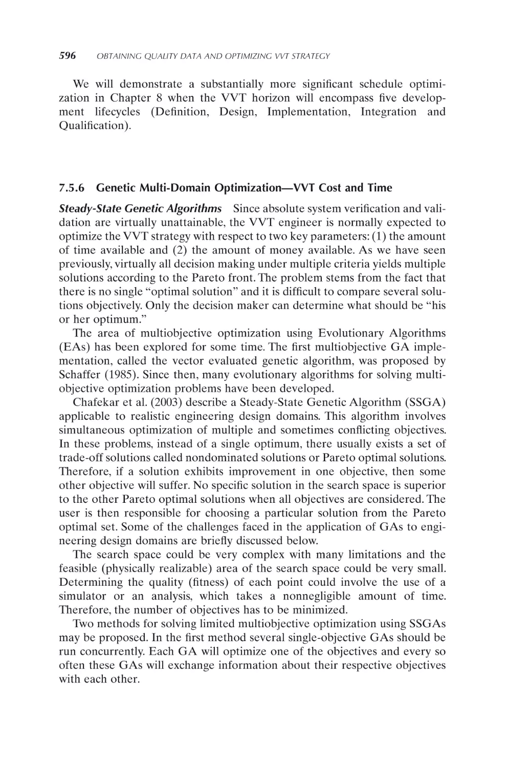


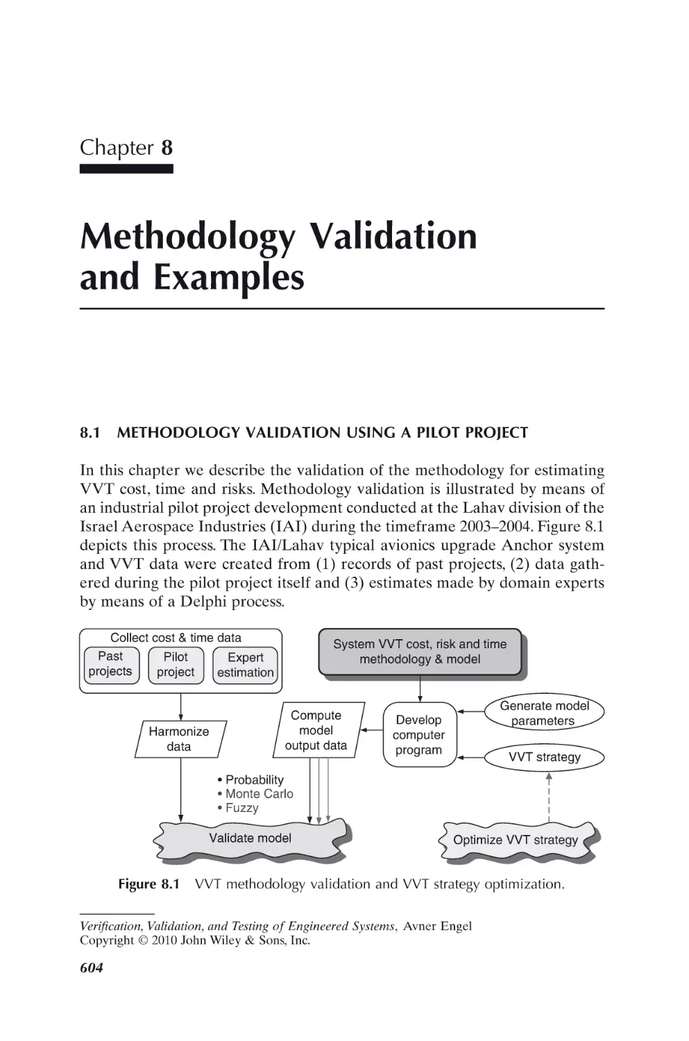


Автор: Engel A.
Теги: engineering electronics technical literature
ISBN: 978-0-470-52751-1
Год: 2010


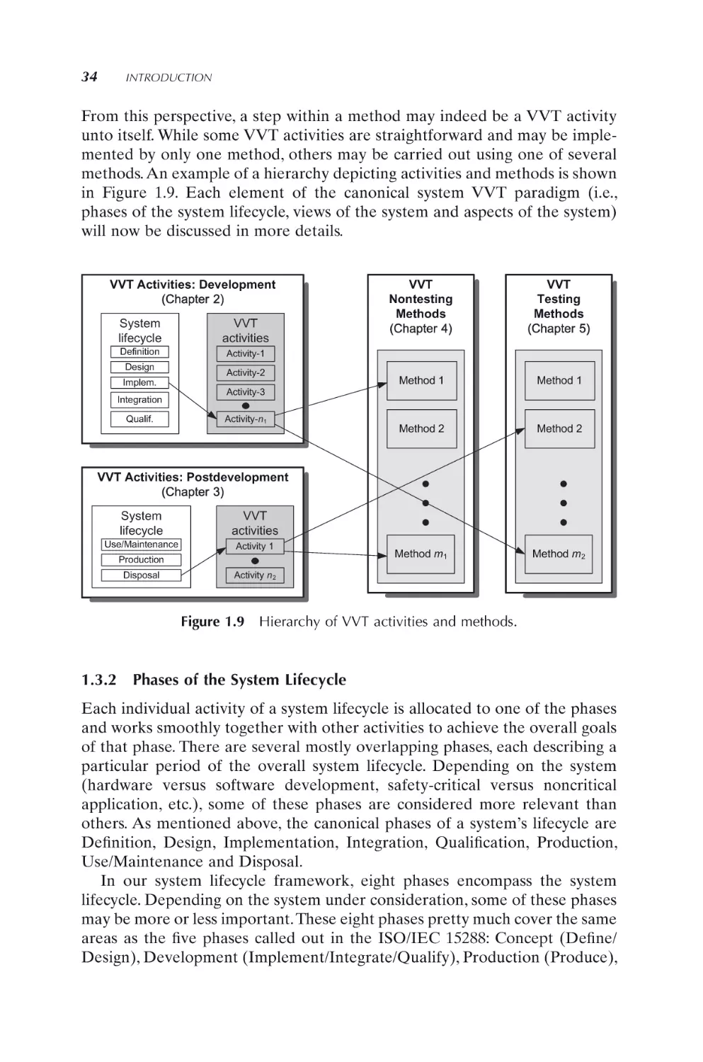
Текст
VERIFICATION, VALIDATION,
AND TESTING OF
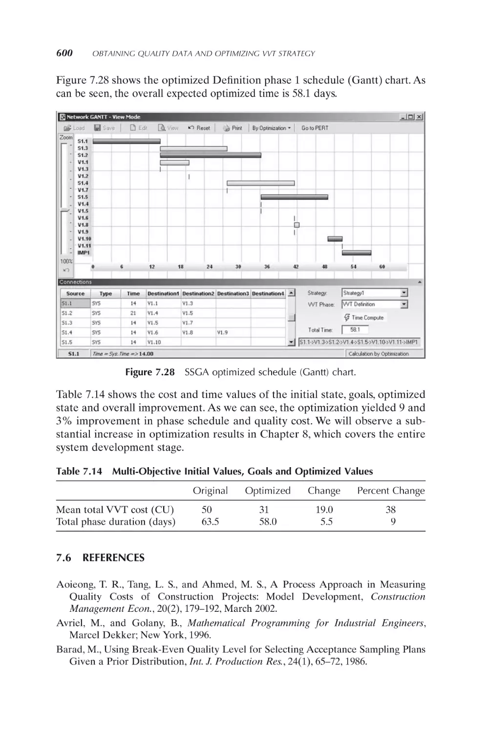
ENGINEERED SYSTEMS
AVNER ENGEL
A JOHN WILEY & SONS, INC., PUBLICATION
VERIFICATION, VALIDATION,
AND TESTING OF
ENGINEERED SYSTEMS
WILEY SERIES IN SYSTEMS ENGINEERING
AND MANAGEMENT
Andrew P. Sage, Editor
A complete list of the titles in this series appears at the end of this volume.
VERIFICATION, VALIDATION,
AND TESTING OF
ENGINEERED SYSTEMS
AVNER ENGEL
A JOHN WILEY & SONS, INC., PUBLICATION
Copyright © 2010 by John Wiley & Sons, Inc. All rights reserved
Published by John Wiley & Sons, Inc., Hoboken, New Jersey
Published simultaneously in Canada
Editorial contribution—Dr. Peter Hahn
No part of this publication may be reproduced, stored in a retrieval system, or transmitted in
any form or by any means, electronic, mechanical, photocopying, recording, scanning, or
otherwise, except as permitted under Section 107 or 108 of the 1976 United States Copyright
Act, without either the prior written permission of the Publisher, or authorization through
payment of the appropriate per-copy fee to the Copyright Clearance Center, Inc., 222
Rosewood Drive, Danvers, MA 01923, (978) 750-8400, fax (978) 750-4470, or on the web at
www.copyright.com. Requests to the Publisher for permission should be addressed to the
Permissions Department, John Wiley & Sons, Inc., 111 River Street, Hoboken, NJ 07030, (201)
748-6011, fax (201) 748-6008, or online at http://www.wiley.com/go/permission.
Limit of Liability/Disclaimer of Warranty: While the publisher and author have used their best
efforts in preparing this book, they make no representations or warranties with respect to the
accuracy or completeness of the contents of this book and specifically disclaim any implied
warranties of merchantability or fitness for a particular purpose. No warranty may be created
or extended by sales representatives or written sales materials. The advice and strategies
contained herein may not be suitable for your situation. You should consult with a professional
where appropriate. Neither the publisher nor author shall be liable for any loss of profit or any
other commercial damages, including but not limited to special, incidental, consequential, or
other damages.
For general information on our other products and services or for technical support, please
contact our Customer Care Department within the United States at (800) 762-2974, outside the
United States at (317) 572-3993 or fax (317) 572-4002.
Wiley also publishes its books in a variety of electronic formats. Some content that appears in
print may not be available in electronic formats. For more information about Wiley products,
visit our web site at www.wiley.com.
Library of Congress Cataloging-in-Publication Data:
Engel, Avner.
Verification, validation, and testing of engineered systems/Avner Engel.
p. cm.—(Wiley series in systems engineering and management)
Includes bibliographical references and index.
ISBN 978-0-470-52751-1 (cloth)
1. Quality assurance. 2. Quality control. 3. Systems engineering. 4. System failures
(Engineering)–Prevention. 5. Testing. I. Title.
TS156.6.E53 2010
658.5′62—dc22
2009045885
Printed in the United States of America
10 9 8 7 6 5 4 3 2 1
To my parents:
Josef Engel, Lea Engel and Tova Engel
and my revered teachers:
Dr. Itzhak Frank, Professor Jerry Weinberg and Professor Miryam Barad
Contents
Preface
xvii
Part I Introduction
1
1. Introduction
3
1.1 Opening
1.1.1
Background
1.1.2
Purpose
1.1.3
Intended audience
1.1.4
Book structure and contents
1.1.5
Scope of application
1.1.6
Terminology and notation
3
4
5
5
6
8
9
1.2 VVT Systems and Process
1.2.1
Introduction—VVT systems and process
1.2.2
Engineered systems
1.2.3
VVT concepts and definition
1.2.4
The fundamental VVT dilemma
1.2.5
Modeling systems and VVT lifecycle
1.2.6 Modeling VVT and risks as cost and time drivers
9
9
10
12
19
20
24
vii
viii
CONTENTS
1.3 Canonical Systems VVT Paradigm
1.3.1
Introduction—Canonical systems VVT paradigm
1.3.2 Phases of the system lifecycle
1.3.3
Views of the system
1.3.4 VVT aspects of the system
32
32
34
37
39
1.4 Methodology Application
1.4.1
Introduction
1.4.2
VVT methodology overview
1.4.3
VVT tailoring
1.4.4
VVT documents
39
39
40
43
50
1.5 References
56
Part II VVT Activities and Methods
61
2. System VVT Activities: Development
63
2.1 Structure of Chapter
2.1.1
Systems development lifecycle phases and
VVT activities
2.1.2
VVT activity aspects
2.1.3
VVT activity format
63
2.2 VVT Activities during Definition
2.2.1
Generate Requirements Verification Matrix (RVM)
2.2.2
Generate VVT Management Plan (VVT-MP)
2.2.3
Assess the Request For Proposal (RFP) document
2.2.4
Assess System Requirements Specification (SysRS)
2.2.5
Assess project Risk Management Plan (RMP)
2.2.6
Assess System Safety Program Plan (SSPP)
2.2.7
Participate in System Requirements Review (SysRR)
2.2.8
Participate in System Engineering Management
Plan (SEMP) review
2.2.9
Conduct engineering peer review of the VVT-MP
document
65
65
67
69
71
72
74
77
2.3 VVT Activities during Design
2.3.1
Optimize the VVT strategy
2.3.2
Assess System/Subsystem Design Description (SSDD)
2.3.3
Validate system design by means of virtual prototype
80
80
83
85
63
64
65
77
79
CONTENTS
2.3.4
2.3.5
2.3.6
Validate system design tools
Assess system design for meeting future
lifecycle needs
Participate in the System Design Review (SysDR)
2.4 VVT Activities during Implementation
2.4.1
Preparing the test cycle for subsystems and components
2.4.2
Assess suppliers’ subsystems test documents
2.4.3
Perform Acceptance Test Procedure—Subsystems/
Enabling products
2.4.4
Assess system performance by way of simulation
2.4.5
Verify design versus implementation consistency
2.4.6
Participate in Acceptance Test Review—Subsystems/
Enabling products
2.5 VVT Activities during Integration
2.5.1
Develop System Integration Laboratory (SIL)
2.5.2
Generate System Integration Test Plan (SysITP)
2.5.3
Generate System Integration Test Description
(SysITD)
2.5.4
Validate supplied subsystems in a stand-alone
configuration
2.5.5
Perform components, subsystem, enabling products
integration tests
2.5.6
Generate System Integration Test Report (SysITR)
2.5.7 Assess effectiveness of the system Built In Test (BIT)
2.5.8
Conduct engineering peer review of the SysITR
2.6 VVT Activities during Qualification
2.6.1
Generate a qualification/acceptance System Test
Plan (SysTP)
2.6.2
Create qualification/acceptance System Test
Description (SysTD)
2.6.3
Perform virtual system testing by means of simulation
2.6.4
Perform qualification testing/Acceptance Test
Procedure (ATP)—System
2.6.5
Generate qualification/acceptance System Test
Report (SysTR)
2.6.6 Assess system testability, maintainability and availability
2.6.7
Perform environmental system testing
2.6.8
Perform system Certification and Accreditation (C&A)
ix
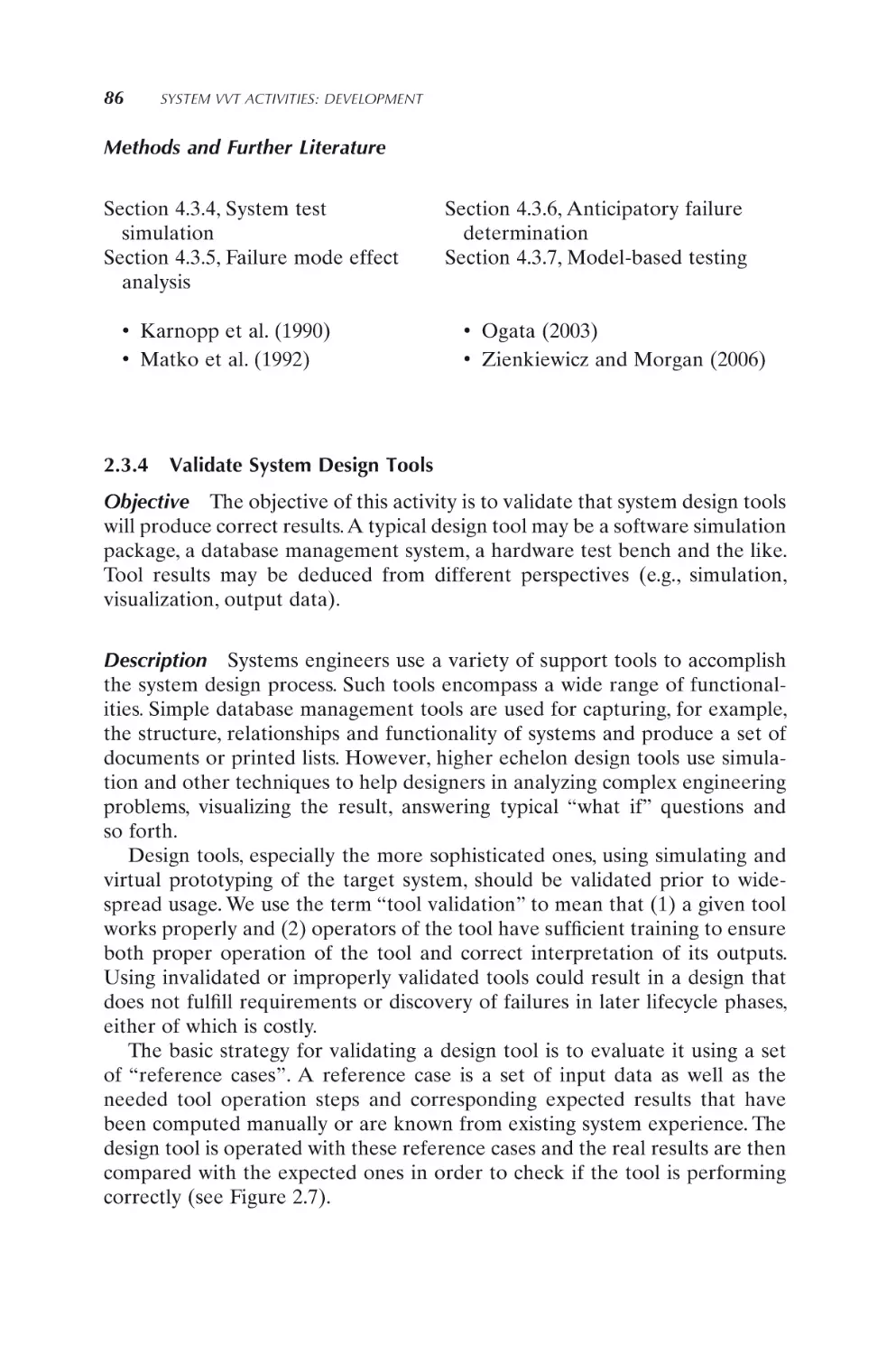
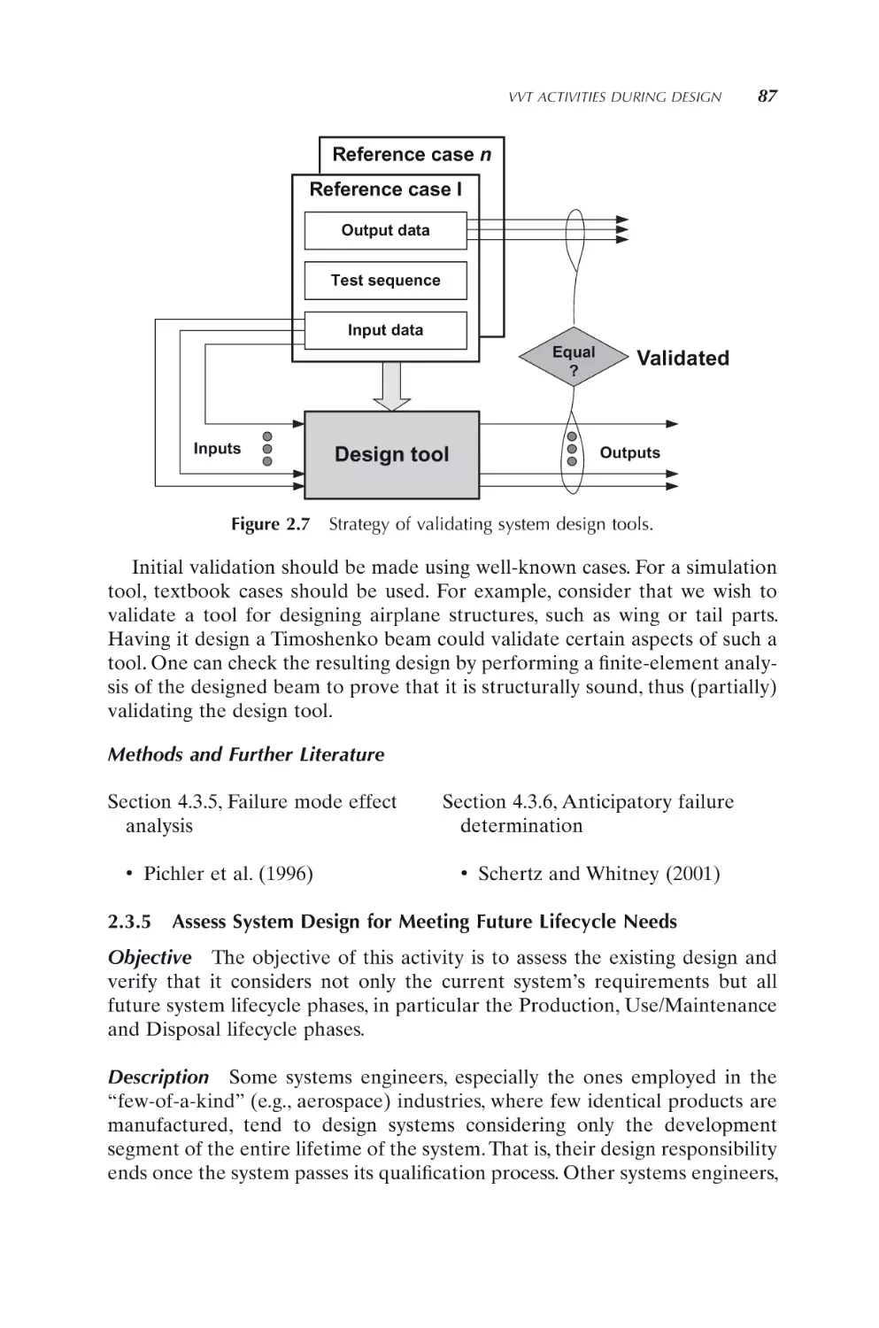
86
87
90
91
91
96
97
100
102
103
104
104
106
108
111
112
114
116
120
120
121
123
125
126
129
131
137
140
x
CONTENTS
2.6.9
2.6.10
2.6.11
Conduct Test Readiness Review (TRR)
Conduct engineering peer review of development
enabling products
Conduct engineering peer review of program and
project safety
144
146
148
2.7 References
149
3. Systems VVT Activities: Post-Development
153
3.1 Structure of Chapter
153
3.2 VVT Activities during Production
3.2.1
Participate in Functional Configuration Audit (FCA)
3.2.2
Participate in Physical Configuration Audit (PCA)
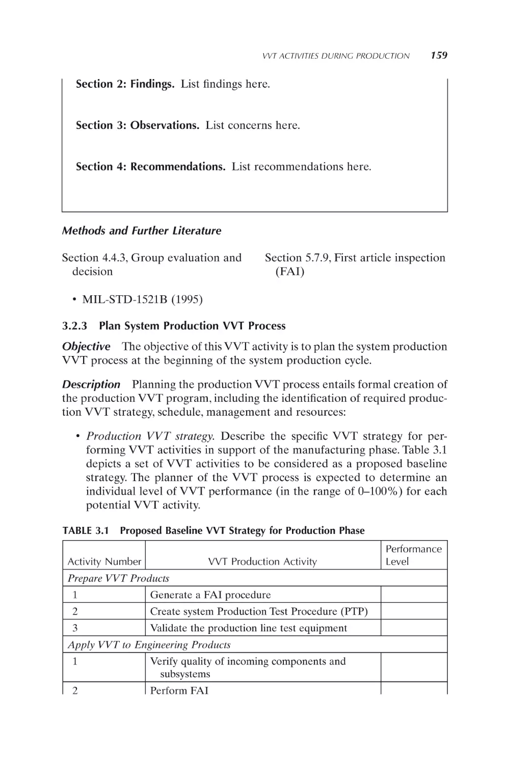
3.2.3
Plan system production VVT process
3.2.4
Generate a First Article Inspection (FAI) procedure
3.2.5
Validate the production-line test equipment
3.2.6
Verify quality of incoming components and subsystems
3.2.7
Perform First Article Inspection (FAI)
3.2.8
Validate pre-production process
3.2.9
Validate ongoing-production process
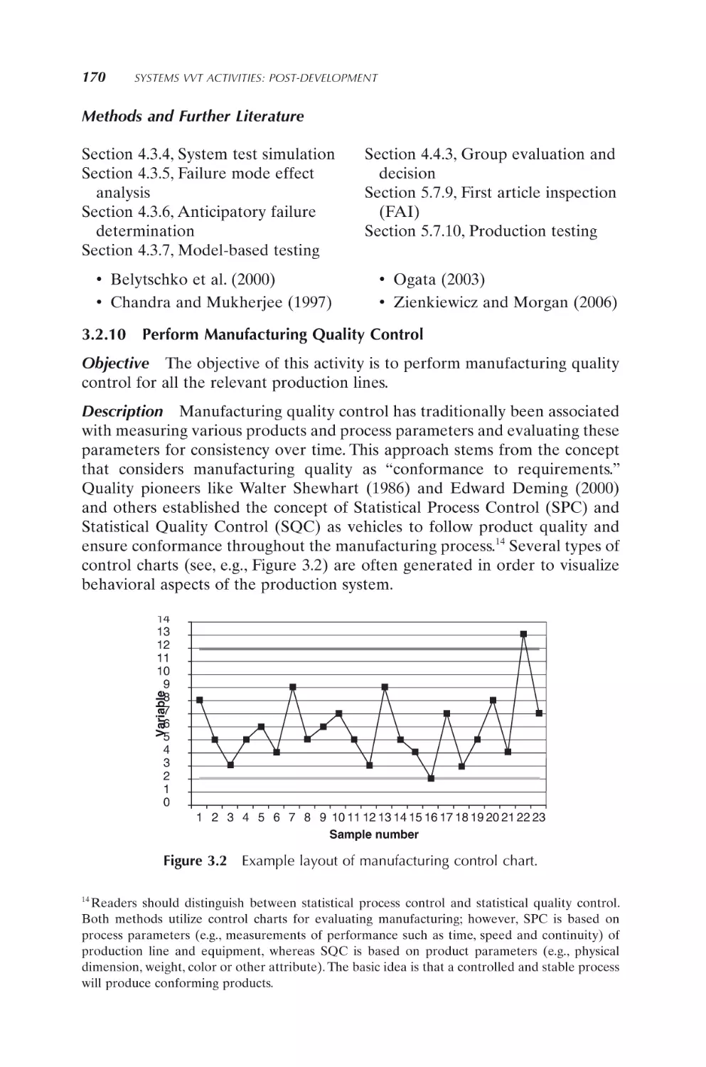
3.2.10 Perform manufacturing quality control
3.2.11 Verify the production operations strategy
3.2.12 Verify marketing and production forecasting
3.2.13 Verify aggregate production planning
3.2.14 Verify inventory control operation
3.2.15 Verify supply chain management
3.2.16 Verify production control systems
3.2.17 Verify production scheduling
3.2.18 Participate in Production Readiness Review (PRR)
154
154
157
159
161
165
165
166
167
168
170
172
174
176
177
180
181
183
184
3.3 VVT Activities during Use/Maintenance
3.3.1 Develop VVT plan for system maintenance
3.3.2
Verify the Integrated Logistics Support Plan (ILSP)
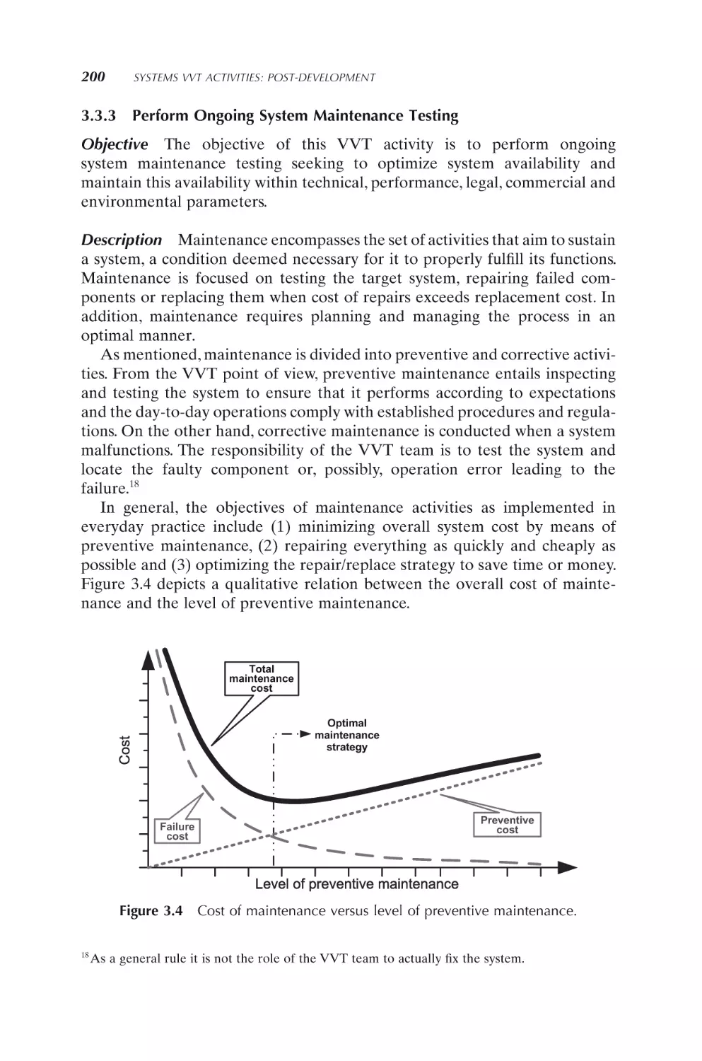
3.3.3
Perform ongoing system maintenance testing
3.3.4
Conduct engineering peer review on system
maintenance process
186
187
191
200
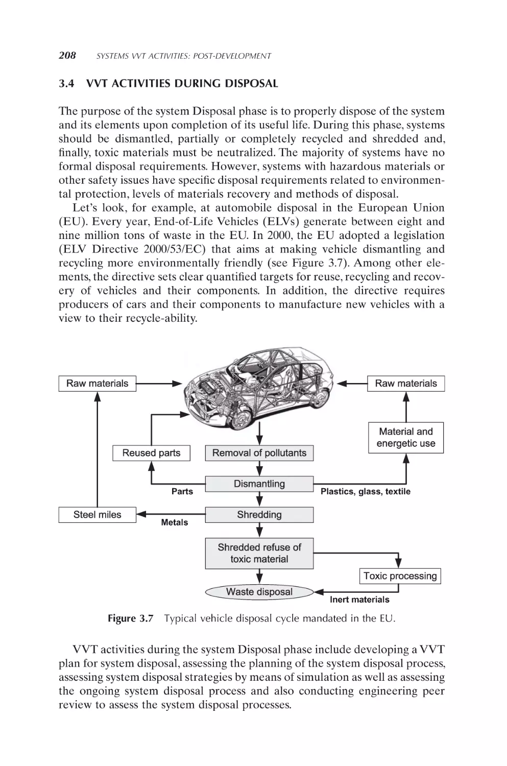
3.4 VVT Activities during Disposal
3.4.1 Develop VVT plan for system disposal
3.4.2
Assess the system disposal plan
208
209
212
204
CONTENTS
3.4.3
3.4.4
3.4.5
Assess system disposal strategies by means of simulation
Assess on-going system disposal process
Conduct engineering peer review to assess system
disposal processes
xi
214
215
219
3.5 References
221
4. System VVT Methods: Non-Testing
223
4.1 Introduction
223
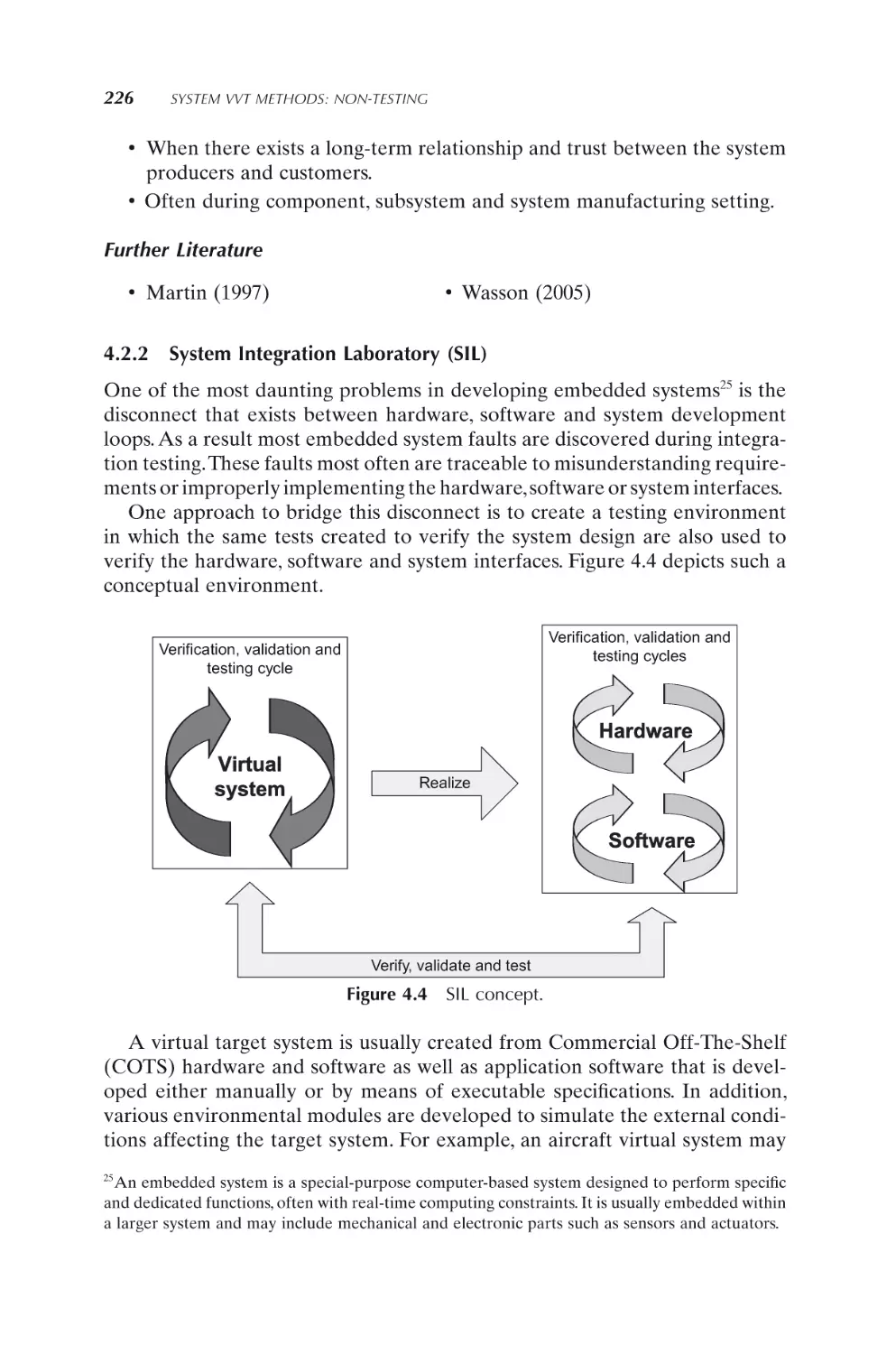
4.2 Prepare VVT Products
4.2.1
Requirements Verification Matrix (RVM)
4.2.2
System Integration Laboratory (SIL)
4.2.3
Hierarchical VVT optimization
4.2.4
Defect management and tracking
4.2.5
Classification Tree Method
4.2.6
Design of Experiments (DOE)
223
223
226
230
234
239
243
4.3 Perform VVT Activities
4.3.1
VVT process planning
4.3.2
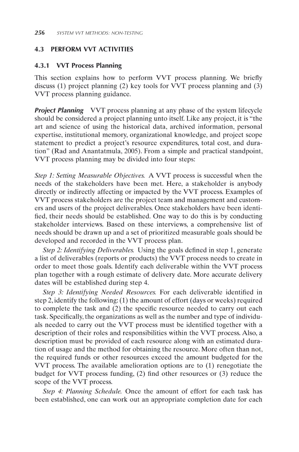
Compare images and documents
4.3.3
Requirements testability and quality
4.3.4
System test simulation
4.3.5
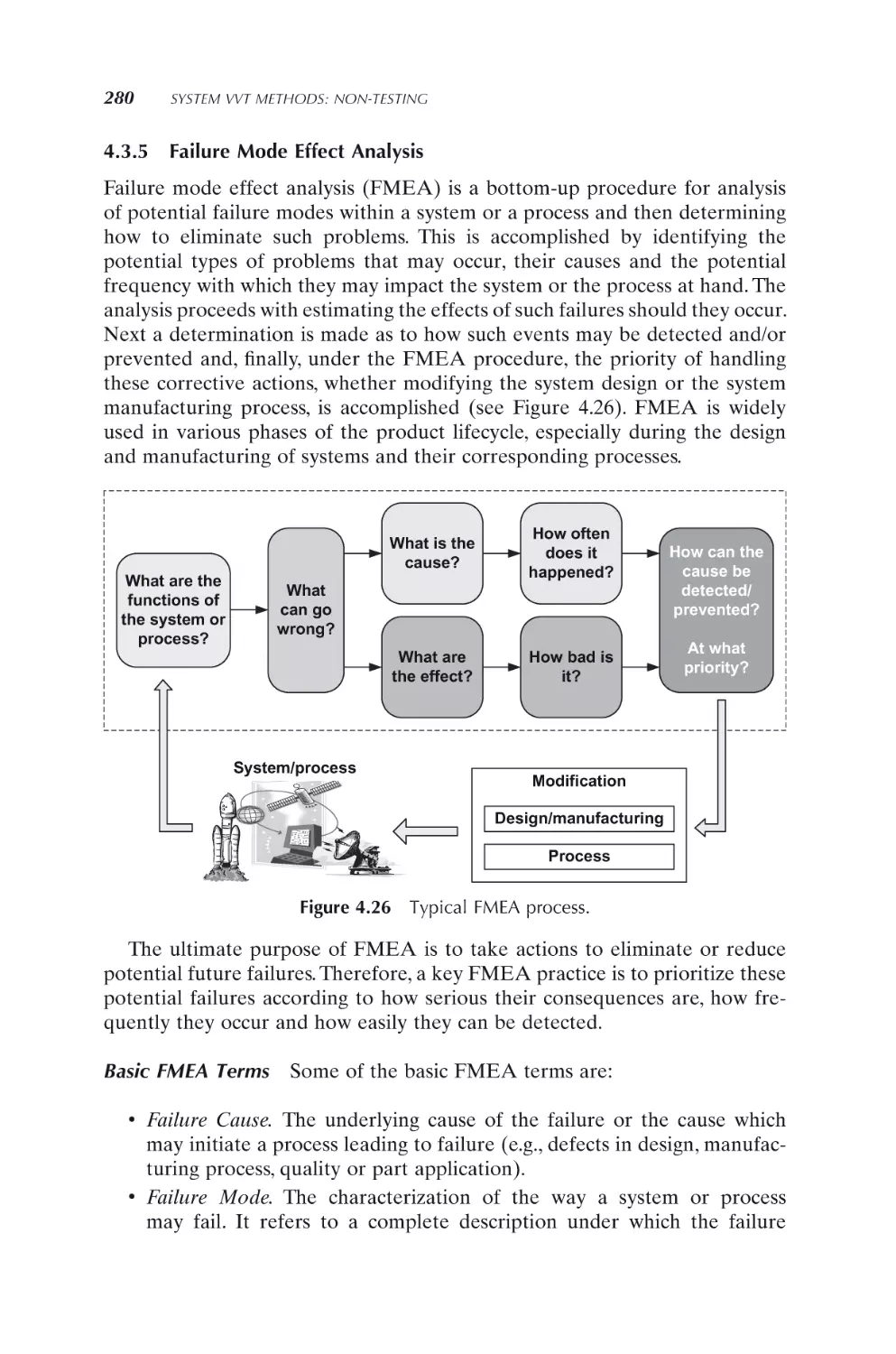
Failure mode effect analysis
4.3.6
Anticipatory Failure Determination
4.3.7
Model-based testing
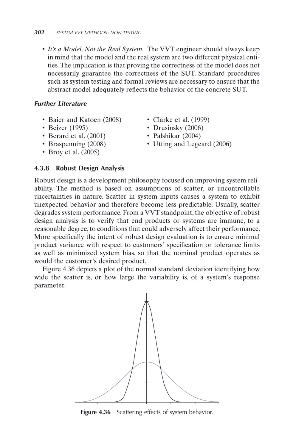
4.3.8
Robust design analysis
256
256
262
265
272
280
286
293
302
4.4 Participate in Reviews
4.4.1
Expert team reviews
4.4.2
Formal technical reviews
4.4.3
Group evaluation and decision
312
312
326
331
4.5 References
346
5. Systems VVT Methods: Testing
351
5.1 Introduction
351
5.2 White Box Testing
5.2.1
Component and code coverage testing
5.2.2
Interface testing
356
356
360
xii
CONTENTS
5.3 Black Box—Basic Testing
5.3.1
Boundary value testing
5.3.2
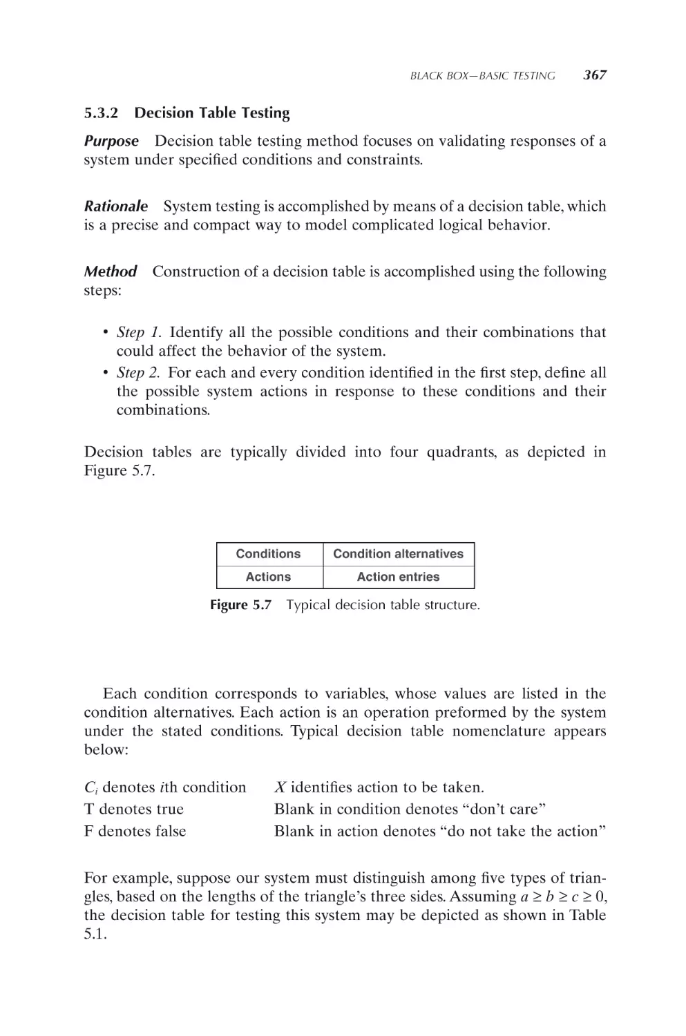
Decision table testing
5.3.3
Finite State Machine testing
5.3.4
Human-system interface testing (HSI)
365
365
367
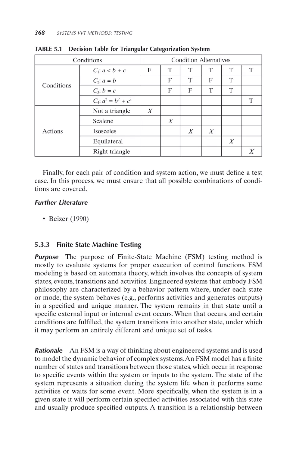
368
373
5.4 Black Box—High-Volume Testing
5.4.1
Automatic random testing
5.4.2
Performance testing
5.4.3
Recovery testing
5.4.4
Stress testing
378
378
381
385
386
5.5 Black Box—Special Testing
5.5.1
Usability testing
5.5.2
Security vulnerability testing
5.5.3
Reliability testing
5.5.4
Search-based testing
5.5.5
Mutation testing
388
388
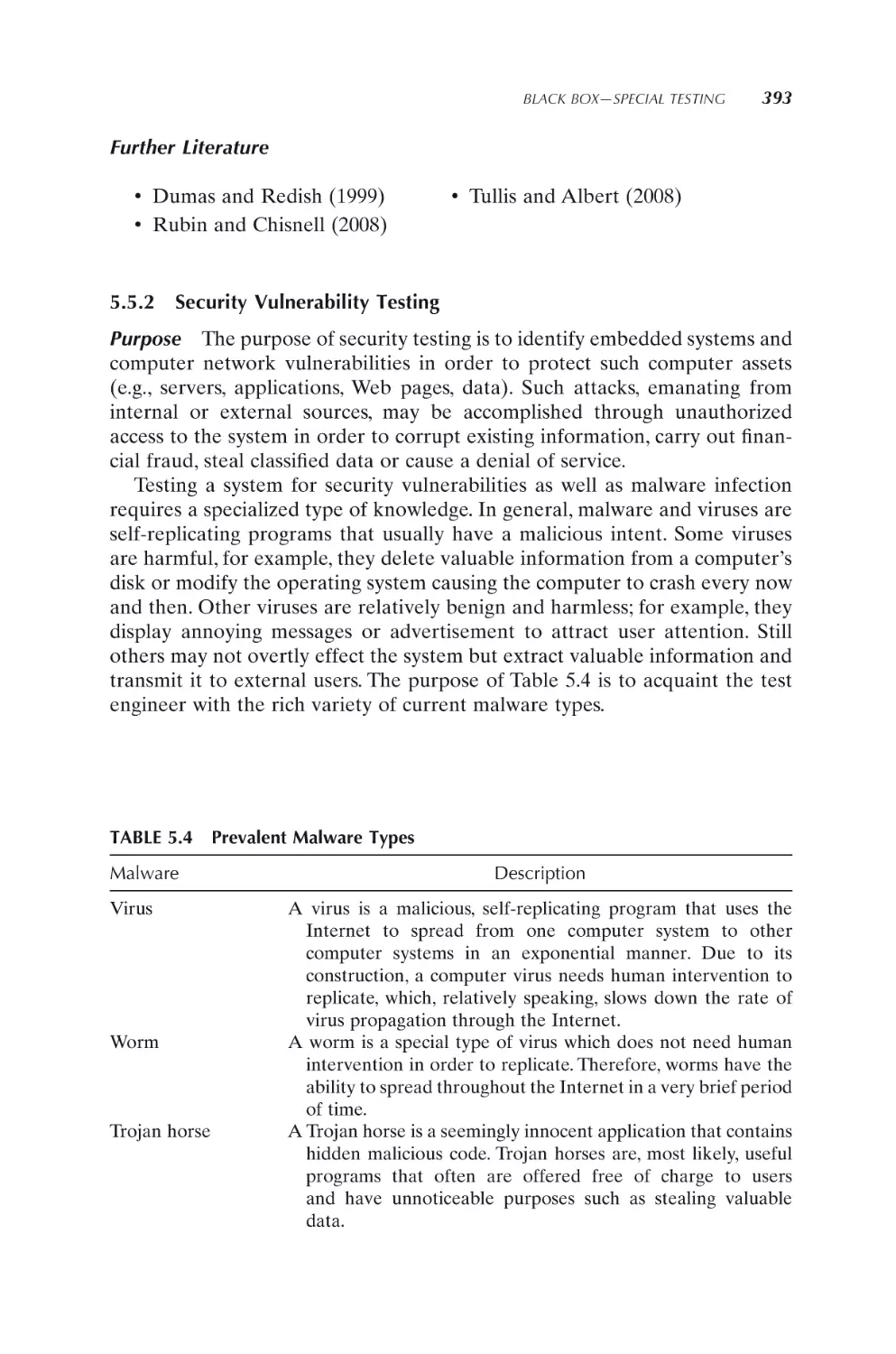
393
402
410
418
5.6 Black Box—Environment Testing
5.6.1
Environmental Stress Screening (ESS) testing
5.6.2
EMI/EMC testing
5.6.3
Destructive testing
5.6.4
Reactive testing
5.6.5
Temporal testing
422
422
424
426
431
436
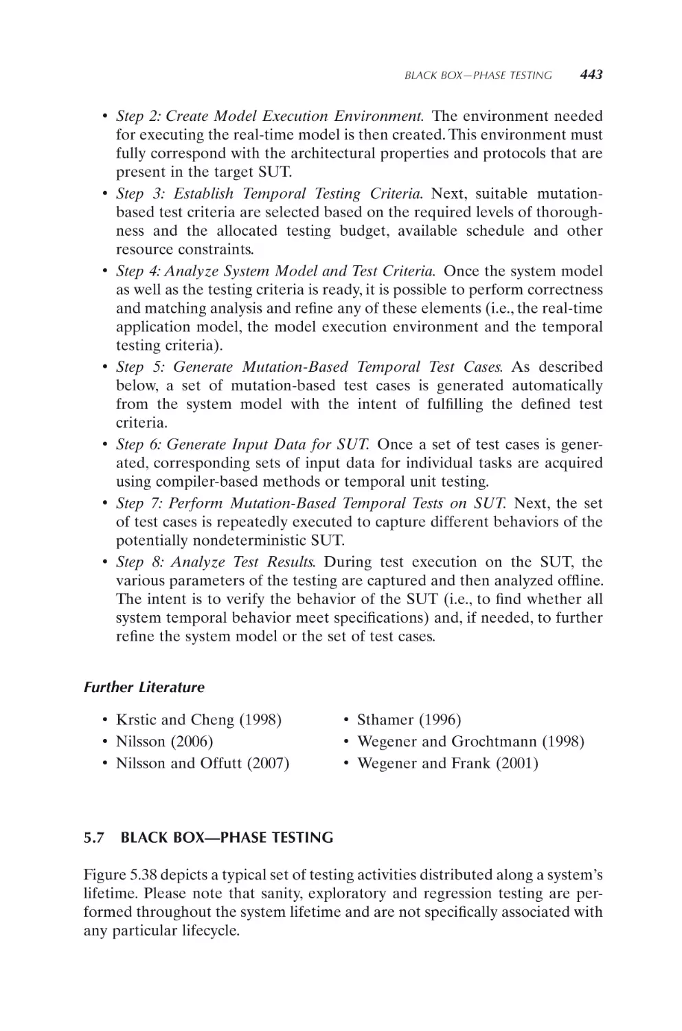
5.7 Black Box—Phase Testing
5.7.1
Sanity testing
5.7.2
Exploratory testing
5.7.3
Regression testing
5.7.4
Component and subsystem testing
5.7.5
Integration testing
5.7.6
Qualification testing
5.7.7
Acceptance testing
5.7.8
Certification and accreditation testing
5.7.9
First Article Inspection (FAI)
5.7.10 Production testing
5.7.11 Installation testing
5.7.12 Maintenance testing
5.7.13 Disposal testing
443
444
445
447
452
455
461
463
466
473
477
481
484
487
5.8 References
488
CONTENTS
xiii
Part III Modeling and Optimizing VVT Process
495
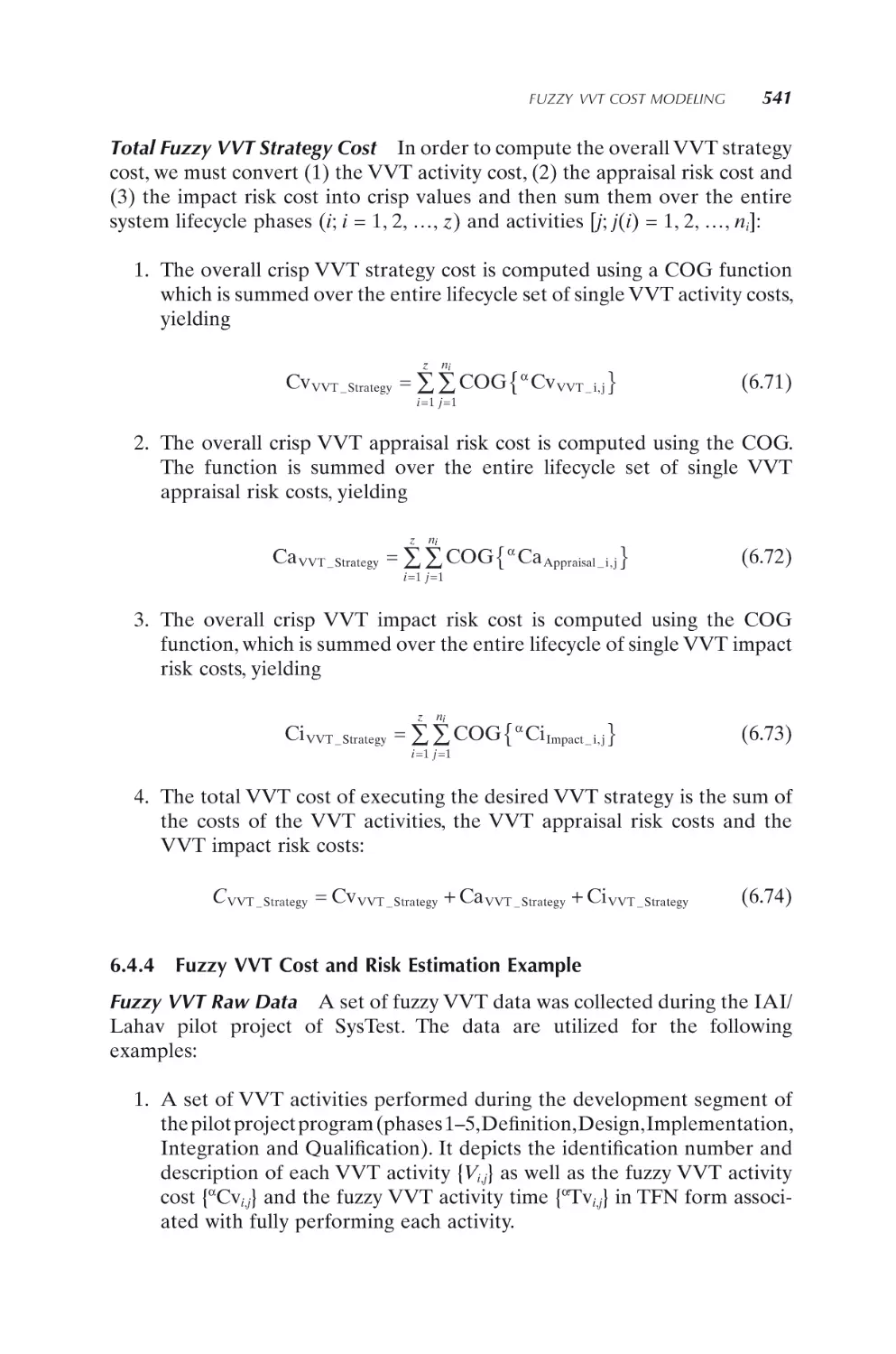
6. Modeling Quality Cost, Time and Risk
497
6.1 Purpose and Basic Concepts
6.1.1
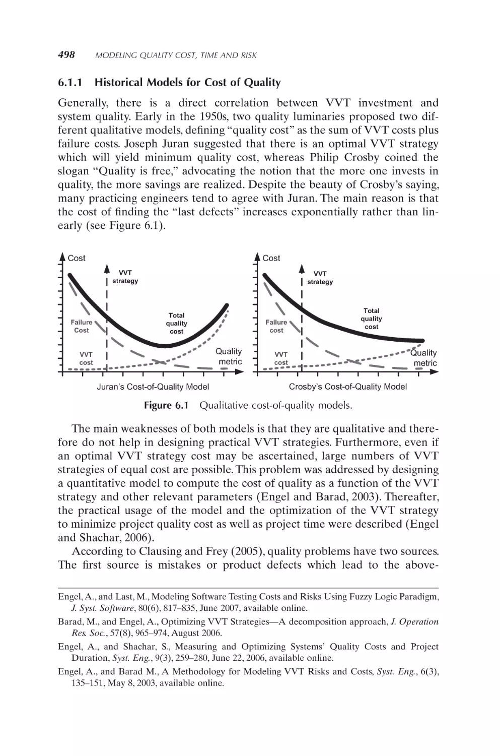
Historical models for cost of quality
6.1.2
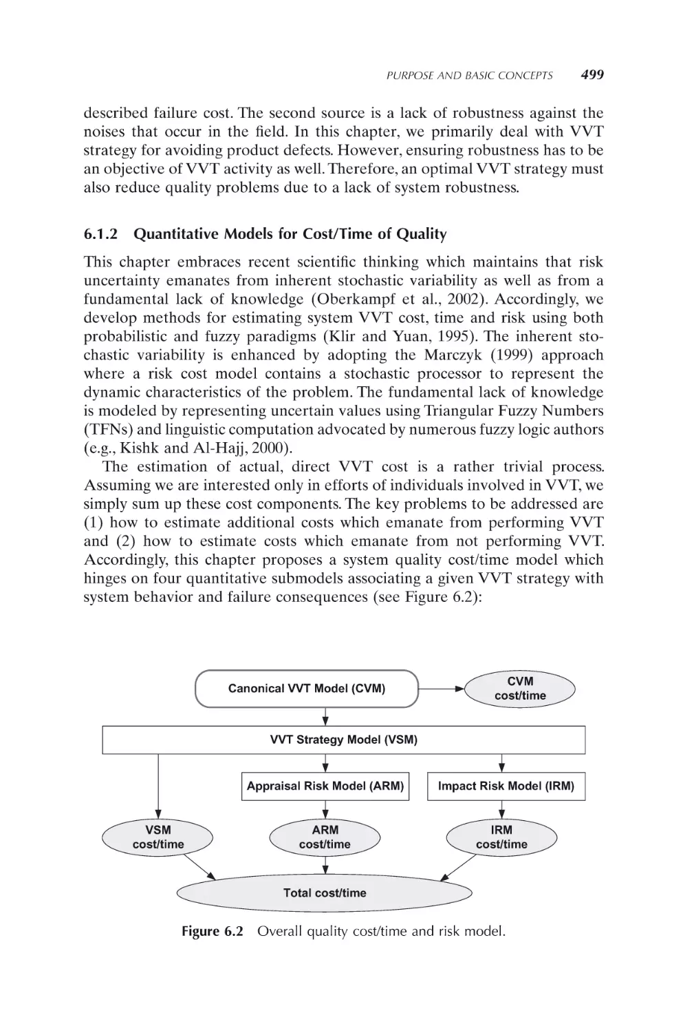
Quantitative models for cost/time of quality
497
498
499
6.2 VVT Cost and Risk Modeling
6.2.1
Canonical VVT cost modeling
6.2.2
Modeling VVT strategy as a decision problem
6.2.3
Modeling appraisal risk cost
6.2.4
Modeling impact risk cost
6.2.5
Modeling total quality cost
6.2.6 VVT cost and risk example
500
500
502
505
511
516
517
6.3 VVT Time and Risk Modeling
6.3.1
System/VVT network
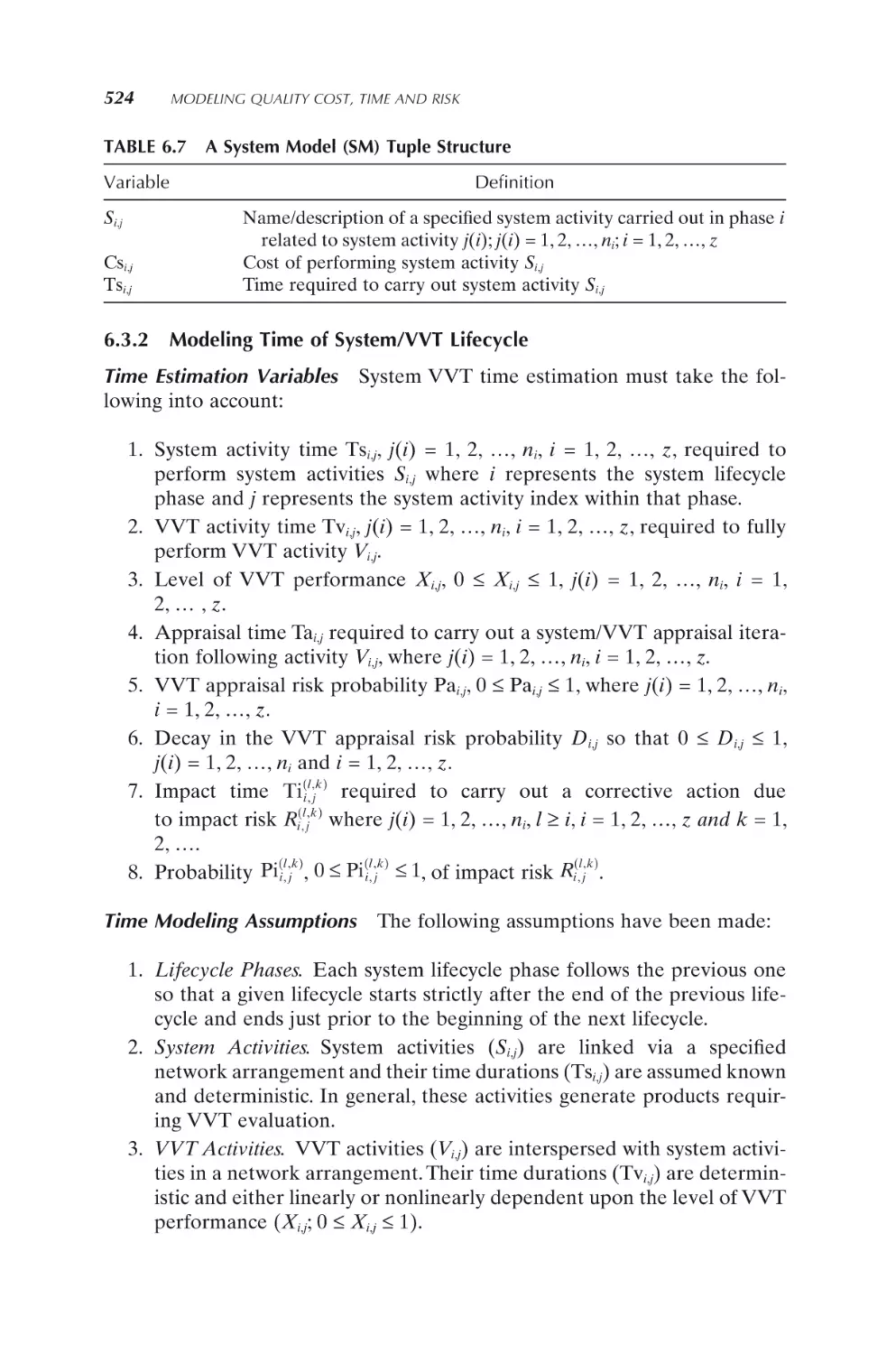
6.3.2
Modeling time of system/VVT lifecycle
6.3.3
Time and risk example
521
521
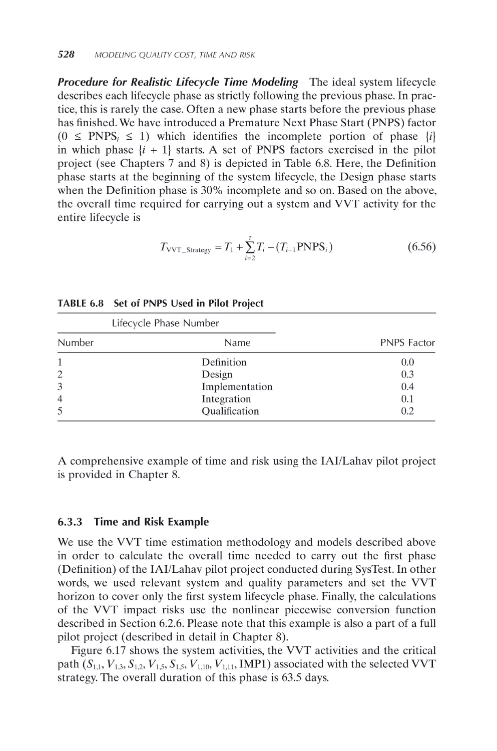
524
528
6.4 Fuzzy VVT Cost Modeling
6.4.1
Introduction
6.4.2
General fuzzy logic modeling
6.4.3
Fuzzy modeling of the VVT process
6.4.4
Fuzzy VVT cost and risk estimation example
6.4.5
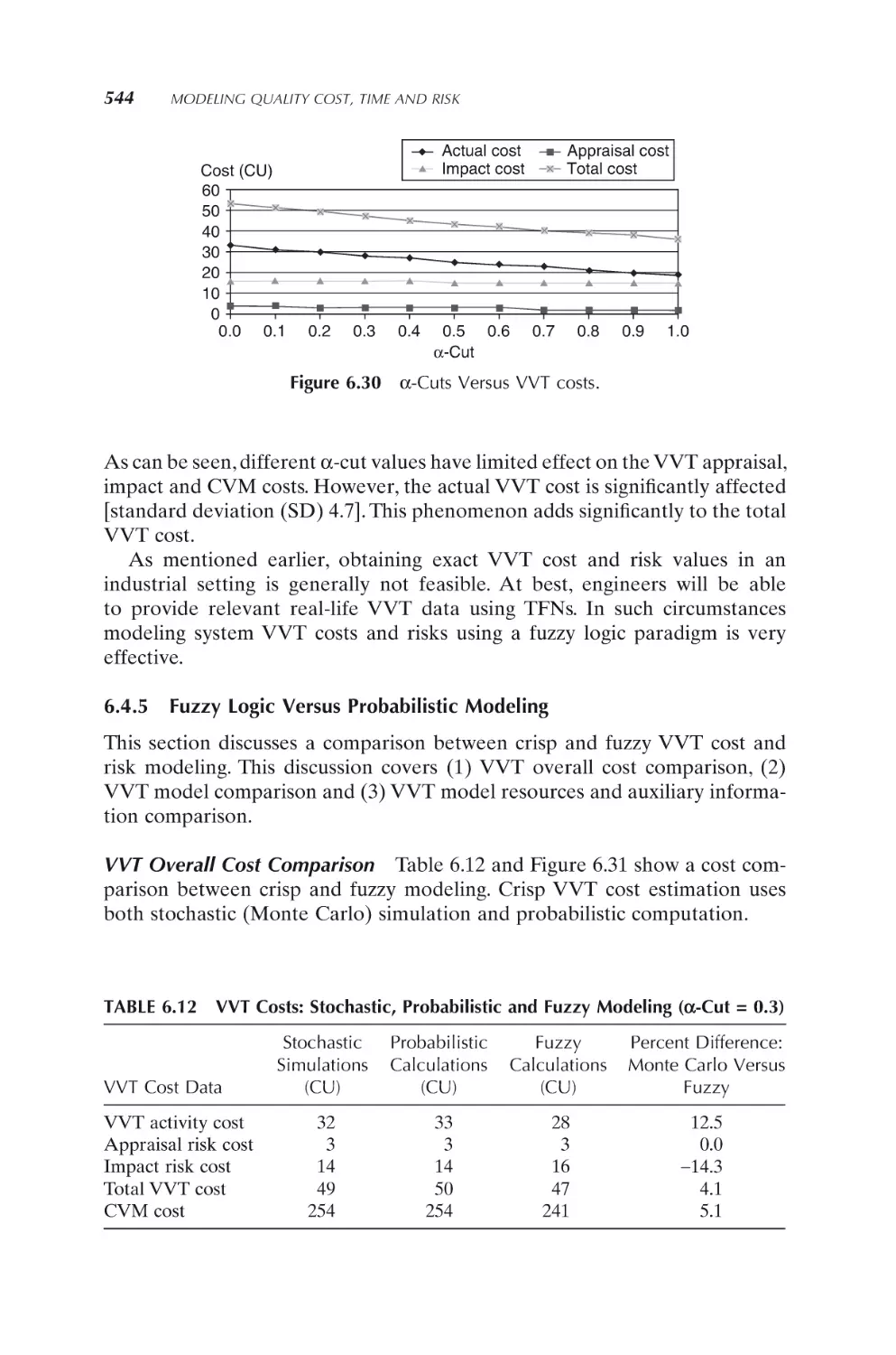
Fuzzy logic versus probabilistic modeling
530
530
530
532
541
544
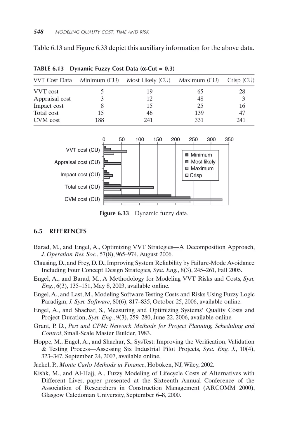
6.5 References
548
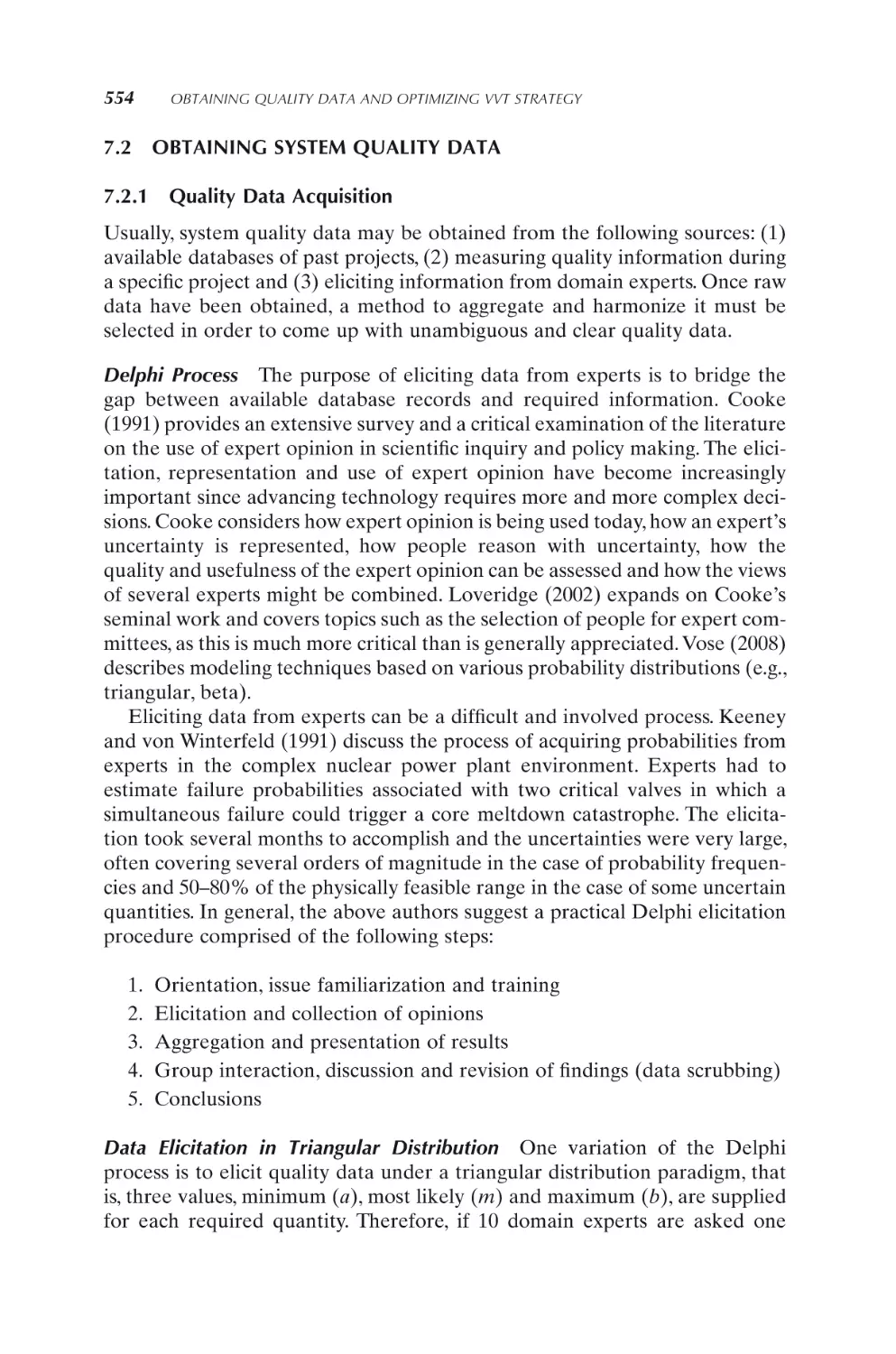
7. Obtaining Quality Data and Optimizing VVT Strategy
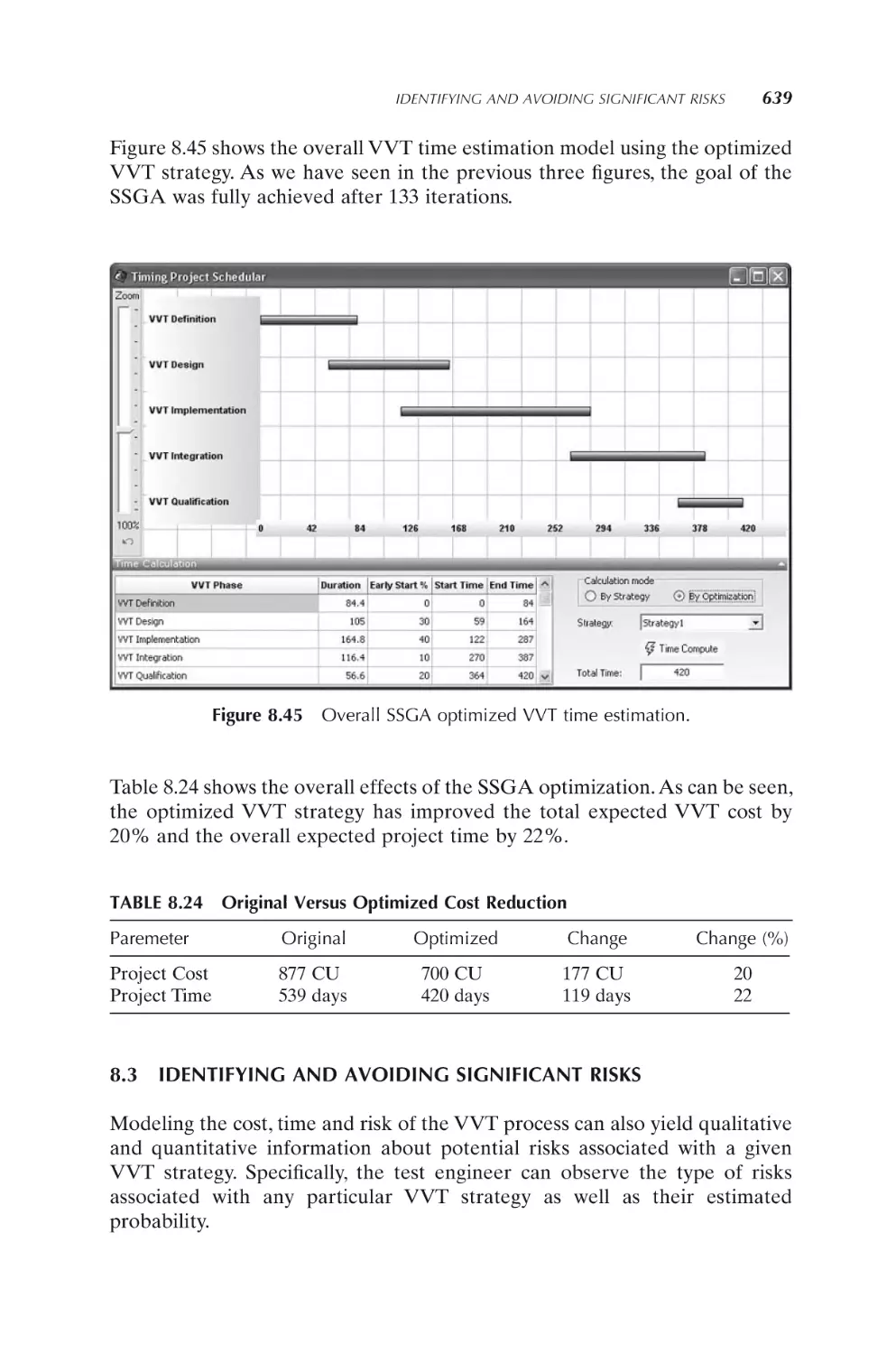
550
7.1 Systems’ Quality Costs in the Literature
550
7.2 Obtaining System Quality Data
7.2.1
Quality data acquisition
7.2.2
Quality data aggregation
554
554
555
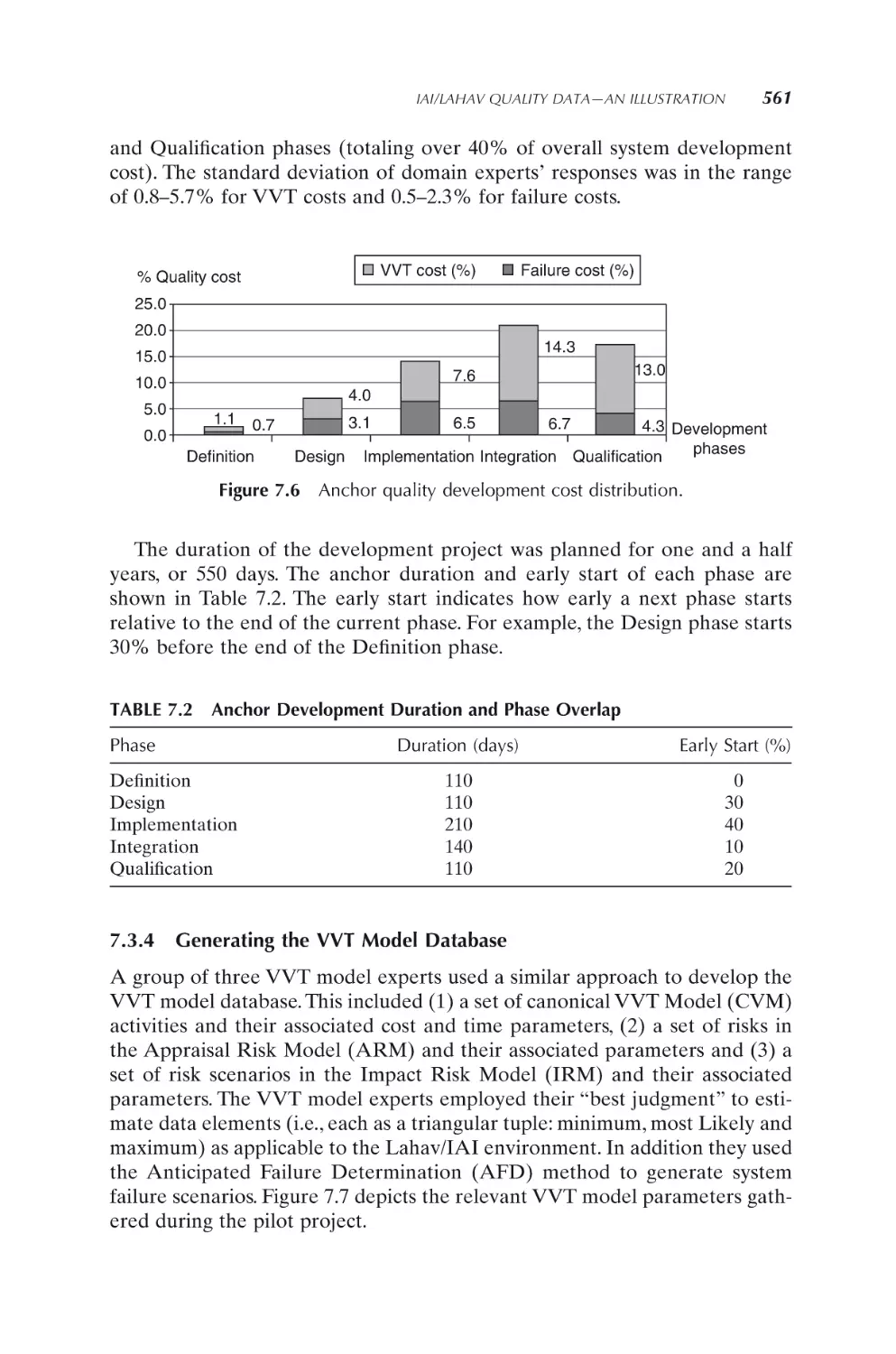
7.3 IAI/Lahav Quality Data—An Illustration
7.3.1
IAI/Lahav pilot project
7.3.2
Obtaining raw system and quality data
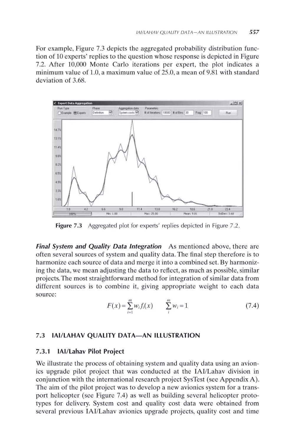
7.3.3
Anchor system and quality data
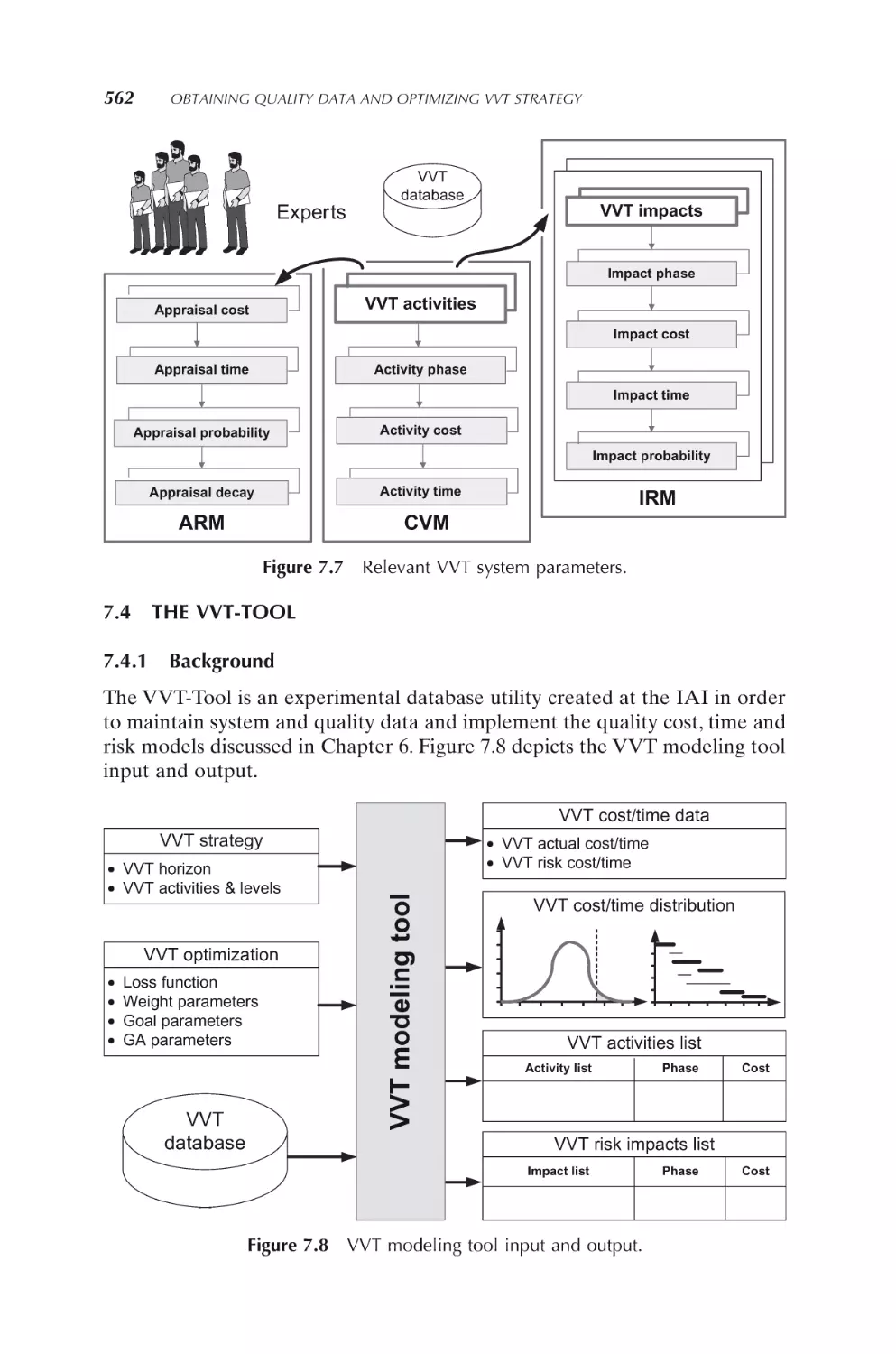
7.3.4
Generating the VVT model database
557
557
559
560
561
xiv
CONTENTS
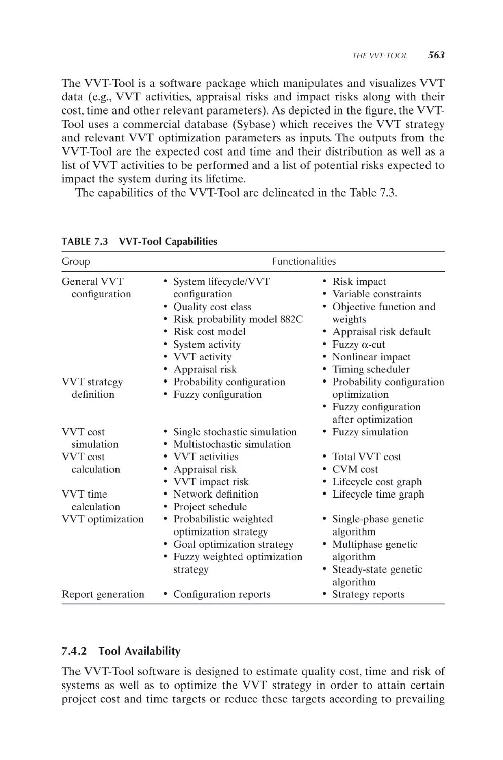
7.4 The VVT-Tool
7.4.1
Background
7.4.2
Tool availability
562
562
563
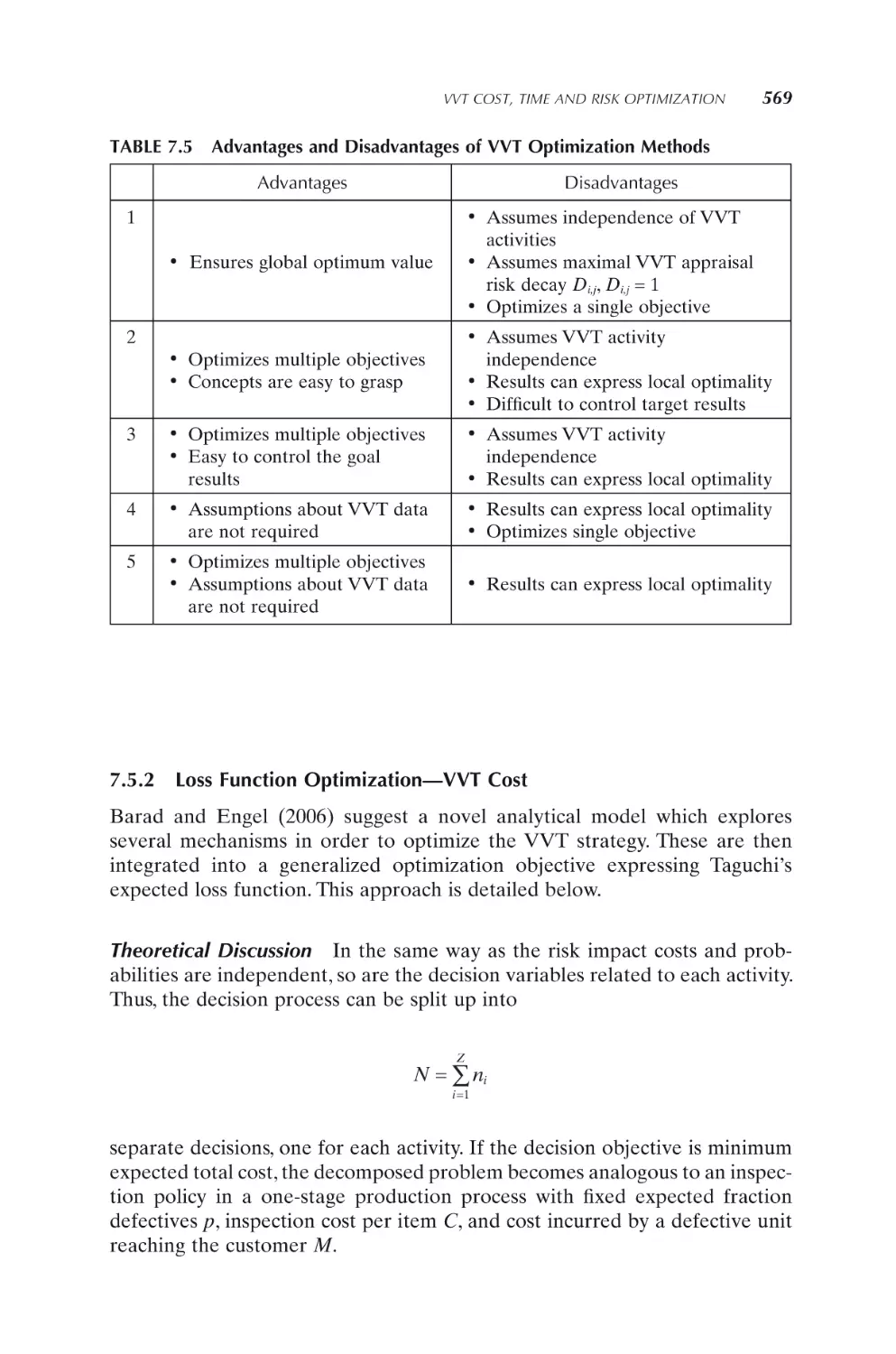
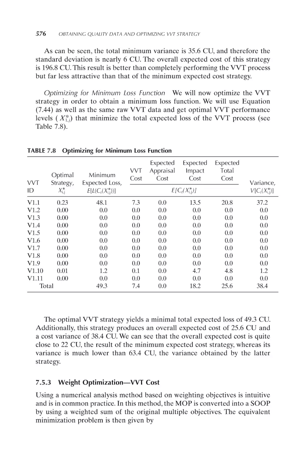
7.5 VVT Cost, Time and Risk Optimization
7.5.1
Optimizing the VVT process
7.5.2
Loss function optimization—VVT cost
7.5.3
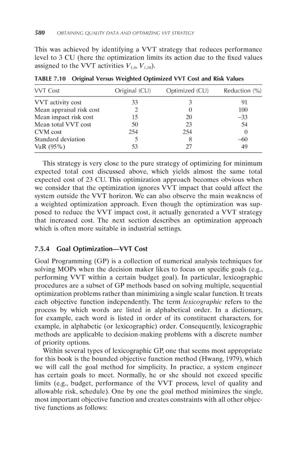
Weight optimization—VVT cost
7.5.4
Goal optimization—VVT cost
7.5.5
Genetic algorithm optimization—VVT time
7.5.6
Genetic multi-domain optimization—VVT cost and time
564
565
569
576
580
584
596
7.6 References
600
8. Methodology Validation and Examples
604
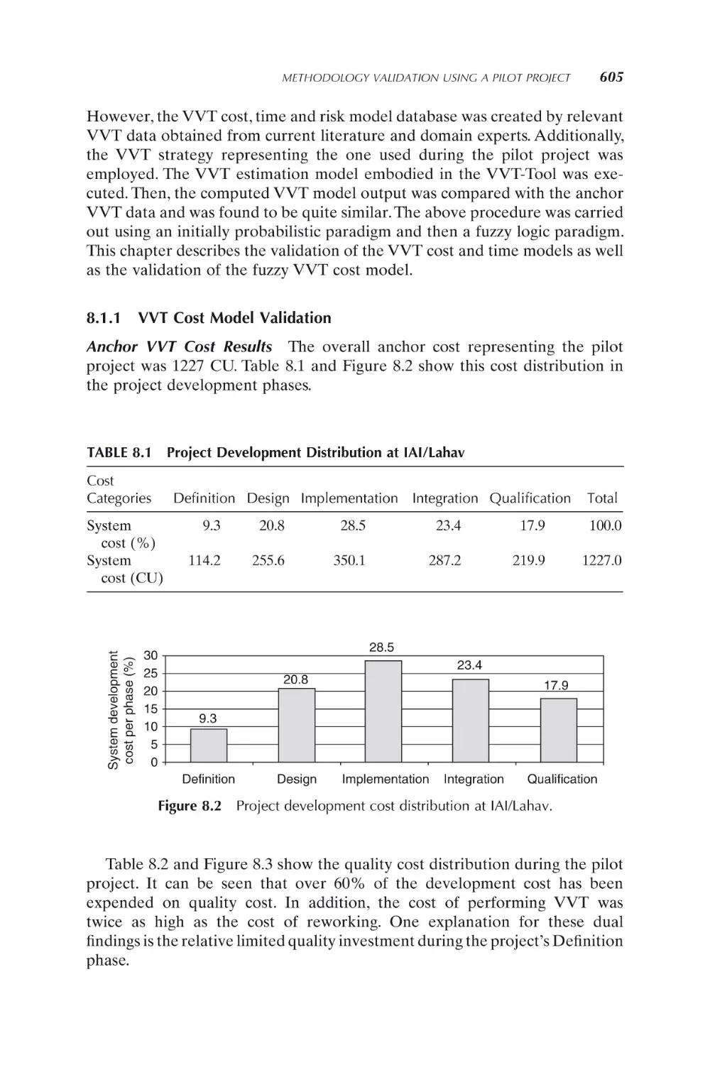
8.1 Methodology Validation Using a Pilot Project
8.1.1
VVT cost model validation
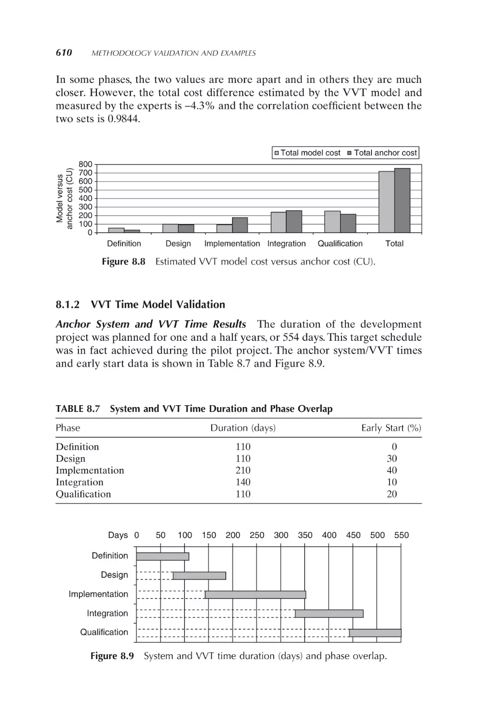
8.1.2
VVT time model validation
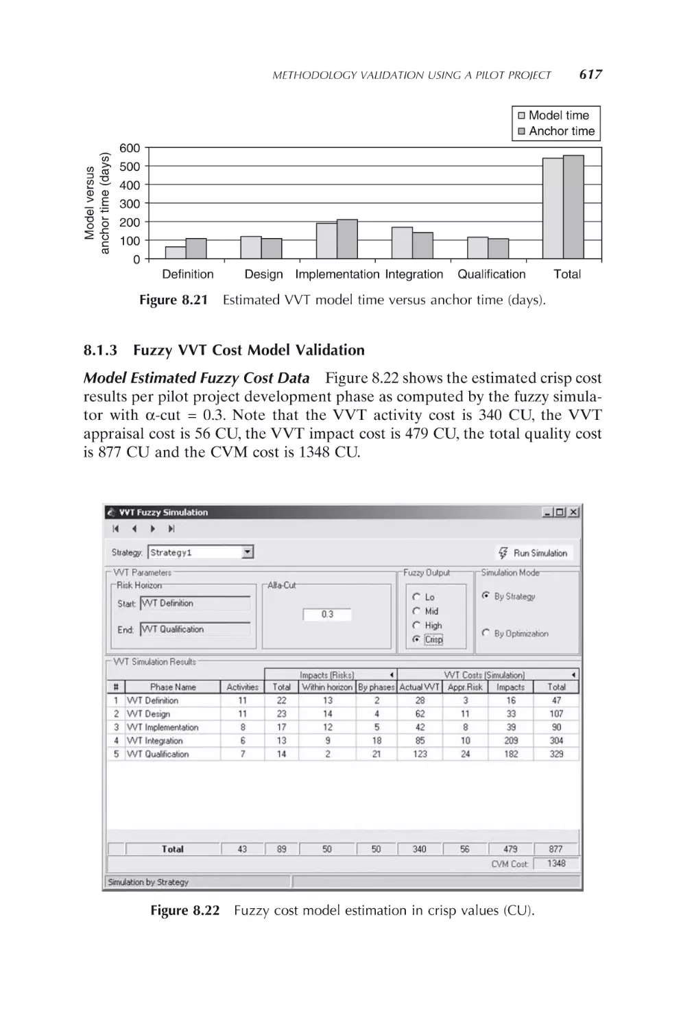
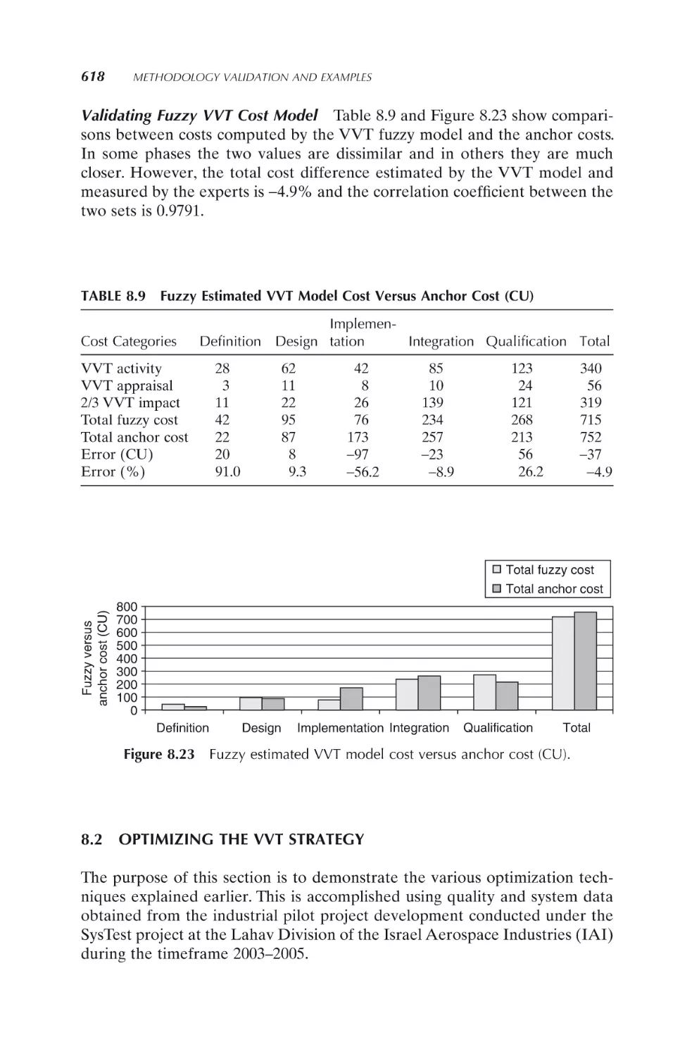
8.1.3 Fuzzy VVT cost model validation
604
605
610
617
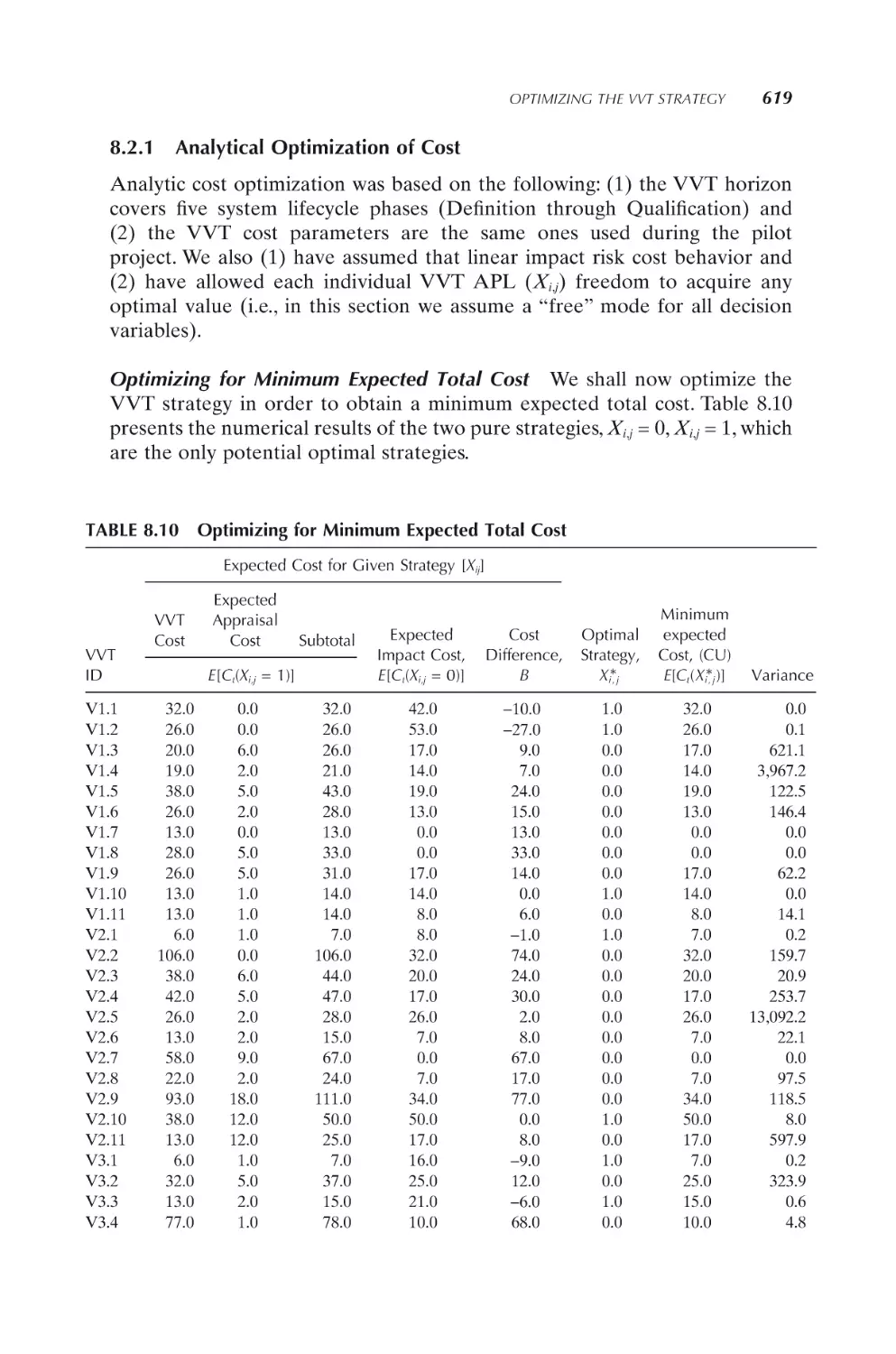
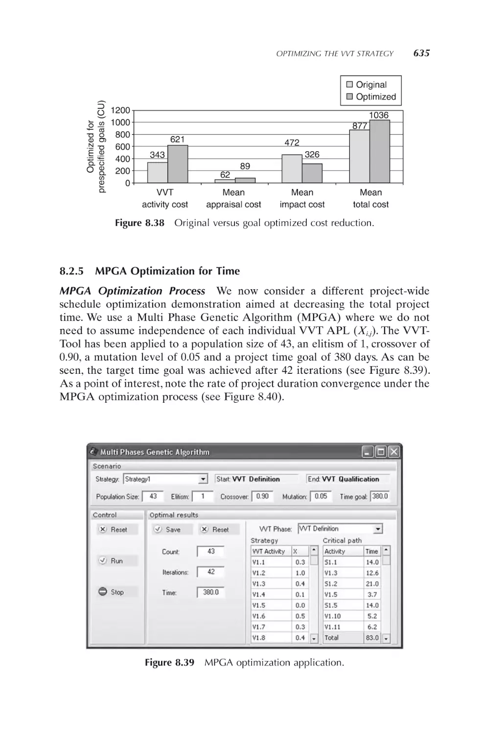
8.2 Optimizing the VVT Strategy
8.2.1
Analytical optimization of cost
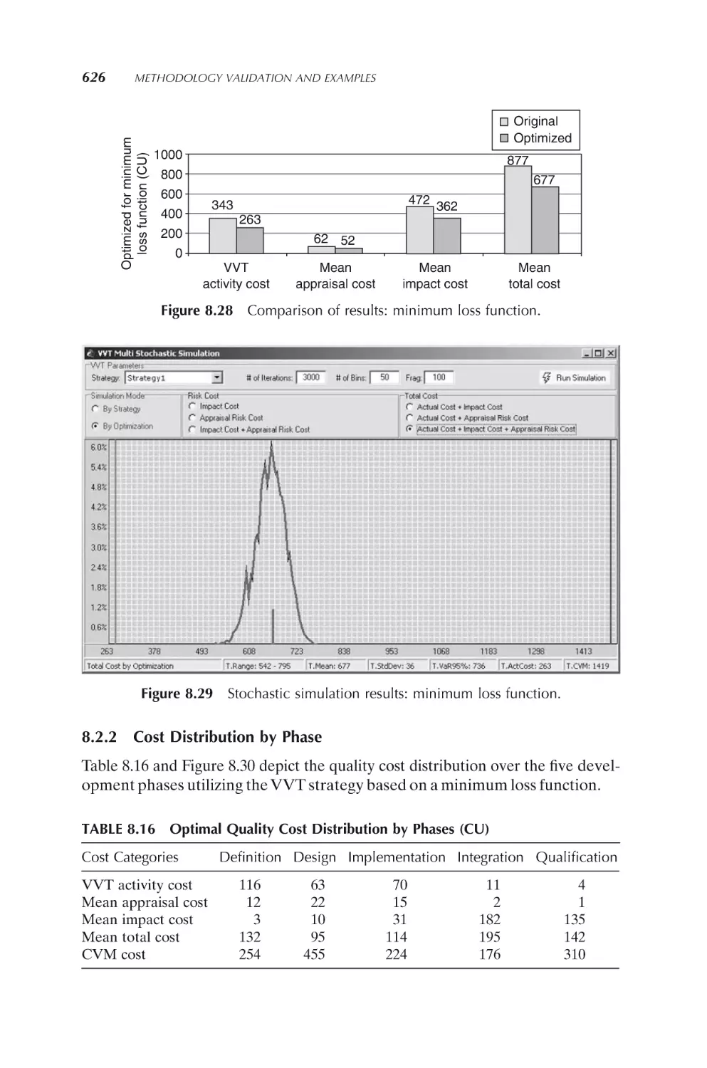
8.2.2
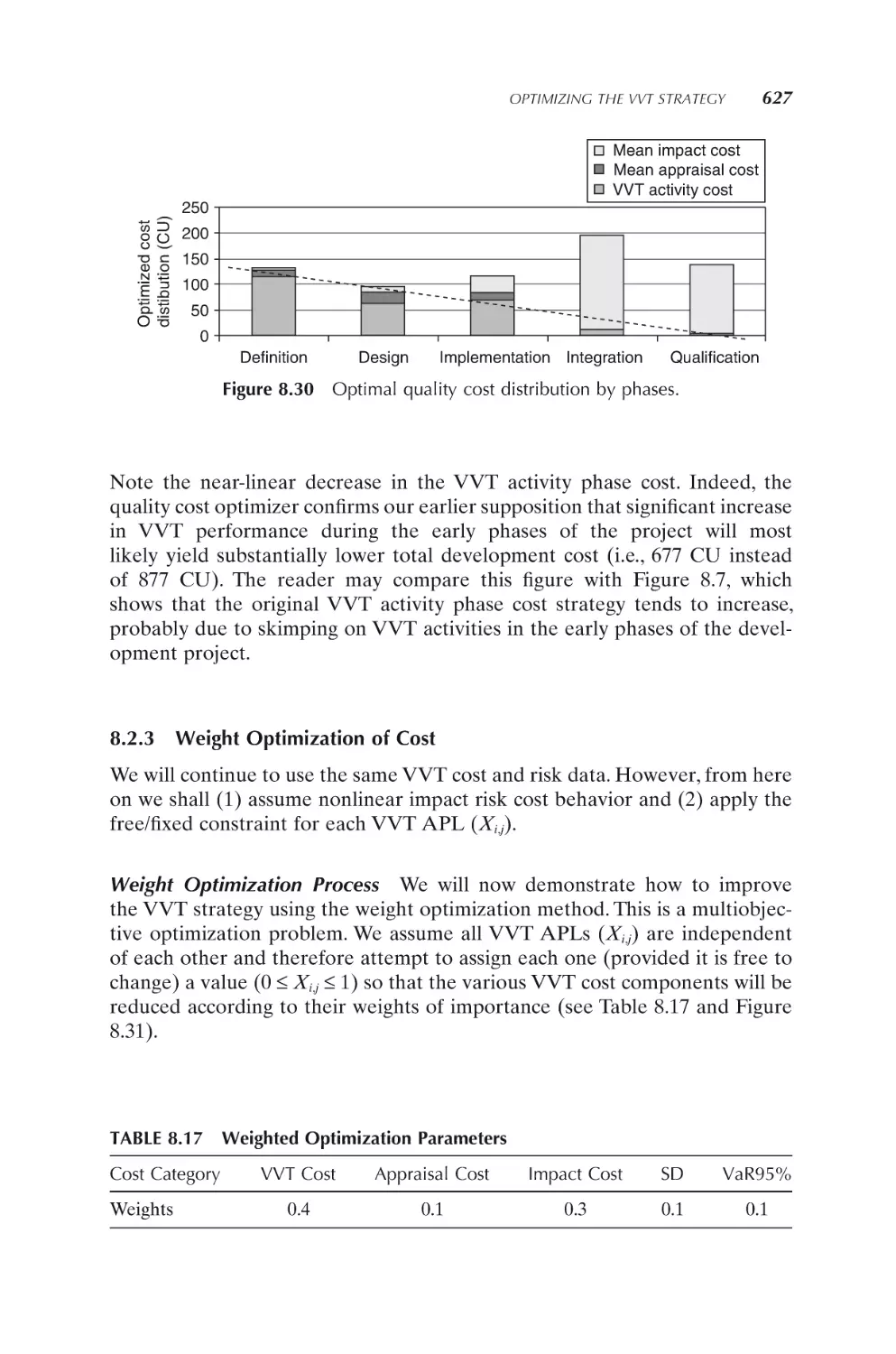
Cost distribution by phase
8.2.3
Weight optimization of cost
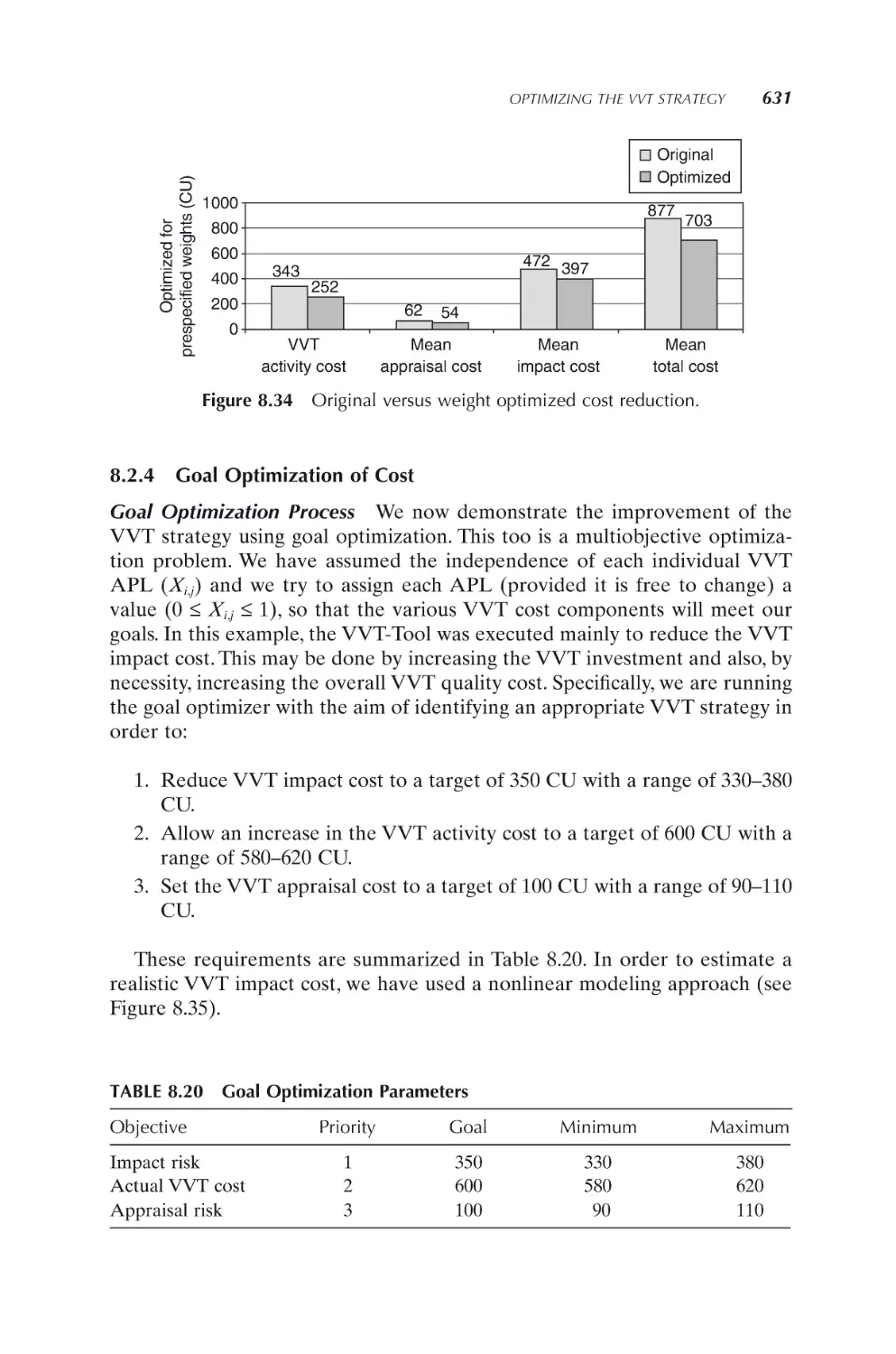
8.2.4
Goal optimization of cost
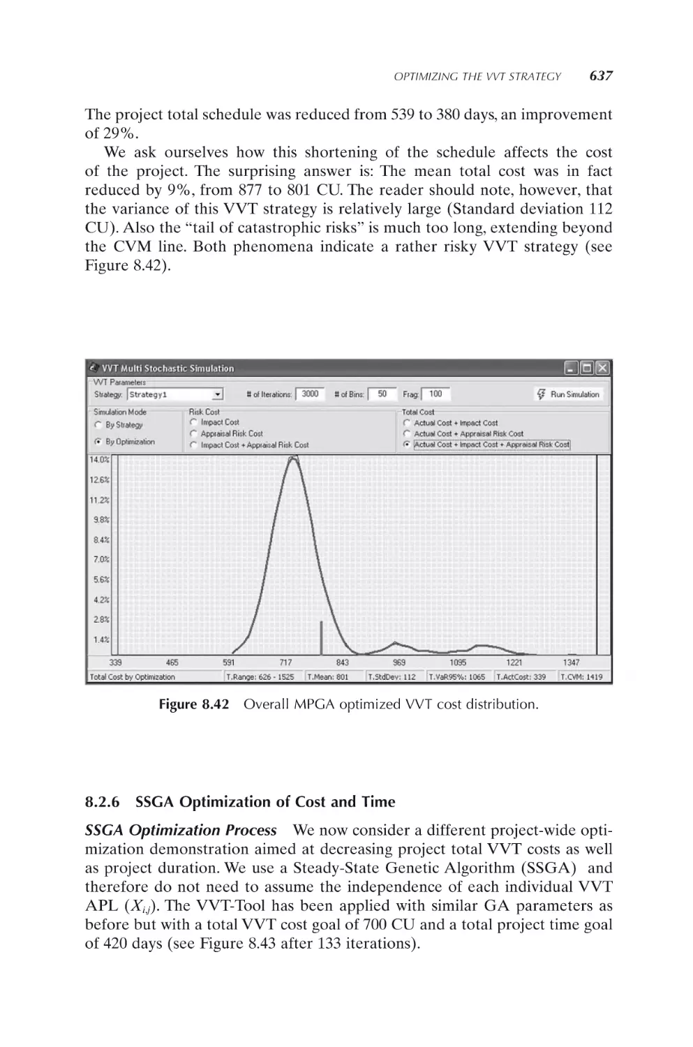
8.2.5
MPGA optimization for time
8.2.6
SSGA optimization of cost and time
618
619
626
627
631
635
637
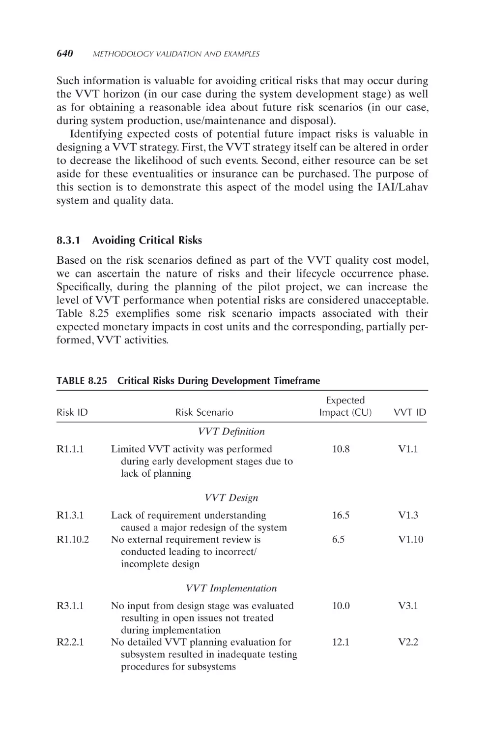
8.3 Identifying and Avoiding Significant Risks
8.3.1
Avoiding critical risks
8.3.2
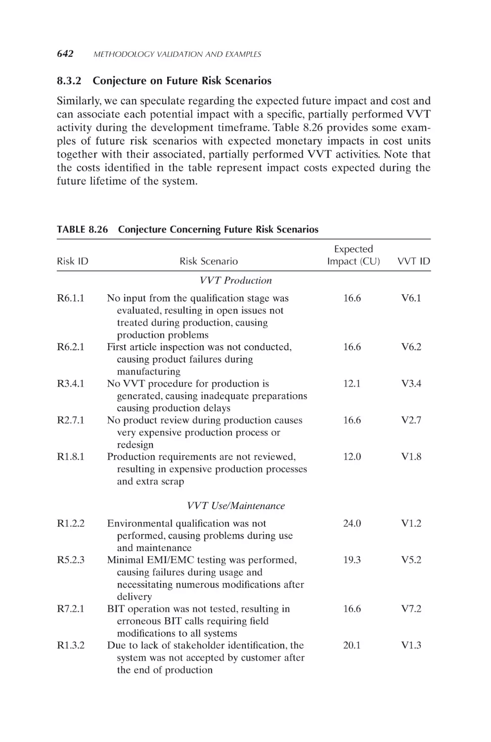
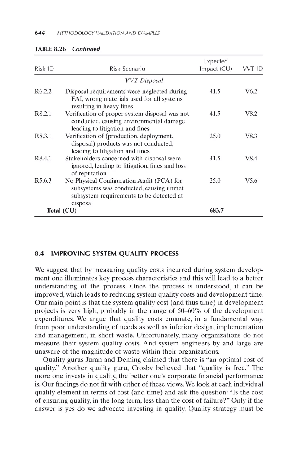
Conjecture on future risk scenarios
639
640
642
8.4 Improving System Quality Process
644
Appendix A SysTest Project
646
A.1 About SysTest
646
A.2 SysTest Key Products
648
A.3 SysTest Pilot Projects
649
CONTENTS
xv
A.4 SysTest Team
653
A.5 EC Evaluation of SysTest Project
655
References
656
Appendix B Proposed Guide: System Verification, Validation
and Testing Master Plan
657
B.1 Background
657
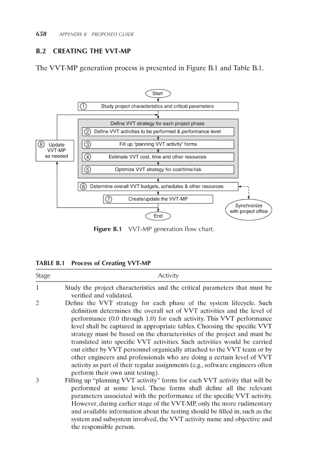
B.2 Creating the VVT-MP
658
B.3 Chapter 1: System Description
B.3.1 Project applicable documents
B.3.2 Mission description
B.3.3 System description
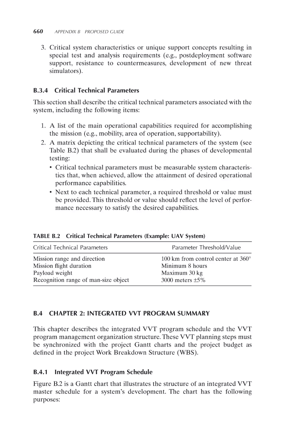
B.3.4 Critical technical parameters
659
659
659
659
660
B.4 Chapter 2: Integrated VVT Program Summary
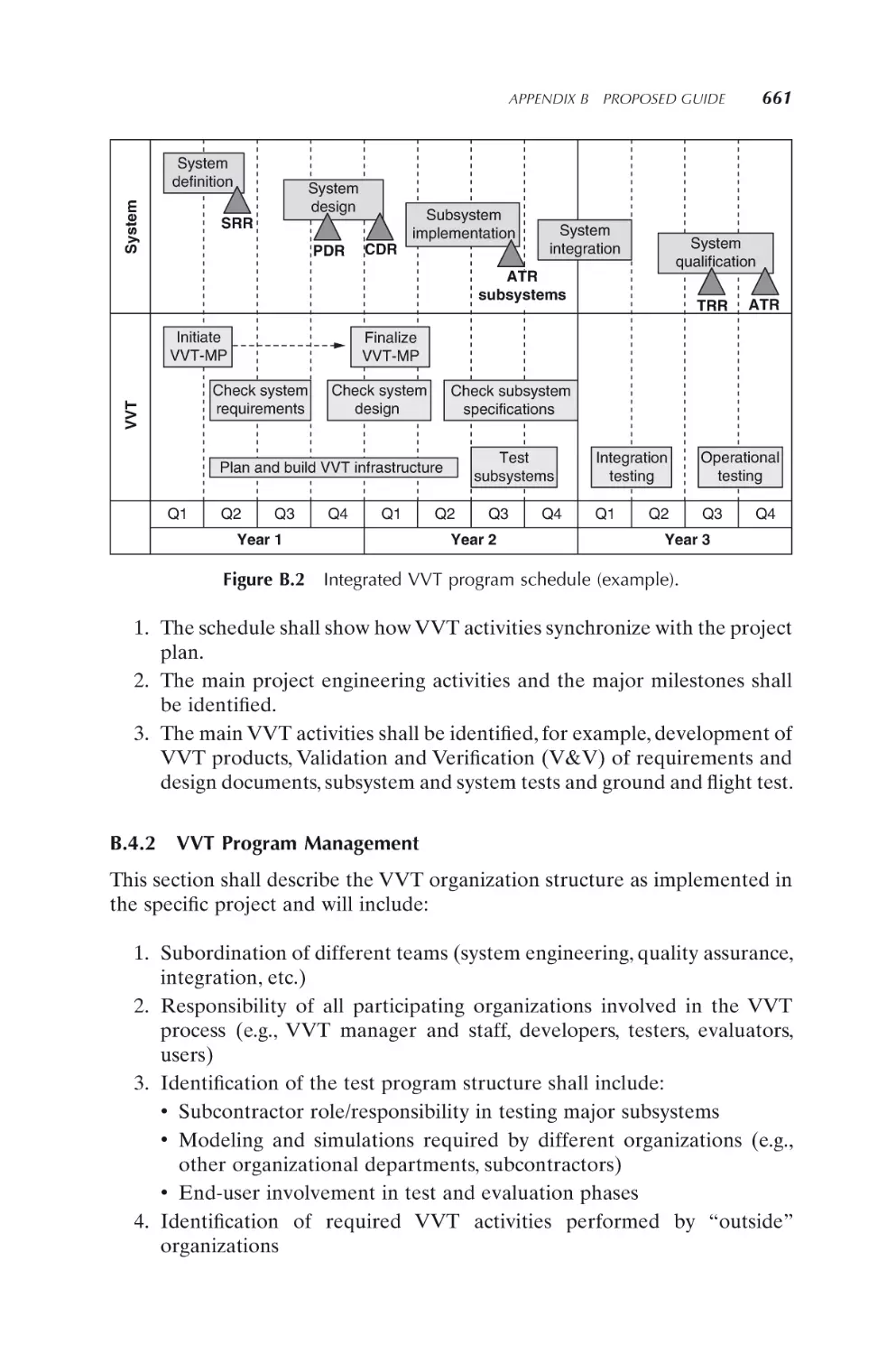
B.4.1 Integrated VVT program schedule
B.4.2 VVT program management
660
660
661
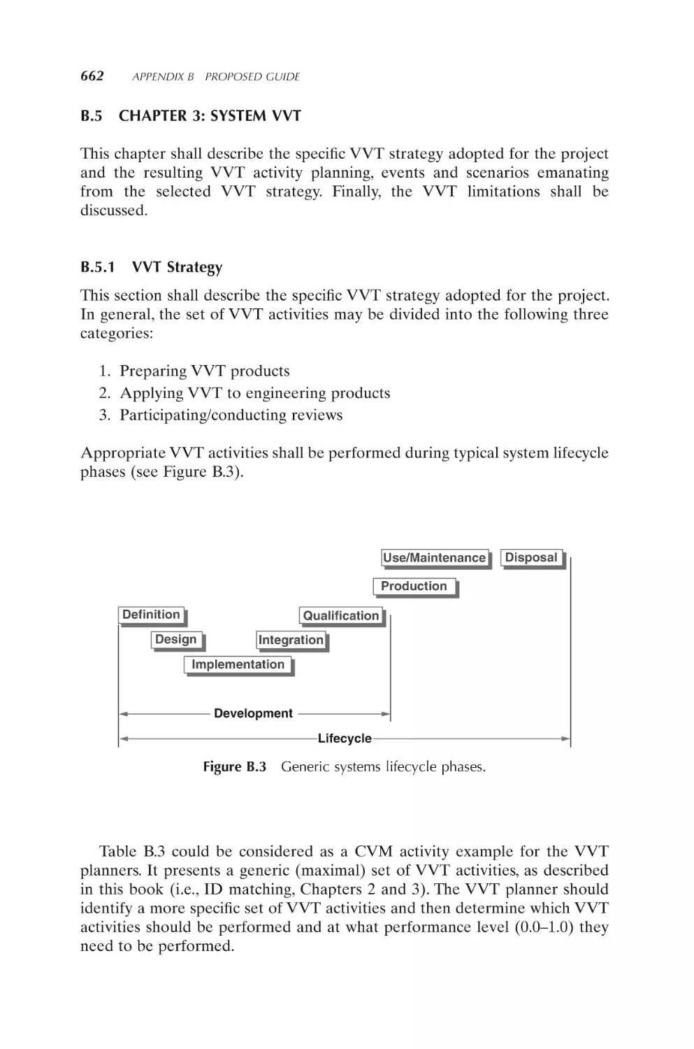
B.5 Chapter 3: System VVT
B.5.1 VVT strategy
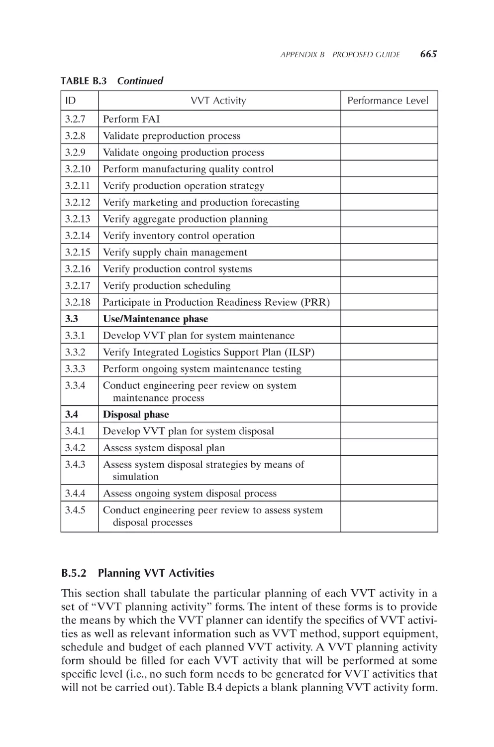
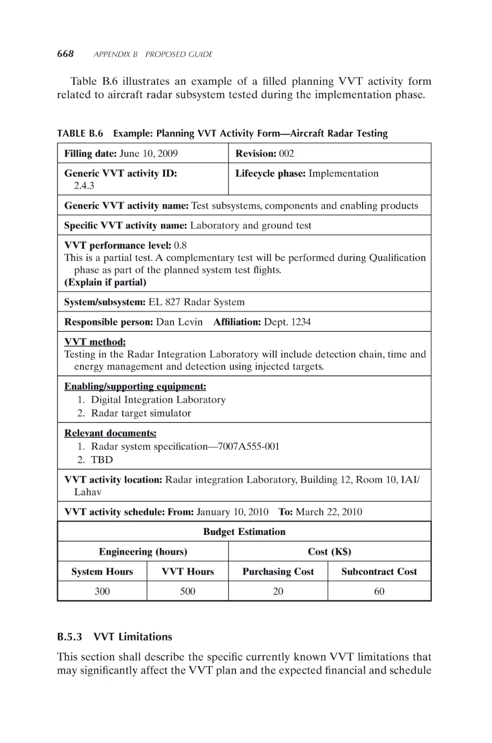
B.5.2 Planning VVT activities
B.5.3 VVT limitations
662
662
665
668
B.6 Chapter 4: VVT Resource Summary
B.6.1 Test articles
B.6.2 Test sites and instrumentation
B.6.3 Test support requisition
B.6.4 Expendables for testing
B.6.5 Operational force test support
B.6.6 Simulations, models and test beds
B.6.7 Manpower/personnel needs and training
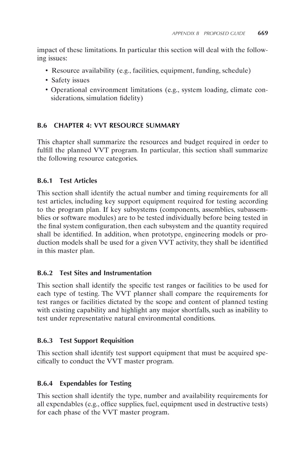
B.6.8 Budget summary
669
669
669
669
669
670
670
670
670
Appendix C List of Acronyms
671
Index
679
Preface
Systems testing is carried out one way or another in all development and
manufacturing projects, but seldom is this done in a truly organized manner
and no book currently available describes the process in a comprehensive and
implementable form. Along the same line of thinking, virtually no systems
Verification, Validation, and Testing (VVT) research is conducted throughout
the academic world. This is especially odd, since some 50–60 percent of a
systems development cost is expended on either performing VVT activities or
correcting system defects during the development process or during the life
of the developed product.
This book attempts to put together a comprehensive compendium of VVT
activities and corresponding VVT methods for implementation throughout
the entire lifecycle of systems (i.e. Definition, Design, Implementation,
Integration, Qualification, Production, Use/Maintenance and Disposal). In
addition, the book strives to alleviate the fundamental testing conundrum,
namely: What should be tested? How should one test? When should one test?
And, when should one stop testing? In other words, how should one select a
VVT strategy and how should it be optimized? Although early quality pioneers (e.g., Juran in the 1950s) proposed a conceptual quality cost model, no
one proposed a quantitative and credible model which can be used to answer
the above questions. This book provides such a model, together with data from
a real-life project, which show significant potential savings in either cost, time
or both. The book is organized in three parts:
The first part (Chapter 1) provides introductory material about systems and
VVT concepts. This part presents a comprehensive explanation of the role of
VVT in the process of engineered systems throughout their lifetime and
explains the essence of systems VVT and the linkage between VVT and
systems development, manufacturing, use/maintenance and retirement.
xvii
xviii
PREFACE
The second part (Chapters 2–5) is essentially a reference guide, describing
typical systems VVT activities which may be conducted during an engineered
systems lifetime. A reciprocal and comprehensive set of methods for carrying
out these VVT activities is also provided. More specifically, the second part
describes 40 systems development VVT activities (Chapter 2) and 27 systems
post-development activities (Chapter 3). Corresponding to these activities,
this part also describes 17 non-testing systems VVT methods (Chapter 4) and
33 testing systems methods (Chapter-5). In-text citations are provided wherever needed, usually within theoretical sections of the book. In addition,
subchapters contain a set of citations for further reading. Readers will undoubtedly be able to absorb and implement some or all of this information in their
daily work-life as systems or test engineers.
The third part of the book (Chapters 6–8) describes ways to model systems
quality cost, time and risk (Chapter 6), as well as ways to acquire quality data
and optimize the VVT strategy in the face of funding, time and other resource
limitations and in accordance with different business objectives (Chapter 7).
Finally, this part describes the methodology used to validate the quality model
along with examples describing a system’s quality improvements (Chapter 8).
Readers will be able to learn how to collect and aggregate quality data within
their organizations. In addition to becoming familiar with this significant information, readers will be introduced to four Cost, Time and Risk Models.
Systems engineers are encouraged to use these models in order to optimize
their VVT strategies, thereby realizing as much as ten percent reduction in
engineering manpower or schedule in the development of engineered systems.
Fundamentally, this book is written with two categories of audience in
mind. The first category is composed of VVT practitioners, including Systems,
Test, Production and Maintenance engineers as well as first and second line
managers. These people may be employed by development and manufacturing industries (e.g., Aerospace, Automobile, Communication, Healthcare
equipment, etc.), by various civilian agencies (e.g. NASA, ESA, etc.) or with
the military (e.g., Air force, Navy, Army, etc.). This book may also be used
as a supplemental graduate level textbook in courses related to systems VVT.
Typical academic readers may be graduate school students or members of
Systems, Electrical, Aerospace, Mechanical, and Industrial Engineering faculties. This book may be fully covered in two to three semesters (although parts
of the book may be covered in one semester). University instructors will most
likely use the book to provide engineering students with knowledge about
VVT, as well as to give students an introduction to formal modeling and optimization of VVT strategy.
PREFACE
xix
ACKNOWLEDGMENTS
Many friends and colleagues have contributed generously to the writing of
this book. To all of them, I would like to express my sincere gratitude and
appreciation. In particular, I wish to thank Dr. Peter Hahn, who has been a
tireless and devoted companion in the book-writing project from its inception.
He edited the original manuscript and contributed numerous and valuable
suggestions to improve the book.
The SysTest project, partially funded by the European Commission (see
Appendix A), focused my attention onto systems verification, validation and
testing. My appreciation goes to all the consortium members and in particular
to professor Eduard Igenbergs of the Technical University of Munich, who
provided both a philosophical foundation and ample encouragement, and to
Professor Tyson Browning of the Texas Christian University, part of whose
scientific writings and words of wisdom are embedded in this book. The
Advanced System and Software Engineering Technology (ASSET) group at
Israel Aerospace Industries (IAI) was a significant milieu for learning and
expanding. My special gratitude goes to ASSET group leader, Dr. Michael
Winokur. I am also grateful to Shalom Shachar of the IAI/Lahav Division,
who conducted the SysTest pilot project at IAI, helped in collecting field data
and became a sounding board and advisor regarding many aspects of the VVT
quantitative model. In addition, I am beholden to Michael Garber of Adi
Mainly Software (AMS), who developed the VVT-Tool software package
which embodies the VVT model.
Several close friends were involved in creating this book. In particular, I
would like to mention Avi Egozi and Arie Rokach, who suggested the book
project in the first place and provided advice throughout the writing process.
Also my sincere appreciation goes to Menachem Cahani (Pampam), who
volunteered to illustrate several caricatures in the book. I also am genuinely
indebted to Professor Miryam Barad of the Tel-Aviv University, an esteemed
teacher who taught me how to conduct scientific research and write about it.
Most of all, my deepest thanks go to my wife, Rachel, and my children,
Ofer, Amir, Jonathan and Michael, who encouraged my book efforts with
advice, patience and love,
Avner Engel
Tel-Aviv, Israel
Part I
Introduction
Chapter 1
Introduction
1.1
OPENING
This chapter serves as motivation for learning about systems Verification,
Validation and Testing (VVT) as well as a map for using the book as a reference source on this complex and multifaceted process. We emphasize here the
multitude of reasons for applying VVT. It sets the tone for the subject matter
we hope to cover. It gives the reader insight into the attitudes of the author
and the care with which the book was prepared. A clear statement is made of
the purpose for which the book has been written.
The book is a compendium of facts about systems VVT. In fact, we think
little has yet been published that is as comprehensive on this subject. By listing
the potential audience for the book, we hope to encourage its wide distribution and to increase among engineers, managers, academicians and students
an appreciation of the benefits of rigorously applying VVT to almost every
endeavor involving a product or service, be it for purposes commercial, private
or public. This chapter contains the following elements:
Opening. This part provides a background, purpose and the intended audience of the book. In addition, it describes its structure and contents as well as
the scope of application and some terminology descriptions.
VVT systems and process. This part introduces VVT systems and processes
as components of engineered systems. In addition, it describes basic VVT definitions and elaborates on the fundamental VVT dilemmas. Also, this part
describes modeling of systems and VVT lifecycle as well as modeling of VVT
processes and risks as cost and time drivers.
Verification, Validation, and Testing of Engineered Systems, Avner Engel
Copyright © 2010 John Wiley & Sons, Inc.
3
4
INTRODUCTION
Canonical systems VVT paradigm. This part introduces the concept of
canonical systems VVT paradigm which includes phases of systems’ lifecycle,
views of systems and VVT aspects of systems.
Methodology application. This part introduces methodology application
including VVT methodology overview, VVT tailoring and typical VVT
documentation.
1.1.1
Background
The manufacturing industry used to be concerned with the design, development, production and maintenance of stand-alone products, whether simple
or complex. Today, however, manufacturing has broadened its scope to
include products, services or solutions that include a variety of components,
integrate a large mix of technologies and involve both people and machines.
It is this broad range of complex entities that we address in this book. The
basic term we use for these complex entities is engineered systems. However,
throughout this book, when appropriate, we will freely use terms such as
products or services. The term engineered systems is distinguished from
systems in the sense that the former is created by engineers who apply science
and mathematics to find suitable solutions to problems.
Traditional and high-technology manufacturing industries are responding
to the challenge to satisfy consumer needs and ensure competitive and sustainable growth by reducing time to market and customizing products (or expanding product ranges) while producing the required goods in the quantities
demanded with the appropriate quality at reduced costs. For instance, in the
automobile sector, the lead time for manufacturing a car at the beginning of
the 1990s was five to six years, whereas today it is about two to three years
and is estimated to be only 18 months in the near future. Therefore, controlling schedules, costs and quality in product development, manufacturing and
maintenance remains a major challenge for today’s industries. Increases in
complexity, decreases in development budgets and shortened time to market
for new products, services and solutions are leading developers to search for
new ways of improving the quality of what they deliver by improving their
technologies, processes, methodologies and tools.
The overall development process is only as strong as its weakest link. A
critical and largely ignored link in this process is system VVT, which comprise
vital activities and involve processes. A tool of systems engineering, VVT
focuses on ensuring that engineered systems are delivered as error free as possible, are functionally sound and meet or exceed the user’s needs. Often VVT
is carried out as merely a vehicle for finding and eliminating errors. It can do
much more than that. Today, many system developers perform VVT only in
the test phase of the project, a late and highly constrained period in the product
development cycle. As a result, increases in overall development time and costs
associated with product rework often exceed 20% of expanded engineering
efforts (Capers, 1996). Admittedly, balancing testing cost and schedule with
quality is difficult. However, quality problems discovered later by the user can
OPENING
5
necessitate expensive repairs and are likely to damage the reputation of the
system or, worse, damage the reputation of the system’s developer.
Given the fundamental role of VVT in achieving product quality and reducing waste, this book aims at rectifying two critical current VVT problems,
namely, lack of comprehensive system VVT methodology and lack of a practical, quantitative VVT process model for selecting a VVT strategy to optimize
testing cost, schedule and economic risk. This book, which to a large measure
is based on the European Commission–supported SysTest project, was written
in order to rectify these problems.
1.1.2
Purpose
One of the central objectives of this book is the creation of generic VVT
methodology. This VVT methodology consists of a selection of VVT activities
and methods which can be applied throughout the system lifecycle in different
industrial application fields and can be tailored according to the individual
project needs.
The VVT methodology delivers generic means for comprehensive costeffective VVT in the industry. In addition, the objectives of this methodology
are as follows:
•
•
•
•
To cover the entire product lifecycles from the definition to the disposal
of the system
To supply tailoring rules for different industry domains (e. g. electronics/
avionics, control systems, automobile, food packaging systems, steel production), development cycles and project types
To specify activities and methods for VVT on the system level together
with their interrelationship
To define VVT strategies that can be used in a broad variety of industrial
applications
1.1.3
Intended Audience
The VVT methodology described in this book is applicable to all regional and
industrial sectors. Although system VVT is performed throughout industry, it
has not become a topic for research within the international community either
in industry or in academia. Therefore, the definition of a generic VVT methodology will provide comprehensive knowledge for many students and practitioners. This book was written for the reader who has a background
knowledge of project management, systems engineering and quality assurance. Those who participate in system development will benefit from the
material covered in this book. These include:
1. Project Managers and VVT Managers. This book can guide project and
VVT managers in the methods they select, adapt and tailor for planning,
control and tracking of projects.
6
INTRODUCTION
2. Quality Assurance (QA)/Quality Control (QC) Staff. For QA and, QC
staff, this book offers an overview of the system QA activities and
methods available and their principal advantages and disadvantages.
Quality assurance staff can apply the VVT methodology guidelines for
the selection of VVT procedures and the estimation of process and
product risks.
3. Members of a VVT Team. This book serves as an aid for test teams by
providing them with an overview of useful procedures for conducting a
VVT process within the context of system development projects and
beyond. Thus, the VVT methodology guidelines of this book become a
useful tool for categorizing VVT activities within the system lifecycle
overall context and by referencing further information.
4. System Developers and Maintainers. This book is relevant for system
developers in that they deliver insight into the measures of error avoidance and error detection. Developers can draw important conclusions
about the functional domains of the system developed that are critical
where VVT are concerned.
5. Mechanical, Electronics and Software Designers. Other specialists need
this book in order to take VVT aspects into account when they determine structures and select the technologies for system development,
production and maintenance. This book can be an important basis for
this, as it shows not only the possibilities but also the limitations of VVT
procedures.
6. Component and Subsystem Suppliers. A clear definition and a specification with respect to VVT measures are essential, especially for system
development projects that involve supplier companies. This book forms
a convenient basis for those projects since it provides a mutual definition, nomenclature and techniques as well as a body of VVT methods.
7. Auditors. To evaluate the maturity of a development project, auditors
and auditing agencies can also apply the VVT methodology. Adherence
to standards, deployment of established procedures, as well as the maturity of the processes’ implementation can be evaluated in this way.
8. Regulatory and Standardization Agencies. Material presented in this
book may be helpful in forming and updating national or international
standards and regulations of standardization committees in which certain
procedures for defined system classes are classified as binding or just
recommended. Of course, it is not the aim of this book to define or force
standardization. However, it could provide important suggestions with
regard to such an endeavor.
1.1.4
Book Structure and Contents
This book is divided into three parts and a set of appendices as described
below.
OPENING
7
Part I: Introduction Part I of this book contains basic introductory material
organized in one chapter. It starts by describing the purpose, the intended
audience, the structure and the content of the book, the scope of the applications and the terminology and notation used throughout this book. It continues by providing basic introduction to systems theory, relevant background
on systems and software VVT as well as risk and uncertainty theory. In
addition, this chapter introduces VVT concepts and discusses the modeling of
systems and the VVT lifecycles. It then defines generic phases, views and
aspects of the system lifecycle that are used in this book. Finally, the chapter
provides a VVT methodology overview, typical VVT documents and a methodology for VVT tailoring.
Part II: VVT Activities and Methods Part II of this book describes the VVT
activities typically associated with each phase of the system lifecycle. For each
VVT activity, the book describes one or more methods for carrying out those
activities:
•
•
•
•
Chapter 2, System VVT Activities: Development, describes typical VVT
activities which may be conducted during system development, that is,
during the Definition, Design, Implementation, Integration and
Qualification phases of the system’s lifecycle.
Chapter 3, System VVT Activities: Postdevelopment, describes typical
VVT activities which may be conducted during system postdevelopment,
that is, during Production, Use/Maintenance and Disposal phases of the
system’s lifecycle.
Chapter 4, System VVT Methods: Nontesting, describes a set of VVT
nontesting methods, complementing the VVT activities described in the
VVT activities chapters. In particular this chapter describes the following
nontesting system VVT methods: preparing VVT products, performing
VVT activities and participating in reviews.
Chapter 5, System VVT Methods: Testing, describes a set of VVT testing
methods, complementing the VVT activities described in the VVT
activities chapters. Specifically, this chapter describes a collection of
system testing methods grouped into the following categories: white-box
testing and black-box testing; the latter is further divided into basic
testing, high-volume testing, special testing, environment testing and
phase testing.
Part III: Modeling and Optimizing VVT Process Part III of this book describes
ways to model system quality cost, time and risk as well as ways to acquire
quality data and optimize the VVT strategy in accordance with different business objectives. In addition, Part III describes the methodology used to validate the quality models along with examples describing a system’s quality
improvements.
8
INTRODUCTION
•
•
•
Chapter 6, Modeling Quality Cost, Time and Risk, describes system
quality modeling—in particular, VVT cost and risk modeling, VVT time
and risk modeling and fuzzy VVT cost modeling.
Chapter 7, Obtaining Quality Data and Optimizing VVT Strategy, presents typical quality data of engineered systems from various industries as
well as practical ways and means to elicit and aggregate quality data (i.e.,
cost, time and risks of VVT activities). The chapter continues by describing various techniques to optimize VVT strategies in order to reduce cost,
time and system risks.
Chapter 8, Methodology Validation and Examples, describes a validation
process which compares actual measurements of system quality cost and
time with model prediction. Finally, this chapter provides several examples of the entire system quality improvement process.
Appendices
follows:
•
•
•
•
This portion of this book contains a collection of appendices as
Appendix A—SysTest Project
Appendix B—VVT Master Plan (VVT-MP)
Appendix C—Acronyms
Appendix D—Glossary of Terms
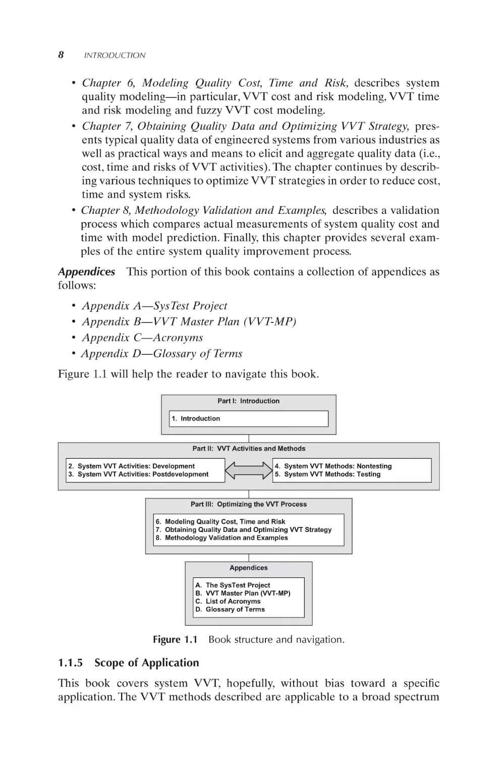
Figure 1.1 will help the reader to navigate this book.
Part I: Introduction
1. Introduction
Part II: VVT Activities and Methods
2. System VVT Activities: Development
3. System VVT Activities: Postdevelopment
4. System VVT Methods: Nontesting
5. System VVT Methods: Testing
Part III: Optimizing the VVT Process
6. Modeling Quality Cost, Time and Risk
7. Obtaining Quality Data and Optimizing VVT Strategy
8. Methodology Validation and Examples
Appendices
A.
B.
C.
D.
Figure 1.1
1.1.5
The SysTest Project
VVT Master Plan (VVT-MP)
List of Acronyms
Glossary of Terms
Book structure and navigation.
Scope of Application
This book covers system VVT, hopefully, without bias toward a specific
application. The VVT methods described are applicable to a broad spectrum
VVT SYSTEMS AND PROCESS
9
of system requirements: whether safety critical or non–safety critical, whether
mission critical or non–mission critical or whether the requirements are
hard real time or nontemporal. The VVT methodology described herein
supports the quality assurance phases all the way from system requirements
definition to system disposal. Furthermore, it supports different system
hierarchy levels of quality measures, from component testing to system
testing. The book’s VVT methodology guidelines can be applied to massproduced systems as well as to small production quantities or few-of-a-kind
paradigms.
The present book is applicable to system developments in various industrial
sectors. They may be regarded as recommendations only. Or, they can be
considered binding for an individual project if the stakeholders for that project
agree upon this course of action.
1.1.6
Terminology and Notation
In this book, when we use the terms has to/must, shall and should we mean
the following:
•
•
•
Has To/Must. This is the highest level of recommendation and describes
cases where the described process, procedure or approach works only in
this way.
Shall. At this level, the user is strongly recommended to use the described
process, procedure or approach in this way.
Should. This level of recommendation describes cases where this
author has experienced that this process, procedure or approach is
the best.
Each VVT activity or method described in this book is presented, as much as
possible, in a common format, thus facilitating the orientation and presentation of more detailed information on each activity.
1.2
1.2.1
VVT SYSTEMS AND PROCESS
Introduction—VVT Systems and Process
This section serves as an introduction to the VVT process. It starts with the
definition of an engineered system, that is, a man-made artifact that depends
upon scientifically based and experiential processes that are logically applied.
VVT attempts to help these systems achieve their full potential in terms of
performance, efficiency and economy of precious resources. What follows is
a detailed discussion of what is meant by VVT in all its manifestations. This
includes a variety of definitions, as given by various experts, industries, engineering organizations and government agencies.
10
INTRODUCTION
As a discipline VVT is an outgrowth and expansion of the earlier disciplines
quality assurance and quality control. It is an evolving concept and thus
will continue to be redefined with time and with the development of new
techniques for design and evaluation of engineered systems. Thus, it is not
surprising that there would be disagreement in the engineering and business
community on just what comprises a VVT program.
Here, we attempt to give an overview of the many perceptions about VVT
from the various stakeholders in the VVT process, that is, customers, manufacturers, regulators, professional organizations and government. Thus, we
break down the differences between VVT definitions as seen by various technical disciplines: electrical and electronics engineering, telecommunications,
artificial intelligence and the modeling and simulation community. The definitions and perceptions of VVT, as seen by the systems engineering community
and more specifically by the International Council on Systems Engineering
(INCOSE), are also covered, as are the VVT definitions used by the author
in this book.
We attempt to give an appreciation of the difficulties of applying VVT to
large and complex systems. Since VVT efforts should begin early in the lifecycles of a system and are not completed until the system is decommissioned
and its components recycled, the issues are complex and manifold. Thus, we
bring a section describing the stages of the system lifecycle and relate it to
complementary VVT lifecycle phases.
Measuring VVT performance is key to good VVT planning. There is a
delicate balance between the risks avoided by good system VVT and the risks
to a system’s development and deployment by too much VVT.
1.2.2
Engineered Systems
General Systems The term system (from Latin systema) has emerged in the
twentieth century as a key building block of systems theory, an area of study
that predominantly refers to the science of systems that resulted from
Bertalanffy’s general system theory (Bertalanffy, 1976).
An intuitive description of a “system” is that it is composed of separate
elements organized in some fashion with certain interfaces among the elements and between the system and its environment. In addition, a system
tends to affect its environment and be affected by it. This involves some type
of input and output (e.g., materials, energy, information). Most importantly,
a system produces results not obtainable from the collection of its individual
elements.
Based on this notion, we can adopt either an elementary definition, “A
system is an interdependent group of items forming a unified whole” (Webster’s
dictionary), or a more sophisticated definition, “A system is a combination of
components that act together to perform a function not possible with any of the
VVT SYSTEMS AND PROCESS
11
individual parts” [Institute of Electrical and Electronics Engineers (IEEE)
Electronic Terms].
Engineered Systems The goal of engineering processes is to develop and
produce efficient and reliable systems (products, services or solutions) that
meet a specific need under a defined set of constraints. To achieve this, the
system will follow a typical creation lifecycle, whose phases could be defined
as Definition, Design, Implementation, Integration, Qualification and
Production. During its useful lifetime, a system will go through a Use/
Maintenance phase, culminating in the disposal of the system.
According to Braha et al. (2006), the classical engineering process has
several notable characteristics: (1) a search for a single solution, namely, engineers tend to seek a single solution, which often revolves around a unique
design concept, for the specified problem, (2) the desire for a well-behaved
system, that is, engineers prefer systems whose behavior can be predicted and
encapsulated by precise description and (3) the application of a top-down
problem-solving approach, which fundamentally depends on the assumption
that any system can be described wholly by describing the behavior of its parts
and their interactions. Therefore, according to Braha et al. (2006), classically
engineered systems have the following attributes: (1) predictability, that is, the
system works in predictable ways; (2) reliability, that is, the system is able to
perform a required function under stated conditions for a stated period of
time; (3) transparency, that is, the structure of the system and its processes
can be described explicitly; and (4) controllability, that is, the system can be
directly governed according to stated instructions under stated conditions.
We can now accept either the definition of the Council on Systems
Engineering (INCOSE) organization: “A system is an integrated set of elements to accomplish a defined objective” adopted in 1995, or a rather sophisticated definition, attributed to Dr. Eberhardt Rechtin (1990):
A system is a construct or collection of different elements that together produce
results not obtainable by the elements alone. The elements, or parts, can include
people, hardware, software, facilities, policies, and documents; that is, all things
required to produce systems-level results. The results include system level qualities, properties, characteristics, functions, behavior and performance. The value
added by the system as a whole, beyond that contributed independently by the
parts, is primarily created by the relationship among the parts; that is, how they
are interconnected.
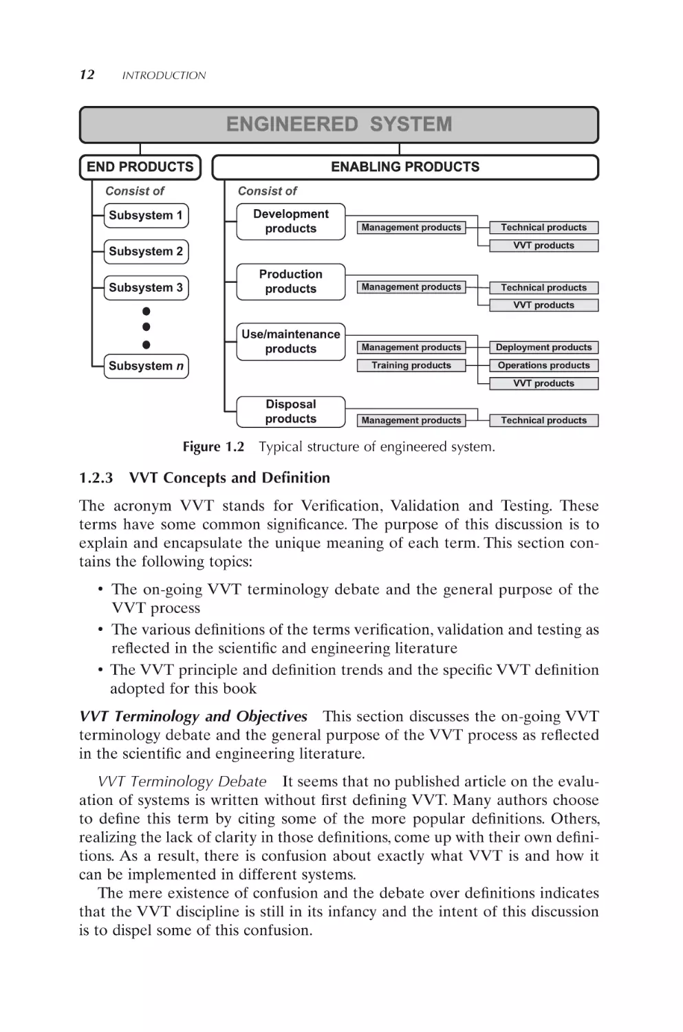
We further accept the distinction that an engineered system is often composed
of “enabling products” required to provide lifecycle support in addition to the
“end products”, which performs the required operational functions (see Figure
1.2). The end product may be a single manifestation of the system or may be
produced in small or large quantity.
12
INTRODUCTION
Consist of
Consist of
Development
products
Subsystem 1
Management products
Technical products
VVT products
Subsystem 2
Production
products
Subsystem 3
Management products
Technical products
VVT products
Use/maintenance
products
Subsystem n
Management products
Deployment products
Training products
Operations products
VVT products
Disposal
products
Figure 1.2
Management products
Technical products
Typical structure of engineered system.
1.2.3 VVT Concepts and Definition
The acronym VVT stands for Verification, Validation and Testing. These
terms have some common significance. The purpose of this discussion is to
explain and encapsulate the unique meaning of each term. This section contains the following topics:
•
•
•
The on-going VVT terminology debate and the general purpose of the
VVT process
The various definitions of the terms verification, validation and testing as
reflected in the scientific and engineering literature
The VVT principle and definition trends and the specific VVT definition
adopted for this book
VVT Terminology and Objectives This section discusses the on-going VVT
terminology debate and the general purpose of the VVT process as reflected
in the scientific and engineering literature.
VVT Terminology Debate It seems that no published article on the evaluation of systems is written without first defining VVT. Many authors choose
to define this term by citing some of the more popular definitions. Others,
realizing the lack of clarity in those definitions, come up with their own definitions. As a result, there is confusion about exactly what VVT is and how it
can be implemented in different systems.
The mere existence of confusion and the debate over definitions indicates
that the VVT discipline is still in its infancy and the intent of this discussion
is to dispel some of this confusion.
VVT SYSTEMS AND PROCESS
13
Purpose of the VVT Process Another question that confronts us is what
should be the final purpose of the VVT process? Should it serve to eliminate
errors or serve as a means to certify that a system is free of errors? Following
are the arguments.
Elimination of errors is akin to debugging a computer program. The
program is exercised to discover an incorrect behavior, and then the bug
causing the incorrect behavior could be identified and removed. This is necessary, not only for computer programs, but also in many other fields where
systems are expected to be dependable. This book reflects the author’s opinion
that VVT must first strive to eliminate errors if it is to be useful. On the other
hand, there is a significant commercial value in being able to say that a system
is free of errors and works as intended. Unfortunately, this is merely wishful
thinking. To guarantee that a system is free of errors is logically impossible
unless a truly exhaustive way of evaluating its functionality can be implemented. This would not be feasible for all but the most trivial systems.
We conclude that the purpose of VVT should be to eliminate as many defects
as possible within existing constraints of available time, money and other
resources.
What is to be achieved by VVT? Fairley (1985) indicates that the goal is to
assess and improve the quality of the system. He also provides quality attributes to evaluate the VVT process. These attributes, which have been altered
to suit the systems arena, are presented in Table 1.1.
TABLE 1.1
VVT Quality Attributes
Function
Correctness
Completeness
Consistency
Reliability
Usefulness
Usability
Efficiency
Standards conformance
Overall cost-effectiveness
Responding to the Following Queries
Given valid inputs, does the system perform its tasks as
expected?
Does the system meet all of the requirements that have
been placed on it?
Are similar things handled in a similar manner? Is the
system consistent with another system that is part of
the same family?
Does the system perform reasonably well in all cases,
even, for instance, in the presence of pathological
conditions?
Does the system provide a useful service?
Is the system convenient to use when carrying out its
designated task?
Is the system efficient in its use of resources, such as
time, memory, network bandwidth, and peripherals?
Does the system conform to standards, both notational
and external standards of interface to the outside
world?
Is the system a cost-effective solution to the problem?
14
INTRODUCTION
VVT Definitions in Various Fields The following discussion presents different definitions for the terms verification, validation and testing as reflected in
the scientific and engineering literature.
1. Nontechnical Community. The nontechnical Merriam-Webster’s dictionary defines the term verify as (1) “to confirm or substantiate in
law by oath” and (2) “to establish the truth, accuracy, or reality of.”
It defines the term validate as (1) “to make legally valid,” (2) “to
grant official sanction to by marking,” (3) “to confirm the validity of
(an election)” and (4) “to support or corroborate on a sound or authoritative basis.” It provides 55 different definitions for the term test. The
most relevant nontechnical ones are (1) “a critical examination, observation, or evaluation,” (2) “the procedure of submitting a statement to
such conditions or operations as will lead to its proof or disproof or to
its acceptance or rejection” and (3) “a basis for evaluation.” The intuitive understanding of the above terms corresponds well with the nontechnical dictionary definition. The technical definition of VVT is
another matter.
2. IEEE Community. The IEEE defines validation and verification for
engineered hardware and software systems as follows (IEEE-610):
• Verification is the process of evaluating a system or component, to
determine whether the products of a given development phase satisfy
the conditions imposed at the start of that phase.
• Validation is the process of evaluating a system or component during
or at the end of the development process, to determine whether it
satisfies specified requirements.
3. Telecommunication Community. In its Telecom Glossary 2000, the
American National Standard for Telecommunications defines the terms
as follows:
• Verification. (1) Comparing an activity, a process, or a product with
the corresponding requirements or specifications. (2) [The] process of
comparing two levels of an information system specification for proper
correspondence (e.g., security policy model with top-level specification, top-level specification with source code or source code with
object code).
• Validation. (1) Tests to determine whether an implemented system
fulfills its requirements. (2) The checking of data for correctness or
for compliance with applicable standards, rules, and conventions.
• Testing. Physical measurements taken (1) to verify conclusions
obtained from mathematical modeling and analysis or (2) for the
purpose of developing mathematical models.
4. Artificial Intelligence Community. Gonzalez and Barr (2000) suggest the
following definitions for these terms in the Artificial Intelligence (AI)
community:
VVT SYSTEMS AND PROCESS
•
•
15
Verification is the process of ensuring that the intelligence system
(1) conforms to specifications and (2) its knowledge base is consistent
and complete within itself. The intent of this definition is that the
process of verification represents an internal benchmark, rather than
an external one. Making it internal is highly significant, as errors can
be found without the need to exercise the system with test cases.
Validation is the process of ensuring that the output of the intelligence
system is equivalent to that of human experts when given the same
input.
5. Modeling and Simulation Community. The Department of Defense
(DoD) Defense Modeling and Simulation Office (DoDD-5000.59) gives
a formal definition. It defines Verification and Validation (V&V) as
follows:
• Verification is the process of determining that a model implementation accurately represents the developer’s conceptual description and
specification.
• Validation is the process of determining the degree to which a model
is an accurate representation of the real world from the perspective
of intended uses of the model.
Balci (1998), a noted researcher in the Modeling and Simulation (M&S)
field, and later Balci et al., (2000) extend the DoD definition for VVT
as follows:
• Model verification is substantiating that the model is transformed
from one form into another, as intended, with sufficient accuracy.
Model verification deals with building the model correctly. The accuracy of transforming a problem formulation into a model specification
or the accuracy of converting a model representation from a micro
flowchart form into an executable computer program is evaluated in
model verification.
• Model validation substantiates that the model, within its domain of
applicability, behaves with satisfactory accuracy, consistent with the
M&S objectives. Model validation deals with building an accurate
model. An activity of accuracy assessment can be labeled as verification or validation based on an answer to the following question: In
assessing the accuracy, “Does the model’s behavior compare well to
the corresponding system behavior?” Even if the answer to the question of accuracy is “yes,” that does not answer the question of whether
the model is the right one.
• Model testing is determining whether inaccuracies or errors exist in
the model. In model testing, the model is subjected to test data or test
cases to determine if it functions properly. Test failure implies the
failure of the model, not the test. A test is devised, and testing is conducted to perform either validation or verification or both. Some tests
16
INTRODUCTION
are designed to evaluate the behavioral accuracy or validity of the
model, and some other tests are intended to determine the accuracy
of model transformation from one domain into another (verification).
Sometimes, the whole process is called model VV&T or, for short,
VVT.
VVT Concepts in System Engineering Lake (1999) explains the formal
definition and intuitive meaning of V&V in system engineering (see Figure
1.3):
Validation
System model
System
requirements
System
realization
Production
to disposal
System
design
Stakeholders
Verification
Testing (Subset of V&V)
Figure 1.3
•
•
Verification and validation in system engineering perception.
Verification is the process of evaluating a system to determine whether
the products of a given development phase satisfy the conditions imposed
at the start of that phase.
Validation is the process of evaluating a system to determine whether it
satisfies the stakeholders of that system.
These terms will now be further elaborated:
1. System Verification. The meaning of the term verification is to evaluate
a realized product against specified requirements. The intent is to determine whether the finished product satisfies the specific requirements for
which it was built. In addition, the verification responds to the question:
“Was the product built (written, built, coded, assembled and integrated)
correctly”? There are two formal definitions of verification:
• Confirmation by examination and provision of objective evidence that
the specified requirements to which a product was built, coded or
VVT SYSTEMS AND PROCESS
•
17
assembled has been fulfilled (American National Standards Institute/
Electronics Industries Association ANSI/EIA-632)
The process of evaluating a system or component to determine whether
the products of a given development phase satisfy the conditions
imposed at the start of that phase (IEEE-610)
According to Lake (1999), verification failure (i.e., lack of confirmation) typically reveals the following types of design or implementation errors:
Specified requirements (specifications, drawings, parts lists) have not
been documented adequately.
• Developers/builders have not followed the specified requirements for
the product.
• Procedures, workers, tools and equipment are improper or have been
improperly used for building the product.
• Procedures and means have been improperly planned for
verification.
• Verification procedures have been improperly implemented.
2. System Validation. The meaning of validation is evaluating a realized
product against specified (or unspecified) requirements in order to
determine whether the product satisfies its stakeholders. In other words,
validating a product is determining whether the product does what it is
supposed to do in the intended operational environments. In addition,
the validation responds to the question: “Was the right product built?”
There are two formal definitions of the term validation:
• Confirmation by examination and provision of objective evidence that
the specific intended use of a product (developed or purchased), or
aggregation of products, is accomplished in an intended usage environment (ANSI/EIA-632)
• “The process of evaluating a system or component during or at the
end of the development process to determine whether it satisfies specified requirements” (IEEE-610)
•
According to Lake (1999) typical validation errors stem from:
Input requirements not adequately identified
Design process incorrectly executed
• Input requirement changes not communicated
• Procedures and means improperly planned for validation
• Validation procedures improperly implemented
3. System Testing. The meaning of the term testing is operating or activating a realized product or system under specified conditions and observing or recording the exhibited behavior. Here are two formal definitions
of this term:
•
•
18
INTRODUCTION
•
•
“An activity in which a system or component is executed under specified conditions, the results are observed or recorded, and an evaluation
is made of some aspect of the system or component” (IEEE-610)
“The process of operating a system or component under specified
conditions, observing or recording the results, and making an evaluation of some aspect of the system or component” (IEEE-610).
VVT Definition in This Book This section concludes this VVT presentation.
It provides the author’s view as to the trends in VVT definitions. These trends
form the basis for the VVT definition which has been adopted for this book.
1. Trends in VVT Definitions. It should by now be obvious that we really
do not have a single concept regarding the meaning of the VVT of
systems, at least from the standpoint of the technical community. Some
say that validation and verification are one and the same thing, others
say verification deals with specifications, others say it is validation that
deals with specifications while still others say that they both do.
Furthermore, some authors relate consistency and completeness to verification while others do so with validation. Nevertheless, some trends
have emerged (see Table 1.2). These trends are not universally accepted
but simply were observed.
TABLE 1.2
Trends in VVT Definition
Trend Number
1
2
3
4
5
6
7
Description
Verification deals with satisfying the written specifications of
systems.
Verification involves the internal structural correctness of
systems.
Verification relates to the evolving lifecycle processes of systems.
Validation compares the system to the needs of stakeholders.
These needs may vary in time.
In order to validate a system, the requirements of the stakeholders,
whether formally specified or not, must be known.
Testing involves some type of exercising the system. This is a
static and dynamic process that evaluates functional correctness.
Testing can be accomplished as a subset of either verification or
validation.
2. Principles of VVT. Balci (1998) suggests a set of principles for carrying
out verification and validation properly. This information, in a condensed form, is provided in Table 1.3 with some adjustments to account
for the systems environment.
VVT SYSTEMS AND PROCESS
TABLE 1.3
19
Principles of VVT
Principle Number
1
Description
VVT has to be conducted throughout the entire system
lifetime and faults should be detected as early as possible
in the system life.
VVT has to be planned, documented and conducted by
unbiased parties.
Performing complete system VVT is not possible and a
successful VVT of each subsystem does not imply overall
system credibility.
2
3
3. VVT Definition in This Book. This book has adopted the systems engineering VVT definition based on the 15 VVT principles suggested by
Balci (1998). Specifically, this is the collection of VVT definitions set
forth in IEEE-610 and elaborated upon by Lake (1999) (see Table 1.4).
The general acceptance of these definitions by the system engineering
community was a factor in this decision.
TABLE 1.4
VVT Definition in This Book
Term
Definition
Verification
Validation
Testing
1.2.4
The process of evaluating a system to determine whether
the products of a given lifecycle phase satisfy the
conditions imposed at the start of that phase.
The process of evaluating a system to determine whether
it satisfies the stakeholders of that system.
An activity in which a system is activated under specified
conditions, the results are observed or recorded, and
an evaluation is made of some aspect of the system.
The Fundamental VVT Dilemma
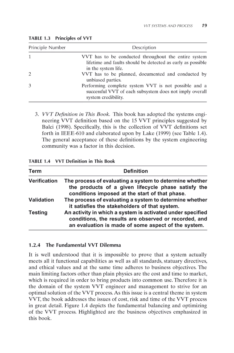
It is well understood that it is impossible to prove that a system actually
meets all it functional capabilities as well as all standards, statuary directives,
and ethical values and at the same time adheres to business objectives. The
main limiting factors other than plain physics are the cost and time to market,
which is required in order to bring products into common use. Therefore it is
the domain of the system VVT engineer and management to strive for an
optimal solution of the VVT process. As this issue is a central theme in system
VVT, the book addresses the issues of cost, risk and time of the VVT process
in great detail. Figure 1.4 depicts the fundamental balancing and optimizing
of the VVT process. Highlighted are the business objectives emphasized in
this book.
20
INTRODUCTION
Figure 1.4
1.2.5
Balancing and optimizing the VVT process.
Modeling Systems and VVT Lifecycle
This section describes major system lifecycle models and in particular systems’
lifecycle definitions used by U.S. government and commercial organizations.
A generic system lifecycle adopted for this book is also presented.
Major System Lifecycle Models An overall system lifecycle model describes
a cradle-to-grave paradigm of engineered systems. Different organizations
[e.g., the National Aeronautics and Space Administration (NASA), DoD] and
industries (e.g., automobile, electronics, telecommunication, aerospace) define
various system lifecycle models. For example, the DoD acquisition lifecycle
process has 4 major phases and 22 minor phases, as defined in Table 1.5.
TABLE 1.5
Major System Lifecycle Phases as Defined by U.S. DoD
Major Systems Lifecycle Phase
0
I
II
III
Concept
Exploration (CE)
Program Definition
& Risk Reduction
(PD&RR)
Engineering &
Manufacturing
Developmen
(EMD)
Production,
Fielding/Deployment
& Operational
Support (PFD&OS)
1.
System analysis
6.
Concept design
update
11.
Detail design
17.
Production rate
verification
2.
Requirements
definition
7.
Subsystem trade-off
12.
Development
18.
Operational test &
evaluation
3.
Conceptual design
8.
Preliminary design
13.
Risk management
19.
Deployment
4.
Technology & risk
assessment
9.
Prototyping, test, &
evaluation
14.
Development test
and evaluation
20.
Operational support
& upgrade
VVT SYSTEMS AND PROCESS
TABLE 1.5
21
Continued
Major Systems Lifecycle Phase
0
I
II
III
5.
Preliminary cost,
schedule & concept
10.
Integration of
manufacturing &
supportability
considerations
15.
System Integration,
test & evaluation
21.
Retirement
16.
Manufacturing
process &
verification
22.
Replacement
planning
0.
Concept Exploration. The CE phase begins with a definition of project
or product objectives, mission definition, definition of functional
requirements, definition of candidate architectures, allocation of
requirements to one or more selected architectures and concepts,
trade-offs and conceptual design synthesis and selection of a preferred
design concept. An important part of this phase is the assessment of
concept performance and technology demands and the initiation of a
preliminary risk management process.
I. Program Definition and Risk Reduction. The PD&RR phase is oriented to a risk management strategy in order to prove that the system
will work prior to committing large amounts of resources to its fullscale engineering and manufacturing development. This is the first
phase in the development cycle where significant effort is allocated to
developing tangible products such as top-level specifications, decomposing and allocating system requirements and design constraints to
lower levels, supporting preliminary design, monitoring integration of
subsystem trade-offs and designs and detailed project plans.
II. Engineering and Manufacturing Development. During the EMD phase,
detailed design and test of all components and the integrated system
are accomplished. This may involve fabrication and testing of engineering models and prototypes in order to check that the design is correct.
The hardware and software design for the EMD usually differ from
those of the PD&RR phase. This is usually justified to minimize the
PD&RR phase costs and to take advantage of lessons learned during
PD&RR in order to improve the EMD design. Thus, most of the
analysis, modeling, simulation, trade-off and synthesis tasks performed
during CE and PD&RR are repeated at a higher fidelity. A requirement validation process should be conducted before the EMD hardware and software is produced. This will ensure that the entire system
will function as envisioned.
III. Production, Fielding/Deployment and Operations and Support. During
production, deployment and operational use, the focus is on solving
22
INTRODUCTION
problems that arise during manufacturing, assembly, integration and
verification as well as the transition into its deployed configuration.
Additionally, attention is given to customer orientation, validation and
acceptance testing. During the phase of operations and support, systems
are usually under the control of the purchasers/operators. This involves
a turnover of the system from experienced developers into less experienced operators. This leads to a strong operations and support presence by the developers in order to train and initially help operate the
system. During this period, there may be upgrades to the system to
achieve higher performance levels.
Government and Commercial Program Phases INCOSE (2007) further illustrates and compares several typical lifecycle phases of government and commercial organizations (see Figure 1.5). This figure emphasizes that system
lifecycles in different domains are fundamentally similar in that they move
from requirements, definition, and design through manufacturing, deployment, operations and support (and sometimes to deactivation), but they differ
in the vocabulary used and nuances within the sequential process.
Typical High-Tech Commercial System Integrator
Study Period
User
Requirement
Definition
Phase
Concept
Definition
Phase
Implementation Period
System
Specification
Phase
Acq Source
Prep Select
Phase Phase
Operation Period
Verification
Phase
Development
Phase
Deployment
Phase
Operation
and
Maintenance
Phase
Deactivation
Phase
Typical High-Tech Commercial Manufacturer
Implementation Period
Study Period
Product
Requirement
Phase
Product
Definition
Phase
Product
Development
Phase
Engr
Model
Phase
Operation Period
External
Teat
Phase
Internal
Test
Phase
Full-Scale
Production
Phase
Manufacturing
Sales and
Support Phase
Deactivation
Phase
ISO/IEC 15288
Development
Stage
Concept Stage
Utilization Stage
Production
Stage
Retirement
Stage
Support Stage
U.S. Department of Defense (DoD) 5000.2
C
B
A
Presystem Acquisition
Concept and Technology Development
IOC
FOC
System Acquisition
System
Production and
Development &
Deployment
Demonstration
Sustainment
Operation and Support
(Including Disposal)
U.S. Department of Energy (DoE)
Project Execution
Project Planning Period
Preproject
Typical
Decision
Gates
Preconceptual
Planning
New Initiative
Approval
Figure 1.5
Concept
Approval
Conceptual
Design
Perliminary
Design
Development
Approval
Final
Design
Construction
Production
Approval
Mission
Acceptance
Operational
Approval
System lifecycle phases as illustrated in INCOSE, 2007.
Operations
Deactivation
Approval
VVT SYSTEMS AND PROCESS
23
Generic System Lifecycle Adopted for This Book This book has adopted the
generic system lifecycle model (see Table 1.6) that is used in the SysTest
project due to its generality and practicality. It is a generic extension of the
model of system lifecycle phases and VVT activities suggested by Addy (1999)
and Boehm (2001). This system lifecycle model extends the well-established
V-Model (Martin and Bahill, 1996), which portrays project evolution during
the development portion of the system lifecycle.
TABLE 1.6
Generic System Lifecycle Definition Model
Phase
Purpose
Development
Definition
Formulate the system operational concepts and develop the
system requirements.
Create a technical concept and architecture for the system.
Create the elements of the system. Each element is built or
purchased, then tested to ensure its stand-alone compliance
with its allocated requirements.
Connect the implemented elements into a complete system.
Perform formal and operational tests on the completed
system to assure the quality of the system as a whole.
Design
Implementation
Integration
Qualification
Postdevelopment
Production
Use/Maintenance
Produce the completed system in appropriate quantities.
Operate the system in its intended environment in order to
accomplish intended functionality, maintain the system
and correct any defects.
Properly dispose of the system and its elements upon
completion of its life.
Disposal
Figure 1.6 depicts the V-Model as a part of the overall generic system lifecycle model developed during the SysTest project and adopted for this book
(Engel et al., 2001).
Disposal
Use/maintenance
Production
V-model
Definition
Design
Qualification
Integration
Implementation
Figure 1.6
V-Model as part of overall generic system lifecycle model.
24
INTRODUCTION
The left-hand side of the V-Model corresponds to satisfying stakeholders’
requirements and the design of the desired system and its components. The
right-hand side of the V-Model consists of building the individual components,
integrating them and then verifying and validating the whole system. Figure
1.6 depicts the V-Model as a part of the overall generic system lifecycle model
developed during the SysTest project and adopted for this book (Engel et al.,
2001). Figure 1.7 depicts a generic system lifecycle model together with the
corresponding generic VVT lifecycle, with which it is associated.
SYSTEM
VVT
1
DEFINITION
VVT DEFINITION
2
DESIGN
VVT DESIGN
3
IMPLEMENTATION
VVT IMPLEMENTATION
4
INTEGRATION
VVT INTEGRATION
5
QUALIFICATION
VVT QUALIFICATION
6
PRODUCTION
VVT PRODUCTION
7
USE/MAINTENANCE
VVT USE/MAINTENANCE
8
DISPOSAL
VVT DISPOSAL
PHASE
Figure 1.7
1.2.6
Modeling generic systems and VVT lifecycles.
Modeling VVT and Risks as Cost and Time Drivers
Traditional Modeling Quality Cost The cost of quality is the overall cost
associated with ensuring the quality of products or services delivered to
customers. In the 1950s, Joseph M. Juran developed his cost-of-quality concepts (see Juran and Gryna, 1980). Later, several researchers (e.g., Montgomery,
2001) encapsulated a lexical qualitative model of cost of quality. Some
researchers augmented the information with field-obtained quality cost
data (e.g., Sörqvist, 1998). Due to the relevancy and fundamental nature
of this qualitative cost-of-quality model, it is presented below with relevant
alterations emanating from the perspective of this book. Specifically, the
cost of quality in manufacturing and service industries is composed of four
components: (1) prevention cost such as quality planning and training, (2)
assessment cost such as product inspection and testing, (3) internal failures
VVT SYSTEMS AND PROCESS
25
cost such as scrap, rework and retest and (4) external failure costs such as
warranty charges, liability cost and indirect cost. We will now map system
quality costs to this model.
1. Prevention Costs. Prevention costs are costs expanded on the prevention of nonconformance to specifications during system development,
manufacturing and maintenance. Important subcategories of prevention
costs are shown in Table 1.7.
TABLE 1.7
Subcategories of Prevention Cost
Subcategories
Quality Planning. Costs associated with the creation of various quality
plans (e.g., inspection plan, reliability plan).
Product/Process Design. Costs incurred during the quality evaluation of
system development and production processes which are intended to
improve the overall quality of products as well as costs incurred during
the evaluation of the development and manufacturing effectiveness
(e.g., input versus output, return on investment)
Process control. The cost of process control activities, such as collecting
samples and generating control charts which monitor the development
or the manufacturing process in an effort to reduce variation and create
quality within system.
Burn-in. The cost of preshipment exercising and evaluation of system in
order to minimize early-life defects in the field.
Training. The cost of developing, implementing, operating, and
maintaining training programs in order to achieve system quality.
Quality Data Acquisition and Analysis. The cost associated with creating,
purchasing, and operating quality of data collection and distribution
system as well as the cost of running the quality data system to obtain
information about systems and process quality performance and
analyzing and publishing it for management, customers and other
stakeholders.
Type
VVT cost
VVT cost
VVT cost
VVT cost
VVT cost
VVT cost
2. Assessment Costs. Assessment costs are those costs associated with
measuring and evaluating purchased materials, components and subsystems as well as verifying, validating and testing systems (i.e., end products and enabling products) to ensure conformance to specified
requirements and standards. The major subcategories of assessment
costs are described in Table 1.8.
26
INTRODUCTION
TABLE 1.8
Subcategories of Assessment Cost
Subcategories
Inspection and Test of Incoming Material. Costs associated with the
inspection and testing of appropriate vendor’s supplied raw material,
components and subcategory either at the vendor’s facility or at the
receiving station of the firm. In addition, this subcategory includes
verification of all vendor-supplied documentation as well as periodic
audit of the vendor’s quality assurance system.
Systems Verification, Validation and Test. The cost of checking the
conformance of the systems throughout the various stages of
development and manufacturing, including final acceptance testing,
packing and shipping checks and any test done at the customer’s
facilities prior to turning systems over to the customer. In general,
assessment cost also covers tests and evaluation associated with
system maintenance activities as well as verification and validation of
appropriate disposal process.
Consumed Materials and Products. The cost of material and products
consumed in destructive quality tests or devalued by reliability tests.
Maintaining Accuracy of Test Equipment. The cost of ensuring that the
measuring instruments and equipment are calibrated on an ongoing
basis.
Type
VVT cost
VVT cost
VVT cost
VVT cost
3. Internal Failure Costs. Internal failure costs are incurred when materials, components, subsystems or systems do not meet quality requirements and these failure are discovered prior to delivery of the systems
to customers. The major subcategories of internal failure costs are
described in Table 1.9.
TABLE 1.9
Subcategories of Internal Failure Cost
Subcategories
Scrap. The net loss of labor, material and overhead resulting from defective
product or systems that cannot economically be repaired or used.
Rework. The cost of correcting system chronic or sporadic defects so
that they meet specifications. This process may transpire once or several
times.
Retest. The cost of repeated verification, validation and testing of systems
that have undergone rework or other modifications.
Failure Analysis. The cost incurred to determine the global causes of
recurring system failures. Note that this subcategory is not referring
to a regular testing process but to a wider phenomenon of persistent
system failures.
Type
Risk cost
Risk cost
Risk cost
Risk cost
VVT SYSTEMS AND PROCESS
TABLE 1.9
27
Continued
Subcategories
Type
Downtime. The cost associated with idle development or production
facilities and manpower that result from nonconformance to
requirements. The development may be halted until certain information
is obtained. A production line may be down while a defective system
or product is evaluated or repaired.
Yield Losses. The cost of process yield that is lower than might be
attainable by improved quality controls.
Downgrading. The cost associated with inferior products and systems
that do not meet the entire customer’s requirements. Downgrading
implies that such products yield less profit relative to products that
conform to specifications. In addition, inferior products adversely affect
the reputation of the firm, causing loss of revenues.
Risk cost
Risk cost
Risk cost
4. External Failure Costs. External failure costs occur when systems do not
perform satisfactorily and the problems are identified after these systems
have been supplied to customers. The subcategories of external failure
costs are described in Table 1.10.
TABLE 1.10
Subcategories of External Failure Cost
Subcategories
Complaint Adjustment. All costs associated with the investigation and
adjustment of either justified or not justified complaints attributable to
the nonconforming product.
Handling Defective Products and Systems. All costs associated with either
fixing systems at customers’ premises or replacing nonconforming
products and systems that are returned from the field.
Warranty Charges. All costs involved in service to customers of faulty
systems under warranty contracts.
Liability Costs. All costs associated with defective products and systems
incurred as a result of system liability litigations.
Indirect Costs. Costs incurred because of customer dissatisfaction with
the level of quality of the delivered system. They include the costs of
business reputation loss, future business loss and market share loss that
may result from delivering defective systems that do not meet the
customer’s expectations.
Type
Risk cost
Risk cost
Risk cost
Risk cost
Risk cost
Waste in Product Development The Lean Aerospace Initiative (LAI) was
born out of declining defense budgets and military industrial overcapacity,
prompting a new defense acquisition paradigm, that is, affordability rather
than performance. The U.S. Air Force (USAF) and the Massachusetts Institute
of Technology (MIT) launched this initiative in 1993.
Researchers dedicated to the philosophy called “lean” are interested in
eliminating waste that occurs during systems’ development phase of projects.
28
INTRODUCTION
Womack and Jones (2003) classified all product-making activities into Value
Adding (VA), to be continually perfected; Non–Value Adding (NVA), to be
eliminated; and Required Non–Value Adding (RNVA), such as those required
by contract or law, to be faithfully executed. No formal study is available on
the relative amounts of NVA and RNVA waste in the aerospace programs
(Oppenheim, 2004). Table 1.11 shows two sets of product development waste
categories as classified by two studies.
TABLE 1.11
Two Sets of Product Development Waste Classifications
Classification by Millard (2001)
1. Overproduction (creating unnecessary
information)
2. Inventory (keeping more information
than needed)
3. Transportation (inefficient transmittal
of information)
4. Unnecessary movement (people
having to move to gain or access
information)
5. Waiting (for information, data, inputs,
approvals, releases, etc.)
6. Defects (insufficient quality of
information, requiring rework)
7. Overprocessing (working more than
necessary to produce the outcome)
Classification by Morgan (2002)
1. Hand off (transfer of process
between parties)
2. External quality enforcement
(including performance
requirements)
3. Waiting
4. Transaction waste
5. Reinvention waste
6. Lack of system discipline
7. High process an arrival variation
8. System overutilization and
expediting
9. Ineffective communication
10. Large batch sizes
11. Unsynchronized concurrent
processes
In an ideal world, systems are created perfectly and VVT procedures would
not be necessary. Therefore, performing VVT and incurring VVT appraisal
and impact risks are clearly NVA activities. Obviously, optimizing the VVT
strategy leads to less costly NVA results. Our world is not ideal and the VVT
process is a necessary expenditure that is required to ensure the quality of
systems. Therefore, one can say that just about all VVT activities lie on the
border between VA and NVA activity regions.
Modeling Cost and Risk VVT cost can be considered a cost associated with
classical prevention and assessment, while risk impact cost is usually associated with sustaining internal and external failures. Developing risk-based cost
models involves three activities:
•
•
•
Identifying VVT risks
Estimating risk probability
Estimating risk effects
In the literature, we find several methodologies dealing with these topics. The
main ones are discussed below.
VVT SYSTEMS AND PROCESS
29
Methodology Based on Perception of Engineering Process A detailed
approximation of the underlying cost and risk of a project can be obtained by
viewing the engineering process as a tree structure and each node in the tree
is an engineering activity. The standard engineering tool of Work Breakdown
Structure (WBS) is an available vehicle to promote and support this methodology. Engineering process parameters such as cost/duration, including the VVT
tasks, are first identified. Experts then assign valuations to them based on the
experts’ technical knowledge. To take into account uncertainties, rather than
assigning only a best estimate of task cost and duration, these experts can
assign a minimum, a most likely and a maximum estimate for each of these
two quantities.
VVT activity costs and durations are fairly easy to predict, whereas the
costs and durations of engineering processes are somewhat less predictable
due to their physical nature. Fortunately, engineering experts are able to do
a fairly good job at estimating risks, risk impact probabilities, and risk impact
costs. Because expert opinions often differ, the cost estimates for normal
engineering activities and the risk cost estimates are recognized to be probability functions across the different categories and expert opinions. The data are
presented to participants and stakeholders as a range of values rather than a
single value in terms of a cost–risk curve (e.g., a histogram of risk–cost density
distribution). It should be noted that more sophisticated approaches for transforming the three estimate levels into probabilistic data are available, for
example, with the aid of a beta distribution (Fente et al., 1999).
Methodology Based on Balancing Cost/Availability and Benefits Browning
(1998, 1999) describes a method for identifying acceptable risks. The
method balances product pricing and availability timing with the value of the
product to the customer. The designers of systems must fit the design process
to optimize this process. Browning’s thesis first addresses the sources of risk
of not meeting this optimization and classifies it into six categories: (1) cost,
(2) schedule, (3) performance, (4) technology, (5) business and (6) market
risks. Then he builds a framework and a model to represent the relationships
between these risks. A stochastic simulation is then used to generate probability distributions of possible costs, schedules and performance outcomes. These
distributions model uncertainty and are analyzed in relation to impact functions. The model provides the means to explore several management options
for optimizing the above parameters.
Methodology Based on Holistic Philosophy of Risk Scenarios Haimes
(1998) coined the term Hierarchical Holographic Modeling (HHM) to depict
complex systems using multiple models created along different perspectives.
Extending this concept, Haimes et al. (2002) proposed an analytic framework
called Risk Filtering, Ranking, and Management (RFRM), which can identify,
prioritize, assess, and manage risk scenarios of large-scale systems. In a nutshell, the risk assessment portion of RFRM follows these steps: First, the
HHM must be developed to describe a multifaceted model of the system’s
“as-planned” scenario. Then, the set of risk scenarios is qualitatively filtered
30
INTRODUCTION
and ranked according to the system stakeholders’ views. Finally, a quantitative
filtering and ranking of possible risks must be carried out based on the likelihood of system failures and the consequences of such events. Lamm and
Haimes (2002) use the HHM and RFRM methodologies to analyze the security of the U.S. national information infrastructures.
Methodology Based on System Safety Program Requirements Muessig
et al. (1997) describe another methodology in the context of a risk–benefit
analysis approach to the selection of an optimal set of Verification, Validation,
and Accreditation (VV&A) activities. This risk modeling is based on an adaptation of the U.S. military standard MIL-STD-882C, System Safety Program
Requirements. In the model, VVT risks are quantified in terms of probability
of occurrence and impact or severity levels within the context of specific applications. Two variables are involved in modeling risks as cost drivers: (1) the
uncertainty of risk occurrence and (2) the severity of risk impact.
1. Uncertainty of Risk Occurrence. The first element affecting risk is the
uncertainty with which undesirable events occur. The risk model defines
the probability of occurrence of a given risk factor in different ways,
depending on the category of the risk factor that is being considered.
The effect of undesirable events impacting the system can be measured
by (1) the number of items affected in a population, (2) the number of
events per unit of time or (3) the total number of events over the life of
the system or product.
The model of Muessig et al. (1997) divides the probability continuum
into five bands and gives guidelines for selecting the appropriate band.
Table 1.12, extracted from MIL-STD-882C, provides these guidelines in
terms of the number of undesirable events over a lifetime and per
number of items in a population.
TABLE 1.12
Probability of Risk Occurrence
Probability Description
Likelihood of Occurrence
over Lifetime of Item
Likelihood of Occurrence
by Number of Items
Frequent
Probable
Likely to occur frequently
Will occur several times
in life of item
Likely to occur sometime
in life of item
Unlikely but possible to
occur in life of item
Widely experienced
Will occur frequently
Occasional
Remote
Improbable
So unlikely it can be
assumed occurrence
may not be experienced
Will occur in several
items
Unlikely but can
reasonably be
expected to occur
Unlikely to occur but
possible
VVT SYSTEMS AND PROCESS
31
The reader may substitute “system” or “product” for the word “item,”
as appropriate.
2. Severity of Risk Impact. The second element affecting risk is the severity
of the impact of an undesirable event, should the event be experienced.
The risk model developed by Muessig et al. (1997) expands the MILSTD-882C while grouping the impact severity into four bands: catastrophic, critical, marginal and negligible. The criterion for assigning one
of these impact bands to a particular risk depends on the category of
that risk. The impact categories that are discussed in the model are
personnel and equipment safety, environmental damage and occupational illness. Depending on the particular use of the system being considered, some of these impact categories might not apply, and additional
categories might be added—for example, impact on end-user capability
or effectiveness, cost, performance, schedule and political or public reaction. A set of criteria for determining the level of impact for each of the
different impact categories is provided in Table 1.13 as an illustrative
guideline.
TABLE 1.13
Severity of Risk Effects
Risk by Impact Levels
Categories
Catastrophic
Critical
Marginal
Negligible
Human safety
Death
Severe injury
Minor injury
Less than
minor injury
Systems safety
Major equipment
loss; broad-scale
major damage
Broad-scale
minor damage
Small-scale
minor damage
Environmental
damage
Severe
Major
Minor
Some trivial
Severe and
broad scale
Severe or broad
scale
Minor or small
scale
Minor and
small scale
Financial
losses of
program
Loss of program
funds; 100% cost
growth
Fund reductions;
50–100% cost
growth
20–50% cost
growth
<20% cost
growth
Functional
performance
of product
Design does not
meet critical
thresholds
Severe design
deficiencies but
thresholds met
Minor design
flaws but
fixable
Some trivial
“out of spec”
design
elements
Slip reduces
overall
capabilities
Slip has major
cost impacts
Slip causes
internal turmoil
Republish
schedules
Occupational
illness
Schedule
slippage of
product
Small-scale
major damage
32
INTRODUCTION
TABLE 1.13
Continued
Risk by Impact Levels
Categories
Catastrophic
Critical
Marginal
Negligible
Political or
public impact
of event
Impact
widespread
(Watergate)
Significant
(Tailhook ‘91)
Embarrassment
($200 hammer)
Local
Negative
impact due to
unidentified
stakeholders
Major
stakeholder
blocks program
(Israeli AWACS
sale to China)
Stakeholder
requires product
modifications
(FAA
disqualifies new
aircraft)
Stakeholder
requires minor
system
modifications
Upgrading
sales campaign
to cover newly
recognized
stakeholders
Future losses
of potential
revenues
Customers
determined to
abandon product
Major market
share loss
Customers
dissatisfied with
product
Competitor
plan to
develop
similar
product
1.3
1.3.1
CANONICAL SYSTEMS VVT PARADIGM
Introduction—Canonical Systems VVT Paradigm
An engineered system does not appear suddenly in just an instant. Like any
other entity, it needs to be brought into being, cared for and nourished, challenged and utilized and finally put to rest. Thus, the concept of a system life
is appropriate. This section discusses that life and describes the role of VVT
in its phases. This is presented in terms of the canonical system VVT paradigm
composed of (1) phases of the systems lifecycle, (2) views of the systems and
(3) aspects of the systems.
A system, in this context, is a set of interacting or interdependent entities,
man made or otherwise, existing and forming an integrated whole that fulfills
a certain purpose or set of objectives. For an engineered system to adequately
meet its objectives, the goal should be to invent, develop, adapt or optimize
system behavior within a set of required properties. The man-made parts of
an engineered system can undergo development from different disciplines,
such as mechanics, hydromechanics, electronics, computation and programming. Other parts, such as human operators or technicians, can also undergo
development from other disciplines, such as education, training and work
experience.
Figure 1.8 helps the reader to envisage the many interactions involved in
the VVT process. It depicts the canonical system VVT paradigm as a threedimensional object:
33
Disposal
Use/Maintenance
Production
Qualification
Integration
Implementation
Design
Definition
CANONICAL SYSTEMS VVT PARADIGM
System management
System engineering
System VVT
System CM
Preparation of VVT products
Applying VVT to engineered products
Participate/conduct review meetings
Figure 1.8
•
•
•
Canonical system VVT paradigm.
First Dimension. Lifecycle phases include all the system lifecycle phases
(i.e., Definition to Disposal).
Second Dimension. System views include, among others, the following
components: System management, Systems engineering, System VVT
and System Configuration Management (CM).
Third Dimension. Aspects of systems include the following components:
Preparation of VVT products, Applying VVT to engineered products and
Participating or conducting reviews.
Knowing the phases of the system lifecycle is essential for understanding
how VVT is implemented throughout the life of a system. Thus, each phase
is discussed separately and the appropriate VVT activities for that phase are
described. During the entire lifecycle, from system definition to system disposal, there are at least four views of the system. Naturally, the most important
view for this book is VVT. For completeness, short descriptions of the remaining views are also provided.
Here each activity of a system lifecycle can be categorized by placing each
of them in one of the cubes depicted in the three-dimensional stack of cubes
shown. These activities describe what has to be done in order to achieve the
desired degree of quality in a system.
The VVT activities, however, indicate only what may be done to assure the
quality of a system. Thus, for each VVT activity, this book provides one or
more VVT implementation methods. These VVT methods describe how to
perform an activity by defining a sequence of steps that should be performed.
34
INTRODUCTION
From this perspective, a step within a method may indeed be a VVT activity
unto itself. While some VVT activities are straightforward and may be implemented by only one method, others may be carried out using one of several
methods. An example of a hierarchy depicting activities and methods is shown
in Figure 1.9. Each element of the canonical system VVT paradigm (i.e.,
phases of the system lifecycle, views of the system and aspects of the system)
will now be discussed in more details.
VVT Activities: Development
System
lifecycle
VVT
activities
Definition
Activity-1
Design
Activity-2
Implem.
Integration
Qualif.
VVT
Nontesting
Methods
VVT
Testing
Methods
Method 1
Method 1
Method 2
Method 2
Method m1
Method m 2
Activity-3
Activity-n1
VVT Activities: Postdevelopment
System
lifecycle
VVT
activities
Use/Maintenance
Activity 1
Production
Disposal
Activity n 2
Figure 1.9
1.3.2
Hierarchy of VVT activities and methods.
Phases of the System Lifecycle
Each individual activity of a system lifecycle is allocated to one of the phases
and works smoothly together with other activities to achieve the overall goals
of that phase. There are several mostly overlapping phases, each describing a
particular period of the overall system lifecycle. Depending on the system
(hardware versus software development, safety-critical versus noncritical
application, etc.), some of these phases are considered more relevant than
others. As mentioned above, the canonical phases of a system’s lifecycle are
Definition, Design, Implementation, Integration, Qualification, Production,
Use/Maintenance and Disposal.
In our system lifecycle framework, eight phases encompass the system
lifecycle. Depending on the system under consideration, some of these phases
may be more or less important. These eight phases pretty much cover the same
areas as the five phases called out in the ISO/IEC 15288: Concept (Define/
Design), Development (Implement/Integrate/Qualify), Production (Produce),
CANONICAL SYSTEMS VVT PARADIGM
35
Utilization and Support (Use and Maintain) and Retirement (Disposal). The
eight phases of a system lifecycle are described in the following.
System Definition During the system Definition phase, the requirements of
the system are elaborated as completely and precisely as possible in terms of
system, hardware and software requirements. Specifications that could constitute the actual system definition could take many forms. For instance, textual
requirements, formal requirements, system models or prototypes can be artifacts of system requirements activity.
From the perspective of VVT, during this phase, a project should produce
a set of system requirements that are complete, clear and consistent. VVT
planning consists of defining forward-looking VVT-related concepts and goals.
Specific details of VVT are few, but the planner should be looking at defining
the overall VVT framework in general terms that support the emerging system
architecture. For example, if the system requirements mandate built-in test
capabilities, the VVT philosophy could emphasize intrinsic self-instrumentation capabilities within components in order to reduce the need for developing
intrusive and expensive instrumentation.
In the Definition phase, allocation of requirements to hardware and software is usually incomplete; so many specifics of VVT cannot be fully developed. Once systems engineering begins to define the Technical Performance
Measures (TPMs) that will assist in meeting system performance requirements, some of the details of VVT requirements can be established. The VVT
philosophy during this phase must be forward looking and flexible, as this is
the time that system definition is most fluid.
The primary objective in VVT planning in this phase is to define the framework for VVT throughout the program to the level of detail possible. Just as
the system receives its architectural concepts during this phase, VVT develops
its own architecture that supports the program needs. As system requirements
are being analyzed and lower level specifications are being written, VVT
planning focuses on the analysis of test requirements and influence of
specifications from a test and instrumentation perspective. If self-test requirements are articulated at a top level, or if requirements analysis and derivation
imply the need for self-instrument requirements, then the VVT planning can
both influence and build upon these expected capabilities as they become
defined.
System Design The technical concept of the system, the principles and the
underlying system architecture for the implementation of the system are
determined during the system Design phase. The total complex system is
divided into manageable subsystems and components and the functions of the
individual elements as well as their interrelations are described.
As requirements get refined and assigned into subsystems and components,
VVT will now have a more concrete structure against which to direct specific
test strategies. General TPMs will become allocated and apportioned to sub-
36
INTRODUCTION
systems and components. The resulting greater specificity allows VVT planning efforts to be directed toward the implementation phase and integration
phase needs.
System Implementation The design concept is realized during the system
implementation phase. If the system is a hardware-based system, this implementation is only a prototype (i.e., the first instance of the system built) that
must be reproduced during the system Production phase. At the completion
of the system Implementation phase, all individual components of the overall
system should be available and functioning.
During system implementation, VVT efforts are directed toward those
emerging subsystems, their verification against system requirements and their
refinement. As requirements are verified with respect to implemented components, they should also be validated against stakeholder needs. This validation
should be a continuous process. Whenever subsystem or component definition
and specificity permit, the associated requirements should be validated.
System Integration The focal point of this phase is the integration of the
implemented subsystems with the aim of setting up the complete system.
VVT activities during system integration are directed at verifying that
the interfaces between subsystems or components as well as between the
system as a whole and external elements meet requirements and that the
whole meets system requirements as well. VVT activity should also be focused
toward validation of each requirement within the relevant integrated subsystem. VVT planning during this phase is directed toward preparing for qualification of the system.
System Qualification The system Qualification phase is a formal phase
during which the system runs through a number of tests often prescribed by
external agencies, customers or standards. The goal is to assure the quality of
the system as a whole. Ideally, during this phase, no constructive developments on the system should be carried out. In practice, however, often certain
parts of the system are being tested while other parts are still under various
stages of development.1
At this point, the formal validation of the verified requirements ensures
that the system meets the stakeholder true needs and that those needs are
accurately reflected in the captured requirements. VVT activities include
testing the system and ensuring that all requirements are verified using the
proper method (i.e., analysis, inspection, demonstration, testing or certification). VVT planning consists of selecting appropriate qualification testing for
inclusion in the Production phase as a subset of acceptance testing. VVT planning starts the preparations to support testing of purchased parts and conduct1
Concurrent engineering is a methodology of developing different parts of a system in an unsynchronized manner so each part may, in parallel, be at a different stage of development (e.g., definition design, implementation, integration, qualification) at any given time. This approach, which
attracted unsavory reputation, is under intensive scientific research and gaining due respect as a
legitimate way to reduce elapsed time required to bring systems into the market.
CANONICAL SYSTEMS VVT PARADIGM
37
ing component qualification before inclusion into the produced systems. VVT
planning also includes developing an efficient production VVT strategy to
assure good system components are delivered with a test subset that is viable
and economical.
System Production Once the system is deemed ready, the next phase is to
produce final products for sale or use. VVT activities include testing of purchased parts and the conduct of component qualification tests. VVT planning
includes preparing to receive and process field failure data when the system
is fielded.
System Use and Maintenance When regarding the overall system lifecycle
one must also consider the VVT activities during the Use and Maintenance
phase. The system is now fielded and under customer control. It operates in
its intended environment and manned by operators who have been trained in
its proper use. Maintenance should be performed in accordance with the policies and guidelines established during its development. Failures may occur due
to component wear, operator error or unanticipated harsh environmental
factors as well as defective design or poor manufacturing process. If these
occur during the warranty period, the program/project team should have
responsibility for correction and possibly additional rework if the failure has
revealed a fundamental system deficiency. Also, during this phase, eventual
improvements to the system functions are introduced, errors are eliminated,
and systems are maintained.
System Disposal After the use of the system, its disposal becomes an important aspect which should have been planned from the earliest days of the
system development. During this phase systems must be dismantled, recycled,
if necessary, and/or finally disposed of.
In general, VVT activities are performed within this phase only for systems
with public safety issues associated with the system disposal or for systems
that had specific disposal-related requirements imposed during their development. In these cases, there are likely to be enabling technologies required
(such as nuclear waste disposal) which will have VVT activities. If the program
is of sufficiently long duration, the disposal-enabling technologies may require
certification or validation that should be planned for in advance and executed
when needed.
1.3.3
Views of the System
During the entire lifecycle, from system definition to system disposal, there
are different views one could have on the system. Naturally, the most important view for this book is the “VVT” view, which focuses on all activities that
are implemented to assure the required quality by means of verification, validation, and testing of the system or system components. Such activities should
be performed during every lifecycle phase to assure the quality of intermediate
or final lifecycle products. Beside this view, there are of course other views,
38
INTRODUCTION
such as system management, systems engineering and configuration management, which are related but of secondary importance for this book.
System Management View System management includes activities concerned with organizational issues associated with a system or a product. These
include:
•
•
•
•
The subdivision of the development and production process into phases
and activities
The division and definition of the work to be done
The regulation of communication
The organization and control of the work flow
The activities set out in system management comprise planning and controlling of various activities, the allocation of internal roles and the setting up of
an interface to units outside the project (i.e., subcontractors, management,
etc.). Typically, system management contains the following main tasks: project
initialization, detailed planning, project control, reporting, cost–benefit
analysis, phase reviews, risk management, resource management, contractor
management and training.
System Engineering View System engineering is that set of activities which
directly leads to the development, production, use and maintenance and finally
disposal of a system, as opposed to other activities related to system management, quality assurance and configuration management, which (crucial though
they are) play a supporting role from the perspective of system construction.
The system development lifecycle covers the following main activities:
•
•
•
•
•
•
System requirement analysis
Software/hardware requirement analysis
System and subsystem design
Component and subsystem implementation (hardware/software units)
System integration
System qualification
In system development, all activities directly relevant to the system development lifecycle process and the respective documents are grouped together. A
system development lifecycle encompasses the complete set of activities that
generate and implement engineering decisions about a system:
•
•
•
•
What it should do (and not do)
Which technologies should be used and where
How it should be structured into parts
How parts should be obtained (design-and-build, reuse-and-adapt,
acquire, etc.)
METHODOLOGY APPLICATION
•
•
•
•
39
How VVT should be done
How integration should be performed
How to produce systems (for mass market or a small number of
products)
How to maintain systems and dispose of obsolete ones
Verification, Validation, and Testing View Conventional wisdom says that
to produce competitive products one must identify the requirements and
proceed to meet these in an efficient and effective way. This is a quality assurance process, which can be separated into three different levels: the organizational level, the process level and the product level. The activities relevant to
the VVT view serve as the basis for the detailed explanation of activities and
methods in the following chapters of this book.
Configuration Management View Configuration Management (CM) comprises those activities that must be performed in order to manage all the parts
and their relationships and to support systems engineers in maintaining the
integrity of the system. It is a service function that allows the various participants involved in the system engineering process to perform their perspective
role confidently.
1.3.4
VVT Aspects of the System
Each individual activity describes one block of work of the project’s complex
network of tasks. Each VVT activity may be assigned to one of the following
VVT aspects:
•
•
•
Prepare VVT Products. This VVT aspect encompasses VVT activities
related to preparation of VVT products, such as developing a certain VVT
plan and designing and fabricating certain VVT tools or simulations.
Perform VVT Activities. This VVT aspect encompasses VVT activities
related to actual VVT of various system engineering products, for example,
verifying a system design document and testing a package of software.
Participate in Reviews. This VVT aspect encompasses VVT activities
related to either participating in or conducting a system review, for
example, participating in a system Preliminary Design Review (PDR) and
conducting a Test Readiness Review (TRR).
1.4
1.4.1
METHODOLOGY APPLICATION
Introduction
In this section we begin to get to the heart of the subject matter in this book.
VVT has developed over the years into a set of tools that are tried and proven
to save time and money and ensure success in the design and building of
complex systems. Having covered the preliminaries in the previous sections,
40
INTRODUCTION
we concentrate here on the tools and techniques available for system VVT.
We begin with an overview of the VVT methodology. The basis of this methodology is a process model that assists VVT planning by providing calculation
of the cost and risk associated with the various VVT strategies. This process
is a guide to modern VVT planning as performed by VVT practitioners,
in coordination with the other stakeholders of the engineered system. As
mentioned, a good VVT process does not “just happen.” It is the product of
thorough planning and strategy.
Since there is no such thing as a “typical” engineered system, what is good
for one system in the way of VVT may not be good for another. So, we go on
to show how VVT can be tailored to different kinds of systems, different
organizations and different project parameters. Heuristics are described for
tailoring VVT concepts to specific engineered systems based on project size/
complexity and type (i.e., system or industry). Specific attention is paid to the
electronics/avionics, aerospace, automotive, food packaging and steel production industries as representative of many other industries. Hints are given for
ameliorating project risks by tailoring VVT.
An important issue is the means by which VVT can be monitored and
stakeholders can be assured that VVT is properly applied. Remember the old
adage, “The job is not complete until the paperwork is done.” Of course, today
paperwork does not necessarily imply the generation of paper documents.
But, records do have to be kept and a trace of VVT steps and functions must
be made. This is the only way to assure that the process works and that monies
allocated for VVT have been properly spent. Among the necessary documents
are the Project Management Plan (PMP), the Systems Engineering
Management Plan (SEMP), the VVT Master Plan (VVT-MP), the Testability
Program Plan (TPP), the Maintainability Program Plan (MPP), the Reliability
Program Plan (RPP), the System Test Plan (SysTP), the Software Test Plan
(STP, if appropriate), the First Article Inspection Plan (FAIP), the Production
Plan (PP), the Maintenance Plan (MP), the Integrated Logistic Support Plan
(ILSP) and the Disposal Plan (DP). While, for any specific system not all of
these plans may be required, we provide fair details of what these documents
consist. In summary, reading this section sets the stage for the following chapters, which cover the “how to” for implementing VVT.
1.4.2
VVT Methodology Overview
The basis of the VVT methodology is to apply an informed strategy and planning process to the selection and sizing of VVT activities. Through such a
process, VVT activities, methods, tools and products are optimized to reduce
project risk while improving cost, quality and development time. This book
describes a process model that assists VVT planning by providing calculation
of cost and risk associated with various VVT strategies. The effort required
for performing the VVT strategy, planning, and modeling should be commensurate with the size of the project, so that the effort expended will be repaid
in improved quality and reduced project cost, risk and development time.
METHODOLOGY APPLICATION
41
Methodology for VVT Strategy and Planning The generic VVT process is
depicted in Figure 1.10 (Lévárdy et al., 2004). It is an iterative process that
can be applied to the entire system lifecycle, to a subset of the system lifecycle
(e.g., system development) or to any of the individual lifecycle phases. The
VVT process has four main segments: (1) VVT tailoring at the organization
and project level, (2) Rough VVT planning at the system level, (3) Detailed
VVT planning and (4) VVT execution.
0.
VVT
tailoring
1.
Define basic
VVT
characteristics
2.
Set up
VVT
strategy
4.
Conduct
detailed
VVT planning
8.
Prepare for
the next
phase
Detailed VVT planning
Rough VVT
planning
3.
Set up
process
model
5.
Conduct pre-VVT
analysis
VVT strategy and planning
VVT execution
Figure 1.10
7.
Conduct post-VVT
synthesis
6.
Conduct VVT
VVT methodology for strategy and planning (Lévárdy et al., 2004).
The VVT for strategy and planning encompass the following steps:
1. VVT Tailoring. Before starting a project, those managing the project
should determine the factors that characterize the project and enterprise. Based on these factors, the project managers should tailor the
VVT methodology to suit the project. Tailoring consists of high-level
decisions about the use of this methodology and its parts based on
knowledge of the organization and insights gained in earlier project.
2. Rough VVT Planning. At the outset of each project, it is necessary to
plan the VVT process, at least in a rough manner, and establish a VVT
strategy. The VVT strategy considers business objectives and their relationship to the project as well as issues related to programmatic and
strategy risks. Strategy consists of creating a set of requirements and
constraints that guide the VVT planning along with primary decisions
about the VVT activities to follow. VVT rough planning uses the following three process groups:
• Define basic VVT characteristics. This determines the basic characteristics that guide and bound the VVT strategy.
• Set up VVT strategy. This codifies the strategy into a selection of
activities and methods while also defining the requirement verification
methods to be used.
42
INTRODUCTION
Set up a VVT process model. This uses the VVT process model to
support the strategy definition by using calculation of cost, time and
risk to explore alternative strategies.
3. Detailed VVT Planning. Throughout the system’s lifecycle and especially at the beginning of each lifecycle phase, VVT engineers should
reexamine or/and establish a detailed VVT plan. This plan should identify specific activities, methods, tools and products that will implement
the actual VVT process. The VVT plan also identifies the types, formality and amount of effort to be applied to each VVT activity.
4. VVT Execution. The VVT execution process for each lifecycle phase
will usually incorporate the following three process groups:
• Conduct a pre-VVT analysis. This analysis will update the VVT strategy to incorporate changes as needed.
• Conduct VVT. This is the actual execution of the VVT process for the
relevant lifecycle phase.
• Conduct a post-VVT synthesis. This analysis will update the future
VVT strategy to incorporate anticipated changes as needed.
•
Importance of VVT Strategy and Planning A vital and effective VVT process
enhances the technical success of a development program. A well-planned
VVT strategy reduces program risk, whereas lack of adequate VVT planning
can contribute to programmatic risks. Program costs are minimized when
redundant testing is reduced or eliminated. Good VVT planning helps to
eliminate redundant testing. Lowest risk is ensured when program strategy
includes VVT at an early point in the program and provides continuous attention to VVT-related details. Figure 1.11 illustrates the areas where the implementation of the VVT methodology tends to improve the traditional company
VVT processes.
TPM Tracking
Early VVT planning
Knowledge exchange
between organizations
Learning from
historic VVT data
Optimizing VVT
strategy by means of
process modeling
Integration of VVT planning
with other SE disciplines
Front loading of
VVT activities
Implementing new VVT
activities and methods
Figure 1.11 Key areas improved by using the VVT methodology (Lévárdy et al., 2004).
METHODOLOGY APPLICATION
43
Philosophy for VVT Strategy and Planning A good VVT process does not
just happen. It is the product of thorough planning and strategy. The philosophy driving VVT should be “Verify early, validate continuously.” VVT must
combine programmatic thinking with technical thinking. Ultimately, project
success is determined in large measure by the effectiveness of its VVT.
Technical success depends upon meeting or exceeding performance requirements. Good VVT supports both. A well-planned VVT will:
•
•
•
•
•
Save money through reduced or eliminated test redundancy
Protect the schedule by being efficient in demands for resources and time
Assure technical success by identifying areas of performance risk
Facilitate the Integration phase by ensuring robust component and subsystem interfaces
Guarantee stakeholder delight by validating requirements against true
needs early enough to effect timely change if needed
1.4.3
VVT Tailoring
The VVT methodology is intended to apply to a broad range of projects
and enterprises. This section provides guidance and heuristic suggestions
on how the unique factors of each project and enterprise may modify the
strategy and planning process. Tailoring should be performed at two different
levels:
•
•
VVT Tailoring for Each Organization/Industry. This tailoring is usually
performed once for the enterprise, with occasional updates. In addition,
it can be performed on an organizational level for different product lines,
thus establishing tailored VVT methodology for each product line. In the
event a business undergoes major organizational changes, there might be
a need to perform the tailoring again.
VVT Tailoring for Specific Projects. This tailoring is usually performed
at the beginning of each project or major replan as part of the VVT planning process.
Tailoring Parameters Three groups of tailoring parameters have been identified for tailoring the VVT methodology: (1) organization/project parameters,
(2) programmatic risks and (3) product characteristics.
1. Organization/Project Parameters. Table 1.14 identifies three typical
major organization and project parameters. These parameters are key
discriminators between diverse organizations and product lines as well
as projects and are used for both organizational and project VVT
tailoring.
44
INTRODUCTION
TABLE 1.14
Typical Organization/Project Parameters
Parameter
Characteristics
Project size
•
•
Project complexity
•
•
Project type
•
•
•
•
•
Large—Multiteam projects usually more than several
million dollars and more than one year duration
Small—Few staff members, limited budget (less than $1
million), few month schedule (less than one year)
High—Involves many diverse entities or high projects
requirements (e.g., performance requirements, aggressive
schedule)
Low—Typically simple products manufactured in large
quantities
Concept exploration—Typically research projects
Technology demonstration—New concept/technology
realization in a prototype (possibly limited) for customers’
demonstration
Full-scale development/manufacturing—New product
development and manufacturing
Maintenance—Improving existing products by fixing
deficiencies or adding limited capabilities
Upgrade—Substantially improving existing products by
introducing new capabilities
2. Programmatic Risk Parameters. Table 1.15 presents three typical
programmatic risks that significantly affect VVT project tailoring and
planning.
TABLE 1.15
Typical Programmatic Risk Parameters
Parameter
Unachievable schedule
Insufficient budget
Insufficient quality
Characteristics
Allocated time to completion is too short to deliver
all required capabilities with required quality and
maturity.
Allocated budget is too small to deliver all required
capabilities with required quality and maturity.
Allocated resources (e.g., people, schedule, budget,
facilities) are not sufficient to meet product quality
requirements.
3. Product Characteristic Parameters. Table 1.16 presents six product
characteristics affecting VVT activities, methods and tool selection.
METHODOLOGY APPLICATION
TABLE 1.16
45
Typical Product Characteristic Parameters
Parameter
Characteristics
Critical
Complex
Innovative
Changed
Precise
Need certification
Mission-critical or safety/health-critical systems parts—
Failure in these parts can cause significant human/financial/
environmental damage.
Contains complex system requirements, architecture, real
time, deployment, use, production or disposal. Complex
systems can be defined as disproportionably large, intricate
or convoluted.
New technology/feature/capability that has not been
previously proved and validated.
Existing system capability that must undergo limited
upgrade/improvement.
Systems require meeting high-performance or precision
requirements.
System which requires formal approval/certification by
regulatory agencies [e.g., Food and Drug Administration
(FDA) and Federal Aviation Administration (FAA)]
Tailoring Heuristics: General Tailoring should always be done within a
context and with the benefit of experience. While creating the VVT methodology, certain heuristics were identified. This section contains tailoring heuristics
for each relevant parameter.
1. Organization/Project Parameters. Table 1.17 presents tailoring heuristics for project size/complexity.
TABLE 1.17
Heuristics for Tailoring Based on Project Size/Complexity
Parameter
Large
Small
VVT Heuristics
•
•
•
•
•
•
•
•
•
•
•
•
•
•
Use incremental or evolutionary VVT lifecycle.
Define detailed VVT process and schedule.
Use frequent informal and formal technical reviews.
Plan for concurrent and early integration activities.
Use formal detailed technical and management VVT documentation.
Use formal requirements and change control.
Adopt the following VVT methods: classification tree method,
evolutionary testing, requirements tracing, hierarchical testing, defect
tracing, regression testing, etc.
Automate VVT as much as practical.
Use high-end VVT tools and facilities.
Use less formal VVT process.
Consider merging VVT phases.
Use less formal reviews.
Focus on less formal and less detailed technical documentation.
Adopt VVT methods such as walkthrough.
46
INTRODUCTION
2. Project Type. Table 1.18 presents tailoring heuristics for project type.
TABLE 1.18
Heuristics for Tailoring Based on Project Type
Parameter
Concept exploration
Technology demonstration
Full-scale development/
manufacturing
Maintenance
Upgrade
VVT Heuristics
Use evolutionary VVT lifecycles.
Use less formal VVT process.
Use informal reviews.
Adopt the following VVT methods: simulation,
model checking, benchmarking, etc.
• Use less formal VVT process.
• Use less formal reviews.
• Adopt the following VVT methods: prototyping, simulation, model checking, benchmarking.
• Use incremental or evolutionary VVT
lifecycles.
• Define detailed VVT process and schedule.
• Use frequent informal and formal technical
reviews.
• Plan for concurrent and early integration
activities.
• Use formal detailed technical and management
VVT documentation.
• Use formal requirements and change control.
• Adopt the following VVT methods: classification tree method, evolutionary testing, requirements tracing, hierarchical testing, defect
tracing, regression testing, etc.
• Automate VVT as much as practical.
• Use high-end VVT tools and facilities.
Use regression testing, impact analysis, inspection
and walkthrough.
Use regression testing, impact analysis, inspection
and walkthrough.
•
•
•
•
3. Industry Type. Tables 1.19–1.22 present additional VVT tailoring characteristics and heuristics unique for each of the industry types examined
in the SysTest project.
METHODOLOGY APPLICATION
TABLE 1.19
•
•
•
•
•
•
•
•
•
•
•
•
•
•
•
•
•
•
•
Heuristics for Tailoring in Aerospace/Avionics Industry
Mostly large projects evolving from previous or existing systems.
Often projects involve large and critical systems of systems that require different
tailoring for different subsystems.
Mostly few-of-a-kind projects. Production is often in a few or tens of units
(emphasizing development rather than production)
Due to each customer’s unique requirements, tailoring is required for essentially
every project.
Certification authorities are major VVT stakeholders.
Real-life tests are generally mandatory.
Many projects have aggressive schedule objectives leading to concurrent VVT and
incremental lifecycles.
Some customers require the transfer of technology and future support knowhow
to their organizations. This implies delivering many enabling products to the
customer and therefore requires their higher quality and increased VVT effort.
Technology development projects require evolutionary lifecycles, prototyping,
simulation, and Design Of Experiments (DOE) methods.
Very long lifecycle (more than 30 years life span is not uncommon)
TABLE 1.20
•
47
Heuristics for Tailoring in Automotive Industry
Production volumes vary between a few hundred cars in the top luxury segment to
several hundred thousand in the economy class.
Typical development cost for a new model lies between $100 million and $1 billion.
New developments are usually introduced in the luxury car sector (because of cost
as well as lower production volumes).
Most automotive embedded systems are large distributed systems running on many
central processing units (CPUs) and communicating via buses.
Most projects impose hard time-to-market constraints resulting in aggressive
schedules leading to concurrent VVT.
High competition with other automobile manufacturers.
Most projects involve a large number of subcontractors for the implementation of
different components, e.g., software modules. This often implies close interaction
with external processes and organizations.
Worldwide distribution of products results in different components and
subcontractors for different regions and in a widespread distribution of enabling
products.
Generally high-quality requirements.
End-user/consumer products resulting in high usability requirements and
corresponding VVT activities such as early simulations
48
INTRODUCTION
TABLE 1.21
•
•
•
•
•
•
•
•
Heuristics for Tailoring in Food Packaging Industry
Standard small–medium size product developments are based on previous
knowledge, historical database and best practices.
Standardized projects require tailoring only for the specific issued product properties.
The other requirements must be comparable with the historical data.
Large, complex and innovative equipment developments require particular attention
to concept development and screening based on objective measurements.
All products are human health critical. A set of procedural VVT activities must be
applied in order to fulfill food production regulations.
Large-scale tailoring is required only for innovative products.
New products start with a technology demonstrations phase. This phase must be
objectively assessed using appropriate metrics.
Continuous VVT monitoring approach is essential for the final customer and the
human health safety.
Physical testing, particularly in the intended environment, is important but entails
great expenditures. VVT tailoring may be appropriate in certain cases.
TABLE 1.22
Heuristics for Tailoring in Steel Production Industry
Steel production is a process of making steel slabs from iron ore. This industry
presents several VVT tailoring characteristics:
• Massive production (e.g., 250.000 tons/year) with a few product critical parameters
to be verified (e.g., weight and size of steel slabs as well as physical and chemical
composition).
• Intensive production and speed rates that require production line monitoring and
optimization.
• In general, faulty steel products can be corrected.
• Steel production lines are similar systems; therefore, VVT tailoring requirements
are basically the same for most projects.
Tailoring Heuristics: Programmatic Risks This section contains some tailoring heuristics for ameliorating project risks (Table 1.23).
METHODOLOGY APPLICATION
TABLE 1.23
49
Heuristics for Tailoring Based on Anticipated Project Risks
Risk
Unrealistic schedule
VVT Heuristics
•
•
•
•
•
•
•
•
•
•
Insufficient budget
•
•
•
•
•
•
•
•
•
Insufficient quality
•
•
•
•
•
•
•
Negotiate the scope of VVT effort to reduce it to a realistic
level.
Negotiate with the customer for a realistic schedule.
Use formal requirements/change control to avoid
unauthorized scope increase.
Move some of the desired functionality into future versions.
Deliver the product in stages so VVT activities could be
stretched over a longer period.
Use incremental VVT lifecycles.
Adapt less formal VVT process (less documentation,
reviews, etc.).
Negotiate the quality of some parts—implement them to
“just enough” quality degree, and not more.
Use testing facility in two or three shifts.
Get another testing facility and team for parallel testing in
two facilities.
Start testing earlier with less mature subsystems.
Use strict requirements/change control to avoid unbudgeted
scope increase.
Negotiate the scope of VVT effort in order to reduce it.
Convince the customer to extend the schedule.
Transfer budget from less critical projects to a more critical
project.
Negotiate acceptable quality. Identify ways to reduce VVT
efforts spent on less critical requirements.
Adapt less formal VVT process (e.g., less documentation,
reviews).
Start VVT with mature work products.
Conduct upstream requirements and design reviews (when
it is least expensive to introduce change).
Plan for increased VVT effort, schedule and budget.
Define Detailed VVT process.
Use domain experts for VVT of complex, risky or critical
parts of the system.
Use frequent informal and formal technical reviews.
Build consensus about acceptable quality.
Adopt the following VVT methods: inspection, walkthrough, boundary value analysis, robustness testing,
behavior testing, back-to-back testing, prototyping, etc.
Use high-end VVT tools and facilities.
50
INTRODUCTION
Tailoring Heuristics: Product Characteristics This section contains some tailoring heuristics to accommodate product characteristics (Table 1.24).
TABLE 1.24
Heuristics for Tailoring Based on Product Characteristics
Characteristic
Critical
VVT Heuristics
•
•
•
•
•
•
•
•
Complex
•
•
•
•
•
Innovative
•
•
•
Changed
•
•
Precise
•
•
Need certification
•
•
1.4.4
Perform criticality analysis and allocate more VVT effort for
critical parts.
Conduct upstream requirements and design reviews,
inspections and walkthroughs.
Use Independent Verification and Validation (IV&V) team.
Use hierarchical testing with caution not to leave out important
tests.
Test enabling products more rigorously.
Adopt the following VVT methods: robustness testing, safety
testing, model checking, boundary value analysis, Failure
Modes and Effects Analysis (FMEA), etc.
Use high-fidelity models and simulations.
Use VVT automated tools to assure engineering data
consistency.
Use domain experts for VVT of complex parts.
Use formal inspections for requirements and design.
Use Model Checking, Simulations, and Back-to-back testing.
Emphasize interface VVT.
Use VVT automated tools to assure engineering data
consistency.
Use evolutionary VVT lifecycle.
Emphasize validation activities with stakeholders.
Adopt the following VVT methods: prototyping, simulation,
model checking and exploratory testing.
Use waterfall VVT lifecycle strategy
Adopt the following VVT methods: regression testing and
impact analysis.
Test enabling products more rigorously
Adopt the following VVT methods: benchmarking, simulation
and model checking.
Often certification requirements are not identified explicitly.
The VVT cost and time required are very high and must be
taken into account.
Employ regulatory domain experts.
VVT Documents
This section provides an overview of various strategy and planning documents
that can be used in conjunction with the VVT methodology. In other words,
these documents either are produced by VVT engineers or contain sections
related to the VVT process. Documents that control the definition of the
METHODOLOGY APPLICATION
51
project from inception to conclusion should contain clear statements about
the VVT strategy. The documents discussed below play specific roles in the
project. Project management usually decides which documents are required
for a specific project.
Project Management Plan (PMP)
1. Review. The PMP, which sometimes is identified as an Engineering
Program Plan (EPP), identifies the activities, critical milestones and
events in relationship to systems engineering management and schedule
control and typically includes the following events as a minimum:
•
•
•
•
•
•
•
•
Formal technical review for the system(s), subsystem(s), and their
corresponding configuration items
Trials and test releases (if applicable)
Engineering releases
Production release
Acceptance tests
Logistic support events
Formal audits
Formal progress reviews
These data identify the major activities and events required by the
Statement of Work (SOW) or similar contract document defining
the scope of the work. Any planned program strategies and build
planning are identified in detail appropriate to the information available.
The project management plan contains the project schedule(s) and
identifies the appropriate activities, showing when each activity is
initiated, the availability of draft and final deliverables and other milestones, and the due date for the completion of each activity. In addition,
entry and exit criteria should be defined for each activity, that is, the
conditions that should exist for the activity to start and for the activity
to stop.
2. Plan Source Pointer. IEEE 1058.1 provides guidance for software PMP
preparation. While its utility for hardware-oriented or hybrid developments is not proven, it is nevertheless an excellent resource. It can be
purchased from the IEEE.
The European Cooperation for Space Standardization document
ECSS-M-30A, Project Phasing and Planning, provides planning principles and guidance but no template for the plan itself. It is an initiative
established to develop a set of user-friendly standards to be utilized in
all European space activities. Another source of PMP templates is the
DI-MGMT-80004 management plan and the older DI-A-5239B management plan, which was superseded by DI-MGMT-80004.
52
INTRODUCTION
Systems Engineering Management Plan (SEMP)
1. Overview. The SEMP establishes the overall plan for the technical
development of a specific project. The SEMP defines the system performance parameters and preferred system configuration to satisfy the
technical requirements and provides the planning and control of technical program tasks. It includes integration of engineering specialties and
management of the entire system development effort. This includes
design engineering, computer software engineering, specialty engineering, test engineering, logistics engineering, quality evaluation, and production engineering. The ultimate objective of the SEMP is to provide
a disciplined framework to meet cost, technical performance, and quality
and schedule objectives for the project or program. It is important that
the SEMP establish the VVT philosophy for the program.
2. Plan Source Pointer. There are several good sources for a model SEMP.
The first is Appendix C of the INCOSE Systems Engineering Handbook.
The second is from The European Cooperation for Space Standardization
document ECSS-E-10, Part 1B, systems engineering (November 2004),
Appendix A. Some online sources are available but are not always free
to the public. For example, the military standard DI-MGMT-81024
System Engineering Management Plan (SEMP). Two older standards
that provide useful templates are the Data Item Description DI-S-3618,
System Engineering Management Plan (SEMP), and DI-E-7144, Simulator System Engineering Management Plan (SEMP), both of which
were superseded by DI-MGMT-81024.
Test and Evaluation Management Plan (TEMP)
1. Overview. The TEMP defines the approach to test and evaluate the
project from both a technical and a management perspective. The TEMP
defines the system test program and preferred test infrastructure necessary to satisfy the VVT philosophy set forth in the SEMP and meets the
verification requirements. The TEMP provides for the planning and
control of test program tasks.
2. Plan Source Pointer. The TEMP is similar in concept to the SEMP in
that it provides an overall plan for the development of the testing
program for the project. It can follow the organization of the SEMP.
Another source of document structure is the U.S. military specification
Data Item Descriptions (DID). One, which could fulfill the needs of the
TEMP, is DI-NDTI-81284, Test and Evaluation Program Plan (TEPP).
Verification Validation and Testing Master Plan (VVT-MP)
1. The Test and Evaluation (TEMP) issued by the U.S. DoD was designed
to manage and plan system testing (in the narrow sense of the term)
during the system qualification phase. It does not deal with the multitude
of VVT activities which are nontesting by nature or occurring at other
METHODOLOGY APPLICATION
53
system lifecycle phases. A proposed VVT-MP which deals with the strategic planning of the entire VVT process in a broader manner is provided
in Appendix B.
Testability Program Plan (TPP)
1. Overview. The TPP identifies the performing activity approach for
implementing a testability program. It is mostly used to provide the
acquirer with a basis for review and evaluation of the testability program.
It usually is applicable for all systems and equipment development
programs.
2. Plan Source Pointer. The TPP should be prepared in accordance
with MIL-HDBK-2165, Testability Handbook for Systems and
Equipment. Data item description and documentation guidance can be
found in DI-MNTY-81604, Maintainability/Testability Demonstration
Test Plan.
System Test Plan (SysTP)
1. Overview. The SysTP elucidates how to implement a system testing
program. The purpose of the SysTP is to assure attainment of the
requirements of the acquisition as stated in the system/subsystem
specification.
Requirement compliance may be proven through one of five methods,
that is, analysis, inspection, demonstration, testing or certification. The
SysTP describes the approach to using all five methods throughout the
program life in a coordinated and efficient fashion. The SysTP considers
resource allocation, facilities planning and overall scheduling of test
activities as they support the overall project schedule.
2. Plan Source Pointer. See Section 2.6.1 on how to generate a qualification/acceptance SysTP.
Software Test Plan (STP)
1. Overview. The STP identifies the performing activity approach for
implementing an organized software verification program. The purpose
of the STP is to assure attainment of the requirements of the software
system as stated in the System/Subsystem Specification. Requirement
compliance may be proven at different levels during the software development process. Requirements proven through an instrumented “test”
at a module or unit level may be verified using a demonstration of performance at higher levels. The STP describes the approach to use the
appropriate verification methods (analysis, inspection, demonstration,
testing or certification) throughout the software development in a coordinated and efficient fashion. The STP considers resource allocation,
facilities planning and overall scheduling of test activities as they support
the overall software development and integration schedule.
54
INTRODUCTION
2. Plan Source Pointer. The STP structure should follow the software
development approach. Object-oriented software is tested and integrated differently than modular or functional software implementations.
Military standards templates appropriate for STP documentation are
DI-IPSC-81438A, Software Development and Documentation, and the
family of documents it superseded—DI-NDTI-80808, Test Plans/
Procedures; DI-MCCR-80307, Software General Unit Test Plan; DIMCCR-80308, Software System Integration and Test Plan; and DIMCCR-80309, Software System Development Test and Evaluation
Plan—all of which provide templates for STP. The legacy DIDs may
be found to be useful with software projects using modular, functional
code architectures. The now-superseded MIL-STD-498, Software Development and Documentation, had a well-organized software approach,
which can be found in IEEE/EIA 12207, Standard for Software Lifecycle
Processes.
Reliability Program Plan (RPP)
1. Overview. The RPP identifies the performing activity approach for
implementing a reliability program. The purpose of the RPP is to assure
attainment of the reliability requirements of the system as stated in the
system/subsystem specification.
Reliability should be stated initially in development specifications
as a goal with a lower minimum acceptable requirement. In this case,
realistic requirements are determined and incorporated later in the
development specification together with the requirements for system
demonstration. In general, both reliability and performance should be
considered of similar importance, although this view may vary from one
project to another.
2. Plan Source Pointer. The RPP should be prepared in accordance
with MIL-STD-785. Additional details can be obtained using MILHDBK-781A, Handbook for Reliability Test Methods, Plans, and
Environments for Engineering, Development Qualification, and
Production.
Maintainability Program Plan (MPP)
1. Overview. The MPP identifies the performing activity approach for
implementing a maintainability program to support the fielded system.
The purpose of the MPP is to improve operational readiness, reduce
maintenance manpower needs, reduce system lifecycle cost and provide
data essential for management. In addition, the MPP should assure
attainment of the maintenance requirements of the system as stated in
the system/subsystem specifications. These usually include:
• Time (e.g., turnaround time, time to repair, time between maintenance actions)
METHODOLOGY APPLICATION
55
Rate (e.g., maintenance hours per operating hours, frequency of preventative maintenance)
• Complexity (e.g., number of people and skill levels, variety of support
equipment)
The expectation of carrying out repairs by substitution of components
is also defined in the MPP.
2. Plan Source Pointer. An MPP should be prepared in accordance
with the MIL-STD-470B. Additional guidance can be obtained from
MIL-HDBK-2084, Handbook for Maintainability of Avionic and
Electronic Systems and Equipment. Another resource for producing the
maintenance plan is MIL-T-81821 (3), General Specification for Trainers,
Maintenance, Equipment and Services.
•
First Article Inspection Plan (FAIP)
1. Overview. The FAIP identifies the performing activity approach for
implementing first article inspection. The purpose of the FAIP is to fulfill
Physical Configuration Audit (PCA) requirements of the acquisition as
articulated in the SOW or other overarching program requirement documentation. The requirements are usually fulfilled by the drawings and
supporting lists.
2. Plan Source Pointer. The FAIP can draw guidance from DIQCIC-81110, Inspection and Test Plan, and either DI-NDTI-81307A,
First Article Qualification Test Plan, or the older DI-T-5315, First
Article Qualification Test Plan.
Production Plan (PP)
1. Overview. The PP identifies the performing activity approach for
implementing production of the system that is being developed and is
being taken into a production phase. The PP defines the planning and
control of production tasks. It includes integration between the production organization and engineering specialties and the management of
an integrated effort. This includes design engineering, computer software engineering, specialty engineering, test engineering, logistics engineering, quality evaluation, and production engineering with the goal of
improving production. The ultimate objective of the PP is to provide a
disciplined framework to meet production cost and quality and schedule
objectives for the system in a production environment. The PP should
establish the VVT philosophy for production.
2. Plan Source Pointer. This plan should be written in accordance with the
specific requirement of the project.
Integrated Logistic Support Plan (ILSP)
1. Overview. The ILSP identifies the approach the performing activity
should take for implementing a logistic program to support the fielded
56
INTRODUCTION
system. The purpose of ILSP is to assure attainment of the logistic
requirements of the system as stated in the system/subsystem specification in a manner that is integrated into all aspects of the program. This
addresses the inclusion of design features, which facilitates logistic
support, including maintenance, transportation and repair.
2. Plan Source Pointer. The European Cooperation for Space Standardization document ECSS-M-70A 19 (April 1996), Integrated L
ogistic Support, provides general information and guidance of integrated
logistic support and planning principles but no template for the plan
itself. ECSS-M-70A 19 is available at the ECSS website (http://www.
ecss.nl). Other online resources of this nature are available but are not
free to the public. Military standards provide a broad spectrum of ILSP
material to considerable depth if the investment is warranted. The U.S.
Department of the Army standard DA PAM 700-50, Integrated Logistic
Support: Developmental Supportability Test and Evaluation Guide,
currently provides top-level guidance on ILSP.
Disposal Plan (DP)
1. Overview. The DP identifies the performing activity approach for disposing of the system. The purpose of the DP is to fulfill requirements of
the acquisition with respect to an orderly and safe disposal of a system
whose components or subsystems impose a public safety hazard or
serious environmental threat. A DP is not ordinarily required in nondangerous procurements.
2. Plan Source Pointer. This plan should be written in accordance with the
specific requirement of the project. The DP could be based on the DoD
4160.21-M, Defense Materiel Disposition Manual, dated August 18, 1997
(see http://www.dtic.mil/whs/directives/corres/html/416021m.htm).
1.5
REFERENCES
Addy, A. E., Verification and Validation in Software Product Line Engineering,
Dissertation, Department of Computer Science and Electrical Engineering, College
of Engineering and Mineral Resources, West Virginia University, 1999.
ANSI/ITAA EIA-632, Processes for Engineering a System, American National
Standards Institute/Information Technology Association of America, Sept. 1, 2003.
Balci, O., Verification, Validation, and Accreditation, in Proceedings of the 1998
Winter Simulation Conference, Washington, DC, Dec. 13–16, Piscataway, NJ, 1998,
pp. 41–48.
Balci, O., Ormsby, F. W., Carr, T. J., and Saadi, D. S., Planning for Verification,
Validation, and Accreditation of Modeling and Simulation Applications, in
Proceeding of the 2000 Winter Simulation Conference, Orlando, FL, Dec. 2000.
Bertalanffy, V. L., General System Theory: Foundations, Development, Applications,
George Braziller. 1976.
REFERENCES
57
Boehm, B., Software Defects Reduction Top 10 List, IEEE Computer, 34(1), Jan. 2001.
Braha, D., Minai, A. A., and Bar-Yam, Y. (Eds.), Complex Engineered Systems: Science
Meets Technology, Springer, 2006.
Browning, R. T., Modeling and Analyzing Cost, Schedule, and Performance in Complex
Systems Product Development, Ph.D. Thesis, Massachusetts Institute of Technology,
Cambridge, MA, 1998.
Browning, R. T., Sources of Performance Risk in Complex Systems Development,
paper presented at INCOSE1999, Brighten England, June 1999.
Capers, J., Applied Software Measurement: Assuring Productivity and Quality, McgrawHill, New York, 1996.
DA PAM 70050;DA PAM 700-50, Integrated Logistic Support: Developmental
Supportability Test and Evaluation, Department of the Army, Washington, DC.
DI-E-7144, Data Item Description, System Engineering Management Plan (SEMP),
superseded by DI-MGMT-81024, June 1984.
DI-IPSC-81438A, Data Item Description, Software Test Plan (STP), Dec. 1999.
DI-MCCR-80307, Data Item Description, Software General Unit Test Plan (STP).
DI-MCCR-80308, Data Item Description, Integration and Test Plan.
DI-MCCR-80309, Data Item Description, Development Test and Evaluation
Plan.
DI-MGMT-81024, Data Item Description, System Engineering Management Plan
(SEMP), Aug. 1990.
DI-MNTY-81604, Data Item Description, Maintainability/Testability Demonstration
Test Plan, Feb. 2001.
DI-NDTI-80808, Data Item Description, Test Plans/Procedures, May 1989.
DI-NDTI-81284, Data Item Description, Test and Evaluation Program Plan (TEPP),
Sept. 1992.
DI-NDTI-81307A, Data Item Description, First Article Qualification Test Plan and
Procedures, Nov. 2006.
DI-QCIC-81110, Data Item Description, Inspection and Test Plan, Dec. 1990.
DI-S-3618, Data Item Description, Systems Engineering Management Plan (SEMP),
U.S. Department of Defense, Feb. 1970.
DI-T-5315, Data Item Description, First Article Qualification Test Plan, U.S.
Department of Defense.
DDoD 4160.21-M, Defense Materiel Disposition Manual, U.S. Department of Defense,
Washington, DC, Aug. 1997.
DDoDD 5000.59, Modeling and Simulation (M&S) Management, Department of
Defense Directive, Jan. 1994.
ECSS-E-10, Part 1B, European Cooperation for Space Standardization, System
Engineering branch, Nov. 2004.
ECSS-M-70A, Integrated Logistic Support, European Cooperation for Space
Standardization, Apr. 1996.
Engel, A., et al., Developing Methodology for Advanced Systems Testing—SYSTEST,
research grant proposal for the European Commission, Research Proposal Office,
GRD1-2001-40487, May 2001.
Fairley, E. R., Software Engineering Concepts, McGraw Hill, New York, 1985.
58
INTRODUCTION
REFERENCES
58
Fente, J., Knutson, K., and Schexnayder, C., Defining a Beta Distribution Function for
Construction Simulation, in Proceedings of the 1999 Winter Simulation Conference,
Vol. 2, Squaw Peak Resort, Phoenix, AZ, Dec. 1999, pp. 1010–1015.
Gonzalez, A., and Barr, V., Validation and Verification of Intelligent Systems—What
Are They and How Are They Different? J. Exper. Theor. Artif. Intell., 12(4), Oct.
2000.
Haimes, Y. Y., Risk Modeling, Assessment, and Management, Wiley-Interscience, New
York, 1998.
Haimes, Y. Y., Kaplan, S., and Lambert, J. H., Risk Filtering, Ranking, and Management
Framework Using Hierarchical Holographic Modeling, Risk Anal., 22(2), 383–398,
2002.
IEEE 6101991IEEE 610-1991, IEEE Computer Dictionary—Compilation of IEEE
Standard Computer Glossaries, Institute of Electrical and Electronics Engineers,
New York, 1991.
IEEE/EIA 12207IEEE/EIA 12207, Standard for Software Lifecycles Processes,
Institute of Electrical and Electronics Engineers/Electronic Industries Association,
1996.
INCOSE-TP-2003-002-03.1, C. Haskins (Ed.), Systems Engineering Handbook—A
Guide for System Lifecycles Processes and Activities, Version 3.1, INCOSE, Aug.
2007.
ISO/IEC 15288ISO/IEC 15288, Systems and Software Engineering—System Lifecycles
Processes, International Organization for Standardization/International Electrotechnical Commission, 2008.
ISO/IEC 15288ISO/IEC 15288, Systems and Software Engineering—System Lifecycles
Processes, International Organization for Standardization/International Electrotechnical Commission, 2008.
Juran, J. M., and Gryna, F. M., Quality Planning and Analysis: From Product
Development Through Use, 2nd ed., McGraw-Hill, New York, 1980.
Lake, J., V & V in Plain English, INCOSE, Brighton, UK, June 1999.
Lamm, A. G., and Haimes, Y. Y., Assessing and Managing Risks to Information
Assurance: A Methodological Approach, Syst. Eng. J., 5(4), 286–314, Nov.
2002.
Lévárdy, V., Hoppe, M., and Honour, E., Verification, Validation & Testing Strategy
and Planning Procedure, in Proceedings of the 14th Annual International Symposium
of INCOSE, Toulouse, France, June 20–24, 2004.
Martin, N. J., and Bahill, A. T., Systems Engineering Guidebook: A Process for
Developing Systems and Products, CRC Press, Boca Raton, FL, 1996.
Millard, R. L., Value stream analysis and mapping for product development, Master’s
thesis in Aeronautics and Astronautics, Massachusetts Institute of Technology,
Cambridge, MA, June 2001.
MIL-HDBK-781A, Handbook for Reliability Test Methods, Plans, and Environments
for Engineering, Development, Qualification, and Production, Revision A.
MIL-HDBK-2084, Handbook for Maintainability of Avionic and Electronic Systems
and Equipment, July 1995.
MIL-HDBK-2165, Testability Handbook for Systems and Equipment, Naval Sea
Systems Command, July 1995.
REFERENCES
59
MIL-STD-470B, Maintainability Program for Systems and Equipment, May 1989.
MIL-STD-498, Software Development and Documentation, Dec. 1994.
MIL-STD-785-Rev B, Reliability Program for Systems and Equipment, Sept. 1980.
MIL-STD-882c, System Safety Program Requirements, U.S. Department of Defense,
Jan. 19, 1993.
MIL-T-81821 (3), Trainers, Maintenance, Equipment and Services General
Specification, Mar. 1983.
Montgomery, C. D., Introduction to Statistical Quality Control, 4th ed., Wiley, New
York, 2001.
Morgan, J. M., High performance product development: a systems approach to a lean
product development process, Ph.D. thesis, University of Michigan, 2002.
Muessig, R. P., Laack, R. D., and Wrobleski, W. J., Optimizing the Selection of VV&A
Activities—A Risk/Benefit Approach, paper presented at Winter Simulation
Conference, Atlanta GA, Dec. 7–10, 1997, pp. 60–66.
Oppenheim, W. B., Lean Product Development Flow, Syst. Eng., 7(4), 352–376, 2004.
Rechtin, E., Systems Architecting, Prentice-Hall, Englewood Cliffs, NJ, 1990.
Sörqvist, L., On Poor Quality Costing, Ph.D. Thesis, Department of Production
Engineering, Royal Institute of Technology, Stockholm, Sweden, Mar. 1998.
Womack, P. J., and Jones, T. D., Lean Thinking: Banish Waste and Create Wealth in
Your Corporation, Free Press; 2nd edition, 2003.
Part II
VVT Activities and Methods
Chapter 2
System VVT Activities:
Development
2.1
STRUCTURE OF CHAPTER
This chapter describes a set of VVT activities that typically occur within the
system development lifecycle phases. We provide detailed information for
each VVT activity in a standard format designed to aid the reader in determining the activity’s applicability to a specific system. As mentioned before, one
should (1) tailor the VVT methodology by using the tailoring guidelines and
(2) consider using the VVT process model for optimizing the VVT strategy.
Also, at the beginning of each system lifecycle phase, one should consider
updating the VVT planning document.
2.1.1
Systems Development Lifecycle Phases and VVT Activities
Typically, each VVT activity may be carried out within one of the system
development lifecycle phases, reviewed here:
1. Definition. This formulates the system operational concepts and develops the system requirements. The overall VVT strategy is determined
and the engineering products of this phase are assessed.
2. Design. This creates a technical concept and architecture for the system.
The engineering products of this phase are assessed.
3. Implementation. This creates the elements of the system. Each element
is built or purchased, then evaluated or tested to ensure its stand-alone
compliance with its allocated requirements.
Verification, Validation, and Testing of Engineered Systems, Avner Engel
Copyright © 2010 John Wiley & Sons, Inc.
63
64
SYSTEM VVT ACTIVITIES: DEVELOPMENT
4. Integration. This combines the implemented elements into a complete
system. Throughout the integration process the emerging system is
assessed on a step-by-step basis against requirements and stakeholders’
desire.
5. Qualification. This performs formal and operational tests on the completed system to assure the quality of the system as a whole. The entire
system is assessed against requirements and stakeholder needs.
2.1.2
VVT Activity Aspects
In general, each VVT activity is related to one of three aspects:
1. Preparation of VVT Products2. This aspect of VVT activities involves:
• Identifying the VVT stakeholders and managing issues related to them
• Planning the VVT process
• Tailoring the VVT process to specific projects and systems
• Preparing various VVT strategic documents [e.g., Verification,
Validation and Testing Management Plan (VVT-MP)] and tactical
documents [e.g., System Test Plan/Description/Report (SysTP, SysTD,
SysTR)]
• Defining, designing, building or purchasing the infrastructure and supporting equipment required for the VVT process
2. Applying VVT to Engineered Systems. This aspect of VVT activities
involves assessing the various system engineering plans [e.g., System
Engineering Management Plan (SEMP)] and other system engineering
documents [e.g., System Requirements/Design Specifications (SysRS,
SysDS)]. In addition and most important, this involves performing actual
assessment of components, subsystems, and enabling products as well as
of systems.
3. Participating in or Conducting Technical Reviews. This aspect of VVT
activities involves participating in and sometimes leading informal and
formal system reviews [e.g., System Requirement Review (SysRR),
System Design Review (SysDR), Test Readiness Review (TRR)].
Technical reviews are performed to provide visibility into the systems’
functional and technical characteristics as well as to establish management controls for assessing project cost, schedule, and quality.
2
From a book organization standpoint, we opted to insert “preparation of VVT products” activities at the same phase they are going to be utilized. The reader should be aware that by and large
such activities take a long time to completion and therefore must be started at earlier stages.
VVT ACTIVITIES DURING DEFINITION
2.1.3
65
VVT Activity Format
In general, each VVT activity in this book is described using the following
elements:
1. Objective. This describes the objective of the pertinent VVT activity.
2. Description. This describes, in some detail, the purpose, implementation and essence of the pertinent VVT activity.
3. Methods and Further Literature. This points to one or more relevant
VVT methods which explain how to carry out the pertinent VVT activity. The reader can find a detailed description of each VVT method in
either Chapter 4 or Chapter 5. In addition, this section provides reference material for gaining a better understanding of the pertinent VVT
activity.
2.2
VVT ACTIVITIES DURING DEFINITION
The purpose of the system Definition phase is to formulate the system
operational concepts and create the system requirements, usually documented
in the form of specifications or models. One purpose of VVT activities
during the system Definition phase is to ensure that the system requirements
and system concepts accurately reflect the real-world operational needs.
VVT activities also lay the foundation for further VVT planning based on
fully understanding the system requirements and concepts. The VVT
tailoring process and the VVT strategy determination typically occur at
the beginning of the system Definition phase. The VVT process model should
be initialized with known or estimated parameters. The following sections
define specific VVT activities that are appropriate for the system Definition
phase.
2.2.1
Generate Requirements Verification Matrix (RVM)
Objective The objective of this VVT activity is to determine (1) the method
of verifying each system requirement, (2) when it will be done within the
lifecycle of the system and (3) the specific procedure according to which the
verification will be accomplished.
Description Creating or updating the Requirements Verification Matrix
(RVM) is an ongoing activity that may start as early as the creation of a
response to a Request For Proposal (RFP) or with the first release of the test
and verification plan. The RVM is a table listing the following elements (see
example in Figure 2.1):
66
SYSTEM VVT ACTIVITIES: DEVELOPMENT
SL-6
SL-7
SL-8
A.1.2
A.1.3
B.5
B.6
K.22
K.23
Procedure ID
Qualification
Integration
Implementation
Design
Definition
X
Certification
X
Verification stage
Test
Analysis
None
Demonstration
A.1.1
Inspection
SL-1
SL-2
SL-3
SL-4
SL-5
Requirement
traceability
Requirement ID
Verification method
X
X
X
X
X
X
X
X
X
Z.1.2
Figure 2.1
X
X
X
X
X
X
X
X
DD-45
XZS-0
VT-00
VT-02
VT-03
RN-33
Example of RVM.
Requirement ID. Identifies a name or an identification number for each
requirement.
Requirement Traceability. Provides traceability to an appropriate document (i.e., usually customer document) and specific requirement.
Verification Method. Typically, there are five types of verification methods:
analysis, inspection, demonstration, testing or certification. In addition
“no verification” is also an option. The following is a short description
of each verification method:
• Analysis. Verification that specification requirements have been met
by technical evaluation of system descriptions, charts, reduced performance data and so on. Typical analysis utilizes mathematical models,
simulations, test algorithms, calculations, charts, graphs and so on.
• Inspection. Verification by physical and visual examination of an item
and comparing appropriate characteristics of the item with referenced
standards in order to determine compliance with requirements. Typical
inspection techniques are visual, auditory, olfactory, touch, physical
manipulation, mechanical or electrical gauging or measurement and
so on.
• Demonstration. Functional confirmation that a specification requirement is met by observing the qualitative results of an operation or
through an exercise performed under a specific condition.
• Testing. Verification of the specification or requirements through the
application of established test procedures within specified environmental conditions as well as subsequent compliance confirmation
through analysis of the generated test data.
• Certification. Verification based on a signed certificate of compliance
(from the producer) stating that a delivered item is a standard product
that meets all procurement specifications, standards, and other requirements.
VVT ACTIVITIES DURING DEFINITION
67
Verification Stage. Indicates when the verification is to be conducted.
Basically there are two orientations to specifying this information: (1)
by event, for example, First Article Verification (FAV), or (2) by lifecycle phase (i.e., Definition, Design, Implementation, Integration,
Qualification, Production, Use/Maintenance or Disposal).
Verification Procedure. The specific procedure required to accomplish verification [e.g., System Test Description (SysTD), First Article Acceptance
Plan (FAAP), Production Acceptance Plan (PAP)]. Note that this
element of the RVM is normally dealt with at a later phase.
Normally a skeleton RVM is created at the beginning of a project identifying each requirement along a single and sometimes multiple assigned verification methods. At a later time, the verification stage (or stages) is added and
finally, the specific verification procedure is identified.
Methods and Further Literature
Section 4.2.1, Requirements verification
matrix (RVM)
Section 4.2.3, Hierarchical VVT
optimization
Section 4.3.2, Compare images and
documents
•
•
Engel (2008)
INCOSE-TP-2003-002-03.1 (2007)
2.2.2
Section 4.3.3, Requirements
testability and quality
Section 4.3.4, System test
simulation
Section 5.7.6, Qualification testing
•
Mooz et al. (2003)
Generate VVT Management Plan (VVT-MP)
Objective The objective of this activity is to thoroughly plan the VVT strategic process for a given project3. The management plan should deal with all
relevant resources and risks concerning technical and management issues and
covering both end products and enabling products.
Description VVT planning constitutes the definition of all VVT activities,
determining budgets and other needed resource and scheduling the entire
VVT process. The planner must identify which development products should
be assessed and to what degree. The VVT process should be scheduled so that
the VVT effort is balanced and the VVT documentation and test articles
become available when they are needed. The optimized VVT plan should
offer VVT termination criteria and timing. For this purpose, it must be decided
in which lifecycle phase a given system property should be assessed. Creating
3
Readers are directed to Appendix B for more information.
68
SYSTEM VVT ACTIVITIES: DEVELOPMENT
or updating the VVT-MP is an ongoing activity that should start at the beginning of a project.
The VVT-MP (described in Appendix B) is an expansion of the Test and
Evaluation Management Plan (TEMP), U.S. Department of Detense (DoD)
directive 5000.2-R4. As a tool for planning the overall VVT process, the TEMP
is unsatisfactory as it concentrates almost exclusively on testing in the narrow
sense of the term and only during the Qualification phase (test and evaluation
in DoD lingo) and is rife with military acronyms.
The VVT-MP provides users with guidance concerning the preparation of
a management plan for performing VVT throughout the development stage
of systems. It contains the following key elements:
•
•
•
System Introduction. Describes the following: (1) project applicable documents, (2) mission description, (3) system description and (4) critical
technical parameters.
System VVT Processes. Describes the following: (1) integrated VVT
program schedule, (2) VVT program management, (3) VVT strategy, (4)
planning the VVT activities and (5) VVT limitations.
VVT Resources. Describes the following: (1) test articles, (2) Test sites
and instrumentation, (3) test support equipment, (4) test expendables, (5)
operational force test support, (6) simulations, models and test beds, (7)
manpower/personnel training and (8) budget summary.
The VVT-MP generation process is presented in Figure 2.2.
Start
Study project characteristics and critical parameters
Define VVT strategy for each project phase
Define VVT activities to be performed & performance level
Update
VVT-MP
as needed
Fill up “planning VVT activity” forms
Estimate VVT cost, time and other resources
Optimize VVT strategy for cost/time/risk
Determine overall VVT budgets, schedules and other resources
Create/update the VVT-MP
End
Figure 2.2
4
Synchronize
cost and schedule
with project office
VVT-MP generation flow chart.
Mandatory Procedures for Major Defense Acquisition Programs (MDAPS) and Major
Automated Information System (MAIS) Acquisition Programs, DoD, 2001.
VVT ACTIVITIES DURING DEFINITION
69
After understanding the project characteristics and the critical parameters that
must be verified, the planner defines the VVT strategy, that is, the set of activities to be performed and the performance level5 of each VVT activity within
each development phase.
A specific “VVT planning form” shall be filled out for each VVT activity
which is to be performed. This form contains description of the VVT activities,
required budgets, schedule estimates and other resource needed (e.g., infrastructure and supporting equipment). The specific VVT strategy shall take
into account the project characteristics and translate them into specific VVT
tasks that must be performed by the VVT organic team and other engineers
performing VVT activities as part of their regular activities. Finally, the VVT
planner creates the VVT-MP and updates it as needed.
All these VVT resource requirements must be negotiated and coordinated
with the project manager or the project office. However, very often, the budget
or schedule allocated to the VVT planner is less than originally required and
he or she must optimize the VVT strategy for the project at hand. This usually
takes time and often can be achieved only during the Design phase.
Methods and Further Literature
Section 4.3.1, VVT process planning
•
•
Beizer (1990)
DeMillo et al. (1987)
2.2.3
Appendix B: VVT-MP
•
•
Koomen and Pol, (1999)
Spillner et al. (2007)
Assess the Request For Proposal (RFP) Document
Objective The objective of assessing the completeness and consistency of the
RFP or a comparable customer document is to verify that the organization is
able to meet all RFP requirements. Additionally, one must verify internal
consistency within the RFP as well as consistency between the RFP requirements and existing regulations, laws, societal values and standards, avoidance
of negative environmental impact and full adherence to the organization’s
regulations and ethics.
Description A RFP is an invitation for system or subsystem producers, often
through a bidding process, to submit a proposal on a specific system or service.
Similarly, a less formal request for system development may be initiated
within the organization itself. Assessment of such documents brings structure
to the procurement decision and allows the risks and benefits of the potential
project to be identified.
5
Generally, the VVT process is abbreviated in order to reduce costs, meet tight schedules or
eliminate the need for expensive or scarce resources. Obviously, a certain level of risk is involved
in eliminating any VVT step and the planner of the VVT process and the stakeholders in the
project must be aware of these risks.
70
SYSTEM VVT ACTIVITIES: DEVELOPMENT
The following describes a practical assessment of an RFP, which typically
has the following structure: (1) background and objectives, (2) services
requested, (3) required documentation, (4) time estimates and fees, (5) bidder
qualifications and (6) submission information.
•
•
•
•
•
•
Background and Objectives. Assess whether the RFP provides sufficient
information and background about the customer or entity issuing the
RFP. In addition, assess whether the RFP lists the objectives of the specific contract work being solicited. Generally, the RFP should include
sufficient information for bidders to appropriately assess customers’
needs and write a proposal detailed enough that can evaluate the suitability of the proposed system.
Services Requested. Assess this most important part of an RFP, the
outline of services requested. Specifically check for internal inconsistencies or if some requirements are vague in describing what is expected of
the contractor. Obviously, the more specific the RFP is, the more likely
responses will be relevant and thorough. An RFP calling for the development and production of a system must be very specific about the exact
system performance requirements, the expected level of VVT, the desired
schedule and the required scale of production.
Required Documentation. Assess the specific documentation required by
the RFP as a part of executing the project. Also verify that management
is aware, ready and able to provide the needed level of documentation.
Also, verify that the organization’s Intellectual Property (IP) will be
protected if the project is undertaken. For example, make sure everyone
involved in the proposal process has signed a confidentiality agreement
covering proprietary information that needs to be protected.
Time Estimates and Fees. Assess the RFP for expected timelines and
payment schedule. The RFP should give bidders sufficient information
to decide if they can realistically fulfill the needs outlined in the RFP.
Inclusion of a fee schedule in an RFP makes it possible to determine
whether the project can be completed for reasonable cost or if the cost
of the project will outweigh the benefits.
Bidder Qualifications. Usually, an RFP asks for documentation to demonstrate the qualifications of bidders to perform the required tasks. In
general, company qualifications should demonstrate the ability to meet
the managerial and technical requirements outlined in the RFP. Assess
these requirements to ensure that your organization is not expected to
divulge confidential or privileged information whose release would hurt
the company, legally, financially or competitively.
Submission Information. Virtually all RFP documents include a deadline
for proposal submission. Assess the company’s ability to generate a complete RFP response package within the allotted time. Submission of an
incomplete proposal or failure to meet the proposal deadline could indicate that the company might be unable to deliver the system on time.
VVT ACTIVITIES DURING DEFINITION
71
Methods and Further Literature
Section 4.3.2, Compare images and
documents
Section 4.4.1, Expert team reviews
•
Section 4.4.3, Group evaluation and
decision
Porter-Roth (2001)
2.2.4 Assess System Requirements Specification (SysRS)
Objective The objective of this activity is to verify the SysRS or comparable
customer document. Specifically, each requirement in that document should
be assessed with regard to consistency and traceability to the RFP, verifiability, clarity, attainability, integrity and future-ability (see definitions below). In
addition, each requirement should have the following supporting information:
necessity, assumptions and accountability (definitions below).
Description The SysRS generated by the engineering staff is evaluated
against the RFP or a similar customer document. It is important to note that
the term “system” includes both enabling products and end products. Ideally,
each requirement should be discussed with the customer of the system as well
as other stakeholders in order to ensure the following:
•
•
•
•
•
6
Consistency with RFP. Verify that each system requirement stated in the
SysRS appears, in one form or another, within the RFP or is directly
derived from it. Also ensure that the intent and meaning of the original
requirement are maintained.
Traceability to RFP. Verify that each system requirement in the SysRS
is traced to one or more paragraphs or sections in the RFP or similar
customer document.
Verifiability. Ensure that each system requirement is verifiable or testable. This means that requirements must be stated in rigorous terms
without ambiguities. For example, requirements containing phrases such
as “maximize”, “minimize”, “support”, “adequate”, “but not limited to”,
“user friendly”, “easy” and “sufficient” are often not verifiable6. Thus, it
will be necessary to clarify with the customer what is really meant by such
requirements.
Clarity. Verify that each requirement is stated in an understandable language, preferably employing short sentences that contain no ambiguities.
Attainability. Verify that each system requirement can be implemented,
with full awareness of the limitations of the organizations that will
be doing the work. Requirement attainability should be verified from
Nevertheless, engineers should not automatically snub at nonverifiable requirements. For
example, industrial designers often generate crucial, “difficult-to-verify” requirements which deal
with aesthetic and alluring qualities of products and systems.
72
SYSTEM VVT ACTIVITIES: DEVELOPMENT
•
•
•
•
•
multiple points of view, including technical, financial, legal, environmental, ethical and programmatic.
Integrity. Verify the overall integrity of the entire system requirement
set. This entails ensuring that all requirements are complete and no
requirement duplicates or contradicts another requirement.
Future-ability. Assess the SysRS relative to future lifecycle phases.
Specifically, verify that, in addition to meeting design and test requirements, the system meets (1) production, (2) use and maintenance and (3)
disposal requirements.
Necessity. Verify that for each system requirement there exists an associated statement justifying the need for the requirement (e.g., by customer
requirement or other reason).
Accountability. Verify that for each system requirement there is a name
of the author (owner) associated with that specific requirement. This
person should be willing and able to defend the requirement and should be
available to assess how a design change may impact a given requirement.
Assumptions. Verify that for each system requirement there exists a statement of assumptions made by the author (owner) of the requirement.
Methods and Further Literature
Section 4.3.2, Compare images and
documents
Section 4.3.3, Requirements testability
and quality
•
INCOSE-TP-2003-002-03.1 (2007)
Section 4.4.1, Expert team reviews
Section 4.4.3, Group evaluation
and decision
•
Mooz et al. (2003)
2.2.5 Assess Project Risk Management Plan (RMP)
Objective The objective of this activity is to assess the Risk Management
Plan (RMP) of a project. In general, this assessment covers four elements: (1)
risk identification, (2) risk quantification, (3) risk responses and (4) risk control.
Description A risk is described in terms of an undesirable event that, were
it to happen, would have an adverse impact on a project or the system. The
phrase “were it to happen” implies a probability P, 0% > P > 100%, and the
phrase “would have an adverse impact” implies some cost C. The expected
cost E of that risk is commonly calculated as E = PC. Assessing the project
risk management plan entails checking the following elements:
•
Assess Risk Identification Element. Evaluate the risk management plan to
verify that all reasonable risks have been identified by name and described
to a sufficient level of detail. In addition, check that each risk has been
assigned an appropriate category. For instance, a new technology that
must be verified under field conditions would be assigned to Technical
VVT ACTIVITIES DURING DEFINITION
•
73
Risk, a delay in delivery of a key component would be assigned to Schedule
Risk, project cost overruns would be assigned to Financial Risk, lack of
qualified system testers would be assigned to Management Risk, and so on.
Also verify that all identified risks include two qualitative components.
The first is the cause of the risk (e.g., shortage of programmers within the
organization) and the second is a description of a potential impact (e.g.,
milestones may not be achieved).
Assess Risk Quantification Element. Risks need to be categorized into
bends of criticality (e.g., high-, mid- and low-level risks). Verify therefore
that the risk management plan contains a general risk level mapping
similar to the example provided in Figure 2.3. In the figure, risks need to
be quantified in two dimensions, namely, (1) the probability of undesirable event occurrence and (2) the cost impact if the undesirable event
will in fact materialize. It is important to note that all impacts, regardless
of risk category, should be evaluated from a strict monetary point of view
(e.g., a delay in delivery of a system leads, usually, to some added cost).
Verify therefore that the RMP identifies probability (P) and cost (C) for
each identified risk.
Probability (P)
0.9
0.8
H
ig
h
0.7
0.6
M
id
0.5
le
ve
l
0.4
0.3
0.2
0.1
ris
ks
ris
ks
Lo
w
ris
ks
Cost (C)
$100K
$200K
Figure 2.3
•
$300K
$400K
$500K
$600K …...
Example of a risk categorization graph.
Assess Risk Response Element. Verify that each identified risk points to
a description of a specific risk response strategy. This strategy should be
evaluated to verify that it identifies (1) what needs to be done, (2) who
is responsible for this action and (3) what should be the scheduled time
for this action.
In general, response strategies map into one of three categories. Verify
that each identified risk has been assigned to one of these categories:
(a) Transfer the risk. The responsibility for a risk may be transferred to
someone else. For example, a dedicated and expert subcontractor
74
SYSTEM VVT ACTIVITIES: DEVELOPMENT
•
can be assigned to handle or mitigate a particularly risky part of a
project.
(b) Mitigate the risk. An action to lessen either the impact or the probability of the risk may be identified. For example, a risk that relates to
lack of available engineers within the organization may be mitigated
by rescheduling lower priority projects or modifying the system design
to eliminate a not-so-necessary high-technology development.
(c) Ignore the risk. A risk may be small enough due to either a very
small probability or a small potential impact. Therefore, mitigation
activity may not be warranted7.
Assess Risk Control Element. Verify that the risk management plan identifies how the ensemble of risks will be monitored and controlled. The
assessor of the plan should check for specific mechanisms (e.g., regular
risk reviews with all cognizant individuals) to identify actions outstanding,
risk probability and impact, removal of obsolete risks and identification
of newly determined or suspected risks.
Methods and Further Literature
Section 4.3.1, VVT process planning
Section 4.4.1, Expert team reviews
•
Section 4.4.3, Group evaluation
and decision
Cooper et al. (2004)
2.2.6
Assess System Safety Program Plan (SSPP)
Objective The objective of this activity is to assess the System Safety Program
Plan (SSPP) of a project. This assessment is carried out to ensure that all
systems, subsystems and their interfaces operate effectively, without sustaining failures or jeopardizing the safety and health of operators, maintenance
personnel or others in the vicinity.
Description Professor Nancy Leveson of the Massachusetts Institute of
Technology (MIT) suggests in her yet-unpublished book, “Engineering a
Safer World” (to be published by MIT Press), that safety accident models and
techniques of modern engineered systems need to change but in reality are
not. This need stems from the following (partial quote from Leveson):
•
7
Fast Pace of Technological Change. Technology is changing faster than
the engineering techniques developed to cope with an undesirable event
Nevertheless, catastrophic risks must be carefully assessed even if the probability of the undesirable event is so small that the expected risk cost (E) seems negligible. For instance, while the
probability (P) of a well-designed and carefully constructed dam collapsing may be extremely
low, the potential harm (C) of such an event is enormous. Thus, on the surface, the risk cost
(E = PC) may seem insignificant. However, one should never permit a catastrophic risk to be
placed in the “ignore” category.
VVT ACTIVITIES DURING DEFINITION
•
•
•
•
•
•
75
or accident. Lessons learned about designing to prevent accidents may
become ineffective for new technologies.
Changing Nature of Accidents. Digital technology has created a revolution in many fields of engineering, but system safety engineering techniques have not kept pace.
New Types of Hazards. The increasing dependence on information
systems is creating a potential for loss or incorrect information that may
lead to physical, scientific or financial loss.
Increasing System Complexity and Coupling. Complexity is increasing in
today’s systems, particularly the interactions between subsystems and
between the system and its environment. We are designing systems with
potential interactions that cannot be thoroughly understood, anticipated
or guarded against, leading to many new failure modes.
More Complex Relationships between Humans and Automation. Humans
are increasingly sharing control of systems with various levels of automation. These changes are leading to new types of human errors and accidents.
Increasing Potential Loss from Accidents. Our new scientific and technological discoveries have created new and increased environmental
hazards. Such systems can harm increasing numbers of people and impact
future generations through pollution, genetic damage and the like.
Changing Regulatory and Public Views of Safety. In today’s complex and
interrelated societal structure, responsibility for safety is shifting from the
individual to governments. Individuals are demanding that government
assume greater responsibility for controlling system behavior through
laws and various forms of oversight and regulation.
A SSPP is a widespread means for identifying potential hazards during the
development process and preventing hazards by addressing their root causes.
As a rule, hazards must be eliminated or reduced to a tolerable level, provided
that the penalties, in terms of cost, time and effort, are not disproportionate
to the improvements gained. This principle, called ALARP (As Low As
Reasonably Practicable), forms the basis for safety management (see Figure 2.4).
Figure 2.4
The ALARP Triangle: Example of hazard concern category model.
76
SYSTEM VVT ACTIVITIES: DEVELOPMENT
The risk associated with a hazard is a product of the severity and probability
(or frequency) of the hazard and is often split into four concern categories,
A, B, C and D. Table 2.1 shows how a hazard concern category is assigned
based on frequency and severity of a given hazard. Note that the hazard
concern category D is never given to a disastrous or catastrophic risk event,
no matter what its probability.
TABLE 2.1
Example definition of hazard categories: A, B, C and D
Hazard Severity Category
Frequency
Frequent
Probable
Occasional
Remote
Improbable
Non-credible
Disastrous
Catastrophic
Critical
Severe
Minor
A
A
A
A
B
C
A
A
A
B
C
C
A
A
B
C
C
D
A
B
C
C
D
D
B
C
C
D
D
D
Assessment of the SSPP should include checking:
•
•
•
•
•
•
•
Whether the SSPP improves the level of safety by identifying hazards,
introducing hazard control measures and making sure that potential
hazards are continually reviewed and dealt with using ALARP throughout the life of the system.
Whether the SSPP establishes and maintains a safety culture among all
persons involved with the project, thus ensuring that safety becomes a
routine part of everybody’s work.
Whether the SSPP establishes safety reviews throughout the life of a
project and that every effort is made to achieve as high a level of safety
as possible.
Whether the SSPP establishes a mechanism to allow undesirable incidents, accidents, near misses or “accidents waiting to happen” to be
reported and acted upon.
Whether the SSPP establishes procedures for identification and recording
of hazards and taking mitigating actions.
Whether the SSPP establishes processes for “top-down” and “bottomup” hazard analyses with the intention of determining how accidents
could happen and how they may be avoided.
Whether the SSPP provides an audit trail for all safety-related
decisions.
VVT ACTIVITIES DURING DEFINITION
77
Methods and Further Literature
Section 4.3.1, VVT process planning
Section 4.3.7, Model-based testing
Section 4.4.1, Expert team reviews
•
Brauer (2005)
Section 4.4.3, Group evaluation
and decision
•
Hollnagel et al. (2006)
2.2.7 Participate in System Requirements Review (SysRR)
Objective The objective of the SysRR is to assess the status of the system
requirements and check that the producer, purchaser and other stakeholders
of the system agree on the intent of the specification and program requirements of the proposed system.
Description The SysRR is normally conducted during the system concept
exploration stage. This is generally the first review, during which the producer
presents his or her preliminary views of the system and the development
process. Such review may take place after agreement on the functional analysis and preliminary requirement allocation to work clusters such as operations,
maintenance and training as well as concord on the initial direction and progress of the producer’s system engineering management effort and his or her
concurrence with a balanced and complete system configuration.
Often, there will be a need for an Internal Software Requirement Review
(I-SRR) and an Internal System Requirement Review (I-SysRR) followed by
a formal Software Requirement Review (SRR) and a formal SysRR. Reviews,
in all cases, should be assessed against the RFP as well as the Software
Requirement Specification (SRS) and the SysRS or equivalent documents.
Methods and Further Literature
Section 4.3.3, Requirements testability
and quality
Section 4.4.2, Formal technical reviews
•
•
INCOSE-TP-2003-002-03.1 (2007)
MIL-STD-1521B (1995)
2.2.8
Section 4.4.3, Group evaluation
and decision
•
Roetzheim (1990)
Participate in System Engineering Management Plan (SEMP) Review
Objective The objective of this review is to assess the SEMP. The SEMP
describes the contractor’s or the developer’s proposed efforts for planning,
controlling and conducting a fully integrated engineering effort.
78
SYSTEM VVT ACTIVITIES: DEVELOPMENT
Description The SEMP is used to encapsulate (1) the technical program
planning and control and (2) the planned system engineering process. It should
be assessed along the following lines:
Format and General Components. The SEMP document should be structured in a manner and format appropriate to the organization8 and should
include some general components. The SEMP assessment should include:
•
•
•
Verification that the SEMP is constructed according to a defined manner
acceptable to the organization and other relevant stakeholders.
Verification that the SEMP identifies the specific program or project and
its purpose. In addition the SEMP should contain an introduction and a
summary of the SEMP document itself.
Verification that the SEMP identifies all the applicable and referenced
documents which are required for the specific program or project.
Engineering Management. The SEMP should define appropriate project
management requirements for the definition, design, implementation, integration, qualification, production, use/maintenance and disposal of the engineered system. The SEMP assessment should include:
•
•
•
•
•
Verification that the SEMP identifies organizational responsibilities and
authority for system engineering management, including control of
subcontractors
Verification that the SEMP explains the integration and coordination of
the program efforts for engineering specialty areas in order to achieve a
best mix of the technical/performance values
Verification that the SEMP identifies levels of control established for
performance and design requirements as well as the method used
Verification that the SEMP identifies plans and schedules for all technical
program reviews
Verification that the SEMP identifies technical program assurance and
configuration control methods for the engineering products and documentation as well as appropriate mechanisms for approval and certification
Engineering Processes. The SEMP should provide detailed description of
the engineering process to be used, including the specific tailoring of the
process to the characteristics of the system or project. The SEMP assessment
should include:
•
•
8
Verification that the SEMP identifies all the procedures to be used in
implementing the engineering processes
Verification that the SEMP identifies all relevant mathematical or simulation models to be used during the development of the system
For example, in accordance with U.S. DoD, Data Item Description DI-MGMT-81024, Draft
MIL-STD-499C, Engineering Management, revised March 24, 2005.
VVT ACTIVITIES DURING DEFINITION
79
Methods and Further Literature
Section 4.3.1, VVT process planning
Section 4.4.2, Formal technical reviews
•
DI-MGMT-81024 (2005)
2.2.9
Section 4.4.3, Group evaluation
and decision
•
Sage and Rouse (1999)
Conduct Engineering Peer Review of the VVT-MP Document
Objective The objective of this activity is to assess the VVT-MP document
by means of a disciplined engineering practice for detecting and correcting
defects.
Description Engineering Peer Review (EPR) refers to a type of review in
which documents and similar work products are examined by the author and
several of his or her “peers”9 in order to evaluate its technical content and
quality. EPRs are focused, in-depth technical reviews used to provide confirmation and offer options by bringing in experts early and at appropriate points
throughout the system’s lifecycle. These reviews are most effective when
accomplished with a small group of reviewers working intimately with the
developers. As much as possible, reviewers should be experts independent of
the executing team. They are responsible for the actual execution as well as
all subsequent closure of issues resulting from the review.
Verifying system work products by means of peer reviews increases the
likelihood that weaknesses will be identified. In fact, this approach is considered to be the most effective method for document assessments. Peer reviews
are distinct from management reviews, which are conducted by management
representatives, as well as from formal project reviews, which are often conducted in the presence of customers. They are also distinct from audit reviews,
which are conducted by personnel external to the project, usually in an adversarial position.
The assessment of the VVT-MP document in a peer review setting is typically conducted along the following stages: (1) planning the peer review, (2)
preparing for the peer review on an individual basis, (3) conducting the peer
review and (4) performing peer review follow-up activity.
Methods and Further Literature
Section 4.4.1, Expert team reviews
•
9
Section 4.4.3, Group evaluation and
decision
Wiegers (2001)
Peers are persons or colleagues who have equal standing within an organization. Management
and especially line managers are typically not involved in the conduct of a peer review.
80
2.3
SYSTEM VVT ACTIVITIES: DEVELOPMENT
VVT ACTIVITIES DURING DESIGN
The purpose of the system Design phase is to develop a technical concept and
architecture for the target system. The architecture identifies the system elements and their interactions as they will be implemented, with sufficient detail
to minimize the risk on the development or purchase of those elements.
Creating this detail requires allocating requirements to each element and
performing enough analysis and preliminary design effort to ensure the feasibility of meeting the requirements.
The remainder of this section covers VVT activities that are appropriate
for the system Design phase.
2.3.1
Optimize the VVT Strategy
Objective The objective of this activity is to optimize the VVT strategy,
thereby reducing the quality cost or quality time with minimal detrimental
effect on the actual quality of the engineered system. Quality cost consists of
VVT costs plus failure costs, whereas quality time is the duration, on the critical path of the system lifecycle, required to develop, manufacture, maintain
and dispose of the engineered system as well as perform VVT activities and
remove defects from engineered systems.
Description Generally, there is a correlation between VVT investment and
system quality. Early in the 1950s, Joseph Juran (1998) proposed a qualitative
model defining “quality cost” as the sum of VVT costs plus failure costs. He
suggested that there is an optimal VVT strategy that will yield minimum
overall quality cost (see Figure 2.5).
VVT
strategy
Failure
cost
Total
quality
cost
VVT
cost
Figure 2.5
Juran’s quality cost model.
VVT ACTIVITIES DURING DESIGN
81
Juran’s quality cost model makes a lot of sense. There is a cost to product
failures, but there is also a cost to avoiding product failure. The idea for most
systems is to minimize total expected quality cost. The main weakness of
Juran’s model is that it is qualitative and therefore does not help in designing
practical VVT strategies. Furthermore, even if an optimal VVT strategy cost
were to be ascertained, large numbers of VVT strategies of equal optimal cost
are possible. This problem was addressed by designing a set of quantitative
models to compute the quality cost as well as quality time as a function of the
VVT strategy and other relevant parameters (for more information, see
Chapters 6, 7 and 8).
Using a quantitative modeling approach can yield quality cost/time savings
of 10–20% of development cost. Since quality cost/time may consist of 50–60%
of engineering system development cost/time, the return on investment,
especially in medium to large projects, could be substantial (Engel and
Shachar, 2006). The process of optimizing the VVT strategy is depicted in
Figure 2.6 and explained below.
Start
Estimate parameters & define the Canonical VVT Model (CVM)
Determine VVT strategy (set decision variables Xi,j values)
Calculate strategy cost based on existing VVT strategy
Reevaluate
VVT
strategy
Estimate parameters & define the Appraisal Risk Model (ARM)
Estimate parameters & define the Impact Risk Model (IRM)
Calculate total quality cost based on existing VVT strategy
Optimize the VVT strategy for a desired {Cost, Time} results
End
Figure 2.6
•
Optimizing the VVT strategy to desired cost or time targets.
Step 1: Estimate Parameters and Define Canonical VVT Model (CVM). An
exhaustive and comprehensive set of possible VVT activities must be
created. Then, an estimated cost and time associated with each activity
should be generated. This CVM is a hypothetical framework encapsulating the performance of a “complete and ideal” set of VVT activities
designed to verify, validate and test a system throughout its lifecycle (see
Chapter 6).
82
SYSTEM VVT ACTIVITIES: DEVELOPMENT
•
•
•
•
•
•
Step 2: Determine VVT Strategy (Set decision variables Xi,j values). A set
of decision variables must be determined in order to enable realistic
qualitative and quantitative modeling of costs, times and risks associated
with carrying out an incomplete set of VVT activities. A decision variable
Xi,j, 0 ≤ Xi,j ≤ 1, defines the VVT activity performance level such that the
entire set defines the VVT strategy (see Chapter 6).
Step 3: Calculate Strategy Cost Based on Existing VVT Strategy. Multiplying
the cost of each VVT activity in the CVM by its corresponding performance level and summing the results yield a practical and realizable VVT
strategy cost. For a given VVT strategy, this cost can be estimated by
summing the individual VVT activity costs. For this purpose, it is permissible to make the simplifying assumption that each VVT activity is independent of any other VVT activity (see Chapter 6).
Step 4: Estimate Parameters and Define Appraisal Risk Model (ARM). A
set of parameters must be estimated in order to calculate the Expected
Appraisal Risk cost. This is the cost of rework and retesting associated
with the discovery of failures during the performance of the VVT activities. This cost is stochastic and is highly dependent on the competency
of people and the quality of processes within the organization (see
Chapter 6).
Step 5: Estimate Parameters and Define Impact Risk Model (IRM). Another
set of parameters must be estimated in order to calculate the Expected
Impact Risk cost. This cost is associated with failures emanating from
partial (or not) performing VVT activities (undertaking a risk). These
risks have a stochastic effect on the system and are discernible only subsequent to the partial performance or nonperformance of the VVT activity. Impact costs are generated based on “failure scenarios” suggested by
risk and domain experts (see Chapter 6).
Step 6: Calculate Total Quality Cost Based on Existing VVT
Strategy. Calculate the total quality cost based on the existing VVT strategy by summing (1) VVT strategy cost, (2) appraisal risk cost and (3)
impact risk cost (see Chapter 6).
Step 7: Optimize VVT Strategy for Desired {Cost, Time} Results. As mentioned in Chapter 1, it is not possible to perform a complete VVT process
(e.g., execute every procedure in the CVM) due to resource constraints:
chiefly time and money. Therefore, optimization (i.e., cost or time minimization) of the VVT strategy is desired. The optimization decisions
must consider, on the one hand, the controllable variables associated
with investments in VVT activities and, on the other hand, the outcome
of these decisions, which are associated with risk impacts and system
failures. In addition, certain real-life constraints must be placed on the
optimized solution, for example, contractual obligations, company policies and environmental concerns. As an initial approximation, one can
assume independence of risk impacts and decompose the decision
VVT ACTIVITIES DURING DESIGN
•
83
process into separate decisions for each VVT activity. It is possible to
use a variety of optimization techniques with the objective of getting
optimal VVT performance levels X i*, j which minimize the total expected
VVT cost or time (see Chapter 7).
Step 8: Reevaluate VVT Strategy. Whenever possible, reevaluate the
assumptions leading to the various parameter estimates and consider
modifying the optimal VVT strategy.
Methods and Further Literature
Section 4.2.3, Hierarchical VVT
optimization
Section 4.2.5, Classification tree
method
Section 4.2.6, Design of experiments
(DOE)
Section 4.3.5, Failure mode effect
analysis
•
Section 4.3.6, Anticipatory failure
determination
Section 4.3.8, Robust design analysis
Chapters 6, 7, 8, Obtaining quality
data and optimizing VVT strategy
Barad and Engel (2006)
2.3.2
Assess System/Subsystem Design Description (SSDD)
Objective The objective of this activity is to assess the System/Subsystem
Design Description (SSDD). The SSDD should be evaluated at both system
and subsystem levels, checking for (1) harmony with system concepts embodied, for example, in the RFP and the SysRS, and (2) content and structure
sufficient to implement the desired system.
Description The SSDD, as the primary instrument of system design, should
fulfill its role as a bridge between the conceptual system as envisioned by its
sponsors and the actual one. Therefore the assessment of the SSDD should
verify the following:
•
•
•
Consistency. The consistency of the system design versus the system
functional requirements and system interface requirements.
Feasibility. The feasibility of system design within the framework bounds
of the contract (e.g., funding, schedule and other resources).
Policy and Ethics. That the system design meets company policies and
ethics as well as existing standards, laws and environmental statutes.
Finally that the system design fulfills any licensing and certification
requirements.
The purpose of the SSDD is to describe the system-wide or subsystem-wide
design. The assessment of the SSDD should verify that it fulfill its role as an
84
SYSTEM VVT ACTIVITIES: DEVELOPMENT
instrument of design containing the elements required to embody a sound
system. This verification process includes the following:
•
•
•
•
•
•
•
Scope. Verify that the SSDD contains a full identification of the system
to which it applies and its purpose as well as identification of all relevant
stakeholders (e.g., project sponsors, acquirers, users, developers and relevant support agencies).
Referenced Documents. Verify that the SSDD identifies all the documents referenced within the SSDD.
Systemwide Design Decisions. Verify that the SSDD presents system
design decisions, including definition of (1) inputs the system must accept
and outputs it should produce, (2) system behavior in response to each
input or condition and handling of improper inputs, (3) handling and
meeting requirements for controlled degradation, safety, security and
privacy and (4) construction choices for the hardware or software.
System Components. Verify that the SSDD contains the system architectural design. More specifically, verify that it (1) identifies the components
of the system and their relationships with other components, (2) states
the purpose of each component and identifies the system requirements
and systemwide design decisions allocated to it and (3) provides computer resource data for each computer subsystem or other aggregate of
computer hardware.
Concept of Execution. Verify that the SSDD describes the concept of
execution among all system components.
Interface Design. Verify that the SSDD describes the interface characteristics of each system element. More specifically, it should identify each
internal and external system interface, the elements it is connected to and
its unique characteristics.
Requirements Traceability. Verify that the SSDD contains a set of twoway traceability between each system element identified in this SSDD
and the system requirements allocated to it.
Methods and Further Literature
Section 4.3.2, Compare images and
documents
Section 4.3.5, Failure mode effect
analysis
Section 4.3.6, Anticipatory failure
determination
•
Sage and Rouse (1999)
Section 4.3.7, Model-based testing
Section 4.4.1, Expert team reviews
Section 4.4.3, Group evaluation
and decision
VVT ACTIVITIES DURING DESIGN
2.3.3
85
Validate System Design by Means of Virtual Prototype
Objective The objective of this activity is to validate, by means of a virtual
prototype, whether a given design meets the system requirements. A further
objective of using a simulated system is to evaluate the selected design for
robustness under a variety of input values as well as assessing the sensitivity
of system behavior to modifications in critical design parameters.
Description This activity is based on simulating the system in order to
validate the system design against the system requirements, capture its
weaknesses and strengths and detect system design failures. Technological
advances make it possible today to virtually define system designs in completely integrated and associative parametric representations that are directly
suitable for functional verification and accurate sensitivity design studies.
Accurate system modeling permits identification of how external parametric
changes affect not only a single component of the system but also the integration of the various components into the final assembly. This new ability
to define design objectives in terms of quantifiable system outputs (when
the system is subject to expected functional constraints) can support true
design optimization.
This activity should continue into later system lifecycle phases, including
Integration and Qualification. The validation of intermediate and final
products may be obtained by comparing the system behavior with the
virtual prototype results. Using the virtual prototype instead of the final
product may even eliminate some physical tests and their corresponding
cost. In some cases, it is appropriate to extend this activity throughout the
useful life of the system. Planned improvements to the real system can first
be tried on the virtual system without the devastating cost of failure should
something go wrong.
Today, a number of commercially available, software-based, simulation
tools support such virtual validation. Such tools also include sensitivity and
optimization capabilities, which may be used to assess system robustness as
well. They are built to discover some constraints on the system or to obtain
the system behavior under external conditions.
System design verification by simulation must be handled with care. In fact,
many pitfalls are concealed behind apparently realistic graphical images. A
complex system’s behavior is difficult to simulate correctly, especially if features belonging to different disciplines have to be considered. Quite often
parameters relevant to very important system characteristics, such as material
behavior, are not well known, and the level of uncertainty may significantly
affect the quality of results. For these reasons, it is recommended that simulation models are kept as simple as possible in order to have control over their
response and to allow an easier interpretation of the results. In addition, such
design tools should always be validated prior to being used in an industrial or
research setting.
86
SYSTEM VVT ACTIVITIES: DEVELOPMENT
Methods and Further Literature
Section 4.3.4, System test
simulation
Section 4.3.5, Failure mode effect
analysis
•
•
Karnopp et al. (1990)
Matko et al. (1992)
2.3.4
Section 4.3.6, Anticipatory failure
determination
Section 4.3.7, Model-based testing
•
•
Ogata (2003)
Zienkiewicz and Morgan (2006)
Validate System Design Tools
Objective The objective of this activity is to validate that system design tools
will produce correct results. A typical design tool may be a software simulation
package, a database management system, a hardware test bench and the like.
Tool results may be deduced from different perspectives (e.g., simulation,
visualization, output data).
Description Systems engineers use a variety of support tools to accomplish
the system design process. Such tools encompass a wide range of functionalities. Simple database management tools are used for capturing, for example,
the structure, relationships and functionality of systems and produce a set of
documents or printed lists. However, higher echelon design tools use simulation and other techniques to help designers in analyzing complex engineering
problems, visualizing the result, answering typical “what if” questions and
so forth.
Design tools, especially the more sophisticated ones, using simulating and
virtual prototyping of the target system, should be validated prior to widespread usage. We use the term “tool validation” to mean that (1) a given tool
works properly and (2) operators of the tool have sufficient training to ensure
both proper operation of the tool and correct interpretation of its outputs.
Using invalidated or improperly validated tools could result in a design that
does not fulfill requirements or discovery of failures in later lifecycle phases,
either of which is costly.
The basic strategy for validating a design tool is to evaluate it using a set
of “reference cases”. A reference case is a set of input data as well as the
needed tool operation steps and corresponding expected results that have
been computed manually or are known from existing system experience. The
design tool is operated with these reference cases and the real results are then
compared with the expected ones in order to check if the tool is performing
correctly (see Figure 2.7).
VVT ACTIVITIES DURING DESIGN
87
Reference case n
Reference case I
Output data
Test sequence
Input data
Equal
?
Inputs
Figure 2.7
Design tool
Validated
Outputs
Strategy of validating system design tools.
Initial validation should be made using well-known cases. For a simulation
tool, textbook cases should be used. For example, consider that we wish to
validate a tool for designing airplane structures, such as wing or tail parts.
Having it design a Timoshenko beam could validate certain aspects of such a
tool. One can check the resulting design by performing a finite-element analysis of the designed beam to prove that it is structurally sound, thus (partially)
validating the design tool.
Methods and Further Literature
Section 4.3.5, Failure mode effect
analysis
•
Pichler et al. (1996)
2.3.5
Section 4.3.6, Anticipatory failure
determination
•
Schertz and Whitney (2001)
Assess System Design for Meeting Future Lifecycle Needs
Objective The objective of this activity is to assess the existing design and
verify that it considers not only the current system’s requirements but all
future system lifecycle phases, in particular the Production, Use/Maintenance
and Disposal lifecycle phases.
Description Some systems engineers, especially the ones employed in the
“few-of-a-kind” (e.g., aerospace) industries, where few identical products are
manufactured, tend to design systems considering only the development
segment of the entire lifetime of the system. That is, their design responsibility
ends once the system passes its qualification process. Other systems engineers,
88
SYSTEM VVT ACTIVITIES: DEVELOPMENT
often employed in the “many-of-a-kind” (e.g., automobile, consumer electronics) industries, which manufacture thousands and sometimes hundreds of
thousands of nearly identical products (though often different variants of
products to different customers), seem to be well aware that their design
responsibility extends to the entire system lifecycle (see Figure 2.8).
Disposal
Use/Maintenance
Production
Definition
Qualification
Design
Integration
Implementation
Figure 2.8
Designers should consider all future system lifecycle phases.
The verification of the system design should consider not only whether or
not the system qualifies in its design review but also all other system lifecycle
phases with particular emphasis on the Production, Use/Maintenance and
Disposal lifecycle phases. The verification concerns should therefore include:
Production Verification Needs
•
•
•
•
Verification that the system design considers the complexity and cost of
components, subsystems and system fabrication and integration as well
as production facilities construction. Optimal design, from a production
standpoint, entails inexpensive system elements which are simple and
cheap to manufacture and assemble in the appropriate quantities.
Verification that the system design utilizes, to the extent possible, components and subsystems that have been already designed, manufactured
and used in other past and present systems. Optimal design, from a production standpoint, entails modular component strategy striving to minimize the overall repertoire of manufactured components and subsystems
as much as possible.
Verification that the system design considers the need to obtain raw
materials as well as other resources such as production tools, floor space
and warehouses. The design should rely, as much as reasonably possible,
on easily obtained raw materials and manufacturing facilities.
Verification that the system design considers the need to validate system
elements after fabrication and integration. The design should support
easy means for manufacturing validation.
VVT ACTIVITIES DURING DESIGN
89
Use/Maintenance Verification Needs
•
•
•
•
Verification that the system design considers the need to use the system
on a continuous basis with high degree of reliability and dependency. The
design should consider long-term durability, sometimes under adverse
environmental conditions, with suitable resilience to recurring users’ mistakes and abuse.
Verification that the system design considers the need to maintain the
system on a regular basis. The design should support easy access to all
parts of the system for examination and parts replacement. In addition,
the design should seek to maximize the use of common elements and
minimize the need for spare parts.
Verification that the system design considers the need to use the system
on a continuous basis without incurring negative environmental impact
or health or injury risks for users, operators, maintenance crews and
others affected by the presence of the system. The design should consider
long term-consumer safety and refrain, as much as reasonably possible,
from utilizing dangerous materials, exposure to hazardous levels of radiation and the like.
Verification that the system design considers possible unplanned future
system upgrades and modifications. The design should strive to support
flexible and adaptable system architecture permitting optimal clustering
of components into modules while minimizing the transaction costs associated with internal interfaces.
Disposal Verification Needs
•
•
Verification that the system design considers the need to dispose of the
system in accordance with existing regulations with minimal adversity to
the environment. The design should ensure, as much as reasonably possible, that the system contains minimal amount of hazardous materials.
Verification that the system design considers the final disassembly at the
end of the system’s lifetime such that it should be achieved in a costeffective manner, recovering as much raw material for recycling as possible.
Methods and Further Literature
Section 4.3.5, Failure mode effect
analysis
Section 4.3.6, Anticipatory failure
determination
•
•
Engel and Browning (2008)
Mumford (2000)
Section 4.3.7, Model-based testing
Section 4.4.1, Expert team reviews
Section 4.4.3, Group evaluation and
decision
•
Suh (1995)
90
SYSTEM VVT ACTIVITIES: DEVELOPMENT
2.3.6
Participate in the System Design Review (SysDR)
Objective The objective of this activity is to participate in the SysDR and,
in general, ensure that (1) SSDD is adequate and cost effective in satisfying
all system requirements, (2) allocated requirements to the subsystems represent a complete and optimal synthesis of the system requirements and
(3) technical program risks are identified, ranked and avoided or reduced to
a manageable level.
Description The SysDR is conducted in order to evaluate the overall system
design against the total system requirements. Many organizations conduct the
SysDR in two stages: Preliminary Design Review (PDR) and Critical Design
Review (CDR). The PDR is usually a formal technical review of the basic
design approach for the system. It is often conducted prior to a detailed design
and summarized in a preliminary SSDD. The overall program risks associated
with each part of the system should also be reviewed on a technical, cost and
schedule basis. The CDR is normally also a formal technical review of the
final design of the system. Ideally it should be conducted prior to the
Implementation phase to ensure that the detailed design solutions, as reflected
in the SSDD, have been stabilized. In reality CDR often occurs after the
Implementation phase was initiated. The VVT engineer should verify that, at
a minimum, implementation deals with well-established and familiar elements
of the system.
The SysDR encompasses the total system requirements (i.e., hardware,
computer software, VVT, operations, training, maintenance facilities, logistical support, etc.). Also included in the review are system engineering management activities (e.g., requirement allocation, manufacturing methods and
processes, program risk analysis, system cost-effectiveness analysis, logistics
support analysis, trade studies, internal and external interface studies, VVT
planning, specialty engineering and configuration management).
Participation in the SysDR involves the following VVT activities:
•
•
•
•
Verification that the SSDD is adequate and cost effective in satisfying
validated mission requirements
Verification that the allocated set of requirements to the subsystems and
components represent a complete and balanced synthesis of the system
requirements
Verification that the technical program risks are identified, ranked and
either avoided or reduced through (1) trade-off studies, (2) subsystem/
component hardware proofing, (3) a responsive test program and (4)
implementation of comprehensive engineering disciplines (e.g., worst
case analysis, failure mode and effects analysis, maintainability analysis,
produce-ability analysis standardization)
Verification that the combination of operations, manufacturing, maintenance and logistics harmonizes with the overall program concepts (e.g.,
VVT ACTIVITIES DURING IMPLEMENTATION
•
91
quantities and equipment, unit product cost, computer software, personnel, facilities)
Verification that a technical understanding of the requirements and the
design of the system has been reached by all responsible parties
Methods and Further Literature
Section 4.4.2, Formal technical
reviews
•
INCOSE-TP-2003-002-03.1 (2007)
2.4
Section 4.4.3, Group evaluation and
decision
•
MIL-STD-1521B (1995)
VVT ACTIVITIES DURING IMPLEMENTATION
The purpose of the system Implementation phase is to create the elements of
the system. Some elements may be purchased from other producers and therefore may require purchase specifications. Other elements may require detailed
engineering design. Each element, whether purchased or built by the system
producer, should be verified against its design and then tested to ensure its
stand-alone compliance with its allocated requirements.
VVT activities during the system Implementation phase include detailed
planning of the testing process as well as performing simulation, analysis or
actual testing, mostly at the subsystem level, in order to verify detailed designs/
specifications against requirements.
2.4.1
Preparing the Test Cycle for Subsystems and Components
Objective The objective of this activity is to prepare the testing process for
subsystems and components. This includes (1) planning the test process with
the objective of specifying the elements necessary to perform and manage
these tests, (2) preparing the infrastructure for executing the various tests, (3)
designing the test cases for all relevant subsystems and components and (4)
creating a test documentation infrastructure which will provide information
to interested parties as test data accumulate throughout the test cycle.
Description Testing subsystems and components during the Implementation
phase is an integral part of the system-building process. It is usually not a
stand-alone activity but rather is performed in parallel with the development.
For instance, when building an embedded component, the development teams
build the hardware, write the software code and integrate the two into a
working entity. Meanwhile, the test team plans the test process, designs and
builds test cases and develops the infrastructure necessary to conduct the tests.
Eventually, the test team performs the actual tests on the components submitted for formal testing. It then assesses and reports on the overall quality and
feature completeness of the test article.
92
SYSTEM VVT ACTIVITIES: DEVELOPMENT
Preparing the test cycle for subsystems and components lays the foundation
for the actual performance of testing activities. These activities are tightly
interconnected and often iterative in execution. They include planning the test
process, building test infrastructure, designing the test cases and creating test
documentation infrastructure (see Figure 2.9). Preparation of the test cycle
must take into account the management of the test articles for the different
development products and related test cases. This includes the collection and
storage of test cases, test data, expected values, actual values, other test and
technical parameters as well as the rules regarding database access rights
and resource distribution.
Subsystem
specifications
Test
planning
Subsystem
test cases
Test
infrastructure
Test
documentation
infrastructure
Test article
Testers
Figure 2.9
Preparing the test cycle for subsystems and components.
The test-planning document should define a specific policy regarding the
level of testing required of products developed by subcontractors as well as
Commercial Off The Shelf (COTS) products. A rather soft policy will mandate
only a review of the testing documents produced by subcontractors and probably accepting COTS products without any functional testing.
1. Planning Test Process. Planning the test process is an important administrative and technical activity. Once it is completed, the test cases can be
designed, built and then managed. Before testing can begin, the test environment must be established for each test article of the developed system and the
enabling products. To test the subsystems, the simulation environments or test
frame must be implemented. If the system component test is carried out
bottom up, it is usually sufficient to create a test driver which provides the test
article with the established test data. In other cases, it may be necessary to
VVT ACTIVITIES DURING IMPLEMENTATION
93
imitate the behavior of system components which have not yet been implemented by means of so-called stubs. The implementation of a suitable test
frame is the precondition for an extensive automation of the test.
Due to the close interaction of embedded systems with their application
environment and their development in host–target environments, the provision of a test environment is more difficult than for conventional software
systems. If the target system is, for example, created in parallel with the software development, or if the necessary hardware is exclusively on the customer’s premises because it is permanently installed as part of a more extensive
system, then early tests on the target system are impossible. The same is true
when system testing may pose a possible danger to people, property or the
environment; extensive tests on target systems are only conceivable with the
aid of costly safety measures. In all cases where testing is prohibitively costly
or profoundly dangerous, methods are necessary which allow for a test on a
host system that is as close to reality as possible. For this purpose, comprehensive simulation environments should be substituted for direct testing of
the system.
The fact that often the target system is inadequately equipped makes the
test more difficult. The target system often lacks storage media, making it only
possible to store actual values or monitoring results by means of the implementation of special communication mechanisms between the host and the
target system.
In addition to the management of the data stocks accumulated during the
test and the provision of the test environment, the test organization should
also ensure that the tests are as reproducible as possible, so that regression
tests can be carried out easily after changes have been made to the system.
The repetition of the identical temporal sequences of input situations involves
considerable organizational effort.
2. Building Test Infrastructure. Test infrastructure is the environment
where test articles are activated during the physical testing process. Sometimes
the test infrastructure is simply a common office environment: desk, power
outlet, computer and so on. However, often the test infrastructure must
provide multiple types of support to the test article, which may include
specialized harnesses supporting environmental, mechanical, electrical, chemical, computing and other interfaces. Test infrastructure planning and building
involves a multitude of concerns. Here are some of them:
•
Hardware and Software Infrastructure. A decision must be made as to
the specific hardware and software elements as well as tools that are
needed for the infrastructure. This issue is naturally related to the fundamental nature of the planned testing, which may be either manual or
automated in some way. Generally, infrastructure for manual testing is
more appropriate for few-of-a-kind systems. Conversely, infrastructure
needed to test large quantities of similar test articles, including embedded
components, should support automatic testing.
94
SYSTEM VVT ACTIVITIES: DEVELOPMENT
•
•
•
•
Commercial Considerations. Commercial considerations are paramount
in designing test infrastructure. The initial purchase or development
cost of the hardware and software test elements or tools could exceed
available budgets and thus compromise the system procurement. In
those cases, one should consider using COTS equipment, reusing
available test equipment from previous test infrastructures or other innovative but sound testing alternatives. Maintenance of the testing infrastructure is also an important consideration. First, various elements
of the infrastructure fail every now and then. Second, test article characteristics may change and therefore the infrastructure must be modified
accordingly.
Standardization and Modularity. A key design decision relates to the
issue of infrastructure standardization and modularity. Long-term considerations dictate virtually always an optimal infrastructure design based
on modular components using standard interfaces. This makes the maintenance more affordable and the resulting test infrastructure more suitable for reuse by future programs.
Safety Considerations. Sometimes, safety issues are neglected in test
infrastructure planning. In fact multifaceted test infrastructures may
present hazardous conditions that risk the safety of testers and others in
the test area. The test designers should consult safety experts as an integral part of test infrastructure planning and design.
Security and Confidentiality. Infrastructure security and confidentiality,
especially related to embedded systems, is also a sometimes neglected
area. Test engineers should be cognizant of security threats such as
hackers, scheming competitors, disgruntled employees and others who
might be able to attack a system via the testing infrastructure. In the same
vein, a system test report should be released only on a need-to-know
basis. For example, competitors, customers and even some engineers of
the provider should not be privy to such information. For systems containing private information about real people, the information must, by
law, be kept from public view (including persons within the organization).
Therefore the test infrastructure must be designed and built to support
privacy requirements.
Different testing objectives dictate different test infrastructure, for example,
some “special-purpose” infrastructures:
•
Infrastructure for Load/Capacity/Volume Testing. This type of infrastructure supports the nonfunctional requirement validation of system performance. For example, it supports the validation of systems’ ability to
process expected load, capacity and volumes under defined production
environment conditions as well as in peak business conditions. In addition, the temporal behavior of the system is also measured to evaluate
whether the system is functioning within the specified acceptable param-
VVT ACTIVITIES DURING IMPLEMENTATION
•
•
95
eters. Normally, the test infrastructure will present multiple-load scenarios to the system and will monitor the system’s ability to process the
various test loads.
Infrastructure for RF/EMI/EMC Testing. This type of infrastructure is
created to verify the Electromagnetic Compatibility (EMC) of a test
article with a noisy, Radio Frequency (RF) environment, in other words,
how an external Electromagnetic Interference (EMI) affects the proper
functioning of test articles and how test articles affect other system elements or the environment through emitted radiation.
Infrastructure for Environmental Testing. This is a test infrastructure for
validating the behavior of the test article under extreme environmental
conditions such as heat, cold, shock, vibration, humidity, rain and so on.
Since infrastructure for environmental testing is expensive and is needed
only on special occasions, most organizations use outside facilities or
laboratories for environmental testing. These facilities or laboratories
deliver a broad range of specialized experimental and analytical services.
An added advantage in using outside organizations is that formal accredited testing enhances the validity to the test results.
Test engineers should remember that the test infrastructure is “a means to
an end” and that end is to improve the probability of detecting potential faults.
The idea is to find a failure before the customer does. In addition, test engineers must remember the costs of maintaining the test infrastructure. Every
piece of software or hardware added to the infrastructure must also be maintained. Since the tested products will inevitably change over time, the infrastructure should be designed with the ability to be modified and expanded.
3. Designing Test Cases. A test case consists of a set of test data for
the input parameters of the test article, additional conditions which are
necessary for the execution of the test case, for example, triggering events
(i.e., specifying the times for the occurrence of an input situations), as well as
the expected values for the output parameters. Test cases should be created
for each test article. They in turn direct the testing of the subsystems or the
enabling products. Therefore, the test designer should take the test-planning
specifications regarding the stipulated test strategy and test goals into account.
If a certain internal system state is specified for a test case, then additional
data should be provided in order to set the subsystem into the desired mode
of operation before the actual test is carried out. A test case definition should
explicitly state the goal of the test, for instance, the execution of a certain
system function, the coverage of internal structures or the achievement of a
certain state or mode. In addition, acceptance criteria must be defined for each
test case so clear pass/fail determination may be achieved.
Test case design determines the quality of the test, because selecting the
test data which are to be applied to a test article determines the type, scope
and therefore performance of the test. If test cases which are relevant to a
96
SYSTEM VVT ACTIVITIES: DEVELOPMENT
particular facet of a system are omitted or forgotten, the likelihood of detecting existing errors in the system decreases.
System and subsystem testing methods are described at length in Chapter
5. Nevertheless it is worth mentioning that test cases may be grouped into
white-box and black-box tests. Test case design using white-box techniques
tend to focus on the internal structure of the test article. However, by and
large, white-box tests do not consider the functionality of the tested article
and therefore the test article cannot be considered to be fully verified. In
contrast, black-box testing methods often disregard the internal structure of
the test article, seeking to discover errors in its functional behavior.
Consequently, both white-box and black-box testing should normatively be
used in industrial practice.
4. Creating Test Documentation Infrastructure. The test plan encompasses
an in-depth explanation of the test strategy, goals and the detailed description
of all further settings for test planning and organization. Test results also
include a list of tested test articles (e.g., development releases and enabling
products), the respective test environment and the corresponding test methods.
Furthermore, the test cases should be documented with test data, expected
values or acceptance criteria as well as by actual values. The test results are
processed in such a way that discrepancies between expected and actual
values, as well as functional and nonfunctional requirements, are clearly
shown. As a result the fulfillment of test goals can be evaluated easily, and
errors detected can statistically be summarized.
All of the above information and more should be collected, organized and
made available for review. It is also important to archive such information as
it can become valuable as a starting point for system upgrades or new similar
projects.
Methods and Further Literature
Section 4.2.3, Hierarchical VVT
optimization
Section 4.2.5, Classification tree
method
Section 4.2.6, Design of
experiments (DOE)
•
Beizer (1990)
2.4.2
Section 4.3.8, Robust design
analysis
Section 5.7.4, Component and
subsystem testing
•
Beizer (1995)
Assess Suppliers’ Subsystems Test Documents
Objective The objective of this VVT activity is to assess the subsystem producers’ test documents. This is a key step in verifying that the delivered subsystem has been adequately tested assuring that the subsystem performance
complies with its specified requirements.
VVT ACTIVITIES DURING IMPLEMENTATION
97
Description A complex system generally comprises components and subsystems. These components and subsystems take on a variety of forms, for
example, mechanical devices, electronic hardware, firmware, software, chemical or physical processes and various combinations of these. Thus, the kind of
testing involved and the resulting test documentation may differ greatly from
subsystem to subsystem. Another consideration is the maturity of the specific
subsystem. If, for instance, the subsystem being purchased has been widely
distributed, utilized, stressed and tested under a variety of environmental
conditions, the documentation for its performance may take on a very different character than the performance test data required for a newly designed
subsystem or a subsystem with very little historical use.
Test data shall be reviewed to verify that the subsystem performs as required
by its specification. For software, a technical understanding shall be reached
on the validity and the degree of completeness of the software test reports
and, as appropriate, of the enabling products, such as training simulators,
various manuals (e.g., operator’s manual, software user’s manual, system diagnostic manual), subsystem packaging and so on.
For some subsystem products, especially those with a history of poor performance, test document assessment shall be a prerequisite to acceptance of
the subsystem. For newer or more complex subsystems, this assessment may
be conducted on a progressive basis throughout the subsystem’s development
and would culminate with the completion of the qualification testing of the
subsystem. The qualification testing shall be conducted on a configuration of
the subsystem that is representative (prototype or preproduction) of the configuration to be released for production. When a prototype or preproduction
article is not produced, the review shall be conducted on a first production
article. For cases where subsystem qualification can only be determined
through integrated system testing, reviews for such subsystems will not be
considered complete until completion of the integrated system testing.
Methods and Further Literature
Section 4.4.1, Expert team reviews
Section 4.4.3, Group evaluation and
decision
•
•
Craig and Jaskiel (2002)
Monczka et al. (2008)
2.4.3
Section 5.7.4, Component and
subsystem testing
•
Pennella (2006)
Perform Acceptance Test Procedure—Subsystems/Enabling Products
Objective The objective of this activity is to perform an Acceptance Test
Procedure (ATP) on subsystems and enabling products—more specifically, to
(1) perform the specified dynamic test suite on the test article, (2) collect, save
and analyze the parameters and behavior of the test article and (3) evaluate
98
SYSTEM VVT ACTIVITIES: DEVELOPMENT
these values against the expected behavior of the test article in order to determine whether the test has passed or a failure has been detected (black-box
objective). A secondary objective of this activity is mostly applicable to either
hardware or software components. Hardware components are tested in terms
of the quality of assembly and manufacturing. Software in embedded test
articles is evaluated in terms of cyclomatic complexity10, program coverage
and meeting stated programming conventions (white-box objective).
Description Throughout the testing of subsystems, components and enabling
products, tests are performed using the test information established during
test case design. As a result, actual values are generated and the dynamic
behavior of the test articles can be determined, monitored, recorded and
compared to expected values and behavior. In addition, hardware components
are tested in terms of the quality of assembly and manufacturing. Similarly,
software code embedded in components and subsystems is analyzed to find
errors and assess coverage and readability. If no errors are found and the
coverage and readability criteria are met, the software can be tested further.
The following describes the testing process in more detail:
1. Execute Testing Process. Following test case design and preparation, the
test article is exercised with the selected test data. This activity is referred to
as “test execution”. The actual values found for the output parameters are
saved for later evaluation.
As previously explained in the description of test planning, tests on the target
system carried out in the real application environment should be as extensive
as reasonable in order to be able to take all the qualities of the test object into
account. Only on the target system is it possible to test functional and nonfunctional program behavior in the real application environment realistically
and to recognize errors in the interplay of system hardware and software.
Due to the high level of specialization of the developed system and its
enabling products and as they are closely intertwined with the real application
environment, commercial testing tools will have limited role in the process.
In-house development is time and cost intensive and is only possible for large
projects. Often the target system lacks storage media for the storage of test
information. Furthermore, regulating or controlling intervention on the part
of the tester during test execution is costly and time consuming. The provision
of test articles with test data capacity can itself become costly and time consuming. Therefore, if the real application environment is not available during
the subsystem and component testing, as is often the case, it is necessary to
implement an extensive environment simulation.
2. Monitor System Testing Process. Monitoring serves to supervise the test
execution and collect appropriate test data. The behavior of the test article
10
Cyclomatic complexity is a software metric developed by Thomas McCabe in 1976 (see McCabe,
1982). It measures the complexity of software code. We evaluate this set of parameters in order
to verify that software is constructed in a simple and straightforwarded manner to support easy
future modifications.
VVT ACTIVITIES DURING IMPLEMENTATION
99
must be observed and recorded in order to create the prerequisites for a comparison between expected and actual values during test evaluation and in
order to recognize deviations from specified behavior. For this purpose, infrastructure functions realized in hardware or software must be provided which
allow the process to be recorded. For this, the system is usually created with
an embedded monitoring technique which registers and records internal
system signals. Such embedded functions can also serve diagnostic support
roles during the system use and maintenance phase. For larger projects, external hardware monitors and logic analyzers are also employed.
If the system is instrumented to carry out some testing functions (e.g., physical characteristics, temporal behavior), then potential problems may arise.
Such problems, which are termed “probe effects,” always change the behavior
of the system to some degree. For this reason, some tests should be repeated
with a test article version that does not have instrumentation. Alternatively,
it is possible to avoid probe effects by integrating capabilities for process
monitoring in the test article from the outset. This is practical only when the
target system has sufficient capacity to handle this additional permanent
instrumentation. For system level evaluation, such permanent instrumentation
has the added benefit that it can be used for a further recording of the process.
3. Evaluate System Testing Results Against Expected Values. During test
evaluation, actual and expected values as well as actual and expected behavior
are compared, taking the defined acceptance criteria into account and thus
ascertaining the test results. A pass/fail decision must be made and recorded
regarding the behavior of the test article during the testing process. An error
is present if the demonstrated behavior does not correspond with the expected
targets. Errors can be caused by three sources and the test engineer must be
cognizant of this reality: (1) the test article is indeed malfunctioning, (2)
the test case defines an incorrect prediction of expected values or expected
behavior and (3) the test process did not occur exactly as it was meant to be,
due to either an error in the test design or an error in the test execution. It is
also an error if the test fails to meet the selected test goals and the test criteria
to the desired extent. If the test goals defined during test planning have not
yet been met by the test, the test may need to be supplemented with additional
test cases.
4. Perform Static Tests and Analysis. This activity is generally applicable
to hardware and software components. It is recommended that static hardware
evaluation be performed as soon as a component is available for testing. This
may be done either manually by simple inspection or automatically using
commercially available tools (e.g., wire harness testing tools, printed circuit
board testers). It is recommended that static software analysis should be performed as soon as the source code is available. This way, problems can be
detected before functional verification, which naturally is more expensive.
When the code is mostly hand written, performing this activity is recommended; however, programs created automatically by certified code generation tools should not be assessed in this manner.
100
SYSTEM VVT ACTIVITIES: DEVELOPMENT
Methods and Further Literature
Section 4.2.5, Classification tree
method
Section 4.2.6, Design of
experiments (DOE)
Section 4.3.4, System test simulation
Section 4.3.5, Failure mode effect
analysis
Section 4.3.6, Anticipatory failure
determination
Section 4.3.7, Model-based testing
Section 4.3.8, Robust design
analysis
Section 5.2.1, Component and code
coverage testing
Section 5.2.2, Interface testing
Section 5.3.1, Boundary value
testing
Section 5.3.2, Decision table testing
Section 5.3.3, Finite State Machine
testing
Section 5.3.4, Human-system
interface testing
Section 5.4.1, Automatic random
testing
•
Beizer (1990)
2.4.4
Section 5.4.2, Performance testing
Section 5.4.3, Recovery testing
Section 5.4.4, Stress testing
Section 5.5.1, Usability testing
Section 5.5.2, Security vulnerability
testing
Section 5.5.3, Reliability testing
Section 5.5.4, Search-based
testing
Section 5.5.5, Mutation testing
Section 5.6.1, Environmental Stress
Screening (ESS) testing
Section 5.6.2, EMI/EMC testing
Section 5.6.3, Destructive testing
Section 5.6.4, Reactive testing
Section 5.6.5, Temporal testing
Section 5.7.1, Sanity testing
Section 5.7.2, Exploratory
testing
Section 5.7.3, Regression testing
Section 5.7.4, Component and
subsystem testing
•
Kaner (1996)
Assess System Performance by Way of Simulation
Objective The objective of this activity is to (1) test a virtual realization of
subsystems or components in an environment that simulates how they would
be exercised in the final complete system, thus determining if they meet design
specifications, (2) provide an early determination of complete system performance in response to a variety of possible input and environmental conditions
and (3) confirm that component and subsystem specifications were complete
and without errors.
Description Simulation models permit virtual testing of system implementation under different conditions, from system concept through the various
VVT ACTIVITIES DURING IMPLEMENTATION
101
stages of implementation and often through deployment and maintenance
phases. The general idea of virtual prototyping is to support development of
complex systems. The main goal in simulations is to study operation and
control of the developed system using computerized models. Furthermore, it
is possible to use a collection of hierarchical models in order to simulate alternative sequences of the steps involved in the implementation phase, allowing
an easier identification of possible sources of problems.
Early in the implementation phase, one can expect the simulation models
to be almost entirely virtual models. That is, little actual system hardware and
software would have been available. The exception is where prior versions of
the system have been developed and possibly even deployed and decommissioned. Simulations with virtual models can give only certain approximate
results. That is why virtual prototypes are not any substitute for the real physical or developed prototypes. Simulations can however support the concurrent
development and design process of a system, be it purely hardware, software
or a combination thereof. As system development progresses, virtual models
are gradually replaced by early physical and real components and subsystem
prototypes. At this point the simulations become more meaningful and the
measurements made can be counted upon to be more realistic. Thus, design
modification decisions would have a more factual basis and risks can be
assessed more accurately.
At a later stage in the development, it is possible to explore the response
of the system to different loading conditions and operating environments. This
allows a deeper understanding of system behavior and a quicker selection of
possible corrective action to unexpected or unwanted responses. At this stage
of system development, the level of knowledge should be enough to allow the
creation of fairly detailed models of the system, taking into account the experience already gained with simplified/partial models used in the previous phases.
If a hierarchical modeling approach was used from the very beginning, the
cost of modeling in terms of human effort and time should be kept at a low
level; otherwise, due to the mature technical stage reached, the complexity of
the virtual system may result in a very expensive modeling effort. High modeling costs can be mitigated if the design environment allows integration and
information sharing among different tools.
Methods and Further Literature
Section 4.3.4, System test simulation Section 5.7.4, Component and
Section 4.3.7, Model-based testing
subsystem testing
•
•
Banks et al. (2004)
Law and Kelton (2006)
•
Lehtonen (2001)
102
SYSTEM VVT ACTIVITIES: DEVELOPMENT
2.4.5
Verify Design Versus Implementation Consistency
Objective The objective of this activity is to verify the consistency between
the design of the test article and its implementation. In addition, if contradictions are found, the objective of this activity is to ascertain whether the design
or the implementation is the correct response to the requirements.
Description This activity calls for a comparison analysis of design versus
implementation. The analysis will indicate whether the implemented test
article has been built according to the current design and, if not, whether the
design or the implementation needs correction.
In some domains, especially in software, the terms design and implementation appear to connote varying degrees of abstraction in the continuum
between some details (design) and complete details (implementation).
However, the amount of detail alone is insufficient to characterize the differences, because design documents often contain information that is not explicit
in the implementation (e.g., design constraints, standards, performance goals)
and therefore they cannot result from omission of details. Thus, we would
expect a distinction to be qualitative as well as quantitative.
The comparison analysis between the design and the implementation of the
test article should seek to find discrepancies between the two and, if detected,
attempt to identify the correct and the erroneous ones. The analysis should
cover the following areas:
•
•
•
•
Design Decisions. Evaluate the design and the implementation of the test
article regarding (1) inputs it accepts and outputs it produces, (2) behavior in response to each input or condition and handling of illegal inputs,
(3) handling and meeting controlled degradation, safety, security and
privacy requirements and (4) construction choices for hardware–software
components.
Elements. Evaluate the design and the implementation of the test article
regarding (1) elements of the test article and their relationships with
other elements, (2) the purpose of each element in relation to requirements allocated to it and (3) computer resource data for any aggregation
of computer hardware.
Execution. Evaluate the design and the implementation of the test article
regarding the concept of execution among its elements.
Interfaces. Evaluate the design and the implementation of the test article
regarding the interface characteristics of each element, more specifically,
each internal and external interface, the elements to which it is connected
and its unique characteristics.
Methods and Further Literature
Section 4.4.1, Expert team reviews
•
Cleland and Ireland (2006)
VVT ACTIVITIES DURING IMPLEMENTATION
103
2.4.6 Participate in Acceptance Test Review—Subsystems/
Enabling Products
Objective The objective of this activity is to participate in Acceptance Test
Reviews (ATRs) of subsystems and enabling products in order to ensure that
the testing of specified components, subsystems and enabling products has
been completed satisfactorily. Another objective is to reach a technical understanding of the test results and the validity and degree of completeness of the
test documents.
Description This is sometimes an informal review that is normally conducted
after the testing of components, subsystems and enabling products has been
completed. It normally takes place toward the end of the Implementation
phase. The subsystem and enabling product testing review should determine
whether the testing process has been conducted in accordance with the testplanning document as well as with the appropriate test case designs. Several
such reviews are sometimes required, in order to properly assess the entire set
of components, subsystems and enabling products within a project. On the
one hand, conducting multiple reviews has the advantage that each component, subsystem or enabling product is reviewed independently and as soon
as it passed its individual functional tests. On the other hand, when there are
multiple reviews, a final acceptance test review should be conducted in order
to assess the overall interoperability of the entire ensemble of components,
subsystems and enabling products.
As mentioned before, the test-planning document should define a specific
policy regarding the level of testing required of products developed by subcontractors as well as COTS products. A rather soft policy will mandate only
a review of the testing documents produced by subcontractors and probably
accepting COTS product without any functional testing. VVT team participation in the review(s) is needed in order to ensure that the following activities
have been accomplished during the review:
•
•
•
•
•
Verification that the test planning document has been reviewed
Verification that the relevant test case design documents used in conducting the component, subsystem and enabling product testing have been
reviewed
Verification that the results acquired during the relevant tests as depicted
in the test result documents have been carefully reviewed
Verification that the traceability between requirements and their associated component, subsystem and enabling product tests have been
reviewed
Verification that all test limitations (e.g., tests that have not been conducted, tests that failed) and their corresponding unverified capabilities
have been identified and reviewed and an explicit action plan has been
devised to deal with all such open issues
104
•
SYSTEM VVT ACTIVITIES: DEVELOPMENT
Verification that all known component, subsystem and enabling product
problems as well as test hardware and software infrastructure and tool
problems have been identified and reviewed
Methods and Further Literature
Section 4.4.2, Formal technical reviews
•
Section 4.4.3, Group evaluation
and decision
Cleland and Ireland (2006)
2.5
VVT ACTIVITIES DURING INTEGRATION
The purpose of the system Integration phase is to combine the system components or subsystems into a complete system. Integration encompasses a
series of planning tasks and activities that bring system elements together in
an orderly manner while verifying that their relationships are in accordance
with the architecture. Integration requires nearly continuous testing.
2.5.1
Develop System Integration Laboratory (SIL)
Objective The objective of this VVT activity is to design and build a System
Integration Laboratory (SIL), otherwise known as a hardware-in-the-loop
integration test facility. The purpose of the SIL is to validate the system during
and after integration within a mixture of virtual and real subsystem environments. This is done by testing an evolving system using a combination of
virtual models of subsystems and real subsystems.
Description The integration and testing of complex systems is normally
achieved by an iterative succession of integration and testing steps. Initially a
virtual prototype of the system is formed by creating a simulated system environment using a collection of virtual subsystems (software and hardware simulators) in lieu of the planned real subsystems.
The virtual prototype of the complete system is exercised to record inputs
for the later more realistic assembly model of the complete system and to
specify the desired subsystem outputs. The assembly model is then exercised
using these inputs and tested against the desired outputs. If the design and
implementation are correct, results of these tests should be identical to the ones
obtained with the virtual prototype model. If the results are the same, there is
a good chance that the actual system when first assembled will work correctly.
All this implies that intermediate models of the subsystems should be designed
with the same level of accuracy and compatibility of inputs and outputs as they
would be in the final configuration. Clearly, this is an engineering challenge.
Finally, each virtual subsystem is replaced with a real subsystem and the
prototype real system must be tested and verified to meet the relevant system
VVT ACTIVITIES DURING INTEGRATION
105
requirements. At the end of the integration and testing process, the entire
prototype system is composed of real subsystems (depicted as the final configuration in Figure 2.10).
Virtual system
environment
Virtual
subsystem I
Virtual system
environment
Figure 2.10
Virtual
subsystem II
Real
subsystem I
Virtual
subsystem n
Real
subsystem II
Real
subsystem n
System integration using virtual and real subsystems.
This evolving setup is the SIL. As this activity uses models coming from
the system Design phase and the system Implementation phase as well as from
subcontractors, the SIL must be planned and created early in the development
process.
A typical SIL consists of multiple simulators, emulators and test beds and
a control center manned by VVT engineers who provide a range of test scenarios. A SIL can be used to dry run integration tests including Multielement
Integration Testing (MEIT) and Flight Element Integration Testing (FEIT)
as well as to conduct integrated software load testing and verify the system
architecture. In addition, the SIL is also available to conduct early hardware/
software integration testing as well as to facilitate system operator and user
crew training.
Finally, the SIL will most probably carry risk reduction, since it can
provide an integrated testing facility available throughout the life of the
system. Specifically, it constitutes a platform to test interface compliance and
interoperability capabilities and reduces the risk of failure during larger scale
testing later in the system lifecycle (e.g., during destruction tests, flight tests,
systems-of-systems tests).
Methods and Further Literature
Section 4.2.2, System integration
laboratory (SIL)
•
Booher (2003)
Section 5.7.5, Integration testing
•
Grady (Ed.) (1994)
106
SYSTEM VVT ACTIVITIES: DEVELOPMENT
2.5.2
Generate System Integration Test Plan (SysITP)
Objective The objective of this activity is to develop a System Integration
Test Plan (SysITP) that guides the verification process such that each component, subsystem and enabling product is integrated within a given system and
works as intended. The objective of this plan is therefore to ensure that no
major interface issues remain unresolved by the time for system functional
testing.
Description The SysITP documents the level of testing necessary to validate
the step-by-step integration of components, subsystems and enabling products
into an overall functioning system. This plan helps the VVT team in comprehending the logical sequence of the test integration activities and assists project
management in tracking the progress of the integration process. The outcome
of this plan is that all relevant parties will agree on how to proceed before the
system is handed off for system functional testing and acceptance testing. The
following is a proposed structure for a SysITP (adopted and tailored from
MIL-STD-498):
Proposed Structure: System Integration Test Plan
Section 1: Scope
1.1: Identification. A full identification of the system undergoing
integration testing.
1.2: System Overview. A brief statement of the purpose of the system
undergoing system integration testing. It shall also describe the general
nature of the system, hardware and software; summarize its operation
and maintenance as well as identify the project key stakeholders (e.g.,
system’s sponsor, acquirer, user, developer, support agencies).
1.3: Document Overview. A summary of the purpose and contents
of this document.
1.4: Relationship to Other Plans. A description of the relationship of
this document to related project management plans and in particular to
the System Integration Test Description (SysITD).
Section 2: Referenced Documents. This section shall list all documents
referenced in this plan.
Section 3: Integration Test Strategy. This section shall describe the
overall integration strategy. Integration tests required to verify that
subsystem integration perform as expected must be described together
VVT ACTIVITIES DURING INTEGRATION
107
with their expected results. At the lower levels, these tests may focus on
testing of interfaces among components within given subsystems. As
more of the system is put together, tests will focus on interfaces among
subsystems and between the system and the environment.
3.1: Integration Entry Criteria. The criteria that must be met before
integration of specific elements may begin.
3.2: Integration Strategy. The integration approach (e.g., top down,
bottom up, functional groupings) and the rationale for choosing that
approach.
3.3: Subsystem Integration Sequence. The order in which subsystems
will be integrated.
3.4: Integration Test Exit Criteria. The criteria for determining that
integration tests have been completed. In addition, this section shall
describe the final set of functional tests to be run at the end of integration in order to verify overall functionality of the system. These functional tests are intended to confirm that the system has been successfully
integrated and that the system is ready to undergo functional and acceptance testing.
Section 4: Integration Test Infrastructure and Logistics
4.1: Tools and Test Equipment Required. A list of all tools and test
equipment needed to accomplish the system integration testing.
Examples are computer workstations, measurement equipment and host
operating systems.
4.2: Participating Organizations and Personnel. The organizations
that will participate in the system integration testing and the roles and
responsibilities of each. In addition, this subsection shall identify the
number, type and skill level of personnel needed during the test period,
the dates and times they will be needed and any special needs to ensure
continuity and consistency in performing the test program.
Section 5: Planned Integration Tests
5.x (x = 1, 2, … , N): Subsystems to be Integrated. The subsystems to
be integrated and tested. In addition, this subsection shall include the
following elements to describe the scope of the planned testing:
•
Test Levels. The levels at which testing will be performed, for
example, subsystem level within a system or system level within
external environment.
108
SYSTEM VVT ACTIVITIES: DEVELOPMENT
•
•
•
Test Classes. The types or classes of tests that will be performed
(e.g., functional tests, interface tests, timing tests, erroneous input
tests, loading tests).
General Test Conditions. The conditions that apply to all of the
tests or to a group of tests.
Data Recording, Reduction and Analysis. The identification and
description of the data recording, reduction and analysis means to
be used during and after the testing process.
Section 6: Test Schedules. This section shall contain or reference the
schedules for conducting the tests identified in this plan.
Section 7: Requirements Traceability. This section shall contain
traceability from each test identified in this plan to the subsystem
requirements and vice versa.
Methods and Further Literature
Section 4.2.3, Hierarchical VVT
optimization
Section 4.2.5, Classification tree
method
Section 4.2.6, Design of experiments
(DOE)
•
Section 4.3.1, VVT process planning
Section 4.3.8, Robust design analysis
Section 5.7.5, Integration testing
MIL-STD-498 (1994)
2.5.3
Generate System Integration Test Description (SysITD)
Objective The objective of this activity is to develop a SysITD containing a
set of test case procedures and associated information necessary to integrate
components, subsystems and enabling products and to produce a whole system
that will satisfy the system architectural design and the customers’ expectations expressed in the system requirements.
Description System level integration testing focuses mainly on verifying both
internal system interfaces and data flow among components, subsystems and
enabling products as well as verifying external system interfaces (from/to
external systems). In addition integration testing will verify the emerging
system level functionalities.
The SysITD defines the procedure and environment for integrating and
testing the elements (i.e., components, subsystems and enabling products)
within the combined and evolving system. Integration of subsystems is an
VVT ACTIVITIES DURING INTEGRATION
109
evolutionary process performed in several iterations. Within each iteration,
an additional mature element is integrated and tested. The order in which
elements are added depends upon their availability and the results of previous
integration efforts. This process continues until all elements have been integrated and proven to be working properly within a real or a simulated
environment.
Figure 2.11 depicts the logic of creating test descriptions. The system operational scenarios and especially the critical operational issues are analyzed
together with the system key performance parameters in order to determine
potential system failure modes. Using the findings of this analysis, a collection
of test scenarios is planned leading to the creation of an appropriate number
of test descriptions.
Figure 2.11
Logic of creating test descriptions.
During the development of the SysITD an integration strategy must be
devised that specifies the integration approach (top down, bottom up, functional groupings, etc.), the integration rationale and the order in which the
subsystems are integrated and tested. A proposed SysITD structure is provided below (adopted and tailored from MIL-STD-498):
Proposed Structure: System Integration Test Description
Section 1: Scope. This section shall be divided into the following
paragraphs:
1.1: Identification. A full identification of the system and the software to which this document applies.
1.2: System Overview. The purpose of the system to which this
document applies. In addition it shall describe the general nature of
the system, operation and maintenance and identify the project stakeholders (e.g., system’s sponsor, acquirer, user, developer and support
agencies).
110
SYSTEM VVT ACTIVITIES: DEVELOPMENT
1.3: Document Overview. A summary of the purpose and contents
of this document.
Section 2: Referenced Documents. This section shall list all the
documents referenced in this document.
Section 3: Interface Test Descriptions. This section shall be divided into
paragraphs, each describing a unique integration test case.
3.x (x = 1, 2, …, N): Integration Test Identifier. These subsections
shall identify a system integration test case by a unique identifier, state
its purpose and provide a brief description. In addition each paragraph
shall provide the following relevant information:
a. Hardware, Software and Other Preparations. Procedures necessary to prepare the hardware, software and other elements for the
system integration test.
b. Requirements Addressed. System requirements addressed by the
integration test case.
c. Prerequisite Conditions. Any prerequisite conditions that must be
established prior to performing the integration test case.
d. Integration Test Inputs. Description of the test inputs necessary for
the test case.
e. Expected Integration Test Results. All the expected test results for
the test case. Both intermediate results as well as final test results
should be provided, as applicable.
f. Criteria for Evaluating Results. The criteria to be used for evaluating the intermediate and final results of the test case.
g. Integration Test Procedure. Definition of the test procedure for the
test case. The test procedure should be composed of a series of
individual steps listed sequentially in the order of the planned
actual execution.
h. Assumptions and Constraints. Any assumptions made and constraints or limitations imposed in the description of the test case
due to system or test conditions, such as limitations on timing,
interfaces, equipment, personnel and database/data.
Section 4: Requirements Traceability. This section shall contain
traceability from each test case in this SysITD to the system requirements
and vice versa.
VVT ACTIVITIES DURING INTEGRATION
111
Methods and Further Literature
Section 4.2.5, Classification tree
method
Section 4.2.6, Design of experiments
(DOE)
•
Section 4.3.8, Robust design analysis
Section 5.7.5, Integration testing
MIL-STD-498 (1994)
2.5.4
Validate Supplied Subsystems in Stand-Alone Configuration
Objective The objective of this activity is to validate each subsystem in a
stand-alone configuration prior to integration with other subsystems. It can be
thought of as an acceptance test for the subsystem. Such validation determines
whether or not the subsystem requirements have been met and often go
further and fully stress the subsystem in order to determine under what conditions it would be likely to fail and how this failure is manifested.
Description It is recommended that, before physical integration, each supplied subsystem should be validated in a stand-alone configuration. This lastminute qualification activity should be performed by the integrator with
appropriate support provided by the producers of the subsystem. Stand-alone
validation is most appropriate when the overall system is based on a modular
structure comprising a variety of subsystems and enabling products.
Stand-alone validation of a subsystem is important because in such a configuration many inputs are available for perturbing the subsystem and many
more outputs are available to expose the true behavior of the subsystem.
Therefore, this activity will improve considerably the reliability and effectiveness of the integrated system.
One should not be tempted to avoid this step by prematurely integrating
the subsystem into a final system configuration, performing the testing on that
configuration and assuming that if the final system works well then automatically the subsystem is perfect. Testing a subsystem in an integrated configuration could easily mask the existence of internal subsystem defects.
Methods and Further Literature
Section 4.3.4, System test simulation
Section 4.3.5, Failure mode effect
analysis
Section 4.3.6, Anticipatory failure
determination
Section 5.3.1, Boundary value testing
Section 5.3.2, Decision table testing
Section 5.3.3, Finite-state machine
testing
Section 5.3.4, Human-system
interface testing
Section 5.4.1, Automatic random
testing
Section 5.4.2, Performance testing
Section 5.4.3, Recovery testing
Section 5.4.4, Stress testing
Section 5.5.1, Usability testing
112
SYSTEM VVT ACTIVITIES: DEVELOPMENT
Section 5.5.2, Security vulnerability
testing
Section 5.5.3, Reliability testing
Section 5.5.4, Search-based testing
Section 5.5.5, Mutation testing
Section 5.6.1, Environmental Stress
Screening (ESS) testing
•
Ogata (2003)
Section
Section
Section
Section
Section
Section
Section
•
5.6.2, EMI/EMC testing
5.6.3, Destructive testing
5.6.4, Reactive testing
5.6.5, Temporal testing
5.7.1, Sanity testing
5.7.2, Exploratory testing
5.7.3, Regression testing
Zienkiewicz and Morgan (2006)
2.5.5 Perform Components, Subsystem, Enabling Products
Integration Tests
Objective The objective of this activity is to validate that the system, created
from the aggregate of components, subsystems and enabling products, is
functioning in accordance with its requirements and will fulfill its acquirer’s
expectations.
Description System integration testing is performed to demonstrate that the
system requirements, as defined in the System/Subsystem Specifications
(SSSs), have been met. The capabilities of the system and its enabling products
are evaluated to assess the overall integrity, functionality, operability and
conformance to the defined requirements. During this process, the system
shall be evaluated using the SysITP and the SysITD.
Sometimes, portions of the tests may be postponed to a later date with prior
approval of the project manager. The rationale for skipping portions of the
test plan and updated test plan should be documented. Integration and test
team members shall be drawn from the development team when possible, as
their expertise and experience with the system are valuable. Exact team composition will be specified in the test plan. The infrastructure configuration
relies on test environments which duplicate field hardware and system conditions. Any exceptions, such as simulated interfaces, shall be noted prior to test
execution. Any requirements that cannot be tested prior to release shall be
documented in the System Integration Test Report (SysITR).
It is recommended that an Integration Readiness Review (IRR) shall be
conducted for critical systems (e.g., flight safety, financial transactions) to
ensure that the system itself as well as the SysITP, SysITD and other documentation are all in order.
If a system is developed in multiple builds (i.e., building stages), integration
testing of the last version of the system will not occur until the final
build. System integration testing in each build should be interpreted to mean
planning and performing tests of the current build of the system to ensure that
VVT ACTIVITIES DURING INTEGRATION
113
the system requirements to be implemented in that build have been met. The
following is a generic procedure for integration and testing the system and its
enabling products (adopted and tailored from MIL-STD-498):
Proposed System Integration Testing Procedure
Section 1: Testing on Target System. The developer’s system integration
testing shall include testing on the target system or an alternative system.
Section 2: Preparing for System Integration Testing. The developer shall
prepare the test data and procedures needed to carry out the integration
test cases. In particular this refers to the SysITP and the SysITD.
Section 3: Performing System Integration Testing. The developer shall
conduct system integration testing. This process shall be conducted in
accordance with the SysITP and the SysITD.
Section 4: Analyzing and Recording System Integration Test Results. The
developer shall analyze and record the results of the system integration
testing. The result will be summarized in the SysITR.
Methods and Further Literature
Section 4.2.5, Classification tree
method
Section 4.2.6, Design of experiments
(DOE)
Section 4.3.5, Failure mode effect
analysis
Section 4.3.6, Anticipatory failure
determination
Section 4.3.8, Robust design analysis
Section 5.3.1, Boundary value testing
Section 5.3.2, Decision table testing
Section 5.3.3, Finite -state machine
testing
Section 5.3.4, Human-system
interface testing
Section 5.4.1, Automatic random
testing
Section 5.4.2, Performance testing
Section 5.4.3, Recovery testing
Section 5.4.4, Stress testing
Section 5.5.1, Usability testing
114
SYSTEM VVT ACTIVITIES: DEVELOPMENT
Section 5.5.2, Security vulnerability
testing
Section 5.5.3, Reliability testing
Section 5.5.4, Search-based testing
Section 5.5.5, Mutation testing
Section 5.6.1, Environmental Stress
Screening (ESS) testing
Section
Section
Section
Section
Section
Section
Section
5.6.3, Destructive testing
5.6.4, Reactive testing
5.6.5, Temporal testing
5.7.1, Sanity testing
5.7.2, Exploratory testing
5.7.3, Regression testing
5.7.5, Integration testing
• MIL-STD-498 (1994)
2.5.6
Generate System Integration Test Report (SysITR)
Objective The objective of this activity is to document and publish the results
of the system integration testing process. System integration testing verifies
that the integration of the components, subsystems and enabling products was
successful and that applications function correctly in an end-to-end testing. It
is an opportunity to identify and solve both procedural and functional problems prior to formal qualification and acceptance tests of the system in the
next phase.
Description The SysITR records the results of verifying the operation of
each component when integrated into the system. It should include a purpose,
introduction, test objectives, a description of how the tests were conducted
and a summary of the test results. In addition the report should describe any
follow-up testing that may be required as a result of problems encountered
during the integration testing.
As a rule, all relevant requirements11 identified in the SSS and/or the RVM
should be tested during integration testing. Rigorous traceability between
specifications and testing will increase the likelihood that the system satisfies
all of the requirements and does not contain undesirable functionalities.
Readers should note that a SysITR often reflects an expanded RVM developed during the Definition phase of the project.
At the completion of each cycle of integration testing, the integration test
report should be updated. Thus documenting test results and listing any discrepancies that must be resolved before the emerging integrated system is
used as the foundation for another integration cycle. A final test report is
generated at the completion of integration testing, indicating any unresolved
difficulties that require management attention. A proposed SysITR structure
is provided below (adopted and tailored from MIL-STD-498):
11
Often, some of the requirements will not be tested during integration, for example, certain
physical automobile road tests under specific environmental conditions.
VVT ACTIVITIES DURING INTEGRATION
115
Proposed Structure: System Integration Test Report
Section 1: Scope. This section shall be divided into the following
paragraphs:
1.1: Identification. A full identification of the system to which this
document applies.
1.2: System Overview. A statement of the purpose of the system to
which this document applies. It shall describe the general nature of the
system; summarize the operations and maintenance and identify the
project stakeholders (e.g., sponsor, acquirer, user, developer, support
agencies).
1.3: Document Overview. A summary of the purpose and contents
of this document.
Section 2: Referenced Documents. This section shall list all the
documents referenced in this report.
Section 3: Overview of Test Results. This section shall be divided into
the following paragraphs to provide an overview of the test results:
3.1: Overall Assessment of System Tested. This subsection shall:
a. Provide an overall assessment of the system based on the test
results indicated in this report
b. Identify all the remaining deficiencies, constraints or limitations
which were detected by the testing process
c. For each remaining deficiency describe:
• Its impact on the system and system performance, including
identification of requirements not met
• Its impact on system and system design
• A recommended solution/approach for correcting the
deficiency.
3.2: Impact of Test Environment. An assessment of the manner in
which the test environment may be different from the operational environment and the effect this difference would have on interpreting the
test results.
3.3: Recommended Improvements. Any recommended improvements in the design, operation or testing of the system tested.
116
SYSTEM VVT ACTIVITIES: DEVELOPMENT
Section 4: Detailed Test Results. This section shall be divided into the
following paragraphs to describe the detailed results for each test, often
composed of a collection of test cases:
4.x (x = 1, 2, …, N): Project-Unique Identifier of Test. These subsections shall describe each individual test. Each subsection shall identify a
test by project-unique identifier and shall summarize the results of the
test. The summary shall include the completion status of each test. When
the completion status indicates a failure, its subsection shall be expanded
to include the following information related to the problem(s) that
occurred:
a. A description of the problem(s) that occurred
b. The deviation(s) if any, from the original test case/procedure (e.g.,
substitution of required equipment, procedural steps not followed,
different input parameters) and the rationale for the deviation(s)
c. An assessment of the impact stemming from each deviation from
the original test
Methods and Further Literature
Section 5.7.5, Integration testing
•
MIL-STD-498 (1994)
2.5.7
Assess Effectiveness of the System Built In Test (BIT)
Objective The objective of this activity is to assess the effectiveness of the
Built-In-Test (BIT) functionality within embedded systems. In particular, the
objective of this activity is to evaluate whether the BIT meets its testability
requirements in terms of level of fault detection, level of fault isolation as well
as level of erroneous fault detection and erroneous fault isolation within
embedded systems.
Description The BIT function is responsible for the automatic or manual
monitoring, detection and isolation of internal system failures and the propagation of such information to a system component having responsibility for
operator notification or for predefined automated error handling or recovery.
BIT detection implies the ability of the BIT function to discover failures as
they occur in real time. BIT isolation implies the ability of the BIT function
to identify the failing element (hardware or software or both) when the failure
does occur. Obviously, requirements for isolation resolution depend on the
system at hand. When we deal with an entire vetronics (vehicle electronics)
system, we seek to isolate the failure to a specific subsystem, whereas when
we deal with a failed electronic board, we seek to isolate the failure to a specific electronic component.
VVT ACTIVITIES DURING INTEGRATION
117
Modern design includes BIT functionality in virtually all embedded systems
from household equipment such as television sets to car and trucks and airplanes. For example, Figures 2.12 and 2.13 depict a Scania truck (Scania is a
Swedish company) together with a block diagram of its vetronics system.
Typical operational requirements for BIT performance in such systems are
that 99% of all vetronics faults and 100% of faults relating to safety-critical
elements must be detected.
Figure 2.12
COO
coordinator
system
Red bus
AUS audio system
ACS
Articulation
control
system
ACC Automatic
climate control
AWD All-wheel-drive
system
WTA Auxiliary
heater system waterto-air
ICL Instrument
cluster system
Black bus
LAS Locking and
alarm system
Blue bus
CSS crash safety
system
EMS Engine
management
system
EEC Exhaust
emission
control
BMS Brake
management
system
SMS
Suspension
management
ISO11992/2
GMS
Gearbox
management
system
ISO11992/3
Diagnostics
ATA Auxiliary heater
Scania truck system.
TCO Tachograph
system
Trailer
CTS Clock and timer
system
RTG Road transport
informatics gateway
RTI Road transport
informatics system
VIS Visibility system
APS Air-processing
system
BWS Body work
system
BCS Body chassis
system
Figure 2.13
Scania truck embedded Vetronics system.
SMD
Suspension
management
dolly
118
SYSTEM VVT ACTIVITIES: DEVELOPMENT
In addition, 100% of the failures must be isolated to the failing vetronics
subsystem. As can be seen, BIT implications for testability, reliability, maintainability and product quality are significant.
Basic BIT Principles Figure 2.14 depicts basic BIT principles. The bit controller is the entity which receives external commands and transmits internal
BIT results. It activates a test pattern generator that exercises the System
Under Test (SUT). Data received from the SUT is evaluated, and if incorrect,
then a fault is declared and isolated to a specific failed component.
External commands
and BIT results
Test pattern generation
BIT
Controller
System Under Test (SUT)
Test response evaluation
Unit
Figure 2.14
Basic BIT principles.
The BIT controller issues a set of test requests either upon a specific external command (i.e., initiated automatically on a power-up sequence or manually by the operator of the system) or continually on a time interval basis. A
typical test case specifies the initial state of the SUT and its environment, the
test inputs, the expected results and the criteria for declaring SUT failure. The
overall BIT output consists of the returned test values, nature of the detected
failures and a message identifying the failed component.
Categories of BITs Fundamentally, there are two main categories of BITs
(see Figure 2.15).
BIT types
Online
Concurrent
Nonconcurrent
Figure 2.15
Offline
Functional
Structural
Categories of BITs.
VVT ACTIVITIES DURING INTEGRATION
119
1. Under online BIT operation, the BIT operation occurs concurrently with
normal SUT operation. Here we distinguish between (1) concurrent
online BIT in which testing occurs simultaneously with normal functioning of the SUT and (2) nonconcurrent online BIT where testing is
carried out while the SUT is placed, for a very short time (measured in
milliseconds), into a nonfunctioning state.
2. Under offline BIT operation, the BIT operation occurs when the SUT
is in an idle operation. Here again we distinguish between (1) functional
offline BIT, which is based on the functional behavior of the SUT (blackbox testing), and (2) structural offline BIT, which is based on the structure of the SUT (white-box testing).
Levels of BITs We distinguish among several levels of BIT operations, that
is, the specific environment in which the BIT operation takes place:
1. Operational BIT. This BIT is intended to diagnose a system during
normal operation. The purpose of this BIT is to detect and isolate faults
down to field-replaceable units.
2. Production BIT. This BIT is intended to diagnose the SUT during the
manufacturing stage. Different BITs for newly manufactured microchips, electronic boards, components, subsystems and systems are used
with the ability to detect and isolate faults down to the appropriately
replaceable elements.
3. Depot BIT. This BIT is intended to diagnose a system during on-going
storage in depot or storage. The purpose of this BIT is to detect and
isolate faults down to the depot-replaceable boards and components.
Problems with BIT BIT contributes significantly to product quality during
the Manufacturing as well as the Use and Maintenance phases of a system’s
lifecycle. Nevertheless, it also embodies some distinct liabilities. First, it invariably necessitates additional BIT hardware and software. This increases the
development and manufacturing cost and time and often is accompanied by
some operational overhead, degraded performance and timing problems
within the SUT. A second liability is related to situations where the BIT
detects an error when, in fact, none exists (type I, or alpha, error) and, conversely, sometimes the BIT does not detect an error when one does exist (type
II, or beta, error). Yet another type of BIT liability stems from isolation of a
fault to an incorrect component.
Methods and Further Literature
Section 4.2.6, Design of experiments Section 4.3.5, Failure mode effect
(DOE)
analysis
Section 4.3.4, System test simulation Section 4.3.6, Anticipatory failure
determination
120
SYSTEM VVT ACTIVITIES: DEVELOPMENT
Section 4.3.8, Robust design analysis Section 5.7.3, Regression testing
Section 5.2.1, Component and code Section 5.7.4, Component and
coverage testing
subsystem testing
Section 5.2.2, Interface testing
•
Archbald (1990)
2.5.8
•
Bardell et al. (1987)
Conduct Engineering Peer Review of the SysITR
Objective The objective of this activity is to assess the SysITR document by
means of a disciplined engineering practice for detecting and correcting defects.
Description Engineering Peer Review (EPR) refers to a type of review in
which the author of the engineering product and a few of his or her peers
examine documents and similar work products in order to evaluate their technical content and quality. Verifying system work products by means of peer
reviews increases the probability that weaknesses will be identified. In fact,
this approach is considered to be the most effective method for document
assessments. Peer reviews are distinct from formal project reviews, which are
often conducted by and in the presence of technical managers and sometimes
customers.
The assessment of the SysITR document in a peer review setting is typically
conducted along the following stages: (1) planning the peer review, (2) preparing for the peer review on an individual basis, (3) conducting the peer review
and finally (4) performing peer review follow-up activity.
Methods and Further Literature
Section 4.3.2, Compare images and
documents
Section 4.4.1, Expert team reviews
•
2.6
Section 4.4.3, Group evaluation and
decision
MIL-STD-498 (1994)
VVT ACTIVITIES DURING QUALIFICATION
The purpose of the system Qualification phase is to perform formal and operational tests on the integrated prototype system to assure the quality of the
system as a whole. Ideally, during the system Qualification phase, no further
construction activities are allowed. Generally, system qualification tests are
made on a physical target system in a real (rather than simulated) environment. Nevertheless, it is possible to perform some verification on a virtual
prototype when actual physical tests are too expensive or pose risk to humans,
property or the environment. In such circumstances, system simulations help
realize substantial cost savings; however, qualification tests should be considered not fully conclusive.
VVT ACTIVITIES DURING QUALIFICATION
121
2.6.1 Generate a Qualification/Acceptance System Test
Plan (SysTP)
Objective The objective of this activity is to develop a qualification/acceptance SysTP that guides the verification process such that the system and its
enabling product work as intended. There are slight differences between a
qualification system test plan and an acceptance system test plan. The objective of the first one is related to an internal developer’s evaluation of the
system, whereas the objective of the second one is related to demonstrating
the system for the customer’s evaluation.
Description The qualification/acceptance SysTP documents the level of
testing necessary to validate the successful completion of the system development. As mentioned above, a qualification SysTP is usually an internal document, reflecting the producer’s view of the system, whereas an acceptance
SysTP is focused more on the customer’s view of the system.
This plan helps the VVT team in comprehending the logical sequence of
the qualification or acceptance test activities. The outcome of this plan is that
all relevant parties will agree on how to proceed before the system is delivered
to the customer. The following is a proposed structure for a qualification/
acceptance SysTP. It was adopted and tailored from MIL-STD-498.
Proposed Structure: Qualification/Acceptance System Test Plan
Section 1: Scope. This section shall be divided into the following
subsections:
1.1: Identification. A full identification of the system undergoing
qualification/acceptance testing.
1.2: System Overview. A brief statement of the purpose of the
system undergoing system qualification/acceptance testing. It shall also
describe the general nature of the system, hardware and software; summarize its operation and maintenance as well as identify the project key
stakeholders (e.g., system’s sponsor, acquirer, user, developer, support
agencies).
1.3: Document Overview. A summary of the purpose and contents
of this document.
1.4: Relationship to Other Plans. The relationship of this document
to related project management plans and in particular to the qualification/acceptance SysTD.
Section 2: Referenced Documents. This section shall list all documents
referenced in this plan.
122
SYSTEM VVT ACTIVITIES: DEVELOPMENT
Section 3: Qualification/Acceptance Strategy. This section shall
describe the overall system’s qualification/acceptance test strategy.
These tests are required to verify that the system performs as expected.
Tests will therefore focus on the functional behavior of the system as
well as interfaces between the system and its environment.
3.1: Qualification/Acceptance Entry Criteria. The criteria that must
be met before qualification/acceptance of the specific system element
may begin.
3.2: Testing Strategy. The testing approach and the rationale for
choosing that approach (e.g., the environment in which the testing
occurs: system integration laboratory, ground/flight tests, live fire tests,
etc.).
3.3: Testing Sequence. The order in which qualification/acceptance
tests shall be executed.
3.4: Testing Exit Criteria. The criteria for determining that tests have
been completed.
Section 4: Test Infrastructure and Logistics
4.1: Tools and Test Equipment Required. This subsection identifies
all the tools and test equipment needed to accomplish the system testing.
Examples are computer workstations, measurement equipment, software and hardware tools and host operating systems.
4.2: Participating Organizations and Personnel. This subsection identifies the organizations that will participate in the system testing and the
roles and responsibilities of each organization. In addition, This subsection shall identify the number, type and skill level of personnel needed
during the test period, the dates and times they will be needed and any
special needs to ensure continuity and consistency in performing the test
program.
Section 5: Planned Qualification/Acceptance Tests
5.x (x = 1, 2, … , N): System Element to be Tested. These subsections
shall identify each system element to be tested. Each subsection shall
include the following aspects of the planned testing:
•
•
Test Levels. The levels at which testing will be performed, for
example, component level and system level.
Test Classes. The types or classes of tests that will be performed
(e.g., functional tests, interface tests, timing tests, illegal input tests,
maximum capacity tests).
VVT ACTIVITIES DURING QUALIFICATION
•
•
123
General Test Conditions. The conditions that apply to all of the
tests or to a group of tests.
Data Recording, Reduction, and Analysis. The identification and
description of the data to be recorded, reduced and analyzed during
and after the testing process.
Section 6: Test Schedules. This section shall contain or reference the
schedules for conducting the tests identified in this plan.
Section 7: Requirements Traceability. This section shall contain
traceability from each test identified in this plan to the system
requirements and vice versa.
Methods and Further Literature
Section 4.2.3, Hierarchical VVT
optimization
Section 4.3.1, VVT process planning
Section 5.7.6, Qualification testing
Section 5.7.7, Acceptance testing
•
Section 5.7.8, Certification and
accreditation testing
Section 5.7.10, Production testing
Section 5.7.11, Installation testing
MIL-STD-498 (1994)
2.6.2
Create Qualification/Acceptance System Test Description (SysTD)
Objective The objective of this activity is to develop a qualification/
acceptance SysTD. It contains a set of test case procedures and associated
information necessary to verify that the system satisfies the architectural
design and the customers’ expectations expressed in the system requirements.
There are slight differences between a qualification system test description
and an acceptance system test description. The objective of the first one is
related to an internal developer’s evaluation of the system, whereas the objective of the second one is related to demonstrating the system for customer
approval.
Description System level qualification/acceptance testing focuses mainly on
verifying the functionality of the system together with its enabling products as
well as verifying external system interfaces (from/to external systems).
The qualification/acceptance SysTD defines the procedure and environment for testing the systems and enabling products. This process continues
until the system is proven to be working properly within a real or simulated
environment.
124
SYSTEM VVT ACTIVITIES: DEVELOPMENT
During the development of the qualification/acceptance SysTD a testing
strategy must be devised that specifies the testing approach (e.g., the setting
in which the testing occurs: system integration laboratory, ground/flight tests,
live fire tests, etc.), the testing rationale and the order in which the system
elements should be tested. A proposed SysTD structure is provided below
(adopted and tailored from MIL-STD-498).
Proposed Structure: Qualification/Acceptance System Test Description
Section 1: Scope. This section shall be divided into the following
paragraphs:
1.1: Identification. A full identification of the system and the software to which this document applies.
1.2: System Overview. A brief statement of the purpose of the system
to which this document applies. In addition it shall describe the general
nature of the system, operation and maintenance and identify the project
stakeholders (e.g., system’s sponsor, acquirer, user, developer, and
support agencies).
1.3: Document Overview. A summary of the purpose and contents
of this document.
Section 2: Referenced Documents. This section shall list all the
documents referenced in this document.
Section 3: Qualification/Acceptante Test Descriptions. This section
shall be divided into paragraphs, each describing a unique test case.
3.x (1, 2, … , N): Test Identifier. These subsections shall identify
system qualification/acceptance test cases by a unique identifier, state
the test’s purpose and provide a brief description of the test. In addition,
each test case paragraph shall provide the following relevant
information:
a. Hardware, Software and Other Preparations. The procedures necessary to prepare the hardware, software and other elements for
the system qualification/acceptance test.
b. Requirements Addressed. The system requirements addressed by
the qualification/acceptance test case.
VVT ACTIVITIES DURING QUALIFICATION
125
c. Prerequisite Conditions. Any prerequisite conditions that must be
established prior to performing the qualification/acceptance test
case.
d. Qualification/Acceptance Test Inputs. The test inputs necessary for
the test case.
e. Expected Test Results. All expected test results for the test case.
Both intermediate test results as well as final test results should be
provided, as applicable.
f. Criteria for Evaluating Results. The criteria to be used for evaluating the intermediate and final results of the test case.
g. Test Procedure. The test procedure for the test case. The test procedure should be defined as a series of individual steps listed
sequentially in the order in which the steps are to be executed.
h. Assumptions and Constraints. Any assumptions made and constraints or limitations imposed in the description of the test case
due to system or test conditions, such as limitations on timing,
interfaces, equipment, personnel and database/data.
Section 4: Requirements Traceability. This section shall contain
traceability from each test case in this qualification/acceptance SysTD
to the system requirements and vice versa.
Methods and Further Literature
Section 5.7.6, Qualification testing
Section 5.7.7, Acceptance testing
Section 5.7.8 Certification and
accreditation testing
•
Section 5.7.10, Production testing
Section 5.7.11, Installation testing
MIL-STD-498 (1994)
2.6.3
Perform Virtual System Testing by Means of Simulation
Objective The objective of this activity is to test a virtual system (rather than
the physical system) in a simulated manner in order to reduce lead time and
decrease overall testing costs as well as reduce the number of required physical
prototypes.
Description Assessment of a developed system often requires many test
sequences on physical prototypes. Sometimes, simulating the behavior of the
system and its environment rather than physical testing of prototypes can be
126
SYSTEM VVT ACTIVITIES: DEVELOPMENT
effective in order to reduce lead time and decrease overall testing costs as well
as reduce the number of required physical prototypes.
For example, virtually all passenger cars are produced to individual buyers’
specifications. In fact, the same make and model of a modern car may be
produced in many thousands of permutations, depending on specific purchase
orders. It is often significantly cheaper and faster to test all these types of car
products in a simulated manner. Likewise, simulating crash tests in the automotive industry depict an instance where using quantitative information to
simulate system behavior reduces the time and cost of a very long and expensive suite of physical tests on fully equipped system prototypes. Along the
same line, studying the consequences of a car crash on humans is only possible
by simulations of the entire process or conducting real crash tests using
dummies to represent human beings.
The ability of modern simulation tools to perform probabilistic design
studies may increase the capabilities in the qualification area even further
allowing the construction of probability density functions for system responses
in different conditions. This is of course very difficult to achieve by any other
test/qualification methods.
Methods and Further Literature
Section 4.2.6, Design of experiments
(DOE)
Section 4.3.4, System test simulation
Section 4.3.7, Model-based testing
Section 4.3.8, Robust design analysis
Section 5.3.1, Boundary value testing
Section 5.3.2, Decision table testing
Section 5.3.3, Finite-state machine
testing
Section 5.3.4, Human-system
interface testing
Section 5.4.1, Automatic random
testing
•
•
Karnopp et al. (1990)
Matko et al. (1992)
Section 5.5.1, Usability testing
Section 5.5.2, Security vulnerability
testing
Section 5.5.3, Reliability testing
Section 5.5.4, Search-based testing
Section 5.5.5, Mutation testing
Section 5.6.3, Destructive testing
Section 5.6.4, Reactive testing
Section 5.6.5, Temporal testing
Section 5.7.3, Regression testing
•
•
Ogata (2003)
Zienkiewicz and Morgan (2006)
2.6.4 Perform Qualification Testing/Acceptance Test Procedure
(ATP)—System
Objective The objective of this activity is to perform either qualification
testing or ATP at the system level in order to assure that the system performs
according to documented requirements and the customer’s expectations.
There are slight differences between system qualification testing and system
VVT ACTIVITIES DURING QUALIFICATION
127
acceptance testing. The objective of the former is to assure the developer’s
satisfaction, whereas the objective of the latter is to assure the customer’s
satisfaction.
Description This activity encompasses the validation of a system composed
of components, subsystems and enabling products and their interrelated functions. The qualification of a system can be performed by comparing it with a
previous version of the system, a similar legacy system or, most commonly,
the specifications and system requirements. The validation of a complete
system may be performed by mixing a complementary set of VVT test methods.
Enabling products are a necessary complement to the integrated system.
They support the Qualification, Production and Use/Maintenance phases by
providing simulation, tools, testers and so on. Examples of enabling products
are dedicated test facilities, laboratories, full-scale or scaled-down test facilities, simulation setups, on-board and external instrumentation and sample
factories having reduced production capabilities. The enabling products must
be qualified separately before system integration in order to be available and
to support the qualification process.
The qualification of the system together with its enabling products can be
achieved either within the real intended environment or by employing a simulation of the real environment. As this may involve lengthy testing, this activity
has direct impact on the risks related to time-to-market and budget of the
project.
The reader should note that we refer to “system qualification testing” to
indicate a developer-internal system testing performed after the component,
subsystem and enabling product integration testing was completed. In contrast, we refer to “system acceptance testing” to indicate a process of validating the system with acquirer participation or, sometimes, acquirer supervision.
The following is a generic procedure to perform system acceptance testing
(adopted and tailored from MIL-STD-498).
Proposed Procedure: System Qualification
Testing/Acceptance Test Procedure
The developer shall perform system acceptance testing in order to demonstrate to the enquirer that the system requirements have been met. It
shall cover the system requirements, as defined, for example, in the SSS.
If a system is developed in multiple builds, final acceptance testing of
the completed system will not occur until the final build. System acceptance testing in each build should be interpreted to mean planning and
performing tests of the current build of the system to ensure that the
system requirements to be implemented in that build have been met.
The following rules should be met:
128
SYSTEM VVT ACTIVITIES: DEVELOPMENT
a. Independence in System Acceptance Testing. The person or persons
responsible for the acceptance testing should not be the person or
persons who actually developed the system. This does not preclude
those who developed the system from contributing their expertise
to the process.
b. Testing on Target System. The developer’s system acceptance
testing shall include testing on the target system or an alternative
system approved by the acquirer.
c. Preparing for System Acceptance Testing. The system developer
shall participate in preparing the test data and procedures needed
to carry out the test cases, as described in the SysTD. In addition,
the system developer shall provide the acquirer advance notice of
the time and location of system acceptance testing.
d. Dry Run of System Acceptance Testing. If system acceptance
testing is to be witnessed by the acquirer, the system developer
shall participate in dry running the system test cases and procedures to ensure that they are complete and accurate and that the
system is ready for witnessed testing. The developer shall record
the results of this activity and shall participate in updating the
system test cases and procedures as appropriate.12
e. Performing System Acceptance Testing. The system acceptance
testing shall be conducted in accordance with the system test cases
and procedures. It is recommended that the system developer also
participate in the system acceptance testing.
f. Revision and Retesting. The developer shall make necessary revisions to the system, provide the acquirer advance notice of retesting, participate in all necessary retesting and update the relevant
documents as needed, based on the results of system acceptance
testing.
g. Analyzing and Recording System Acceptance Test Results. The
developer shall participate in analyzing and recording the results
of the system acceptance testing and sum it up in the SysTR.
Methods and Further Literature
Section 4.2.5, Classification tree
Section 4.3.4, System test simulation
method
Section 4.3.5, Failure mode effect
Section 4.2.6, Design of experiments
analysis
(DOE)
12
This paragraph refers, in fact, to internal system qualification tests, which are often much
broader than normal acceptance test procedures.
VVT ACTIVITIES DURING QUALIFICATION
Section 4.3.6, Anticipatory failure
determination
Section 4.3.7, Model-based testing
Section 4.3.8, Robust design analysis
Section 5.3.1, Boundary value testing
Section 5.3.2, Decision table testing
Section 5.3.3, Finite state machine
testing
Section 5.3.4, Human-system
interface testing
Section 5.4.1, Automatic random
testing
Section 5.4.2, Performance testing
Section 5.4.3, Recovery testing
Section 5.4.4, Stress testing
Section 5.5.1, Usability testing
Section 5.5.2, Security vulnerability
testing
•
•
•
Karnopp et al. (1990)
Matko et al. (1992)
MIL-STD-498 (1994)
2.6.5
129
Section 5.5.3, Reliability testing
Section 5.5.4, Search-based testing
Section 5.5.5, Mutation testing
Section 5.6.1, Environmental Stress
Screening (ESS) testing
Section 5.6.2, EMI/EMC testing
Section 5.6.3, Destructive testing
Section 5.6.4, Reactive testing
Section 5.6.5, Temporal testing
Section 5.7.1, Sanity testing
Section 5.7.2, Exploratory testing
Section 5.7.3, Regression testing
Section 5.7.6, Qualification
testing
Section 5.7.7, Acceptance testing
Section 5.7.8, Certification and
accreditation testing
Section 5.7.11, Installation testing
•
•
Ogata (2003)
Zienkiewicz and Morgan (2006)
Generate Qualification/Acceptance System Test Report (SysTR)
Objective The objective of this activity is to document and publish the results
of the system qualification/acceptance testing process. These tests verify that
the qualification/acceptance of the system and enabling products were successful and applications function correctly in end-to-end testing.
Description The qualification or acceptance SysTR records the results of
verifying the operation of the system. It should include a purpose, an introduction, test objectives, a description of how the test was conducted and a summary
of the test results. In addition, the report should describe any follow-on testing
that may be required as a result of problems found during the qualification/
acceptance testing.
Each requirement identified in the SSS must be tested during qualification/
acceptance testing. This ensures that the product will satisfy all of the requirements and will not include inappropriate or extraneous functionality. A proposed SysTR structure is provided below (adopted and tailored from
MIL-STD-498).
130
SYSTEM VVT ACTIVITIES: DEVELOPMENT
Proposed Structure: Qualification/Acceptance System Test Report
Section 1: Scope. This section shall be divided into the following
subsections:
1.1: Identification. A full identification of the system to which this
document applies.
1.2: System Overview. A brief statement of the purpose of the system
to which this document applies. It shall describe the general nature of
the system; summarize the operations and maintenance and identify the
project stakeholders (e.g., sponsor, acquirer, user, developer, support
agencies).
1.3: Document Overview. A summary of the purpose and contents
of this document.
Section 2: Referenced Documents. This section shall list all the
documents referenced in this report.
Section 3: Overview of Test Results. This section shall be divided into
the following subsections to provide an overview of test results:
3.1: Overall Assessment of System Tested
a. An overall assessment of the system should be provided based
on the test results indicated in this report.
b. Any remaining deficiencies, constraints or limitations which were
detected by the testing performed should be identified.
c. For each remaining deficiency, the following should be described:
(1) its impact on the system and system performance, including
identification of requirements not met, (2) the impact on system
and system design and (3) a recommended solution/approach for
correcting the deficiency.
3.2: Impact of Test Environment. An assessment of the manner in
which the test environment may be different from the operational environment and the effect of this difference on the test results.
3.3: Recommended Improvements. Any recommended improvements in the design, operation or testing of the system.
Section 4: Detailed Test Results. This section shall be divided into the
following paragraphs to describe the detailed results for each test, often
composed of a collection of test cases:
VVT ACTIVITIES DURING QUALIFICATION
131
4.x (x = 1, 2, …, N): Project-Unique Identifier of a Test. These subsections shall describe each individual test. Each test shall be assigned a
project-unique identifier and its corresponding paragraph shall summarize the results of the test. This summary shall include the completion
status of each test. When the completion status indicates a failure, its
paragraph shall be expanded to include the following information related
to the problem(s) that occurred:
a. A description of the problem(s) that occurred
b. The deviation(s) if any, from the original test case/procedure (e.g.,
substitution of required equipment, procedural steps not followed,
different input parameters) and the rationale for the deviation(s)
c. An assessment of the testing deviations and their impact on the
validity of each given test.
Methods and Further Literature
Section 5.7.6, Qualification testing
Section 5.7.7, Acceptance testing
•
Section 5.7.8, Certification and
accreditation testing
Section 5.7.10, Production testing
MIL-STD-498 (1994)
2.6.6 Assess System Testability, Maintainability and Availability
Objective The objective of this activity is to assess the testability, maintainability and availability of the system. Meeting these objectives is not simple
because the concepts themselves are often not agreed upon and quantitatively
measuring or calculating their value is often a problematic task.
Assessing Testability At an intuitive level, the word testability is used to
indicate how easy (or difficult) it might be to test a given system. A better
description for testability is the degree to which a system facilitates testing in
a given “test context.” The test context typically includes the intended use of
the system (e.g., life critical, financial), the test criteria applied, the test tools
used and the test constraints (e.g., available budget and time, required quality).
This definition of testability is similar to the IEEE definition,13 but it emphasizes that testability is a context-dependent attribute of the system.
Complex systems and software contain a large number of components but
have only a limited number of inputs and outputs. This causes problems, as it
13
The degree to which a system or component facilitates the establishment of test criteria and
the performance of tests to determine whether those criteria have been met (IEEE Std.
610.12-1990).
132
SYSTEM VVT ACTIVITIES: DEVELOPMENT
is difficult to control individual components and to observe their behavior,
because their inputs and outputs have to pass through many intermediate elements. This phenomenon is illustrated in Figure 2.16 depicting a SUT: Input
1 to component A and input 2 to component B are fully controllable, but as
we move to other components, the control of inputs is more and more tenuous.
Similarly, output 1 generated by component C and outputs 2, 3 and 4 generated by component G are fully observable; however, outputs from other
components are less and less observable.
System Under Test (SUT)
Output 1
Input 1
Output 2
Output 3
Output 4
Input 2
Controllable
Figure 2.16
Observable
Controllable Inputs and Observable Outputs of an SUT.
Testability of distributed real-time systems is a major challenge. First, the
behavior of such systems is often nonreproducible so it is difficult to perform
regression testing. Second, the observation itself may cause undesired effects
on the timing behavior of the system (i.e., the probe effect).
One approach to improve system testability is to increase the controllability
and observeability of the SUT. This includes adding internal test points that
allow monitoring the status of intermediate components or to bypass intermediate components and directly control particular system elements.
Quantitative measuring of system testability is quite difficult and often
uneconomical. Nevertheless there are several approaches for estimating
testability in a rather qualitative way, for example, testability assessment by
“mutation testing.” This concept, also called “mutation analysis,” was first
introduced as a software testing concept. The original idea was to mutate the
code by introducing small errors.
The system then is tested, and if the errors do not damage the performance
of the code, then there are two possibilities: (1) either the original code had
no effect on performance (i.e., it is not observable) or (2) the test is not effective (i.e., it has no controllability upon the damaged code). More recently, this
concept has been extended to hardware testing by adding a step in the testing
regime, namely verifying that a checker in the test bench will actually detect
the difference in an output when one tampers with a hardware component.
This added step serves to give assurance that the system is testable.
VVT ACTIVITIES DURING QUALIFICATION
133
The likelihood that faults are hiding from a particular testing scheme is a
function of (1) the likelihood that a particular system element is, in fact, activated, (2) the likelihood of a fault at that location causing a wrong behavior
and (3) the likelihood of this wrong behavior propagating to the output of the
system.
As far as hardware systems, sometimes, faults can physically be inserted into
the system (e.g., components, boards or cables may be removed from their
place; switches may be set into the wrong position) and the system is tested
(preferably by a person or a team unaware of the existence or details of the
faults). The fault detection ability of the test suite provides a rough estimate of
the system’s testability. Similarly, for software systems, tools which automatically generate mutant programs are readily available in the market. Such tools
can create “mutant software programs,” run the test suite and calculate the
testability of programs. In addition, this approach is able to highlight hardware
and software areas that require more elaborate testing in order to flash out
potential hidden faults. If this solution is not possible, then the next best thing
is to increase either the controllability or the observability of the relevant SUT.
Assessing Maintainability Maintainability is broadly understood as the ease
with which a system can be modified in order to correct defects and meet new
requirements, including coping with a changed environment. Good maintainability means low average duration of all preventive and corrective maintenance activities during a certain period of time.
Researchers have pointed out that the cost of failing to build maintainability
into a system is very high and designing for ease of maintenance should already
begin when the system is originally conceived. For example, Figure 2.17,
adopted (and slightly modified) from the National Aeronautics and Space
Administration (NASA) Handbook (NHB 5300.4 1E, 1987), depicts the effect
of implementing the maintainability program versus the system lifecycle. The
X axis shows, broadly, system lifecycle stages and the Y axis represents both
cost and the amount of design flexibility for application of maintainability.
Figure 2.17
Cost versus design flexibility over system lifecycle.
134
SYSTEM VVT ACTIVITIES: DEVELOPMENT
Two plots are shown in the diagram. The first plot, representing the amount
of flexibility associated with the application of maintainability, begins at a
maximum value, drops nonlinearly and levels off at its minimum value once
the operation phase is reached. The second plot, depicting the cost of applying
maintainability principles, begins at a minimum value at the start of the definition phase and increases nonlinearly and continues to increase even during
the operational phase.
The VVT team should verify system maintainability by assessing the following criteria:
•
•
•
•
•
Visibility. Verify that the system is designed for maintenance visibility so
that maintainers have maximum visual access to system components. In
general, inspecting a component blocked from view will increase a system’s downtime.
Accessibility. Verify that the system is designed for maintenance accessibility so that a component can be easily accessed during maintenance,
which will greatly reduce maintenance times. When accessibility is poor,
other failures are often caused by removal of components or subsystems
followed by an incorrect reinstallation.
Simplicity. Verify that the system is designed for simplicity of maintenance. For example, verify that, within reason, the system is composed
of a small number of subsystems, the number of components in any given
subsystem is small and, whenever possible, these components are standard rather than special purpose. System simplification reduces spares
investment, enhances the effectiveness of maintenance troubleshooting
and reduces the overall cost of the system while increasing its reliability.
Systems designed for simplicity of maintenance will also reduce maintenance training costs as maintenance requires skilled personnel in quantities and skill levels commensurate with the complexity of the maintenance
characteristics of the system. An easily maintainable system can often be
quickly restored to service by maintenance personnel, thus increasing the
availability of the system.
Interchangeability. Verify that the system is designed for maintenance
interchangeability, that is, similar components are used within different
parts of the system and can be replaced with a similar component if
needed. This flexibility in system design usually reduces the extent of
the maintenance process and therefore reduces maintenance costs.
Interchangeability also allows for system growth with minimum associated costs due to the use of standard components.
Human Factors. Verify that the design takes into account relevant human
factors needed during system’s maintenance. Verify that the system
designers identify requirements necessary to provide an efficient workspace for maintainers and the design does not contain structures and
equipment features that impede or prohibit maintainer body movement.
VVT ACTIVITIES DURING QUALIFICATION
135
The benefits of this assessment include less time to perform repairs, lower
maintenance costs, improved supportability and improved safety.
Unfortunately, today we do not have any useful commonly defined standard for measuring maintainability. Current definitions are too general and
do not offer any detailed specification of maintainability. The most detailed
quality standard today is ISO 9126 (2007) which defines a set of six (software)
quality attributes; one of them is maintainability, defined on a very abstract
and general level.
The IEEE Standard Computer Dictionary (1991)) defines maintainability
as “the ease with which a (software) system or component can be modified to
correct faults, improve performance, or other attributes, or adapt to a changed
environment.” This vague and incomplete definition is crucially lacking in two
respects. First, it does not consider the critical role of the specific context of
the system at hand. Second, it fails to provide a precise quantitative definition
of maintainability, one that could be used for actual measuring.
Assessing Availability As a practical approach, one can calculate “maintainability of a system” as a function of (1) how frequently, on average, the system
fails and (2) how long, on average, it takes to repair it. The first element is
measured by the Mean Time Between Failures (MTBF), which represents the
average time between failures of a system during its useful life. Calculations
of MTBF are made on the assumption that the system is completely repaired
after each failure and returns to service immediately.
The second element is measured by the Mean Time To Repair (MTTR).
This is the average time required to repair a failure and return the equipment
to a condition in which it can perform its intended function. The MTTR takes
into account the time it takes for the fault to be correctly identified as well as
the time required for maintenance personnel and spare parts to become available. A more rigorous and useful measure is the Mean Down Time (MDT),
which is the average time that a system is nonoperational. This includes the
amount of time devoted to repair, corrective and preventive maintenance as
well as any additional logistics or administrative delays.
As the exact quantitative definition of maintainability is not agreed upon
by many researchers, we can adopt a quantitative system availability definition
as the ratio of system operating time to total time, where the denominator,
total time, can be divided into operating time (“uptime”) and “downtime.”
Underpinning system availability, then, are the reliability and maintainability
attributes of the system design, but other logistic support factors also play
significant roles. If these attributes, support factors and the operating environment of the system are unchanging, then several measures of steady-state
availability can be readily calculated. The equations below depict three concepts of steady-state availability calculations for systems that can be repaired:
1. Inherent Availability. System availability assuming corrective maintenance is only undertaken when the system fails:
136
SYSTEM VVT ACTIVITIES: DEVELOPMENT
Inherent availability =
MTBF
MTBF + MTTR
2. Achieved Availability. System availability assuming maintenance is
undertaken for both corrective and preventive actions and all logistics
(e.g., spare parts, manpower resources, and technical knowledge) is
available on location:
Achieved availability =
MTBMA
MTBMA + MMT
3. Operational Availability. System availability assuming maintenance is
undertaken for both corrective and preventive actions and average logistic delays are encountered:
Operational availability =
MTBMA
MTBMA + MDT
The meanings of the relevant system lifecycle and maintenance acronyms are
given in Table 2.2. MTBF values may be obtained from similar fielded systems
or through system reliability analysis. MTTR or MDT values may also be
obtained from similar fielded systems or by inserting various hardware faults
and then executing operational scenarios designed to measure the required
repair time. Furthermore, it is possible to use stochastic simulation models to
assess probabilities of system failures and consequently estimate the variable
described above.
TABLE 2.2
Meaning of System Lifecycle and Maintenance Times
Terms
MTBF
MTTR
MTBMA
MMT
MDT
Meaning
Mean Time Between Failures
Mean Time To Repair (corrective maintenance only)
Mean Time Between Maintenance Actions (corrective and
preventive maintenance)
Mean Maintenance Time (corrective and preventative maintenance)
Mean Downtime (includes downtime due to active maintenance and
logistics delays)
Methods and Further Literature
Section 4.3.4, System test simulation Section 5.7.2, Exploratory testing
Section 5.7.1, Sanity testing
Section 5.7.6, Qualification testing
•
•
•
•
Friedman and Voas (1995)
IEEE STD 610.12 (1990)
ISO/IEC TR 9126 (2007)
MIL-STD-470B (1989)
•
•
•
NHB 5300.4 (1E) (1987)
Pecht and Arinc (1995)
SAE International (1995)
VVT ACTIVITIES DURING QUALIFICATION
2.6.7
137
Perform Environmental System Testing
Objective The objective of this activity is to plan and perform an environmental system testing. Environmental testing is used to determine a system’s
ability to perform its expected functions during or after exposure to a host of
detrimental environmental conditions. The objective of these tests is to prove
a product’s integrity, verify manufacturer’s claims regarding operational limits,
determine realistic warranty terms and prepare procedures for proper and safe
operation.
Description Virtually all systems are subject to environmental stress during
their lifetime and they must be able to operate correctly under these circumstances. Environmental testing involves scientific testing of systems under a
variety of stressful environmental conditions. Such tests simulate environments with extreme temperatures, humidity levels, altitude, radiation, wind,
bacteria, dust, chemical exposure and the like. Environmental testing checks
whether a system meets its environmental requirements and therefore is
expected to perform successfully during its useful lifetime.
A broad range of standards and custom-designed environmental test facilities are available worldwide. Environmental test equipment sizes range from
small bench-top gear to full walk-in/drive-in facilities with a full range of
environmental conditions designed to test systems. For example, Figure 2.18
depicts a thermal vacuum chamber for climatic testing and a mechanical vibration apparatus used in dynamic testing.
(a)
(b)
Figure 2.18 (a) Climatic and (b) dynamic environmental testing (NASA photos).
Choosing an environmental test strategy requires unique specialization and
meticulous research. Most testing programs begin by using a specification that
identifies environmental requirements and then the procedures to be used for
the testing program. Usually engineers familiar with the system should define
138
SYSTEM VVT ACTIVITIES: DEVELOPMENT
its test procedure and tests characteristics. The test procedure focuses on
ensuring the functionality of the product and has a main goal of improving
the product’s reliability.
As mentioned, there are several environmental test standards, for example,
MIL-STD-810F, Test Method Standard for Environmental Engineering
Considerations and Laboratory Tests, Version-F, 2000. This is, in fact, a series
of standards issued by the U.S. Army’s Developmental Test Command,
specifying various environmental tests to prove that equipment qualified to
the standard will survive in the field. For the sake of readers’ general knowledge, we discuss briefly some of the more frequently used environmental
test activities:
1. Temperature Variation Testing. In this test, the external temperature is
varied between extreme high and extreme low values in a cyclical manner,
stressing the SUT. Another variation of this testing is to expose the SUT to
simulated solar radiation in order to verify its ability to properly conduct or
transmit heat.
2. Thermal Shock Testing. Thermal shock is performed to determine the
resistance of the SUT to sudden changes in temperature. In this test the SUT
undergoes cycles of very low temperature and, within a short period of time,
is exposed to a very high temperature. Such temperature shock may cause a
permanent change in electrical performance and can cause sudden overloading of materials.
3. Altitude Testing. Equipment used in aircraft or at high altitude is subjected to pressures differing from those at sea level. This can cause problems
ranging from (1) an increased corona effect on operating electronic equipment
to (2) actual equipment failure due to trapped gases. This test simulates the
effects of altitude cycling to check the behavior of an SUT under repeated
pressure changes. Often, this test is combined with other stress environment
conditions (e.g., temperature, humidity).
4. Mechanical Shock Testing. In this test the SUT is subjected to a controlled mechanical shock, for example, simulating SUT drop testing and SUT
compression testing. In addition, the SUT may be subjected to high levels of
accelerations to verify its mechanical properties.
5. Vibration Testing. In this test the SUT is vibrated in multiple ways (e.g.,
ambient and climatic three-axis, random, sine wave, resonant track and dwell).
Such tests simulate expected SUT lifetime experience and verify that a system
can withstand the rigorous environment of its intended use.
6. High- and Low-Humidity Testing. In this test the SUT is subjected to
excess moisture to verify that the SUT is not damaged due to corrosion and
oxidation. In addition the SUT is subjected to very low humidity to verify that
the SUT is not becoming brittle. Similarly, the SUT is subjected to high humidity to verify that components in close proximity are not vulnerable to high
electrostatic discharge conditions.
VVT ACTIVITIES DURING QUALIFICATION
139
7. Wet Environment Testing. In this test the SUT is subjected to typical
wet environments, often found in exposed locations and in vessels at sea.
These also include rain or freezing rain, wind, icing conditions, salt fog and
salt spray. The purpose of the test is to check that the SUT functions properly
without rusting, corroding or breaking.
8. Mold and Fungus Testing. Products that are exposed to a warm or
humid environment are subject to attack by a variety of fungi. These can cause
electrical shorts in electronic components as well as mechanical failures and
discoloration of exterior surfaces. Finally, fungi may negatively affect human
health. In this test the SUT is exposed to warm, moist air in the presence of
fungus to see if it grows on the SUT.
9. Sand and Dust Testing. Dust and sand blowing occur anywhere in the
world as well as in ordinary industrial environments. Products need to be
tested for their ability to endure contaminants or abrasion by exposure to
them. In this test the SUT is exposed to such conditions to verify proper
working conditions and meeting requirements related to surface protection.
10. EMI/EMC Compatibility Testing. The past decade has witnessed a
significant increase in computer processing speed. As a consequence, electromagnetic radiation of many electronic systems has increased significantly. This
causes increased interference with nearby electronic devices as well as
increased electromagnetic hazards to humans. Environmental testing of EMI
emission from an SUT implies measuring the level and frequency of the electromagnetic energy radiating from the SUT and evaluating it against existing
emission requirements and standards. Testing the EMC of an SUT involves
ascertaining its ability to operate within the prevailing electromagnetic spectrum and to perform its desired functions without unacceptable degradation
under predefined levels of electromagnetic interference.
11. Explosion Testing. An explosion test confirms the ability of a component, subsystem or system to operate safely in the presence of hazardous
vapors (e.g., oxygen, hydrogen). These tests are common for motors, lighting
systems and many aerospace components. The tests can be combined with
temperature and altitude variations. In this test the SUT is placed within an
appropriate test chamber containing relevant hazardous vapors and the intent
is to verify whether sparks created by the SUT device can trigger an
explosion.
12. Highly Accelerated Life Testing (HALT). The intent of the HALT
process is to subject the SUT to stimuli well beyond the expected field environments to determine its operating and destruct limits. It uses step-by-step
cycling of environmental variables such as temperature, shock and vibration,
simulating accelerated real-world operating environments. The intent of
HALT is to ascertain, within a relatively short time, whether the SUT can
endure lifetime environmental stress without failing.
13. Highly Accelerated Stress Screening (HASS). The HASS is a rather
specialized type of environmental screening procedure. It applies stresses
140
SYSTEM VVT ACTIVITIES: DEVELOPMENT
similar to those used in HALT, but it does not intend to damage the SUT. The
objective here is to flash out failing parts (mostly in electronic-based systems)
resulting from device defects and manufacturing flaws. HASS exploits the statistical “bathtub phenomenon,” which indicates a relatively high level of component failure rate during their early life. Once all the infant mortality failures
are exposed, the failure rate diminishes to a low “useful life” rate that is relatively constant (see Figure 2.19).
Ware out
failures
Infant
mortality
failures
Stochastic
failures
Figure 2.19
Total
failures
Bathtub curve: failure rate versus cumulative operating time.
Methods and Further Literature
Section 4.2.6, Design of experiments
Section 4.3.4, System test simulation
Section 4.3.5, Failure mode effect
analysis
Section 4.3.6, Anticipatory failure
determination
•
Section 4.3.8, Robust design analysis
Section 5.7.3, Regression testing
Section 5.7.6, Qualification testing
Section 5.7.8, Certification and
accreditation testing
MIL-STD-810F (2000)
2.6.8 Perform System Certification and Accreditation (C&A)
Objective The objective of this activity is to plan and perform systems
Certification and Accreditation (C&A). This is a lifetime, cyclical process
involving verification, validation and testing of critical systems in order to
insure their proper functionality.
Description Certification and accreditation (C&A) is a process that ensures
that systems and major applications adhere to formal and established requirements that are well documented and authorized.
VVT ACTIVITIES DURING QUALIFICATION
141
Certification Certification has to do with meeting some criteria. For example
U/L certification means that a device or appliance has been successfully tested
for safety by Underwriters Laboratories—an independent product safety certification organization that has been testing products and writing standards for
safety for more than a century. According to the international standard conformity assessment—vocabulary and general principles (ISO/IEC 17000,
2004), certification is defined as a “third-party attestation related to products,
process, systems or persons.” In other words, couched in systems VVT terminology, certification is the process in which a third party (e.g., accredited laboratory, the customer) issues a statement indicating that the specified system
meets its requirements.
Accreditation Accreditation has the element of permission. Namely, if one
is accredited, one is permitted to do certain things legally. For instance, The
American Association for Laboratory Accreditation (A2LA) is a nongovernmental, public service membership society which engages in accreditation of
a wide range of testing laboratories and industries. According to ISO/IEC
17000, accreditation is defined as a “third-party attestation related to conformity assessment body conveying formal demonstration of competence to carry
out specific conformity assessment tasks.” In other words, accreditation is a
process by which some Designated Approving Authority (DAA) declares, on
the basis of some evaluation and review, that a specified organization demonstrated it has the competence to perform specific assessment tasks.
The overall purpose of C&A is therefore to establish uniform standardsbased policy for the C&A of systems, provide a disciplined approach to
managing the VVT process, use a lifecycle management approach to help
program managers implement C&A and identify roles and responsibilities
for C&A.
The following is a proposed approach for planning and executing a general
system C&A program that is adopted and tailored from the DoD Information
Technology Security Certification & Accreditation Process (DITSCAP). We
start by adopting the following C&A definitions (from the above source):
•
•
Certification. Certification is “a comprehensive assessment of technical
and non-technical features associated with the use and environment of
a system to establish whether the system meets a set of specified
requirements.”
Accreditation. Accreditation is “a formal declaration by Designated
Accrediting Authority (DAA) that the system is approved for operation,
using a prescribed set of safeguards based on residual risks identified
during certification.”
The two key players that take part in the C&A process should be mutually
independent from one another in order to ensure fairness and a biasless
process:
142
•
•
SYSTEM VVT ACTIVITIES: DEVELOPMENT
The Desingated Accrediting Authority (DAA) is the person authorized
to formally declare the system’s accreditation. The DAA assumes the
responsibility for operating a system at an acceptable level of risk based
on the status of a system, business case and available budget.
The Program Manager (PM) is the person ultimately responsible for the
overall procurement, development, integration, modification, operation
and maintenance of the system.
When performing C&A, the entire system is evaluated within the normal
operational environment. This includes the systems and all its components
(e.g., hardware, software, enabling products). In the normal course of events,
a system is certified and then approved by the DAA to become accredited.
The C&A is considered a life time process. It must be repeated periodically
throughout the entire system’s lifecycle, from development to production to
maintenance until the system’s disposal.
From a top-level view, the C&A process consists of four phases (see Figure
2.20).
Phase I:
Definition
Phase II:
Verification
Phase III:
Validation
Phase IV:
Post Accreditation
Requirements and
design
System
implementation
Verification,
validation & testing
Deployment. use &
maintenance
Define system
requirements
and design
Register the
system
Develop C&A
implementation
plan
Failure
Figure 2.20
Refine C&A
implementation
plan
Develop the
system
Perform
certification
analysis
Failure
Refine C&A
implementation
plan
Perform VVT
certification
Generate
certification
recommendations
Refine C&A
implementation
plan
Use/maintain
the system
System
modification is
required
Failure
Certification & Accreditation Process—four phases.
Phase I: Definition This phase deals with the requirements and the design
activities:
1. Define the system requirements and design. This step calls for thorough
understanding of the system requirements, capabilities and system architecture as well as potential problems, risks and vulnerabilities. Finally,
the operational environment of the system must be understood.
2. Register the system. This step includes identifying the DAA, identifying
the organizations involved in the development, operation, maintenance
and upgrade of the system. Finally, it involves identifying the system’s
VVT ACTIVITIES DURING QUALIFICATION
143
C&A scope and estimating funding, schedule and other resources
needed for the C&A process.
3. Develop a system Certification and Accreditation Implementation Plan
(C&AIP). This step is a formal plan to perform the system C&A. It is
used throughout the entire C&A process to guide actions, document
decisions, specify requirements, document certification tailoring and
level-of-effort, identify potential solutions and maintain operational
system functionality.
The C&AIP must be negotiated and approved by relevant stakeholders and in particular by the DAA and the PM. It is important to note
that, if during any phases the system is unable to obtain approval to go
on to next stage, it needs to return to the initial phase for redesign.
Phase II: Verification This phase deals with the system implementation
activities:
1. Refine the C&AIP to reflect the current state of the system.
2. Develop or modify the system strictly following the C&AIP to ensure
that the system is developed correctly. In addition, seek DAA and PM
approval to all changes to the system.
3. Perform certification analysis. This step includes system architecture
analysis, hardware and software design analysis, integrity analysis, lifecycle management analysis and vulnerability assessment. Sometimes this
certification analysis fails and the system must be further developed or
modified. At other times, if this certification analysis is passed, check
whether the system is ready for certification. If it is ready, then the
process moves on to phase III—Validation. Otherwise it goes back to
phase I—Definition.
Phase III: Validation This phase deals with the verification validation and
testing activities:
1. Refine the C&AIP. This step entails an update to reflect changes and
the current state of the system while making sure that all the rules of
the C&AIP apply to the developed system. Finally, seek approval of all
relevant parties.
2. Perform VVT certification. This step entails system functional verification, validation and testing as well as system management analysis. In
addition, this process includes an environment interface accreditation
survey, contingency plan evaluation and risk-based management review.
3. Develop certification recommendations based on the above VVT certification results. This step entails creation of a document with all the
certification findings for the system as well as recommendations for the
system accreditation. If required, the DAA can decide whether to
144
SYSTEM VVT ACTIVITIES: DEVELOPMENT
accredit the system. If not recommended, then the process reverts back
to phase I—Definition.
Phase IV: Post Accreditation This phase deals with the deployment, use
and maintenance activities:
1. Review C&AIP making sure it is still applicable and maintained up to
date. If the plan must be updated, then the DAA and the PM must
approve all changes.
2. Use the system and perform ongoing system maintenance and system
management operations as well as contingency planning throughout its
lifecycle. Whenever appropriate, review the C&AIP to verify its applicability and correctness to any point in time.
3. Whenever a system modification is required, for example, by way of
a change request, then first the change request to the system must
be reviewed and approved by the DAA and the PM. If approved and
it invalidates the system’s C&AIP requirement, then the process
must go back to phase I for redevelopment. If the change request was
not approved, then system operations must be continued without
interruption.
Methods and Further Literature
Section 4.2.5, Classification tree
method
Section 4.2.6, Design of experiments
(DOE)
Section 4.3.4, System test simulation
Section 4.3.5, Failure mode effect
analysis
Section 4.3.6, Anticipatory failure
determination
•
•
•
DITSCAP (1997)
Green and Green (1997)
Hunter (2009)
Section 4.3.7, Model-based testing
Section 4.3.8, Robust design analysis
Section 5.7.1, Sanity testing
Section 5.7.2, Exploratory testing
Section 5.7.3, Regression testing
Section 5.7.8, Certification and
accreditation testing
•
•
ISO/IEC 17000 (2004)
RTCA/DO-178B (1992)
2.6.9 Conduct Test Readiness Review (TRR)
Objective The objective of this activity is to ensure that the customer or the
contracting agency is satisfied that the developer of the system is in fact ready
to begin formal system testing. Another objective is to reach technical understanding of the informal system test results and the validity and degree of
completeness of the project’s key test documents: System Test Plan, System
Test Description and System Test Report.
VVT ACTIVITIES DURING QUALIFICATION
145
Description The TRR is normally a formal review conducted after the internal system qualification tests have been completed, which take place toward the
end of the Qualification phase. The TRR process should determine whether
internal testing at the subsystem and integration levels and especially at the
system level have been conducted in accordance with the test procedures and
that the tests are either complete or problem areas are known and a strategy to
resolve them has been established. This review determines whether the system
is ready for independent acceptance testing. Reviews of very large systems
and certainly Systems Of Systems (SOS) are often broken down into several
stages. On the one hand, conducting multiple TRRs has the advantage that
each stage is reviewed independently right after the system passes its partial
individual qualification tests. On the other hand, if there are multiple TRRs,
a final TRR must be conducted in order to assess the overall integrated system.
VVT personnel must either lead or participate in the TRR in order to ensure
that during the review the following has been accomplished and verified:
•
•
•
•
•
•
•
•
•
•
•
Changes to the System Requirements Specification (SysRS) that impact
the system testing have been carefully reviewed.
Any changes to the SSDD that impact the system testing have been carefully reviewed.
Any changes to the SysTP have been carefully reviewed.
Any changes to the SysTD that was used in conducting the internal
system testing, including retest procedures for test anomalies and corrections, have been carefully reviewed.
Verification that the results acquired during the internal system tests, as
depicted in the SysTR, have been carefully reviewed.
All system test resources, including the status of the development facility,
test hardware and software infrastructure and test tools as well as test
personnell, have been carefully reviewed.
The traceability between requirements and their associated system tests
has been carefully reviewed.
All system test limitations (e.g., tests that have not been conducted, tests
that failed) and their corresponding unverified system capabilities have
been identified and carefully reviewed.
All known system problems as well as test infrastructure and tool problems have been identified and carefully reviewed.
The schedules and milestones for the remaining duration of the project
have been carefully reviewed.
The status of all evolving and previously delivered system documentation
has been carefully reviewed.
Whereas VVT personnel are expected only to participate in most technical
reviews, the TRR is unique in that, often, VVT staff is expected to conduct
it. This entails the following responsibilities:
146
•
•
•
SYSTEM VVT ACTIVITIES: DEVELOPMENT
Gathering all necessary testing information and delivering a “TRR
package” on time to the customer and other interested parties
Attending to the logistics of the TRR, planning it and seeking customer
concurrence to an agenda, issue invitations and, finally, leading and controlling the review itself
After completing the TRR, publishing and distributing copies of “TRR
minutes” and seeking the customer’s formal approval
Methods and Further Literature
Section 4.4.2, Formal technical
reviews
•
•
Faulconbridge and Ryan (2002)
Horch (2003)
Section 4.4.3, Group evaluation and
decision
•
MIL-STD-1521B (1995)
2.6.10 Conduct Engineering Peer Review of Development
Enabling Products
Objective The objective of this activity is to conduct an engineering peer
review related to development of enabling products that were defined,
purchased or created during the development period. The intent is to verify
that these enabling products appropriately harmonize with the system end
products.
Description As mentioned before, engineered systems are, by definition,
composed of products that satisfy the operational or mission functions of the
system (end products) and products that satisfy the lifecycle support functions
of the system (enabling products). Whereas the end products (e.g., hardware,
software, databases, communications) provide the desired system capability,
the enabling products perform the nonoperational functions of the system. In
summary, the enabling products provide lifecycle support to the system that
facilitates the progression and use of the operational end product through its
lifecycle. Since the end product and its enabling products are interdependent,
they are viewed as the engineered system.
The enabling products are assessed to verify their intended functionality
vis-à-vis their related end products. Development of an enabling product
should be initiated after its requirements have been identified and, often, after
the related end product has been defined. Enabling products facilitate the
activities of system development (e.g., definition, design, implementation,
integration and qualification) as well as production, use/maintenance and,
eventually, disposal. Project responsibility therefore, includes the duty of
acquiring services from the relevant enabling products in each lifecycle phase.
VVT ACTIVITIES DURING QUALIFICATION
147
Engineering peer reviews of development of enabling products generated
during the development period (Figure 2.21) should encompass the following
three types of products:
Consist of
Subsystem 1
Consist of
Development
products
Technical products
VVT products
Subsystem 2
Subsystem 3
Management products
Production
products
Use/maintenance
products
Subsystem n
Disposal
products
Figure 2.21
Enabling products associated with the development period.
1. Management Products. Review the management products including
various plans (e.g., SEMP and system integration plan), configuration
management audits, program management presentations/summaries/
action items, project performance measurements, engineering risk
issues, and so on.
2. Technical Products. Review the technical products including key technical documentation (e.g., system requirements, system design), COTS
tools (e.g., development workstations, laboratory equipment, software
compilers, analytical and database tools), in-house development tools
(e.g., hardware infrastructure, internally developed software tools and
simulators), physical models and system prototypes and presentations
from various technical reviews (e.g., SysRR, SysDR).
3. VVT Products. Review the VVT products, including VVT plans, policies, procedures and schedules (e.g., RVM, VVT-MP, SysITP, SysITD,
qualification/acceptance SysTP/SysTD), special test tools, test facilities
and test laboratories (e.g., test-measuring tools, SIL, environmental test
facilities, ground, flight and fire test facilities), test demonstrations and
test results (e.g., qualification/acceptance SysTR).
148
SYSTEM VVT ACTIVITIES: DEVELOPMENT
Methods and Further Literature
Section 4.3.2, Compare images and
documents
Section 4.4.1, Expert team reviews
•
•
ANSI/EIA-632 (2003)
Martin (1997)
2.6.11
Section 4.4.3, Group evaluation and
decision
•
•
Ogata, (2003)
Zienkiewicz and Morgan (2006)
Conduct Engineering Peer Review of Program and Project Safety
Objective The objective of this activity is to conduct an EPR of the program
and project safety, that is, to verify whether the project applies to engineering
and management principles, criteria and techniques to achieve acceptable
level of mishap risk within the constraints of operational effectiveness and
suitability, time and cost throughout all phases of the system lifecycle.
Description This EPR assesses the project for meeting specific system safety
requirements. Safety is defined as the “Freedom from those conditions that
can cause death, injury, occupational illness, damage to or loss of equipment
or property, or damage to the environment.” (MIL-STD-882D, 2000). The
proposed system safety requirements assessed during the EPR are based on
MIL-STD-882D—Standard Practice for System Safety, issued by the U.S.
DoD on February 10, 2000. The EPR should examine the following system
safety lifecycle requirements:
1. Verification that the system’s safety approach has been documented.
This should include (1) identification of each hazard analysis and mishap
risk assessment process used, (2) information on system safety integrated into the overall program structure and (3) definition of the
individual(s) who should be informed of any hazards and the formal
mechanism to do so.
2. Verification that hazards have been identified by means of a systematic
hazard analysis process encompassing detailed analysis of system hardware and software, the environment and the intended use or application.
3. Verification that a mishap risk assessment of the severity and probability
of mishap risks associated with each identified hazard related to potential negative impact on personnel, facilities, equipment, operations, the
public and the environment as well as on the system itself has been
carried out.
4. Verification that mishap risk mitigation measures have been identified,
including alternatives and the expected effectiveness of each mitigation
measure. Risk mitigation activity is an iterative process that aims at
minimizing any residual mishap risk to a level acceptable to the cognizant authority.
REFERENCES
149
5. Verification that the mishap risk was reduced to an acceptable level and
was communicated and agreed to by the developer and other stakeholders of the system.
6. Verification that mishap risk reduction and mitigation have been carried
out through appropriate analysis, testing or inspection and the residual
mishap risk was appropriately documented.
7. Verification that a hazards and residual mishap risk review is conducted
with the appropriate authority, program manager, system users and
other stakeholders of the system. The status of the remaining hazards
and residual mishap risk should be reviewed and accepted by the appropriate risk acceptance authority.
8. Verification that the status of hazards and residual mishap risks is
tracked. Specifically, all hazards, their closure actions and residual
mishap risk should be tracked and maintained throughout the system
lifecycle.
Methods and Further Literature
Section 4.4.3, Group evaluation and
decision
•
•
2.7
Leveson (1995)
MIL-STD-882D (2000)
•
Roland and Moriarty (1990)
REFERENCES
ANSI/ITAA EIA-632, Processes for Engineering a System, American National
Standards Institute, Information Technology Association of America, September
2003.
Archbald, W. R., Built-in test, Fellows Pub, 1990.
Banks, J., Carson, J., Nelson, L. B., and Nicol, D., Discrete-Event System Simulation,
4th ed., Prentice Hall, Upper Saddle River, NJ, 2004.
Barad, M., and Engel, A., Optimizing VVT Strategies—A Decomposition Approach,
J. Oper. Res. Soc., 57(8), 965–974. Aug. 2006.
Bardell, H. P., McAnney, H. W., and Savir, J., Built In Test for VLSI: Pseudorandom
Techniques, Wiley-Interscience, New York, 1987.
Beizer, B., Software Testing Techniques, 2nd ed., International Thomson Computer
Press, 1990.
Beizer, B., Black-Box Testing: Techniques for Functional Testing of Software and
Systems, Wiley, New York, 1995.
Booher, R. H., Handbook of Human Systems Integration, Wiley-Interscience,
HoboKen, NJ, 2003.
150
SYSTEM VVT ACTIVITIES: DEVELOPMENT
Brauer, L. R., Safety and Health for Engineers, Wiley-Interscience, HoboKen, NJ,
2005.
Cleland, D., and Ireland, L., Project Management: Strategic Design and Implementation,
5th ed., McGraw-Hill Professional, New York, 2006.
Cooper, F. D., Grey, S., Raymond, G., and Walker, P., Project Risk Management
Guidelines: Managing Risk in Large Projects and Complex Procurements, Wiley,
HoboKen, NJ, 2004.
Craig, D. R., and Jaskiel, P. S., Systematic Software Testing, Artech House, 2002.
Demillo, A. R., McCracken, M. W., Martin, J. R., and Passafiume, F. J., Software
Testing and Evaluation, Addison-Wesley, Reading, MA, 1987.
DI-MGMT-81024, Data Item Description, System Engineering Management Plan
(SEMP), Draft MIL-STD-499C, Engineering Management, revised March 24, 2005.
DITSCAP, DoD Information Technology Security Certification & Accreditation
Process, (DITSCAP), available: http://iase.disa.mil/ditscap/, December 1997.
Engel, A., Requirements Verification Matrix (RVM): A Practical Means for Planning
the Systems’ Verification Process, paper presented at the 7th International
Conference on Software QA and Testing on Embedded Systems, Bilbao, Spain,
October, 29–31, 2008.
Engel, A., and Browning, R. T., Designing Systems for Adaptability by Means of
Architecture Options, Systems Eng. J., 11(2), 125–146, February 25, 2008.
Engel, A., and Shachar, S., Measuring and Optimizing Systems’ Quality Costs and
Project Duration, Systems Eng. J., 9(3), 259–280, June 22, 2006.
Faulconbridge, I. R., and Ryan, J. M., Managing Complex Technical Projects: A Systems
Engineering Approach, Artech House Publishers, 2002.
Friedman, A. M., and Voas, M. J., Software Assessment: Reliability, Safety, Testability,
Wiley-Interscience, New York, 1995.
Grady, J. (Ed.), Systems Integration, CRC Press, Boca Raton, FL, 1994.
Green, D. G., and Green, D., ISO 9000, Quality Systems Auditing, Gower Publishing
1997.
Hollnagel, E., Woods, D. D., and Leveson, N. (Ed.), Resilience Engineering: Concepts
and Precepts, Ashgate, 2006.
Horch, W. J., Practical Guide to Software Quality Management, 2nd ed., Artech House,
2003.
Hunter, D. R., Standards, Conformity Assessment, and Accreditation, CRC Press, Boca
Raton, FL, 2009.
IEEE STD 610.12-1990, IEEE Standard Glossary of Software Engineering Terminology,
1990.
INCOSE-TP-2003-002-03.1, Cecilia Haskins (Ed.), Systems Engineering Handbook—A
Guide for System Lifecycle Processes and Activities, Version 3.1, International
Council on Systems Engineering, August 2007.
ISO/IEC TR 9126, Software Engineering—Product Quality, American National
Standards Institute, 2007.
ISO/IEC 17000, International Standard ISO/IEC 17000, Conformity Assessment—
Vocabulary and General Principles, 2004.
REFERENCES
151
Juran, J., and Godfrey, B. A., Juran’s Quality Handbook, McGraw-Hill Professional;
5th ed., 1998.
Kaner, C., Software Negligence and Testing Coverage, available: http://www.kaner.com/
coverage.htm, 1996.
Karnopp, D., Margolis, L. D., and Rosenberg, C. R., System Dynamics: A Unified
Approach, 2nd ed., Wiley-Interscience, New York, 1990.
Koomen, T., and Pol, M., Test Process Improvement: A Step-by-Step Guide to Structured
Testing, Addison-Wesley Professional, 1999.
Law, A., and Kelton, D., Simulation Modeling and Analysis, 4th ed., McGraw-Hill,
New York, 2006.
Lehtonen, M. (Ed.), Virtual Prototyping: VTT Research Programme 1998–2000 (VTT
Symposium 210), Technical Research Centre of Finland, 2001.
Leveson, G. N., Safeware: System Safety and Computers, Addison-Wesley Professional,
1995.
Martin, N. J. (Ed.), Systems Engineering Guidebook: A Process for Developing Systems
and Products, CRC Press, Boca Raton, FL, 1997.
Matko, D., Zupancic, B., and Karba, R., Simulation and Modelling of Continuous
Systems: A Case-Study Approach, Prentice-Hall, Englewood Cliffs, NJ, 1992.
McCabe, J. T., Structured testing: A software testing methodology using the cyclomatic
complexity metric (Computer science and technology), NBS, 1982.
MIL-STD-470B, Maintainability Program for Systems and Equipment, U.S. Department
of Defense, May 1989.
MIL-STD-498, Software Development and Documentation, U.S. Department of
Defense, December 1994.
MIL-STD-810F, Test Method Standard for Environmental Engineering Considerations
and Laboratory Tests, Version F, U.S. Army Developmental Test Command,
2000.
MIL-STD-882D, Standard Practice for System Safety, U.S. Department of Defense,
February 2000.
MIL-STD-1521B, Military Standard—Technical Reviews and Audits for Systems,
Equipments, and Computer Software, U.S. Department of Defense, 1995.
Monczka, M. R., Handfield, B. R., Giunipero, C. L., and Patterson, L. J., Purchasing
and Supply Chain Management, 4th ed., South-Western College/West, 2008.
Mooz, H., Forsberg, K., and Cotterman, H., Communicating Project Management: The
Integrated Vocabulary of Project Management and Systems Engineering, Wiley,
HoboKen, NJ, 2003.
Mumford, E., A Socio-Technical Approach to Systems Design, Requirements Eng.,
5(2), 125–133, September, 2000.
NHB 5300.4 (1E), Maintainability Program Requirements for Space Systems, NASA
Headquarters, March 1987.
Ogata, K., System Dynamics, 4th ed., Prentice Hall, Upper Saddle River, NJ, 2003.
Pecht, G. M., and Arinc Inc., Product Reliability Maintainability Supportability
Handbook, CRC Press, Boca Raton, FL, 1995.
Pennella, R. C., Managing Contract Quality Requirements, ASQ Quality Press, 2006.
152
SYSTEM VVT ACTIVITIES: DEVELOPMENT
Pichler, F., Moreno-Diaz, R., and Albrecht, R. (Ed.), Computer Aided Systems
Theory—EUROCAST ′95: A Selection of Papers from the Fifth International
Workshop on Computer Aided Systems Theory, Innsbruck, Springer, 1996.
Porter-Roth, B., Request for Proposal: A Guide to Effective RFP Development,
Addison-Wesley Professional, 2001.
Roetzheim, H. W., Developing Software to Government Standards, Prentice Hall,
Englewood Cliffs, NJ, 1990.
Roland, E. H., and Moriarty, B., System Safety Engineering and Management, WileyInterscience, New York, 1990.
RTCA/DO-178B, Software Considerations in Airborne Systems and Equipment
Certification, Radio Technical Commission for Aeronautics (RTCA), December
1992.
SAE International, RMS: Reliability, Maintainability, and Supportability Guidebook,
Society of Automotive Engineers, January 1995.
Sage, P. A., and Rouse, B. W. (Ed.), Handbook of Systems Engineering and
Management, Wiley-Interscience, New York, 1999.
Schertz, K., and Whitney, T., Design Tools for Engineering Teams: An Integrated
Approach, Delmar Cengage Learning, 2001.
Spillner, A., Linz, T., and Schaefer, H., Software Testing Foundations: A Study Guide
for the Certified Tester Exam, 2nd ed., Rocky Nook, 2007.
Suh, P. N., Design and Operation of Large Systems, J. Manufacturing Systems, 14(3),
203–213, 1995.
Wiegers, E. K., Peer Reviews in Software: A Practical Guide, Addison-Wesley
Professional, 2001.
Zienkiewicz, C. O., and Morgan, K., Finite Elements and Approximation, Dover
Publications, 2006.
Chapter 3
Systems VVT Activities:
Post-Development
3.1
STRUCTURE OF CHAPTER
This chapter describes a set of VVT activities that typically occur within
the system post development phases (Production, Use/Maintenance, and
Disposal). We provide detailed information for each VVT activity in a
standard format designed to aid the reader in determining the activity’s applicability to a specific system lifecycle phase. As mentioned before, one should
(1) tailor the VVT methodology by using the tailoring guidelines presented in
the first, introductory chapter and (2) consider using the VVT process model
for optimizing the VVT strategy. Subsequently, at the beginning of each
system lifecycle phase, one should consider updating the VVT planning
document. Typically, each VVT activity may be carried out within one of the
following system post development lifecycles:
1. Production. This produces the completed system in appropriate
quantities.
2. Use/Maintenance. This operates the system in its intended environment
in order to accomplish intended functionality, maintains the system and
corrects any defects.
3. Disposal. This properly disposes of the system and its elements upon
completion of its life.
As mentioned in Chapter 2, each VVT activity is related to one of three
aspects: (1) preparing the VVT products, (2) applying VVT to engineered
products and (3) participating in or conducting technical reviews. Also, the
Verification, Validation, and Testing of Engineered Systems, Avner Engel
Copyright © 2010 John Wiley & Sons, Inc.
153
154
SYSTEMS VVT ACTIVITIES: POST-DEVELOPMENT
reader should note that we continue to describe each VVT activity in terms
of objectives, description and methods and further literature.
3.2
VVT ACTIVITIES DURING PRODUCTION
The purpose of the system Production phase is to reproduce the completed
system in appropriate quantities. VVT activities during the system Production
phase intend to verify the quality of the incoming material components and
subsystems, validate the production process and perform ongoing product
quality control (illustrated in Figure 3.1). The following sections define specific
VVT activities that are appropriate for the system Production phase.
Figure 3.1
3.2.1
Assembly line testing: comparing products to specifications.
Participate in Functional Configuration Audit (FCA)
Objective The objective of the Functional Configuration Audit (FCA) is to
formally validate that the development of Configuration Items (CIs) as well as
the completed operation and support documents has been completed satisfactorily and that each CI has achieved the performance and functional characteristics specified in the functional or allocated configuration identification.
Description This description is based on Section 70 (FCA) of MILSTD-1521 (now withdrawn) and various National Aeronautics and Space
Administration (NASA) documents. A FCA verifies that each CI (e.g.,
VVT ACTIVITIES DURING PRODUCTION
155
component, subsystem or system) meets all the functional requirements,
including performance reliability and the like. The FCA embodies a review
of the item’s performance to ensure it meets the specification without unintended functional characteristics. In addition, the FCA verifies the complete
set of operation and support documents. Representatives of the VVT team
should verify the availability and quality of the documents needed for the FCA
as well as the appropriate execution of the audit itself.
•
•
•
FCA Inputs. Primary inputs for the FCA are the functional requirements
for the system and test or operational data showing how it operates.
Functional requirement information should include verification methods
(analysis, inspection, demonstration, testing or certification) used. FCAs
may use, but need not be limited to, data from the following processes
and tests:
a. Functional testing
b. User trials
c. Environmental testing
d. Interface checks and tests
e. Reliability, availability and maintainability tests and analysis
f. Software testing, including independent verification and validation
(if safety-critical software is involved)
FCA Process. Customarily, the FCA process follows these steps:
Step 1. Ensure the availability of a verification matrix showing the requirements, verification method and testing procedure name. Ensure that
each requirement has a verification method (and procedure) defined.
Step 2. Add columns to the matrix for test status (i.e., pass, fail and outstanding action items). In addition, add columns to record other details
of interest, such as the date the test was conducted and the quality
assurance person who witnessed the test as well as any additional
information relevant to the FCA process.
Step 3. Review the test result documentation or inspection/analysis
reports that are associated with verifications for each requirement.
Record the appropriate information in the expanded verification
matrix. When reviewing, ensure that the test was, in fact, sufficient to
verify each requirement.
Step 4. Identify any requirements that are open (i.e., either failed or
constitute an outstanding action item).
Step 5. Write a report which will document the functional configuration
audit and its findings.
Step 6. Resolve any findings and other issues with the project management and, as appropriate, the project stakeholders.
FCA Output. An FCA report, culminating the functional configuration
audit, should be generated summarizing the FCA process as well as the
156
SYSTEMS VVT ACTIVITIES: POST-DEVELOPMENT
findings, observations and recommendations emanating from the audit.
A simple report template is provided below. Tailor the template to fit the
needs of the audit.
Functional Configuration Audit Report: Project […XXX…]
Prepared by: _________________________________
Name, Affiliation
Approved by: _________________________________
Name, Affiliation
Date: _________________________________
Section 1: General
1.1
1.2
1.3
1.4
1.5
.
.
.
Reference to relevant document
List of configuration items
Test procedures and result versus requirements
FCA date and list of attendees
Minutes of FCA
Section 2: Findings. List findings here.
Section 3: Observations. List concerns here.
Section 4: Recommendations. List recommendations here
Methods and Further Literature
Section 4.4.3, Group evaluation and
decision
•
MIL-STD-1521B (1995)
Section 5.7.9, First Article Inspection
(FAI)
VVT ACTIVITIES DURING PRODUCTION
3.2.2
157
Participate in Physical Configuration Audit (PCA)
Objective The objective of the Physical Configuration Audit (PCA) is to
technically examine a set of designated CIs and check if each CI “as built”
conforms to the technical documentation which defines it.
Description This description is based on Section 80 (PCA) of MILSTD-1521 (now withdrawn) and various NASA documents.
For complex components, subsystems or systems, the PCA involves comparison of the developed item in its as-built version against its design documentation to ensure that the physical characteristics and interfaces conform
to the product specification. In addition, The PCA determines whether the
acceptance testing requirements prescribed by the documentation is adequate
for acceptance of production units of a CI by the quality assurance activities.
The PCA includes a detailed audit of engineering drawings, specifications,
technical data and tests utilized in the production of Hardware Configuration
Items (HWCIs) and a detailed audit of design documentation, listings and
manuals for Software Configuration Items (CSCIs). The review should include
an audit of the released engineering documentation and quality control records
to verify that the as-built or as-coded configuration is reflected by these documents. For software, the software product specification and software version
description must be a part of the PCA review.
Representatives of the VVT team should verify the availability and quality
of the documents needed for the PCA as well as the appropriate execution of
the audit itself.
•
•
PCA Inputs. The PCA may use, but need not be limited to, data from
the following processes and tests:
a. FCA report
b. Physical HWCIs and CSCIs
c. Component, subsystem or system specification
d. Testing and verification reports
e. Programming process plan
f. Configuration management records
g. Deviations and waivers
h. Problem reports
PCA Process. Customarily, the PCA process follows these steps:
Step 1. Gather relevant PCA data and documents.
Step 2. Review FCA reports and verify incorporation (or other appropriate disposition) of action items and findings.
Step 3. Review the system and its specifications to ensure that (1) the
requirements are implemented in the design, (2) the design matches
the specifications and (3) the specifications match the actual HWCIs
and CSCIs
158
•
SYSTEMS VVT ACTIVITIES: POST-DEVELOPMENT
Step 4. Review all system testing and verification reports and ensure that
all design errors that were detected by verification processes were
corrected.
Step 5. Review the process plan for component programming or
otherwise adjustment to specific configuration. Ensure that the plan
has been followed according to the design specifications. Review configuration management records to ensure that the correct design was
used.
Step 6. Review problem reports, deviations and waivers to ensure that
there are no open issues with the design of the components, subsystems or system.
Step 7. Generate a status report documenting the PCA process and findings of the audit.
Step 8. Resolve any open issues and irregular findings with the project.
PCA Output. A PCA report culminating the physical configuration audit
should be generated summarizing the PCA process as well as findings,
observations and recommendations emanating from the audit. A simple
report template is provided below. Tailor the template to fit the needs of
the audit.
Physical Configuration Audit Report: Project […XXX…]
Prepared by: ____________________________________
Name, Affiliation
Approved by: ____________________________________
Name, Affiliation
Date: ____________________________________
Section 1: General
1.1
1.2
1.3
1.4
1.5
.
.
.
Reference to relevant document
List of configuration items
Test procedures and result versus requirements
PCA date and list of attendees
Minutes of PCA
VVT ACTIVITIES DURING PRODUCTION
159
Section 2: Findings. List findings here.
Section 3: Observations. List concerns here.
Section 4: Recommendations. List recommendations here.
Methods and Further Literature
Section 4.4.3, Group evaluation and
decision
•
Section 5.7.9, First article inspection
(FAI)
MIL-STD-1521B (1995)
3.2.3 Plan System Production VVT Process
Objective The objective of this VVT activity is to plan the system production
VVT process at the beginning of the system production cycle.
Description Planning the production VVT process entails formal creation of
the production VVT program, including the identification of required production VVT strategy, schedule, management and resources:
•
Production VVT strategy. Describe the specific VVT strategy for performing VVT activities in support of the manufacturing phase. Table 3.1
depicts a set of VVT activities to be considered as a proposed baseline
strategy. The planner of the VVT process is expected to determine an
individual level of VVT performance (in the range of 0–100%) for each
potential VVT activity.
TABLE 3.1
Proposed Baseline VVT Strategy for Production Phase
Activity Number
VVT Production Activity
Prepare VVT Products
1
Generate a FAI procedure
2
Create system Production Test Procedure (PTP)
3
Validate the production line test equipment
Apply VVT to Engineering Products
1
Verify quality of incoming components and
subsystems
2
Perform FAI
Performance
Level
160
SYSTEMS VVT ACTIVITIES: POST-DEVELOPMENT
TABLE 3.1
Continued
Activity Number
VVT Production Activity
3
Validate preproduction process
4
Validate ongoing production process
5
Perform manufacturing quality control
6
Verify the production operations strategy
7
Verify marketing and production forecasting
8
Verify aggregate production planning
9
Verify inventory control operation
10
Verify supply chain management
11
Verify production control systems
12
Verify production scheduling
Performance
Level
Participate / Conduct Reviews
1
Participate in FCA
2
Participate in PCA
3
Participate in Production Readiness Review (PRR)
•
•
•
•
•
•
•
Production VVT Schedule. Plan the production VVT schedule. Production
engineering activities and the major milestones shall be identified on
Gantt and Program Evaluation Review Technique (PERT) charts,
together with the planned production VVT activities as identified above.
Production VVT Management. The VVT organization structure supporting the production phase should be identified and include (1) responsibility of each participating organization involved in the VVT process and
(2) identification of subcontractor roles and responsibilities.
Production VVT Limitations. Describe specific limitations that may significantly affect the production VVT plan as well as the expected financial
and schedule impact of these limitations. In particular, consider the following issues: (1) resources availability (e.g., manpower, facilities, equipment, funding, schedule) and (2) safety issues (e.g., human health hazards,
facilities and equipment protection).
Production VVT Personnel and Training. Identify the required manpower and personnel as well as their training needs for properly carrying
out the production VVT plan.
Production VVT Sites/Facilities. Identify the specific sites and facilities
needed to carry out the production VVT activities.
Production VVT Support Equipment. Identify the specific test support
equipment required to carry out the production VVT plan.
Production VVT Expendables. Identify the type, number and availability
requirements for all expendables required to carry out the production
VVT plan.
VVT ACTIVITIES DURING PRODUCTION
•
161
Production VVT Budget. Determine the budget required for performing
the identified production VVT activities during the course of the VVT plan.
Methods and Further Literature
Section 4.3.1, VVT process planning
•
•
Bothe (1997)
Brauer and Cesarone (1991)
•
Loch et al. (2003)
3.2.4 Generate a First Article Inspection (FAI) Procedure
Objective The objective of this activity is to create a FAI procedure. FAI
provides objective evidence that all engineering design and specification
requirements are properly understood, accounted for, verified and documented, so once the inspection has been carried out successfully, system
production can commence.
Description The FAI refers to actions that are necessary to maintain high
quality and verify the features and characteristics of a material, process,
product, service or activity to specified requirements. FAI may be characterized as the analysis of the first item built during the Production phase to
confirm correct setup and process configuration. In other words, FAI helps
organizations to ensure and review proper documentation of design characteristics, manufacturing parts, referenced exhibits, drawing requirements and
product specifications. Having proper documentation helps manufacturers in
(1) understanding the appropriate production methods, (2) accounting for all
parts of development, (3) verifying the process for reproduction and (4)
reporting the findings for management visibility. When complex and critical
systems are created, it is of the utmost importance that they are built correctly
and repeatedly. Making a mistake in this process could jeopardize people’s
lives and property. Some of the basic information within an FAI document
should includes the following:
•
•
•
•
•
•
Product name and number
Specification requirements
Dimensional measurement
Detailed statistical analysis
Design characteristics
Easy-to-read customer reports
The following proposed FAI procedure is based on the Society of
Automotive Engineers (SAE), Aerospace Standard (AS) number SAEAS9102, Revision A, published in January 2004. The purpose of this standard
is to provide unified requirements and consistent documentation for first
article inspections in the aerospace industry.
162
SYSTEMS VVT ACTIVITIES: POST-DEVELOPMENT
Proposed Procedure: System Level First Article Inspection
1. Purpose. The following specifies the FAI procedure for verification
that a system can be manufactured, assembled and tested in accordance with the prerequisite specifications and drawings with respect
to production scheduling, job sheets, production resources and staff
skills.
2. Field of Application. This procedure applies to manufacturing,
assembly and inspection of initial production as a basis for subsequent
serial production. The FAI must be carried out for new systems, new
producers, relocation of production and significant modifications to
the design or procedure and after lengthy interruptions of production.
3. Definition of “First Article.” The first article is an assembled
system from the pilot production run, first produced with the facilities
and processes and under the conditions anticipated for serial
production.
4. Responsibility. The producer shall be responsible for (1) manufacturing and testing of products in accordance with the technical specifications, contractual agreements, approved quality assurance
scheduling, approved procedures and manufacture and test scheduling
and (2) implementation of the FAIs and issue of appropriate reports.
5. Procedure. The actual FAI procedure shall be comprised of the following elements: (1) the inspection process itself, (2) documentation
of the process and its results, (3) deviation handling, (4) representative witnesses at the inspection, (5) subsequent FAI requirements and
(6) final system acceptance.
5.1. Inspection. The first serial-produced system must be fully
inspected, ensuring the following:
a. Accuracy and integrity of manufacture and test scheduling
b. Configuration conformity
c. Use of the correct material or parts for production or
assembly
d. Correct heat treatment appropriate to the base material
e. Conformity of the dimensions of the features to the relevant
drawings
f. Conformity of the surface treatment requested
g. Implementation of the nondestructive testing requirements
h. Implementation of the test requirements
i. Meeting interchangeability/replace-ability requirements
j. Marking of parts in accordance with the requirements of the
specifications
VVT ACTIVITIES DURING PRODUCTION
163
k. Conformity to the specifications in accordance with the
drawings
l. Conformity to the procedural specifications and monitoring
of procedures
m. Implementation of the procedures by approved personnel
using approved facilities
n. Compliance with any additional customer’s purchasing
requirements
o. Ability of the production machinery to produce acceptable
parts
p. Conformity to the specifications regarding serviceability of
the test gauges
q. Verification of the manufacturing and testing software used
r. Compliance with the acceptance inspection conditions
5.2. Documentation. Documentation needs are:
a. The FAI must be completely documented in the First Article
Inspection Report (FAIR).
b. All applicable requirements under Section 5.1 must be formally confirmed.
c. The production and test schedule documents, test specifications and procedural instructions that are subject to approval
must be listed.
d. All the main manufacturing and testing resources must be
listed.
e. All test figures, measurements and other results obtained
during the inspection must be recorded.
f. The first inspected article must be identified in order to
enable a subsequent inspection to be carried out.
g. One copy of the fully completed FAI report is to be submitted to the customer with the first article.
5.3. Deviations. If any deviation is established during the FAI,
preventing conformity to the technical specifications or the purchase requirements, corrective action must be taken. All such
deviations must be recorded in a nonconformity report. A corrective action must be specified before acceptance of the FAI
report.
5.4. Representatives. Selected representatives (e.g., customer’s
quality assurance, system’s licenser or certifier, prospective
clients) should be present at the FAI and confirm the orderly
conduct of the inspection. The producer must coordinate the FAI
procedures and inform the customer’s quality assurance in
advance of the scheduled FAI.
164
SYSTEMS VVT ACTIVITIES: POST-DEVELOPMENT
5.5. Subsequent FAI Requirements. Subsequent FAI requirements
are:
a. If system’s features are modified or added, the customer may
request a partial FAI for the first system with the new configuration. The new FAI should cover only the modified or added
features.
b. If a change in manufacturing capability of sufficient gravity is
reported or established, the customer may demand that the
first article manufactured after that change be subjected to a
full or partial FAI.
c. Should significant system problems be discovered at the customer site, causing a significant rise in the rate of failures, the
customer may instruct a partial or full FAI to guarantee the
quality of the supplied systems.
d. The following definitions are used to specify the nature and
importance of a production change vis-à-vis the FAI:
• Change in Facilities. Change in processing equipment,
machinery, tools, adjustment and testing gauges, testing
resources or processing facilities.
• Change in Processes. Change in the manufacturing and
testing methods or process parameters.
• Change in Personnel. Change in the staff members that
carry out the manufacturing, process, installation or testing
operations with special monitoring, so that there is a major
change in the group of persons carrying out the work,
requiring prior training and teaching of skills courses.
• Change in Location. Full or partial relocation of production. A change in location may, but need not, include a
change in facilities, procedures or staff.
• Change in Producer. Such changes concern the shift of
implementation of procedures from the producer to a subcontractor or from the subcontractor to the producer or
from one subcontractor to another subcontractor.
5.6. Final System Acceptance. Release and acceptance of the system
(e.g., pilot production range, serial production batches) shall take
place on approval of the FAI report.
Methods and Further Literature
Section 5.7.1, Sanity testing
Section 5.7.2, Exploratory testing
•
•
Bossert (2004)
Geng (2004)
Section 5.7.9, First article inspection
(FAI)
•
SAE-AS9102A (2004)
VVT ACTIVITIES DURING PRODUCTION
3.2.5
165
Validate the Production-Line Test Equipment
Objective The objective of this activity is to verify the status of the production line test equipment and to calibrate and test the test equipment, on a
regular basis, in order to reduce risk of production line failure.
Description The production line test equipment should be regularly calibrated and validated as part of the production process. The production line
test equipment refers to the physical devices that take measurements of products and processes, closing the information loop in order to make decisions
about possible modifications in the process. The validation of test equipment
can be classified as mitigating strategy risk and must be carefully undertaken
in order to optimize this validation process. The main technical characteristics
to be considered for the testing equipment are:
•
•
•
•
•
Reliability
Maintainability (calibration)
Precision
Resistance
Safety
The test equipment must be calibrated and tested under real production conditions. It is recommended that the most critical precision equipment (e.g.,
gauges) should be calibrated by external laboratories.
Methods and Further Literature
Section 4.3.5, Failure mode effect
analysis
Section 4.3.6, Anticipatory failure
determination
•
•
Bossert (2004)
Geng (2004)
Section
Section
Section
Section
•
5.4.3, Recovery testing
5.7.1, Sanity testing
5.7.2, Exploratory testing
5.7.3, Regression testing
Jones (1998)
3.2.6 Verify Quality of Incoming Components and Subsystems
Objective The objective of this activity is to verify that incoming materials
(i.e., inventory used in the manufacturing process), components or subsystems
meet specifications before they are embedded into the produced system.
Description Materials, components and subsystems to be incorporated into
a product (i.e., system) must be checked before they are integrated into the
system since the system depends strongly on the quality of its parts. The objective of checking the received components and subsystems is to verify that they
166
SYSTEMS VVT ACTIVITIES: POST-DEVELOPMENT
meet the required specifications. This activity will reduce costs since faulty
systems detected further along the production line would lead to expensive
corrective action.
Methods and Further Literature
Section 4.3.5, Failure mode effect
analysis
Section 4.3.6, Anticipatory failure
determination
Section 4.4.1, Expert team reviews
•
Juran and Godfrey (2000)
Section
Section
Section
Section
•
5.4.3, Recovery testing
5.7.1, Sanity testing
5.7.2, Exploratory testing
5.7.3, Regression testing
Stephens (2001)
3.2.7 Perform First Article Inspection (FAI)
Objective The objective of this activity is to provide objective evidence that
all engineering design and specification requirements applicable to a first
article manufactured in a production line are properly understood, accounted
for, verified and well documented.
Description The FAI should be carried out in accordance with the FAI plan
described above. As mentioned, the FAI process consists of a complete, independent and documented physical and functional inspection process to verify
that prescribed production methods have produced a fully conforming first
article product, as specified.
The first article should be produced on production equipment and using
processes which will be utilized on production runs. Subsequent repeated
FAIs should be conducted following every major tooling or design change and
subsequent to any evident quality degradation for a specific article, component, subsystem or system.
The inspection records and data should identify each characteristic and
feature required by design data, the allowable tolerance limits and the actual
dimension measured as objective evidence that each characteristic and feature
have been inspected and accepted. When testing is required, the parameters
and results of the test should also be recorded for the same purpose.
Methods and Further Literature
Section 4.2.5, Classification tree
Section 4.3.5, Failure mode effect
method
analysis
Section 4.2.6, Design of experiments Section 4.3.6, Anticipatory failure
(DOE)
determination
VVT ACTIVITIES DURING PRODUCTION
Section 5.4.3, Recovery testing
Section 4.3.8, Robust design
analysis
Section 4.4.1, Expert team reviews
Section 5.7.1, Sanity testing
•
•
Section 5.7.2, Exploratory testing
Section 5.7.3, Regression testing
Section 5.7.9, First article inspection
(FAI)
Bothe (1997)
Brauer and Cesarone (1991)
3.2.8
167
•
•
Loch et al. (2003)
SAE-AS9102A (2004)
Validate Pre-Production Process
Objective The objective of this activity is to guarantee, to a reasonable
extent, the preproduction validation of product and process quality as well as
compliance with national and international regulations.
Description The validation of the preproduction product quality and process
must follow a set of rules that emanate from the system’s specification and,
sometimes, from existing national and international regulations. The intent
here is to validate the production system before starting full-scale production.
Specifically, this entails validating the quality of products and the production
process at the earliest possible time after constructing the manufacturing line.
•
•
Product Quality Validation. Product quality is intended as conformity to
the supply conditions (e.g., geometrical parameters, dimensional tolerances, material characteristics, absence of defects) defined for the system.
Usually validation of the product quality is carried out by the customer
of the system through a specific “formal review.” The customer can be
internal (e.g., the manufacturing plant that receives the production system
from the development department of the same company) or external
(e.g., a car manufacturer plant that receives an engine component from
a vendor producer).
Process Quality Validation. Evaluating a mass production process often
involves the use of a pilot plant. The pilot plant is equipped with the final
production lines, so it is possible to carry out the tests without interference with live production lines. The verification and validation conditions
are the same as those in the real plant. This further verification is usually
carried out in the presence of all the relevant producers, each of them
controlling the correct production/assembly of the component, integrated
within the final process.
Validation of process quality is measured in terms of process performance such as production efficiency (production capacity) and acceptable
waste production where the percentage of scrap material must be under a
defined threshold. In addition, all the necessary documentation must be
generated [e.g., Failure Mode Effect Analysis (FMEA)] in conformance
168
•
SYSTEMS VVT ACTIVITIES: POST-DEVELOPMENT
with the quality procedure of the company. At the end of this activity, the
production reliability is validated and the production process is certified.
The first set of products built in the pilot plant is used to definitively
validate the production process. When the equipment has been tested
and the process performance is acceptable, the responsibility for product
quality formally passes from the development team to the production
team.
National and International Regulation Compliance. Certification requires
that a recognized third-party organization (e.g., not the producer or the
retailer) attests that a product, a process or a service is in compliance with
dispositions, or “essential” requirements, fixed from the technical directives concerning the environment, health, safety and security. Usually a
product is compliant if it meets relevant international and national standards. When there is no specific disposition, the conformity is determined
from national norms and these dispositions allow the commercialization
and circulation of the product.
In some cases the pioneers in one sector or the most skilled producer
define a de facto reference standard that can be recognized by successive
producers of the product. Sometimes the market defines a reference
product that is universally recognized. It is important to emphasize that
regulation conformity appraisal procedures are most often directed to
eliminating potential threats to life or well-being.
Methods and Further Literature
Section 4.3.4, System test simulation
Section 4.3.5, Failure mode effect
analysis
Section 4.3.6, Anticipatory failure
determination
Section 4.3.7, Model-based testing
•
•
Bothe (1997)
Brauer and Cesarone (1991)
3.2.9
Section 4.4.3, Group evaluation and
decision
Section 5.7.9, First article inspection
(FAI)
Section 5.7.10, Production testing
•
Loch et al. (2003)
Validate Ongoing-Production Process
Objective The objectives of this activity are three-fold: (1) to continuously
monitor and validate the production tools and process, (2) to assess ways and
means to reduce production cycle time and cost and (3) to evaluate, on an
ongoing basis, the manufactured products and systems and to ensure that they
fulfill their specified roles.
VVT ACTIVITIES DURING PRODUCTION
169
Description During the Production phase, assessment of the production
tools, production processes and resulting products or systems should be undertaken on a continual basis. The intent is to identify faulty products as soon as
possible and to improve tooling and processes over time. Continual product
modification and improvement requires that the production tools and production processes be updated regularly. In particular, the quality acceptance
procedures should be fitted and harmonized before introducing a new version
of the product into production.
Throughout the production phase and as a general rule, a sample of
each product leaving the assembly line should be tested to verify proper
behavior. This activity is required despite the ongoing process control
activity as there is still uncertainty about the quality of the produced
systems. In addition, failure diagnoses from defective products are useful
for process correction planning and improvement. The decision about how
much product validation should be performed must be taken after considering
other information sources about the product. More specifically and depending
upon the situation, one of the following levels of validation may be
appropriate:
•
•
•
•
No Validation. There is sufficient statistical evidence that the product
fulfills its specified requirements (i.e., the cost of validation outweighs the
risk of no validation).
Small-Sample Validation. There is good historical data on the product
that can be confirmed with limited sampling. Without sufficient historical
data on the product, small product samples are not enough to draw conclusions, since a batch with as many as 30% defective products may not
be detected.
Large-Sample Validation. When there is no substantial previous knowledge of the product, the only way to reliably determine product quality
is validation by random sampling. The final decision about how many
samples are required depends on economic considerations as well as on
the acceptable level of defects in the delivered product. Economic considerations include the cost of validation (which is easy to estimate) and
the expected cost resulting from faulty products (which is more difficult
to estimate).
Complete Validation. This is the appropriate option for (1) critical
system components or subsystems, (2) complex systems or (3) situations
when the production process may have difficulty meeting the product
specifications. In very critical cases, even more than “complete” validation is attempted as a precaution against the possibility of failure in the
validation process itself (This is sometimes called redundant validation).
When the objective is “zero defects,” due to safety, commercial, legal or
political reasons, complete validation is attempted (but in reality seldom
achieved).
170
SYSTEMS VVT ACTIVITIES: POST-DEVELOPMENT
Methods and Further Literature
Section 4.3.4, System test simulation
Section 4.3.5, Failure mode effect
analysis
Section 4.3.6, Anticipatory failure
determination
Section 4.3.7, Model-based testing
•
•
Belytschko et al. (2000)
Chandra and Mukherjee (1997)
3.2.10
Section 4.4.3, Group evaluation and
decision
Section 5.7.9, First article inspection
(FAI)
Section 5.7.10, Production testing
•
•
Ogata (2003)
Zienkiewicz and Morgan (2006)
Perform Manufacturing Quality Control
Objective The objective of this activity is to perform manufacturing quality
control for all the relevant production lines.
Description Manufacturing quality control has traditionally been associated
with measuring various products and process parameters and evaluating these
parameters for consistency over time. This approach stems from the concept
that considers manufacturing quality as “conformance to requirements.”
Quality pioneers like Walter Shewhart (1986) and Edward Deming (2000)
and others established the concept of Statistical Process Control (SPC) and
Statistical Quality Control (SQC) as vehicles to follow product quality and
ensure conformance throughout the manufacturing process.14 Several types of
control charts (see, e.g., Figure 3.2) are often generated in order to visualize
behavioral aspects of the production system.
Variable
14
13
12
11
10
9
8
7
6
5
4
3
2
1
0
1 2 3 4 5 6 7 8 9 10 11 12 13 14 15 16 17 18 19 20 21 22 23
Sample number
Figure 3.2
14
Example layout of manufacturing control chart.
Readers should distinguish between statistical process control and statistical quality control.
Both methods utilize control charts for evaluating manufacturing; however, SPC is based on
process parameters (e.g., measurements of performance such as time, speed and continuity) of
production line and equipment, whereas SQC is based on product parameters (e.g., physical
dimension, weight, color or other attribute). The basic idea is that a controlled and stable process
will produce conforming products.
VVT ACTIVITIES DURING PRODUCTION
171
Typically, the VVT team will perform the following:
Proposed Procedure: Manufacturing Quality Control
Step 1: Planning. The VVT team will define the statistical quality and
process control parameters appropriate for the manufacturing plant.
These include, among others, the type and size of the product samples
as well as the rate of sample collection. In addition, determine (1) which
production quality failures would require production intervention (i.e.,
correcting or adjusting the production process) and (2) the type of
control charts the organization would find appropriate for monitoring
production. Most common control charts are:
•
•
•
•
X Control Chart. An X control chart is used to determine the shift
in the mean value of a process.
R Control Chart. An R control chart is used to determine the shift
in the variance of a process.
p Control Chart. A p control chart is used to determine the shift in
a process based on a true proportion of defective elements within
a sample. Such charts are appropriate when classifying any given
product as either suitable or faulty.
c Control Chart. A c control chart is used to determine the shift in
a process based on a number of defects found in individual products. Such charts are appropriate when products can be permitted
to have certain levels of minor defects.
Step 2: Sampling. The VVT team will collect appropriate parameters
and product samples from the production line and on a regular basis
measure the defined relevant parameters. Thereafter, update the various
control charts and determine the status of the manufacturing/production
line.
Step 3: Optimizing. The intent of quality control in manufacturing is to
reduce operating costs by preventing the propagation of defective
products through the manufacturing plant and into customer hands. The
VVT team must balance between these costs and the cost emanating
from performing manufacturing quality control. Here is a summary of
this optimization problem:
•
Out-of-Control Cost. When a manufacturing plant operates without
adequate controls, the likelihood of manufacturing defective components and systems increases. The resulting defective products
172
SYSTEMS VVT ACTIVITIES: POST-DEVELOPMENT
•
must be repaired or scrapped, which is costly. If, in addition, these
defective products were already inserted into larger assemblies,
then the cost of extracting/reinserting would add to the cost of
product failure. Worst of all, if defective products were used by
customers, they might cause harm to people or property, resulting
in warranty payments and sometimes lawsuits.
Manufacturing Quality Control Costs. The manufacturing quality
control costs may be divided into two categories: (1) sampling and
charting cost and (2) failure identification cost:
a. Sampling and Charting Cost. Sampling-and-charting cost
involves employing people to extract product samples from the
production line, measuring their relevant parameters, inserting
the data into a computer and running analyses as needed.
Sometimes the sample itself is destroyed in the testing process,
which adds to the sampling cost.
b. Failure Identification Cost. When the production process appears
to be out of control, the cause for this phenomenon must be
determined. Sometimes, the problem stems from an incorrect
sampling or charting process. At other times, the production
process is indeed out of control, in which case the relevant manufacturing cell or the entire production line must be halted and
the specific problem identified and resolved. The cost of VVT
personnel involved in the identification process as well as halting
production and fixing the problem is obviously quite high.
Methods and Further Literature
Section 4.4.1, Expert team reviews
Section 5.7.9, First article inspection
(FAI)
•
•
•
Deming (2000)
Geng (2004)
Kalpakjian and Schmid (2005)
3.2.11
Section 5.7.10, Production testing
•
•
•
Nahmias (2004)
Shewhart (1986)
Tanner (1990)
Verify the Production Operations Strategy
Objective The objective of this activity is to verify the production operation
strategy of the manufacturing organization.
Description A production operation strategy is the approach taken by organizations to deploy its resources in order to obtain stated economic and societal goals. The purpose of the VVT actions is to verify the chosen operation
strategy in light of the organization’s goals. Typically, the VVT team will:
VVT ACTIVITIES DURING PRODUCTION
173
1. Verify that the producer has a clear vision statement elaborated, in a
formal (written) way, in its mission statement.
2. Verify that the producer has a clear operation strategy, which includes
the following:
• Strategy Time Horizon. Verify that all operation strategies are
designed for short-, medium- or long-term implementation, where the
strategy time horizon is the length of time required for operation
strategy decisions to affect the firm.
• Strategy Focus. Verify that the manufacturing strategy focus is optimally appropriate for the organization and matches the firm’s vision
statement. In general, this may include (1) adjusting the strategy to
market demands (e.g., price levels, required lead time, product reliability), (2) adjusting the production volume at any given period according
to projected needs, (3) ensuring an appropriate overall product quality,
(4) selecting the appropriate manufacturing mix for each manufacturing location and (5) choosing the optimal manufacturing process technology, that is, balancing technology advantages and risks.
• Strategy Consistency. Normally the term strategy refers to a multitude
of company policies, procedures, rules and decisions that affect the
entire production organization. This set should be verified for overall
consistency. Consistency concerns include (1) clear definition of manufacturing tasks and production capacity, (2) dynamic product proliferation and (3) evolving personnel tasks and responsibilities.
• Strategy Evaluation. Periodical evaluation of the firm’s production
operation strategy, especially in terms of product cost and quality as well
as the overall profitability of the organization and customers’ satisfaction.
3. Verify that the firm periodically rejuvenates itself and considers new
strategic initiatives. This is in response to new production operation
techniques that emerge from industry or academia that would be considered appropriate by the producer’s management. Examples of such
manufacturing operation strategic initiatives are:
• Just-In-Time (JIT). JIT is a strategy based on establishing close
working relationships with suppliers, ensuring a high quality of incoming material components and subsystems and maintaining minimal
levels of inventory. The effectiveness of the JIT strategy should be
evaluated within organizations adhering to this strategic initiative.
• Time-Based Competition (TBC). TBC is a strategy in which the entire
value delivery system is considered. The intent is to minimize the time
required for introduction of new features and innovations into the
market. The effectiveness of the TBC strategy should be evaluated
within organizations adhering to this strategic initiative.
4. Verify that there is an appropriate planning for manufacturing
capacity growth. Such planning will determine the ability of the
174
SYSTEMS VVT ACTIVITIES: POST-DEVELOPMENT
manufacturing plant to deliver the optimal number of products or
systems in the future and thus is critical in ensuring the commercial
viability of the organization. Evaluate the capacity growth plan to verify:
• Planning Factors. Typical capacity growth planning factors are (1)
appropriate prediction of demand patterns, (2) cost of maintaining
current plants and construction of new ones, (3) economical ramifications of introducing new technologies and manufacturing processes
and (4) information about competing manufacturers.
• Capacity Change Issues. If a manufacturing capacity growth plan calls
for changes in current manufacturing capacity (either increase or
decrease), then it should be further evaluated for an appropriate
approach in terms of (1) the specific volume of planned production
increase/decrease in capacity, (2) the location where the increase/
decrease must take place and (3) the timing of the change.
Methods and Further Literature
Section 4.3.4, System test simulation
Section 4.3.5, Failure mode effect
analysis
Section 4.3.6, Anticipatory failure
determination
•
•
Geng (2004)
Kalpakjian and Schmid (2005)
3.2.12
Section 4.4.1, Expert team reviews
Section 4.4.3, Group evaluation and
decision
•
•
Nahmias (2004)
Tanner (1990)
Verify Marketing and Production Forecasting
Objective The objective of this activity is to verify the marketing and production forecasting of the manufacturing organization.
Description Marketing and production forecasting is a mechanism to predict
sales of products and systems and to plan future production operations. The
purpose of the VVT actions is to verify that these forecasts are performed
under a sound process and produce reliable and accurate results. Typically,
the VVT team will:
1. Verify that the firm utilizes a well-defined mechanism for marketing and
production forecasting which is evaluated periodically and typically
includes the following time horizons:
• Days/Weeks. Verify that a short-time forecasting is utilized dealing,
typically, with near-term sales, minor manufacturing schedule shifts
and immediate resources allocations.
VVT ACTIVITIES DURING PRODUCTION
175
Weeks/Months. Verify that an intermediate-time forecasting is utilized dealing, typically, with forecasting future labor force requirements, overall plant maintenance, intermediate-term resource
requirements and the like.
• Months/Years. Verify that long-term forecasting is utilized dealing,
typically, with long-term capacity needs as well as expected long-term
sales pattern and growth trends.
2. Verify that the firm utilizes a well-defined subjective (i.e., based mostly
on human judgment) forecasting method; for example:
• Customers’ Survey. Verify that formal and informal customers’
surveys are conducted regularly in order to determine customers’
preferences and expectations.
• Sales Force Composites. Verify that a long-term forecast regarding
customers’ preferences and expectations is solicited from the organization’s sales force.
• Management Survey. Verify that formal and informal management
surveys are conducted in order to independently forecast customers’
preferences and expectations.
•
3. Verify that the firm utilizes a well-defined objective (i.e., based on formal
data analysis) forecasting method; for example:
• Time Series Methods. These methods predict future behavior based
on historical behavior. Verify that short-, intermediate- and long-term
forecasts are derived by analyzing time series date to predict (1)
behavior trends, (2) cyclical variations, (3) seasonal patterns and (4)
no pattern (i.e., only randomness in the time series).
• Causal Models. These methods use data from other sources [e.g.,
inflation rate, unemployment level, Gross Domestic Product (GDP),
exchange rate, consumers’ confidence parameters] to forecast future
marketing and production parameters.15 The accuracy of these models
and the validity of their input data should be verified.
4. Verify that both the subjective forecasting data sets obtained from the
above sources (i.e., customers’ surveys, sales force composites and management surveys) and the objective forecasting data sets (obtained
through time series methods or causal models or some other method)
are correctly aggregated into a single coherent forecast utilizing relevant
weights for each set of raw data.
15
Readers may wonder why the Consumer Price Index (CPI), Gross Domestic Product (GDP)
and employment numbers run counter to their personal and business experiences. The problem
lies in biased and often manipulated government reporting throughout the western world. Readers
should seek ungimmicked parameters with which to base their marketing and production forecasting (see for example: http://www.shadowstats.com/).
176
SYSTEMS VVT ACTIVITIES: POST-DEVELOPMENT
5. Verify that the firm formally evaluates the accuracy of the forecasting
on an ongoing basis. Two common methods to evaluate the accuracy of
forecasting and therefore to improve the forecasting ability of the organization are (1) the Mean Absolute Deviation (MAD) and (2) the Mean
Square Error (MSE) between a given forecast and the actual performance data.
Methods and Further Literature
Section 4.3.4, System test simulation Section 4.4.1, Expert team reviews
Section 4.3.6, Anticipatory failure
Section 4.4.3, Group evaluation and
determination
decision
•
•
Geng (2004)
Kalpakjian and Schmid (2005)
3.2.13
•
•
Nahmias (2004)
Tanner (1990)
Verify Aggregate Production Planning
Objective The objective of this activity is to verify the aggregate production
planning of the manufacturing organization.
Description Aggregate production planning is the process of determining
how many products or systems are going to be produced and in what mix as
well as how many employees are needed at each skill level for a given planning
horizon. The purpose of the VVT actions is to verify the aggregate production
planning in light of the organization’s goals and the marketing and production
forecasting. Typically, the VVT team will:
1. Verify the multifaceted handling of the aggregate production-planning
problem. This entails the following:
• Resource Smoothing. Verify that the aggregate production planning
considers the multitude cost trade-offs associated with changes in
production workforce levels.
• Production Bottlenecks. Verify that production bottlenecks are, in
fact, eliminated or minimized. Such bottlenecks may result from inadequate production level due to a transitory surge in demand, lack of
key resource, machinery failure and so on.
• Planned Horizon Determination. Verify that the planned horizon
is determined reasonably and in accordance with market and production plant conditions. In general, rolling schedules are often
utilized.
• Demand Variation. Verify that the aggregate production planning
considers numerous variations between marketing forecasts and actual
sales at any given time. Also verify that the production planning provides an appropriate level of buffer to handle forecast errors.
VVT ACTIVITIES DURING PRODUCTION
177
2. Verify that the aggregate production planning is optimized to minimize
typical production waste costs. This entails the following:
• Cost of Smoothing. Verify that the aggregate production plan minimizes the costs emanating from recurring changes in production levels
and, in particular, the size and mixture of the workforce.
• Cost of Inventory. Verify that the aggregate production plan minimizes the costs emanating from tying up capital in inventory. At the
same time, verify that the planned level of inventory will not lead to
undesired cost of shortage, that is, the cost emanating from lack of
needed inventory.
• Cost of Unit Production. Verify that the aggregate production plan
considers the realistic production cost of each unit, product or system.
This cost is composed of direct and indirect personnel cost, material
and other manufacturing expenses.
• Cost of Plant Underutilization. Verify that the aggregate production
plan considers realistic underproduction costs emanating from occasional delays in deliveries of raw materials, components, subsystems
and other supplies, failures of machinery and production lines, underutilization of the workforce and the like.
Methods and Further Literature
Section 4.3.1, VVT process planning
Section 4.3.4, System test simulation
Section 4.3.5, Failure mode effect
analysis
Section 4.3.6, Anticipatory failure
determination
•
•
Geng (2004)
Kalpakjian and Schmid (2005)
3.2.14
Section 4.4.1, Expert team reviews
Section 4.4.3, Group evaluation and
decision
•
•
Nahmias (2004)
Tanner (1990)
Verify Inventory Control Operation
Objective The objective of this activity is to verify the inventory control
operation of the manufacturing organization.
Description Inventory control is the process of optimizing the quantity
of inventory within a manufacturing organization. In general, demand for
inventory emanates from customer purchases of end products or systems as
well as the demand for raw materials, lower level assemblies and components
needed by the various manufacturing entities. The inventory control problem
is a complex one, since demand is not constant and not known a priori,
whereas filling inventory needs must be undertaken at earlier stages. Therefore,
178
SYSTEMS VVT ACTIVITIES: POST-DEVELOPMENT
inventory control operation deals primarily with the problem of the type and
quantity of inventory needed and when to purchase it. The purpose of the
VVT actions with regards to this matter is to verify the inventory control
operation, in light of the organization’s goals and the marketing and production forecasting. Typically, the VVT team will:
1. Verify that inventory control distinguishes between different types of
inventories. This usually entails the following:
• Raw Material Inventory. Verify that all basic materials required for
the production process are considered.
• Work-In-Process (WIP) Inventory. Verify that all WIP that is
currently in production throughout the manufacturing plant is
considered.
• Components and Subsystem Inventory. Verify that all components
and subsystems that have been completed and are waiting for further
integration into larger systems are considered.
• End Products and Systems. Verify that all completed products and
systems which have been accumulated within the manufacturing plant
or are in transit (i.e., to distribution centers or to customers) or, in
general, are not being delivered to customers are considered.
2. Verify that inventory is being optimally refilled at all times in order to
meet the organization’s goals as well as marketing forecasts and production plans. This usually entails the following:
• Response to Uncertainties. Verify that an inventory analysis regarding
uncertainties (e.g., customer demand, supply availability, inventory
lead time) has been conducted and a well-balanced inventory control
strategy has been devised and implemented. In particular, smoothing
changes in demand patterns due to anticipated factors like seasonality
can reduce inventory through comprehensive aggregate production
planning.
• Economies of Scale. Verify that the inventory mix and quantity are
designed to match production runs. In addition, verify that inventory
is optimally obtained (e.g., purchased, transported) due to economies
of scale.
• Market Considerations. Verify that inventory control is designed to
consider economic market opportunities as they arise. This may be
accomplished by, for example, increasing inventory when a price rise
is anticipated or decreasing inventory when the cost of capital is
expected to increase.
• Pipeline Inventories. Pipeline inventories cover raw material and
components that are acquired from outside sources as well as subassemblies and subsystems that are shipped among production cells or
sometimes individual manufacturing plants. Pipelined inventory refers
also to finished products or systems transported to customers and
VVT ACTIVITIES DURING PRODUCTION
179
markets in general. Verify that the economic effects of inventory
transport are carefully considered in the inventory control operation.
Sometimes, changing suppliers or reorganizing production distribution configuration may be prudent.
3. Verify that inventory control operations differentiate inventories according to typical characterizations. This usually entails the following:
• Demand Inventory. Verify that inventory control operations identify
inventory that is characterized as demand dependent. Such inventory
should constitute a response to variations in internal production
demand levels as well as the erratic nature of external end products
and system demand.
• Lead Time Inventory. Verify that inventory control operations identify inventory requiring explicit lead time to be fulfilled. Such inventory should constitute a response to the elapsed time that takes place
from ordering certain items until they are available at the assembly
line of the manufacturing plant.
• Limited Lifespan Inventory. Verify that inventory control operations identify inventory items having limited lifespan. For example,
drugs, foods, various chemicals and other perishable goods have
inherently limited shelf life. Sometimes, machinery spare parts
become obsolete once these machines or systems conclude their
lifecycle.
• Unfulfilled Inventory. Verify that the inventory control operations
recognize the characteristics of unfulfilled or excess demand inventory
(i.e., needed inventory which is unavailable at a given time). Unfulfilled
inventory may be manifested at supplier chains, at the manufacturing
plant or at the end-customer retail level. In general, such unfulfilled
inventory will either be satisfied at a later date (back ordered) or be
lost (probably fulfilled by other sources).
4. Verify that inventory control operations differentiate inventories according to their cost characteristics. This usually entails the following:
• Carrying Cost. Verify that inventory control operations identify
the carrying cost of the inventory. Carrying cost is usually directly
proportional to the amount and mix of the inventory and by and large
includes storage and insurance as well as certain levels of break and
tear typical of any inventory. In addition, the cost of cash tied up in
the inventory should also be considered.
• Order Cost. Verify that inventory control operations identify the
order cost of the inventory. Order cost depends on the amount or the
size of ordered inventory. Often, order cost is composed of a fixed
component representing “order set-up cost” and a variable component which is computed on a “per-item cost.”
• Penalty Cost. Penalty cost is described as cost emanating from either
delivering defective products or lost sales due to reasons such as
180
SYSTEMS VVT ACTIVITIES: POST-DEVELOPMENT
product unavailability and late delivery of products, leading in general
to customer dissatisfaction. The VVT team should verify that the
inventory control operations identify penalty cost and properly estimate its economic effect on the manufacturing operations.
Methods and Further Literature
Section 4.3.4, System test simulation
Section 4.3.5, Failure mode effect
analysis
Section 4.3.6, Anticipatory failure
determination
•
•
Section 4.4.1, Expert team reviews
Section 4.4.3, Group evaluation and
decision
Geng (2004)
Kalpakjian and Schmid (2005)
3.2.15
•
•
Nahmias (2004)
Tanner (1990)
Verify Supply Chain Management
Objective The objective of this activity is to verify the supply chain management of the manufacturing organization.
Description Supply chain management may be defined as the management
of materials, information and financial flows in networks consisting of producers, manufacturers, distributors and customers. Supply chain management
attempts to optimize the flow of raw materials, products and systems as well
as information and money between suppliers and manufacturers within the
manufacturing entity and between manufacturers and customers. The purpose
of the VVT actions is to verify that the supply chain management is optimally
efficient in light of the organization’s goals and the marketing and production
forecasting. Typically, the VVT team will:
1. Verify that all goods in the manufacturing network are transported in
an efficient way. This usually entails verifying the optimal scheduling
and flow of:
• Raw materials and required components from suppliers to the manufacturing plants
• Subassemblies and subsystems among manufacturing cells and production plants
• Final products and systems from various manufacturing plants into
warehouses and final market distributions
2. Verify that the products and systems are designed, among other characteristics, to support efficient supply chain strategy. This usually entails
verifying the following two design characteristics:
VVT ACTIVITIES DURING PRODUCTION
181
That products and systems, especially bulky ones, are designed to
permit transportation in parts and then be assembled at the final
destination.
• That products and systems are designed to allow postponing, as much
as possible, their final configuration. This strategy supports late product
variation and modifications due to evolving market conditions or customer requirements.
3. Verify that the supply chain system includes effective electronic
commerce capability. Beyond the use of standard commerce enabling
tools such as emails and public and privet Web services, verify that the
organization uses satisfactory supply chain resources; for example:
• Electronic Data Interchange (EDI). Verify the effective real-time use
of regular, computer-to-computer, business transactions both within
the organization and between the organization and its suppliers, distributors, customers and other relevant entities.
• Web-Based Transaction Systems. Verify the effective real-time use of
Web-based transaction systems for both Business-to-Customers (B2C)
and Business-to-Business (B2B) applications.
•
Methods and Further Literature
Section 4.3.4, System test simulation Section 4.4.1, Expert team reviews
Section 4.3.5, Failure mode effect
Section 4.4.3, Group evaluation and
analysis
decision
Section 4.3.6, Anticipatory failure
determination
•
•
Geng (2004)
Kalpakjian and Schmid (2005)
3.2.16
•
•
Nahmias (2004)
Tanner (1990)
Verify Production Control Systems
Objective The objective of this activity is to verify the production control
systems of the manufacturing organization.
Description Production control is the approach used by the organization to
obtain raw material and components for the manufacturing process as well as
move products and subassemblies within the manufacturing plant. Often,
manufacturers select either the Material Requirements Planning (MRP) or
Just-In-Time (JIT) approaches.
1. The MRP approach is based on an estimation of the number and mix of
end products per unit of time as well as the structure or subassemblies
of these products or systems. If the organization is using the MRP
approach, then the VVT team should:
182
SYSTEMS VVT ACTIVITIES: POST-DEVELOPMENT
Verify that the Master Production Schedule (MPS), stating the schedule, amounts and mix of all end products needed for a given production horizon, is based on up-to-date, known customer orders and
realistic forecasts for future end-product demands, seasonal variations, safety stock considerations and so on.
• Verify that the MRP stating the exact quantity of each individual
component needed in the production process, reflects accurately the
latest definition of each end-product and system and takes into account
yield parameters related to incoming material and components as well
as production process yield.
• Verify that the Job Shop Production Schedule (JSPS), stating the
scheduling and utilization of each production cell subject to various
production line limitations, is sound. The JSPS is a complex problem
since, in the real world, there are always various uncertainties and
constraints. Verify that the JSPS provides a robust scheduling optimization elucidation that is based on a realistic model using an established optimization technique (e.g., a genetic algorithm) rather than a
less accurate heuristic algorithm.
2. The JIT approach is based on the philosophy of reducing the amount of
inventory to a minimum and whatever inventory does exist at each production cell is replenished as late as possible. If the organization is using
the JIT approach, then the VVT team should:
• Verify that all production cells are operating at optimal level and the
JIT approach is effective at all levels of production (i.e., the JIT
approach does not hinder the production process).
• Verify that quality problems discovered at one production cell are
relayed immediately to all relevant outside suppliers and relevant
production cells so they may be corrected as soon as possible. Verify
that the JIT approach significantly reduces the amount of manufacturing quality problems.
• Verify that implementation of the JIT approach is based on full management and worker commitment to the success of the JIT approach.
Verify that management trusts and empowers workers on the production line. Also verify that employees seek to achieve quality work and
are prepared to act in the long-term interests of the producing organization. For example, verify that employees would halt the production process if it were determined that defective parts, components or
subassemblies may flow into higher level assemblies.
• Verify that the JIT approach is extended to each supplier. Verify that
management treats suppliers as partners with significant influence on
the success of the organization. Also verify that suppliers are, to the
extent practical, located in close proximity to the manufacturing plant
and, to the extent possible, sharing computerized databases with the
manufacturing organization.
•
VVT ACTIVITIES DURING PRODUCTION
183
3. Verify that the correct production control approach (MRP, JIT or
another one) is adopted by the organization on the basis of sound management, economic and social considerations.
• In general, verify that the MRP approach is adopted when
(1) the level of uncertainty regarding future demand for the end products is low,
(2) the level of uncertainty regarding the production capacity and
production yield is low and
(3) it is possible to forecast relatively accurately the level of endproduct demand.
• In general, verify that the JIT approach is strongly considered when
(1) suppliers are exceptionally reliable, not too numerous and located
in close proximity to the manufacturing plant;
(2) the nature of end-product demand is stable and predictable and
(3) the working environment enables management and workers to
cooperate in setting goals and with mutual respect to achieve a
successful JIT operation.
Methods and Further Literature
Section 4.3.4, System test simulation Section 4.4.1, Expert team reviews
Section 4.3.5, Failure mode effect
Section 4.4.3, Group evaluation and
analysis
decision
Section 4.3.6, Anticipatory failure
determination
•
•
Geng (2004)
Kalpakjian and Schmid (2005)
3.2.17
•
•
Nahmias (2004)
Tanner (1990)
Verify Production Scheduling
Objective The objective of this activity is to verify the production scheduling
of the manufacturing organization.
Description Production scheduling is concerned with sequencing activities
within a plant or a job shop. The purpose of the VVT actions is to verify that
the production scheduling is optimally efficient in light of the production
forecasting. Typically, the VVT team will:
1. Verify that all production scheduling considers the characteristics of job
shop scheduling problems:
• Job Arrival Patterns. Verify that the production scheduling takes into
account the stochastically dynamic number and types of jobs waiting
to be processed at any given time.
184
SYSTEMS VVT ACTIVITIES: POST-DEVELOPMENT
Number and Types of Production Units. Verify that production scheduling takes into account the number, types and locations of machines
and production facilities within the plant or job shop.
• Number of Workers and Their Skills. Verify that the production
scheduling takes into account the number of workers in the plant and
their individual skills.
2. Verify that the production scheduling considers balanced multiobjective
optimization for job shop management. Typical objectives are:
• Meeting product target due dates
• Minimize production cost
• Maximize machine and worker utilization
• Maximize product yield level
• Minimize Work-In-Process (WIP) inventory
3. Verify that the production scheduling considers optimal sequencing
rules: The most common ones are:
• First-Come, First-Served (FCFS). Verify that, if this rule is applied in
the production scheduling, then jobs are processed in the order they
arrive at the machine or production cell.
• Shortest Processing Time (SPT). Verify that, if this rule is applied in
the production scheduling, then jobs requiring short processing time
are performed before jobs requiring longer time to process.
• Earliest Due Date (EDD). Verify that, if this rule is applied in the
production scheduling, then jobs with an early due date are performed
before jobs with a late due date.
•
Methods and Further Literature
Section 4.3.4, System test simulation
Section 4.3.5, Failure mode effect
analysis
Section 4.3.6, Anticipatory failure
determination
•
•
Geng (2004)
Kalpakjian and Schmid (2005)
3.2.18
Section 4.4.1, Expert team reviews
Section 4.4.3, Group evaluation
and decision
•
•
Nahmias (2004)
Tanner (1990)
Participate in Production Readiness Review (PRR)
Objective The objective of the PRR is to determine the status of specific
actions that must be satisfactorily accomplished prior to undertaking a production go-ahead decision.
Description The PRR is often the last checkpoint before full rate production
is initiated. The PRR is concerned with the gross level manufacturing issues,
such as the need for identifying high-risk or low-yield manufacturing processes
VVT ACTIVITIES DURING PRODUCTION
185
or materials or any specific requirements for manufacturing development
efforts to satisfy design requirements. In addition, the review deals with such
concerns as production planning, facilities allocation, incorporation of produce-ability oriented changes, identification and fabrication of tools/test
equipment and long lead item acquisition. The VVT team should therefore
be involved in the PRR process as follows:
•
•
•
Installation Qualification. Review whether the production equipments
and machinery are installed correctly within the production plant.
Operation Qualification. Review whether the manufactured products,
subsystems and end systems created in early pilot runs meet all their
specifications.
Process Qualification. Review whether the production plant meets
expected production capabilities within a stable statistical quality control
process.
The PRR is usually organized by a project leader associated with the management of the production system to be reviewed. Representatives of the VVT
team should verify the availability and quality of the documents needed for
the PRR as well as the appropriate execution of the review itself. The project
leader organizes the PRR and determines the date and location of the review,
invites the participants and assembles and distributes the documentation a
reasonable amount of time prior to the PRR. He or she also proposes the list
of critical points to be reviewed.
Invariably, the PRR is conducted in a formal manner. The project leader
should invite the customer’s representatives as well as the key managers from
the manufacturing organization. In addition, a few specialists working on the
reviewed production system as well as individuals representing the VVT and
quality assurance teams will participate in the review.
The VVT team should verify that the list of issues to be addressed during
the formal review meeting has been agreed upon in advance along the following typical set of issues:
•
•
Integration Issues. Review typical production integration issues, including (but not limited to) subjects such as:
a. Geometrical compatibility (e.g., dimensions, envelopes)
b. Interface compatibility (e.g., mechanical, electrical, data flow)
c. Thermal compatibility (e.g., dissipated power)
System Issues. Review typical production system issues, including subjects such as:
a. Completeness of design documentation
b. Performance specifications and test results
c. Verification of static and dynamic behavior
d. Choice of materials in terms of compatibility with specifications
186
•
•
•
•
SYSTEMS VVT ACTIVITIES: POST-DEVELOPMENT
Logistic Issues. Review typical production logistic issues, including subjects such as:
a. Construction sites and logistics
b. Preassembly, assembly and storage sites and logistics
c. Transport, delivery and installation logistics
Production Engineering Issues. Review typical production engineering
issues, including subjects such as:
a. Production operation strategy
b. Marketing and production forecasting
c. Aggregate production planning
d. Inventory control operation
e. Supply chain management
f. Production control systems
g. Production scheduling
Quality Assurance Issues. Review typical production quality assurance
issues, including subjects such as:
a. Construction follow-up
b. Quality control during construction
c. Acceptance tests
Safety Issues. Review typical production safety issues, including safety
measures as a consequence of chosen materials, construction method,
operation handling and test and operation procedures.
At the end of the PRR, the project leader is expected to summarize the review
in a written conclusion and propose appropriate recommendations.
Methods and Further Literature
Section 4.4.2, Formal technical
reviews
Section 4.4.3, Group evaluation and
decision
•
3.3
AFSCR 64-2 (1995)
Section 5.7.9, First article inspection
(FAI)
•
Webb (2000)
VVT ACTIVITIES DURING USE/MAINTENANCE
The purpose of the system Use and Maintenance phase is to operate the
system in its actual anticipated user environment and to fulfill its intended
purposes. During this phase, the system requires a variety of VVT activities
as routine operations performed either automatically by the system (e.g., BIT)
VVT ACTIVITIES DURING USE/MAINTENANCE
187
or manually by operators and maintenance personnel (e.g., daily checking of
the assembly line, yearly checking of an automobile). Such activities are conducted as a scheduled preventive maintenance or whenever problems occur.
The appropriateness of all such maintenance operations should be verified
prior to actually conducting any maintenance activity. In addition, the proper
behavior of the systems undergoing maintenance should also be verified.
3.3.1
Develop VVT Plan for System Maintenance
Objective The objective of this activity is to plan the VVT activities during
the system Use/Maintenance phase.
Description The longest system lifecycle phase is, normally, Use/Maintenance.
During this phase all necessary VVT activities are accomplished to sustain the
fielded system in the most cost-effective manner possible. During this phase,
modifications and product improvements are usually implemented to update
and maintain the required levels of operational capability as technologies and
users’ desires evolve. The following covers maintenance concepts, maintenance types, maintenance cost, maintenance obstacles and the role of the VVT
engineer within this lifecycle phase:
1. Maintenance Concepts. The system’s maintenance concepts should be
developed early by the maintenance stuff, including the VVT team. The maintenance concept should embody such considerations as how the system will
be used, its operational availability goals, anticipated useful life and physical
environments. The system maintenance concept should first describe the
anticipated levels of maintenance, general repair policies regarding both
emergency and nonemergency maintenance, assumptions about supply system
responsiveness, the availability of new or existing facilities and the maintenance environment.
Initially, the system maintenance concept may be based on experience
with similar systems and should use appropriate optimization analysis. In
some cases, maintenance and testing operations are so complex that simulation is required in order to design proper maintenance sequences. For example,
maintenance and testing of large power plants or nuclear reactors must be
meticulously planned as decreasing output power may cause a system’s
instability. Such a procedure is usually achieved by means of simulation.
Another common use of simulation is in assessing the lifetime fatigue characteristics and preventive testing requirements for a wide variety of systems,
from an aircraft’s outer skin to machine parts. This is usually accomplished by
comparing simulation results to given material data after some statistical
extrapolations. Simulation methods may be used in order to create an optimal
testing and maintenance operation plan where historical data on the lifecycle
of system components or specific material data for fatigue analysis are
available.
188
SYSTEMS VVT ACTIVITIES: POST-DEVELOPMENT
Usually, an Integrated Logistics Support Plan (ILSP) defines the system
maintenance concept. In addition the ILSP covers issues such as maintainability and testing principles, a timetable for performing scheduled maintenance and testing, required manpower and other resource, facilities needed
for conducting the maintenance and testing as well as spare-parts policies, test
and support equipment and the like. All in all, the role of the VVT team is to
participate in the development of the system maintenance concept and derive
its own VVT planning. This VVT plan should include long-term schedule,
budget, manpower and funding needs.
2. Maintenance Types. Broadly speaking, system maintenance is the totality of activities required to provide cost-effective support to systems. These
activities lay the groundwork for the system maintenance and are performed
throughout usage of the engineered systems. Maintenance is needed to ensure
that the system continues to satisfy user requirements over a long period of
time. Different maintenance activities may be combined into specific groups;
however, undertaking major system change (e.g., substantial system modifications or implementation of costly new user requirements) is not considered
below as maintenance and should be carried out as a separate new development projects.
•
•
•
Emergency Maintenance. Unscheduled corrective maintenance which
may be classified into two categories:
a. Production Issues. Urgent work which halts a system’s operations and
must be undertaken as soon as possible. Often, such activities are
performed without full VVT attention. Often this strategy assumes
greater risk due to the reduced levels of quality assurance and testing.
b. Pressing Issues. Urgent work that significantly impacts business operations but can be undertaken while the system is operational. While
the corrective work is considered quite critical, there is more room to
perform a more thorough VVT process. Often these conditions lead
to some risk, which should be weighted in accordance with the functional criticality of the system at hand.
Corrective Maintenance. Identification and removal of noncritical system
defects which in general are well documented and operators know how
to get around them. Typically, different corrective actions are identified
and processed according to a defined maintenance procedure. VVT of a
system’s corrective maintenance should be rigorous and thorough as it
may be accomplished with nominal cost and schedule pressure and no
undue risk is necessary.
Perfective Maintenance. Upgrading the system functionality and performance in a rather limited fashion. This may include improvement in
performance, dependability, maintainability, safety, reliability, efficiency
or cost effectiveness of an operation. Similar conditions suggest VVT
thoroughness level should be similar to corrective maintenance.
VVT ACTIVITIES DURING USE/MAINTENANCE
•
•
189
Adaptive Maintenance. Modifying the system to keep it up to date with
its environment. This includes adapting the system to a new or changed
environment (e.g., new hardware, interfaces) or a new regulation that
impacts the system’s operations. Similar conditions suggest that VVT
thoroughness level should be similar to corrective maintenance.
Preventive Maintenance. Identification of activities performed in advance
of an immediate need for a system’s repair or in advance of accumulated
deterioration. The purpose of preventive maintenance is therefore to
reduce the rate and severity of system failures in the long term.
Consequently, emergency maintenance should be eliminated or reduced
to an acceptable level. These activities are usually cyclical in nature and
planned in advance, so VVT thoroughness is vital.
3. Maintenance Cost. System maintenance and, especially, VVT cost and
time investment consumes a major share of the system lifecycle financial
resources. A common perception of system maintenance is that it merely fixes
faults. However, studies over the years have indicated that only 20% of the
system maintenance effort is used for emergency and corrective actions.
Additional findings indicate that a strategy of frequent cyclical minor maintenance efforts is consistently more cost effective than infrequent major maintenance efforts. The cost effectiveness of reasonably frequent maintenance
may be explained by the exponential increase in disruption affecting unmaintained systems. This is illustrated in Figure 3.3 where the dashed lines represent disruptions to normal system operations and each vertical bar represents
accumulated system repair cost over a given time period.
Repair
Repair
Cost
Repair
Major repairs
Time
Repair
Repair
Repair
Repair
Cost
Minor repairs
Time
Figure 3.3
Cyclical system maintenance: major/minor repair strategies.
190
SYSTEMS VVT ACTIVITIES: POST-DEVELOPMENT
4. Maintenance Obstacles. When maintaining a deployed system, the VVT
engineers should pay particular attention to the following problems:
•
•
•
•
•
Planning Maintenance Process. Often, a system’s maintenance tends to
be viewed as a simple process that can be done on an ad hoc basis rather
than planned carefully in advance. The VVT team should verify that all
maintenance activities, including VVT activities, are carefully planned in
advance. That planning should include a flexible schedule and an estimate
of needed resources. If the resources are insufficient, then the plan should
be reformulated to mitigate and control the budget risk.
Maintenance and Operational Conflicts. The VVT team should plan perfective,16 adaptive or preventive maintenance in a flexible enough manner
to accommodate unforeseen schedule changes caused by unanticipated
circumstances. The reason is that in most organizations operational obligations determine the availability of the system for maintenance activity
and significant schedule conflicts between operational and maintenance
needs often end up in favor of postponing maintenance activities.
Configuration Management. The VVT team should be fully cognizant of
the three system configurations associated with any deployed system
undergoing maintenance: (1) the existing configuration of the system
prior to any modification, (2) the temporary modified configuration which
is used during the modification and testing of the system and (3) the final
system configuration. It is a classical role of VVT to verify that the configuration management of the system is verified properly throughout
these stages.
Logistics Compatibility. Modification may change the system’s configuration, which in most cases will change the supply, support and maintenance considerations. The VVT team should verify that, if logistics are
affected by maintenance activity, then coordination with the logistics
community is undertaken.
Legacy Systems. Older systems may not have a producer with a corporate knowledge of the particular system functions and design and the
maintenance personnel often do not have complete product baseline data
for the system. In addition, legacy systems often use original commercial
components that are not available anymore in the market. In such cases,
maintaining the system could be a major effort. The VVT team should
review maintenance plans of such legacy systems very early in order to
identify potential legacy problems.
5. VVT Engineer’s Role. As was elaborated before, the fundamental role
of VVT engineers is to evaluate whether a system behaves in accordance with
16
Perfective maintenance is a term first coined for software systems. In the context of this book
it means maintenance performed to improve the performance, maintainability or other attributes
of a system or a product.
VVT ACTIVITIES DURING USE/MAINTENANCE
191
its specification as well as evaluate whether a process is carried out in accordance with its approved procedure. This philosophy is also valid during the
Use/Maintenance phase. The VVT test engineer’s role is therefore confined
to testing the system for proper behavior before actual maintenance operations and retesting it after such activities to ensure that maintenance operations did not introduce defects into the system. From a VVT standpoint, the
only unique aspects of this lifecycle phase is that various preventive tests are
called for before the system actually exhibits visible and concrete failure
phenomena.
Methods and Further Literature
Section 4.3.1, VVT process planning
•
•
•
Matko et al. (1992)
NASA/SP-2007 6105 (2007)
Ogata (2003)
3.3.2
Section 5.7.12, Maintenance testing
•
•
•
SEF DoD (2001)
Zahavi and Barlam (2000)
Zienkiewicz and Morgan (2006)
Verify the Integrated Logistics Support Plan (ILSP)
Objective The objective of this activity is to verify the ILSP for the maintenance of the system and associated elements.
Description The ILSP identifies the support elements, management objectives, tasks and events associated with the maintenance of equipment, subsystems and systems. The following verification procedure for system ILSP was
created on the basis of U.S. military standard DoD-STD-1702 (1985) and,
more specifically, Data Item Description (DID) DI-ILSS 80095 (1985).
Proposed Procedure: System Integrated Logistics Support Plan
Step 1: Verify Integrated Logistic Support Management
1.1: System Description. Verify that the ILSP, or “plan” for short,
provides a description of the system, including a summary of performance and operational characteristics.
1.2: List of Equipment. Verify that the plan identifies all components
of the system and equipment addressed in this plan, test equipment or
special tools required for maintenance of the system, including (1) equipment logistics data sheets, (2) system block diagrams and (3) documentation of support concepts.
192
SYSTEMS VVT ACTIVITIES: POST-DEVELOPMENT
1.3: Support Transition. Verify that the plan includes a description
for the transition of support responsibility from the producer to the
acquirer of the system.
1.4: Support Validation. Verify that the plan describes methods to be
used to validate and evaluate the support processes established in the
ILSP.
1.5: Points of Contact. Verify that the plan identifies specific persons
within delineated organizations as Points Of Contact (POC) for all significant ILS actions to be implemented.
Step 2: Verify Maintenance
2.1: General. Verify that the plan provides a narrative description of
the maintenance planning for the system and test equipment and when
the planning should be initiated in order to support the system in its
operational environment.
2.2: Maintenance Concept. Verify that the plan summarizes the
general maintenance concept to be used for support of the system and
equipment. Also verify that the plan defines how and when effective
maintenance can be performed and by whom. This should include:
•
•
•
•
Initial Maintenance. Summarizing general maintenance procedures
for on-site and off-site as well as providing guidance for the return
of defective Lowest Replaceable Units (LRUs).
Follow-On Maintenance. Summarizing of general maintenance
procedures or other activities on-site and off-site.
Contract Maintenance. Listing hardware, firmware and software
end items selected for contract maintenance.
Depot Maintenance. Identifying system or equipment needed at the
depot level to test and maintain the fielded system.
2.3: Maintenance Management. Verify that the plan identifies applicable maintenance management requirements.
2.4: Reliability, Availability, Maintainability. Verify that the plan
includes reliability, availability and maintainability requirements.
2.5: Maintenance, Test and Support Equipment. Verify that the plan
includes specific requirements for Maintenance, Test and Support
Equipment (MT&SE), including Built-In Test Equipment (BITE) to the
maximum extent practical. In addition, the plan should include requirements and organizational responsibilities for their maintenance and
calibration.
2.6: Maintenance Technical Assistance. Verify that the plan describes
established procedures for obtaining external entities (e.g., original
system producer, other government or commercial agencies) as well as
technical assistance concerning engineering support problems.
VVT ACTIVITIES DURING USE/MAINTENANCE
193
2.7: Repair/Return Procedures for Faulty Lowest Replaceable Units
(LRUs). Verify that the plan describes established procedures for
repair/return of faulty LRUs.
Step 3: Perform Test and Evaluation
3.1: Test Program. Verify that the plan identifies applicable regulations, directives, specifications and other documents that describe and
define the Test and Evaluation (T&E) requirements.
3.2: Development Test and Evaluation (DT&E). Verify that the plan
describes and makes reference to the DT&E.
3.3: Operational Test and Evaluation (OT&E). Verify that the plan
describes and makes reference to the OT&E.
3.4: Test Support. Verify that the plan includes:
•
•
DT&E. Support material and documentation required for completion of the DT&E phase.
OT&E. Support material and documentation required for completion of the OT&E phase.
3.5: Emissions Security (EMSEC) testing. EMSEC is a U.S. military
and North Atlantic Treaty Organization (NATO) terminology referring
to unintentional intelligence-bearing transmission emanating from computers and other information-processing systems. For such systems, containing sensitive military or commercial information, verify that the plan
identifies specific EMSEC testing requirements for each relevant element
of the system.
Step 4: Verify Supply Support and Provisioning
4.1: General. Verify that the plan describes the supply support concepts and provisioning tasks for the system and a general description of
the responsibilities of each organization in this process.
4.2: Applicable Documents. Verify that the plan makes reference
to applicable documents or contracts for supply support and
provisioning.
4.3: Stock Management/Inventory. Verify that the plan defines the
responsibilities for spares management on-site and identify the organizational responsibilities and method of management to be used.
4.4: Provisioning. Verify that the plan provides the scope of provisioning to be accomplished in support of the system or equipment.
4.5: Support Detail. Perform the following verification activities:
194
SYSTEMS VVT ACTIVITIES: POST-DEVELOPMENT
•
•
•
Verify that the plan describes the initial support, which begins with
end item or system installation and checkout at the customer or
user site. The plan should also describe the follow-on support subsequent to the initial support and is normally the responsibility of
the lifecycle support authority. The period of follow-on support is
usually for the usable life of the system and equipment.
Verify that the plan defines the following: (1) duration of the initial
support period, (2) disposition of installation spares and (3) specific
spare/repair parts to be initially provided. In addition, the plan
should describe plans and responsibilities for funding and acquiring
initial spare/repair parts as well as responsibilities for additional
supply support requirements that may develop during the initial
support period.
Verify that the plan defines the duration of the follow-on responsibilities and the date/event/phase they will commence. In addition, verify that the plan should identify organizational responsibilities
for providing follow-on supply support.
4.6: Supply Support during Operation and Maintenance Period. Verify
that the plan identifies the organization responsible for supply support
and provides names, addresses and telephone numbers of responsible
personnel. In addition, the plan should describe the repair parts/supplies
that must be maintained at the site as well as repair parts/supplies that
must be maintained off-site. The plan should also describe procedures
for the inventory utilization and turnaround requirements for repaired
parts.
4.7: Recording/Storage Media Management. Verify that the plan
identifies requirements for storage of media (e.g., category and size of
media, type of media containers, packaging requirements, quantities,
shipping address and forwarding instructions, funding method, disposition of used media, magnetic degaussing and reuse procedures, security
requirements).
4.8: Special Tools and Test Equipment. Verify that the plan defines
supply support responsibilities for special tools and test equipment.
4.9: Depot Test Equipment. Verify that the plan identifies any special
requirement(s) for depot test equipment.
4.10: Mission Expendable Supplies. Verify that the plan identifies
expendable supplies (e.g., computer and office supplies, fuel) as well as
organizational responsibility for providing expendable supplies initially
and during the follow-on phase.
4.11: Disposition of Nonserviceable, Obsolete, Salvaged or Excess
Equipment. Verify that the plan identifies the applicable references for
disposition of nonserviceable, obsolete, salvaged or excess equipment
and outline any specific directions.
VVT ACTIVITIES DURING USE/MAINTENANCE
195
4.12: Equipment Accountability. Verify that the plan identifies the
applicable references for providing equipment accountability and outline
any special directions as well as the organization responsible for equipment accountability once the system is deployed and accepted on-site.
4.13: Cannibalization.17 Verify that the plan identifies the applicable
cannibalization of equipment policy and any special directions toward
that end.
Step 5: Verify Packaging, Handling, Storage and Transportation
5.1: Purpose. Verify that the plan states the purpose of this chapter
and identifies applicable regulations, directives, specifications and other
documents that describe and define both domestic and international
transportation, packaging, handling and shipping requirements.
5.2: Organizational Responsibilities. Verify that the plan describes
the organizational responsibilities for ensuring packaging, handling,
storage and transportation functions. In addition, verify that the plan
identifies any requirements for notifying the affected sites of the shipment of the subject system or equipment and the methods and
responsibilities.
5.3: Material Movement Plans. Verify that the plan identifies shipping instructions and the shipping coordinator, applicable document
reference(s) that provide requirements for material movement, delivery
schedules and shipment priorities as well as modes of transportation to
be used.
5.4: Special Handling. Verify that the plan identifies and describes
any special handling requirements for moving, loading, unloading, transporting and storing the system or equipment, such as preservation, temperature control, humidity control, protection from shock or radiation,
security requirements and similar information.
5.5: Preservation and Packaging. Verify that the plan identifies applicable reference(s) that provide requirements for preservation, packaging and packing of components, subsystems and spare parts.
5.6: Transportation Requirements. Verify that the plan provides
general planning for transportability requirements related to gross
weight and outside dimensions.
5.7: Technical Data. Verify that the plan identifies technical data
such as documents, drawings and plans that are required to support
transportation and handling.
17
Cannibalization is the process of removing serviceable parts from either a nonfunctioning
system or a functioning system (thus making it unusable for its original intended use) with the
aim of building or repairing another system of the same kind.
196
SYSTEMS VVT ACTIVITIES: POST-DEVELOPMENT
5.8: Marking. Verify that the plan identifies applicable requirements
for container markings for shipment and storage.
5.9: Damage or Loss. Verify that the plan identifies applicable
requirements for reporting damaged or lost shipments.
Step 6: Verify Technical Data and Data Management
6.1: Purpose and Scope. Verify that the plan provides a summary of
and complete information concerning the data deliverables necessary to
support the system. In addition, verify that the plan discusses the management techniques and organizational responsibilities to ensure the
data are properly specified, obtained in adequate quantities, provided
when needed and maintained in an accurate, complete state throughout
the system’s lifecycle.
6.2: Data Management. Verify that the plan describes how the data
requirements were established and identifies organizational responsibilities for obtaining it. In addition, verify that the plan describes procedures
for reviewing the data for accuracy and completeness, ships it when
needed, and monitors and/or revises the data when necessary.
6.3: Data Deliverables. Verify that the plan summarizes the data
deliverables by category of equipment to be supported and type of
support the data will provide, that is, operational maintenance, test
specification and so on. The plan should also provide the title of each
data product as it appears on the applicable DID and its DID number.
6.4: Training Documentation. Verify that the plan describes the
types of training and the schedule for development, delivery and validation of training materials and devices.
Step 7: Verify Configuration Management
7.1: General. Verify that the plan identifies the objectives of configuration management, the practices to be used and the participating organizations and their respective functional responsibilities.
7.2: Organization Responsible for Configuration Management. Verify
that the plan identifies the organization responsible for hardware, firmware and software Configuration Management (CM), the function of the
CM Configuration Control Board (CCB) and the applicable references
that provide guideline for the CCB.
7.3: Addresses of Configuration Management Organization. Verify
that the plan identifies the CM organization and the POC responsible
for system/equipment configuration management.
VVT ACTIVITIES DURING USE/MAINTENANCE
197
7.4: Configuration Items. Verify that the plan identifies each hardware, firmware and computer program configuration item related so the
system and equipment.
7.5: Configuration Identification. Verify that the plan identifies the
technical data that form the product baseline for the system, equipment,
computer software or firmware configuration items.
7.6: Configuration Control Procedures. Verify that the plan includes
configuration control procedures containing the following general
steps:
•
•
•
Submission of Engineering Change Proposals (ECPs). Identification
of applicable references that provide guidance for the preparation
and processing of ECPs and establishing the chain of review for
ECP submittal and provision of a guideline for the preparation of
supplementary documentation.
Assessment of Impact. Provisioning criteria for the review of ECPs
for determination and assessment of the impact of the change.
CM Organizational Review. Identification of CM organizational
CCB responsibilities for reviewing and processing of ECPs.
7.7: On-Site Configuration Audit. Verify that the plan identifies
requirements and provides a procedure for the conduct of on-site configuration audits leading to system/equipment acceptance.
Step 8: Verify Installation and Facilities
8.1: General. Verify that the plan provides a general description of
how the system/equipment will be integrated into an existing site or
installed in a new site.
8.2: Site Survey Requirements. Verify that the plan includes requirements for site surveys which are conducted to determine facility requirement for installation of new systems/equipments. These requirements
should include installation of electrical power, heating, cooling, physical
space, security and so on. Verify that the plan discusses the purpose of
the surveys, organizational responsibilities for their accomplishment and
the schedule (plan) for conducting the surveys.
8.3: Site Preparation and Installation Plan. Verify that the plan identifies the organizational responsibilities for the preparation of an installation plan with drawings or alternative means.
8.4: System/Equipment Layout. Verify that the plan provides a
general layout of the equipment comprising the system.
198
SYSTEMS VVT ACTIVITIES: POST-DEVELOPMENT
Step 9: Verify Personnel and Training
9.1: General. Verify that the plan provides a general description of
the personnel and training requirements for the system and organizational responsibilities for the operation and maintenance training of the
equipment, subsystem or system.
9.2: Personnel. Verify that the plan includes (1) operational personnel, (2) maintenance personnel and (3) software personnel (as needed). In
addition, verify that the plan states the maintenance man-hour standards
as well as identifies either increases or decreases in all man-power categories caused by the installation and subsequent operation of the system.
9.3: Training. Verify the plan as follows:
•
•
•
•
•
Training Requirements. Verify that the plan includes training
requirements for the initial and follow-on supervisory, operator and
maintenance courses and the specific training approach that will be
used to satisfy these requirements.
Initial Training. Verify that the plan identifies and describes the
initial supervisory, operator and maintenance courses of instruction
available to complement the skills identified above as well as
funding and contracting responsibilities, organizations responsible
for the conduct of the initial training courses and students’ prerequisites, load and schedule plans.
Follow-On Training. Verify that the plan identifies and describes
follow-on supervisory, operator and maintenance courses of instruction needed to complement the skills identified above.
Training Equipment. Verify that the plan summarizes the training
equipment requirements and that their delivery schedule is included
in the relevant milestone charts.
Training Test and Evaluation. Verify that the plan identifies the
materiel elements of the training subsystem that will be required to
be on-hand for DT&E and OT&E.
Step 10: Verify Funding
10.1: Referenced Documents. Verify that the plan refers the reader
to the appropriate documentation containing information on the funding/
budgeting for items of logistic support for the subject project.
Step 11: Verify Computer Resource Support
11.1: Software Conventions and Standards. Verify that the plan identifies the source document establishing software design, documentation
as well as change authority, convention and standards.
VVT ACTIVITIES DURING USE/MAINTENANCE
199
11.2: Maintenance of Software Programs. Verify that the plan defines
the policies and control requirements for on-site maintenance of software programs, including software lifecycle support responsibility, the
method of distribution of programs and updates to the software.
11.3: Specific Software Configuration Management Requirements.
Verify the following:
•
•
•
•
Software Configuration Management. Verify that the plan explains
unique characteristics of configuration management as it applies to
software programs.
Software Documentation. Verify that the plan identifies the
organization(s) responsible for ensuring that accurate documentation changes are made and that the documentation is matching the
actual software system.
Software Change Policy and Authority. Verify that the plan discusses the policy and authority for making changes to software
programs.
Preservation of Superseded Program Versions. Verify that the
plan explains or references the procedures for ensuring that
superseded software programs are protected until approval for
their destruction has been received from the software lifecycle
support authority.
11.4: Software Development, Test and Reviews. Verify that the plan
includes a subplan for developing, testing and reviewing software programs. Such a subplan should identify specific test plans/procedures for
testing the operational programs and identify the facilities required to
accomplish the test program.
11.5: Firmware Maintenance. Verify that the plan assigns firmware
maintenance responsibilities by organization/activity. Also verify that
the plan describes facilities/resources required for creating replacement
Programmable Read-Only Memories (PROMs) and equipment required
to embed the program in the Integrated Circuits (ICs) and provides
procedures for certifying them.
Methods and Further Literature
Section 4.3.1, VVT process planning
Section 4.4.1, Expert team reviews
•
•
DI-ILSS 80095 (1985)
DoD-STD-1702 (NS) (1985)
Section 4.4.3, Group evaluation and
decision
•
Jones (1998)
200
SYSTEMS VVT ACTIVITIES: POST-DEVELOPMENT
3.3.3
Perform Ongoing System Maintenance Testing
Objective The objective of this VVT activity is to perform ongoing
system maintenance testing seeking to optimize system availability and
maintain this availability within technical, performance, legal, commercial and
environmental parameters.
Description Maintenance encompasses the set of activities that aim to sustain
a system, a condition deemed necessary for it to properly fulfill its functions.
Maintenance is focused on testing the target system, repairing failed components or replacing them when cost of repairs exceeds replacement cost. In
addition, maintenance requires planning and managing the process in an
optimal manner.
As mentioned, maintenance is divided into preventive and corrective activities. From the VVT point of view, preventive maintenance entails inspecting
and testing the system to ensure that it performs according to expectations
and the day-to-day operations comply with established procedures and regulations. On the other hand, corrective maintenance is conducted when a system
malfunctions. The responsibility of the VVT team is to test the system and
locate the faulty component or, possibly, operation error leading to the
failure.18
In general, the objectives of maintenance activities as implemented in
everyday practice include (1) minimizing overall system cost by means of
preventive maintenance, (2) repairing everything as quickly and cheaply as
possible and (3) optimizing the repair/replace strategy to save time or money.
Figure 3.4 depicts a qualitative relation between the overall cost of maintenance and the level of preventive maintenance.
Total
maintenance
cost
Optimal
maintenance
strategy
Failure
cost
Figure 3.4
18
Preventive
cost
Cost of maintenance versus level of preventive maintenance.
As a general rule it is not the role of the VVT team to actually fix the system.
VVT ACTIVITIES DURING USE/MAINTENANCE
201
The system failure cost emanating from breakdowns, idle time and extra wear
and tear or damage due to late repairs is shown together with the cost of
preventive maintenance. Here, the failure cost decreases exponentially with
the amount of preventive maintenance, whereas the cost of preventive maintenance is drawn as an increasing linear function. Therefore, the total cost of
maintenance is the sum of these two components.
Different engineered systems require different levels of maintenance.
We can model this phenomenon and draw some inferences from the
following:
1. A hair comb is one the oldest tools (engineered systems); it has been
used for over 5000 years. It does not require maintenance, other than
cleaning and removing an occasional broken tine.
2. The light bulb, invented by Thomas Alva Edison in 1879, is an engineered system an order-of-magnitude more complex which is fully
replaceable and does not require maintenance, other than occasional
cleaning.
3. An artificial pacemaker is an engineered medical system that delivers
electrical impulses to the heart muscles in order to regulate heartbeat.
As a system, it is probably an order-of-magnitude more complex than a
light bulb but it is maintained only within the larger system—the human
body. Pacemakers are programmable systems containing a BIT mechanism. This is a sophisticated means to test and record automatically the
deviations from critical operational parameters, log system failures and
the like. Maintenance activities such as charging batteries, evaluating
BIT results and adjusting operational parameters every year or a few
years are common.
4. Another engineered system, the passenger car, used for transporting
passengers and goods, is arguably another order-of-magnitude more
complex than a pacemaker. The typical modern automobile contains
20–50 embedded microcomputers, which makes driving safer and
relatively comfortable. For example, a modern car will have safetyrelated systems such as an Anti-lock Braking System (ABS), an
Electronic Stability Program (ESP, see Figure 3.5), a Trace Control
System (TCS), an airbag control system, a drowsiness monitoring
system as well as convenience-related systems such as navigation systems
(using GPS), cruise control, automatic parallel parking systems and
performance and efficiency systems such as engine fuel injection control.
All these systems contain sophisticated BIT mechanisms that inform
drivers of any system problem encountered in real time and are used
extensively during preventive and corrective maintenance. So automated system testing and driver’s advice are performed on a continuous
basis during operation. In addition, general maintenance is carried out
a few times a year.
202
SYSTEMS VVT ACTIVITIES: POST-DEVELOPMENT
2
11
12
KONTROLLE
3
4
REGELUNG
5
ESP
6
17
18
ABS
7
ASR EDS EBV MSR
8
KONTROLLE
1
9
10
Figure 3.5
13
14
15
19
16
Vehicle stability system (Bosch GmbH, Germany).
5. Commercial jet aircrafts are able to fly at altitudes of 10–15 km and
speed of up to 900 km/h to a range of 6,000–14,000 km carrying 100–400
passengers or cargo. They are marvelous systems from many engineering perspectives and, again, an order-of-magnitude more complex than
an automobile. In addition to continuous automated testing, ongoing
system testing is performed several times a day, before, during and after
each flight by pilots and ground maintenance crews. Preventive and corrective maintenance is performed on a daily or weekly basis as a matter
of necessity and strict international regulations.
Figure 3.6 depicts a positive correlation between complexity and cost of the
above engineered systems on a semilog chart. It is the contention of the author
that the level of maintenance and, in particular, the testing of engineered
systems follow the same pattern (i.e., the more expensive the system, the more
funding and other resources must be allocated to system maintenance activities). During systems maintenance VVT includes (1) planning and organizing
for a smooth maintenance process and (2) carrying out the actual testing of
the system.
VVT ACTIVITIES DURING USE/MAINTENANCE
Sophistication ; Cost
Complexity
203
Midrange cost [$]
100,000,000
10,000,000
1,000,000
100,000
10,000
1,000
100
10
1
Hair comb
Figure 3.6
Light bulb
Pacemaker
•
•
•
•
•
Jet aircraft
Cost and complexity of engineered systems.
Planning/Organizing Maintenance Process
and organizing should be carried out:
•
Passenger car
The following VVT planning
Maintenance Concept. Define a general test maintenance concept to be
used for testing and validating the system.
Test and Support Equipment. Define specific requirements for
Maintenance, Test and Support Equipment (MT&SE), including Built-In
Test Equipment (BITE).
List of System Elements. Identify all components and subsystems that
may require testing.
Personnel. Provide a general description of the test personnel and training requirements and identify manpower requirements needed to test the
system during prevention as well as corrective maintenance. Manpower
planning should identify either increases or decreases in manpower categories caused by the installation and subsequent operation of the system.
Training. Identify training requirements for the initial and follow-on
system testing activities and the specific training approach and training
equipment that will be used.
Software, Test and Reviews. If the system includes software and/or
embedded computers, then plan for testing and reviewing software programs. This should include specific test plans/procedures for verifying the
operational programs. In addition, the facilities required to accomplish
the test program should be identified.
Carrying Out a System’s Test and Evaluation The following system testing
should be carried out:
•
•
Preventive Maintenance Testing. Test the system on a predefined schedule basis and in accordance with the maintenance test plan and identify
all failing components that do not meet required specifications.
Corrective Maintenance Testing. Test the system whenever it fails and in
accordance with the maintenance test plan and identify the failing component or components causing the system malfunction.
204
SYSTEMS VVT ACTIVITIES: POST-DEVELOPMENT
Methods and Further Literature
Section 4.2.5, Classification tree
method
Section 4.2.6, Design of experiments
Section 4.3.5, Failure mode effect
analysis
Section 4.3.6, Anticipatory failure
determination
•
Blanchard et al. (1995)
3.3.4
Section
Section
Section
Section
Section
Section
•
4.3.8, Robust design analysis
5.7.1, Sanity testing
5.7.2, Exploratory testing
5.7.3, Regression testing
5.7.9, First article inspection
5.7.12, Maintenance testing
Knezevic (1997)
Conduct Engineering Peer Review on System Maintenance Process
Objective The objective of this activity is to conduct an ongoing engineering
peer reviews in order to verify the effectiveness of the system maintenance
process.
Description Engineering peer reviews are conducted periodically to verify
the effectiveness of the system maintenance process. The peer review should
be based on a status report summarizing the maintenance activities and the
overall condition of the system. In general, the objective of the peer review
team is to evaluate, based on available information, whether the system is
maintained in a manner acceptable to all stakeholders and in a most costeffective way. The following provides a list of topics that may be considered
for a maintenance peer review. Such peer reviews may be conducted on a
cyclical basis covering different topics each time. It was created on the basis
of U.S. military standard DoD-STD-1702 (1985) and, more specifically, DIILSS 80095 (1985).
Proposed Topics: Engineering Peer Review of System Maintenance
Topic 1: Review Integrated Logistic Support Management
•
Review whether all components of the system, test equipment and
special tools required for maintenance of the system have been
properly identified and updated over time.
Topic 2: Review Maintenance Planning and Concepts
•
Review whether there is a clear description of the maintenance
planning and maintenance concept to be used for support of the
VVT ACTIVITIES DURING USE/MAINTENANCE
•
•
•
•
205
system and the test equipment. In addition, review whether this
description is up to date.
Review whether the requirements for reliability, availability and
maintainability are in fact met by the system.
Review whether the requirements for system MT&SE, including
BITE, have been met.
Review whether the procedures for obtaining outside technical
engineering assistance have been exercised successfully.
Review whether the established procedures for repair/return of faulty
Lowest Replaceable Units (LRUs) have been exercised successfully.
Topic 3: Review Test and Evaluation
•
Review whether the maintenance testing adheres to applicable
regulations, directives, specifications and other documents that
define the Development Test and Evaluation (DT&E) and the
Operational Test and Evaluation (OT&E).
Topic 4: Review Supply Support and Provisioning
•
•
•
Review whether the supply support concepts and provisioning tasks
for the system/equipment as well as the provisioning responsibilities
of each organization are being met.
Review whether there is a clear definition of responsibilities for
on-site spares management and whether the actual level of spare
parts provisioning for all system elements as well special tools and
test equipment is sufficient. The review should refer to the system’s
replaceable parts as well as expendables (e.g., computer supplies)
located on-site as well as off-site.
Review whether all nonserviceable, obsolete, salvaged or excess
equipment is disposed of in accordance with approved technical,
legal, civic and environmental requirements.
Topic 5: Review Packaging, Handling, Storage and Transportation
•
•
Review whether the applicable regulations, directives, specifications and other documents that describe and define both domestic
and international transportation, packaging, handling and shipping
requirements are in fact adhered to.
Review whether the organizations responsible for packaging,
handling, storage and transportation are performing their duties
206
SYSTEMS VVT ACTIVITIES: POST-DEVELOPMENT
effectively and in accordance with shipping instructions, following
requirements for material movement, delivery schedules and shipment priorities as well as modes of transportation.
Topic 6: Review Technical Data and Data Management
•
•
•
Review whether the specified data management techniques and
organizational responsibilities to ensure data integrity are properly
carried out. That is, review whether data related to the system have
been created according to established requirements by organizations responsible for obtaining it.
Review whether the data are maintained in an accurate, complete
state throughout the system’s lifecycle. In addition, review whether
the procedures for monitoring, analyzing and/or revising the data for
accuracy and completeness are, in fact, satisfying the stakeholders.
Review whether the shipping of a system’s related data is carried
out when necessary or needed to the full satisfaction of the system’s
stakeholders.
Topic 7: Review Configuration Management
•
•
•
Review whether the objectives of Configuration Management
(CM), the CM practices used and the participating organizations
and their respective functional responsibilities are adequate.
Review whether the hardware, firmware, and software CM and
Configuration Control Board (CCB) are, in fact, performed in
accordance with established procedures to the satisfaction of all
stakeholders.
Review whether the configuration control follows, in fact, defined
procedures and includes the following general steps:
a. Submission of Engineering Change Proposals (ECPs)
b. Assessment of impact on the system by the CCB
c. Carrying out the engineering change and testing the system
according to requirements
Topic 8: Review Installation and Facilities
•
Review whether the system was integrated into an existing site or
installed in a new site in accordance with prescribed site survey
requirements. These requirements should include installation of
electrical power, heating, cooling, physical space and security.
VVT ACTIVITIES DURING USE/MAINTENANCE
207
Topic 9: Review Personnel and Training
•
•
•
Review whether the personnel assigned to maintain the equipment,
subsystem or system (i.e., operational, maintenance and software
personnel) as well as their training met the original planning and
actual requirements.
Review whether the actual maintenance needed to install, maintain
and subsequently operate the system was sufficient and met manhour standards typical to the attributes and character of the system.
Review whether the training for the initial and follow-on supervisory, operator and maintenance activities was effective and satisfied
all system stakeholders. Such training should include supervisory,
operator and maintenance courses to complement and enhance
staff skills.
Topic 10: Review Maintenance Funding
•
Review whether the funding/budgeting for all maintenance activities as well as system logistics is adequate, available on time and
meets original planning requirements.
Topic 11: Verify Computer Resource Support
•
•
•
Review whether the maintained software meets software conventions and standards (e.g., software design, code, documentation).
Review that the software is maintained according to defined policies
and control requirements for on-site maintenance, including software lifecycle support responsibility, identified method for distribution of programs and updates to the software.
Review whether the software and firmware are developed and
tested in a controlled manner, including specific test plans/procedures for verifying the updated operational programs and identifying the facilities required to accomplish the testing process.
Methods and Further Literature
Section 4.4.3, Group evaluation and
decision
•
•
DI-ILSS 80095, (1985)
DoD-STD-1702 (NS) (1985)
Section 5.7.12, Maintenance testing
•
Jones (1998)
208
SYSTEMS VVT ACTIVITIES: POST-DEVELOPMENT
3.4
VVT ACTIVITIES DURING DISPOSAL
The purpose of the system Disposal phase is to properly dispose of the system
and its elements upon completion of its useful life. During this phase, systems
should be dismantled, partially or completely recycled and shredded and,
finally, toxic materials must be neutralized. The majority of systems have no
formal disposal requirements. However, systems with hazardous materials or
other safety issues have specific disposal requirements related to environmental protection, levels of materials recovery and methods of disposal.
Let’s look, for example, at automobile disposal in the European Union
(EU). Every year, End-of-Life Vehicles (ELVs) generate between eight and
nine million tons of waste in the EU. In 2000, the EU adopted a legislation
(ELV Directive 2000/53/EC) that aims at making vehicle dismantling and
recycling more environmentally friendly (see Figure 3.7). Among other elements, the directive sets clear quantified targets for reuse, recycling and recovery of vehicles and their components. In addition, the directive requires
producers of cars and their components to manufacture new vehicles with a
view to their recycle-ability.
Parts
Plastics, glass, textile
Metals
Inert materials
Figure 3.7
Typical vehicle disposal cycle mandated in the EU.
VVT activities during the system Disposal phase include developing a VVT
plan for system disposal, assessing the planning of the system disposal process,
assessing system disposal strategies by means of simulation as well as assessing
the ongoing system disposal process and also conducting engineering peer
review to assess the system disposal processes.
VVT ACTIVITIES DURING DISPOSAL
3.4.1
209
Develop VVT Plan for System Disposal
Objective The objective of this activity is to develop a VVT plan for the
system Disposal phase.
Description A VVT disposal Program Management Plan (PMP) is a document used to coordinate the VVT activities during the Disposal phase and
help guide the program’s execution and control from the VVT point of view.
The outline of the PMP provided below has been tailored from the Institute
of Electrical and Electronics Engineers standard for software project management plans (IEEE 1058-1998). While the title implies guidance for software
projects, the content, scope and flexibility of the IEEE standard facilitate
application to a variety of projects that typify wide-ranging system engineering
projects.
Proposed Structure: VVT Plan for System Disposal
Section 1: Overview
1.1: VVT Disposal Program Summary
•
•
•
•
Define the purpose, scope and objectives of the VVT disposal
program.
Describe the assumptions on which the VVT disposal program is
based and impose constraints on program factors such as the
schedule, budget, resources and components to be reused.
List the work products that will be delivered, the delivery dates,
delivery locations and quantities required.
Provide a summary of the schedule and budget for the VVT disposal program.
1.2: Evolution of Plan. Specify the strategy for generating both
scheduled and unscheduled updates to this planning document.
Section 2: References
2.1: Standards and Documents. Provide a list of all documents and
other sources of information referenced in the document.
2.2: Deviations and Waivers. Lists deviations and waivers from the
referenced documents.
Section 3: Definitions. Provide references and definitions of acronyms
used in the planning document.
210
SYSTEMS VVT ACTIVITIES: POST-DEVELOPMENT
Section 4: VVT Disposal Program Organization
4.1: External Interfaces. Describe the organizational boundaries
between the VVT disposal program and external entities.
4.2: Internal Structure. Describe the internal structure of the VVT
disposal program organization to include the interfaces among the units
of the development team.
4.3: VVT Disposal Program Roles and Responsibilities. Identify the
nature of each major work activity as well as the supporting process.
Section 5: Management Process
5.1: Start-Up
•
•
•
•
Specify the cost and schedule for conducting the VVT disposal
program as well as methods, tools and techniques used to estimate
the program cost, schedule, resource requirements and associated
confidence levels.
Specify the number of VVT staff required by skill level, the VVT
disposal program phases in which the numbers of personnel and
types of skills are needed and the duration of the need.
Specify the means for acquiring the resources in addition to personnel needed to successfully complete the VVT disposal program.
Specify the training needed to ensure that necessary skill levels
in sufficient numbers are available to successfully conduct the
VVT disposal program.
5.2: Work Planning
•
•
•
•
Specify the work activities to be performed in the VVT disposal
program.
Specify the scheduling relationships among work activities in
a manner that identifies the functional or time-sequencing
constraints and illustrates opportunities for concurrent work
activities.
Specify the resources allocated to each major work activity in the
VVT disposal program Work Breakdown Structure (WBS).
List of the necessary resource budgets for each of the major work
activities in the WBS.
5.3: VVT Disposal Program Controls
•
Specify the control mechanisms for measuring, reporting and controlling changes to the VVT product requirements.
VVT ACTIVITIES DURING DISPOSAL
•
•
•
•
•
211
Specify the control mechanisms to be used to measure the progress of work completed at the major and minor VVT disposal
program milestones.
Specify the control means to be used to measure the cost of work
completed and compare it to the planned budget.
Specify the mechanisms to be used to measure and control the
quality of the work processes and the resulting VVT work
products.
Specify the methods, tools and techniques to be used in collecting
and retaining VVT disposal program metrics.
Specify the reporting mechanisms and dissemination of VVT disposal program status to entities external to the program. Typical
information includes status of requirements, schedule, budget and
quality.
5.4: Risk Management. Specify the risk management plan for identifying, analyzing and prioritizing VVT disposal program risk factors.
5.5: VVT Disposal Program Closeout. Specify plans necessary to
ensure orderly closeout of the VVT disposal program.
Section 6: Technical Process
6.1: Process Model. Define the relationships among major VVT disposal program work activities and supporting processes by specifying the
flow of information and work products among activities and functions,
the timing of work products to be generated, reviews to be conducted,
major milestones to be achieved, baselines to be established, VVT disposal program deliverables to be completed and required approvals that
span the duration of the VVT disposal program.
6.2: Methods, Tools and Techniques. Specify the development methodologies, tools and techniques to be used to develop and maintain the
VVT disposal program work products.
6.3: VVT Disposal Program Infrastructure. Specify the plan for
establishing and maintaining the development environment, policies,
procedures, standards and facilities required to conduct the VVT disposal program.
6.4: Product Acceptance. Specify the acceptance criteria of the deliverable work products generated by the VVT disposal program.
Section 7: Supporting Processes
7.1: Configuration Management. Define the configuration management plan for the VVT disposal program.
212
SYSTEMS VVT ACTIVITIES: POST-DEVELOPMENT
7.2: Independent Verification and Validation. Identify an Independent
Verification and Validation (IV&V) mechanism to audit the VVT disposal program and, subsequently, its execution.
7.3: Documentation. Define the documentation plan for the VVT
disposal program.
7.4: Quality Assurance. Submit the VVT disposal PMP to an independent assessor in order to verify that it fulfills its commitments to the
process and the product as specified in the requirement specification and
any standards, procedures or guidelines to which the process or the
product must adhere.
7.5: Reviews and Audits. Specify the schedule, resources, methods
and procedures to be used in conducting VVT disposal program reviews
and audits.
7.6: Problem Resolution. Specify the resources, methods, tools, techniques and procedures to be used in reporting, analyzing, prioritizing
and processing problem reports generated during the VVT disposal
program.
7.7: Contractor Management. Specify plans for selecting and managing any subcontractors that may contribute to the VVT disposal program.
7.8: Process Improvement. Include plans for periodically assessing
the VVT disposal program, determining areas for improvement and
implementing improvement plans.
Methods and Further Literature
Section 4.3.1, VVT process planning Section 5.7.13, Disposal testing
•
IEEE 1058-1998 (1998)
3.4.2
•
Spinner (1991)
Assess the System Disposal Plan
Objective The objective of this activity is to assess the system’s disposal
process plan notwithstanding safety, environmental and economic issues as
well as relevant statutory considerations.
Description The majority of fielded systems have few, if any, requirements
associated with disposal. Most often, the components are removed, transported to various disposal locations and discarded. In certain circumstances,
the system may have materials whose disposal has statutory requirements due
to hazard or safety considerations. An example is spent uranium fuel rods
from nuclear reactors whose disposal raises both safety and long-term hazard
issues.
VVT ACTIVITIES DURING DISPOSAL
213
The system disposal team must identify an appropriate disposal strategy
and then develop a disposal plan. This must comply with relevant environmental and economic regulations and current legislation. While the Disposal
phase is identified as the final phase of the system lifecycle, the implications
for the disposal of components and systems must be considered throughout a
system’s lifetime. More specifically, the initial disposal planning should be
addressed during the system Definition phase and the system Design phase.
Disposal of enabling products should also be considered during the system
Design and system Production phases when individual system component
designs solidify. The planning of the disposal process should be verified in
earlier phases, whereas the validation and the verification of actual disposal
of the system and the enabling products should take place as part of the
Disposal phase.
The disposal plan must be assessed by the VVT team, which should verify
that (1) the plan calls for system disposal in accordance with relevant statutory
requirements, mainly to avoid hazardous wastes, and (2) the process provides
maximum economic benefit as the system comes to its end-of-life stage.
The VVT team should verify, first, that the disposal team is fully satisfied
that there is no further practicable use for the system and that it is truly surplus
to current requirements before declaring it for disposal. Second, the VVT
team should verify that all other, creative system end-use scenarios, which may
comprise significant economic value, have been considered. For example:
•
•
•
Redeploying the system for a different purpose, for example, as a training/instructional or demonstration platform or as a spare system used for
parts cannibalization
Reclamation of the system and expending its lifetime or recycling the
usable portions of the system or remanufacturing and upgrading the
system
Reselling the system to other users as potential customers may be interested in deploying the system under a less stringent set of requirements
Third, the VVT team should verify that the system disposal plan clearly
defines its goals in realistic and specific terms. The plan should identify all
the main issues which need to be addressed as well as the budgetary,
manpower requirements and organizational structure with clear responsibilities and accountabilities. In addition, the VVT team should verify that the
disposal plan refers to the disposal requirements and how they will be met,
the schedule of the plan and all major events and specific strategies for plan
implementation.
The VVT team should pay particular attention to the system’s disposal
requirements since a typical system has a long Use/Maintenance phase and
statutory requirements for system disposition may have changed drastically
over the life of the system. An example is when the electric generation
industry switched from Askarel dielectric and cooling oils to polychlorinated
214
SYSTEMS VVT ACTIVITIES: POST-DEVELOPMENT
biphenyl (PCB)–based dielectric and cooling oils for large high-voltage transformers. It was discovered that PCBs have serious environmental issues;
therefore, disposal of damaged or decommissioned transformers had to be
conducted in accordance with new laws and disposal processes had to be
developed to meet the new regulations.
Finally, a key VVT activity is to verify that the disposal procedure and
infrastructure, as detailed in the system disposal plan, address safety and
environmental issues as well as associated statutory obligations. The disposal
of a system may require a significant infrastructure, especially if the disposal
requirements relate to safety or environmental issues. An example is the shipping industry where, under U.S. and European law, older vessels and especially oil tanker and chemical transport ships must be scrapped under quite
stringent regulations.
Verification of the disposal procedures and infrastructure prior to commencement of disposal activities is critical in order to ensure that they meet
needed requirements. Often disposal requirements encompass severe economic considerations as well. Therefore, the infrastructure must also be validated against such constraints.
Methods and Further Literature
Section 4.3.1, VVT process planning Section 5.7.13, Disposal testing
Section 4.4.1, Expert team reviews
Section 4.4.3, Group evaluation and
decision
•
•
•
Blanchard and Fabrycky (2005)
NASA/SP-2007 6105 (2007)
Ogata (2003)
3.4.3
•
•
•
SEF DoD (2001)
Zahavi and Barlam (2000)
Zienkiewicz and Morgan (2006)
Assess System Disposal Strategies by Means of Simulation
Objective The objective of system disposal simulation is to assess the environmental impacts and the level of recycle-ability related to different disposal
solutions available. Eventually, an optimal disposal strategy is identified and
the optimality of this strategy is assessed during this activity
Description Simulation methods may be used in order to assess whether the
system disposal strategy is optimal. The advantage of this approach stems from
the fact that under simulated conditions the input parameters can be easily
adjusted, whereas physical evaluation of different disposal strategies is very
complex, time consuming and sometimes hazardous.
A valid assessment of suitable system disposal strategies is not an easy
task. As a result, this issue is often ignored or analyzed superficially. Several
simulation methods may be used to assess available disposal technologies
for the system under study. For example, common techniques such as landfill
VVT ACTIVITIES DURING DISPOSAL
215
or incineration may be evaluated. Existing tools provide a general indication
regarding the diffusion of harmful substances or the efficiency of the combustion process. Well-established models of this type are commonly used, for
example, in the area of nuclear waste storage to assess the risk of contamination
due to leaching.19 Disassembly and recycling activities may also take advantage of simulation results in estimating the amount of salvageable material
to be recycled and in the visualization and comprehension of an optimal
sequence of disposal operations that are both safer and less expensive.
Usually stochastic simulation techniques are used to define the probability
density function needed to assess environmental risk levels and the salvageability level associated with different disposal strategies.
Methods and Further Literature
Section 4.3.4, System test simulation Section 4.4.1, Expert team reviews
Section 4.3.7, Model-based testing
Section 5.7.13, Disposal testing
•
•
•
Blanchard and Fabrycky (2005)
NASA/SP-2007 6105 (2007)
Ogata (2003)
3.4.4
•
•
•
SEF DoD (2001)
Zahavi and Barlam (2000)
Zienkiewicz and Morgan (2006)
Assess On-Going System Disposal Process
Objective The objective of this activity is to verify that the ongoing system
disposal process is performed according to applicable environmental and
health regulations and policies. This objective includes verifying that (1) the
remains of the system contain no harmful substances to the environment, (2)
the disposal process does not constitute any health risk to persons involved in
the process and to living organisms in general and (3) the economic maximization of the residual value of obsolete systems by recycling usable components
and salvaging exploitable materials.
Description The enormous number of disposed systems every year generate
massive amount of hazardous waste. In general, wastes are hazardous if they
are toxic to living organisms or ignitable, corrosive and/or reactive or if they
appear on a list of about 100 industrial waste streams (Lippitt et al., 2000).
Obsolete systems such as electrical and electronic equipment, automobiles,
industrial machinery, aircraft, ships and buildings often contain hazardous
waste. This may include contaminated sludge, solvents, acids, heavy metals
and other chemical wastes. Improper waste disposal is hazardous to human
and animal health and the environment and also represents significant economic loss.
19
This occurs when perched water table conditions exist in the soil profile during rainy seasons.
Consequently, after cessation of the rainy seasons, the pollutants are convected downward by the
declining perched water table, contaminating large tracts of land as well as the freshwater aquifer.
216
SYSTEMS VVT ACTIVITIES: POST-DEVELOPMENT
Today there are many states, national and international regulations mandating safe disposal of systems and waste material. These regulations also
direct the salvaging of certain substances for industrial recycling. The role of
the VVT team during the disposal phase is to verify that actual disposal processes adhere to existing disposal regulations and policies. Since VVT disposal
activities are unique to specific industries, we will give below, by way of
example, typical verification activities associated with the disposal of electrical
and electronic systems.
Until recently the standard method for disposing of electrical and electronic
components, cathode ray tubes (CRTs) and computers was solid-waste landfill
disposal. Thousands of tons of such obsolete systems containing vast quantities
of toxic materials entered the waste stream annually and caused serious health
problems and significant environmental damage near electronic dump sites,
notoriously in China India and some parts of Africa. Table 3.2 provides a list
of the potential health hazards of materials commonly used in electronic
equipment.
TABLE 3.2
Material
Lead
Cadmium
Mercury
Chromium
PVC
20
Hazardous Materials in Electrical and Electronic Systems
Characteristic Location in Systems and Nature of Hazard
Lead is a metal used for soldering electronic components onto printed
circuit boards and in CRTs. Lead causes damage to blood, kidney
systems, central and peripheral nervous systems and the reproductive
system in humans.
Cadmium occurs in certain components such as chip resistors, infrared
detectors, semiconductor chips and batteries. Cadmium and its
compounds are toxic to humans and animals and accumulate in the
body, particularly the kidneys.
Mercury is used in electrical and electronic equipment. It is used
in thermostats, sensors, relays, switches, medical equipment,
lamps, mobile phones and batteries. Mercury can cause damage to
human organs, especially the brain and kidneys. In addition, fetus
development is highly susceptible to mercury exposure.
Chromium is used as corrosion protection of untreated and galvanized
steel plates and as a decorative or hardener for steel housings. It is
easily absorbed into the human body and then produces various toxic
effects within the contaminated cells. Chromium can cause damage
to DNA and is extremely toxic in the environment.
Polyvinyl Chloride (PVC) is mainly found in cabling and computer
plastic housings, although many computer moldings are now made
with the somewhat more benign ABS20 plastics. As with other
chlorine-containing compounds, dioxin can be formed when PVC
burns.
ABS (Acrylonitrile, Butadiene and Styrene) is used in the preparation of a wide spectrum of
plastics that combine the properties of resins and elastomers, offering toughness, high impact
strength and surface hardness.
VVT ACTIVITIES DURING DISPOSAL
TABLE 3.2
Material
BFR
Beryllium
Phosphor
Toners
217
Continued
Characteristic Location in Systems and Nature of Hazard
Brominated Flame Retardant (BFR) is used in the plastic housings of
electronic equipment and in circuit boards to prevent flammability.
Several researchers [e.g., U.S. Environmental Protection Agency
(EPA)], suggest that chemical compounds emanating from BFR are
toxic and could have harmful effects on humans, animals and waterliving organisms.
Beryllium is commonly found on electronic motherboards and “finger
clips”. Beryllium has been classified as a human carcinogen since
exposure to it can cause lung cancer. The primary health concern
with respect to this metal is inhalation of beryllium dust, fume or
mist.
Phosphor is applied as a coat on the interior of the CRT faceplate. The
phosphor is toxic and its coating contains very toxic heavy metals,
such as cadmium, zinc and vanadium, as additives.
Toners are stored in plastic printer cartridges. Ingredients of black
toners have been classified as possibly carcinogenic to humans. Some
reports indicate that color toners (cyan, yellow and magenta) contain
heavy metals, which are hazardous to animals and humans.
There are numerous privacy and environmental protection regulation
related to electrical and electronic systems. The EU directives 2002/95/EC21
on the restriction of the use of certain hazardous substances in electrical and
electronic equipment and 2002/96/EC22 on waste electrical and electronic
equipment are designed to tackle the fast increasing waste stream of electrical
and electronic equipment and complement EU measures on landfill and incineration of waste. Increased recycle of electrical components will limit the total
quantity of waste moving into final disposal. Producers will have to take back
and recycle their electrical and electronic equipment. This will also give incentives to design systems in an environmentally efficient way which takes waste
management aspects into account. This may include:
1. Verify Alternative Disposition. The VVT team should verify that alternative disposition of electronic systems such as computers and peripherals, cell phones and other embedded electronics extracted from
household equipment to automobiles, machinery and other engineered
systems has been considered prior to actual disposal. This may include:
• Verification of whether a reasonable effort was made to give the
obsolete systems to other units within the organization
21
Directive 2002/95/EC of the European Parliament and of the Council of January 27, 2003, on
the restriction of the use of certain hazardous substances in electrical and electronic equipment.
22
Directive 2002/96/EC of the European Parliament and of the Council of January 27, 2003, on
Waste Electrical and Electronic Equipment (WEEE).
218
SYSTEMS VVT ACTIVITIES: POST-DEVELOPMENT
Verification of whether obsolete systems that have residual value
could be sold to outside organizations or donated to charitable or
community projects, schools and so on.
2. Verify Removal of Sensitive Data. The VVT team should verify that
any sensitive or confidential data stored within electronic equipment
and any software licensed to the organization have been removed. This
includes:
• Verification of whether all sensitive data held on computers and other
equipment containing memory have been irrevocably erased or
destroyed before transferring the systems for reuse or disposal. In
particular, verify that various privacy legislations be met as such information discovered by a later owner may cause controversy, adverse
publicity and lawsuits (see, e.g., in the United States23 and other countries24). Merely deleting the visible files is often not sufficient to achieve
irrevocable data erasing since data recovery software could sometimes
be used to “undelete” such files.
• Verification of whether adequate destruction of data was carried out
under clear responsibility of the unit that owns the equipment and not
delegated to an outside organization without adequate contractual
obligations being imposed.
• Verification of whether data stored in devices which were not in
working order were disposed of. Verify that such data were still erased
(e.g., by adequately exposing magnetic storage devices to a powerful
magnetic field).
• Verification of whether information-carrying media (e.g., disks, tapes,
CD-ROMs) containing extremely sensitive or secret information have
been physically destroyed or shredded prior to disposal in accordance
with relevant procedures.
3. Verify the Disposal Process. The VVT team should verify that if systems
cannot be reused in one way or the other, then they should be disposed
of in an environmentally friendly manner and appropriate constituents
should be recycled to maximize economic benefits and meet existing
regulations. This includes:
• Verification of whether obsolete electronic equipment is completely
disassembled and recycled in compliance with rigorous American,
European, Japanese or other health and environmental regulations.
That is, verify that toxic electronic components have been eliminated
•
23
The Gramm-Leach-Bliley Act (GLB), Health Insurance Portability and Accountability Act
(HIPAA) and Sarbanes-Oxley Act of 2002.
24
Canada’s Personal Information Protection and Electronic Documents Act (Bill C-6) and the
EU’s Safe Harbor Accord for the European Commission’s Directive on Data Protection.
VVT ACTIVITIES DURING DISPOSAL
•
•
•
219
prior to burial of the remaining material in landfills and the process
was accomplished without harming the workers in the industry.
Verification of whether the disposal process includes harvesting of raw
materials such as plastics and heavy metals for reuse.
Often organizations use external vendors to dispose of their obsolete
electronic equipment. The VVT team should verify that the organization has direct and specific knowledge regarding the vendor’s disposal
practices. A vendors’ involvement in offshore dumping or other illegal
and environmentally unsound disposal techniques may lead to the
vendor’s prosecution as well as lawsuits against organizations that
used their services.
Sometimes external disposal vendors give organizations a “certificate
of disposal” providing evidence of services performed. The VVT team
should verify that the disposal organization maintains such a certificate
and demand a full audit trail showing the stage and outcome of each
disposal process.
Methods and Further Literature
Section 4.3.4, System test simulation
Section 4.3.5, Failure mode effect
analysis
Section 4.3.6, Anticipatory failure
determination
•
Lippitt et al. (2000)
Section 4.4.1, Expert team reviews
Section 4.4.3, Group evaluation and
decision
Section 5.7.3, Regression testing
Section 5.7.13, Disposal testing
•
Richard (2002)
3.4.5 Conduct Engineering Peer Review to Assess System
Disposal Processes
Objective The objective of this activity is to utilize engineering peer review
in order to assess whether the ongoing system disposal process is performed
in accordance with the system’s disposal process plan and according to applicable environmental and health regulations and policies.
Description Engineering peer review may be used to assess a system disposal
process as it is actually performed and should be an ongoing verification
process conducted throughout the system Disposal phase. The basis for the
peer review should be the system disposal process plan as well as appropriate
documents summarizing the ongoing disposal process (e.g., certificates of disposal, disposal audit trail). The following provides a list of topics that may be
considered by disposal peer reviews. Such peer reviews may be conducted on
a cyclical basis covering different topics each time.
220
SYSTEMS VVT ACTIVITIES: POST-DEVELOPMENT
Proposed Topics: Engineering Peer Reviews of System Disposal
Topic 1: Review Alternative System Disposition
•
•
Review whether a reasonable effort was made to give the obsolete
systems to other units within the organization.
Review whether systems that had residual value were in fact sold
to outside organizations or donated to charitable or community
projects, schools and so on.
Topic 2: Verify Removal of Sensitive Data
•
•
•
•
Review whether all sensitive data held on computers and other
equipment containing memory have been irrevocably erased before
transferring the systems for reuse or disposal.
Review whether adequate destruction of data was carried out under
clear responsibility of the unit that owns the system.
Review whether data stored in devices which were not in working
order were also disposed of.
Review whether media containing extremely sensitive or secret
information have been physically destroyed or shredded prior to
disposal in accordance with relevant procedures.
Topic 3: Verify Disposal Process
•
•
•
•
Review whether obsolete electronic equipment was, in fact, completely disassembled and recycled in compliance with relevant
health and environmental regulation.
Review whether the disposal process includes the harvesting of raw
materials for reuse.
Review whether the organization has direct and specific knowledge
about the disposal process indicating that disposal vendors do not
engage in illegal and environmentally harmful disposal activities
such as offshore dumping.
Review whether disposal vendors give the organization certificates
of disposal and the organization maintains these documents along
with a full audit trail showing the stage and outcome of the disposal
process.
REFERENCES
221
Methods and Further Literature
Section 4.4.3, Group evaluation
and decision
•
3.5
Section 5.7.13, Disposal testing
Richard (2002)
REFERENCES
AFSCR 64-2, Air Force System Command Regulation 64-2, Production Readiness
Rev., June 1995.
Belytschko, T., Liu, W. K., and Moran, B., Nonlinear Finite Elements for Continua and
Structures, Wiley, New York, 2000.
Blanchard, S. B., and Fabrycky W. J., Systems Engineering and Analysis, 4th ed.,
Prentice Hall, Upper Saddle River, NJ, 2005.
Blanchard, S. B., Verma, C. D., and Peterson, E. L., Maintainability: A Key to
Effective Serviceability and Maintenance Management, Wiley-Interscience, New
York, 1995.
Bossert, L. J. (Ed.), Supplier Management Handbook, 6th ed., ASQ Quality Press,
2004.
Bothe, R. D., Measuring Process Capability: Techniques and Calculations for Quality
and Manufacturing Engineers, McGraw-Hill, New York, 1997.
Brauer, C. D., and Cesarone, J., Total Manufacturing Assurance, CRC Press, Boca
Raton, FL, 1991.
Chandra, A., and Mukherjee, S., Boundary Element Methods in Manufacturing, Oxford
University Press, 1997.
Deming, E. W., Out of the Crisis, MIT Press, Cambridge, MA, 2000.
DI-ILSS 80095, U.S. Department of Defense (DoD), Integrated Logistics Support Plan
(ILSP), approved December 17, 1985.
DoD-STD-1702 (NS), U.S. Department of Defense (DoD), Military Standard
Integrated Logistics Support Programs for Equipment, Subsystems, and Systems,
December 17, 1985.
Geng, H., Manufacturing Engineering Handbook, McGraw-Hill Professional, New
York, 2004.
IEEE 1058-1998, Standard for Software Project Management Plans, IEEE Computer
Society, New York, 1998.
Jones, V. J., Integrated Logistics Support Handbook, special reprint ed., McGraw-Hill
Professional, 1998.
Juran, M. J., and Godfrey B. A., Juran’s Quality Handbook, 5th ed., McGraw-Hill
Professional, 2000.
Kalpakjian, S., and Schmid, S., Manufacturing, Engineering & Technology, Prentice
Hall, Upper Saddle River, NJ, 2005.
Knezevic, J., Systems Maintainability, Springer, 1997.
222
SYSTEMS VVT ACTIVITIES: POST-DEVELOPMENT
Lippitt, J., Webb, P., and Martin, W., Hazardous Waste Handbook, 3rd ed., ButterworthHeinemann, 2000.
Loch, H. C., van der Heyden, L., van Wassenhove, N. L., Huchzermeier, A., and
Escalle, C., Industrial Excellence: Management Quality in Manufacturing, Springer,
2003.
Matko, D., Zupancic, B., and Karba, R., Simulation and Modelling of Continuous
Systems: A Case-Study Approach, Prentice-Hall, Englewood Cliffs, NJ, 1992.
MIL-STD-1521B, Military Standard—Technical Reviews and Audits for Systems,
Equipments, and Computer Software, U.S. Department of Defense, 1995.
Nahmias, S., Production and Operations Analysis, 5th ed., McGraw-Hill Higher
Education, 2004.
NASA/SP-2007 6105, NASA Systems Engineering Handbook, Revision 1, National
Aeronautics and Space Administration, NASA Headquarters, Washington, DC,
December 2007.
Ogata, K., System Dynamics, 4th ed., Prentice Hall, Upper Saddle River, NJ, 2003.
Richard, C. P., The Economics of Waste, RFF Press, 2002.
SAE-AS9102A, Aerospace First Article Inspection Requirement, Society of
Automotive Engineers, January 2004.
SEF DoD, Systems Engineering Fundamentals (SEF), Department of Defense,
Supplementary Text Prepared by the Defense Acquisition University Press, Fort
Belvoir, VA, 2001.
Shewhart, A. W., Statistical Method from the Viewpoint of Quality Control, Dover,
1986.
Spinner, P. M., Elements of Project Management: Plan, Schedule, And Control, PrenticeHall, Englewood Cliffs, NJ, 1991.
Stephens, S. K., The Handbook of Applied Acceptance Sampling: Plans, Procedures &
Principles, ASQ Quality Press, 2001.
Tanner, P. J., Manufacturing Engineering, CRC Press, Boca Raton, FL, 1990.
Webb, A., Project Management for Successful Product Innovation, 2nd ed., Gower
Publishing, 2000.
Zahavi, E., and Barlam, D., Nonlinear Problems in Machine Design, CRC Press, Boca
Raton, FL, 2000.
Zienkiewicz, C. O., and Morgan, K., Finite Elements and Approximation, Dover, 2006.
Chapter 4
System VVT Methods:
Non-Testing
4.1
INTRODUCTION
As discussed in Chapter 1, VVT engineers often use the term “testing” colloquially to mean VVT. But, in a narrower sense, following the VVT definition, testing is a subset of verification and validation, dealing with actively
operating the system and verifying or validating it. The term nontesting refers
to all the VVT activities which are not specifically testing per se. Accordingly,
this chapter describes system nontesting VVT methods in the narrow sense.
The chapter is divided into three parts: (1) prepare VVT products, (2) perform
VVT activities and (3) participate in reviews. Each part describes nontesting
VVT methods characteristic of the relevant group.
4.2
4.2.1
PREPARE VVT PRODUCTS
Requirements Verification Matrix (RVM)
A Requirement Verification Matrix (RVM) is usually composed of (1) a
requirement identification code, (2) requirement traceability to higher level
documents, (3) verification methods to be used, (4) the stage(s) where verification takes place and (5) the verification procedure identification code.
Verification methods often listed in the RVM are Analysis, Inspection,
Demonstration, Testing and Certification (see typical RVM structure in
Figure 4.1).
Verification, Validation, and Testing of Engineered Systems, Avner Engel
Copyright © 2010 John Wiley & Sons, Inc.
223
SYSTEM VVT METHODS: NON-TESTING
Procedure ID
Qualification
Integration
Implementation
Design
Verification stage
Definition
Certification
Test
Inspection
Figure 4.1
Demonstration
Analysis
None
Verification method
Requirement
traceability
Requirement ID
224
Typical RVM structure.
The following guidance is proposed in order to assign a specific verification
method to a given system requirement:
Verification by Analysis Heuristically, a system analysis method may be used:
•
•
When other verification methods are not possible (e.g., verifying system
reliability) or are too expensive (e.g., verifying system behavior in destructive conditions) or endanger humans or property (e.g., test flights outside
the normal flight envelope).
Based on the following means: mathematical models, simulations, algorithms, calculations, charts, graphs and so on.
Verification by Inspection Heuristically, a system inspection method (illustrated in Figure 4.2) typically includes the use of human senses (e.g., sight,
hearing, smell and/or touch) or simple physical tools for manipulation or
mechanical and electrical gauging and measurements and may be used:
Figure 4.2
•
•
•
Verification by inspection.
When the intent is to show compliance with very simple requirements
(e.g., size, weight, shape and color of a component or a system).
When it consists of nondestructive examination of items without special
laboratory equipment/procedures.
Typically in component subsystem and system production phase.
PREPARE VVT PRODUCTS
225
Verification by Demonstration A system demonstration method is similar to
a system testing method. However, system demonstration is considered a
“softer” approach to the verification process. Heuristically, it may be used:
•
•
When the intent is only to generally watch a system accomplishing a
certain undertaking within typical operating conditions.
Quite rarely. For example, Charles Lindbergh “demonstrated” a solo
nonstop flight from New York to Paris in a single-seat, single-engine monoplane, the Spirit of St. Louis, on May 20–21, 1927. As another example,
Richard Rutan and Jeana Yeager piloted the Voyager aircraft and “demonstrated” a record-breaking (9 days, 3 minutes, and 44 seconds), nonstop,
unrefueled flight around the globe on December 23, 1986 (see Figure 4.3).
(a)
Figure 4.3
(b)
(a) Spirit of St. Louis and (b) Voyager (NASA photos).
Verification by Testing A system testing method should be considered as the
default choice for each entry in the RVM. Naturally, most system requirements will be verified by means of testing. Other verification methods will be
selected only under special circumstances. As a general rule it is considered
the most rigorous verification method.
Verification by Certification System “certification” may be accepted instead
of a test, based on a “verified article” which has been proven under similar
operational conditions (e.g., verification of new engine by basing its design on
that of a well-performing existing engine). Such certification must indicate the
standard/procedure to which the testing was conducted and when, where and
by which organization the testing was conducted, state that the testing was
successful and state the reason why a certification method is used. Heuristically,
a system certification method may be used:
•
•
When a new system is a variant of an existing, tested and proven system.
When the full verification cycle would be expensive and time
consuming.
226
•
•
SYSTEM VVT METHODS: NON-TESTING
When there exists a long-term relationship and trust between the system
producers and customers.
Often during component, subsystem and system manufacturing setting.
Further Literature
•
Martin (1997)
4.2.2
•
Wasson (2005)
System Integration Laboratory (SIL)
One of the most daunting problems in developing embedded systems25 is the
disconnect that exists between hardware, software and system development
loops. As a result most embedded system faults are discovered during integration testing. These faults most often are traceable to misunderstanding requirements or improperly implementing the hardware, software or system interfaces.
One approach to bridge this disconnect is to create a testing environment
in which the same tests created to verify the system design are also used to
verify the hardware, software and system interfaces. Figure 4.4 depicts such a
conceptual environment.
Verification, validation and
testing cycles
Verification, validation and
testing cycle
Realize
Verify, validate and test
Figure 4.4
SIL concept.
A virtual target system is usually created from Commercial Off-The-Shelf
(COTS) hardware and software as well as application software that is developed either manually or by means of executable specifications. In addition,
various environmental modules are developed to simulate the external conditions affecting the target system. For example, an aircraft virtual system may
25
An embedded system is a special-purpose computer-based system designed to perform specific
and dedicated functions, often with real-time computing constraints. It is usually embedded within
a larger system and may include mechanical and electronic parts such as sensors and actuators.
PREPARE VVT PRODUCTS
227
include simulators to represent flexible body movements, distributed aerodynamics, gravity and fuel slosh. The virtual system may also be interfaced with
physical support systems such as hydraulic motion tables and robotic manipulators in order to evaluate certain functionalities such as aircraft’s thrust
vector control, system actuators and navigation sensors. See, for example,
Figure 4.5, where real subsystems A, B and C have already been integrated
into the virtual system and others remain to be integrated.
Virtual system control bus
Physical
support
systems
System
environment
simulation
Real
system
Real
subsystem A
Database
Real
subsystem B
Virtual
subsystem I
Virtual
subsystem n
Real
subsystem C
Real system bus
Figure 4.5
Typical System Integration Laboratory facility.
Once the virtual system has been created, a master system level test suite
should be generated. This environment-driven test suite is needed to verify
the system behavior in realistic nominal and off-nominal scenarios and to
gather system performance metrics. Specifically, it will be used to verify and
validate the behavior of the virtual system. In parallel, a prototype of the real
system is developed and integrated step by step into the virtual system such
that simulated elements are eventually replaced with their real prototype
counterparts. The beauty of this approach lies in the ability to apply tests from
the master system level test suite to the partially real/partially virtual system
in stages. The process continues until the entire target system replaces the
simulated components and all tests conducted by the master system level pass
satisfactorily.
Testing the system by way of virtual SIL provides both test realism of
“good” system behavior as well as realistic failure simulation. A typical SIL
228
SYSTEM VVT METHODS: NON-TESTING
is capable of exhibiting various levels of “degraded functionality” states. Such
ability allows for testing of problematic situations before they occur in the
field. For example, one failure condition could be the functional failure (loss)
of an individual subsystem. Such loss can be simulated in multiple ways: avoid
simulating the subsystem, physical removal of the real subsystem, disconnecting the power cable from the real subsystem and so on.
A properly created SIL offers a unified control structure for the SIL operator, a controlled dynamic environment and a start/stop mechanism. Another
important advantage is that individual test engineers may configure the testing
environment to interact with their individual test article as well as any desired
portion of the system with minimal resource contention issues. In addition,
every test engineer may interact with the latest system configuration or any
of the earlier versions of the system making regression testing that much
easier. Finally, such a system can provide an embedded training platform for
mission rehearsal and mission planning evaluation as well as a full environment for testing postrelease fixes, system enhancements and other aspects of
system lifecycle considerations.
SIL Description As discussed above, the SIL provides the test engineer or
system operator with a real-time dynamic simulation of the target system and
its physical environment. During the system Integration phase, real system
components gradually replace corresponding software-simulated subsystems
in order to achieve an efficient integration process. In general, the SIL facility
consists of the following:
•
•
•
•
•
Equipment and facilities necessary to operate the SIL
Simulation of the elements necessary to operate the system in a real-time
environment
Monitoring and test equipment engaged in the performance of the tests
applied to the system and the operational programs
Facilities to analyze the performed tests
Real system components [e.g., subsystems, lowest replaceable units
(LRUs)]
Typically, the following hardware elements are included in a SIL facility:
•
•
•
•
•
•
•
Simulation host computers and peripherals
Input/output PCs
Lifelike operational consoles
Power supplies and a power distribution panel
Monitoring/test equipment and test point panels
Operational software development equipment (computers, PCs, etc.)
Operational subsystems
PREPARE VVT PRODUCTS
229
The SIL software facility provides the capability to test the target system
in real time using a simulated system target as well as a simulated environment. In addition the SIL software usually supports saving of simulation data
for later analysis. The simulation software is segmented into modules and the
modular structure of the software is enhanced by use of the operating system
multiprocessing features. Typically, the SIL software is organized within the
following packages:
•
•
•
•
•
Mission Planning. Software used offline that permits users (i.e., system
and test engineers) to interactively define different mission scenarios.
This package creates data files for the target system mission
initialization.
SIL Control. Software designed to allow users to control physical target
subsystems or real-time target simulations or a combination thereof as
well as the environment of the target system.
SIL Simulation. Real-time software, which simulates the target systems
and their environment and enables the execution of system tests in a
realistic, lifelike simulated condition.
SIL Monitor. Software designed to extract relevant data from the realtime target simulation and physical target subsystems as well as the simulated environment, record the data for later analysis and display a subset
of the data for users.
Post Mission Analysis. Software designed to read stored simulation data,
which was recorded during mission execution, and then analyze it and
display the results for users.
Distributed SIL Sometimes, very large systems dispersed over a large geographic area must be tested concurrently. In this case a Distributed System
Integration Laboratory (DSIL) may be constructed to provide virtual test
systems for multiple test scenarios. Typically, a DSIL comprises multiple
simulators, emulators, test beds and control centers interacting with local elements of the target system components and each other over a broadband
network (e.g., NASA manned flight missions). A DSIL will be used to perform
integration and operational tests (e.g., multielement integration testing, flight
element integration testing) as well as system load/stress tests and operational
training in much the same way as would a localized SIL.
Distributed system testing presents unique challenges relative to traditional
localized testing, especially in terms of system latency, security, timing, data
integrity and service availability. At the same time, distributed system testing
is sometimes unavoidable and may even yield significant cost benefits in terms
of decreased duplication of system hardware, utilization of assets already in
place, reduction in maintenance and operations, usage of the most up-to-date
system representations, reduction in travel cost and utilization of the more
230
SYSTEM VVT METHODS: NON-TESTING
experienced personnel maintaining each system and minimization of system
transportation among different facilities.
Distributed system testing may also yield schedule benefits when resources
are limited, allowing early testing and yielding less rework due to anomalies
in test support equipment. Finally, distributed testing may reduce system
development risks by supporting integrated testing throughout the development period. This may be achieved by providing facilities to test prototype
system interfaces early to ensure, for example, interface compliance and C3I
interoperability.26 In addition, risk may be reduced by, de facto, performing
early checkout of operational and maintenance procedures.
Generic SIL Sometimes an organization is advised to build and maintain a
Generic System Integration Laboratory (GSIL). Such a facility can be instrumental in providing credible proposal data by demonstrating the technical
readiness levels of a company’s new systems and processes. A functional and
technologically up-to-date GSIL may also provide a better starting point from
which a program-specific SIL can be tailored, thus reducing the risk of having
to start a new SIL design from scratch. A new program’s integration and test
activity could be performed in a SIL to verify many of the system level requirements using realistic real-time environmental and external stimulus or simulations applied to actual operational hardware and software.
Further Literature
•
•
Braspenning (2008)
Martinez et al. (2008)
4.2.3
•
Obaidat and Papadimitriou (2003)
Hierarchical VVT Optimization
The goal of a hierarchical VVT optimization method is to improve the VVT
plans for the complete system, subsystems and its components. Using an iterative process, we can try to reduce or eliminate redundant VVT activities
adopting, as much as possible, less costly VVT methods.
Hierarchical VVT optimization may be used when the system development
process is underway. At this point, the system has been decomposed into
subsystems and components. In addition, it is assumed that the set of requirements at the system level has been prepared and appropriate requirements
have been allocated to the various subsystems and components. For example,
Figure 4.6 depicts such an allocation of requirements.
26
C3I interoperability refers to a Command, Control, Communications and Information architecture that provides interoperability between all elements of such a system.
PREPARE VVT PRODUCTS
231
System
level
requirements
Subsystem
level
requirements
Component
level
requirements
Figure 4.6
System requirements allocated to subsystems and components.
Here, system level requirement 1 is allocated to subsystem A and then further
allocated to components A–A and A–B.
In addition, a prerequisite for carrying out the hierarchical VVT method
is that the initial versions of the RVMs for the system, subsystems and
components are available. Typically each entry in the RVM is composed of
requirement identification, requirement traceability to higher level documents, a verification method, a verification stage and verification procedures.
Often verification methods consist of analysis, inspection, demonstration,
testing and certification. Similarly, the verification stage often follows typical
system, subsystem and component development phases: Definition, Design,
Implementation, Integration and Qualification.
Hierarchical VVT As mentioned, the intent of hierarchical VVT optimization is to reduce or eliminate, as much as possible, the amount of redundant
VVT activities that naturally occur at different levels of the system hierarchy.
The inputs to the hierarchical VVT optimization process are the original
RVMs associated with the system, subsystem and components as well as a set
of constraints applicable to the VVT process. The outputs of the process are
updated and hopefully shorter set of RVMs (see Figure 4.7).
232
SYSTEM VVT METHODS: NON-TESTING
Figure 4.7
Hierarchical optimization of system, subsystem and component RVMs.
At the beginning of the process, all the requirements should be evaluated
at the system, subsystem and component levels. Naturally, the first versions
of the RVMs may contain many overlapping VVT activities. For instance,
requirement 1 in the above example may be tested at the component level
(within components A–A and A–B) as well as at the subsystem level (subsystem A) as well as at the system level. Often some testing redundancy could
be eliminated based on the nature of the requirements, the test method to be
used, the criticality of the function under test and the stakeholders’ tolerances
for failures.
The optimization process entails reviewing each requirement at each hierarchical level and determining which VVT activity could be eliminated. For
example, reviewing the example depicted in Figure 4.6, may suggest that
requirement 1 could be tested at the subsystem level and may not require proof
at a system level as it must be met in its entirety at the subsystem (A) level.
Hierarchical VVT optimization must be carried out with caution, since
individual optimization steps are often subject to various constraints. First and
foremost, constraints on funding, schedule or manpower may limit the options
here. For example, if VVT funding is only partially available at the
Implementation phase (when the subsystem ideally should be tested), then it
may be necessary to test it at both the subsystem phase and the system
Integration phase. Other constraints may include availability of testing facilities, criticality and safety considerations, geographical distribution as well as
stakeholders’ involvement in the VVT process. For example, customers
wishing to observe the system during acceptance testing may impose an otherwise unnecessary testing activity.
Guidance for Hierarchical Optimization The following guidance can be
helpful to someone carrying out hierarchical VVT optimization:
PREPARE VVT PRODUCTS
233
1. Subsystem requirements are derived from the system requirements.
Similarly, component requirements are derived from the subsystem
requirements. Therefore, requirements at all levels are strongly related
and similar validation means may be applied. If such validations are
redundant, they should be eliminated if possible.
2. As a general rule, VVT activities should be performed as early as possible. Early corrections of defects are always less expensive than late
corrections. As the development progresses from phase to phase, the
cost of the correction grows more than linearly.
3. As a general rule, VVT activities should be performed at the component
level. Testing components provide better access into the inner recesses
of the components (i.e., due to improved controllability). Furthermore,
either correct or flawed behavior is more easily observed by testing lowlevel elements (i.e., due to improved observability).
4. Different verification methods require different investment. Although
the testing method may be used most frequently, one should evaluate
various verification methods and choose the most effective one.
5. If a given VVT activity is highly critical (e.g., safety- or health-related
test) and has a high failure probability, it is recommended that it
be performed at the subsystem level and then repeated at the system
level.
6. If a given VVT activity has a very low failure probability, it is sometimes recommended that it be performed only at the system level.
Savings from this guidance may be realized in terms of both cost and
schedule.
7. The hierarchical VVT optimization method often requires negotiations
among different system developers, subcontractors and purchasers of
the system. This is due to the fact that optimizing the VVT process
entails elimination of some VVT activities or transfer of responsibilities
among the different organizations involved in system development and
validation. For example, if tests to be performed by the suppliers are
replaced by tests at the system level, development costs for component
or subsystem suppliers may be reduced while cost for the system developer will surely increase. It is then necessary to reach an agreement
regarding the development contract.
Advantages of Hierarchical VVT Approach The following advantages are
offered by the hierarchical VVT optimization approach:
1. The hierarchical VVT optimization approach can reduce redundancy of
the VVT activities by eliminating or scaling down activities that can be
made at one level, rather than repeating them at multiple levels.
2. Hierarchical VVT optimization is easy to implement with a limited
number of experts.
234
SYSTEM VVT METHODS: NON-TESTING
3. Reducing the number of tests through hierarchical VVT optimization
provides both cost savings and time-to-market advantages. In addition,
it optimizes the VVT cost of individual verifications by seeking to utilize
inexpensive VVT methods whenever possible.
4. This approach fosters a comprehensive and unified visibility of the VVT
process at the system, subsystem and component levels and helps to
identify the gaps (e.g., missing or inadequate VVT areas) in the overall
VVT strategy.
Further Literature
•
Siegel (1996)
4.2.4
•
Tian (2005)
Defect Management and Tracking
In many organizations the VVT team is tasked not only with the detection of
system defects but also with defect management and tracking. The drive for
increased system quality demands that developers implement a system to keep
track of problems and defects. Customers are increasingly impatient with
recurrent system failures. Implementing a system to list and prioritize defects
so they are fixed in some logical sequence makes economic sense. This may
well be because most of the time spent resolving problems is actually understanding what the fault is and how to eliminate it. In addition, defect tracking
helps gain some idea of the amount of work involved in identifying, locating
and fixing defects. This knowledge can have quite an impact on resource
allocations.
Defect management and tracking may be among the least glamorous
aspects of the system development and maintenance process. It lacks appeal,
but its importance is at a premium. It is a critical component of a successful
quality effort. This laudable practice has mainly been conducted by software
developers. We take the liberty of extrapolating and modifying it to the engineered system domain.
Underlying causes of operational failures and defects in products and
services are unique in each organization and may be categorized using a
Basic Risk Factor (BRF) table. Evaluating the performance of an organization
by measuring BRFs provides information about the relative strengths and
weaknesses of the organization. Adequately controlling these BRFs will minimize the risk of business disturbances, such as financial losses and diminished
reputation. For example, Table 4.1 depicts a list of BRFs associated with an
organization engaged in developing and manufacturing large and complex
engineered systems.
PREPARE VVT PRODUCTS
TABLE 4.1
235
Example: BRFs for System Development Organization
Category
Description of Basic Risk Factors
Design
Hardware
Ergonomically poor design of tools, equipment and offices
Poor quality, condition, suitability or availability of
materials: tools, equipment and components
None or inadequate performance of maintenance tasks and
repairs
None or insufficient attention to keeping the workplace
clean and tidy
Unsuitable physical conditions and other influences that
have a harmful effect on human functioning
Inadequate quality, insufficient availability of procedures,
instructions and manuals
Insufficient competence or experience among employees
Ineffective communication between facilities, departments
or employees or with other organizations
Pursuit of production, financial, political, social or individual
goals that conflict with optimal working methods
according to established rules
Shortcomings in the organization’s structure, philosophy,
processes or management strategies, resulting in reduced
revenues
Insufficient protection of people, material and environment
leading to operational disturbances
Maintenance
Housekeeping
Error-enforcing
conditions
Procedures
Training
Communication
Incompatible goals
Organization
Defenses
Defect Management and Tracking Aims
aims to:
•
•
•
•
•
Defect management and tracking
Analyze fault history in order to determine the organization’s BRFs as
well as develop an organization’s individual risk profile.
Identify general weaknesses of an organization in order to improve
key development parameters that may improve the organization’s
quality.
Define a new strategy to better manage fault and risk.
Help in defining acceptable quality standard of manufacturing equipment, based on equipment histories, frequency of components failures,
and so on.
Help in managing quality problems during the entire product lifetime,
that is, through product Development, production Use/Maintenance and
Disposal phases.
Defect Classification Before starting to manage and track any system quality
metric, including data about defects, a company or project team should define
236
SYSTEM VVT METHODS: NON-TESTING
goals to rationalize such an undertaking. Such goals will directly affect the
specific data that are tracked and the complementary analysis effort. With
these goals in mind, the team or company can determine the exact data to be
collected. For example, the goal of a defect tracking program could be to
determine the cause and origin of defects in order to improve the development
processes.
Classifying defects is difficult and may result in ambiguous, overlapping or
incomplete categories. Yet, the classification of defects into categories can
yield important insights, enabling an organization to improve its system development and maintenance process. Consider Figure 4.8, which depicts a variant
of the Hewlett-Packard defect categorization scheme of software defect origins
and types that was published in the late 1990s.
Disposal
Use/
Maintainance
Production
Qualification
Integration
Implementation
Design
Definition
(When the defect was created)
(The area that is responsible for the defect)
Requirement
Specifications
Communication
Data definition
System design
Logical
description
Error checking
Standards
HW interface
SW interface
User interface
Environment
interface
Functional
description
Logic
Computation
Data handling
System
implementation
H/W integration
S/W integration
H/W testing
S/W testing
Developmental
tools
(Designator of why the defect occurred )
Missing
Unclear
Figure 4.8
Wrong
Changed
Better way
Defect classification: origin and type.
As seen in the figure, defects are first categorized by their “origin,” that is,
the phase in which the defect was introduced into the system. Depending on
the phase, each defect is assigned a “type,” that is, the area, within a particular
origin, that is responsible for the defect as shown in the middle layer of the
diagram. All defects, regardless of origin, are further classified based on the
defect “mode,” that is, a designator of why the defect occurred. For example,
a defect which was introduced during the Design phase where a user input
control had been omitted would be classified under “missing.” An Integration
phase defect where a system implementation was incorrect would be classified
under “wrong.”
Often defects are assigned various attributes. For example, Table 4.2
describe typical defect severity attributes and Table 4.3 describes typical defect
priority attributes. In general, defects should be worked on in severity order.
PREPARE VVT PRODUCTS
TABLE 4.2
Defect Severity Attributes
Defect Severity
Critical
Major
Average
Minor
Enhancement
Change request
Deferred
TABLE 4.3
Description
Application or system shuts down
Errors that prevent continuing system workload
System still functions with a workaround but not as designed
Minor errors such as user message with spelling or grammar
error
System application needs enhancement
System application functions as designed but not as needed by
users
Defect will not be fixed immediately or will not be fixed in the
current phase
Defect Priority Attributes
Defect Priority
Resolve immediately
Give high attention
Normal queue
Low priority
237
Description
Defect requires immediate attention in order to prevent
delay in system operations
Defect requires high attention and may delay system
operations
Defect requires normal attention and will not delay system
operations
Defect requires low attention, will not delay system
operations and will be addressed after all other defects
When a critical or major error occurs, other VVT activities may be suspended
until the defects causing the error have been corrected or a suitable workaround has been identified.
In addition, ancillary information may be collected or computed as part of
the defect and management tracking process. For example:
•
•
•
•
•
Number of defects
Defect discovery rate
Defect closure rate
Effort to close a defect
Elapsed time to close a defect
Defect Management and Tracking Process While not all defects can be
avoided, it is possible to minimize their number and impact on a project. One
way is to implement a defect management process that focuses on either preventing or identifying defects as early in the process as possible in order to
minimize their impacts. A reasonable investment in this process can yield
significant returns. The defect management process should be based on the
following general principles:
238
•
•
SYSTEM VVT METHODS: NON-TESTING
The process should be risk driven. That is, strategies, priorities and
resources should be based on the extent to which risk can be reduced.
The process should implement defect measurement as an integral part of
the development process and be used by the project team to improve the
process.
The primary reason for gathering defect information is to improve development processes. When a defect or failure has been detected, a well-designed
activity work flow should be followed. Figure 4.9 depicts such a defect management and tracking process. To achieve the aforementioned goals, development teams involved should examine the types of defects that occur most
frequently as well as the number and types of defects that occur in each subsystem and component. These latter measures help the VVT team identify
system elements that require extra testing or major modification. Additionally,
development teams should examine the phases in which defects are encountered. The data gathered could be plotted to identify defect trends.
Start
Upgrade goals/enhance organization
Establish well-defined goals
Get management support for the effort and
agreement on the goals
Determine the metrics for data collection
Train personnel in defect data collection methods
and tools
Collect the data
Database
Validate the data
Analyze the data
Publish results and seek to achieve goals
Stop
Figure 4.9
Defect management and tracking process.
Defect analysis efforts should focus on the circumstances leading to their
introduction as well as the nature of the discovered defects. The intent of using
this information is usually to characterize or analyze the environment or a
specific development process and then to improve the process in order to
eliminate the causes of defects.
PREPARE VVT PRODUCTS
239
Many suppliers of subsystems or components have made defect tracking a
part of their ongoing procedures. Usually, it is part of their VVT management
system or configuration management. Supplier organizations thus gain understanding about both the products they develop and their development processes. Once defect data are collected, an organization will be able to build a
baseline that will allow the VVT team to run statistical analyses to better
understand the product and processes. This level of understanding will allow
the various development teams to focus their efforts on improving processes.
The organization can then recognize its strengths and weaknesses in order to
take concrete measures to improve system quality.
Further Literature
•
Pfleeger and Atlee (2009)
4.2.5
•
Garvey (2008)
Classification Tree Method
A technique for optimizing the functional testing process of systems is the
Classification Tree Method (CTM), introduced by Grochtmann and Grimm
(1993). These and other authors referenced in this section assess the input
domain (i.e., space of potential input or environment values) of a test object
(system or subsystem) under various operational circumstances. In such a
manner, disjoint and complete classifications for test cases are formed. The
stepwise partition of the input domain is accomplished by means of classifications represented graphically as a tree. Although the CTM was originally
envisioned to classify test objects based on the input domain, we believe the
method is also viable when one constructs classification trees associated with
structural or functional domains (i.e., systems, subsystems or functional
capabilities).
The CTM supports functional test case design by systematically and completely segmenting the test object requirement domain into a finite number
of mutually disjoint equivalence classes. This is done according to operational
aspects relevant to the testing process. Test cases are then generated through
a judicious combination of classes.
One of the attributes of the CTM is its simplicity. For that reason, the
method is applicable without extensive and time-consuming training.
Therefore, over the past few years the CTM has been successfully applied in
many industrial software development projects in fields such as aviation and
space technology, rail electronics, defense electronics, car electronics, engine
electronics and automation technology as well as commercial data-processing
applications (Grochtmann and Wegener, 1995).
The CTM is well suited for tool implementation. This is mainly due to (1)
the separation of the test case design process into several steps, (2) the graphical representation of a classification tree and (3) the generation of a combina-
240
SYSTEM VVT METHODS: NON-TESTING
tion table. Accordingly a Classification Tree Editor (CTE-XL)27 tool was
developed. It recognizes the syntactic rules of the CTM and can act as a stepwise instruction to select test cases.
Method Description The following steps should be undertaken when using
the CTM for real-world applications.
Step 1: Selecting Test Objects. A large, real-world system often cannot be
tested reasonably with a single classification tree and, as such, a tree would
become too large to handle. Therefore, during this step, either the structure
or the functionality of the system under test has to be divided into several
separate test objects or subsystems. This has to be done in such a way that
each of the resulting subsystems can be tested individually and, by testing the
combined set of the subsystems, the complete system is tested thoroughly.
Step 2: Designing a Classification Tree. The classification tree identifies
specific and relevant requirements for each subsystem. The most important
pieces of information required for this task are the relevant functional specifications or requirement documents. Additionally, in order to define the pertinent and critical areas of concern, creativity and expertise on the part of the
test engineer are indispensable. For each operational aspect, the input domain
should be divided into disjoint subsets. Division into subsets should allow a
precise and clear differentiation of possible testing inputs. The partitioning into
classes is done separately for each capability of the system and therefore should
be easily carried out.
Normally it is useful to introduce subclassifications that include just one
component of an existing classification. This use of subclassifications can be
continued recursively over several levels until a precise differentiation of all
test relevant operational aspects and their classes are achieved. The result is
a tree of classifications and classes (i.e., the classification tree).
Step 3: Combining Classes to Form Test Cases. Next, one must build test
cases based on the classes in the classification tree. A test case is defined
through the combination of classes from different classifications. For each test
case, exactly one class of each classification is considered. For this purpose the
classification tree is used as head of a combination table wherein the classes
that are to be combined are marked. Each line in the table represents a test case
and each column represents a final refined class of the classification tree. The
number of test cases depends on the test engineer’s choice of combinations.
Step 4: Optimizing Testing Process. First, we define a minimality criterion
as the minimum number of test cases that is necessary to consider each class
of the classification tree in at least one test case. Likewise, the maximality
criterion is defined as all possible combinations of the classification tree classes.
27
The CTE is a syntax-directed, graphical editor for test case design. It was originally developed
by DaimlerChrysler and is marketed by Berner & Mattner Systemtechnik GmbH, Munich,
Germany (www.berner-mattner.com).
PREPARE VVT PRODUCTS
241
Selecting a set of test cases meeting the minimality criterion is a straightforward optimization test strategy. However, readers should note that minimizing the number of test cases is not necessarily an optimized testing strategy.
In fact, the effectiveness of a system test depends on additional operational
aspects such as the interdependency among system functionalities and the
criticality of individual test object. Fundamentally, an optimal test strategy
entails the execution of a specific set of test cases, where the size of this optimal
set is in between the minimality and maximality criterion. Unfortunately, the
CTM is silent about this process and the test engineer must use heuristics and
common sense to identify this set.
Classification Tree Example The following is an example28 of a CTM depicting a simplified mobile telephone as the system under test. The inputs to the
system include a high-frequency electromagnetic input stream, touch buttons,
audio voice and visual images. Similarly, the outputs from the system are a
high-frequency electromagnetic output stream, lights, audio and visual images
(see Figure 4.10).
Figure 4.10
Simplified mobile telephone system and its environment.
Appropriate operational aspects for the test in this particular case would
be, for example, proper functionality of the various Input/Output (I/O) devices
of the system under test, that is, a receiver, switches, a microphone, a camera,
a transmitter, an LED (Light-Emitting Diode), a speaker and an LCD (Liquid
Crystal Display). The classification based on the radio interface functionality
leads to a partition of the I/O domain into a receiver functionality and trans28
This example was inspired by E. Lehmann and J. Wegener, Test Case Design by Means of the
CTE XL, in Proceedings of the 8th European International Conference on Software Testing,
Analysis & Review (EuroSTAR 2000), Copenhagen, Denmark, December 2000.
242
SYSTEM VVT METHODS: NON-TESTING
mitter functionality and the classification based on the human interface functionality leads to a partition of the I/O domain into a button functionality,
audio functionality and visual functionality. Additional operational aspects
are introduced for (1) the button class, namely the switches and LEDs, (2) the
audio class, namely the microphone and speaker, and (3) the visual class,
namely the camera and LCDs. The above classifications and classes are
depicted in the classification tree shown in Figure 4.11. Also shown in the
figure is the combination table associated with the classification tree.
Mobile telephone
Radio interface
Receiver
Transmitter
Human interface
Buttons
Switches
LED
Audio
Microphone
Visual
Speaker
Camera
LCD
Combination table
Test 1
Test 2
Test 3
Test 4
Test 5
Figure 4.11 Example of a classification tree and combination table for mobile
phone testing.
In this combination table, some possible test cases are identified. Test 1,
for instance, describes a test involving acquiring microphone audio voice and,
under specific switch settings, transmitting it to the external environment (i.e.,
the relevant cellular antenna tower).
From the minimality criterion, it requires three test cases (i.e., tests 1, 3 and
4) in order to cover all classes of the classification tree in at least one test case.
Similarly, in order to compute the maximality criterion (e.g., all possible class
combinations), we have to consider the set of all single-system interface tests
plus the set of all double-system interface tests and so on up to the set of all
system interface tests. This may be computed as follows:
⎛ 8⎞ ⎛ 8⎞ ⎛ 8⎞ ⎛ 8⎞ ⎛ 8⎞ ⎛ 8⎞ ⎛ 8⎞ ⎛ 8⎞
n = ⎜ ⎟ +⎜ ⎟ +⎜ ⎟ +⎜ ⎟ +⎜ ⎟ +⎜ ⎟ +⎜ ⎟ +⎜ ⎟
⎝ 1⎠ ⎝ 2⎠ ⎝ 3⎠ ⎝ 4⎠ ⎝ 5⎠ ⎝ 6⎠ ⎝ 7⎠ ⎝ 8⎠
= 8 + 28 + 56 + 70 + 56 + 28 + 8 + 1 = 255
PREPARE VVT PRODUCTS
243
Classification Tool Editor The CTE-XL can be used in a wide range of
industry and academic applications since it is independent of specific system
functionality. It supports a formal, yet flexible way of specifying and selecting
test cases using natural language. In addition, it helps to identify redundant
test cases and therefore reduce the overall number of required test cases.
The CTE-XL uses a structured graphical representation of test cases.
Each test case is specified in a separate line in the combination table.
The chronological sequences can be specified by the test engineer in the
combination table using an appropriate mechanism. Also, events in the lifecycle of a system could be a classification with corresponding classes in the
classification tree. Finally, CTE-XL may be linked with requirement management tools in order to associate requirements with classifications, classes and
test cases.
Further Literature
•
•
•
Alekseev et al. (2007)
Chen et al. (2000)
Grochtmann and Grimm (1993)
•
•
•
Grochtmann and Wegener (1995)
Lehmann and Wegener (2000)
Yu et al. (2003)
4.2.6 Design of Experiments (DOE)
Design of Experiments (DOE) encompasses a set of statistical methodologies
to efficiently plan and optimize testing processes as well as to analyze their
results. The goal of DOE is to maximize the information/cost ratio according
to specific objectives. DOE enables the study of complex systems, in particular
systems affected by multiple or reciprocal factors. DOE methods are used
widely in different disciplines, from social science to economics to engineering.
In summary, DOE supports the following three major experimental and
testing objectives:
Optimization. DOE helps identify the minimal number of tests necessary
to ensure a required level of certainty and robustness.
Screening. DOE helps identify the most influential factors and their interactions affecting responses. As a result, test engineers can determine the
necessary investigative direction to achieve optimal testing.
Robustness. DOE helps determine whether the system is robust enough
under both controlled and uncontrolled conditions.
According to Montgomery (2004), the DOE encompasses seven steps. The
following comparable steps have been elaborated to specifically suit the system
testing domain:
244
SYSTEM VVT METHODS: NON-TESTING
1. Recognition and Statement of Test Problem. The purpose of this step is
to identify the specific system testing problems and the objectives of each
individual system test. Focusing on test objectives will lead to an optimal
test design and a superior model to extract the maximum information
from the VVT to be performed. This step should answer in detail the
questions of why and for what purpose the test should be performed and
what is the desired result.
2. Selection of Input and Output Variables. The purpose of this step is to
clearly identify how we want to implement tests, what kind of response
is expected from the system and whether or not a given response of a
test constitutes a success or failure.
3. Choice of Factors, Levels and Ranges. The purpose of this step is to
define the metric of the selected factors to be investigated (e.g., controllable, uncontrollable, quantitative, qualitative, multilevel, formulation)
as well as their range of interest. Factors, levels and ranges are characterized by the following attributes:
• Typical factors would be classified into design factors, held-constant
factors and allowed-to-vary factors. These factors could further be
classified into quantitative and qualitative factors.
• Typical test levels would be either two levels (high or low) or three
levels (high, medium or low) and rarely higher levels
• Typical test ranges will be based on the previous process knowledge
of the test engineer or on a best-guess approach.
4. Choice of Testing Design. The purpose of this step is to determine
how to organize the experimentation plan. This includes specifics such
as test sample size or the choice of test replications as well as the specific
order and desired blocking of tests. Available literature can guide testers
as to the most appropriate design among the ones available for a given
objective. In addition, a fair number of COTS software packages are
available to the test engineer for statistical data analysis of various
design methods.
5. Performing Tests. The purpose of this step is to actually execute the
system test according to the established specifications.
6. Statistical Analysis of Test Results. The purpose of this step is to analyze
the results of the test in accordance with its objectives. For example, a
regression analysis is widely used by testers in order to fit raw data to a
relevant mathematical model of a system, with the aim of predicting the
system behavior. Typically, such models will exhibit linear, quadratic or
higher order behavior, depending on the complexity of the system.
Another analysis may be aimed at identifying strong interactions between
two or more factor inputs, which may imply further testing would be
desirable for specific factors.
7. Conclusion and Recommendations. First, if the tests revealed any system
defects, then in most cases these problems must be corrected and the
PREPARE VVT PRODUCTS
245
system should be progressively tested until it meets its specifications and
all requirements have been positively proven. Second, the analysis
should identify if there are weak points in the test strategy. If weak
points are found to exist, then depending on required resources (funding,
schedule, manpower and other resource availability), the test strategy
should be amended at those weak points.
Statistical Analysis in Testing Testing systems require the use of multiple
tests that replicate the conditions under which the system will actually be used.
Clearly, the testing environment is limited in its ability to fully represent actual
operating conditions over the life of the tested entity. Thus, tests could a priori
be evaluated mathematically to see how close they are to the reality to which
the system will be exposed. Statistical analysis is the mathematical set of tools
we as engineers depend upon to give us the answers. Engineers involved in
system testing need not be mathematicians, but they should be knowledgeable
and competent in the use of statistical analysis.
The most important issue in system, subsystem or component testing is the
desire to determine if the component, subsystem or system is capable of performing the task for which it is designed. There is never a perfect “yes-or-no”
answer to this question. One can only hope to make a yes-or-no decision based
on the probabilities determined through statistical analysis. The specific
mathematical tool for dealing with this issue is called “hypothesis testing.”
A second important issue is to determine the minimum number of test
samples required to be reasonably convinced that a given set of system tests
will achieve its goal. Namely, does the item being tested fail to meet its stated
requirements? This question can be answered with a statistical procedure
called “statistical power analysis,” which is one of the procedures involved
in hypothesis testing. Statistical power is the ability of the statistical analysis
of test data to correctly determine that the device or system being tested
has failed to meet a requirement. These statistical tools enable the VVT
team to efficiently use testing resources, thus making it possible to reduce
testing cost.
We summarize here the basics of hypothesis testing and statistic power
analysis and then illustrate how these analyses are performed using the free
G*Power29 software package. Additionally, once a set of system, subsystem
or component tests have been executed, it is advisable to analyze the test
results in order to discover dominating interactions among the various system
inputs that affect system behavior. For all these purposes, Analysis-of-Variance
(ANOVA) statistical software packages are available free of charge, as are
many popular commercial packages, such as SPSS.30
29
A downloadable G*Power software package, as well as various user guides and other relevant
materials, is maintained at the Institute for Experimental Psychology, Heinrich-Heine-University,
Düsseldorf, Germany. See http://www.psycho.uni-duesseldorf.de/abteilungen/aap/gpower3/.
30
The SPSS Statistics software package provides a predictive analytic tool for solving scientific,
business, engineering and other domain problems. See http://www.spss.com/.
246
SYSTEM VVT METHODS: NON-TESTING
Hypothesis Testing The term null hypothesis (labeled H0) is used by statisticians to indicate a presumed or desired “state of nature.” For example, a
VVT team receives a newly developed system with the hypothetical but
unproven claim that “the system has been constructed in accordance with the
required specifications.” This might be our null hypothesis. The goal of the
VVT team is to determine whether the null hypothesis should be accepted31
or if it should be rejected in favor of the alternative hypothesis (H1), that is:
The system has not been constructed in accordance with the required
specifications.
A test of some sort is conducted leading to two possibilities: Either the test
confirms the null hypothesis or the test rejects the null hypothesis. Because
the testing process itself may be flawed, each possibility contains, in fact, two
subpossibilities, as depicted in Table 4.4. The test may identify correctly the
system as meeting or not meeting its specifications. On the other hand, if the
results of the test do not correspond to the actual state of nature, then a testing
error has occurred. Broadly, there are two types of testing errors, classified as
Type-I and Type-II, depending upon which hypothesis has incorrectly been
selected as the true state of nature:
TABLE 4.4
Type-I and Type-II Errors
Real (but Unknown) Situation
Correct Test Results
Incorrect Test Results
System meets specifications
System passes
System does not meet
specifications
System fails
System fails (Type-I, or
alpha error)
System-passes (Type-II,
or beta error)
•
•
31
Type-I error, also known as an α error, is the error of rejecting a null
hypothesis when the null hypothesis actually is the true state of nature.
In VVT parlance, we are finding a defect in a system when in fact the
system operates according to its required specifications. Usually Type-I
system errors do not constitute a grave problem and are eliminated with
relative ease.
Type-II error, also known as a β error, is the error of failing to reject a
null hypothesis when it is in fact not the true state of nature. Again, in
VVT parlance, this is the error of failing to identify a system defect when
in truth it exists. Obviously, the consequence of this type of error may be
quite severe.
As mentioned, the VVT team cannot positively prove the above null hypothesis but merely
assert that the team is unable to disprove it. In other words, the most the testers can say is: “We
did not find discrepancies between the systems’ behavior and its specifications” (i.e., no defect
was found). This is the normal affairs in statistical analysis where the null hypothesis often makes
inferences about a universal set based on a limited sample. The null hypothesis may be invalidated
but never proved.
PREPARE VVT PRODUCTS
247
There are several approaches to hypothesis testing. The classical test statistic
approach computes a test statistic from empirical data and then compares it
with a critical value. If the test statistic is larger than the critical value or if the
test statistic falls into the rejection region, the null hypothesis is rejected. In
general, hypothesis testing follows these steps:
•
•
•
•
State a null (H0) and an alternative (H1) hypothesis.
Determine significance level (α).
Compute a test statistic.
Accept or reject the null hypothesis.
Components of Statistical Power Analysis We can perform statistical power
analyses with respect to components, subsystems or the system itself in order
to determine the minimum number of test samples required to be reasonably
convinced that the system has been adequately tested. For example, a statistical power analysis utilizing the point-biserial correlation32 model explores
relationships among the following four components:
•
•
•
•
Sample size (N)
Population effect size (r)33
Alpha error probability
Power (1 − β error probability)
Sample Size (N) Sample size (N) is the number of observations in a
sample. In VVT terminology, this is the number of tests needed to provide
reasonable assurance that a system meets a given specification. Often, this is
the parameter we seek to determine prior to actually conducting a series of
tests. In a priori power analyses,34 sample size N is computed as a function of
the required power level (1 − β), α and the population effect size. A priori
statistical power analyses provide an effective method for minimizing the
number of test runs. It is especially desired whenever resources such as the
time and money required for the execution of tests are severely limited.
Population Effect Size (r) Effect size (identified as r in the t-test model of
the point-biserial correlation) indicates the minimum degree of violation
of H0 a tester would like to detect with a probability not less than 1 − β.
Information about a plausible population often comes from previous test runs.
However, in the system VVT arena, such data are often not available and we
need to derive this value using other means. For example, we can adopt the
32
The point-biserial correlation is a measure of association between a continuous variable X and a
binary variable Y, the latter of which takes on the values 0 and 1. It is assumed that the continuous
variables X at Y = 0 and Y = 1 are normally distributed with means μ0, μ1 and equal variance s.
33
Effect size, in general, is defined as the amount of influence that an independent variable (i.e.,
the defect being sought) exerts on the dependent variable (the performance of the tested item).
34
Power analyses prior to actually performing a set of tests.
248
SYSTEM VVT METHODS: NON-TESTING
conventions recommended by Cohen (1988), suggesting that in a t-test of the
point-biserial correlation a meaningful set of values of the effect size is
⎧0.1 Small ⎫
⎪
⎪
r = ⎨0.3 Medium ⎬
⎪0.5 Large ⎪
⎩
⎭
Alpha Error Probability Alpha is often called significance level and is the
probability of committing a Type-I error. As mentioned above, this error
occurs when a null hypothesis is rejected when in fact it is true. The counterpart (1 − α) is called the confidence level, which is used in the form
(1 − α) × 100% confidence interval of a parameter. Alpha is related to the
extent that we are willing to accept a risk of erroneously declaring a system
defective when in fact the system functions perfectly. This parameter is chosen
subjectively, usually, in the range of 0.01–0.1. A hypothesis test using a lenient
α of 0.1 (10%) is more likely to lead to the rejection of the null hypothesis.
But if the null hypothesis is concluded on the basis of a lenient α, this conclusion is less convincing than it would be if the same conclusion were reached
on the basis of α = 0.01. An a of 0.01 identifies significant effects only when
the deviation from H0 is unlikely, leading to a more convincing conclusion.
Power (1 − β Error Probability) As mentioned above, the Type-II error (β)
represents the probability of failing to identify a system defect when in truth it
is there. The counterpart to this concept is the power of a statistical test (1 − β),
which is the probability that the test will reject a false null hypothesis. As
statistical power increases, the chances of committing a Type-II error decrease.
Component Effects on Statistical Power
Sample Size Generally, a larger sample size increases statistical power.
The reason is that when sample size increases, standard error becomes smaller
and thus makes the standardized effect size larger. In other words, sample size
affects the balance between Type-I errors (α) and Type-II errors (β). In the
t-test, for instance, the standard error is a sample standard deviation divided
by the square root of the sample size (N):
Sx =
Sx
N
Alpha Error Probability Maintaining other parameters constant and increasing α is tantamount to increasing the probability of a Type-I error, which
simultaneously decreases the probability of Type-II errors, leading to an
increase in the statistical power. Another way to put it is: If a tester changes
the significance level from 0.05 to a more lenient value of, say, 0.1, the critical
values are shifted to the left, increasing the rejection regions. As a result, β
decreases and consequently the statistical power (1 − β) increases.
PREPARE VVT PRODUCTS
249
Statistical Power Example We now illustrate how to calculate the required
number of independent system tests (sample size) at a given statistical power
using the free statistical software package G*POWER 3.
The Problem An Unmanned Air Vehicle (UAV) has been designed for
an autolanding capability. The UAV should be able to navigate and fly autonomously from any point within a defined three-dimensional (3D) space to a
landing strip (i.e., an airstrip, currently designated for landing) and land there
without human intervention (see Figure 4.12).
Z
X
Y
Figure 4.12
UAV location:
- UAV-X
- UAV-Y
- UAV-Z
3D view of UAV autolanding system.
Purpose of Test Let us first clarify the purpose of the test. System testing
provides answers to various questions about how well the system meets the
specified contractual requirements. These questions include:
1. Does the system design meet specified system performance?
2. If the system is produced in quantity, what is the percentage of produced
systems that fail to perform as specified?
3. Under what conditions will the system continue to perform its function,
even when used outside of specified environmental parameters?
4. Will the system meet its specified performance throughout its lifetime?
For our example, the purpose is merely to provide the answer to question
1. Even though we are confining the testing to only one of the four basic questions, we nevertheless have a daunting task ahead of us. System requirements
usually specify a range of ambient conditions over which the system must
perform well. Also, the system must meet its performance requirement when
it has aged as well as when it is brand new. Thus, system performance testing
must give appropriate attention to all these issues if the tests are to be unbi-
250
SYSTEM VVT METHODS: NON-TESTING
ased. In our example, we shall assume that due consideration has been given
to make the tests realistic and representative of conditions found in the
deployed system. In other words, the test shall be planned so that:
•
•
•
•
Several different UAV replicas shall be tested.
The environmental conditions (temperature, wind velocity, precipitation,
etc.) shall be varied over the specified ranges.
Maintenance shall be performed in accordance with specified procedures
(no more, no less).
Selection of which UAV for which test condition shall be entirely random.
This design capability must be tested under simplified but realistic conditions to see whether or not the system meets the requirements. More specifically, the UAV autolanding capability must be tested by bringing the UAV
to any location within a 3D space located in front of the landing strip and
initiating the automatic landing sequence.
So we can describe the experiment as a system with three inputs factors {X,
Y, Z} representing the initial location of a UAV in space and an output which
indicates a Test Success Score (TSS). Here TSS is a continuous variable representing either total success (TSS = 1), partial success (0 > TSS > 1) or complete failure (TSS = 0). The TSS is computed based on the UAV touchdown
rate of descent, UAV angles (i.e., pitch, roll, yaw) relative to landing strip
centerline and speed as well as landing strip locations of touchdown as well
as completion of UAV rolling. A failed test (i.e., TSS = 0) is declared if (1)
the ground operator has to abort the UAV autolanding sequence and manually control it or (2) the UAV either touches down or completes its rolling run
outside the confines of the landing strip or (3) the UAV has been damaged in
the landing process.
X
Y
Z
UAV autolanding test
TSS = f ( X , Y , Z ) TSS = {0 − 1}
Constrained Problem The number of possible tests for this problem is, for
all purposes, infinite. However, the cost of each test is considerable, and if we
can consider the effect on performance by a given defect within certain intervals to be linear and continuous, we can reduce the number of tests to a
reasonable number. For example, we may limit the number of tests by defining
a specific set of values for each factor or, similarly, defining a set of rules for
determining these values (see Table 4.5). As can be seen, the total number of
initial points, and hence tests according to the rules defined in the table is,
3 × 5 × 4 = 60.
251
PREPARE VVT PRODUCTS
TABLE 4.5
Rules of Initial UAV Locations
UAV Initial Location (km)
Factor Name
UAV-X
UAV-Y
UAV-Z
Minimum
Maximum
Step Size
Number of
Alternatives
3.0
−2.0
0.5
5.0
2.0
3.5
1.0
1.0
1.0
3
5
4
According to these rules, the initial UAV positions for this example are
depicted as small circles in Figure 4.13.
View along +X axis
Z km
Z km
Y km
Figure 4.13
View along –Y axis
X km
Views of UAV initial autoland starting position in space.
Optimizing Number of Tests Due to budget and time constraints, our
intent is to further reduce the number of autolanding tests by about 75% (i.e.,
to execute some 10–15 tests). The problem is how to select the most meaningful tests for actual execution. Usually, in the testing domain, we refer to
meaningful tests as the ones that have the highest probability of detecting
system failure. Sometimes, selection of such tests can be done intuitively.
For example, let us compare initiating a test from either UAV location {X,
Y, Z, = 3, 2, 3.5} or UAV location {X, Y, Z = 4, 0, 1.5}. The first test seems to
require a more complex autolanding maneuver; therefore, heuristically, we
prefer it as a more meaningful test. However, often the problem does not lend
itself to this kind of selection. Furthermore, one facet of this example is the
interactions between factors. This is often the case in engineered systems, and
therefore the testing problem should be better defined as follows:
TSS = f ( X , Y , Z, XY , XZ, YZ, XYZ ) TSS = {0.0 − 1.0}
Suppose we have an initial set of tests but cannot identify a preferred subset
of tests for actual execution. We would like to find a priori (prior to actually
performing the set of tests) a reasonable minimum number of system tests of
a given statistical power.
252
SYSTEM VVT METHODS: NON-TESTING
We initiate the software package G*POWER 3 and choose the statistical
test “t-test correlation: point-biserial mode.”35 Next, we select the type of
power analysis to be “a priori: compute required sample size” with the intention of performing an upper one-tailed test. We intentionally select a statistical
power of 0.8, which introduces relatively large error probability due to the
substantial cost of performing each UAV autolanding test. The total cost of
the experiments is the dominating factor here.
We proceed by selecting a relatively large effect size of 0.5 as well as a relatively large alpha of 0.1. Finally, we command the software to commence
computation and we obtain the results depicted in Figure 4.14 and Table 4.6.
Figure 4.14
35
Sample size plot for one sample t-test.
For a problem as complex as this, the model may be an oversimplification. The use of this model
depends heavily on the truth of the assumption that UAV autolanding performance success or
failure depends mainly on its initial position in space relative to the landing strip in order to land
safely.
253
PREPARE VVT PRODUCTS
TABLE 4.6
Sample Size Computations for One Sample t-Test
I/O
Input
Output
Parameter
Value
Tail(s)
Effect size |r|
Significance level or error probability (α)
Power of statistical test (1 − β)
Non-centrality parameter (δ)
Critical t
Degrees of freedom
Total sample size
Actual power
1
0.5
0.1
0.8
2.236
1.350
13
15
0.811
As can be seen, the recommended number of tests (total sample size) is 15
and the actual statistical power is calculated to be 0.811.
Now that we know how many tests should be performed, we can in principle
determine the initial locations for starting the 15 or 16 UAV tests. If we do
not have any inkling as to more effective locations, we can simply choose these
initial locations randomly using an initial set of 60 predefined locations.
We can then plot any selected parameter (α, 1 − β, effect size or sample
size) against any other parameter. Of the remaining two parameters, one can
choose to draw a family of graphs, whereas the fourth parameter is kept constant. For instance, Figure 4.15 depicts the power (1 − β) against total sample
Figure 4.15
Exemplary parameter relationships in statistical power analysis.
254
SYSTEM VVT METHODS: NON-TESTING
size at three levels of effect sizes (0.3, 0.4 and 0.5) while α is kept constant at
0.1. We can observe that, at statistical power level 0.8 and effect size 0.5, the
sample size or number of tests (N) is 14.49 (rounded to 15 in the a priori power
analysis, in order to guarantee that the test power is at least 0.8). As soon as
we select effect sizes of 0.4 and 0.3, the numbers of tests increase dramatically
to 25 and 46, respectively.
Post test Analysis Literature on DOE describes many ways of analyzing
the results after tests have been performed. In this case, we describe a “2cubed factorial” test design. In such a design we examine the result of a set
of UAV flight tests starting at different initial locations in space. In particular,
we like to analyze the results of the tests in order to determine the joint effects
of the factors on the success or failure of the flight tests.
In 2-cubed factorial tests one assumes three factors, that is, initial UAV
location in three-dimensional space (x, y, z), and limits the test to only two
levels, that is, minimum and maximum. In this case we randomly run a set of
8 tests and repeat the process twice, so there are a total of 16 tests. The initial
UAV flight configurations are depicted in Figure 4.16.
Z
T7=(5, -2, 3.5)
T8=(5, 2, 3.5)
T5=(3, -2, 3.5)
X
T6=(3, 2, 3.5)
T3=(5, -2, 0.5)
T4=(5, 2, 0.5)
T1=(3, -2, 0.5)
T2=(3, 2, 0.5)
Y
UAV landing strip
Figure 4.16
Initial location of UAV test flights in 3D space.
A 2-cubed factorial test design analysis of the UAV flight tests are depicted
in Table 4.7. This is a typical computerized ANOVA software package output.
The results of the 16 tests are shown under the “TSS” or Test Success Score
columns 1 and 2. A “1” indicates a fully successful test, any value below one
indicates a less and less successful test score and a “0” indicates a failed test.
PREPARE VVT PRODUCTS
TABLE 4.7
255
Results and Analysis of UAV Flight Tests
TSS
Run
T1 = (3, −2, 0.5)
T2 = (3, 2, 0.5)
T3 = (5, −2, 0.5)
T4 = (5, 2, 0.5)
T5 = (3, −2, 3.5)
T6 = (3, 2, 3.5)
T7 = (5, −2, 3.5)
T8 = (5, 2, 3.5)
1
2
0.8
0.0
0.9
0.3
0.8
0.4
0.1
0.6
0.2
0.1
1.0
0.5
0.1
0.8
0.5
0.9
Variation Sum of Degrees of Mean
Source Squares Freedom Square
X
Y
Z
XY
XZ
YZ
XYZ
Error
0.04
0.16
0.01
0.01
0.64
0.16
0.04
0.66
Total
1.72
1
1
1
1
1
1
1
8
0.04
0.16
0.01
0.01
0.64
0.16
0.04
0.08
F
P value
0.48
1.94
0.12
0.12
7.76
1.94
0.48
0.506
0.201
0.737
0.737
0.024
0.201
0.506
As can be seen, one test was fully successful, one test failed, and all the other
tests were partially successful.
In this case, the analysis identifies the XZ interaction (i.e. the interaction
between the initial X and Z locations of the UAV) as the dominating variation
source in this process, accounting for 60% of the total variability. Each of the
other factors and interacting factors account for only 16% or less of the total
variability. In this example, the P value for the variation emanating from the
XZ interaction is 0.024, or 2.4%. (P < 0.24 indicates that the probability of
observing these data, given that the null hypothesis H0 is true, is smaller than
0.24.) Customarily, we accept any value below 5% as indicating that the test
data are significant and not a result of a random event.
The sum of squares, the mean squares as well as F (the statistic for testing
for no differences in treatment means) often provide rough but reliable indicators as to the relative importance of each factor or combination thereof. The
identified significant variability of the XZ interaction leads to the conclusion
that this area may contain more of a potential for hidden system defects.
Therefore, if the VVT team has some extra budget, time and other relevant
resources, they should add supplementary UAV flight tests adjusting the X or
Z parameters in the initial locations of the UAV rather than modifying the Y
parameter.
Further Literature
•
•
•
Antony (2003)
Cohen (1988)
Kenett and Zacks (1998)
•
•
•
Montgomery (2004)
Montgomery (2008)
Murphy et al. (2008)
256
4.3
4.3.1
SYSTEM VVT METHODS: NON-TESTING
PERFORM VVT ACTIVITIES
VVT Process Planning
This section explains how to perform VVT process planning. We briefly
discuss (1) project planning (2) key tools for VVT process planning and (3)
VVT process planning guidance.
Project Planning VVT process planning at any phase of the system lifecycle
should be considered a project planning unto itself. Like any project, it is “the
art and science of using the historical data, archived information, personal
expertise, institutional memory, organizational knowledge, and project scope
statement to predict a project’s resource expenditures, total cost, and duration” (Rad and Anantatmula, 2005). From a simple and practical standpoint,
VVT process planning may be divided into four steps:
Step 1: Setting Measurable Objectives. A VVT process is successful when the
needs of the stakeholders have been met. Here, a stakeholder is anybody
directly or indirectly affecting or impacted by the VVT process. Examples of
VVT process stakeholders are the project team and management and customers and users of the project deliverables. Once stakeholders have been identified, their needs should be established. One way to do this is by conducting
stakeholder interviews. Based on these interviews, a comprehensive list of
needs should be drawn up and a set of prioritized measurable goals should be
developed and recorded in the VVT process plan.
Step 2: Identifying Deliverables. Using the goals defined in step 1, generate
a list of deliverables (reports or products) the VVT process needs to create in
order to meet those goals. Identify each deliverable within the VVT process
plan together with a rough estimate of delivery date. More accurate delivery
dates will be established during step 4.
Step 3: Identifying Needed Resources. For each deliverable identified in
step 2, identify the following: (1) the amount of effort (days or weeks) required
to complete the task and (2) the specific resource needed to carry out each
task. Specifically, the organizations as well as the number and type of individuals needed to carry out the VVT process must be identified together with a
description of their roles and responsibilities within the VVT process. Also, a
description must be provided of each resource along with an estimated duration of usage and the method for obtaining the resource. More often than not,
the required funds or other resources exceed the amount budgeted for the
VVT process. The available amelioration options are to (1) renegotiate the
budget for VVT process funding, (2) find other resources or (3) reduce the
scope of the VVT process.
Step 4: Planning Schedule. Once the amount of effort for each task has
been established, one can work out an appropriate completion date for each
PERFORM VVT ACTIVITIES
257
deliverable. One may use manual means or a software package such as
Microsoft Project to generate the VVT process schedule. A common problem
discovered at this point is that some VVT activities do not meet required
system or project deadlines. Again, the amelioration options available in this
situation are similar to the ones mentioned above.
Key Tools for VVT Process Planning
planning, we mention the following:
Of the many tools supporting project
VVT Process Planning Matrix The VVT Process Planning Matrix (PPM)
shows activities and results as well as the conditions necessary for achieving
both. These conditions are important assumptions on which rest key process
decisions. The PPM usually originated at stakeholder workshops that are
scheduled throughout the life of a system.
The PPM is usually a matrix of four columns and four rows, providing 16
squares for a comprehensive description of a VVT process. The PPM lists the
links between VVT inputs/activities and VVT objectives to be achieved under
certain assumptions. The information in the PPM is organized along two axes
in order to show (a) why the VVT process is being undertaken and (b) what
are the VVT process outputs.
Objectives or
Activities
Objectively
Verifiable
Indicators
Means of
Verification
Assumptions
Overall Goal
The broader
development
impact to
which the
VVT process
contributes
Measures of
extent to which a
contribution to
the goal is made
Sources of
information and
methods used to
collect and report
these data
Process Purpose
The
development
outcome
expected at the
end of the
VVT process
Conditions at the
end of the VVT
process (used to
evaluate the
VVT process at
completion)
Sources of
information and
methods used to
collect and report
these data
Assumptions
concerning the
purpose or
goals of the
VVT process
258
SYSTEM VVT METHODS: NON-TESTING
Objectively
Verifiable
Indicators
Objectives or
Activities
Means of
Verification
Assumptions
Results or Outputs
The direct
measurable
results of the
VVT process
Measures of the
quantity and
quality of outputs
and the timing of
their delivery
Sources of
information and
methods used to
collect and report
these data
Assumptions
concerning the
output or
components
objective of
the VVT
process
Activities or Inputs
The activities
carried out to
implement the
VVT process
and deliver the
identified
outputs
The resources required for
implementation of the VVT process
(i.e., funding, manpower, facilities,
raw materials, etc.)
Assumptions
concerning
activities or
input
requirements
PERT Chart A PERT (Program Evaluation Review Technique) chart is a
tool used to schedule, organize and coordinate project tasks. A PERT chart
presents a graphic illustration of a VVT process as a network diagram consisting of nodes representing VVT process activities or tasks linked by directional
arcs representing the execution sequence of these tasks. A PERT chart can
easily indicate task dependencies, but the VVT process status is not immediately apparent on the chart. Figure 4.17 depicts an example of a PERT chart
containing five system activities (S1.1 through S1.5) and eleven VVT activities
(V1.1 through V1.11) and an impact activity (IMP1) representing a system defect
correction task.
V1.4
V1.3
S1.1
V1.10
S1.5
S1.2
V1.5
V1.6
V1.7
V1.8
S1.3
V1.1
V1.11
S1.4
V1.2
V1.9
Figure 4.17
Example of a PERT chart.
IMP1
259
PERFORM VVT ACTIVITIES
Gantt Chart A Gantt chart is a horizontal bar chart providing a graphical
illustration of a schedule that helps to plan, coordinate and track specific tasks
in, for example, a VVT process. The horizontal axis represents the total time
span of the VVT process broken down into increments (e.g., days, weeks or
months) and the vertical axis represents the tasks that make up the VVT
process. Horizontal bars of varying lengths represent the order and time span
for each task. A Gantt chart can give a clear illustration of the VVT process
status, but indicating task dependencies is rather tricky. Figure 4.18 depicts an
example of a Gantt chart containing the same tasks as depicted in the PERT
chart of Figure 4.17.
S1.1
S1.3
S1.2
V1.1
V1.3
V1.2
V1.7
S1.4
V1.4
V1.5
S1.5
V1.6
V1.8
V1.9
V1.10
V1.11
IMP1
0
6
12
18
24
Figure 4.18
30
36
42
48
54
60
Example of a Gantt chart.
Automated PERT as well as Gantt tools may store a great deal of additional information such as cost, dependencies and other resources needed for
carrying out each task, number of people and their skill levels as well as names
of individuals assigned to specific tasks. Such tools also offer the benefit of
being easy to change, which is helpful. Charts may be adjusted frequently to
reflect the actual status of the VVT process.
VVT Process Planning Guidance
General Planning
guidances:
•
•
Guidance
The following are general planning
The VVT planner should read and reread the requirement document (or
contract). It nearly always contains clauses that impact the VVT process
plan.
An effective way to perform VVT process planning is by way of iterations, regarding the specific VVT tasks, their cost and other resources
and their timing and schedule.
260
•
•
•
•
•
•
•
•
•
•
36
SYSTEM VVT METHODS: NON-TESTING
Creating a VVT process plan forces one to think about reducing risk,
because various strategies and approaches are considered and the most
sensible approach is usually selected during a properly implemented
VVT process.
When planning a given VVT task, it is often prudent to start by first
specifying the outputs of the given VVT task and only then considering
the inputs needed and the required resources for that task.
The VVT planner should consider very early on which organization or
individuals should perform each VVT task. Similarly the planner should
determine who should contribute detailed sections to the VVT process
plan itself and at what time these sections are operative in the system
lifecycle.
It is an effective practice, when starting a new project, to copy a previous
VVT process plan or import relevant sections from other similar plans
and use them as a template in order to retain some of the previous
insights and settings.
Planning assumptions are always made whether one is aware of them or
not. Similarly, constraints on resources are always considered by the VVT
planner. It is a useful practice to always recognize and document these
assumptions and constraints in an organized fashion.
Although controversial, the VVT planner should always consider adding
“hidden slack” into his or her estimates. This strategy is warranted in
order to negate a frequent underestimation of time, budget and other
resources. Unfortunately, the VVT planner must also participate in the
all-too-common, built-in game of negotiated estimation. In this game the
planner guesses the required resources in anticipation of a downward
negotiation where the project manager forces down all engineering estimates in order to push the schedule and price of the system into alignment with customer expectations.
Most VVT planners have more experience of a few particular operational
aspects and less experience in other areas. Therefore, it is advisable for
planners to seek advice from colleagues, experts in areas unfamiliar to
the planners.
VVT planners are advised to make the best use of known benchmarks
or other examples to calibrate their own plans.
The VVT planner should remember to include training as part of the
VVT process plan. Training usually occurs at the beginning of a VVT
process so that team members can learn the fundamentals of any new
skills that they will need. Some training will also be needed throughout
the VVT process, particularly for new staff.
Engel’s 5–5–50 law36 states: “The first 5% and the last 5% of a project
takes 50% of the time.” Thus, the planner is encouraged to set aside
The author’s observation derived over many years of project engineering and management
experience.
PERFORM VVT ACTIVITIES
261
sufficient and reasonable amount of additional time just for starting and
closing out each VVT task.
Estimating Guidance
•
•
•
•
•
•
•
The best estimates are done by (usually experienced) VVT engineers
who are doing the actual VVT work. After all, their reputations are at
stake and they do learn from experience.
Cost and time estimates performed by way of “bottom-up” procedures
are considered superior to “top-down” estimates, because estimates for
small tasks tend to be more accurate than estimates for general tasks.
When resources are limited, cost and time estimates performed by way
of top-down procedures are necessary. Only in this way is it possible to
allocate limited resources to vital activities.
A procedure for achieving minimal over- or underestimations of needed
resources calls for conducting both top-down and bottom-up estimates
and then negotiating in order to achieve a single and acceptable estimated
solution.
An effective approach to cost and time estimation is to produce a data
triplet (minimum, most likely and maximum) range (see Chapter 7). In
general, the further into the future that a VVT task is to be conducted,
the greater will the range of the estimate need to be.
It is recommended to update cost and time estimates throughout the
VVT process. As actual values are becoming known and the dates of
VVT task execution come closer, the planner may have a better idea as
to what the estimate parameters will actually be.
Once cost and time estimates of individual VVT activities are made, one
can use optimization methodologies and tools to fine tune the VVT strategy in order to assure delivery of the required product for a reasonable
price at a suitable level of quality (see Chapter 7).
Scheduling Guidance
•
•
•
The following are estimating guidances:
The following are schedule guidances:
Top-level scheduling should be undertaken early on in the project schedule, with the proviso that detailed and accurate planning should be undertaken only for near-future tasks. The recommended approach is to
implement a cyclical Just In Time (JIT) planning strategy, that is, when
the status and needs of the VVT process are well known.
The engineers working on the deliverable product should be actively
involved in the VVT process scheduling. They are motivated to get it
right, they have skills to understand the dependencies and they need to
be in agreement with the project work schedule.
VVT task scheduling should be reviewed and revised iteratively, producing a list of specific deliverables at the end of each scheduled iteration.
Only in this way can VVT task progress be validly measured, as these
262
•
SYSTEM VVT METHODS: NON-TESTING
reviews provide concrete documentation that the VVT process tasks are
actually being performed.
It is highly recommended to schedule demonstrations of the VVT process
accomplishments to management, internal and external groups, customers and other stakeholder representatives at the end of each (or some)
schedule iterations. This is an opportunity to confirm the approach taken
by the VVT team vis-à-vis its ongoing VVT process.
Further Literature
•
Rad and Anantatmula (2005)
4.3.2
Compare Images and Documents
Comparing images is the process of observing two images, schemas and so on,
usually, in order to verify whether dissimilar details exist between them.
Similarly, comparing documents is the process of reading two documents and
analyzing them, usually, in order to verify whether both documents contain
similar or related text.
A considerable amount of VVT effort involves document comparisons, for
example, when assessing completeness and accuracy of a system proposal
against a Request For Proposal (RFP), when generating a RVM from a project
proposal or an RFP, when assessing a System Requirement Specification
(SysRS) against user requirements and when assessing a System/Subsystem
Design Description (SSDD) against systems requirements.
Method There are several heuristic methods to compare two objects. Some
are more methodical than others, but virtually all of them are based on a
“divide-and-conquer” strategy. That is, divide a complex object into smaller
and simpler segments and then compare between each relevant pair of segments, rather than attempting to compare the original objects themselves.
One strategy of comparing two rectangular images, illustrated in Figure
4.19, is relatively straightforward. First, each of the two images is divided into
n × m rectangular segments. Thereafter, each individual segment in image A
is compared to its corresponding segment in image B (i.e., comparing A1,1 and
B1,1, A1,2 and B1,2 and so on, until An,m and Bn,m). Clearly the number of comparison for a full image is equal to the number of segments, or n × m.
A1,1 A1,2
A1,m
A2,1 A2,2
A2,m
An,1 An,2
An,m
Figure 4.19
Compare
B1,1 B1,2
B1,m
B2,1 B2,2
B2,m
Bn,1 Bn,2
Bn,m
Method for comparing two images.
PERFORM VVT ACTIVITIES
263
Simple as it may appear, sometimes it still requires considerable human
effort to identify differences between two images, especially when the number
of different features is unknown (computers, of course, can find such differences easily). Readers are invited to identify the differences between Figures
4.20 and 4.21. (Hint: There are five differences between the two images.)
Figure 4.20
Example of an original image for an image comparison exercise.
Figure 4.21
Example of a modified image for an image comparison exercise.
264
SYSTEM VVT METHODS: NON-TESTING
Comparing two documents is quite a challenge that VVT professionals
undertake often. Performing this activity manually is a laborious process and
is also error prone. Sometimes two documents that have evolved from one
another and therefore have similar structures and text must be compared. This
problem can be fairly easily solved by using various word processors with a
side-by-side comparison feature. Such comparisons are especially relevant for
tracking version differences between documents. Microsoft Word as well as
several other commercially available tools have a document comparison
feature, but this is only applicable if the documents are basically similar.
Comparing any two general structured documents is, by far, more complicated and time consuming. The reason for it is that such documents, in general,
may express similar or dissimilar concepts and ideas in quite different wording
and manners and, in general, have different structures and sizes. Therefore,
after dividing a document into segments we must, in principle, compare each
segment from the first document with each segment from the second document. The document comparison process is illustrated in Figure 4.22. The first
document is divided into m segments and the second document is divided into
n segments. Thereafter, each individual segment in document A is compared
with each of the segments in document B (i.e., comparing A1 and B1, A1 and
B2, …, Am and Bn). Clearly the number of comparisons for a pair of documents
is equal to the number of segments in document A multiplied by the number
of segments in document B, or n × m.
Document A
Document B
A1
B1
A2
A3
B2
Compare
B3
B4
Am
Bn
Figure 4.22
Method for comparing two documents.
The subject of automated comparison of documents and texts is a hot topic
in computer science and linguistics. One approach among many is indeed
document segmentation (i.e., predetermined number of sequential words)
and then comparing each segment in one document to all segments in the
other document and identifying equal segments. Obviously, the segment size
is critical to the effectiveness of the comparison. This size together with the
overall size of each document will determine the amount of resources (in
particular computer time) needed to perform the process. There are many
segmentation methods and we will mention only one of them, called sentence
segmentation.
Sentence segmentation seems to be the obvious method for segmenting a
text, but one must decide how to deal with punctuation such as dots, commas,
PERFORM VVT ACTIVITIES
265
semicolons, exclamation marks and question marks. A variant of this approach
is to use overlapping word segmentation. In this case a segment begins at every
word and contains the next predetermined number of words. In total, then,
the number of segments per document is equal to the number of words in that
text, which makes this method the most reliable in terms of identifying equivalent texts but the worst in terms of resource requirements.
The real problem arises when we must compare documents in terms of
ideas or reciprocal concepts, for example, verifying that a system design
defined in an SSDD document meets a set of requirements defined in a SysRS
document. Here, a manual approach is the only practical method and the VVT
engineer must have appropriate skills and comprehensive domain knowledge
as a prerequisite.
Further Literature
•
•
Cooper et al. (2002)
Mitra and Chaudhuri (2000)
4.3.3
•
Monostori et al. (2002)
Requirements Testability and Quality
System requirements must be understood by acquirers of the system, users,
developers, testers and other stakeholders. Consequently, they are usually
written in a natural language. Unfortunately, the use of natural language to
describe complex, dynamic systems has severe problems, including ambiguity,
inaccuracy and inconsistency. Many words and phrases have multiple meanings which can be interpreted differently by different people. Therefore, it is
critical and essential that the VVT team validate all system requirements for
both testability and quality.
Evaluating Requirement Testability According to IEEE STD 610.12 (1990),
requirement testability is “the degree to which a requirement is stated in terms
that permit establishment of test criteria and performance of tests to determine whether those criteria have been met.” Requirement testability analysis
verifies whether the requirements are indeed testable. The focus of this evaluation is on the system test level and in particular on questions such as “Is it
possible to derive test cases from the requirements?” and “Is it possible to
define expected system behavior for each test case?”
Requirement testability is performed by checking each requirement individually for testability in order to create the RVM and later to proceed to test
planning, design and execution of system testing.
By and large, a testable requirement could be described in terms of (1) the
state of the system under test, (2) the inputs to the system under test, (3) the
condition or action associated with the requirement and (4) the expected
266
SYSTEM VVT METHODS: NON-TESTING
result. This implies that requirements must be stated in a deterministic manner.
Determinism means that for a given starting system state, a set of inputs to
the system and a set of other conditions specified in the requirement, the
results of the test are totally predictable. Testable requirement means that
each statement can then be used to prove or disprove whether the behavior
of the system is correct. This proof is applicable each time the test is repeated
by any tester. For example, the requirement that “the system shall be user
friendly” is not testable because the above characteristics are not present.
Evaluating requirements for testability is a tricky business. Researchers
suggest that, in combination, the following attributes may be used as a litmus
test for this purpose:
1. Operability. Operability is an attribute of a system related to its ability
to operate satisfactorily under both normal and slightly abnormal conditions which are different from the nominal design conditions. For
example, electrical generating power plants rely upon generators with a
high degree of operability in order to meet variations in power demand,
ambient conditions, fuel supply and so on. A requirement possessing this
attribute is more testable because during testing we strive to subject the
system not only to normal conditions but also to somewhat abnormal
conditions.
2. Controllability. Controllability is an attribute of a system related to the
ability of an external user to affect system elements (i.e., to compel the
system to shift into a desired state or to produce a required output) in
its entire configuration space using only external inputs. A requirement
possessing this attribute is more testable because performing tests on a
system that can be better controlled will allow a more effective testing
process.
3. Observability. Observability is a measure of how well the internal states
of a system can be inferred by knowledge of its external outputs. This
means that from the system’s outputs it is possible to determine the
behavior of the entire system. If a system is not observable, this means
the current values of some of its states cannot be determined by observing the output of the system. Obviously, if the requirement possesses
this attribute, each operation activity can be easily observed, leading to
more effective testing.
4. Decomposability. Decomposability is an attribute of a system related
to its ability to be broken into components or basic elements. Typically,
a simple system has few or weak interactions between its various
components. Severing some of these connections usually results in the
system behaving more or less as before. On the other hand, complex
systems are often irreducible. Sometimes, a complex system cannot be
decomposed into isolated subsystems without suffering an irretrievable
loss of the essence that makes it a system. Severing any of the connec-
PERFORM VVT ACTIVITIES
267
tions linking its parts usually destroys essential aspects of the system’s
behavior. A requirement possessing this attribute is more testable
because such a requirement may be tested within a framework of a
subsystem or a component and these tests can, by and large, validate the
entire system.
5. Stability. In physics, stability is the property of a body that causes it,
when disturbed from a condition of equilibrium, to develop forces or
moments that restore the original condition. Similarly, in systems engineering, stability refers to the capability of a system to behave in accordance with expected rules. In other words, a stable system is one where,
for any given initial state and a specified sequence of inputs, will always
behave in the same way and produce the same expected sequence of
outputs.
A requirement possessing this attribute is more testable because
testing such a requirement within a stable system will always yield the
same result. In this sense the requirement “The display map shall have
appealing colors” is not stable since different testers will pronounce different test results for the same system output.
6. Understandability. Understandability is an attribute of a requirement
where the information provided by it is such that a person with a reasonable knowledge of the subject matter and a willingness to study it with
appropriate diligence will be capable of perceiving its significance. An
understandable requirement should not leave out anything material but
also should not be so comprehensive that the main points of significance
are obscured. A requirement possessing this attribute is more testable
because testing a requirement which is well understood will usually be
carried out in a more effective manner.
7. Simplicity. Simplicity is an attribute of a system related to the burden it
puts on someone trying to understand it. Something which is easy to
understand or explain is simple, in contrast to something complicated.
In many uses (e.g., information technology, programming, user interfaces), simplicity often implies beauty, purity or clarity. A requirement
possessing this attribute is more testable because testing a requirement
which is stated in a simple manner will often entail less testing, which
makes the verification process more effective.
Requirement testability may be performed by evaluating each of
the requirements individually for testability by means of the attributes
defined above. Each requirement should be designated testable only if the test
attributes regarding the requirement can be answered positively (e.g., see
Table 4.8). Sometimes, under particular circumstances, there might be good
reasons for a check not to be fulfilled. In this case, it is appropriate to justify
the deviation explicitly.
268
SYSTEM VVT METHODS: NON-TESTING
TABLE 4.8
Requirement Testability Matrix: Example
Requirement ID
Operability
Observability
Controllability
Decomposability
Stability
Understandability
Simplicity
Pass/
Fail
System 1
System 2
System 3
Y
Y
Y
Y
Y
Y
Y
Y
No
Y
Y
Y
Y
Y
Y
Y
Y
Y
Y
Y
No
Pass
Pass
Fail
Evaluating Requirements Quality by Attributes The objectives of evaluating
requirement quality are to analyze the quality characteristics of each
requirement. Good requirements should be organized and written so that
information is readily understandable to developers, test engineers, customers
as well as all other stakeholders. By and large, system requirements answer
the “What” questions, that is, what actions must be carried out by the system
under specific conditions. A requirement possesses quality when it encompasses all the following attributes:
1. Traceable. Each requirement should first have a unique identifier. In
addition, it must be traceable to one or more, higher level documents
such as user’s Request For Proposal (RFP), system and subsystem
requirement documents and system and subsystem design
documents.
2. Understandable. Each requirement must be clearly understood by the
implementers and testers of the system as well as by customers, end
users and operators of the system. As end users are not engineers, each
requirement must be stated in terms that are commonly understood by
anyone involved with the system.
3. Precise. The bounds of the requirement should be evident and unambiguous. In particular, in the case of numerical bounds, it ought to be
evident whether the endpoints are included or not. This may often be
achieved by representing requirement bounds in a consistent manner.
For example, stating the requirement “The system shall accept valid
part numbers from 1 to 1000” raises the question whether the value 03
is a valid input? It is more precise to state “The system shall accept
valid integers between 1 and 1000 inclusive, represented without
leading zeros.”
4. Succinct. Requirements should consist of only the necessary information, without additional details and arguments. For example, a requirement may state “Because we feel that this system may be expanded in
the future, we require six serial interfaces instead of just four, as asked
by the customer.” A succinct requirement will state “The system shall
have six serial interfaces.” One practical approach for maintaining
additional information is to create, along with the formal requirement
database, a secondary depository or database, where relevant comments, insights, explanations and justifications are maintained.
PERFORM VVT ACTIVITIES
269
5. Clear. Natural language lends itself to an infinite number of ways to
state requirements. Sometimes, specifications are stated in ways that
may be unclear to some engineers or end users. For example, the
requirement “On a standard day, either rainy or dry, with temperatures
between 15 and 25 degrees Celsius, the vehicle will not consume more
than 10 liters of gasoline per 100 kilometers on a level road and no
more than 15 liters of gasoline per 100 kilometers on a road of 10%
upward incline and no more than 8 liters of gasoline per 100 kilometers
on a road of 10% downward incline.” Perhaps it could be clearer to
most people if this requirement was divided into four separate
requirements:
•
•
•
•
A “standard day” is defined as either a rainy or a dry day with temperatures between 15 and 25 degrees Celsius.
On a standard day, the vehicle will not consume more than 10 liters
of gasoline per 100 kilometers on a level road.
On a standard day, the vehicle will not consume more than 15 liters
of gasoline per 100 kilometers on a road of 10% upward incline
On a standard day, the vehicle will not consume more than 8 liters
of gasoline per 100 kilometes on a road of 10% downward incline.”
6. Noncompounded. A compounded requirement is characterized by
having multiple subrequirements folded into a single requirement. The
example above represents this phenomenon well. Beyond the issue of
clarity, the problem with a compounded requirement is twofold. First,
several individual tests are needed in order to verify such a requirement. Second, a single failed test may flag the entire requirement as a
failure whereas some clearly delineated elements of the requirement
meet the specifications. Restructuring a compounded requirement into
several unique requirements will again resolve the issue.
7. Correct. A correct requirement must reflect the true wishes of the
customer. This is not as easy as it sounds. Often different customers
(or stakeholders) have different wishes. Sometimes the customer
changes his or her perception about the system and so forth.
Nevertheless the most common mistake is an incorrect interpretation
of customer wishes. For example, the customer requirement was “The
system will indicate the length of time associated with each telephone
call” and the requirement engineer stated the requirement as “The
system shall tag each telephone call with a time-stamp.”
Correct implies “completely correct.” That is, the requirement
must indicate the fullest possible conditions. For example, a requirement stating “The Radar will be able to track at least 100 targets”
may be considered correct, but if the system is expected to eventually
expand to track 200 targets, then the requirement should reflect it.
270
SYSTEM VVT METHODS: NON-TESTING
8.
9.
10.
11.
For example, “The Rader system will initially be able to track 100
targets; however, the design should support expending this capability
to track 200 targets.”
Complete. A requirement should be complete and give all relevant
information on what is required. In other words, the requirement
should be considered complete only if it provides all the information
that separates an acceptable system behavior from one that is not
acceptable. For example, a requirement may be stated as “The system
shall provide the operator with safety information needed to shut
down the machinery when unsafe conditions occur.” The requirement does not specify what type of safety information the system is to
provide or the specifics of the machinery to be stopped. A better
requirement specification may be “The system shall display a ‘High
temperature warning’ if the temperature inside the boiler will exceed
96.00 degrees Celsius no later than one second after an unsafe condition occurs.”
Consistent. Different requirements should agree with each other. In
other words, one requirement should not specify something that is in
conflict with other requirements. For example, one requirement may
state “The telephone exchange system shall support a maximum of
10,000 users” while another requirement may state “Up to 15,000 subscribers shall be connected to the telephone exchange.” In addition, it
is always advisable to create requirements in a similar format so their
structures also appear consistent to readers.
Unambiguous. Requirement ambiguity is perhaps one of the greatest
problems that affect system development, because the exact meaning
of normal human language is notoriously vague and imprecise. An
unambiguous requirement must be precise and must have one and only
one interpretation. For example, “The aircraft will fly at an altitude of
30,000 feet” is ambiguous since the requirement does not state relative
to what this measure is stated. It may be relative to sea level or relative
to ground level below the aircraft or any other interpretation.
Feasible. Feasible means that the requirement has a sound physical and
economic basis. That is, there is a known way to accomplish the stated
requirement. A requirement stating “Build one more space shuttle for
$10,000” is not feasible. Similarly, the requirement “The rocket should
be able to fly at two times the speed of light” is probably traceable and
also understandable, precise, succinct, clear, noncompounded, correct,
complete, consistent and unambiguous, but it is certainly not feasible
due to the laws of physics as we know them today.
Each system requirement should be analyzed using the above characteristics and approved if it meets all the above quality attributes (e.g., see
Table 4.9).
TABLE 4.9
Requirement Quality Matrix: Example
Traceable
Understandable
Precise
Succinct
Clear
Noncompounded
Correct
Complete
Consistent
Unambiguous
Feasible
Pass/Fail
271
Requirement ID
PERFORM VVT ACTIVITIES
System 1
System 2
System 3
Y
Y
Y
Y
Y
Y
No
Y
Y
Y
Y
Y
Y
Y
Y
No
Y
Y
Y
Y
Y
No
Y
Y
Y
Y
Y
Y
Y
Y
Y
Y
Y
Fail
Pass
Pass
Evaluating Requirements by Syntactic and Semantic Means In the late
1990s and early 2000s, several researchers developed tools to automatically
evaluate the quality of requirements through their syntactic and semantic
attributes. For example, an Automated Requirement Measurement (ARM)
tool37 was developed by the Software Assurance Technology Center (SATC)
at the NASA Goddard Space Flight Center as an early lifecycle tool for
assessing requirements that are specified in natural language. The objective
of the ARM tool was to provide measures that can be used by project managers to assess the quality of a requirement specification document (Wilson
et al., 1997).
Similarly, an Italian team from the Istituto di Elaborazione dell’Informazione
del CNR in Pisa developed a tool called QuARS (Quality Analyzer of
Requirements Specification) for the analysis of natural language requirements.38 This tool aims at providing a quantitative, corrective and repeatable
evaluation of requirement documents. The Italian team defined a set of indicators for automatic syntactic and semantic analysis of requirements; some of
these indicators are described below [adapted from Fabbrini et al. (2001) and
Gnesi et al. (2005)]:
1. Optionality. An optionality indicator exposes a requirement containing
an optional part (i.e., a part that may or may not be considered). Typical
optionality-revealing words are possibly, eventually, if case, if possible,
if appropriate and if needed.
2. Subjectivity. A subjectivity indicator exposes a requirement containing
personal opinions or feelings. Subjectivity-revealing wordings may be
37
The ARM tool and other supporting materials are available at http://satc.gsfc.nasa.gov/. The
tool is accessible to the public at no cost. Unfortunately, it has not been maintained for nearly a
decade due to lack of SATC funding and is not functioning properly.
38
Work on analysis of natural language requirements is alive and well at CNR. A description of
the QuARS tool and other supporting materials are available at http://quars.isti.cnr.it.
272
SYSTEM VVT METHODS: NON-TESTING
similar, better, similarly, worse, having in mind, take into account, take
into consideration and as [adjective] as possible.
Vagueness. A vagueness indicator exposes a requirement containing
words holding inherent vagueness, for example, words having a nonuniquely quantifiable meaning. Typical vagueness-revealing words are
clear, easy, strong, good, bad, efficient, useful, significant, adequate, fast,
recent, far, close and in front.
Weakness. A weakness indicator exposes a requirement which contains
a weak main verb. Typically weak verbs are can, could and may.
Implicity. An implicity indicator exposes a requirement where the
subject is generic rather than specific. Typically this appears in demonstrative adjective (e.g., this, these, that, those) or pronouns (e.g., it, they)
or a subject specified by an adjective (e.g., previous, next, following, last)
or a preposition (e.g., above, below).
Multiplicity. A multiplicity indicator exposes a requirement which has
more than one main verb or more than one direct or indirect complement that specifies its subject. Typically multiplicity-revealing words are
and, or, and and/or.
Unexplanation. A unexplanation indicator exposes a requirement when
it contains an acronym not explicitly defined within the requirement
document itself.
3.
4.
5.
6.
7.
Although such tools cannot evaluate requirements in terms of their natural
language meaning, it is relatively simple to use the QuARS tool or construct
such utilities and use them to reveal syntactic and semantic traps in requirement documents.
Further Literature
•
•
•
•
•
Fabbrini et al. (2001)
Gause and Weinberg (1989)
Gnesi et al. (2005)
IEEE STD 610.12 (1990)
IEEE STD 830-1998 (1998)
4.3.4
•
•
•
•
IEEE STD 1522 (2005)
MIL-HDBK-2165 (1995)
Robertson and Robertson (2006)
Wilson et al. (1997)
System Test Simulation
In the context of this book, simulation means the modeling of engineered
systems in an embedded system composed of hardware and computer software. Simulations are useful because they allow us to study phenomena that
otherwise are difficult to observe as well as experiment with ideas that other-
PERFORM VVT ACTIVITIES
273
wise are impossible or quite difficult to implement. In addition, simulations
allow us to study advanced systems, subsystems or components that are costly
to build.
The concept of simulation is naturally associated with modeling. Modeling
and simulation are in fact strictly joined together to include the complex activities needed to construct models representing engineered system behavior and
experimentation using these models to obtain required data.
If we loosely define a system as a collection of identifiable interacting parts,
called components or subsystems, then the state of the system at a certain time
instant is known from the actual conditions of each element at that instant.
Not all conditions need to be included in this description, only the ones that
are relevant for the study at hand. The time evolution of the system is then
described by the time history of the states in their chronological sequence. A
model of the system is then a representation of the system itself. This representation can be a physical replica or a symbolic one. In every case the model
will not represent all the operational aspects of the system being modeled, and
there will be an abstraction level in the model since some properties are
omitted or approximated. Given a system and a model, simulation is the use
of the model for the chronological production of a history of states of the
model, which is considered equivalent to the history of the states of the
modeled system. A model once it is used for simulation is called a simulation
model.
Based on various definitions available in the literature, we define test simulation as the process of designing and creating a computerized model of an
engineered system for the purpose of conducting various tests in order to
evaluate the behavior of the corresponding real system under a given set of
conditions.
Test Simulation Classification There are many kinds of problems that need
simulation and one approach of doing simulation cannot satisfy all needs.
Different kinds of problems characterize different simulations, for example,
(1) when mathematical models of the system exist, (2) when only empirical/
statistical data exist or (3) when only words or abstractions exist. Another way
of looking at simulations is by classifying them according to the way they are
built:
•
Top Down. In a top-down approach, the simulation is constructed from
mathematical models that are known to capture the system’s behavior.
In this case, the system behavior is known to obey some mathematical
model, which is mostly unsolvable, as an analytical solution does not
exist. Therefore we use numerical methods for approximation of the
original equations. Such simulations are used to simulate the behavior of
complex physical systems such as aircraft dynamics, force impacts and
fluid dynamics.
274
•
•
SYSTEM VVT METHODS: NON-TESTING
Bottom Up. In a bottom-up approach, we build a “virtual” system from
the ground up reflecting real behavior of components and subsystems as
much as possible and study it instead of the real-world system. In this
case, the system behavior is known statistically or empirically. Here, a
model of each individual element of the system may be governed by
dynamic inputs to the simulated elements as well as a rule-based or
probabilistic principle. A computer program integrates this ensemble to
reflect the behavior of the system as realistic as possible. Such an approach
may be used to simulate a system of production and distribution, information flow within an organization and the like.
Indirect. Sometimes system behavior is not fully known or is too complex
to be directly simulated. In an indirect approach, we simulate much
simpler models which globally capture the characteristics of the system
concerned. Such an approach may be used to understand business growth,
crowed behavior under stress and so on.
Another way to classify simulations is on the basis of their construction (see
Figure 4.23):
Figure 4.23
•
Test simulator classification.
Dynamic Versus Static. Dynamic simulation includes the passage of time.
It looks at state changes as they occur over time. In contrast, time does
not play a role in a static simulation.
PERFORM VVT ACTIVITIES
•
•
275
Continuous Versus Discrete. In continuous simulations, the state of the
system can change continuously over time, while in discrete simulations,
change can occur only at separate points in time.
Deterministic Versus Stochastic. Deterministic simulations have no
random input, while stochastic simulations operate with at least some
inputs being random.
Developing Test Simulations The main objective of test simulation is to
evaluate the robustness of a system design with respect to the variation of
input parameters. Other objectives may be related to the identification of the
functional characteristics of a system and the validation of the design tools by
comparing the simulation testing results with a real system being tested under
the same initial states and input conditions.
The overall development process of a test simulation is depicted in Figure
4.24. The process alternates between a theoretical phase and an empirical
phase. In the theoretical phase the target system (i.e., the system to be tested)
is defined in an increasing degree of detail and sophistication. Correspondingly,
the models are implemented by means of software and hardware components
such that the emerging system can be progressively and iteratively simulated
and analyzed. The empirical phase consists of performing manual or automatic
tests utilizing the simulated system in place of the real one.
Figure 4.24
Concept of system simulation testing.
Many authors (see Further Literature) offer similar sets of steps to construct and use a simulation process for system verification and validation.
Figure 4.25 and Table 4.10 illustrate a derivative procedure considered appropriate for this book.
276
SYSTEM VVT METHODS: NON-TESTING
Start
1. Problem formulation
11. Strategic planning of simulation testing
2. Training participants
12. Tactical planning of simulation testing
3. Setting objectives and
project plan
4. Model
conceptualization
13. Running and analyzing simulation testing
5. Data
preparation
14. More tests needed?
Yes
No
15. New tests needed?
6. Checking model concept and
macrodata
7. Model translation
8. Model verification
Yes
No
19. Analysis of
simulation results
16. Specifying
simulation goal
20. Presenting
simulation results
17. Correct
algorithm?
9. Testing model with macrodata
21. Implementation
Yes
No
18. Model
changing
10. Model validation
Stop
Figure 4.25
TABLE 4.10
Step
System’s testing simulation development.
Steps in Developing Test Simulation
Meaning
1
Problem formulation
2
Training project
participants
3
Setting objectives and
project plan
4
Model conceptualization
5
Data preparation
6
Checking model concepts
and macrodata
Comment
Identify and define the system testing problem to be
solved.
Train relevant involved individuals about test
simulation methodologies and how to implement
them.
Specify the simulation objectives and plan the
simulation process, including personnel identification, needed resources, schedule and relevant
simulation parameter.
Specify the simulated system and the conceptual model
algorithm as well as the important features to be
simulated and the expected level of abstraction.
Create appropriate data for valid test simulations
corresponding with real-life system or its
environment. The simulation of random system
behavior must be based on realistic statistical
considerations.
Evaluate the conceptual model as well as internal and
external data elements (e.g., values of key variables
at key simulation events).
PERFORM VVT ACTIVITIES
TABLE 4.10
Step
277
Continued
Meaning
7
Model translation
8
Model verification
9
Testing model with
macrodata
10
Model validation
11
Strategic planning of
simulation testing
12
13
Tactical planning of
simulation testing
Running and analyzing
simulation testing
14
More tests needed
15
16
17
18
New tests needed?
Specifying simulation goal
Correct algorithm?
Model changing
19
Analysis of simulation
results
20
Presenting simulation
results
21
Implementation
Comment
Implement the conceptual model by means of the
appropriate software and hardware system. Many
commercial tools are available to support most
simulations, but under special circumstances a
simulation environment must be created from the
ground up.
Verify that the realized simulated model accurately
reflects the authentic behavior of the real system to
be tested.
Evaluate whether the simulated model is sensitive to a
particular set of input parameters. If such parameters
are identified, then the peculiar behavior of the
system should be further investigated and all
anomalies must be noted for future retest on the real
system.
Within the defined constraints of the system model,
verify that the developed model and the real system
operate in an exactly equivalent manner.
Plan the overall (strategic) system testing using the
simulation model. The planner should consider
testing the simulation model in the same way as it
would have been done with a real system.
Develop the test procedure (i.e., the test suite set) to
validate the functionality of the simulated model.
Perform the actual simulation tests which have been
planned and designed in the previous two steps and
record the results.
Based on the test results, evaluate whether additional
tests are necessary in order to achieve a higher
confidence in the simulation results as well as the
behavior of the real system to be tested.
If new tests are required, then it is good practice to
update the simulation goal specifications. If the
model algorithm itself is correct, then the strategic
planning of the simulation testing must be updated
and the new tests must be run as needed. However,
if the model algorithm is incorrect, then it must be
fixed and the test simulations must be repeated
appropriately.
Analyze the simulation results including both the
behavior of the simulation model itself as well as
correctness of the simulated system.
Share the results of the test simulation with all relevant
stakeholders (e.g., development team, management,
customer).
If any defect was discovered, in either the simulation
model itself or the real system to be tested, then it
is the responsibility of the cognizant system engineers
to fix the simulation model or the real system
appropriately and submit it for retesting.
278
SYSTEM VVT METHODS: NON-TESTING
Test Simulation Advantages and Disadvantages Modern engineering practice is greatly supported by system modeling and test simulation. Profound
insights may be obtained from this technology for many different aspects of
system behavior and endurance under severe conditions. In particular, some
advantages of using test simulations are listed below:
•
•
•
•
•
•
Shortening Schedules. Modeling and simulation provide means for parallel efforts of developing the target system as well as modeling and testing
the simulated system within a virtual environment. The use of simulation
can thus result in a substantial time saving.
Deeper Knowledge. Simulated testing can provide very detailed description of system behavior under very different operating conditions.
Furthermore, some information available from modeling and simulation
may be difficult, if not impossible, to obtain by testing the actual system
under stressful conditions.
Increasing Flexibility. Simulation models are often based on parametric
architectures which offer inexpensive and rapid means for evaluation
systems with alternative solution space.
Repeating Tests. Simulated testing provides possibilities for initializing,
recording of internal variables and playback of simulated system and
performing repeated tests starting from a precisely known state of the
simulated system. Such exact repetition of tests is difficult to achieve in
complex systems under realistic conditions.
Improving Products and Processes. The advances in software or
hardware technology are useful in offering the means for constructing
highly sophisticated testing scenarios. For example, it is now possible
to build hierarchies of simulation models that follow a product and
related processes in every phase of their lifecycle, thus allowing deeper
control of the overall quality and effectiveness. Simulation models
are especially useful in diagnosing system problems and reducing risk
by testing system potential improvements before attempting to actually
implement them.
Exploitation of Past Experience. The use of simulation models increases
product knowledge. A simulation model, once validated, can easily be
reused for different similar products. Furthermore, the use of hierarchical
sets of models can give a detailed description of the product development
process, thus highlighting areas of concern.
On the other hand some disadvantages or limits of test simulations are:
•
Return on Investments. The trend in simulation tools is to evolve in capabilities, complexity and modularity, causing continuous increase in acquisition, maintenance and training costs. The actual return of investments
PERFORM VVT ACTIVITIES
•
•
•
•
•
279
or maintenance expenses is only possible if careful planning and control
of simulation activities are exerted.
Results Misinterpreted. A critical aspect of using modeling or simulation
techniques in system VVT is the correct assessment and understanding
of the results. Interpretation of simulation results is completely under the
responsibility of the user and requires great care. For example, sometimes a simulation test fails, not because the underlying system has a
defect but, possibly, due to wrong input value or a defect in the model
itself. Conversely, a simulation run indicates a valid system under test
when in fact the system may contain a defect that is not revealed by a
particular test run.
Validation Difficulties. Models used for test simulation reflect the level
of knowledge of the system under test. Sometimes, aspects of the modeling process are not known precisely and therefore may be decided upon
in quite an arbitrary manner. As a result the validation of the system
under test is questionable and subject to interpretations.
Capturing Subtleties of Reality. Model simulations always represent a
subset of reality and therefore may obscure some significant problems.
Simple analytical models are unable to capture the subtleties of reality
whereas complex analytical models may be difficult to construct and fully
understand.
Overshooting Problems. Computer simulations offer dramatically
improved testing capabilities. They can support complex varieties of
testing scenarios unimaginable in the past. However, sometimes, VVT
personnel may be caught up in a frenzy of system testing beyond economic justification.
People and Organization Commitments. Technology improvements
in the last decades led to the development of user-friendly robust
interfaces enabling inexperienced people to use these tools after a
short training time. Unfortunately the scientific bases of these tools
are usually quite complex so a nontrivial level of knowledge is required
for a thorough understanding and correct interpretation of simulation
results.
Further Literature
•
•
•
•
Banks (1998)
Kheir (1995)
Kim (2000)
Matko et al. (1992)
•
•
•
•
SEF DoD (2001)
Severance (2001)
Woods and Lawrence (1997)
Zienkiewicz and Taylor (2006)
280
SYSTEM VVT METHODS: NON-TESTING
4.3.5
Failure Mode Effect Analysis
Failure mode effect analysis (FMEA) is a bottom-up procedure for analysis
of potential failure modes within a system or a process and then determining
how to eliminate such problems. This is accomplished by identifying the
potential types of problems that may occur, their causes and the potential
frequency with which they may impact the system or the process at hand. The
analysis proceeds with estimating the effects of such failures should they occur.
Next a determination is made as to how such events may be detected and/or
prevented and, finally, under the FMEA procedure, the priority of handling
these corrective actions, whether modifying the system design or the system
manufacturing process, is accomplished (see Figure 4.26). FMEA is widely
used in various phases of the product lifecycle, especially during the design
and manufacturing of systems and their corresponding processes.
What are the
functions of
the system or
process?
What is the
cause?
How often
does it
happened?
What are
the effect?
How bad is
it?
What
can go
wrong?
System/process
How can the
cause be
detected/
prevented?
At what
priority?
Modification
Design/manufacturing
Process
Figure 4.26
Typical FMEA process.
The ultimate purpose of FMEA is to take actions to eliminate or reduce
potential future failures. Therefore, a key FMEA practice is to prioritize these
potential failures according to how serious their consequences are, how frequently they occur and how easily they can be detected.
Basic FMEA Terms Some of the basic FMEA terms are:
•
•
Failure Cause. The underlying cause of the failure or the cause which
may initiate a process leading to failure (e.g., defects in design, manufacturing process, quality or part application).
Failure Mode. The characterization of the way a system or process
may fail. It refers to a complete description under which the failure
PERFORM VVT ACTIVITIES
•
•
281
may occur, how the system is being used and the final results of the
failure.
Failure Effect. The immediate consequences of a failure on operation,
function or functionality or status of the system at hand.
Failure Severity. The consequences of a failure mode, that is, the worst
potential consequence of that type of failure, determined by the degree
of injury, property damage or system damage that could ensue.
Basic Types of FMEAs There are four basic types of FMEA processes,
although most practitioners tend to match and mix them as they see fit:
•
•
•
•
Design FMEA. This procedure is performed on a system or service
during the Design phase. Systems must be analyzed in order to determine
how failure modes affect the system operation. This leads to better
understanding of design deficiencies which can then be corrected so
impact of failure modes is reduced.
Functional FMEA. This FMEA ingredient focuses on the intended function, or use, of a system. For example, the FMEA on an automobile
design would investigate the behavior of an automobile of that design
without paying much attention to its detailed structure. The FMEA could
(1) analyze the potential problem or loss from each potential loss of
functionality, (2) estimate the statistical probability of such problem and
(3) estimate the potential damage on the automobile, its occupants or the
environment of the car. Finally the functional FMEA would attempt to
offer remedy to such problems and a priority for implementing each
solution.
System FMEA. This “white-box” FMEA can be used to analyze a system
at any level, from the piece-part level up to the system level. At the lowest
level, it looks at each component in the system to determine the ways
in which it can fail and how these failures affect the system. In this
procedure the detailed structure of the system takes central stage. The
focus shifts from mere system functionality to clear understanding of
potential failures and mutual interactions of each individual part of the
entire complex system. In the automobile example above, this would
mean attention would be given to the intricacies and failure modes of the
steering mechanism, the tires and the gas tank as well as every other
essential part of the vehicle.
Process FMEA. This procedure is mostly performed on the manufacturing processes, although other engineering processes (e.g., system development, systems VVT) may be examined. The procedure identifies possible
failure modes in the process, limitations in resources, equipment, tooling,
gauges, operator training or potential sources of error. As in the other
FMEA types, this information is used to determine the corrective actions
that need to be taken.
282
SYSTEM VVT METHODS: NON-TESTING
FMEA Standards There are several FMEA standards available. Virtually all
provide sample inspection forms and instruction documents. They also identify criteria for the quantification of risk associated with potential failures and
offer general guidelines on the mechanics of completing FMEA procedures.
In addition, most standards describe FMEA procedures encompassing functional, interface, and detailed FMEAs as well as certain preanalysis activities
(FMEA planning and functional requirement analysis), postanalysis activities
(failure latency analysis, FMEA verification and documentation) and applications to hardware, software and process design. Most FMEA software tools
support these standards. The following are a few examples of available FMEA
standards:
•
•
•
MIL-STD-1629A (1980). This FMEA standard describes a method used
mostly by government, military and commercial organizations worldwide. As found in all FMEA standards, this standard provides formulas
for determining criticality and allows rating of failure modes by severity
class.
SAE J1739 (2002). This FMEA standard is based on a procedure defined
by major international automobile companies and their suppliers. It has
been adopted and recommended by the Society of Automotive Engineers
(SAE).
ARP5580 (2001). The SAE recommends this FMEA standard for nonautomobile applications. It is intended for use by organizations whose
product or system development processes use FMEA as a tool for assessing the safety and reliability of system elements within their product
improvement processes.
Many organizations use a combination of different standards, modifying them
to suit their needs for their particular applications.
Implementing FMEA The FMEA procedure may be divided into four main
steps:
Step 0: FMEA Preparation. Before starting with a FMEA, it is important to
complete some preliminary work to confirm that robustness and past history
are considered in the analysis.
FMEA is initiated by describing the system and its functions or the process
that must undergo FMEA evaluation. A good understanding of the FMEA
object simplifies the further analysis. This way a test engineer can observe
which uses of the system are desirable and which are not. It is important to
consider both intended and unintended uses of the system, where unintended
use includes improper operation, unexpected environmental effects on the
system or perhaps malicious use by a hostile user.
Next, a system block diagram is created depicting an overview of the major
components or process steps and how they are related. These are the logical
PERFORM VVT ACTIVITIES
283
relations around which the FMEA can be developed. Finally, a well-defined
set of procedures, forms and worksheets must be created which define important information about the system (e.g., revision dates, names of the components). In addition, all the items or functions of any corresponding element
should be listed in a logical manner.
FMEA activities should be supported by appropriate database tools as the
procedure tends to be tedious and time consuming. Several techniques can be
used to reduce the tedium, time and thus cost of performing a FMEA. For
example, failure mode distribution standards can be used to assign common
failure modes. Standard reports and input formats may be created to streamline the failure data collection and reporting process. Custom failure mode
libraries can also be created and reused for future projects. Several software
tools supporting efficient FMEA procedures and standards are available
commercially. Such tools can reduce the overall cost of performing and
improve the robustness of the FMEA process.
Step 1: FMEA Severity Determination. In this step, we determine all potential failure modes based on the functional requirements of the system and their
effects. Examples of failure modes are loss of braking ability in a car and malfunction of a lathe machine in an assembly line. As one failure can lead to
another failure mode, it is critical to analyze all the ramifications of each failure
type that can occur. A failure effect is defined as the result of a failure mode on
the function of the system as perceived by the user, operator or other affected
individuals. Examples of failure effects are degraded performance, noisy operation or discomfort by or even injury to a user. Customarily, each potential
failure effect is assigned a severity rating (S) from 1 to 10. For example, Table
4.11 depicts a design FMEA standard SAE-J1739 with some modifications.
TABLE 4.11
Design FMEA Severity Evaluation Criteria (SAE-J1739)
Effect
Hazardous,
without warning
Hazardous, with
warning
Very high
High
Moderate
Low
Severity of Effect
Rating
Very high severity rating when a potential failure
mode affects safe system operation or involves
noncompliance with government regulation
without warning
Very high severity rating when a potential failure
mode affects safe system operation or involves
noncompliance with government regulation
with warning
System inoperable (loss of primary function)
System operable but at a reduced level of
performance; customer very dissatisfied
System operable but comfort/convenience
item(s) inoperable; customer dissatisfied
System operable but comfort/convenience
item(s) operable at a reduced level of
performance; customer somewhat dissatisfied
10
9
8
7
6
5
284
SYSTEM VVT METHODS: NON-TESTING
TABLE 4.12
Continued
Effect
Severity of Effect
Very low
Fit and finish/squeak and rattle item does not
conform; defect noticed by most customers
(greater than 75%)
Fit and finish/squeak and rattle item does not
conform; defect noticed by 50% of customers
Fit and finish/squeak and rattle item does not
conform; defect noticed by discriminating
customers (less than 25%)
No discernible effect.
Minor
Very minor
None
Rating
4
3
2
1
These rating numbers help an engineer to prioritize the failure modes and
their effects. If the severity of an effect is high (i.e., say 9 or 10), actions must
be taken to change the system by either eliminating the failure mode or protecting the user from the effect. A severity rating of 9 or 10 is generally associated with those effects that would cause injury to a user or otherwise result in
litigation.
Step 2: FMEA Occurrence Determination. In this step it is necessary to
look at the cause of a failure and the frequency with which it may occur.
Looking at similar products or processes and the failures that have been
documented for them can help in this task. A failure cause may be a design
weakness or manufacturing flaws. All potential causes for a failure mode
should be identified, analyzed and documented. An occurrence rating (O),
customarily in the range of 1–10 (see Table 4.12), should be assigned to each
failure mode.
TABLE 4.12
Design FMEA Occurrence Evaluation Criteria (SAE-J1739)
Probability of Failure
Very high: persistent failures
High: frequent failures
Moderate: occasional failures
Low: relatively few failures
Remote: failure unlikely
Likely Failure Rates Over
Design Life
Rating
≥100 per thousand items
50 per thousand items
20 per thousand items
10 per thousand items
5 per thousand items
2 per thousand items
1 per thousand items
0.5 per thousand items
0.1 per thousand items
≤0.01 per thousand items
10
9
8
7
6
5
4
3
2
1
PERFORM VVT ACTIVITIES
285
Step 3: FMEA Detection Determination by Design Control. A detection
rating (D) represents the general ability to detect a system defect or a failure
mode by means of a planned set of tests and inspections. In this step, test
engineers look at the system mechanisms that are responsible for detecting
potential failures, thus preventing actual failures from occurring. For example,
the oil pressure indicator in a car is a mechanism that detects low oil pressure
and warns the driver about a potential engine seizure. Test engineers then
identify testing, analysis, monitoring and other means that may detect or
prevent failures. From these design control efforts, an engineer can learn how
likely it is for a failure to be identified or detected. Typical detection ratings
are depicted in Table 4.13.
TABLE 4.13
Design FMEA Detection Evaluation Criteria (SAE-J1739)
Detection
Absolute uncertainty
Very remote
Remote
Very low
Low
Moderate
Moderately high
High
Very high
Almost certain
Likelihood of Detection by Design Control
Rating
Design control will not or cannot detect a
potential cause or mechanism and subsequent
failure mode or there is no design control
Very remote chance the design control will detect
a potential cause or mechanism and subsequent
failure mode
Remote chance the design control will detect a
potential cause or mechanism and subsequent
failure mode
Very low chance the design control will detect a
potential cause or mechanism and subsequent
failure mode
Low chance the design control will detect a
potential cause or mechanism and subsequent
failure mode
Moderate chance the design control will detect a
potential cause or mechanism and subsequent
failure mode
Moderately high chance the design control will
detect a potential cause or mechanism and
subsequent failure mode
High chance the design control will detect a
potential cause or mechanism and subsequent
failure mode
Very high chance the design control will detect a
potential cause or mechanism and subsequent
failure mode
Design control will almost certainly detect a
potential cause or mechanism and subsequent
failure mode
10
9
8
7
6
5
4
3
2
1
286
SYSTEM VVT METHODS: NON-TESTING
Step 4: Computing Risk Priority Numbers. A risk priority number (RPN)
is a quantitative determination of risk based on multiple factors. Traditionally,
RPN is defined as the product of the severity rating (S), occurrence rating (O),
and detection rating (D) values of each failure mode:
RPN = S × O × D
The failure modes that have the highest RPN should be given the highest
priority for corrective action. While the above traditional RPN computation
is widely used, every project has a unique set of circumstances, and a one-sizefits-all approach to RPN calculation may not produce the most effective results
for an analyses. In some situations, such as where human safety is at risk, the
RPN could be more meaningful if the severity rating (S) is weighted much
more heavily:
RPN = S 2 × O × D
Further Literature
•
•
•
ARP5580 (2001)
Dyadem Press (2003)
Modarres et al. (1999)
4.3.6
•
•
•
MIL-STD-1629A (2001)
SAE J1739 (2002)
Stamatis (2003)
Anticipatory Failure Determination
As we have seen, traditional risk analysis and prevention methods such
as FMEA and Hazards and Operations Analysis (HAZOP) do not offer a
systematic procedure for identifying beforehand the dangerous or harmful
events that might be associated with a system. The following method,
called Anticipatory Failure Determination™ (AFD™),39 does provide a
systematic way for identifying either potential future failures or root
causes for already manifesting failures. The following description of the
AFD methodology is based mostly on Visnepolschi (2009). However, the
reader should note that our presentation is confined only to issues related to
a systematic approach to failure prediction. Much wisdom embedded in
AFD but not directly related to VVT issues was intentionally left out of this
discussion.
AFD methodology offers several strategies to identify failure scenarios.
The one that interests us is the concept of finding possible failure initiation
events and drawing the resulting failure trees from each. Initiating events are
39
Research on innovation processes (TRIZ, a precursor to AFD) was conducted in the former
USSR over the last half century. These efforts led to the creation of an American company—
Ideation International. The company provides consultation and software tools to support AFD
process. It is the owner of the trademarks Anticipatory Failure Determination and AFD. See
http://www.ideationtriz.com/home.asp.
PERFORM VVT ACTIVITIES
287
defined as failures of individual subsystems or components of the system as
well as unexpected external events. Thus, in a given system, one would work
through each system element, asking, “What would happen if this part failed?”
or “What kind of external event can cause this part to behave in an unplanned
manner?” This process works because identification of initiating events or
failure scenario trees can be carried out at various levels of detail and thoroughness and every failure scenario can be broken down into subscenarios.
Example—Combination of Risk Assessment and AFD Analysis We will
present relevant Anticipatory Failure Determination (AFD) ideas by example
of a Unmanned Air Vehicle (UAV) mission. Prior to performing a risk assessment for this system, one should be very clear on exactly what that system is.
In other words, for a failure scenario to be understood, the “success” (or asplanned) scenario must be clearly specified. Risk assessment denotes this
scenario by S0. In our example, we define five phases of a successful UAV
operational scenario (see below and in Figure 4.27:
2
Cruise to
target
Perform
mission
3
Cruise
to home
1
Automatic
takeoff
Automatic
landing
Figure 4.27
•
•
•
•
•
4
5
Planned UAV operational scenario (S0).
Phase 1: Take Off Automatically. The UAV performs an automatic
takeoff from an airstrip.
Phase 2: Cruise to Target. The UAV flies along a designated route to a
designated altitude and location.
Phase 3: Perform Mission. The UAV flies in a predefined flight path and
directs its cameras to a certain set of locations.
Phase 4: Cruise to Home. The UAV flies along a designated route back
to the original airstrip.
Phase 5: Land Automatically. The UAV performs an automatic landing
on the airstrip and comes to a standstill at a designated place on the
airstrip.
288
SYSTEM VVT METHODS: NON-TESTING
Risk assessment considers S0 as a trajectory in the state space of the system,
depicting general relations between the system’s mission phases and time (see
Figure 4.28). Since S0 is the planned scenario, any failure scenario (Si) that
departs from this plan must have a point of departure from normal system
operation.
Mission
phase
Time
Figure 4.28
UAV system state (system mission phases versus time).
The Initiating Event (IEi,j) of Si may be generated due to internal system
failure or due to an unanticipated external disturbance. Two such initiating
events are depicted in Figure 4.29.
Mission
phase
S0
•
•
•
0,1,A
IE0,1
0,1,B
0,1,C
0,0,A
0,0,B
0,0,C
IE0,0
0,0,D
Figure 4.29
Time
UAV system states with several failure scenarios.
PERFORM VVT ACTIVITIES
289
From each initiating event, an outgrowth of related failure scenarios
emerges, which is referred to as a failure scenario tree. Each path through the
tree represents a particular scenario, depending on what happens after the
initiating event. Each branch of the tree continues until it reaches some system
End State (ESi,j,k). For example, Figure 4.29 depicts two failure scenario trees.
The first failure tree, occurring during the mission phase “cruise to target,”
emanates from event IE0,0 and ends at one of four system end states {ES0,0,A,
…, ES0,0,D}, and a second failure scenario, occurring during mission state
“cruise to home,” emanates from event IE0,1 and ends at one of three system
end states {ES0,1,A, …, ES0,1,C}.
AFD employs the concept of resources to denote all the substances, components, configurations or other factors presented in a situation that can
provide means for failure realization. For example, a simplified set of resources
in the above-mentioned UAV system example is the six subsystems described
below and depicted in Figure 4.30.
GPS
ATC
Tactical
comm.
round
ontrol
tation
Operators
Figure 4.30
•
•
A UAV system architecture.
Ground Control System (GCS). The GCS is a small shelter, often
mounted on a small truck, housing a UAV pilot and other UAV operators. The UAV team pilots the unmanned aircraft, observes the video
and infrared image stream acquired by the UAV and controls the entire
UAV system.
Ground Data Terminal (GDT). The GDT is a ground unit containing a
powerful transmitter and receiver. It receives commands from the GCS
290
•
•
•
•
SYSTEM VVT METHODS: NON-TESTING
and transmits them to the UAV and, similarly, it receives UAV telemetry
status as well as video and television streams and sends them to the GCS.
Air Vehicle (AV). The AV is an unmanned craft designed to take off, fly
and land automatically or manually and carry various payloads and
support systems to a desired altitude and location and transmit live video
and infrared pictures from that location.
Air Data Terminal (ADT). The ADT is the airborne counterpart of the
GDT performing quite similar activities.
Payload (PYLD). The PYLD is a unit containing specialized cameras
mounted on a gimbaled platform attached to the AV. It is capable of
viewing the external world in visible as well as infrared frequencies and
sending the data to the ADT for transmission to the ground.
Air Vehicle Bus (AVB). The AVB is a data bus connecting the ADT,
AV and PYLD and allowing the transfer of command, status and other
data among these subsystems.
Figure 4.31 depicts the six UAV subsystems along the vertical axis, which
we consider a spacelike axis. Similarly, the particular UAV mission S0 has
distinct phases of operation represented along the horizontal axis, forming a
timelike axis. For each combination of UAV subsystem and mission phase,
we can identify any number of initiating events (IEi,j). Next we draw outgoing
failure tree (Si, i ≠ 0) from each of these initiating events. This is done so that
the set of paths in each tree represents a complete set of scenarios emerging
from that event and leading to multiple end states (ESi,j,k). For a given resolution of system structure and mission phases, the combination of components
and phases is finite; therefore, a “complete” set of system failure scenarios
may be created.
n, ...
1.
2.
3.
4.
5.
1, ...
0, ...
GCS
GDT
AV
0,0
0,1
ADT
PYLD
AVB
Figure 4.31
Three-dimensional space of initiating failure events in a UAV system.
PERFORM VVT ACTIVITIES
291
For example (as seen in Figures 4.29 and 4.31), several potential problems
may be caused by the initiating event IE0,0—loss of communication between
the Ground Data Terminal (GDT) and the UAV which occurs during the
cruise-to-target phase of the UAV mission. This situation means that the
UAV operators at the Ground Control Center (GCS) are unable to
control the UAV or receive any data from it. Four end states have been
identified:
•
•
•
•
ES0,0,A—The UAV is out of control. It flies until it runs out of fuel, at
which time it crashes to the ground.
ES0,0,B—The UAV recognizes the loss of transmission condition and initiates its automatic “return-to-home” procedure. The UAV then returns
to and automatically lands safely at home base.
ES0,0,C—Similar to ES0,0,B but, unfortunately, the global coordinate address
provided to the UAV was pointing to the southern hemisphere instead
of the northern hemisphere. The UAV procees to fly away from home
base, runs out of fuel and crashes to the ground.
ES0,0,D—The UAV operators initiate a GDT emergency procedure, reestablishing the proper operation of the GDT. The communication between
the GDT and the UAV is restored; however, the UAV mission is aborted
and the UAV is returned home.
Let us now consider the second initiating event IE0,1—UAV fuel runs out—
which occurs during the cruise-to-home phase of the UAV mission. This situation means that the UAV engine will stop running within a minute or so.
Three end states have been identified:
•
•
•
ES0,1,A—The engine in the UAV stops. Without propulsion the UAV
loses its ability to remain airborne. The air vehicle exits its flight envelope
and crashes to the ground.
ES0,1,B—The UAV operators recognize the problem and direct the UAV
to glide without propulsion and then land at a secondary landing strip
located in the vicinity of the stricken UAV. This procedure is successful.
ES0,1,C—Similar to ES0,1,B but the procedure is unsuccessful due to a lack
of automatic landing facilities at the secondary landing strip. The UAV
hits the landing strip toward its end and crashes against the landing strip
perimeter.
Inverted Logic in AFD As mentioned, AFD has two broad applications. The
first applies to finding the cause of failures that have already occurred (i.e.,
failure analysis). The other is concerned with identifying possible failure scenarios that have not yet occurred (i.e., failure prediction). Failure prediction
is what interests us in this section. To this end, AFD applies the following
philosophy:
292
•
•
•
SYSTEM VVT METHODS: NON-TESTING
Changing Attitude Toward Failure. Instead of asking “What can go
wrong with the system?” AFD suggests asking the question “How can
we make the system fail in the most effective way?”
Adopting Concept of Resources. For any system failure to occur, all
the necessary components must be present within the system or its
environment.
Eliminating or Reducing Failure. Any failure, once revealed, can be eliminated or reduced.
Human beings are often subject to a psychological phenomenon called denial,
in which they resist thinking about unpleasant things. There is much historical
evidence of denial playing a role in disasters and failures. AFD methodologists
suggest that inverted questions are useful in counteracting the tendency of
humans to deny. So when one asks the inverted question “How can I sabotage
the system?” one applies his or her engineering skills and the mind opens up
to the full spectrum of failure possibilities.
In addition, there is a plethora of information about the causes of system
success. In fact, the literature associated with triumphant war stories like
“How we succeeded in building the XXX system” is very rich and hints are
often given about avoiding failures. On the other hand, in day-to-day situations, engineers seldom document and publicize failures. Thus, by asking the
question “What problems were avoided in building a successful system?” a
vast body of useful information becomes available.
AFD Procedure for Failure Prediction Based on the above philosophy, we
seek to identify all the possible initiating events (IEi,j) as well as all the possible
scenarios (Si, i ≠ 0) leading to all the failed end states (ESi,j,k) using the following procedure:
•
•
Step 1: Formulating Original Problem. In this step, the original problem
is formulated. For example, considering the UAV system, we can state
the following:
1. There exists a UAV system designed to take off automatically from
an airstrip, cruise to a given altitude and location, perform its visual
surveillance mission and then cruise back home and land automatically
at the home base.
2. We wish to find all possible undesired effects or failures that can occur
within the system or as a result of external events and to identify the
ways in which these undesired phenomena can occur.
Step 2: Identifying Success Scenario. In this step, the system success scenario S0 is described in terms of the phases of the process and the results
achieved at the end of each phase.
PERFORM VVT ACTIVITIES
•
•
•
•
293
Step 3: Formulating Inverted Problem. In this step, the problem stated in
step 1 is inverted. For example, considering the UAV system, the first sentence remains unchanged and the second sentence becomes “It is necessary to produce all possible undesired effects or failures capable of leading
to the system’s malfunction or its negative impact on the environment.”
Step 4: Making System Fail. In this step, all potentially harmful end states
(ESi,j,k) and their initiating events (IEi,j) generating failure scenarios (Si)
are stated. One may search for failure scenarios by employing the commercially available AFD software package. This software contains a
knowledge base consisting of numerous failure checklists. Using these
checklists, one can identify categories of harmful end states that might
be present, and evaluate initiating events necessary for these end states’
spontaneous realization.
Step 5: Identifying Available Failure Scenario Resources. In this step,
all the resources (i.e., conditions) available in or around the system
that might be instrumental in contributing to a failure are identified.
Again, the commercially available AFD software contains a prefabricated template identifying many resources (conditions) that might be
present.
Step 6: Inventing New Solutions. In this step, which in fact is not connected with the procedure for failure prediction, one can use the AFD
principle that all the resources (conditions) necessary for an initiating
event must be present in a situation in order that the event will actually
occur. Conversely, if at least one of the necessary resources is not present,
then that event will not occur. This principle is most valuable in guiding
the search for system failure elimination, namely, remove from the system
one of these necessary resources.
Further Literature
•
•
Brue and Launsby (2003)
Haimes (2009)
4.3.7
•
•
Kaplan et al. (1999)
Middleton and Sutton (2005)
Model-Based Testing
A model is a description of a system’s behavior that is constructed to help us
understand and predict its operational behavior. Invariably, models are
simpler than the systems they describe. This is so because the model is necessarily an abstraction of the actual system’s salient properties. Trying to model
every aspect of a system, such as its size, weight, shape or smell, would be both
costly and not very useful. Model-based testing is typically achieved using a
variety of modeling paradigms such as a finite-state machine, a pre-/postcondition model and a labeled transition model.
294
SYSTEM VVT METHODS: NON-TESTING
Common methods for the quality assurance of systems are simulation,
testing and deductive reasoning.40 These techniques, however, often fail to
ensure the high levels of quality required for critical systems, where human
life or property may be at risk. Formal methods, on the other hand, provide
proof of system correctness based on mathematical models. More specifically,
while simulation and testing explore some of the possible behaviors of the
systems, model checking conducts an exhaustive exploration of all possible
behaviors. Thus, when the model checker verifies a given system property, it
implies that all behaviors have been explored, and the question of adequate
coverage or a missed behavior becomes irrelevant. Nevertheless, the mathematical formalizations themselves are a possible source of errors and much
care and expertise are needed in undertaking these methods.
Model checking, one of several formal system verification methods, may be
considered an alternative to simulation and testing. It is a technique for verifying finite-state concurrent and reactive systems such as control systems,
sequential circuit designs and communication protocols. Beyond its ability of
proving the correctness of system behavior, model checking is highly automatic. Typically the user must provide a high-level representation of the
model and the specification to be checked.
Also, if either the system model or its specification contains an error, model
checking will produce a counterexample that can be used to pinpoint the
source of the error. That is, the model checker will either terminate with the
answer true, indicating that the model satisfies the specification, or give a
counterexample that shows the conditions under which the specification is
not satisfied.
The behavior of reactive systems is usually modeled by transition systems.
The inputs to a model checker are finite-state descriptions of the system to be
analyzed and properties, often expressed by means of temporal logic, that are
expected to hold in the system.
Assume we can create a system model and define a desired set of system
properties. Then, a model checker can explore the entire state space of the
system model and check whether the system properties are satisfied by the
model.
Model-Checking Theory The following are some basic model-checking
definitions:
•
A model (M) of a system can be represented by a Labeled Transition
System (LTS) such that
LTS = S, δ, I , AP, L
40
Deductive reasoning is a formal method as well (in fact more general than model checking since
it handles parameterized properties) but is difficult to be mechanized.
PERFORM VVT ACTIVITIES
295
where
•
•
S = set of states
δ ⊆ (S × S) = transition relation
I⊆S = an initial state
AP = finite set of atomic propositions
L : S → 2AP = labeling function
a. A run of LTS is an ω-sequence s0, s1, … s.t. s0 ∈ I and ∀j (sj, sj+1) ∈ δ.
b. A trace of LTS is an ω-sequence σ0, σ1, … s.t. there exists a run of LTS
s0, s1, … for which ∀j L(sj) = σj.
c. The set of all behaviors enabled by a model is the set of all possible
traces of the model, denoted by LM.
A property is a formal description of a requirement. The formalism used
to express properties is temporal logic [i.e., Linear Temporal Logic (LTL)
or Computation Tree Logic (CTL) or ω-automata]. For instance, LTL
consists of atomic propositions, propositional operators such as: ∨ (or)
and ¬ (not) and special temporal operators such as 䊐 (always), ◊ (eventually) and U (until) that are capable of expressing behaviors along the time
axis. For instance, the formula 䊐 (p ∨ q) means that at every time instant
either p or q must hold; the formula p U q means that q necessarily holds
at some time instant in the future and p must hold at every time instant
until then. Thus, the meaning of an LTL formula ϕ is the set of behaviors
that satisfies ϕ, denoted by LP.
Model checking is a technique (algorithm) that, given a model of a system
M and a property P, verifies that every behavior of M is indeed a behavior
allowed by P. This is stated in formal notation: LM ⊆ LP. Also, model
checking is capable of presenting a counterexample in case of a negative
result.
Typical employment of the model-checking procedure is described below:
•
•
•
•
Step 1. Choose a model-checking tool that appropriately supports the
needed type of validation. Different tools have been created to deal with
various types of issues (e.g., control, timing).
Step 2. Create a model of the system. Design of a system is usually
expressed in a formal form (programming language, VHDL, mechanical
design, etc.); hence converting it to a Labeled Transition System (LTS)
is carried out automatically by relevant tools.
Step 3. Create the formal specification of the system. Convert the natural
language requirements of the system into a formal set of expressions.
Step 4. Activate the model-checking tool and analyze the results. If
the property does not hold, examine in detail the countersequence
provided to check whether the system model or the specifications are
incorrect.
296
SYSTEM VVT METHODS: NON-TESTING
Model-Based Testing in Practice
depicted in Figure 4.32.
Create model
A typical model-based testing process is
Create tests
Test the model
Figure 4.32
Model-based test process.
A mental image of a system is a natural starting point for developing a simplified model of a system. The model is usually an abstract, partial representation
of the system’s actual behavior. A set of test cases and the test oracle41 are
derived from this model. These are functional tests on the same level of
abstraction as the model and are collectively known as the abstract test suite.
One of many model-based specification and conformance testing tools is then
employed to generate executable tests and these tests are run against the
system’s model.
The test results indicate whether the system as depicted by its model
meets the specifications or not. Discrepancies between actual and expected
results are described as conformance failures. Such failures may indicate (1) a
system failure, (2) a modeling error, that is, a defect in the model definition
itself, or (3) a specification error. A specification error may result from a
mistake or ambiguity in the system specification (i.e., erroneous representation of the intended system behavior). If the system under test (SUT) has
already been built, then this SUT may behave differently than the explicit
model embodied within the model-based test tool. The problem then may
be located either in the modeling segment or the real system implementation
portion.
41
A test oracle is a mechanism for determining whether a system has passed or failed a test. It is
used by comparing the output(s) of the system for a given test case input to the outputs expected
by the oracle. Test oracles are always separate from the system under test.
PERFORM VVT ACTIVITIES
297
Model Checking—First Example One approach to testing systems that
depend heavily on sequences of events or stimuli is to model their behavior
using a finite-state machine. Fundamentally, finite-state machines are tested
by different “coverage” strategies: (1) state coverage attempts to visit through
every state in the model in one or more test cases and (2) transition coverage
attempts to traverse through each transition between states in one or more
test cases.
However, the problem is more acute when we take into account several
additional elements. First, each transition from state to state is dependent on
a set of preconditions and postconditions. Should we test separately with
respect to all such conditions? Second, we should not automatically assume
that states are memoryless. The importance of knowing whether or not the
system states have memory is that when they have memory there is a distinction based on what path was taken to reach each given state. In order to
achieve all state path coverage when states have memory, the test case should
traverse each path that reaches each state.
The number of test case permutations can increase dramatically with the
number of states and transitions. Several ways of testing are proposed if it
is not feasible to conduct exhaustive testing. For example, we can take a
prespecified number of random-walk tests. Another approach is to take a
predetermined number of paths of length-N tests.
For example, Figure 4.33 depicts a state machine model of an ordinary
digital watch. Superimposed on this model, we can see a single path of a
test case traversing from the “time keeping” state through six states and
then returning to the original state (i.e., the external stimuli are {A, C, C, C,
C, C, A}).
S
C
A
C
A
Seconds
A
D
Seconds
A
C
C
Minutes
A
C
Minutes
A
Hours
A
Days
A
C
A
Seconds A
Minutes
C
Stop
C
Re-start
Minutes
C
A
Hours
Stop
A
A
A
5.3.2011
Clear
C
12:41:00
D
C
Years
A
B
C
B
Months
A
C
Hours
C
A
C
C
D
A
C
C
D
Hours
C
C
A
Start
D
C
C
C
C
Light
D
C
Figure 4.33
Digital watch model tested by means of a state machine.
Model Checking—Second Example Model checking is an effective approach
for verifying system requirements or design. A model-checking tool accepts
system requirements or design (model) and their properties (specification)
that the final system is expected to satisfy. The tool concurs when the given
298
SYSTEM VVT METHODS: NON-TESTING
model satisfies the given specifications and generates a counterexample otherwise. By studying such a counterexample, one can identify the source of the
error either in the model or in its specifications and correct it. For control
systems, an Extended Finite-State Machine (EFSM) is widely used as an ideal
abstract notation for defining requirements and design of real-time, embedded
systems.
We introduce an example42 of a steel mill production system, described in
Figure 4.34. Molten steel is poured into a vessel of steel and then, when the
steel vessel gate is opened, the molten steel flows into a cooling escalator,
creating a steel slab. Each steel slab is produced in a predefined width, height
and length. The steel production team controls the gate manually. The gate
should always be closed, regardless of manual commands, under the following
conditions:
Steel slab
Figure 4.34
Controlling the production of steel slabs.
1. The amount of molten steel in the vessel is low.
2. The steel slab reached the end of the cooling escalator.
3. After manual command to shut the steel gate, it may not open until the
current slab completely clears the cooling escalator, at which time a new
steel slab may be produced. Thus, an automatic device (controller)
makes sure that these rules are obeyed.
The steel vessel has two level sensors to detect whether its molten steel
level is low (Lo) or high (Hi). The vessel level is defined as middle (Mid) if
the amount of molten steel is between Lo and Hi. The cooling escalator has
multilevel sensors to detect whether the cooling escalator is empty (Empty)
or full (Full). Similarly, the escalator level is defined as continue (Cont) if it
is between empty and full.
42
This example was inspired by Dr. G. K. Palshikar’s paper, An Introduction to Model Checking,
published by Embedded Systems Design, February 12, 2004.
PERFORM VVT ACTIVITIES
299
Initially, the steel vessel is empty (Lo) and the cooling escalator carries no
steel slab (Empty) and the gate is closed (Shut). The production team may
open the gate as soon as there is a certain amount (Mid) of molten steel in
the vessel. The gate may remain open as long as the steel vessel is not empty,
the steel slab does not reach the end of the escalator and the operators did
not shut the gate. However, the controller will shut the gate automatically if
either the amount of molten steel in the vessel is too low (Lo) or the steel slab
reaches the end of the cooling escalator.
Table 4.14 shows a formal model and specification of this system which may
use one of several Symbolic Model Verifier (SMV) tools available freely or
commercially. First the three system variables {Vessel, Escalator, Gate} are
declared, each with its own set of allowable values.
TABLE 4.14
SMV Portion
Model and Specifications of System
SMV Tool Input
Input variable declaration MODULE main
VAR
Vessel: {Lo, Mid, Hi};—Steel vessel (Vessel)
Escalator: {Empty, Cont, Full};—Slab cooling escalator
(Escalator)
Gate: {Shut, Open};—Steel vessel gate (Gate)
Assignment statements
ASSIGN
next (Vessel): = case
Vessel = Lo & Gate = Shut: {Lo, Mid};
Vessel = Lo & Gate = Open: {Lo, Mid, Hi};
Vessel = Mid & Gate = Shut: {Mid, Hi};
(Vessel)
Vessel = Mid & Gate = Open: {Lo, Mid, Hi};
Vessel = Hi & Gate = Shut: Hi;
Vessel = Hi & Gate = Open: {Mid, Hi};
esac;
next(Escalator): = case
Escalator = Empty & Gate = Shut: Empty;
Escalator = Empty & Gate = Open: {Cont};
Escalator = Cont & Gate = Shut: {Full};
(Escalator)
Escalator = Cont & Gate = Open: {Full};
Escalator = Full & Gate = Shut: {Empty};
esac;
next(Gate): = case
Gate = Shut & (Vessel = Mid | Vessel = Hi) &
(Escalator = Empty): Open;
(Gate)
Gate = Open & (Vessel = Lo | Escalator = Full): Shut;
esac;
Initialization statement
INIT
(Gate = Shut & Vessel = Lo & Escalator = Empty)
Specifications
SPEC
䊐((Vessel = Empty ∨ Escalator = full) → Gate = Shut)
300
SYSTEM VVT METHODS: NON-TESTING
Next the assignment section defines how the system state changes from one
state to another. For visibility they are grouped according to the system variables, but in fact they operate in parallel with each other. In this case the state
of the system is defined by a tuple of values for each of these three variables.
For example, (Vessel = Lo, Escalator = Full, Gate = Shut) is a system state in
which the steel vessel is empty (Lo), the escalator fully occupied with a steel
slab (Full) and the gate is shut. Each assignment statement defines how the
value of a particular variable changes. For example, the third assignment state,
Vessel = Mid & Gate = Shut: {Mid, Hi}, indicates that if molten steel level is
in the midpoint and the gate is shut, then the next state will be Mid or Hi (if
more molten steel will be poured into the steel vessel). Finally the initialization section defines initial values of the system (the gate is shut, the vessel is
low and the escalator is empty).
Specifications usually define rules for system behavior sequence (i.e., state
execution trees). In this case, we wish to specify that the controller must shut
the gate if either the amount of molten steel in the vessel is too low (Lo) or
the steel slab reaches the end of the cooling escalator. In this case, we specify
properties of paths and states within the paths by using temporal logic constructs. More specifically, we use Linear Temporal Logic (LTL) consisting of
atomic propositions and propositional operators.
As can be seen in Figure 4.35, the depiction of a state diagram of even a
relatively simple system generates an almost incomprehensible diagram (see
more on the “state explosion” below.
•
•
•
Mid,
Empty,
Shut
Lo,
Empty,
Shut
Hi,
Empty,
Shut
Hi,
Empty,
Open
Mid,
Empty,
Open
Lo,
Empty,
Open
Hi,
Cont,
Open
Hi,
Cont,
Shut
Mid,
Cont,
Open
Lo,
Cont,
Shut
Lo,
Cont,
Open
Mid,
Cont,
Shut
Lo,
Full,
Shut
Mid,
Full,
Shut
Figure 4.35
Hi,
Full,
Shut
Lo,
Full,
Open
Mid,
Full,
Open
State transitions: steel slab production.
Hi,
Full,
Open
PERFORM VVT ACTIVITIES
301
Benefits of Model-Based Testing As seen in the above examples, even
simple systems exhibit complex behavior. In fact, the number of test cases
needed to verify a system is derived from the number of state paths, which
tends to be very large. Therefore, the effectiveness of model-based testing
is very much dependent on how amenable it is to being automated. Automatic
test generation and execution permit running many permutations of test strategies sequentially or in parallel on multiple test stations. Since models are
formal entities, their behavior is well defined. Therefore, executing test cases
can provide a proof of correctness rather than just evidence that a given set
of faults was found. In other words, if full coverage testing can be guaranteed,
then the testing process ensures the correctness of the model.
Another benefit of model-based testing is the ability to test early in the
system development cycle, perhaps even from the start of the specification
stage. This involves the testing early enough to enable detection of engineering design and specification faults.
Weaknesses of Model-Based Testing The model-based testing paradigm
encompasses the following major weaknesses:
•
•
•
State Explosion. The main challenge in model checking is dealing
with the state space explosion problem which is common in real-life
applications. This problem occurs in systems with many interacting
components with data structures assuming many different values. In
such cases the number of global states can be massive. A widespread
approach to deal with this problem is by means of abstraction. This
is a process of pruning the system properties by abstracting and simplifying its model. The simplified system may not satisfy exactly the same
properties as the original one; therefore, a further process of refinement
is often required. Frequently, available resources only permit to analyze
a rather coarse model of the system. A positive verdict from the model
checker is then of limited value because inconsistencies may well be
hidden by the simplifications that had to be applied to the model.
Mathematical Limitations. Whereas model checking for discrete system
behavior that can be modeled using a state machine has been successful,
such is not the case when dealing with continuous or analogue systems
and less so when dealing with heterogeneous systems (i.e., systems that
have different properties, depending on what portion of the system is
examined). The same limitation applies when dealing with certain data
domains. For example, floating point data calculations are not dealt with
by most model-checking tools.
Nontriviality. Implementing a model-checking process is not trivial. This
method requires experts that understand both the requirements of the
model under verification and the technology to implement formal
properties.
302
•
SYSTEM VVT METHODS: NON-TESTING
It’s a Model, Not the Real System. The VVT engineer should always keep
in mind that the model and the real system are two different physical entities. The implication is that proving the correctness of the model does not
necessarily guarantee the correctness of the SUT. Standard procedures
such as system testing and formal reviews are necessary to ensure that the
abstract model adequately reflects the behavior of the concrete SUT.
Further Literature
•
•
•
•
•
Baier and Katoen (2008)
Beizer (1995)
Berard et al. (2001)
Braspenning (2008)
Broy et al. (2005)
4.3.8
•
•
•
•
Clarke et al. (1999)
Drusinsky (2006)
Palshikar (2004)
Utting and Legeard (2006)
Robust Design Analysis
Robust design is a development philosophy focused on improving system reliability. The method is based on assumptions of scatter, or uncontrollable
uncertainties in nature. Scatter in system inputs causes a system to exhibit
unexpected behavior and therefore become less predictable. Usually, scatter
degrades system performance. From a VVT standpoint, the objective of robust
design analysis is to verify that end products or systems are immune, to a
reasonable degree, to conditions that could adversely affect their performance.
More specifically the intent of robust design evaluation is to ensure minimal
product variance with respect to customers’ specification or tolerance limits
as well as minimized system bias, so that the nominal product operates as
would the customer’s desired product.
Figure 4.36 depicts a plot of the normal standard deviation identifying how
wide the scatter is, or how large the variability is, of a system’s response
parameter.
Figure 4.36
Scattering effects of system behavior.
PERFORM VVT ACTIVITIES
303
Minimizing the standard deviation will lead to a smaller range of variability;
that is, the chance that the response parameters will differ largely from the
mean value decreases. So we can state that the goal of a robust design analysis
is to minimize the standard deviation of a response parameter.
The importance of this process may be gleaned from Figure 4.37. A product
or a system is designed to meet a certain specification (mean) with tolerances
±6 σ. This defines the Lower Specification Limit (LSL) and the Upper
Specification Limit (USL), respectively. Sometimes, in the presence of noise,43
the mean is shifting in either direction. If the standard deviation of the system
is large, a certain behavior may violate the specification limits, thus producing
a system fault. This may be avoided if the system was designed with much
narrower required standard deviation.
LSL
Figure 4.37
6σ
6σ
USL
System scatter effect due to noise.
From a probabilistic point of view, a system may be considered robust if it
is reliable. Therefore, conducting a robust design analysis verifies that the
system has been optimized for reliability. Here, reliability is the probability
that the product functions as expected, that is, conforms to specifications.
Taguchi’s Loss Function According to the traditional view, products and
systems are designed and manufactured to meet a specific target value T with
allowable tolerance (±t). So a resistor, for instance, in an electronic circuit may
be defined as having a resistance of 50 kΩ with tolerance of ±5%. Therefore,
in Statistical Process Control (SPC), as long as the design or the production
is kept within the defined tolerances, we are satisfied.
In the language of Taguchi, one of the quality movement luminaries,
according to the traditional view, the quality loss function L(x), is a discontinuous step function: As long as the process or product is within the tolerance
limits and quality loss is zero but outside those tolerances, quality loss C
becomes unacceptable (see Figure 4.38):
43
Natural or man-made disturbances (both internal and external to the system) that usually have
a deleterious effect on a system’s performance.
304
SYSTEM VVT METHODS: NON-TESTING
T-t
T
T+t
C
LSL
Figure 4.38
USL
Traditional view of loss function.
⎧C ; x < T − t
⎪
L ( x ) = ⎨0; T − t ≤ x ≤ T + t
⎪C ; x > T + t
⎩
mm
Taguchi recognized that the traditional view of quality as a step function is
not realistic. First, even if a product is manufactured within allowable tolerance, it may not function properly and some added cost will be required to
bring it to proper working conditions.
We illustrate this idea in the following example: A box and a cover are
produced in an automatic assembly line. Four bolts are welded onto each
corner of the box and four holes, fitting perfectly to the bolts, are drilled in
each corner of the cover. Each item must be located in a nominal position plus
or minus Δ. For simplicity let assume that, for each corner, each bolt or hole
is located in one of nine positions. That is, nominal, nominal ± ΔX, nominal ± ΔY
and nominal ± ΔX ± ΔY (see Figure 4.39).
200
Cover – X123
400 mm
Nominal hole/bolt position
Box – X123
Figure 4.39
Example: cover attached to a box by means of four bolts.
PERFORM VVT ACTIVITIES
305
The number of bolt-welding combinations is 94 = 9561. Similarly, the
number of hole-drilling combinations is 94 = 9561. Therefore, the number of
combinations for the entire box-and-cover system is 98 = 43,046,721. However,
for each bolt combination, there is one and only one fitting hole combination,
so there are 94 = 9561 cases where holes in the cover perfectly fit bolts in the
box, and therefore the probability of a perfect match is 94/98 ≈ 0.0152%. In
other words, although all operations were performed within tolerance, virtually every box/cover combination will require some adjustment necessitating
extra effort and rendering boxes and covers not exchangeable.
Second, Taguchi suggested that if a system moves away from the nominal
specifications outside the tolerance limits, it often still retains some value to
its users. A book with a torn page is annoying to a reader but does not render
the book worthless. Moreover, in real life, loss of value is often not a linear
function of the deviation from nominal specifications. Taguchi suggested a loss
function model based on a quadratic function so that gradual deviations from
the nominal specifications create squared increments in customer dissatisfaction. Figure 4.40 depicts this model. The loss function L(x) at point x is equal
to a loss coefficient C multiplied by the square of the difference between the
actual value x and the target value T.
T
C
LSL
Figure 4.40
USL
Taguchi’s view of loss function.
If we accept Taguchi’s assertion that quality loss is a quadratic function of
the deviation from a nominal value, then the goal of our quality improvement
efforts should be to minimize the squared deviations or variance of the product
around the nominal specifications rather than the number of units within the
tolerance limits (as is done in traditional SPC procedures):
L ( x) = C ( x − T )
2
Taguchi’s Signal-to-Noise Ratios According to Taguchi and other researchers, all engineered systems should (ideally) always respond in exactly the same
manner to the signals generated by the user. In other words, ideal systems will
306
SYSTEM VVT METHODS: NON-TESTING
only respond to the operator’s signals and will be unaffected by random noise
factors. As a result, we would like to design, manufacture and operate systems
having minimum performance variability in the presence of noise.
Taguchi uses the term signal to indicate the inputs users employ to control
a given system. For example, we can control a radio receiver by turning it on
and off, selecting AM or FM channels and tuning it to different broadcasting
frequencies. In contrast, noise is the undesired and usually uncontrolled input
affecting our system behavior during design, manufacturing and usage. Noise
factors such as manufacturing tolerances, aging, usage patterns and environmental conditions are disturbances that cause system behavior to fluctuate
away from the original specifications. They must be identified and quantified
so that accurate choices can be made about which effects require compensation. During the system design phase, engineers must therefore compensate
for such noise factors that could significantly influence the system away from
nominal performance.
Therefore, the goal of a robust design effort is to find the best settings of
the controlled factors that are involved in the design, production and operational process in order to maximize the Signal-to-Noise (S/N) ratio of the
system. Taguchi (1986) and other researchers suggested several ways to quantify the respective product’s response to noise factors and signal factors. Few
of them are considered rather controversial while others are more widely
accepted. We described some S/N relationships below:
•
Smaller-the-Better. The following S/N ratio computation may be used in
order to measure the occurrences of undesirable product characteristics.
In this equation, yi is the respective characteristic and n is the number of
observations on the particular product. For example, the number of
errors in a document could be measured as the y variable and analyzed
via this S/N ratio:
{
⎛ S ⎞ = −10 log 1 n y2
∑ i
10
⎝ N ⎠ (1)
n i =1
•
}
i = 1, 2, … , n
Nominal-the-Best. Computation of the S/N ratio could be based on
a fixed signal (or nominal) value and its production variance around
this value, which may be considered the result of noise factors. This equation could be used whenever target quality is equated with a nominal
value. For example, the diameter of a bolt must be as close to specification as possible to ensure high fitting to a corresponding nut:
2
⎛ S ⎞ = 10 log ⎧ μ ⎫
10 ⎨ 2 ⎬
⎝ N ⎠ (2)
⎩σ ⎭
PERFORM VVT ACTIVITIES
•
307
Larger-the-Better. The following equation should be used when we
would like to ascertain the S/N ratio associated with a system’s performance, for example, the power of a motorbike engine relative to its fuel
consumption:
⎛ S ⎞ = −10 log ⎧ 1 n 1 ⎫ i = 1, 2, … , n
∑ 2⎬
10 ⎨
⎝ N ⎠ ( 3)
⎩ n i = 1 yi ⎭
•
Signed Target. The following equation should be used when we would
like to compute the S/N ratio associated with a system where the quality
characteristic of interest has a target value of zero and both positive and
negative values of the quality characteristic may occur, for example, a
pump system that must ensure a zero difference in the pressure of chemicals stored in two tanks within a petrochemical plant. In this equation
σ 2 stands for the variance of the quality characteristic across the
measurements:
⎛ S ⎞ = −10 log σ 2
}
10 {
⎝ N ⎠ (4)
•
Fraction Defective. The following equation should be used when we
would like to compute the S/N ratio associated with efforts to minimize
the number of failing elements, scrap and so on. Here, p is the proportion
of defective failing elements, for example, of a production batch:
⎛ S ⎞ = −10 log ⎧ p ⎫
⎬
10 ⎨
⎝ N ⎠ ( 5)
⎩1− p ⎭
Robust Design Analysis Procedure From a VVT standpoint, the objective of
a robust design analysis procedure is to verify, in an organized manner,
whether or not the system meets its performance requirements with the
highest possible system reliability and within an acceptable systems cost. The
process often follows these steps:
•
•
Step 1: Parameter Identification. This step entails the identification of the
relevant parameters affecting the system. More specifically, it covers (1)
the selection of signals for controlling the system, (2) the noise that is
always present in the environment of the system and (3) the performance
metrics that constitute the response of the system.
Step 2: Performance Objective. This step entails a determination of a set
of performance objectives appropriate to the system at hand and other
relevant considerations (e.g., available knowhow, resources, budget).
Typically, one or more of the following S/N ratios would be selected as
the performance objectives:
308
•
•
•
•
SYSTEM VVT METHODS: NON-TESTING
a. Smaller-the-better
b. Nominal-the-best
c. Larger-the-better
d. Signed target
e. Fraction defective
Step 3: Planning the Test. This step entails the planning of the test runs
in the presence of typical environmental noise in order to elicit the desired
effects. Depending on economics and other relevant factors, real tests
may be conducted or more often than not a set of simulated tests may
be performed. The following types of tests are commonly undertaken:
a. Use of full or fractional factorial designs to identify interactions
b. Use of an orthogonal array to identify the main effects with minimum
of examinations
c. Use of inner and outer arrays to see the effects of noise factors
Step 4: Running the Test. This step entails the actual conduct of the
test(s). In particular, the control and noise factors must represent real-life
system usage. The performance metrics should be recorded and the performance objective should be computed.
Steps 5: Analyzing Test Results. In this step the analysis of the test results
is performed. In particular, the mean value of the performance objective
for each factor setting must be computed and an analysis should reveal
which control factors reduce the effects of noise and which ones can be
used to scale the response.
Step 6: Evaluating Control Factor Points. This step entails the evaluation
of the selected system design settings to maximize or minimize the selected
performance objectives while considering existing variations with great
care.
Robust Design Analysis The Mean-Squared Deviation (MSD) measures how
closely are the dual objectives of (1) achieving average performance close to
target and (2) achieving low variation about that target. In the equation below,
n is the number of observations, yi is the measured performance value for
observation i, and T is the target value:
MSD =
1 n
2
∑ ( yi − T )
n i =1
Minimizing MSD requires meeting both of the following objectives:
•
•
Adjusting the settings of the controllable inputs to center the performance of a system or process at its target value T
Adjusting the settings of the controllable inputs to minimize the variation
in performance of a system or process about its average value.
PERFORM VVT ACTIVITIES
309
Selection of the appropriate adjustments to achieve both objectives requires
that we carry out the following two tasks:
•
•
First we must identify the controllable inputs that influence the average
performance and generate equations describing the relationship between
average performance and those controllable inputs.
Second, we must identify the controllable inputs that influence the variation in performance and generate equations describing the relationship
between variation in performance and those controllable inputs.
Robust Design Example The UAV autolanding example given in a previous
section can also be used here to demonstrate the Taguchi procedure for robust
design and S/N computations. The three controllable inputs are shown in
Table 4.15. They are the UAV autolanding starting locations in three-dimensional (3D) space.
TABLE 4.15
Factor
UAV-X
UAV-Y
UAV-Z
System Controllable Inputs (UAV Autolanding Starting Locations)
Low Setting (−1), km
High Setting (+1), km
3
−2
0.5
5
2
3.5
Two uncontrolled variables—wind speed and UAV weight—constitute
“noise” factors that affect the behavior of the autolanding system in an unpredictable way. The wind speed may be negligible (denoted Wind = −1) or up
to 10 knots per hour (denoted Wind = +1). The UAV may carry a small
payload weighing 5 kg and have a near-empty tank of fuel, weighing 1 kg
(denoted Weight = −1), or may carry a payload weighing 25 kg and a full tank
of fuel, weighing 15 kg (denoted Weight = +1).
The system performance is now calculated on the basis of the following
simplified autolanding success model: The UAV landing strip is divided into
five zones plus a sixth zone outside the landing strip itself (Figure 4.41). Ideally
the UAV should touch down in the front and center of the landing strip but
not too close to the beginning of the landing strip (zone A). Similarly, the
landing roll of the UAV should end in the center of the landing strip, but not
too close to the end of the landing strip (zone A). Each landing performance
is calculated based on the sum scores of the UAV touchdown zone and end
of the roll zone. For example, an automatic landing with a touchdown at zone
D (Score = 1) and end roll at zone B (Score = 2) will produce a total score of
1 + 2 = 3 points for this autolanding test.
310
SYSTEM VVT METHODS: NON-TESTING
F=0
D=1
2
B=
A=3
C=2
E=1
Figure 4.41
UAV landing strip divided into success level zones.
The results from a 32-simulation design run combining inner and outer
arrays are shown in Table 4.16.
TABLE 4.16
X
Y
Z
Autolanding Test Results Under Uncontrolled Wind and Weight Noise
Wind
−1
−1
1
1
Weight
−1
1
−1
1
Average
σ
ln(σ)
0.65
−1 −1 −1
A A 6 B A 5 C A 5 F D 1
4.25
1.92
−1
A A 6 A A 6 A A 6 A B 5
5.75
0.43 −0.84
1 −1 −1
C A 5 C E 3 C D 3 C D 3
3.50
0.87 −0.14
1 −1
A D 4 D C 3 D A 4 D C 3
3.50
0.50 −0.69
1
1 −1
−1 −1
1
C C 4 B C 4 D D 2 D F 1
2.75
1.30
0.26
−1
1
1
C F 2 C E 3 A E 4 F F 0
2.25
1.48
0.39
1 −1
1
B A 5 A E 4 B E 3 D C 3
3.75
0.83 −0.19
1
1
B F 2 A B 5 B E 3 E F 1
2.75
1.48
1
Touchdown zone
End roll zone
Autolanding score
0.39
PERFORM VVT ACTIVITIES
311
Figure 4.42 depicts the main effects plots for the average performance of
this UAV autolanding example. Such plots, according to Taguchi, identify the
controllable inputs that influence the average performance. Accordingly, the
initial height of the UAV (Z location) has the largest effect on average performance (autolanding success).
X chart
4.5
Y chart
4.5
4.0
4.0
4.0
3.5
3.5
3.5
3.0
3.0
3.0
2.5
2.5
–1
0
1
Figure 4.42
Z chart
4.5
2.5
–1
0
1
–1
0
1
Main effects plots for average performance.
A similar analysis performed on the natural log of the standard deviation
(lne σ ) produces the results shown in Figure 4.43. These plots suggest that all
of the controllable inputs may similarly influence the variation in system performance (autolanding success).
X chart
0.3
0.2
0.1
0.0
–0.1
–0.2
–0.3
–1
0
Figure 4.43
Y chart
0.3
0.2
0.1
0.0
–0.1
–0.2
–0.3
1
–1
0
1
0.3
0.2
0.1
0.0
–0.1
–0.2
–0.3
Z chart
–1
0
1
Main effects, natural log of standard deviation, autoland performance.
We now compute the relevant S/N ratio, which in our case is larger-thebetter. Here, the number of simulated experiments is n = 32, yi (i = 1, 2, …,
32), and represents the autolanding scores of all the landing tests, and the
computed S/N ratio is 7.67:
⎛ S ⎞ = −10 log ⎧ 1 n 1 ⎫ = −10 log ⎧ 1 32 1 ⎫ = 7.67
∑ 2⎬
∑ 2⎬
10 ⎨
10 ⎨
⎝ N ⎠ ( 3)
⎩ 32 i = 1 yi ⎭
⎩ n i = 1 yi ⎭
Further Literature
•
•
Park (1996)
Taguchi (1986)
•
Wang (2005)
312
SYSTEM VVT METHODS: NON-TESTING
4.4
PARTICIPATE IN REVIEWS
4.4.1
Expert Team Reviews
We use the phrase expert team reviews as a generic term which includes inspections, walkthroughs, audits and peer reviews. A systematic description of the
first three methods is available from, among other places, Institute of Electrical
and Electronics Engineers Standard for Software Reviews (IEEE-STD-1028,
1997). Notionally, there are clear differences among the four types of reviews,
but in practice, they often are carried out in a pretty similar ways. The following is a short description of the four types of reviews:
•
•
•
•
Inspections. Inspections are a class of review processes developed at the
International Business Machine (IBM) by Fagan (1976). This process was
later improved by Radice (2001) and then Gilb and Graham (1993) and
again by Gilb (2008). The process is characterized by examining documents (and computer code in case of software inspections) as well as
collecting various metrics about the inspection process itself. This information is used to manage future individual inspections as well as for
long-term process improvement. The method of studying documentation
is often based on an analysis of a primary document; however, the process
is not necessarily sequential. It is characterized by any analysis tactic (e.g.,
assigning specialized roles to individual inspectors and selecting particular documents or sections of them) that best suits the inspection objectives (e.g., maximizing the effectiveness of inspections, measuring defect
density, helping engineers learn specs).
Walkthroughs. Structured walkthroughs are considered descendants of
the IBM inspection methodology. Usually, the creator of the evaluated
object (most often a document or software code) presents it to a group
and they in turn analyze it sequentially and hopefully recognize errors,
coding bugs or potential performance problems. IBM carried out research
which showed that walkthroughs were less effective than were inspections in identifying software defects. However, the walkthrough format
is still favored by many organizations.
Audits. Audits are another variation of team review, which tends to be
adversarial in nature. Audits use sampling of actual process performance
to determine if an organization is actually following proscribed practices,
or the practices they claim to be following. This is quite different
from examination of documents, specification and code described above.
For example, evaluating an organization to determine its Capability
Maturity Model Integration (CMMI) level is typically carried out by
means of an audit.
Peer Reviews. Peer reviews are made by people that are normally not the
managers of the person whose work is being reviewed, nor are they fulltime checkers or inspectors. They are usually peers of the responsible
PARTICIPATE IN REVIEWS
313
engineer or author (i.e., individuals of the same type and level doing
similar work). The primary idea of a peer review is to achieve open and
honest reviews by, among other things, protecting the responsible engineer from being threatened. The implication is that criticism for the
person doing the work is confidential and management will neither ask
nor expect to hear the criticism. In principle, peers may carry out any
inspection, walkthrough or even audit.
Inspections, which we considered most relevant for this book, are perceived
in a rather different way by the software community versus the system community. Software inspections are viewed as a disciplined engineering practice
to review technical documents as well as software code in order to detect and
prevent the leakage of defects into the field. In contrast, system inspections
are viewed as a mostly formal process of verifying the condition of existing
systems and infrastructures, such as electrical equipment, automobiles, houses,
aircraft, buildings, roads, bridges, pipelines and power plants. This section will
discuss document inspection methods and system inspections methods leaning
toward the software community philosophy.
Document Inspections A document inspection is a disciplined engineering
practice for detecting defects in technical documentation and preventing the
consequence of their inaccuracies from leaking into production and actual use.
Inspection methods are now widely used within various engineering industries
so we here describe these topics only briefly. Readers are encouraged to
review the existing literature.
Each organization or project must agree on “inspection entry conditions,”
that is, the quality level of the document or software listing to be inspected
(e.g., “at a minimum, the work product is complete and has been signed off
by one person besides the author”). Similarly, “inspection exit conditions”
must be agreed upon indicating when the inspection process should be terminated (e.g., “no more defects are found and the requirements can go forward
to the design phase with little risk”).
Document and software listing inspections may be performed with different
objectives. But the most important purpose is (1) to identify defects and (2)
to reach inspectors’ consensus, approving the document for use, once it is
considered defect free. Typically, a document inspection process comprises
the following steps:
•
•
•
•
Step 1: Inspection Planning. The inspection leader plans the inspection
and selects the inspection team.
Step 2: Initial Meeting. During an initial meeting the author of the work
product explains the document or software code to the inspection team.
Step 3: Inspection Preparation. Each inspector on the team examines the
document or software listing to identify possible defects.
Step 4: Inspection Meeting. During the inspection meeting the document
or software listing is discussed, section by section, and the inspectors
314
•
•
SYSTEM VVT METHODS: NON-TESTING
point out the defects for every section. The meeting ends with the writing
of an action plan.
Step 5: Product Correction. The author makes changes to the work
product in accordance with the action plan from the inspection meeting.
Step 6: Inspection Follow-Up. The inspectors make sure that all problems
have been eliminated by checking the changes made by the author.
The following provides guidance for conducting and optimizing the inspection of a system’s technical documents. It is an adaptation and generalization
of the paper by (Gilb, 1998) on optimizing software inspections for engineered
systems. According to Gilb, inspections consist of two main processes: the
defect detection process and the defect prevention process. The defect detection
process is expected to find most of the existing defects in a document, whereas
the defect prevention process is expected to achieve even greater benefit by
teaching engineers how to improve their writing as they go through the defect
prevention process. This process will hopefully reduce the number of mistakes
made in subsequent work products. The following are some tips about how to
conduct and optimize a document’s inspection process.
Tips on Optimizing Document Inspection Process44
Tip Group 1: Establishing Inspection Purpose
1. Some people seem to think that the only purpose for document
inspection is to clean up bad work and defects. More important,
inspections should be used to motivate and teach proper document
preparation, improve the way we locate the defects remaining in a
document, improve document quality as well as improve the document or software preparation processes. In other words, the greatest payback comes when inspection improves future work, that is,
reduces the number of documentation defects.
2. Inspections should cover both technical documents and management documents such as contracts, marketing strategies and
product development plans.
3. Inspections should be planned to address a set of specific purposes.
For example, ensuring document quality, identifying and removing
defects, job training and reducing maintenance costs are among the
possible purposes. Inspection planning is done by selecting the
44
Adopted and slightly modified with permission from Gilb (1998).
PARTICIPATE IN REVIEWS
315
appropriate document types, choosing an appropriate number of
inspectors with relevant skills, assigning them suitable roles and
scheduling the timing and duration of inspections in accordance
with their purpose.
Tip Group 2: Choosing Work Products Intelligently
1. Resources are always limited in one way or another. Therefore,
inspecting upstream work products is more profitable. In particular, inspection of requirements and design documents is rewarding
since most system problems tend to reach the implementation
phase and beyond.
2. The main purpose of inspections is economic: to reduce lead time
and people costs caused by downstream defects. Therefore, we do
not like to start document inspection when it is immature and,
conversely, we do not like to continue inspecting a document ad
infinitum. Document defect sampling is an inexpensive technique
to determine entry and exit conditions. Defect sampling is carried
out by devoting a short time to inspect a few pages of a document
in order to ascertain the amount of major defects in this sample.
Such sampling indicates if the document is stable enough to justify
a formal inspection process. At a further stage sampling indicates
whether the document is mature and is economically safe to release
it into the downstream flow.
3. Management inspection is advisable when system development
starts with contracts, management and marketing plans.
4. Often organizations waste time checking document features that
do not have significant impact on the quality of the final product
(e.g., typographical errors in a design document). Defects in such
features do not trigger major consequences. One strategy to save
inspectors time is to have the author of the document identify
important text or graphics that can translate into serious downstream costs in order to distinguish these from less important (commentary or boiler-plate) areas.
Tip Group 3: Focusing on Finding Major Defects
1. Document inspection involves checking each page against several
related source documents, checklists and standards. In other words,
one must check a single line against many sources. As a result,
checking the rate on specific document types may range between
0.2 and 1.8 pages of 300 words per checking hour. This rate range
316
SYSTEM VVT METHODS: NON-TESTING
is seen in the checking carried out both before and during the
inspection meeting.
2. A major defect is a document error that, if not dealt with, will
probably have an order-of-magnitude or larger cost to find and fix
when it reaches the operational stage. It does not matter if a defect
is visible or not to a customer. If an error can potentially lead to
significant cost were it to escape downstream, classify it as a “major
defect” and take care of correcting it as soon as possible.
3. Often inspectors waste time identifying a great deal of minor
defects. This “90 percent minor defect” syndrome should be
avoided. From an economic standpoint, a clear message must be
given to not waste time on minor defects. For example, one should
insist only on inspection rules or checklists that emphasize finding
major defects or recording only major defects at a meeting. In
addition, it is advisable to highlight for management attention all
supermajor defects that have been uncovered.
Tip Group 4: Applying Good Inspection Practice
1. Often, organizations do not have the discipline to set up and
respect inspection entry conditions. As a result, inspections often
start when a given work product is not quite ready, leading to waste
of time and money and causing frustration within the inspection
team. An important entry condition should be that upstream
source documents are available in order to inspect a given document. Another effective entry condition is the assurance that
source documents are of high quality. A good step in doing this is
to give a numeric quality measure to each source.
2. Inspection necessitates effective work standards, which in turn
provides the rules for the authors writing technical documents and
then for the inspectors to subsequently check those documents.
Standards are built by hard experience. They need to be brief, to
the point, monitored for usefulness and, most importantly,
respected by the development team.
3. An overall master plan for the entire inspection sequence of a
project should be generated early in the project lifecycle. Thereafter,
each individual inspection should be specifically planned to include
the formal purpose of this specific inspection and the inspected
work product, the required supporting documents, the assigned
individual inspectors and their roles, the total checking time allocated and any other important issues.
4. Inspection generates a lot of information that is fundamental and
useful for managing the process. The inspection team should utilize
PARTICIPATE IN REVIEWS
5.
6.
7.
8.
9.
317
commercial or proprietary software tools to capture the data, summarize it and present trends and reports.
Because inspection is an imperfect process, one should also
focus on defects that may be present in source and kin documents
associated with the work product under inspection. For example,
if a functional specification is the work product under inspection,
there should be a requirement document as one of the source
documents and a testing document as one of the kin documents.
There is a good chance that these other documents contain defects
as well.
By and large, an optimum number of people are needed on a specific inspection team. This optimum depends heavily on the purpose
of the inspection. Our experience has been that two to four people
are needed for an efficient inspection process, four to six people
are needed to be effective at finding major defects and larger
numbers of people in an inspection team may be justified for teaching purposes.
An effective inspection team strategy is to allocate specific defectsearching roles to people on the team such that each person on the
inspection team should be looking for different kinds of defects,
for example, identification of time and budget risks, checking
against corporate standards for engineering documentation and
checking security loopholes.
Inspection should be performed by professionals committed to
making maximum, meaningful progress on the project. Inspectors
should avoid suggesting fixes and solutions. The inspection team
should not engage in gossip, search for the guilty or malign others
on the project team.
Exit conditions, if correctly formulated and taken seriously, can be
crucial to the success of an inspection. The exit condition “Exit
inspection only when the maximum remaining major defects are
estimated to be less than 0.2% of the statements in the document”
could prove to be very effective. Management must understand the
benefits of making clear policy about the levels of major defects that
will be allowed.
Tip Group 5: Providing Adequate Training and Follow-Up
1. In order to achieve effective inspections, team leaders must be
properly trained. Such training takes about a week (half lectures
and half practice). After initial training, they need to be periodically coached by an experienced person and receive a formal
inspection certification.
318
SYSTEM VVT METHODS: NON-TESTING
2. An engineering organization should ensure that there are an adequate number of trained people to support inspections. We recommend that at least 20% of all professionals in the organization be
qualified to participate in inspections.
Tip Group 6: Publicizing Inspection Results and Statistics
1. Inspections improve the quality of systems and products, prevent
embarrassments and save money. Inspection teams should be
proud of their contributions to the firm and should publicize their
achievements for all to see and follow. The team should place
relevant inspection artifacts, standards, statistics, samples of
detected problems and experiences on a corporatewide website as
soon as possible.
Tip Group 7: Continuously Improving Inspection Process
1. The inspection process should be continuously and systematically
improved. Initially, this is required in order to learn the inspection
process properly and to tailor it to the needs of the organization.
However, over time the inspection process should be more efficient, namely yield detection of more major defects using fewer
inspectors devoting less inspection time.
System Inspections System inspections are often portrayed from a maintenance point of view and may be characterized as any task undertaken to
determine the condition of a system. Sometimes, people consider the determination of labor, materials, tools and equipment required to repair the
system as an organic part of the system inspection process.
Inspection issues are discussed at some length in standard AS-9100, which
is derived from standard ISO-9001 (see Myhrberg and Crabtree, 2006). This
is a quality management standard specifically written for the aerospace industry. It provides a common set of quality requirements, facilitates development
of unified quality systems and enables customers to share results of quality
system audits. For example, AS-9100 ensures right of access by the purchaser,
the customer and regulatory authorities to all facilities involved in all applicable quality records such as design, test, examination, inspection and customer acceptance requirements and any related instructions and requirements.
In addition, it grants access to all requirements for test specimens (production
method, number, storage conditions, etc.) for design approval, inspection and
PARTICIPATE IN REVIEWS
319
investigation or auditing. In fact, AS-9100 is now a family of standards applicable to different areas of the aerospace industry, which include, in particular,
AS-9102, the Aerospace First Article Inspection Requirements standard.
The following provides guidance for the inspection of quality systems
and processes. It could be used for assessing manufacturer’s compliance
with quality products and processing. It is an adaptation and generalization
of the U.S. Food and Drug Administration’s Guide to Inspections of
Quality Systems (Quality System Inspections Reengineering Team, 1999)
for engineered systems. This set of Quality System Inspection Techniques
(QSITs) provides ways to conduct an efficient, effective and comprehensive
inspection enabling evaluators to focus on key elements of a firm’s quality
system.
Guide for Inspection of Quality Systems and Processes45
This guide concentrates on a “top-down” approach in order to address
organizations’ quality products and processes from a system point of
view. Figure 4.44 shows the seven components of the quality systems and
processes. We describe a set of suggested techniques for inspecting each
of four key quality system elements which, we think, are the basic foundation of a firm’s quality system:
Corrective and
preventive actions
Design
controls
Production and
process controls
Material
controls
Equipment and
facility controls
Records,
documents and
change control
Figure 4.44
45
Quality system elements (Quality System, 1999).
Based on the document: “Quality System Inspection Techniques (QSIT)”, US Food and Drug
Administration (FDA, 1999).
320
SYSTEM VVT METHODS: NON-TESTING
1.
2.
3.
4.
Management control
Design controls
Corrective and preventive actions
Production and process controls
The QSIT uses the “established approach” in conducting the inspection. In this context, the established approach means assuring a defined
and written document implemented routinely. For each quality system
element, one first determines if the firm has defined and documented
the requirements for that element by looking at procedures and policies.
Then, one continues looking at both raw and processed data to determine if the firm is meeting its own procedures and policies and if its
program for executing the requirement is adequate.
The duration of inspection is dependent on the depth of the inspection. This guide was designed to accomplish a complete review of all four
quality system elements in approximately one week. While the length of
inspections vary, following rigorous steps will help assure that one looks
at the most important elements of the firm’s quality system during the
inspection.
Part 1: Management Control
The purpose of management control is to provide adequate resources
for system design, manufacturing, quality assurance, distribution, installation and servicing activities; assure the quality system is functioning
properly; monitor the quality system; and make necessary adjustments.
A quality system that has been implemented effectively and is monitored
to identify and address problems is more likely to produce systems that
function as intended.
A primary purpose of the inspection is to determine whether management with executive responsibility ensures that an adequate and effective quality system has been established (i.e., defined, documented and
implemented) at the firm. Because of this, each inspection should begin
with an evaluation of this quality system element. The inspection method
should include the following steps:
1. Verify that the following have been defined and documented: (1)
quality policy, (2) management review, (3) quality audit procedures, (4) quality plan and (5) quality system procedures and
instructions.
2. Verify that quality policies and objectives are in fact
implemented.
3. Review the established organizational structure to verify that it
includes provisions for responsibilities, authorities and necessary
resources.
PARTICIPATE IN REVIEWS
321
4. Confirm that a management representative has been appointed
and evaluate his or her range of management authority and
representative.
5. Verify that management reviews are conducted on a regular
basis and include the suitability and effectiveness of the quality
system.
6. Verify that quality audits, including repeated audits of previously
identified deficient issues of the quality system, are being conducted on a regular basis.
7. Verify that management with executive responsibility ensures that
an adequate and effective quality system has been established and
maintained.
Part 2: Design Controls
The purpose of the design control quality element is to control the design
process to assure that systems meet user needs, intended uses and specified requirements. This should include (1) attention to design and development planning, (2) identifying design inputs, (3) developing design
outputs, (4) verifying that design outputs meet design inputs, (5) validating the design, (6) controlling design changes, (7) reviewing design
results, (8) transferring the design to production and (9) compiling a
design history file in order to assure that resulting designs will meet user
needs, intended uses and requirements.
Sometimes, the inspection assignment mandates the inspection of a
particular design project. Otherwise, select any project that reflects a
good representative of the organization’s design control system. This
project will be used to inspect the process, the methods and the procedures that the firm has established to implement the requirements for
design controls.
If the project selected involves a system that contains software, consider reviewing the software’s validation while proceeding through the
assessment of the firm’s design control system. The inspection method
should include the following steps:
1. Select a single design project.
2. Verify that the design control procedures for the selected project
meet any regulation requirements if they exist (e.g., aerospace,
FDA).
3. Review the design plan for the project at hand to understand the
proposed design and development activities, including project
assigned responsibilities and interfaces.
4. Confirm that design inputs were established.
322
SYSTEM VVT METHODS: NON-TESTING
5. Verify that the design outputs essential for the proper functioning
of the system were identified.
6. Confirm that acceptance criteria were established prior to carrying out the actual verification and validation activities.
7. Determine if design verification actually confirmed that the design
outputs met the design input requirements.
8. Confirm that the design validation data prove that the agreed–
upon design met the predetermined user needs and intended
uses.
9. Confirm that the completed design validation did not leave any
unresolved inconsistencies.
10. If the system contains software, confirm that the software was
validated.
11. Confirm that risk analysis was performed.
12. Determine if design validation was accomplished using initial
production systems or their equivalents.
13. Confirm that all modifications and changes were formally controlled. This includes validation or, where appropriate, verification of such processes.
14. Determine if design reviews were conducted.
15. Determine if the design was correctly transferred into production
specifications.
Part 3: Corrective and Preventive Actions
•
General. The purpose of Corrective And Preventive Action
(CAPA) is to collect information, analyze information, identify and
investigate product and quality problems and take appropriate and
effective corrective or preventive action to prevent their recurrence.
Verifying or validating corrective and preventive actions as well as
communicating such activities and providing relevant information
for management review and documenting these activities are all
essential in dealing effectively with product and quality problems,
preventing their recurrence and preventing or minimizing system
failures. One of the most important quality system elements is the
corrective and preventive action. Corrective action taken to address
an existing product or quality problem should include action to
correct the existing product nonconformity or quality problems and
prevent the recurrence of the problem. The inspection method
should include the following steps:
1. Determine if the correct reason for product and quality problems
has, in fact, been identified. Confirm that data from these sources
PARTICIPATE IN REVIEWS
•
323
have been analyzed to identify existing systems and quality problems that may require corrective action.
2. Determine if sources of systems and quality information that
may show unfavorable trends have been identified. Confirm that
data from these sources are analyzed regularly to identify potential systems and quality problems that may require preventive
action.
3. Challenge the quality data information system. Verify that the
data generated by the CAPA system are complete, accurate and
timely.
4. Verify that appropriate statistical methods are employed to
detect recurring quality problems. Determine if results of analyses are compared across different data sources to identify and
develop the degree of product and quality problems.
5. Determine whether failure investigation procedures are followed. Determine if the degree to which a quality problem or
nonconforming product is, in fact, investigated in accordance
with the level of risk involved. Determine if failure investigations
are conducted to determine the root cause of the problem. Verify
that preventing distribution of nonconforming product is in fact
under control.
6. Determine if appropriate actions have been taken for significant
systems and quality problems identified from data sources.
7. Determine if corrective and preventive actions were, in fact,
effective and verified or validated prior to implementation.
Confirm that corrective and preventive actions do not adversely
affect the finished system.
8. Verify that corrective and preventive actions for systems and
quality problems were implemented and documented.
9. Determine if information regarding nonconforming systems and
quality problems and corrective and preventive actions has been
properly disseminated and reviewed by management.
Malfunction Product Reporting. The purpose of malfunction
product reporting is to ensure the identification, investigation and
reporting of all malfunction information related to a firm’s products
and systems. This is usually the first step in a process of product
corrections and removals as well as product tracking. For example,
the medical device reporting regulation mandates that medical
device or system manufacturers, device or system use facilities and
importers of medically related equipment or substances establish a
system that ensures the prompt identification, timely investigation,
reporting, documentation and filing of system-related death, serious
injury and malfunction information. Such event may require the
324
SYSTEM VVT METHODS: NON-TESTING
•
•
relevant authority to initiate corrective actions to protect the public
health. Therefore, compliance with appropriate device reporting
must be verified to ensure that an appropriate surveillance program
receives both timely and accurate information. The inspection
method should include the following steps:
1. Verify that the firm has defined an appropriate System Reporting
Procedure (SRP) and this SRP is indeed established and maintained. In certain industries (e.g., aircraft, health and medicine,
nuclear power) such SRPs must address appropriate regulatory
requirements.
2. Confirm that the appropriate SRP information is being identified, reviewed, reported, documented and filed.
3. Confirm that the firm follows its SRP and they are effective in
identifying reportable malfunctions and their consequences.
Systems Corrections and Removals. The purpose of system corrections and removals is to ensure that manufacturers and importers
of products and systems notify the public or appropriate authorities
of any product or system correction or removal initiated to reduce
a risk to the public. In other words, the inspection should ensure
that a system posing known hazards to users, operators or the public
be corrected or removed from use. For example, an automobile
with a known defect should be recalled for a corrective action. The
inspection method should include the following steps:
1. Determine if the manufacturer initiated corrections or removals
of a system.
2. Verify that the organization has established and continues to
maintain a database for all nonreportable corrections and
removals.
3. If formal reporting to government authorities or the public
is required by law or appropriate regulation, then confirm that
the firm’s management has implemented that reporting
requirement.
System Tracking. The purpose of system tracking is to ensure that
manufacturers or importers of products and systems expeditiously
locate and remove defective systems from the market or notify
appropriate authorities and the public of significant system problems. The inspection method should include the following steps:
1. Determine if the firm manufactures or imports a tracked system
or product.
2. Verify that the firm has established a written Standard Operating
Procedure (SOP) for tracking of defective systems and products.
In certain industries such SOPs must also comply with appropriate regulatory requirements.
PARTICIPATE IN REVIEWS
325
3. Verify that the firm’s quality assurance program includes audits
of its failed systems, devices and product-tracking system within
an appropriate and acceptable timeframe.
Part 4: Production and Process Controls
The purpose of production and process control is to manufacture systems
and products that meet specifications. Developing processes that are
adequate to produce systems or products that meet specifications, validating those processes and monitoring and controlling the processes are
all steps that help assure the result will be systems that meet
specifications.
In order to meet the production and process control requirements the
firm must understand when deviations from system specifications could
occur as a result of the manufacturing process or environment.
Determination of such deviations may be accomplished via product and
process risk analyses.
For inspection purposes one should select for evaluation a manufacturing process in which deviations from system specifications could occur
as a result of the process or its environment. The inspection method
should include the following steps:
1. Select a process for review based on the following criteria:
• CAPA indicators of process problems
• Use of the process for manufacturing higher risk systems
• Degree of risk of the process to cause system failures
• Firm’s lack of familiarity and experience with the process
• Use of the process in manufacturing of multiple systems
• Variety in process technologies and profile classes
• Processes not covered during previous inspections
2. Review the specific procedures for the manufacturing process
selected and the methods for controlling and monitoring the
process. Verify that the process is controlled and monitored.
3. If review of system history records (including process control and
monitoring records) reveals that the process is outside the firm’s
tolerance for operating parameters or rejects or that product nonconformance exists:
• Determine whether any nonconformance was handled
appropriately.
• Review equipment adjustment, calibration and maintenance.
• Evaluate the validation study in full to determine whether the
process has been adequately validated.
326
SYSTEM VVT METHODS: NON-TESTING
4. If the results of the process reviewed cannot be fully verified,
confirm that reviewing the validation study validated the process.
5. If the process is software controlled, verify whether the software
was validated.
6. Verify that personnel have been appropriately qualified to implement validated processes or appropriately trained to implement
processes that yield results that can be fully verified.
Further Literature
•
•
•
•
Fagan (1976)
Freedman and Weinberg (1990)
Gilb (1998, 2005, 2008)
Gilb and Graham (1993)
4.4.2
•
•
•
•
IEEE STD 1028 (1997)
Myhrberg and Crabtree (2006)
Quality System (1999)
Radice (2001)
Formal Technical Reviews
A formal technical system review is used to evaluate the quality of a system
at various points throughout its lifecycle. The role of a formal technical review
is to bring together the most relevant people to criticize the work done, solve
open issues and decide on the action items required to pass to the next formal
review. These formal reviews often coincide with milestones in the management of a project and carry contractual obligations on both supplier and
purchaser. A formal meeting constitutes the peak of the technical review
where the most qualified people review the results presented.
Formal system technical reviews are conducted in order to assess the
degree of completion of technical efforts related to major milestones before
proceeding with further technical effort. More specifically, the objective of
reviews is to satisfy all relevant individuals (e.g., system developers and maintainers, management and customer representatives as well as other relevant
stakeholders) that the system and its comprising hardware and software satisfy
all aspects of the system requirement and mission needs. In addition, the
formal technical review assures timely and effective attention to the technical
interpretation of contract requirements and monitors program progress and
risk. It also evaluates the validity and completeness of technical documentation
in order to assess the maturity of the development effort. Finally, the review
provides a vehicle for communicating the status of the system to all interested
parties.
At the end of a formal review, a decision must be made whether or not to
declare the review “passed.” Such a declaration is reached if critical action
PARTICIPATE IN REVIEWS
327
items are fulfilled within a date specified during the review meeting. Otherwise,
the team must do some rework and schedule another review. The term “formal”
attests that the review is governed by agreed-to written rules. Most commonly,
formal reviews are mandated by the Statement Of Work (SOW), usually reflect
major system lifecycle milestones and are given well-defined entry and exit
criteria. Research studies support the conclusion that formal reviews greatly
outperform informal reviews in their cost effectiveness.
Typical Formal Technical Reviews/Audits Formal system technical reviews
and audits are performed at different phases of a system’s lifecycle. The most
common reviews are depicted in Table 4.17.
TABLE 4.17
Typical Technical Reviews and Audits
• Alternative System Review (ASR)
• Software Requirement Review (SRR)
• System Requirement Review (SysRR)
• System Functional Review (SFR)
• Preliminary Design Review (PDR)
• Critical Design Review (CDR)
• System Design Review (SysDR)
• Integration Readiness Review (IRR)
• System Verification Review (SVR)
• Acceptance Test Review (ATR)
• Functional Configuration Audit (FCA)
• Physical Configuration Audit (PCA)
• Test Readiness Review (TRR)
• Production Readiness Review (PRR)
Other Advantages of Formal Technical Reviews The most obvious value of
formal technical reviews is that they can identify problematic issues earlier
and more economically than they would be through testing or field use. The
cost to find and fix a defect by a well-conducted review may be one or two
orders of magnitude less than when the same defect is found by testing or in
the field.
In addition, formal reviews are a mechanism to make major system decisions. A formal review has a key role in project management because management, quality and financial issues are naturally intertwined with technical
considerations. As mentioned, formal reviews facilitate information exchange,
as many experts are around the table to give and receive valuable inputs and
comments on the work done. Stopping to prepare and evaluate the work
completed to date creates an opportunity for reflection on the technical and
management issues. Additionally, the documents and presentations prepared
for the review are useful not only for the project at hand but also to guide
future projects.
Generic Process of Formal Technical Reviews IEEE STD 1028 defines a
common set of activities for formal (software) reviews. The following is a
variant of this procedure oriented for engineered system formal reviews:
•
Step 0: Entry Evaluation. The review leader is expected to use a standard
checklist of entry criteria to ensure that optimum conditions shall exist
for a successful review.
328
•
•
•
•
•
•
•
SYSTEM VVT METHODS: NON-TESTING
Step 1: Management Preparation. Responsible management ensures that
the review will be appropriately resourced with staff, time, materials and
tools and will be conducted according to policies, standards or other
relevant criteria.
Step 2: Planning Review. The review leader identifies or confirms the
objectives of the review, organizes a team of reviewers and ensures that
the team is equipped with all necessary resources for conducting the
review.
Step 3: Overview of Review Procedures. The review leader ensures that
all reviewers understand the review goals and the review procedures. In
addition, he or she is responsible for making all necessary material available to the participants and all relevant procedures for conducting the
review are well known.
Step 4: Individual Preparation. The reviewers individually prepare for
group examination of the work under review by examining it carefully
for anomalies, the nature of which will vary with the type of review and
its goals.
Step 5: Conducting Review. The reviewers meet at a planned time to pool
the results of their preparation activity and arrive at a consensus regarding the status of the system and the activities or documents to be reviewed.
Step 6: Rework/Follow-Up. The persons responsible for the reviewed
objects undertake whatever actions are necessary to satisfy the requirements agreed to at the review meeting. The review leader verifies that all
action items are closed.
Step 7: Exit Evaluation. The review leader verifies that all activities necessary for successful review have been accomplished and that all outputs
appropriate to the type of review have been finalized.
VVT Activities: Pre-Review The VVT team leader should prepare for formal
technical reviews along the following steps:
•
•
•
Collect Results of Activities. The VVT team leader must collect all relevant VVT data from subproject leaders before the review and ensure that
all VVT documentation has been produced and approved internally.
Prepare Material for Review. The VVT team leader has to prepare, with
the help of the project team, all VVT material necessary to the review:
a. Agenda for VVT issues to be discussed during the review
b. Technical VVT documents
c. Material for VVT status presentation
Analyze Material. The VVT team leader must analyze all VVT-related
data and provide a synthesis to the reviewers that must show both the
technical and management status of each VVT activity under review.
PARTICIPATE IN REVIEWS
•
329
Create Review Package. The VVT team leader must provide all VVTrelated material for the creation of the review package. Normally such a
package includes an agenda and the material to be examined by the
review participants.
VVT Activities: During Review The VVT team leader should contribute
VVT-related input and be involved in technical reviews along the following
lines:
•
•
•
•
•
Review Meeting Agenda. The agenda is formally presented at the beginning of the meeting and some adjustments may be proposed and decided
during the meeting. The VVT team leader should ensure that key VVT
issues are presented and discussed during the review.
Review Project and System Status. The project master plan is presented
and actual as well as potential delays are discussed. In addition, a summary
of the budget-planned resources versus the actual expenses is presented.
The role of the VVT team leader is to ensure that both schedule and
budget issues related to VVT are presented and discussed.
Review Technical Items. A technical status is presented to the attendees,
including achievements and open issues. All specialists, including VVT
domain experts, should make a presentation of their work. They will
receive remarks and critics from the review team.
Review Open Issues and Action List. Toward the end of the review
meeting, the attendees will usually reconsider all the open issues. An
action list is created showing the open issues to be resolved. Each action
item is assigned to a person in charge of solving the related issues within
a precise completion deadline. Naturally the VVT team leader will attend
to any VVT problem discovered during the review.
Decisions: Pass or Fail. The review team together with management,
customers and contract specialist’ representatives conducts a synthesis of
the review meeting. These individuals make a decision of whether the
review has passed or not. Generally, if the review is “not passed,” critical
action items have to be closed first before another partial review can be
conducted to address these problems and move ahead in the project. A
decision can be taken to “pass” the review, pending the closure of a given
set of action items, if it is not a critical one. Again, the role of the VVT
team leader is to monitor all open VVT issues and provide professional
advice to the rest of the group.
VVT Activities: Post-Review At the end of a formal technical review, the
review leader should create minutes of the review, recording decisions and
agreements reached along with a list of follow-up action items. The review’s
final report should be completed and distributed within a reasonable time
(e.g., a week or two) and should include meeting minutes (review topics,
330
SYSTEM VVT METHODS: NON-TESTING
objectives, participants, agenda, list of materials covered), an action item list,
a review of score results and the scoring system used and lessons learned. The
VVT team leader should contribute all data and advice related to his or her
specialty.
Guidance for Technical Reviews
•
•
•
•
•
•
•
•
•
Each formal technical system review should have a clear and predefined
set of objectives and a clear statement of purpose.
It is always advisable to conduct a meaningful set of internal reviews first,
and they must produce honest criticism. Furthermore, training reviewers
in formal technical system review procedures and techniques prior to
assigning them to a project is most advisable.
Scheduling technical reviews too early, before relevant system documentation and work products are available, may lead to decisions based on
insufficient information. Conversely, scheduling technical reviews too
late can mean that project commitments have already been made which
cannot be changed without incurring heavy financial or time losses.
Within technical reviews, careful attention should be paid to areas that
contain new and unfamiliar problems. It is good practice to call in outside
experts to provide such advice.
Selecting proper reviewers is crucial. One should strive to bring tough
reviewers and challenge them to find faults in the material presented to
them.
It is recommended that the review team be comprised of (1) representatives of the customer and relevant stakeholders, (2) the program manager,
(3) the chief system engineer, (4) one or more quality assurance, configuration control and process improvement representatives and (5) one
or more system developers, maintainers, and user domain experts. Keep
in mind that too many reviewers may create havoc in the reviewing
process.
Reviews should be encouraged to perform the following: (1) agree on the
scope of the review, (2) collect and review data, (3) inspect the review
package, (4) assess review readiness, (5) present findings to the review
team, (6) assess review completeness and (6) improve the review process.
Reviewers are not put on for purposes of gaining approval for a project.
They should educate the participants and project team as well as emphasize process improvement. Hiding project weaknesses is counterproductive. Asking for advice is the wisest strategy.
Management support is a prerequisite to a successful review. This should
include allocating adequate manpower, facilities and time for the review
and encouraging the review team to bring all significant problems into
focus.
PARTICIPATE IN REVIEWS
•
•
331
In the final analysis, a good review produces constructive criticism and
removes confusion. Therefore, all involved in a review should recognize
that a success criterion, more important than “passing,” is the illumination of validly identified problems.
Often (but not always) having the customer as an active participant in the
review is valuable. It gives the customer visibility as to the level of requirement understanding and progress of the project. Conversely, it gives the
producers and maintainers of the system a better understanding of customer expectations.
Further Literature
•
•
Faulconbridge and Ryan (2002)
IEEE STD 1028 (1997)
4.4.3
•
•
MIL-STD-499B (1993)
MIL-STD-1521B (1995)
Group Evaluation and Decision
This collection of methods is based on a group’s evaluation and decision meetings, attended by technical experts, convened specifically to evaluate engineered systems and make a decision regarding the suitability of the system to
meet relevant requirements. Such group meetings may be partially active
throughout the entire system lifecycle and are scheduled whenever needed.
For example, a group evaluation and decision may verify a system’s design,
test and qualification process, production of some objects, a maintenance
activity or the disposal of the system.
Typically, technical reviews are conducted by means of the group evaluation and decision process. They provide leaders, system designers, builders,
test engineers and production engineers with valuable insight into the state of
the system with which they are involved.
Evaluation and decision processes carried out within groups have distinct
advantages over similar processes performed by individuals due to the
following:
•
•
•
Research shows that the effectiveness of groups as decision makers is
generally superior to individual members. Groups can discuss issues and
process information and are more likely to identify errors in logic and
facts as well as reject incorrect solutions.
By nature, groups bring to the table a broad representation of opinions
and personalities so that more ideas are generated and the option for
evaluation increases. In addition, a group represents greater informational resources and possesses a more accurate memory of facts and
events than do its individual members.
Groups generally set standards for conducting evaluations and making
decisions. Usually, following formal procedures solidifies the process and
332
•
SYSTEM VVT METHODS: NON-TESTING
ensures that all aspects of a problem have been addressed. Well-defined
decision rules (e.g., majority rule, unanimous decision, quantitative decision procedures) ensure, at least to some extent, that all group members
had a chance to air their opinions and open issues were settled in a fair
manner.
By and large, people are more likely to follow through if decisions have
been made by means of an accepted group process. This increased commitment for implementation fosters diligence and expedience as well as
better cooperation among the members of the group.
Group Evaluation and Decision Process We assume in this discussion that
the members of the group of which we are speaking are suited to the task put
to the group. For instance, if the task involves reviewing a technical issue, all
group members have some expertise and knowledge that apply to the technology involved. Based on this assumption, the basic phases involved in a typical
group evaluation and decision process are:
•
•
•
Phase 1: Defining Issue at Hand. The first phase of the group evaluation
and decision process starts with a group orientation and development of
shared mental model of the issue. More specifically, the group tries to
arrive at an accurate understanding of the system to be evaluated by
means of discussion as well as exchanging and sharing information. If
initial evaluation of the data available to the group identifies a problem,
then the nature of the problem, the extent and seriousness of the problem
as well as the likely cause of the problem and the possible consequences
of not dealing effectively with it are analyzed. Based on this analysis, the
group generates a number of appropriate and feasible alternative lines
of action among which an acceptable choice of one or more actions
should exist.
Phase 2: Making a Decision. During the next phase, the group uses one
of several decision schemes to select a single alternative line of action
from the various alternatives originally proposed by the group. Typical
decision schemes are an individual (usually managers) who makes the
decision for the group, voting using a majority rule, consensus rule (where
all members of the group must agree to a certain decision), and so on.
Phase 3: Implementing and Evaluating the Decision. During the next
phase the group reviews the implementation of the selected solution and
evaluates the consequences of this process. In particular, the group needs
to be fully cognizant of the relative merits and disadvantages of all available alternatives in order to learn how the group can be more effective
in the future. More specifically, postmortem (i.e., after the problem has
been solved or after the problem could not be solved) discussions provide
valuable learning lessons to the group, facilitating a retrospective look at
past decisions and the decision-making process itself.
PARTICIPATE IN REVIEWS
333
Factors in Group Processes Research in several disciplines (e.g., economics,
business, engineering, psychology) indicates that both individual and group
characteristics influence group dynamics and decision-making processes.
Current research shows that group process effectiveness in terms of decisionmaking speed, correctness or accuracy often depends on the following
characteristics:
•
•
•
•
•
•
•
Individual and Group Skills. Individual and group skills, communication
skills and problem-solving skills among group members are important
components of effective groups. Similarly, group skills such as conflict
resolution, group goal setting or egalitarian leadership foster effective
group performance.
Cognitive Mechanisms. Cognitive mechanisms include the mental activities involved in processing information and their related dynamic mental
models. Cognitive strategies are the formal mechanism controlling the
mental processing of information, whereas heuristics are informal mechanisms controlling the mental processing of information.
Communication Dynamics. Beyond the communications skills of individuals within the group, the characteristics of the communication process
itself is significant to group dynamics and decision making. Communication
patterns among group members expose information power relationships
and the social status of group members.
Decision Policies. Decision policies are the agreed-upon rules that
cement the required discipline for group decision making. Such decision
policies may be formal, for example, Delphi technique or majority vote
or nominal group methods. Conversely, decision policies may be informal, for example, discursive group processes. The aim of informal processes is to deliberate openly and democratically in order to obtain
reasoned agreement among equally qualified group participants.
Task Complexity. Task complexity significantly affects the behavior and
dynamics of the group. Complexity can be measured in many ways,
including the amount of information that must be absorbed and processed, the number of possible decision options available to the group or
the number of steps required to perform a certain task (e.g., evaluating
the behavior of a system’s performance).
Social Factors. Social factors determine the nature and dynamics of interpersonal relationships within the group. They often include interpersonal
influence and power as group network cohesiveness and role definitions
assumed by group members.
Environmental Influences. Environmental factors affect group decision
making. Organizational characteristics such as size, formal structure and
culture influence the decision-making processes. In addition factors such
as working environment and financial or time pressure can produce stress,
which affects group behavior.
334
SYSTEM VVT METHODS: NON-TESTING
Group Process Leadership Styles Typically, leaders of evaluation and decision groups may be categorized into the following decision-making styles:
•
•
•
Autocratic. Under the autocratic management style, leaders tend to solve
problems on their own based on information available to them at the
time. The information or advice provided by group members is utilized
only when it coincides with their own ideas or when proof that they are
wrong is irrefutable. Otherwise, they seldom seek information or advice
from group members.
Consultative. Consultative leaders tend to share problem solving with
members of the group. However, they still rely heavily on their own
knowledge, experience and opinions.
Participative. Participative leaders discuss the problems with the members
of the group and together the leader and members devise an appropriate
solution. In this management style the leader acts as a chairperson of a
committee and, by and large, accepts a group decision, which typically is
arrived at on the basis of decision by majority or consensus.
Group Process Risks Group evaluation and decision processes are not always
successful. First, all such group processes are time consuming. If derived solutions and appropriate mitigating solutions are not timely, the group process
may be a failure. In addition, sometimes the group makes a bad decision.
Among causes that may be to blame for a bad decision are bias in sharing
information, cognitive limitations, group polarization and, most notoriously,
groupthink phenomena as well as plain old social loafing. The following
describes these pitfalls, often found in bad decisions made by groups:
•
•
Shared Information Bias. Shared information bias is the tendency for
groups to discuss issues familiar to all members and avoid examining
information that only a few members know. This leads to poor decisions
making due to ignorance of important facts by the group. For example,
evaluating system test information where certain failures are known to
some members but are not exposed to the rest of the group may cause
judgment errors and heuristic biases.
Cognitive Limitations. Poor communication skills as well as biases in an
individual’s cognition and motivation can often lead to judgment errors
on the part of individuals in the group. Another cognitive limitation on
the part of individuals is the tendency to seek out information that confirms their inferences rather than disconfirms them. Again, this may lead
to errors in judgment and a failed decision process. In addition, individuals tend to overestimate their judgmental accuracy because they remember mostly the times their decisions were confirmed. Finally, some group
participants lack inquiry and problem-solving skills or their information
processing is limited relative to other persons, affecting their cognitive
abilities.
PARTICIPATE IN REVIEWS
•
Group Polarization. Research in social comparison theory identifies the
phenomenon of group polarization, the tendency to respond in a more
extreme way when making a choice as part of a group. Under this condition a group has difficulty assessing the facts rationally and often fails to
reach a decision acceptable to all (illustrated in Figure 4.45).
Figure 4.45
•
335
Polarization—not an effective group strategy.
There are a number of possible explanations to group polarization
incidents: First it is likely that extreme majority alternatives get more
group discussion time. Second, often extreme individuals become more
extreme in the heat of an argument. More often than not, group polarization manifests itself when the group (1) lacks maturity and heterogeneity,
(2) contains persons tending to egocentrism or (3) most commonly is
managed by a person lacking conflict resolution skills.
Groupthink. Irving Janis’s (1972) groupthink theory states that decisionmaking groups will sometimes succumb to a groupthink phenomenon.
This occurs when group members become so focused on achieving concurrence that the search for consensus overrides any realistic assessment of
other views. Groups affected by groupthink ignore alternatives and tend
to take irrational actions. A group is especially vulnerable to groupthink
when the group is insulated from outside opinions and is highly cohesive.
Symptoms of groupthink are group pressures toward uniformity,
invariably expressed in either overt or covert criticism of any dissenting
views. Typically, the group tends to overestimate its power and invulnerability and manifest close-mindedness and stereotype views about the
world outside the group. Other typical causes for groupthink are structural failures in the makeup of the group, entrapment in sunk costs,
336
SYSTEM VVT METHODS: NON-TESTING
control by an autocratic leader or a domineering member in the group
and finally plainly defective decision-making processes.
Groupthink is a particularly vicious phenomenon resulting in a system
that either does not meet requirements or contains problems that were
not properly addressed. Groupthink can be prevented or their effect can
be greatly reduced by taking the following steps:
1. Enhance the group process. This entails assigning the role of devil’s
advocate to one or a few members of the group. Given this title, a
person would more readily voice different or contradictory views in
the group discussions. In addition, the enhanced group process should
mandate the obligation to always create multiple alternatives for an
eventual selection and adoption of a preferred approach. It will also
require reexamining advantages, weaknesses and potential risks of
each alternative discussed by the group. Finally the enhanced group
process should require that a contingency plans be established in case
something goes wrong with the current approach.
2. The group should attempt to obtain expert or outside advice. This is
important in order to correct group misperceptions and biases.
3. The group should adopt an effective decision-making technique that
will eliminate the tendency of the group to get trapped in stereotyped
views. One technique that may be effective is to divide the evaluation
and decision group into two smaller groups which would discuss the
issues separately and then present their findings in a joint session.
4. Finally, autocratic leaders should adopt a more open style of leadership. In addition, domineering members of the group must be persuaded to make their suggestions later, after others members have had
their say.
We should hastily add that the groupthink phenomenon is rarely recognized by members of such groups. As a result, the group will not usually
take steps to remedy this tendency. Unfortunately, only after a particularly disastrous error in judgment on the part of the group will it be open
to corrective action.46
•
46
Social Loafing. Research shows that, sometimes, people do not work as
hard in groups as they work alone. This is especially true on easy tasks
in which individual contributions are blended and indistinguishable. For
For example, after the Bay of Pigs invasion fiasco (1961), U.S. President John Kennedy sought
to avoid groupthink in his cabinet meetings. He encouraged cabinet members to discuss possible
solutions within their own departments and invited outside experts to share their viewpoints.
Occasionally, he divided his cabinet into subgroups to break the group cohesion and sometimes
he deliberately left the cabinet room for a while in order to avoid pressing his own opinion. Later,
in September 1962, the Soviet government placed offensive nuclear missiles in Cuba, precipitating
a crisis that came closest to a strategic nuclear war. The same group that blundered into the Bay
of Pigs tackled this political and military challenge with notable wisdom and ingenuity.
PARTICIPATE IN REVIEWS
337
example, in rope-tugging experiments, Ringelman (1880s) showed that
the larger the group, the less effort individual expand (i.e., one person
pulled a rope at 100 units, two people at 186, three people at 255, and
eight people at 392 units). Researchers suggest the following reasons for
social loafing:
a. Diffusion of Responsibility. Naturally, in a group setup the responsibility for the final outcome is diffused among members of the
group. More specifically, often, members of the group are less exposed
to individual responsibility and this may lead to a reduction of efforts.
b. Free-Rider Effect. Sometimes members of a group sense the benefit
of belonging to a group in terms of prestige and power and yet
feel that their individual contribution is not essential. As a result, they
are likely to offer little in return and often practice decisional avoidance tendencies (e.g., avoiding responsibility, ignoring alternatives,
procrastination).
c. Sucker Effect. In a group situation, everyone is benefiting and getting
credit. Often individual members do not want to be ones who do all
the work without specific recognition. As a result, members are willing
to do what they conceive as their fair share but not more than that. In
other words, contribute as little as possible.
Based on this phenomenon, it is fair to conclude that quite often some
of the participants in an evaluation-and-decision group do not contribute
to the full extent of their capabilities. However, research shows that individuals contribute their best when they think their efforts will help them
achieve outcomes they personally value. Therefore, it is possible to identify several social factors that may eliminate or at least reduce social
loafing tendencies.
From a positive standpoint, group work should include public acknowledgment of each individual’s personal efforts and contributions. Social
research shows that people rise to the occasion when the task is challenging and appealing. Therefore, group leaders should instill within the group
the notion that evaluating the system and making the correct decisions is
a most meaningful and important task. Another factor affecting social
loafing is group size as well as familiarity among the group members and
cohesiveness within the group. In general, people prefer to work with
friends rather than strangers, within a smaller and neatly tied group where
they can speak their minds freely.
From a negative standpoint, individuals within a group tend to work
hard and contribute to the limit of their abilities if they expect the entire
group to be punished for poor performance. Within the well-motivated
environment of the VVT engineering community, this latter approach is
certainly not a good choice.
Group Decision Methods This section describes specific group evaluation
and decision methods (see Figure 4.46).
338
SYSTEM VVT METHODS: NON-TESTING
Group evaluation and decision methods
Informal
approach
Brainstorming
Figure 4.46
Formal
approach
Consensus
agreement
Parliamentary
procedure
Quantitative
approach
Modeling Group
Decision Making
Group evaluation and decision methods.
Informal Approach: Brainstorming Brainstorming is an informal but useful
method that can help a team or group of people generate creative ideas for
evaluating technical problems. Often, brainstorming provides several alternatives for potential solutions to seemingly intractable problems. It also lets
everyone in the group know how an idea has evolved and the level of ownership each one has on the outcome, thus setting the stage for consensus and
action. Usually one person, perhaps the leader of the team or another experienced person (the facilitator), leads the brainstorming session. Within the
expected chaos and confusion of such meetings, the facilitator should enforce
the following typical rules:
•
•
•
•
No Egos. As much as possible people should leave their egos outside the
brainstorming process.
Anything Goes. Bizarre and sometimes offbeat ideas are bound to come
up. All ideas, however unusual, should be encouraged. Participants in
brainstorming should not criticize or propose to modify an idea no matter
how wild it is.
Quantity over Quality. The more ideas, the better the chance of finding
a desired solution to the problem at hand. It may go against commonly
held beliefs, but research shows that, at the early stage of brainstorming,
generating lots of ideas should take precedence over generating good
ideas.
Evolving Ideas. One advantage of brainstorming is that one person’s idea
may trigger a derivative inspiration in someone else’s mind. Within the
context of brainstorming, the facilitator should encourage the evolving
generation of ideas based on the ideas of others.
Typical brainstorming may follow these steps:
•
Step 1. Brainstorming is often most productive if it is preceded by a
preliminary discussion that allows people to share their understanding of
the problem, its root causes, the barriers to change, the specifics of the
present situation and a vision of the ideal solution. Once the problem or
PARTICIPATE IN REVIEWS
•
•
•
339
issue is clearly defined, brainstorming usually starts as an inventory or
listing of old, familiar ideas. Brainstorming works best when the group
starts adapting or combining old solutions creatively into new ones.
Step 2. The group is allocated some interval of time in order to brainstorm privately, that is, write their ideas regarding the problem on a piece
of paper. This is an effective way to captures one’s own ideas. This technique is also helpful in avoiding the syndrome of “group thinking”
whereby the entire group goes off in one direction without exploring the
full range of possibilities.
Step 3. Each member of the group shares his or her ideas with the other
members of the group. As mentioned, the facilitator ensures that no criticism or cynical comments will be expressed. However, a reasonable
amount of questioning for better understanding of the ideas should be
allowed. At the same time, the facilitator should discourage full-fledged
discussion of these ideas. Usually one person (the recorder) notes the
group’s ideas on the board or on a laptop connected to a projector.
Step 4. Next, the set of ideas generated by the group must be narrowed,
focused and combined if any are redundant. This activity should extract
a reasonable number of ideas on which the group can work. This may be
achieved by means of group discussion as to the practicality and desirability of each idea. Some ideas will be considered outright unacceptable
by the entire group and so be eliminated. The remaining ideas should be
prioritized. One effective approach to prioritizing is based on a scheme
whereby each member of the team rates each idea on a scale of 1–10. A
few ideas with the highest combined score will be discussed, further
leading to a final decision on the optimal solution.
Formal Approach: General Formal group evaluation and decision represent a process diametrically inverse to obtaining ideas and reaching conclusions
by way of brainstorming. Often, a formal approach seems advantageous since
evaluating complex technical problems is extremely difficult. First, such difficulty stems from the complexity of the technical issues associated with modern
systems facing the VVT team as well as the organization at large. Second, the
diversity of agendas and people who are involved in the evaluations, reviews
and decisions make the entire process that much more difficult.
Conducting an effective meeting requires the active participation of every
person in the group. In general, all group members are expected to actively
engage in the group’s work, share their views and pay attention to the flow of
the meeting. There are various schemes to manage the group evaluation and
decision process, but the two basic roles needed are the team leader and the
recorder.
Fundamentally, the team leader is responsible for initiating and organizing
group meetings as well as guiding the discussions and supporting all who want
to participate. Often, the team leader tracks the passage of time and enforces
340
SYSTEM VVT METHODS: NON-TESTING
the time limits established in the agenda, although any member can perform
that task. The role of the recorder is to capture all relevant information that
comes up during the group evaluation and decision process. Sometimes it is a
good idea to have these notes taken on a laptop and projected on the wall so
people can respond to these summaries in real time. Sometimes, though, this
approach causes too much disruption to the ongoing flow of the meeting and
the projection may have to be suspended. It is wise to never assign the role
of recorder to the team leader.
Chronologically, formal group evaluation and decision will follow these
three stages:
•
•
•
Step 1: Preliminaries. The team leader has to prepare the evaluation and
decision process. He or she must collect all necessary data needed for the
evaluation and prepare it for the review. Once the supporting information package is available, the team leader must prepare an agenda, schedule a group meeting and send invitations along with the information
packages.
Step 2: Evaluation and Decision. During the group evaluation and decision meeting, the team leader will start by presenting the team members
and the agenda. The main objective of such an evaluation meeting is to
check whether the technical solutions that are presented are correct relative to the system requirements.
Therefore, during the meeting, individuals may present their work to
the evaluation group with all relevant information. For example, design
activity information can be an analysis of several alternative designs.
Similarly, information may be related to a system’s test strategy and
results or measurements of production performance versus expected
target data.
The evaluation group will examine the presented material based on
their knowledge and previous experiences and make a decision regarding
the outcome of the evaluation process. Any open issue, especially questions that raise a substantial risk for the project, shall be postponed to a
future meeting.
Step 3: Closure and Implementation. The team leader has to prepare a
summary of the group findings as well as the decisions made by the group.
In addition, the team leader must prepare a list of open actions together
with planned closure dates and the details of people responsible for rectifying these problems.
Formal Approach: Consensus Agreement Consensus agreement is a
process of coming to an agreement on a particular technical issue. A group
evaluation and decision meeting conducted by consensus is usually less formal
and the team leader must be willing to share control and allow more leeway
in the group discussions.
PARTICIPATE IN REVIEWS
341
As a rule, an issue brought up for discussion will be debated until the group
reaches an agreement that all sides can accept. In other words, the group
cannot take action that is not agreeable to each and every member in the
group. Consensus does not necessarily mean unanimity, nor does it mean that
all sides are satisfied with the solution but, at least, everyone must agree that
they can “live with” and support the decision since it is the best solution
acceptable to the group. Depending on national culture, personalities and the
specific technical issues, reaching consensus takes considerable time, but the
outcome is often worth it.
First, consensus agreement fosters open communication. People talk with
one another regarding the technical issues at hand and their ideas about possible solutions. This exchange provides the basis for designing workable and
acceptable alternatives.
Second, consensus agreement encourages more informed decisions. It is
based on diverse opinions delivered in an open atmosphere and it encourages
greater creativity and a larger number of options leading to more satisfactory
decisions.
Third, people who interact together to understand the issues and who have
developed solutions using consensus will see the reasoning behind a specific
decision and, once consensus is reached, members tend to accept it. As a
result, all members of the group will cooperate in the implementation and give
the proposed decision ample opportunity to succeed.
There are situations where consensus agreement does not seem to be the
most prudent way to conduct group evaluation and decision. For example,
sometimes the issues are simply not so important or the alternative solutions
are not significantly different in their effect on the problem. A one-sided
management decision can be taken with minimal risk. Sometimes the extreme
opposite occurs where the group is so polarized and emotionally charged that
productive face-to-face discussions are not possible. Another example presents itself occasionally where an immediate decision is needed. In such situations, a wrong choice is better than a late choice and no time to convene the
group, let alone debate the issue, is available.
Formal Approach: Parliamentary Procedure Parliamentary procedure is
also a process of coming to an agreement on a particular technical issue, and
its purpose is also to help a group evaluate technical subjects efficiently while
preserving a spirit of harmony. It is based on democratic principles as practiced at national levels. Namely, the decisions of the majority are upheld, but
voices of dissenting opinions are heard. Parliamentary procedure is simple to
implement. First every member of the evaluation and decision group has equal
rights. (This precludes the team leader from having unilateral decision power.)
Second, each issue presented to the group is entitled to discussion time.
Using parliamentary procedure, the dynamic within evaluation and decision groups is usually quite accommodating and informal. Sometimes, however,
this is not the case. For instance, when the technical issues are complex or
342
SYSTEM VVT METHODS: NON-TESTING
when they are controversial, disagreements can cause an impasse. Another
example is when the evaluation group is rather large or representing different
organizations subscribing to different agendas. In such situations, the conflict
resolution skills of the team leader and the careful managing of the evaluation
and decision process are paramount.
We can sum up by stating that the key difference between consensus agreement and parliamentary procedure is that in parliamentary procedure voting
results tend to create a “win–lose situation.” As a result, the losers often are
unwilling to support the winning position, which hampers implementation of
the decision. In contrast, under consensus agreement, usually synthesis of
values and ideas manifest itself rather than one side wins and the other loses.
By and large, such a result brings about more harmony and individual willingness to participate in implementing the decision.
Quantitative Approach: Modeling Group Decision Group Decision Making
(GDM) is a formal quantitative method of making a judgment based on the
opinion of different people. Proper decision making is crucial to the functioning of organizations. GDM is an active area of research within MultiCriteria
Decision Making (MCDM) studies. Often, we are mostly interested in the
aggregation of multiple opinions within a group containing individuals
who may be considered not equally influential within the group (i.e., one
individual’s opinion may be considered more/less valued relative to another
individual).
In a group, every person has individual preferences so he or she may
choose between a given set of alternatives. More precisely, each individual
may choose his or her favorite alternative from each pair of alternatives.
For example, given three alternatives a1, a2 and a3, each person could
choose between each pair of these alternatives, for instance the combination
{a1>a2, a1>a3 and a3>a2} could be the preference set of an individual in the
group.
Social choice or, more appropriate for our domain, Engineering Choice
(EC), is the collection of all possibilities in conjunction with their respective
choice sets, and the aggregation of individual preferences. That is, given that
each individual has a certain profile of preferences, the engineering choice is
a function that transforms the aggregate set into the level of the collective.
For example, in a dictatorship the social choice function that aggregates the
preferences of the citizens is, in fact, the preference of just one particular
individual, the dictator. We can express this concept formally as follows. For
a given set of alternatives X = {a1, …, an}, we define the tuple of alternatives
and preferences (Y, D), where Y denotes the subset of all the pairs in X
and D denotes individual preference information. Thus, we can define an
Engineering Choice (EC) function:
F : X × D → P (X)
PARTICIPATE IN REVIEWS
where
343
X = set of all possible Ys
D = set of all possible preference sets
P(X) = set of all subsets of X
For example, assume X contains two engineering alternatives: a1 (Test
subsystem-A) and a2 (Test subsystem-B). Suppose the group is composed of
only two persons. Each one either prefers the first alternative (+1) or the
second alternative (−1) or is indifferent to the two alternatives (0). Here D
specifies the preferences (or indifferences) and therefore D for the two individuals has 3 × 3 = 9 elements (see Figure 4.47). However for each of the 9 D,
F(X, D) can take three output values, i.e. {+1, 0, −1} thus there are a total of
39=19,683 engineering choice functions that could be defined.
Second
person
Figure 4.47
(–1,+1)
(0,+1)
(+1,+1)
(–1,0)
(0,0)
(+1,0)
(–1,–1)
(0,–1)
(+1,–1)
First
person
Example: universe of engineering preferences for the group.
There are many mathematical ways to obtain data from individuals in a
group and then aggregate it into a unified group decision. Let us visualize one
simple method of making a group decision by the following example: A technical committee is convened to decide how to deal with a serious budget overrun
and a significant schedule delay in a development project. The committee
comprises 13 members. It must rank four alternative actions:
•
•
•
•
Action A. Replace the main contractor.
Action B. Redesign and rebuild one problematic subsystem.
Action C. Develop and produce the system in two builds, postponing
problematic capabilities by a year.
Action D. Terminate the entire project.
Each member has equal voting weight within the committee. He or she ranks
the four alternatives (A, B, C, D) in order of importance.
344
SYSTEM VVT METHODS: NON-TESTING
This is done by assigning four points to the most attractive action, three points
to the next alternative and so forth. The result of the committee members’
voting is depicted in Table 4.18.
TABLE 4.18
First Example: Committee Member Vote
Alternatives
Support
A supporters
C supporters
B supporters
Total
Member
A
B
C
D
1
2
3
4
5
6
7
8
9
10
11
12
13
4
4
4
4
3
3
3
2
2
2
2
2
2
37
2
2
2
2
1
1
1
4
4
4
4
4
4
35
1
1
1
1
4
4
4
3
3
3
3
3
3
34
3
3
3
3
2
2
2
1
1
1
1
1
1
24
As can be seen, alternative A is the most valued choice. Nevertheless, it is
quite puzzling to see these results (i.e., four members selected one ranking
set, three members selected a second ranking set and six members selected a
third ranking set). Typically, one would expect that independent individuals
with integrity would exhibit much greater variance in their alternative action
rankings.
Let us examine the results. First, we might ask, what is the probability that
such results would have occurred if each ranking set had equal probability?
(Unrealistic but still an interesting yardstick.) We start by noting that each
committee member has a total of 4! = 24 possible ranking combinations. So
13 members have a total of S = 2413 ranking set combinations. We select 3
combinations out of 24 and then further select 1 combination out of the 3 and
assign it to the first group of 4 out of 13 individuals. We then select 1 combination out of the remaining 2 and assign it to the second group of three individuals out of the remaining 9. Last, we select 1 combination out of the remaining
1 and assign it to the last 6 committee members:
⎛ 24⎞ ⎛ 3⎞ ⎛ 13⎞ ⎛ 2⎞ ⎛ 9⎞ ⎛ 1⎞ ⎛ 6⎞
N 1 = ⎜ ⎟ ⎜ ⎟ ⎜ ⎟ ⎜ ⎟ ⎜ ⎟ ⎜ ⎟ ⎜ ⎟ = 2024 × 3 × 715 × 2 × 84 × 1 × 1 = 729, 368, 640
⎝ 3 ⎠ ⎝ 1⎠ ⎝ 4 ⎠ ⎝ 1⎠ ⎝ 3⎠ ⎝ 1⎠ ⎝ 6⎠
PARTICIPATE IN REVIEWS
345
As can be seen, the probability of this result (based on our yardstick as our
sampling space) is extremely low:
P1 =
N 1 729, 368, 640
=
= 8.32 × 10 −10
2413
S
The above result may be contrasted with a hypothetical case where each committee member selects a unique ranking solution. In this case we select 13
combinations out of 24 and assign it to 13 committee members:
⎛ 24⎞
N 2 = ⎜ ⎟ × 13! = 2, 496, 144 × 6, 227, 020, 800 = 1.554 × 10¹⁶
⎝ 13⎠
As can be seen, the probability of this result seems “within an expectable
range”:
P2 =
N 2 1.554 × 1016
=
= 0.0177
2413
S
So we observe P1 is about seven or eight orders of magnitude smaller than P2,
a very significant difference. One way to explain this puzzling situation is to
speculate that the committee members did not vote as free agents with total
dedication to the interest of the project but, possibly, were aware of what
decision would be acceptable to their respective bosses.47
Further analysis of the voting patterns brings another possible “deceptive”
strategy common in group decision making, that is, adding a nonrealistic
alternative in order to distort the voting results.48 Let us look at the voting
patterns if we eliminate the fourth alternative. Now, each committee member
will assign three points to the most attractive alternative, two points to the
next alternative and so forth. The result of the committee members’ voting is
depicted in Table 4.19. Now, alternative B scored the highest and, remarkably,
alternative A got the lowest score.
47
Some readers may disagree with the validity of this example. Is it reasonable to use the above
yardstick? Is the resulting speculation valid? Nineteenth-century British Prime Minister Benjamin
Disraeli characterized three kinds of lies: “Lies, damned lies, and statistics.” We are aware that
mathematicians may exercise professional caution about the applicability of statistical inference,
knowing that sometimes reality may not conform to assumptions on which these inferential
models are constructed. Nevertheless, we think that within engineering this example is telling. As
observed by Laplace (Théorie analytique des probabilités, 1820), “The theory of probabilities is
at bottom nothing but common sense reduced to calculus.”
48
Kenneth Joseph Arrow was a joint winner of the Nobel Prize in Economics in 1972. He is mostly
known for contributions to social choice theory, notably, Arrow’s impossibility theorem. The
condition of Independence of Irrelevant Alternatives (IIA) was first proposed by Arrow in 1951.
346
SYSTEM VVT METHODS: NON-TESTING
TABLE 4.19
Second Example: Committee Member Vote
Alternatives
Group
A supporters
C supporters
B supporters
Member
A
B
C
1
2
3
4
5
6
7
8
9
10
11
12
13
3
3
3
3
2
2
2
1
1
1
1
1
1
24
2
2
2
2
1
1
1
3
3
3
3
3
3
29
1
1
1
1
3
3
3
2
2
2
2
2
2
25
Total
As this area is under intensive research, readers are encouraged to further
study the existing multifaceted literature dealing with GDM.
Further Literature
•
•
•
•
4.5
Arrow et al. (2002)
Best (2001)
Gallagher (2008)
Hirokawa and Poole (1996)
•
•
•
•
Janis (1972)
Lu et al. (2007)
Torrence (1991)
Vroom and Yetton (1976)
REFERENCES
Alekseev, S., Tiede, R., and Tollkühn, P., Systematic Approach for Using the
Classification Tree Method for Testing Complex Software-Systems, in Proceedings
of the 25th Conference on IASTED International Multi-Conference: Software
Engineering, Innsbruck, Austria, 2007, pp. 261–266.
Antony, J., Design of Experiments for Engineers and Scientists, ButterworthHeinemann, 2003.
ARP5580, Recommended Failure Modes and Effects Analysis (FMEA) Practices for
Non-Automobile Applications, July 2001.
Arrow, J. K., Sen, K. A. K., and Suzumura, K. (Eds.), Handbook of Social Choice and
Welfare, Vol. 1, North Holland, 2002.
Baier, C., and Katoen, J. P., Principles of Model Checking, MIT Press, Cambridge,
MA, 2008.
REFERENCES
347
Banks, J. (Ed.), Handbook of Simulation: Principles, Methodology, Advances,
Applications, and Practice, Wiley-Interscience, New York, 1998.
Beizer, B., Black-Box Testing: Techniques for Functional Testing of Software and
Systems, Wiley, New York, 1995.
Berard, B., Bidoit, M., Finkel, A., Laroussinie, F., Petit, A., Petrucci, L., and
Schnoebelen, P., Systems and Software Verification: Model-Checking Techniques
and Tools, Springer, 2001.
Best, J., Damned Lies and Statistics: Untangling Numbers from the Media, Politicians,
and Activists, University of California Press, 2001.
Braspenning, N., Model-Based Integration and Testing: Bridging the Gap between
Academic Theory and Industrial Practice, VDM Verlag, 2008.
Broy, M., Bengt, J., Katoen, J.-P., Leucker, M., and Pretschner, A. (Eds.), Model-Based
Testing of Reactive Systems: Advanced Lectures, Springer, 2005.
Brue, G., and Launsby, R., Design for Six Sigma, McGraw-Hill Professional, 2003.
Chen, Y. T., Poon, L. P., and Tse, H. T., An integrated Classification-Tree Methodology
for Test Case Generation, Int. J. Software Eng. Knowledge Eng., 10(6), 647–679,
December 2000.
Clarke, M. E., Grumberg, O., and Peled, A. D., Model Checking, MIT Press, Cambridge,
MA, 1999.
Cohen, J., Statistical Power Analysis for the Behavioral Sciences, 2nd ed., Lawrence
Erlbaum, 1988.
Cooper, W. J., Coden, R. A., and Brown, W. E., Detecting Similar Documents Using
Salient Terms, in Proceedings of the Eleventh International Conference on
Information and Knowledge Management, McLean, VA, 2002.
Drusinsky, D., Modeling and Verification Using UML Statecharts: A Working Guide
to Reactive System Design, Runtime Monitoring and Execution-based Model
Checking, Newnes, 2006.
Dyadem Press, Guidelines for Failure Mode and Effects Analysis (FMEA), for
Automotive, Aerospace, and General Manufacturing Industries, CRC Press, Boca
Raton, FL, 2003.
Fabbrini, F., Fusani, M., Gnesi, S., and Lami, G., An Automatic Quality Evaluation
for Natural Language Requirements, in Proceedings of the Seventh International
Workshop on RE: Foundation for Software Quality, 2001.
Fagan, M. E., Design and Code Inspections to Reduce Errors in Program Development,
IBM Systems Journal, Vol. 15, No. 3, 1976.
Faul, F., Erdfelder, E., Lang, A. G., and Buchner, A., G*Power 3: A Flexible Statistical
Power Analysis Program for the Social, Behavioral, and Biomedical Sciences,
Behav. Res. Methods, 39, 175–191, 2007.
Faulconbridge, I., and Ryan, M., Managing Complex Technical Projects: A Systems
Engineering Approach, Artech House, 2002.
Freedman, P. D., and Weinberg, M. G., Handbook of Walkthroughs, Inspections, and
Technical Reviews: Evaluating Programs, Projects, and Products, Dorset House, 1990.
Gallagher, S., Brainstorming: Views and Interviews on the Mind, Academic, New York,
2008.
Garvey, R. P., Analytical Methods for Risk Management: A Systems Engineering
Perspective, Chapman & Hall/CRC, Boca Raton, FL, 2008.
348
SYSTEM VVT METHODS: NON-TESTING
Gause, C. D., and Weinberg, M. G., Exploring Requirements: Quality Before Design,
Dorset House, 1989.
Gilb, T., Optimizing Software Inspections, Crosstalk, 11(3), 16–18, March 1998.
Gilb, T., Competitive Engineering: A Handbook for Systems Engineering, Requirements
Engineering, and Software Engineering Using Planguage, Butterworth-Heinemann,
2005.
Gilb, T., Engineer Your Review Process: Some Guidelines for Engineering Your
Engineering Review Processes for Maximum Efficiency, available: http://www.gilb.
com/tiki-download_file.php?fileId=143, 2008.
Gilb, T., and Graham, D., Software Inspection, Addison-Wesley Professional, Reading,
MA, 1993.
Gnesi, S., Lami, G., Trentanni, G., Fabbrini, F., and Fusani, M., An Automatic Tool
for the Analysis of Natural Language Requirements, Int. J. Comput. Syst. Sci. Eng.
(IJCSSE), Special Issue, 20(1), January 2005.
Grochtmann, M., and Grimm, K., Classification-Trees for Partition Testing, J. Software
Test. Verif. Reliabil., 3(2), 63–82, 1993.
Grochtmann, M., and Wegener, J., Test Case Design Using Classification Trees and
the Classification-Tree Editor CTE, in Proceedings of Quality Week ’95, May 30–
June 2, 1995, San Francisco, CA.
Haimes, Y. Y., Risk Modeling, Assessment, and Management, 3rd ed., Wiley Blackwell,
2009.
Hirokawa, Y. R., and Poole, S. M., (Eds.), Communication and Group Decision
Making, 2nd ed., Sage Publications, 1996.
IEEE STD 610.12-1990, IEEE Standard Glossary of Software Engineering Terminology,
1990.
IEEE STD 830-1998, IEEE Recommended Practice for Software Requirements
Specification, October 1998.
IEEE STD 1028-1997, IEEE Standard for Software Reviews, IEEE Computer Society,
December 1997.
IEEE STD 1522, IEEE Standard for Testability and Diagnosability Characteristics and
Metrics, IEEE (Trial-Use), 2005.
Janis, L. I., Victims of Groupthink: A Psychological Study of Foreign-Policy Decisions
and Fiascoes, Houghton Mifflin, 1972.
Kaplan, S., Visnepolshi, S., Zlotin, B., and Zusman, A., Tools for Failure & Risk
Analysis: Anticipatory Failure Determination (AFD) & the Theory of Scenario
Structuring, Ideation International, 1999.
Kenett, R., and Zacks, S., Modern Industrial Statistics: The Design and Control of
Quality and Reliability, Duxbury, 1998.
Kheir, N. (Ed.), Systems Modeling and Computer Simulation (Electrical and Computer
Engineering), 2nd ed., CRC, Boca Raton, FL, 1995.
Kim, G. T., Theory of Modeling and Simulation, 2nd ed., Academic, San Diego, CA,
2000.
Lehmann, E., and Wegener, J., Test Case Design by Means of the CTE XL, in
Proceedings of the 8th European International Conference on Software Testing,
Analysis & Review (EuroSTAR 2000), Copenhagen, Denmark, December 2000.
Lu, J., Zhang, G., and Ruan, D., Multi-Objective Group Decision Making: Methods,
Software and Applications with Fuzzy Set Techniques, Imperial College Press, 2007.
REFERENCES
349
Martin, N. J., Systems Engineering Guidebook: A Process for Developing Systems and
Products, CRC, Boca Raton, FL, 1997.
Martinez, R. D., Bond, A. R., and Vai, M. M., (Eds.), High Performance Embedded
Computing Handbook: A Systems Perspective, CRC, Boca Raton, FL, 2008.
Matko, D., Zupancic, B., and Karba, R., Simulation and Modeling of Continuous
Systems: A Case-Study Approach, Prentice-Hall, Englewood Cliffs, NJ, 1992.
Middleton, P., and Sutton, J., Lean Software Strategies: Proven Techniques for Managers
and Developers, Productivity, 2005.
MIL-HDBK-2165, Testability Program for Systems and Equipments, in Department
of Defense Handbook, July 1995.
MIL-STD-499B, Draft, Military Standard Systems Engineering, Joint OSD/Services/
Industry Working Group, September 1993.
MIL-STD-1521B, Military Standard, Technical Reviews and Audits for Systems,
Equipments, and Computer Software, U.S. Department of Defense, 1995.
MIL-STD-1629A, Military Standard Procedures for Performing a Failure Mode,
Effects and Criticality Analysis, U.S. Department of Defense, November
1980.
Mitra, M., and Chaudhuri, B. B., Information Retrieval from Documents: A Survey,
Inform. Retrieval J., 2(2/3), 141–163, May 2000.
Modarres, M., Kaminskiy, M., and Krivtsov, V., Reliability Engineering and Risk
Analysis: A Practical Guide, CRC, Boca Raton, FL, 1999.
Monostori, K., Finkel, R., Zaslavsky, A., Hodasz, G., and Pataki, M., Comparison of
Overlap Detection Techniques, paper presented at the 2002 International
Conference on Computational Science, Amsterdam, The Netherlands, April 21–24,
2002; (I) pp. 51–60, 2002.
Montgomery, C. D., Design and Analysis of Experiments, 6th ed., Wiley, Hoboken, NJ,
2004.
Montgomery, C. D., Design and Analysis of Experiments, Student Solutions Manual,
7th ed., Wiley, Hoboken, NJ, 2008.
Murphy, R. K., Myors, B., and Wolach, A., Statistical Power Analysis: A Simple and
General Model for Traditional and Modern Hypothesis Tests, 3rd ed., Psychology
Press, 2008.
Myhrberg, V. E., and Crabtree, H. D., A Practical Field Guide for AS9100, ASQ
Quality Press, 2006.
Obaidat, S. M., and Papadimitriou, I. G. (Eds.), Applied System Simulation:
Methodologies and Applications, Springer, 2003.
Palshikar, G. K., An Introduction to Model Checking, Embedded Syst. Design,
February 12, 2004.
Park, S., Robust Design and Analysis for Quality Engineering, Springer, 1996.
Pfleeger, L. S., and Atlee, M. J., Software Engineering, 4th ed., Prentice Hall, Upper
Saddle River, NJ, 2009.
Quality System Inspections Reengineering Team, Guide to Inspections of Quality
Systems, U.S. Food and Drug Administration, Offices of Regulatory Affairs and
Center for Systems and Radiological Health, Washington, DC, August 1999.
Rad, F. P., and Anantatmula, S. V., VVT Process Planning Techniques, Management
Concepts, 2005.
350
SYSTEM VVT METHODS: NON-TESTING
Radice, A. R., High Quality Low Cost Software Inspections, Paradoxicon Publishing,
2001.
Robertson, S., and Robertson, C. J., Mastering the Requirements Process, AddisonWesley Professional, 2006.
SAE J1739SAE J1739, Potential Failure Mode and Effects Analysis in Design (Design
FMEA) and Potential Failure Mode and Effects Analysis in Manufacturing and
Assembly Processes (Process FMEA) and Effects Analysis for Machinery
(Machinery FMEA), Society for Automotive Engineers, August 2002.
SEF DoD, Systems Engineering Fundamentals (SEF), Department of Defense,
Supplementary Text Prepared by the Defense Acquisition University Press, Fort
Belvoir, VA, 2001.
Severance, L. F., System Modeling and Simulation: An Introduction, Wiley, Hoboken,
NJ, 2001.
Siegel, S., Object-Oriented Software Testing: A Hierarchical Approach, Wiley, New
York, 1996.
Stamatis, H. D., Failure Mode and Effect Analysis: FMEA from Theory to Execution,
2nd rev. ed., Quality Press, 2003.
Taguchi, G., Introduction to Quality Engineering: Designing Quality into Products and
Processes, Quality Resources, 1986.
Tian, J., Software Quality Engineering: Testing, Quality Assurance and Quantifiable
Improvement, Wiley, Hoboken, NJ, 2005.
Torrence, R. S., How to Run Scientific and Technical Meetings, Van Nostrand Reinhold,
1991.
Utting, M., and Legeard, B., Practical Model-Based Testing: A Tools Approach,
Morgan Kaufmann, 2006.
Visnepolschi, S., and Ramsey, J. D. (Editors), How to Deal with Failure—Failure
Prediction and Analysis Using Anticipatory Failure Determination, Aptimise-edu,
2009.
Vroom, H. V., and Yetton, W. P., Leadership and Decision-Making, University of
Pittsburgh Press, Pittsburgh, PA, 1976.
Wang, X. J., Engineering Robust Designs with Six Sigma, Prentice Hall, Upper Saddle
River, NJ, 2005.
Wasson, S. C., System Analysis, Design, and Development: Concepts, Principles, and
Practices, Wiley-Interscience, Hoboken, NJ, 2005.
Wilson, M. W., Rosenberg, H. L., and Hyatt, E. L., Automated Analysis of Requirement
Specifications, in Proceedings of the 19th International Conference on Software
Engineering, Boston, MA, 1997, pp. 161–171.
Woods, L. R., and Lawrence, L. K., Modeling and Simulation of Dynamic Systems,
Prentice-Hall, Englewood Cliffs, NJ, 1997.
Yu, T. Y., Ng, P. S., and Chan, K. Y. E., Generating, Selecting and Prioritizing Test
Cases from Specifications with Tool Support, paper presented at the Third
International Conference on Quality Software, 2003.
Zienkiewicz, C. O., and Morgan, K., Finite Elements and Approximation, Dover
Publications, 2006.
Chapter 5
Systems VVT Methods: Testing
5.1
INTRODUCTION
As discussed in Chapter 1, VVT engineers often use the term “testing” colloquially to mean VVT. But, in a narrower sense, following the VVT definition, “testing” is a subset of verification and validation, dealing with actively
operating the system and verifying or validating it. Accordingly, this chapter
describes system VVT testing methods in the narrow sense. After the introduction, this chapter is divided into two main parts: white-box system testing
and black-box system testing. The second part is further divided into (1) basic
testing, (2) high-volume testing, (3) special testing, (4) environment testing
and (5) phase testing. Each section describes relevant VVT methods.
The fundamental system testing process is depicted in Figure 5.1. System
specifications, which include a list of system requirements and other important
elements, are the very basis for the design and building of the target system.
These are the “musts” and “shoulds” that dictate what the system must be
and must do and for which the customer is willing to pay. These same
system specifications are therefore the measure by which the system must
be judged. Thus, system specifications are instrumental in generating the
test cases needed to verify and validate the system. A test engineer or a group
of test engineers then perform the specification-directed testing process
and thus determine whether or not the system succeeds in meeting all of its
specifications.
Verification, Validation, and Testing of Engineered Systems, Avner Engel
Copyright © 2010 John Wiley & Sons, Inc.
351
352
SYSTEMS VVT METHODS: TESTING
System
specifications
Test
cases
System
Under
Test
(SUT)
Pass/fail
Tester
Figure 5.1
Fundamental system testing process.
During any system testing, it must be confirmed that (1) the system is doing
what it should be doing (conform to requirements) and (2) the system does
not do what it should not be doing. One could say that this issue is the concern
of the writers of the requirements documents. As it turns out, however, one
finds few requirements directed toward the avoidance of undesired system
behavior. One reason for this is that system engineers and engineers in general
tend to concentrate on “what must be done.” Less often do they focus on
“what should not be done.” The more problematic aspect here is that the
behavior space of what the system should not do is much greater than the
performance space of what the system should do. This can be illustrated in a
mortgage approval system shown in Figure 5.2. The requirements for this
system are that the principle is permitted to vary between $100,000 and
$600,000, the fixed interest rate must be in the range of 5–10%, while the
inflation rate is expected to fluctuate in the range of 2–6%. In this example,
the above variable may take significantly larger values.
Figure 5.2
A system’s legal and illegal behavior space.
INTRODUCTION
353
For this trivialized example, we assume that the input ranges of the principle,
interest and inflation could be $0–20,000,000, 0–25% and 0–20%, respectively.
In this case, the portion of legal testing space versus illegal testing space is
ϕ = 100 ×
( x2 − x1 ) ( y2 − y1 ) (z2 − z1 )
(600 − 100) (6 − 2) (10 − 5)
= 100 ×
(X 2 − X 1 ) (Y2 − Y1 ) ( Z2 − Z1)
( 20, 000 − 0) ( 20 − 0) ( 25 − 0)
= 0.10%
The net result of this phenomenon is the following set of empirical testing
principles: First, the VVT engineer must select a testing strategy, that is, a
compromise between the impossible and the inadequate. On the one hand,
an impossible strategy is by definition not achievable, due to limitations
in funding, time or other resources. On the other hand, inadequate testing
is a fact of life. But, the crucial issue, as discussed in Chapter 7, is to identify
a strategy for optimal testing, that is, one that has high potential of uncovering
system faults and that costs as little as possible. Second, the VVT engineer
should pay close attention and verify that the system requirements contain
sufficient references to requirements delineating what the system should
not do, especially with regards to safety, security and other important
concerns.
This chapter is generally divided into white-box and black-box testing.
These terms describe the point of view a test engineer takes when designing
the test process. White-box testing is undertaken with an internal or structural
view, whereas black-box testing is mainly concerned with a functional or
external view of the item being tested. This top-level delineation is important
as each type of testing can find different kinds of system faults. More specifically, white-box tests are usually conducted at the unit or component level and
tend to discover structural problems, whereas, black-box tests are usually
conducted at the subsystem and system levels and typically detect functional
defects (see Figure 5.3).
System
testing
Black-box
(functional) Testing
White-box
(structural) Testing
Figure 5.3
Subsystem
testing
Unit/
component
testing
Unit/
component
testing
Subsystem
testing
Subsystem
testing
Unit/
component
testing
Hierarchical testing: white or black-box testing.
Unit/
component
testing
354
SYSTEMS VVT METHODS: TESTING
1. White-Box Testing. White-box testing is sometimes referred to as structural testing. Conducting white-box testing requires an implicit knowledge of
the system’s inner workings, and testing is generally done by using special
features of the development environment. The testing is carried out on individual subsystems or modules which are partitioned on the basis of the system’s internal structure.
White-box testing invariably demands that the test engineer select test case
inputs that will exercise all paths and determine the appropriate outputs.
Therefore, the testing strategy deals with internal logic and structure of the
unit under test and seeks to incorporate coverage of each element of the unit
under test. In a software unit, tests will incorporate coverage of software code,
branches, paths, internal logic of code and so on.
The advantages of white-box testing are derived from the intimate knowledge the VVT engineer has relative to the internal structure of the System
Under Test (SUT). In such a case, it is easy to generate input data for testing
the application effectively, that is, attacking potential week design points.
White-box testing has the added benefit that such testing encourages the test
engineers to reason carefully about implementation of the testing process. We
should also add that, in case of white-box testing of software, there are many
tools available to identify software test coverage as well as measure the complexity of the code.
The disadvantages of white-box testing stem from the fact that the VVT
engineer must have skills in the subject matter domains (e.g., hardware, software), as well as having intimate and specific knowledge about the internal
structure of the system under test. Another drawback of white-box testing is
the limitations to performing exhaustive tests. Modern hardware makes it
impossible to reach large portions of the electronic circuitry, and even short
pieces of code are so intractable that fully covering all aspects of their structure is difficult. In addition white-box testing will often not detect missing or
incorrect functionalities in the system under test.
2. Black-Box Testing. Black-box testing is referred to as functional
or behavioral testing. The intent here is to validate whether or not a given
system conforms to its specifications. The tests present a series of inputs to a
system and compare the outputs to a predefined test specification (i.e., test
oracle). The fundamental difference between black- and white-box testing is
the fact that tests do not deal with how a given output is produced, only
whether it is the desired and expected output. The VVT engineer, therefore,
focuses solely on the outputs generated in response to selected inputs and
execution conditions and ignores the internal mechanism of the system.
Therefore, the VVT engineer does not required any specific knowledge of the
underlying system, and the testing is carried out at the system or individual
subsystem level where the partitioning criteria is based on the system’s functional specifications.
INTRODUCTION
355
Another advantage of black-box testing is that it is appropriate at all levels
of development (i.e., component, subsystems and system) and throughout the
system’s lifecycle (i.e., development, production maintenance, etc.). In fact
black-box testing gradually becomes more suitable at higher levels of integration. Finally, black-box testing is perfectly suited, indeed it is designed, to
uncover system functionality faults.
VVT engineers must have deep understanding of system specifications as
well as stakeholders’ expectations. They must be capable of judiciously
hypothesizing undesired system responses that have not been specified, even
those that have not shown up in previously engineered systems. The very
nature of black-box testing (i.e., not having to know the internal structure of
the system) generally precludes test engineers from applying extra test efforts
in verifying fragile elements of the system design. In fact, in black-box testing,
test engineers are naturally oblivious to the internal workings of the unit being
tested. The structure of this chapter and a proposed system testing taxonomy
is depicted in Figure 5.4.
5.3–5.7 Black box (functional)
5.2 White box
(structural)
5.2.1
5.2.2
Component & code coverage testing
Interface testing
5.3 Black box—basic testing
5.3.1
5.3.2
5.3.3
5.3.4
Boundary value testing
Decision table testing
Finite-state machine testing
Human–system interface testing
5.4 Black box—high-volume testing
5.4.1
5.4.2
5.4.3
5.4.4
Automatic random testing
Performance testing
Recovery testing
Stress testing
5.5 Black box—special testing
5.5.1
5.5.2
5.5.3
5.5.4
5.5.5
Usability testing
Security vulnerability testing
Reliability testing
Search-based testing
Mutation testing
5.6 Black box—environment testing
5.6.1
5.6.2
5.6.3
5.6.4
5.6.5
Environmental Stress Screening (ESS) testing
EMI/EMC testing
Destructive testing
Reactive testing
Temporal testing
5.7 Black box—phase testing
5.7.1
5.7.2
5.7.3
5.7.4
5.7.5
5.7.6
5.7.7
Sanity testing
Exploratory testing
Regression testing
Component and subsystem testing
Integration testing
Qualification testing
Acceptance testing
Figure 5.4
5.7.8
5.7.9
5.7.10
5.7.11
5.7.12
5.7.13
Certification and accreditation testing
First Article Inspection (FAI)
Production testing
Installation testing
Maintenance testing
Disposal testing
Chapter structure and system testing taxonomy.
356
5.2
5.2.1
SYSTEMS VVT METHODS: TESTING
WHITE BOX TESTING
Component and Code Coverage Testing
Coverage Testing of Hardware Components or Software Code The emphasis
in hardware component or software code testing is on verifying that as large
a portion as possible of the Unit Under Test (UUT) has been covered by a
given set of individual tests. The goal here is to determine input test patterns
that will expose existing faults in a UUT by triggering the fault and making
its impact visible at the output of the unit. Additional testing goals are high
detection rate of real defects in short testing time and low testing cost per
UUT with high fault diagnosis (i.e., finding what failed).
In hardware, “component coverage testing”49 refers to the process of verifying that a certain test sequence has covered (i.e., tested) all the components
in a circuit or a system. In software, “code coverage testing” refers to the
process of verifying that a certain set of input patterns has traversed (i.e.,
covered) the entire unit.
Rationale We first ask: Why test at the unit level? (e.g., an integrated circuit,
an electronic board or a software unit). The answer is that we seek to detect
failure at the lowest package level since, as a rough rule, when a test fails to
detect an error at a given level of packaging, it will cost an order-of-magnitude
more to detect the error at the next higher level of packaging. The reasons
for this cost rule are numerous, but the key difficulty relates to the issues of
controllability and observability. Controllability is the ability to control individual inputs to individual subunits within the system. The larger the system,
the more difficult it is to control these inputs. Similarly, observability is the
ability to observe individual outputs from individual subunits within the
system. The larger the system, the more difficult it is to observe these outputs.
Often, “unit test coverage” measures the percentage of the unit’s devices
or lines of code which a particular test suite covers. This measure is highly
depended on what is termed “short coverage,” that is, the percentage of a
board- or chip-accessible node, as well as the number of software unit outputs.
Nowadays, short coverage of boards and chips is extremely small, due to
increased density and minute space between conducting lines as well as
complex Three-Dimensional (3D) space geometry layouts. In addition the
high-frequency signals often demand precise layouts and offer no room for
probe targets. Similarly, software designers tend to avoid inserting software
probes into already intricate software in order to avoid the probe effect, affecting the behavior of a system by embedding extraneous elements into it.
49
While “software code coverage testing” is commonly found in the literature, “hardware component coverage testing” is not as well known. Nevertheless, the analogy is strong, so that we feel
justified in using the analogy from now on.
WHITE BOX TESTING
357
Method In white-box testing, we discuss separately test methods for hardware systems and for software systems.
1. Component Coverage Testing in Hardware. The universe of potential
hardware defects is very large. In fact, defects are too numerous and diverse
for simple enumeration. The approach commonly taken is based on creating
fault models that identify a well-defined, manageable failure space as targets
for the generation of test patterns, analysis and validated by means of testing.
Popular fault models called “stuck-at” models (i.e., stuck-at zero, stuckat-one) typically affect digital components such as electronic gates (And,
Or, Not, etc.) as well as higher level components such as shift registers, latches
and memories. More sophisticated fault models identify fault characteristics,
such as:
•
•
•
Variability. Nonpermanent hardware faults may appear on an intermittent basis or in relation to transient events within the circuit.
Multiplicity. Sometimes, multiple hardware faults affect the behavior of
the unit under test in unexpected ways.
Effect on Function and Operating Speed. Faults may affect the overall
functional behavior of hardware. Such faults often manifest themselves
only after a specific sequence of inputs.
Current research suggests clever ways of generating and validating test patterns (sometimes called test vectors) either manually or automatically. Test
pattern generators based on these new techniques determine test vectors for
a given fault model that will propagate error all the way to an observable
output. Fault simulations are used to determine the degree of test coverage.
Such simulations contain a definition of the hardware circuit under test (i.e.,
analog and digital components and gates), and they simulate the behavior of
the system under both correct conditions (good machine) and faulty machines
(bad machine), when test vectors are injected into the system. Bad machine
simulations must be repeated many times where, usually, each simulation runs
under a single fault assumption. As a result, such simulations require considerable amount of execution time and therefore are often restricted to relatively
limited size circuits or portions of larger circuits. Hardware test pattern generation techniques include the following:
•
•
Manual Generation. Test patterns may be generated manually by test
engineers for functional verification of a UUT. A model of the system
should be simulated in order to verify the level of fault detection as well
as to identify components whose failure has not been detected.
Pseudorandom Generation. Test patterns are generated using a random
number generator and then simulated (most commonly within a stuck-at
model) at the circuit level. This technique is often used early in the testing
process in order to identify easy-to-detect faults from a fault list.
358
•
•
SYSTEMS VVT METHODS: TESTING
Algorithmic Generation Using D-Algorithm. The D-algorithm uses a
single stuck-at fault model and defines the notions of Primitive D Cubes
of Failure (PDCFs) and Propagation D Cubes (PDCs). The D-algorithm
is essentially a “branch-and-bound” optimization approach where optimal
solutions are made in a sequential manner within the algorithm. The main
weakness of the D-algorithm is the fact that its complexity grows exponentially with the number of circuit nodes.
Algorithmic Generation Using Path-Oriented DEcision Making (PODEM)
Algorithm. This is an improved D-algorithm in the sense that its
complexity grows exponentially with the number of UUT inputs and
not with the (much larger) number of circuit nodes. In addition, this
algorithm is more efficient in the way it searches the failure space.
Several commercial tools are available to support various types of hardware verifications. These model-based tools deal with both digital and
analog circuits and perform various functions related to design as well as
behavioral modeling, formal verification and physical verification and
circuit simulation.
2. Code Coverage Testing in Software. In software, code coverage testing
results can help improve test cases that will increase code coverage over vital
functions. Of the many types of software code coverage, three popular ones
(i.e., statement coverage, branch coverage and condition coverage) will be
explained by means of a simple software example with three inputs (X, Y, Z)
as depicted in Figure 5.5.
Start
1
X>1 and Y==0 ?
Yes
Statement
number
Code
statements
1
Is X>1 and Y=0 ?
2
R=Z–1
3
Is X=2 or X>0 ?
4
R=Z+1
2
No
3
X==2 or Z>0 ?
R=Z–1
Yes
4
No
R=Z+1
End
Figure 5.5
•
Software code coverage testing example.
Statement Coverage. In statement coverage testing we verify that one or
more test patterns causes the execution of each and every software code
statement at least once. In the example depicted in Figure 5.5, a single
test pattern where {X, Y, Z} = {2, 0, 0} will cause the execution of code
WHITE BOX TESTING
•
•
359
statement numbers 1, 2, 3 and 4. Therefore, under these conditions the
statement coverage is fulfilled.
Branch Coverage. In branch coverage testing we verify that one or more
test patterns cause the execution of each and every branch of the control
flow at least once. In the example depicted in Figure 5.5, one test pattern
where {X, Y, Z} = {2, 0, 0} will cause the execution of the two YES
branches of code statement numbers 1 and 3. Similarly, a second test
pattern where {X, Y, Z} = {0, 0, 0} will cause the execution of the two NO
branches of code statement numbers 1 and 3. Therefore, under these
conditions the branch coverage is fulfilled.
Condition Coverage. In condition coverage testing we verify that one or
more test patterns causes the execution of each and every branch of the
control flow and all values of constituents of compound conditions are
exercised at least once. So in the example depicted in Figure 5.5, in addition to the test patterns identified in the branch coverage example, we
need to create a test pattern where X > 1 and Y ≠ 0, so the NO branch
will be selected in code statement number 1. In addition, we need to
create a test pattern where X ≠ 2 and Z is not greater than 0 so the NO
branch will be selected in code statement number 3. For example, we
can select a test pattern {X, Y, Z} = {3, 1, 0} which meets the above
requirements. Therefore, under these conditions the condition coverage
is fulfilled.
Several commercial tools are available to support various types of software
verifications. These model-based tools deal with a multitude of software languages and computer types by generating instrumentation at both the source
code level as well as the runtime code. In particular, model-based tools support
unit testing by enhancing the functionality of unit test case generation, static
analysis and regression testing as well as provision for coverage metrics of test
cases that execute at various levels, including function, module, class, component and system levels.
Current scientific research seeks to find ways for automatic generation
of test vectors that will provide maximum code coverage. Search methods
using evolutionary genetic algorithms and similar optimization techniques
seem to be a promising research direction. Such an approach yielded
high coverage degrees in laboratory experiment and, to a degree, in
some advanced industries. Nevertheless, evolutionary testing is not
equally well applicable to different items being tested. For example, evolutionary testing of an item being tested with complex predicates might fail.
Currently, researchers evaluate the suitability of structure-based complexity
measures for the assessment of whether or not evolutionary testing can be
performed successfully for a given item being tested (see, e.g., Lammermann
et al., 2008).
360
SYSTEMS VVT METHODS: TESTING
Further Literature
•
•
•
Beizer (1990)
David (1998)
Kabisatpathy et al. (2005)
5.2.2
•
•
Lammermann et al. (2008)
Lavagno et al. (2006)
Interface Testing
Purpose Interfaces are agreed-upon mechanisms for interactions and communication between different parts of a system and between different systems.
The purpose of interface testing is to evaluate whether systems or components
interact properly between them or pass data or control correctly to one
another. Usually system testing takes place when modules or subsystems are
integrated to create larger systems and interface faults may be detected due
to invalid assumptions about the interface requirements.
Rationale Viewing interfaces in a broad manner, we can distinguish among
the following categories of interactions:
•
•
•
•
Material. Material interaction identifies the needs for materials exchange
between two elements or systems. For example, a material interface
between a pump and a carburetor in a car is the gasoline flowing in a pipe
connected between the two system elements.
Spatial. Spatial interaction identifies a need for adjacency, force transfer
or orientation between two elements. For example, a dish antenna
mounted on a house must have mechanical and spatial interface with the
house structure in a prescribed orientation, transferring forces from one
system to the other.
Energy. Energy interaction identifies requirements for energy transfer
between two elements. For example, a kettle is plugged into a socket
mounted on the wall and connected to the electricity grid. The kettle has
energy interface with the socket by means of electricity transfer from one
system to the other. Similarly, the water in the kettle has energy interface
with the kettle heating element by means of heat transfer from one
system to the other.
Information. Information interaction identifies requirements for information or signal exchange between two elements. For example, earphones are plugged to a radio transistor via a cable. The earphones have
information interface with the radio set by means of electrical signal
transfer from one system to the other. The subsequent subsections will
concentrate on this type of interface.
Many test engineers will agree that information interface testing is one of
the most important types of testing carried out during VVT of complex
WHITE BOX TESTING
361
systems. The following discussion centers primarily on testing of information
interfaces. One should keep in mind, however, that proper care and attention
should be given to other interface types. Customarily, information interfaces
are grouped into the following classes:
•
•
•
•
Hardware/Hardware Interfaces. This type of interface supports communication between hardware units. For example, a controller in one unit
is connected to a relay in another unit. The electrical wires between the
two units typify such an interface.
Hardware/Software Interfaces. This type of interface supports interaction
between hardware and software. For example, a toggle switch that is
monitored by the software and its position affects the behavior of the
runtime software typifies such an interface.
Software/Software Interfaces. This type of interface supports communication between software components or subsystems. For example, database software transferring data to display-handling software typifies such
an interface.
Human/System Interfaces. This type of interface supports interactions
between users and a system. For example, a Graphical User Interface
(GUI) used by a programmer developing software code on a console
typifies such interface.
Method Normally, interface testing is performed in two phases: During the
first phase, each side of an interface is tested using a trusted stub or a “dummy”
element representing the other side. This is done in order to mimic the other
systems and create a simplified and controlled closed-loop test environment.
During the second phase, the two systems are integrated and tested together
to verify the proper interaction and communication of the expanded system.
In general, the test engineer should be cognizant of the following classes of
interface errors:
•
•
•
Interface Misuse. This interface error is generated when one component
or system does not follow the prescribed interface rules. For example,
one component calls another component and sends more (or fewer)
parameters than are required or places the parameters in the wrong
order.
Interface Erroneous Assumptions. This interface error is generated when
one component or system makes erroneous assumptions about the
dynamic behavior of the other system. For example, a calling component
assumes at a given time that the called component has sufficient room on
the stack, whereas, in fact, the stack is full.
Interface Timing Errors. This interface error is generated when the
calling and called component operate at different speeds and obsolete
information is used. Another timing problem that may transpire between
362
SYSTEMS VVT METHODS: TESTING
two nonsynchronized systems may emanate from the inability of a receiving system to handle incoming information leading to the intermittent
loss of data between the two systems.
Hardware Interface Testing Testing hardware related to information interfaces should be conducted at several communication interface layers. Testing
of some of the most common ones is described below:
•
•
•
Physical Level Interfaces. Testing the physical connection between
different parts of the system, for example, physical layout of electrical
harnesses, wiring integrity, correctness, and separation between each
conductor as well as isolation from the ground, plugs and sockets
compatibility.
Electrical Level Interfaces. Testing the electrical and electronic compatibility of hardware units, that is compatibility of the two systems in terms
of signal voltage, current, duration and shape. In other words, test whether
an electrical signal created by one system can be accepted by another
system.
Protocol Level Interfaces. Testing the internal structure and format of
signals between two or more hardware systems. For example, the military
standard MIL-STD-1553B (1987) specifies a Mux-Bus communication
system that may connect several systems or subsystems. It specifies the
physical level and electrical level interfaces as well as a specific protocol
level interface; that is, the nature, structure and order of data flow through
the interface.
Software Interface Testing Testing of software interfaces should verify the
proper interprocesses transfer of control and data among different software
components. Testing of some of the more common software interfaces is discussed below:
•
•
Parameter Interface. Software parameter interface is based on a protocol
whereby a calling procedure or routine transfers control to another procedure together with a predefined set of parameters. Testing a parameter
interface entails verifying that both the calling and the called elements
agree on the parameters protocol, namely the number and order of the
parameters and their exact format and meanings.
Message-Passing Interface. Software message-passing interface is based
on a protocol whereby one procedure or routine may pass messages to
another procedure. The sender may lock-up, waiting for an acknowledgment or continue execution. All of these operations are usually accomplished by using appropriate operating system services. Testing a
message-passing interface entails verifying that both the calling and the
called software elements agree on the nature of the message (i.e., number
WHITE BOX TESTING
•
363
and order of the parameters as well as their exact format and meanings).
In addition, testing must verify that the control hand-shaking dynamics
between the two procedures is properly structured so that the receiving
procedure is, in fact, able to actually obtain the message and no mutual
locking condition can occur under any circumstances.
Shared Memory Interfaces. Software memory interface is based on an
agreement between one software element and one or more other software elements whereby one procedure or routine may write predefined
information into an agreed memory space and other procedures may read
it when they are executed. The advantage here is that usually the operating system is completely oblivious to these transactions. Testing a shared
memory interface entails verifying that both the calling and the called
elements agree on the number and order of the parameters as well as
their exact format and meanings. In addition, testing must verify the
appropriate synchronization between the creator of the data and the
users of the data. This entailed ensuring that the receiving procedure does
not attempt to read data before it has been actually written into memory
as well as ensuring that data has not been trampled and updated before
the receiving procedure had a chance to acquire it.
Human–System Interface Testing Testing of human interfaces should
verify the proper Human–System Interaction (HSI) in terms of controlling
the system and receiving appropriate and timely information from it (see
Figure 5.6). Testing of some of the most common user interfaces is described
below:
Control:
Actions through human
hands, legs, voice, etc.
Information processing
Input:
Devices & controls
Information:
Perception through
human senses
Output:
Information display
Figure 5.6
MRI system
Human–system interaction cycle—example.
364
SYSTEMS VVT METHODS: TESTING
Human factors engineering is a discipline that applies ergonomic principles
to the design and testing of human interactions with a system. Testing of HSIs
is critical because good design and implementation of such interfaces can
make systems easy to use, that is, better adapted to the person using them
and reduce human errors due to misinterpreted information. Testing human–
system interfaces is difficult since systems are complex and constantly changing, and information about system operations may also be multifaceted and
sometimes inconsistent. Therefore such testing must take into consideration
the following:
•
•
•
•
Unpredictability of Users. Testing must cover the variability among individuals. Often such differences in human behavior are difficult to model.
For example, a person’s ability to work varies throughout the day, his or
her learning abilities and experiences vary and, of course, different individuals hold diverse beliefs systems and cultures. Therefore, test engineers should try to mimic this rich behavioral repertoire during their test
processes.
System Missions. Engineered systems are expected to perform large varieties of tasks necessitating enormous range of interactions carried out
through HSIs. As a result, testing of users’ tasks is influenced by the
requirements for interface support as well as the type of information that
needs to be available and how it needs to be entered. Testing must take
into account what it is that the system end users will be doing and why
they will be doing it and design the testing process accordingly.
System Technology. Modern systems tend to evolve fairly rapidly. For
example, different generations of passenger cars provide new features,
especially in the embedded system area, which changes the total driving
experience. Often, the driver’s understanding of the interface technology
lags behind the technological advances. Therefore, testing of the human–
system interface should consider this and attempt to assure a smooth
operation of the system at hand.
Operational Environment. Human–system interface testing must also
consider the physical layout of the system at hand. An aircraft cockpit is
different, of course, from a workstation in an office. Therefore, testing
must match factors such as vibration, speed, ambient temperature, noise
level, lighting level and ergonomics of the specific system.
The following is a set of HSI testing heuristics:
•
•
Simple and Natural. The interface should be tested for a simple and
natural dialogue, manifested in aesthetic and minimalist interactions and,
to the extent possible, utilizing language familiar to the user.
Minimal User Memory Load. The interface should be tested for minimal
user memory load. This may be achieved by verifying that the interface
BLACK BOX—BASIC TESTING
•
365
was designed in a consistent manner, providing adequate user control,
flexibility and freedom of actions within appropriate bounds. The interface should also be tested for providing sufficient user feedback and
visibility of system status.
Handling Users Errors. The interface should be tested for providing
good error messages as well as immediate mechanism to help users recognize, diagnose and recover from errors.
Further Literature
•
Reorda et al. (2005)
5.3
•
Shneiderman et al. (2009)
BLACK BOX—BASIC TESTING
5.3.1
Boundary Value Testing
Purpose Boundary value testing is a method to verify the behavior of systems
at operating boundary areas by selecting test data values that lie at operating
extremes. Boundary test values may include maximum or minimum values
within the normal operating domain, values just inside and just outside operating domain boundaries, typically encountered operating values or specific
error condition operating values.
Rationale The objective of this method is to test systems at boundaries of
the operating domain where a substantial number of errors tend to concentrate. Generally, this method is applicable to software, embedded systems and
systems that contain some software components. The weakness of boundary
value testing is that the testing process is not exhaustive and the method is
not appropriate for complete validation of a system.
Method The boundary value testing method is based on selecting test cases
within sets of equivalence classes at the “edge” of the class rather than selecting any element at random. As a result, this method facilitates a possible
reduction in the number of test cases relative to the number of detected errors.
In summary, the system is not fully validated but a high proportion of errors
can be found. The method entails two-step operation: (1) defining equivalence
partitioning and (2) generating and executing test cases at extreme ends of
equivalence classes.
•
Step I: Identifying Equivalent Classes. This step entails dividing the input
domain into “equivalent” classes of data. Under equivalence partitioning
we define a test case that uncovers classes of errors, thereby reducing
the number of test cases required. In other words, an equivalence class
366
•
SYSTEMS VVT METHODS: TESTING
represents a set of valid or invalid states for input conditions. Customarily
we can identify either two or three types of equivalent classes:
a. If an input condition specifies a range of values, then one valid and
two invalid equivalence classes will be defined, for example, a month
in a year:
Valid range:
1 ≤ month ≤ 12
Invalid range I:
Month ≤ 0
Invalid range II:
Month ≥ 13
b. If an input condition specifies a specific value, then one valid and one
invalid equivalence class will be defined, for example, the height of an
aircraft above ground in meters:
Valid range:
0 ≤ object height
Invalid range:
Object height < 0
c. If an input condition specifies a set of values, then one valid and one
invalid equivalence classes shall be defined, for example, names of
family members:
Valid range:
{Tom, Norma, Peter, Amenda}
Invalid range:
{X, 77, Sophia, …}
Step II: Boundary Value Testing. Applying boundary value testing
requires a selection of test cases at each side of the boundary between
equivalent classes. That is, for a valid range of values bounded by
a minimum (a) and a maximum (b), the test case values should be
{a − 1, a} and {b, b + 1}. Therefore, in the above first example, a month
specification within a date input stream will entail selecting test data
of {0, 1} for the lower boundary as well as a second test data of {12, 13}
for the upper boundary. All told, testing will be done by means of
four test cases where each of these pairs consists of a “clean” and a
“dirty” pair. Clean test cases should result in valid operation, whereas
dirty test cases should result in error treatments. More specifically, in case
of HSI, the system should issue a warning message and a request to enter
the correct data.
Along the same line, the above second example, a height specification,
will entail selecting test data of {−1, 0} for the single boundary. That is,
testing will be done by means of two test cases. Similarly, in the above
third example, names of family members will entail selecting test data of
the entire valid sets. Obviously the invalid range in this case is infinitely
large and, therefore, reasonable judgment must prevail as to the appropriate number of required invalid test cases.
Further Literature
•
Beizer (1990)
BLACK BOX—BASIC TESTING
5.3.2
367
Decision Table Testing
Purpose Decision table testing method focuses on validating responses of a
system under specified conditions and constraints.
Rationale System testing is accomplished by means of a decision table, which
is a precise and compact way to model complicated logical behavior.
Method Construction of a decision table is accomplished using the following
steps:
•
•
Step 1. Identify all the possible conditions and their combinations that
could affect the behavior of the system.
Step 2. For each and every condition identified in the first step, define all
the possible system actions in response to these conditions and their
combinations.
Decision tables are typically divided into four quadrants, as depicted in
Figure 5.7.
Conditions
Condition alternatives
Actions
Action entries
Figure 5.7
Typical decision table structure.
Each condition corresponds to variables, whose values are listed in the
condition alternatives. Each action is an operation preformed by the system
under the stated conditions. Typical decision table nomenclature appears
below:
Ci denotes ith condition
T denotes true
F denotes false
X identifies action to be taken.
Blank in condition denotes “don’t care”
Blank in action denotes “do not take the action”
For example, suppose our system must distinguish among five types of triangles, based on the lengths of the triangle’s three sides. Assuming a ≥ b ≥ c ≥ 0,
the decision table for testing this system may be depicted as shown in Table
5.1.
368
SYSTEMS VVT METHODS: TESTING
TABLE 5.1
Decision Table for Triangular Categorization System
Condition Alternatives
Conditions
C1: a < b + c
Conditions
F
T
T
T
T
C2: a = b
F
T
F
T
C3: b = c
F
F
T
T
C4: a2 = b2 + c2
Not a triangle
Scalene
Actions
Isosceles
Equilateral
Right triangle
T
T
X
X
X
X
X
X
Finally, for each pair of condition and system action, we must define a test
case. In this process, we must ensure that all possible combinations of conditions are covered.
Further Literature
•
Beizer (1990)
5.3.3
Finite State Machine Testing
Purpose The purpose of Finite-State Machine (FSM) testing method is
mostly to evaluate systems for proper execution of control functions. FSM
modeling is based on automata theory, which involves the concepts of system
states, events, transitions and activities. Engineered systems that embody FSM
philosophy are characterized by a behavior pattern where, under each state
or mode, the system behaves (e.g., performs activities and generates outputs)
in a specified and unique manner. The system remains in that state until a
specific external input or internal event occurs. When that occurs, and certain
conditions are fulfilled, the system transitions into another state, under which
it may perform an entirely different and unique set of tasks.
Rationale An FSM is a way of thinking about engineered systems and is used
to model the dynamic behavior of complex systems. An FSM model has a finite
number of states and transitions between those states, which occur in response
to specific events within the system or inputs to the system. The state of the
system represents a situation during the system life when it performs some
activities or waits for some event. More specifically, when the system is in a
given state it will perform certain specified activities associated with this state
and usually produce specified outputs. A transition is a relationship between
BLACK BOX—BASIC TESTING
369
two states, indicating that an entity in the first state will perform certain actions
and enter the second state when a specified event occurs and specified conditions are satisfied. This is usually shown by a state machine diagram, which
shows the behavior of the system in response to external stimuli or internal
events and in activity diagrams, which show the behavior of the system in terms
of internal processing.
Fundamentally, all engineered systems transition through superstates: (1)
initial state, where power-up and initialization takes place, (2) operation state,
where the system performs its assigned activities and (3) final state, where the
system performs closure operations and shuts down.
State machine diagrams describe the states an entity (in this case, engineered system) can have during its lifetime, the behavior in those states and
the events that can cause the state to change. States represent the distinct
behaviors of a class or system and transitions represent the processes by which
the class or subsystem changes behavior. More specifically, transitions must
specify the circumstances under which the behavior may change, the paths
relating two states, logical conditions necessary to actually perform the transition and any guard conditions which may prevent the transition.
Events are defined as a class, triggering state changes or other system
operations. They may occur in response to external events or as a part of a
system’s operation or may be periodic or be associated with a timer.
Furthermore, events may be triggered on entry into a state or exit from a state
(i.e., entry events, exit events). They may activate other state machines (i.e.,
make events happen), generate other events (i.e., call events) or may invoke
other system operations (i.e., actions). Also, events may reflect condition
changes (i.e., condition events) or times (i.e., time events). Activity diagrams
complement the state machine diagrams. They describe the system structure
in terms of its subsystems and its work flow, as well as the environment outside
the system.
In addition to state charts, an FSM model may be described mathematically
using a formal definition. An FSM is described by a 6-tuple (I, S, s0,, O, SF,
OF) where:
•
•
•
•
•
•
I is a set of inputs {i0, i1, …, im}
S is a set of all states {s0, s1, …, sn}
s0 is the initial state
O is a set of outputs {o0, o1, …, om}
SF is a next-state function (S × I → S)
OF is an output function (S → O)
State charts are commonly used to model the behavior of complex, real-time
embedded systems and other applications. Several commercial vendors
provide tools to support graphical modeling, simulation, dynamic testing and
code generation for a rapid development of such systems (e.g., IBM-Telelogic’s
Statemate tool).
370
SYSTEMS VVT METHODS: TESTING
Method From a testing point of view, a system may fail a test if it is exposed
to an internal or external event, the guard conditions are appropriate and the
system either does not transition to another state or transition to a wrong state.
A system may also fail if it does not produce an expected output while in a
given state. The following paragraphs discuss the details:
•
•
•
State Machine Coverage. With an FSM model, test coverage criteria can
be based on the structure of the state–machine model. This includes
testing based on (1) state–event combinations, (2) transition structure
and (3) paths specified by the state–machine.
Testing Strategies. There are several coverage criteria for testing an FSM.
Transitioning through all the states of an FSM-based system is considered
to be the minimum acceptable coverage. Transitioning through all state–
event combinations can detect problems when an FSM is not completely
specified or there are either missing or extra transitions. Next, transition
through all possible one-time transition paths starting from any state can
uncover errors stemming from undefined FSM model components or
variables.
Typical FSM Testing. Testing for errors in systems based on FSM should
include the following:
a. Test for action fault—the actions on a transition are incorrect, or
missing.
b. Test for guard condition fault—the guard condition on a transition
may be incorrect.
c. Test for an unspecified event or missing transition—there might be no
transition specified for a legal event at a particular state.
d. Test for illegal event failure—an unexpected event may cause a failure.
e. Test for unintended event failure—the system may accept an event
which should not be accepted at any time.
f. Test for state fault—there might be either extra or missing states.
g. Test for a next state fault—the system may transfer to illegal or incorrect state.
h. Test for extra transition—a generally legal event may appear in a
particular state, when it was not expected to occur in that state.
Finite-State Machine Example The following depicts a Vehicle Autonomous
Driver (VAD) assistant system, described by an activity chart, coupled with
a state chart. The purpose of the system is to assist the driver by issuing advice
and by controlling the vehicle in an emergency. This system is capable of
driving the vehicle autonomously, using various sensors, a computer system
and actuators to control the vehicle. In this example, we are interested only
in the performance of the VAD controller and assume that the sensors and
actuators have already been integrated into the vehicle. From our perspective,
the VAD controller is composed of five subsystems and the flow of data and
control as well as the operating environment is as depicted in Figure 5.8.
BLACK BOX—BASIC TESTING
C
Control
Driver
Driver
A
371
HSI
handler
B
Vehicle
controller
B
Cyclical BIT
Figure 5.8
C
BIT
D
Vehicle
Sensors
Sensor
handler
Sensors
Vehicle
D
A
Vehicle autonomous driver assistant controller system.
The functionality of each of its subsystems is described separately in Table
5.2.
TABLE 5.2
Functionality of VAD Controller Subsystems
Subsystem
Control
HSI handler
Sensor handler
Vehicle controller
Cyclical BIT
Functionality
Managing VAD’s states and transitions
Handling driver inputs and maintenance inputs
Handling sensors inputs
Generating Built-In Test (BIT) warning
Generating VAD status data for driver dashboard
Generating VAD audio and visual warnings
Commanding the sensor handler subsystem
Commanding the vehicle controller subsystem
Handling vehicle and sensor data
Handling commands to VAD sensors
Generating sensor status data for HSI handler
Generating sensor data for vehicle controller
Handling HSI handler data
Handling sensor handler data
Analyzing “road picture”
Generating commands for vehicle control
Generating vehicle status for HSI display
Obtaining system cyclical BIT data
Performing system cyclical BIT
Generating BIT for HSI display
372
SYSTEMS VVT METHODS: TESTING
Figure 5.9 depicts the VAD assistant system modes of operations using
state chart transition diagram. These modes are described below:
e10
Power
off
Termination
mode
Initialization
mode
e1
e9
e2
Operation
Main modes
D
Advisor
mode
e5
e4
e6
S
e3
Supervisor
mode
e7
e8
Figure 5.9
•
•
•
•
•
•
•
Autonomous
mode
Sensor
monitor
&
traffic
solution
mode
VAD assistant modes of operations.
Power-Off Mode. This is the initial mode of the system when the vehicle
is not operational.
Initialization Mode. During this mode the VAD assistant system performs the initialization procedure.
Operation Mode. This mode is composed of three parallel submodes:
main mode, sensor monitor and traffic solution mode and BIT mode. The
main mode is further composed of the following:
Adviser Mode. In this mode the VAD system is passive but provides
visual and audio warning to the driver whenever needed.
Supervisor Mode. In this mode the VAD system is semiactive. It provides visual and audio warning to the driver whenever needed. But in
case of emergency, it takes control of the vehicle by taking over vehicle
steering, braking and acceleration.
Autonomous Mode. In this mode the VAD system is active, fully controlling the vehicle in terms of steering, braking and accelerating, optimizing
passenger safety, and adjusting driving speed and maneuvers of the
vehicle to meet road and traffic conditions.
Termination Mode. During this mode the VAD system performs termination procedure.
Further Literature
•
BIT
mode
Harel and Naamad (1996)
•
Lavi and Kudish (2004)
BLACK BOX—BASIC TESTING
5.3.4
373
Human-System Interface Testing (HSI)
Purpose The purpose of this testing method is to validate that the HSI is
functioning properly from both the ergonomic and the functional point of
view. HSI testing should consider both the input as well as the output boundaries between people, operators and users of systems and the system itself.
Rationale The discipline of HSI deals with the boundary area between
humans and engineered systems. More specifically, HSI deals with input
devices, which are the means by which humans control systems, and output
devices, which are the means by which humans interpret systems information.
HSI performance determines how easily a user may control and comprehend
underlying functions of a given system. HSI often is the part of the system
that determines the acceptability of the system by end users.
Testing HSIs concentrates on two aspects: the proper functioning of the
interfaces and the ergonomics of interface activities. Ergonomics focuses on
people’s abilities and limitations, as well as what they must do in order to deal
with or operate the system. The objectives of ergonomic design activities are
to optimize the effectiveness with which work and other human activities are
carried out, to maintain important human values such as health, safety and
the like and, to the extent possible, stimulate work interest and satisfaction.
Testing for proper HSI ergonomic design will assure easily manipulated
operator control interfaces and clear and intuitive representations of system
conditions. This will decrease the probability of operator mistakes and misinterpretation of system conditions. Moreover, HSI ergonomic testing increases
the likelihood of cost savings in operator training and knowledge retainment.
In spite of the importance of this subject, we will not discuss ergonomics in
this book, as this is an entire discipline that requires specific specialization.
Testing HSIs is also the process of evaluating user input into the system
as well as system output to ensure that the system satisfies the specified
requirements. Therefore testing must ensure that systems will not blindly
accept any input that the user enters. Conversely, testing must verify whether
the system’s output is fully comprehensible to users having appropriate
capability and training.
Method Humans control systems by issuing appropriate commands. The
outputs of these systems, stemming from these commands, are then monitored. Commands may take many forms, including thrown switches, keyboard
strokes, mouse moves, screen touches and voice commands. Individual
commands or a sequence of commands directs the behavior of the system,
provided that the commands are well defined and a complete set of actions is
entered by means of the available input devices. Monitors also take on a
variety of forms, including computer screens, Liquid Crystal Displays (LCDs)
and Light-Emitting Diodes (LEDs), printing on paper and meter dials.
Monitors provide humans the information they need to control the system
provided that it is unambiguous and easily comprehended.
374
SYSTEMS VVT METHODS: TESTING
When one considers the testing task of HSI he or she should be aware of
the range of devices50 used for interfacing with systems (see, e.g., Table 5.3).
Test engineers must take into account that each and every interface device
connected to the system may introduce a certain problem, distinctive to the
given device. For example, switches and buttons may typically introduce
timing errors or wrong sequence phenomena, keyboards may introduce text
string errors or a display may show incorrect information.
TABLE 5.3
Range of Selected HSI Devices
Input Devices
•
•
•
•
•
•
Output Devices
Switches or buttons
Electronic pen or tablet
Joysticks
Mouse
Keyboards
Microphones
•
•
•
•
•
•
LEDs
Displays or Cathode Ray Tubes
(CRTs)
LCDs
Head-Up Display (HUD)
3D goggles
Earphones or speakers
Combined Input/
Output Devices
•
Touch displays
As can be seen many, HSIs are uniquely designed to meet the needs of
specific applications. For example, Figure 5.10 depicts a ruggedized package
of switches, lights, keyboard and display typically used in aircrafts, mobile
control centers, and Computer Numerical Controlled (CNC) machine tools.
Figure 5.10
50
Example of an HSI device.
Of course, there is a broad range of other engineered systems with their own specialized Input/
Output (I/O). A shower stall is an engineered system with human input consisting of countless
types of faucets and we use our sense of sight and touch in lieu of a system output device.
BLACK BOX—BASIC TESTING
375
Human Input Testing To test a human input interface (i.e., a human
controlling a system), one must first validate that the system responds
correctly to proper commands or sequences thereof. Second one must
verify that the system recognizes, tolerates and properly handles operator
errors. Here we combine these actions into the requirement that “the
system is able to properly process both expected and unexpected input
values.”
Test cases should be developed to ensure that a system fulfills this latter
requirement. In other words, the test engineer must select test data that
attempts to show the presence or absence of specific faults pertaining to this
input tolerance. In general, we test the input-tolerant properties of systems
by verifying that the system is consistently able to (1) detect and handle
proper user inputs, (2) detect user input errors, (3) stop input errors from
propagating beyond the HSI area, (4) indicate the existence of input error to
the user, (5) provide some further suggestion about the nature of the input
error and how to correct the error and (6a) permit the user to correct his or
her error or (6b) to completely remove the erroneous input from the input
interface. When the system is designed to correct specific error inputs, test
sequence should be generated to verify the ability of systems to correct those
errors automatically and appropriately notify the human operator that the
error was corrected.
Essentially, validating human input interfaces encompass generating
and executing test sequences composed, first, of proper user commands.
In this mode we activate the system under test according to specified procedures and user language definition and validate proper system reaction
(e.g., the system meets its specifications and all operational documentations
are correct).
Next, we validate suitable system response to improper user commands.
This normally includes generating invalid input sequence and illegal text commands while validating proper error handling by the system. Improper user
commands may contain invalid syntax, illegal characters and extremely long
messages. Such system evaluations may include:
•
•
•
Violate Data Type or Size. Attempting to violate either the data type or
size (e.g., entering alphabet characters in a numerical field and vice versa,
inserting special characters instead of either alphabet characters or
numerical value when not expected, or entering more or less characters
than required).
Violate User Input Restrictions. Attempting to violate restrictions on user
inputs (e.g., negative or unreasonable high data in age field, unreasonable
short or extremely long information in name field or illegal values in date/
time fields).
Skip Mandatory Fields. Attempting to skip some mandatory (required)
fields in an input form.
376
•
•
SYSTEMS VVT METHODS: TESTING
Inundate System. Inserting extremely large number of characters (e.g.,
pressing a key in a keyboard or a button for a long time).
Generate Unexpected Sequences. Activating input switches in unexpected
sequence or in a random manner.
Another way to discover system weakness is to study how a system issues
an exception to a user input. (An exception is an internal system event that
signals that an error condition has occurred during the running of the system.)
After detecting an exception, the test engineer may utilize this knowledge in
order to initiate system failure. Generally, a system may take the following
strategies checking for illegal human commands:
•
•
•
Real-Time Validation. After each keystroke, mouse interaction or switch
activation, the system checks to see whether the input meets expected
value or event. Otherwise the system issues an exception.
Committed-Value Validation. After the user has filled out a given field
completely and commits his entry (e.g., by pressing a key to move to the
next field). The system checks whether the entire input field meets
expected values. Otherwise the system issues an exception.
Pass-Through Validation. After the user has filled out an entire form and
commits his entry (e.g., by pressing the carriage return key). The system
checks all the fields in the form at once and issues exceptions for the
invalid fields.
Readers should note that a substantial gray area exists in the HSI input
domain. Should an automobile system check that the driver commands it to
travel too fast relative to the road conditions? As it turns out, more and more
sophistication is built into engineered systems so they can detect improper and
unexpected human inputs. Obviously the test engineer must ensure that such
system capabilities are tested.
Human Output Testing In a similar fashion, validating HSI outputs (i.e.,
human monitoring a system) involves generating and executing test sequences
intended first to verify that the system meets its specifications and second that
humans react properly to the output information. Since testing human output
interfaces is dependent on the specifics of the system and its output devices,
we will describe such testing by means of a simple example in the context of
a typical Windows operating system. Figure 5.11 depicts a display with an
abbreviated flight plan form for which we must first verify the following proper
functionality:
•
Text Box. This field is available for free text insertion. Virtually always,
there are limitations on the allowable number of characters, permitted
set of characters and the like.
BLACK BOX—BASIC TESTING
377
Flight plan
Pilot name:
Destination:
Flight:
V
Scheduled
Payload:
Passengers
Cargo
Enter
Unscheduled
Text box
Selection
Radio buttons
Check boxes
Cancel
Buttons
Figure 5.11
•
•
•
•
Example of an interface display dialogue window.
Selection Box. All relevant destinations are available for selection in the
Destination field.
Radio Box. There are only two possible types of flights available (e.g.,
scheduled and unscheduled), and only one type of flight can be selected,
as depicted in the Flight field.
Check Box. There are two possible types of payload available (e.g., passengers and cargo) and either one or both may be selected as depicted
in the Payload field.
Buttons. Pressing the Enter button will activate the flight plan and pressing the Cancel button will terminate the request, without activating the
flight plan.
In addition, we must validate suitable system outputs to improper or unexpected user requests. Again, using the same example we could invoke the
following tests:
•
•
•
•
Inundate System. Attempt to write extremely long text string into the
Pilot Name field and see what appears in this field.
Violate Data Type or Size. Attempts to insert into the Pilot Name field
characters which are outside the 26-alphabet character set (numbers,
punctuations marks, control characters, etc.).
Violate User Input Restrictions.
a. Attempt to write a random text string into the Destination field and
see what appears in this field.
b. Attempt to select or unselect both radio buttons in the Flight field and
see what appears in this field.
Skip Mandatory Fields. Do not select any check box in the Payload field
and see what appears in this field.
378
SYSTEMS VVT METHODS: TESTING
In general, the system should reject such types of human inputs. This may be
done explicitly by the system (e.g., issuing an error message) or implicitly (e.g.,
not allowing the selection of multiple radio buttons at the same time).
Further Literature
•
•
Charlton and O’Brien (2001)
Guastello (2006)
5.4
5.4.1
•
•
Shneiderman and Plaisant (2004)
Wise et al. (1993)
BLACK BOX—HIGH-VOLUME TESTING
Automatic Random Testing
Purpose Automatic random (or statistical or stochastic) testing is based on
the concept of automatically injecting very large quantities of random inputs
into a system in order to test its behavior. This approach is the opposite of
using predetermined and manually selected tests.
Rationale The motivation for conducting random testing stems from the fact
that it offers the ability to test the system against a very large and, often unexpected, range of system tests generated automatically and with limited investment. The use of broad test samples assesses the stability and reliability of the
system by mimicking, to a large measure, its behavior over a long period of
time. On the other hand, random testing in its purest application is somewhat
risky, due to the lack of a reliable test oracle (i.e., specifiable failure output
values). Without such a test oracle, one could miss finding discrepancies in the
specification and can assure finding only obvious faults such as system crashes
or certain error conditions. Another concern about this method is that we may
need to be careful to restrict the random test data generation to only external
conditions that could possibly occur. Otherwise, we would waste valuable time
and resources evaluating test results or making system improvements that
make no sense.
Method The objective of automatic random testing is to evaluate system
performance under unexpected conditions over time. Such high-volume
testing, involving a long sequence of tests, where random input values are
presented to the system. In this context, we mean random in the mathematical
sense, such that a stream of pseudorandom numbers are, in fact, mapped into
sequence test cases.
On the one hand, although individual random tests are not very powerful
or all that compelling, the generation of a huge number of tests can achieve
results beyond the practical abilities of systematic testing. For example,
running very large arbitrarily long random sequence of tests can often expose
BLACK BOX—HIGH-VOLUME TESTING
379
typical long-term software problems such as memory leaks, stack corruption,
wild pointers or other garbage that accumulate over time and finally cause
system failures. In addition, random testing is inexpensive and the testing
environment of the SUT does not require a detailed model of the SUT and is
relatively simple to construct and run (see Figure 5.12).
Interface
Box
Figure 5.12
Typical environmental setting for random testing.
On the other hand, random testing has severe limitations related to oracle
problems. Just figuring out if a random test is functionally allowable is often
difficult. Therefore, random testing cannot demonstrate that the system under
test meets its specifications. It can only detect SUT failures based on system
crashes, error conditions detected by the SUT or improper interactions with
other systems. Even then, some test cases yield failures that are very hard to
fathom. It is simple to realize that a given failure occurred in a given test, but
often the actual trigger may have instigated many tests earlier.
Another problem typifying random testing is that it is not too effective in
detecting boundary condition failures. This stems from the fact that boundary
conditions are rare in the statistical universe, and this method is not oriented
to look for statistically “interesting” places. For example, there is a slim chance
that a random algorithm will initiate a flight test at altitude zero.
Similarly, the algorithm is not too effective when an error depends on an
unlikely sequence or relationship between inputs. For example, if the system
crashes only when a specific input value (A) plus specific input value (B) is
equal to, say, specific input value (C), then the probability that this phenomena will be discovered is slim.
Finally the generation of a random input stream is not always trivial. First,
often a stream of random numbers is in fact not random at all (i.e., it depends
on the random generating algorithm). Second, the random input values must
fit reasonably with the operational profile. As random testing invokes a lot of
redundant or uninteresting tests, one should consider whether the potential
failures hidden in the system are truly important to detect. In this test as in
all other VVT activities, test engineers are encouraged to regard ReturnOn-Investment (ROI) considerations.
380
SYSTEMS VVT METHODS: TESTING
Enhanced Random Testing Several ways have been proposed in order to
alleviate some of the problems associated with random testing. We will
describe some of them briefly here, assuming that interested readers can find
further information in the referenced literature and other sources.
Parameterized Random Test Data Generation This method is based on the
automatic generation of random data sets, but the data is parameterized in
order to control the range and characteristics of those random values. In
principle, parameterized random testing allows us to isolate the traits of the
data sets. More specifically, it is possible to create a hybrid between equivalence class partitioning and random testing. Under equivalence classes the
overall amount of data can decrease substantially depending on the testing
strategy:
•
•
•
•
•
Repeating versus nonrepeating attribute values
Missing versus no missing attribute values
Categorical versus noncategorical data
Zero or one label versus nonnegative integer labels
Predictable versus nonpredictable data sets
Directed Automated Random Testing This method has been used to automate software unit testing. The motivation for this is the recognition that in
software practice unit testing is rarely done properly. One reason is that performing manually written tests using specialized harness and driver code is
expensive. As a result many software bugs that should have been caught
during unit testing remain undetected until late in the development cycle or
even into field deployment.
This method proposes to automate unit testing by eliminating or reducing
the need for manually written test drivers (i.e., instructions for performing the
test) and harness codes. Directed automated random testing using appropriate
tools automatically extracts the program interface from source code and generates the test driver for random testing through the interface. The dynamic
test generator directs the execution of the software unit along alternative
program paths and detects program crashes when they occur.
Specification-Based Random Testing This method combines random
testing with formal specification of properties-embedded systems. The method
forces people to think in new ways, increasing the understanding of system
under test and claims to minimize the difficulty of generating test cases.
Specification-based random testing tools (e.g., QuickCheck) accept assertions
regarding the properties a given program should satisfy. Then the tool tests
whether these properties hold under a large number of randomly generated
test cases.
State Model Random Testing This method employs finite-state machine
methodology for constructing test cases and test oracles. For any system state,
BLACK BOX—HIGH-VOLUME TESTING
381
the test engineer can identify the specific actions the user may take and the
results of each action in terms of (1) unique system output, as well as (2) the
transition to a new state under (3) specific system conditions and guards.
Random test cases are executed and the system is evaluated to verify its actual
transitions.
Random Testing of Interrupt-Driven Embedded Systems This method
has been used to automate testing of interrupt-driven embedded systems
by verifying their behavior in the presence of external events impacting
the system at random timing. The motivation here is that testing interruptdriven systems for proper timing behavior typically exercises only a small part
of the state space. Random interrupt testing is done by generating interrupts
at random times and verifying that the system does not crash or lock up.
However, test engineers must be aware of the risk that random interrupts may
violate application semantics as interrupts can reenter and overflow the stack
of the system. Therefore, the test engineer must restrict interrupt arrivals
appropriately.
Regression Random Testing This method is used to enhance and invigorate
regression testing. The set of input and output data sequence of previously
passed tests are collected and edited so that they don’t reset system state.
Afterwards, these tests are run in a random sequential order and the results
are checked against expected actual outcome. This type of random sequential
testing often reveals failures, even though all of the tests have been passed
individually.
Random Testing of Integrated Circuits Enhanced random testing is also
carried out in numerous types of analog and digital integrated circuit hardware. As this subject is beyond the scope of this book, readers are encouraged
to review some of the references mentioned in this section or the many published books and research papers.
Further Literature
•
•
David (1998)
Dustin et al. (1999)
5.4.2
•
•
Nelson (2004)
Yarmolik and Demidenko (1988)
Performance Testing
Purpose The purpose of performance testing is to demonstrate that a system
meets its defined set of performance requirements. This includes the discovery
of performance bottlenecks, verifying that the system contains no discernable
faults associated with operating the system at full load and establishing a
baseline for future regression testing. Performance testing entails a carefully
controlled process of measurement and analysis of the behavior of a system
382
SYSTEMS VVT METHODS: TESTING
that is being tested which is sufficiently stable so that regular operation can
proceed smoothly.
Rationale In general, the motivation for conducting performance testing is
to evaluate whether a system can operate at full performance loading within
its nominal intended operational environment (e.g., mechanical, thermal, electromagnetic, chemical). In addition, embedded systems should be able to
handle external loads given their underlying hardware and software configuration. In nontechnical words, it questions if the system is capable enough to
make customers happy.
Some type of system performance testing should be undertaken during
different stages of the system lifecycle. Subsystem performance testing should
be performed when the the subsystem is implemented in order to verify that
the underlying hardware and software supports the application. Nevertheless,
significant performance testing should be performed before a system completes its development period so as to verify whether the system meets specifications and is reliable enough to go into production. Finally, during ongoing
operations, if the system exhibits performance degradation, performance
testing should be repeated to ascertain the cause of this phenomenon.
Since failure of a fielded system can be very costly and embarrassing to a
system developer, assuring performance and functionality under real-world
conditions and locating potential problems before customers do are paramount to a sensible business strategy. So we can summarize the rationale issue
by noting that all testing is risk-driven. Functional testing deals with the risk
that the system does not function properly, whereas performance testing deals
with the risk that the system will not perform well enough. Ignoring performance risks yields usable systems that may be slow, systems that may be
functionally perfect but unusable or systems that are unreliable. Such situations invariably lead to lost business and sometimes may expose companies
to costly litigation and payment of damages.
Method A prudent starting point for conducting a system performance test
is to develop a Performance Test Plan (PTP) document. This document should
cover information related to the entire process of performance testing, including system performance requirements. The PTP should also describe the
required resources such as funding, manpower and schedule, as well as needed
materials and support infrastructure, which include the target system itself and
the testing apparatus setup.
A typical performance testing apparatus setup for evaluating the computational performance of a system under test is depicted in Figure 5.13. The SUT
is connected to an environment simulator such that it behaves as if it is performing a nominal mission. The environment simulator can be directed to
increase various load parameters, and an observer monitoring the performance of the system can record and analyze appropriate behavior of the
system being tested.
BLACK BOX—HIGH-VOLUME TESTING
383
Interface
Box
Control
Box
Figure 5.13
Performance testing environment setup.
In summary, the tester must verify whether each system parameter meets
its required performance envelope under a required system load. For example,
Figure 5.14 depicts such test performance results. In this example a radar
system must meet the requirement of acquiring and displaying up to 50 targets
using no more than 50% of the CPU (Central Processing Unit) time resource.
As can be seen, the system performance varies with load; nevertheless the
system does meet its requirement.
System performance
(% CPU idle)
System
performance
curve
System load
(number of targets)
Figure 5.14
Performance and load envelope and actual performance curve.
System performance testing usually includes load and volume testing; that
is, testing geared to assess the system’s ability to deal with the required I/O
384
SYSTEMS VVT METHODS: TESTING
throughput as well as maximum utilization of all its other resources. Such tests
typically include the following:
•
•
•
•
Task Response Times. How long does it take to complete a task?
System External Capacity. How many external systems, communication
channels or users can the system handle?
System Resources. How many resources are utilized by the system?
System Reliability. How stable is the system under maximum required
workload?
A typical procedure for conducting a performance tests usually covers the
following steps:
•
•
•
•
•
•
•
•
•
Step 1. Gather and document the performance requirements emanating from the system specifications.
Step 2. Develop a PTP which will include elements like parameters to
be tested and their performance/load envelope as well as test resources
(e.g., funding, manpower, facilities and test environment set up), test
schedule, and so on.
Step 3. Select and purchase performance test tool(s) and then train
a number of test engineers in their use. Various automation tools
are available commercially (e.g., Mercury—Load-Runner). Although
such tools are fairly expensive and complex to operate, they can
help test engineers in generating performance test scenarios and test
scripts as well as in actual execution and analysis of the performance
tests.
Step 4. Develop test scenarios and test scripts for performance testing
the system being tested.
Step 5. Develop the performance testing environment setup suit and
then install and integrate it with the system being tested.
Step 6. Execute the performance test scenarios using automated test
tools iteratively, increasing the SUT load gradually.
Step 7. Collect test results, statistics and graphs and analyze the data
to determine whether the system being tested meets the performance
specification for each requirement.
Step 8. If the system being tested does not meet specifications, then it
is up to the system engineers to carry out appropriate performance
tuning or, sometimes, replace hardware or software elements of the
system.
Step 9. Generate a performance test report. Such a report will summarize the results of the performance tests and will indicate whether
the system meets its performance requirements.
BLACK BOX—HIGH-VOLUME TESTING
385
Further Literature
•
•
Jain (1991)
Molyneaux (2009)
5.4.3
•
Musumeci and Loukides (2002)
Recovery Testing
Purpose Many engineered systems, especially real-time, embedded systems
as well as computer-based systems and, in particular, distributed systems, are
required to have some degree of fault tolerance. That is, certain hardware or
network faults, software errors, human errors or loss of data must not cause
the system to cease operating or crash. In general, the system must recover
from a large variety of faults and resume operating without loss of data and
within a specified recovery time.
Recovery testing forces the system to fail in a variety of ways with the
intention of verifying that system recovery is properly performed. If recovery
is automatic (i.e., performed by the system itself), re-initialization, checkpoint
mechanisms, data recovery and restart are examined in terms of process correctness and elapsed time. More specifically, a test engineer should validate
that systems with automatic recovery have means for detecting failures and
malfunctions, the ability to remove or ignore a failed hardware or software
element, perform a switch-over to a standby mode or component and initialize
it properly, and, of course, record the system states and all relevant parameters
that must be preserved for later corrective action.
If recovery requires human intervention for repair purposes, then recovery
testing must examine whether or not the Mean-Time-To-Repair (MTTR)
meets specified requirements.
Rationale Error recovery51 testing is an important part of system testing,
especially for safety-critical systems and transactional systems. For example,
designers must design various “driver assist” systems (e.g., cruise control
system, antilock brake systems, electronic stability system) to meet specific
failure behavior requirements or else certain disaster may occur. The rational
of testing such mechanism is self-evident.
Similarly, data recovery testing is an extremely important type of evaluation in computer-based transactional systems that contain various data storage
devices, databases, distributed client–server architecture and the like. Error
detection capabilities that allow an orderly shutdown of a system rather than
allow uncontrolled system error propagation should complement data recovery and system restart procedures. If possible however, such mechanism
51
Error recovery is a preplanned set of procedures for handling system failures in order to minimize disruption and danger to the system itself, the users and the environment.
386
SYSTEMS VVT METHODS: TESTING
should record the problem, bypass any damaged data and continue processing
as an alternative to a system shutdown.
It is critical therefore that a test engineer evaluate such functionalities and
verify that system recovery requirements are indeed being met.
Method Principally, recovery testing is undertaken by injecting some type of
fault into the system, observing its behavior and evaluating it against relevant
recovery specifications. The technique of fault injection is normally used to
induce faults at a hardware level. These type of fault injections involved shorting connections or disconnecting cables and circuit boards and observing the
effect on the system. In addition, specialized software may be developed to
simulate such processes.
Recovery testing of software-controlled systems can be undertaken by software mutation techniques. Under this approach, software tools are used to
deliberately modify software code in order to cause system crashes or other
abnormal system behavior. The test engineer then observes the resulting
behavior of the software-modified system and determines whether or not it
meets the required recovery specifications.
Recovery testing also employs more ordinary, albeit aggressive, measures,
attempting to sabotage normal system operation, monitoring system failure
and examining whether or not the system recovers without loss of data or
functionality. For example, such abnormal operation could be achieved by
inundating the system with service requests, thus consuming system resources
such as memory, disk space, real-time resources, aborting various applications
or causing unexpected loss of communication by, for example, disconnect a
cable or simply cutting off power.
Beyond validating the proper functional behavior of the recovered system,
the test engineer must validate the system data integrity. This involves, among
other things, verifying that the last transactions were consistent and robust
and that the database and other memory elements remain consistent and
integrated.
Further Literature
•
•
Burnstein (2003)
Myers et al. (2004)
5.4.4
•
von Mayrhauser et al. (2000)
Stress Testing
Purpose Stress testing is similar in many ways to performance testing.
However, the purpose of stress testing is to operate the system beyond normal
operating conditions and observe the results. In stress testing we try to break
the system under test by (1) exposing the system to the external environment
(e.g., mechanical, thermal, electromagnetic, chemical) beyond nominal opera-
BLACK BOX—HIGH-VOLUME TESTING
387
tional specifications or (2) overwhelming its resources. The system should be
designed with sufficient elasticity so that, when it is overloaded, the system
should degrade gracefully rather than fail catastrophically. Furthermore, the
system, under certain classes of loads, should fully recover when the unrealistic
load is removed. For example, we expect a telephone exchange system to
possibly deny some services if the number of callers increase beyond a nominal
specifications, but we do not expect the system to crash.
Rationale Stress testing is required to validate robustness and elasticity
requirements of the system under test. Robustness is a property of a system
to withstand stresses, pressures or changes in procedure or circumstance. In
other words it is the degree to which a system can still function in the presence
of external adverse or abnormal conditions. Elasticity is the ability of a system
to return to its performance parameters after it has been stressed and the
stress is removed. Additionally, stress testing often exposes design and implementation flaws that may have remained hidden under traditional testing.
Method As mentioned, the method of performing stress tests is quite similar
to the method of carrying out performance tests except that in stress tests (1)
we continue to stress the system beyond nominal system specifications and (2)
we then decrease the stress all the way to nominal levels while tracking system
behavior, as depicted in Figure 5.15.
Rampup
system
Stress
test 1
Stress
test 2
Stress
test n
Rampdown
system
System
loading
Time
Figure 5.15
General procedure for performing stress tests.
Typically, a number of subtests are performed when the system is stressed
beyond its nominal specifications. Most common tests for embedded systems
include: (1) testing at maximum input/output data rates, (2) testing at maximum
communication channel and data bus usage, (3) exhausting available internal
resources such as memory, CPU time and stack level and (4) executing processes that cause transient resource loads.
Typically, performing stress tests is characteristically scripted and generally
automated, allowing tests to be repeatable. Post test analysis is performed
to identify unexpected anomalies occurring during test and, of course, all
problems must be corrected in order to meet system specifications.
388
SYSTEMS VVT METHODS: TESTING
Further Literature
•
•
5.5
Chan (2001)
Porter (2004)
•
Stamatis (2002)
BLACK BOX—SPECIAL TESTING
5.5.1 Usability Testing
Purpose Usability is the ability of a specific group of users to perform a
specific set of activities within a specific environment with effectiveness, efficiency and satisfaction. The purpose of usability testing is to find out practical
information about how users actually use a system. Ultimately, usability
testing ensures that the design of engineered systems will meet the needs of
a representative group of users and, very likely, meet the business needs of
the company.
Usability testing involves the observation of typical users performing real
system tasks, recording what they do, analyzing the results and recommending
appropriate changes if needed. Such user feedback on specific features is of
particular interest to the developers of systems. In particular, developers
are interested in (1) the level of satisfaction typical users may derive from
the system, (2) the efficiency with which users can operate the system,
(3) the degree to which users can successfully learn and use the system
and (4) the amount of errors that typical users may make while operating
the system.
Rationale Usability testing reveals system defects and therefore contributes
to the following improvements in the system under test: (1) evaluates functional suitability, that is, whether the system encompass the functionality
required by users, (2) evaluates how easy it is to learn and operate the system,
that is, whether the users of the system are able to understand how to operate
the system accurately (i.e., without errors) and efficiently (i.e., producing the
intended result without wasting time, energy or materials) and (3) evaluates
the memorability of the system, that is, whether users can easily maintain
knowledge of a system’s operation over time.
Method Usability testing involves recording the performance of typical users
doing typical tasks in a controlled environmental setting. The data is used to
calculate performance times and to identify and explain users’ operational
errors. In addition, user satisfaction is evaluated using questionnaires and
interviews where the goals and questions focus on how well users operate the
system under test. Quite often, when the design of the system has not been
BLACK BOX—SPECIAL TESTING
389
solidified, the users are provided with two or more variants of the system
embodying different Human-System Interfaces (HSIs) or concepts of operations. In this situation the performance measurements as well as users preferences provide comparison among various system prototypes.
Generally speaking, usability testing is conducted during the system design
phase. In the early stages an organization is likely to utilize low-fidelity prototypes and at first employ experts from various disciplines as well as focus
groups. Later on in the design process, full usability testing is more likely
to be undertaken. Normally usability testing will be conducted by a crossfunctional team, as people from different disciplines within the organization
bring varying expertise to the team. In addition human factors experts and
user interface designers can provide helpful principles about users and design.
Typically, usability testing will yield measurements on how well test subjects
respond in four areas:
•
•
•
•
Emotional Response (Satisfaction). A system should be pleasant to use;
therefore we try to measure how users feel about each completed task
(e.g., confident, confused, stressed).
Time on Task (Learnability). A system should be easy to learn so users
can get started quickly; therefore, we measure how long it takes for users
to complete basic tasks (e.g., completing a local calling sequence on a
mobile phone).
Accuracy. A system should be easy to use, resulting in high productivity.
In addition, it should have low error rate and allow error recovery; therefore, we measure how many mistakes users made, what type of error it
was (e.g., fatal or recoverable) and how long it took users to recover from
their mistakes.
Recall (Memorability). Operating an engineered system should be easy
to remember; therefore, we measure how much a user remembers after
a period away from operating the system.
Usability testing consists of three broad phases: (1) preparing for the testing,
(2) running the actual test and (3) analyzing test results. This process is
described in details below.
Preparing for Testing First, the objectives of the usability testing must be
defined. This is usually done during the user/task analysis and product scoping.
Objectives must be measurable and should indicate the type of user, the task
to be performed and the specific performance criteria.
Next, a test plan should be created which will explain what must be tested
and how the testing process will be conducted. A usability test plan should
not necessary be a very long or detailed document, but rather it should provide
a platform for thinking about and organizing the test process. Typically, a
usability plan should cover the following topics:
390
•
•
•
•
•
•
•
•
•
SYSTEMS VVT METHODS: TESTING
Objectives. These will identify the usability objectives of the testing.
Method. This will detail how the tests will be conducted.
Measurements. These will define the exact test data which will be collected throughout the testing.
Analysis. This will define the nature of the required analysis of the test
data.
User Profile. This will describe who are the users and their defining
characteristics.
Test Environment. This will define the specific environment where testing
will occur (e.g., a laboratory, early system prototype, a system simulation,
a fielded system).
Test Team. This will define the roles of individuals supporting the usability test.
Resources and Schedule. This will include all required resources, tasks to
be completed, projected schedule, required state of system to be tested
and the like.
Conclusion. This will include a list of the expected posttesting activities
(e.g., generation of reports, corrective actions).
The last activity prior to actually conducting the usability tests are to create a
users questionnaire and to select the test participants. The questionnaire
should contain a section for users to provide very general and relevant information about themselves and another section for users to provide their subjective impression about the system under test. Before selecting the test
participants, one should gather additional details about the participants’
knowledge and experience and ensure that each participant meets the user
profile. The number of participants depends on the number of user groups
where the target could be two to three individuals from each user area group.
Running Actual Usability Test Usability test sessions should start by participants filling up their personal data in the questionnaire. The facilitator, who
is the main contact person with the test engineers, is expected to conduct an
appropriate briefing for the user team. As part of the briefing, he or she should
assure users that they are helping in evaluating the system. He should also
describe to them what will happen during the test process.
The users will then conduct the actual tests one by one while the data
recorder, the person assigned to log the usability testing results, will record
the results of the usability tests, as well as relevant user comments. Normally,
after each task is completed, the users are asked to fill out a questionnaire in
order to capture their subjective feelings about the system while the experience
is fresh. In the meantime, the facilitator should look and listen for the unexpected. He or she should be ready to handle unplanned situations and should
avoid intervening in the normal flow of the test, unless it is necessary.
Analyzing Test Results Normally the analysis phase starts with a debriefing
session with the users. The users are asked to elaborate on significant testing
BLACK BOX—SPECIAL TESTING
391
events or make general comments. Sometimes they may be asked to watch a
video recording of the test and explain what their thoughts were at certain
points and the reasons for their specific behavior.
The three areas of test data (i.e., learnability, accuracy and memorability)
are then analyzed to verify test performance measurements against required
levels. In addition the overall level of users’ satisfaction is also considered.
The analysis should culminate in a pass or fail decision. If the system does not
meet the usability requirements, then further action is required in order to
elicit ways to improve the usability of the system.
Example of Usability Test Consider a simulator developed to demonstrate
the concept of usability testing. The simulator can evaluate the learnability,
accuracy and memorability under normal operations of two different designs
of kitchen gas ranges, as depicted in Figures 5.16 and 5.17.
Figure 5.16
Figure 5.17
Example 1: kitchen gas range first design layout.
Example 2: kitchen gas range second design layout.
392
SYSTEMS VVT METHODS: TESTING
A single usability task was defined as an operational test sequence consisting of 20 steps. In each one of these steps the user is asked to turn on either
the small or the large burner from a set of four by right or left clicking on the
appropriate gas control. The simulator indicates to the user whether a given
test step was successful, in which case it moves on to the next step, or in case
of a failure it asks the user to try again. The time required to complete each
step is recorded as well as the number of errors the user has made throughout
the usability test.
The results of two usability tasks (one for the first design and one for the
second design) are depicted in Figure 5.18. The X axis represents the step
number and the Y axis represents the amount of time required to complete
each step.
Time (msec)
Design 1
Design 2
12,000
11,000
10,000
9,000
8,000
7,000
6,000
5,000
4,000
3,000
2,000
1,000
1
2
3
4
5
6
7
8
9
10 11 12 13 14 15 16 17 18 19 20
Steps
Design
Number of
steps
Number of
errors
Time total
(sec)
Time average
(msec)
Learning rate slope
(deg)
1
20
3
89.70
4485.00
–10.62
2
20
0
37.90
1895.00
–2.72
Figure 5.18
Usability test results of the two kitchen gas range designs.
As can be seen in the figure, the overall time required to perform the task
using the first design (the upper set of two plots) is 89.70 seconds and the
number of errors is 3. The learning rate (represented by the overall slope of
the performance measurements) is −10.62, indicating noteworthy performance
improvement on the part of the user.
The overall time required to perform the task, using the second design (the
lower set of two plots), is 37.90 seconds, less than half the amount of time of
the previous test, without any error. Here the learning rate (represented by
the overall slope of the performance measurements) is −2.72, indicating limited
practical performance improvement on the part of the user.
As can be seen, the second design is substantially superior to the first design,
as the gas controls are naturally aligned with their respective gas burners.
BLACK BOX—SPECIAL TESTING
393
Further Literature
•
•
Dumas and Redish (1999)
Rubin and Chisnell (2008)
5.5.2
•
Tullis and Albert (2008)
Security Vulnerability Testing
Purpose The purpose of security testing is to identify embedded systems and
computer network vulnerabilities in order to protect such computer assets
(e.g., servers, applications, Web pages, data). Such attacks, emanating from
internal or external sources, may be accomplished through unauthorized
access to the system in order to corrupt existing information, carry out financial fraud, steal classified data or cause a denial of service.
Testing a system for security vulnerabilities as well as malware infection
requires a specialized type of knowledge. In general, malware and viruses are
self-replicating programs that usually have a malicious intent. Some viruses
are harmful, for example, they delete valuable information from a computer’s
disk or modify the operating system causing the computer to crash every now
and then. Other viruses are relatively benign and harmless; for example, they
display annoying messages or advertisement to attract user attention. Still
others may not overtly effect the system but extract valuable information and
transmit it to external users. The purpose of Table 5.4 is to acquaint the test
engineer with the rich variety of current malware types.
TABLE 5.4
Malware
Virus
Worm
Trojan horse
Prevalent Malware Types
Description
A virus is a malicious, self-replicating program that uses the
Internet to spread from one computer system to other
computer systems in an exponential manner. Due to its
construction, a computer virus needs human intervention to
replicate, which, relatively speaking, slows down the rate of
virus propagation through the Internet.
A worm is a special type of virus which does not need human
intervention in order to replicate. Therefore, worms have the
ability to spread throughout the Internet in a very brief period
of time.
A Trojan horse is a seemingly innocent application that contains
hidden malicious code. Trojan horses are, most likely, useful
programs that often are offered free of charge to users
and have unnoticeable purposes such as stealing valuable
data.
394
SYSTEMS VVT METHODS: TESTING
TABLE 5.4
Malware
Continued
Description
Backdoor
A backdoor is malware that creates a covert access channel that
the attacker may use at any time for connecting, controlling,
spying or otherwise interacting with the target system.
Mobile code
Mobile code is a class of either benign or malicious programs
obtained from remote systems and downloaded and executed
on a local system without explicit installation or execution by
end users. Malicious mobile code is downloaded either into
client mobile phones through normal telephone connections
or Short Message Service (SMS) messages or may be installed
in workstations on opening certain emails or while visiting
Web pages on the Internet. Results of mobile code attacks
include disclosure of confidential information, damage or
modification of internal data and denial of service.
Sticky software
Sticky software implements methods that prevent or deter users
from uninstalling it manually, for example, by not offering an
uninstall capability. Often, under the Windows operating
systems, this code sets up the program registry keys to instruct
Windows to always launch the malware as soon as the system
is booted. This annoying malware method is sometimes
perpetrated by software vendors who sell their products
aggressively.
Cryptographic worm Cryptographic worm is a rather new and less common way of
using worms to encrypt important data on victims’ computers.
Such an encrypted data becomes virtually useless to the owner
of the data. The perpetrator’s intent is to keep the data
hostage, demanding ransom for releasing the key that then
can restore the information to its rightful owner in its original
form.
Adware
Adware is a program that forces unsolicited advertising on end
users. Adware is often bundled with a free, limited capability,
trial software used to demonstrate and promote the actual,
full capability, software package.
Phishing attack
An email message that urges an unsuspecting recipient
to provide personal information including bank account
numbers, Social Security number, personal data or user name
and passwords to Web sites or business accounts. Usually
these messages mimic real messages from a reliable source.
Security can be strengthened by physically limiting the access of computers
to trusted users. This may be achieved by means of various hardware mechanisms (e.g., physical locks, biometric sensors) or software mechanisms (e.g.,
imposing rules on entrusted programs, antivirus software to detect malware,
secure coding techniques to make software less vulnerable to security attacks).
BLACK BOX—SPECIAL TESTING
395
Rationale The threat to information technology systems is changing. More
and more systems with poorly implemented security measures and running
critical missions are vulnerable to the changing landscape. First, more systems
support Web applications, which are the primary targets of hackers. Second,
open-source hacking tools keep improving while the perpetrator population is
shifting from amateur hackers to organized crime figures. Third, the sophistication of viruses, spyware and other malwares are increasing dramatically. In this
context, malware (i.e., malicious software) is any program that works against
the interest of the system user or owner. Typical purposes of malware are:
•
•
•
•
Backdoor Access. The intent of the attacker is to gain unlimited access
to a target computer system.
Denial of Service. The attacker infects a large number of computer
systems with the intent to try simultaneously to attack a target server
system in the hope of overwhelming it and making it crash.
Vandalism. The intent of the attacker is to disrupt the operations of a
target computer system, for example, erasing its disk or defacing a Web
site.
Resource and Information Theft. The intent of the attacker is to steal
valuable information such as credit card parameters, business or military
classified information, and the like.
Malware attacks/year
The number of yearly malware attacks increases exponentially throughout
the industrial world. Different numbers of such attacks are reported but, for
example, F-Secure Corporation, a computer security service provider located
in Helsinki, Finland, suggests that the recent explosion of malware is a result
of an industrialization of malware production by hackers who sell their services to professional criminals, who in turn launch worldwide attacks, issue
millions of phishing emails or engage in industrial espionage (see Figure 5.19).
500,000
450,000
400,000
350,000
300,000
250,000
200,000
150,000
100,000
50,000
0
1991 1993 1995 1997 1999 2001 2003 2005 2007
Year
Figure 5.19
Numbers of malware attacks per year (F-Secure Corporation).
396
SYSTEMS VVT METHODS: TESTING
Yearly vulnerabilities
The Computer Emergency Response Team (CERT) coordination center,
at Carnegie Mellon University (www.cert.org), collects statistics on the total
number of vulnerabilities that have been cataloged based on reports from
public sources and those submitted to the CERT directly. Here, the term
vulnerability is applied to a weakness in a system which allows an attacker to
violate the integrity of that system. According to CERT, incident statistics
collected between 1995 and 2008, the number of such computer and software
vulnerabilities has increased by about two orders of magnitudes during this
period (see Figure 5.20).
10,000
1,000
100
10
1
1995 1996 1997 1998 1999 2000 2001 2002 2003 2004 2005 2006 2007 2008
Year
Figure 5.20
Yearly vulnerabilities reported by CERT (Carnegie Mellon University).
The financial impact of a system’s security breach is usually manifested in
numerous ways. A company may incur financial liabilities due to inappropriate
disclosure of sensitive information or it may have to pay fines due to regulatory noncompliance. Or, a company may lose its technical and business edge
as competitors access its confidential or proprietary information or, possibly,
fail to win new business due to bad press associated with a security breach.
Then, if a security breach does occur, the company will incur the cost related
to detection, containment, repair and reconstitution of the breached system.
Last but not least, after a breach a company must often bear an increase in
insurance premiums.
In light of these problems, the rationale for performing security testing may
be summarized as follows: finding vulnerabilities in the system before attackers find them and significantly reducing system rehabilitation cost stemming
from breaches in system security.
Method A secured system must be able to deal with someone, within or
outside the organization, who is intentionally trying to exploit vulnerabilities
in the system. Such attack is invariably directed at the system’s “attack
surface,” that is, the interface points where a user may gain access to application resources, that is, Application Programming Interfaces (APIs), network
ports, permanent and temporary files and the like. Therefore the objective of
security testing is to focus and identify vulnerabilities to unauthorized access
or manipulation and thus protect the system.
Security testing can be conducted on a developmental system or an operational system. Test methods depend on the stage of the system’s lifecycle and
BLACK BOX—SPECIAL TESTING
397
on the security testing process chosen. The U.S. National Institute of Standards
and Technology (NIST) has created a recommended set of security requirements. It is defined in Special Publication (NIST 800-53, 2009) Recommended
Security Controls for Federal Information Systems. In general, the security
requirements needs to be adjusted as a function of the information confidentiality, integrity and the mission criticality of the system undergoing test, as
well as the manner in which the system has been implemented. Such matching
or augmentation is normally accomplished through a security risk assessment
of the system.
The overall objective of the security testing is to ensure that a comprehensive testing activity is identified, covering all appropriate security requirements and involving all necessary individuals. If the system is in operational
use, the common approach for testing will use a nonintrusive set of tests. The
security testing will include manual as well as mechanized review of critical
files from the live system and review of operational procedures. The requirements that will be placed on the operational system should be identified in the
system security test plan. This test approach must be designed to avoid any
disruption to the ongoing activities. In general, security tests will be conducted
in close coordination with individuals familiar with administration of the
system to draw on their expertise in system operation and to identify any
potential for system disruption.
The testing of an information system’s security features starts usually with
a series of formal systems tests and operational tests:
•
•
System Tests (STs). This group of tests is designed to verify that a system
meets its specified requirements. Subsets of the system test are development tests, operational tests, environmental tests and acceptance tests.
Each of these elements must verify the fulfillment of all the requirements
associated with a system.
Operational Tests (OTs). This group of tests demonstrates that the
system is operationally effective and operationally suitable for use. These
tests focus on demonstrating that operational requirements have, in fact,
been met and that a mitigation plan which resolves known deficiencies
has been developed and accepted.
After passing the system tests and the operational tests, the actual security
tests are conducted. This includes a vulnerability test and penetration tests:
•
•
Vulnerability Tests (VTs). This group of tests are undertaken in order to
identify current security vulnerabilities that may compromise the system
by using an approved vulnerability scanning method. These may include,
but are not limited to, port scans, available services, password checks,
system patches and the like.
Penetration Tests (PTs). This group of tests evaluate whether the test
team can succeed in gaining access to the system by attempting to
398
SYSTEMS VVT METHODS: TESTING
circumvent its security features. Usually, penetration testing on live information systems must have advanced coordination and formal authorization from an appropriate staff officer that owns the system as well as the
owners of the information stored on the computer system. Furthermore,
if the penetration test could impact one or more related systems, then
coordination must include all affected system managers.
A system security test plan should be generated to serve as a tool for developing, implementing and managing the security testing process. A test plane
which was derived from NIST 800-53 could contain the following elements:
•
•
•
•
•
Phase 1: Scope and Rules of Engagement. In this phase the planner must
first determine what elements of the system are to be tested (e.g., applications, databases, servers, interface with other systems or services). In
addition, a general security vulnerability test plan must be formulated
which should include an estimate of required resources (e.g., funding,
equipments, facilities, manpower) as well as schedule for both the testing
and the expected corrective process. Finally, the rules of engagement
vis-à-vis the conduct of the testing project as well as a list of deliverables
must be defined.
Phase 2: Develop Evaluation Methods. In this phase, a detailed, stepby-step test procedure should be developed, identifying the specific
test methods (based either on white- or black-box testing categories)
applicable for each system element. In addition, the test team should
select tools for performing the security tests. Many applicable tools are
available commercially, for example, antivirus software Symantec (http://
www.symantec.com) and McAfee (http://www.mcafee.com) and a large
variety of other hardware and software tools available commercially.
Phase 3: Security Testing Execution. In this phase the actual security
evaluation takes place. The system hardware and software architecture
should be examined. Similarly the operating procedures are evaluated so
that at the end of this phase the overall system vulnerabilities are identified. Next, a security test report should be written which identifies the
findings of the test and provides recommendations for corrective action.
A possible approach for such a document is to follow the standard FIPS
PUB 199 established by the U.S. Computer Security Division, Information
Technology Laboratory, NIST.
Phase 4: Perform Corrective Measures. In this phase the corrective
actions related to the elimination of system vulnerability must be undertaken. This activity should be based on the general planning undertaken
in phase 1, utilizing the resources allocated for that purpose.
Phase 5: Retesting. In this phase the planner should establish expected
retesting intervals in order to ensure that the system maintains its secured
status on a permanent basis.
BLACK BOX—SPECIAL TESTING
399
Security Architecture Security architecture is a specification that is used as
a guide to enforce security constraints. It specifies where security mechanisms
(e.g., firewalls, intrusion detection systems, encryption) need to be positioned
in the system architecture as well as the individual security level of various
applications which constitute key components of the system. Typical security
architecture is comprised of the following elements (see Figure 5.21):
• IDS — Intrusion Detection System
• DNS — Domain Name System
• ISP — Internet Service Provider
• DMZ — Demilitarized Zone
External DMZ network
External firewall
Internal DMZ network
Internal firewall
Internal protected network
Figure 5.21
•
•
•
Example of two-tiered firewall security architecture.
Subsystems. For example, Web servers, application servers, databases,
directories, Web applications and legacy applications.
Communication Links between Subsystems. For example, external and
internal networks, local and remote calling facilities and communication
protocols.
Security Means. For example, authentication and authorization points,
encryption methods, mechanisms for audits, logging, monitoring, intrusion detection, registration, backup and recovery.
There are many security vulnerabilities which arise from poorly designed
security architecture, most notable, unauthorized access to data and applications, confidential and restricted data flowing as unencrypted text over unsecured network connections and the like. Accordingly, security architecture is
validated using a process called threat modeling. This is usually carried out
manually within an inspection process, similar to system requirements or
design inspection. Threat modeling is the responsibility of the test team which
400
SYSTEMS VVT METHODS: TESTING
is commonly composed of systems security experts, test engineers and managers. The test team will typically carry out the following activities:
•
•
•
•
•
•
Identification of Assets. This activity includes identifying valuable information stored within the system which is possibly coveted by intruders.
This may include credit card numbers, social Security numbers, computing resources, trade secrets, financial data, and the like.
Creation of Architecture Overview. This activity includes definition of the
required system architecture and identification of the trust boundaries
and the authentication mechanisms. Trust boundaries define systems and
software area limits where users may be admitted depending on their
access prerogatives.
Decomposition of Application. This activity includes the identification of
data flows, encryption processes, password flows, and the like.
Identification of Threats. This activity includes analysis and identification
of existing security threats to the system; for example, verifying if unauthorized users can view or change data, the security limitations imposed
on legitimate users and unauthorized access by users to various system
resources.
Documentation of Threats. This activity includes the formal description
of issues such as system threats, target components, potential forms of
attack, possible countermeasures to prevent such attacks, and the like.
Ranking of Threats. This activity includes the ranking of each threat
according to its threat area category and level of threat, usually on a scale
of low, medium and high (see Table 5.5).
TABLE 5.5
Ranking Security Threats
Rank
Category
Description
Damage
potential
The damage potential of each security
threat (e.g., damage to property,
data integrity, financial loss).
Success
probability
The probability that an attempt to
compromise the system will, in fact,
succeed.
Exploitability/
discoverability
Both the level of difficulty in achieving
unauthorized penetration into the
system as well as quick discovery
of such system breaching by the
system’s security elements.
Affected users
The number and the types of users who
might be affected by any given
security threat.
Low
Medium
High
BLACK BOX—SPECIAL TESTING
401
Examples of Established Security Tests A proactive approach to security
testing will prevent repeated security crises in a computer and embedded
computer systems. In general, proactive measures entail the integration of
security testing within the system development lifecycle, retesting security
elements and recertifying the system if there are significant changes to the
system or to the environment and performing recurring architecture review
and security gap analysis. The following is a short description of prevailing
security tests:
•
•
•
•
•
•
Network Scanning. This security testing involves using a port scanner to
identify all hosts connected to an organization’s network and the network
services operating on those hosts as well as the specific applications
running on the identified services. The result of these tests is a comprehensive list of all active hosts and services, printers, switches and routers
operating in the scanned address space.
Vulnerability Scanning. This security testing is similar to network scanning but also provides information on various associated vulnerabilities
and permits mitigation of the discovered vulnerabilities. This test provides the system and network administrators means by which to identify
vulnerabilities before an intruder can find them. Commercially available
tools enable relatively efficient ways to quantify an organization’s exposure to such vulnerabilities.
Password Cracking. In today’s computer systems, virtually all passwords
are stored and transmitted in an encrypted form called a hash. When
logging on to a computer system, a hash code is generated and compared
to stored hash. If entered and stored hashes match, then the user is
authenticated. This security testing is used to identify weak passwords by
verifying that users select and thus employ sufficiently strong passwords.
Log Reviews and Analysis. This security testing involves automated
review of various system logs in order to identify deviations from the
organization’s security policy. These logs normally collect vast amounts
of audit data on the system. Log audits and analysis can provide a dynamic
picture of the ongoing system activities that can also be compared with
security policy.
File Integrity Checkers. These security testing devices provide tools for
the system administrator to recognize unauthorized changes to systems
files. Integrity checkers compute the checksum of every protected file and
establish an encrypted database of these checksums. The encrypted
checksums are regularly compared with current values checksums in
order to identify any file that was modified illegally.
Malware Detectors. These security testing devices ascertain whether the
system contains malware such as viruses, Trojan horses, worms and the
like by having been connected to Internet or via users downloading contaminated software programs or data. The impact of this malware may
402
•
•
•
SYSTEMS VVT METHODS: TESTING
be negligible or very serious. It also presents a risk of exposing confidential information to unauthorized individuals.
Modem Dialing. This security testing involves the identification of unauthorized dialup modems that are connected to the computer system surreptitiously. Such modems could provide means to bypass the security
measures in place and gain illegal entrance to the system. Several commercially available tools allow network administrators (as well as computer hackers) to dial large blocks of phone numbers in search of such
modems.
Wireless LAN. A wireless Local Area Network (LAN) links an external
computer to a system by means of radio transmission. This gives users
the mobility to move around within a coverage area and still be connected
to the network. However, such communication systems are often vulnerable and enable attackers to bypass the security systems. This security
testing involves periodic verifications that the organization’s wireless connection policy is, in fact, fully maintained and unauthorized users are
prevented from entering the system. In addition, the testing involves
radio scanning for external incoming signals from neighboring wireless
LANs.
Penetration Attempts. This security testing attempts to identify methods
of gaining access to the system by using common tools and techniques.
The aim here is to identify security weaknesses based on understanding
of system design and implementation.
Further Literature
•
•
•
Basta and Halton (2007)
Belapurkar et al. (2009)
DoD 5200.28-STD (1985)
5.5.3
•
•
•
FIPS PUB 199 (2004)
NIST 800-53 (2009)
Solomon and Chapple (2005)
Reliability Testing
Purpose The purpose of reliability testing is to verify that a system meets its
reliability requirements. As a general rule, such testing should not occur
during the normal defect testing process because testing for defects does not
reflect normal system operations. In addition, making reliability inferences
about the system should be based on a sample data which is statistically
significant.
Rationale Reliability testing measures the quality of systems and predicts the
potential for future failures. It provides mechanisms to make management
decisions on an impartial basis, for example, in determining when to release
a system to its customers and in estimating testing requirements (i.e., to
achieve the reliability targets) and costs.
BLACK BOX—SPECIAL TESTING
403
Reliability testing is especially important for safety-related systems, that is,
preventing the system from harming users, other individuals, financial interests or the environment. Highly reliable systems are ultimately safer systems,
preventing unintended consequences throughout the industrial and service
sectors, as well as transportation, space exploration, military operations, and
the like.
In the final analysis, the rationale for conducting reliability tests is the
simple fact that reliable systems are a prerequisite for satisfied customers,
users and the society at large. The ultimate goal here is to adhere to the user’s
requirements. In addition, a reliable system increases the likelihood of business success for the company, as reliability saves time and money.
Method In order to test the reliability of a system, an operational profile
should be generated that reflects as much as possible normal operations of the
system. Generating normal test inputs requires significant effort but is a fairly
straightforward task. Unfortunately, operational profile includes also “reasonable but unlikely” inputs, and VVT practitioners should be aware that predicting and creating an exhaustive set of such test inputs is a daunting task. The
system should then be tested under this operational profile. Failure statistics
are gathered and the system reliability is predicted based on appropriate statistical analysis models and tools.
If a system does not meet its specified reliability requirements, then it
should be corrected and retested prior to delivery. According to current reliability growth models, system reliability can be improved over time, as the
system undergoes this process of testing and defect removal. Nevertheless,
reliability does not necessarily increase with such changes, as modifications
can introduce new faults. These same mathematical models can also be
used to predict future system reliability, by extrapolating from current
failure data.
To summarize, reliability validation is usually composed of the following
steps:
•
•
•
•
Step 1. Establish an operational profile for the system. This should
include both normal operator inputs as well as reasonable unusual or
abnormal inputs.
Step 2. Construct test data reflecting this operational profile.
Step 3. Test the system and observe the number of failures, the time of
failure occurrence and their severity.
Step 4. Assess the reliability of the system by means of available reliability tools. This process should take place after a statistically significant
number of failures have been observed. This step is accomplished by
reviewing the system’s failure data, selecting an appropriate statistical
model that fits the failure data and estimating the model parameters.
Next, verifying the appropriateness of the selected model and parameters
404
SYSTEMS VVT METHODS: TESTING
by performing “goodness-of-fit” operation. Finally, make the actual reliability predictions based on the selected models.
System Reliability Models System reliability is the probability that a
system will not fail for a specified period of time under specified conditions.
Although hardware faults often emanate from material fatigue or heating
of components, software does not wear out, and failures are mainly related
to design and implementation faults, which are harder to detect, correct
and model.
Existing engineered systems tend to fail a fair number of times in the
course of their lives. This necessitates correcting inherent problems. Therefore,
reliability models show that system reliability tends, in fact, to grow over
time. The dynamic of this process is this: We assume that a system fails at
times {t1, t2, t3, …, tn}, and we ask what is the probability of its failure at time
tn+1? In pure hardware we can adopt the uniform model and further assume
that the probability of all failures is constant as we simply replace a defective
hardware component with an identical one. However, in complex, computerembedded systems we often correct the problem by treating a core design or
production problem (i.e., often fixing the software). This reduces the probability of failure after a repair or increases the expected duration until the next
failure at tn+2.
There are two prevalent families of reliability growth models related to our
discussion: (1) the basic exponential model which assumes finite failures (ν0)
in infinite time and (2) the logarithmic Poisson model which assumes infinite
failures in infinite time. The parameters involved in the above reliability
growth models are:
•
Mean Failures Experienced (μ). This is the mean failures experienced (μ)
for a given time period (e.g., one day, week, month, year, of operations).
Assuming that Pi is the occurrence probability of failure i and where n is
the total number of failures, it is calculated as
n
μ = ∑ ipi
i =1
•
•
Failure Intensity (λ). This is the failure rate or the number of failures
per unit of time.
Execution Time (τ). This is the duration of time the system is
operating.
The relationships between these parameters, mean failures experienced (μ),
failure intensity (λ) and execution time (τ) are presented in Table 5.6.
BLACK BOX—SPECIAL TESTING
TABLE 5.6
405
Relationships between Reliability Growth Parameters
Comparison
Failure intensity (λ) versus
mean failures experienced (μ)
Basic Exponential
Model
Logarithmic Poisson
Model
λ (μ ) = λ 0 e − θμ
μ
λ (μ ) = λ 0 ⎛⎜ 1 − ⎞⎟
⎝
ν0 ⎠
)
1
Mean failures experienced (μ)
μ ( τ ) = v0 [1 − e − (λ v ) τ ]
μ ( τ ) = ⎛⎝ ln ( λ 0θτ − 1)
θ
versus execution time (τ)
λ0
Failure intensity (λ) versus
λ (τ ) =
λ ( τ ) = λ 0 e(− λ / v ) τ
execution time (τ)
λ 0θτ − 1
where: λ0 is the initial failure intensity, ν0 is the total failures and θ is the decay
parameter.
0
0
0
0
As VVT professionals, we are interested in verifying that a system meets
its reliability requirements. As we can see in the above equations, reliability
(R) of a system changes over time and follows the general equation:
R ( τ ) = e − λ (τ ) τ
where λ(τ) is a dynamic (time-dependent) failure intensity and τ is a natural
unit, usually time in terms of days, weeks, or months. Reliability is a complementary concept to failure so, in order to compute it, we typically, seek failure
specification such as (1) time of each failure, (2) time interval between failures
and (3) cumulative failures up to a given time. VVT practitioners can use a
plethora of system reliability tools. For example, we will demonstrate the
computation of system reliability utilizing the Computer-Aided Systems
Reliability Estimation (CASRE52) tool. Once historical failure data is entered
into the tool, CASRE can generate reliability information using a collection
of probability models which may be appropriate for different input data and
circumstances.
System Reliability Example Toward the end of a software-intensive project,
the system was handed over to two test engineers for a comprehensive evaluation which lasted a total of 60 working days. The system developers received
defect information on a daily basis, proceeded to correct the system immediately and submitted the fixed system for retesting. Table 5.7 identifies a total
of 117 defects found during this period, tabulated on a daily basis.
52
CASRE is a PC-based tool that was developed by the Jet Propulsion Laboratories in the United
States. It is freely available at: http://www.openchannelfoundation.org/orders/index.php?
group_id=250.
406
SYSTEMS VVT METHODS: TESTING
TABLE 5.7
Results of 60-Day System Evaluation
Day
Defects
1
2
3
4
5
6
7
8
9
10
11
12
13
14
15
11
7
9
7
5
6
6
9
5
4
5
5
7
7
1
Day
Defects
Day
Defects
Day
16
17
18
19
20
21
22
23
24
25
26
27
28
29
30
3
1
2
0
2
9
1
0
0
0
1
0
1
0
0
31
32
33
34
35
36
37
38
39
40
41
42
43
44
45
0
1
0
0
0
0
1
0
0
0
0
0
0
0
0
46
47
48
49
50
51
52
53
54
55
56
57
58
59
60
Total
Defects
1
0
0
0
0
0
0
0
0
0
0
0
0
0
0
117
CASRE provides operations to either display or transform or smooth the
failure data. For example, Figure 5.22, created by CASRE, depicts the raw
number of detected failures per day during this period.
+ Raw data
12.50
Number of failures
10.00
7.50
5.00
2.50
0.00
0.00
10.00 20.00 30.00 40.00 50.00
Cumulative time to failure (days)
Figure 5.22
Results of 60-day system evaluation.
60.00
BLACK BOX—SPECIAL TESTING
407
CASRE also provides a collection of reliability models to capture the dynamics of the failure data. Such results are displayed graphically, in terms of failure
counts per test interval, times between successive failures and the cumulative
number of errors discovered.
For example, Figure 5.23 depicts failure intensity (number of failures per
day) distributed over time, using a Non-Homogeneous Poisson Process
(NHPP) model. One reason for the attractiveness of the NHPP model is its
assumption that the cumulative number of failures detected at any time follows
a Poisson distribution. This distribution is a special case of binomial distribution which (1) takes into account rare events as well as assumes that (2) all
events are independent and (3) the average rate of failures does not change
over the period of interest.
+ Raw data
NHPP (intervals)
12.50
Failures per day
10.00
7.50
5.00
2.50
0.00
0.00
10.00 20.00 30.00 40.00 50.00 60.00 70.00
Cumulative time to failure (days)
Figure 5.23
Failure intensity plot using NHPP model.
As can be seen in Figure 5.24, the yearly reliability of the system has
improved markedly over the 60-day testing and fixing period, but at a yearly
reliability level of approximately 0.75 it is just not sufficient for most
applications.
408
SYSTEMS VVT METHODS: TESTING
+ Raw data
NHPP (intervals)
Reliability for next 365.000 days
1.000
0.750
0.500
0.250
0.000
0.00
10.00 20.00 30.00 40.00 50.00 60.00 70.00
Cumulative time to failure (days)
Figure 5.24
System yearly reliability plot using NHPP model.
We can use CASRE to predict system reliability if we continue our testing
program and assuming a continuous improvement in the reliability of the
systems. For example, if the system testing was to be extended by 30 days,
then the yearly reliability prediction of the NHPP model increases to close to
1 (see Figure 5.25).
+ Raw data
NHPP (intervals)
Reliability for next 365.000 days
1.000
0.750
0.500
0.250
0.000
0
20
40
60
80
100
Test interval number
Figure 5.25
System yearly reliability prediction after further testing.
BLACK BOX—SPECIAL TESTING
409
Note of Caution VVT practitioners should view system testing using reliability estimation methods with some skepticism or, more appropriately,
follow the dictum: “Suspect the numbers, accept the trend.” Reliability estimation is always based on a system’s operational profiles, that is, the set of input
events that the system will receive during operation, along with the expected
behavior of the system. However, reliability estimations are problematic due
to the following reasons:
•
•
•
•
•
Statistical Limitations. When a population is too large for exhaustive
study (e.g., computer-based systems), a statistically correct sample
must be drawn as a basis for inferences about the population. In classical
statistics we can define the population in quite clear terms. This is not the
case in statistical testing where we are unable to specify the reciprocal
component, namely the entire system behavior space. Similarly, in classical statistics, we can define a statistical sample and make valid statistical
generalizations, whereas in statistical testing we can define a set of test
cases but we are unable to make complete and accurate inferences about
the behavior of the system resulting from executing each test case.
Rare Inputs. A “rare” input value is one that is unlikely to be selected
according to the system’s operational profile. Therefore, we must consider rarity as a probability issue, not an abnormality issue. The problem
is that, by and large, system testing employs legal inputs applied in a
well-organized order. However, during normal operation of a complex
system over a long time, the system, being itself in different internal
states, is exposed to a deluge of anomalous inputs and their combinations.
As a result, systems, and especially digital systems, respond to rare inputs
in a quite unpredictable manner. Since any testing cannot be exhaustive,
it stands to reason that the domain of system failures is not known a
priori and, therefore, true computation of system reliability is, in fact,
impossible.
Unanticipated Events. Digital systems are highly susceptible to unanticipated events and drastic changes in a system’s state. When the system
design or implementation is not robust, such events can corrupt internal
data and program states during execution, rendering the behavior of the
system unpredictable. It is a fair bet that statistical testing is a limited tool
in predicting such events.
Cost and Efforts. Statistical testing is a labor-intensive work requiring
sizable resources. In particular, the effort of gathering historical failure
data is considerable. In addition, it may be impossible to generate enough
credible failure data to draw statistically valid conclusions, especially
during the development of new systems.
Validity of Statistical Models. Complex systems, especially digital ones,
tend to undergo periodical revisions throughout their lifecycle.
Immediately after such revisions systems tend to exhibit a large increase
in the number of failures that are then flushed out over time.
410
SYSTEMS VVT METHODS: TESTING
Failure rate
Invariably, reliability models are most effective during a single revision
period rather than the whole lifecycle. This phenomenon is depicted in
Figure 5.26.
System revisions tend
to increase failure rate
Slope due
to system
aging
Time
System
release
Figure 5.26
First system
revision
Second system
revision
Lifecycle failure rate during multiple system revisions.
Further Literature
•
•
•
Fenton and Pfleeger (1998)
Kan (2002)
MIL-HDBK-781A (1996)
5.5.4
•
•
O’Connor (2002)
Wasserman (2002)
Search-Based Testing
Purpose Search-based testing reformulates testing tasks into optimization
problems. The objective becomes that of discovering an optimum set of meaningful test cases from among a huge number of possible test cases, one that is
sufficiently good according to an appropriate fitness metric. This reformulation enables automation of previously manually intensive tasks. It solves problems that are intractable by other methods, and often leads to an innovative
and insightful view of the system under test.
Genetic algorithms53 (GAs) are general-purpose, computer-based search
procedures patterned after the natural selection mechanisms of biological
organisms that have adapted and flourished in a changing and highly competitive earth environment for millions of years. Genetic algorithms have been
successfully applied to problems in a variety of engineering and other disci53
In this section, we use genetic algorithms, which are just one of a number of metaheuristic search
techniques such as gradient ascent or descent, simulated annealing, taboo search, particle swarm
intelligence, ant colony optimization and greedy algorithm.
BLACK BOX—SPECIAL TESTING
411
plines, and their popularity continues to increase because of their effectiveness, applicability and relative ease of use. Examples of test applications using
genetic algorithms are depicted in Table 5.8.
TABLE 5.8
Examples of Test Applications Using Genetic Algorithm
GA Test Type
Structural testing
Functional testing
Temporal testing
Safety testing
Robustness testing
Mutation testing
Stress testing
Test Search Objectives
Find test cases which will maximize the white-box
coverage of software program constructs.
Find test cases which will seek system operation and
logical errors.
Find test cases which will search for either the longest or
shortest system execution time.
Find test cases which will seek violation of system safety
constraints.
Find test cases which will stress the system and overcome
fault-tolerance mechanisms.
Find test cases which will try to detect errors in a
mutated system (i.e., a system within which errors
have intentionally been injected).
Find test cases which will seek to stress a system beyond
its capabilities.
Rationale In certain circumstances, search-based testing can increase the
effectiveness and efficiency of the testing process. This type of testing will
automatically generate test cases which will evolve and improve over successive iterations of the algorithm. Evolutionary testing is characterized by the
use of search techniques for test case generation. The test aim is transformed
into an optimization problem. The input domain of the system under test
forms the search space in which one searches for test data that fulfill the
respective test aim. Due to the naturally nonlinear behavior of computerbased systems, the conversion of test problems into optimization tasks mostly
results in complex, discontinuous and nonlinear search spaces. Therefore,
various search methods are employed, for example, evolutionary algorithms
and simulated annealing. In most cases, evolutionary algorithms are used to
generate test data because their robustness and suitability for the solution of
different test activities have already been proven in an industrial setting.
In order to transform a test aim into an optimization task, a numeric representation of the test aim is necessary from which a suitable fitness function
for the evaluation of the generated test data can be derived. Depending on
the specific pursued test aim, different fitness functions may be adopted in
order to evaluate the test data.
The advantages of this approach are:
•
Automatability of Test Case Design. Assuming a test oracle is available
(i.e., we know what are the expected results based on a fitness function),
412
•
•
•
•
SYSTEMS VVT METHODS: TESTING
a genetic algorithm apparatus can generate automatically test cases. This
is not possible with classic test case design procedures.
Large Amount of Test Data. Due to this automatability characteristic,
testing can be performed with a large amount of error-sensitive test data
and be completed in a relatively short time. This strengthens the confidence in the correct functioning of the system under test.
Estimating Test Duration. It is possible to calculate an optimal time for
the completion of the test by analyzing the test’s convergence status. For
example, if the test has converged, the probability of ascertaining further
error-sensitive test cases with the same test run is low.
Human Factor Advantages. Evolutionary tests can be used to process
complex test problems that could not be covered by a test engineer with
sufficient quality and justifiable time expenditure. In addition, errors,
which test engineers can make during test case design, are avoided by
evolutionary tests.
Numerous Test Aims. Evolutionary tests are suitable for a great number
of test aims. Evolutionary tests can, for instance, be deployed for structural testing, functional testing, temporal testing, safety testing, robustness testing, mutation testing, stress testing and so on.
At the same time, not all the testing needs can be transformed into an optimization problem easily. In many cases, particularly in that of functional tests,
the definition of a suitable fitness function for the evaluation of the test data
generated can be difficult. In addition, a search-based approach for system
testing is relatively new and not many VVT practitioners are familiar with
these methods.
Method: Setup Process In comparison with common test activities, evolutionary testing results in an extension of the setup process, particularly within
the context of the following activities:
•
•
Classification of Test Problem. In order to classify the test problem, the
VVT engineer must investigate how the system under test is defined,
which interfaces are available or must be installed and how the test
problem can be formalized for the item being tested. This includes establishing input data, defining additional parameters if needed, as well
as establishing the means for monitoring the output data. In the final
stages the system must be encapsulated in such a way that it is controlled
entirely by the input data generated and, depending on the dynamics of
execution, returns the values required for the fitness calculation.
Definition of Fitness Function. The definition of a particular and unique
fitness function for evaluating the test data is always dependent on
the test problem addressed. For example, if a temporal or real-time
behavior of a system is being tested, the fitness evaluation will typically
BLACK BOX—SPECIAL TESTING
•
•
•
54
413
be based on the execution times measured during the performance of
the test. For safety tests, the fitness values are derived from pre- and post
conditions of systems or components; for robustness tests, the number of
controlled errors can form the starting point for the fitness evaluation;
for functional testing, constraints on the output values will dictate the
nature of the fitness evaluation; and for structural testing, the coverage
values achieved by a test datum are a suitable basis for the fitness
evaluation.
Analysis and Visualization of System Behavior. In order to investigate
the behavior and the properties of the system under test, its search space
structures must be analyzed and visualized. By and large, systems under
test have a large number of input parameters that may result in a complex
output behavior. Therefore, producing a comprehensible textual or
graphical representation of the fitness landscape is not trivial. If the
fitness landscape is limited to one- or two-dimensional domain, then it is
possible to illustrate it directly with standard diagrams. If, however, the
fitness landscape is composed of more dimensions, only two or at most
three dimensions of the fitness search space are suitable for human representation at any given time.
Selection of Optimization Process. The appropriate optimization procedure to be applied and a suitable system configuration are naturally
derived from the analysis of the system behavior. Usually, the search
spaces of real-life systems are quite complex. Therefore, evolutionary
computation is used as a preferred optimization technique. The suitability of such algorithms for optimizing the test process is mainly based on
their ability to produce effective solutions and also to do so for complex
and little understood search spaces with many dimensions. The reader
should also note that the dimensions and the complexity of the search
space are directly related to the amount of input parameters of the system
under test as well as the complexity and search space discontinuities
inherent in the system under test.
Configuration of Optimization Procedure. Next, the specific parameters
of the optimization procedure must be determined. The efficiency and
effectiveness of evolutionary tests can be increased considerably by an
appropriate configuration of the optimization procedure. For evolutionary algorithms the test case population size, the parents selection procedure to be used, the operators for elitism,54 recombination and mutation55
and the survival strategy, for example, must be established.
Elitism is a very successful variant of the general process of constructing a new test population
that allows some of the better tests from the current generation to carry over to the next,
unaltered.
55
Recombination (also known as crossover) and mutation serve to evolve the population in one
generation (i.e., parents) of tests to the next generation (i.e., offspring) of tests.
414
SYSTEMS VVT METHODS: TESTING
Method: Testing Process The overall genetic evolutionary and testing cycles
are described in Figure 5.27. It is based on a testing cycle (described in the
left circle) combined with a genetic algorithm cycle (described in the right
circle) working in tandem. The individual activities from which this testing
process is composed are described below.
Y
Figure 5.27
•
•
•
•
•
N
Evolutionary and testing cycles.
Initialization. The testing starts at the initialization process. The initial
set of test data is usually generated at random. In principle, if test data
has been obtained by a previous systematic test, this could also be inserted
into the initial set of test data. The evolutionary test could thus benefit
from the test engineer’s knowledge of the system under test.
Creating Test Cases. At this stage, the input test data is examined to
ensure compatibility with the interface definition of the system under test.
Thereafter, the actual test cases are created, using first the initial data
and then, on successive iterations, offspring test data that has been generated within the genetic algorithm cycle.
Executing Tests. At this stage, the system under test is executed using
the current test cases.
Monitoring Tests. At this stage, the results of the test execution are
evaluated with respect to the selected test aim. The fitness values for the
individual test data are calculated using these monitored results. The aim
here is to establish whether an “interesting” datum was encountered (e.g.,
error, minimum, maximum).
Evaluating for Stopping Criteria. At this stage, the stopping criterion
is evaluated against the test results, and a decision is made to either
continue and go to the next stage or terminate the testing process.
Such termination may be a result of actually achieving the predefined
BLACK BOX—SPECIAL TESTING
•
•
•
•
•
415
stopping criteria or a termination request, issued by the person conducting the test.
Selecting Elitists. At this stage, the first genetic algorithm operation (i.e.,
elitism) is performed. One or a few of the fittest members of the current
generation pool are transferred into the pool of the new generation in
order to ensure survival of the fittest individuals.
Selecting Parents. At this stage, the next genetic algorithm operation of
parents selection is performed. Parents are selected at random with selection chances biased on the fitness measure.
Combining Genes. At this stage, the next genetic algorithm operation of
gene combination is performed. Here genetic material from two parents
is combined in order to produce the next generation offspring.
Generating Mutants. At this stage, the next genetic algorithm operation
of mutant generation is performed. This operation is carried out on a very
small portion of the test case population in order to introduce randomness into the population therefore bringing diversity into the test cases.
Creating New Generation. At this stage, a new generation pool is created.
The surviving individuals (i.e., test points) are selected on the basis of
fitness measure and according to the predefined survival procedure.
These individuals constitute the next generation of the test case
population.
The above process repeats itself until the test objective is fulfilled or some
appropriate stopping condition is reached.
Example: Autonomous Parking System We illustrate the concept of functional search-based testing using an Autonomous Parking System (APS) for
passenger cars, a real-life industrial problem, which has been described in the
referenced literature.56 Typical APS sequence evolves as follows: The passenger car drives slowly along a potential parking space, the system measures
parking space size, using appropriate sensors. On finding a potentially satisfactory location, it informs the driver of a suitable parking space. If the driver
grants an autoparking authorization, the system determines the position of the
car with respect to the parking space, plans the trajectory path for the parking
maneuver and autonomously drives the car into the parking space.
The aim of testing is to detect errors in the functional behavior of the
system. In particular, we are interested in finding out (1) whether or not
there exists an initial parking scenario leading to a collision and (2) whether
or not there exist parking scenarios leading to an “impossible” attempt to
park. In this context, we use the term “scenario” to mean the parameters of
the parking space, as well as the initial position of the car relative to this space
(see Figure 5.28).
56
This example was inspired by Wegener and Bühler (2004).
416
SYSTEMS VVT METHODS: TESTING
Figure 5.28
Starting parameters for Autonomous parking system.
In this example we can define the smallest (or a negative) distance between
the car and any collision surface as the objective value, execute a search-based
testing and seek to find a scenario leading to a parking maneuver which generates a negative objective value.
Ideally complex and critical systems of this nature should undergo exhaustive testing of all possible scenarios, but this is not practical. Assuming the
system behaves in a linear fashion within a short interval of the input parameters, testing it within 3 centimeters of distance or 3 degrees of car angle could
be considered acceptable (see Table 5.9). However, under these assumptions,
the number of exhaustive combinations is over 14 million, clearly an unreasonable number of individual tests.
TABLE 5.9
Input
Parameters
Permutations of Scenarios: Autonomous Parking System
Units
Minimum
Space width
cm
140
Space length
cm
480
Car distance
cm
−20
Car gap
cm
10
Car angle
deg
−15
Total number of combinations
Maximum
Steps
Combinations
200
600
100
80
30
3
3
3
3
3
21
41
41
25
16
14,120,400
The very real risk here is that the system may not behave in a linear fashion
for all scenarios depicted in the table and, therefore, may cause collisions at
some obscure combinations of input parameters. The objective of the exercise
then is to search for such potential combinations and, if they exist, find them
and eliminate any problem within a reasonable time.
BLACK BOX—SPECIAL TESTING
417
Investment in search-based testing seems justified as such systems are critical, safety related and may be installed in hundreds of thousands of vehicles.
Any residual defect could result in a high number of failures in the field,
accompanied by lawsuits and the necessity of expensive recalls.
Tool Support Three components are required for the technical realization
of evolutionary testing: (1) for test data generation, a toolbox is required
which will provide efficient evolutionary operators, (2) for the proper execution of the system under test, a test driver for implementing the test sequence
has to be implemented and (3) for evaluating the fitness of individual
test results, a process monitor is required which is appropriate for the specific
test goal.
•
•
•
Test Data Generation. In order to generate appropriate test data, a
toolbox of evolutionary algorithms is required. This toolbox could be
implemented as a test data generator that produces the appropriate
parameters having the required ranges and types of data. The test
data generator will then automatically ensure that these constraints
are being met when generating individual test data. On the basis of the
constraint information, the test data generator will generate the initial
test case population with which the test driver will execute the system
under test.
Test Driver. The test driver will transform the individual test points
into test cases for the system under test. In the simplest case, the
variable values of the individual data points may be assigned to the
input parameters of the system under test on a one-to-one basis. However,
if a variable defines a more complex process, such as an event sequence
or a time interval between the occurrences of two events, then the test
driver will have to transform it into a suitable test sequence. The test
driver has to execute the system under test with a corresponding sequence
of events or to maintain the given time interval for the generation
of events.
Process Monitor. Process monitoring is a critical element for achieving
the testing goals. It determines how to transform the test goal into an
optimization task and how to calculate the fitness values for the test data
generated. Process monitoring is unique for each test goal and cannot be
created in a general manner.
Further Literature
•
•
•
•
Bin et al. (2007)
Karr and Freeman (1998)
Lammermann et al. (2004)
Miettinen et al. (1999)
•
•
•
Wegener and Grochtmann (1998)
Wegener et al. (2001)
Wegener and Bühler (2004)
418
SYSTEMS VVT METHODS: TESTING
5.5.5
Mutation Testing
Purpose Mutation testing of software is attributed to Richard Lipton in 1971,
but the general idea was implemented in engineered systems much earlier,
and it is employed in conjunction with traditional testing techniques. The
purpose of mutation tests, sometimes called error seeding or fault seeding
testing, is to measure the adequacy of test cases and use this measure to estimate the amount of remaining defects in the system as well as get a general
notion of the reliability of the system under test.
In mutation testing, defects, usually one at a time, are deliberately introduced into the system design or implementation. This is done either in hardware by disconnecting a cable, removing a component from a socket, or
grounding a certain signal or in software by modifying a program either manually or by using automated means. Each temporarily modified system is called
a mutant and, of course, many versions of mutants can be created (see, e.g.,
Figure 5.29).
Original
system
Mutant-A
Mutant-B
Mutant-C
Figure 5.29
Bridge system and three-bridge design mutants.
The test cases are applied to the original system as well as to each version
of the mutant system with the expectation that the mutant system will fail but
with the real goal of causing the mutant program to succeed, thus exposing
weaknesses in the test case suite.
Fault-based testing is a widely used in semiconductor manufacturing using
models of typical manufacturing faults (e.g., gates stuck-at-one or stuck-atzero). Several variants of fault-based testing play a role in research of software
BLACK BOX—SPECIAL TESTING
419
testing, and some advanced organizations do use this method in critical or
safety-related software systems. However, fault-based testing for design errors
is more challenging and, in general, is not widely used in industry. The VVT
practitioner should be aware that mutation testing rests on some troubling
assumptions about seeded faults, which may not be statistically representative
of real faults. Nevertheless, a model of typical or important faults is definitely
valuable information for designing and assessing test suites.
Rationale The rationale for performing mutant testing is based on the “competent programmer hypothesis” which states, in systems terminology, that
engineers are generally very competent and do not design or implement
grossly faulty systems. Therefore, an engineer may create a faulty system, but
that will be very close to a correct one. Furthermore, an incorrect system (i.e.,
a mutant) can be created from a nearly correct system by making some minor
changes to it.
These facts allow us to evaluate the adequacy of test cases. A test case is
adequate if it is able to detect faults in a system containing defects. Therefore,
a collection of test cases should prove to be adequate by distinguishing between
mutants and the original system. More specifically, adequate collection of test
cases will show that each mutant system generates a different output than does
the original system. (This demonstration of difference is termed “killing a
mutant.”) Conversely, if the original system and some mutant systems generate the same output, then the test cases are considered inadequate. The reader
should note that it is entirely possible to create mutants which are functionally
equivalent to the original system. Obviously, the test suite will not succeed in
killing such mutants (see Figure 5.30).
R
Figure 5.30
R
R
R
Example of original system and functionally equivalent mutants.
If some of the mutants are not killed under the current set of system tests,
then we can make a rough calculation in order to estimate the number of
remaining faults in the system. Although this approach is simple to implement
and useful, the main drawback of mutation testing is the difficulty of establishing that the seeded faults really represent the actual ones.
Method Under mutant-based testing we would like to judge the effectiveness
of a test suite in finding real faults, by measuring how well it kills these mutant
systems. This approach is valid to the extent that the seeded faults are representative of real system defects. The algorithm of mutation testing follows
these steps:
420
•
•
•
•
•
SYSTEMS VVT METHODS: TESTING
Step 1: Generate System Test Cases. This step entails the creation of a
set of test cases needed to verify that the system under test meets its
requirements.
Step 2: Perform System Testing. This step entails conducting the system
tests. If the output of the system under test is incorrect, then either the
system or the test case suite contains one or more defects. Corrections
must be undertaken and the system then must be retested.
Step 3: Construct Hardware or Software Mutants. This step entails planning and creating mutant systems either manually or, in case of software
systems, by means of one of several commercially available tools.
Step 4: Test Mutant Systems. This step entails executing the set of test
cases against each mutant system. If the output of the mutant differs from
the output of the original system, the mutant is considered killed. Two
kinds of mutants may survive: either not killable or killable.
As mentioned, nonkillable mutants are ones that are functionally
equivalent to the original system. For example, we can create a mutant
system by grounding a spare or unused wire. Another example is setting
a variable in a software program to an incorrect value. However, as it
happens, this same variable is initialized to the desired value by the
program prior to its use. In both cases, testing such a mutant system will
not identify any problem.
Killable mutants are ones that are functionally different from the
original system. However, if the existing set of test cases is unable to kill
individual mutants, then additional test cases must be created to do the
job.
Step 5: Compute System Fault Statistics. This step entails the computation
of the system’s fault statistics. If all mutated systems have been detected,
then we may guess that test suit is comprehensible and the system under
test is fault free. However, as mentioned, this hypothesis is subject to
certain limiting assumptions and in particular it depends on the errorrevealing capability of the test set.
Estimating Remaining Faults We can empirically estimate the number of
faults remaining after mutant testing by using a method based on statistical
maximum-likelihood approximation. This may be done by assuming that the
ratio of detected seeded faults to the total seeded faults is the same as the
ratio of the detected nonseeded faults to total nonseeded faults. In other
words, seeded and nonseeded faults are equally easy or hard to detect, after
some period of testing. This may be expressed as:
Detected seeded faults ( s ) detected nonseeded faults ( x )
=
Total seeded faults ( S )
total nonseeded faults ( X )
BLACK BOX—SPECIAL TESTING
421
Therefore, the total number of nonseeded faults is approximately
X≅x
S
s
Therefore, the remaining faults X̄ in the system could be calculated as
X =X−x=x
( )
S
S
− x = x −1
s
s
For example, a system is seeded with S = 50 faults (i.e., 50 system mutants are
generated, each with a single defect). The test team performs system testing
by executing the test suite against each mutant system and find s = 40 seeded
faults and x = 8 nonseeded (indigenous) faults. Therefore, it is likely that the
remaining number of faults is
X=x
( ) (
)
S
50
−1 = 8
−1 = 2
s
40
Estimating Confidence Level We can also estimate the confidence or the
likelihood that the system is fault-free. Suppose we seed a system with S faults
and claim that it still has X nonseeded (indigenous) faults. We test the system
until we find all S of the seeded faults. If x is the actual number of real faults
discovered during testing, then the confidence can be calculated as follows:
if x > X
⎧1
⎪
C=⎨
S
⎪⎩ S − X + 1 if x ≤ X
For example, suppose we claim that our system is fault free, that is, to the best
of our knowledge, there are no hidden faults and therefore X = 0. Suppose
we again seed our system with a total of S = 50 faults. Thereafter, we find all
of these 50 faults without uncovering any indigenous faults. We than proceed
to calculate the confidence level that indeed the system is fault free:
C≅
50
≅ 98%
50 − 0 + 1
Obviously, the level of confidence depends on the number of tested mutant
systems. Suppose, in the above example, we generate only S = 5 mutant
systems. Then our confidence in the assertion that the system is fault free
becomes
C≅
5
≅ 83%
5−0+1
422
SYSTEMS VVT METHODS: TESTING
Further Literature
•
•
5.6
Benso and Prinetto (2003)
Burnstein (2003)
•
Voas and McGraw (1998)
BLACK BOX—ENVIRONMENT TESTING
5.6.1 Environmental Stress Screening (ESS) Testing
Purpose The purpose of Environmental Stress Screening (ESS) is to precipitate and eliminate latent defects in systems which are introduced either
during the design of the system or during the manufacturing, assembling and
packaging processes. ESS tests, also known as “burn-in,” attempt to catch
“infant mortality” failures. Such failures rarely emerge during normal testing
or visual inspection.
The topic of ESS is highly specialized and we will describe it in a very
superficial manner. Interested readers are directed to the references identified
in this section for more information. They describe the historical evolution of
ESS and its basic concepts as well as statistical and physical quantification of
ESS phenomena. By and large, the references concentrate mainly on environmental stress screening of electronic equipment, which typically includes ESS
conditions, durations of exposure, procedures, equipment operation, actions
taken upon detection of defects and screening documentation.
Rationale The rationale for conducting environmental stress screening is for
effectively disclosing manufacturing defects in systems, mainly electronic
equipment caused by poor workmanship and faulty or marginal parts. ESS
can also identify design problems if the design is inherently fragile or if qualification and reliability growth tests were not effective. The objectives of ESS
testing is, therefore, to improve the overall system’s economy through fault
detection and correction during the product development and manufacturing
cycle, to reduce the number of system failures during the warranty period and,
in general, to improve product quality.
Undertaking ESS is most appropriate for complex systems that have limitations such as size, weight, and power consumption which are used in critical
and safety-related applications. Such system failure could have serious consequences (e.g., avionics, space, medical equipment).
Although the most common elements practiced within ESS are temperature cycling and random vibration, a reasonable ESS program must be dynamic
and also be tailored to the particular characteristics of the equipment being
tested. In addition, ESS testing should be performed during both the system
development phase as well as the manufacturing phase.
BLACK BOX—ENVIRONMENT TESTING
423
Method The environmental stress screening method is based on the technique of applying various types of stresses on systems and components within
a controlled manner. The commonly applied stresses are temperature, vibration, humidity and electrical stimuli, and the levels of applied stresses are
much greater than the stresses that the product is likely to encounter during
normal operation. This is done in order to simulate the expected overall lifecycle stresses within an accelerated manner.
ESS has been proven to find latent defects that would very likely precipitate
in end-use applications, causing product failures in the field. As a result, the
ESS process can effectively intensify product reliability. ESS tests include the
following two variants:
•
•
HALT (Highly Accelerated Life Testing). HALT is used during the
design phase of a system by applying increased stress to a product in
steps and fixing faults, if discovered, to improve the design. This
process continues beyond the limits of normal shipping, storage and
operational conditions normally encountered in the fields until the
destruction limits of the material in the product are reached. Such a
procedure is meant to find weak design spots within the system and
helps to define the operating limits of a system. It normally consists of
the following steps:
a. Applying environmental stress in steps until the system fails.
b. Making a temporary change to fix the failure.
c. Stepping stress further until the system fails again and repeating the
stress–fail–fix process.
d. Finding the fundamental operational and destruct limits of the system
beyond which fixing the system is not economic.
HASS (Highly Accelerated Stress Screening). HASS is used after the
stresses versus destruction limits from the HALT process are already
known. It is performed on manufactured systems in order to identify weak
individual products and it helps to verify product performance during the
estimated lifetime of the product. HASS is a nondestructive test designed
to apply high levels of stress on a system under test in order to reduce
test time with the intention of confirming that all reliability improvements
made in HALT are maintained. More specifically, it ensures that no
defects are introduced due to variations in the manufacturing process and
vendor parts. It normally consists of the following steps:
a. Stress predetermined percentage of the products in order to turn
latent defects into exposed defects.
b. Detect manufacturing defects and perform failure analysis.
c. Perform corrective actions. This may include fixing failed systems and
repeating the stress testing or redesigning appropriate portions of the
failed system.
424
SYSTEMS VVT METHODS: TESTING
Further Literature
•
•
Chan (2001)
Kececioglu and Sun (2003)
5.6.2
•
MIL-HDBK-2164A (1996)
EMI/EMC Testing
Purpose Electromagnetic Compatibility (EMC) deals with unintentional
generation, propagation and reception of electromagnetic energy with specific
attention to Electromagnetic Interference (EMI). Electromagnetic interference covers individual electromagnetic pulses, as well as frequencies of tens
of hertz to GHz range.
The purpose of EMI/EMC testing is to verify the correct operation of a
system in an electromagnetic environment where different equipment may
emit or be susceptible to electromagnetic interference effects. EMI/EMC
testing must verify the system’s susceptibility to both continuous and transient
interference.
Continuous interference arises when a source of electromagnetic noise,
either within or outside the system, regularly emits a constant range of frequencies. Typical man-made emitters of radio frequencies may be mobile
telephone, television and radio receivers as well as industrial, scientific and
medical equipment. There are several natural sources of electromagnetic
interference, for example, cyclical solar activity and various unstable isotopes
that emit interfering frequencies during their natural decay process.
Transient interferences are typically a result of electromagnetic pulses
where the source emits a short-duration pulse of energy. Typically, such interference is generated during the operation of electromechanical systems like
electric motors as well as bursts of electrical current surge (e.g., switching
action of electrical circuitry, power line pulses). The most important natural
source of electromagnetic pulse interference is lightning.
Rationale EMI/EMC testing is often carried out when a system is composed
of numerous electromagnetic emitting subsystems with potential electromagnetic interference problems. The rationale for performing EMI/EMC testing
is twofold: (1) to verify whether the system under test operates, with adequate
safety margins and without malfunction or degradation of performance, in the
intended electromagnetic environment generated by the system itself and any
other system likely to be in its vicinity, and (2) to verify that the system does
not emit to the environment electromagnetic radiation above the required
threshold, meeting appropriate standards and regulations.
Method EMI/EMC testing verifies that the electromagnetic interference
(emission and susceptibility) characteristics of an electronic, electrical and
electromechanical system meets its specifications, when it functions in its
natural operational and nonoperational environment.
BLACK BOX—ENVIRONMENT TESTING
425
Various U.S., European and other nations military as well as civilian standards establish general testing techniques for use in the measurement and
determination of the electromagnetic emission and susceptibility characteristics of such systems. Such test methods are usually divided into the following
categories: (1) conducted emissions, (2) radiated emissions, (3) conducted
susceptibility and (4) radiated susceptibility.
For example, MIL-STD-461E defines a total of 17 different EMI/EMC
areas of testing. Depending on the nature of a given system, appropriate
requirements should be selected in order to meet specific electromagnetic
compatibilities and resistance to interference. Table 5.10, which contains
information from the above military standard, describes a set of verification
requirements for the control of the electromagnetic emission and susceptibility characteristics of electronic, electrical and electromechanical systems.
TABLE 5.10
Requirement
CE101
CE102
CE106
CS101
MIL-STD-461E: Emission and Susceptibility Requirements
Type of Test
Description
Frequency Range
Conducted emissions
Conducted emissions
Conducted emissions
Conducted
susceptibility
Conducted
susceptibility
Conducted
susceptibility
Conducted
susceptibility
Conducted
susceptibility
Conducted
susceptibility
Conducted
susceptibility
Conducted
susceptibility
Power leads
Power leads
Antenna terminal
Power leads
30 Hz–10 kHz
10 kHz–10 MHz
10 kHz–40 GHz
30 Hz–150 kHz
Antenna port
Structure current
Intermodulation,
15 kHz–10 GHz
Signal rejection,
30 Hz–20 GHz
Cross-modulation,
30 Hz–20 GHz
60 Hz–100 kHz
Bulk cable injection
10 kHz–400 MHz
Ground–bulk cable
injection
Power & I/O
Impulse excitation
RE101
RE102
RE103
Radiated emissions
Radiated emissions
Radiated emissions
RS101
RS103
RS105
Radiated susceptibility
Radiated susceptibility
Radiated susceptibility
Magnetic field
Electric field
Antenna spurious &
harmonic outputs
Magnetic field
Electric field
Transient
electromagnetic
field
CS103
CS104
CS105
CS109
CS114
CS115
CS116
Antenna port
Antenna port
Damped sinusoid
transients,
10 kHz–100 MHz
30 Hz–100 kHz
10 kHz–18 GHz
10 kHz–40 GHz
30 Hz–100 kHz
10 kHz–40 GHz
Pulsed EMI–EMP
426
SYSTEMS VVT METHODS: TESTING
This standard also establishes general techniques for use in the measurement
and determination of the electromagnetic emission susceptibility characteristic of equipment and systems. These test procedures, test facilities and equipment requirements could be used to determine compliance with the applicable
emission and susceptibility requirements of the standard.
By and large, EMI/EMC testing is performed within a shielded enclosure
covered internally by a radio-frequency absorbing material in order to reduce
the reflected electromagnetic energy. Commonly, each subsystem must pass
an individual EMI/ECM test prior to system level tests. Also, all the test and
accessory equipment used in conjunction with EMI/EMC measurement must
not be affected by electromagnetic noise, nor be degraded during the testing
process.
Further Literature
•
•
Mardiguian (1999)
MIL-STD-461E (1999)
5.6.3
•
•
Montrose and Nakauchi (2004)
Paul (2006)
Destructive Testing
Purpose Destructive testing is a generic term for all tests, which permanently
impair the subsequent usefulness of a component, subsystem or system. We
hasten to note that, in the context of this book, we refer to destructive testing
of whole engineered systems rather than material or component destruction
tests (e.g., a slab of cement, a steel beam). Such system testing combines
experimental procedures with numerical simulation typically undertaken by
the transportation, aerospace and defense industries. Since the cost of conducting physical destructive testing is quite exorbitant, several analysis and
mathematical modeling and simulation tools have been developed in order to
compute the behavior of materials and structures under dynamic loading
conditions.
The most prevalent and well-known destructive testing is carried out in the
automotive industry where passenger safety and care for the environment
have become important buzz words in the auto world and all world-class car
manufacturers have begun to apply the stringent safety norms in the manufacturing of their vehicles.
In the passenger automobile industry, virtual (i.e., simulated) crash testing
is carried out from the earliest stage of developing a new model of vehicle and
continues into the systems integration phase. Then, physical tests are undertaken in parallel with simulated destructive tests. By law, passenger cars in
most regions of the world must undergo formal certification that involves
destructive testing. In addition, automobile manufacturers concerned with
BLACK BOX—ENVIRONMENT TESTING
427
vehicle safety rating (i.e., in terms of vehicle safety classification above and
beyond the minimums required by law) design their vehicles to withstand such
tests in order to enhance the public image of their companies and increase
sales as well as avoiding potential lawsuits.
Motorcycles are also crash tested in order to evaluate their safety design
parameters, but this type of activity is done rather sparsely as public concerns
about motorcycle safety is apparently relatively low. In addition, various road
elements like precast concrete barriers or box-beam roadside barriers are
subjected to destructive tests.
Destructive testing is not confined to the automobile industry. Several train
crash tests have been conducted to understand the resilience of locomotives
under extreme impact conditions, as well as to verify the safety sealing mechanisms of nuclear fuel shipping containers. Only a few, fully fledged destructive
tests are conducted in the aircraft industry. For example, one or more bird
strike tests are conducted on every new type of jet engine. The term bird strike
is used in aviation to identify a collision between a bird and an aircraft. It is
a common threat to aircraft safety and has caused numerous fatal accidents.
Bird strikes happen most often during takeoff or landing or during lowaltitude flights. The point of impact is usually any forward-facing edge of the
aircraft such as a wing leading edge, nosecone and cockpit windscreen or
engine inlet. The impact of such collision depends on the point of impact,
weight of the bird and the relative speed of the bird and the aircraft. However,
most hazardous bird strike accidents occur when the bird hits the windscreen
or is ingested into the engines.
In contrast to automobiles, aircrafts hardly evolve to improve passenger
safety. Every year there occur several dozen serious aircraft accidents in which
several hundred individuals lose their life so the suffering and economic
impact is significant. The reason for this limited proactive action on the part
of the industry seems to be the industry’s success in convincing the public that
air transport is safer than passenger car transport by more than an order of
magnitude.57
Probably the most spectacular aircraft physical destructive test was conducted in December 1984 by the U.S. National Aeronautics and Space
Administration (NASA), Dryden Flight Research Center, and the Federal
Aviation Administration (FAA) under the Controlled Impact Demonstration
(CID)58 program. A remotely piloted Boeing 720 aircraft with no crew aboard
was deliberately crashed into a barrier intended to rupture its fuel tanks. The
57
According to the Air Transport Association (ATA) the U.S. yearly fatality rates per 100 million
passenger miles between 1989 and 2004 was 0.02 for air travel versus 0.87 for passenger car travel.
The fallacy of this statistics is obvious if one realizes that 99% of the commercial air transport
accidents occur either in the first few minutes after takeoff or the last few minutes before landing
(i.e., the distance covered by each flight is virtually irrelevant). Computing travel safety on the
basis of the number of trips taken by either aircrafts or passenger automobiles reveals that the
safety record of air travel is, in fact, inferior to that of car travel.
58
For more details, see http://www1.dfrc.nasa.gov/Gallery/Photo/CID.
428
SYSTEMS VVT METHODS: TESTING
aircraft contained 76,000 lb of antimisting kerosene designed to inhibit fires
and prevent flame propagation of the released fuel in case of an aircraft crash.
From the standpoint of antimisting kerosene the test was a major failure, as
seconds after the picture depicted in Figure 5.31 was taken, a spectacularly
large fireball enveloped and burnt the Boeing 720 aircraft.
Figure 5.31
Controlled impact demonstration preimpact skid (Courtesy of NASA).
Rationale The rationale for either physical or simulated destructive tests is
that such tests can reveal hidden system defects that may only be detected
under uncommon and very rare events in the life of engineered systems.
However, physical destructive tests are inherently very wasteful, as virtually
an entire system must be sacrificed for each individual test. For example, in
the automobile industry, at least 10 prototypes of cars must usually be
destroyed at test facilities to develop the final safe car that can pass formal
certification and be put on the road. Vehicle manufacturers often spend $100
to $150 million on developing a new model of car that is both user-friendly
and safe for both passengers and the environment. In a dynamic rollover, one
of a battery of destructive tests performed on an actual racing track, a car is
sent rolling sideways at a speed of over 50 km/h to study the impact of the
collision on the vehicle and the passengers. There are also elaborate tests to
evaluate the passenger comfort from the seats and head rests as well as their
safety aspects in the event of a collision.
In addition the system itself or at least in its prototype form must be available for the test. So, it is not possible to conduct such tests during the early
requirements and design phases. Another weakness is the presumption that
the destroyed system represents all similar such systems (i.e., the fact is that
systems evolve over their lifetime. The system that passed an initial destructive
test may not pass it in its upgraded form). Finally, physical destructive tests
are very special occasions where test engineers establish a large number of
test variables. By definition the test cannot be repeated over and over with
different parameter values. As a result, this situation limits the test ability to
detect potentially fatal flaws.
Conversely, simulated destructive tests do not require the sacrifice of
good parts or systems. Furthermore such virtual tests can verify whether a
BLACK BOX—ENVIRONMENT TESTING
429
system meets its safety requirements already during the concept and design
phases. It also provides a better understanding of safety dynamic and usually
decreases the amount of physical destructive tests substantially. Another
important advantage of virtual destructive tests is the potential of studying the
biomechanical dynamics of humans within such catastrophic situations using
simulated models of human beings rather than dummies.
At the same time, virtual (i.e., simulated) destructive tests necessitate the
combined operation of several complex software tools. Typically, such tools
may include a tool for numerical simulation, a tool for geometry calculation
and more tools to simulate humans occupying the system and their related biomechanical behavior within that environment. Another problem to consider is
the potential divergence between a simulated and an actual test. In other
words, virtual testing may not represent actual real-life system behavior.
Method Due to the specialty of the subject, we will describe destructive
testing within the passenger car industry in lieu of general engineered systems.
There are a number of automobile crash testing programs around the world
dedicated to providing consumers with a source of comparative information
in relation to the safety performance of new and used vehicles. Variants of
the New Car Assessment Program (NCAP) include USNCAP, EuroNCAP,
JapNCAP and ANCAP. They are practiced in the United States, Europe,
Japan, Australia and New Zealand, respectively. For example, Figure 5.32
depicts several collision tests defined by the U.S. National Highway Traffic
Safety Administration. Although each program is structured in a slightly
different way, the main destructive automobile tests contain the following
subtests:
Full-width frontal
US IIHS
Frontal offset
AU/EU/JP/US NCAP
AU/EU/JP NCAP
(a)
Side impact
27°
US NCAP
IIHS/JP/AU/EU NCAP
(b)
Figure 5.32
(a) Front and (b) side automobile destructive tests (USNCAP).
430
•
•
•
•
•
•
SYSTEMS VVT METHODS: TESTING
Front-Impact Tests. These destructive tests involve a head-on test
between a vehicle under test and either a stiff barrier or a relatively soft
entity like another vehicle.
Offset Tests. These destructive tests are similar to front-impact tests, but
only part of the front of the vehicle under test impacts with a barrier or
with another vehicle. Although the collision forces may be less, the
smaller fraction of the car which is involved in the collision has to absorb
all of the force.
Side-Impact Tests. These destructive tests involve side impact. Although
the relative speed between the vehicle under test and the impacting
object may not be too high, such tests are very important as cars do not
have a significant crumple zone to absorb the impact forces before an
occupant is injured.
Roll-Over Tests. These destructive tests evaluate the ability of the vehicle
under test to maintain its rigid physical configuration in a dynamic, multidirectional impact, in particular the structure holding the roof.
Old versus New Designs. These destructive tests involve collisions
between either an old and big car against a new small vehicle under test
or between two different generations of the same car model. These tests
are performed to evaluate the improvements in crashworthiness.
Roadside Element Crash Tests. These destructive tests are used to verify
whether crash barriers and crash cushions installed on highways will, in
fact, protect vehicle occupants from roadside hazards, such as guard rails,
sign posts, light poles and similar road-related elements.
The study of a passive emergency situation in the automotive field, leading
to the provisions that are designed into the automobile system in order to limit
the consequences of accidents, are chiefly derived from destructive tests
between two bodies in relative motion. Currently, the level of vehicle passive
emergency performance is heavily dependent on the design of new automobiles, and the international safety norms prescribe in fact more and more strict
tests in order to obtain the homologation (i.e., formal certification). Moreover,
during the past few years, some automotive companies subject new vehicles
to tests (rating) even stricter than those required for accreditation, due to the
increasing public impact on the image of individual vehicles. The result of this
trend requires detailed study of vehicle behavior under collision profiles, and
such activity must start in the earliest phases of the product planning.
Computer-Aided Engineering (CAE) tools are used to simulate the behavior of an automobile system. The tools may be divided into three categories:
preprocessors, model calculators and postprocessors. Preprocessor tools are
used to define the simulation model and the boundary conditions of the
system. Often the model is a Finite-Element Model (FEM), and the process
starts with a formal description of the system geometry using standard elements such as beams, axles, poles and bolts. The number of simulated ele-
BLACK BOX—ENVIRONMENT TESTING
431
ments may vary from a few tens to thousands, depending on the system
complexity and the requested detail level. Model calculator tools perform the
actual model calculations while the postprocessor tools extract the relevant
data and present the results to the users.
The behavior of the automobile system, subjected to various load and
stress conditions, could then be investigated with such CAE tools. The FEM
calculates a static geometry diagram and takes care of the characteristics of
the materials used. During these computations the model takes into consideration both external forces as well as the internal propagation of forces
within the material. The user then obtains the stress state, which indicates
the probable areas of criticality (e.g., probability of breach in some parts or
components).
The CAE tools can also simulate specific collision scenarios between two
entities in a relative motion. The fundamental difference regarding the structural analysis is that the calculation refers not to a static condition but to a
dynamic one. That is, boundary conditions may vary in time. In addition, while
static structural analysis generally considered only the elastic deformation of
materials, virtual destructive analysis considers also plastic deformation. This
necessitates more sophisticated CAE tools having further knowledge about
material behavior as well as an embedded algorithm to compute both elastic
and plastic behavior of these mechanical elements.
Further Literature
•
•
Hiermaier (2007)
Nordhoff et al. (2007)
5.6.4
•
Society of Automotive Engineers
(SAE) (2005)
Reactive Testing
Purpose Reactive testing is a dynamic approach to systems testing whereby
the individual test cases are affected by the behavior of the system under test.
In other words, a reactive test is not fully and precisely defined by the test
engineer a priori, but rather the test facility itself is able to react and evolve,
depending upon the behavior of the SUT itself. This is done by creating
mechanisms in the test facility to observe dynamically the output of the SUT
during each test execution step. Needless to say, the system under test and the
test facility are required to run synchronously, so that test actions can be
performed using the same timing framework.
Reactive testing is usually undertaken when a system is either especially
complex or exhibits nonlinear or erratic behavior, often necessitating a test
strategy of covering a large number of input data combinations. The characteristic behavior of such systems is often not fully predictable. Thus, testing
must look for odd behavior in remote niches of the system behavior space.
432
SYSTEMS VVT METHODS: TESTING
Automating the test runs in such a way that each test will react to the system’s
behavior on the previous test constitutes reactive testing.
Rationale Reactive testing is particularly suited for automated testing which,
in some manner, depends on the response of the system itself. Advantages of
reactive testing are:
•
•
•
•
•
Automation. Reactive testing is an automatic process and thus enables
the testing of systems with a very large amount of test data. Often, being
able to fully automate continuous test cases becomes possible only by
using reactive testing. However, when testing complex systems, the input
test data must match the exact temporal behavior of the system under
test.
Reusability. Reactive testing lends itself to easy reusability during system
development stages. This stems from the fact that the temporal behavior
of the system, a relatively straightforward issue in reactive testing, is the
dominant factor that changes in the course of development. In addition
reactive testing also lends itself to easy reusability of test specification
across several systems with similar functions.
Effectiveness. Reactive testing of complex systems is significantly more
effective at finding defects than are scripted tests. In addition, since the
tests evolve from mechanized observations of actual system behavior,
reactive testing is effective even when the system is poorly documented
and the testing process is under severe time pressure.
Robustness. Scripted tests tend to lose their effectiveness over time, since
the faults that they are designed to detect have already been detected.
In contrast, reactive tests are more dynamic because of their natural
variance over time. Therefore, they tend to be effective indefinitely.
Efficiency. Reactive testing requires less paperwork than other forms of
testing and is easier to maintain for the long run because individual test
runs are generated automatically. In this respect, some scientists claim
that reactive testing is cheaper, when measured in terms of cost per defect
found.
Reactive testing has several significant disadvantages. Here are some of the
more pronounced ones:
•
•
Coverage Gaps. Purely reactive testing approach can lead to coverage
gaps in the testing space as the automated testing process may, unintentionally, ignore problem spots. However, in a predesigned testing
approach, the test strategy is consciously considered, planned and carried
out in an orderly fashion. In reactive testing the specific tests are generated on the fly and often in an opaque manner to the test engineer.
Repeatability Limitation. The nature of reactive tests is twofold. First,
they evolve over time depending on the behavior of the system under
BLACK BOX—ENVIRONMENT TESTING
•
433
test. Second, such tests are executed automatically, following one another
at a very rapid rate. Under real test conditions, it is often impractical to
repeat a test run sequence right after it is run. That is, if the system under
test has no memory and its behavior depends only on the test input data,
then we can easily repeat any individual test. However, if the system
under test does have memory and its behavior depends on past states,
then it is quite difficult to repeat the sequence of test runs leading to the
same failure.
Test Oracle Problems. With predesigned tests, there is typically a defined
expected result or some other way of determining whether the test is
passed. In some reactive testing cases, the only test oracle is the judgment
of the test engineer. Therefore, the unbiased evaluation of test results is
more difficult, as compared to the difficulty of evaluating results under a
scripted testing methodology.
Method By and large, traditional functional testing is carried out by intuition. The selection of test data is usually ad hoc and is based on a few typical
cases of system use as well as extreme use scenarios and cases with high probability of producing system errors.
Reactive testing facilitates test automation by interacting intelligently with
the output of the SUT in order to generate new dynamic tests and derive
conclusions (pass/fail) about the behavior of the system. Obviously, a reactive
testing procedure requires that the system under test be executable so that a
dynamic test can be performed. In addition, in order to guarantee the creation
of legal test data, the input and output interface of the system to be tested
must be defined explicitly since the system to be tested and the test facility
must interact in a closed loop. This is done through channels that transmit
data throughout the testing process. The test facility generates test cases that
(1) stimulate the system’s input channels with appropriate signals and (2)
observe the system’s output channels, in order to react to the system behavior,
as required.
In reactive testing, the test facility acts as the environment of the system
under test. In general, behavior within a real-world environment is subject to
temporal constraints (e.g., residual magnetism or hysteresis phenomenon
occurring in ferromagnetic materials); therefore, functionalities are usually
also subject to timing constraints. For embedded systems this means each test
criterion needs to account for a temporal sequence in order to validate the
proper functioning of the system.
The following is a typical procedure for implementing reactive testing:
•
Step 1: Define SUT. The specific SUT, its boundary and its environment
must first be specified. For example, in the example below, the system
under test comprises a controller and a variable-speed electric induction
motor.
434
•
•
•
•
•
•
•
SYSTEMS VVT METHODS: TESTING
Step 2: Define Test Requirements. The specific system requirements
to be tested must be specified in a formal way. This includes the
specific elements to be tested and their test oracle, that is, the constraints
on their values. In the example below, the following must be verified:
(1) change time, (2) settling time and (3) the maximum surge speed of
the motor.
Step 3: Define Test Suite. The structure and capabilities of the test suite
must be specified in details. In the example below, the test manager
element and the next test generator element must be specified. In addition, means for dynamically measuring the motor speed as well as a
method (e.g., genetic algorithm) for the automatic computation of the
next test case based on current system parameters must be defined.
Step 4: Define Interfaces. The interface details between the test suite and
the SUT must be defined. In the example below, the content and structure of the data flowing from the test manager element into the system
under test as well as the data (i.e., motor speed) flowing from the system
into the next test generator must be specified.
Step 5: Define Initial Test Data. The initial test data must be specified. In
the example below, a randomly selected initial speed of the motor constitutes this data.
Step 6: Define Test-Stopping Criteria. A test-stopping criterion as well as
the actual stopping mechanism must be defined in order to govern the
stopping of the reactive testing process. In the example below, a successful test criterion could be that all tested variables (i.e., change time, settling time and maximum surge speed of the motor) have not been violated
after certain (large) numbers of iterations of motor speed change requests.
Step 7: Perform Reactive Tests. In this step, the actual reactive tests take
place. In the example below, the test manager element sends repeated
requests designed to change the speed of the motor; the real-time results
(i.e., the motor speed dynamic measurements) are compared to the speed
command, the results are stored within a database and a new speed data
is generated by the next test generation element. This process continues
until the stopping criterion is met, indicating either a successful or a failed
end of test.
Step 8: Analyze Test Results. In this step, the test results stored within
the database are analyzed and a test pass/fail decision is made.
Reactive Testing Example Figure 5.33 depicts a system under test composed
of a controller and a variable-speed electric induction motor, together with its
test facility.59 The controller inverts a three-phase input alternating current,
first into direct current and then into a controlled voltage/frequency source
using a digital converter.
59
This example was inspired by Zander-Nowicka (2007).
BLACK BOX—ENVIRONMENT TESTING
Sine wave
power
Variablefrequency
power
435
Mechanical
power
AC motor
Variablefrequency
controller
1540
Power conversion
Power conversion
Operator
interface
Database
Figure 5.33
Variable-speed electric motor and reactive test facility.
The system allows adjusting the speed of the motor in the range of 0 to Vmax
Revolutions Per Minute (RPM), either manually or remotely by an external
command.
The SUT in this example must meet three response characteristic requirements related to speed transitions from one value to another. More specifically, change time (tC), settling time (tS) and maximum surge speed (vS) must
be within specified limits (see Figure 5.34):
V2
Speed
command
V1
Time
T
V2
Motor
speed
vS
V1
tC
tS
Time
T
Figure 5.34 Variable-speed electric motor: Speed command and resulting motor
speed.
436
SYSTEMS VVT METHODS: TESTING
tC ≤ K1 ( V2 − V1 ) ∀ V1, V2
tS ≤ K 2 ( V2 − V1 ) ∀ V1, V2
vS ≤ K 3
Assuming K1 = 0.002 s/RPM, K2 = 0.004 s/RPM, K3 = 100 RPM and the motor
is commanded to increase its speed from 1000 to 1500 RPM, then the change
time (tC) must not exceed 0.002 × (1500 − 1000)=1 s, the settling time (tS) must
not exceed 0.004 × (1500 − 1000) = 2 s and the maximum surge speed (vS) must
not exceed 100 RPM above the commanded 1500 RPM.
A reactive test is conducted under the control of the test manager element
that commands the electrical motor in the SUT to transition from one speed
value to another speed value. This information, together with data about the
actual speed dynamics of the motor, is evaluated by the next test generator
element and stored on a database for later analysis. Based on the evaluation
result, a new test speed is computed using, for example, the genetic algorithm
method (see search-based testing in this chapter). Here the fitness function of
the genetic algorithm search increases upon finding motor speed commands
leading to increased target test parameters (i.e., tC, tS and vS). When the stopping criterion is met, then the reactive test process ends (either as a success
or failure). Otherwise the cyclical process continues.
Further Literature
•
•
Black (2007)
Broy et al. (2005)
5.6.5
•
•
Raheja and Allocco (2006)
Zander-Nowicka (2007)
Temporal Testing
Purpose For many embedded systems, correct system functioning depends
on temporal correctness as well as on logical correctness. Accordingly, the
verification purpose of temporal behavior is to assess whether the Worst-Case
Execution Time (WCET) does not exceed a system’s specified time for performing an operation. Less prevalent, but still an aspect of temporal testing,
is the verification that the Best-Case Execution Time (BCET) always meets
the relevant minimum system timing interval. In other words, temporal testing
evaluate whether relevant system operations are bounded within the BCET
to WCET range.
Dynamic testing is the most important analytical method for verifying the
temporal quality of embedded systems. During temporal testing we check if
BLACK BOX—ENVIRONMENT TESTING
437
the implementation fulfills the specified requirements. Since a complete testing
process (i.e., a set of tests with all possible input combinations) cannot be
carried out in practical situations, the most appropriate test data must be
selected according to some relevant criteria. Ultimately, the aim of temporal
testing is to apply test inputs which will cause the system to violate performance timing requirements.
Rationale The motivation for temporal testing of real-time systems stems
from the criticality of timing issues found in most embedded systems. Take,
for example, an airbag in a passenger car. In order to protect passengers, an
airbag must fully inflate within 40 ms from an initial impact. If the airbag will
inflate in, say, 100 ms, then the system will be mostly ineffective in protecting
the passengers.
Unfortunately, estimating temporal behavior is often unreliable due
to errors introduced in computing execution times, estimating system
loading and other unknown factors. In addition, specification complexity
stemming from unforeseen effects of combinations of time and resource
constraints as well as mistakes in scheduling analysis, make such estimation
less useful.
The temporal testing of embedded systems is also complex due to requirements like timeliness, simultaneity and predictability, as well as the embodiment of digital and analog components that often characterize embedded
systems. Also, technical characteristics like the strong connection with the
system environment or the frequent use of parallelism, distribution and faulttolerant mechanisms complicate the test. Nevertheless, temporal testing
should be a mandatory part of the verification and validation process of certain
embedded systems. It is a method that examines runtime behavior based on
an execution in the application environment. Temporal testing is a way to
consider dynamic aspects, which are especially important to rule out malfunctioning of embedded systems, for example, the synchronization of parallel
processes or subsystems.
The temporal behavior of a real-time system is defective when the system
is in a given state and the input data causes the system to violate specified
timing constraints. In most cases, a temporal violation means that outputs are
produced too late, relative to other components of the system or to the external environment of the system.
The task of the test engineer, therefore, is to find whether or not such
system states and/or input combinations exist. In other words, the test
engineer must generate a set of test cases that exercise system behaviors
that are likely to reveal temporal defects. For example, in order to detect
system timeliness defects, criteria must be defined for selecting the “right”
test cases and appropriate time constraints must be extracted. In addition, in
case of an event-triggered real-time system, the test engineer must consider
factors like the nondeterministic execution order typically exhibited by such
systems and the temporal impact exerted on the system by its environment.
438
SYSTEMS VVT METHODS: TESTING
Therefore, the contents of a temporal test case will typically include input data
and expected result, event sequence, test process and system state and event
sequence.
We will now discuss several methods for performing temporal testing of
embedded, real-time systems. This includes (1) constrained random-based
temporal testing, (2) stress-based temporal testing, (3) search-based temporal
testing and (4) mutation-based temporal testing. Several researchers show
and it is generally agreed that whereas the first two methods are easier
and relatively inexpensive to implement, the last two methods are substantially more effective in identifying temporal failures in embedded or complex
systems.60
Method 1: Constrained Random-Based Temporal Testing Random-based
temporal testing is based on automatically creating test cases with randomized
input, running the SUT with these test cases and measuring the temporal
parameters exhibited by the system. On the one hand, this approach is quick,
simple and straightforward to implement. It produces large amounts of easily
created test cases using a pseudorandom number generator and it provides a
ready mathematical basis for analysis.
On the other hand, random-based temporal testing might be a poor
choice when dealing with complex systems or with complex adequacy criteria.
The probability of selecting a defect revealing input by chance is, naturally,
quite low. Therefore, one of the major issues in any random-based temporal
testing approach is that it samples only a small fraction of all possible input
space and a lot of important ranges of input could be missed completely as
the input data distribution may not be distributed uniformly. Last but not
least, not all random inputs may be applicable to the SUT. Certain input
combinations are often illegal, could damage the system and thus should be
avoided.
Since the combinatorial space of system inputs is so huge, we would like to
restrict, in some way, the input space and not use a purely random method.
For example, we can use principles of boundary value testing to divide each
system’s input into domains of interest. Thereafter, we can constrain the
random input generator to produce input data representing different domains
of interest rather than producing random inputs representing the same domain.
Figure 5.35 captures a typical constrained random-based temporal testing
procedure.
60
Several computer scientists have experimented with determining WCET using strictly static
software code analysis of real-time embedded systems. Some commercially available tools
produce results ranging from 10 to 50% overestimation of WCET depending on the complexity
of the programs involved and processor types (see e.g., AbsInt Angewandte Informatik, Germany,
at http://www.absint.com).
BLACK BOX—ENVIRONMENT TESTING
439
N
Y
Figure 5.35
Typical constrained random-based temporal testing procedure.
The following depicts a typical constrained random-based temporal testing
procedure:
•
•
•
•
•
•
Step 1: Define Input Domains of Interest for SUT. First, the range
of each input variable affecting the SUT is divided into domains of
interests.
Step 2: Define Legal/Illegal SUT Input Parameters. Next, the specific
ranges and combinations of ranges of legal and illegal input parameters
are defined.
Step 3: Build Restricted Input Random Generator. The environment
needed for executing the target SUT is created. The input random generator is built in such a way that input variables within individual test
cases represent, to a large extent, different domains of interest.
Steps 4 and 5: Generate Input Data for SUT. A predefined number of test
cases are generated automatically. However, if a test case contains an
illegal combination of input data, then it is scraped and another attempt
is made to generate a test case with legal input values.
Step 6: Perform Random-Based Temporal Tests on SUT. Next, the set of
test cases is repeatedly executed to capture different behaviors of the
potentially nondeterministic system under test.
Step 7: Analyze Test Results. During test execution on the SUT, the
various parameters of the testing are captured and then analyzed offline.
The intent is to verify the behavior of the system under test. That is, to
find whether all systems temporal behavior meets specifications.
440
SYSTEMS VVT METHODS: TESTING
Method 2: Stress-Based Temporal Testing Stress-based temporal testing is
similar in many respects to the restricted random-based temporal testing. The
difference lies in the efforts to apply test cases when the system is stressed,
that is, many of its resources are utilized to the maximum.
Method 3: Search-Based Temporal Testing Search-based temporal testing
using, for example, GA searches automatically for temporal test inputs that
will produce extreme execution times (i.e., either the longest or the shortest
durations). The aim, of course is to discover whether such test input can cause
the system to violate its temporal requirements.
A search method, often called evolutionary testing, can then be regarded
as an optimization problem. Here, evolutionary computation forms the generic
term for direct, probabilistic search and optimization algorithms is gleaned
from the model of biological evolution.
Since this subject is discussed under the heading Search-Based Testing in
this chapter as well as in Chapter 7, it will suffice to describe a typical search
based temporal testing procedure using Genetic Algorithm (GA) (see Figure
5.36).
Y
N
End test
Figure 5.36
Typical search-based temporal testing procedure.
The following depicts a typical search-based temporal testing procedure:
•
•
Step 1: Build Ga Infrastructure. First, the infrastructure surrounding the
SUT must be built. This should include the mechanical, electrical and
communication environment to the system under test as well as the
search engine which can generate new and improved test cases using,
typically, GA means.
Step 2: Create Initial Set of Test Cases. The initial set of test cases is
usually generated at random. The test engineer must ensure that only
legal input values shall be generated and presented to the SUT so it will
function properly on the first evolutionary iteration.
BLACK BOX—ENVIRONMENT TESTING
•
•
•
441
Step 3: Perform Search-Based Temporal Tests of SUT. The SUT is
now subjected to the current test case and its temporal behavior is
monitored.
Step 4: Evaluate Stopping Criteria. The stopping criteria are evaluated
against the test results, and the decision is made to either continue and
go to the next stage or terminate the testing process. Such termination
may be a result of actually achieving the predefined stopping criteria or
a termination request issued by the test engineer.
Step 5: Use GA to Create Improved Set of Test Cases. The search engine
is activated in order to find an improved test case. The intent is, of course,
to identify a set of input values that will violate the temporal constrains
imposed on the system through its specifications. In case of a GA-based
search engine, the entire sequence of selecting elitists, selecting parents
for mating, combining their genes, generating mutants and replacing the
old generation with the new one takes place. Thereafter the procedure
continues at Step 3.
Method 4: Mutation-Based Temporal Testing Mutation-based temporal
testing61 utilizes temporal behavior of real-time application models within
an appropriate system environment. This method is based on modeling
the temporal behavior of the SUT and its environment. Naturally, each
system model exhibits specific physical laws or causality constraints that, by
design, limit certain task activation and other events from happening
simultaneously.
The inputs to mutation-based temporal testing are a real-time system model
(representing the real SUT) and a test criterion. A mutation-based testing
criterion determines the level of thoroughness of testing and what kind of test
cases should be produced, by specifying what mutation operators to use.
Mutation operators change some property of the system model to mimic faults
and deviations from assumptions that may lead to timeliness violations. Several
mutation operators for testing of timeliness may be defined:
•
•
•
61
Execution Time Operators. Execution time mutation operators increase
the execution time of a task.
Lock Time Operators. Lock time mutation operators increase the interval when a particular resource is locked. An increase in the time a
resource is locked may increase the maximum blocking time for a higher
priority task.
Unlock Time Operators. Unlock time mutation operators delay the time
required to unlock resources so it may become available to other system
elements only after a certain delay.
This section is based on Nilsson (2006).
442
SYSTEMS VVT METHODS: TESTING
A real-time model is invariably software based, so that a mutant generator
tool can apply mutation operators onto these software modules creating a
mutated copy of the original real-time model. Each mutated model is fed with
inputs so that the resulting execution process can be analyzed. Different activation patterns are then modified using heuristics that guide the mutant to
either require more time for execution or to exhibit abnormal temporal behavior (e.g., nonschedulability, missing specified time for performing an operation). If execution analysis actually reveals such abnormal temporal behavior
in a mutated model, the model is identified, in the lingo of mutation, as
“killed,” and activation parameters that can kill mutated models are later used
to create temporal test cases for the real target SUT.
Next, test execution is performed by executing the target system with the
temporal test case and injecting the appropriate activation patterns. Since the
target system often exhibits nondeterministic behavior patterns, multiple execution runs are required. The target system outputs are collected so that an
analysis can be performed offline. Such analysis can reveal whether a temporal
violation has occurred during a set of test runs
Figure 5.37 captures a typical mutation-based temporal testing procedure.
The following depicts a typical mutation-based temporal testing procedure:
Figure 5.37
•
Typical mutation-based temporal testing procedure.
Step 1: Create Real-Time Application Model. A system model is created
by first building a real-time application model that mimics the temporal
behavior of the target SUT. In addition, the corresponding triggering
entities are modeled (by estimations or measurements).
BLACK BOX—PHASE TESTING
•
•
•
•
•
•
•
443
Step 2: Create Model Execution Environment. The environment needed
for executing the real-time model is then created. This environment must
fully correspond with the architectural properties and protocols that are
present in the target SUT.
Step 3: Establish Temporal Testing Criteria. Next, suitable mutationbased test criteria are selected based on the required levels of thoroughness and the allocated testing budget, available schedule and other
resource constraints.
Step 4: Analyze System Model and Test Criteria. Once the system model
as well as the testing criteria is ready, it is possible to perform correctness
and matching analysis and refine any of these elements (i.e., the real-time
application model, the model execution environment and the temporal
testing criteria).
Step 5: Generate Mutation-Based Temporal Test Cases. As described
below, a set of mutation-based test cases is generated automatically
from the system model with the intent of fulfilling the defined test
criteria.
Step 6: Generate Input Data for SUT. Once a set of test cases is generated, corresponding sets of input data for individual tasks are acquired
using compiler-based methods or temporal unit testing.
Step 7: Perform Mutation-Based Temporal Tests on SUT. Next, the set
of test cases is repeatedly executed to capture different behaviors of the
potentially nondeterministic SUT.
Step 8: Analyze Test Results. During test execution on the SUT, the
various parameters of the testing are captured and then analyzed offline.
The intent is to verify the behavior of the SUT (i.e., to find whether all
system temporal behavior meet specifications) and, if needed, to further
refine the system model or the set of test cases.
Further Literature
•
•
•
5.7
Krstic and Cheng (1998)
Nilsson (2006)
Nilsson and Offutt (2007)
•
•
•
Sthamer (1996)
Wegener and Grochtmann (1998)
Wegener and Frank (2001)
BLACK BOX—PHASE TESTING
Figure 5.38 depicts a typical set of testing activities distributed along a system’s
lifetime. Please note that sanity, exploratory and regression testing are performed throughout the system lifetime and are not specifically associated with
any particular lifecycle.
444
SYSTEMS VVT METHODS: TESTING
Time
Disposal
testing
Sanity testing
Maintenance
testing
(1)
Installation
testing
Exploratory
testing
Production
testing
(2)
First article
testing
Regressive
testing
Accreditation
testing
Acceptance
testing
(3)
Qualification
testing
Integration
testing
Component
& subsystem
testing
Group
System
development
Figure 5.38
5.7.1
System
production
System
use/maintenance & disposal
Testing activities distribution along a typical system lifetime.
Sanity Testing
Purpose Sanity testing is a rudimental testing process. The purpose is to
evaluate quickly the general validity of a performance claim or the overall
functionality of a system. In other words, to assure that a system or methodology works, in general, as expected.
Rationale Sanity testing, sometime called “smoke testing,” is usually carried
out prior to a more exhaustive round of testing at different levels of testing
granularity (i.e., component, subsystem, system and system of systems levels).
The rationale here is to perform cursory, fast and inexpensive testing, sufficient to show that the SUT is functioning reasonably well.
Method Sanity testing is similar in many respects to exploratory testing. It
is an ad hoc and unscripted type of testing where the discovery or unexpected
system behavior triggers further exploration and testing.
For example, a hardware engineer builds a new electronics board, connects
it to its appropriate power source and checks first that the unit does not overheat or burn (thus, the term “smoke test”). Beyond this cursory look, hopefully, the board shows healthy signs of life. In another example, a software
engineer may execute a new program and verify first that it does not crash the
application or that the application enters into an endless loop. Then he or she
verifies that the program responds appropriately to a few sets of input values.
Another example, applicable to the usage phase, relates to the purchasing
of a new television set. The customer starts by performing a sanity test: He
or she plugs the TV to the appropriate power source, as well as to an antenna
or a cable TV and turns on the set, adjusts the volume control and tries
out several TV channels. If nothing unpleasant happens, the TV passes the
sanity test.
BLACK BOX—PHASE TESTING
445
Further Literature
•
Ahmed (2009)
5.7.2
Exploratory Testing
Purpose The purpose of exploratory testing is to verify system behavior by
means of exploration and learning about the behavior of the system under
test. The term “exploratory testing” is sometimes attributed to Dr. Cem
Kaner, a professor of software engineering at Florida Institute of Technology.
Exploratory testing may be defined as “simultaneous learning and performing test design and test execution.” As such, it is fundamentally different from
scripted testing. Whereas scripted tests are conducted on the basis of a predefined manual or automated test procedures, exploratory tests are elaborated
in a rudimentary manner and, typically, are not carried out precisely according
to plan. In other words, exploratory testing does not entailed test plans, checklists, and the like. The testing strategy here involves systems functional exploration and uses past testing experience in order to make educated guesses
about places and functionality that may be problematic.
Exploratory testing is located somewhere between purely scripted testing
at one extreme and purely ad hoc testing on the other. It requires specific
knowledge of test techniques and tools and is an individual exercise, difficult
to pass on the knowledge gained and remarkably dependent on a test engineer’s skills and knowledge of the SUT.
Rationale Exploratory testing, being a nonscripted testing approach, is
attractive since little formal preparation is required prior to actual testing.
Another major advantage stems from the fact that the test engineer is not
bound to a specific course of action, dictated by a predesigned test procedure.
This allows freedom to explore the system and concentrate on problem areas
as they appear in a dynamic fashion. In summary, good exploratory testing
involves investigating systems behavior vis-à-vis a mental model of the system
present in the test engineer’s mind.
On the other hand exploratory testing tends to be unstructured, even
chaotic, and often test engineers do not document their testing process
and observations. As a result, they may skip testing important portions of
the system and be unable to recreate certain system defects by repeating
specific sequence of test inputs. In addition, exploratory testing requires
certain abilities and skills that often are beyond scripted testing. First and
foremost, a test engineer must possess thorough knowledge of the system
under test at hand. This requirement is due to the fundamental characteristics
of unscripted testing where the expected behavior of the system under each
test (i.e., the oracle), must be known to the test engineer as he or she proceeds
with the testing process. Finally, test engineers must be able think critically,
pose useful system questions and craft tests that systematically explore and
446
SYSTEMS VVT METHODS: TESTING
analyze the system, as well as considering a multitude of risk issues relevant
to the SUT.
Based on the above characteristics, exploratory testing is often employed
in conjunction with other, more formal testing methods. Typically such a
system is well known to the test engineers (e.g., a computer game designer
acting as a test engineer, verifying a hardware or software test facility).
Typically, there are limited or no specifications or requirements, and there is
limited time to specify and design formal tests. In summary, the beauty of
blending scripted and nonscripted testing methods stems from the fact that
scripted tests are good at building confidence that the system has been thoroughly tested and meets its specifications. On the other hand, exploratory tests
are good for discovering interesting and unexpected problems, since test engineers design tests in response to the reaction of the system, a process that is
quite different from formally planning a test process.
Method As mentioned above, in scripted testing, tests are first designed and
recorded. Then, at a later time, they are executed, possibly by persons other
than the person who designed the original tests. In contrast, exploratory tests
are designed and executed one right after the other by the same person based
on a mental model of the SUT. This model includes what the system is and
how it is supposed to behave.
Exploratory testing is usually a manual process conducted by professional
skilled test engineers having the freedom, flexibility and enjoyment of the test
process. The process is optimized to find failures by following individual
hunches and continually adjusting plans, refocusing on the most promising risk
areas while minimizing time spent on documentation.
Some test organizations endorse pair testing (two test engineers) as an
effective strategy for encouraging discussion, promoting creativity and, in
general, speeding up the testing process. Also, system tests jointly conducted
by more than one person are often more effective, advancing more orderly
progression of the test and tend to produce a more coherent documentation
of the process.
In exploratory testing we stress the dynamic questioning of the SUT, such
that each question answered properly increases our confidence in the system.
Therefore, the testing process becomes a problem of choosing appropriate
questions to get the best information we can. These questions are designed to
(1) focus thinking on a problem by examining it from multiple angles and (2)
seek to identify ways for finding the most appropriate solution.
As becomes clear, exploratory testing is not based on a hard and fast
method but rather on the test engineers skills and experience coupled with
heuristics. Readers should note that using exploratory testing is not applicable
or correct for all situations. As mentioned, it is most applicable when a system
must be tested in a short period of time and there are no clear and concise
formal specifications; yet, intuitively, test engineers are familiar with the operational behavior of the SUT. By and large, test engineers should focus on
BLACK BOX—PHASE TESTING
447
system risks. They should ask themselves questions such as: What kind of risk
can this system create for individuals, stakeholders, property and the environment? In other words, adopt a test strategy elevating risk concerns above other
functional requirements. Nevertheless, test engineers should always be aware
that heuristics are fallible guides for a testing process. One may use heuristics,
but one should never fully rely on them.
One neglected aspect of exploratory testing is documentation. Test engineers should make it a habit of generating adequate documentation during
the execution of the tests. This should include notes about what happened
during testing, that is, what tests were conducted and what were the results,
what was the status of the system and what resources (e.g., equipment, manpower) were utilized. Finally a list of open issues that must be dealt with in
the preceding tests should be noted. Such minimal documentation is not too
difficult to generate, and it may be used to assess the quality of the SUT as
well as a basis for future planning.
Finally, a short note about the ad hoc versus exploratory testing controversy:
The term ad hoc testing is sometimes used, in a rather derogatory way, to
denote sloppy testing. That is, testing based on improvising or using intuition
and experience rather than on planning the test process methodically. Some
test engineers equate ad hoc testing with exploratory testing but, as we have
seen above, exploratory testing has important and valuable features.
Practitioners who have exploratory testing experience argue that even ad hoc
testing is not quite the random, careless and unfocused approach to testing
but rather an improvised testing that deals well with verifying a specific subject.
Nevertheless, the controversy continues.
Further Literature
•
•
Black (2002)
Copeland (2004)
5.7.3
•
•
Kaner et al. (2001)
Shore and Warden (2007)
Regression Testing
Purpose Regression testing refers to a selective retesting process of a system
that has been modified, to ensure that the new modifications have been properly introduced and that no other previously working functions of the system
malfunction as a result of this modification. Typical modifications involve
fixing system problems, adding new system features or changing and adapting
the system to a new set of operational conditions
Regression testing may be performed at different lifecycle stages starting
from unit level and continuing to the component, subsystem and system levels.
The unit developers often do unit regression testing, whereas regression
testing at higher level of system is assigned to the quality assurance personnel
448
SYSTEMS VVT METHODS: TESTING
or test engineers. Customarily, these individuals perform their tasks using
system or software change information, updated system or software requirements and design specifications as well as user manuals. In addition regression
testers, especially at the subsystem and system levels use system regression
testing procedures, pass/fail criteria and overall test strategy documentation.
Researchers suggest that the cost of regression testing often comprises over
20% of the total testing costs of a complex system development project.
Therefore, system regression testing is often the target of cost reduction activities, in order to reduce system cost, as well as shorten delivery time. Regression
testing is usually a major cost of system maintenance. In fact, during the maintenance phase, the cost of regression testing invariably far exceeds the cost of
making the changes necessary to meet performance requirements. Several
strategies have been suggested for improving the efficiency of regression
testing, such as regression test selection, test suite reduction, and test case prioritization. The concern in using any of these strategies is that reducing the
amount of testing will invariably increase the risk of leaving hidden faults in
the system.
Rationale The goals of regression testing are to validate the updated aspects
of the system as well as validate the whole system. The rationale of regression
testing stems from two fundamental problems associated with modifying or
maintaining systems.
Maintaining Correct System First, we must manage the risks associated
with modifying the SUT. Typical problems in regression testing are:
(1) a modification that did not solve the problem or did not provide the
needed improvement, (2) a modification that had a side effect on the
system, (3) error in rebuilding the system, so it does not behave in the expected
way or (4) a faulty localization, that is, the modification was, in fact, performed
on a different portion of the system (obviously not producing the expected
result).
Regression testing of embedded and/or distributed systems presents particularly challenging problems. Test engineers contemplating regression
testing must first classify the type of system modification in a systematic way,
for example, requirements or specification changes, design changes, system
implementation changes, various user manuals or other documentation
changes and/or systems environment or technology changes. More importantly, system test engineers must clearly identify and map system parts which
have been changed and determine how each particular change impacts the
overall system. Ultimately, the major challenge in system regression testing is
how to minimize the retesting efforts and achieve a sufficient confidence in
the level of risk taking.
Maintaining Valid Test Suite Second, we must maintain a current and
proper test suite. The reason for these dynamics stems from the fact that
BLACK BOX—PHASE TESTING
449
functional modifications in the SUT compel, in the majority of cases, a revision
of test suite elements affected by this change. Therefore, the problem boils
down to questions such as: Which test cases should be removed or replaced?
Which test cases should be added? Since test case maintenance is inevitable,
designers of test suites are advised to design and build them in a modular
fashion and avoid unnecessary dependence. Also, generating concrete test
cases from more generic test case specifications can significantly reduce system
maintenance cost.
Method Regression testing involves reusing, and updating as necessary, test
suites from previous versions of the system. A basic system regression procedure is described below:
•
•
•
•
•
•
Step 1: Analyze System Modifications. During this step, the test engineer
should analyze the exact nature and scope of system modifications. That
is, what are the components or subsystems which have been changed and
in what specific ways.
Step 2: Analyze System Modification Impacts. During this step, the test
engineer should analyze the specific system impact stemming from the
above modifications. That is, in what ways (e.g., functional behavior, data
flow, state transition control) does the system behave differently as a
result of the above modifications.
Step 3: Define Regression Test Strategy and Criteria. Next, the regression
test strategy and test success criteria should be defined. A test strategy
provides test engineers a guideline to perform system regression testing
activities. It usually refers to a rational way to define regression testing
scope, coverage and success criteria as well as order testing sequence.
There are several frequently used regression test strategies, which will be
discussed shortly.
Step 4: Update Test Case Suite for Current Regression Testing. During
this step, the test engineer should update the test case suite (i.e., the entire
set of the test cases) in order to harmonize it to the updated system. This
includes (1) selection of an appropriate subset of relevant test cases to
be used during the current run of the regression test, (2) removal of
obsolete test cases from the current test suite and (3) updating test cases
that have been affected by the latest system modifications.
Step 5: Perform Regression Testing. During this step, the test engineer
should perform the regression testing at the appropriate system level in
accordance with the selected regression test strategy and evaluate the
results against the chosen test success criteria.
Step 6: Analyze and Report Regression Test Results. During this step, the
test engineer should analyze the overall test results and generate an
appropriate report identifying the specific regression test strategy and
criteria, the composition and content of the test suite used during the
current test run and any remaining system problems.
450
SYSTEMS VVT METHODS: TESTING
Regression Test Strategies In general, all system regression test strategies
involve a static analysis of the SUT, instrumentation of the system in order to
collect relevant test data, execution of the system using the test suite and collecting system behavior information. The following describes established
regression testing strategies:
•
•
•
•
•
•
Strategy 1: Test All. Under this strategy, the entire test suite for a given
system is executed each time a system has been changed. This strategy is
rarely implemented since it constitutes an exceedingly expensive and
time-consuming process.
Strategy 2: Prioritized and Rotating Regression Testing. Under this strategy, the entire set of test cases is prioritized and executed on a piecemeal
basis. That is, every time the system is modified, a different subset of the
test suite is executed so, eventually, all the test cases are executed. Several
ordering and priority schemes have been suggested, for example: (1)
round robin scheme where priority is assigned to the least recently run
test cases, (2) track record scheme where priority is assigned to test cases
that have detected faults before and (3) structural scheme where priority
is assigned to test cases covering components or subsystems that have not
been recently executed
Strategy 3: Heuristic Minimization Regression Testing. Under this strategy, the investment in time, money and other resources of regression
testing are reduced by selecting a subset of the existing test suite cases
based on information about the system, its modifications and their impact.
This is done heuristically, by considering the economic impact of the test
strategy against the risks of not fully testing the entire updated system.
Often, the test cases are performed in a prioritized order so that those
with the highest priority are executed earlier. If the resources allocated
to regression testing are exhausted, then the less important subset of the
test suite (i.e., test cases that are able to reveal less critical defects) are
disregarded.
Strategy 4: Specification-Based Regression Testing. Under this strategy, a
selected subset of test cases is executed, primarily to verify the new functionality of the SUT. In addition, related functionality that may have been
damaged during the system modifications is also tested.
Strategy 5: Control Flow and Data Flow Regression Testing. Under this
strategy, a selected subset of test cases is executed, primarily to verify the
new control flows and data flows. Such selection necessitates a reasonable
structural knowledge of the system, and in this respect it is akin to whitebox testing. Of course, related control flows and data flows that may have
been damaged during the system modifications are also tested.
Strategy 6: Risk-Based Regression Testing. Under this strategy, a subset
of test cases is selected, primarily on the basis of risks emanating from
system defects that, possibly, have not been flushed out. The important
BLACK BOX—PHASE TESTING
•
451
aspect here is that risk-based testing brings formal risk assessment
methods (risk identification, risk analysis and risk prioritization) into the
testing process. The overall aim of risk-based testing is to focus the test
effort on the most critical areas of the system. This is done by analyzing
the cost of performing each regression test, versus the risk of not performing it. The subject of modeling and optimizing the cost, time and risk of
the overall VVT process is discussed at length in Chapters 6 and 7.
Strategy 7: Firewall-Based Regression Testing. Under this strategy, a
subset of test cases is selected, primarily on the basis of a firewall concept.
A firewall area within a system refers to a changed element within a
system, together with all other elements within the system that have possibly been impacted by the change. We define the test cases associated
with the firewall as the test suite for a particular system modification. By
executing only this test suite, we can reduce intelligently the system
regression testing to a smaller scope. Different types of firewalls may be
created based on various test models, for example, functional firewall,
data flow firewall and state transition firewall.
Figure 5.39 depicts an example of a particular system regression test
where, in this case, subsystem B had been modified. The test engineer,
analyzing this change, determines the impacted by this change and the
relevant regression testing firewall zone.
• Test case A1
• Test case A2
• Test case A3
• Test case B1
• Test case B2
• Test case B3
• Test case E1
• Test case E2
Figure 5.39
• Test case F1
• Test case C1
• Test case C2
• Test case D1
• Test case H1
• Test case H2
• Test case H3
Firewall example of a system regression test.
Based on this analysis, he determines the particular test cases that constitute the test suite for this regression event (see Table 5.11).
452
SYSTEMS VVT METHODS: TESTING
TABLE 5.11
Analysis Results of Firewall System Regression Test Example
System Element
System A
Subsystem B
Subsystem C
Component F
Modification Effect
Test Cases
Impact
Change
Impact
Impact
A1, A2, A3
B1, B2, B3
C1, C2
F1
Further Literature
•
•
Apiwattanapong and
Harrold (2003)
Beck (2002)
5.7.4
•
•
•
Do and Rothermel (2006)
Mao et al. (2007)
Marick (1994)
Component and Subsystem Testing
Purpose A component may be described as “a hardware or software element
used in the building of a system or subsystem.” A subsystem may be characterized as “a major part of a system which itself has the characteristics of a system,
usually consisting of one or more components.”
Testing at the component level concentrates mainly on its functionality
(black-box testing) and, to some extent, on its structure (white-box testing).
In contrast, subsystem testing concentrates on verifying inter-subsystem functionality as well as intra-subsystem functionality.
Typically, subsystem testing will include not only functional correctness but
also attributes such as reliability, robustness, performance, usability and security. By and large, subsystem tests are functionally grouped so that related
functions can be tested by using similar setup procedures and stimuli.
Components and subsystems are tested by means of specially designed
hardware or software harness. Such test environment is not part of the
final version of the system; however, once built they can be used to perform
regression testing whenever needed. Also, whereas components are often
tested by individual developers in an informal way, testing of subsystem
usually consists of a rigidly controlled sequence of steps designed to verify
all critical functionalities. Actual testing of components and subsystems
starts when these elements have been built; however, planning the process
and creating the necessary supporting test infrastructure must be accomplished earlier.
Rationale The rationale for testing components and subsystems rather than
testing the entire system at once stems from controllability and observability
limitations inherited in large systems. Testing at the component or the subsystem level reduces the complexity of testing and simplifies the process of locating faults to specific parts of the system. This undertaking must be broken up
BLACK BOX—PHASE TESTING
453
and staged, so that it is carried out at different times and often by different
groups of people. Testing any real-life system as a whole is likely to require a
massive amount of resources and time and, probably, will miss a fair number
of defects.
Test engineers must also consider and make decisions regarding what component or subsystem should be tested and how much. Since it is impractical
to test everything and because we only have limited budgets and time to test
a system, one needs to prioritize what gets tested. One strategy for testing is
to test elements that have the greatest risk and the greatest cost of failure.
Method In order to perform component or subsystem testing, one must plan
the test process, build a test requirement checklist, develop a set of test cases,
develop the test infrastructure environment, perform the actual component
and subsystems tests and, finally, evaluate, report and improve the tests. Here
are typical steps for components and subsystem testing:
•
Step 1: Plan Test Process. Testing should be undertaken after clearly
defining objectives (and what the testing is to achieve). A well-defined
understanding should be reached as to the features to be tested and the
ones not to be tested. In addition, the general test approach as well as
the test deliverables, test schedule and resource allocation should be
addressed.
Next, a test plan, used to organize and guide a systematic testing
process, should be developed. For each stage of testing the plan should
describe the methods needed to perform each test. In other words, a test
plan is used to organize the activities of testing so that testing is synchronized with components and subsystem development and adequate
resources, so that time, people, tools and the like are allocated to the
testing process. Finally, a test plan should be utilized so other stakeholders can audit the testing process, critique it and determine whether or not
it has been carried out properly.
•
Step 2: Develop Set of Test Cases. Once the test plan is ready and
approved, the actual set of test cases for a component or the subsystem
is created. The intent, of course, is that the ensemble of test cases will
fully exercise a component or the subsystem with the purpose of causing
failures and detecting defects.
Although experienced test engineers may claim that developing test
cases is an art, there are some common heuristics to do so, for example,
using relevant tests from an earlier development program, “restating”
component or subsystem specifications into tests, utilizing failure reports
to predict likely weakness and developing tests to uncover such pitfalls
and considering potential functional risks and developing tests to uncover
them. In summary, test case development involves combining relevant
requirements into individual test cases, which will normally include:
454
SYSTEMS VVT METHODS: TESTING
a.
b.
c.
d.
e.
f.
g.
Name or ID of the test
Objective of the test
Component or subsystem feature to be tested
Test environment infrastructure
Detailed test procedure
Input data needed to perform the test
Description of expected component or system output behavior and
test result
h. Pass/fail criteria
•
•
•
Step 3: Develop Test Infrastructure Environment. When developing a test
infrastructure environment, we should consider first the mechanical, electrical and environmental harness that is needed to grasp, control and
observe the component or SUT. More specifically, we must consider the
controllability of the tested unit (i.e., inputs/outputs, operations, behavior) and observability of the tested unit (i.e., incoming and outgoing
interfaces and traceability of interface events). The test infrastructure
environment therefore should be composed of two types of elements:
a. A collection of test stubs. These are a partial implementation of
mechanical, electrical and computerized components on which the
tested element depends. Each stub consists of interfaces that are identical to the actual component but, usually, with simpler implementation. (Note that another fully implemented component or subsystem
can also be used as a stub.)
b. A collection of test drivers. These elements simulate the part of the
system that controls (drives) the component or subsystem under test.
It imparts the test inputs to the component under test and displays the
test result.
Step 4: Perform Actual Component and Subsystem Tests. At this step, the
component or the subsystem is tested. The test infrastructure applies
individual test cases, and the behavior of the component or subsystem is
compared to the expected output that was defined in the specification.
Step 5: Evaluate, Report and Improve Tests. As a final step, the test engineer is expected to check the test result and report any error discovered.
The test engineer must be aware that the specification or the test case
documentation or the test case itself is sometimes incomplete, ambiguous, contradictory or even wrong, whereas the component or subsystem
under test may be fault free. Often, this is a further opportunity to find
undertested or missing test requirements and perhaps an opportunity to
write better test specifications and test cases.
Further Literature
•
Fox (2005)
•
Yang and EI-Haik (2008)
BLACK BOX—PHASE TESTING
5.7.5
455
Integration Testing
Purpose Integration testing is the testing of systems elements (e.g., component, subsystem) to prove that they interact properly together. The intent is
to expose faults in the interfaces and in the interaction between the elements.
This process continues progressively until the entire system has been integrated, no element has adverse impact on another and the overall functionality
of the system is achieved.
Integration testing is characterized as higher order testing compared with
unit, component or subsystem testing in the sense that our aim is to detect
defects primarily emanating from interactions between integrated elements.
This type of testing presumes that a lower level testing has been successfully
performed.
Rationale The harsh reality is that, more often than not, individual system
elements that seem to work fine in isolation fail to work together properly due
to functional, timing or other interface problems or just naturally interfere in
the smooth operation of one another. Therefore, integration testing is needed
in order to verify that the system under construction is working properly. That
is, each component or subsystem performs its functionality correctly without
disturbing other system components.
Very simple engineered systems may not require integration testing, but
this is not the case for medium to large systems composed of hardware and
software elements or systems having a large number of internal or external
interfaces. In particular, integration testing is vital when the system being
developed must meet real-time requirements or its architecture involves distributed computing elements or when it integrates Commercial Off-The-Shelf
(COTS) with custom-developed hardware and software. Similarly, integration
testing is often required when the system must meet high-quality requirements, for example, due to criticality, reliability and safety issues.
Method As mentioned, the primary goal of integration testing is to identify
errors in a given configuration of a system. For that end, integration testing
procedure follows these typical steps62:
•
•
62
Step 1: Prepare Integration Test Process. This step includes defining the
integration test objectives, determining the overall integration strategy,
developing an integration test plan, design, create and verify the test case
suite as well as the infrastructure for conducting the integration tests.
Step 2: Select Component to be Integrated. This step includes selecting a
component to be integrated with the current system. Ideally, this should
be done based on the integration test plan, but often certain system
Readers should distinguish between different integration process responsibilities. By and large
system engineers undertake to connect system elements and see that they pass basic sanity tests
(i.e., the system seems to be working). Test engineers undertake to verify whether the integrated
system performs its functionality in accordance with its specifications.
456
•
•
•
•
SYSTEMS VVT METHODS: TESTING
components are not available as planned so certain ingenuity and flexibility is required to update the test plan and act accordingly.
Step 3: Integrate Selected Component with SUT. This step includes connecting the selected component together with the rest of the system. This
usually entails replacing a temporary driver or stub with an actual component or subsystem, as well as performing a rudimentary operational
verification of the updated system.
Step 4: Perform Integration Tests. This step includes executing the appropriate test suite. Ordinarily, this entails performing functional testing as
well as structural and some performance testing.
Step 5: Update Relevant Testing Documentation. This step includes
updating the relevant testing documents, indicating the updated system
configuration, information regarding the executed test cases and the
results obtained.
Step 6: Perform Next Integration Test Cycle. This step includes making a
decision regarding the status of the integrated system and the available
new components or subsystems for integration. Afterwards the next integration testing cycle is initiated (i.e., go to Step 2 above).
Customarily, the integration test plan is used as the vehicle to plan the
technical and management implementation process. This document describes
the testing pass/fail criteria, the specific testing activities and the funding manpower and other resources necessary to undertake the integration test process.
Specifically, a test plan should include the test approach as well as a detailed
list of test cases for each stage of testing, the manner of recording and documenting the testing process at each stage and how results are to be analyzed.
In addition, the test plan should include estimation of the required resources,
infrastructure and tools.
System integration test strategy provides guidelines to test engineers on
how to perform system testing activities in a rational way. Such strategy
usually refers to a sequence of steps to integrate different components or
subsystems. Different integration testing strategies are employed under different circumstances. We describe below the most prevalent ones: (1) topdown integration testing, (2) bottom-up integration testing, (3) sandwich
integration testing and (4) big-bang integration testing.
Top-Down Integration Testing Top-down integration testing strategy is an
incremental approach to the building of systems. Elements are integrated by
downward moves through system hierarchy, starting with the top component
or subsystem in the hierarchy. In most cases, this component is the system
itself or at least the shell representing the system to which all other subsystems
or components are connected. The top-level system component or subsystem
is used as a test driver, and test stubs are placed for the next lower level system
components directly subordinate to it. These test stubs are temporary compo-
BLACK BOX—PHASE TESTING
457
nents or software programs used to emulate the behavior of the missing subsystems. Stubs are replaced, one at a time with subordinate subsystems in
either depth-first (down the hierarchy) or breadth-first (across a hierarchical
level) manner. The incremented system is tested and the process continues
until the entire system is integrated and tested (see Figure 5.40).
System
A
Subsystem
B
Subsystem
C
Subsystem
D
Component
E
A
B
Test
A,B
Test
A,B,C
Test
A,B,C,D
C
D
Component
F
Test
A,B,C,D,E
E
Test
A,B,C,D,E,F
F
Integration order/time
Figure 5.40
Top-down integration testing example.
The advantage of top-down integration testing strategy lies in the incremental approach that simplifies fault localization. In addition few or no system
drivers are needed as the higher level components supply this control functionality. Another advantage of this strategy is that it is possible to obtain an
early prototype depicting or simulating the general behavior of the final
system. This can also help in early discovery of major design flaws.
The disadvantage of this strategy is the need for numerous temporary test
stubs or mock objects. This requires investment in planning, designing, creating, testing, integrating and, sometimes also, maintaining these objects.
Furthermore, testing upper level modules using test stubs is sometimes incomplete, as the stubs do not faithfully represent the actual component for which
they temporary stand. Another disadvantage stems from low-level components, critical to system operation, which are integrated and tested late in the
integration cycle. This, of course, presents an undesirable development risk.
A more sophisticated top-down approach to integration and testing of very
complex systems is described earlier in Section 2.5.1 (Develop System
Integration Laboratory). This approach, used in industry for a long time (i.e.,
over four decades in the aerospace industry), is called model-based integration
testing. Several academic researchers (e.g., Braspenning, 2008) describe how
executable models can replace unavailable component or subsystems, enabling
458
SYSTEMS VVT METHODS: TESTING
early system integration and testing which expose system level problems
earlier, resulting in lower costs and shorter delivery times.
Bottom-Up Integration Testing Bottom-up integration testing strategy is also
an incremental approach to the building of systems. Modules are integrated
by moving upwards through the system hierarchy, starting with the bottom
(i.e., lowest level) components or subsystems.
Low-level components or subsystems are combined into a partial system
that performs particular functions. Temporary test drivers are created in order
to provide a hardware and software environment to the dynamically emerging
partial systems. Test drivers, such as test stubs, are hardware and software
elements that must be developed, tested and maintained. They simulate a test
activation mechanism from a parent (higher level) object to a subordinate
(lower level) object as well as a window for observing the behavior of the
subordinate object. After this testing is completed, the test drivers are removed
and the current cluster is combined or integrated with the next higher level of
components or subsystems. The incrementally assembled system is tested and
the process continues until the entire system is integrated and tested (see
Figure 5.41).
System
A
Subsystem
B
Subsystem
C
Subsystem
D
Component
E
D
E
Test
D,E
Test
D,E,F
Test
A,D,E,F
F
A
Component
F
Test
A,C,D,E,F
C
Test
A,B,C,D,E,F
B
Integration order/time
Figure 5.41
Bottom-up integration testing example.
The advantage of bottom-up integration testing strategy also lies in the
incremental approach that simplifies fault localization. Another advantage of
this approach is that integration and testing can be undertaken early, in fact,
in parallel with the implementation of the system. Also testing of upper-level
subsystems is easier and more thorough because lower components and subsystems are fully developed objects rather than stubs emulating them.
The disadvantage of this strategy is the need for numerous temporary test
drivers, which require investment in planning, designing, creating, testing,
BLACK BOX—PHASE TESTING
459
integrating and, sometimes, also maintaining these support objects. Another
disadvantage of bottom-up integration testing is the lack of a skeletal system
until late in the integration test process. Demonstrating the system and identifying major requirements, design or implementation weaknesses are thus
significantly delayed.
Sandwich Integration Testing Sandwich integration testing strategy is a combination of top-down and bottom-up strategies. Usually, two teams of engineers are working in parallel. One team uses the top-down approach to build
the upper portion of the system and the other team uses the bottom-up
approach to build the lower portion of the system. The process continues until
there are two partial systems (upper and lower portions of the system) which
then are combined, integrated and tested into the final system (see Figure 5.42).
Similar to the previous strategies, this testing strategy is incremental, simplifying fault localization. The key advantage of sandwich integration testing,
however, is that top and bottom portions of the system can be done in parallel,
which could result in significantly shortening the integration and test period.
System
A
Subsystem
B
Subsystem
C
Subsystem
D
Component
E
A
B
Test
A,B
Component
F
Test
A,B,C
C
D
E
Test
A,B,C,D,E,F
Test
D,E
Test
D,E,F
F
Integration order/time
Figure 5.42
Sandwich integration testing example.
The disadvantage in this approach is that it requires more manpower
resources and necessitates more coordination between the two teams. As
integrating and testing the top portion requires stubs and integration and
testing on the bottom portion requires drivers, the sandwich strategy inherits
certain weaknesses from the previously discussed methods.
460
SYSTEMS VVT METHODS: TESTING
Big-Bang Integration Testing Big-bang integration testing strategy is an
approach based on connecting and testing the entire set of components and
subsystems into a single integrated system in one fell swoop (see Figure 5.43).
System
A
Subsystem
B
A
Subsystem
D
Subsystem
C
Component
E
Component
F
B
C
D
Test
A,B,C,D,E,F
E
F
Integration order/time
Figure 5.43
Big-bang integration testing example.
Obviously, this is a nonincremental strategy so, in an ideal situation, when
the components and subsystems have been thoroughly tested, the integration
and testing will take a short time as no test stubs or test drivers are required.
Unfortunately, in the real world, this is not the case, and this strategy may be
recommended only for very small or simple systems. The fact of the matter is
that under the big-bang integration and testing strategy, it will be very difficult
to localize system failures and figure out the exact mechanisms leading to
individual faults. Another disadvantage of this approach is that, generally,
integration testing can only begin when the vast majority of the components
or subsystems are ready. Along the same line, users cannot see a skeletal
system until very late in the integration and test cycle.
Further Literature
•
•
Braspenning (2008)
de Jong (2008)
•
•
Duvall et al. (2007)
Sommerville (2006)
BLACK BOX—PHASE TESTING
5.7.6
461
Qualification Testing
Purpose The purpose of system qualification testing is to verify that a complete, integrated engineered system, composed of hardware and software
elements, behaves in compliance with its specified requirements within its
intended environment. The system must also be verified for proper interface
with external system elements and the environment itself. System testing primarily focuses on verifying system functionality as well as certain “ancillary”
test areas. Typically, these areas include many of the 16 following tests:
Performance testing
Stress testing
Security testing
Interface testing
Usability testing
Recovery testing
HSI testing
Environmental testing
EMI/EMC testing
Destructive testing
Random testing
Temporal testing
State machine testing
Reliability testing
Search-based testing
Mutation testing
As systems become more complex and the number of possible test scenarios
increase, system testing become a formidable challenge. This is so because
testing consumes more time and money, and exhaustive testing is simply
impossible, as testing time and resources are always limited. Therefore the
challenge remains: How to assess system reliability and when to stop testing?
Rationale System qualification testing is required due to human inability to
develop a system that operates perfectly on the first try. Therefore, the rationale of system qualification testing is to ensure that, after qualification testing
and appropriate corrections, the system will adhere to the requirements specifications, as well as to assured system’s utility and operating stability.
In practice, qualification testing provides only an overview of a system’s
behavior. It is generally impossible to test all aspects of the capabilities of the
system under all the potential vagaries presented by its environment.
Therefore, from the standpoint of instrumentation, manpower and other
resources, it is not practical to test all the functional requirements at a system
level. In fact, confidence in the system’s behavior must also rely on extrapolating certain test results at subsystem or component levels.
Method Qualification testing is planned in accordance with the qualification/
acceptance System Test Plan (SysTP) and is conducted in accordance with the
qualification/acceptance System Test Description (SysTD). The test results
are recorded in the qualification/acceptance System Test Report (SysTR).
The reality of system qualification testing is that not all problems with
system performance will be found, no matter how thorough or systematic
the testing process. This is so because of the enormous number of possible
system behaviors and the inevitable limitations on testing resources
(staff, time, tools, equipment, etc.). In addition, specifications are frequently
462
SYSTEMS VVT METHODS: TESTING
incomplete, ambiguous and dynamic. Nevertheless, the testing process is vital
and can be counted upon to work well when it is carefully planned and is
performed by those who are independent of the developing team.
Usually, qualification testing begins only after the components, subsystems
and integration tests have been completed and problems identified during
those tests have been resolved. Similarly, qualification testing ends only when
functional and nonfunctional tests satisfy system requirements or specifications and defects found are either eliminated or are redefined as acceptable
system limitations.
Traditionally, system qualification testing employs functional as well as
structural tests. Functional tests depend on a black-box approach to check that
the system performs its functions as specified in the requirements. Testing the
system, therefore, is based on exercising the system’s inputs (using both valid
and invalid inputs) and observing system outputs and performance. The SysTD
must define the specific system output that should follow any input actions
under a specific system state. Here, the testing coverage criteria as well as
stopping criteria are based on system functional behavior. Additionally, system
qualification testing should verify the error-handling capability of the system.
Furthermore, the intersystem handling capability, that is, system interactions
with external systems as well as the environment, must be verified as well.
Structural testing, using a white-box approach, is usually performed at the
unit or component level. However, certain system level tests may be undertaken, which require a reasonable knowledge of the structure of the system
under test. These white-box tests are linked to physical parts of the system
under test. For example, the following tests could be considered as belonging
to this category:
Performance testing
Stress testing
Interface testing
Recovery testing
Destructive testing
State machine testing
Reliability testing
Mutation testing
Each test case within the test suite may be in either a control flow63 testing
category or a data flow64 testing category.
In control flow testing, a test case verifies an individual control flow path
segment that connects parts or nodes of the SUT. First, the functional specifications of the SUT are modeled as a directed graph. Here each element in
the SUT is identified as a dedicated processing node. In addition, arcs between
appropriate nodes represent the flow of control among the nodes. Next, the
test engineer chooses input values that will cause the system to traverse each
control path, such that each set of input control values per arc will define a
test case for the system.
63
Control flow refers to the order in which the individual commands, processes or operations by
a system are executed. Control flow testing follows the same path.
64
Data flow refers to the path that data takes through the system. Data flow testing follows the
same path.
BLACK BOX—PHASE TESTING
463
In data flow testing, a test case verifies an individual data flow path segment
that connects parts or nodes of the SUT. The generation of test cases is similar,
except that the arcs in the system model represent the flow of data among the
nodes rather than the flow of control.
Test Automation In virtually every project, qualification testing is performed
many times. Test cases, once created, are used again many times during regression testing. Testing is a repetitive process, tedious and error prone. Therefore,
automating the system qualification test process, that is, running large number
of test cases without human intervention, can result in fewer errors and can
be accomplished in significantly shorter time.
However, the ROI question always comes up. Does the payoff from test
automation justify the expense and effort involved? The test engineer must
balance the advantages of test automation against its drawbacks: First, using
test automation tools oblige test engineers to learn how to use them and get
along with their peculiarities. Second, tests cases have a finite lifetime, and
automated tests can lose relevancy when the SUT is modified. Updating test
suites within automated testing is naturally more complex and therefore time
consuming.
Further Literature
•
•
Abramovici et al. (1994)
Black (2002)
5.7.7
•
Petschenik (2004)
Acceptance Testing
Purpose Acceptance testing is a formal testing process, often defined, performed and owned by the customer or the user of the system, with the aim of
determining whether a system satisfies its acceptance criteria. Acceptance test
is, therefore, a contractual mechanism enabling users to determine if the
system built really meets their needs and expectations and whether to accept
it. In other words, the purpose of acceptance testing is to confirm that the
system meets the agreed-upon criteria, identify and resolve discrepancies, if
there are any, and determine the readiness of the system for deployment at a
user’s site. These tests are often prespecified by the user and then carried out
by either the user or a joint user and system developer team or by an
Independent Verification and Validation (IV&V)65 team. Of course, a user
may refuse delivery of a system if acceptance test fails.
65
IV&V is an audit process performed by an organization that is technically, managerially, and
financially independent of the project and the developer to verify whether the system produced
fulfills the specified requirements and to validate whether the project has met all of the stakeholders’ requirements.
464
SYSTEMS VVT METHODS: TESTING
Acceptance testing is usually done when a system is specifically developed
for a given user (e.g., corporation, government, military) by a contractor or a
manufacturer and under specified contract. The unique aspect of acceptance
testing is that, by and large, end users run the system in their environment
using real-life, actual data to evaluate whether the system meets their criteria.
In particular, acceptance testing focuses on input processing, use of the system
in the user organization environment and whether or not the specifications
meet the true needs of the user. The breadth of the testing is usually a subset
of system qualification testing, and the test covers functionality as defined in
formal documents, most often created by the user or approved by him, for
example, Request For Proposal (RFP). Sometimes, auxiliary testing strategies
are employed in addition, or in parallel, with a full-scale acceptance testing.
This may include:
•
•
•
Benchmarking. In this testing process, a predetermined set of test cases
corresponding to typical system usage is performed in order to measure
specific aspects of system behavior.
Pilot Testing. In this testing strategy, users deploy the system as a smallscale experiment or in a controlled environment prior to a commitment
on a full deployments’.
Parallel Testing. In this testing strategy, the superseded as well as the
new system are deployed in parallel and then the old system is gradually
phased out.
Rationale The justification for acceptance testing is that it often uncovers
requirement discrepancies as well as helps users to find out what they really
want. As such, testing is owned and often carried out by the user. Acceptance
testing offers an added opportunity to evaluate the system from users’ perspectives rather than from system developers’.
Acceptance testing toward the end of the development cycle is also an
important contractual milestone, often affecting payment schedule, transfer
of the system into the user’s possession and other management issues. In addition, formal system acceptance testing often occurs after each major corrective
or upgrade of the system. Finally, as a lifecycle process, acceptance testing
provides an opportunity to demonstrate to the user that the system is acceptable based on real-life data drawn from user sources. In addition, this
process enables a formal mechanism for detection and correction of system
problems.
Method System acceptance testing is an incremental process of approving or
rejecting systems at the end of the development cycle or, sometimes, during
maintenance. It is formally performed prior to the user accepting the ownership of that system using an acceptance test procedure. If test results of each
test case consisting of the test suite meet systems specification, then the accep-
BLACK BOX—PHASE TESTING
465
tance testing process is declared successful. Otherwise, the system may either
be rejected or partially accepted on condition that it will be repaired upon an
agreed date. Once the system has been accepted, the user will then sign off
on the system as satisfying the contract.
Usually, the entry criteria for an acceptance testing are that the system
qualification testing is completed and defects identified, are either fixed or
documented and will be corrected within a specified timeframe. In addition,
an acceptance plan has been prepared and adequate resources including test
environment for the acceptance testing have been identified and are available.
Likewise, exit criteria are based on completion of performing the acceptance
test suite such that an acceptance decision has been reached and agreed to by
the user.
The acceptance plan should include, among other items, a section on system
acceptance criteria created jointly by the user and the system development
team. It should define numeric values or ranges of values as well as pass or
fail criteria related to each test case within the following requirement groups:
•
•
•
•
Group 1: Functionality Requirements. These requirements relate to the
technical or business aspect that the SUT must fulfill.
Group 2: Performance Requirements. These requirements relate to the
system operational aspects, such as time or resource constraints.
Group 3: Internal and External Interface Requirements. These requirements relate to interfaces among components and subsystems as well
as interfaces between the system and external systems and the
environment.
Group 4: Overall System Quality Requirements. These requirements
specify quantitative system quality attributes such as reliability, testability, correctness and usability.
Inevitably, during the execution of the acceptance testing, some test criteria
will not be completely satisfied. In such circumstances, the system developers
and the user coordinate the resolution of any problem discovered until the
user is satisfied. Thereafter, a system acceptance decision occurs after a formal
verification proves that the delivered system meets all user requirements and
its supporting documentation is adequate and consistent with the actual delivered system.
Roles in Acceptance Testing Depending on contractual matters, acceptance
testing can become quite an involved type of system testing. Test engineers
from a development organization who previously assumed a pivotal role may
find themselves either completely noninvolved in testing or advisors to the
user or active participants in the acceptance testing process. Acceptance
testing is first and foremost the user’s responsibility; therefore test engineers
usually lead or are involved in the following activities:
466
•
•
•
•
•
SYSTEMS VVT METHODS: TESTING
Requirements and Acceptance Criteria. The user is expected to be
involved in developing the system requirements as well as the acceptance
criteria throughout the system development process.
Acceptance Planning. The user is expected to plan the system acceptance
testing process. This includes among, other issues, how and by whom each
acceptance activity will be performed and the testing schedule and associated resources, particularly, if gradual system capability and acceptance
testing is contemplated.
Infrastructure Arrangement. The user is expected to generate a test suite
composed of individual test cases. In addition, the user is expected to
arrange the hardware and software infrastructure and tool suite to
conduct and manage the acceptance test process. Each test case must
cover one or more system requirement together with appropriate test
acceptance criteria.
System Testing. The user is expected to assume primary responsibility
for conducting a formal acceptance testing.
Decision Making. The user should analyze actual acceptance test results,
compare them with the expected ones and make a decision as to accepting or rejecting the system under test. More specifically, the user must
determine whether the system is ready for production/deployment or
specific additional work is needed before approval can be granted.
Further Literature
•
•
Adzic (2009)
Black (2002)
5.7.8
•
•
Cimperman (2007)
Windle (2007)
Certification and Accreditation Testing
Purpose Different scholars and organizations interpret the terms “certification” and “accreditation” in different ways. In systems engineering, certification66 is the process of attesting that a certain product has passed
performance or quality assurance tests or qualification requirements stipulated in regulations such as a building code or nationally accredited test
standards or that it complies with a set of regulations governing quality or
minimum performance requirements. Certification programs are often fostered or supervised by some certifying agency, such as government agencies
and professional associations.
Accreditation67 is the formal certification that a system is acceptable for use
for a specific purpose. Accreditation is conferred by the organization best
66
67
A slightly modified definition based on INCOSE (2007).
This slightly modified definition is based on the Defense Acquisition University (DAU, 2005).
BLACK BOX—PHASE TESTING
467
positioned to make the judgment that the system in question is acceptable.
That organization may be an operational user, the program office or a contractor, depending upon the purposes intended.
In general, the purpose of certification and accreditation testing is to ensure
that systems and services demonstrate that specified requirements are fulfilled
and these characteristics are consistent from system to system and service
to service.
In addition, certain systems and services must be certified and accredited
as mandated by several U.S. federal laws, for example, the three leading types
related to NIST, the National Information Assurance Partnership (NIAP) and
the Defense Information Technology Security Certification and Accreditation
Program (DITSCAP).
Rationale The rationale for performing certification and accreditation testing
is that modern engineered systems are becoming more and more complex.
Safety-critical software-rich systems, especially distributed, real-time embedded ones, permeate contemporary life and present enormous engineering
challenge. Critical engineered system are used in various sectors: for example,
transportation (e.g., aviation, automobile, trains, ships), energy (e.g., nuclear
and conventional power stations and electrical distribution and control
systems), manufacturing and chemical industries, communication, medical and
the banking and financial sectors.
The rationale for performing certification and accreditation testing is that
such activities should ensure, to the greatest possible degree, a secured, robust
and available system that performs its intended mission with no essential flaws
in design or implementation. Regrettably, the state of the art in certification
and accreditation of engineered systems is that there are some support tools
that, by and large, are not scalable to real-life systems. Furthermore, some of
these support tools have no clear scientific or engineering foundation. The fact
remains that virtually any real-life engineered system exhibits enormous
behavioral permutations, so it is simply not possible to accredit it in absolute
totality.
The current scientific and engineering challenge for factual certification and
accreditation testing is to develop tools for assured applications which can
guarantee robust, self-checking, self-healing, controllable systems, exhibiting
comprehensive safety design and analysis. Such systems should provide
evidence-based design assuring certifiably dependable behavior.
Method A typical certification and accreditation procedure necessary to
assess systems and to provide reasonable assurance that the key concerns of
such a system are carefully addressed is depicted in Figure 5.44. The key participants in the certification and accreditation process of engineered systems
are relevant regulatory authorities or agencies, accredited test laboratories,
system manufacturers or vendors and system users.
468
SYSTEMS VVT METHODS: TESTING
Figure 5.44
•
Typical system certification and accreditation process.
Regulatory Authority or Agency. The primary role of a regulatory authority or agency is to ensure that the design, implementation and manufacturing of candidate systems submitted for certification and accreditation
testing meet specified requirements in accordance with existing laws,
regulations and technical standards.
In addition, such bodies establish normative standards as well as refine
and keep standards current. Also, they accredit testing laboratories provided that these laboratories show the required level of technical competence as well as the availability of qualified system assessors or evaluators.
Finally, they monitor the performance of fielded accredited systems in
order to follow up any noncompliant or defective systems and determine
the appropriate response to each failure event.
In order to achieve the above, regulatory authorities or agencies establish management structures and quality process control in order to initiate regulatory improvements, provide clarification or interpretations to
the public and respond to petitions, appeals or complaints.
Regulatory authorities or agencies frequently struggle with a multitude of fundamental certification and accreditation concerns, such as:
What are the minimal criteria for systems to be considered acceptable?
What, in fact, is the qualification of each accredited testing laboratory
and staff? Will vendors deliver systems within manufacturing tolerances
to those tested in the laboratory? Will users of certified and accredited
systems, in reality, use the systems as intended?
BLACK BOX—PHASE TESTING
•
•
•
469
Accredited Testing Laboratory. The primary role of an accredited testing
laboratory is to evaluate and test candidate systems based on existing
regulations, individual system descriptions and technical specifications.
The process is designed to eventually confer an appropriate certification
or accreditation to that system.
The accredited testing laboratory will receive candidate systems for
testing and evaluation along with their system descriptions and technical
specifications. The laboratory examiner for an engineered system will
develop a test plan and then proceed to perform the actual certification
or accreditation testing. The process and the results are often observed
or witnessed by a technical review team as well as manufacturers or
vendors. This is followed by the generation of a test report and system
certification. Sometimes, certification will be issued together with certain
qualifications regarding various aspects of system performance.
System Manufacturers or Vendors. The primary role of the system manufacturer or vendor in the certification and accreditation process entails
quality assurance, which verifies the quality of manufactured systems and
processes. In addition, configuration control ensures the compatibility of
all products and support documentation. Management within the manufacturing or vendor organization should ensure that all delivered certified
or accredited systems meet and continue to meet the requirements over
their useful life.
System Users. The primary role of the users in the certification and
accreditation process is to install, maintain and use these systems in the
field in accordance with their intended use. In addition, users are expected
to monitor the performance of their certified or accredited systems and
regularly issue a system performance report regarding any failure or
unexpected system behavior. This report is then made available to the
relevant organizations (i.e., the regulatory authority or agency, accredited
testing laboratory and the system manufacturer or vendor) for further
evaluation and problem management.
Anecdote I: Mammography Systems Many modern medical devices are by
definition safety critical. They can cause injury or death to patients or to
medical staff. Defects associated with their design, manufacturing or operation
can be grounds for multi-million-dollar litigation and court settlements.
A mammography system is a case in point where patient confidence is critical and facilities must meet the highest standards. Accreditation of these
systems is considered a success story in the annals of system accreditations.
According to the U.S. National Cancer Institute and the American Cancer
Society, mammography is a technique for early diagnosis of breast cancer.
However, radiation from routine mammography, similar to that from a chest
X-ray, poses cumulative risks of initiating and promoting breast cancer.
Fortunately, annual clinical breast examination by a trained health professional together with monthly breast self-examination is safe, effective and low cost.
470
SYSTEMS VVT METHODS: TESTING
In 1987 the American College of Radiology (ACR) initiated a voluntary
mammography accreditation program which later was transformed into specific legislation by the U.S. Congress called the Mammography Quality
Standards Act (it was officially effective in 1994 and then extended in 2004).
The U.S. Food and Drug Administration (FDA), which is the regulatory
agency in these subjects, issued a final ruling on the matter which went into
effect with new detailed requirements in 1999. Over the years, ACR members
sent to the FDA over 30,000 pieces of information related to mammographic
machine status as well as relevant proposals developed by radiologists, medical
physicists and technologists, closing the certification and accreditation loop.
Anecdote II: Election Voting Equipment The effort to certify election voting
equipment is not a success story. The effort started as an enactment of U.S.
Congress Public Law 107-252, named “Help America Vote Act of 2002”.68
The importance of certification and accreditation of election voting equipment
is self-evident. The consequence of having a person or a group manipulate the
software embedded in such machines is of the highest national consequence.
In accordance with the above mandate, a collection of Voting System
Standards (VSSs) were developed and administered by the National
Association of State Election Directors (NASED) in 2002. However, this set
of standards was not fully testable by independent testing laboratories.
Consequently, the Voluntary Voting System Guidelines (VVSG) was developed by the Technical Guidelines Development Committee (TGDC) in conjunction with NIST in 2005.
As this book goes to print and $4 billion later, the promise of totally secured
voting equipment has not been fulfilled. Some would say that the very nature
of voting equipment certification is illusory and simply can not exist in the real
world. More specifically, detractors of the certification and accreditation of
voting equipment raise the following arguments:
•
•
68
Meeting Standards. Based on the above-mentioned regulations, the
maximum allowable error rate in the recording and processing of voting
data is one in 10 million votes. With 4000 different ballot designs in the
United States, the certification process is too lengthy and complex to
meet these standards.
Computer System Modifications. The reality of computer systems and
especially of election voting equipment is that their software must be
modified frequently (i.e., practically prior to each election). This is due
to local, state and federal legislation changes affecting specific ballot
requirements as well as fixes to eliminate newly discovered defects.
The preamble to the law states its purpose: “To establish a program to provide funds to States
to replace punch card voting systems, to establish the Election Assistance Commission (EAC)
to assist in the administration of Federal elections and to otherwise provide assistance with
the administration of certain Federal election laws and programs, to establish minimum election
administration standards for States and units of local government with responsibility for the
administration of Federal elections, and for other purposes”.
BLACK BOX—PHASE TESTING
•
471
Regrettably, system development and modification times are notoriously
unpredictable and modified systems must be recertified in an accredited
test laboratory in order to enable election officials to legally use these
systems during an election. So, a looming specter for each election is that
certified systems will not be ready for election time and voting will have
to revert to hand-counted paper ballots.
Financial Considerations. As it turns out, numerous municipalities and
states cannot afford to update and recertify their voting equipment on a
frequent cyclical basis.
In conclusion, we provide an illuminating summary of a testimony made by
Dr. David Dill, Professor of Computer Science, Stanford University, before
the Senate Committee on Rules and Administration, hearing on Voter
Verification in the Federal Election Process, June 21, 200569:
In summary, paperless electronic voting is a technology that is fundamentally
hostile to election transparency. No one can tell what is going on inside the
machines, and there are no procedural changes that can remedy that flaw. Instead
of seeking a technological quick fix to our election problems, we should return
to paper ballot systems, and focus our energy on making our elections trustworthy
by improving election practices. This can be done without reducing accessibility
to voters with disabilities. Furthermore, it is the fiscally responsible choice.
Anecdote III: Columbia Space Shuttle Disaster Sometimes a certification
and accreditation story can take a rather bizarre and tragic turn of events. On
February 1, 2003, the space shuttle Columbia disintegrated during reentry into
Earth’s atmosphere and all seven crewmembers of flight STS-107 (Figure 5.45)
perished.
(a)
(b)
Figure 5.45 Space shuttle Columbia and (b) flight STS-107 crewmembers (left to right):
Brown, Husband, Clark, Chawla, Anderson, McCool and Ramon (NASA pictures).
69
Dr. David Dill’s testimony is available at http://www.verifiedvoting.org/article.php?id=5789.
472
SYSTEMS VVT METHODS: TESTING
During the early phase of Columbia’s launch, engineers observed a large piece
of thermal insulation foam dropping from the external tank and hitting the
leading edge of the left wing. Small foam debris dislodging from the external
tank is a common sight during shuttle launche, however, here, a relatively
large piece hit a critical wing area made of reinforced carbon–carbon composite material at a fairly high speed.
The incident was analyzed immediately after launch by NASA engineers
using a certified simulator called Crater and, according to the Columbia
Accident Investigation Board (CAIB F6.3-11, 2003) findings: “Crater initially
predicted tile damage deeper than the actual tile depth. … But engineers used
their judgment to conclude that damage would not penetrate the dense layer
of tile.” In other words, a certified tool (granted, with its own significant limitations) indicates a probable catastrophic failure, but this finding is overruled
on the basis of an engineering hunch.70
A physical test approximating the dynamic conditions of the actual event
was conducted shortly after the accident. A similar piece of foam weighing
approximately 0.5 kg was catapulted at a speed of approximately 230 m/sec
onto a similar leading edge of a shuttle wing, creating a hole of about 20 cm.
This demonstrated that the “foam debris is, in fact, the most probable cause
creating the breach that led to the accident of the Columbia and the loss of
the crew and vehicle.”
NASA made numerous changes and safety improvements in the wake of
the Columbia accident. In particular, the simulation and modeling accreditation policy has been revised in light of this fundamental problem: how to validate and accredit a modeling and simulation system in a cost-effective manner
with little or no real-world data. Among other renovations, NASA accreditation of models and simulations use several accreditation layers depending on
the specific purpose by the modeling and simulation users:
•
•
•
•
70
Informal Accreditation. This type of accreditation does not include stringent mathematical formalism and the accreditation tools and approaches
rely on human reasoning and subjectivity.
Static Accreditation. This type of accreditation assesses the accuracy of
the static model design or source code but does not require machine
execution of the model. A static walk-through of the execution is sufficient to achieve accreditation.
Dynamic Accreditation. This type of accreditation requires a model
execution-and-accreditation process that evaluates the model based on
its execution behavior.
Formal Accreditation. This type of accreditation is based on a formal
mathematical proof or correctness and requires significant effort. Formal
accreditations are best suited to complex problems.
This is not meant to denigrate engineering “gut feelings” which are important tools in any
engineer’s arsenal. However, such feelings cannot be trusted when contrary data are presented.
BLACK BOX—PHASE TESTING
473
Further Literature
•
•
•
Defense Acquisition University
(2005)
Hilderman et al. (2007)
Hunter (2009)
5.7.9
•
•
•
INCOSE-TP-2003-002-03.1 (DAU)
(2007)
Taylor (2006)
Tobi (2006)
First Article Inspection (FAI)
Purpose The purpose of a First Article Inspection (FAI) is to compare an
early manufactured physical sample or system with the specifications against
which it was manufactured. The sample is usually one of the first parts or
systems manufactured during the preproduction phase.
An FAI process consists of a complete, independent and documented physical and functional inspection and testing process undertaken to verify that
the system under test meets all requirements and specifications. In addition,
FAI consists of verifying that the methods employed during production are
appropriate and fully conform to production specifications. In other words,
the FAI process must assure that parts or systems can be manufactured continually and inexpensively, complying with the specification and with minimum
disparity.
In the aerospace industry, this type of testing is done in accordance with
aerospace standard AS9102A,71 which establishes the requirements for performing and documenting a FAI. Primarily, the standard applies at the component level (i.e., parts, subassemblies and assemblies) but can also be effective
in testing at higher levels, that is, subsystems and systems.
Rationale Within the context of this book, a FAI involves evaluating a supplier’s initial, preproduction or sample system to ensure that the supplier can
furnish a product conforming to all contract requirements as well as relevant
quality standards and regulatory authority specifications.
The rationale for this activity stems from the methodical manner in which
new systems are tested prior to transitioning to full-rate production. First
article testing and approval ensure that suppliers can furnish products that
conform to all contract requirements. Here, the term “approval” means the
written notification from a customer to a supplier attesting to the fact that the
test results of a given system have been successful so a full-scale production
may proceed. The evaluation of the system under test will show if the supplier
has correctly taken into consideration all the specifications. This is particularly
important when the supplier has not previously furnished this type of system.
Another relevant case is when the supplier did furnish such a system previously, but there have been subsequent changes in processes or specifications
71
See SAE website, http://www.sae.org/technical/standards/AS9102A.
474
SYSTEMS VVT METHODS: TESTING
or that production has been discontinued for an extended period of time or
an approved system developed a problem during its life.
Sometimes, a FAI is not justified. For example, such approval is not required
in contracts for research and development effort only (i.e., no full-scale production is intended) or for products normally sold in the commercial market.
Therefore, before requiring a first article testing and approval, the customer
company should consider the nature of the contract as well as the impact of
FAI on cost or time of delivery, the risk of foregoing such a test and the availability of other, less costly, methods of ensuring the desired quality.
Method A procedure for performing system FAI is presented below. It is
based on standard SAE-AS9102A with specific orientation to systems rather
than parts, subassemblies or assemblies.
Proposed Procedure: System First Article Inspection
Section 1: Scope and Objectives. This procedure defines the activities
required to perform a FAI on new or modified customer systems. The
objective of an FAI is to verify that all applicable specifications and
requirements pertaining to a given system are satisfied by providing
objective evidence of system conformance to specification. Another
objective of an FAI is to provide evidence showing that the manufacturing
process is capable of creating conforming systems. Approval to
manufacture additional systems with the process being monitored will
be given when the FAI indicates all contract requirements have been
satisfied.
Section 2: Applicability. This subsection defines applicable systems for
which an FAI is required. This usually includes components, subsystems
and systems. In addition this subsection specifies the customers for
whom the systems are produced.
Section 3: Related Documents. This subsection defines the relevant
documents associated with the FAI process (e.g., system specifications
and contractual requirements, relevant quality manuals and FAI reports
or relevant government and regulatory authority documents and
specifications).
Section 4: Process Flowchart for FAI. This subsection depicts a flowchart
of the process for the FAI. For example, see Figure 5.46.
BLACK BOX—PHASE TESTING
475
Creating FAI plan and procedure
System
specification
Defining FAI process
Ongoing
evaluation
of FAI
result
validity
Performing a FAI
Reject
FAI test results
Accept
Approval given for system manufacturing
Figure 5.46
Process flowchart for FAI.
Section 5: Procedure. This subsection defines in detail the process flow
for the FAI as follows:
•
•
•
•
Step 1: Create FAI Plan and Procedure. During this step the FAI
plan and procedure are defined. In addition, FAI is often performed
in accordance with specified customer contract requirements.
Step 2: Define FAI Process. During this step the FAI process is
defined. This includes the process of inspecting new systems together
with all relevant documentation. Typical documents to be inspected
are system specifications, customer contract, customer and regulatory authority process specifications, system parts lists, bills of material, work orders, change orders and so on. Production personnel
must also define the process that will be used to manufacture these
systems. This may include customer models, documentation and
customer change requests and machine tool data as well as standard
machining practices.
Step 3: Perform FAI. During this step the first article system
is inspected to verify and document all applicable specifications
and customer requirements that are produced and/or affected
by the process. During this step, production personnel are not
expected to continue manufacturing pending results of the FAI.
However, production may continue at an appropriate rate under
special circumstances, including considerations of system complexity and cost.
Step 4: FAI Test Results. After completion of the FAI, a decision is
made based on system conformance to specification. If the system
does not conform to its specification and manufacturing process,
476
SYSTEMS VVT METHODS: TESTING
•
•
then the inspection is rejected and the system or the process must
be modified to correct errors before a new first article part is
performed.
Step 5: Approval for System Manufacturing. If the system does
conform to its specifications under the specified manufacturing
process, then the system is declared accepted and it is authorized
for production.
Step 6: Ongoing Evaluation of FAI Results Validity. Evaluation of
the validity of FAI results takes place on an ongoing basis. A new
first article is required under the following conditions: (1) major
process modification has occurred, for example change in manufacturing machines and change in manufacturing process strategy, (2)
revision in system specification that affects the manufacturing or
current process and (3) major nonconformance identified during
the manufacturing or use timeframe.
Section 6: Responsibilities. This subsection defines organizational
responsibilities for the FAI process (e.g., customer, government and
regulatory authority). This definition will cover the following:
•
•
•
•
Responsibility for creating and maintaining FAI documentation.
Responsibility for fabricating and supplying the first article as well
as modifying the process as required.
Responsibility for performing the first article system inspection and
rendering an accept/reject decision.
Responsibility for assigning a quality manager for the FAI process.
Such a person should ensure that documents are maintained and
regularly reviewed and updated.
Section 7: Record Retention. This subsection defines a record retention
period of three years minimum for all documents. However, customers
may stipulate longer retention times. Obsolete documents shall be
removed and disposed of appropriately. By and large, all records should
be available for customer or regulatory agency review.
Section 8: Document Control. This subsection defines the custodian of
the documents related to the FAI process. Often, this is the quality
manager which has document review and approval authority
BLACK BOX—PHASE TESTING
477
Further Literature
•
Myhrberg and Crabtree (2006)
5.7.10
•
SAE (2008)
Production Testing
Purpose System manufacturing is a complex and precise process which
invariably is not perfect. Each time a system or subsystem is fabricated, there
is a finite probability that at least one of its components, wires or other elements will be faulty or exhibit abnormal behavior. Since users of a system
expect each and every manufactured system to function properly, we need to
have some method to identify all failing systems during the manufacturing
phase. This process is called production testing and, given the complexity of
today’s systems, it is a critical part of manufacturing.
The purpose of conducting production tests is therefore to verify that the
manufactured system meet its specifications. This testing is carried out with
the basic assumption that the system was designed to specifications. Therefore
only a limited subset of system functionality is tested during production. In
addition, the test measures production line correctness and efficiency. This is
achieved by gathering statistical information on sources of system faults as
well as machine tool and assembly procedure failures.
Test engineers must define what tests are to be carried out during the production process. On the one hand, testing must cover as many potential problems as possible but, on the other hand, the intent is to test only manufacturing
problems. So, the strategy is to test only to the extent necessary to ensure that
the system has been manufactured correctly.
Within reason, production testing should be described in simple terms
using nontechnical language where possible. Tests should be easy to perform
by nontechnical people and should exercise a reasonable number of components and subsystems. In addition, it is not practical to test software in detail,
but it should be possible to check the basic functionality of the software.
Rationale Experience shows that even if a system design is fully correct the
manufacturing process invariably introduces some randomly distributed
defects to the fabricated system. These defects come from many sources, in
particular from defective components of the systems or poor workmanship or
due to error introduced during the development period (e.g., incorrect requirement definition, faulty design, poor selection of components). Therefore, the
rationale for performing production testing is to detect these anomalies prior
to shipping systems to customers.
For example, a manufacturer of microchips produces Ultra Large Scale
Integration (ULSI) having over one million transistors per microchip
with 99.9% defects free. Each microchip therefore contains on average 0.1%
478
SYSTEMS VVT METHODS: TESTING
defective parts, that is, 1000 Defects Per Million (DPM). Imagine this product
is not tested and in fact is released as is to customers with an average of 1000
defects per microchip—clearly, an alarming situation.
Testing should be carried out as an integral part of the manufacturing
process to ensure quality. It is usually performed by the manufacturer or,
sometimes, by an independent third party. The amount of production testing
and the level of coverage should be inversely proportional to the stability of
the system under test. That is, if the manufactured system is new, then usually
more production testing will be needed and more defects are likely to be
detected. Thus, higher test coverage is required in order to avoid releasing a
system that is not properly debugged.
As discussed previously, the process of controlling inputs and observing
outputs is called “sensitizing” a path to a particular fault. Sometimes, there is
no combination of inputs that will sensitize a particular fault. Production
testing also exhibits the problem that the test engineer may not be able to
sensitize a path to a particular area he or she would like to test. This controllability and observability problem may be difficult to solve without the use of
special instrumentation embedded within the system. The risk in accepting
this solution is that the very existence of such probes may adversely affect the
system under test.
Method Figure 5.47 depicts a manufacturing facility and a typical set of
production test activities, which will be explained below:
Raw materials
Return
Creating production test plan
Fail
OK
Building production test infrastructure
Manufacturing facility
Performing production testing
Fixing:
Fail
Manufactured systems
Pass
Releasing systems to customers
Figure 5.47
Manufacturing system and production test process.
BLACK BOX—PHASE TESTING
479
Step 1: Create Production Test Plan. The VVT production testing starts
by generating a production test plan. Planning the production test entails
defining the scope, approach, resources and schedule of the testing activities
as well as identifying the specific items to be tested, features to be tested,
testing tasks to be performed, personnel responsible for each task and risks
associated with this plan. In many ways, creating a production test plan is
similar to the creation of a qualification/acceptance SysTP. This entails the
following activities:
•
•
•
•
•
•
•
•
•
•
Test Items. This includes identifying the test items as well as their version/
revision level and supplying appropriate references and documentation
to the test items.
Features to be Tested. This includes identifying system features and combinations of system features to be tested as well as identifying the test
design apparatus associated with each feature and each combination of
features.
Features not to be Tested. This includes identifying all features and significant combinations of features that will not be tested and the reasons
for these decisions.
Approach. This includes description of the overall approach to testing
and the major activities, techniques and tools used for testing. It also
includes estimation of the time required to do each activity and identification of any significant constraints on testing.
Items Pass/Fail Criteria. This includes specifying criteria to determine
whether a test item passed or failed during the testing process.
Test Deliverables. This includes identifying the specific documents that
must be generated and delivered to management, customers and other
interested parties.
Testing Tasks. This includes identifying the required pretesting activities
and all intertask dependencies and special skills required.
Environmental Needs. This includes specifying the necessary properties
of the test environment. This covers physical characteristics of the facilities (e.g., hardware, software, communications and any other system or
supplies needed for testing). All other special test tools, publications and
so on should also be specified.
Responsibilities. This includes identifying the groups responsible for test
management, design, preparation, evaluation, witnessing and resolving
problems. In addition, this includes identification of groups responsible
for providing the test items and the environmental needs.
Staffing and Training Needs. This includes specifying all test-staffing
needs by skill level and identifying training options for providing the
necessary skills.
480
•
•
SYSTEMS VVT METHODS: TESTING
Schedule. This includes all relevant test milestones and timetables, that
is, estimation of the time required to do each testing task and its schedule
as well as association of needed resources per each timeframe.
Risks and Contingencies. This includes identifying all the high-risk
assumptions of the test plan and specifying appropriate contingency plans
for each.
Production testing is time critical in the sense that during the production phase
the VVT team must finish the testing process without disturbing the manufacturing process. This, in reality, means that only a subset of the design parameters may be tested.
Identifying this subset is one of the roles of the production test engineer.
He or she can start by examining either each requirement in the System
Requirements Specification (SysRS) or each test case in the qualification/
acceptance SysTD document. Then, reducing test time can usually be achieved
by identifying a minimum set of critical requirements/test cases which are
fundamentally sensitive to system production issues. In addition, the test
engineer can consider known system design weaknesses and create tests
addressing these potential problems.
Step 2: Build Production Test Infrastructure. Building the test infrastructure
entails the designing and purchasing or in-house building of tools and facilities
to support the production test process. A key question to be addressed
is whether to purchase COTS infrastructure and, especially, test equipment
and test tools or develop and build the entire test infrastructure within
the production organization. The advantage of producing in-house test
equipment and tools is that one gets exactly what one wants. In addition,
such strategy allows easy maintenance and repairs when it malfunctions.
The disadvantages of this approach are often related to the time and cost
involved in developing and building such equipment. Also, many production
organizations do not have the resources to develop the test gear themselves.
On the other hand, the advantage of purchasing COTS equipment and
tools is that it is likely to perform tests in accordance with accepted
standards, although it may be expensive and difficult to set up, use, maintain
and repair.
Step 3: Performing Production Testing. Production testing can be divided
into two groups of activities:
•
Incoming Inspections. The purpose of incoming inspections is to ensure
the quality of purchased raw materials, components and subsystems, that
is, to avoid putting defective elements into the produced system. Incoming
inspection is similar to production testing, but it is considered the responsibility of the receiving organization rather than the producing ones. The
breadth of incoming inspection is generally tuned to the specific system
application where the process investment strategy is that the cost of
BLACK BOX—PHASE TESTING
•
481
incoming inspections will not exceed the diagnosis and repair cost of the
produced system.
Production Testing. Production testing includes both the manufactured
systems and the production line itself. This includes functional characteristics applied to selected portions of the produced system as well as some
environmental characteristics such as effects of temperature and humidity on the behavior of the system. In addition, production line testing
evaluates the manufacturing and fabrication machinery and process and
collects, for example, the reliability and failure rate of the system under
test as well as the production infrastructure.
Step 4: Determining Pass/Fail Status of Production Testing. Each component of the production testing—incoming inspections, manufactured
systems and production line testing—may fail or succeed. If an incoming
inspection fails, then the defective raw material or components must be
rejected and returned to the supplier. If a manufactured system fails, then
it must be corrected and the root cause of the failure (e.g., inappropriate
raw materials, faulty components or subsystems, poor workmanship) must
be ascertained and eliminated. If a production line testing fails, then the
defects must be noted and fixed prior to releasing manufactured systems to
the customers. Of course, data relating to all failures must be gathered and
analyzed in order to correct any broad problems permeating the production
system.
Step 5: Releasing Systems to Customers. Systems that successfully passed
the production testing will be released to the customers.
Further Literature
•
•
Bray and Stanley (1997)
Breyfogle (1992)
•
Papadakis (2006)
5.7.11 Installation Testing
Purpose In general, system installation is the process of relocating a system
from its development environment, establishing it in a customer’s or user’s
site and making it operational for the people who will use it. Usually, both the
customer and the producer of the system are involved in the installation
process where the customer gradually takes over responsibility as installation
proceeds. However, in “turnkey” contracts, the system’s producer assumes
sole responsibility for system installation.
Common installation categories are new-system installation, system uninstallation and system reinstallation after repair or upgrade. The installation
process itself can vary from simply updating a software package on an existing
482
SYSTEMS VVT METHODS: TESTING
computer to constructing new facilities with complete infrastructure and
installing newly produced systems. Regardless of the simplicity or complexity
of the installation process, the system must be tested to ensure that the customer will be able to operate it successfully.
The purpose of installation testing therefore is to ensure that the installed
system operates in accordance with all specified requirements within the system’s operational environment. Often, the deployment of a newly installed
system must be synchronized with an operating, live environment in order to
minimize disruption to ongoing operations. In such cases, the deployment
plans should include optional back-out procedures for rolling the target environment back on unsuccessful deployment.
Rationale In some cases, systems may be integrated at the place where they
will actually be operated, but usually systems, especially computer-based ones,
are designed, implemented and integrated at the developer’s premises and
then delivered to the customer for installation and deployment. The probability that such a system will automatically work harmoniously within the
customer environment is slim. Therefore, the rationale for conducting installation testing is to verify that all necessary components of the system are
indeed installed and to ensure that all installed features and options function
properly.
Method Depending on the nature of the system being installed, the process
may be simple (e.g., installing new application software in a personal computer) or complex, taking minutes, days, weeks or months to complete. The
more complex installations must be carefully planned and carried out. The
installation test engineer must appreciate the widespread problems associated
with installation of new systems; in particular, physical problems (e.g., services
at the installation facility are not ready or are unsuitable), compatibility problems (e.g., inappropriate interfaces between the installed system and other
systems) and human problems (e.g., operators are not fully familiar with the
system or resist its new operational features). This is especially relevant to
installations of “few-of-a-kind” systems (e.g., system integration laboratory,
plant assembly line). The following provides guidelines for the installation
testing of typically complex systems:
•
Installation Planning. The test engineer should verify that the manufacturer and the customer carry out installation planning. This will minimize
the cost and time of the installation process as well as lessen the disruption to the customer’s business. Such planning should take into account
customer and manufacturer staff and equipment availability, customer
intents for system introduction as well as phasing out any old systems. In
addition, the test engineer should ensure that the training of relevant
customer personnel who need to operate the new system is adequately
planned.
BLACK BOX—PHASE TESTING
•
•
•
•
•
•
Installation Preparations. The test engineer should verify that the manufacturer together with the customer appraises the physical site where the
system will be installed. The chosen site must be accessible to vehicles
and people (and sometimes air and rail transport) and all needed utilities
(water, electricity, communications, etc.) should be available to support
the installed system and associated environment.
Data Harmonization. The test engineer should verify that the manufacturer together with the customer harmonizes existing data elements in
the old/original systems with data elements within the installed new
system. Data harmonization is a dynamic process in which either the new
system must be built to utilize original data or a new data structure must
be redefined and then permeates throughout the organization. That is,
when a new system is installed, it is often necessary to convert the original
data used by the organization to the new data structure used by the new
system.
Installation Process. First, the manufactured system should be physically
moved from the manufacturer’s site to the customer’s site and be installed
there. Thereafter, the test engineer should verify that the manufacturer
together with the customer carries out the installation of the hardware
and software according to plan and in an appropriate manner.
Installation Testing. Once the system is installed, the test engineer should
start the testing sequence with, as close as possible, real data. He or she
may encounter initial operational problems such as interface incompatibility between the installed system and other systems in the same environment, configuration mismatch requiring readjusting the installed
system, data definition and format problems.
Training Operators. In parallel with the above activities, the test engineer should verify that the manufacturer or an organization on his or her
behalf carries out appropriate training of the personnel who will have to
operate the new system.
Parallel Operations. Often, it is necessary to run the new installed system
in parallel with the existing old system during a transition period. The
test engineer should verify that the parallel operation process is harmonized and processing results from the two systems are periodically compared. One way to achieve parallel operation is by dividing the system
users such that some of them are serviced by the old system and some by
the newly installed system. Sometimes, it may be necessary to maintain
the old system as a backup for the newly deployed system.
Further Literature
•
•
483
Lewis (2000)
Pfleeger and Atlee (2009)
•
Wasson (2005)
484
5.7.12
SYSTEMS VVT METHODS: TESTING
Maintenance Testing
Purpose The purpose of maintenance testing is to identify system or equipment problems, confirm that repair measures have been effective or establish
that system adaptation to a new environment or system improvement has been
successful.
To be more specific, preventive maintenance includes performing systematic inspection, detection, and correction of system failures before they
actually occur. This is done in order to decrease the operational cost of the
system and increase overall system maintainability and availability.
Maintenance testing must validate that overall maintainability and availability
have increased according to stated specifications. Corrective maintenance
includes correcting problems that arise during the course of using the system.
Maintenance testing must validate that the updated system does not exhibit
the previously detected problems and no new defects have been introduced.
Adaptive maintenance includes the hardware or software modification to the
system necessitated due to changes in the physical environment of the system.
Maintenance testing must validate that an updated system operates within the
new environment according to stated specifications and all previously functional capabilities have been maintained. Finally, perfective72 maintenance
includes modifying and improving the system emanating from new and different user requirements. Maintenance testing must validate that the updated
system fulfills new user requirements and that all previously functional capabilities have been maintained.
A comprehensive maintenance testing process can be illustrated via an inservice scheduled inspection of a passenger car. During such a process, certain
components and perishables are replaced based on manufacturer recommendations as a preventive maintenance measure. Periodic vehicle inspections are
usually mandated by regulatory authorities for testing safety features (e.g.,
brakes, lights) and environmental protection features (e.g., exhaust emissions)
and faulty parts are replaced as a maintenance corrective measure. If, for
example, the environment regulations are changed, then the vehicle may be
fitted with a more effective catalytic converter, for example, as an adaptive
maintenance measure. Finally, if the owner wants to upgrade his car and
install, for example, an automatic parking system to perform parallel parking,
then such a system may be incorporated into the vehicle as a perfective maintenance measure.
Rationale The justification for maintenance testing is that, by and large,
systems naturally age and components deteriorate; however, equipment
failure is not inevitable. An effective maintenance testing program identifies
and recognizes factors leading to a system’s decline. It provides measures for
72
See definition later in this section.
BLACK BOX—PHASE TESTING
485
reversing these effects and avoiding failures. A well-administered maintenance testing program can prevent accidents, save lives and minimize costly
breakdowns or repairs. Users and the public at large are becoming progressively more dependent upon continued, uninterrupted system operation. The
reliability and integrity of a system are based on an established program of
maintenance and operational testing. The maintenance procedures and frequencies should follow those recommended by manufacturers, standards and
relevant legislation.
Maintenance testing may be performed at different levels, for instance, at
the system level (e.g., aircraft avionics) or at a subsystem level [e.g., Inertial
Navigation System (INS)] or at a component level (e.g., INS power supply
unit). In addition, maintenance testing tends to shift its emphasis over time.
During the system’s introductory stage, the emphasis is on user support.
During the system’s continuous-usage stage, the emphasis is on correcting
faults. During the system’s maturity stage, the emphasis is on enhancements
to the system, and during the system’s decline, the emphasis is on technology
upgrades.
Method Generally, in system engineering, the term maintenance refers to
any activity such as tests, measurements, replacements, adjustments and
repairs intended to retain or restore a system to a specified state in which it
can perform its required functions and, as a rule, maintenance testing uses
system performance requirements as the basis for testing. Obviously, the
method of testing is dependent on the category of maintenance testing:
•
•
Preventive Maintenance Testing. Preventive maintenance is a strategy of
replacing system elements on a scheduled basis, regardless of their condition, in order to reduce the risk of operational failure. The role of the
test engineer is to verify whether the preventive maintenance is done in
accordance with the relevant specifications and whether it does not introduce unexpected defects into the system. Preventive maintenance specifications should indicate when and which specific activities must be
performed at any given time slot as well as the nature of allowable
system and service interruption. Testing the system for proper functional
behavior after a preventive maintenance is essentially a regression testing
which must correspond to the type and nature of the preventive
activities.
Corrective Maintenance Testing. Corrective maintenance consists of
activities aimed at restoring a failed system to operational status. This
usually involves replacing or repairing the elements which are responsible
for the failure of the system. The role of the test engineer includes inspection of the system under test on a regular basis in order to identify failure
modes which lend themselves to condition monitoring. Such a process
may allow reclassification of corrective activities into preventive mainte-
486
•
•
SYSTEMS VVT METHODS: TESTING
nance, in other words, enabling the corrective process to be performed
prior to actual system failure and under a planned schedule in tandem
with preventive maintenance. Once a problem has been identified in the
operational system, the test engineer should also diagnose the system
problem and identify the failed system element or otherwise the causes
of the system failure. Once the system has been repaired, the test engineer must verify whether the repair action has brought the system into a
full operating state and no other system functionality has been compromised. Finally, the test engineer must analyze and identify the reason for
the failure so actions may be taken to eliminate or reduce the root cause
and frequency of future similar failures.
Adaptive Maintenance Testing. Adaptive maintenance is an activity of
changing elements of a system in order to adapt it to changes in its physical, regulatory or operational environment. Generally, adaptive maintenance does not provide new system capabilities. The role of the test
engineer is to verify whether the modified system meets the specifications
of the new environment and no other system functionality has been
compromised.
Perfective Maintenance Testing. Perfective maintenance is an activity of
changing elements of a system in order to enhance it in accordance with
specific requirements stated by users and stakeholders. In general,
enhancements may involve additional functional capabilities or improvements in the safety, reliability, efficiency or cost-effectiveness of the
system. Similarly, the role of the test engineer is to verify whether the
modified system meets the new specified requirements and no other
system functionality has been compromised.
Maintenance Testing Data The test engineering group should maintain a
record of all maintenance test actions and results. These data should be analyzed for trends and serve as the basis for decisions on appropriate testing
frequency, need to replace or upgrade system elements, performance improvement opportunities and the like.
Commercially available database software tools should be used to support
the maintenance testing process. Such tools help test engineers improve the
availability of systems as well as reduce costs and system idle time during
repairs. Specifically, such tools can assist in performing project maintenance
planning and managing the execution of events, administer the organization’s
system assets (systems, components and tools inventories), interface with a
relevant organization’s departments, suppliers and customers as well as
improve the organization’ knowledge base. Examples of knowledge base management may include preserving a maintenance service history and calculating
reliability data such as Mean Time Between Failure (MTBF) and Mean Time
To Repair (MTTR) as well as generation and maintenance of repair documentation and best practices.
BLACK BOX—PHASE TESTING
487
Further Literature
•
•
•
Jarzabek (2007)
Levitt (2002)
Palmer (2005)
•
•
Pigoski (1996)
Polo et al. (2002)
5.7.13 Disposal Testing
Purpose Upon completion of its useful life, systems and their constituent
elements are disposed of, one way or another. During this phase, systems
should be dismantled, partially or completely recycled and shredded and
finally any toxic materials found must be neutralized. The majority of engineered systems have no formal disposal requirements. However, most systems
with hazardous materials or other safety issues have specific disposal requirements related to environmental protection, levels of materials recovery and
methods of disposal.
The purpose of disposal testing is to participate in the system disposal
process by (1) developing a VVT plan for the system disposal, (2) assessing
the overall system disposal process plan, notwithstanding safety, environmental and economic issues as well as relevant statutory considerations, (3) assessing the optimality of the system disposal strategy in terms of environmental
impact and the level of recycle-ability by means of simulation and (4) verifying
that the ongoing system disposal process is performed according to the relevant system disposal plan as well as applicable environmental and health regulations and policies.
Rationale The justification for disposal testing is threefold. First, system
disposal is often required by law in many industries and therefore must be
verified by the relevant VVT team of the disposing organization. Second,
proper disposal yields considerable economic savings by extracting from obsolete systems various substances, metals and other materials for recycling purposes. Finally, proper disposal of systems and protection of the environment
as well as the existing ecosystems are a vital interests of society at large and
therefore apply to each member of the VVT team.
Method Disposal methods are unique to individual industries as well
as to specific legislations applicable to individual countries. Therefore,
no specific method is described here. The reader is advised to go to Chapter
3 and also to the appropriate literature recommended below for further
information.
488
SYSTEMS VVT METHODS: TESTING
Further Literature
•
•
•
•
•
5.8
Blanchard and Fabrycky (2005)
IEEE 1058-1998 (1998)
Lippitt et al. (2000)
NASA/SP-2007 6105 (2007)
Ogata (2003)
•
•
•
•
•
Spinner (1991)
Richard (2002)
SEF DoD (2001)
Zahavi and Barlam (2000)
Zienkiewicz and Morgan (2006)
REFERENCES
Abramovici, M., Breuer, A. M., and Friedman, D. A., Digital Systems Testing &
Testable Design, rev. ed., Wiley-IEEE Press, New York, 1994.
Adzic, G., Bridging the Communication Gap: Specification by Example and Agile
Acceptance Testing, Neuri Limited, 2009.
Ahmed, A., Software Testing as a Service, Auerbach Publications, 2009.
Apiwattanapong, T. O., and Harrold, M. J., Leveraging Field Data for Impact Analysis
and Regression Testing, in Proc. of the 9th European Software Engineering
Conference, 2003.
Basta, A., and Halton, W., Computer Security and Penetration Testing, Delmar Cengage
Learning, 2007.
Beck, K., Test Driven Development: By Example, Addison-Wesley Professional,
Reading, MA, 2002.
Beizer, B., Software Testing Techniques, 2nd ed., International Thomson Computer
Press, 1990.
Belapurkar, A., Chakrabarti, A., Ponnapallis, H., Varadarajan, N., Padmanabhuni, S.,
and Sundarrajan, S., Distributed Systems Security: Issues, Processes and Solutions,
Wiley, Hoboken, NJ, 2009.
Benso, A., and Prinetto, P. (Eds.), Fault Injection Techniques and Tools for Embedded
Systems Reliability Evaluation, Springer, 2003.
Bin, E., Ziv, A., and Shmuel, U. (Eds.), Hardware and Software, Verification and
Testing: Second International Haifa Verification Conference, HVC 2006, Haifa,
Israel, October 23–26, 2006, Springer, 2007.
Black, R., Managing the Testing Process: Practical Tools and Techniques for Managing
Hardware and Software Testing, 2nd ed., Wiley, Hoboken, NJ, 2002.
Black, R., Pragmatic Software Testing: Becoming an Effective and Efficient Test
Professional, Wiley, Hoboken, NJ, 2007.
Blanchard, S. B., and Fabrycky, W. J., Systems Engineering and Analysis, 4th ed.,
Prentice Hall, upper Saddle River, NJ, 2005.
Braspenning, N., Model-Based Integration and Testing: Bridging the Gap between
Academic Theory and Industrial Practice, VDM Verlag, 2008.
Bray, E. D., and Stanley, K. R., Nondestructive Evaluation: A Tool in Design,
Manufacturing, and Service, CRC Press, Boca Raton, FL, 1997.
REFERENCES
489
Breyfogle, W. F., Statistical Methods for Testing, Development, and Manufacturing,
Wiley-Interscience, New York, 1992.
Broy, M., Jonsson, B., Katoen, J.-P., Leucker, M., and Pretschner, A. (Eds.), ModelBased Testing of Reactive Systems: Advanced Lectures, Springer, 2005.
Burnstein, I., Practical Software Testing: A Process-Oriented Approach, Springer,
2003.
Chan, A. H. (Ed.), Accelerated Stress Testing Handbook: Guide for Achieving Quality
Products, Wiley-IEEE Press, Hoboken, NJ, 2001.
Charlton, G. S., and O’Brien, G. T. (Eds.), Handbook of Human Factors Testing and
Evaluation, 2nd ed., CRC Press, Boca Raton, FL, 2001.
Cimperman, R., UAT Defined: A Guide to Practical User Acceptance Testing, AddisonWesley Professional (Kindle edition), Reading, MA, 2007.
Copeland, L., A Practitioner’s Guide to Software Test Design, Artech House, 2004.
David, R., Random Testing of Digital Circuits: Theory and Application, CRC Press,
Boca Raton, FL, 1998.
Defense Acquisition University (DAU), Systems Engineering Fundamentals, DAU,
2005.
de Jong, I., Integration and Test Strategies for Complex Manufacturing Machines:
Integration and Testing Combined in a Single Planning and Optimization Framework,
VDM Verlag, 2008.
Do, H., and Rothermel, G., An Empirical Study of Regression Testing Techniques
Incorporating Context and Lifetime Factors and Improved Cost-Benefit Models,
paper presented at the International Symposium on Foundations of Software
Engineering, Portland, OR, November 2006.
DoD 5200.28-STD, Trusted Computer System Evaluation Criteria, U.S. Department
Of Defense, December 1985.
Dumas, S. J., and Redish, C. J., A Practical Guide to Usability Testing, Intellect,
1999.
Dustin, E., Rashka, J., and Paul, J., Automated Software Testing: Introduction,
Management and Performance, Addison-Wesley, Reading, MA, 1999.
Duvall, P., Matyas, S., and Glover, A., Continuous Integration: Improving
Software Quality and Reducing Risk, Addison-Wesley Professional, Reading, MA,
2007.
Fenton, E. N., and Pfleeger, L. S., Software Metrics: A Rigorous and Practical Approach,
2nd ed., Course Technology, 1998.
FIPS PUB 199, Federal Information Processing Standards Publication, Standards for
Security Categorization of Federal Information and Information Systems, U.S.
Computer Security Division, Information Technology Laboratory, National
Institute of Standards and Technology, February 2004.
Fox, B., Test and Evaluation Trends and Costs for Aircraft and Guided Weapons,
RAND Corporation, 2005.
Guastello, J. S., Human Factors Engineering and Ergonomics: A Systems Approach,
Lawrence Erlbaum Associates, 2006.
Harel, D., and Naamad, A., The STATEMATE Semantics of Statecharts, ACM Trans.
Software Eng. Methodol., 5(4), 293–333, October 1996.
490
SYSTEMS VVT METHODS: TESTING
Hiermaier, J. S., Structures Under Crash and Impact: Continuum Mechanics,
Discretization and Experimental Characterization, Springer, 2007.
Hilderman, V., Baghai, T., and Buckwalter, L. (Ed.), Avionics Certification: A
Complete Guide to DO-178 (Software), DO-254 (Hardware), Avionics Communications, 2007.
Hunter, D. R. Standards, Conformity Assessment, and Accreditation for Engineers,
CRC Press, Boca Raton, FL, 2009.
IEEE 1058-1998, Standard for Software Project Management Plans, sponsored by
IEEE Computer Society, New York, December 22, 1998.
INCOSE-TP-2003-002-03.1, C. Haskins (Ed.), Systems Engineering Handbook—A
Guide for System Lifecycles Processes and Activities, Version 3.1, International
Council on Systems Engineering, August 2007.
Jain, K. R., The Art of Computer Systems Performance Analysis: Techniques for
Experimental Design, Measurement, Simulation, and Modeling, Wiley, New York,
1991.
Jarzabek, S., Effective Software Maintenance and Evolution: A Reuse-Based Approach,
Auerbach Publications, 2007.
Kabisatpathy, P., Barua, A., and Sinha, S., Fault Diagnosis of Analog Integrated
Circuits, Springer, 2005.
Kan, H. S., Metrics and Models in Software Quality Engineering, 2nd ed., AddisonWesley Professional, Reading, MA, 2002.
Kaner, C., Bach, J., and Pettichord, B., Lessons Learned in Software Testing, Wiley,
Hoboken, NJ, 2001.
Karr, C., and Freeman, M. L. (Eds.), Industrial Applications of Genetic Algorithms,
CRC Press, Boca Raton, FL, 1998.
Kececioglu, B. D., and Sun, F.-B., Environmental Stress Screening: Its Quantification,
Optimization and Management, DEStech Publications, 2003.
Krstic, A., and Cheng, K.-T., Delay Fault Testing for VLSI Circuits, Springer,
1998.
Lammermann, F., Baresel, A., and Wegener, J., Evaluating Evolutionary
Testability with Software Measurements, in Proceedings of the Genetic and
Evolutionary Computation Conference, Part 2—GECCO 2004, Seattle, WA, June
26–30, 2004.
Lammermann, F., Baresel, A., and Wegener, J., Evaluating Evolutionary Testability
for Structure-Oriented Testing with Software Measurements, Appl. Soft Comput.,
8(2), 1018–1028, March 2008.
Lavagno, L., Martin, G., and Scheffer, L., Electronic Design Automation for Integrated
Circuits Handbook, CRC, Press, Boca Raton, FL, 2006.
Lavi, Z. J., and Kudish, J., Systems Modeling and Requirements Specification Using
ECSAM: An Analysis Method for Embedded and Computer-Based Systems, Dorset
House Publishing, 2004.
Levitt, J., Complete Guide to Predictive and Preventive Maintenance, Industrial Press,
2002.
Lewis, W., Software Testing and Continuous Quality Improvement, Auerbach,
2000.
REFERENCES
491
Lippitt, J., Webb, P., and Martin, W., Hazardous Waste Handbook, 3rd ed., ButterworthHeinemann, 2000.
Mao, C., Lu, Y., and Zhang, J., Regression Testing for Component-Based Software
via Built-In Test Design, in Proc. of the ACM Symposium on Applied Computing
(SAC 2007), Seoul, Korea, March 11–15, 2007.
Mardiguian, M., EMI Troubleshooting Techniques, McGraw-Hill Professional, New
York, 1999.
Marick, B., The Craft of Software Testing: Subsystems Testing Including Object-Based
and Object-Oriented Testing, Prentice-Hall PTR, Englewood Cliffs, NJ, 1994.
Miettinen, K., Neittaanmäki, P., Mäkelä, M. M., and Périaux, J. (Eds.), Evolutionary
Algorithms in Engineering and Computer Science: Recent Advances in Genetic
Algorithms, Evolution Strategies, Evolutionary Programming, Genetic Programming
and Industrial Applications, Wiley, New York, 1999.
MIL-HDBK-781A, Reliability Test Methods, Plans and Environments for
Engineering, Development, Qualification and Production, U.S. Department of
Defense, 1996.
MIL-HDBK-2164A, Handbook Environment Stress Screening Process for Electronic
Equipment, Revision A, U.S. Department of Defense, June 19, 1996.
MIL-STD-461E, Interface Standard Requirements for the Control of Electromagnetic
Interference Characteristics of Subsystems and Equipment, Revision E, U.S.
Department of Defense, August 20, 1999.
Molyneaux, I., The Art of Application Performance Testing: Help for Programmers
and Quality Assurance, O’Reilly Media, 2009.
Montrose, I. M., and Nakauchi, M. E., Testing for EMC Compliance: Approaches
and Techniques, Wiley-IEEE Press, Hoboken, NJ, 2004.
Myers, J. G., Sandler, C., Badgett, T., and Thomas, M. T. (Eds.), The Art of Software
Testing, 2nd ed. Wiley, Hoboken, NJ, 2004.
Myhrberg, V. E., and Crabtree, H. D., A Practical Field Guide for AS9100, ASQ
Quality Press, 2006.
Musumeci, D. G. P., and Loukides, M. (Ed.), System Performance Tuning, 2nd ed.,
O’Reilly Media, 2002.
NASA/SP-2007 6105, NASA Systems Engineering Handbook, Revision 1, National
Aeronautics and Space Administration, NASA Headquarters, Washington, DC,
December 2007.
Nelson, B. W., Accelerated Testing: Statistical Models, Test Plans, and Data Analysis,
Wiley-Interscience, Hoboken, NJ, 2004.
Nilsson, R., A Mutation-Based Framework for Automated Testing of Timeliness,
Ph.D. Thesis, No. 10030, Department of Computer and Information Science,
Linkoping University, Sweden, October 18, 2006.
Nilsson, R., and Offutt, J., Automated Testing of Timeliness: A Case Study, paper
presented at the Second International Workshop on Automation of Software Test,
(AST ’07), Minneapolis, USA, May 20–26, 2007.
NIST 800-53, Recommended Security Controls for Federal Information Systems
and Organizations, National Institute of Standards and Technology, February
2009.
492
SYSTEMS VVT METHODS: TESTING
Nordhoff, S. L., Freeman, D. M., and Siegmund, P. G., Human Subject Crash Testing:
Innovations and Advances, SAE International, 2007.
O’Connor, T. D. P., Practical Reliability Engineering, 4 ed., Wiley, Hoboken, NJ,
2002.
Ogata, K., System Dynamics, 4th ed., Prentice-Hall, Upper Saddle River, NJ,
2003.
Palmer, R., Maintenance Planning and Scheduling Handbook, 2nd ed., McGraw-Hill
Professional, New York, 2005.
Papadakis, P. E., Financial Justification of Nondestructive Testing: Cost of Quality in
Manufacturing, Press, Boca Raton, FL, 2006.
Paul, R. C., Introduction to Electromagnetic Compatibility, 2nd ed., Wiley-Interscience,
Hoboken, NJ, 2006.
Petschenik, N., System Testing with an Attitude, Dorset House, 2004.
Pfleeger, L. S., and Atlee, M. J., Software Engineering: Theory and Practice, 4th ed.,
Prentice-Hall, Upper Saddle River, NJ, 2009.
Pigoski, M. T., Practical Software Maintenance: Best Practices for Managing Your
Software Investment, Wiley, New York, 1996.
Polo, M., Piattini, M., and Ruiz, F., Advances in Software Maintenance Management:
Technologies and Solutions, IGI Global, 2002.
Porter, A., Accelerated Testing and Validation, Newnes, 2004.
Raheja, G. D., and Allocco, M., Assurance Technologies Principles and Practices: A
Product, Process, and System Safety Perspective, 2nd ed., Wiley-Interscience,
Hoboken, NJ, 2006.
Reorda, S. M., Peng, Z., and Violante, M. (Eds.), System-Level Test and Validation of
Hardware/Software Systems, Springer, 2005.
Richard, C. P., The Economics of Waste, RFF Press, 2002.
Rubin, J., and Chisnell, D., Handbook of Usability Testing: How to Plan, Design, and
Conduct Effective Tests, 2nd ed., Wiley, Hoboken, NJ, 2008.
SEF DOD, Systems Engineering Fundamentals, Department of Defense, supplementary text prepared by the Defense Acquisition University Press, Fort Belvoir, VA,
2001.
Shneiderman, B., and Plaisant, C., Designing the User Interface: Strategies for
Effective Human-Computer Interaction, 4th ed., Addison-Wesley, Reading, MA,
2004.
Shneiderman, B., Plaisant, C., Cohen, M., and Jacobs, S., Designing the User Interface:
Strategies for Effective Human-Computer Interaction, 5th ed., Addison-Wesley,
Reading, MA, 2009.
Shore, J., and Warden, S., The Art of Agile Development, O’Reilly Media, 2007.
Society of Automotive Engineers (SAE), Advances in Modeling and Testing of
Materials and Vehicle Structures for Crash Safety Applications, SAE, 2005.
Society of Automotive Engineers (SAE), 2008 SAE Handbook, SAE, 2008.
Solomon, G. M., and Chapple, M., Information Security Illuminated, Jones and Bartlett,
2005.
Sommerville, I., Software Engineering: Update, 8th ed., Addison-Wesley, Reading,
MA, 2006.
REFERENCES
493
Spinner, P. M., Elements of Project Management: Plan, Schedule, and Control, PrenticeHall, Englewood Cliffs, NJ, 1991.
Stamatis, H. D., Six Sigma and Beyond: Design for Six Sigma, Vol. VI, CRC Press,
Boca Raton, FL, 2002.
Sthamer, H. H., The Automatic Generation of Software Test Data Using Genetic
Algorithms, Ph.D. Thesis, Department of Electronics and Information Technology,
University of Glamorgan, Wales, UK, 1996.
Taylor, L., FISMA Certification & Accreditation Handbook, Syngress, 2006.
Tobi, N., The EAC Voting Equipment Certification Ponzi Scheme, paper presented
at We Count Conference, Cleveland, OH, 2006, available: http://www.bbvforums.
org/forums/messages/73/PONZI-45278.ppt.
Tullis, T., and Albert, W., Measuring the User Experience: Collecting, Analyzing, and
Presenting Usability Metrics, Morgan Kaufmann, 2008.
Voas, M. J., and McGraw, G., Software Fault Injection: Inoculating Programs Against
Errors, Wiley, New York, 1998.
von Mayrhauser, A., Scheetz, M., Dahlman, E., and Howe, E. A., Planner Based Error
Recovery Testing, Software Reliability Engineering, in ISSRE 2000 Proceedings,
11th International Symposium on Software Reliability Engineering, San Jose, CA
October 8–11, 2000, pp. 186–195.
Wasserman, G., Reliability Verification, Testing, and Analysis in Engineering Design,
CRC Press, Boca Raton, FL, 2002.
Wasson, S. C., System Analysis, Design, and Development: Concepts, Principles, and
Practices, Wiley-Interscience, Hoboken, NJ, 2005.
Wegener, J., Baresel, A., and Sthamer, H., Evolutionary Test Environment for
Automatic Structural Testing, Inform. Software Technol., 43, 841–854, 2001.
Wegener, J., and Bühler, O., Evaluation of Different Fitness Functions for the
Evolutionary Testing of an Autonomous Parking System, in Proceedings of the
Genetic and Evolutionary Computation Conference, Part 2—GECCO 2004, Seattle,
WA, June 26–30, 2004.
Wegener, J., and Frank, M., A Comparison of Static Analysis and Evolutionary
Testing for the Verification of Timing Constraints, Real-Time Syst., 21(3), 241–268,
2001.
Wegener, J., and Grochtmann, M., Verifying Timing Constraints of Real-Time
Systems by Means of Evolutionary Testing, Real-Time Systems, 15(3), 275–298,
1998.
Windle, J., User Acceptance Testing—A Practical Approach, James Windle,
2007.
Wise, A. J., Hopkin, D. V., and Stager, P. (Eds.), Verification and Validation of
Complex Systems: Human Factors Issues, Springer, 1993.
Yang, K., and EI-Haik, B., Design for Six Sigma: A Roadmap for Product Development,
2nd ed. McGraw-Hill Professional, 2008.
Yarmolik, N. V., and Demidenko, N. S., Generation and Application of Pseudorandom
Sequences for Random Testing, Wiley, New York, 1988.
Zahavi, E., and Barlam, D., Nonlinear Problems in Machine Design, CRC Press, Boca
Raton, FL, 2000.
494
SYSTEMS VVT METHODS: TESTING
Zander-Nowicka, J., Reactive Testing and Test Control of Hybrid Embedded Software,
paper presented at 5th Workshop on System Testing and Validation STV07, in
conjunction with ICSSEA 2007, Paris, France, December 1, 2007.
Zienkiewicz, C. O., and Morgan, K., Finite Elements and Approximation, Dover
Publications, 2006.
Part III
Modeling and Optimizing
VVT Process
Chapter 6
Modeling Quality Cost,
Time and Risk
6.1
PURPOSE AND BASIC CONCEPTS
The purpose of this chapter is to examine difficult questions that concern
anyone involved with verification, validation and testing, namely, what to
test, when to test, how to test and how much to test and when to stop testing.
In other words, how one should select a VVT strategy and how one should
optimize it.
In this chapter, we address the above questions by presenting a VVT
cost and risk model as well as a VVT time and risk model. Once such
models are established, it is possible to optimize the VVT strategy to minimize
quality cost, time and risk. Three VVT model variants are presented utilizing
probabilistic, simulation (Monte Carlo–based) and fuzzy logic paradigms for
estimating and optimizing system VVT cost, time and risk. Chapter 7 describes
ways to acquire quality data and optimize the VVT strategy in the face of
funding, time and other resource limitations and in accordance with different
business objectives. Finally, Chapter 8 describes the methodology used to
validate the quality model along with examples describing a system’s quality
improvements.73
73
Chapters 6, 7, and 8 are partially based on published papers (see below). Permission to include
updated portions of these papers has been granted by the original publishers and coauthors.
Hoppe, M., Engel, A. and Shachar, S., SysTest: Improving the Verification, Validation & Testing
Process—Assessing Six Industrial Pilot Projects, Syst. Eng. J., 10(4), 323–347, September 24,
2007, available online.
Verification, Validation, and Testing of Engineered Systems, Avner Engel
Copyright © 2010 John Wiley & Sons, Inc.
497
498
MODELING QUALITY COST, TIME AND RISK
6.1.1
Historical Models for Cost of Quality
Generally, there is a direct correlation between VVT investment and
system quality. Early in the 1950s, two quality luminaries proposed two different qualitative models, defining “quality cost” as the sum of VVT costs plus
failure costs. Joseph Juran suggested that there is an optimal VVT strategy
which will yield minimum quality cost, whereas Philip Crosby coined the
slogan “Quality is free,” advocating the notion that the more one invests in
quality, the more savings are realized. Despite the beauty of Crosby’s saying,
many practicing engineers tend to agree with Juran. The main reason is that
the cost of finding the “last defects” increases exponentially rather than linearly (see Figure 6.1).
Cost
Cost
VVT
strategy
Failure
Cost
VVT
strategy
Total
quality
cost
Quality
metric
VVT
cost
Juran’s Cost-of-Quality Model
Figure 6.1
Total
quality
cost
Failure
cost
Quality
metric
VVT
cost
Crosby’s Cost-of-Quality Model
Qualitative cost-of-quality models.
The main weaknesses of both models is that they are qualitative and therefore do not help in designing practical VVT strategies. Furthermore, even if
an optimal VVT strategy cost may be ascertained, large numbers of VVT
strategies of equal cost are possible. This problem was addressed by designing
a quantitative model to compute the cost of quality as a function of the VVT
strategy and other relevant parameters (Engel and Barad, 2003). Thereafter,
the practical usage of the model and the optimization of the VVT strategy
to minimize project quality cost as well as project time were described (Engel
and Shachar, 2006).
According to Clausing and Frey (2005), quality problems have two sources.
The first source is mistakes or product defects which lead to the aboveEngel, A., and Last, M., Modeling Software Testing Costs and Risks Using Fuzzy Logic Paradigm,
J. Syst. Software, 80(6), 817–835, June 2007, available online.
Barad, M., and Engel, A., Optimizing VVT Strategies—A decomposition approach, J. Operation
Res. Soc., 57(8), 965–974, August 2006.
Engel, A., and Shachar, S., Measuring and Optimizing Systems’ Quality Costs and Project
Duration, Syst. Eng., 9(3), 259–280, June 22, 2006, available online.
Engel, A., and Barad M., A Methodology for Modeling VVT Risks and Costs, Syst. Eng., 6(3),
135–151, May 8, 2003, available online.
PURPOSE AND BASIC CONCEPTS
499
described failure cost. The second source is a lack of robustness against the
noises that occur in the field. In this chapter, we primarily deal with VVT
strategy for avoiding product defects. However, ensuring robustness has to be
an objective of VVT activity as well. Therefore, an optimal VVT strategy must
also reduce quality problems due to a lack of system robustness.
6.1.2
Quantitative Models for Cost/Time of Quality
This chapter embraces recent scientific thinking which maintains that risk
uncertainty emanates from inherent stochastic variability as well as from a
fundamental lack of knowledge (Oberkampf et al., 2002). Accordingly, we
develop methods for estimating system VVT cost, time and risk using both
probabilistic and fuzzy paradigms (Klir and Yuan, 1995). The inherent stochastic variability is enhanced by adopting the Marczyk (1999) approach
where a risk cost model contains a stochastic processor to represent the
dynamic characteristics of the problem. The fundamental lack of knowledge
is modeled by representing uncertain values using Triangular Fuzzy Numbers
(TFNs) and linguistic computation advocated by numerous fuzzy logic authors
(e.g., Kishk and Al-Hajj, 2000).
The estimation of actual, direct VVT cost is a rather trivial process.
Assuming we are interested only in efforts of individuals involved in VVT, we
simply sum up these cost components. The key problems to be addressed are
(1) how to estimate additional costs which emanate from performing VVT
and (2) how to estimate costs which emanate from not performing VVT.
Accordingly, this chapter proposes a system quality cost/time model which
hinges on four quantitative submodels associating a given VVT strategy with
system behavior and failure consequences (see Figure 6.2):
Canonical VVT Model (CVM)
CVM
cost/time
VVT Strategy Model (VSM)
Appraisal Risk Model (ARM)
VSM
cost/time
ARM
cost/time
Impact Risk Model (IRM)
IRM
cost/time
Total cost/time
Figure 6.2
Overall quality cost/time and risk model.
500
MODELING QUALITY COST, TIME AND RISK
1. Canonical VVT Model (CVM). An ideal, maximal set of VVT activities
together with their performance cost and time.
2. VVT Strategy Model (VSM). A corresponding set of decision variables
identifying the VVT performance levels.
3. Appraisal Risk Model (ARM). A set of VVT appraisal risks together
with their appraisal costs, times, likelihood of occurrence and rates of
decay.
4. Impact Risk Model (IRM). A set of VVT impact risks together with
their impact costs, time, likelihood of occurrence and time of potential
impact.
6.2
6.2.1
VVT COST AND RISK MODELING
Canonical VVT Cost Modeling
The CVM paradigm is introduced in order to capture the qualitative
and quantitative implications of performing a system’s VVT process. A CVM
is a conceptual, almost philosophical entity with unique individual components for each industry, product and sometimes project. This model of
the VVT process entails definition of a collection of VVT activities together
with their costs and times where each activity is associated with a system’s
lifecycle phase.
The VVT activities are linked together defining a sequence of VVT
tasks. In order to simplify the problem of modeling the system VVT process,
we assume here a sequential process. From a feedback perspective, this
model is simplistic, as it assumes a linear progression of the VVT process.
Loops and feedbacks are left for future research. A CVM is defined as
a complete set of activities and associated costs and time parameters
designed to verify, validate and test a system throughout its lifecycle. It is
worth noting that the CVM is an idealized concept. It is not likely to be carried
out in practical applications in its all-inclusive form, since it would require
excessive financial and time resources. Many industrial and governmental
organizations perform about 15–25% of CVM and, in special circumstances
(e.g., spaced manned missions), perhaps 25–50% of CVM is performed.
The intent here is to create a yardstick for evaluating selected (partial) sets
of activities with respect to the complete set. An example of typical system
CVM activities is depicted in Figure 6.3. A list of CVM activities used in the
Israel Aerospace Industries (IAI) pilot project of SysTest is provided in
Appendix B.
The CVM exhibits the following characteristics:
VVT COST AND RISK MODELING
•
•
•
•
Generate VVT management plan
Assess system requirement specification
Generate requirements verification matrix
Participate in system requirement review
•
•
•
•
• Generate a qualification system test plan
• Perform qualification/acceptance system testing
• Conduct test readiness review
Optimize the VVT strategy
Assess system/subsystem design description
Assess system design for meeting future lifecycle needs
Participate in the system design review
•
•
•
•
• Test subsystems, components and enabling products
• Verify design versus implementation
• Participate in subsystem testing reviews
Plan system production VVT process
Participate in production readiness review
Perform first article inspection
Validate ongoing production process
• Develop VVT plan for system maintenance
• Perform ongoing system maintenance testing
• Develop system integration laboratory
• Perform subsystem integration tests
• Assess effectiveness of the system built-in test
Figure 6.3
501
• Develop VVT plan for system disposal
• Assess ongoing system disposal process
Example of typical system CVM activities.
1. VVT phases are chained serially, depicting the execution order of the
overall VVT process. Similarly, the activities within each VVT phase are
performed serially.
2. The VVT lifecycle phase {L} is a vector defined such that
Li = i
{i = 1, 2, … , z}
(6.1)
where, in the CVM model, z = 8.
3. Within the {Li} VVT lifecycle phase, there are {n1, n2, … , ni, … , nz} sets
of VVT activities. Each activity is designated as
Vi , j { j ( i ) = 1, 2, … , ni , i = 1, 2, … , z}
(6.2)
4. The cost of performing activity {Vi,j} is
Cv i , j { j ( i ) = 1, 2, … , ni , i = 1, 2, … , z}
(6.3)
5. The terms “executing the CVM” and “performing the VVT process in
accordance with (IAW) the CVM” entail serially performing all the
VVT activities described above in the defined order. The ensemble of
all CVM activities is designated VCVM:
502
MODELING QUALITY COST, TIME AND RISK
z
ni
VCVM = ∪ ∪ Vi , j
(6.4)
i =1 j =1
6. The total CVM cost (CvCVM) incurred will be
z
ni
CCVM = ∑ ∑ Cv i , j
(6.5)
i =1 j =1
The methodology for collecting cost data associated with performing each
CVM activity is based on available data from the literature being supplemented by empirical data provided by an actual industrial pilot project conducted by IAI/Lahav under the SysTest project (see Chapter 7). Figure 6.4
describes the CVM paradigm. It depicts the lifecycle phases {Li}, the VVT
activities {Vi,j}, costs {Cvi,j} and time {Tvi,j} elements of the model.
Start
L1=1
Definition
VVT - V1,1
Cv1,1
Tv1,1
.......................................
VVT - V1,n1
Cv1,n1
Tv1,n1
L5=5
Qualification
VVT – V5,1
Cv5,1
Tv5,1
.......................................
VVT - V5,n5
Cv5,n5
Tv5,n5
L2=2
Design
VVT - V2,1
Cv2,1
Tv2,1
.......................................
VVT - V2,n2
Cv2,n2
Cv3,1
Tv3,1
.......................................
Cv3,n3
Tv3,n3
1 ≤ j ≤ ni
Tv6,n6
VVT - V7,1
Cv7,1
L7=7
Tv7,1
.......................................
Cv7,n7
Tv7,n7
Cv8,1
Tv8,1
L4=4
Integration
Cv4,1
Tv4,1
.......................................
VVT – V4,n4
Cv6,n6
Use/Maintainance
VVT - V7,n7
VVT – V4,1
Tv6,1
L3=3
Implementation
VVT – V3,n3
Cv6,1
1≤i≤8
.......................................
VVT - V6,n6
VVT – V3,1
L6=6
Production
VVT - V6,1
Tv2,n2
Li = Lifecycle
Vi,j = VVT activity
Cvi,j = CVM cost
Tvi,j = CVM time
Cv4,n4
Tv4,n4
L8=8
Disposal
VVT – V8,1
.......................................
VVT – V8,n8
Cv8,n8
Tv8,n8
Stop
Figure 6.4
6.2.2
A Canonical VVT Model (CVM).
Modeling VVT Strategy as a Decision Problem
As mentioned, executing the all-inclusive CVM is not practical due to
VVT funding limitations and Time-To-Market (TTM) considerations.
VVT COST AND RISK MODELING
503
Therefore, industrial organizations elect to perform only a subset of the CVM,
and within this subset, some VVT activities are only partially performed. We
have called such policy a VVT strategy and have encapsulated this concept in
a VVT Strategy Model (VSM). We define the cost of actually carrying out this
VVT subset as the actual VVT cost.
The detailed design of an optimal VVT strategy for a given project will
be discussed in Chapter 7; however, the VVT cost and risk dimension
(approximately 40–60% of the overall engineering lifecycle cost) dictates a
prudent consideration of this issue. The VVT strategy for rockets or spacecraft, which are produced in very small quantities and cannot be repaired after
launch, is very different from VVT procedures implemented in a vehicle production line, which are produced in as much as tens of thousands of units per
year. At the core, a VVT strategy should support organization business objectives. Examples of such objectives are as follows:
•
•
•
•
•
•
To reduce product cost
To reduce time to market
To reduce internal and external failure costs
To increase market share
To increase quality of products
To improve delivery time accuracy
Other considerations less directly linked to business objectives are meeting
standards and statutory directives as well as following ethics and human
values. In order to deal with realistic qualitative and quantitative modeling of
the costs and risks associated with an incomplete set of VVT activities, some
basic concepts are introduced.
VVT Horizon and Strategy
1. A VVT horizon is defined in this book as a specific sequence of system
VVT phases for which the modeling results of VVT cost and risk data
are of interest to the stakeholders of a given system.
2. A VVT strategy is defined in this book as a policy for a given system
lifecycle under which a subset of CVM activities is fully performed
another subset of activities is partially performed and the remaining
activities are not performed at all.
Activity Performance Level
1. A decision variable, Xi,j, 0 ≤ Xi,j ≤ 1, of a VVT strategy defines the performance level of any activity Vi,j{j(i) = 1, 2, …, ni, i = 1, 2, …, z}. These
represent the set of Activity Performance Levels (APLs) associated with
the given strategy. It should be noted that Xi,j = 1 means that VVT activ-
504
MODELING QUALITY COST, TIME AND RISK
ity Vi,j is to be fully performed, whereas Xi,j = 0 means that VVT activity
Vi,j is not to be performed at all. A VSM is depicted in Figure 6.5.
Start
L1=1
Definition
X5,1
X1,n1
X5,n5
L2=2
Design
X6,1
X2,n2
X6,n6
L3=3
Use/Maintainance L7=7
X3,1
X7,1
X3,n3
X7,n7
Integration
Xii,j = decision
variable
L6=6
Production
X2,1
Implementation
L5=5
Qualification
X1,1
L4=4
L8=8
Disposal
X4,1
X8,1
X4,n4
X8,n8
Stop
Figure 6.5
A VVT Stategy Model (VSM).
2. In principle, the decision variable can be modeled as a linguistic variable,
that is, high, medium, low and so on (see Section 6.4).
Overall VVT Activity Set
1. Defining a VVT strategy within the CVM results in a realistic, qualitative and quantitative VVT activity and a cost model of a practical VVT
process. As defined below, V_itemi,j is a symbolic representation of the
individual VVT activity performed at respective APLs:
V _ item i , j = Vi , j ( X i , j )
(6.6)
2. By extension, VVVT_Strategy as defined below is a symbolic representation
of the ensemble of VVT activities performed at their respective APLs:
z
ni
VVVT _ Strategy = ∪ ∪ {V _ item i , j }
i =1 j =1
(6.7)
VVT COST AND RISK MODELING
505
3. Assumption. The cost invested in an activity Vi,j performed at level Xi,j,
0 ≤ Xi,j ≤ 1, represents an Xi,j fraction of the cost Cvi,j for fully performing
the activity. Accordingly, the individual VVT strategy cost Cv_itemi,j
incurred will be:
Cv _ item i , j = Cv i , j X i , j
(6.8)
4. By extension, the total VVT strategy cost CvVVT_Strategy incurred would be
ni
z
Cv VVT _ Strategy = ∑ ∑ {Cv _ item i , j }
(6.9)
i =1 j =1
z
ni
Cv VVT _ Strategy = ∑ ∑ {Cv i , j X i , j }
(6.10)
i =1 j =1
6.2.3
Modeling Appraisal Risk Cost
System/VVT Interactions In many industrial and research organizations,
systems are created by various system groups and then submitted for evaluation by one or more VVT teams. Let us define a specific system activity and
its subsequent VVT activity as a system/VVT sequence. In an ideal system/
VVT sequence the outcome of the VVT activity would suggest that the system
product is correct.
In reality, some products exhibit defects due to an imperfection inherent
in their development or manufacture or due to incorrect usage. In other
words, there is a certain risk that a VVT activity will identify a defective
product.74 We have labeled the risk of detecting such deficiencies during the
VVT process as an appraisal risk and we have encapsulated this phenomenon
in the Appraisal Risk Model (ARM).
It is common practice in most industries to return a defective product for
a corrective procedure and then to reevaluate it. As a rule, rectified products
exhibit some decay in the probability of finding further defects. Executing a
corrective procedure of a product found defective and reevaluating it is
denoted here as a VVT iteration. We carry out VVT iterations until the evaluations do not reveal any more defects and call this course of action a corrective
process. The length of a corrective process (i.e., the number of VVT iterations)
depends on the risk that a VVT activity will detect any defects and on the
decay factor of this risk. These parameters are typical of the system or field
74
The reader should note that this model suggests that by merely testing a system one runs the
risk of discovering faults which then must be fixed. If one does not test, this type of risk disappears
altogether (of course, if one does not test, then the impact risk increases dramatically, but this is
another matter).
506
MODELING QUALITY COST, TIME AND RISK
in question as well as of the process maturity level of the organization. For
example, software development in immature organizations exhibits high
defect risk coupled with low rates of decay.
The level of a VVT performance reflects the relative effort of performing
a given VVT activity and therefore it affects the appraisal risk. In one extreme
case, if the VVT performance level is zero, then no VVT activity takes place
and the appraisal risk becomes zero. Conversely, if the VVT performance
level is 1, then the VVT activity is fully performed and the appraisal risk
reaches its maximum value.
Appraisal Risk: Assumptions In analyzing the quality cost data associated
with appraisal risks, we aim to make inferences about the mathematical model
that we believe explains the physical circumstances appropriately. We then
are making the following assumptions:
1. Imperfection. Some products and systems contain inherent flaws which
can be detected during a VVT activity. As mentioned above, the probability (p; 0 ≤ p ≤ 1) of detecting such a flaw for a fully performed activity
depends on the system or field in question and on the process maturity
level of the organization.
2. Decay Factor. Following each rectification and reevaluation procedure,
the probability of an error is reduced by a constant decay factor in the
failure probability (Decay; 0 ≤ Decay ≤ 1). We have called the complementary factor L, L = 1 − Decay (L; 0 ≤ L ≤ 1), the lingering factor.
Accordingly, the probability of detecting deficiencies following each
corrective procedure diminishes by a factor L.
3. Independence. The outcome (detecting or not detecting a defective
product) of any system/VVT iteration is independent of the outcome of
any previous VVT iteration.
Appraisal Risk Scenario We describe an appraisal risk scenario (see
Figure 6.6) with the premise that a system product (SYS) is constructed.
System
activities
VVT
activities
SYS
Sys-Fix1
Sys-Fix2
N
N
VVT1
OK1?
Y
VVT2
OK2?
Y
Quality
costs/
time
Figure 6.6
Appraisal risk scenario.
VVT3
VVT COST AND RISK MODELING
507
Next, a partial or full VVT evaluation (X > 0) is carried out (VVT1). Depending
on the probability of failure p, the product will be returned for rectification
or fixing (thus becoming SYS-Fix1) or will be identified as acceptable. A
rectified product will be retested (via VVT2) and then, depending on the
above parameters subject to the lingering factor L, the product will be returned
for rectification (thus becoming SYS-Fix2), with the probability p × L that
it will continue to be identified as acceptable. The relevant parameters are
as follows:
•
•
•
•
•
•
p = probability of product or system failure
L = lingering factor
Pn = probability of n VVT iterations (i.e., the probability that the product
is considered fault free for the first time on the nth VVT iteration),
n = 1, 2, …
EN = expected number of system/VVT iterations
Ca = cost of appraisal per iteration
Ta = time of appraisal per iteration
Number of System/VVT Iterations
1. According to the above, we see that the number of VVT iterations is a
stochastic variable whose distribution can be calculated for given parameters. Let us consider a VVT sequence of a fully performed activity and
calculate the probability associated with any number of VVT iterations
and then calculate the expected number of VVT iterations EN (see
Table 6.1).
TABLE 6.1
Pn as Function of n, p and L
N
Pn
1−p
p(1 − pL)
p2L(1 − pL2)
p3L3(1 − pL3)
p4L6(1 − pL4)
1
2
3
4
5
pn−1L(n−1)(n−2)/2(1 − pLn−1)
N
2. Let us now calculate the expected number of system/VVT iterations EN
(given X = 1):
EN =
∞
∑ npn
n=1
(6.11)
508
MODELING QUALITY COST, TIME AND RISK
EN =
∞
∑ npn −1 L(n −1)(n − 2) 2 ( 1 − pLn −1 )
(6.12)
n=1
3. Note 1. For L = 1 (no decay), the probability Pn that a product is considered fault free for the first time at the nth iteration follows the geometric distribution pn = pn−1(1 − p) and its expected value EN is explicitly
calculated as EN = 1/(1 − p).
4. Note 2. For 0 < L < 1 there is no explicit result for EN. However, the
calculation can be carried out by means of iterative approximation.
VVT Performance Level A fully performed VVT activity (X = 1) results in
defect detection with probability p while not performing the VVT activity at
all (X = 0) implies that a product is fault free. We have assumed that the
performance level of a VVT activity (X; 0 ≤ X ≤ 1) affects the probability of
detecting faults linearly. That is, the probability of detecting a defect is multiplied by the level of the VVT performance (pX; 0 ≤ p ≤ 1; 0 ≤ X ≤ 1). Under
these conditions, the expected number of VVT iterations given the performance level X becomes
EN X =
∞
n−1
∑ n ( pX ) L(n −1)(n − 2) 2 ( 1 − pXLn −1 )
(6.13)
n=1
Cost of Appraisal Risk
1. Length of Corrective Process. The first VVT operation in a system/VVT
sequence represents normal VVT activity and is not considered a part
of the appraisal risk cost. Therefore, we have subtracted one from the
expected number of VVT iterations and have called the result the
number of corrective iterations given the performance level X (NCI|X):
NCI X = EN X − 1
(6.14)
2. Note. For L = 0 (100% decay), the expected number of system/VVT
iterations is
E ( NX ) = 1 − pX + 2 pX = 1 + pX
and
E ( NX ) − 1 = pX
3. Cost Calculations. We have assumed that the cost (Ca) of correcting and
retesting a given system product depends only on the nature of this
product and otherwise it is fixed. Therefore, the expected item appraisal
risk cost of a system/VVT sequence carried out at performance level X,
Ca_item|X, is a function of the appraisal cost per iteration (Ca) multiplied by the number of corrective iterations performed given the performance level X (NCI|X):
VVT COST AND RISK MODELING
Ca _ item X = Ca NCI X
509
(6.15)
4. Substituting for EN in equation (6.14) yields
Ca _ item X = Ca ( EN X − 1)
(6.16)
Example: Comparing Two Organizations Let us consider four cases of
system/VVT sequences. An immature organization performing a noncritical
VVT activity is compared to a very mature organization performing a very
demanding, life-critical software application. Each of the two organizations
contemplates two strategies for performing the VVT activity (see Table 6.2).
TABLE 6.2
Appraisal Risk Example Input Parameters
Parameters
Organization 1
Organization 2
Immature (CMMI75
level 1)
Very mature
(CMMI level 5)
Noncritical application
“Clean room” (most
demanding, life-critical
software application)
Failure probability p
0.90
0.15
Rate of decay D
0.20
0.95
Organization maturity
Application
Strategy A
0.5
VVT performance X
Strategy B
1.0
Strategy A
0.5
Strategy B
1.0
Table 6.3 shows the number of system/VVT iterations of the two organizations
as a function of the two contemplated VVT strategies:
TABLE 6.3
Number of System/VVT Iterations
Parameter
NCI|X
Organization 1
Organization 2
Strategy A
Strategy B
Strategy A
Strategy B
0.66
2.17
0.075
0.15
1. First Inference. Immature organization contemplating the above two
strategies, will increase the number of corrective iterations by a factor
of 2.17/0.66 = 3.29.
2. Second Inference. Very mature organization contemplating the above
two strategies, will increase the number of corrective iterations by a
factor 0.15/0.075 = 2.
75
The CMMI is a model for appraising and improving the performance of development organizations. It stands for Capability Maturity Model Integration. It is published and developed by the
Software Engineering Institute in Pittsburgh, PA.
510
MODELING QUALITY COST, TIME AND RISK
3. Third Inference. If each of these organizations would fully perform the
above VVT activity, the immature organization will conduct on average
2.17/0.15 = 14.47 times more system/VVT iterations than the very mature
organization.
Appraisal Risk Model Figure 6.7 shows the lifecycle of Appraisal Risk Model
(ARM) with phases Li, i = 1, 2, …, z. Each phase i in the ARM contains j(i),
j(i) = 1, 2, …, ni, appraisal risk tuples.
Start
L1=1
Definition
Ca1,n1
Ta1,n1
Pa1,n1
Ca5,1
Ta5,1
Pa5,1
D5,1
......................................................
D1,n1
Ca5,n5
D5,n5
Ta2,n2
Pa2,n2
D2,n2
Ta6,n6
Pa6,n6
D6,n6
Pa3,n3
L7=7
Use/Maintainance
Ca3,1
Ta3,1
Pa3,1
D3,1
......................................................
Ta3,n3
L6=6
L3=3
Implementation
Ca7,1
Ta7,1
Pa7,1
D7,1
......................................................
D3,n3
Ca7,n7
Ta7,n7
Pa7,n7
D7,n7
L4=4
Integration
Ca4,1
Ta4,1
Pa4,1
D4,1
......................................................
Ta4,n4
Pa4,n4
D4,n4
Li = Lifecycle
Cai,j = ARM cost
Tai,j = ARM time
Pai,j = ARM prob.
Di,j = ARM decay
Ta6,1
Pa6,1
Ca6,1
D6,1
......................................................
Ca6,n6
Ca4,n4
Pa5,n5
Production
Ca2,1
Ta2,1
Pa2,1
D2,1
......................................................
Ca3,n3
Ta5,n5
L2=2
Design
Ca2,n2
L5=5
Qualification
Ca1,1
Ta1,1
Pa1,1
D1,1
......................................................
L8=8
Disposal
Ca8,1
Ta8,1
Pa8,1
D8,1
......................................................
Ca8,n8
Ta8,n8
Pa8,n8
D8,n8
Stop
Figure 6.7
An Appraisal Risk Model (ARM).
Each ARM tuple is associated with a corresponding VVT activity (Vi,j) defined
in the Canonical VVT Model (CVM). The meanings of the ARM elements
are given in Table 6.4.
TABLE 6.4
Definition of Appraisal Risk Model (ARM) Tuples Elements
ARM Tuple Elements
Cai,j
Tai,j
Pai,j
Di,j
Meaning
Cost of performing a system/VVT appraisal iteration following
activity Vi,j (appraisal cost per iteration)
Time required to carry out a system/VVT appraisal iteration
following activity Vi,j (appraisal time per iteration)
Probability of detecting a product or a system appraisal failure
through VVT activity Vi,j, 0 ≤ Pai,j ≤ 1 (appraisal risk
probability)
Decay factor of appraisal risk probability Pai,j; 0 ≤ Di,j ≤ 1
(appraisal risk decay)
511
VVT COST AND RISK MODELING
Lifecycle Appraisal Risk Let us determine the system lifecycle appraisal risk
associated with a given VVT strategy (Xi,j; 0 ≤ Xi,j ≤ 1).
1. ARM Intermediary Values. Utilizing the above equations for the ARM,
we get the following intermediary values for each ARM item. The
expected number of system/VVT iterations per item is given as
EN i , j =
∞
n−1
∑ n ( Pa i, j X i, j ) L(in, j−1)(n − 2) 2 ( 1 − Pa i, j X i, j Lni,−j 1 )
(6.17)
n=1
where
Li , j = 1 − Di , j
(6.18)
2. The expected length of the corrective process per item is given as
NCIi , j = EN i , j − 1
(6.19)
3. Expected appraisal cost per item is determined as
Ca _ item i , j = Ca i , j NCI i , j
(6.20)
4. The appraisal risk cost of a VVT strategy is defined as
z
ni
Ca VVT _ Strategy = ∑ ∑ Ca _ item i , j
(6.21)
i =1 j =1
z
ni
Ca VVT _ Strategy = ∑ ∑ Ca i , j ( EN i , j − 1)
(6.22)
i =1 j =1
6.2.4
Modeling Impact Risk Cost
Selecting a VVT strategy entails designating the performance level of each
VVT activity during the VVT process, including the partially performed activities, as well as those that are not performed at all. A basic assumption of this
methodology is that any partially performed VVT activity or any VVT activity
not performed at all constitutes a risk. These risks have uncertain effects on
the system and, of course, they constitute undesirable expenditure that can be
regarded as outcomes of implementing a selected VVT strategy. They are
discernible only subsequent to the risk insertion (during the same lifecycle
phase or at later lifecycle phases). We have labeled the risks emanating from
the partial performance of the CVM as impact risks and we have encapsulated
this situation in the Impact Risk Model (IRM).
512
MODELING QUALITY COST, TIME AND RISK
VVT Impact Risk Scenario We describe an impact risk scenario (see
Figure 6.8) with the premise that a system product is constructed (SYS);
however, this system product is intentionally either not tested or only partially
tested (X < 1). As a result, risk scenario impact may actually occur, causing
unplanned expenditure or time delay. Impact may occur during the current
phase or during any subsequent phase. The model assumes that multiple
impacts may occur due to a single source (e.g., a VVT activity that was partially performed or not performed at all). A VVT Impact Risk Model (IRM)
is defined as a model for ascertaining impact risk, given probability of impact
and cost of impact. The IRM concept is comprised of risk identification attributes and risk variables:
System
activities
VVT
activities
SYS
N
N
VVT1
Impact1 ?
Y
Penalty1
Impact2 ?
Y
Penalty2
Quality
costs/
time
Figure 6.8
•
•
Impact risk scenario.
Risk Identification Attributes. The risk identification attributes encompass (1) risk source, (2) risk qualitative description and (3) risk destination. A risk source Si,j is a specific activity Vi,j which was not fully performed
and may thus generate undesirable impact. For each such activity, the
specific risks that can impact the system can be identified and qualitatively described. The risk destination is the system lifecycle phase within
which a risk generated by a specific activity incompletely performed may
impact the system. A risk destination may be reached from several risk
sources and also several times from the same risk source.
Risk Variables. There are two risk variables for any given risk: (1)
probability that the risk will in fact impact the system and (2) impact
severity.
Impact Risk Concept The impact risk exhibits the following characteristics:
1. When a particular VVT activity Vi,j is not fully performed, Xi,j < 1, it
gives rise to one or more risks and consequently is defined as a risk
source Si,j so that
Si , j { j ( i ) = 1, 2, … , ni , i = 1, 2, … , z}
(6.23)
VVT COST AND RISK MODELING
513
2. Therefore, any given VVT strategy other than performing the entire
CVM gives rise to a collection of VVT risk sources associated with it.
3. Any risk source Si,j {j(i) = 1, 2, …, ni, i = 1, 2, …, z} can give rise to one
or more impact risks which may impact the system in the same or any
subsequent lifecycle l. Several risk impacts emanating from a single risk
source and occurring at the same phase l are identified as k = 1, 2, …. It
should be noted that the impact cannot occur in a lifecycle phase earlier
than i, l ≥ i. Accordingly,
Ri(i l, ,jk ) { j ( i ) = 1, 2, … , ni , i = 1, 2, … , z, l ≥ i, k = 1, 2, …}
(6.24)
4. Each impact risk Ri(,lj,k ) can cause an impact cost Cii(,lj,k ) in phase l, l ≥ i,
with probability Pi(,lj,k ):
Ci(i l, ,jk ) { j ( i ) = 1, 2, … , ni , i = 1, 2, … , z, l ≥ i, k = 1, 2, …}
(6.25)
Pi(i l, ,jk ) { j ( i ) = 1, 2, … , ni , i = 1, 2, … , z, l ≥ i, k = 1, 2, …}
(6.26)
Impact Risk Model Figure 6.9 shows a VVT IRM and Table 6.5 gives definitions of the IRM tuple elements:
L1=1
L5=5
Li = Lifecycle
Ri,j = IRM risk
Cii,j = IRM cost
Tii,j = IRM time
Pii,j = IRM prob.
L2=2
L6=6
L3=3
L7=7
L4=4
Figure 6.9
L8=8
A VVT Impact Risk Model (IRM).
514
MODELING QUALITY COST, TIME AND RISK
TABLE 6.5
VVT Impact Risk Model (IRM) Tuple Elements
IRM Tuple Elements
Ri(,l j, k )
Ci (il, ,jk )
Ti (il, ,jk )
Pi (il, ,jk )
Definition
Name/description of specified impact risk k, k = 1, 2, …,
occurring in phase l, l ≥ i, when VVT activity Vi,j is
partially performed (Xi,j < 1)
Cost associated with impact risk Ri(,l j, k ) (impact cost)
Time required to carry out a corrective action due to
impact risk Ri(,l j, k ) (impact time)
Probability of impact risk Ri(,l j, k ) occurrence, 0 ≤ Pi (il, ,jk ) ≤ 1
(impact risk probability)
1. We have assumed a negative linear model in order to describe the functional relationships between the impact cost and the APLs. An item
impact risk cost associated with a given VVT strategy (Xi,j; 0 ≤ Xi,j ≤ 1)
is given as
z
Ci _ item i , j = ∑
∑ {Ci (il, ,jk ) Pi (il, ,jk ) (1 − X i, j )}
(6.27)
l = i k = 1, 2…
2. The system’s lifecycle impact risk cost associated with a given VVT
strategy (Xi,j; 0 ≤ Xi,j ≤ 1) is given as
z
ni
Ci VVT _ Strategy = ∑ ∑ Ci _ item i , j
(6.28)
i =1 j =1
z
ni
z
Ci VVT _ Strategy = ∑ ∑ ∑
∑ {Ci(il, ,jk ) Pi (il, ,jk ) ( 1 − X i, j )}
(6.29)
i = 1 j = 1 l = i k = 1, 2…
VVT Horizon and Strategy Example Figure 6.10 shows an example of the
combined effect of appraisal and impact risk emanating from a specific VVT
strategy within a defined horizon. In this example the VVT strategy is to
perform a part or none of each VVT activity during the first four system
lifecycle phases and to fully perform each VVT activity during the fifth
system lifecycle phase. In this example, the test engineer defines the VVT
horizon from phase Definition until phase Qualification, thereby ignoring
the rest of the lifecycle. This strategy and horizon selection creates risks
to the system, as depicted in the figure. We can see that, based on this
VVT strategy, there is an appraisal risk affecting each system phase within the
VVT horizon. In addition, each of the first four phases creates impact risks
affecting the current phase as well as all the following phases within the VVT
horizon.
VVT COST AND RISK MODELING
515
Full
VVT horizon
Appr.
Impact
Appr.
Appr.
Appr.
Impact
Impact
Impact
Appr.
Impact
Impact
Impact
Impact
Impact
Impact
Impact
Impact
Impact
Impact
Figure 6.10
VVT horizon and strategy example.
Nonlinear APL Effects We have assumed so far that the effect of the APLs
on the computation of the total VVT cost is linear. However, in general, the
effects of the APL are not quite linear, in particular, the effect of the VVT
strategy on the impact risk. The reason for this is that, in reality, performing
testing at low levels will detect many glaring and simple errors with minimal
effort, thus decreasing the impact risk. Conversely, testing at high levels
requires substantial efforts for detecting obscure faults. Such faults tend to
remain in the system, increasing the impact risks. This nonlinear situation is
characterized by a function having an inflection point76 about midway, which
can be modeled by a piecewise linear function, as shown in Figure 6.11, and
having the following features:
1. Low APL. If a VVT activity is performed at a level Xi,j below the
inflection point (but above zero), then a partial impact cost Ci li,,kj ( 1 − X i , j )
will potentially occur. However, under a nonlinear assumption the
impact cost Ci li,,kj ( 1 − Yi , j ) will be lower than under a linear assumption
(Yi,j > Xi,j).
2. High APL. If a VVT activity is performed at a level Xi,j above the inflection point (but below 1), then a partial impact cost will potentially occur.
However, under a nonlinear assumption the impact cost will be higher
than under a linear assumption (Yi,j < Xi,j):
76
An inflection point is a point on a curve at which the sign of the curvature (i.e., the concavity)
changes.
516
X
0.0
0.1
0.2
0.3
0.4
0.5
0.6
0.7
0.8
0.9
1.0
MODELING QUALITY COST, TIME AND RISK
Linear X
0.000
0.100
0.200
0.300
0.400
0.500
0.600
0.700
0.800
0.900
1.000
Nonlinear Y
0.000
0.200
0.350
0.425
0.475
0.500
0.525
0.577
0.650
0.800
1.000
Y
1.0
0.9
0.8
0.7
0.6
0.5
0.4
0.3
Linear
Nonlinear
0.2
0.1
0.0
0.0 0.1 0.2 0.3 0.4 0.5 0.6 0.7 0.9 0.8 1.0
X
Figure 6.11
Linear and nonlinear VVT impact effects.
3. In a nonlinear impact computation, we have
Yi , j = f ( X i , j )
0 ≤ Yi , j ≤ 1
(6.30)
4. A nonlinear item impact risk cost associated with a given VVT strategy
(Xi,j; 0 ≤ Xi,j ≤ 1) is
z
Ci _ item i , j = ∑
∑ {Ci(i,lj,k ) Pi (il, ,jk ) ( 1 − Yi, j )}
(6.31)
l = i k = 1, 2...
5. The system lifecycle nonlinear impact risk cost associated with a given
VVT strategy (Xi,j; 0 ≤ Xi,j ≤ 1) is
z
ni
Ci VVT _ Strategy = ∑ ∑ Ci _ item i , j
(6.32)
i =1 j =1
z
ni
z
Ci VVT _ Strategy = ∑ ∑ ∑
∑ {Ci(il, ,jk ) Pi(il, ,jk ) ( 1 − Yi, j )}
(6.33)
i = 1 j = 1 l = i k = 1, 2…
6.2.5 Modeling Total Quality Cost
Within the overall context of quality cost modeling, the total cost is the sum
of (1) the VVT actual cost, (2) the VVT appraisal risk cost and (3) the VVT
impact risk cost:
C VVT _ Overall = Cv VVT _ Strategy + Ca VVT _ Strategy + Ci VVT _ Strategy
(6.34)
VVT COST AND RISK MODELING
517
1. Where the total VVT strategy cost is
z
ni
Cv VVT _ Strategy = ∑ ∑ {Cv i , j X i , j }
(6.35)
i =1 j =1
2. The total VVT appraisal risk cost is
z
ni
Ca VVT _ Strategy = ∑ ∑ {Ca i , j ( EN i , j − 1)}
(6.36)
i =1 j =1
3. And the expected number of system/VVT iterations per item is
EN i , j =
∞
n−1
∑ n ( Pa i, j X i, j ) L(in, j−1)(n − 2) 2 ( 1 − Pa i, j X i, j Lni,−j 1 )
(6.37)
n=1
4. The total VVT impact cost is
z
ni
z
Ci VVT _ Strategy = ∑ ∑ ∑
∑ {Ci(il, ,jk ) Pi (il, ,jk ) ( 1 − X i, j )}
(6.38)
i = 1 j = 1 l = i k = 1, 2…
5. Similarly, the total nonlinear impact risk cost is
z
ni
z
Ci VVT _ Strategy = ∑ ∑ ∑
∑ {Ci(il, ,jk ) Pi(il, ,jk ) ( 1 − Yi, j )}
(6.39)
i = 1 j = 1 l = i k = 1, 2…
6.2.6 VVT Cost and Risk Example
We will use the VVT cost estimation methodology and models described
above in order to illustrate a simple practical derivation of VVT cost data.
This example is derived from part of a pilot project (described in detail in
Chapters 7 and 8) carried out by the Lahav division of the IAI during the
SysTest project, which was designed to upgrade an avionic suite for a transport
helicopter.
System and Quality Data The following system and quality data were collected during the SysTest project and harmonized with previously collected
data:
1. A set of VVT activities performed during the development segment of
the pilot project program (phases 1–5: Definition, Design, Implementation,
Integration and Qualification). It identifies the identification number
and description of each VVT activity {Vi,j} as well as the VVT activity
cost {Cvi,j} and the VVT activity time {Tvi,j} associated with fully performing each activity.
518
MODELING QUALITY COST, TIME AND RISK
2. The VVT strategy adopted for the pilot project development. Specifically,
it identifies the set of VVT activity performance level {Xi,j} for each VVT
activity.
3. A set of VVT appraisal risks associated with each VVT activity.
Specifically, it provides information about the VVT appraisal cost {Cai,j},
VVT appraisal time {Tai,j} as well as the probability of appraisal risk
occurrence {Pai,j} and the decay rate in the probability of the appraisal
risk {Di,j}.
4. A set of VVT impacts associated with each VVT activity. Specifically, it
provides information about the impact risk scenario { Ri(,lj,k )}, the probability that the impact will occur { Pi(i l, ,jk )}, the phase in which the impact is
likely to occur {l} as well as the impact cost { Ci(i l, ,jk ) } and the impact time
{ Ti(i l, ,jk ) } if the impact does, in fact, occur.
Estimating VVT Cost and Risk To simplify this example, the VVT horizon
selected covers only the first system lifecycle phase (Definition). The actual
VVT strategy used during the pilot project was adopted for this example and
the calculations of the VVT impacts used a nonlinear piecewise conversion
function.
Direct Probabilistic Computations Figure 6.12 shows the result of direct
probabilistic computations of the VVT cost and risk (in CU).77
Figure 6.12
77
Definition phase: quality costs using probabilistic computations.
Actual costs are confidential and therefore identified as CU, or Cost Units.
VVT COST AND RISK MODELING
519
The VVT strategy cost is 32.40 CU, the expected VVT appraisal risk is 3.03 CU
and the impact cost is 14.42 CU for a total of 49.85 CU. The high impact cost
can be attributed to the low overall VVT activity performance level selected
for this phase of the pilot project.
Monte Carlo Simulation Monte Carlo simulations are extensively used
for modeling complex system behavior in engineering, finance, network,
bioinformatics, radiation therapy, project planning, physics and meteorology,
to name a few (Jackel, 2002). In Monte Carlo simulation, a random number
generator is used to simulate occurrence (or nonoccurrence) of given probabilistic events (here appraisal and impact risks) according to given probability
distributions. A large number of hypothetical scenarios of risk impacts
may thus be generated. These are then used to construct hypothetical overall
risk costs and the distribution of these costs. For a given VVT strategy and
VVT horizon the Monte Carlo simulation process performs the following
operations:
•
•
•
•
•
Calculates the deterministic VVT costs of the performed activities.
Simulates the appraisal risk costs stemming from imperfection in the
system development process.
Simulates the impact risk cost stemming from the partially performed
activities.
Repeats the above process a large number of times.
Eventually, sums up the overall VVT and risk impact costs and builds a
cost distribution representation (histogram) of the results.
Figure 6.13 shows a single run of the Monte Carlo stochastic simulator.
Figure 6.13
Single stochastic quality cost simulation: Definition phase.
520
MODELING QUALITY COST, TIME AND RISK
As can be observed, by comparing the results obtained by direct probabilistic
computation with the single run, the individual runs may differ from one
another substantially. Chapter 8 presents a considerably richer single run of
the Monte Carlo stochastic simulator.
Figure 6.14 shows a multiple run (3000 iterations) of the Monte Carlo
stochastic simulator. The left vertical line represents the VVT strategy cost
(33.0 CU), the right vertical line represents CVM cost (254.0 CU) and the total
cost distribution is depicted graphically in between these two lines. The simulated total cost results (50.0 CU) are comparable to the results obtained in the
probabilistic computations (49.85 CU). One advantage stemming from a simulated approach is the visualization of the cost distribution and the added
information.
Figure 6.14
Multiple stochastic quality costs simulations: Definition phase.
Table 6.6 summarizes the key VVT cost data of this example.
TABLE 6.6
Overall Definition Phase Quality Cost Results
VVT Cost Data
VVT activity cost
Mean appraisal risk cost
Mean impact risk cost
Mean total VVT cost
CVM cost
Standard deviation
VaR (95%)
Probabilistic
Calculation (CU)
Monte Carlo
Simulation (CU)
Percent
32
3
14
50
254
—
—
33
2
15
50
254
5
53
66
4
30
100
508
10
106
VVT TIME AND RISK MODELING
521
When considering only the Definition phase, it is clear that the selected VVT
strategy, leading to a mean total VVT cost of 50 CU, is significantly preferable
to executing the entire CVM (costing 254 CU).
6.3
VVT TIME AND RISK MODELING
At the individual level, VVT time modeling mirrors VVT cost modeling.
Therefore, we do not repeat the entire previously provided derivation. This
section will however describe the unique features of VVT modeling related
to the time domain. Specifically, it extends the VVT methodology elaborated
before in order to perform estimation of the time required to carry out system
VVT processes.
6.3.1
System/VVT Network
The basic issue of planning and estimating the duration of projects is well
established and in common use. For example, the Critical Path Method (CPM)
and the Program Evaluation and Review Technique (PERT) were developed
in the late 1950s by DuPont and Remington Rand in order to manage plant
maintenance and by Lockheed for the Polaris Missile program (Grant, 1983).
We will cite a few relevant project-scheduling definitions and then expand our
discussion to cover the system/VVT lifecycle domain.
Project Scheduling Definitions
the following relevant ones:
Among various definitions, we have chosen
1. A project is an interrelated set of activities that has definite starting and
ending points and results in unique products or services.
2. Project duration is the elapsed time from the project start date through
the project finish date.
3. A project network diagram is a schematic display of the logical precedence relationships of project activities. It is drawn from left to right to
reflect project chronology.
4. An Activity-On-Node (AON) network is a network diagram whose
nodes represent activities and arrows which represent the precedence
relationships of activities in a project. (The complementary notation,
which we are not using in this book, is Activity-On-Arc, or AOA).
5. A logical relationship is a dependency between two project activities. In
this book, we have used the Finish-To-Start (FTS) relationship, namely
the “from” activity must finish before the “to” activity can start.
6. PERT is an event-oriented network analysis technique used to estimate
project duration. Often, PERT is used where events or activities incorporate components of stochastic duration.
522
MODELING QUALITY COST, TIME AND RISK
7. A path is a connected sequence of activities in the network diagram
which leads from the project start node to the project end node.
8. A critical path is the longest path in a project network diagram, which
determines the total length of the project.
9. The Critical Path Method (CPM) is a technique used to estimate project
duration by analyzing which sequence (or sequences) of activities are in
the critical path. Originally, the CPM was designed for events or activities having deterministic duration.
Characterizing System/VVT Time Estimate Here, we are interested in lifecycle time estimates and, in particular, in the duration of each phase of
the lifecycle. This means that we must deal with estimating the duration of
each phase of the system’s lifecycle starting with the Definition phase and
ending either at the Disposal phase or at any phase defined by the VVT
horizon. Although our primary interest is with VVT processes, estimation of
time is necessarily intertwined with system activities. Therefore, we must
consider the timing of the combined system and VVT schedules. Another
concern is the logical interrelation network and the duration of each system
and VVT activity. In addition, we must take into account the level of VVT
performance (Xi,j) associated with each VVT activity Vi,j. Finally, we must
factor in the stochastic phenomena of VVT appraisal risk time Tai,j and the
VVT impact risk time Tii,j.
Figure 6.15 shows an example of a system/VVT activity network diagram.
As mentioned before, in an ideal world each system lifecycle phase follows
the previous one. However, in order to compute a realistic overall project
duration, we must deal with a nonideal situation.
System VVT phases
Phase 1
Start
Phase 2
Phase 3
Phase z
End
PERT
V1.4
S1.1
V1.10
S1.5
S1.2
V1.3
V1.5
V1.6
V1.7
V1.8
S1.3
V1.1
V1.2
V1.11
S1.4
V1.9
Figure 6.15
System/VVT network example.
IMP1
VVT TIME AND RISK MODELING
523
Within each phase, system and VVT activities are connected in a complex
network. Sometimes, VVT activities are carried out in order to support other
VVT activities (e.g., VVT planning, VVT infrastructure building). On other
occasions, VVT activities are performed after the completion of corresponding system activities. Similarly, further system activities are performed after
VVT activities have been completed.
The system/VVT network example represents a typical set of system/VVT
activities commonly adhered to by many industries during the Definition
phase. System activities {S1.1, S1.2, …, S1.5} are intertwined with VVT activities
{V1.1, V1.2, …, V1.11}. Each VVT activity is performed at a selected level (Xi,j,
0 ≤ X1,j ≤ 1) and therefore gives rise to both VVT appraisal risks and VVT
impact risks.
In principle, VVT impact risks affecting a given phase may occur at any
time within that phase. However, we make the simplifying assumption that
these VVT time impacts occur serially, taking place at the end of the phase
and constituting a single event (IMP1) per phase.
VVT System Model We introduce a System Model (SM). Our interest in this
model is primarily with the description of each system activity as well as the
time required to perform each system activity. To a lesser degree, we are
interested in the cost incurred in performing each system activity (see Figure
6.16 and Table 6.7).
Start
L1=1
Definition
System S1,1
Cs1,1
Ts1,1
.......................................
System S1,n1
Cs1,n1
Ts1,n1
Cs5,1
Ts5,1
System S5,1
.......................................
System S5,n5
Cs2,1
Ts2,1
System S2,1
.......................................
Cs2,n2
Ts2,n2
L6=6
Cs6,1
System S6,1
Ts6,1
.......................................
Cs6,n6
Ts6,n6
L3=3
Implementation
System S3,1
Cs3,1
Ts3,1
.......................................
Cs3,n3
Ts2,n3
L7=7
Use/Maintainance
Cs7,1
System S7,1
Ts7,1
.......................................
System S7,n7
Cs7,n7
Ts7,n7
L4=4
Integration
System S4,1
Ts4,1
Cs4,1
.......................................
System S4,n4
Ts5,n5
Production
System S6,n6
System S3,n3
Cs5,n5
L2=2
Design
System S2,n2
L5=5
Qualification
Cs4,n4
Ts4,n4
L8=8
Disposal
Cs8,1
System S8,1
Ts8,1
.......................................
System S8,n8
Cs8,n8
Ts8,n8
Stop
Figure 6.16
A VVT System Model (SM).
Li = Lifecycle
Si,j = SM activity
Csi,j = SM cost
Tsi,j = SM time
524
MODELING QUALITY COST, TIME AND RISK
TABLE 6.7
Variable
Si,j
Csi,j
Tsi,j
6.3.2
A System Model (SM) Tuple Structure
Definition
Name/description of a specified system activity carried out in phase i
related to system activity j(i); j(i) = 1, 2, …, ni; i = 1, 2, …, z
Cost of performing system activity Si,j
Time required to carry out system activity Si,j
Modeling Time of System/VVT Lifecycle
Time Estimation Variables System VVT time estimation must take the following into account:
1. System activity time Tsi,j, j(i) = 1, 2, …, ni, i = 1, 2, …, z, required to
perform system activities Si,j where i represents the system lifecycle
phase and j represents the system activity index within that phase.
2. VVT activity time Tvi,j, j(i) = 1, 2, …, ni, i = 1, 2, …, z, required to fully
perform VVT activity Vi,j.
3. Level of VVT performance Xi,j, 0 ≤ Xi,j ≤ 1, j(i) = 1, 2, …, ni, i = 1,
2, … , z.
4. Appraisal time Tai,j required to carry out a system/VVT appraisal iteration following activity Vi,j, where j(i) = 1, 2, …, ni, i = 1, 2, …, z.
5. VVT appraisal risk probability Pai,j, 0 ≤ Pai,j ≤ 1, where j(i) = 1, 2, …, ni,
i = 1, 2, …, z.
6. Decay in the VVT appraisal risk probability Di,j so that 0 ≤ Di,j ≤ 1,
j(i) = 1, 2, …, ni and i = 1, 2, …, z.
7. Impact time Ti(i l, ,jk ) required to carry out a corrective action due
to impact risk Ri(,lj,k ) where j(i) = 1, 2, …, ni, l ≥ i, i = 1, 2, …, z and k = 1,
2, ….
(l , k )
(l , k )
(l , k )
8. Probability Pi i , j , 0 ≤ Pi i , j ≤ 1, of impact risk Ri , j .
Time Modeling Assumptions The following assumptions have been made:
1. Lifecycle Phases. Each system lifecycle phase follows the previous one
so that a given lifecycle starts strictly after the end of the previous lifecycle and ends just prior to the beginning of the next lifecycle.
2. System Activities. System activities (Si,j) are linked via a specified
network arrangement and their time durations (Tsi,j) are assumed known
and deterministic. In general, these activities generate products requiring VVT evaluation.
3. VVT Activities. VVT activities (Vi,j) are interspersed with system activities in a network arrangement. Their time durations (Tvi,j) are deterministic and either linearly or nonlinearly dependent upon the level of VVT
performance (Xi,j; 0 ≤ Xi,j ≤ 1).
VVT TIME AND RISK MODELING
525
4. VVT Appraisal Risk. An appraisal risk may require a VVT appraisal
corrective process. We have called the time required to perform this
corrective process as correction time (Ta). We have assumed that the
correction time needed to perform a corrective and retesting process of
a given system product is fixed and depends on the nature of the specific
product. We have modeled it as occurring immediately after the relevant
VVT activity. Therefore, corrective time appears to extend the duration
of the relevant VVT activity.
5. VVT Impact Risk. Impact risks could emanate from partial VVT performance conducted during either previous or current lifecycle phases.
They could cause unplanned delays and unexpected remedial processes
extending the system schedule in a serial manner. We have called these
delays and the time required to perform any remedial process the VVT
impact risk time. For modeling simplicity, we have serially clustered all
the materialized VVT impact times at the end of the relevant lifecycle
phase. Therefore, impact time extends the duration of the phase in which
it occurs.
Procedure for Time Modeling of Specific Phase The following steps have
been used in order to compute the time of a specific system lifecycle phase l,
l = i°:
1. Identify each system activity time Tsi°, j associated with each system activity Si°,j in phase i°.
2. Select the performance level Xi°,j associated with each VVT activity Vi°,j
in phase i°.
3. Compute each VVT activity time item of each VVT activity Vi°,j in phase
i° based on the level of VVT performance Xi°,j and the time Tvi°,j associated with each VVT activity:
Tv _ itemi °, j X = X i °, jTvi °, j
j ( i°) = 1, 2, … , ni °
(6.40)
4. Compute each appraisal risk time item associated with each VVT activity in phase i° based on the appraisal risk time per iteration Tai°,j multiplied by the expected number of corrective iterations given performance
level X(NCI|X):
Ta _ item i °, j X = Ta i °, j NCIi °, j X
j ( i°) = 1, 2, … , ni
(6.41)
where, according to Equation (6.14),
NCI i , j = EN i , j − 1
(6.42)
and, according to Equation (6.13),
EN i , j =
∞
n−1
∑ n (Pa i, j X i, j ) L(in, j−1)(n − 2) 2 ( 1 − Pa i, j X i, j Lni,−j 1 )
n=1
(6.43)
526
MODELING QUALITY COST, TIME AND RISK
5. Compute each combined VVT impact risk time item affecting lifecycle
phase i° by summing the relevant impact risk time that emanates from
the individual VVT activity Vi°,j:
Ti _ item i °, j X =
∑ Ti(ii°°, ,jk ) Pi(ii°°, ,jk ) ( 1 − X i °, j )
(6.44)
k = 1, 2,…
6. Similarly, we have used the piecewise linear function described within
this chapter to compute nonlinear impact risk effects:
Ti _ item i °, j X =
∑ Ti(ii°°, ,jk ) Pi(ii°°, ,jk ) ( 1 − Yi °, j )
(6.45)
k = 1, 2,…
7. The computed data are searched in order to find the longest path using
the Critical Path Method (CPM). Each time component associated with
all critical path is summed as follows:
Ts _ phasei ° =
Tv _ phasei ° =
Ta _ phasei ° =
{Tsi °, j }
(6.46)
∑
{Tv _ item i °, j }
(6.47)
∑
{Ta _ item i °, j }
(6.48)
∑
j = Critical _ path
j = Critical _ path
j = Critical _ path
Aggregating Impact Times As stated earlier, impact cost aggregation is
achieved by simply adding up all the impact costs which occurred during a
given project phase. The above approach, however, is not simple when dealing
with impact times. The reason is that individual impacts occur randomly
(sometimes serially, sometimes in parallel with other VVT activities) during
a given lifecycle phase. The duration of each impact time (the time required
to fix a problem) is stochastic. In addition, the availability of staff to deal with
the problem is also stochastic. Therefore, the question we are dealing with is:
What will be the overall effect of a group of impact times on the total duration
of a given lifecycle phase? One can envision several models to represent this
problem:
1. Maximal Aggregated Impact. Adding all the individual impact times serially gives
Ti _ phasei ° =
∑
j = Critical _ path
Ti _ item i °, j
(6.49)
This approach produces a nonrealistic high overall aggregated impact time. In
reality, many impact times are dealt with in parallel and therefore a realistic
aggregated impact time will be shorter.
VVT TIME AND RISK MODELING
527
2. Minimal Aggregated Impact. Considering the largest impact time only
gives
Ti _ phasei ° = max {Ti _ item i °, j }
j = Critical _ path
(6.50)
This approach produces a nonrealistic low aggregated impact time.
In reality, several small impact times will affect the overall aggregated impact
time, and therefore a realistic aggregated impact time will be larger.
3. Aggregating Impact Times Using Measurement Error Propagation
Analogy. Expert VVT engineers suggest modeling the above problem analogously to modeling measurement error propagation. Impact times are similar
to measurement errors in the following properties: (1) they occur stochastically and (2) they are independent of one another. We can envision measuring
N components, say resistors, where each measurement is subject to a known
potential error εi. We ask the question: What will be the overall error if we
measure all the resistors connected serially? Based on Taylor (1996), we can
compute the total propagated error ε:
ε = ε 12 + ε 22 + ε 23 + + ε 2N =
N
∑ ε i2
(6.51)
i =1
We model the aggregated impact time by applying the above approach and
assuming it occurs at the end of each lifecycle phase:
Ti _ phasei ° =
∑
j = Critical _ path
{(Ti _ item
i °, j
)2 }
(6.52)
This equation provides the most realistic result, which is between the above
maximal and minimal aggregated impacts.
Earlier Phases Impact Times We must now consider that impact times emanating from earlier phases affect the system during the current phase i°:
Ti _ early _ phasei0 =
i0 − 1
∑ Ti _ phasei _ phasei0
(6.53)
i =1
Therefore
Ti _ total _ phasei ° = Ti _ phasei ° + Ti _ early _ phasei °
(6.54)
Total Phase Time The above four time components are summed to arrive at
the overall phase i° time:
Ti ° = ∑ {Ts _ phasei ° + Tv _ phasei ° + Ta _ phasei ° + Ti _ total _ phasei ° }
(6.55)
528
MODELING QUALITY COST, TIME AND RISK
Procedure for Realistic Lifecycle Time Modeling The ideal system lifecycle
describes each lifecycle phase as strictly following the previous phase. In practice, this is rarely the case. Often a new phase starts before the previous phase
has finished. We have introduced a Premature Next Phase Start (PNPS) factor
(0 ≤ PNPSi ≤ 1) which identifies the incomplete portion of phase {i}
in which phase {i + 1} starts. A set of PNPS factors exercised in the pilot
project (see Chapters 7 and 8) is depicted in Table 6.8. Here, the Definition
phase starts at the beginning of the system lifecycle, the Design phase starts
when the Definition phase is 30% incomplete and so on. Based on the above,
the overall time required for carrying out a system and VVT activity for the
entire lifecycle is
z
TVVT _ Strategy = T1 + ∑ Ti − (Ti − 1 PNPSi )
(6.56)
i=2
TABLE 6.8
Set of PNPS Used in Pilot Project
Lifecycle Phase Number
Number
1
2
3
4
5
Name
PNPS Factor
Definition
Design
Implementation
Integration
Qualification
0.0
0.3
0.4
0.1
0.2
A comprehensive example of time and risk using the IAI/Lahav pilot project
is provided in Chapter 8.
6.3.3
Time and Risk Example
We use the VVT time estimation methodology and models described above
in order to calculate the overall time needed to carry out the first phase
(Definition) of the IAI/Lahav pilot project conducted during SysTest. In other
words, we used relevant system and quality parameters and set the VVT
horizon to cover only the first system lifecycle phase. Finally, the calculations
of the VVT impact risks use the nonlinear piecewise conversion function
described in Section 6.2.6. Please note that this example is also a part of a full
pilot project (described in detail in Chapter 8).
Figure 6.17 shows the system activities, the VVT activities and the critical
path (S1,1, V1,3, S1,2, V1,5, S1,5, V1,10, V1,11, IMP1) associated with the selected VVT
strategy. The overall duration of this phase is 63.5 days.
VVT TIME AND RISK MODELING
Figure 6.17
529
Overall phase 1 (Definition) PERT and critical path.
Figure 6.18 shows the overall phase 1 (Definition) GANTT. As can be
seen, the critical path can be identified by a darker track and the length of the
critical path is 63.5 days.
Figure 6.18
Overall phase 1 (Definition) GANTT and critical activities.
530
6.4
6.4.1
MODELING QUALITY COST, TIME AND RISK
FUZZY VVT COST MODELING
Introduction
A key problem associated with the VVT cost, time and risk estimation procedures presented in the previous sections is that input data such as costs, risk
levels and VVT performance levels are inexact by nature. As a result, it is
difficult to obtain valid data in order to populate the various VVT models.
However, using a fuzzy logic paradigm can reduce this predicament greatly.
Specifically, parameters such as VVT costs can be better quantified in terms
of minimum, most-likely and maximum values. Likewise, parameters such as
levels of risk occurrence can be better encapsulated in linguistic terms such as
“high” or “low” rather than in exact values of probability. This chapter extends
the methodology for estimating the cost and risk of system VVT by modeling
it by means of a fuzzy logic paradigm. The proposed fuzzy logic methodology
for estimating cost and risk will be illustrated using a similar example of developing an avionics suite for a transport helicopter. This chapter demonstrates
that applying the VVT cost and risk estimation methodology using a fuzzy
logic paradigm yields beneficial results.
6.4.2
General Fuzzy Logic Modeling
Fuzzy theory was introduced by Lotfi Zadeh (1965) of the University of
California at Berkeley in the 1960s. Fuzzy logic is a superset of conventional
(Boolean) logic which has been extended to handle the concept of partial
truth—truth values which are somewhere between “completely true” and
“completely false” (Kosko, 1996). The fuzzy principle states that everything
in nature is a matter of degree. Fuzziness permeates our physical world.
The importance of fuzzy logic derives from the fact that most modes of
human reasoning and especially commonsense reasoning are approximate in
nature. The arithmetic and calculus of fuzzy sets and fuzzy numbers provide
us with a method for manipulating these imprecise representations. Fuzzy
numbers and their associated arithmetic and calculus are the subject of many
publications and several textbooks (e.g., Klir and Yuan, 1995). Many authors
describe application of fuzzy set theory to model systems incorporating uncertain input data.
Triangular Fuzzy Numbers As mentioned above, most raw cost and time
information related to VVT is available in an inexact manner. For this model,
we shall assume availability of data in Triangular Fuzzy Numbers (TFNs).
That is, each data element (e.g., the cost of performing a given VVT activity)
forms a tuple: A; {Minimum, Most Likely, Maximum}.
Alpha-cut (α-cut) represents the level of uncertainty where α-cut = 0.0
corresponds to maximum uncertainty (i.e., somewhere between the minimum
and maximum values) and α-cut = 1.0 represents certainty (i.e., a crisp78 quan78
The word “crisp” in fuzzy logic is used to describe exact, sharp and concise values without
ambiguities. That is, a number typical to Aristotelian logic.
FUZZY VVT COST MODELING
531
tity equal to the most likely value). Defuzzyfication is performed using the
Center Of Gravity (COG) method (see Figure 6.19).
mA (x)
Most likely
1.0
a
0.0
X
Minimum
Maximum
COG
Figure 6.19
Fuzzification/defuzzyfication of approximate values.
Modeling Intrinsic Fuzzy Levels In order to model various types of fuzzy
levels (e.g., VVT performance levels as well as appraisal and impact risk
levels), we define intrinsic VVT fuzzy levels using natural language adjectives
and adverbs and then translate from natural language words to fuzzy values
using membership functions. The selected adjectives are low (L), medium (M)
and high (H). In addition we add the adverb (hedge word) very (V). This set
and the translation from natural language words to fuzzy values is depicted in:
•
•
Figure 6.20a—adjective words only (L, M, H)
Figure 6.20b—adjective combined with other adjective words and adjective combined with hedge word (VL, L, ML, M, MH, H, VH).
L
1.0
H
M
0.3
0.0
0.0
1.0
VL
0.167
0.333
0.5
(a)
0.667
0.833
1.0
L
ML
M
MH
H
VH
0.167
0.333
0.5
(b)
0.667
0.833
1.0
0.3
0.0
0.0
Figure 6.20
(a) Selected fuzzy value assignments with (b) modifying terms.
532
MODELING QUALITY COST, TIME AND RISK
It was found that human experts find it very convenient to deal with the division of the intrinsic fuzzy level spectrum into seven segments along the line
described above.
Fuzzy Calculus Arithmetic operations on the fuzzy numbers A and B are
reduced to operations on the intervals A and B as defined by α-cuts. Let us
consider two triangular fuzzy numbers A and B given by the tuples:
A = ( a1, a2 , a3 )
and
B = ( b1, b2 , b3 )
(6.57)
Then, there are the following definitions (Klir and Yuan, 1995):
1. Fuzzy addition:
A + B = ( a1 + b1, a2 + b2 , a3 + b3 )
(6.58)
2. Fuzzy subtraction:
A − B = ( a1 − b1, a2 − b2 , a3 − b3 )
(6.59)
3. Fuzzy multiplication:
AB = {min ( a1b1, a1b3, a3 b1, a3 b3 ) , a2 b2 , max ( a1b1, a1b3, a3 b1, a3 b3 )}
(6.60)
4. Fuzzy division:
{
A
⎛a a a a ⎞ a
⎛a a a a ⎞
= min ⎜ 1 , 1 , 3 , 3 ⎟ , 2 , max ⎜ 1 , 1 , 3 , 3 ⎟
⎝ b1 b3 b1 b3 ⎠ b2
⎝ b1 b3 b1 b3 ⎠
B
}
(6.61)
5. Defuzzyfication: based on the Center-Of-Gravity (COG) method,
∫a [ A ( x ) x ] dx
COG = 1a3
∫a1 [ A ( x )] dx
a3
6.4.3
(6.62)
Fuzzy Modeling of the VVT Process
The fuzzy VVT methodology extension for estimating VVT cost and risk may
also be described through the corresponding four concepts: (1) fuzzy canonical
VVT model, (2) fuzzy VVT strategy, (3) fuzzy appraisal risk model and (4)
fuzzy impact risk model.
Fuzzy Canonical VVT Model (F-CVM) Figure 6.21 describes the F-CVM
proposed. It depicts the lifecycle phases {Li}, the VVT activities {Vi,j}, fuzzy
FUZZY VVT COST MODELING
L1=1
L5=5
VVT V1,1
VVT V5,1
VVT V1,n1
533
Li = Lifecycle
Vi,j = VVT activity
Cvi,j = CVM cost
Tvi,j = CVM time
VVT V5,n5
L2=2
L6=6
VVT V2,1
VVT V6,1
VVT V2,n2
VVT V6,n6
L3=3
L7=7
VVT V3,1
VVT V7,1
VVT V3,n3
VVT V7,n7
L4=4
L8=8
VVT V4,1
VVT V8,1
VVT V4,n4
VVT V8,n8
Figure 6.21
Fuzzy Canonical VVT Model (F-CVM).
costs {αCvi,j} and fuzzy times {αTvi,j}. In the fuzzy paradigm, the cost and time
of each VVT activity are provided in a fuzzified manner as a TFN, that is,
minimum, most likely and maximum for a specified α-cut. Time issues are a
straightforward extension and will not be described further.
Note: The reader should note that the F-CVM is an ideal concept. It
represents a set of VVT activities which may be performed only if an
unlimited amount of money and time is available. Many industrial and
governmental organizations perform about 15–25% of CVM and, in special
circumstances (e.g., spaced manned missions), perhaps 25–50% of CVM is
performed.
The defuzzyfied “CVM cost,” namely, the cost of performing the entire
CVM procedure for a specified α-cut, using the COG method is
Z ni
CCVM = ∑ ∑ COG { α Cv i , j }
(6.63)
i =1 j =1
where i, 1 ≤ i ≤ Z, represents the entire systems lifecycle set of phases and j,
1 ≤ j ≤ ni, represents the different VVT activities within each phase.
534
MODELING QUALITY COST, TIME AND RISK
Fuzzy VVT Strategy Model (F-VSM) As mentioned above, executing the allinclusive CVM is not practical due to VVT funding limitations and time
considerations. In order to deal with a realistic quantitative modeling of the
costs and risks associated with an incomplete set of VVT activities, we have
defined the concept of VVT strategy as a representation of the partial performance of the CVM.
The VVT strategy is, in fact, a set of decision variables which identify how
much each VVT activity is to be performed—from none at all to partial to
fully performed. In a crisp world, these decision variables (Xi,j; 0.0 ≤ Xi,j ≤ 1.0)
are precisely known. In a fuzzy world, we have defined a linguistic variable:
α
Fxi,j ≡ Fuzzy VVT Performance Level. We have assigned each of the αFxi,j to
one of the linguistic terms: {VL, L, ML, M, MH, H, VH}.
The VVT strategy, defines the performance level of any VVT activity
Vi,j{j(i) = 1, 2, …, ni, i = 1, 2, …, z} within the system lifecycle (see
Figure 6.22). In other words, αFxi,j = VL means that the VVT activity Vi,j is
performed at a very low level whereas αFxi,j = VH means that the VVT activity
Vi,j is performed at a very high level.
L1=1
L5=5
L2=2
L6=6
L3=3
L7=7
L4=4
L8=8
Figure 6.22
Fuzzy VVT Strategy Model (F-VSM).
Fxi,j = decision
variable
FUZZY VVT COST MODELING
535
A single fuzzy VVT activity cost is computed by multiplying the full cost
of performing the VVT activity by the level of activity performance at the
designated α-cut:
α
Cv vvt _ i , j = α Cv i , j α Fx i , j
(6.64)
This cost model makes two assumptions (1) each VVT activity Vi,j is completely independent from any other VVT activity and (2) VVT performance
level αFxi,j corresponds to a linear cost of the VVT activity.
Figure 6.23 shows an example of computing a single cost of partially performed VVT activity using software developed during the SysTest project. In
this case, α-cut = 0.2 and VVT performance level equals medium–low (ML).
A complete VVT activity cost is Minimum = 100 CU, Most likely = 200 CU
and Maximum = 500 CU. The actual cost of the VVT activity in TFN terms is
{20.0 CU, 66.6 CU, 233.5 CU} and in crisp terms (using the COG method for
defuzzification) is 98.0 CU.
Figure 6.23
Example 1: computing VVT cost.
Fuzzy Appraisal Risk Model (F-ARM) As mentioned before, some products
exhibit defects due to inherent imperfection in their development, their
manufacturing or incorrect usage. In other words, there is a certain probability
that a VVT activity will identify a defective product. We label the risk of
detecting such deficiencies during the VVT process as an appraisal risk. This
appraisal risk involves the probability that the system defect must be corrected
at a certain cost and then retested. Depending on the type of system and the
536
MODELING QUALITY COST, TIME AND RISK
field in question, the probability of finding further problems tends to decrease
after corrective iteration.
In a crisp world, the level of a VVT performance reflects the relative efforts
of performing a given VVT activity, and therefore this VVT effort affects the
appraisal risk. In one extreme case, if the VVT performance level is 0.0, then
no VVT activity takes place and the appraisal risk becomes zero. Conversely,
if the VVT performance level is 1.0, then the VVT activity is fully performed
and the appraisal risk reaches its maximum value.
In a fuzzy paradigm, we have defined αCai,j as the full appraisal risk cost in
TFN values. We also defined a linguistic variable, αFai,j ≡ Fuzzy Appraisal Risk
Level, which may accept any value from the linguistic terms {VL, L, ML, M,
MH, H, VH}. This appraisal risk level represents the likelihood of finding
defects and its decay in a fuzzy logic paradigm. Figure 6.24 depicts a VVT
Fuzzy Appraisal Risk Model (F-ARM).
L1=1
L2=2
L3=3
L4=4
Figure 6.24
L5=5
Li = Lifecycle
Cai,j = Fuzzy ARM cost
Tai,j = Fuzzy ARM time
Fai,j = CARM likelihood
L6=6
L7=7
L8=8
Fuzzy VVT Appraisal Risk Model (F-ARM).
A single fuzzy VVT appraisal cost is computed by multiplying the full
appraisal risk cost by the level of appraisal risk and then by the VVT performance level at the designated α-cut:
α
Ca Appraisal _ i , j = α Ca i , j α Fa i , j α Fx i , j
(6.65)
FUZZY VVT COST MODELING
537
Figure 6.25 depicts an example of the appraisal risk associated with the first
activity which was performed at level ML. The estimated appraisal risk cost
is in the range of 50–350 CU, with a most likely value of 300 CU. The presumed
level of the appraisal risk is high (H), yielding a fuzzy appraisal cost in the
range 7.0–157.9 CU, with a most likely fuzzy value of 83.2 CU and a crisp
(COG) value of 80.0 CU.
Figure 6.25
Example 2: computing a VVT appraisal risk cost.
Fuzzy Impact Risk Model (F-IRM) Selecting a VVT strategy entails designating the performance level of each VVT activity during the VVT process,
including the partially performed activities and those that are not performed
at all. The VVT strategy must be selected in accordance with the combined
business objective and vision of the system’s stakeholders.
A basic assumption of this book is that any partially performed VVT activity or any VVT activity not performed at all constitutes a risk. These risks
have stochastic effects on the system and, of course, they constitute undesirable expenditures that can be regarded as the result of implementing a selected
VVT strategy. They are discernible only subsequent to the risk insertion
(during the same lifecycle phase or at later lifecycle phases). Another concern
to bear in mind is that a single risk may generate multiple impacts, affecting
the system at more than one lifecycle phase.
538
MODELING QUALITY COST, TIME AND RISK
Figure 6.26 depicts a VVT Fuzzy Impact Risk Model (F-IRM). The risk
identification attribute encompasses a risk qualitative description ( Ri(,lj,k ) ). A
risk source is a specific VVT activity Vi,j which was not fully performed and
may thus generate undesirable impact. The risk destination l is the system
lifecycle phase within which a risk may occur and the index k, k = 1, 2, …,
represents the impact risk number.
L1=1
L2=2
L3=3
L4=4
Figure 6.26
L5=5
Li = Lifecycle
Ri,j = Fuzzt IRM risk
Cii,j = Fuzzt IRM cost
Tii,j = Fuzzt IRM time
Fii,j = Fuzzt IRM prob
L6=6
L7=7
L8=8
Fuzzy VVT Impact Risk Model (F-IRM).
In addition, the F-IRM encompasses three risk variables for any given risk:
(1) impact severity in cost terms ( α Ci(i l, ,jk ) ), (2) time impact ( α Ti(i l, ,jk ) ), which we
will ignore here, and (3) the degree or fuzzy level of impact risk severity
( α Fi(i l, ,jk )). VVT impact increases as the level of the VVT performance decreases.
Therefore, we define a reciprocal level of VVT activity performance as α Fx i , j
so that: α Fx i , j = 1 − α Fx i , j . As previously mentioned, we have defined α Ci(i ,Lji ,k )
as the full impact risk cost in TFN values. In addition, we have defined a linguistic variable as α Fi(i l, ,jk ) ≡ Fuzzy Impact Risk Level, which accepts any of the
linguistic terms {VL, L, ML, M, MH, H, VH}.
The total impact cost due to the partial performance of a single VVT activity is computed by summing the multiplication of the full impact risk costs by
the fuzzy level of impact risks and then multiplying the result by the reciprocal
of the fuzzy VVT performance level. At the designated α-cut this yields.
α
⎧ Li
⎫
Ci Impact _ i , j = ⎨∑ ∑ α Ci(i l, ,jk ) α Fi(i l, ,jk ) ⎬ α Fx i , j
⎩ l = 1 k = 1, 2,…
⎭
(6.66)
FUZZY VVT COST MODELING
539
Figure 6.27 shows an example of the impact risk associated with an activity
which was performed at level ML. The estimated impact risk cost is in the
range of 1000–5000 CU, with a most likely value of 2000 CU. The presumed
level of impact risk is medium (M), yielding a fuzzy impact cost in the range
292.8–1689.6 CU, with the most likely fuzzy value of 667.0 CU and the crisp
(COG) value of 866.0 CU.
Figure 6.27
Example 3: computing impact risk cost.
Nonlinear Fuzzy APL Effects Similar to the point made in our discussion of
the probabilistic paradigm in the section on modeling impact risk cost, the
effects of the APLs are not quite linear. In particular, the computation of the
effect of the VVT strategy on the impact risk cost exemplifies this situation.
This nonlinearity has the following characteristics. In general, the less testing
that is performed, the more VVT impact risk is expected. However, in the
neighborhood of Fxi,j ≈ VL, performing tests at low levels decreases the VVT
impact risk to a disproportionably high extent since most of the glaring errors
are detected with minimal effort.
Conversely, the more testing that is performed, the less the expected VVT
impact. At the same time, in the neighborhood of Fxi,j ≈ VH, performing
testing at high levels decreases the VVT impact risk to a disproportionably
low extent since the most intricate faults are difficult to detect and require a
great deal of effort.
540
MODELING QUALITY COST, TIME AND RISK
1. For example, this nonlinearity can be modeled by shifting the fuzzy
impact APL values, as depicted in Figure 6.28. We have defined another
set of nonlinear activity performance levels as Fxnl so that
Fxnl = { VL nl , L nl , ML nl , M nl , MH nl , H nl , VH nl }
1.0
(6.67)
VL
L
ML
M
MH
H
0.0
0.167
0.333
0.5
0.667
0.833
VH
0.3
0.0
Figure 6.28
1.0
Nonlinear fuzzy impact activity performance levels.
2. We have also defined a corresponding set of constant, nonlinear shifts
(NLS) as
NLS = {NLSVL , NLSL , NLSML , NLSM , NLSMH , NLS H , NLS VH ,} (6.68)
3. Finally, the nonlinear activity performance levels (Lxnl) are generated
by adding constant nonlinear shifts to the APL at the desired α-cut
levels:
α
VL nl = α VL + NLSVL , … , α VH nl = α VH + NLSVH
(6.69)
4. The total nonlinear impact cost due to partial performance of a given
VVT activity is computed in a manner similar to the one depicted earlier
for the probabilistic paradigm but using the fuzzy nonlinear VVT performance level:
α
⎧ Li
⎫
Ci Impact _ i , j = ⎨∑ ∑ α Ci(i l, ,jk ) α Fi(i l, ,jk ) ⎬ α Fxnl i , j
⎩ l = 1 k = 1, 2,…
⎭
(6.70)
FUZZY VVT COST MODELING
541
Total Fuzzy VVT Strategy Cost In order to compute the overall VVT strategy
cost, we must convert (1) the VVT activity cost, (2) the appraisal risk cost and
(3) the impact risk cost into crisp values and then sum them over the entire
system lifecycle phases (i; i = 1, 2, …, z) and activities [j; j(i) = 1, 2, …, ni]:
1. The overall crisp VVT strategy cost is computed using a COG function
which is summed over the entire lifecycle set of single VVT activity costs,
yielding
ni
z
Cv VVT _ Strategy = ∑ ∑ COG { α Cv VVT _ i , j }
(6.71)
i =1 j =1
2. The overall crisp VVT appraisal risk cost is computed using the COG.
The function is summed over the entire lifecycle set of single VVT
appraisal risk costs, yielding
ni
z
Ca VVT _ Strategy = ∑ ∑ COG { α Ca Appraisal _ i , j }
(6.72)
i =1 j =1
3. The overall crisp VVT impact risk cost is computed using the COG
function, which is summed over the entire lifecycle of single VVT impact
risk costs, yielding
z
ni
Ci VVT _ Strategy = ∑ ∑ COG { α Ci Impact _ i , j }
(6.73)
i =1 j =1
4. The total VVT cost of executing the desired VVT strategy is the sum of
the costs of the VVT activities, the VVT appraisal risk costs and the
VVT impact risk costs:
CVVT _ Strategy = Cv VVT _ Strategy + Ca VVT _ Strategy + Ci VVT _ Strategy
(6.74)
6.4.4 Fuzzy VVT Cost and Risk Estimation Example
Fuzzy VVT Raw Data A set of fuzzy VVT data was collected during the IAI/
Lahav pilot project of SysTest. The data are utilized for the following
examples:
1. A set of VVT activities performed during the development segment of
the pilot project program (phases 1–5, Definition, Design, Implementation,
Integration and Qualification). It depicts the identification number and
description of each VVT activity {Vi,j} as well as the fuzzy VVT activity
cost {αCvi,j} and the fuzzy VVT activity time {αTvi,j} in TFN form associated with fully performing each activity.
542
MODELING QUALITY COST, TIME AND RISK
2. A set of fuzzy VVT strategies adopted for the pilot project development.
Specifically, it identifies the set of fuzzy VVT activity performance levels
{αFxi,j} for each VVT activity.
3. A set of VVT appraisal risks associated with each VVT activity.
Specifically, it provides information about the VVT appraisal cost {αCai,j},
VVT appraisal time {αTai,j} as well as level of appraisal risk occurrence
{αFai,j}.
4. A set of VVT impacts associated with each VVT activity. Specifically, it
provides information about the impact risk scenario { Ri(,lj,k ) }, the likelihood that the impact will occur {α Fi(i l, ,jk )}, the phase in which the impact
is likely to occur {l} as well as the impact cost { α Ci(i l, ,jk )} and the impact
time {α Ti(i l, ,jk ) } if the impact in fact occurs.
Fuzzy VVT Horizon and Strategy The actual VVT strategy used during the
pilot project was used for this example. However, in order to simplify this
example, the VVT horizon selected covers only the first system lifecycle phase
(Definition). Figure 6.29 presents this VVT strategy in fuzzy vocabulary. It
depicts the identification of each activity V1,j and the selected fuzzy VVT performance level value (αFx1,j; αFx1,j = {VL, L, ML, M, MH, H, VH}) where αCut = 0.3 is arbitrarily selected for this example.
Figure 6.29
VVT fuzzy strategy: Definition phase.
Nonlinear VVT Impact Function The calculations of the VVT impact used
realistic, nonlinear, shifted, fuzzy impact APL values, as depicted in Table 6.9.
FUZZY VVT COST MODELING
TABLE 6.9
543
Nonlinear Shifted Fuzzy Impact APL Values
Linear Impact
Nonlinear Impact
APL
Min
ML
Max
Shift
Minimum
ML
Maximum
VL
L
ML
M
MH
H
VH
0.000
0.000
0.167
0.333
0.500
0.667
0.833
0.000
0.167
0.333
0.500
0.667
0.833
1.000
0.167
0.333
0.500
0.667
0.833
1.000
1.000
0.04
0.08
0.08
0.00
−0.08
−0.08
−0.04
0.040
0.080
0.247
0.333
0.420
0.587
0.793
0.040
0.247
0.413
0.500
0.587
0.753
0.960
0.207
0.413
0.580
0.667
0.753
0.920
0.960
Fuzzy VVT Cost Estimates Table 6.10 depicts the results of a VVT cost and
risk fuzzy simulation for computing the VVT cost and risk of the selected VVT
strategy and horizon. The computation is based on a nonlinear model using
α-cut = 0.3.
TABLE 6.10
Fuzzy Cost: Definition Phase
VVT Cost Data
Fuzzy Calculations (CU)
VVT activity cost
Appraisal risk cost
Impact risk cost
Total VVT cost
CVM cost
28
3
16
47
241
α-Cut Sensitivity Analysis It is interesting to explore the sensitivity of
the obtained results when the α-cut is allowed to fluctuate. Table 6.11 and
Figure 6.30 show the estimated crisp cost results for different α-cut values.
TABLE 6.11
α-Cuts Versus VVT Costs
Crisp α-Cut Costs (CU)
α-Cut
0.0
0.1
0.2
0.3
0.4
0.5
0.6
0.7
0.8
0.9
1.0
Average
SD
Actual Cost
33
31
30
28
27
25
24
23
21
20
19
26
4.7
Appraisal Cost
4
4
3
3
3
3
3
2
2
2
2
3
0.8
Impact Cost
Total Cost
CVM Cost
16
16
16
16
16
15
15
15
15
15
15
15
0.5
53
51
49
47
45
43
42
40
39
38
36
44
5.6
242
242
242
241
241
241
241
241
241
241
241
241
0.5
544
MODELING QUALITY COST, TIME AND RISK
Cost (CU)
60
50
40
30
20
10
0
0.0 0.1
Actual cost
Impact cost
0.2
0.3
Figure 6.30
0.4
0.5 0.6
α-Cut
Appraisal cost
Total cost
0.7
0.8
0.9
1.0
α-Cuts Versus VVT costs.
As can be seen, different α-cut values have limited effect on the VVT appraisal,
impact and CVM costs. However, the actual VVT cost is significantly affected
[standard deviation (SD) 4.7]. This phenomenon adds significantly to the total
VVT cost.
As mentioned earlier, obtaining exact VVT cost and risk values in an
industrial setting is generally not feasible. At best, engineers will be able
to provide relevant real-life VVT data using TFNs. In such circumstances
modeling system VVT costs and risks using a fuzzy logic paradigm is very
effective.
6.4.5
Fuzzy Logic Versus Probabilistic Modeling
This section discusses a comparison between crisp and fuzzy VVT cost and
risk modeling. This discussion covers (1) VVT overall cost comparison, (2)
VVT model comparison and (3) VVT model resources and auxiliary information comparison.
VVT Overall Cost Comparison Table 6.12 and Figure 6.31 show a cost comparison between crisp and fuzzy modeling. Crisp VVT cost estimation uses
both stochastic (Monte Carlo) simulation and probabilistic computation.
TABLE 6.12
VVT Costs: Stochastic, Probabilistic and Fuzzy Modeling (α-Cut = 0.3)
VVT Cost Data
VVT activity cost
Appraisal risk cost
Impact risk cost
Total VVT cost
CVM cost
Stochastic
Simulations
(CU)
Probabilistic
Calculations
(CU)
Fuzzy
Calculations
(CU)
Percent Difference:
Monte Carlo Versus
Fuzzy
32
3
14
49
254
33
3
14
50
254
28
3
16
47
241
12.5
0.0
−14.3
4.1
5.1
FUZZY VVT COST MODELING
(CU) Stochastic, probabilistic and fuzzy cost modeling
300
250
200
Stochastic simulations
Probabilistic calculations
150
Fuzzy calculations
545
254 254 241
100
50
49 50 47
32 33 28
3
0
VVT
activity cost
Figure 6.31
3
3
Appraisal
risk cost
14 14 16
Impact
risk cost
CVM cost
VVT cost comparison: stochastic, probabilistic versus fuzzy modeling.
All three estimation techniques use data obtained during the Definition phase
of the above case study. It is apparent that the estimated total VVT costs using
different methods yield results within about the 5% range.
VVT Model Comparison
comparisons:
The following section provides VVT model
1. VVT Lifecycle Phases/Horizon. Both crisp modeling and fuzzy VVT
modeling employ the same system lifecycle definition. The definition
consists of eight lifecycle phases where each phase is associated with a
specialized set of VVT activities. Similarly, both modeling approaches
utilize the same system lifecycle horizon.
2. VVT Activity/Cost. Both crisp modeling and fuzzy VVT modeling
employ the same concept of VVT strategy, which customarily leads to
partial performance of an idealized set of VVT activities (CVM). The
following are distinct characteristics of each approach:
Probabilistic
model
Fuzzy
model
The VVT cost of a given VVT activity is
calculated using (1) the concept of decision
variables (Xi,j; 0.0 ≤ Xi,j ≤ 1.0) where each Xi,j
defines the performance level of any VVT
activity and (2) only a single VVT cost data.
The VVT cost of a given VVT activity is
calculated using (1) the concept of a level of
VVT activity performance (αFxi,j; αFxi,j = {VL,
L, ML, M, MH, H, VH}), which defines the
fuzzy performance level of any VVT activity
and (2) a TFN VVT cost data tuple.
546
MODELING QUALITY COST, TIME AND RISK
3. VVT Appraisal Risk/Cost. Both crisp modeling and fuzzy VVT modeling employ the concept of VVT appraisal risk. Appraisal risk represents
the well-known fact that the VVT process often detects failures that
must be corrected. The model ascertains the expected appraisal cost for
a given VVT strategy. The following are distinct characteristics of each
approach:
Probabilistic
model
Fuzzy
model
The VVT appraisal cost is calculated using both
probabilistic computation and stochastic
simulation. In both cases we use (1) VVT
appraisal risk probability (Pai,j; 0.0 ≤ Pai,j ≤ 1.0)
and (2) only single VVT appraisal cost data.
The VVT appraisal cost is calculated using the
fuzzy concept of (1) level of appraisal risk
(αFai,j; αFai,j = {VL, L, ML, M, MH, H, VH})
and (2) a TFN VVT appraisal cost data tuple.
4. VVT Impact Risk/Cost. Both crisp modeling and fuzzy VVT modeling
employ the concept of VVT impact risk. Impact risk represents the
likelihood that a product, not adequately tested, will exhibit some malfunction in the future. The model ascertains the expected impact risk
cost for a given VVT strategy. The following are distinct characteristics
of each approach:
Probabilistic
model
Fuzzy
model
The individual VVT impact cost is calculated
using the concept of (1) impact risk
probabilities ( Pi(il, ,jk ) ; 0.0 ≤ Pi(il, ,jk ) ≤ 1.0 ) associated with a given, partially performed VVT
activity, (2) the reciprocal of the decision
variable (1 − Xi,j) such that Xi,j; 0.0 ≤ Xi,j ≤ 1.0
and (3) only a single VVT impact cost data.
The VVT impact cost is calculated using (1) the
fuzzy concept of level of impact risk ( α Fi(il, ,jk ) ;
α
Fi (i l, ,jk ) = {VL, L, ML, M, MH, H, VH} ), (2) the
reciprocal VVT
activity
performance
(1 − Lxi,j), where αFxi,j = {VL, L, ML, M, MH,
H, VH}, and (3) a single TFN VVT impact
cost data tuple.
VVT Model Resources and Auxiliary Information Comparison Here we
compare the required resources and the availability of dynamic cost information using crisp and fuzzy logic modeling.
FUZZY VVT COST MODELING
547
Probabilistic Computation Probabilistic modeling requires minimal computation resources. However, no dynamic range may be obtained.
Stochastic Simulation Useful results can be obtained after several dozen
iterations, but the stochastic VVT simulator reaches a robust and stable output
after some 3000 iterations. Therefore, computer resources or, more specifically, the duration required for obtaining robust stochastic VVT cost and risk
values are two orders of magnitudes larger than carrying out a similar estimation using a fuzzy paradigm (Maskey, 2001). Often, medium- to large-size
engineering projects entail several hundred and even thousands of VVT activities. In such circumstances, the computer resources required to execute the
VVT cost and risk model become significant.
Applying the stochastic simulator provides typical statistical auxiliary
dynamic information related to the cost and risk data. Figure 6.32 shows this
information plotted as a histogram with auxiliary dynamic statistical data (i.e.,
VVT cost range, average, cost distribution, VVT cost standard deviation and
value at risk). In addition, relevant information can be superimposed (e.g.,
actual VVT cost, CVM cost).
Actual
VVT cost
CVM cost
Std-Dev
Average
VVT cost
distribution
Range
VaR95
Figure 6.32
Dynamic stochastic data.
Fuzzy simulation Fuzzy computation requires a single iteration. This
is comparable to performing crisp probabilistic cost computation (though
somewhat more demanding computationally). Applying the fuzzy simulator
provides auxiliary dynamic data information, namely (1) minimum value,
(2) most likely value, (3) maximum value, (4) crisp value and (5) CVM value.
548
MODELING QUALITY COST, TIME AND RISK
Table 6.13 and Figure 6.33 depict this auxiliary information for the above data.
TABLE 6.13
Dynamic Fuzzy Cost Data (α-Cut = 0.3)
VVT Cost Data
Minimum (CU)
Most Likely (CU)
Maximum (CU)
Crisp (CU)
VVT cost
Appraisal cost
Impact cost
Total cost
CVM cost
5
3
8
15
188
19
12
15
46
241
65
48
25
139
331
28
3
16
47
241
0
50
100
150
200
VVT cost (CU)
250
300
350
Minimum
Most likely
Maximum
Crisp
Appraisal cost (CU)
Impact cost (CU)
Total cost (CU)
CVM cost (CU)
Figure 6.33
6.5
Dynamic fuzzy data.
REFERENCES
Barad, M., and Engel, A., Optimizing VVT Strategies—A Decomposition Approach,
J. Operation Res. Soc., 57(8), 965–974, August 2006.
Clausing, D., and Frey, D. D., Improving System Reliability by Failure-Mode Avoidance
Including Four Concept Design Strategies, Syst. Eng., 8(3), 245–261, Fall 2005.
Engel, A., and Barad, M., A Methodology for Modeling VVT Risks and Costs, Syst.
Eng., 6(3), 135–151, May 8, 2003, available online.
Engel, A., and Last, M., Modeling Software Testing Costs and Risks Using Fuzzy Logic
Paradigm, J. Syst. Software, 80(6), 817–835, October 25, 2006, available online.
Engel, A., and Shachar, S., Measuring and Optimizing Systems’ Quality Costs and
Project Duration, Syst. Eng., 9(3), 259–280, June 22, 2006, available online.
Grant, P. D., Pert and CPM: Network Methods for Project Planning, Scheduling and
Control, Small-Scale Master Builder, 1983.
Hoppe, M., Engel, A., and Shachar, S., SysTest: Improving the Verification, Validation
& Testing Process—Assessing Six Industrial Pilot Projects, Syst. Eng. J., 10(4),
323–347, September 24, 2007, available online.
Jackel, P., Monte Carlo Methods in Finance, Hoboken, NJ, Wiley, 2002.
Kishk, M., and Al-Hajj, A., Fuzzy Modeling of Lifecycle Costs of Alternatives with
Different Lives, paper presented at the Sixteenth Annual Conference of the
Association of Researchers in Construction Management (ARCOMM 2000),
Glasgow Caledonian University, September 6–8, 2000.
REFERENCES
549
Klir, J. G., and Yuan, B., Fuzzy Sets and Fuzzy Logic: Theory and Applications,
Prentice-Hall, Englewood Cliffs, NJ, 1995.
Kosko, B., Fuzzy Engineering, Prentice-Hall, Englewood Cliffs, NJ, 1996.
Marczyk, J., Principles of Simulation-Based Computer-Aided Engineering, FIM
Publications, Dep. Legal B-38994-99, Barcelona, Spain, 1999.
Maskey, S., Uncertainty Analysis in Flood Forecasting and Warning System Using
Expert Judgment and Fuzzy Set Theory, in Proceedings of European Safety and
Reliability International Conference, ESREL-2001, Turin, Italy, 2001, September
16–20, pp. 1787–1794.
Oberkampf, L. W., Trucano, G. T., and Hirsch, C., Verification, Validation and
Predictive Capability in Computational Engineering and Physics, paper presented
at the Foundation for V&V in the 21st Century Workshop, John Hopkins University,
Laural, MD, October 22–23, 2002.
Taylor, R. J., An Introduction to Error Analysis: The Study of Uncertainties in Physical
Measurements, University Science Books, 1996.
Zadeh, L. A., Fuzzy Sets, Inform. Control, 8, 338–353, 1965.
Chapter 7
Obtaining Quality Data and
Optimizing VVT Strategy
The purpose of this chapter is to discuss system quality cost information available in the literature and to show a practical and straightforward way to obtain
such quantitative data. This process is illustrated utilizing a real-life pilot
project conducted by the Israel Aerospace Industries (IAI)/Lahav division
during the SysTest project.
Next, the chapter discusses the VVT-Tool, which was developed at IAI to
support the modeling of quality cost and optimization of the VVT strategy
discussed in this book. Finally, this chapter provides a collection of optimization techniques which may be used during the development of engineered
systems, facilitating a reduction of 10–15% in engineering manpower or
schedule.
7.1
SYSTEMS’ QUALITY COSTS IN THE LITERATURE
System VVT encompass the ensemble of activities used in order to ensure the
quality of engineered systems. The main objective of the VVT process is to
identify system problems (e.g., in requirement definition, system design,
system implementation, production processes, maintenance practices, system
disposal).
Most of the system research (as opposed to software research) related to
quality cost does not provide actual and specific data. Kumar et al. (1998)
discuss the subject of collecting, measuring and reporting quality cost data
in various countries. They also compare between different quality cost components based on empirical findings. Hwang and Aspinwall (1996) review
Verification, Validation, and Testing of Engineered Systems, Avner Engel
Copyright © 2010 John Wiley & Sons, Inc.
550
SYSTEMS’ QUALITY COSTS IN THE LITERATURE
551
different quality cost models, comparing both the strengths and the weaknesses of each model, and highlight their application in different areas. Several
researchers describe models and applications in specific industries such
as telecommunications (Hwang and Aspinwall, 1999), construction (Aoieong
et al., 2002) and automotive (De Ruyter et al., 2002). Other researchers
expand the traditional definition of quality cost to so-called invisible and, in
particular, intangible costs (Chiadamrong, 2003).
Some system researchers provide real hard quality cost data. For example,
Burns (1976) measured the quality costs in a machine tool company, and these
costs were the equivalent of 5% of the sales turnover. The distribution of the
total 100% quality costs was prevention 3.3%, appraisal 40.3% and failure
56.4%. In a study of a steel foundry, Moyers and Gilmore (1979) reported the
quality costs at 38% of sales. The quality costs were allocated as prevention
cost 6%, appraisal cost 14% and failure cost 80%. Wheelright and Hayes
(1985) indicated that IBM’s quality costs in the early 1980s were 30% of its
manufacturing costs. Sorqvist (1998) surveyed 30 medium-to-large Swedish
companies over a period of 3 years. His findings indicated average losses of
9–16% of a company’s yearly financial turnover due to poor quality.
Specifically, the term loss refers to the cost of poor quality, which Juran
(1952) defined as “the sum of all costs that would disappear if there were no
quality problems.” Simga-Mugan and Erel (2000) discuss quality cost categories and their distribution in the total quality cost. They describe a case study
in the (Turkish) aeronautical defense industry showing that 13.16% of the
total production cost is spent on quality. More specifically, detection cost is
51% of total quality cost whereas prevention and correction costs are 26 and
23% of total quality cost, respectively. Tang et al. (2004) concentrate on the
cost of nonconformance (failure cost) in the construction industry. They
describe a construction project of 38-story-high, twin residential block housing
with 760 residential units. In this setting, the failure cost was 3.55% of the
overall building cost. Huber (1999) shows that balancing testing cost and
schedule with quality is a difficult task. In other words, one can optimize either
cost alone or time alone. (In fact, we show in Chapter 8 that this is not a
foregone conclusion.) However, quality problems discovered late in the system
lifecycle necessitate expensive rework and may adversely affect the system’s
and the organization’s reputation.
Giakatis et al. (2001) suggest that a distinction should be made between
quality costs and quality losses. They define quality cost as “money spent on
a successful prevention and appraisal activities” whereas quality loss is defined
as “money spent on an unsuccessful prevention and unsuccessful appraisal
activities plus costs of all failures” (development, manufacturing, maintenance, etc.). Therefore, instead of considering the total quality costs, it
would be better for a company to try to reduce quality losses. We are under
the impression that, in general, the Giakatis et al. notion has not been accepted
by the quality community, possibly because the term “quality loss” was
already “taken” by Genichi Taguchi, who asserted that the “Quality Loss
552
OBTAINING QUALITY DATA AND OPTIMIZING VVT STRATEGY
Function gives a financial value for customers’ increasing dissatisfaction as
the product performance goes below the desired target performance” (Taguchi
et al., 1988).
Measuring the software VVT process has become a central issue for many
software-intensive organizations and researchers (e.g., Ghiassi, 1994). Jones
(1996) provides a massive amount of data gathered from over 6700 software
projects. It includes raw data, such as the number of software faults discovered
at a given lifecycle phase, as well as derived information, such as the cost of
software rework. Observations suggest that the Definition phase of the software and system lifecycle is the most critical in terms of VVT. Real-life statistics from a number of U.S. military software-intensive projects show that
50% of the errors detected in the testing phase have been the result of mistakes made in the Definition phase. The approach proposed by Ittner (1996)
is to optimize the process by performing regression tests on specific software
components. The selection of candidates for regression testing should be
based on the associated fault history. The paper provides specific values for
cost of quality. Ittner collected relevant data from 49 manufacturing units
belonging to 21 companies and reported that the cost of quality represents,
on the average, 11.2% of sales. Of this amount, 56.7% is a result of internal
and external failures.
Houston and Keats (1998) were interested in the cost of quality in the software industry in relationship to the organization’s maturity level, as measured
against the Test Maturity Model integration (TMMi). The TMMi is a detailed
model for test process improvement and is complementary to the Capability
Maturity Model Integrated (CMMI). Their findings were that organizations at
maturity level 1 (the least capable) waste 55% of the software development
budget on fixing errors. This figure is reduced to about 30% for organizations
at maturity level 3 (the midpoint on the CMM scale). This is attributed to the
fact that the vast majority of industrial organizations spend considerable funds
to promote product quality using suboptimal VVT processes. Kim et al. (2000)
deal with software regression testing. The key finding is that the cost of identifying, correcting and retesting these errors is approximately 40% of the
overall rework cost of this phase. The approach proposed in the paper is to
optimize the process by performing regression tests on specific and most critical
software components.
Barry Boehm, the creator of the COnstructive COst MOdel (COCOMO)
model for estimating software development cost, is a leading authority in the
software industry. Boehm et al. (2000) utilized over 100 person-years of software cost estimation experience to calibrate and validate software cost data
fitting both expert judgment and 161 specifically collected software project
data points. In a distillation of this model, Boehm (2001) provided interesting
findings on software quality costs: (1) Finding and fixing a software problem
after delivery often costs 100 times more than finding and fixing it during the
requirement and design phase. (2) Current software projects spend about
40–50% of their efforts on avoidable rework. (3) About 80% of avoidable
rework comes from 20% of the defects. (4) About 80% of the defects come
SYSTEMS’ QUALITY COSTS IN THE LITERATURE
553
from 20% of the modules and about half of the modules are defect free. (5)
About 90% of downtime comes from, at most, 10% of the defects. (6) It costs
50% more to develop high-dependency software products than to develop
low-dependency software products. (7) A typical lifecycle cost distribution is
30% development and 70% maintenance.
A comprehensive set of system quality cost data has been gathered during
the SysTest project (Engel and Shachar, 2006). SysTest was a research project
partially funded by the European Commission (contract G1RD-CT-200200683) and conducted by a consortium of eight European companies and
research institutes (see more information about the SysTest project in
Appendix A). Table 7.1 and Figure 7.1 depict system quality cost data obtained
from the following five industrial pilot projects conducted by the SysTest
industrial partners: (1) IAI, (2) Centro Ricerche Fiat (CRF), (3) Daimler
Chrysler AG (DC), (4) Hispano-Suiza (HS) and (5) Tetra Pak Carton Ambient
(TPCA). The data are shown as a percentage of system development cost
where mean quality cost is 58.9% with 5.5% standard deviation(SD).
TABLE 7.1
Quality Cost as Percentage of System Development Cost (%)
VVT cost
Failure cost
Quality cost
IAI
CRF
DC
HS
TPCA
Mean
SD
41.0
20.3
61.3
45.8
19.0
64.8
38.3
11.3
49.6
38.0
18.0
56.0
50.6
12.3
62.9
42.7
16.2
58.9
4.8
3.7
5.5
(CU) SysTest quality costs
Failure cost (%)
VVT cost (%)
80.0
60.0
40.0
20.0
0.0
IAI
Figure 7.1
CRF
DC
HS
TPCA
Quality cost as percentage of system development cost.
Researchers studying the Lean Aerospace Initiative (LAI, 2006) are interested in waste occurring during the product development stage. Womack and
Jones (1996) extended the LAI work in order to improve the value delivery
process in the manufacturing sector by eliminating waste. They classified all
product-making activities into Value Adding (VA), to be continually perfected; Non–Value Adding (NVA), to be eliminated; and Required Non–
Value Adding (RNVA), such as those required by contract or law. Several
product development specifications are suggested by researchers in the field
(e.g., Millard, 2001; Morgan and Henrion, 1992). However, no formal study is
available on the portions of NVA and RNVA waste in aerospace programs
(Oppenheim, 2004).
554
7.2
7.2.1
OBTAINING QUALITY DATA AND OPTIMIZING VVT STRATEGY
OBTAINING SYSTEM QUALITY DATA
Quality Data Acquisition
Usually, system quality data may be obtained from the following sources: (1)
available databases of past projects, (2) measuring quality information during
a specific project and (3) eliciting information from domain experts. Once raw
data have been obtained, a method to aggregate and harmonize it must be
selected in order to come up with unambiguous and clear quality data.
Delphi Process The purpose of eliciting data from experts is to bridge the
gap between available database records and required information. Cooke
(1991) provides an extensive survey and a critical examination of the literature
on the use of expert opinion in scientific inquiry and policy making. The elicitation, representation and use of expert opinion have become increasingly
important since advancing technology requires more and more complex decisions. Cooke considers how expert opinion is being used today, how an expert’s
uncertainty is represented, how people reason with uncertainty, how the
quality and usefulness of the expert opinion can be assessed and how the views
of several experts might be combined. Loveridge (2002) expands on Cooke’s
seminal work and covers topics such as the selection of people for expert committees, as this is much more critical than is generally appreciated. Vose (2008)
describes modeling techniques based on various probability distributions (e.g.,
triangular, beta).
Eliciting data from experts can be a difficult and involved process. Keeney
and von Winterfeld (1991) discuss the process of acquiring probabilities from
experts in the complex nuclear power plant environment. Experts had to
estimate failure probabilities associated with two critical valves in which a
simultaneous failure could trigger a core meltdown catastrophe. The elicitation took several months to accomplish and the uncertainties were very large,
often covering several orders of magnitude in the case of probability frequencies and 50–80% of the physically feasible range in the case of some uncertain
quantities. In general, the above authors suggest a practical Delphi elicitation
procedure comprised of the following steps:
1.
2.
3.
4.
5.
Orientation, issue familiarization and training
Elicitation and collection of opinions
Aggregation and presentation of results
Group interaction, discussion and revision of findings (data scrubbing)
Conclusions
Data Elicitation in Triangular Distribution One variation of the Delphi
process is to elicit quality data under a triangular distribution paradigm, that
is, three values, minimum (a), most likely (m) and maximum (b), are supplied
for each required quantity. Therefore, if 10 domain experts are asked one
OBTAINING SYSTEM QUALITY DATA
555
question (e.g., “What is the cost of VVT activities during the project definition
phase as a percentage of the overall phase cost?”), then together they generate
30 values which must be aggregated and combined into a single response.
7.2.2
Quality Data Aggregation
Approach and Assumptions In order to aggregate the raw quality data, one
may take the following approach:
1. Postulate that the investigated phenomenon is random, bounded within
a certain minimum (a) and maximum (b) range.
2. Assume also that the random variable representing the phenomenon has
a most likely value (m) within the range a ≥ m ≥ b.
3. Consider a collection of n experts as “measuring instruments” with builtin errors in their measurement abilities. The most likely (m) value represents the actual measurements of the instruments and the minimum
(a) and maximum (b) values represent the respective lower and upper
boundaries measured by the instruments.
4. Assume that each of the n instruments introduces an unbiased, random
measuring error. Then aggregate the results using a numerical analysis,
in this case, a Monte Carlo simulation (for a detailed description of
Monte Carlo statistical methods, see Robert and Casella, 2005).
Based on the above, one can aggregate all the responses and present
the results to the group in a second, “scrubbing” meeting. During that
second meeting, each expert has a chance to review his or her original responses
in light of the groups’ aggregated data. Some debates may take place as to
the exact meaning of certain questions. But, eventually, all experts came
to a shared collective understanding of the issues. A few experts may change
their original response along the line of the group. But, usually, the majority
will not change their opinions, even when their data are quite different
from that of the group. For example, see a distinct outlier in Figure 7.2. The
data are then reaggregated and the participating experts are informed of the
final results.
It should be noted that eliciting expert data within the system and quality
domain is substantially simpler in comparison to the earlier reported work by
Keeney and von Winterfeld (1991). First, experts supply actual cost and time
estimates rather than probabilities (let alone conditional probabilities) of
certain rare events. Second, these experts do these kind of estimations throughout their careers. Thus, they have ample opportunity to hone their estimating
skill by observing historical project data over many years.
Aggregating Expert Data Each expert is assumed to have a probability pk,i
of being correct, where pk,i is associated with response cluster k, representing
556
OBTAINING QUALITY DATA AND OPTIMIZING VVT STRATEGY
individual expert i. For a total of n experts, the aggregated response cluster is
represented by a generalized discrete distribution:
{( pk,1, fk,1( x )) , ( pk,2, fk,2( x )) , … , ( pk,n, fk,n( x ))}
(7.1)
10
8
ML
6
4
2
0
0
n
Mi
5
10
Figure 7.2
10
5
15
20
25
Max
Response-cluster for ten experts.
This means that the aggregated probability density function of a value x in
response cluster k for a total of n experts is
n
Fk ( x ) = ∑ pk ,i fk ,i ( x )
(7.2)
i =1
This equation satisfies the mathematical and behavioral approaches discussed
by Clemen and Winkler (1999).
Note that the sum of several triangular distributions is not a triangular
distribution, and this nonlinearity suggests that closed mathematical expressions for statistical moments of the aggregated distribution are impractical.
Therefore, a credible data aggregation could be accomplished by means of a
numerical analysis, for example by Monte Carlo simulation79 (Vose, 2006).
Also, note that each of the n experts dealing with all the response clusters was
assumed to be correct equally likely; thus
pk ,i =
79
1
n
∀k, i
(7.3)
There are several commercial tools that may support the aggregation and analysis of
expert data, for example, @RISK (http://www.palisade-europe.com) and Crystalball (http://www.
crystalball.com).
IAI/LAHAV QUALITY DATA—AN ILLUSTRATION
557
For example, Figure 7.3 depicts the aggregated probability distribution function of 10 experts’ replies to the question whose response is depicted in Figure
7.2. After 10,000 Monte Carlo iterations per expert, the plot indicates a
minimum value of 1.0, a maximum value of 25.0, a mean of 9.81 with standard
deviation of 3.68.
Figure 7.3
Aggregated plot for experts’ replies depicted in Figure 7.2.
Final System and Quality Data Integration As mentioned above, there are
often several sources of system and quality data. The final step therefore is to
harmonize each source of data and merge it into a combined set. By harmonizing the data, we mean adjusting the data to reflect, as much as possible, similar
projects. The most straightforward method for integration of similar data from
different sources is to combine it, giving appropriate weight to each data
source:
m
F ( x ) = ∑ wi fi ( x )
i =1
7.3
7.3.1
m
∑ wi = 1
(7.4)
i
IAI/LAHAV QUALITY DATA—AN ILLUSTRATION
IAI/Lahav Pilot Project
We illustrate the process of obtaining system and quality data using an avionics upgrade pilot project that was conducted at the IAI/Lahav division in
conjunction with the international research project SysTest (see Appendix A).
The aim of the pilot project was to develop a new avionics system for a transport helicopter (see Figure 7.4) as well as building several helicopter prototypes for delivery. System cost and quality cost data were obtained from
several previous IAI/Lahav avionics upgrade projects, quality cost and time
558
OBTAINING QUALITY DATA AND OPTIMIZING VVT STRATEGY
measurements during the pilot project and cost and time estimations provided
by domain experts (Engel and Shachar, 2006).
Figure 7.4
Pilot project transport helicopter.
The project replaced older designed avionics and a pilot control system
with a modern system. The helicopter was also upgraded to support SearchAnd-Rescue (SAR) missions. In addition, IAI was to provide product support
for several years. The following system characteristics, grouped into three
categories, were identified:
Project Characteristics
•
•
•
•
•
•
Development Type. typical IAI/Lahav avionics project.
Project Development Scale. Full-scale development covering Definition,
Design, Implementation, Integration and Qualification phases.
Project Lifecycle. Includes several prototype productions and 15 years of
avionics system support and spare parts.
Project Size. Large (multiteam, multi-million-dollar development, production and maintenance efforts).
Project Complexity. High (involves many and diverse organizational
entities).
Historical Reference Data. Available from similar projects.
System Characteristics
•
•
•
System Criticality. Life- and mission-critical system.
System Complexity. Contains complex system requirements and
architecture.
System Precision. Must meet high performance and precision
requirements.
IAI/LAHAV QUALITY DATA—AN ILLUSTRATION
559
Project Risks
•
•
Schedule. Very aggressive.
Developer/Customer/User communication. Complex structure of partners, contractors and subcontractors.
7.3.2 Obtaining Raw System and Quality Data
We used historical IAI /Lahav project databases and data acquired during the
pilot project itself as well as interviews with domain experts in order to obtain
the required system and VVT data. The data were generated from the following sources:
•
•
•
Historical Lahav/IAI Projects. Typical IAI /Lahav projects for upgrading
aircraft avionics were selected as historical benchmarks. These data
were adjusted to harmonize each past project with the IAI/Lahav pilot
project.
Pilot Project Itself. Relevant systems, VVT cost and time data as
well as failure data were collected during the execution of the pilot
project.
Domain Experts. The typical Delphi procedure mentioned above was
followed. All the experts were gathered for an initial meeting and given
an explanation about the Delphi procedure as well as instructions about
the nature and meaning of each question on the questionnaire. Then the
experts were instructed to provide answers without interacting with each
other.
The first question was designed to ascertain the distribution of the
overall engineering expenditures over the individual phases of a typical
IAI/Lahav aircraft avionics upgrade development project:
1. What is the typical Lahav/IAI engineering cost of each one of
the project development phases as a percentage of the total development cost?
The next two questions were designed to determine the quality
engineering cost parameters, namely, the cost of performing VVT and
the cost of failure:
2. What is the typical Lahav/IAI engineering cost of VVT activities in
each project phase as a percentage of the phase cost?
3. What is the typical Lahav/IAI failure cost in each project phase as a
percentage of the phase cost?
The last two questions were designed to obtain the project time parameters, namely, the typical time of performing aircraft avionics upgrade
and VVT activities per each development phase and the percentage of
overlapping among lifecycle phases:
560
OBTAINING QUALITY DATA AND OPTIMIZING VVT STRATEGY
4. What is the typical Lahav/IAI time duration of system development
and VVT activities in each project phase?
5. What is the typical Lahav/IAI percentage time overlap in each
project phase (“early start” of the next phase before the current
phase ends)?
7.3.3
Anchor System and Quality Data
The system and quality data obtained from the experts was aggregated using
Monte Carlo techniques. Thereafter, we conducted a final system and quality
data integration of the three sources mentioned above. As the difference
between each data source was ±5%, it was decided to consider each source
equally reliable and therefore these data were averaged. This information was
defined as the “anchor data.”
Figure 7.5 depicts the anchor system cost distribution covering the system
development phases. One may note that about 10% of the total development
effort was spent on the Definition phase. At the same time, each of the other
phases consumed about twice or more of the overall effort. One may hypothesize that the high costs of system integration and qualification (totaling over
40% of the development cost) may be attributed to the low investment level
in the system Definition phase. The figure also depicts that the standard deviation in experts’ response ranges from 3.6 to 10.6%.
System cost (%)
% cost
30.0
25.0
20.0
15.0
9.3
10.0
3.6
5.0
0.0
Definition
Std-Dev (%)
28.5
23.4
20.8
17.9
10.6
7.7
Design
Figure 7.5
6.4
Implementation Integration
8.7
Qualification
Development
phases
Anchor system development cost distribution.
Figure 7.6 depicts the anchor quality costs distributed over the development
segment. As mentioned, quality cost is composed of VVT cost and failure
cost. This information is presented as the percentage of overall development
cost.
One may note that the overall engineering quality cost constitutes 61.3%
of the engineering development cost. This cost is composed of approximately
two-thirds VVT cost and one-third failure cost. Again, one may assume that
the very low quality costs and especially VVT expenditure (just over 1% of
overall system development cost) spent during the system Definition phase is
directly responsible for the high quality costs incurred in the system Integration
IAI/LAHAV QUALITY DATA—AN ILLUSTRATION
561
and Qualification phases (totaling over 40% of overall system development
cost). The standard deviation of domain experts’ responses was in the range
of 0.8–5.7% for VVT costs and 0.5–2.3% for failure costs.
VVT cost (%)
% Quality cost
Failure cost (%)
25.0
20.0
14.3
15.0
13.0
7.6
10.0
4.0
5.0
1.1
0.0
3.1
0.7
Definition
Design
Figure 7.6
6.5
6.7
4.3 Development
phases
Implementation Integration Qualification
Anchor quality development cost distribution.
The duration of the development project was planned for one and a half
years, or 550 days. The anchor duration and early start of each phase are
shown in Table 7.2. The early start indicates how early a next phase starts
relative to the end of the current phase. For example, the Design phase starts
30% before the end of the Definition phase.
TABLE 7.2
Anchor Development Duration and Phase Overlap
Phase
Definition
Design
Implementation
Integration
Qualification
7.3.4
Duration (days)
Early Start (%)
110
110
210
140
110
0
30
40
10
20
Generating the VVT Model Database
A group of three VVT model experts used a similar approach to develop the
VVT model database. This included (1) a set of canonical VVT Model (CVM)
activities and their associated cost and time parameters, (2) a set of risks in
the Appraisal Risk Model (ARM) and their associated parameters and (3) a
set of risk scenarios in the Impact Risk Model (IRM) and their associated
parameters. The VVT model experts employed their “best judgment” to estimate data elements (i.e., each as a triangular tuple: minimum, most Likely and
maximum) as applicable to the Lahav/IAI environment. In addition they used
the Anticipated Failure Determination (AFD) method to generate system
failure scenarios. Figure 7.7 depicts the relevant VVT model parameters gathered during the pilot project.
562
OBTAINING QUALITY DATA AND OPTIMIZING VVT STRATEGY
VVT
database
VVT impacts
Experts
Impact phase
VVT activities
Appraisal cost
Impact cost
Appraisal time
Activity phase
Impact time
Appraisal probability
Activity cost
Impact probability
Activity time
Appraisal decay
ARM
Figure 7.7
7.4
IRM
CVM
Relevant VVT system parameters.
THE VVT-TOOL
7.4.1
Background
The VVT-Tool is an experimental database utility created at the IAI in order
to maintain system and quality data and implement the quality cost, time and
risk models discussed in Chapter 6. Figure 7.8 depicts the VVT modeling tool
input and output.
VVT cost/time data
• VVT actual cost/time
• VVT risk cost/time
VVT optimization
•
•
•
•
Loss function
Weight parameters
Goal parameters
GA parameters
VVT
database
VVT modeling tool
VVT strategy
• VVT horizon
• VVT activities & levels
VVT cost/time distribution
VVT activities list
Activity list
Phase
Cost
VVT risk impacts list
Impact list
Figure 7.8
VVT modeling tool input and output.
Phase
Cost
THE VVT-TOOL
563
The VVT-Tool is a software package which manipulates and visualizes VVT
data (e.g., VVT activities, appraisal risks and impact risks along with their
cost, time and other relevant parameters). As depicted in the figure, the VVTTool uses a commercial database (Sybase) which receives the VVT strategy
and relevant VVT optimization parameters as inputs. The outputs from the
VVT-Tool are the expected cost and time and their distribution as well as a
list of VVT activities to be performed and a list of potential risks expected to
impact the system during its lifetime.
The capabilities of the VVT-Tool are delineated in the Table 7.3.
TABLE 7.3
VVT-Tool Capabilities
Group
Functionalities
General VVT
configuration
VVT strategy
definition
•
•
•
•
•
•
•
•
•
System lifecycle/VVT
configuration
Quality cost class
Risk probability model 882C
Risk cost model
System activity
VVT activity
Appraisal risk
Probability configuration
Fuzzy configuration
•
Risk impact
Variable constraints
Objective function and
weights
Appraisal risk default
Fuzzy α-cut
Nonlinear impact
Timing scheduler
Probability configuration
optimization
Fuzzy configuration
after optimization
Fuzzy simulation
•
•
•
•
Total VVT cost
CVM cost
Lifecycle cost graph
Lifecycle time graph
•
•
•
•
•
•
•
•
•
VVT cost
simulation
VVT cost
calculation
Single stochastic simulation
Multistochastic simulation
VVT activities
Appraisal risk
VVT impact risk
Network definition
Project schedule
Probabilistic weighted
optimization strategy
• Goal optimization strategy
• Fuzzy weighted optimization
strategy
VVT time
calculation
VVT optimization
•
•
•
•
•
•
•
•
Report generation
•
7.4.2
Configuration reports
Single-phase genetic
algorithm
• Multiphase genetic
algorithm
• Steady-state genetic
algorithm
• Strategy reports
•
Tool Availability
The VVT-Tool software is designed to estimate quality cost, time and risk of
systems as well as to optimize the VVT strategy in order to attain certain
project cost and time targets or reduce these targets according to prevailing
564
OBTAINING QUALITY DATA AND OPTIMIZING VVT STRATEGY
business objectives. Provided various legal obstacles are resolved, it is hoped
the tool could be made available to the public under the following provisions:
1. The VVT-Tool is noncommercial, research-based software. It has not
been fully tested and therefore it may be made available to users under
a Beta release policy. This means the software may be provided at no
cost to users. However, no liability for the correct functioning of the
software as well as maintaining the software is undertaken by the software developer or any other person or entity.
2. The VVT-Tool is bundled together with a user guide, sample data and
a commercial Sybase database system. The commercial Sybase database
may be run freely for certain duration (dependent on Sybase company
policy). Thereafter, users who may be interested in using the VVT-Tool
software on a continual basis must purchase a license to run the Sybase
database.
3. Provided the legal obstacles are resolved, Adi Mainly Software (AMS)
will make the software available to users via its Internet site (http://www.
adisw.com) in binary form under Beta release conditions. Under such
circumstances, a user may be free to install the VVT-Tool on his or her
PC, execute it and modify the data in the database.
Disclaimer
The VVT-Tool software is provided on an “as-is” basis and any express
or implied warranties, including but not limited to the implied warranties
of merchantability and fitness for a particular purpose, are disclaimed.
In no event shall Adi Mainly Software or any other person or entity
associated with this software be liable for any direct, indirect, incidental,
special, exemplary or consequential damages (including but not limited
to procurement of substitute goods or services; loss of use, data, or
profits; or business interruption) however caused and on any theory of
liability, whether in contract, strict liability or tort (including negligence
or otherwise), arising in any way out of the use of this software, even if
advised of the possibility of such damage.
7.5
VVT COST, TIME AND RISK OPTIMIZATION
As mentioned before, it is virtually impossible to carry out a complete VVT
process due to resource constraints, chiefly time and money. Nevertheless,
once we can estimate the cost, time and risk of system VVT and model the
process mathematically, we can provide VVT engineers and organizations in
general with a tool to select a VVT strategy for specific business objectives.
Operations Research (OR) (i.e., optimization theory and practice)
based on mathematical programming is a well-established field described in
VVT COST, TIME AND RISK OPTIMIZATION
565
hundreds of books and thousands of articles. In their book, Avriel and Golany
(1996) have bridged the gap between the theory of mathematical programming and the real-world practice of industrial engineering. This reference text
presents issues in linear, integer, multiobjective, stochastic, network and
dynamic programming.
7.5.1
Optimizing the VVT Process
Single-Objective Optimization Problems According to Avriel and Golany
(1996), any Single Objective Optimization Problem (SOOP) is composed of
three basic ingredients: (1) an objective function, which we want to minimize
or maximize, (2) unknowns or variables, which affect the value of the objective
function, and (3) constraints that permit the unknowns to take on certain
values but exclude others.
The optimization problem then is: Find values of the variables that minimize or maximize the objective function while satisfying the constraints. For
example, in choosing to optimize the VVT strategy, we seek to minimize the
cost of carrying out the system’s VVT while complying with regulatory agency
directives (i.e., constraints). Unfortunately, real-life problems are more
complex and most realistic optimization problems require the simultaneous
optimization of more than one objective function.
Multiobjective Optimization Most problems in engineering, economics
and so on have several (frequently conflicting) objectives to be satisfied. Many
of these problems are frequently treated as single-objective optimization
problems by transforming all but one objective into constraints. Consider
the following: Osyczka (1985) defines the Multiobjective Optimization
Problem (MOP) as the problem of finding: “A vector of decision variables
which satisfies constraints and optimizes a vector function whose elements
represent the objective functions. These functions form a mathematical
description of performance criteria, which are usually in conflict with each
other. Hence, the term Optimizing means finding such a solution which would
give the values of all the objective functions acceptable to the decision maker.”
Triantaphyllou (2000) deals with Multi-Criteria Decision Making (MCDM).
He asserts that the key problem is how to appraise a set of alternative solutions based on independent criteria. Although this problem is often applicable,
there are limited practical solution methods available. Essentially, MCDM is
an attempt to solve a MOP. In general, a MOP can be formally defined as
follows: Find a vector
X * = [ x1*, x*2 , … , x*n ]
(7.5)
which satisfies the m inequality constraints
gi ( X ) ≥ 0
i = 1, 2, … , m
(7.6)
566
OBTAINING QUALITY DATA AND OPTIMIZING VVT STRATEGY
and the p equality constraints
hi ( X ) = 0
i = 1, 2, … , p
(7.7)
and which optimizes the vector function
F ( X ) = [ f1( X ) , f2( X ) , … , fk ( X )]
(7.8)
The notion of optimum in MOP was defined by Vilfredo Pareto in 1896.
It is called the definition of Pareto optimality: A state A(X*) (a set of
object parameters) is said to be Pareto optimal if there is no other state
B(X) dominating the state A(X*) with respect to a set of objective functions.
A state A(X*) dominates a state B(X) if A(X*) is better than B(X) in at
least one objective function and not worse with respect to all other objective
functions.
In reality, this concept usually leads to a set of solutions called the Pareto
optimal set. The vector X* corresponding to multiple solutions which are
included in the Pareto optimal set are called nondominated. The plot of the
objective function whose nondominated vectors in the Pareto optimal set is
called a Pareto front. The Pareto optimal set is usually an infinite set. The
decision maker therefore has to choose the desired solution from the set.
This input usually consists of ranking or weighting the objectives so that a
MOP can be converted into a SOOP. Two of the many MOP techniques
(weighting objectives method and goal programming) are particularly suited
to the problem at hand.
MOP Building Blocks VVT cost and risk optimization are composed of the
following primary building blocks:
1. VVT strategy cost CvVVT_Strategy|X and time TvVVT_Strategy|X, which are
deterministic and dependent upon the corresponding VVT performance
level (X).
2. VVT appraisal cost CaVVT_Strategy|X and time TaVVT_Strategy|X, which are
stochastic and dependent upon the corresponding VVT performance
level (X).
3. VVT impact cost CiVVT_Strategy|X and time TiVVT_Strategy|X, which are stochastic and dependent upon the corresponding VVT performance level
X.
4. Total VVT cost CVVT_Strategy|X, which is composed of the sum of the VVT
strategy cost, VVT appraisal cost and VVT impact cost.
5. Total VVT time TVVT_Strategy|X, which is composed of the sum of the VVT
strategy time, VVT appraisal time and VVT impact time associated with
the critical path.
567
VVT COST, TIME AND RISK OPTIMIZATION
Optimization Assumptions The following assumptions have been made:
1. The risk impact is independent of one another, that is, the selected performance level Xi,j, 0 ≤ Xi,j ≤ 1, of any VVT activity Vi,j, j(i) = 1,2,…,ni,
i = 1,2,…,z, may only affect the impact associated with this particular
VVT activity.
2. The impact probability Pi li,,kj , j(i) = 1,2,…,ni, i = 1,2,…,z, l ≥ i, k = 1,2,…,
is constant, that is, it is independent of level Xi,j at which VVT activity
Vi,j is performed.
3. There is a negative linear relationship between the VVT activity Vi,j
performance level Xi,j, 0 ≤ Xi,j ≤ 1, j(i) = 1,2,…,ni, i = 1,2,…,z, and its risk
impact cost Cii,j.
4. There is a positive linear relationship between the VVT activity Vi,j
performance level Xi,j, 0 ≤ Xi,j ≤ 1, j(i) = 1,2,…,ni, i = 1,2,…,z, and its
actual cost Cvi,j.
5. There is a positive linear relationship between the VVT activity Vi,j
performance level Xi,j, 0 ≤ Xi,j ≤ 1, j(i) = 1,2,…,ni, i = 1,2,…,z, and the Vi,j
risk appraisal probability Pi,j.
6. Following each rectifying and reevaluation procedure, the probability of
an error is reduced by a constant decay factor in the failure probability
Decay, 0 ≤ Decay ≤ 1. We denote the complementary factor L,
L = 1 − Decay, 0 ≤ L ≤ 1, the lingering factor.
VVT Optimization Objectives We are seeking to optimize the VVT strategy
with respect to the following objectives: (1) VVT activity cost, (2) expected
VVT appraisal cost, (3) VVT appraisal cost variance, (4) expected VVT
impact cost, (5) VVT impact cost variance and (6) VVT risk cost Valueat-Risk (VaR). Corresponding time domain objectives can be defined when
time optimization is performed. The features and optimization of each cost
objective is explained below:
1. VVT Activity Cost. As regards the CVM, the VVT strategy cost
(CvVVT_Strategy) is deterministic and dependent solely on the VVT selected
strategy. The objective is to minimize the cost of performing the VVT
process, which is the VVT strategy cost:
min {Cv VVT _ Strategy X }
(7.9)
2. Expected VVT Appraisal Cost. The VVT appraisal risk cost
(CaVVT_Strategy) is a stochastic component which is dependent on the
number and cost of failed VVT activities. The objective is to minimize
the expected VVT appraisal cost:
min E {Ca VVT _ Strategy X }
(7.10)
568
OBTAINING QUALITY DATA AND OPTIMIZING VVT STRATEGY
3. Variance of VVT Appraisal Cost. The variance of the VVT appraisal
cost (V{CaVVT_Strategy}) represents the dispersion or the uncertainty of the
risk measure. The objective is to minimize this uncertainty in order to
reduce the possibility of facing extremely risky, high-appraisal-cost
situations:
min V {Ca VVT _ Staregy X }
(7.11)
4. Expected VVT Impact Cost. The VVT impact cost (CiVVT_Strategy) is a
stochastic component dependent upon the individual impact cost and
the impact probability as well as the definition of the VVT strategy. The
objective is to minimize the expected VVT impact cost:
min E {Ci VVT _ Strategy X }
(7.12)
5. Variance of VVT Impact Cost. The variance of the VVT impact cost
(V{CiVVT_Strategy}) represents the dispersion or the uncertainty of the risk
measure. The objective is to minimize this uncertainty in order to reduce
the possibility of facing extremely risky, high-impact-cost situations:
min V {Ci VVT _ Staregy X }
(7.13)
6. VVT Risk Cost VaR. A frequently used financial risk measure is Valueat-Risk (VaR) (Jorion, 2001). VaR is defined as the maximum loss over
a target horizon within a given confidence interval. In systems engineering terminology, VaR measures the worst loss under normal system
conditions over a specific time interval at a given confidence level. The
objective is to minimize risk losses above 95%. We can say with 95%
probability that the risk cost will not exceed a certain value. The objective is to minimize the VaR cost:
min VaR 95%{Cv VVT _ Strategy X + Ca VVT _ Strategy X + Ci VVT _ Strategy X } (7.14)
Comparison of VVT Optimization Methods This section describes several
optimization methods implemented in the VVT domain. Specifically, five
illustrative optimization approaches are described having the characteristics
in Table 7.4. Table 7.5 shows the advantages and disadvantages of all of the
VVT optimization methods described in this chapter.
TABLE 7.4
Illustrative Optimizations and Characteristics
Optimization Number
Method
Category
1
Loss function optimization
Mathematical analysis
2
Weight optimization
3
Goal optimization
4
Genetic algorithm
optimization
5
VVT domain
VVT cost
Numerical analysis
VVT time
VVT cost and time
VVT COST, TIME AND RISK OPTIMIZATION
TABLE 7.5
569
Advantages and Disadvantages of VVT Optimization Methods
Advantages
Disadvantages
Assumes independence of VVT
activities
• Assumes maximal VVT appraisal
risk decay Di,j, Di,j = 1
• Optimizes a single objective
1
•
•
Ensures global optimum value
•
•
Optimizes multiple objectives
Concepts are easy to grasp
3
•
•
Optimizes multiple objectives
Easy to control the goal
results
•
4
•
Assumptions about VVT data
are not required
•
•
Results can express local optimality
Optimizes single objective
5
•
•
Optimizes multiple objectives
Assumptions about VVT data
are not required
•
Results can express local optimality
Assumes VVT activity
independence
• Results can express local optimality
• Difficult to control target results
2
7.5.2
•
Assumes VVT activity
independence
• Results can express local optimality
Loss Function Optimization—VVT Cost
Barad and Engel (2006) suggest a novel analytical model which explores
several mechanisms in order to optimize the VVT strategy. These are then
integrated into a generalized optimization objective expressing Taguchi’s
expected loss function. This approach is detailed below.
Theoretical Discussion In the same way as the risk impact costs and probabilities are independent, so are the decision variables related to each activity.
Thus, the decision process can be split up into
Z
N = ∑ ni
i =1
separate decisions, one for each activity. If the decision objective is minimum
expected total cost, the decomposed problem becomes analogous to an inspection policy in a one-stage production process with fixed expected fraction
defectives p, inspection cost per item C, and cost incurred by a defective unit
reaching the customer M.
570
OBTAINING QUALITY DATA AND OPTIMIZING VVT STRATEGY
The fraction of defectives and the cost M are respectively equivalent to the
risk probability and risk impact cost in our model (see Chapter 6). Barad
(1986) has shown that for a linear cost structure such as the above and a fixed
expected fraction of defectives, sampling (a mixed strategy) cannot be an
optimal inspection policy. Under these conditions, even if inspection is not
perfect, an optimal inspection policy can only be represented by a pure strategy, either “no inspection” or 100% inspection.
From an analogy perspective, a pure strategy is expressed in our model by
Xi,j = 0 or Xi,j = 1 and a sampling strategy by 0 < Xi,j < 1. Barad used the breakeven economic concept to prove her arguments and to suggest an optimal
sampling inspection policy for the expected fraction of defectives, which are
not fixed but vary according to a given prior distribution.
Here, our first decision objective is minimum expected total cost. We apply
the break-even concept to define an optimal strategy for any activity Vi,j,
j(i) = 1,2,…,ni, i = 1,2,…,Z, and show that the optimal values of Xi,j consist
solely of Xi,j = 0 or Xi,j = 1. Next, we consider an additional decision objective,
that is, minimum variance of total cost. Eventually, we combine the two objectives through the well-known Taguchi loss function.
Our generalized objective will be an optimal strategy leading to the
minimum expected loss function. It will be shown that by, adopting this strategy, optimal values for Xi,j, 0 ≤ Xi,j ≤ 1, representing the optimal performance
level of each activity can be directly determined by a simple formula (as a
function of the parameters Cvi,j Cii,j Pii,j). To accomplish the above, we use the
assumptions stated earlier.
First Optimization Objective: Minimum Expected Total Cost For the sake
of simplicity, let us use the term Ct(Xi, j) to denote total cost instead of
CtVVT_Strategy|X.
1. Let Ct(Xi,j) be the total cost for performing VVT activity Vi,j at level Xi,j,
0 ≤ Xi, j ≤ 1, j(i) = 1, 2, …, ni, i = 1, 2, …, Z. Thus E[Ct(Xi, j)] is the expected
value of Ct(Xi, j).
2. For each VVT activity Vi,j, j(i) = 1, 2, …, ni, i = 1, 2, …, Z, the objective is
min {E [Ct ( X i , j )]}
(7.15)
0 ≤ X i , j ≤1
3. According to the linearity assumptions stated above, the total VVT cost
is composed of the cost of performing the VVT process, the VVT
appraisal cost and the VVT impact cost:
Z
Ct ( X i , j ) = Cv i , j X i , j + Ca i , j N i , j X i , j + (1 − X i , j ) ∑
∑ Ci li,,kj Pi li,,kj
l = i k = 1, 2 ,…
(7.16)
VVT COST, TIME AND RISK OPTIMIZATION
571
where Ni, j|Xi, j is the number of corrective iterations related to VVT
activity Vi, j performed at level Xi,j. We can see that the stochastic variables in (7.16) are composed of appraisal costs Cai,j Ni,j|Xi,j and impact
costs Ci li,,kj , l ≥ i, i = 1, 2, …, Z, k = 1, 2, …, which occur with probability
Pi li,,kj. In practice, the lingering factor is very small. Therefore, assuming
Li, j = 0, we have the result
E [ Ni, j X i, j ] = Pa i, j X i, j
V [ Ni, j X i, j ] = Pa i, j X i, j (1 − Pa i , j X i , j )
(7.17)
4. Hence the expected value is
Z
E [Ct ( X i, j )] = Cv i, j X i, j + Ca i, j Pa i , j X i , j + (1 − X i , j ) ∑
∑ Ci li,,kj Pi il,,kj (7.18)
l = i k =1, 2 ,..
5. Rearranging gives
Z
E [Ct ( X i , j )] = BX i , j + ∑
∑ Ci li,,kj Pi li,,kj
(7.19)
∑ Ci li,,kj Pi li,,kj
(7.20)
l = i k =1, 2 ,..
where
Z
B = Cv i, j + Ca i, j Pa i , j − ∑
l = i k =1, 2 ,..
6. The break-even condition, for which all alternatives are economically
equal, is
B=0
(7.21)
7. It is easily seen that the optimal strategy for any activity is Vi,j, j(i) = 1,
2, … , ni, i = 1, 2, … , Z, becomes:
min {E [Ct ( X i, j )]} =
(7.22)
E [Ct ( X i , j = 1)] = Cv i, j + Cai, j Pai, j
Z
E [Ct ( X i , j = 0 )] = ∑
for B < 0
(7.23)
∑ Ci li,,kj Pi li,,kj for B > 0
(7.24)
l = i k =1, 2 ,..
Second Optimization Objective: Minimum Variance of Total Cost
1. Let V[Ct(Xi,j)] be the variance of Ct(Xi,j).
2. For each activity Vi,j, j(i) = 1, 2, … , ni, i = 1, 2, … , Z, the objective is now
min {V [Ct ( X i, j )]}
0 ≤ X i , j ≤1
(7.25)
572
OBTAINING QUALITY DATA AND OPTIMIZING VVT STRATEGY
3. Applying basic probability calculations on (7.16) we obtain
V [Ct ( X i, j )] = Ca i2, j Pa i , j X i , j (1 − Pa i , j X i , j ) + (1 − X i , j ) D
2
(7.26)
4. Rearranging gives
V [Ct ( X i, j )] = Ca i2, j[ Pa i, j X i, j − Pa i2, j X i2, j ] + (1 − X i , j ) D
2
(7.27)
where
Z
D=∑
∑ [Ci li,,kj ] [Pi li,,kj ][1 − Pi li,,kj ]
2
(7.28)
l = i k = 1, 2 ,..
5. Further rearranging yields
V [Ct ( X i, j )] = EX i, j − FX i2, j + (1 − X i, j ) D
(7.29)
E = Ca i2, j Pa i , j
(7.30)
2
where
and
F = Ca i2, j Pa i2, j
6. Our objective is now to find optimal values for Xi,j, j(i) = 1, 2, …, ni, i = 1,
2, …, Z, so that the variance of the total cost is minimized:
min {V [Ct ( X i, j )]}
0 ≤ X i , j ≤1
(7.31)
7. By calculating the derivative of Equation (7.29), equaling it to zero and
checking the second derivative we obtain a simple equation for the
optimal value of Xi,j:
X i, j (Optimum ) =
D−E 2
D− F
(7.32)
Note: It is apparent from Equation (7.29) that the variance for the two
pure strategies X1,j = 0, X1,j = 1, can be calculated as follows:
V [Ct ( X i, j = 0 )] = D
V [Ct ( X i, j = 1)] = E − F
(7.33)
Generalized Optimization Objective: Minimum Expected Loss Function
We note that if (7.23) prevails (B < 0), Xi,j = 1 is the optimal decision for
the first optimization objective as defined in (7.15), that is, the minimum
expected total cost. Substituting X = 1 in Equation (7.27), we obtain
V [Ct ( X i , j )] = Ca i2, j Pa i , j[1 − Pa i , j ]. In most cases the value of this expression is
very small and can be disregarded. Accordingly, for X = 1, the second objective, that is, the minimum variance of total cost as defined in (7.31), is also
VVT COST, TIME AND RISK OPTIMIZATION
573
achieved. This is not the case for (7.24). Hence, let us now seek generalized
optimal decision integrating objectives (7.15) and (7.25) when condition (7.24)
prevails, that is, for B > 0:
1. To consider objectives (7.15) and (7.25) together, we will make use of
the well-known Taguchi loss function L(Y) according to which each
deviation of a quality characteristic from a target value gives rise to
customer dissatisfaction, which is proportional to the squared deviation
from the target (e.g., Ross, 1996). Accordingly,
L (Y ) = C (Y − T )
2
(7.34)
where Y is the numerical value of the product quality characteristic, T
is its numerical target value and C is a constant. Assuming that the
quality characteristic Y is a random variable with expected value E[Y]
and variance V[Y], the expected value of the loss function, E[L(Y)], over
the product population becomes
2
E [ L (Y )] = CE ⎡⎣(Y − T ) ⎤⎦
(7.35)
2. It is easily proved that
2
2
CE ⎡⎣(Y − T ) ⎤⎦ = C ⎡⎣V (Y ) + ( E (Y ) − T ) ⎤⎦
(7.36)
3. Taguchi used this expression as the main argument for showing that by
reducing the variance of any quality characteristic, customer satisfaction
is improved. In our case the quality characteristic Y is superseded by
Ct(Xi,j), the total cost for performing activity Vi,j at level Xi,j, 0 ≤ Xi,j ≤ 1,
j(i) = 1, 2, …, ni, i = 1, 2, …, Z, and the target value T is superseded by
the minimum expected total cost. Since we are looking for an optimal
solution under condition (7.24), that is, for (B > 0), the target T is
Z
min {E [Ct ( X i, j )]} = E [Ct ( X i, j = 0 )] = ∑
∑ Ci li,,kj Pi li,,kj
(7.37)
l = i k =1, 2 ,..
4. Assigning C = 1 and substituting Ct(Xi,j) as defined in (7.16) for Y and
the above min{E[Ct(Xi,j)]} for T in Equation (7.36), the expected loss
function for Ct(Xi,j) will be
2
Z
⎧
⎫
E {L [Ct ( X i , j )]} = V [Ct ( X i , j )] + ⎨E [Ct ( X i, j )] − ∑ ∑ Ci li ,,kj Pi li ,,kj ⎬ (7.38)
l = i k =1,, 2 ,..
⎩
⎭
5. From Equation (7.19) we obtain
Z
E [Ct ( X i , j )] − ∑
∑ Ci li,,kj Pi li,,kj = X i, j B
l = i k =1, 2 ,..
(7.39)
574
OBTAINING QUALITY DATA AND OPTIMIZING VVT STRATEGY
6. Substituting (7.27) and (7.38) in (7.39), we obtain
V [Ct ( X i, j )] = Ca i2, j[ Pa i, j X i, j − Pa i2, j X i2, j ] + (1 − X i , j ) D
2
(7.40)
E {L [Ct ( X i , j )]} = Ca i2, j[ Pa i , j X i , j − Pa i2, j X i2, j ] + (1 − X i , j ) D + [ BX i , j ] (7.41)
2
2
or
E {L [Ct ( X i , j )]} = EX i , j − FX i2, j + (1 − X i , j ) D + ( BX i , j )
2
2
(7.42)
7. Our objective is now to find optimal values for Xi,j, j(i) = 1, 2, …, ni, i = 1,
2, …, Z, so that the expected loss is minimal:
min {E ( L [Ct ( X i , j )])}
0 ≤ X i , j ≤1
(7.43)
8. By calculating the derivative of Equation (7.42), equaling it to zero and
checking the second derivative, we obtain a simple equation for the
optimal value of Xi,j, namely,
X i, j (Optimum ) =
D−E 2
B2 + D − F
(7.44)
Numerical Example We will continue to use the VVT cost and risk data from
the IAI/Lahav pilot project of SysTest. In order to simplify this example, (1)
the VVT horizon will only continue to apply to the first system lifecycle phase
(Definition) and (2) the VVT cost parameters will be the same ones used
during the pilot project. Also we assume linear impact risk cost behavior.
Optimizing for Minimum Expected Total Cost We will now optimize the
VVT strategy in order to obtain a minimum expected total cost using Equation
(7.22). Table 7.6 presents the numerical results of the two pure strategies:
X1,j = 0, X1,j = 1, which, according to Equation (7.22), are the only potential
optimal strategies.
As can be observed, the optimal strategy for obtaining minimum expected
total cost is not to perform any of the 11 VVT activities ( X 1*, j = 0 , j =
1, 2, … , 11). This optimal strategy yields a total expected cost of 22 CU. The
main reason for this situation is that the VVT horizon only covers the Definition
phase and most of the VVT impacts tend to occur during later phases. The
cost variance of this strategy is 63.4 CU, and accordingly, its standard deviation
is 7.96 CU.
VVT COST, TIME AND RISK OPTIMIZATION
TABLE 7.6
575
Optimizing for Minimum Expected Total Cost
Expected Cost for Given Strategy (Xi,j)
VVT
Cost
VVT ID
V1.1
V1.2
V1.3
V1.4
V1.5
V1.6
V1.7
V1.8
V1.9
V1.10
V1.11
Total
Expected
Appraisal
Cost
Subtotal
E[Ct(Xi,j = 1)]
32.0
26.0
20.0
19.0
38.0
26.0
13.0
28.0
26.0
13.0
13.0
254.0
0.0
0.0
6.0
2.0
5.0
2.0
0.0
5.0
5.0
1.0
1.0
27.0
32.0
26.0
26.0
21.0
43.0
28.0
13.0
33.0
31.0
14.0
14.0
281.0
Expected
Impact Cost
E[Ct(Xi,j = 0)]
Cost
Difference,
B
Optimal
Strategy,
X i*, j
17.0
0.0
0.0
0.0
0.0
0.0
0.0
0.0
0.0
5.0
0.0
22.0
15.0
26.0
26.0
21.0
43.0
28.0
13.0
33.0
31.0
9.0
14.0
259.0
0.0
0.0
0.0
0.0
0.0
0.0
0.0
0.0
0.0
0.0
0.0
Minimum
Expected
Cost[CU],
E [ Ct( X i*, j )]
Var
17.0
0.0
0.0
0.0
0.0
0.0
0.0
0.0
0.0
5.0
0.0
22.0
62.2
0.0
0.0
0.0
0.0
0.0
0.0
0.0
0.0
1.2
0.0
63.4
Optimizing for Minimum Variance of Expected Total Cost We will now
optimize the VVT strategy in order to obtain a minimum variance of the
expected total cost. We will use Equation (7.32) and the same raw VVT data
in order to obtain optimal VVT performance levels ( X 1,*j) (see Table 7.7).
TABLE 7.7
VVT ID
V1.1
V1.2
V1.3
V1.4
V1.5
V1.6
V1.7
V1.8
V1.9
V1.10
V1.11
Total
Optimizing for Minimum Variance of Expected Total Cost
Optimal
Strategy,
Xi,j*
1.00
1.00
0.53
0.60
0.60
0.60
1.00
0.53
0.53
1.00
0.60
Minimum
Variance,
V [ Ct( Xi,j*)]
0.0
0.1
9.0
2.2
9.0
2.2
0.3
6.3
6.3
0.0
0.2
35.6
VVT
Cost
Expected
Appraisal
Cost
Expected
Impact
Cost
Expected
Total
Cost
E [ Ct( Xi,j*)]
32.0
26.0
10.5
11.4
22.9
15.7
13.0
14.7
13.7
13.0
7.8
180.7
0.0
0.1
3.0
1.5
3.0
1.5
0.5
2.5
2.5
1.0
0.5
16.1
0.0
0.0
0.0
0.0
0.0
0.0
0.0
0.0
0.0
0.0
0.0
0.0
32.0
26.1
13.5
12.9
25.9
17.2
13.5
17.2
16.2
14.0
8.3
196.8
576
OBTAINING QUALITY DATA AND OPTIMIZING VVT STRATEGY
As can be seen, the total minimum variance is 35.6 CU, and therefore the
standard deviation is nearly 6 CU. The overall expected cost of this strategy
is 196.8 CU. This result is better than completely performing the VVT process
but far less attractive than that of the minimum expected cost strategy.
Optimizing for Minimum Loss Function We will now optimize the VVT
strategy in order to obtain a minimum loss function. We will use Equation
(7.44) as well as the same raw VVT data and get optimal VVT performance
levels ( X 1,*j) that minimize the total expected loss of the VVT process (see
Table 7.8).
TABLE 7.8
VVT
ID
Optimizing for Minimum Loss Function
Optimal
Strategy,
Xi,j*
V1.1
V1.2
V1.3
V1.4
V1.5
V1.6
V1.7
V1.8
V1.9
V1.10
V1.11
Total
0.23
0.00
0.00
0.00
0.00
0.00
0.00
0.00
0.00
0.01
0.00
Minimum
Expected Loss,
E[L(Ct( Xi,j*))]
48.1
0.0
0.0
0.0
0.0
0.0
0.0
0.0
0.0
1.2
0.0
49.3
VVT
Cost
Expected
Appraisal
Cost
Expected
Impact
Cost
Expected
Total
Cost
E [ Ct( Xi,j*)]
7.3
0.0
0.0
0.0
0.0
0.0
0.0
0.0
0.0
0.1
0.0
7.4
0.0
0.0
0.0
0.0
0.0
0.0
0.0
0.0
0.0
0.0
0.0
0.0
13.5
0.0
0.0
0.0
0.0
0.0
0.0
0.0
0.0
4.7
0.0
18.2
20.8
0.0
0.0
0.0
0.0
0.0
0.0
0.0
0.0
4.8
0.0
25.6
Variance,
V[Ct( Xi,j*)]
37.2
0.0
0.0
0.0
0.0
0.0
0.0
0.0
0.0
1.2
0.0
38.4
The optimal VVT strategy yields a minimal total expected loss of 49.3 CU.
Additionally, this strategy produces an overall expected cost of 25.6 CU and
a cost variance of 38.4 CU. We can see that the overall expected cost is quite
close to 22 CU, the result of the minimum expected cost strategy, whereas its
variance is much lower than 63.4 CU, the variance obtained by the latter
strategy.
7.5.3
Weight Optimization—VVT Cost
Using a numerical analysis method based on weighting objectives is intuitive
and is in common practice. In this method, the MOP is converted into a SOOP
by using a weighted sum of the original multiple objectives. The equivalent
minimization problem is then given by
VVT COST, TIME AND RISK OPTIMIZATION
577
N
min f ( x ) = ∑ wi fi ( x )
(7.45)
i =1
subject to
g j( x) ≤ 0
j = 1, 2, … , J
(7.46)
hk ( x ) = 0
k = 1, 2, … , K
(7.47)
where the Wi’s are the weighting coefficients satisfying the conditions
0 < wi ≤ 1 ∀i
N
and
∑ wi = 1
(7.48)
i =1
The weighting coefficients are chosen a priori. If the problem is convex, a
complete set of Pareto solutions can be obtained by varying the weighting
coefficients.
Practical Optimization Constraints The following practical optimization
constraints were defined for this example:
1. Full Set. In order to reduce the computation time associated with the
optimization process, each decision variable Xi,j, 0 ≤ Xi,j ≤ 1, is constrained so that it assumes one value from the set Xi,j = {0.0, 0.1, 0.2, 0.3,
0.4, 0.5, 0.6, 0.7, 0.8, 0.9, 1.0}.
2. Predetermined (Fixed) Values. In general, decision variables are allowed
to assume different values during the optimization process. However,
under certain circumstances, we have to perform (or avoid performing)
a certain VVT activity regardless of purely optimization considerations.
In this example, VVT activity V1,4 is never carried out due to organization policy and therefore the performance level must be “fixed” (in this
case X1,4 = 0). Similarly, VVT activity V1,10 must be performed at some
nominal level due to nominal contractual obligations. Again, the performance level has to be fixed (in this case X1,10 = 0.2).
Weighting Method Optimization In explaining weighting method optimization, we continue to use the same VVT cost and risk data. Specifically, in order
to simplify this example, (1) the VVT horizon will continue to cover only the
first system lifecycle phase (Definition) and (2) the VVT cost parameters will
be the same ones used during the pilot project.
Multiobjective Weight For this multiobjective weight example (utilizing
numerical analysis technique), the objective functions fi, i = 1, 2, …, 5, shown
in Table 7.9 are linearly normalized so that 0 ≤ fi ≤ 1, ∀i and their sum equals
578
OBTAINING QUALITY DATA AND OPTIMIZING VVT STRATEGY
1 ( ∑ i=1 fi = 1). Additionally, in this example, we are trying to minimize the
actual VVT cost as well as the expected VVT impact cost. We are less interested in reducing (1) the expected appraisal risk cost, (2) the standard deviation of the VVT strategy cost and (3) the VaR.
5
TABLE 7.9
Objective
Weight
Multiobjective Weights
VVT Actual
Cost (1)
Expected
VVT Impact
Cost (2)
Expected
VVT
Appraisal
Cost (3)
Standard
Deviation
of VVT
Cost (4)
VaR of
VVT Cost
(5)
0.4
0.3
0.1
0.1
0.1
Weight Optimization Figure 7.9 depicts the VVT multiobjective weighted
optimization input layout. As can be seen, the decision variable is limited in
terms of the set of 11 values it is able to accept (Xi,j = {0, 0.1, 0.2, 0.3, 0.4, 0.5,
0.6, 0.7, 0.8, 0.9, 1}).
Figure 7.9
VVT multiobjective weighted optimizer input.
Figure 7.10 shows the original versus the optimized values of the decision
variables. This optimization procedure has utilized nonlinear modeling of
impact risk cost. This model reflects the real-life system behavior more
accurately.
VVT COST, TIME AND RISK OPTIMIZATION
Figure 7.10
579
Original versus weighted optimized decision variables.
VVT Optimization Results Figure 7.11 shows the VVT cost distribution
results derived from the stochastic simulator after 3000 iterations utilizing the
above optimized VVT strategy. Table 7.10 shows the original (preoptimization
VVT cost and risk values derived earlier) versus the optimized VVT cost and
risk results using the weighted optimized VVT strategy. In this example, the
optimized VVT strategy has reduced the expected total VVT cost by 54%.
Figure 7.11
VVT cost based on weighted optimized VVT strategy.
580
OBTAINING QUALITY DATA AND OPTIMIZING VVT STRATEGY
This was achieved by identifying a VVT strategy that reduces performance
level to 3 CU (here the optimization limits its action due to the fixed values
assigned to the VVT activities V1,4, V1,10).
TABLE 7.10
Original Versus Weighted Optimized VVT Cost and Risk Values
VVT Cost
VVT activity cost
Mean appraisal risk cost
Mean impact risk cost
Mean total VVT cost
CVM cost
Standard deviation
VaR (95%)
Original (CU)
Optimized (CU)
Reduction (%)
33
2
15
50
254
5
53
3
0
20
23
254
8
27
91
100
−33
54
0
−60
49
This strategy is very close to the pure strategy of optimizing for minimum
expected total cost discussed above, which yields almost the same total
expected cost of 23 CU. This optimization approach becomes obvious when
we consider that the optimization ignores VVT impact that could affect the
system outside the VVT horizon. We can also observe the main weakness of
a weighted optimization approach. Even though the optimization was supposed to reduce the VVT impact cost, it actually generated a VVT strategy
that increased cost. The next section describes an optimization approach
which is often more suitable in industrial settings.
7.5.4
Goal Optimization—VVT Cost
Goal Programming (GP) is a collection of numerical analysis techniques for
solving MOPs when the decision maker likes to focus on specific goals (e.g.,
performing VVT within a certain budget goal). In particular, lexicographic
procedures are a subset of GP methods based on solving multiple, sequential
optimization problems rather than minimizing a single scalar function. It treats
each objective function independently. The term lexicographic refers to the
process by which words are listed in alphabetical order. In a dictionary,
for example, each word is listed in order of its constituent characters, for
example, in alphabetic (or lexicographic) order. Consequently, lexicographic
methods are applicable to decision-making problems with a discrete number
of priority options.
Within several types of lexicographic GP, one that seems most appropriate
for this book is the bounded objective function method (Hwang, 1979), which
we will call the goal method for simplicity. In practice, a system engineer
has certain goals to meet. Normally, he or she should not exceed specific
limits (e.g., budget, performance of the VVT process, level of quality and
allowable risk, schedule). One by one the goal method minimizes the single,
most important objective function and creates constraints with all other objective functions as follows:
VVT COST, TIME AND RISK OPTIMIZATION
581
Find: x ∈ X
To minimize: Fs(x)
Subject to: αi ≤ Fi(x) ≤ βi; i = 1, 2, …, k; i ≠ s
The decision maker selects Fs(x), which is called the primary objective
function, as well as the values of αi, βi, which represent, respectively, the
lower and upper limits of the objective function Fs(x). Like the lexicographic
methods, these added constraints reduce the region of the feasible solution
(see Figure 7.12).
Max 2
Goal 2
Max 3
Goal 3
Min 3
Max 1
Min 2
Goal 1
Min 1
Figure 7.12
MOP using bounded objective function method.
Multiobjective Goal Optimization Example For this example, we will continue to use the VVT cost and risk data defined earlier. Specifically, in order
to simplify this example, (1) the VVT horizon will continue to apply to the
first system lifecycle phase (Definition) and (2) the VVT cost parameters will
be the same ones which were used in the pilot project.
In practical, industrial situations we tend to seek no more than two or three
risk goals. In this example we look for a VVT strategy leading to the goals
depicted in Table 7.11. Usually, we try to minimize the total VVT expected
cost. However, in this example, we assume severe limitations on the actual
engineering VVT budget. Hence, we are looking for a VVT strategy which,
first and foremost, ensures specific VVT budget allocation for VVT actual
cost. As a secondary goal, we seek a VVT strategy which will set the VVT
impact within a certain range. Lastly, at the lowest priority, we like to reduce
the appraisal cost to a predefined level.
582
OBTAINING QUALITY DATA AND OPTIMIZING VVT STRATEGY
TABLE 7.11
Goal Optimization Parameters
Desired Values
Objectives
VVT activity cost
VVT impact cost
VVT appraisal cost
Priority
Goal
Minimum
Maximum
1
2
3
12
15
2
10
8
1
15
17
4
Here, again, VVT activity V1,4 and VVT activity V1,10 are fixed and the
optimization procedure utilizes a nonlinear model.
The VVT multiobjective goal optimization layout is shown in Figure 7.13.
As we see, a VVT strategy was found such that all three objectives have been
achieved. If we will implement this VVT strategy, the VVT actual cost will be
15 CU, the expected VVT impact cost will be 17 CU and the expected VVT
appraisal cost will be only 1 CU.
Figure 7.13
VVT multiobjective goal optimizer input.
Figure 7.14 shows the original versus the optimized VVT strategy (decision
variables). Figure 7.15 shows the results obtained when executing the VVT
stochastic simulation 3000 times using the goal optimized VVT strategy.
VVT COST, TIME AND RISK OPTIMIZATION
Figure 7.14
583
Original versus goal optimized decision variables.
Figure 7.15
Goal optimized overall VVT cost.
Table 7.12 shows the original versus the goal optimized VVT cost and risk.
Again, it is clear that when we consider only the Definition phase, the strategy
can be “improved” significantly. As we will see in Chapter 8, optimizing
584
OBTAINING QUALITY DATA AND OPTIMIZING VVT STRATEGY
the VVT strategy for the five phases of the product development stage, the
optimization results will be radically different.
TABLE 7.12
Original Versus Goal Optimized VVT Cost and Risk Values
Total VVT Cost
VVT activity cost
Mean appraisal risk cost
Mean impact risk cost
Mean total VVT cost
CVM cost
Standard deviation
VaR (95%)
7.5.5
Original (CU)
Optimized (CU)
Reduction (%)
33
2
15
50
254
5
53
16
1
17
34
254
6
37
52
50
−13
32
0
−20
30
Genetic Algorithm Optimization—VVT Time
Evolutionary algorithms are powerful techniques used to find solutions to
many multiple objectives, real-world search and optimization problems. Deb
(2001) compiled the first complete and updated text on Multi-Objective
Evolutionary Algorithms (MOEAs) covering all major areas. Using such techniques is a highly effective way of finding multiple solutions in a single simulation run.
A Genetic Algorithm (GA) is a numerical analysis technique that seems
particularly suitable for solving multiobjective optimization problems because
they deal simultaneously with a variety of possible solutions (the so-called
population set). This allows us to find several members of the Pareto optimal
set in a single run of the algorithm, instead of having to perform a series of
separate runs, as is the case for traditional mathematical programming techniques. Additionally, GAs are less susceptible to the shape or continuity of
the Pareto front (e.g., they can easily deal with discontinuous or concave
Pareto fronts). These two issues are a real concern when using other mathematical programming techniques.
Theory of Genetic Algorithms This section, which has been adapted with
permission from Obitko and Slavik (1999), introduces some of the fundamentals of GAs. The intent is to provide a basic understanding of GAs. A subset
of evolutionary computing, GAs are classified by some researchers as belonging to artificial intelligence. Genetic algorithms are motivated by Darwin’s
theory of evolution.
Computer simulations of evolution started in 1954 with the work of Nils
Aall Barricelli. Later, evolutionary computing was introduced in the 1960s
(Rechenberg, 1994) and these ideas were then developed by other researchers.
GAs were proposed in the early 1970s by John Holland and developed by him
VVT COST, TIME AND RISK OPTIMIZATION
585
and his students and colleagues (Holland, 1992). Goldberg (1989) described
numerous GAs and covers all of the important topics in the field, including
crossover, mutation, classifier systems and fitness scaling. Koza (1992) used
genetic algorithms to evolve programs in order to perform certain tasks.
Biological Background All living organisms consist of cells in which there
are specific sets of chromosomes. Chromosomes serve as a pattern for the
construction of the entire organism. A chromosome consists of genes that each
encodes a particular trait or capability of the organism for, example, the ability
to run fast.
During reproduction, a recombination (or crossover) occurs. Genes from
parents combine to form a completely new chromosome. The newly created
offspring may then be mutated. Mutation means that the elements of DNA
are slightly changed. These changes are mainly caused by errors in inheriting
genes from one’s parents. The fitness of an organism is measured by the
success of the organism to survive.
Search Space When we are solving a problem with multiple solutions, we
usually look for a solution which will be better than all the others. The space
of all feasible solutions, for example, the set of all solutions, is called the search
space. Each element in the search space represents a single possible solution.
Each possible solution can be assessed by its survival fitness.
By using GAs, we are looking for the best solution from a number of
other possible solutions—represented by one point in the search space.
Looking for a solution is equal to looking for some extreme value (minimum
or maximum) in the search space. At times, the search space can be well
defined, but usually we only know a few points in the search space. In the
process of using GAs, finding solutions generates other possible solutions as
evolution proceeds.
There are several possible methods for finding a suitable solution, but these
methods do not necessarily provide the best solution. Some of these methods
are hill climbing, simulated annealing and GAs. The solutions found by these
methods are usually considered to be good or very good solutions, though it
is sometimes impossible to reach an absolute optimum.
Genetic Algorithm Genetic algorithms use an evolutionary process beginning with a set of initial solutions (represented by chromosomes) called the
population. This population is then used to form a new population on a cyclical
basis. The strategy is based on the anticipation that the new population will
be better than the old one. New solutions (offspring) are selected according
to their suitability—the more suitable they are, the more chance they have to
reproduce. This is repeated until some condition, for example, improvement
of the best solution, is satisfied. As can be seen, the outline of the basic GA
is very general. Many parameters and settings can be implemented differently
in various problems. The basic GA is outlined in Table 7.13.
586
OBTAINING QUALITY DATA AND OPTIMIZING VVT STRATEGY
TABLE 7.13
Basic Genetic Algorithm
Step
Stage
1
Start
2
Suitability
3
New population
4
Elitism
5
Selection
6
Crossover
7
Mutation
8
Replace
9
Test
10
Loop
Actions
Generate random population of n chromosomes
(suitable solutions for the problem).
Evaluate the suitability f(x) of each chromosome x in the
population.
Create a new population by repeating the following
steps until the new population is complete.
Select one or more of the most suitable parent
chromosomes and transfer them to the new population.
Select two parent chromosomes from a population
according to their suitability (the more suitable they
are, the higher chance they have to be selected).
With a crossover probability, a selected set of parents
form new offspring. If no crossover was performed,
the offspring will be the exact copy of parents.
With a mutation probability, mutate new offspring at
each locus (the position in the chromosome).
Place the new offspring in the new population and
replace/remove part or all the old population. The
current population is used to continue the algorithm.
If the end condition is satisfied, stop, and return the best
solution in the current population.
Proceed to step 2.
Encoding Chromosomes A chromosome should contain information about
the solution it represents. Encoding chromosomes is the first step required
in order to solve a problem with the GA and depends on the problem at
hand. There are many ways to encode chromosomes and we will describe two
common encoding approaches.
Binary Encoding Binary encoding is the most common, mainly because of
its relative simplicity. In binary encoding, every chromosome is a string of
different pieces, 0 or 1. The following is an example of chromosomes with
binary encoding
Chromosome A
Chromosome B
1
1
0
1
1
1
1
1
0
1
0
1
1
1
0
0
1
0
1
0
0
0
1
1
0
1
Binary encoding gives many possible chromosomes even with a small number
of alleles80. On the other hand, this encoding is often not natural for many
problems and sometimes corrections have to be made after crossover and/or
mutation.
Wikipedia definition: “An allele (from the Greek αλληλoς, allelos, meaning “other”) is one of
a series of different forms of a gene.”
80
VVT COST, TIME AND RISK OPTIMIZATION
587
Value Encoding Direct value encoding is used in problems where some
specific values such as real numbers are required. In value encoding, every
chromosome is a sequence of some value. Values can be anything connected
to the problem, such as (real) numbers, characters or any objects. The following is an example of chromosomes with value encoding:
Chromosome A
Chromosome B
0.4
0.0
0.5
0.4
1.0
0.9
1.0
0.5
0.5
1.0
0.2
1.0
0.4
0.5
0.6
0.2
Value encoding is a good choice for some special problems. For this encoding
it is necessary to develop a problem-specific crossover and mutation. We used
this type of encoding to solve the VVT optimization problem.
Determining Population Size Several GA researchers struggled with the
question of determining the optimal population size. In a 2002 paper, Gotshall
and Rylander seek to find the optimal population size needed in order to
obtain rapid convergence with high accuracy. The paper concludes that:
1. For arbitrarily large population size the accuracy of the GA approaches
but does not reach 100%.
2. Increase in population size causes the number of generations required
for convergence to increase.
3. Optimal population for a given problem implementation is the point at
which the benefit of low numbers of generations as regards convergence
balances with the benefit of increased accuracy as the population size
increases.
A complementary view suggests that optimal population size is related to the
size of the chromosomes. It means that if one encodes a GA problem with 32
genes per chromosome, then the population will be larger than when one
encodes a chromosome with 16 genes. A good approximation for a reasonable
population size suggests that the size of the population will be approximately
equal to the number of genes in a chromosome. We adopted this approach
for this book.
Selecting the Best in a Population As mentioned above, chromosomes are
selected from the population in order to contribute their genes to the next
generation. Parents are selected according to their suitability. The better the
chromosomes are, the more chance there is to be selected. There are numerous methods for selecting the best chromosomes for parenting, for example,
roulette wheel selection, Boltzmann selection, tournament selection, rank
selection and steady-state selection.
The selection process approach adopted for this book is roulette wheel
selection. Here, each chromosome in the population will be placed in one
groove of the roulette wheel. The size of the section on the roulette wheel is
proportional to the value of the suitability function of every chromosome.
588
OBTAINING QUALITY DATA AND OPTIMIZING VVT STRATEGY
The higher the value is, the larger the selection is. A marble is thrown onto
the roulette wheel and the chromosome is selected where it stops. Clearly, the
chromosomes with the highest fitness value will be selected more often. This
process may be described by the following algorithm:
•
•
•
Sum. Calculate the sum of all the suitable chromosomes in the
population.
Select. Generate a random number from the interval (0, S), R.
Loop. Go through the population and list the fittest from 0 to S. When
R is greater than S, stop and return the chromosome to where you are.
Otherwise, go to “Select.”
Genetic Algorithm Operators Elitism, crossover and mutation are three
basic operators of the GA. The performance of GAs is very dependent on
them. The type and implementation of the operators depend on the encoding
and the specific problem at hand. There are many ways of performing elitism,
crossover and mutation. We will briefly give some examples and suggestions
on how to perform them.
Elitism When creating a new population by crossover and mutation, there
exists a certain chance that we will lose the best chromosome. Therefore, the
purpose of elitism is to ensure that the best chromosomes are always transmitted to the new generation. Elitism is the name of the method which copies a
few of the best chromosomes to the new population and the rest of the population is constructed by way of crossover and mutation. Elitism invariably
increases the performance of GAs, because it prevents a loss of the one or
more best-found solution. As a rule, adopted also in this book, approximately
5–10% of the population will be treated as the elite of the current population
and thus copied onto the new population.
Crossover Crossovers operate on selected genes from the parents’ chromosomes and create new offspring. The simplest way to do this is to choose
some crossover point at random and then to copy everything before this point
from the first parent and then copy everything after the crossover point from
the other parent. Crossover can be illustrated as follows:
Chromosome A
Chromosome B
1
1
1
0
0
0
1
1
1
1
0
1
0
1
1
0
0
1
1
0
1
0
Offspring A
Offspring B
1
1
1
0
0
0
1
1
1
1
1
0
1
0
0
1
1
0
0
1
0
1
There are other ways to make a crossover, for example, we can choose one,
two or more crossover points. A crossover can be complicated and it depends
mainly on the encoding of chromosomes.
589
VVT COST, TIME AND RISK OPTIMIZATION
Crossover probability defines how often the crossover is performed. If there
is no crossover, then the offspring will be the exact copies of parents. If there
is crossover, offspring are made from parts of both parents’ chromosomes. If
crossover probability is 100%, then all offspring are created by the crossover.
If it is 0%, a whole new generation is made from exact copies of chromosomes
from the old population. A crossover is made with the expectation that new
chromosomes will contain good parts of old chromosomes and therefore the
new chromosomes will be better. However, it is good to let some part of the
old populations survive to the next generation. The crossover rate is normally
about 80–95%.
Mutation Mutation is intended to prevent the algorithm from sinking into
a local optimum. In other words, mutation introduces randomness and divergence into the population. Most often mutation will create unattractive solutions. But every now and then it will lead to a breakthrough solution. Mutation
randomly changes an offspring which has resulted from a crossover operation.
In the case of binary encoding, we can randomly switch a few chosen bits from
1 to 0 or from 0 to 1. Mutation can be then illustrated as follows:
Original offspring
1
1
0
1
1
1
1
0
0
0
0
Mutated offspring
1
1
0
0
1
1
1
0
1
0
0
In the case of value encoding, mutation can be performed by randomly modifying selected gene values, for example:
Original offspring
1.2
5.6
2.8
4.1
5.5
Mutated offspring
1.2
5.6
6.5
4.2
5.5
Mutation probability defines how often parts of a chromosome will be mutated.
If the mutation probability is 100%, a whole chromosome is changed. If the
probability is 0%, then mutation will not occur at all. Mutation therefore
should not occur very often because then GAs will in fact change to a random
search. In general, if the population is small or the fitness function is extremely
uneven, the mutation rate has to be high (∼10%). However, most GAs use a
large population, mirroring the complexity of the problem, so a very small
mutation rate (1% or less) is often used.
VVT Time Optimization Optimizing VVT duration is more complex than
optimizing VVT cost, since we cannot separate the decision processes to optimize one VVT activity at a time. In other words, to compute time duration
we must identify the critical path (and ignore other system or VVT activities).
To calculate the critical path duration, we must take into account the entire
VVT strategy associated with that critical path.
Optimizing the VVT time is not necessarily always the same as minimizing
VVT duration. A more general approach, common in industry, is to seek a
VVT strategy matching with a time goal (TGoal) for each lifecycle phase. The
590
OBTAINING QUALITY DATA AND OPTIMIZING VVT STRATEGY
reason is that often a certain amount of VVT time is planned as part
of commonsense project management. Decreasing the VVT efforts to an
absolute minimum tends to increase the likelihood of defective products.
Accordingly, for a given lifecycle phase l, l = i0, we seek to find a VVT strategy
{Xi°,j}, 0 ≤ Xi°,j ≤ 1, where j(i°) = 1,2, …, ni°, that will yield a critical path length
closest to a time goal TGoal,i°. This can be described as follows:
min {ABS [TGoal ,i ° − τ ( X i °, j ; j ≡{Critical _ Path} )]}
(7.49)
Subject to
0 ≤ X i °, j ≤ 1 ∀j
TGoal ,i ° ≥ 0
1 ≤ i° ≤ z
(For this Book z = 8.) This section will describe the utilization of a GA in
order to optimize the VVT time for a given system lifecycle phase.
Encoding VVT Strategy Every chromosome should contain a definition of
the VVT strategy which we choose to optimize. Chromosomes consist of genes
and each gene encodes a particular trait. We have translated this concept into
our problem domain by associating each VVT performance level Xi,j with a
certain gene in the chromosome. Because the VVT strategy is composed of a
set of decision variables [Xi,j; 0 ≤ Xi,j ≤ 1; j(i) = 1, 2, …, ni, i = 1, 2, …, z], it will
be natural to use value encoding where each gene is represented by the value
of Xi,j. For example, a given lifecycle phase 1 VVT strategy could be encoded
by the following chromosome:
Gene ID
X1,1
X1,2
X1,3
…
X 1,n1
Gene value 0.4
0.1
0.7
…
1.0
VVT Population Size Selection of population size affects the rate of GA
convergence in a significant way. Because the size of the VVT strategy (as
well as the size of the chromosome) per lifecycle phase is in the 10–20 range,
we found that a similar population size yielded a reasonable convergence rate
for the optimization algorithm.
VVT Population Initialization On initiation of the optimization procedure,
each gene within each chromosome in the current population is assigned a
random value in the range 0 ≤ Xi,j ≤ 1.
VVT Strategy Selection At this point, we have to ascertain the “fitness” or
“value” of each chromosome within the current population. Once this information is available, we have to select individual parents in order to perform
elitism, crossover and mutation operations. The following procedure is carried
out on the current population for each lifecycle phase l, l = i0:
1. Critical Path. Compute the duration of each system and VVT activity
and determine the length of the critical path (Ti°,j) for each chromosome/
VVT strategy (j).
VVT COST, TIME AND RISK OPTIMIZATION
591
2. Optimal Value. Because this is a minimization problem, the optimal
value of each chromosome is the reciprocal of the critical path time
(Valuei°,j = 1/Ti°,j).
3. Integer Value. For simplicity of computation, multiply the optimal
values by a sufficiently large number (say, 10,000) in order to shift
the solution space into the integer world (Integer_valuei°,j ⇐ 10,000 ×
Valuei°,j).
4. Sum Value. Construct an imaginary roulette with a wheel size (Si°) equal
to the sum of the integer values ( Si ° = ∑ j Integer _ valuei °, j).
5. Random. Generate a random number (Ri°) in the range (0, Si°).
6. Selection. Select the chromosome in the range of Ri° as the next parent
for the crossover process.
VVT Strategy Operators
The following VVT strategy operators were used:
1. Elitism. As mentioned above, elitism ensures that one or more of the
best VVT strategies within the current poptulation will be transmitted
to the new population. The procedure to achieve this is as follows. The
present population was ordered according to its optimal value (Valuei°,j)
and the upper 10% was copied from the current population to the future
population.
2. Crossover. As mentioned above, the purpose of a crossover is to initiate
natural selection processes. This translates into our VVT time optimization domain as follows: (1) Select VVT strategies with a random preference to their value as defined above and (2) randomly combine VVT
performance levels of two existing parent VVT strategies in order to
create two new child VVT strategies. The procedure to achieve this is
as follows.
• Two parent VVT strategies were extracted from the current population
based on the selection method described above. Crossover operation
was randomly performed with a probability of 0.9. If no crossover was
performed, the first VVT strategy offspring was set equal to the first
VVT strategy parent and vice versa.
• If a crossover procedure was required, then a first VVT strategy child
was constructed by copying everything before this crossover point from
the first VVT strategy parent and then copying everything after the
crossover point from the other VVT strategy parent. Similarly, a second
VVT strategy child was created by copying everything before this point
from the second parent and then copying everything after the crossover
point from the first parent.
3. Mutation. As mentioned above, the purpose of mutation is to avoid
locking the VVT strategy solution onto a local maximum, which may
not be necessarily a global optimum. The procedure to achieve this is as
follows. Mutation was conducted on the two VVT strategy children
emanating from the crossover operation. For each VVT performance
592
OBTAINING QUALITY DATA AND OPTIMIZING VVT STRATEGY
level Xi,j (gene) in each VVT strategy (chromosome), a new value was
generated with probability of 0.01. Therefore in 1% of the new population the VVT performance level was recalculated using a random generator: Xi,j ← Random (0,1).
Constrained Solution Sometimes, the GA must be constrained as various
VVT activities must meet additional criteria. For example, performing certain
VVT activities at certain levels are mandated by customer requirements or by
regulatory agencies. Similarly, other VVT activities cannot be performed at
an optimal level due to lack of equipment or expertise. In both cases, the
optimization algorithm ignores these activities so they may be performed at
predefined levels.
Single-Phase VVT Time Optimization Example We will use the VVT time
and risk data defined above in a simple example where (1) the VVT horizon
will only cover the first system lifecycle phase (Definition) and (2) the VVT
time parameters will be the same ones that were used in the pilot project. The
GA software within VVT-Tool was run seeking to find a VVT strategy which
would bring the phase 1 duration to a goal of 50.0 days. Here, again, VVT
activity V1,4 and VVT activity V1,10 were fixed (were not optimized) and the
optimization procedure utilized nonlinear modeling. The GA determined an
improved VVT strategy but was manually stopped after 167 genetic generations. (See Figures 7.16–7.19.)
Figure 7.16
GA optimization at initialization.
VVT COST, TIME AND RISK OPTIMIZATION
Figure 7.17
Figure 7.18
GA optimization after first elitism step.
GA optimization during first crossover and mutation steps.
593
594
OBTAINING QUALITY DATA AND OPTIMIZING VVT STRATEGY
Figure 7.19
GA optimization after stabilization.
Figure 7.20 depicts the original and optimized VVT strategy. The original
critical path has been changed under this optimized VVT strategy.
Figure 7.20
Original and GA optimized VVT strategy.
Figure 7.21 shows the Definition phase 1 activity network [Program Evaluation
and Review Technique (PERT)]. As can be seen, the critical path is composed
of the following ordered set of system and VVT activities: {S1,1, V1,1, V1,2, S1,4,
V1,8, V1,11, IMP1}. The original phase 1 schedule was 63.5 days.
VVT COST, TIME AND RISK OPTIMIZATION
Figure 7.21
595
GA optimized VVT PERT.
Figure 7.22 shows this optimized VVT Gantt timetable, derived from the GA
optimized VVT strategy, having a critical path duration of 55.9 days. In this
case, there is a schedule optimization of 12%.
Figure 7.22
GA optimized VVT Gantt.
596
OBTAINING QUALITY DATA AND OPTIMIZING VVT STRATEGY
We will demonstrate a substantially more significant schedule optimization in Chapter 8 when the VVT horizon will encompass five development lifecycles (Definition, Design, Implementation, Integration and
Qualification).
7.5.6
Genetic Multi-Domain Optimization—VVT Cost and Time
Steady-State Genetic Algorithms Since absolute system verification and validation are virtually unattainable, the VVT engineer is normally expected to
optimize the VVT strategy with respect to two key parameters: (1) the amount
of time available and (2) the amount of money available. As we have seen
previously, virtually all decision making under multiple criteria yields multiple
solutions according to the Pareto front. The problem stems from the fact that
there is no single “optimal solution” and it is difficult to compare several solutions objectively. Only the decision maker can determine what should be “his
or her optimum.”
The area of multiobjective optimization using Evolutionary Algorithms
(EAs) has been explored for some time. The first multiobjective GA implementation, called the vector evaluated genetic algorithm, was proposed by
Schaffer (1985). Since then, many evolutionary algorithms for solving multiobjective optimization problems have been developed.
Chafekar et al. (2003) describe a Steady-State Genetic Algorithm (SSGA)
applicable to realistic engineering design domains. This algorithm involves
simultaneous optimization of multiple and sometimes conflicting objectives.
In these problems, instead of a single optimum, there usually exists a set of
trade-off solutions called nondominated solutions or Pareto optimal solutions.
Therefore, if a solution exhibits improvement in one objective, then some
other objective will suffer. No specific solution in the search space is superior
to the other Pareto optimal solutions when all objectives are considered. The
user is then responsible for choosing a particular solution from the Pareto
optimal set. Some of the challenges faced in the application of GAs to engineering design domains are briefly discussed below.
The search space could be very complex with many limitations and the
feasible (physically realizable) area of the search space could be very small.
Determining the quality (fitness) of each point could involve the use of a
simulator or an analysis, which takes a nonnegligible amount of time.
Therefore, the number of objectives has to be minimized.
Two methods for solving limited multiobjective optimization using SSGAs
may be proposed. In the first method several single-objective GAs should be
run concurrently. Each GA will optimize one of the objectives and every so
often these GAs will exchange information about their respective objectives
with each other.
VVT COST, TIME AND RISK OPTIMIZATION
597
In the second method, a single GA will run multiple objectives in a
sequence, switching at certain intervals between objectives. The main idea
in the second method is to use a single GA that optimizes multiple objectives
in a sequential order. Every objective is optimized for a certain number
of iterations; then a switch will be made and the next objective will be
optimized. The population is not changed when objectives are switched.
This process continues until all the objectives are reached or the maximum
number of iterations is completed. An illustration of an SSGA convergence
toward two goals (quality cost and time) is shown in Figure 7.23.
Here, the GA performs four iterations moving toward the cost goal. This is
followed by the next four iterations moving towards the time goal and vice
versa. Often, moving toward one goal tends to worsen the solution of the other
goals, but after a certain number of genetic cycles an optimal multiobjective
solution will emerge.
Cost goal
Quality
time
Cost & time
goals
Figure 7.23
Pareto front
Quality
cost
Illustration of SSGA convergence toward cost and time goals.
Optimizing VVT Cost and Time: Example We will use the VVT data
presented in the previous sections in order to demonstrate a multigoal
optimization. Here, VVT cost includes the expected total VVT cost
within the Definition phase. The VVT time includes the total length
of the critical path along the VVT activity network within the selected VVT
horizon.
Figure 7.24 shows a multiobjective optimization using a SSGA method. It
attempts to optimize the VVT cost toward its cost goal of 30 CU for 5 iterations and then attempts to optimize the VVT time toward its time goal of 55
days for the next 5 iterations and vice versa. Here, again, VVT activity V1,4
and VVT activity V1,10 are fixed and the optimization procedure utilizes nonlinear modeling.
598
OBTAINING QUALITY DATA AND OPTIMIZING VVT STRATEGY
Figure 7.24
Multiobjective optimizer: SSGA.
The two goals are nearly reached after 76 iterations. Figure 7.25 shows
the original and the optimized VVT strategies for the Definition phase.
Figure 7.25
Original and SSGA optimized VVT strategy.
VVT COST, TIME AND RISK OPTIMIZATION
599
Figure 7.26 shows the result of the optimized cost simulation. As can be seen,
after 3000 iterations of the stochastic simulator, the overall expected optimized cost is 31 CU.
Figure 7.26
VVT cost simulation under optimized conditions.
Figure 7.27 shows the Definition phase 1 time network (PERT). As can be
seen, the critical path is composed of the following ordered set of system and
VVT activities: {S1,1, V1,3, S1,2, V1,4, S1,5, V1,10, V1,11, IMP1}.
Figure 7.27
SSGA optimized schedule (PERT) chart.
600
OBTAINING QUALITY DATA AND OPTIMIZING VVT STRATEGY
Figure 7.28 shows the optimized Definition phase 1 schedule (Gantt) chart. As
can be seen, the overall expected optimized time is 58.1 days.
Figure 7.28
SSGA optimized schedule (Gantt) chart.
Table 7.14 shows the cost and time values of the initial state, goals, optimized
state and overall improvement. As we can see, the optimization yielded 9 and
3% improvement in phase schedule and quality cost. We will observe a substantial increase in optimization results in Chapter 8, which covers the entire
system development stage.
Table 7.14
Multi-Objective Initial Values, Goals and Optimized Values
Mean total VVT cost (CU)
Total phase duration (days)
7.6
Original
Optimized
Change
Percent Change
50
63.5
31
58.0
19.0
5.5
38
9
REFERENCES
Aoieong, T. R., Tang, L. S., and Ahmed, M. S., A Process Approach in Measuring
Quality Costs of Construction Projects: Model Development, Construction
Management Econ., 20(2), 179–192, March 2002.
Avriel, M., and Golany, B., Mathematical Programming for Industrial Engineers,
Marcel Dekker; New York, 1996.
Barad, M., Using Break-Even Quality Level for Selecting Acceptance Sampling Plans
Given a Prior Distribution, Int. J. Production Res., 24(1), 65–72, 1986.
REFERENCES
601
Barad, M., and Engel, A., Optimizing VVT Strategies—A Decomposition Approach,
J. Operation Res. Soc., 57(8), 965–974, August 2006.
Boehm, W. B., Software Defects Reduction Top 10 List, IEEE Comput., 34(1), 135–
137, January 2001.
Boehm, W. B., Horowitz, E., Madachy, R., and Reifer, D., Software Cost Estimation
with COCOMO II, Prentice-Hall, Englewood Cliffs, NJ, 2000.
Burns, C. R., Quality Costing Used as a Tool for the Reduction in the Machine Tool
Industry, Qual. Assurance, 2, 25–32, 1976.
Chafekar, D., Xuan, J., and Rasheed, K., Constrained Multi-Objective Optimization
Using Steady State Genetic Algorithms, paper presented at the Genetic and
Evolutionary Computation Conference (GECCO-2003), Chicago IL, 12–16, July
2003.
Chiadamrong, N., The Development of an Economic Quality Cost Model, Total Qual.
Manag. Bus. Excellence, 14(2), 999–1014, November 2003.
Clemen, R. T., and Winkler, R. L., Combining Probability Distributions from Experts
in Risk Analysis, Risk Anal., 19, 187–204, 1999.
Cooke, M. R., Experts in Uncertainty: Opinion and Subjective Probability in Science,
Oxford University Press, Oxford, 1991.
Deb, K., Multi-Objective Optimization Using Evolutionary Algorithms, Wiley,
Hoboken, NJ, 2001.
De Ruyter, S. A., Cardew-Hall, J. M., and Hodgson, D. P., Estimating Quality Costs
in an Automotive Stamping Plant through the Use of Simulation, Int. J. Prod. Res.,
40(15), 3835–3848, October 2002.
Engel, A., and Shachar, S., Measuring and Optimizing Systems’ Quality Costs and
Project Duration, Syst. Eng., 9(3), 259–280, 2006.
Ghiassi, M., Dual Programming Approach to Software Testing, Software Qual. J.,
45(3), 45–58, 1994.
Giakatis, G., Enkawa, T., and Washitani, K., Hidden Quality Costs and the Distinction
between Quality Cost and Quality Loss, Total Qual. Manag. Bus. Excellence, 12(2),
179–190, March 2001.
Goldberg, E. D., Genetic Algorithms in Search, Optimization and Machine Learning,
Addison-Wesley Professional, Reading, MA, 1989.
Gotshall, S., and Rylander, B., Optimal Population Size and the Genetic Algorithm,
paper presented at the 2nd WSEAS International Conference on Soft Computing,
Optimization, Simulation and Manufacturing Systems 2002 (SOSM 2002), Cancun,
Mexico, 12–16, May 2002.
Holland, H. J., Adaptation in Natural and Artificial Systems: An Introductory Analysis
with Applications to Biology, Control, and Artificial Intelligence, Bradford Book,
1992.
Houston, D., and Keats, J. B., Cost of Software Quality: A Means of Promoting
Software Process Improvement, Qual. Eng., 10(3), 563–574, 1998.
Huber, J., Efficiency and Effectiveness Measures to Help Guide the Business of
Software Testing, paper presented at the Int. Conf. Software Management Appl.
Software Measure, San Jose, CA, February 1999.
Hwang, H. G., and Aspinwall, M. E., Quality Cost Models and Their Application: A
Review, Total Qual. Manag. Bus. Excellence, 7(3), 267–282, June 1996.
602
OBTAINING QUALITY DATA AND OPTIMIZING VVT STRATEGY
Hwang, H. G., and Aspinwall, M. E., The Development of a Quality Cost Model in a
Telecommunications Company, Total Qual. Manag. Bus. Excellence, 10(7), 949–
965, September 1999.
Hwang, L. C., Multiple Objective Decision Making, Methods and Applications: A
State of the Art Survey, Lecture Notes in Economics and Mathematical Systems, No.
164, Springer-Verlag, Berlin, 1979.
Ittner, C. D., Exploratory Evidence on the Behavior of Quality Costs, Oper. Res.,
44(1), 114–130, 1996.
Jones, C., Applied Software Measurement, McGraw-Hill, New York, 1996.
Jorion, P., Value-at-Risk, McGraw Hill, New York, 2001.
Juran, J., Quality Control Handbook, McGraw-Hill, New York, 1952.
Keeney, L. R., and von Winterfeld, D., Eliciting Probabilities from Experts in Complex
Technical Problems, IEEE Trans. Eng. Manag., 38(3), 191–201, 1991.
Kim, M. J., Porter, A., and Rothermel, G., An Empirical Study of Regression Test
Application Frequency, paper presented at the 22nd Int. Conf. Software Eng., ICSE
2000, June 4–11, 2000, Toronto, Canada, ACM, New York, 2000, pp. 126–135.
Koza R. J., Genetic Programming: On the Programming of Computers by Means of
Natural Selection (Complex Adaptive Systems), Bradford Book, 1992.
Kumar, K., Shah, R., and Fitzroy, T. P., A Review of Quality Cost Surveys, Total Qual.
Manag. Bus. Excellence, 9(6), 479–486, August 1998.
Lean Aerospace Initiative (LAI), available: http://web.mit.edu/lean/, 2006.
Loveridge, D., Experts and Foresight: Review and Experience, Paper 02-09, PRES,
University of Manchester, Manchester, UK, June 2002.
Millard, R. L., Value Stream Analysis and Mapping for Product Development, Master’s
thesis in Aeronautics and Astronautics, Massachusetts Institute of Technology,
Cambridge, MA, June 2001.
Morgan M. G., and Henrion, M. (Eds.), Uncertainty: A Guide to Dealing with
Uncertainty in Quantitative Risk and Policy Analysis, Cambridge University Press,
Cambridge, MA, 1992.
Moyers, D. R., and Gilmore, L. H., Product Conformance In the Steel Foundry Jobbing
Shop, Qual. Prog., 12, 17–19, May 1979.
Obitko, M., and Slavik, P., Visualization of Genetic Algorithms in a Learning
Environment, Spring Conference on Computer Graphics, SCCG’99, pp. 101–106,
Bratislava Comenius University, 1999.
Oppenheim, W. B., Lean Product Development Flow, Syst. Eng. 7(4), 352–376, 2004.
Osyczka, A., Multicriterion Optimization for Engineering Design, in Design
Optimization, J. S. Gero (Ed.), Academic, New York, 1985, pp. 193–227.
Rechenberg, I., Evolutionsstrategie, Frommann Holzboog, 1994.
Robert, P. C., and Casella, G., Monte Carlo Statistical Methods, 2nd ed., Springer, New
York, 2005.
Ross, P. J., Taguchi Techniques for Quality Engineering: Loss Function, Orthogonal
Experiments, Parameter and Tolerance Design, McGraw-Hill, New York, 1996.
Schaffer, D. J., Multi-objective optimization with vector evaluated genetic algorithms.
In Proceedings of the International Conference on Genetic Algorithms and Their
Applications, pp. 93–100, J. J. Grefenstette, Ed., Pittsburgh, PA, July 24–26, 1985.
REFERENCES
603
Simga-Mugan, C., and Erel, E., Distribution of Quality Costs: Evidence from an
Aeronautical Firm, Total Qual. Manag. Bus. Excellence, 11(2), 227–234, March
2000.
Sorqvist, L., On Poor Quality Costing, Ph.D. Thesis, Royal Institute of Technology,
Department of Production Engineering, Stockholm, 1998.
Taguchi, G., Elsayed, A. E., and Hsiang, C. T., Quality Engineering in Production
Systems, McGraw-Hill, New York, 1988.
Tang, L. S., Aoieong, T. R., and Ahmed, M. S., The Use of Process Cost Model (PCM)
for Measuring Quality Costs of Construction Projects: Model Testing, Constr.
Manag. Econ., 22(3), 263–275, March 2004.
Triantaphyllou, E., Multi-Criteria Decision Making Methods: A Comparative Study
(Applied Optimization, Vol. 44), Kluwer Academic, 2000.
Wheelright, S. C., and Hayes, R. H., Competing through Manufacturing, Harvard Bus.
Rev., 99–109, January/February 1985.
Womack, P. J., and Jones, T. D., Lean Thinking: Banish Waste and Create Wealth in
Your Corporation, Simon & Schuster, New York, 1996.
Vose, D., Correct Way of Incorporating Differences in Expert Opinion, Decisioneering,
Inc., available: http://www.crystalball.com/support/risktips/risktip-4.html, 2006.
Vose, D., Risk Analysis: A Quantitative Guide, 3rd ed., Wiley, Hoboken, NJ, 2008.
Chapter 8
Methodology Validation
and Examples
8.1
METHODOLOGY VALIDATION USING A PILOT PROJECT
In this chapter we describe the validation of the methodology for estimating
VVT cost, time and risks. Methodology validation is illustrated by means of
an industrial pilot project development conducted at the Lahav division of the
Israel Aerospace Industries (IAI) during the timeframe 2003–2004. Figure 8.1
depicts this process. The IAI/Lahav typical avionics upgrade Anchor system
and VVT data were created from (1) records of past projects, (2) data gathered during the pilot project itself and (3) estimates made by domain experts
by means of a Delphi process.
Collect cost & time data
Past
Pilot
Expert
projects
project
estimation
Harmonize
data
System VVT cost, risk and time
methodology & model
Compute
model
output data
Generate model
parameters
Develop
computer
program
VVT strategy
• Probability
• Monte Carlo
• Fuzzy
Validate model
Figure 8.1
Optimize VVT strategy
VVT methodology validation and VVT strategy optimization.
Verification, Validation, and Testing of Engineered Systems, Avner Engel
Copyright © 2010 John Wiley & Sons, Inc.
604
605
METHODOLOGY VALIDATION USING A PILOT PROJECT
However, the VVT cost, time and risk model database was created by relevant
VVT data obtained from current literature and domain experts. Additionally,
the VVT strategy representing the one used during the pilot project was
employed. The VVT estimation model embodied in the VVT-Tool was executed. Then, the computed VVT model output was compared with the anchor
VVT data and was found to be quite similar. The above procedure was carried
out using an initially probabilistic paradigm and then a fuzzy logic paradigm.
This chapter describes the validation of the VVT cost and time models as well
as the validation of the fuzzy VVT cost model.
8.1.1
VVT Cost Model Validation
Anchor VVT Cost Results The overall anchor cost representing the pilot
project was 1227 CU. Table 8.1 and Figure 8.2 show this cost distribution in
the project development phases.
TABLE 8.1
Project Development Distribution at IAI/Lahav
Cost
Categories
Definition Design Implementation Integration Qualification
System development
cost per phase (%)
System
cost (%)
System
cost (CU)
30
25
20
15
10
5
0
Total
9.3
20.8
28.5
23.4
17.9
100.0
114.2
255.6
350.1
287.2
219.9
1227.0
28.5
23.4
20.8
17.9
9.3
Definition
Figure 8.2
Design
Implementation
Integration
Qualification
Project development cost distribution at IAI/Lahav.
Table 8.2 and Figure 8.3 show the quality cost distribution during the pilot
project. It can be seen that over 60% of the development cost has been
expended on quality cost. In addition, the cost of performing VVT was
twice as high as the cost of reworking. One explanation for these dual
findings is the relative limited quality investment during the project’s Definition
phase.
606
METHODOLOGY VALIDATION AND EXAMPLES
TABLE 8.2
Quality Cost Distribution by Phases at IAI/Lahav
ImplemenDefinition Design tation
Integration Qualification
Failure cost [%]
VVT cost [%]
Quality cost [%]
Quality cost [CU]
0.7
1.1
1.8
21.8
3.1
4.0
7.1
86.9
6.5
7.6
14.1
173.5
6.7
14.3
21.0
257.4
4.3
13.0
17.3
212.6
Quality cost of
development cost (%)
VVT cost (%)
Total
21.3
40.0
61.3
752.2
Failure cost (%)
25
20
14.3
15
5
0
13.0
7.6
10
4.0
1.1
3.1
0.7
Definition
Figure 8.3
Design
6.5
Implementation
6.7
Integration
4.3
Qualification
Quality cost distribution at IAI/Lahav.
Model Estimated Cost Data The VVT-Tool software package was used to
simulate the nondeterministic nature of the problem using a Monte Carlo
approach. A single random Monte Carlo simulation result, covering the five
development phases of the pilot project, is shown in Figure 8.4. This VVT cost
estimation represents a single stochastic datum.
Figure 8.4
Single run of Monte Carlo cost simulator.
METHODOLOGY VALIDATION USING A PILOT PROJECT
607
The figure identifies the number of VVT activities that were performed within
each phase as well as the number of activities with risk [namely their corresponding Activity Performance Level (APL) Xi,j, Xi,j < 1], the number of
performed VVT activities and their associated stochastic appraisal risks and
the number of impacts during this single run. Finally, all the cost components
incurred during each phase of this single stochastic run are depicted.
Figure 8.5 depicts the total quality cost density distribution (histogram)
derived from modeling the pilot project development quality data. This result
was obtained after performing 3000 Monte Carlo iterations within the VVTTool. The X axis represents the cost and the Y axis represents the percentage
of iterations associated with each of 60 histogram bins. The vertical line on
the left-hand side of the figure represents the fixed VVT cost of 343 CU (i.e.,
Cost Units) associated with the pilot project VVT strategy. Similarly, the
vertical line on the right-hand side represents the Canonical VVT Model
(CVM) cost of 1419 CU. Note the large variance of the expected total cost
associated with the pilot project VVT strategy and, most ominously, the righthand side “tail of catastrophic risk” representing costly outliers which may
approach or even exceed (albeit very rarely) the CVM cost.
Figure 8.5
Cost distribution after 3000 iterations of Monte Carlo simulator.
The overall cost estimations obtained during the Monte Carlo simulation
as well as the cost results obtained via direct probabilistic calculations are
shown in Table 8.3 and Figure 8.6. As can be seen, the VVT activity cost (343
CU) is significantly less than the CVM cost (1419 CU). Likewise the total
quality cost (877 CU) is also appreciably less than the CVM cost.
608
METHODOLOGY VALIDATION AND EXAMPLES
TABLE 8.3
Model Estimated VVT Cost Categories
Simulation
Cost Categories
Quality cost (CU)
VVT activity cost
Mean VVT appraisal cost
Mean VVT impact cost
Mean total VVT cost
CVM
Standard deviation (SD)
VaR95%
Probability
CU
Percent of Total
CU
Percent of Total
343
62
472
877
1419
106
1126
39.1
7.1
53.8
100.0
161.8
12.1
128.4
343
62
472
877
1419
39.1
7.1
53.8
100.0
161.8
1419
1500
877
1000
500
472
343
62
0
VVT activity
cost
Figure 8.6
Mean VVT
appraisal cost
Mean VVT
impact cost
Mean total
VVT cost
CVM
Model estimated VVT cost categories (CU).
Table 8.4 shows the system cost as well as the overall quality cost. As can
be seen, the overall planned project cost was 700 CU. However, the actual
cost was 1227 CU, an overrun of 75%. Domain experts suggest that that third
of the VVT impact cost was borne by the system and two-thirds as quality
cost. Under the VVT strategy practiced at IAI/Lahav, about 41% of the cost
was spent on system activities and 59% on quality. This is very close to the
40/60 ratio estimated by the domain experts.
TABLE 8.4
System Level and Overall Quality Cost Levels
System cost (CU)
Quality cost (CU)
Total (CU)
Planned
Actual
Appraisal
Impact
Total
Percent of Total
400
300
700
350
343
693
62
62
157
315
472
507
720
1227
41.3
58.7
100.0
Table 8.5 and Figure 8.7 show the VVT cost distribution as estimated by
the VVT cost model. One can clearly observe the near-linear increase in the
VVT activity phase cost. In addition, we can observe that very high VVT
impact is incurred during the Integration and Qualification phases, when the
system is put together and many untested functionalities and interfaces show
609
METHODOLOGY VALIDATION USING A PILOT PROJECT
up as defects. We can speculate that the cost overruns of the project, as well
as the high VVT impact cost, partially stem from the limited VVT activities
(and hence cost) incurred during the Definition and Design phases.
TABLE 8.5
Estimated VVT Costs per Development Phases (CU)
Cost Categories
Definition Design Implementation Integration Qualification
VVT activity cost
Mean appraisal cost
Mean impact cost
Mean total cost
CVM cost
SD
VaR95%
33
2
15
50
254
5
53
67
12
34
113
455
21
153
49
11
40
101
224
6
114
88
12
202
301
169
17
327
106
25
181
312
317
57
479
Quality cost (CU)
Mean impact cost
Mean appraisal cost
VVT activity cost
350
300
250
200
150
100
50
0
Definition
Figure 8.7
Design
Implementation
Integration
Qualification
Estimated VVT costs per development phases.
Validating VVT Cost Model Table 8.6 and Figure 8.8 show comparisons
between costs estimated by the VVT model and the anchor costs.
TABLE 8.6
Estimated VVT Model Cost Versus Anchor Cost (CU)
Cost Categories
VVT activity
VVT appraisal
2/3 VVT impact
Total model cost
Total anchor cost
Error (CU)
Error (%)
ImplemenDefinition Design tation
Integration Qualification Total
33
2
10
45
22
23
106.3
67
12
23
102
87
15
17.0
49
11
27
87
173
−87
−50.0
88
12
135
235
257
−23
−8.8
106
25
121
252
213
39
18.4
343
62
315
720
752
−32
−4.3
610
METHODOLOGY VALIDATION AND EXAMPLES
In some phases, the two values are more apart and in others they are much
closer. However, the total cost difference estimated by the VVT model and
measured by the experts is −4.3% and the correlation coefficient between the
two sets is 0.9844.
Model versus
anchor cost (CU)
Total model cost
Total anchor cost
800
700
600
500
400
300
200
100
0
Definition
Design
Figure 8.8
Implementation Integration
Qualification
Total
Estimated VVT model cost versus anchor cost (CU).
8.1.2 VVT Time Model Validation
Anchor System and VVT Time Results The duration of the development
project was planned for one and a half years, or 554 days. This target schedule
was in fact achieved during the pilot project. The anchor system/VVT times
and early start data is shown in Table 8.7 and Figure 8.9.
TABLE 8.7
System and VVT Time Duration and Phase Overlap
Phase
Duration (days)
Early Start (%)
110
110
210
140
110
0
30
40
10
20
Definition
Design
Implementation
Integration
Qualification
Days 0
50
100
150
200
250
300
350
400
450
500
Definition
Design
Implementation
Integration
Qualification
Figure 8.9
System and VVT time duration (days) and phase overlap.
550
METHODOLOGY VALIDATION USING A PILOT PROJECT
611
Model Estimated Time Data Figures 8.10–8.19 illustrate the VVT-Tool
model computation of the Program Evaluation and Review Technique (PERT)
and Gantt charts for all phases of the pilot projects.
Figure 8.10
Estimated model: Definition phase PERT.
Figure 8.11
Estimated model: Definition phase Gantt.
612
METHODOLOGY VALIDATION AND EXAMPLES
Each PERT chart shows the network of the system activities as well as the
VVT activities. It also identifies the critical path within the given development
phase. The critical path is dependent upon the VVT strategy, as the duration
of each VVT activity as well as the extra duration emanate from each appraisal
risk and impact risk.
Figure 8.12
Estimated model: Design phase PERT.
Figure 8.13
Estimated model: Design phase Gantt.
METHODOLOGY VALIDATION USING A PILOT PROJECT
613
This is a function, among others, of the corresponding APL (Xi,j). Each Gantt
chart shows the duration in days of each system activity as well as each VVT
activity. Time calculations take into account the actual VVT time as well as
the expected appraisal time and impact time. In addition, each chart identifies
the critical path within the given development phase.
Figure 8.14
Estimated model: Implementation phase PERT.
Figure 8.15
Estimated model: Implementation phase Gantt.
614
METHODOLOGY VALIDATION AND EXAMPLES
Figure 8.16
Estimated model: Integration phase PERT.
Figure 8.17
Estimated model: Integration phase Gantt.
METHODOLOGY VALIDATION USING A PILOT PROJECT
Figure 8.18
Estimated model: Qualification phase PERT.
Figure 8.19
Estimated model: Qualification phase Gantt.
615
616
METHODOLOGY VALIDATION AND EXAMPLES
The last Gantt chart (Figure 8.20) depicts the duration in days of the entire
pilot project as modeled by the VVT-Tool. This includes the duration of each
development phase as well as the “early start” component provided by the
domain experts and used by the VVT model.
Figure 8.20
Estimated model: Overall system development Gantt.
Validating VVT Time Model Table 8.8 and Figure 8.21 show the phased correlation between times predicted by the VVT simulation model and anchor
times. Here, too, in some phases, the two values are different and in others
they are quite similar. However, the total time difference estimated by the
VVT model and measured by the experts is −3.7% and the correlation coefficient between the two sets is 0.9885.
TABLE 8.8
Estimated VVT Model Time Versus Anchor Time (days)
Time Categories
Model time (days)
Anchor time (days)
Error (days)
Error (%)
Definition
Design
Implementation
Integration
Qualification
Total
63.5
110.0
−46.5
−42.3
119.6
110.0
9.6
8.7
191.6
210.0
−18.4
−8.8
169.7
140.0
29.7
21.2
115.0
110.0
5.0
4.5
539.0
554.0
−20.6
−3.7
METHODOLOGY VALIDATION USING A PILOT PROJECT
617
Model versus
anchor time (days)
Model time
Anchor time
600
500
400
300
200
100
0
Definition
Figure 8.21
8.1.3
Design Implementation Integration
Qualification
Total
Estimated VVT model time versus anchor time (days).
Fuzzy VVT Cost Model Validation
Model Estimated Fuzzy Cost Data Figure 8.22 shows the estimated crisp cost
results per pilot project development phase as computed by the fuzzy simulator with α-cut = 0.3. Note that the VVT activity cost is 340 CU, the VVT
appraisal cost is 56 CU, the VVT impact cost is 479 CU, the total quality cost
is 877 CU and the CVM cost is 1348 CU.
Figure 8.22
Fuzzy cost model estimation in crisp values (CU).
618
METHODOLOGY VALIDATION AND EXAMPLES
Validating Fuzzy VVT Cost Model Table 8.9 and Figure 8.23 show comparisons between costs computed by the VVT fuzzy model and the anchor costs.
In some phases the two values are dissimilar and in others they are much
closer. However, the total cost difference estimated by the VVT model and
measured by the experts is −4.9% and the correlation coefficient between the
two sets is 0.9791.
TABLE 8.9
Fuzzy Estimated VVT Model Cost Versus Anchor Cost (CU)
Cost Categories
ImplemenDefinition Design tation
Integration Qualification Total
VVT activity
VVT appraisal
2/3 VVT impact
Total fuzzy cost
Total anchor cost
Error (CU)
Error (%)
28
3
11
42
22
20
91.0
62
11
22
95
87
8
9.3
42
8
26
76
173
−97
−56.2
85
10
139
234
257
−23
−8.9
123
24
121
268
213
56
26.2
340
56
319
715
752
−37
−4.9
Fuzzy versus
anchor cost (CU)
Total fuzzy cost
Total anchor cost
800
700
600
500
400
300
200
100
0
Definition
Figure 8.23
8.2
Design
Implementation Integration
Qualification
Total
Fuzzy estimated VVT model cost versus anchor cost (CU).
OPTIMIZING THE VVT STRATEGY
The purpose of this section is to demonstrate the various optimization techniques explained earlier. This is accomplished using quality and system data
obtained from the industrial pilot project development conducted under the
SysTest project at the Lahav Division of the Israel Aerospace Industries (IAI)
during the timeframe 2003–2005.
OPTIMIZING THE VVT STRATEGY
8.2.1
619
Analytical Optimization of Cost
Analytic cost optimization was based on the following: (1) the VVT horizon
covers five system lifecycle phases (Definition through Qualification) and
(2) the VVT cost parameters are the same ones used during the pilot
project. We also (1) have assumed that linear impact risk cost behavior and
(2) have allowed each individual VVT APL (Xi,j) freedom to acquire any
optimal value (i.e., in this section we assume a “free” mode for all decision
variables).
Optimizing for Minimum Expected Total Cost We shall now optimize the
VVT strategy in order to obtain a minimum expected total cost. Table 8.10
presents the numerical results of the two pure strategies, Xi,j = 0, Xi,j = 1, which
are the only potential optimal strategies.
TABLE 8.10
Optimizing for Minimum Expected Total Cost
Expected Cost for Given Strategy [Xij]
VVT
ID
V1.1
V1.2
V1.3
V1.4
V1.5
V1.6
V1.7
V1.8
V1.9
V1.10
V1.11
V2.1
V2.2
V2.3
V2.4
V2.5
V2.6
V2.7
V2.8
V2.9
V2.10
V2.11
V3.1
V3.2
V3.3
V3.4
VVT
Cost
Expected
Appraisal
Cost
Subtotal
E[Ct(Xi,j = 1)]
32.0
26.0
20.0
19.0
38.0
26.0
13.0
28.0
26.0
13.0
13.0
6.0
106.0
38.0
42.0
26.0
13.0
58.0
22.0
93.0
38.0
13.0
6.0
32.0
13.0
77.0
0.0
0.0
6.0
2.0
5.0
2.0
0.0
5.0
5.0
1.0
1.0
1.0
0.0
6.0
5.0
2.0
2.0
9.0
2.0
18.0
12.0
12.0
1.0
5.0
2.0
1.0
32.0
26.0
26.0
21.0
43.0
28.0
13.0
33.0
31.0
14.0
14.0
7.0
106.0
44.0
47.0
28.0
15.0
67.0
24.0
111.0
50.0
25.0
7.0
37.0
15.0
78.0
Expected
Impact Cost,
E[Ct(Xi,j = 0)]
Cost
Difference,
B
Optimal
Strategy,
X i*, j
Minimum
expected
Cost, (CU)
E[Ct ( Xi*, j )]
42.0
53.0
17.0
14.0
19.0
13.0
0.0
0.0
17.0
14.0
8.0
8.0
32.0
20.0
17.0
26.0
7.0
0.0
7.0
34.0
50.0
17.0
16.0
25.0
21.0
10.0
−10.0
−27.0
9.0
7.0
24.0
15.0
13.0
33.0
14.0
0.0
6.0
−1.0
74.0
24.0
30.0
2.0
8.0
67.0
17.0
77.0
0.0
8.0
−9.0
12.0
−6.0
68.0
1.0
1.0
0.0
0.0
0.0
0.0
0.0
0.0
0.0
1.0
0.0
1.0
0.0
0.0
0.0
0.0
0.0
0.0
0.0
0.0
1.0
0.0
1.0
0.0
1.0
0.0
32.0
26.0
17.0
14.0
19.0
13.0
0.0
0.0
17.0
14.0
8.0
7.0
32.0
20.0
17.0
26.0
7.0
0.0
7.0
34.0
50.0
17.0
7.0
25.0
15.0
10.0
Variance
0.0
0.1
621.1
3,967.2
122.5
146.4
0.0
0.0
62.2
0.0
14.1
0.2
159.7
20.9
253.7
13,092.2
22.1
0.0
97.5
118.5
8.0
597.9
0.2
323.9
0.6
4.8
620
METHODOLOGY VALIDATION AND EXAMPLES
TABLE 8.10
Continued
Expected Cost for Given Strategy [Xij]
VVT
ID
V3.5
V3.6
V3.7
V3.8
V4.1
V4.2
V4.3
V4.4
V4.5
V4.6
V5.1
V5.2
V5.3
V5.4
V5.5
V5.6
V5.7
Total
VVT
Cost
Expected
Appraisal
Cost
Subtotal
E[Ct(Xi,j = 1)]
19.0
13.0
51.0
13.0
6.0
22.0
64.0
38.0
26.0
13.0
10.0
83.0
38.0
13.0
70.0
90.0
13.0
1,419.0
3.0
2.0
12.0
6.0
3.0
5.0
8.0
5.0
0.0
0.0
1.0
18.0
3.0
3.0
16.0
14.0
0.0
204.0
Expected
Impact Cost,
E[Ct(Xi,j = 0)]
Cost
Difference,
B
Optimal
Strategy,
X i*, j
Minimum
expected
Cost, (CU)
E[Ct ( Xi*, j )]
17.0
19.0
14.0
27.0
21.0
17.0
15.0
7.0
13.0
0.0
7.0
7.0
0.0
0.0
0.0
0.0
0.0
651.0
5.0
−4.0
49.0
−8.0
−12.0
10.0
57.0
36.0
13.0
13.0
4.0
94.0
41.0
16.0
86.0
104.0
13.0
972.0
0.0
1.0
0.0
1.0
1.0
0.0
0.0
0.0
0.0
0.0
0.0
0.0
0.0
0.0
0.0
0.0
0.0
10.0
17.0
15.0
14.0
19.0
9.0
17.0
15.0
7.0
13.0
0.0
7.0
7.0
0.0
0.0
0.0
0.0
0.0
574.0
22.0
15.0
63.0
19.0
9.0
27.0
72.0
43.0
26.0
13.0
11.0
101.0
41.0
16.0
86.0
104.0
13.0
1,623.0
Variance
62.2
2.3
97.5
1.7
5.5
28.2
36.2
22.1
44.2
0.0
22.1
22.1
0.0
0.0
0.0
0.0
0.0
19,977.9
As can be observed, the optimal strategy for obtaining minimum expected
total cost is to fully perform 10 VVT activities and to not perform any of
the other VVT activities. This optimal strategy yields a minimal total
expected cost of 574 CU (578 CU under the stochastic simulation). The cost
variance of this strategy is 19,977.9 CU and, accordingly, its standard deviation
is 141.3 CU. We can execute the stochastic simulator using this optimized VVT
strategy yielding comparable results (see Table 8.11 and Figures 8.24 and
8.25).
TABLE 8.11
Stochastic Simulation Results for Minimum Expected Total Cost
Minimum Expected Total Cost
Cost Categories
VVT activity cost
Mean appraisal cost
Mean impact cost
Mean total cost
CVM cost
SD
VaR95%
Original (CU)
Optimized (CU)
Change (CU)
Change (%)
343
62
472
877
1419
106
1126
166
33
378
578
1419
141
962
177
29
94
299
0
−35
164
52
47
20
34
0
−33
15
Optimized for minimum
total cost (CU)
OPTIMIZING THE VVT STRATEGY
621
Original
Optimized
1000
877
800
578
600
400
472
343
166
200
62
0
VVT
activity cost
Figure 8.24
Figure 8.25
378
33
Mean
appraisal cost
Mean
impact cost
Mean
total cost
Comparisons under minimum expected total cost.
Stochastic simulation results: minimum expected total cost.
Optimizing for Minimum Variance of Expected Total Cost We now optimize
the VVT strategy in order to obtain a minimum variance of the expected total
cost. We will use the same raw VVT data in order to obtain optimal VVT
performance levels ( X i*, j ) (see Table 8.12).
As can be seen, the minimal variance is 707.2 CU and therefore the standard deviation is nearly 26.6 CU. The overall expected cost of this strategy is
1196.1 CU. This result is better than fully performing the VVT process but far
less attractive than that of the minimum expected cost strategy.
622
METHODOLOGY VALIDATION AND EXAMPLES
TABLE 8.12
VVT
ID
V1.1
V1.2
V1.3
V1.4
V1.5
V1.6
V1.7
V1.8
V1.9
V1.10
V1.11
V2.1
V2.2
V2.3
V2.4
V2.5
V2.6
V2.7
V2.8
V2.9
V2.10
V2.11
V3.1
V3.2
V3.3
V3.4
V3.5
V3.6
V3.7
V3.8
V4.1
V4.2
V4.3
V4.4
V4.5
V4.6
V5.1
V5.2
V5.3
V5.4
V5.5
V5.6
V5.7
Total
Optimizing for Minimum Variance of Expected Total Cost
Optimal
Strategy,
X i*, j
Minimum
Variance,
V[Ct( X i*, j )]
1.00
1.00
1.00
1.00
1.00
1.00
1.00
0.53
1.00
1.00
1.00
1.00
0.99
0.00
1.00
1.00
1.00
0.53
1.00
0.26
0.13
1.00
1.00
1.00
1.00
0.67
1.00
1.00
0.00
1.00
1.00
1.00
0.16
0.00
0.98
1.00
1.00
0.49
1.00
0.60
0.53
0.53
1.00
0.0
0.1
1.7
1.3
5.1
1.3
0.3
6.3
1.2
0.0
0.1
0.2
4.7
20.9
5.1
2.3
1.3
20.3
1.3
132.0
71.0
8.0
0.2
5.1
0.6
2.8
2.3
2.3
97.5
1.7
5.5
5.1
37.1
22.1
1.7
0.3
0.9
95.6
9.0
4.0
72.3
56.3
0.3
707.2
VVT Cost
Expected
Appraisal
Cost
Expected
Impact Cost
Expected
Total Cost
E[Ct( Xi*, j )]
32.0
26.0
20.0
19.0
38.0
26.0
13.0
14.7
26.0
13.0
13.0
6.0
104.5
0.0
42.0
26.0
13.0
30.5
22.0
23.8
4.9
13.0
6.0
32.0
13.0
51.7
19.0
13.0
0.0
13.0
6.0
22.0
10.3
0.0
25.5
13.0
10.0
40.8
38.0
7.8
36.8
47.4
13.0
944.7
0.0
0.1
5.7
2.5
5.0
2.5
0.5
2.5
4.8
1.0
0.8
0.7
0.5
0.0
5.0
1.5
2.5
4.5
2.5
4.6
1.6
12.4
0.7
5.0
1.7
0.4
3.3
1.5
0.0
5.7
3.4
5.0
1.3
0.0
0.3
0.5
1.3
8.9
3.0
2.0
8.5
7.5
0.5
121.7
0.0
0.0
0.0
0.0
0.0
0.0
0.0
0.0
0.0
0.0
0.0
0.0
0.4
20.0
0.0
0.0
0.0
0.0
0.0
25.3
43.9
0.0
0.0
0.0
0.0
3.1
0.0
0.0
14.1
0.0
0.0
0.0
12.6
6.7
0.2
0.0
0.0
3.4
0.0
0.0
0.0
0.0
0.0
129.7
32.0
26.1
25.7
21.5
43.0
28.5
13.5
17.2
30.8
14.0
13.8
6.7
105.4
20.0
47.0
27.5
15.5
35.0
24.5
53.7
50.4
25.4
6.7
37.0
14.7
55.2
22.3
14.5
14.1
18.7
9.4
27.0
24.2
6.7
26.0
13.5
11.3
53.1
41.0
9.8
45.3
54.9
13.5
1196.1
623
OPTIMIZING THE VVT STRATEGY
We can now use this optimized strategy and run the stochastic simulation
which yields comparable results (see Table 8.13 and Figures 8.26 and 8.27).
TABLE 8.13
Stochastic Simulation: Minimum Variance of Expected Total Cost
Minimum Variance of Expected Total Cost
Cost Categories
Original (CU)
Optimized (CU)
Change (CU)
Change (%)
343
62
472
877
1419
106
1126
950
150
117
1217
1419
15
1239
−607
−88
355
−340
0
91
−113
−177
−142
75
−39
0
86
−10
Optimized for minimum
variance of total cost (CU)
VVT activity cost
Mean appraisal cost
Mean impact cost
Mean total cost
CVM cost
SD
VaR95%
Original
Optimized
1500
1217
1200
950
877
900
472
600
343
300
150
117
62
0
VVT
activity cost
Figure 8.26
Figure 8.27
Mean
appraisal cost
Mean
impact cost
Mean
total cost
Comparison of minimum variance of expected total cost.
Stochastic simulation: minimum variance of expected total cost.
624
METHODOLOGY VALIDATION AND EXAMPLES
Optimizing for Minimum Loss Function We shall now optimize the VVT
strategy in order to obtain a minimum loss function using the same raw VVT
data. Our objective is to get optimal VVT performance levels ( X i*, j ) that minimize the total expected loss of the VVT process (see Table 8.14).
TABLE 8.14
VVT ID
V1.1
V1.2
V1.3
V1.4
V1.5
V1.6
V1.7
V1.8
V1.9
V1.10
V1.11
V2.1
V2.2
V2.3
V2.4
V2.5
V2.6
V2.7
V2.8
V2.9
V2.10
V2.11
V3.1
V3.2
V3.3
V3.4
V3.5
V3.6
V3.7
V3.8
V4.1
V4.2
V4.3
V4.4
V4.5
V4.6
Optimizing for Minimum Loss Function
Optimal
Strategy,
X i*, j
Minimum
Expected
Loss,
E[L(Ct( X i*, j ))]
0.93
0.44
0.92
0.99
0.16
0.38
0.00
0.00
0.23
1.00
0.31
0.84
0.03
0.01
0.21
1.00
0.20
0.00
0.23
0.00
0.13
1.00
0.63
0.68
0.76
0.00
0.74
0.78
0.01
0.73
0.58
0.12
0.00
0.01
0.21
0.00
96.0
322.6
65.0
50.3
105.2
91.9
0.0
0.0
50.5
0.1
9.8
2.5
155.5
20.9
204.1
3.8
18.5
0.0
75.5
118.5
71.0
75.1
49.7
112.5
31.3
4.7
21.1
18.9
97.4
51.1
86.0
26.6
36.2
22.1
35.3
0.0
VVT
Cost
Expected
Appraisal
Cost
Expected
Impact Cost
Expected
Total Cost
E[Ct( X i*, j )]
29.6
11.5
18.4
18.8
6.1
9.9
0.0
0.0
6.0
13.0
4.0
5.1
2.9
0.3
8.7
26.0
2.6
0.0
5.2
0.0
4.9
13.0
3.8
21.9
9.9
0.0
14.1
10.1
0.4
9.5
3.5
2.6
0.0
0.2
5.3
0.0
0.0
0.0
5.2
2.5
0.8
1.0
0.0
0.0
1.1
1.0
0.3
0.6
0.0
0.0
1.0
1.5
0.5
0.0
0.6
0.0
1.6
12.4
0.4
3.4
1.3
0.0
2.5
1.2
0.1
4.2
2.0
0.6
0.0
0.0
0.1
0.0
3.1
29.7
1.4
0.2
16.0
8.2
0.0
0.0
13.4
0.0
5.7
1.3
30.6
19.8
13.2
0.0
5.4
0.0
5.3
34.0
43.9
0.0
5.7
7.8
5.1
9.5
4.5
4.3
14.0
7.1
8.7
14.6
15.0
6.7
10.6
0.0
32.7
41.2
25.0
21.5
22.9
19.1
0.0
0.0
20.5
14.0
10.0
7.0
33.5
20.1
22.9
27.5
8.5
0.0
11.1
34.0
50.4
25.4
9.9
33.1
16.3
9.5
21.1
15.6
14.5
20.8
14.2
17.8
15.0
6.9
16.0
0.0
Variance,
V[Ct( X i*, j )]
7.1
180.1
7.9
1.9
90.5
57.8
0.0
0.0
41.0
0.0
6.9
0.6
151.3
20.9
164.4
2.3
15.5
0.0
58.5
118.5
71.0
8.0
18.4
41.2
8.2
4.7
8.0
6.0
97.3
17.9
39.7
25.1
36.2
22.0
28.3
0.0
625
OPTIMIZING THE VVT STRATEGY
TABLE 8.14
VVT ID
V5.1
V5.2
V5.3
V5.4
V5.5
V5.6
V5.7
Total
Continued
Optimal
Strategy,
X i*, j
Minimum
Expected
Loss,
E[L(Ct( X i*, j ))]
0.50
0.00
0.00
0.00
0.00
0.00
0.00
11.8
22.1
0.0
0.0
0.0
0.0
0.0
2163.6
VVT
Cost
Expected
Appraisal
Cost
Expected
Impact Cost
Expected
Total Cost
E[Ct( X i*, j )]
5.0
0.0
0.0
0.0
0.0
0.0
0.0
272.3
0.7
0.0
0.0
0.0
0.0
0.0
0.0
46.6
3.4
6.7
0.0
0.0
0.0
0.0
0.0
354.9
9.1
6.7
0.0
0.0
0.0
0.0
0.0
673.8
Variance,
V[Ct( X i*, j )]
6.5
22.1
0.0
0.0
0.0
0.0
0.0
1385.8
The optimal VVT strategy yields a minimal total expected loss of 2163.6.
Additionally, this strategy produces an overall expected cost of 673.8 CU
and a cost variance of 1385.8 CU or standard deviation of 37.2 CU. We
can see that the overall expected cost is quite close to 574 CU, the result of
the minimum expected cost strategy, whereas its variance is much lower than
the 19,978 CU variance obtained by the latter strategy. We can now use this
strategy and run the stochastic simulation which yields similar results (see
Table 8.15 and Figures 8.28 and 8.29).
TABLE 8.15
Stochastic Simulation Results: Minimum Loss Function81
Minimum Loss Function
Cost Categories
VVT activity cost
Mean appraisal cost
Mean impact cost
Mean total cost
CVM cost
SD
VaR95%
81
Original (CU)
Optimized
(CU)
Change (CU)
Change (%)
343
62
472
877
1419
106
1126
263
52
362
677
1419
36
736
80
10
110
200
0
70
390
23
16
23
23
0
66
35
We can also see that the original (preoptimized) 95% Value-at-Risk (VaR95%) generated by
the stochastic simulator (1126 CU) corresponds with the expected mean total VVT cost (877 CU)
plus two standard deviations (106 CU), yielding 877 + 2 × 106 = 1089, which is 96.7% of our
expectation. Similarly, for the optimized strategy, VaR95% generated by the stochastic simulator
(736 CU) approximately corresponds with the expected mean total VVT cost (677 CU) plus two
standard deviations (36 CU), yielding 677 + 2 × 36 = 749, which is 101.8% of our expectation.
METHODOLOGY VALIDATION AND EXAMPLES
Optimized for minimum
loss function (CU)
626
Original
Optimized
1000
877
800
677
600
343
400
263
200
62 52
0
VVT
activity cost
Figure 8.28
Figure 8.29
8.2.2
472 362
Mean
appraisal cost
Mean
impact cost
Mean
total cost
Comparison of results: minimum loss function.
Stochastic simulation results: minimum loss function.
Cost Distribution by Phase
Table 8.16 and Figure 8.30 depict the quality cost distribution over the five development phases utilizing the VVT strategy based on a minimum loss function.
TABLE 8.16
Optimal Quality Cost Distribution by Phases (CU)
Cost Categories
VVT activity cost
Mean appraisal cost
Mean impact cost
Mean total cost
CVM cost
Definition Design Implementation Integration Qualification
116
12
3
132
254
63
22
10
95
455
70
15
31
114
224
11
2
182
195
176
4
1
135
142
310
627
OPTIMIZING THE VVT STRATEGY
Optimized cost
distibution (CU)
Mean impact cost
Mean appraisal cost
VVT activity cost
250
200
150
100
50
0
Definition
Figure 8.30
Design
Implementation Integration
Qualification
Optimal quality cost distribution by phases.
Note the near-linear decrease in the VVT activity phase cost. Indeed, the
quality cost optimizer confirms our earlier supposition that significant increase
in VVT performance during the early phases of the project will most
likely yield substantially lower total development cost (i.e., 677 CU instead
of 877 CU). The reader may compare this figure with Figure 8.7, which
shows that the original VVT activity phase cost strategy tends to increase,
probably due to skimping on VVT activities in the early phases of the development project.
8.2.3
Weight Optimization of Cost
We will continue to use the same VVT cost and risk data. However, from here
on we shall (1) assume nonlinear impact risk cost behavior and (2) apply the
free/fixed constraint for each VVT APL (Xi,j).
Weight Optimization Process We will now demonstrate how to improve
the VVT strategy using the weight optimization method. This is a multiobjective optimization problem. We assume all VVT APLs (Xi,j) are independent
of each other and therefore attempt to assign each one (provided it is free to
change) a value (0 ≤ Xi,j ≤ 1) so that the various VVT cost components will be
reduced according to their weights of importance (see Table 8.17 and Figure
8.31).
TABLE 8.17
Cost Category
Weights
Weighted Optimization Parameters
VVT Cost
Appraisal Cost
Impact Cost
SD
VaR95%
0.4
0.1
0.3
0.1
0.1
628
METHODOLOGY VALIDATION AND EXAMPLES
Figure 8.31
Weight optimization application.
The weight-optimized strategy is depicted in Table 8.18. (Note that certain
VVT activities are fixed, that is, are not allowed to change due to external
considerations.)
TABLE 8.18
Original Versus Weight Optimized VVT Strategies
System VVT Phase
VVT Definition
VVT Design
Activity
Perform
Mode
Optimized Value
V1.1
V1.2
V1.3
V1.4
V1.5
V1.6
V1.7
V1.8
V1.9
V1.10
V1.11
V2.1
V2.2
V2.3
V2.4
V2.5
V2.6
V2.7
V2.8
V2.9
0.20
0.10
0.00
0.00
0.20
0.05
0.20
0.10
0.20
0.2
0.10
0.00
0.05
0.10
0.20
0.60
0.10
0.00
0.10
0.20
Free
Free
Free
Fixed
Free
Free
Free
Free
Free
Fixed
Free
Free
Free
Free
Free
Free
Free
Free
Free
Free
0.20
1.00
0.30
0.00
0.10
0.40
0.00
0.00
0.00
0.2
0.00
0.10
0.00
0.00
0.10
0.10
0.20
0.00
0.40
0.00
OPTIMIZING THE VVT STRATEGY
TABLE 8.18
629
Continued
System VVT Phase
VVT Implementation
VVT Integration
VVT Qualification
Activity
Perform
Mode
Optimized Value
V2.10
V2.11
V3.1
V3.2
V3.3
V3.4
V3.5
V3.6
V3.7
V3.8
V4.1
V4.2
V4.3
V4.4
V4.5
V4.6
V5.1
V5.2
V5.3
V5.4
V5.5
V5.6
V5.7
0.3
0.10
0.00
0.30
0.00
0.05
0.50
0.40
0.40
0.00
0.00
0.50
0.50
0.6
0.80
0.10
0.00
0.30
0.8
0.60
0.6
0.00
0.10
Fixed
Free
Free
Free
Free
Free
Free
Free
Free
Free
Free
Free
Free
Fixed
Free
Free
Free
Free
Fixed
Free
Fixed
Free
Free
0.3
0.20
0.80
0.20
0.10
0.00
1.00
1.00
0.00
1.00
1.00
0.20
0.00
0.6
0.00
0.00
0.10
0.00
0.8
0.00
0.6
0.00
0.00
The VVT strategy performed during the pilot project as well as the optimized VVT strategy is illustrated in Figure 8.32. The X axis represents the set
of VVT APL IDs and the Y axis represents the level of each VVT performance (0 ≤ Xi,j ≤ 1). The connecting lines are drawn for improved visibility
only.
Perform
Optimized value
APL level
1.0
0.9
0.8
0.7
0.6
0.5
0.4
0.3
0.2
0.1
0.0
1
3
5
7
Figure 8.32
9 11 13 15 17 19 21 23 25 27 29 31 33 35 37 39 41 43 APL ID
VVT strategies: performed versus weight optimized strategy.
630
METHODOLOGY VALIDATION AND EXAMPLES
Weight Optimization Results Figure 8.33 shows the overall VVT cost estimation modeled on this optimized VVT strategy. These results were obtained
after performing 3000 Monte Carlo iterations within the VVT-Tool using the
nonlinear VVT impact cost modeling approach.
Figure 8.33
Overall weight optimized VVT cost estimation.
Table 8.19 and Figure 8.34 show the effects of the VVT strategy of weight
optimization. As can be observed, all the VVT cost parameters have been
improved. This result clearly indicates that the VVT strategy currently
employed at IAI/Lahav is far from optimal and future projects can achieve an
approximately 15% total VVT cost decrease.
TABLE 8.19
Original Versus Weight Optimized Cost Reduction
Cost Categories
VVT activity cost
Mean appraisal cost
Mean impact cost
Mean total cost
CVM cost
SD
VaR95%
Original (CU)
Optimized
(CU)
Change
(CU)
Change (%)
343
62
472
877
1419
106
1126
252
54
397
703
1419
128
1011
91
8
75
174
0
−22
115
27
13
16
20
0
−21
10
Optimized for
prespecified weights (CU)
OPTIMIZING THE VVT STRATEGY
Original
Optimized
1000
877
800
600
400
343
0
703
472 397
252
200
62
VVT
activity cost
Figure 8.34
8.2.4
631
54
Mean
appraisal cost
Mean
impact cost
Mean
total cost
Original versus weight optimized cost reduction.
Goal Optimization of Cost
Goal Optimization Process We now demonstrate the improvement of the
VVT strategy using goal optimization. This too is a multiobjective optimization problem. We have assumed the independence of each individual VVT
APL (Xi,j) and we try to assign each APL (provided it is free to change) a
value (0 ≤ Xi,j ≤ 1), so that the various VVT cost components will meet our
goals. In this example, the VVT-Tool was executed mainly to reduce the VVT
impact cost. This may be done by increasing the VVT investment and also, by
necessity, increasing the overall VVT quality cost. Specifically, we are running
the goal optimizer with the aim of identifying an appropriate VVT strategy in
order to:
1. Reduce VVT impact cost to a target of 350 CU with a range of 330–380
CU.
2. Allow an increase in the VVT activity cost to a target of 600 CU with a
range of 580–620 CU.
3. Set the VVT appraisal cost to a target of 100 CU with a range of 90–110
CU.
These requirements are summarized in Table 8.20. In order to estimate a
realistic VVT impact cost, we have used a nonlinear modeling approach (see
Figure 8.35).
TABLE 8.20
Goal Optimization Parameters
Objective
Impact risk
Actual VVT cost
Appraisal risk
Priority
Goal
Minimum
Maximum
1
2
3
350
600
100
330
580
90
380
620
110
632
METHODOLOGY VALIDATION AND EXAMPLES
Figure 8.35
Goal optimization application.
The goal optimized strategy is shown in Table 8.21. (Note that certain
VVT activities are fixed, i.e., are not allowed to be optimized due to external
considerations.)
TABLE 8.21
Original Versus Goal Optimized VVT Strategies
System VVT Phase
VVT Definition
VVT Design
Activity
Perform
Mode
Optimized Value
V1.1
V1.2
V1.3
V1.4
V1.5
V1.6
V1.7
V1.8
V1.9
V1.10
V1.11
V2.1
V2.2
V2.3
V2.4
V2.5
V2.6
V2.7
V2.8
0.20
0.10
0.00
0.00
0.20
0.05
0.20
0.10
0.20
0.20
0.10
0.00
0.05
0.10
0.20
0.60
0.10
0.00
0.10
Free
Free
Free
Fixed
Free
Free
Free
Free
Free
Fixed
Free
Free
Free
Free
Free
Free
Free
Free
Free
0.80
0.60
0.40
0.00
0.80
0.80
0.80
0.10
0.20
0.20
0.00
0.70
1.00
0.00
0.40
1.00
0.90
0.90
0.40
OPTIMIZING THE VVT STRATEGY
TABLE 8.21
633
Continued
System VVT Phase
VVT Implementation
VVT Integration
VVT Qualification
Activity
Perform
Mode
Optimized Value
V2.9
V2.10
V2.11
V3.1
V3.2
V3.3
V3.4
V3.5
V3.6
V3.7
V3.8
V4.1
V4.2
V4.3
V4.4
V4.5
V4.6
V5.1
V5.2
V5.3
V5.4
V5.5
V5.6
V5.7
0.20
0.30
0.10
0.00
0.30
0.00
0.05
0.50
0.40
0.40
0.00
0.00
0.50
0.50
0.60
0.80
0.10
0.00
0.30
0.80
0.60
0.60
0.00
0.10
Free
Fixed
Free
Free
Free
Free
Free
Free
Free
Free
Free
Free
Free
Free
Fixed
Free
Free
Free
Free
Fixed
Free
Fixed
Free
Free
0.20
0.30
0.60
0.90
0.30
0.20
0.10
0.50
0.30
0.30
0.40
0.30
0.20
0.70
0.60
0.50
0.40
0.40
0.00
0.80
0.10
0.60
0.00
0.50
The different VVT strategies can be seen graphically in Figure 8.36. The X
axis represents the set of VVT APL IDs and the Y axis represents the VVT
performance level (0 ≤ Xi,j ≤ 1).
Perform
Optimized value
APL level
1.0
0.9
0.8
0.7
0.6
0.5
0.4
0.3
0.2
0.1
0.0
1
3
5
7
9 11 13 15 17 19 21 23 25 27 29 31 33 35 37 39 41 43 APL ID
Figure 8.36
VVT strategies: performed versus goal optimized strategy.
634
METHODOLOGY VALIDATION AND EXAMPLES
Goal Optimization Results Figure 8.37 shows the overall VVT cost estimation model for the goal optimized VVT strategy. These results were obtained
after performing 3000 Monte Carlo iterations within the VVT-Tool.
Figure 8.37
Overall goal optimized VVT cost estimation.
Table 8.22 and Figure 8.38 show the effects of the VVT strategy goal optimization. As expected, the optimized VVT strategy has improved the VVT impact
cost by 31%; however, the VVT activity, appraisal and total costs increased.
Here, a general business objective aiming at minimizing the potential impact
by investing more in the VVT process is exemplified.
TABLE 8.22
Original Versus Goal Optimized Cost Reduction
Cost Categories
VVT activity cost
Mean appraisal cost
Mean impact cost
Mean total cost
CVM cost
SD
VaR95%
Original (CU)
Optimized
(CU)
Change
(CU)
Change (%)
343
62
472
877
1419
106
1126
621
89
326
1036
1419
70
1165
−278
−27
146
−159
0
36
−39
−81
−44
31
−18
0
34
−3
Optimized for
prespecified goals (CU)
OPTIMIZING THE VVT STRATEGY
Original
Optimized
1200
1000
800
600
400
200
0
1036
877
621
472
326
343
89
62
VVT
activity cost
Figure 8.38
8.2.5
635
Mean
appraisal cost
Mean
impact cost
Mean
total cost
Original versus goal optimized cost reduction.
MPGA Optimization for Time
MPGA Optimization Process We now consider a different project-wide
schedule optimization demonstration aimed at decreasing the total project
time. We use a Multi Phase Genetic Algorithm (MPGA) where we do not
need to assume independence of each individual VVT APL (Xi,j). The VVTTool has been applied to a population size of 43, an elitism of 1, crossover of
0.90, a mutation level of 0.05 and a project time goal of 380 days. As can be
seen, the target time goal was achieved after 42 iterations (see Figure 8.39).
As a point of interest, note the rate of project duration convergence under the
MPGA optimization process (see Figure 8.40).
Figure 8.39
MPGA optimization application.
636
METHODOLOGY VALIDATION AND EXAMPLES
Planned and
optimized (days)
Planned
Optimized
550
500
450
400
350
GA
iteration
1 3 5 7 9 11 13 15 17 19 21 23 25 27 29 31 33 35 37 39 41
Figure 8.40
MPGA: project duration convergence.
MPGA Optimization Results Figure 8.41 shows the overall VVT time estimation based on the MPGA optimized VVT strategy.
Figure 8.41
Overall MPGA optimized VVT time estimation.
Table 8.23 shows the effects of the MPGA optimization. As can be seen, the
optimized VVT strategy has shortened the project schedule significantly.
TABLE 8.23
Original Versus GA Multiphase Optimized Time Reduction
Expected MPGA Optimized Time (days)
Original
539
Optimized
Change
Change (%)
380
159
29
OPTIMIZING THE VVT STRATEGY
637
The project total schedule was reduced from 539 to 380 days, an improvement
of 29%.
We ask ourselves how this shortening of the schedule affects the cost
of the project. The surprising answer is: The mean total cost was in fact
reduced by 9%, from 877 to 801 CU. The reader should note, however, that
the variance of this VVT strategy is relatively large (Standard deviation 112
CU). Also the “tail of catastrophic risks” is much too long, extending beyond
the CVM line. Both phenomena indicate a rather risky VVT strategy (see
Figure 8.42).
Figure 8.42
8.2.6
Overall MPGA optimized VVT cost distribution.
SSGA Optimization of Cost and Time
SSGA Optimization Process We now consider a different project-wide optimization demonstration aimed at decreasing project total VVT costs as well
as project duration. We use a Steady-State Genetic Algorithm (SSGA) and
therefore do not need to assume the independence of each individual VVT
APL (Xi,j). The VVT-Tool has been applied with similar GA parameters as
before but with a total VVT cost goal of 700 CU and a total project time goal
of 420 days (see Figure 8.43 after 133 iterations).
638
METHODOLOGY VALIDATION AND EXAMPLES
Figure 8.43
The SSGA optimization application.
SSGA Optimization Results Figure 8.44 shows the overall VVT cost
estimation using the optimized VVT strategy. These results were obtained
after performing 3000 Monte Carlo iterations by means of the VVT-Tool.
Figure 8.44
Overall SSGA optimized VVT cost estimation.
639
IDENTIFYING AND AVOIDING SIGNIFICANT RISKS
Figure 8.45 shows the overall VVT time estimation model using the optimized
VVT strategy. As we have seen in the previous three figures, the goal of the
SSGA was fully achieved after 133 iterations.
Figure 8.45
Overall SSGA optimized VVT time estimation.
Table 8.24 shows the overall effects of the SSGA optimization. As can be seen,
the optimized VVT strategy has improved the total expected VVT cost by
20% and the overall expected project time by 22%.
TABLE 8.24
Original Versus Optimized Cost Reduction
Paremeter
Original
Optimized
Change
Change (%)
Project Cost
Project Time
877 CU
539 days
700 CU
420 days
177 CU
119 days
20
22
8.3
IDENTIFYING AND AVOIDING SIGNIFICANT RISKS
Modeling the cost, time and risk of the VVT process can also yield qualitative
and quantitative information about potential risks associated with a given
VVT strategy. Specifically, the test engineer can observe the type of risks
associated with any particular VVT strategy as well as their estimated
probability.
640
METHODOLOGY VALIDATION AND EXAMPLES
Such information is valuable for avoiding critical risks that may occur during
the VVT horizon (in our case during the system development stage) as well
as for obtaining a reasonable idea about future risk scenarios (in our case,
during system production, use/maintenance and disposal).
Identifying expected costs of potential future impact risks is valuable in
designing a VVT strategy. First, the VVT strategy itself can be altered in order
to decrease the likelihood of such events. Second, either resource can be set
aside for these eventualities or insurance can be purchased. The purpose of
this section is to demonstrate this aspect of the model using the IAI/Lahav
system and quality data.
8.3.1
Avoiding Critical Risks
Based on the risk scenarios defined as part of the VVT quality cost model,
we can ascertain the nature of risks and their lifecycle occurrence phase.
Specifically, during the planning of the pilot project, we can increase the
level of VVT performance when potential risks are considered unacceptable.
Table 8.25 exemplifies some risk scenario impacts associated with their
expected monetary impacts in cost units and the corresponding, partially performed, VVT activities.
TABLE 8.25
Risk ID
Critical Risks During Development Timeframe
Risk Scenario
Expected
Impact (CU)
VVT ID
VVT Definition
R1.1.1
Limited VVT activity was performed
during early development stages due to
lack of planning
R1.3.1
Lack of requirement understanding
caused a major redesign of the system
No external requirement review is
conducted leading to incorrect/
incomplete design
10.8
V1.1
16.5
V1.3
6.5
V1.10
10.0
V3.1
12.1
V2.2
VVT Design
R1.10.2
VVT Implementation
R3.1.1
R2.2.1
No input from design stage was evaluated
resulting in open issues not treated
during implementation
No detailed VVT planning evaluation for
subsystem resulted in inadequate testing
procedures for subsystems
IDENTIFYING AND AVOIDING SIGNIFICANT RISKS
TABLE 8.25
Risk ID
641
Continued
Risk Scenario
Expected
Impact (CU)
VVT ID
VVT Integration
R1.1.2
R4.1.1
R1.2.1
R2.3.1
R3.3.2
R2.9.2
R2.10.1
VVT-related simulators, tools and
equipment were not purchased/
developed, so integration was hampered
No input from implementation stage was
evaluated, resulting in open issues not
treated during integration
VVT-related support for subsystems was
not developed, affecting the functional
integration of subsystems
Internal review of subsystems not
performed; design of subsystem
interfaces does not meet requirements
VVT procedures for subsystems are not
fully complete, causing responsibility
arguments and delays at integration
Subsystem verifications are not reviewed,
leading to untested subsystems
delivered to integration, causing delays
Inadequate design review leads to
incomplete design at the system level,
causing loss of hardware and delays
15.0
V1.1
13.4
V4.1
39.8
V1.2
16.0
V2.3
16.6
V3.3
13.0
V2.9
17.4
V2.10
15.0
V2.2
24.9
V3.8
10.8
V1.9
11.6
V2.10
13.2
V2.11
VVT Qualification
R2.2.2
Detailed acceptance procedures are not
planned, resulting in insufficient budgets
and logistics for proper qualification
R3.8.1
Stakeholders are not consulted, resulting
in major rework detected in system
qualification
R1.9.1
Lack of system review leads to
inconsistencies with the customer, which
is detected/corrected at qualification
R2.10.2
Inadequate software (S/W) design review
causes functionality gap between the
customer and the developer, leading to
S/W redesign substantial solution
R2.11.2
Design not discussed with key
stakeholders leading to major redesign
of system at great cost
Total (CU)
262.6
642
METHODOLOGY VALIDATION AND EXAMPLES
8.3.2
Conjecture on Future Risk Scenarios
Similarly, we can speculate regarding the expected future impact and cost and
can associate each potential impact with a specific, partially performed VVT
activity during the development timeframe. Table 8.26 provides some examples of future risk scenarios with expected monetary impacts in cost units
together with their associated, partially performed VVT activities. Note that
the costs identified in the table represent impact costs expected during the
future lifetime of the system.
TABLE 8.26
Risk ID
Conjecture Concerning Future Risk Scenarios
Risk Scenario
Expected
Impact (CU)
VVT ID
16.6
V6.1
16.6
V6.2
12.1
V3.4
16.6
V2.7
12.0
V1.8
24.0
V1.2
19.3
V5.2
16.6
V7.2
20.1
V1.3
VVT Production
R6.1.1
R6.2.1
R3.4.1
R2.7.1
R1.8.1
No input from the qualification stage was
evaluated, resulting in open issues not
treated during production, causing
production problems
First article inspection was not conducted,
causing product failures during
manufacturing
No VVT procedure for production is
generated, causing inadequate preparations
causing production delays
No product review during production causes
very expensive production process or
redesign
Production requirements are not reviewed,
resulting in expensive production processes
and extra scrap
VVT Use/Maintenance
R1.2.2
R5.2.3
R7.2.1
R1.3.2
Environmental qualification was not
performed, causing problems during use
and maintenance
Minimal EMI/EMC testing was performed,
causing failures during usage and
necessitating numerous modifications after
delivery
BIT operation was not tested, resulting in
erroneous BIT calls requiring field
modifications to all systems
Due to lack of stakeholder identification, the
system was not accepted by customer after
the end of production
IDENTIFYING AND AVOIDING SIGNIFICANT RISKS
TABLE 8.26
Continued
Risk ID
Risk Scenario
R2.3.2
External review of subsystems not performed;
design of subsystems does not meet user
needs
Minimum VVT for subsystems performed,
causing many defects, rework and
commercial embarrassment at usage
No environmental plans were evaluated,
contributing to unexpected costs during use
phase
No VVT procedures for enabling products
were generated, leading to bad
documentation, delaying system delivery
User input was not obtained, leading to
dissatisfied customers and major loss of
market
Control degradation not checked, causing
product modification (redesign, retest,
modification) during usage
FCA for the subsystems was not conducted.
As a result, unfulfilled requirements were
identified during usage
No product review regarding maintenance
causes lengthy/expensive maintenance, not
meeting Mean Time To Repair (MTTR)
requirements
Partial testing was carried out leading to late
discovery of problems and dissatisfied
customer
Maintenance requirements not reviewed
resulting in high MTTR, low Mean Time
Between Maintenance Actions (MTBMA)
and High Mean Maintenance Time (MMT)
No product review regarding facility
construction caused delay in system
delivery
Integrated Logistics Support (ILS) test
procedure not reviewed, causing inadequate
ILS provisions affecting usage and product
availability
Stakeholders did not provide input, resulting
in missing requirements which caused usage
problems
Design not discussed with key stakeholders
leading to program cancellation due to
incorrect design
R4.3.3
R1.4.2
R3.4.3
R7.4.1
R2.5.2
R5.6.2
R2.7.2
R3.7.1
R1.8.2
R2.8.2
R2.9.4
R1.11.2
R2.11.1
643
Expected
Impact (CU)
VVT ID
33.2
V2.3
33.2
V4.3
20.0
V1.4
15.0
V3.4
33.0
V7.4
11.7
V2.5
16.6
V5.6
16.6
V2.7
15.6
V3.7
53.6
V1.8
13.3
V2.8
19.5
V2.9
53.6
V1.11
20.4
V2.11
644
METHODOLOGY VALIDATION AND EXAMPLES
TABLE 8.26
Risk ID
Continued
Risk Scenario
Expected
Impact (CU)
VVT ID
41.5
V6.2
41.5
V8.2
25.0
V8.3
41.5
V8.4
25.0
V5.6
VVT Disposal
R6.2.2
Disposal requirements were neglected during
FAI, wrong materials used for all systems
resulting in heavy fines
R8.2.1
Verification of proper system disposal was not
conducted, causing environmental damage
leading to litigation and fines
R8.3.1
Verification of (production, deployment,
disposal) products was not conducted,
leading to litigation and fines
R8.4.1
Stakeholders concerned with disposal were
ignored, leading to litigation, fines and loss
of reputation
R5.6.3
No Physical Configuration Audit (PCA) for
subsystems was conducted, causing unmet
subsystem requirements to be detected at
disposal
Total (CU)
8.4
683.7
IMPROVING SYSTEM QUALITY PROCESS
We suggest that by measuring quality costs incurred during system development one illuminates key process characteristics and this will lead to a better
understanding of the process. Once the process is understood, it can be
improved, which leads to reducing system quality costs and development time.
Our main point is that the system quality cost (and thus time) in development
projects is very high, probably in the range of 50–60% of the development
expenditures. We argue that quality costs emanate, in a fundamental way,
from poor understanding of needs as well as inferior design, implementation
and management, in short waste. Unfortunately, many organizations do not
measure their system quality costs. And system engineers by and large are
unaware of the magnitude of waste within their organizations.
Quality gurus Juran and Deming claimed that there is “an optimal cost of
quality.” Another quality guru, Crosby believed that “quality is free.” The
more one invests in quality, the better one’s corporate financial performance
is. Our findings do not fit with either of these views. We look at each individual
quality element in terms of cost (and time) and ask the question: “Is the cost
of ensuring quality, in the long term, less than the cost of failure?” Only if the
answer is yes do we advocate investing in quality. Quality strategy must be
IMPROVING SYSTEM QUALITY PROCESS
645
related to corporate business objectives. Sometimes investment in quality is
paramount; at other times, market consideration dictates lower product quality.
It should be noted that very little research was carried out in the system VVT
arena. As a result, limited system quality cost data are published. The SysTest
project and the individual pilot projects conducted under it are a fresh promise
for increases in studying this critical area. We consider the IAI/Lahav as a
good, midsize development project in which to start measuring and analyzing
quality costs. We used straightforward methods for gathering and aggregating
the cost and time data, and we think other organizations can follow suit.
The IAI/Lahav project findings indicate that over 60% of development cost
is spent on quality. In addition, about 10% of the total development effort
was spent on the Definition phase and within that phase only 1–2% of the
total development cost was invested in quality. Under the VVT strategy of
the pilot project, the VVT model (embodied in the VVT-Tool) generated
quality costs commensurable with real-life data. This gives us the confidence
in the viability and accuracy of the model, at least for this project. Finally, the
results of the optimization runs indicate a potential savings of 15–25% of total
engineering expenditures in quality cost and project duration. Furthermore,
the presented optimized VVT strategy significantly reduced the variance of
the VVT strategy solution and its Value-at-Risk (VaR). Most importantly, the
outliers, the catastrophic risks that may rarely occur, can be greatly reduced
and perhaps eliminated. In addition, the VVT model shows quantitatively that
additional investment in the upfront phases would reduce the overall quality
costs. This then is not just an intuitive conjecture.
Some of the cost data presented here have also been reported in the
software industry as well as under the SysTest project. However, this author
is quick to admit that the above results reflect data emanating from a single
system development project. Another limitation is the dependence on inexact
historical database, as well as estimates made by domain experts. We think,
however, that in systems engineering one data point is substantially more
than no data at all. As system engineering is a young discipline, this data
point is significant as a starting stage for better awareness of the system quality
cost issue. Hopefully it will trigger extensive collection and publication of such
data in the future.
Appendix A
SysTest Project
A.1 ABOUT SYSTEST
Those who are not engineers are often oblivious to the dramas occurring
during the birth of each engineered system. All systems, as well as end products, carry with them engineers jockeying for position and seeking honor and
appreciation by peers and managers. But the beauty of engineering stems from
a group search for a single solution to a fuzzily specified problem, a desire for
a predicted and encapsulated result through the application of a top-down
problem-solving approach82. In short, engineering is a human endeavor.
Projects funded by the European Commission (EC) bring many engineers
and managers from different nationalities, cultures, languages and industries
to solve problems within a prespecified length of time and budget. Successful
EC projects provide an environment for cross-cultural understandings, way
beyond engineering, building shared dreams and lasting comradeships. SysTest
(Full title: Developing Methodology for Advanced Systems Testing) was such
a project. The SysTest team generated 20 formal deliverables and disseminated 24 presentations in 13 conferences plus 5 publications in refereed trade
journals. Five SysTest team members obtained their Ph.D. in direct or indirect
connection with this project. This appendix, however, deals with the technical
aspects of SysTest. Readers interested in the engineering and political drama
of engineered systems can find several books in this genre (see, e.g., Chaisson,
1998; Carroll, 1994). SysTest83 was a five million Euro research and development project. It was partially funded by the EC under the Competitive and
82
83
The above was derived from a Braha et al. (2006) observation.
This Appendix is adapted with permission from Hoppe et al. (2007).
Verification, Validation, and Testing of Engineered Systems, Avner Engel
Copyright © 2010 John Wiley & Sons, Inc.
646
APPENDIX A SYSTEST PROJECT
647
Sustainable Growth Fifth Framework Program (contract number G1RD-CT2002-00683). The SysTest consortium was composed of eight companies,
research institutes and organizations from six European and affiliated countries. The project was launched in March 2002 and ended in March 2005.
The overall objective of the SysTest project was to develop a Verification,
Validation and Testing (VVT) methodology and economic model in order to
realize improved product quality at reduced cost and increased availability.
The strategy of SysTest is summarized as follows:
1. It addresses a broad variety of system categories emanating from diverse
industrial segments, namely, aircraft avionics and jet engines, automobile engine castings and embedded software, liquid food packaging
manufacturing and steel production.
2. It regards entire systems’ lifetime from cradle (Definition phase) to
grave (Disposal phase).
3. It identifies and describes numerous system level VVT activities and
methods.
4. It provides heuristic tailoring rules for different industry domains, development cycles and project types.
5. It assesses the SysTest products by means of real-life pilot projects.
Based on the above approach, we consider the SysTest products as enablers
sustaining the implementation of effective VVT processes by users from different engineering domains. A spectrum of industries in conjunction with
academic and research centers enabled the project to develop generic VVT
products and assess their effectiveness by means of real-life pilot projects.
Figure A.1 depicts the SysTest project methodology and model concept which
is applicable for the entire system lifecycle phases.
System Lifecycle
Use/Maintenance
Disposal
Production
Definition
Qualification
Design
Integration
Implementation
System VVT methodology
System VVT modeling
Time
Cost
Figure A.1
Parameter Value
Cost
XX
Time
YY
Risk
ZZ
Risk
SysTest methodology and model concept.
648
APPENDIX A SYSTEST PROJECT
A.2 SYSTEST KEY PRODUCTS
The SysTest consortium developed two key products: (1) a VVT Methodology
Guidelines (VVTMG), a document containing SysTest’s collected body
of knowledge related to system VVT and (2) a VVT Process Model
(VVTPM), a quantitative model as well as a software embodiment to
appraise system VVT strategies in terms of project time, cost, risk and product
quality.
1. VVT Methodology Guidelines. The purpose of the VVTMG document
(SysTest, 2005) was to provide a generic and customizable VVT methodology. The VVTMG describes a collection of 41 VVT activities and
31 methods applicable to the various system lifecycles. In addition,
the VVTMG provides a collection of tailoring rules for different
environments (industrial sectors, lifecycles and project types). The
SysTest consortium agreed to make the VVTMG a public domain
document. Therefore it was distributed widely around the globe. The
VVTMG was a key source for writing Chapters 2–5 of this book and the
author wishes to express deep appreciation and gratitude to the entire
SysTest team.
2. VVT Process Models. Two quantitative VVTPM packages were developed during SysTest. These models embody an iterative planning
technique which offers an effective method for smooth integration
of the VVT planning with other system engineering activities. This
technique supports maximal fulfillment of project goals and objectives.
The specific objectives of this effort were to (1) predict the VVT
cost, duration and resulting product quality as a function of a selected
VVT strategy, (2) calculate the risk of not achieving cost, duration
and quality targets based on the uncertainties inherent in future
predictions and (3) define an optimal VVT strategy with respect to
cost, duration and resulting product quality. Software packages
were developed by SysTest for VVTPM that simulate the nondeterministic nature of the VVT optimization problem using a Monte Carlo
approach. The VVTPM was developed in two variants, which are
described below:
• Official SysTest VVTPM. The official SysTest VVTPM was designed
primarily as a risk management tool (Nguyen, 2008). It helps identify
potential risk sources caused by insufficient verification and validation.
It (1) calculates the likelihood of a product not satisfying the quality
requirements, (2) calculates the likelihood of the VVT strategy
exceeding cost and duration targets and (3) produces a list of the
consequences of the above. Thus, the model establishes a decision
structure for determining the best risk mitigation strategy. The
SysTest VVTPM should be employed repeatedly during system
development. Since VVT is an important means to reduce project
APPENDIX A SYSTEST PROJECT
•
A.3
649
risk, VVT planning defines the optimal risk reduction strategy in the
form of the VVT process and a measurement system to track project
risks throughout its lifetime. This model and software tool is designed
for estimating VVT cost and schedule and the resulting product quality
(along with the accompanying risk) for a given VVT strategy. The
strategy consists of identifying (1) the VVT goals and objectives, (2)
the project VVT scope and (3) the key VVT parameters. The VVT
strategy and planning procedure assists in the risk management efforts
by feeding the results of risk analysis directly into the VVT planning
and the system engineering measurement process (Hoppe et al.,
2004)].
Unofficial VVTPM. The unofficial SysTest VVTPM was designed
primarily as a tool for identifying optimal VVT strategies in order
to optimize quality cost (cost of performing the VVT activities plus
cost emanating from system failure) and system availability throughout their lifetime. This model is meant to be used once at the inception
of system development. It is based on modeling VVT risks and
costs by means of a Canonical VVT Model (CVM). This is a hypothetical framework encapsulating the performance of a “complete and
ideal” set of VVT activities designed to verify, validate, and test a
system throughout its lifetime. The user may define a VVT Activity
Performance Level (APL) for each activity such that the entire APL
set delineates the VVT strategy. Capturing a VVT strategy yields a
practical and realizable VVT process. The unofficial VVTPM was
used in writing Chapters 6–8 of this book.
SYSTEST PILOT PROJECTS
Six real-life pilot projects were conducted by the SysTest industrial partners
in order to assess the effectiveness of the SysTest products. For each pilot
project, we provide in this section a short description of the project, its cost
and its duration. For more information, see Hoppe et al. (2007).
1. New Avionics Systems for Transport Helicopters at Israel Aerospace
Industries (IAI). The IAI/Lahav division is developing military and
commercial aerospace systems. The pilot project at IAI is depicted
in Figure A.2. The transport helicopters provided to IAI contained
obsolete avionics and the task of IAI/Lahav was to replace it with a
state-of-the-art display and control system as well as enhance the helicopters with improved mission capabilities (e.g., search-and-rescue
mission):
650
APPENDIX A SYSTEST PROJECT
Industry: Avionics
Pilot Project: Development of new avionics systems for transport
helicopters
Project Cost: 20 Million Euros
Project Duration: 18 Months
Figure A.2
Pilot project at IAI.
2. Engine Controller at Hispano-Suiza (HS), France. HS manufactures aircraft and missile engines. The pilot project at HS, depicted in Figure A.3,
is an engine controller for the M88 type 3 jet engine:
Industry: Aircraft engines
Pilot Project: Upgrading the control unit of the M88 type 3 jet engines.
Project Cost: >2 Million Euros
Project Duration: 33 Months
Figure A.3
Pilot project at HS.
APPENDIX A SYSTEST PROJECT
651
3. Cylinder Head Mold at Centro Ricerche Fiat (CRF), Italy. CRF is a
research institute of the Fiat Group with a mission to create and introduce new products, processes and methods, develop and use advanced
engineering techniques for product development and production and
provide state-of-the-art facilities, equipment and laboratories. The pilot
project was undertaken by TEKSID Aluminum, a Fiat Group company
(see Figure A.4). The main objective of TEKSID was the development
and industrialization of adequate technology and tooling for the pouring
of a cylinder head:
Industry: Automobile manufacturing
Pilot Project: Developing a mold for a new automobile engine cylinder
head.
Project Cost: 10 Million Euros
Project Duration: 24 Months
Figure A.4
Pilot project at CRF.
4. Driver Assistance System at DaimlerChrysler (DC) Research and
Technology Berlin, Germany. DC is one of several research facilities of
DaimlerChrysler (today Daimler) worldwide. The department involved
in SysTest is mainly concerned with research in the area of software verification and validation. The pilot project, consisting of the development
of a navigation-based driver assistance system, is depicted in Figure A.5:
Industry: Automobile manufacturer
Pilot Project: Development of a navigation-based driver assistance
system for top-of-the-line-passenger cars
Project Cost: 3 Million Euros
Project Duration: 24 Months
652
APPENDIX A SYSTEST PROJECT
Figure A.5
Pilot project at DC.
5. Cap Applicator at Tetra Pak Carton Ambient (TPCA), Italy. TPCA
develops and manufactures liquid food packaging as well as packaging
lines, filling machines and downstream equipment. The pilot project was
the development of a flexible cap applicator for liquid food packaging
(see Figure A.6):
Figure A.6
Pilot project at TPCA.
APPENDIX A SYSTEST PROJECT
653
Industry: Liquid food-packaging manufacturing
Pilot Project: Development of a flexible cap applicator for liquid food
packaging
Project Cost: 8 Million Euros
Project Duration: 12 Months
6. Improved Tinplate Production Line at Arcelor Corporación Siderúrgica
(ACS). ACS is a large steel producer located in Aviles, Spain. The
selected pilot project was an improvement in the efficiency of a tinplate
production line (see Figure A.7):
Industry: Steel production
Pilot Project: Improvement of a tinplate production line
Project Cost: N/A
Project Duration: N/A
Figure A.7
Pilot project at ACE.
A.4 SYSTEST TEAM
SysTest partners represent five different industrial sectors (electronics/
avionics, automobile, control systems for aerospace, steel producing, food
packaging). Table A.1 depicts the names of the participants in the SysTest
project, their affiliation and country. Figure A.8 portrays some members of
the SysTest team.
654
APPENDIX A SYSTEST PROJECT
TABLE A.1
SysTest Team Members and Affiliations
Name
Organization and country
Dr. Avner Engel, Dr. Michael
Winokur, Izhak Bogomolni, Shalom
Shachar, Arie Grinman, Ariav Savir
Anamul (Andy) Hoque
Hugues Granier, Alain Varizat, Julien
Gandelot
Mario Gambera, Guido Scarafiotti,
Zezza Vincenzo, Salvatore Asaro
Professor Eduard Igenbergs, Dr.
Andreas Vollerthun, Dr. Viktor
Lévárdy, Dr. Markus Hoppe
Dr. Joachim Wegener, Dr. Harbhajan
Singh, Andreas Kraemer, Eckard
Lehmann, Frank Lammermann
Dr. Cecilia Haskins, Dr. Eric Honour,
Professor Tyson Browning,
Roberto Borsari, Andrea Sereni,
Carlo Leardi
Juan Gonzalez, Nicolas De Abajo,
Vanesa Lobato
Dr. Mikel Sorli, Iñigo Mendikoa
Hans-Hartmann Pedersen
Dr. Michel Seebacher
Figure A.8
Israel Aerospace Industries (IAI), Ben
Gurion International Airport, 70100,
Israel
(Subcontractor: Alma Consulting Group,
Lyon, France)
Hispano-Suiza (HS), BP 42, 77552 Moissy
Cramayel, Cedex France
Fiat Research Centre (CRF), Strada
Torino, 50—10043 Orbassano (To), Italy
Technische Universität München (TUM),
Institute of Astronautics, Boltzmannstr.
15, 85748 Garching, Germany
DaimlerChrysler AG (DC), Research &
Technology, Alt-Moabit 96 A, 10559
Berlin, Germany
Norwegian Systems Engineering Council
(NORSEC), Box 810 Sentrum, 5807
Bergen, Norway
Tetra Pak Carton Ambient S.p.A.
(TPCA), Via Delfini nr. 1, 41100
Modena, Italy
Arcelor Corporación Siderúrgica (ACS),
PO Box 90, 33400 Aviles, Spain
(Subcontracor: Labein, Bilbao)
SysTest project officer, European
Commission (EC), Brussels, Belgium
SysTest Project Technical Assistant
(PTA), Wien, Austria
Some members of the SysTest team.
APPENDIX A SYSTEST PROJECT
A.5
655
EC EVALUATION OF SYSTEST PROJECT
August 3, 2005
Dear Avner:
Below are my comments on the SysTest evaluation which are agreed
upon by Hans (Hans-Hartmann Pedersen):
1. Satisfaction with Technical/Scientific Outcome of Project. Despite
minor adaptations, the technical/scientific outcome fulfilled 100% of
the objectives stated in the description of work at the beginning of
the project. Additionally some originally not foreseen tasks were
performed during the pilot phase, proving the theory by more and
better test results.
2. Observations Regarding Project Management. The project was very
well managed by the coordinator IAI as well as by the supporting
subcontractor ALMA. All efforts were set to ensure a successful
performance of the project. All reports and deliverables were submitted on time.
3. Potential Improvement on Part of SysTest Consortium/IAI/
Coordinator. The technical and management performance of all partners was excellent from my point of view. Only the financial planning
could have been performed better. At least for me it was in some way
confusing that after the first project year and also at midterm the
impression was given that the project might run out of budget, whereas
after the second year the consortium was seeking for additional tasks
to utilize the relatively high unspent budget.
4. “SysTest Experience” Versus Experience Gained on Other EC
Projects. Compared to the other eight projects I am monitoring as
PTA the SysTest project performed best. The consortium as well as
the objectives regarding technical content, budget and timeframe for
the overall project remained unchanged from the beginning, and
these objectives were fully achieved. Also efforts for exploitation and
communication of project results started comparably early with training units and a large number of publications.
5. Conclusion. I hope that all partners will be able to utilize the SysTest
results to the best possible extent in order to achieve a maximum of
economic and scientific advantage for their organizations.
Best regards,
Dr. Michael Seebacher Unternehmensberatung
Technical evaluator for the European Commission
656
APPENDIX A SYSTEST PROJECT
REFERENCES
Braha, D., Minai, A. A., and Bar-Yam, Y. (Eds.), Complex Engineered Systems: Science
Meets Technology, Springer, 2006.
Carroll, P., Big Blues: The Unmaking of IBM, Three Rivers Press, 1994.
Chaisson, J. E., The Hubble Wars: Astrophysics Meets Astropolitics in the TwoBillion-Dollar Struggle over the Hubble Space Telescope, Harvard University Press,
1998.
Hoppe, M., Engel, A., and Shachar, S., SysTest: Improving the Verification, Validation
& Testing Process—Assessing Six Industrial Pilot Projects, Syst. Eng. J., 10(4),
323–347, September 24, 2007, available online.
Hoppe, M., Levardy, V., Leardi, C., Mendikoa, I., and de Abajo, N., Application
Experiences of the VVT Process Modeling Procedure at the Verification and
Validation Planning, in Proc. 14th Annual Int. Symp. INCOSE, Toulouse, France,
June 20–24, 2004.
Nguyen, H. H., Applicability of the SysTest VVT Process Model for the Die
Manufacturing Process, Ph.D. Thesis in Computer Science, Department of
Computer Science, Technical University of Munich, January 15, 2008.
SysTest Consortium, VVT Methodology Guidelines (VVTMG), Deliverable D7.1,
SysTest-SYT901/021042, April 2005.
Appendix B
Proposed Guide: System
Verification, Validation and
Testing Master Plan
B.1
BACKGROUND
The Verification, Validation and Testing Master Plan (VVT-MP) is a proposed expansion to the Test and Evaluation Master Plan (TEMP), a U.S.
Department of Defense (DoD) 5000.2-R directive84. It is the opinion of the
author that the TEMP document does not constitute a satisfying basis for
strategic VVT planning of engineered systems. This is because: (1) it deals
only with the Qualification phase of systems development, (2) it is quite
general thus difficult to put into practical use and (3) it contains great amount
of jargon unique to the US-DOD. This VVT-MP guide provides users with
guidance concerning the preparation of a master plan for planning strategic
VVT processes in medium to large projects. Please note the following:
1. The scope of the document is to provide a template to help VVT engineers and managers responsible for VVT to plan the VVT process as
well as determine the cost and other resources associated with all VVT
activities in projects.
2. It is imperative to plan the VVT activity in an evolutionary way
throughout the lifecycle of the system and to update the VVT-MP
accordingly.
3. The project manager or any appropriate functionary should nominate a
person who will be responsible for creating and maintaining the VVT-MP
based on data gathered from all relevant stakeholders of the system.
84
Mandatory Procedures for Major Defense Acquisition Programs (MDAPS) and Major
Automated Information System (MAIS) Acquisition Programs, DOD, 2001.
Verification, Validation, and Testing of Engineered Systems, Avner Engel
Copyright © 2010 John Wiley & Sons, Inc.
657
658
B.2
APPENDIX B PROPOSED GUIDE
CREATING THE VVT-MP
The VVT-MP generation process is presented in Figure B.1 and Table B.1.
Start
1
Study project characteristics and critical parameters
Define VVT strategy for each project phase
8
Update
VVT-MP
as needed
6
2
Define VVT activities to be performed & performance level
3
Fill up “planning VVT activity” forms
4
Estimate VVT cost, time and other resources
5
Optimize VVT strategy for cost/time/risk
Determine overall VVT budgets, schedules & other resources
7
Create/update the VVT-MP
End
Figure B.1
TABLE B.1
Stage
1
2
3
Synchronize
with project office
VVT-MP generation flow chart.
Process of Creating VVT-MP
Activity
Study the project characteristics and the critical parameters that must be
verified and validated.
Define the VVT strategy for each phase of the system lifecycle. Such
definition determines the overall set of VVT activities and the level of
performance (0.0 through 1.0) for each activity. This VVT performance
level shall be captured in appropriate tables. Choosing the specific VVT
strategy must be based on the characteristics of the project and must be
translated into specific VVT activities. Such activities would be carried
out either by VVT personnel organically attached to the VVT team or by
other engineers and professionals who are doing a certain level of VVT
activity as part of their regular assignments (e.g., software engineers often
perform their own unit testing).
Filling up “planning VVT activity” forms for each VVT activity that will be
performed at some level. These forms shall define all the relevant
parameters associated with the performance of the specific VVT activity.
However, during earlier stage of the VVT-MP, only the more rudimentary
and available information about the testing should be filled in, such as the
system and subsystem involved, the VVT activity name and objective and
the responsible person.
APPENDIX B PROPOSED GUIDE
TABLE B.1
Continued
Stage
4
659
Activity
Also, the above forms should include more complete information, including
testing method and location of testing, expected schedule, cost and VVT/
engineering hours as well as other required resources.
The VVT engineer should proceed by performing optimization of the VVT
strategy in order to meet existing business objective, such as reducing cost,
shortening schedule and improving reliability.
Next, the overall VVT budget and other resources must be calculated and
an agreement must be reached with the project office and with other
relevant engineering and non engineering players.
The VVT-MP should be created in an evolutionary manner.
The VVT-MP should be updated as needed.
5
6
7
8
B.3
CHAPTER 1: SYSTEM DESCRIPTION
Chapter 1 of the VVT-MP shall provide a brief description of the mission and
the system as well as a set of critical technical parameters of the system.
B.3.1 Project Applicable Documents
This section shall include the list of project documents relevant to the VVT
planning [such as Request for Proposal (RFP), operational requirements,
system specifications].
B.3.2 Mission Description
This section shall describe the mission in terms of objectives and general
capabilities. This section shall also include a description of the operational and
logistical environment envisioned for the system.
B.3.3 System Description
This section shall describe the system design, including the following items:
1. Key features and subsystems, both hardware and software (such as
architecture, interfaces and security levels), allowing the system to
perform its required operational mission.
2. Interfaces with external systems (existing or planned) that are required
for mission accomplishment. A diagram should show the system interfaces with the external environment.
660
APPENDIX B PROPOSED GUIDE
3. Critical system characteristics or unique support concepts resulting in
special test and analysis requirements (e.g., postdeployment software
support, resistance to countermeasures, development of new threat
simulators).
B.3.4 Critical Technical Parameters
This section shall describe the critical technical parameters associated with the
system, including the following items:
1. A list of the main operational capabilities required for accomplishing
the mission (e.g., mobility, area of operation, supportability).
2. A matrix depicting the critical technical parameters of the system (see
Table B.2) that shall be evaluated during the phases of developmental
testing:
• Critical technical parameters must be measurable system characteristics that, when achieved, allow the attainment of desired operational
performance capabilities.
• Next to each technical parameter, a required threshold or value must
be provided. This threshold or value should reflect the level of performance necessary to satisfy the desired capabilities.
TABLE B.2
Critical Technical Parameters (Example: UAV System)
Critical Technical Parameters
Mission range and direction
Mission flight duration
Payload weight
Recognition range of man-size object
B.4
Parameter Threshold/Value
100 km from control center at 360°
Minimum 8 hours
Maximum 30 kg
3000 meters ±5%
CHAPTER 2: INTEGRATED VVT PROGRAM SUMMARY
This chapter describes the integrated VVT program schedule and the VVT
program management organization structure. These VVT planning steps must
be synchronized with the project Gantt charts and the project budget as
defined in the project Work Breakdown Structure (WBS).
B.4.1 Integrated VVT Program Schedule
Figure B.2 is a Gantt chart that illustrates the structure of an integrated VVT
master schedule for a system’s development. The chart has the following
purposes:
661
APPENDIX B PROPOSED GUIDE
System
System
definition
System
design
SRR
PDR
CDR
Subsystem
implementation
System
integration
System
qualification
ATR
subsystems
Initiate
VVT-MP
VVT
ATR
Finalize
VVT-MP
Check system
requirements
Check system
design
Check subsystem
specifications
Test
subsystems
Plan and build VVT infrastructure
Q1
TRR
Q2
Q3
Q4
Q1
Figure B.2
Q2
Q3
Year 2
Year 1
Q4
Integration
testing
Operational
testing
Q1
Q3
Q2
Q4
Year 3
Integrated VVT program schedule (example).
1. The schedule shall show how VVT activities synchronize with the project
plan.
2. The main project engineering activities and the major milestones shall
be identified.
3. The main VVT activities shall be identified, for example, development of
VVT products, Validation and Verification (V&V) of requirements and
design documents, subsystem and system tests and ground and flight test.
B.4.2
VVT Program Management
This section shall describe the VVT organization structure as implemented in
the specific project and will include:
1. Subordination of different teams (system engineering, quality assurance,
integration, etc.)
2. Responsibility of all participating organizations involved in the VVT
process (e.g., VVT manager and staff, developers, testers, evaluators,
users)
3. Identification of the test program structure shall include:
• Subcontractor role/responsibility in testing major subsystems
• Modeling and simulations required by different organizations (e.g.,
other organizational departments, subcontractors)
• End-user involvement in test and evaluation phases
4. Identification of required VVT activities performed by “outside”
organizations
662
APPENDIX B PROPOSED GUIDE
B.5
CHAPTER 3: SYSTEM VVT
This chapter shall describe the specific VVT strategy adopted for the project
and the resulting VVT activity planning, events and scenarios emanating
from the selected VVT strategy. Finally, the VVT limitations shall be
discussed.
B.5.1 VVT Strategy
This section shall describe the specific VVT strategy adopted for the project.
In general, the set of VVT activities may be divided into the following three
categories:
1. Preparing VVT products
2. Applying VVT to engineering products
3. Participating/conducting reviews
Appropriate VVT activities shall be performed during typical system lifecycle
phases (see Figure B.3).
Use/Maintenance
Disposal
Production
Definition
Qualification
Design
Integration
Implementation
Development
Lifecycle
Figure B.3
Generic systems lifecycle phases.
Table B.3 could be considered as a CVM activity example for the VVT
planners. It presents a generic (maximal) set of VVT activities, as described
in this book (i.e., ID matching, Chapters 2 and 3). The VVT planner should
identify a more specific set of VVT activities and then determine which VVT
activities should be performed and at what performance level (0.0–1.0) they
need to be performed.
APPENDIX B PROPOSED GUIDE
TABLE B.3
663
CVM Activities Example for VVT Planners
ID
VVT Activity
2.2
Definition phase
2.2.1
Generate Requirement Verification Matrix (RVM)
2.2.2
Generate VVT Management Plan (VVT-MP)
2.2.3
Assess Request For Proposal (RFP) document
2.2.4
Assess System Requirement Specification (SysRS)
2.2.5
Assess Project Risk Management Plan (PRMP)
2.2.6
Assess System Safety Program Plan (SSPP)
2.2.7
Participate in System Requirement Review
(SysRR)
2.2.8
Participate in System Engineering Management
Plan (SEMP) review
2.2.9
Conduct Engineering Peer Review (EPR) of
VVT-MP document
2.3
Design phase
2.3.1
Optimize the VVT strategy
2.3.2
Assess System/Subsystem Design Description
(SSDD)
2.3.3
Validate system design by means of virtual
prototype
2.3.4
Validate system design tools
2.3.5
Assess system design for meeting future lifecycle
needs
2.3.6
Participate in System Design Review (SysDR)
2.4
Implementation phase
2.4.1
Prepar test cycle for subsystems and components
2.4.2
Assess subsystem producer test documents
2.4.3
Perform Acceptance Test Procedure (ATP)—
subsystems/enabling products
2.4.4
Assess system performance by way of simulation
2.4.5
Verify design versus implementation consistency
2.4.6
Participate in Acceptance Test Review (ATR)—
subsystems/enabling products
2.5
Integration phase
2.5.1
Develop System Integration Laboratory (SIL)
2.5.2
Generate System Integration Test Plan (SysITP)
2.5.3
Generate System Integration Test Description
(SysITD)
Performance Level
664
APPENDIX B PROPOSED GUIDE
TABLE B.3
Continued
ID
VVT Activity
2.5.4
Validate supplied subsystems in a stand-alone
configuration
2.5.5
Perform component, subsystem and enabling
product integration tests
2.5.6
Generate System Integration Test Report (SysITR)
2.5.7
Assess effectiveness of the system Built-In Test
(BIT)
2.5.8
Conduct engineering peer review of SysITR
2.6
Qualification phase
2.6.1
Generate qualification/acceptance System Test Plan
(SysTP)
2.6.2
Create qualification/acceptance System Test
Description (SysTD)
2.6.3
Perform virtual system testing by means of
simulation
2.6.4
Perform qualification testing/ATP—system
2.6.5
Generate qualification/acceptance System Test
Report (SysTR)
2.6.6
Assess system testability, maintainability and
availability
2.6.7
Perform environmental system testing
2.6.8
Perform system Certification and Accreditation
(C&A)
2.6.9
Conduct Test Readiness Review (TRR)
2.6.10
Conduct Engineering Peer Review of development
enabling products
2.6.11
Conduct engineering peer review of program and
project safety
3.2
Production phase
3.2.1
Participate in Functional Configuration Audit
(FCA)
3.2.2
Participate in Physical Configuration Audit (PCA)
3.2.3
Plan system production VVT process
3.2.4
Generate a First Article Inspection (FAI)
procedure
3.2.5
Validate the production line test equipment
3.2.6
Verify quality of incoming components and
subsystems
Performance Level
APPENDIX B PROPOSED GUIDE
TABLE B.3
665
Continued
ID
VVT Activity
3.2.7
Perform FAI
3.2.8
Validate preproduction process
3.2.9
Validate ongoing production process
3.2.10
Perform manufacturing quality control
3.2.11
Verify production operation strategy
3.2.12
Verify marketing and production forecasting
3.2.13
Verify aggregate production planning
3.2.14
Verify inventory control operation
3.2.15
Verify supply chain management
3.2.16
Verify production control systems
3.2.17
Verify production scheduling
3.2.18
Participate in Production Readiness Review (PRR)
3.3
Use/Maintenance phase
3.3.1
Develop VVT plan for system maintenance
3.3.2
Verify Integrated Logistics Support Plan (ILSP)
3.3.3
Perform ongoing system maintenance testing
3.3.4
Conduct engineering peer review on system
maintenance process
3.4
Disposal phase
3.4.1
Develop VVT plan for system disposal
3.4.2
Assess system disposal plan
3.4.3
Assess system disposal strategies by means of
simulation
3.4.4
Assess ongoing system disposal process
3.4.5
Conduct engineering peer review to assess system
disposal processes
Performance Level
B.5.2 Planning VVT Activities
This section shall tabulate the particular planning of each VVT activity in a
set of “VVT planning activity” forms. The intent of these forms is to provide
the means by which the VVT planner can identify the specifics of VVT activities as well as relevant information such as VVT method, support equipment,
schedule and budget of each planned VVT activity. A VVT planning activity
form should be filled for each VVT activity that will be performed at some
specific level (i.e., no such form needs to be generated for VVT activities that
will not be carried out). Table B.4 depicts a blank planning VVT activity form.
666
APPENDIX B PROPOSED GUIDE
TABLE B.4
A Blank Planning VVT Activity Form
Filling date:
Revision:
Generic VVT activity ID:
Lifecycle phase:
Generic VVT activity name:
Specific VVT activity name:
VVT performance level:
(Explain if partial)
System/subsystem:
Responsible person:_________________________
Affiliation:________________________
VVT method:
Enabling/supporting equipment:
Relevant documents:
VVT activity location:
VVT activity schedule: From: ______________ To:_____________
Budget Estimation
Engineering (hours)
System Hours
VVT Hours
Cost (K$)
Purchasing Cost
Subcontract Cost
Table B.5 explains the meaning of each field in the planning VVT activity
form.
TABLE B.5
Meaning of Fields in Planning VVT Activity Form
Field Number
Field Name
1
Filling date
2
Revision
3
Generic VVT activity ID
4
Lifecycle phase
Meaning
Latest date when VVT planning
form was filled
Latest revision number of VVT
planning form
Generic identification (ID) of
VVT activity (i.e., as defined in
CVM activities list)
Lifecycle phase in which VVT
activity is to be carried out
APPENDIX B PROPOSED GUIDE
TABLE B.5
Continued
Field Number
Field Name
5
Generic VVT activity
name
6
Specific VVT activity name
7
VVT performance level
8
System/subsystem
9
Responsible person and
affiliation
10
VVT method
11
Enabling/supporting
equipment
12
Relevant documents
13
VVT activity location
14
VVT activity schedule
15–17
Engineering (hours)
System hours
VVT hours
•
•
18–20
667
Cost (thousands of dollars)
• Purchasing cost
• Subcontract cost
Meaning
Generic identification name of
VVT activity (i.e., as defined in
CVM activities list).
Specific VVT activity name
associated with project at hand
Level of VVT performance
(0.0–1.0); explanation is desired
if this level is less than 1.0
Specific system or subsystem
involved in VVT activity
Name of person in charge of
performing VVT activity
together with his or her
organization affiliation
Method or methods to be used in
performing VVT activity
List of facilities and enabling or
supporting equipment required
to accomplish VVT activity
List of documents needed to
accomplish VVT activity,
including quantities and
schedule of required availability
Specific location where VVT
activity shall be performed
Planned schedule (starting and
ending date) when VVT activity
shall be performed
Estimated engineering man-hours
required to perform VVT
activity:
• Man-hour estimates for system
engineers and other engineering
disciplines
• Man-hour estimates for organic
VVT personnel
Estimated overall dollar cost
required to perform VVT
activity:
• Dollar cost of purchasing
equipment or materials needed
to carry out VVT activity
• Dollar cost of subcontracting
VVT efforts to external
organizations and entities
668
APPENDIX B PROPOSED GUIDE
Table B.6 illustrates an example of a filled planning VVT activity form
related to aircraft radar subsystem tested during the implementation phase.
TABLE B.6
Example: Planning VVT Activity Form—Aircraft Radar Testing
Filling date: June 10, 2009
Revision: 002
Generic VVT activity ID:
2.4.3
Lifecycle phase: Implementation
Generic VVT activity name: Test subsystems, components and enabling products
Specific VVT activity name: Laboratory and ground test
VVT performance level: 0.8
This is a partial test. A complementary test will be performed during Qualification
phase as part of the planned system test flights.
(Explain if partial)
System/subsystem: EL 827 Radar System
Responsible person: Dan Levin
Affiliation: Dept. 1234
VVT method:
Testing in the Radar Integration Laboratory will include detection chain, time and
energy management and detection using injected targets.
Enabling/supporting equipment:
1. Digital Integration Laboratory
2. Radar target simulator
Relevant documents:
1. Radar system specification—7007A555-001
2. TBD
VVT activity location: Radar integration Laboratory, Building 12, Room 10, IAI/
Lahav
VVT activity schedule: From: January 10, 2010
To: March 22, 2010
Budget Estimation
Engineering (hours)
Cost (K$)
System Hours
VVT Hours
Purchasing Cost
Subcontract Cost
300
500
20
60
B.5.3 VVT Limitations
This section shall describe the specific currently known VVT limitations that
may significantly affect the VVT plan and the expected financial and schedule
APPENDIX B PROPOSED GUIDE
669
impact of these limitations. In particular this section will deal with the following issues:
•
•
•
Resource availability (e.g., facilities, equipment, funding, schedule)
Safety issues
Operational environment limitations (e.g., system loading, climate considerations, simulation fidelity)
B.6
CHAPTER 4: VVT RESOURCE SUMMARY
This chapter shall summarize the resources and budget required in order to
fulfill the planned VVT program. In particular, this section shall summarize
the following resource categories.
B.6.1 Test Articles
This section shall identify the actual number and timing requirements for all
test articles, including key support equipment required for testing according
to the program plan. If key subsystems (components, assemblies, subassemblies or software modules) are to be tested individually before being tested in
the final system configuration, then each subsystem and the quantity required
shall be identified. In addition, when prototype, engineering models or production models shall be used for a given VVT activity, they shall be identified
in this master plan.
B.6.2
Test Sites and Instrumentation
This section shall identify the specific test ranges or facilities to be used for
each type of testing. The VVT planner shall compare the requirements for
test ranges or facilities dictated by the scope and content of planned testing
with existing capability and highlight any major shortfalls, such as inability to
test under representative natural environmental conditions.
B.6.3
Test Support Requisition
This section shall identify test support equipment that must be acquired specifically to conduct the VVT master program.
B.6.4
Expendables for Testing
This section shall identify the type, number and availability requirements for
all expendables (e.g., office supplies, fuel, equipment used in destructive tests)
for each phase of the VVT master program.
670
APPENDIX B PROPOSED GUIDE
B.6.5 Operational Force Test Support
For each lifecycle phase, this section shall identify the type and timing of
operational force test support (e.g., aircraft flying hours, vehicle road test,
customer personnel involvement).
B.6.6 Simulations, Models and Test Beds
For each lifecycle phase, this section shall identify the models and simulations
to be used, including computer-driven simulation models and hardware/
software-in-the-loop test beds. In addition, the VVT planner shall explain how
these models and simulations shall be used as well as identify the resources
required to accredit their usage.
B.6.7 Manpower/Personnel Needs and Training
This section shall identify the specific requirements for man-power and personnel as well as training needs that are required in order to implement the
VVT process as defined in the master plan.
B.6.8 Budget Summary
This section shall depict a summary of the estimated budget required for
performing all the identified VVT activities during the course of the VVT
program (see Table B.7). Individual budget figures shall be extracted from the
various VVT planning forms discussed above.
TABLE B.7
VVT Budget Summary
Budget
Engineering (hours)
Activity ID
Activity Name
Total
System
VVT
Cost (thousands of dollars)
Purchasing
Subcontract
Appendix C
List of Acronyms
ABS
ABS
ACR
ACS
ADT
AFD
AI
ALARP
ANOVA
ANSI
AOA
AON
API
APL
ARM
AS
ASR
ATA
ATP
ATP
ATR
AV
AVB
AWACS
Anti-lock Braking System
Acrylonitrile, Butadiene and Styrene
American College of Radiology
Arcelor Corporación Siderúrgica
Air Data Terminal
Anticipatory Failure Determination
Artificial Intelligence
As Low As Reasonably Practicable
ANalysis Of VAriance
American National Standards Institute
Activity-On-Arc
Activity-On-Node
Application Programming Interface
Activity Performance Level
Appraisal Risk Model
Aerospace Standard
Alternative System Review
Air Transport Association
Acceptance Test Procedure
Acceptance Test Plan
Acceptance Test Review
Air Vehicle
Air Vehicle Bus
Airborne Warning And Control System
Verification, Validation, and Testing of Engineered Systems, Avner Engel
Copyright © 2010 John Wiley & Sons, Inc.
671
672
APPENDIX C LIST OF ACRONYMS
B2B
B2C
BCET
BFR
BIT
BITE
BRF
Business-to-Business
Business-to-Customers
Best-Case Execution Time
Brominated Flame Retardant
Built In Test
Built In Test Equipment
Basic Risk Factor
C&A
C&AIP
C3I
CAE
CAIB
CAPA
CASRE
CCB
CD
CDR
CE
CERT
CI
CID
CM
CMM
CMMI
CNC
COCOMO
COG
COTS
CPM
CPU
CRF
CRT
CSCI
CTE
CTM
CU
CVM
Certification and Accreditation
Certification and Accreditation Implementation Plan
Command, Control, Communications and Information
Computer Aided Engineering
Columbia Accident Investigation Board
Corrective And Preventive Action
Computer-Aided Systems Reliability Estimation
Configuration Control Board
Compact Disk
Critical Design Review
Concept Exploration
Computer Emergency Response Team
Configuration Item
Controlled Impact Demonstration
Configuration Management
Capability Maturity Model
Capability Maturity Model Integration
Computer Numerically Controlled
COnstructive COst MOdel
Center Of Gravity
Commercial Off-The-Shelf
Critical Path Method
Central Processing Unit
Centro Ricerche Fiat
Cathode Ray Tube
Computer Software Configuration Item
Classification Tool Editor
Classification Tree Method
Cost-Units
Canonical VVT Model
DAA
DC
DID
DITSCAP
Designated Accrediting Authority
DaimlerChrysler
Data Item Description
Defense Information Technology Security Certification and
Accreditation Program
APPENDIX C LIST OF ACRONYMS
DMSO
DNA
DoD
DOE
DP
DPM
DSIL
DT&E
Defense Modeling and Simulation Office
Deoxyribonucleic acid
Department of Defense
Design Of Experiments
Disposal Plan
Defects Per Million
Distributed System Integration Laboratory
Development Test and Evaluation
EA
EAC
EC
ECP
EDD
EDI
EFSM
EIA
ELV
EMC
EMD
EMI
EMSEC
EPA
EPP
EPR
ESA
ESS
EU
Evolutionary Algorithm
Election Assistance Commission
European Commission
Engineering Change Proposals
Earliest Due Date
Electronic Data Interchange
Extended Finite State Machines
Electronic Industries Alliance
End of Life Vehicles
Electro-Magnetic Compatibility
Engineering & Manufacturing Development
Electro-Magnetic Interference
Emissions Security
Environmental Protection Agency
Engineering Program Plan
Engineering Peer Review
European Space Agency
Environmental Stress Screening
European Union
FAA
FAAP
FAI
FAIP
FAIR
F-ARM
FAV
FCA
FCFS
F-CVM
FDA
FEIT
FEM
F-IRM
FMEA
Federal Aviation Administration
First Article Acceptance Plan
First Article Inspection
First Article Inspection Plan
First Article Inspection Report
Fuzzy-Appraisal Risk Model
First Article Verification
Functional Configuration Audit
First-Come, First-Served
Fuzzy-Canonical VVT Model
Food and Drug Administration
Flight Element Integration Testing
Finite Element Model
Fuzzy-Impact Risk Model
Failure Modes and Effects Analysis
673
674
APPENDIX C LIST OF ACRONYMS
FSM
FTS
F-VSM
Finite-State Machine
Finish-To-Start
Fuzzy-VVT Strategy Model
GA
GCS
GDM
GDT
GP
GPS
GSIL
GUI
Genetic Algorithms
Ground Control System
Group Decision Making
Ground Data Terminal
Goal Programming
Global Positioning System
Generic Systems Integration Laboratory
Graphical User Interface
HALT
HASS
HAZOP
HCI
HHM
HIPAA
HS
HSI
HUD
HWCI
Highly Accelerated Life Testing
Highly Accelerated Stress Screening
Hazards and Operations Analysis
Hardware Configuration Item
Hierarchical Holographic Modeling
Health Insurance Portability and Accountability Act
Hispano-Suiza
Human-System Interactions
Head-Up Display
Hardware Configuration Items
I/O
IAI
IAW
IC
IEC
IEEE
IIA
ILS
ILSP
INCOSE
IP
IRM
IRR
ISO
I-SRR
I-SysRR
IV&V
Input Output
Israel Aerospace Industries
In Accordance With
Integrated Circuits
International Electrotechnical Commission
Institute of Electrical and Electronics Engineers
Independence of Irrelevant Alternatives
Integrated Logistics Support
Integrated Logistics Support Plan
International Council on Systems Engineering
Intellectual Property
Impact Risk Model
Integration Readiness Review
International Organization for Standardization
Internal Software Requirement Review
Internal System Requirement Review
Independent Verification & Validation
JIT
JSPS
Just-In-Time
Job Shop Production Schedule
APPENDIX C LIST OF ACRONYMS
LAI
LAN
LCD
LED
LRU
LSL
LTL
Lean Aerospace Initiative
Local Area Network
Liquid Crystal Displays
Light Emitting Diode
Lowest Replaceable Units
Lower Specification Limit
Linear Temporal Logic
M&S
MAD
MAIS
MCDM
MDAPS
MDR
MDT
MEIT
MIT
MMT
MOEA
MOOP
MPGA
MPP
MPS
MRP
MSD
MSE
MT&SE
MTBF
MTBMA
MTTR
Modeling and Simulation
Mean Absolute Deviation
Major Automated Information System
Multi-Criteria Decision Making
Major Defense Acquisition Programs
Medical Device Report
Mean Down Time
Multi-Element Integration Testing
Massachusetts Institute of Technology
Mean Maintenance Time
Multi-Objective Evolutionary Algorithms
Multi-Objective Optimization Problem
Multi Phase Genetic Algorithm
Maintainability Program Plan
Master Production Schedule
Material Requirements Planning
Mean Square Deviation
Mean Square Error
Maintenance, Test and Support Equipment
Mean Time Between Failures
Mean Time Between Maintenance Actions
Mean-Time-To-Repair
NASA
NASED
NATO
NCAP
NHPP
NIAP
NIST
NORSEC
NVA
National Aeronautics and Space Administration
National Association of State Election Directors
North Atlantic Treaty Organization
New Car Assessment Program
Non-Homogeneous Poisson Process
National Information Assurance Partnership
National Institute of Standards and Technology
NORwegian Systems Engineering Council
Non-Value-Adding
OT
OT&E
Operational Test
Operational Test and Evaluation
675
676
APPENDIX C LIST OF ACRONYMS
PAP
PC
PCA
PD&RR
PDC
PDCF
PDR
PERT
PFD&OS
PM
PMP
PNPS
POC
PODEM
PP
PPM
PROM
PRR
PT
PTP
PTP
PVC
PYLD
Production Acceptance Plan
Personal Computer
Physical Configuration Audit
Program Definition & Risk Reduction
Propagation D Cubes
Primitive D Cubes of Failure
Preliminary Design Review
Program Evaluation and Review Technique
Production, Fielding/Deployment & Operational Support
Program Manager
Program Management Plan
Premature Next Phase Start
Point Of Contact
Path Oriented DEcision Making
Production Plan
Process Planning Matrix
Programmable Read Only Memories
Production Readiness Review
Penetration Test
Performance Test Plan
Production Test Procedure
Poly-Vinyl-Chloride
Payload
QA
QC
QSIT
Quality Assurance
Quality Control
Quality System Inspection Techniques
RF
RFP
RFRM
RMP
RNVA
ROI
ROM
RPM
RPN
RPP
RVM
Radio Frequency
Request For Proposal
Risk Filtering, Ranking, and Management
Risk Management Plan
Required Non-Value Adding
Return On Investment
Read Only Memory
Revolutions Per Minute
Risk Priority Number
Reliability Program Plan
Requirements Verification Matrix
S/N
S/W
SAE
SAR
SATC
Signal-to-Noise
Software
Society of Automotive Engineers
Search-And-Rescue
Software Assurance Technology Center
APPENDIX C LIST OF ACRONYMS
SCADA
SEMP
SFR
SIL
SM
SMS
SMV
SOOP
SOP
SoS
SPC
SPSS
SPT
SQC
SRP
SRR
SRS
SSDD
SSGA
SSPP
SSR
SSS
ST
STP
SUT
SVR
SWCI
SWTP
SysDR
SysITD
SysITP
SysITR
SysRR
SysRS
SysTD
SysTP
SysTR
Supervisory Control And Data Acquisition
System Engineering Management Plan
System Functional Review
System Integration Laboratory
System Model
Short Message Service
Symbolic Model Verifiers
Single Objective Optimization Problem
Standard Operating Procedure
Systems of Systems
Statistical Process Control
Statistical Package for the Social Sciences
Shortest Processing Time
Statistical Quality Control
System Reporting Procedure
Software Requirement Review
Software Requirements Specification
System Subsystem Design Description
Steady State Genetic Algorithms
System Safety Program Plan
Software Specification Review
System/Subsystem Specifications
System Test
Software Test Plan
System Under Test
System Verification Review
Software Configuration Item
Software Test Plan
System Design Review
System Integration Test Description
System Integration Test Plan
System Integration Test Report
System Requirements Review
System Requirements Specification
System Test Description
System Test Plan
System Test Report
T&E
TBC
TCS
TEMP
TEPP
TFN
TGDC
Test and Evaluation
Time-Based Competition
Trace Control System
Test & Evaluation Management Plan
Test and Evaluation Program Plan
Triangular Fuzzy Numbers
Technical Guidelines Development Committee
677
678
APPENDIX C LIST OF ACRONYMS
TMMi
TPCA
TPM
TPP
TRR
TSS
TTM
TUM
Test Maturity Model integration
Tetra Pak Carton Ambient
Technical Performance Measures
Testability Program Plan
Test Readiness Review
Test Success Score
Time To Market
Technische Universität München
UAV
ULSI
US
USAF
USL
UUT
Unmanned Air Vehicle
Ultra Large Scale Integration
United States
United States Air Force
Upper Specification Limit
Unit Under Test
V&V
VA
VAD
VaR
VSM
VSS
VT
VV&A
VV&T
VVSG
VVT
VVTMG
VVT-MP
VVTPM
Verification and Validation
Value Adding
Vehicle Autonomous Driver
Value-at-Risk
VVT Strategy Model
Voting System Standards
Vulnerability Test
Verification, Validation, and Accreditation
Verification Validation & Testing
Voluntary Voting System Guidelines
Verification Validation and Testing
VVT Methodology Guidelines
VVT Master Plan
VVT Process Model
WBS
WCET
WEEE
WIP
Work Breakdown Structure
Worst-Case Execution Time
Waste Electrical and Electronic Equipment
Work In Process
Index
acceptance, test, 463–466
acronyms, list of, 671–678
Activity Performance Levels (APL)
linear, 503–505
non-linear, 515–516
aggregate production, plan (elements)
demand variation, 176
planned horizon determination, 176
production bottlenecks, 176
resource smoothing, 176
aggregate production, plan (optimize)
cost of inventory, 177
cost of plant underutilization, 177
cost of smoothing, 177
cost of unit production, 177
alpha-cut, fuzzy
definition, 530
sensitivity analysis, 543–544
Anticipatory Failure Determination
(AFD), 286–293
end state, 289
failure scenario, 288–289
initiating event, 289
inverted logic, 291–292
planned scenario, 287–288
As Low as Reasonably Practicable
(ALARP), 75–76
automatic random, test, 378–381
black box
basic, test, 365
environment, test, 422
high volume, test, 378
phase, test, 443
special, test, 388
book structure, 6–8
boundary value, test, 365–366
Built In Test (BIT), assess, 116–120
Certification and Accreditation (C&A),
test, 140–144, 466–473
Classification Tree Method (CTM),
239–243
component and code coverage, test,
356–360
component and subsystem, test,
452–454
configuration, audit
Functional Configuration Audit
(FCA), 154–156
Physical Configuration Audit (PCA),
157–159
control chart, 170–172
c-Control chart, 171
p-Control chart, 171
R-Control chart, 171
X-Control chart, 171
Verification, Validation, and Testing of Engineered Systems, Avner Engel
Copyright © 2010 John Wiley & Sons, Inc.
679
680
INDEX
decision table, test, 367–368
defect management/tracking, 234–239
classification, 235–236
priority, 237
process, 237–239
risk factors, 234–235
severity, 236–237
Design Of Experiments (DOE), 243–255
design tools, validate, 86–87
design vs. implementation, verify, 102
destructive, test, 426–431
development, VVT activities
definition, 65
design, 80
implementation, 91
integration, 104
qualification, 120
dilemma, fundamental VVT, 19–20
disposal
ongoing, assess, 215–219
peer review, conduct, 219–221
process, test, 487–488
simulation, assess by, 214–215
system plan, assess, 212–214
VVT plan, develop, 209–212
Electro-Magnetic Compatibility (EMC),
test, 424–426
Electro-Magnetic Interference (EMI),
test, 424–426
electronic commerce capability
Electronic Data Interchange (EDI),
181
web-based transaction systems, 181
emissions security (EMSEC), test, 193
enabling products, peer review of,
146–148
engineered systems, 11–12
enabling products, 11–12
end products, 11–12
Engineering Choice (EC), 342–345
Environmental Stress Screening (ESS),
422–424
Highly Accelerated Life Testing
(HALT), 423
Highly Accelerated Stress Screening
(HASS), 423
environmental system, test, 137–140
evaluation / decision, group, 331–345
example, determine quality data, 557
IAI/Lahav pilot project, 557–559
system/quality data, anchor, 560–561
system/quality data, obtain, 559–560
VVT model database, generate,
561–562
example, fuzzy VVT cost/risk estimation,
541–544
example, identify/avoid significant risks,
639
critical risks, avoid, 640–641
future risk scenarios, conjecture on,
642–644
example, optimize VVT strategy, 617
analytical optimization, cost, 619–626
distribution by phase, cost, 626–627
goal optimization, cost, 631–635
Multi Phase Genetic Algorithm
(MPGA), time optimization,
635–637
Steady State Genetic Algorithms
(SSGA), cost/time optimization,
637–639
weight optimization, cost, 627–631
example, time and risk modeling,
528–529
example, VVT cost and risk, 517–521
expert team reviews, 312–326
exploratory, test, 445–447
Extended Finite State Machines
(EFSM), 368–373
events, 369–370
states, 369–370
transitions, 369–370
Failure Modes and Effects Analysis
(FMEA), 280–286
basic terms, 280–281
basic types, 281
implementing, 282–286
standards, 282
First Article Inspection (FAI)
carrying out, 166–167
creating procedure, 161–164
method, proposed, 473–477
formal technical reviews, 326–331
Functional Configuration Audit (FCA),
participate in, 154–156
future lifecycles, assess for, 87–89
INDEX
fuzzy logic vs. probabilistic, model
overall cost, 544–545
resources/auxiliary information,
546–548
VVT model, 545–546
fuzzy quality cost/time model
Fuzzy Appraisal Risk Model
(F-ARM), 535–537
Fuzzy Canonical VVT Model
(F-CVM), 532–533
Fuzzy Impact Risk Model (F-IRM),
537–539
Fuzzy VVT Strategy Model (F-VSM),
534–535
fuzzy theory/VVT cost, model, 530
fuzzy VVT cost model, validate, 618
model estimated fuzzy cost data, 617
Fuzzy VVT Strategy Model (F-VSM)
linear, 534–535
non-linear, 539–540
general systems, 10–11
genetic algorithm
best in population, selection, 587–588
chromosomes, encode, 586–587
example, single phase VVT time,
optimize, 592–596
operators, 588–589
population size, determine, 587
theory of, 584–586
VVT time, optimize, 589–592
group evaluations and decisions
formal/consensus, agreement, 340–341
formal/general, 339–340
formal/parliamentary, procedure,
341–342
informal/brainstorming, 338–339
quantitative, 342–345
group process, evaluation
factors, 333
leadership styles, 334
process, 332
risks, 334–337
hazardous materials (electrical/electronic
systems), 216–217
heuristics for tailoring
in aerospace/avionics industry, 46–47
in automotive industry, 47
681
based on anticipated project risks,
48–49
based on product characteristics, 50
based on project size/complexity, 45
based on project type, 46
in food packaging industry, 48
in steel production industry, 48
hierarchical VVT optimization, 230–234
human-system interface, test, 373–378
human input, 375–376
human output, 376–378
images and documents, compare,
262–265
incoming components/subsystems, verify,
165–166
inspections, technical documents
corrective/preventive actions, 322–325
design controls, 321–322
management control, 320–321
production and process controls,
325–326
installation, test, 481–483
integration, strategy, 455–460
big-bang, 460
bottom-up, 458–459
sandwich, 459
top-down, 456–458
integration tests, activity, 112–114
interface, categories
energy, 360
information, 360
material, 360
spatial, 360
interface, test, 360–365
hardware interface, test, 362
human-system interface, test, 363–365
software interface, test, 362–363
interface, types
hardware/hardware, 561
hardware/software, 361
human/system, 361
software/software, 361
inventory characteristics
demand, 179
lead-time, 179
limited lifespan, 179
unfulfilled, 179
inventory control, verify, 177–180
682
INDEX
inventory cost characteristics
carrying cost, 179
order cost, 179
penalty cost, 179–180
inventory replenishment
economies of scale, 178
market consideration, 178
pipeline, 178
uncertainty, response to, 178
inventory types
components or subsystems, 178
end products/systems, 178
raw materials, 178
Work In Process (WIP), 178
lean aerospace initiative, 27–28
lifecycle models, systems, 20–24
lifecycle phases, Department of Defense
(DoD), 20–22
Concept Exploration (CE), 20
Engineering & Manufacturing
Development (EMD), 20
Production, Fielding/Deployment &
Operational Support (PFD&OS),
20–21
Program Definition & Risk Reduction
(PD&RR), 20
lifecycle phases, generic, 23–24
definition, 23
design, 23
disposal, 23
implementation, 23
integration, 23
production, 23
qualification, 23
use/maintenance, 23
maintenance, obstacles
configuration management, 190
legacy systems, 190
logistics compatibility, 190
maintenance/operations, conflict, 190
maintenance process, plan, 190
maintenance, test, 187–191, 484–487
adaptive, 189, 486
corrective, 188, 485–486
emergency, 188,
perfective, 188, 486
preventive, 189, 485
marketing/production, forecast (horizon)
days/weeks, 174
weeks/months, 175
months/years, 175
marketing/production, forecast
(objective)
causal models, 175
time series methods, 175
marketing/production, forecast
(subjective)
customers’ survey, 175
management survey, 175
sales force composites, 175
model checking
Extended Finite State Machines
(EFSM), 298
Linear Temporal Logic (LTL), 300
Symbolic Model Verifiers (SMV),
299–300
model/methodology, validate
fuzzy VVT, cost, 617–618
pilot project, by means of, 604–605
VVT, cost, 605–610
VVT, time, 610–617
model-based, test, 293–302
modeling appraisal risk, cost, 505–511
modeling group decision
engineering choice, 342
Group Decision Making (GDM),
342–345
social choice, 342
modeling impact risk, cost, 511–516
modeling quality cost (traditional),
24–27
modeling time, of system/VVT lifecycle,
524–528
modeling total quality, cost, 516–517
modeling, VVT strategy, 502–505
mutation, test, 418–422
confidence level, estimate, 421
remaining faults, estimate, 420–421
operations strategy, verify, 172–174
optimization, analytical (cost example)
cost distribution by phase, 626–627
minimum expected total cost, 619–621
minimum loss function, 624–626
minimum variance of expected total
cost, 621–623
INDEX
optimization, general
assumptions, 567
building blocks, 566
methods comparison, 568–569
multi-objective, 565–566
objectives, 567–568
single-objective, 565
optimization, genetic algorithm
Multi Phase Genetic Algorithm
(MPGA), time example, 635–637
Steady State Genetic Algorithms
(SSGA), cost/time example,
637–639
VVT cost/time, 596–600
VVT time, 589–596
optimization, goal
cost example, 581–584, 631–635
VVT cost, 580–581
optimization, loss function
example, 574–576, 619–627
theory, 569–574
optimization, weight
cost example, 577–580, 627–631
VVT cost, 576–577
performance by simulation, assess,
100–101
performance, test, 381–385
Physical Configuration Audit (PCA),
participate in, 157–159
pilot project
anchor quality data, 559–561
IAI/Lahav, 557–557
project characteristics, 557–559
planning, documents, 50–56
Disposal Plan (DP), 56
First Article Inspection Plan (FAIP),
55
Integrated Logistic Support Plan
(ILSP), 55–56
Maintainability Program Plan (MPP),
54
Production Plan (PP), 55
Project Management Plan (PMP), 51
Reliability Program Plan (RPP), 54
Risk Management Plan (RMP), 72–74
Software Test Plan (STP), 53–54
System Integration Test Plan
(SysITP), 106–108
683
System Safety Program Plan (SSPP),
74–77
System Test Plan (SysTP), 53
Systems Engineering Management
Plan (SEMP), 52
Test and Evaluation Management
Plan (TEMP), 52
Testability Program Plan (TPP), 53
VVT-Management Plan (VVT-MP),
52–53, 657–670
post-test, analysis, 254–255
pre-production, validate, 167–168
national/international regulation,
compliance, 168
process quality, validate, 167–168
product quality, validate, 167
production capacity growth, strategy
capacity change issues, 174
planning factors, 174
production control, verify, 181–183
production operations, strategy
Just-In-Time (JIT), 173
Time-Based Competition (TBC),
173
production quality control, perform,
170–172
Production Readiness Review (PRR),
184–186
installation qualification, 185
integration issues, 185
logistic issues, 186
operation qualification, 185
process qualification, 185
production engineering issues, 186
quality assurance issues, 186
safety issues, 186
systems issues, 185
production strategy, parameters
consistency, 173
evaluation, 173
focus, 173
time horizon, 173
production test equipment, validate,
165
production validation level, 168–170
complete, 169
large sample, 169
none, 169
small sample, 169
684
INDEX
production, test, 477–481
incoming inspections, 480–481
production testing, 481
production, validate ongoing, 168–170
production, VVT post-development
activities, 154
project scheduling, definitions,
521–522
qualification, test, 461–463
quality cost model, qualitative, 498–499
Philip Crosby, 498
Joseph Juran, 498
quality cost model, quantitative,
499–500
quality cost modeling, total, 516–517
quality cost/time model
Appraisal Risk Model (ARM), 499–
500, 505–511
Canonical VVT Model (CVM),
499–502
Impact Risk Model (IRM), 499–500,
511–516
VVT Strategy Model (VSM), 499–500,
503–505
quality costs in systems, literature
survey, 550–553
quality data, acquisition, 554–555
Delphi process, 554
triangular distribution, 554–555
quality data, aggregation, 555–557
quality VVT modeling, terminology
VVT horizon, 503, 514–515
VVT strategy, 497–503, 514–515
reactive, test, 431–436
recovery, test, 385–386
regression, test, 447–452
reliability models, 402–410
reliability, test, 402–410
Request For Proposal (RFP), assess,
69–71
requirements quality, attributes
clear, 269
complete, 270
consistent, 270
correct, 269–270
feasible, 270
non-compounded, 269
precise, 268
succinct, 268
traceable, 268
unambiguous, 270
understandable, 268
requirements quality, syntactic/semantic
implicity, 272
multiplicity, 272
optionality, 271
subjectivity, 271–272
un-explanation, 272
vagueness, 272
weakness, 272
requirements testability / quality,
265–272
requirements, testability
controllability, 266
decomposability, 266–267
observability, 266
operability, 266
simplicity, 267
stability, 267
understandability, 267
Requirements Verification Matrix
(RVM), 65–67, 223–226
analysis, 224
certification, 225–226
demonstration, 225
inspection, 224
testing, 225
reviews, expert team
audits, 312
inspections, 312
peer reviews, 312–313
walkthroughs, 312
reviews, participate in, non-testing
methods, 312
Risk Priority Number (RPN), 286
detection rating, 285
occurrence rating, 284
severity rating, 283–284
robust design analysis, 302–311
safety, peer review of, 148–149
sanity, test, 444–445
scheduling production, verify, 183–184
job arrival patterns, 183
number of workers/their skills, 183
number/types of production unit, 183
INDEX
scheduling sequencing, production
Earliest Due Date (EDD), 184
First-Come, First-Served (FCFS),
184
Shortest Processing Time (SPT), 184
search-based, test, 410–417
functional, 411
mutation, 411
robustness, 411
safety, 411
stress, 411
structural, 411
temporal, 411
security vulnerability, test, 393–402
adware, 394
backdoor, 394
cryptographic worm, 394
mobile code, 394
phishing attack, 394
sticky software, 394
Trojan horse, 393
virus, 393
worm, 393
statistical analysis, in testing
alternative hypothesis, 246
hypothesis testing, 246
null hypothesis, 246
statistical analysis, 245
type-I (alpha) error, 246
type-II (beta) error, 246
statistical analysis, power
alpha error probability, 247–248
effect size, 247
example, 249–254
point biserial correlation, 247
power of a statistical test, 247–248
sample size, 247
stress, test, 386–388
system elasticity, 387
system robustness, 387
subsystems
Acceptance Test Procedure (ATP),
perform, 97–100
Acceptance Test Review (ATR),
participate in, 103–104
test cycle, prepare, 91–96
validate, 111–112
supply chain management, verify,
180–181
685
system, availability, 135–136
system, documents
system Acceptance Test Procedure
(ATP), 126–129
System Integration Test Description
(SysITD), 108–111
System Integration Test Report
(SysITR), 114–116, 120
System Requirements Specification
(SysRS), 71–72
System Subsystem Design Description
(SSDD), 83–84
System Test Description (SysTD),
123–125
System Test Report (SysTR),
129–131
System Integration Laboratory (SIL),
develop, 104–105, 226–230
system, maintainability, 133–135
system model, VVT, 523–524
system quality data, obtain, 554
system testability, maintainability,
availability, assess, 131–136
system, test simulation, 272–279
system/VVT time network, 521–524
systems quality process, improve, 644
SysTest project, 646–656
Taguchi, loss function, 303–307
Taguchi, Signal-to-Noise (STN)
fraction defective, 307
larger-the-better, 307
nominal-the-best, 306
signed target, 307
smaller-the-better, 306
tailoring for
organization/project parameters,
44
product characteristic parameters,
45
programmatic risk parameters, 44
technical reviews, formal process
guidance for, 330–331
post-review, VVT activities, 329–330
pre-review, VVT activities, 328–329
review, VVT activities, 329
technical reviews/audits, types
Acceptance Test Review (ATR),
327
686
INDEX
technical reviews/audits, types (cont’d)
Alternative System Review (ASR),
327
Critical Design Review (CDR), 327
Functional Configuration Audit
(FCA), 327
Integration Readiness Review (IRR),
327
Physical Configuration Audit (PCA),
327
Preliminary Design Review (PDR),
327
Production Readiness Review (PRR),
327
Software Requirement Review (SRR),
327
System Design Review (SysDR),
90–91, 327
System Functional Review (SFR), 327
System Requirements Review
(SysRR), 77, 327
System Verification Review (SVR),
327
Test Readiness Review (TRR), 144–
146, 327
temporal, test, 436–443
constrained random-based, 438–439
mutation-based, 441–443
search-based, 440–441
stress-based, 440
test documents, assess suppliers’, 96–97
test simulations
advantages/disadvantages, 278–279
bottom-up, 274
continuous vs. discrete, 275
deterministic vs. stochastic, 275
developing, 275–277
dynamic vs. static, 274
indirect, 274
top-down, 273
testing categories
black box, 354–355
white box, 353–354
testing, coverage
hardware components, 357–358
software code, 358–359
testing process, fundamental, 351
system must do, 351
system must not do, 351–352
time modeling, procedure
lifecycle, 528
phase, 525
Triangular Fuzzy Numbers (TFN),
530–531
usability, test, 388–393
accuracy, 389
learnability, 389
memorability, 389
satisfaction, 389
use/maintenance
peer review, conduct, 204–207
testing, perform ongoing, 200–204,
484–487
VVT development, plan, 187–191
VVT post-development, activities, 186
views, system lifecycle, 37–39
virtual prototype, validate, 85–86
virtual system testing, perform, 125–126
VVT-Master Plan (VVT-MP)
creation, 67–69
description, full, 657–670
description, short, 52–53
peer review, 79
VVT activities, perform non-testing
methods, 256
VVT cost and risk, estimation example
direct probabilistic, computation,
518–519
Monte-Carlo, simulation, 519–521
VVT cost and risk, model, 500
VVT cost model, validate, 609–610
anchor VVT, cost results, 605–606
VVT cost model data, estimate,
606–609
VVT cost, time and risk optimization,
564
VVT definitions
in various fields, 12–19
within this book, 19
VVT methodology, 39–43
VVT process, plan, 256–262
VVT products, prepare non-testing
methods, 223
VVT strategy, optimize, 80–83
VVT, tailor, 43–50
VVT terminology, 12
INDEX
VVT time and risk, model, 521
VVT time model, validate
anchor system and VVT, time results,
610
VVT time model data, estimate,
611–616
687
VVT time model, validate, 616–617
VVT-Tool, 562
background, 562–563
tool availability, 563–564
white box, test, 356
WILEY SERIES IN SYSTEMS ENGINEERING
AND MANAGEMENT
Andrew P. Sage, Editor
ANDREW P. SAGE and JAMES D. PALMER
Software Systems Engineering
WILLIAM B. ROUSE
Design for Success: A Human-Centered Approach to Designing Successful
Products and Systems
LEONARD ADELMAN
Evaluating Decision Support and Expert System Technology
ANDREW P. SAGE
Decision Support Systems Engineering
YEFIM FASSER and DONALD BRETTNER
Process Improvement in the Electronics Industry, Second Edition
WILLIAM B. ROUSE
Strategies for Innovation
ANDREW P. SAGE
Systems Engineering
HORST TEMPELMEIER and HEINRICH KUHN
Flexible Manufacturing Systems: Decision Support for Design
and Operation
WILLIAM B. ROUSE
Catalysts for Change: Concepts and Principles for Enabling Innovation
LIPING FANG, KEITH W. HIPEL, and D. MARC KILGOUR
Interactive Decision Making: The Graph Model for Conflict Resolution
DAVID A. SCHUM
Evidential Foundations of Probabilistic Reasoning
JENS RASMUSSEN, ANNELISE MARK PEJTERSEN,
and LEONARD P. GOODSTEIN
Cognitive Systems Engineering
ANDREW P. SAGE
Systems Management for Information Technology and Software Engineering
ALPHONSE CHAPANIS
Human Factors in Systems Engineering
YACOV Y. HAIMES
Risk Modeling, Assessment, and Management, Third Edition
DENNIS M. BUEDE
The Engineering Design of Systems: Models and Methods, Second Edition
ANDREW P. SAGE and JAMES E. ARMSTRONG, Jr.
Introduction to Systems Engineering
WILLIAM B. ROUSE
Essential Challenges of Strategic Management
YEFIM FASSER and DONALD BRETTNER
Management for Quality in High-Technology Enterprises
THOMAS B. SHERIDAN
Humans and Automation: System Design and Research Issues
ALEXANDER KOSSIAKOFF and WILLIAM N. SWEET
Systems Engineering Principles and Practice
HAROLD R. BOOHER
Handbook of Human Systems Integration
JEFFREY T. POLLOCK AND RALPH HODGSON
Adaptive Information: Improving Business Through Semantic
Interoperability, Grid Computing, and Enterprise Integration
ALAN L. PORTER AND SCOTT W. CUNNINGHAM
Tech Mining: Exploiting New Technologies for Competitive Advantage
REX BROWN
Rational Choice and Judgment: Decision Analysis for the Decider
WILLIAM B. ROUSE AND KENNETH R. BOFF (editors)
Organizational Simulation
HOWARD EISNER
Managing Complex Systems: Thinking Outside the Box
STEVE BELL
Lean Enterprise Systems: Using IT for Continuous Improvement
J. JERRY KAUFMAN AND ROY WOODHEAD
Stimulating Innovation in Products and Services: With Function Analysis and
Mapping
WILLIAM B. ROUSE
Enterprise Tranformation: Understanding and Enabling Fundamental Change
JOHN E. GIBSON, WILLIAM T. SCHERER, AND WILLAM F. GIBSON
How to Do Systems Analysis
WILLIAM F. CHRISTOPHER
Holistic Management: Managing What Matters for Company Success
WILLIAM B. ROUSE
People and Organizations: Explorations of Human-Centered Design
GREGORY S. PARNELL, PATRICK J. DRISCOLL, AND DALE L. HENDERSON
Decision Making in Systems Engineering and Management
MO JAMSHIDI
System of Systems Engineering: Innovations for the Twenty-First Century
ANDREW P. SAGE AND WILLIAM B. ROUSE
Handbook of Systems Engineering and Management, Second Edition
JOHN R. CLYMER
Simulation-Based Engineering of Complex Systems, Second Edition
KRAG BROTBY
Information Security Governance: A Practical Development and
Implementation Approach
JULIAN TALBOT AND MILES JAKEMAN
Security Risk Management Body of Knowledge
SCOTT JACKSON
Architecting Resilient Systems: Accident Avoidance and Survival and
Recovery from Disruptions
JAMES A. GEORGE AND JAMES A. RODGER
Smart Data: Enterprise Performance Optimization Strategy
YORAM KOREN
The Global Manufacturing Revolution: Product-Process-Business Integration
and Reconfigurable Systems
AVNER ENGEL
Verification, Validation, and Testing of Engineered Systems