/


Автор: Goldberg S.
Теги: mathematics higher mathematics difference equations john wiley and sons incorporated
Год: 1958


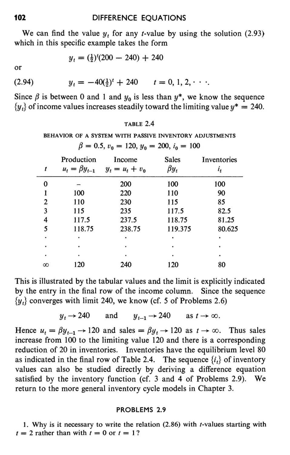
Текст
Introduction
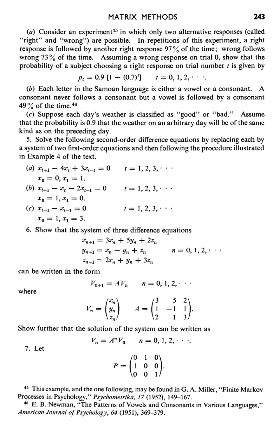
to
Difference
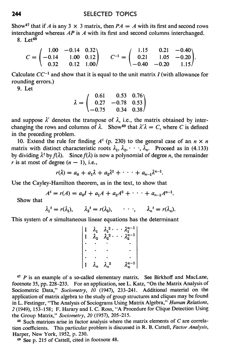
Equations
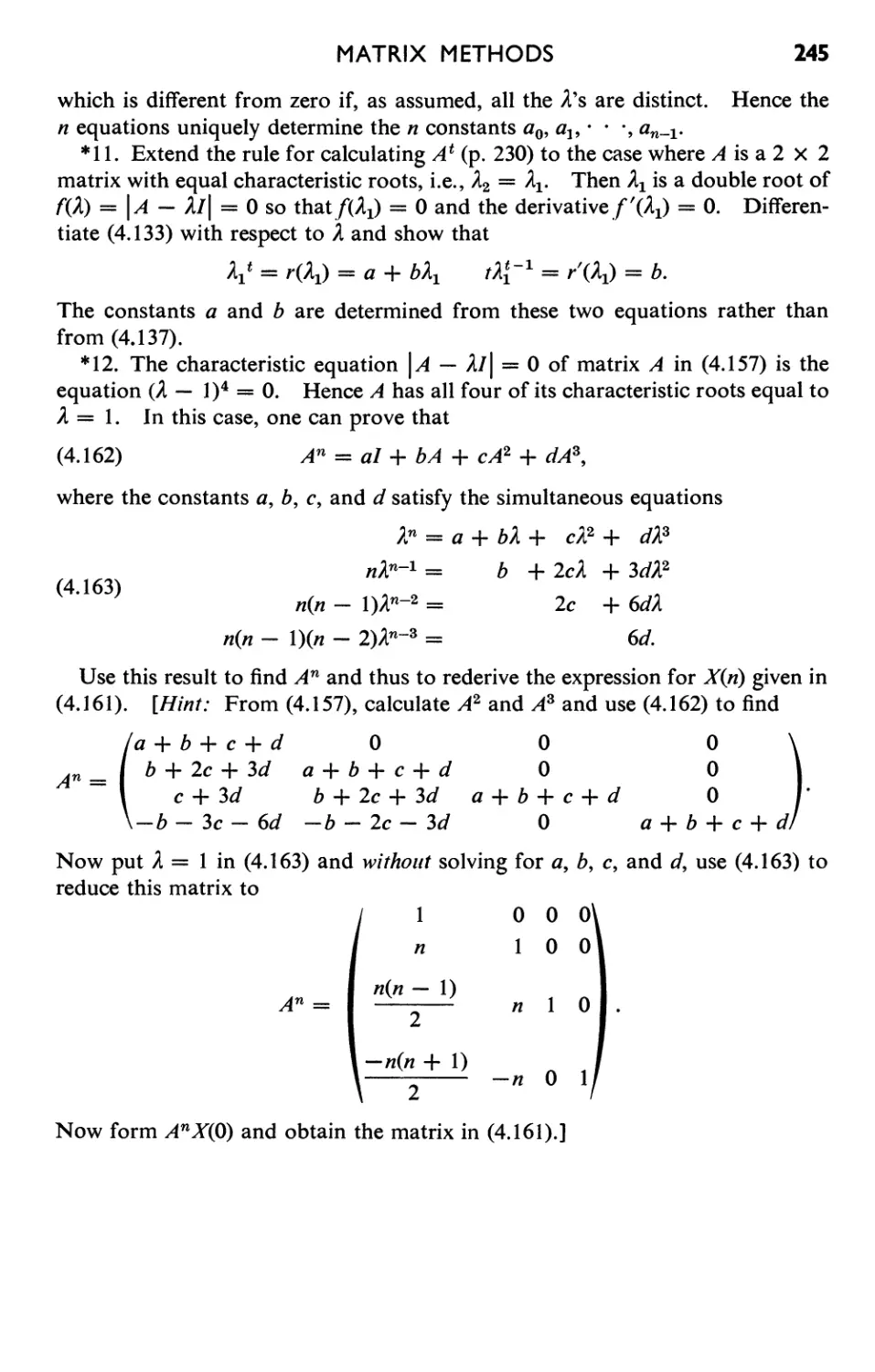
New York
london ·
· John Wiley & Sons, Inc.
Chapman & Hall, limited
Introduction
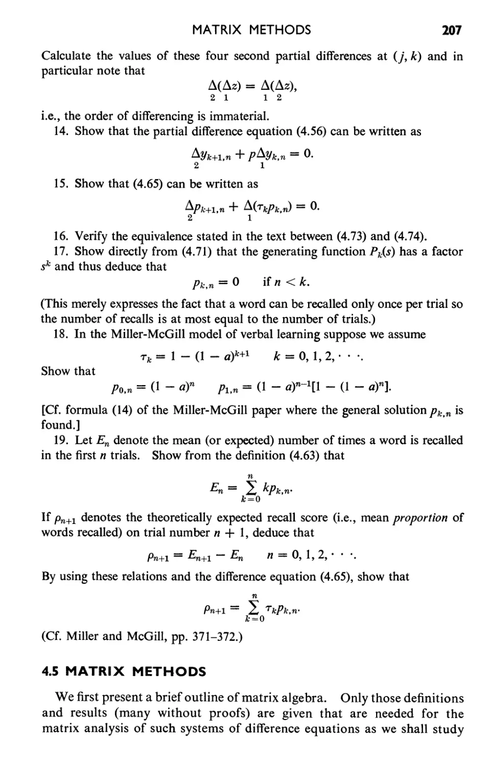
to
Difference
Equations
with illustrative examples from
Economics, Psychology, and Sociology
SAMUEL GOLDBERG
Associate Professor of Mathematics
Oberlin College
Copyright @ 1958
by
JOHN WILEY & SONS, INC.
All rights reserved. This book or any part there-
of must not be reproduced in any form with-
ou t the wri tten permission of the publisher.
Library of Congress Catalog Card Number: 58-10223
Printed in the United States of America
To
Marcia
Preface
This volume is a much expanded and entirely revised version of a
short monograph on difference equations originally written in 1954 at
the invitation of the Social Science Research Council Committee on
the Mathematical Training of Social Scientists. Although I hope it
will find favor with students and teachers of mathematics, this book
is primarily intended for social scientists who wish to understand the
basic ideas and techniques involved in setting up and solving difference
equations. Wherever possible, the mathematical topics in the text are
related to and illustrated by material drawn from the social sciences,
especially economics, psychoiogy, and sociology. Problems for solu-
tion, as well as illustrative examples throughout the text, often have
their source in research papers and books in these fields. References
to this literature are given in footnotes.
Some facility with standard algebraic techniques and an acquaint-
ance with the essentials of trigonometry, together with at least a
modicum of that elusive quality known as mathematical maturity,
should be adequate preparation for reading this book. Such topics
as the summation notation, proof by mathematical induction, the
binomial formula, determinants, polar form of complex numbers, and
de Moivre's theorem-which some readers may recall only faintly-
are briefly reviewed as they are needed in the text. Only four sections
treat special topics requiring some knowledge of material ordinarily
taught in a college course in calculus. These sections (three of which
explore the striking similarities between difference and differential
equations, and the fourth involves infinite series) are starred and are
nei ther used nor referred to in the remainder of the text. Of course,
students whose mathematical training does not extend beyond algebra,
trigonometry, or even a first course in calculus cannot expect to be
introduced to more than a small part of the extensive literature on
difference equations. Happily, however, this small part is quite im-
vii
viii
PREFACE
portant, for it is the foundation upon which the more advanced mathe-
matical theory is built, and it is very widely applied in many fields,
including the social sciences.
In the short introductory Chapter 0 we look at two examples: the
experimental extinction of a learned response, and a multiplier-ac-
celerator interaction process in economic dynamics. Although treated
in greater detail later on, they are introduced here to illustrate how
difference equations (and the need for mathematical methods to ex-
plore the implications of these equations) arise in the context of
social science problems.
Those parts of the calculus of finite differences that are essential to
the main theme of this book are carefully developed in Chapter 1.
The finite difference operators are defined here and their important
properties are elaborated. The function concept is introduced early
and used to the fullest in order to present this material in a way con-
sistent with modern mathematical usage. Readers who prefer to meet
difference equations early in their study program could proceed im-
mediately to Chapter 2, referring back to Chapter 1 as the need arises.
Difference equations are introduced in Chapter 2, where a complete
treatment of the simplest first-order difference equation with constant
coefficients is given. Since the solution of a difference equation is a
sequence, we define sequences of real numbers and carefully introduce
the ideas of limit and convergence. I t is then possible to discuss the
variety of limiting behaviors exhibited by solutions of even this very
simple difference equation. There follow some applications of this
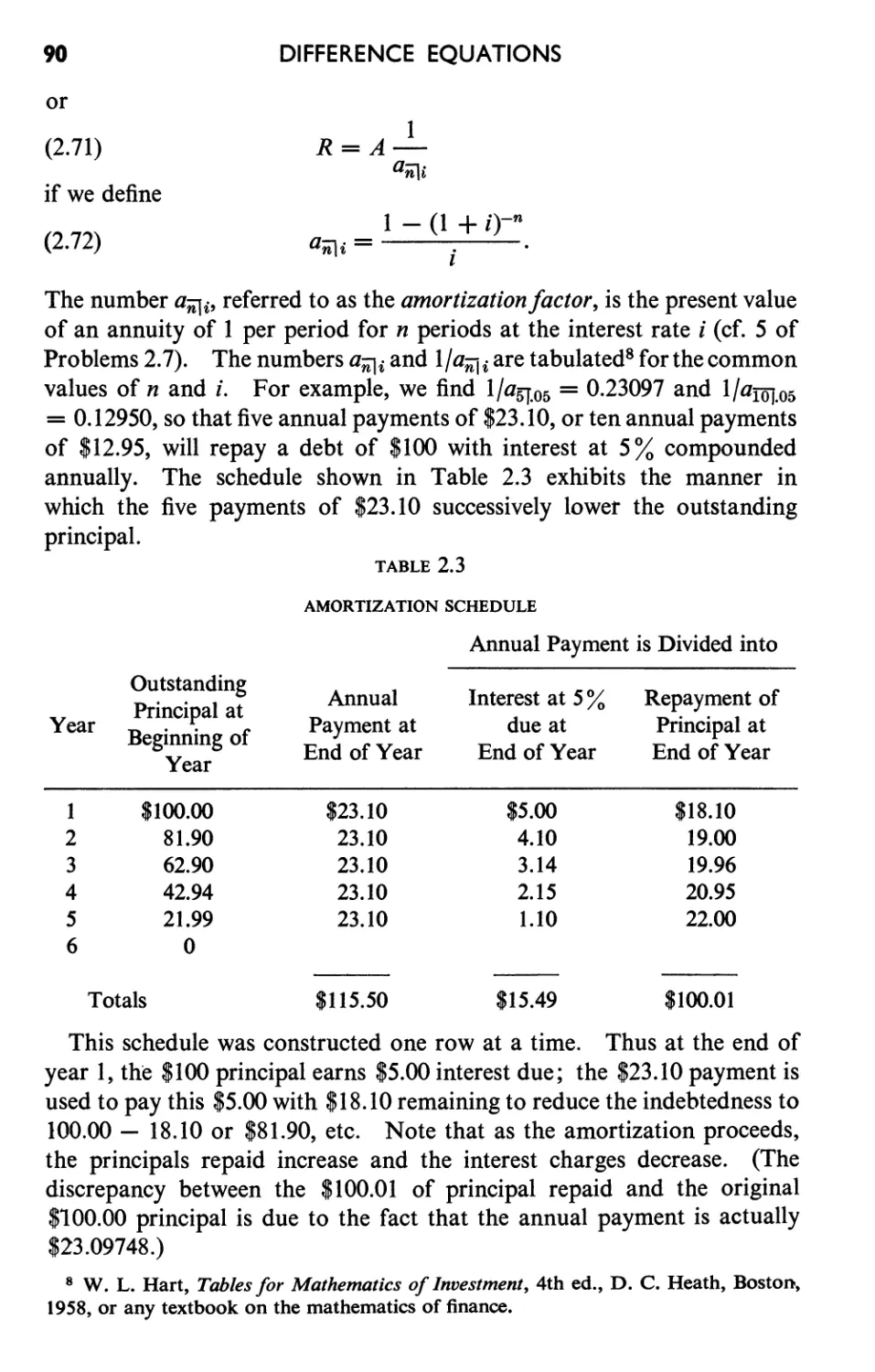
equation in the social sciences: compound interest and amortization
of debts, the classical Harrod-Domar-Hicks model for growth of
national income, Metzler's pure inventory cycle, the Bush-Mosteller
probability model for simple learning, the Bernoulli utility-wealth
relation, and the Weber-Fechner law.
Chapter 3 treats the linear difference equation with constant coef-
ficients. For simplicity, the case of order 2 is discussed in detail
(including the oft-neglected idea of a fundamental set of solutions)
and the methods developed are later carried over to the general case
of order n. Again the important question of limiting behavior of
solutions is discussed and applied to a variety of social science examples.
Chapter 4 consists of five sections, three of which, on equilibrium
values and stability of difference equations, first-order equations and
cobweb cycles, and a boundary-value (or characteristic-value) prob-
lem, are quite brief. One of the two fairly long concluding sections
treats generating functions (with special emphasis on their use in
studying ordinary and partial difference equations) ; the other develops
PREFACE
ix
matrix methods for the solution of systems of simultaneous difference
equations. Although these topics are separately treated and in some
ways unrelated, their inclusion in this final chapter is due to the fact
that they share the following properties: (1) they require no greater
mathematical background than assumed of readers of this book, (2)
they are presently being used in the social science literature, and
(3) aside from their many applications, they are of intrinsic mathe-
matical worth and interest. In addition, the sections on generating
functions and matrix methods open the way for the inclusion of some
introductory material from the field of probability, a mathematical
theory of increasing importance in the social sciences. As usual, the
line had to be drawn somewhere; limitations of space prevented the
treatment of still other topics, such as finite difference interpolation
formulas, functional equations, and approximate solutions of certain
nonlinear difference equations. A selected list of references for further
study follows Chapter 4.
Problems for solution are intended to supplement the worked-out
illustrative examples in the text and to enable the reader to check his
understanding of new definitions, theorems, and methods. A brief
hint or even a concise outline of the procedure to follow in solving the
problem is often given. Answers to a representative selection of about
115 problems (out of a total of over 250) are collected in a separate
section at the end of the book. As mentioned earlier, many problems
are designed to illustrate the application of finite differences and dif-
ference equations in the social sciences. Although I have tried to
select applications that would interest the social scientist, I have made
no attempt to evaluate the worth of these applications. This seems
to me rather in the domain of those whose competence in the applied
fields is considerably greater than mine.
Throughout, stress is laid on the explanation of fundamental con-
cepts and patterns of mathematical reasoning, rather than merely on
techniques of problem-solving. For didactic reasons, it was often felt
desirable to develop mathematical methods in the context of a partic-
ular application, to repeat basic concepts for emphasis, to consider
simplified models at the outset, and to generalize (if possible at the
level of this book) only after a thorough analysis of the simple situ-
ation had been made. For example, many of the important ideas and
methods associated with boundary-value problems are introduced in
Section 4.3 by means of an exhaustive treatment of a fairly simple
particular example. It did not seem appropriate to go into the general
theory in this volume, but the value of having studied this section
will be apparent to a reader pursuing the subject in a more advanced
x
PREFACE
work. Similarly, a good deal of the material on matrix methods in
Section 4.5 is presented in the context of some problems leading to
a system of two simultaneous difference equations. The consequent
limitation to 2 X 2 matrices makes the material easy to grasp; never-
theless it allows immediate extension to more general systems. I
am hopeful that such procedures will make this book more appealing
and understandable to the mathematically oriented social scientist.
Students of mathematics will also find this volume of some interest,
for two reasons. First, this introduction to difference equations may
be of value in promoting an increased awareness on the part of such
studen ts for the applications of mathematics in the social sciences.
The second and more weighty reason stems from the fact that some
very important mathematical ideas (such as function, operator, con-
vergence, fundamental set of solutions, generating function trans-
formation, characteristic value, and matrix) are carefully introduced
here in a fairly simple and intuitive context. I t should be helpful
for a student to learn about them first in this form, without the analytic
difficulties usually accompanying them in later, more advanced courses.
It is with genuine appreciation that I here express my thanks to the
following individuals who have read one or another of the preliminary
versions of the manuscript and who were kind enough to send me their
criticisms and suggestions for improvement: R. R. Bush, C. Christ,
W. G. Madow, G. A. Miller, F. Mosteller, H. Raiffa, P. A. Samuelson,
P. M. Solow, G. L. Thompson, and R. M. Thrall.
Comments from readers are always welcome.
SAMUEL GOLDBERG
Oberlin, Ohio
March 1958
Contents
o Introduction
1 The Calculus of Finite Differences
1.1 The First Difference Function 9
1.2 Second and Higher Differences 18
1.3 The Operator E 21
1.4 Some Properties of d and E 24
1.5 Equivalence of Operators 34
1.6 Indefinite Summation: The Operator d- 1 41
* 1.7 Analogies between the Difference and Differential Cal-
culus 46
2 Difference Equations
2.1 Basic Definitions 50
2.2 Solutions of a Difference Equation SS
2.3 An Existence and Uniqueness Theorem 60
/2.4 The Equation Yk+l = AYk + B 63
2.5 Sequences 69
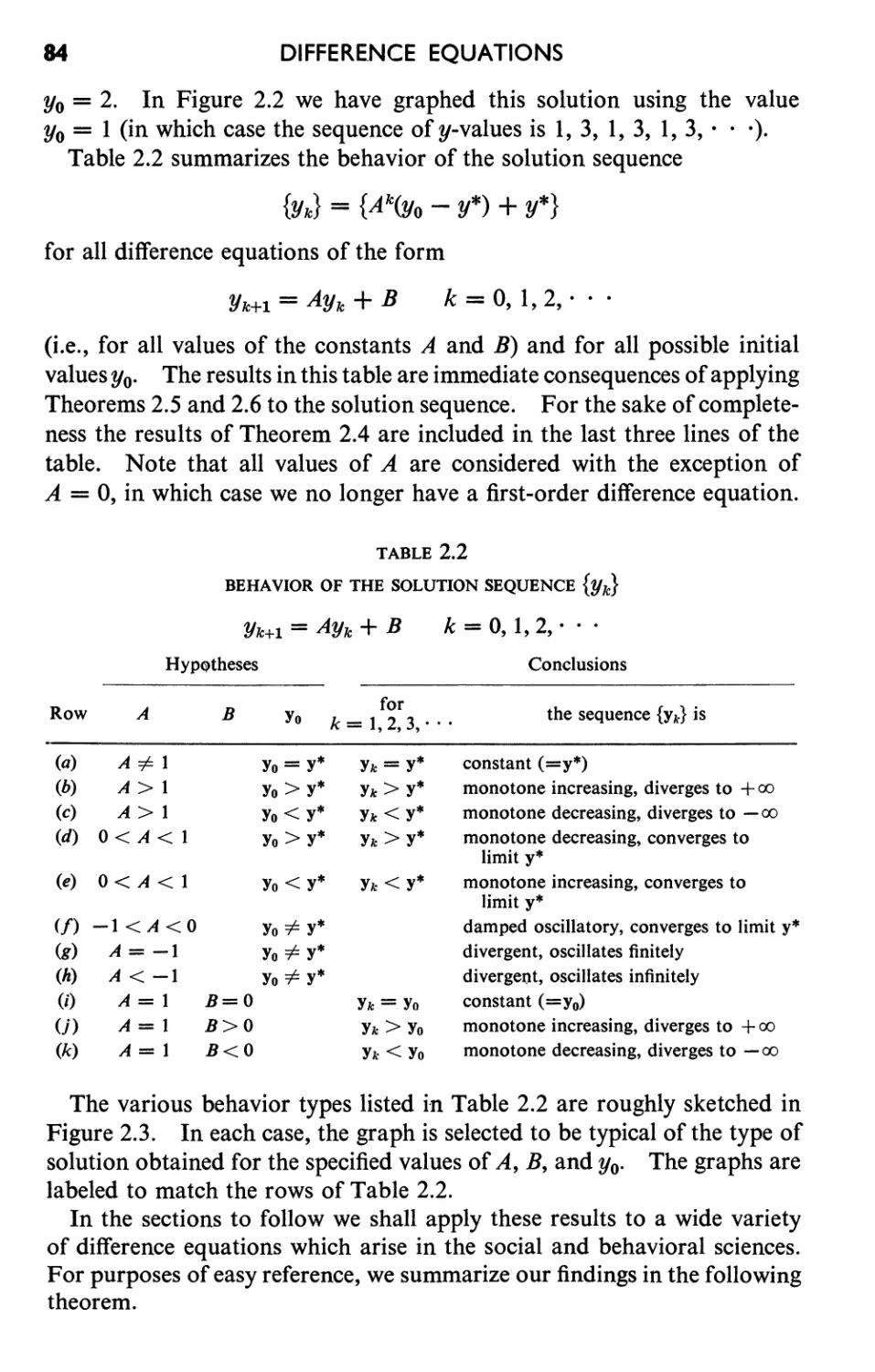
2.6 Solutions as Sequences 77
2.7 Simple and Compound Interest 87
2.8 Economic Dynamics 93
2.9 Inventory Analysis 98
2.10 A Probability Model for Learning 103
2.11 Geometric Growth 110
* 2.12 Approximating a Differential Equation by a Difference
Equation 116
1
9
50
3 Linear Difference Equations with Constant Coefficients 121
3.1 Some Basic Theorems 121
3.2 Fundamental Sets of Solutions 128
xi
xii CONTENTS
3.3 General Solution of the Homogeneous Equation 134
3.4 Particular Solutions of the Complete Equation 143
3.5 Limiting Behavior of Solutions 148
3.6 Illustrative Examples from the Social Sciences 153
3.7 The General Case of Order n 163
* 3.8 Linear Differential Equations with Constant Coeffi-
cients 167
4.1
4.2
4.3
* 4.4
4.5
.4 Selected Topics
Equilibrium and Stability 169
First-Order Equations and Cobweb Cycles
A Characteristic-Value Problem 184
Generating Functions 189
Matrix Methods 207
176
Selected References
Answers to Problems
Index
169
246
248
255
@
Introduction
Problems in which some variable may conveniently be assumed to have
only a discrete set of possible values often lead to mathematical models
involving difference equations. In economics, for example, such a variable
is time. The values of important economic quantities (income, savings,
consumption, etc.) are ordinarily available at certain uniformly spaced
time intervals. Data may be accumulated each month, quarter, year, or
even each 10 years, as in the national census. All quantities are dated,
each with the time period for which it applies. Thus we may speak of
the national income at some initial time, which we choose to denote by
t = 0, and then at the end of the next time period, at t = 1, and then 'at
t = 2, etc. The economist, in what is called period analysis, studies the
behavior of national income, and other ecoJIomic variables, over this
discrete set of time values. We shall see that an important ingredient of
this analysis is the difference equation.
As a second example, consider free-recall verbal learning experiments in
which a list of words is read aloud to a subject who is then asked to write
down all the words he can recall. This constitutes one trial of the total
experiment. Then the order of the words is randomized and the procedure
is repeated, thus completing the second trial. At each trial we may com-
pute the proportion of words recalled by the subject. The experiment,
continued until this proportion is approximately equal to its ultimate
stable value, yields the values of the proportion of words recalled in trial
number 1, in trial number 2, etc. The psychologist is interested in studying
the properties of this sequence of values. In this case, the discrete variable
is the trial number and once again a difference equation may be expected
to be a helpful mathematical tool.
In panel surveys in sociological investigations, a fixed group of people
(the panel) may be asked the same set of questions at periodic time intervals,
say at the end of each of the 6 months preceding an election. Here we
1
2
INTRODUCTION
have a first poll, then a second, a third, etc., and one studies a person's
responses as a function of the poll number. The existence of this discrete
variable, assuming the integer values 1 to. 6 in the example cited, allows the
use of a difference equation model for the study of such data.
A large number of illustrative examples of this kind, all leading to a
mathematical analysis involving difference equations, will be given in this
book. Difference equations have appeared, and continue to appear, in
the literature of the social and behavioral sciences. Before developing
the mathematical theory of such equations, it might be well to consider
one or two examples in greater detail. Our only aim here is to point out,
without regard for mathematical niceties, how a difference equation can
arise in connection with problems of the social sciences. The crucial
problems of justifying the assumptions to be made and of testing the useful-
ness of this particular mode of analysis in the social sciences are not within
our purview. These are problems for the social scientist, not the
mathematician.
Example 1
Let us suppose that a subject is introduced into the following over-
simplified learning situation: (I) a stimulus is presented, (2) the subject
mayor may not react to this stinlulus, but (3) if he does respond positively,
he is by some means discouraged from repeating this response. To fix
ideas, consider the example in which a rat, previously perfectly conditioned
to running a straight runway to find food at its end, is placed in the
starting box. In a specified subsequent time interval (long enough to
permit completion of the run, but not long enough to allow dawdling along
the way) the rat either makes the complete run or does not. Ifhe does, he
is disappointed to find that the food reward is no longer present. Let us
call the completion of the run in the allotted time a positive response.
After this trial run, the rat is once again placed in the starting box and
another trial takes place. In this way the rat is subjected to many
repeated trial runs, each of which mayor may not result in a positive
response. If we imagine a large number of rats similarly, but indepen-
dently, used as subjects in these repeated runway trials, then we can compute
the proportion of rats responding positively in trial numbe 1, in trial
number 2, etc. Intuitively, we expect that the response of running to the
end of the runway in the fixed allotted time interval will be extinguished
owing to the absence of reward and that this "learning" will manifest
itself in an ever-decreasing proportion of the rats who respond positively.
Now it actually turns out to be more convenient for the mathematical
model to study a subject's probability of making a positive response, rather
than the proportion of positive responses in a large group of subjects. (Of
INTRODUCTION
3
course, when using this probability model one ordinarily takes this
empirical proportion as an estimate of the theoretical probability. The
reader may, if he chooses, think of proportion, expressed in decimal form,
rather than probability.) This probability is 0 if the response is never
made, is I if the stimulus always elicits a positive response, and generally
is some number between these extreme values. Since the subject learns
as the experimental trials are run, the probability of a positive response
will change from trial to trial. So we let n assume the integral values
0, I, 2,. · · (to represent the trial number) and then define Pn as the prob-
ability of a positive response in trial number n. We thus have a sequence
of probabilities Po, PI' P2, · · · describing the behavior of subjects in
repeated trials of the kind delineated.
A subject's behavior will depend on his conditioning before the experi-
ment. The symbol Po denotes the initial probability of a positive response
before the first trial. Thus Po = 1 would be interpreted as perfect condi-
tioning toward the positive response; a subject equally disposed toward
positive and negative responses would be assigned the value Po = 0.5.
If the probabilities change from trial to trial, we must specify the way
in which they vary. Since we want the probabilities to decrease as the
subject learns, we require that (Pn+I - Pn) be negative for n = 0, 1, 2,. · ..
If we introduce the notation Llpn = (Pn+I - Pn) for the difference in prob-
ability of positive response in trials nand (n + 1), we may write this
assumption as follows:
(i)
Llpn < 0
n = 0, 1, 2,. · ..
Now assumption (i) clearly gives us too much leeway. We need to know
not only the direction of change in probabilities but also its magnitude.
For this purpose we choose the following simple assumption: the prob-
ability of a positive response in any trial is a fixed fraction, say {3, of this
probability in the preceding trial. Written in symbols, we assume
PI = {3po, P2 = {3PI' · · ., or
(ii)
Pn+I = {3Pn
n = 0, 1, 2,. · ..
Since the probabilities must remain between 0 and 1, we require that
(iii)
o < {3 < 1.
Assumption (ii) may be written in the form
Pn+I - Pn = {3Pn - Pn = (1 - fJ)( -Pn)
or
(iv)
Pn = (1 - {3)( -Pn).
4
INTRODUCTION
Formula (iv) may be translated as follows: the actual decrease in prob-
ability in going from any trial to the next, Pn' is a fixed fraction, (1 - fJ),
of the maximum possible decrease, -Pn. (Note: if the probability is Pn
and cannot fall below 0, then the maximum possible decrease is 0 - Pn
or -Pn.) Assumptions (ii) and (iv) are different ways of saying the same
thing; either expresses the precise way in which the probabilities Pn are
postulated to vary from trial to trial. The relation in (ii) or equivalently,
in (iv), is a difference equation. We shall use the form in (ii) for our
analysis.
If we have a subject with initial probability Po, then (ii) tells us, with
n = 0, that
(0.1 )
Pl = fJpo.
Now we may use (ii) again, with n = 1, to obtain P2 = fJpl. With the
aid of (0.1) this becomes
(0.2)
P2 = fJ2pO.
Similarly, we may put n = 2 in (ii) and then use (0.2) to obtain
(0.3)
P3 = fJp2 = fJ3pO.
Inspection of (0.1) through (0.3) leads us to conjecture that
(0.4)
Pn = fJnpo
n = 0, 1, 2,. · .,
and indeed our later work will actually prove that (0.4) is the unique
solution of the difference equation (ii) with Po prescribed. For the
present, we take this fact as reasonable, even if not rigorously proved.
Equation (0.4) relates the subject's probability of making a positive
response to three variables: n, the number of times the subject has found
himself in this stimulus situation; Po, the probability of a positive response
before the experiment begins; and fJ, the measure of the extent to which
a positive response in any trial lowers the probability of a similar response
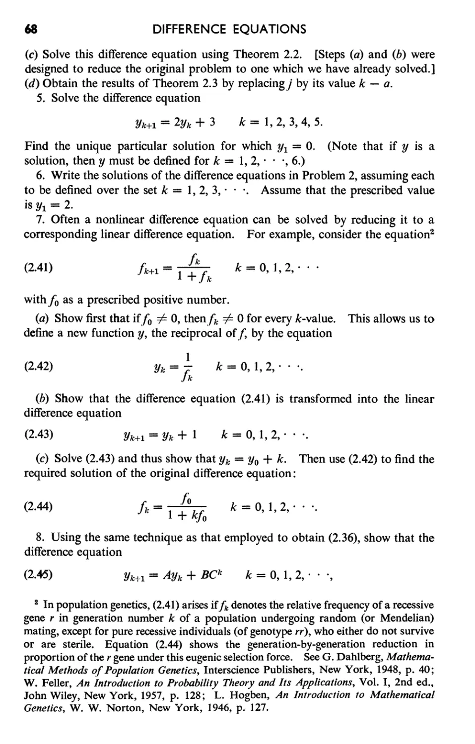
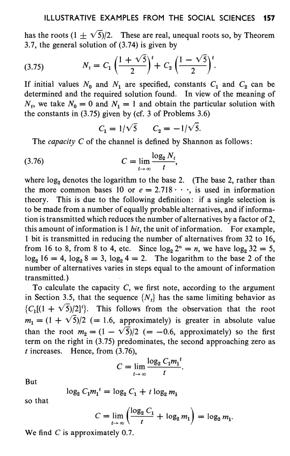
in the following trial. For example, if Po = 1 and fJ = 0.6, then
(0.5)
Pn = (0.6)n
n = 0, 1, 2,. · · ,
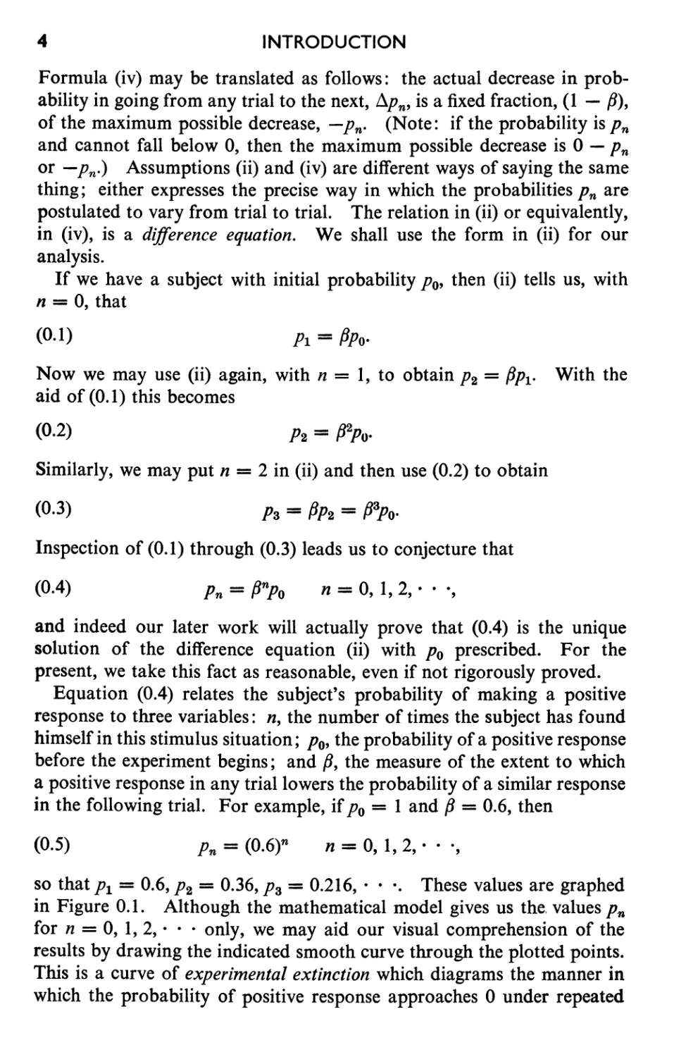
so that Pl = 0.6, P2 = 0.36, P3 = 0.216, · ... These values are graphed
in Figure 0.1. Although the mathematical model gives us the, values Pn
for n = 0, 1, 2,. · · only, we may aid our visual comprehension of the
results by drawing the indicated smooth curve through the plotted points.
This is a curve of experimental extinction which diagrams the manner in
which the probability of positive response approaches 0 under repeated
INTRODUCTION
5
trials in the absence of reward. Such a curve may be drawn for each pair
of values of Po and f3.
The problem of how to estimate the values of Po and f3 appropriate for a
given experimental situation, as well as the problem of testing the useful-
ness of this particular analysis for summarizing data or for predictive
purposes, are outside the scope of this work. These problems, together
1.0
:c
ro
.c
o
a..
0.5
00 1 2 3 4 5
Trial number n
Figure 0.1
with a careful development of more elaborate probability models for
learning, are treated in the recent book by R. R. Bush and F. Mosteller.
References may be found in Section 2.10, where we study a more general
difference equation model for learning.
Example 2
This economic example is concerned with the study of national income
and its variation in time. National income, in any accounting period, is
made up of three components: (1) consumer expenditures (for purchase
of so-called consumer goods), (2) induced private investments (for buying
capital equipment, e.g., machinery used to increase production), and (3)
government expenditure. Let us introduce symbols for these quantities
as follows: Yt:;c national income, C t = consumer expenditure, It = in-
induced private investment, G t = government expenditure. The sub-
script t identifies the accounting period for which the variable is evaluated.
We assume that data are available for equal periods, say annually, and
let t take on the values 1, 2, 3,. · ., denoting the first, second, third,. · .,
of these periods. Our discussion so far leads to the accounting equation
(0.6) Y t = C t + It + G t .
6
INTRODUCTION
Following Samuelson,l we now make three additional assumptions
relating these variables.
(i) Consumption expenditure (in any period) is proportional to the
national income of the preceding period.
(ii) Induced private investment in any period is proportional to the
increase in consumption of that period over the preceding (the so-called
acceleration principle).
(iii) Government expenditure is the same in all periods.
Our problem is to analyze the behavior of national income subject to
these conditions. We proceed by first restating the assumptions mathema-
tically and then attempting to derive a single equation in which all variables
but the national income are eliminated. This attempt will succeed and
the resulting difference equation will enable us to study the national
income as a function of time. With this as our program, we now proceed
with the details.
The (positive) constant of proportionality in (i), denoted by ex, is called
the marginal propensity to consume. We therefore translate (i) by the
equation
(0.7)
C t = exY t - l .
Note that we have a one-period lag between income and consumption as
indicated by the subscripts in (0.7).
The (positive) constant of proportionality in (ii), denoted by f3, is called
the relation. Since the increase in consumption is given by the difference
(C t - C t - 1 ), we rewrite (ii) in the form
(0.8)
It = f3(C t - C t - 1 ).
{If consumption is decreasing, then (C t - C t - l ) < 0 and therefore
It < o. This may be interpreted as a withdrawal from funds committed
for investment purposes, for example, by not replacing depreciated
machinery.]
Finally, since we are assuming in (iii) that government expenditure is
the same in each period, we may as well choose our units so that this
expenditure is equal to 1. Then
(0.9)
G t = 1
and equations (0.6) through (0.9) embody all our assumptions.
1 P. A. Samuelson, "Interactions Between the Multiplier Analysis and the Principle
of Acceleration," Review o.f Economic Statistics, 21 (1939), 75-78; reprinted in Readings
in Business Cycle Theory, Blakiston Co., Philadelphia, 1944.
INTRODUCTION
7
To derive a single equation for national income, we start with (0.6)
and use the other relations to obtain
Y t = Y -l + (3(C t - C t - 1 ) + 1
= Y t - 1 + (3( Y t - 1 - Y t - 2 ) + 1.
Algebraic simplification prpduces the difference equation for national
Jncome:
(0.10)
Y t = (1 + fJ) Y t - 1 - (3 Y t - 2 + 1.
This difference equation, relating the national income in any period to
the national income of the two preceding periods, contains two para-
meters: the marginal propensity to consume, , and the relation, (3.
Assume now that two initial values of the national income are given, say
Y 1 = 2 and Y 2 = 3, and consider some special cases.
If ex = 0.5 and (3 = 1, then (0.10) becomes
(0.11 )
Y t = Y t - 1 - 0.5 Y t - 2 + 1.
Putting t = 3 and using our initial values, we obtain
Y 3 = Y 2 - 0.5 Y 1 + 1 = 3 - (0.5)(2) + 1 = 3.
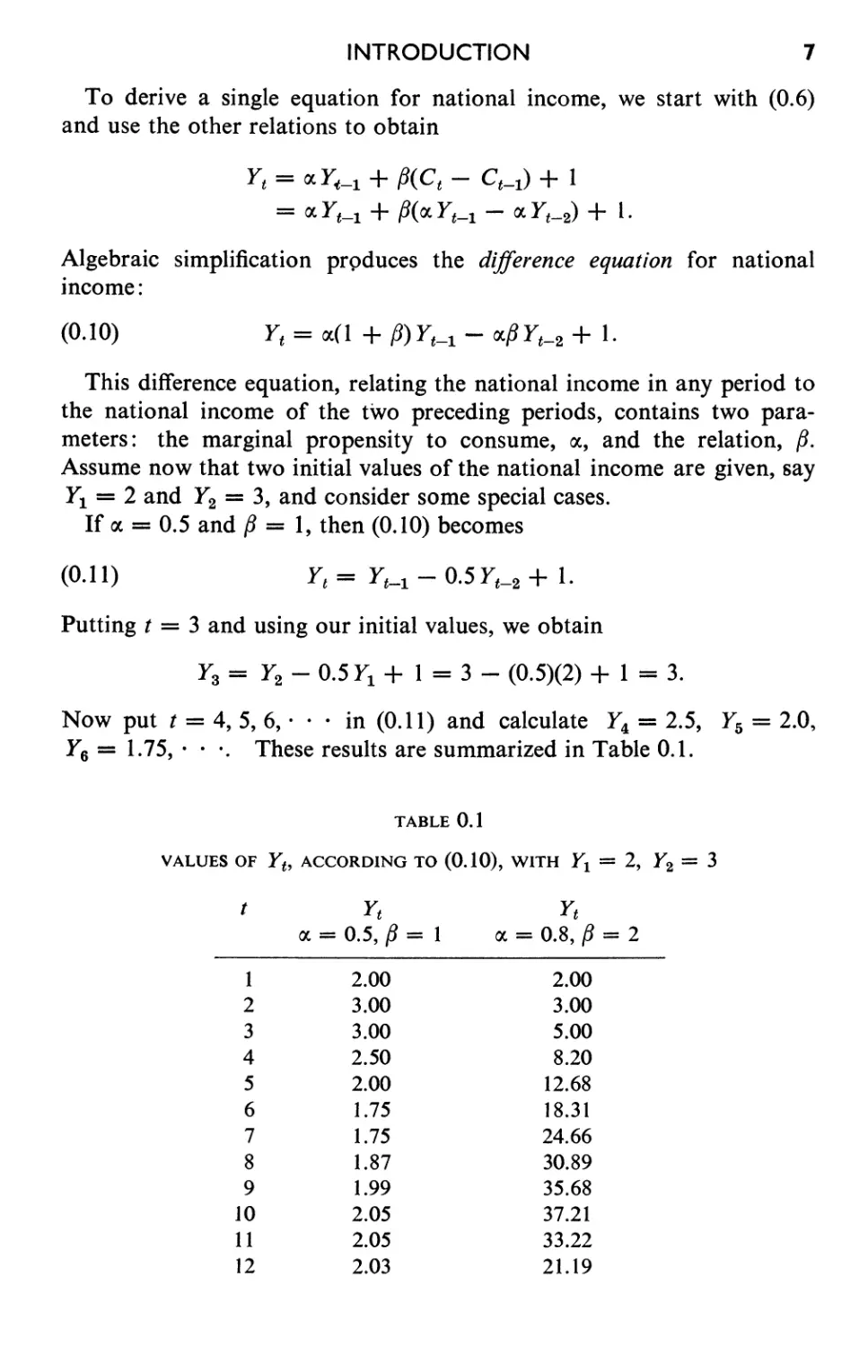
Now put t = 4, 5, 6,. · · in (0.11) and calculate Y 4 = 2.5, Y s = 2.0,
Y6 = 1.75, · · .. These results are summarized in Table 0.1.
TABLE 0.1
VALUES OF Yf, ACCORDING TO (0.10), WITH Y 1 = 2, Y 2 = 3
t
Y t
= 0.5, (3 = 1
2.00
3.00
3.00
2.50
2.00
1.75
1.75
1.87
1.99
2.05
2.05
2.03
1
2
3
4
5
6
7
8
9
10
11
12
Y t
= 0.8, (3 = 2
2.00
3.00
5.00
8.20
12.68
18.31
24.66
30.89
35.68
37.21
33.22
21.19
8
INTRODUCTION
If we consider the case (X = 0.8 and fJ = 2, then (0.10) becomes
Y t = 2.4Y t - 1 - 1.6Y t - 2 + I
and with the same initial values of Y 1 and Y 2 , we now compute Y a = 5,
Y 4 = 8.2, · · .. The first 12 values of Y t are given in the last column
of Table 0.1.
It seems that in both cases we have oscillatory behavior of the national
income, the oscillations being greater in the second of the two numerical
examples. But surely we have not convinced ourselves of this fact from
a sequence of 12 values in each case. Is it not possible that in one of these
cases, or in both, the national income stops oscillating at some time and
begins a steady decrease or increase? It is clear that no table, however
far extended in time, will be able to prove that the behavior already observed
will continue. And, granting for the moment that we are certain of the
behavior of Y t when (X = 0.5 and f3 = 1, how does national income vary
with time when (X = 0.4 and f3 = I? And in what way does this behavior
depend on the initial values prescribed for Y 1 and Y 2 ? To answer these
questions, we must return to the difference equation (0.10) and use mathe-
matical t chniques which will enable us not only to identify the various
possible.behaviors of national income as time goes on but also to determine
the values of (X and f3 for which each of these behaviors occurs. This
analysis will, for example, enable us to prove that if (X = 0.5 and f3 = 1,
then if Y 1 and Y 2 are not both equal to 2, Y t undergoes damped oscillatory
motion which approaches the income value 2 as time increases, whereas
for (X = 0.8 and (3 = 2, the income undergoes greater and greater oscilla-
tions as t increases. Nonoscillatory income behaviors are also possible
for suitable values of (X and f3. We shall return to these considerations in
Chapter 3, after having developed the necessary mathematical techniques.
In this second example, as in the first, our only concern has been to
point out two facts: difference equations arise in the mathematical
description of social science problems and mathematical techniques are
required in order to answer relevant questions concerning the variables
under analysis. The following chapters develop some elementary parts
of the theory of difference equations. Wherever possible, illustrative
material and exercises are selected to illustrate the applications of this
theory to problems in the social sciences.
a
The
Calculus
of
Finite
Differences
1.1 THE FIRST DIFFERENCE FUNCTION
Before studying difference equations and their solutions, it is necessary
to introduce the basic operations of the calculus of finite differences and
to explore some properties of the corresponding difference operators.
These tasks, in turn, require some background concerning the fundamental
mathematical ideas of function and graph.
The study of relations among variables is a fundamental concern of all
sciences. One particular kind of relation, the functional relation, is
singled out here because of its major importance. Let us first consider
an example or two. Given a positive real number x, denote by A(x) the
area of the square having a length of side equal to x. Then the equation
A(x) = x 2 is a means of stating a rule by which we associate with each
positive number x (representing length of side) another positive number
A(x) (representing the corresponding area). The rule is very simple in
this case: to find A(x), merely square the number x. That is,
A(2) = 2 2 = 4,
A(1.3) = (1.3)2 = 1.69, etc.
Tables and graphs are other common means of indicating functional
relationships. For example, the first two columns of Table 0.1 tell us
the number (representing national income) to assign to each of the first
12 positive integers (the t-values).
9
10
THE CALCULUS OF FINITE DIFFERENCES
The definition which follows makes precise our understanding of the
common properties of these examples:
DEFINITION 1.1. A function is specified when we are given a set of
numbers (the domain of the function) together with a rule by which one and
only one number is associated with each number in the domain. The value
of a function for (or at) the number x is that number which the rule assigns
to x. If the function is denoted by y, the value of y at x is denoted by
y(x) or Yx.
A function may usefully be thought of as a machine for which two
characteristics are known: (1) the collection of x-values that can be used
as inputs of the machine, and (2) the operating rule by which the machine
converts any input value to its corresponding output value.
It is important to keep clearly in mind the distinction between the func-
tion itself, denoted by y, and the numerical value, denoted by y(x) or Yx,
which the function rule assigns to a number x.
In our mathematical discourse we shall usually use x to represent a
number in the domain of a function. However, when these numbers are
to be interpreted in some particular way, we choose more natural notation.
So, for example, we use t to represent a number in the domain when it is
to be interpreted as a value of time, C in an economic example in which
the numbers in the domain represent consumer expenditures, etc.
The functions we shall deal with are all fairly simple. In particular,
the domain of our functions will usually be clear from the context and we
shall therefore be able to specify a function by stating only the rule which
assigns exactly one number to each element in the domain. Almost
always, this rule will be specified by an equation. We agree, unless
explicitly stated otherwise, to consider the domain as the largest set of
numbers for which the rule is applicable, remembering that we are limited
to the aggregate of real numbers. 1
Examples
(a) Let y be the function which assigns to each real number x the constant 2,
i.e., y(x) = 2. Such a function, whose value is the same for all numbers in its
domain, is called a constant function.
(b) Let p be the function which assigns to each nonnegative integer n the
number (0.6)n. Then with pn denoting the value of p at n,
pn = (0.6)n n = 0, 1, 2,. . ·
which we interpreted (p. 4) as the probability of a positive response in the nth
of a series of experimental learning trials.
(c) Let y be the function specified by the equation
(1.1) y(x) = kx
1 See E. G. Begle, Introductory Calculus, Henry Holt, New York, 1954, p. 44.
THE FIRST DIFFERENCE FUNCTION
11
where k is some arbitrary number (positive, negative, or zero). The domain of
y is understood to be the set of all real numbers unless some other domain is
indicated. The value of Y when x = 1 is y(l) = k. Similarly, y(2) = 2k,
y(3) = 3k,. . .. No matter what the value of k, any two nonzero values of y
have the same ratio as the corresponding x-values. The proof of this statement
is given by the equations
y(x 1 ) _ kX 1 _ Xl
y(x 2 ) - kX 2 - x 2 .
Because of this property, y is said to be proportional to x and k is called the
constant of proportionality.
If we know that y is proportional to x, this means that for all x-values in the
domain of the function y, there is some number k for which (1.1) holds. Addi-
tional information, such as a known pair of values, x and y(x), is required to
determine the particular value of the constant k. For example, let y(x) denote
the time required to read x pages in this book. To say that y is proportional to
x (or, in words, that total reading time is proportional to pages read) means that
(1.1) holds. (Here x might sensibly be restricted to the integers 0, 1, 2,. · ..)
If we are now told that it takes 9 minutes to read 1 page, then y(l) = k · 1 = 9,
so k = 9 and y(x) = 9x. It follows that 2 pages require 18 minutes reading
time, etc.
Often a slight generalization of these ideas is needed. If YI and Y2 are two
functions defined for the same set of x-values, and if there is some number k
(the constant of proportionality) such that
YI (x) = kY2(X)
for all x-values in the common domain of these functions, then we shall say that
Yl is proportional to Y2. For example, if C(x) denotes consumption expenditure
and Y(x) denotes income in month x (here x could be restricted to the values
1, 2, 3,. · .), then the a sumption that consumption is proportional to income
would be translated by the equation C(x) = k Y(x) for some constant k.
It is often helpful to have a pictorial representation or graph of a func-
tion. The framework for such a picture is a coordinate system, established
when one chooses a horizontal x-axis, a vertical y-axis, and an arbitrary
distance to serve as a unit of measurement along each axis. Any point on
the x-axis to the right of the origin (the point of intersection of the axes)
is assigned the positive number of units in the interval from the origin to
the point. Points on the x-axis to the left of the origin are assigned the
corresponding negative numbers. Similarly, one associates real numbers
with the points on the y-axis, agreeing to assign positive numbers to
points above the origin and negative numbers to those below. The
origin itself is assigned the x-value 0 and the y-value o. It is possible to
show that (on each axis) each point is given one and only one real number
and each real number is assigned to one and only one point.
Now if P is any point in the plane, we proceed as follows to identify
it with two numbers. Let a vertical line be drawn through P. The
12
THE CALCULUS OF FINITE DIFFERENCES
intersection of this line with the x-axis determines a point whose x-value
is defined to be the x-coordinate (or abscissa) of P. Similarly, a horizontal
line through P determines a point on the y-axis whose y-value is the
y-coordinate (or ordinate) of P. By this procedure, each point in the
plane is assigned a pair of real numbers (x, y), and, conversely, each pair
of real numbers corresponds to one and only one point. The coordinates
of a point are always written in the form (x, y) with the x-coordinate first
and then the y-coordinate. Thus (3, 2) denotes the point reached by
moving (from the origin) 3 units to the right on the x-axis and then 2 units
up in the vertical direction; moving (again from the origin) 1 unit to the
left and 5 units down yields the point ( -1, - 5). The origin is assigned
the coordinates (0, 0). In this way, a one-to-one correspondence is
established between the set of points in the plane and the set of ordered
pairs of real numbers. This correspondence is the basic idea of plane
analytic geometry.
With these preliminaries understood, we can now make the following
definition: the graph of a function consists of all those points in the plane,
and only those points, whose y-coordinate is the value 0.1. the function at the
x-coordinate; i.e., the graph of the function y is the totality 0.( points whose
coordinates are of the form (x, Yx)' where x is a number in the domain of y.
Examples
(a) For the constant function given by the equation y(x) = 2, we know that
points of the form (x, 2) constitute the graph of the function. Thus, no matter
what the x-value, we must go up 2 units and the point (x, 2) is on the graph.
This graph is a horizontal line 2 units above the x-axis. The graph of any
constant function, say y(x) = k, is a horizontal line above (if k > 0) or below
(if k < 0) the x-axis. The x-axis itself is the graph of the function whose value
is zero for every x.
(b) For the function given by y(x) = x + 1, we may plot the points (0, 1),
(1, 2), (2, 3), (-1, 0), all of which lie on the graph since the y-value in each case
satisfies the defining equation. The graph of y is the straight line which meets
the y-axis 1 unit above the x-axis, Le., at the point (0, 1), and rises 1 unit for each
unit increase in x. (The reader should note that no finite set of points, however
many are plotted, can prove this last statement. The proof is given in any
analytic geometry textbook.)
(c) If y(x) = kx, then the graph of the function y is a straight line passing
through the origin and rising (if k is positive) or falling (if k is negative) k units
per unit increase in x. If k = 2, for example, we may plot the points (0, 0),
(1, 2), (2, 4), (-1, -2), etc. For k = -3, the points (0,0), (1, -3), (2, -6),
and (-1, 3) are all on the graph of y.
(d) If Y is a function whose value for any real number x is given by
(1.2) Yx = mX + b
where m and b are arbitrary constants, then y is said to be a linear function of x.
This terminology is due to the fact that the graph of a linear function of x is a
THE FIRST DIFFERENCE FUNCTION
13
straight line. Since Yo = b, this line intersects the y-axis at the point (0, b),
b units above (or below if b is negative) the x-axis. For this reason the number
b is called the y-intercept of the straight line. Also
YX+l = m(x + 1) + b = mx + m + b = Yx + m
so that a unit increase in x always produces a change of m units in the correspond-
ing y-value. If m is positive, the straight line rises as x increases; if m is negative
it falls as x increases; if m = 0, the line is horizontal. The number m is the
slope of the straight line. A line is completely specified by giving both its
y-intercept and slope. To say that y is a linear function of x is to say that there
is some y-intercept b and some slope m for which (1.2) hold . Note the special
cases (a) m = 0, b = 2, (b) m = 1, b = 1, (c) m = k, b = 0, already considered.
(e) We have already graphed the function p given by pn = (O.6)n for n =
0, 1, 2,. · .. The graph (Figure 0.1) actually consists of only the discrete
points obtained for n = 0, 1, 2,. · · but we drew a smooth curve through these
points, as if the domain of the function was extended to the set of all real non-
negative values of n.
Very often we are given some function and are interested in studying
changes in the value of the function as we move from one number to
another in its domain. For example, in the learning experiment of
Chapter 0, where Pn denotes the probability of a positive response in trial
number n, we are interested in some measure of the amount of learning
that takes place in each trial run. We may define a new function whose
value at n is given by the difference between the probability of a positive
response in trial n + 1 and trial n. Since this new function is related to
p, we call it IIp so that (with Ilpn as the value of IIp at n)
Ilpn = Pn+1 - Pn.
The number IlP1 is the change in probability of positive response in going
from trial 1 to trial 2, IlP2 is the corresponding change in going from
trial 2 to trial 3, etc.
As another example, if y denotes a population function, with y(x) being
the size of the population in census year x, we may define a new function
whose value at x is the difference between the population size in years
x and x + 10. Since this new function is related to y, we call it y,
so that [with Ily(x) as the value of Ily at x]
Ily(x) = y(x + 10) - y(x).
Ily(x) is the change in population size in the two consecutive census years
x and x + 10. If the population has increased, then y(x) > 0; if the
population has declined, then y(x) < 0; if the population size is
unchanged, then y(x) = o.
14
THE CALCULUS OF FINITE DIFFERENCES
Similarly, if C is the function whose value at t is denoted by C t , then
we may define another function C by specifying that its value at t is the
difference (C t + 2 - C t ). If the value of C at t is denoted by Ct, then
Ct = C t + 2 - C t
and we may choose to interpret ihis as the difference between consumer
expenditures in the 2-year interval between periods t and t + 2.
In the first of these examples our difference interval was 1, in the second
10, in the third 2. This interval may be any number provided both the
y-axis
h
y(x+h)
x
x+h
x-axis
Figure 1.1
initial and final values at which the function is to be evaluated are in its
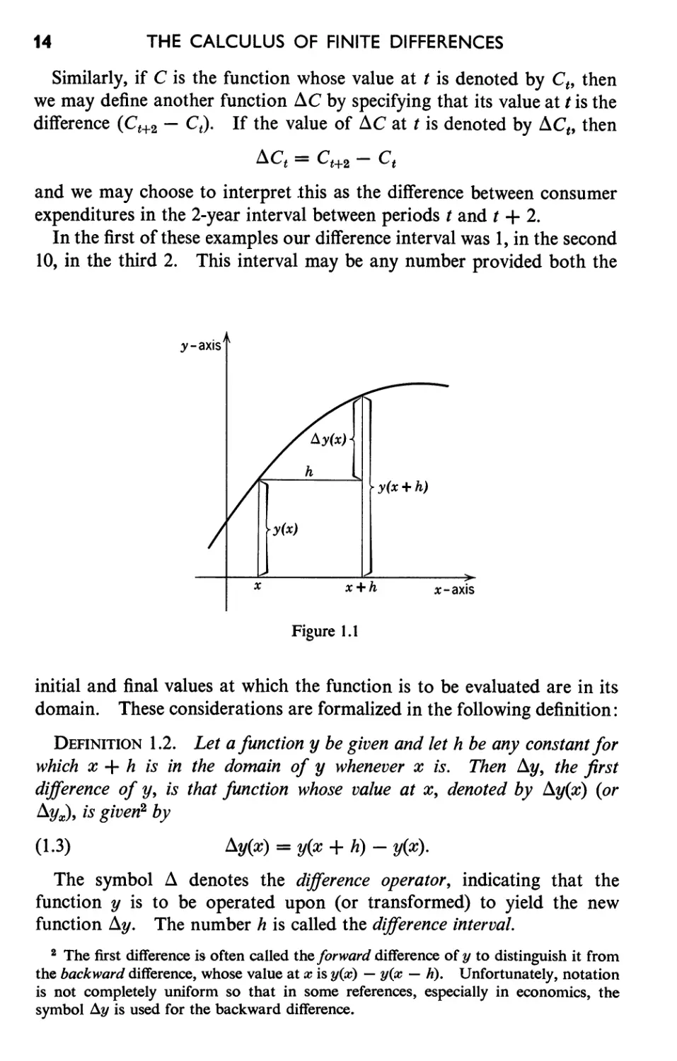
domain. These considerations are formalized in the following definition:
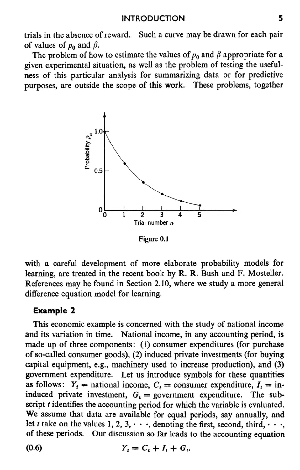
DEFINITION 1.2. Let a function y be given and let h be any constant for
which x + h is in the domain of y whenever x is. Then y, the first
difference of y, is that function whose value at x, denoted by y(x) (or
yx), is given 2 by
(1.3)
y(x) = y(x + h) - y(x).
The symbol denotes the difference operator, indicating that the
function y is to be operated upon (or transformed) to yield the new
function y. The number h is called the difference interval.
2 The first difference is often called the forward difference of y to distinguish it from
the backward difference, whose value at x is y(x) - y(x - h). Unfortunately, notation
is not completely uniform so that in some references, especially in economics, the
symbol dy is used for the backward difference.
THE FIRST DIFFERENCE FUNCTION
15
We shall understand, unless it is specifically indicated otherwise, that
we are always using the same difference interval h. Because of this
agreement, we shall not explicitly indicate the dependence of y on h.
(Some authors write y in order to avoid all possibility of misunder-
h
standing.) For the simple function given by y(x) = x, we find, using (1.3),
y(x) = = (x + h) - x
or
=h.
For this reason, the difference interval is often denoted by .
y-axis
4
y-axis
4
3
3
2
2
I
I y(O)
__..J
1 2 3 x-axis
-1
1 2 3 x-axis
-1
-1
(a) y(x)=x+ 1
( b) y( x) = x 2
Figure 1.2
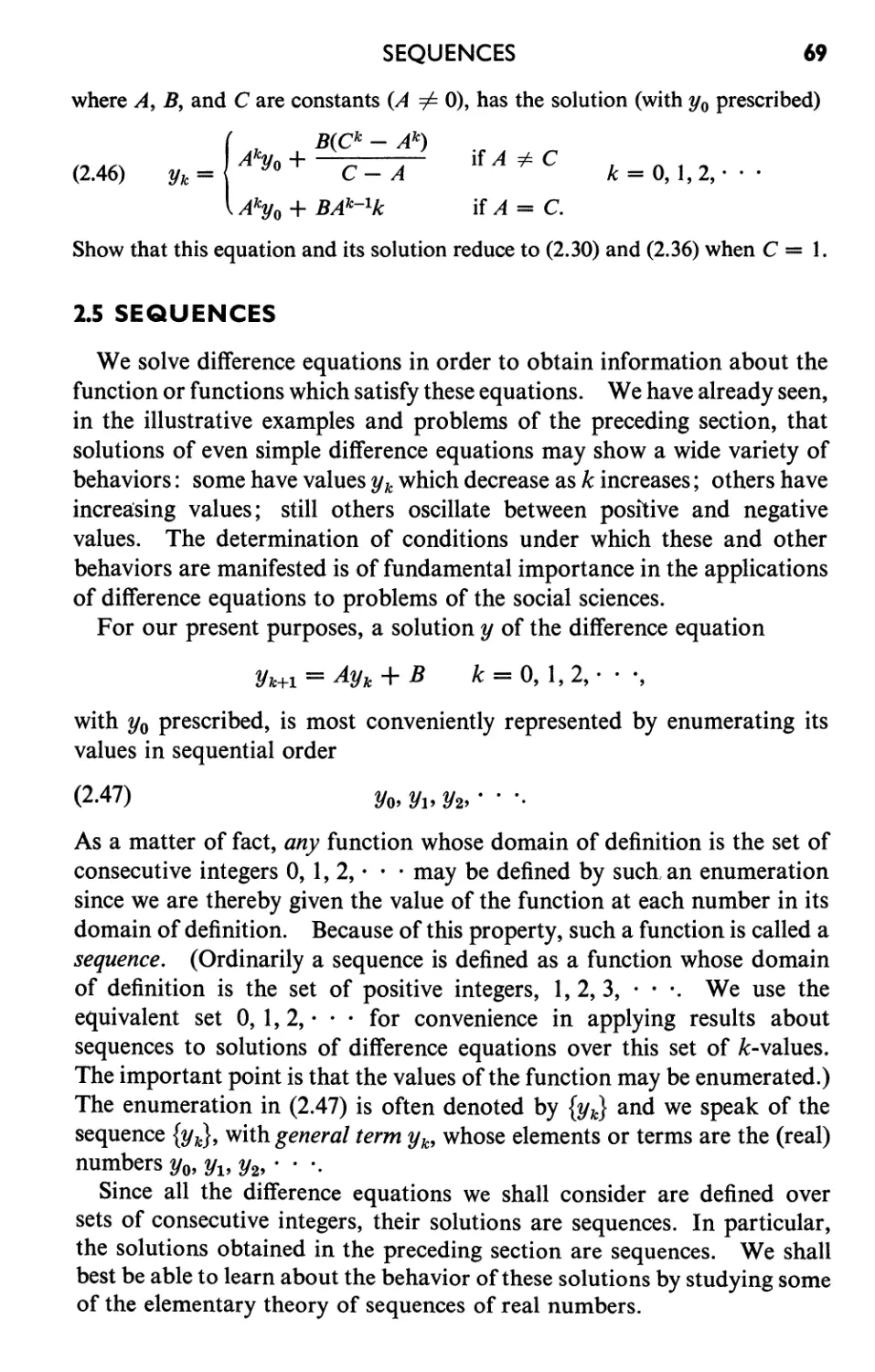
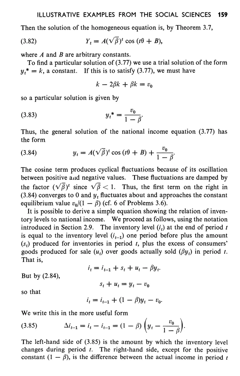
A graphical analysis may be helpful here. In Figure 1.1, as one moves
from x to x + h in the domain of y, the value of y changes from y(x) to
y(x + h). The first difference of y may be interpreted as the function
whose value at x is the increment or change in y which corresponds to the
increment h (or x) in x.
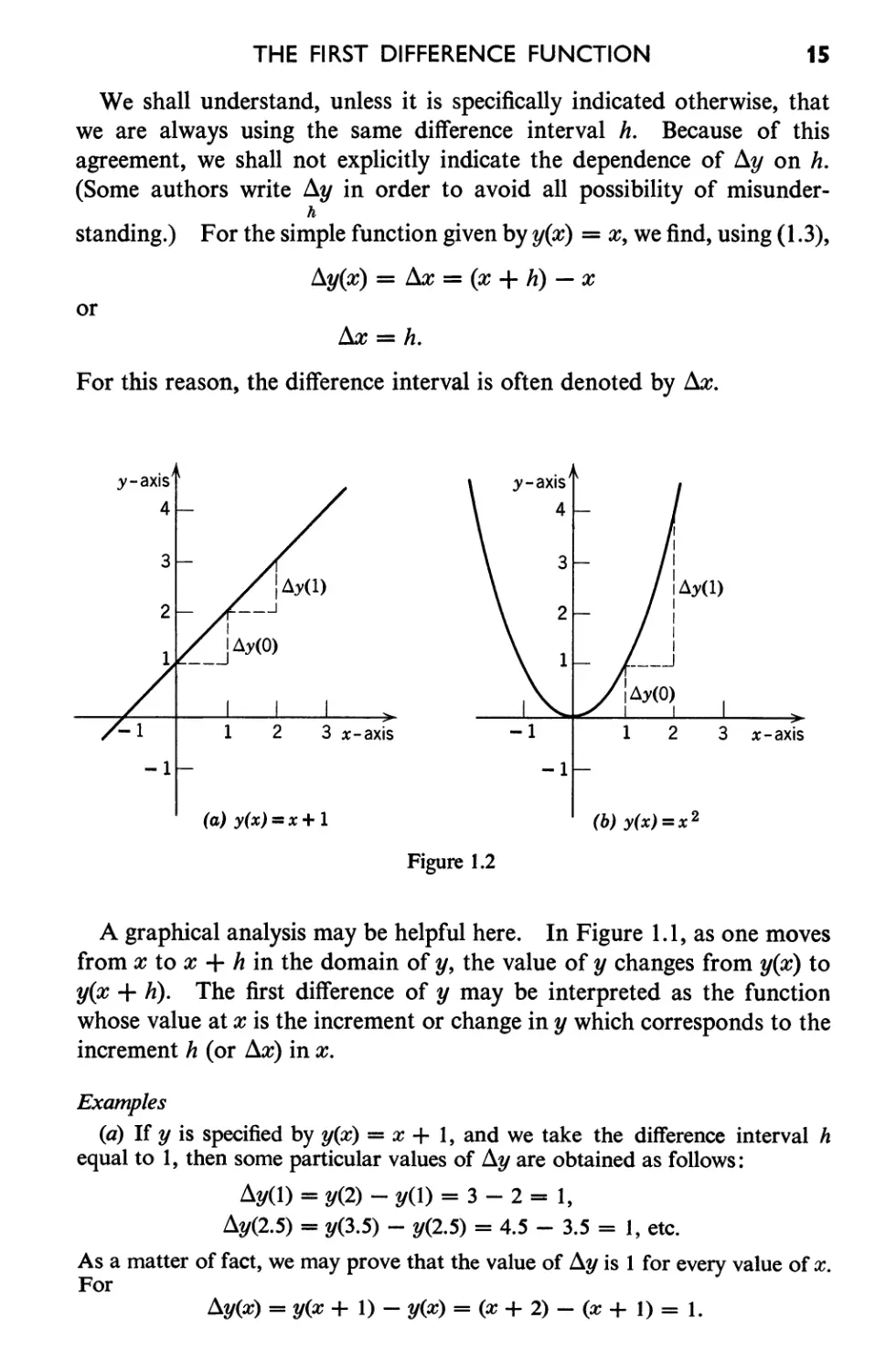
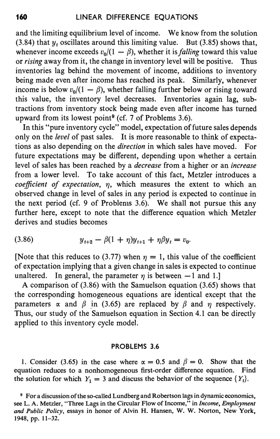
Examples
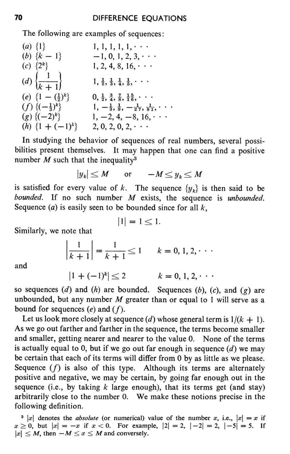
(a) If y is specified by y(x) = x + 1, and we take the difference interval h
equal to 1, then some particular values of y are obtained as follows:
y(1) = y(2) - y(1) = 3 - 2 = 1,
y(2.5) = y(3.5) - y(2.5) = 4.5 - 3.5 = 1, etc.
As a matter of fact, we may prove that the value of y is 1 for every value of x.
For
y(x) = y(x + 1) - y(x) = (x + 2) - (x + 1) = 1.
16
THE CALCULUS OF FINITE DIFFERENCES
This result is not surprising since the graph of the function y is a straight line for
which, independently of the starting value x, each unit change in x produces the
same change in the value of y. See Figure 1.2(a).
(b) If y(x) = x 2 , then (again taking h = 1)
y(l) = y(2) - y(l) = 2 2 - 1 2 = 3,
y(2.5) = y(3.5) - y(2.5) = (3.5)2 - (2.5)2 = 6, etc.
In general,
y(x) = y(x + 1) - y(x) = (x + 1)2 - x 2
= (x 2 + 2x + 1) - x 2
=2x+1.
For this function, the value of y is not constant, but depends upon x. The
increment in y caused by moving from x to x + 1 increases as x increases. See
Figure 1.2(b).
The procedure is precisely the same if we want to calculate y for a general
difference interval equal to h. Now, using (1.3),
(1.4) y(x) = y(x + h) - y(x) = (x + h)2 - x 2 = 2xh + h 2 .
Of course, this formula, when h is put equal to 1, reduces to the one previously
calculated.
(c) For the function given by pn = (0.6)n for n = 0, 1,2,. · ., with h = 1,
Pn = (0.6)n+l - (0.6)n = (0.6)n(0.6 - 1)
= (-0.4)(0.6)n
= (-0.4)pn.
The actual change in p in going from trial n to trial n + 1 is Pn. If by the
relative change in p we mean the actual change divided by the initial value of p,
then the relative change in p from trial n to trial n + 1 is
Pn = -0.4
pn
Le., this relative change is a constant from trial to trial. It is negative or a
decrease of numerical value 0.4 or 40 %. [Cf. assumptions (i) and (iv) in Example
1 of Chapter 0.]
PROBLEMS 1.1
In Problems 1-10, a function y is specified by giving its value y(x) for any
number x. Find (a) y(O), y(I), y(2); (b) y(O), y(I), y(2), y(x), assuming
h = 1; (c) y(x) with a difference interval equal to h. The symbols a, b, and c
denote constants.
1. y( x) = 1
2. y(x) = x - 2
3. y(x) = 3x + 5
4. y(x) = ax + b
5. y(x) = x 2 + 1
6. y(x) = x(x - h)
7. y(x) = ax 2 + bx + c
8. y(x) = x(x - h)(x - 2h)
9. y(x) = 2 x
10. y(x) = 3 x
THE FIRST DIFFERENCE FUNCTION
17
11. Sketch the graphs of the functions in Problems 1-5.
12. Consider the functions given by Yl(X) = x and Y2(X) = x 2 . Show that
Yl(X) = x = h and Y2(X) = X2 = 2xh + h 2 . Note the difference in
meaning (and value) between X2 and ( X)2.
13. Consider the following table: 3
x II 0 I 1 I 2 I 3 I 4 I 5 I 6 I 7
y(x) II A I A I A I BIB I c I c I c
where A, B, and C are numbers. Verify directly from the definition that y is a
function of x. What is the domain of definition of this function?
14. Let l(t) be the intensity of light required to produce a certain fixed photo-
chemical decomposition on an illuminated substance in time t. Bartl ey 4 derives
the equation
1
l(t) = C. - + D t > 0
t
where C and D are constants. Put C = 1 and D = 0 and make a rough sketch
of the graph of the function 1. As t increases, note that l(t) decreases. Con-
clude that I(t) is negative. Finally, show that your conclusion is not changed
if D is different from o.
15. Let the function Y be defined with domain the set of x-values between 0
and 1 inclusive, and suppose that
y(x) = x(1 - x).
Show algebraically that
y(x) = 1 - (x - !)2
and thus conclude that the largest value of Y is 1 and that this value is assumed
when x = t.
16. In a certain population, let Yt denote the proportion of the articulate
population who openly favor war at time t. The proportion who do not openly
favor war at time t is therefore 1 - Yt. Richardson 5 assumes that Yt is propor-
tional to the product Yt(1 - Yt), Le.,
Yt = kYt(1 - Yt)
for some constant k. Note that Yt, being a proportion, is a number between 0
and 1 inclusive, and use the result of the preceding problem to show that the
change in proportion of those who favor war at time t + t as compared with
time t is greatest when Yt = !, i.e., when half the population openly favors war.
3 See S. A. Stouffer et aI., Measurement and Prediction, Vol. IV of Studies in Social
Psychology in World War II, Princeton Univ. Press, Princeton, 1950, pp. 63-65.
4 S. H. Bartley, "The Psychophysiology of Vision," Chap. 24 in S. S. Stevens (ed.),
Handbook of Experimental Psychology, John Wiley, New York, 1951. cr. equation
6, p. 940.
6 L. F. Richardson, "War-moods: I," Psychometrika, 13 (1948), 147-174. The
differential calculus is used in this paper.
18
THE CALCULUS OF FINITE DIFFERENCES
17. The demand function in economics specifies the quantity of a certain
commodity that people will buy at each price at which it is offered. If p denotes
price, we let D(P) denote the quantity demanded at price p. Express the follow-
ing assumption in suitable mathematical notation: an increase in price causes a
fall in the quantity demanded. If the demand function is linear, what does the
assumption tell us of the slope of the straight-line graph of this function?
18. The supply function specifies the quantity of a certain commodity that will
be offered for purchase at a given price. Let S(P) denote this supply at price p.
Express in suitable mathematical notation the assumption that an increase in
price causes an increase in the quantity supplied. If the supply function is
linear, show that the slope of its straight-line graph is positive.
19. The supply and demand functions for sugar from 1890 to 1915 were
estimated 6 to be given by
S(P) = O.7p + 0.4
D(p) = 1.6 - O.5p.
If the market price is defined as that value of p at which supply and demand are
equal, show that the market price is p = 1. What quantity is demanded at this
market price? Draw the graphs of the supply and demand functions on the
same set of axes and interpret the point of intersection of the resulting straight
Jines.
20. If D(P) is the quantity demanded at the price p, then D(p + p) is
demanded at the price p + p and D(P) denotes the difference in demand due
to this price change of amount p. The quantity
p / p P D(P)
D(P) D(p) = D(p) . p
is referred to as the average or arc elasticit y 7 of demand for the price interval
p to p + p. With the assumption of Problem 17, show that this average
elasticity is a negative number. If the demand function is linear, say D(p) =
mp + b, show that D(p) = m p and conclude that the average elasticity,
although dependent upon the initial price p, does not depend on the price
change, p.
1.2 SECOND AND HIGHER DIFFERENCES
Starting with a function y, we defined the new function y which
results when the operator is applied to (the operand) y. We can, if
we like, apply the operator to this new function y. Let us consider a
simple example. If y is specified by the equation y(x) = x 2 , then we find,
in (1.4), that y is given by y(x) = 2xh + h 2 , where h is the interval of
6 H. Schultz, Statistical Laws of Demand and Supply with Special Applications to
Sugar, Univ. of Chicago Press, Chicago, 1928.
7 R. G. D. Allen, "The Concept of Arc Elasticity of Demand," Review of Economic
Studies, 1 (1934), 226-229.
SECOND AND HIGHER DIFFERENCES
19
differencing. Now ( y) is that function, according to Definition 1.2,
whose value at x is [ y(x + h) - y(x)]. But
y(x) = 2xh + h 2 ,
so that
f1y(x + h) = 2(x + h)h + h 2 = 2xh + 3h 2
and
y(x + h) - y(x) = 2h 2 .
Thus the value of the function ( y) for any x is the constant 2h 2 . The
notation 2y is used to denote this function and its value at x is denoted
by 2y(x). We have found
2y(X) = 2X2 = 2h 2 .
Undaunted, we march ahead and obtain yet another function by applying
the operator to the function 2y. This function we call 3y and, again
from Definition 1.2, we know that the value of 3y at x is [ 2y(X + h)
- 2y(X)]. Having found that 2y(X) is constant (= 2h 2 ), we know
f13y(X) = 2y(X + h) - 1l 2 y(x) = 2h 2 - 2h 2 = o.
We may continue this process indefinitely. Since 3y is zero for every x,
the function 1l4y will also be identically zero. In fact, fl5y, 6y, · · ·
will all be constant functions (= 0 for every x) when the function y is
given by y(x) = x 2 .
DEFINITION 1.3. Suppose a .function y and its first difference y are
given. Then the second difference of y, denoted by 2y, is the difference
of the first difference of y, i.e.,
(1.5)
f12y = ( y).
[The value of the function 2y at x, denoted by 2y(X), is therefore given by
(1.6)
2y(X) = y(x + h) - y(x).]
Similarly, the third difference of y, denoted by fl3y, is the difference of the
second difference of y, i.e.,
3y = (fl2y),
and, in general, the nth df/Jerence of y, denoted by ny, is the difference
of the (n - l)st difference of y, i.e.,
( 1.7)
ny = ( n-1y)
n = 2, 3, 4,. · ..
Note that (1.7), when n = 2, yields the identity 2y = ( 1y). In
order that this be consistent with (1.5), we agree to omit the superscript
when writing the first difference of a function; Le., we write y (as we
20
THE CALCULUS OF FINITE DIFFERENCES
have been doing all along) rather than ly. One other convention is
useful since it enables (1.7) to be meaningful for n = 1. With n = 1,
(1.7) reads y = ( Oy). If this is to be correct, we must agree that
Oy = y; Le., o is the operator which, when applied to a function y,
leaves y unchanged. Such an operator is called an identity operator.
DEFINITION 1.4. The identity operator, denoted by I, is that operator
which, applied to any function y, produces a new function Iy identical with
y. That is, for any x in the domain ofy, we have
(1.8)
Iy(x) = y(x).
The symbol o is defined as the identity operator, Le.,
(1.9) Oy = Iy
and, as was our intent in making this particular definition, (1.7) is now
correct for n = 1.
Example
Let y be the function for which y(x) = x 3 . Then
y(x) = x3 = (x + h)3 - x 3 .
We apply the binomial theorems to expand (x + h)3 as follows:
(x + h)3 = x3 + 3x 2 h + 3xh 2 + h 3 .
Then
y(x) = 3x 2 h + 3xh 2 + h 3 .
In comparing the function values y(x) and y(x), we note that the highest power
of x has been reduced by 1. The function y is cubic in x (highest power of x
appearing is 3) and y is a quadratic function of x (highest power of x is 2).
Now
2y(X) = y(x + h) - y(x)
= [3(x + h)2h + 3(x + h)h 2 + h 3 ] - (3x 2 h + 3xh 2 + h 3 )
= (3x 2 h + 9xh 2 + 7 h - (3x 2 h + 3xh 2 + h 3 )
= 6xh 2 + 6h 3 .
Again we have lowered the degree of our function by applying the operator ,
for 1l 2 y is a linear function of x (highest power of x is 1). Finally,
3y(X) = 2y(x + h) - 2y(X)
= [6(x + h)h 2 + 6h 3 ] - (6xh 2 + 6h 3 )
= 6h 3 , a constant,
8 For any positive integer n,
n n ( n - 1) n(n - 1)(n - 2)
(A + B)n = An + - An-IB + An-2B2 + An-3B3 + . . . +Bn.
1 1.2 1.2.3
The sum on the right has (n + 1) terms and is said to be the expansion of (A + B)n.
THE OPERATOR E.
21
so that
1l4y(x) = fl3y(X + h) - fl3 y (X)
= 6h 3 - 6h 3 = 0,
and, of course, all higher differences are likewise zero.
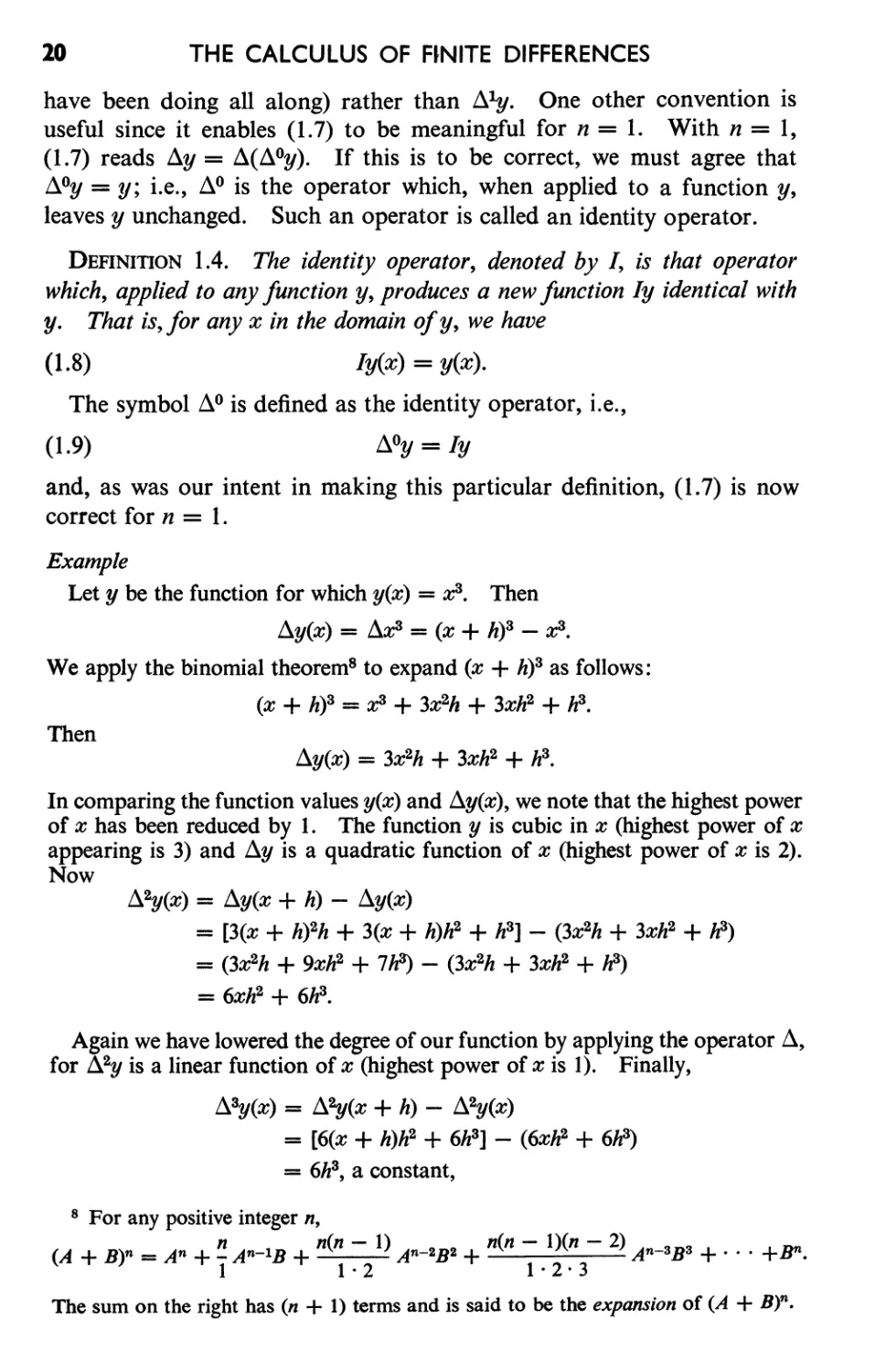
We may summarize these results, as well as some others, in Table 1.1.
TABLE 1.1
y(x) fly(x) 1l 2 y(x) fl3y(X) flny(x), n > 4
1 0 0 0 0
x h 0 0 0
x 2 2xh + h 2 2h 2 0 0
x 3 3x 2 h + 3xh 2 + h 3 6xh 2 + 6h 3 6h 3 0
We have found a number of functions for which repeated applications
of the operator 11 eventually yield a function fln y whose values are
constant, so that all higher differences of yare identically zero. In
Section 1.4 we shall show that these results are special cases of a more
general theorem.
PROBLEMS 1.2
1-10. For each of the functions in 1-10 of Problems 1.1, find (a) 1l2y(I) and
2y(x), assuming h = 1; (b) 1l2 y (X) with a difference interval equal to h.
11. If y(x) = 2 and c = 2'" - 1, show that Ily(x) = cy(x), 1l 2 y(x) = c2y(x),
1l3 y (X) = c3y(x). What is your conjecture for Ilny(x) for any positive integer n?
12. Show that
1l2y(x) = y(x + 2h) - 2y(x + h) + y(x),
1l 3 y(x) = y(x + 3h) - 3y(x + 2h) + 3y(x + h) - y(x).
1.3 THE OPERATOR E.
The operator 11 applied to a function y requires that we perform two
operations to get Ily(x): we change y(x) to y(x + h) and then subtract
y(x) from the result. It turns out to be extremely useful to introduce a
special symbol for the first of the operations.
DEFINITION 1.5. Let a function y be given and let h be any constant.
Then Ey is that function whose value at x, denoted by Ey(x) (or Ey ), is
given by
(1.10)
Ey(x) = y(x + h).
n
THE CALCULUS OF FINITE DIFFERENCES
Of course, the number (x + h) must be in the domain of y. We can
now write
(1.11 )
y(x) = Ey(x) - y(x).
The operator E, like , may be applied more than once to a function.
So, for example, with notation similar to that employed in Definition 1.3,
E2 y (X) = E[Ey(x)] = Ey(x + h) = y(x + 2h),
E3 y (X) = E[E2(X)] = Ey(x + 2h) = y(x + 3h),
and, in general, we can show that with the definition
(1.12)
Eny(x) = E[En-1y(x)]
n = 1, 2, 3, ·
we have
(1.13)
Eny(x) = y(x + nh)
n = 1, 2, 3,. · ..
Before proving this, let us agree to write E rather than El. As with the
operator , in order that (1.12) be correct for n = 1, we must make the
definition:
(1.14)
EOy(x) = Iy(x) = y(x).
With these conventions, (1.13) is correct for n = 0, 1,2,. · ..
Examples
(a) Ify(x) = 3x, then Ey(x) = y(x + h) = 3(x + h) = 3x + 3h. From (1.13),
Eny(x) = y(x + nh) = 3(x + nh) = 3x + 3nh.
(b) If y(x) = 2 x , then EOy(x) = 2 x , Ey(x) = y(x + h) = 2 x + h = 2 h 2 x , and in
general Eny(x) = y(x + nh) = 2 x + nh = 2 nh 2 x .
(c) Let C be a function whose value, C t , at the positive integer t denotes
consumer expenditure in period t. Then (with h = 1), EC t = C t + 1 is the con-
sumer expenditure in the following period. The equ3:tions EC t = C t (t =
1, 2,. · .) assert that consumer expenditure is constant from period to period.
To prove (1.13) is true for any positive integer, we make use of the
method of proof known as mathematical induction. Although most
readers will be familiar with this method, it is important enough for our
purposes to justify the following very brief review.
Let P(n) denote a proposition involving the positive integer n. If n is put
equal to 1, 2, 3,. . ., we obtain the propositions P(l), P(2), P(3),. ... Each of
these propositions is either true or false. For example, if
P(n): the number n 2 is less than 5,
then P(l) and P(2) are true statements, but P(3), P(4),. . . are all false.
THE OPERATOR E.
23
To prove, by mathematical induction, that P(n) is true for all positive integers n,
it suffices to prove two statements: (1) the proposition P(I) is true, and (2) for any
positive integer k, if P(k) is true, then P(k + 1) is also true.
Step (1) verifies the truth of P(n) when n = 1; step (2) shows that the truth of
the proposition for any integer follows from its truth for the preceding integer.
Taken together, these steps prove (by mathematical induction) that P(n) is true
for any positive integer. (It is as if to prove we may reach any rung on an
infinitely extended ladder, we first show that we may step onto the first rung, and
then show that we are able to step from any rung to the next higher one.)
The following examples illustrate this method of proof.
Examples
(a) To prove that
( ) h f h fi ... . n(n + 1)
P n : t e sum 0 t erst n positIve Integers IS 2 '
or, in symbols, that
n(n + 1)
P(n): 1 + 2 + 3 + · · · + n = 2
is true for all values of n, we construct the required two-step proof. (1) P(I) is
the statement 1 = [1(1 + 1)]/2 and this is clearly true. (2) We assume P(k) is
true and must prove P(k + 1) is also true. Now
k(k + 1)
P(k) : 1 + 2 + 3 + · · · + k = 2
being true (by hypothesis), we obtain another true statement by adding (k + 1)
to both sides of the equation. That is,
1 + 2 + 3 + · · · + k + (k + 1) = k(k i 1) + k + 1
= (k + 1) ( + 1 )
(k + 1)(k + 2)
2
But this final statement is just P(k + 1). Hence P(k + 1) is a consequence of
P(k) and the proof is complete.
(b) We prove that
P(n): Eny(x) = y(x + nh)
is true for all positive integral values of n. This is (1.13). (1) P(I) is true. For
P(I): El y (X) = y(x + h)
and this is true by Definition 1.5 and our agreement to identify El with E.
(2) We now assume
P(k): Eky(X) = y(x + kh)
is true, and attempt to prove that P(k + 1) is true. We apply the operator E
to both sides of the equation P(k) to get
E[Eky(X)] = Ey(x + kh).
24
THE CALCULUS OF FINITE DIFFERENCES
Now we use the definition of Ek+l given by (1.12), as well as the definition of the
operator E, to rewrite this in the form
Ek+ly(X) = y(x + kh + h)
= y[x + (k + l)h].
But the final equality is the proposition P(k + 1) obtained by replacing n in
P(n) by k + 1. Hence we have proved that P(k) implies P(k + 1) and step (2)
[and therefore the proof of (1.13) by mathematical induction] is complete.
PROBLEMS 1.3
1--4. For each of the functions in 1--4 of Problems 1.1 find (a) Ey(x); (b)
E2y(x); (c) Eny(x). Use a difference interval equal to h.
5. If y(x) = 3 , show that Eny(x) = 3 nh y(x) for n = 0, 1, 2,. · ..
6. Show that (cf. 12 of Problems 1.2)
j),2 y (X) = E2 y (X) - 2Ey(x) + Iy(x)
j),3 y (X) = E3 y (X) - 3E2 y (X) + 3Ey(x) - Iy(x).
( 1.15)
7. Show that
(1.16)
E2 y (X) = y(x) + 2j),y(x) + j),2 y (X)
E3 y (X) = y(x) + 3 y(x) + 3 2y(X) + j),3 y (X).
8. Let P be the function whose value, pn, at the positive integer n is interpreted
as the probability of a positive response in the nth experimental trial. What is
the interpretation of EPn? If Pn = (O.6)n, show that EPn = (O.6)Pn. [Cf.
assumption (ii) in Example 1 of Chapter 0.]
9. If we define the operator In for n = 2, 3, 4,. · · in the same recursive
manner used to define j),n and En, Le., ]ny = ](]n-l)y, then show using mathe-
matical induction that ]ny(x) = ]y(x).
1.4 SOME PROPERTIES OF D,. AND E.
Since the operators D,. and E are of fundamental importance, we should
like to be able to calculate the values of y and Ey with some degree of
ease, at least for the functions y which arise fairly often. Table 1.1 gives
us the results of applying D,. to four simple functions. But what if we
must apply to some combination of these functions, say y(x) = x + x 2 ?
Now
D,.y(x) = y(x + h) - y(x)
= [(x + h) + (x + h)2] - (x + x 2 )
= [(x + h) - x] + [(x + h)2 - X2]
= Llx + Llx2.
Thus we find
(x + x 2 ) = &l + Llx2.
SOME PROPERTIES OF D,. AND E.
15
Had we known this fact (namely, the difference of the sum 9 of two functions
is equal to the sum of the differences of the functions) we could have
avoided the above algebra and obtained D,.(x + x 2 ) directly from Table 1.1.
Such considerations lead to the search for formulas by which, having
calculated dy(x) directly from Definition 1.2 for a number of functions y,
we may find the differences of still other functions by using the results of
these calculations rather than again resorting to the basic definition. If
the differences of a large class of functions can be obtained with relatively
few such formulas and if these are fairly simple to use, then we certainly
have a net gain. Some of these formulas of the calculus of finite differences
will be developed here.
THEOREM 1.1. The Commutative Law with Respect to Constants. If
c is any constant, the difference of the junction cy is equal to c times the
difference of y, i.e.,
(1.1 7)
D,.[cy(x)] = cD,.y(x).
PROOF. We use Definition 1.2 to write
[cy(x)] = cy(x + h) - cy(x)
= c[y(x + h) - y(x)]
= cD,.y(x).
Formula (1.17) enables us to use the results of Table 1.1 to find the
following differences with essentially no calculation:
(3x) = 3D,.x = 3h,
D,.( 5x 2 ) = 5 D,.x 2 = 5(2xh + h 2 ), etc.
THEOREM 1.2. The Distributive Law. The difference of the sum of two
functions is equal to the sum of their differences, i.e., if Yl and Y2 are two
functions,
(1.18)
D,.[yl(X) + Y2(X)] = Yl(X) + Y2(X).
9 If Yl and Y2 are two functions, then the sum of these functions is a new function
whose domain consists of those numbers in both the domain of Yl and Y2; if x is such
a number, then the sum function has, by definition, the value Yl(X) + Y2(X). Similar
natural definitions are given for the difference, product, and quotient of two functions.
Also, two functions are said to be equal if they have the same domain of definition and
the same value for each number in this common domain. For full details and examples,
see E. G. Begle, Introductory Calculus, Henry Holt, New York, 1954, especially
pp. 42-47, 56-58.
26
THE CALCULUS OF FINITE DIFFERENCES
PROOF. From Definition 1.2,
[yl(X) + Y2(X)] = [Yl(X + h) + Y2(X + h)] - [Yl(X) + Y2(X)]
= [Yl(X + h) - Yl(X)] + [Y2(X + h) - Y2(X)]
= Yl(X) + Y2(X).
COROLLARY 1. If C 1 and C2 are arbitrary constants,
(1.19) [CIYl(X) + C 2 Y2(X)] = Cl Yl(X) + C2 Y2(X).
PROOF. Apply Theorem 1.2 to the functions C1Yl and C2Y2 and obtain
[CIYl(X) + C 2 Y2(X)] = [CIYl(X)] + [C2Y2(X)].
The result follows by applying (1.17) to the two terms on the right.
COROLLARY 2. Let Yl, Y2' · · ., Yn be n functions and C 1 , C2, · · ., C n
be arbitrary constants. Then for any positive integer n,
(I .20) [CIYl(X) + C2Y2(X) + · · · + cnYrl x )]
= C1D,.Yl(X) + C2 Y2(X) + · · · + cn Yn(x).
The result is trueforn = 1 by(I.I7)andforn = 2 by(1.I9). Byassuming
(1.20) true for n = k and proving it true for n = k + 1, which we omit
here, the proof of Corollary 2 by mathematical induction can be completed.
This brief digression concerns a convenient notation, to be used henceforth,
for writing sums like those in (1.20). If Yk denotes the value of a function Y at
the integer value k and if a and b are any integers (b > a), the sum
Ya + Ya+l + Ya+2 + · . . + Yb
is instead written in the condensed form
b
! Yk.
k=a
This symbol is read "the sum of Yk from k = a to k = b." Some examples will
help to clarify the use of this summation notation. In each example, the sum is
alsd written out in long form and described in words.
Examples
(0) The sum of the first n positive integers:
n
! k = 1 + 2 + 3 + · · · + n.
k=l
(b) The sum of the first ten odd integers:
9
! (2k + 1) = 1 + 3 + 5 + . · · + 19.
k=O
SOME PROPERTIES OF AND E.
27
(e) The sum of the first, second, and third differences of the function Y; each
evaluated at x:
3
! ky(X) = y(x) + 2y(X) + ay(x).
k=l
It is convenient to know the following rules concerning summation. We let
y and z be any two functions and e an arbitrary constant. Then
n
(1) ! e = ne.
k=l
n n
(2) ! eYk = e ! Yk.
k=l k=l
n n n
(3) ! (Yk::!: Zk) = ! Yk::!: ! Zk.
k=l k=l k=l
We prove (2) and leave the others for the reader. The proof is given by
n
! CYk = eYl + CY2 + CYa + · · · + eYn = e(Yl + Y2 + Ya + · · · + Yn)
k=l
n
= e ! Yk.
k=l
As an example of the use of these rules, let Yh Y2,. · ., Yn be n measurements
of some variable (weights, IQ scores, etc.). The arithmetic mean of these n
measurements is
Y + y +...+ y In
- 1 2 n
Y = = - k Yk.
n n k=l
An important property of the arithmetic mean is the following: the sum of the
deviations of the measurements from their arithmetic mean is 0, Le.,
n
! (:uk - fj) = o.
k=l
To prove this result, write
n n n
! (Yk - fj) = ! Yk - ! fj
k=l k=l k=l
n
= ! Yk - nfi
k=l
[by rule (3)]
[by rule (1)]
= 0 (by definition of fi).
Now we can use the summation notation lO to rewrite (1.20) in the form
( 1.20')
n n
! CkYk(X) = ! Ck Yk(X)
k=l k=l
10 For future reference, we remark that this notation can be used to write the binomial
formula as
! n n(n - 1 )(n - 2). . . (n - k + 1)
(A + B)n = AkBn-k.
k=O 1 · 2.3. · . k _
Cf. footnote 8.
28
THE CALCULUS OF FINITE DIFFERENCES
Formula (1.20') enables us to find the difference of any linear combina-
tion of functions provided that we can find the differences of the functions
themselves.
Examples
(a) We may use Table 1.1 and (1.19) to obtain
(3X2 + 5x) = 3 X2 + 5 = 3(2xh + h 2 ) + 5h
(b) By (1.20'), with a, b, and c constants (cf. 7 of Problems 1.1)
(a + bx + cx 2 ) = a l + b + C X2
= a · 0 + b · h + c(2xh + h 2 )
= bh + ch 2 + 2chx.
(c) Suppose we have a function C whose value at N, denoted by eN' is given by
c _ a + bN
N-1-b-
a b
1-b + 1-b N ,
where a and b are constants, b =1= 1. Then
/).C N = /). ( 1 b ) + ( 1 b N) = 0 + 1 b N
so that!1
CN b
N = 1 - b.
We may use (1.20) to prove the following very important result.
THEOREM 1.3. Let y be a polynomial of degree n, i.e.,
(1.21)
Y(X) = a o + alx + aiX 2 + · · · + anx n
with a o , a I ,. · ., an arbitrary constants and an =1= o. Then the nth difference
of y is a constant function (equal to n!hna n ) and all succeeding differences
are zero, i.e.,
( 1.22)
Py(x) = 0
if P > n.
PROOF. By (1.20)
(1.23) y(x) = ao l + a1 x + a2 2 + · · · + an n.
11 See Thomas C. Schelling, National Income Behavior, McGraw-Hill, New York,
1951, p. 38. There C and N are interpreted as consumer and nonconsumer expenditures
respectively.
SOME PROPERTIES OF Ll AND E
29
But if m is any positive integer, the binomial theorem may be used to
obtain
Llxm = (x + h)m - x m
m(m - 1)
= x m + mxm-1h + xm-2h2 + · · · + h m - x m
2
m(m - 1)
= mxm-1h + x m - 2 h 2 + · · · + h m ;
2
i.e., application of L\ to x m produces a finite number of terms with xm-l
as the highest power of x appearing. So by applying L\ to y(x) we get,
using this fact and (1.23), a sum of terms, each a constant times a power
of x and the highest power of x appearing is (n - 1). In other words,
application of Ll to a polynomial of degree n results in a polynomial of
degree (n - 1). By the same reasoning, L\2y will be a polynomial of
degree (n - 2) and after n applications of Ll we are reduced to a polynomial
of degree 0 or a constant. This proves that L\ny is a constant and the
final part of the theorem follows immediately since the difference of a
constant is zero. The evaluation of L\ny is outlined in 6-8 of Problems 1.4.
Theorem 1.3 is of great importance in the theory of polynomial inter-
polation. (Cf. Section 1.5.)
We are severely limited in using the formulas already developed due to
the fact that we have at our disposal such a small collection of functions
whose differences We know. Instead of extending Table 1.1 by considering
x 4 , x 5 , · · ., we introduce another useful set of functions.
DEFINITION 1.6. The factorial function of order n (n = 1, 2, 3,. · .) is
that function whose value at.x is given by
x(n) = x(x - h) (x - 2h). · · [x - (n - l)h].
For example,
x(1) == x
X(2) = x(x - h)
X(3) == x(x - h)(x - 2h)
so that, if h == 2,
(x + h)(1) == x + h
(x + h)(2) == (x + h)x
(x + h)(3) == (x + h)(x)(x - h),
3(1) == 3
4(1) == 4
3(2) == 3 · 1 == 3
4(2) == 4 · 2 == 8
3 (3) == 3 · 1 · -1 == - 3
4(3) == 4 · 2 · 0 == 0,
whereas, if h == 3,
3(1) = 3
4(1) = 4
3(2) = 3 · 0 = 0
4(2) = 4 · J == 4
3(3) = 3 · 0 · -3 = 0
4(3) = 4 · 1 · -2 = -8.
30
THE CALCULUS OF FINITE DIFFERENCES
The factorial function of order n has n factors. Nevertheless, it is very
easy to find its difference. For
Llx(n) = (x + h )(n) - x(n)
c: (x + h)(x)(x - h). · · [x - (n - 2)h]
- x(x - h)(x - 2h). · · [x - (n - I)h].
Both terms on the right have the common factor x(n-l). Therefore
Llx(n) = x(n-l){(x + h) - [x - (n - I)h]}
= nhx(n-l).
This derivation, since it involves x(n-l), is valid for any n > I, but not
for n = I, since x(O) is undefined. But x(l) = x and Llx = h so if we
extend the definition of the factorial function by the requirement
(1.24)
x(O) = I,
we can summarize our result by writing the following formula ,(or the
difference of factorial functions:
(1.25)
Llx(n) = nhx(n-l)
n - 123 ...
- , " .
Note that except for a constant factor, the difference of a factorial
function is another factorial function of order 1 lower than the original.
This makes repeated differencing of x(n) easy to perform. For example,
Ll2 x (n) = Ll(Llx(n») = Ll(nhx(n-l»)
= nhLlx(n-l)
= nh · (n - l)hx(n-2)
= n(n - l)h 2 x(n-2).
We may similarly show that
Ll3 x (n) = n(n - 1 )(n - 2)h 3 x(n-3)
and repeating the Ll operation n times,
Llnx(n) = n(n - I)(n - 2). · · 3 · 2 · Ih n .
The number 1 · 2 · 3. · · (n - 2)(n - I)n in this result is the product of
the first n positive integers and arises so often that a special symbol is
introduced for it.
DEFINITION 1.7. The product of the first n positive integers is denoted
by n! (read "n factorial"), i.e.,
( 1.26)
n! = 1 · 2 · 3. · · (n - l)n.
SOME PROPERTIES OF d AND E
31
In addition, we agree to define zero factorial by
( 1.27)
01 = 1.
With this notation we can write
(1.28)
dnx(n) = n!h n
n = 0, 1, 2, - - -.
Examples
(a) 3! = 1 · 2 · 3 = 6, 4! = 1 · 2 · 3 · 4 = 24,
5! 1.2.3.4.5 6! 1.2.3.4-5.6
3! = 1 - 2. 3 = 20, 2!4! = (1 · 2)(1 · 2 · 3 · 4) = 15,
(b) dX(3) = 3hx(2) = 3hx(x - 1)
L\2 X (3) = 3 · 2h 2 x(1) = 6h 2 x
L\3 X (3) = 3 !h 3 = 6h 3
L\ n X(3) = 0 if n = 4, 5, 6,. · ..
(c) Using (1.20) and (1.25) we have
L\(3 + 5x(l) - 2x(2) + 4X(3» = 3L\1 + 5dx(1) - 2L\X(2) + 4L\X(3)
= 0 + 5h - 2 · 2hx(1) + 4 · 3hx(2)
= 5h - 4hx(1) + 12hx(2).
One of the factors contributing to the importance of the factorial
functions is the fact that any positive integral power of x can be written
as a sum of factorial functions. We do not prove this here (cf. 6 of
Problems 1.4) but instead give some illustrative examples. It is easy to
verify that x = x(1) and x 2 = X(2) + hx(1). Now let us try to write x 3 in
terms of X(3), X(2), and x(1). The factorial X(3), when multiplied out,
involves terms in x3, x 2 , and x, so we try to add to X(3) just the proper
proportions of X(2) and X(l) in order to cancel the x and x 2 terms and
leave just x3. We therefore begin by assuming constants Al and A 2 can
be found for which, identically in x,
x 3 = X(3) + A 2 x(2) + A1x(l).
To find Al and A 2 we put x = h and x = 2h in this equation and obtain
(noting that X(3) = X(2) = 0 when x = h, and X(3) = 0 when x = 2h)
h 3 = A1h
(2h)3 = A 2 2h - h + A 1 2h.
From the first of these we have Al = h 2 and from the second, A 2 = 3h.
Thus
(1.29)
x 3 = X(3) + 3hx(2) + h 2 x(l)
32
THE CALCULUS OF FINITE DIFFERENCES
and
Llx 3 = 3hx(2) + 6h 2 x(l) + h 3
= 3hx(x - h) + 6h 2 x + h 3
= 3hx 2 + 3h 2 x + h 3 ,
the same result, of course, as in Table 1.1, p. 21.
We conclude this section by pointing out that the difference of a product
of two functions can be expressed in terms of the operations E and L\ on
the functions themselves. The proof of the following result is left as an
exercise. Additional properties of the operators Ll and E will be con-
sidered in the next section.
THEOREM 1.4. Let u and v be two functions. Then
(1.30)
Ll[u(x)v(x)] = Eu(x) · Llv(x) + v(x) · Llu(x).
Example
L\x4 = Ll(x. x3), so [with u(x) = x and vex) = x3]
= Ex Llx3 + x 3 Llx
= (x + h)(3hx 2 + 3h 2 x + h 3 ) + x3h
Llx 4 = 4Jzx3 + 6h 2 x 2 + 4/rx + h 4 .
(1.31)
PROBLEMS 1.4
1. Find Lly(x) if y is given by
(a) y(x) = 3 + 2x + x 2
(b) y(x) = 6 - x 2
(c) y(x) = 5x(1 - x)
2. Use (1.25) to find Lly(x), fl2y(X), L\3 y (X),. . ., if
(a) y(x) = 5x(3)
(b) y(x) = 2 + 3x(l) - 2X(2) + 3X(3) - X(4)
(c) y(x) = 2.5x(2) + 3.1x(3)
3. Prove the following properties of the operators Ll and E:
(a) E[cy(x)] = cEy(x)
(b) E[C1YI(X) + C2Y2(X)] = cIEYI(X) + c 2 EY2(X)
(c) E L l CiYi(X)] = i l CiEYi(X)
(d) En[C1YI(x) + C2Y2(X)] = cIEnYI(X) + C2EnY2(X)
(e) Lln[CIYI(x) + C2Y2(X)] = CI LlnYI(X) + C2 nY2(x)
4. Prove (1.28) by mathematical induction.
5. (a) Write x 4 as a sum of factorial functions. (Hint: Put x 4 = X(4) +
A 3 x(3) + A 2 x(2) + A1x(l). Then put x = h, 2h, 3h in turn to find Al = h 3 ,
A 2 = 7h 2 , A3 = 6h.) (b) Find Llx 4 using the result of (a) and check with (1.31).
n=OI2...
, , ,
n=OI2...
, , ,
SOME PROPERTIES OF d AND E
33
6. Show that x n can be written as a sum of factorial functions for any positive
integer n. Let
x n = x(n) + A n _ 1 x(n-l) + A n _it(n-2) + · · · + Ait(2) + A 1 x(l).
Then show, without doing the calculations, that Al is determined by putting
x = h, A 2 by putting x = 2h, etc.
7. Use the result of Problem 6 together with rules for the difference of factorial
functions to prove that d nx n = n !h n .
8. Prove that if y is the polynomial of degree n given by (1.21) then /lny(x) =
n!hna n . [Hint: Use Theorem 1.3 to show that dny(x) = an/lnx n and then use
the result of Problem 7.]
9. Let y(x) = x 5 . Find /ly(x) in the following three different ways and check
that each gives the same result: (a) directly from Definition 1.2 ; (b) by writing
x 5 as the sum of factorial functions and using (1.25); (c) by writing x 5 = x 2 · x 3
and using (1.30) and Table 1.1.
10. Prove Theorem 1.4.
11. Derive the following formula for the difference of the quotient of two
functions u and v:
/l u(x) = v(x)du(x) - u(x)/lv(x)
v (x) v (x)Ev(x)
if v(x)Ev(x) =1= O.
12. Let Y (income), I (investment expenditure), S (savings), and C (consumer
expenditure) be four functions whose values in period t are denoted by Y t , It, St,
and C t respectively. Assume 12 the two relations
Y t = It + C t
and
St = It
and prove if
dY t
k = dI t '
dS t
s = dYt'
and
/lC t
C = dYt'
that
1
k=-
s
and
1
k = .
1 - c
13. Let G (government expenditure), D (government deficit), and Y (national
income) be functions of time t related in such a way that
/l Y t = dG t + 4/lDt.
Make' the following inference 13 from this relation: "Then, an extra dollar of
deficit would allow a four dollar reduction in tax-financed government spending
without affecting the magnitude of national income. · .."
11 A. H. Hansen, A Guide to Keynes, McGraw-Hill, New York, 1953, p. 96.
18 R. L.Bishop, "Alternative Expansionist Fiscal Policies: A Diagrammatic Analysis,"
in Income, Employment and Public Policy, essays in honor of Alvin H. Hansen, W. W.
Norton, New York, 1948, pp. 317-340.
34
THE CALCULUS OF FINITE DIFFERENCES
14. Suppose P (price of securities) is related to M (money deposits in banks)
and B (stock of securities in banks) in such a way that for each time t,
Mt
Pt = k -
Bt
k a constant > O.
Suppose in a time interval 111, taken equal to 1, B increases by an amount I1Bt
and M by an amount I1Mt. Use the result of Problem 11 to ShOW 14 that the
corresponding change in price of securities is given by
11 _ Bt l1M t - Mt l1B t
Pt - k BlBt + I1Bt) ·
Prove from this that the price of securities rises, falls, or stays the same (in the
interval 111) according as (I1M t )f Mt (the relative increase in money) is greater
than, less than, or equal to (I1Bt)f Bt (the relative increase in securities).
15. Let Tt denote the number of occurrences of a certain response R up to time
period t, and Xt the number of stimulus elements (of a certain class) which are
conditioned to R in period 1. Estes 15 shows that
I1Xt S - Xt I1Tt Xt
--s and ---
I1Tt - S 111 - Sh
where h, s, and S are constants. Show that
I1Xt s(S - xt)x t
111 = hS 2
1.5 EQUIVALENCE OF OPERATORS
Let us look back for a moment to (1.11) which we rewrite here:
(1.11 ')
l1y(x) = Ey(x) - Iy(x).
One might translate this equation by saying that the same result is obtained
by applying the operator 11 to any function as by applying the operator
(E - I). (We make the natural definition that E - I is the operator
which, when applied to the function y, produces the function Ey - Iy.)
Such pairs of operators arise fairly often and a special terminology is
introduced for describing them.
DEFINITION 1.8. Two operators, 0 1 and O 2 , are said to be equivalent
(denoted by 0 1 == O 2 ) if for any.function y to which 0 1 and O 2 are each
applicable, the functions 0IY and 02Y are equal.
14 K. E. Boulding, Economic Analysis, 3rd ed., Harper, New York, 1955, p. 380.
15 W. K. Estes, "Toward a Statistical Theory of Learning," Psychological Review
57 (1950), 94-107.
EQUIVALENCE OF OPERATORS
35
Thus (1.11') can be written as the equivalence
( 1.32)
Ll == E - I.
Since (1.11') can also be written in the form
Ey(x) = Lly(x) + Iy(x),
we are able to write
( 1.33)
E == +I.
Note that (1.33) follows from (1.32) ifwe assume that we can manipulate
operators in equivalence equations as we do algebraic quantities in
ordinary equations. We shall not prove this here, but such manipulations
are indeed possible and this fact accounts for the great usefulness of
operator methods in the calculus of finite differences.
Other relations, already proved, can be rewritten in our new notation.
For example, (1.9), (1.14), and (1.15) are translated by (1.34), (1.35),
and (1.36) respectively.
(1.34) o == I
(1.35) EO == I
(1.36) 2 == E2 - 2E + I Ll3 == E3 - 3E2 + 3E - I.
We shall show further on that (1.36) could have been obtained from (1.32)
had we regarded (1.32) as an algebraic equation and first squared and then
cubed both and E - I. The reader will do well to note that this
analogy between equivalence relations among operators and algebraic
relations among real numbers is illustrated in all of the results which
follow.
For any function y we may first apply Ll and then apply E to he
resulting function Lly, Le., we may form E(Lly). We denote this two-step
operation by ELl so that (ELl)y = E( y). Note that the operator written
symbolically as ELl means that we perform Ll first and E second. The
order of operations is indicated by reading from right to l rt. Similarly,
we may first apply E to the function y and then apply Ll to Ey, Le., we may
form Ll(Ey). This two-step operation is denoted by E.
As an example, consider the factorial function y given by
y(x) = X(2).
Applying first and then E:
y(x) = 2hx(1)
Edy(x) = 2h(x + h).
In the opposite order we obtain the same final result:
Ey(x) = (x + h)(2) dEy(x) = 2h(x + h).
36
THE CALCULUS OF FINITE DIFFERENCES
There is no a priori reason for assuming that the order of operations is
always immaterial; nevertheless, this is the case for the operators d and E.
THEOREM 1.5. The operators L\ and E are commutative, i.e.,
( 1.37)
dE == EL\.
PROOF" We determine (dE)y(x) and (Ed)y(x) and observe that they
are identical. For
and
(L\E)y(x) = L\[Ey(x)] = L\y(x + h)
= y(x + 2h) - y(x + h),
(EL\)y(x) = E[L\y(x)] = E[y(x + h) - y(x)]
= y(x + 2h) - y(x + h).
If x is a number, the index law for exponents tells us that x3 · x 4 = x 4 · x3
= x 7 . We leave to the reader the proof of the following result which
shows that powers of the operators L\ and E obey the same rule of
combination.
THEOREM 1.6. The operators L\ and E satisfy the index law, i.e., for
m and n nonnegative integers,
(1.38)
(1.39)
L\m L\n == d n L\m == L\m+ n ,
EmEn == E"'Em == Em+fl.
The operators L\ and E are commutative; each obeys the index law and
as we have seen (Theorems 1.1 and 1.2, and 3 of Problems 1.4) also obeys
the commutative law with respect to constants and the distributive law.
The familiar rules for combining numbers stem from the fact that num-
bers obey the above fundamental laws. The fact that L\ and E also obey
these laws accounts for the possibility of using these operators as if they
were algebraic symbols representing numbers.
Formula (1.36) shows that both L\2 and L\3 can be written in equivalent
form in terms of the operator E. Moreover, as we have already remarked,
if we manipulate operators as numbers in algebra, we obtain both results
in (1.36). Let us detail the computations involved in the second of these.
We want an operator, involving E, equivalent to L\3. So we use (1.32)
and cube both sides to obtain
d 3 == (E - /)3.
Now, we carry out the cubing operation by using the binomial theorem:
d 3 == £3 - 3£21 + 3£[2 - P.
EQUIVALENCE OF OPERATORS
37
But (cf. 9 of Problems 1.3) 1 3 == 1 2 == I. Also for any operator 0, we
have 01 == 10 == 0 (cf. 1 of Problems 1.5). Therefore
Ll3 == E3 - 3£2 + 3£ - I,
which is precisely the result in (1.36). The above reasoning does not
prove (1.36) since we have not rigorously proved that algebraic manipula-
tions performed with operators are valid. Such calculations will be used
only to suggest results that will then have to be verified by other means.
In fact, we can express any positive integral power of L\ in terms of E.
The above calculation, carried out for n = 3, will be imitated to produce
the general result for L\n. We take the nth power of both sides of (1.32)
to obtain
(1.40)
Lln == (£ _ I)n.
We want to apply the binomial theorem, but first we use this oppor-
tunity to rewrite the theorem in a more concise form than that given in
footnote 10, p. 27. Using the notation introduced in (1.26) and (1.27),
the new symbol (Z), for k and n nonnegative integers (k < n), is defined by
(1.41) (Z) = k!(n n k)r
By dividing n! by (n - k)! we find
( n ) = n(n - 1)(n - 2). · · (n - k + 1) .
k k!
Rewriting the formula in footnote 10 using this new notation, we have the
alternate form of the binomial formula:
(A + B)n = i ( n ) AkBn-k.
k=O k
It is for this reason that the numbers (Z) for k = 0, I, 2,. · · n are
( 1.42)
known as binomial coefficients.
Applying (1.42) to (1.40),
d n = i ( n ) (_l)n-k£kJn-k.
k=O k
But Ek]n-k == E k , so
L\n == i ( n ) (_l)n-kEk.
k=O k
38
THE CALCULUS OF FINITE DIFFERENCES
That this heuristic derivation actually has led to a true result is the content
of the following theorem, whose long, but straightforward, proof (by
mathematical induction) we omit.
THEOREM 1.7. If n is a positive integer, then
(1.43)
!1 n y(x) = k O (z) (-1)1I-kEk y (x).
Theorem 1.7 shows that n may be written in terms of E. The inverse
problem of relating En to the operator will now be considered. We
have seen in (1.16) the solution of this problem for E2 and E3. In the
general case, we proceed formally from the fundamental equivalence (1.33)
and raise both sides to the nth power. Once again we use the binomial
formula (1.42) and regard the operators as if they were algebraic quantities.
Then '
En == ( + I)n
= 1: ( n ) kln-k.
k=O k
But kln-k == k so that
( 1.44)
En = 1: ( n ) k.
k=O k
These manipulations are again fruitful since it can be proved (by
mathematical induction) that (1.44) is, in fact, a valid equivalence. We
omit the proof.
THEOREM 1.8. If n is a positive integer, then
Eny(x) = kt (Z) !1 k y(x).
Theorem 1.8 can be used to solve simple problems of polynomial
interpolation. For example, suppose we are given the following informa-
tion about a function y: (1) y is a polynomial of degree 3, and (2) y(O)
= -4, y(l) = -6, y(2) = -8, y(3) = -4. We require the value y(4).
The information in item (2) enables us to construct the difference table,
( 1.45)
TABLE 1.2
x y(x) y(x) 2y(X) 3y(X)
0 -4 -2 0 6
1 -6 -2 6
2 -8 4
3 -4
4 ?
EQUIVALENCE OF OPERATORS
39
Table 1.2. The first two columns list the x-values and the corresponding
prescribed y-values; a question mark indicates the y-value to be found.
We have added columns listing the values of l1y, 112y, and 113y (with a
difference interval equal to 1).
To calculate these entries is an easy task. For example, we compute
l1y(O) = y(l) - y(O) = -6 - (-4) = -2
l1y(l) = y(2) - y(l) = -8 - (-6) = -2, etc.
and the column of second differences is obtained from the first differences:
11 2 y(0) = l1y(l) - l1y(O) = -2 - (-2) = 0, etc.
Finally, we have
11 3 y(0) = 112y(l) - 11 2 y(0) = 6 - 0 = 6.
Now we use Theorem 1.8 to write
y(4) = £4y(O) = kt (z) I1 k y(O)
= y(O) + 4I1y(0) + 611 2 y(0) + 411 3 y(0) + 114y(0).
The successive differences of y at x = 0 can be read from the first row of
the difference table since they are the leading entries in each column. The
assumption that y is a polynomial of degree 3 implies (Theorem 1.3) that
11 4 y(0) = O. Hence
y(4) = -4 + 4( -2) + 6(0) + 4(6) = 12.
PROBLEMS 1.5
1. If 0 is any operator, prove that 01 = 10 = o.
2. If n is any positive integer, prove that In = 1. (Cf. 9 of Problems 1.3.)
3. If in the definition of the factorial function we put h = 1, then show
( n ) n(k)
k = k! ' where nand k are integers and n > k > o.
4. Prove the following identities for binomial coefficients (m and j integers,
m > j > 0):
(a) ( ) = (:) = I
(b) (7) = (m j)
(c) C m 1) + (7) = (m ; 1)
40
THE CALCULUS OF FINITE DIFFERENCES
(d) ( ) + (7) + (;) + · · · + (:) = 2 m
(e) ( ) - (7) + (;) - · · · (:) = 0
[Hint: To prove (d) and (e), use the binomial theorem to write (1 + x)m and
then let x = 1 and x = - 1 respectively.]
5. Show that from a group of N individuals, we may select ( ) different
individuals, ( ) different groups of two individuals,I6 ( ) different groups of
three, etc. [In general, the number of combinations of N different objects taken
k at a time is (Z). This accounts for the notation C k N, sometimes used in
place of the symbol adopted here.]
6. Compute I1Ey(x) and El1y(x) and thus verify Theorem 1.5 if (a) y(x) = x,
(b) y(x) = X(3), (c) y(x) = cf£.
7. Apply (1.43) to the function y for which y(x) = c, a constant, and use
identity (e) of Problem 4 to show that (1.43) reduces 'to the trivial result that if n
is a positive integer, I1 n c = o.
8. Apply (1.43) to the function y for which y(x) = cf£ and thus show that
n = f ( n ) (_I)n- k c kh .
k=O k
Recognize the indica1ed sum as the result of applying the binomial theorem to
expand (c h - l)n so that the equation may be written
I1ncf£ = (c h - l)ncX.
9. Apply (1.43) to the function y for which y(x) = x m , m a positive integer,
and thus derive the formula
nxm = f ( n ) (-I)n-k(x + kh)m.
k=O k
10. The numbers I1 n x m when x is put equal to 0 (and h = 1) are denoted by
I1no m and called differences of zero. Using the result of Problem 9, calculate the
following differences of zero:
110 1 = 1
110 2 = 1
110 3 = 1
112Q1 = 0
11 2 0 2 = 2
11 2 0 3 = 6
11 3 0 1 = 0
11 3 0 2 = 0
113Q3 = 6
11. Show that 110 m = 1 for every positive integer m. (Hint: Write the result
of Problem 9 with n = h = 1 and then put x = 0.)
16 For an application in a formula for "group cohesion" see C. H. Proctor and
C. P. Loomis, "Analysis of Sociometric Data," Chap. 17 in Research Methods in Social
Relations, Part Two: Selected Techniques. Dryden Press, New York, 1951, p. 572.
INDEFINITE SUMMATION: THE OPERATOR -l 41
12. In the example following Theorem 1.8, show that y(5) = 46. Then
check this result by finding the values belonging in the empty cells of the difference
table, Table 1.2. (Work to the left from the last column, all of whose entries
equal 6.)
1.6 INDEFINITE SUMMATION: THE OPERATOR -l
Up to this point we have defined n and En only for positive integral
(and zero) values of n. Separate considerations are required for negative
indices. Consider, for example, the operator -1. We should like to
extend our definitions in such a manner that certain basic properties (such
as the linearity properties of Theorems 1.1 and 1.2 and the index law of
Theorem 1.6) remain valid. So we require that the operator -1 be
defined in such a way that
(1.46)
[ -1y(x)] = l-1y(X) = Oy(x) = y(x).
Thus, if the index law is to be preserved, then -1y should be defined as a
function whose first difference is the function y . For this is precisely
what is stated by (1.46).
DEFINITION 1.9. If Y is a function whose first difference is the function
y, then Y is called an indefinite sum of y and denoted by -1y, i.e.,
(1.47)
if' Y(x) = y(x), then -1y(x) = Y(x).
Finding an indefinite sum of y is the problem inverse to finding the
difference of y. Instead of starting with y and differencing it, we rather
seek another function which results in y when differenced. (The inverse
operations of addition and subtraction, multiplication and division,
squaring and taking square roots, etc., are familiar from arithmetic.) The
two equations in (1.47) express the same relation between the functions
y and Y; we use the first in going from Y to y via the operator , the
second in going from y to Y via the operator -1.
As an example, let us find an indefinite sum of the constant function
equal to h, the difference interval. Since x = h, we have -lh = x.
But the function whose value at x is given by x + 2 also has a first difference
equal to h, so that -lh = X + 2 as well. In fact, (x + C) = h for any
constant C and therefore
( 1.48)
Ll-1h = x + c.
42
THE CALCULUS OF FINITE DIFFERENCES
But still more is true. For if p is any function with period h, i.e., a function
for which 17
(1.49)
I1p(x) = p(x + h) - p(x) = 0
for all x in the domain of p, then
l1[x + p(x)] = I1x + I1p(x) = h + 0 = h,
so that
(1.50)
11- 1 h = x + p(x).
Since (1.50) is true for any periodic function p (with period h), we see
that the constant function h has infinitely many indefinite sums. In
particular, every constant function is periodic, so (1.50) includes (1.48) as a
special case. But there are also nonconstant periodic functions, such as
the sine and cosine functions in trigonometry. (Cf. S of Problems 1.6.)
This example illustrates the following fact: if Y is any indefinite sum of
y, then Y + P is another indefinite sum of y if P is a function with a period
equal to the difference interval. That we have thereby included all indefinite
sums of y follows from the following result.
THEOREM 1.9. If Y 1 and Y 2 are any two indefinite sums of the same
function y, then their difference (Y 1 - Y 2 ) is a function with period h, the
difference interval.
PROOF. We must prove that the first difference of (Y 1 - Y 2 ) IS
identically zero. But
I1(Y 1 - Y 2 ) = I1Y 1 - I1Y 2
= Y - Y (by hypothesis)
_ 0
- .
Given a function y, we may choose anyone of its indefinite sums, say Y,
add to it an arbitrary function p of period h, and write
(1.51 )
11-1y(x) = Y(x) + p(x).
This equation expresses the fact, proved in Theorem 1.9, that if Z is a
function for which I1Z = y, then there is a periodic function p such that
Z = Y + p.
17 If h is any number for which (1.49) is true for all x, then h is properly referred to as
a period of the function p. The period of p is then defined as the smallest such h.
For our purposes, it suffices to consider h as any period of p.
INDEFINITE SUMMATION: THE OPERATOR -l 43
In view of (1.47), a formula concerning indefinite sums corresponds to
every formula for differencing. For example, from (1.25)
X(2)
- = x(1)
2h '
so we have
X(2)
-lX(l) = - + p(x).
2h
Similarly, since
X(3)
- = X(2)
3h '
we have
X(3)
-lX(2) = 3h + p(x),
and, in general, (1.25) yields a formula for the indefinite sum of any factorial
function:
(1.52)
x(n+l)
-lx(n) = + p(x)
(n + l)h
n = 0, 1, 2,. · ..
Before considering formulas for the indefinite sum of other special
functions, we prove some general results.
THEOREM 1.10. If Y 1 and Y 2 are indefinite sums of the functions Yl and
Y2 respectively, and if Cl and C 2 are arbitrary constants, then C 1 Y 1 + C 2 Y 2
is an indefinite sum of the function C1Yl + C 2 Y2' i.e.,
(1.53)
-l(CIYl + C 2 Y2) = Cl -lYl + C2 -Ly2.
PROOF. We are given Y 1 = Yl and Y 2 = Y2 and must prove that
the difference of Cl Y 1 + C2 Y 2 is equal to C1Yl + C 2 Y2. We use (1.19) to
obtai n
(CIYl + C 2 Y 2 ) = Cl Yl + C2 Y2
= CIYl + C 2 Y2.
Formula (1.53) may be extended to a linear combination of n functions
by using (1.20'), the corresponding result for the difference operator. We
obtain
( 1.54)
n n
-l ! CkYk = ! Ck -lYk.
k=l k=l
Example
To find Ll- 1 x3 we first write x 3 as a sum of factorials. From (1.29) we have
x3 = X(3) + 3hx(2) + h 2 x(1)
44
THE CALCULUS OF FINITE DIFFERENCES
so that, using (1.54),
-Ix3 = -IX(3) + 3h -IX(2) + h2 -IX(1).
But (1.52) may now be used to find an indefinite sum of each factorial function:
X(4) (2)
-Ix3 = 4h + PI(X) + X(3) + P2(X) + 2 + P3(X)
X(4) (2)
= 4h + X(3) + T + p(x),
where we have written the single periodic function P in place of the sum PI + P2
+ P3 since the sum of a finite number of functions of period h is a function of
period h (cr. 5 and 6 of Problems 1.6).
We may define the operator E-1 as well as -1. In fact, we define
E-1 as the operator inverse to E.
DEFINITION 1.10. If Y is a function for which EY is the function y,
then we write E-Ly = Y, i.e.,
(1.55)
if EY(x) = y(x), then E-Ly(x) = Y(x).
The operator E-1 is less interesting (and less useful) than -1, for
directly from (1.55) we see that
(1.56)
E-1 y (X) = y(x - h).
This is due to the fact that Ey(x - h) = y(x). Therefore, if a function y
is given and we are asked to find another function Y such that EY = y,
this problem is completely and trivially solved by (1.56).
In order to complete the picture, we merely mention here that the
operators -2, -3, · · ., E-2, E-3, · · · may also be defined. In fact,
for any positive integer n, we define -ny as a function whose nth difference
is y. Similarly, E-n y is a function for which En(E-n y ) = y. Noting that
Eny(x - nh) = y(x), we have
( 1.57)
E-ny(x) = y(x - nh).
PROBLEMS 1.6
1. Write X2 as a sum of factorials and thus show that
X(3) X(2)
-IX2 = 3h + 2 + p(x).
2. Show similarly (cr. 5 of Problems 1.4) that
X(5) 3X(4) 7 hx(3) h 2 x(2)
Ll- 1 X 4 = - + - + + - + p( x)
5h 2 3 2 ·
INDEFINITE SUMMATION: THE OPERATOR Ll-l 45
3. Show that, if c =1= 1,
Cf£
Ll-Icf£ = h 1 + p(x).
c -
4. If Y is a function with period h, show that
xy(x)
Ll-Ly(x) = h + p(x).
5. If PI and P2 are each functions with period h, prove, directly from the
definition of a periodic function, that PI + P2 is also a function with period h.
6. Prove that the sum of any finite number of functions of period h is a function
of period h.
7. Use Theorem 1.9 to show that if Lly = 0, then y is a function with period h.
8. (a) Let y be the sine function: i.e., the value of y for any real number x is
given by y(x) = sin x. Using the trigonometric identity
sin (A + B) = sin A cos B + cos A sin B
with A = x and B = 27T, show that y is a function with period 27T. (Recall that
sin 27T = 0, cos 27T = 1.)
(b) Let y be the cosine function with y(x) = cos x. Using the identity
cos (A + B) = cos A cos B - sin A sin B
with A = x and B = 27T, show that y is a function with period 27T.
9. Let Y be the function given by the equation y(x) = x. Show that
Ll-Iy(X) = x but Ll-ILly(x) = x + p(x) where p(x) is any function with period
h. (This means that the index law of Theorem 1.6 cannot be extended to negative
exponents.)
10. Find a function for which Ll-I Ey(x) and ELl-Iy(X) are unequal. Compare
with Theorem 1.5.
11. Use (1.30) to prove the following formula for summation by parts:
Ll-I[V(x)Llu(x)] = u(x)v(x) - Ll-I[Eu(x). Llv(x)].
12. Using the formula for summation by parts-t. show that
X2f£ h2 x + h
Ll-l(x2f£) = 2 h _ 1 - (2 h _ 1)2 + p(x).
[Hint: Let v(x) = x, Llu(x) = 2f£. Then use the result of Problem 3 to find
u(x).]
13. (Application to finding sums of finite series.) Prove the following theorem:
Let y be a given function with domain the set of positive integers and let Y be any
indefinite sum o.f y. Then
n
! y(k) = Y(n + 1) - Y(l).
k=l
[Hint: By hypothesis, Ll Y(k) = y(k) for any positive integer k. Write this for
k = 1, 2, 3,. · ., n and add the resulting equations.]
46
THE CALCULUS OF FINITE DIFFERENCES
14. By applying the theorem of Problem 13, derive each of the following sum
formulas:
n(n + 1)
(a) k k = 2
k=l
n a - ar n
(b) ! ar k - 1 =
k=l 1 - r
(r #- 1)
n
(c) ! (2k - 1) = n 2
k=l
[Hints: (a) y(k) = k so take Y(k) = k(2)/2. (b) y(k) = ark-I; use the result of
Problem 3 to find Y(k) = (ar k - 1 )/(r - 1) if r #- 1. (c) y(k) = 2k - 1 so choose
Y(k) = k 2 - 2k.]
15. Write the sum a + ar + ar 2 + · · · + ar n - 1 using the summation symbol
and thus observe that the result of Problem 14(b) can be stated as follows: the
sum of the first n terms of a geometric progression with first term a and common
ratio r is equal to (a - ar n )/(1 - r) if r #- 1. Show also that if r = 1, the
sum equals na.
*1.7 ANALOGIES BETWEEN THE DIFFERENCE AND
DIFFERENTIAL CALCULUS
The fact that the derivative of a function is defined as a limit of a
difference quotient accounts for the many interesting analogies between
the calculus of finite differences and the differential calculus. Let us
review this definition as a preliminary to the exploration of some of these
analogies.
A function y being given, the new function Dy, whose value at x is
(1.58)
D ( ) 1 . y(x + h) - y(x) I . l1y(x)
y x = 1m = 1m ,
h-..O h h-..O h
(whenever this limit exists) is called the derivative of y. D is the differ-
entiation operator which, when applied to a function, produces the
derivative of that function. The number [l1y(x)]/h is the slope of the
straight line connecting the points on the graph of y at x and x + h;
the number Dy(x) is the slope of the tangent line at x. For example, we
know that
X2 = 2xh + h 2 .
· Starred sections treat special topics requiring some knowledge of the differential
and/or integral calculus. The material they contain is neither used nor referred to in
the remainder of the text.
THE DIFFERENCE AND DIFFERENTIAL CALCULUS 47
Therefore, by (1.58)
Dx 2 = lim ( 2xh h+ h 2 ) = lim (2x + h) = 2x.
h O h O
In operator notation, successive differentiations of a function are
indicated by successive applications of the operator D; i.e., the second
derivative of y is denoted by D2y and defined as the function D(Dy), the
third derivative is denoted by D3y, etc.
Consider now the operation inverse to differentiation. If a function Y
is such that D Y = y, then Y is said to be an antiderivative (or primitive)
of y. To be consistent with our notation for the inverse of the difference
operator (which we denoted by -l), we should denote the inverse of
differentiation by D-l and write Y = D-Ly. Although this notation is
useful in many contexts, it is more usual to write Y = fy and call Y an
indefinite integral of the function y. Recall that there are infinitely many
indefinite integrals of a function y, since if D Y = Y then D( Y + C) = y,
for any constant C.
TABLE 1.3
Difference Calculus
Differential Calculus
1. y(x) = y(x + h) - y(x)
2. ny = ( n-ly) n = 1, 2, · · ·
3. (cy) = c y
4. (ClYl + C2Y2) = Cl Yl + C2 Y2
5. If Y is a polynomial of degree n,
then ny is constant and higher
order differences are zero
6. Lll;<n) = nhx<n-l)
7. (u. v) = (Eu) v + v u
8. ( ) = v u - u v
v vEv
9. If y = y, then -ly = Y + p,
where pis a function with period h
y(x)
I'. Dy(x) = lim h
h O
2'. Dny = D(Dn-ly) n = t, 2, · · .
3'. D(cy) = cDy
4'. D(ClYl + C2Y2) = c1Dyl + c 2 DY2
5'. If Y is a polynomial of degree n,
then Dny is constant and higher
order derivatives are zero
6'. Dxn = nx n - 1
7'. D(u. v) = uDv + vDu
, ( u ) vDu - uDv
8.D - =
v v 2
9'. If D Y = y, then fy = Y + C,
where C is a constant
Using this notation, we list in Table 1.3 some familiar results from the
differential calculus together with the analogous formulas from the
difference calculus. Some of these results in the differential calculus may
be easily proved from their counterparts in the difference calculus with the
aid of some elementary properties of limits.
48
THE CALCULUS OF FINITE DIFFERENCES
For example, a proof of 3' proceeds as follows:
. 11 (cy)
D(cy) = hm h
h O
1 . cl1y
= Im-
h O h
. l1y
= c hm -
h O h
(from 1')
(from 3)
(limit of constant times function equals
constant times limit of function)
= cDy
(from 1 ').
Property 4' may be similarly proved. In addition, the formulas for
differentiation of products and quotients of functions follow, under
suitable restrictions, from the -corresponding results 7 and 8. For
example, to derive 7' we note (using l' and 7)
( ) 1 . l1(u · v) 1 . (Eu)l1v + vl1u
D u · v = 1m = 1m
h O h h O h
( 1.59)
[ I1v l1u ]
= lim (Eu)- + v-
h O h h
1 . ( I1v 1 . l1u
= 1m Eu) - h + 1m v - h
h O h O
. ( ) 1 . I1v 1 . 1 . l1u
= hm Eu 1m - h + 1m v 1m -,
h O h O h O h O h
the final two equalities following from the fact that the limit of the sum
(product) of two functions is the sum (product) of the limits of the
functions.
To continue the derivation of 7', we assume u and v are differentiable
functions. It then follows that u is continuous, i.e., that u(x + h)
u(x) as h O. This continuity condition is expressed in finite difference
operator notation by requiring that Eu u as h O. In (1.59) we now
have only to evaluate the indicated limits to obtain 7'.
If y(x) denotes the distance moved (along a straight line) by a particle
in time x, then the difference quotient (writing I1x in place of h)
l1y( x)
x
(1.60)
is, for the time interval from x to x + x, the ratio of the distance moved
to the time required to move this distance. That is, (1.60) gives the
average speed in the time interval from x to x + dx. The limit (as
THE DIFFERENCE AND DIFFERENTIAL CALCULUS 49
t:,.x ---+ 0) of the average speed is defined as the instantaneous speed at time x.
From (1.60), the instantaneous speed at x is given by Dy(x).
Similar distinctions between average rates of change (given by difference
quotients) and instantaneous rates of change (given by derivatives) are
made in other fields. For example, if y(x) is the total cost of producing
x units of a commodity, then (1.60) is the average rate of change of cost
with respect to the number of units produced, computed for an output
change from x to x + units. The derivative Dy(x) is the corresponding
instantaneous rate of change. It is called the marginal cost at output x.
Similarly, if y(x) is the total revenue at output x, then Dy(x) is the marginal
revenue at output x.
The concept of elasticity in economics is defined in a similar manner.
The (instantaneous) elasticity of y with respect to x is a function e whose
value at x is given by
e(x) = lirn fly(x)jy(x) ;
AX-O xjx
i.e., e is the limit of the ratio of the relative increment in y to the relative
increment in x. Since this ratio is equal to
x y(x)
-.
y(x) '
we see, from (1.58), that
x
e(x) = - ) Dy(x).
y(x
[The reader may want to show that if y is proportional to x, Le., y(x) = kx,
then e(x) = + 1; if y is inversely proportional to x, Le., y(x) = kjx, then
e(x) = -1; in general, e will not be a constant function, as in these
extreme examples, but will vary in value as x varies.]
Two other examples of average and instantaneous rates: If y(x)
represents the proportion of a population favoring war at time x, Richardson
(see 16 of Problems 1.1) studies the function Dy, whose value at x is the
instantaneous rate of conversion to the prowar opinion at time x. Finally,
if one is studying responses to some stimulus and y(x) is the number of
responses up to time x, then y(x)j x is the average response rate in the
time interval from x to x + x, and Dy(x) is the instantaneous rate of
responding at time x.
In view of the limit relation (1.58), it may be expected that, in general, if
the difference interval h is small, then the derivative Dy(x) and the difference
quotient y(x)/h will be approximately equal. This fact is used in many
applications (see Section 2.12).
Difference
Equations
2.1 BASIC DEFINITIONS
In this chapter we begin our study of difference equations with a detailed
analysis of one simple type of equation and its applications in the social
sciences. This analysis presupposes a clear understanding of what is
meant when we speak of a difference equation and "solving" such an
equation. It is to these basic matters that we devote the first two sections
of this chapter.
DEFINITION 2.1. An equation relating the values of a function y and one
or more of its differences fly, fl2y, · · · for each x-value of some set of
numbers S (for which each of these functions is defined) is called a difference
equation over the setS.
A difference equation is a relation involving differences. It is important
to keep in mind that a particular function y being given, a difference
equation over the set S may be a true relation (if, for this y, the equation
is a true statement for each x-value in S) or it may be a false relation (if,
for this y, the equation is false for one or more of the x-values in S). We
are familiar with a simpler, but analogous, situation in algebra. Thus, a
particular x-value being given, the algebraic equation 2x - 4 = 0, for
example, may be true (if x = 2) or it may be false (if x i= 2).
In algebra, one studies various methods for solving algebraic equations,
i.e., for finding all those x-values for which a given equation is true. In
the theory of difference equations, we are similarly led to the following
important problem: given a difference equation over some set S, find an
those functions y for which this relation is true. We begin our study of
this problem in the next section. But first we give some examples of
difference equations and take up certain other preliminary matters.
50
BASIC DEFINITIONS
S1
If we consider functions y defined for all real numbers x, the following
equations are examples of difference equations over the set S of real
numbers:
(1)
(2)
(3)
(4)
(5)
y(x) + 3y(x) = 0
11 2 y(x) + 2fly(x) + y(x) = 0
fl2y(X) - xy(x) = 2x + 7
y(x)11 3 y(x) = t
[flY(X)]2 + [Y(X)]2 = -I.
It is important to recognize that these equations may also be thought of
as difference equations over some set other than that of all real numbers.
Since y is defined for all real numbers x, it is a fortiori defined for all
positive integral values of x. If we use h = 1 (or any other positive
integer), then fly(x), fl2y(X), · · · will also be meaningful, for under these
circumstances they will involve values of y at the integers x + h, x + 2h,
· · .. Therefore equations (1 )-(5) may be regarded as difference equations
over the set of positive integers. One cannot tell by looking at equations
(1)-(5) whether they are difference equations over the set of all real
numbers, over the set of all positive integers, or over some other set. This
information must be explicitly given. To say, as in Definition 2.1, that
we have a difference equation over some set S tells us two things: (1) the
relation among the values of y, fly, fl2y, · · · given by the equation, and
(2) the set of values, denoted by S, for which this relation is said to hold.
As a matter of fact, in practically all of our work we shall need to
consider difference equations over only special sets of values of x charac-
terized as follows: the set of x-values contains some number Xo and either
a finite number or all of the successive values Xo + h, Xo + 2h, Xo + 3h,
· · .. The set of values is a finite or infinite set of equally spaced x-values
(with Xo denoting the starting value and h the number to be added to each
x-value to get the next x-value). For a discussion of the extent to which
such discrete sets of x-values arise in social science problems, see the
beginning paragraphs of Chapter o.
It is possible, without loss of generality, to go one step further in simpli-
fying the set S of values for which the difference equations we shall study
are defined. We shall assume that Xo is a nonnegative integer and that h
is equal to 1. Then the set S consists of either a finite or infinite set of
successive integers. (It will often be convenient to have this set start with
o although this is not necessary.)
Before proving that if S consists of some finite or infinite set of equally spaced
x-values, then, without loss 0.( generality, we can assume this set to be a set of
52
DIFFERENCE EQUATIONS
consecutive integers, we make the result plausible with an example. Suppose
that we are given a function defined at the end of the 10-year intervals starting
with 1900, i.e., the function, which may denote total population in some country,
is known for 1900, 1910, 1920, . ... Suppose we want to reduce this set of
x-values to the set of consecutive integers 1, 2, 3,. . .. We first subtract 1890
from each date to obtain the sequence 10, 20, 30,. . ., and then we have only to
divide each of these values by 10 to obtain the desired set. This is just the
mathematical way of saying that we may think of 1900 as the first period, 1910
as the second period, etc. If we know the year in the original sequence, we
obtain the period by subtracting by 1890 and dividing by 10. If we know the
period in the new sequence, we obtain the original year by multiplying by 10 and
adding 1890.
To prove the general result, suppose we are given some set of equally spaced
x-values beginning with any number (not necessarily an integer) and with spacing
h (not necessarily an integer), Le., we are given the set of x-values
(2.1 )
x: xo, Xo + h, Xo + 2h,. . ..
Now, if we let the new variable k be related to x by the equation
(2 2) k _ _ x - (x o - ah) . .
· h a any nonnegatIve Integer,
then k = a if x = xo, k = a + 1 if x = Xo + h, and in general the set of x-values
(2.1) is transformed into the set of consecutive integers
k : a, a + 1, a + 2, · · ..
We lose no generality in thinking of our functions as defined for this set pf
k-values, for each k-value is just a code number for one and only one of the
original x-values. Given any k-value, we find the corresponding x by solving
(2.2) for x:
(2.3) x = (x o - ah) + kh.
To emphasize the restriction of the set S to consecutive integers, we
shall use the symbol k rather than x to denote a number in the domain of
the functions related by the difference equation, and write Yk rather than
y(k) for the value of y at k. All difference operators are taken with a
difference interval equal to 1 since we have consecutive values of k. Now
equations (1 )-(5) are written as follows:
(1') IlYk + 3Yk = 0
(2') 112Yk + 2 Yk + Yk = 0
(3') 1l 2 Yk - kYk = 2k + 7
(4') Yk 3Yk = !
(5') ( Yk)2 + (Yk)2 = -1.
BASIC DEFINITIONS
53
A difference equation written in this form will be understood as being
defined over some set of consecutive nonnegative integers. This set may
start with any integer and may be finite or infinite. In each case we must
specify the range of values of the integer k.
Because of Theorem 1.7 we can write any difference equation as a
relation among the values of Y and one or more of the functions Ey,
£2y,. · · as well as among Y and l1y, 11 2 y,. · .. Thus, since
I1Yk = EYk - Yk,
equation (1') may be rewritten in the form
(2.4) EYk + 2Yk = o.
But we know from (1.13) that
(2.5)
En Yk = Yk+n.
Therefore, we can write any difference equation as a relation among the
values of Y at various points of the set S for which the difference equation is
defined. For example, from (2.4) and (2.5), we obtain equation (1')
in the form
( 1 ")
Yk+l + 2Yk = o.
In the same way, since
112Yk = £2Yk - 2£Yk + Yk'
we may write equation (2') in the form
(2 ")
Yk+2 = o.
Similarly, we may rewrite equations (3'), (4'), and (5'):
(3") Yk+2 - 2Yk+l + (1 - k)Yk = 2k + 7
(4") YkYk+3 - 3YkYk+2 + 3YkYk+l - Yk 2 = l
(5") (Yk+l - Yk)2 + Yk 2 = -1.
When written in this form, as we shall do from now on, the range of
values of the integer k must be specified for each equation.
Equations (1 "), (2"), and (3") are said to be linear difference equations.
In general, we make the following definition:
DEFINITION 2.2. A difference equation over a set S is linear over S if
it can be written in the form
(2.6) fo(k)Yk+n + h(k)Yk+n-l + . · · + fn-l(k)Yk+l + fn(k)Yk = g(k),
S4
DIFFERENCE EQUATIONS
where 10, fl' · · ., fn-l' fn' and g are each functions of k (but not of Yk)
defined for all values of k in the set S.
Equation (I") is of this form with n = 1,Io(k) = l,fl(k) = 2, g(k) = O.
Equation (2") may be written in the form (2.6) by putting n = 2,Io(k) = I,
fl(k) = 0, f2(k) = 0, g(k) = O. In these equations, the coefficients 10,
fl' · · ., fn are constant functions, i.e., they do not vary with k. Such
equations, called linear equations with constant coefficients, are of funda-
mental importance and will form the subject matter of the next chapter.
Note that equation (3") is not of this form; although linear, it does not
have constant coefficients because off2(k) being equal to (1 - k). Finally,
equations (4") and (5") are examples of nonlinear difference equations.
Equations (1 "), (2"), and (3"), although all linear equations, are different
in the following sense: equation (I") relates the value Yk with the one
neighboring value Yk+l; equation (2") relates the value Yk+2 with no other
values; equation (3") relates the value of Yk with the two neighboring
values Yk+l and Yk+2. We say that equ tion (I") is of order 1, equation
(2") of order 0, and equation (3") of order 2. In general, we make the
following definition.
DEFINITION 2.3. A linear equation over a set S is of order n over S if,
when written in the form (2.6), both.1o and fn are different from zero at
each point of s.
This is merely a formal way of saying that a linear equation is of order n
if it actually relates values of Y for k-values (in the set S) differing by n
but no more than n. The following difference equations are all linear
with the order indicated:
Yk+2 + 5Yk+l - 7Yk = 2k
Yk+2 + 5Yk+l = 2k
Yk+2 - 7Yk = 2k
kYk+2 + 2Yk+l - 6Yk = 0
4 k Yk+3 - 3 k Yk+2 + 2kYk+l - Yk = 1
(order 2)
(order 1)
(order 2)
(order 2 if S does not contain 0)
(order 3).
Only the first three of these equations are linear difference equations with
constant coefficients.
If when written in the form (2.6), either 10 or fn is 0 at some point of S,
then Definition 2.3 does not apply. Thus, the order of the fourth differ-
ence equation in our list is undefined if S does contain o. Although it is
possible to extend Definition 2.3 to cover these cases, it will suffice for
our purposes to leave the order of such difference equations undefined.
SOLUTIONS OF A DIFFERENCE EQUATION
PROBLEMS 2.1
S5
1. Write each of the following difference equations in the same form as that of
equations (1 ")-(5"):
(a) IlYk = 0
(b) IlYk - 2Yk = 5
(c) 1l 2 Yk = 1
(d) 1l 2 Yk + 31lYk - 3Yk = k
(e) 1l 3 Yk + 1l 2 Yk + IlYk + Yk = 0
2. The difference equations in Problem 1 are all linear with constant coeffi-
cients. Find the order of each equation. (Note that your answers do not
depend on the set of k-values over which the difference equations are defined.
This is not generally the case.)
2.2 SOLUTIONS OF A DIFFERENCE EQUATION
In elementary algebra, solving the algebraic equation
(2.7)
2x-1=3
was defined to mean finding all those values of x which satisfy this equation,
Le., all values of x which, when substituted in (2.7), make the equation a
true statement. Such a value of x was said to be a solution of the equation.
We know that (2.7) has exactly one solution, x = 2. The more compli-
cated quadratic equation
x 2 -4x+3=O
has exactly two solutions, x = 1 and x = 3. The reader should recall
the fact that an equation may not have any solutions; it is possible that
none of the real numbers at our disposal are able to meet the condition
imposed by the equation. Such is the case with the equation
(2.8) x 2 = -1
since the square of any real number must be nonnegative. (Of course, it is
possible to extend the number system to include not only the real numbers
but also the so-called complex numbers. Then (2.8) has two solutions:
the complex numbers x = v=I and x = - v=T This emphasizes
the need for stating what numbers are available to us in solving an
algebraic equation.)
Now suppose we are given a difference equation, say
(2.9) Y k+ 1 - 2y k = 0 k = 0, 1, 2,. · ·
(defined over the indicated set of k-values) and asked to solve this equation.
We must first ask, "What is meant by a solution of a difference equation?"
Let us discuss this question in the context of (2.9).
56
DIFFERENCE EQUATIONS
Equation (2.9) is a relation between values of a function Y at the points
k and k + 1. Is there a function, defined with domain the set of non-
negative integers, which makes this equation a true statement for every
one of the k-values over which the equation is defined? The answer is
yes, as is shown by the function
(2.10)
Yk = 2 k
k=012...
, , ,
For this function Y we have
Yk+l - 2Yk = 2k+l - 2 · 2 k = 0
k = 0, 1, 2,. · ·
so that Y satisfies the difference equation (2.9). The function Y defined in
(2.10) is said to be a solution of the difference equation (2.9). It is one of
many solutions. Each of the functions whose value at the nonnegative
integer k is given by
(2.11 )
Yk = 3 · 2 k ,
Yk = 4 · 2 k ,
Y - 1. . 2 k
k - 5 ,
can similarly be shown to satisfy the difference equation. As a matter of
fact, if C is any constant and Y is given by
(2.12)
Yk = C. 2 k
k=O 12...
, " ,
then Y is a solution of (2.9). This follows by noting that
Yk+l - 2Yk = c. 2k+l - 2 · C · 2 k = C(2 k + 1 - 2k+l) = 0,
so that the function Y of (2.12) satisfies the difference equation (2.9).
By suitably choosing the value of the arbitrary constant in the solution
(2.12), we can obtain any of the other solutions in (2.1 I). In this sense,
solution (2.12) is more general than any of the others. Anyone of the
functions y given in (2.10) or (2.11) is called a particular solution of
the difference equation (2.9). The function Y in (2.12), containing the
arbitrary constant C, is called the general solution of the difference equation.
Just as in algebraic equations, difference equations may have no solution.
Equation (5") is of this character since there is no real-valued function
y for which
(Yk+l - Yk)2 + Yk 2 = -1.
DEFINITION 2.4. A function Y is a solution of a difference equation over
a set S if the values of y reduce the difference equation to an identity over S,
i.e., if the values of Y make the difference equation a true statement for every
point of S.
If a function is a solution of a difference equation, then it is said to
satisfy the difference equation.
SOLUTIONS OF A DIFFERENCE EQUATION
57
Examples
(a) The function Y given by
2
(2.13) Yk = 1 - k
k=123...
, , ,
is a solution of the first-order difference equation
(2.14) (k + I)Yk+l + kYk = 2k - 3 k = 1, 2,. · ..
To prove this we have only to substitute the values of Y into (2.14) and see that an
identity results for all positive integral values of k. From (2.13) we know that
Y -1- 2
k+l - k + 1
so (2.14) becomes
(k + 1) ( 1 - 2 ) + k ( 1 - 2 ) = 2k - 3
k+l k ·
Simplifying the left-hand side of this equation, we see it is equal to
(k + 1) - 2 + k - 2 = 2k - 3
so the function Y does satisfy the difference equation (2.14).
(b) The difference equation
(2.15) Yk+2 - 4Yk+l + 4Yk = 0
has the solution
k =012...
, , ,
(2.16) Yk = 2 k (C l + C 2 k) k = 0, 1, 2,. · ·
for any constants C 1 and C 2 .
Proof. Substitute (2.16) into (2.15) and obtain
(2.17) 2 k + 2 [C l + C 2 (k + 2)] - 4.2k+l[C l + C 2 (k + 1)] + 4. 2 k (C l + C 2 k) = o.
We need only show that this is an identity. Simplifying the left-hand side by
factoring 2k+2 (noting that 4 · 2k+l = 2 · 2k+2, 4 · 2 k = 2k+2), we find it equal to
2 k + 2 {C l + C 2 (k + 2) - 2[C 1 + C 2 (k + 1)] + C 1 + C 2 k}.
Algebraic simplification shows that the quantity in braces is 0 for every k =
0, 1, 2,. · · and for every C 1 and C 2 . Thus (2.17) is an identity and (2.16)
satisfies (2.15).
Note that we have found infinitely many different solutions of (2.15),
one for each pair of values of the constants C 1 and C 2 . Suppose we are
asked to find a solution of (2.15) for which
Yo = 1 and Yl = 6.
These so-called initial conditions are requirements to be met by a function
Y in addition to that of satisfying the difference equation. Let us see
whether there is such a pa ticular solution among all those already found.
If we put k = 0 and k = 1 in (2.16) we find
Yo = C 1 and Yl = 2(C 1 + C 2 ),
58
DIFFERENCE EQUATIONS
so we require the constants C l and C 2 to satisfy the equations
C l = 1
and
2(C l + C 2 ) = 6.
These two simultaneous algebraic equations for C l and C 2 are easy to
solve. We find
C l = I
Therefore the function given by
and
C 2 = 2.
(2.18)
Yk = 2 k (I + 2k)
is a particular solution of the difference equation (2.15) satisfying the
prescribed initial conditions.
Consider another example. We have already found that the function
(2.19) Yk = C. 2 k k = 0, 1, 2,. · ·
satisfies the difference equation
(2.20)
Yk+l - 2Yk = 0
k=O 12...
, , ,
for every value of the constant C. If we want to find a solution of (2.20)
satisfying the initial condition
(2.21 )
Yo = 3,
one way to proceed would be to inquire whether among all the solutions
given by (2.19) there is a solution satisfying this additional condition.
From (2.19) we find
Yo = C. 2 0 = C,
so if we choose C = 3, we have the solution
(2.22) Yk = 3 · 2 k k = 0, 1, 2, ·
satisfying both the difference equation (2.20) and the initial condition (2.21).
It will follow as a consequence of the theorem proved in the next section
that (2.22) is the one and only solution of the difference equation (2.20)
which in addition satisfies the initial condition (2.21). But we may easily
prove this result directly in this special case. For the knowledge of the
value Yo determines a unique value Yl, which in turn determines a unique
value Y2' etc. The function Y is thus uniquely determined. The difference
equation has infinitely many solutions, but only one which satisfies the
given initial condition.
As we have seen, in general a difference equation may be expected to
have many solutions. Solving a difference equation means finding all
solutions. However, in most of the applications of difference equations
to applied problems (in both the social and natural sciences) we are often
SOLUTIONS OF A DIFFERENCE EQUATION
59
required to find the solution or solutions of a difference equation satisfying
one or more subsidiary conditions. The standard method of solving
such a problem is first to solve the difference equation, i.e., find all the
solutions of the difference equation, and then to select the particular
solution or solutions satisfying the subsidiary conditions. This is the
procedure we shall follow when we discuss linear difference equations with
constant coefficients of order 2 or more. In the next section, we prove a
fundamental theorem which guarantees both the existence and uniqueness
of particular solutions of linear difference equations (of any order)
satisfying certain subsidiary conditions.
PROBLEMS 2.2
1. A difference equation over the set 0, 1, 2,. . . and a function are given. In
each case, show that the function is a solution of the difference equation.
(C, C 1 , and C 2 denote arbitrary constants.)
(a) Yk+l - Yk = 0 Yk = 5
(b) Yk+l - Yk = 0 Yk = C
(c) Yk+l - Yk = 1 Yk = k
(d) Yk+l - Yk = 1 Yk = k + C
k(k- 1)
(e) Yk+l - Yk = k Yk = 2
k(k - 1)
(f) Yk+l - Yk = k Yk = 2 + C
(g) Yk+2 - 3Yk+l + 2Yk = 0 Yk = C 1 + C 2 . 2 k
(h) Yk+2 - 3Yk+l + 2Yk = 1 Yk = C 1 + C 2 . 2 k - k
(i) Yk+2 - Yk = 0 Yk = C 1 + C 2 ( -1)k
. Yk C
(j) Yk+l = 1 + Yk Yk = 1 + Ck
2. For the difference equations in Problem 1 (d), (f), and (j), find the particular
solutions satisfying the initial condition Yo = 1. (Hint: Use the solution and
the initial condition to find the value of C for the required particular solution.)
3. For the difference equations in Problt?m 1 (g), (h), and (i), find the particular
solutions satisfying the two initial conditions Yo = 1 and Yl = 2. (Hint: Use
the given solution and the initial conditions to obtain two simultaneous equations
for the constants C 1 and C 2 .)
4. Consider the difference equation
Dk+ 1 - 2Dk + D k - 1 = 2 k = 1, 2,. . ., (n - 1)
defined over the indicated finite set of k-values where n is a positive integer
greater than 1. When k = 1, the equation involves the value Do and when
k = (n - 1), it involves Dn. Therefore, if D is a solution of this difference
equation, D must be defined for k = 0, 1, 2,. . ., n. Show that
Dk = k(n - k)
k=OJ 2... n
, " ,
60
DIFFERENCE EQUATIONS
is a solution of both this difference equation and the boundary conditions
Do = Dn = O.
5. Starting from the solution of Problem I(c), we may write
Yk = k + C and Yk+1 = k + 1 + C.
Now eliminate C from these two equations to obtain
Yk+1 = Yk + I,
the difference equation satisfied by the solution with which we started. In this
way, starting with the solutions of Problem I(f) and (j), recover the correspond-
ing difference equations.
6. Use the method of Problem 5 to obtain the difference equations of Problem
l(g), (h), 'and (i). (Hint: Use the solutions to write Yk, Yk+b and Yk+2 and then
use these three equations to eliminate the two constants C 1 and C 2 .)
2.3 AN EXISTENCE AND UNIQUENESS THEOREM
Since some difference equations have infinitely many solutions whereas
others have no solutions at all, it is important (and comforting) to know
that for the class of linear difference equations we can always find at
least one solution and, under certain conditions, only one solution.
Theorems establishing such results are referred to as existence and
uniqueness theorems. They are of fundamental importance in many
branches of mathematics.
Before stating and proving the theorem for the linear difference equation
of order n, let us first look at the special case of order 2. The second-order
linear difference equation has the form
(2.23) lo(k)Yk+2 + A(k)Yk+l + f2(k)Yk = g(k)
k=O 12...
, , ,
and we know the coefficients of Yk and Yk+2 are never zero, i.e.,
(2.24) Io(k) =F 0, f2(k) i= 0 k = 0, 1, 2,. · ..
With k = 0, (2.23) reads
1o(0)Y2 + A(O)Yl + f2(0)yO = g(O),
so knowing anyone of the values Yo, Yl, or Y2 does not enable us to find
the other two. But if we know two consecutive values, Yo and Yl, we can
find Y2. For
fO(0)Y2 = g(O) - A(0)Y1 - f2(0)yO
and in view of (2.24) we may divide 1 by 10(0) to obtain Y20 Now we use
1 Division by 0 is prohibited. If e =1= 0, then ex = ey may be divided by e to obtain
x = y. But one cannot divide both sides of the true equation 0 .2 = o. 3 by 0 to
obtain 2 = 3.
AN EXISTENCE AND UNIQUENESS THEOREM 61
the pair of known values Yl and Y2 to find Ya. We have only to write the
difference equation with k = 1 and transpose terms to get
1o(I)Ya = gel) - hJl)Y2 - f2(1)Yl.
Again division by 10(1) is allowed so Ya is uniquely determined. And we
can continue in this way, generating the unique solution of the second-
order equation (2.23) initiated by the two values Yo and Yl.
Any other pair of consecutive values of Y would similarly suffice for
the determination of a single solution. So, if Ys and Y6 were specified, for
example, we could use the difference equation to successively obtain
Y4, Ya, Y2, Yl, and Yo as well as Y7' Ys,. · ..
The fact that our difference equations were assumed to be over the set
of k-values 0, 1, 2, · · · certainly is not crucial here. If instead we start
with some integer a and either continue indefinitely or end with another
integer b, i.e., if the difference equations are defined over one of the sets
of integral k-values defined by
(2.25) a < k or a < k < b a, b nonnegative integers,
then again a unique solution of the second-order equation is obtained
when two consecutive y-values are given. For purposes of generality, we
shall formulate the following theorem, assuming the difference equation
defined over either one of the sets given by (2.25). Our result will then
apply to all linear difference equations over sets S of the type previously
delimited for our consideration, Le., sets of finitely or infinitely many
consecutive nonnegative integers.
THEOREM 2.1. The linear difference equation of order n
(2.26) lo(k)Yk+n + fl(k)Yk+n-l + · · · + fn-l(k)Yk+l + fn(k)Yk = g(k)
over a set S of consecutive integer values of k has one, and only one, solution
Y for which values at n consecutive k-values are arbitrarily prescribed.
PROOF. By hypothesis, S is a set of one of the types in (2.25). Suppose
first that the n prescribed values of yare Ya, Ya+l'. · ., Ya+n-l. We prove,
using mathematical induction, that the value of Y at each point of S is
uniquely determined, thus proving that there is a unique solution.
The prescribed values determine the value Ya+n uniquely. For with
k = a in (2.26) we have
lo(a)Ya+n = g(a) - !t(a)Ya+n-l - · · · - !n-l(a)Ya+l - fn(a)Ya
from which Ya+n is determined by division by the (nonzero) number .to(a).
Now let us make the induction hypothesis that Y is known for all
k-values in S up to and including Ya+;' where j > n. We complete the
proof by showing that the following value, Ya+;+l, is uniquely determined.
62
DIFFERENCE EQUATIONS
Write the difference equation (2.26) with k = k l = a + j + 1 - n to
obtain
(2.27) Jo(kl)Ya+;+l
= g(k l ) - Il(kl)Ya+i - 12(k l )Ya+;-l - . · · - In(kl)Ya+;-n+l.
By our induction assumption, the values of Y appearing on the right-hand
side of this equation are known. Also, Jo(k l ) i= 0, since Jo is never zero
in S. Thus division by Jo(k l ) is permitted and we can find Ya+;+l from
(2.27). We have now proved that Y is uniquely determined for all k in S
provided that the values Ya, Ya+l, · · ., Ya+n-l are prescribed.
If the first of the n consecutive prescribed values of Y is Ym (m > a)
rather than Ya, we may first successively determine unique values for
Ym-l, Ym-2,. · ., Ya+l' Ya and then proceed as before to show that all other
values of yare uniquely determined. The proof that this may be done is
also by mathematical induction. We show here that Ym-l is determined.
The remainder of the proof may be supplied by the reader. Write the
difference equation with k = m - 1 to obtain
(2.28) In(m - I)Ym-l
= gem - 1) - Jo(m - I)Ym-l+n - · · · - In-l(m - I)Ym.
Since we are supposing that Ym, Ym+l, · · ., Ym+n-l are the prescribed Y
values, the right-hand side of (2.28) is known. Furthermore, In is never
zero so we may divide by In(m - 1) to determine Ym-l.
In any case, whether S is the finite set a < k < b or the infinite set
k > a, and no matter which n consecutive values of yare prescribed, we
have a unique value of Y determined for every k-value in S and therefore
have a unique function which satisfies the difference equation and assumes
the prescribed values.
This theorem is valuable, not because it tells us how to find a solution,
but because it assures us that once we have managed to find a solution of
the difference equation satisfying the prescribed subsidiary conditions, we
can rest assured that it is the only possible solution.
PROBLEMS 2.3
1. The difference equation
kYk+l - Yk = 0
k =012...
, , ,
is linear but not of first order over the indicated set of k-values. (Why?) If
the initial condition Yo = 0 is prescribed, show that Yl is not uniquely determined
and there are infinitely many solutions of the difference equation with Yo = o.
Show also that if the value qf Y at any k-value different from 0 is prescribed,
there is a unique solution of the difference equation.
THE EQUATION Yk+l = AYk + B
63
2. Consider the linear difference equation of order 2
Yk+2 - kYk+l - Yk = 0 k = 0, 1, 2
over the indicated set of three k-values. Show that there is no solution of this
difference equation for which Yo = 0 and Y2 = 1. Show also that if the pre-
scribed values Yo and Y2 are equal (say Yo = Y2 = 1), there are infinitely many
different solutions of the difference equation. Why is Theorem 2.1 not violated
by these facts?
2.4 THE EQUATION Yk+l = AYk + B
The linear first-order difference equation has the form
(2.29)
fo(k)Yk+1 + Il(k)Yk = g(k)
k - O 1 2...
- , , ,
over the indicated set of k-values. The functions 10 and h are never zero
so if they are constant functions, they are nonzero constants. Dividing
(2.29) by lo(k) and transposing terms, we obtain
11(k) g(k)
Yk+l = - fo(k) Yk + fo(k)'
If we now assume that 10 and 11' as well as g, are constant functions, we
can write this equation in the form
(2.30)
Yk+1 = AYk + B
k=O 12...
, " ,
where A and B are constants and A i= O. (The constant B may be zero
since g may have been identically zero in the original equation.) In this
section we solve the simple difference equation (2.30).
Suppose first that Yo is prescribed. Then (2.30), with k = 0, tells us that
(2.31 )
Y1 = Ayo + B.
Now, with k = 1, we find from the difference equation and (2.31),
Y2 = AYI + B = A(Ayo + B) + B.
Therefore
(2.32)
Y2 = A2yo + B(l + A).
We now use our knowledge of Y2 to find Y3 from the difference equation.
We put k = 2 to obtain
Y3 = AY2 + B = A[A2yo + B(l + A)] + B.
Simplification produces the value
(2.33)
Y3 = A3yo + B(l + A + A2).
64 DIFFERENCE EQUATIONS
The reader who sees (2.31), (2.32), and (2.33) should be willing to
conjecture that the pattern visible in these expressions persists. If this is
the case, then
(2.34) Yk = Akyo + B(1 + A + A2 + · · · + Ak-l)
k - 123 ...
- , " .
We first simplify this expression and then prove that our conjecture is
indeed a correct one.
The quantity in parenthesis in (2.34) is the sum of k terms of a geometric
progression with first term 1 and common ratio A. Therefore (see 15 of
Problems 1.6)
( 1 - A k
(2.35) 1 + A + A2 + · · · + Ale-I = - A
and we may write
if A =F 1
if A = 1
(2.36)
( 1 - A k
A k + B
Yk = Yo 1 - A
Yo + Bk
if A i= 1
if A = 1.
k=012...
, , ,
(Note that we include k = 0 since this formula does reduce to Yo when
k = 0.)
THEOREM 2.2. The function y given by (2.36) is a solution, and the only
solution, of the difference equation (2.30) with Yo prescribed.
PROOF. We have already noted that the solution (2.36) does in fact
reduce to Yo when k = O. That we have a solution can be shown by
direct substitution into the difference equation. From (2.36), with
Ai=l,wehave
1 - Ak+l
Yk+l = Ak+lyo + B 1 _ A '
so we must show that
(2.37)
1 - Ak+l ( 1 - Ak )
Ak+l y + B = A Ak y + B + B
o I-A 0 I-A
is an identity, i.e., true for k = 0, 1, 2, · · .. It suffices to simplify the
right-hand side. Now the right-hand side is equal to
Ak+1yo + B [I + A\l = :k) J.
We have only to observe that
A(I - Ak) 1 - A + A(l - Ak) 1 - Ak+l
1+ = =
I-A I-A I-A
THE EQUATION Yk+l = AYk + B
65
to complete the proof that in the case A =1= 1 we do indeed have a solution
of the difference equation. If A = 1, a similar proof can be given (see
1 of Problems 2.4).
That this is the only solution for which Yo is prescribed follows immedi-
ately from Theorem 2.1.
COROLLARY. Let y be a solution of the difference equation (2.30) over
the set k = 0, 1, 2,. · .. Then there is a constant C for which
( 1 A k
CAk + B
(2.38) Yk = 1 - A
C+Bk
if A =1= 1
if A = 1.
k = 0, 1, 2,. · ·
PROOF. We have only to equate the constant C with the value of the
solution Y at k = 0 and use Theorem 2.2.
Formula (2.38) gives all the solutions of the difference equation (2.30),
one solution for each value of the arbitrary constant C. Remembering
that solving a difference equation means finding all its solutions, we can
say that we have now solved the difference equation (2.30).
Examples
(a) Suppose we are given the difference equation
Yk+l = 2Yk + 1 k = 0, 1, 2,. . ·
with the initial condition Yo = 5. From (2.36) we find (since A = 2, B = 1) the
unique solution
1 - 2 k
Y = 5 · 2 k + 1 ·
lc 1 - 2
or
Yk = 6 · 2 k - 1 k = 0, 1, 2,. · ·
If we write the consecutive values of Y serially, starting with Yo = 5, we have the
sequence of increasing values 5, 11, 23, 47, 95, 191, · · ..
(b) Given the difference equation
2Yk+ 1 - Yk = 4 k = 0, 1, 2,. . ·
with the initial condition Yo = 3, we first rewrite the difference equation in the
form (2.30):
Y k+ 1 = ty k + 2 k = 0, 1, 2,. · ..
Now, from (2.36) with A = t and B = 2, we find the solution
Yk = (!)k · 3 + 2 11- ( k
-2
which, upon simplification, may be written as
Yk = 4 - (t)k.
66
DIFFERENCE EQUATIONS
The sequence of values Yo, Yb Y2,. · . is again an i.ncreasing sequence:
3, 3t, 31, 3-1, 3ft,. ... The reader should note an Important difference
between this increasing sequence and the one obtained in the preceding example.
In the present case the values of Y steadily increase but always remain below the
value 4, whereas the y-values of Example (a) increase without bound.
(c) As a third example we consider the difference equation
Yk+l = -Yk + 1 k = 0, 1, 2,. · ·
with the initial condition Yo = 1. We find from (2.36), with A = -1, B = 1,
1 - (- l)k
Yk = (-I)k + 1 _ (-1)
which, upon simplification, yields the solution
Yk = ![l + (-I)k] k = 0, 1, 2,. · .
If k is 0 or an even integer, then (-l)k = 1; if k is an odd integer, then
(-I)k = -1. The quantity in brackets therefore alternates in value between
2 and o. Thus we obtain the following sequence of Y values: 1, 0, 1, 0, 1, 0, · · ..
This solution may be described as showing oscillations of constant amplitude.
In the next sections we shall discuss in some detail the various possible
behaviors of the sequence of y-values obtained from solving a linear first-
order difference equation of the type given in (2.30). We conclude this
section with some remarks about Theorem 2.2.
To determine a unique solution of the difference equation does not
require the specification of the particular value Yo. Any other value of y
will suffice. We have only to use whatever value of y is given to determine
the constant C in the solution (2.38). For example, to find the solution of
the difference equation
Yk+l = 2Yk - 1
k=012...
, , ,
for which Y3 = 9, we put k = 3 in (2.38) and find (with A = 2, B = -1)
1 - 2 3
Y3 = C. 2 3 - 1 _ 2 = 8C - 7.
Therefore, we choose C = 2 and have the solution
1 - 2 k
Y = 2 · 2 k -
k 1 - 2
or
Yk = 2 k + 1
k = 0, 1, 2,. · ..
Finally, we remark that the results already obtained do not depend
upon the assumption, made up to now merely for convenience, that the
difference equation is defined over the set of k-values 0, i, 2,. ... We
can, in fact, prove the following result precisely as we proved Theorem 2.2.
The proof is outlined in 4 of Problems 2.4.
THE EQUATION Yk+l = AYk + B
THEOREM 2.3. The linear first-order difference equation
(2.39) Yk+l = AYk + B k = a, a + 1, a + 2, · · ·
taken over the indicated set of k-values (which mayor may not continue
indefinitely) has infinitely many solutions. If Y is a solution, there is a
constant C such that
67
( 1 - A k-a
(2 40) _ CAk-a + B if A i= I
. Yk - 1 - A
C + B(k - a) if A = 1.
If a single value of Y is prescribed for one of the k-values a, a + 1, a + 2,
· · ., then a unique solution oj' (2.39) is determined. In particular, t( Ya is
prescribed, then the unique solution 0.( (2.39) is given by (2.40) with C = Ya.
k=a a + 1 a + 2 ...
, , ,
Note that when a = 0, these results reduce to those of Theorem 2.2
and its corollary.
PROBLEMS 2.4
1. Complete the proof of Theorem 2.2 by showing that the function (2.36) is
a solution of a difference equation (2.30) when A = 1.
2. Each of the following difference equations is assumed to be defined over
the set of k-values 0, 1, 2,. . .. In addition, suppose Yo is prescribed in each
case and is equal to. 2. Find the solution of the difference equation, write out
the first six values of Y in sequence form, and describe the apparent behavior of
Y in this sequence.
(a) Yk+l = 3Yk - 1
(b) Yk+l = Yk + 2
(c) Yk+l + Yk - 2 = 0
(d) 3Yk+l = 2Yk + 3
(e) 2Yk+l + Yk - 3 = 0
(t) Yk+l + 3Yk = 0
3. Repeat Problem 2, assuming that the prescribed value. of Y is Yo = 6.
Again write out the first six values of Y, starting with Yo. Does the behavior in
this sequence change as the initial condition is changed from Yo = 2 to Yo = 6?
4. To prove Theorem 2.3 proceed as follows, starting with the difference
equation (2.39): (a) Define the new indexj by the relationj = k - a so that the
k-values a, a + 1, a + 2,. . . are transformed into j-values 0, 1, 2,. . . . (b)
Note that
Yk = Ya+'J = Ea y ; = Zj
where the last equality defines a new function z. Show that the difference
equation (2.39) can be written in the form
Zj+l = Az, + B j = 0, 1, 2,. . ..
68
DIFFERENCE EQUATIONS
(c) Solve this difference equation using Theorem 2.2. [Steps (a) and (b) were
designed to reduce the original problem to one which we have already solved.]
(d) Obtain the results of Theorem 2.3 by replacingj by its value k - a.
5. Solve the difference equation
Yk+l = 2Yk + 3
k = 1, 2, 3, 4, 5.
Find the unique particular solution for which Yl = O. (Note that if Y is a
solution, then Y must be defined for k = 1, 2,. . ., 6.)
6. Write the solutions of the difference equations in Problem 2, assuming each
to be defined over the set k = 1, 2, 3,. . .. Assume that the prescribed value
is Yl = 2.
7. Often a nonlinear difference equation can be solved by reducing it to a
corresponding linear difference equatiQn. For example, consider the equation 2
Ik
Ik+1=t+h
with 10 as a prescribed positive number.
(a) Show first that ir.fo i= 0, then,fk i= 0 for every k-value. This allows us to
define a new function Y, the reciprocal of,f, by the equation
(2.41)
k = 0, ], 2, ·
1
Yk =-
Ik
(b) Show that the difference equation (2.41) is transformed into the linear
difference equation
(2.43) Yk+l = Yk + 1 k = 0, 1, 2,. · .
(2.42)
k = 0, 1, 2,. . ..
(c) Solve (2.43) and thus show that Yk = Yo + k. Then use (2.42) to find the
required solution of the original difference equation:
(2.44)
t .I
Jk = 1 + kl o
8. Using the same technique as that employed to obtain (2.36), show that the
difference equation
k = 0, 1, 2, .
(2.45)
Yk+l = AYk + BCk
k=012...
, " ,
2 In population genetics, (2.41) arises if fk denotes the relative frequency of a recessive
gene r in generation number k of a population undergoing random (or Mendelian)
mating, except for pure recessive individuals (of genotype rr), who either do not survive
or are sterile. Equation (2.44) shows the generation-by-generation reduction in
proportion of the r gene under this eugenic selection force. See G. Dahlberg, Mathema-
tical Methods 0.( Population Genetics, Interscience Publishers, New York, 1948, p. 40;
W. Feller, An Introduction to Probability Theory and Its Applications, Vol. I, 2nd ed.,
John Wiley, New York, 1957, p. 128; L. Hogben, An Introduction to Mathematical
Genetics, W. W. Norton, New York, 1946, p. 127.
SEQUENCES
69
where A, B, and C are constants (A =F 0), has the solution (with Yo prescribed)
( B(Ck - Ak)
- Akyo + C A
Yk - -
Akyo + BAk- 1 k
(2.46)
if A =1= C
k =012...
, , ,
if A = C.
Show that this equation and its solution reduce to (2.30) and (2.36) when C = 1.
2.5 SEQUENCES
We solve difference equations in order to obtain information about the
function or functions which satisfy these equations. We have already seen,
in the illustrative examples and problems of the preceding section, that
solutions of even simple difference equations may show a wide variety of
behaviors: some have values Yk which decrease as k increases; others have
increasing values; still others oscillate between positive and negative
values. The determination of conditions under which these and other
behaviors are manifested is of fundamental importance in the applications
of difference equations to problems of the social sciences.
For our present purposes, a solution Y of the difference equation
Yk+l = AYk + B
k=012...
, " ,
with Yo prescribed, is most conveniently represented by enumerating its
values in sequential order
(2.47)
Yo, Yl, Y2, · · ..
As a matter of fact, any function whose domain of definition is the set of
consecutive integers 0, I, 2,. · · may be defined by such; an enumeration
since we are thereby given the value of the function at each number in its
domain of definition. Because of this property, such a function is called a
sequence. (Ordinarily a sequence is defined as a function whose domain
of definition is the set of positive integers, I, 2, 3, · · · . We use the
equivalent set 0, I, 2,. · · for convenience in applying results about
sequences to solutions of difference equations over this set of k- values.
The important point is that the values of the function may be enumerated.)
The enumeration in (2.47) is often denoted by {Yk} and we speak of the
sequence {Yk}, with general term Yk, whose elements or terms are the (real)
numbers Yo, Yl, Y2, · · ..
Since all the difference equations we shall consider are defined over
sets of consecutive integers, their solutions are sequences. In particular,
the solutions obtained in the preceding section are sequences. We shall
best be able to learn about the behavior of these solutions by studying some
of the elementary theory of sequences of real numbers.
70
DIFFERENCE EQUATIONS
The following are examples of sequences:
(a) {I} 1,1,1,1,1,. · ·
(b) {k - I} -1,0, ],2,3,. · .
(c) {2k} 1, 2, 4, 8, 16,. · ·
(d) { k I } 1, i, 1. t !,. · ·
(e) {I - (!)k} 0, !, 1, k, ii,. · ·
(f) {( _!)k} I, -1, t, --l'-i, -ly, ·
(g) {(_2)k} I, -2,4, -8, 16,. · ·
(h) {I + (-1)k} 2,0,2,0,2,...
In studying the behavior of sequences of real numbers, several possi-
bilities present themselves. It may happen that one can find a positive
number M such that the inequalit y 3
IYkl < M or -M < Yk < M
is satisfied for every value of k. The sequence {Yk} is then said to be
bounded. If no such number M exists, the sequence is unbounded.
Sequence (a) is easily seen to be bounded since for all k,
1]1=1 < 1.
Similarly, we note that
1
k+l
1
<1
k+1-
k = 0, 1, 2, ·
and
11 + (-I)kl < 2
k=O 12...
, , ,
so sequences (d) and (h) are bounded. Sequences (b), (c), and (g) are
unbounded, but any number M greater than or equal to 1 will serve as a
bound for sequences (e) and (f).
Let us look more closely at sequence (d) whose general term is I/(k + I).
As we go out farther and farther in the sequence, the terms become smaller
and smaller, getting nearer and nearer to the value O. None of the terms
is actually equal to 0, but if we go out far enough in sequence (d) we may
be certain that each of its terms will differ from 0 by as little as we please.
Sequence (f) is also of this type. Although its terms are alternately
positive and negative, we may be certain, by going far enough out in the
sequence (i.e., by taking k large enough), that its terms get (and stay)
arbitrarily close to the number o. We make these notions precise in the
following definition.
3 Ix I denotes the absolute (or numerical) value of the number x, i.e., Ixl = x if
x > 0, but Ixl = -x if x < O. For example, 121 = 2, 1-21 = 2, I-51 = 5. If
Ixl < M, then -M < x < M and conversely.
SEQUENCES
71
DEFINITION 2.5. A sequence {Yk} is called a null sequence if, corres-
ponding to any positive number e, no matter how small, there may be found
a positive integer N (depending on c), such that IYkl < e for all k > N.
The number e may be thought of as a challenge number; we think of
ourselves challenged to discover whether it is possible to go far enough out
in the sequence (Le., find a value N in response to the challenge number c)
in order to have all terms of the sequence from that point on less in
absolute value than the challenge number e. A null sequence is one for
which this challenge may be successfully met for every positive challenge
number, however small. Let us consider these ideas in the context of
sequence (d) with general term IJ(k + 1). Suppose we are given the
challenge number e = 1. Then we may respond with N = 3 since all
terms from Y3 on are less than 1, Le.,
1 1
k+l <3
for all k > 3.
If a different challenge number is presented to us, we will in general have
to offer a different response value. This is what is meant by the paren-
thetic remark in Definition 2.5 that N depends on e. Thus, if e = 1 1 6,
we must go farther out in sequence (d) to get all terms less than 116 than to
get all terms less than 1. In fact, we must go to the term YIO = I1f before
we meet the new challenge represented by e = 1 1 6, Le.,
1 1
k + 1 < 10
for all k > 10.
We now prove that we can successfully meet any challenge number e.
If e > 1 we have a trivial challenge since every term of the sequence after
Yo is less than e. We may choose N = 1 to meet such a challenge number.
Now let 0 < e < 1. We want to have
(2.48)
1 1
k + 1 = k + 1 < e.
This will be the case as soon as
1
k+l>-
e
or
1
k>--l.
e
We then respond to the challenge number e by choosing for N any integer
exceeding (l/e) - 1. For all k greater than such an N we shall have
k > (1 / c) - 1 and therefore also have (2.48) satisfied. Thus, we are able
to satisfy the requirement in Definition 2.5 and this proves {l/(k + I)} is
a null sequence.
72
DIFFERENCE EQUATIONS
Sequence (e), whose terms are
O 1 3 7 15 . . .
, "2, 4', '8, 16, ,
is not a null sequence, but it has one very important property in common
with null sequences. It too has terms which seem to get nearer and nearer
to some number as we go farther and farther out in the sequence. For
null sequences this number is 0, whereas the terms of sequence (e) appear
to be approaching the number 1. If we want to detect this property in a
sequence, how should we proceed? Suppose we subtract 1 from every
term of sequence (e) to form the new sequence
-1, -!, -1, -1, -11. 6 ,. · ·
and suppose further that we are able to prove this new sequence is a null
sequence. Our intuitive ideas about numbers would now support the
following claim: the original sequence (e) must have terms which get
closer and closer to 1 as we go farther and farther out in the sequence
since the new sequence has terms 1 less than the corresponding terms in
(e) and these new terms get close to O.
These intuitive notions are formalized in the following very important
definition.
DEFINITION 2.6. If {Yk} is a given sequence and there is a number L such
that the sequence {Yk - L} is a null sequence, then the given sequence is
said to have the limit L (or converge to L). The elements Yk of the sequence
are said to approach (or tend to or converge to) the limit L.
The fact that a sequence {Yk} has a limit L is expressed symbolically by
writing
lim Yk = L
k oo
or more simply
Yk L ask oo.
A sequence {Yk} with a limit L is called convergent. A sequence without
a limit is called divergent. It is clear that a null sequence is convergent
with limit O.
Let us use Definition 2.6 to prove that sequence (e) is convergent with
a limit equal to 1. We must prove that after subtracting 1 from each term
of sequence (e), the resulting sequence
{I - (!)k - I} = {_(!)k}
is a null sequence. If a challenge number e > 0 is prescribed, we must
be able to find a number N so that
(2.49)
I-(t)kl < e
whenever k > N.
SEQUENCES
73
But
1
I-(!)kl = (!)k = 2 k < e
1
2 k > -,
e
whenever
so it suffices to choose for N any positive integer for which
1
2 IS > -.
e
(2.50)
For example, if e = 11- 0 , then l/e = 10. Since 2 4 > 10 we may choose
N = 4 and be certain that (2.49) is satisfied. If e = ylo, then l/e = 100.
Since 2 7 > 100 we may choose N = 7 and satisfy (2.49). That sequence
(e) has the limit 1 follows from the fact that we can successfully respond
to [Le., satisfy (2.49) for] any challenge number e by choosing N in
accordance with (2.50).
Let us take a closer look at sequences (a), (d), (e), and (f), all of which
are convergent, since they demonstrate a number of different possibilities.
Sequence (a) has unchanging terms all equal to 1. The limit is 1 and all
terms of the sequence are equal to this limiting value. We call such a
sequence a constant sequence. Sequences (d), (e), and (f) are not of this
variety. The terms of sequence (d) become steadily smaller and approach
the limit 0 from above, the terms of sequence (e) become steadily larger
and approach the limit 1 from below, and the terms of sequence (f) are
alternately above and below the limiting value o.
The following definition intr04uces the usual mathematical terminology
for the description of such sequences.
DEFINITION 2.7. (a) The sequence {Yk} is said to be monotone (or
steadily) increasing ifYk+l > Ykfor all k. Similarly, {Yk} is monotone (or
steqdily) decreasing ifYk+l < Ykf or all k. (b) The sequence {Yk}, if conver-
gent with limit L, is said to be damped oscillatory (around the value L) if
each element of the sequence less than L is followed by some element (not
necessarily the next one) greater than L, and vice versa.
The reader should note that a damped oscillatory sequence is necessarily
convergent according to Definition 2.7(b). But monotone sequences
need not be convergent. This is clearly shown by sequence (e), with
general term Yk = 2 k , which has no limit but is steadily increasing. It
can be proved 4 that if a monotone sequence is bounded, then it is con-
vergent. A monotone sequence which is unbounded must be one of two
4 See R. Courant and H. Robbins, What is Mathematics? Oxford U niv. Press, New
York, 1941, pp. 295-296.
74
DIFFERENCE EQUATIONS
types, typified by the sequences {2k} and {-2 k }. In the first the terms
steadily increase, becoming more and more positive; the terms of the
second decrease and become more and more negative as we go out in the
sequence. To distinguish these cases we say that the former diverges to
+ 00 (positive infinity) and the latter diverges to - 00 (negative infinity).
The precise meaning of these notions is embodied in the following
definition.
DEFINITION 2.8. The sequence {Yk} is said to diverge to + 00 (positive
infinity) if, corresponding to any positive number P, however large, we can
find a positive integer N (depending on P), such that Yk > P for all k > N.
If the sequence {Yk} diverges to + 00, we write Yk + 00 as k 00.
A similar definition holds for sequences which diverge to - 00. Note
that sequences which diverge to + 00 or to - 00 need not be monotone
(cf. 10 of Problems 2.5).
The reader's understanding of Definition 2.8 may be aided by thinking
of the number P as a challenge number. To demonstrate that Yk + 00
we must be able to meet this challenge by going far enough out in the
sequence (Le., finding a term Y1V) so that all terms from that point on
(Le., Yk for all k > N) are larger than the challenge number P. Consider,
for example, the sequence {2k} and let P = 10. Then we respond to this
challenge by moving to the term 2 4 (i.e., N = 4) and observing that this,
and all succeeding terms, exceed P = 10. If we are challenged with the
larger number 100, then we may respond with N = 7, since all terms
from 2 7 on are larger than 100. To say that the sequence {2k} diverges to
+ 00 means that we can respond in this way to any positive challenge
number. We need only respond to the challenge number P by choosing
N so that 2 k > P for all k > N. The response N = P (although not the
smallest response number) certainly meets this requirement.
We conclude this survey of behaviors of sequences of real numbers by
considering two additional ways by which a sequence may diverge. As
prototypes we think of sequences (g) and (h) with terms 1, -2, 4, -8,
16, · · · and 2, 0, 2, 0, 2, · · · respectively. Both sequences diverge but
neither diverges to + 00 or to - 00. The terms of the first are alternately
positive and negative and increase in numerical value over all bounds,
whereas the terms of the second oscillate between the finite values 2 and o.
We make the following definition to cover these behaviors.
DEFINITION 2.9. If the sequence {Yk} is divergent, but does not diverge to
+ 00 or to - 00, then {Yk} is said to oscillate finitely if it is bounded, and to
oscillate infinitely if it is unbounded.
We may now summarize our findings: sequences are either convergent
or divergent. We have defined four behaviors under each category; see
SEQUENCES
75
Table 2.1. (These are not the only possibilities, but they suffice for our
purposes. )
TABLE 2.1
Convergent Sequences
Cl. Constant
C2. Bounded and monotone increasing
C3. Bounded and monotone decreasing
C4. Damped oscillatory
Divergent Sequences
D 1. Diverges to + 00
D2. Diverges to - 00
D3. Oscillates finitely
D4. Oscillates infinitely
Some examples of each of the behaviors given in Table 2.1 are:
Cl. Constant:
{2}
2, 2, 2, 2, 2, ·
(limit = 2)
C2. Bounded, monotone increasing:
Ck 3 I }
{s - 2 1 k }
{ k I }
o 2 8 26 80 .
, 3, "9, 27, '81,
(limit = 1)
4, 4t, 41, 4k, 4ft, ·
(limit = 5)
o 1 ...
, , 3, 4, 5,
(limit = 2)
C3. Bounded, monotone decreasing:
{ 500 }
k+l
{s + ;k }
QQ QQ QQ QQ QQ .
1 , 2 , 3 , 4, 5 ,
(limit = 0)
6, 5t, 5!, 51, 5 1 .1 6 , ·
(limit = 5)
C4. Damped oscillatory:
{I + (- t )k} 2, t, I!, k, 1 1 \, ·
{ 10oo }
( k 1000, -200, 40, -8, I!. ·
-5)
(limit = 1)
(limit = 0)
D 1. Diverges to + 00 :
{3 k }
{1.01 k}
{k}
{k + (-I)k}
1,3,9,27,81,.. ·
1,1.01,1.0201,1.030301, ·
0, 1, 2, 3, 4, ·
1, 0, 3, 2, 5, ·
76
DIFFERENCE EQUATIONS
D2. Diverges to - 00 :
{I - 2k}
{I - 4k}
D3. Oscillates finitely:
{( -1)k}
{5 + (- l)k k : I }
o -1 -3 _ 7 -1 5 · · ·
, , , , ,
1 -3 -7 -11 -1 5 · · ·
, , , , ,
1 -1 1 -1 1 · · ·
, " "
5, 4i, 5j, 41, 5t, ·
D4. Oscillates infinitely:
{I + (-2)k} 2, -], 5, -7, 17, ·
{( - 1 ) k k } 0 - 1 2 - 3 4 · · ·
, " "
PROBLEMS 2.5
1. Consider the following sequences {Yk}. In each case, write the first five
terms of the sequence and determine its type by placing it in one of the classes
CI-C4 or DI-D4.
1
(a) Yk = (k + 2)3
(b) Yk = 10 k
1
(c) Yk = 10k
k + (-l)k
(d) Yk = k + 1
1 ( 1 ) (-1
(e) Yk = 100 (-5)k (j) Yk = k (k * 0)
2. Determine which of the sequences in Problem 1 are bounded and which
unbounded. Is each bounded sequence convergent?
3. Use Definition 2.5 to prove that the sequence {l/lOk} is a null sequence.
4. Use Definition 2.8 to prove that the sequence {I Ok} diverges to + 00.
5. Use Definition 2.6 to prove that the sequence {(k + 1)/(k + 2)} converges
and has the limit 1.
6. Prove that if {Yk} diverges to + 00 and Zk = -Yk, then {Zk} diverges to - 00.
7. Consider the pairs of sequences (a) {( -1)k} and {( _l)k+l}, (b) {( -1)k} and
{( - ])k}, and thus show that if two sequences, {Yk} and {Zk}, both oscillate
finitely, then their sum, the sequence {Yk + Zk}, may converge or oscillate
finitely.
8. Consider the pairs of sequences (a) {k} and {-k}, (b) {k 2 } and {-k},
(c) {k} and {-k 2 }, (d) {k + (-I)k} and {-k}, (e) {k 2 + (-l)kk} and {-k 2 },
and thus show that if {Yk} diverges to + 00 and {Zk} diverges to - 00, then
{Yk + Zk} may converge, diverge to + 00, diverge to - 00, oscillate finitely, or
oscillate infinitely.
k+l
(I) Yk = k + 2
(g) Yk = 100 - 2 k
(h) Yk = 2 + (_!)k
k1T
(i) Yk = sin 2"
SOLUTIONS AS SEQUENCES
77
9. Consider the pairs of sequences (a) {k} and {2 + (-I)k}, (b) {k} and
{-2 - (-l)k}, (c) {k} and {(-l)k}, and thus show that if {Yk} diverges to +00
and {Zk} oscillates finitely, the product sequence {YkZk} may diverge to + 00,
diverge to - 00, or oscillate infinitely.
10. Show that the sequence {k + (-l)k} diverges to + 00 but is not monotone
increasing. Construct a sequence which diverges to - 00 but is not monotone
decreasing.
2.6 SOLUTIONS AS SEQUENCES
Our study of sequences may now be applied to the problem of deter-
mining the possible behaviors of solutions of the linear first-order difference
equation
(2.51) Y k+ 1 = Ay k + B k = 0, 1, 2,. · ..
We have found (Theorem 2.2) that the specification of the value Yo deter...
mines the (unique) solution of this difference equation given by
( 1 - Ak
(2.52) Yk = Akyo + B 1 _ A if A =F 1
Yo + Bk if A = 1.
It is convenient to think of the prescribed initial value Yo determining
(or generating) the sequence {Yk}, with Yk defined by (2.52), the determina-
tion of the elements of the sequence being made in accordance with the
difference equation (2.51). A definite sequence of real numbers is obtained
as soon as we specify the particular initial value Yo and the values of the
constants A and B which determine the difference equation under con-
sideration. Our aim in this section is to give a complete description of the
possible behaviors of the solution sequences {Yk} and, in particular, to
determine the range of values of the three parameters Yo, A, and B for
which each behavior type is exhibited.
The special case in which A = 1 is particularly simple and we dispose
of it first.
k = 0, 1, 2, ·
THEOREM 2.4. If {Yk} is the solution (sequence) of the difference equation
Y k+ 1 = Y k + B k = 0, 1, 2,. · ·
with Yo prescribed, then {Yk} is a constant sequence if B = 0, diverges to
+ 00 if B > 0, and diverges to - 00 if B < O.
PROOF. We know from (2.52) that Yk = Yo + Bk. If B = 0, then
Yk = Yo for k = 0, 1, 2,. · · and {Yk} is a constant sequence, as claimed.
Now suppose B > o. We must prove that {Yk} diverges to + 00, Le., by
Definition 2.8, given any positive number P, we must find a corresponding
78
DIFFERENCE EQUATIONS
integer N so that Yk > P for all k > N. Let the challenge number P
be given. If P < Yo, then
Yk = Yo + Bk > P
for all k greater than 0, so we may take N = I and be sure that Yk > P
for all k > N. If P > Yo, then we first solve the required inequality
Yk = Yo + Bk > P
for k. We find (remembering that if x > Y, ax > ay if a > 0, but
ax < ay if a < 0)
Bk > P - Yo
p - Yo
k> .
B
It is now easy to see that if we choose for N any integer greater than
(P - Yo)/B we shall have Yk > P for all k > N. A similar argument for
the case B < 0 completes the proof of the theorem.
We turn now to the difference equation (2.51) in the case A =F I and
first rewrite its solution in a more convenient form. From (2.52)
_ k B
Yk - A Yo + 1 _ A
B k
I-A A
_ Ak ( B ) B
- Yo - I - A + I - A
so that
B k ( B )
Yk - 1 _ A = A Yo - 1 - A
or
(2.53)
Yk - y* = Ak(yo - y*)
k=O 12. .
, , ,
if we simplify our notation by writing
(2.54)
B
y* = .
I-A
From (2.53) it is clear that if the prescribed initial value Yo is equai to
the number y*, then no matter what the value of A,
Yk - y* = 0
or
Yk = y*
for all values of k. But if Yo is not equal to y*, then Yk depends on A k
and the behavior of the sequence {Yk} will depend upon the behavior of
the sequence {Ak}. The following theorem summarizes the results we
need for this most important special sequence.
SOLUTIONS AS SEQUENCES
79
THEOREM 2.5. The sequence {Ak} is convergent if -1 < A < 1, divergent
otherwise. If A = 0 or A = 1, the sequence is constant (with limit 0 and
1 respectively); if 0 < A < 1, it is monotone decreasing with limit 0;
if -1 < A < 0, it is damped oscillatory with limit 0; if A = -1, it
oscillates finitely; if A < -1, it oscillates infinitely; if A > 1, it diverges
to + 00.
We shall need to know a useful inequality in order to complete the
proof of this theorem.
LEMMA. If x > -1, then
(1 + X)k > 1 + kx
k = 0, 1, 2,. · ..
This lemma is easily proved by mathematical induction (cf. 4 of Problems
2.6) .
We now proceed to prove Theorem 2.5. If A = 0 or A = 1, the
result is obvious. 5 If A = -1, the indicated result is also immediate
since the sequence {Ak} becomes 1, -1, 1, -1, 1, -1,. · ..
Now consider the case A > 1. Then we may write A = 1 + x with
x > 0 and apply the lemma to obtain
A k = (1 + X)k > 1 + kx > kx.
Thus, if any positive number P is given, then A k > P for all k > Pix.
We let N be any integer greater than Pix and then know that A k > P for
all k > N. This proves that the sequence {A k} diverges to + 00 if A > 1.
If A < -1, then the terms of the sequence {A k} are alternately positive
and negative and so, although divergent, the sequence neither diverges to
+ 00 nor to - 00. The reasoning of the preceding paragraph may be
used to show that the positive terms of the sequence increase without
bound. The entire sequence is then certainly unbounded and therefore
oscillates infinitely.
For the moment we combine the ranges 0 < A < 1 and -1 < A < 0
and prove that {Ak} converges to 0 (Le., is a null sequence) if -1 < A < 1.
If A is in this range and A -=F 0, we can write
1
IAI = 1 + x
where x is some positive number. Hence, by the lemma,
1
IAlk = (1 + X)k > 1 + kx > kx
5 A very interesting commentary on the use of the word "obvious" in mathematics
may be found in G. H. Hardy, A Course of Pure Mathematics, 9th ed., Macmillan,
New York, 1949, footnote on p. 130.
80
DIFFERENCE EQUATIONS
or
1
o < IAkl = JAlk < kx .
To proceed in accordance with Definition 2.5, with e > 0 given, we let
N be any integer greater than I/(ex). Then [since I/(kx) < e if k > I/(ex)],
IAlk < e for all k > N
so that {A k} is a null sequence.
If 0 < A < 1, we have in addition to prove that {Ak} is monotone
decreasing. This is obvious since Ak+l = A · Ak < Ak in this case.
If -1 < A < 0, we must prove that {Ak} is damped oscillatory. Since
we have already shown that the sequence is convergent with limit 0, it
suffices to observe that the terms of the sequence are alternately positive
and negative. The proof of Theorem 2.5 is now complete. (Cf. 6 and 7
of Problems 2.6.)
Theorem 2.5 tells us about the behavior of A k as k gets large, but we
must study the behavior of Yk, which from (2.53) is given by
(2.55) Yk = A k(yo - y*) + y*.
To find Yk we must first multiply A k by the constant (Yo - y*) and then
add the constant y* to the result. To study the sequence {Yk} therefore
requires that we discover how the behavior of a sequence is affected by
first multiplying each term by a constant and then adding some constant
to each term of the resulting sequence. For example, the bounded
monotone increasing sequence {k/(k + I)} has limit 1. If we multiply
each term by the constant 2, then the resulting sequence {(2k)/(k + I)} is
still bounded and monotone increasing, but now has limit 2. However,
if we multiply each term by the constant -2, then the new sequence
{( -2k)/(k + I)} is bounded and monotone decreasing with limit -2.
And if we multiply by the constant 0 we obtain a constant sequence all
of whose terms are O. In this same way, the reader may explore for him-
self the outcomes of multiplying (and adding) constants to each term of
various types of sequences. By the type of sequence we mean its limiting
behavior, Le., type CI (constant), C2 (bounded, monotone, increasing),
· · ., type D4 (oscillates infinitely), as listed in Table 2.1.
THEOREM 2.6. Let {Yk} be any sequence and c any constant. If {Yk}
converges with limit L, then {CYk} and {Yk + c} also converge with limits
cL and L + c respectively. If {Yk} diverges, then {CYk} diverges ( r c =1= 0)
and {Yk + c} also diverges. Moreover, the sequences {CYk} and {Yk + c}
are both of the same type as {Yk} with the following exceptions: (a) for any
{Yk}, if C = 0, then {CYk} is a constant sequence (with all terms equal to 0);
SOLUTIONS AS SEQUENCES
81
(b) if e < 0, then {eYk} is of type C3 if {Yk} is of type C2 (and vice versa)
and {CYk} is of type D1 if {Yk} is of type D2 (and vice versa).
PROOF. We shall prove in detail that if Yk L as k 00, then
CYk eL and Yk + e L + e. The remainder of the proof will be left
as an exercise for the reader.
Let e > 0 be given. In view of Definitions 2.5 and 2.6 we must show
that positive integers N l and N 2 exist so that
(2.56) leYk - eLl = le(Yk - L)I = lei .IYk - LI < e
and
for k > N l
(2.57)
l(yk + c) - (L + e)1 = IYk - LI < e
for k > N 2 .
By hypothesis, Yk L as k 00 so if the challenge number e is offered,
we know the challenge is met by the existence of some positive integer,
say N 3 , for which
(2.58)
IYk - LI < e
if k > N 3 .
But this challenge can be met for any challenge number. Let N 4 denote
the response for challenge number ellel if e i= 0, i.e.,
(2.59)
e
IYk - LI <
if k > N 4 .
Requirement (2.56) is now easily met by choosing N l = 1 if e = 0
and N l = N 4 if e i= 0; (2.57) is satisfied by choosing N 2 = N 3 . The
existence of N l and N 2 proves that eYk eL and Yk + e L + e as
k 00.
The results of this theorem, together with those of Theorem 2.5, allow
us to determine the behavior of the (solution) sequence
(2.60)
{Yk} = {Ak(yO - y*) + y*}
for all possible combinations of values of Yo, A, and B. For example,
if we put A = B = ! in (2.51), our difference equation becomes
(2.61 )
Yk+l = !Yk + i
k=012...
, , ,
and the solution, given by (2.55), is
Yk = (!)k(yo - 1) + 1.
In this case
B
y* =
I-A
1
- 1 2 1 =1.
-2
82
DIFFERENCE EQUATIONS
Now Theorem 2.5 tells us {(!)k} is convergent with limit 0 and is of type
C3 (bounded and monotone decreasing). If Yo > 1, then we are multi-
plying {(!)k} by the positive constant (Yo - 1) so the resulting sequence
{(!)k(yO - I)} is again a monotone decreasing null sequence by Theorem
2.6 [with L = 0 and c = (Yo - 1) > 0]. Finally, we obtain the sequence
y-axis
2
1
o 1
234
k - axis
(a) Yo=2
y-axis
2
y-axis
2
1
1
0 1 2 3 4 0 1 2 3 4
k - axis k - axis
(b) Yo= 0 (c) Yo= 1
Figure 2.1. Yk+l = !Yk + i k = 0, 1, 2,. · ..
{Yk} by adding the constant 1 and again by Theorem 2.6 we deduce that
the solution sequence
{Yk} = {(!)k(yo - 1) + I}
is a monotone decreasing convergent sequence with limit 1, if Yo > 1.
A similar argument shows that this solution is convergent with limit 1,
but monotone increasing, if Yo < 1. And, of course, if Yo = 1, then
{Yk} is again convergent with each term equal to the limiting value 1.
These three possible behaviors for the solution of the difference equation
(2.61) may conveniently be indicated graphically. In Figure 2.1(a), we
SOLUTIONS AS SEQUENCES
83
have used the special value Yo = 2 as typical of values greater than I.
Along the horizontal axis the values of k appear in sequential order starting
with k = 0, and the values of yare measured along the vertical axis.
Each point thus represents the pair of values (k, Yk), the point being
placed on the vertical1ine through the value k on the horizontal axis at a
height Yk above this axis. (If Yk is negative, then we move below the
k-axis rather than above.) The y-values, starting with Yo = 2, are
2, I!, 11, 1 -1, · · .. The resulting points are joined by straight-line
segments in order to aid in seeing the way in which these values vary as k
y-axis
3
2
1
o
1
2
3
4 k-axis
Figure 2.2. Yk+l = -Yk + 4, Yo = 1.
increases. In Figure 2.1(b) we have used the special value Yo = 0, and in
Figure 2.1(c), the value Yo = 1. Note how the graphs clearly exhibit the
monotone decreasing, monotone increasing, and constant behaviors of the
sequences {Yk}, in each case convergent with limit 1.
Let us consider another example. If A = -1 and B = 4, then the
difference equation under consideration is
(2.62)
Yk+l = -Yk + 4
k = 0, 1, 2, ·
and (2.55) yields the solution
(2.63)
Yk = (-I)k(yo - 2) + 2
sInce
B 4
y* - - - 2
-I-A-I-(-I)- .
Starting with {( - 1 )k} which oscillates finitely, we first multiply by
(Yo - 2) and then add 2 and Theorem 2.6 tells us that we end up with a
sequence of the same type as the one with which we began unless Yo = 2.
Thus the solution of the difference equation (2.62) oscillates finitely unless
84
DIFFERE.NCE EQUATIONS
Yo = 2. In Figure 2.2 we have graphed this solution using the value
Yo = 1 (in which case the sequence of y-values is 1, 3, 1, 3, 1, 3, · · .).
Table 2.2 summarizes the behavior of the solution sequence
{Yk} = {Ak(yo - y*) + y*}
for all difference equations of the form
Yk+l = AYk + B
k = 0, 1, 2, ·
(i.e., for all values of the constants A and B) and for all possible initial
values Yo. The results in this table are immediate consequences of applying
Theorems 2.5 and 2.6 to the solution sequence. For the sake of complete-
ness the results of Theorem 2.4 are included in the last three lines of the
table. Note that all values of A are considered with the exception of
A = 0, in which case we no longer have a first-order difference equation.
TABLE 2.2
BEHAVIOR OF THE SOLUTION SEQUENCE {Yk}
Yk+l = AYk + B
HYPQtheses
k =012...
, , ,
Conclusions
Row A B for the sequence {Yk} is
Yo k= 1,2,3,...
(a) A * 1 Yo = y* Yk = y* constant (=y*)
(b) A> 1 Yo > y* Yk > y* monotone increasing, diverges to + 00
(c) A>1 Yo < y* Yk < y* monotone decreasing, diverges to - 00
(d) O<A<l Yo > y* Yk > y* monotone decreasing, converges to
limi t y*
(e) O<A<1 Yo < y* Yk < y* monotone increasing, converges to
limit y*
(I) -1 < A < 0 Yo * y* damped oscillatory, converges to limit y*
(g) A =-1 Yo * y* divergent, oscillates finitely
(h) A <-1 Yo * y* divergent, oscillates infinitely
(i) A = 1 B=O Yk = Yo constant (=Yo)
(j) A = 1 B>O Yk > Yo monotone increasing, diverges to + 00
(k) A=1 B<O Yk < Yo monotone decreasing, diverges to - 00
The various behavior types listed in Table 2.2 are roughly sketched in
Figure 2.3. In each case, the graph is selected to be typical of the type of
solution obtained for the specified values of A, B, and Yo. The graphs are
labeled to match the rows of Table 2.2.
In the sections to follow we shall apply these results to a wide variety
of difference equations which arise in the social and behavioral sciences.
For purposes of easy reference, we summarize our findings in the following
theorem.
SOLUTIONS AS SEQUENCES
85
\D
LO LO
q- q--.
C\I C\I
Y""'4 Y""'4
0 0
.lit * *
\D \D
LO LO
-.::t-. q-
c:,)
C\I C\I
Y""'4 Y""'4
0 0 \D
.lIt * * M
N
LO
q-
::s
bD
.-
u..
\D \D C\I
LO LO Y""'4
q--. q- 0
..Q .lIt
C\I C\I
Y""'4 Y""'4
0 0 \D
.lIt * *
LO
q-:-::-
\D \D C\I
LO LO Y""'4
-q- q- 0
C\I C\I-'
Y""'4 .-4
0 .. 0
.lit * .lIt *
86
DIFFERENCE EQUATIONS
THEOREM 2.7. The linear first-order d[fference equation
Yk+l = AYk + B
k=OI2...
, , ,
(with Yo prescribed and A and B constants) has the unique solution
{ Ak(yo - y*) + y*
Yk =
Yo + Bk
if A =F 1
if A = 1
where y* = B/(l - A). The behavior of the solution sequence {Yk} is
given in Table 2.2 (and graphed in Figure 2.3) for all possible values of A,
B, and Yo. In particular, if -1 < A < 1, then {Yk} converges with limiting
value y*, and if I A I > 1, then {Yk} diverges unless Yo = y*.
PROBLEMS 2.6
1. Each of the following difference equations is assumed to be defined over
the set of k-values 0, 1, 2,. . .. In each case (i) find the solution of the equation
with the indicated value of Yo, (ii) characterize the behavior of the (solution)
sequence {Yk} as in Table 2.2, and (iii) draw a graph of this sequence {Yk},
carefully labeling both axes and indicating the scale used on each.
(a) Yk+l = 3Yk - 1 Yo = t
(b) Yk+l = 3Yk - 1 Yo = 1
(c) Yk+l + 3Yk + 1 = 0 Yo = 1
(d) 2Yk+l - Yk = 2 Yo = 4
(e) 3Yk+l + 2Yk = 1 Yo = 1
(I) Yk+l = Yk - 1 Yo = 5
(g) Yk+l + Yk = 0 Yo = -1
2. Same as Problem 1 parts (ii) and (iii), for the difference equations in 2 of
Problems 2.4, with Yo = 2 in each case.
3. Complete the proof of Theorem 2.4 by writing out in detail the proof that
{Yk} diverges to - 00 if B < O. [Hint: Given any positive number P, we must
find a corresponding number N such that Yk < - P for all k > N. Since
Yk = Yo + Bk < - P implies Bk < - P - Yo, show that we can take N = 1 if
Yo < -P and N any integer greater than [-(P + Yo)]/B otherwise.]
4. Prove the lemma needed for Theorem 2.5 by mathematical induction.
[Hint: First show the inequality true if k = O. Then, assuming the inequality
true for k = m, prove it true for k = m + 1; Le., assuming
(2.64)
(1 + x)m > 1 + mx,
prove that
(1 + x)m+l > 1 + (m + l)x.
SIMPLE AND COMPOUND INTEREST
87
Multiply both sides of (2.64) by the quantity (1 + x), which is positive (why?),
to get
(1 + x)m+l > (1 + mx)(1 + x).
Complete the proof by showing that
(I + mx)(1 + x) > 1 + (m + I)x.]
5. Prove that if {Yk} is convergent with limit L, then the sequence {Yk+l} also
converges to L and if {Yk} diverges to + 00 or - 00, then {Yk+ I} does likewise. 6
(Illustration: If {Yk} is the sequence 0, 1, 2, 3,. · · with general term k, then
{Yk+l} is the sequence 1, 2, 3, 4,. . . with general term k + 1; if {Yk} is the
sequence {1/(k + I)}: 1, i, 1,. · ., then {Yk+l} is the sequence {1/(k + 2)}:
i, 1, 1,. . .. In general, {Yk+l} is the sequence {Yk} with first term omitted.)
6. If A > 1, show that {Ak} is monotone increasing and always greater than 1.
Then conclude that {Ak} either converges to some limit L (which must be greater
than 1) or diverges to + 00. To prove that the latter alternative is correct,
suppose that {Ak} actually converges to L and deduce a contradiction as follows:
use Problem 5 to show that
L = lim Ak+l = Urn A · Ak = A lim Ak = AL.
k-+ 00 k-+ 00 k-+ 00
But it is impossible that L = AL since both A and L are greater than 1. Hence
{Ak} diverges to + 00 if A > 1.
7. If 0 < A < 1, show that {Ak} is monotone decreasing and must therefore
converge to some limit, say L, or diverge to - 00. Reject the second possibility
by noting that Ak is always positive. Using an argument similar to that of
Problem 6, show that L = AL and thus prove that L = O.
8. Complete the proof of Theorem 2.6 by showing that the sequences {CYk}
and {Yk + c} are both of the same type as {Yk} with the exceptions noted.
Consider each of the types C 1,. · ., C4, D 1,. · ., D4 separately.
2.7 SIMPLE AND COMPOUND INTEREST
If a sum of money earns simple interest at the rate r (Le., percentage
annual rate 1oor%), the amount on deposit at any interest date is equal to
the amount on deposit 1 year before that date plus the interest earned in
that year on the initial principal invested. If we denote by Sk the sum on
deposit after year number k and let So equal the initial deposit, we can
express this simple interest law symbolically in the form
(2.65)
Sk+l = Sk + rS o
k = 0, 1, 2,. · ..
8 After thinking through this result the reader should convince himself that limit
properties of a sequence are unchanged by the omission of any finite number of terms
from the sequence.
88
DIFFERENCE EQUATIONS
This is a linear first-order difference equation of the type considered in the
preceding section. We find its unique solution (with So prescribed) by
invoking 7 Theorem 2.7 with A = 1 and B = rS o . We find
Sk = So + rSok
or
(2.66)
Sk = So(1 + kr)
k = 0, 1, 2, ·
This is the well-known simple interest formula, expressing the amount
after k years as a function of the initial amount, the number of years at
which this amount has been accumulating, and the annual simple interest
rate. Of course, if r > 0 and So > 0, then B > 0 and (see Table 2.2) the
sequence {Sk} diverges to + 00.
The situation is different when the initial amount accumulates at
compound interest. We let i stand for the interest rate per conversion
period (e.g., if the annual rate is 4 %, compounded semiannually, then
i = 0.02; the same annual rate compounded quarterly makes i = 0.01,
etc.). Again let Sk denote the sum on deposit at the end of k conversion
periods and So the initial sum deposited. The interest earned in any
period is now computed on the total sum on deposit at the beginning of
that period rather than on the initial principal, as in simple interest. Thus
we obtain the equation
Sk+l = Sk + iS k
or
Sk+l = (1 + i)Sk
k=012...
, , ,
which is again a linear first-order difference equation with constant
coefficients. From Theorem 2.7, with A = (1 + i) and B = 0, we obtain
the solution
(2.67)
Sk = (1 + i)kS O
which is the standard compound interest formula. Table 2.2 shows
that here, as in the case of simple interest, the sum on deposit diverges to
+ 00 (since 1 + i > 1). Note, however, from the typical graphs (b) and
(j) in Figure 2.3, that the growth of S in simple interest is linear whereas
it is more rapidly increasing in the case of compound interest.
Amortization is a method of repaying a debt, including both principal
and interest, by a series of periodic payments, usually equal in amount,
each of which is part payment of interest and part payment to reduce
7 In Theorem 2.7 (and throughout the preceding sections) we have considered the
function y and yet we are applying these results to the difference equation (2.65) for the
function S. It should be clearly understood that Theorem 2.7 tells us about any
function whose values are related as indicated therein. Equation (2.65) says that S
is such a function. The name of the function is irrelevant.
SIMPLE AND COMPOUND INTEREST
89
outstanding principal. Suppose that the debt to be repaid is A, interest
charges are at the compound rate i per conversion period, and the periodic
payment (made at the end of each conversion period) is R. Let P k be
the outstanding principal after the kth payment of R (or, equivalently, at
the beginning of the (k + 1 )st period). Before the next payment is made,
the debt increases by the interest due on the principal P k. After the
(k + l)st payment of R, the outstanding debt is P k + 1 . Hence
P k + 1 = P k + iP k - R
or
(2.68)
P k + 1 = (1 + i)P k - R
k = 0, ], 2, ·
In addition, we know the initial debt, Le.,
(2.69)
Po = A.
The solution of this difference equation with the prescribed initial
condition can be found by Theorem 2.7. We must identify the A, B,
and Yo of that theorem with (1 + i), - R, and Po = A respectively. Then
-R
P* =
1 - (1 + i)
R
I
and
k ( R ) R
P k = (1 + i) A - i + i
or
(2.70) P k = A(1 + i)k - R (l + it - 1
I
k - O 12 ...
- , " .
The first term on the right is, by (2.67), the amount to which the initial
debt accumulates (at the compound interest rate i) after k periods; the
second term is the amount to which the k periodic payments accumulate
in this same time (cf. 3 of Pro blems 2.7). Their difference is the remaining
debt.
Suppose now that we wish to determine the periodic payment R in
order to amortize the debt A by exactly n payments. Then Pn = 0 in
(2.70) so that R may be determined from the equation
o = A(1 + i)" _ R (l + it - 1 .
I
We find
R=A i
1 - (1 + i)-n
90
or
(2.71 )
DIFFERENCE EQUATIONS
1
R=A-
a1il i
if we define
(2.72)
1 - (1 + i)-n
a . =
nit
i
The number a1i1i, referred to as the amortization factor, is the present value
of an annuity of 1 per period for n periods at the interest rate i (cf. 5 of
Problems 2.7). The numbers a1ili and Ija nl i are tabulated 8 for the common
values of nand i. For example, we find Ijar;r.o5 = 0.23097 and IjaIOl.o5
= 0.12950, so that five annual payments of $23.10, or ten annual payments
of $12.95, will repay a debt of $100 with interest at 5 % compounded
annually. The schedule shown in Table 2.3 exhibits the manner in
which the five payments of $23.10 successively lower the outstanding
princi pal.
Year
1
2
3
4
5
6
TABLE 2.3
AMORTIZATION SCHEDULE
Annual Payment is Divided into
Outstanding Annual Interest at 5 % Repayment of
Principal at Payment at due at Principal at
Beginning of End of Year End of Year End of Year
Year
$100.00 $23.10 $5.00 $18.10
81.90 23.10 4.10 19.00
62.90 23.10 3.14 19.96
42.94 23.10 2.15 20.95
21.99 23.10 1.10 22.00
0
Totals
$115.50
$15.49
$100.01
This schedule was constructed one row at a time. Thus at the end of
year 1, the $100 principal earns $5.00 interest due; the $23.10 payment is
used to pay this $5.00 with $18.10 remaining to reduce the indebtedness to
100.00 - 18.10 or $81.90, etc. Note that as the amortization proceeds,
the principals repaid increase and the interest charges decrease. (The
discrepancy between the $100.01 of principal repaid and the original
$100.00 principal is due to the fact that the annual payment is actually
$23.09748.)
8 w. L. Hart, Tables for Mathematics of Investment, 4th ed., D. C. Heath, Boston,
1958, or any textbook on the mathematics of finance.
SIMPLE AND COMPOUND INTEREST
91
If a given debt is to be amortized and we are given a periodic payment,
then an ambrtization schedule may be constructed. This schedule will
show the. total number of full payments to be made and will, in general,
indicate the necessity for some additional final partial payment (cf. 7 of
Problems 2.7). The retirement of a debt by the accumulation of a sinking
fund is considered in 8-12 of Problems 2.7.
PROBLEMS 2.7
1. Find the number of years required for a given sum of money to double
itself at (a) simple interest rate 2 % per year, (b) compound interest rate 2 % per
year. [Hint: Put Sk = 2S o in (2.66) and (2.67) and solve for k. You will need
to know the value of k for which (1.02)k = 2. Tables of (1 + i)k are available
for common values of i and k. From these one finds (1.02)35 = 1.9998896.]
2. Show that if the amount A(1 + i)-k is left to accumulate interest at the
compound rate i, th resulting sum after k periods is A. [The quantity A(1 + i)-k
is said to be the discounted value of A, discounted for k compound interest
periods. ]
3. Suppose the constant sum R is deposited at the end of each conversion
period in a bank which credits interest at the compound rate i per period. Let
Ak denote the total amount in the account at the end of k conversion periods.
Show that
Ak+l = (1 + i)Ak + R
k = 0, 1, 2,. . .
with Ao = o. Solve this difference equation and thus show that
(2.73)
Ale = Rskfi
where
(1 + i)k - 1
sk{i =
i
[An ordinary annuity is a set of periodic payments, usually equal in am0.unt,
payable at equal intervals of time, with payments being made at the end of each
payment interval. The amount (or final value) of an ordinary annuity is defined
as the sum of the amounts of all the payments, accumulated at compound
interest to the time of the last payment. Formula (2.73) gives the amount of an
ordinary annuity of k payments of R at the compound rate i per period under
the assumption that the payment interval equals the conversion period.]
4. Using the value s2O].03 = 26.8704 and the result of Problem 3, find (a) the
amount of an ordinary annuity at 3 % after 20 yearly payments of $100, (b) the
yearly payment required in order to have 20 payments amount to $5000 at 3 %.
5. The term of an annuity is defined as the time from the beginning of the
first payment interval to the end of the last one. The present value of an annuity
is its value at the beginning of the term. Prove that
s1i]i = (1 + i)nanJi
92
DIFFERENCE EQUATIONS
and thus show that an]i is the present value of an annuity of 1 per period for n
periods at the interest rate i.
6. Since l/aIO].05 = 0.12950, ten annual payments of $12.95 will amortize a
debt of $100 with interest at 5 % compounded annually. Construct an
amortization schedule for the extinction of this debt.
7. A debt of $100 is to be amortized by equal payments of $30 at the end of
each year, plus a final partial payment 1 year after the last $30 is paid. If
interest is at the rate 5 % compounded annually, construct an amortization
schedule and thus show that three full $30 payments are required together with
a final partial payment of $22.25 at the end of the fourth year.
8. In the sinking.fund method of repaying a debt, it is assumed that the entire
principal remains outstanding until maturity of the debt, that interest on the
original principal is paid each period when due, and that the equal periodic
payments into the sinking fund accumulate at compound interest to an amount
which allows the repayment of the entire principal when it comes due. If S
is the amount of the debt, n the number of payments into the sinking fund, and
i the compound interest rate earned by the sinking fund, show that S = Rs1i]i or
1
R = S.-
Sn)i
if payments are made as often as interest is converted. (Hint: Interpret the
sinking fund as an annuity whose amount is S and use Problem 3.)
9. Prove the following identity:
1 1
- = - - i.
snI i an] i
(Note that this allows the calculation of the sinking fund factor, l/s1iIi, by an
easy subtraction from the corresponding entry in the tables for 1/an]i, rather
than by a more difficult long division after finding SnIi.) ,
10. A debt of $100 bearing interest at 5 % compounded annually is to be
repaid at the end of 10 years by accumulating a sinking fund for this time period.
What is the annual sinking fund payment required if the fund can be invested to
yield (a) 5%, (b) 6%? (Note: l/aror.05 = 0.12950, l/aIQJ.06 = 0.13587.)
11. Find the annual payment to a depreciation fund, by the sinking fund
method, for replacing a machine costing $120 new, having a probable life of
10 years and a scrap value of $20, if funds can be invested at 5 % per annum.
(See Problem 10.) If the book value at any time is the original cost minus the
amount in the depreciation fund at that time, calculate the book value at the
end of the first, fifth, and tenth payments. (s51.05 = 5.5256.)
12. Prove: If the sinking fund can be invested at the same rate of interest as
that on the debt, the total periodic .payment for interest and sinking fund is equal
to the periodic payment required to amortize the debt.
13. An annuity in which the successive periodic payments increase (decrease)
by a constant amount is called an increasing (decreasing) annuity. Let Ak
denote the amount accumulated at the end of k conversion periods in an in-
creasing annuity whose payments are R, 2R, 3R,. . . at the end of conversion
ECONOMIC DYNAMICS
93
periods I, 2, 3,. . ., with interest credited at the compound rate i per period.
Show that
Ak+l = (I + i)A k + (k + I)R
k=OI2...
, , ,
with Ao = O. This is not a difference equation of the type in Theorem 2.7 since
(k + l)R is not a constant independent of k. But show that
R
Ak = -:- [(I + i)sfli - k]
1
is a solution of both the difference equation and initial condition.
14. Consider the difference equation 9
Pt = (1 - ) pt-l + p
1=123...
, " ,
where Pt denotes the price of bonds n period t, and e, D, and P are constants.
Solve this equation (assuming Po specified) and thus show that the sequence {Pt}
converges to P if e/ D > 0 and e/ D < 2. Show further that the nature of the
approach toward this equilibrium price depends upon the size of e/ D, the
sequence {Pt} being monotone if e/ D < 1, oscillatory if e/ D > 1.
2.8 ECONOMIC DYNAMICS
We shall describe one of the classical models 10 used to study the growth
of national income in an expanding economy. National income is made
up of two components: consumption and investment (or desired accumu-
lation). In this analysis, we are interested in following the variations in
these quantities as time goes on. We shall suppose that time is divided into
periods of equal length, say years, and introduce the functions Y, C, and
I for national income, consumption, and investment respectively. These
functions are thought of as defined with domain the set of t-values 0, 1,
2, · · · with Y t , C t , and It denoting their respective values at time t. The
make-up of national income is then given by
(2.74) Y t = C t + It t = 0, 1, 2, ·
Consumption expenditures are related to the national income level by
the consumption function which we here assume to be linear. That is,
we assume a straight-line graph of consumption plotted against income.
The general form of such a relation is given by [cf. Example (d) p.12]
(2.75) C t = C + m Y t t = 0, 1, 2,. · ·
9 R. W. Clower, "Productivity, Thrift, and the Rate of Interest," Economic Journal,
64 (1954), 107-115.
10 Actually we adapt Boulding's graphical analysis of what he calls "the Harrod-
Domar-Hicks dynamic." See K. E. Boulding, "In Defense of Statics," Quarterly
Journal of Economics, 69 (1955), 485-502, especially Section V.
94
DIFFERENCE EQUATIONS
where c and m are constants with the following geometric interpretations:
the straight-line graph intersects the vertical consumption axis at the
consumption value equal to c (i.e., when Y t = 0, C t = c), and the slope
of the straight line is equal to m (i.e., Ct = m Y t ). The constant m is
called the marginal propensity to consume (of this year's consumption
related to this year's income). Note that we are assuming c and m
independent of t so the relation between consumption and income is
unchanging as t increases. We make the following restrictions on
parameters c and m:
(2.76)
c > o
o < m < 1.
The second of these inequalities merely expresses the fact that any increase
in income is in part, but not entirely, converted into an increase in
consumption.
Suppose, for the sake of orientation, that we are in a period of full
employment, with income at a level so that it is not all consumed, but a
certain portion remains for investment. When invested, this portion will
cause an increase in the capacity (or total national income) of the system
and if full employment is to be maintained, investment expenditures will
also have to grow. And this increase in investment will again increase
capacity which in turn will increase investment, etc. The rate of growth
of investment required to maintain full employment is Harrod's "warranted
rate." Our aim is to determine this warranted rate and to describe the
growth of both investment and national income with time.
We must, of course, make some statement about the precise manner in
which the investment level influences the national income. We assume
that there exists a onstant, called the growth factor, denoted by r, for
which
(2.77) Yt = Y t + 1 - Y t = rIt t = 0, 1, 2,. · ..
The increase in capacity caused by unit investment is thus equal to rand
we assume
(2.78)
r > O.
Relations (2.76) through (2.78) enable us to carry out the analysis of
this dynamic "economy." Our first object is to derive difference equations
satisfied by the functions Y and I.
Starting with (2.77) and using (2.74) and (2.75) in turn, we write
Y t + 1 - Y t = rIt
=r(Yt-C t )
= rY t - r(c + mY t )
ECONOMIC DYNAMICS
95
or
(2.79)
Y t + 1 = [1 + r(1 - m)] Y t - re
t = 0, I, 2,. · ..
This is the linear first-order difference equation with constant coefficients
satisfied by the national income function.
To find the corresponding equation for investment expenditures, we
begin with (2.74) and write
It+l - It = (Y t + 1 - C t + 1 ) - (Y t - C t )
= (Y t + 1 - Y t ) - (C t + 1 - C t ).
Now use (2.77) and (2.75) to simplify the right-hand side and qbtain
It+l - It = rIt - m(Y t + 1 - Y t )
= rIt - mrIt.
Thus
(2.80) It+l = [1 + r(1 - m)]It t = 0, I, 2,. · ..
Note that r(1 - m) > 0 from (2.76) and (2.78), so I is an increasing
function of t. Investment grows at the constant rate r( 1 - m), this
positive proportion of the investment It being added to It to yield I t + 1 ,
the investment one period later. The difference equation (2.80) has the
solution (with 10 prescribed)
(2.81) It = [1 + r(1 - m)]tIoo t = 0, 1,2,. · ·
and the sequence {It} diverges to + 00. (More realistic models with built-
in ceilings and floors for investment and income levels have also been
considered. 11)
The national income difference equation (2.79) can also be solved by
using Theorem 2.7 with A = 1 + r(1 - m), B = -re, so that
(2.82)
B
y* =
I-A
e
-
1 - m.
The solution (with Yo given) is
(2.83) Y t = [I + r(1 - m)]t(y o - Y*) + Y* t = 0, 1,2,. · ·
so if Yo > Y*, the sequence {Y t } also diverges to + 00.
Harrod considered the special case in which e = 0, i.e., the consumption-
income straight line passes through the origin. In trus case, as may best
11 For example, in J. R. Hicks, "Mr. Harrod's Dynamic Theory," Economica, New
Series, 16 (1949), 106-121. This article, as well as the basic Harrod paper, has been
reprinted in Readings in Business Cycles and National Income, A. H. Hansen and R. V.
Clemence (eds.), W. W. Norton, New York, 1953.
96
DIFFERENCE EQUATIONS
be seen from the fact that the difference equations (2.79) and (2.80)
assume precisely the same form, income and investment must grow at the
same warranted rate of growth, given by the constant r(1 - m), in order
to maintain full employment.
PROBLEMS 2.8
1. Show that if Yo = Y*, then C t = y* and It = 0 for all 1.
2. In the simple multiplier model, two basic assumptions are made: (i) Y t
(total income) = It (investment) + C t (consumption), and (ii) consumption in
any period is a linear function of the income of the preceding period, or C t =
c + m Y t - 1 , m being the marginal propensity to consume (of this year's consump-
tion with respect to last year's income). Show that the income function
satisfies the difference equation
Y t + 1 = It+l + c + mY t
1=012...
, , ,
and find the solution of this equation assuming that investment is constant from
period to period, say It = i for all t. Assuming 0 < m < 1, show that {Y t } is
convergent with limiting value y* = (i + c)/(l - m). If Dt = y* - Y h show
that Dt+l = mDt so that 12 "this system follows a path of simple exponential
decline of Dt, the difference between Y t and the equilibrium value. · .."
3. Following Baumol's description 13 of the Harrod model, let Y t , Sh and It
denote the income received, total savings, and entrepreneur's desired investment,
respectively, of a community during period t. Translate the following assump-
tions into mathematical form: (i) the realized investment (savings) in any
period is a constant proportion, s, of the income of that period, (ii) the entre-
preneur's desired investment during any period is equal to a constant multiple,
g, of the increase of the income of that period over the income of the preceding
period, and (iii) the investors' desires are to be realized, Le., savings in any
period are equal to desired investment. From the equations expressing these
assumptions, show that if g =1= sand c = g/(g - s), then
Y t + 1 = cY t
1 = 0, 1, 2,. · ..
Solve this difference equation (with Yo prescribed) and then, assuming Yo > 0,
s > 0, and g > s, show that income will be positive, nonoscillatory, and steadily
increasing with time.
4. Consider the model of the preceding problem in the case when s is greater
than g. Show that the income sequence {Y t } is damped oscillatory, oscillates
finitely, or oscillates infinitely according as s is greater than, equal to, or less
than 2g.
12 P. 490 of Boulding, cited in footnote 10.
13 W. J. Baumol, Economic Dynamics, Macmillan, New York, 1951, pp. 42, 150;
also "Pormalisation of Mr. Harrod's ModeJ," Economic Journal, 59 (1949), 625-629.
ECONOMIC DYNAMICS
97
5. In Problem 3 modify assumption (i) so that the savings during any period
are proportional to the income of the preceding period. With the other
assumptions unchanged, show that now
Y t + l = kY t
1=012...
, , ,
where k = (g + s)fg. Thus prove that if sand g are both positive, Y t steadily
increases as 1 increases. (Note that the relative magnitudes of sand g are no
longer crucial to the behavior of the sequence {Y t } and compare with Problems
3 and 4.)
6. In Problem 3, modify assumption (i) so that the savings during any period
are proportional to the income anticipated in the nexl period and then show, with
other assumptions unchanged, that income satisfies the second-order difference
equation
g g
Y t + 2 = - Y t + l - - Y t
s s
1 = 0, 1, 2,. · ..
Suppose we have prescribed the initial values Yo = 2 and Y 1 = 3. Calculate
the first ten terms of the sequence {Y t } if (a) s = f-o, g = t, and (b) s = f-o,
g = -1. Verify, in these particular cases, the following general result to be
established in the next chapter: if g > 4s > 0, then {Y t } diverges to + 00, but
if 0 < g < 4s, income oscillates.
7. In Problem 3, modify assumption (ii) to include both additional investment
demand proportional to income and investment which is entirely independent of
income, Le., let It = g( Y t - Y t - l ) + KY t + L, where K and L are constants.
Retaining the other assumptions, show that income now satisfies the difference
equation
-g L
Y t + l = Y t +
s-g-K s-g-K
(Note that this reduces to the difference equation of Problem 3 in the extreme
case K = L = 0.) Solve this equation to find
1 = 0, 1, 2,. · ..
( -g ) t ( L ) L
Y t = Yo - +
s-g-K s-K s-K
Verif y l4 that if g > 0 and L > 0, then whereas in Problem 3 (Y t + l - Yt)f Y t + l is
constant (= sfg), now this quantity, "the ratio of the increase of income to the
original level of income, must increase as the latter increases."
8. (Expectational Price Cycles. 15 ) If rt denotes the amount of money demand
for a commodity and Pt the price of the commodity in period 1, assume a market
equation of the form Pt = Krh where K is a constant. Suppose further that
"people project the trend of prices, so that rising prices lead to the expectation
of further rise, and so to an increase in demand, while falling prices lead to an
expectation of further fall, and so to a decrease in demand." To express this in
1 = 0, 1, 2,. · ..
14 P. 45 of Baumol's Economic Dynamics, cited in footnote 13.
15 K. E. Boulding, Economic Analysis, 3rd ed., Harper, New York, 1955, p. 426.
98
DIFFERENCE EQUATIONS
simple form, assume that rt is equal to some "normal" level ro plus a factor
proportional to the increase of the price Pt over the price Pt-l of the preceding
period, Le., rt = ro + rx(Pt - Pt-l). Derive the difference equation
-Krx Kro
pt+l = 1 - Krx Pt + 1 - Krx
1=012...
, " ,
and find its solution with Po prescribed. Show that if Krx > 1, then the sequence
{Pt} diverges to + 00 (if Po > Kro) or diverges to - 00 (if Po < Kr o ), but if
o < Krx < 1, then {Pt} oscillates infinitely, oscillates finitely, or undergoes
damped oscillations as Krx is greater than, equal to, or less than !. In the case
of damped oscillations, show that the equilibrium (limiting) price is Kro.
9. Suppose the market price, Pt, is determined by that period's supply, qt.,
according to the relation
Pt = 2 - qt.
At the end of period 1, suppliers make an estimate of the next period's price.
Let this expected price in period 1 + 1 be pi+ 1 and suppose production in period
1 + 1 is related to the expected price by the equation
qt+l = Pi+l + 1.
(a) Show if Pi+l = l, then .Pi+l = Pt+l, but that, in general, the actual and
expected prices are unequal.
_ (b) Suppose some agency makes a public forecast 16 that the price in period
1 + 1 will be P and let
Pi+l = rxP + (1 - rx)Pt 0 < rx < 1.
(The constant rx measures the extent to which suppliers have confidence in the
public prediction as a better guide to the next period's price than the current
price: rx = 1 meanspi+l = Porperfectconfidence,rx = Omeanspt+l = ptorno
confidence.) Show that the value of P for which the actual price in period
1 + 1 is equal to this public forecast is given by
1 1 - rx
P = 1 + rx - 1 + rx Pt.
2.9 INVENTORY ANALYSIS
A comprehensive mathematical model using difference equations has
been presented 17 by L. A. Metzler in an analysis of inventory cycles. We
shall outline only the beginning of this theory here. It is an example of
16 E. Grunberg and F. Modigliani, "The Predictability of Social Events," Journal o.f
Political Economy, 62 (1954), 465-478. See also W. J. Baumol, "Interactions Between
Successive Polling Results and Voting Intentions," Public Opinion Quarterly, 21 (1957),
318-323, and the references there cited.
17 L. A. Metzler, "The Nature and Stability of Inventory Cycles," Review of Economics
and Statistics, 23 (1941), 113-129.
INVENTORY ANALYSIS
99
period analysis, in which time is divided into intervals of constant length
(which may be thought of as years) and all functions are dated with the
period at which they are to be evaluated.
Entrepreneurs produce consumer goods for two purposes: (1) for sales,
and (2) for maintaining certain optimum inventory levels. With units of
measurement appropriately chosen, we let U t = number of units of
consumers' goods produced for sale in period t, and St = number of units
of consumers' goods produced for inventories in period t. We assume
there is a constant noninduced net investment, denoted by Do, in each
period. The total income produced in period t is equal to the total
production of consumers' goods plus net investment. If Yt = total income
produced in period t, then
(2.84)
Yt = U t + St + Do
t = 0, 1, 2, e
Producers planning their output for sales for any period do so at the
beginning of that period and base their production plans on the sales of
the preceding period. We assume actual sales of any period are a fraction,
fJ, of the total income of that period. We further assume that planned
output for period t is taken to be equal to actual sales of period t - 1, Le.,
(2.85) U t = fJYt-l t = 1,2,3, e e e.
The constant fJ is the marginal propensity to consume (of this year's
consumption with respect to last year's income). Note that (2.85) holds
for t-values starting with t = 1 (rather than t = 0), since we are relating
variables for period t and the preceding period t - 1.
Production for inventory stocks during any period is also decided at the
beginning of each period and we assume that an attempt is made to
maintain inventories at some constant (normal) level. That is, "business-
men will ordinarily attempt to replenish inventories depleted by an
unforeseen rise in demand, or to reduce inventory accumulations resulting
from unpredicted depressions."
To be definite, Metzler assumes that production of goods for inventories
in any period t is equal to the difference between actual and anticipated
sales of the preceding period t - 1. If this difference is + 10, then actual
sales exceeded expected sales by 10 units, inventory stocks were used to
make up this difference, and production for inventory is planned to make
up this loss of 10 units of stock. If this difference is -10, then inventory
gained 10 units and production is planned so that in the next period these
additional units will be used for sales. (Throughout we are assuming
adequate inventories are maintained so that all differences between produc-
tion and consumer demand can be met by inventory fluctuations rather
than by price changes.)
100
DIFFERENCE EQUATIONS
Now anticipated sales of period (- 1 are U t - 1 , which, by (2.85), is
equal to PYt-2. And by an assumption already made, actual sales of
period ( - 1 are P times the income of period ( - 1, i.e., actual sales of
period ( - 1 are PYt-l. Hence
(2.86) St = PYt-l- PYt-2 (= 2,3, - · -0
It is now possible to derive a difference equation for the net incom y.
Starting with (2.84) and using (2.85) and (2.86), we obtain
Yt = PYt-l + PYt-l - PYt-2 + Do
or
(2.87)
Yt - 2PYt-l + PYt-2 = Do
( = 2 3 -
, ,
If we wish to have our difference equation defined over the set of (-values
beginning with ( = 0, we rewrite (2.87) in the equivalent form
(2.88) Yt+2 - 2PYt+l + / Yt = Do ( = 0, 1, 2, - - -.
We recognize (2.88) as a second-order linear difference equation with
constant coefficients. Having available only the theory of first-order
difference equations, we postpone consideration of this particular model
until Chapter 3. We shall then be able to show that income undergoes
damped oscillatory movement toward some new equilibrium if an existing
equilibrium is disturbed by an increase of noninduced investment.
Metzler terms this "a pure inventory cycle" in the sense that it is produced
by attempts to maintain inventories at some fixed level, Le., by investment
( or disinvestment) for inventory purposes.
Suppose, in the interest of obtaining a first-order difference equation,
we abandon one of the assumptions already made and thus simplify our
model. In fact, let us make the unrealistic assumption that all consumers'
goods are produced for sale and no attempt is made by producers to
maintain inventory levels. This is equivalent to assuming St = 0 rather
than as given in (2.86). Equation (2084) still stands and now reads
(2.89) Y t = U t + Do.
Production for sales is still governed by sales of the preceding period
(which in turn are related to income of that period) by (2.85). Inserting
this value of U t in (2.89) yields the sought-for linear first-order difference
equation with constant coefficients
(2.90) Yt = PYt-l + Do t = 1,2, - - -.
We rewrite (2.90) as a difference equation over a set of t-values starting
with t = o. Then
(2.91 )
Yt+l = fJYt + Do
( - 012 ---
- , " .
INVENTORY ANALYSIS
101
Theorem 2.7 may be applied with A = fJ, B = Do, and
* _ Do
(2.92) Y - 1 - {3
to yield the solution (with Yo prescribed)
(2.93) Yt = pt(yo - y*) + y* t = 0, 1, 2,. · ..
With 0 < p < 1, the sequence {Yt} converges to the limiting income value
y*. The value y* is that income sustainable by the noninduced invest-
ment Do. If Yo > y*, the income decreases monotonically to y*; if
Yo < y*, then y increases steadily toward y*; and if Yo = y*, then y t = y*
for all t.
To illustrate this result, we pose the following problem. With p = 0.5
and V o = 100, suppose we are in the equilibrium position in which the
total income produced is 200 units. New investments are made so that
Do is increased to 120 units. How does income respond to this injection
of new investment? Let us first understand what is meant when we say
that initially we are in an equilibrium position. We mean simply that as
long as p and Do are unchanged, the level of income produced (in this case,
200) is maintained in all future time intervals. Note that, with p = 0.5
and Do = 100, the limiting value y* as given by (2.92) is just 200. That
this is the equilibrium value for income follows immediately from (2.93)
since, as we have already observed, if Yo = y*, then Yt = y* for all later
times.
This equilibrium is disturbed when Do is increased 20 units to its new
value of 120. Let us write t = 0 as the first period for which Do = 120
and suppose that in this period the net income is the old equilibrium value
Yo = 200. Assume further that the inventory level at the end of this
initial period is at 100 units. With these data given, we are now able to
follow the variations in income, sales, and inventories as time moves
forward in the sequence 0, 1, 2,. · ..
Production for sales in period 1 is denoted by U 1 and equals PYo, or
100, in the specific case under consideration. Then Y1 = U 1 + Do = 220
and actual sales' in period 1 are PY1' or 110 units. Thus 10 more units are
sold than produced and inventory stocks decrease by this amount to the
level 90 by the end of period 1. Production in period 2 is U 2 = PY1 = 110
units, Y2 = U 2 + V o = 230, and actual sales are PY2 = 115 units, so inven-
tories again decrease, but this time only 5 units to the new level 85. In
this way, we can continue to compute the values of these functions for
perio.ds 3, 4, 5,. · .. The results up to t = 5 are summarized in Table
2.4. 18 We let it denote the level of inventories at the close of period t.
18 Adapted from Table 1 of Metzler, cited in footnote 17.
102
DIFFERENCE EQUATIONS
We can find the value Yt for any (-value by using the solution (2.93)
which in this specific example takes the form
Yt = (t)t(200 - 240) + 240
or
(2.94)
Yt = -40(!)t + 240
( = 0, 1, 2, ·
Since fJ is between 0 and 1 and Yo is less than y*, we know the sequence
{Yt} of income values increases steadily toward the limiting value y* = 240.
TABLE 2.4
BEHAVIOR OF A SYSTEM WITH PASSIVE INVENTORY ADJUSTMENTS
fJ = 0.5, V o = 120, Yo = 200, io = 100
Production Income Sales Inventories
t Ut = fJYt-l Yt = Ut + V o fJYt it
0 200 100 100
1 100 220 110 90
2 110 230 115 85
3 115 235 117.5 82.5
4 117.5 237.5 118.75 81.25
5 118.75 238.75 119.375 80.625
00
120
240
120
80
This is illustrated by the tabular values and the limit is explicitly indicated
by the entry in the final row of the income column. Since the sequence
{Yt} converges with limit 240, we know (cf. 5 of Problems 2.6)
Yt 240 and Yt-l 240 as ( 00.
Hence U t = fJYt-l 120 and sales = fJYt 120 as t 00. Thus sales
increase from 100 to the limiting value 120 and there is a corresponding
reduction of 20 in inventories. Inventories have the equilibrium level 80
as indicated in the final row of Table 2.4. The sequence {it} of inventory
values can also be studied directly by deriving a difference equation
satisfied by the inventory function (cf. 3 and 4 of Problems 2.9). We
return to the more general inventory cycle models in Chapter 3.
PROBLEMS 2.9
1. Why is it necessary to write the relation (2.86) with (-values starting with
t = 2 rather than with ( = 0 or ( = 1 ?
A PROBABILITY MODEL FOR LEARNING
103
2. Discuss the behavior of a system with passive inventory adjustments if
the equilibrium positions (a) fJ = 0.2, Yo = 125, Vo = 100, and (b) fJ = 0.8,
Yo = 500, V o = 100, are disturbed by an increase in net investment, vo, from 100
to 120 units. In each of the two cases, solve the difference equation (2.91), and
draw up a table like Table 2.4. Is there a difference in the speed with which the
limiting values are attained in the three cases fJ = 0.2, fJ = 0.5, and fJ = 0.8?
3. If it denotes the level of inventories at the close of period t, show that
it = it-l + St + Ut - fJYt.
With passive ipventory adjustments, Le., St = 0, use (2.89) and show that
it - 't - 1 = Yt(1 - fJ) - vo.
Now use (2.91) to eliminate Y and obtain the equation
it+l - fJit = it - fJ i t-l.
Thus, show that it+l - fJit = c, a constant, from which (with fJ =1= 1)
it = pt (i o - 1 p ) + 1 P '
4. With io = 100, i 1 = 90, and fJ = 0.5, use the result of the preceding
problem to show that c = 40 and
it = 20(0:5)t + 80
t = 0, 1, 2,. · ..
Calculate i 2 , i 3 , i4'. . . from this formula and compare with the values in
Table 2.4.
5. Check the tabular inventory entries made for the two cases of Problem 2
by calculating it from the solution found in Problem 3.
2.10 A PROBABILITY MODEL FOR LEARNING19
Suppose we wish to study how behavior changes under certain experi-
mental conditions. We think, in particular, of a sequence of events
starting with the perception of a stimulus, followed by the performance of
a response (pressing bar, running maze, etc.), and ending with the occur-
rence of an environmental event (presentation of food, electric shock, etc.);
Behavior is measured by the probability, p, that the response will occur
during some specified time interval after the sequence is initiated. The
general idea is that p denotes the subject's level of performance and is
increased or decreased after each occurrence of the response according as
the environmental factors are reinforcing or inhibiting.
19 As described by R. R. Bush and F. Mosteller, "A Mathematical Model for Simple
Learning," Psychological Review, 58 (1951), 313-323. See also these authors' Stochastic
Models for Learning, John Wiley, New York, 1955.
104
DIFFERENCE EQUATIONS
If we imagine an experiment in which a subject is repeatedly exposed to
this sequence of events (stimulus-response-environmental event), we may
divide the experiment into stages, each stage being a trial during which
the subject is run through the sequence. The subject's level of performance
is then a function of the trial number, denoted by n, and we let Pn be the
probability of the response (during the specified time interval following
the stimulus) in the nth trial run. The number Po will be taken as the
initial value describing the disposition of the subject toward the response
when he is first introduced to the experiment proper. The function P is
then defined with domain the set of n-values 0, 1, 2,. · .. By calling p
a probability we impose the norming
(2.95)
o < Pn < 1
n = 0, 1, 2, ·
which merely identifies the extremes of no response and certain response
with the values 0 and 1 respectively.
We first assume that Pn+l depends on Pn only and not on the earlier
values of the function p. In other words, the subject's performance in
trial n + 1, although dependent on his level of behavior in the preceding
trial (as measured by Pn)' is independent of the past record of performance
leading to trial n. This is referred to as the Markov propert y 20 of the
model. Following Bush and Mosteller, we make the simplifying assump-
tion that this dependence of Pn+l on Pn is a linear one, Le., a straight line
results when Pn+l is graphed as a function of Pn. The slope-intercept form
of the equation of this straight line is [cf. Example (d), p. 12]
(2.96)
Pn+l = a + mpn
n=012...
, " ,
where a is the intercept (i.e., the value of Pn+l when Pn is 0) and m is the
slope of the line (i.e., the amount by which Pn+l changes per unit increase
of Pn).
For our purposes, it is more convenient to write this linear relation in
the "gain-loss" form. We introduce the parameter b by the defining
equation
(2.97)
m=l-a-b
so relation (2.96) may be written as
(2.98) Pn+l = Pn + a(1 - Pn) - bpn
n = 0, 1, 2,. · ..
[Note: if we know the values of a and m, then b is uniquely determined
from (2.97); if a and b are known, then we may likewise determine m.
20 See W. Feller, An Introduction to Probability Theory and Its Applications, Vol. I,
2nd ed., John Wiley, 1957, p. 369.
A PROBABILITY MODEL FOR LEARNING
105
Thus (2.96) and (2.98) are alternate but equivalent equations for the
straight-line relation between Pn and Pn+l.]
If the subject's level of performance at trial number n is given by Pn,
then 1 - Pn is the maximum possible increase in level and -Pn is the
maximum possible decrease in moving to trial n + 1. This follows since
1 and 0 are the largest and smallest values of Pn+l. Equation (2.98) may
be translated by saying that the change in performance level, Pn
= Pn+l - Pn, is proportional to the maximum possible gain and maximum
possible loss. [It is for this reason that (2.98) was named the "gain-loss"
form.] The constants of proportionality are a and b and we may there-
fore measure by the parameter a those environmental events which are
reinforcing (e.g., presenting a reward) and by b those events which are
inhibiting (e.g., punishing the subject).
Restrictions on a and b are imposed only in order to ensure that no
matter what value Pn has, consistent with (2.95), the following value,
Pn+l, will also be between 0 and 1 inclusive. If Pn = 0, then Pn+l = a,
so we requIre
(2.99)
o < a < 1.
If Pn = 1, then Pn+l = 1 - b, so (1 - b) must be between 0 and 1. But
this means we require
(2.100)
o < b < 1.
We have proved that conditions (2.99) and (2.100) are necessary for
Pn+l to be between the values 0 and 1. It is not hard to show that they are
also sufficient conditions (cf. 1 of Problems 2.10). These restrictions are
the only ones imposed on the parameters a and b appearing in the funda-
mental difference equation (2.98). Thus, a = 0 describes a situation in
which no reward is given after the response occurs, b = 0 describes a
no-punishment trial, and a = b implies that the measures of reward and
punishment are equal.
Quoting Bush and Mosteller, "we may now describe the progressive
change in the probability of a response in an experiment such as the
Graham-Gagne runway or Skinner box in which the same environmental
.
events follow each occurrence of the response." Let us consider a specific
example first. If a = 0.4 and b = 0.1, (2.98) becomes
Pn+l = Pn + 0.4(1 - Pn) - O.lpn
or
(2.101) Pn+I = 0.5Pn + 0.4 n = 0,1,2, ·
If Po is assumed equal to 0.2, we may successively compute PI = 0.5(0.2)
+ 0.4 = 0.5, P2 = 0.5(0.5) + 0.4 = 0.65, .... To solve (2.101) and
106
DIFFERENCE EQUATIONS
thus have Pn for every n, we use Theorem 2.7 with A = 0.5, B = 0.4, and
B
p* =
I-A
0.4 _ 0
- 1 - 0.5 - .8
to obtain (with Po = 0.2)
Pn = (0.5)n(0.2 - 0.8) + 0.8
or
(2.102)
Pn = -0.6(0.5)n + 0.8
n = 0, 1, 2,. · ..
This solution shows the precise manner in which performance level varies
with trial number. Since 0 < A < 1 and Po < p*, we know (see Table
2.2) that the sequence {Pn} is monotone increasing with limit p* = 0.8.
Thus for repeated trials in which reward and punishment are weighted in
the ratio 4 : 1 (as with a = 0.4 and b = 0.1 in this particular example),
the response and nonresponse probabilities, Pn and 1 - Pn' approach
limiting values p* and 1 - p* having this same ratio.
To return to the general case, we note that (2.98) may be rewritten in
the standard form
(2.103)
Pn+l = (1 - a - b)Pn + a
n = 0, 1, 2,. · ..
This we recognize as a linear first-order difference equation with constant
coefficients. In fact, with the notation of Theorem 2.7, A = 1 - a - b,
B = a, and
(2.104)
B
p* =
I-A
a
a+b
if a and b are not both 0 (in which case A = 1). We therefore have the
solution
(2.105)
( I-a-b)n ( po- a b ) + a
Pn = a + a + b
Po
if a + b =1= 0 /1 = 0 1 2 . . .
, , ,
if a + b = O.
In view of (2.99) and (2.100), the constant A = 1 - a - b is between
- 1 and 1, with the end points of this interval attained only if a and b
are both 1 or both O. If a = b = 1, then A = -1 and {Pn} oscillates
finitely between the two values Po and 1 - Po. But in all other cases the
sequence {Pn} converges, to the limit Po if a = b = 0, and to the limit p*
otherwise. If 0 < a + b < 1, then 0 < A < 1 and {Pn} is monotone
decreasing to p* if Po > p*, monotone increasing to p* if Po < p*, and
always equal to p* if Po = p*. If 1 < a + b < 2, then -1 < A < 0
A PROBABILITY MODEL FOR LEARNING
107
and {Pn} is a damped oscillatory sequence with limit p*. The special
case a + b = 0 yields a constant sequence (with value Po); a + b = 1
produces a sequence each of whose elements is p*.
Let us conclude with two special cases: (1) a = 0 and (2) a = b.
Case (1) assumes that no reward is given after the response occurs. The
difference equation (2.98) becomes
Pn+l = (1 - b)Pn
with the solution
Pn = (1 - b)npo
n = 0, 1, 2,. · ..
This is an equation which describes the steady decrease in response prob-
ability (as n (0) from the initial probability Po. By plotting p as a
function of n we obtain a curve of experimental extinction. (Cf. the
discussion in Chapter 0, Example 1.)
In case (2), a = b, the measures of reward and punishment are equal.
If the extreme cases a = b = 0 and a = b = 1 are discounted, then the
quantity (1 - a - b)n 0 as n 00 and (2.105) shows that Pn p*,
which is equal to 0.5 in case (2), a = b. That is, ultimately the response
tends to occur (in the specified time interval after the stimulus is presented)
in half the trials. The balancing of reward and punishment forces pro-
duces, in the long run, a corresponding symmetry in performance.
PROBLEMS 2.10
1. If pn+l = pn + a(1 - Pn) - bpn and 0 < pn < 1, show if 0 < a < 1 and
o < b < 1, then 0 < pn+l < 1. [Hint: Establish the inequalities pn + a(1 - Pn)
- bpn < pn + 1 . (1 - Pn) - 0 = 1 and pn + a(l - Pn) - bpn > pn + 0(1 - Pn)
- pn = 0.]
2. Using (2.98) with a = 0.5 and b = 0.2, calculate the values of pn+l when
pn = 0, 0.1, 0.2,. . ., 0.9, 1, and plot the straight-line graph measuringpn along
a horizontal and pn+l along a vertical axis.
3. (a) Solve the difference equation (2.98) in the case Po = 0.5, a = 0.1, and
b = 0.4, and show that when reward and punishment measures are in the ratio
t : 4 the limiting probabilities of response and nonresponse are in the same ratio.
(b) Generalize this result by showing that when reward and punishment
measures are in the ratio a: b the limiting probabilities of response and non-
response are in the same ratio.
4. With n measured along a horizontal and pn along a vertical axis, plot
graphs of the function P if (a) a = 0, b = 0.2, (b) a = 0, b = 0.5, and (c) a = 0,
b = 0.8. Assume Po = 0.5 and show that the larger b is, the faster pn o.
5. Repeat the preceding problem with Po = 0.5 but (a) a = 0.2, b = 0,
(b) a = 0.5, b = 0, and (c) a = 0.8, b = o.
108
DIFFERENCE EQUATIONS
6. Suppose that a = 0.3 and b = 0.2. If Po = 0.1, calculate Pb P2, Pa, .
show that pn 0.6 as n 00, and sketch the resulting curve of acquisition.
7. Consider the difference equation (2.98) with solution (2.105) in the special
case a = 1, b = O. Show that no matter what Po is prescribed, we have PI = 1
as well as pn = 1 for all n > 1. (This is interpreted as insightful or one-trial
learning.) How would you interpret the other extreme case in which a = 0,
b = I?
8. Let the operators Q (reward present) and E (reward absent) be defined by
the equations
Qp = P + 0(1 - p) - bp
Ep = P - bp.
Start with Po and consider the sequence of probabilities PI = Qpo, P2 = Epb
Pa = Qp2' P4 = Ep3,. . . obtained by alternately applying the operators Q and
E. Show that
P2 = Po + a'(1 - Po) - b'po
where
a/ = a( 1 - b)
b' = 1 - (1 - b)2.
Show further that if Pn = P2n, then
P n + l = Pn + a'(1 - Pn) - b'P n
n=012...
, , ,
and thus show that lim Pn = lim P2n = a'f(a' + b') as n 00.
9. Generalize the preceding problem to the fixed-ratio reinforcement 21 schedule
where only every kth response is rewarded. That is, starting with Po, we obtain
the sequence PI = Qpo, P2 = EpI' P3 = Ep2'. · ., Pk = EPk-I' Pk+I = QPk,
Pk+2 = Epk+l'. . ., P2k = Ep2k-I' P2k+1 = Qp2k,. . .. Show that
Pk = Po + a'(1 - Po) - b'po
where
a/ = a(1 - b)k-l
b' = 1 - (1 - b)k.
Show further that if Pn = pnb then
P n + l = Pn + a'(1 - Pn) - b'P n
n=OI2...
, , ,
and thus show lim pnk = a/ f (a/ + b') as n 00. If a and b are fixed, what
happens to this limiting value as k oo?
10. Denote 22 by c(k, n) the probability that a relevant cue k has been condi-
tioned at the beginning of the nth trial. Show that the hypothesis "on each trial
of a given problem a constant proportion, 0, of unconditioned relevant cues
become conditioned" may be translated by the equation
c(k, n + 1) = c(k, n) + O[! - c(k, n)]
n = 1, 2, 3,. · . .
21 Pp. 55, 66-68 of Bush and Mosteller's Stochastic Models for Learning, cited in
footnote 19. Note that the operator denoted by Ehere is not the displacement operator
of Chapter 1.
22 F. Restle, "A Theory of Discrimination Learning," Psychological Review, 62
(1955), 11-19.
A PROBABILITY MODEL FOR LEARNING
109
Note that this is a difference equation for the function c considered as a function
of n. Solve this equation with the prescribed initial condition c(k, 1) = 0 and
show that
c(k, n) = 1 - (1 - O)n-l
n = 1, 2, 3,. . ..
11. Letting Sc denote the number of elements in a population of stimuli,
R a class of behaviors, Sc the mean number of elements from Sc effective on any
one trial, and X k the expected number of elements from Sc which are conditioned
to R in trial number k, Estes 23 derives the equation
Sc - X k
Xlc+l - Xk = Sc S
c
k = 0, 1, 2, ·
Solve this difference equation (with Xo prescribed) to obtain
x k = Sc - (Sc - xo) (1 _ : ) k,
12. In deriving expressions for spontaneous recovery and regression, Estes 24
introduces the following stimulus fluctuation model. A total set of stimuli,
S*, is subdivided into two sets, an available set S and an unavailable set S/. In
each period of time, an element in S may either become a member of S/ (with
probability j) or remain in S (with probability 1 - j). Similarly, an element
originally in S/ moves into S or stays in S/ with probabilities j/ and 1 - j/
respectively. Let[(I) denote the probability that a given element of S* is in Sat
the end of period t. This element is in S at the end of period 1 + 1 if and only
if one of the following occur: (a) it was in S at the end of period 1 and stayed
there; (b) it was in S/ at the end of period 1 and then moved into S. Thus
show that
,((I + 1) = [(I) . (1 - j) + [1 - [(I)] .j/
t = 0, 1, 2,. · ..
Solve this difference equation to find (formula [1] in Estes' paper, cited In
footnote 24)
,((1) = J - [J - ,((0)](1 - j - j/)t
where J = j//V + .i/).
13. Reinterpret the preceding problem, using the following new meanings for
the symbols introduced there. Let set S* be a panel 25 of individuals who are
asked a certain questipn (capable of being answered by "yes" or "no"). Set S*
is divided into two sets: S (those individuals answering "yes") and S/ (those
answering "no"). In two successive panel polls in which the same question is
23 W. K. Estes, "Toward a Statistical Theory of Learning," Psychological Review,
57 (1950), 94-107. Compare the result obtained in this problem with Estes' formula 3,
p. 98, derived using differential equations.
24 W. K. Estes, "Statistical Theory of Spontaneous Recovery and Regression,"
Psychological Review, 62 (1955), 145-154.
25 T. W. Anderson, "Probability Models for Analyzing Time Changes in Attitudes,"
Chap. 1 in P. F. Lazarsfeld (ed.), Mathematical Thinking in the Social Sciences, Free
Press, Glencoe, 1954, especially p. 30.
110
DIFFERENCE EQUATIONS
asked, an individual may move from S to S/ or stay in S, and an individual in S/
may move to S or stay in Sf. That is, each person, whether answering "yes" or
"no" in any poll, may keep or change his opinion in the next poll. The proba-
bility [(I) is the probability that an individual answers "yes" in poll number 1.
Show that ifj = 0.1 and i' = 0.2,
[(I) = i - [i - .(0)](0.7)t
so that[(I) -+ i as t -+ 00.
14. Show that the difference equation for the function F L
/=012...
, , ,
FL(n + 1) = (1 - ()L)FL(n) + 0LT/'
n = 0, 1, 2, ·
where T/' and () L are constants independent of n, has the solution 26
FL(n) = T/' - [T/' - F L (O)](1 - ()L)n.
The parameter ()L is actually a probability so 0 < ()L < 1. Show that as
n -+ 00, FL(n) -+ T/' unless ()L = O.
15. Show that the difference equation 27
An = (An-l + i)(1 - p) n = 1, 2, 3, .
with Ao = 0 has the solution (i and p being constants)
An = A*[1 - (1 - p)n]
where A* = [i(1 - p)]/p.
n = 0, 1, 2, ·
2.11 GEOMETRIC GROWTH
A number of problems, from diverse fields, may be placed in the
following general form. Two related functions, X and Y, are given, with
X assuming the values Xo, Xl' X 2 , · · ., and Y being defined for each of
these X-values. We write Y k for the value of Y when X = X k . If X
changes in value from X k to X k + 1 , i.e., if X undergoes the increment Xk'
then Y k = Y k + l - Y k denotes the corresponding change induced in the
function Y. The relative change in Y is the absolute change divided by
the original value of Y, i.e., Ykl Y k . We are interested here in studying
pairs of such functions for which
Yk
Xk = C -
Y k
i.e., the absolute change in X is proportional to the corresponding relative
change in Y, the constant of proportionality being denoted by c.
(2.106)
k=012...
, " ,
26 See C. J. Burke, W. K. Estes, and S. Hellyer, "Rate of Verbal Conditioning in
Relation to Stimulus Variability," Journalo.fExperimentalPsychology, 48 (1954), 153-161,
especially pp. 154-155.
27 R. B. Ammons, "Acquisition of Motor Skill: 1. Quantitative Analysis and
Theoretical Formulation," Psychological Review, 54 (1947), 263-281.
GEOMETRIC GROWTH
111
Let us consider two examples. (Others may be found in Problems 2.11.)
Example 1
In connection with his researches on the so-called St. Petersburg
paradox in probability theory, Daniel Bernoulli in 1738 enunciated his
principle of "moral expectation, "28 the essential feature of which was the
observation that the value (or utility) of a certain sum of money is very
different according to the amount of money already owned. He suggested
a law by which an increment of gain has a utility proportional to this gain
but inversely proportional to the amount owned before this gain. Roughly
speaking, the value of $1 decreases steadily as one's wealth increases, its
utility for one person being twice the utility of $1 for another person
twice as wealthy as the first.
Let us denote by W the function representing the wealth (say in monetary
units) of a person and assume the sequence of values wo, W b W 2 , · · · as
possible values for w. The utility function will be denoted by U so that
Uk is the utility associated with wealth Wk. The Bernoulli hypothesis
then reads
(2.107)
Wk
Uk = c-
W k
k=012...
, " ,
where Uk = U k + 1 - Uk is the increment of utility resulting from an
increment Wk = lV k +l -- W k of wealth. It is customary to norm the
utility function so that the utility associated with the wealth necessary for
existence is zero. If we assume Wo to be this subsistence level of wealth,
then this norming makes U o = O. Note that this utility-wealth equation
may be obtained from (2.106) by identifying the variables X and Y with
U and W respectively.
Example 2
The physiologist Ernst Heinrich Weber (1795-1878) observed that if
two weights differ by a just noticeable amount, when the weights are
increased their difference also must be proportionately increased in order
that this difference remain just noticeable. A weight must be increased
by about one-fortieth of its amount for a change to be perceived. Stimuli
other than weight were seen to have the same property. Illumination, for
28 See the discussion and references cited in J. Stigler, "The Development of Utility
Theory, II," The Journal of Political Economy, 58 (1950), 373-396. A more mathema-
tical exposition may be found in C. Jordan, "On Daniel Bernoulli's 'Moral Expectation'
and on a New Conception of Expectation," American Mathematical Monthly, 31 (1924),
183-190. For historical and critical comments on utility, see L. J. Savage, The Founda-
tions of Statistics, John Wiley, New York, 1954, pp. 91-104.
112
DIFFERENCE EQUATIONS
example, must be increased by about one-hundredth of its amount for the
change to be just noticeable.
Let us introduce the notation So, SI' S2'. · · for a sequence of stimulus
values, with So denoting a threshold stimulus which is just short of eliciting
a response. Weber's law stems from his observations on just noticeable
changes in stimuli and thus applies under the restrictive condition that the
sequence So, Sb S2'. · · proceed in just noticeable steps; i.e., starting with
So, we first notice a difference when the stimulus value is increased to SI;
starting at SI' we must move to S2 before noticing the change; etc. Under
this assumption, Weber's laJv may be written in the form
(2.108)
Sk Sk+l - Sk .
- = = a constant (Independent of k).
Sk Sk
(This constant would be -i 'o if S represents weight, 1!0 if S denotes an
illumination function, etc.)
Gustav Fechner (1801-1887) took Weber's equation and used it to define
the magnitude of the sensation (or response) resulting from any given
stimulus. He took the constant defined by (2.108) for just noticeable
difference in S as the unit of sensation and considered the sequence
So, SI' S2' · .. with no conditions imposed other than that So be the
threshold stimulus. If Rk denotes the sensation due to stimulus Sk' then
Fechner assumed the increment in sensation, Rk' due to the increment
Sk in stimulus, is proportional to the relative change in the stimulus;
i.e., with c denoting the constant of proportionality,
(2.109)
Sk
Rk = C -
Sk
k = 0, 1, 2,. · ..
This equation is known as the Weber-Fechner law. 29 It is the special
case of (2.106) in which X and Yare interpreted as response (sensation)
and stimulus respectively.
Returning to (2.106), we make the additional hypothesis that the
sequence of X-values under consideration is a sequence of equally spaced
values. That is, we assume the sequence {X k } is of the form Xo, Xo + h,
29 See E. G. Boring, A History of Experimental Psychology, 2nd ed., Appleton-
Century-Crofts, New York, 1950, pp. 284-291; J. P. Guilford, Psychometric Methods,
2nd ed., McGraw-Hill, New York, 1954, pp. 37-42. For an interesting interpretation
of this law, see M. L. De Fleur, "A Mass Communication Model of Stimulus Response
Relationships: An Experiment in Leaflet Message Diffusion," Sociometry, 19 (1956),
] 2-25.
GEOMETRIC GROWTH
113
Xo + 2h, · · · with any two consecutive values differing by the same
positive constant h. In general, we assume
(2.110)
X k = Xo + kh
k -012...
- , , ,
with h > O. It follows that Xk = h for every k so that (2.106) becomes
c Yk = h
Y k
k = 0, 1, 2, ·
If we simplify notation by writing
(2.111 )
h
oc=-
c
this equation reduces to
(2.1 12)
Y k = (X Y k
or
(2.113)
Y k + 1 = (1 + (X) Y k
k=O 12...
, " ,
a linear first-order difference equation with constant coefficients for the
function Y. This equation, as shown by (2.112), is satisfied by any
function Y whose increment ( Yk) is proportional to its magnitude (Y k ),
or, equivalently, whose relative increment ( Ykl Y k ) is a constant.
The solution of the difference equation (2.113) is easily found to be
(2.114)
Y k = (1 + (X)k Yo
k = 0, 1, 2,. . ..
If Y is always positive (as in most applications), (2.112) and (2.113)
show that (X > 0 if Y increases with k (i.e., Y k > 0) and -1 < (X < 0
if Y decreases (i.e., Y k < 0). Now if (X > 0, we observe from (2.114)
that the sequence {Y k } increases without bound (diverges to + (0). On
the other hand, if -1 < (X < 0, {Y k } is steadily decreasing with limiting
value O. A function Y with values Y k satisfying (2.114) is said to grow
geometrically (if (X > 0) or decay geometrically (if -1 < (X < 0). It is
sometimes also referred to as growth (or decay) at a constant rate. [See
9 of Problems 2.11 and the compound interest law (2.67).]
Let us apply these results to the two examples used to illustrate (2.106).
We have already assumed in Example 1 that U o = 0 so to satisfy (2.110)
we need only suppose that Uk = kh, Le., the utility value associated with
wealth W k is k times a unit of utility, denoted by the constant h. Then
(2.107) becomes
h
Wk = - W k
C
k=012...
, , ,
114
DIFFERENCE EQUATIONS
with solution given by (2.114),
(2.115) W k = (1 + r W o
Similarly, if we assume Rk = h In the Weber-Fechner law, which
amounts to considering sensations (or responses) which differ by the
constant h, then (2.109) becomes
h
Sk = - Sk
C
k = 0, 1, 2,. · ..
with solution
(2.116)
Sk = (1 + : rso.
Solution (2.115) shows the manner in which wealth (w k ) increases with
increasing utility (i.e., as k increases) and (2.116) similarly indicates the
geometric growth of stimulus with response. In both cases, we have
growth, rather than decay, since hand c are both positive constants.
The utility-wealth and stimulus-response relations derived here are
finite difference analogues of more usual differential relations. These
latter lead to exponential growth curves rather than the geometric growth
discussed here. In the next section, we shall derive limiting forms of
(2.115) and (2.116) and thereby illustrate the close connection between
difference and differential equations.
PROBLEMS 2.11
1. For the utility-wealth relation given by the Bernoulli hypothesis (2.107)
with solution (2.115), assume h = 0.5, c = 0.5, and W o = 1. Since Uk = kh,
we may plot a graph of this utility-wealth relation. Do this, plotting Uk on the
vertical and Wk on the horizontal axis. [For example, when k = 0 we obtain
the point (w o = 1, U o = 0); when k = 1 we have (WI = 2, VI = 0.5), etc.]
2. Sketch graphs as in the preceding problem, leaving the values of Wo and h
unchanged, but with (a) c = 0.1 and (b) c = 1.5. Observe that as c increases,
the rate of increase of W decreases, the graphs approaching the constant (no-
growth) horizontal line Wk = W 0 0
3. Show that a relabeling of the axes in the preceding problems allows the
graphs sketched there to be interpreted as graphs of the response-stimulus
relations given in the solution (2.116) of the Weber-Fechner law.
4. Suppose 30 the members of a group are to be ranked according to the extent
to which each participates in some group task. Let Pk denote the value of some
30 F. F. Stephan and E. G. Mishler, "The Distribution of Participation in Small
Groups: An Exponential Approximation," American Sociological Review, 17 (1952),
598-608; reprinted in A. P. Hare, E. F. Borgatta, and R. F. Bales (eds.), Small Groups
(Studies in Social Interaction), Knopf, New York, 1955.
GEOMETRIC GROWTH
115
quantitative (actual or estimated) measure of participation for an individual in
rank k, and let
Pk = ark k = 0 1 2 . . .
, " ,
where a and r are positive constants and r < ]. (a) Show that a is the measure
of participation for an individual in rank o. (b) Show that Pk+1 = rpk so that r
is the ratio of participation for any rank to the participation for the next lower
rank. (c) Show that the function P decreases geometrically.
5. Denote by Nt the number of individuals in a certain population at the end
of year t (1 = 0, 1, 2,. . .). Show that the difference equation Nt = N t + 1 -
Nt = 0.02N t expresses the assumption that the population undergoes a 2 %
relative increase in size per year, or, equivalently, that the increase in size in any
year is proportional to the size at the beginning of that year, the constant of
proportionality being 0.02. Solve this difference equation to obtain
Nt = (1 + 0.02)tN o 1 = 0, 1, 2,. · .,
where No denotes the initial population size. Note that the population grows
geometrically. To find the number of years required for doubling the population
size, put Nt = 2N o and solve for t. Compare with 1 (b) of Problems 2.7.
6. Suppose the natural increase in population size of the preceding problem is
offset by a constant annual loss of ten individuals due to adverse conditions.
Show that
N t + 1 = (1.02)N t - 10
and solve this difference equation to find
Nt = (1.02)t(N o - 500) + 500
1=012...
, , ,
t = 0, 1, 2,. . ..
To find the number of years required for doubling the population size put
Nt = 2N o and solve for t. Show that this value of t satisfies the equation
t _ 2N o - 500
(1.02) - No - 500
and thus depends upon the initial population size No. (Cf. the preceding prob-
lem.) Show that this value of 1 is 41 years if No = 2500. (Note: (1.02)41 =
2.25 correct to two decimal places.)
7. Suppose the natural increase in population size of Problem 5 is augmented
by an annual immigration of ten individuals. Formulate the appropriate
difference equation for N and show that
Nt = (1.02)t(N o + 500) - 500
t = 0, 1, 2,. . ..
Show that approximately 31 years are required for an initial population of 2500
individuals to double itself. (Note: (1.02)30 = 1.81, (1.02)31 = 1.85.) Does
this number of years depend upon the initial population size?
8. Suppose 31 a well produces qn barrels of oil per day during time interval n
(n = 0, 1, 2,. . .) and let there be a constant percentage relative decline in
31 E. Schweyer, Process Engineering Economics, McGraw-Hill, New York, 1955, p. 41.
116
DIFFERENCE EQUATIONS
production assumed to occur only at the end of each time interval. If the
numerical value of this fixed percentage equals 1 O f%, show that qn = - fq n
so that q decreases geometrically according to the formula qn = (1 - J>nqo.
9. According to Boulding,32 the profit-making process may be thought of as
the process by which the total net worth of the economy grows. Suppose the
net worth at the end of year t is denoted by W t (1 = 0, 1, 2,. . .) and assume
net worth has a constant rate of growth of 5 % per year. Show that the function
W satisfies the difference equation
W t + 1 - W t = 0.05W t
t=012...
, , ,
and solve to find
W t = (1.05)tW o
1 = 0, 1, 2,. . ..
Sketch a graph of the growth of net worth assuming t = 0 is a base year for
which W o = 1. Measure t along the horizontal and W t along the vertical axis.
10. Suppose 33 time is divided into practice periods of constant length and that
the level of attainment in certain learning experiments is measured by Y b the
number of successful acts performed in practice period k (k = 0, 1, 2,. · .). If
L is a constant measuring the limit of attainment in terms of number of successful
acts performed per period, then Yk = L - Y k is defined as the margin of attain-
ment in period k. If the relative change of the margin of attainment is a constant
decrease of magnitude I/R, show that Yk = -(I/R)Yk and solve the difference
equation to obtain
Yk = Yo (1 - r k = 0, 1, 2,' . '.
With Yo = 10 and R = 5, calculate Yb Y2,. · ., Y7, graph the margin of attain-
ment as a function of the number of practice periods, and show that Y decreases
geometrically.
*2.12 APPROXIMATING A DIFFERENTIAL EQUATION BY A
DIFFERENCE EQUATION
In view of the close relation between the finite difference operator
and the differential operator D (see Section 1.7) it should not be
surprising to find many close connections between difference equations
and differential equations. In this section we illustrate this point by
showing that it is possible to find the solution of a differential equation
as an appropriate limit of the solution of a corresponding difference
equation. We restrict our attention here to the linear first-order differ-
ential equation with constant coefficients. Let y be a function, defined
32 P. 844 of reference cited in footnote 15, page 97.
33 H. J. Ettlinger, "A Curve of Growth Designed to Represent the Learning Process,"
Journal of Experimental Psychology, 9 (1926), 409-414, especially footnote on p. 414.
APPROXIMATING A DIFFERENTIAL EQUATION 117
for real values x in some interval a < x < b, satisfying such a differential
equation. Then
dy(x)
(2.117) Dy(x) = dX = Ay(x) + B a < x < b,
where A and B are arbitrary constants with A =1= o. We suppose the
value of y at x = a is prescribed, Le., we seek a function y satisfying the
differential equation (2.117) and the initial condition
(2.118)
yea) = Yo,
where Yo is some given constant.
To approximate this differential equation by some difference equation
first requires that we replace the continuous interval a < x < b by a
,discrete set of x-values over which the difference equation may be defined.
Let us choose any positive integer n and divide the interval from a to b
into n equal parts, each of length
b-a
(2.119) h = ,
n
by the points of subdivision
(2.120) Xo = a, Xl = a + h, x 2 = a + 2h, · · ·
Let us further simplify the notation by writing
x = a + nh = b.
n
(2.121)
Yk = y(x k ) = y(xo + kh).
Recalling that
(2.122)
( 1 . Yk
Dy x k ) = 1m - h '
lt O
it seems reasonable to replace the differential equation (2.117) by the
difference equation
(2.123)
Yk
- = AYk + B
h
k -O 12... n -l
- , " ,
or 34
(2.124)
Yk+l = (1 + Ah)Yk + Bh
k = 0, I, 2,. · ., n - 1.
The initial condition (2.118) means that the value Yo is prescribed.
34 When k = n - 1 the difference equation involves the value Yn. Since the function
Y may not be defined for values of x beyond X n = b, we cannot define the difference
equation beyond k = n - 1.
118
DIFFERENCE EQUATIONS
The difference equation (2.124) is a first-order linear equation with
constant coefficients and can easily be solved by the application of
Theorem 2.7. We have
* _ Bh B
Y - 1 - (1 + Ah) - - A
and therefore
(2.125) Yk = 0 + Ah)k (YO + ) -
k = 0, 1, 2,. · ., n - l.
Proceeding formally, without regard for rigorous proof, it appears that
starting with the difference equation (2.123), if we let
(2.126) h --+ 0 and X k = Xo + kh --+ x,
then (2.123) becomes the differential equation (2.117). It is therefore of
some interest to inquire whether the difference equation solution approaches
a solution of the differential equation under these same limiting conditions.
We now show that this actually is the case.
y(x) = lim Yk
= lim [0 + Ah)k (YO + ) - ]
= (Yo + B ) lim(l + Ah)k _ B .
\ A A
(2.127)
But
x-x o
lim (1 + Ah)k = lim (1 + Ah)--;;:-
which we write in the form
1
lim [(1 + e)"i ].A<x-xo)
with e writt n in place of Ah. Let us now recall that the number e,
approximately equal to 2.71828, is defined as a limit:
1
e = lim (1 + e)"i.
e O
Under the limiting conditions in (2.126), h --+ 0 and since A is a constant,
Ah = e also approaches O. Hence
1
lim [(1 + e)"i ].A(X-xo) = eA(x-x o )
and from (2.127),
(2.128) y(x) = lim Yk = (YO + ) ("'-"'.) - .
APPROXIMATING A DIFFERENTIAL EQUATION 119
That the function y whose value at x is given by (2.128) is actually a
solution of the differential equation (2.117) can be proved by taking its
derivative and showing (2.117) is satisfied for every x in the interval
a < x < b. We leave this calculation for the reader. Note also that
(2.128) satisfies the initial condition (2.118). In fact, the function given
by (2.128) is the unique solution of the differential equation which satisfies
this condition.
The special case in which B = 0 is of particular interest because of
important applications. Then
(2.129)
dy(x)
Dy(x) = dx = Ay(x)
or the instantaneous rate of change of the function y with respect to x is
proportional to the function y. The corresponding difference equation
approximation is obtained from (2.124). It is
(2.130)
Yk+l = (1 + Ah)Yk
k=O 12...n-1
, " ,
with solution
(2.131)
Yk = yo(l + Ah)k.
Under the limiting conditions already described, the corresponding
solution of the differential equation (2.129) is given by the exponential
function
(2.132)
y(x) = yoeA(X-x o )
with Yo denoting the prescribed value of y when x = xo. If y assumes
positive values (as in most applications), y is said to undergo exponential
growth (if A > 0) or exponential decay (if A < 0) as x increases from
x = xo. Exponential growth is thus seen to be the continuous analog of
the discontinuous geometric growth discussed in the preceding section.
One often encounters formulations of "laws" in the framework of this
continuous differential equation with an exponential solution rather than
in the corresponding discrete difference equation form. For example, the
utility-wealth relation (2.115)
W k = (1 + rwo
is of the form (2.131) with A replaced by 1/ c. In the limiting exponential
form (2.132) we identify y and x with the new symbols wand U to obtain
(since U o = 0)
(2.133)
u
w(U) = woe c .
120
DIFFERENCE EQUATIONS
Recalling the relation between the natural logarithmic function (denoted
by In) and the exponential function, we may write (2.133) in the equivalent
and more usual form in which the utility of a given wealth is explicitly
gIven as
w
U = c In -.
Wo
Similarly, we find the limiting form of the Weber-Fechner law as
R
S = Soe C ,
or equivalently
S
R = c In -.
So
These examples merely illustrate some of the possibilities involved in
using difference equations as approximations for differential equations.
This has proved to be an important analytic tool in the numerical solution
of differential equations whose explicit solutions are difficult to obtain.
But the reader should take note of the fact that problems in this field are
generally difficult. In addition to the question of choosing an appropriate
difference equation approximation for a given differential equation, there
is the troublesome problem of analyzing the propagation of errors in
such numerical techniques. 35
35 For a brief indication of some possible difficulties in approximating a differential
equation by a difference equation, see W. T. Martin and E. Reissner, Elementary
Differential Equations, Addison-Wesley, Cambridge, Mass., 1956, pp. 205-208. For
error analysis in the numerical solution of differential equations, consult one of the
treatises on numerical analysis, e.g., F. B. Hildebrand, Introduction to Numerical
Analysis, McGraw-Hili, New York, 1956, Chap. 6.
Linear
Difference
Equations
with
Constant
Coefficients
3.1 SOME BASIC THEOREMS
A difference equation over the set of k-values 0, I, 2,. · · is said to be
linear (see Definition 2.2) if it is of the form
(3.1) lo(k)Yk+n + A(k)Yk+n-l + · · · + .f -l(k)Yk+l + In(k)Yk = gk
where 10, · · ., In' and g are functions of k defined for k = 0, 1, 2, ·
If the coefficients 10, · · ., In are each constant functions, the difference
equation is linear with constant coefficients. (The function g is arbitrary
and may but need not, be constant.) If both 10 and In are nonzero con-
stants, (3.1) is a linear difference equation with constant coefficients and of
order n. For example, the linear difference equations
2Yk+l - Yk = 6
3Yk+2 + 2Yk+l + Yk = 3 k
Yk+3 - Yk = k
(3.2)
have constant coefficients and are of orders 1, 2, and 3 respectively.
When the leading coefficient (Le., the coefficient of Yk+n) is not 1, it is
convenient to divide the equation through by this leading coefficient.
121
122
LINEAR DIFFERENCE EQUATIONS
The third of the equations in (3.2) is already in this form, but the first
two become
(3.3)
Yk+l - !Yk = 3
Yk+2 + iyk+l + lYk = 3 k - l .
In general, if (3.1) is of order n, thenfo is different from zero and we may
divide by to and rename our coefficients a l = Al.ro, a 2 = f2/1o, · · .,
an = fn/fo, r k = gkl.f . We obtain
(3.4) Yk+n + aIYk+n-1 + · · · + an-1Yk+1 + anYk = r k .
(Since fn is also different from zero, we know an i=- 0.) It is in this form
that we shall develop the theory of linear difference equations with
constant coefficients. We assume throughout this chapter that the coeffi-
cients aI' a 2 , · · ., an are constants (with an i=- 0) and that the right-hand
term r is an arbitrary function defined for k = 0, I, 2,. · .. Unless the
contrary is explicitly indicated, we assume that (3.4) is defined over this
same set of k-values.
With this notation, we have the following general forms for the linear
difference equations with constant coefficients of orders I, 2, and 3:
(3.5)
(3.6)
(3.7)
Yk+l + alYk = r k _
Yk+2 + alYk+1 + a 2 Yk = r k
Yk+3 + a l Yk+2 + a 2 Yk+1 + a 3 Yk = r k .
Thus, with a l = -! and r k = 3, (3.5) becomes the first of the two equa-
tions in (3.3), whereas the second requires that we put a l = i, a 2 = 1-,
and r k = 3 k - 1 in (3.6). The final equation in (3.2) is the special case of
(3.7) in which a l = a 2 = 0, a 3 = -1, and r k = k.
Equation (3.4) with the right-hand side identically zero,
(3.8) Yk+n + aIYk+n-1 + · · · + an-1Yk+1 + anYk = 0,
is said to be the homogeneous (or reduced) difference equation corresponding
to the nonhomogeneous (or complete) difference equation (3.4).
The properties of linear difference equations (whether with constant
coefficients or not) which account for the satisfactory state of their theory
are embodied in the following results.
THEOREM 3.1. If y(1) and y(2) are any two solutions of the linear homo-
geneous difference equation (3.8), then C 1 y(1) + C 2 y(2) is also a solution
for arbitrary constants C 1 and C 2 .
SOME BASIC THEOREMS
123
PROOF. We write out the details of the proof in the case n = 2, i.e.,
for the homogeneous linear difference equation of order 2,
(3.9)
Yk+2 + a1Yk+l + a 2 Yk = 0
corresponding to the complete equation (3.6). We must prove that if
y(1) and y(2) each satisfy (3.9), then C 1 y(1) + C 2 y(2) likewise does so.
Thus we must show that
(CIyP 2 + C2y 2 2) + al(Cly l l + C2Yk2 1) + a2(C 1 yP) + C2y 2» = 0
is an identity, i.e., is true for k = 0, 1, 2,. · ..
We rewrite the left-hand side of this equation by collecting values of
y(1) and y(2) and obtain
Cl(yP 2 + alYP ] + a2YP» + C2(y 2 2 + aly 2 1 + a2y 2».
That this sum is indeed 0 is clear, since each sum in parentheses is 0 by
virtue of the assumption that both y(1) and y(2) are solutions of (3.9).
We note that this same direct proof, although more cumbersome to
write, may be given for the general difference equation of order n in (3.8).
It is also important to understand that the proof in no way uses the fact
that the coefficients are constants, so that this is indeed a property of
linear equations, whether with constant coefficients or not.
We add a corollary whose proof is left for the reader (see 6 of Problems
3.1). It asserts that we may add more than two solutions and still have a
solution of the difference equation. By a .finite linear combination oj.
solutions we mean the sum of a finite number of solutions, each multiplied
by an arbitrary constant, i.e.,
C 1 y(1) + C 2 y(2) + C 3 y(3) + · · · + cny(n).
Then the following extension of Theorem 3.1 can be proved.
COROLLARY. Any finite linear combination of solutions of the linear
homogeneous difference equation (3.8) is also a solution of this difference
equation.
We are interested in finding solutions of the complete equation. In
fact, our aim is to solve this nonhomogeneous difference equation, i.e., find
all its solutions. The theorem just proved together with the following
one are key results in this direction.
THEOREM 3.2. If Y is a solution of the homogeneous equation (3.8) and
y* is a solution of the complete equation (3.4), then Y + y* is a solution
of (3.4).
124
LINEAR DIFFERENCE EQUATIONS
PROOF. We write out the details of the proof for the difference equation
(3.6) of order 2. The method of proof is identical in the general case. By
hypothesis,
Y k + 2 + a1Y k + 1 + a 2 Y k = 0
and
YZ+2 + a1yZ+l + a 2 Yk * = r k .
Now add these equations to obtain
(Y k + 2 + yZ+2) + a1(Y k + 1 + yZ+l) + a 2 (Y k + Yk*) = r k ,
which is the desired conclusion.
This theorem points to a possible mode of attack in seeking to solve the
complete difference equation (3.4). It may (and indeed does) turn out to
be sound strategy to break the problem up into two parts. Instead of
finding all the solutions of the complete equation, we settle for anyone,
which we name y*. Inasmuch as there are, in general, other solutions,
we call y* a particular solution of the complete equation. This particular
solution does not solve our problem. We want the general solution of
the complete equation, by which we mean a formula which includes all
solutions as special cases.
Now turn to the homogeneous equation. Theorem 3.2 tells us that
if Y is a solution of this homogeneous equation, then Y + y* will be a
solution of the complete equation. Let us look at this from a different
point of view. With y* already found, is there a choice of the function Y
for which Y + y* will include all solutions of the complete equation?
The best we can hope to do is let Y denote the general solution of the
homogeneous equation, i.e., let Y be of sufficient generality to yield all
solutions of this equation. It turns out that our best is good enough.
As a matter of fact, we shall be able to prove that the general solution
of the complete equation is obtainable as the sum of the general solution
of the homogeneous equation and any particular solution of the complete
equation.
To illustrate the use of this methodology, let us solve the simplest linear
equation, that of first order with constant coefficients,
y k+ 1 + a1y k = r k k = 0, I, 2,. · ..
We first consider the corresponding homogeneous equation
Yk+l + a1Yk = 0,
which is a special case of the difference equation solved in the preceding
chapter. In fact, from the corollary to Theorem 2.2 we know (with
A = -aI' B = 0) that the function Y whose value at k is
Y k = C( -a1)k,
SOME BASIC THEOREMS
125
with C an arbitrary constant, is the general solution of this homogeneous
difference equation.
Let us now suppose that by some means one particular solution, y*,
of the complete equation has been discovered. By Theorem 3.2, the sum
C( -a 1 )k + Yk * is also a solution of the complete equation. But have we
found all the solutions in this way? The answer is affirmative, as we
now prove.
THEOREM 3.3. Consider the linear first-order difference equation with
constant coefficients
Yk+1 + a 1 Yk = r k .
(a) The function Y given by
Y k = C( -a 1 )k,
with C an arbitrary constant, is the general solution of the corresponding
homogeneous equation
Yk+1 + a 1 Yk = o.
(b) If y* is any particular solution of the complete equation, then Y + y*
is the general solution oj'the complete equation. That is, if Y is any solution
of the complete difference equation, there is a value of the constant C for
which
Yk = C(-a1)k + Yk*.
PROOF. As we have already observed, (a) is a consequence of the
corollary to Theorem 2.2. To prove (b), let Y be any solution of the com-
plete equation. By Theorem 3.2, the function Y + y* is a solution of
the complete equation for every value of the constant C. We must
prove that a value of C exists for which Y + y* and yare the same
solution. But two solutions of a linear first-order difference equation
which have the same value when k = 0 are identical. This was the
substance of the uniqueness theorem of Section 2.3. Thus, our proof
will be complete if C can be determined so that
Yo = C( -a 1 )0 + Yo*.
But (-a 1 )0 = 1 so
C = Yo - Yo *
is the required value.
Examples
(a) Consider the difference equation
(3.10)
Yk+l - 2Yk = 5.
126
LINEAR DIFFERENCE EQUATIONS
The homogeneous equation
(3.11) Yk+l - 2Yk = 0
has the general solution Y given by
(3.12) Y k = C. 2 k .
Since we need any particular solution of the complete equation, we try finding
one among the simplest of functions, the constants. Suppose we put Yk * = A
and try to determine the constant A so that y* will satisfy the complete equation.
We must have
A-2A=5
so that
Yk* = A = -5.
Thus the general solution of (3.10) is Y + y* or
(3.13) Yk = C. 2 k - 5.
If we are asked to find that solution of (3.10) for which
(3.14) Yo = 4,
we determine the particular value of C in (3.13) for which this initial condition is
satisfied. Put k = 0 in (3.13) to find
Yo = C - 5.
In view of (3.14) we take C = 9. Thus, if
Yk = 9 · 2 k - 5,
Y is the solution satisfying both the difference equation (3.10) and the initial
condition (3.14). This is, of course, the same result as that obtainable by using
Theorem 2.7.
(b) Now consider the difference equation
(3.15) Yk+l - 2Yk = k + 1.
Since the corresponding homogeneous equation is again (3.11), we have the
general solution (3.12) as in the preceding example. The only problem is to find
y*. It is now impossible to find a constant function which will satisfy (3.15).
For if we again put Yk * = A, we find
A - 2A = k + 1.
Thus A = -k - 1 is not constant, but depends upon k. So we optimistically
try to find y* among the slightly more complicated functions of the form
Yk * = Ak + B,
where A and B are constants. (This method of finding particular solutions is
known as the method of undetermined coefficients and is treated in Section 3.4.)
Now
YZ+l = A(k + 1) + B
so if y* is to satisfy (3.15), we require that
A(k + 1) + B - 2(Ak + B) = k + 1.
SOME BASIC THEOREMS
127
Collecting all terms on the left,
(-A - l)k + (A - B-1) = O.
This will be an identity, Le., true for every value of k, if the terms in parentheses
are o. Then A = - 1 and B = - 2, so that
Yk * = -k - 2.
Thus the general solution of the complete equation (3.15) is given by
(3.16) Yk = c. 2 k - k - 2.
(Note that this result could not be obtained from Theorem 2.7, since (3.15) does
not have a constant right-hand term.)
The particular solution of (3.15) which satisfies the initial condition (3.14) is
found by putting k = 0 and Yo = 4 in (3.16) and solving for C. One finds
C = 6, so this particular solution is
Yk = 6 · 2 k - k - 2.
In the next section we show that the same methodology, with some
unavoidable complications, applies to the problem of finding the general
solution of the linear second-order difference equation having constant
coefficients. In what follows, we shall be concentrating on the second-
order equation. This is not a serious restriction in view of the fact that
the theory of the nth-order (n > 2) linear difference equation with constant
coefficients is easily obtainable as a natural extension of the theory for
the second-order equation. The results for the general case of order n
are summarized in Section 3.7.
PROBLEMS 3.1
1. In the general forms (3.5) through (3.7) for the linear difference equations
with constant coefficients of orders 1, 2, and 3, identify the values of the coeffi-
cients aI' a2, a3, and the right-hand member rk if
(a) Yk+l + 3Yk = 8 (d) Yk+2 - Yk = k 2
(b) Yk+l - Yk = 1 (e) Yk+2 - Yk+1 + 3Yk = 6
(c) 2Yk+1 - 5Yk = 3k + 1 (I) 2Yk+3 - 5Yk+2 + Yk = 2 k
2. Write the general form of the linear difference equations with constant
coefficients of orders 4 and 5. Assume in each case that the leading coefficient
is 1. [Hint: Use (3.4) with n = 4 and n = 5.]
3. Show that each function y* is a particular solution of the difference equation
in the corresponding part of Problem 1:
(a) Yk* = 2 (d) Yk* = l(k 3 - 3k 2 + 2k)
(b) Yk* = k (e) Yk * = 2
(c) Yk* = -k - 1 (I) Yk* = -12 k
4. Using the results of Problems 3 and Theorem 3.3, find the general solutions
of the difference equations in Problem l(a), (b), (c). In each case, also find the
particular solution for which Yo = 4.
128
LINEAR DIFFERENCE EQUATIONS
5. Carry out the proof of Theorem 3.1 in the two cases n = 1 and n = 3, i.e.,
for the first- and third-order homogeneous equations corresponding to the
complete equations (3.5) and (3.7).
6. Prove the corollary to Theorem 3.1 by mathematical induction, writing out
the details in the case of the difference equation of order 2.
7. In the hypothesis of Theorem 3.3, it is assumed that the difference equation
is of order 1, i.e., the coefficient al "* o. Where is this fact used in the proof?
3.2 FUNDAMENTAL SETS OF SOLUTIONS
We now consider the problem of solving (or, equivalently, finding the
general solution of) the linear second-order difference equation with
constant coefficients
(3.17)
Yk+2 + a1Yk+l + a 2 Yk = 'k.
The corresponding homogeneous equation is
(3.18) Yk+2 + a1Yk+l + a 2 Yk = o.
Such second-order equations have many applications in the social sciences,
as we shall see in Section 3.6.
It will help in later theoretical developments if we have a concrete
example before us. For this purpose, consider
(3.19) Yk+2 - 5Yk+l + 6Yk = 4
with the homogeneous equation
(3.20) Yk+2 - 5Yk+l + 6Yk = o.
As in the preceding section, we attempt to find the general solution of
(3.20) and a particular solution of (3.19). Then we hope to prove that
the sum of these solutions is the sought-for general solution of (3.19).
It may be verified by direct substitution into (3.20) that this homo-
geneous difference equation has the two solutions y(1) and y(2) given by
(3.21) y l) = 2 k and y 2) = 3 k .
(In the next section we develop systematic methods for finding these solu-
tions. For the present, it is important only to check that they do indeed
satisfy the equation.)
By Theorem 3.1, the function Y for which
(3.22) Y k = C 1 2 k + C 2 3 k
is also a solution of (3.20) for any values of the constants C 1 and C 2 .
As a matter of fact, Y is the general solution of (3.20), as we now show.
This means that if y is any solution of (3.20), then values of C 1 and C 2
FUNDAMENTAL SETS OF SOLUTIONS
129
can be found for which Y and yare identical. But the uniqueness
theorem of Section 2.3 shows that two solutions of the linear equation of
order 2 are identical if they coincide in value at two consecutive k-values,
say k = 0 and k = 1. It therefore suffices to show that C I and C 2 may
be determined so that
Yo = Yo and
for any numbers Yo and YI. From (3.22),
Yo = C 1 2° + C 2 3° = C I + C 2
Y I = C l 2 1 + C 2 3 1 = 2C I + 3C 2
so that C 1 and C 2 must satisfy the two equations
C I + C 2 = Yo
2C I + 3C 2 = YI.
Y I = Yl
(3.23)
This set of two simultaneous linear equations for the two unknowns
C I and C 2 can be solved for any numbers Yo and YI. Multiply the first
equation by 2 arr ri subtract the result from the second equation to obtain
C 2 = YI - 2yo. Then from the first equation, C I = 3yo - YI and our
proof is complete. To summarize: the solution Y may be specialized,
by appropriate choices for C I and C 2 , to agree with the values Yo and Yl
of any solution. This makes Y and Y identical, thus showing that Y is
the general solution of the homogeneous difference equation.
-
- Let us return now to the nonhomogeneous equation (3.19) which we
are trying to solve. A particular solution of (3.19) is easy to find, since
the constant function given by Yk * = A satisfies (3.19) if A = 2. Thus,
Yk * = 2 is the required particular solution. Again, as for the first-order
equation of the preceding section, it is possible to show that the sum
Y = Y + y* for which
Yk = Y k + Yk * = C l 2 k + C 2 3 k + 2
is the general solution of the complete equation (3 .19). We omit this
proof since it is precisely the same as that just given showing that Y is th'e
general solution of the homogeneous equation.
Lest the reader think that we can start with any solutions y(l) and y(2)
in place of those in (3.21), it is well to outline the consequences in the
above proof if we take
Yk 1 ) = 2 k and Yk 2 ) = 5 · 2 1c
both of which are certainly solutions of the homogeneous equation
(3.20). Then
Y k = C 1 2 k + C 2 5 · 2 k
130
LINEAR DIFFERENCE EQUATIONS
is again a solution, but this time not the general solution. For if we
proceed as before, the requirements Yo = Yo and Y l = Yl lead to the
equations
(3.24)
C l + 5C 2 = Yo
2C l + IOC 2 = Yl.
But this set of two simultaneous linear equations for the unknowns C l
and C 2 does not have a solution for all pairs of initial values Yo and Yl.
I n fact, if Yl = 2yo, then the second equation is identical to the first after
division by the factor 2. This means that we actually have just one equa-
tion in two unknowns and there are infinitely many pairs of values of
C l and C 2 satisfying such an equation. On the other hand, if Yl =F 2yo,
then the two equations in (3.24) are incompatible and there is no solution.
This illustrative example raises a number of questions for the general
theory of equation (3.17):
I. What condition( s) must be met by two particular solutions y(l) and
y(2) of the homogeneous equation (3.18) in order that the function Y
given by
Y - C Y O) + C Y (2)
k- Ik 2k'
with C l and C 2 arbitrary constants, be the general solution of (3.18)?
II. If y* is a particular solution of the complete equation (3.17) and Y
is the general solution of the homogeneous equation (3.18), is Y + y*
the general solution of (3.17)?
III. Are there systematic methods for obtaining the particular solutions
y(1), y(2), and y* required in I and II?
We answer the first two questions in this section and Question III (in
the affirmative) in. Sections 3.3 and 3.4.
We need to know a result from algebra concerning systems of simultaneous
linear equations. The system of two equations in the two unknown x and y
(3.25)
ax+by=e
ex + dy =,f,
where a, b, e, d, e, and f are constants, is said to have a solution (x o , Yo) if both
equations are true when x = Xo and y = Yo. The fundamental theorem for our
purpose is as follows:
THEOREM 3.4. The system of simultaneous equations (3.25) has a unique
solution if and only !f ad - be =F o.
The number ad - be is often written as a deternlinant in the form
a b
= ad - be.
e d
FUNDAMENTAL SETS OF SOLUTIONS
131
This number is said to be the determinant formed by the coefficients of x and y
in the system (3.25). The reader may check that the determinant of the system
(3.23), for which we found a unique solution, is
1 ]
= 1.3 - 1.2= 1-'-0
2 3 T ,
whereas that of (3.24), for which no unique solution exists, is
1 5
210 = 1.]0-5.2=0.
A proof of Theorem 3.4 together with additional facts about determinants may
be found in most algebra textbooks.
We are now able to answer Question I.
THEOREM 3.5. Let y(l) and y(2) be two solutions of the homogeneous
difference equation (3.18) and let
Y = C 1 y(1) + C 2 y(2),
where C 1 and C 2 are arbitrary constants. If
Yb 1 ) Yb 2 )
( 3.26) = Y (1) y (2) - Y (2) y (1) -=F 0
(1) (2) 0 1 0 1 ,
Yl Yl
then Y is the general solution of (3.18).
PROOF. The proof is similar to that already given for the difference
equation (3.20). By Theorem 3.1, Y is a solution of (3.18). We need
only show that if y is any solution of (3.18), C 1 and C 2 may be determined
so that Y and yare identical. By the uniqueness Theorem 2.1, it suffices
to show that Y and yare equal at k = 0 and k = 1. That is, we must
determine C 1 and C 2 so that Yo = Yo and Y 1 = Yl for any choice of
Yo and Yl. But
y - C Y (1) + C Y (2)
o - 1 0 2 0
and
y - C Y (1) + C Y (2)
1 - 1 1 2 1
so C 1 and C 2 must satisfy the equations
yb1)C 1 + yb 2 )C 2 = Yo
Y (1) C + Y (2) C - Y
1 1 1 2 - 1.
This is a set of two simultaneous linear equations for the unknowns
C 1 and C 2 . By hypothesis, the determinant formed by the coefficients
of C 1 and C 2 is different from zero. By Theorem 3.4, we can solve to
find a unique pair of values of C 1 and C 2 for each choice of Yo and Yl.
This concludes the proof.
132
LINEAR DIFFERENCE EQUATIONS
DEFINITION 3.1. Two solutions, y(l) and y(2), of (3.18) which satisfy
condition (3.26) are said to form a fundamental set (or fundamental system)
of solutions of (3.18).
This terminology may be used to restate Theorem 3.5: The general
solution of (3.18) is given by
Y = C 1 y(1) + C 2 y(2),
where y(l) and y(2) form a fundamental set oj'solutions and C 1 and C 2 are
constants.
For the complete equation (3.17) we have the following result, which
answers Question II.
THEOREM 3.6. If y* is a particular solution of (3.17) and y(l) and y(2)
form a fundamental set of solutions of (3.18), then the general solution of
(3.17) is given by
y = C1y(1) + C 2 y(2) + y*,
where C 1 and C 2 are constants.
PROOF. That y is a solution of (3.17) follows from Theorem 3.2. That
it is the general solution is proved precisely as the corresponding result
for Y in Theorem 3.5. The only change is that, in the present case,
C 1 and C 2 must exist which satisfy the simultaneous equations
Ybl)C 1 + Yb 2 )C 2 = Yo - Yo*
Y (1) C + Y (2) C - Y - Y *
11 12- 1 1.
As before, the hypothesis that y(l) and y(2) form a fundamental set ensures
the existence of C 1 and C 2 for any choice of Yo and Yl.
Example
The difference equation
(3.27) Yk+2 - 3Yk+l + 2Yk = -1
has the particular solution given by Yk * = k, as may be verified by direct substi-
tution. Similarly, it may be shown that the homogeneous equation
(3.28) Yk+2 - 3Yk+l + 2Yk = 0
has the two solutions y(1) and y(2) given by
yJ?) = 1 and yJc2) = 2 k .
(Again we remind the reader that systematic methods for obtaining these solu-
tions are yet to be considered. The present purpose is to show that they are
worth having.)
These two solutions form a fundamental set since
y l) y 2) 1 1
= = 2 - 1 = 1 * O.
yi 1 ) y{2) 1 2
FUNDAMENTAL SETS OF SOLUTIONS
133
Hence, by Theorems 3.5 and 3.6,
Y k = C 1 + C 2 2 k
gives the general solution of the homogeneous equation (3.28) and
(3.29) Yk = C 1 + C 2 2 k + k
the general solution of (3.27).
If we want a solution of (3.27) for which
(3.30) Yo = 0 and Yl = 3,
we determine the values of C 1 and C 2 as follows. From (3.29), putting k = 0
and k = 1 and using the initial conditions (3.30), we obtain
o = C 1 + C 2
3 = C 1 + 2C 2 + 1.
Therefore we must solve the system of equations
C 1 + C 2 = 0
C 1 + 2C 2 = 2.
One obtains the solution C 1 = - 2, C 2 = 2. Thus the solution given by
Yk = - 2 + 2k+l + k
satisfies both the difference equation (3.27) and the initial conditions (3.30).
It may similarly be shown that if the initial conditions are
Yo = -3
and
Yl = 5,
we must put C 1 = -10 and C 2 = 7 to obtain the solution
Yk = -10 + 7 · 2 k + k.
In general, each set of initial conditions prescribing any two consecutive y-values
(not necessarily Yo and Yl) will enable us to determine the values of C 1 and C 2 for
which the solution (3.29) satisfies these conditions.
PROBLEMS 3.2
1. Show that the functions y(l) and y(2) given by
y l) = 1 and y 2) = (-I)k
are solutions of the difference equation
Yk+2 - Yk = 0
and that they form a fundamental set. Find the general solution of the difference
equation and a particular solution for which Yo = 0 and Yl = 2.
2. Find the particular solution of the difference equation in Problem 1 which
satisfies the initial conditions Yl = 2 and Y2 = O. Note that this is the same
solution as that obtained in Problem 1. Explain.
134
LINEAR DIFFERENCE EQUATIONS
3. Use the result of 3(d) of Problems 3. I and Problem 1 to find the general
solution of the difference equation
Yk+2 - Yk = k 2 .
Find a particular solution of this equation for which Yo = 0 and Yl = 2.
4. In each of the following parts, a difference equation and three functions,
y(l), y(2), and y*, are given. Show in each case that (a) y(1) and y(2) are solutions
of the corresponding homogeneous equation ; (b) y(1) and y(2) form a funda-
mental set of solutions; (c) y* is a solution of the complete equation. Then
(d) use Theorem 3.6 to write the general solution of the complete equation, and
(e) find the particular solution satisfying the initial conditions Yo = 0 and Yl = 1.
(i) Yk+2 - 4Yk+l + 4Yk = 1 yj/) = 2 k Yk 2 ) = k2 k Yk * = I
(ii) Yk+2 - 7Yk+l + 12Yk = 2 Yk 1 ) = 3 k Yk 2 ) = 4 k Yk * = 1
(iii) Yk+2 - 4Yk = 9 Yk 1 ) = 2 k Yk 2 ) = (-2)k Yk* = -3
(iv) 2Yk+2 + 3Yk+l - 2Yk = 3k + 1 yJ/) = (!)k yJc2) = (- 2)k Yk * = k - 2
(v) 8y 6y + Y - 2 k Y (l) - ( l ) k Y (2) - ( l ) k Y * - _1_ 2 k
k+2 - k+l k - k -"2 k - 4 k - 21
5. Let y(1) and y(2) be any two solutions of (3.18) and let W be the function
whose value at k is given by
Yk1) y(2)
W k = (1) k (2) - Y (1) y (2) _ Y (2) y (1)
Yk+l Yk+l - k k+l k k+l.
(Note that W o =F 0 is the condition for y(1) and y(2) to form a fundamental set.)
Write W k + 1 and use the fact that y(1) and y(2) satisfy (3. I 8) to show that W k + 1 =
a 2 W k . But a2 =F 0 (why?). Conclude that either W is identically zero, Le.,
W k = 0 for all k, or W is never zero.
3.3 GENERAL SOLUTION OF THE HOMOGENEOUS
EQUATION
In view of Theorem 3.5 the problem of finding the general solution of
the homogeneous equation
(3.31) Yk+2 + a1Yk+l + a 2 Yk = 0
reduces to the problem of finding two solutions which form a fundamental
set, i.e., for which (3.26) is satisfied. This problem is completely solved
in this section.
It is easy to find solutions of the difference equation for which
(3.32) Yk = m k
where m is some suitably chosen constant different from zero. (We
disallow m = 0 because it makes Y identically zero, a solution which
cannot be one of a fundamental set.) If this trial solution is substituted
in (3.31), we obtain, after division by the common factor m k ,
(3.33) m 2 + aIm + a 2 = o.
GENERAL SOLUTION OF THE HOMOGENEOUS EQUATION 135
This quadratic equation is called the auxiliary equation (or characteristic
equation) of the difference equation (3.31). We have shown that if m is
a number satisfying the auxiliary equation (m is then called a root of the
equation), (3.32) is a solution of the difference equation (3.31).
The auxiliary equation is a quadratic algebraic equation and therefore
has two nonzero roots, say ml and m 2 . [Zero roots are excluded since
a 2 -=F 0, a requirement which is needed for (3.31) to be of second order.]
To these roots there correspond the solutions y(l) and y(2) given by
(3.34)
Y O) - m k
k - 1
and
Y (2) _ m k
k - 2.
It is now most convenient to consider three cases: (1) the roots ml and
m2 are real numbers and unequal, (2) the two roots are real and equal, and
(3) the two roots are complex numbers. These exhaust the possibilities
for a quadratic equation since it is impossible to have one real and one
complex root. The following examples illustrate these three cases.
Examples
(a) The homogeneous difference equation
(3.35)
Yk+2 - 3Yk+l + 2Yk = 0
has the auxiliary equation
m 2 - 3m + 2 = o.
This equation may be factored since
(m 2 - 3m + 2) = (m - 1)(m - 2).
Hence the two roots, ml = 1 and m2 = 2, are real and unequal.
(b) The difference equation
(3.36)
Yk+2 - 2Yk+l + Yk = 0
has the auxiliary equation
m 2 - 2m + 1 = o.
Thus
(m - 1)(m - 1) = 0
and the two roots, ml = 1 and n1 2 = I, are real and equal.
(c) The difference equation
(3.37)
Yk+2 + Ylc = 0
has the auxiliary equation
m 2 +1=O
or
m 2 = -1.
This quadratic equation has the two roots ml = j and m2 = - i, where i = V - 1.
These roots, involving square roots of a negative number, are complex numbers.
136
LINEAR DIFFERENCE EQUATIONS
CASE 1. ROOTS REAL AND UNEQUAL
In this case, the solutions in (3.34) form a fundamental set. To prove
this, we calculate the determinant as given in Theorem 3.5. We obtain
y l) Yb 2 ) 1 1
- = m2 - m l
(3.38) Yi l ) Yi 2 ) m 1 m2
which is different from zero since ml =1= m 2 . Hence, by Theorem 3.5, the
general solution of the homogeneous difference equation (3.31) is given by
(3.39) Y k = C1m 1 k + C 2 m 2 k .
Examples
(a) Tbe difference equation (3.35) was found to have an auxiliary equation
with real, unequal roots ml = 1 and m2 = 2. Hence, the general solution of
(3.35) is given by
Y k = C1lk + C 2 2 k = C l + C 2 2 k .
(b) The difference equation
(3.40) Yk+2 + 3Yk+l + Yk = 0
has the auxiliary equation
m 2 + 3m + 1 = O.
The roots of this equation (as of any quadratic equation) may be calculated using
the quadratic formula. l These roots are
-3 V9 - 4
2
- 3 VS
2
These are real and unequal roots, so the general solution of (3.40) is given by
( -3 + V5 ) k ( -3 - V5 ) k
Y k = C 1 2 + €2 2 ·
CASE 2. ROOTS REAL AND EQUAL
Now the solutions y(l) and y(2) in (3.34) no longer form a fundamental
set since the determinant (3.38) is zero. We keep y(1), but must find a
new function y(2) which together with y(1) will form a fundamental set.
Such a solution is given by
(3.41)
Y (2) = km k
k 1 .
1 The roots of the quadratic equation 0:£ 2 + bx + c = 0 are
-b :i: vb 2 - 4ac
2a
one root being obtained using the plus sign, the other using the minus sign before the
square root. By adding and multiplying these roots, one may show that their sum is
-bla and their product is cIa.
GENERAL SOLUTION OF THE HOMOGENEOUS EQUATION 137
[A systematic, but somewhat involved, procedure exists for deriving this
solution, as well as those in (3.34), rather than "guessing" them as we have
done. See 4 of Problems 3.3.]
To prove that ifml = m 2 , then (3.41) actually is a solution, we substitute
y(2) for Y in the difference equation (3.31) and check that the equation is
satisfied:
Yk 2 + a l Yk 2 +1 + a2y 2) = (k + 2)mf+2 + a 1 (k + l)mf+l + a2kml'
(3.42) = kmlk(m12 + aIm + a2) + mf+l( 2m l + al).
But the terms in the first parenthesis add to 0 since m l is a root of the
auxiliary equation. Furthermore, the sum of the roots of the auxiliary
equation (see footnote 1) is -ale But if ml = m 2 , this sum is 2m l .
Hence 2ml + al = O. This makes (3.42) identically zero, so (3.41) is
indeed a solution of the difference equation.
Moreover, the two solutions
y l) = ml k and Yk 2 ) = kmlk
form a fundamental set. For
Yb 1 ) Yb 2 ) 1 0
- =ml
Yi 1 ) yi 2 ) m l ml
which is different from zero since, as we have already noted, no root of
the auxiliary equation is zero.
Thus, when the two roots ml and m 2 are equal, the general solution of
(3.31) is given by
Y k = Clm l k + C 2 km k
or
(3.43)
Y k = (C l + C 2 k)ml k .
Examples
(a) The difference equation (3.36) was found to have an auxiliary equation
with the two equal roots m 1 = m2 = 1. Hence the general solution of (3.36) is
given by
Y k = C 1 + C 2 k.
(b) The difference equation
(3.44) 4Yk+2 + 4Yk+l + Yk = 0
has the auxiliary equation
4m 2 + 4m + 1 = O.
[Technically, we should first put (3.44) into standard form and then write
m 2 + m + ! = 0 as the auxiliary equation. The roots are the same, of course.]
This quadratic equation factors into
(2m + 1)2 = 0
138
LINEAR DIFFERENCE EQUATIONS
so that ml = m2 = -t. Hence the general solution of (3.44) is given by
Yk = (C I + C 2 k) ( _!)k.
CASE 3. COMPLEX ROOTS
Before considering the case of complex roots of the auxiliary equation, we
review some material on complex numbers. Any complex number can be
written in the form a + bi, where a and b are real numbers and i is the "imagin-
ary" unit for which i 2 = -1. The numbers a + bi and a - bi are said to be
complex conjugates (or a conjugate pair).
The complex number a + bi can be
represented graphically, using a rect-
angular coordinate system as in Figure
3.1, by the point P with coordinates
(a, b). However, point P can also be
identified by its polar coordinates, Le.,
by specifying the length r of the line
segment from the origin to P and the
angle 0 that this segment makes with
the positive x-axis. Since a = r cos 0
and b = r sin 0, it follows that
a + bi = r(cos 0 + i sin 0).
y-axis
P( a, b)
b
o
a
x-axis
Figure 3.1 This latter form is called the polar or
trigonometric form of the complex
number a + bi.
The angle 0 is determined only to within integral multiples of 360 0 . But, if
counterclockwise (from the positive x-axis) rotations about 0 are represented by
positive angles and clockwise rotations by negative angles, we account for all
possible positions of point P by allowing 0 to vary only in the interval
-'/T < 0 < '/T. (We use a radian angle measure: 7T radians = 180°.) Now the
identity sin 2 0 + cos 2 0 = 1 shows that a 2 + b 2 = r 2 or
(3.45) r = Va 2 + b 2 .
Hence, 0 may be taken as the unique angle such that
a . b
(3.46) cos () = Sin () = V -7T < () < 7T.
Va 2 +b 2 a 2 +b 2
Formulas (3.45) and (3.46) are used to find the polar form of a complex number.
The positive length r is called the modulus of the number and the angle 0, its
amplitude. It is advisable to plot the complex number (as in Figure 3.1) as an
aid in determining its modulus and amplitude.
Arithmetic operations are defined for complex numbers in such a way that the
ordinary algebraic rules can be used with the proviso that any resulting expres-
sion be simplified by using the equations i 2 = - 1, ;3 = - i, i 4 = 1,. . .. In
polar form, the product of two complex numbers is a complex number whose
GENERAL SOLUTION OF THE HOMOGENEOUS EQUATION 139
modulus is the product of their moduli and whose amplitude is the sum of their
amplitudes. For by direct multiplication, using i 2 = - 1, we find that
r 1 (cos ()l + i sin ()l) · r2(cos ()2 + i sin ()2)
= r1r 2 [(cos ()l cos ()2 - sin ()l sin ()2) + i(sin ()l cos ()2 + COS ()l sin ()2)]
= r1r2[cos «()l + ()2) + i sin «()l + ()2)],
where we have used the standard trigonometric formulas for the sine and cosine
of the sum of two angles (cf. 8 of Problems 1.6). By repeated applications of
this multiplication rule, we find that if n is any positive integer,
[r( cos () + i sin ())]n = r n ( cos n() + i sin n()),
a result known as de Moivre's theorem. A formal proof by mathematical
induction, together with an expanded treatment of all of these topics, can be
found in many textbooks. 2
Example
To write the complex number 1 + i in polar form, we calculate r = V 1 2 + 1 2
= V2, cos () = I/V2, and sin () = I/V2. Hence [this is obvious from a plot
of 1 + i since the line segment from the origin to (1, 1) bisects the first quadrant],
() = 'TT/4 or 45°. Therefore
1 . /- 2 ( 'TT .. 7T )
+ I = V cos 4 + I sln"4 ·
By de Moivre's theorem,
(1 + ;)5 = (V 2) 5 ( cos 5; + i sin 5; )
... /- ( -3'TT -3'TT )
= 4'v2 cosT + isinT
.../- ( -1 -1 )
= 4'v 2 V2 + i V2
= -4 - 4i,
a result that can be checked by expanding (1 + i)5 using the binomial theorem.
For our present purposes, it is noteworthy that complex roots of a
quadratic equation always occur in conjugate pairs. Therefore, if ml and
m2 are complex roots of the auxiliary equation, then ml =1= m2, and the
calculation in (3.38) shows that the two solutions y l) = m 1 k and Yk 2 ) = m2 k
form a fundamental set. The general solution is given in (3.39). The
only difficulty with this general solution is that
Y k = C1mlk + C 2 m 2 k
2 E.g., E. A. Cameron and E. T. Browne, College Algebra, rev. ed., Henry Holt,
New York, 1956, Chap. 15.
140
LINEAR DIFFERENCE EQUATIONS
may be a complex number if m 1 and m 2 are themselves complex. We
require solutions which have real number values for all k-values for
which they are defined. It is possible to show that if C 1 and C 2 are com-
plex conjugates, Y k is always a real number. To prove this, we write
all complex numbers in polar form.
The roots of the auxiliary equation are complex conjugates and hence
have polar form
(3.47)
m 1 = r(cos 0 + i sin 0)
m 2 = r( cos 0 - i sin 0).
We are assuming C 1 and C 2 are complex conjugates:
C 1 = a( cos B + i sin B)
C 2 = a(cos B - i sin B).
By de Moivre's theorem,
ml k = rk( cos kO + i sin kO) m 2 k = rk( cos kO - i sin kO).
Therefore, using the rules for multiplying complex numbers, we obtain
the following simplification for Y k :
Y k = C1m 1 k + C 2 m 2 k = ark[cos (kO + B) + i sin (kO + B)]
+ ark[cos (kO + B) - i sin (kO + B)]
(3.48) = 2ar k cos (kO + B).
And this is a real number, as claimed.
The numbers rand 0 are determined from (3.47) by writing the roots of
the auxiliary equation in polar form, using (3.45) and (3.46) to find rand O.
The constants a and B in (3.48) take the place of C 1 and C 2 . If we denote
the constant 2a by A, then the general solution of the homogeneous
difference equation when the auxiliary equation has complex roots can
be written in the form
(3.49)
Y k = Ark cos (kO + B),
where A and Bare arbi'trary constants.
Examples
(a) The difference equation (3.37) was found to have an auxiliary equation
m 2 + 1 = 0 with roots m 1 = i and m2 = - i. To write m 1 in polar form we use
(3.45) and (3.46). (Note that i = 0 + Ii.) We find r = 1, and 0 must be
determined so that cos 0 = 0 and sin 0 = 1. Hence
'TT
0=-
2
and
'TT . 'TT
ml = i = cos - + i sIn -.
2 2
Therefore, from (3.49), the general solution is given by
(3.50) Y k = A cos ( k; + B ) .
GENERAL SOLUTION OF THE HOMOGENEOUS EQUATION 141
If we seek a particular solution of (3.37) satisfying the initial conditions Yo=O
and Yl = 1, we find from (3.50) that A and B must satisfy the equations
O=AcosB l=ACOS( ; +B).
The first of these is satisfied by B = 'TT/2. Then the second becomes 1 =
A COS'TT, which makes A = -1, since cos 'TT -1. We find the required
particular solution of (3.37) by putting these values of A and B in (3.50):
Yk = -cos ( 7 + 1).
But for any 0,
cos ( 0 + ; ) = -sin O.
Hence
. k'TT
Yk = sIn 2
yields that solution of (3.37) for which Yo = 0 and Yl = 1.
(b) The difference equation
(3.51) Yk+2 - 2Yk+l + 2Yk = 0
has an auxiliary equation m 2 - 2m + 2 = O. From the quadratic formula, we
find the roots m 1 = 1 + i and m2 = 1 - i. In polar form,
1 . /- 2 ( 'TT .. 'TT )
ml = + I ='V cos 4" + I SIn 4 ·
Therefore, the general solution of (3.51) is given by
Y k = A(V 2) kCOS ( + B).
The following theorem summarizes our results.
THEOREM 3.7. !f
(3.'52)
Yk+2 + a 1 Yk+l + a 2 Yk = 0,
where al and a 2 are constants and a 2 =1= 0, and if m 1 and m2 are the t.vo
roots of the auxiliary equation
(3.53)
m 2 + aIm + a 2 = 0,
the general solution of the difference equation (3.52) is given by
(3.54)
Y k = C1mlk + C 2 m 2 k
if'm 1 and m 2 are real and unequal; by
(3.55)
Y k = (C 1 + C 2 k)m 1 k
142
LINEAR DIFFERENCE EQUATIONS
if m2 is equal to m l ; and by
(3.56) Y k = Ark cos (kO + B)
if ml and m 2 are complex conjugates with polar forms
(3.57)
r( cos 0 ::l: i sin 0).
PROBLEMS 3.3
1. Find the general solution of each of the following hon1ogeneous difference
equations:
(a) Yk+2 - Yk = 0
(b) 2Yk+2 - 5Yk+l + 2Yk = 0
(c) Yk+2 + 2Yk+l + Yk = 0
(d) 9Yk+2 - 6Yk+l + Yk = 0
(e) 3Yk+2 - 6Yk+l + 4Yk = 0
(I) Yk+2 + 6Yk+l + 25Yk = 0
2. For each of the equations in Problem 1, find a particular solution satisfying
the initial conditions Yo = 0 and Yl = 1.
3. For each of the particular solutions obtained in Problem 2, find the first
seven terms of the solution sequence {Yk}. Conjecture as to the type of sequence
obtained. (Review Section 2.5 first.)
4. Write the difference equation (3.52) in operator notation as
(E2 + alE + a2)Yk = 0,
where E is the displacement operator of the calculus of finite differences (see
Section 1.3). If m l and m 2 are roots of the auxiliary equation (3.53), show that
(see Section 1.5)
(E 2 + alE + a 2 ) == (E - ml)(E - n12).
Hence the difference equation becomes
(3.58)
(E - n1l)(E - m2)Yk = o.
Let Z be a new function for which
(3.59)
Then (3.58) becomes
(E - n12)Yk = Zlc.
(E - nh)zk = o.
Solve this first-order difference equation and thus show that
Zk = n1lk
is a solution. With this z, show that (3.59) may be written in the form
Yk+l - m2Yk = mIke
PARTICULAR SOLUTIONS OF THE COMPLETE EQUATION 143
Finally show (cf. 8 of Problems 2.4) that the solution of this equation is of the
form
Yk = C1m 1 k + C 2 m 2 k
if m 1 :f=. m2, and
Yk = C1ml k + C 2 km 1 k
jf m 1 = m2.
3.4 PARTICULAR SOLUTIONS OF THE COMPLETE
EQUATION
We turn now to methods for finding solutions of the complete equation
(3.60)
Yk+2 + a1Yk+l + a 2 Yk = r k .
Having already found the general solution of the corresponding homo-
geneous equation, if we add to it any solution of (3.60), the sum, according
to Theorem 3.6, will be the general solution of the complete equation.
A number of special techniques exist for finding particular solutions of
(3.60). The most useful of these is the method of undetermined coefficients.
Some examples will illustrate this method and serve to clarify the general
discussion which follows.
Examples
(a) Consider the equation
(3.61) Yk+2 - 3Yk+l + 2Yk = 3 k
and let us try to find a solution of the form
Yk* = A3 k
where the constant coefficient A is as yet undetermined. We seek a value of A,
jf one exists, for which y* will be a solution of (3.61). Now
YZ+2 - 3Y:+l + 2Yk * = A3 k + 2 - 3A3 k + 1 + 2A3 k
= A3 k (9 - 9 + 2)
= 2A3 k .
In order that y* satisfy (3.61), we must choose A = t. Then Yk * = t3 k is the
desired particular solution and (since the auxiliary equation m 2 - 3m + 2 = 0
has the roots m 1 = 1 and m2 = 2) ,the general solution of (3.61) is given by
Yk = C 1 + C 2 2 k + !3 k ,
where C 1 and C 2 are arbitrary constants.
(b) We now attempt to find a particular solution of the more general equation
(3.62) Yk+2 - 3Yk+l + 2Yk = a k ;
where a is some constant. [Equation (3.61) is the special case a = 3.] As in
Example (a), we attempt a trial solution of the form
(3.63) Yk * = Aa k
144
LINEAR DIFFERENCE EQUATIONS
and obtain
Y%+2 - 3Y:+l + 2Yk * = Aak+ 2 - 3Aa k + 1 + 2Aa k
= Aa k (a 2 - 3a + 2)
= Aak(a - 1)(a - 2).
Hence we require that
A(a - l)(a - 2) = 1,
an equation from which A may be found provided that a is not equal to 1 or 2,
Le., provided that a is not a root o.f the auxiliary equation.
Thus, if a is not equal to 1 or 2,
* _ 1 k
Yk - (a _ 1)(a _ 2) a
yields a particular solution of (3.62).
Separate considerations are required if a = 1 or if a = 2, for in these two cases
there is no value of the coefficient A for which the trial function in (3.63) becomes
a solution of the nonhomogeneous difference equation (3.62). In fact, for every
value of A, (3.63) is a solution of the corresponding homogeneous equation if a
is a root of the auxiliary equation, Le., if a = 1 or a = 2. We here anticipate
the theory to be outlined below which tells us, in these circumstances, first to
modify the trial solution (3.63) by multiplying by k and then to determine the
coefficient A so that the new function given by Yk * = Aka k becomes a solution
of (3.62). We perform the calculations in the case a = 1, Le., when (3.62)
becomes
Yk+2 - 3Yk+l + 2Yk = 1
and the trial function is Yk * = Ak. Now
Y%+2 - 3Y:+l + 2Yk* = A(k + 2) - 3A(k + 1) + 2Ak = -A
so the choice A = -1 yields a particular solution given by Yk * = - k. Thus,
if a = 1, the general solution of (3.62) is
Yk = C 1 + C 2 2 k - k.
The reader may similarly show that when a = 2, the trial function becomes
Yk * = Ak2 k and the coefficient A must be equal to t if y* is to be a solution of
(3.62). This difference equation,
Yk+2 - 3Yk+l + 2Yk = 2 k ,
is thereby found to have the general solution given by
Yk = C 1 + C 2 2 k + k2 k - 1 .
(c) To find a particular solution of
5 · k'TT
(3.64) 8Yk+2 - 6Yk+l + Yk = sin "2
we try a solution of the form
. k1T k'TT
Yk* = A slnT + BcosT'
PARTICULAR SOLUTIONS OF THE COMPLETE EQUATION 145
where A and B are constant coefficients to be determined. Now
8 * 6 * * [ . (k + 2)7T (k + 2)7T ]
Yk+2 - Yk+l + Yk = 8 A sIn 2 + B cos 2
[ . (k + 1)7T (k + 1)7T ] [ . k7T k7T ]
- 6 A sIn 2 + B cos 2 + A sIn 2 + B cos 2" ·
Using the trigonometric identities
. (k + 2)7T . ( k7T ) . k17'
sIn 2 = SIn 2 + '11' = - sIn 2
(k + 2)17' ( k'11' ) k'TT
COS 2 = cos 2 + '11' = -cos 2"
. (k + 1)'11' . ( k17' 'TT ) k'TT
sIn 2 = sIn 2 + 2 = cos 2
(k + 1)'11' ( k'11' '11' ) . k'11'
COS 2 = cos 2 +"2 = -sIn 2'
this simplifies to
. k'TT k17'
8yZ+2 - 6YZ+l + Yk* = (-7A + 6B)sln2" + (-6A - 7B)cOSTe
If y* is to satisfy (3.64), A and B must satisfy the equations
-7A + 6B = 5 -6A - 7B = O.
Multiplying the first of these equations by 7 and the second by 6 and adding, we
obtain -85A = 35 or A = -1.'I j . Then we find B = Ift j . Hence
1 ( . k'11' k'TT )
Y *=--- -7sln- + 6cos-
k 17 2 2
is a particular solution of (3.64).
From these examples we learn that the form of a particular solution
may often be inferred from the form of the function r in the complete
equation (3.60). The method of undetermined coefficients can be applied
successfully when the function r is a linear combination of sums and
products of functions with the following values: a k , sin bk, cos bk, and
k n , where a and b are any constants and n is any nonnegative integer. 3
3 If the family of a function f is defined as the set of all functions of which f and
Ef, E2J, E3f,. . . are linear combinations, then only these functions have .finite families.
For example, the family of the function f given by fk = a k consists of the single function
f (since Ef, E2J, E3f,. . . are all just constant multiples of f) whereas the family of the
function given by fk = k n consists of the (n + 1) functions with values k n , kn-l, kn-2,
. · ., k, 1. See the discussion in F. B. Hildebrand, Methods o.f Applied Mathematics,
Prentice-Hall, New York, 1952, pp. 242-245. A proof that the method outlined is
indeed successful in producing a solution may be found in T. Fort, Finite Differences,
Oxford Univ. Press, London, 1948, pp. 127-128. For a brief discussion of the method
of undetermined coefficients as used to find' solutions of differential equations, see
H. W. Reddick and D. E. Kibbey, Differential Equations, 3rd ed., John Wiley, New
York, 1956, pp. 148-156.
146
LINEAR DIFFERENCE EQUATIONS
Table 3.1 indicates the form of the trial solution to be used corresponding
to some simple functions 1". If the right member r in (3.60) is the sum of
several different functions, each function should be treated separately
(see 5 of Problems 3.4). If the trial solution y* includes a function which
is a solution of the homogeneous equation, this y* should first be multiplied
by k and the new trial function used. If this function also contains a
term which satisfies the reduced equation, then multiply again by k. For
a second-order difference equation, one need go no further in seeking trial
solutions. In each case, the constant coefficients must be determined so
that y* satisfies the complete difference equation for all k-values. One
final example is given to illustrate this procedure.
TABLE 3.1
rk in (3.60)
Trial Solution Yk *
a k
sin bk or cos bk
k n
kna k
a k sin bk or a k cos bk
Aa k
A sin bk + B cos bk
Ao + Alk + A 2 k 2 + . · · + An kn
a"(A o + Alk + A 2 k 2 + · · · + Ankn)
ak(A sin bk + B cos bk)
Example
Find the general solution of
Yk+2 - 4Yk+1 + 4Yk = 3k + 2 k .
The auxiliary equation m 2 - 4m + 4 = 0 has the equal roots m i = m2 = 2.
The general solution of the reduced equation is therefore given by
Y k = (C I + C 2 k)2 k .
To this we must add a particular solution of the complete equation. The right-
hand term 3k leads to the trial solution Yk * = Ao + AIk; the term 2 k leads to
the trial solution A2 k . But 2 k is a solution of the reduced equation. Therefore,
we multiply by k and try Ak2 k , but since this too is a solution of the reduced
equation we must again multiply by k and so arrive at the trial solution Ak 2 2 k .
Combining terms, we attempt a tria] solution of the form
Yk * = Ao + Alk + Ak 2 2 k .
To determine the coefficients Ao, AI' and A we perform the necessary calculations
to find
YZ+2 - 4YZ+I + 4Yk* = (Ao - 2A I ) + Alk + 8A2 k .
Thus if y* is to satisfy the difference equation, we must have
Ao - 2AI = 0 Al = 3 8A = 1
or Ao = 6, Al = 3, and A = i.
PARTICULAR SOLUTIONS OF THE COMPLETE EQUATION 147
The general solution of the complete equation is therefore given by
Yk = (C 1 + C 2 k)2 k + 6 + 3k + lk 2 2 k .
Other methods, such as those involving an operator or a variation of
parameters technique, are known for obtaining particular solutions of the
complete equation. 4 Although of considerable theoretical interest, these
techniques are fairly difficult to apply except for the very simplest right-
hand functions r. In any case, the method of undetermined coefficients
suffices for our purposes.
PROBLEMS 3.4
1. Find particular solutions of the following difference equations by the
method of undetermined coefficients:
(a) Yk+2 - 5Yk+l + 6Yk = 2
(b) 8Yk+2 - 6Yk+l + Yk = 2 k
(c) Yk+2 - 3Yk+l + 2Yk = 1
(d) Yk+2 - Yk+l - 2Yk = k 2
k1T
(e) Yk+2 + Yk = sin 2
(f) 4Yk+2 - 4Yk+l + Yk = 2
(g) Yk+2 - 2Yk+l + Yk = 5 + 3k
(h) Yk+2 - 2Yk+l + Yk = 2 k (k - 1)
2. Find the general solutions of the difference equations in Problem 1. (First
find the general solutions of the corresponding homogeneous equations and then
use Theorem 3.6.)
3. Find the solutions of the difference equations in Problem 1 which satisfy
the initial conditions Yo = 1 and Yl = -1. (Hint: Find appropriate values for
the arbitrary constants in the general solutions found in Problem 2.)
4. For the difference equation in Problem 1 (a), find the solution which satisfies
the initial conditions Yl = -1 and Y2 = -9. Note that your answer is the
solution obtained in Problem 3 for the initial conditions Yo = 1 and Yl = - 1.
Why is this so?
5. Show that if y(l) is a solution of
Yk+2 + a1Yk+l + a2Yk = rJcl)
and y(2) is a solution of
+ + _ (2)
Yk+2 a1Yk+l a2Yk - r k ,
4 A method of combining solutions of the homogeneous equation to obtain a particular
solution of the complete equation is discussed (and applied) by T. Haavelmo, "The
Inadequacy of Testing Dynamic Theory by Comparing Theoretical Solutions and
Observed Cycles," Econometrica, 8 (1940), 312-321. For the method of operators,
see C. H. Richardson, An Introduction to The Calculus of Finite Differences, D. Van
Nostrand, New York, 1954, pp. 111-117.
148
LINEAR DIFFERENCE EQUATIONS
then y(1) + y(2) is a solution of
+ + _ (1) + (2)
Yk+2 Q1Yk+1 a2Yk - r k r k .
3.5 LIMITING BEHAVIOR OF SOLUTIONS
We now know how to go about obtaining the general solution of the
complete second-order difference equation (3.60). But solving an equation
is not enough. From the point of view of applications, in the social
sciences and elsewhere, it is crucial to study the solution in order to
obtain iuformation about the function or functions which satisfy the
difference equation.
When two initial values of yare prescribed, say Yo and Y1' we have seen
that the arbitrary constants in the general solution can be determined to
find that unique solution of (3.60) which assumes the given values at
k = 0 and k = 1. As in the case of the first-order difference equation
considered in Section 2.6, this solution is a sequence {Yk}. In this section
we study the variety of limiting behaviors exhibited by such solution
sequences. The reader would do well to reread Sections 2.5 and 2.6 at
this time. We shall use the notation and terminology introduced there.
The following examples illustrate the possible types of convergent and
divergent sequences obtainable from second-order difference equations.
Since our primary aim here is to study the solutions, we omit the details
of their derivation. The reader may supply these by using the methods
of the preceding ections.
Examples
(a) The homogeneous equation
Yk+2 - 3Yk+1 + 2Yk = 0
has general solution given by
Y k = C 1 + C 2 2 k .
]f the initial conditions Yo = 0 and Y1 = 1 are prescribed, we obtain the solution
Yk = 2 k - 1.
The solution sequence {2 k - I} is 0, 1, 3, 7, 15, 31,. ... It is clear that the
sequence is of type Dl (diverges to + (0).
If the initial conditions are changed to Yo = -1 and Y1 = - 2, Y k specializes
to the solution
Y - - 2 k
k- ·
Now the sequence {Yk} is -1, -2, -4, -8, -16,. · ., and thus diverges to
- 00 (type D2).
Finally, we obtain a sequence {Yk} of type Cl if Yo and Y1 are equal. For then
the solution is the constant sequence Yo, Yo, Yo,. · ..
(b) The difference equation
2Yk+2 + 3Yk+l - 2Yk = 0
LIMITING BEHAVIOR OF SOLUTIONS
149
has general solution given by
Y k = C1(t)k+ C 2 (-2)k.
If Yo = 1 and Yl = t, we find the particular solution Y given by
Yk = (t)k.
The solution sequence {Yk} is 1, t, 1, t,. . . and is therefore bounded and
monotone decreasing with limit o. It is of type C3.
If the initial conditions are Yo = 1 and Yl = - 2, the solution becomes
Yk = (-2)k,
or 1, -2,4, -8, 16, -32,. ... This solution sequence is divergent and
oscillates infinitely (type D4).
Finally, we note that if the initial conditions are Yo = 2 and Yl = --!, we
obtain the solution
Yk = (t)k + (-2)k,
or 2, t - 2, 1 + 4, 1 - 8, -h + 16,. ... The sequence {Yk} is the sum of the
two sequences {(t)k} and {( -2)k}. The second of these dominates the first and
the sum again oscillates infinitely.
(c) The difference equation
Yk+2 + Yk = 0
has the general solution given by
Y k = A cos ( k 2 7T + B ) .
With initial conditions Yo = 1 and Yl = 0, we get the particular solution
k1T
Yk = cos 2.
But
if k = 0, 4, 8, 12, ·
if k = 2, 6, 10, 14,. . .
if k = 1, 3, 5, 7,. · .
so the solution sequence {Yk} is 1, 0, -1, 0, 1, 0, -1, 0,. .. This sequence is
divergent and is of type D3 (oscillates finitely). Note the periodicity of this
sequence: each term is repeated four steps further along.
(d) The difference equation
4Yk+2 + Yk = 0
has the general solution given by
Y k = A(t)kCOS ( k 2 7T + B).
( 1
k1T
cos2" = -
If Yo = 1 and Yl = 0 are prescribed, we obtain the special solution
k1T
Yk = (t)k cos -
2
with terms 1, 0, -i, 0, -h, 0, - iI, 0, 216,. ... This sequence is again oscil-
latory, as in the preceding example, but now the factor (!)k creates damped
oscillations. The solution sequence is convergent and of type C4.
150
LINEAR DIFFERENCE EQUATIONS
With these illustrative examples before us, a number of general remarks
may be made: (1) the solution sequence, if convergent, may remain
constant, steadily increase or decrease, or exhibit damped oscillations; if
divergent, it may steadily increase (to + (0), steadily decrease (to - (0),
or exhibit steady (finite) or explosive (infinite) oscillations; (2) the behavior
of the solution sequence depends upon both the difference equation and the
initial conditions; and (3) the roots of the auxiliary equation are important
factors in the determination of the limiting behavior of the solution.
To study these matters in greater detail, we first concentrate on the
homogeneous difference equation and consider separately the three forms
for the general solution (as given in Theorem 3.7).
CASE 1. REAL ROOTS, ml =I=- m2
Suppose that the root with the greater absolute value has been named
m l , i.e., Imll > Im21. Then the limiting behavior of the solution sequence
{Clm l k + C 2 m 2 k } is the same as that of {Clm l k }, provided C I =I=- O. To
prove this, write
C1m 1 k + C 2k = m 1 k [C 1 + C 2 ( :: fJ
and note that the quantity in brackets approaches C I as k -+ 00 since
-1 < m2/ml < 1. (This statement follows formally from Theorems 2.5
and 2.6.) Then
Clm l k
C I -+ C I = 1
C 1 + C 2 ( :: )k C 1
as k -+ 00
Clm l k + C 2 m 2 k
so that the ratio of Clm l k to Clm l k + C 2 m 2 k is arbitrarily close to 1 for
sufficiently large k-values. Their limiting behavior is then seen to be
identical.
Thus, if C I =I=- 0, it suffices to study the sequence {Clm l k }. But this has
already been done in detail in Theorems 2.5 and 2.6. We mention only
some of the more important results: (1) if Imll < 1, then the sequence
converges; (2) if Imll > 1, then it diverges; (3) if -1 < ml < 0, it is
damped oscillatory; and (4) if m l < - 1, it oscillates infinitely.
If C I = 0, then the solution becomes {C 2 m 2 k } and similar considerations
must be applied to this sequence. The condition C 1 = 0 means, for the
homogeneous equation, that the solution has the value C 2 at k = 0 and
C 2 m 2 at k = 1. This exceptional case arises whenever the initial values
are so related. [Cr. Example (a) above.]
LIMITING BEHAVIOR OF SOLUTIONS
151
CASE 2. REAL ROOTS, m 1 = m 2
The solution sequence is now {(C I + C 2 k)m l k }. This certainly diverges
if Imll > 1 (unless both C I and C 2 are 0), and also diverges if Imll = 1
(unless C 2 = 0). Now consider the case Imll < 1. Then it can be proved 5
that the sequence {kmlk} converges to O. Hence, if Imll < 1, the solution
sequence also converges to O. As in the preceding case, oscillatory
behavior is exhibited if m l is negative.
CASE 3. COMPLEX ROOTS
The solution sequence is {Ark cos (ke + B)} and we assume A =I=- O.
The reader should recall from trigonometry that the function given by
cos (ke + B) is a periodic function, with values between -1 and + 1.
The period is (21Tfe), the amplitude is 1. The sequence {cos (ke + B)}
oscillates finitely. This steady oscillation is unchanged, damped, or
magnified, in the solution sequence, as the factor r k is equal to, less than,
or greater than 1. As examples, consider the sequences
{cos } = 1, 0, -I, 0, 1, 0, - 1, 0,' · ·
{( l ) k cos k1T } - 1 0 _1 0 -1_ 0 __1_ 0 · · ·
"2 2 - " 4" 1 6" 6 4, ,
{ k k 1T }
2 cos 2 = 1, 0, - 4, 0, 16, 0, - 64, 0,. · ..
In general, it can be shown that the solution sequence converges to 0 if
o < r < 1 and diverges if r > 1. But the sequence is always oscillatory
due to the presence of the cosine function.
The foregoing analysis is basic to the complete characterization of the
solution sequences of the homogeneous equation. A classification 6 of
types of solutions is cumbersome owing to the exceptional initial values
for which one or both of the arbitrary constants C I and C 2 are o. Addi-
tional difficulties are introduced when one studies the complete difference
aquation, for the right-hand member may create a divergent solution
when the solution of the corresponding homogeneous equation is conver-
gent. For example, the solution of the homogeneous equation
8Yk+2 - 6Yk+1 + Yk = 0
5 Actually knm i k -+ 0 for any positive integer n, if Imil < 1. Although k n -+ 00,
the factor mi k -+ 0 and this latter effect predominates. See G. H. Hardy, A Course of
Pure Mathematics, 9th ed., Macmillan, New York, 1949, p. 141.
6 See W. J. Baumol, Economic Dynamics, Macmillan, New York, 1951, pp. 196-204.
152
LINEAR DIFFERENCE EQUATIONS
is given by
Y k = CI(!)k + C 2 Cl)k
and is therefore convergent. But the complete equation
8Yk+2 - 6Yk+1 + Yk = 2 k
has the general solution given by
2 k
Yk = Y k + 21
and is therefore divergent.
We shall return to nonhomogeneous equations and their solution
sequences in Section 4.1 where we take up the stability of such equations.
In spite of the multitude of possible behaviors for the homogeneous
equation, in one case we may be certain, whatever the initial values, the
solution sequence will converge to O. We shall need the following
theorem in Section 4.1. Its proof is implicitly contained in the results
already stated for the homogeneous equation.
We first define the number
p = max (Imll, Im 2 1)
which is the larger of Imll and Im 2 1 if they are different, and either Imll
or Im 2 1 if they are equal. ("max" stands for "maximum".) Thus if
m l = ! and m 2 = 3, then p = 3; if m l = - 2 and m 2 = 1, then p = 2;
if ml = m 2 = -3, then p = 3. If one defines the absolute value of a
complex number as -its modulus when written in polar form, then when
m l and m 2 are the complex conjugate roots given by r( cos 0 ::i: i sin 0),
we have Imll = Im 2 1 = r and therefore p = r. Since no root of the
auxiliary equation of the second-order equation is zero, we know that
p > O.
THEOREM 3.8. Let
p = max (Imll, 1 m 2!)'
where m l and m2 are the roots 0.( the auxiliary equation o.f the homogeneous
second-order difference equation
Yk+2 + alYk+1 + a 2 Yk = O.
Then p < 1 is a necessary and sufficient condition for the solution sequence
{Yk} to converge with limit 0 for all initial values Yo and YI.
PROBLEMS 3.5
1. In 2 of Problems 3.3, particular solutions of six difference equatioris were
obtained. (i) Determine the limiting behavior of each solution. (ii) Calculate
IllUSTRATIVE EXAMPLES FROM THE SOCIAL SCIENCES 153
p for each difference equation and show that the condition p < 1 is satisfied for
only one of these equations.
2. Consider the nonhomogeneous difference equations in 1 of Problems 3.4.
The general solutions of the corresponding homogeneous equations were found
in 2 of Problems 3.4. (i) Find the particular solutions of these homogeneous
equations which satisfy the initial conditions Yo = 1 and Yl = - 1. (ii) Deter-
mine the limiting behavior of each solution.
In 3 of Problems 3.4, solutions of the complete equations were found subject
to these same initial conditions. (iii) Determine the limiting behavior of each
solution of the complete equation and compare with the behavior of the solution
of the corresponding homogeneous equation.
3. Consider the equation
Yk+2 - r:J..Yk+l + r:J..Yk = 0,
where r:J.. is a positive constant. Solve the equation for r:J.. = !, r:J.. = 1, and r:J.. = 2
and show that the solutions are oscillatory, but with damped, finite, and infinite
oscillations respectively.
3.6 ILLUSTRAT.IVE EXAMPLES FROM THE SOCIAL
SCIENCES
Example 1. National Income
In Chapter 0, following Samuelson (see the reference cited), we derived
the difference equation 7 (0.10) for the national income function Y. With
Y t denoting the national income in period t, and r:J.. and {3 positive constants
(r:J.. being the marginal propensity to consume and f3 the relation), the
difference equation is
Y t = r:J..( 1 + (3) Y t - 1 - r:J..{3 Y t - 2 + 1
t = 2, 3, 4,. · ·
We rewrite this equation in the equivalent standard form
(3.65)
Y t + 2 - r:J..( 1 + (3) Y t + 1 + r:J..fJ Y t = 1
t = 0, 1, 2, ·
The national income Y is determined as a solution of this second-order
nonhomogeneous difference equation with constant coefficients. As soon
as two initial values, Yo and Y 1 , are specified, the income is determined for
all later periods by (3.65).
For a discussion of the economic significance of this and related mathematical
models, see W. Fellner, Trends and Cycles in Economic Activity, Henry Holt, New York,
1956, pp. 308-338. A large variety of mathematical models in economics, including
this interaction model, are discussed in E. F. Beach, Economic Models, John Wiley,
New York, 1957.
154
LINEAR DIFFERENCE EQUATIONS
In order to compare the present analysis with the arithmetical one
summarized in Table 0.1, we treat the same two special cases considered
in Chapter o. The initial values are
(3.66)
Yo = 2
and
Y 1 = 3.
(Note that we are starting with t = 0, but in Chapter 0 it was more natural
to start with t = 1. Thus the present Yo and Y 1 are the Y 1 and Y 2 of
Table 0.1 and all other values must be similarly relabeled.)
Now consider the difference equation (3.65) in the special case when
fY.. = 0.5 and (3 = 1. It reduces to
(3.67)
Y t + 2 - Y t + 1 + - Y t = 1.
We solve this equation by first finding the general solution of the corres-
ponding homogeneous equation and then adding to that a particular
solution of the complete equation. The homogeneous equation has
m 2 -m+i=0
as its auxiliary equation. By the quadratic formula, we find the roots
_1 + 1.
m l - 2 2 1
_ 1 1.
m2 - 2 - 2 1 .
We use (3.45) and (3.46) to transform these complex numbers to polar
form:
r = v(i)2 + (t)2 = I/V2
cos () = V2/2
sin () = V2/2.
Hence, () = 1T/4 and the polar form of the roots is
1 ( 1T . 1T )
- cos - ::l: sIn -
V2 4 4.
By Theorem 3.7 the solution of the homogeneous equation is given by
(3.56) in the form
(3.68)
Y t = A ( 2 rcos r: + B).
The problem of finding a particular solution of (3.67) is simple. We
assume a trial solution of the form Yt * = k, a constant. If this is to
satisfy (3.67) we must take k = 2. The general solution of (3.67) is
therefore given by
(3.69)
Y t = A ( rcos C: + B) + 2.
ILLUSTRATIVE EXAMPLES FROM THE SOCIAL SCIENCES 155
The initial conditions (3.66) enable us to determine the constants A and B.
Putting t = 0 and t = 1 in (3.69) we find
A cos B = 0 A J2 cos ( + B) = l.
The first of these is satisfied if we take B = 1T/2. Since cos (31T/4)
= -(I/V 2) , the second equation requires that A = -2. Thus, the
particular solution of (3.67) which satisfies the initial conditions (3.66)
is given by
Y t = -2 ( fcos C: + ) + 2.
This may be simplified by noting that cos [x + (1T/2)] = -sin x. There-
fore
Y t = 2 ( J2 fsin t: + 2.
The presence of the sine term makes Y an oscillating function of time.
Since r = I/V2 < 1, the oscillations are damped and the first term on
the right in (3.70) approaches zero as t increases. The constant term, 2,
remains and the sequence { Y t } converges to this limit, undergoing damped
oscillations above and below the level Y t = 2. Thus, "A constant
continuing level of government expenditure will result in damped oscilla-
tory movements of national income, gradually approaching the asymptote
1/( 1 - ex) times the constant level of government expenditure." (Samuel-
son, p. 267.) We have just considered the special case of this result
when ex = 0.5. [The constant level of government expenditure was
assumed in (0.9) to be 1.]
The case ex = 0.8 and (3 = 2 is treated in much the same way. Now
(3.65) becomes
(3.71) Y t + 2 - 2.4 Y t + 1 + 1.6 Y t = 1.
The auxiliary equation
(3.70)
m 2 - 2.4m + 1.6 = 0
has the two roots
m 1 = 1.2 + 0.4i and m 2 = 1.2 - 0.4i,
as may be calculated from the quadratic formula. Since the roots are
complex, we are certain of oscillatory movement of national income.
To find out if these oscillations are damped, steady, or explosive, we
calculate the modulus r:
r = V(I.2)2 + (0.4)2 = v l.6.
156
LINEAR DIFFERENCE EQUATIONS
Since r > 1, the oscillations are unbounded. The general solution of
(3.71) can be obtained, but it is unnecessary for the conclusion that in this
case we have "explosive, ever-increasing oscillations around an asymptote
computed as above."
This difference equation (3.65) will be studied again in Section 4.1
with reference to the stability of its equilibrium value and the dependence
of income behavior on the values of the parameters rx and p. (Cf. 1 and 2
of Problems 3.6.)
Example 2. The Transmission of InformationS
Imagine a signaling system that has only two signals, Sl and S2 (e.g.,
the dots and dashes in telegraphy). Messages are transmitted over some
channel by first coding them into sequences of these two signals. Suppose
8 1 requires exactly 1 1 units of time and S2 exactly 1 2 units of time to be
transmitted. Let Nt denote the number of possible message sequences of
duration 1.
Consider first those messages of duration 1 which end with an Sl.
Since Sl takes 1 1 units of time, this last signal must start at time 1 - 1 1 .
Up to time 1 - 1 1 there are N t - tt possible messages to which the last Sl
may be appended. Hence, the total number of messages of duration 1
which end with an Sl is just N t - tt . Similarly, the total number of messages
of duration 1 which end with an S2 is given by N t - t2 . But a message of
duration 1 must end in either an Sl or an S2. Hence
(3.72) Nt = N t - tl + N t - t2 .
We consider the special case 1 1 = 1 and 1 2 = 2, Le., where one signal
takes twice as long to be transmitted over the channel as the other. Then
(3.73)
Nt = N t - 1 + N t - 2
which we can rewrite in the standard form
(3.74)
N t + 2 - N t + 1 - Nt = 0
with 1-values 0, 1, 2,. · ..
This is a linear homogeneous second-order difference equation with
constant coefficients. Its auxiliary equation is m 2 - m - 1 = 0 which
8 C. E. Shannon and W. Weaver, The Mathematical Theory of Communication,
Univ. of Illinois Press, Urbana, 1949, pp. 7-8. A bibliography of papers on information
theory of direct interest to psychologists may be found in G. A. Miller, "What is
Information Measurement?" American Psychologist, 8 (1953), 3-11. A more up-to-
date and complete bibliography is in R. D. Luce, A Survey of the Theory of Selective
Information and Some of its Behavioral Applications, Columbia Univ. Bureau of Applied
Social Research, New York, June 1956 (hectographed).
IllUSTRATIVE EXAMPLES FROM THE SOCIAL SCIENCES 157
has the roots (1 ::i: V 5) /2. These are real, unequal roots so, by Theorem
3.7, the general solution of (3.74) is given by
( 1 + V 5 ) t ( 1 - V 5 ) t
Nt = C I 2 + C 2 2 ·
(3.75)
If initial values No and N I are specified, constants C I and C 2 can be
determined and the required solution found. In view of the meaning of
Nt, we take No = 0 and N I = 1 and obtain the particular solution with
the constants in (3.75) given by (cf. 3 of Problems 3.6)
C I = I/V5 C 2 = -1/V5.
The capacity C of the channel is defined by Shannon as follows:
(3.76) C = lim log; Nt ,
t-oo
where log2 denotes the logarithm to the base 2. (The base 2, rather than
the more common bases 10 or e = 2.718. · ., is used in information
theory. This is due to the following definition: if a single selection is
to be made from a number of equally probable alternatives, and if informa-
tion is transmitted which reduces the number of alternatives by a factor of2,
this amount of information is 1 bit, the unit of information. For example,
1 bit is transmitted in reducing the number of alternatives from 32 to 16,
from 16 to 8, from 8 to 4, etc. Since log22n = n, we have log2 32 = 5,
log2 16 = 4, log2 8 = 3, log2 4 = 2. The logarithm to the base 2 of the
number of alternatives varies in steps equal to the amount of information
transmi tted. )
To calculate the capacity C, we first note, according to the argument
in Section 3.5, that the sequence {Nt} has the same limiting behavior as
{C I [(1 + V 5) /2]t}. This follows from the observation that the root
m i = (1 + V5)/2 (= 1.6, approximately) is greater in absolute value
than the root m 2 = (1 - V 5) /2 (= -0.6, approximately) so the first
term on the right in (3.75) predominates, the second approaching zero as
t increases. Hence, from (3.76),
C = lim log2 Cim i t .
t- 00 t
But
log2 Cim i t = log2 C 1 + t log2 mi
so that
. ( 10g2 Cl )
C = hm + log2 m 1 = log2 mI.
t- 00 t
We find C is approximately 0.7.
158
LINEAR DIFFERENCE EQUATIONS
General results relating to the difference equation (3.72) and to the
capacities of channels which allow the transmission of more complex
message sequences may be found in the Shannon work cited in footnote 8.
Example 3. Inventory Analysis
It would be well to reread Section 2.9 at this time for we now are able
to complete the discussion initiated there of Metzler's "pure inventory
cycle. "
The income function y was shown, with assumptions given in the
previous discussion, to satisfy the second-order difference equation (2.88)
which we repeat here:
(3.77)
Yt+2 - 2{3Yt+l + {3Yt = Do.
The constant {3 (the marginal propensity to consume) is restricted by the
condition
(3.78)
O<{3<l
and Do is the constant level of noninduced investment.
We now find the solution of (3.77) and show that the sequence {Yt} of
income values will undergo damped oscillatory behavior around a limit
determined by the values of (3 and Do.
The auxiliary equation of the homogeneous difference equation corres-
ponding to (3.77) is
m 2 - 213m + {3 = 0
with roots (obtained using the quadratic formula)
(3.79 )
{3 :t V {32 - {3.
Since 0 < {3 < I, the quantity {32 - {3 under the square root sign is negative
and the roots are the complex numbers
(3.80)
{3 :t iV (3( 1 - (3).
We use (3.45) and (3.46) to write these complex conjugate roots in polar
form. Their modulus r is given by
(3.81 )
r = V {32 + (3(1 - (3) = V {3
and () is that angle between -1T and 1T for which
fJ /-
cos () = - = 'v fJ
r
sin 0 = V{3(I - {3) = VI - {3 .
r
IllUSTRATIVE EXAMPLES FROM THE SOCIAL SCIENCES 159
Then the solution of the homogeneous equation is, by Theorem 3.7,
(3.82)
Y t = A(V (3 )t cos (to + B),
where A and B are arbitrary constants.
To find a particular solution of (3.77) we use a trial solution of the form
Yt* = k, a constant. If this is to satisfy (3.77), we must have
k - 2{3k + {3k = Do
so a particular solution is given by
(3.83)
V o
Y *-
t - .
1 - (3
Thus, the general solution of the national income equation (3.77) has
the form
(3.84)
Yt = A(V (3 )t cos (to + B) + DO {3 '
1 -
The cosine term produces cyclical fluctuations because of its oscillation
between positive al1d negative values. These fluctuations are damped by
the factor (v (3 )t since V (3 < 1. Thus, the first term on the right in
(3.84) converges to 0 and Yt fluctuates about and approaches the constant
equilibrium value v o /(1 - (3) (cf. 6 of Problems 3.6).
It is possible to derive a simple equation showing the relation of inven-
tory levels to national income. We proceed as follows, using the notation
introduced in Section 2.9. The inventory level (it) at the end of period t
is equal to the inventory level (it-I) one period before plus the amount
(St) produced for inventories in period t, plus the excess of consumers'
goods produced for sale (u t ) over goods actually sold ({3Yt) in period t.
That is,
it = it-I + St + U t - {3Yt.
But by (2.84),
St + U t = Yt - V o
so that
it = it-I + (1 - f3)Yt - v o .
We write this in the more useful form
(3.85) !1i t - 1 = it - i t - 1 = (l - (3) (Yt - I (3 )'
The left-hand side of (3.85) is the amount by which the inventory level
changes during period t. The right-hand side, except for the positive
constant (1 - (3), is the difference between the actual income in period t
160
LINEAR DIFFERENCE EQUATIONS
and the limiting equilibrium level of income. We know from the solution
(3.84) that Yt oscillates around this limiting value. But (3.85) shows that,
whenever income exceeds vo/(I - fJ), whether it isfalling toward this value
or rising away from it, the change in inventory level will be positive. Thus
inventories lag behind the movement of income, additions to inventory
being made even after income has reached its peak. Similarly, whenever
income is below vo/(I - fJ), whether falling further below or rising toward
this value, the inventory level decreases. Inventories again lag, sub-
tractions from inventory stock being made even after income has turned
upward from its lowest point 9 (cf. 7 of Problems 3.6).
In this "pure inventory cycle" model, expectation of future sales depends
only on the level of past sales. It is more reasonable to think of expecta-
tions as also depending on the direction in which sales have moved. For
future expectations may be different, depending upon whether a certain
level of sales has been reached by a decrease from a higher or an increase
from a lower level. To take account of this fact, Metzler introduces a
coefficient of expectation, 'Y), which measures the extent to which an
observed change in level of sales in any period is expected to continue in
the next period (cf. 9 of Problenls 3.6). We shall not pursue this any
further here, except to note that the difference equation which Metzler
derives and studies becomes
(3.86)
Yt+2 - fJ(1 + 'Y))Yt+l + 'Y)fJYt = V o .
[Note that this reduces to (3.77) when 'Y) = I, this value of the coefficient
of expectation implying that a given change in sales is expected to continue
unaltered. In general, the parameter 'Y) is between -I and I.]
A comparison of (3.86) with the Samuelson equation (3.65) shows that
the corresponding homogeneous equations are identical except that the
parameters rl and fJ }n (3.65) are replaced by fJ and 'Y) respectively.
Thus, our study of the Samuelson equation in Section 4.1 can be directly
applied to this inventory cycle model.
PROBLEMS 3.6
1. Consider (3.65) in the case where rl = 0.5 and f3 = O. Show that the
equation reduces to a nonhomogeneous first-order difference equation. Find
the solution for which Y 1 = 3 and discuss the behavior of the sequence {Y t }.
9 For a discussion of the so-called Lundberg and Robertson lags in dynamic economics,
see L. A. Metzler, "Three Lags in the Circular Flow of Income," in Income, Employment
and Public Policy, essays in honor of Alvin H. Hansen, W. W. Norton, New York,
1948, pp. 11-32.
IllUSTRATIVE EXAMPLES FROM THE SOCIAL SCIENCES 161
2. Consider (3.65) with tJ.. = 0.8 and f3 = 4. Show that one obtains an
"ever-increasing national income, eventually approaching a compound interest
rate of growth," except if Yo = Y 1 = 5, when Y t = 5 for all 1.
3. A sequence of positive integers is determined by requiring that each term
(after the first two) of the sequence is the sum of the two preceding terms. Let
Yk denote the kth term (k = 0, 1, 2,. . .). The values Yo = 0 and Yl = 1 are
prescribed. (This sequence, with terms 0, 1, 2, 3, 5, 8, 13,. . ., is the so-called
Fibonacci sequence.) Show that Yk+2 = Yk+l + Yk so that Y satisfies the same
difference equation as the function N considered in text Example 2. Find the
solution subject to the given initial conditions and thus show that term number k
in the Fibonacci sequence is
Yk = S [ C +2 VS f - C -2 VS fJ.
4. Consider (3.72) in the special case 11 = 1 2 = J, i.e., where both signals SI
and S2 take 1 unit of time for transmission over the channel. Show that
N t + 1 = 2N t (1 = 1, 2, 3,. . .) and solve with the initial condition N 1 = 2.
Show that the capacity of the channel is C = 1.
5. Consider (3.72) in the special case 11 = 1 2 = 2, Le., where both signals Sl
and S2 take 2 units of time for transmission over the channel. Show that
N t + 2 = 2N t (t = 2, 3, 4,. . .) and solve with the initial conditions N 2 = 2,
N 3 = 2. Show that the channel capacity is C = t.
6. Follow the analysis in the text, starting with (3.77), assuming f3 = ! and
DO = 500. If the initial values Yo = 1000 and Yl = 1100 are prescribed, show
that the national income in period t is given by
Yt = 200 ( 2 ) t sin f; + 1000.
Calculate the values Y2, Y3,. . ., Ys and note the damped oscillations.
7. Using the data of Problem 6, show that (3.85) reduces to
it - it-l = i(Yt - 1000).
Assume an initial inventory level io = 500 and use this equation and the values
YH. . ., Y8 obtained in Problem 6 to calculate the inventory levels i 1 ,. . ., is.
Note the way in which inventory lags behind income.
8. In Example 3, show that if f3, the marginal propensity to consume, is
greater than 1, the income function Y of (3.77) does not oscillate. If initial
values are excluded for which the arbitrary constants in the solution of the
homogeneous equation become 0, show that the sequence {Yt} diverges to :I:: 00
in this case. [Hint: Both roots (3.79) of the auxiliary equation are positive and
the larger is greater than 1.]
9. Suppose levels of sales in periods t - 1 and t - 2 are known and sales in
period 1 are to be estimated. Metzler defines the coefficient of expectation, 'Y),
as follows:
_ expected change of sales between periods 1 and t - 1
1] - observed change of. sales between periods 1 - t and 1 - 2.
162
LINEAR DIFFERENCE EQUATIONS
Show (a) if rJ = 0, then a given level of sales in period t - 1 is expected to be
maintained in period t ; (b) if rJ = 1, sales in period t are expected to differ from
sales in period t - 1 in precisely the same way as sales in period t - 1 differed
from sales in period t - 2; (c) if rJ = -1, an observed change of sales between
periods t - 1 and t - 2 is expected to be temporary so that sales in period tare
expected to return to their level in period t - 2.
If sales equal 120 in period t - 1 and sales equal 100 in period t - 2, calculate
anticipated sales in period t if 1} = 0, t, 1, -!, and - 1.
10. In 13 of Problems 2.7, the difference equation
A kt1 = (1 + i)Ak + (k + I)R,
with A 0 = 0, was derived for the amount of an increasing annuity. Obtain the
solution given there by using Theorem 3.3. (Find a particular solution of the
complete equation by the method of undetermined coefficients.)
11. Suppose
Pt+-2 = K,o + Kr:J..(Pt+l - Pt),
where K, r:J.., and ro are positive constants. Find the general solution and
determine its limiting behavior if (a) Kr:J.. = 1; (b) Kr:J.. = 2, (c) Kr:J.. = . (See 8 of
Problems 2.8 and footnote 15 cited there.)
12. Consider the difference equation
c C
Y t - L 2 - - Y t ..J...l + - Y t = 0,
"s' S
where C and S are positive constants and Y t is warranted income in period t.
By studying the roots of the auxiliary equation, show 10 that "For C > 4s this
gives an explosive time path for warranted income . . ., but for C < 4s war-
ranted income behaves cyclically." (Cf. 6 of Problems 2.8.)
13. Consider the difference equation 11
Pn+2 - (2 - A)P n + 1 + (1 - A + B)Pn = 0,
where A and B are constants. If Po = 0 and PI = Pe are prescribed, show that
pe
Pn = - ('In - r2 n ),
r:J..
where
r:J.. = yI A2 - 4B
,
2-A+Cl
'1 =
2
2-A-r:J..
r 2 =
2
10 W. J. Baumol, "Formalisation of Mr. Harrod's Model," Economic Journal, 59
(1949), 625-629.
11 R. R. Bush and J. W. M. Whiting, "On the Theory of Psychoanalytic Displace-
ment," Journal of Abnormal and Social Psychology, 48 (1953), 261-272. We have written
A = P + pe + pw and B = pPe in their equation [] 5], p. 268.
THE GENERAL CASE OF ORDER n
3.7 THE GENERAL CASE OF ORDER n
163
The theory of the linear nth-order difference equation with constant
coefficients
(3.87)
Yk+n + a I Yk+n-1 + . · · + a n - 1 Yk+1 + anYk = r k
is a straightforward extension of that already developed in the special
case n = 2. We outline the general results without giving proofs. In
each case, the proof assumes precisely the same form as the corresponding
proof for the second-order equation.
The homogeneous equation
(3.88)
Yk+n + a I Yk+n-1 + · · · + a n - 1 Yk+1 + anYk = 0
is studied first.
The auxiliary equation is now
m n + a 1 m n - 1 + · · · + a n - 1 m + an = 0,
(3.89)
which is an algebraic equation of degree n. It has exactly n roots, denoted
by m 1 , m 2 , · · ., m n . These may be real or complex numbers, and any
root may be distinct from the others or may be a repeated root.
A fundamental set of solutions is now defined as a set of n solutions
Y (1) Y (2) · . · Y (n) for which the nth order determinant 12
, , , ,
y l) y 2) y&n)
y l) y 2) y n)
Y (1)
n-l
(2)
Y n -- 1
(n)
Yn-1
is different from zero. [When n = 2, this reduces to the 2 X 2 determi-
nant (3.26).] Such a fundamental set of solutions is obtained as follows
(the A's, B's, and C's are arbitrary constants):
(1) For each real unrepeated root m, write the solution (containing
one ar bi trary constant)
C 1 m lc .
12 A definition of a determinant of order n may be found in L. E. Dickson, New
First Course in the Theory of. Equations, John Wiley, New York, 1939, pp. 110-111.
From this definition it is shown that a determinant of order n may be evaluated in
terms of determinants of order (n - 1). When n = 3, this yields the equation
y(l) y(2) y(3)
o 0 0 y(2) y(3) y l) y 3) (3) y l) y 2)
y(l) y(2) Y (3) = Y (l) 0 0 Y (2) +
1 1 1 2 y(2) Y 1 (3) - 2 Y 1 (l) Y 1 (3) Y2 Y 1 (l) Y 1 (2)
y ) y ) y ) 1
The reader can use this equation, together with the definition of second-order determi-
nants in (3.26), o check that the solutions obtained for the difference equations of
order 3 in Example (a) of this section and 1 of Problems 3.7 do indeed form fundamental
sets.
164
LINEAR DIFFERENCE EQUATIONS
(2) If a real root m is repeated p times, write the solution (containing p
arbitrary constants)
(C I + C 2 k + C 3 k 2 + · · · + CpkP-I)m'i;.
(3) For each pair of unrepeated complex conjugate roots with modulus
r and amplitude 0, write the solution (containing two arbitrary constants)
Ark cos (kO + B).
(4) If a pair of complex conjugate roots is repeated p times, write the
solution (containing 2p arbitrary constants)
rk[AI cos (kO + B I ) + A 2 k cos (kO + B 2 ) + · · · + ApkP-I cos (kO + B p )].
The sum of the solutions obtained in this way contains n arbitrary
constants and is the general solution of the homogeneous equation (3.88).
This generalizes Theorems 3.5 and 3.7.
The method of undetermined coefficients, as outlined in Section 3.4,
may be used to obtain particular solutions of the complete equation
(3.87). Theorem 3.6 (extended to the nth-order case) shows that the
general solution of (3.87) is obtained as the sum of the general solution of
the homogeneous equation and any particular solution of the complete
equation. We know (Theorem 2.1) that the specification of the n initial
values Yo, YI'. · ., Yn-l allows a determination of the n arbitrary constants
in this general solution and thus yields a unique solution of (3.87) satisfying
the prescribed conditions.
As in Section 3.5, the limiting behavior of solutions depends upon both
the initial values and on the roots of the auxiliary equation. Setting
aside those exceptional initial values for which one or more of the constants
in the general solution vanish, the limiting behavior of the solution of the
homogeneous equation is determined by that part of the solution due to
the root of the auxiliary equation which is largest in absolute value. If
this maximum absolute value is denoted by p, as in Theorem 3.8, then the
solution 0.( the homogeneous equation converges to 0, independently of the
prescribed initial conditions, if and only if p < 1. If p > 1, one generally
obtains divergent solution sequences. A negative or complex root always
contributes an oscillatory component to the solution and if p corresponds
to. such a root, then the limiting behavior of the solution is oscillatory,
being damped or infinite as p is less or greater than 1.
In most cases, the roots of the auxiliary equation (3.89) are extremely
difficult to calculate. Alternate methods of analysis must then be em-
ployed which enable conclusions to be made concerning the magnitude
and nature of these roots without their explicit values being known.
Some of these methods are discussed in Section 4.].
THE GENERAL CASE OF ORDER n
165
Exanzp/es
(a) The third-order difference equation
Yk+3 - 9Yk+2 + 26Yk+l - 24Yk = 3
has the auxiliary equation
m 3 - 9n1 2 + 26nl - 24 = O.
This equation can be factored into
(m - 2)(m - 3)(nl - 4) = 0
so that the three roots are 2, 3, and 4.
The general solution of the homogeneous equation is given by
Y k = C 1 2 k + C 2 3 k + C 3 4 k .
We try a constant function as a trial solution for the complete equation. If
Yk * = C is to satisfy the equation,
C - 9C + 26C - 24C = 3
or C = - t. Hence the general solution of the complete difference equation
is given by
Yk = C 1 2 k + C 2 3 k + C 3 4 k - t.
Only if the initial conditions are Yo = Yl = Y2 = -! do all three constants
C b C 2 , and C 3 become zero. In all other cases, the solution sequence will
diverge to + 00 or - 00, depending upon whether the coefficient of the
dominating term is positive or negative.
(b) The difference equation 13
(3.90) Y t + 1 = 1.35 Y t - 0.35 Yt-3
can be rewritten in the standard form
(3.91 )
The auxiliary equation
(3.92)
Y t + 4 - ] .35 Y t + 3 + 0.35 Y t = O.
m 4 - 1.35m 3 + 0.35 = 0
is easily seen to have nl = 1 as a root. It therefore has (m - 1) as a factor and
we perform a long division 14 (of m 4 - 1. 35m 3 + 0.35 by m - 1) to find that the
auxiliary equation becomes
(m - 1)[m 3 - 0.35(m 2 + n1 + 1)] = O.
We may detect one other real root by noting that the bracketed factor is negative
when m = 1 and positive when m = 2. Hence a root exists between 1 and 2.
The quantity in brackets is also positive when m = 1.1, so that the root is actually
between 1 and 1.1. In this way, the root may be pinned down to any desired
degree of accuracy. (Neisser finds it to be approximately 1.025.)
13 This equation is considered in H. Neisser, "Depreciation, Replacement and
Regular Growth," Economic Journal, 65 (1955), 159-161.
14 The reader familiar with the process of synthetic division will find it a time-saving
device here and in 1 of Problems 3.7.
166
LINEAR DIFFERENCE EQUATIONS
That n1 I = 1 and m 2 = 1.025 are the only real roots of the auxiliary equation
(3.92) follows from Descartes' rule of signs. 15 For f(m) = n1 4 - 1.35m 3 + 0.35
has two changes of sign so there are at most these two positive roots. And
.f( - m) = m 4 + 1.35m 3 + 0.35 has no changes of sign so there are no negative
roots. And of course, zero is not a root.
The auxiliary equation, being of degree 4, has four roots, two of which we
know to be real. The other two are complex numbers and are found as follows.
The bracketed quantity may be divided by its factor (m - 1.025). The resulting
quadratic factor (the reader should check this long division) is m 2 + 0.675m
+ 0.342. Hence the two remaining roots of (3.92) are the roots of the
quadratic equation
m 2 + 0.675m + 0.342 = o.
(Actually, this is only approximate due to the fact that m2 is not exactly 1.025.)
The quadratic formula yields the roots
m3 = -0.34 + iV O.23 m4 = -0.34 - iV O.23 .
The modulus of these roots is found, using (3.45), to be approximately r = 0.6.
The general solution of (3.91) is therefore
Y t = C I + C 2 (1.025)t + A(0.6)t cos (to + B).
If C 2 =I=- 0, the term C 2 (1.025)t predominates and the sequence {Y t } diverges.
The cosine term creates damped cyclical variations which are superimposed on
the dominant explosive term. But if initial values are chosen for which C 2 = 0,
then the constant term C I predominates and Y undergoes (convergent) damped
oscillations about its limiting value C I .
PROBLEMS 3.7
1. The following difference equations have been constructed so that their
auxiliary equations have at least one integral root and hence can easily be
factored. Find the remaining roots and write the general solution of each
difference equation,
(a) Yk+3 - 6Yk+2 + llYk+1 - 6Yk = 0
(b) 2Yk+3 - 9Yk+2 + 12Yk+1 - 4Yk = 3
(c) Yk+3 - 3Yk+2 + 4Yk+1 - 2Yk = 0
(d) Yk+4 - 2Yk+3 + 2Yk+2 - 2Yk+1 + Yk = 0
(e) Yk+4 - 4Y7c+3 + 6Yk+2 - 4Yk+1 + Yk = 0
15 Let f(m) = Co + clm + c 2 m 2 + . . . + cnm n , where the c's are constants and
Co =1= O. A change oj'sign is said to occur at any particular term if that term has the
opposite sign as the preceding, terms with zero coefficient not being counted. For
example, f(m) = m 6 - 2m 5 + 3m 3 + m 2 - m + 2 has four changes of sign, occurring
at the terms -2m 5 , +3m 3 , -m, and +2. If.( -m) denotes the value of f at -In,
thenf( -m) = m 6 + 2m 5 - 3m 3 + m 2 + m + 2, so f( -m) has two changes of sign.
Descartes' rule of signs: The equation f(m) = 0 cannot have more positive roots than
.f(m) has changes of sign, or more negative roots than f( -m) has changes of sign.
A proof may be found on pp. 76-80 of Dickson, cited in footnote 12.
LINEAR DIFFERENTIAL EQUATIONS
167
2. Consider the difference equation 16
Y t + n + 1 - (1 + A) Y t + n + A Y t = 0,
where A is a constant greater than 11n. Show that In = 1 is a root of the auxili-
ary equation and thus obtain the auxiliary equation in the form
(m - 1)[m n - A(m n - 1 + mn-2 + . . . + nl + 1)] = o.
Use Descartes' rule of signs to show that the auxiliary equation can have at most
one positive root in addition to m = 1. Show that the bracketed quantity is
negative when m = 1 and positive for some sufficiently large value of m and
conclude that this additional root exists and is greater than 1. What then is
the nature of the solution sequence {Y t }?
*3.8. LINEAR DIFFERENTIAL EQUATIONS WITH CONSTANT
COEFFICIENTS
It is worth remarking that the theory of linear nth-order differential
equations with constant coefficients is entirely analogous to the corres-
ponding theory of difference equations. To illustrate this point, we briefly
indicate the main results in the case n = 2. Detailed statements and
proofs may be found in most textbooks on differential equations.
The linear second-order differential equation with constant coefficients
can be written in the form
(3.93)
d 2 y dy
dx 2 + a l dx + a 2 y = rex),
where y and r are functions defined for real numbers x in some interval
a < x < b, and a l and a 2 are constants, with a 2 i= o. Suppose the
value of y and its first derivative are specified at a single point of this
interval. Then an existence and uniqueness theorem shows that there is
one and only one solution of (3.93) satisfying these two initial conditions.
The general solution of (3.93) is the sum of the general solution of the
homogeneous equation
d2y dy
dx 2 + a l dx + a 2 y = 0
and any particular solution of the complete equation (3.93). The general
solution of the homogeneous equation is given by Cly(l) + C 2 y(2) pro-
16 Equation (3.91) is the special case for which n = 3 and A = 0.35. For the economic
significance of the general equation of order n, see the reference cited in footnote 13 as
well as E. D. Domar, "Depreciation, Replacement and Growth," Economic Journal,
63 (1953).
168
LINEAR DIFFERENCE EQUATIONS
vided that the two solutions y(1) and y(2) form a fundamental set of solu-
tions in the interval a < x < b. Fundamental sets may be defined by
the requirement that a certain determinant (the Wronskian) be different
from zero.
Such fundamental sets are easy to find and one can prove the following
key result in the theory (cf. Theorem 3.7):
THEOREM. Ij'
(3.94)
d 2 y dy
dx 2 + a l dx + a 2 y = 0,
where a l and a 2 are constants and a 2 i= 0, and if mi and m 2 are the t vo
roots of the auxiliary equation
m 2 + aIm + a 2 = 0,
the general solution of the differential equation (3.94) is given by
CIe mlX + C 2 e m2X
if m i and m 2 are real and unequal; by
(C I + C 2 x)e mlX
if m 2 is equal to ml; and by
Ae ax cos (bx + B)
if m i and m 2 are complex conjugates a :l: bi.
To this general solution must be added a particular solution of the
complete equation. The method of undetermined coefficients, as well as
other techniques, is available for finding such particular solutions.
The theory of the general nth-order linear differential equation with
constant coefficients is a straightforward generalization of the case
n = 2 just considered.
The extraordinary similarity of this theory of differential equations
with the corresponding theory of difference equations is a consequence
of the close connections, discussed in Sections 1.7 and 2.12, between the
fundamental operations of the difference and differential calculus.
We conclude by referring the advanced reader to a treatise I7 on mixed
difference-differential equations.
17 Edmund Pinney, Ordinary Difference-Differential Equations, Univ. of California
Press, Berkeley, 1958. An equation studied by Tinbergen in a theory of cycles in
the shipbuilding industry is considered on p. 188.
'fi
Selected
Topics
4.1 EQUiliBRIUM AND STABiliTY
As noted and illustrated in Section 3.5, the nature of the solution of a
linear difference equation with constant coefficients, especially its limiting
behavior, is dependent upon both the initial values prescribed for the
solution and the roots of the auxiliary equation. However, for the
second-order homogeneous equation
(4.1 )
Yk+2 + a l Yk+l + a 2 Yk = 0
we were able, in Theorem 3.8, to formulate a necessary and sufficient
condition for the solution to converge to 0 independently of the initial
values Yo and YI. This condition requires that both the roots of the
auxiliary equation
(4.2)
m 2 + aIm + a 2 = 0
be less than 1 in absolute value. Theorem 3.8 is a key result in the
discussion of the stability of a difference equation, to which we now turn.
Consider the complete difference equation
(4.3)
Yk+2 + a l Yk+l + a 2 Yk = r
where we write r in place of the usual r k since we now assume a constant
(= r) right-hand term.
If (4.3) has a constant function as solution, then the value of this
function is called an equilibrium (or stationary) value of y. Putting
Yk = y*, a constant, in (4.3), we find
y* + a1y* + a 2 y* = r.
169
170
SELECTED TOPICS
Hence, if 1 + a 1 + a 2 =I=- 0, then
r
y* =
1 + a1 + a2
is an equilibrium value of y. Such an equilibrium value has the following
property: if two consecutive values of any solution Y of (4.3) are equal to
y*, then all succeeding values of yare equal to y*. This is an immediate
consequence of the fact that if Yk and Yk+1 are put equal to y* in (4.3),
then Yk+2 = y* also.
The equilibrium value is said to be stable 1 (or the difference equation (4.3)
is stable) if every solution of (4.3), independently of the prescribed initial
conditions Yo and Y1, converges to y*, i.e., if
(4.4)
(4.5)
lim Yk = y*
k-+ 00
(for all Yo and Y1).
Since a displacement from the equilibrium value is equivalent to considering
a new solution with different initial conditions, we may alternatively define
a stable equilibrium as one for which any displacement from equilibrium
is followed by a sequence of values of Y which again converge to this
equilibrium.
It is convenient to define a new function z which measures the deviation
of a solution y of (4.3) from its equilibrium value y*; Le., we let
(4.6)
Zk = Yk - y*.
Then
Zk+2 + a 1 z k + 1 + a 2 z k = (Yk+2 + a 1 Yk+1 + a 2 Yk) - (1 + a 1 + a 2 )y*
= Yk+2 + a 1 Yk+l + a 2 Yk - r
=0
since Y is a solution of (4.3). Hence Z is a solution of the homogeneous
difference equation (4.1). The definition of stability requires that z,
1 A number of different definitions of stability appear in the literature. We here
define what is known as "perfect stability of the first kind." See P. A. Samuelson,
Foundations of Economic Analysis, Harvard Univ. Press, Cambridge, 1948, p. 261. For
a nonmathematical discussion of various kinds of stability, see H. Leibenstein, A
Theory of Economic-Demographic Development, Princeton Univ. Press, Princeton, 1954,
Chap. 3. (In this book difference equations are used to study the relationships between
factors causing economic growth and those affe ting population size.) A related
concept of stability occurs in numerical analysis, where a stable numerical procedure
is one for which an error, once made, is damped as the calculations proceed. See
P. D. Lax and R. D. Richtmeyer, "Survey of the Stability of Linear Finite Difference
Equations," Communications on Pure and Applied Mathematics, 9 (1956), 267-293.
Stability of differential equations is discussed in R. Bellman, Stability Theory of
Differential Equations, McGraw-Hill, New York, 1953.
EQUiliBRIUM AND STABiliTY
171
the deviation of y from its equilibrium value, converge to 0 for every pair
of initial values Zo and ZI. Since Z is a solution of (4.1), Theorem 3.8
supplies an immediate proof of the following result.
THEOREM 4.1. A necessary and sufficient condition for the equilibrium
value y* in (4.4) to be stable is p < 1, where
p = max (Imll, Im 2 1)
and m i and m 2 are the roots of the auxiliary equation (4.2).
Because of this theorem it becomes important to learn what restrictions
should be placed on coefficients a l and a2 in the auxiliary equation so that
p will indeed be less than 1. By the quadratic formula, the two roots of
(4.2) are
(4.7)
-a l :::t: va I 2 - 4a 2
2
The quantity a I 2 - 4a2 appearing under the square root sign is the
discriminant of the auxiliary equation. The two roots mi and m2 are real
and unequal, real and equal, or complex conjugates, according as the
discriminant is positive, zero, or negative.
Necessary conditions for p < 1 may be obtained by assuming p < 1
and determining the resulting restrictions placed on coefficients a l and a 2 .
We do this by considering separately the cases of (1) real and (2) complex
roots.
CASE 1. REAL ROOTS
Since p < 1, both roots are between -1 and]. Hence, from (4.7) we
have the two inequalities,
-2 < -a l + va I 2 - 4a 2 < 2
or, adding al throughout,
- 2 < - a l - va I 2 - 4a 2 < 2,
(4.8)
(4.9)
-2 + al < va I 2 - 4a2 < 2 + aI'
-2 + a l < -va l 2 - 4a 2 < 2 + a l .
The sum of the roots is -a l and since we are assuming each root is
between -1 and 1, we certainly have -2 < -al < 2 or -2 + a l < 0
and 2 + al > o. Thus the first inequality in (4.8) and the second in
(4.9) are always true and hence yield no restrictions on a l and a 2 . The
second inequality in (4.8), when squared, reads
a l 2 - 4a 2 < (2 + a l )2
172
SELECTED TOPICS
or
0 1 2 - 4a 2 < 4 + 4al + a 1 2 ,
from which
( 4.10)
1 + a 1 + a 2 > O.
The first inequality in (4.9), when squared,2 becomes
( - 2 + a 1 )2 > a1 2 - 4a2
or, upon simplification,
(4.11 )
I - a 1 + a 2 > O.
Conditions (4.10) and (4.11) are necessary if both real roots of the
auxiliary equation are to be less than 1 in absolute value.
CASE 2. COMPLEX CONJUGATE ROOTS
Here a necessary condition is easy to obtain. F or if the two roots are
m 1 = a + bi and m 2 = a - bi, the product of these roots is m 1 m 2 = a 2 + b 2
and this, by (3.45), is just r 2 , the square of the modulus (or absolute value)
of each complex root. We are assuming r < 1. Hence r 2 = m 1 m 2 < 1.
But mlm2, the product of the roots of (4.2), is equal to a 2 . Hence it is
necessary that a 2 < 1 or
( 4.12) 1 - a 2 > O.
The three necessary conditions (4.10), (4.11), and (4.12) turn out also
to be sufficient for p < 1. This may be verified by showing, using these
inequalities, that it is possible to reverse the steps in the above calculations
and arrive at p < 1 in each case. In this way, one completes the proof
of the following result.
THEOREM 4.2. The conditions
(4.13)
1 + a 1 + a2 > 0
1 - al + a2 > 0
l-a 2 >0
are necessary and sufficient for both roots of
m 2 + aIm + = 0
to be less than 1 in absolute value.
In view of Theorem 4.1, it follows that the three inequalities in (4.13)
are necessary and sufficient conditions for the stability of the equilibrium
value y*.
2 Squaring inequalities requires care: If a < b and a and b are both positive, then
a 2 < b 2 , but if a < b and a and b are both negative, then a 2 > b 2 . Thus 3 < 4 implies
3 2 < 4 2 , but -3 < -2 implies (-3)2 > (-2)2.
EQUiliBRIUM AND STABiliTY
173
Example
Return to the Hansen-Samuelson difference equation (3.65) which we repeat
here:
(4.14) Yt+2 - ex.(1 + fJ) Yt+l + ex.fJ Y t = 1.
Recall that Y t denotes the national income in period t and ex. and fJ are the
marginal propensity to consume and the relation respectively. We assume
ex. > 0 and fJ > o.
If y* is a constant solution of (4.14),
y* - ex.(1 + fJ) Y* + ex.fJ y* = 1
from which we find the equilibrium value of national income
(4.15) y* = 1 ex. =1= 1.
I-ex.
The stability conditions (4.13) when applied to the difference equation (4.14)
become
1 - ex.(1 + fJ) + ex.fJ > 0 1 + ex.(1 + fJ) + ex.fJ > 0 1 - ex.fJ > O.
The second of these is satisfied automatically since ex. and fJ are both positive.
The first and third may be rewritten as
(4.16) ex. < 1 and ex.fJ < 1.
These two conditions are the necessary and sufficient conditions for the
income Y* to be a stable equilibrium value: both the marginal propensity to
consume and its product with the relation must be less than 1. If these require-
ments are fulfilled, the sequence of income values will converge to y* indepen-
dently of the initial conditions prescribed.
This convergence to y* will be oscillatory if the roots are complex numbers.
For this, the discriminant a 1 2 - 4a2 must be negative. In the present case,
ex. 2 ( 1 + fJ)2 - 4ex.fJ < 0
or
4fJ
ex. < (1 + fJ)2.
The roots of the auxiliary equation are complex if (4.17) is satisfied and real
otherwise. These calculations can be conveniently summarized graphically, but
for this we refer the reader to the Samuelson article cited on p. 6.
(4.17)
Similar definitions of equilibrium value and its stability apply to
difference equations of order 1 (cf. 1 of Problems 4.1) and order n with
n > 2. In the general case, conditions are known 3 for which the auxiliary
3 P. A. Samuelson, "Conditions that the roots of a polynomial be less than unity in
absolute value," Annals of Mathematical Statistics, 12 (1941), 360-364; J. S. Chipman,
"The Multi-Sector Multiplier," Econometrica, 18 (1950), 355-374. For examples of
the application of these conditions to difference equation models of income determina-
tion, see R. S. Eckaus, "The Stability of Dynamic Models," Review of Economics and
Statistics, 39 (1957), 172-182.
174
SELECTED TOPICS
equation, which is now the polynomial of nth degree in (3.89), has all its
roots less than I in absolute value. As in the case n = 2, this is necessary
and sufficient for stability.
Return to the difference equation (4.3) but now with an arbitrary right-
hand member rather than a constant:
(4.18)
Yk+2 + a1Yk+l + a 2 Yk = r k .
A particular solution, y*, of this complete equation will not be a constant
function, but will vary with k. The general solution of (4.18) is given by
Yk = Y k + Yk *,
where Y is the solution of the corresponding homogeneous equation. If
the roots of the auxiliary equation are both less than 1 in absolute value,
we know the sequence {Y k } will converge to o. When this happens, the
remaining part of the solution is called a moving equilibrium, the solution
Y approaching (as k increases) this equilibrium function y* as the influence
of Y diminishes.
Example 4
Make the following assumptions relating income (y), consumption (C), and
investment (i):
(i) Income equals consumption plus investment, all for period n; Le.,
Yn = C n + in.
(ii) Consumption in any period is a linear function of the incomes of the two
preceding periods; Le.,
C n = cIYn-l + c2Yn-2 + K,
where Cb C2, and K are constants.
(iii) Investment increases a fixed amount h each period; I.e.,
in+l = in + h
or
in = io + nh.
Combining these relations, the following difference equation is obtained for
the income function:
Yn = cIYn-l + c2Yn-2 + K + io + nh.
We write this in the equivalent form
(4.19) Yn+2 - cIYn+l - c2Yn = nh + A,
where, for simplicity, we have combined all constants into A (= K + io + 2h).
Consider the special case Cl = !, C2 = 1. (The general case is taken up in 5
of Problems 4.1.) Now
(4.20)
Yn+2 - !Yn+l - !Yn = nh + A.
4 J. R. Hicks, A Contribution to the Theory 0.( the Trade Cycle, Oxford Univ. Press,
London, 1950, pp. 174-175.
EQUiliBRIUM AND STABiliTY
175
The auxiliary equation
m 2 - !m - ! = 0
has coefficients which satisfy (4.13) and so the solution of the homogeneous
equation converges to O. This solution is actually given by
Y n = C1m 1 n + C 2 m 2 n ,
where m 1 = (1 + V5)/4 and m 2 = (1 - V5)/4.
A solution of the complete equation (4.20) can be found by the method of
undetermined coefficients. A trial solution of the form
Yn * = ('J.. + fJn,
if substituted into (4.20), is found to satisfy the equation if
fJ = 4h
('J.. = 4(A - 6h).
The general solution of (4.20) is therefore
Yn = Y n + Yn * .
Since Y n -+ 0 as n increases, the income becomes increasingly close to its moving
equilibrium, the linear function y*. Thus, the income adjusts to the expansion
caused by an investment function which, according to assumption (iii), is
increasing linearly with time.
PROBLEMS 4.1
1. If
Yk+l = AYk + B,
show that an equilibrium value of Y is given by B/(l - A) if A =F 1. Prove,
using Theorem 2.7, that - 1 < A < 1 is a necessary and sufficient condition for
this equilibrium to be stable.
2. (a) Verify that the values ('J.. = 0.5 and fJ = 1 satisfy both (4.16) and (4.17)
and conclude that in this case the solution Y of (4.14) undergoes damped
oscillations toward the stable equilibrium value y* = 2. (b) Verify that
('J.. = 0.8 and fJ = 2 do not satisfy the stability conditions (4.16) but do satisfy
(4.17). Conclude that Y now undergoes infinite oscillations. (Review the
discussion in Example 1 of Section 3.6.)
3. If the second-order difference equation is written in the form
Yk+2 - BYk+l + CYk = 0
with Band C constants, show 5 that the stability conditions (4.13) may be written
-l-C<B<l+C
C<1.
5 For an economic application, see W. S. Vickrey, "Stability Through Inflation,"
Chap. 4 in K. K. Kurihara (ed.), Post Keynsian Economics, Rutgers Univ. Press, New
Brunswick, 1954.
176
SELECTED TOPICS
4. Consider the difference equation 6
(1 - E2 + fJ) Y k + 2 - [EIY - E2Y + ('J.. + fJ(1 + y)] Y k + 1 + fJy Y k
= 'Yj(E 1 - E2) + c5 1 + ()2
where all coefficients are positive constants with
1 > EI > E2 ('J.. < 1 - EIY - E2(1 - Y) Y < 1.
Find the equilibrium value of Yand apply the conditions (4.13) to show that the
equilibrium is stable.
5. In (4.19) assume ICII + Ic 2 1 < 1. (a) Show, by verifying conditions (4.13),
that the solution of the corresponding homogeneous equation converges to o.
(b) Show that the moving equilibrium is of the form ('J.. + fJn.
6. In (4.19) suppose C2 = 0 (Le., consumption depends only on income one
period before.) Solve the difference equation and show that Yn = C(Cl)n +
('J.. + fJn and hence deduce that the moving equilibrium is of the form ex + fJn
if I cII < 1.
4.2 FIRST-ORDER EQUATIONS AND COBWEB CYCLES
No general method exists for solving linear difference equations of
order greater than 1 if the coefficients are not constants. But as we now
show, it is possible to solve the first-order linear equation
(4.21)
Yk+l - 0kYk = r k
k= O I2...
, " ,
where ° and r are functions defined for the indicated set of k-values.
We assume Ok =I=- 0 for all k.
By the existence and uniqueness theorem of Section 2.3, there is exactly
one solution of (4.21) for which the value Yo can be prescribed.
The homogeneous equation
( 4.22)
Yk+l - 0kYk = 0
allows a stepwise calculation of a solution. For we find
YI = 0oYo,
and, in general, if
Y2 = 0IYI = 000IYO,
Ya = 02Y2 = 000I02YO
(4.23) Yo = C, Yk = C(OOOI02. · · Ok-I) k = 1,2,3,. · .,
then Y is a solution of (4.22). Since Yo is arbitrary, we write it as a con-
stant C. Particular solutions of the homogeneous equation are found for
each choice of this constant.
6 A. Smithies, "The Behavior of Money National Income under Inflationary Condi-
tions," Quarterly Journal of Economics, 57 (1942), 113-128; reprinted in American
Economic Association, Readings in Fiscal Policy, Richard D. Irwin, Homewood, Ill.,
1955.
FIRST-ORDER EQUATIONS AND COBWEB CYCLES 177
Just as a sum of terms is written more easily using the I notation, so a
product is written using the symbol II. The following examples illustrate
this notation:
3
1.2.3=IIj
j=l
3
1 2 · 2 2 · 3 2 = II j2
j=l
3
a O a 1 a 2 aa = II aj
j=O
1 2 3 4 4 j
-.-.-.-=II
2 3 4 5 j=l j + 1
2
x(x - 1)(x - 2) = II (x - j)
j=O
9
a O a 1 a 2 . · · a 9 = II a j
j=O
With this notation, (4.23) becomes
( 4.24)
k-1
Yk = c II a j
j=O
Now let Y denote a solution of the complete equation and suppose Y
may be written in the form
Yo = C,
k = 1, 2, 3,. · ..
( 4.25)
Yk = UkV k
as the product of two functions U and v to be determined. Then
Yk+1 - akYk = U k + 1 V k + 1 - akukv k
= U k + 1 (V k + Vk) - akukv k
= V k (U k + 1 - aku k ) + Uk+1 Vk.
From this calculation it follows if we choose the functions u and v so that
(4.26)
U k +1 - aku k = 0
and
( 4.27)
Uk+l Vk = r k ,
then y is indeed a solution of the complete equation (4.21). The function
u is a solution of the homogeneous equation (4.26) and we have already
seen that such a solution is given by
(4.28)
Uo = C,
k-l
Uk = C II aj
j=O
k =123...
, , ,
for any value of C. Since a j =1= 0 for all j, we obtain a solution u for which
Uk -# 0 for all k by choosing C =1= o.
For such a solution we can divide (4.27) by U k + 1 to obtain
r k
f1v k = -.
U k + 1
178
SELECTED TOPICS
Since r k and Uk+ 1 are known, the first difference of v is a known function
and v is an indefinite sum of this function. This indefinite sum is deter-
mined up to an additive constant. With the notation of Section 1.6,
with c a constant,
( 4.29)
r
v k = -1 -2-. + c.
U k +l
To summarize: find u as a nonzero solution of the homogeneous
equation (4.22); such a solution is given by (4.28) with C -:/= O. Find v
as the indefinite sum in (4.29) containing the arbitrary constant c. Then
the product of U and v is a solution of the first-order equation (4.21) for
every value of c. It is the general solution of (4.21), for if a particular
solution with Yo specified is required, this initial condition may be used to
determine the value of c.
Examples
(a) It is instructive to first apply this procedure to the difference equation
Yk+1 = AYk + B,
where A and B are constants. Here ak = A, rk = B. We choose C = 1 in
(4.28) to find
k-l
Uk = II A = Ak
j=O
k=012...
, , ,
For v we use (4.29) and obtain
A-I B B A-I ( 1 ) k
Ll Ak+1 = A Ll A .
But, as may be checked by taking differences of both sides, or by applying the
result of Problem 3, Section 1.6,
-1 ( t= ( A A ( t if A =F 1
if A = 1.
Hence
(B 1 k
Vk = 1 - A ( A ) + C if A =1= 1
Bk + c if A = 1
and the solution Y is given by ( B
CAk +
Yk = UkVk = 1 - A
c + Bk
if A =1= 1
if A = 1.
It is easy to find c in terms of Yo. This solution is then identical to that
obtained in Section 2.4.
FIRST-ORDER EQUATIONS AND COBWEB CYCLES 179
(b) For the difference equation
Yk+l- (k + l)Yk = (k + I)!
we find
k-l
Uk = 11 (i + 1) = 1 . 2 . 3. . . k = k!
j=O
is a particular solution of the homogeneous equation. Then, by (4.29),
v = -1 (k + I)! + c = -11 + c = k + c
k (k + I)! .
Hence the solution is given by
Yk = k!(k + c).
If Yo = 2 is prescribed, then (O! = 1)
Yo = c = 2
and the required solution is
Yk = k!(k + 2).
The so-called "cobweb" phenomena 7 in economics afford excellent
examples in which simple first-order difference equations may be applied.
For definiteness, consider the following kind of situation. Farmers
decide on the basis of this year's price for a certain commodity the acreage
they will plant with that crop. Anticipating that the price level will be
maintained, if the price is high one year, farmers tend to plant heavily.
The following year, when the crop is harvested and brought to market,
the supply exceeds. the demand, prices fall, and farmers cut acreage devoted
to this particular commodity. When the next crop is harvested, supply
may be below demand (we assume no inventory carry-over), prices increase,
farmers plant more, next year's crop exceeds demand, prices fall, etc.
F or a mathematical analysis, we study three functions defined for
t = 0, 1, 2,. · · as follows: St = number of units supplied in period t,
Dt = number of units demanded in period t, Pt = price per unit in
period t . We make the following assumptions:
(i) A price-demand relation is specified in which quantity demanded is
determined by the price at the time of purchase; i.e., a function I exists for
which Dt = I(pt).
(ii) A price-supply curve relates the supply in any period with the price
one period before; i.e., a function g exists for which St+l = g(Pt).'
(iii) The market price is determined by the available supply, transactions
occurring at the price at which the quantity demanded and the quantity
7 M. Ezekiel, "The Cobweb Theorem," Quarterly Journal 0.( Economics, 52 (1938),
255-280; reprinted in Readings in Business Cycle Theory, Blakiston Co., Philadelphia,
1944. N. S. Buchanan, "A Reconsideration of the Cobweb Theorem," Journal 0.(
Political Economy, 47 (1939), 67-81; reprinted in R. V. Clemence (ed.), Readings in
Economic Analysis, Vol. 1 , Addison-Wesley, Cambridge, Mass., 1950.
180
SELECTED TOPICS
supplied are equal; i.e., Pt is determined as the solution of the equation
St = Dt.
Now suppose Po is prescribed. If the functions f and g are known, we
may calculate SI from (ii) and D 1 from (iii) and so obtain PI from the
price-demand curve in (i). The process may be repeated (starting with
PI) to obtain P2, etc. The sequence of prices {Pt} = Po, PI' P2,. · · is to
be studied, special interest attaching to the possibility of oscillatory
behavior.
To proceed further we assume f and g are linear functions or, equi-
valently, the price-demand and price-supply curves are straight lines. 8 The
equations in (i) and (ii) are thereby simplified to
(4.30) Dt = -mdPt + b d m d > 0, b d > 0
(4.31) St+l = mspt + b s ms > 0, b s > 0
where -m d and b d are the slope and D-intercept for the demand curve,
with ms and b s the corresponding constants for the supply curve. The
slope of the demand curve is taken to be negative, that of the supply
curve positive: an increase of 1 unit in price produces a decrease of m d
units in demand, but an increase ofm s units in supply. At price 0, demand
and supply are b d and b s respectively.
By hypothesis (iii), price is determined by the equality of supply and
demand, or writing this for period t + 1,
( 4.32)
St+l = Dt+l.
Hence,
mspt + b s = -m d Pt+l + b d
or
( 4.33)
Pt+l = Apt + B
where
ms
A=--
m d
b d - b s
B= .
m d
8 This restriction is made only to simplify the mathematical analysis. Nonlinear
supply and demand curves were first studied by W. Leontief in "Verzogerte Angebot-
sanpassung und Partielles Gleichgewicht," Zeitschrift .fur Nationalokonomie, 5 (1934),
670-676. An example can be found in P. A. Samuelson, "Dynamic Process Analysis,"
in H. S. Ellis (ed.), A Survey of Contemporary Economics, Blakiston Co., Philadelphia,
1948. For the consequences of allowing time-dependent supply and demand schedules
as well as of permitting suppliers to learn from experience (instead of constantly being
disappointed in their expectation that the price level will remain the same from one
period to the next), see R. M. Goodwin, "Dynamical Coupling With Especial Reference
to Markets Having Production Lags," Econometrica, 15 (1947), 181-204.
FIRST-ORDER EQUATIONS AND COBWEB CYCLES 181
The first-order difference equation (4.33) was studied in Section 2.4.
Since A is negative, it follows from Theorem 2.7 that the sequence {Pt} is
always oscillatory, being damped or convergent [with limit p* = B/(I - A)]
if -I < A < 0, undergoing finite oscillations if A = -I, and infinite
oscillations if A < -1. Since A is the ratio of the slopes of the supply
Quantity
D tor S t + 1
11 P 4 P 2 Po Price Pt ·
(a)
Quantity
Dt or St+ 1
Qua ntity
Dt or St+ 1
*
PPo
(c)
P 4 Price Pt
P l
p*
Price Pt
(b)
Figure 4.1
and demand curves, this ratio is seen to determine the behavior of the
prIce sequence.
The reason for calling this "cobweb" behavior becomes clear with a
graphical analysis. In Figure 4.1 we illustrate the three cases -I < A < 0,
A = - 1, and A < -1. Starting with Po we find 8 1 by moving vertically
to the supply line, then move horizontally (since D 1 = 8 1 ) to find Db
which determines the price PIon the price axis. The supply 8 2 is found on
the supply line directly above Pb and again D 2 (= 8 2 ) is found by moving
182
SELECTED TOPICS
horizontally to the demand line, etc. The intersection of the supply and
demand lines determines the equilibrium price p*. In Figure 4.1(a) we
find a cobweb moving toward this equilibrium point, prices alternating
above and below, but converging to, p*. In Figure 4.I(b), the cobweb
consists of one square endlessly repeated, prices oscillating finitely between
just two values. In Figure 4.I(c), the cobweb moves away from the
intersection point, prices oscillating infinitely about the equilibrium value
p*. The equilibrium p* is stable only in the first of these three cases.
Without the linearity assumptions made above, the difference equation
for the determination of price will be nonlinear. Such problems are
difficult at best and in general incapable of explicit solution. We do not
consider nonlinear difference equations, but mention a few sources of
further information. 9
PROBLEMS 4.2
1. Find the general solution of each difference equation and then find the
particular solution for which Yo = 1.
(a) Yk+l - (k + l)Yk = 0
(b) Yk+ 1 - (k + 1 )Yk = 2 k (k + ])!
(c) Yk+l - 3 k Yk = 0
(d) Yk+l + (-l)k Yk = 0
2. In the difference equation
Y +l - 3Yk+lY1c + 2Yk 2 = 0
make the substitution Zk = Yk+l/Yk and show that the equation becomes
(Zk - 2)(Zk - 1) = 0, from which Zk = 2 or Zk = 1. Hence find the two
solutions y(I) and y(2) given by
Yi 1 ) = Y02k
and
Y (2) _ Y
k - o.
These are two different solutions, both assuming the same initial value Yo. Why
does this fact not violate the uniqueness theorem of Section 2.3 ?
3. IfYk+l = 1/(1 - Yk) and Yo = a i= 1 is prescribed, show thatYl = 1/(1 - a),
Y2 = (a - l)/a, Y3 = a. Conclude that the sequence {Yk} is an unending repeti-
tion of only three values.
9 The difference equation Yk+l = aYk 2 + bYk + c is analyzed in T. W. Chaundy and
E. Phillips, "The Convergence of Sequences Defined by Quadratic Recurrence-
Formulae," Quarterly Journal 0.( Mathematics (Oxford Series), 7 (1936), 74-80.
Graphical methods are applied to a nonlinear difference equation in M. S. Klamkin,
"Geometric Convergence," American Mathematical Monthly, 60 (1953), 256-259. An
analysis of the general difference equation of first order, especially with respect to
stability properties, can be found in P. A. Samuelson, Foundations of Economic Analysis,
Harvard Univ. Press, Cambridge, 1948, pp. 302-308. See also footnote 10.
FIRST-ORDER EQUATIONS AND COBWEB CYCLES 183
4. Show that the difference equation 10
{3
Yk+1 = (1.. - Yk
becomes the linear equation
Zk+2 - (1..Zk+l + {3Zk = 0
if y" = Zk+1/Zk' In the special case (1.. = (3 = 4, find Zk and show that
C 1 + C 2 (k + 1)
Yk = 2 C 1 + C 2 k .
Show that the sequence {Yk} converges with limit 2.
5. (a) Suppose the slopes and intercepts in the price-demand and price-supply
equations (4.30) and (4.31) are md = b d = 2 and ms = b s = 1. Sketch a graph
like Figure 4.1 and analyze the behavior of the price sequence. Find p* and
determine whether this equilibrium price is stable. (b) Sam with md = 1,
b d = 5, ms = b s = 1. (c) Same with md = 1, b d = 7, ms = 2, b s = 1.
6. The following second-order difference equation arises in finding the
equilibrium distribution of individuals in various income ranges :11
0.3 ( 0.3 )
x n = -;; x n - 1 + 0.9 - n + 1 X n + 0.1x n + 1
with Xo and Xl = 3x o prescribed. This equation is linear but does not have
constant coefficients. To find the solution proceed as follows:
(a) Show that algebraic simplification allows the equation to be written in the
form
n = 1, 2, 3, ·
3 3
xn+1 - X n = X n - -x n - 1
n + 1 n
n - 123 ...
- , " .
(b) Let
3
Yn = X n - --x n - 1
n
n = 1, 2, 3,. . .
and conclude that Yn+1 = Yn from which Yn = C, a constant. Use the prescribed
initial conditions to show Y1 = C = 0 so that Yn = 0 or
3
x n - - x n - 1 = 0
n
n - 123 ...
- , " .
(c) Solve this first-order homogeneous difference equation to find
3n
X n = n! x o
n = 0, 1, 2,. · ..
10 For a detailed analysis of this nonlinear equation see L. Brand, "A Sequence
Defined by a Difference Equation," American Mathematical Monthly, 62 (1955),
489-492.
11 D. G. Champernowne, "A Model of Income Distribution," Economic Journal,
63 (1953), 318-351.
184
SELECTED TOPICS
7. Show that if
X n = n-lxn-l + (1 - n - fJn)x n + fJn+l x n+1
n=123...
, , ,
with Xo and Xl = ( OlfJI)XO prescribed, and o, l' 2' .
arbitrary numbers (no fJ being 0), then
n-l ( )
x n = Xo JI fJ j ·
.1 =0 3+1
. . and fJb fJ2' fJ3' ·
(Hint: Write the equation in the form
fJn+l X n+l - nxn = fJnxn - n-lxn-l
n=123...
, , ,
and follow the method of Problem 6 which is the special case given by
0.3
=
n n + 1
fln+l = 0.1
n = 0, 1, 2,. · ..)
4.3 A CHARACTERISTIC-VALUE PROBLEM
Consider the homogeneous second-order difference equation
(4.34) Yk+2 - (2 - )Yk+l + Yk = 0
k-012".N-1
- , " ,
defined over the indicated set of Nk-values, where is a constant and
N some positive integer. Suppose we prescribe the boundary conditions
(4.35)
Yo = 0
YN+l = 0
and pose the following boundary-value problem :12 Find all the solutions
of (4.34) that simultaneously satisfy the boundary conditions (4.35).
One solution is immediately given by the function which is identically
zero fOf all k-values. This is referred to as a trivial solution and interest
centers on the possibility of finding nontrivial solutions of the boundary-
value problem. The uniqueness theorem of Section 2.3 does not apply
here, since Y is not prescribed at two consecutive k-values. Hence,
nontrivial solutions may exist.
The auxiliary equation of (4.34) is
(4.36)
m 2 - (2 - )m + 1 = 0
12 Such boundary-value problems arise in the mathematical theory of scale analysis.
For an expository introduction see L. Guttman, "The Principal Components of Scalable
Attitudes," Chap. 5 in P. F. Lazarsfeld (ed.), Mathematical Thinking in the Social
Sciences, Free Press, Glencoe, 1954. The mathematical development may be found in
L. Guttman, "The Principal Components of Scale Analysis," Chap. 9 in S. A. Stouffer
(ed.), Measurement and Prediction, Vol. 4 of Studies in Social Psychology in World War 11,
Princeton Univ. Press, Princeton, 1950.
A CHARACTERISTIC-VALUE PROBLEM
185
with roots m 1 and m 2 given, after simplification, by
( 4.37)
![(2 - ex) :!: V ex( ex - 4)].
There are three cases, depending upon whether the discriminant of the
auxiliary equation is positive (real, unequal roots), zero (real, equal roots),
or negative (complex conjugate roots). The discriminant is ex( ex - 4),
which is negative when 0 < ex < 4, zero when ex = 0 or ex = 4, and
positive for all other values of ex.
Suppose 0 < ex < 4. Then roots m 1 and m 2 are complex conjugates,
say
( 4.38)
r( cos 0 :!: i sin 0).
The value of r may be found most easily by noting that the product of .
these roots is just r 2 :
m 1 m 2 = r( cos 0 + i sin O)r( cos 0 - i sin 0)
= r 2 ( cos 2 0 + sin 2 0) = r 2 .
But the product of the roots of the quadratic equation (4.36) is (footnote,
p. 136) equal to 1. Hence r 2 = 1 and r = 1.
It follows from Theorem 3.7 that the solut 1 .on Y may be written in the
form
(4.39)
Yk = A cos (kO + B),
where A and B are constants. The constants must be evaluated so as to
make this solution satisfy the boundary conditions (4.35).
The condition Yo = 0 requires
Yo = A cos B = o.
Since we seek nontrivial solutions we do not put A = 0, but instead
satisfy this equation by choosing B = 1T/2. Then
Yk = A cos (kO + ; )
or
( 4.40)
Yk = -A sin kO.
The second of the boundary conditions (4.35) requires
YN+l = -A sin (N + 1)0 = O.
186
SELECTED TOPICS
Again we avoid A = 0 and instead observe that there are values of 0 for
which we may satisfy this equation. Since sin n7T = 0 for every integer n,
we must choose 0 so that
(N + 1)0 = n7T
or
n7T
0=
N+ 1
The values n = 0 and n = N + 1 must be omitted since they lead to
trivial solutions. If we define
(4.41)
o = n7T
n N+I
n=12...N
" "
each of these N values of 0 determines a nontrivial solution obtained by
putting 0 = On in (4.40). This solution, with A = - I, we call y(n).
Then
. n7Tk
Y (n) = SIn
k N+I
Since A is arbitrary in (4.40), any constant multiple of y(n) is also a solution
of the boundary-value problem.
Furthermore, owing to the periodicity of the sine function, no additional
nontrivial solutions are obtained by letting n = N + I, N + 2, N + 3,
· · .. For example, n = N + 1 yields the trivial solution, as does n = o.
When 11 = N + 2,
(4.42)
11 = I, 2,. · ., N.
. (N + 2 )7Tk . ( 7Tk ) . 7Tk
SIn 1 = sIn + 7Tk =::i:: sIn
N+ N+I N+I
so we get the same set of solutions with n = N + 2 as with n = 1.
Each value of 0 in (4.41) is the amplitude of the corresponding complex
conjugate roots of the auxiliary equation (4.36). Each such pair of roots
is determined by a particular value of the constant (J... The relation
between (J.. and 0 may be obtained as follows. Since r = I, the sum of the
roots given in (4.38) is 2 cos O. But (footnote, p. 136) the sum of the roots
of (4.36) is 2 - (J... Hence
2 - (J.. = 2 cos 0
or
(J.. = 2(1 - cos 0).
But recall the following identity from trigonometry:
1 - cos 0 . 2 0
2 = SIn 2.
Using this, we may write
. 2 ()
(J.. = 4 SIn -
2
A CHARACTERISTIC-VALUE PROBLEM
187
or, letting (J..,n be the value of (J.., which corresponds to 0 = On'
( 4.43)
4 . 2 n7T
(J.., = SIn
n 2(N + I)
n = 1, 2,. · ., N.
Thus, in solving the boundary-value problem for the difference equation
(4.34) with boundary conditions (4.35), we are led to nontrivial solutions
if (J.., has one of the N-values in (4.43). To (J.., = (J..,n there corresponds the
solution y(n) given in (4.42).
The values of (J.., for which nontrivial solutions of the boundary-value
problem exist are called characteristic values (or eigenvalues) of the
problem. The corresponding nontrivial solutions are called characteristic
functions (or eigenfunctions).
We have proceeded from the assumption 0 < (J.., < 4. We shall soon
prove that if (J.., is outside this range of values, no nontrivial solutions of
the boundary-value problem exist. Assuming this for the moment, we
may summarize our results in the following theorem.
THEOREM 4.3. The homogeneous second-order difference equation
Yk+2 - (2 - (J..,)Yk+l + Yk = 0 k = O I, 2,. · ., N - 1
with boundary conditions
Yo = 0 Ylv+l = 0
determines N characteristic values of (J.., given by
ot n '= 4 sin 2 2(;: 1)
To (J.., = (J..,n there corresponds the characteristic function y(n) given by
n = I, 2,. · ., N.
. n7Tk
Y (n) = SIn
k N+l
n = I, 2,. · ., N.
To prove that these N characteristic values are the only ones for this
boundary-value problem we have to show that no additional ones are
obtained if (J.., is outside the range 0 < (J.., < 4.
If (J.., =F 0 or ex =F 4, the roots of (4.36) are real and unequal and, by
Theorem 3.7, the solution of (4.34) is of the form
Yk = Clm l k + C 2 m 2 k .
If the first of the boundary conditions (4.35) is to be satisfied,
Yo = C l + C 2 = 0
or C 2 = - Cl. Hence
Yk = C1(m 1 k - m 2 k ).
188
SELECTED TOPICS
For the second boundary condition, we require
(4.44) YN+1 = C 1 (mf+1 - mf+l) = o.
F or the quantity in parenthesis to be 0 it is necessary (but not sufficient)
that mi and m 2 have equal absolute values. Since m 1 m2 = 1, this can
happen for real values of the roots only when m 1 = m2 = 1 or mi = m2
= - I. But we have assumed (/.., =1= 0 and (/.., =1= 4 so that mi and m 2 are
real and unequal. Hence the quantity in parenthesis cannot be 0 and
(4.44) is satisfied only when C I = o. Thus the trivial solution is the only
solution of the boundary problem if (/.., < 0 or (/.., > 4.
If (/.., = 0 or (/.., = 4, then m 1 = m 2 and the solution becomes
Yk = (C 1 + C 2 k)mI k .
A similar argument shows that for the boundary conditions (4.35) to be
satisfied, both C 1 and C 2 must be 0, so Y is again a trivial solution. This
completes the argument leading to Theorem 4.3.
The problem just considered is intended to serve as an elementary
example to illustrate some important aspects of the theory of characteristic-
value problems for difference equations. 13
PROBLEMS 4.3
1. Show that the difference equation (4.34) may be written in the form
2Yk = (/..,EYh
where and E are the operators (with a difference interval equal to 1) introduced
in Chapter 1. (In general, a function is drastically changed when the operator
2 is applied to it, but a characteristic function yen) is merely multiplied by the
characteristic value (/..,n and displaced 1 unit.)
2. With notation as in Theorem 4.3, show that if
r k = C1Yk 1 + C2Yk 1 + · . . + CnYk h
then
C 1 ( 1 C2 C n
Y =- Y >+_ y (2)+.. .+_ y <n>
k (/..,1 k (/..,2 (/..,n k
is a solution of the difference equation 2Yk = rk and also satisfies the boundary
conditions (4.35).
3. Consider the boundary-value problem of the text when N = 2. Find the
characteristic values (/..,n and the corresponding characteristic solutions.
13 This theory and its applications to problems in physics and engineering are
discussed in F. B. Hildebrand, Methods of Applied Mathematics, Prentice-Hall, New
York, 1952, pp. 249-275. A corresponding theory for differential equations is well
developed and has many important applications.
GENERATING FUNCTIONS
189
4. Consider the difference equation
Yk+2 - Yk+l + rJ..Yk = 0
k =OI2...N-l
, " ,
with the boundary conditions
Yo=O YN+l=O.
Follow the method of the text to find a set of characteristic values and functions
for this boundary-value problem.
*4.4 GENERATING FUNCTIONS
Powerful methods of analysis, among them the method of generating
functions, have been developed to study the particular functions called
sequences. As we have seen, the solution of a difference equation defined
over the set of k-values 0, 1, 2,. · · is a sequence. It is not surprising
therefore to find generating functions extremely useful in solving and
studying the solutions of difference equations. 14
DEFINITION 4.1. If Yo, Yl, Y2,. · · is a sequence of real numbers, the
function Y (defined for some interval of real numbers containing zero)
whose value at s is given by the series
(4.45) Y(s) = Yo + Y1s + Y2S2 + · · · + Yk Sk + ·
is the generating function of the sequence {Yk}.
Examples
(a) The function given by
1
Y(s) = 1
-s
is the generating function of the constant sequence 1, 1, 1,. .. For if we
perform the division of 1 by (1 - s), we find
1
(4.46) = 1 + s + s2 + . . · + Sk + · . ..
1 - s
Hence, in view of (4.45), Yo = 1, Yl = 1, Y2 = 1,. · ..
(b) Again by a long division [or, for those familiar with infinite series, by
forming the Cauchy product of the series (4.46) with itself, or by termwise
differentiation of (4.46)], we calculate
(4.47)
1
(1 _ s )2 = 1 + 2s + 3s 2 + · · · + (k + 1 )Sk + · · · ·
14 The reader may consult almost any calculus textbook for those elementary aspects
of the theory of infinite series used in this section. That same textbook will also include
the rules for differentiating power and composite functions needed in some of the
illustrative material from the theory of probability.
190
SELECTED TOPICS
Hence the generating function of the sequence {k + I} or 1, 2, 3,. . . is given
by 1/(1 - S)2. By multiplying (4.47) by s we obtain the series s + 2S2 + 3s 3 +
. · . and thus are able to identify sl(1 - S)2 as the generating function of the
sequence {k} or 0, 1, 2,. . ..
(c) To find the generating function of the sequence {Ak} where A =1= 0 is a
constant, we observe that
yes) = 1 + As + A 2 s2 + · . . + Aksk + . . .
is an infinite geometric series with a common ratio equal to As. If s is restricted
to the intervallsl < IliA I, then this ratio is less than 1 in absolute value and we
may apply the formula 15 for the sum of an infinite geometric progression to
obtain
1
yes) = 1 - As .
(d) From the binomial theorem [see (1.42)] we find
(A + Bs)n = i (n) A n-"B"s" ,
k=O k
Hence, for any positive integer n, (A + Bs)n is the generating function of the
sequence {y,,} for which y" = (Z) An-IrB" if k = 0, 1,2,' . ., nand Yk = 0
if k > n.
Table 4.1 summarizes these calculations. From this table we can find
the generating function of any of the special sequences on the left as well
as identify the sequence if one of the generating functions on the right
IS gIven.
TABLE 4.1
Line General Term of Sequence {Yk}
Generating Function yes)
(I)
1
1
1 - s
(2)
k
s
(1 - S)2
2s
(1 - S)3
1
1 - As
(3)
k(k + 1)
(4)
Ak
(5) (( ) An-"B"
k = 0, 1,. . ., n
(A + Bs)n
k>n
15 If -1 < r < ], the infinite geometric series a + ar + ar 2 +. . . has sum
a/(1 - r). This is the limit as n 00 of the sum of the first n terms of this series.
[See the formula for this partial sum in 15 of Problems 1.6.]
GENERATING FUNCTIONS
191
It is useful to think of the calculation of a generating function as a
transformation from the sequence (i.e., a function whose domain of
definition is the set of integers 0, 1, 2,. · .) to its generating function
(i.e., a function whose domain is a set of real numbers in some interval
containing s = 0). We read the result of this transformation by moving
from left to right on any line of the above table. Moving in the opposite
direction, Le., from a given generating function to its corresponding
sequence, is known as performing the inverse transformation.
The fundamental property of the generating function transformation
is its linearity: if {y l)} has the generating function Y l and {y 2)} has the
generating function Y 2 , then {Cly l) + C2y 2)} has the generating function
C l Y l + C 2 Y 2 , for any constants C l and C 2 . F or a proof of this property, we
need only add the two given equations
Yl(S) = y l) + yil)s + y l)S2 + · · · + y l)Sk + ·
Y2(S) = y 2) + yi 2 )s + y 2)S2 + · · · + y 2)Sk + ·
after multiplying the first by Cl and the second by C 2 . (This termwise
multiplication and addition of series, although not generally valid opera-
tions, are permissible for power series.) We obtain
C l Yl(S) + C 2 Y 2 (s) = (Cly l) + C2y 2») + (clyi l ) + c 2 yi 2 »s
+ (Cly l) + C2y 2»)S2 + · · ·
+ (Cly l) + C2y 2»)Sk + · · .,
which identifies C l Y l + C 2 Y 2 as the generating function of the sequence
with general term Cly l) + C2y 2).
We note one other result before applying generating functions to the
study of difference equations. If the generating function of the sequence
{Yk} is known, we may easily find the generating functions of the sequences
{Yk+l}, {Yk+2}' · · .. For starting with (4.45) we find
yes) - Yo
= Yl + Y2 S + Y3 S2 + · · · + Yk+l Sk + · · ·
s
( 4.48)
so that the sequence {Yk+l} has a generating function given by the left-
hand member of (4.48). Similarly, one finds that the generating function
of {Yk+2} is given by
yes) - Yo - Yls
2 = Y2 + Y3 S + Y4 S2 + · · · + Yk+2 Sk + · · ..
s
These results, given in Table 4.2, are a continuation of the five entries in
Table 4.1.
192
SELECTED TOPICS
The use of generating functions in solving difference equations arises
from two facts: (1) often the generating function of the solution sequence
is more easily obtained than the solution itself, and (2) with its generating
function known, the solution sequence can be explicitly calculated (by
performing the inverse transformation mentioned above); even if this
TABLE 4.2
Line General Term of Sequence Generating Function
(6) Yk Y(s)
(7) Y(s) - Yo
Yk+l s
(8) Y(s) - Yo - YIS
Yk+2 S2
(9) Y(s) - Yo - YIS - · · · - Yn_l Sn - 1
Yk+n sn
(10) CIy l> + C2Y:;> Cl Y1(s) + c 2 Y 2 (s)
calculation is not feasible, an analysis of its generating function may
indirectly reveal important properties of the solution.
In order to illustrate these remarks without excessive computational
difficulties we shall apply the generating function technique to the first-
order difference equation
(4.49)
Yk+l = AYk + B
k=OI2...
, " ,
where A and B are constants. With Yo prescribed, we know (Theorem
2.7) the unique solution of (4.49) to be
( Ak(yO - y*) + y*
(4.50) Y'c =
Yo + Bk
if A =1= 1
if A = 1
where
(4.51 )
B
y* = .
I-A
We want now to obtain (4.50) via the method of generating functions.
Letting Y denote the generating function of {Yk}, we read from line (7)
in Table 4.2 the generating function of {Yk+l} and from lines (10) and (1)
of Tables 4.1 and 4.2 we find A yes) + B [1/(1 - s)] as the generating
function of {AYk + B}. Hence, (4.49) is transformed into
Yi ( s ) - Y B
o = A yes) +
s 1 - s
GENERATING FUNCTIONS
193
(4.52)
which when simplified becomes
Yo Bs
Y(s) = + .
1 - As (1 - s)(1 - As)
This is the generating function of the solution sequence of the difference
equation (4.49) and our task is to perform the inverse transformation,
i.e., identify the sequence {Yk} having (4.52) as its generating function.
From line (4) of Table 4.1, we immediately recognize {YoAk} as the sequence
having Yo/(l - As) as its generating function. However, the second
term on the right side of (4.52) must first be simplified somewhat before
we are able to identify its corresponding sequence. To do this, we use the
method of partial fractions,16 i.e., we determine constants r:J.. and fJ for which
s r:J.. fJ
= +
(1 - s)(l - As) 1 - s 1 - As
( 4.53)
is an identity. To find r:J.. and fJ we write
s r:J..(1 - As) + (3(I - s)
-
(1 - s)(l - As) (1 - s)(1 - As)
and then equate numerators to obtain
s = (r:J.. + (3) + (- r:J..A - fJ)s.
For this to be true for all values of s, r:J.. and fJ must satisfy the equations
r:J..+{3=0
-r:J..A - fJ = 1.
From the first equation fJ = - r:J.., and the second equation becomes
r:J..(1 - A) = 1. Hence, if A #- 1,
1
r:J..=
I-A
1
{3 = - 1 - A '
and recalling (4.53)
s 1 ( 1 1 )
(1 - s)(1 - As) = 1 - A 1 - s - 1 - As
A =F 1.
We are now able to write the generating function (4.52) in the form
V ( ) _ Yo B ( 1 1 )
..lIS - + -
1 - As 1 - A 1 - s 1 - As
A =F 1,
16 The technique of decomposing a rational function into partial fractions is outlined
in most calculus textbooks. A proof of the validity of this technique is found in
C. C. MacDuffee, Theory of Equations, John Wiley, New York, 1954, pp. 41-44.
194
SELECTED TOPICS
or using (4.51) and collecting terms, in the still more convenient form
1 1
Y(s) = (Yo - y*) 1 - As + y* 1 - s .
Now, moving from right to left on lines (10), (4), and (1) of our tables of
generating functions, we obtain
Yk = (Yo - y*)Ak + y*
A #- 1.
This is the solution (4.50) in the case A *- 1. To complete the argument,
note that if A = 1 the generating function (4.52) becomes
Y(s) = Yo + Bs
1 - s (1 - S)2
which, directly from the first two lines of Table 4.1, leads to the solution
Yk = Yo + Bk,
again as in (4.50).
The following example applies the method of generating functions to
solve a second-order difference equation.
Example
If we are given
Yk+2 - 2Yk+l + Yk = 2 k
with Yo = 2 and Yl = 1 prescribed, then directly from lines (8), (7), (6), and (4)
of our tables of generating functions we find
yes) - 2 - s _ 2 yes) - 2 Yi( ) = 1
2 + s 1 2 .
s s - s
To simplify, we multiply through by S2, collect terms, and find
S2
(1 - S)2 yes) = 2 - 3s +
1 - 2s
or
Y( ) 2 3s S2
S = (1 _ S)2 - (1 - S)2 + (1 - s )2( 1 - 2s r
We must reduce this last term by partial fractions:
S2 r:/.. {3 Y
= + +
(1 - s)2(1 - 2s) 1 - s (1 - S)2 1 - 2s
r:/..(1 - s)(1 - 2s) + P(1 - 2s) + y(1 - S)2
(1 - s)2(1 - 2s)
(r:/.. + (3 + y) + (-3r:/.. - 2{3 - 2y)s + (2r:/.. + Y)S2
(I - s)2(1 - 2s)
GENERATING FUNCTIONS
195
Since these numerators must be identical, we obtain the three simultaneous
linear equations for <x, {3, and y:
r:J.. + {3 + Y = 0, - 3r:J.. - 2{3 - 2y = 0, 2r:J.. + Y = 1,
from which r:J.. = 0, (3 = -1, and y = 1. Hence
1 3s 1
Y(s) = (1 _ s )2 - (1 - s )2 + 1 - 2s
and from our tables of generating functions, we identify the solution
Yk = (k + 1) - 3k + 2 k = 1 - 2k + 2 k .
In general, the method of generating functions is outlined as follows:
(1) A difference equation is given together with the prescribed initial
condition(s), and its solution, a sequence {Yk}, is to be found. (2) The
generating function transformation is applied to the difference equation
which thereby is transformed into an algebraic equation easily solved
(with the aid of the initial conditions) for Y, the generating function of the
solution sequence {Yk}. (3) The inverse transformation is then performed
on Y in order to obtain the desi ed solution {Yk}. Much of the theory
of difference equations, in particular equations with constant coefficients,
can be developed using such generating function techniques. Of course,
this requires a much more extensive knowledge of pairs of sequences and
their generating functions than that summarized in the ten lines of Tables
4.1 and 4.2. 17
Other transformations, e.g., those named after Laplace, Dirichlet, and
Laurent, have also been used in this way to solve and study not only
difference equations 18 but also differential, integral, and other functional
equations. We shall not pursue these matters here but instead return to
the method of generating functions and some questions in the theory of
probability where this method has been found extremely usefu1. 19
17 See C. Jordan, Calculus of Finite Differences, Budapest, 1939, for the calculation
of many generating functions (pp. 20-44) and for the application of the generating
function method to the solution of linear difference equations (pp. 572-576, 586-587).
18 For applications of the Laplace transform to difference equations see R. V.
Churchill, Modern Operational Mathematics in Engineering, McGraw-Hill, New York,
1944, pp. 23-28; M. F. Gardner and J. L. Barnes, Transier'ts in Linear Systems, Vol. 1,
John Wiley, New York, 1942, Chap. IX; E. J. Scott, Transform Calculus, Harper,
New York, 1955, Chap. VI. For the Dirichlet transform see T. Fort, "Linear Difference
Equations and the Dirichlet Series Transform," American Mathematical MORthly, 62
(1955), 641-645. For the Laurent transform see D. F. Lawden, "On the Solution of
Linear Difference Equations," Mathematical Gazette, 36 (1952), 193-196.
19 In fact, generating functions were first introduced by Laplace in his Theorie
analytique des probabilites, Paris, 1812. They are used to solve some special problems
in J. V. Uspensky, Introduction to Mathematical Probability, McGraw-Hill, New York,
1937, and are systematically developed and applied in W. Feller, An Introduction to
Probability Theory and Its Applications, Vol. 1, 2nd ed., John Wiley, New York, 1957,
especially Chap. XI.
196
SELECTED TOPICS
Consider an experiment each of whose outcomes has been unambiguously
classified as either a success (S) or a failure (F). For example, in tossing a
coin we may call heads a success and tails a failure; in running a subject
through a T-maze, we may label a turn to the right an S, to the left an F;
in asking a question in a poll, we may call the answer "yes" an S, any other
answer ("no," "don't know,". · .) an F. Let the probability of a success
be denoted by p. Then 0 < p < I and the probability of a failure is
given by q = 1 - p.
Now suppose this experiment is repeated a certain number of times,
say n, each trial being independent of the others. Since each experiment
results in an S or an F, repeating the experiment produces a sequence of
S's and F's. Thus in three tosses of a coin, the result heads, tails, heads, in
that order, may be denoted by SFS. We want to study the variable X
defined as the total number of successes obtained in the n repetitions of the
experiment.
X is called a random variable: it may assume anyone of the values
0, 1, 2,. · ., n each with a certain probability which measures the relative
frequency with which the n repetitions lead to 0 or 1 or 2, · · ., or n
successes. We denote by Yk,n the probability that the number of successes
in the n repetitions will be exactly k, Le.,
(4.54)
Yk,n = P(X = k)
k=0,1,2,.. .,n,
where we write P( ) as shorthand for the probability of the event specified
in parentheses. Of course, we are certain (hence the probability is 1) that
we will obtain exactly one of the numbers 0, 1, 2,. · ., n as the value of
X each time we do these n experiments, i.e.,
n
(4.55) Yk,n = YO,n + Y1.n + Y2,n + · · · + Yn,n = 1.
k=O
The (n + 1) numbers YO,n, Y1.n, · · ., Yn,n defined by (4.54) tell us the
way in which this total probability of 1 is distributed among the (n + 1)
possible different values of X. For this reason, the function Y is called the
probability distribution of X. The parameter n being fixed, Y is defined for
the set of k-values 0, 1, 2,. · ., n. To find Y we derive a difference equa-
tion which it satisfies and then solve this equation using generating
functions.
The event that (k + 1) successes occur in (n + 1) repetitions of the
experiment is possible only in the following two mutually exclusive ways:
(1) by having (k + 1) successes after n repetitions and then a failure in the
(n + 1 )st experiment, or (2) by having k successes after n repetitions and
then a success in the (n + 1 )st experiment. The probability of the event
GENERATING FUNCTIONS
197
in (I) is the product of the probability of (k + 1) successes in the first n
experiments and the probability of a failure in the (n + 1 )st. (This
follows from the multiplication rule for the probability of the joint occur-
rence of two independent events.) The probability of the event in (1) is
therefore qYk+1.n. Similarly, the probability of the event in (2) is PYktn.
Hence (by the addition rule for the probability of the occurrence of one
or the other of two mutually exclusive events)
(4.56) Yk+1.n+l = QYk+1.n + PYkt'n
k = 0, 1, 2,. · ., n
n - 012 ...
- , " .
The above argument breaks down when k = - 1 since the event that
zero successes occur in (n + 1) repetitions is possible only by having zero
successes after n repetitions and then a failure in the (n + l)st experiment.
Hence we obtain the equation
( 4.57)
YOtn+l = QYOtn
n=O 12...
, , ,
Finally, we note the initial conditions
(4.58)
YOtO = 1
Yk,O = 0
if k > 0
which express the fact that in 0 repetitions of the experiment it is impossible
to have any number of successes other than zero.
Equation (4.56) is a partial difference equation (see 13 and 14 of Problems
4.4) for the function y. Together with the initial conditions (4.57) and
(4.58), this difference equation can be solved to find Y, the probability
distribution of the random variable x.
If we consider n an arbitrary but fixed integer, then Yktn may be thought
of as the general term of the sequence {Yktn} and we may therefore define
the generating function Y n of this sequence as follows:
(4.59)
Yn(S) = YO,n + Y1.n s + Y2tn S2 + · · · + Yk,n sk + · · ..
There is one such generating function for each value of n. Now we
apply the generating function transformation to the difference equation
( 4.56). We use line (7) of Table 4.2 to obtain
Y n +1(s) - YO.n+1 = Yn(s) - YO.n + y (s)
S Q S P n
n=012...
, , ,
which when simplified (by multiplying through by s and collecting terms)
becomes
Y n + 1 (s) = (q +'ps) Yn(s) + (yO.n+l - qyo,n)
n = 0, 1, 2,. · ..
198
SELECTED TOPICS
Because of condition (4.57), this may be further simplified to
( 4.59')
Yn+l(S) = (q + ps) Yn(s)
11=0] 2...
, , ,
which is a first-order difference equation for the generating function Y.
From (4.58) we note that
( 4.60)
Yo(s) = Yo,o + Y1.0 s + Y2,oS2 + · . . = Yo,o = 1.
The solution of (4.59') subject to the initial condition (4.60) can be
obtained from Theorem 2.7 (with A = q + ps, B = 0). We find
(4.61 )
Yn(s) = (q + ps)n
n = 0, 1, 2,. . ..
To calculate the probability distribution function given by the sequence
{Yk,n} we need only apply the inverse transformation to the generating
function in (4.61). Directly from line (5) of Table 4.1, we obtain
(4.62) Yk.n = P(X = k) = (Z) pkqn-k
but Yk,n = 0 if k > n.
The probabilities specified in (4.62) define the so-called binomial
probability distribution (with parameters nand p) and a random variable
having this probability distribution is said to be binomially distributed.
Thus we may summarize our calculations as follows: the number of
successes in n independent repetitions of an experiment allowing only the
two outcomes success (with probability p) and failure (with probability
q = 1 - p) is binomially distributed (with parameters nand p), i.e., the
probability that this number of successes is exactly k is given by (4.62).
k=012...n
, " ,
Examples
(a) If, in tossing a fair die, we regard a 1 or 2 as success and any other number
as failure, then the probability of success in anyone toss is 1 and the probability
of exactly two successes in four independent tosses of the die is
( 4 ) ( 1 ) 2 ( 2 ) 2 4! 1 4 8
Y2,4=P(X=2)= 2 "3 "3 = 2!2! .9.9= 27 .
(b) In running ten rats through a maze, it is observed that eight turn right
and only two turn left at the first choice-point. If it is hypothesized that each
rat is equally likely to turn right or left and does so independently of the others,
what is the probability P of obtaining at least this many turning right? We
have an experiment whose outcomes are dichotomized into success (right turn)
and failure (left turn). This experiment is repeated ten independent times with
the constant probability of success equal to t. The number of right turns is
therefore binomially distributed (with parameters n = 10 and p = -1). The
GENERATING FUNCTIONS
199
probability of at least eight successes is the probability of eight, nine, or ten
successes. Hence
P = YS,lO + Y9,lO + YIO.IO
= C ) Gf Gf+ C ) Gf Gf+ C ) G(
45 10 1 56 .
= 1024 + 1024 + 1024 = 1024 = 0.055, approximately.
Calculations of this kind are basic in many statistical problems and
extensive tables of the binomial distribution probabilities (4.62) are
available. 20 Many properties of the binomial distribution may be
obtained directly from the generating function (4.61). We note here
only one result, leaving some others for the problems.
The mean value, E(X), of a random variable X, sometimes referred to
as the average value, expected value, or mathematical expectation of X,
is defined as follows: if X assumes the values xo, Xl' X 2 , · · · with prob-
abilities Po' PI' P2, · · · respectively, then
(4.63)
E(X) = ! XkPk'
k=O
where the summation is extended over all values of X. (This definition
applies only to discrete random variables, i.e., those whose values form a
finite or infinite sequence.) In words, E(X) is the weighted average cf
the values of X, each weighted by the probability of its occurrence. For
example, if a random variable can assume only the two values 1 and 3.
each with probability j, then E(X) = 1 · j + 3 · j = 2.
We want to use the generating function (4.61) to prove that if X is
binomially distributed (with parameters nand p), then E(X) = np. From
the definition of mean value, since X assumes the value k with probability
Yk,n and k goes from 0 to n,
( 4.64)
n
E(X) = ! kYk,n.
k=O
We must prove this sum equal to np. Directly from the definition of the
generating function Yn(s) in (4.59), differentiation with respect to s leads
to (with a prime indicating differentiation)
Y ' ( s ) = Y + 2 y s + . · · + k y Sk-l + · · ·
n l.n 2,n k,n
which when s is put equal to 1 is seen to reduce to precisely the sum (4.64).
20 For example, Tables of the Cumulative Binomial Probability Distribution, Harvard
Univ. Press, Cambridge, 1955. Section IV of the Introduction, written by F. Mosteller,
illustrates 17 different statistical applications of the binomial distribution.
200
SELECTED TOPICS
Hence to find the mean value of X we need only find Yn'(I), the value of
the derivative of the generating function Y n when s = 1. From (4.61)
we easily calculate Yn'(s) = n(q + ps)n-lp and (remembering that
p + q = 1)
E(X) = n(q + p)n-lp = np,
as claimed.
Examples
(a) The mean number of rats turning right at a choice-point in a maze when
ten rats, each equally likely to turn right or left, are independently run through
the maze is 10 . ! or 5.
(b) If 1000 people are sampled and it is assumed that each answers indepen-
dently of the others and each person answers "yes" with probability! and "no"
with probability 1, then the mean or expected number of people who answer
"yes" in such samples of size 1000 is 1000 · ! or 250.
We conclude this section with an application of generating functions to
a mathematical model of verballearning. 21 The experimental procedure
is as follows: A subject is presented with a list of words after which he
writes down all the words he can remember. This procedure is then
repeated on successive trials, the order of the words being randomized
before each presentation.
A word will be said to be in state k if it has been recalled exactly k
times on the preceding trials. Let Pk.n = probability that a word is in
state k on trial number nand Tk = probability that a word in state k is
recalled, with both k and n assuming the values 0, 1, 2,. · .. The fact
that Tk is defined to be independent of the trial number n means that the
following assumption has been made: "The degree to which any word in
the test material has been learned is completely specified by the number of
times the word has been recalled on the preceding trials." (Miller and
McGill, p. 369.) The numbers TO' Tl, T2, · · · are estimated from the
experimental data and we shall assume them known. The probabilities
Pk.n are to be determined. The first step is the derivation of a partial
difference equation satisfied by these probabilities.
The event that a word is in state k + 1 on trial number n + 1 can
occur in only two mutually exclusive ways: either (1) the word is in state
k + 1 on trial n and is not recalled on trial n + 1, or (2) the word is in
state k on trial n and is recalled on trial n + 1. If we assume successive
trials are statistically independent, then the probability of event (1) is
the product of Pk+1.n, the probability that the word is in state k + 1 on
trial n, and (1 - Tk+l)' the probability that this word is not recalled on the
21 G. A. Miller and W. J. McGill, "A Statistical Description of Verbal Learning,"
Psychometrika, 17 (1952), 369-396.
GENERATING FUNCTIONS
201
following trial. Similarly, event (2) has as its probability the product of
Pk,n and 'T k . Hence
(4.65)
Pk+1.n+l = (1 - 'T k +l)Pk+1.n + 'TkPk,n
k = 0, 1, 2,. · .; n = 0, 1, 2, ·
Note that the above argument does not apply to PO,n+l since a word can
be in state 0 (i.e., never recalled) on trial n + 1 only if it is in state 0 on
trial n and then is not recalled on trial n + 1. Hence
(4.66)
PO,n+l = (1 - 'To)PO,n
n = 0, 1, 2,. · ..
A set of initial conditions may be written expressing the fact that no
words are recalled before the first trial, Le.,
(4.67)
PO,O = 1
Pk,O = 0
if k = 1, 2, 3,. · ..
Equation (4.65) is a partial difference equation somewhat more difficult
to solve, but of the same general form as (4.56). Miller and McGill
use matrix analysis to solve (4.65) but we shall apply the method of
generating functions. 22
If k is considered fixed and Pk,n viewed as the general term of the
sequence Pk,O, Pk,l' Pk,2, · · ., we can define the generating function
(4.68)
00
Pk(S) = ! Pk,n Sn .
n=O
This generating function transformation is now applied to both (4.65)
and (4.66). Taking (4.66) first [and using line (7) of Table 4.2] we
obtain
Po(s) - Po.o = (1 - 'To)Po(s)
S
which, in view of the first initial condition in (4.67), simplifies to
(4.69)
1
Po(s) = ·
1 - s( 1 - 'To)
In a similar manner we transform (4.65) into
Pk+1(S) - Pk+1.0 (
= 1 - 'Tk+l)P k + 1 (S) + 'TkPk(S)
S
k = 0, 1, 2,. · ·
22 This is the method used in M. A. Woodbury, "On a Probability Distribution,"
Annals of Mathematical Statistics, 20 (1949), 311-313, to which the reader is referred for
results or proofs omitted here.
202
SELECTED TOPICS
which, again using (4.67), becomes
(4.70)
S'T k
P k +1(s) = 1 _ (1 _ ) Pk(S)
S 'T k+ 1
k = 0, 1, 2,. · ..
Equation (4.70) is a homogeneous, first-order difference equation which
can be solved by the method used in Section 4.2 to solve (4.22). We find
k-1 S'T.
Pk(S) = PO(S) n 1 - (1 . )
J =0 S 'T 3 +1
and this, together with (4.69) for Po(s), determines (for each value of k)
the generating function P k of the sequence {Pk.n}.
The problem of finding the probabilities Pk.n is now reduced to that of
performing the inverse transformation on the generating functions in
(4.69) and (4.71). This is easy to do in the case k = 0 for, directly from
line (4) of Table 4.1, we invert (4.69) to obtain
(4.72) PO,n = (1 - 'To)n n = 0, 1, 2, ·
Putting k = 1 in (4.71) we find
'ToS
P1(S) =
[1 - s(1 - 'To)][1 - s(1 - 'T1)]
(4.71 )
k=123...
, , ,
(4.73)
which, by using the method of partial fractions, may be written in the
equivalent form
'To { II }
(4.74) P1(S) = -
'T1 - 'To 1 - s(1 - 'To) 1 - s(1 - 'T1)
Now we use lines (4) and (10) of the tables of generating functions to
invert and thus to obtain, if'T1 =I=- 'To,
'T 1 =I=- 'To.
(4.75)
'To
P1.n = [(1 - 'To)n - (1 - 'T1)n].
'T 1 - 'To
The probabilities Pk,n for k = 2, 3, 4,. · · can also be explicitly found,
but we do not reproduce these here. Very often information may be
directly obtained from the generating function, thus obviating the necessity
of finding explicit solutions.
To illustrate this point, suppose we ask for the probability that a word
is recalled k times and then is never recalled again as repeated trials take
place. The product Pk.n'Tk is the probability that a word is recalled k
times preceding trial number n and then is recalled. Since n may assume
any integer value, if we form the sum
00
7Tk = ! Pk,n'Tk
11.=0
GENERATING FUNCTIONS
203
we are finding the probability that a word is recalled k times and then is
recalled again. Since 'Tk is independent of the summation variable n,
we may write
(4.76)
00
7Tk = 'Tk ! Pk,n°
n=O
But the sum in (4.76) is precisely the value when s = 1 of the generating
function P k defined in (4.68). Hence
( 4.77)
7Tk = 'TkPk(l)
and we need only calculate Pk(l) to evaluate the probability 7Tk. From
(4.69) we find Po(l) = l/'To (assuming 'To =1= 0) so that
7To = 'ToPo(l) = 1.
From (4.71) we likewise calculate (assuming 'To =1= 0, 'T1 =1= 0, · · ·
'Tk =1= 0),
k-1
'T.
Pil) = Po(1) JI 1 - (I :.-. )
J =0 'Tj+1
1 k-1
'T.
= - II -2..
'To j = 0 'T j+ 1
1 'To 'T1 'T2 'Tk-2 'Tk-1
=_e_e_e_.. ._._
'To 'T1 'T2 'T3
'Tk-1 'Tk
1
- -,
'Tk
since the denominator of each fraction but the last is canceled by the
numerator of the following (raction. Hence, recalling (4.77), if all the
transition probabilities 'Tk (k = 0, 1, 2,. · .) are positive, then
(4.78)
7Tk = 1
k =012...
, " ,
i.e., a word in state k has probability 1 to move to state k + 1 if the
learning trials are indefinitely continued. It follows that in the limit
(as the number of trials increases without bound) the probability of any
finite number of recalls is o.
F or further aspects of this learning model the reader is referred to the
original paper cited in footnote 21. Additional material on free-recall
verbal learning may also be found in Bush and Mosteller's book. 23
23 R. R. Bush and F. Mosteller, Stochastic Models for Learning, John Wiley, New
York, 1955, Chap. 10.
204
SELECTED TOPICS
PROBLEMS 4.4
1. Find the generating function of the sequence {Yk} if
(a) Yk = 2 + 3k (d) Yk = (k + 1)(k + 2)
k(k - 1)
(b) Yk = pkq (e) Yk = 2
(c) Yo = Yl = 0, Y,o; = 1 if k > 1 (j) Yo = 0, Yl = 1, Yk = 0 if k > 1.
2. If {Yk} has a generating function Y(s), show that the generating function of
{IlYk} where IlYk = Yk+l - Yk is given by (lfs)[(1 - s) Y(s) - Yo].
3. Find the sequence {Yk} having the generating function Y given by
3 1 s
(a) Y(s) = 1 _ s + 1 _ 2s (d) Y(s) = 1 - 2s
s s
(b) Y(s) = (1 _ S)2 + 1 - s
S2
( c) Y(s) = 1 _ s
4. Consider the difference equation
Yk+l = Yk + k
(e) Y(s) = (1 + S)4
(j) Y(s) = (3 - s)n
k=012...
, , ,
with the initial condition Yo = 1. (a) By applying the generating function
transformation to this difference equation, show that the generating function of
the solution sequence {Yk} is given by
S2 1
Y(s) = (1 _ S)3 + 1 - s .
(b) Apply the inverse transformation to find the solution
k(k - 1)
Yk = 2 + 1.
5. Use the method of generating functions to find the solution of the difference
equation
Yk+2 - 5Yk+l + 6Yk = 2
with initial conditions Yo = 1, Yl = 2.
6. The deck of cards used in extrasensory perception (ESP) experiments
consists of 25 cards-5 cards of each of 5 different designs. A guess is made as
to the design of a single card selected at random from this deck. This card is
then replaced, the deck shuffled, and another guess made as to the design of
another card selected. This procedure is repeated for a total of five guesses.
Use the binomial probabilities (4.62) to calculate the probability of (a) exactly
four correct guesses, (b) at least four correct guesses. Show that the mean value
of the number of correct guesses is 1.
GENERATING FUNCTIONS
205
7. Use the generating function found in (4.61) to prove property (4.55) of the
sequence {Yk.n}.
8. A random variable X has a geometric probability distribution if it can
assume any positive integer value with probabilities given by
P(X = k) = pk-lq k = 1, 2, 3,. · .,
p and q being positive constants with p = 1 - q. Show that the generating
function of this distribution is Y(s) = qsf(1 - ps) and then show by computing
Y'(I) that E(X) = Ifq. [P(X = k) is the probability that the first failure in a
sequence of independent trials (of the type described on p. 196) occurs at the
kth trial. We tacitly agree to putP(X = 0) = 0.]
9. In independent repetitions of an experiment allowing only the two outcomes
success (with probability p) and failure (with probability q = 1 - p), let X
denote the length of a run 24 of successes, Le., the number of consecutive successes
initiated by a specified success. For example, in the sequence SSFSSSFSF
there are three success runs of lengths 2, 3, and 1 and initiated by successes at
trial numbers 1,4, and 8 respectively. (a) Show that the random variable X has
the geometric distribution defined in Problem 8. (b) What is the mean or
expected length of a run of heads in tossing a fair coin?
10. The variance of a random variable X, denoted by (]2, is defined as the mean
value of the square of the deviations of the variable from its mean value, Le.,
(]2 = E([X - E(X)]2).
(The nonnegative square root of the variance is called the standard deviation of
X.) It may be shown 25 that
(]2 = E(X2) - [E(X)]2
where, for a discrete random variable assuming integral values only, E(X2) is
given by
00
E(X2) = ! k 2 P(X = k).
k=O
If Yis the generating function of the sequence {P(X = k)}, show that E(X2) =
Y"(l) + Y'(I) (the primes indicate differentiations) and thus obtain the formula
(]2 = Y"(I) + Y'(I) - [Y'(I)]2.
11. The formula obtained in Problem 10 allows the calculation of the variance
of a random variable X directly from the generating function of the probability
distribution of X. Using the generating functions in (4.61) and in Problem 8,
24 Generating functions are used to develop the theory of runs in Chap. 13 of Feller,
cited in footnote 19. See also pp. 100-104 of Bush and Mosteller, cited in footnote 23.
For a brief indication of the use of the theory of runs to test certain statistical hypotheses
(e.g., testing for lack of randomness in sequences of observations) see P. G. Hoe],
Introduction to Mathematical Statistics, 2nd ed., John Wiley, New York, 1954, pp.
293-299.
25 See p. 213 of Feller, cited in footnote 19.
206
SELECTED TOPICS
calculate the variance of X if (a) X is binomially distributed with parameters
nand p, and (b) if X has the geometric distribution defined in Problem 8.
12. Reconsider the binomial probability model of the text (pp. 196-200) with
the following modification: the probability of success is no longer constant from
trial to trial but depends on the trial number. Let Pk denote the probability of
success on trial number k. (qk = 1 - Pk is then the probability of failure on
trial number k.) Suppose n independent trials are performed and let X and
Yk.n be defined as in the text. Show that the difference equation (4.56) and
subsidiary conditions (4.57) and (4.58) become
Yk+l,n+l = qn+IYk+I.n + Pn+IYk.n
YO.n+l = qn+IYO.n
k = 0 1 2 · · . n. n = 0 1 2 · · ·
", " ",
Yo.o
= 1
Yk.O = 0
if k > o.
With the generating function Y n defined as in (4.59), show that (4.61) now
becomes
Yn(s) = (qi + PIS)(q2 + P2 S ). · · (qn + Pn s )
n=123...
, , ,
with Yo(s) = 1 as before. Finally, use this generating function to show that
E(X) = PI + P2 + · . . + Pn.
(Note that all of these results reduce to the corresponding formulas in the
binomial probability model of the text in the special case when PI = P2 = · . ·
= pn = p.)
13. Let Z be a function of two variables defined at all points (x, y) with non-
negative integral coordinates. The value of Z at (j, k) is denoted by zi.k. In
moving to the neighboring point (j + 1, k + 1), we define a number of new
functions: the first partial difference 26 of Z with respect to x, denoted by Z,
1
whose value at (j, k) is given by
Zj.k = Zj+1.k - Zj.k,
1
and the first partial d lference of Z with respect to Y, denoted by z, whose value
at (j, k) is given by
Zi.k = Zj.k+I - Zi.k.
2
Four second partial differences of Z may be defined:
( z),
I I
( Z),
2 2
( z),
2 1
( z).
I 2
26 Partial difference operators and partial difference equations are discussed in
Chaps. X and XII of Jordan, cited in footnote 17, and in L. M. Milne-Thomson, The
Calculus of Finite Differences, Macmillan, London, 1933, pp. 423-429, 475-476.
MATRIX METHODS
207
Calculate the values of these four second partial differences at (j, k) and in
particular note that
( z) = ( z),
2 1 1 2
Le., the order of differencing is immaterial.
14. Show that the partial difference equation (4.56) can be written as
Yk+l,n + p Yk,n = o.
2 1
15. Show that (4.65) can be written as
Pk+l,n + ('TkPk,n) = o.
2 1
16. Verify the equivalence stated in the text between (4.73) and (4.74).
17. Show directly from (4.71) that the generating function Pk(s) has a factor
Sk and thus deduce that
pk.n = 0 if n < k.
(This merely expresses the fact that a word can be recalled only once per trial so
the number of recalls is at most equal to the number of trials.)
18. In the Miller-McGill model of verbal learning suppose we assume
'Tk = 1 - (1 - a)k+l k = 0, 1, 2,. · ..
Show that
PO,n = (1 - a)n pl,n = (1 - a)n-l[1 - (1 - a)n].
[Cf. formula (14) of the Miller-McGill paper where the general solution pk,n is
found.]
19. Let En denote the mean (or expected) number of times a word is recalled
in the first n trials. Show from the definition (4.63) that
n
En = ! kPk,n.
k=O
If Pn+l denotes the theoretically expected recall score (Le., mean proportion of
words recalled) on trial number n + 1, deduce that
Pn+l = En+l - En
n = 0, 1, 2,. · ..
By using these relations and the difference equation (4.65), show that
n
Pn+l = ! 'Tkpk.n.
k=O
(Cf. Miller and McGill, pp. 371-372.)
4.5 MATRIX METHODS
We first present a brief outline of matrix algebra. Only those definitions
and results (many without proofs) are given that are needed for the
matrix analysis of such systems of difference equations as we shall study
208
SELECTED TOPICS
Jater. Additional material may be found in the many textbooks on
matrix theory. 27
A matrix is a rectangular array of numbers indicated as follows:
all a 12 a 1n
a 21 a 22 a 2n
(4.79)
A=
ami a m2 a mn
A is an m X n (to be read "m by n") matrix, Le., it has m rows and n
columns, and thus is made up of mn numbers. Each of these numbers
is called an element of the matrix. The two subscripts on each element
specify the row and the column (always in that order) in which this
element is to be found. For example, a 12 is the number appearing in the
first row and second column; the matrix element in the ith row and
jth column is au. For an m X n matrix, the subscripts i and j range from
1 to m and from 1 to n respectively, and the matrix A is often written in
the more space-conserving form
A = (au)
i-I 2 · · · m . J .- 1 2 ·
-" "-,,
· ., n.
The following are examples of matrices:
A = ( 1 3 )
-2 0
B = (-D
(4.80)
c= (3
-6 t -1)
D= (
o 0 )
-5 O.
o 3
A is a square matrix with 2 rows and 2 columns. (A square matrix is
of order n if it has n rows and n columns.) B is a matrix with 2
rows but just 1 column. It is an example of a column vector. (Any
m X 1 matrix is said to be a column vector with m components.) C is
a matrix with 1 row and 4 columns. It is a row vector with 4 components.
(A 1 X n matrix is called a row vector with n components.) Finally,
D is a 3 X 3 diagonal matrix. [A square matrix is diagonal if all the
elements off the main (upper left to lower right) diagonal are 0.]
27 Of particular interest to students of the social sciences are the presentations in
J. G. Kemeny, J. L. Snell, and G. L. Thompson, Introduction to Finite Mathematics,
Prentice Hall, New York, 1957, especially Chaps. 5 and 7; L. L. Thurstone, Multiple-
Factor Analysis, Univ. of Chicago Press, Chicago, 1947, pp. 1-50; R. G. D. Allen,
Mathematical Economics, Macmillan, London, 1956, Chaps. 12-14.
MATRIX METHODS
209
Although a matrix is not a number, it is nevertheless possible to con-
struct an algebra of matrices just as one constructs an algebra of numbers.
To do this we must specify rules for combining matrices in various ways,
i.e., by addition, multiplication, etc. We shall define and illustrate the
following concepts of matrix algebra: (1) equality of two matrices, (2)
addition of matrices, (3) multiplication of a matrix by a number, (4)
multiplication of a matrix by a matrix, and (5) inverse (or reciprocal) of
a matrix.
Two m X n matrices are said to be equal if each element of the first is
equal to the corresponding element of the second. Letting
(4.81) A = (aij),
B = ( b.. )
'l3 ,
i-I 2 · · · m. J .= 12 · · · n
-" " " "
this means A = B if and only if
(4.82)
a.. = b..
'tj 'tj
i = 1, 2,. · ., m; j = 1, 2,. · ., n.
It is important to note that the single matrix equation A = B is equi-
valent to the mn equations specified in (4.82). For example, numbers
x, y, z, and w which satisfy the matrix equation
( X + y y + Z ) = ( 1 0 )
z+w w+x 0 1
must simultaneously satisfy all four algebraic equations
X + y = 1,
y + z = 0,
z + w = 0,
w + X = 1.
Addition of matrices, as equality, is defined only for matrices of the
same orper, i.e., those having the same number of rows and columns.
The sum of two m X n matrices is defined as the m X n matrix obtained by
adding corresponding elements. Thus, with A and B as in (4.81), if
C = A + B = (cij)
then by definition,
c.,.: = a.. + b..
'tJ 'tj 'tj
i= 12 · · · m. J .= 12 · · · n
" " " "
i = 1, 2,. · ., m; j = 1, 2,. · ., n.
For example,
(i -D + (- D = G )
and the sum of two column vectors is again a column vector:
(;) + (- D = (; + ).
210
SELECTED TOPICS
If A is any matrix and c any number, the matrix obtained by multiplying
every element of the matrix A by c is called the (scalar) multiple of A by c
and is denoted by cA or Ac. For example, with the matrices A and B
in (4.80), we have
2A = (_; ) (-l)B = -B = (-n.
If A and B are any two m X n matrices, then we define
A - B = A + (-l)B,
so that the difference A - B is obtained by subtracting from each element
of A the corresponding element of B.
With these definitions of scalar multiplication and addition of matrices,
it is possible to prove the following important theorems of matrix algebra.
These are obvious counterparts of (and as may be expected, their proofs
depend upon) the analogous results in the algebra of numbers.
Commutative Law of'Addition. If A and B are any two m x n matrices,
then
A + B = B + A.
Associative Law of Addition. If A, B, and C are any three m x n
matrices, then
A + (B + C) = (A + B) + C.
Distributive Law. If C I and C 2 are any numbers and A and B any
m x n matrices, then
(c i + c 2 )A = cIA + c 2 A,
cl(A + B) = cIA + ciB.
Existence 0.1' a Zero. If A is any m X n matrix and if 0 is the m x n
matrix whose elements are all zero, then
A + 0 = 0 + A = A.
(Note that although there is only one zero in the algebra of numbers, in
matrix algebra there are infinitely many zero matrices, one for each pair of
integers m and n.)
As a preliminary to defining the product of two matrices, consider first
the special case in which R is a row vector and C a column vector, each
with n components:
Yl
Y2
R = (Xl X 2 ... X a), C =
Yn
MATRIX METHODS
211
The product of the row vector R and the column vector C, denoted by RC,
is defined to be the 1 X 1 matrix (which is identified with the corresponding
number)
n
(4.83) RC = I XkYk = XIYI + X 2 Y2 + · · . + XnYn.
k=1
For example,
(5 -1 2)( ) = (5)(6) + (-1)(10) + (2)(-5) = 10.
Now if A is any m X n matrix, we may schematically write
Rl
R 2
(4.84) A = (a ij ) =
[ .- 1 2 · · · m. J .= 12 · · .n
-" " " ,
Rm
where R i is the 1 X n row vector forming the ith row of the matrix A,
( 4.85)
R, = ( a ' I a ' 2 ... a, )
l n
i = 1, 2,. · ., m.
Similarly, if B is any n X p matrix, we may write
(4.86) B = (b i ,) = (C I C 2 ... C p )
i = 1, 2,. · ., n; j = 1, 2,. · ., i),
where the jth column of the matrix B is the column vector
b 1i
b 2i
( 4.87)
C.=
1
- 12 ... p
- " ,.
b nj
The product RiC j has been defined in (4.83) and is thus given by
II.
(4.88) RiC j = I aikb kj = ailblj + a i2 b 2j + · · · + ainb nj ,
k=1
where, as indicated in (4.85) and (4.87), the subscript i varies from 1 to
m and the subscript j from 1 to p.
212
SELECTED TOPICS
The product of the two matrices A and B in (4.84) and (4.86) is defined
as the matrix
RIC I R I C 2 RIC p
R 2 C I R 2 C 2 R 2 C p
(4.89)
AB=
RmCI R m C 2 RmC p
Thus, the element in the ith row and jth column of AB is the product of the
ith row of A and the jth column of B, this product being RiC j as given
in (4.88).
The following matrix multiplications can be performed using this
definition:
( 1 4 ) ( 3 ) ( 1 - 3 + 4 - 1 ) ( 7 )
-1 5 1 = -1-3+5-1 = 2
( 4.90)
G
G ;) G
-1 )( 1 2 ) = ( 1-1+-1-3 1-2+-1-4 ) = ( -2 -2 2)
o 34 1-1+ 0-31-2+ 0-4 1
-1 ) = ( 1 - 1 + 2 - 1 1 - -1 + 2 - 0 ) = ( 3 -1 ) .
o 3-1+4-1 3--1+4-0 7-3
According to this definition of matrix multiplication, to form the
product AB it is necessary that the number of columns in A be equal to
the number of rows in B. If A is an m X n matrix and B an n X p
matrix, then AB is an m x p matrix.
It is important to observe that matrix multiplication, unlike ordinary
algebraic multiplication of numbers, is not commutative. The product
AB is in general not equal to BA. In fact, recalling the remark made in the
preceding paragraph, it is entirely possible for AB to be defined without
BA being defined. This happens, for example, if A is a 2 x 4 and B a
4 x 3 matrix. Then AB is a 2 x 3 matrix but BA is undefined since one
cannot multiply a matrix having 3 columns by one having 2 rows. But
even when both AB and BA are defined, it may still happen that AB *- BA.
The last two matrix multiplications in (4.90) illustrate this noncommuta-
tivity.
Matrix multiplication does share the following properties of number
multiplication:
Associative Law of Multiplication. If A, B, and C are any three m x 11,
n X p, and p x q matrices respectively, then
A(BC) = (AB)C.
MATRIX METHODS
213
Distributive Law. If A, B, and C are any three m X n, n X p, and
n X p matrices respectively, then
A(B + C) = AB + AC.
Existence of a Unit Matrix. Let the n X n unit matrix In be defined for
each positive integer n as the n X n diagonal matrix whose diagonal
elements are all ual to 1, Le.,
1 0 0
o 1 0
I =
n
o 0 1
Then if A is any n X n matrix,
AIn = InA = A.
(The n X n unit matrix In is ordinarily written as I, the particular value
of the subscript n being inferred from the context.)
The associative law enables us to define positive integral powers of
matrices. The square matrix A being given, we write A2 for the product
AA. (Note that this product is defined if and only if A is square.) Since
by the associative law
A2A = (AA)A = A(AA) = A(A2),
i.e., A2 multiplied by A or A multiplied by A2 gives the same result, we
denote this product by A3. Continuing in this same manner, we observe
that the product
AA · · · A
(n times)
is independent of the manner in which the matrices may be bracketed for
multiplication and this product can therefore legitimately be denoted by
An. With this definition, the laws of exponents in ordinary algebra
carryover to matrix algebra:
Am An = Am+n
,
(Am)n = Amn,
where m and n are any positive integers.
In the algebra of real numbers, the reciprocal (or inverse) of a number
a is defined as a number b, if it exists, such that ab = ba = 1. All
numbers have reciprocals with the single exception of the number 0 and
the reciprocal of a if a ¥= 0 is that (unique) number denoted by a-I or l/a.
214
SELECTED TOPICS
A similar procedure is followed in matrix algebra. If A is any matrix,
then a n1atrix B, if it exists, such that
A B = BA = I,
where I is a unit matrix, is called an inverse of A.
For both the products AB and BA to be defined and equal, it is necessary
that both A and B be square matrices of the same order. Hence non-
square matrices cannot possess an inverse.
But not even all square matrices have inverses. With each square
matrix A of order n,
all a l2 a ln
a 21 a 22 a 2n
A=
anI a n2 ann
there is associated a number called the determinant of A and denoted
by IAI,
all a l2 a ln
a 21 a 22 a 2n
IAI =
ani a n2 ann
This is the determinant which the reader has met before in algebra and in
this book (p. 130). If A is a 2 x 2 matrix,
A = ( all aI2 ) ,
a 21 a 22
the determinant of the matrix A is the number
IA I = a ll a 22 - a 12 a 21 .
(Formulas for the determinants of higher order matrices can also be
written, as in footnote 12, p. 163, but we shall not need them.) Thus, if
(4.91 )
A = G ),
B = G ;),
then
IAI = (5)(4) - (2)(1) = 18,
IBI = (1)(4) - (2)(2) = o.
A square matrix A is said to be singular if I A I = 0, nonsingular if
I A I ¥= O. It is possible to prove that the necessary and sufficient condition
MATRIX METHODS
215
for a square matrix A to possess an inverse is that I A I *- O. Hence, only
nonsingular matrices possess inverses and all singular matrices in matrix
algebra share the fate of 0 in ordinary algebra in not having reciprocals
or inverses. It can further be proved that a nonsingular matrix A has a
unique inverse. This inverse is denoted by A-I so that
AA-I = A-IA = I.
The reader can verify that the nonsingular matrix A in (4.91) has an
,inverse given by
A-I = (-i
-1. 1 8 )
5 .
-1-8
and as a further exercise can show that the matrix I is its own inverse
(just as 1 is its own reciprocal in number algebra). Since B in (4.91) is a
singular matrix, it has no inverse.
The three examples that follow, although an interruption of the main
mathematical development of this section, serve two purposes. Leading
as they do to systems of simultaneous difference equations, they enable
us to formulate such systems using matrix algebra, and thus illustrate
the relevance of the algebra of matrices to the subject matter of this book.
And perhaps more important, our interest in solving such systems of
difference equations will lead us to the consideration of some important,
more advanced aspects of matrix theory.
Example 1
Neural networks have been the subject of much recent research,28
both by psychologists interested in studying the animal nervous system
and by mathematicians and engineers exploring the potentialities of large-
scale electronic computing machines. Consider the network from a to
b (Figure 4.2) which may be considered a rudimentary memory unit.
With time divided into intervals of equal length (approximately the
duration of synaptic delay), we assume neuron b fires only in the interval
following that in which neuron a transmits an impulse to b. If a is once
stimulated, say at t = 0, then one impulse reaches b and fires it at t = 1,
while another returns to a at t = 1, thus restimulating a to send another
impulse causing b to fire at t = 2. Simultaneously, the cycle is com-
pleted by restimulating neuron a at t = 2, which fires b at t = 3, etc. Thus
the original stimulus to a is remembered, as it were, and b is fired in each
28 See, e.g., A. S. Householder, "Neural Structure in Perception and Response,"
Psychological Review, 54 (1947), 169-176, and the articles in C. E. Shannon and J.
McCarthy (eds.), Automata Studies, Annals of Mathematics Studies, No. 34, Princeton
U niv. Press, Princeton, 1956.
216
SELECTED TOPICS
later time interval. According to Householder (p. 174), "physiological
learning might consist in the activation of such cycles. · .."
But now suppose 29 that this memory unit has a certain fallibility which
allows the possibility of neuron a not restimulating itself when it is once
fired or of firing spontaneously in the absence of any stimulus. Suppose
we denote by e the probability of making either type of error. It is
Figure 4.2
convenient to think of this unit as being in one of two states at any time t
(with t = 0, 1, 2,. · .): state 1 when neuron a is stimulated and thus
fires b (at time t + 1) and state 2 when a is inactive. In each time interval
(Le., in going from any time t to time t + 1) neuron a may continue in its
existing state or, because of the allowed possibility of error, may alter its
state. The following transitions may take place with the indicated
pro ba bili ties:
From State to State with Probability
1 -+ 1 1 - e
1 -+ 2 e
2 -+ 1 e
2 -+ 2 1 - e
If we assume that initially (at t = 0) the unit is in state 1 (Le., neuron a
transmits an impulse to b), then we are interested in the state of the unit
at subsequent times. If e = 0, the memory unit works without error and
we have already seen that it remains in state 1 for all time. But with
e > 0, we are unable to say with certainty whether neuron a will or will
not fire. For example, if e = 0.01, then in the long run neuron a will
transmit another impulse to b in 99 and be inactive in lout of every 100
time intervals following one in which it is in state 1.
Let Pt = probability that unit is in state 1 at time t, and qt = probability
that unit is in state 2 at time t, where t = 0, 1, 2,. · .. (Of course,
qt = 1 - Pt so that qt is easily computed as soon as one finds Pt. But
29 J. yon Neumann, "Probabilistic Logics and the Synthesis of Reliable Organisms
from Unreliable Components," p. 62 of Shannon and McCarthy, cited in footnote 28.
MATRIX METHODS
217
it turns out to be more convenient for our matrix analysis to write one
difference equation for each of the two unknown functions p and q.)
The unit can be in state 1 at time 1 + 1 only by being in state 1 at time 1
and then undergoing the transition 1 -+ l, or by being in state 2 at time t
and moving from state 2 to state 1 in the time interval from 1 to 1 + t.
Hence
(4.92)
Pt+l = pt(l - e) + qt e
1 - 012 ...
- , " .
A similar analysis of the possible ways of being in state 2 at time 1 + 1
leads to the corresponding equation
(4.93)
qt+l = Pt e + qt(l - e)
1 = 0, l, 2,. · ..
Equations (4.92) and (4.93) together constitute a pair of difference
equations and we must find functions p and q which satisfy both. With
the initial conditions
( 4.94)
Po = 1
qo = 0
expressing the fact that neuron a is stimulated at time 1 = 0, we shall
apply matrix methods to reformulate and then solve this system of
difference equations.
Example 2
In panel surveys a sample of individuals is selected from the population
under study and the members of this panel are interviewed on repeated
occasions. The basic data obtained are the successive responses of the
same individuals to a series of questions. Such surveys are therefore
especially well suited for gathering information not only on percentages
of responses in different categories at different times but also on percen-
tages of individuals who change in successive interview from one response
to another. I t is, for example, a matter of some interest to know not only
that a panel is evenly split on a given question on two successive inter-
views but also whether the second 50-50 division is due to all respondents
maintaining their previous answers or to the fact that an equal number of
indi vid uals reversed themselves.
Consider 30 an individual on such a panel confronted with a question
allowing only one of the two answers "yes" or "no." With respect to
30 T. W. Anderson, "Probability Models for Analyzing Time Changes in Attitudes,"
Chap. 1 in P. F. Lazarsfeld (ed.), Mathematical Thinking in the Social Sciences, Free
Press, Glencoe, 1954. This paper discusses much more general mathematical models
than those presented here and also applies the analysis to data actually obtained in the
panel survey of voters reported in P. F. Lazarsfeld, B. Berelson, and H. Gaudet, The
People's Choice, Columbia Univ. Press, New York, 1948.
218
SELECTED TOPICS
this particular question, the respondent may be classified into one of two
states: state 1 if his answer is "yes" and state 2 if his answer is "no."
The same question being asked of this panel member in a succeeding
interview, he may again be placed in either state 1 or state 2. An individual
may maintain or change his answer from one interview to the next.
Hence the foIlowing transitions may take place with the indicated
probabilities:
From State to State with Probability
1 -+ 1 l-oc
1 -+ 2 oc
2 -+ 1 fJ
2 -+ 2 I-fJ
For the sake of generality, we have introduced the symbols oc and fJ
to denote the probabilities of an individual changing his answer from
"yes" to "no" and from "no" to "yes" respectively. Of course,
o < oc < 1, 0 < fJ < 1, and the probabilities with which the panel member
maintains his "yes" and "no" response in two successive interviews are
1 - oc and 1 - fJ respectively.
Now if we know the initial opinion (with respect to the question under
discussion) of an individual in the first panel interview (denoted by
t = 0) and if we assume his subsequent answers governed by the afore-
mentioned transition probabilities, then we should be able to calculate the
probability of any sequence of opinions held in later panel interviews
(denoted by t = 1, 2, 3,. · .). A sample computation follows in the
special case where the panel is evenly divided at t = 0 with oc = 0.2 and
fJ = 0.3. Then in the next interview, Le., at t = 1, of the 50 % who said
"yes," 1 - oc = 0.8 or 80 % again say "yes" whereas oc = 0.2 or 20 %
change their minds and say "no." Hence (80)(50) = 40% of the total
panel are characterized by the sequence of answers "yes" at t = 0,
"yes" at t = 1, whereas (20)(50) = 10% follow the sequence "yes" at
t = 0, "no" at t = 1. Similarly, we find (30)(50) = 15 % saying "no"
at t = 0, "yes" at t = 1, and (70)(50) = 35 % saying "no" at t = 0,
"no" at t = 1. Thus in the second interview, the original 50-50 split
has changed to a yes-no percentage of 55-45. Proceeding in the same
way, this calculation may be continued for interviews number 2, 3, 4,. . .
to find the yes-no percentages 57.5-42.5, 58.75-41.25, 59.375-40.625, · . ..
These appear to be approaching a 60-40 split and those limiting propor-
tions will actually be shown to be correct when the analysis in the general
case is performed.
For this purpose we let Pt denote the probability that an individual is in
state 1 (i.e., answers "yes") in panel interview number t. Similarly,
MATRIX METHODS
219
qt = 1 - Pt denotes the probability of being in state 2 (Le., answerIng
"no") in this same interview.
An individual answering "yes" in interview number [+ 1 either
answered "yes" in interview number [ and then maintained his opinion
in the next interview or answered "no" in interview number [ and then
reversed himself in the following interview. Hence
(4.95)
Pt+l = ptC l - oc) + qtf3
[ = 0, 1, 2, ·
A similar analysis of an individual answering "no" in interview number
[ + 1 leads to the corresponding equation
(4.96)
qt+l = Pt OC + qt(l - (3)
[ = 0, 1, 2,. · ..
Here, as in (4.92) and (4.93), we have a system of two simultaneous
difference equations for the two unknown functions P and q. We shall
see that these equations, together with the prescribed values Po and qo
(which specify the yes-no split in the initial panel interview), will determine
Pt and q t and therefore the yes-no split in interview number [ for all
subsequent [-values.
Example 3
In certain approaches to statistical theories of learning,31 with any given
organism there is associated a set S* whose elements are all the stimulus
events (visual, auditory, etc.) that may occur in the organism in any
situation whatever. On any experimental trial, some of these elements
of S* may occur and others may fail to occur. Behavior on a given trial
is assumed to be a function of the stimulus elements which are sampled
on that trial.
On this basis, Estes 32 has constructed a theory to account for changes in
response tendencies (e.g., spontaneous recovery, forgetting) during time
intervals when the organism and the stimulus situation are well separated.
One aspect of this work is a theory of stimulus fluctuation which we
consider here. During any trial run in a given experiment, not all of the
stimulus elements in S* are present. In any time period the complete
set S* is, in fact, subdivided into two sets: the subset S of stimulus
elements which are available during that time period and the comple-
mentary set S' of elements not available. In this theory, the probability
of a response is equal to the proportion of elements in the available set S
31 See the discussion and references in Chap. 2 of Bush and Mosteller, cited in foot-
note 23.
32 W. K. Estes, "Statistical Theory of Spontaneous Recovery and Regression,"
Psychological Review, 62 (1955), 145-154.
220
SELECTED TOPICS
that are conditioned to that response and it is therefore of some interest
to study the fluctuations in membership of the two sets Sand S'.
Time is divided into periods of equal length ;)"t, with an initial experi-
mental period t = 0 followed by t-values 1, 2, 3,. · · denoting later times
;)"t, 2;)"t, 3;)"t, · · .. Concentrating on a specified element in the total set
S*, let us say that this element is in state 1 at any time t if it is available
(Le., in S) and in state 2 if it is not available (i.e., in S'). Because of
environmental fluctuations, in any time interval ;)"t a stimulus element
may either maintain or alter its state, i.e., "there is some probability j
that an element in the available set S will become unavailable, i.e., go
into S', during any given interval ;)"t, and a probability j' that an element
in S' will enter S." (Estes, p. 147.)
Hence the following transitions may take place (in any time interval
of length ;)"t) with the indicated probabilities:
From State to State with Probability
1 --+ 1 1 -.i
1 -+ 2 j
2 1 ./
-+ ]
2 -+ 2 1 - i'
We want to study the functions p and q defined as follows: Pt = prob-
ability that a given element of S* is in state 1 (i.e., available) at time t,
and qt = probability that this element is in state 2 (Le., unavailable) at
time t. Although it is clear that qt = 1 - Pt, we again prefer to prepare
the way for the matrix analysis to follow by treating p and q as equally
important and writing a difference equation for each.
The given element is in state 1 at time t + 1 if and only if one of the
following mutually exclusive events occurs: (1) it was in state 1 at time t
and stayed there in the time interval from t to t + 1, or (2) it was in
state 2 at time t and moved into state 1 in this time interval. Hence
(4.97)
Pt+l = ptCl - j) + qt}'
t - O 12 ...
- , " .
A similar analysis of the possibilities for being in state 2 at t + 1 leads
to the equation
( 4.98)
qt+l = Pt} + qt(1 - j')
t = 0, 1, 2,. · ..
We shall show, using matrix methods, that with the initial probabilities
Po and qo prescribed, the system of two difference equations (4.97) and
(4.98) uniquely determines the probabilities Pt and qt for all t-values.
With these probabilities known, it is possible (see Estes, p. 151) to derive
MATRIX METHODS
221
expressions for the proportions of conditioned elements, and therefore
the response probabilities, in Sand S' respectively, at time t following an
experimental period. And these expressions yield theoretical curves of
spontaneous recovery and regression capable of empirical testing.
It should be clear that these three examples have identical mathematical
structures and differ only in the interpretations of the symbols used. All
fall within the following general framework: a sequence of trials, each
with only two possible outcomes, takes place at times t = 0, 1, 2,. · ..
It is customary to introduce a new terminology and say that the system is
in state 1 or state 2 at any time t according as the trial taking place at that
time results in one or the other of the two possible outcomes. The initial
probabilities Po and qo (= 1 - Po) for the system to be in state 1 and state 2,
respectively, at t = 0 are prescribed, as are the constant transition prob-
abilities for the system to pass from any state to any state from one trial
to the next, i.e., in the time interval between consecutive t-values:
P(1 -+ 1) = 1 - oc
P(2 -+ 1) = f3
P(1 -+ 2) = oc
P(2 -+ 2) = 1 - (3.
Here oc and f3 are any numbers between 0 and 1 inclusive, and P(j -+ k)
denotes the probability of the transition from state j to state k.
With Pt and qt denoting the probabilities of finding the system in state 1
and state 2, respectively, at time t, we have seen in each of the examples
that we are led to the system of difference equations
(4.99)
Pt+l = (1 - oc)Pt + f3qt
qt+l = OCPt + (1 - f3)qt
t = 0, 1, 2, ·
We want to find expressions for Pt and qt in terms of the given initial
probabilities Po and qo, the probabilities oc and f3, and the time t. That is,
we want to find the probability distribution of the state of the system at
any time t from the prescribed data: the probability distribution of the
initial state of the system at t = 0, the transition probabilities governing
the random fluctuations in the state of the system from trial to trial, and
the elapsed time from t = 0 (or the number of trials which have taken place).
A sequence of trials of the type just described is called a Markov chain.
For the sake of simplicity, we have considered Markov chains with only
two states, but the general theory is concerned with trials having any
number of possible outcomes. For example, in the panel survey model of
Example 2 it is actually more realistic to allow respondents to answer
"don't know" in addition to "yes" and "no," and this leads to a Markov
chain with three states.
m
SELECTED TOPICS
The stud y 33 of finite Markov chains is an important part of modern
probability theory and has many applications. But we shall not dwell on
the probability aspects of this subject since our main interest is in the
systems of difference equations which arise in such chains.
The system of two simultaneous difference equations (4.99) can be
written as a single matrix difference equation. We let V t denote the
column vector with two components Pt and qt, i.e.,
(4.100)
V t = :)
t = 0, 1, 2,. · ..
If we denote by A the matrix of transition probabilities
A = ( 1 - oc fJ )
ex I-fJ'
then the system (4.99) may be written
(4.102) V t + 1 = AV t t = 0,1,2,.
That this matrix equation is actually equivalent to the two equations in
(4.99) follows by use of the rules for equality and multiplication of
matrices. For (4.102) is shorthand for
(4.101)
:::) = C : oc 1 P p) ( :),
which upon performing the matrix multiplication becomes
( Pt+l ) = ( 1 - oc)Pt + fJqt ) .
qt+l OCPt + (1 - fJ)qt
But this is equivalent to (4.99) since two matrices are equal if and only if
their corresponding elements are equal.
The matrix
(4.1 03)
V o = ( :)
being prescribed (since Po and qo are given), the matrix difference equation
(4.102) enables us to calculate V t for any value of t . For, putting t = 0
in (4.102) we obtain
(4.104)
VI = AVo.
33 See Chaps. 15 and 16 in W. Feller, An Introduction to Probability Theory and Its
Applications, Vol. 1, 2nd ed., John Wiley, New York, 1957. Feller uses the method of
generating functions in his algebraic treatment of probabilities in finite Markov chains.
Comparable results using matrix theory may be found in M. Frechet, Recherches
theoriques modernes sur Ie calcul des probabilites, Vol. 2 (Theorie des evenements en
chaine dans Ie cas d'un nombre finit d'etats possibles), Gauthier-Villars, Paris, 1938.
MATRIX METHODS
223
Now putting t = 1 in (4.102),
V 2 = AV I = A(AV o ), by (4.104),
= (AA) Yo, by the associative law for matrix multiplication,
= A2V O _
Similarl y, we find
V 3 = AV 2 = A(A2V O ) = (AA2)V O = A3V O '
and it is not difficult to show (by mathematical induction) that
(4.105) V t = AtV o t = 0, 1, 2, - - -.
[For (4.105) to be correct, i.e., reduce to Yo, when t = 0 requires the
agreement that AO = I, the identity or unit matrix.]
The problem of solving the system of difference equations (4.99) has
now been reduced to the problem of finding the tth power of matrix A.
For with At known, we can perform the matrix multiplication AtV o and
thus, by (4.105), find V t . And the two components of the column vector
V t are just the desired probabilities Pt and qt.
Unfortunately, the elements of the tth power of an arbitrary matrix,
and in particular matrix A, are not easy to find directly. But the powers
of a diagonal matrix are very easy to 0 btain. For if
( 4.106)
D = ( AI 0 )
o A '
2
then, by the definition of matrix multiplication, we calculate
D2 = ( A12 0 ) D3 = ( A13 0 )
o A 2 ' 0 A 3 '
2 2
and, in general, D t is the diagonal matrix obtained by raising each diagonal
element of D to the tth power:
(4.107)
Dt = ( lt J
In view of the ease with which D t may be found, it is of some practical
importance to investigate the possibility of reducing the problem of
calculating A t to that of calculating Dt for some appropriate .choice of the
diagonal matrix D. For this purpose we introduce the notion of similar
matrices.
A square matrix A is said to be similar to another matrix B if there
exists a nonsingular matrix M such that
t = 1, 2, 3, - · -.
(4.108)
B = M-IAM.
224
SELECTED TOPICS
One reason for the importance of similar matrices (and this accounts
for our interest) is the fact that if (4.108) holds, then
(4.109)
Bt = M-IAtM
t=123....
, " ,
i.e., the very same matrix M guaranteed by the hypothesis that A is similar
to B also makes At similar to B t for all positive integral powers t. To
prove that (4.109) follows from (4.108) we note that
B2 = (M-IAM)(M-IAM),
= M-IA(MM-l)AM, by associativity,
= M-IAIAM, since MM-l = I,
= M-IA2M, since AlA = A2.
Similarly,
B3 = B2B = (M-IA2M)(M-IAM)
= M-IA2(MM-l)AM
= M-IA 2 IAM
= M-IA3M,
and a formal proof that (4.109) is true for all indicated t-values may be
completed using mathematical induction.
We are interested in finding At for matrix A in (4.101). Suppose A is
similar to some matrix B. Then (4.108) and hence (4.109) hold. From
(4.109) we obtain, by premultiplication by M,
MB t = M(M-IAtM) = (MM-l)A t M = IAtM = AtM,
and then by postmultiplication by M-l,
MBtM-l = (A t M)M-l = At(MM-l) = Atl = At,
or, In summary,
(4.110)
At = MB t M-l
t = 0, 1, 2,. · ..
[Since matrix multiplication is not commutative, it is crucial to distinguish
between premultiplication and postmultiplication. In the argument
leading to (4.110) we perform first one, then the other, in order to twice
obtain the simplifying combination MM-l = I.]
Thus, if A is similar to B, (4.110) shows that the calculation of At
may be replaced by the calculation of B t followed by two matrix multiplica-
tions (premultiplication by M and postmultiplication by M-l) to obtain
MBtM-l.
MATRIX METHODS
us
Since powers of diagonal matrices are trivial to compute, it is natural
to inquire whether A is similar to some diagonal matrix D. For then,
(4.111)
and, by (4.110),
(4.112)
D = M-IAM
At = M DtM-I
t -0 12 ...
- , " ,
so that At may be computed fairly easily.
Suppose, for the moment, that an arbitrary 2 X 2 matrix A is similar to
some diagonal matrix D with diagonal elements Al and A 2 . From (4.111)
there follows by premultiplication by M,
AM = MD.
If we denote by C I and C 2 the two column vectors of the 2 X 2 matrix
M, then
(4.113)
M = (C I C 2 )
and
(4.114)
A(C I C 2 ) = (C I C 2 ) ( l J.
But by the definition of matrix multiplication,
A(C I C 2 ) = (AC I AC 2 ),
and
(C I C 2 ) ( l J = (AIC I A 2 C 2 ).
Hence (4.114) becomes
(AC I AC 2 ) = (AIC I A 2 C 2 )
which, by the definition of equality of matrices, leads to the two equations
(4.115)
AC I = AIC I
AC 2 = A 2 C 2 .
These equations enable us to introduce two important concepts in
matrix theory. Any nonzero column vector X is said to be a characteristic
vector of the matrix A if there exists a number A such that
(4.116)
AX = AX.
The number A is called a characteristic root of A corresponding to the
characteristic vector X and vice versa. (Characteristic vectors are also
called eigenvectors and characteristic roots are often called latent roots
or eigenvalues.)
226
SELECTED TOPICS
From (4.115) it follows that if (4.111) holds, i.e., !f A is similar to a
diagonal matrix D, then the columns of matrix M are characteristic vectors
of A and the diagonal elements of D are the corresponding characteristic
roots of A.
Let us apply these results to matrix A in (4.101). To find the charac-
teristic roots.and vectors of A we must solve the matrix equation AX = AX
or, letting Xl and x 2 denote the components of the column vector X,
C : oc 1 P p) (: ) = A (:J
Performing the indicated matrix and scalar multiplication, we have
( :+OC 71! ::) = ( ).
By the definition of equality of matrices,
(1 - oc)x I + f3x 2 = AX I
ocx I + (1 - (3)x 2 = AX 2 ,
and transposing terms, we obtain
(1 - oc - A)X I + f3x 2 = 0
OCX I + (1 - f3 - A)x 2 = o.
The equations in (4.117) form a set of two simultaneous linear equations
in the two unknowns Xl and x 2 . We require a nontrivial solution (i.e.,
not both Xl = 0 and x 2 = 0) since, by definition, a characteristic vector
must be a nonzero vector. In order to have a nontrivial solution of the
system (4.117) it is necessary and sufficient for the determinant formed by
the coefficients to be zer0 34 :
(4.117)
l-oc-A f3
oc I - P - A = O.
Equation (4.118) is known as the characteristic equation of matrix A.
Its roots are the characteristic roots of A. (In general, for any square
matrix A, if the determinant of the matrix A - AI is denoted by I A - ; II,
then the equation
(4.118)
(4.119)
IA - All = 0
is called the characteristic equation of matrix A. If A is n X n, then this
equation is a polynomial of the nth degree in the unknown A.)
34 For a proof see L. E. Dickson, New First Course in the Theory of Equations, John
Wiley, New York, 1939, p. 131. This result is actually equivalent to Theorem 3.4.
MATRIX METHODS
227
Expanding (4.118) we find
(1 - oc - A)(l - f3 - A) - ocf3 = 0
or
A 2 - (2 - oc - f3)A + (1 - oc - f3) = o.
This quadratic equation for A factors into
(A - 1)[A - (1 - oc - f3)] = 0
so we have the two characteristic roots
( 4.120)
Al = 1
A 2 = 1 - oc - f3.
When A = Al = 1, both equations in (4.117) become
(4.121) -ocx I + f3x 2 = 0
so that Xl and x 2 are not uniquely determined (there being one equation
for two unknowns), but are determined up to a multiplicative constant.
[This is a consequence of the fact that if (4.116) holds, then also A(kX)
= A(kX) for arbitrary constant k. Thus, if X i a characteristic vector of
A corresponding to the characteristic root A, then so is kX.]
We choose as a solution to (4.121)
Xl = f3
X 2 = oc,
and letting C I denote the characteristic vector corresponding to
A=AI=l,
(4.122)
C 1 = ( ).
Since we require nonzero characteristic vectors, we insist that oc and f3
are not both zero. [The limiting case oc = f3 = 0 is of no interest since
the Markov chain then allows no transitions from one state to the other,
the difference equations (4.99) become trivial, and there is no need for
any matrix analysis.]
When A = A 2 = 1 - oc - f3, the equations (4.117) reduce to
f3x I + f3x 2 = 0 ocx I + ocx 2 = 0,
which are satisfied if we choose
Xl = 1
X 2 = -1.
Letting C 2 denote the characteristic vector corresponding to A = A 2
= 1 - oc - fJ,
(4.123) C 2 = (_ D.
ns
SELECTED TOPICS
If oc + fJ =F 0, the two characteristic roots Al and A 2 of matrix A are
unequal. In this case, it may be shown 35 that A is indeed similar to a
diagonal matrix, i.e., (4.111) and hence (4.112) hold. From our previous
discussion it follows that the elements of this diagonal matrix D are the
characteristic roots Al = 1 and A 2 = 1 - oc - f3 of A and the columns of
matrix M are the corresponding vectors C I and C 2 in (4.122) and (4.123).
Hence (4.112) becomes
( 4.124)
A t - M ( 1 0 ) M -I
- 0 (1 - oc - (3)t
t = 0, 1, 2,. · ·
where
(4.125) M = (C 1 C 2 ) = ( -D.
To complete the calculation of At, the inverse M-I of matrix M must be
found and then the matrix multiplications indicated in (4.124) can be
performed. We leave the details of these computations for the problems,
merely state the results here, and then consider a much simpler method
for computing At.
One finds the inverse of M is
( 4.126 ) M-I = 1 ( 1 )
IX + (3 IX - ,
so that, performing the multiplications required in (4.124),
( 4.127)
At = 1 ( f3 (3 ) + (I - IX - (3)t ( oc - (3 ) .
oc + f3 oc oc oc + f3 -oc f3
Hence, recalling (4.105) (and the fact that Po + qo = 1),
(4.128)
fJ
1 ( f3 ) Po - oc + f3
V t = AtV o = (3 + (l - IX - (3)t ·
oc+ oc oc
qo - oc + f3
Since the components of V t are Pt and qt, we find the following solution
of the system of difference equations (4.99):
(4.129)
Pt = IX (3 + (l - IX - (3)1 (PO - IX : (3 )
qt = IX : (3 + (I - IX - (3)t (qO - IX : (3 )
t = 0, 1, 2,. · .
35 For a proof that every square matrix A with distinct characteristic roots is similar
to a diagonal matrix see G. Birkhoff and S. MacLane, A Survey of Modern Algebra,
rev. ed., Macmillan, New York, 1953, p. 327.
MATRIX METHODS
229
Before interpreting this solution for each of the three examples with
which this section began, we pause to present a much simpler method of
finding At. This method depends on the fundamental Cayley-Hamilton
theorem: 36 Every square matrix satisfies its characteristic equation.
This means that if each power Ai in the characteristic equation of the
n X n matrix A,
(4.130)
f(A) = IA - All = ao + alA + a2 A2 + · · · + anA n = 0,
is replaced by the same power Ai of the matrix (and if a o = aoA o is replaced
by aoAo = aoI), the result is the zero matrix, i.e.,
(4.131)
f(A) = aoI + alA + a2A2 + · · · + anAn = o.
To illustrate this result, consider the matrix
A = ( D
whose characteristic equation is
3 - A 2
IA - All = 4 1 _ A = (3 - A)(1 - A) - 8 = A 2 - 4A - 5 = o.
The Cayley-Hamilton theorem asserts that
A2 - 4A - 51 = 0,
a fact which may be verified by first computing
A2 = AA = ( 17 8 )
16 9 '
and then noting that
A2 - 4A - 51 = G ) - G ) - ( ) = ( ) = O.
For the argument to follow, we shall assume A is a 2 X 2 matrix.
(The general case of an n X n matrix is treated in precisely the same way;
see 10 of Problems 4.5.) As we have seen, with A a 2 X 2 matrix, its
characteristic equation is a quadratic equation, i.e., n = 2 in (4.130) and
(4.132)
f(A) = a o + alA + a 2 A 2 .
Now suppose At is divided by f(A). We obtain a quotient polynomial
q(A) and a remainder polynomial reA), i.e.,
(4.133)
At = f(A)q(A) + reA),
36 See p. 320 of Birkhoff and MacLane, cited in footnote 35, for a proof.
230
SELECTED TOPICS
and since we are dividing by a quadratic polynomial, the remainder r(A)
is at most of first degree. Thus constants a and b exist such that
(4.134)
r(A) = a + bA.
(The situation here is entirely analogous to what happens when dividing
two numbers. For example, when 13 is divided by 5, we obtain a
quotient 2 and remainder 3, i.e., 13 = 5 · 2 + 3. Of course, when dividing
by 5, we are certai n that the remainder is at most 4.)
Since (4.133) is an identity in A, we may37 replace A by matrix A and
obtain
At = f(A)q(A) + r(A).
But, by the Cayley-Hamilton theoremf(A) = O. Hence
(4.135) At = r(A) = aI + bA.
The problem of finding the power At is thus reduced to identifying the
coefficients a and b in (4.135). To do this, we use the fact that the roots
of the characteristic equation f(A) = 0 are the characteristic roots of
matrix A. If these roots are denoted by Al and A 2 , then
(4.136) f(A 1 ) = 0
and from (4.133) and (4.134),
(4.137) A 1 t = r(A 1 ) = a + bA I
f(A 2 ) = 0,
A 2 t = r(A 2 ) = a + bA 2 .
The determinant of this system of two simultaneous linear equations
for the unknowns a and b,
1
1
1 = A 2 - AI'
2
is different from zero if the characteristic roots are distinct. This is
precisely the condition (see Theorem 3.4) which allows a and b to be
uniquely determined from the two equations in (4.137). We summarize
in the following rule:
RULE FOR FINDING At: Let A be a 2 X 2 matrix with distinct 38 charac-
teristic roots Al and A 2 . These roots are found by solving the quadratic
equation
( 4.138)
IA - All = O.
37 This requires proof. See the very brief mention in Birkhoff and MacLane, p. 316
cited in footnote 35, and in R. R. Stoll, Linear Algebra and Matrix Theory, McGraw-Hili,
New York, 1952, pp. 163-164.
38 The adjustments required in the case of n x n matrices and equal characteristic
roots are considered in 10 and 11 of Problems 4.5.
MATRIX METHODS
231
Determine the constants a and b by solving the simultaneous system of
linear equations (4.137). Then
( 4.139)
At = aJ + bA.
Let us use this rule to calculate A t for the matrix (4.101) and thus to
verify the expression in (4.127). The characteristic equation of A,
given by (4.118), has the two characteristic roots Al = 1 and A 2 = 1 - (X, - {3.
Since we have assumed (X, + (3 =1= 0, these roots are unequal and the rule
applies. The system of linear equations (4.137) becomes
l=a+b
(1 - (X, - (3) t = a + b( I - (X, - (3),
which is found to have the solution
(1 - (X, - (3) t - (1 - (X, - (3)
a=
(X,+{3
1 - (1 - (X, - (3) t
b=
(X,+{3
Hence, by substitution in (4.139),
At=a( )+bC oc oc 1 P p)
= ( a + b - b(X, b{3 )
b(X, a + b - b{3
1 ( {3 + (X,( 1 - (X, - (3)t {3 - {3( 1 - (X, - (3)t )
- (X, + {3 (X, - (X,(1 - (X, - (3)t (X, + {3(1 - (X, - (3)t
= 1 ( fJ (3 ) + (1 - oc - P)t ( X, -fJ ) ,
(X, + {3 (X, (X, (X, + {3 - (X, (3
as in (4.127).
This example illustrates the advantage of using the rule rather than
(4.112) to calculate At. Once having calculated the characteristic roots,
the use of the rule eliminates the calculation of matrix M and its inverse
as well as the matrix multiplications involved in (4.112).
Now we return to the system of difference equations (4.99) which we
rewrite here for easy reference:
( 4.140)
Pt+l = (1 - (X,)Pt + fJqt
qt+l = (X,Pt + (1 - fJ)qt
t = 0, 1, 2,. · ..
Recall that (X, and fJ are transition probabilities so that 0 < (X, < 1 and
o < fJ < 1. We first consider the two limiting cases (1) = 0 and
fJ = 0, and (2) = 1 and fJ = 1.
232
SELECTED TOPICS
If (X, = 0 and {3 = 0, then (4.140) reduces to
Pt+l = Pt
from which it follows that
qt+l = qt
t = 0, 1, 2, ·
Pt = Po
qt = qo
t = 0, 1, 2,. · ..
This means that no transitions from any state to any other state are
possible in this Markov chain. If the system is initially in state 1, for
example (i.e., if Po = 1, qo = 0), then Pt = 1 and the system remains in
state 1 for all time.
The second case, (X, = 1 and {3 = 1, is of only slightly greater interest.
Now (4.140) becomes
Pt+I = qt
from which we find
qt+l = Pt
t =012...
, " ,
Pt+2 = qt+l = Pt
qt+2 = Pt+l = qt
t = 0, 1, 2,. · ..
It follows (by putting t = 0, 1, 2,. · · in turn) that
P2 = P4 = P6 = · · · = Po
PI = P3 = P5 = · · · = qo = 1 - Po.
Thus, if the system is initially in state 1 (i.e., Po = 1, qo = 0), then the
system moves to state 2 at t = 1 (since PI = 0), returns to state 1 at
t = 2 (since P2 = 1), and continues to alternate between its two states.
We have a Markov chain in which transitions from one state to the other
are certain in each time interval.
The case where 0 < (X, + fJ < 2 remains to be considered. For this
purpose return to the solutions (4.129) of the system of difference equations
(4.140). We repeatpt here:
(4.141) Pt = at : fJ + (1 - at - fJ)t (PO - at fJ ) t = 0, 1, 2,. , .,
Two questions are of special interest: (1) Is there a limiting value of
the probability Pt as time increases, i.e., does lim Pt exist? (2) Assuming
t-+ 00
this limiting value does exist, what is its dependence on the prescribed
initial values Po and qo ?
In the case under consideration, the quantity 1 - (X, - fJ is a number
between -1 and + 1 and (1 - (X, - (3)t therefore approaches the limiting
value 0 as t -+ 00. Hence we find
(4.142)
{3
Pt -+ (X, + fJ
as t -+ 00.
MATRIX METHODS
233
As t increases without bound, i.e., as more and more trials are performed,
the probability Pt of finding the system in state 1 approaches the value
(3/«X, + (3). This limiting value is clearly independent 0.( Po and qo and
therefore is not i'!fluenced by the initial state of the system at t = o. We
interpret this result for each of the three examples which began this section.
Example 1 (continued from p. 215). Here (X, = {3 = 8 so that Pt --+ t
as t --+ 00. Therefore, "after a long time, the memory content of the
machine disappears, since it tends to equal likelihood of being right or
wrong, i.e., to irrelevancy."39
Example 2 (continued from p. 217). Here Pt, the probability of a
respondent answering "yes" in poll number t, approaches a value indepen-
dent of Po, his initial probability of answering "yes." "Thus, knowledge
of the present opinion of the person is of less and less use in prediction as
the time span increases. This confirms our intuition that our ability to
predict a person's opinion decreases as the time interval increases."4o
Example 3 (continued from p. 219). Following Estes, the probabilities
(X, and {3 are denoted by j and j' respectively. Here Pt, the probability
that a stimulus element is in the available set S at time t, "will settle down
to a constant value J [= j' /(j + j')] after a sufficiently long interval of
time, and the total numbers of elements in Sand S' will stabilize at mean
values Nand N', respectively, which satisfy the relation N = J(N + N')."41
This last equation follows from the fact that, in the limit, a proportion J
of the total number of elements (N + N') will on the average belong to the
available set S.
We conclude this section with some further examples of the use of
matrix methods to solve systems of difference equations.
Example 4.
Suppose a function x, defined for t-values 0, 1, 2, ·
second-order difference equation
satisfies the
(4.143)
Xt+l - 3x t + 2xt-1 = 0
t = 1, 2, 3,. · ·
with the prescribed initial values
Xo = 0
Xl = 1.
This is a homogeneous difference equation with constant coefficients
and can be solved by the method of Chapter 3. Since the auxiliary
39 See p. 62 of von Neumann, cited in footnote 29.
40 See p. 30 of Anderson, cited in footnote 30.
41 See p. 151 of Estes, cited in footnote 32.
234
SELECTED TOPICS
equation m 2 - 3m + 2 = 0 has roots 1 and 2, the general solution is
given by x t = A + B2 t. Taking into consideration the initial values,
we find A = - 1, B = 1, so that
Xt = 2 t - 1
1 = 0, I, 2,. . ..
We want to show that this second-order equation is equivalent to a
system of two first-order difference equations and may therefore be solved
using matrix methods. This is only a special instance of an important
result pertaining to the transformation of a single high-order equation
into a number of first-order equations. 42
We introduce a new function Y (defined only for (-values 1, 2, 3,. · .)
in order to write the given difference equation as a system of two first-
order equations:
(4.144)
Xt+l = 3x t - 2Yt
Yt+1 = Xt
( = I, 2, 3,. · ..
If we define the column vectors
V t = (;:)
1=123...
, " ,
the system (4.144) may be written in matrix form as
( 4.145)
V t + 1 = AV t
1=123...
, " ,
where A is the matrix formed by the coefficients, i.e.,
A= G
-2 )
o .
From (4.145) we obtain
V - AV - A 2 V -... - A t V
t+1 - t - t-I - - 1
(=012...
, " ,
which, as indicated, is correct for 1 = 0 as well as 1 = 1, 2, 3,. · ·
The vector VI is known since
VI = (; ) = (: ) = (b)'
'T 0 find A t we use the rule on p. 230. The characteristic equation is
3 - l -2
'] = l2 - 3l + 2 = (l - I)(l - 2) = 0,
] -I\.
42 See the discussions in P. A. Samuelson, Foundations of Economic Analysis, Harvard
Univ. Press, 1948, pp. 383-388, and B. Friedman, Principles and Techniques of Applied
Mathematics, John Wiley, New York, 1956, pp. 122-123.
MATRIX METHODS 235
so the characteristic roots of A are Al = 1 and A 2 = 2. Hence
At = aI + bA
and the constant coefficients a and b are determined from the simultaneous
equations
l=a+b
2 t = a + 2b.
Solving this system we find a = 2 - 2 t and b = 2 t - 1 so that
At = (2 - 2 t ) (b ) + (2 t - 1) G
Finally, we calculate
( 2 t + 1 - 1 )
V t + 1 = AtV l = 2 t _ 1
-2 )
o ·
t = 0, 1, 2,. · ..
Since Xt = Yt+l is the second component of this column vector, we find
the solution of (4.143) given by
Xt = 2 t - 1
t = 0, 1, 2,. · ..
Example 5.
Consider the following foreign trade model 43 where, for simplicity, we
treat the special case of two countries. We assume
(i) National income (Y) equals consumption outlays (C) plus net
investment (i) plus exports (X) minus imports (M).
(ii) Outlays for domestic consumption (D) equal total consumption
(C) minus imports (M).
(iii) Time is divided into periods of equal length, denoted by
t = 0, 1, 2,. · ., so, for example, Y(t) denotes the national income in
period t. All quantities vary from period to period with the exception of
net investment which is assumed to maintain a constant level.
We use subscripts 1 and 2 to distinguish the two countries. Thus
Y 1 (t) is the national income of country 1 in period t and X 2 (t) denotes
the exports of country 2 in that same period.
43 For the economics background and generalization to any finite number of countries,
see L. A. Metzler, "Underemployment Equilibrium in International Trade," Econo-
metrica, 10 (1942), 97-112, and "A Multiple-Region Theory of Income and Trade,"
Econometrica, 18 (1950), 329-354; R. M. Goodwin, "The Multiplier as Matrix,"
Economic Journal, 59 (1949), 537-555; J. S. Chipman, "Prefessor Goodwin's Matrix
Multiplier," Economic Journal, 60 (1950), 753-763, and "The Multi-Sector Multiplier,"
Econometrica, 18 (1950), 355-374.. See also F. Machlup, International Trade and the
National Income Multiplier, Blakiston Co., Philadelphia, 1943, where, in Appendix A,
the technique of Chapter 3, rather than matrix methods, is used to develop a formula
giving income increments at any time after an autonomous increase in export in a
foreign trade model involving only two countries.
236
SELECTED TOPICS
Assumptions (i) and (ii), when written for country 1 in period t, become
Y 1 (t) = C 1 (t) + ;1(t) + X 1 (t) - M 1 (t),
D1(t) = C 1 (t) - M 1 (t).
With the aid of the second of these equations, the first can be written
(4.146)
Y 1 (t) = D1(t) + X 1 (t) + ;1'
where we have written i 1 for the constant net investment.
We obtain a corresponding equation when assumptions (i) and (ii)
are applied to country 2:
(4.147)
Y 2 (t) = D2(t) + X 2 (t) + ;2.
Now domestic consumption as well as the level of imports are reasonably
assumed to depend on the national income level. In fact, we suppose that
this dependence is of the following simple type:
(iv) Domestic consumption (D) and imports (M) of each country in
any period are constant multiples of the country's national income (Y)
one time period earlier. In symbols,
D1(t) = m 11 Y 1 (t - 1)
D2(t) = m 22 Y 2 (t - 1)
M 1 (t) = m 2 1 Y 1 (t - 1)
M2(t) = m12Y2(t - 1),
where mIl' m21, m 22 , m12 are constants (called marginal propensities).
Since we consider only two countries, the exports of one must be the
imports of the other, i.e.,
M 1 (t) = X 2 (t)
M2(t) = X 1 (t).
(4.148)
Inserting these equations and those resulting from assumption (iv),
(4.146) and (4.147) become
Y1(t) = mIl Y 1 (t - 1) + m1 2 Y 2 (t - 1) + i 1
Y 2 (t) = m 21 Y 1 (t - 1) + m 22 Y 2 (t - 1) + i 2 .
This system of difference equations may be written in matrix form as
( Y1(t» ) = ( mIl m12 ) ( Y1(t - 1» ) + ( 1 )
Y 2 (t) m 2 1 m 22 Y 2 (t - 1) 1 2
or, with the obvious definitions of matrices Y, M (the matrix multiplier),
and i,
(4.149)
Y(t) = MY(t - 1) + i
t = 1, 2, 3,. · ..
We assume that Y 1 and Y 2 are given for t = 0 so that Y(O) is prescribed.
MATRIX METHODS
237
Putting t = 1, 2,. · · in turn in (4.149), we find
Y(I) = MY(O) + i,
Y(2) = MY(I) + i = M[MY(O) + i] + i = M2 Y(O) + (M + I)i,
and, in general, as can be proved by mathematical induction,
(4.150)
Y(t) = Mt Y(O) + (Mt-l + Mt-2 + · · · + I)i.
But, by performing the required matrix multiplications, we can show
(I + M + M2 + · · · + M t -l)(1 - M) = 1 - Mt.
Thus, if the matrix (I - M) is nonsingular [so that its inverse (I - M)-l
exists] ,
(I + M + M2 + · · · + M t -l),= (I - Mt)(1 - M)-l.
In this case, the solution (4.150) can be written as
(4.151)
Y(t) = M t Y(O) + (I - Mt)(I - M)-li
t = 0, 1, 2,. · ..
It follows that a necessary and sufficient condition for the national
income matrix Y to approach a matrix of constant (equilibrium) values
independently of the initial matrix Y(O) is that M t --+ 0 (i.e., each element
of M t approach 0) as t --+ 00. Then
(4.152)
Y(t) --+ (I - M)-li.
To discover conditions under which we may be sure that Mt --+ 0,
assume that the characteristic values, say Al and A 2 , of matrix Mare
distinct. Then (see footnote 35) M is similar to a diagonal matrix D
whose diagonal elements are Al and A 2 , i.e., a nonsingular matrix S
exists for which D = S-lMS. It follows [with obvious notational changes
from (4.112)] that M t = SD t S-l. Since the nonzero elements of D t are
Al t and A 2 t, it further follows that if Al and A 2 are less than 1 in absolute
value, each element of D t will approach 0 as t --+ 00 and hence Mt --+ o.
For this reason, the following result is of some interest:
THEOREM 4.4. If" the elements of matrix M are positive and if the sum
o.l the elements in each column is less than 1, the characteristic roots of Mare
less than 1 in absolute value.
PROOF. If A is a characteristic root of M, then, as in (4.115), there is a
nonzero column vector C with components C 1 and C 2 for which AC = MC.
By performing the multiplications in AC = MC, we have
AC 1 = mIl C 1 + m 12 c 2
AC 2 = m 2I c] + m 22 c 2 .
238
SELECTED TOPICS
Taking absolute values, we find
IAcl1 = Imilc i + m l2 c 2 1
IAC 2 / = Im 2l c i + m 22 c 2 /.
Now, using the facts that the absolute value of a product is the product
of the absolute values of the factors and the absolute value of a sum is at
most the sum of the absolute values of the individual terms, we have
IAI/cil < /mllcll + Im I2 c 2 1 = miI/cll + m I2 I c 2/'
/AI/c 2 / < /m 2I c i / + Im 22 c 2 1 = m 21 lc i / + m 22 /c 2 /.
Adding these inequalities and using the hypothesis, we obtain
IAI(/cll + Ic 2 1) < (mIl + m 21 )lc l l + (m 12 + m2 2 )lc 2 1 < Icll + Ic 2 1.
Hence IAI < 1, which was to be proved.
Note that if the characteristic roots of M are less than 1 in absolute
value, matrix (I - M) is nonsingular, as required in the argument leading
to (4.151) and (4.152). (To prove this, observe that the characteristic
equation 1M - All = 0 is not satisfied by A = 1 and therefore the
determinant 1M - II is different from zero.)
We summarize: If every marginal propensity m ij (i,j = 1, 2) is positive,
and if each country"s marginal propensity to spend (for consumption
and imports) is less than 1, i.e.,
mIl + m 21 < 1
m l2 + m 22 < I,
then the national incomes of countries 1 and 2 approach equilibrium
values given by the components of the limit column vector in (4.152).
Example 6.
The social structure of the Natchez Indians has been studied in great
detail in the anthropological literature. This example describes a simple
mathematical formulation of the rules of marriage and descent in this
society.44
The Natchez consist of two classes, the Honored and the Stinkards.
Honored individuals are further subdivided into three groups: the Suns,
the Nobles, and the Honored.
44 The mathematical model presented here is due to R. R. Bush, who has kindly
permitted the use of his unpublished discussion. For the anthropological background
and other references, see C. W. M. Hart, "A Reconsideration of the Natchez Social
Structure," American Anthropologist, New Series, 45 (1943), 374-386. For a different
mathematical treatment of marriage rules, see A. Weil, "Sur l'etude algebrique de certains
types de lois de mariage," Chap. XIV in C. Levi-Strauss, Les Structures Elementaires
de la Parente, Presses U niversitaires de France, Paris, 1949.
MATRIX METHODS
239
Both marriage and descent rules can conveniently be summarized in
Table 4.3. The entry in each cell gives the class of a child of parents in
the corresponding margins; X indicates that the corresponding marriage
is not allowed.
TABLE 4.3
Father
Mother
Sun Noble Honored Stinkard
Sun x x x Sun
Noble x x x Noble
Honored x x x Honored
Stinkard Noble Honored Stinkard Stinkard
We see, for example, that Suns, Nobles, and Honoreds must marry
Stinkards whereas Stinkards may marry in any class. Also, children
whose mother is a Sun are Suns but children whose father is a Sun become
Nobles.
The question of interest here (and this is the subject of Hart's paper
cited in footnote 44) is whether it is possible to have a table distribution,
i.e., a situation in which each of the four classes maintains constant
membership, under these rules of marriage and descent. The development
to follow, with additional hypotheses to be stated shortly, will supply a
negative answer to this question. .
The assumptions to be made are: (i) each class has an equal number of
men and women in each generation, (ii) each individual marries once and
only once, and (iii) each married couple has exactly one son and one
daughter.
Let xin) denote the number of men in class i in generation n, where the
classes are numbered 1, 2, 3, 4 representing Suns, Nobles, Honoreds, and
Stinkards respectively. By assumption (i), xi(n) is also the number of
women in class i in generation n.
Every Sun mother has precisely one son and mothers of other classes
cannot produce Sun children. Hence
(4.153) x 1 (n + 1) = x 1 (n) n = 0, 1, 2,. · ..
A Noble son is produced by every Sun father and every Noble mother
and by no other parents. Hence
(4.154) x 2 (n + 1) = x 1 (n) + x 2 (n) n = 0,1,2,. . ..
240
SELECTED TOPICS
An Honored son is produced by every Noble father and every Honored
mother and by no other parents. Hence
(4.155)
x 3 (n + 1) = x 2 (n) + x 3 (n)
n = 0, 1, 2,. · ..
To obtain a difference equation for the number of Stinkards in generation
(n + 1), we note that, by hypothesis, the total number of men (and
women) is the same in each generation. Hence
xl(n + 1) + x 2 (n + 1) + x 3 (n + 1) + x 4 (n + 1)
= xl(n) + x 2 (n) + x 3 (n) + x 4 (n).
By using (4.153), (4.154), and (4.155), we can simplify and find
(4.156) x 4 (n + 1) = -xl(n) - x 2 (n) + x 4 (n) n = 0,1,2, - - -.
The system of equations (4.153) through (4.156) can be put into matrix
form. We let
( 4.157)
Xl (n)
X(n) = x 2 (n)
x 3 ( n)
x 4 (n)
A=
1 000
1 100
o 1 1 0
-1 -1 0 1
and then can verify by performing the matrix multiplication that
(4.158)
X(n + 1) = AX(n)
n = 0, 1, 2,. · ..
Hence, we have
(4.159)
X(n) = Anx(o)
n = 0, 1, 2,. · ·
and are once again faced with the problem of calculating the powers of a
matrix.
We employ an interesting (and often useful) trick. We write
A = I + B,
where I is the 4 X 4 unit matrix and
B=
o 0 0 0
1 000
o 1 0 0 ·
-1 -1 0 0
Because I and B commute, we may use the binomial expansion to get An
in terms of powers of I and B. (See 1 (f) of Problems 4.5.)
n(n - 1)
(4.160) An = (I + BY = In + nIn-lB + In-2B2 + · · · + Bn.
2
MATRIX METHODS
241
What makes this method successful is the fact (easily verified by doing
the multiplications) that
B2 =
000 0
000 0
1 0 0 0 '
-1 0 0 0
but B3 and hence all higher powers of B equal the zero matrix. Since all
powers of I are equal to I, (4.160) becomes
n(n - 1)
An = I + nB + 2 B2.
(4.161)
Multiplying this by the initial vector X(O), we get the column vector
Xl (0)
x 2 (0) + nx 1 (0)
n(n - 1)
x 3 (0) + nx 2 (0) + 2 Xl (0) ,
n(n + 1)
x 4 (0) - nx 2 (0) - xl(O)
2
X(n) = Anx(o) =
which gives the number of men (or women) in each of the four classes
in any generation n.
From this solution one sees that if and only if xI(O) = x 2 (0) = 0, i.e.,
if Suns and Nobles are initially absent from the population, will there be a
1imiting stable distribution. But then the vector X(n) = X(O) for every
n and there are never any fluctuations in numbers among the various classes.
But with Suns and Nobles present, there is no stable distribution under
the marriage and descent laws assumed here. The number of Stinkards
decreases with n until there are an insufficient number of Stinkard men
to marry all the Sun, Noble, and Honored women as required by the
marriage rules. Thus the social system as described cannot persist.
PROBLEMS 4.5
1. Let
A = ( ;)
( -1 0 1 )
B = 1
c= G)
D = ( ).
(a) Calculate A + B, B + D, and A + D. Is A + C defined?
(b) Calculate AB and BA. Are they equal?
(c) Calculate DA and AD and compare the results with A. Generalize by
proving that premultiplication (postmultiplication) of any square matrix A by
242
SELECTED TOPICS
any diagonal matrix D multiplies each row (column) of A by the corresponding
diagonal element of D.
(d) Calculate A C. Is CA defined?
(e) Show that A(B + D) = AB + AD.
(f) Calculate A2 and B2. Show that
(A + B)2 = (A + B)(A + B) = A 2 + AB + BA + B2,
but the usual formula of ordinary algebra is incorrect, i.e.,
(A + B)2 # A2 + 2AB + B2.
Explain. Show that this formula is valid if AB = BA.
(g) Show that A is nonsingular. Calculate the inverse of A as follows:
Let A-I = (: ) and write the four equations expressed by the matrix identity
AA-l = I. Solve to find x = -t, Y = t, z = i, w = -1.
(h) Use the method of part (g) to show that B- 1 = ( } ).
(i) Show that the characteristic roots of A are - 1 and 4 and find correspond-
ing characteristic vectors.
(j) Show that A is similar to a diagonal matrix by finding M and D such that
D = M-1AM.
(k) Use the result of part <.i) and (4.112) to show that
At = t G ) + (-5 1 )t (_ - ).
(I) Use the rule on p. 230 to calculate At.
(m) Show that the system of difference equations
Xt+l = Xt + 2Yt Yt+l = 3x t + 2Yt t = 0, 1, 2,. . ·
can be written in matrix form as
Xt+l = AX t t = 0, 1, 2, ·
What are the components of the column vector Xt? Show that Xt = At Xo
and then use the result of part (k) to find (assuming Xo = 1 and Yo = 0)
Xt = 1[2(4)t + 3( -1)t] Yt = ![(4)t - (-I)t] t = 0, 1, 2, .
(n) Show that the characteristic roots of Bare (-1 ::I:: V 5) /2.
(0) What are the characteristic roots of matrix D?
2. Use the method of Problem leg) to calculate the inverse M-l given in
(4.126).
3. Perform the calculations (omitted in the text) leading to (4.128) and (4.129).
4. Place each of the following in the context of the two-state Markov chain
model described on pp. 221 ff. and illustrated by Examples 1-3, pages 215-221.
Identify the meanings of states 1 and 2, probabilities Pt and qt, and transition
probabilities if.. and f3 in each case. Specialize the system of difference equations
(4.99) to each case and use (4.142) to arrive at the limiting value of the probability
of finding the system in state 1.
MATRIX METHODS
243
(a) Consider an experiment 45 in which only two alternative responses (called
"right" and "wrong") are possible. In repetitions of this experiment, a right
response is followed by another right response 97 % of the time; wrong follows
wrong 73 % of the time. Assuming a wrong response on trial 0, show that the
probability of a subject choosing a right response on trial number t is given by
Pt = 0.9 [I - (0.7)t] t = 0, 1, 2,. . ..
(b) Each letter in the Samoan language is either a vowel or a consonant. A
consonant never follows a consonant but a vowel is followed by a consonant
49 % of the time. 46
(c) Suppose each day's weather is classified as "good" or "bad." Assume
that the probability is 0.9 that the weather on an arbitrary day will be of the same
kind as on the preceding day.
5. Solve the following second-order difference equations by replacing each by
a system of two first-order equations and then following the procedure illustrated
in Example 4 of the text.
(a) Xt+l - 4x t + 3x t - 1 = 0
Xo = 0, Xl = 1.
(b) Xt+l - Xt - 2Xt-1 = 0
Xo = 1, xl = O.
(c) Xt+l - x t - l = 0
Xo = 1, Xl = 3.
1 = 1, 2, 3, ·
1 = 1, 2, 3, .
1=123...
, , ,
6. Show that the system of three difference equations
xn+l = 3x n + 5Yn + 2z n
Yn+l = X n - Yn + Zn n = 0, 1, 2, .
zn+l == 2x n + Yn + 3z n
can be written in the forn1
V n + l = A V n n=012...
, , ,
where
V n = G:) A=(! 5 D.
-1
1
Show further that the solution of the system can be written as
J-t: n = An V" o n = 0 ] 2 . . .
, , ,
7. Let
( 0 1 0 )
p= 1 0 0 .
001
45 This example, and the one following, may be found in G. A. Miller, "Finite Markov
Processes in Psychology," Psychometrika, 17 (1952), 149-167.
46 E. B. Newman, "The Patterns of Vowels and Consonants in Various Languages,"
American Journal of Psychology, 64 (1951), 369-379.
244
SELECTED TOPICS
Show 47 that if A is any 3 x 3 matrix, then PA = A with its first and second rows
interchanged whereas AP is A with its first and second columns interchanged.
8. Let 48
( 1.00 -0.14 0.32 )
C = -0.14 1.00 0.12
0.32 0.12 1.00
( 1.15 0.21 -0.40 )
C-I = 0.21 1.05 -0.20.
-0.40 -0.20 1.15
Calculate CC-I and show that it is equal to the unit matrix I (with allowance for
rounding errors.)
9. Let
( 0.61
A = 0.27
-0.75
0.53 0.76 )
-0.78 0.53
0.34 0.38
and suppose A' denotes the transpose of A, i.e., the matrix obtained by inter-
changing the rows and columns of A. Show 49 that A' A = C, where C is defined
in the preceding problem.
10. Extend the rule for finding At (p. 230) to the general case of an n X n
matrix with distinct characteristic roots AI' A 2 ,. · ., An. Proceed as in (4.133)
by dividing At bY.f(A). Since t(A) is now a polynomial of degree n, the remainder
r is at most of degree (n - 1), i.e.,
r(A) = a o + alA + a2A2 + · · · + an_lAn-I.
Use the Cayley-Hamilton theorem, as in the text, to show that
At = r(A) = aol + alA + a 2 A2 + . · · + an_lAn-I.
Show that
Al t = r(A I ), A 2 t = r(A 2 ), An t = r(An).
This system of n simultaneous linear equations has the determinant
1 Al AI2... ,1 -1
1 ,12 ,122... A -l
1 An An 2
,1 n - 1
n
47 P is an example of' a so-called elementary matrix. See Birkhoff and MacLane,
footnote 35, pp. 228-233. For an application, see L. Katz, "On the Matrix Analysis of
Sociometric Data," Sociometry, 10 (1947), 233-241. Additional material on the
application of matrix algebra to the study of group structures and cliques may be found
in L. Festinger, "The Analysis of Sociograms Using Matrix Algebra," Human Relations,
2 (1949),153-158; F. Harary and I. C. Ross, "A Procedure for Clique Detection Using
the Group Matrix," Sociometry, 20 (1957),205-215.
48 Such matrices arise in factor analysis where the matrix elements of C are correla-
tion coefficients. This particular problem is discussed in R. B. Cattell, Factor Analysis,
Harper, New York, 1952, p. 230.
49 See p. 215 of Cattell, cited in footnote 48.
MATRIX METHODS
245
which is different from zero if, as assumed, all the A's are distinct. Hence the
n equations uniquely determine the n constants a o , a],. . ., an-I.
* 11. Extend the rule for calculating At (p. 230) to the case where A is a 2 X 2
matrix with equal characteristic roots, i.e., A 2 = AI. Then Al is a double root of
reA) = I A - All = 0 so that,f(A I ) = 0 and the derivative ,f'(A I ) = O. Differen-
tiate (4.133) with respect to A and show that
A l t = reAl) = a + bA I tA -1 = r'(A I ) = b.
The constants a and b are determined from these two equations rather than
from (4.137).
*12. The characteristic equation IA - All = 0 of matrix A in (4.157) is the
equation (A - 1)4 = O. Hence A has all four of its characteristic roots equal to
A = 1. I n this case, one can prove that
(4.162) An = al + bA + cA2 + dA 3 ,
(4.163)
where the constants a, b, c, and d satisfy the simultaneous equations
)"n = a + bA + CA 2 + dA 3
nA n - 1 = b + 2cA + 3dA 2
n(n - I)A n - 2 = 2c + 6dA
n(n - 1)(n - 2)A n - 3 = 6d.
Use this result to find An and thus to rederive the expression for X(n) given in
(4.161). [Hint: From (4.157), calculate A2 and A 3 and use (4.162) to find
( a + b + c + d 0 0 0 )
An = b + 2c + 3d a + b + c + d 0 0
c + 3d b + 2c + 3d a + b + c + dO.
-b - 3c - 6d -b - 2c - 3d 0 a + b + c + d
Now put A = 1 in (4.163) and without solving for a, b, c, and d, use (4.163) to
reduce this matrix to
An =
1 0 0 0
n 1 0 0
n(n - 1)
2
n 1 0
-n(n + 1)
-n 0 1
2
Now form Anx(o) and obtain the matrix in (4.161).]
Selected
References
References to the literature are given in footnotes throughout the text. Here we
list a dozen sources from the many which can profitably be consulted by a reader
interested in further study of the theory and applications of difference equations.
1. Allen, R. G. D., Mathematical Economics, Macmillan and Company, London, 1956.
Chapter 6 treats linear difference equations and many examples of their use in
economics appear throughout the text.
2. Baumol, William J., Economic Dynamics, The Macmillan Company, New York,
1951.
Part III contains an elementary treatment of difference and differential equations with
applications to simple dynamic models in economics.
3. Boole, George, 'A Treatise on the Calculus of Finite Differences, G. E. Stechert, New
York, 3rd ed. (reprint of 1872 2nd ed.), 1926.
An early textbook valuable for its emphasis on the analogies between the calculus
of finite differences and the differential calculus as well as for its large number of
worked-out illustrative examples.
4. Fort, Tomlinson, Finite Differences and Difference Equations in the Real Domain,
Oxford University Press, London, 1948.
An advanced textbook.
5. Hicks, J. R., The Tra e Cycle, Oxford University Press, London, 1950.
Selected material on difference equations is very concisely discussed in an appendix.
6. Hildebrand, F. B., Methods of Applied Mathematics, Prentice-Hall, New York, 1952.
Chapter 3 presents methods for solving difference equations and describes the
application of finite difference methods to the approximate solution of problems
(mostly from physics and engineering) governed by partial differential equations.
7. Jordan, Charles, Calculus of Finite Differences, Chelsea Publishing Company, New
York, 2nd ed., 1947.
A 654-page encyclopedic treatise with two final chapters devoted to ordinary and
partial difference equations.
8. Milne, William Edmund, Numerical Calculus, Princeton University Press, Princeton,
1949.
An introductory text with chapters on interpolation, finite differences, and simple
difference equations.
246
SELECTED REFERENCES
247
9. Milne-Thomson, L. M., The Calculus of Finite Differences, Macmillan and Company,
London, 1933.
An advanced, comprehensive treatise. Finite difference operators and their applica-
tions in numerical analysis are presented in the first half and the second half is devoted
to difference equations.
10. Richardson, C. H., An Introduction to the Calculus of Finite Differences, D. Van
Nostrand Company, New York, 1954.
An introductory textbook with a final chapter on difference equations.
11. Samuelson, Paul Anthony, Foundations of Economic Analysis, Harvard University
Press, Cambridge, 1948.
Mathematical Appendix B contains a very concise, mathematically advanced treat-
ment of difference and other functional equations.
12. Samuelson, Paul Anthony, "Dynamic Process Analysis," in F. Ellis (ed.), A Survey
of Contemporary Economics, The Blakiston Company, Philadelphia, 1948.
A brief and elementary introduction to difference and differential equations illustrated
with economic examples.
Note: Differences and indefinite sums of functions as well as solution forms for
difference equations are conveniently tabulated in E. J. Cogan and R. Z. Norman,
Handbook 0.( Calculus, Difference and Differential Equations, Prentice-Hall, New
York, ]958.
AnSlvers
to
Problems
PROBLEMS 1.1
1 (a) 1, 1, 1. (b) 0, 0, 0, o. (c) O. 3 (0) 5, 8, 11. (b) 3, 3, 3, 3. (c) 3h. 5 (0) 1, 2, 5.
(b) 1, 3, 5, 2x + 1. ( c) 2xh + h 2 . 7 (0) c, a + b + c, 40 + 2b + c . (b) 0 + b,
3a + b, 5a + b, 2ax + 0 + b. (c) 2ahx + oh 2 + bh. 9 (0) 1, 2, 4. (b) 1, 2, 4, 2 x .
(c) (211, - I)2 x . 11 1-4 straight lines, 5 a parabola. 13 Domain is the set of integers
0, 1, 2, · · ., 7. 17 L1D(p) < 0; negative slope. 19 Put S(p) = D(p) and solve to
find p = 1; D(1) = 1.1; intersection is at market price.
PROBLEMS 1.2
1-4 (a) 0, O. (b) O. 5 (0) 2, 2. (b) 2h 2 . 7 (a) 20, 20. (b) 20h 2 . 9 (0) 2, 2 x . (b)
(211, - I)22 x . 11 cny(x).
PROBLEMS 1.3
1 (a) 1. (b) 1. (c) 1. 3 (0) 3x + 3h + 5. (b) 3x + 6h + 5. (c) 3x + 3nh + 5.
PROBLEMS 1.4
1 (a) 2h + 2xh + h 2 . (b) -2xh - h 2 . (c) 5h - IOxh - 5h 2 . 2 (a) 15hx(2),
30h 2 x, 30h 3 , 0, 0, . · .. 9 i1y(x) = 5x4h + IOx3h 2 + IOx2h 3 + 5xh 4 + h 5 . 13 If
L1xt L1xt i1Tt
i1Dt = 1 and i1G t = -4, then i1Y t = O. 15 Use = · --;-.
ut uTt ut
PROBLEMS 1.5
3 n(k) = n !/(n - k)!. 5 To select groups of three: N choices for first person, (N - 1)
choices for second, (N - 3) choices for third. Therefore N(N - 1)(N - 2) ways to
select group of three in which order of choice counts. Identifying as the same all
groups differing only in order (e.g., 123, 132, 231, 213, 312, 321) requires dividing
N(N - I)(N - 2) by 31. 11 Put x = 0 in i1xm = (x + l)m - x m .
PROBLEMS 1.6
1-4 It suffices to show that difference of right-hand side equals difference of left-hand
side of the equation. 7 Since y = 0, if Y 2 is an indefinite sum of some function, then
so is Y 1 = Y 2 + y. Now use Theorem 1.9.
248
ANSWERS TO PROBLEMS
249
PROBLEMS 2.1
1 (a) Yk+l - Yk = O. (c) Yk+2 - 2Yk+l + Yk = 1. (e) Yk+3 - 2Yk+2 + 2Yk+l = O.
2 (a) 1. (c) 2. (e) 2.
PROBLEMS 2.2
k(k - 1) 1
2 (d) Yk = k + 1. (I) Yk = 2 + 1. (j) Yk = 1 + k . 3 (g) Yk = 2 k . (h)
Yk = -1 + 2k+l - k. (i)Yk =! - t(-I)k.
PROBLEMS 2.3
1 The coefficient of Yk+l is 0 at k = 0; if Yo = 0, then Yl may be assigned any value
and there is one solution for each such assignment; if Yk with k "* 0 is prescribed, then
Yl is uniquely determined, as is every other y-value. 2 When k = 0, the equation
becomes Y2 - Yo = 0, hence Yo must be equal to Y2; if Yo = Y2, then Yl remains arbitrary;
Theorem 2.1 requires that two consecutive y-values be prescribed.
PROBLEMS 2.4
2 (a) Yk = t (3 k + 1 + 1); 2, 5, 14, 41, 122, 365; Y increases without bound. (c) Yk =
1 + (-I)k; 2,0, 2, 0, 2, 0; Y oscillates between the values 2 and O. (e) Yk = 1 + (-t)k;
2, t, -1-, t, ii, -it; y approaches the value 1 but is alternately above and below 1.
3 (a) Yk = 1. 2 1. . 3 k + t. (c) Yk = 1 + 5( -1)k. (e) Yk = 1 + 5( -t)k; behavior of
y-values does not change. 5 Yk = 3(2 k - 1 - 1), k = 1, 2,. . ., 6.
PROBLEMS 2.5
1 (a) C3. (b) DI. (c) C3. (d) C4. (e) D4. (t) C2. (g) D2. (h) C4. (i) D3.
(j) D4. 2 (a), (c), (d), (t) (h), and (i) are bounded, the others unbounded; sequence (i)
is bounded but not convergent.
PROBLEMS 2.6
1 (a) Yk = t, row (a) in Table 2.2. (b) Yk = t(3 k + 1), row (b) in Table 2.2. (c)
Yk = i[5( _3)k - 1], row (h) in Table 2.2. (d) Yk = 2[(t)k + 1], row (d) in Table 2.2.
(e) Yk = i[4( -i)k + 1], row (t) in Table 2.2. (t) Yk = 5 - k, row (k) in Table 2.2.
(g) Yk = (_I)k+l, row (g) in Table 2.2.
PROBLEMS 2.7
1 (a) 50 years. (b) 35 years. 4 (a) $2687.04. (b) R = $186.08. 6 Outstanding
principals at beginning of year 1, 2, 3, . . . are $100.00, 92.05, 83.70, 74.93, 65.73,
56.07, 45.92, 35.27, 24.08, 12.33, O. 10 (a) $7.95. (b) $7.59. 11 Must accumulate
$100 in 10 years so annual payment is $7.95. Book values after first, fifth, and last
payments are $112.05, $76.07, and $20.03 respectively. 12 If debt is S and interest
1
rate i, then periodic payment for interest and sinking fund is Si + S - and for
s1i1 i,
1
amortization is S -. Now use the identity in Problem 9. 13 Note that Ak+l
anJi
R
= -:- [(1 + i)Sk+T(i - (k + 1)] and use the identity S k + Ii i = s kl i(1 + i) + 1.
I
PROBLEMS 2.8
1 If Yo = Y*, then Y t = y* (for all t) by (2.83); d Y t = 0 so It = 0 by (2.77); C t = y*
follows from (2.74). 3 (i) St = sY t ; (H) It =g(Y t - Y t - 1 ); (iH) st = It. Put (i)
and (H) in (Hi) and simplify to find the difference equation; Y t = Yoc t ; under given
250
ANSWERS TO PROBLEMS
conditions, c > 1 so {Y t } steadily diverges to + 00. 5 (i) becomes St = s Y t - 1 ; if
s > 0 and g > 0, then k > 1. 7 St = It is now s Y t = g( Y t - Y t - 1 ) + K Y t + L;
.. Y t + 1 - Y t c - I
use Theorem 2.7; use the difference equatIon of Problem 3 to show - -
Y t + 1 c
S .
= -; Write St+l = It+l or sY t + 1 = g(Y t + 1 - Y t ) + KY t + 1 + L, transpose KY t + 1 + L,
g
Y - Y (s - K) L
and then divide both sides by g Y t + 1 to obtain t+l t - - -; since the
Y t + 1 g g Y t + 1
subtracted amount gets smaller as Y t + 1 increases, the whole quantity increases. 9 (a)
Pt+l = 2 - qt+l = 2 - (Pi+l + 1) = 1 - Pi+l so Pt+l = Pi+l only if each is equal to
t. (b) Use result of (a) to write Pt+l = 1 - p - (1 - iX)Pt, put Pt+l = P, and solve
for P.
PROBLEMS 2.9
1 The equation involves Yt-2 and Y is defined only for nonnegative (-values. 2 (a)
Yt = -25(0.2)t + 150; with headings as in Table 2.4, first three rows of table are
0, -, 125,25, 100; 1,25,145,29,96; 2,29,149,29.8,95.2. (b) Yt = -100(0.8)t + 600;
first three rows of table are 0, -, 500, 400, 100; 1, 400, 520, 416, 84; 2, 416, 536, 428.8,
71.2; convergence toward limiting values is slower as {3 increases. 3 Inventory level
at end of period ( (it) = inventory level at end of previous period (it-I) + goods pro-
duced for inventory (St) + [goods produced for sale (Ut) - goods sold ({3Yt)]. 5 In
(a) use ;0 = 100, i 1 = 96, {3 = 0.2 to get c = 76 and it = 5(0.2)t + 95; in (b) use
io = 100, i 1 = 84, {3 = 0.8 to get c = 4 and it = 80(0.8)t + 20; in both cases, sub-
stituting ( = 2, 3,. . . will yield values of it which should match those in the tables of
Problem 2.
PROBLEMS 2.10
3 (a) pn+l = 0.5Pn + 0.1 has the solution (by Theorem 2.7) pn = (0.3)(0.5)n + 0.2 so
that pn 0.2; i.e., the limiting probabilities of response and nonresponse are 0.2 and
a
0.8 respectively, or in ratio 1 : 4. (b) From solution (2.105), pn --+ b ; i.e., the
a+
a b
limiting probabilities of response and nonresponse are - and - respectively,
a+b a+b
or in ratio a : b. 5 pn increases steadily and approaches 1 in each case. 7 If a = 0
and b = 1, then, independently of po, (2.105) shows that pn = 0 for all n (one-trial
extinction). 9 Pk = EPk-l = (1 - b)Pk-l = (1 - b)Epk-2 = (1 - b)2pk_2 = . . . =
(1 -b)k-lpl = (1 - b)k-lQpo = (1 - b)k-l[pO + a(1 - Po) - bpo]. 11 Use Theorem 2.7
with A = ( I - ), B = sc. 13 Note that the limiting probability of an individual
answering "yes" does not depend on ,(0), his initial probability of answering "yes."
15 Write the equation in standard form An+l = (1 - p)A n + i(l - p) and use
Theorem 2.7.
PROBLEMS 2.11
1 Wk = 2 k , Uk = (0.5)k. 3 Changing Wk to Sk and Uk to Rk reduces (2.115) to (2.116).
4 (a) po = a. (b) Pk+l = ar k + 1 = rpk. (c) Solution for p is of form (2.114) with
ex = r - 1 < O. 5 Relative increase is given by NtI Nt; solution by Theorem 2.7
with A = 1.02, B = 0; (= 35 years required for doubling. 7 N t + 1 = (1.02)N t + 10;
. t 2N o + 500
solution by Theorem 2.7 with A = 1.02, B = 10; If Nt = 2N o , then (1.02) = No + 500
ANSWERS TO PROBLEMS
251
and number of years required for doubling does depend upon No. 9 Constant rate of
growth is interpreted as W t = c We, and c = 0.05 here.
PROBLEMS 3.1
1 (a) a 1 = 3, rk = 8. (b) a 1 = -1, r", = 1. (c) a 1 = -f, rk = l(3k + 1). (d)
a 1 = 0, a 2 = -1, rk = k 2 . 3 In each case, show that the equation is satisfied for all
k if Yk is replaced by Yk*. 4 (a) Yk = C( -3)k + 2, (b) Yk = C + k, (c) Y1c = C(f)lc
- k - 1; for particular solutions put (a) C = 2, (b) C = 4, (c) C = 5. 5 Model
proofs on that of Theorem 3.1. 7 In asserting (-a 1 )0 = 1.
PROBLEMS 3.2
1 Y11 2 = Y11> = 1 and Y12 2 = (_I)k+2 = (-I)k( -1)2 = (-I)k = Y1 2 ) so y(l) and
y(2) are both solutions. They form a fundamental set since determinant (3.26) equals
-2 =1= o. The general solution is given by Yk = C 1 + C 2 ( -1)\ the particular solution
is Yk = 1 - (-I)k. 3 Yk = C 1 + C 2 ( -1)k + t(k 3 - 3k 2 + 2k); the particular solu-
tion is obtained by choosing C 1 = 1, C 2 = -1.
PROBLEMS 3.3
V3
1 (a) Y k = C 1 + C 2 ( -1)1.;. (c) Y k = (C 1 + C 2 k)( -1)k. (e) Roots: 1:1: 3 i
= 3 (coS :f:iSin )'Yk=A ( 3 rcos( k; +B). 2(a)Yk=!U -(-l)k]. (c)
Yk = k(-I)k+l. (e) Yk = v3 ( 2_ ) k sin k'TT . 3 Using the notation of Section 2.5,
v3 6
sequences are of type (a) D3, (b) Dl, (c) D4, (d) C3, (e) D4, (t) D4.
PROBLEMS 3.4
1 (a) Let Yk* = A and show that A = 1. (c) Yk* = A fails; let Yk* = Ak and find
k'TT k'TT k'TT k'TT
A = -1. (e) Yk* = A sin - + B cos - fails; let Yk* = Ak sin - + Bk cos - and
2 2 2 2
find A = -i, B = O. (g) Try lIk* = Ak 2 + Bk 3 and find A = 1, B = t. 2 To the
particular solutions obtained in Problem 1 add the general solution Y of the homo-
geneous equation, where Y k equals (a) C 1 2 k + C 2 3k, (c) C 1 + C 2 2 k , (e) A cos ( k7T + B ) ,
,2
(g) C 1 + C 2 k, (h) C 1 + C 2 k. 3 (a) Y k = 2k+l - 2 . 3'" + 1. ( c) Yk = 2 - 2 k - k.
V5 ( k'TT ) ' k k'TT 1
(e) Yk = - cos - + B - - sin -, where B is the acute angle for which sin B = -
2 2 2 2 v5
2
and cos B = -::. (g) Yk = t(2 - 7k + 2k 2 + k 3 ).
v5
PROBLEMS 3.5
1 (a) Oscillates finitely, p = 1. (c) Oscillates infinitely, p = ]. (e) Oscillates infinitely,
2
p = v3 > 1. 2 (a) (i) Yk = 2k+2 - 3 k + 1 ; (ii) diverges to - 00; (iii) diverges to - 00.
(c) (i) Yk = 3 - 2k+l; (ii) diverges to -00; (iii) diverges to -00. (d) (i) Yk = (-I)k;
/- ( k'TT 'TT )
(ii) oscillates finitely; (iii) diverges to - 00. (e) (i) Yk = v 2 cos "2 + '4 ;
252
ANSWERS TO PROBLEMS
(ii) oscillates infinitely; (iii) oscillates infinitely. (g) (i) Yk = 1 - 2k; (ii) diverges to
-00; (iii) diverges to +00. (h) (i) Yk = 1 - 2k; (ii) diverges to -00; (iii) diverges to
+00. 3 p = r = v .
PROBLEMS 3.6
1 Y t + 2 - ! Y t + l = 1, Y t = (!)t-l + 2 (1 = 1, 2,. . 0), {Y t } steadily decreases to limit 2.
3 Same as derivation of (3.75) in text. 5 Nt = C l (v2)t + C 2 ( -V2)t and using initial
1 1 1 1
conditions, find C l = - + ---::, C 2 = - - ---=; simplifying the solution shows that
2 2v2 2 2v2
t-l
Nt = (V2)t if 1 is even, Nt = (V2)t-l if 1 is odd; since ('V2)t = 2 2 and C V 2)t-l = 2 2 ,
1 1 - 1
we calculate log2 Nt = 2 if 1 is even and log2 Nt = 2 if 1 is odd, hence C = t.
6 Auxiliary equation m 2 - m + t = 0 has roots = 2 ( cos :I: i sin ); solution is
Yt = A ( 2 ) tcos r: + B) + 1000; find A = -200, B = ; ; to reduce to required
form note that cos (x + ) = -sin x; Y2 = 1100, Y3 = 1050, Y4 = 1000, Y. = 975,
Y6 = 975, Y7 = 987.5, Ys = 1000. 7 i l = 550, i 2 = 600, is = 625, i4 = 625, is = 612.5,
i6 = 600, i7 = 593.75, is = 593.75; although income stops rising after 1 = 2, inventory
continues to increase up to 1 = 4; Yt starts rising again at 1 = 6 but it does not increase
until 1 = 8. 9 Anticipated sales in period 1 equal 120 (if 17 = 0), 130 (if 17 = i),
140 (if 1) = I), 110 (if 1) = -t), 100 (if 1) = -I). 11 (a) Pt = A cos C; + B) + Kro;
oscillates finitely. (b) pt = A(V2)t cos ( 7 + B) + Kro; oscillates infinitely. (c)
Pt = A ( 2 ) t cos (to + B) + Kro, where 0 is angle for which sin 0 = V;4 ,
v2
cos () = 4; damped oscillations around limit Kro. 13 Auxiliary equation is
m 2 - (2 - A)m + (1 - A + B) = 0; find roots by quadratic formula; solution is
Pn = Clr l n + C 2 r 2 n and determine C l and C 2 by using prescribed values Po and Pl.
PROBLEMS 3.7
1 (a)Yk = C 1 + C 2 2 k + C 3 3 k , (c) Roots: I, 1 + i, 1 - i, Yk = A(V2)k cos ( 7r + B)
+ c. (d) Roots: I, I, i, -i,Yk = C 1 + C 2 k + A cos ( "; + B). (e)Yk = C 1 + C
+ C s k2 + C 4 k3. 2 Auxiliary equation mn+l - (1 + A)m n + A = 0; use long division
1
to divide by m - 1; when m = 1, bracketed quantity is 1 - nA < 0 since A > -;;;
when m =1= 1, by summing geometric progression, write bracketed quantity as
1 - m n ( A ) A h . h . 0 0 O f 1 A
m n - A = m n 1 - + w IC IS pOSItIve 1 m - > .
I-m m-l m-l
ANSWERS TO PROBLEMS
253
PROBLEMS 4.1
1 Let Yk * = B . Stability requires the solution Y (given in Theorem 2.7) to
1 - A
approach y* for all Yo and this occurs (see Table 2.2) if and only if -1 < A < 1.
3 al = -Band a 2 = C in (4.13); the first two inequalities, when solved for B, yield
B < 1 + C and B > -1 - C, and the third inequality is C < 1. 5 (a) In (4.13) put
at = -C l and a 2 = -C2. The first inequality in (4.13) becomes 1 - C l - C 2 > 0
and is proved as follows: 1- C l - C2 = 1 - (Cl + C2) > 1 - (Icll + Ic 2 1) > 1 - 1 = 0;
the other two inequalities in (4.13) also follow from the hypothesis. (b) Put Yn *
= + {In for Yn in (4.19) and equate constant terms and coefficients of n on both sides
to obtain two linear equations for the undetermined coefficients and {J. The second
equation is (J(1 - C l - C2) = h from which (J may be found if 1 - C l - C2 =1= O. The
constant cx may likewise be determined if Cl + C 2 =1= 1.
PROBLEMS 4.2
1 (a) Yk = Ck!; put C = 1. (b) Yk = k!(2 k + c); put C = O. (c) Yk = C3°. 3 1 .3 2
k(k-l) k(k-l)
. . . 3 k - l = C3 l + 2 +...+(k-l) = C3 2 put C = 1. (d) Yk = C( -1) put
C = 1. 5 (a) pt+l = -!Pt +!, p* = t, stable. (b) pt+l = -Pt + 4, p* = 2,
unstable. (c) pt+l = - 2pt + 6, p* = 2, unstable.
PROBLEMS 4.3
1 Use d 2 Yk = Yk+2 - 2Yk+l + Yk and EYk = Yk+l. 3 Use the results of Theorem 4.3,
with N = 2 to obtain cx = 1 cx = 3 Y (l) = sin k1T Y (2) = sin 2k1T 4 Characteristic
, 1,2, k 3' k 3.
J- ) k. n1Tk
functions are given by Y1 n ) = (v CX n SIn (n = 1, 2,. . ., N) and corresponding
N+ 1
characteristic values are CX n = 1- sec 2 n1T (n = 1, 2,. . ., N). All nontrivial solu-
N+ 1
tions are obtained when 1- < cx.
PROBLEMS 4.4
2 3s q S2
1 (a) 1 _ S + (1 _ S)2 . (b) . (c) -. (d) Use lines (3) and (7) of Tables
1 - ps 1 - s
2 S2
4.1 and 4.2 to get (1 _ S)3 . (e) (1 _ S)3 . (t) s. 3 (a) Yk = 3 + 2 k . (b) Yo = 0,
Yk = k + 1 if k > O. (c) Yo = Yl = 0, Yk = 1 if k > 1. (d) Yo = 0, Yk = 2 k - l if
k > O. (e) Yo = 1, Yl = 4, Y2 = 6, Y3 = 4, Y4 = 1, Yk = 0 if k > 4. (t) Yk =
( z) (-] )k3 n - k if k = 0, ],. · ., n; Yk = 0 if k > n. 5 Apply the generating function
transformation and simplify to find
"V: ( ) 5S2 - 4s + 1 1 -1 1
J..IS= =-+ + .
(1 - s)(1 - 2s)(1 - 3s) 1 - S 1 - 2s 1 - 3s
Apply an inverse transformation to get Yk = 1 - 2 k + 3 k . 6 (a) 0.0064. (b) 0.0067
7 The sum in (4.55) is equal to Yn(1) which in turn is equal to 1 since p + q = 1.
9 (a) P(X = k) = probability that the specified success is followed by (k - 1) consecu-
tive successes and then a failure = pk-lq. (b) Use result of Problem 8 to get
254
ANSWERS TO PROBLEMS
E(X) = 2. 11 (a) npq. (b) p/q2. 13 ( z) = Zj+2,k - 2Zj+lk + Zj,h ( z) = :::j,"k+2
1 1 2 2
- 2Z j ,k+l + Zj,k, ( Z) = ( Z) = Zj+l,k+l - Zj+l,lc - Zj.k+l + Zj,k. 15 Note that
1 2 2 1
(TkPk,n) = Tk+lPk+l,n - TkPk,n. 17 The product contains k factors each containing s,
1
so P k has the form Pk.kSk + Pk,k+lSk+1 + . . .. The probabilities pk.n with n < k
are the coefficients of sn with n < k and must therefore be O. 19 If X n denotes the num-
ber of times a word is recalled in the first n trials, then X n assumes the value k with
probability pk,n (k = 0, 1, 2,. . ., n) and the formula for En = E(X n ) follows from
(4.63). The difference Xn+l - X n is the number of times a word is recalled on trial
number n + 1. This difference is either 0 or 1 and its expected value is the probability
that the difference is lor, equivalently, the proportion of words recalled on trial number
n + 1. Hence Pn+l = E(X n + 1 - X n ) = En+l - En. See cited reference for proof of
equation for Pn+l.
PROBLEMS 4.5
1 (a) A + B = ( ;); B + D = C ), A + C undefined. (b) AB = (_ ) ,
BA = ( ) . (d) A C = (: ), CA undefined. (f) In general, AB =I=- BA. Hence
one cannot simplify by writing 2AB in place of the sum AB + BA. (g) IA I = -4
=1= O. (i) IA - All = (1 - A)(2 - A) - 6 = (A + 1)(A - 4). Characteristic vectors
associated with Al = -1 and .1 2 = 4 are C 1 = (_ ) and C 2 = (;) respectively.
(j) D = (- ), M = (C 1 C 2 ) = (_: ;). (0) 2 and 3. 4 (a) State 1 = right
response given, state 2 = wrong response; ex = 0.03, fJ = 0.27; Pt = probability of
right response in experiment number t; use (4.141) to find Pt; Pt -+ 0.9 as t -+ 00.
(b) State 1 = vowel, state 2 = consonant; ex = 0.49, fJ = 1; Pt = probability that letter
number t is a vowel; Pt -+ 0.67 as t -+ 00. (c) State 1 = good weather, state 2 = bad
weather; ex = f3 = 0.1; Pt = probability that day number t following some prescribed
initial day has good weather; Pt -+ t. 5 (a) Xt = t(3 t - 1). (b) Xt = t[2 t + 2( -l)t].
(c)Xt = 2 - (-l)t.
Index
Absolute value, of complex number, 152
of real number, 70
Accelera tion principle, 6
Allen, R. G. D., 18, 208
Ammons, R. B., 110
Amortization, 88-91
Amplitude, of complex number, 138
of cosine, 151
Anderson, T. W., 109,217,233
Annuity, 91, 92
Arithmetic mean, 27
Associative law for matrices, 210, 212
Auxiliary equation, 135, 163
Average rate of change, 49
Bales, R. F., 114
Barnes, J. L., 195
Bartley, S. H., 17
Baumol, W. J., 96, 97, 98, 151, 162
Beach, E. F., 153
Begle, E. G., 10, 25
Bellman, R., 170
Berelson t B., 217
Bernoulli, D., 111
Binomial coefficien t, 37, 39, 40
Binomial distribution, 198-200, 206
Binomial theorem, 20, 27, 37, 240
Birkhoff, G., 228, 229, 230, 244
Bishop, R. L., 33
Borgatta, E. F., 114
Boring, E. G., 112
Boulding, K. E., 34, 93, 96, 97, 116
Boundary condition, 184
Boundary-value problem, 184-189
Bounded sequence, 70
Brand, L., 183
Browne, E. T., 139
Buchanan, N. S., 179
Burke, C. J., 110
Bush, R. R., 5, 103, 104, 105, 108, 162
203, 205, 219, 238
Cameron, E. A., 139
Capacity of a channel, 157
Cattell, R. B., 244
Cayley-Hamilton theorem, 229
Champernowne, D. G., 183
Characteristic equation, of a difference
equation, 135
of a matrix, 226
Characteristic function, 187
Characteristic root, 225
Characteristic value, 187
Characteristic-value problem, 184-189
Characteristic vector, 225
Chaundy, T. W., 182
Chipman, J. S., 173, 235
Churchill, R. V., 195
Clemence, R. V., 95, 179
Clower, R. W., 93
Cobweb cycle, 179-182
Code number, 52
Coefficient of expectation, 160, 161
Column vector, 208, 211
Commutative law, for , 25, 36
for E, 32, 36
for matrices, 210, 212
Complete difference equation, 1-22
Complex numbers, 138-139
Compound interest, 88-93
Constant function, 10
Constant of pr.oportionality, 11
Constant sequence, 73
Consumer expenditure, 5, 28, 33, 93, 99,
174, 235
Convergent sequence, 72, 75
Cosine, 45, 145, 151
Courant, R., 73
Dahlberg, G., 68
De Fleur, M. L., 112
Demand function, 18, 179
de Moivre's theorem, 139, 140
Derivative, 46-49
Descartes' rule of signs, 166
Determinant, of a matrix, 214
of a system of equations, 131, 163
Diagonal matrix, 208
matrix similar to, 225
255
256
Dickson, L. E., 163, 166, 226
Difference, backward, 14
first, 14
forward, 14
in terms of E, 36-38
nth, 19
of factorial, 30
of polynomial, 28
of product, 32
of quotient, 33
of zero, 40
partial, 206
Difference-differential equation, 168
Difference equation, definition of, 50
exam pies of, in economics, see
Economics
in population genetics, 68
in psychology, see Psychology
in sociology, see Sociology
first-order, 63, 176
nonlinear, 68, 182, 183
order of, 54, 121, 163
partial, 197, 206, 207
solu tion of, 56
stability of, 169
systems of, 221-243
with constant coefficients, 54, 121
See also Linear difference equation
Difference interval, 14, 52
Difference operator A, 14
properties of, 24 ff.
Difference table, 38
Differential equation, as limit of differ-
ence equation, 116
Differential equations, solutions of, 168
Dirichlet transform, 195
Discriminant, 171
Distributive law, for A, 25, 32
for A -1, 43
for E, 32
for matrices, 210, 213
Divergent sequence, 72, 74, 75
Division by zero, 60
Domain of a function, 10
Domar, E. D., 93, 167
Eckhaus, R. S., 173
Economics exam pies using difference
equations, Baumol's formalisation
of Harrod model, 96-97, 162
INDEX
cobweb cycles, 179-182
compound interest, annuities, amorti-
zation, 88-93, 162, 165
demand-supply relations, 18, 180
expectational price cycles, 97
foreign trade, 235-238
Harrod-Domar-Hicks dynamic model,
93-97
Hicks' moving equilibrium, 174-175
Metzler's inventory cycles, 98-103,
158-161
Samuelson's multiplier-accelerator in-
teraction model, 5-8, 153-156,
173
utili ty-wealth relation, 111, 113-114,
119
Elasticity, arc or average, 18
ins tan taneous, 49
Ellis, H. S., 180
Equilibrium value, definition of, 169
moving, 174
stable, 170
Eq uivalence of opera tors, 34
Estes, W. K., 34, 109, 110, 219, 220,
233
Ettlinger, H. J., 116
Existence theorem, 60
Expecta tional price cycle, 97
Experimental extinction, 4, 107
Exponential decay, 119
Exponential growth, 119
Exports, 235
Extrasensory perception (ESP), 204
Ezekiel, M., 179
Factorial (n!), 30
Factorial function, definition of, 29
difference of, 30
rela ted to binomial coefficient, 39
used to expand powers, 31-33
Family of a function, 145
Fechner, G., 112
Feller, W., 68, 104, 195, 205, 222
Fellner, W., 153
Festinger, L., 244
Fibonacci sequence, 161
Fixed-ratio reinforcement, 108
Foreign trade, 235-238
Fort, T., 145, 195
Frechet, M., 222
Friedman, B., 234
Function, constant, 10
defini tion of, 10
derivative, 46
difference, 14, 19
domain of, 10
equality of, 25
exponential, 120
factorial, 29
family of, 145
graph of, 12
indefinite sum, 41
linear, 12
linear combination of, 28
logarithm, 120
periodic, 42, 45
polynomial, 28
proportional, 11
relative change in, 16
sequence, 69
sum of, 25
value of, 10
Fundamental set, 132, 163
Gardner, M. F., 195
Gaudet, H., 217
General solution, 56, 124, 131, 134, 141,
164, 178
General term of sequence, 69
Generating function, definition of, 189
for Markov chains, 222
for runs, 205
in probability theory, 195 ff.
linearity of, 191
tables, 190, 192
Generating function, transformation, 191
used to solve difference eq ua tions, 192 ff.
Geometric decay, 113, 116
Geometric distribution, 205
Geometric growth, 110
Geometric progression, 46, 64, 190
Goodwin, R. M., 180, 235
Government expenditure, 5, 33, 155
Graph, 12, 15
Growth, exponential, 119
geometric, 110
Growth factor, 94
Grunberg, E., 98
Guilford, J. P., 112
INDEX
257
Guttman, L., 184
Haavelmo, T., 147
Hansen, A. H., 33, 95, 173
Harary, F., 244
Hardy, G. H., 79, 151
Hare, A. P., 114
Harrod, R. F., 93, 95, 96
Hart, C. W. M., 238, 239
Hart, W. L., 90
Hellyer, S., 110
Hicks, J. R., 93, 95, 174
Hildebrand, F. B., 120, 145, 188
Hoel, P. G., 205
Hogben, L., 68
Homogeneous difference equation, 122
Householder, A. S., 215
Identity operator, 20
Imports, 235
Income, see National income
Indefinite sum, definition of, 41
of factorial, 43
used for summing series, 45-46
with first-order equations, 178
Index law, 36, 41, 45
Induction, proof by mathematical, 22-24
Information transmission, 156-158
Initial conditions, 57
Instantaneous rate, 49
Integral, 47
In tercept, 13
Interpolation, 29, 38-39
Interval, difference, 14
Inventory cycle, 98-103, 158-161
Inverse of a matrix, 214, 242
Investment expenditure, 5, 33, 93, 99,
158,174
Jordan, C., 111, 195, 206
Katz, L., 244
Kemeny, J. G., 208
Kibbey, D. E., 145
Klamkin, M. S., 182
Kurihara, K. K., 175
Laplace transform, 195
Laurent transform, 195
Lawden, D. F., 195
258
Lax, P. D., 170
Lazarsfeld, P. F., 109, 184,217
Learning, acquisition curve, 108
experimental extinction, 4, 107
fixed-ratio reinforcement, 108
insightful, 108
level of attainment, 116
probability model of, 2-5, 103-110
stimulus fluctuation theory, 109, 219-
221, 233
verbal, 1, 200-203, 207
Leibenstein, H., 170
Leontief, W., 180
Limit, derivative as, 46
instan taneous ra te as, 49
of a sequence, 72
of solution of difference equation, 118,
148, 164
properties of, 48
Linear combination, 123
Linear difference equation, defined, 53
existence of solution, 60
first-order, 63, 67, 86, 176
homogeneous (reduced), 122
nonhomogeneous (complete), 122
order of, 54, 121, 163
reduction of nonlinear equation to, 68
uniq ueness of solu tion, 60
wi th constan t coefficients, 121
See also Difference eq ua tion
Linear function, 12
Loomis, C. P., 40
Luce, R. D., 156
McCarthy, J., 215
MacDuffee, C. C., 193
McGill, W. J., 200, 207
Machlup, F., 235
MacLane, S., 228, 229, 230, 244
Marginal cost, 49
Marginal propensity, 6, 94, 96, 173, 236,
238
Marginal reven ue, 49
Market price, 18, 179
Markov chain, 221, 222, 227, 232, 242,
243
Markov property, 104
Martin, W. T., 120
Mathematical induction, 22-24
Matrix, addition, 209
associative law, 210, 212
INDEX
Cayley-Hamilton theorem, 229
characteristic equation, 226
characteristic root, 225, 237
characteristic vector, 225
column vector, 208
commutative law, 210, 212
determinant, 214
diagonal, 208
distributive law, 210, 213
elemen t, 208
elemen tary, 244
inverse, 214, 242
multiplier, 235
nonsingular, 214
order, 208
powers, 213, 223, 229
product, 210-212
row vector, 208
scalar multiple, 210
similar, 223
singular, 214
sq uare, 208
systems of difference equa tions, 221-
243
unit, 213
zero, 210
Matrix algebra, 209-215, 222 ff., 244
Mean, arithmetic, 27
of random variable, 199
Metzler, L. A., 98, 99, 100, 101, 158, 160,
161, 235
Miller, G. A., 156, 200, 207, 243
Milne-Thomson, L. M., 206
Mishler, E. G., 114
Modigliani, F., 98
Modulus of a complex number, 138
Monotone sequence, 73
Moral expectation, 111
Mosteller, F., 5, 103, 104, 105, 108, 199,
203, 205, 219
Moving equilibrium, 174
Multiplier, 6, 235
M ul ti plier-accelera tor in teraction, 5-8,
153-156, 173
Natchez Indians, 238-241
National income, 33
in foreign trade, 235
in Harrod-Domar-Hicks dynamics, 93,
174
in inventory cycles, 99, 158
260
St. Petersburg paradox, 111
Samoan language, 243
Samuelson, P. A., 6, 153, 155, 160, 170,
173,180,182,234
Savage, L. J., 111
Savings, 33, 96
Scale analysis, 184
Schelling, T. C., 28
Schultz, H., 18
Schweyer, E., 115
Scott, E. J., 195
Securities, 34
Sequence, bounded, 70
constant, 73
convergent, 72, 75
damped oscillatory, 73
defini tion of, 69
divergent, 72, 74, 75
examples of, 70, 75
finite oscillatory, 74
general term of, 69
graphs of, 82, 83, 85
infinite oscillatory, 74
limit of, 72
monotone, 73
null, 71
solution of difference equation as, 77,
148
type of, 80
Series, geometric, 46, 64, 190
sums of finite, 45-46
Set, 50, 51, 61
Shannon, C. E., 156, 157, 158, 215
Sigma notation, 26-27, 177
Similar matrices, 223
Simple interest, 87
Simultaneous linear equations, 130
Sine function, 45, 145, 186
Sinking fund, 92
Slope, of straight line, 13
of tangen t line, 46
Smithies, A., 176
Snell, J. L., 208
Sociology examples using difference equa-
tions, Guttman's scale analysis, 184
leaflet message diffusion, 112
panel survey, 109, 110, 217-219, 233
participation in small groups, 114
population growth, 115-116
public forecasts, 98
INDEX
social structure of Natchez Indians,
238-241
Solution of difference equation, 56
as a sequence, 69, 77, 148
existence of, 60
limit of, 118, 148, 164
uniqueness of, 60
Stability, 169
Standard deviation, 205
Stephan, F. F., 114
Stevens, S. S., 17
Stigler, J., 111
Stimulus fluctuation, 109, 219-221, 233
Stimulus-response relation, 112, 114, 120
Stoll, R. R., 230
Stouffer, S. A., 17, 184
Straight line, 13, 104
Summa tion by parts, 45
Summation notation, 26-27, 177
Sums of finite series, 45-46
Supply function, 18, 179
Synthetic division, 165
System of difference equations, 221-243
Thompson, G. L., 208
Thurstone, L. L., 208
Trigonometric identity, 45, 145
Undetermined coefficients, 143-147, 164
Uniqueness theorem, 60, 164
Unit matrix, 213
Uspensky, J. V., 195
Utility-wealth relation, 111, 113-114, 119
Variance, 205
Verbal learning, 1, 200-203, 207
Vickrey, W. S., 175
von Neumann, J., 216, 233
Warranted rate, 94
Weaver, W., 156
Weber, E. H., 111. 112
Weber-Fechner law, 112, 114, 120
Weber's law, 112
Weil, A., 238
Whiting, J. W. M., 162
Woodbury, M., 201
Zero, differences of, 40
Zero matrix, 210