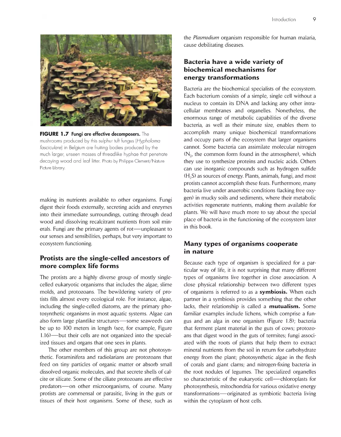
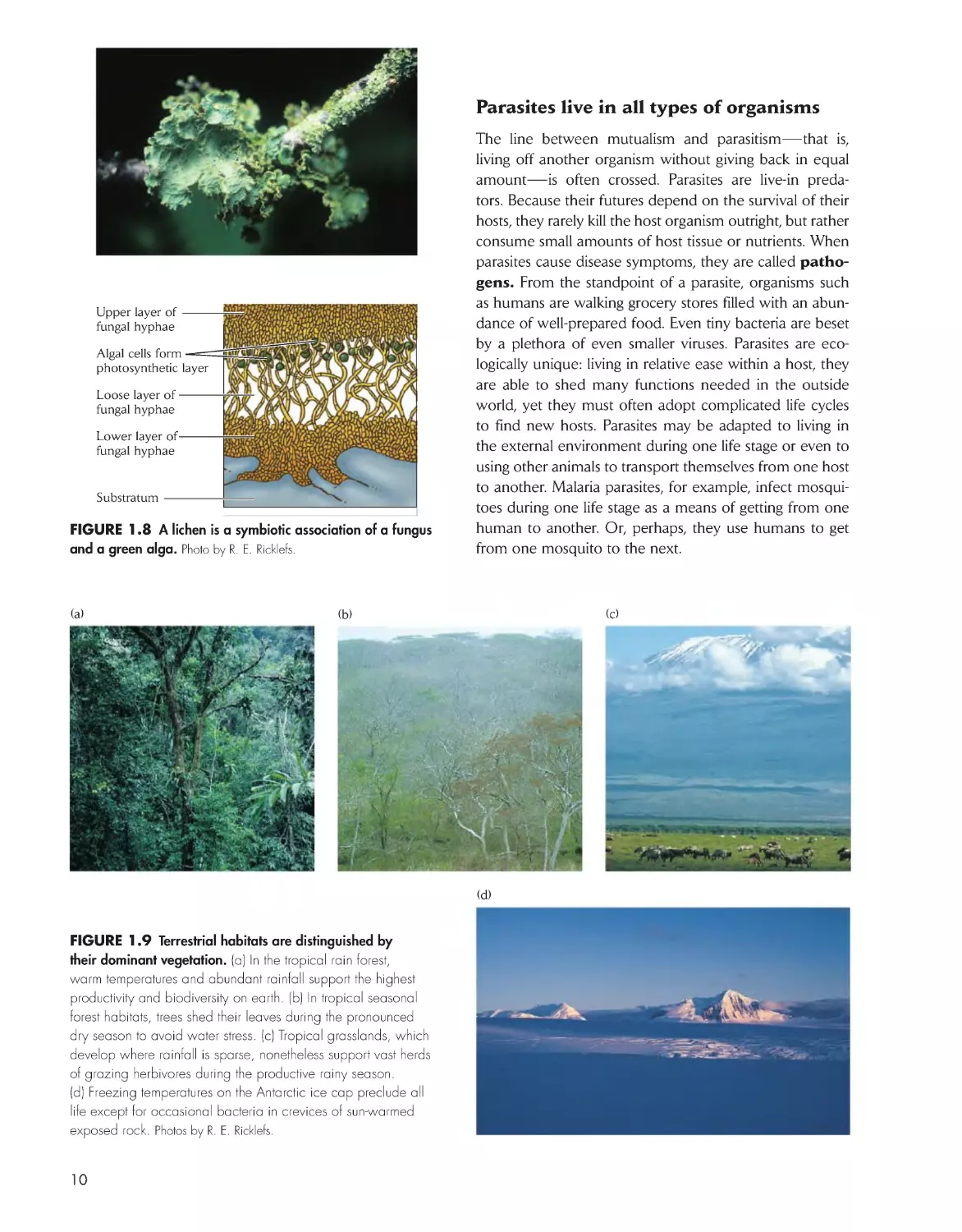
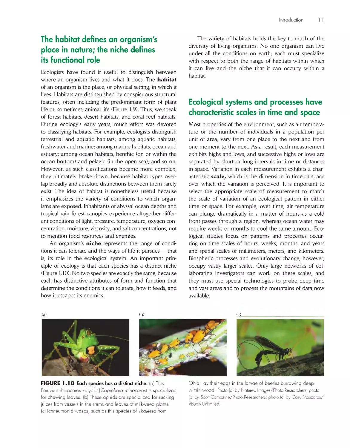
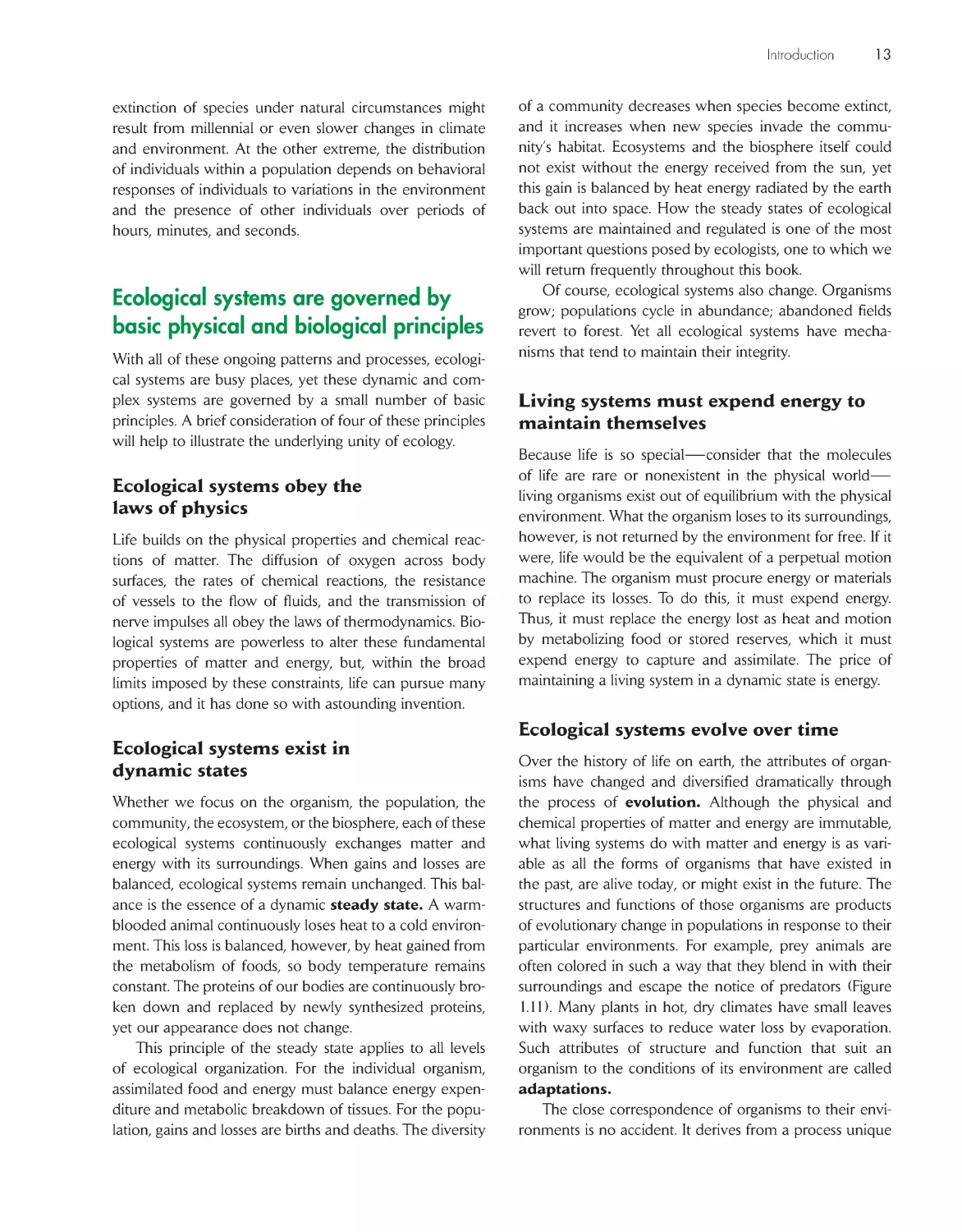
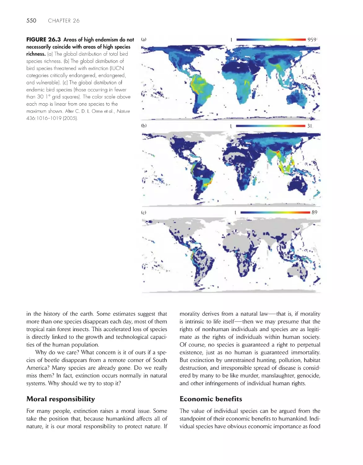
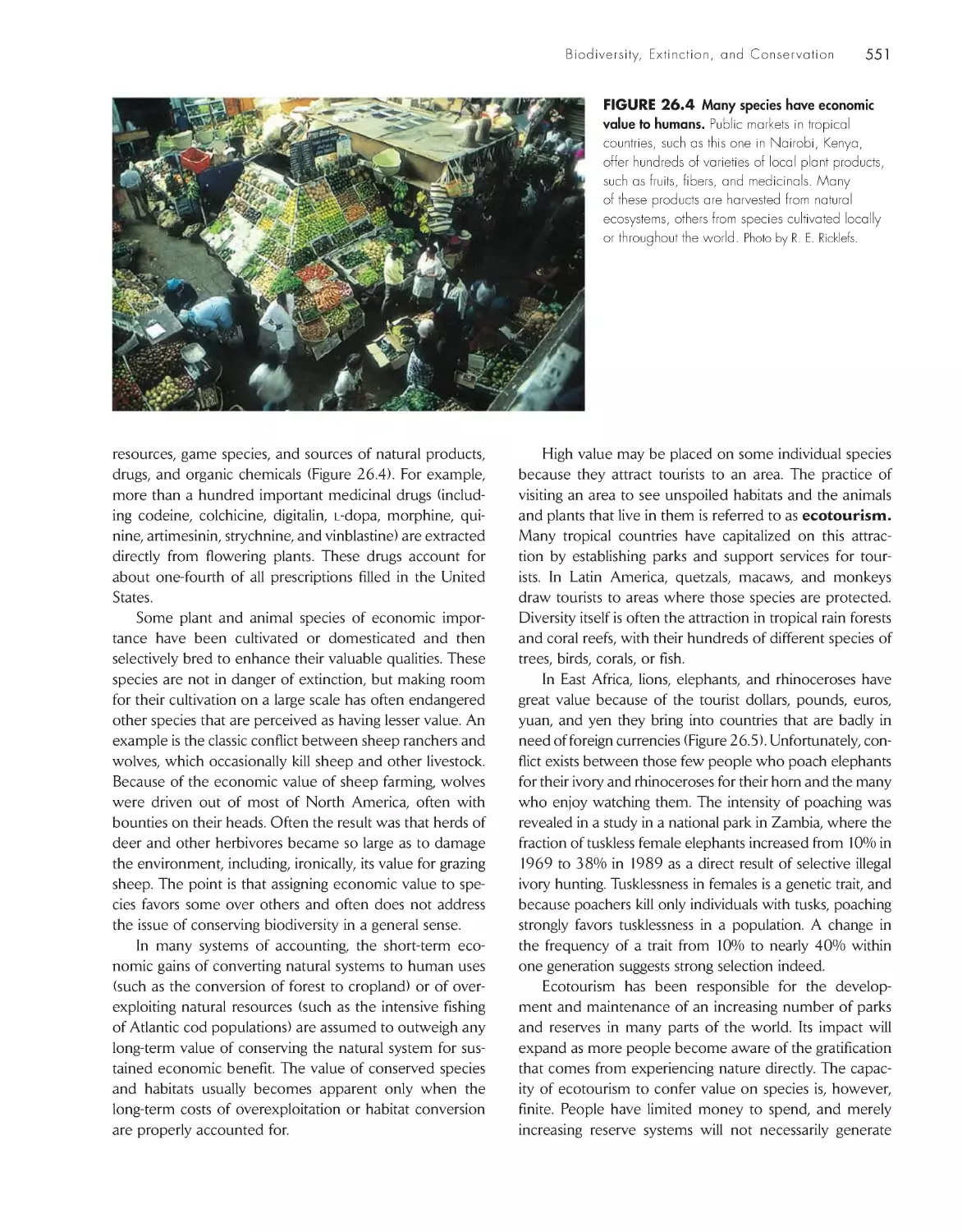
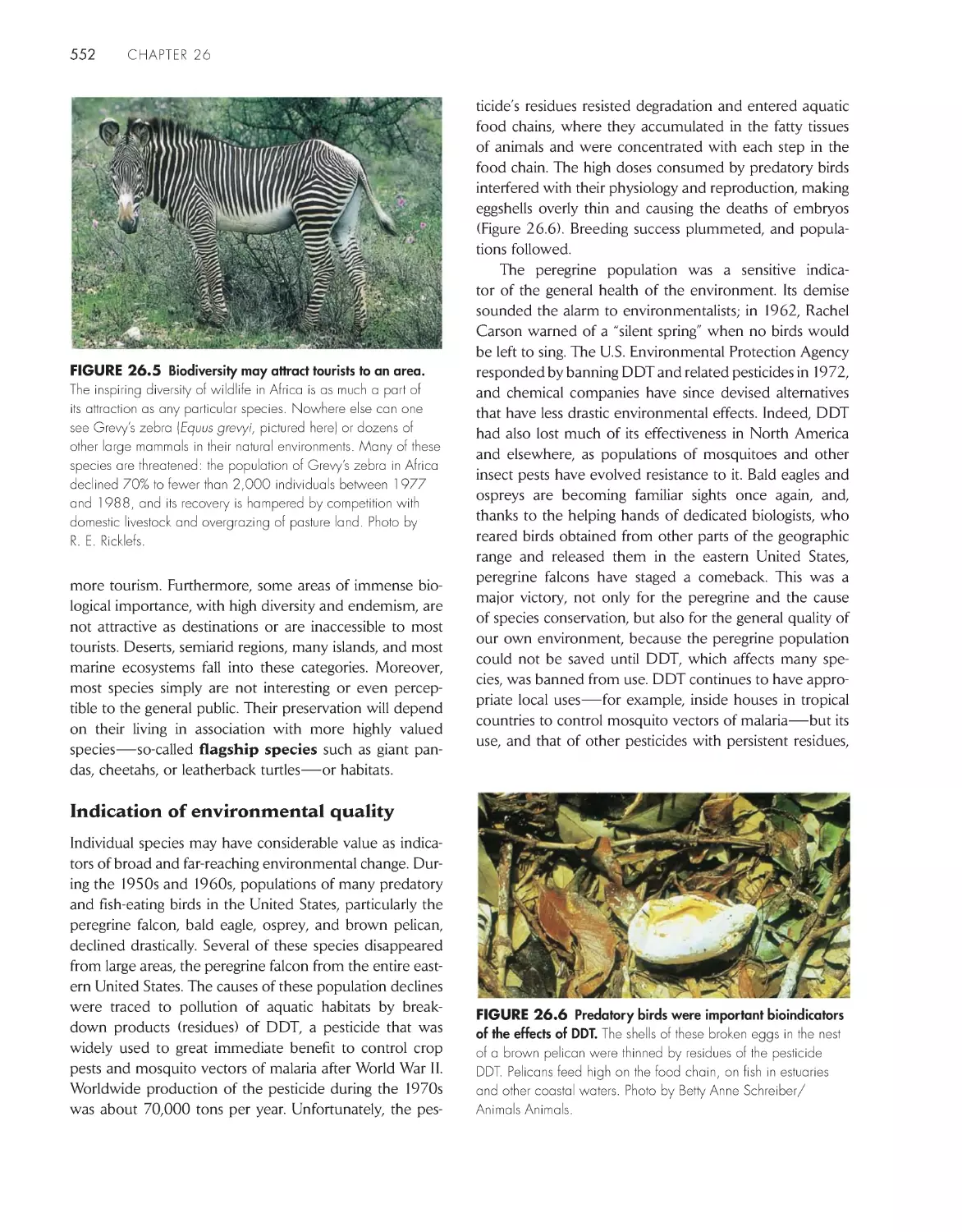
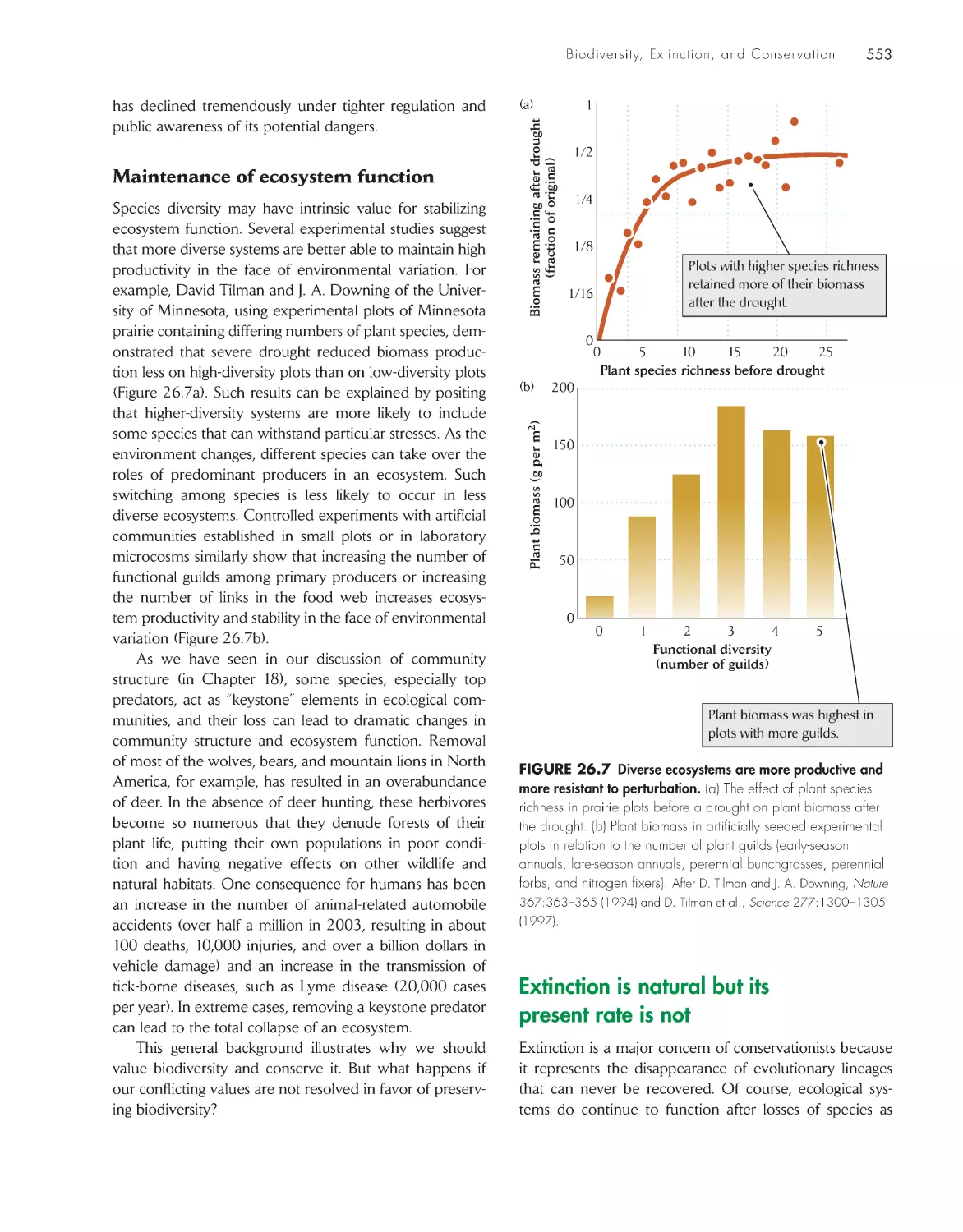
/


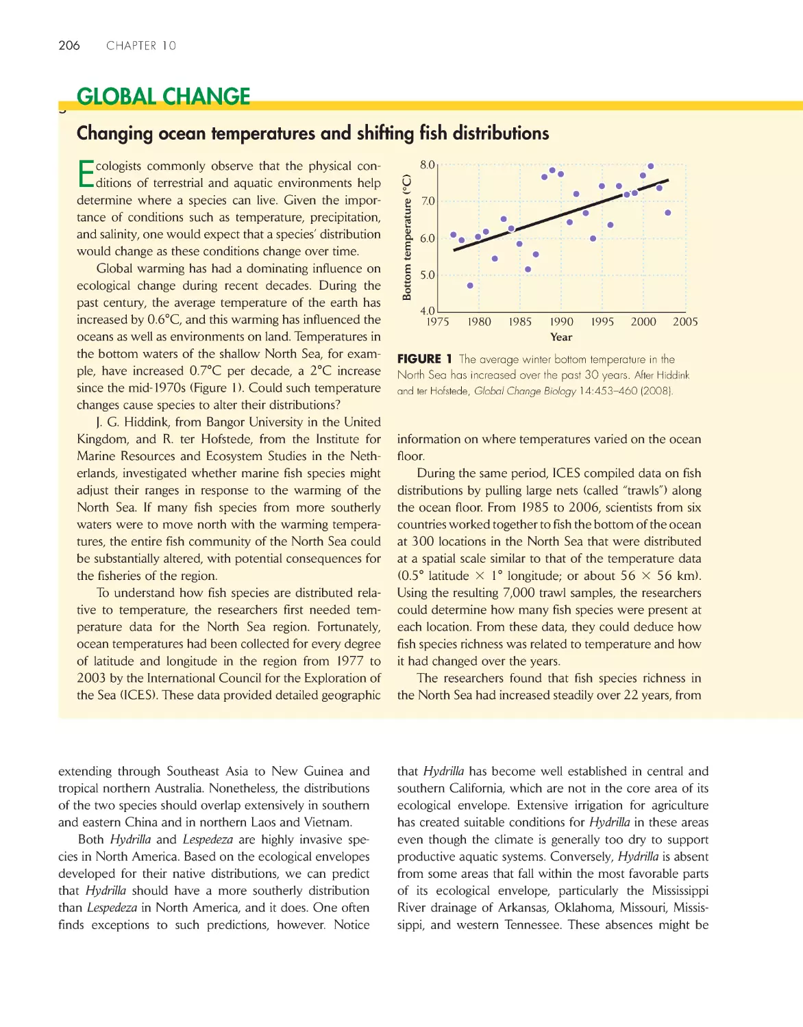


Текст
The Economy of Nature
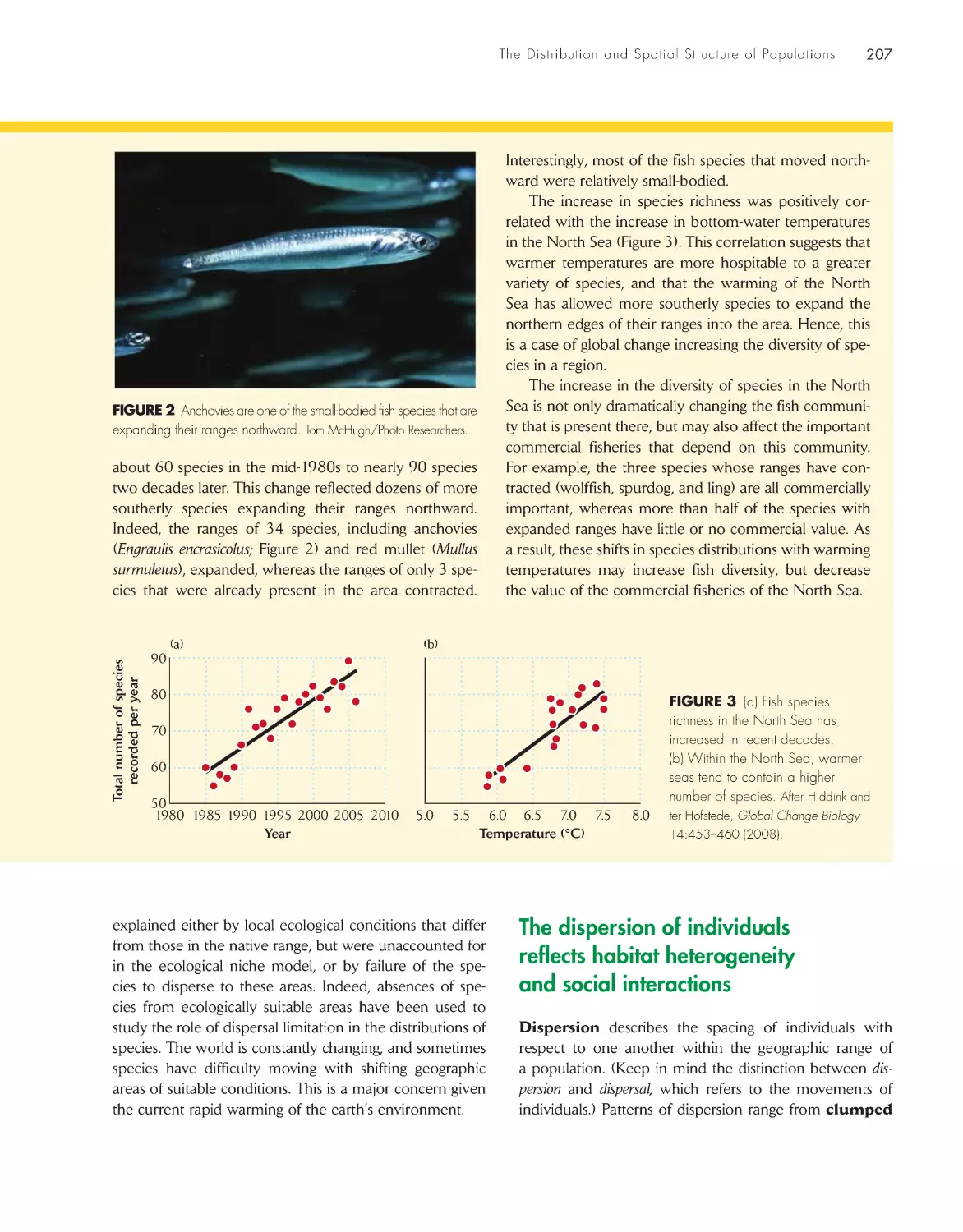
Sixth Edition
About the Author
Robert E. Ricklefs is Curators’ Professor of Biology at the University of Missouri–St. Louis,
where he joined the faculty in 1995 after 27 years in the Biology Department at the University
of Pennsylvania. Professor Ricklefs is a native of California and holds an undergraduate degree
from Stanford University and a Ph.D. from the University of Pennsylvania. His interests include
the energetics of reproduction in birds, evolutionary differentiation of life histories, biogeogra-
phy, and the historical development of biological communities, including the generation and
maintenance of large-scale patterns of biodiversity. His research has taken him to a wide variety
of habitats from the lowland tropics to seabird islands in Antarctica. Professor Ricklefs is a Fellow
of the American Association for the Advancement of Science and the American Academy of
Arts and Sciences. He is also the coauthor of Ecology, now in its fourth edition, and Aging: A
Natural History, both published by W. H . Freeman and Company.
The Economy
of Nature
Robert E. Ricklefs
University of Missouri–St. Louis
The Economy
of Nature
Sixth Edition
Robert E. Ricklefs
University of Missouri–St. Louis
W. h. Freeman and Company
New York
Acquisitions Editor: Jerry Correa
Developmental Editor: Susan Moran
Associate Director of Marketing: debbie Clare
Supplements and Media Editor: daniel Gonzalez
Project Editor: Georgia Lee hadler
Copy Editor: norma Sims Roche
Cover Designer: Paula Jo Smith
Text Designer: Victoria tomaselli
Photo Editor: Cecilia Varas
Photo Researcher: Julie tesser
Illustration Coordinator: Susan timmons
Illustrations: dragonfly Media Group
Production Manager: Julia deRosa
Composition: Matrix Publishing Ser vices
Manufacturing: RR donnelley & Sons
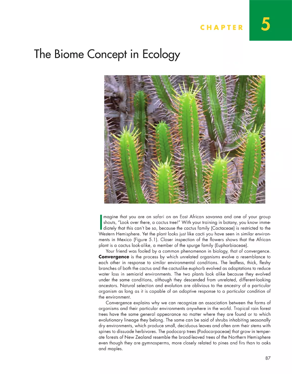
The chapter opening images were provided by the following photographers: Chapter 1, Luiz C. Marigo/
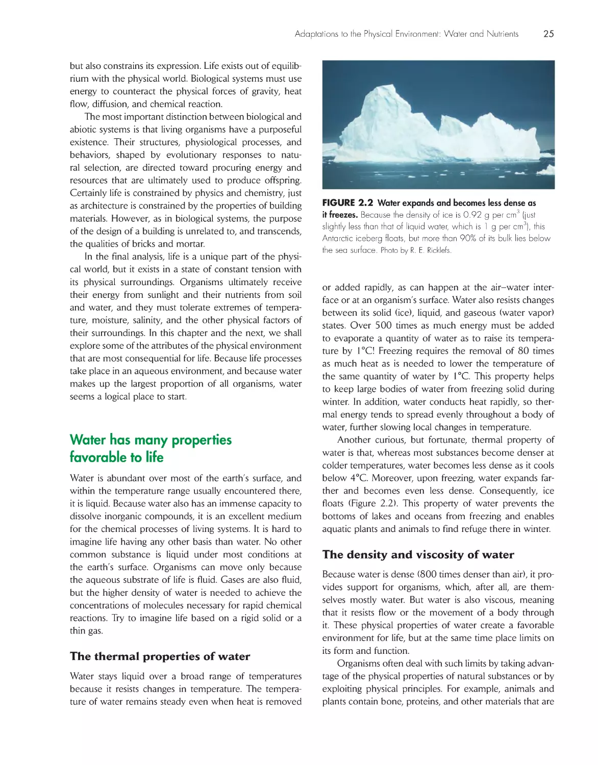
Peter Arnold; Chapter 2, Francois Gohier/ Photo Researchers; Chapter 3, Hanne & Jens Eriksen/ Nature
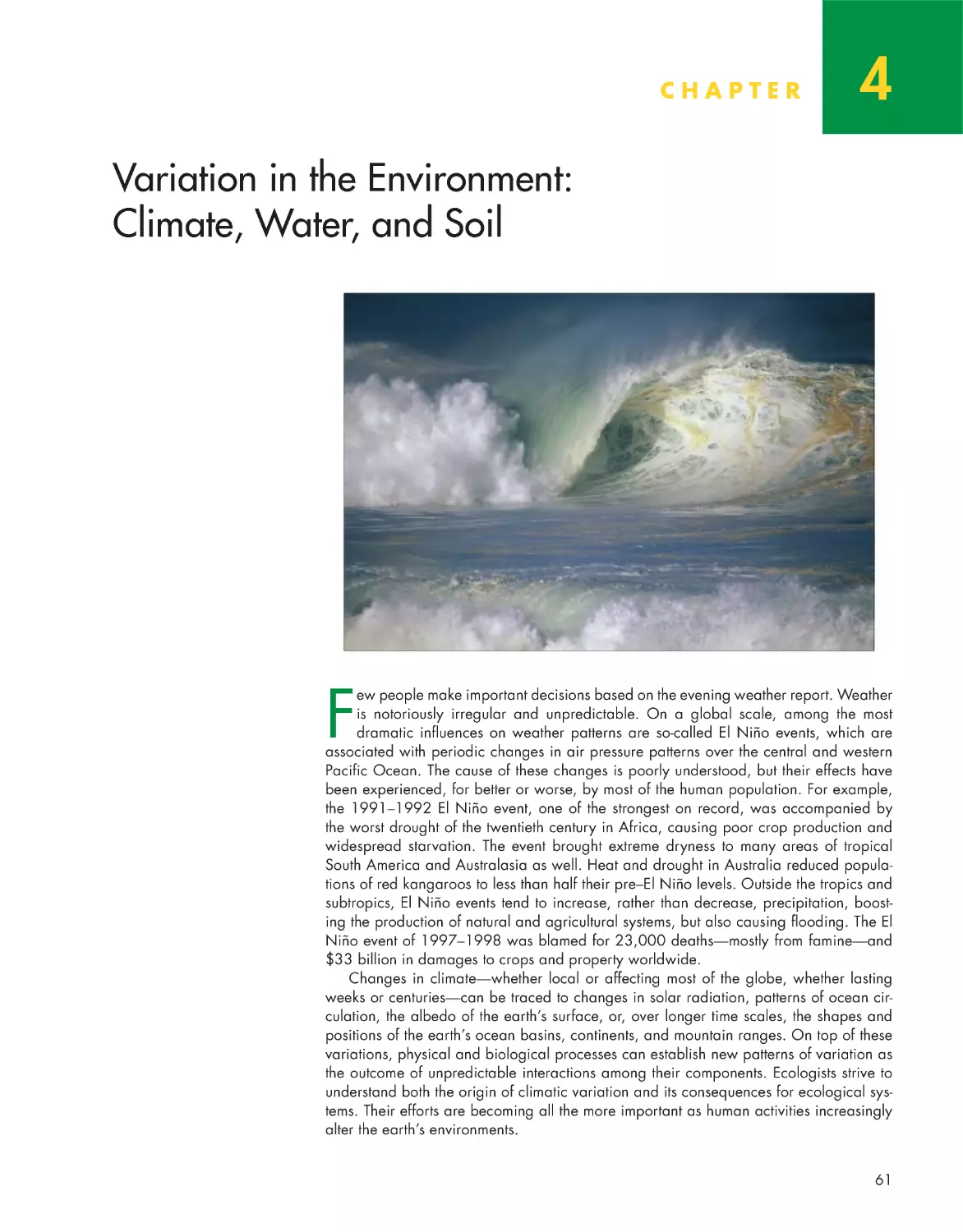
Picture Library; Chapter 4, Bill Brooks/Alamy; Chapter 5, Alan and Linda Detrick/Photo Researchers;
Chapter 6, Adrienne Gibson/Animals Animals—Earth Scenes; Chapter 7, Michel Roggo-Bios/Peter Arnold;
Chapter 8, Simon D. Pollard/Photo Researchers; Chapter 9, John R. MacGregor/ Peter Arnold; Chapter 10,
E. R . Degginger; Chapter 11, Images & Stories/Alamy; Chapter 12, Ernst Haas/Getty Images; Chapter 13,
Stockbyte/Alamy; Chapter 14, Peggy Greb/Agricultural Research Services/U.S. Department of Agriculture;
Chapter 15, Tom Brakefield/DRK Photo; Chapter 16, Boris Karpinski/Alamy; Chapter 17, Andy Rouse/
DRK Photo; Chapter 18, Tom Bean/DRK Photo; Chapter 19, NASA; Chapter 20, Jim Edds/Photo
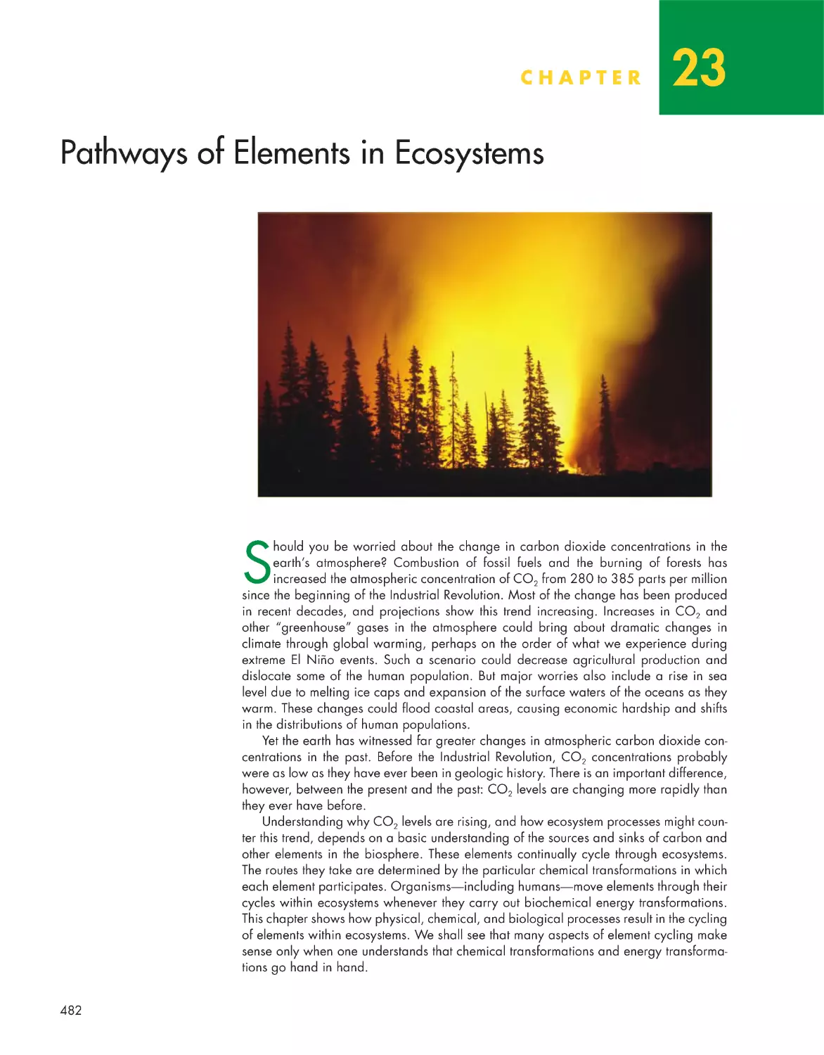
Researchers; Chapter 21, John Cancalosi/DRK Photo; Chapter 22, R. E. Ricklefs; Chapter 23, Tom & Pat
Leeson/ Photo Researchers; Chapter 24, Will & Deni McIntyre/ Photo Researchers; Chapter 25, James P.
Blair/Corbis; Chapter 26, William Campbell/Peter Arnold; Chapter 27, Jim Wilson/The New York Times/
Redux.
Library of Congress Control Number 2008932083
ISBN-13: 978-0 -716-78697-9
ISBN-10: 0-7167-8697-4
© 2008 by W. H . Freeman and Company
All rights reserved
Printed in the United States of America
First printing
W. H. Freeman and Company
41 Madison Avenue, New York, NY 10010
Houndmills, Basingstoke, RG21 6XS, England
www.whfreeman.com
brieF CoNteNts
ChApter 1 introduction
1
Part I LIfe and the PhysIcaL envIronment
ChApter 2 Adaptations to the physical environment: Water and Nutrients
23
ChApter 3 Adaptations to the physical environment: Light, energy, and heat
38
ChApter 4 Variation in the environment: Climate, Water, and soil
61
ChApter 5 the biome Concept in ecology
87
Part II organIsms
ChApter 6 evolution and Adaptation
113
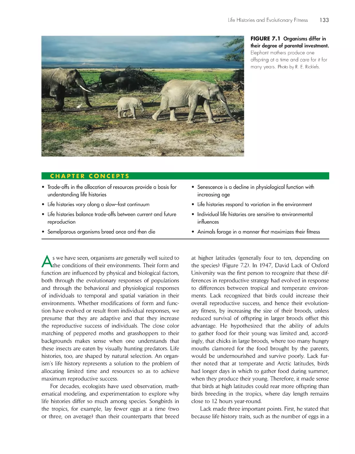
ChApter 7 Life histories and evolutionar y Fitness
132
ChApter 8 sex and evolution
159
ChApter 9 Family, society, and evolution
180
Part III PoPuLatIons
ChApter 10 the Distribution and spatial structure of populations
198
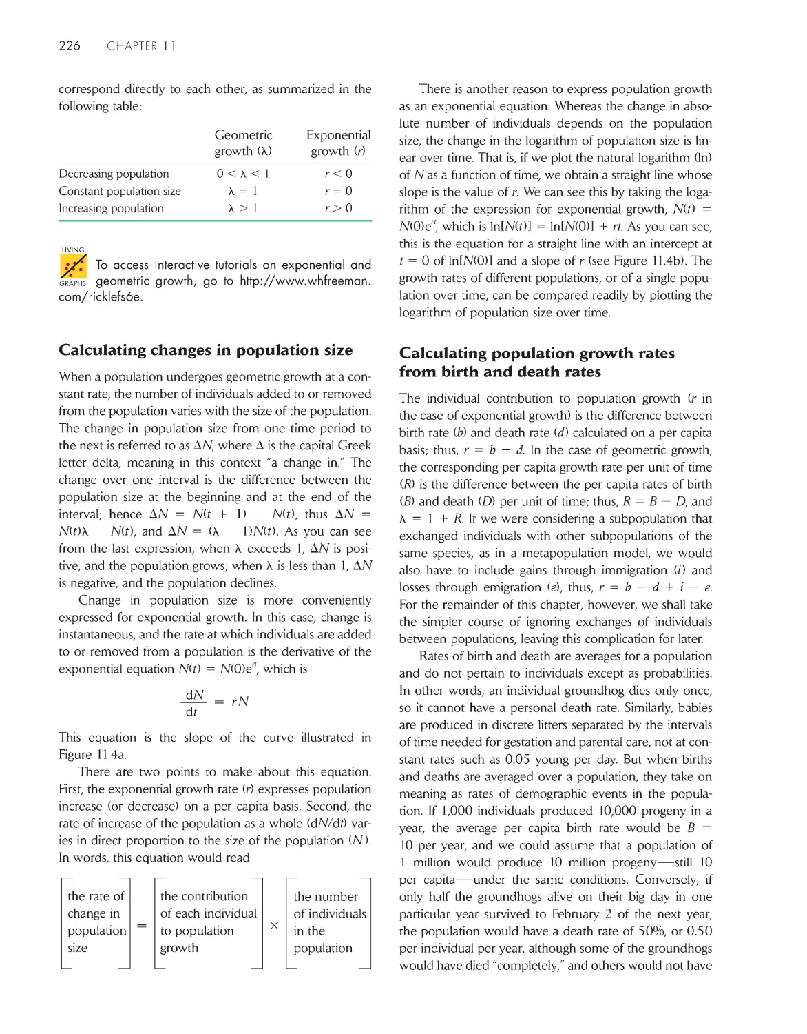
ChApter 11 population Growth and regulation
222
ChApter 12 temporal and spatial Dynamics of populations
248
ChApter 13 population Genetics
267
Part Iv sPecIes InteractIons
ChApter 14 species interactions
287
ChApter 15 Dynamics of Consumer–resource interactions
302
ChApter 16 Competition
328
ChApter 17 evolution of species interactions
346
Part v communItIes
ChApter 18 Community structure
369
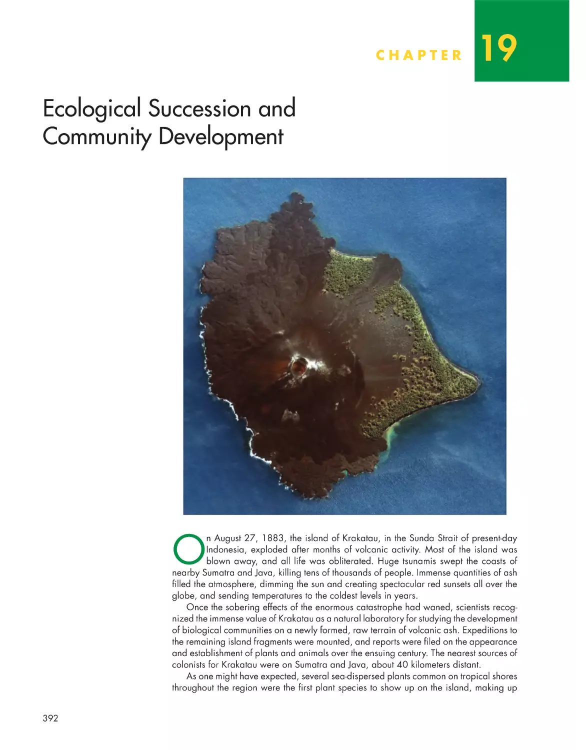
ChApter 19 ecological succession and Community Development
392
ChApter 20 biodiversity
411
ChApter 21 histor y, biogeography, and biodiversity
440
vi
Brief contents
Part vI ecosystems
ChApter 22 energy in the ecosystem
463
ChApter 23 pathways of elements in ecosystems
482
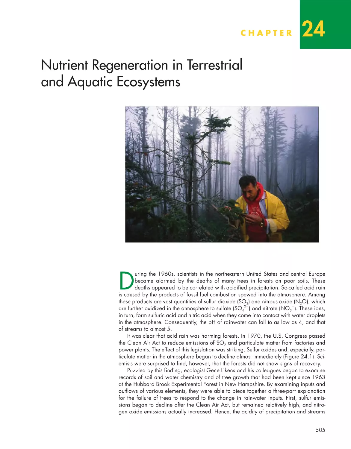
ChApter 24 Nutrient regeneration in terrestrial and Aquatic ecosystems
505
Part vII ecoLogIcaL aPPLIcatIons
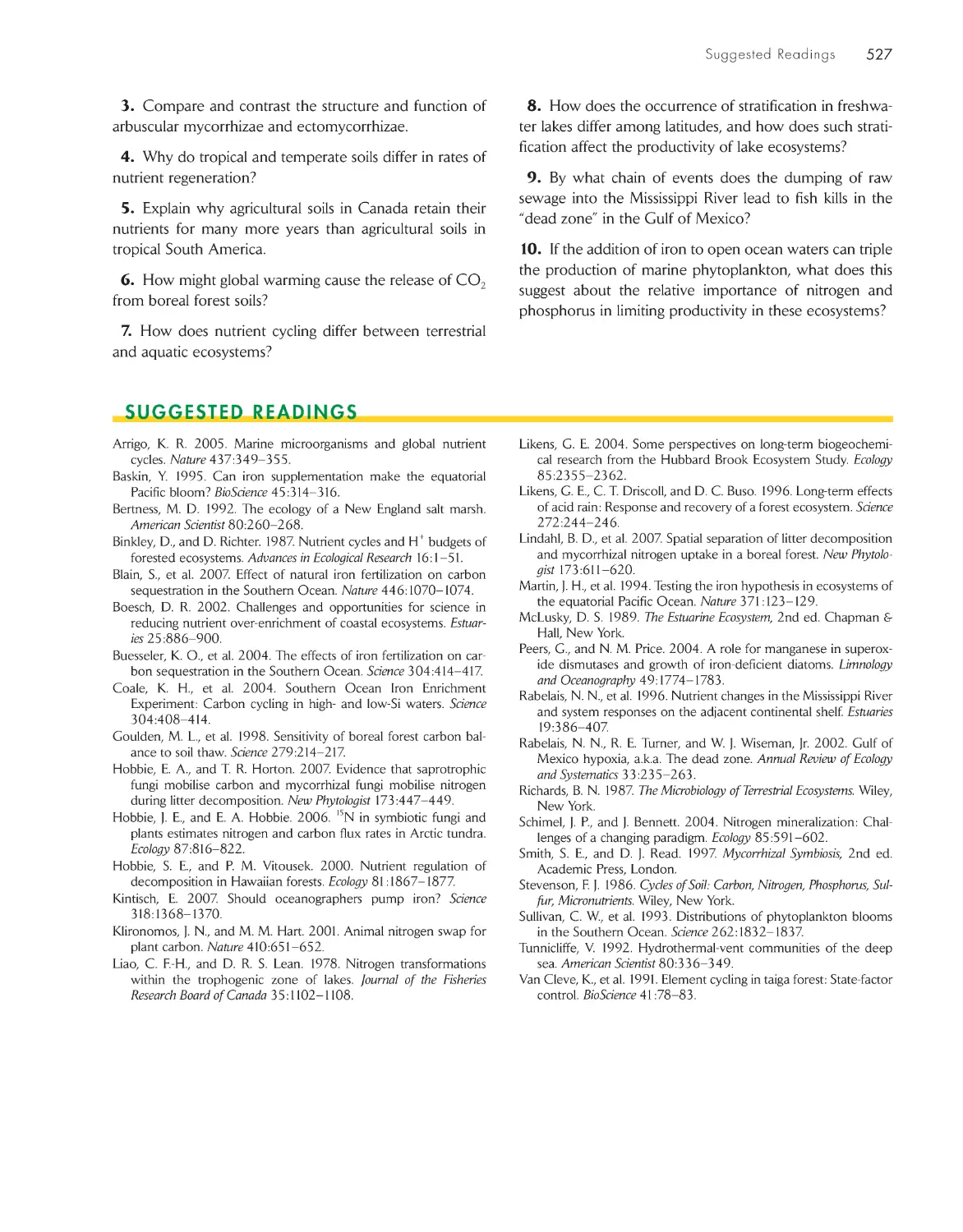
ChApter 25 Landscape ecology
528
ChApter 26 biodiversity, extinction, and Conser vation
545
ChApter 27 economic Development and Global ecology
570
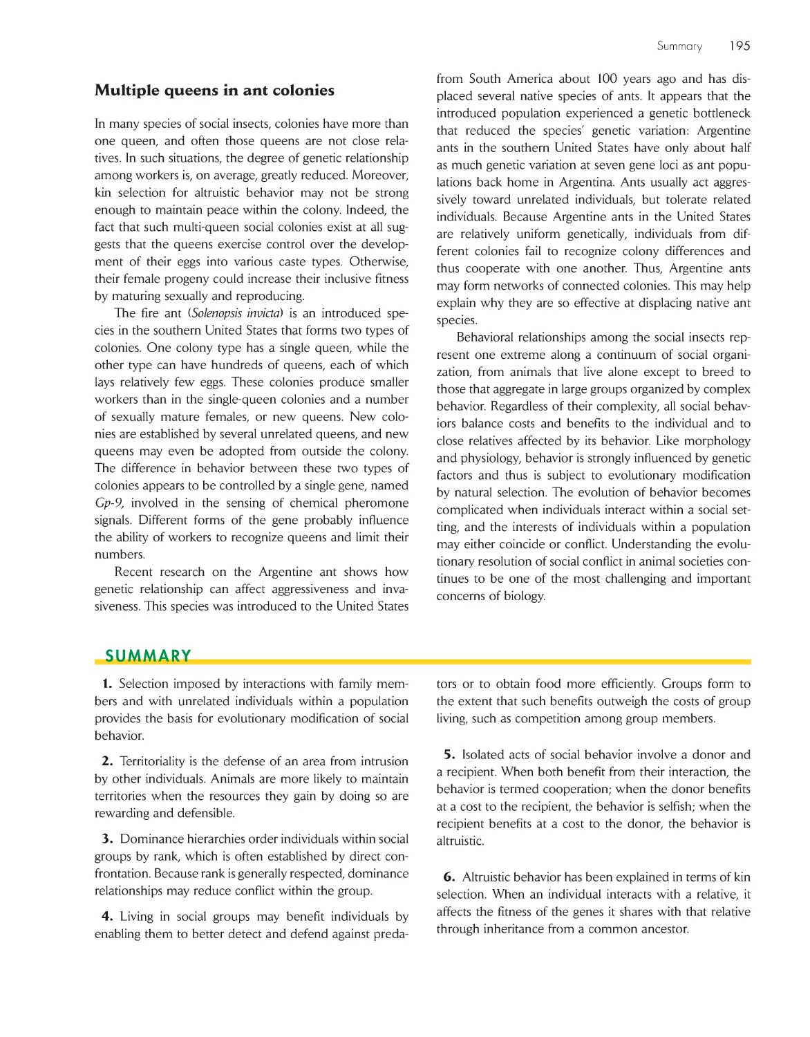
Preface
xiii
Acknowledgments
xviii
Chapter 1 Introduction
1
Ecological systems can be as small as individual
organisms or as large as the biosphere
3
Ecologists study nature from several perspectives
5
Plants, animals, and microorganisms play different
roles in ecological systems
7
The habitat defines an organism’s place in nature; the
niche defines its functional role 11
Ecological systems and processes have characteristic
scales in time and space 11
Ecological systems are governed by basic physical and
biological principles 13
Ecologists study the natural world by observation and
experimentation
14
Humans are a prominent part of the biosphere
17
Human impacts on the natural world have increasingly
become a focus of ecology 19
eCologIsts In the FIeld
Introduction of the Nile perch into Lake Victoria 17
The California sea otter
18
part I lIFe and the physICal envIronment
Chapter 2 adaptations to the physical
environment: Water and nutrients 23
Water has many properties favorable to life 25
Many inorganic nutrients are dissolved in water
26
Plants obtain water and nutrients from the soil by the
osmotic potential of their root cells 29
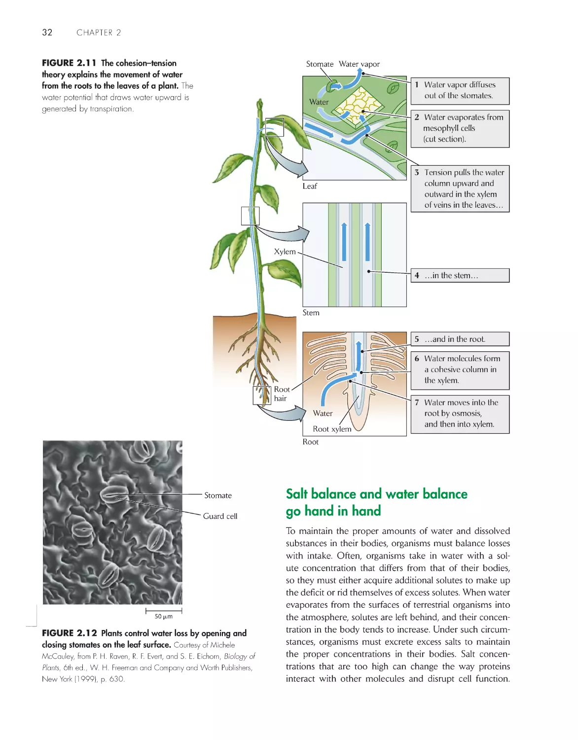
Forces generated by transpiration help to move water
from roots to leaves
31
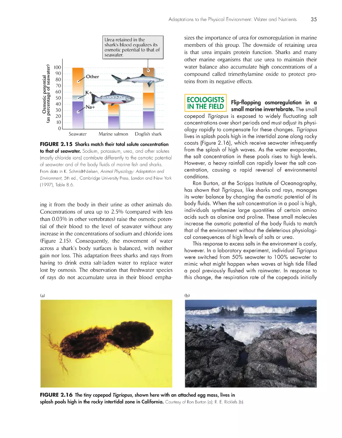
Salt balance and water balance go hand in
hand 32
Animals must excrete excess nitrogen without losing
too much water
36
eCologIsts In the FIeld
Flip-flopping osmoregulation in a small marine
invertebrate
35
Chapter 3 adaptations to the physical
environment: light, energy, and heat
38
Light is the primary source of energy for the
biosphere
39
Plants capture the energy of sunlight
by photosynthesis 41
Plants modify photosynthesis in
environments with high water
stress
42
Diffusion limits uptake of dissolved
gases from water
46
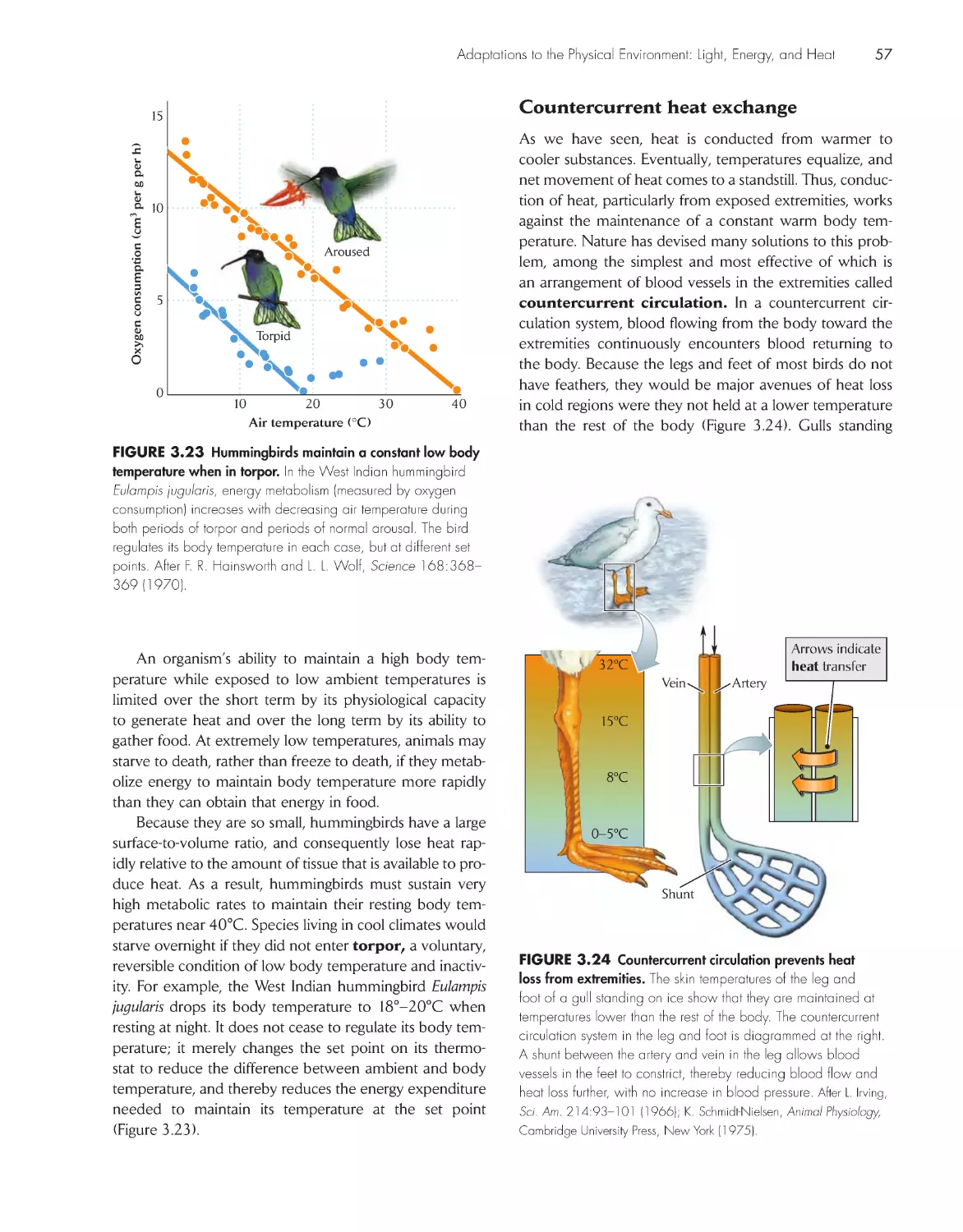
Temperature limits the occurrence
of life 48
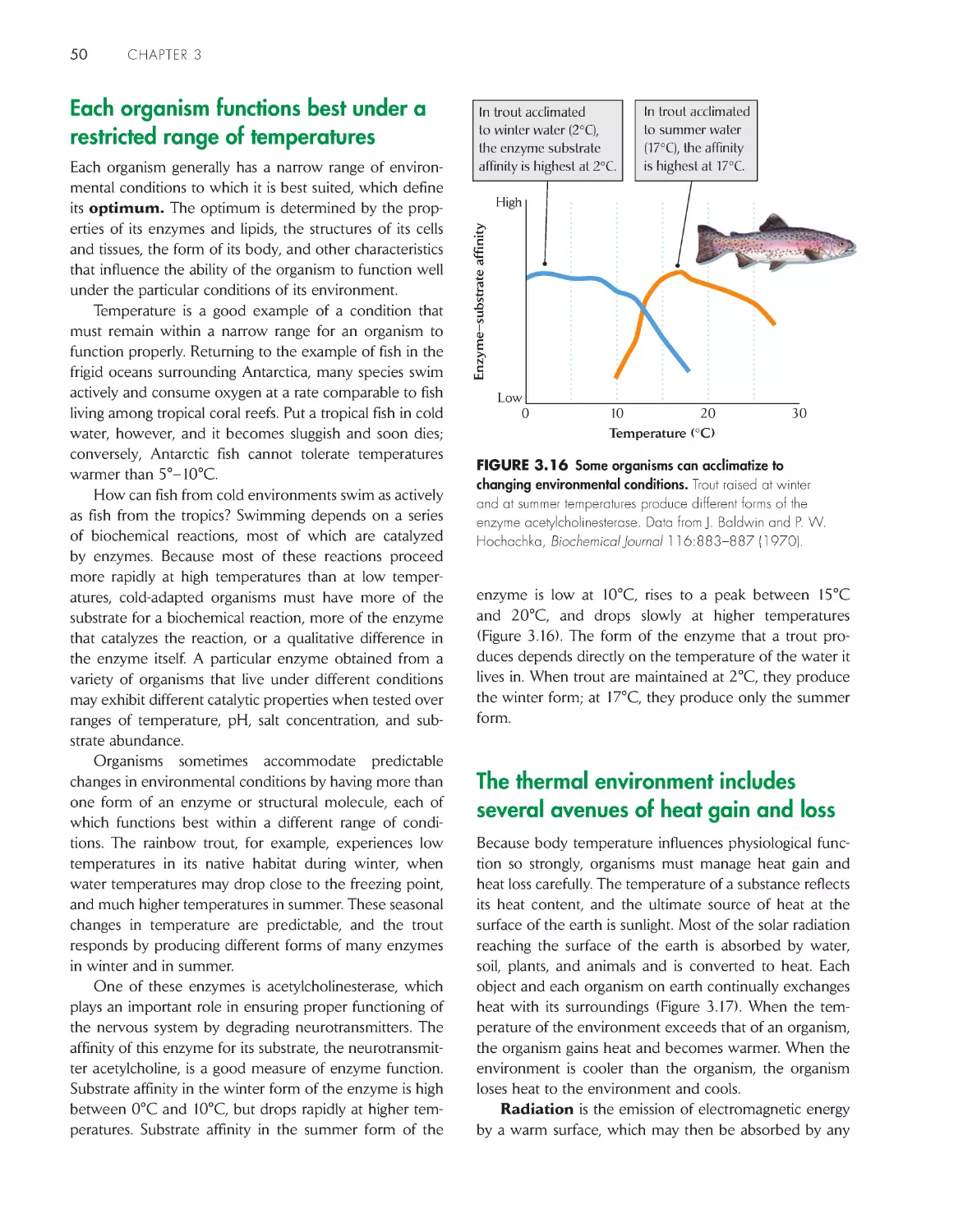
Each organism functions best under a restricted range of
temperatures
50
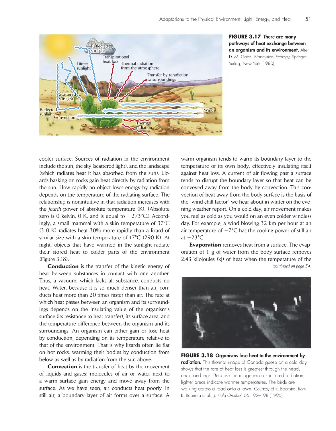
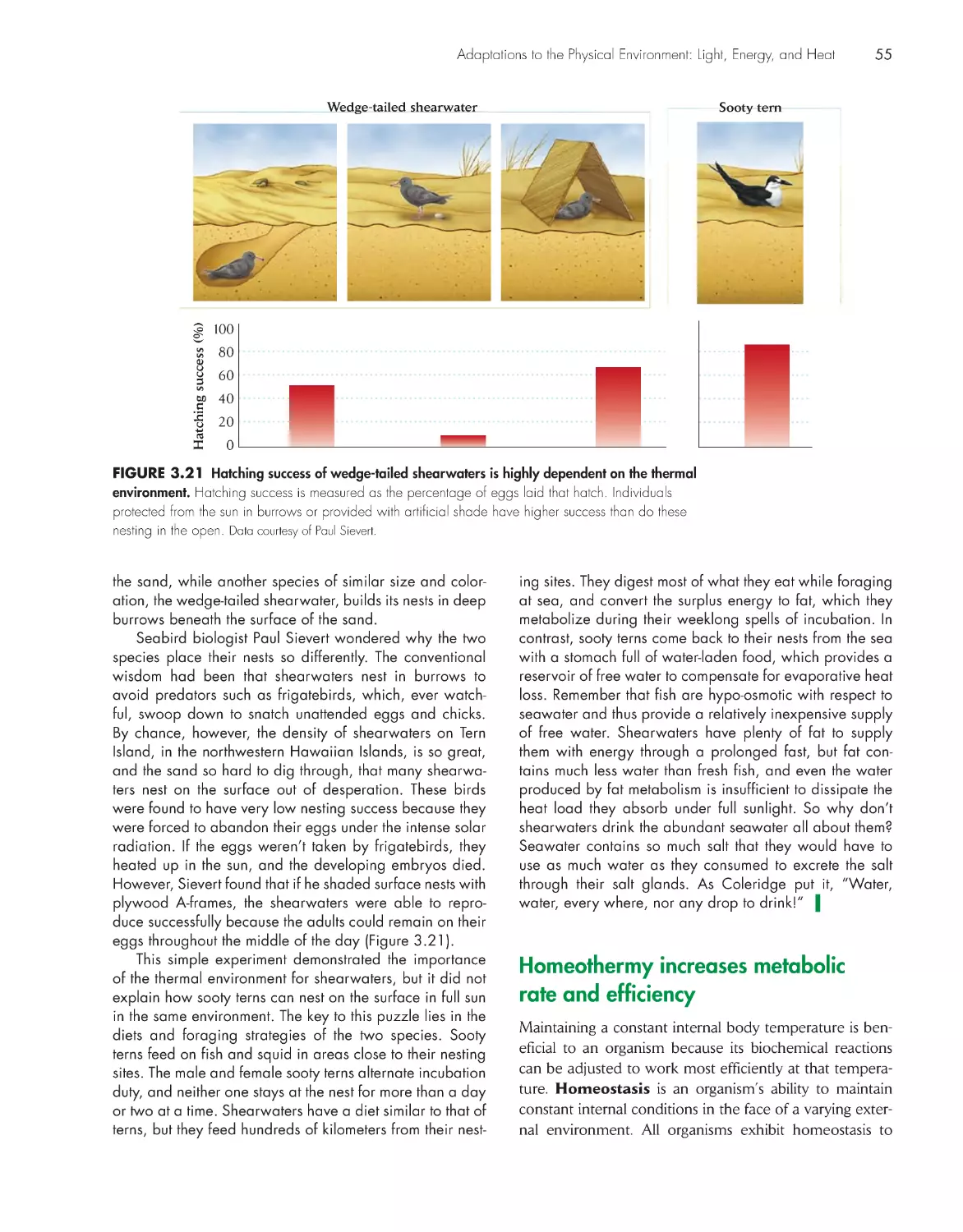
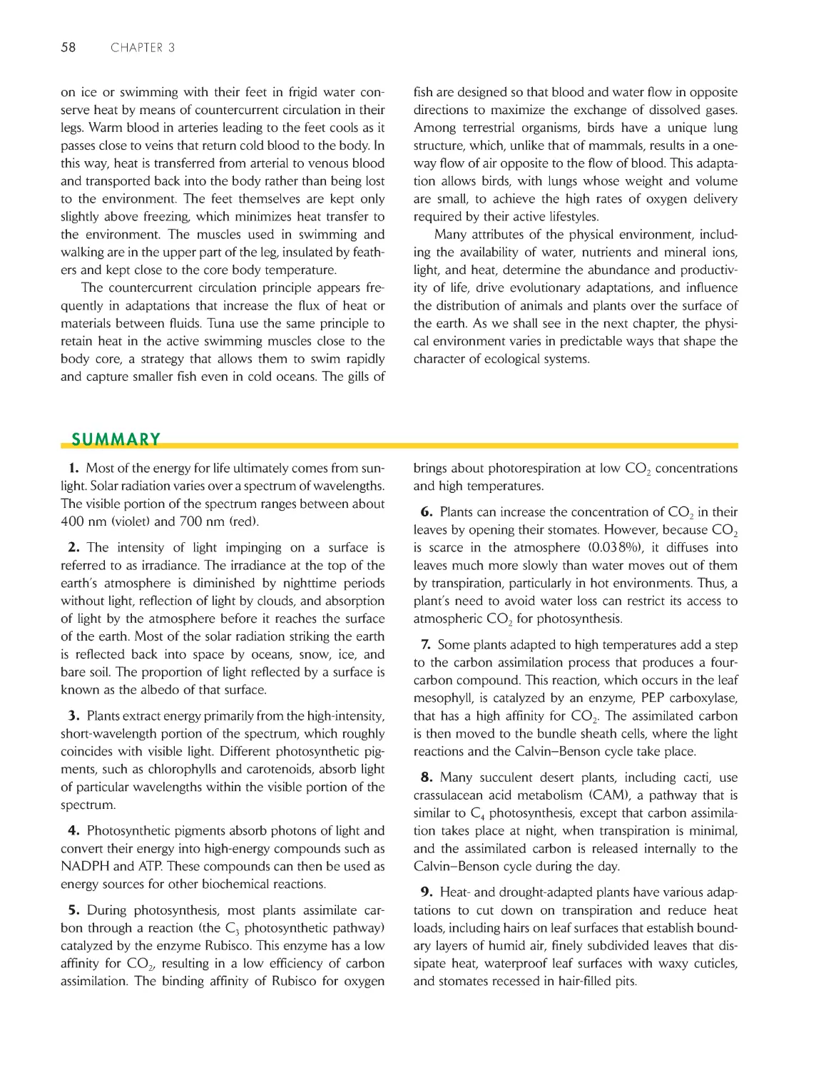
The thermal environment includes several avenues of
heat gain and loss 50
Homeothermy increases metabolic rate and
efficiency 55
global Change
Carbon dioxide and global warming 52
eCologIsts In the FIeld
Keeping cool on tropical islands 54
Chapter 4 variation in the environment:
Climate, Water, and soil 61
Global patterns in temperature and precipitation are
established by solar radiation
62
Ocean currents redistribute heat
67
Latitudinal shifting of the sun’s zenith causes seasonal
variation in climate
69
Temperature-induced changes in water density drive
seasonal cycles in temperate lakes 70
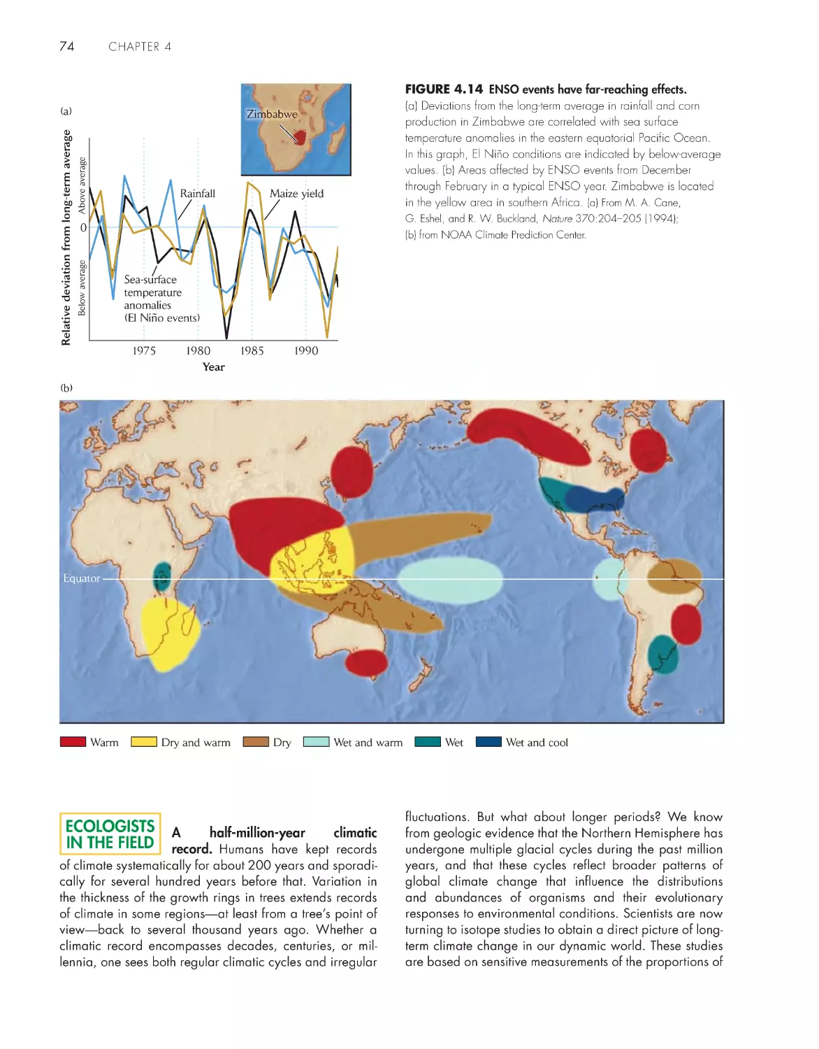
Climate and weather undergo irregular and often
unpredictable changes 72
Topographic features cause local variation in
climate
75
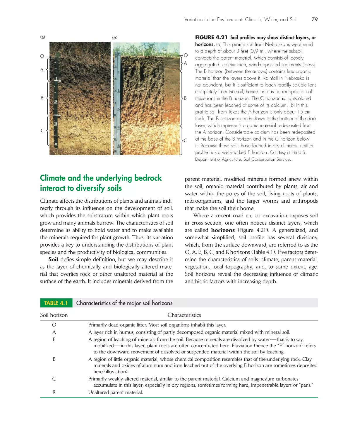
Climate and the underlying bedrock interact to diversify
soils 79
eCologIsts In the FIeld
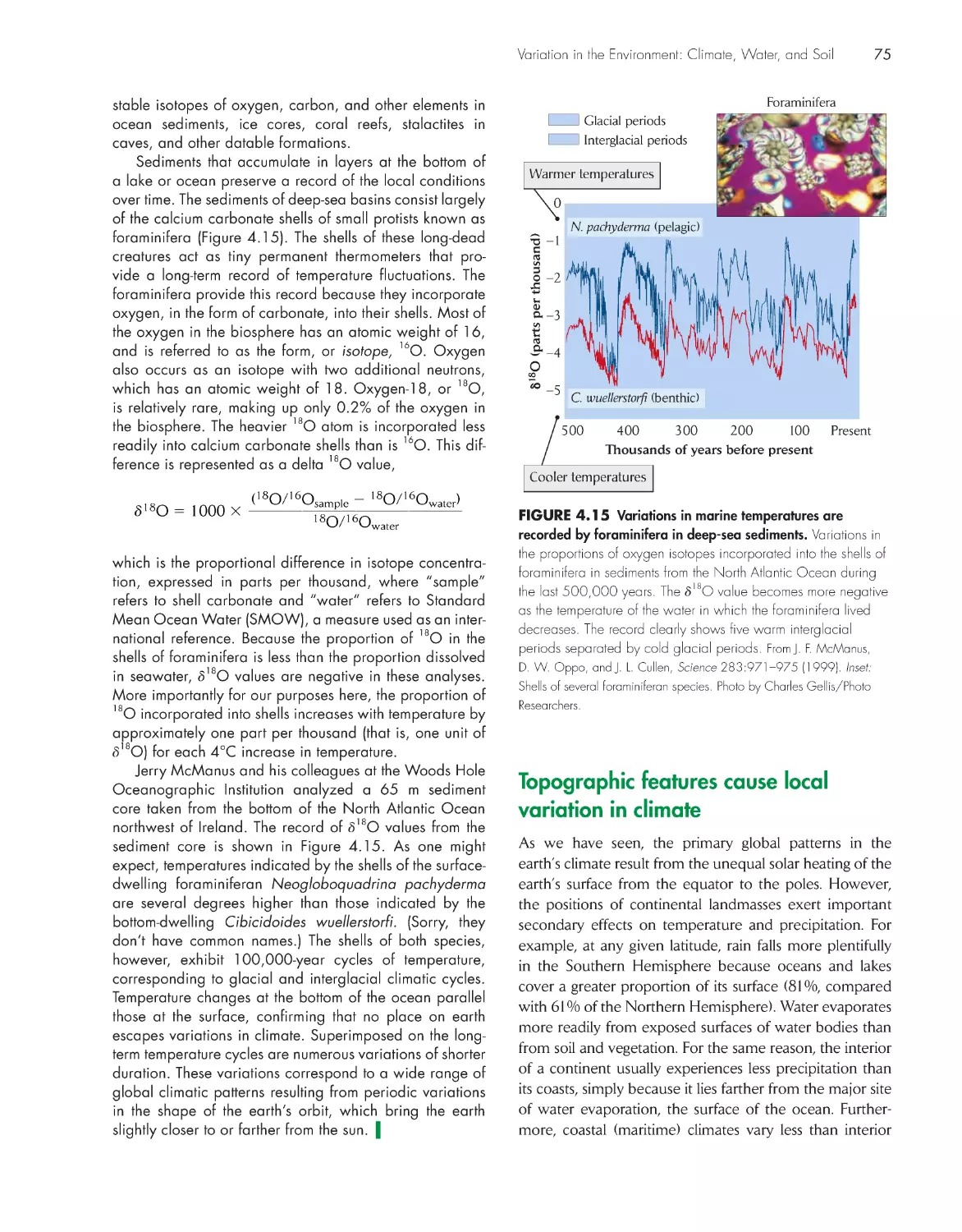
A half-million-year climatic record 74
Which came first, the soil or the forest?
83
Contents
viii
contents
ChApter 5 the biome Concept in ecology 87
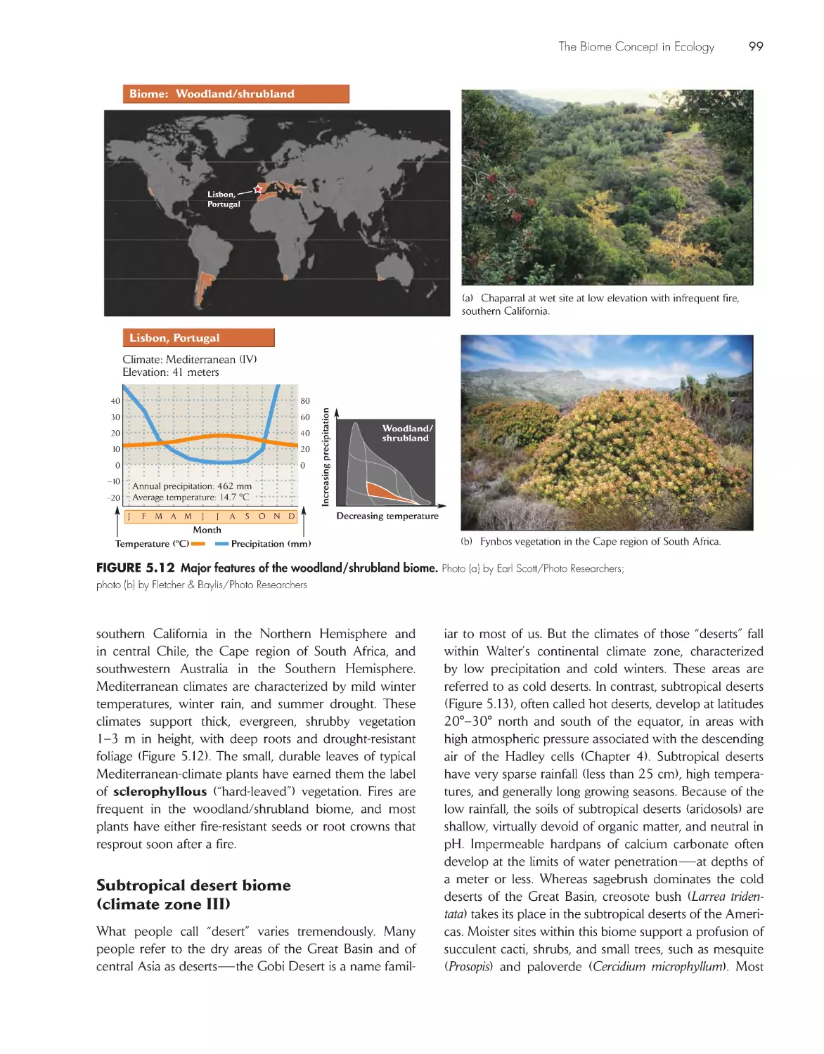
Climate is the major determinant of plant growth form
and distribution
89
Climate defines the boundaries of terrestrial
biomes
91
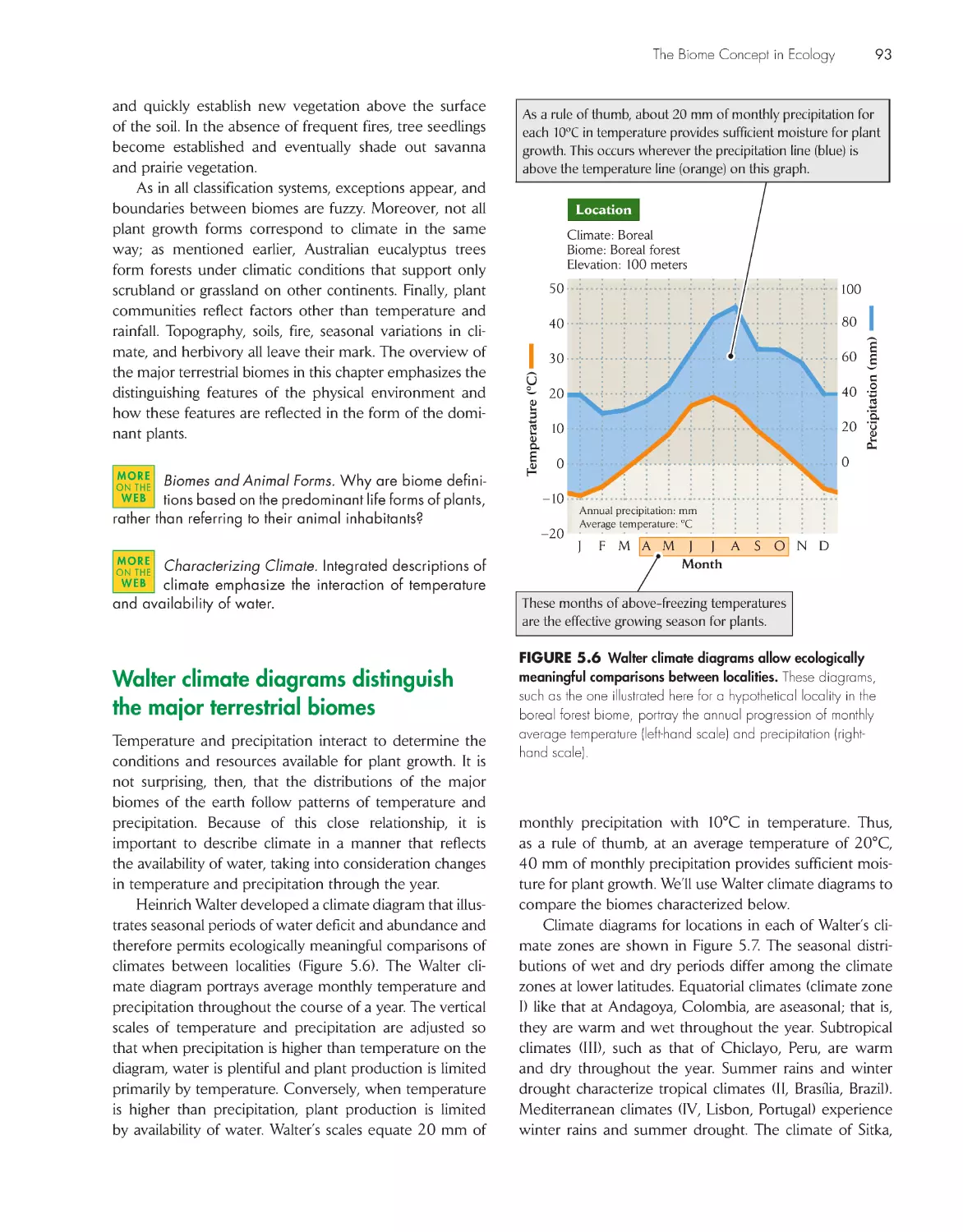
Walter climate diagrams distinguish the major terrestrial
biomes
93
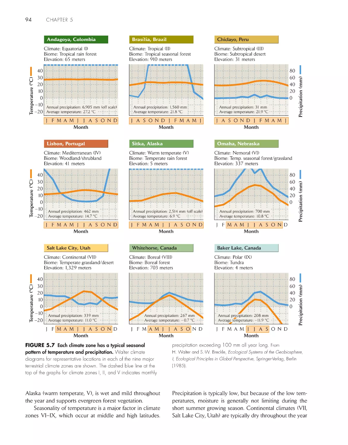
Temperate climate zones have average annual
temperatures between 5°C and 20°C 95
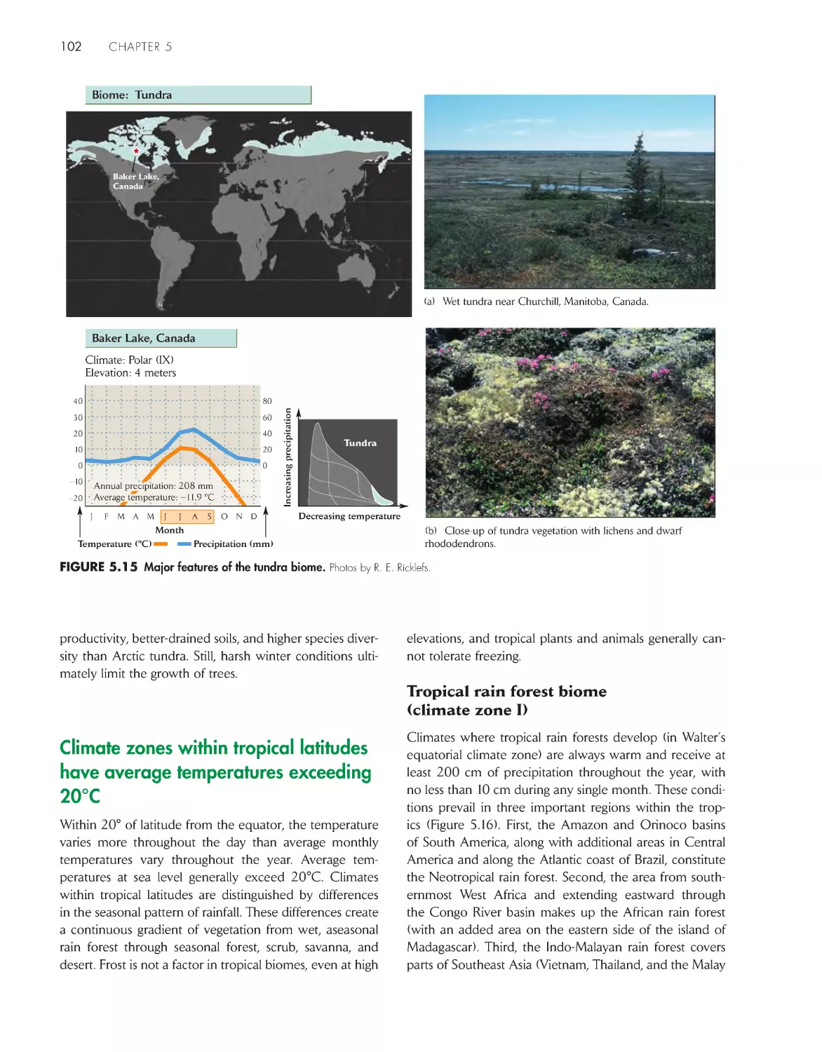
Boreal and polar climate zones have average
temperatures below 5°C 100
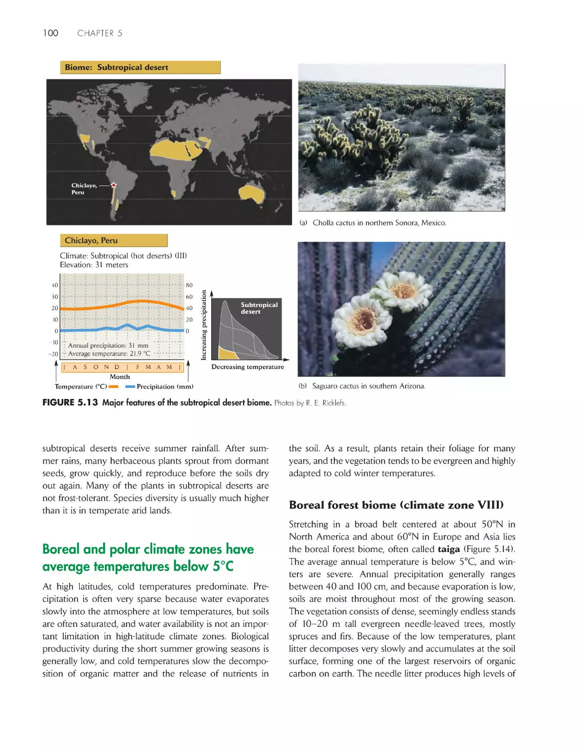
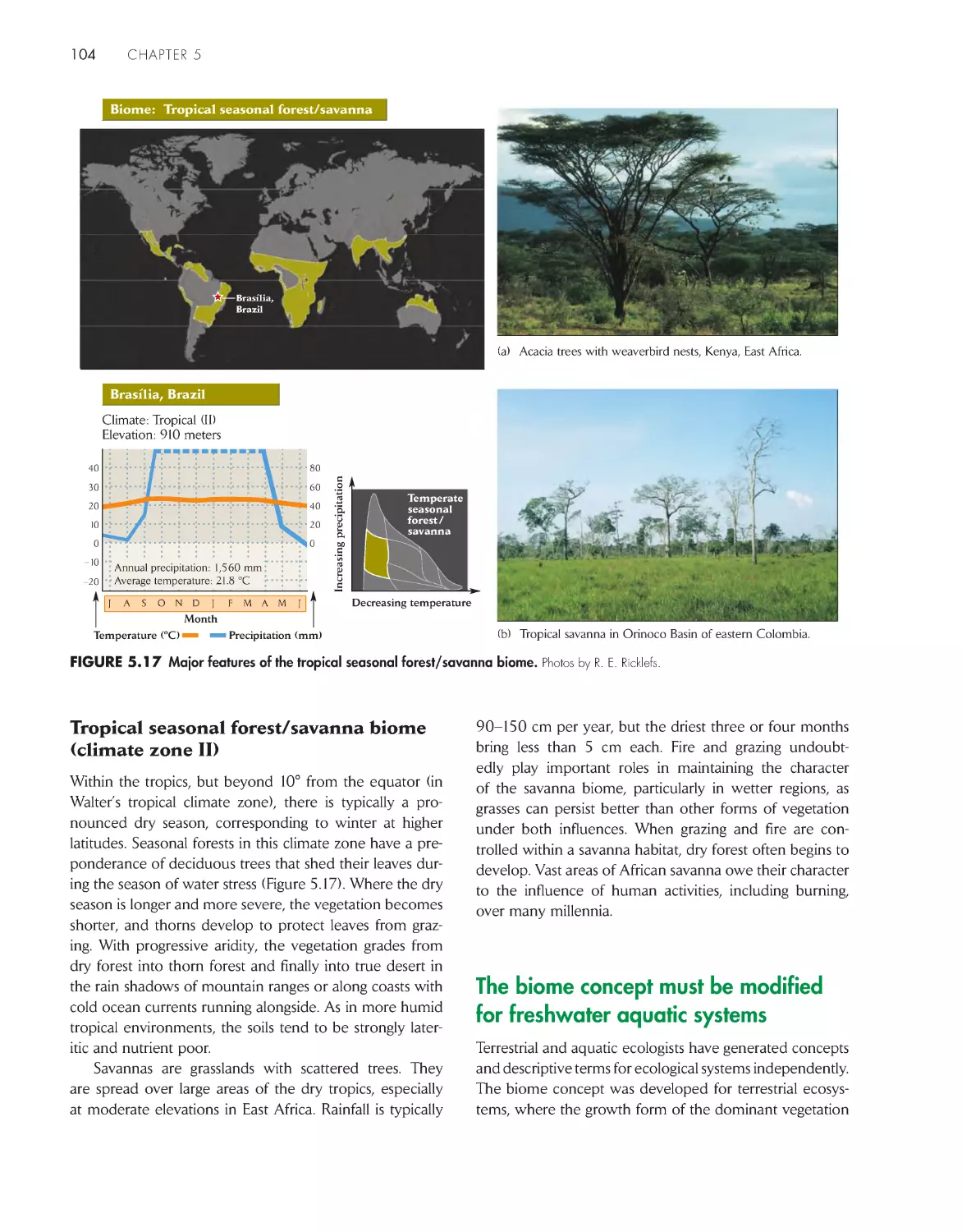
Climate zones within tropical latitudes have average
temperatures exceeding 20°C 102
The biome concept must be modified for freshwater
aquatic systems
104
Marine aquatic systems are classified principally by
water depth 108
pArt ii orGANisms
ChApter 6 evolution and Adaptation
113
The phenotype is the outward expression of an
individual’s genotype 115
Adaptations result from natural
selection on heritable variation in
traits that affect
evolutionary fitness
117
Evolutionary changes in allele
frequencies have been
documented in natural
populations
121
Individuals can respond to their
environments and increase their
fitness
124
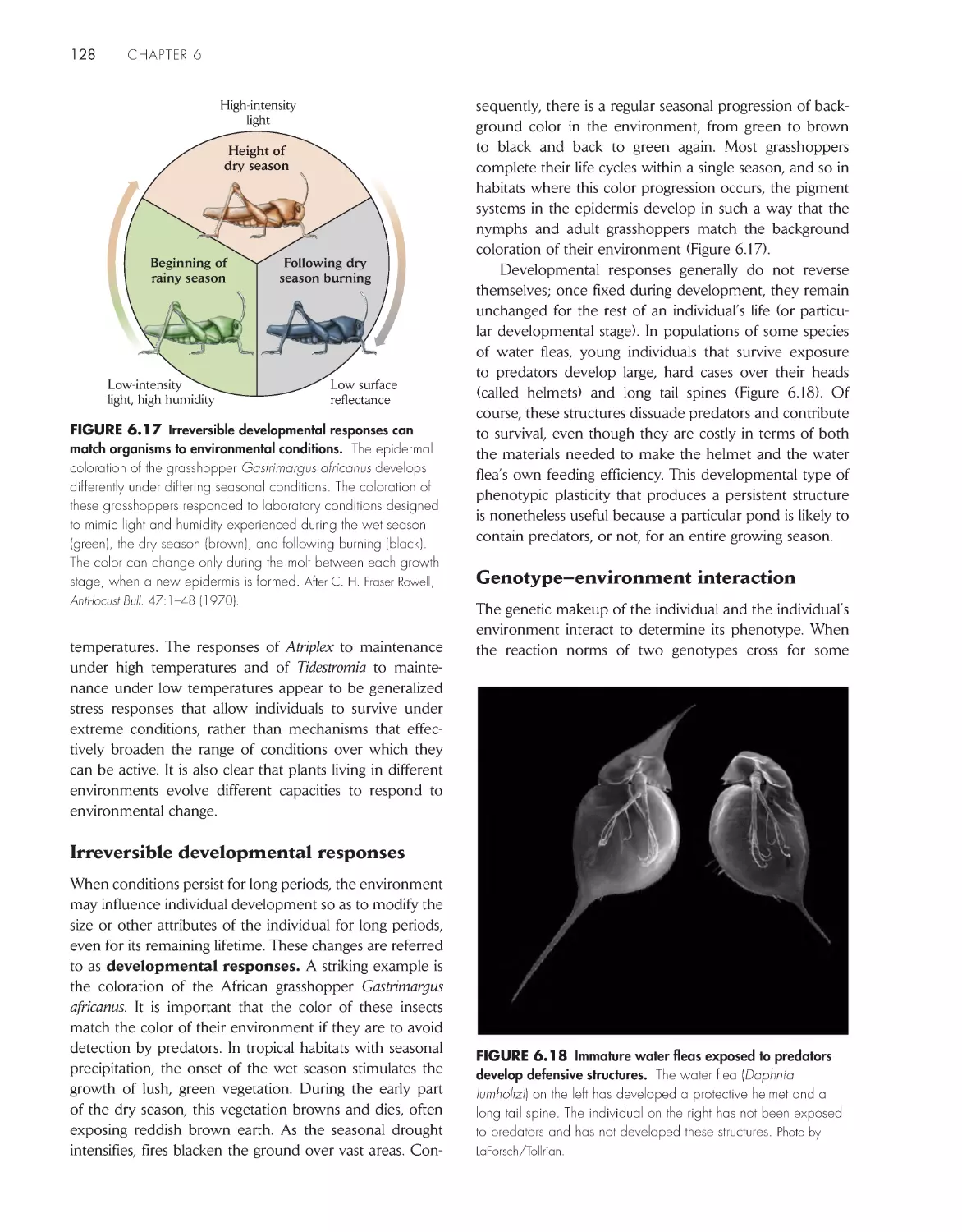
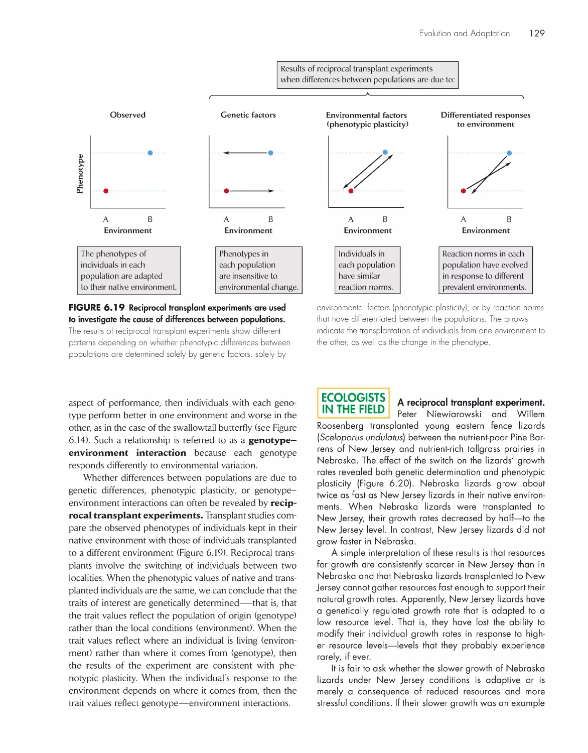
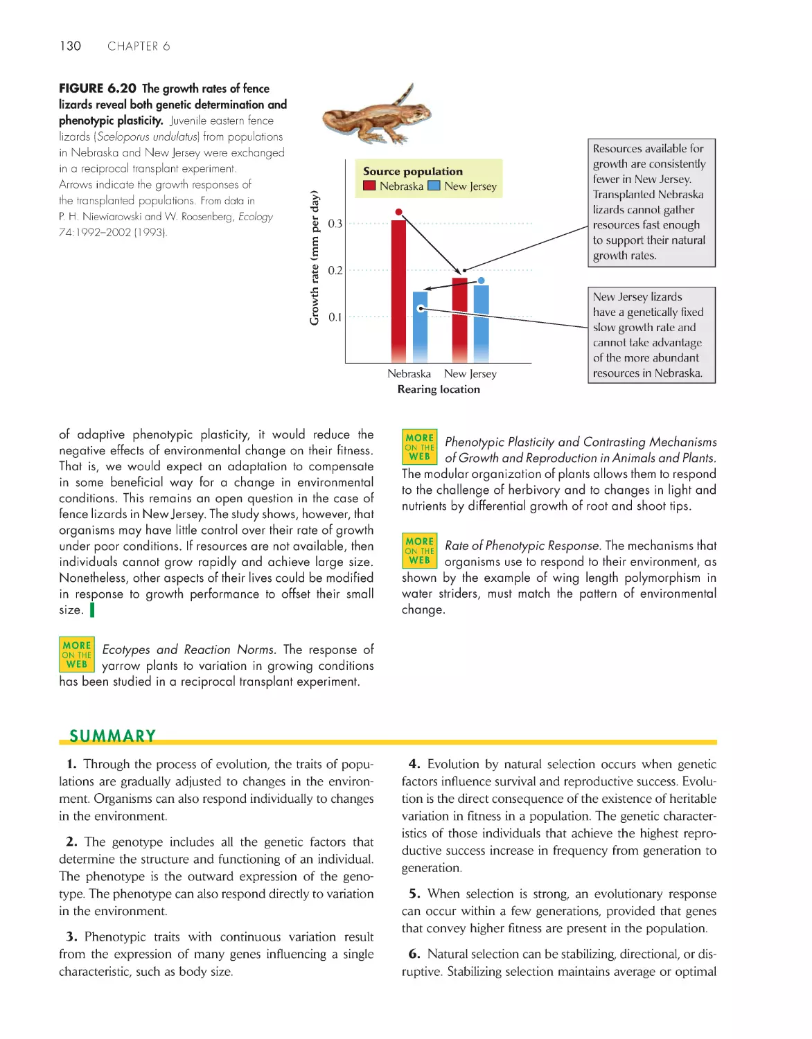
Phenotypic plasticity allows individuals to adapt to
environmental change 126
eCoLoGists iN the FieLD
Rapid evolution in response to an introduced
parasitoid 119
A reciprocal transplant experiment
129
ChApter 7 Life histories and evolutionar y
Fitness
132
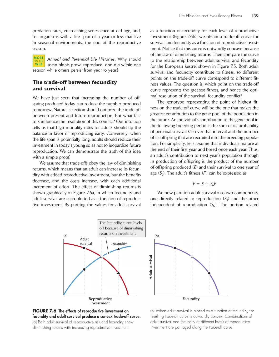
Trade-offs in the allocation of resources provide a
basis for understanding life histories 135
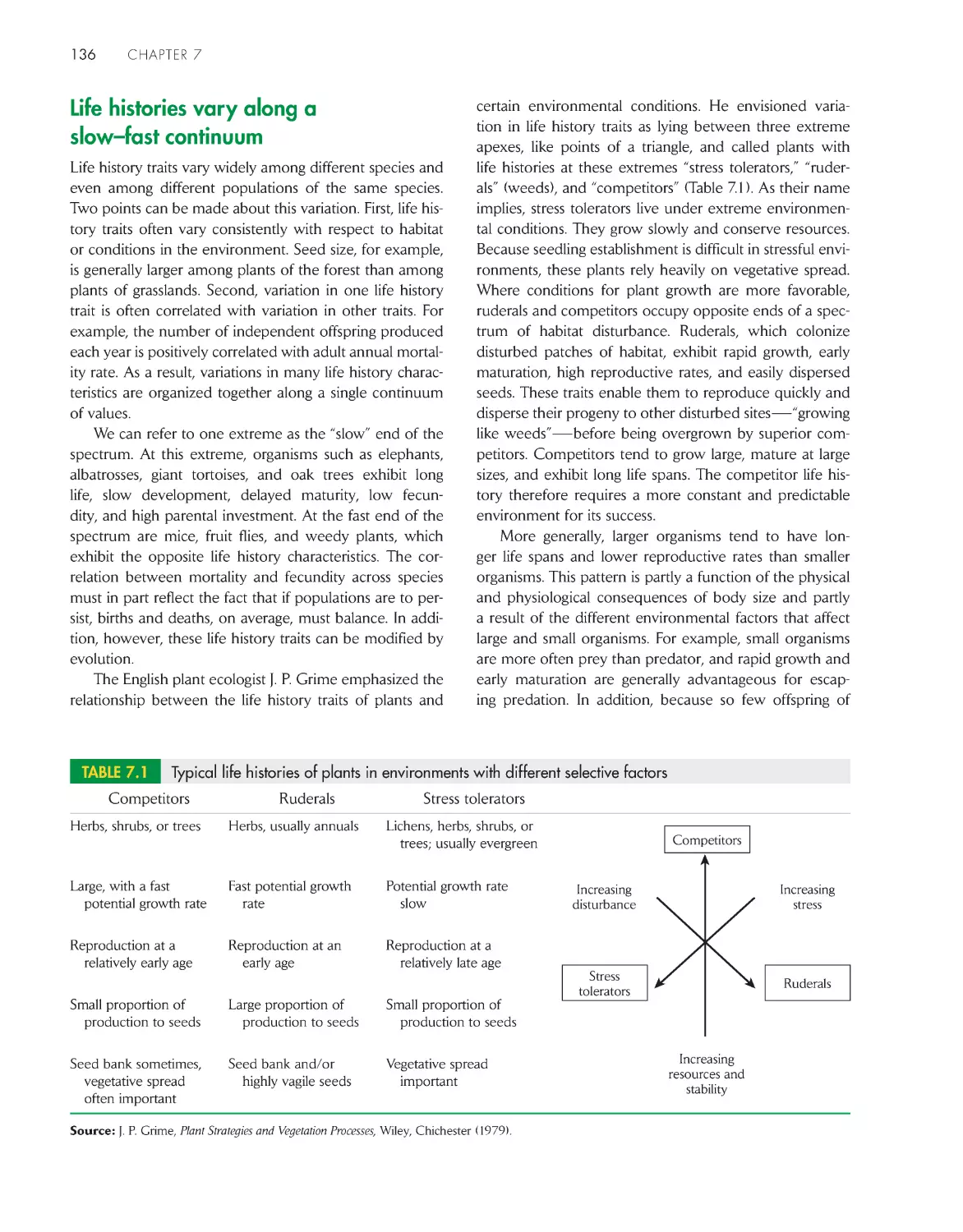
Life histories vary along a slow–fast continuum 136
Life histories balance trade-offs between current and
future reproduction
137
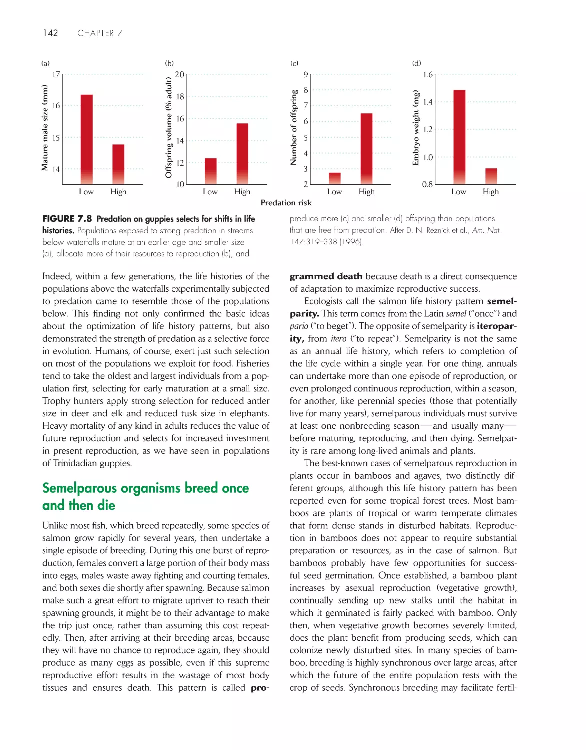
Semelparous organisms breed once and then
die 142
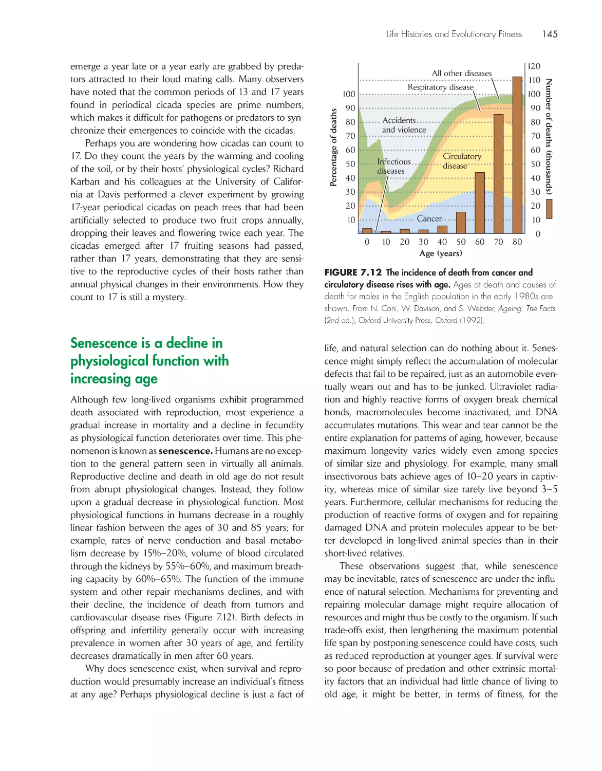
Senescence is a decline in physiological function with
increasing age 145
Life histories respond to variation in the
environment
148
Individual life histories are sensitive to environmental
influences
150
Animals forage in a manner that maximizes their
fitness
152
GLobAL ChANGe
Global warming and flowering time
146
eCoLoGists iN the FieLD
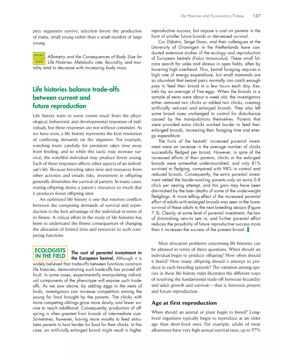
The cost of parental investment in the European
kestrel 137
Optimal foraging by starlings 152
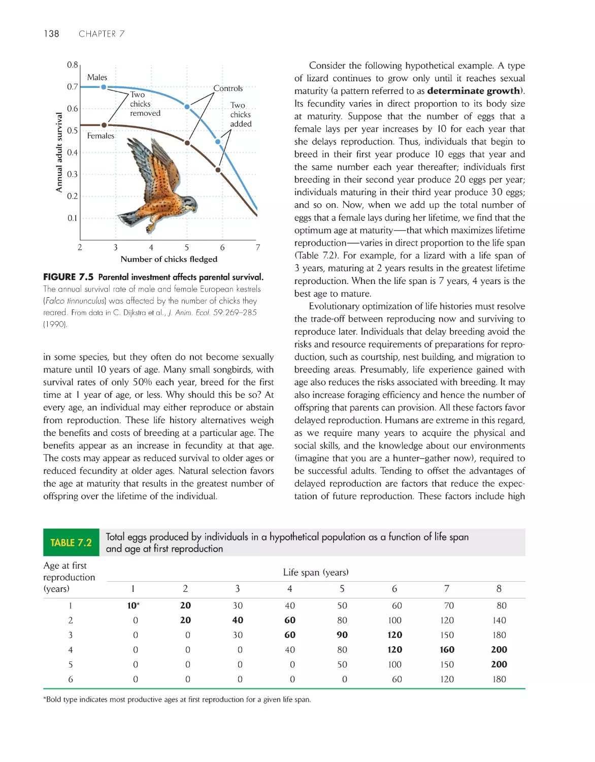
DATA
ANALYSIS
DAtA ANALYsis moDuLe 1
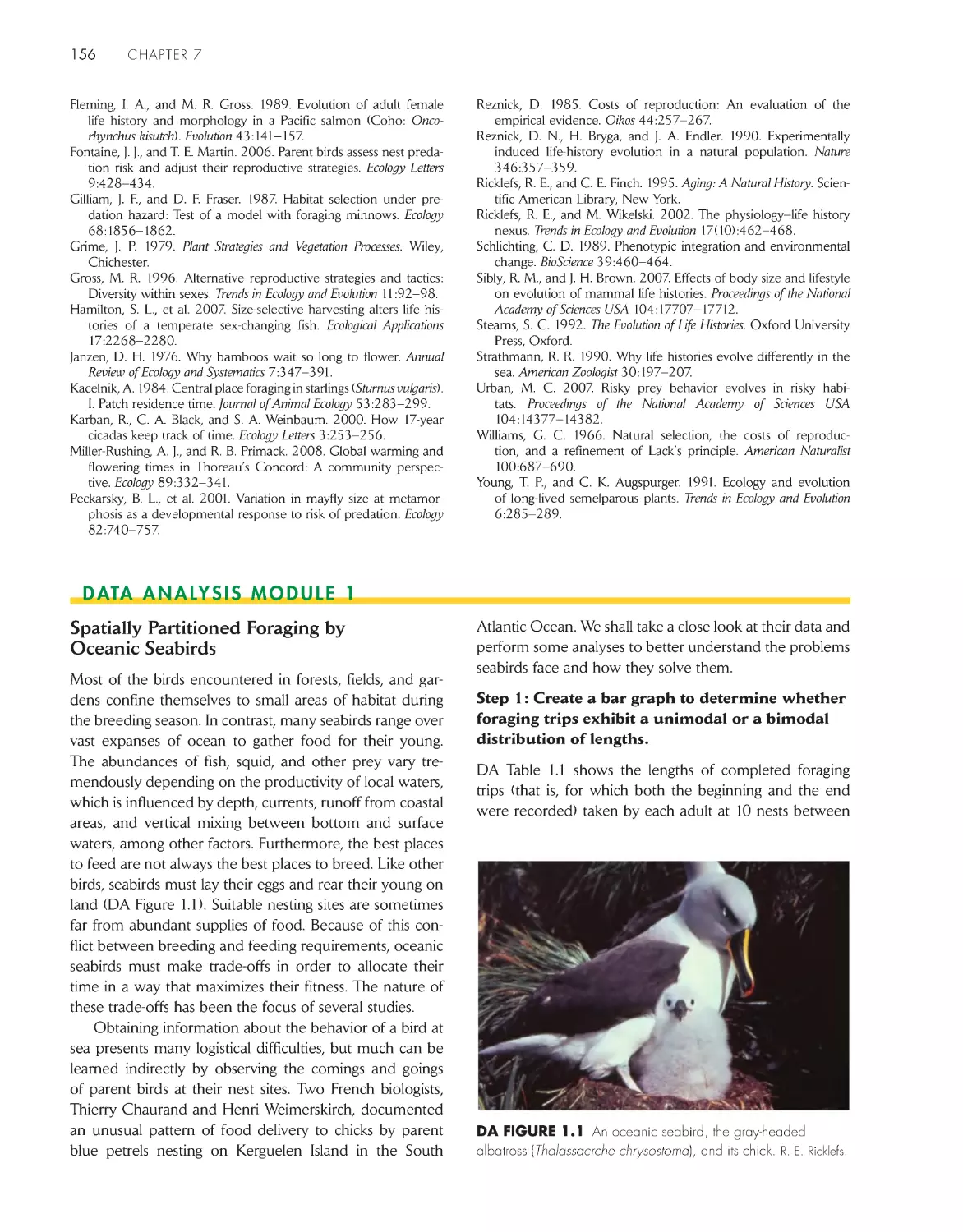
Spatially Partitioned Foraging by Oceanic Seabirds 156
ChApter 8 sex and evolution
159
Sexual reproduction mixes the genetic material of two
individuals 161
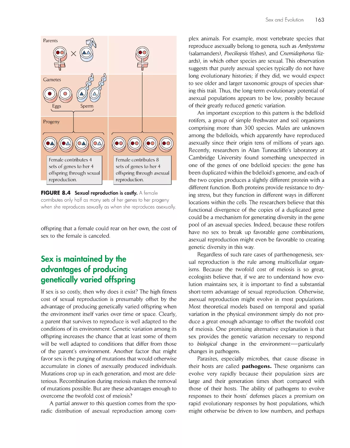
Sexual reproduction is costly 162
Sex is maintained by the advantages of producing
genetically varied offspring 163
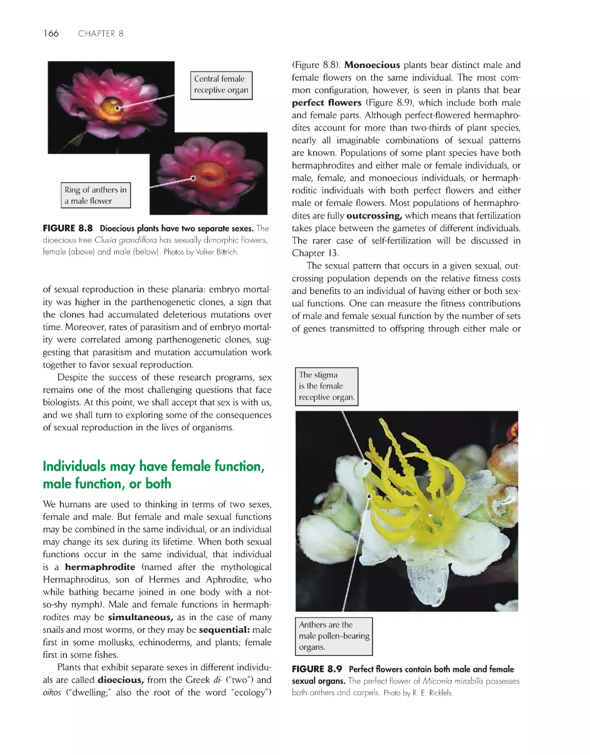
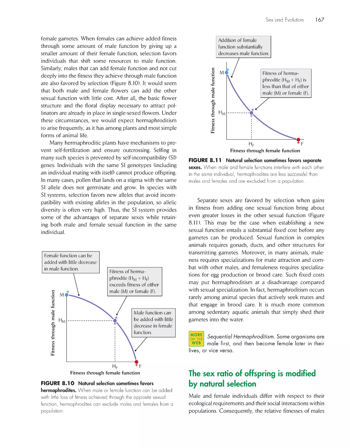
Individuals may have female function, male function, or
both 166
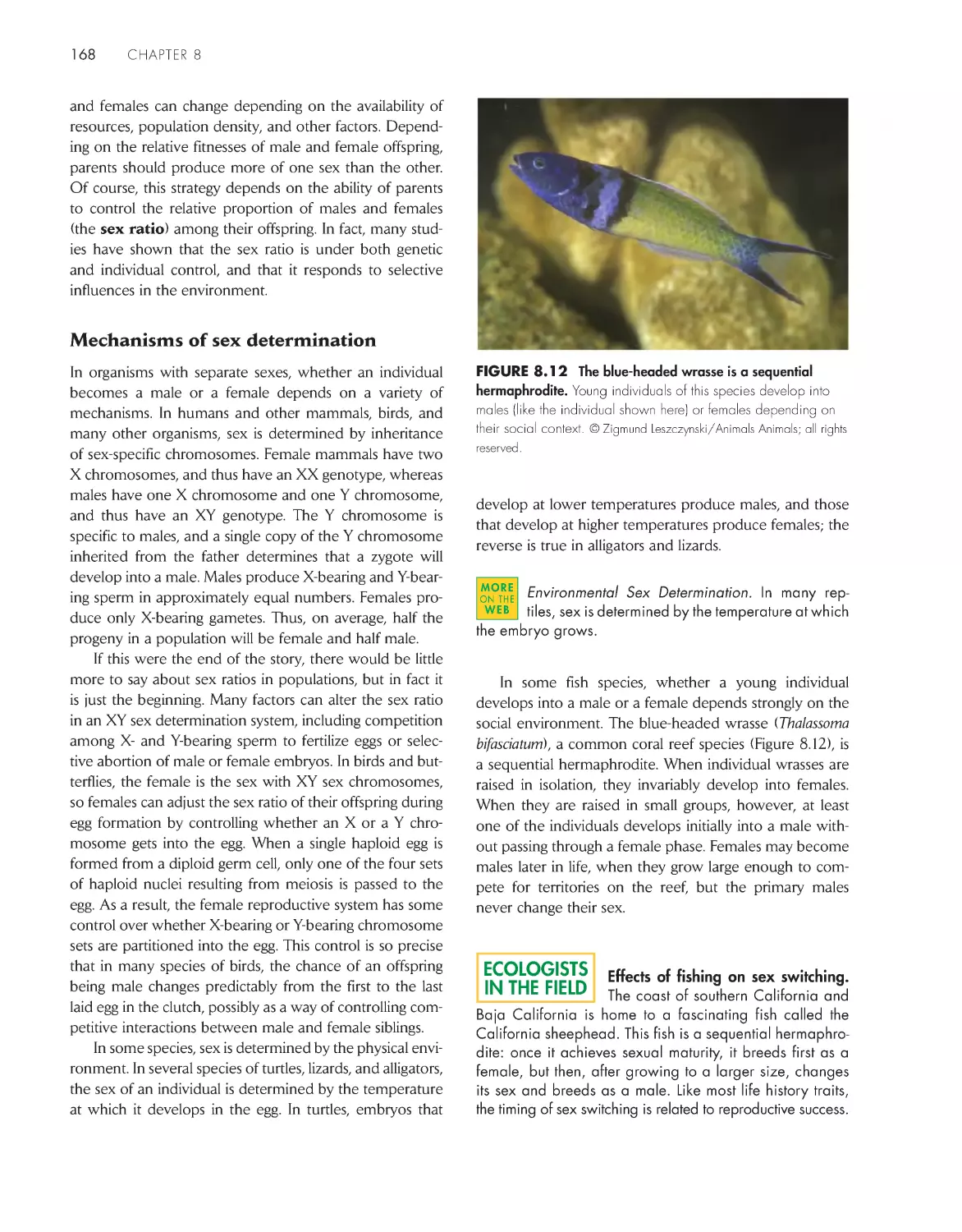
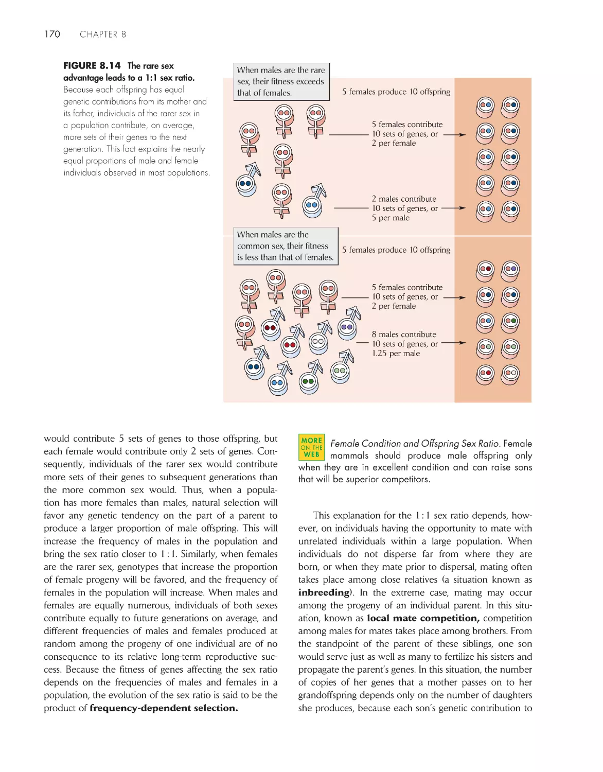
The sex ratio of offspring is modified by natural
selection
167
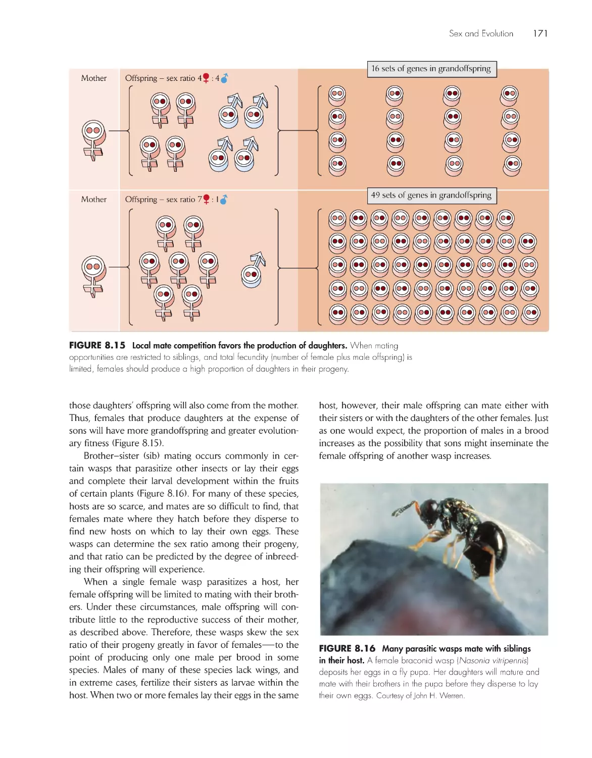
Mating systems describe the pattern of pairing of males
and females within a population
172
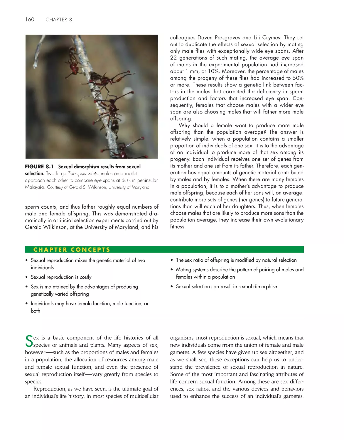
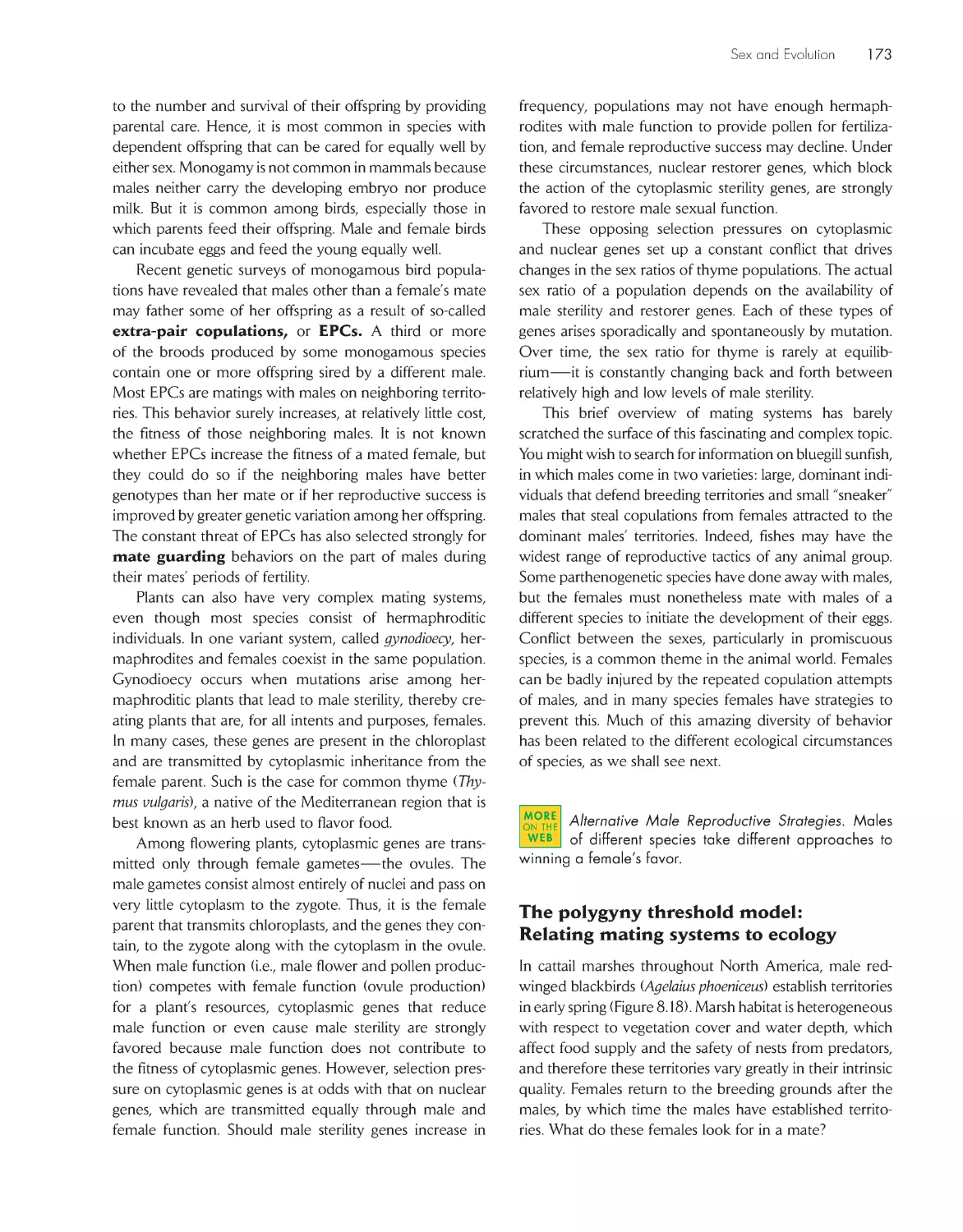
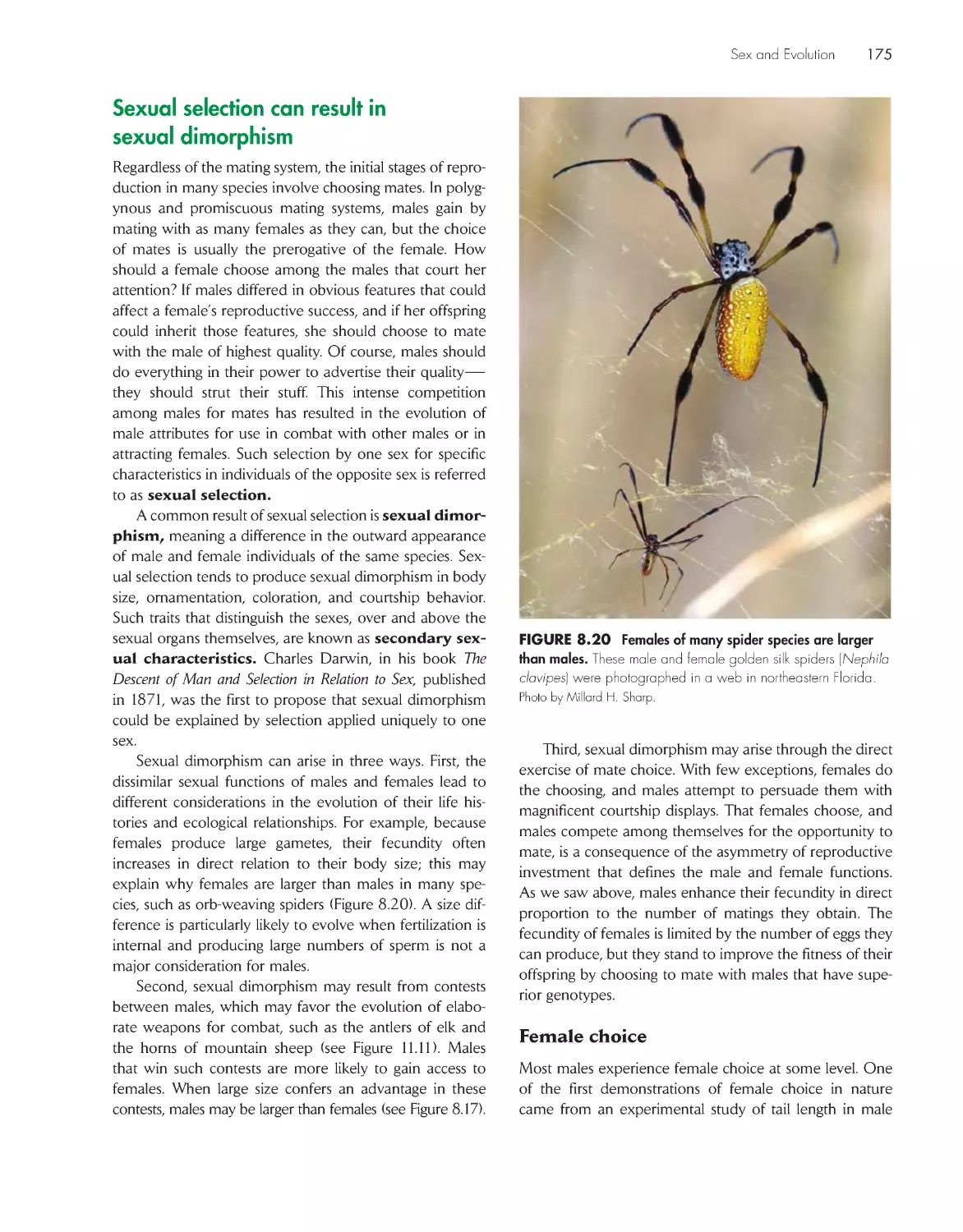
Sexual selection can result in sexual
dimorphism
175
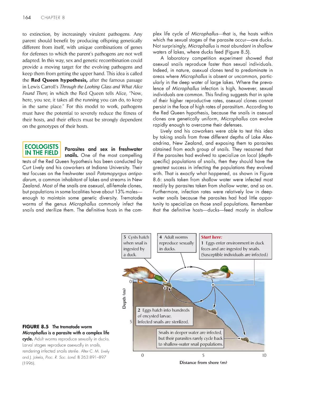
eCoLoGists iN the FieLD
Parasites and sex in freshwater snails 164
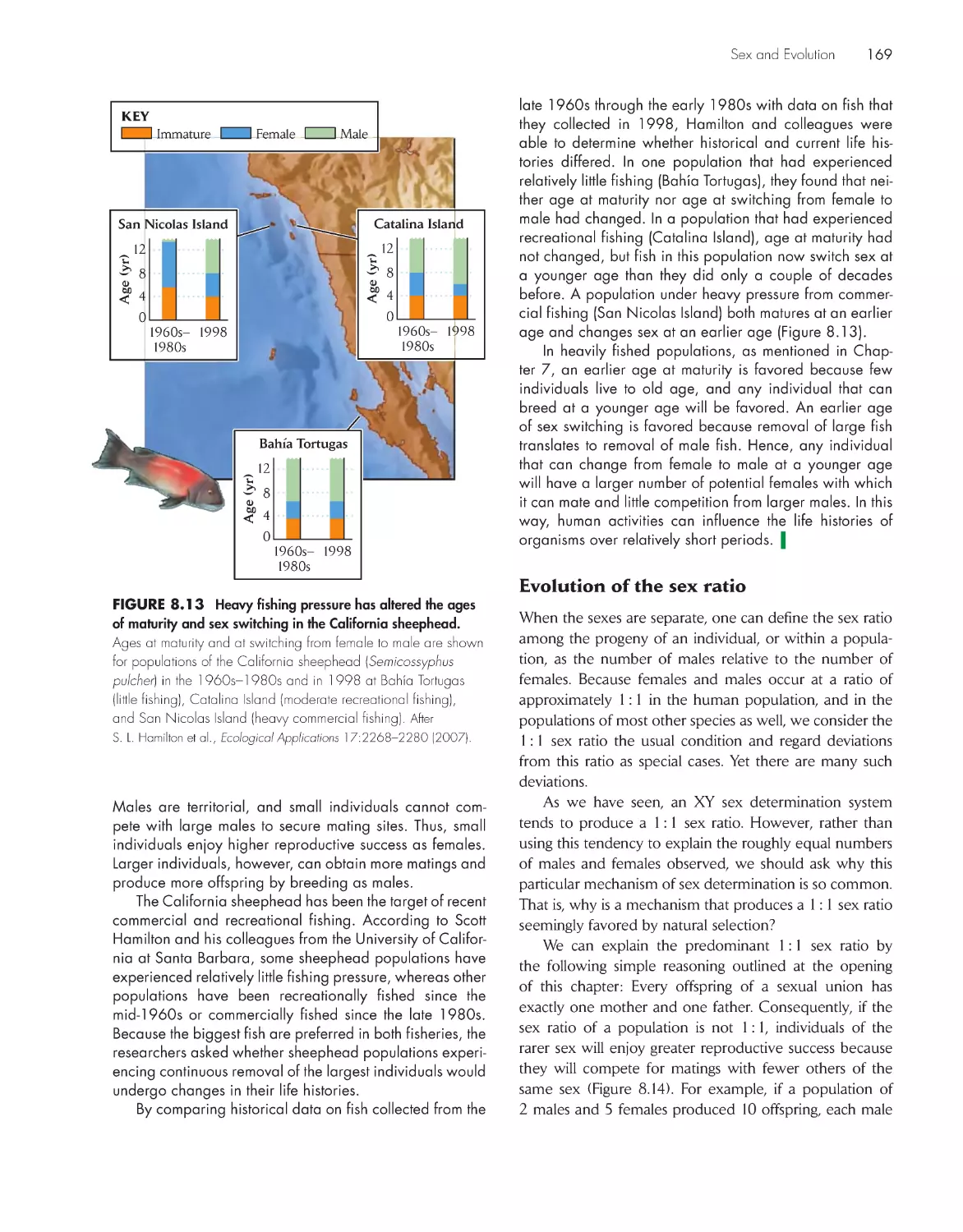
Effects of fishing on sex switching 168
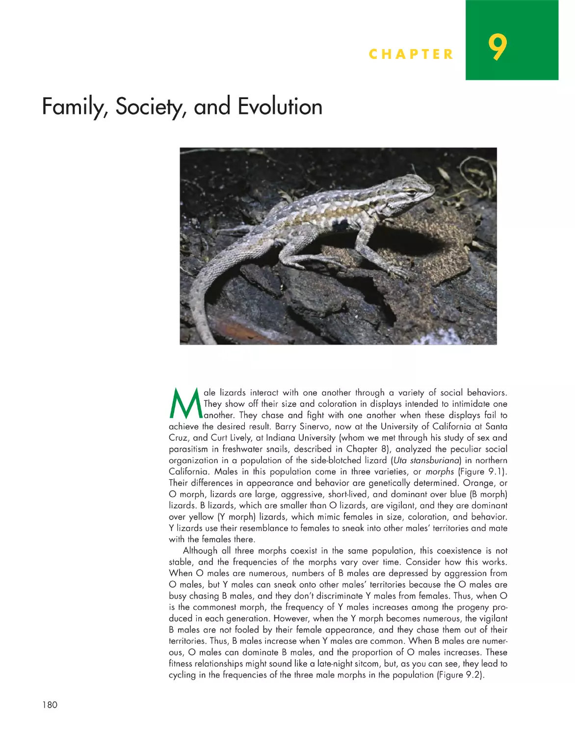
ChApter 9 Family, society, and evolution
180
Territoriality and dominance hierarchies organize social
interactions within populations
182
Individuals gain advantages and suffer disadvantages
from living in groups 183
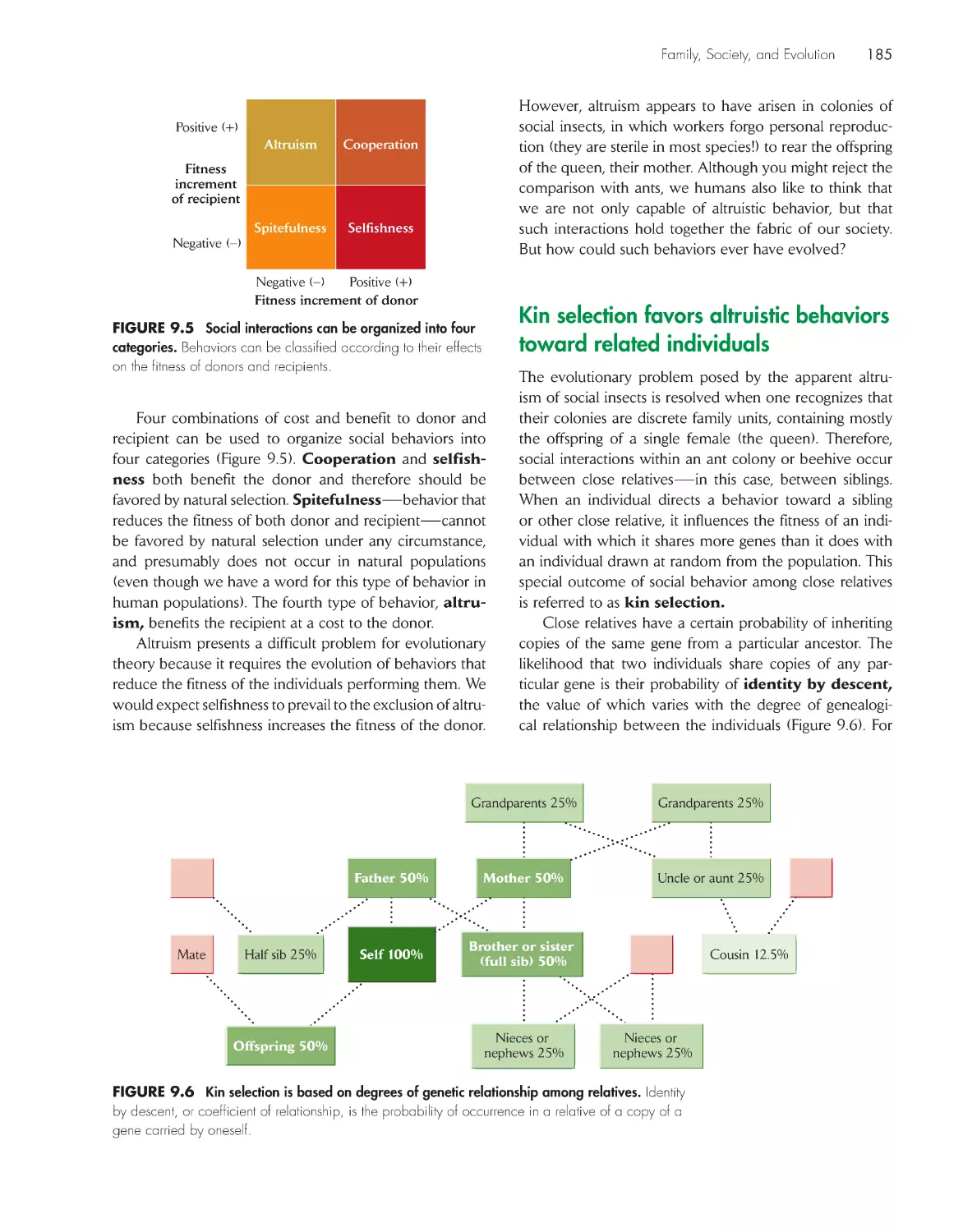
Natural selection balances the costs and benefits of
social behaviors
184
Kin selection favors altruistic behaviors toward related
individuals 185
Cooperation among individuals in extended families
implies the operation of kin selection
189
Game theory analyses illustrate the difficulties for
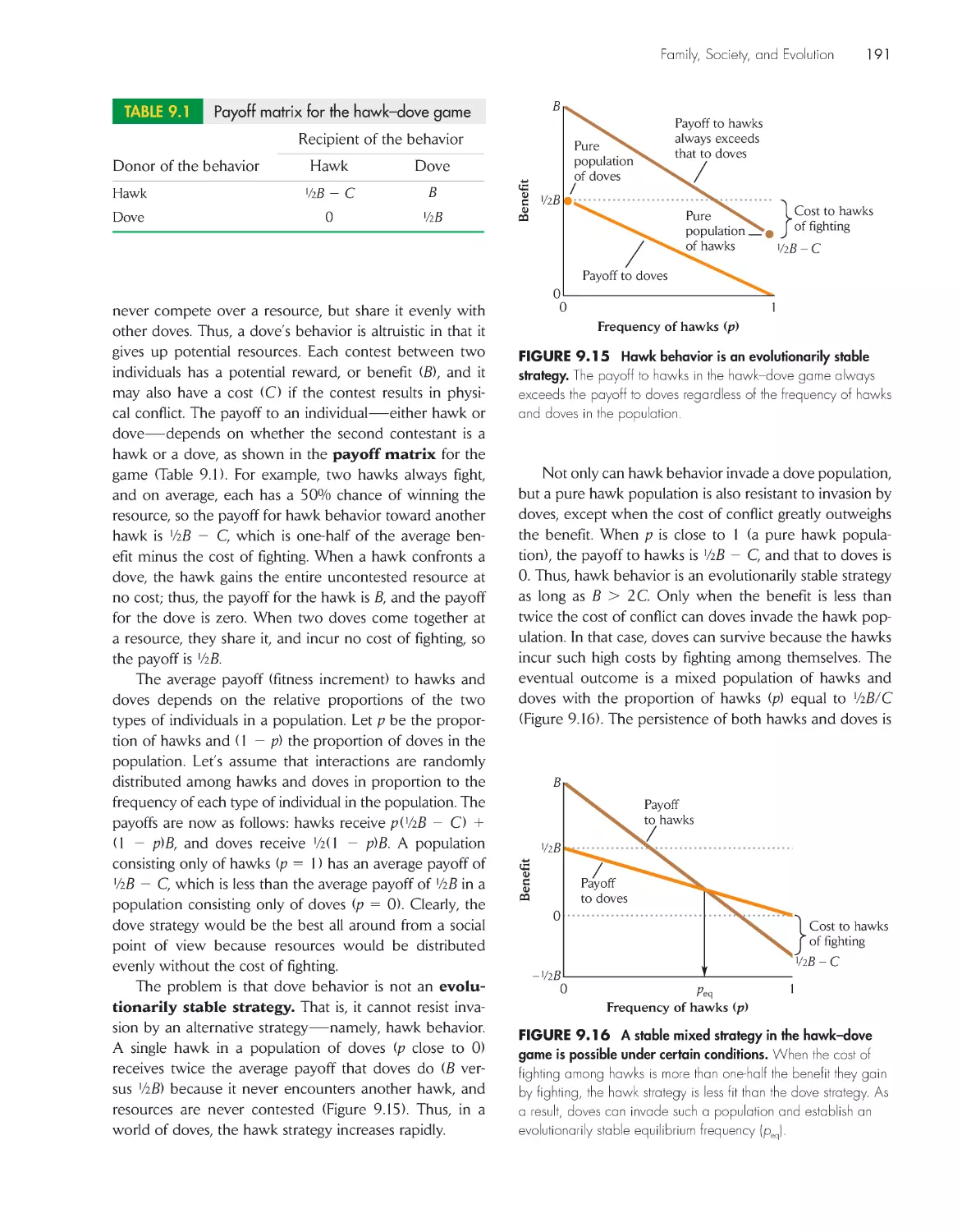
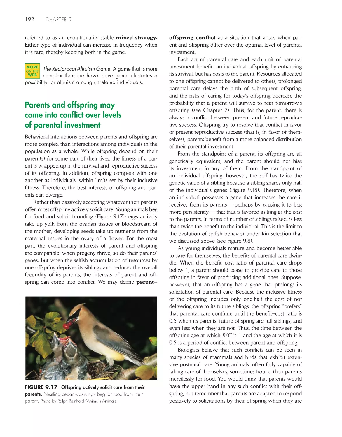
cooperation among unrelated individuals 190
ix
contents
Parents and offspring may come into conflict over
levels of parental investment
192
Insect societies arise out of sibling altruism and parental
dominance
193
eCoLoGists iN the FieLD
Are cooperative acts always acts of altruism? 188
pArt iii popuLAtioNs
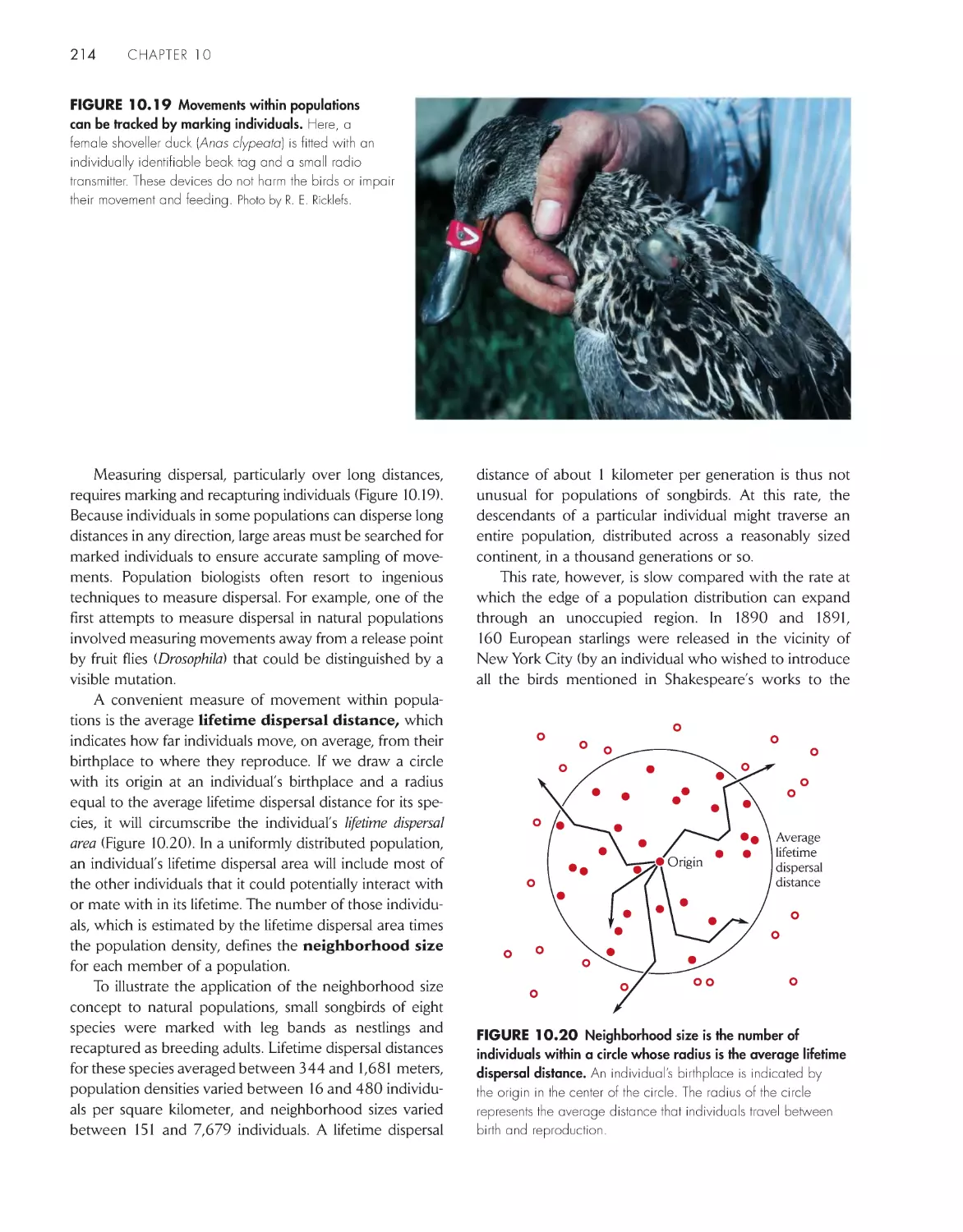
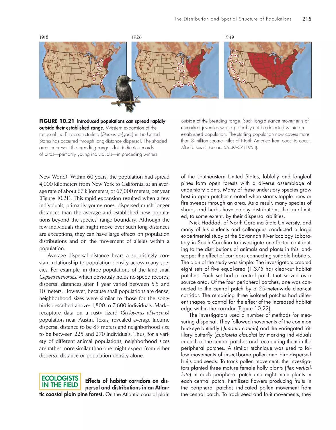
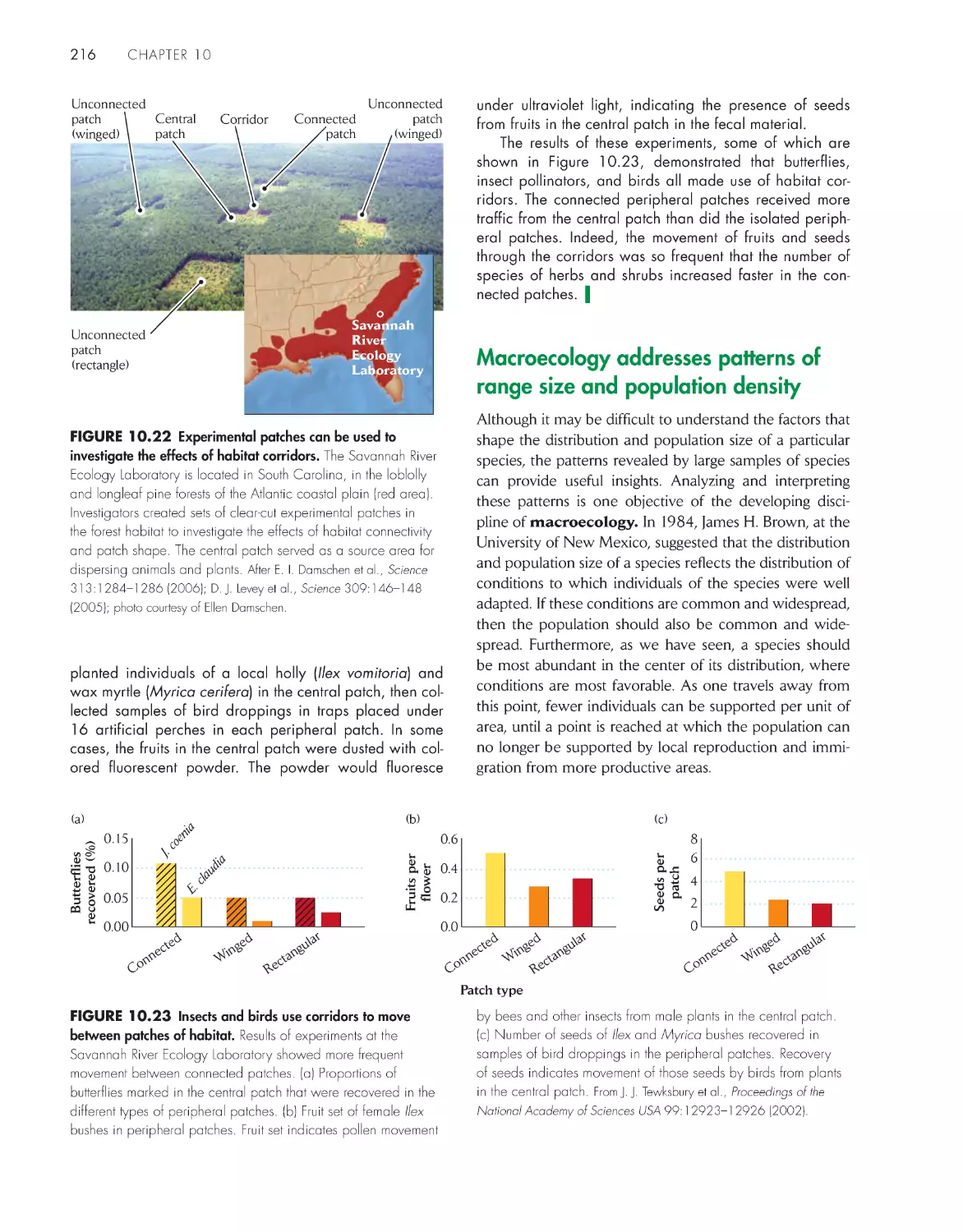
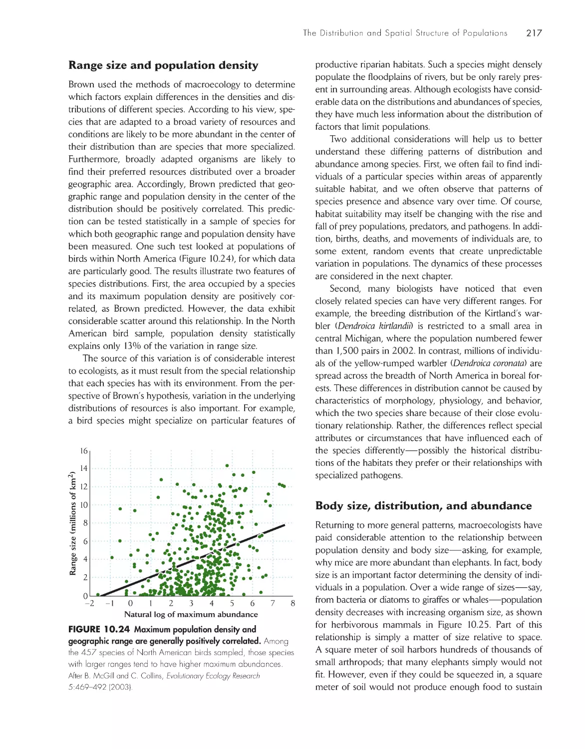
ChApter 10 the Distribution and spatial structure
of populations
198
Populations are limited to ecologically suitable
habitats
200
Ecological niche modeling predicts the distributions
of species 204
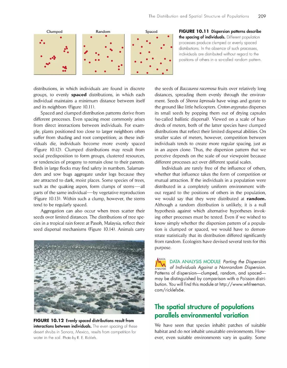
The dispersion of individuals reflects habitat
heterogeneity and social interactions
207
The spatial structure of populations parallels
environmental variation
209
Three types of models describe the spatial structure of
populations
212
Dispersal is essential to the integration of
populations
213
Macroecology addresses patterns of range size and
population density 216
GLobAL ChANGe
Changing ocean temperatures and shifting
fish distributions
206
eCoLoGists iN the FieLD
Effects of habitat corridors on dispersal and distributions in
an Atlantic coastal plain pine forest
215
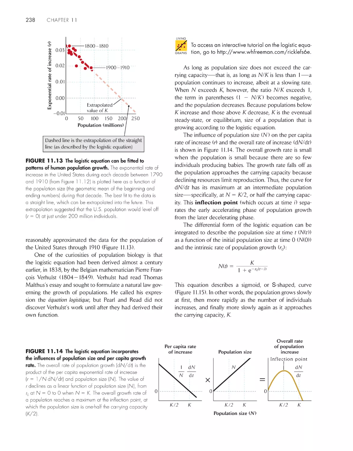
ChApter 11 population Growth and
regulation
222
Populations grow by multiplication rather than
addition
224
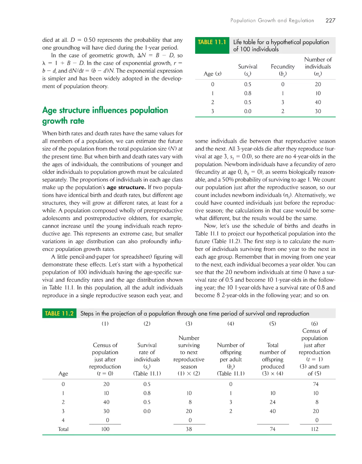
Age structure influences population growth rate
227
A life table summarizes age-specific schedules of
survival and fecundity 229
The intrinsic rate of increase can be estimated from the
life table 234
Population size is regulated by density-dependent
factors
239
eCoLoGists iN the FieLD
Building life tables for natural populations
232
DATA
ANALYSIS
DAtA ANALYsis moDuLe 2
Birth and Death Rates Influence Population Age Structure and
Growth Rate
246
ChApter 12 temporal and spatial Dynamics of
populations
248
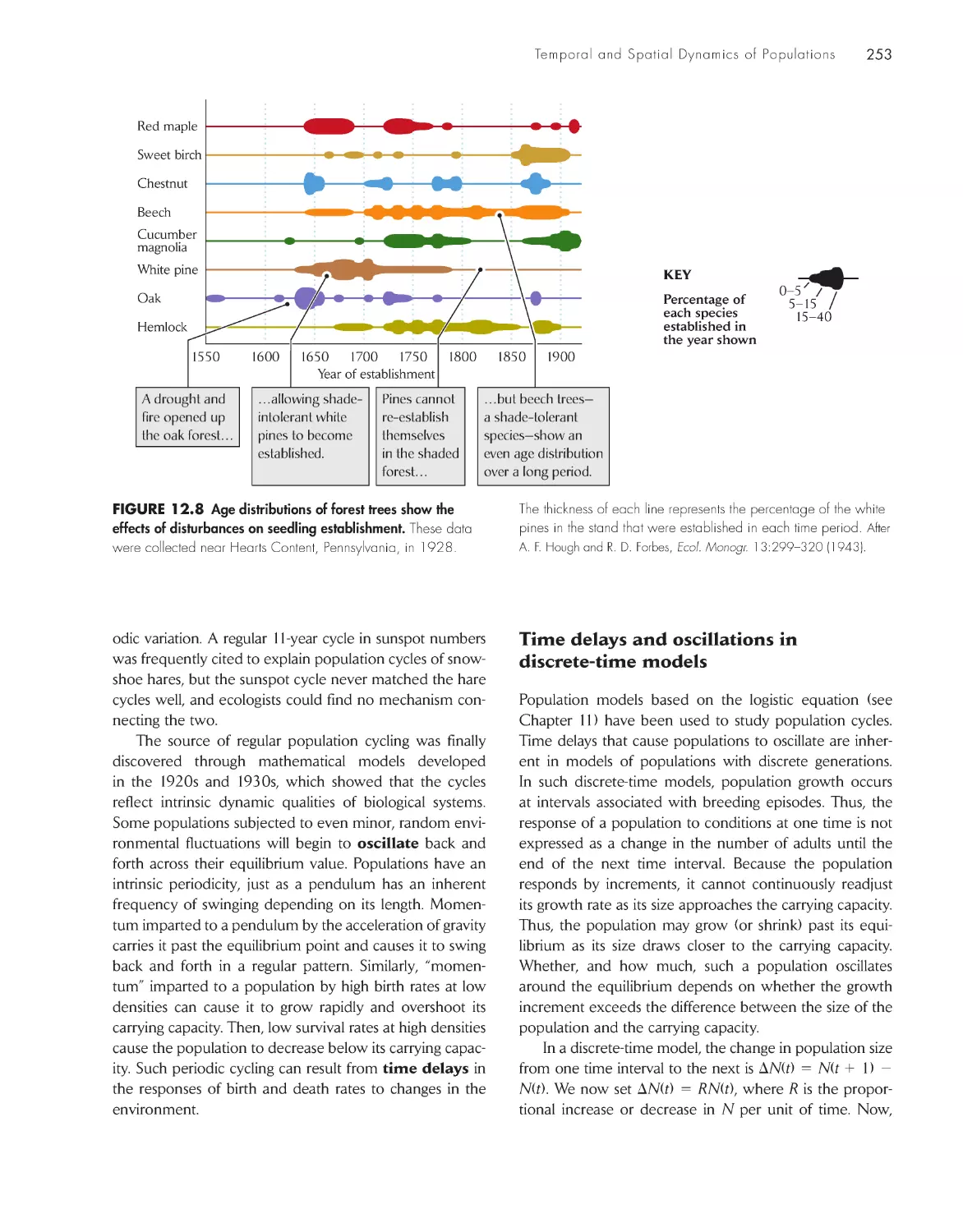
Fluctuation is the rule for natural populations
250
Temporal variation affects the age
structure of populations
252
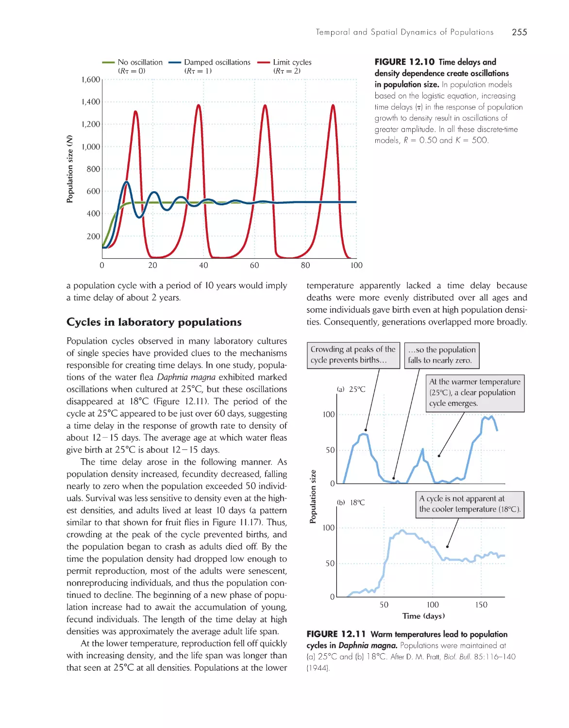
Population cycles result from time
delays in the response
of populations to their
own densities 252
Metapopulations are discrete subpopulations
linked by movements of individuals 257
Chance events may cause small populations to go
extinct
260
eCoLoGists iN the FieLD
Time delays and oscillations in blowfly populations
256
DATA
ANALYSIS
DAtA ANALYsis moDuLe 3
Stochastic Extinction with Variable Population Growth
Rates
264
ChApter 13 population Genetics 267
The ultimate source of genetic variation is
mutation
268
Genetic markers can be used to study population
processes
269
Genetic variation is maintained by mutation, migration,
and environmental variation
270
The Hardy–Weinberg law describes the frequencies of
alleles and genotypes in ideal populations
272
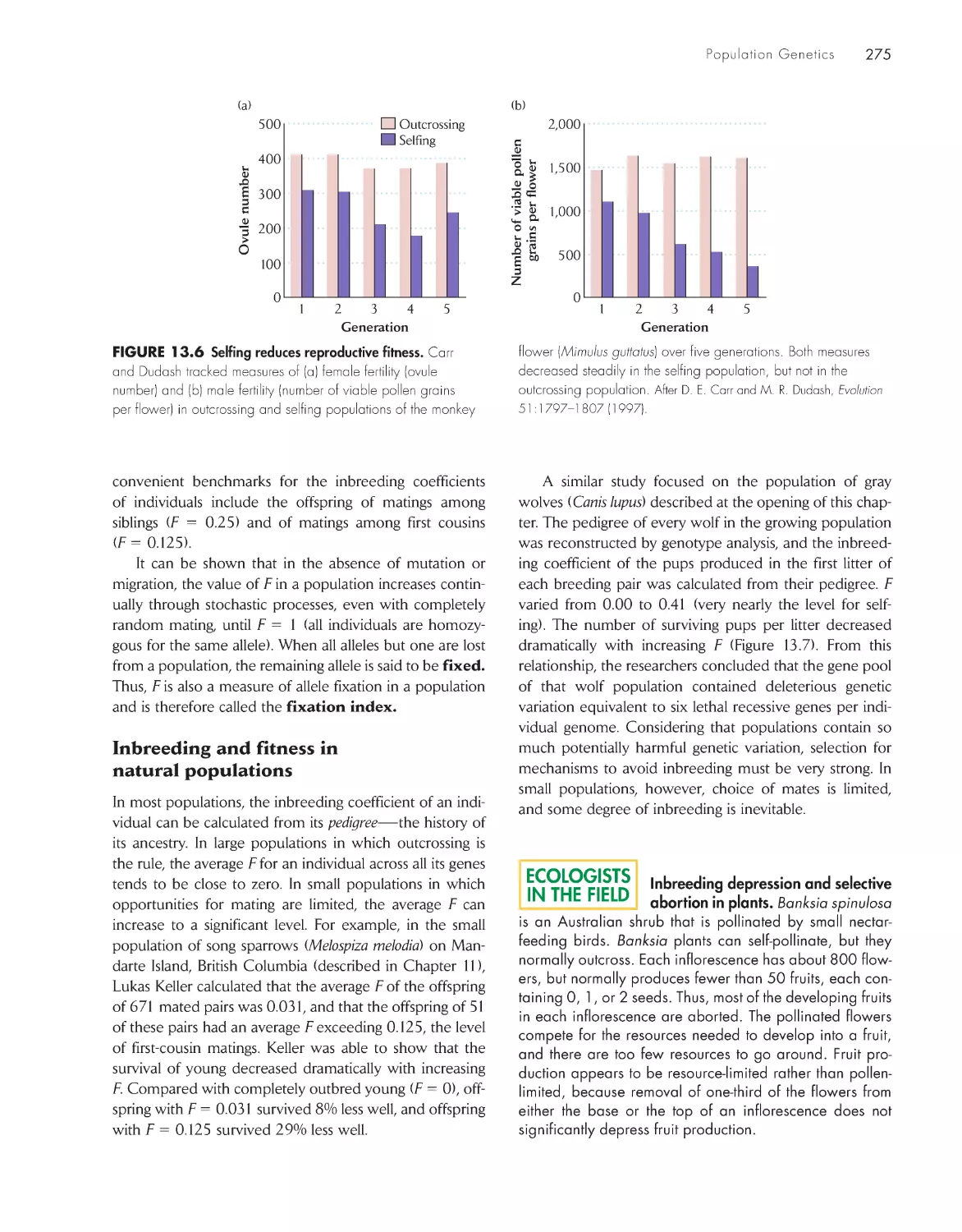
Inbreeding reduces the frequency of heterozygotes in a
population
273
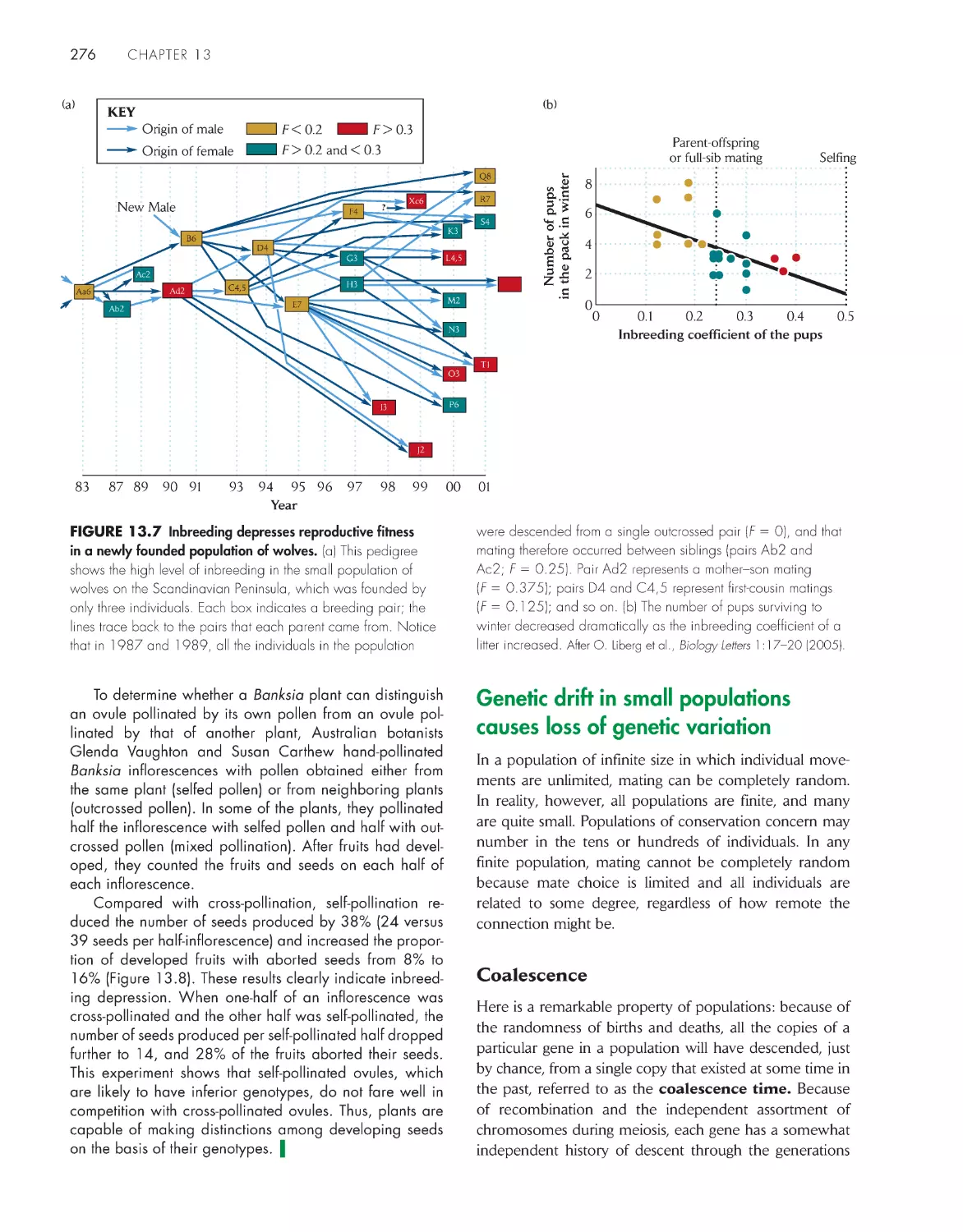
Genetic drift in small populations causes loss of genetic
variation
276
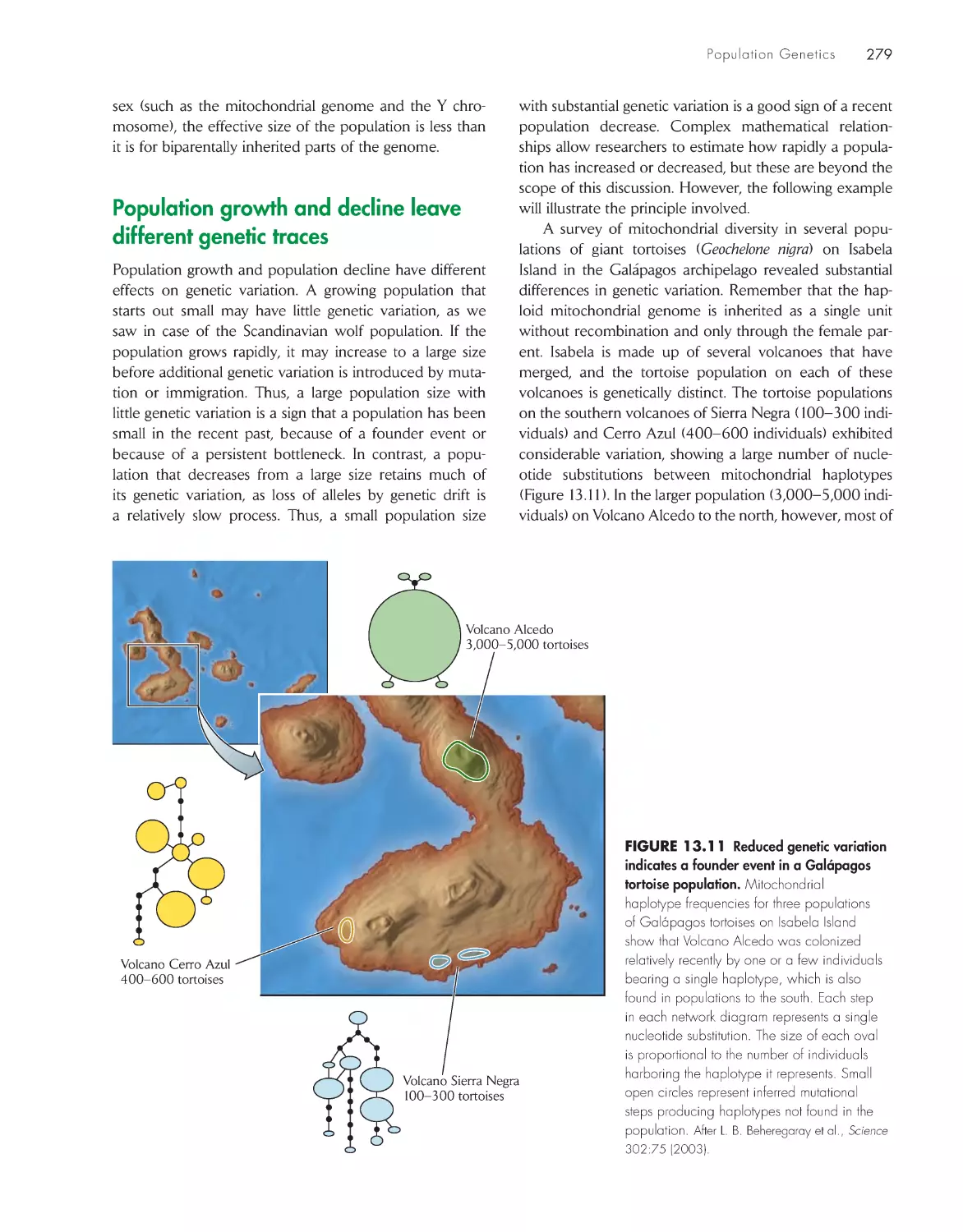
Population growth and decline leave different genetic
traces
279
Loss of variation by genetic drift is balanced by
mutation and migration
280
Selection in spatially variable environments can
differentiate populations genetically 282
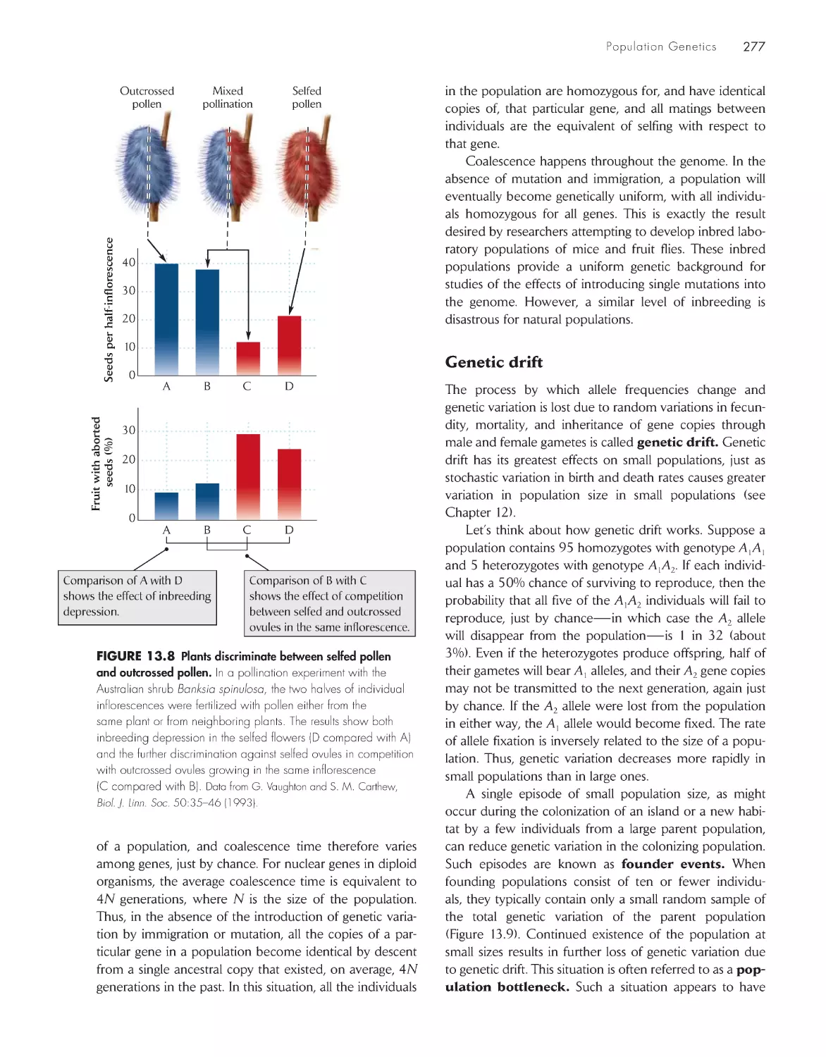
eCoLoGists iN the FieLD
Inbreeding depression and selective abortion in
plants
275
pArt iV speCies iNterACtioNs
ChApter 14 species interactions
287
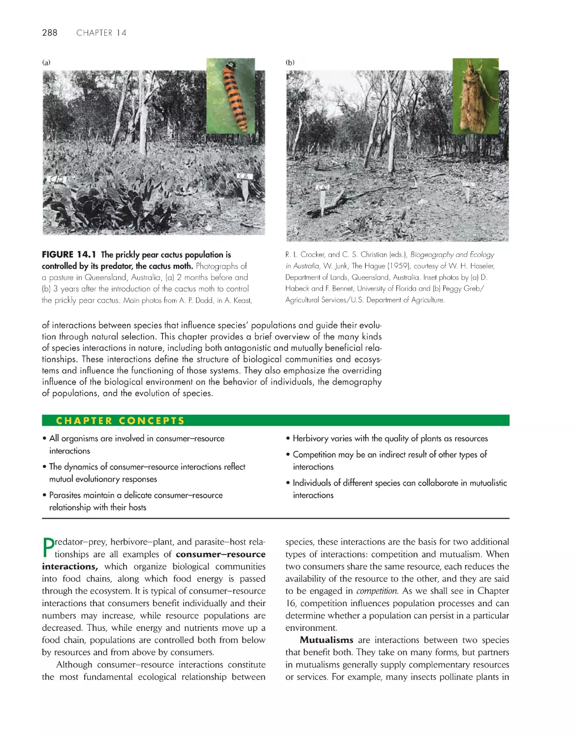
All organisms are involved in consumer–resource
interactions
289
The dynamics of consumer–resource interactions reflect
mutual evolutionary responses
290
x
contents
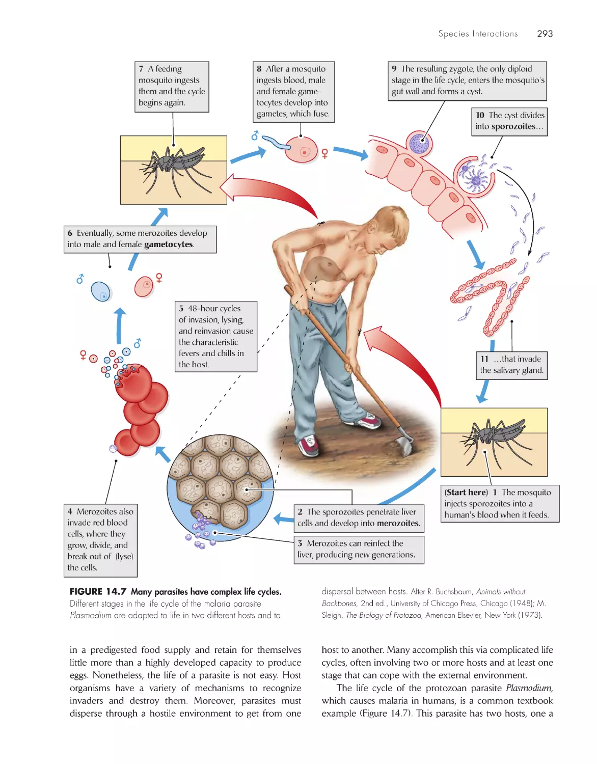
Parasites maintain a delicate consumer–resource
relationship with their hosts
292
Herbivory varies with the quality of
plants as resources
294
Competition may be an indirect
result of other types of
interactions
296
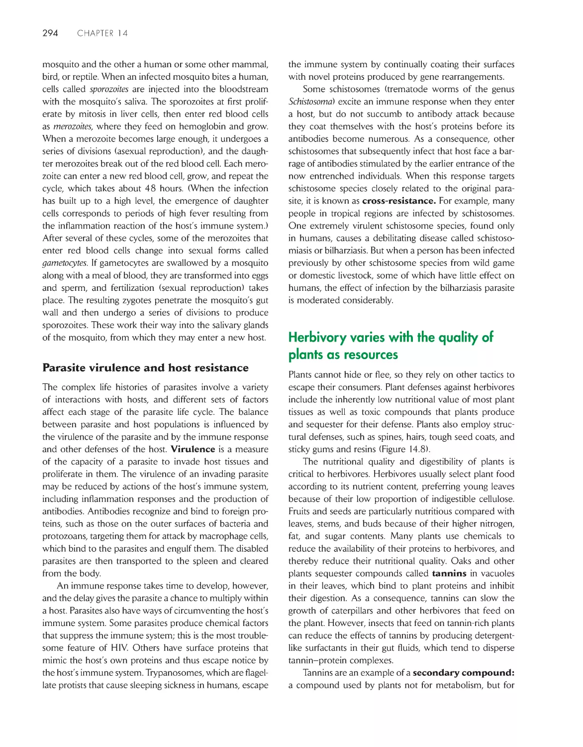
Individuals of different species
can collaborate in mutualistic
interactions
297
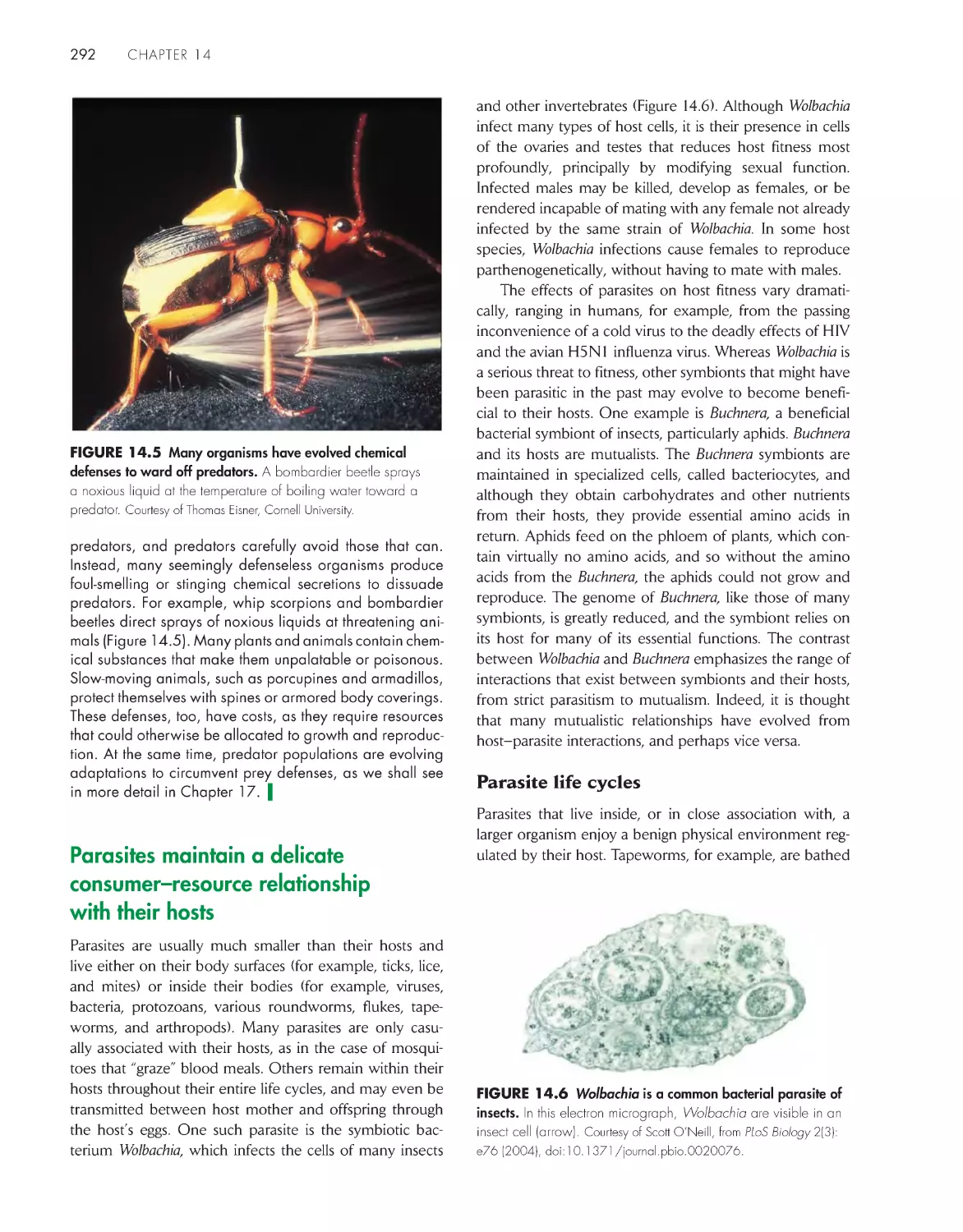
eCoLoGists iN the FieLD
Predator avoidance and growth performance in frog
lar vae
291
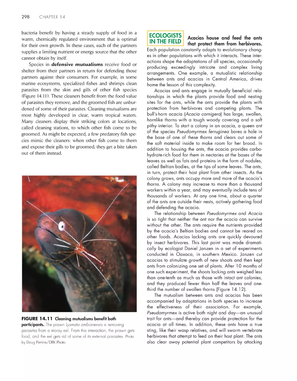
Acacias house and feed the ants that protect them from
herbivores
298
ChApter 15 Dynamics of Consumer–resource
interactions
302
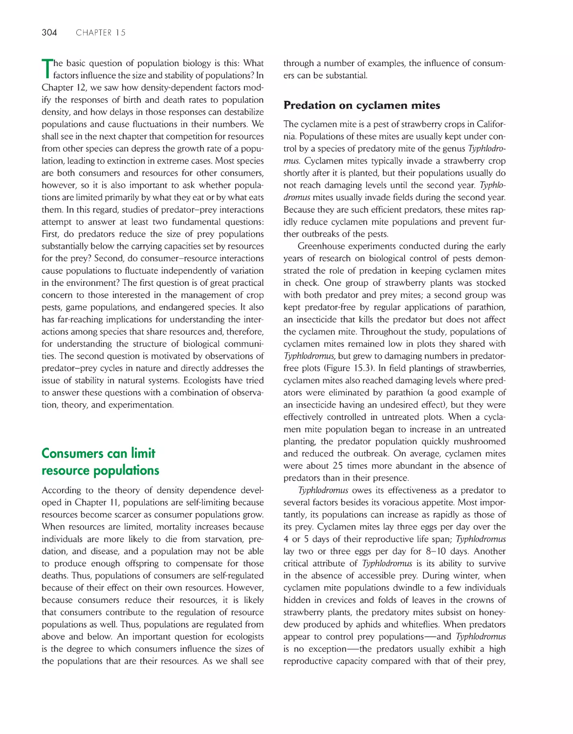
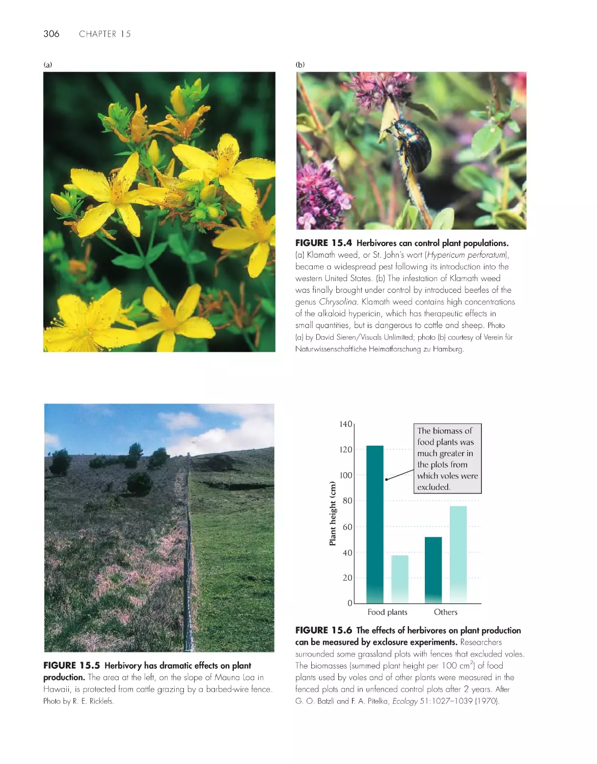
Consumers can limit resource populations
304
Many predator and prey populations increase and
decrease in regular cycles 307
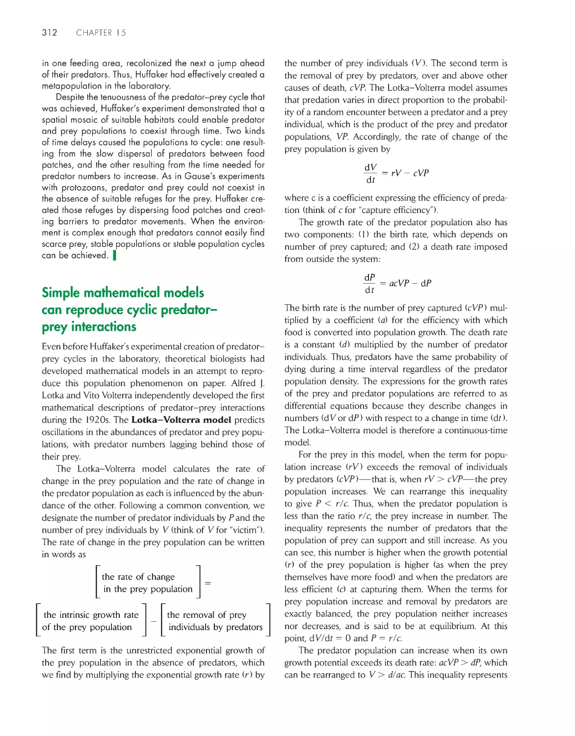
Simple mathematical models can reproduce cyclic
predator–prey interactions
312
Pathogen–host dynamics can be described by the S-I -R
model 315
The Lotka–Volterra model can be stabilized by predator
satiation
318
A number of factors can reduce oscillations in
predator–prey models 321
Consumer–resource systems can have more than one
stable state
321
eCoLoGists iN the FieLD
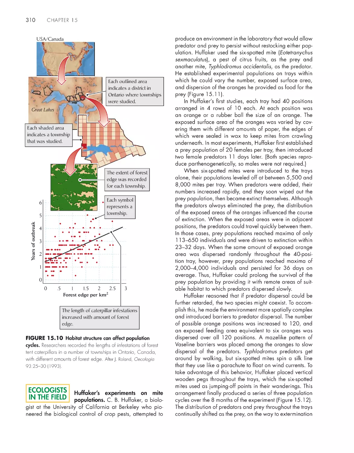
Huffaker’s experiments on mite populations
310
Testing a prediction of the Lotka–Volterra model 315
The chytrid fungus and the global decline of
amphibians
317
DATA
ANALYSIS
DAtA ANALYsis moDuLe 4
Maximum Sustainable Yield: Applying Basic Ecological
Concepts to Fisheries Management
324
ChApter 16 Competition
328
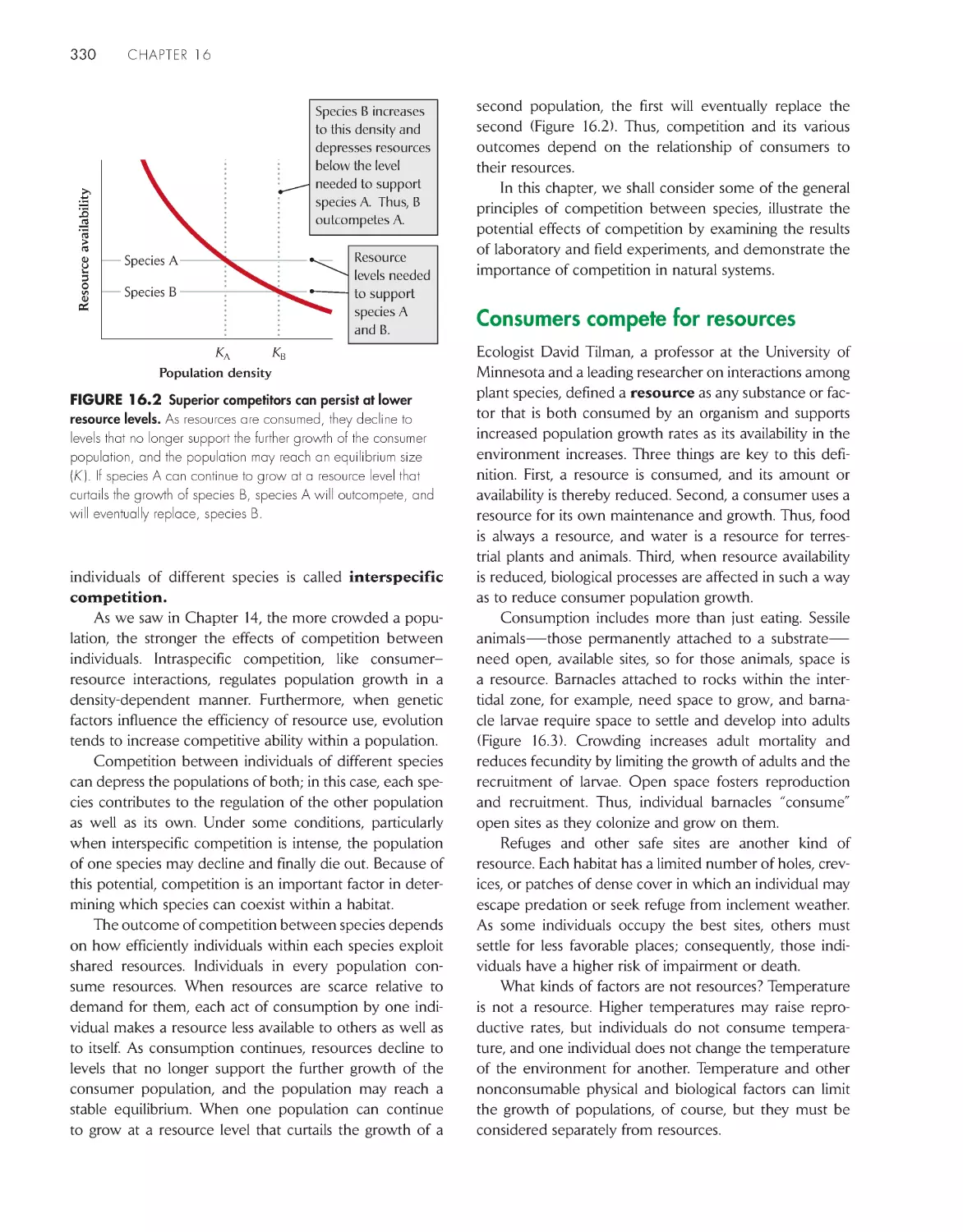
Consumers compete for resources
330
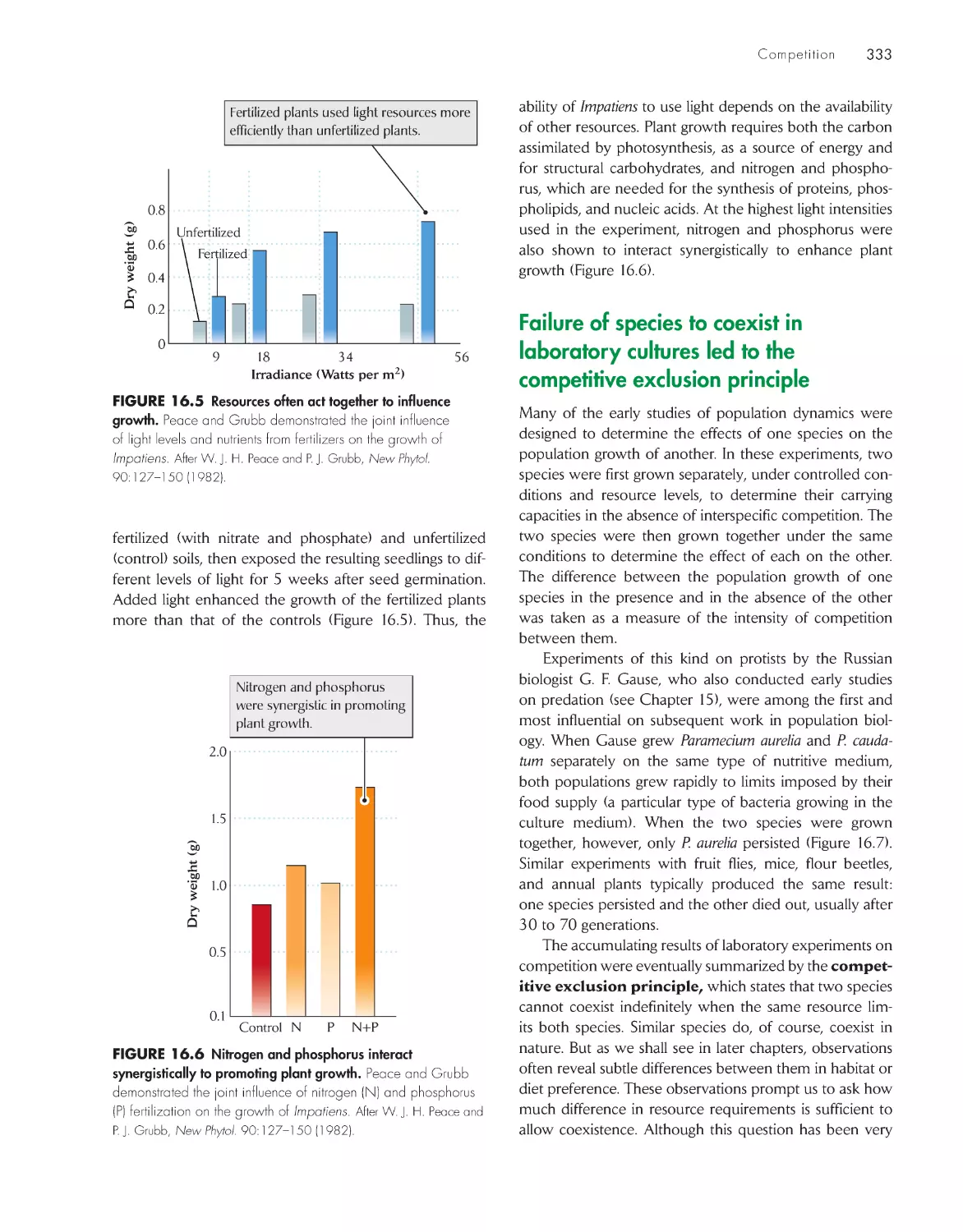
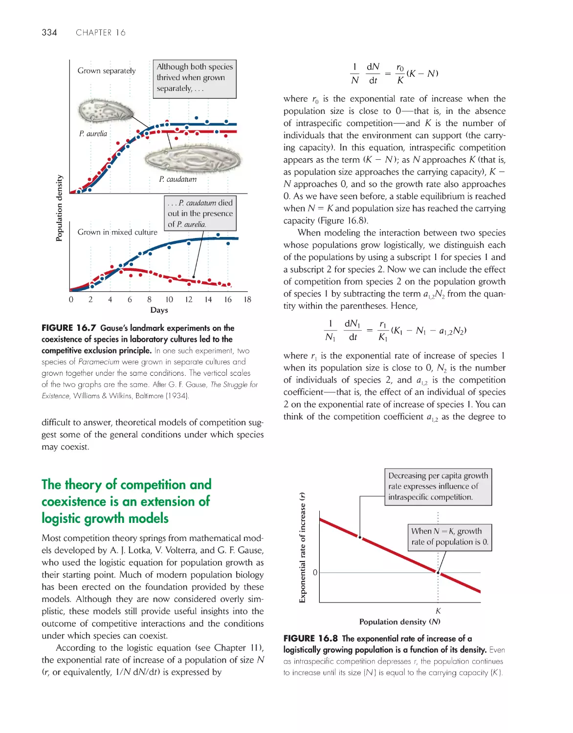
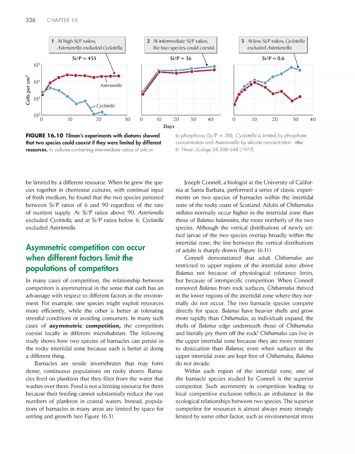
Failure of species to coexist in laboratory cultures led to
the competitive exclusion principle 333
The theory of competition and coexistence is an
extension of logistic growth models 334
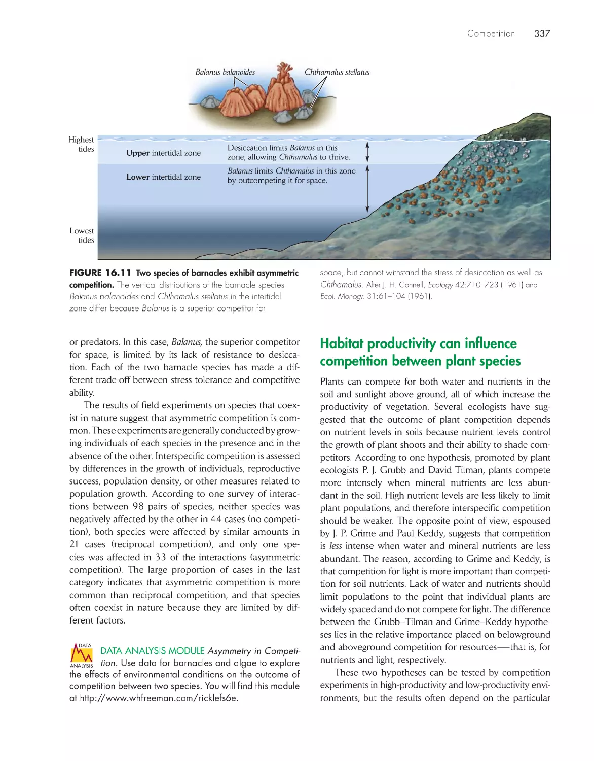
Asymmetric competition can occur when different
factors limit the populations of competitors
336
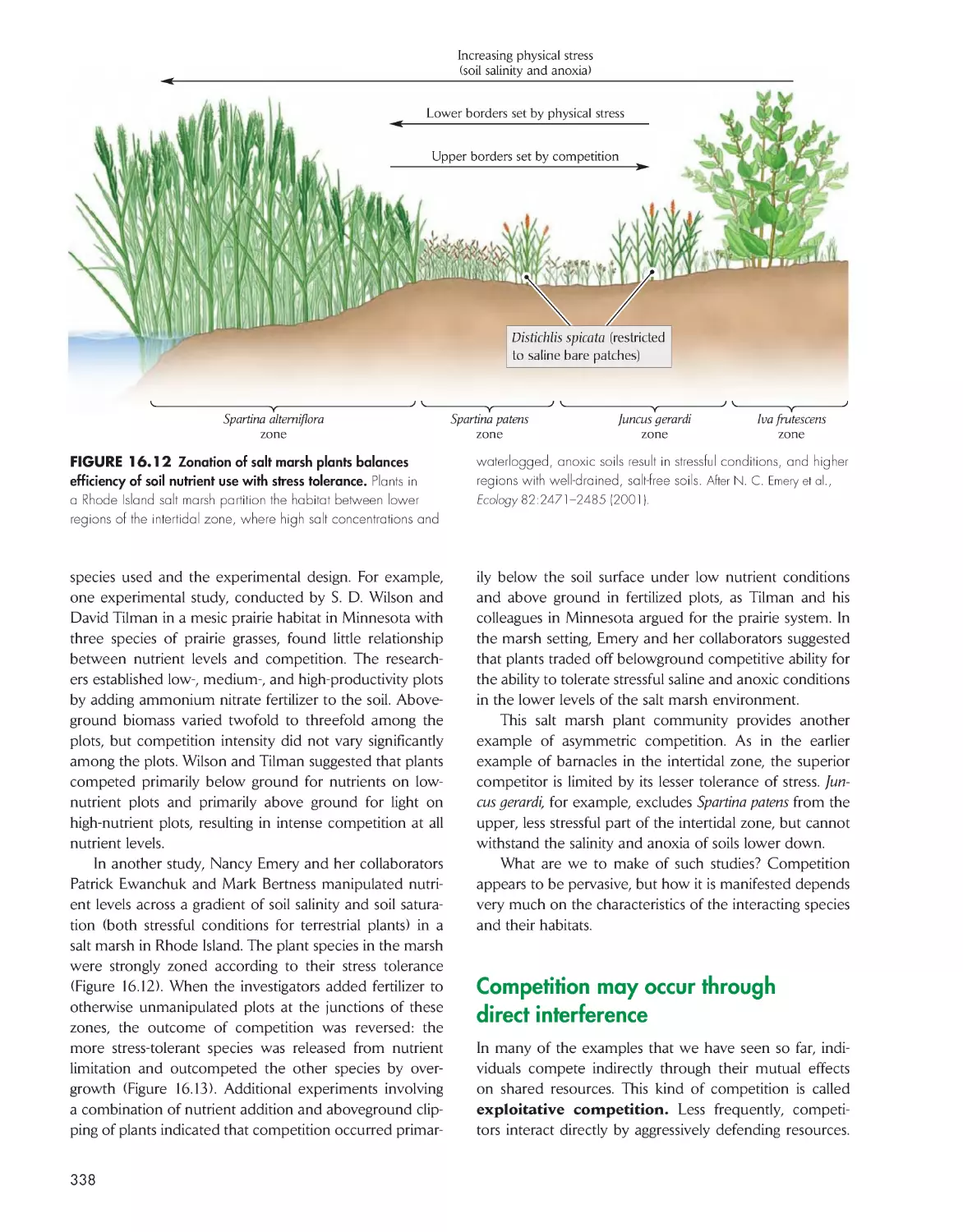
Habitat productivity can influence competition between
plant species 337
Competition may occur through direct
interference
338
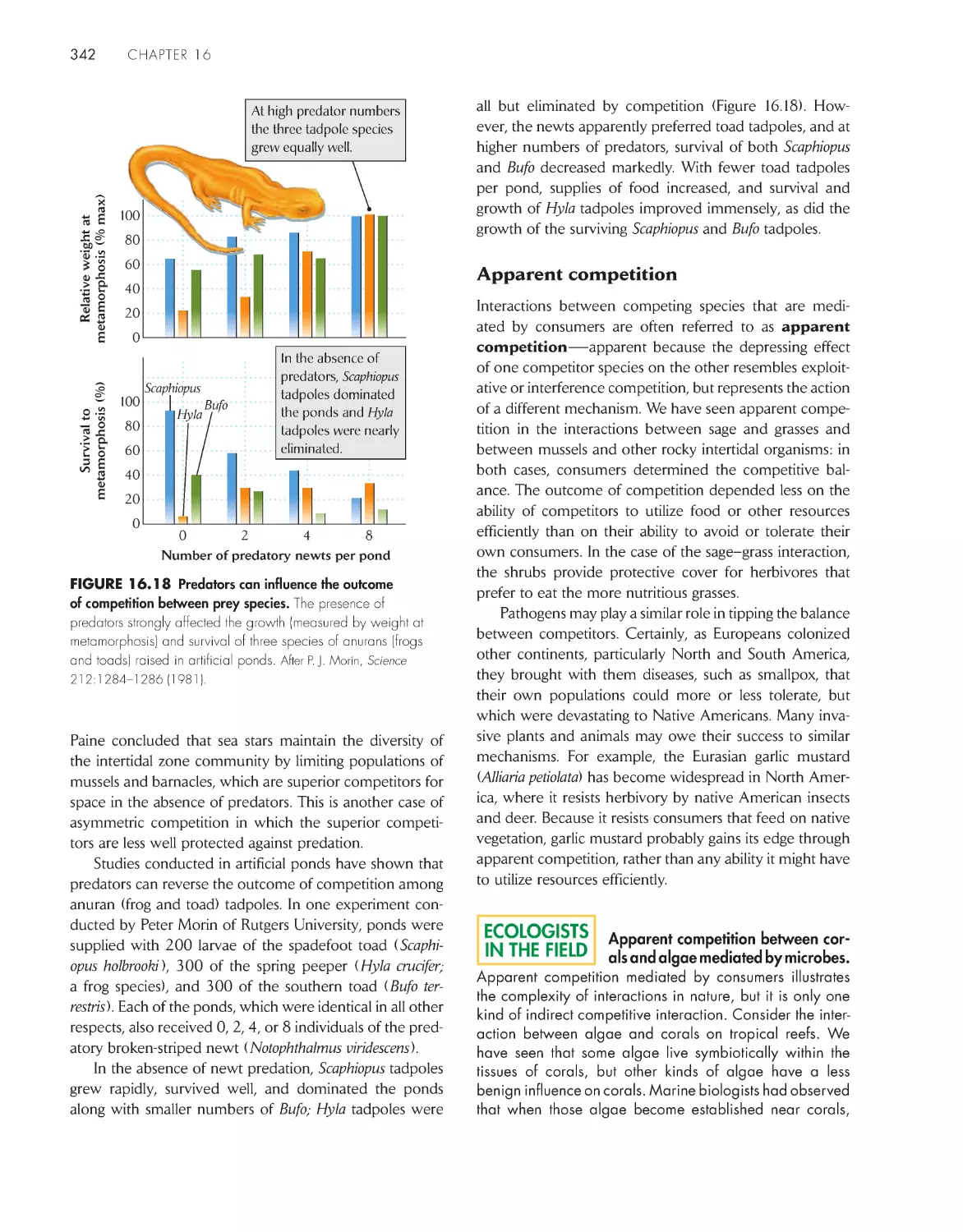
Consumers can influence the outcome of
competition
340
eCoLoGists iN the FieLD
Apparent competition between corals and algae mediated
by microbes 342
ChApter 17 evolution of species
interactions
346
Adaptations in response to predation demonstrate
selection by biological agents
349
Antagonists evolve in response to each other
351
Coevolution in plant-pathogen systems reveals
genotype–genotype interactions
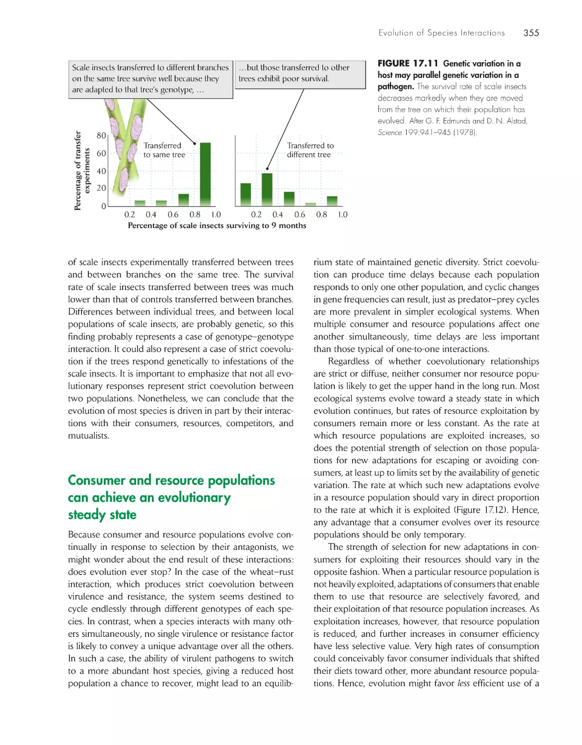
354
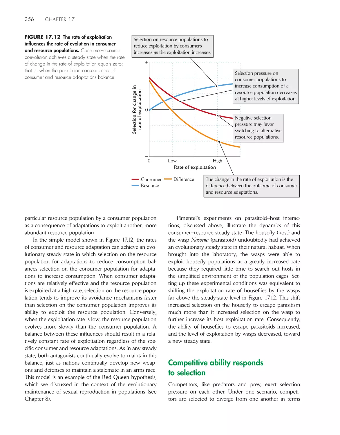
Consumer and resource populations can achieve an
evolutionary steady state
355
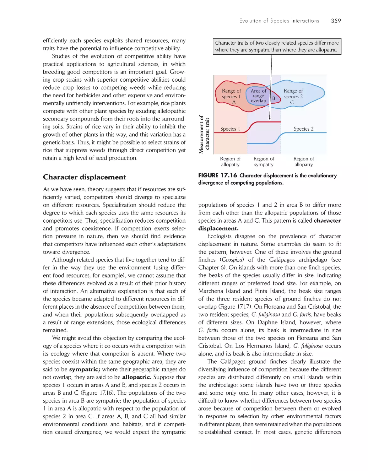
Competitive ability responds to selection
356
Coevolution involves mutual evolutionary responses by
interacting populations
360
GLobAL ChANGe
Invasive plant species and the role of herbivores
364
eCoLoGists iN the FieLD
Evolution in houseflies and their parasitoids 352
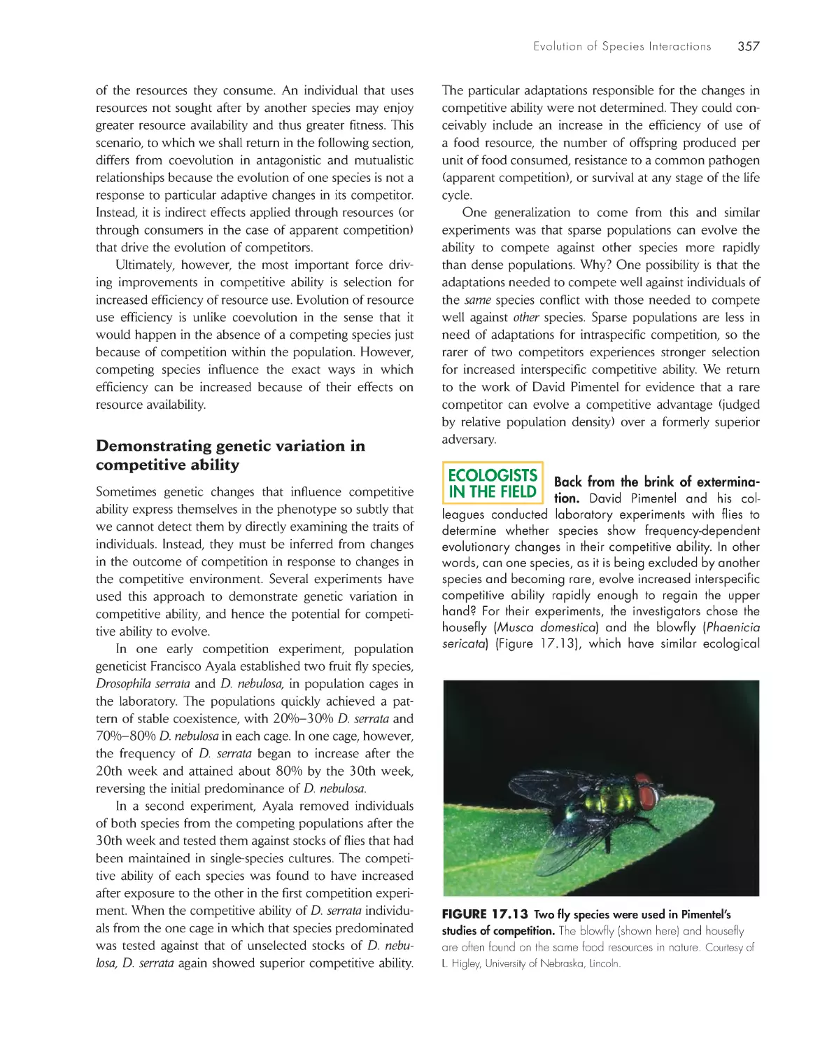
Back from the brink of extermination
357
A counterattack for every defense
361
pArt V CommuNities
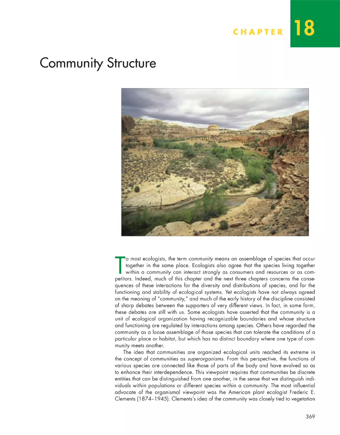
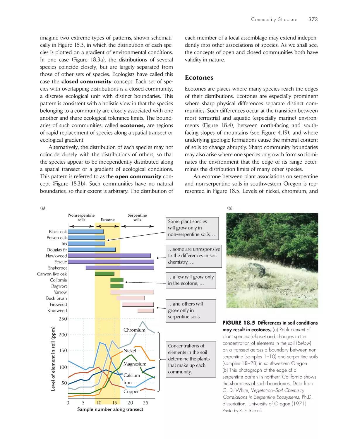
ChApter 18 Community structure
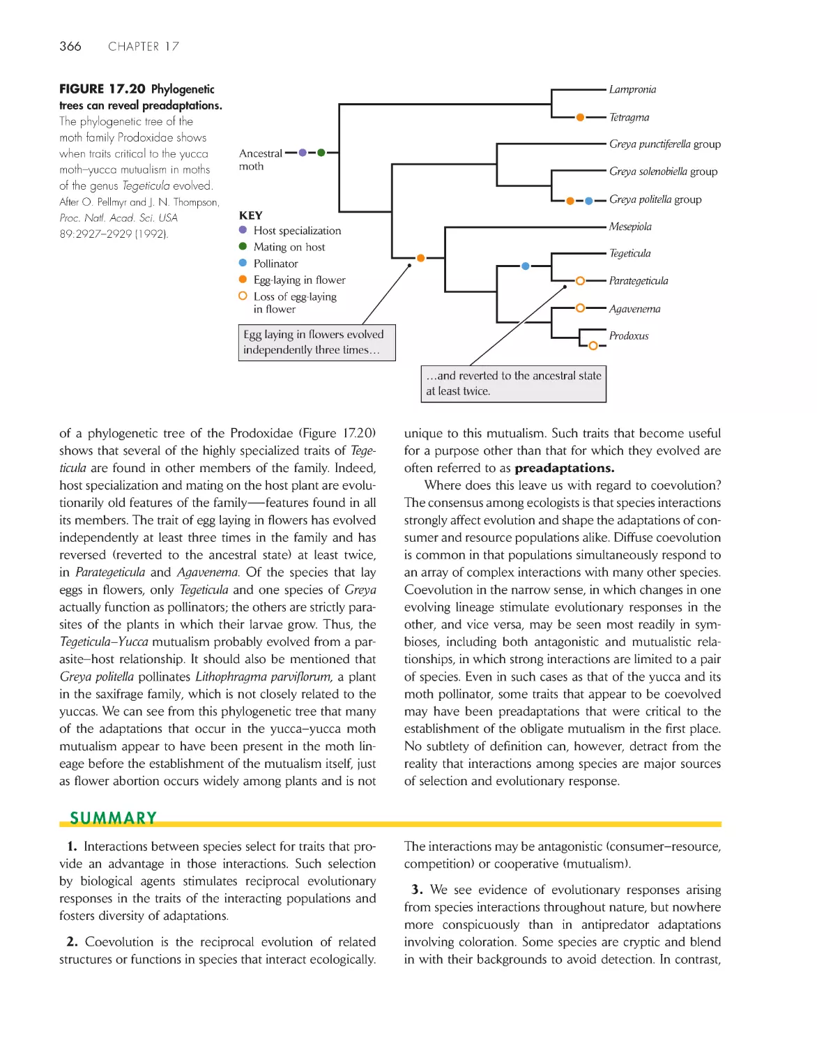
369
A biological community is an association of interacting
populations
371
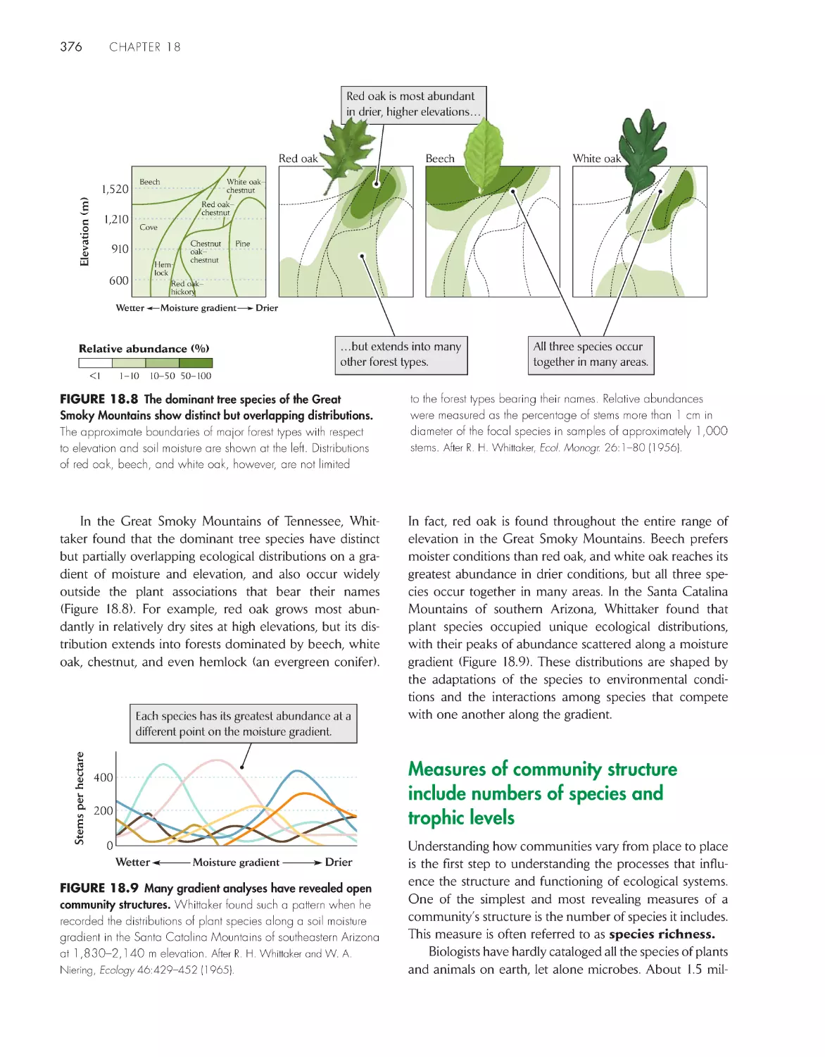
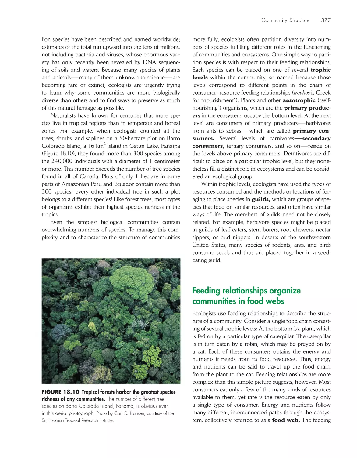
Measures of community structure include numbers of
species and trophic levels 376
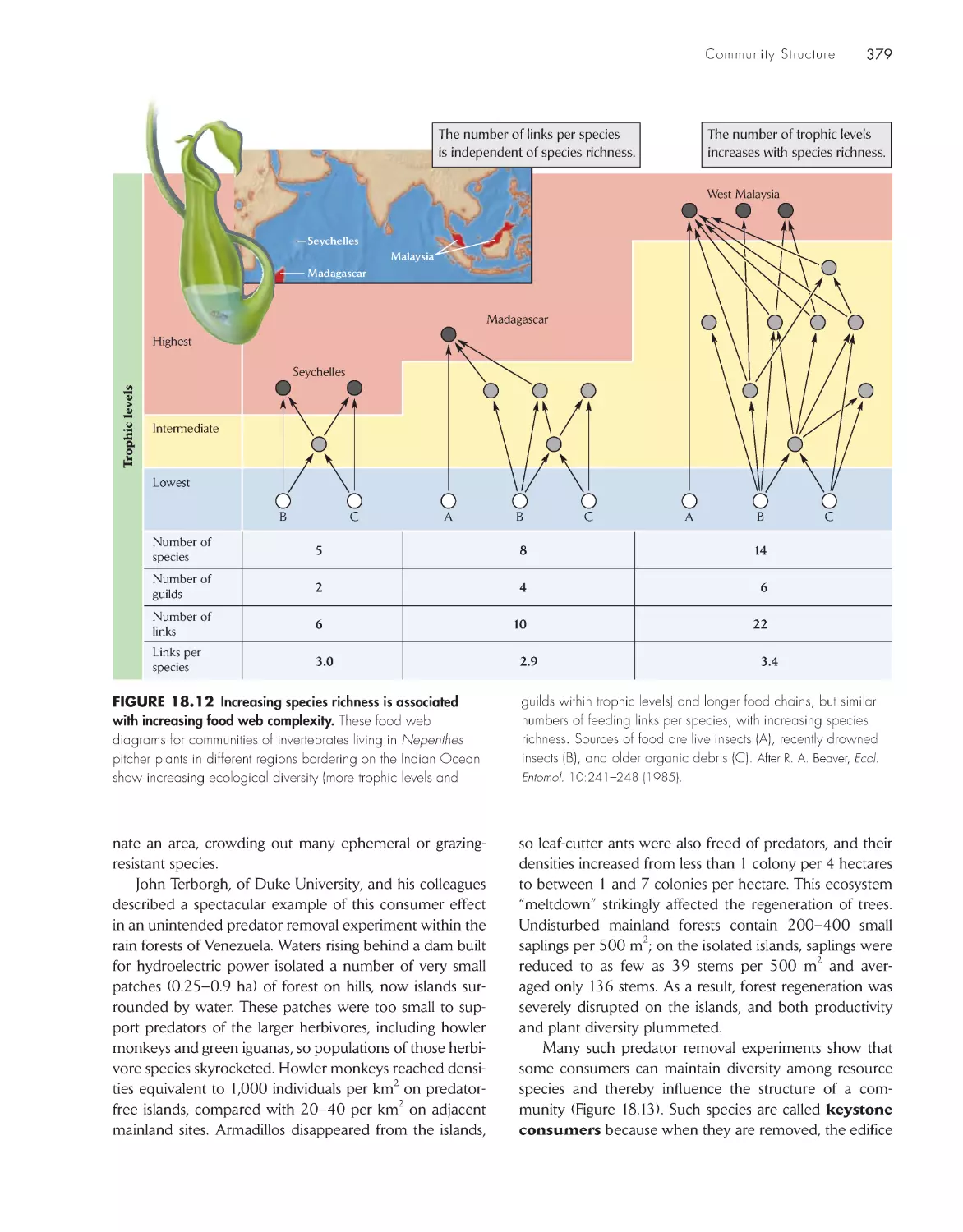
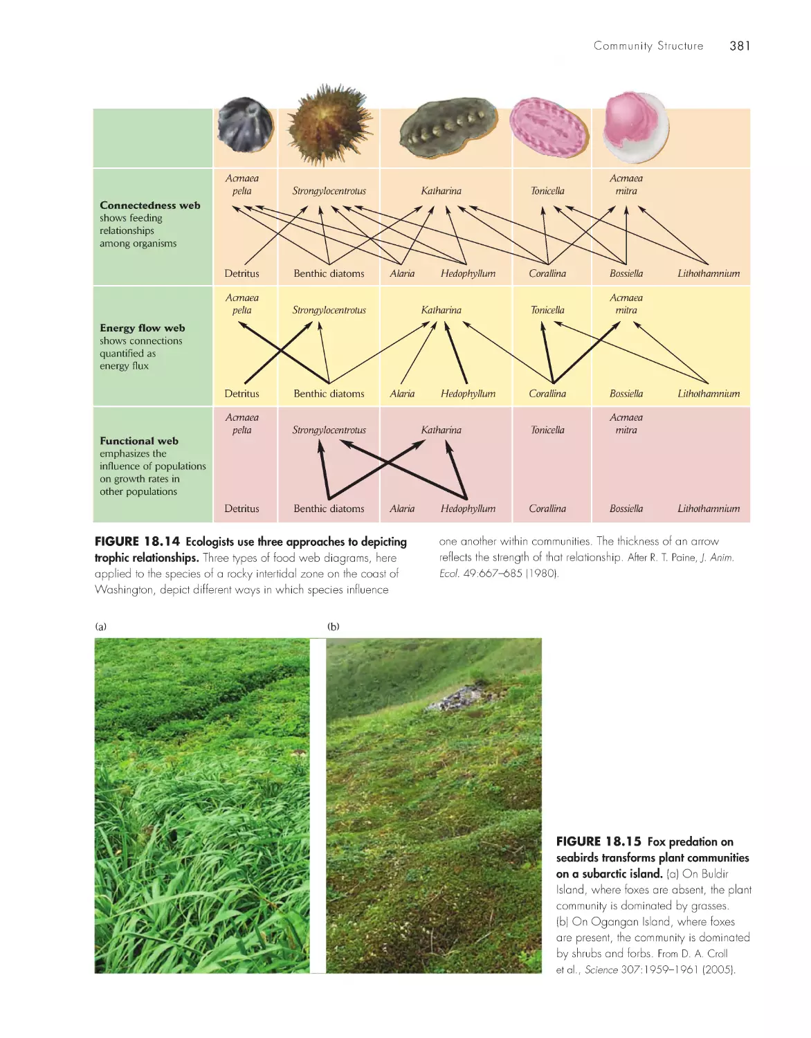
Feeding relationships organize communities in food
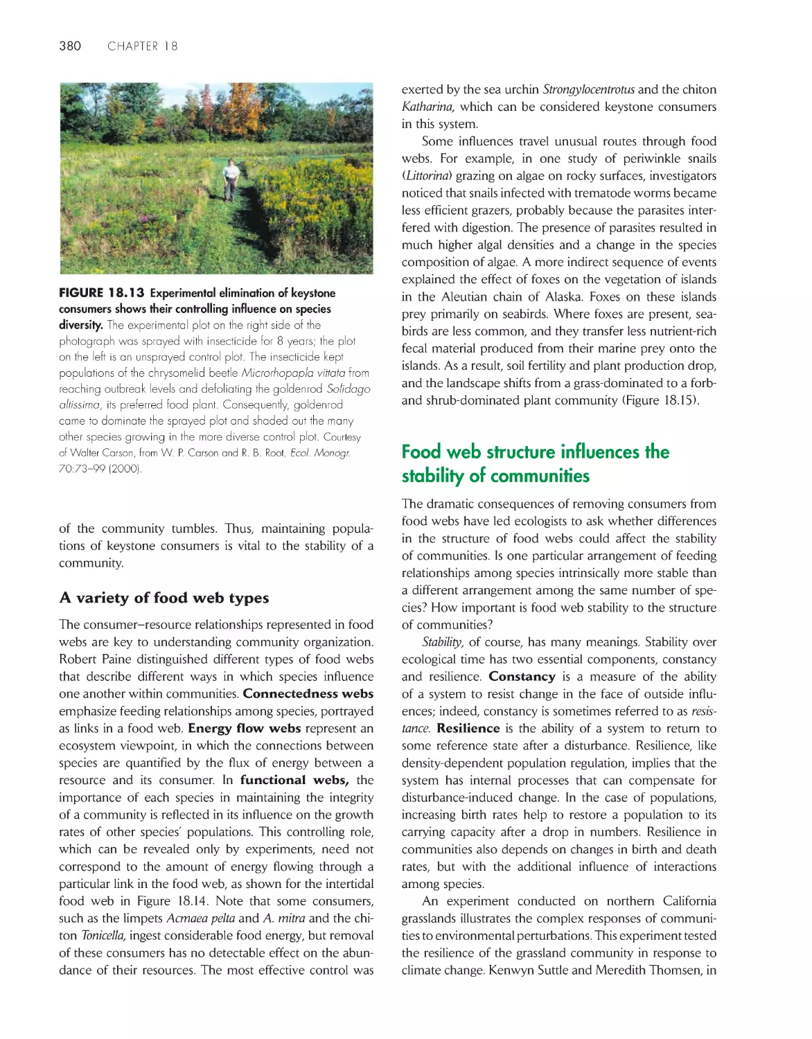
webs 377
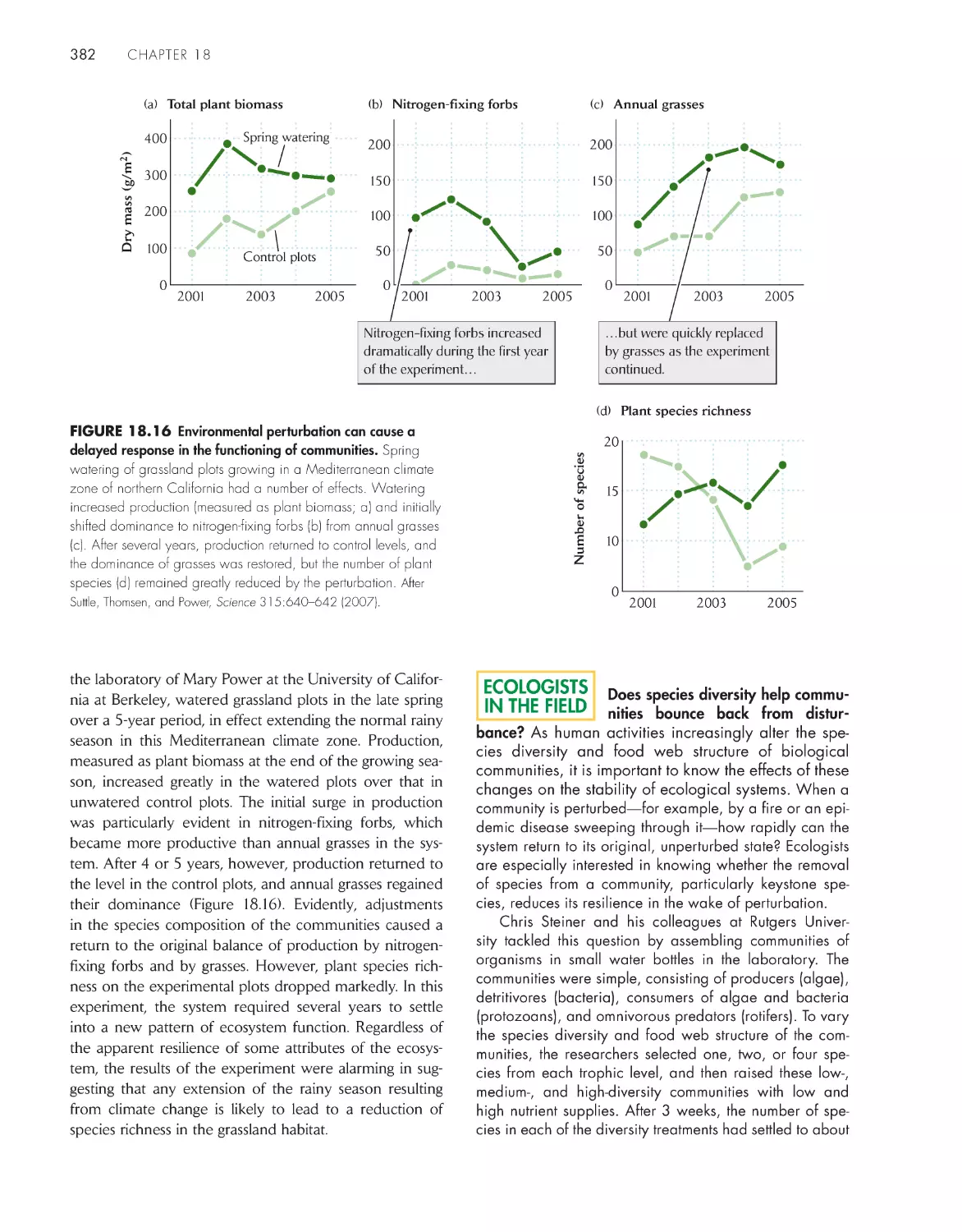
Food web structure influences the stability of
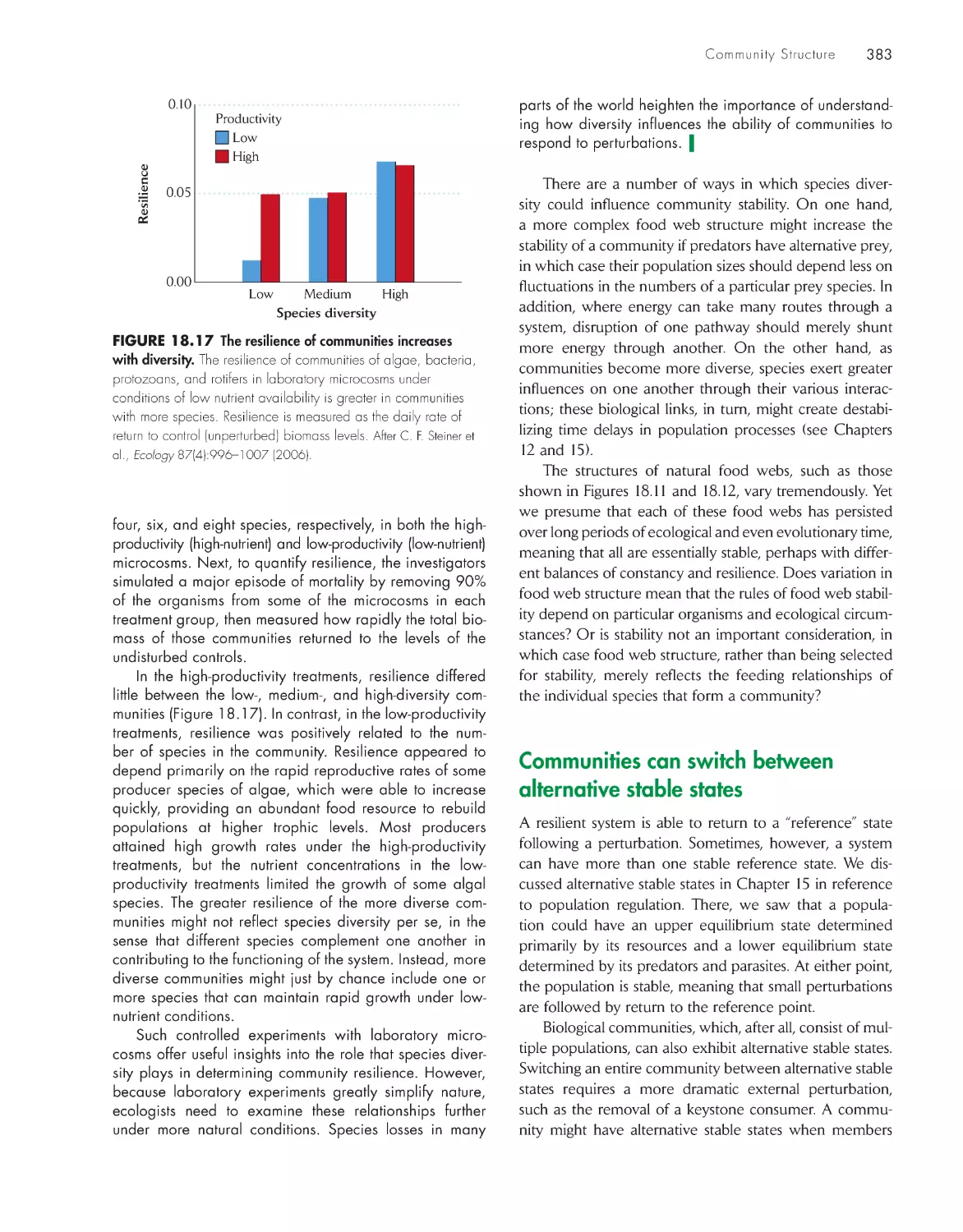
communities 380
Communities can switch between alternative stable
states
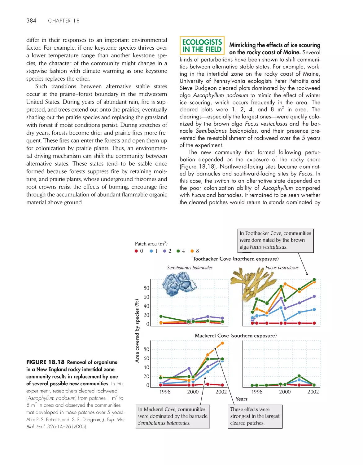
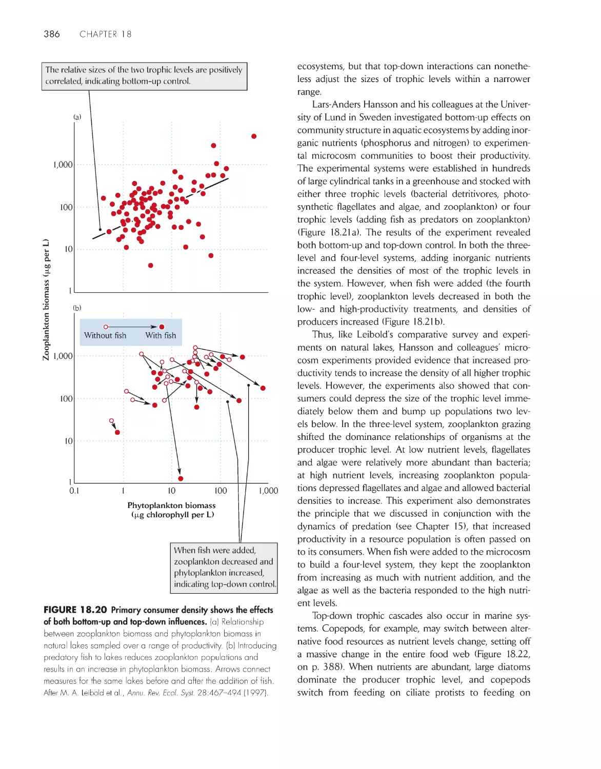
383
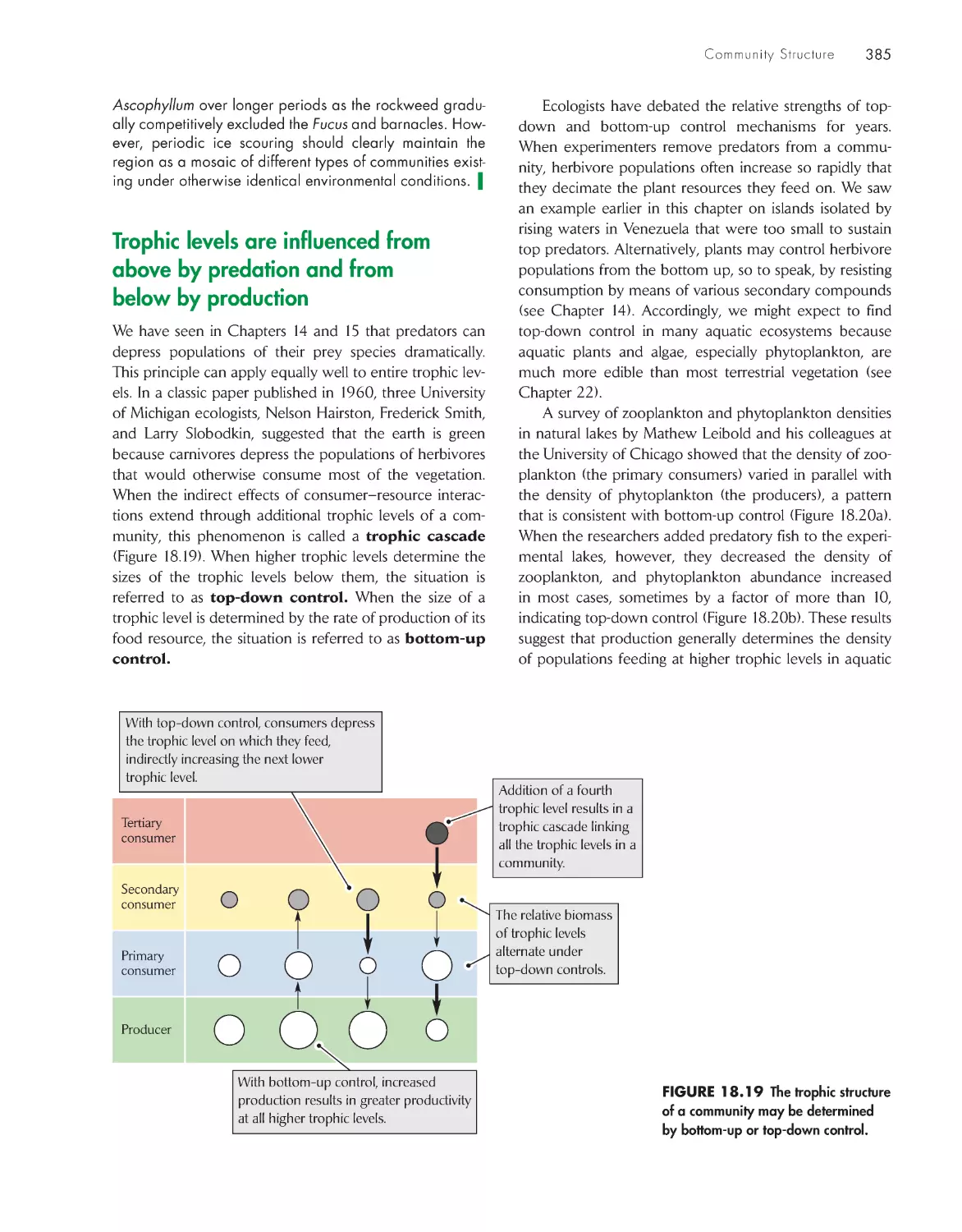
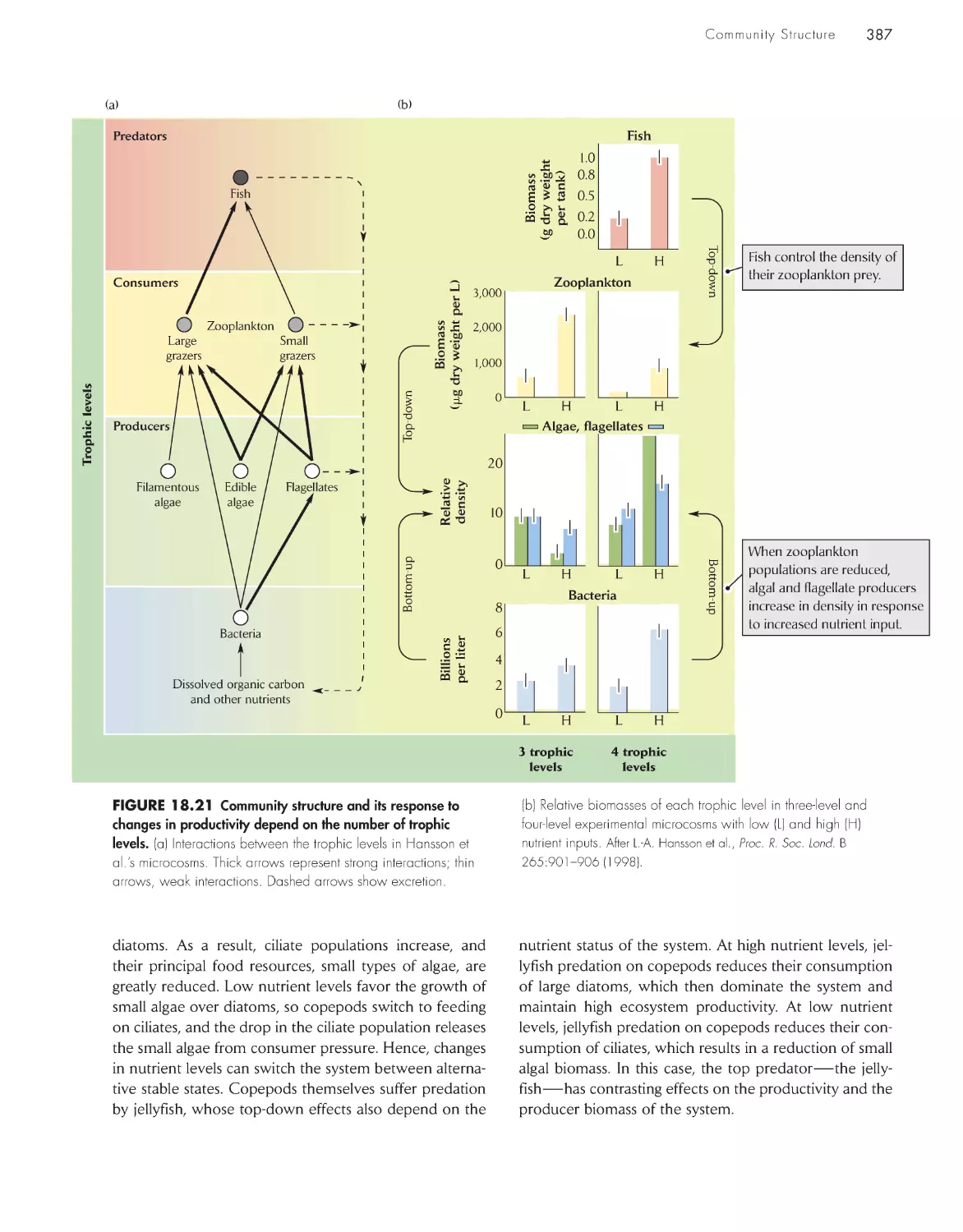
Trophic levels are influenced from above by predation
and from below by production
385
eCoLoGists iN the FieLD
Does species diversity help communities bounce back from
disturbance?
382
xi
contents
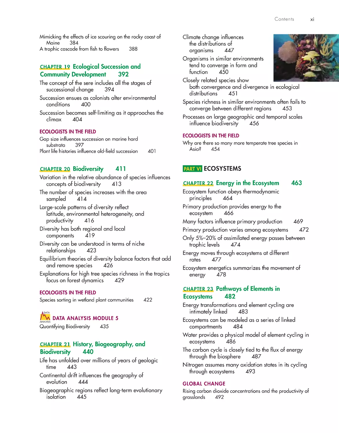
Mimicking the effects of ice scouring on the rocky coast of
Maine
384
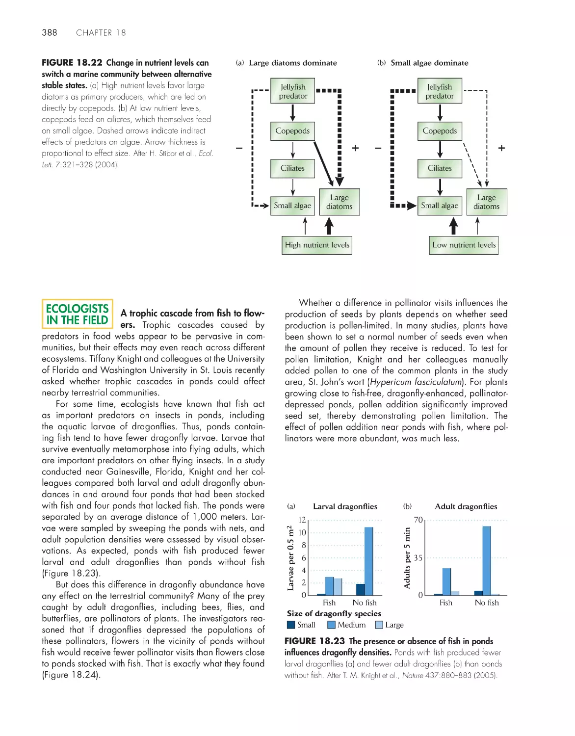
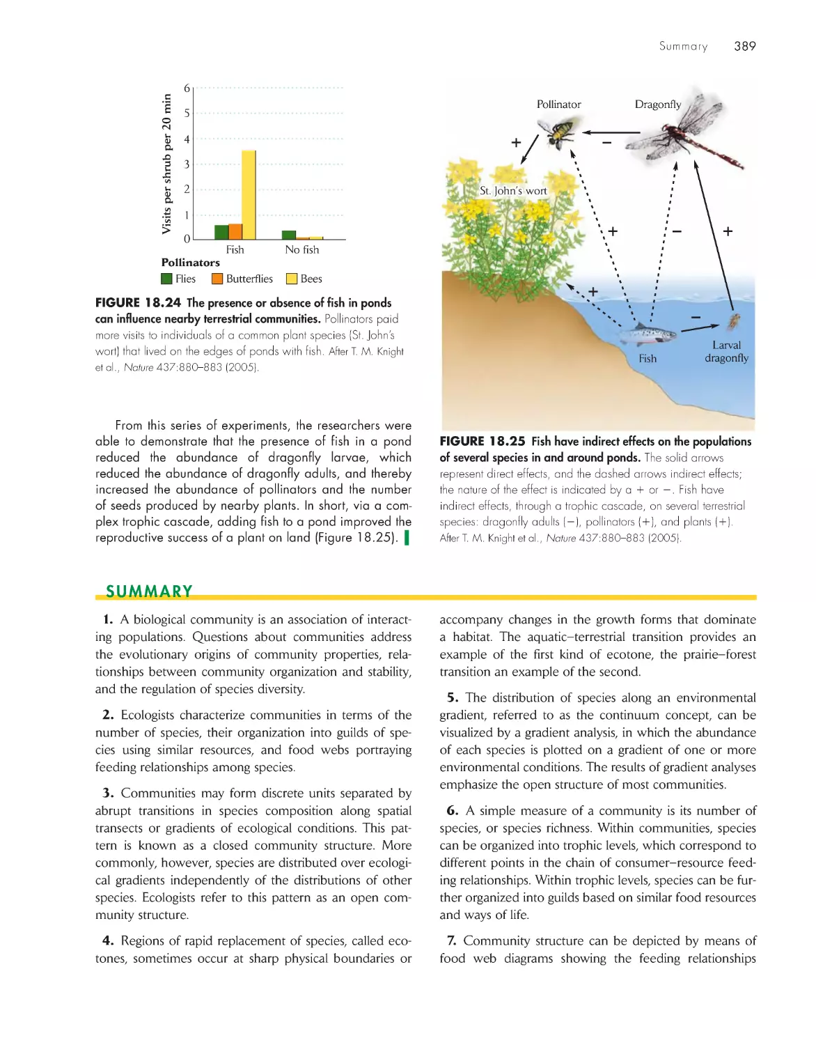
A trophic cascade from fish to flowers
388
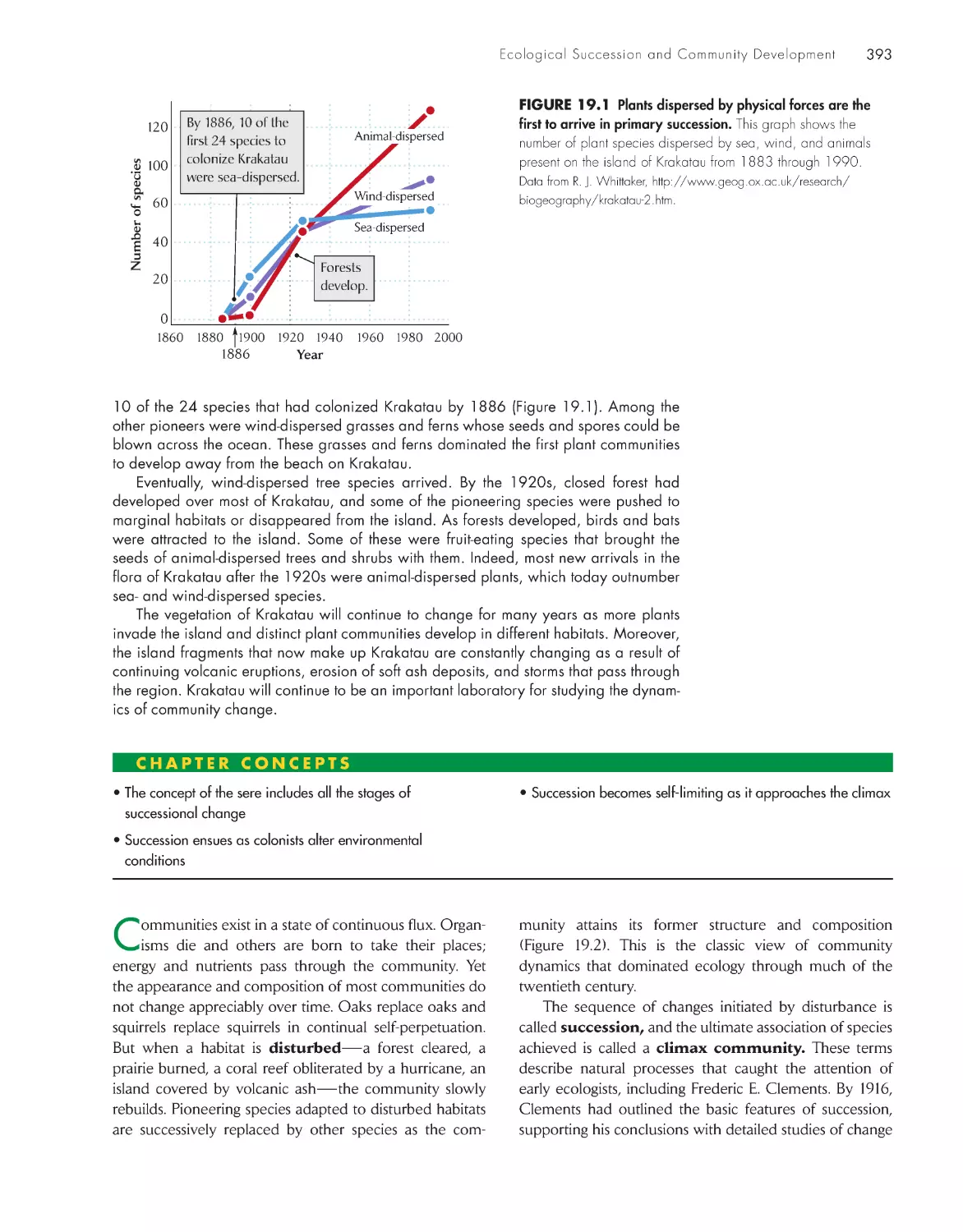
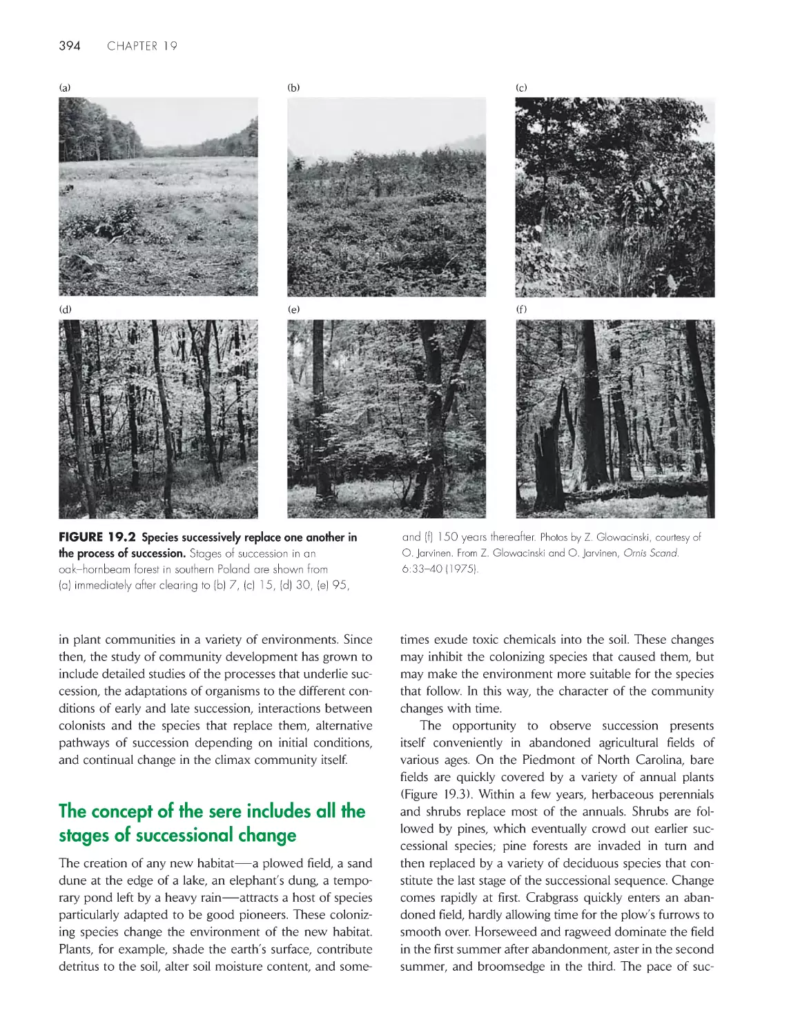
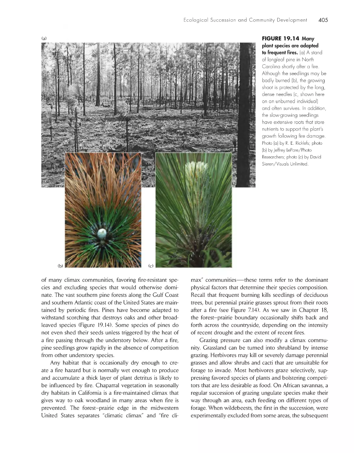
ChApter 19 ecological succession and
Community Development
392
The concept of the sere includes all the stages of
successional change 394
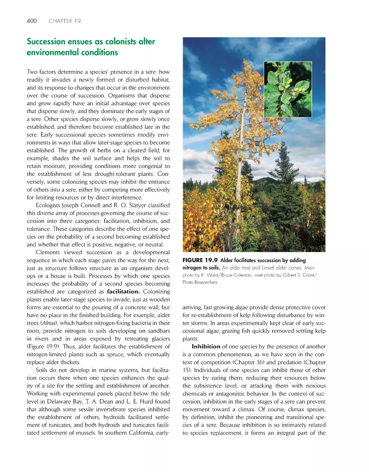
Succession ensues as colonists alter environmental
conditions
400
Succession becomes self-limiting as it approaches the
climax
404
eCoLoGists iN the FieLD
Gap size influences succession on marine hard
substrata
397
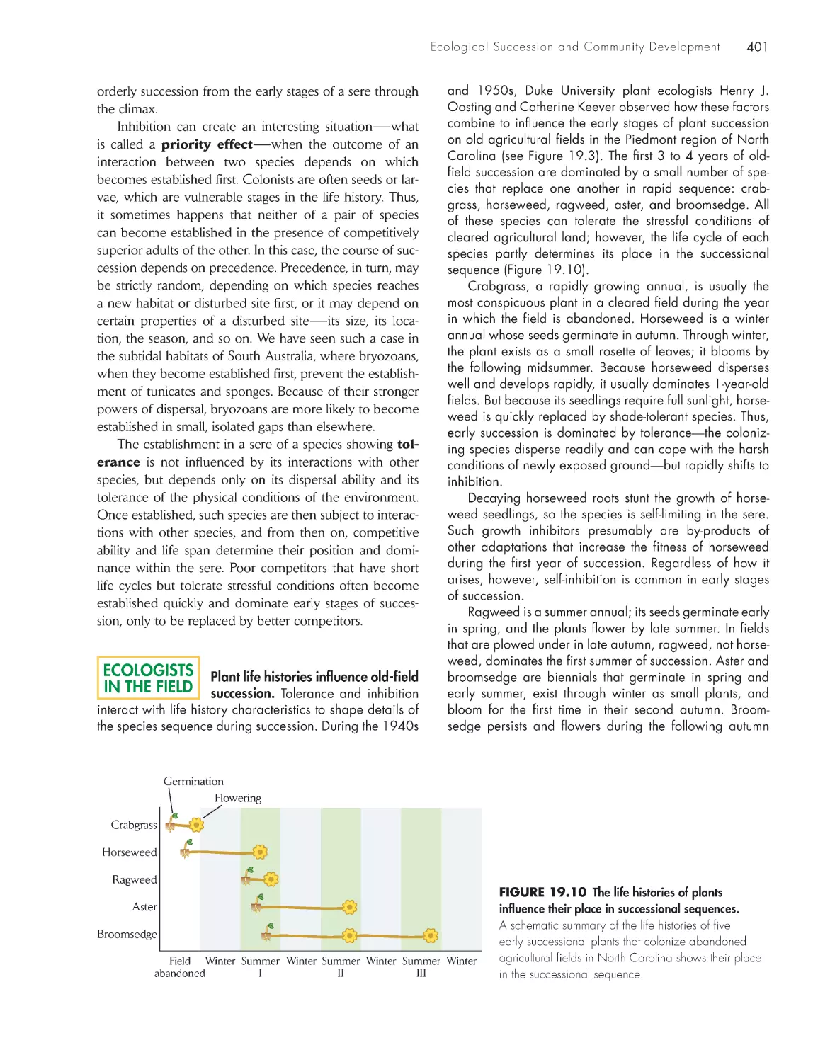
Plant life histories influence old-field succession
401
ChApter 20 biodiversity 411
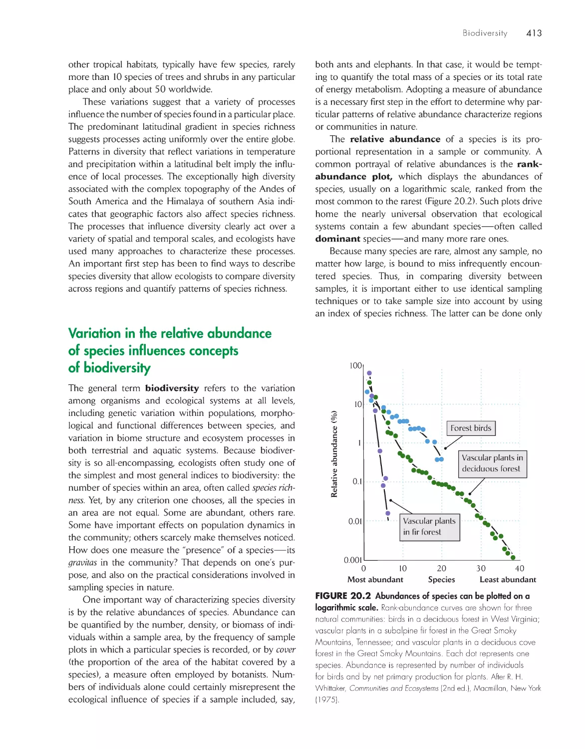
Variation in the relative abundance of species influences
concepts of biodiversity 413
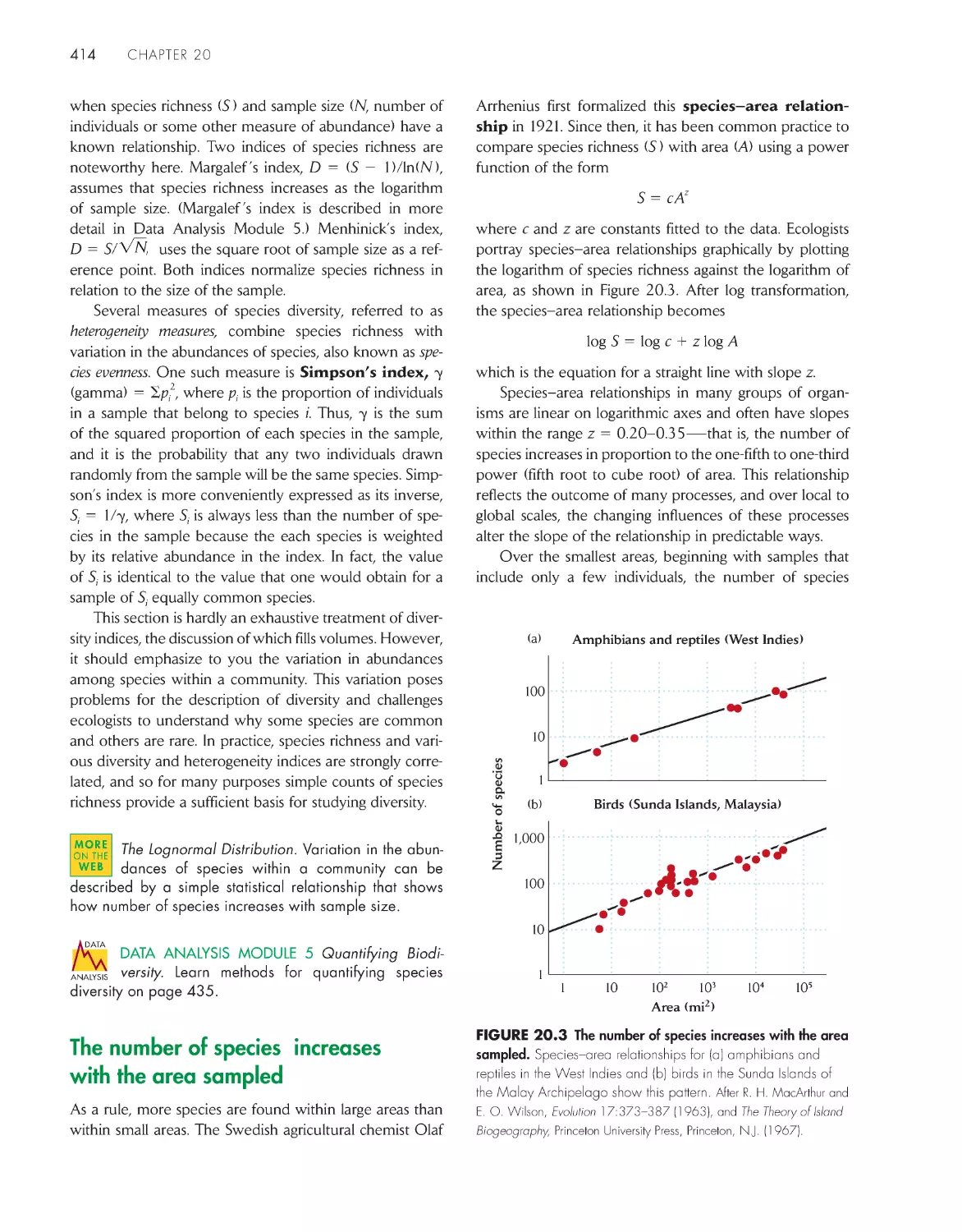
The number of species increases with the area
sampled 414
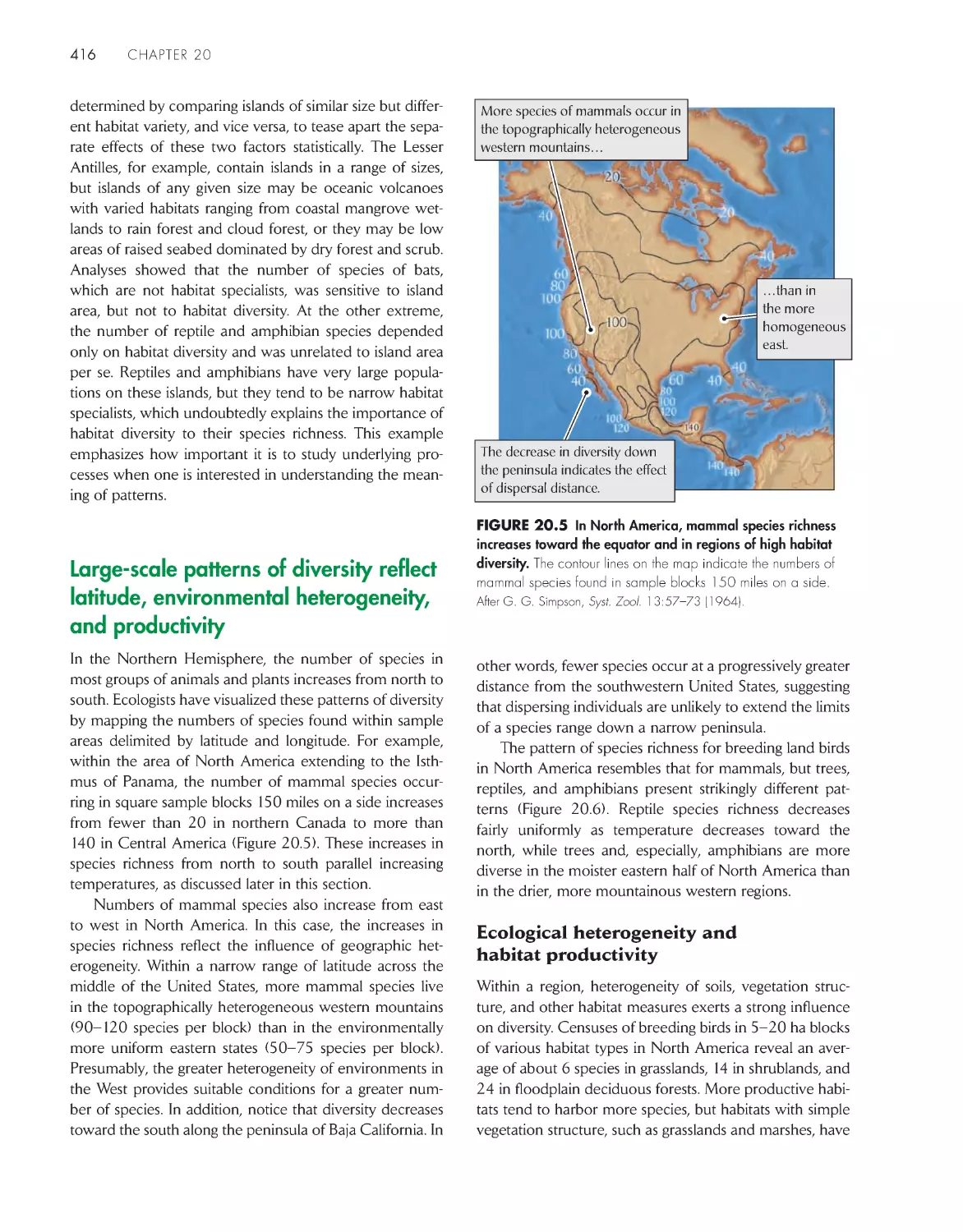
Large-scale patterns of diversity reflect
latitude, environmental heterogeneity, and
productivity 416
Diversity has both regional and local
components
419
Diversity can be understood in terms of niche
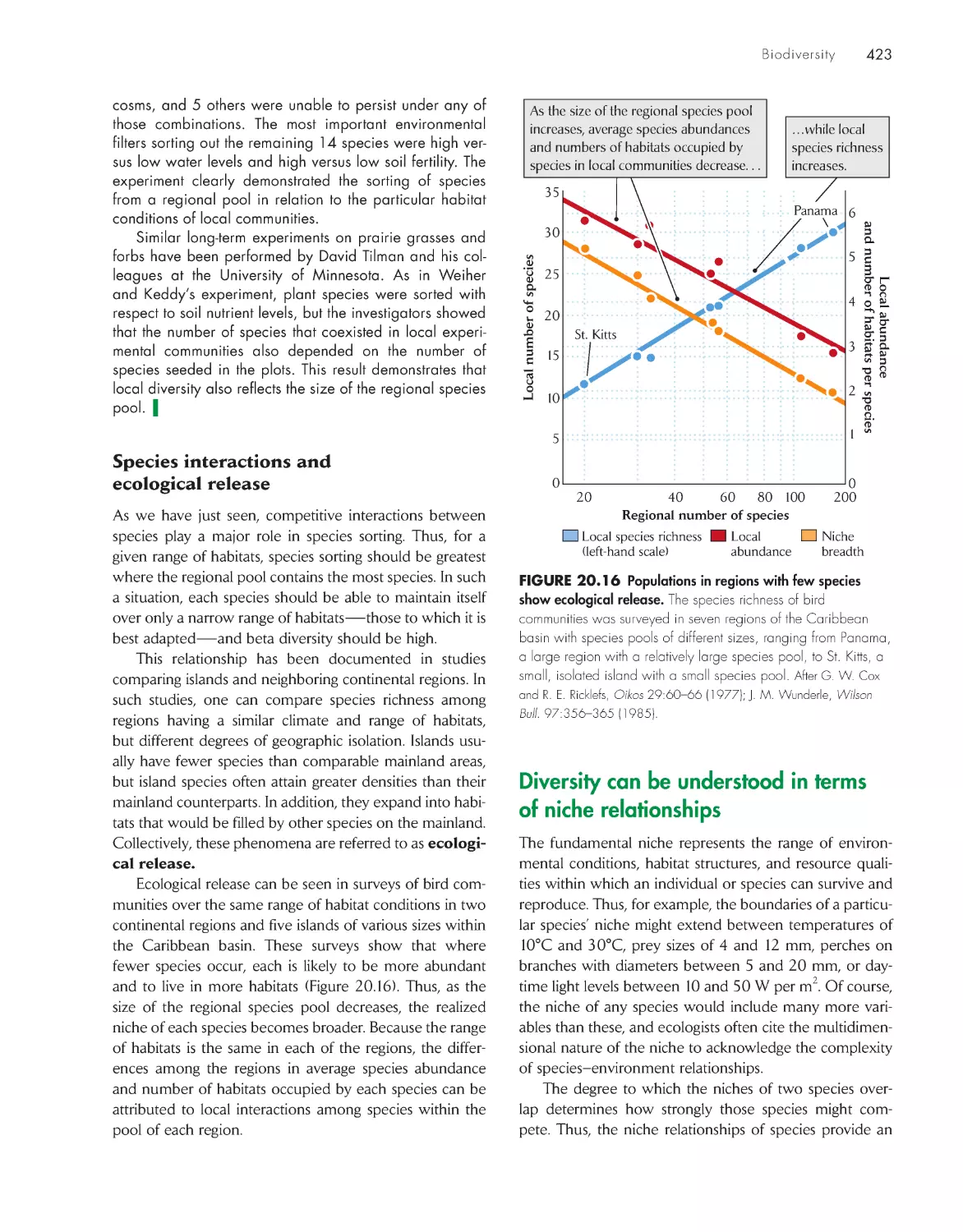
relationships 423
Equilibrium theories of diversity balance factors that add
and remove species 426
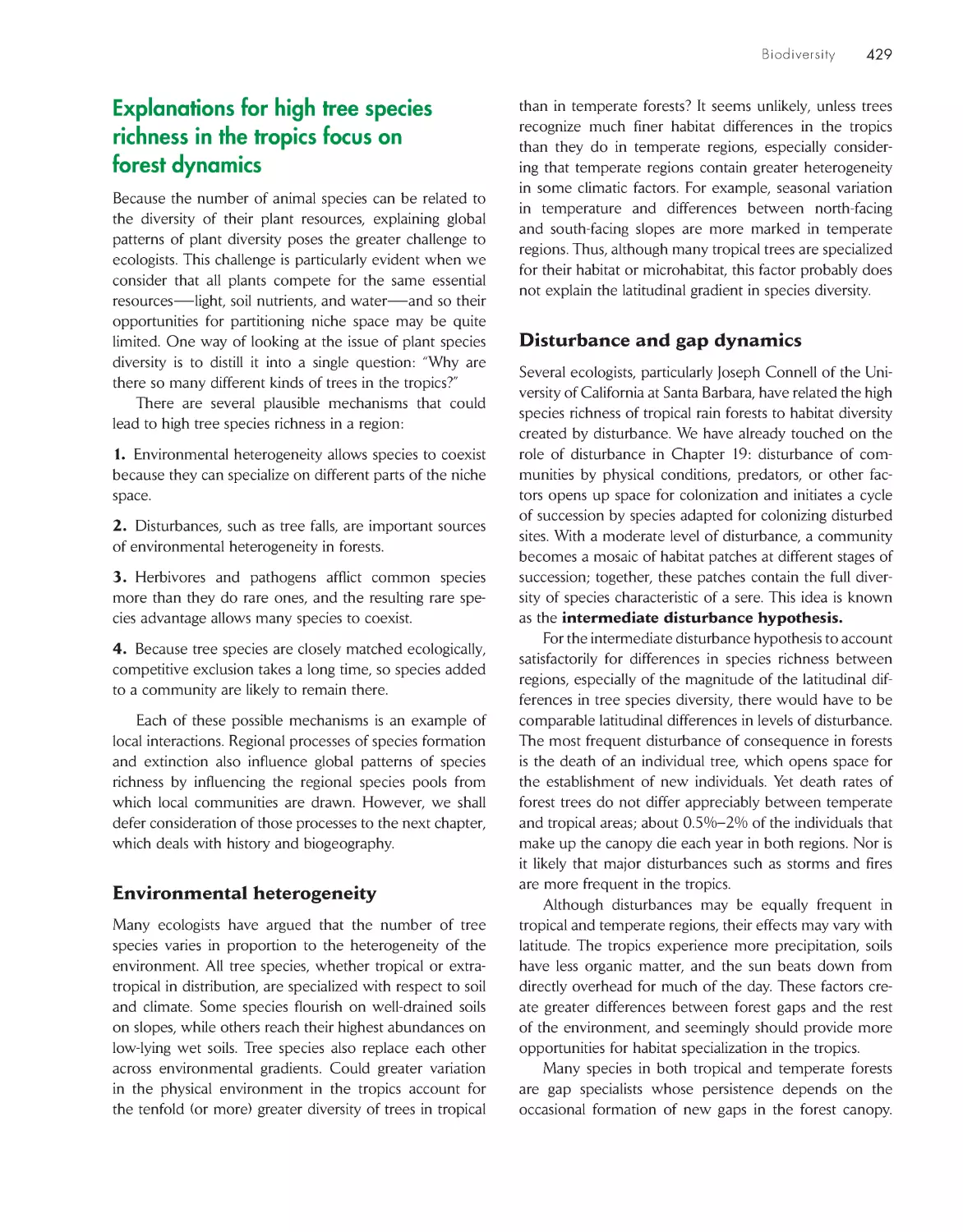
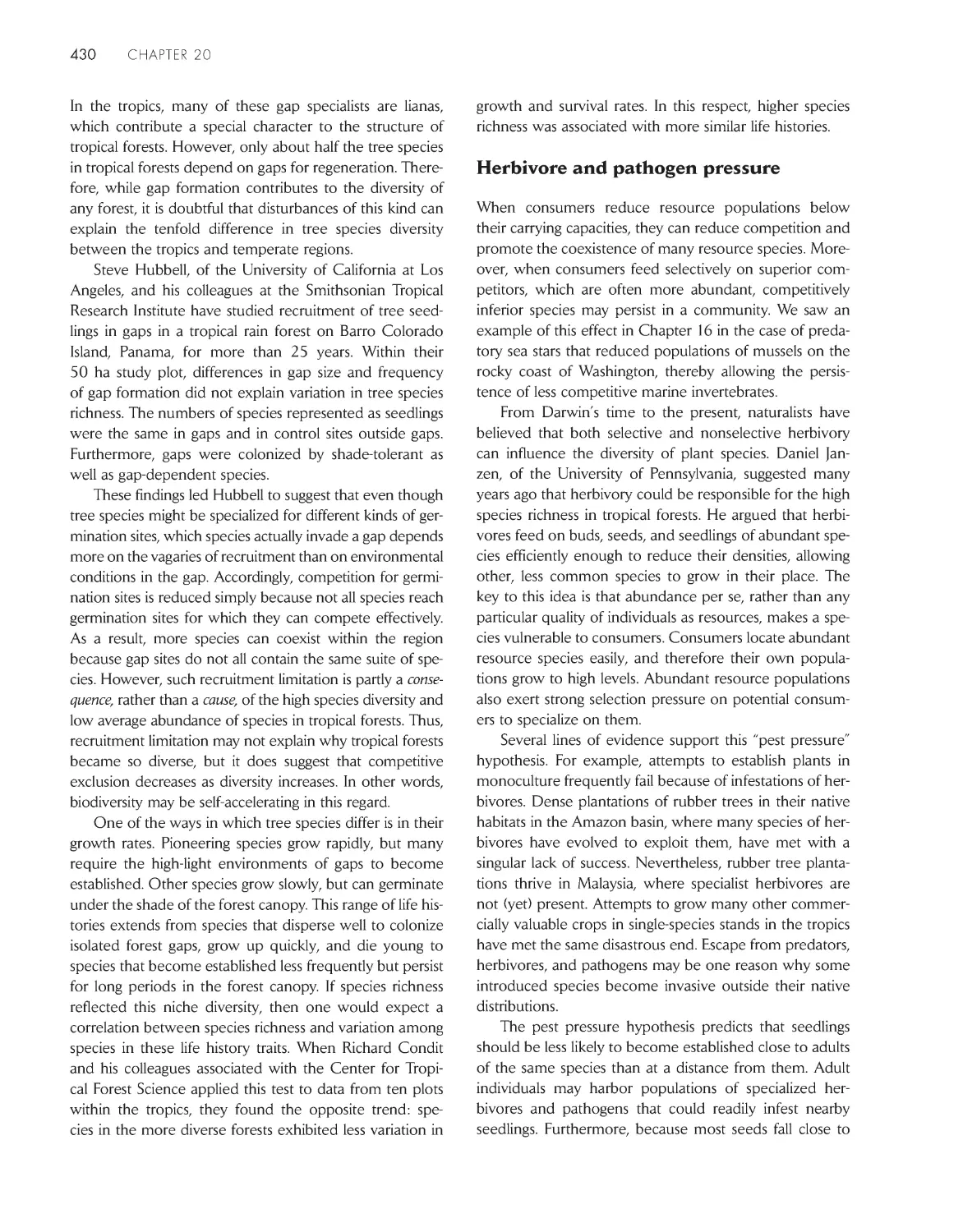
Explanations for high tree species richness in the tropics
focus on forest dynamics 429
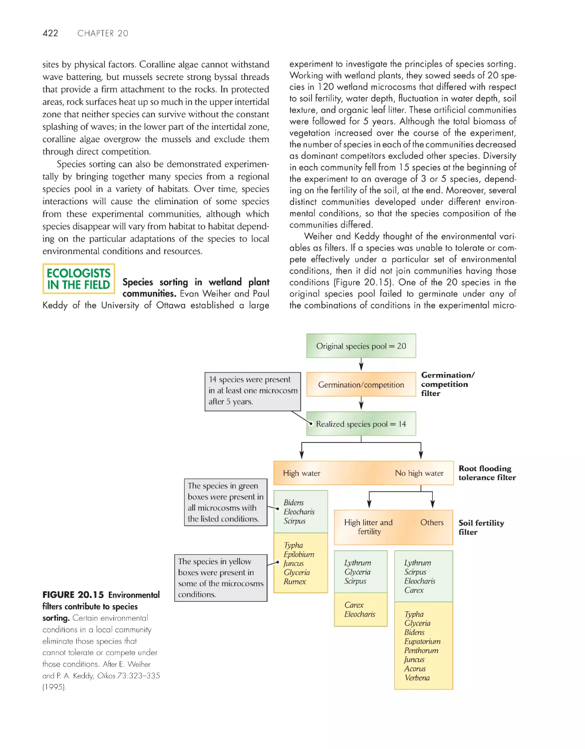
eCoLoGists iN the FieLD
Species sorting in wetland plant communities 422
DATA
ANALYSIS
DAtA ANALYsis moDuLe 5
Quantifying Biodiversity 435
ChApter 21 histor y, biogeography, and
biodiversity 440
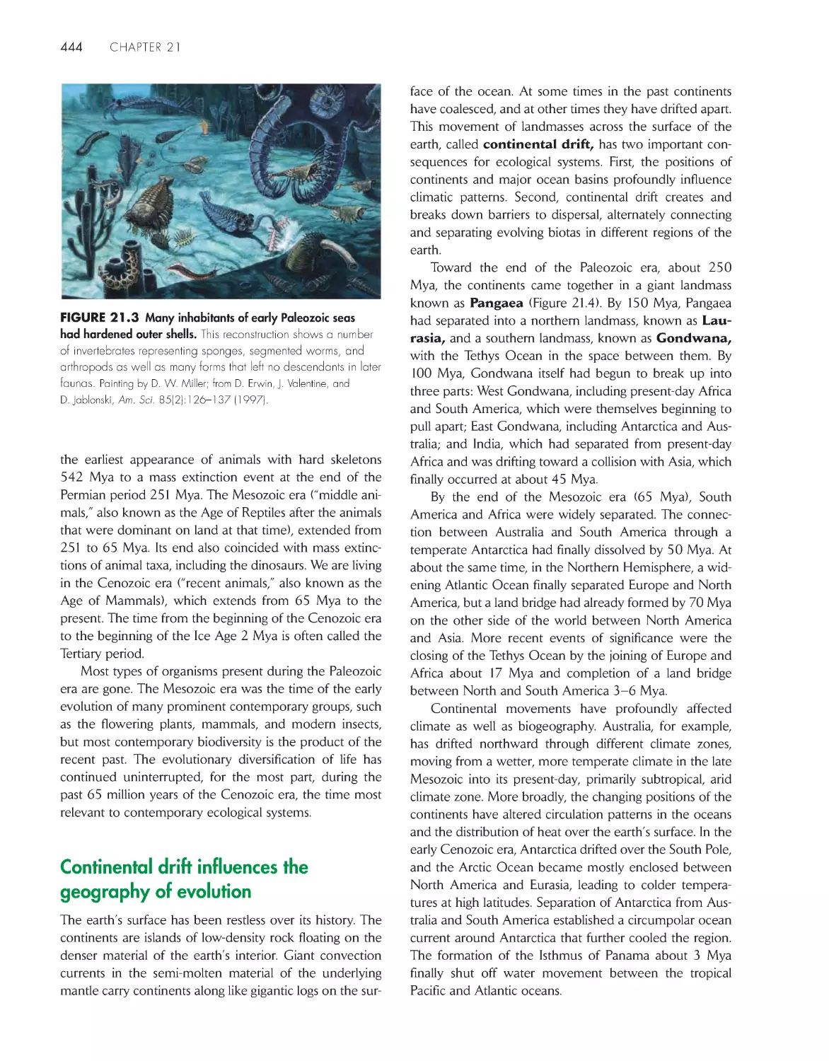
Life has unfolded over millions of years of geologic
time
443
Continental drift influences the geography of
evolution
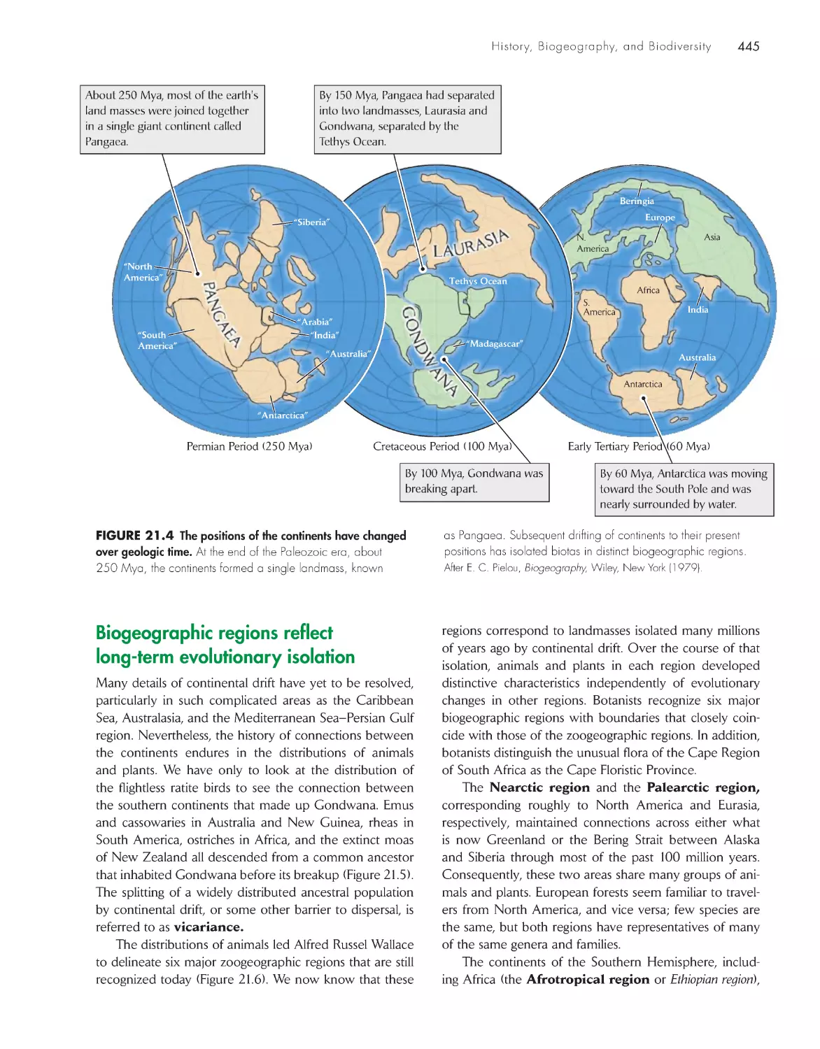
444
Biogeographic regions reflect long-term evolutionary
isolation
445
Climate change influences
the distributions of
organisms
447
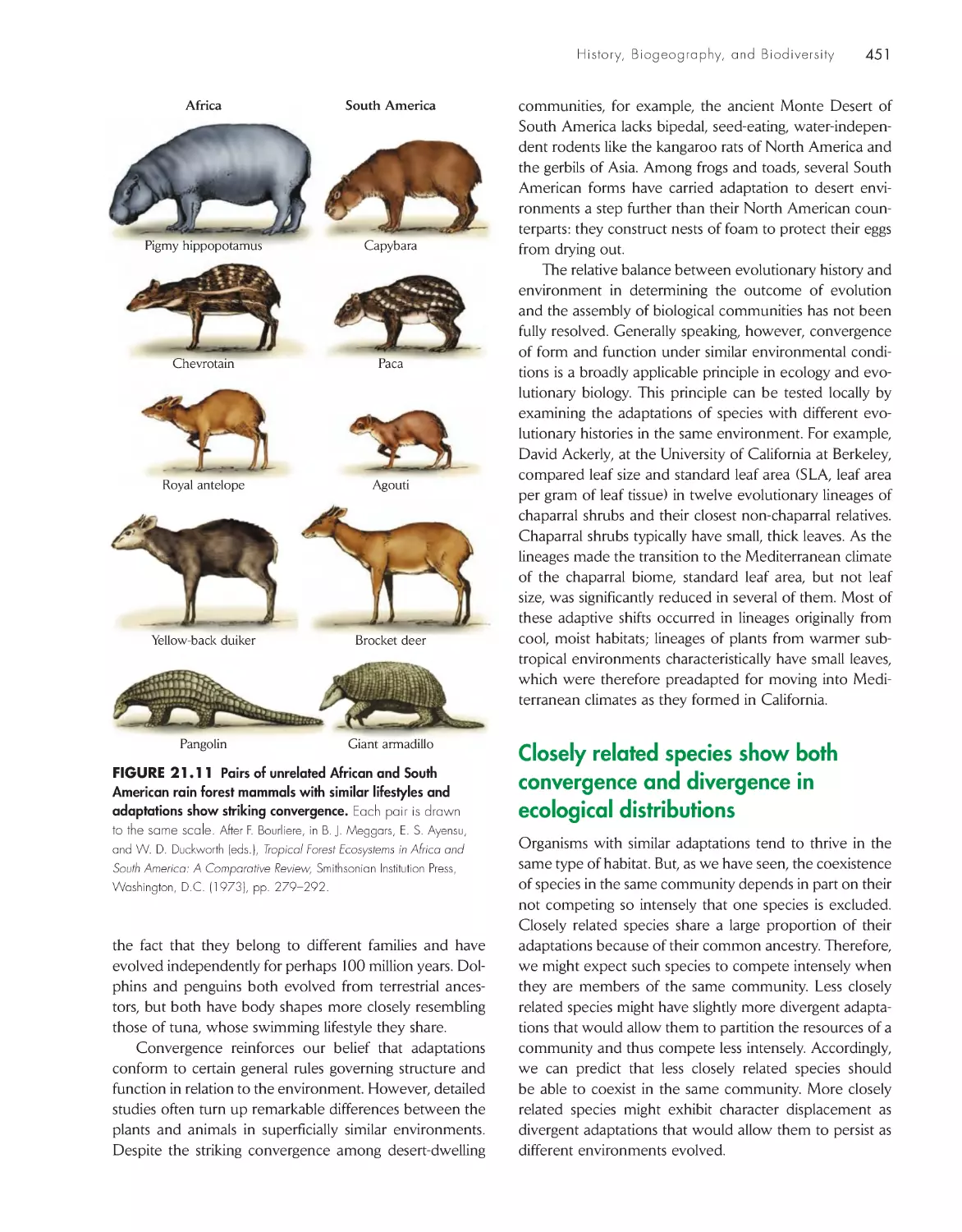
Organisms in similar environments
tend to converge in form and
function
450
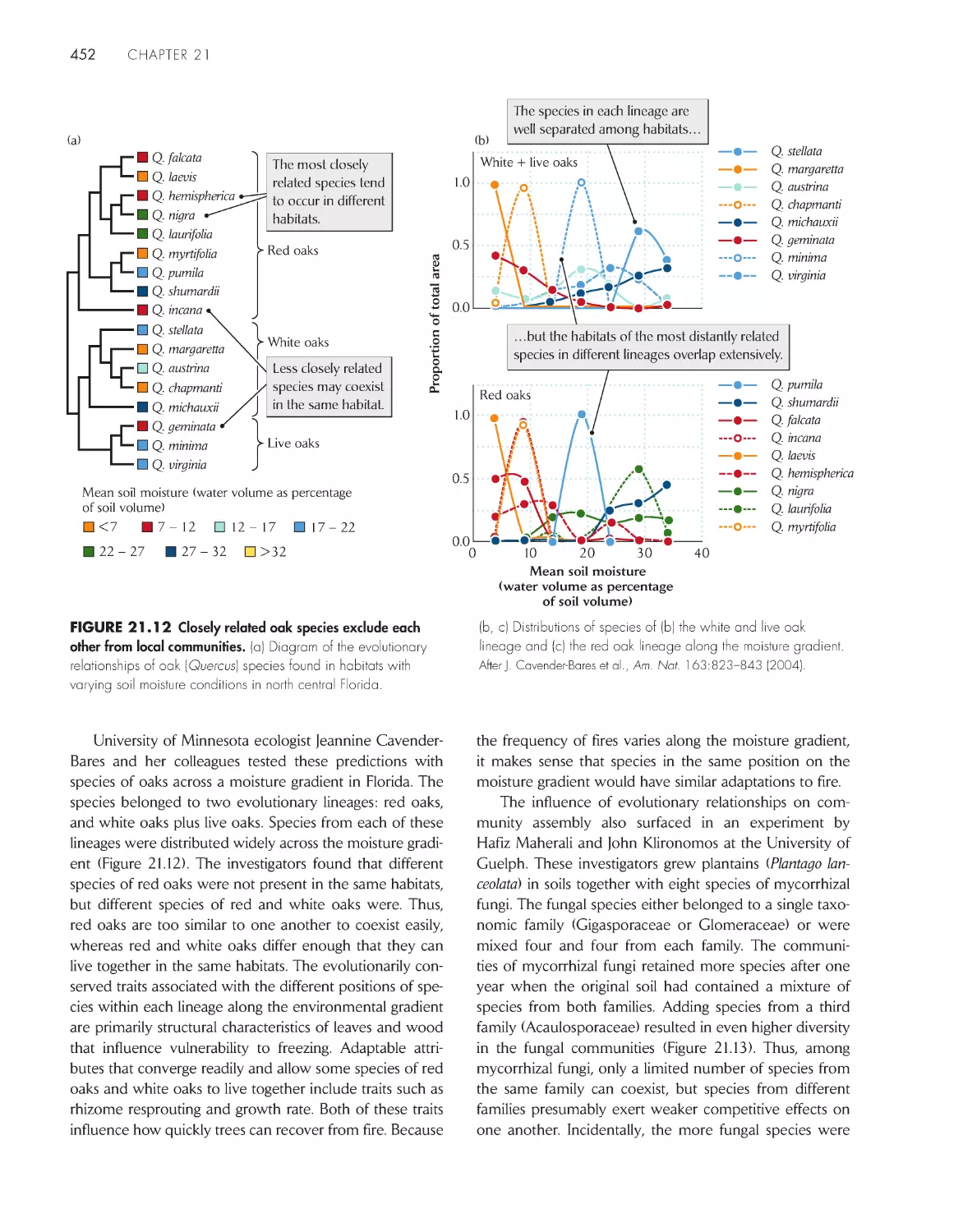
Closely related species show
both convergence and divergence in ecological
distributions
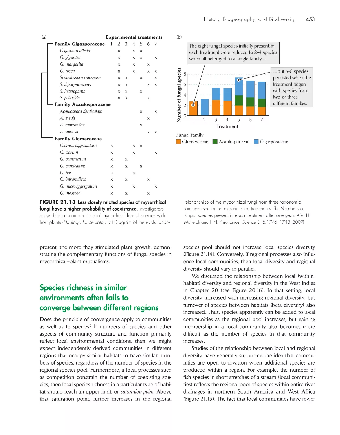
451
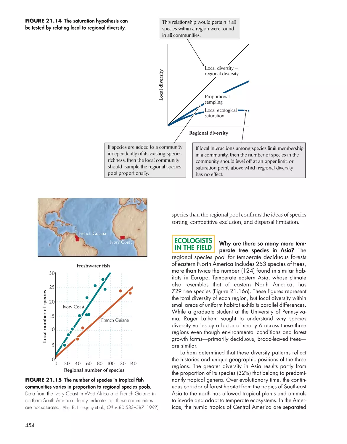
Species richness in similar environments often fails to
converge between different regions
453
Processes on large geographic and temporal scales
influence biodiversity 456
eCoLoGists iN the FieLD
Why are there so many more temperate tree species in
Asia? 454
pArt Vi eCosYstems
ChApter 22 energy in the ecosystem
463
Ecosystem function obeys thermodynamic
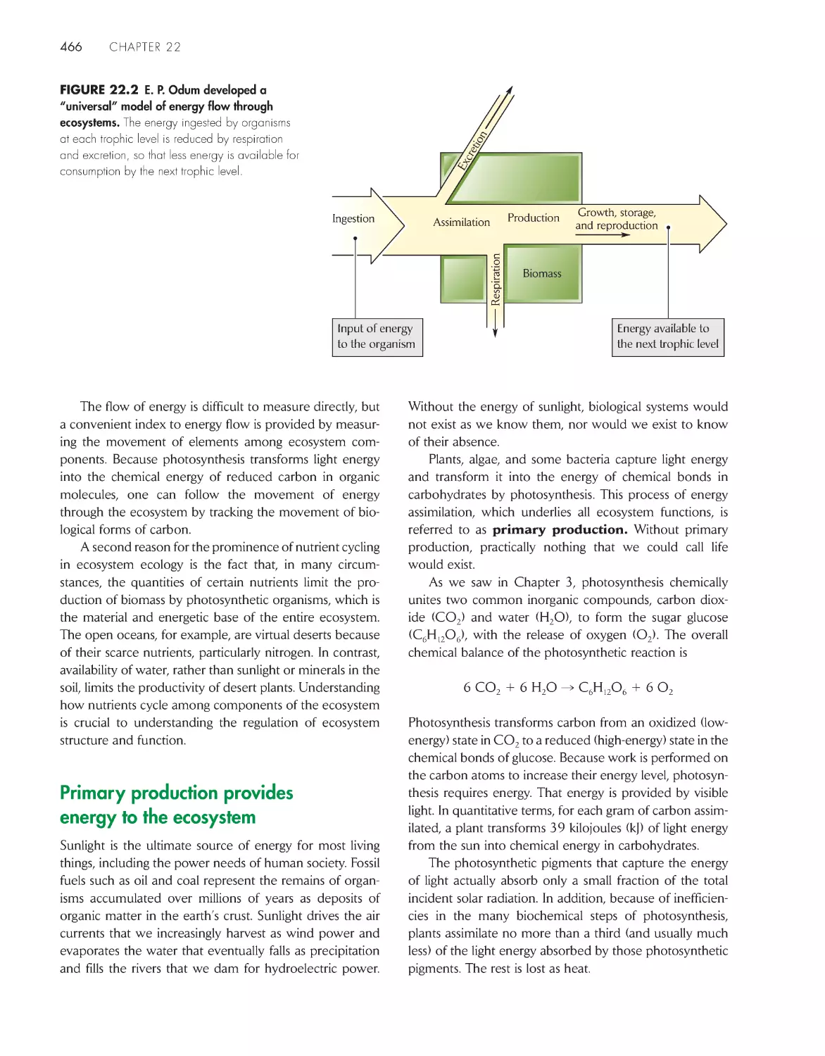
principles 464
Primary production provides energy to the
ecosystem
466
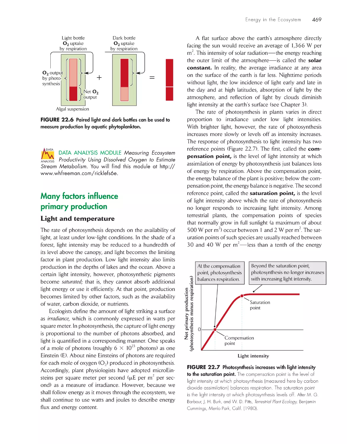
Many factors influence primary production
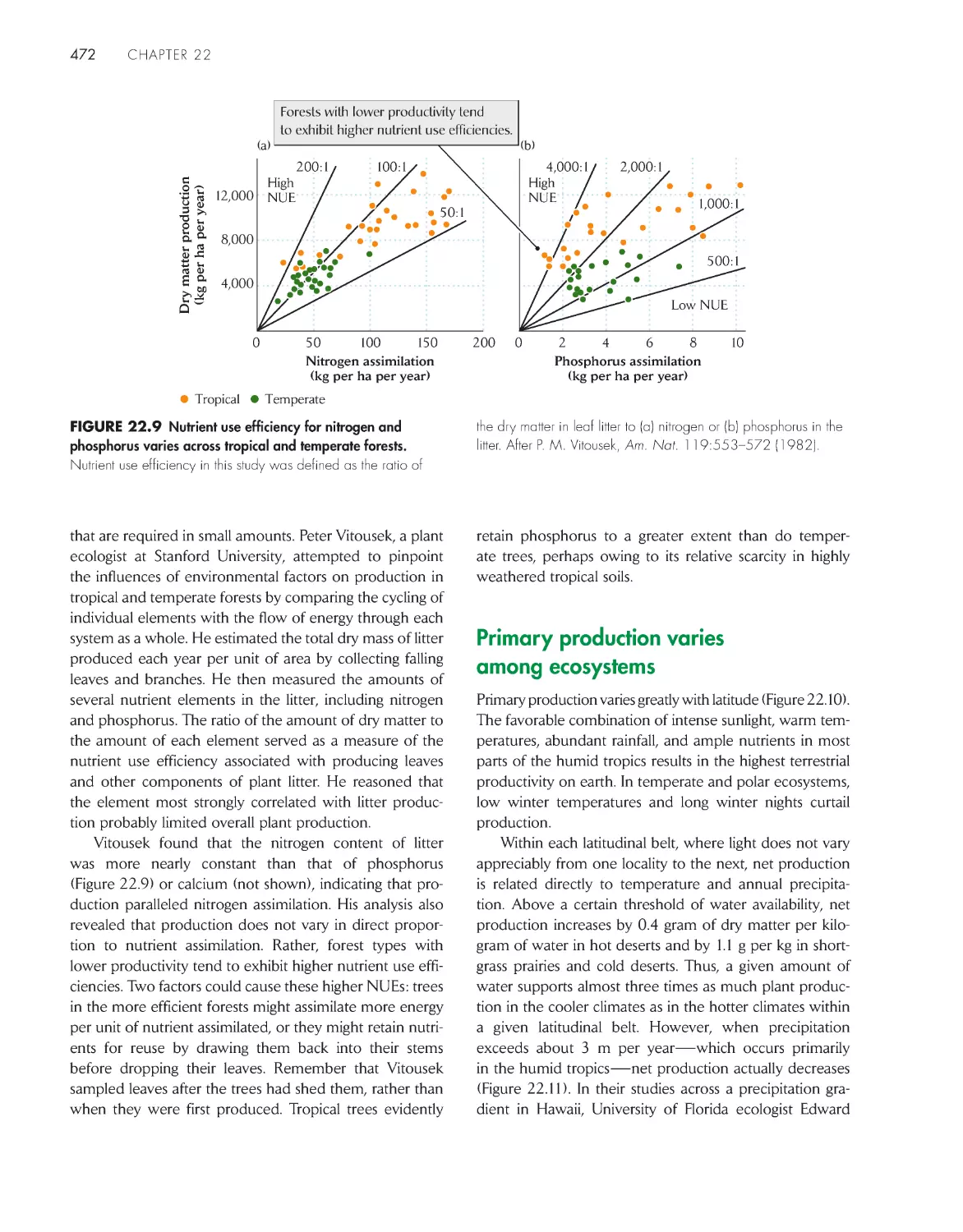
469
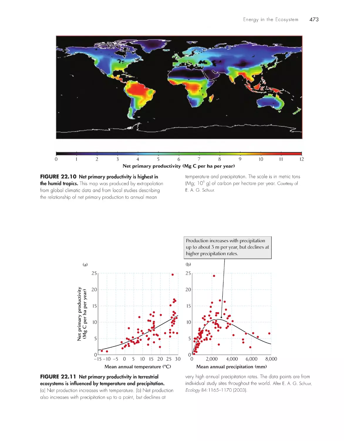
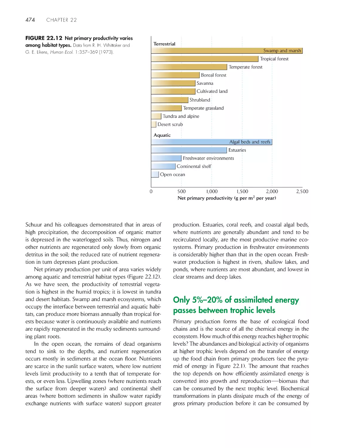
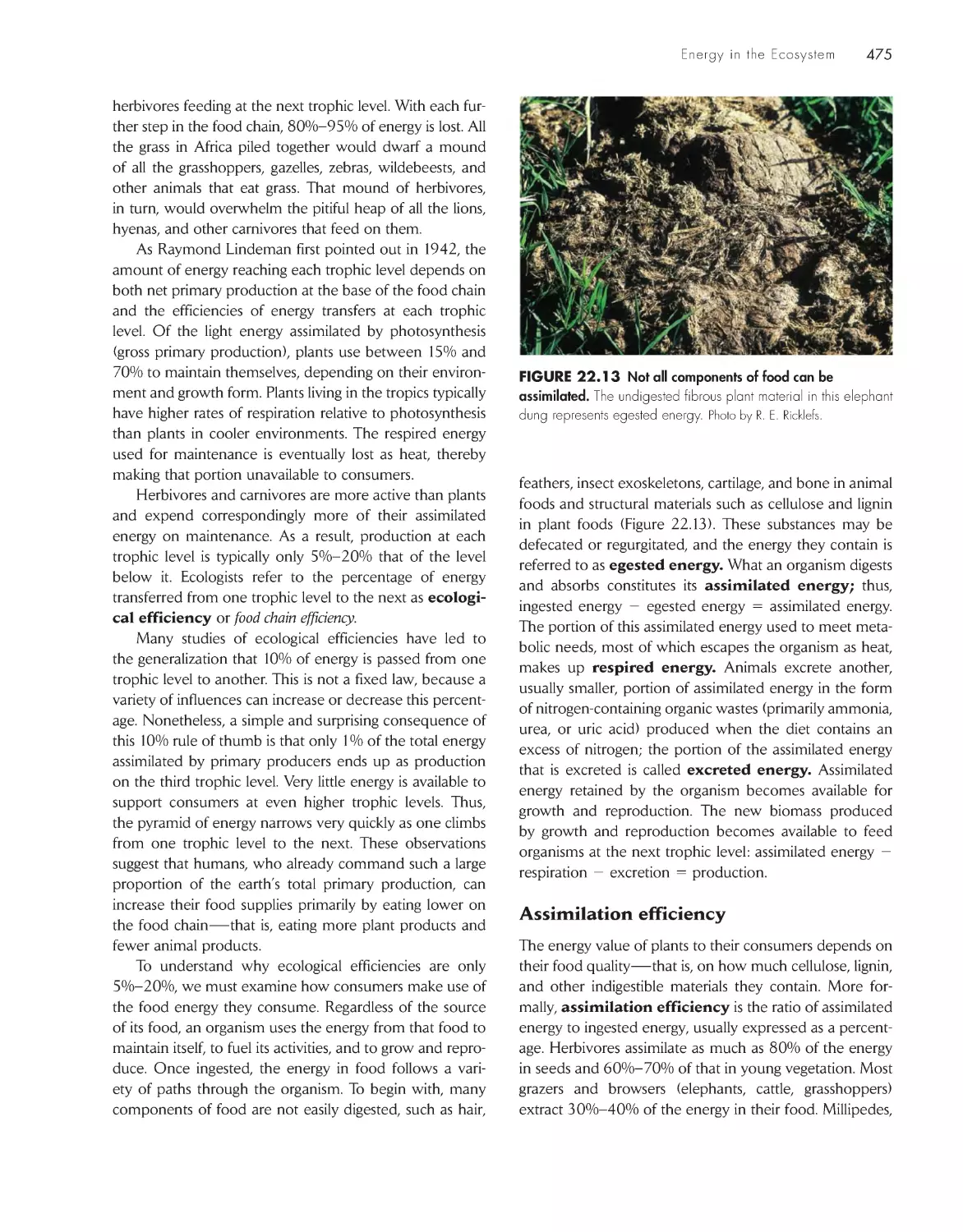
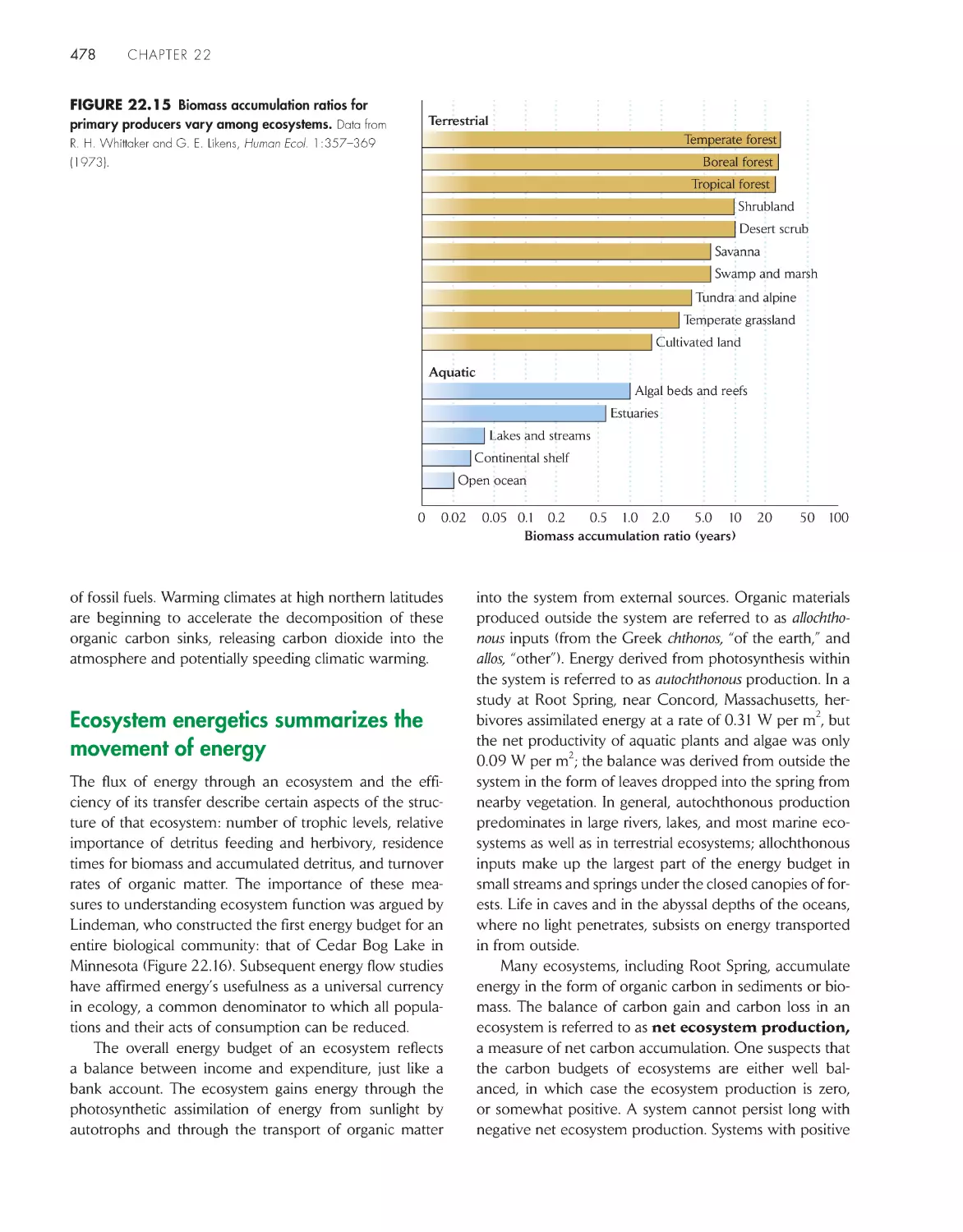
Primary production varies among ecosystems
472
Only 5%–20% of assimilated energy passes between
trophic levels 474
Energy moves through ecosystems at different
rates
477
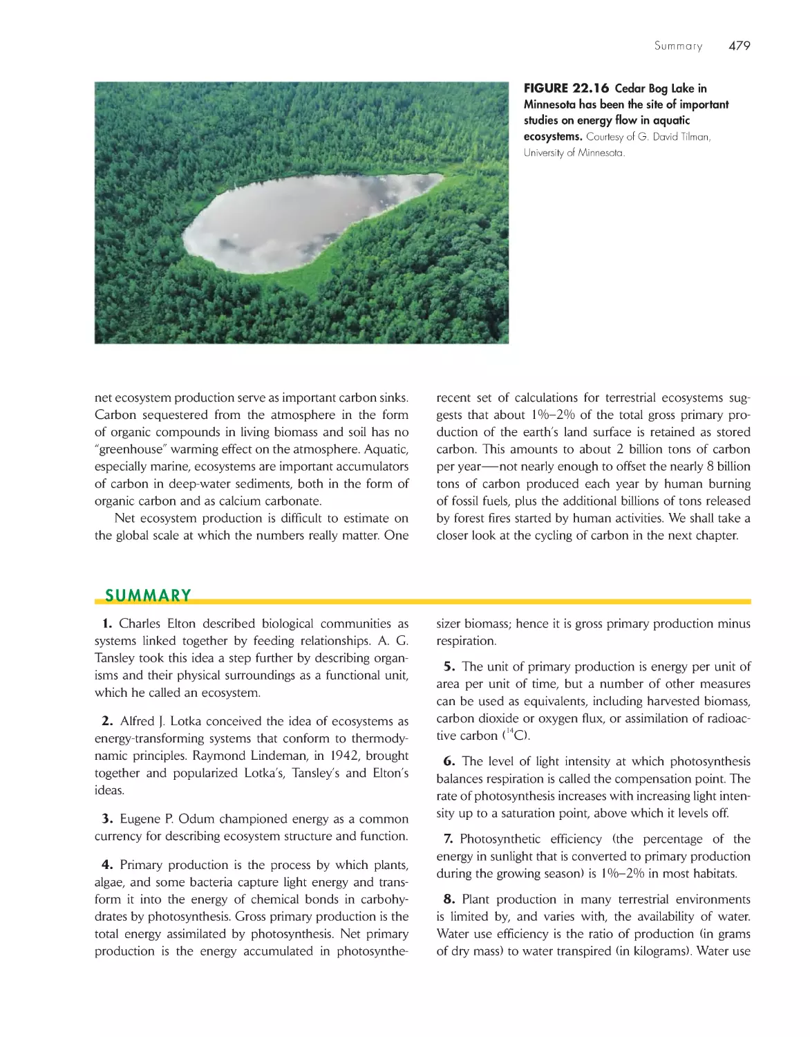
Ecosystem energetics summarizes the movement of
energy 478
ChApter 23 pathways of elements in
ecosystems
482
Energy transformations and element cycling are
intimately linked 483
Ecosystems can be modeled as a series of linked
compartments
484
Water provides a physical model of element cycling in
ecosystems
486
The carbon cycle is closely tied to the flux of energy
through the biosphere
487
Nitrogen assumes many oxidation states in its cycling
through ecosystems
493
GLobAL ChANGe
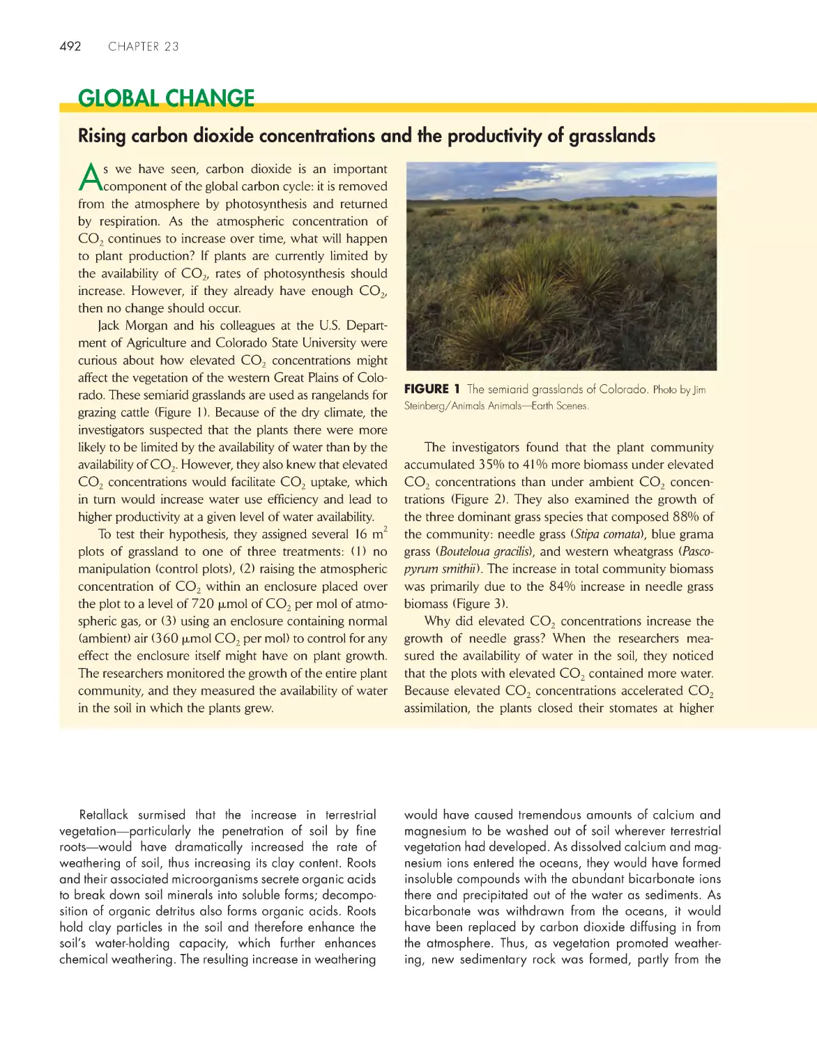
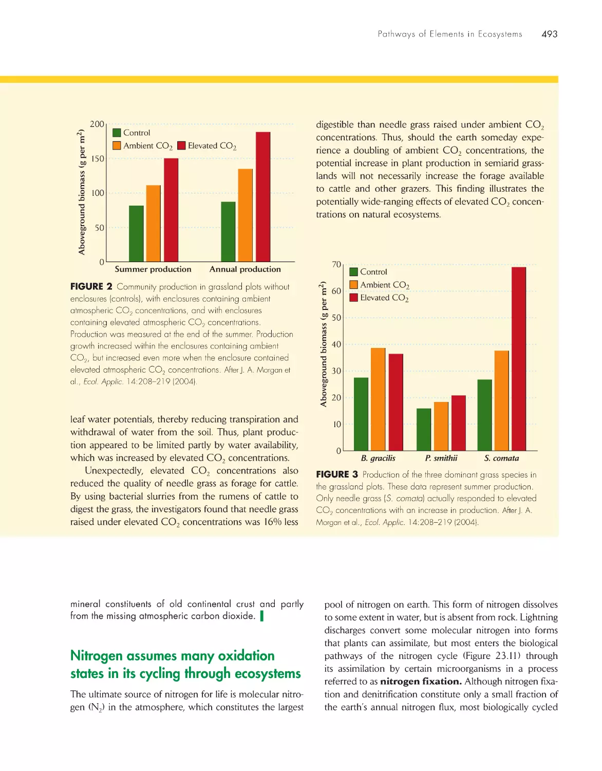
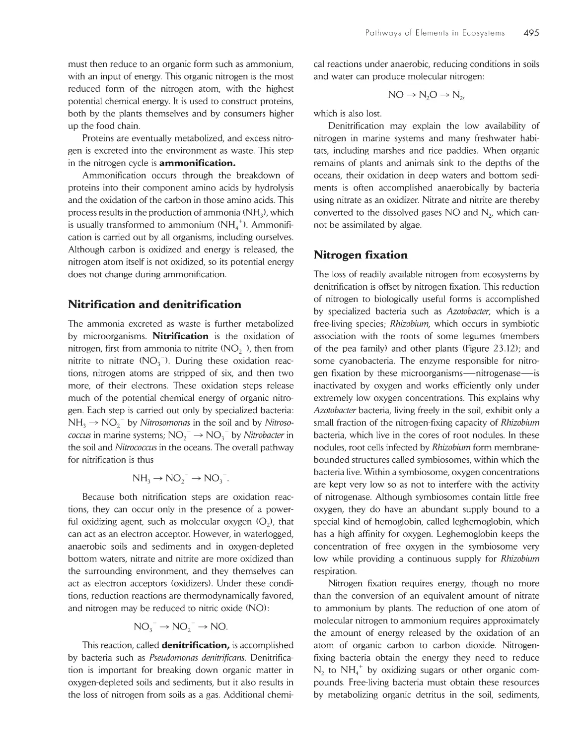
Rising carbon dioxide concentrations and the productivity of
grasslands 492
xii
contents
eCoLoGists iN the FieLD
What caused the rapid decline in atmospheric carbon dioxide
during the Devonian? 491
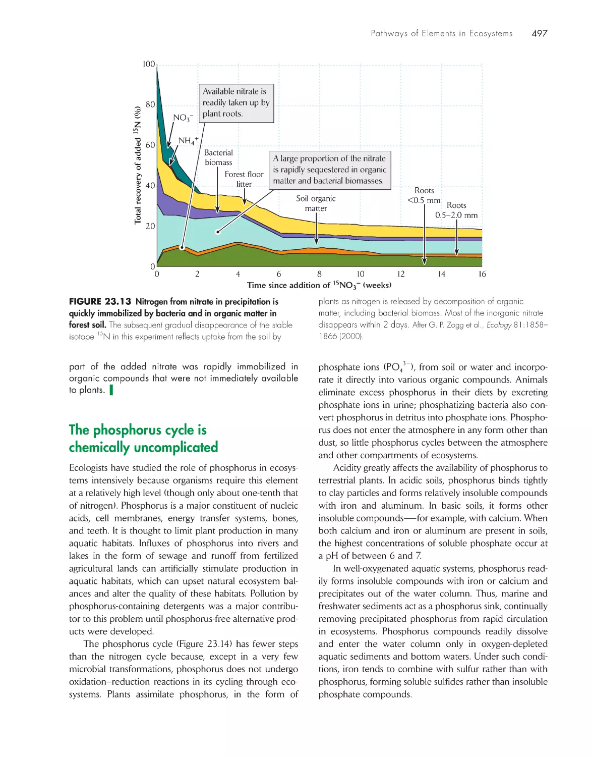
The fate of soil nitrate in a temperate forest
496
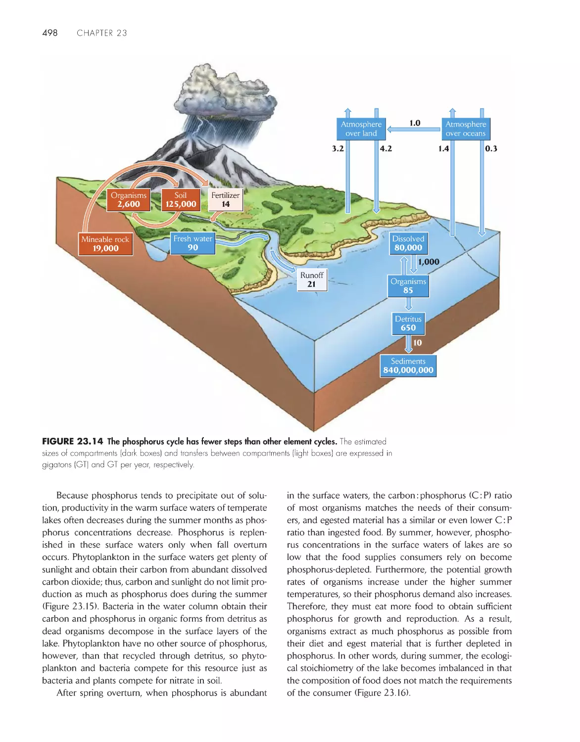
The phosphorus cycle is chemically uncomplicated 497
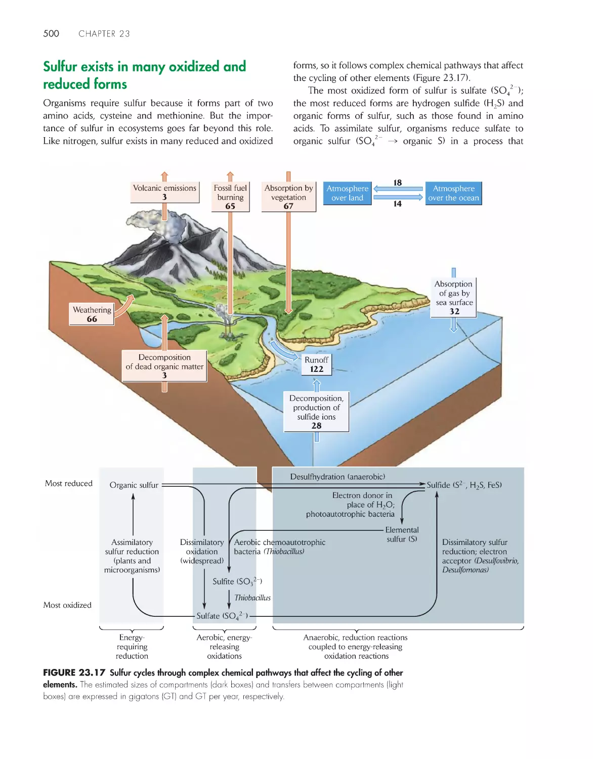
Sulfur exists in many oxidized and reduced forms
500
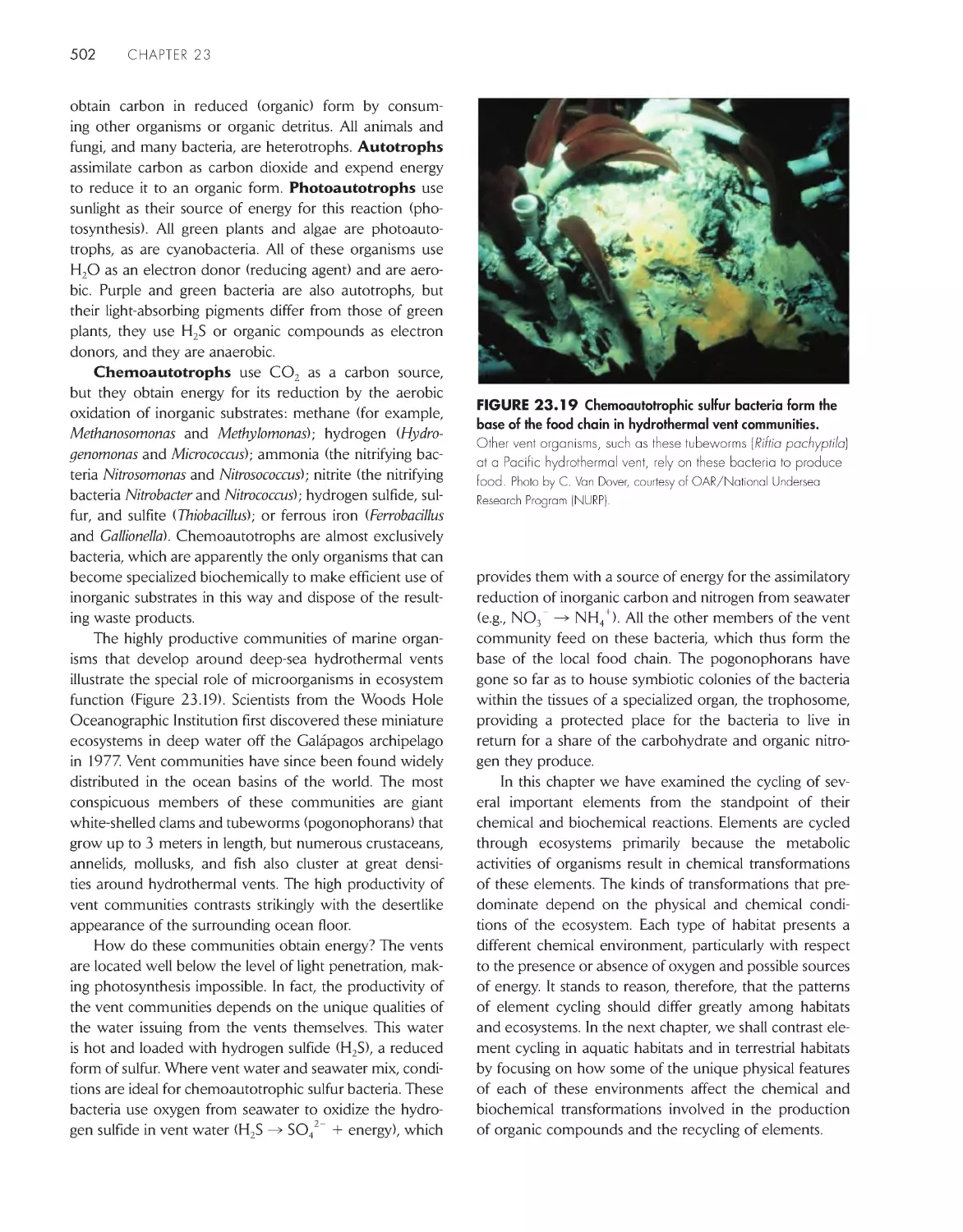
Microorganisms assume diverse roles in element
cycles 501
ChApter 24 Nutrient regeneration in terrestrial
and Aquatic ecosystems
505
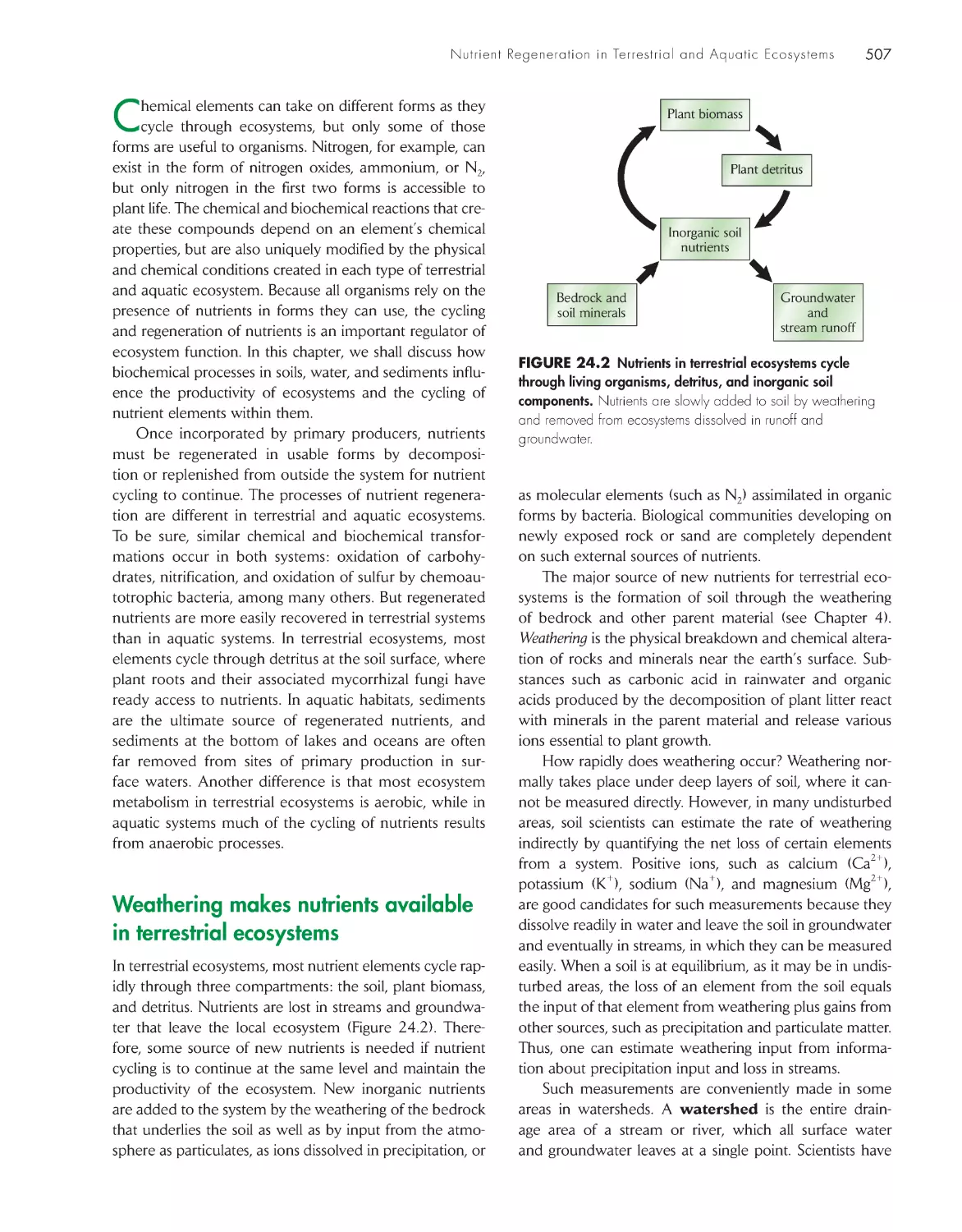
Weathering makes nutrients available in terrestrial
ecosystems
507
Nutrient regeneration in terrestrial ecosystems occurs in
the soil 508
Mycorrhizal associations of fungi and plant roots
promote nutrient uptake 509
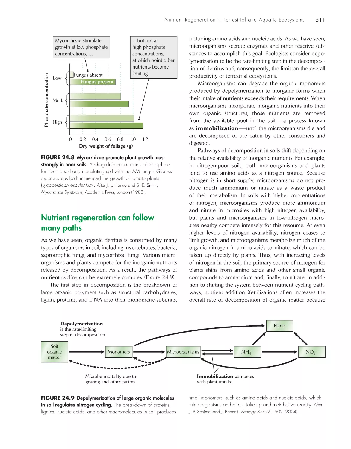
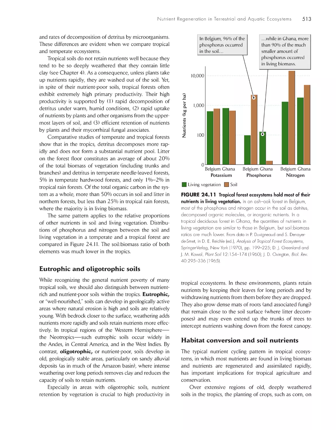
Nutrient regeneration can follow many paths 511
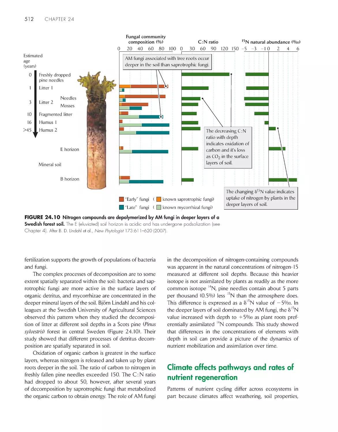
Climate affects pathways and rates of nutrient
regeneration
512
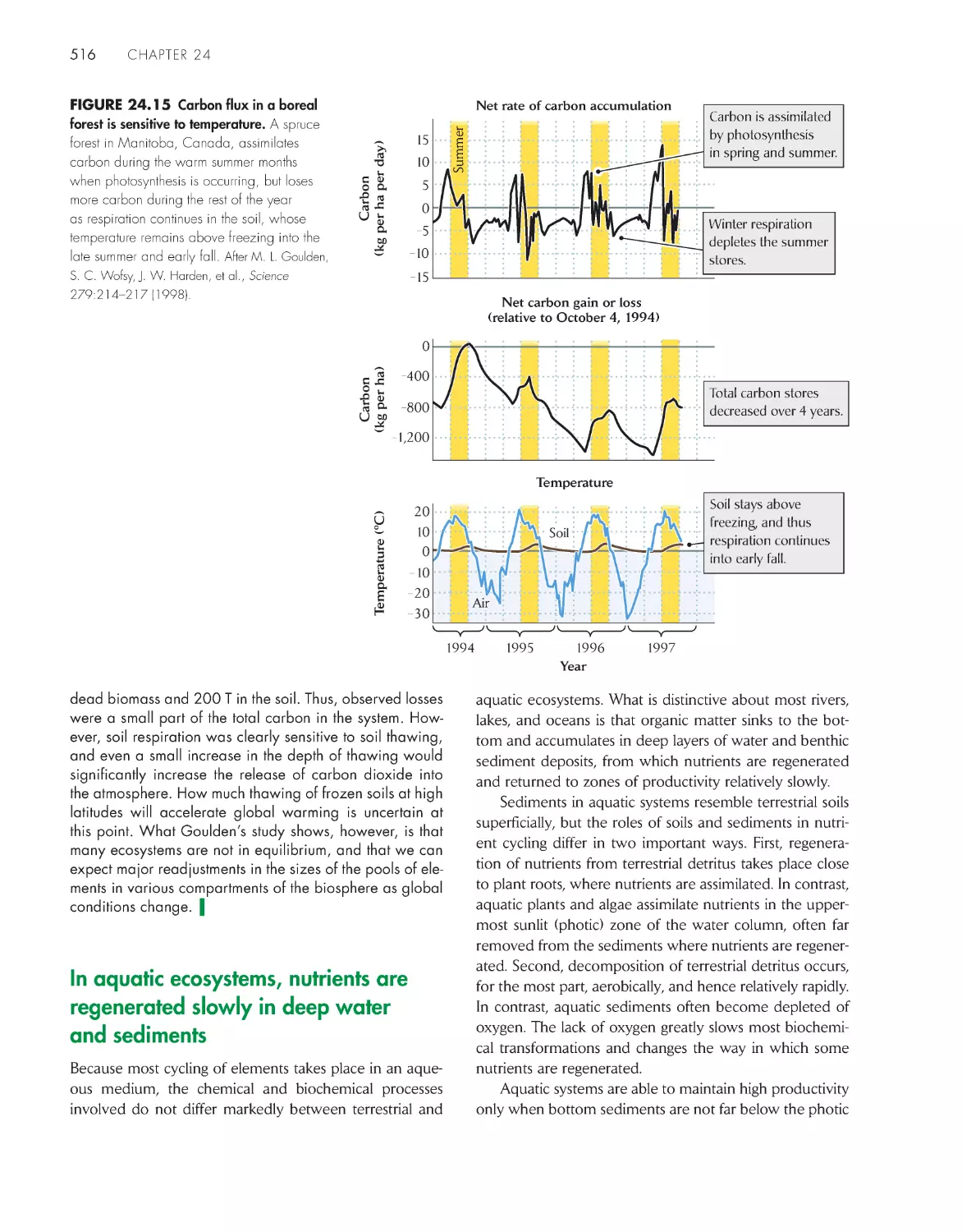
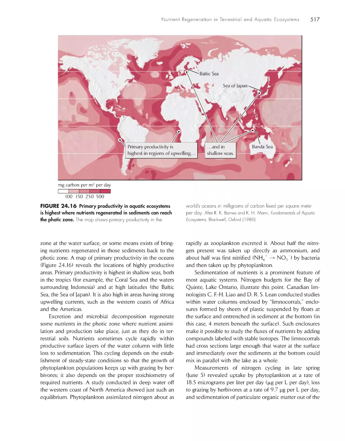
In aquatic ecosystems, nutrients are regenerated slowly
in deep water and sediments
516
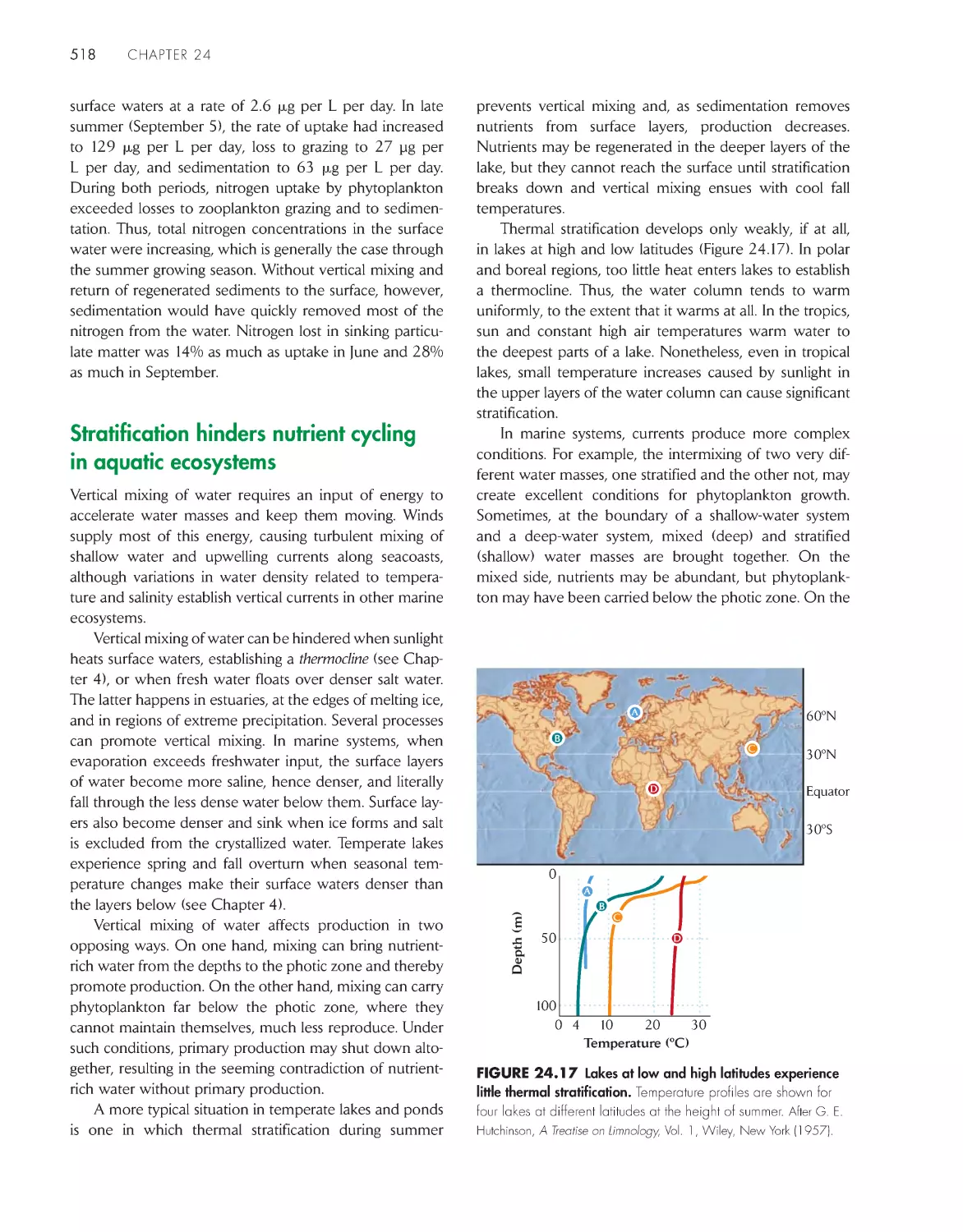
Stratification hinders nutrient cycling in aquatic
ecosystems
518
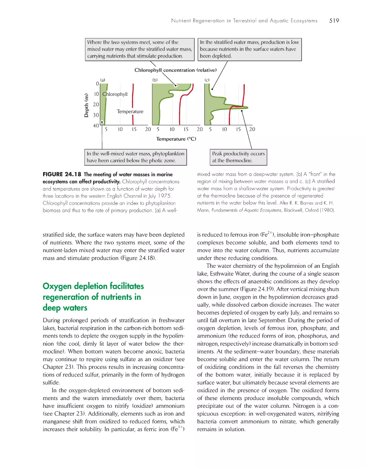
Oxygen depletion facilitates regeneration of nutrients in
deep waters
519
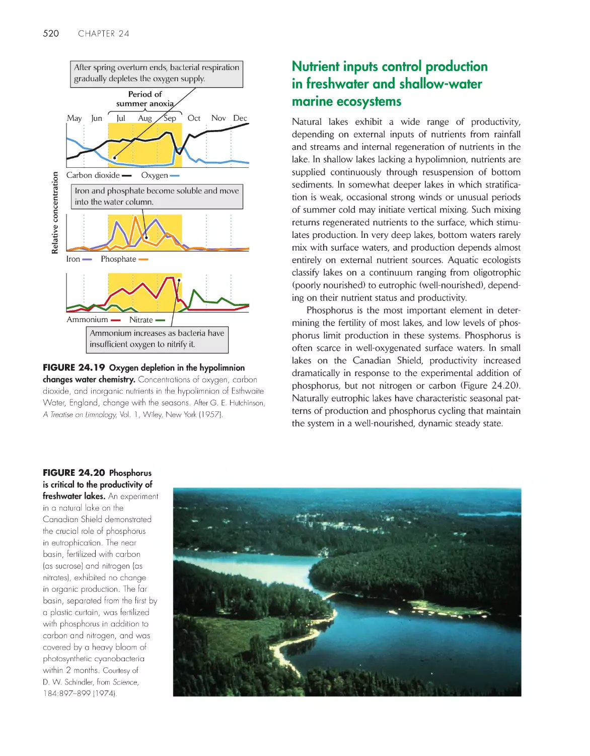
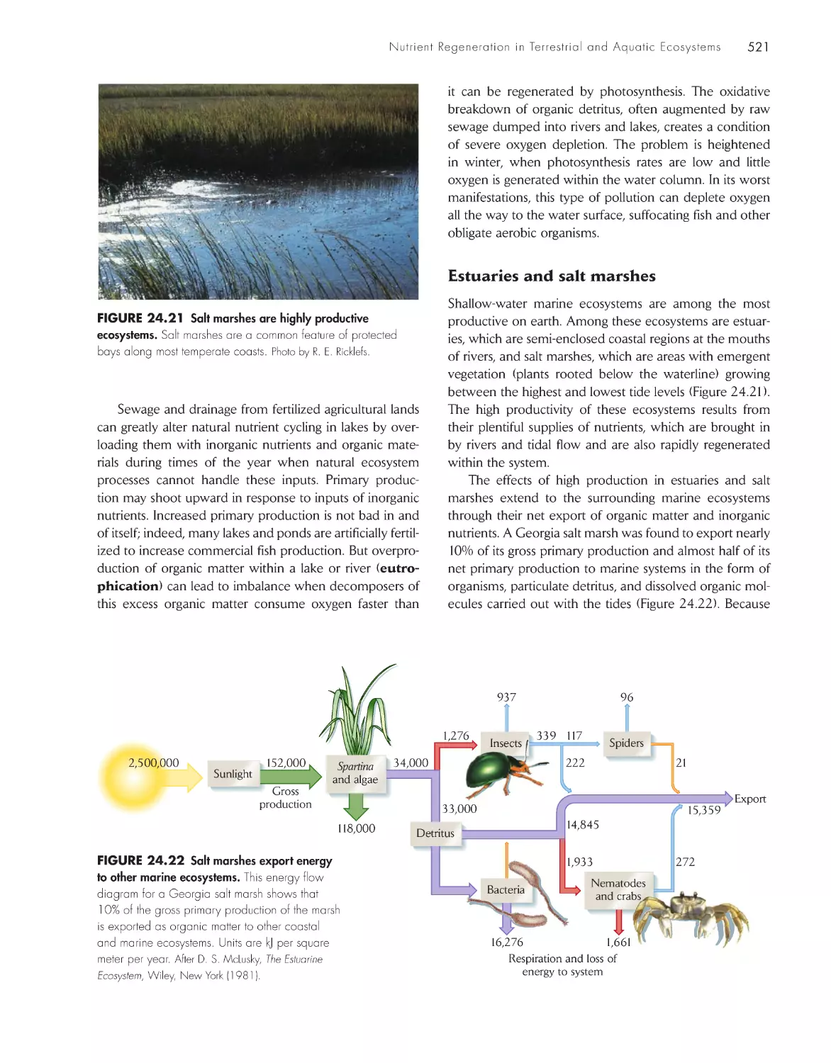
Nutrient inputs control production in freshwater and
shallow-water marine ecosystems
520
Nutrients limit production in the oceans
523
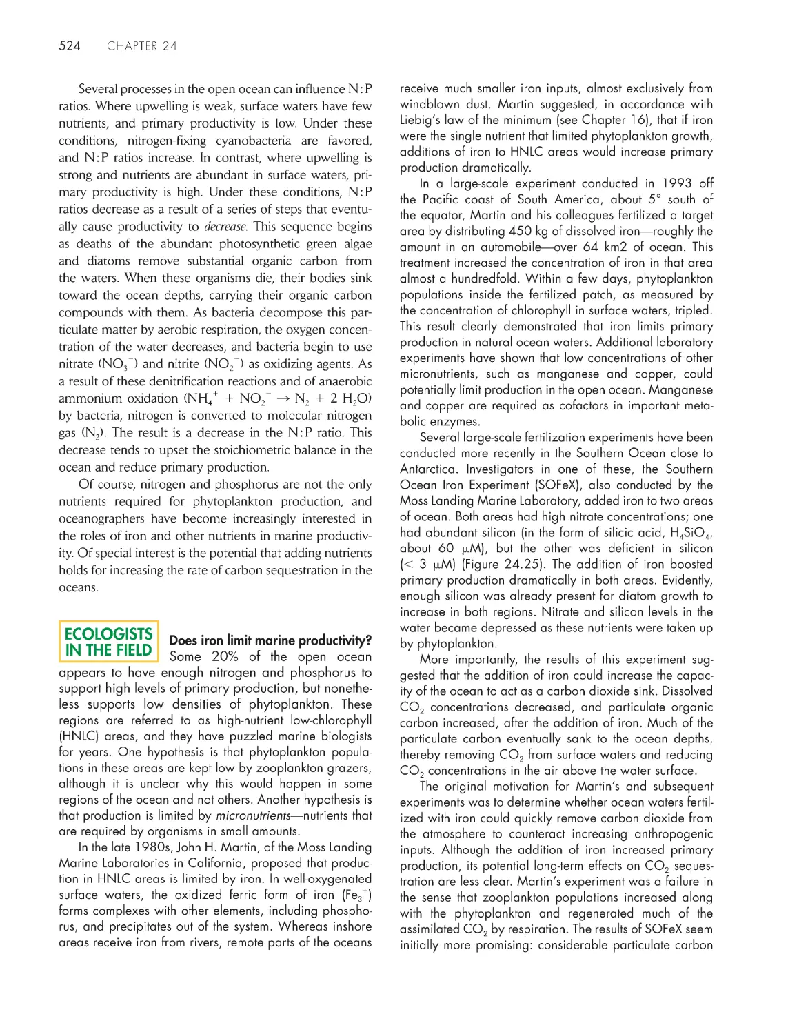
eCoLoGists iN the FieLD
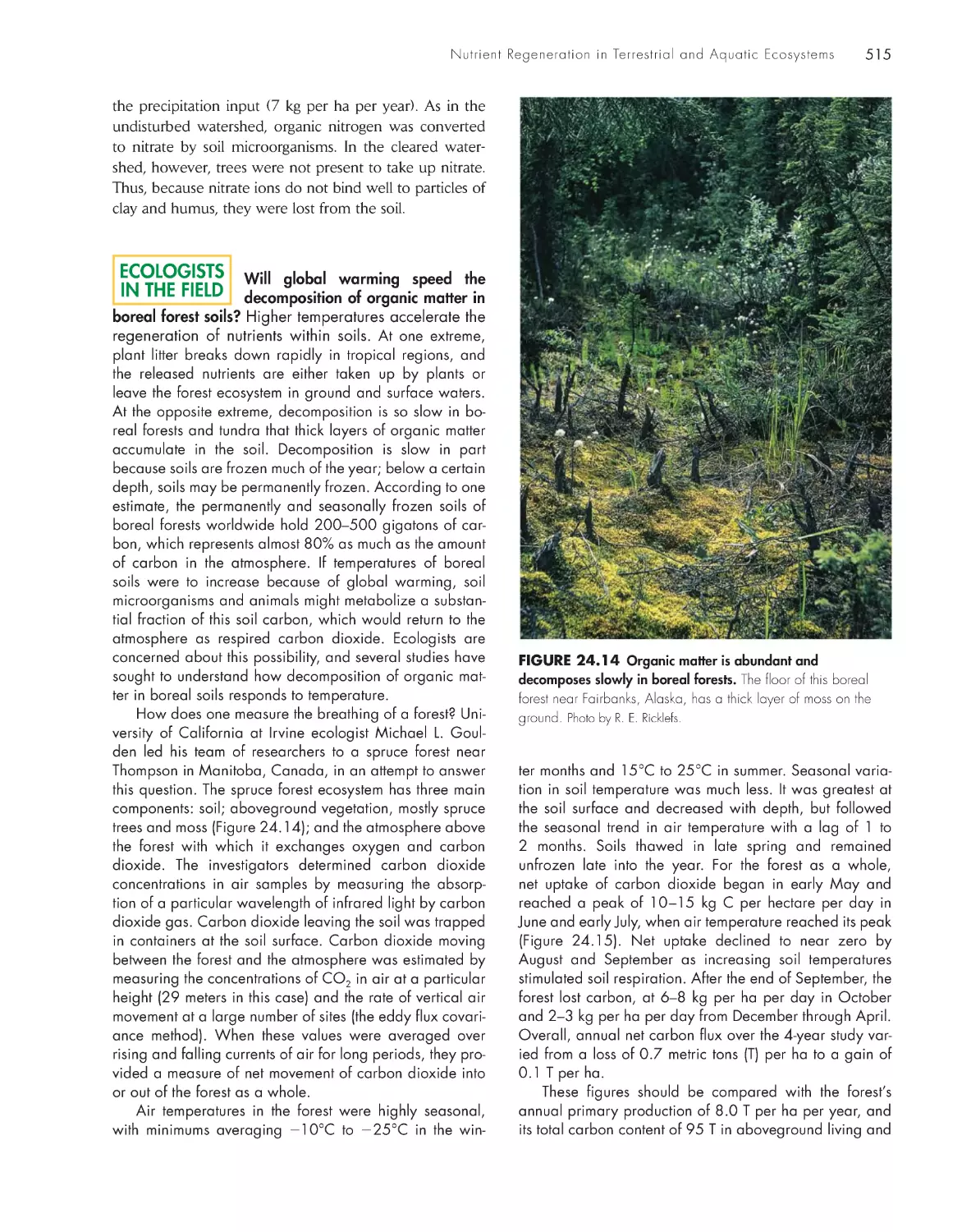
Will global warming speed the decomposition of organic
matter in boreal forest soils? 515
Does iron limit marine productivity? 524
pArt Vii eCoLoGiCAL AppLiCAtioNs
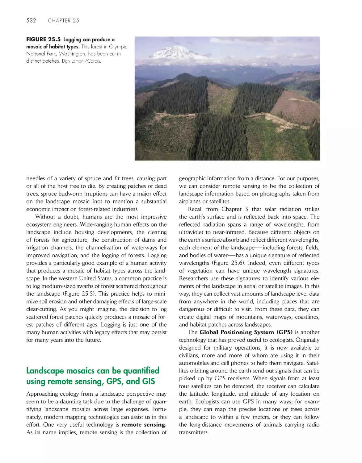
ChApter 25 Landscape ecology 528
Landscape mosaics reflect both natural and human
influences
530
Landscape mosaics can be
quantified using remote sensing,
GPS, and GIS 532
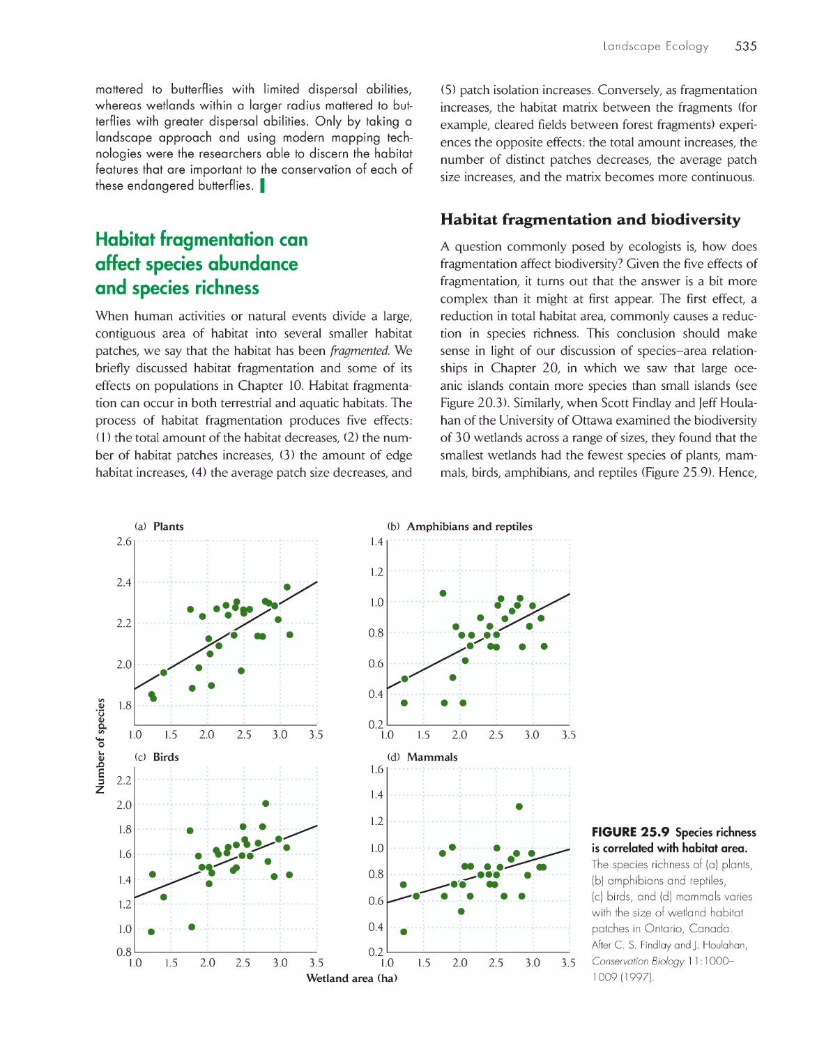
Habitat fragmentation can affect
species abundance and species
richness
535
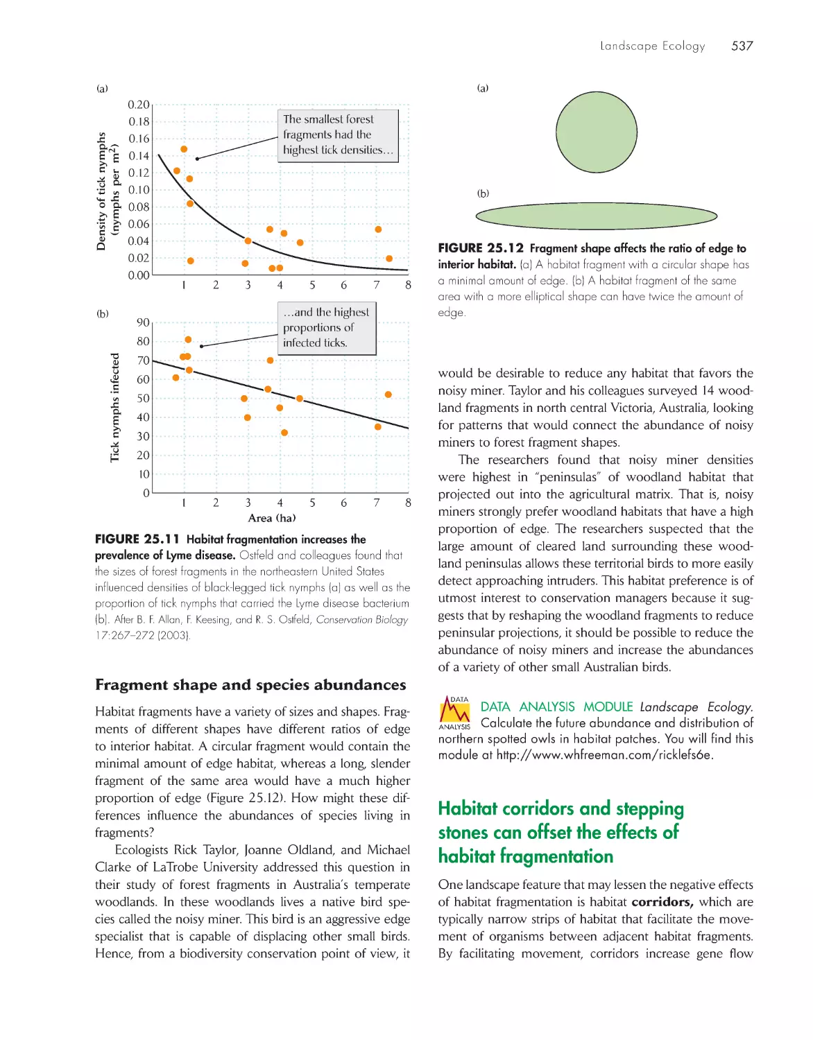
Habitat corridors and stepping
stones can offset the effects of
habitat fragmentation
537
Landscape ecology explicitly considers the quality of the
matrix between habitat fragments
538
Different species perceive the landscape at different
scales 540
Organisms depend on different landscape scales
for different activities and at different life history
stages 542
eCoLoGists iN the FieLD
Quantifying the habitat preferences of butterflies in
Switzerland 533
ChApter 26 biodiversity, extinction, and
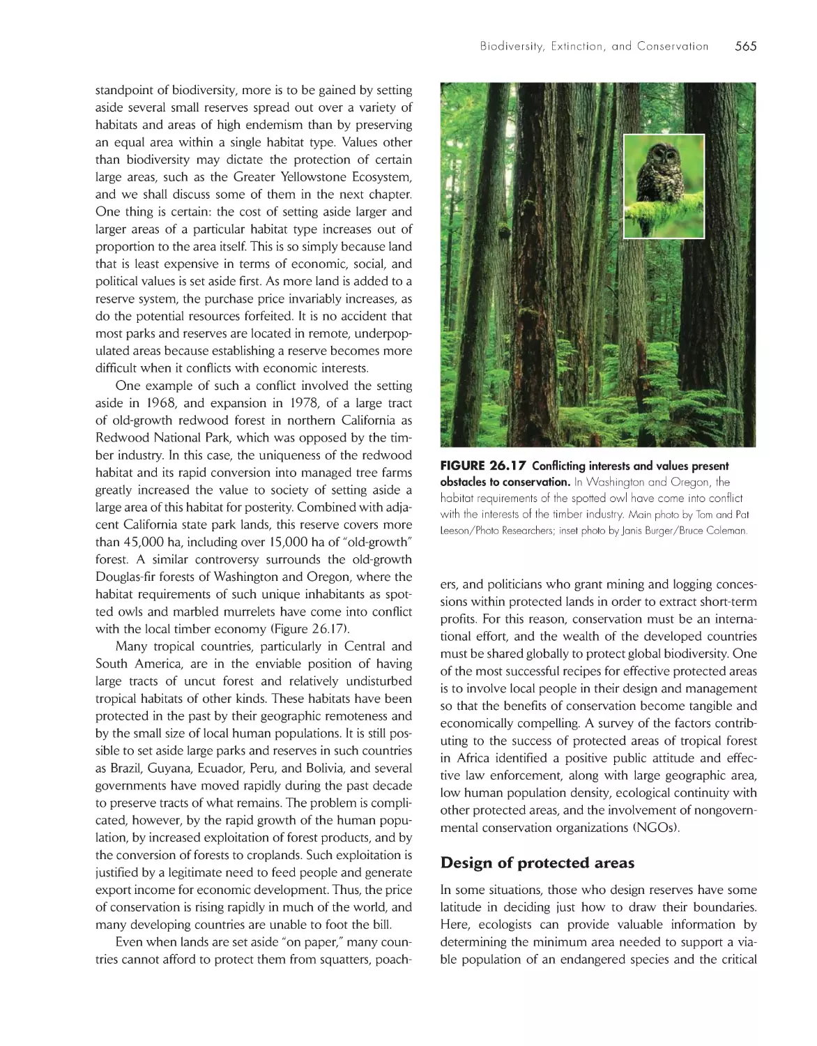
Conser vation
545
Biological diversity has many components
547
The value of biodiversity arises from social, economic,
and ecological considerations
549
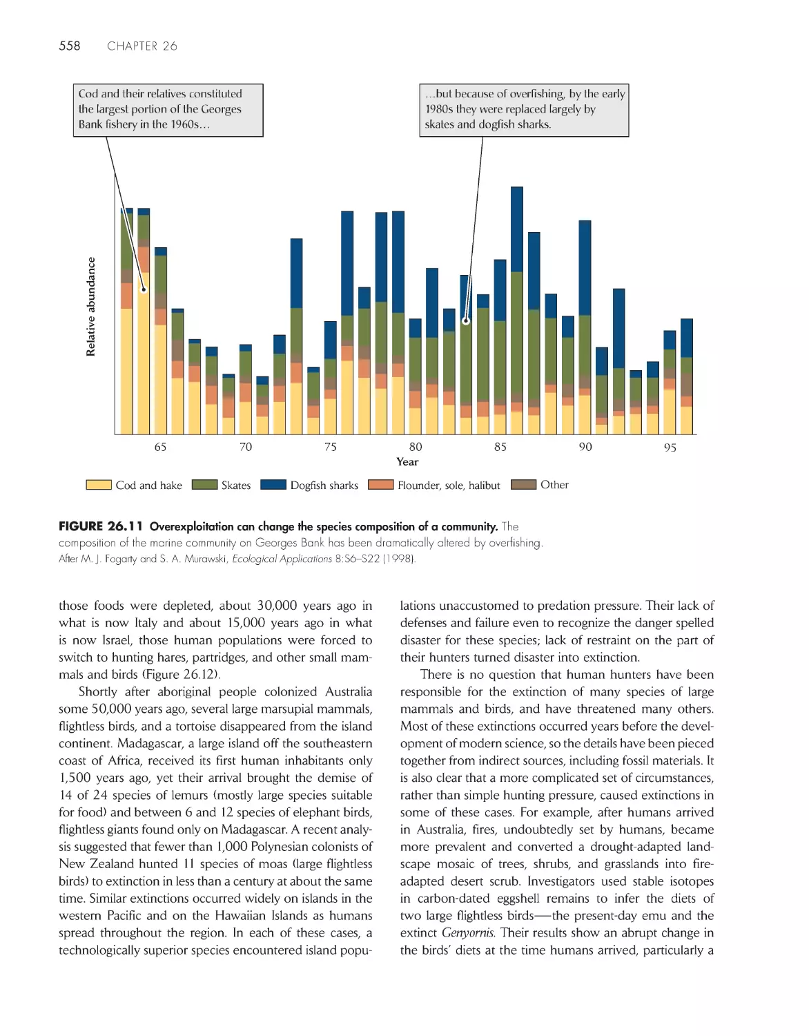
Extinction is natural but its present rate is not
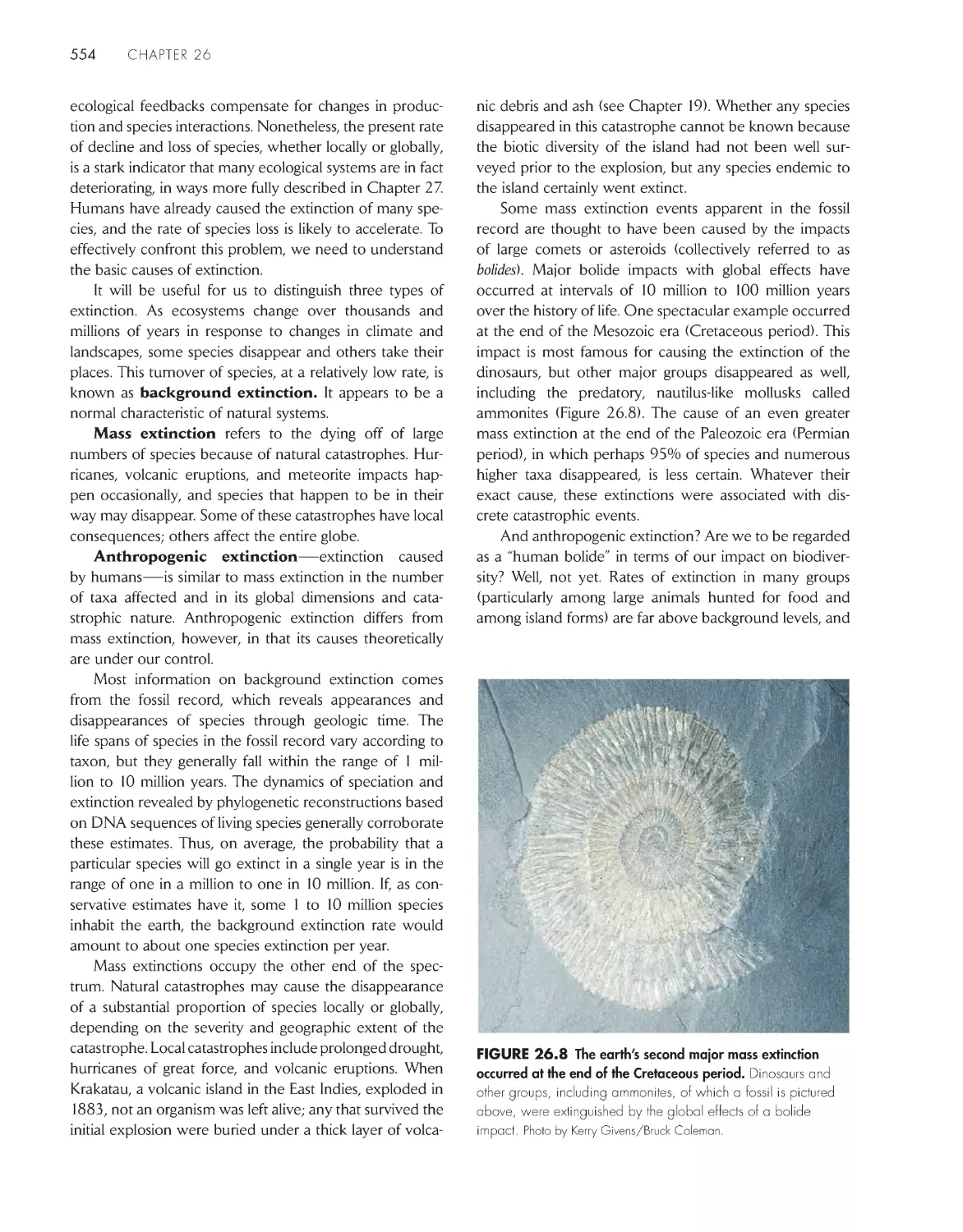
553
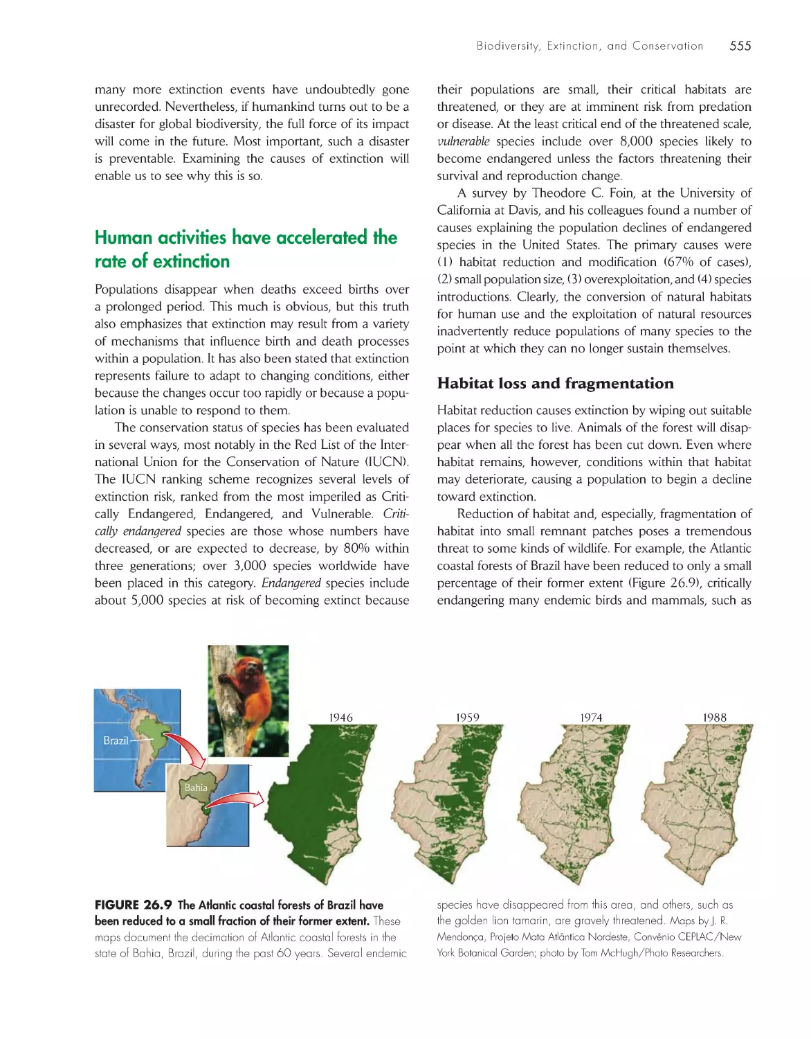
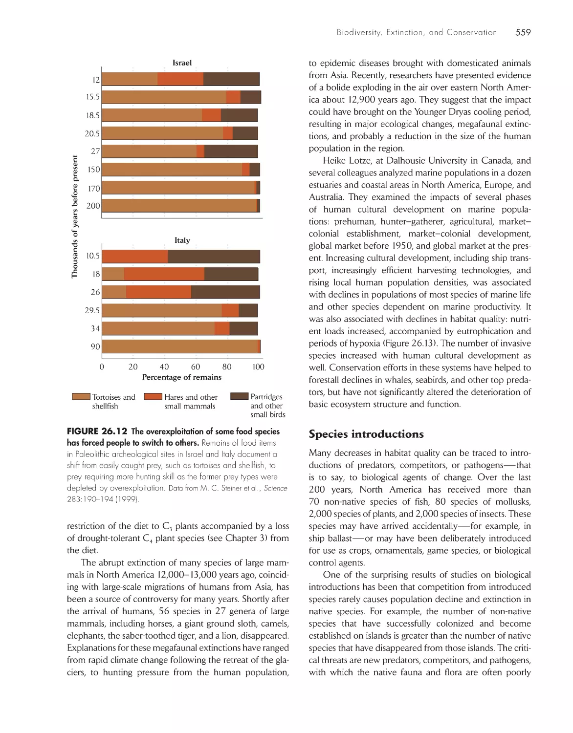
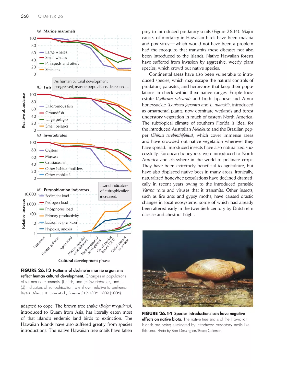
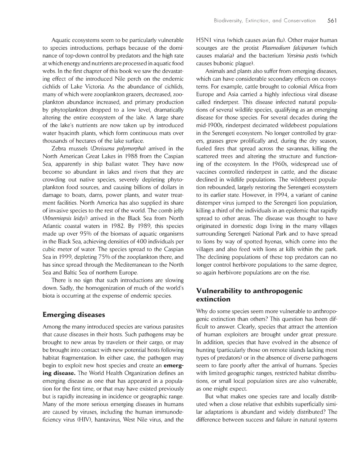
Human activities have accelerated the rate of
extinction
555
Reserve designs for individual species must guarantee a
self-sustaining population
562
Some critically endangered species have been rescued
from the brink of extinction
566
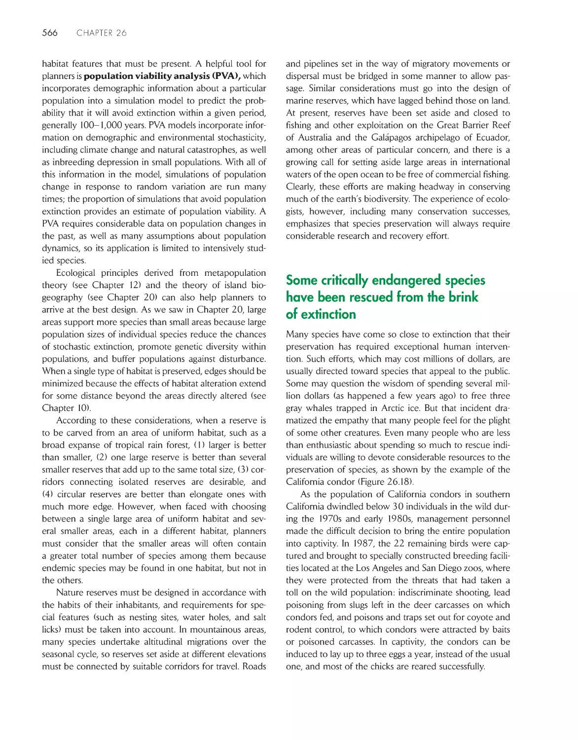
eCoLoGists iN the FieLD
Identifying biodiversity hotspots for conservation
548
ChApter 27 economic Development and Global
ecology 570
Ecological processes hold the key to environmental
policy 572
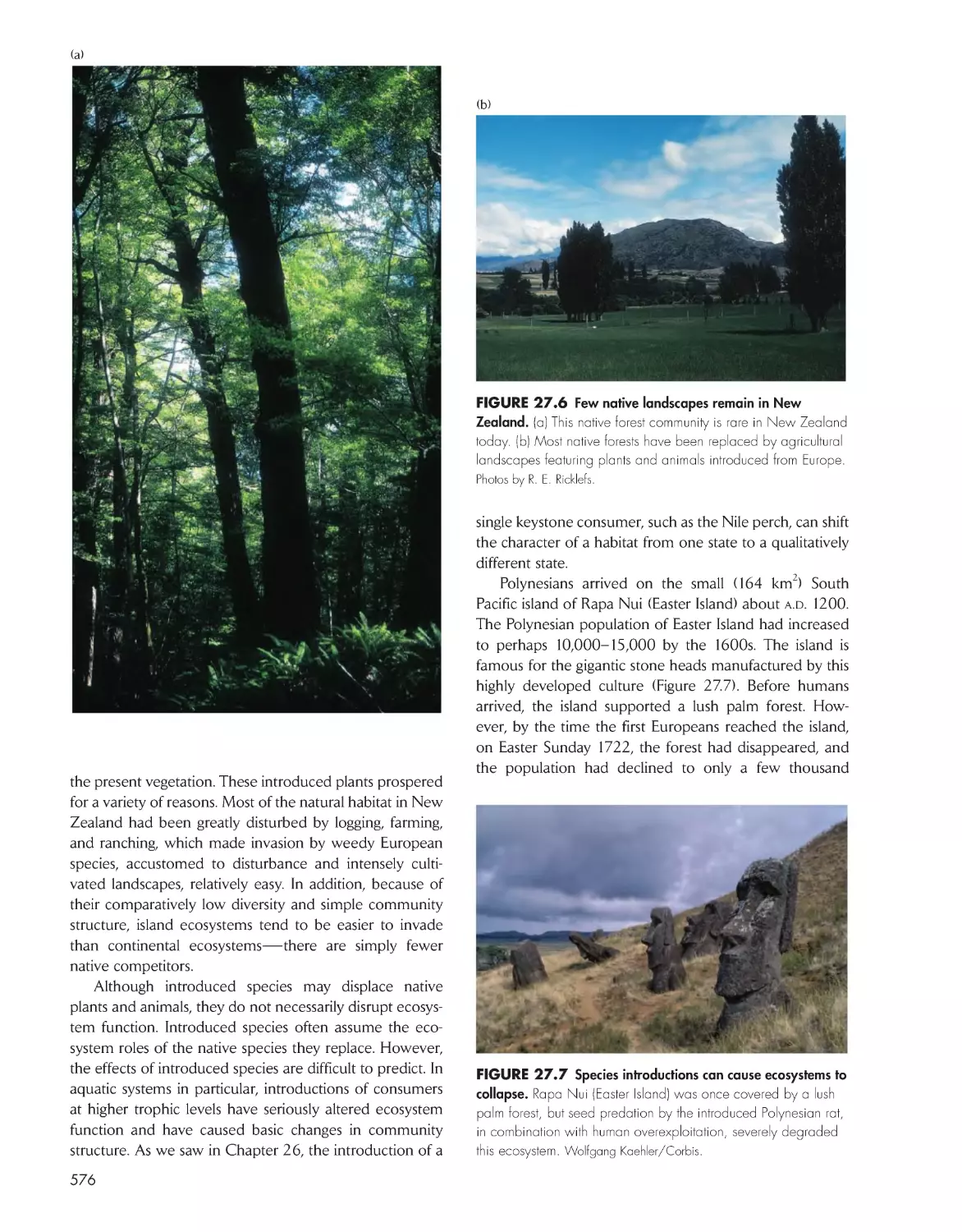
Human activities threaten local ecological
processes
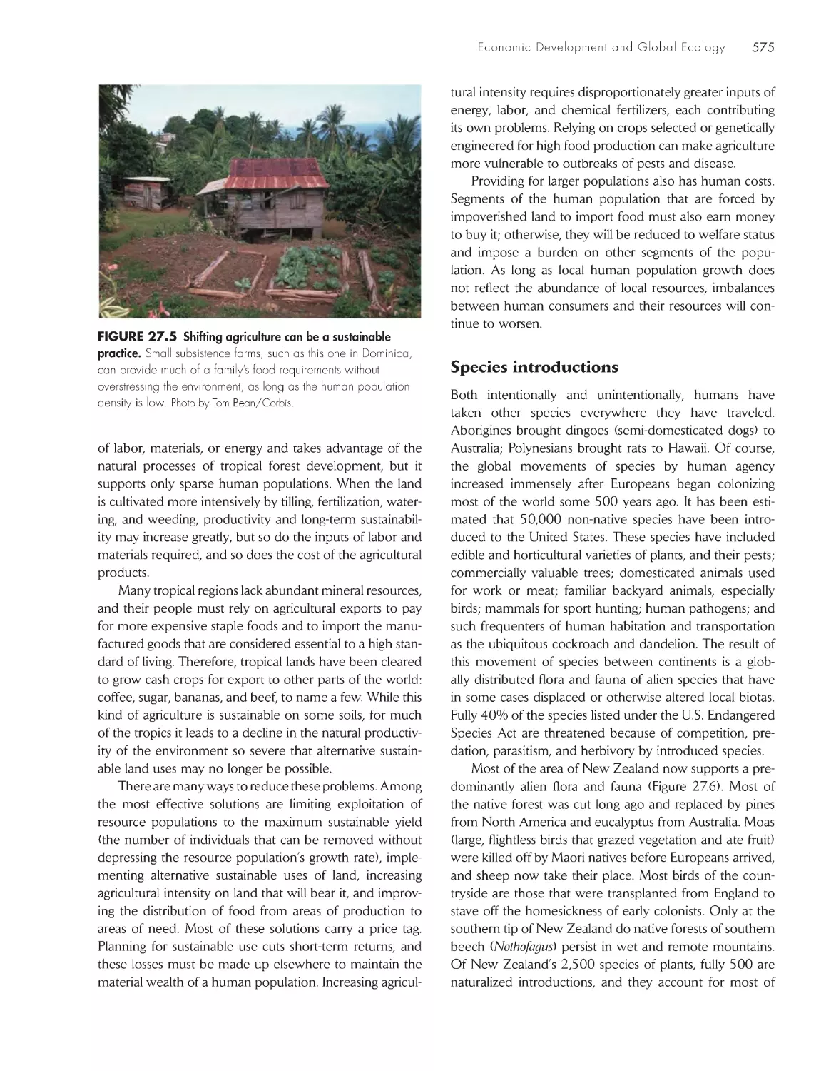
573
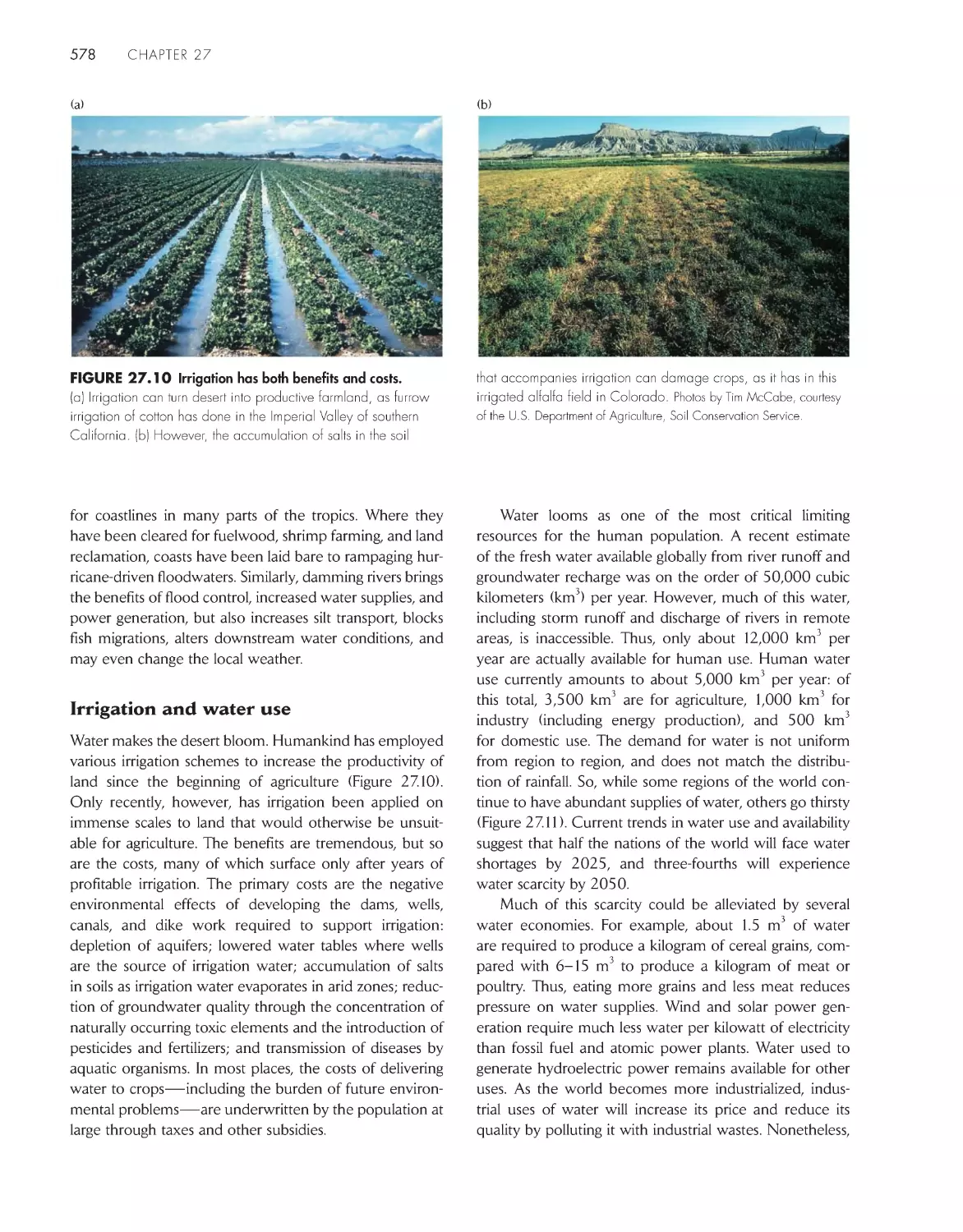
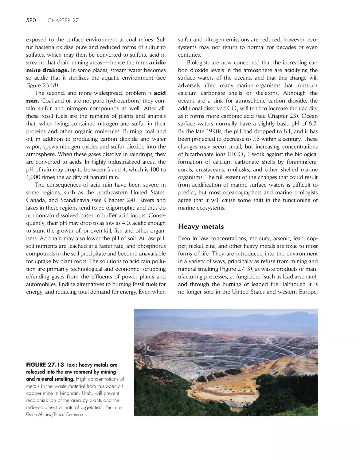
Toxins impose local and global environmental
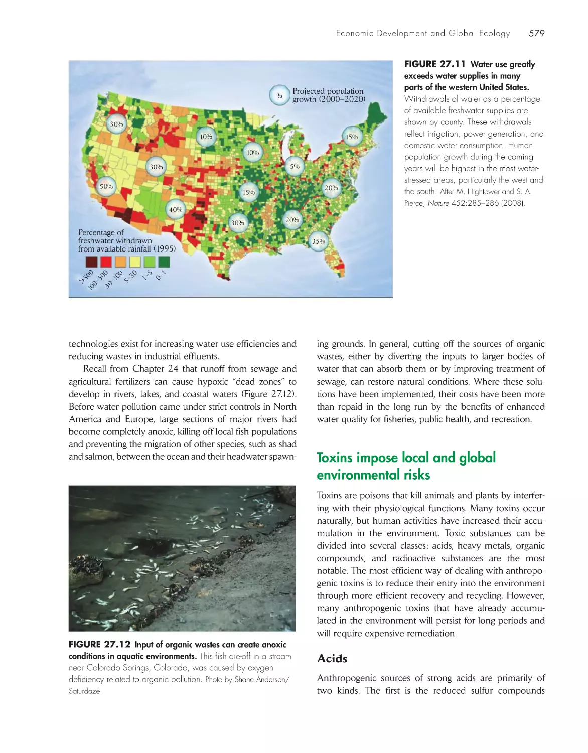
risks 579
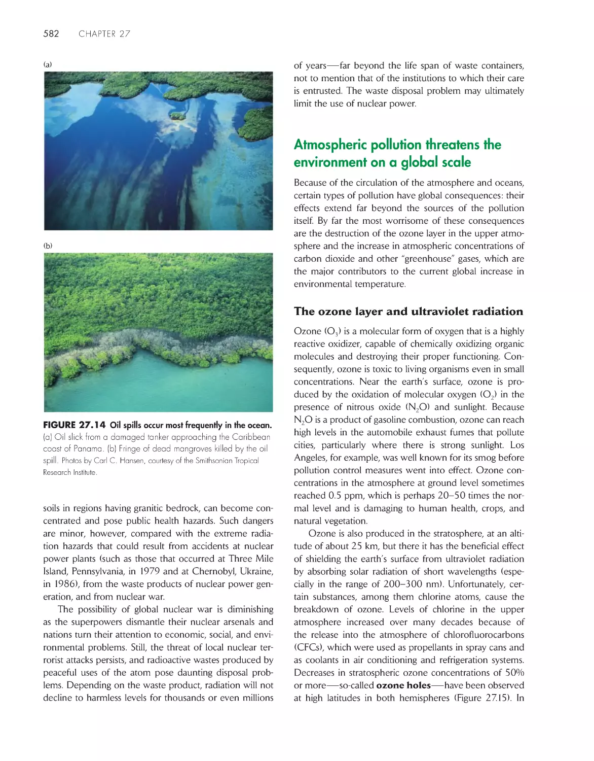
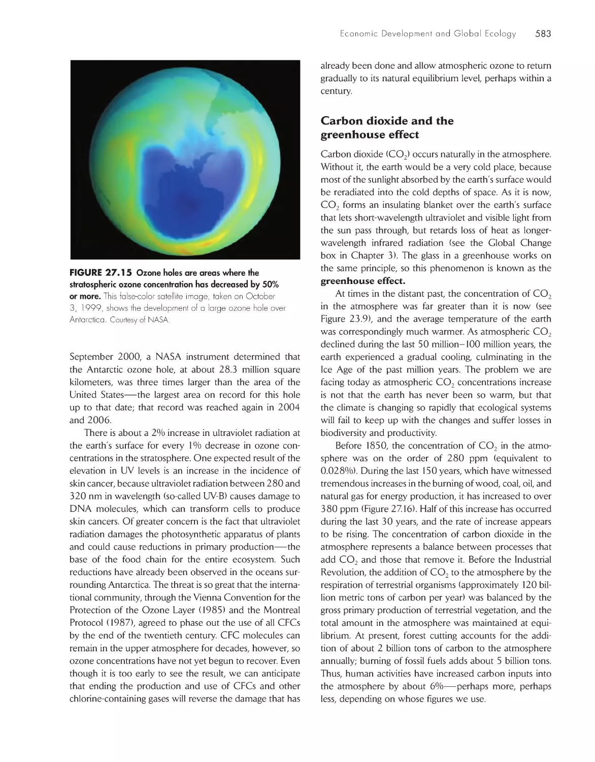
Atmospheric pollution threatens the environment on a
global scale 582
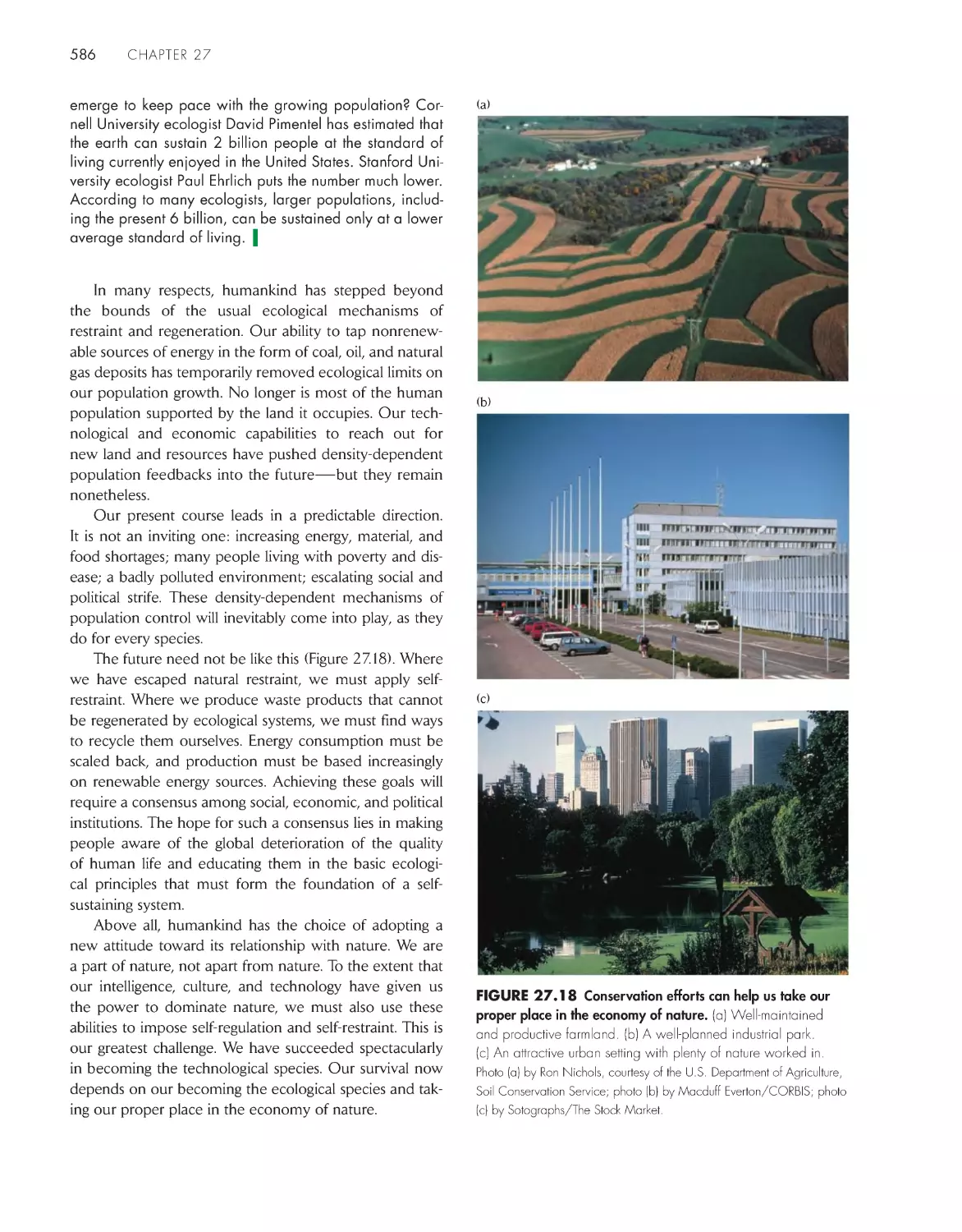
Human ecology is the ultimate challenge 585
eCoLoGists iN the FieLD
Assessing the earth’s carr ying capacity for
humankind 585
Glossary 589
Index
605
xiii
Enduring Vision
Since the first edition of The Economy of Nature appeared in 1976, it has maintained a
consistent vision of the teaching of ecology based on three fundamental tenets:
• First, a solid grounding in natural history. The more we know about habitats
and their resident organisms, the better we can understand how ecological and evolu-
tionary processes have shaped the natural world.
• Second, an appreciation of the organism as the fundamental unit of ecol-
ogy. The structures and dynamics of populations, communities, and ecosystems express
the activities of, and interactions among, the organisms they comprise.
• Third, the central position of evolutionary thinking in the
study of ecology. The qualities of all ecological systems express the
evolutionary adaptations of their component species.
Readers familiar with the fifth edition of this book will find the same
emphasis on field ecology in this edition. Most chapters contain one or
more Ecologists in the Field essays highlighting the research of ecolo-
gists working in a variety of systems and on a variety of problems through
field observation, experimentation, and laboratory research. These essays
emphasize to students the importance of ecology as a living science.
Students will also have the opportunity to analyze datasets them-
selves in the Data Analysis Modules provided at the ends of several
chapters and on the Companion Web Site at www.whfreeman.com/
ricklefs6e. These modules introduce students to the importance of data
analysis for interpreting patterns in the natural world as well as results
of experimental manipulations, while providing some grounding in basic
statistical procedures.
New to This Edition
The revision of this textbook has been guided by three overarching
goals:
• To apply the insights of ecology to understanding the impact
of human activities on the environment. As we continue to alter
our surroundings, our effects on populations and ecosystems will depend on the par-
ticular responses of individual plants, animals, and microorganisms to changes in their
environment.
• To further emphasize the principles of evolution as a foundation of ecol-
ogy, with repercussions that extend even to managing global change. For
example, the rate of speciation influences large-scale patterns of species richness over
the surface of the earth, and understanding the dynamics of this process provides guide-
lines for preserving biodiversity.
• To show how modern approaches to studying ecology are illuminating
ecological structures and functions. For example, the increasing availability of a
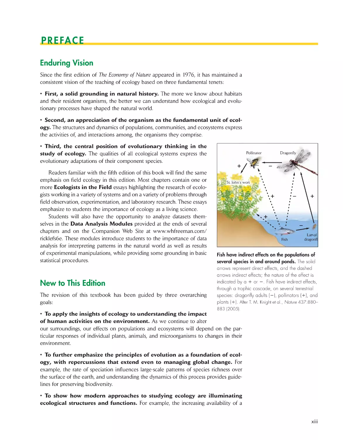
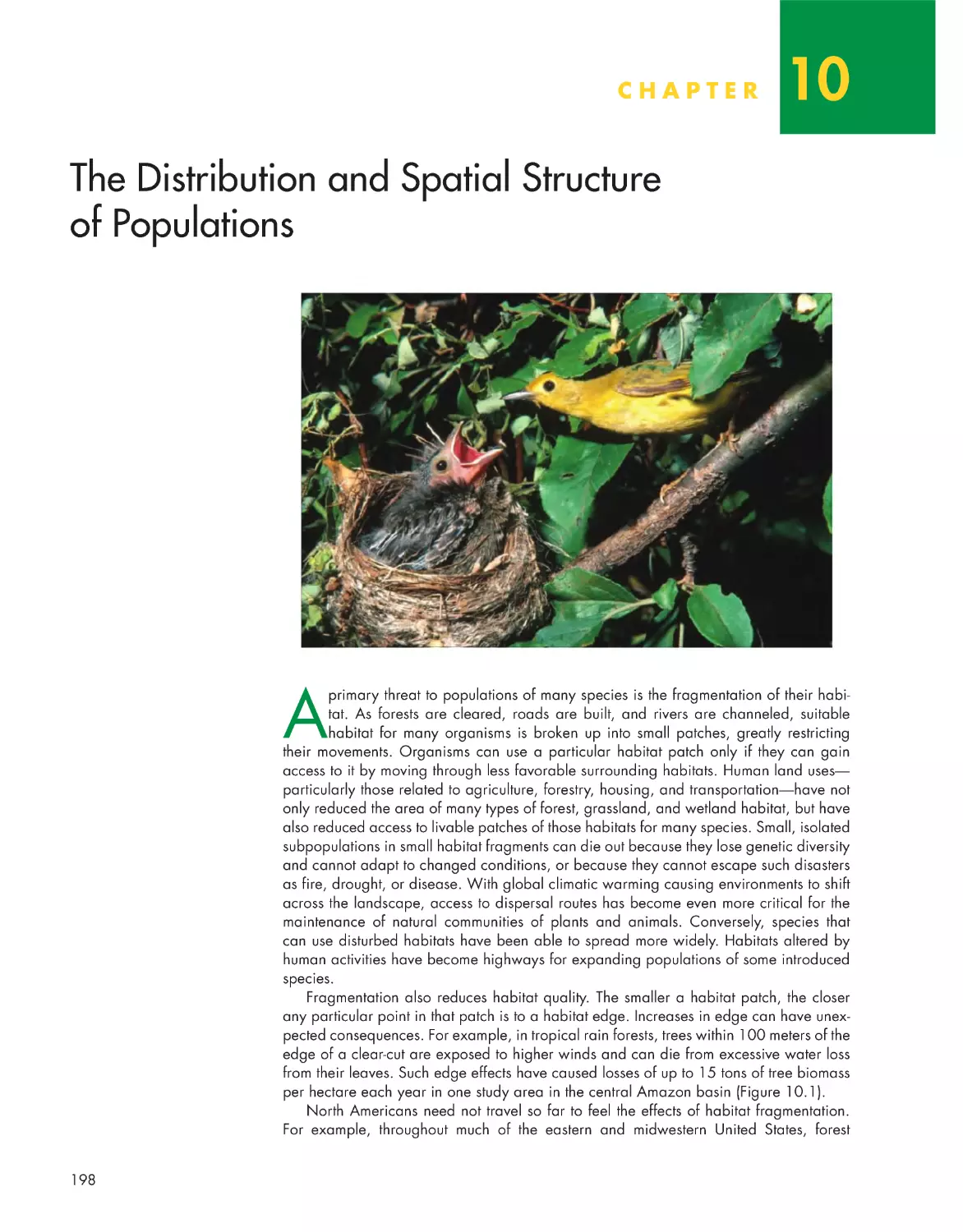
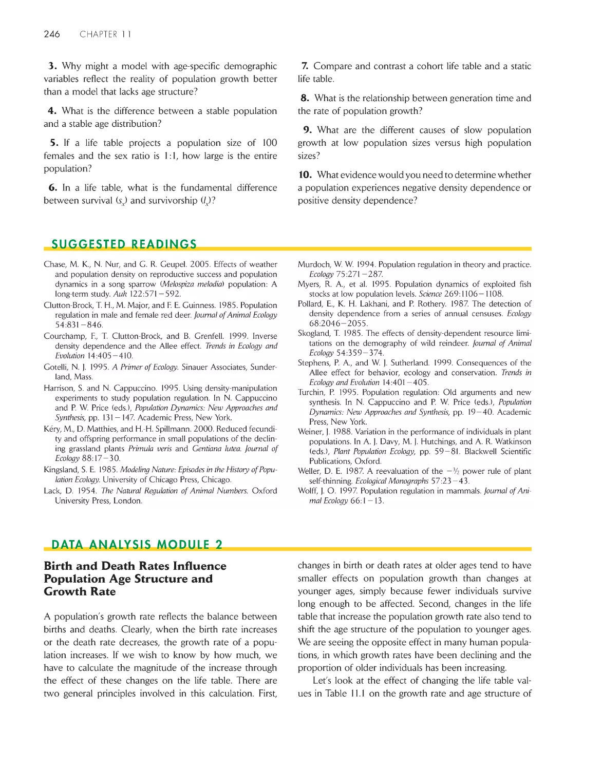
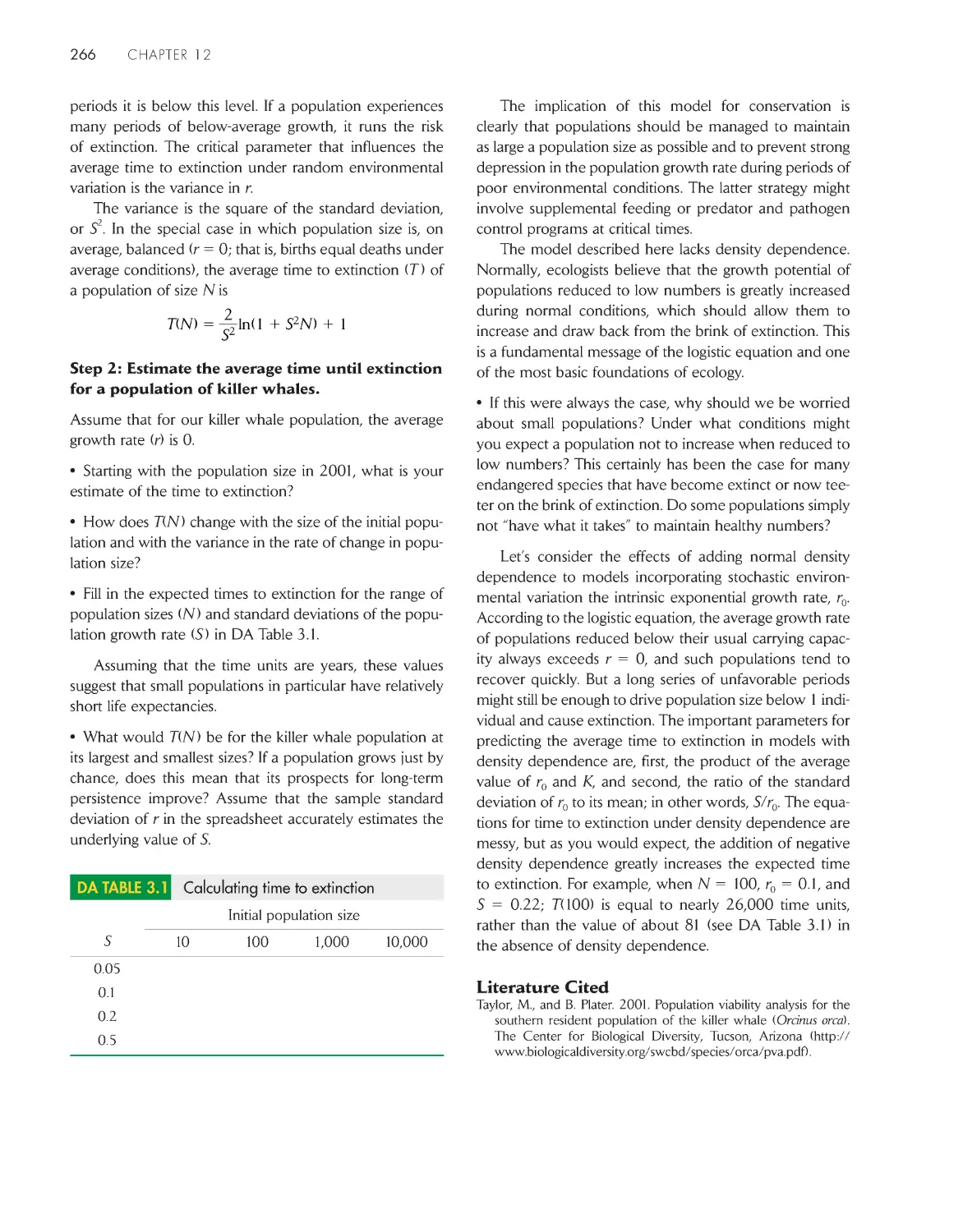
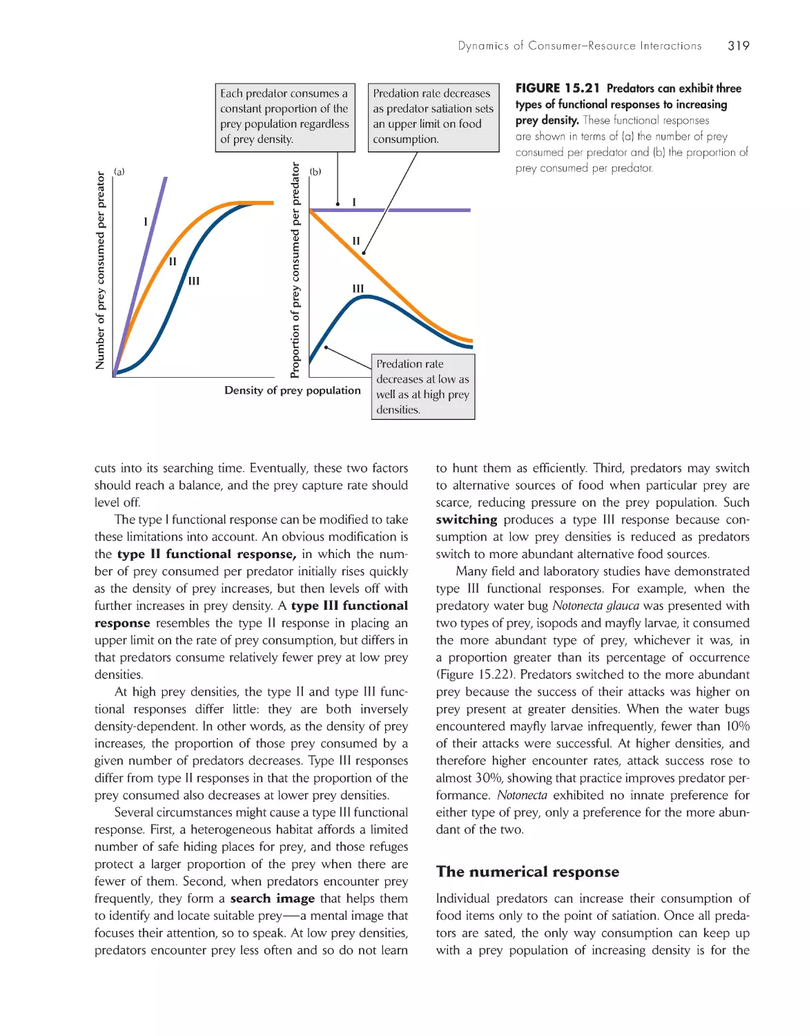
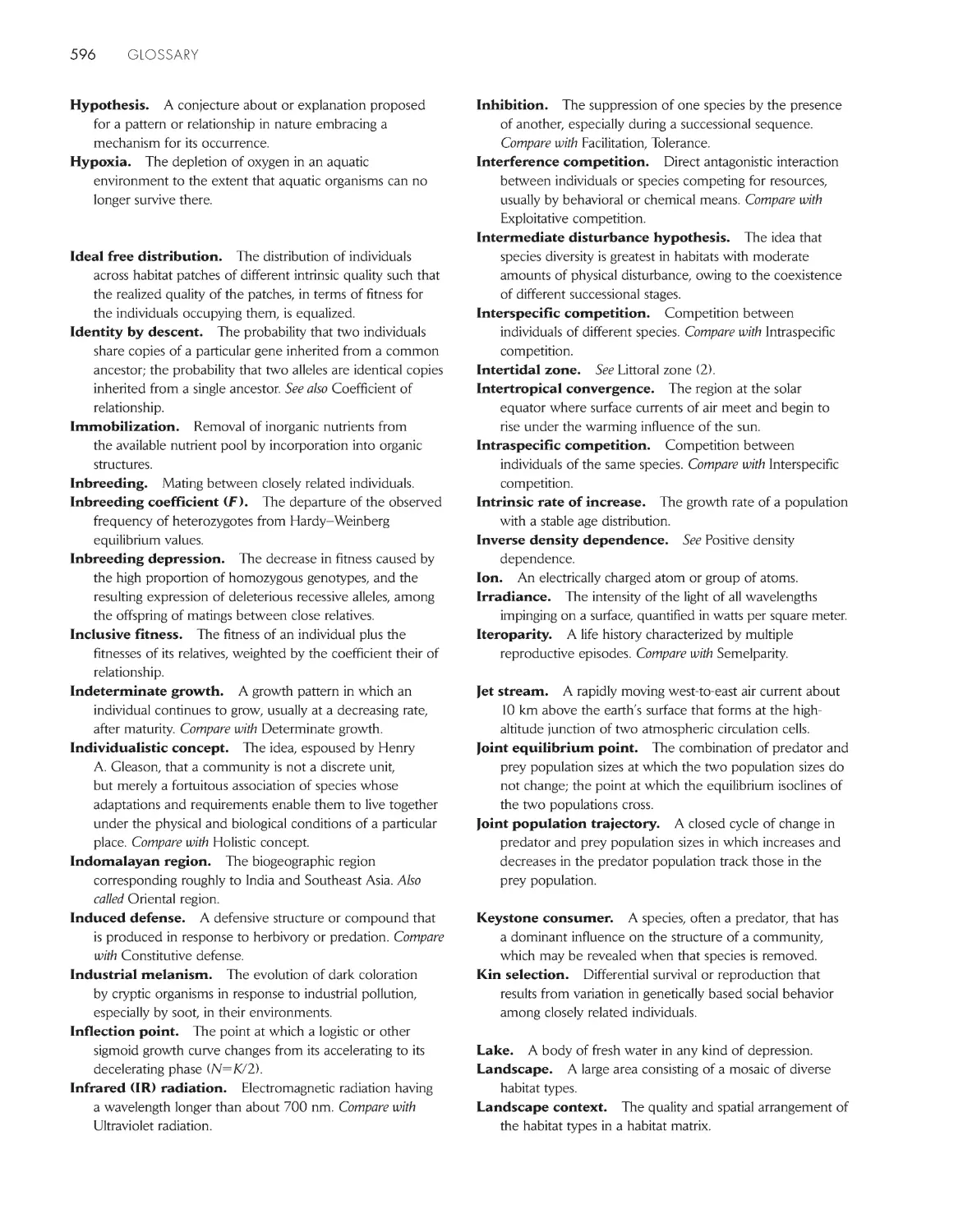
Fish
Larval
dragonfly
Dragonfly
Pollinator
St. John’s wort
St. John’s wort
+
+
+
–
–
–
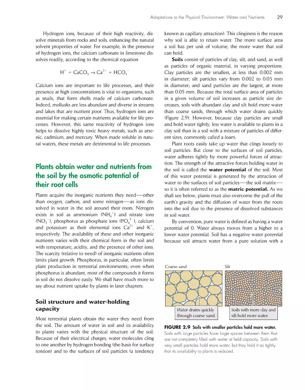
+
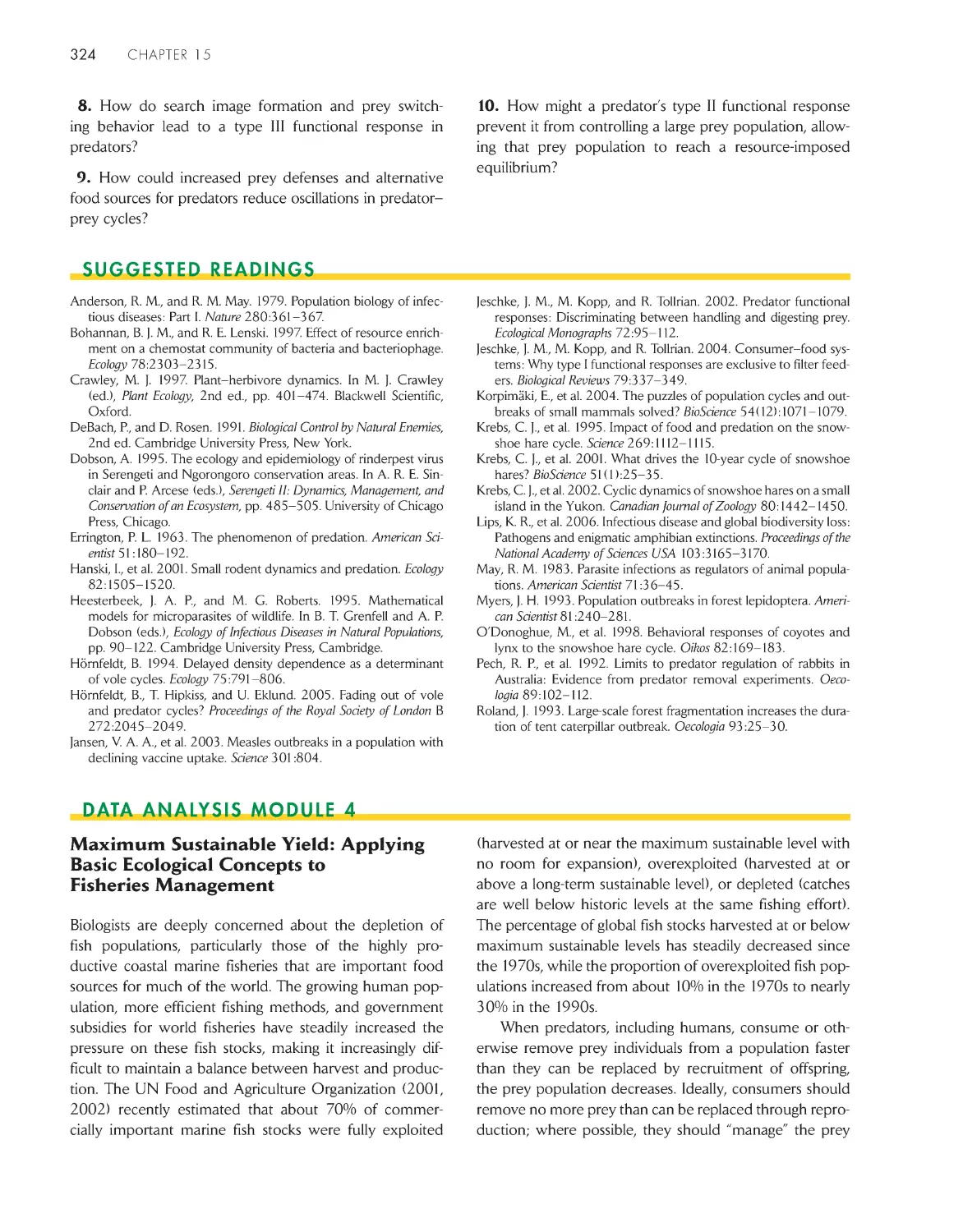
Fish have indirect effects on the populations of
several species in and around ponds. The solid
arrows represent direct effects, and the dashed
arrows indirect effects; the nature of the effect is
indicated by a or . Fish have indirect effects,
through a trophic cascade, on several terrestrial
species: dragonfly adults (), pollinators (), and
plants (). After T. M . Knight et al., Nature 437:880–
883 (2005).
prEFacE
xiv
preFAce
wide variety of markers of genetic variation now allows ecologists
to take into account the history of movements of individuals and
changes in the size of populations over time in analyzing population
structure.
What’sNew...
Consolidated Coverage of Evolution. The newly reworked
Chapter 6 presents Darwinian evolutionary principles, including natu-
ral selection, adaptation as a process, and relevant topics from popu-
lation genetics. The chapter provides a more focused discussion of
evolution by bringing together topics previously covered separately
across several chapters. In a complementary way, at the end of the
section on populations, Chapter 13 summarizes recent advances in
the use of genetic markers to study population processes, including
the estimation of effective population size, fitness effects of inbreeding
in small populations, and historical changes in population size. These
genetic tools have made significant contributions to the conservation
and management of wild populations.
Increased Emphasis on Global Change. Five two-page spreads, all but the first
written by Rick Relyea of the University of Pittsburgh, explore “global change” as an
important ecological principle:
• Carbon Dioxide and Global Warming (Chapter 3, p. 52)
• Global Warming and Flowering Time (Chapter 7, p. 146)
• Changing Ocean Temperatures and Shifting Fish Distributions (Chapter 10, p. 206)
• Invasive Plant Species and the Role of Herbivores (Chapter 17, p. 364)
• Rising Carbon Dioxide Concentrations and the Productivity of Grasslands (Chapter
23, p. 492)
By considering the extent of human impacts on ecosystems in these spreads and else-
where in the chapters, students will gain an understanding of the relationship between
humans and their environment. In addition, they will learn about potential approaches
to preventing future ecological crises, such as climatic warming, decreased crop produc-
tion, emerging diseases, and species extinctions.
New Chapter on Landscape Ecology. To address an increasing interest in landscape
ecology, Chapter 25, written by Rick Relyea of the University of Pittsburgh, presents a
modern synthesis of large-scale ecology, including human influences on landscapes and
the ways in which landscape structure affects individuals, populations, and communities.
The chapter focuses on the way in which the scale of spatial heterogeneity in the envi-
ronment matches the scale of organismal behavior, including foraging activity and dis-
persal between suitable habitat patches, a key to understanding ecological complexity.
New Organization. Coverage of ecosystems ecology has been moved to follow the
material on community ecology, bringing the table of contents into closer alignment with
the order in which ecology is taught in most courses. Thus, The Economy of Nature now
follows a hierarchical organization scheme by sequentially addressing increasing levels of
ecological complexity from organisms to populations, communities, and ecosystems.
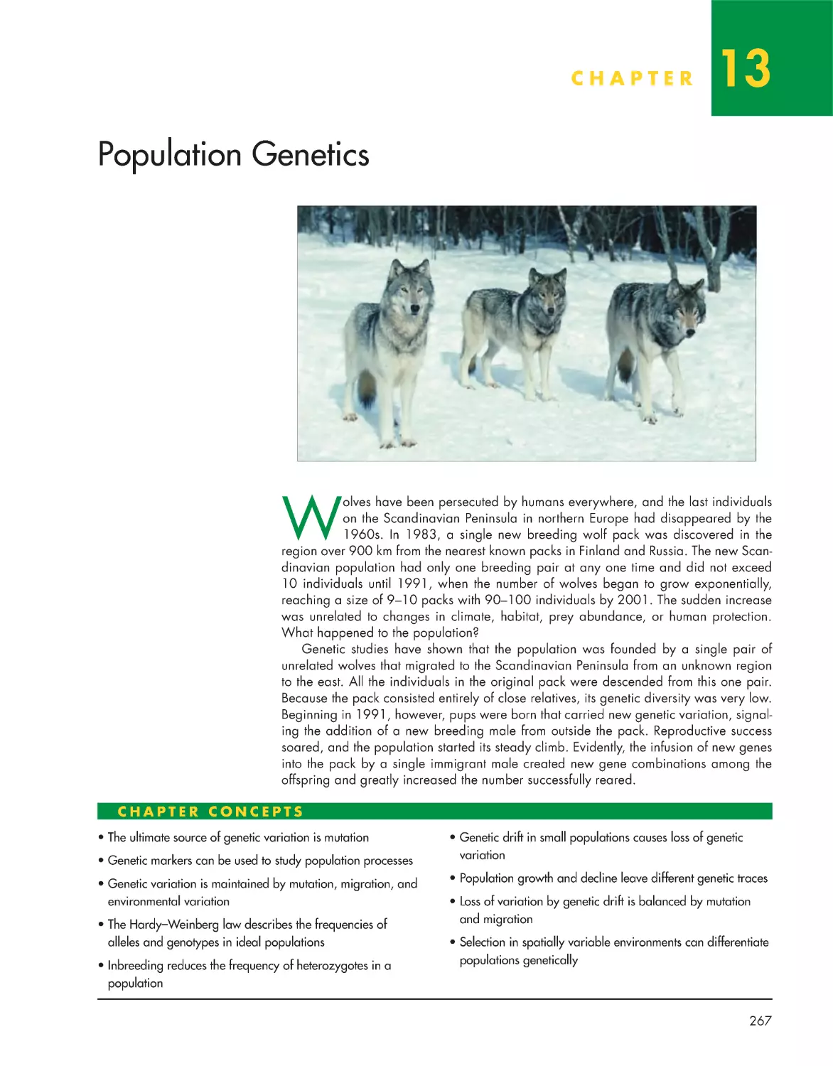
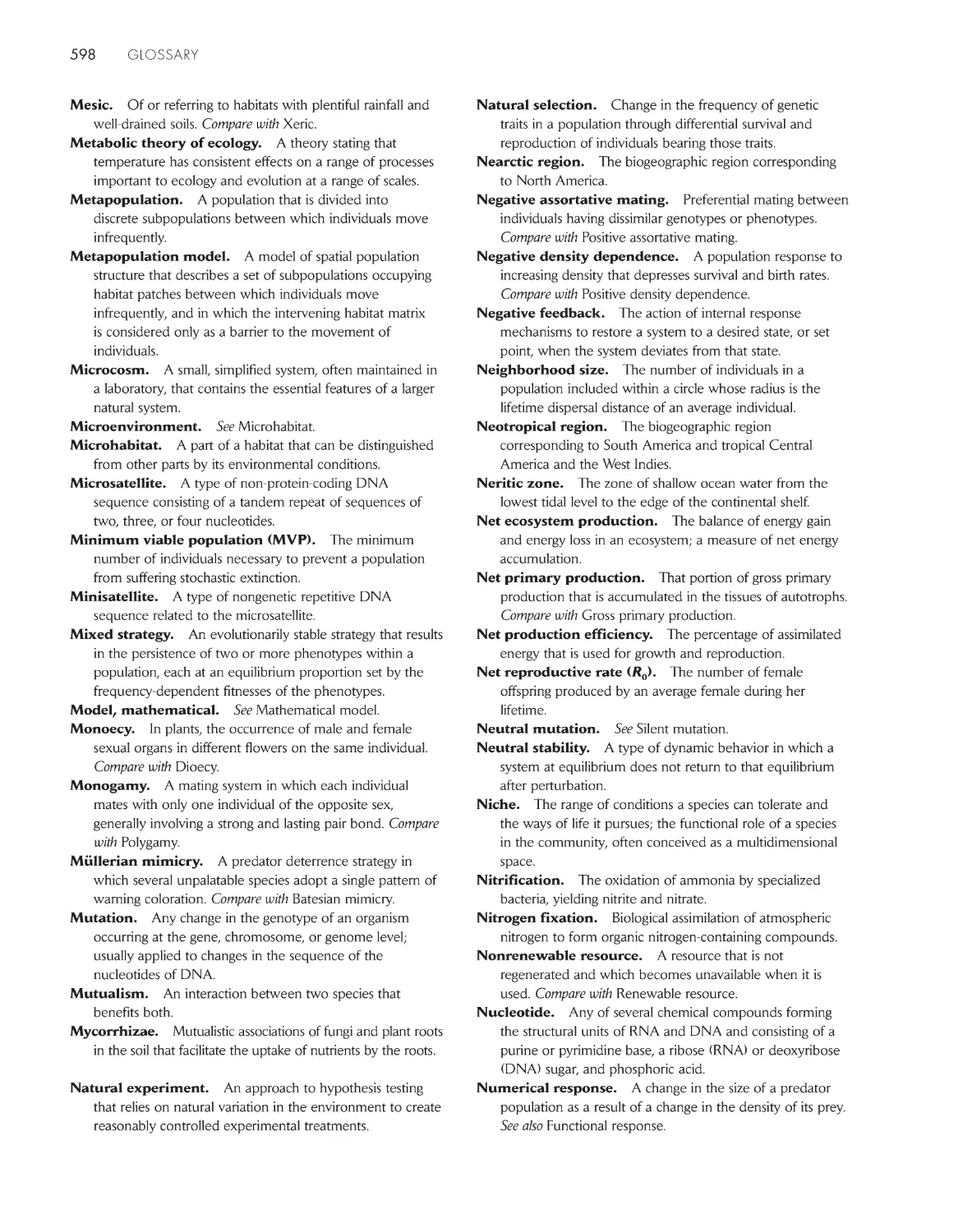
0
1
2
3
T
h
o
u
s
a
n
d
s
o
f
b
i
r
d
s
Year
1980
1990
2000
2010
Bird Island
Ram Island
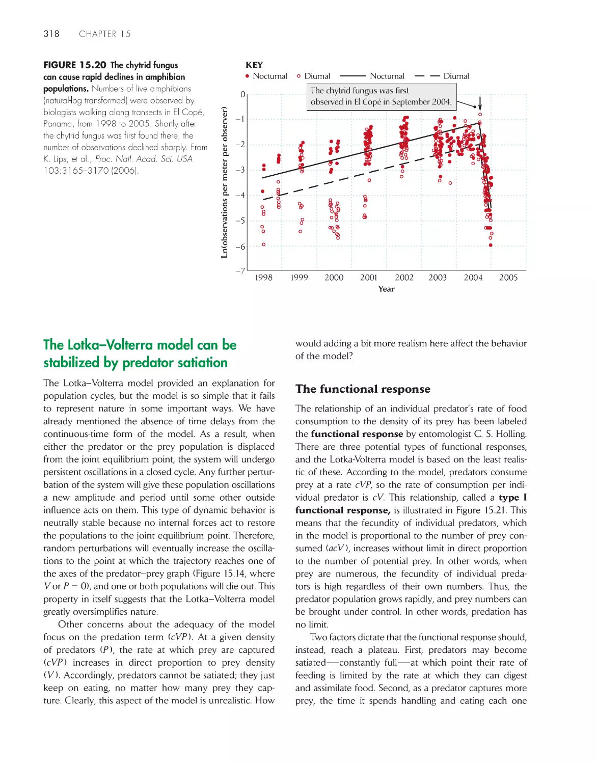
Penikese Island
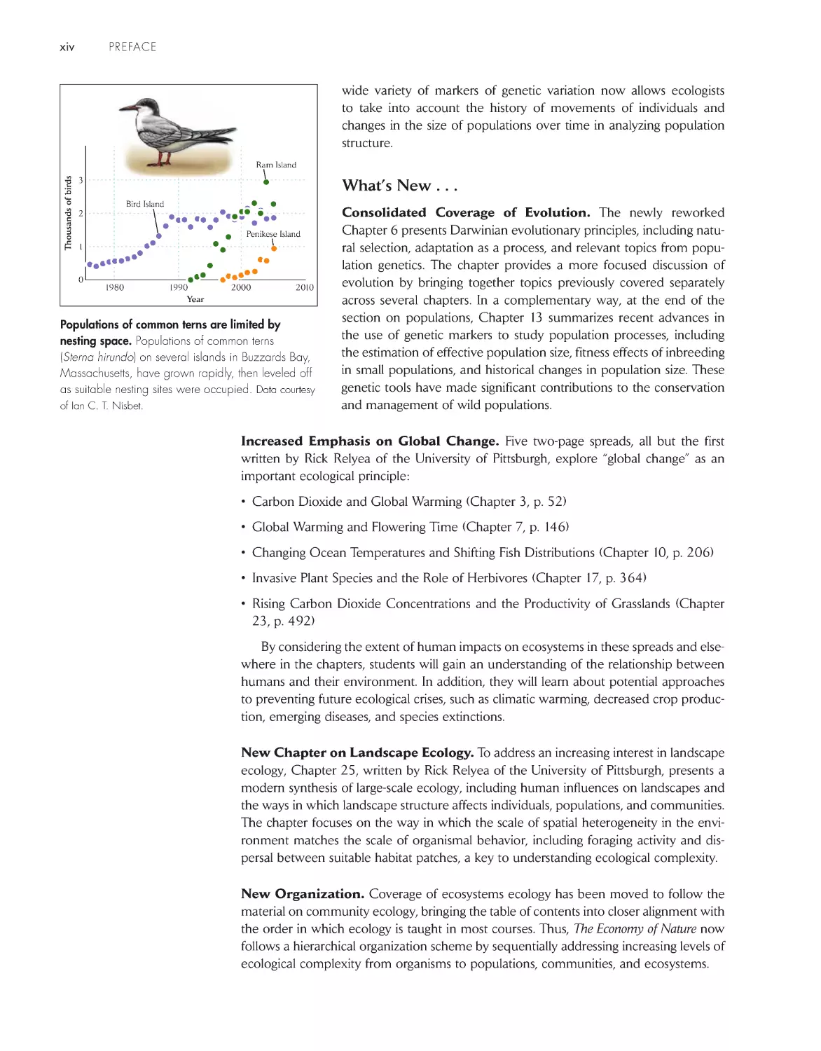
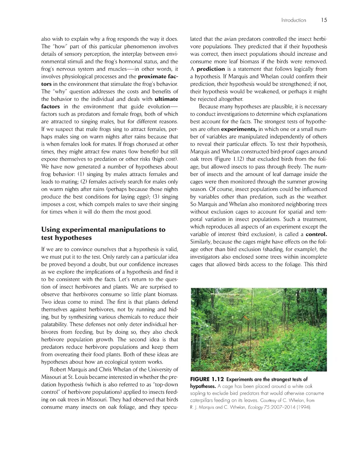
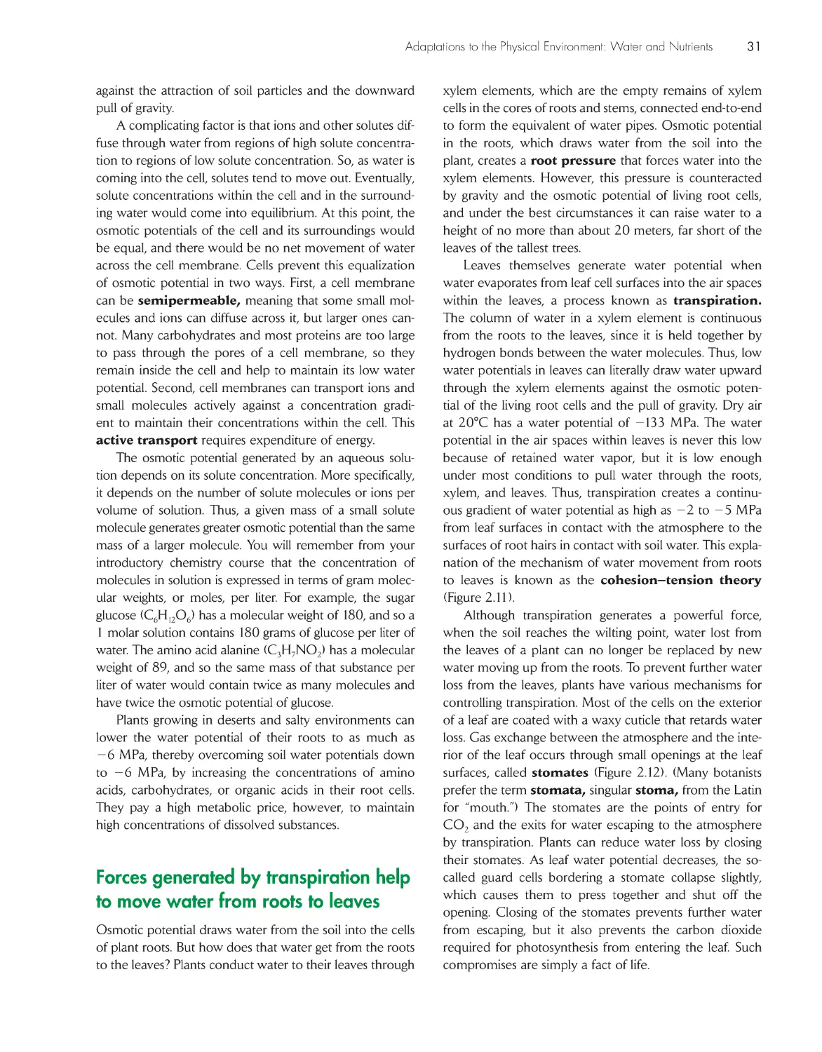
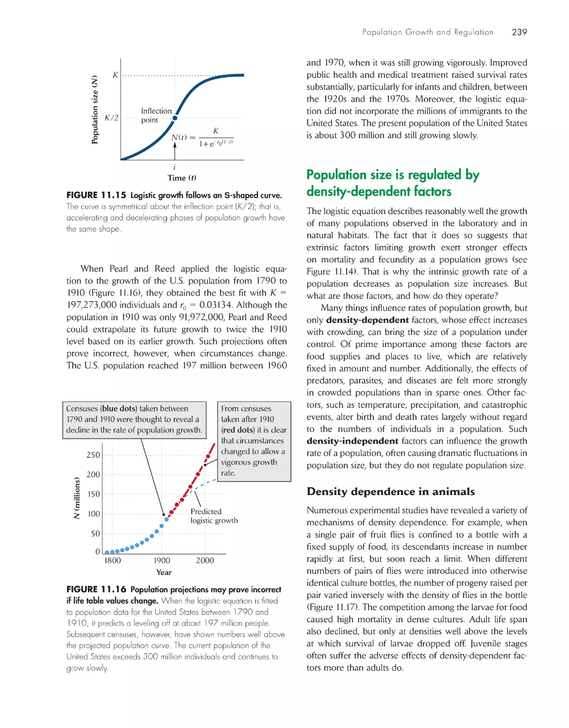
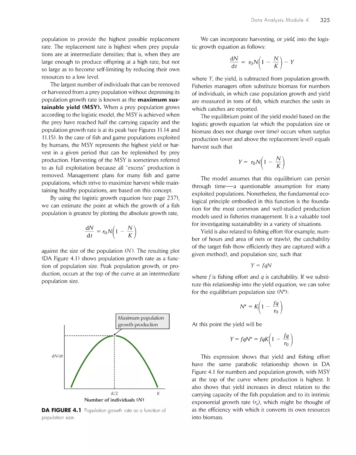
populations of common terns are limited by
nesting space. populations of common terns
(Sterna hirundo) on several islands in Buzzards Bay,
Massachusetts, have grown rapidly, then leveled off
as suitable nesting sites were occupied. Data courtesy
of Ian c. T. Nisbet.
xv
preface
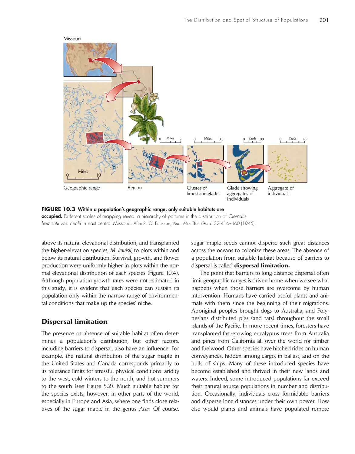
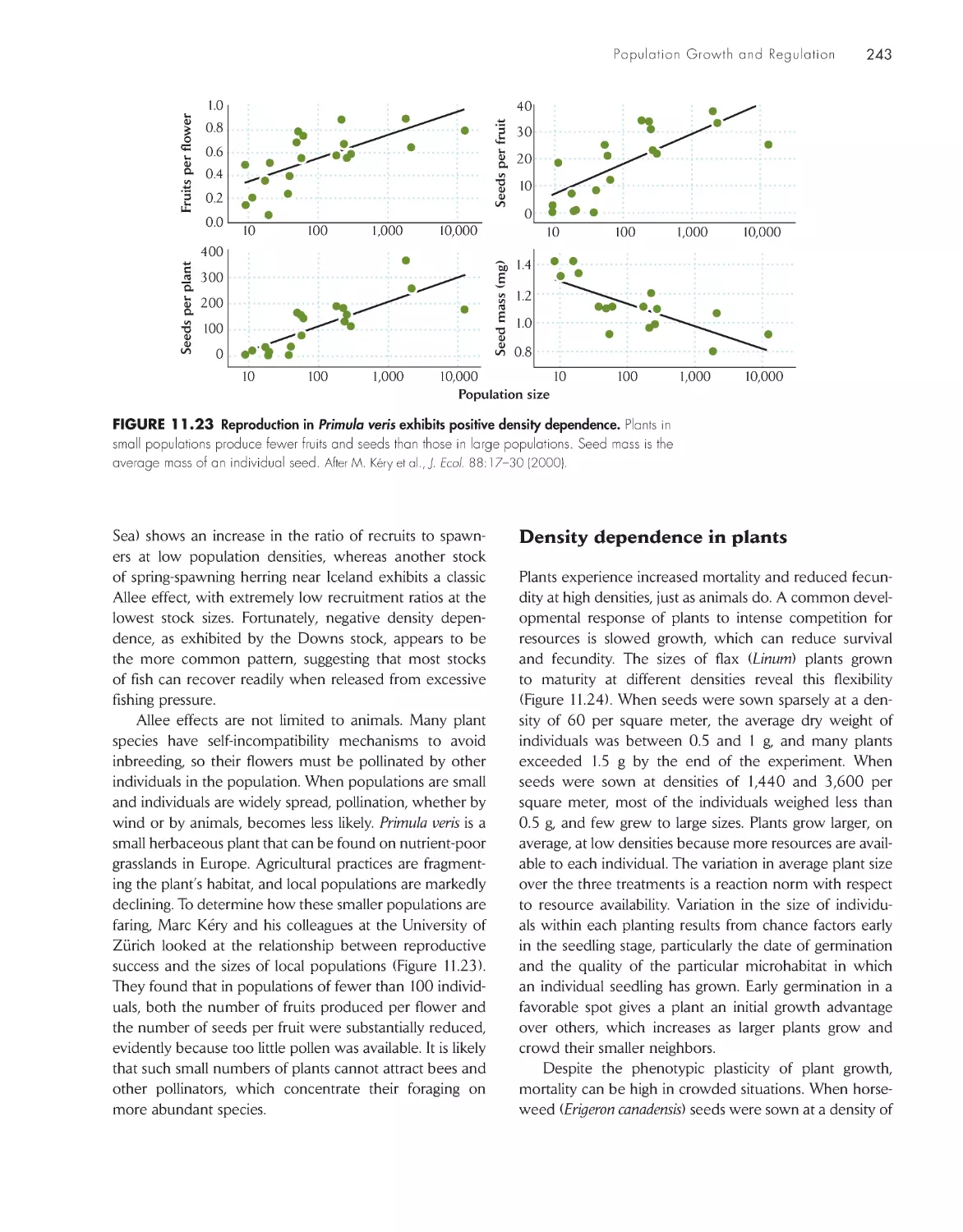
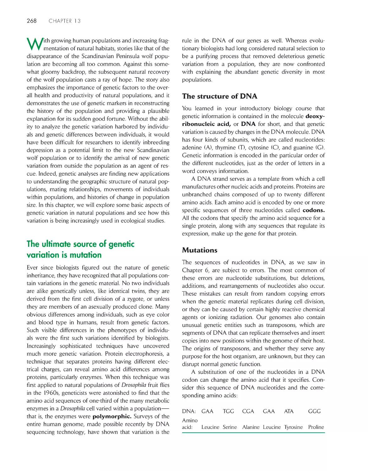
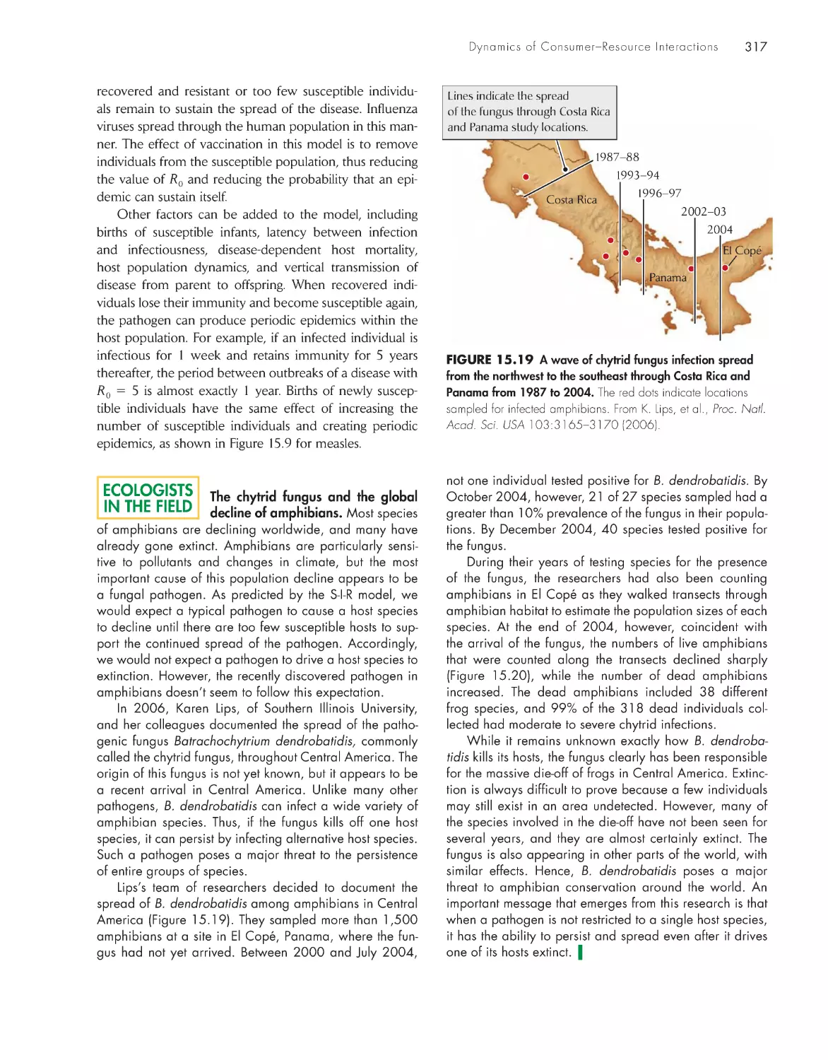
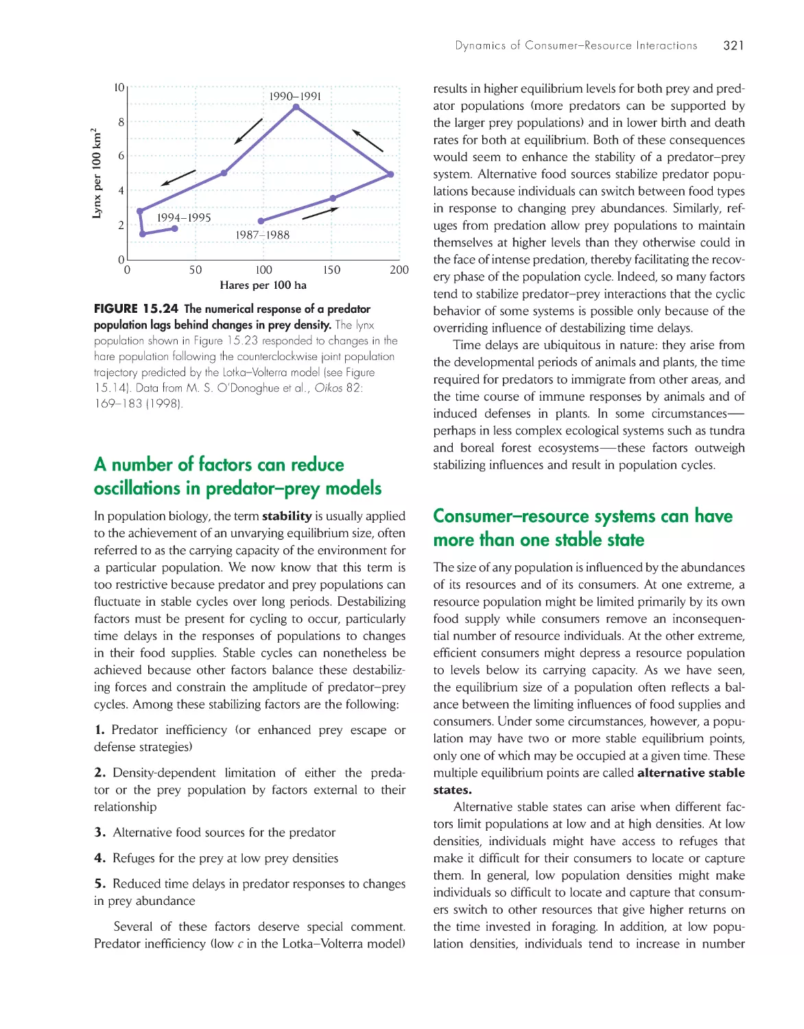
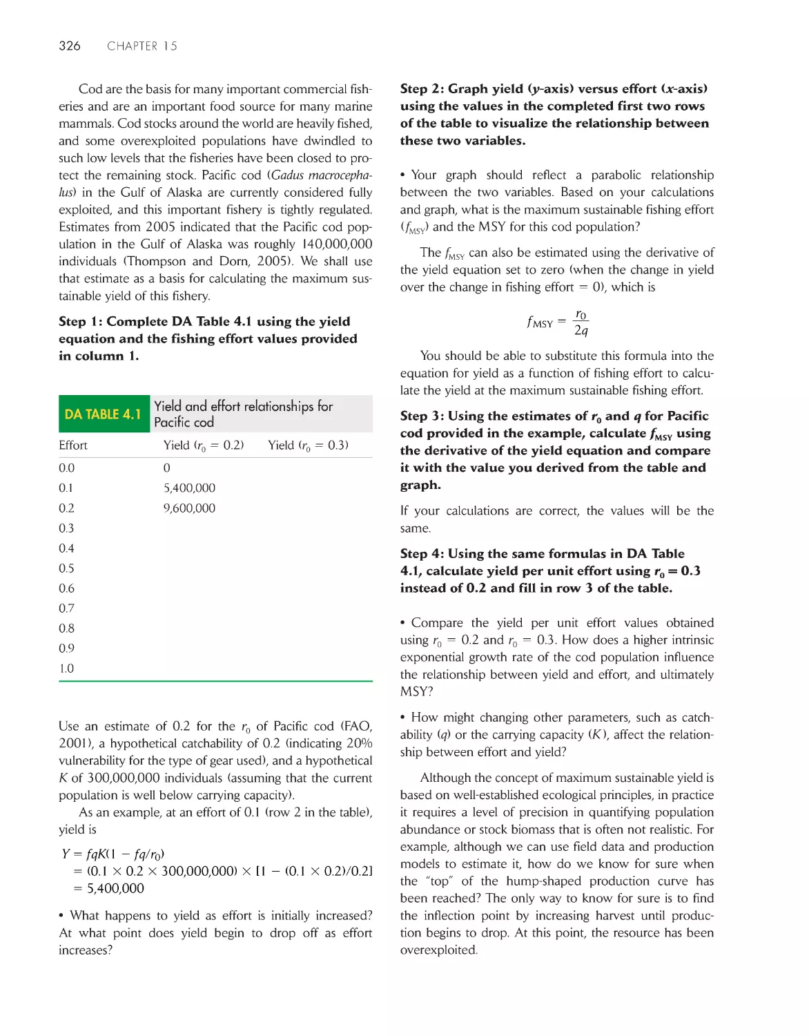
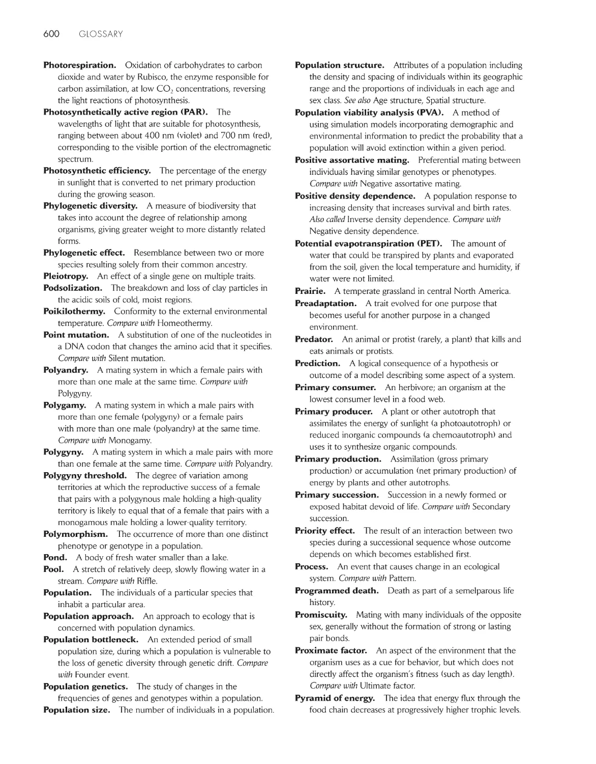
Lines indicate the spread
of the fungus through Costa Rica
and Panama study locations.
19 87–88
Costa Rica
Panama
El Copé
19 93–94
19 96–97
2002–03
2004
Clear Connections Between Adaptations and the Physical Environment. To
help students make a more meaningful connection between the physical environment
and an organism’s adaptations to it, Chapters 2 and 3 have been reconceived as a
chapter on water (Chapter 2) and a chapter on energy (Chapter 3). Water and energy,
including heat, are two of the most important drivers of ecological function and are
becoming increasingly important to the study of ecology as emissions of carbon dioxide
and other greenhouse gases cause our climate to heat up at a rate never before experi-
enced over the history of the earth.
New Aquatic Examples. Significant advances in aquatic research are introduced
throughout the book as Ecologists in the Field essays and elsewhere in the chapters,
providing more balanced treatment of terrestrial and aquatic examples. The Economy of
Nature has always provided students with a broad view of the diversity of organisms and
natural systems, and this tradition is further expanded in the sixth edition. Rick Relyea,
an aquatic ecologist at the University of Pittsburgh, has provided several of these new
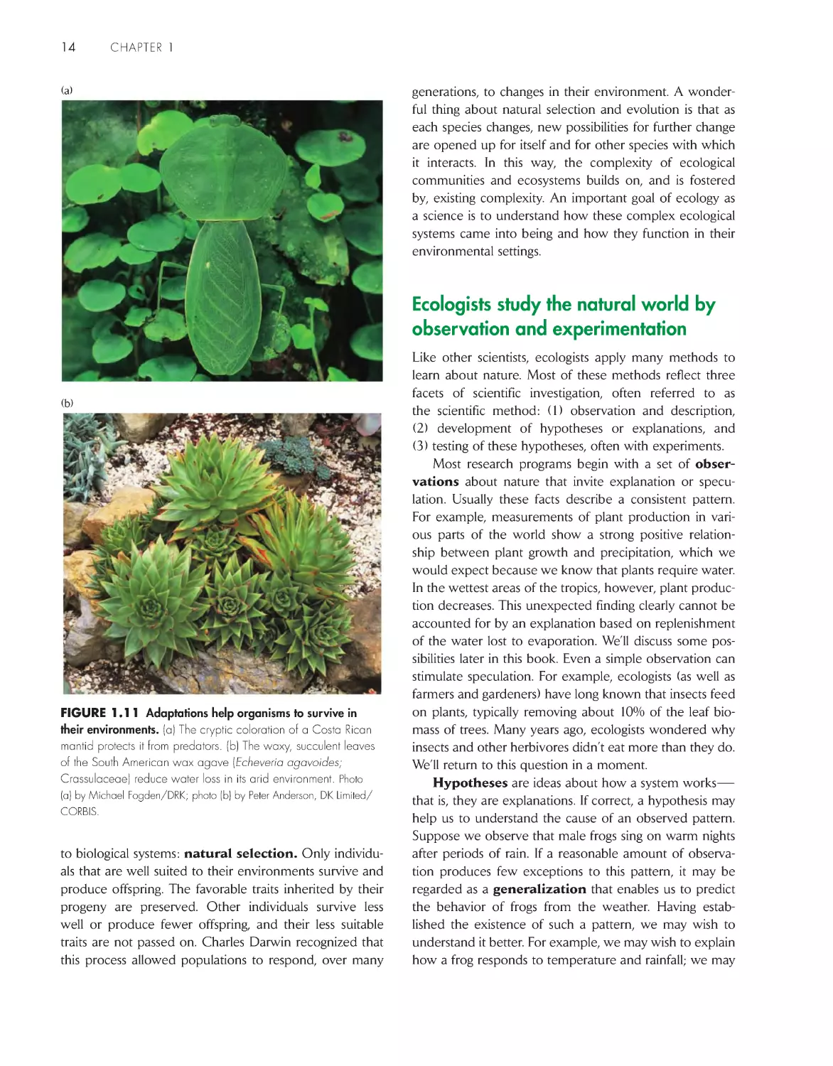
examples:
• Effects of predation on the evolution of guppy life histories (Chap-
ter 7, p. 141)
• Effects of fishing on sex switching (Chapter 8, p. 168)
• The chytrid fungus and the global decline of amphibians (Chapter
15, p. 317)
• Apparent competition between corals and algae mediated by
microbes (Chapter 16, p. 342)
• Mimicking the effects of ice scouring on the rocky coast of Maine
(Chapter 18, p. 384)
• A trophic cascade from fish to flowers (Chapter 18, p. 388)
Up-to-Date Coverage. The new edition incorporates modern devel-
opments in ecology, both technical and conceptual, including appli-
cations of stable isotopes and phylogenetics, recent developments in
macroecology, neutral theory, invasion biology, and global processes
connected with human activities. Among the new topics included in
this edition are the following:
• Ecological niche modeling (Chapter 10, p. 204)
• Macroecologic correlation between abundance and geographic distribution; inverse
correlation between population size and body size (Chapter 10, p. 216)
• Use of genetic markers to study population processes (Chapter 13, p. 269)
• Pathogen-host dynamics (Chapter 15, p. 315)
• Apparent competition (Chapter 16, p. 342)
• Alternative stable community states (Chapter 18, p. 383)
• New measures of relative abundance and new beta diversity indices (Chapter 20,
p. 413)
• Expanded discussion of Hubbell’s neutral model (Chapter 20, p. 432)
• The influence of phylogenetic relationships on community assembly (Chapter 21,
p. 450)
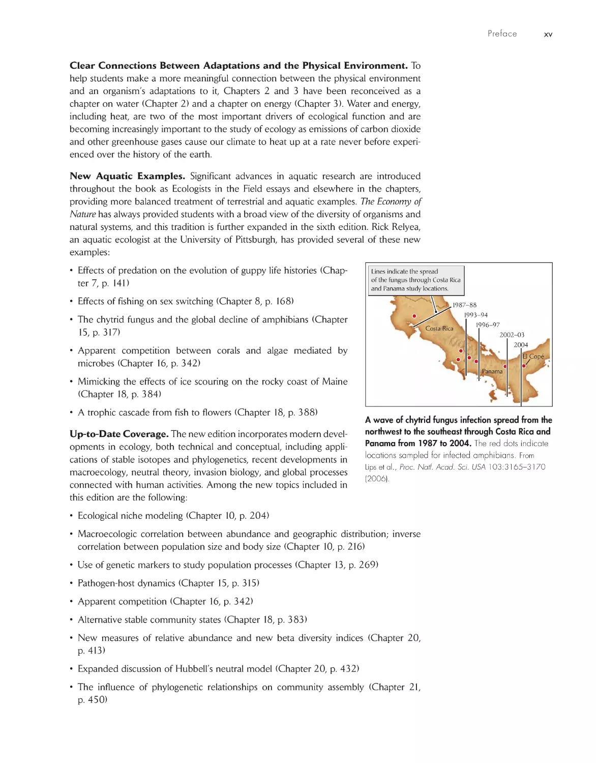
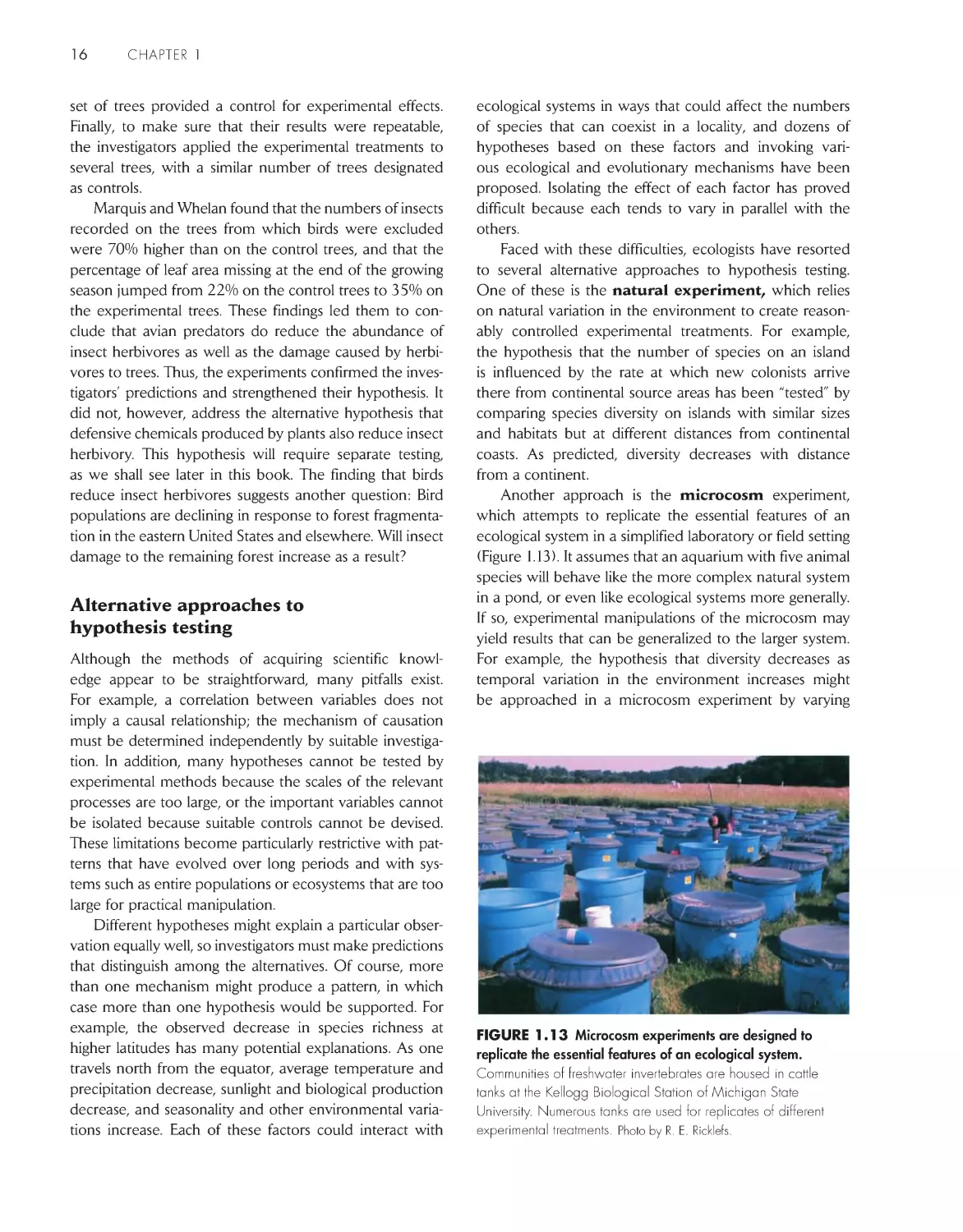
a wave of chytrid fungus infection spread from the
nor thwest to the southeast through costa rica and
panama from 1987 to 2004. The red dots indicate
locations sampled for infected amphibians. From
Lips et al., Proc. Natl. Acad. Sci. USA 103:3165–3170
(2006).
xvi
preFAce
• Using phylogenetic trees to test hypotheses explaining high species diversity in the
tropics (Chapter 21, p. 457)
• The fossil record of diversity: studies of pollen morphotypes and fossil mammal assem-
blages (Chapter 21, p. 458)
• Stoichiometry and nutrient balances (Chapter 22, p. 476)
• Using isotopes to trace the fate of nitrates in rainwater (Chapter 23, p. 496)
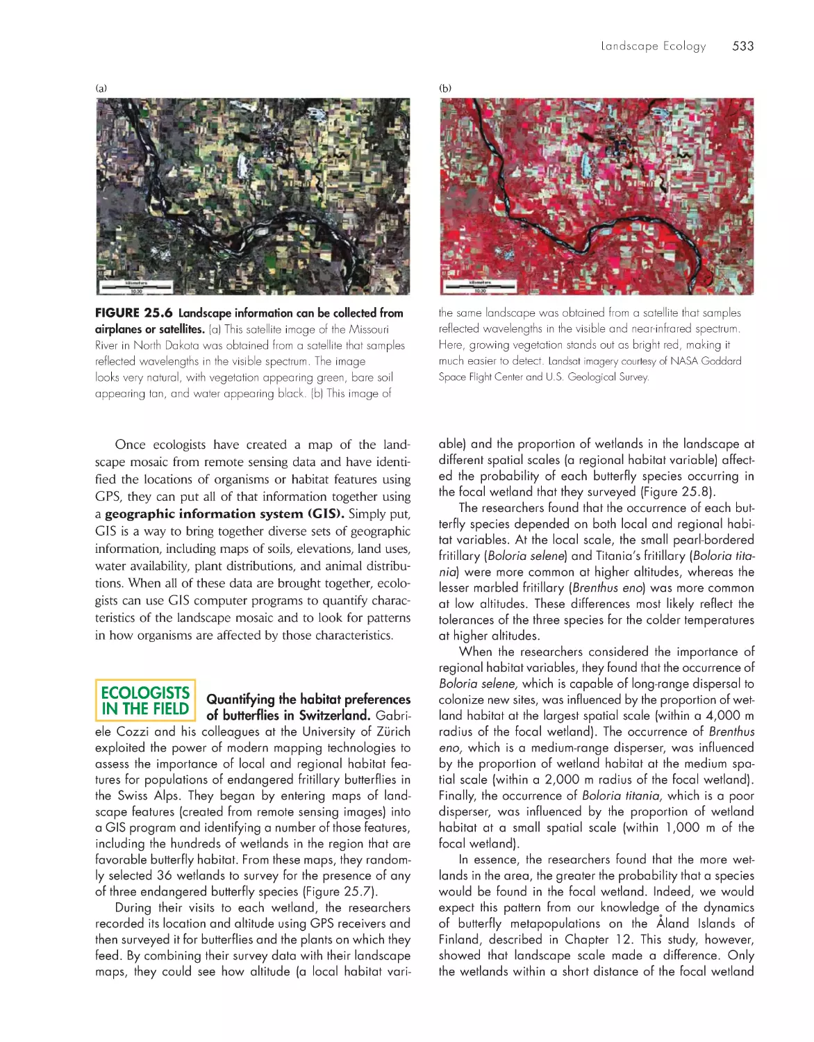
• Large-scale mapping of habitats using satellites and GIS (Chapter 25, p. 532)
• Emerging diseases and their effects on rates of extinction (Chapter 26, p. 561)
• Using population viability analysis (PVA) to predict the probability that a population
will avoid extinction (Chapter 26, p. 566)
New End-of-Chapter Review Questions. Each chapter now includes 8 to 10 ques-
tions that will help students review the most important material in the chapter.
resources for the Student
The Companion Web Site (www.whfreeman.com/ricklefs6e) provides a place for
students to enhance, test, and expand their knowledge of the material. The following
resources are available to students online:
GRAPHS
LIVING
• Living Graph Simulations are interactive tutorials that allow students to
practice manipulating variables on a graph and to master important quantitative
concepts such as exponential growth, Lotka–Volterra predator–prey interactions, logistic
growth, and the Hardy–Weinberg principle. Living Graph Simulations help students
hone their data analysis and data interpretation skills. See page xviii for a complete list
of Living Graph Simulations.
DATA
ANALYSIS
• Data Analysis Modules provide inquiry-based exercises to help students
learn important quantitative topics in a step-by-step manner in the context of a
real experiment. Five Data Analysis Modules are included in the text, while seven addi-
tional modules have been posted on the Companion Web Site. Datasets for all twelve
modules are available to instructors online in Excel spreadsheets for student assign-
ments. See page xviii for a complete list of Data Analysis Modules.
morE
on the
wEb
• More on the Web icons are found throughout the book to indicate supple-
mentary topics now discussed on the Companion Web Site that will enhance
those presented in the book. These topics include phenotypic plasticity and contrasting
mechanisms of growth in animals and plants; sequential hermaphroditism; the origin of
female choice; and environmental sex determination. See page xviii for a complete list
of More on the Web topics.
• Online Quizzes that allow students to review for exams are available for each chap-
ter. Students get instant feedback on their progress and can take the quizzes more than
once for practice.
• The eBook allows instructors and students access to the entire textbook anywhere,
anytime. It is also available as a download for use offline. The eBook is fully searchable
and can be annotated with note-taking and highlighting features. The eBook is offered
at about half the price of the printed textbook. For more information visit www.cours-
esmart.com (1-4292-3335-4).
xvii
preface
resources for the Instructor
The following resources for the instructor are available in both the Instructor view of the
Companion Web Site (1-4292-3547-0) and on an Instructor Resource CD-ROM
(1-4292-3549-7):
• Fully optimized JPEGs of every illustration, photograph, and table in the text-
book are offered in labeled and unlabeled versions. The type size, configuration, and
color saturation of every image have been individually treated for maximum clarity and
visibility.
• PowerPoint Image Set includes fully optimized JPEGs of all the illustrations, photos,
and tables in the textbook.
• Test Bank provides instructors with questions (and accompanying answers) for
each chapter. Developed by Thomas Wentworth of North Carolina State University,
questions test knowledge, comprehension, application, and analysis. Question formats
include multiple choice, fill-in-the-blank, and essay. Among the essay questions are at
least five interrelated application and analysis questions based on case histories drawn
from actual experiments or hypothetical situations.
• Living Graph Simulations can be used in class to review important quantitative
topics in an interactive fashion that is less intimidating to students.
• Datasets for each Data Analysis Module in the textbook and on the Companion
Web Site are available for student assignment.
The following resources are also available for instructors:
• Overhead Transparencies. Available on demand, the transparency set contains
over 200 figures from the textbook, formatted for maximum visibility in large lecture
halls (1-4292-3676-0) .
• WebCT/Blackboard. Cartridge downloads are available for instructors using either
WebCT or Blackboard. Cartridges include the entire suite of student and instructor
resources from the Companion Web Site (1-4292-3548-9).
companion web resources
A number of Living Graph Simulations, Data Analysis Modules, and More on the Web
topics are available to students and instructors on the Companion Web Site (www.
whfreeman.com/ricklefs6e), in addition to practice tests and study aids. Page numbers
indicate the location in the text of the icon referring to the module, simulation, or topic.
GRAPHS
LIVING
Living Graph Simulations
Chapter 11 Population Growth and Regulation
Exponential and Geometric Growth
226
Life Table Analysis
235
The Logistic Equation
238
Chapter 13 Population Genetics
The Hardy–Weinberg Equation
273
Chapter 15 Dynamics of Consumer–Resource Interactions
The Lotka–Volterra Predator–Prey Model
314
Chapter 16 Competition
Competition and Coexistence
335
Chapter 20 Biodiversity
Island Biogeography
427
DATA
ANALYSIS
Data Analysis Modules
Data Analysis Modules available in the text
Chapter 7 Life Histories and Evolutionary Fitness
Spatially Partitioned Foraging by Oceanic Seabirds 152
xviii
preFAce
Chapter 11 Population Growth and Regulation
Birth and Death Rates Influence Population Age
Structure and Growth Rate
229
Chapter 12 Temporal and Spatial Dynamics of
Populations
Stochastic Extinction with Variable Population
Growth Rates
262
Chapter 15 Dynamics of Consumer–Resource
Interactions
Maximum Sustainable Yield: Applying Basic
Ecological Concepts to Fisheries Management
324
Chapter 20 Biodiversity
Quantifying Biodiversity
435
Data Analysis Modules available on the Companion Web Site
Chapter 10 The Distribution and Spatial Structure of
Populations
Testing the Dispersion of Individuals Against a
Nonrandom Dispersion
209
Chapter 12 Temporal and Spatial Dynamics of
Populations
Tracking Environmental Variation
252
Chapter 15 Dynamics of Consumer–Resource
Interactions
Simulation Models of Predator–Prey Interactions 315
Chapter 16 Competition
Asymmetry in Competition
337
Chapter 22 Energy in the Ecosystem
Measuring Ecosystem Productivity: Using Dissolved
Oxygen to Estimate Stream Metabolism
469
Chapter 24 Nutrient Regeneration in Terrestrial and
Aquatic Ecosystems
Consumer Populations and Energy Flow: Estimating
Secondary Production
525
Chapter 25 Landscape Ecology
Landscape Ecology: Abundance and Distribution of
Northern Spotted Owls in Habitat Patches
537
morE
on the
wEb
More on the Web Topics
Chapter 5 The Biome Concept in Ecology
Biomes and Animal Forms
93
Characterizing Climate
93
Chapter 6 Evolution and Adaptation
Rates of Evolution in Populations
123
Selection on Traits That Exhibit Continuous
Variation
123
Modeling Selection Against a Deleterious
Recessive Gene
123
Ecotypes and Reaction Norms
130
Phenotypic Plasticity and Contrasting Mechanisms
of Growth and Reproduction in Animals
and Plants
130
Rate of Phenotypic Response
130
Chapter 7 Life Histories and Evolutionary Fitness
Metabolic Ceilings
135
Allometry and the Consequences of Body Size
for Life Histories
137
Annual and Perennial Life Histories
139
Variable Food Supplies and Risk-Sensitive Foraging 154
Chapter 8 Sex and Evolution
Sequential Hermaphroditism
167
Environmental Sex Determination
168
Female Condition and Offspring Sex Ratio
170
Alternative Male Reproductive Strategies
173
The Origin of Female Choice
176
Chapter 9 Family, Society and Evolution
Ritualized Antagonistic Behavior Reduces the
Incidence of Fighting
183
Social Groups as Information Centers
184
Alarm Calls as Altruistic Behaviors
188
The Reciprocal Altruism Game
192
Chapter 11 Population Growth and Regulation
Density Dependence in Laboratory Cultures of
Water Fleas
240
Chapter 14 Species Interactions
Seed Dispersal
299
Pollination
299
Chapter 15 Dynamics of Consumer–Resource
Interactions
Predator–Prey Dynamics in a Metapopulation of
the Cinnabar Moth
322
Three-Level Consumer Systems
322
Chapter 17 Evolution of Species Interactions
Inferring Phylogenetic History
362
Chapter 20 Biodiversity
The Lognormal Distribution
414
acknowledgments
I particularly want to acknowledge the contributions of the two people with whom I
worked most closely on this edition: Jerry Correa, Acquisitions Editor, and Susan Moran,
Senior Development Editor. Jerry provided the overall direction for the new edition,
always giving support and encouragement, while Susan worked closely with me to
improve the organization, writing, and illustrations.
xix
preface
I appreciate the proficiency and professionalism of Georgia Lee Hadler, Senior
Project Editor; Norma Sims Roche, Copy Editor; Julia DeRosa, Senior Production
Manager; Victoria Tomaselli, Senior Designer; Cecilia Varas, Photo Editor; Julie Tesser,
Photo Researcher; Susan Timmons, Illustration Coordinator; and Daniel Gonzalez,
Supplements and Media Editor. Debbie Clare ably directed the marketing of the book.
I am particularly grateful to Matt Whiles, Southern Illinois University Carbondale,
who drew on his own experience as a teacher to create most of the Data Analysis
Modules. Jeff Ciprioni and especially Elaine Palucki shepherded the modules through
production with enthusiasm and intelligence, making the process painless and enjoyable.
I am also grateful to Rick Relyea, University of Pittsburgh, for enriching this textbook
through his contributions of the Landscape of Ecology chapter and many Global Change
and Ecologists in the Field essays.
Of particular importance to me are the many colleagues who read the manuscript
and provided useful advice and guidance:
Jonathan M. Adams, Rutgers University
Loreen Allphin, Brigham Young University
Anthony H. Bledsoe, University of Pittsburgh
Chad E. Brassil, University of Nebraska
Robert S. Capers, Oklahoma State University
Walter P. Carson, University of Pittsburgh
Lisa M. Castle, Glenville State College
Samantha Chapman, Villanova University
Patricia Clark, Indiana University–Purdue University,
Indianapolis
Kenneth Ede, Oklahoma State University–Tulsa
Llody Fitzpatrick, University of North Texas
Jason Fridley, Syracuse University
Jack Grubaugh, University of Memphis
Stephen J. Hecnar, Lakehead University
Tara Jo Holmberg, Northwestern Connecticut Community
College
Claus Holzapfel, Rutgers University
Thomas R. Horton, SUNY College of Environmental
Science and Forestry
R. Stephen Howard, Middle Tennessee State University
Anthony Ippolito, DePaul University
Thomas W. Jurik, Iowa State University
Jamie Kneitel, California State University, Sacramento
John L. Koprowski, University of Arizona
Dr. Mary E. Lehman, Longwood University
Patrick Mathews, Friends University
Dean G. McCurdy, Albion College
Rob McGregor, Institute of Urban Ecology, Douglas College
Bill McMillan, Malaspina University–College
Randall J. Mitchell, University of Akron
L. Maynard Moe, California State University, Bakersfield
Patrick L. Osborne, University of Missouri–St. Louis
Diane Post, University of Texas–Permian Basin
Mark Pyron, Ball State University
Rick Relyea, University of Pittsburgh
John P. Roche, Boston College
Steven J. Rothenberger, University of Nebraska–Kearney
Ted Schuur, University of Florida
Erik P. Scully, Towson University
William R. Teska, Pacific Lutheran University
Diana F. Tomback, University of Colorado–Denver
William Tonn, University of Alberta
Joseph von Fischer, Colorado State University
Diane Wagner, University of Alaska
William E. Walton, University of California–Riverside
Xianzhong Wang, Indiana University–Purdue University,
Indianapolis
Thomas Wentworth, North Carolina State University
Bradley M. Wetherbee, University of Rhode Island
Susan K. Willson, St. Lawrence University
Mosheh Wolf, University of Illinois at Chicago
John A. Yunger, Governors State University
The following people provided valuable expertise
and assisted with the development of the Data Analysis
Modules written by Matt Whiles: Walter K. Dodds,
Kansas State University; James E. Garvey, Southern Illinois
University Carbondale; Alexander D. Huryn, University of
Alabama; Clayton K. Nielson, Southern Illinois University
Carbondale; John D. Reeve, Southern Illinois University
Carbondale; and Eric M. Schauber, Southern Illinois
University Carbondale.
Many thanks also to the readers who reviewed the
Data Analysis Modules: Patricia Clark, Indiana University–
Purdue University, Indianapolis; Robert Colwell, University
of Connecticut; Theodore Fleming, University of Miami;
Michael Ganger, Massachusetts College of Liberal Arts;
Zachary Jones, Colorado College; Aaron King, University
of Michigan; Timothy McCay, Colgate University; George
Robinson, University at Albany-SUNY; John P. Roche,
Boston College; Joseph von Fischer, Colorado State
University; I. Michael Weis, University of Windsor; Thomas
Wentworth, North Carolina State University; Peter White,
University of North Carolina at Chapel Hill.
This page intentionally left blank
1
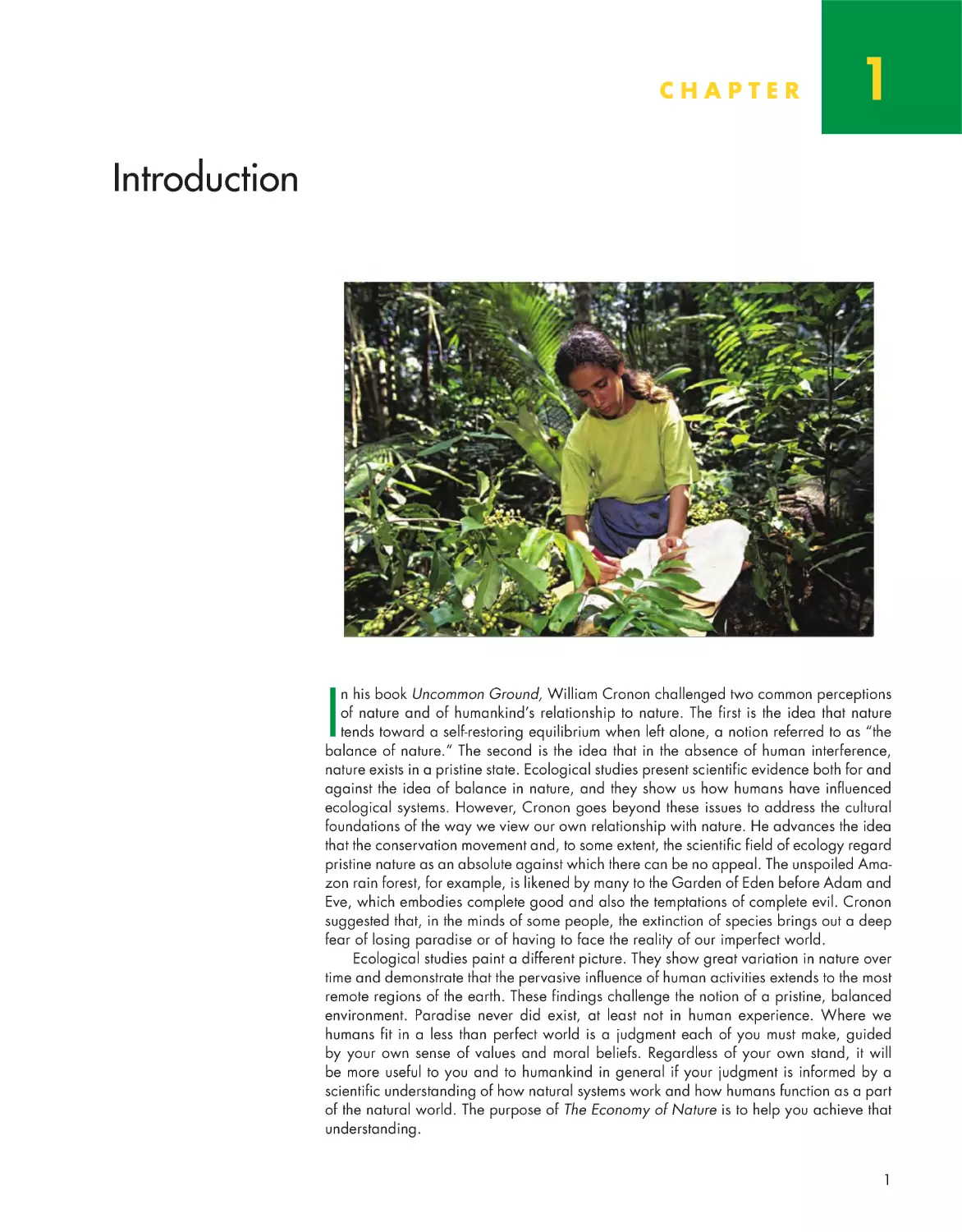
In his book Uncommon Ground, William Cronon challenged two common perceptions
of nature and of humankind’s relationship to nature. The first is the idea that nature
tends toward a self-restoring equilibrium when left alone, a notion referred to as “the
balance of nature.” The second is the idea that in the absence of human interference,
nature exists in a pristine state. Ecological studies present scientific evidence both for and
against the idea of balance in nature, and they show us how humans have influenced
ecological systems. However, Cronon goes beyond these issues to address the cultural
foundations of the way we view our own relationship with nature. He advances the idea
that the conser vation movement and, to some extent, the scientific field of ecology regard
pristine nature as an absolute against which there can be no appeal. The unspoiled Ama-
zon rain forest, for example, is likened by many to the Garden of Eden before Adam and
Eve, which embodies complete good and also the temptations of complete evil. Cronon
suggested that, in the minds of some people, the extinction of species brings out a deep
fear of losing paradise or of having to face the reality of our imperfect world.
Ecological studies paint a different picture. They show great variation in nature over
time and demonstrate that the per vasive influence of human activities extends to the most
remote regions of the earth. These findings challenge the notion of a pristine, balanced
environment. Paradise never did exist, at least not in human experience. Where we
humans fit in a less than perfect world is a judgment each of you must make, guided
by your own sense of values and moral beliefs. Regardless of your own stand, it will
be more useful to you and to humankind in general if your judgment is informed by a
scientific understanding of how natural systems work and how humans function as a part
of the natural world. The purpose of The Economy of Nature is to help you achieve that
understanding.
chapter
Introduction
1
1
chapter 1
2
The English word ecology is taken from the Greek oikos,
meaning “house,” and thus refers to our immediate sur-
roundings, or environment. In 1870, the German zoolo-
gist Ernst Haeckel gave the word a broader meaning:
By ecology, we mean the body of knowledge
concerning the economy of nature—the
investigation of the total relations of the
animal both to its organic and to its inorganic
environment; including above all, its friendly and
inimical relation with those animals and plants
with which it comes directly or indirectly into
contact—in a word, ecology is the study of all the
complex interrelationships referred to by Darwin
as the conditions of the struggle for existence.
Thus, ecology is the science by which we study how
organisms interact in and with the natural world.
The word ecology came into general use only in the late
1800s, when European and American scientists began to
call themselves ecologists. The first societies and journals
devoted to ecology appeared in the early decades of the
twentieth century. Since that time, ecology has grown and
diversified, and professional ecologists now number in the
tens of thousands. The science of ecology has produced an
immense body of knowledge about the world around us.
At the same time, the rapid growth of the human popula-
tion and our increasing technology and materialism have
accelerated change in our environment, frequently with
dramatic consequences. Now more than ever, we need to
understand how ecological systems function if we are to
develop the best policies for managing the watersheds, agri-
cultural lands, wetlands, and other areas—what are gen-
erally called environmental support systems—on which
humanity depends for food, water, protection against natu-
ral catastrophes, and public health. Ecologists provide that
understanding through studies of population regulation by
predators, the influence of soil fertility on plant growth,
the evolutionary responses of microorganisms to environ-
mental contaminants, the spread of organisms, including
pathogens, over the surface of the earth, and a multitude of
similar issues. Managing biotic resources to sustain a reason-
able quality of human life depends on the wise application
of ecological principles to solve or prevent environmental
problems and to inform our economic, political, and social
thought and practice.
This chapter will start you on the road to ecologi-
cal thinking. We shall first view ecological knowledge
and insight from several different vantage points—for
example, as levels of complexity, varieties of organisms,
types of habitat, and scales in time and space. We shall see
how organisms, assemblages of organisms, and organisms
together with their environment are united to form larger
ecological systems by the regular interaction and inter-
dependence of their parts. Although ecological systems
vary in scale from a single microbe to the entire biosphere
blanketing the surface of the earth, they all obey similar
principles. Some of the most important of these princi-
ples concern their physical and chemical attributes, the
regulation of their structure and function, and evolution-
ary change. Applying these principles to environmental
issues can help us to meet the challenge of maintaining
a supportive environment for natural systems—and for
ourselves—in the face of increasing ecological stresses.
As we begin this journey of inquiry and exploration,
we should be mindful of two points. First, ecology as a
science is distinct from environmental science, applied
ecology, conservation biology, and related fields. Those
fields use an ecological understanding (obtained through
scientific investigation) to solve problems concerning
the environment and its inhabitants. Of course, science
and applications of science are intimately connected,
chapter concepts
• Ecological systems can be as small as individual organisms
or as large as the biosphere
• Ecologists study nature from several perspectives
• Plants, animals, and microorganisms play different roles in
ecological systems
• The habitat defines an organism’s place in nature; the niche
defines its functional role
• Ecological systems and processes have characteristic scales
in time and space
• Ecological systems are governed by basic physical and
biological principles
• Ecologists study the natural world by observation and
experimentation
• Humans are a prominent part of the biosphere
• Human impacts on the natural world have increasingly
become a focus of ecology
3
Introduction
and information flows between them in both directions.
Indeed, much of the science of ecology has developed
through research on practical problems in pest manage-
ment, species conservation, habitat restoration, and the
like. Throughout this book, we shall see the connections
between science and application, between the generation
of knowledge and its use.
The second point concerns the nature of science itself.
Science is a process, not the knowledge it generates. As
we shall see later in this chapter, scientific investigation
makes use of a variety of tools to develop an understand-
ing of the workings of nature. This understanding is never
complete or absolute, but constantly changes as scientists
discover new ways of thinking. Much of our knowledge
about the natural world is well established because it
has withstood many tests and is consistent with a large
body of observations and with the results of experimental
manipulations. Our understanding of many issues, how-
ever, is incomplete and imperfect. For example, ecologists
have yet to agree broadly on the factors that determine
many patterns and processes, such as global patterns of
species richness, how and where the biosphere sequesters
carbon dioxide, the role of certain mineral nutrients in
marine production, and the role of predators in control-
ling prey populations and shifting the character of natural
communities. These are areas of active research in which
ecologists are exploring alternative explanations for natu-
ral phenomena.
Ecological systems can be as
small as individual organisms
or as large as the biosphere
An ecological system may be an organism, a population,
an assemblage of populations living together (often called
a community), an ecosystem, or the entire biosphere. Each
smaller ecological system is a subset of the next larger
one, so that the different types of ecological systems form
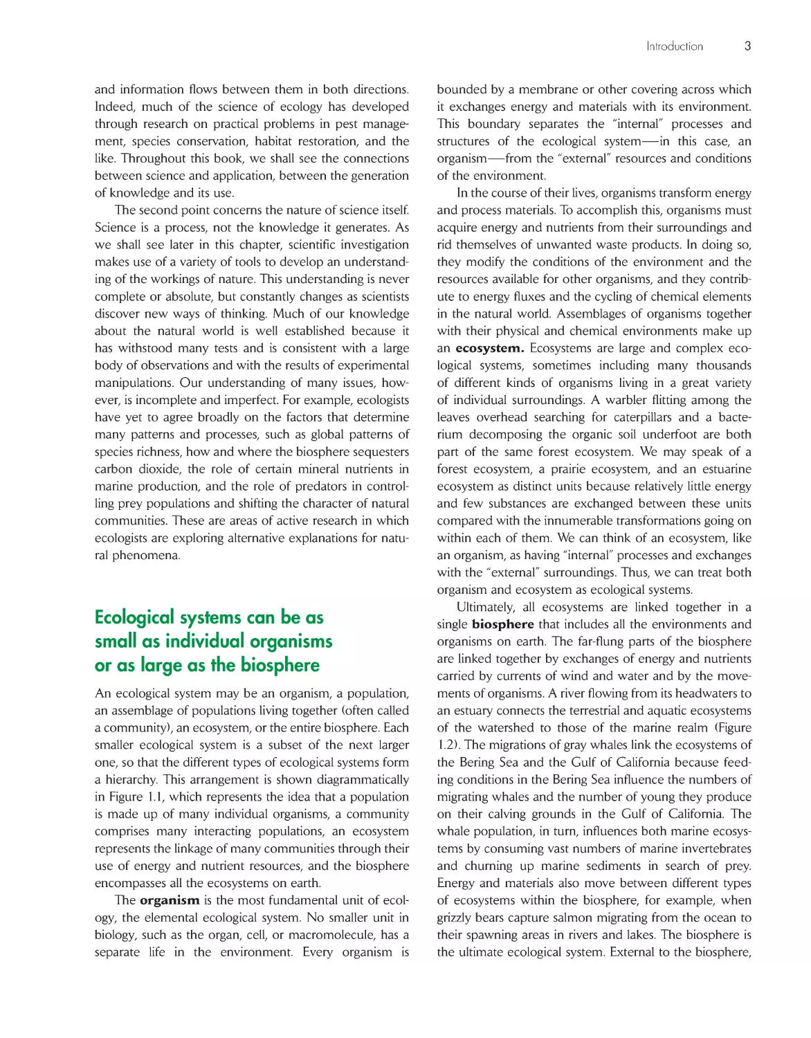
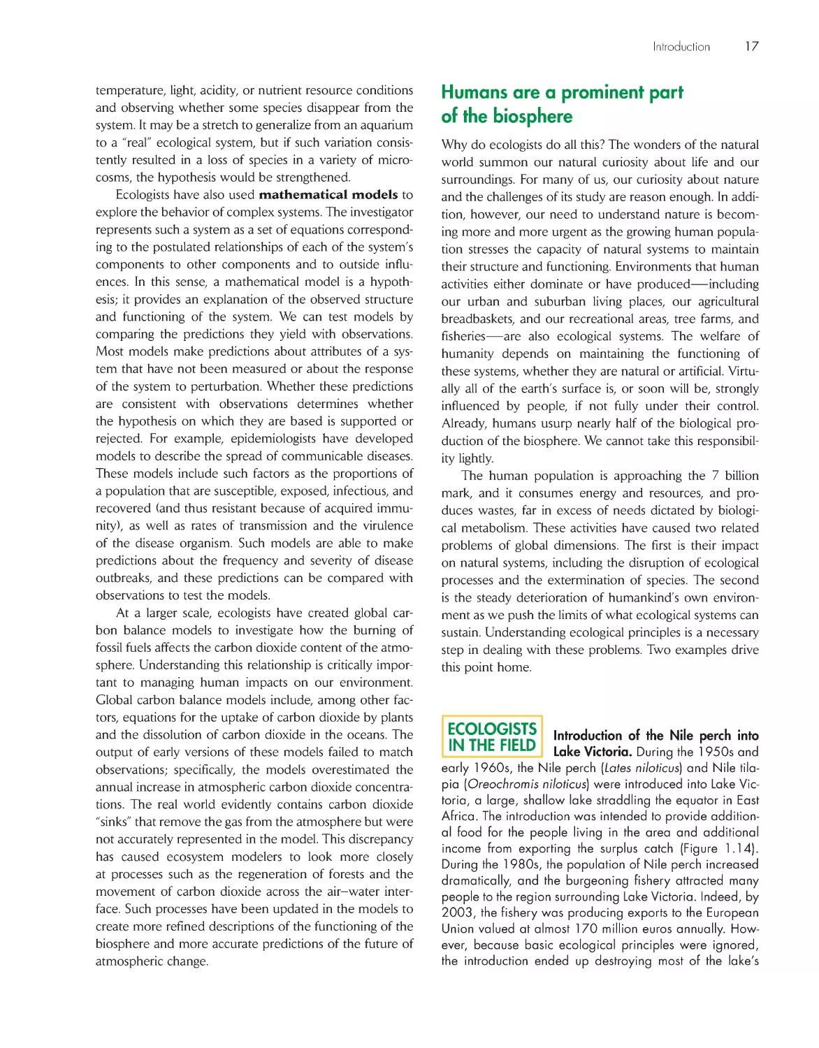
a hierarchy. This arrangement is shown diagrammatically
in Figure 1.1, which represents the idea that a population
is made up of many individual organisms, a community
comprises many interacting populations, an ecosystem
represents the linkage of many communities through their
use of energy and nutrient resources, and the biosphere
encompasses all the ecosystems on earth.
The organism is the most fundamental unit of ecol-
ogy, the elemental ecological system. No smaller unit in
biology, such as the organ, cell, or macromolecule, has a
separate life in the environment. Every organism is
bounded by a membrane or other covering across which
it exchanges energy and materials with its environment.
This boundary separates the “internal” processes and
structures of the ecological system—in this case, an
organism—from the “external” resources and conditions
of the environment.
In the course of their lives, organisms transform energy
and process materials. To accomplish this, organisms must
acquire energy and nutrients from their surroundings and
rid themselves of unwanted waste products. In doing so,
they modify the conditions of the environment and the
resources available for other organisms, and they contrib-
ute to energy fluxes and the cycling of chemical elements
in the natural world. Assemblages of organisms together
with their physical and chemical environments make up
an ecosystem. Ecosystems are large and complex eco-
logical systems, sometimes including many thousands
of different kinds of organisms living in a great variety
of individual surroundings. A warbler flitting among the
leaves overhead searching for caterpillars and a bacte-
rium decomposing the organic soil underfoot are both
part of the same forest ecosystem. We may speak of a
forest ecosystem, a prairie ecosystem, and an estuarine
ecosystem as distinct units because relatively little energy
and few substances are exchanged between these units
compared with the innumerable transformations going on
within each of them. We can think of an ecosystem, like
an organism, as having “internal” processes and exchanges
with the “external” surroundings. Thus, we can treat both
organism and ecosystem as ecological systems.
Ultimately, all ecosystems are linked together in a
single biosphere that includes all the environments and
organisms on earth. The far-flung parts of the biosphere
are linked together by exchanges of energy and nutrients
carried by currents of wind and water and by the move-
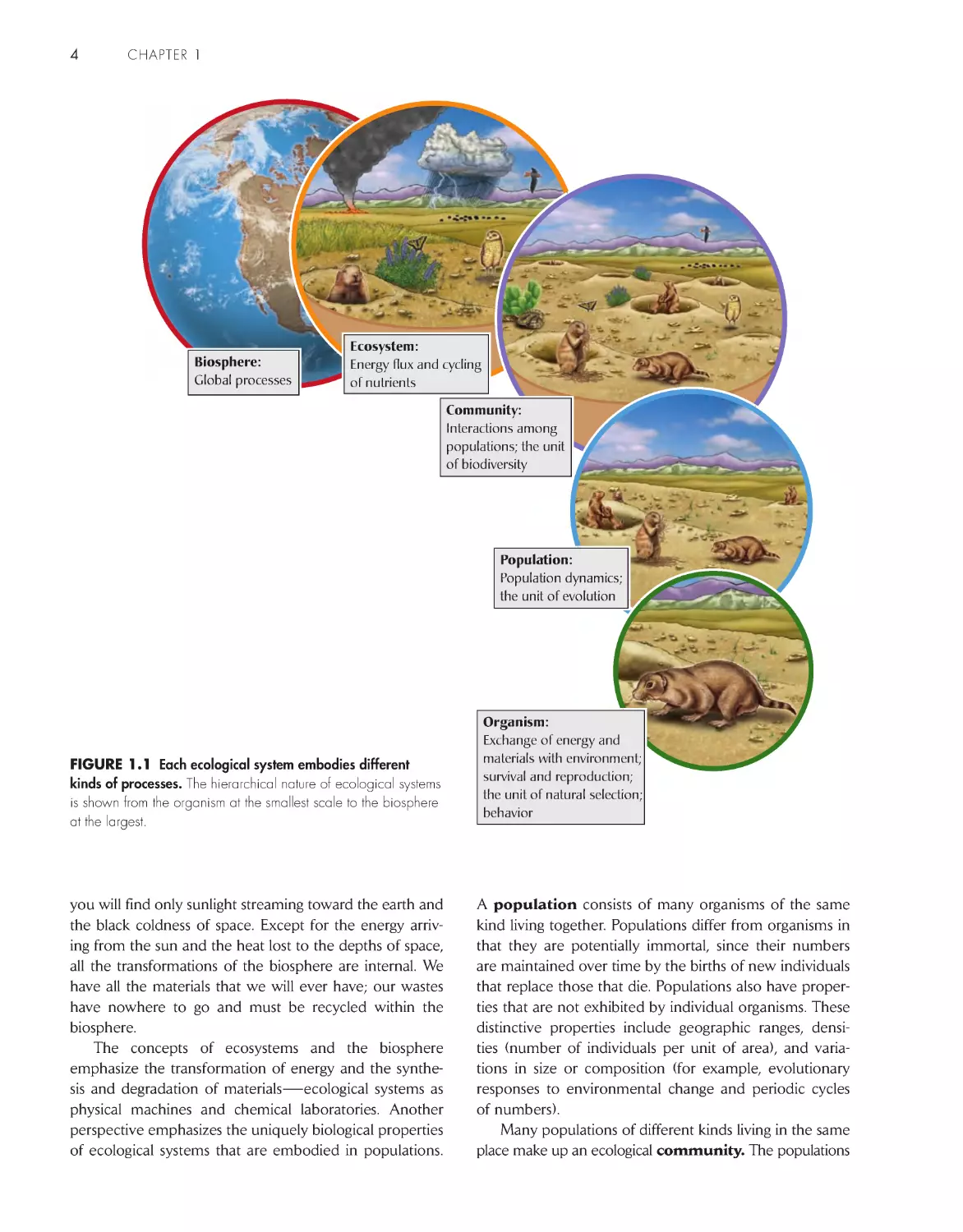
ments of organisms. A river flowing from its headwaters to
an estuary connects the terrestrial and aquatic ecosystems
of the watershed to those of the marine realm (Figure
1.2). The migrations of gray whales link the ecosystems of
the Bering Sea and the Gulf of California because feed-
ing conditions in the Bering Sea influence the numbers of
migrating whales and the number of young they produce
on their calving grounds in the Gulf of California. The
whale population, in turn, influences both marine ecosys-
tems by consuming vast numbers of marine invertebrates
and churning up marine sediments in search of prey.
Energy and materials also move between different types
of ecosystems within the biosphere, for example, when
grizzly bears capture salmon migrating from the ocean to
their spawning areas in rivers and lakes. The biosphere is
the ultimate ecological system. External to the biosphere,
4
chapter 1
you will find only sunlight streaming toward the earth and
the black coldness of space. Except for the energy arriv-
ing from the sun and the heat lost to the depths of space,
all the transformations of the biosphere are internal. We
have all the materials that we will ever have; our wastes
have nowhere to go and must be recycled within the
biosphere.
The concepts of ecosystems and the biosphere
emphasize the transformation of energy and the synthe-
sis and degradation of materials—ecological systems as
physical machines and chemical laboratories. Another
perspective emphasizes the uniquely biological properties
of ecological systems that are embodied in populations.
A population consists of many organisms of the same
kind living together. Populations differ from organisms in
that they are potentially immortal, since their numbers
are maintained over time by the births of new individuals
that replace those that die. Populations also have proper-
ties that are not exhibited by individual organisms. These
distinctive properties include geographic ranges, densi-
ties (number of individuals per unit of area), and varia-
tions in size or composition (for example, evolutionary
responses to environmental change and periodic cycles
of numbers).
Many populations of different kinds living in the same
place make up an ecological community. The populations
Biosphere:
Global processes
Ecosystem:
Energy flux and cycling
of nutrients
Organism:
Exchange of energy and
materials with environment;
survival and reproduction;
the unit of natural selection;
behavior
Community:
Interactions among
populations; the unit
of biodiversity
Population:
Population dynamics;
the unit of evolution
Figure 1.1 Each ecological system embodies different
kinds of processes. the hierarchical nature of ecological systems
is shown from the organism at the smallest scale to the biosphere
at the largest.
5
Introduction
within a community interact in various ways. For exam-
ple, many species are predators that eat other kinds of
organisms; almost all species are themselves prey. Some,
such as bees and the plants whose flowers they pollinate,
and many microorganisms living together with plants and
animals, enter into cooperative interactions from which
both parties benefit. All these interactions influence the
numbers of individuals in populations. Unlike organisms,
but like ecosystems, communities have no rigidly defined
boundaries; no perceptible skin separates a community
from what surrounds it. The interconnectedness of eco-
logical systems means that interactions among popula-
tions spread across the globe as individuals and materials
move between habitats and regions.
Ecologists study nature from
several perspectives
Each level in the hierarchy of ecological systems is dis-
tinguished by unique structures and processes. Therefore,
each level has given rise to a different approach to the
study of ecology. Of course, all the approaches inter-
sect. Within these areas of overlap, ecologists may bring
several perspectives to the study of particular ecological
problems.
The organism approach to ecology emphasizes the
way in which an individual’s form, physiology, and behav-
ior help it to survive in its environment. This approach
also seeks to understand why each type of organism is
limited to some environments and not others, and why
related organisms living in different environments have
different characteristic appearances. For example, as we
shall see later in this book, the dominant plants of warm,
moist environments are trees, while regions with cool, wet
winters and hot, dry summers typically support shrubs
with small, tough leaves.
Ecologists who use the organism approach are often
interested in studying the adaptations of organisms.
Adaptations are modifications of structure and function
that better suit an organism for life in its environment:
enhanced kidney function to conserve water in deserts;
cryptic coloration to avoid detection by predators; flowers
shaped and scented to attract certain kinds of pollinators.
Adaptations are the result of evolutionary change through
the process of natural selection. Because evolution occurs
through the replacement of one genetically distinct type
of organism by another within a population, the study
of adaptations represents a point of overlap between the
organism and population approaches to ecology.
The population approach is concerned with varia-
tion in the numbers of individuals, the sex ratio, the
Movement of
soil and plants
by animals
Movement of water
Wind, movement
of air
Movement of water
from land to ocean
Movement of
industrial wastes
Migrating
birds
Soil carried
by water
Evaporation
Migrations of fish
and whales between
ecosystems
Figure 1.2 Different par ts of the biosphere are linked together by the movement of air, water,
and organisms.
6
chapter 1
relative sizes of age classes, and the genetic makeup of
a population through time. Together these constitute
the study of population dynamics. Changes in numbers
reflect births and deaths within a population. These events
may be influenced by physical conditions of the environ-
ment, such as temperature and the availability of water.
In the process of evolution, genetic mutations may alter
birth and death rates, new genetically distinct types of
individuals may become common within a population,
and the overall genetic makeup of the population may
change. Organisms of other species, which might be food
items, pathogens, or predators, also influence the births
and deaths of individuals within a population. In some
cases, interactions with other species can produce dra-
matic oscillations of population size or less predictable
population changes. Interactions between different kinds
of organisms are the common ground of the population
and community approaches.
The community approach to ecology is concerned
with understanding the diversity and relative abundances
of different kinds of organisms living together in the same
place. The community approach focuses on interactions
between populations, which both promote and limit the
coexistence of species. These interactions include feeding
relationships, which are responsible for the movement of
energy and materials through the ecosystem, providing a
link between the community and ecosystem approaches.
Community studies have considerably expanded their
scale in recent years to consider the distribution of species
over the surface of the earth and the history of change in
community composition—or more generally, global pat-
terns of biodiversity.
The ecosystem approach to ecology describes
organisms and their activities in terms of common “cur-
rencies,” principally amounts of energy and various chem-
ical elements essential to life, such as oxygen, carbon,
nitrogen, phosphorus, and sulfur. The study of ecosystems
deals with movements of energy and materials and how
these movements are influenced by climate and other
physical factors. Ecosystem function reflects the activities
of organisms as well as physical and chemical transforma-
tions of energy and materials in the soil, atmosphere,
and water.
Plants, algae, and some bacteria transform the energy
of sunlight into the stored chemical energy of carbohy-
drates through photosynthesis. In eating those photosyn-
thetic organisms, animals transform some of the energy
available in those carbohydrates into animal biomass.
Thus, the activities of organisms as different as bacteria
and birds can be compared by describing the energy
transformations of populations in such units as watts per
square meter of habitat. In spite of their commonalties,
however, community and ecosystem approaches to ecol-
ogy provide different ways of looking at the natural world.
We may speak of a forest ecosystem, or we may speak of
the community of animals and plants that live in the for-
est, using different jargon and referring to different facets
of the same ecological system.
The biosphere approach to ecology is concerned
with the largest scale in the hierarchy of ecological systems.
This approach tackles the movements of air and water,
and the energy and chemical elements they contain, over
the surface of the earth (see, for example, Figure 1.3).
Ocean currents and winds carry the heat and moisture
that define the climates at each location on earth, which in
turn govern the distributions of organisms, the dynamics
of populations, the composition of communities, and the
productivity of ecosystems. Another important goal of the
biosphere approach is to understand the ecological con-
sequences of natural variations in climate, such as El Niño
events, and human-abetted changes, including the forma-
tion of the ozone hole over the Antarctic, the conversion
Figure 1.3 Ocean currents and winds carr y moisture and
heat over the ear th. this satellite image of the North atlantic
Ocean during the first week of June, 1984, shows the Gulf
Stream moving along the coast of Florida and breaking up into
large eddies as it begins to cross the atlantic toward northern
europe. Warm water is indicated by red and cold water by
green or blue, and then by red at the top of the picture. courtesy
of Otis Brown, robert evans, and Mark carle, University of Miami
rosenstiel School of Marine and atmospheric Science.
7
Introduction
of grazing lands to desert over much of Africa, and the
increase in atmospheric carbon dioxide, which is having a
global impact on climate.
Plants, animals, and microorganisms
play different roles in
ecological systems
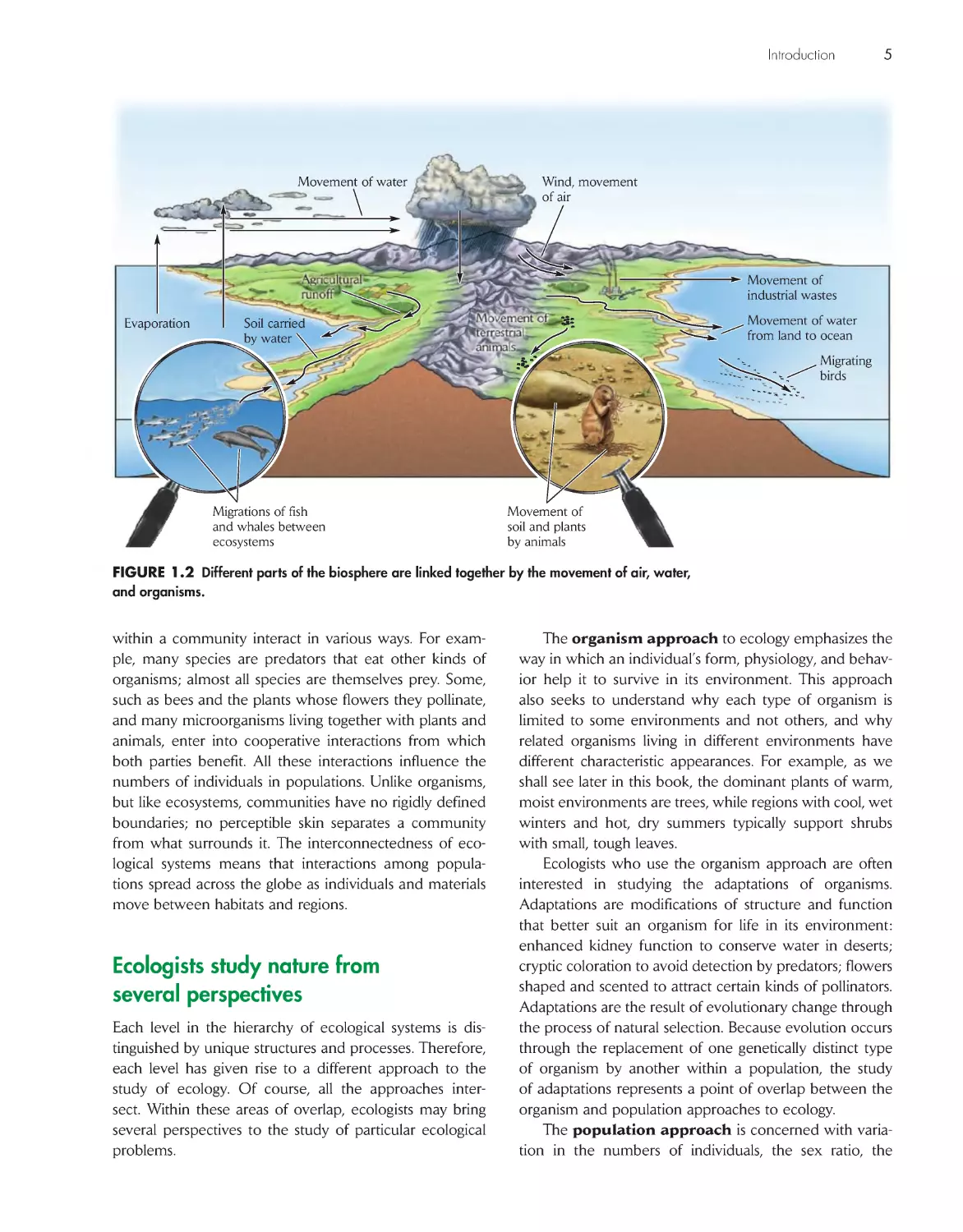
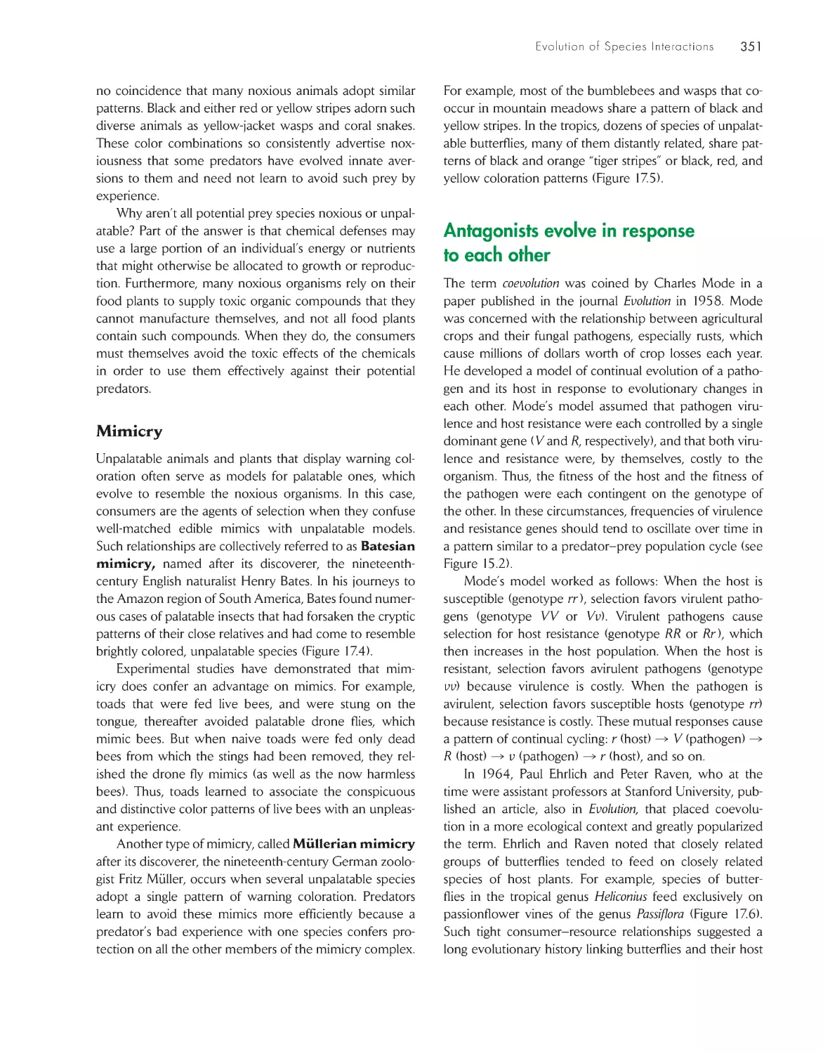
The largest and most conspicuous forms of life, plants
and animals, perform a large share of the energy trans-
formations within the biosphere, but no more so than the
countless microorganisms in soils, water, and sediments.
The characteristics that distinguish plants, animals, fungi,
protists, and bacteria have important implications for the
way we study and come to understand nature because
different kinds of organisms have different functions in
natural systems (Figure 1.4).
Early ecosystems were dominated by bacteria of vari-
ous forms. Bacteria not only gave rise to all other forms
of life, but modified the biosphere, making it possible
for more complex forms of life to exist. Photosynthetic
bacteria present over 3 billion years ago in the earliest
ecosystems on earth produced oxygen as a by-product of
carbon dioxide assimilation. The resulting increase in oxy-
gen concentration in the atmosphere and oceans eventu-
ally permitted the evolution of complex, mobile life forms
with high metabolic requirements, which have dominated
the earth for the last 500 million years. As these new
forms of life evolved, however, their simpler ancestors
persisted because their unique biochemical capabilities
allowed them to use resources and tolerate ecological
conditions that their more complex descendants could
not. Indeed, the characteristics of modern ecosystems
depend on the activities of many varied forms of life, with
each major group filling a unique and necessary role in
the biosphere.
Eukaryotes probably evolved when
one prokaryote engulfed another
and “hijacked” its biochemical
processes for its own advantage.
Secondary symbiosis involving
the capture of red algae provided
photosynthesis capability.
Archaebacteria
Simple prokaryotic organisms lacking an organized nucleus and
other cell organelles. Adapted to living in extreme conditions of high
salt concentration, high temperature, and pH (both acid and alkaline).
Various protists
An extremely diverse group of mostly single-celled eukaryotes–organisms
having nuclear membranes and other cell organelles–ranging from slime
molds and protozoans to the photosynthetic dinoflagellates, brown algae,
and diatoms.
Red algae
Perhaps 6000 species of photosynthetic protists distinguished by several
accessory photosynthetic pigments. Predominately coastal in distribution,
the coralline algae are important reef builders.
Green algae
One of the lines of phototsynthetic protists, which are responsible
for most of the biological production in aquatic systems, and thought
to have been the ancestor of green plants.
Green plants
Complex, primarily terrestrial photosynthetic
(photoautotrophic) organisms responsible for
fixing most of the organic carbon in the biosphere.
Fungi
Primarily terrestrial heterotrophic organisms of great importance in
recycling plant detritus in ecosystems. Many forms are pathogenic and
others form important symbioses (lichens, mycorrhizae).
Animals
Aquatic and terrestrial heterotrophic organisms that feed on other
forms of life or their remains. Complexity and mobility have led to
remarkable diversification of animal life.
Eubacteria
Like archaebacteria, simple prokaryotic organisms having a wide
variety of biochemical reactions of ecological importance in cycling
elements through the ecosystem. Many forms are symbiotic or parasitic.
Common
ancestor
Origin of
mitochondrion
Origin of
plastid
Figure 1.4 Different organisms have different functions in natural systems. the major divisions
of life and their evolutionary relationships are shown by the branching pattern at left.
8
chapter 1
Plants use the energy of sunlight to
produce organic matter
All ecological systems depend on transformations of
energy. For most systems, the ultimate source of that
energy is sunlight. Plants and other photosynthetic organ-
isms use the energy of sunlight to synthesize organic mol-
ecules from carbon dioxide and water. On land, most
plants have structures with large exposed surfaces—their
leaves—to capture the energy of sunlight. Their leaves
are thin because surface area for light capture is more
important than bulk. Rigid stems support their aboveg-
round parts. To obtain carbon, terrestrial plants take up
gaseous carbon dioxide from the atmosphere. At the same
time, they lose prodigious amounts of water by evapora-
tion from their leaf tissues to the atmosphere. Thus, plants
need a steady supply to replace water lost during photo-
synthesis. Not surprisingly, most plants are firmly rooted
in the ground, in constant touch with water in the soil.
Those that are not, such as orchids and other tropical “air
plants” (epiphytes), can be actively photosynthetic only in
humid environments bathed in clouds (Figure 1.5).
Animals feed on other organisms or
their remains
The organic carbon produced by photosynthesis provides
food, either directly or indirectly, for the rest of the eco-
logical community. Some animals consume plants; some
consume animals that have eaten plants; others, such as fly
larvae, consume the dead remains of plants or animals.
Animals and plants differ in many important ways
besides their sources of energy (Figure 1.6). Animals, like
plants, need large surfaces for exchanging substances with
their environment. However, because they don’t need to
capture light as an energy source, their exchange surfaces
can be enclosed within the body. A modest pair of human
lungs has a surface area of about 100 square meters,
which is half the size of a tennis court. By internalizing
their exchange surfaces in lungs, gills, and guts, animals
can achieve bulk and streamlined body shapes, and they
can develop the skeletal and muscular systems that make
mobility possible. In addition, the internalized exchange
surfaces of terrestrial animals lose less water by evapora-
tion than do the exposed leaves of plants, so that animals
need not be continuously supplied with water.
Fungi are highly effective decomposers
The fungi assume unique roles in the ecosystem because
of their distinctive growth form. Fungi, like plants and ani-
mals, are multicellular (except for the unicellular yeasts and
their relatives). Most fungal organisms consist of threadlike
structures called hyphae that are only a single cell in diam-
eter. These hyphae may form a loose network, which can
invade plant or animal tissues or dead leaves and wood
on the soil surface, or they can grow together into the
reproductive structures that we recognize as mushrooms
(Figure 1.7). Because fungal hyphae can penetrate deeply,
they readily decompose dead plant material, eventually
Figure 1.5 Epiphytic air plants grow high above the
ground on the limbs of trees in tropical rain forests. photo by
r. e. ricklefs.
Figure 1.6 Plants derive their energy from sunlight, and
animals derive their energy from plants. a mammal browsing
on vegetation on a savanna in east africa emphasizes the
fundamental differences between plants, which assimilate the
energy of sunlight and use it to convert atmospheric carbon
dioxide into organic carbon compounds, and animals, which
derive their energy ultimately from the production of plants.
photo by r. e . ricklefs.
9
Introduction
making its nutrients available to other organisms. Fungi
digest their foods externally, secreting acids and enzymes
into their immediate surroundings, cutting through dead
wood and dissolving recalcitrant nutrients from soil min-
erals. Fungi are the primary agents of rot—unpleasant to
our senses and sensibilities, perhaps, but very important to
ecosystem functioning.
Protists are the single-celled ancestors of
more complex life forms
The protists are a highly diverse group of mostly single-
celled eukaryotic organisms that includes the algae, slime
molds, and protozoans. The bewildering variety of pro-
tists fills almost every ecological role. For instance, algae,
including the single-celled diatoms, are the primary pho-
tosynthetic organisms in most aquatic systems. Algae can
also form large plantlike structures—some seaweeds can
be up to 100 meters in length (see, for example, Figure
1.16)—but their cells are not organized into the special-
ized tissues and organs that one sees in plants.
The other members of this group are not photosyn-
thetic. Foraminifera and radiolarians are protozoans that
feed on tiny particles of organic matter or absorb small
dissolved organic molecules, and that secrete shells of cal-
cite or silicate. Some of the ciliate protozoans are effective
predators—on other microorganisms, of course. Many
protists are commensal or parasitic, living in the guts or
tissues of their host organisms. Some of these, such as
the Plasmodium organism responsible for human malaria,
cause debilitating diseases.
Bacteria have a wide variety of
biochemical mechanisms for
energy transformations
Bacteria are the biochemical specialists of the ecosystem.
Each bacterium consists of a simple, single cell without a
nucleus to contain its DNA and lacking any other intra-
cellular membranes and organelles. Nonetheless, the
enormous range of metabolic capabilities of the diverse
bacteria, as well as their minute size, enables them to
accomplish many unique biochemical transformations
and occupy parts of the ecosystem that larger organisms
cannot. Some bacteria can assimilate molecular nitrogen
(N2, the common form found in the atmosphere), which
they use to synthesize proteins and nucleic acids. Others
can use inorganic compounds such as hydrogen sulfide
(H2S) as sources of energy. Plants, animals, fungi, and most
protists cannot accomplish these feats. Furthermore, many
bacteria live under anaerobic conditions (lacking free oxy-
gen) in mucky soils and sediments, where their metabolic
activities regenerate nutrients, making them available for
plants. We will have much more to say about the special
place of bacteria in the functioning of the ecosystem later
in this book.
Many types of organisms cooperate
in nature
Because each type of organism is specialized for a par-
ticular way of life, it is not surprising that many different
types of organisms live together in close association. A
close physical relationship between two different types
of organisms is referred to as a symbiosis. When each
partner in a symbiosis provides something that the other
lacks, their relationship is called a mutualism. Some
familiar examples include lichens, which comprise a fun-
gus and an alga in one organism (Figure 1.8); bacteria
that ferment plant material in the guts of cows; protozo-
ans that digest wood in the guts of termites; fungi associ-
ated with the roots of plants that help them to extract
mineral nutrients from the soil in return for carbohydrate
energy from the plant; photosynthetic algae in the flesh
of corals and giant clams; and nitrogen-fixing bacteria in
the root nodules of legumes. The specialized organelles
so characteristic of the eukaryotic cell—chloroplasts for
photosynthesis, mitochondria for various oxidative energy
transformations—originated as symbiotic bacteria living
within the cytoplasm of host cells.
Figure 1.7 Fungi are effective decomposers. the
mushrooms produced by this sulphur tuft fungus (Hypholoma
fasciculare) in Belgium are fruiting bodies produced by the
much larger, unseen masses of threadlike hyphae that penetrate
decaying wood and leaf litter. photo by philippe clement/Nature
picture Library.
chapter 1
Parasites live in all types of organisms
The line between mutualism and parasitism—that is,
living off another organism without giving back in equal
amount—is often crossed. Parasites are live-in preda-
tors. Because their futures depend on the survival of their
hosts, they rarely kill the host organism outright, but rather
consume small amounts of host tissue or nutrients. When
parasites cause disease symptoms, they are called patho-
gens. From the standpoint of a parasite, organisms such
as humans are walking grocery stores filled with an abun-
dance of well-prepared food. Even tiny bacteria are beset
by a plethora of even smaller viruses. Parasites are eco-
logically unique: living in relative ease within a host, they
are able to shed many functions needed in the outside
world, yet they must often adopt complicated life cycles
to find new hosts. Parasites may be adapted to living in
the external environment during one life stage or even to
using other animals to transport themselves from one host
to another. Malaria parasites, for example, infect mosqui-
toes during one life stage as a means of getting from one
human to another. Or, perhaps, they use humans to get
from one mosquito to the next.
Upper layer of
fungal hyphae
Loose layer of
fungal hyphae
Lower layer of
fungal hyphae
Algal cells form
photosynthetic layer
Substratum
Figure 1.8 A lichen is a symbiotic association of a fungus
and a green alga. photo by r. e. ricklefs.
Figure 1.9 Terrestrial habitats are distinguished by
their dominant vegetation. (a) In the tropical rain forest,
warm temperatures and abundant rainfall support the highest
productivity and biodiversity on earth. (b) In tropical seasonal
forest habitats, trees shed their leaves during the pronounced
dry season to avoid water stress. (c) tropical grasslands, which
develop where rainfall is sparse, nonetheless support vast herds
of grazing herbivores during the productive rainy season.
(d) Freezing temperatures on the antarctic ice cap preclude all
life except for occasional bacteria in crevices of sun-warmed
exposed rock. photos by r. e . ricklefs.
(a)
(b)
(c)
(d)
10
Introduction
11
The habitat defines an organism’s
place in nature; the niche defines
its functional role
Ecologists have found it useful to distinguish between
where an organism lives and what it does. The habitat
of an organism is the place, or physical setting, in which it
lives. Habitats are distinguished by conspicuous structural
features, often including the predominant form of plant
life or, sometimes, animal life (Figure 1.9). Thus, we speak
of forest habitats, desert habitats, and coral reef habitats.
During ecology’s early years, much effort was devoted
to classifying habitats. For example, ecologists distinguish
terrestrial and aquatic habitats; among aquatic habitats,
freshwater and marine; among marine habitats, ocean and
estuary; among ocean habitats, benthic (on or within the
ocean bottom) and pelagic (in the open sea); and so on.
However, as such classifications became more complex,
they ultimately broke down, because habitat types over-
lap broadly and absolute distinctions between them rarely
exist. The idea of habitat is nonetheless useful because
it emphasizes the variety of conditions to which organ-
isms are exposed. Inhabitants of abyssal ocean depths and
tropical rain forest canopies experience altogether differ-
ent conditions of light, pressure, temperature, oxygen con-
centration, moisture, viscosity, and salt concentrations, not
to mention food resources and enemies.
An organism’s niche represents the range of condi-
tions it can tolerate and the ways of life it pursues—that
is, its role in the ecological system. An important prin-
ciple of ecology is that each species has a distinct niche
(Figure 1.10). No two species are exactly the same, because
each has distinctive attributes of form and function that
determine the conditions it can tolerate, how it feeds, and
how it escapes its enemies.
The variety of habitats holds the key to much of the
diversity of living organisms. No one organism can live
under all the conditions on earth; each must specialize
with respect to both the range of habitats within which
it can live and the niche that it can occupy within a
habitat.
Ecological systems and processes have
characteristic scales in time and space
Most properties of the environment, such as air tempera-
ture or the number of individuals in a population per
unit of area, vary from one place to the next and from
one moment to the next. As a result, each measurement
exhibits highs and lows, and successive highs or lows are
separated by short or long intervals in time or distances
in space. Variation in each measurement exhibits a char-
acteristic scale, which is the dimension in time or space
over which the variation is perceived. It is important to
select the appropriate scale of measurement to match
the scale of variation of an ecological pattern in either
time or space. For example, over time, air temperature
can plunge dramatically in a matter of hours as a cold
front passes through a region, whereas ocean water may
require weeks or months to cool the same amount. Eco-
logical studies focus on patterns and processes occur-
ring on time scales of hours, weeks, months, and years
and spatial scales of millimeters, meters, and kilometers.
Biospheric processes and evolutionary change, however,
occupy vastly larger scales. Only large networks of col-
laborating investigators can work on these scales, and
they must use special technologies to probe deep time
and vast areas and to process the mountains of data now
available.
(a)
(b)(
c)
Figure 1.10 Each species has a distinct niche. (a) this
peruvian rhinoceros katydid (Copiphora rhinoceros) is specialized
for chewing leaves. (b) these aphids are specialized for sucking
juices from vessels in the stems and leaves of milkweed plants.
(c) Ichneumonid wasps, such as this species of Thalessa from
Ohio, lay their eggs in the larvae of beetles burrowing deep
within wood. photo (a) by Nature’s Images/photo researchers; photo
(b) by Scott camazine/photo researchers; photo (c) by Gary Maszaros/
Visuals Unlimited.
12
chapter 1
Temporal variation
We perceive temporal variation as our environment
changes over time, for example, with the alternation of
day and night and with the seasonal progression of tem-
perature and precipitation. Superimposed on these more
or less predictable cycles are irregular and unpredictable
variations, such as droughts and fires, as well as long-term
trends, such as the current warming of the earth’s climate.
The term climate refers to average atmospheric conditions
over long periods, whereas weather refers to atmospheric
phenomena that vary over periods of days or hours. Win-
ter climates are generally cold and wet, but the weather at
any particular time cannot be predicted much in advance;
it varies perceptibly over intervals of a few hours or days
with the passage of cold fronts and other atmospheric
phenomena. Some irregularities in conditions, such as a
string of especially wet or dry years, occur over long peri-
ods. Other events of great local ecological consequence,
such as fires and tornadoes, strike a particular place only
at very long intervals.
How organisms and populations respond to change
in their environment depends on how often it occurs. In
general, the more extreme the condition, the less frequent
it is. However, both the severity and the frequency of
events are relative measures, depending on the organism
that experiences them. Forest fires may touch an individ-
ual tree many times, but skip dozens of generations of an
insect population.
Patterns of temporal variation may be intrinsic to an
ecological system or imposed by variation in external fac-
tors. In pine woodlands, for example, the probability of
a destructive fire increases with time since the last such
event. As litter and other fuels accumulate and burn, they
produce a characteristic fire cycle. Similarly, a communi-
cable disease may spread through a population at regular
intervals, reappearing whenever there are enough young
individuals lacking immunity gained from previous expo-
sure. Such processes within ecological systems help to
regulate their temporal dynamics.
Spatial variation
The environment also differs from place to place. Varia-
tions in climate, topography, and soil type cause large-
scale heterogeneity (across meters to hundreds of kilome-
ters; see the variation in water temperature in the western
Atlantic Ocean illustrated in Figure 1.3) . At smaller scales,
heterogeneity is generated by the structures of plants, the
activities of animals, and the content of soils. As with tem-
poral variation, a particular scale of spatial variation may
be important to one organism and not to another. The
difference between the top and the underside of a leaf is
important to an aphid, but not to a moose, which happily
eats the whole leaf, aphid and all.
As an individual moves through an environment that
varies in space, it encounters environmental variation as
a sequence in time. In other words, a moving individual
perceives spatial variation as temporal variation. The faster
an individual moves, and the smaller the scale of spatial
variation, the more quickly it encounters new environ-
mental conditions, and the shorter the temporal scale of
the variation. This principle applies to plants as well as to
animals. Roots growing through soil may encounter new
conditions if the scale of spatial variation in soil character-
istics is small enough. Wind and animals disperse seeds,
which may land in a variety of habitats depending on how
far they travel relative to the scale of spatial variation in
the habitat.
Correlation of spatial and
temporal dimensions
With regard to ecologically important phenomena, dura-
tion in time usually increases with the extent of the space
affected. For example, tornadoes last only a few minutes
and affect small areas, whereas hurricanes inflict devasta-
tion across hundreds of kilometers over days or weeks. In
the oceans, at one extreme, small eddy currents may last
only a few days; at the other extreme, ocean gyres (cir-
culating currents encompassing entire ocean basins) are
stable over millennia.
Compared with marine and, especially, atmospheric
phenomena, variations in landforms have very long tem-
poral scales at any spatial scale. The reason is simply that
topography and geology are transformed at a snail’s pace
by such processes as mountain building, volcanic erup-
tions, erosion, and even continental drift. In contrast, spa-
tial heterogeneity in the open ocean results from physical
processes in water, which are obviously more changeable
than those in rock and soil. Because air is even more fluid
than water, atmospheric processes have very short time
scales at a given spatial scale.
The spatial and temporal scales of patterns that we
measure in nature often match the scales of the processes
that produce them. For example, the large-scale processes
of species formation and extinction create a global pattern
of increasing species richness in most groups of organisms
from high latitudes to the equator. The formation of new
species generally requires evolutionary periods of time
and continental scales of space (new species do not form
readily on individual small islands, for example), and the
Introduction
13
extinction of species under natural circumstances might
result from millennial or even slower changes in climate
and environment. At the other extreme, the distribution
of individuals within a population depends on behavioral
responses of individuals to variations in the environment
and the presence of other individuals over periods of
hours, minutes, and seconds.
Ecological systems are governed by
basic physical and biological principles
With all of these ongoing patterns and processes, ecologi-
cal systems are busy places, yet these dynamic and com-
plex systems are governed by a small number of basic
principles. A brief consideration of four of these principles
will help to illustrate the underlying unity of ecology.
Ecological systems obey the
laws of physics
Life builds on the physical properties and chemical reac-
tions of matter. The diffusion of oxygen across body
surfaces, the rates of chemical reactions, the resistance
of vessels to the flow of fluids, and the transmission of
nerve impulses all obey the laws of thermodynamics. Bio-
logical systems are powerless to alter these fundamental
properties of matter and energy, but, within the broad
limits imposed by these constraints, life can pursue many
options, and it has done so with astounding invention.
Ecological systems exist in
dynamic states
Whether we focus on the organism, the population, the
community, the ecosystem, or the biosphere, each of these
ecological systems continuously exchanges matter and
energy with its surroundings. When gains and losses are
balanced, ecological systems remain unchanged. This bal-
ance is the essence of a dynamic steady state. A warm-
blooded animal continuously loses heat to a cold environ-
ment. This loss is balanced, however, by heat gained from
the metabolism of foods, so body temperature remains
constant. The proteins of our bodies are continuously bro-
ken down and replaced by newly synthesized proteins,
yet our appearance does not change.
This principle of the steady state applies to all levels
of ecological organization. For the individual organism,
assimilated food and energy must balance energy expen-
diture and metabolic breakdown of tissues. For the popu-
lation, gains and losses are births and deaths. The diversity
of a community decreases when species become extinct,
and it increases when new species invade the commu-
nity’s habitat. Ecosystems and the biosphere itself could
not exist without the energy received from the sun, yet
this gain is balanced by heat energy radiated by the earth
back out into space. How the steady states of ecological
systems are maintained and regulated is one of the most
important questions posed by ecologists, one to which we
will return frequently throughout this book.
Of course, ecological systems also change. Organisms
grow; populations cycle in abundance; abandoned fields
revert to forest. Yet all ecological systems have mecha-
nisms that tend to maintain their integrity.
Living systems must expend energy to
maintain themselves
Because life is so special—consider that the molecules
of life are rare or nonexistent in the physical world—
living organisms exist out of equilibrium with the physical
environment. What the organism loses to its surroundings,
however, is not returned by the environment for free. If it
were, life would be the equivalent of a perpetual motion
machine. The organism must procure energy or materials
to replace its losses. To do this, it must expend energy.
Thus, it must replace the energy lost as heat and motion
by metabolizing food or stored reserves, which it must
expend energy to capture and assimilate. The price of
maintaining a living system in a dynamic state is energy.
Ecological systems evolve over time
Over the history of life on earth, the attributes of organ-
isms have changed and diversified dramatically through
the process of evolution. Although the physical and
chemical properties of matter and energy are immutable,
what living systems do with matter and energy is as vari-
able as all the forms of organisms that have existed in
the past, are alive today, or might exist in the future. The
structures and functions of those organisms are products
of evolutionary change in populations in response to their
particular environments. For example, prey animals are
often colored in such a way that they blend in with their
surroundings and escape the notice of predators (Figure
1.11). Many plants in hot, dry climates have small leaves
with waxy surfaces to reduce water loss by evaporation.
Such attributes of structure and function that suit an
organism to the conditions of its environment are called
adaptations.
The close correspondence of organisms to their envi-
ronments is no accident. It derives from a process unique
14
chapter 1
to biological systems: natural selection. Only individu-
als that are well suited to their environments survive and
produce offspring. The favorable traits inherited by their
progeny are preserved. Other individuals survive less
well or produce fewer offspring, and their less suitable
traits are not passed on. Charles Darwin recognized that
this process allowed populations to respond, over many
generations, to changes in their environment. A wonder-
ful thing about natural selection and evolution is that as
each species changes, new possibilities for further change
are opened up for itself and for other species with which
it interacts. In this way, the complexity of ecological
communities and ecosystems builds on, and is fostered
by, existing complexity. An important goal of ecology as
a science is to understand how these complex ecological
systems came into being and how they function in their
environmental settings.
Ecologists study the natural world by
obser vation and experimentation
Like other scientists, ecologists apply many methods to
learn about nature. Most of these methods reflect three
facets of scientific investigation, often referred to as
the scientific method: (1) observation and description,
(2) development of hypotheses or explanations, and
(3) testing of these hypotheses, often with experiments.
Most research programs begin with a set of obser-
vations about nature that invite explanation or specu-
lation. Usually these facts describe a consistent pattern.
For example, measurements of plant production in vari-
ous parts of the world show a strong positive relation-
ship between plant growth and precipitation, which we
would expect because we know that plants require water.
In the wettest areas of the tropics, however, plant produc-
tion decreases. This unexpected finding clearly cannot be
accounted for by an explanation based on replenishment
of the water lost to evaporation. We’ll discuss some pos-
sibilities later in this book. Even a simple observation can
stimulate speculation. For example, ecologists (as well as
farmers and gardeners) have long known that insects feed
on plants, typically removing about 10% of the leaf bio-
mass of trees. Many years ago, ecologists wondered why
insects and other herbivores didn’t eat more than they do.
We’ll return to this question in a moment.
Hypotheses are ideas about how a system works—
that is, they are explanations. If correct, a hypothesis may
help us to understand the cause of an observed pattern.
Suppose we observe that male frogs sing on warm nights
after periods of rain. If a reasonable amount of observa-
tion produces few exceptions to this pattern, it may be
regarded as a generalization that enables us to predict
the behavior of frogs from the weather. Having estab-
lished the existence of such a pattern, we may wish to
understand it better. For example, we may wish to explain
how a frog responds to temperature and rainfall; we may
Figure 1.11 Adaptations help organisms to sur vive in
their environments. (a) the cryptic coloration of a costa rican
mantid protects it from predators. (b) the waxy, succulent leaves
of the South american wax agave (Echeveria agavoides;
crassulaceae) reduce water loss in its arid environment. photo
(a) by Michael Fogden/DrK; photo (b) by peter anderson, DK Limited/
cOrBIS.
(a)
(b)
Introduction
15
also wish to explain why a frog responds the way it does.
The “how” part of this particular phenomenon involves
details of sensory perception, the interplay between envi-
ronmental stimuli and the frog’s hormonal status, and the
frog’s nervous system and muscles—in other words, it
involves physiological processes and the proximate fac-
tors in the environment that stimulate the frog’s behavior.
The “why” question addresses the costs and benefits of
the behavior to the individual and deals with ultimate
factors in the environment that guide evolution—
factors such as predators and female frogs, both of which
are attracted to singing males, but for different reasons.
If we suspect that male frogs sing to attract females, per-
haps males sing on warm nights after rains because that
is when females look for mates. If frogs chorused at other
times, they might attract few mates (low benefit) but still
expose themselves to predation or other risks (high cost).
We have now generated a number of hypotheses about
frog behavior: (1) singing by males attracts females and
leads to mating; (2) females actively search for males only
on warm nights after rains (perhaps because those nights
produce the best conditions for laying eggs); (3) singing
imposes a cost, which compels males to save their singing
for times when it will do them the most good.
Using experimental manipulations to
test hypotheses
If we are to convince ourselves that a hypothesis is valid,
we must put it to the test. Only rarely can a particular idea
be proved beyond a doubt, but our confidence increases
as we explore the implications of a hypothesis and find it
to be consistent with the facts. Let’s return to the ques-
tion of insect herbivores and plants. We are surprised to
observe that herbivores consume so little plant biomass.
Two ideas come to mind. The first is that plants defend
themselves against herbivores, not by running and hid-
ing, but by synthesizing various chemicals to reduce their
palatability. These defenses not only deter individual her-
bivores from feeding, but by doing so, they also check
herbivore population growth. The second idea is that
predators reduce herbivore populations and keep them
from overeating their food plants. Both of these ideas are
hypotheses about how an ecological system works.
Robert Marquis and Chris Whelan of the University of
Missouri at St. Louis became interested in whether the pre-
dation hypothesis (which is also referred to as “top-down
control” of herbivore populations) applied to insects feed-
ing on oak trees in Missouri. They had observed that birds
consume many insects on oak foliage, and they specu-
lated that the avian predators controlled the insect herbi-
vore populations. They predicted that if their hypothesis
was correct, then insect populations should increase and
consume more leaf biomass if the birds were removed.
A prediction is a statement that follows logically from
a hypothesis. If Marquis and Whelan could confirm their
prediction, their hypothesis would be strengthened; if not,
their hypothesis would be weakened, or perhaps it might
be rejected altogether.
Because many hypotheses are plausible, it is necessary
to conduct investigations to determine which explanations
best account for the facts. The strongest tests of hypothe-
ses are often experiments, in which one or a small num-
ber of variables are manipulated independently of others
to reveal their particular effects. To test their hypothesis,
Marquis and Whelan constructed bird-proof cages around
oak trees (Figure 1.12) that excluded birds from the foli-
age, but allowed insects to pass through freely. The num-
ber of insects and the amount of leaf damage inside the
cages were then monitored through the summer growing
season. Of course, insect populations could be influenced
by variables other than predation, such as the weather.
So Marquis and Whelan also monitored neighboring trees
without exclusion cages to account for spatial and tem-
poral variation in insect populations. Such a treatment,
which reproduces all aspects of an experiment except the
variable of interest (bird exclusion), is called a control.
Similarly, because the cages might have effects on the foli-
age other than bird exclusion (shading, for example), the
investigators also enclosed some trees within incomplete
cages that allowed birds access to the foliage. This third
Figure 1.12 Experiments are the strongest tests of
hypotheses. a cage has been placed around a white oak
sapling to exclude bird predators that would other wise consume
caterpillars feeding on its leaves. courtesy of c. Whelan, from
r. J. Marquis and c. Whelan, Ecology 75:2007–2014 (1994).
chapter 1
16
set of trees provided a control for experimental effects.
Finally, to make sure that their results were repeatable,
the investigators applied the experimental treatments to
several trees, with a similar number of trees designated
as controls.
Marquis and Whelan found that the numbers of insects
recorded on the trees from which birds were excluded
were 70% higher than on the control trees, and that the
percentage of leaf area missing at the end of the growing
season jumped from 22% on the control trees to 35% on
the experimental trees. These findings led them to con-
clude that avian predators do reduce the abundance of
insect herbivores as well as the damage caused by herbi-
vores to trees. Thus, the experiments confirmed the inves-
tigators’ predictions and strengthened their hypothesis. It
did not, however, address the alternative hypothesis that
defensive chemicals produced by plants also reduce insect
herbivory. This hypothesis will require separate testing,
as we shall see later in this book. The finding that birds
reduce insect herbivores suggests another question: Bird
populations are declining in response to forest fragmenta-
tion in the eastern United States and elsewhere. Will insect
damage to the remaining forest increase as a result?
Alternative approaches to
hypothesis testing
Although the methods of acquiring scientific knowl-
edge appear to be straightforward, many pitfalls exist.
For example, a correlation between variables does not
imply a causal relationship; the mechanism of causation
must be determined independently by suitable investiga-
tion. In addition, many hypotheses cannot be tested by
experimental methods because the scales of the relevant
processes are too large, or the important variables cannot
be isolated because suitable controls cannot be devised.
These limitations become particularly restrictive with pat-
terns that have evolved over long periods and with sys-
tems such as entire populations or ecosystems that are too
large for practical manipulation.
Different hypotheses might explain a particular obser-
vation equally well, so investigators must make predictions
that distinguish among the alternatives. Of course, more
than one mechanism might produce a pattern, in which
case more than one hypothesis would be supported. For
example, the observed decrease in species richness at
higher latitudes has many potential explanations. As one
travels north from the equator, average temperature and
precipitation decrease, sunlight and biological production
decrease, and seasonality and other environmental varia-
tions increase. Each of these factors could interact with
ecological systems in ways that could affect the numbers
of species that can coexist in a locality, and dozens of
hypotheses based on these factors and invoking vari-
ous ecological and evolutionary mechanisms have been
proposed. Isolating the effect of each factor has proved
difficult because each tends to vary in parallel with the
others.
Faced with these difficulties, ecologists have resorted
to several alternative approaches to hypothesis testing.
One of these is the natural experiment, which relies
on natural variation in the environment to create reason-
ably controlled experimental treatments. For example,
the hypothesis that the number of species on an island
is influenced by the rate at which new colonists arrive
there from continental source areas has been “tested” by
comparing species diversity on islands with similar sizes
and habitats but at different distances from continental
coasts. As predicted, diversity decreases with distance
from a continent.
Another approach is the microcosm experiment,
which attempts to replicate the essential features of an
ecological system in a simplified laboratory or field setting
(Figure 1.13). It assumes that an aquarium with five animal
species will behave like the more complex natural system
in a pond, or even like ecological systems more generally.
If so, experimental manipulations of the microcosm may
yield results that can be generalized to the larger system.
For example, the hypothesis that diversity decreases as
temporal variation in the environment increases might
be approached in a microcosm experiment by varying
Figure 1.13 Microcosm experiments are designed to
replicate the essential features of an ecological system.
communities of freshwater invertebrates are housed in cattle
tanks at the Kellogg Biological Station of Michigan State
University. Numerous tanks are used for replicates of different
experimental treatments. photo by r. e . ricklefs.
Introduction
17
temperature, light, acidity, or nutrient resource conditions
and observing whether some species disappear from the
system. It may be a stretch to generalize from an aquarium
to a “real” ecological system, but if such variation consis-
tently resulted in a loss of species in a variety of micro-
cosms, the hypothesis would be strengthened.
Ecologists have also used mathematical models to
explore the behavior of complex systems. The investigator
represents such a system as a set of equations correspond-
ing to the postulated relationships of each of the system’s
components to other components and to outside influ-
ences. In this sense, a mathematical model is a hypoth-
esis; it provides an explanation of the observed structure
and functioning of the system. We can test models by
comparing the predictions they yield with observations.
Most models make predictions about attributes of a sys-
tem that have not been measured or about the response
of the system to perturbation. Whether these predictions
are consistent with observations determines whether
the hypothesis on which they are based is supported or
rejected. For example, epidemiologists have developed
models to describe the spread of communicable diseases.
These models include such factors as the proportions of
a population that are susceptible, exposed, infectious, and
recovered (and thus resistant because of acquired immu-
nity), as well as rates of transmission and the virulence
of the disease organism. Such models are able to make
predictions about the frequency and severity of disease
outbreaks, and these predictions can be compared with
observations to test the models.
At a larger scale, ecologists have created global car-
bon balance models to investigate how the burning of
fossil fuels affects the carbon dioxide content of the atmo-
sphere. Understanding this relationship is critically impor-
tant to managing human impacts on our environment.
Global carbon balance models include, among other fac-
tors, equations for the uptake of carbon dioxide by plants
and the dissolution of carbon dioxide in the oceans. The
output of early versions of these models failed to match
observations; specifically, the models overestimated the
annual increase in atmospheric carbon dioxide concentra-
tions. The real world evidently contains carbon dioxide
“sinks” that remove the gas from the atmosphere but were
not accurately represented in the model. This discrepancy
has caused ecosystem modelers to look more closely
at processes such as the regeneration of forests and the
movement of carbon dioxide across the air–water inter-
face. Such processes have been updated in the models to
create more refined descriptions of the functioning of the
biosphere and more accurate predictions of the future of
atmospheric change.
Humans are a prominent part
of the biosphere
Why do ecologists do all this? The wonders of the natural
world summon our natural curiosity about life and our
surroundings. For many of us, our curiosity about nature
and the challenges of its study are reason enough. In addi-
tion, however, our need to understand nature is becom-
ing more and more urgent as the growing human popula-
tion stresses the capacity of natural systems to maintain
their structure and functioning. Environments that human
activities either dominate or have produced—including
our urban and suburban living places, our agricultural
breadbaskets, and our recreational areas, tree farms, and
fisheries—are also ecological systems. The welfare of
humanity depends on maintaining the functioning of
these systems, whether they are natural or artificial. Virtu-
ally all of the earth’s surface is, or soon will be, strongly
influenced by people, if not fully under their control.
Already, humans usurp nearly half of the biological pro-
duction of the biosphere. We cannot take this responsibil-
ity lightly.
The human population is approaching the 7 billion
mark, and it consumes energy and resources, and pro-
duces wastes, far in excess of needs dictated by biologi-
cal metabolism. These activities have caused two related
problems of global dimensions. The first is their impact
on natural systems, including the disruption of ecological
processes and the extermination of species. The second
is the steady deterioration of humankind’s own environ-
ment as we push the limits of what ecological systems can
sustain. Understanding ecological principles is a necessary
step in dealing with these problems. Two examples drive
this point home.
EcOlOgisTs
in THE FiElD
introduction of the nile perch into
lake Victoria. During the 1950s and
early 1960s, the Nile perch (Lates niloticus) and Nile tila-
pia (Oreochromis niloticus) were introduced into Lake Vic-
toria, a large, shallow lake straddling the equator in East
Africa. The introduction was intended to provide addition-
al food for the people living in the area and additional
income from exporting the surplus catch (Figure 1.14).
During the 1980s, the population of Nile perch increased
dramatically, and the burgeoning fisher y attracted many
people to the region surrounding Lake Victoria. Indeed, by
2003, the fisher y was producing exports to the European
Union valued at almost 170 million euros annually. How-
ever, because basic ecological principles were ignored,
the introduction ended up destroying most of the lake’s
18
chapter 1
traditional fisher y and eventually led to the demise of the
new fisher y as well.
Until the introduction of the Nile perch, Lake Victoria
supported a sustainable catch of a variety of local fishes,
mostly species belonging to the family Cichlidae. One of
these native species was a tilapia that feeds primarily on
dead organic matter, plants, and small aquatic inverte-
brates. Nile perch are ver y large, and they eat vast quan-
tities of other fish: the smaller cichlids, in this instance.
Moreover, because energy is lost with each step in the
food chain, predator y fish populations cannot be har vest-
ed at as high a rate as their prey species, even though they
may be easier to catch. Because the Nile perch was alien
to Lake Victoria, the local cichlids had few adaptations
to help them escape this predator. Inevitably, the perch
annihilated the cichlid populations, driving many unique
species to extinction, destroying the native fisher y, and
severely reducing its own food supply. Consequently, the
perch’s voracious habits among defenseless prey brought
about its own demise as an exploitable fish species and
completely changed the Lake Victoria ecosystem.
At the present time, the Nile perch fisher y in Lake Vic-
toria has collapsed. Introduction of the Nile perch had
secondar y consequences for the terrestrial ecosystems sur-
rounding the lake as well. The flesh of the perch is oily and
must be preser ved by smoking rather than sun drying, so
local forests were cut for firewood. To be sure, the native
fisher y was already precariously close to being overex-
ploited as a result of the growing local human population
and the use of advanced, nontraditional fishing technol-
ogies. However, rather than by introducing an efficient
predator on the local fishes, these problems might have
been more appropriately addressed by regulating fishing
methods, enforcing limits on the total annual catch of local
fishes, and developing alternative non-fish food sources.
EcOlOgisTs
in THE FiElD
The california sea otter. Half a world
away from Lake Victoria, efforts to
save the sea otter (Enhydra lutris) along the coast of Cali-
fornia illustrate the intricate intermingling of ecology and
other human concerns (Figure 1.15). The sea otter was
once widely distributed around the northern Pacific Rim
from Japan to Baja California. In the 1700s and 1800s,
intense hunting for otter pelts reduced the population near-
ly to extinction. Predictably, the fur industry collapsed as it
overexploited its economic base. Following the rediscov-
ery of a small population in the 1930s, the California sea
otter population was placed under strict protection. It had
increased to several thousand individuals by the 1990s,
but it is now decreasing again.
Initially, the sea otter’s recover y irked some Califor-
nia fishers, who claim that the otters—which do not need
commercial fishing licenses—drastically reduce stocks of
valuable abalone, sea urchins, and spiny lobsters. Matters
deteriorated at one point to the marine equivalent of a
range war between the fishing industry and conser vation-
ists, with the otter caught in the line of fire, often fatally.
Ironically, the otters benefited one commercial marine
enterprise: the har vesting of kelps. Kelps, which are large
seaweeds often used in making fertilizer, grow in shallow
water in stands called kelp forests, which provide refuge
and feeding grounds for larval fish (Figure 1.16). Kelps
are also grazed by sea urchins, which, when abundant,
can denude an area. The sea otter is a principal preda-
tor of sea urchins. When the expanding otter population
spread into new areas, the otters kept urchin populations
in check, and kelp forests could regrow.
In recent years, the gill nets used to exploit a newly
developed fisher y along the California coast inadvertently
killed otters in substantial numbers until new legislation
moved the fisher y farther offshore. Recent otter deaths
have been attributed to the protozoan parasites Toxo-
plasma gondii and Sarcocystis neurona. These parasites
Figure 1.14 The introduction of a new species into an
ecosystem can have drastic effects. Nile perch were introduced
into Lake Victoria in the 1950s to improve the local fishery, but
they have driven many native fishes to extinction and completely
changed the ecosystem of the lake. photo courtesy of tim Baily/the
african angler and Joe Bucher tackle company.
Africa
Lake Victoria
Tanzania
Kenya
Uganda
Introduction
19
normally infect cats, but might have entered the marine
ecosystem by way of kitty litter flushed through the sewer
system.
Elsewhere, where other factors are at work, the otter
population is also dwindling. In a report published in 1998
in the journal Science, J. A . Estes and his colleagues at the
University of California at Santa Cruz showed that popula-
tions of otters in the vicinity of the Aleutian Islands, Alaska,
had declined precipitately during the 1990s. The reason?
Killer whales, or orcas (Orcinus orca), which previously
had not preyed on otters, have been coming close to shore
and taking large numbers of them. A predictable result
of the decline in otter populations has been a dramatic
increase in urchins and decimation of kelps in affected
areas. Why did killer whales adopt this new behavior?
Estes pointed out that populations of the principal prey
of killer whales—seals and sea lions—collapsed during
the same period, perhaps inducing the whales to seek
alternative food sources. Why did the seals and sea lions
decline? One can only speculate at this point. However,
intense human fisheries have reduced fish stocks exploited
by the seals to levels low enough to seriously threaten seal
populations.
Human impacts on the natural
world have increasingly become
a focus of ecology
Although the plight of endangered species arouses us
emotionally, ecologists increasingly realize that the only
effective means of preserving natural resources is through
the conservation of entire ecological systems and the
management of large-scale ecological processes. Individual
Hunt
Eat
Protect
Nurture
Eat
Harvest
Eat
Eat
Eat
Exploit
Eat
Eat
Commercial shellfish
(abalone, lobsters)
Kelp
Sea otters
Humans
Urchins
Killer whales
Seals, sea lions
Fish
Figure 1.15 Human activities have
complex effects on ecosystems. Several
components of the otter–urchin–kelp
ecosystem are altered when humans reduce
populations of sea otters by hunting them.
after J. a . estes et al., Science 282:473–476
(1998).
Figure 1.16 The integrity of kelp forest habitat depends
on the presence of sea otters. the kelp forest provides feeding
grounds and refuge for many fishes and invertebrates. the otters
eat sea urchins that would other wise destroy young kelp. photo by
Jeff rotman/photo researchers.
20
chapter 1
species, including the ones that humans rely on for food
and other products, themselves depend on the mainte-
nance of environmental support systems. We have already
seen that predators such as the Nile perch and the sea
otter may assume key roles in the functioning of eco-
logical systems. Human activities that changed the abun-
dances of these predators have altered entire ecosystems.
Local impacts of human activities on ecological systems
can often be managed once we understand the under-
lying mechanisms responsible for change. Increasingly,
however, our activities have multiple, widespread impacts
that are more difficult for scientists to characterize and
for legislative and regulatory bodies to control. For this
reason, a sound scientific understanding of environmental
problems is a necessary prerequisite to action.
The daily newspapers are filled with environmen-
tal problems: disappearing tropical forests, depleted fish
stocks, emerging diseases, global warming. Wars create
staggering environmental catastrophe as well as human
tragedy. But there are success stories as well. Many devel-
oped countries have made great strides in cleaning up
their rivers, lakes, and air. Fish are once again migrat-
ing up the major rivers of North America and Europe
to spawn. Acid rain has decreased, thanks to changes in
the combustion of fossil fuels. The release of chlorofluo-
rocarbons, which damage the ozone layer that shields the
earth’s surface from ultraviolet radiation, has decreased
dramatically. The inevitability of global warming caused
by increasing atmospheric carbon dioxide concentrations
has set off an international research effort and provoked
global concern. Conservation efforts, including the breed-
ing of endangered species in captivity, have saved some
animals and plants from certain extinction. They have also
heightened public awareness of environmental issues, and
they have sometimes sparked public controversy. With-
out public concern and understanding, however, political
action is impossible.
Particularly encouraging is the growing level of inter-
national cooperation exemplified in such organizations
as the International Union for Conservation of Nature
(IUCN) and the World Wildlife Fund (WWF). In addi-
tion, the nations of the world have concluded important
agreements for the protection of wildlife and nature.
One of these is the Convention on International Trade in
Endangered Species (CITES), which forbids transport of
endangered species or their products (hides, feathers, and
ivory, for example) across international borders, depriving
poachers of markets. The Rio Convention on Biological
Diversity recognizes the proprietary interest of countries
in their own biological heritage and guarantees fees and
royalties for the exploitation of local plants and animals
for uses such as pharmaceutical products. The Kyoto Pro-
tocol on climate change, an agreement designed to limit
the emission of greenhouse gases, may prove to be inef-
fective, but it is an initial commitment to do something
about global change in the biosphere.
These successes would not have been possible with-
out general consensus founded on evidence produced by
scientific study of the natural world. Understanding ecol-
ogy will not by itself solve our environmental problems in
all their political, economic, and social dimensions. How-
ever, as we contemplate the need for global management
of natural systems, our effectiveness in this enterprise will
hinge on our understanding of their structure and
functioning—an understanding that depends on know-
ing the principles of ecology.
suMMAry
11. Ecology is the scientific study of the natural environ-
ment and of the relationships of organisms to one another
and to their surroundings.
12. An ecological system may be an organism, a popula-
tion, a community, an ecosystem, or the entire biosphere.
These ecological systems represent levels of organization
of ecological structure and functioning and form a hierar-
chy of progressively more complex entities.
13. Ecologists use several different approaches to study
nature, focusing on the interactions of organisms with
their environment; the resulting transformations of energy
and chemical elements in ecosystems and the biosphere;
the dynamics of populations, including evolutionary
change; and the interactions of populations within eco-
logical communities.
14. Different kinds of organisms play different roles in the
functioning of ecosystems. Plants, algae, and some bacte-
ria transform the energy of sunlight into stored chemical
energy. Animals and protozoans consume these biological
forms of energy. Fungi play an important role in decom-
posing biological materials and replenishing nutrients in
the ecosystem. Bacteria are biochemical specialists, able
to accomplish such transformations as the assimilation of
nitrogen and the use of hydrogen sulfide as an energy
source.
21
Suggested readings
15. Different kinds of organisms may form mutually ben-
eficial partnerships, as in the case of the algae and fungi
that constitute lichens. Many organisms live parasitically
on or within other organisms, feeding on their hosts’ nutri-
ents or tissues and often causing disease.
16. An individual’s habitat is the place where it lives. The
habitat concept emphasizes the structure and conditions
of the environment. An individual’s niche includes the
range of conditions that it can tolerate and the ways of
life that it can pursue—that is, its functional role in the
natural system.
17. Ecological processes and structures have characteristic
temporal and spatial scales. In general, the scales of pat-
terns and processes in time and in space are correlated;
large systems tend to change more slowly than small
systems.
18. Ecological systems are governed by a small number
of basic ecological principles. Ecological systems function
within the physical and chemical constraints governing
energy transformations. Furthermore, all ecological sys-
tems exchange materials and energy with their surround-
ings. When inputs and outputs are balanced, the system is
said to be in a dynamic steady state.
19. All living systems must expend energy to maintain their
integrity. Organisms must expend energy to replace the
energy and materials they lose through natural processes.
10. All ecological systems are subject to evolutionary
change, which results from the differential survival and
reproduction within populations of individuals that exhib-
it different genetically determined traits. As a result of
natural selection, organisms exhibit adaptations of struc-
ture and function that suit them to the conditions of their
environment.
11. Ecologists employ a variety of techniques to study nat-
ural systems. The most important of these are observation,
development of hypotheses to explain observations, and
testing of those hypotheses. Experiments are an impor-
tant tool for testing hypotheses. When natural systems do
not lend themselves readily to experimentation, ecologists
may work with microcosms or mathematical models.
12. Humans play a dominant role in the functioning of
the biosphere, and human activities have created an envi-
ronmental crisis of global proportions. Solving our acute
environmental problems will require an understanding of
the principles of ecology and their application within the
framework of political, economic, and social action.
16. Describe how ecological systems are governed by
general physical and biological principles.
17. In the Northern Hemisphere, many species of birds
fly south during the autumn months. Propose a proximate
and an ultimate cause for this behavior.
18. When experimental manipulations are conducted
to test a hypothesis, what is the purpose of including a
control?
19. In what ways do experimental manipulations differ
from natural experiments and microcosm experiments?
10. How can our knowledge of ecological systems help
humans to manage these systems?
11. Why do ecologists consider both organisms and eco-
systems to be ecological systems?
12. What are the unique processes and structures that are
examined when taking the organism, population, commu-
nity, and ecosystem approaches to studying ecology?
13. How do the sources of energy acquired by plants,
animals, and fungi differ?
14. Compare and contrast an organism’s habitat and an
organism’s niche.
15. What is the relationship between the frequency of
change in environmental conditions and the spatial extent
of the change?
rEViEw QuEsTiOns
suggEsTED rEADings
Barel, C. D . N. et al. 1985. Destruction of fisheries in Africa’s lakes.
Nature 315:19–20.
Bartholomew, G. A. 1986. The role of natural history in contempo-
rary biology. BioScience 36:324–329.
Berner, R. A. et al. 2003. Phanerozoic atmospheric oxygen. Annual
Review of Earth and Planetary Sciences 31:105–134.
Booth, W. 1988. Reintroducing a political animal. Science 2 41 :
156–158.
Cohn, J. P. 1998. Understanding sea otters. BioScience 48(3):
151–155 .
Cronon, W. (ed.) . 1996. Uncommon Ground: Rethinking the Human
Place in Nature. W. W. Norton, New York.
22
chapter 1
Estes, J. A. et al. 1998. Killer whale predation on sea otters linking
oceanic and nearshore systems. Science 282:473–476.
Franklin, J. F., C. S. Bledsoe, and J. T. Callahan. 1990. Contribu-
tions of the Long-Term Ecological Research Program. BioScience
40:509–523.
Goldschmidt, T., F. Witte, and J. Wanink. 1993. Cascading effects of
the introduced Nile perch on the detritivorous/phytoplanktivo-
rous species in the sublittoral areas of Lake Victoria. Conservation
Biology 7:686–700.
Harley, J. L . 1972. Fungi in ecosystems. Journal of Animal Ecology
41:1–16.
Kitchell, J. F. et al. 1997. The Nile perch in Lake Victoria: Interac-
tions between predation and fisheries. Ecological Applications 7(2):
653–664.
Leibold, M. A. 1995. The niche concept revisited—mechanistic
models and community context. Ecology 76:1371–1382.
Marquis, R. J ., and C. Whelan. 1994. Insectivorous birds increase
growth of white oak through consumption of leaf-chewing
insects. Ecology 75:2007–2014.
McIntosh, R. P. 1985. The Background of Ecology: Concept and Theory.
Cambridge University Press, Cambridge.
Nichols, F. H . et al. 1986. The modification of an estuary. Science
231:567–573.
Price, P. W. 1996. Empirical research and factually based theory:
What are their roles in entomology? American Entomologist 42(2):
209–214.
Reisewitz, S. E ., J. A. Estes, and C. A . Simenstad. 2006. Indirect food
web interactions: Sea otters and kelp forest fishes in the Aleutian
archipelago. Oecologia 146(4):623–631.
Schneider, D. C . 2001. The rise of the concept of scale in ecology.
BioScience 51(7):545–553.
Sinclair, A. R. E., and J. M. Frywell. 1985. The Sahel of Africa: Ecol-
ogy of a disaster. Canadian Journal of Zoology 63:987–994.
Urban, D. L., R. V. O’Neill, and H. H. Shugart, Jr. 1987. Landscape
ecology. BioScience 37:119–127.
Wilson, E. O. 1992. The Diversity of Life. W. W. Norton, New York.
Worster, D. 1994. Nature’s Economy. Cambridge University Press,
Cambridge.
23
2
chapter
Adaptations to the Physical Environment:
Water and Nutrients
Sperm whales routinely dive to depths of 500 meters, staying below the surface for
more than an hour searching for fish, squid, and other food items that are found at
these depths. Like all mammals, sperm whales breathe air to obtain oxygen. While
diving, however, a sperm whale has to rely on oxygen stored in its body. It might surprise
you to learn that ver y little of this oxygen resides in the lungs. Most of it is bound to hemo-
globin in the blood or to a similar oxygen storage molecule, myoglobin, in the muscles.
While under water, deep-diving mammals slow down their metabolism considerably by
reducing blood flow to nonvital organs, such as the skin, viscera, lungs, kidneys, and
muscles (which have their own oxygen supply bound to myoglobin); blood flow is main-
tained primarily to the brain and heart. Consequently, the temperature of all but a few
key organs drops, the heart rate slows, and demand for oxygen drops to a minimum.
If having enough oxygen is one challenge faced by deep-diving mammals, another is
keeping warm. Most deep-diving mammals living in cold waters, including the Weddell
seal, a native of Antarctic waters (Figure 2.1), are well insulated by a thick layer of fat
under the skin, which slows the conduction of heat generated by its internal organs to
the surrounding water. Unlike mammals, diving birds, such as the Adélie penguin, are
insulated against the cold by air trapped in their plumage. Although air makes great
insulation, it creates a problem for diving animals because it increases buoyancy. Imag-
ine trying to dive under water wearing a life jacket! Indeed, a penguin expends most of
its energy during a dive overcoming its positive buoyancy. The air trapped in its plumage
also enlarges a penguin’s waistline and therefore increases the drag of the water on its
body. As the penguin dives deeper, however, the pressure of the water compresses the
air in the plumage. As its volume decreases, buoyancy and drag also decrease, until
24
Chapter 2
at 60 meters depth (where the pressure is 6 times that at
the surface), the penguin has the same density as seawa-
ter and is neutrally buoyant. At the end of a dive, as the
penguin swims upward, the air trapped in the plumage
expands, and its positive buoyancy now propels the pen-
guin toward the surface, fast enough that it can jump onto
an ice floe a meter or more above the surface.
These aerobic and hydrodynamic limits confronting
diving mammals and birds illustrate some of the ways in
which organisms are restricted by their physical environ-
ments. In this chapter, we shall explore ways in which the
properties of water both support and constrain aquatic
and terrestrial plants and animals. These properties also
direct the evolution of adaptations. The tendency of organ-
isms to adapt to their environments helps us to understand
why they are found under the conditions to which they
are best suited. After all, whales are pretty helpless out
of water!
• Water has many properties favorable to life
• Many inorganic nutrients are dissolved in water
• Plants obtain water and nutrients from the soil by the
osmotic potential of their root cells
• Forces generated by transpiration help to move water from
roots to leaves
• Salt balance and water balance go hand in hand
• Animals must excrete excess nitrogen without losing too
much water
chapter concepts
We often speak of the living and the nonliving as
opposites. But although we can easily distinguish
the two, life does not exist in isolation from its abiotic
environment. Life depends on the physical world. Water
is the basic medium of life, and energy powers life pro-
cesses. Indeed, living organisms themselves are physical as
well as biological systems.
Organisms, in turn, affect the physical world: soils, the
atmosphere, lakes and oceans, and many sedimentary
rocks owe their properties in part to the activities of organ-
isms. Many conditions favorable for the development
and maintenance of life depend on the activities of living
organisms. The oxygen in the atmosphere, for example,
owes its existence to photosynthetic microorganisms early
in the history of life and, later, to plants. Today, for the
first time in the earth’s history, a single species is capable
of significantly changing the physical world within the life-
time of a single individual. This sobering realization that
we humans have an overriding global impact emphasizes
the close relationship between the physical and biological
dominions.
Although they are distinct from purely abiotic systems,
organisms nonetheless function within limits set by physi-
cal laws. The physical world provides the context for life,
(a)
(b)
Figure 2.1 The Weddell seal and the Adélie penguin are
excellent divers. (a) the Weddell seal (Leptonychotes weddellii),
though clumsy on land, can dive to over 500 meters depth and
remain submerged for up to an hour and 20 minutes. (b) the
adélie penguin (Pygoscelis adeliae) must overcome the buoyancy
of its plumage to descend, but that buoyancy also allows it to
ascend rapidly. photo (a) by r. e . ricklefs; photo (b) by roland
Seitre/peter arnold.
25
adaptations to the physical environment: Water and Nutrients
but also constrains its expression. Life exists out of equilib-
rium with the physical world. Biological systems must use
energy to counteract the physical forces of gravity, heat
flow, diffusion, and chemical reaction.
The most important distinction between biological and
abiotic systems is that living organisms have a purposeful
existence. Their structures, physiological processes, and
behaviors, shaped by evolutionary responses to natu-
ral selection, are directed toward procuring energy and
resources that are ultimately used to produce offspring.
Certainly life is constrained by physics and chemistry, just
as architecture is constrained by the properties of building
materials. However, as in biological systems, the purpose
of the design of a building is unrelated to, and transcends,
the qualities of bricks and mortar.
In the final analysis, life is a unique part of the physi-
cal world, but it exists in a state of constant tension with
its physical surroundings. Organisms ultimately receive
their energy from sunlight and their nutrients from soil
and water, and they must tolerate extremes of tempera-
ture, moisture, salinity, and the other physical factors of
their surroundings. In this chapter and the next, we shall
explore some of the attributes of the physical environment
that are most consequential for life. Because life processes
take place in an aqueous environment, and because water
makes up the largest proportion of all organisms, water
seems a logical place to start.
Water has many properties
favorable to life
Water is abundant over most of the earth’s surface, and
within the temperature range usually encountered there,
it is liquid. Because water also has an immense capacity to
dissolve inorganic compounds, it is an excellent medium
for the chemical processes of living systems. It is hard to
imagine life having any other basis than water. No other
common substance is liquid under most conditions at
the earth’s surface. Organisms can move only because
the aqueous substrate of life is fluid. Gases are also fluid,
but the higher density of water is needed to achieve the
concentrations of molecules necessary for rapid chemical
reactions. Try to imagine life based on a rigid solid or a
thin gas.
The thermal properties of water
Water stays liquid over a broad range of temperatures
because it resists changes in temperature. The tempera-
ture of water remains steady even when heat is removed
or added rapidly, as can happen at the air–water inter-
face or at an organism’s surface. Water also resists changes
between its solid (ice), liquid, and gaseous (water vapor)
states. Over 500 times as much energy must be added
to evaporate a quantity of water as to raise its tempera-
ture by 1°C! Freezing requires the removal of 80 times
as much heat as is needed to lower the temperature of
the same quantity of water by 1°C. This property helps
to keep large bodies of water from freezing solid during
winter. In addition, water conducts heat rapidly, so ther-
mal energy tends to spread evenly throughout a body of
water, further slowing local changes in temperature.
Another curious, but fortunate, thermal property of
water is that, whereas most substances become denser at
colder temperatures, water becomes less dense as it cools
below 4°C. Moreover, upon freezing, water expands far-
ther and becomes even less dense. Consequently, ice
floats (Figure 2.2). This property of water prevents the
bottoms of lakes and oceans from freezing and enables
aquatic plants and animals to find refuge there in winter.
The density and viscosity of water
Because water is dense (800 times denser than air), it pro-
vides support for organisms, which, after all, are them-
selves mostly water. But water is also viscous, meaning
that it resists flow or the movement of a body through
it. These physical properties of water create a favorable
environment for life, but at the same time place limits on
its form and function.
Organisms often deal with such limits by taking advan-
tage of the physical properties of natural substances or by
exploiting physical principles. For example, animals and
plants contain bone, proteins, and other materials that are
Figure 2.2 Water expands and becomes less dense as
it freezes. Because the density of ice is 0.92 g per cm
3
(just
slightly less than that of liquid water, which is 1 g per cm
3
), this
antarctic iceberg floats, but more than 90% of its bulk lies below
the sea surface. photo by r. e . ricklefs.
26
Chapter 2
denser than salt water and much denser than fresh water.
These materials would cause aquatic organisms to sink,
were it not for a variety of adaptations that reduce their
density or retard their rate of sinking. Many fish species
have a gas-filled swim bladder whose size can be adjusted
to make the density of the fish’s body equal to that of the
surrounding water. Some large kelps have gas-filled bulbs
that float their leaves to the sunlit surface waters (see
Figure 1.16). At the other end of the size spectrum, many
of the microscopic unicellular algae that float in great
numbers in the surface waters of lakes and oceans use
droplets of oil as flotation devices. With 90%–93% of the
density of pure water, these droplets compensate for the
natural tendency of the algal cells to sink (Figure 2.3) .
The high viscosity of water hampers movement, so it is
no surprise that fast-moving aquatic animals have evolved
streamlined shapes, which reduce the drag encountered
in moving through a dense and viscous medium (Figure 2.4).
As animals become smaller, the momentum of their move-
ment decreases relative to the viscosity of water. A tiny
water flea, viewed from a human perspective, seems to be
swimming in molasses. But what impedes swimming also
prevents sinking. Many tiny marine animals have evolved
long, filamentous appendages that take advantage of the
viscosity of water to retard sinking (Figure 2.5), just as a
parachute slows the fall of a body through air.
Many inorganic nutrients are
dissolved in water
Organisms require a variety of chemical elements to build
necessary biological structures and maintain life processes
(Table 2.1). The elements they require in the greatest quan-
tities are hydrogen, carbon, and oxygen, which are the ele-
ments in carbohydrates. Organisms also require varying
quantities of nitrogen, phosphorus, sulfur, potassium, cal-
cium, magnesium, and iron. Certain organisms need other
elements in abundance as well. For example, diatoms con-
struct their glassy shells from silicates (Figure 2.6); tunicates,
which are sessile marine invertebrates, accumulate vana-
dium in high concentrations, possibly as a defense against
predators; nitrogen-fixing bacteria require molybdenum
as a part of the enzyme they use to assimilate nitrogen
from the atmosphere. Animals ultimately acquire these
nutrients from plants, and plants acquire most of them
from water.
Figure 2.3 The droplets of oil in these algal cells provide
buoyancy. photo by Larry Jon Friesen/Saturdaze.
Figure 2.5 Appendages prevent small aquatic animals
from sinking. these long, filamentous and feathery projections
from the body of a tropical marine planktonic crustacean retard
sinking. photo by Image Quest 3-D.
Figure 2.4 Streamlined shapes reduce the drag of water.
the sleek bodies of barracudas (Sphyraena) allow them to swim
rapidly through water with a relatively low expenditure of energy.
photo by Larry Jon Friesen/Saturdaze.
27
adaptations to the physical environment: Water and Nutrients
The solvent capacity of water
Water has an impressive capacity to dissolve various sub-
stances, making them accessible to living systems and pro-
viding a medium within which they can react to form new
compounds. Water is a powerful solvent because water
molecules are strongly attracted to many solids. Some
solid compounds consist of electrically charged atoms or
groups of atoms called ions. For example, common table
salt, sodium chloride (NaCl), contains positively charged
sodium ions (Na
1
) and negatively charged chloride ions
(Cl2) . In its solid state, these ions are arranged in close
proximity in a crystal lattice. In water, however, the crystal
lattice dissolves. The charged sodium and chloride ions
are powerfully attracted by water molecules, which them-
selves have both positive and negative charges. In fact,
these forces of attraction are stronger than the forces that
hold salt crystals together. Therefore, the crystals readily
separate into their component ions when surrounded by
water molecules—another way of saying that the salt
dissolves.
The powerful solvent properties of water are respon-
sible for the presence of minerals in streams, rivers, lakes,
and oceans. Water vapor in the atmosphere condenses to
form clouds and, eventually, precipitation (rain and snow).
When it condenses, the water is nearly pure, except for
dissolved atmospheric gases (principally nitrogen, oxy-
gen, and carbon dioxide). Rainwater acquires some min-
erals from dust particles and droplets of ocean spray in
the atmosphere as it falls. As it flows over and under the
ground toward the ocean, it picks up additional minerals
from rocks and soils. So-called “hard” water has high con-
centrations of dissolved calcium. The water in most lakes
and rivers contains 0.01%–0 .02% dissolved minerals, far
less than the average concentration of the ocean (3.4% by
weight), in which salts and other minerals have accumu-
lated over several billion years.
The ocean functions like a large still, concentrating
ions as mineral-laden water arrives via streams and riv-
ers and as pure water evaporates from its surface. Here
the concentrations of some elements, particularly calcium,
reach limits set by the maximum solubility of the com-
pounds they form. In the oceans, calcium ions (Ca
21
)
readily combine with dissolved carbon dioxide to form
calcium carbonate, which is soluble only to the extent
of 0.014 grams per liter (g per L) of water, or 0.0014%
by weight. Its concentration in the oceans reached this
level eons ago, so the excess calcium carbonate formed
from calcium ions washing into the oceans each year
Element
Function
Nitrogen (N)
Structural component of proteins and nucleic acids
Phosphorus (P)
Structural component of nucleic acids, phospholipids, and bone
Sulfur (S)
Structural component of many proteins
Potassium (K)
Major solute in animal cells
Calcium (Ca)
Structural component of bone and of material between woody plant cells; regulator of
cell permeability
Magnesium (Mg)
Structural component of chlorophyll; involved in the function of many enzymes
Iron (Fe)
Structural component of hemoglobin and many enzymes
Sodium (Na)
Major solute in extracellular fluids of animals
TAble 2.1 Major nutrients required by organisms, and some of their primary functions
(a)
(b)
5m
30 m
Figure 2.6 Diatoms use silicates to build their shells. the
glassy outer shells of these photosynthetic protists take diverse
forms, as shown by these scanning election micrographs of
(a) Entogonia and (b) Cyclotella. photo (a) by F. rossi; photo (b) by
ann Smith/photo researchers.
28
Chapter 2
precipitates to form limestone sediments (Figure 2.7). This
reaction serves as an important sink for carbon dioxide. At
the other extreme, the solubility of sodium compounds,
such as sodium chloride (360 g per L) and sodium bicar-
bonate (69 g per L), far exceeds the concentration of
sodium in seawater (approximately 10 g per L at present).
Most of the sodium chloride washing into ocean basins
remains dissolved, so the concentration of this compound
in seawater has continued to increase over geologic time.
Hydrogen ions in ecological systems
Among dissolved substances in water, hydrogen ions (H1)
deserve special mention because they are extremely reac-
tive. At high concentrations, they affect the activities of
most enzymes and have other, generally negative conse-
quences for life processes. They also play a crucial role in
dissolving minerals from rocks and soils.
The concentration of hydrogen ions in a solution is
referred to as its acidity. The acidity is commonly mea-
sured as pH, which is the negative of the common loga-
rithm of hydrogen ion concentration, measured in moles
per liter (Figure 2.8). In pure water at any given time, a
small fraction of the water molecules (H2O) are dissoci-
ated into their hydrogen (H1) and hydroxide (OH2) ions.
The pH of pure water, which is defined as neutral pH, is
7, which means that the concentration of hydrogen ions
is 1027
(0.0000001) moles per liter, or one ten-millionth
of a gram per kilogram of water. In contrast, strong acids,
such as sulfuric acid (H2SO4) and hydrochloric acid (HCl),
dissociate almost completely when dissolved in water.
At high concentrations, these acids can produce pH val-
ues approaching 0, which is 1 mole (the equivalent of
1gram)ofH
1
per liter. The acid in your stomach has a
pH of 1 (0.1 mole per liter). Most natural waters contain
weak acids, such as carbonic acid (H2CO3), formed when
atmospheric CO2 dissolves in water. These waters tend to
have pH values close to neutral. Some natural waters are
somewhat basic, or alkaline (pH 7), having an excess of
OH2
over H
1
.
The normal range of pH in natural waters
is between 6 and 9, although small ponds and streams in
regions with acid rainfall, or which are polluted by sulfuric
acid draining out of coal mining wastes, can reach pH
values as low as 4.
Figure 2.7 limestone is made
of calcium carbonate. the limestone
sediments that form many mountains
represent calcium carbonate precipitated
out of solution in shallow seas. photo by Larry
Jon Friesen/Saturdaze.
pH
value
H+ ion concentration
(moles per liter)
Neutral Most streams and rivers
Basic
Acidic
Oceans
Alkaline lake
Carbonated beverages
Human blood
Acid rain
Stomach acid
0
1
2
3
4
5
6
7
8
9
10
11
12
13
14
1
10 –1
10 –2
10 –3
10 –4
10 –5
10 –6
10 –7
10 –8
10 –9
10 –10
10 –11
10 –12
10 –13
10 –14
Figure 2.8 The pH scale of hydrogen ion concentration
extends from 0 (highly acidic) to 14 (highly alkaline).
29
adaptations to the physical environment: Water and Nutrients
Hydrogen ions, because of their high reactivity, dis-
solve minerals from rocks and soils, enhancing the natural
solvent properties of water. For example, in the presence
of hydrogen ions, the calcium carbonate in limestone dis-
solves readily, according to the chemical equation
H1
1CaCO3→Ca
21
1 HCO3
2
Calcium ions are important to life processes, and their
presence at high concentrations is vital to organisms, such
as snails, that form shells made of calcium carbonate.
Indeed, mollusks are less abundant and diverse in streams
and lakes that are nutrient poor. Thus, hydrogen ions are
essential for making certain nutrients available for life pro-
cesses. However, this same reactivity of hydrogen ions
helps to dissolve highly toxic heavy metals, such as arse-
nic, cadmium, and mercury. When made soluble in natu-
ral waters, these metals are detrimental to life processes.
Plants obtain water and nutrients from
the soil by the osmotic potential of
their root cells
Plants acquire the inorganic nutrients they need—other
than oxygen, carbon, and some nitrogen—as ions dis-
solved in water in the soil around their roots. Nitrogen
exists in soil as ammonium (NH4
1
) and nitrate ions
(NO3
2
), phosphorus as phosphate ions (PO4
32
), calcium
and potassium as their elemental ions Ca
21
and K1
,
respectively. The availability of these and other inorganic
nutrients varies with their chemical form in the soil and
with temperature, acidity, and the presence of other ions.
The scarcity (relative to need) of inorganic nutrients often
limits plant growth. Phosphorus, in particular, often limits
plant production in terrestrial environments; even when
phosphorus is abundant, most of the compounds it forms
in soil do not dissolve easily. We shall have much more to
say about nutrient uptake by plants in later chapters.
Soil structure and water-holding
capacity
Most terrestrial plants obtain the water they need from
the soil. The amount of water in soil and its availability
to plants varies with the physical structure of the soil.
Because of their electrical charges, water molecules cling
to one another by hydrogen bonding (the basis for surface
tension) and to the surfaces of soil particles (a tendency
known as capillary attraction). This clinginess is the reason
why soil is able to retain water. The more surface area
a soil has per unit of volume, the more water that soil
can hold.
Soils consist of particles of clay, silt, and sand, as well
as particles of organic material, in varying proportions.
Clay particles are the smallest, at less than 0.002 mm
in diameter; silt particles vary from 0.002 to 0.05 mm
in diameter; and sand particles are the largest, at more
than 0.05 mm. Because the total surface area of particles
in a given volume of soil increases as particle size de-
creases, soils with abundant clay and silt hold more water
than coarse sands, through which water drains quickly
(Figure 2.9). However, because clay particles are small
and hold water tightly, less water is available to plants in a
clay soil than in a soil with a mixture of particles of differ-
ent sizes, commonly called a loam.
Plant roots easily take up water that clings loosely to
soil particles. But close to the surfaces of soil particles,
water adheres tightly by more powerful forces of attrac-
tion. The strength of the attractive forces holding water in
the soil is called the water potential of the soil. Most
of this water potential is generated by the attraction of
water to the surfaces of soil particles—the soil matrix—
so it is often referred to as the matric potential. As we
shall see below, plants must also overcome the pull of the
earth’s gravity and the diffusion of water from the roots
into the soil due to the presence of dissolved substances
in soil water.
By convention, pure water is defined as having a water
potential of 0. Water always moves from a higher to a
lower water potential. Soil has a negative water potential
because soil attracts water from a pure solution with a
Water drains quickly
through coarse sand.
Soils with more clay and
silt hold more water.
Coarse sand
Silt
Figure 2.9 Soils with smaller par ticles hold more water.
Soils with large particles have large spaces between them that
are not completely filled with water at field capacity. Soils with
very small particles hold more water, but they hold it so tightly
that its availability to plants is reduced.
30
Chapter 2
water potential of 0. Consequently, plants must develop a
water potential lower than that of the soil to overcome the
matric potential and extract water. Soil scientists quantify
water potential in units of pressure, called megapascals
(MPa). For reference, the standard atmospheric pressure
at the surface of the earth is approximately one-tenth of a
megapascal (0.1 MPa).
Matric potential is greatest right at the surfaces of soil
particles and decreases with distance from them. Water
held by a matric potential of less than about 20.01 MPa
drains out of the soil under the pull of gravity and joins the
groundwater in the crevices of the bedrock below. Water
drains through the interstices between large soil particles
as long as it is more than about 0.005 mm (five thou-
sandths of a millimeter!) from their surfaces. The amount
of water held against gravity by a matric potential of less
than 20.01 MPa is called the field capacity of the soil.
The field capacity represents the maximum amount of
water available to a plant in well-drained soil. How much
water is this? Imagine a particle of silt with a diameter of
0.01 mm enlarged to the size of this page (25,000). The
film of water held at field capacity would be as thick as
half the width of the page. The volume of water in soil
at field capacity varies from about 10% of the total soil
volume for sandy soils to 50% for soils dominated by fine
clay particles.
As soils dry out, the remaining water is held ever more
tightly because a greater proportion of that water lies close
to the surfaces of soil particles. Soils with water potentials
as low as 210 MPa are very dry. Most crop plants can
extract water from soils with water potentials down to
about 21.5 MPa. At lower water potentials, these plants
wilt, even though some water still remains in the soil.
Agronomists and ecologists refer to a water potential of
2
1.5 MPa as the wilting coefficient or wilting point
of the soil. This is only a general rule of thumb, however,
because many drought-adapted species can extract water
from even drier soils.
Osmotic potential and water
uptake by plants
Water in the environment, and in organisms, contains dis-
solved substances, called solutes, which influence the
diffusion of water molecules. Plants take advantage of
the tendency of water to move from regions of low sol-
ute concentration to regions of high solute concentration
(Figure 2.10). When the fluid in a cell has a high concen-
tration of ions and other solutes (and thus a low water
potential), water tends to move from the surrounding
environment into the cell. This process is called osmosis.
The force with which an aqueous solution attracts water
by osmosis is known as its osmotic potential. Like the
matric potential of soil, osmotic potential is expressed in
units of pressure. It is the osmotic potential in the roots
of trees that causes water to enter the roots from the soil
Because the solutes are at high
concentration, water tends to
move across the membrane into
the inverted funnel.
Within the funnel,
the increasing volume
pushes fluid up the stem.
Eventually, the osmotic pressure of
the fluid, which decreases as the solutes
become more diluted, is balanced by
the gravitational pressure exerted by
the fluid in the stem.
Osmotic
pressure
Water
Osmotic
pressure
Water
Pull of
gravity
(a)
(b)
Figure 2.10 Solutes enclosed within
a membrane that is permeable to water
create an osmotic potential. plant roots use
this principle to draw water from the soil and
to develop sufficient osmotic pressure to push
water up into the stem.
31
adaptations to the physical environment: Water and Nutrients
against the attraction of soil particles and the downward
pull of gravity.
A complicating factor is that ions and other solutes dif-
fuse through water from regions of high solute concentra-
tion to regions of low solute concentration. So, as water is
coming into the cell, solutes tend to move out. Eventually,
solute concentrations within the cell and in the surround-
ing water would come into equilibrium. At this point, the
osmotic potentials of the cell and its surroundings would
be equal, and there would be no net movement of water
across the cell membrane. Cells prevent this equalization
of osmotic potential in two ways. First, a cell membrane
can be semipermeable, meaning that some small mol-
ecules and ions can diffuse across it, but larger ones can-
not. Many carbohydrates and most proteins are too large
to pass through the pores of a cell membrane, so they
remain inside the cell and help to maintain its low water
potential. Second, cell membranes can transport ions and
small molecules actively against a concentration gradi-
ent to maintain their concentrations within the cell. This
active transport requires expenditure of energy.
The osmotic potential generated by an aqueous solu-
tion depends on its solute concentration. More specifically,
it depends on the number of solute molecules or ions per
volume of solution. Thus, a given mass of a small solute
molecule generates greater osmotic potential than the same
mass of a larger molecule. You will remember from your
introductory chemistry course that the concentration of
molecules in solution is expressed in terms of gram molec-
ular weights, or moles, per liter. For example, the sugar
glucose (C6H12O6) has a molecular weight of 180, and so a
1 molar solution contains 180 grams of glucose per liter of
water. The amino acid alanine (C3H7NO2) has a molecular
weight of 89, and so the same mass of that substance per
liter of water would contain twice as many molecules and
have twice the osmotic potential of glucose.
Plants growing in deserts and salty environments can
lower the water potential of their roots to as much as
26 MPa, thereby overcoming soil water potentials down
to 26 MPa, by increasing the concentrations of amino
acids, carbohydrates, or organic acids in their root cells.
They pay a high metabolic price, however, to maintain
high concentrations of dissolved substances.
Forces generated by transpiration help
to move water from roots to leaves
Osmotic potential draws water from the soil into the cells
of plant roots. But how does that water get from the roots
to the leaves? Plants conduct water to their leaves through
xylem elements, which are the empty remains of xylem
cells in the cores of roots and stems, connected end-to-end
to form the equivalent of water pipes. Osmotic potential
in the roots, which draws water from the soil into the
plant, creates a root pressure that forces water into the
xylem elements. However, this pressure is counteracted
by gravity and the osmotic potential of living root cells,
and under the best circumstances it can raise water to a
height of no more than about 20 meters, far short of the
leaves of the tallest trees.
Leaves themselves generate water potential when
water evaporates from leaf cell surfaces into the air spaces
within the leaves, a process known as transpiration.
The column of water in a xylem element is continuous
from the roots to the leaves, since it is held together by
hydrogen bonds between the water molecules. Thus, low
water potentials in leaves can literally draw water upward
through the xylem elements against the osmotic poten-
tial of the living root cells and the pull of gravity. Dry air
at 20°C has a water potential of 2133 MPa. The water
potential in the air spaces within leaves is never this low
because of retained water vapor, but it is low enough
under most conditions to pull water through the roots,
xylem, and leaves. Thus, transpiration creates a continu-
ous gradient of water potential as high as 22 to 25 MPa
from leaf surfaces in contact with the atmosphere to the
surfaces of root hairs in contact with soil water. This expla-
nation of the mechanism of water movement from roots
to leaves is known as the cohesion–tension theory
(Figure 2.11).
Although transpiration generates a powerful force,
when the soil reaches the wilting point, water lost from
the leaves of a plant can no longer be replaced by new
water moving up from the roots. To prevent further water
loss from the leaves, plants have various mechanisms for
controlling transpiration. Most of the cells on the exterior
of a leaf are coated with a waxy cuticle that retards water
loss. Gas exchange between the atmosphere and the inte-
rior of the leaf occurs through small openings at the leaf
surfaces, called stomates (Figure 2.12). (Many botanists
prefer the term stomata, singular stoma, from the Latin
for “mouth.”) The stomates are the points of entry for
CO2 and the exits for water escaping to the atmosphere
by transpiration. Plants can reduce water loss by closing
their stomates. As leaf water potential decreases, the so-
called guard cells bordering a stomate collapse slightly,
which causes them to press together and shut off the
opening. Closing of the stomates prevents further water
from escaping, but it also prevents the carbon dioxide
required for photosynthesis from entering the leaf. Such
compromises are simply a fact of life.
32
Chapter 2
50 m
Guard cell
Stomate
Salt balance and water balance
go hand in hand
To maintain the proper amounts of water and dissolved
substances in their bodies, organisms must balance losses
with intake. Often, organisms take in water with a sol-
ute concentration that differs from that of their bodies,
so they must either acquire additional solutes to make up
the deficit or rid themselves of excess solutes. When water
evaporates from the surfaces of terrestrial organisms into
the atmosphere, solutes are left behind, and their concen-
tration in the body tends to increase. Under such circum-
stances, organisms must excrete excess salts to maintain
the proper concentrations in their bodies. Salt concen-
trations that are too high can change the way proteins
interact with other molecules and disrupt cell function.
1 Water vapor diffuses
out of the stomates.
2 Water evaporates from
mesophyll cells
(cut section).
6 Water molecules form
a cohesive column in
the xylem.
7 Water moves into the
root by osmosis,
and then into xylem.
4 ...in the stem...
5 ...and in the root.
3 Tension pulls the water
column upward and
outward in the xylem
of veins in the leaves...
Stomate Water vapor
Root
Stem
Leaf
Root xylem
Root
hair
Water
Water
Xylem
Figure 2.11 The cohesion–tension
theor y explains the movement of water
from the roots to the leaves of a plant. the
water potential that draws water upward is
generated by transpiration.
Figure 2.12 Plants control water loss by opening and
closing stomates on the leaf surface. Courtesy of Michele
McCauley, from p. h . raven, r. F
.
evert, and S. e . eichorn, Biology of
Plants, 6th ed., W. h . Freeman and Company and Worth publishers,
New York (1999), p. 630 .
33
adaptations to the physical environment: Water and Nutrients
Figure 2.13 Mangroves have adaptations for coping with
a high salt load. (a) the roots of mangroves are immersed in
salt water at high tide. (b) Specialized glands in the leaves of
the button mangrove (Conocarpus erecta) excrete salt, which
precipitates on their outer surfaces. photos by r. e. ricklefs.
(a)
(b)
Because solutes determine the osmotic potential of body
fluids, the mechanisms that organisms use to maintain a
proper salt balance are referred to as osmoregulation.
Management of salt balance by plants
Terrestrial plants transpire hundreds of grams of water
for every gram of dry matter they accumulate in tissue
growth, and they inevitably take up dissolved salts along
with the water that passes into their roots. Where salt
concentrations in soil water are high, plants pump excess
salts back into the soil by active transport across their root
surfaces, which therefore function as the plant’s “kidneys.”
Mangroves are plants that grow on coastal mudflats that
are inundated daily by high tides (Figure 2.13). Not only
does this habitat impose a high salt load, but the high
osmotic potential of the saltwater environment also makes
it difficult for the roots to take up water. To counter these
problems, many mangroves maintain high concentrations
of organic solutes—various amino acids and small sugar
molecules—in their roots and leaves to increase their
osmotic potential. In addition, salt glands in the leaves
secrete salt by active transport to the exterior leaf sur-
face. Many mangrove species also exclude salts from their
roots by active transport. Because many of these adap-
tations parallel those of plants from environments with
scarce water, the mangrove habitat can be thought of as
an osmotic desert, even though plant roots are frequently
immersed in water.
Water balance and salt balance in
terrestrial animals
Water is as important to animals as it is to plants. Terres-
trial animals, with their internalized gas exchange surfaces,
are less vulnerable to respiratory water loss than plants
are, and because they are not immersed continuously
in water like aquatic organisms, they have little trouble
retaining ions. They acquire the mineral ions they need in
the water they drink and the food they eat, and they use
water to eliminate excess salts in their urine. Where fresh
water abounds, animals can drink large quantities of water
to flush out salts that would otherwise accumulate in the
body. Where water is scarce, however, animals must pro-
duce concentrated urine to conserve water.
As one would expect, desert animals have cham-
pion kidneys. For example, whereas human kidneys can
concentrate most solutes in their urine to about 4 times
the levels in their blood plasma, the kangaroo rat’s kid-
neys produce urine with solute concentrations as high as
14 times the levels in its blood. However, because sodium
34
Chapter 2
and chloride ions participate in the mechanism by which
the animal kidney retains water, the kidney does not
excrete these ions efficiently. Hence, many animals lack-
ing access to fresh water have specialized salt-secreting
organs that work on a different principle than the kidney,
more like the salt glands of mangrove plants. The “salt
glands” of birds and reptiles, which are particularly well
developed in marine species, are actually modified tear
glands located in the orbit of the eye, capable of secreting
a concentrated salt solution.
These adaptations help animals to balance their water
budget on land, but even aquatic animals face challenges
in the management of water.
Water exclusion in freshwater animals
The water balance of aquatic animals is closely tied to
the concentrations of salts and other solutes in their body
tissues and in the environment. The body fluids of verte-
brate animals, which have an osmotic potential of about
20.3 to 20.5 MPa, occupy an intermediate position
between fresh water (with an osmotic potential close to
zero) and seawater (21.2 MPa). Thus, the tissues of fresh-
water fish have higher salt concentrations than the sur-
rounding water. Such organisms, which are referred to as
hyperosmotic, tend to gain water from their surround-
ings and lose solutes.
Freshwater fish continuously gain water by osmo-
sis across the surfaces of the mouth and gills, which are
the most permeable of their tissues that are exposed to
the freshwater environment, as well as in their food
(Figure 2.14). To counter this influx, the fish eliminate
excess water in their urine. If the fish did not also selec-
tively retain solutes, however, they would soon become
lifeless bags of water. The kidneys of freshwater fish retain
salts by actively removing ions from the urine and infusing
them back into the bloodstream. In addition, the gills can
selectively absorb ions from the surrounding water and
release them into the bloodstream.
Water retention in marine animals
Marine fish are surrounded by water with a salt concentra-
tion higher than that of their bodies; in other words, they
are hypo-osmotic. As a result, they tend to lose water
to the surrounding seawater and must drink seawater to
replace it (see Figure 2.14). The salts that come in with
that water and with their food, as well as the salts that
diffuse in across their body surfaces, must be excreted by
the gills and kidneys.
Some sharks and rays have found a unique solution
to the problem of water balance. Sharks retain urea—a
common nitrogenous by-product of protein metabolism
in vertebrates—in the bloodstream, instead of excret-
Marine fish
must drink to
acquire water.
The gills and kidneys actively
retain solutes to maintain salt
balance.
The gills and kidneys actively
exclude solutes to maintain salt
balance.
Water
Drinking
Urine
Urine
Osmotic loss
(gills)
Osmotic gain
(gills)
Marine fish
(hypo-osmotic body fluids)
Freshwater fish
(hyperosmotic body fluids)
Solutes
Salts from
seawater
Food
Na+
,Cl–
secretion (gills)
Active uptake
(gills)
Diffusion (gills)
Mg2+
,SO4
2–
(in urine)
Urine (with most
solutes removed)
Marine fish
must drink to
acquire water.
The gills and kidneys actively
retain solutes to maintain salt
balance.
The gills and kidneys actively
exclude solutes to maintain salt
balance.
Water
Drinking
Urine
Urine
Osmotic loss
(gills)
Osmotic gain
(gills)
Marine fish
(hypo-osmotic body fluids)
Freshwater fish
(hyperosmotic body fluids)
Solutes
Salts from
seawater
Food
Na+,Cl–
secretion (gills)
Active uptake
(gills)
Diffusion (gills)
Mg2+,SO4
2–
(in urine)
Urine (with most
solutes removed)
Figure 2.14 exchanges of water and
solutes differ between freshwater and
marine fish. the body fluids of freshwater
fish are hyperosmotic (have a higher
salt concentration than the surrounding
water), whereas those of marine fish are
hypo-osmotic. the gills and kidneys of
fish actively exclude or retain solutes to
maintain salt balance. Marine fish must drink
to acquire water. after K. Schmidt-Nielsen,
Animal Physiology: Adaptation and Environment,
Cambridge University press, Cambridge (1975).
35
adaptations to the physical environment: Water and Nutrients
ing it from the body in their urine as other animals do.
Concentrations of urea up to 2.5% (compared with less
than 0.03% in other vertebrates) raise the osmotic poten-
tial of their blood to the level of seawater without any
increase in the concentrations of sodium and chloride ions
(Figure 2.15). Consequently, the movement of water
across a shark’s body surfaces is balanced, with neither
gain nor loss. This adaptation frees sharks and rays from
having to drink extra salt-laden water to replace water
lost by osmosis. The observation that freshwater species
of rays do not accumulate urea in their blood empha-
sizes the importance of urea for osmoregulation in marine
members of this group. The downside of retaining urea
is that urea impairs protein function. Sharks and many
other marine organisms that use urea to maintain their
water balance also accumulate high concentrations of a
compound called trimethylamine oxide to protect pro-
teins from its negative effects.
ecologiSTS
in THe FielD
Flip-flopping osmoregulation in a
small marine invertebrate. The small
copepod Tigriopus is exposed to widely fluctuating salt
concentrations over short periods and must adjust its physi-
ology rapidly to compensate for these changes. Tigriopus
lives in splash pools high in the intertidal zone along rocky
coasts (Figure 2.16), which receive seawater infrequently
from the splash of high waves. As the water evaporates,
the salt concentration in these pools rises to high levels.
However, a heavy rainfall can rapidly lower the salt con-
centration, causing a rapid reversal of environmental
conditions.
Ron Burton, at the Scripps Institute of Oceanography,
has shown that Tigriopus, like sharks and rays, manages
its water balance by changing the osmotic potential of its
body fluids. When the salt concentration in a pool is high,
individuals synthesize large quantities of certain amino
acids such as alanine and proline. These small molecules
increase the osmotic potential of the body fluids to match
that of the environment without the deleterious physiologi-
cal consequences of high levels of salts or urea.
This response to excess salts in the environment is costly,
however. In a laborator y experiment, individual Tigriopus
were switched from 50% seawater to 100% seawater to
mimic what might happen when waves at high tide filled
a pool previously flushed with rainwater. In response to
this change, the respiration rate of the copepods initially
Urea retained in the
shark‘s blood equalizes its
osmotic potential to that of
seawater.
0
100
O
s
m
o
t
i
c
p
o
t
e
n
t
i
a
l
(
a
s
p
e
r
c
e
n
t
a
g
e
o
f
s
e
a
w
a
t
e
r
)
10
20
30
50
70
90
40
60
80
Seawater
Dogfish shark
Marine salmon
Na+
K+
Other
Figure 2.15 Sharks match their total solute concentration
to that of seawater. Sodium, potassium, urea, and other solutes
(mostly chloride ions) contribute differently to the osmotic potential
of seawater and of the body fluids of marine fish and sharks.
From data in K. Schmidt-Nielsen, Animal Physiology: Adaptation and
Environment, 5th ed., Cambridge University press, London and New York
(1997), table 8.6 .
Figure 2.16 The tiny copepod Tigriopus, shown here with an attached egg mass, lives in
splash pools high in the rocky intertidal zone in california. Courtesy of ron Burton (a); r. e . ricklefs (b).
(a)
(b)
36
Chapter 2
declined, owing to salt stress, and then increased as they
synthesized alanine and proline to restore their water bal-
ance. In a second experiment, the copepods were switched
from 100% seawater to 50% seawater. In this case, the
copepods’ respiration rate immediately increased as they
rapidly degraded and metabolized excess free amino
acids to reduce their osmotic potential to that of their new
environment.
Certain environments pose special osmotic challenges.
The salt concentrations in some water-filled landlocked
basins greatly exceed those of seawater and even splash
pools, particularly in arid regions where evaporation out-
paces precipitation. The Great Salt Lake in Utah contains
5%–27% salt—that is, up to 8 times more than normal
seawater—depending on the water level. The osmotic
potential of its water—well in excess of 210 MPa—would
shrivel most organisms. However, a few aquatic creatures,
such as brine shrimp (Artemia), thrive in the Great Salt
Lake, providing an important food resource for birds and
other creatures. Brine shrimp can sur vive in the Great Salt
Lake because they excrete salt at a prodigious rate, and
at a high energetic cost. They obtain the energy they need
by feeding on the abundant photosynthetic bacteria that
live in their hypersaline environment.
Animals must excrete excess nitrogen
without losing too much water
Most carnivores, whether they eat crustaceans, fish, insects,
or mammals, consume excess nitrogen. This nitrogen is
part of the proteins and nucleic acids in their diet, and
it must be eliminated from the body when these com-
pounds are metabolized. Most aquatic animals produce
a simple metabolic by-product of nitrogen metabolism:
ammonia (NH3). Although ammonia is mildly poisonous
to tissues, aquatic animals eliminate it rapidly in copious
dilute urine, or directly across the body surface, before it
reaches a dangerous concentration within the body.
Terrestrial animals cannot use large quantities of water
to excrete excess nitrogen. Instead, they produce meta-
bolic by-products that are less toxic than ammonia and
which can therefore accumulate to higher levels in the
blood and urine without danger. In mammals, this meta-
bolic by-product is urea [CO(NH2)2], the same substance
that sharks produce and retain to achieve osmotic balance
in marine environments. Because urea dissolves in water,
excreting it still requires some urinary water loss—how
much depends on the concentrating power of the kid-
neys. Birds and reptiles have carried adaptation to terres-
trial life one step further: they excrete nitrogen in the form
of uric acid (C5H4N4O3), which crystallizes out of solution
and can then be excreted as a highly concentrated paste
in the urine.
Although excreting urea and uric acid conserves
water, it is costly in terms of the energy lost in the organic
carbon used to form these compounds. For each atom of
nitrogen excreted, 0.5 and 1.25 atoms of organic carbon
are lost in urea and uric acid, respectively. None are lost
in the excretion of ammonia.
natural waters have pH values between 6 (slightly acidic)
and 9 (slightly alkaline).
6. Because water clings tightly to the surfaces of soil par-
ticles, its availability depends in part on the physical struc-
ture of soil. Soils containing a high proportion of small
clay particles hold water more tightly than do sandy soils.
The force by which soil holds water is called the water
potential of the soil. Most plants cannot remove water
from soils with a water potential more negative than 21.5
megapascals (MPa). This water potential is referred to as
the wilting point of the soil.
7. Plants extract water from soils by maintaining high
solute concentrations in their root cells to generate high
osmotic potentials.
8. According to the cohesion–tension theory, water is
drawn from the roots to the leaves of a plant by a gradi-
1. Water is the basic medium of life. It is abundant over
most of the earth’s surface, it is liquid within the range of
temperatures usually encountered there, and it is a pow-
erful solvent. These properties of water make it an ideal
medium for living systems.
2. Water conducts heat rapidly and resists changes in
temperature and state. Temperatures are therefore rela-
tively evenly distributed throughout bodies of water.
3. Water is denser, and provides more buoyancy, than
air, but it is also more viscous and therefore impedes
movement.
4. All natural waters contain dissolved substances picked
up in the atmosphere or from soils and rocks through
which water flows.
5. The concentration of hydrogen (H1) ions in a solu-
tion is referred to as acidity and is expressed as pH. Most
SummAry
37
Suggested readings
ent in water potential generated by transpiration—the
evaporation of water from leaf cell surfaces. When under
water limitation, plants can reduce transpirational water
losses by closing their stomates.
9. Terrestrial animals reduce their use of water for elimi-
nating excess salts by concentrating salts in their urine or
by excreting them through salt glands.
10. To maintain salt and water balance, freshwater ani-
mals, which are hyperosmotic, retain salts while excreting
the water that continuously diffuses into their bodies.
11. Marine animals, which are hypo-osmotic, actively
exclude salts. Some marine animals increase the concen-
trations of solutes, such as urea and amino acids, in their
body fluids to match the osmotic potential of seawater and
thus reduce the movement of water out of their bodies.
12. Nitrogenous by-products of protein metabolism are
excreted as ammonia by most aquatic organisms, as urea
by mammals, and as uric acid by birds and reptiles.
6. How can we be sure that root pressure is not sufficient
to explain the movement of water in trees?
7. For saltwater and freshwater fish, describe what
would happen if they lacked their adaptations to control
the movement of water and salts across their external
surfaces.
8. Describe the costs and benefits associated with the dif-
ferent nitrogen products excreted by fish, mammals, and
birds.
1. For aquatic organisms, how can the viscosity of water
both hinder and facilitate movement?
2. Describe how water changes in mineral content as one
moves from rainwater to lake water and, eventually, to
ocean water.
3. Why might bodies of water with low pH pose a danger
to organisms that live in them?
4. Explain the relationship between soil particle size and
the field capacity of soil.
5. Explain why the availability of water to plants is high-
est in soils with particle sizes intermediate between sand
and clay.
revieW QueSTionS
Somero, G. N . 1986. From dogfish to dogs: Trimethylamines protect
proteins from urea. News in Physiological Sciences 1:9–12 .
Thomas, D. N., and G. S . Dieckmann. 2002. Antarctic sea ice—a
habitat for extremophiles. Science 295:641–644.
Tracy, R. L., and G. E. Walsberg. 2002. Kangaroo rats revisited: Re-
evaluating a classic case of desert survival. Oecologia 133:449–
457.
Tyree, M. 1997. The cohesion–tension theory of sap ascent: Cur-
rent controversies. Journal of Experimental Botany 48(315):1753–
1765.
Vogel, S. 1981. Life in Moving Fluids: The Physical Biology of Flow. Prince-
ton University Press, Princeton, N.J .
Vogel, S. 1988. Life’s Devices. Princeton University Press, Princeton,
N.J .
Wijesinghe, D. K., et al. 2001. Root system size and precision in
nutrient foraging: Responses to spatial pattern of nutrient supply
in six herbaceous species. Journal of Ecology 89:972–983 .
Canny, M. J . 1998. Transporting water in plants. American Scientist
86:152–159.
Chapin, F. S ., I I I. 1991. Integrated responses of plants to stress. BioSci-
ence 41:29–36 .
Feldman, L. J . 1988. The habits of roots. BioScience 38:612–618.
Hochachka, P. W., and G. N. Somero. 1984. Biochemical Adaptation.
Princeton University Press, Princeton, N.J .
Koch, G., et al. 2004. The limits to tree height. Nature 428:851–
854.
Kooyman, G. L., and P. J . Ponganis. 1997. The challenges of diving to
depth. American Scientist 85:530–539.
Phleger, C. F. 1998. Buoyancy in marine fishes: Direct and indirect
role of lipids. American Zoologist 38:321–330 .
Ryan, M., and B. Yoder. 1997. Hydraulic limits to tree height and tree
growth. BioScience 47:235–242 .
Schenk, H. J ., and R. B . Jackson. 2002. The global biogeography of
roots. Ecological Monographs 72:311–328.
Schmidt-Nielsen, K. 1998. Animal Physiology: Adaptations and Envi-
ronment, 5th ed. Cambridge University Press, London and
New York.
SuggeSTeD reADingS
chapter
38
3
chapter
Adaptations to the Physical Environment:
Light, Energy, and Heat
Among the mammals, kangaroo rats and camels are well suited to life in nearly
waterless deserts. When air temperatures approach the maximum tolerable body
temperature, animals can dissipate heat only by evaporating water from their
skin and respirator y surfaces. In hot deserts, however, water is scarce, and evapora-
tive cooling is costly. Instead, animals become less active, seek cool microclimates, and
sometimes undertake seasonal migrations to cooler regions.
Kangaroo rats avoid the desert’s greatest heat by venturing out only at night
(Figure 3.1); during the blistering heat of the day, they remain comfortably below ground
in their cool, humid burrows. Ground squirrels take a different approach. They remain
active during the day, and as you would expect, their body temperatures rise as they
forage above ground, exposed to the hot sun. However, before their body temperatures
become dangerously high, they return to their cool burrows, where they can lose heat
without losing water. When their body temperatures have dropped enough, they are
back out on the surface foraging. By shuttling back and forth between their burrows and
the surface, ground squirrels can extend their activity into the heat of the day and pay a
relatively small price in terms of water loss.
Camels are famous desert animals. To conser ve water, they too allow their body
temperatures to rise in the heat of the day—by as much as 6°C. The camel’s large body
size gives it a distinct advantage, however. With increasing size, the surface area of an
animal, across which it absorbs heat and intercepts solar radiation, increases less rap-
idly than the animal’s volume, which is the bulk that heats up. Consequently, the camel
heats up so slowly that it can remain in the sun most of the day. It dumps excess heat at
night to the cooler desert surroundings.
39
Faced with the same problem of sur viving in the intense heat of the desert, the kan-
garoo rat, ground squirrel, and camel take different approaches to avoiding excessive
heat loads. Each in its own way makes use of spatial and temporal variation in the
environment to lose excess heat without having to use the most limiting resource in the
desert—water.
Figure 3.1 Kangaroo rats and ground squirrels are adapted to the deser t heat. (a) Kangaroo
rats hide from the heat in their burrows during the day, then forage during the cooler night. (b) Ground
squirrels forage during the day, retreating to their burrows periodically to cool down. Photo (a) by Mary
MacDonald/Nature Picture Library; photo (b) by Peter Chadwick/Photo Researchers.
chapter concepts
• Light is the primary source of energy for the biosphere
• Plants capture the energy of sunlight by photosynthesis
• Plants modify photosynthesis in environments with high
water stress
• Diffusion limits uptake of dissolved gases from water
• Temperature limits the occurrence of life
• Each organism functions best under a restricted range of
temperatures
• The thermal environment includes several avenues of heat
gain and loss
• Homeothermy increases metabolic rate and efficiency
The ability to counteract external physical forces distin-
guishes the living from the nonliving. A bird in flight,
expending energy to maintain itself aloft against the pull
of gravity, supremely expresses this quality. Like internal
combustion engines, organisms transform energy to per-
form work. An automobile engine burns gasoline chemi-
cally, and it transmits power from the cylinder to the tires
mechanically. When a bird metabolizes carbohydrates
to provide the energy to flap its wings, it follows related
chemical and mechanical principles.
The ultimate source of energy for most life processes
is light from the sun. Plants harness this energy by photo-
synthesis, which produces the high-energy bonds of the
organic molecules that form the basis of the food chain in
ecological systems. Sunlight is also the ultimate source of
the thermal energy that creates suitable conditions for life.
It imposes an excessive heat load in some environments,
but organisms in cool environments can use it to warm
themselves and speed their life processes.
In this chapter, we shall explore some of the challenges
that plants and animals face, and some of the mechanisms
they employ, to harness the energy of sunlight and man-
age gains and losses of heat. We shall begin by considering
photosynthesis, which converts the energy of sunlight into
the chemical energy that powers organism activities and
the functioning of ecological systems.
Light is the primar y source of energy
for the biosphere
Solar radiation is essential for the existence of life on
earth. Plants, algae, and some bacteria absorb sunlight and
assimilate its energy by photosynthesis. Not all the sunlight
(a)
(b)
40
ChaPteR 3
striking the earth’s surface can be used in this way, how-
ever. As rainbows and prisms show, that light consists of a
spectrum of wavelengths that we perceive as different col-
ors (Figure 3.2). Visible light represents only a small part of
the spectrum of electromagnetic radiation, which extends
from gamma rays (the shortest wavelengths) to radio waves
(the longest). Wavelengths are usually expressed in nano-
meters (nm; one-billionth of a meter). The visible portion
of the spectrum, which corresponds to the wavelengths of
light that are suitable for photosynthesis, ranges between
about 400 nm (violet) and 700 nm (red). This range is
called the photosynthetically active region (PAR) of
the spectrum. Light of wavelengths shorter than 400 nm
makes up the ultraviolet (UV) part of the spectrum. Light
of wavelengths longer than 700 nm, called infrared (IR)
radiation, is perceived by us primarily as heat.
Sunlight is packaged in small particle-like units of energy
called photons. The energy intensity of individual photons
varies inversely with their wavelength: the photons mak-
ing up shorter-wavelength blue light vibrate more rapidly
and have a higher energy level, or light intensity, than the
photons that make up longer-wavelength red light.
Only a small proportion of the solar radiation that
reaches the earth is converted into biological produc-
tion through photosynthesis. The intensity of the light of
all wavelengths impinging on a surface is referred to as
irradiance, which can be quantified as watts per square
meter. The irradiance at the top of the earth’s atmosphere
is diminished by nighttime periods without light, reflec-
tion of light by clouds, and absorption of light by the
atmosphere before the light even reaches the surface of
the earth. At the earth’s surface, still more light is reflected
back into space by the oceans, snow and ice, and other
surfaces. The proportion of light that is reflected by a
particular surface is the albedo of that surface. Fresh
snow and clouds have the highest recorded albedos, up
to 80%–90%. Sand, dry soils, and deserts have albedos
in the 20%–30% range; savannas, meadows, and most
crops close to 20%, and forests and water surfaces 10%
or less. The average albedo of the earth is about 30%,
primarily because of reflection from clouds. All of this
reflected light represents potential light energy lost to the
earth.
The light absorption spectra of plants
The visible portion of the solar spectrum harnessed by
photosynthetic organisms is also that portion of the solar
spectrum with the greatest irradiance at the earth’s sur-
face. Leaves contain several kinds of pigments, particu-
larly chlorophyll and carotenoids, that absorb this light
and harness its energy (Figure 3.3) . Chlorophyll, which
is primarily responsible for capturing light energy in the
Photosynthetically
active region (PAR)
Sunlight at top of
the atmosphere
Radiation at
sea level
Higher
energy
Lower
energy
0
0.5
1
1.5
2
2.5
S
p
e
c
t
r
a
l
i
r
r
a
d
i
a
n
c
e
(
W
p
e
r
m
2
p
e
r
n
m
)
Wavelength (nm)
UV
Infrared
Infrared
Visible
Visible
5001
000
15 00
2,000
Figure 3.2 The solar energy that reaches Ear th consists
of a spectrum of wavelengths. the graph shows irradiance of
various wavelengths across the spectrum at the top of the earth’s
atmosphere and at sea level (in watts per square meter of surface
area). Data from the american Society for testing and Materials (aStM)
terrestrial Reference Spectra (http://rredc.nrel.gov/solar/spectra/
am1.5/); after a graph by R. a. Rohde for Global Warming art.
Chlorophyll absorbs mostly in the
violet and red wavelengths. What
is not absorbed green and yellow
is reflected back, which is why
photosynthetic plants look green.
Wavelength (nm)
700
5006
00
400
R
e
l
a
t
i
v
e
a
b
s
o
r
p
t
i
o
n
Carotenoids
Chlorophylls
—
—
Figure 3.3 Two groups of photosynthetic pigments—
chlorophylls and carotenoids—absorb different wavelengths
of light. after R. emerson and C. M. Lewis, J. Gen. Physiol. 25:579–
595 (1942).
41
adaptations to the Physical environment: Light, energy, and heat
light reactions of photosynthesis, absorbs red and violet
light while reflecting green and blue light. Hence, leaves
are predominantly green in color. Other pigments found
in plant chloroplasts include two major classes of carot-
enoids: carotenes and xanthophylls. They are referred to as
accessory pigments because they pass on the light energy
they capture to chlorophyll to begin the sequence of reac-
tions in photosynthesis. Carotenes, which give carrots
their orange color, absorb primarily blue and green light
and reflect light in the yellow and orange wavelengths
of the spectrum. Thus, they complement the absorption
spectrum of chlorophyll.
Water absorbs light in the visible region of the spec-
trum only weakly; therefore, a glass of water appears col-
orless. The transparency of a glass of water is deceptive,
however. Although it appears colorless in small quantities,
water absorbs or scatters enough light to limit the depth of
the sunlit zone of the sea (referred to as the photic zone).
In pure seawater, the intensity of light in the visible part
of the spectrum diminishes to 50% of the surface value
at a depth of 10 m, and it drops to less than 7% within
100 m. Moreover, water absorbs longer (red) wavelengths
more strongly than shorter ones; most infrared radiation
disappears within the topmost meter of water. The short-
est visible wavelengths (violet and blue) tend to scatter
when they strike water molecules, so they too fail to pen-
etrate deeply. Because of the absorption and scattering
of these wavelengths by water, green light predominates
with increasing depth.
The photosynthetic pigments of aquatic algae paral-
lel this spectral shift with depth. Algae that live near the
surface of the oceans, such as the green sea lettuce Ulva,
which grows in shallow water along rocky coasts, have
pigments resembling those of terrestrial plants that absorb
blue and red light and reflect green light. The deep-water
red alga Porphyra has additional pigments that enable it to
use green light more effectively (Figure 3.4).
Plants capture the energy of sunlight
by photosynthesis
During photosynthesis, photons of light interact with pig-
ments such as chlorophyll, to which the energy of light
is transferred. Photosynthetic organisms then convert this
energy into chemical energy stored in the high-energy
bonds of organic compounds. They create these com-
pounds by reducing an atom of carbon—the basic build-
ing block of organic compounds—from carbon dioxide
(CO2). The process of photosynthesis is often represented
Ulva
Porphyra
Wavelength (nm)
700
5006
00
400
R
e
l
a
t
i
v
e
r
a
t
e
o
f
p
h
o
t
o
s
y
n
t
h
e
s
i
s
Figure 3.4 The photosynthetic pigments of aquatic algae
are adapted to the available wavelengths of light. (a) Relative
rates of photosynthesis by the green alga Ulva and the red alga
Porphyra differ as a function of the color of light. (b) Porphyra
appears red in this photograph because its photosynthetic
pigments absorb light most strongly in the green portion of the
spectrum and reflect red when photographed in artificial light
resembling the spectrum at the surface. after F. t. haxo and L. R.
Blinks, J. Gen. Physiol. 33:389–422 (1950). Photo by Larry Jon Friesen/
Saturdaze.
(a)
(b)
42
ChaPteR 3
by a single equation describing the overall balance of reac-
tants and products:
6CO26H2Ophotons→C6H12O66O2
In fact, this simple equation summarizes a long chain of
complex chemical reactions.
The light reactions
The first step in photosynthesis is the capture of light
energy by photosynthetic pigments. When chlorophyll
molecules in a chloroplast absorb photons, they release
electrons, which are then passed along a chain of reac-
tions to produce the high-energy compounds adenosine
triphosphate (ATP) and NADPH. The cell then uses the
energy in these compounds to reduce carbon and make
glucose (C6H12O6). The events from the absorption of light
to the production of high-energy compounds are referred
to collectively as the “light reactions” because of their
dependence on light energy. Incidentally, chlorophyll mol-
ecules regain the electrons they lose in the light reactions
by taking single electrons from water (H2O) molecules,
producing molecular oxygen (O2) as a waste product.
C3 photosynthesis
For most plants, the first stage in photosynthesis is the
conversion of CO2 into an atom of reduced carbon in
a three-carbon sugar. In the process, a single molecule
of CO2, obtained from the atmosphere or surrounding
water, is combined with a five-carbon sugar (ribulose
bisphosphate, or RuBP) to eventually produce two mol-
ecules of glyceraldehyde 3-phosphate (G3P). This stage is
one part of the light reactions. We can represent it as
CO2 RuBP → 2G3P
1 carbon
5 carbons
3 carbons
Because the product of this stage is a three-carbon com-
pound, biologists call this pathway C3 photosynthesis.
The two molecules of G3P then enter what is known
as the Calvin–Benson cycle, which regenerates one mol-
ecule of RuBP while making one reduced carbon atom
available to synthesize glucose and other organic com-
pounds. In most plants, these processes occur in the mes-
ophyll cells of the leaves.
The enzyme responsible for the assimilation of carbon,
RuBP carboxylase-oxidase, or Rubisco, has a low
affinity for CO2. Consequently, at the low concentrations
of CO2 found in mesophyll cells, plants assimilate carbon
inefficiently. To achieve high rates of carbon assimilation,
plants must pack their mesophyll cells with large amounts
of Rubisco, which constitutes up to 30% of the dry weight
of leaf tissue in some species.
Rubisco binds oxygen as well as carbon dioxide, par-
ticularly under high O2 and low CO2 concentrations, and
especially at elevated leaf temperatures. When Rubisco
binds O2 instead of CO2, it initiates a series of reactions
that reverse the light reactions:
2G3P→CO2RuBP
The overall process resembles respiration in that it uses
O2 and produces CO2. Because it also requires ATP and
NADPH from the light reactions, it is referred to as pho-
torespiration. The tendency of Rubisco to undergo this
reaction, which partially undoes what the enzyme accom-
plishes when it assimilates carbon, makes photosynthesis
inefficient and self-limiting. Photorespiration is a wasteful
and counterproductive process, and carbon assimilation
therefore tends to inhibit itself as levels of CO2 decline in
the leaf tissue.
Plants modify photosynthesis in
environments with high water stress
Because of the self-limiting nature of C3 photosynthesis as
CO2 levels in leaves decrease, plants face serious limita-
tions on their rate of photosynthesis and, therefore, on
their growth and reproduction. Their solution to this prob-
lem is to maintain high CO2 levels in their leaf cells. Plants
can accomplish this to some extent by keeping the sto-
mates of their leaves open to the surrounding atmosphere
to allow free gas exchange.
Keeping the stomates open works as long as plants
can replace the water they lose through the stomates by
transpiration. But that may not be possible in hot, dry
environments. Carbon dioxide has an extremely low con-
centration in the atmosphere (about 0.038% by volume
at present). It enters plant cells because its concentration
in the atmosphere is higher than its concentration in the
cells, where it is continually used up by photosynthesis.
However, the atmosphere-to-plant difference in the con-
centration of CO2 is much, much less than the plant-to-
atmosphere difference in the concentration of water vapor,
which drives water out of plant cells into the surrounding
air. This imbalance makes water conservation a problem
for terrestrial plants, especially in hot, arid environments.
Even the most drought-adapted plants evaporate a hun-
dred or more grams of water from their leaves for every
gram of carbon they assimilate (Figure 3.5).
C4 photosynthesis
To address the problem of photorespiration, many herba-
ceous plants, particularly grasses growing in hot climates,
43
adaptations to the Physical environment: Light, energy, and heat
have modified the usual C3 photosynthetic process
(Figure 3.6a) by adding a step to the initial assimilation of
CO2. Biologists call this modification C4 photosynthesis
because CO2 is first joined with a three-carbon molecule,
phosphoenol pyruvate (PEP), to produce a four-carbon
molecule, oxaloacetic acid (OAA):
CO2PEP→OAA
This reaction is catalyzed by the enzyme PEP carboxy-
lase, which, unlike Rubisco, has a high affinity for CO2.
This preliminary assimilation step occurs in the meso-
phyll cells of the leaf. In most C4 plants, actual photo-
synthesis (including the Calvin–Benson cycle) takes place
in the bundle sheath cells surrounding the leaf veins
(Figure 3.6b). To get carbon from the mesophyll into the
bundle sheath cells, the plant converts oxaloacetic acid
into malic acid, which then diffuses into the bundle sheath
cells, where another enzyme breaks it down to produce
CO2 and pyruvate, a three-carbon compound. The CO2 is
then used in the light reactions to make G3P, which enters
the Calvin–Benson cycle, just as it does in C3 plants. The
pyruvate is converted back to PEP, and the PEP moves
back into the mesophyll cells to complete the C4 carbon
assimilation cycle.
This strategy solves the problem of photorespiration
by allowing CO2 to reach much higher concentrations
within the bundle sheath cells than it could by diffusion
from the atmosphere. At this higher CO2 concentration,
the Calvin–Benson cycle operates more efficiently. In
addition, because the enzyme PEP carboxylase has a high
affinity for CO2, it can bind CO2 at a lower concentra-
tion in the cell, thereby allowing the stomates to remain
closed longer and reduce water loss. C4 photosynthesis
has two disadvantages that reduce its efficiency, however:
less leaf tissue is devoted to photosynthesis, and some
of the energy produced by the light reactions is used up
in the C4 carbon assimilation reactions. Because of their
greater efficiency, C3 plants are favored in cooler climates
with abundant soil water. Nonetheless, many of our most
important crop plants, such as corn (maize), sorghum, and
sugarcane, are C4 plants that are highly productive during
hot growing seasons.
Carbon assimilation in CAM plants
Certain succulent plants that inhabit water-stressed envi-
ronments, such as cacti and pineapple plants, use the
same biochemical pathways as C4 plants, but segregate
CO2 assimilation and the Calvin–Benson cycle between
night and day. The discovery of this arrangement in plants
of the family Crassulaceae (the stonecrop family; sedum is
one example), and their initial assimilation and storage of
CO2 as four-carbon organic acids (malic acid and OAA),
led botanists to call this photosynthetic pathway crassu-
lacean acid metabolism, or CAM.
CAM plants open their stomates for gas exchange
during the cool desert night, when transpiration is mini-
mal. CAM plants initially assimilate CO2 into four-carbon
OAA, which is converted to malic acid and stored at high
concentrations in vacuoles within the mesophyll cells of
the leaf (Figure 3.6c). During the day, the stomates close,
and the stored organic acids are gradually broken down
to release CO2 to the Calvin–Benson cycle. The enzyme
responsible for the assimilation of CO2 works best at the
cool temperatures that occur at night, when the stomates
are open. A different enzyme with a higher temperature
optimum, geared to promote daytime photosynthesis,
regulates the regeneration of PEP from pyruvate follow-
ing the release of CO2. Thus, CAM photosynthesis results
in extremely high water use efficiencies and enables some
types of plants to exist in habitats too hot and dry for
other, more conventional species.
The tendency of water to leave the leaf far
exceeds the tendency of CO2 to enter the leaf.
Lower
epidermis
Stomate
Transpiration of
water out of leaf
CO2 atmospheric
pressure (0.03% atm)
Figure 3.5 The tendency of water to evaporate from a
leaf exceeds the tendency of CO2 to enter a leaf. the surface
of a leaf is relatively impermeable to water, so gas exchange
occurs primarily through stomates. Because the plant uses CO2 in
photosynthesis, the concentration of that gas remains lower in the
leaf than in the surrounding air, so CO2 diffuses into the leaf. the
movement of water vapor out of the leaf, however, is much more
rapid than the diffusion of CO2 in.
45
Adaptations to the Physical Environment: Light, Energy, and Heat
Structural adaptations to
control water loss
In addition to these biochemical modifications of photo-
synthesis, heat- and drought-adapted plants have anatomic
and physiological modifications that reduce transpiration
across their surfaces, reduce heat loads, and enable the
plants to tolerate high temperatures. When plants absorb
sunlight, they heat up, and as their temperatures increase,
they lose water more rapidly. Plants can minimize over-
heating by protecting their surfaces from direct sunlight
with dense hairs and spines (Figure 3.7).
Spines and hairs also produce a still boundary
layer of air that traps moisture and reduces evapora-
tion. However, because thick boundary layers retard
heat loss as well, hair-covered surfaces are prevalent in
arid environments that are cool, but less so in hot deserts.
Insulating boundary layers of still air also form on the
flat surfaces of leaves, but those layers are broken up by
air turbulence at leaf edges. Accordingly, many plants in
hot deserts reduce their heat loads by producing finely
subdivided leaves with a large ratio of edge to surface
area (Figure 3.8) . Some desert plants have no leaves
at all. Many cacti rely entirely on their stems for
Mesquite (Prosopis) leaves are
subdivided into leaflets that
facilitate dissipation of heat.
Paloverde (Cercidium) leaflets are
tiny and the thick stems, which
contain chlorophyll, are responsible for
much of the plant’s photosynthesis.
Limberbush ( Jatropha) has broad,
succulent leaves for a few weeks
during the summer rainy season.
Figure 3.7 Spines and hairs help plants
adapt to heat and drought. (a) Cross section
and (b) surface view of the leaf of the desert
perennial herb Enceliopsis argophylla, which
uses this strategy. Courtesy of J. R. Ehleringer.
From H. R. Ehleringer, in E. Rodrigues, P. Healy,
and I. Mehta (eds.), Biology and Chemistry of
Plant Trichomes, Plenum Press, New York (1984),
pp. 113–132.
Figure 3.8 Leaves of deser t plants have adaptations that
increase heat dissipation. These three species from the Sonoran
Desert in Arizona all have adaptations that help them cope with
hot, dry conditions. (a) Leaves subdivided into numerous small
leaflets facilitate the dissipation of heat because the leaf edges
break down boundary layers of still air on the leaf surface.
(b) Leaves of the paloverde (Cercidium) are tiny and the thick
stems, which contain chlorophyll, are responsible for much of
the plant’s photosynthesis (hence the name paloverde, which
is Spanish for “green stick”). (c) Unlike most desert plants,
limberbush ( Jatropha) has broad succulent leaves, but it produces
them for only a few weeks during the summer rainy season, then
drops them. Photographs by R. E . Ricklefs.
(a)
(a)
(b)
(c)
(b)
45
adaptations to the Physical environment: Light, energy, and heat
Structural adaptations to
control water loss
In addition to these biochemical modifications of photo-
synthesis, heat- and drought-adapted plants have anatomic
and physiological modifications that reduce transpiration
across their surfaces, reduce heat loads, and enable the
plants to tolerate high temperatures. When plants absorb
sunlight, they heat up, and as their temperatures increase,
they lose water more rapidly. Plants can minimize over-
heating by protecting their surfaces from direct sunlight
with dense hairs and spines (Figure 3.7).
Spines and hairs also produce a still boundary
layer of air that traps moisture and reduces evapora-
tion. However, because thick boundary layers retard
heat loss as well, hair-covered surfaces are prevalent in
arid environments that are cool, but less so in hot deserts.
Insulating boundary layers of still air also form on the
flat surfaces of leaves, but those layers are broken up by
air turbulence at leaf edges. Accordingly, many plants in
hot deserts reduce their heat loads by producing finely
subdivided leaves with a large ratio of edge to surface
area (Figure 3.8) . Some desert plants have no leaves
at all. Many cacti rely entirely on their stems for
Mesquite (Prosopis) leaves are
subdivided into leaflets that
facilitate dissipation of heat.
Paloverde (Cercidium) its leaflets are
tiny and the thick stems, which
contain chlorophyll, are responsible for
much of the plant’s photosynthesis.
Limberbush ( Jatropha) has broad,
succulent leaves for a few weeks
during the summer rainy season.
Figure 3.7 Spines and hairs help plants
adapt to heat and drought. (a) Cross section
and (b) surface view of the leaf of the desert
perennial herb Enceliopsis argophylla, which
uses this strategy. Courtesy of J. R. ehleringer.
From h. R. ehleringer, in e. Rodrigues, P. healy,
and I. Mehta (eds.), Biology and Chemistry of
Plant Trichomes, Plenum Press, New York (1984),
pp. 113–132.
Figure 3.8 Leaves of deser t plants have adaptations that
increase heat dissipation. these three species from the Sonoran
Desert in arizona all have adaptations that help them cope with
hot, dry conditions. (a) Leaves subdivided into numerous small
leaflets facilitate the dissipation of heat because the leaf edges
break down boundary layers of still air on the leaf surface.
(b) Leaves of the paloverde (Cercidium) are tiny and the thick
stems, which contain chlorophyll, are responsible for much of
the plant’s photosynthesis (hence the name paloverde, which
is Spanish for “green stick”). (c) Unlike most desert plants,
limberbush ( Jatropha) has broad succulent leaves, but it produces
them for only a few weeks during the summer rainy season, then
drops them. Photographs by R. e . Ricklefs.
(a)
(a)
(b)
(c)
(b)
46
ChaPteR 3
photosynthesis; their leaves are modified into thorns
for protection.
Plants may further reduce transpiration by covering
their surfaces with a thick, waxy cuticle that is impervious
to water or by recessing the stomates in deep pits, often
themselves filled with hairs (Figure 3.9).
Diffusion limits uptake of dissolved
gases from water
Carbon dioxide
Getting enough carbon for photosynthesis is a particular
challenge for aquatic plants and algae. The solubility of
CO2 in fresh water is about 0.0003 liters of gas per liter
of water, which is 0.03% by volume, or about the same as
its concentration in the atmosphere. When CO2 dissolves
in water, however, most of the molecules form carbonic
acid (H2CO3). Depending on the acidity of the water, car-
bonic acid molecules release hydrogen ions (H) to form
bicarbonate ions (HCO3
2
) or carbonate ions (CO3
22
).
Within the range of acidity that is typical of most fresh and
salt water (pH values between 6 and 9), the more com-
mon form is bicarbonate, which dissolves readily in water.
As bicarbonate forms, CO2 is removed from solution, and
more of the gas can then enter into solution from the
atmosphere:
CO2H2O→H2CO3→H
HCO3
2
This process continues until the concentration of bicar-
bonate ions is equivalent to 0.03 –0.06 liters of CO2 gas
per liter of water (3%–6%), more than 100 times the
concentration of CO2 in air (Figure 3.10). Thus, bicarbon-
ate ions provide a large reservoir of inorganic carbon in
aquatic systems.
Inorganic carbon is abundant in water, to be sure, but
rate of supply is the key, and because carbon moves so
slowly through water, plants do not have free access to that
supply. Carbon dioxide diffuses through unstirred water
about 10,000 times more slowly than it does through air,
and the larger bicarbonate ions diffuse even more slowly.
Every surface of an aquatic plant, alga, or microbe is sur-
rounded by a boundary layer of unstirred water through
which carbon must diffuse. The thickness of this bound-
ary layer may range from as little as 10 micrometers (m)
for single-celled algae in turbulent waters to 500 m
(0.5 mm) for a large aquatic plant in stagnant water
(Figure 3.11). Thus, despite the high concentration of bicar-
bonate ions in the water surrounding these organisms,
photosynthesis may be limited by carbon availability.
Both CO2 and bicarbonate ions enter the cells of
aquatic plants. Once inside the cells, bicarbonate ions can
be used directly as a source of carbon for photosynthesis,
Guard cell
Hair
Figure 3.9 Oleander plants
reduce water loss by placing the
stomates in their leaves in hair-
filled pits. (a) Cross section of a
leaf, showing a pit on the leaf’s
undersurface. (b) a pit in detail,
magnified about 400 times. the hairs
reduce water loss by slowing air
movement and trapping water. Photos by
Jack M. Bostrack/Visuals Unlimited.
(a)
(b)
Water can hold much
more CO2 as bicarbonate
ions than as CO2 in solution.
Water
Bicarbonate
ion (HCO3
–
)
Atmospheric
carbon dioxide
Dissolved
carbon dioxide
CO2
CO2
Figure 3.10 Carbon dioxide dissolved in water exists in
equilibrium with a larger concentration of bicarbonate ions.
47
adaptations to the Physical environment: Light, energy, and heat
although not as efficiently as CO2, which is the primary
carbon source. As CO2 itself is taken up from the water
during photosynthesis and thereby depleted, bicarbonate
ions associate once more with hydrogen ions to produce
more CO2 (Figure 3.12).:
H
HCO3
2
→CO2H2O
Thus, bicarbonate ions and CO2 exist in a chemical equi-
librium, which represents the balance achieved between
H
and HCO3
2
, on one hand, and CO2 and H2O on the
other.
Oxygen
Oxygen is abundant in the atmosphere, but much less so
in water. The low solubility of oxygen in water often limits
the metabolism of animals in aquatic habitats. Compared
with its present-day concentration of 0.21 liters per liter
of air (21% by volume) in the atmosphere, the solubility
of oxygen in water reaches a maximum (at 0°C in fresh
water) of 0.01 liters per liter (1%). This limitation is com-
pounded by the vastly lower rate of diffusion of oxygen in
water than in air. Furthermore, below the photic zone in
deep bodies of water and in waterlogged sediments and
soils, no oxygen is produced by photosynthesis. Therefore,
as animals and microbes living in deep water in lakes and
in the mucky sediments of marshes use oxygen to metabo-
lize organic materials, these habitats may become severely
depleted of dissolved oxygen. Habitats that are devoid of
oxygen are referred to as anaerobic or anoxic. Such
conditions pose problems for terrestrial plants, whose
roots need oxygen for respiration. Many plants that live in
waterlogged habitats, such as bald cypress trees and many
mangroves, have special vascular tissues extending from
the roots that conduct air directly from the atmosphere
(Figure 3.13).
The smaller the molecule,
the faster the diffusion
across the boundary layer.
0.1 mm
Epidermis
Boundary layer
HCO3
–
(MW = 63)
CO2 (MW = 46)
O2(MW=32)
Figure 3.11 The boundar y layer at
the surface of an aquatic plant retards the
exchange of gases between its leaves and
the surrounding water. (MW molecular
weight.) after h. B . a . Prins and J. t. M . elzenga,
Aquatic Botany 34:59–83 (1989).
Bicarbonate replenishes dissolved
CO2 as it is used by plants.
Bicarbonate and CO2
are in equilibrium.
Bicarbonate
ion (HCO3
–
)
Bicarbonate
ion (HCO3
–
)
Glucose
(C6H12 O6)
(b)
(a)
CO2
CO2
Figure 3.12 Bicarbonate ions are a
source of CO2 in aquatic systems. When
aquatic plants and algae deplete the supply
of CO2, it is replenished from the pool of
bicarbonate ions in their immediate vicinity
or within their cells. (a) Bicarbonate and
dissolved CO2 reach an equilibrium in water.
(b) When plants and algae remove CO2 from
the water during photosynthesis, the reduced
CO2 concentration causes bicarbonate to
release additional CO2 into solution (h+
+
hCO3
2
→ h2O CO2).
48
ChaPteR 3
Temperature limits the occurrence
of life
All life depends on the energy of the sun, not just for the
food supply created by photosynthesis, but also for the
temperature conditions required by life. Most physiologi-
cal processes occur only within the range of temperatures
at which water is liquid: 0°–100°C at the earth’s surface.
Relatively few plants and animals can survive body tem-
peratures above 45°C, which defines the upper limit of
the physiological range for most eukaryotic organisms.
Heat and biological molecules
Much of the influence of temperature on physiologi-
cal processes results from the way in which heat affects
organic molecules. Heat imparts a high kinetic energy
to living systems, causing biological molecules to move
and change their shapes rapidly. By increasing the rate of
movement of molecules, heat also accelerates chemical
reactions. The rates of most biological processes increase
between 2 and 4 times for each 10°C rise in temperature
throughout the physiological range (Figure 3.14). The ratio
of the rate of a physiological process at one temperature
to its rate at a temperature 10°C cooler is referred to as
the Q10 of that process.
Higher temperatures mean that organisms can develop
more rapidly; swim, run, and fly faster; and digest and
assimilate more food. Thus, increasing temperature has a
positive effect on biological productivity. In fact, because
of the physics of kinetic energy, biological productivity
within the physiological range is almost directly propor-
tional to the temperature in degrees Celsius. The influ-
ence of temperature is so ubiquitous that some ecologists,
including J. H . Brown and his colleagues at the University
of New Mexico, have proposed a metabolic theory of
ecology, which states that temperature has consistent
effects on a range of processes important to ecology and
evolution. These processes range from rates of metabo-
lism and development of individuals to the productivity
of ecosystems to rates of genetic mutation, evolutionary
change, and species formation.
There is no question that heat energy accelerates life
processes. Moreover, increasing global temperatures will
undoubtedly speed these processes even more, with as
yet unforeseen consequences. High temperatures can also
have a depressing effect on life processes, however. In par-
ticular, proteins and other biological molecules become
less stable at higher temperatures and may not function
properly or retain their structure. The molecular motion
caused by heat tends to open up, or denature, those
molecules.
To exist at high temperatures, proteins must be bound
by strong forces of attraction within and between mol-
ecules to resist being literally shaken apart. The proteins of
thermophilic (“heat-loving”) bacteria have higher pro-
portions of amino acids that form strong bonds between
one another than do the proteins of other, heat-intolerant
organisms. Consequently, some photosynthetic bacteria
can tolerate temperatures as high as 75°C, and some
Figure 3.13 The knees of bald cypress trees conduct air
from the atmosphere to their roots. this adaptation provides the
roots with oxygen when the swamp where they grow is flooded
and the waterlogged sediments contain little or no dissolved
oxygen. Photo by David Muench/CORBIS.
Q10
Temperature (oC)
50
100
200
400
51
01
52
02
53
0
O
2
c
o
n
s
u
m
e
d
(
L
p
e
r
g
p
e
r
h
)
Q10 =
O2 at 20oC
O2 at 10oC
Figure 3.14 Oxygen consumption increases as a function
of temperature. these data are for the Colorado potato beetle.
after M. Marzusch, Zeitschr. Vergl. Physiol. 34:75–92 (1952).
49
adaptations to the Physical environment: Light, energy, and heat
archaebacteria can live in hot springs at temperatures
up to 110°C, the temperature of boiling water! No won-
der that such organisms are referred to as extremophiles.
Temperature affects other biological compounds as well.
The physical properties of fats and oils, which are major
components of cell membranes and constitute the energy
reserves of animals, depend on temperature. When cold,
fats become stiff (picture in your mind the fat on a piece
of meat taken from the refrigerator); when warm, they
become fluid.
Cold temperatures and freezing
Temperatures on the earth’s surface rarely exceed 50°C,
except in hot springs and at the soil surface in hot deserts.
However, temperatures below the freezing point of water
are common, particularly on the land and in small ponds,
which may become solid ice during winter. When living
cells freeze, the crystal structure of ice disrupts most life
processes and may damage delicate cell structures, even-
tually causing death. Many organisms successfully cope
with freezing temperatures, either by maintaining their
body temperatures above the freezing point of water or
by activating chemical mechanisms that enable them to
resist freezing or tolerate its effects.
It might surprise you to learn that marine vertebrates
are susceptible to freezing in cold seawater. You might
wonder how blood and body tissues could freeze solid
in liquid water. The answer is that dissolved substances
depress the freezing temperature of water and other liq-
uids. While pure water freezes at 0°C, seawater, which
contains about 3.5% dissolved salts, freezes at 21.9°C,
or almost 2°C colder. The blood and body tissues of
most vertebrates contain less than half the salt content
of seawater, and thus freeze at a higher temperature than
seawater.
Two questions come to mind. First, why don’t polar
fish have high salt levels in their blood and tissues? Sec-
ond, how can these fish survive at such low temperatures?
Fish do not use salts to keep their body fluids from freez-
ing because high salt concentrations would interfere with
many biochemical processes. Instead, some Antarctic fish
have circumvented their susceptibility to freezing by rais-
ing their blood and tissue concentrations of compounds
such as glycerol—a three-carbon alcohol, common drug-
store glycerin. A 10% glycerol solution lowers the freezing
point of water by about 2.3°C without severely disrupting
biochemical processes. Glycoproteins, the class of proteins
that contain one or more carbohydrates, also lower the
freezing temperature of water. Such antifreeze-like com-
pounds in their tissues allow fish in Antarctic regions to
remain active in seawater that is colder than the freezing
point of the blood of fish inhabiting temperate or tropical
seas (Figure 3.15). Some terrestrial invertebrates also use
the antifreeze approach; their body fluids may contain up
to 30% glycerol, in extreme cases, as winter approaches.
Supercooling provides a second physical solution to
the problem of freezing. Under certain circumstances, liq-
uids can cool below the freezing point without ice crys-
tals developing. Ice generally forms around some object,
called a seed, which can be a small ice crystal or other
particle. In the absence of seeds, pure water may cool
more than 20°C below its freezing point without freezing.
Such supercooling has been recorded to 28°C in reptiles
and to 218°C in invertebrates. Glycoproteins in the blood
of these cold-adapted animals impede ice formation by
coating developing crystals, which would otherwise act as
seeds.
Figure 3.15 Glycoproteins act as biological antifreeze in
the Antarctic cod. the fish’s blood and tissues are prevented
from freezing by the accumulation of high concentrations of
glycoproteins, which lower its freezing point to below the
minimum temperature of seawater (21.8°C) and prevent ice
cr ystal formation. this fish is being pulled through a hole in the
ice near McMurdo Station, antarctica. Note the bright red color
of its gills, which indicates a rich blood supply. Photo by John
Bortniak, courtesy of NOaa.
50
ChaPteR 3
Each organism functions best under a
restricted range of temperatures
Each organism generally has a narrow range of environ-
mental conditions to which it is best suited, which define
its optimum. The optimum is determined by the prop-
erties of its enzymes and lipids, the structures of its cells
and tissues, the form of its body, and other characteristics
that influence the ability of the organism to function well
under the particular conditions of its environment.
Temperature is a good example of a condition that
must remain within a narrow range for an organism to
function properly. Returning to the example of fish in the
frigid oceans surrounding Antarctica, many species swim
actively and consume oxygen at a rate comparable to fish
living among tropical coral reefs. Put a tropical fish in cold
water, however, and it becomes sluggish and soon dies;
conversely, Antarctic fish cannot tolerate temperatures
warmer than 5°–10°C.
How can fish from cold environments swim as actively
as fish from the tropics? Swimming depends on a series
of biochemical reactions, most of which are catalyzed
by enzymes. Because most of these reactions proceed
more rapidly at high temperatures than at low temper-
atures, cold-adapted organisms must have more of the
substrate for a biochemical reaction, more of the enzyme
that catalyzes the reaction, or a qualitative difference in
the enzyme itself. A particular enzyme obtained from a
variety of organisms that live under different conditions
may exhibit different catalytic properties when tested over
ranges of temperature, pH, salt concentration, and sub-
strate abundance.
Organisms sometimes accommodate predictable
changes in environmental conditions by having more than
one form of an enzyme or structural molecule, each of
which functions best within a different range of condi-
tions. The rainbow trout, for example, experiences low
temperatures in its native habitat during winter, when
water temperatures may drop close to the freezing point,
and much higher temperatures in summer. These seasonal
changes in temperature are predictable, and the trout
responds by producing different forms of many enzymes
in winter and in summer.
One of these enzymes is acetylcholinesterase, which
plays an important role in ensuring proper functioning of
the nervous system by degrading neurotransmitters. The
affinity of this enzyme for its substrate, the neurotransmit-
ter acetylcholine, is a good measure of enzyme function.
Substrate affinity in the winter form of the enzyme is high
between 0°C and 10°C, but drops rapidly at higher tem-
peratures. Substrate affinity in the summer form of the
enzyme is low at 10°C, rises to a peak between 15°C
and 20°C, and drops slowly at higher temperatures
(Figure 3.16). The form of the enzyme that a trout pro-
duces depends directly on the temperature of the water it
lives in. When trout are maintained at 2°C, they produce
the winter form; at 17°C, they produce only the summer
form.
The thermal environment includes
several avenues of heat gain and loss
Because body temperature influences physiological func-
tion so strongly, organisms must manage heat gain and
heat loss carefully. The temperature of a substance reflects
its heat content, and the ultimate source of heat at the
surface of the earth is sunlight. Most of the solar radiation
reaching the surface of the earth is absorbed by water,
soil, plants, and animals and is converted to heat. Each
object and each organism on earth continually exchanges
heat with its surroundings (Figure 3.17). When the tem-
perature of the environment exceeds that of an organism,
the organism gains heat and becomes warmer. When the
environment is cooler than the organism, the organism
loses heat to the environment and cools.
Radiation is the emission of electromagnetic energy
by a warm surface, which may then be absorbed by any
In trout acclimated
to winter water (2°C),
the enzyme substrate
affinity is highest at 2°C.
In trout acclimated
to summer water
(17°C), the affinity
is highest at 17 °C.
Temperature (°C)
10
03
0
20
High
Low
E
n
z
y
m
e
–
s
u
b
s
t
r
a
t
e
a
f
f
i
n
i
t
y
Figure 3.16 Some organisms can acclimatize to
changing environmental conditions. trout raised at winter
and at summer temperatures produce different forms of the
enzyme acetylcholinesterase. Data from J. Baldwin and P. W.
hochachka, Biochemical Journal 116:883–887 (1970).
51
adaptations to the Physical environment: Light, energy, and heat
cooler surface. Sources of radiation in the environment
include the sun, the sky (scattered light), and the landscape
(which radiates heat it has absorbed from the sun). Liz-
ards basking on rocks gain heat directly by radiation from
the sun. How rapidly an object loses energy by radiation
depends on the temperature of the radiating surface. The
relationship is nonintuitive in that radiation increases with
the fourth power of absolute temperature (K). (Absolute
zero is 0 kelvin, 0 K, and is equal to 2273°C.) Accord-
ingly, a small mammal with a skin temperature of 37°C
(310 K) radiates heat 30% more rapidly than a lizard of
similar size with a skin temperature of 17°C (290 K). At
night, objects that have warmed in the sunlight radiate
their stored heat to colder parts of the environment
(Figure 3.18).
Conduction is the transfer of the kinetic energy of
heat between substances in contact with one another.
Thus, a vacuum, which lacks all substance, conducts no
heat. Water, because it is so much denser than air, con-
ducts heat more than 20 times faster than air. The rate at
which heat passes between an organism and its surround-
ings depends on the insulating value of the organism’s
surface (its resistance to heat transfer), its surface area, and
the temperature difference between the organism and its
surroundings. An organism can either gain or lose heat
by conduction, depending on its temperature relative to
that of the environment. That is why lizards often lie flat
on hot rocks, warming their bodies by conduction from
below as well as by radiation from the sun above.
Convection is the transfer of heat by the movement
of liquids and gases: molecules of air or water next to
a warm surface gain energy and move away from the
surface. As we have seen, air conducts heat poorly. In
still air, a boundary layer of air forms over a surface. A
warm organism tends to warm its boundary layer to the
temperature of its own body, effectively insulating itself
against heat loss. A current of air flowing past a surface
tends to disrupt the boundary layer so that heat can be
conveyed away from the body by convection. This con-
vection of heat away from the body surface is the basis of
the “wind chill factor” we hear about in winter on the eve-
ning weather report. On a cold day, air movement makes
you feel as cold as you would on an even colder windless
day. For example, a wind blowing 32 km per hour at an
air temperature of 27°C has the cooling power of still air
at 223°C.
Evaporation removes heat from a surface. The evap-
oration of 1 g of water from the body surface removes
2.43 kilojoules (kJ) of heat when the temperature of the
Thermal
radiation
Convection
Wind
Scattered
sunlight
Reflected
sunlight
Thermal
radiation
Convection
Wind
Reflected
sunlight
Reflected
sunlight
Transpirational
heat loss Thermal radiation
from the atmosphere
Transfer by reradiation
to surroundings
Direct
sunlight
Scattered
sunlight
Reflected
sunlight
Figure 3.18 Organisms lose heat to the environment by
radiation. this thermal image of Canada geese on a cold day
shows that the rate of heat loss is greatest through the head,
neck, and legs. Because the image records infrared radiation,
lighter areas indicate warmer temperatures. the birds are
walking across a road onto a lawn. Courtesy of R. Boonstra, from
R. Boonstra et al., J. Field Ornithol. 66:192–198 (1995).
Figure 3.17 There are many
pathways of heat exchange between
an organism and its environment. after
D. M . Gates, Biophysical Ecology, Springer-
Verlag, New York (1980).
(continued on page 54)
52
ChaPteR 3
GLOBAL ChAnGE
Carbon dioxide and global warming
Most of the energy in the visible portion of the solar
spectrum that reaches the earth’s surface is absorbed
by vegetation, soil, and surface waters and converted to
heat energy. That heat is then radiated from the warmed
surface of the earth back toward space as lower-intensity
infrared radiation. Much of this radiation is absorbed by
gases in the atmosphere, such as carbon dioxide, water
vapor, and methane. The atmosphere thereby acts as a
blanket covering the earth and keeping its surface warm.
Because this warming effect resembles the manner in
which glass keeps a greenhouse warm, it is called the
greenhouse effect (Figure 1). Eventually, the absorbed
energy reaches the upper levels of the atmosphere and is
lost to space, but at a much slower rate than it would be
in the absence of the infrared-absorbing components of
the atmosphere—the so-called greenhouse gases.
Overall, the greenhouse effect greatly benefits life by
maintaining temperatures on earth within a range that is
favorable for life. However, the addition of CO2 to the
atmosphere by human activities, such as the clearing of
forests and the burning of fossil fuels, has intensified the
greenhouse effect—enough to cause rapid global warm-
ing, according to extensive analyses of climatic data and
models of global carbon and energy dynamics.
In the late 1950s, Charles Keeling began recording
atmospheric CO2 concentrations atop 3,400-m-high
Mauna Loa on the island of Hawaii. From the standpoint
of air quality, this volcanic mountaintop is one of the
most pristine places on earth. Keeling wanted to deter-
mine whether anthropogenic emissions were increasing
the concentration of CO2 in the atmosphere. At the time
Keeling began his study, scientists had no accurate long-
term measurements of atmospheric CO2 concentrations.
At the start of his observations in 1958, the CO2 concen-
tration was about 316 parts per million (ppm; 316 CO2
molecules per million molecules of air, mostly nitrogen
[N2] and oxygen [O2]).
Scientists have now developed ways of measuring
CO2 concentrations in atmospheric gases trapped in the
Greenland and Antarctic ice caps. Those measurements
show that CO2 levels during the past 0.5 million years
have varied with glacial cycles, from about 200 ppm
during the peaks of glacial periods to 300 ppm during
warm interglacial periods—including the recent epoch
up to the beginning of the Industrial Revolution in the
1800s. In the decades following the beginning of Keel-
ing’s study, his measurements showed that atmospheric
CO2 concentrations were increasing dramatically, to
352 ppm by 1990 and 384 ppm by 2007, with no sign
of leveling off (Figure 2). As demand for energy and agri-
cultural land increases, the rate of emissions of CO2 to
the atmosphere is likely to increase even further.
Carbon dioxide is a potent greenhouse gas. Predic-
tions about how much the surface temperature of the
earth will warm as a result of increased atmospheric CO2
vary considerably, however. Current climate models are
consistent in predicting an increase of between 1.1°C
and 6.4°C over 1990 temperatures by 2100. During the
twentieth century, the earth’s average surface tempera-
ture increased by 0.74°C (Figure 3). These temperature
increases will not be distributed uniformly over the sur-
face of the earth, however. It is likely that temperatures
within the humid tropics will remain relatively stable, and
the most dramatic increases will occur at northern high
latitudes, including much of the area currently covered
by boreal forest and tundra. The effects of temperature
1 Short wavelength
sunlight passes
through atmosphere.
2 Absorbed light
warms surface.
3 Warm surface
emits infrared radiation.
4 Infrared radiation
is absorbed by
atmosphere (CO2 ,
H2O) and converted
to heat.
Atmosphere
Figure 1 The greenhouse effect results from the
absorption of infrared radiation by CO2 and other
“greenhouse” gases in the atmosphere.
53
Adaptations to the Physical Environment: Light, Energy, and Heat
increases in these regions are likely to accelerate global
warming. Reduced snow and ice cover will reduce the
albedo of the earth’s surface, allowing it to absorb more
solar radiation. Increased soil temperatures and thawing
of permafrost will enhance the respiration rates of soil
organisms and their release of CO2 to the atmosphere.
Organisms are already beginning to respond to the
climate changes of the past century. Long-term data
for a wide range of primarily northern temperate zone
species show that distributional limits are moving pole-
ward at a rate of about 6 km per decade. The timing
of spring events, such as leaf bud break, flowering time,
and arrival of birds on northward migrations, is advanc-
ing by an average of 2.3 days per decade. The earth has
been warm in the past, and it has recently gone through
several glacial cycles, in which climatic conditions have
changed from warm to cold and back again. The differ-
ence now is in the rate at which these changes are taking
place and the disruptions to both natural systems and
human populations that are likely to result from them.
The timing and nature of these disruptions are difficult to
predict, but it is certain that disruptions will occur.
C
O
2
c
o
n
c
e
n
t
r
a
t
i
o
n
(
p
p
m
)
200
250
300
C
O
2
c
o
n
c
e
n
t
r
a
t
i
o
n
(
p
p
m
)
350
4004
00
Thousands of years ago
0
100
200
350
300
250
200
Year
1200
16 00
2000
Ice age
cycles
(a)
(b)
(c)
310
320
330
340
350
360
370
380
C
O
2
c
o
n
c
e
n
t
r
a
t
i
o
n
(
p
p
m
)
Year
1960 19 70 1980 1990 2000
C
O
2
c
o
n
c
e
n
t
r
a
t
i
o
n
(
p
p
m
)
200
250
300
C
O
2
c
o
n
c
e
n
t
r
a
t
i
o
n
(
p
p
m
)
350
4004
00
Thousands of years ago
0
100
200
350
300
250
200
Year
12 00
16 00
2000
Ice age
cycles
(a)
(b)
(c)
310
320
330
340
350
360
370
380
C
O
2
c
o
n
c
e
n
t
r
a
t
i
o
n
(
p
p
m
)
Year
1960 1970 1980 1990 2000
Annual average
5 year average
T
e
m
p
e
r
a
t
u
r
e
a
n
o
m
a
l
y
(
°
C
)
– 0.6
– 0.4
– 0.2
0
0.2
0.4
0.6
Year
1860 1880 19 00 19 20 1940 1960 1980 2000
Figure 2 CO2 concentrations in the atmosphere have changed over
time. (a) Changes in atmospheric CO2 concentrations estimated from gases
trapped in the Antarctic ice cap during the past 250,000 years, including the
last two major glacial cycles of the Pleistocene epoch. (b) Concentrations of
CO2 from ice cores dated over the past thousand years through the beginning
of the Industrial Revolution. The combustion of fossil fuels accelerated in the
early 1800s. (c) Direct measurements of atmospheric CO2 concentrations at
Mauna Loa, Hawaii. The curve oscillates because the CO2 concentration in
the Northern Hemisphere is lower during summer, when plant photosynthesis
removes carbon from the atmosphere, and higher during winter, when
respiration exceeds plant production. (a, b) Data from H. Fischer et al., Science
283:1712–1714 (1999); (c) data from NOAA (http://www.esrl.noaa.gov/gmd/ccgg/
trends/co2_mm_mlo.dat), after a graph by R. A . Rohde for Global Warming Art.
Figure 3 Anomalies (differences from the average
temperature during the period 1961–1990) show the
increase in the global mean surface temperature of
the ear th since 1850. Data compiled by the United Kingdom
Meteorological Office Hadley Centre (dataset HadCRUT3); see
P. Brohan et al., Journal of Geophysical Research 111:D12106,
DOI:10.1029/2005JD006548 (2006).
54
ChaPteR 3
surface is 30°C. As plants transpire and animals breathe,
water evaporates from their exposed gas exchange sur-
faces, especially at higher temperatures. In dry air, the rate
of evaporation nearly doubles with each 10°C increase in
temperature.
All of the gains and losses of heat by an organism con-
stitute its heat budget, which relates the rate of change
in its heat content to gains and losses through radiation,
conduction, convection, and evaporation, plus the internal
heat it generates by metabolizing foods. When gains and
losses are perfectly balanced, the change in heat content
is zero. Because evaporation and metabolism influence
heat content, the heat budget is connected to the organ-
ism’s water, food, and salt budgets, as illustrated in
Figure 3.19. Food is the source of metabolically produced
heat, and it also contains water and salts. Evaporative heat
loss is always accompanied by the loss of water, which
can be replenished by drinking (where freestanding water
is available). Water is also produced by the metabolism of
organic compounds.
Body size and thermal inertia
Most exchanges of energy and materials between an
organism and its environment occur across body sur-
faces. Larger organisms have less surface area compared
with the bulk of their tissues than smaller organisms do,
so exchanges between the organism and its environment
become more difficult as body size increases. When organ-
isms differ only in size, and not shape, surface area (S)
tends to increase as the square of length (L), whereas vol-
ume (V ) tends to increase as the cube of length. Accord-
ingly, the surface-to-volume ratio actually decreases in
proportion to length:
V
S
L
L
2
3
1
L
The lower surface-to-volume ratio of larger organisms
is a mixed blessing. On one hand, larger individuals lose
heat across their surfaces less rapidly than smaller indi-
viduals, and this thermal inertia can be an advantage in
cold environments. On the other hand, larger individuals
cannot rid themselves of excess heat as rapidly as smaller
individuals, and therefore run a greater risk of overheating
in warm environments. In general, however, larger size
and lower surface-to-volume ratio make it easier for an
organism to maintain a constant internal environment
in the face of varying external conditions. This principle
applies to the regulation of water, salts, and other sub-
stances as well as heat.
ECOLOGiSTS
in ThE FiELD
Keeping cool on tropical islands. Sit-
ting on a sandy beach on a tropical
island, you gain a tremendous amount of heat by radia-
tion from the sun overhead. You rid yourself of much this
heat load by the evaporation of sweat from your skin.
Although few animals sweat the way that humans do, all
lose heat by evaporation from their respirator y surfaces.
Where water is scarce, evaporative cooling is less of an
option, and animals tend to reduce their heat loads by
staying out of the sun. Why, then, do several species of
seabirds, such as sooty terns (Figure 3.20), nest in full sun
on bare sand on small coral atolls in the tropics? Sooty
terns are exposed to punishing levels of solar radiation
during the middle of the day, including light reflected from
convection
conduction
radiation
evaporation
Metabolism −±
Heat
budget
Food
water
ions
++
++
Metabolizable
molecules
Excretion Nitrogenous
wastes
excess
water
excess
ions
Figure 3.19 The heat, water, food, and salt budgets of
animals are coupled by diet, evaporative water loss, and
excretion.
Figure 3.20 Sooty terns can tolerate a hot nesting
environment. this sooty tern (Sterna fuscata) is sitting on its egg
in the hot sun on Christmas Island, located on the equator in the
central Pacific Ocean. Photo by R. e . Ricklefs.
55
adaptations to the Physical environment: Light, energy, and heat
the sand, while another species of similar size and color-
ation, the wedge-tailed shear water, builds its nests in deep
burrows beneath the surface of the sand.
Seabird biologist Paul Sievert wondered why the two
species place their nests so differently. The conventional
wisdom had been that shear waters nest in burrows to
avoid predators such as frigatebirds, which, ever watch-
ful, swoop down to snatch unattended eggs and chicks.
By chance, however, the density of shear waters on Tern
Island, in the northwestern Hawaiian Islands, is so great,
and the sand so hard to dig through, that many shear wa-
ters nest on the surface out of desperation. These birds
were found to have very low nesting success because they
were forced to abandon their eggs under the intense solar
radiation. If the eggs weren’t taken by frigatebirds, they
heated up in the sun, and the developing embryos died.
However, Sievert found that if he shaded surface nests with
plywood A-frames, the shearwaters were able to repro-
duce successfully because the adults could remain on their
eggs throughout the middle of the day (Figure 3.21).
This simple experiment demonstrated the importance
of the thermal environment for shear waters, but it did not
explain how sooty terns can nest on the surface in full sun
in the same environment. The key to this puzzle lies in the
diets and foraging strategies of the two species. Sooty
terns feed on fish and squid in areas close to their nesting
sites. The male and female sooty terns alternate incubation
duty, and neither one stays at the nest for more than a day
or two at a time. Shearwaters have a diet similar to that of
terns, but they feed hundreds of kilometers from their nest-
ing sites. They digest most of what they eat while foraging
at sea, and convert the surplus energy to fat, which they
metabolize during their weeklong spells of incubation. In
contrast, sooty terns come back to their nests from the sea
with a stomach full of water-laden food, which provides a
reser voir of free water to compensate for evaporative heat
loss. Remember that fish are hypo-osmotic with respect to
seawater and thus provide a relatively inexpensive supply
of free water. Shear waters have plenty of fat to supply
them with energy through a prolonged fast, but fat con-
tains much less water than fresh fish, and even the water
produced by fat metabolism is insufficient to dissipate the
heat load they absorb under full sunlight. So why don’t
shear waters drink the abundant seawater all about them?
Seawater contains so much salt that they would have to
use as much water as they consumed to excrete the salt
through their salt glands. As Coleridge put it, “Water,
water, ever y where, nor any drop to drink!”
homeothermy increases metabolic
rate and efficiency
Maintaining a constant internal body temperature is ben-
eficial to an organism because its biochemical reactions
can be adjusted to work most efficiently at that tempera-
ture. Homeostasis is an organism’s ability to maintain
constant internal conditions in the face of a varying exter-
nal environment. All organisms exhibit homeostasis to
Wedge-tailed shearwater
0
20
40
60
80
100
Sooty tern
H
a
t
c
h
i
n
g
s
u
c
c
e
s
s
(
%
)
Figure 3.21 hatching success of wedge-tailed shear waters is highly dependent on the thermal
environment. hatching success is measured as the percentage of eggs laid that hatch. Individuals
protected from the sun in burrows or provided with artificial shade have higher success than do these
nesting in the open. Data courtesy of Paul Sievert.
56
ChaPteR 3
some degree, as we have seen in the case of water and
salt balance, although the occurrence and effectiveness of
homeostatic mechanisms vary. Regardless of how organ-
isms regulate their internal environments, all homeo-
static systems exhibit negative feedback, meaning that
when the system deviates from its desired state, or set
point, internal response mechanisms act to restore that
state (Figure 3.22). The thermostat used to regulate room
temperature in your home works by the same principle.
When the house is cold, a temperature-sensitive switch
turns on a heater, which restores the temperature to its
desired setting.
Most mammals and birds maintain their body tem-
peratures between 36°C and 41°C, even though the tem-
perature of their surroundings may vary from 250°C to
50°C. Such temperature regulation, which is referred to
as homeothermy (the Greek root homos means “same”),
creates constant temperature (homeothermic) conditions
within the cells, under which biochemical processes can
proceed efficiently. In contrast, the body temperatures of
poikilothermic organisms, such as frogs and grasshop-
pers, conform to the external temperature (the Greek
root poikilo means “varying”). Thus, frogs cannot function
at either high or low temperature extremes, and so they
are active only within a narrow part of the temperature
range over which mammals and birds thrive.
Ectotherms
Many organisms, including reptiles, insects, and plants,
adjust their heat balance behaviorally, simply by moving
into or out of shade, by changing their orientation with
respect to the sun, or by adjusting their contact with warm
substrates. Because the heat they use to elevate their body
temperatures comes from outside the body, biologists
refer to these animals as ectotherms (the Greek root ecto
means “outside”). Ectotherms tend to be small (insects) or
have low metabolic rates (reptiles and amphibians) that
are not sufficient to offset heat loss in most environments.
In contrast, animals that can generate sufficient heat meta-
bolically to raise their body temperatures are referred to
as endotherms (the Greek root endo means “inside”).
When horned lizards are cold, they lie flat against the
ground and gain heat by conduction from the sun-warmed
surface. When they are hot, they decrease their exposure
to the surface by standing erect on their legs. Basking
behavior is widespread among reptiles and insects, which
can use it effectively to regulate their body temperatures
within a narrow range. Indeed, their temperatures may
rise considerably above that of surrounding air, well into
the range of birds and mammals.
Endothermic homeotherms
Organisms with high internal body temperatures, such as
birds and mammals, gain the added benefit of acceler-
ated biological activity, which makes them better able to
forage, escape predators, and compete with other indi-
viduals. However, sustaining internal conditions that differ
significantly from conditions in the external environment
requires work and energy. Consider the costs to birds and
mammals of maintaining constant high body tempera-
tures in cold environments. As air temperature decreases,
the gradient (difference) between internal and external
environments increases. Heat is lost across body surfaces
in direct proportion to this gradient. An animal that main-
tains its body temperature at 40°C loses heat twice as
fast at an ambient (surrounding) temperature of 20°C (a
gradient of 20°C) as at an ambient temperature of 30°C
(a gradient of only 10°C). To maintain a constant body
temperature, endothermic organisms must replace heat
lost to their environment by generating heat metabolically.
Thus, the rate of metabolism required to maintain body
temperature increases in direct proportion to the differ-
ence between body and ambient temperatures, all other
things being equal.
Neural or
hormonal
signals
If set point
is reached
If set point
is not reached
Hypothalamus (in brain)
senses body temperature
and signals "heater."
Body organs ("heater")
increase metabolism
(or shivering).
Heat produced causes
body temperature to rise.
Set point
(37° C in humans)
Feedback
OFF
ON
Figure 3.22 The essential features of a negative feedback
system include sensors and switches. the hypothalamus, like a
thermostat, compares body temperature with a desired set point.
When the two differ, it signals the body organs to bring the
temperature back into line with the set point.
57
adaptations to the Physical environment: Light, energy, and heat
An organism’s ability to maintain a high body tem-
perature while exposed to low ambient temperatures is
limited over the short term by its physiological capacity
to generate heat and over the long term by its ability to
gather food. At extremely low temperatures, animals may
starve to death, rather than freeze to death, if they metab-
olize energy to maintain body temperature more rapidly
than they can obtain that energy in food.
Because they are so small, hummingbirds have a large
surface-to-volume ratio, and consequently lose heat rap-
idly relative to the amount of tissue that is available to pro-
duce heat. As a result, hummingbirds must sustain very
high metabolic rates to maintain their resting body tem-
peratures near 40°C. Species living in cool climates would
starve overnight if they did not enter torpor, a voluntary,
reversible condition of low body temperature and inactiv-
ity. For example, the West Indian hummingbird Eulampis
jugularis drops its body temperature to 18°–20°C when
resting at night. It does not cease to regulate its body tem-
perature; it merely changes the set point on its thermo-
stat to reduce the difference between ambient and body
temperature, and thereby reduces the energy expenditure
needed to maintain its temperature at the set point
(Figure 3.23).
Countercurrent heat exchange
As we have seen, heat is conducted from warmer to
cooler substances. Eventually, temperatures equalize, and
net movement of heat comes to a standstill. Thus, conduc-
tion of heat, particularly from exposed extremities, works
against the maintenance of a constant warm body tem-
perature. Nature has devised many solutions to this prob-
lem, among the simplest and most effective of which is
an arrangement of blood vessels in the extremities called
countercurrent circulation. In a countercurrent cir-
culation system, blood flowing from the body toward the
extremities continuously encounters blood returning to
the body. Because the legs and feet of most birds do not
have feathers, they would be major avenues of heat loss
in cold regions were they not held at a lower temperature
than the rest of the body (Figure 3.24). Gulls standing
Air temperature (°C)
0
10
20
30
40
15
O
x
y
g
e
n
c
o
n
s
u
m
p
t
i
o
n
(
c
m
3
p
e
r
g
p
e
r
h
)
5
10
Aroused
Torpid
Arrows indicate
heat transfer
32oC
15oC
8oC
0–5oC
Vein
Shunt
Artery
Figure 3.23 hummingbirds maintain a constant low body
temperature when in torpor. In the West Indian hummingbird
Eulampis jugularis, energy metabolism (measured by oxygen
consumption) increases with decreasing air temperature during
both periods of torpor and periods of normal arousal. the bird
regulates its body temperature in each case, but at different set
points. after F. R . hainsworth and L. L. Wolf, Science 168:368–
369 (1970).
Figure 3.24 Countercurrent circulation prevents heat
loss from extremities. the skin temperatures of the leg and
foot of a gull standing on ice show that they are maintained at
temperatures lower than the rest of the body. the countercurrent
circulation system in the leg and foot is diagrammed at the right.
a shunt between the artery and vein in the leg allows blood
vessels in the feet to constrict, thereby reducing blood flow and
heat loss further, with no increase in blood pressure. after L. Ir ving,
Sci. Am. 214:93–101 (1966); K. Schmidt-Nielsen, Animal Physiology,
Cambridge University Press, New York (1975).
58
Chapter 3
on ice or swimming with their feet in frigid water con-
serve heat by means of countercurrent circulation in their
legs. Warm blood in arteries leading to the feet cools as it
passes close to veins that return cold blood to the body. In
this way, heat is transferred from arterial to venous blood
and transported back into the body rather than being lost
to the environment. The feet themselves are kept only
slightly above freezing, which minimizes heat transfer to
the environment. The muscles used in swimming and
walking are in the upper part of the leg, insulated by feath-
ers and kept close to the core body temperature.
The countercurrent circulation principle appears fre-
quently in adaptations that increase the flux of heat or
materials between fluids. Tuna use the same principle to
retain heat in the active swimming muscles close to the
body core, a strategy that allows them to swim rapidly
and capture smaller fish even in cold oceans. The gills of
fish are designed so that blood and water flow in opposite
directions to maximize the exchange of dissolved gases.
Among terrestrial organisms, birds have a unique lung
structure, which, unlike that of mammals, results in a one-
way flow of air opposite to the flow of blood. This adapta-
tion allows birds, with lungs whose weight and volume
are small, to achieve the high rates of oxygen delivery
required by their active lifestyles.
Many attributes of the physical environment, includ-
ing the availability of water, nutrients and mineral ions,
light, and heat, determine the abundance and productiv-
ity of life, drive evolutionary adaptations, and influence
the distribution of animals and plants over the surface of
the earth. As we shall see in the next chapter, the physi-
cal environment varies in predictable ways that shape the
character of ecological systems.
11. Most of the energy for life ultimately comes from sun-
light. Solar radiation varies over a spectrum of wavelengths.
The visible portion of the spectrum ranges between about
400 nm (violet) and 700 nm (red).
12. The intensity of light impinging on a surface is
referred to as irradiance. The irradiance at the top of the
earth’s atmosphere is diminished by nighttime periods
without light, reflection of light by clouds, and absorption
of light by the atmosphere before it reaches the surface
of the earth. Most of the solar radiation striking the earth
is reflected back into space by oceans, snow, ice, and
bare soil. The proportion of light reflected by a surface is
known as the albedo of that surface.
13. Plants extract energy primarily from the high-intensity,
short-wavelength portion of the spectrum, which roughly
coincides with visible light. Different photosynthetic pig-
ments, such as chlorophylls and carotenoids, absorb light
of particular wavelengths within the visible portion of the
spectrum.
14. Photosynthetic pigments absorb photons of light and
convert their energy into high-energy compounds such as
NADPH and ATP. These compounds can then be used as
energy sources for other biochemical reactions.
15. During photosynthesis, most plants assimilate car-
bon through a reaction (the C3 photosynthetic pathway)
catalyzed by the enzyme Rubisco. This enzyme has a low
affinity for CO2, resulting in a low efficiency of carbon
assimilation. The binding affinity of Rubisco for oxygen
Summary
brings about photorespiration at low CO2 concentrations
and high temperatures.
16. Plants can increase the concentration of CO2 in their
leaves by opening their stomates. However, because CO2
is scarce in the atmosphere (0.038%), it diffuses into
leaves much more slowly than water moves out of them
by transpiration, particularly in hot environments. Thus, a
plant’s need to avoid water loss can restrict its access to
atmospheric CO2 for photosynthesis.
17. Some plants adapted to high temperatures add a step
to the carbon assimilation process that produces a four-
carbon compound. This reaction, which occurs in the leaf
mesophyll, is catalyzed by an enzyme, PEP carboxylase,
that has a high affinity for CO2. The assimilated carbon
is then moved to the bundle sheath cells, where the light
reactions and the Calvin–Benson cycle take place.
18. Many succulent desert plants, including cacti, use
crassulacean acid metabolism (CAM), a pathway that is
similar to C4 photosynthesis, except that carbon assimila-
tion takes place at night, when transpiration is minimal,
and the assimilated carbon is released internally to the
Calvin–Benson cycle during the day.
19. Heat- and drought-adapted plants have various adap-
tations to cut down on transpiration and reduce heat
loads, including hairs on leaf surfaces that establish bound-
ary layers of humid air, finely subdivided leaves that dis-
sipate heat, waterproof leaf surfaces with waxy cuticles,
and stomates recessed in hair-filled pits.
59
Review Questions
10. Although CO2 is scarce in the atmosphere, it is more
abundant in aquatic systems, where it dissolves to form
bicarbonate ions. The availability of carbon in aquatic
systems is limited, however, by the rate of diffusion of
CO2 gas and bicarbonate ions through water, especially
through the boundary layers of still water that form at the
surfaces of plants and algae.
11. Oxygen is abundant in the atmosphere, but is rela-
tively scarce in water, where its solubility and rate of dif-
fusion are low. Oxygen may be depleted by respiration
(producing anoxic conditions), especially in environments
where it cannot be replenished by photosynthesis.
12. The rates of most physiological processes increase by
a factor of 2 to 4 for each 10°C increase in temperature
within the physiological range. This factor is known as the
Q10 of a process. The generality of this temperature effect
has been captured in the metabolic theory of ecology.
13. Higher temperatures generally accelerate physiologi-
cal processes, but can also cause proteins and other bio-
logical molecules to unfold and lose their structure and
function. Some extremophiles can tolerate very high tem-
peratures because their proteins are chemically designed
to generate strong forces of attraction to hold molecules
together.
14. Organisms in cold environments withstand freezing
temperatures by lowering the freezing point of their body
fluids with glycerol or glycoproteins, or by supercooling
their body fluids.
15. Most organisms function best within a narrow range
of environmental conditions. This optimum is determined
by characteristics, such as the structure, function, and
quantity of its enzymes, that influence the organism’s abil-
ity to function under various conditions.
16. The temperature of an organism is closely tied to its
thermal environment, which influences gains and losses
of heat through radiation, conduction, convection, and
evaporation. Together with metabolically produced heat,
these factors make up the heat budget of the organism.
17. Maintenance of constant internal conditions, called
homeostasis, depends on negative feedback mechanisms.
Organisms sense changes in their internal environment
and respond in such a manner as to return those condi-
tions to a set point.
18. Homeostasis requires energy when a gradient between
internal and external conditions must be maintained. For
example, endotherms must generate heat metabolically to
balance loss of heat to their cooler surroundings.
19. Organisms employ a variety of mechanisms to control
heat loss. One of the most effective of these is countercur-
rent circulation. In the extremities of birds and mammals,
countercurrent circulation transfers heat from arterial to
venous blood, and the extremities are kept cooler than
the rest of the body.
11. Explain how light serves as the ultimate source of
energy for a meat-eating animal.
12. What wavelengths of light should algae living in deep
water use for photosynthesis?
13. Why is C3 photosynthesis inefficient when the con-
centration of CO2 in a leaf is low?
14. Describe the costs and benefits of a plant opening
its stomates to increase the concentration of CO2 in its
leaves.
15. How does C4 photosynthesis solve the problem of
low CO2 concentrations in a leaf?
16. How do CAM plants solve the problem of obtaining
CO2 for photosynthesis while minimizing water loss?
17. Explain how plants use structural adaptations to
reduce water loss.
rEviEw QuESTiOnS
18. How do boundary layers that surround aquat-
ic plants impede a plant’s ability to obtain CO2 for
photosynthesis?
19. If oxygen is very abundant in air, why is the metabo-
lism of aquatic organisms often limited by oxygen?
10. Describe the different adaptations that animals have
evolved to survive freezing temperatures.
11. How does having different forms of an enzyme allow
organisms to live across a wide range of temperatures?
12. If a snake is lying on a rock in the desert sun, how is
the snake’s body temperature affected by radiation, con-
duction, convection, and evaporation?
13. Why is torpor a particularly good adaptation for
small-bodied endotherms?
60
ChaPteR 3
Karov, A. 1991. Chemical cryoprotection of metazoan cells. BioSci-
ence 41:155–160.
Keeley, J. E. 1990. Photosynthetic pathways in freshwater aquatic
plants. Trends in Ecology and Evolution 5(10):330–333 .
Lee, R. E ., Jr. 1989. Insect cold-hardiness: To freeze or not to freeze.
BioScience 39:308–313.
Munns, R. 2002. Comparative physiology of salt and water stress.
Plant, Cell & Environment 25:239–250.
Sage, R. F. 2004. The evolution of C4 photosynthesis. New Phytologist
161:341–370.
Watanabe, M. E. 2005. Generating heat: New twists in the evolution
of endothermy. BioScience 55:470–475.
Whorf, T. P., and C. D . Keeling. 1998. Rising carbon. New Scientist
157(2124):54.
Angilletta, M. J., Jr., P. H. Niewiarowski, and C. A . Navas. 2002. The
evolution of thermal physiology in ectotherms. Journal of Thermal
Biology 27:249–268.
Bennett, A. F., and J. A . Ruben. 1979. Endothermy and activity in
vertebrates. Science 206:649–654.
Black, C. C., and C. B . Osmond. 2003. Crassulacean acid metabo-
lism photosynthesis: “working the night shift.” Photosynthesis
Research 76:329–341.
Brock, T. D. 1985. Life at high temperatures. Science 230:132–138.
Brown, J. H., et al. 2004. Toward a metabolic theory of ecology.
Ecology 85:1771–1789.
Ehleringer, J. R ., et al. 1991. Climate change and the evolution of C4
photosynthesis. Trends in Ecology and Evolution 6:95–99.
Fenchel, T., and B. J. Finlay. 1994. The evolution of life without oxy-
gen. American Scientist 82:22–29.
Gates, D. M. 1965. Energy, plants, and ecology. Ecology 46:1–13.
Huey, R. B., and R. D . Stevenson. 1979. Integrating thermal physi-
ology and ecology of ectotherms: A discussion of approaches.
American Zoologist 19:357–366.
SuGGESTED rEADinGS
61
4
chapter
Variation in the Environment:
Climate, Water, and Soil
Few people make important decisions based on the evening weather report. Weather
is notoriously irregular and unpredictable. On a global scale, among the most
dramatic influences on weather patterns are so-called El Niño events, which are
associated with periodic changes in air pressure patterns over the central and western
Pacific Ocean. The cause of these changes is poorly understood, but their effects have
been experienced, for better or worse, by most of the human population. For example,
the 1991–1992 El Niño event, one of the strongest on record, was accompanied by
the worst drought of the twentieth century in Africa, causing poor crop production and
widespread star vation. The event brought extreme dryness to many areas of tropical
South America and Australasia as well. Heat and drought in Australia reduced popula-
tions of red kangaroos to less than half their pre–El Niño levels. Outside the tropics and
subtropics, El Niño events tend to increase, rather than decrease, precipitation, boost-
ing the production of natural and agricultural systems, but also causing flooding. The El
Niño event of 1997–1998 was blamed for 23,000 deaths—mostly from famine—and
$33 billion in damages to crops and property worldwide.
Changes in climate—whether local or affecting most of the globe, whether lasting
weeks or centuries—can be traced to changes in solar radiation, patterns of ocean cir-
culation, the albedo of the earth’s surface, or, over longer time scales, the shapes and
positions of the earth’s ocean basins, continents, and mountain ranges. On top of these
variations, physical and biological processes can establish new patterns of variation as
the outcome of unpredictable interactions among their components. Ecologists strive to
understand both the origin of climatic variation and its consequences for ecological sys-
tems. Their efforts are becoming all the more important as human activities increasingly
alter the earth’s environments.
62
Chapter 4
The physical environment varies widely over the sur-
face of the earth. Differences in temperature, light,
substratum, moisture, salinity, soil nutrients, and other
factors have shaped the distributions and adaptations
of organisms. The earth has many distinct climate zones
whose extents are broadly determined by patterns of solar
radiation and by the redistribution of heat and moisture
by wind and water currents. Within climate zones, such
geologic factors as topography and the composition of
bedrock further differentiate the environment on a finer
spatial scale. This chapter explores some important pat-
terns of variation in the physical environment that under-
lie diversity in the biological components of ecosystems.
The surface of the earth, its waters, and the atmosphere
above it make up a giant heat-transforming machine. Cli-
matic patterns originate with differences in the intensity
of sunlight falling on different parts of the earth’s surface.
Because its surface varies from bare rock to forested soil,
open ocean, and frozen lake, its ability to absorb sunlight
varies as well, thus creating differential heating and cool-
ing. The heat energy absorbed by the earth eventually
radiates back into space, after further transformations that
perform the work of evaporating water and driving the
circulation of the atmosphere and oceans. All these factors
have created a great variety of physical conditions that, in
turn, have fostered the diversification of ecosystems.
Global patterns in temperature and
precipitation are established by
solar radiation
In spite of its many variations, climate—the character-
istic meteorological conditions that prevail at a particu-
lar place—exhibits some broadly defined patterns. The
earth’s climate tends to be cold and dry toward the poles
and hot and wet toward the equator. On a global scale,
this pattern originates in the greater intensity of sunlight at
the equator than at higher latitudes. The sun warms the
atmosphere, oceans, and land most when it lies directly
overhead (Figure 4.1). A beam of sunlight spreads over a
greater area when the sun approaches the horizon, and it
also travels a longer path through the atmosphere, where
much of its energy either is reflected or is absorbed and
reradiated back into space as heat. The sun’s highest posi-
tion each day (its zenith) varies from directly overhead in
the tropics to near the horizon in polar regions; thus, the
warming effect of the sun diminishes from the equator to
the poles.
Winds and ocean currents, mountain ranges, and even
the positions of the continents create finer-scale climatic
patterns. Changes over time follow astronomical cycles.
chapter concepts
• Global patterns in temperature and precipitation are
established by solar radiation
• Ocean currents redistribute heat
• Latitudinal shifting of the sun’s zenith causes seasonal
variation in climate
• Temperature-induced changes in water density drive
seasonal cycles in temperate lakes
• Climate and weather undergo irregular and often
unpredictable changes
• Topographic features cause local variation in climate
• Climate and the underlying bedrock interact to diversify
soils
At higher latitudes, light strikes the earth’s surface at a lower
angle, and is spread over a greater area.
At the equator, the sun is closer to the perpendicular and
shines directly down on the earth's surface.
E
q
u
a
t
o
r
Sun
Lower angle = greater area
Higher angle = smaller area
Incident sunlight
Figure 4.1 The warming effect of the sun is greatest at
the equator. the sun’s position in the middle of the day varies
from directly overhead in the tropics to near the horizon in polar
regions.
63
Variation in the environment: Climate, Water, and Soil
The rotation of the earth on its axis causes daily cycles of
light and dark, and of temperature; the revolution of the
moon around the earth creates lunar cycles of 28 days in
the amplitude of the tides; and the revolution of the earth
around the sun brings seasonal change.
The distribution of solar energy with
respect to latitude
The equator is tilted 231⁄2° with respect to the path the
earth follows in its orbit around the sun. Therefore, the
Northern Hemisphere receives more solar energy than
the Southern Hemisphere during the northern summer
and less during the northern winter (Figure 4.2). Seasonal
variation in temperature increases with distance from the
equator, especially in the Northern Hemisphere, where
there is less area of ocean to moderate temperature
changes (Figure 4.3) . At high latitudes in the Northern
Hemisphere, mean monthly temperatures vary by an aver-
age of 30°C over the year, and extremes vary by more
than 50°C annually. For example, at 60°N, the average
coldest month is 12°C and the average warmest month
Night lasts 24 hours
within Arctic Circle.
Night lasts 24 hours
within Antarctic Circle.
Daylight lasts 24 hours
within Antarctic Circle.
Daylight lasts 24 hours
within Arctic Circle.
S
Northern hemisphere
winter solstice
(December 22)
Northern hemisphere
summer solstice
(June 21 )
E
q
u
a
t
o
r
S
o
l
a
r
E
q
u
a
t
o
r
N
S
N
Sun
Fall
Spring
E
q
u
a
t
o
r
S
o
l
a
r
E
q
u
a
t
o
r
Arctic
Circle
Antarctic
Circle
Temperatures vary more in the
Northern Hemisphere where the
moderating influence of water is less.
Temperature (oC)
30oS
0
30oN
60oN
60oS
–100 10 20 30
L
a
t
i
t
u
d
e
Figure 4.2 The tilt of the ear th’s axis causes seasonal variation in climate. Because of that
tilt, the orientation of the earth’s axis relative to the sun, and thus the incident solar radiation at each
latitude, changes as the earth orbits the sun. the position of the solar equator also changes with the
seasons.
Figure 4.3 Annual temperature variation
is greatest at high latitudes in the Nor thern
Hemisphere. Mean monthly temperatures (red area)
var y more over the year in the Northern hemisphere
because the moderating influence of water is less
there.
64
Chapter 4
is 16°C, a difference of 28°C. The average temperatures of
the warmest and coldest months in the tropics are much
higher, and they differ by as little as 2°–3°C.
The tilt of the earth’s axis also results in a seasonal shift
in the latitudinal belt near the equator that receives the
greatest amount of sunlight. This area moves north and
south seasonally with the solar equator, which is the
parallel of latitude lying directly under the sun’s zenith.
The solar equator reaches 231⁄2°N on June 21 and
231⁄2°S on December 21. This variation causes complex
seasonal patterns of precipitation within the tropics, with
none, one, or two peaks of precipitation each year.
Water vapor in the atmosphere
At a given temperature, liquid water has a certain ten-
dency to evaporate, and water vapor has a certain ten-
dency to condense back to a liquid state. The amount of
water vapor in the atmosphere when these two tendencies
are balanced is referred to as the equilibrium water
vapor pressure. Water vapor pressure is measured as
the contribution of water vapor to the total pressure of
the atmosphere, which is approximately 100 kilopascals
(kPa), or 105 Pa, at sea level. The equilibrium vapor pres-
sure of water increases with temperature, as shown in
Figure 4.4. Thus, warm air can hold more water vapor
than cold air.
Any air mass can contain less than the equilibrium
water vapor pressure, in which case water will continue
to evaporate from wet surfaces in contact with air. If the
water vapor pressure exceeds the equilibrium value—
for example, when the temperature of the air decreases
rapidly—the excess water vapor (gas) will condense and
leave the atmosphere as rain (liquid) or snow (solid). This
relationship between temperature and the equilibrium
water vapor pressure controls patterns of evaporation and
precipitation and, in combination with air currents, estab-
lishes the distributions of wet and dry environments.
Hadley circulation
Warming air expands, becomes less dense, and tends to
rise. As air heats up, its equilibrium water vapor pressure
also increases, and evaporation quickens, nearly doubling
with each 10°C rise in temperature. We have seen that
the warming effect of the sun is greatest near the equa-
tor. Thus, air close to the earth’s surface in the tropics
heats up and begins to rise in a broad, upward-moving
convection current. As this air reaches the upper layers
of the atmosphere, 10–15 kilometers above the earth’s
surface, it begins to spread to the north and south toward
higher latitudes. This tropical air is replaced from below
by surface-level air moving in from subtropical latitudes,
which forms the trade winds.
The rising tropical air mass cools as it expands under
the lower pressure of the upper atmosphere and radiates
heat into space. By the time this air has extended to about
30° north and south of the equator, it has become dense
enough to sink back to the earth’s surface and spread out
to the north and south, thus completing a cycle within the
atmosphere (Figure 4.5). This type of circulation pattern
is called Hadley circulation, and the closed cycle of
rising and falling air within the tropics is referred to as a
Hadley cell.
One Hadley cell forms immediately to the north of
the equator and another to the south, like a pair of giant
waistbands girdling the earth. The sinking air of the tropi-
cal Hadley cells drives less distinct secondary cells, called
Ferrel cells, in temperate regions, which circulate in the
opposite direction. The circulation of Ferrel cells in tem-
perate latitudes (roughly 30°–60° north and south of the
equator) causes air to rise at about 60°N and 60°S, which
in turn leads to the formation of Polar cells. All of this air
circulation is driven by the differential solar heating of the
atmosphere at different latitudes.
The Coriolis effect and jet streams
In the Northern Hemisphere, the trade winds blow from
northeast to southwest. In the early 1700s, George Hadley
(for whom Hadley circulation is named) applied the prin-
ciple that we now know as the Coriolis effect to explain
why they do so, rather than flowing due north to south.
In general, winds veer to the right of their direction
of travel in the Northern Hemisphere and to the left in
Temperature (°C)
051015202530354045
E
q
u
i
l
i
b
r
i
u
m
w
a
t
e
r
v
a
p
o
r
p
r
e
s
s
u
r
e
(
k
P
a
)
0
1
2
3
4
5
6
7
8
Figure 4.4 The equilibrium vapor pressure of water
increases with temperature. From data in r. J . List, Smithsonian
Meteorological Tables, 6th ed., Smithsonian Institution, Washington, D.C.
(1966).
65
Variation in the environment: Climate, Water, and Soil
the Southern Hemisphere. As Hadley realized, this is a
direct consequence of the rotation of the earth and the
conservation of momentum. As the earth rotates, a point
on the surface at the equator is traveling from west to east
at a rate of 1,670 km per hour relative to a fixed point—
say, directly under the sun. This is also the velocity of the
atmosphere at the earth’s surface (fortunately, the ground
underneath is moving at the same speed!). At 30°N, how-
ever, the circumference of the earth is smaller, and a point
on the surface is traveling west to east at only 1,447 km
per hour. Thus, the air that is rising at the equator is trav-
eling more than 200 km per hour faster to the east than
the air descending to the surface at 30°N. Accordingly,
although this air inevitably loses some of its momentum
to friction and turbulence, it gets far ahead to the east rela-
tive to the earth’s surface as it moves north.
The opposite happens on the southward journey of
the trade winds at the earth’s surface. As they move to
the south, they fall behind the rotation of the earth and
therefore tend to veer to the west (Figure 4.6). Similarly,
surface winds moving northward from about 30°N in
the Ferrel cell veer to the east, becoming westerly winds.
Thus, weather in temperate latitudes tends to move from
west to east.
As the warm tropical air mass moving away from the
equator in the upper atmosphere converges with cooler air
moving toward the equator from higher latitudes, it tends
to form a rapidly moving west-to-east air current, the sub-
tropical jet stream, about 10 km above the earth’s sur-
face. Although the formation of the jet stream is not fully
understood, it is associated with the high-altitude junction
of the Hadley and Ferrel cells. A similar, more powerful
Warm, moist air rises in
the tropics, which results
in abundant rainfall.
Cool, dry air descends to
the surface at subtropical
latitudes, creating desert
conditions.
60oN
60oS
30oN
30oS
0o Equator
Desert
Tropical rain forest
Temperate forest
Sun heats
air at equator
Low
altitude
High
altitude
Desert
Rain forest
Desert
Hadley cell
Hadley cell
Polar cell
Ferrel cell
Ferrel cell
Desert
Figure 4.5 Differential warming of the earth’s surface creates Hadley circulation. Warm, moist
air rises in the tropics, and cool, dry air moves toward the tropics from subtropical latitudes to replace
it, forming hadley cells. this circulation pattern drives the secondary Ferrel cells and polar cells at
higher latitudes.
Forests
Cold deserts
30oN
Hot deserts
Forests
0o Equator
30oS
Hot deserts
Forests
Cold deserts
60oN
60oS
Westerlies
Westerlies
Northeast trades
Southeast trades
Figure 4.6 The Coriolis effect causes air currents to veer
to the right in the Nor thern Hemisphere and to the left in the
Southern Hemisphere. It results in the prevailing surface wind
patterns known as the trade winds and the westerlies.
66
Chapter 4
jet stream forms where the Ferrel and Polar cells meet, as
surface air with west-to-east momentum gained at lower
latitudes (the westerlies) rises into the upper atmosphere.
The jet streams that form at these higher latitudes average
55 km per hour in summer and 120 km per hour in win-
ter, with maximum recorded speeds of 400 km per hour.
These rapid air currents, which form and dissipate and
may course to the north or the south, have a tremendous,
if somewhat unpredictable, influence on weather.
The intertropical convergence and
subtropical high-pressure belt
The region where surface currents of air from the northern
and southern subtropics meet near the equator and begin
to rise under the warming influence of the sun is referred
to as the intertropical convergence. As the moisture-
laden tropical air rises and begins to cool, the moisture
condenses to form clouds and precipitation. Thus, the
tropics are humid not because there is more water at
tropical latitudes than elsewhere, but because water
cycles more rapidly through the tropical atmosphere. The
heating effect of the sun causes water to evaporate and
warmed air masses to rise; the cooling of the air as it rises
and expands causes precipitation because colder air has a
lower equilibrium water vapor pressure.
The air masses moving high in the atmosphere to the
north and south, away from the intertropical convergence,
have already lost much of their water to precipitation in the
tropics. Because this air has cooled, it becomes denser and
begins to sink. This descending mass of heavy air creates
a high atmospheric pressure, and so these regions north
and south of the equator are known as the subtropi-
cal high-pressure belts. As the air sinks and begins to
warm again at subtropical latitudes, its equilibrium water
vapor pressure increases. Descending to ground level and
spreading to the north and south, the air draws moisture
from the land, creating zones of arid climate centered
at approximately 30° north and south of the equator (Fig-
ure 4.7). The great deserts of the world—the Arabian,
Sahara, Kalahari, and Namib of Africa; the Atacama of
South America; the Mojave, Sonoran, and Chihuahuan of
North America; and the Australian—all fall within sub-
tropical high-pressure belts.
Ocean currents and mountains
create high rainfall in some
temperate areas.
Despite their prevalent ice
and snow, polar regions
have little precipitation.
Subtropical deserts form in
areas of high pressure
associated with dry, descending
air masses.
Humid tropical climates
are associated with rising
air masses at the
intertropical convergence.
Tropical rain forests also occur
at higher latitudes because of
the Asian monsoon, a northerly
summer wind driven by heating
of the Asian landmass.
Annual precipitation:
Deserts
Under 25 cm
Polar deserts
Tropical and subtropical rain forests
Over 150 cm
Temperate rain forests
Figure 4.7 The distribution of the ear th’s major deser ts and humid areas is established by Hadley circulation.
67
Variation in the environment: Climate, Water, and Soil
Ocean currents redistribute heat
Physical conditions in the oceans, like those in the atmo-
sphere, are complex. Variation in marine conditions is
caused partly by winds, which propel the major surface
currents of the oceans, and partly by the topography of
the ocean basins. In addition, deep-water currents are
established by differences in the density of ocean water
caused by variations in temperature and salinity. In large
ocean basins, cold surface water circulates toward the
tropics along the western coasts of continents, and warm
surface water circulates poleward along the eastern coasts
of continents (Figure 4.8) . The direction of ocean circula-
tion is another manifestation of the Coriolis effect: ocean
currents tend to veer to the right (clockwise) in the North-
ern Hemisphere and to the left (counterclockwise) in the
Southern Hemisphere.
Surface currents have profound effects on the climate
of nearby continental landmasses. For example, the cold
Peru Current of the eastern Pacific Ocean, which moves
northward from the Southern Ocean along the coasts of
Chile and Peru, creates cool, dry environments along the
west coast of South America all the way to the equator.
As a result, the coasts of northern Chile and Peru have
some of the driest deserts on earth. Conversely, the warm
Gulf Stream, emanating from the Gulf of Mexico, carries
a mild climate far to the north into western Europe and
the British Isles (see Figure 1.3).
Any upward movement of ocean water is referred to
as upwelling. Upwelling occurs wherever surface cur-
rents diverge, as in the western tropical Pacific Ocean.
As surface currents move apart, they tend to draw water
upward from deeper layers. Strong upwelling zones are
also established on the western coasts of continents where
surface currents move toward the equator and then veer
from the continental margins. As surface water moves
away from the continents, it is replaced by water rising
from greater depths. Because deep water tends to be rich
in nutrients, upwelling zones are often regions of high bio-
logical productivity. The most famous of these support the
Upwelling zones of high biological productivity occur where
winds move surface waters away from continental margin.
Figure 4.8 The major ocean surface currents are driven by winds and the ear th’s rotation. after
a. C . Duxbury, The Earth and Its Oceans, addison-Wesley, reading, Mass. (1971).
68
Chapter 4
rich fisheries of the Benguela Current along the western
coast of southern Africa (Figure 4.9) and the Peru Current
along the western coast of South America.
Thermohaline circulation
Both surface and deep-water currents are also driven by
changes in the density of water caused by variations in tem-
perature and salinity. This thermohaline circulation is
responsible for the global movement of great masses of
water between the major ocean basins. As wind-driven
surface currents, such as the Gulf Stream, move toward
higher latitudes, the water cools and becomes more
dense. In the far north, toward Iceland and Greenland, the
surface of the ocean freezes in winter. Because salts are
excluded from the forming sea ice, the salt concentration
of the underlying water rises. This cold water becomes
even more dense and begins to sink, forming a current
known as the North Atlantic Deep Water. Similar sinking
currents are formed around the edges of Antarctica in the
Southern Ocean. These dense waters then flow through
the abyssal depths of the ocean basins back into equato-
rial regions, eventually surfacing as upwelling currents in
distant corners of the globe. By one estimate, some of the
North Atlantic Deep Water makes it into the North Pacific
Ocean, by way of southern Africa and the Indian Ocean,
after a journey of more than a millennium.
Thermohaline circulation causes extensive mixing of
the oceans and, more importantly, distributes heat energy
from the tropics to higher latitudes. The southward move-
ment of the North Atlantic Deep Water toward the trop-
ics is also crucial to the northward movement of the Gulf
Stream on the surface. That is why oceanographers some-
times refer to the global thermohaline circulation pattern
as the ocean conveyor belt.
Shutdown of thermohaline circulation
and the Younger Dryas
One of the concerns of scientists who study climate
change, and the current warming of the earth’s climate in
particular, is that accelerated melting of the Greenland ice
sheet and the sea ice of the Arctic Ocean will flood the
North Atlantic with low-salinity surface waters and pre-
vent the formation of the North Atlantic Deep Water. The
disappearance of this deep-water current would effec-
tively shut down the Gulf Stream as a conveyor belt for
heat from the tropics. The effect on the climate of Europe
would be devastating.
There is some evidence that such an event happened
at the end of the most recent glacial period, about 12,700
years ago. As temperatures warmed and the glaciers cov-
ering much of northern Europe and North America began
to melt, vast quantities of fresh water flowed out to sea
and probably cut off the North Atlantic thermohaline
circulation. The resulting disruption of the Gulf Stream
precipitated a period of cold weather in the region—the
Younger Dryas period—lasting about 1,300 years, even
as the overall climate of the earth was leaving the gla-
cial period behind. Because the Younger Dryas cold spell
coincided in time with the origin of agriculture in what
is now the Middle East, some authors have speculated
that the development of agriculture was an inevitable con-
sequence of this climate change. Colder climates would
have made hunting so unproductive for the growing
human population at this time that humans turned to
Figure 4.9 Upwelling currents often
suppor t high biological productivity. the
Benguela Current off the western coast of South
africa has a zone of upwelling and supports an
important fishery. the Cape gannets in this dense
nesting colony feed on small fish in the adjacent
cold, nutrient-rich waters. accumulated guano
is occasionally scraped off the rocks during the
nonbreeding season and used for fertilizer. photo
by r. e . ricklefs.
69
Variation in the environment: Climate, Water, and Soil
raising crops and domesticating livestock, and thereafter
to the establishment of permanent settlements.
Regardless of the forces that shaped the early devel-
opment of human civilization, it is clear that climate is
subject to variation over many time scales. Global climatic
patterns can slowly shift over periods much longer than
even those of the glacial cycles. Over millions and tens of
millions of years, for example, they have been influenced
by continental drift, which opens or closes connections
between ocean basins and alters the flow of ocean cur-
rents, changing the distribution of heat over the earth’s
surface. At the other extreme, on the much shorter time
scales experienced by individuals during their lifetimes,
climate is influenced by more predictable factors, particu-
larly over the course of the seasons each year.
Latitudinal shifting of the sun’s zenith
causes seasonal variation in climate
Within the tropics, the seasonal northward and south-
ward movement of the solar equator determines when
the rainy season comes. The intertropical convergence fol-
lows the solar equator, producing a moving belt of rainfall.
Therefore, wet and dry seasons are most pronounced in
broad latitudinal belts lying about 20° north and south of
the equator.
Mérida, located on Mexico’s Yucatán Peninsula, lies
about 20° north of the equator. The intertropical conver-
gence reaches Mérida only during the Northern Hemi-
sphere summer, which is the rainy season for that region
(Figure 4.10). During winter, the intertropical convergence
lies far to the south of Mérida, and the local climate comes
under the influence of the subtropical high-pressure belt.
Rio de Janeiro, at the same latitude as Mérida, but to the
south of the equator, has its rainy season during the North-
ern Hemisphere winter, roughly six months after Mérida.
Close to the equator, at Bogotá, Colombia, the intertropi-
cal convergence passes overhead twice each year, at the
time of the equinoxes, resulting in two rainy seasons, with
peak rainfall in April and October. Thus, as the seasons
change, tropical regions alternately come under the influ-
ence of the intertropical convergence, which brings heavy
rains, and subtropical high-pressure belts, which bring
clear skies.
Farther to the north, outside the tropics, climates
come under the influence of the westerly winds that
blow at middle latitudes. Here, temperatures, as well as
rainfall, vary between winter and summer. The differ-
ence in climate between tropical and subtropical regions
can be illustrated by temperature and rainfall graphs of
three locations in northern Mexico and the southwestern
United States (Figure 4.11). At 25°N, in the Chihuahuan
Desert of central Mexico, rainfall comes only during the
summer, when the intertropical convergence reaches its
Mérida, Mexico has a
single rainy season and
a marked dry season.
Bogotá, Colombia
has two rainy seasons
and two moderately
dry seasons.
Rio de Janeiro,
Brazil has a single dry
season and a single
rainy season each year.
Months
F
JMMJ SN
AJAOD
M
i
l
l
i
m
e
t
e
r
s
o
f
r
a
i
n
0
180
0
180
0
180
0o
23o N
23o S
Figure 4.10 The movement of the
inter tropical convergence affects precipitation
patterns. the seasonal latitudinal movement of
the solar equator (see Figure 4.2) results in two
seasons of heavy precipitation at the equator
and a single rainy season alternating with a
pronounced dry season at the edges of the
tropics.
70
Chapter 4
northward limit. During the rest of the year, this region
falls within the subtropical high-pressure belt. Summer
rainfall extends north into the Sonoran Desert of southern
Arizona and New Mexico, at 32°N. This area also receives
moisture during the winter from the Pacific Ocean, car-
ried by the southwesterly winds emanating from the sub-
tropical high-pressure belt farther south. Thus, the Sono-
ran Desert experiences both a winter and a summer peak
of rainfall. Southern California, at the same latitude, lies
to the west of the summer rainfall belt and has a winter-
rainfall, summer-drought climate, often referred to as a
Mediterranean climate. Named for the Mediterra-
nean region of Europe, which has the same seasonal pat-
tern of temperature and rainfall, Mediterranean climates
are also found in western South Africa, Chile, and West-
ern Australia—all regions lying along the western sides
of continents at about the same latitude north or south
of the equator.
Temperature-induced changes in
water density drive seasonal
cycles in temperate lakes
As we have seen, water gains and loses heat slowly. This
property of water tends to reduce temperature fluctuations
in large bodies of water, such as oceans and large lakes,
as well as in terrestrial environments lying near them. In
contrast, small midcontinental lakes in the temperate zone
respond quickly to the changing seasons (Figure 4.12). In
such lakes, changes in temperature drive changes in water
density, which determine the pattern of mixing of the lake
water.
Where winters are cold and summers are warm, a lake
undergoes two periods of vertical mixing and two periods
when the water column is layered, with little vertical mix-
ing. During the winter, such a lake exhibits an inverted
temperature profile; that is, the coldest water (0°C)
lies at the surface, just beneath the ice. Because the den-
sity of water increases between the freezing point and
4°C, the warmer water within this range sinks, and the
temperature increases to as much as 4°C toward the bot-
tom of the lake.
In early spring, the sun warms the lake surface gradu-
ally. But until the surface temperature exceeds 4°C, the
sun-warmed surface water tends to sink into the cooler
layers immediately below. This vertical mixing distributes
heat throughout the water column from the surface to
the bottom, resulting in a uniform temperature profile.
At the same time, winds drive surface currents that can
cause deep water to rise, in a manner similar to upwell-
ing currents in the oceans. This spring overturn brings
nutrients from the bottom sediments to the surface and
oxygen from the surface to the depths.
Later in spring and in early summer, as the sun rises
higher each day and the air above the lake warms,
T
e
m
p
e
r
a
t
u
r
e
(
o
C
)
M
e
a
n
p
r
e
c
i
p
i
t
a
t
i
o
n
(
m
m
)
Month
JF
MJ JASOND
A
M
120
30
160
40
Monterrey, Mexico
25° 40’ N
San Diego, California
32° 43’ N
Phoenix, Arizona
33° 29’ N
Monterrey, Mexico
25° 40’ N
San Diego, California
32° 43’ N
Phoenix, Arizona
33° 29’ N
80
20
40
10
0
0
120
30
160
40
80
20
40
10
0
0
120
30
160
40
80
20
40
10
0
0
(b)
(a)
(c)
Figure 4.11 Seasonal climatic patterns differ among
subtropical localities. (a) the Chihuahuan Desert in central
Mexico has a summer rainy season. (b) the Sonoran Desert has
a combined climatic pattern, with rainfall in summer and winter.
(c) San Diego on the pacific coast and the Mojave Desert have a
winter rain and summer drought (Mediterranean) climatic pattern.
71
Variation in the environment: Climate, Water, and Soil
surface layers of water gain heat faster than deeper layers,
creating a zone of abrupt temperature change at inter-
mediate depth, called the thermocline. Once the ther-
mocline is well established, water does not move across
it because the warmer, less dense surface water literally
floats on the cooler, denser water below. This condition
is known as stratification. The depth of the thermocline
varies with local winds and with the depth and turbidity
of the lake. It may be located anywhere between 5 and
20 m below the surface; lakes less than 5 m deep usually
lack stratification.
The upper layer of warm water above the thermo-
cline is called the epilimnion, and the deeper layer of
cold water below it is called the hypolimnion. Most of
the production of a lake occurs in the epilimnion, where
sunlight is most intense. Oxygen produced by photosyn-
thesis supplements oxygen entering the lake at its surface,
keeping the epilimnion well aerated and thus suitable for
animal life. However, plants and algae often deplete the
supply of dissolved mineral nutrients in the epilimnion.
In doing so, they curtail their own production. The ther-
mocline isolates the hypolimnion from the surface of the
lake, so animals and bacteria that remain below the ther-
mocline, where there is little or no photosynthesis, may
deplete the water of oxygen, creating anaerobic condi-
tions. Oxygen is in particularly short supply deep in pro-
ductive lakes that generate abundant organic matter in the
epilimnion. Bacteria deep in the lake use up any available
oxygen while decomposing the organic matter drifting
down from the surface. During late summer, the produc-
tivity of temperate lakes may become severely depressed,
as nutrients needed to support plant growth are depleted
in surface waters and oxygen needed to support animal
life is depleted in the depths.
During the fall, the surface layers of the lake cool more
rapidly than the deeper layers, become denser than the
underlying water, and begin to sink. This vertical mixing,
called fall overturn, persists into late fall, until the tem-
perature at the lake surface drops below 4°C and winter
stratification ensues. Fall overturn speeds the movement
of oxygen to deep waters and pushes nutrients to the
surface. In lakes where the hypolimnion becomes warm
by midsummer, deep vertical mixing may take place in
late summer, while temperatures remain favorable for
plant growth. The resulting infusion of nutrients into sur-
face waters may cause an explosion in the population of
Seasonal winds cause vertical
movement of water, bringing
nutrients up from sediments
and oxygen to deeper water.
Thermal stratification develops in
summer and prevents mixing between
the epilimnion and hypolimnion.
The depth at which
temperature changes most
rapidly is the thermocline.
The bottom of the lake remains
unfrozen.
In winter, less dense water
below 4°C floats to the surface
where ice forms.
Fall
Wind
Winter
Ice
Spring
Wind
Summer
22o
20o
18o
8o
6o
5o
4o
4o
4o
0o
2o
4o
4o
4o
4o
4o
4o
4o
4o
4o
4o
4o
4o
4o
4o
4o
4o
Nutrients
4o
4o
4o
4o
4o
4o
4o
4o
4o
4o
4o
Nutrients
Figure 4.12 Seasonal changes in the temperature profile of a temperate lake influence ver tical
mixing of water layers. Vertical mixing is aided by wind-driven currents when the temperature of
water is uniform from the surface to the bottom of the lake.
72
Chapter 4
phytoplankton—the fall (autumn) bloom. In deep,
cold lakes, vertical mixing does not penetrate to all depths
until late fall or early winter, when water temperatures are
too cold to support phytoplankton growth.
The seasonality of vertical mixing is much less dramatic
in lakes that are not exposed to continental climates. In
tropical and subtropical lakes (and those in temperate cli-
mates closer to the oceans), lake water temperatures do
not fall below 4°C. Such lakes do not stratify in the cool
season, and many have only one mixing event each year,
which follows summer stratification.
In some tropical lakes, a uniform temperature profile
makes it possible for surface winds to foster deep verti-
cal mixing. For example, the basins of Lake Tanganyika,
a large tropical lake in East Africa, are more than 1,000
m deep, yet the temperature of the water in these basins
varies by less than 1°C from a depth of 100 m to near the
bottom. At both depths, the temperature is about 23°C.
Deep vertical mixing in such lakes brings oxygenated
water to the depths and mineral nutrients to the surface,
supporting high overall productivity. In temperate zones,
deep lakes are often permanently stratified and can be
very unproductive. A concern in tropical regions is that
climatic warming will increase the temperature of lake
surface waters and create a thermocline at shallow depths,
impairing vertical mixing and reducing lake production.
There is already evidence that this is happening in Lake
Tanganyika.
Climate and weather undergo irregular
and often unpredictable changes
Everyone knows that weather is difficult to forecast far
in advance. We often remark that a certain year was
particularly dry or cold compared with others. Recent
intense hurricanes along the Gulf Coast of the United
States, flooding in Europe and southern Asia, drought in
Africa—all drive home the capriciousness of nature. Such
extremes occur infrequently, but they affect ecological
systems disproportionately.
The rich Peruvian fishing industry thrives on the abun-
dant fish in the cold, nutrient-rich waters of the Peru Cur-
rent. The Peru Current flows north along the west coast
of South America and finally veers offshore at Ecuador,
heading west toward the Galápagos archipelago. North
of this point, warm, tropical inshore waters prevail along
the coast. Each year, a warm countercurrent known as
El Niño (“little boy” in Spanish, a name referring to the
Christ child because this countercurrent appears around
Christmastime) moves down the coast toward Peru. In
some years, it flows strongly enough and far enough south
to force the cold Peru Current well offshore and shut
down the local fishing industry.
During “normal” years between El Niño “events,” the
cool waters of the Peru Current warm up as they move
westward across the equatorial Pacific Ocean. The tem-
perature at the sea surface thus increases from east to
west. This temperature difference creates a steady sur-
face wind blowing across the equatorial central Pacific
Ocean in the same direction, from an area of high atmo-
spheric pressure and descending air in the east to an area
with a warmer sea surface temperature, lower atmo-
spheric pressure, and ascending air centered in the west
(Figure 4.13a). The difference in atmospheric pressure over
this gradient has traditionally been measured between
Tahiti and Darwin, Australia. Typically, conditions are
cooler and drier in the eastern equatorial Pacific, closer
to the coast of South America, and warmer and wetter
in the west.
An El Niño event appears to be triggered by a reversal
of these pressure areas (the so-called Southern Oscilla-
tion) and of the winds that flow between them. As a
result, the westward-flowing equatorial currents stop or
even reverse, upwelling off the coast of South America
weakens or ceases, and warm water—the El Niño
current—piles up along the coast of South America
(Figure 4.13b). Historical records of atmospheric pressure
at Tahiti and Darwin, and of sea surface temperatures on
the Peruvian coast, reveal pronounced El Niño–Southern
Oscillation (ENSO) events at irregular intervals of 2 to 10
years (Figure 4.13c).
The climatic and oceanographic effects of an ENSO
event extend over much of the world, affecting ecosys-
tems in such distant areas as India, South Africa, Brazil,
and western Canada. A strong ENSO event in 1982–1983
disrupted fisheries and destroyed kelp beds in Califor-
nia, caused reproductive failure of seabirds in the central
Pacific Ocean, and killed off widespread areas of coral
in Panama. Precipitation was also dramatically affected
in many terrestrial ecosystems. The deserts of northern
Chile, normally the driest place on earth, received their
first recorded rainfall in over a century.
The 1982–1983 ENSO event drew the world’s atten-
tion to the far-reaching effects of oceanographic and
atmospheric changes in many parts of the world. For
example, data from Zimbabwe for the period 1970–1993
show striking variation in yields of corn (maize). As one
might expect, these variations in yield were correlated
with variations in rainfall, but more surprisingly, they were
also correlated with sea surface temperatures in the east-
ern tropical Pacific Ocean (Figure 4.14). One can see the
73
Variation in the Environment: Climate, Water, and Soil
3 Warm water
piles up along the
coast of North
America.
1 Sea surface is
warm in the central
and eastern Pacific.
1 The cold Peru current
flows along the coast of
South America.
2 The Peru current
moves westward and
warms.
2 Warm air rises in
the central Pacific,
travels east and west,
then descends.
3 Warm air rises
in the Western Pacific
and travels eastward,
then descends over
South America.
–2
–1
0
1
2
3
D
e
p
a
r
t
u
r
e
f
r
o
m
m
u
l
t
i
v
a
r
i
a
t
e
E
N
S
O
i
n
d
e
x
Year
19 50
1
955 1960 19 65
19 70
1975
1980 19 85
1990 19 95
2000 2005
2010
(a) Normal year
80°W
12 0°E
Equator
80°W
12 0°E
(b) El Ni~no year
(c) El Ni~no versus La Ni~na
Convective loop
El Ni~no conditions
El Ni~no conditions
La Ni~na conditions
La Ni~na conditions
H
H
H
L
L
Figure 4.13 El Niño–Southern Oscillation (ENSO)
events result in dramatic climate changes. (a) Sea surface
temperatures, ocean thermocline, and wind patterns during
normal conditions in the Pacific, when warm surface waters
are driven to the east. (b) Conditions during an ENSO event,
when the trade winds weaken and warm water approaches the
coast of South America. (c) ENSO events are marked by large
positive anomalies in the multivariate ENSO index, which is
calculated from a combination of sea-level atmospheric pressure,
wind velocity, sea surface and surface air temperatures, and
cloudiness fraction of the sky measured at various localities in
the Pacific. (a, b) Courtesy of NOAA/Pacific Marine Environmental
Laboratory/Tropical Atmosphere Ocean (TAO) project; (c) courtesy of
NOAA/ESRL/Physical Science Division (http://www.cdc.noaa.gov/
ENSO/enso.mei_index.html).
far-reaching effects of the 1982–1983 and 1991–1992 El
Niño events in these data.
El Niño events also have predictable consequences for
the climate of North America. The warm tropical waters
that dominate the eastern Pacific Ocean during El Niño
events create strong Hadley cell circulation, resulting in a
persistent subtropical jet stream that brings cooler, wet-
ter, often stormy weather to the southern United States
and northern Mexico. The polar jet stream weakens, and
warm, dry conditions settle in to the northern states and
southern Canada and Alaska.
El Niño–Southern Oscillation events are often
followed by La Niña, a period of strong trade winds
that accentuate normal ocean surface and upwelling
currents and bring extreme weather of a different
sort than ENSO to much of the world. La Niña is
characterized by heavy rainfall in many regions of
the tropics, drought in north-temperate regions, and
an increase in hurricane activity in the North Atlantic
Ocean. Colder waters in the eastern Pacific weaken
the subtropical jet stream and strengthen the polar
jet stream.
74
Chapter 4
ECOLOGiSTS
iN THE FiELD
A half-million-year
climatic
record. Humans have kept records
of climate systematically for about 200 years and sporadi-
cally for several hundred years before that. Variation in
the thickness of the growth rings in trees extends records
of climate in some regions—at least from a tree’s point of
view—back to several thousand years ago. Whether a
climatic record encompasses decades, centuries, or mil-
lennia, one sees both regular climatic cycles and irregular
fluctuations. But what about longer periods? We know
from geologic evidence that the Northern Hemisphere has
undergone multiple glacial cycles during the past million
years, and that these cycles reflect broader patterns of
global climate change that influence the distributions
and abundances of organisms and their evolutionar y
responses to environmental conditions. Scientists are now
turning to isotope studies to obtain a direct picture of long-
term climate change in our dynamic world. These studies
are based on sensitive measurements of the proportions of
(a)
(b)
0
R
e
l
a
t
i
v
e
d
e
v
i
a
t
i
o
n
f
r
o
m
l
o
n
g
-
t
e
r
m
a
v
e
r
a
g
e
B
e
l
o
w
a
v
e
r
a
g
e
A
b
o
v
e
a
v
e
r
a
g
e
Zimbabwe
Year
1975
1980
19 85
1990
Warm
Equator
Dry and warm
Dry
Wet and warm
We tW
et and cool
Sea-surface
temperature
anomalies
(El Niño events)
Sea-surface
temperature
anomalies
(El Niño events)
Rainfall
Maize yield
Rainfall
Maize yield
Figure 4.14 ENSO events have far-reaching effects.
(a) Deviations from the long-term average in rainfall and corn
production in Zimbabwe are correlated with sea surface
temperature anomalies in the eastern equatorial pacific Ocean.
In this graph, el Niño conditions are indicated by below-average
values. (b) areas affected by eNSO events from December
through February in a typical eNSO year. Zimbabwe is located
in the yellow area in southern africa. (a) From M. a . Cane,
G. eshel, and r. W. Buckland, Nature 370:204–205 (1994);
(b) from NOaa Climate prediction Center.
75
Variation in the environment: Climate, Water, and Soil
stable isotopes of oxygen, carbon, and other elements in
ocean sediments, ice cores, coral reefs, stalactites in
caves, and other datable formations.
Sediments that accumulate in layers at the bottom of
a lake or ocean preser ve a record of the local conditions
over time. The sediments of deep-sea basins consist largely
of the calcium carbonate shells of small protists known as
foraminifera (Figure 4.15). The shells of these long-dead
creatures act as tiny permanent thermometers that pro-
vide a long-term record of temperature fluctuations. The
foraminifera provide this record because they incorporate
oxygen, in the form of carbonate, into their shells. Most of
the oxygen in the biosphere has an atomic weight of 16,
and is referred to as the form, or isotope,
16
O. Oxygen
also occurs as an isotope with two additional neutrons,
which has an atomic weight of 18. Oxygen-18, or
18
O,
is relatively rare, making up only 0.2% of the oxygen in
the biosphere. The heavier
18
O atom is incorporated less
readily into calcium carbonate shells than is
16
O. This dif-
ference is represented as a delta
18
O value,
d18O 1000 3
(18O/16Osample
18O/16Owater)
18O/16Owater
which is the proportional difference in isotope concentra-
tion, expressed in parts per thousand, where “sample”
refers to shell carbonate and “water” refers to Standard
Mean Ocean Water (SMOW), a measure used as an inter-
national reference. Because the proportion of
18
Ointhe
shells of foraminifera is less than the proportion dissolved
in seawater, d
18
O values are negative in these analyses.
More importantly for our purposes here, the proportion of
18
O incorporated into shells increases with temperature by
approximately one part per thousand (that is, one unit of
d18O) for each 4°C increase in temperature.
Jerr y McManus and his colleagues at the Woods Hole
Oceanographic Institution analyzed a 65 m sediment
core taken from the bottom of the North Atlantic Ocean
northwest of Ireland. The record of d18O values from the
sediment core is shown in Figure 4.15. As one might
expect, temperatures indicated by the shells of the surface-
dwelling foraminiferan Neogloboquadrina pachyderma
are several degrees higher than those indicated by the
bottom-dwelling Cibicidoides wuellerstorfi. (Sorry, they
don’t have common names.) The shells of both species,
however, exhibit 100,000-year cycles of temperature,
corresponding to glacial and interglacial climatic cycles.
Temperature changes at the bottom of the ocean parallel
those at the surface, confirming that no place on earth
escapes variations in climate. Superimposed on the long-
term temperature cycles are numerous variations of shorter
duration. These variations correspond to a wide range of
global climatic patterns resulting from periodic variations
in the shape of the earth’s orbit, which bring the earth
slightly closer to or farther from the sun.
Topographic features cause local
variation in climate
As we have seen, the primary global patterns in the
earth’s climate result from the unequal solar heating of the
earth’s surface from the equator to the poles. However,
the positions of continental landmasses exert important
secondary effects on temperature and precipitation. For
example, at any given latitude, rain falls more plentifully
in the Southern Hemisphere because oceans and lakes
cover a greater proportion of its surface (81%, compared
with 61% of the Northern Hemisphere). Water evaporates
more readily from exposed surfaces of water bodies than
from soil and vegetation. For the same reason, the interior
of a continent usually experiences less precipitation than
its coasts, simply because it lies farther from the major site
of water evaporation, the surface of the ocean. Further-
more, coastal (maritime) climates vary less than interior
Figure 4.15 Variations in marine temperatures are
recorded by foraminifera in deep-sea sediments. Variations in
the proportions of oxygen isotopes incorporated into the shells of
foraminifera in sediments from the North atlantic Ocean during
the last 500,000 years. the d
18
O value becomes more negative
as the temperature of the water in which the foraminifera lived
decreases. the record clearly shows five warm interglacial
periods separated by cold glacial periods. From J. F
.
McManus,
D. W. Oppo, and J. L. Cullen, Science 283:971–975 (1999). Inset:
Shells of several foraminiferan species. photo by Charles Gellis/photo
researchers.
Cooler temperatures
Warmer temperatures
500
Present
�
1
8
O
(
p
a
r
t
s
p
e
r
t
h
o
u
s
a
n
d
)
–1
–2
–3
–4
–5
0
Thousands of years before present
4001
00
3002
00
Foraminifera
Glacial periods
Interglacial periods
N. pachyderma (pelagic)
C. wuellerstorfi (benthic)
76
Chapter 4
(continental) climates because the heat storage capacity
of ocean water reduces temperature fluctuations near the
coast. For example, the hottest and coldest mean monthly
temperatures near the Pacific coast of North America at
Portland, Oregon, differ by only 16°C. Farther inland, this
range increases to 18°C at Spokane, Washington; 26°C at
Helena, Montana; and 33°C at Bismarck, North Dakota.
Surface winds and rain shadows
Global wind patterns interact with other features of the
landscape to create precipitation. Mountains force air
upward, causing it to cool and lose its moisture as precipi-
tation on the windward side. As the dry air descends the
leeward slope and travels across the lowlands beyond, it
picks up moisture and creates arid environments called
rain shadows (Figure 4.16). The Great Basin deserts of
the western United States and the Gobi Desert of Asia are
in the rain shadows of extensive mountain ranges.
Panama lies at 10°N, and like other areas in the north-
ern part of the tropics, it experiences a dry and windy win-
ter under the influence of the trade winds and a humid,
rainy summer under the influence of the intertropical
convergence. Because the trade winds come from the
north and east, Panama’s climate is wetter on the north-
ern (Caribbean) side of the isthmus than on the southern
(Pacific) side. Mountains intercept moisture coming
from the Caribbean coast and produce a rain shadow
PA CIFIC
OCEAN
CARIBBEAN SEA
Costa Rica
Panama
Colombia
Figure 4.16 Mountain ranges influence local precipitation
patterns. In the Sierra Nevada of California, the prevailing wind
comes from the west across the Central Valley of California. as
moisture-laden air is deflected upward by the mountains, it cools,
and its moisture condenses, resulting in heavy precipitation on the
western slope. as the air rushes down the eastern slope, it warms
and begins to pick up moisture, creating arid conditions in the
Great Basin. after e. r. pianka, Evolutionary Ecology, 4th ed., harper
& row, New York (1988).
Figure 4.17 Trade winds create a rain shadow in Central
America. this false-color satellite image of western panama
during the dry season shows heavy forest (brown) to the north of
the continental divide, where the prevailing winds blow humid air
from the Caribbean Sea. to the south of the continental divide,
on the pacific side of the isthmus, the green color indicates
pasture and dry forest. Courtesy of Marcos a. Guerra, Smithsonian
tropical research Institute.
Cross section of Sierra Nevada
shown in graph.
Nevada
California
W
i
n
d
W
i
n
d
W
i
n
d
Central
Valley
Foot-
hills
Great
Basin
Sierra
Nevada
crest
W
i
n
d
Central
Valley
Foot-
hills
Great
Basin
Sierra
Nevada
crest
0
2,000
3,000
4,000
5,000
1,000
0
05
01
00
15 02
00
50
100
200
A
v
e
r
a
g
e
a
n
n
u
a
l
p
r
e
c
i
p
i
t
a
t
i
o
n
(
c
m
)
Kilometers
West
East
A
l
t
i
t
u
d
e
(
m
)
77
Variation in the environment: Climate, Water, and Soil
(Figure 4.17). Indeed, the Pacific lowlands are so dry dur-
ing the winter months that most trees lose their leaves to
avoid the water stress (Figure 4.18).
Topographic influences on climate
Topography and geology can modify the environment on
a local scale within regions of otherwise uniform climate.
In hilly areas, the slope of the land and its exposure to
the sun influence the temperature and moisture content
of the soil. Soils on steep slopes may drain well, caus-
ing drought stress for plants on the hillside at the same
time water saturates the soils of nearby lowlands. In arid
regions, stream bottomlands and seasonally dry riverbeds
may support well-developed riparian forests, which
accentuate the contrasting bleakness of the surrounding
desert. In the Northern Hemisphere, south-facing slopes
receive more sunlight, and its warmth and drying power
limit vegetation to shrubby, drought-resistant xeric forms.
The adjacent north-facing slopes remain relatively cool
and wet and harbor moisture-requiring mesic vegetation
(Figure 4.19).
Figure 4.18 Many trees shed their leaves during the dry
season. these trees are growing in the rain shadow on the
pacific slope of panama. photo by r. e . ricklefs.
Figure 4.19 Topography can modify the environment on a
local scale. exposure influences the vegetation growing on slopes
of the San Gabriel Mountains, near Los angeles, California. the
cooler north-facing slope (left) supports pine–oak forest, while
shrubby, drought-resistant chaparral vegetation grows on the
south-facing slope (right). photo by r. e . ricklefs.
Air temperature decreases by about 6°–10°C for each
1,000 m increase in elevation, depending on the region.
This decrease in temperature, which is caused by the expan-
sion of air in the lower atmospheric pressures at higher
altitudes, is referred to as adiabatic cooling. Climb high
enough, even in the tropics, and you will encounter freez-
ing temperatures and perpetual snow. In regions where
the temperature at sea level averages 30°C, freezing tem-
peratures are reached at about 5,000 m, the approximate
elevation of the snow line on tropical mountains.
In north-temperate latitudes, a 6°C drop in tempera-
ture with each 1,000 m of elevation corresponds to the
temperature change encountered over an 800 km increase
in latitude. In many respects, the climate and vegetation of
high-elevation locations resemble those of sea-level locali-
ties at higher latitudes. But despite these similarities, mon-
tane environments usually vary less from season to season
than their low-elevation counterparts at higher latitudes.
Temperatures in tropical montane environments vary less
seasonally than those of montane environments at higher
latitudes (although they can vary quite markedly from
day to night), and some of these areas remain frost-free
over the year, which makes it possible for many tropical
plants and animals to live in the cool environments found
there.
In the mountains of the southwestern United States,
changes in plant communities with elevation result
in more or less distinct belts of vegetation, which the
nineteenth-century naturalist C. Hart Merriam referred to
as life zones. Merriam’s scheme of classification included
78
Chapter 4
five broad zones, which he named, from low to high
elevation (or from south to north), the Lower Sonoran,
Upper Sonoran, Transition, Canadian (or Hudsonian), and
Alpine (or Arctic–Alpine) (Figure 4.20). At low elevations,
one encounters a cactus and desert shrub association
characteristic of the Sonoran Desert of northern Mexico
and southern Arizona. In the riparian forests along stream-
beds, the plants and animals have a distinctly tropical fla-
vor. Many hummingbirds and flycatchers, ring-tailed cats,
jaguars, and peccaries make their only temperate zone
appearances in this area. In the Alpine zone, 2,600 m
higher, one finds a landscape resembling the tundra of
northern Canada and Alaska. Thus, by climbing 2,600 m,
one experiences changes in climate and vegetation that
would occur in the course of a journey to the north of
2,000 km or more at sea level.
Figure 4.20 Vegetation changes with increasing elevation
in the mountains of Arizona. at the lowest elevations (top
photos), the Lower Sonoran zone supports mostly saguaro cactus,
small desert trees such as paloverde and mesquite, numerous
annual and perennial herbs, and small succulent cacti. agave
and grasses are conspicuous elements of the Upper Sonoran
zone, and oaks appear toward its upper edge. at higher
elevations, large trees predominate: ponderosa pine in the
transition zone, spruce and fir in the Canadian zone. these trees
gradually give way to bushes, willows, herbs, and lichens in the
alpine zone above the tree line. photos by tom Bean/DrK photo.
Lower Sonoran zone
Upper Sonoran zone, upper edge
Canadian zone
Upper Sonoran zone
transition zone
alpine zone
79
Variation in the environment: Climate, Water, and Soil
parent material, modified minerals formed anew within
the soil, organic material contributed by plants, air and
water within the pores of the soil, living roots of plants,
microorganisms, and the larger worms and arthropods
that make the soil their home.
Where a recent road cut or excavation exposes soil
in cross section, one often notices distinct layers, which
are called horizons (Figure 4.21). A generalized, and
somewhat simplified, soil profile has several divisions,
which, from the surface downward, are referred to as the
O, A, E, B, C, and R horizons (Table 4.1). Five factors deter-
mine the characteristics of soils: climate, parent material,
vegetation, local topography, and, to some extent, age.
Soil horizons reveal the decreasing influence of climatic
and biotic factors with increasing depth.
Climate and the underlying bedrock
interact to diversify soils
Climate affects the distributions of plants and animals indi-
rectly through its influence on the development of soil,
which provides the substratum within which plant roots
grow and many animals burrow. The characteristics of soil
determine its ability to hold water and to make available
the minerals required for plant growth. Thus, its variation
provides a key to understanding the distributions of plant
species and the productivity of biological communities.
Soil defies simple definition, but we may describe it
as the layer of chemically and biologically altered mate-
rial that overlies rock or other unaltered material at the
surface of the earth. It includes minerals derived from the
A
O
B
C
O
B
A
C
Figure 4.21 Soil profiles may show distinct layers, or
horizons. (a) this prairie soil from Nebraska is weathered
to a depth of about 3 feet (0.9 m), where the subsoil
contacts the parent material, which consists of loosely
aggregated, calcium-rich, wind-deposited sediments (loess).
the B horizon (between the arrows) contains less organic
material than the layers above it. rainfall in Nebraska is
not abundant, but it is sufficient to leach readily soluble ions
completely from the soil; hence there is no redeposition of
these ions in the B horizon. the C horizon is light-colored
and has been leached of some of its calcium. (b) In this
prairie soil from texas the a horizon is only about 15 cm
thick. the B horizon extends down to the bottom of the dark
layer, which represents organic material redeposited from
the a horizon. Considerable calcium has been redeposited
at the base of the B horizon and in the C horizon below
it. Because these soils have formed in dry climates, neither
profile has a well-marked e horizon. Courtesy of the U.S .
Department of agriculture, Soil Conser vation Service.
(a)
(b)
Soil horizon
Characteristics
O
Primarily dead organic litter. Most soil organisms inhabit this layer.
A
A layer rich in humus, consisting of partly decomposed organic material mixed with mineral soil.
E
A region of leaching of minerals from the soil. Because minerals are dissolved by water—that is to say,
mobilized—in this layer, plant roots are often concentrated here. Eluviation (hence the “E” horizon) refers
to the downward movement of dissolved or suspended material within the soil by leaching.
B
A region of little organic material, whose chemical composition resembles that of the underlying rock. Clay
minerals and oxides of aluminum and iron leached out of the overlying E horizon are sometimes deposited
here (illuviation).
C
Primarily weakly altered material, similar to the parent material. Calcium and magnesium carbonates
accumulate in this layer, especially in dry regions, sometimes forming hard, impenetrable layers or “pans.”
R
Unaltered parent material.
TAbLE 4.1 Characteristics of the major soil horizons
80
Chapter 4
Soils exist in a dynamic state, changing as they develop
on newly exposed rock. Even after soils achieve stable
properties, they remain in a constant state of flux. Ground-
water removes some substances; other materials enter the
soil from vegetation, in precipitation, as dust from above,
and from the parent rock below. Where little rain falls, the
parent material breaks down slowly, and plant production
adds little organic detritus to the soil. Thus, arid regions
typically have shallow soils, with bedrock lying close to
the surface. Soils may not form at all where decomposed
bedrock and detritus erode as rapidly as they form. Soil
development also stops short on alluvial deposits, where
fresh layers of silt deposited each year by floodwaters bury
older material. At the other extreme, soil formation pro-
ceeds rapidly in parts of the humid tropics, where chemi-
cal alteration of parent material may extend to depths of
100 m. Most soils of temperate zones are intermediate in
depth, extending to an average of about 1 m. The variety
of soil types, their characteristics, and their distributions
are presented in Table 4.2.
Weathering
Weathering—the physical and chemical alteration of
rock material near the earth’s surface—occurs wher-
ever surface water penetrates. The repeated freezing and
thawing of water in crevices physically breaks rock into
smaller pieces and exposes a greater surface area to chem-
ical action. Initial chemical alteration of the rock occurs
when water dissolves some of its more soluble minerals,
especially sodium chloride (NaCl) and calcium sulfate
(CaSO4). Other materials, such as the oxides of titanium,
aluminum, iron, and silicon, dissolve less readily.
The weathering of granite illustrates some basic pro-
cesses of soil formation. The minerals responsible for the
grainy texture of granite—feldspar, mica, and quartz—
consist of various combinations of oxides of aluminum,
iron, silicon, magnesium, calcium, and potassium, along
with other, less abundant compounds. The key aspect of
the process of weathering is the displacement of certain
elements in these minerals—notably calcium, magne-
sium, sodium, and potassium—by hydrogen ions, fol-
lowed by the reorganization of the remaining oxides into
new minerals. This chemical process provides the basic
mineral structure of soil. Quartz, a type of silica (SiO2), is
relatively insoluble under cool, temperate conditions and
remains little altered as grains of sand in soil derived from
granite parent material.
Feldspar and mica grains consist of aluminosilicates
of potassium, magnesium, and iron. Hydrogen ions per-
colating through granite displace potassium and magne-
sium ions, and the remaining iron, aluminum, and silicon
form new, insoluble materials, particularly clay particles.
These particles are important to the water-holding and
nutrient-holding capacity of soils. When magnesium
(Mg2
) is replaced by hydrogen (H), a clay particle gains
TAbLE 4.2 Soil types, their charcteristics, and their distribution
Alfisols –
Moist, moderately weathered
mineral soils
Aridosols – Dry mineral soils with little
leaching and accumulations
of calcium carbonate
Histosols – Organic soils of peat bogs; mucks
Inceptisols – Young, weakly weathered soils
Mollisols – Well-developed soils high in
organic matter and calcium;
very productive
Oxisols/ – Deeply weathered, lateritic soils
of moist tropics (not represented
in continental United States)
Entisols –
Recent mineral soils lacking
development of soil horizons
Andisols
Spodosols – Acid, podsolized soils of moist,
often cool climates with shallow
leached horizon and a deeper
layer of deposition
Ultisols –
Highly weathered soils of warm,
moist climates with abundant
iron oxides
Vertisols – High content of swelling-type
clays developing deep cracks
in dry seasons
81
Variation in the environment: Climate, Water, and Soil
a negative charge; when aluminum (Al3
) is replaced by
iron (Fe
2
) or magnesium, the clay particle gains another
negative charge. These negative charges accumulate on
the outside surface of the clay particle, where they hold
basic cations—positively charged ions, such as calcium
(Ca
2
), magnesium (Mg2
), potassium (K), and sodium
(Na
). The ability of a soil to retain these cations, called
its cation exchange capacity, provides an index to
the fertility of that soil. Young soils have relatively few
clay particles and little added organic material, so the
soil profile is poorly developed and the fertility of the
soil is relatively low. Soil fertility improves with time, up
to a point. Eventually, however, weathering breaks down
clay particles, cation exchange capacity decreases, and
soil fertility drops.
Where do the hydrogen ions involved in weathering
come from? They are derived from two sources. One of
these is the carbonic acid that forms when carbon diox-
ide dissolves in rainwater (see Chapter 2). In regions not
affected by acidic pollution, concentrations of hydrogen
ions in rainwater produce a pH of about 5. The other
source of hydrogen ions is the oxidation of organic mate-
rial in the soil itself. The metabolism of carbohydrates, for
example, produces carbon dioxide, and dissociation of
the resulting carbonic acid generates additional hydrogen
ions. In the Hubbard Brook Experimental Forest of New
Hampshire (see Chapter 24), these internal processes
account for about 30% of the hydrogen ions needed for
the weathering of bedrock; the remainder come from
precipitation.
The changes in chemical composition as granite weath-
ers from rock to soil in different climatic regions show
that weathering is most severe under tropical conditions
of high temperature and rainfall (Figure 4.22). Highly
weathered tropical soils tend to have low cation exchange
capacities and little natural fertility. The high productivity
of some tropical rainforests depends more on the rapid
cycling of nutrients close to the surface of the soil than on
the nutrient content of the soil itself.
Podsolization
Under mild temperatures and moderate precipitation in
the temperate zone, sand grains and clay particles resist
weathering and form stable components of the soil. In
acidic soils in cool, moist regions of the temperate zone,
however, clay particles break down in the E horizon, and
their soluble ions are transported downward and depos-
ited in the lower B horizon. This process, known as pod-
solization, reduces the fertility of the upper layers of
the soil.
Acidic soils occur primarily in cool regions where
needle-leaved trees dominate the forests. The slow decom-
position of the leaf litter shed by spruce and fir trees pro-
duces organic acids, which promote high concentrations
of hydrogen ions. In addition, rainfall usually exceeds
evaporation in regions of podsolization. Under these moist
conditions, because water continuously moves downward
through the soil profile, little clay-forming material is trans-
ported upward from the weathered bedrock below.
Weathering of parent rock is more
severe in the climate of Guyana.
Total
MgO
K2O
CaO
Na2O
05
01
00 05
0
Massachusetts diabase
Standard
Standard
Locality and source rock
Guyana diorite
100
Fe2O3
SiO2
Al2O3
Percentage remaining in soil
Figure 4.22 Weathering is more severe in tropical
than in temperate climates. Differential weathering results in
differential removal of minerals from granitic parent material
in Massachusetts (42°N) and in Guyana (6°N). the bars
show the amount of each mineral remaining in the soil as a
percentage of the amount of the mineral (aluminum oxide or iron
oxide) assumed to be the most stable component of the soil in
its region (labeled Standard). after e. W. russell, Soil Conditions
and Plant Growth, 9th ed., Wiley, New York (1961).
82
Chapter 4
In North America, podsolization advances farthest
under spruce and fir forests in New England and the
Great Lakes region and across a wide belt of southern and
western Canada. A typical profile of a highly podsolized
soil (Figure 4.23) reveals striking bands corresponding to
the regions of leaching (eluviation) and redeposition (illu-
viation). The A horizon is dark and rich in organic matter.
It is underlain by a light-colored E horizon that has been
leached of most of its clay content. As a result, the E hori-
zon consists mainly of sandy material that holds neither
water nor nutrients well. One usually finds a dark band
immediately below the E horizon. This is the uppermost
layer of the B horizon, where iron and aluminum oxides
are redeposited. Other, more mobile minerals may accu-
mulate to some extent in lower parts of the B horizon,
which then grades almost imperceptibly into a C horizon
and the parent material (R horizon).
Laterization
Soils weather to great depths in the warm, humid climates
of many tropical and subtropical regions. One of the most
conspicuous features of weathering under these condi-
tions is the breakdown of clay particles, which results in
the leaching of silicon from the soil, leaving oxides of iron
and aluminum to predominate in the soil profile. This pro-
cess is called laterization, and the iron and aluminum
oxides give lateritic soils their characteristic reddish color-
ation (Figure 4.24). Even though the rapid decomposition
of organic material in tropical soils contributes an abun-
dance of hydrogen ions, bases formed by the breakdown
of clay particles neutralize them. Consequently, lateritic
soils usually are not acidic, even though they may be
deeply weathered. Laterization is enhanced in certain soils
that develop on parent material that is deficient in quartz
(SiO2), but rich in iron and magnesium (basalt, for exam-
ple); these soils contain little clay to begin with because
they lack silicon. Regardless of the parent material, weath-
ering reaches deepest, and laterization proceeds farthest,
Figure 4.23 Podsolized soils have reduced fer tility. this
1-meter deep profile of a podsolized soil in northern Michigan
shows strong leaching of the a horizon. the light-colored e
horizon and the dark-colored B horizon immediately below it
form distinct bands. Compare the general absence of roots in the
heavily eluviated e horizon with their presence in the illuviated B
horizon below it. photo by r. e . ricklefs.
Figure 4.24 Lateritic soils have little clay and hold few
nutrients. (a) a fresh road cut in the amazon basin in ecuador
shows a typical lateritic soil profile. (b) Notice the roots at the
top of the B horizon in a layer of illuviated organic matter.
(c) highly oxidized and deeply weathered soils are also found in
the southeastern United States, as in this eroded area in western
tennessee. photos (a) and (b) by r. e . ricklefs; photo (c) courtesy of the
U.S. Department of agriculture, Soil Conser vation Ser vice.
(a)
(b)
(c)
83
Variation in the environment: Climate, Water, and Soil
on low-lying soils, such as those of the Amazon basin,
where highly weathered surface layers are not eroded
away and the soil profiles are very old.
One of the consequences of laterization is that many
tropical soils have a low cation exchange capacity. In the
absence of clay and organic matter, mineral nutrients
are readily leached from the soil. Where soils are deeply
weathered, new minerals formed by the decomposition
of the parent material are simply too far from the sur-
face to contribute to soil fertility. Besides, heavy rainfall
keeps water moving down through the soil profile, pre-
venting the upward movement of nutrients. In general,
the deeper the ultimate sources of nutrients in the unal-
tered bedrock, the poorer the surface layers. Rich soils do,
however, develop in many tropical regions, particularly
in mountainous areas where erosion continually removes
nutrient-depleted surface layers of soil, and in volcanic
areas where the parent material of ash and lava is often
rich in nutrients such as potassium.
Soil formation emphasizes the role of the phys-
ical environment—particularly climate, geology, and
landforms—in creating the tremendous variety of envi-
ronments for life that exist at the surface of the earth
and in its waters. In the next chapter, we shall see how
this variety affects the distribution of life forms and the
appearance of biological communities.
ECOLOGiSTS
iN THE FiELD
Which came first, the soil or the for-
est? When the most recent glaciers
retreated from most of Europe and North America,
beginning about 18,000 years before the present (BP),
dramatic changes in vegetation and soils moved across
the landscape. In central Europe, cold, dry steppes were
replaced by coniferous forests and then by the deciduous
forests that occur throughout the region today. At about the
same time as the coniferous–deciduous forest transition,
there was a change from strongly podsolized soils (spodo-
sols) to richer brown forest soils (alfisols). But, as British
ecologist Kathy Willis and her colleagues at Cambridge
University asked, “Which changed first? Did climatic
warming result in a transformation from one soil type to
another, which in turn resulted in a change in forest com-
position, or did the vegetation change first and subse-
quently alter the soil?”
The answer, at least for one area in northeastern Hun-
gar y, comes from a sediment core removed from small,
shallow Lake Kis-Mohos Tó. Pollen grains (Figure 4.25)
become trapped in lake sediments, as do minerals carried
in water draining from soils surrounding the lake. The pol-
len and minerals in the sediments tell the stor y of changes
in vegetation and soils over time.
What does the sediment core from Lake Kis-Mohos Tó
reveal? First, the pollen record tells us that the local for-
est changed from coniferous to deciduous in a few cen-
turies. You can see in Figure 4.26 that spruce, pine, and
birch—trees typical of boreal forests—abruptly disap-
peared from the region about 9,500 years BP, and were
just as quickly replaced by an oak–hornbeam deciduous
forest. Up until this transition, most of the sediments in the
lake were inorganic, suggesting that the area was cold
and unproductive. Abundant aluminum, potassium, and
magnesium in the sediment core suggested rapid break-
down and leaching of clay particles in the surrounding
soils, typical of a heavily podsolized area. The first indica-
tion of change was a release of large amounts of strontium
and barium into the lake. Spruce trees preferentially take
up these elements from the soil instead of calcium. The
strontium and barium are then deposited in the spruce nee-
dles that accumulate as a thick layer of litter on the forest
floor. Willis and her colleagues interpreted the release of
(a)
(b)
(c)
Figure 4.25 Pollen grains from different types of plants
have distinctive surface patterns that allow them to be
identified. these scanning electron micrographs (3500) depict
pollen grains of three subtropical plants from North america.
(a) Callirhoe involucrata (geranium poppy mallow), (b) Ceanothus
americanus (New Jersey tea), and (c) Polygonella americana
(small southern jointweed). photos (a) and (b) by t. Nutall, J. torrey,
and a. Gray; photo (c) by F. von Fischer and C. von Meyer.
84
Chapter 4
these elements into ground and surface water flowing into
Lake Kis-Mohos Tó as resulting from a rapid breakdown
of the spruce litter.
What triggered this rapid breakdown? It is difficult
to know with certainty, but again, the sediment core pro-
vides a clue in the form of a contemporaneous increase
in charcoal particles entering the lake. Climate modelers
suggest that central Europe experienced a warm, dry peri-
od between 10,000 and 9,000 BP, after the end of the
Younger Dryas. This climate may have promoted natural
fires that burned away the litter layers of the coniferous for-
ests. The appearance of charcoal in the sediment core is
also associated with a spike in fern spores, which is a sure
sign of frequent fires. Ferns colonize burned areas quickly
and produce luxuriant growth for a few years after a fire
has swept through a forest (Figure 4.27). The fires mark
the transition from coniferous to deciduous forest because
pines disappear and are replaced by oaks at this time.
Once broad-leaved deciduous trees became estab-
lished, large quantities of iron, magnesium, and phos-
phorus were released into the lake during another brief
period. This release represents a period of leaching of
these elements under the still acidic conditions of the forest
soils, probably accompanied by a transient reduction in
soil fertility. The final phase of the transition is marked by
an increase in calcium in the sediment core. Calcium is not
particularly abundant in the rock underlying the region,
but deciduous trees such as oaks preferentially take up cal-
cium from the soil and begin to enrich the calcium content
of the top layers of soil through annual leaf fall.
So, which changed first, the soil or the forest? Clearly,
the soil retained its acidic, podsolized nature until well
after the establishment of deciduous vegetation, so appar-
ently the vegetation change caused the soil change in
this case, illustrating the contribution of vegetation to the
development of soil. The change in the vegetation itself
was evidently sparked, so to speak, by warmer and drier
climates, which were less favorable for spruce and fos-
tered fires that created openings in the pine forests. These
openings allowed oak and other broad-leaved species to
invade.
Charcoal
Calcium
Phosphorus
Manganese
Iron
Barium
Strontium
Hornbeam
Oak
Ferns
Birch
Pine
Spruce
Charcoal
Calcium
Phosphorus
Manganese
Iron
Barium
Strontium
Hornbeam
Oak
Ferns
Birch
Pine
Spruce
R
e
l
a
t
i
v
e
o
c
c
u
r
r
e
n
c
e
o
f
e
l
e
m
e
n
t
s
a
n
d
c
h
a
r
c
o
a
l
R
e
l
a
t
i
v
e
o
c
c
u
r
r
e
n
c
e
o
f
p
o
l
l
e
n
Thousands of years before present
8,000
10,000
12,000
14,000
Figure 4.26 Layers of sediments in lakes preser ve
the histor y of environmental change in the surrounding
watershed. the content of a sediment core from Lake Kis-Mohos
tó in hungary shows the replacement of needle-leaved forest
by broad-leaved deciduous forest and accompanying changes
in soils about 10,000 years ago. From K. J . Willis et al., Ecology
78(3):740–750 (1997).
Figure 4.27 Ferns grow abundantly in recently burned
areas. the floor of this recently burned aspen forest in northern
Michigan is covered with ferns. photo by r. e . ricklefs.
85
review Questions
ment of the solar equator, results in pronounced rainy and
dry seasons. At higher latitudes, the seasons are expressed
primarily as annual cycles of temperature.
18. Seasonal warming and cooling influence the charac-
teristics of lakes in the temperate zone that experience
surface freezing in winter. During summer, such lakes are
stratified, with a warm surface layer (epilimnion) sepa-
rated from a cold bottom layer (hypolimnion) by a sharp
thermocline. In spring and fall, the temperature profile
becomes more uniform, allowing vertical mixing.
19. Irregular and unpredictable variations in climate, such
as El Niño–Southern Oscillation events, may cause major
changes in temperature and precipitation and disrupt bio-
logical communities on a global scale.
10. Topography and geology superimpose local variation
in environmental conditions on more general climatic pat-
terns. Mountains intercept rainfall, creating arid rain shad-
ows on their leeward sides. At high latitudes, north- and
south-facing slopes receive differing amounts of sunlight.
Because temperature decreases about 6°C for every 1,000
m of elevation, conditions at higher elevations resemble
conditions at higher latitudes.
11. The characteristics of soil reflect the influences of the
parent material from which it forms as well as climate and
vegetation. Weathering of bedrock results in the break-
down of some of its minerals and their incorporation into
clay particles, which mix with organic detritus entering
the soil from the surface. These processes usually result in
distinct soil horizons.
12. Clay particles have negative charges on their surfaces,
which hold cations. The cation exchange capacity of a soil
determines its fertility.
13. In acidic (podsolized) soils of cool, moist regions of
the temperate zone, and in deeply weathered (lateritic)
tropical soils, clay particles break down and the fertility of
the soil is much reduced.
11. Global climatic patterns result from differential input
of solar radiation at different latitudes and from the redis-
tribution of heat energy by winds and ocean currents.
12. Periodic climatic cycles follow astronomical cycles,
including the rotation of the earth on its axis (daily), revo-
lution of the moon around the earth (roughly monthly),
and revolution of the earth around the sun (annually).
Variations in atmospheric and ocean circulation occur at
longer periods of tens to many thousands of years.
13. Solar radiation and winds are responsible for the
evaporation and circulation of water vapor in the atmo-
sphere and thus for global and seasonal patterns of precip-
itation. The equilibrium vapor pressure of water increases
with temperature.
14. Air is warmed and rises at the equator, where solar
radiation is most intense, then cools and sinks at about
30° north and south, forming Hadley cells over the trop-
ics. The sinking air of the Hadley cells drives secondary
cells, called Ferrel cells, over the temperate zones, which
in turn drive Polar cells at higher latitudes. This global pat-
tern is known as Hadley circulation.
15. Variation in marine conditions is determined on a
global scale by wind-driven ocean currents. These cur-
rents redistribute heat over the surface of the earth and
greatly affect climates on land. Upwelling currents, caused
by winds, ocean basin topography, and variations in water
density related to temperature and salinity, bring cold,
nutrient-rich water to the surface in some areas.
16. Thermohaline circulation, caused by differences in
the density of water masses, moves water masses at great
depth between ocean basins. This circulation pattern can
be interrupted by climate changes that melt glacial or sea
ice, changing the salinity of surface waters.
17. Seasonality in terrestrial environments is caused by
the tilt of the earth’s axis of rotation in relation to the sun.
In the tropics, the northward and southward movement
of the intertropical convergence, which follows the move-
SUMMAry
3. Given that the position of the solar equator moves
throughout the year, what does its varying position sug-
gest about the location of the intertropical convergence
throughout the year?
1. Why is solar energy input greater near the equator
than near the poles?
2. Explain the factors that drive the movement of air in
Hadley cells, Ferrel cells, and Polar cells.
rEViEW QUESTiONS
86
Chapter 4
Muller, R. A., and G. J . MacDonald. 1997. Glacial cycles and astro-
nomical forcing. Science 277:215–218.
Philander, G. 1989. El Niño and La Niña. American Scientist 77:451–
459.
Rasmussen, E. M . 1985. El Niño and variations in climate. American
Scientist 73:168–177.
Shelford, V. E . 1963. The Ecology of North America. University of Illi-
nois Press, Urbana.
Sherman, K., L. M . Alexander, and B. D. Gold (eds.). 1990. Large
Marine Ecosystems: Patterns, Processes, and Yields. American Asso-
ciation for the Advancement of Science, Washington, D.C .
Suplee, C. 1999. El Niño, La Niña. National Geographic 195(3):73–
95.
Verburg, P., R. E . Hecky, and H. Kling. 2003. Ecological conse-
quences of a century of warming in Lake Tanganyika. Science
301:505–507.
Willis, K. J., et al. 1997. Does soil change cause vegetation change
or vice versa? A temporal perspective from Hungary. Ecology
78(3):740–750.
Wunsch, C. 2004. Quantitative estimate of the Milankovitch-forced
contribution to observed Quaternary climate change. Quaternary
Science Reviews 23:1001–1012.
Wurtsbaugh, W. A . 1992. Food-web modification by an invertebrate
predator in the Great Salt Lake (USA). Oecologia 89:168–175.
Barber, R. T., and F. P. Chavez. 1983. Biological consequences of El
Niño. Science 222:1203–1210.
Buchdahl, J. 1999. ARIC Global Climate Change Student Guide. Atmo-
sphere, Climate & Environment Information Programme, Man-
chester Metropolitan University. http://www.ace .mmu.ac .uk/
resources/gcc/contents.html.
Cairns, S. C., and G. C. Grigg. 1993. Population dynamics of red
kangaroos (Macropus rufus) in relation to rainfall in the South
Australian pastoral zone. Journal of Applied Ecology 30:444–458.
Cane, M. A., G. Eshel, and R. W. Buckland. 1994. Forecasting Zim-
babwean maize yield using eastern equatorial Pacific sea surface
temperature. Nature 370:204–205.
Graedel, T. E ., and P. J . Crutzen. 1995. Atmosphere, Climate, and
Change. Scientific American Library, New York.
Hays, J. D ., J. Imbrie, and N. J . Shackleton. 1976. Variations in the
earth’s orbit: pacemaker of the Ice Ages. Science 194:1121–1132.
Inouye, D. W., et al. 2000. Climate change is affecting altitudinal
migrants and hibernating species. Proceedings of the National Acad-
emy of Sciences USA 97:1630–1633.
Jenny, H. 1980. The Soil Resource: Origin and Behavior. Springer-
Verlag, New York.
McManus, J. F., D. W. Oppo, and J. L. Cullen. 1999. A 0.5-million-
year record of millennial-scale climate variability in the North
Atlantic. Science 283:971–975.
SUGGESTED rEADiNGS
4. Based on our knowledge of the ocean conveyor belt,
how might melting of the ice in the Arctic Ocean affect
the climate of Europe?
5. What processes cause spring and fall overturn in tem-
perate zone lakes?
6. If upwelling zones are important for marine fish pro-
duction, what would you predict about the effect of an El
Niño event on fish populations off the coast of Peru?
7. Why do many mountain ranges have high precipita-
tion on one side and low precipitation on the other side?
8. Why might you expect to find similar plants living
on mountains at low latitudes and in lowlands at high
latitudes?
9. Compare and contrast the soil weathering processes of
podsolization and laterization.
87
5
chapter
The Biome Concept in Ecology
Imagine that you are on safari on an East African savanna and one of your group
shouts, “Look over there, a cactus tree!” With your training in botany, you know imme-
diately that this can’t be so, because the cactus family (Cactaceae) is restricted to the
Western Hemisphere. Yet the plant looks just like cacti you have seen in similar environ-
ments in Mexico (Figure 5.1). Closer inspection of the flowers shows that the African
plant is a cactus look-alike, a member of the spurge family (Euphorbiaceae).
Your friend was fooled by a common phenomenon in biology, that of convergence.
convergence is the process by which unrelated organisms evolve a resemblance to
each other in response to similar environmental conditions. The leafless, thick, fleshy
branches of both the cactus and the cactuslike euphorb evolved as adaptations to reduce
water loss in semiarid environments. The two plants look alike because they evolved
under the same conditions, although they descended from unrelated, different-looking
ancestors. Natural selection and evolution are oblivious to the ancestry of a particular
organism as long as it is capable of an adaptive response to a particular condition of
the environment.
Convergence explains why we can recognize an association between the forms of
organisms and their particular environments anywhere in the world. Tropical rain forest
trees have the same general appearance no matter where they are found or to which
evolutionar y lineage they belong. The same can be said of shrubs inhabiting seasonally
dry environments, which produce small, deciduous leaves and often arm their stems with
spines to dissuade herbivores. The podocarp trees (Podocarpaceae) that grow in temper-
ate forests of New Zealand resemble the broad-leaved trees of the Northern Hemisphere
even though they are gymnosperms, more closely related to pines and firs than to oaks
and maples.
88
Chapter 5
Climate, topography, and soil—and parallel influences
in aquatic environments—determine the changing
character of plant and animal life, as well as ecosystem
functioning, over the surface of the earth. Although no
two locations harbor exactly the same assemblage of spe-
cies, we can group biological communities and ecosys-
tems into categories based on climate and dominant plant
form, which give them their overall character. These cat-
egories are referred to as biomes. Ecosystems belonging
to the same biome type in different parts of the world
develop a similar vegetation structure and similar ecosys-
tem functioning, including productivity and rates of nutri-
ent cycling, under similar environmental conditions. Thus,
biomes provide convenient reference points for compar-
ing ecological processes on a global scale. Ecosystems of
the woodland/shrubland biome characteristic of Mediter-
ranean climates (cool, wet winters and hot, dry summers),
for example, look similar and function similarly whether
in southern California, southern France, Chile, South
Africa, or Australia.
The important terrestrial biomes of the United States
and Canada are tundra, boreal forest, temperate seasonal
forest, temperate rain forest, shrubland, grassland, and sub-
tropical desert. As one would expect, the geographic dis-
tributions of these biomes correspond closely to the major
climate zones of North America. To the south in Mexico
and Central America, tropical rain forest, tropical decidu-
ous forest, and tropical savanna are important biomes.
Although each biome is immediately recognizable by its
distinctive vegetation, it is important to realize that different
systems of classification make coarser or finer distinctions,
and that the characteristics of one biome usually intergrade
with those of the next. The biome concept is nonetheless
a useful tool that enables ecologists throughout the world
chapter concepts
• Climate is the major determinant of plant growth form and
distribution
• Climate defines the boundaries of terrestrial biomes
• Walter climate diagrams distinguish the major terrestrial
biomes
• Temperate climate zones have average annual temperatures
between 5°C and 20°C
• Boreal and polar climate zones have average temperatures
below 5°C
• Climate zones within tropical latitudes have average
temperatures exceeding 20°C
• The biome concept must be modified for freshwater aquatic
systems
• Marine aquatic systems are classified principally by water
depth
(a)
(b)
Figure 5.1 Unrelated organisms
can evolve similar forms in
response to common environmental
conditions. (a) a tree-forming cactus
near Oaxaca, Mexico, and
(b) an east african euphorb tree
have converged in response to arid
conditions. photos by r. e . ricklefs.
89
the Biome Concept in ecology
to work together toward understanding the structure and
functioning of large ecological systems.
That biomes can be distinguished at all reflects the
simple fact that no single type of plant can endure the
whole range of conditions at the surface of the earth. If
plants had such broad tolerance of physical conditions,
the earth would be covered by a single biome. To the
contrary, trees, for example, cannot grow under the dry
conditions that shrubs and grasses can tolerate, simply
because the physical structure, or growth form, of trees
creates a high demand for water. The grassland biome
exists because grasses and other herbs (called forbs) can
survive the cold winters typical of the Great Plains of the
United States, the steppes of Russia, and the pampas of
Argentina.
This matching of growth form and environment allows
us to understand the global distributions of vegetation types
and the extents of biomes. If that were the whole of it,
however, the study of ecology could simply focus on the
relationships of individual organisms to their physical envi-
ronments, and everything else in ecology would emanate
from that point. However, we must remind ourselves that
life is not so simple. In addition to physical conditions, two
other kinds of factors influence the distributions of species
and growth forms. The first of these is the myriad interac-
tions between species—such as competition, predation,
and mutualism—that determine whether a species or
growth form can persist in a particular place. For example,
grasses can grow perfectly well in eastern North America,
as we see along roadsides and on abandoned agricultural
lands, but trees predominate in that environment, and in
the absence of disturbance, they exclude grasses, which
cannot grow and reproduce under their deep shade.
The second kind of factor is that of chance and history.
The present biomes have developed over long periods,
during which the distributions of landmasses, ocean basins,
and climate zones have changed continuously. Most spe-
cies fail to occupy many suitable environments simply
because they have not been able to disperse to all ends
of the earth. This fact is amply illustrated by the successful
introduction by humans of such species as European star-
lings (Sturnus vulgaris) and Monterey pines (Pinus radiata)
to parts of the world that have suitable environmental
conditions but which were far outside the restricted natu-
ral distributions of these species.
In addition, evolution has proceeded along indepen-
dent lines in different parts of the world, leading in some
cases to unique biomes. Australia has been isolated from
other continents for the past 40 million to 50 million
years, which accounts both for its unusual flora and fauna
and for the absence of many of the kinds of plants and
animals familiar to outsiders. Because of its unique his-
tory, areas of Australia with a climate that would support
scrubland or oak savanna in California are clothed instead
with tall eucalyptus woodland. Similarities between
chaparral—as scrublands are called in California—and
eucalyptus woodland include drought and fire resistance,
but the predominant plant growth forms differ, primar-
ily because of historical accident. We shall consider these
biological and historical factors later in this book. As we
shall see in the present chapter, the physical environment
ultimately defines the character and distribution of the
major biomes.
Climate is the major determinant of
plant growth form and distribution
We can classify ecosystems into biomes because climate,
along with other influences, determines the plant growth
form best suited to an area, and because plants with par-
ticular growth forms are restricted to particular climates.
These principles establish the close relationship between
climate and vegetation. Keep in mind, however, that
there are other, less conspicuous similarities among areas
of the same biome type, including biological productivity,
nutrient regeneration in soils, and the structure of animal
communities.
One cannot understand the adaptations of an organ-
ism independently of the environment in which it lives.
Different physical conditions characterize each biome,
and its inhabitants are adapted to live under those condi-
tions. The leaves of deciduous forest trees growing in the
temperate seasonal forest biome are typically broad and
thin, providing a large surface area for light absorption but
little protection from desiccation or frost. In contrast, the
leaves of many desert species are small and finely divided
to dissipate heat (see Figure 3.8), and some desert species
have no leaves at all.
Because of these adaptations, the vegetation of the
temperate seasonal forest and subtropical desert biomes
differs dramatically. These differences extend to the spac-
ing of plants as well as their form. In temperate forests,
trees form closed canopies, and the entire surface of the
ground is shaded. In drier environments, including des-
erts, woodlands, and savannas, trees and shrubs are more
widely spaced owing to competition among their root sys-
tems for limited water, and this spacing allows drought-
resistant grasses to grow in the gaps between trees. In the
most extreme deserts, much of the soil surface is bare
because the scarce water cannot support an uninterrupted
expanse of vegetation.
90
Chapter 5
Given that organisms are adapted to the physical con-
ditions of their biome, it is not surprising that the ranges
of many species are limited by those same physical condi-
tions. In terrestrial environments, temperature and mois-
ture are the most important variables, particularly for
plants. The distributions of several species of maples in
eastern North America show how these factors operate.
The sugar maple (Acer saccharum), a common forest tree
in the northeastern United States and southern Canada,
is limited by cold winter temperatures to the north, by
hot summer temperatures to the south, and by summer
drought to the west. Thus, the sugar maple is confined to
roughly the northern portion of the temperate seasonal
forest biome in North America (Figure 5.2). Attempts to
grow sugar maples outside their normal range fail because
these trees cannot tolerate average monthly summer
temperatures above about 24°C or winter temperatures
below about 18°C. The western limit of the sugar maple,
determined by dryness, coincides with the western limit
of forest in eastern North America. Because temperature
and rainfall interact to control the availability of mois-
ture, sugar maples require less annual precipitation at the
northern edge of their range (about 50 cm) than at the
southern edge (about 100 cm). To the east, the range of
the sugar maple stops abruptly at the Atlantic Ocean.
The distributions of the sugar maple and other tree-
sized maple species—black, red, and silver—reflect differ-
ences in the range of conditions within which each species
can survive (Figure 5.3). Where their geographic ranges
overlap, the maples exhibit distinct preferences for certain
local environmental conditions created by differences in
The sugar maple's range is limited
by cold winter temperatures
(below 18 °C) to the north.
The sugar maple's range is limited by hot summer
temperatures (above 24°C) to the south.
The sugar maple's range, like
that of most trees, is limited by
summer drought to the west.
Sugar maple
Range of sugar maple.
Black maple
Red maple
Silver maple
Figure 5.2 The distributions of species are limited by
physical conditions of the environment. the red area shows
the range of sugar maple in eastern North america. after h. a .
Fowells, Silvics of Forest Trees of the United States, U.S. Department of
agriculture, Washington, D.C . (1965).
Figure 5.3 Related species may differ in their ecological
tolerances. the red areas show the ranges of black, red, and
silver maples in eastern North america. the range of the sugar
maple is outlined on each map to show the area of overlap.
after h. a. Fowells, Silvics of Forest Trees of the United States, U.S .
Department of agriculture, Washington, D.C . (1965).
91
the Biome Concept in ecology
soil and topography. Black maple (A. nigrum) frequently
occurs in the same areas as the closely related sugar maple,
but usually on drier, better-drained soils higher in calcium
content (and therefore less acidic). Silver maple ( A. sac -
charinum) occurs widely in the eastern United States, but
especially on the moist, well-drained soils of the Ohio and
Mississippi river basins. Red maple ( A. rubrum) grows best
either under wet, swampy conditions or on dry, poorly
developed soils—that is, under extreme conditions that
limit the growth of the other species. Nonetheless, these
trees all have a similar growth form and naturally occur
within—and partially define—the temperate seasonal
forest biome.
Climate defines the boundaries of
terrestrial biomes
One of the most widely adopted climate classification
schemes is the climate zone system developed by the
German ecologist Heinrich Walter. This system, which
has nine major divisions, is based on the annual cycle of
temperature and precipitation. The important attributes
of climate and characteristics of vegetation in each of
these zones are set out in Figure 5.4. The values of tem-
perature and precipitation used to define climate zones
correspond to the conditions of moisture and cold stress
that are particularly important determinants of plant form.
For example, within tropical latitudes, the tropical climate
zone is distinguished from the equatorial climate zone
by the occurrence of water stress during a pronounced
dry season. The subtropical climate zone, which occurs at
somewhat higher latitudes, is perpetually water-stressed.
The typical vegetation types in these three climate zones
are evergreen rain forest (equatorial), seasonal forest or
savanna (tropical), and desert scrub (subtropical), respec-
tively. We will look at Walter’s climate zones in more detail
below.
Many classification schemes for biomes exist. Walter’s
is based first on climate, with boundaries between climate
zones drawn to match changes between major vegetation
types. Cornell University ecologist Robert H. Whittaker
defined biomes first by their vegetation type, and then
devised a simple climate diagram on which he plotted
Vegetation
Climate zone
Tr opical rain forest
Tr opical seasonal forest /
savanna
Subtropical desert
Temperate rain forest
Temperate
seasonal forest
Temperate grassland/
desert
Boreal forest
Tundra
Biome name
Evergreen tropical rain forest
Seasonal forest, scrub, or savanna
Desert vegetation with considerable
exposed surface
Temperate evergreen forest,
somewhat frost-sensitive
Frost-resistant, decidous, temperate forest
Grasslands and temperate deserts
Evergreen, frost-hardy needle-leaved
forest (taiga)
Low, evergreen vegetation, without trees,
growing over permanently frozen soils
I
Equatorial: Always moist and lacking temperature
seasonality
II Tropical: Summer rainy season and “winter”
dry season
III Subtropical (hot deserts):
Highly seasonal, arid climate
V Warm temperate:
Occasional frost, often with
summer rainfall maximum
VI Nemoral: Moderate climate with winter freezing
Woodland/shrubland
Sclerophyllous (drought-adapted),
frost-sensitive shrublands and woodlands
IV Mediterranean:
Winter rainy season and summer drought
VIII Boreal: Cold temperate with cool summers and
long winters
IX Polar:
Very short, cool summers and long, very
cold winters
VII Continental (cold deserts):
Arid, with warm or hot summers and
cold winters
Figure 5.4 Heinrich Walter classified the climate zones of the world according to the annual
cycle of temperature and precipitation. the biome names given to these zones under Whittaker’s
classification scheme are shown in the left-hand column.
92
Chapter 5
the approximate boundaries of his biomes with respect to
average temperature and precipitation (Figure 5.5). The
result is similar to Walter’s scheme, as one would expect,
and their nine biome types correspond directly. When
plotted on Whittaker’s diagram, most locations on earth
fall within a triangular area whose three corners repre-
sent warm moist, warm dry, and cool dry climates. (Cold
regions with high rainfall are rare because water does not
evaporate rapidly at low temperatures and because the
atmosphere in cold regions holds little water vapor.)
At tropical and subtropical latitudes, where average
temperatures range between 20°C and 30°C, vegeta-
tion ranges from rain forest, which is wet throughout the
year and generally receives more than 250 cm (about
100 inches) of rain annually (Walter’s equatorial climate
zone), to desert, which generally receives less than 50 cm
of rain (Walter’s subtropical climate zone). Intermediate
climates support seasonal forests (150–250 cm rainfall),
in which some or all trees lose their leaves during the dry
season, or scrub and savannas (50–150 cm rainfall).
Plant communities at temperate latitudes follow the
pattern of tropical communities with respect to rainfall,
falling conveniently into four vegetation types: temperate
rain forest (as in the Pacific Northwest of North America),
temperate seasonal forest, woodland/shrubland, and tem-
perate grassland/desert. At higher latitudes, precipitation
varies so little from one locality to another that vegetation
types are poorly differentiated by climate. Where average
temperature falls between 0°C and 5°C, boreal forest
predominates. Where average annual temperatures are
below 5°C, all plant communities may be lumped into
one type: tundra.
Toward the drier end of the precipitation spectrum
within each temperature range, fire plays a distinct role in
shaping plant communities. The influence of fire is great-
est where moisture availability is intermediate and highly
seasonal. Deserts and moist forests burn infrequently
because deserts rarely accumulate enough plant debris
to fuel a fire and moist forests rarely dry out enough to
become highly flammable. Grassland and shrubland have
the combination of abundant fuel and seasonal drought
that make fire a frequent visitor. In these biomes, fire is a
dominating factor to which all community members must
be adapted and, indeed, for which many are specialized.
Some species require fire for germination of their seeds
and growth of their seedlings. Toward the moister edges
of African savannas and North American prairies, frequent
fires kill the seedlings of trees and prevent the encroach-
ment of forests, which could be sustained by the local
precipitation if it were not for fire. Burning favors peren-
nial grasses and forbs with extensive root systems and
meristems (growth centers) that can survive underground.
(Grasses tolerate grazing for the same reason.) After an
area has burned, grass and forb roots sprout fresh shoots
Tr opical
rain forest
Tr opical
seasonal
forest/
savanna
Subtropical
desert
Woodland/
shrubland
Boreal
forest
Tundra
Temperate
seasonal forest
A
n
n
u
a
l
p
r
e
c
i
p
i
t
a
t
i
o
n
(
c
m
)
–10
30
20
10
0
Average temperature (oC)
Increasing
precipitation
Decreasing temperature
0
100
200
300
400
Temperate
grassland/desert
Temperate
rain forest
Figure 5.5 Whittaker’s biomes are delineated
according to average temperature and precipitation.
Whittaker plotted the boundaries of obser ved
vegetation types with respect to average temperature
and precipitation. In climates intermediate between
those of forest and desert biomes, climatic seasonality,
fire, and soils determine whether woodland, grassland,
or shrubland develops. Inset: average annual
temperature and precipitation for a sample of localities
more or less evenly distributed over the land area of
the earth. Most of the points fall within a triangular
region that includes almost the full range of climates.
Only the climates of high mountains do not fall within
the triangle. From r. h . Whittaker, Communities and
Ecosystems, 2nd ed., Macmillan, New York (1975).
93
the Biome Concept in ecology
and quickly establish new vegetation above the surface
of the soil. In the absence of frequent fires, tree seedlings
become established and eventually shade out savanna
and prairie vegetation.
As in all classification systems, exceptions appear, and
boundaries between biomes are fuzzy. Moreover, not all
plant growth forms correspond to climate in the same
way; as mentioned earlier, Australian eucalyptus trees
form forests under climatic conditions that support only
scrubland or grassland on other continents. Finally, plant
communities reflect factors other than temperature and
rainfall. Topography, soils, fire, seasonal variations in cli-
mate, and herbivory all leave their mark. The overview of
the major terrestrial biomes in this chapter emphasizes the
distinguishing features of the physical environment and
how these features are reflected in the form of the domi-
nant plants.
moRe
on ThE
Web
Biomes and Animal Forms. Why are biome defini-
tions based on the predominant life forms of plants,
rather than referring to their animal inhabitants?
moRe
on ThE
Web
Characterizing Climate. Integrated descriptions of
climate emphasize the interaction of temperature
and availability of water.
Walter climate diagrams distinguish
the major terrestrial biomes
Temperature and precipitation interact to determine the
conditions and resources available for plant growth. It is
not surprising, then, that the distributions of the major
biomes of the earth follow patterns of temperature and
precipitation. Because of this close relationship, it is
important to describe climate in a manner that reflects
the availability of water, taking into consideration changes
in temperature and precipitation through the year.
Heinrich Walter developed a climate diagram that illus-
trates seasonal periods of water deficit and abundance and
therefore permits ecologically meaningful comparisons of
climates between localities (Figure 5.6). The Walter cli-
mate diagram portrays average monthly temperature and
precipitation throughout the course of a year. The vertical
scales of temperature and precipitation are adjusted so
that when precipitation is higher than temperature on the
diagram, water is plentiful and plant production is limited
primarily by temperature. Conversely, when temperature
is higher than precipitation, plant production is limited
by availability of water. Walter’s scales equate 20 mm of
monthly precipitation with 10°C in temperature. Thus,
as a rule of thumb, at an average temperature of 20°C,
40 mm of monthly precipitation provides sufficient mois-
ture for plant growth. We’ll use Walter climate diagrams to
compare the biomes characterized below.
Climate diagrams for locations in each of Walter’s cli-
mate zones are shown in Figure 5.7. The seasonal distri-
butions of wet and dry periods differ among the climate
zones at lower latitudes. Equatorial climates (climate zone
I) like that at Andagoya, Colombia, are aseasonal; that is,
they are warm and wet throughout the year. Subtropical
climates (III), such as that of Chiclayo, Peru, are warm
and dry throughout the year. Summer rains and winter
drought characterize tropical climates (II, Brasília, Brazil).
Mediterranean climates (IV, Lisbon, Portugal) experience
winter rains and summer drought. The climate of Sitka,
These months of above-freezing temperatures
are the effective growing season for plants.
As a rule of thumb, about 20 mm of monthly precipitation for
each 10oC in temperature provides sufficient moisture for plant
growth. This occurs wherever the precipitation line (blue) is
above the temperature line (orange) on this graph.
T
e
m
p
e
r
a
t
u
r
e
(
o
C
)
P
r
e
c
i
p
i
t
a
t
i
o
n
(
m
m
)
Biome: Boreal forest
Elevation: 100 meters
Climate: Boreal
Location
20
0
60
80
100
40
50
40
–20
–10
0
10
20
30
Month
JD
N
O
S
A
J
J
M
A
M
F
Annual precipitation: mm
Average temperature: oC
Figure 5.6 Walter climate diagrams allow ecologically
meaningful comparisons between localities. these diagrams,
such as the one illustrated here for a hypothetical locality in the
boreal forest biome, portray the annual progression of monthly
average temperature (left-hand scale) and precipitation (right-
hand scale).
94
Chapter 5
Alaska (warm temperate, V), is wet and mild throughout
the year and supports evergreen forest vegetation.
Seasonality of temperature is a major factor in climate
zones VI–IX, which occur at middle and high latitudes.
Precipitation is typically low, but because of the low tem-
peratures, moisture is generally not limiting during the
short summer growing season. Continental climates (VII,
Salt Lake City, Utah) are typically dry throughout the year
40
30
20
10
–20
–10
0
20
60
80
40
0
40
30
20
10
–20
–10
0
20
60
80
40
0
40
30
20
10
–20
–10
0
20
60
80
40
0
Biome: Tropical rain forest
Elevation: 65 meters
Climate: Equatorial (I)
Climate: Tropical (II)
Climate: Subtropical (III)
Biome: Tropical seasonal forest
Elevation: 910 meters
Biome: Subtropical desert
Elevation: 31 meters
Biome: Woodland/shrubland
Elevation: 41 meters
Biome: Temperate rain forest
Elevation: 5 meters
Biome: Temp. seasonal forest/grassland
Elevation: 337 meters
Climate: Mediterranean (IV)
Climate: Warm temperate (V)
Climate: Nemoral (VI)
Biome: Temperate grassland/desert
Elevation: 1,329 meters
Biome: Boreal forest
Elevation: 703 meters
Biome: Tundra
Elevation: 4 meters
Climate: Continental (VII)
Climate: Boreal (VIII)
Climate: Polar (IX)
Month
JD
N
O
S
A
J
J
M
A
M
F
Month
JJ
M
A
M
F
J
D
N
O
S
A
JD
N
O
S
A
J
J
M
A
M
F
JD
N
O
S
A
J
J
M
A
M
F
JD
N
O
S
A
J
J
M
A
M
F
JJ
M
A
M
F
J
D
N
O
S
A
Month
Month
Month
Month
JD
N
O
S
A
J
J
M
A
M
F
Month
Month
JD
N
O
S
A
J
J
M
A
M
F
Month
JD
N
O
S
A
J
J
M
A
M
F
Annual precipitation: 6,905 mm (off scale)
Average temperature: 27.2 oC
Annual precipitation: 462 mm
Average temperature: 14.7 oC
Annual precipitation: 339 mm
Average temperature: 11 .0 oC
Annual precipitation: 267 mm
Average temperature: – 0 .7 oC
Annual precipitation: 2,514 mm (off scale)
Average temperature: 6.9 oC
Annual precipitation: 700 mm
Average temperature: 10.8 oC
Annual precipitation: 1,560 mm
Average temperature: 21.8 oC
Annual precipitation: 31 mm
Average temperature: 21.9 oC
Annual precipitation: 208 mm
Average temperature: –11.9 oC
Andagoya, Colombia
Brasília, Brazil
Chiclayo, Peru
Lisbon, Portugal
Sitka, Alaska
Omaha, Nebraska
Salt Lake City, Utah
Whitehorse, Canada
Baker Lake, Canada
P
r
e
c
i
p
i
t
a
t
i
o
n
(
m
m
)
P
r
e
c
i
p
i
t
a
t
i
o
n
(
m
m
)
P
r
e
c
i
p
i
t
a
t
i
o
n
(
m
m
)
T
e
m
p
e
r
a
t
u
r
e
(
o
C
)
T
e
m
p
e
r
a
t
u
r
e
(
o
C
)
T
e
m
p
e
r
a
t
u
r
e
(
o
C
)
Figure 5.7 each climate zone has a typical seasonal
pattern of temperature and precipitation. Walter climate
diagrams for representative locations in each of the nine major
terrestrial climate zones are shown. the dashed blue line at the
top of the graphs for climate zones I, II, and V indicates monthly
precipitation exceeding 100 mm all year long. From
h. Walter and S.-W. Breckle, Ecological Systems of the Geobiosphere,
I, Ecological Principles in Global Perspective, Springer-Verlag, Berlin
(1985).
95
the Biome Concept in ecology
and become warm enough in summer to develop signifi-
cant water stress. Such areas, which include much of the
Great Basin of the western United States, support shrubby
desert vegetation.
The same climate zones can be recognized where they
occur around the world. For example, the tropical climates
of Brasília (Brazil), Harare (Zimbabwe), and Darwin (Aus-
tralia) all share the even year-round warm temperatures
and summer rainfall typical of climate zone II. And each
of these areas supports deciduous forest vegetation grad-
ing into savanna where precipitation is particularly low.
Indeed, each climate zone supports characteristic vegeta-
tion that defines the biome type and makes it easy for us
to recognize the general attributes of these ecosystems in
any region.
Walter’s climate zones are one of several systems of
biome classification. While these systems differ in the
number of biomes recognized, and some emphasize bio-
logical characteristics more than the physical environment,
they all present essentially the same picture of ecosystem
variation over the surface of the earth. For example, the
World Wildlife Fund recognizes fourteen biomes, rather
than Walter’s nine, adding (i) temperate and (ii) tropical
coniferous forests, both characterized by seasonal climates
but tending to be drier and existing on poorer soils than
biomes with broad-leaved trees; (iii) montane grasslands
and shrublands, including the puna and páramo zones
of the high Andes; (iv) seasonally flooded grasslands and
savannas in both tropical and temperate regions, and
(v) mangrove wetlands, which comprise a specialized veg-
etation type within the marine intertidal zone. Its system
is designed to identify the major ecological regions of the
earth whose conservation would preserve the largest part
of the diversity of the earth’s ecosystems.
The worldwide distribution of biome types arranged
by any system follows the same general patterns of tem-
perature and precipitation over the earth (Figure 5.8). We
shall consider the biomes and general ecological charac-
teristics of each of the major Walter climate zones in the
series of vignettes that follow. Because most readers of
this book live within temperate latitudes, this is a good
place to start.
Temperate climate zones have
average annual temperatures
between 5°C and 20°C
The climates within temperate latitudes are characterized
by average annual temperatures in the range of 5°–20°C
at low elevations. Such climates are distributed approxi-
mately between 30°N and 45°N in North America and
Asia and between 40°N and 60°N in Europe, which
is warmed by the Gulf Stream and by westerly winds.
Frost is an important factor throughout the temperate
latitudes, perhaps even defining their general character.
Within those latitudes, biomes are distinguished primarily
Tropical rain forest
Tropical seasonal forest/
savanna
Subtropical desert
Temperate rain forest
Temperate seasonal forest
Woodland /shrubland
Temperate grassland/desert
Boreal forest
Tundra
Alpine
Polar ice cap
Figure 5.8 Global
distribution of the major
biomes.
96
Chapter 5
by total amounts and seasonal patterns of precipitation.
The length of the frost-free season, which is referred to as
the growing season, and the severity of frost are also
important.
Temperate seasonal forest biome
(climate zone VI)
Often referred to as deciduous forest, the temperate sea-
sonal forest biome occurs under moderate conditions with
winter freezing. In North America, this biome is found
principally in the eastern United States and southeastern
Canada; it is also widely distributed in Europe and eastern
Asia (Figure 5.9) . This biome is poorly developed in the
Southern Hemisphere because the larger ratio of ocean
surface to land moderates winter temperatures and pre-
vents frost. In the Northern Hemisphere, the length of
the growing season in this biome varies from 130 days at
higher latitudes to 180 days at lower latitudes. Precipita-
tion usually exceeds evaporation and transpiration; conse-
quently, water tends to move downward through soils and
to drain from the landscape as groundwater and as surface
streams and rivers. Soils are often podsolized, tend to be
slightly acidic and moderately leached, and are brown in
color owing to abundant organic matter. Deciduous trees
are the dominant plant growth form. The vegetation often
includes a layer of smaller trees and shrubs beneath the
dominant trees as well as herbaceous plants on the for-
est floor. Many of these herbaceous plants complete their
growth and flower early in spring, before the trees have
fully leafed out.
Warmer and drier parts of the temperate seasonal for-
est biome, especially where soils are sandy and nutrient
poor, tend to develop needle-leaved forests dominated by
pines. The most important of these ecosystems in North
America are the pine forests of the coastal plains of the
Atlantic and Gulf states of the United States; pine forests
also exist at higher elevations in the western United States.
Because of the warm climate in the southeastern United
States, soils there are usually lateritic and nutrient poor.
40
30
20
10
–20
–10
0
20
60
80
40
0
Elevation: 337 meters
Climate: Nemoral (VI)
Month
JD
N
O
S
A
J
J
M
A
M
F
Annual precipitation: 700 mm
Average temperature: 10.8 oC
Biome: Temperate seasonal forest
Precipitation (mm)
Temperature (oC)
(a) Beech–maple forest in fall, New York.
(b) Young deciduous forest in winter, Massachusetts.
Omaha,
Nebraska
I
n
c
r
e
a
s
i
n
g
p
r
e
c
i
p
i
t
a
t
i
o
n
Decreasing temperature
Temperate
seasonal
forest
Omaha, Nebraska
Figure 5.9 major features of the temperate seasonal forest biome. photos by r. e . ricklefs.
97
the Biome Concept in ecology
The low availability of nutrients and water favors ever-
green, needle-leaved trees, which resist desiccation and
give up nutrients slowly because they retain their needles
for several years. Because soils tend to be dry, fires are
frequent, and most species are able to resist fire damage.
Temperate rain forest biome
(climate zone V)
In warm temperate climates near the Pacific coast in
northwestern North America, and in southern Chile, New
Zealand, and Tasmania, mild winters, heavy winter rains,
and summer fog create conditions that support extremely
tall evergreen forests (Figure 5.10). In North America,
these forests are dominated toward the south by coast
redwood (Sequoia sempervirens) and toward the north by
Douglas-fir (Pseudotsuga spp.). These trees are typically
60–70 m tall and may grow to over 100 m. Ecologists do
not understand why these sites are dominated by needle-
leaved trees, but the fossil record shows that these plant
communities are very old and that they are remnants of
forests that were vastly more extensive during the Meso-
zoic era, as recently as 70 million years ago. In contrast to
rain forests in the tropics, temperate rain forests typically
support few species.
Temperate grassland/desert biome
(climate zone VII)
In North America, grasslands develop within continen-
tal climate zones where rainfall ranges between 30 and
85 cm per year and winters are cold (Figure 5.11). The
growing season increases from north to south from about
120 to 300 days. These grasslands are often called prai-
ries. Extensive grasslands are also found in central Asia,
where they are called steppes. Precipitation is infrequent,
so organic detritus does not decompose rapidly, and the
soils are rich in organic matter. Because of their low acid-
ity, prairie soils, which belong to the mollisol group, are
not heavily leached and tend to be rich in nutrients. The
Annual precipitation: 2,514 mm (off scale)
Average temperature: 6.9 oC
I
n
c
r
e
a
s
i
n
g
p
r
e
c
i
p
i
t
a
t
i
o
n
Decreasing temperature
Temperate
rain forest
40
30
20
10
–20
–10
0
20
60
80
40
0
Elevation: 5 meters
Climate: Warm temperate (V)
Month
Sitka, Alaska
Biome: Temperate rain forest
Precipitation (mm)
Temperature (oC)
(a) California redwoods.
(b) Old-growth Douglas fir forest, Pacific Northwest.
Sitka,
Alaska
JD
N
O
S
A
J
J
M
A
M
F
Figure 5.10 major features of the temperate rain forest biome. photo (a) by photoSphere Images/pictureQuest; photo (b) by tom and pat
Leeson/photo researchers.
98
Chapter 5
vegetation is dominated by grasses, which grow to heights
over 2 m in the moister parts of these grasslands and
to less than 0.2 m in more arid regions. Forbs are also
abundant. Fire is a dominant influence in these grasslands,
particularly where the habitat dries out during the late
summer. Most grassland species have fire-resistant under-
ground stems, or rhizomes, from which shoots resprout,
or they have fire-resistant seeds.
Where precipitation ranges between 25 and 50 cm
per year, and winters are cold and summers are hot, grass-
lands grade into deserts. The temperate desert biome cov-
ers most of the Great Basin of the western United States.
In the northern part of the region, sagebrush (Artemisia)
is the dominant plant, whereas toward the south and on
somewhat moister soils, widely spaced juniper and piñon
trees predominate, forming open woodlands less than
10 m in stature with sparse coverings of grass. In these
temperate deserts, evaporation and transpiration exceed
precipitation during most of the year, so soils are dry and
little water percolates through them to form streams and
rivers. Calcium carbonate leached from the surface layers
of the soil tends to accumulate at the depths to which
water usually penetrates. Fires are infrequent in temperate
deserts because the habitat produces little fuel. However,
because of the low productivity of the plant community,
grazing can exert strong pressure on the vegetation and
may even favor the persistence of shrubs, which are not
good forage. Indeed, many dry grasslands in the western
United States and elsewhere in the world have been con-
verted into deserts by overgrazing.
Woodland/shrubland biome
(climate zone IV)
The Mediterranean climate zone is found at 30°–40°
north and south of the equator—and at somewhat
higher latitudes in Europe—on the western sides of
continental landmasses, where cold ocean currents and
winds blowing from the continents dominate the climate.
Mediterranean climates are found in southern Europe and
Annual precipitation: 339 mm
Average temperature: 11 .0 oC
I
n
c
r
e
a
s
i
n
g
p
r
e
c
i
p
i
t
a
t
i
o
n
Decreasing temperature
Temperate
grassland/
desert
40
30
20
10
–20
–10
0
20
60
80
40
0
Elevation: 1,329 meters
Climate: Continental (cold deserts) (VII)
Month
JD
N
O
S
A
J
J
M
A
M
F
Salt Lake City, Utah
Biome: Temperate grassland/desert
Precipitation (mm)
Temperature (oC)
(a) Great Basin grassland, western Colorado.
(b) Sagebrush, eastern Washington.
Salt Lake City,
Utah
Figure 5.11 major features of the temperate grassland/deser t biome. photos by r. e . ricklefs.
99
the Biome Concept in ecology
southern California in the Northern Hemisphere and
in central Chile, the Cape region of South Africa, and
southwestern Australia in the Southern Hemisphere.
Mediterranean climates are characterized by mild winter
temperatures, winter rain, and summer drought. These
climates support thick, evergreen, shrubby vegetation
1–3 m in height, with deep roots and drought-resistant
foliage (Figure 5.12). The small, durable leaves of typical
Mediterranean-climate plants have earned them the label
of sclerophyllous (“hard-leaved”) vegetation. Fires are
frequent in the woodland/shrubland biome, and most
plants have either fire-resistant seeds or root crowns that
resprout soon after a fire.
Subtropical desert biome
(climate zone III)
What people call “desert” varies tremendously. Many
people refer to the dry areas of the Great Basin and of
central Asia as deserts—the Gobi Desert is a name famil-
iar to most of us. But the climates of those “deserts” fall
within Walter’s continental climate zone, characterized
by low precipitation and cold winters. These areas are
referred to as cold deserts. In contrast, subtropical deserts
(Figure 5.13), often called hot deserts, develop at latitudes
20°–30° north and south of the equator, in areas with
high atmospheric pressure associated with the descending
air of the Hadley cells (Chapter 4). Subtropical deserts
have very sparse rainfall (less than 25 cm), high tempera-
tures, and generally long growing seasons. Because of the
low rainfall, the soils of subtropical deserts (aridosols) are
shallow, virtually devoid of organic matter, and neutral in
pH. Impermeable hardpans of calcium carbonate often
develop at the limits of water penetration—at depths of
a meter or less. Whereas sagebrush dominates the cold
deserts of the Great Basin, creosote bush (Larrea triden-
tata) takes its place in the subtropical deserts of the Ameri-
cas. Moister sites within this biome support a profusion of
succulent cacti, shrubs, and small trees, such as mesquite
(Prosopis) and paloverde (Cercidium microphyllum). Most
Annual precipitation: 462 mm
Average temperature: 14.7 oC
I
n
c
r
e
a
s
i
n
g
p
r
e
c
i
p
i
t
a
t
i
o
n
Decreasing temperature
Woodland/
shrubland
40
30
20
10
–20
–10
0
20
60
80
40
0
Elevation: 41 meters
Climate: Mediterranean (IV)
Month
JD
N
O
S
A
J
J
M
A
M
F
Lisbon, Portugal
Lisbon,
Portugal
Biome: Woodland/shrubland
Precipitation (mm)
Temperature (oC)
(a) Chaparral at wet site at low elevation with infrequent fire,
southern California.
(b) Fynbos vegetation in the Cape region of South Africa.
Figure 5.12 major features of the woodland/shrubland biome. photo (a) by earl Scott/photo researchers;
photo (b) by Fletcher & Baylis/photo researchers
100 Chapter 5
subtropical deserts receive summer rainfall. After sum-
mer rains, many herbaceous plants sprout from dormant
seeds, grow quickly, and reproduce before the soils dry
out again. Many of the plants in subtropical deserts are
not frost-tolerant. Species diversity is usually much higher
than it is in temperate arid lands.
boreal and polar climate zones have
average temperatures below 5°C
At high latitudes, cold temperatures predominate. Pre-
cipitation is often very sparse because water evaporates
slowly into the atmosphere at low temperatures, but soils
are often saturated, and water availability is not an impor-
tant limitation in high-latitude climate zones. Biological
productivity during the short summer growing seasons is
generally low, and cold temperatures slow the decompo-
sition of organic matter and the release of nutrients in
the soil. As a result, plants retain their foliage for many
years, and the vegetation tends to be evergreen and highly
adapted to cold winter temperatures.
Boreal forest biome (climate zone VII I)
Stretching in a broad belt centered at about 50°N in
North America and about 60°N in Europe and Asia lies
the boreal forest biome, often called taiga (Figure 5.14).
The average annual temperature is below 5°C, and win-
ters are severe. Annual precipitation generally ranges
between 40 and 100 cm, and because evaporation is low,
soils are moist throughout most of the growing season.
The vegetation consists of dense, seemingly endless stands
of 10–20 m tall evergreen needle-leaved trees, mostly
spruces and firs. Because of the low temperatures, plant
litter decomposes very slowly and accumulates at the soil
surface, forming one of the largest reservoirs of organic
carbon on earth. The needle litter produces high levels of
JJ
M
A
M
F
J
D
N
O
S
A
Annual precipitation: 31 mm
Average temperature: 21.9 oC
I
n
c
r
e
a
s
i
n
g
p
r
e
c
i
p
i
t
a
t
i
o
n
Decreasing temperature
Subtropical
desert
40
30
20
10
–20
–10
0
20
60
80
40
0
Climate: Subtropical (hot deserts) (III)
Month
Chiclayo, Peru
Biome: Subtropical desert
Precipitation (mm)
Temperature (oC)
(a) Cholla cactus in northern Sonora, Mexico.
(b) Saguaro cactus in southern Arizona.
Chiclayo,
Peru
Elevation: 31 meters
Figure 5.13 major features of the subtropical deser t biome. photos by r. e . ricklefs.
101
the Biome Concept in ecology
Annual precipitation: 267 mm
Average temperature: –0 .7 oC
I
n
c
r
e
a
s
i
n
g
p
r
e
c
i
p
i
t
a
t
i
o
n
Decreasing temperature
Boreal
forest
40
30
20
10
–20
–10
0
20
60
80
40
0
Elevation: 703 meters
Climate: Boreal (VIII)
JD
N
O
S
A
J
J
M
A
M
F
Whitehorse, Canada
Whitehorse,
Canada
Biome: Boreal forest
Precipitation (mm)
Temperature (oC)
(a) Boreal forest, near Fairbanks, Alaska.
(b) Boreal forest with willow scrub in fall, Denali National
Park, Alaska.
Month
organic acids, so the soils are acidic, strongly podsolized,
and generally of low fertility. Growing seasons are rarely
as much as 100 days, and often half that. The vegeta-
tion is extremely frost-tolerant, as temperatures may reach
–6 0°C during the winter. Species diversity is very low.
Tundra biome (climate zone IX)
To the north of the boreal forest, in the polar climate zone,
lies the Arctic tundra, a treeless expanse underlain by per-
manently frozen soil, or permafrost (Figure 5.15). The
soils thaw to a depth of 0.5–1 m during the brief summer
growing season. Precipitation is generally less, and often
much less, than 60 cm, but in low-lying areas where drain-
age is prevented by permafrost, soils may remain saturated
with water throughout most of the growing season. Soils
tend to be acidic because of their high organic matter
content, and they contain few nutrients. In this nutrient-
poor environment, plants hold their foliage for years. Most
plants are dwarf, prostrate woody shrubs, which grow low
to the ground to gain protection under the winter blanket
of snow and ice. Anything protruding above the surface of
the snow is sheared off by blowing ice crystals. For most of
the year, the tundra is an exceedingly harsh environment,
but during the 24-hour-long summer days, the rush of
biological activity in the tundra testifies to the remarkable
adaptability of life.
At high elevations within temperate latitudes, and
even within the tropics, one finds vegetation resem-
bling that of the Arctic tundra and even including some
of the same species, or their close relatives. These areas
of alpine tundra above the tree line occur most broadly
in the Rocky Mountains of North America, the Alps of
Europe, and especially on the Plateau of Tibet in central
Asia. In spite of their similarities, alpine and Arctic tundra
have important points of dissimilarity as well. Areas of
alpine tundra generally have warmer and longer growing
seasons, higher precipitation, less severe winters, greater
Figure 5.14 major features of the boreal forest biome. photos by r. e . ricklefs.
102 Chapter 5
productivity, better-drained soils, and higher species diver-
sity than Arctic tundra. Still, harsh winter conditions ulti-
mately limit the growth of trees.
Climate zones within tropical latitudes
have average temperatures exceeding
20°C
Within 20° of latitude from the equator, the temperature
varies more throughout the day than average monthly
temperatures vary throughout the year. Average tem-
peratures at sea level generally exceed 20°C. Climates
within tropical latitudes are distinguished by differences
in the seasonal pattern of rainfall. These differences create
a continuous gradient of vegetation from wet, aseasonal
rain forest through seasonal forest, scrub, savanna, and
desert. Frost is not a factor in tropical biomes, even at high
elevations, and tropical plants and animals generally can-
not tolerate freezing.
Tropical rain forest biome
(climate zone I)
Climates where tropical rain forests develop (in Walter’s
equatorial climate zone) are always warm and receive at
least 200 cm of precipitation throughout the year, with
no less than 10 cm during any single month. These condi-
tions prevail in three important regions within the trop-
ics (Figure 5.16). First, the Amazon and Orinoco basins
of South America, along with additional areas in Central
America and along the Atlantic coast of Brazil, constitute
the Neotropical rain forest. Second, the area from south-
ernmost West Africa and extending eastward through
the Congo River basin makes up the African rain forest
(with an added area on the eastern side of the island of
Madagascar). Third, the Indo-Malayan rain forest covers
parts of Southeast Asia (Vietnam, Thailand, and the Malay
Annual precipitation: 208 mm
Average temperature: –11.9 oC
I
n
c
r
e
a
s
i
n
g
p
r
e
c
i
p
i
t
a
t
i
o
n
Decreasing temperature
Tundra
40
30
20
10
–20
–10
0
20
60
80
40
0
Elevation: 4 meters
Climate: Polar (IX)
Month
JD
N
O
S
A
J
J
A
M
F
Baker Lake, Canada
Biome: Tundra
Precipitation (mm)
Temperature (oC)
(a) Wet tundra near Churchill, Manitoba, Canada.
(b) Close-up of tundra vegetation with lichens and dwarf
rhododendrons.
Baker Lake,
Canada
M
Figure 5.15 major features of the tundra biome. photos by r. e . ricklefs.
103
the Biome Concept in ecology
Peninsula); the islands between Asia and Australia, includ-
ing the Philippines, Borneo, and New Guinea; and the
Queensland coast of Australia.
The tropical rain forest climate often exhibits two
peaks of rainfall centered on the equinoxes, correspond-
ing to the periods when the intertropical convergence lies
over the equator (see Chapter 4). Rain forest soils are
typically old and deeply weathered oxisols. Because they
are relatively devoid of humus and clay, they take on the
reddish color of aluminum and iron oxides and retain
nutrients poorly. In spite of the low nutrient status of the
soils, rain forest vegetation is dominated by a continuous
canopy of tall evergreen trees rising to 30–40 m. Occa-
sional emergent trees rise above the canopy to heights
of 55 m or so. Because water stress on emergent trees
is great due to their height and exposure, they are often
deciduous, even in a mostly evergreen rain forest. Tropi-
cal rain forests typically have several understory layers
beneath the canopy, containing smaller trees, shrubs, and
herbs, but these are usually quite sparse because so little
light penetrates the canopy. Climbing lianas, or woody
vines, and epiphytes, plants that grow on the branches
of other plants and are not rooted in soil (also called air
plants; see Figure 1.5), are prominent in the forest canopy
itself. Species diversity is higher than anywhere else on
earth.
Per unit of area, the biological productivity of tropical
rain forests exceeds that of any other terrestrial biome, and
their standing biomass exceeds that of all other biomes
except temperate rain forests. Because of the continu-
ously high temperatures and abundant moisture, plant lit-
ter decomposes quickly, and the vegetation immediately
takes up the released nutrients. This rapid nutrient cycling
supports the high productivity of the rain forest, but it
also makes the rain forest ecosystem extremely vulner-
able to disturbance. When tropical rain forests are cut and
burned, many of the nutrients are carted off in logs or go
up in smoke. The vulnerable soils erode rapidly and fill the
streams with silt. In many cases, the environment degrades
rapidly and the landscape becomes unproductive.
Annual precipitation: 6,905 mm (off scale)
Average temperature: 27.2 oC
I
n
c
r
e
a
s
i
n
g
p
r
e
c
i
p
i
t
a
t
i
o
n
Decreasing temperature
Tr opical
rain forest
40
30
20
10
–20
–10
0
20
60
80
40
0
Elevation: 65 meters
Climate: Equatorial (I)
JD
N
O
S
A
J
J
M
A
M
F
Andagoya, Colombia
Biome: Tr opical rain forest
Precipitation (mm)
Temperature (oC)
(a) Cloud forest during dry season, central Panama.
(b) Mid-elevation cloud forest, Jamaica, West Indies.
Andagoya,
Colombia
Month
Figure 5.16 major features of the tropical rain forest biome. photos by r. e . ricklefs.
104 Chapter 5
Tropical seasonal forest/savanna biome
(climate zone II)
Within the tropics, but beyond 10° from the equator (in
Walter’s tropical climate zone), there is typically a pro-
nounced dry season, corresponding to winter at higher
latitudes. Seasonal forests in this climate zone have a pre-
ponderance of deciduous trees that shed their leaves dur-
ing the season of water stress (Figure 5.17). Where the dry
season is longer and more severe, the vegetation becomes
shorter, and thorns develop to protect leaves from graz-
ing. With progressive aridity, the vegetation grades from
dry forest into thorn forest and finally into true desert in
the rain shadows of mountain ranges or along coasts with
cold ocean currents running alongside. As in more humid
tropical environments, the soils tend to be strongly later-
itic and nutrient poor.
Savannas are grasslands with scattered trees. They
are spread over large areas of the dry tropics, especially
at moderate elevations in East Africa. Rainfall is typically
90–150 cm per year, but the driest three or four months
bring less than 5 cm each. Fire and grazing undoubt-
edly play important roles in maintaining the character
of the savanna biome, particularly in wetter regions, as
grasses can persist better than other forms of vegetation
under both influences. When grazing and fire are con-
trolled within a savanna habitat, dry forest often begins to
develop. Vast areas of African savanna owe their character
to the influence of human activities, including burning,
over many millennia.
The biome concept must be modified
for freshwater aquatic systems
Terrestrial and aquatic ecologists have generated concepts
and descriptive terms for ecological systems independently.
The biome concept was developed for terrestrial ecosys-
tems, where the growth form of the dominant vegetation
Annual precipitation: 1,560 mm
Average temperature: 21.8 oC
I
n
c
r
e
a
s
i
n
g
p
r
e
c
i
p
i
t
a
t
i
o
n
Decreasing temperature
Temperate
seasonal
forest /
savanna
40
30
20
10
–20
–10
0
20
60
80
40
0
Elevation: 910 meters
Climate: Tropical (II)
Month
JJ
M
A
M
F
J
D
N
O
S
A
Brasília, Brazil
Biome: Tr opical seasonal forest/savanna
Precipitation (mm)
Temperature (oC)
(a) Acacia trees with weaverbird nests, Kenya, East Africa.
(b) Tropical savanna in Orinoco Basin of eastern Colombia.
Brasília,
Brazil
Figure 5.17 major features of the tropical seasonal forest/savanna biome. photos by r. e. ricklefs.
105
the Biome Concept in ecology
reflects climatic conditions. In aquatic systems, however,
depth, water temperature, flow rate, and oxygen and
nutrient concentrations are the dominant physical factors,
and the structural attributes of aquatic organisms do not
differ much in relation to these factors. As a consequence,
aquatic “biomes” do not exist in the sense in which the
term is applied to terrestrial ecosystems. Indeed, defining
aquatic biomes according to vegetation would be impos-
sible, because the producers in many aquatic systems are
single-celled algae, which do not form “vegetation” with a
characteristic structure. As a result, aquatic systems have
been classified primarily by such physical characteristics as
salinity, water movement, and depth. The major kinds of
aquatic environments are streams and rivers, lakes, wet-
lands, estuaries, and oceans, and each of these can be
subdivided further with respect to many factors.
Flowing water: Streams and rivers
Streams form wherever precipitation exceeds evapora-
tion and excess water drains from the land. Streams grow
with distance as they join together to form rivers. Stream
and river systems are often referred to as lotic systems, a
term generally applied to flowing fresh waters. The con-
tinuous change in environments and ecosystems from the
small streams at the headwaters of a river system to the
mouth of the river is the basis for the river continuum
concept. As one moves downstream, water flows more
slowly and becomes warmer and richer in nutrients;
ecosystems become more complex and generally more
productive.
Within small streams, ecologists distinguish areas of
riffles, where water runs rapidly over a rocky substratum,
and pools, which are deeper stretches of more slowly
moving water (Figure 5.18). Water is well oxygenated in
riffles, whereas pools tend to accumulate silt and organic
matter. Both areas tend to be unproductive because
the nutrients needed for life are washed away in riffles,
whereas the oxygen and sunlight needed for life are lack-
ing in pools.
In general, streams lack the richness and diversity of
life seen in other aquatic systems. Toward the headwa-
ters of rivers, where small streams are often shaded and
nutrient poor, the productivity of algae and other photo-
synthetic organisms tends to be low. Streams are usually
bordered by a riparian zone of terrestrial vegetation
that is influenced by seasonal flooding and elevated water
tables. Much of the food web of headwater ecosystems
depends on leaves and other organic matter that falls or
washes into streams from this surrounding vegetation.
Such organic material that enters the aquatic system from
the outside is termed allochthonous.
The larger a river, the more of its organic material is
homegrown, or autochthonous. As one moves down
the river continuum, rivers become wider, slower mov-
ing, more heavily nutrient laden, and more exposed to
direct sunlight (Figure 5.19). The nutrients and sunlight
support the growth of algae and plants within the river
itself. However, rivers also become more heavily laden
with sediments washed into them from the land and car-
ried downstream. The high turbidity caused by suspended
sediments in the lower reaches of silt-laden rivers can
block light and reduce production. Fluvial systems, as
rivers are sometimes called, are also distinguished by the
fact that currents continuously move material, including
animals, plants, and nutrients, downstream. To maintain a
fluvial system in a steady state, this downstream drift must
be balanced by the upstream movement of animals, pro-
duction in the upstream portions of the system, and input
of allochthonous materials.
All aquatic ecosystems interact with the terrestrial
biomes that surround them. We have seen that streams
receive runoff, groundwater, and organic matter from the
surrounding land. A variety of organisms live their lives in
both aquatic and terrestrial environments. Many frogs and
salamanders, for example, have aquatic larval stages and
terrestrial adult stages. Some terrestrial animals feed on
organisms that grow in streams and lakes, effectively mov-
ing nutrients from aquatic to nearby terrestrial systems.
Figure 5.18 Within a stream, conditions differ between
pools and riffles. photo by ed reschke/peter arnold.
106 Chapter 5
Conversely, many organisms with aquatic larval stages,
such as mosquitoes, feed on terrestrial organisms. Thus,
while aquatic and terrestrial biomes have recognizable
borders, organisms readily cross these borders, and the
borders themselves move, extending onto and retreating
from floodplains as rivers rise and fall.
Lotic systems are extremely sensitive to any modifica-
tion of their water flow. Tens of thousands of dams of
all sizes interrupt stream flow in the United States alone.
These dams are built for flood control, to provide water
for irrigation, or to generate electricity. Dams alter rates
of flow, water temperature, and sedimentation patterns.
Typically, water behind dams becomes warmer, and bot-
tom habitats become choked with silt, destroying habitat
for fish and other aquatic organisms. Large dams used for
hydroelectric power often release water downstream that
has low concentrations of dissolved oxygen. Using dams
for flood control changes the seasonal cycles of flooding
necessary for maintaining many kinds of riparian habitats
on floodplains. Dams also disrupt the natural movement
of aquatic organisms upstream and downstream, frag-
menting river systems and isolating populations. Thus,
lotic systems are among the most vulnerable of all biomes
to habitat modification.
Standing water: Lakes and ponds
Lakes and ponds, referred to as lentic systems, are
distinguished by nonflowing water. Lakes and ponds can
form in any kind of depression. They range in size from
small, temporary rainwater pools a few centimeters deep
to Lake Baikal, in Russia, which has a maximum depth of
1,740 m (about a mile) and contains about one-fifth of
all the fresh water at the surface of the earth. Many lakes
and ponds are formed by the retreat of glaciers, which
leave behind gouged-out basins and blocks of ice buried
in glacial deposits, which eventually melt. The Great Lakes
of North America formed in glacial basins, overlain until
10,000 years ago by thick ice. Lakes are also formed in
geologically active regions, such as the Great Rift Valley of
Africa, where vertical shifting of blocks of the earth’s crust
creates basins within which water accumulates. Broad
river valleys, such as those of the Mississippi and Amazon
rivers, have oxbow lakes, which are broad bends of the
former river cut off by shifts in the main channel.
An entire lake could be considered a biome, but it is
usually subdivided into several ecological zones, each of
which has distinct physical conditions (Figure 5.20). The
littoral zone is the shallow zone around the edge of a lake
or pond within which one finds rooted vegetation, such as
water lilies and pickerelweed. The open water beyond the
littoral zone is the limnetic (or pelagic) zone, where the
producers are floating single-celled algae, or phytoplankton.
Lakes may also be subdivided vertically on the basis of
light penetration and the formation of thermally stratified
layers of water (the epilimnion toward the surface and the
hypolimnion at depth; see Figure 4.12). The sediments at
the bottoms of lakes and ponds constitute the benthic
zone, which provides habitat for burrowing animals and
microorganisms.
Lakes and ponds are not permanent. Small temporary
ponds can dry out each year, often multiple times during
a season. Most small temperate lakes that formed when
glaciers retreated will gradually fill in with sediment until
Figure 5.19 Nutrient-laden large
rivers are highly productive. this river
is a tributary in the vast wetland area
of the lower amazon river floodplain
in pará State, Brazil. photo by Jacques
Jangoux/peter arnold.
107
the Biome Concept in ecology
there is no open water. The formerly aquatic ecosystem
will gradually change into a terrestrial ecosystem, first a
wet meadow and later the natural terrestrial biome of the
region.
Wetlands
Aquatic and terrestrial communities often come together
in wetlands, which are areas of land consisting of soil that
is saturated with water and supports vegetation specifically
adapted to such conditions. Wetlands include swamps,
marshes, and bogs when they derive from freshwater, and
salt marshes and mangrove wetlands when they are asso-
ciated with marine environments. Wetlands range in size
from vernal pools formed in the aftermath of spring rains
to vast areas of river deltas, such as the Okavango Swamp
of Botswana, the Everglades of southern Florida, and the
Pantanal of Brazil, Bolivia, and Paraguay—at 195,000
km
2
, the world’s largest wetland. Most of the plants that
grow in wetlands can tolerate low oxygen concentrations
in the soil; indeed, many are specialized for these anoxic
conditions and grow nowhere else. Wetlands also provide
important habitat for a wide variety of animals, notably
waterfowl and the larval stages of many species of fish
and invertebrates characteristic of open waters. Wetlands
protect coastal areas from the ravages of hurricanes and
other storms. Wetland sediments immobilize potentially
toxic or polluting substances dissolved in water and are
thus natural water purifying plants.
Unfortunately, wetlands also occupy space, and they
have been cut, drained, and filled to obtain wood products,
to develop new agricultural lands, and for ever-increasing
urban and suburban sprawl. Since the 1970s, increasing
awareness of the natural values of wetland habitats, and
legislation, such as the U.S . Clean Water Act (1977), have
helped to conserve large areas of wetlands and restore
them as closely as possible to their natural state.
Estuaries
Estuaries are found at the mouths of rivers, especially
where the outflow is partially enclosed by landforms or
barrier islands (Figure 5.21). Estuaries are unique because
of their mix of fresh and salt water. In addition, they are
abundantly supplied with nutrients and sediments carried
downstream by rivers. The rapid exchange of nutrients
between the sediments and the surface in the shallow
waters of the estuary supports extremely high biological
Limnetic zone
The benthic zone consists
of the lake’s sediments.
Little light penetrates deep water,
limiting growth of plants.
The littoral zone—closest to
shore—supports a wide variety
of rooted aquatic plants.
Primary production in the
limnetic zone is accomplished
by phytoplankton.
Littoral
zone
Benthic
zone
Limnetic zone
Figure 5.20 A lake can be divided horizontally or ver tically into ecological zones.
108 Chapter 5
productivity. Because estuaries tend to be areas of sedi-
ment deposition, they are often edged by extensive tidal
marshes at temperate latitudes and by mangrove wetlands
in the tropics. Tidal marshes are among the most produc-
tive habitats on earth, owing to a combination of high
nutrient levels and freedom from water stress. They con-
tribute organic matter to estuarine ecosystems, which in
turn support abundant populations of oysters, crabs, fish,
and the animals that feed on them.
Human inputs into freshwater biomes
Freshwater biomes of all kinds are subject to a variety of
inputs produced by human activities that can dramatically
change their quality and ecological functioning. The most
important of these are acid rain and eutrophication, which
we shall discuss in more detail in later chapters. These
inputs and their effects further demonstrate the intimate
connections between terrestrial and aquatic biomes.
Acid rain forms when various gases produced by the
combustion of fossil fuels, particularly sulfur dioxide and
nitrogen oxides, dissolve in atmospheric moisture to form
sulfuric and nitric acids. This acidified precipitation enters
lakes and streams, where it can reduce the pH to as low
as 4, well beyond the tolerance limits of many organisms.
Acidified waters lose plant life and algae, and the low pH
disrupts the normal reproduction of fish and other aquatic
animals. In the most extreme case, the entire ecosystem
can collapse.
Eutrophication is the addition of limiting nutrients,
such as phosphorus, to aquatic ecosystems. These nutri-
ents may come from runoff carrying sewage, industrial
wastes, or fertilizers or animal wastes from agricultural
lands. A sudden abundance of nutrients may not only
increase production dramatically, but may also disrupt
normal ecosystem functioning by favoring certain organ-
isms over others. The abundant organic material stimu-
lates the growth of exploding populations of decompos-
ing bacteria, but the process of decomposition depletes
waters of oxygen that other organisms need.
marine aquatic systems are classified
principally by water depth
Oceans cover the largest portion of the surface of the
earth. Beneath the surface of the ocean lies an immensely
complex realm harboring a great variety of physical con-
ditions and ecological systems (Figure 5.22). Variation in
marine environments comes from differences in tempera-
ture, salinity, depth (which influences light and pressure),
currents, substrata, and at the edge of the oceans, tides.
Many marine ecologists categorize marine ecological
zones according to depth. The littoral zone (also called
the intertidal zone) extends between the highest and low-
est tidal water levels, and thus is exposed periodically to
air (Figure 5.23). Ecological conditions within the littoral
zone change rapidly as the tide flows in or out. A frequent
consequence is the sharp zonation of organisms accord-
ing to their ability to tolerate the stresses of terrestrial con-
ditions, to which they are exposed to a varying extent
depending on their position within the intertidal range.
Beyond the range of the lowest tidal level, the neritic
zone extends to depths of about 200 m, which corre-
spond to the edge of the continental shelf. The neritic
zone is generally a region of high productivity because
the sunlit surface layers of water are close enough to the
nutrients in the sediments below that strong waves can
move them to the surface. Beyond the neritic zone, the
seafloor drops rapidly to the great depths of the oceanic
zone. Here, nutrients are sparse, and production is strictly
limited. The seafloor beneath the oceanic zone constitutes
the benthic zone. Both the neritic and the oceanic zones
may be subdivided vertically into a superficial photic
zone, in which there is sufficient light for photosynthesis,
and an aphotic zone without light. Organisms in the
Figure 5.21 estuaries are extremely productive
ecosystems. estuaries develop at the mouths of rivers and are
often bordered by extensive salt marshes, as in this view along
the Georgia coast. photo by S. J. Krasemann/peter arnold.
109
the Biome Concept in ecology
aphotic zone depend mostly on organic material raining
down from above.
Other systems of marine biome classification divide
the oceans into biomes in different ways. One example is
provided by the World Wildlife Fund’s global list of 200
habitat types that are priorities for conservation. The World
Wildlife Fund has singled out the following marine biomes
as among the most productive and diverse on earth:
polar, temperate shelves and seas, temperate upwelling,
tropical upwelling, and tropical coral reefs. These biomes
have traditionally provided most of the marine resources
exploited by humans. Polar regions, which contain large
areas of shallow seas, and continental shelves at temper-
ate latitudes are highly productive because nutrients in
seafloor sediments are not far below the surface waters, as
indicated above. Upwelling zones are also highly produc-
tive because upwelling currents carry nutrients from the
ocean depths to the sunlit surface waters.
Whereas the open ocean has been compared to a
desert because of its low productivity, coral reefs are
like tropical rain forests, both in the richness of their bio-
logical production and the diversity of their inhabitants
(Figure 5.24). Reef-building corals are found in shallow
waters of warm oceans, usually where water tempera-
tures remain above 20°C year-round. Coral reefs often
surround volcanic islands, where they are fed by nutri-
ents eroding from the rich volcanic soil and by deep-water
currents forced upward by the profile of the island. Cor-
als are doubly productive because photosynthetic algae
within their tissues generate the carbohydrate energy that
fuels the corals’ phenomenal rates of growth. Moreover,
the complexity of the structure built by the corals over
time provides a wide variety of substrata and hiding places
for algae and animals, making coral reefs among the most
diverse biomes on earth. Unfortunately, rising sea surface
temperatures in the tropics are killing the algal symbionts
Photic
zone
Littoral
zone
Neritic
zone
Oceanic
zone
Aphotic
zone
Benthic
zone
Continental shelf
High-tide line
Low-tide line
Figure 5.23 The littoral zone is exposed to terrestrial
conditions twice each day. Nonetheless, it may support prolific
growth of algae and a variety of marine animals, as in this area
of the New Brunswick coast in Canada. photos by r. e . ricklefs.
Figure 5.22 The oceans can be divided
into several major ecological zones. this
variation results from differences in factors such
as temperature, depth, and tidal immersion.
110 Chapter 5
vegetation types of each of these latitudinal bands. Within
each of these latitudinal bands, annual precipitation, the
seasonality of precipitation, and additional factors such as
fire further differentiate terrestrial biomes.
5. Within temperate latitudes, the major biomes are
temperate seasonal forest, temperate rain forest, and tem-
perate grassland/desert. The woodland/shrubland biome
is found at lower temperate latitudes in areas with a Medi-
terranean climate. Subtropical deserts lie between temper-
ate and tropical latitudes.
6. At high latitudes, one encounters boreal forest, usual-
ly consisting of needle-leaved trees with evergreen foliage
on nutrient-poor, acidic soils, and tundra, a treeless biome
that develops on permanently frozen soils, or permafrost.
7. Tropical latitudes are dominated by tropical rain for-
est and tropical seasonal forest, which grades from decidu-
ous forest to thorn forest as aridity increases, and some-
1. The geographic distributions of plants are determined
primarily by climate. Each climatic region has characteris-
tic types of vegetation that differ in growth form.
2. Because plant growth form is directly related to cli-
mate, the major types of vegetation match temperature
and precipitation closely. Major vegetation types can be
used to classify ecosystems into categories called biomes.
3. Two ways of classifying biomes are represented by
the climate zone approach of Walter and the vegetation
approach exemplified by Whittaker. The first classifies
regions on the basis of climate, within which a charac-
teristic type of vegetation normally develops. The second
classifies regions according to vegetation type, which gen-
erally reflects the local climate.
4. Climate zones and biomes are grouped within tropi-
cal, temperate, boreal, and polar latitudes. The adaptations
of plants to different temperature ranges distinguish the
SUmmARy
of corals over large areas—a phenomenon known as
coral bleaching. The stability of these biomes is now
at risk.
Other marine biomes have physical conditions that
foster unique forms of life and distinctive ecosystem prop-
erties. For example, the kelp forests that develop in shal-
low, fertile waters along continental coasts provide habitat
for a rich variety of marine life (see Figure 1.16). Large
areas of shallow polar seas are covered with pack ice that
seals the air–water interface and increases the salinity of
water as salts are excluded from ice. The result is a dim,
salty environment without any wave disturbance. Hydro-
thermal vents are deep-sea environments dominated by
the input of hot water laden with hydrogen sulfide, which
provides the reducing power used by chemosynthetic
bacteria to fuel high productivity in the otherwise sterile
abyssal environment.
The physical qualities that characterize each terrestrial
and aquatic biome constitute the environments to which
their inhabitants are adapted in form and function. The
close association between organisms and their environ-
ments over evolutionary time is the basis for ecological
specialization and the resulting limits of the distributions
of organisms and populations. Adaptations, however,
reflect not only these physical factors in the environment,
but also the many interactions of organisms with individu-
als of their own and other species. In the next part of
this book, we shall examine the process of evolutionary
adaptation and see how it has created the tremendous
diversity of life on earth.
Figure 5.24 Coral reefs are productive and diverse
ecosystems. In contrast to the open ocean, where productivity is
low, coral reef ecosystems provide abundant food for a diverse
biological community. this photo was taken in the red Sea, near
egypt. photo by eric hanauer.
111
Suggested readings
times to savanna, which is grassland with scattered trees
maintained by fire and grazing pressure.
8. Aquatic systems are not usually classified as biomes
because they lack the equivalent of terrestrial vegetation
with a characteristic structure. One may, however, distin-
guish streams (lotic systems), lakes (lentic systems), wet-
lands, estuaries, and oceans, and each of these systems
can be further subdivided on the basis of other factors,
such as depth of water.
9. The river continuum concept describes changes
in the character of lotic systems from their headwaters
to their mouths. Headwater streams tend to be shaded
by surrounding vegetation, have low nutrient levels,
and receive most of their organic material from outside
(allochthonous) sources.
10. The lower reaches of rivers are wide and slow mov-
ing, carry heavy nutrient and sediment loads, receive
plentiful sunlight, and grade into surrounding terrestrial
habitats on floodplains.
11. Lakes and ponds vary tremendously in size, but are
all distinguished by containing nonflowing water. Large
lakes can be differentiated into ecological zones that differ
in water depth, temperature, nutrients, oxygen, and light.
12. Wetlands are areas in which the soil is saturated with
water, including marshes, swamps, bogs, and mangrove
wetlands. Wetlands support unique plants and animals
and also serve important ecosystem functions, such as
removing pollutants from water.
13. Estuaries, which occur at the mouths of rivers where
fresh water mixes with seawater, support high levels of
productivity. Because they are areas of sediment deposi-
tion, many estuaries are edged by extensive tidal marshes
at temperate latitudes and by mangrove wetlands in the
tropics.
14. Marine ecosystems are categorized mainly by depth.
They include the littoral zone, on the shoreline between
high and low tide levels; the neritic zone, made up of
open waters to a depth of about 200 m; and the deep
waters of the oceanic zone. Light penetration divides the
oceans into a superficial photic zone and a deep aphotic
zone, lacking all light. Many specialized types of marine
ecosystems are found in connection with upwelling cur-
rents and tropical coral reefs.
7. How can fire shift an area from one biome type to
another?
8. Compare and contrast the factors used to categorize
terrestrial biomes with those used to categorize aquatic
biomes.
9. How do headwater streams and larger rivers differ in
their major source of organic material?
10. How do the littoral zone and the limnetic zone of a
lake differ in their source of production?
11. What conditions allow coral reefs to be highly
productive?
1. Why do unrelated plants often assume the same
growth form in different parts of the world?
2. Which types of environmental conditions limit the
distributions of plants?
3. What climatic conditions are used to define biomes?
4. What types of plants are found in each of the four
biomes at temperate latitudes, and what environmental
condition differs among these biomes?
5. Why is the boreal forest biome found on several dif-
ferent continents, including North America, Europe, and
Asia?
6. Explain why tropical rain forests experience two
peaks of rainfall.
RevieW QUeSTioNS
Cushing, C. E ., and J. D . Allan. 2001. Streams: Their Ecology and Life.
Academic Press, San Diego.
Dodson, S. 2004. Introduction to Limnology. McGraw-Hill, New
York.
Giller, P. S., and B. Malqvist. 1998. The Biology of Streams and Rivers.
Oxford University Press, Oxford and New York.
Jeffree, E. P., and C. E. Jeffree. 1994. Temperature and biogeographi-
cal distributions of species. Functional Ecology 8:640–650.
Allan, J. D . 1995. Stream Ecology: Structure and Function of Running
Waters. Chapman & Hall, London.
Allen, C. D., and D. D. Breshears. 1998. Drought-induced shift of a
forest–woodland ecotone: Rapid landscape response to climate
variation. Proceedings of the National Academy of Sciences USA
95:14839–14842.
Barnes, R. S . K ., and R. N . Hughes. 1999. An Introduction to Marine
Ecology. 3rd ed. Blackwell Scientific Publications, Oxford.
SUGGeSTed ReAdiNGS
112 Chapter 5
McLusky, D. S. 1989. The Estuarine Ecosystem. 2nd ed. Chapman &
Hall, New York.
Nybakken, J. W. 2005. Marine Biology: An Ecological Approach. 6th
ed. Benjamin Cummings, San Francisco.
Olson, D. M., and E. Dinerstein. 2002. The global 200: Priority
ecoregions for global conservation. Annals of the Missouri Botani-
cal Garden 89:199–224 .
Olson, D. M ., et al. 2001. Terrestrial ecoregions of the world: A new
map of life on earth. BioScience 51(11):933–938.
Prentice, I. C., et al. 1992. A global biome model based on plant
physiology and dominance, soil properties and climate. Journal of
Biogeography 19:117–134.
Primack, R., and R. Corlett. 2005. Tropical Rain Forests: An Ecologi-
cal and Biogeographical Comparison. Blackwell Publishers, Malden,
Mass.
Smith, T. M ., H. H . Shugart, and F. I . Woodward. 1997. Plant Function-
al Types: Their Relevance to Ecosystem Properties and Global Change.
Cambridge University Press, Cambridge.
Teal, J., and M. Teal. 1969. Life and Death of a Salt Marsh. Little Brown,
Boston.
Vannote, R. L., et al. 1980. The river continuum concept. Canadian
Journal of Fisheries and Aquatic Sciences 37(1):130–137.
Woodward, F. I . 1987. Climate and Plant Distribution. Cambridge Uni-
versity Press, Cambridge.
113
6
chapter
Evolution and Adaptation
The Galápagos archipelago, lying a thousand kilometers off the Pacific coast of Ecua-
dor, was a source of inspiration to Charles Dar win 175 years ago on his famous
globe-circling voyage on H.M.S. Beagle. Dar win noticed that several of the organ-
isms living in the archipelago had different forms on different islands. He surmised that
these differences must have arisen by independent modification of the descendants of
the original colonists, which came from the mainland of South America. This idea helped
Dar win to develop his theory of evolution by natural selection. Ever since Dar win’s time,
the Galápagos archipelago has held a special fascination for evolutionary biologists,
and many have returned there to pursue evolutionar y studies. Peter and Rosemar y Grant,
of Princeton University, have obser ved populations of Darwin’s finches for many years.
Among their many findings was that the reproductive success and survival of individuals
with different-sized beaks differed between El Niño and La Niña years.
The Galápagos archipelago normally comes under the influence of the cold Peru Cur-
rent and is relatively dry. During El Niño years, however, prolonged warm sea surface
temperatures greatly increase rainfall, and the resulting luxuriant growth of vegetation
produces abundant insects and seeds for the populations of birds and reptiles that rely
on these foods (Figure 6.1). La Niña years can bring periods of unremitting drought and
food scarcity.
The medium ground finch (Geospiza fortis) subsists primarily on seeds, which it
cracks open with its beak. During one La Niña drought period in the mid-1970s, seeds
became scarce as the vegetation shriveled and died. The seeds that did remain were
generally the hardest to crack, and were thus avoided by the finches during times of
plenty. However, with few seeds available, the finches had no choice other than to tackle
the hard ones. Consequently, the population of the medium ground finch on the tiny
island of Daphne Major dropped from about 1,400 individuals in 1975 to about 200
by the end of 1977.
114 Chapter 6
Finches do not survive or die at random. Because
the average hardness of seeds increased as the drought
intensified and the softest seeds were consumed, birds
with larger beaks that could generate the forces needed
to crack hard seeds sur vived better than individuals with
smaller beaks. Thus, the average beak size of sur viv-
ing individuals, and their progeny, increased signifi-
cantly between 1976 and 1978 (Figure 6.2). Here was
a case of evolution in action! During the exceedingly
wet El Niño year of 1983, small seeds were produced
in abundance. Birds with smaller beaks handled the
smaller seeds more efficiently, so more of them survived,
and they produced more offspring than individuals with
larger beaks. Consequently, the average beak size of
the population returned to a lower value. Although these
evolutionar y responses were small, they nonetheless illus-
trate the capacity of a population to respond to changes
in the environment.
Figure 6.1 Heavy rains during El Niño events suppor t lush
plant growth in the Galápagos archipelago. these photos show
a hillside on tower Island (Isla Genovesa) at the end of a normal
dry season in January 1982 (a) and in the middle of a strong el
Niño event in March 1983 (b). the most important difference
is the dramatic increase in understory shrubs and vines. the
larger Bursera trees are not affected by the exceptionally wet
conditions. Courtesy of robert L. Curry, Villanova University.
As seeds became harder, the
average beak size increased.
As seed abundance
decreased, the population fell.
(a)
(b)
́75 ́76
́77
́78
Beak size
index
Beak size
index
Seed
hardness
Seed
hardness
Year
́75 ́76
́77
́78
R
e
l
a
t
i
v
e
a
m
o
u
n
t
Population
size
Population
size
Seed
abundance
Seed
abundance
Figure 6.2 Dar win’s finches show evolutionar y
responses to changes in food resources associated
with climate changes. (a) Changes in the abundance
of seeds and in the population size of the medium
ground finch (Geospiza fortis) on Daphne Major, in the
Galápagos archipelago, during the drought period of
1975–78. (b) Changes in relative seed hardness and
in the average beak size in the medium ground finch
population during the same period. From p. r. Grant,
Ecology and Evolution of Darwin’s Finches, princeton University
press, princeton, N.J. (1986).
(a)
(b)
115
evolution and adaptation
chapter concepts
• The phenotype is the outward expression of an individual’s
genotype
• Adaptations result from natural selection on heritable
variation in traits that affect evolutionary fitness
• Evolutionar y changes in allele frequencies have been
documented in natural populations
• Individuals can respond to their environments and increase
their fitness
• Phenotypic plasticity allows individuals to adapt to
environmental change
Evolution provides a straightforward explanation for the
way in which the form and functioning of organisms is
shaped by the properties of their environments—including
physical conditions, food resources, and interactions with
competitors, predators and pathogens, and other individu-
als of the same species. Through the process of evolution,
traits of individuals within populations are continually
adjusted to changes in the environment, just as beak size
in the medium ground finch population responded to the
availability of hard and soft seeds in the example at the
opening of this chapter. The results of evolution cannot be
understood without considering the environment, so ecol-
ogy establishes a context for evolution. In this chapter, we
shall examine the many ways in which populations and
individuals respond to changes in their surroundings.
We are largely products of our genes, and all of us
differ in our genetic makeup. Individuals with a particular
genetic makeup may produce a greater number of off-
spring over their lifetimes than other individuals. In this
way, some variations of genes will be passed on to future
generations more frequently than others and will come
to predominate in the population. These changes appear
slowly in populations as parental generations are replaced
by their progeny, but organisms can also respond individ-
ually to changes in the environment, whether they occur
in an instant or over most of an individual’s life. Popula-
tion evolution and individual responses enable a species
to adapt to the conditions of its environment and produce
the close correspondence that we observe between form,
function, and environment.
The phenotype is the outward
expression of an individual’s genotype
Each individual in a population is endowed with a unique
genetic constitution, or genotype, that includes all of the
individual’s genes. The outward expression of the geno-
type in the individual’s structure and function is called the
phenotype. Thus, a genotype is a set of genetic instruc-
tions, and a phenotype is the rendering, or expression, of
the genotype in the form of an organism. Of course, the
environment also influences this rendering, but the genetic
makeup of an individual sets limits on phenotypic expres-
sion. Obviously, an animal with the genotype of a mouse
cannot develop into a rat, but it might become a large or
a small mouse depending on its particular genetic makeup
and the nature of its environment. To put it another way,
the genotype is to the phenotype as blueprints are to the
structure of a building. In this analogy, the effects of envi-
ronmental influences are like details in a blueprint that
are left up to the discretion of the building contractor,
which may hinge, for example, on unpredictable changes
in the availability of certain construction materials. How-
ever, when presented with the blueprints for a house, the
contractor will not build a warehouse.
While all phenotypic traits have a genetic basis, they
are also influenced by variations in the environment,
either through the effects of environmental conditions
on individuals (such as the influence of temperature or
food supply on growth and development) or through the
behavioral and physiological responses of individuals to
variation in their environments. The capacity of an indi-
vidual to exhibit different responses to its environment,
called phenotypic plasticity, may itself be an evolved trait.
That is, the way in which the individual responds to envi-
ronmental variation is also subject to evolution by natural
selection. We shall look at phenotypic plasticity in more
detail later in this chapter, but we should keep in mind the
difference between these plastic responses of individuals
and the evolutionary responses of populations as we con-
sider the relationship of organisms to their environments.
Genetic variation
Different forms of a particular gene are referred to as
alleles. In many cases, alleles create perceptible and mea-
surable differences in an organism’s phenotype. The ABO
blood groups in humans, for example, are determined by
the inheritance of one of three alleles (A, B, and O) from
116 Chapter 6
each parent. The gene involved is responsible for produc-
tion of the antigens A and B (the O allele does not pro-
duce an antigen), which are molecules on the surfaces of
our red blood cells that interact with the immune system.
Individuals with blood type A have AA or AO genotypes;
individuals with blood type B have BB or BO genotypes;
and the remaining individuals have either AB or OO gen-
otypes. In this case, the link between the genotype and
the phenotype is direct, and the pattern of inheritance
is straightforward. Children of an AA father and a BB
mother will all have the AB genotype, for example. Some
other traits, such as eye color in humans, reflect several
genes acting together. Eye color reflects the influence of
at least three genes that control pigments in different parts
of the iris of the eye. In this case, patterns of phenotype
inheritance can be quite complex, as they depend on
interactions among the genotypes for each gene.
Every individual has two copies of each gene, one
inherited from its mother and one from its father (excep-
tions include sex-linked genes and organisms that repro-
duce without the sexual union of gametes). An individual
that has two different alleles of a particular gene is said to
be heterozygous for that gene, as in the case of a per-
son with the AB blood type. When both copies of a gene
are the same, the individual is homozygous (AA, for
example). When an individual is heterozygous, the two
different alleles may produce an intermediate phenotype,
or one allele may mask the expression of the other. In
the latter case, one allele is said to be dominant and the
other recessive. When heterozygotes have an intermedi-
ate phenotype—as in the case of a person with the AB
blood type, who expresses both alleles—the alleles are
said to be codominant. Most harmful alleles are reces-
sive, and the normal gene product of the dominant allele
masks the defective function of the gene product of the
recessive mutant allele in heterozygotes.
All the alleles of all the genes of every individual in a
population constitute that population’s gene pool. The
gene pools of most sexually reproducing populations con-
tain substantial genetic variation. With respect to the ABO
blood type gene, the human population of the United
States includes 61.3% O alleles, 30.0% A alleles, and 8.7%
B alleles. The proportions of these alleles vary among
populations. For example, Asians tend to have higher fre-
quencies of B alleles, and the Irish more of the O alleles.
Of course, population biologists are very much interested
how this variation arises and how it is maintained. The
answers to these questions require an understanding of
the genetic mechanisms of inheritance and the influence
of the alleles in each genotype on the evolutionary fitness
of individuals.
Sources of genetic variation
How does genetic variation arise? The human genome
contains 20,000–25,000 protein-coding genes, which rep-
resent only a small fraction of the genome’s total DNA.
A part of the rest produces many types of RNA, some
of which are used to control gene expression. However,
the function of much of our DNA remains a mystery.
Genes that encode proteins are responsible for producing
the structural molecules and enzymes that make up our
bodies and carry out the biochemical transformations of
life. Associated with these genes are nearby regions of the
DNA that control the expression of genes, switching them
on and off in response to variation in the physical and
chemical environment of the nucleus of the cell. Changes
in the DNA may cause changes in either the structure of
the protein product itself or in the amount of the protein
produced.
One important way in which such changes to proteins
occur is through mutation. Mutations result from any
change in the sequence of the nucleotides (adenine, thy-
mine, cytosine, guanine, represented by the letters A, T,
C, and G in the genetic code) that make up a gene or in
regions of the DNA that control the expression of a gene.
Such changes include substitution of one nucleotide for
another, deletions or insertions of nucleotides, rearrange-
ments of the DNA molecules involving inverted regions,
duplicated regions, or exchanges of DNA sequences
between chromosomes. Some of these events cause
drastic, often lethal, changes in the phenotype. However,
other events, particularly simple nucleotide substitutions,
may alter the appearance, physiology, or behavior of
the individual. Many human genetic disorders, such as
sickle-cell anemia, Tay-Sachs disease, cystic fibrosis, and
albinism, as well as tendencies to develop certain cancers
and Alzheimer’s disease, are caused by single-nucleotide
mutations of individual genes. Still other nucleotide sub-
stitutions have no detectable effect and are referred to
as silent, or synonymous, mutations. Occasionally, muta-
tions produce new phenotypes that are better suited to
the local environment, and these phenotypes will tend to
increase in the population.
Many mutations have multiple effects. For exam-
ple, a mutation of a gene called daf-2 lengthens the life
span of the roundworm Caenorhabditis elegans—a common
animal model in laboratory studies of genetics and devel-
opment. Not surprisingly, daf-2 and related genes in other
organisms, including humans, are of great interest to biol-
ogists. However, the action of the mutant daf-2 allele is
quite complex because the gene influences the expres-
sion of other genes and gene regulators, resulting in a
117
Evolution and Adaptation
cascade of effects with different influences on life span
and other physiological processes. Such effects of a single
gene on multiple traits are referred to as pleiotropy.
Indeed, worms with the daf-2 mutation overexpress doz-
ens of gene products compared with “wild-type” (non-
mutant) individuals and underexpress many others. With
the many thousands of genes in the genome of even a
simple worm, the relationship between the genotype and
the phenotype is bound to be complex.
The genetic basis of continuously
varying phenotypic traits
Up to this point, we have discussed phenotypic traits
mostly in terms of simple genetic determination, in which
a single gene with two or more alternative alleles gives
rise to discrete, readily distinguishable differences in
form or function, such as the A and B antigens produced
by the gene for the ABO blood types. Many genes act in
this fashion. However, many phenotypic traits with eco-
logical relevance vary continuously over a range of values
(Figure 6.3) . Body size is a good example. In most popula-
tions, individuals exhibit a normal, or bell-shaped, distri-
bution of body sizes, with a concentration of individuals
toward the middle of the distribution and fewer toward
the large and small extremes.
A part of this continuous variation might be due to
differences in the environments individuals experience
during development, but much of it can be attributed to
the actions of many genes, each with a relatively small
influence on the value of the trait. Thus, if each of sev-
eral genes has an allele that tends to increase body size,
while the alternative allele tends to decrease body size,
the actual size of an individual will depend on the mix of
alleles for all of these genes in its genome. The tendency
of individuals to be concentrated toward the center of the
distribution reflects the relative improbability of an indi-
vidual inheriting mostly alleles causing large size, or mostly
alleles causing small size. Think of this in terms of flipping
pennies. The chance of getting ten tails in a row (about
one in a thousand) is much more remote than the chance
of getting a more even mix of tails and heads. Exactly five
heads and five tails will come up about one time in four.
Adaptations result from natural
selection on heritable variation in
traits that affect evolutionar y fitness
Genetic variation among individuals within a popula-
tion is pervasive and has many consequences. The most
important of these consequences for the study of ecol-
ogy is evolution by natural selection. The term evolu-
tion pertains to any change in a population’s gene pool.
When genetic factors cause differences among individuals
in survival and reproductive success, evolutionary change
comes about through natural selection. Individuals whose
traits enable them to achieve higher rates of reproduction
leave more descendants, and therefore the alleles respon-
sible for those traits increase in the gene pool of the popu-
lation. The traits themselves are referred to as adaptations,
or evolutionary adaptations, and the process itself is often
referred to as adaptation. The process of evolution by natu-
ral selection has three main ingredients:
1. Variation among individuals
2. Inheritance of that variation
3. Differences in survival and reproductive success, or fit-
ness, related to that variation
Variation refers to the differences in a particular trait
among individuals in a population, and thus to the varia-
tion in that trait contained in the gene pool of the popula-
tion as a whole. Bird beaks, for example, come in a variety
of sizes under the control of genetic factors; different indi-
viduals have different-sized beaks.
The inheritance of variation is the genetic basis of evo-
lution. Heritable traits remain stable as they are passed
from parent to offspring. Thus, a trait, such as the size
of a bird’s beak, has an existence of its own in a popula-
tion independently of the particular individual to which it
belongs. An individual does not possess a trait except for
the brief period of its lifetime. The individual merely “bor-
rows” a trait, or rather the genetic factors that influence
it, from the population by way of its ancestors and then
passes it on to its descendants. Thus, the trait—or rather,
its heritable underlying genetic influences—is a part of
the makeup of the population as a whole.
Phenotypic trait value
F
r
e
q
u
e
n
c
y
o
f
p
h
e
n
o
t
y
p
e
i
n
t
h
e
p
o
p
u
l
a
t
i
o
n
Mean of
distribution
Mean of
distribution
Figure 6.3 Many phenotypic traits show continuous
variation. Traits such as sizes and rates of processes are often
influenced by many genes. The phenotypic values of such
continuously varying traits assume normal distributions.
118 Chapter 6
Fitness refers to the production of descendants over
an individual’s lifetime. The more offspring an individual
produces, the greater the fitness of that individual, and
the greater the contribution of its “borrowed” traits to the
makeup of future generations. Heritable traits that pro-
mote reproductive success are passed on at a high rate
and eventually replace those traits conferring lower fit-
ness. The resulting change in the genetic makeup of the
population is called evolution.
Consider how these principles apply in the following
example of evolutionary change in a California citrus pest.
Early in the twentieth century, certain species of scale
insects were serious pests in citrus orchards in southern
California. Growers discovered that they could control
scale populations effectively by fumigating orchards with
cyanide gas. However, after several years of such treat-
ment, the gas killed fewer of the insects, and before long
the scale regained its pest status. Researchers determined
that scale insects had evolved a genetically based resis-
tance to cyanide poisoning (Figure 6.4). Furthermore,
when they surveyed orchards in areas that had never
been fumigated, they found that small numbers of indi-
viduals possessed an innate resistance to cyanide. In other
words, cyanide resistance had a genetic basis, and the
alleles involved were present at low frequencies in scale
populations. The presence of a few individuals with these
alleles endowing cyanide resistance was the initial genetic
variation required for evolution.
Cyanide fumigation was initially very effective, killing
off all nonresistant individuals. As a result, only those indi-
viduals with alleles for cyanide resistance reproduced and
left offspring. Over time, the proportion of resistant indi-
viduals in the remaining population increased, until all the
individuals were resistant and fumigation was no longer
effective. Thus, despite their initial successes, the fumiga-
tion programs had, in the end, changed the insects’ envi-
ronment so as to favor reproduction by cyanide-resistant
individuals, whose progeny then increased to epidemic
proportions.
Any phenotypic variation can cause variation in fit-
ness among individuals. The traits of those individuals that
leave the most offspring are said to be selected, and the
differential survival and reproduction of individuals having
different traits is referred to as natural selection. Biolo-
gists use “natural” to distinguish what happens in nature
from artificial selection, the result of conscious deci-
sions made by humans concerning desirable qualities of
domesticated or laboratory animals and crops.
Sometimes the environment can influence the pheno-
type directly. Variation in the availability of food to indi-
viduals, for example, can produce variation in body size
and other attributes. Such phenotypic changes in an indi-
vidual sometimes improve that individual’s relationship to
its environment (think of the suntan that reduces damage
from solar radiation to the underlying skin). Although such
changes can beneficial, they are not adaptations in the evo-
lutionary sense, but are referred to as acclimatization. Such
environmental influences create phenotypic variation in
the population, which may result in differential survival
and reproduction (that is, differences in fitness). Without
an underlying genetic basis for the variation, however, the
gene pool of the population remains unchanged by such
selection, and individuals in successive generations will
exhibit the same range of traits. It is important to realize
Selection is imposed by
cyanide fumigation...
Individuals resistant to
cyanide have higher
reproductive success...
...and their genes
increase in proportion
over time.
Typical individuals
Population at generation 0
Population at generation 1
Population at generation 2
Cyanide-resistant
individuals
Figure 6.4 Evolutionar y change in a population may result
from a change in the environment. alleles that confer resistance
to cyanide are present at low frequencies in populations of scale
insects that have never been exposed to cyanide, simply because
of recurrent mutations. In the absence of cyanide, the trait may
actually be mildly harmful. When populations are fumigated on
a regular basis, however, the gene for cyanide resistance confers
high fitness, and its frequency in populations rapidly rises. photo
by Jack Kelly Clark, courtesy of the University of California Statewide IpM
project.
119
evolution and adaptation
that an evolutionary response across generations requires
a genetic basis for variation in the phenotype, for it is only
genes that are passed on from generation to generation
and which can therefore cause heritable change in the
phenotypes of a population. We’ll have more to say about
acclimatization later in this chapter.
Most evolutionary biologists believe that the diversi-
fication of living beings over the long history of life has
been guided primarily by natural selection. It is important
to understand, however, that natural selection is not an
external force that urges organisms toward some prede-
termined goal, in the sense that humans artificially “select”
cows to achieve a higher rate of milk production. Quite the
opposite. Natural selection occurs because of differences
in reproductive success among individuals endowed with
different form or function in a particular environment.
The process that creates selection is ecological—the
interaction of individuals with their environments, includ-
ing physical conditions, food resources, predators, other
individuals of the same species, and so on. A cold winter
wind doesn’t care whether a bird is well insulated by its
plumage. Whether a rabbit runs fast or not is irrelevant
to evolution. All that matters is whether fast rabbits leave
more offspring, perhaps because they are more likely to
escape foxes. One presumes that foxes would prefer to
chase slow rabbits, but, alas, by catching the slow ones,
they end up favoring reproduction by faster ones.
EcoloGisTs
iN THE FiElD
Rapid evolution in response to an
introduced parasitoid. All attributes
of morphology, physiology, and behavior are subject to
evolutionar y modification. For example, the males of many
animal species display structures or behaviors that attract
females for the purpose of mating. These traits are under
strong selection by choosy females that find certain male
traits desirable because they signal some attribute of the
male that can contribute to the success of their offspring.
Female choice is an important component of sexual selec-
tion, which is responsible for many of the differences
between the sexes that one obser ves in natural popula-
tions (see Chapter 8). However, attractiveness to females
can be a double-edged sword.
Consider the recent histor y of the field cricket Teleo-
gryllus oceanicus in Hawaii. This insect, which is native
to Australia and islands of the South Pacific Ocean, was
introduced to Hawaii in the 1800s. There it coexists with
another more recently introduced insect, from North Amer-
ica in this case: the parasitoid fly Ormia ochracea. This fly
locates potential hosts (such as field crickets) by homing in
on their mating calls. Female flies lay their eggs in the hap-
less victims, which are consumed from the inside by the
developing fly lar vae. In the course of studies on sexual
selection on the mating call of the field cricket on Kauai,
Marlene Zuk, of the University of California at Riverside,
noticed that males had become mostly silent during the
past two decades. One can imagine the crickets becom-
ing mute with fear in the presence of the parasitoid fly. In
this case, however, the silence of the crickets is caused by
a mutant allele that has increased in the cricket gene pool.
Male field crickets make their mating calls by rubbing
together structures on the wing that work like a file and
scraper to produce the sound (Figure 6.5). Females lack
these structures. The mutant allele produces male wings
that look like female wings and are incapable of making
sound.
Clearly, the Ormia fly’s use of sound to find hosts
would apply strong selection favoring any modification of
the male cricket wing that reduced sound production—a
case of predator behavior having a selective effect on the
prey that makes life more difficult for the predator. The
mutant wings solved one problem for the crickets, but what
about the problem of attracting mates? If the mutant males
had failed to reproduce, any advantage they had gained
by avoiding parasitism would have been cancelled out.
In fact, a few calling males remain, and the silent males
tend to gather around these individuals and attempt to
mate with females attracted by their calls. Indeed, when
the investigators played male calls in the presence of other
males, those with silent wings approached the speakers
more closely than the normal-winged males. In popula-
tions with all calling males (in locations lacking the parasi-
toid flies, of course), individuals space themselves to avoid
competition for the mates they attract. Evidently, strong
selection favoring silent wings in males has also favored
behaviors that draw males close to callers so that they can
compete for the attracted females.
This example illustrates the basic features of adapta-
tion in response to a change in the environment (the pres-
ence of a parasitoid fly). Wing morphology is inherited
and varies by genetic mutation; under new conditions, a
different morphology confers more fitness and increases in
frequency. In this case, because selection was ver y strong
(as in the case of cyanide fumigation and the scale insect),
the adaptive response was nearly completed in a few
tens of generations. Notice also that the advantages of a
particular adaptation (parasite avoidance) may be part-
ly balanced by disadvantages conferred by some other
selective agent (in this case, choosy females). Therefore,
most adaptations represent the best compromise between
alternatives.
Stabilizing, directional, and
disruptive selection
Selection can influence the distribution of traits in a pop-
ulation in three different ways, depending on how the
environment varies over time and space. Stabilizing
120 Chapter 6
(a)
(b)
(c)
(d)
(e)
500 m
500 m
500 m
(f)
(g)
Figure 6.5 Parasitoid flies have caused evolutionar y
changes in the wings of male field crickets. Underside
of the right forewing from (a) a normal-winged male, (b) a
silent-winged male, and (c) a female Teleogryllus oceanicus.
(d–f) SeM micrographs of these wings. (d) the many evenly
spaced teeth and the scraper of the normal-winged male
are used to produce the mating call. (e) these structures
are much reduced in size and relocated on the wing in the
silent-winged male. (f) the sound-producing apparatus is
absent in the female. (g) a male Teleogryllus oceanicus.
(a–f) Courtesy of r.M . tinghitella, from M. Zuk, J. t. rotenberry,
and r. M . tinghitella, Biol. Lett. 2:521–524 (2006); (g) robin M.
tinghitella.
Directional selection
favors one extreme.
Disruptive selection
favors both extremes.
Stabilizing selection
favors average traits.
Selection
Directional selection
Favored
traits
Phenotypic value
Selection
Disruptive selection
Favored
traits
F
r
e
q
u
e
n
c
y
o
f
p
h
e
n
o
t
y
p
e
i
n
t
h
e
p
o
p
u
l
a
t
i
o
n
Stabilizing selection
Selection
Favored
traits
Progeny
Parents
Figure 6.6 Natural selection can be stabilizing, directional,
or disruptive. the top panels show the phenotypic values
favored by each type of selection (shaded areas). In the bottom
panels, the distributions of phenotypes after selection (in the
progeny generation; solid lines) are compared with those before
selection (in the parental generation; dotted lines).
121
evolution and adaptation
selection occurs when individuals with intermediate, or
average, phenotypes—generally the commonest pheno-
types in a population—have higher reproductive success
than those with extreme phenotypes (Figure 6.6) . Stabiliz-
ing selection tends to draw the distribution of phenotypes
within a population toward an intermediate, optimum
point, and thus counteracts the tendency of phenotypic
variation to increase through mutation. In the case of dis-
crete traits, stabilizing selection tends to maintain a single
fittest phenotype. Stabilizing selection performs genetic
housekeeping for a population, sweeping away harmful
genetic variation. When the environment of a population
is relatively unchanging, stabilizing selection is the domi-
nant mode, and little evolutionary change takes place.
Directional selection occurs when the fittest indi-
viduals have a more extreme phenotype than the aver-
age of the population. In this case, individuals whose
phenotypes fall at one end of the population distribution
produce the most progeny, and the distribution of phe-
notypes in succeeding generations shifts toward a new
optimum. When that new optimum is reached, selection
becomes stabilizing. In the case of discrete traits, direc-
tional selection results in the replacement of one trait by
another over time, as we shall see below in the case of the
peppered moth.
Individuals with extreme phenotypes at either end of
the population distribution might, under some circum-
stances, have higher fitness than individuals with inter-
mediate phenotypes. This situation leads to disruptive
selection, which tends to increase genetic and pheno-
typic variation within a population and, in the extreme
case, creates a bimodal distribution of phenotypes with
peaks toward both ends of the original distribution. Dis-
ruptive selection is thought to be relatively uncommon.
It might occur, however, when individuals can specialize
on one of a small number of food resources that differ in
size or some other attribute (Figure 6.7). Strong compe-
tition among individuals for a preferred resource might
also increase the fitness of individuals that avoid that
competition by specializing on one of several alternative
resources.
Evolutionar y changes in allele
frequencies have been documented
in natural populations
Cyanide resistance in scale insects was one of the first
documented cases of a population that responded geneti-
cally to a change in its environment. Similar cases of pesti-
cide and herbicide resistance among agricultural pests and
disease vectors, as well as increasing antibiotic resistance
among pathogenic bacteria, are further examples of how
the gene pools of populations can respond to changes
wrought by humankind in their environments. In each
case, preexisting variation in the gene pool allowed the
population to respond rapidly to the changed conditions.
Selection and change in the frequency
of melanistic moths
One of the most striking demonstrations of evolution in
action is the case of melanism in the peppered moth (Bis-
ton betularia), a species widely distributed in woodlands
(Figure 6.8). Early in the nineteenth century, occasional
dark, or melanistic, specimens of the peppered moth were
collected in England. Over the next hundred years, this
dark form became increasingly common in forests near
heavily industrialized regions, which is why the phenome-
non is often referred to as industrial melanism. In the
Width of lower beak (mm)
0
20
40
60
80
100
120
12
14
16
18
N
u
m
b
e
r
o
f
b
i
r
d
s
Beak adapted
for soft seeds
Beak adapted
for hard seeds
Figure 6.7 Disruptive selection increases phenotypic
variation in a population. a population of the african estrildid
finch Pyrenestes ostrinus in Cameroon shows the result of
disruptive selection on beak size. Large-beaked birds can crack
the hard seeds of one species of sedge (Scleria) more rapidly
than small-beaked birds. although both forms of the birds can
crack open the soft seeds of another species of sedge, the small-
beaked form can do this more efficiently. these circumstances
have led to a bimodal distribution of beak size. after t. B. Smith,
Nature 329:717–719 (1987).
122 Chapter 6
absence of factories and other heavy industry, the pale, or
typical, form of the moth still prevailed.
This phenomenon aroused considerable interest
among geneticists, who showed by mating pale and dark
forms that melanism in the peppered moth is an inher-
ited trait determined by a single dominant allele. Because
melanism is inherited, its increase and spread must have
resulted from genetic changes (evolution) in the popula-
tion. It seemed reasonable to suppose that natural selec-
tion had led to the replacement of typical pale individu-
als with melanistic individuals. That is, where melanistic
individuals had become common, the environment must
somehow have been altered to give dark forms a survival
advantage over pale forms.
Working during the 1950s, the English biologist H. B. D.
Kettlewell tested this hypothesis by measuring the relative
fitnesses of the two forms. He had to do this indepen-
dently of the changes in their frequencies. That is, Ket-
tlewell could not infer the relative fitnesses of typical and
melanistic moths from the fact that one had decreased
and one had increased in frequency, as that would be cir-
cular reasoning. To determine whether the melanistic form
had greater fitness than the typical form in regions where
melanism occurred, Kettlewell chose the mark–recapture
method. He marked adult male moths of both forms with
a dot of cellulose paint and then released them. The mark
was placed on the underside of the wing so that it would
not attract the attention of predators to a moth resting
on a tree trunk. Kettlewell recaptured moths by attracting
them to a mercury vapor lamp in the center of the woods
or to caged virgin females at the edge of the woods. (Only
males could be used in the study because females are
attracted neither to lights nor to virgin females.)
In one experiment, Kettlewell marked and released
201 typical and 601 melanistic individuals in a wooded
area near industrial Birmingham. The results were as
follows:
Typical
Melanistic
Number of moths released
201
601
Number of moths recaptured
134
205
Percentage recaptured
116
134
These figures indicated that a higher percentage of the
dark individuals had survived over the course of the
experiment. A similar experiment in a nonindustrial area
revealed higher survival by pale individuals.
The specific agent of selection was easily identified.
Peppered moths rest on branches of trees during the day.
Kettlewell reasoned that in industrial areas, air pollution
had darkened the branches so much that typical moths
stood out against them and were readily found by preda-
tors (see Figure 6.8). The dark forms were better cam-
ouflaged against darkened branches, so their coloration
increased their chances of survival. Eventually, differential
survival of dark and pale forms had led to changes in their
relative frequencies in those populations.
To test this idea, Kettlewell placed equal numbers
of pale and dark moths on tree trunks in polluted and
unpolluted woods and watched them carefully at a dis-
tance from behind a blind. (A blind is a tentlike structure
intended to conceal observers from their subjects, more
appropriately called a hide in England.) He quickly dis-
covered that several species of birds regularly searched
tree trunks for moths and other insects, and that these
birds more readily found a moth that contrasted with its
background than one that resembled the bark it clung to.
Kettlewell tabulated the following instances of predation:
Individuals taken by birds
Typical
Melanistic
Unpolluted woods
26
164
Polluted woods
43
115
These data were consistent with the results of the mark–
recapture experiments. Together, Kettlewell’s results dem-
onstrated the operation of natural selection, which, over a
century, had resulted in genetic changes—evolution—in
populations of the peppered moth in polluted areas.
Although Kettlewell was praised for providing the
first demonstration that natural selection had caused evo-
Figure 6.8 industrial melanism in the peppered moth
demonstrates genetic change in response to selective factors
in the environment. Melanistic (left) and typical forms of the
peppered moth at rest on a soot-darkened tree trunk. photo by
Stephen Dalton/photo researchers.
123
evolution and adaptation
lutionary changes in a natural system—truly a textbook
example—he also had his detractors. They complained
that the moths he had used for the mark–recapture
experiments were reared in the laboratory, which might
have affected their behavior—such as their choice of rest-
ing locations—and that he had released the experimen-
tal moths at unnaturally high densities, which might have
affected the behavior of predators so as to bias the results.
However, recent detailed studies by Michael Majerus
at Oxford University and others have fully confirmed
Kettlewell’s original results.
One of the most gratifying aspects of the peppered
moth story is that, with the advent of pollution control
programs and the return of forests to a cleaner state, fre-
quencies of melanistic moths have decreased, as evolu-
tionary theory predicted they should. In the area around
the industrial center of Kirby in northwestern England, for
example, the melanistic form decreased from more than
90% of the population to about 30% over a period of
20 years (Figure 6.9) .
Population genetics and the prediction
of evolutionary change
The dynamics of natural selection and genetic change in
populations are a focus of the branch of ecology known
as population genetics. The study of population genet-
ics has shown that populations are continually engaged
in dynamic evolutionary relationships with their envi-
ronments that shape ecological interactions. A primary
goal of population genetics since the 1920s has been to
develop methods for predicting changes in gene frequen-
cies in response to selection. As we have just seen, such
changes are the essence of evolution, and the ability to
predict them is important because it can tell us whether
the genetic changes we observe in nature are consistent
with our understanding of how evolution works. The the-
ory of population genetics has led to mathematical mod-
els that allow us to predict such changes as well as the
direction of evolution under a particular type of selection.
The topic is too extensive to take up in detail here, but
additional information on the Web explains some of the
basic features of population genetic analyses.
MoRE
on ThE
wEb
Rates of Evolution in Populations. Population
genetic models can predict how rapidly genes will
be replaced within populations.
MoRE
on ThE
wEb
Selection on Traits that Exhibit Continuous Varia-
tion. Most attributes of organisms are controlled
by many genes with small effects, which must be analyzed
by the methods of quantitative genetics.
MoRE
on ThE
wEb
Modeling Selection Against a Deleterious Reces-
sive Gene. The rate of change in allele frequency
depends on how the allele is expressed in the phenotype
and the strength of selection.
Population genetics has a number of important mes-
sages for ecologists. First, every population harbors some
genetic variation that influences fitness. This means that
the potential for evolution exists in all populations.
Second, changes in the environment will almost
always be met by an evolutionary response that shifts the
frequencies of genotypes within the population. These
shifts are adaptive in that over time, a larger proportion
of individuals will inherit structures and mechanisms that
increase their fitness under the new environmental condi-
tions. The magnitude of the evolutionary response is not
always predictable and depends on the genetic variation
present in the population at a given time. Most contin-
The lag in evolutionary response to changes in
air pollution levels reflects the time required for
forests to return to a more natural (unpolluted)
state, as well as a low initial frequency of the
recessive allele for typical coloration.
Year
2010
19 50
1990
19 70
100
200
300
0
20
40
60
80
100
M
e
a
n
w
i
n
t
e
r
S
O
2
c
o
n
c
e
n
t
r
a
t
i
o
n
(
g
p
e
r
m
3
)
M
e
l
a
n
i
s
t
i
c
m
o
t
h
f
r
e
q
u
e
n
c
y
(
p
e
r
c
e
n
t
a
g
e
)
Melanistic
moth frequency
SO2
concentration
Figure 6.9 A change in the environment can result in a
change in the frequency of a phenotype. the frequency of the
melanistic form of the peppered moth has decreased since the
beginning of pollution control programs in england in the 1950s.
the index to pollution is the winter level of sulfur dioxide (SO2),
which directly affects lichens growing on tree trunks, against
which moths rest by day. after C. a . Clarke, G. S. Mani, and
G. Wynne, Biol. J . Linn. Soc. 26:189–199 (1985); G. S. Mani and
M. e . N. Majerus, Biol. J. Linn. Soc. 48:157–165 (1993).
124 Chapter 6
uously varying traits, such as size, have enough genetic
variation to respond to selection, but the range and extent
of a response may be limited by the negative fitness conse-
quences of other changes influenced by the same genetic
factors. Given enough time, populations may reach some
sort of evolutionary optimum and become stabilized, at
least until the environment changes again.
Third, rapid environmental changes brought about by
the appearance of new adaptations in populations of ene-
mies, or by human-caused changes in the environment,
such as habitat destruction or the introduction of preda-
tors or pathogens, can exceed the capacity of a popula-
tion to respond by evolution. Under these circumstances,
the decline of a population toward extinction is a distinct
possibility.
Although much remains to be learned, it is clear that
populations are engaged in evolutionarily dynamic rela-
tionships with their environments, particularly with the
biological components of their environments (competi-
tors, predators, and pathogens), which are also evolving in
response to other kinds of organisms. These interactions
among different species can exert powerful effects on
populations, influencing the evolutionary and population
dynamics of species and determining whether species can
coexist with one another.
individuals can respond to their
environments and increase their fitness
Evolution occurs through the replacement of less fit indi-
viduals by the progeny of more fit individuals in a popula-
tion over time. Although evolutionary responses help to
match the adaptations of organisms to their environments,
the individual itself does not benefit from evolution. It
is the gene pool of the population that evolves, not the
individual. Nevertheless, individuals can undergo changes
that help them cope with variation in their environments
during their lifetimes. The capacity to respond to environ-
mental variation, which is called phenotypic plasticity,
can itself be an adaptation that enhances the individual’s
fitness. Environments change over time and space, and
individuals adjust to these changes by altering their behav-
ior, their physiology, and even their structure.
Animals are free to move about their environment,
and at any given time they may choose that part of the
environment that best enhances their survival or repro-
duction because of its temperature, moisture, salinity, or
other conditions. Parts of the environment that can be dis-
tinguished by their conditions are referred to as micro-
habitats or microenvironments. In deserts, for exam-
ple, the shaded ground under a shrub is often cooler and
moister than surrounding areas exposed to direct sunlight,
although these conditions vary through the course of the
daily cycle and with the seasons.
The cactus wren (Figure 6.10) is an insectivorous bird
that lives in deserts of the southwestern United States
and northern Mexico. Because the wren has no source
of drinking water, it must avoid gaining too much heat
from its environment. Otherwise, it would have to use
the water in its body to dissipate excess heat through the
cooling effect of evaporation from its respiratory tract (see
Chapter 3). In the desert near Tucson, Arizona, cactus
wrens seek favorable microhabitats within which to feed
as the thermal environment changes throughout the day
(Figure 6.11). During cool early mornings, the wrens for-
age throughout most of the environment, searching for
food among foliage and on the ground. As the day brings
warmer temperatures, the wrens select cooler parts of
their habitat, particularly in the shade of small trees and
large shrubs, always managing to avoid being where the
temperature exceeds 35°C. When the minimum temper-
ature in the environment rises above 35°C, at which point
the birds must use evaporative cooling to maintain their
body temperatures even when inactive, the wrens stop
feeding and perch quietly in deep shade.
Figure 6.10 The cactus wren is adapted to its
deser t environment. the cactus wren (Campylorhynchus
brunneicapillus) is a conspicuous resident of deserts in the
southwestern United States and northern Mexico. photo by Craig
K. Lorenz/photo researchers.
125
Evolution and Adaptation
Although an adult cactus wren can move without
restraint to any part of its habitat, its nest is fixed in place,
and wren chicks cannot move among microhabitats until
they are old enough to leave the nest. The microenvi-
ronment of the nest must therefore be within the toler-
ance range of chicks at all times. Cactus wrens appear to
achieve this both by choosing particular nest sites and by
orienting their nests in particular directions. Cactus wrens
build untidy, enclosed nests—bulky, somewhat haphaz-
ardly constructed balls of grass—with side entrances. Of
course, once a nest is built, its position and orientation
cannot be changed. For a month and a half, from the time
the first egg is laid until the young fly off, the nest must
provide a suitable environment day and night, in hot and
cool weather.
During the long breeding period (March through Sep-
tember) in southern Arizona, cactus wrens usually rear
several broods of young. Early in spring, most individu-
als build their nests so that the entrances face away from
the direction of the cold winds; during the hot summer
months, they orient their nests to face prevailing afternoon
breezes, which circulate air through the nest chamber and
facilitate heat loss (Figure 6.12). This strategy makes a dif-
ference! Nests oriented properly for the season are con-
sistently more successful (82% produce viable offspring)
than nests facing in the wrong direction (only 45% are
successful). The behavioral flexibility of the cactus wren
in choosing where to forage and how to orient its nest is
a good example of the more general ability of the pheno-
type to respond to variation in the environment.
Temperature of microhabitat (oC)
20
50
40
30
P
r
o
p
o
r
t
i
o
n
o
f
t
i
m
e
s
p
e
n
t
i
n
e
a
c
h
m
i
c
r
o
h
a
b
i
t
a
t
beda
c
7:00 A.M .
8:00 A.M .
9:00 A.M .
11:30 A.M.
2:30 P.M .
6:30 P.M .
b
e
d
a
c
In cool weather, nest entrances
face away from the cooling wind.
In hot weather, nest
entrances face the
cooling wind.
Early nests
Late nests
Wind
direction
Wind
direction
15–20 kph at
20oC in March
15–20 kph at
35oC in June
N
N
Figure 6.11 Temperature affects microhabitat use by
cactus wrens. The microhabitats available to the wrens, from
exposed ground (a) to the deep shade of trees (e), var y in their
degree of thermal stress. The bars show the proportion of their
time wrens spent in each microhabitat type as temperatures
changed over the course of a day in late spring. From R. E . Ricklefs
and F. R. Hainsworth, Ecology 49:227–233 (1968). Photo by R. E .
Ricklefs.
Figure 6.12 The orientation of cactus wren nest entrances
changes over the breeding season. The lengths of the bars
represent relative numbers of nests with each orientation. After
R. E . Ricklefs and F. R. Hainsworth, Condor 71:32–37 (1969).
126 Chapter 6
Phenotypic plasticity allows individuals
to adapt to environmental change
Virtually all attributes of an individual are affected by
environmental conditions and by the response of the
individual to those conditions. The observed relationship
between the phenotype of an individual and the environ-
ment is referred to as a reaction norm (Figure 6.13).
Some reaction norms are a simple consequence of
the influence of the physical environment on life pro-
cesses. The same genotype may result in different phe-
notypes under different conditions. Heat energy, for
example, accelerates most life processes. This response
to heat explains why caterpillars of the swallowtail but-
terfly Papilio canadensis grow faster at higher tempera-
tures. The relationship between temperature and an
individual’s growth rate describes the reaction norm
of growth rate with respect to temperature for that
individual. However, individuals of the same butterfly
species from Michigan and from Alaska exhibit differ-
ent relationships between growth rate and temperature
(Figure 6.14). In one experiment, larvae from Alaskan
populations grew more rapidly than those from Michi-
gan populations at low temperatures, and larvae from
Michigan grew more rapidly than those from Alaskan
populations at high temperatures, as one might have
predicted from the temperatures typically found in
their environments during the growing season. This
finding indicates that reaction norms may be modified
by evolution to improve performance under the partic-
ular conditions experienced by a population, as shown
diagrammatically in Figure 6.15.
Acclimatization
Growing thicker fur in winter, producing smaller leaves
during the dry season, increasing the number of red cells
in the blood at high elevations, producing enzymes with
different temperature optima or lipids that remain fluid at
different temperatures—all of these are forms of adap-
tive phenotypic plasticity referred to as acclimatiza-
tion. Acclimatization may be thought of as a shift in an
individual’s range of physiological tolerances. The body’s
structure and metabolic machinery are actually modified
to perform better under the new conditions of tempera-
ture or water availability or elevation. Such modifications
sometimes require days to weeks. Thus, acclimatization is
generally useful in response to seasonal and other persis-
tent changes in conditions. Acclimatization is reversible,
so it allows organisms to follow the ups and downs of
their environments. As long as the environmental change
is persistent, acclimatization is a good strategy. However,
increased tolerance of one extreme often brings reduced
tolerance of the other.
By producing differing forms of enzymes and other
molecules with different temperature optima, animals and
plants can adjust their metabolism in response to prevail-
ing environmental conditions, as described in Chapter 3.
Larrea divaricata (creosote bush) inhabits subtropical des-
Phenotype B
Phenotype A
Environment
B
A
Temperature of environment
40
60
20
12 °C2
4°C
I
n
c
r
e
a
s
e
i
n
m
a
s
s
p
e
r
d
a
y
(
%
)
Alaska Michigan
Figure 6.13 A reaction norm is the obser ved relationship
between the phenotype and the environment. the graph
shows the reaction norm of a single genotype over a range of
environments. the conditions of each particular environment (for
example, a or B) produce a characteristic phenotype.
Figure 6.14 The reaction norms of populations adapted
to different environments may differ. Caterpillars of the
swallowtail butterfly Papilio canadensis were obtained from
populations in alaska and in Michigan and reared on balsam
poplar leaves in the laboratory at temperatures of 12°C and
24°C. although caterpillars from both environments grew more
rapidly at the higher temperature, caterpillars from alaska grew
more rapidly than those from Michigan at the lower temperature.
after M. p
.
ayres and J. M. Scriber, Ecol. Monogr. 64:465–482 (1994).
127
Evolution and Adaptation
erts in western North America and maintains photosyn-
thetic activity during the cool winters as well as the hot
summers. In response to changing temperatures, these
plants shift their temperature optima with the seasons
(Figure 6.16). When individual plants are acclimatized to
different temperatures in a greenhouse and then tested
over a wide range of temperatures, the maximum photo-
synthetic rate reaches the same level in plants acclimatized
to 20°C and to 45°C, but plants acclimatized to 20°C do
not perform as well at 45°C as plants acclimatized to that
temperature, and vice versa. In these plants, acclimatiza-
tion seems to result from changes in the viscosity of the
membranes directly involved in photosynthesis. These
changes are brought about by shifts in the biosynthetic
pathways for the fatty acids that form membrane lipids,
reflecting increases or decreases in the expression of genes
encoding the enzymes involved in these processes.
An organism’s capacity for acclimatization often
reflects the range of conditions experienced in its natu-
ral environment. Where the environment is relatively
constant, we would not expect organisms to evolve the
capacity to respond strongly to environmental variation or
to tolerate conditions that differ from the norm. Evolution
favors economical designs, and the capacity to respond
to environmental change imposes a cost on an organism.
Some plants that experience narrow ranges of tempera-
tures through the year have limited phenotypic plasticity.
Atriplex glabriuscula is a species of saltbush native to cool
coastal regions of California, where temperatures during
the growing season rarely exceed 20°C. Unlike Larrea, if
Atriplex is maintained at 40°C in a greenhouse, it does not
increase its photosynthetic rate at high temperatures (see
Figure 6.16), although it may respond to high tempera-
tures in other ways. The physiological changes that occur
during acclimatization to high temperatures also cause
saltbush plants to perform less well at lower temperatures.
In contrast, the thermophilic (heat-loving) species Tidestro-
mia oblongifolia acclimatizes poorly to low temperatures.
Prolonged maintenance of this plant at low temperatures
reduces its photosynthetic rate over a wide range of leaf
...reduces fitness in
alternative conditions
Two populations maintained under different conditions evolve in response
to prevalent conditions, indicated by the white background in each panel.
Adaptation
to prevalent
conditions...
Environment
Prevalent conditions
Prevalent conditions
Environment
P
h
e
n
o
t
y
p
e
(
p
e
r
f
o
r
m
a
n
c
e
)
Leaf temperature (oC)
10203040
Larrea
Seasonal
climate
Atriplex
Cool
climate
Tidestromia
Hot
climate
50
1020304050
1020304050
R
e
l
a
t
i
v
e
p
h
o
t
o
s
y
n
t
h
e
t
i
c
r
a
t
e
Figure 6.15 Reaction norms may be modified
by evolution. Reaction norms may diverge when
two populations of the same species exist for long
periods under different conditions. Very often an
increase in performance under the prevalent conditions
(indicated by the white background in each panel) is
accompanied by a decrease in performance when
individuals are exposed to conditions outside the
population’s normal range.
Figure 6.16 A species’ capacity for
acclimatization may reflect the range of conditions
in its environment. Photosynthetic rate as a function
of leaf temperature is shown for three species of
plants (genera Larrea, Atriplex, and Tidestromia)
maintained at 20°C (blue line) and at 45°C (red
line). From P. W. Hochachka and G. N. Somero,
Biochemical Adaptation, Princeton University Press,
Princeton, N.J. (1984); after O. Bjorkman, M. R. Badger,
and P. A. Arnold, in N. C. Turner and P. J. Kramer (eds.),
Adaptation of Plants to Water and High Temperature Stress,
Wiley, New York (1980), pp. 231–249.
128 Chapter 6
temperatures. The responses of Atriplex to maintenance
under high temperatures and of Tidestromia to mainte-
nance under low temperatures appear to be generalized
stress responses that allow individuals to survive under
extreme conditions, rather than mechanisms that effec-
tively broaden the range of conditions over which they
can be active. It is also clear that plants living in different
environments evolve different capacities to respond to
environmental change.
Irreversible developmental responses
When conditions persist for long periods, the environment
may influence individual development so as to modify the
size or other attributes of the individual for long periods,
even for its remaining lifetime. These changes are referred
to as developmental responses. A striking example is
the coloration of the African grasshopper Gastrimargus
africanus. It is important that the color of these insects
match the color of their environment if they are to avoid
detection by predators. In tropical habitats with seasonal
precipitation, the onset of the wet season stimulates the
growth of lush, green vegetation. During the early part
of the dry season, this vegetation browns and dies, often
exposing reddish brown earth. As the seasonal drought
intensifies, fires blacken the ground over vast areas. Con-
sequently, there is a regular seasonal progression of back-
ground color in the environment, from green to brown
to black and back to green again. Most grasshoppers
complete their life cycles within a single season, and so in
habitats where this color progression occurs, the pigment
systems in the epidermis develop in such a way that the
nymphs and adult grasshoppers match the background
coloration of their environment (Figure 6.17).
Developmental responses generally do not reverse
themselves; once fixed during development, they remain
unchanged for the rest of an individual’s life (or particu-
lar developmental stage). In populations of some species
of water fleas, young individuals that survive exposure
to predators develop large, hard cases over their heads
(called helmets) and long tail spines (Figure 6.18). Of
course, these structures dissuade predators and contribute
to survival, even though they are costly in terms of both
the materials needed to make the helmet and the water
flea’s own feeding efficiency. This developmental type of
phenotypic plasticity that produces a persistent structure
is nonetheless useful because a particular pond is likely to
contain predators, or not, for an entire growing season.
Genotype–environment interaction
The genetic makeup of the individual and the individual’s
environment interact to determine its phenotype. When
the reaction norms of two genotypes cross for some
Height of
dry season
Following dry
season burning
Low-intensity
light, high humidity
High-intensity
light
Low surface
reflectance
Beginning of
rainy season
Figure 6.17 irreversible developmental responses can
match organisms to environmental conditions. the epidermal
coloration of the grasshopper Gastrimargus africanus develops
differently under differing seasonal conditions. the coloration of
these grasshoppers responded to laboratory conditions designed
to mimic light and humidity experienced during the wet season
(green), the dry season (brown), and following burning (black).
the color can change only during the molt between each growth
stage, when a new epidermis is formed. after C. h. Fraser rowell,
Anti-locust Bull. 47:1–48 (1970).
Figure 6.18 immature water fleas exposed to predators
develop defensive structures. the water flea (Daphnia
lumholtzi) on the left has developed a protective helmet and a
long tail spine. the individual on the right has not been exposed
to predators and has not developed these structures. photo by
LaForsch/tollrian.
129
evolution and adaptation
aspect of performance, then individuals with each geno-
type perform better in one environment and worse in the
other, as in the case of the swallowtail butterfly (see Figure
6.14). Such a relationship is referred to as a genotype–
environment interaction because each genotype
responds differently to environmental variation.
Whether differences between populations are due to
genetic differences, phenotypic plasticity, or genotype–
environment interactions can often be revealed by recip-
rocal transplant experiments. Transplant studies com-
pare the observed phenotypes of individuals kept in their
native environment with those of individuals transplanted
to a different environment (Figure 6.19). Reciprocal trans-
plants involve the switching of individuals between two
localities. When the phenotypic values of native and trans-
planted individuals are the same, we can conclude that the
traits of interest are genetically determined—that is, that
the trait values reflect the population of origin (genotype)
rather than the local conditions (environment). When the
trait values reflect where an individual is living (environ-
ment) rather than where it comes from (genotype), then
the results of the experiment are consistent with phe-
notypic plasticity. When the individual’s response to the
environment depends on where it comes from, then the
trait values reflect genotype–environment interactions.
EcoloGisTs
iN THE FiElD
A reciprocal transplant experiment.
Peter Niewiarowski and Willem
Roosenberg transplanted young eastern fence lizards
(Sceloporus undulatus) between the nutrient-poor Pine Bar-
rens of New Jersey and nutrient-rich tallgrass prairies in
Nebraska. The effect of the switch on the lizards’ growth
rates revealed both genetic determination and phenotypic
plasticity (Figure 6.20). Nebraska lizards grow about
twice as fast as New Jersey lizards in their native environ-
ments. When Nebraska lizards were transplanted to
New Jersey, their growth rates decreased by half—to the
New Jersey level. In contrast, New Jersey lizards did not
grow faster in Nebraska.
A simple interpretation of these results is that resources
for growth are consistently scarcer in New Jersey than in
Nebraska and that Nebraska lizards transplanted to New
Jersey cannot gather resources fast enough to support their
natural growth rates. Apparently, New Jersey lizards have
a genetically regulated growth rate that is adapted to a
low resource level. That is, they have lost the ability to
modify their individual growth rates in response to high-
er resource levels—levels that they probably experience
rarely, if ever.
It is fair to ask whether the slower growth of Nebraska
lizards under New Jersey conditions is adaptive or is
merely a consequence of reduced resources and more
stressful conditions. If their slower growth was an example
Results of reciprocal transplant experiments
when differences between populations are due to:
Phenotypes in
each population
are insensitive to
environmental change.
The phenotypes of
individuals in each
population are adapted
to their native environment.
Reaction norms in each
population have evolved
in response to different
prevalent environments.
Individuals in
each population
have similar
reaction norms.
Environment
AB
Environment
AB
Environment
AB
AB
Environment
P
h
e
n
o
t
y
p
e
Observed
Genetic factors
Environmental factors
(phenotypic plasticity)
Differentiated responses
to environment
Figure 6.19 Reciprocal transplant experiments are used
to investigate the cause of differences between populations.
the results of reciprocal transplant experiments show different
patterns depending on whether phenotypic differences between
populations are determined solely by genetic factors, solely by
environmental factors (phenotypic plasticity), or by reaction norms
that have differentiated between the populations. the arrows
indicate the transplantation of individuals from one environment to
the other, as well as the change in the phenotype.
130 Chapter 6
4. Evolution by natural selection occurs when genetic
factors influence survival and reproductive success. Evolu-
tion is the direct consequence of the existence of heritable
variation in fitness in a population. The genetic character-
istics of those individuals that achieve the highest repro-
ductive success increase in frequency from generation to
generation.
5. When selection is strong, an evolutionary response
can occur within a few generations, provided that genes
that convey higher fitness are present in the population.
6. Natural selection can be stabilizing, directional, or dis-
ruptive. Stabilizing selection maintains average or optimal
1. Through the process of evolution, the traits of popu-
lations are gradually adjusted to changes in the environ-
ment. Organisms can also respond individually to changes
in the environment.
2. The genotype includes all the genetic factors that
determine the structure and functioning of an individual.
The phenotype is the outward expression of the geno-
type. The phenotype can also respond directly to variation
in the environment.
3. Phenotypic traits with continuous variation result
from the expression of many genes influencing a single
characteristic, such as body size.
suMMARy
of adaptive phenotypic plasticity, it would reduce the
negative effects of environmental change on their fitness.
That is, we would expect an adaptation to compensate
in some beneficial way for a change in environmental
conditions. This remains an open question in the case of
fence lizards in New Jersey. The study shows, however, that
organisms may have little control over their rate of growth
under poor conditions. If resources are not available, then
individuals cannot grow rapidly and achieve large size.
Nonetheless, other aspects of their lives could be modified
in response to growth performance to offset their small
size.
MoRE
on ThE
wEb
Ecotypes and Reaction Norms. The response of
yarrow plants to variation in growing conditions
has been studied in a reciprocal transplant experiment.
MoRE
on ThE
wEb
Phenotypic Plasticity and Contrasting Mechanisms
of Growth and Reproduction in Animals and Plants.
The modular organization of plants allows them to respond
to the challenge of herbivory and to changes in light and
nutrients by differential growth of root and shoot tips.
MoRE
on ThE
wEb
Rate of Phenotypic Response. The mechanisms that
organisms use to respond to their environment, as
shown by the example of wing length polymorphism in
water striders, must match the pattern of environmental
change.
Resources available for
growth are consistently
fewer in New Jersey.
Transplanted Nebraska
lizards cannot gather
resources fast enough
to support their natural
growth rates.
New Jersey lizards
have a genetically fixed
slow growth rate and
cannot take advantage
of the more abundant
resources in Nebraska.
Rearing location
0.1
0.2
0.3
Nebraska New Jersey
G
r
o
w
t
h
r
a
t
e
(
m
m
p
e
r
d
a
y
)
Source population
Nebraska New Jersey
Figure 6.20 The growth rates of fence
lizards reveal both genetic determination and
phenotypic plasticity. Juvenile eastern fence
lizards (Sceloporus undulatus) from populations
in Nebraska and New Jersey were exchanged
in a reciprocal transplant experiment.
arrows indicate the growth responses of
the transplanted populations. From data in
p. h . Niewiarowski and W. roosenberg, Ecology
74:1992–2002 (1993).
131
Suggested readings
phenotypes in a population. Directional selection shifts
the phenotype toward a new optimum.
7. When individuals with extreme phenotypes have
the highest fitness, selection can be disruptive. Disrup-
tive selection increases genetic and phenotypic variation
and can create a bimodal distribution of phenotypes in a
population.
8. The evolution of melanism in populations of the pep-
pered moth (Biston betularia) illustrates natural selection
and the evolutionary response over a short period.
9. The branch of ecology known as population genetics
has produced mathematical models that allow us to pre-
dict changes in gene frequencies.
10. Individual organisms can respond to changes in their
environments by altering their behavior, physiology, or
morphology. For example, animals select microhabitats
whose physical conditions fall within a suitable range,
thereby optimizing their relationship to the environment.
11. The capacity of the phenotype to respond to the
environment is referred to as phenotypic plasticity. The
observed relationship between the phenotype of an indi-
vidual and the environment is called a reaction norm.
12. Acclimatization is a shift in an individual’s range of
physiological tolerances in response to changes in the
environment. It involves reversible changes in structure or
metabolic pathways. Such changes require longer periods
(usually days or weeks) than behavioral changes. Acclima-
tization plays a prominent role in responses of long-lived
organisms to seasonal change.
13. Different environmental conditions during develop-
ment may lead to different characteristic, irreversible struc-
tures and appearances. Such developmental responses
result from the interaction between an organism and its
environment during its growth.
14. Different reaction norms in populations from dif-
ferent environments result from genotype–environment
interactions, which show that phenotypic plasticity is sub-
ject to evolutionary change to benefit individuals in their
particular environments.
6. Suppose that rapid environmental change—for exam-
ple, change caused by human activities—exerts very
strong selection on a population. Contrast the changes
that one might observe in allele frequencies and in popu-
lation size.
7. Individual cactus wrens orient their nests in one direc-
tion during the cool spring months, but in a different
direction during the hot summer months. What does this
observation suggest about the kinds of traits that selection
has acted on during the evolution of this behavior?
8. Why are organisms living in variable environments
more likely to evolve phenotypically plastic traits than
organisms living in relatively constant environments?
1. Why is it essential that traits be inherited for evolution
to occur?
2. The insecticide DDT has been widely used to con-
trol the mosquitoes that carry malaria. How would you
explain the fact that many mosquito populations are now
resistant to DDT?
3. What are the sources of genetic variation, and why is
genetic variation important to evolution?
4. Compare and contrast evolution by artificial selection
with evolution by natural selection.
5. How should stabilizing selection and disruptive selec-
tion affect the magnitude of phenotypic variation from
one generation to the next?
REviEw QuEsTioNs
Schlichting, C. D ., and M. Pigliucci. 1998. Phenotypic Evolution: A
Reaction Norm Perspective. Sinauer Associates, Sunderland, MA.
Schluter, D. 1993. Adaptive radiation in sticklebacks: Size, shape
and habitat use efficiency. Ecology 74:699–709.
Via, S., et al. 1995. Adaptive phenotypic plasticity: Consensus and
controversy. Trends in Ecology and Evolution 10:212–217.
Zuk, M., J. T. Rotenberry, and R. M . Tinghitella. 2006. Silent night:
Adaptive disappearance of a sexual signal in a parasitized popula-
tion of field crickets. Biology Letters 2:521–524 .
Dodson, S. 1989. Predator-induced reaction norms. BioScience
39:447–452 .
Majerus, M. E . N. 1998. Melanism: Evolution in Action. Oxford Univer-
sity Press, Oxford, New York.
Palumbi, S. R . 2001. The Evolution Explosion: How Humans Cause
Rapid Evolutionary Change. Norton, New York and London.
Quayle, H. J . 1938. The development of resistance to hydrocyanic
acid in certain scale insects. Hilgardia 11:183–210.
Ricklefs, R. E ., and F. R. Hainsworth. 1968. Temperature dependent
behavior of the cactus wren. Ecology 49:227–233.
suGGEsTED READiNGs
132
7
chapter
Life Histories and Evolutionary Fitness
Aremarkable fact about reproductive success is that the end result is always nearly
the same. That is, each individual, on average, produces one offspring that lives
to reproduce. This must be so, for other wise populations would either dwindle
rapidly to extinction because individuals failed to replace themselves, or they would
grow out of all bounds.
Nonetheless, how organisms grow and produce offspring varies in all imaginable
ways. A female sockeye salmon, after swimming up to 5,000 km from her Pacific Ocean
feeding ground to the mouth of a coastal river in British Columbia, faces another 1,000
km upriver journey to her spawning ground. There she lays thousands of eggs, and then
promptly dies, her body wasted from the exertion. A female African elephant produces
a single offspring at a time at inter vals of several years, lavishing intense care on her
baby until it is old enough and large enough to fend for itself in the world of elephants
(Figure 7.1). Thrushes start to reproduce when they are 1 year old, and may produce
several broods of three or four chicks each year, but rarely live beyond 3 or 4 years.
Storm petrels, which are seabirds the size of thrushes, do not begin to reproduce until
they are 4 or 5 years old, and rear at most a single chick each year, but may live for
30 or 40 years.
The schedule of an individual’s life—age at maturity, number of offspring, life span—
makes up what ecologists call the life history of the individual. In effect, life histo-
ries include all the behavioral and physiological adaptations of organisms, and all the
individual responses of organisms to their environments, because all of these ultimately
contribute to reproductive success. Life histories are complex phenomena influenced by
physical conditions, food supply, predators, and other aspects of the environment, and
constrained by the general body plan and lifestyle of the individual.
133
Life Histories and Evolutionary Fitness
As we have seen, organisms are generally well suited to
the conditions of their environments. Their form and
function are influenced by physical and biological factors,
both through the evolutionary responses of populations
and through the behavioral and physiological responses
of individuals to temporal and spatial variation in their
environments. Whether modifications of form and func-
tion have evolved or result from individual responses, we
presume that they are adaptive and that they increase
the reproductive success of individuals. The close color
matching of peppered moths and grasshoppers to their
backgrounds makes sense when one understands that
these insects are eaten by visually hunting predators. Life
histories, too, are shaped by natural selection. An organ-
ism’s life history represents a solution to the problem of
allocating limited time and resources so as to achieve
maximum reproductive success.
For decades, ecologists have used observation, math-
ematical modeling, and experimentation to explore why
life histories differ so much among species. Songbirds in
the tropics, for example, lay fewer eggs at a time (two
or three, on average) than their counterparts that breed
at higher latitudes (generally four to ten, depending on
the species) (Figure 7.2). In 1947, David Lack of Oxford
University was the first person to recognize that these dif-
ferences in reproductive strategy had evolved in response
to differences between tropical and temperate environ-
ments. Lack recognized that birds could increase their
overall reproductive success, and hence their evolution-
ary fitness, by increasing the size of their broods, unless
reduced survival of offspring in larger broods offset this
advantage. He hypothesized that the ability of adults
to gather food for their young was limited and, accord-
ingly, that chicks in large broods, where too many hungry
mouths clamored for the food brought by the parents,
would be undernourished and survive poorly. Lack fur-
ther noted that at temperate and Arctic latitudes, birds
had longer days in which to gather food during summer,
when they produce their young. Therefore, it made sense
that birds at high latitudes could rear more offspring than
birds breeding in the tropics, where day length remains
close to 12 hours year-round.
Lack made three important points. First, he stated that
because life history traits, such as the number of eggs in a
chapter concepts
• Trade-offs in the allocation of resources provide a basis for
understanding life histories
• Life histories vary along a slow–fast continuum
• Life histories balance trade-offs between current and future
reproduction
• Semelparous organisms breed once and then die
• Senescence is a decline in physiological function with
increasing age
• Life histories respond to variation in the environment
• Individual life histories are sensitive to environmental
influences
• Animals forage in a manner that maximizes their fitness
Figure 7.1 Organisms differ in
their degree of parental investment.
Elephant mothers produce one
offspring at a time and care for it for
many years. Photo by R. E. Ricklefs.
134 CHaPtER 7
clutch (the set of eggs laid together in a nest), contribute to
reproductive success, they also influence evolutionary fit-
ness. Second, he demonstrated that life histories vary con-
sistently with respect to factors in the environment, such
as the length of time available for feeding young. This
observation suggested that life history traits are molded
by natural selection. Third, he proposed a hypothesis that
could be subjected to experimental testing. In the case of
clutch size, Lack suggested that the number of offspring
that parents can rear is limited by food supply. To test
this idea, one could add eggs to nests to create enlarged
clutches and broods. According to Lack’s hypothesis, parents
should be unable to rear added chicks because they cannot
gather the additional food required by a larger brood.
This experiment has been conducted many times over
the last several decades, usually with the result predicted
by Lack. For example, the Swedish ecologist Gören Hog-
stedt manipulated the clutch sizes of European magpies
by moving eggs between nests, enlarging some clutches
and reducing the sizes of others. His results showed that
magpies lay a clutch that corresponds to the maximum
number of offspring that a pair can rear to the point
at which they leave the nest, or fledge. Either adding
or subtracting eggs resulted in fewer offspring fledged
(Figure 7.3), just as Lack had predicted.
Because evolution tends to increase the average fit-
ness of individuals within a population, you might wonder
why populations do not continually increase in numbers,
at an ever faster rate, as evolution improves the match
of the gene pool to the environment. The answer is that
selection favors individuals with the highest fitness rela-
tive to other individuals in the same population. Evolution is a
property of a single population, but other populations are
also evolving to exploit their food resources or to avoid
being caught by their predators. Consequently, relation-
ships among species are kept more or less in balance by
evolution taking place within each of the populations, and
no species gains an advantage, on average, over the long
run. We shall return to the regulation of population size
later in this book. In this chapter, we shall focus on the
factors that shape the life histories of organisms.
Figure 7.2 Organisms differ in the number of offspring
they produce. Birds breeding at high latitudes typically lay larger
clutches of eggs than tropical species. (a) this five-egg clutch
was laid by a snow bunting (Plectrophenax nivalis) in alaska.
(b) this two-egg clutch was laid by a red-capped manakin (Pipra
mentalis) in Panama. Photos by R. E . Ricklefs.
4
3
2
1
0
C
h
i
c
k
s
f
l
e
d
g
e
d
Number of eggs
9
8
7
6
5
Figure 7.3 Clutch size reflects the maximum number of
offspring the parents can rear. the average European magpie
(Pica pica) clutch size of seven was manipulated by adding or
removing eggs to make up clutches of five to nine eggs. the
most productive clutch size was seven. after G. Hogstedt, Science
210:1148–1150 (1980).
(a)
(b)
135
Life Histories and Evolutionary Fitness
Trade-offs in the allocation of
resources provide a basis for
understanding life histories
Organisms have limited time, energy, and nutrients at
their disposal. Adaptive modifications of form and func-
tion either increase the resources available to individu-
als or allow them to use those resources to their best
advantage. Many such modifications involve trade-offs,
meaning that time, energy, or materials devoted to one
body structure, physiological function, or behavior cannot
be allotted to another. Therefore, the adaptations of an
organism must solve the problem of allocation: given
that time and resources are limited, how can the organism
best use them to achieve its maximum possible fitness?
Practical solutions to the allocation problem depend
on how a change in any given structure or function affects
the fitness of the individual. When the modification of a
trait influences several components of survival and repro-
duction, as is often the case, the evolution of that trait
can be understood only by considering the entire life his-
tory strategy. For example, an increase in the number of
seeds produced by an oak tree may contribute to fitness
by increasing the number of offspring. But such a modi-
fication may also reduce the survival of seedlings (if seed
size is reduced to make more of them), the survival of
adult trees (if resources are shifted from root growth to
support increased seed production), or subsequent seed
production (if seed production in one year reduces adult
tree growth, and therefore size, or nutrient reserves in sub-
sequent years).
From an evolutionary point of view, individuals exist
to produce successful progeny—as many as possible.
Reproduction involves many allocation problems: when
to begin to breed, how many offspring to have at one
time, how much care to bestow upon them. How the
resolution of these problems influences an individual’s
survival and reproduction at each age governs the evolu-
tion of the life history. Each life history has many com-
ponents, the most important of which are age at matu-
rity—that is, first reproduction; parity, or number of
episodes of reproduction; fecundity, or number of off-
spring produced per reproductive episode; and longevity
(Figure 7.4).
mOre
on The
web
Metabolic Ceilings. Can organisms increase over-
all performance without trading one function off
against another?
When to undergo
metamorphosis?
How fast to grow
and develop?
At what age and
size to reproduce?
How often
to breed?
How long
to live?
A few large offspring
or many small?
How much time to invest
in parental care versus
self-maintenance?
G
e
n
e
r
a
t
i
o
n
s
Time
Parity
Maturity
Fecundity
Parents
2
n
d
g
e
n
e
r
a
t
i
o
n
O
f
f
s
p
r
i
n
g
P
a
r
e
n
t
s
Reproduction
Parental investment
Reproduction
Adult
death
Adult survival
Longevity
Figure 7.4 A life histor y is governed by the resolution of allocation problems influencing
sur vival and reproduction.
136 CHaPtER 7
Life histories var y along a
slow–fast continuum
Life history traits vary widely among different species and
even among different populations of the same species.
Two points can be made about this variation. First, life his-
tory traits often vary consistently with respect to habitat
or conditions in the environment. Seed size, for example,
is generally larger among plants of the forest than among
plants of grasslands. Second, variation in one life history
trait is often correlated with variation in other traits. For
example, the number of independent offspring produced
each year is positively correlated with adult annual mortal-
ity rate. As a result, variations in many life history charac-
teristics are organized together along a single continuum
of values.
We can refer to one extreme as the “slow” end of the
spectrum. At this extreme, organisms such as elephants,
albatrosses, giant tortoises, and oak trees exhibit long
life, slow development, delayed maturity, low fecun-
dity, and high parental investment. At the fast end of the
spectrum are mice, fruit flies, and weedy plants, which
exhibit the opposite life history characteristics. The cor-
relation between mortality and fecundity across species
must in part reflect the fact that if populations are to per-
sist, births and deaths, on average, must balance. In addi-
tion, however, these life history traits can be modified by
evolution.
The English plant ecologist J. P. Grime emphasized the
relationship between the life history traits of plants and
certain environmental conditions. He envisioned varia-
tion in life history traits as lying between three extreme
apexes, like points of a triangle, and called plants with
life histories at these extremes “stress tolerators,” “ruder-
als” (weeds), and “competitors” (Table 7.1). As their name
implies, stress tolerators live under extreme environmen-
tal conditions. They grow slowly and conserve resources.
Because seedling establishment is difficult in stressful envi-
ronments, these plants rely heavily on vegetative spread.
Where conditions for plant growth are more favorable,
ruderals and competitors occupy opposite ends of a spec-
trum of habitat disturbance. Ruderals, which colonize
disturbed patches of habitat, exhibit rapid growth, early
maturation, high reproductive rates, and easily dispersed
seeds. These traits enable them to reproduce quickly and
disperse their progeny to other disturbed sites—“growing
like weeds”—before being overgrown by superior com-
petitors. Competitors tend to grow large, mature at large
sizes, and exhibit long life spans. The competitor life his-
tory therefore requires a more constant and predictable
environment for its success.
More generally, larger organisms tend to have lon-
ger life spans and lower reproductive rates than smaller
organisms. This pattern is partly a function of the physical
and physiological consequences of body size and partly
a result of the different environmental factors that affect
large and small organisms. For example, small organisms
are more often prey than predator, and rapid growth and
early maturation are generally advantageous for escap-
ing predation. In addition, because so few offspring of
Competitors
Ruderals
Stress tolerators
Herbs, shrubs, or trees
Herbs, usually annuals Lichens, herbs, shrubs, or
trees; usually evergreen
Large, with a fast
potential growth rate
Fast potential growth
rate
Potential growth rate
slow
Reproduction at a
relatively early age
Reproduction at an
early age
Reproduction at a
relatively late age
Small proportion of
production to seeds
Large proportion of
production to seeds
Small proportion of
production to seeds
Seed bank sometimes,
vegetative spread
often important
Seed bank and/or
highly vagile seeds
Vegetative spread
important
Source: J. P. Grime, Plant Strategies and Vegetation Processes, Wiley, Chichester (1979).
TAbLe 7.1 Typical life histories of plants in environments with different selective factors
Increasing
disturbance
Stress
tolerators
Increasing
stress
Increasing
resources and
stability
Competitors
Ruderals
z
z
z
137
Life Histories and Evolutionary Fitness
prey organisms survive, selection favors the production
of many, small young rather than a small number of large
young.
mOre
on The
web
Allometry and the Consequences of Body Size for
Life Histories. Metabolic rate, fecundity, and mor-
tality tend to decrease with increasing body mass.
Life histories balance trade-offs
between current and
future reproduction
Life history traits to some extent result from the physi-
ological, behavioral, and developmental responses of indi-
viduals, but these responses are not without constraint. As
we have seen, a life history represents the best resolution
of conflicting demands on the organism. For example,
watching more carefully for predators takes time away
from feeding, and so while this tactic may increase sur-
vival, the watchful individual may produce fewer young.
Each of these responses affects other aspects of an individ-
ual’s life. Because breeding takes time and resources from
other activities and entails risks, investment in offspring
generally diminishes the survival of parents. In many cases,
rearing offspring drains a parent’s resources so much that
it produces fewer offspring later.
An optimized life history is one that resolves conflicts
between the competing demands of survival and repro-
duction to the best advantage of the individual in terms of
its fitness. A critical effort in the study of life histories has
been to understand the fitness consequences of changing
the allocation of limited time and resources to such com-
peting functions.
eCOLOgisTs
in The FieLd
The cost of parental investment in
the european kestrel. Although it is
widely believed that trade-offs between functions constrain
life histories, demonstrating such trade-offs has proved dif-
ficult. In some cases, experimentally manipulating individ-
ual components of the phenotype will expose such trade-
offs. As we saw above, by adding eggs to the nests of
birds, investigators can increase competition among the
young for food brought by the parents. The chicks with
more competing siblings grow more slowly, and fewer sur-
vive to reach adulthood. Consequently, production of off-
spring is often greatest from broods of intermediate size.
Sometimes, however, having more mouths to feed stimu-
lates parents to hunt harder for food for their chicks. In this
case, an artificially enlarged brood might result in higher
reproductive success, but impose a cost on parents in the
form of smaller future broods or decreased sur vival.
Cor Dijkstra, Serge Daan, and their colleagues at the
University of Groningen in the Netherlands have con-
ducted extensive studies of the ecology and reproduction
of European kestrels (Falco tinnunculus). These small fal-
cons search for voles and shrews in open fields, often by
hovering high overhead. Thus, kestrel foraging requires a
high rate of energy expenditure, but small mammals are
so abundant that kestrel pairs normally can catch enough
prey to feed their brood in a few hours each day. Kes-
trels lay an average of five eggs. When the broods in a
sample of nests were about a week old, the investigators
either removed two chicks or added two chicks, creating
artificially reduced and enlarged broods. They also left
some brood sizes unchanged to control for disturbance
caused by the manipulations themselves. Parents that
were provided extra chicks worked harder to feed their
enlarged broods, increasing their foraging time and ener-
gy expenditure.
The fruits of the kestrels’ increased parental invest-
ment were an increase in the average number of chicks
successfully fledged per brood. However, in spite of the
increased efforts of their parents, chicks in the enlarged
broods were somewhat undernourished, and only 81%
sur vived to fledging, compared with 98% in control and
reduced broods. Consequently, the extra parental invest-
ment netted the harder-working parents only an extra 0.8
chick per nesting attempt, and this gain may have been
diminished by the later deaths of some of the under weight
fledglings. A more telling effect of the increased parental
effort of adults with enlarged broods was seen in the lower
sur vival of these adults to the next breeding season (Figure
7.5). Clearly, at some level of parental investment, the law
of diminishing returns sets in, and further parental effort
reduces the possibility of future reproductive success more
than it increases the success of the present brood.
Most allocation problems concerning life histories can
be phrased in terms of three questions: When should an
individual begin to produce offspring? How often should
it breed? How many offspring should it attempt to pro-
duce in each breeding episode? The variation among spe-
cies in these life history traits illustrates the different ways
of resolving the fundamental trade-off between fecundity
and adult growth and survival—that is, between present
and future reproduction.
Age at first reproduction
When should an animal or plant begin to breed? Long-
lived organisms typically begin to reproduce at an older
age than short-lived ones. For example, adults of most
albatrosses have very high annual survival rates, up to 97%
138 CHaPtER 7
in some species, but they often do not become sexually
mature until 10 years of age. Many small songbirds, with
survival rates of only 50% each year, breed for the first
time at 1 year of age, or less. Why should this be so? At
every age, an individual may either reproduce or abstain
from reproduction. These life history alternatives weigh
the benefits and costs of breeding at a particular age. The
benefits appear as an increase in fecundity at that age.
The costs may appear as reduced survival to older ages or
reduced fecundity at older ages. Natural selection favors
the age at maturity that results in the greatest number of
offspring over the lifetime of the individual.
Consider the following hypothetical example. A type
of lizard continues to grow only until it reaches sexual
maturity (a pattern referred to as determinate growth).
Its fecundity varies in direct proportion to its body size
at maturity. Suppose that the number of eggs that a
female lays per year increases by 10 for each year that
she delays reproduction. Thus, individuals that begin to
breed in their first year produce 10 eggs that year and
the same number each year thereafter; individuals first
breeding in their second year produce 20 eggs per year;
individuals maturing in their third year produce 30 eggs;
and so on. Now, when we add up the total number of
eggs that a female lays during her lifetime, we find that the
optimum age at maturity—that which maximizes lifetime
reproduction—varies in direct proportion to the life span
(Table 7.2). For example, for a lizard with a life span of
3 years, maturing at 2 years results in the greatest lifetime
reproduction. When the life span is 7 years, 4 years is the
best age to mature.
Evolutionary optimization of life histories must resolve
the trade-off between reproducing now and surviving to
reproduce later. Individuals that delay breeding avoid the
risks and resource requirements of preparations for repro-
duction, such as courtship, nest building, and migration to
breeding areas. Presumably, life experience gained with
age also reduces the risks associated with breeding. It may
also increase foraging efficiency and hence the number of
offspring that parents can provision. All these factors favor
delayed reproduction. Humans are extreme in this regard,
as we require many years to acquire the physical and
social skills, and the knowledge about our environments
(imagine that you are a hunter–gather now), required to
be successful adults. Tending to offset the advantages of
delayed reproduction are factors that reduce the expec-
tation of future reproduction. These factors include high
Two
chicks
removed
Controls
Two
chicks
added
Females
Males
0.8
0.7
0.6
0.5
0.4
0.3
0.2
0.1
A
n
n
u
a
l
a
d
u
l
t
s
u
r
v
i
v
a
l
Number of chicks fledged
47
6
5
23
Figure 7.5 Parental investment affects parental sur vival.
the annual sur vival rate of male and female European kestrels
(Falco tinnunculus) was affected by the number of chicks they
reared. From data in C. Dijkstra et al., J. Anim. Ecol. 59:269–285
(1990).
Age at first
reproduction
Life span (years)
(years)
1
2
3
4
5
6
7
8
1
10*
20
30
40
50
060
070
080
2
00
20
40
60
80
100
120
140
3
00
00
30
60
90
120
150
180
4
00
00
00
40
80
120
160
200
5
00
00
00
00
50
100
150
200
6
00
00
00
00
00
060
120
180
TAbLe 7.2
Total eggs produced by individuals in a hypothetical population as a function of life span
and age at first reproduction
*Bold type indicates most productive ages at first reproduction for a given life span.
139
Life Histories and Evolutionary Fitness
predation rates, encroaching senescence at old age, and,
for organisms with a life span of a year or less that live
in seasonal environments, the end of the reproductive
season.
mOre
on The
web
Annual and Perennial Life Histories. Why should
some plants grow, reproduce, and die within one
season while others persist from year to year?
The trade-off between fecundity
and survival
We have just seen that increasing the number of off-
spring produced today can reduce the number produced
tomorrow. Natural selection should optimize the trade-off
between present and future reproduction. But what fac-
tors influence the resolution of this conflict? Our intuition
tells us that high mortality rates for adults should tip the
balance in favor of reproducing early. Conversely, when
the life span is potentially long, adults should reduce their
investment in today’s young so as not to jeopardize future
reproduction. We can demonstrate the truth of this idea
with a simple proof.
We assume that trade-offs obey the law of diminishing
returns, which means that an adult can increase its fecun-
dity with added reproductive investment, but the benefits
decrease, and the costs increase, with each additional
increment of effort. The effect of diminishing returns is
shown graphically in Figure 7.6a, in which fecundity and
adult survival are each plotted as a function of reproduc-
tive investment. By plotting the values for adult survival
as a function of fecundity for each level of reproductive
investment (Figure 7.6b), we obtain a trade-off curve for
survival and fecundity as a function of reproductive invest-
ment. Notice that this curve is outwardly concave because
of the law of diminishing returns. Then compare the curve
to the relationship between adult survival and fecundity
for the European kestrel shown in Figure 7.5. Both adult
survival and fecundity contribute to fitness, so different
points on the trade-off curve correspond to different fit-
ness values. The question is, which point on the trade-off
curve represents the greatest fitness, and hence the opti-
mal resolution of the survival–fecundity conflict?
The genotype representing the point of highest fit-
ness on the trade-off curve will be the one that makes the
greatest contribution to the gene pool of the population in
the future. An individual’s contribution to the gene pool in
the following breeding period is the sum of its probability
of personal survival (S ) over that interval and the number
of its offspring that are recruited into the breeding popula-
tion. For simplicity, let’s assume that individuals mature at
the end of their first year and breed once each year. Thus,
an adult’s contribution to next year’s population through
its production of offspring is the product of the number
of offspring produced (B) and their survival to one year of
age (S0). The adult’s fitness (F ) can be expressed as
FSS0B
We now partition adult survival into two components,
one directly related to reproduction (SR) and the other
independent of reproduction (SN). The portion related
The fecundity curve levels
off because of diminishing
returns on investment.
A
d
u
l
t
s
u
r
v
i
v
a
l
Reproductive
investment
Fecundity
Adult
survival
Fecundity
(a)
(b)
Figure 7.6 The effects of reproductive investment on
fecundity and adult sur vival produce a convex trade-off cur ve.
(a) Both adult survival of reproductive risk and fecundity show
diminishing returns with increasing reproductive investment.
(b) When adult sur vival is plotted as a function of fecundity, the
resulting trade-off curve is outwardly convex. Combinations of
adult survival and fecundity at different levels of reproductive
investment are portrayed along the trade-off curve.
140 Chapter 7
to reproduction includes the chance of mortality due to
risks such as the stress of breeding, greater susceptibility to
parasites and disease because of a depressed immune sys-
tem, and increased exposure to predation as a parent for-
ages to feed offspring. The portion that is independent of
reproduction includes the chance of mortality due to risks
such as predation and starvation during the nonbreeding
period of the year. Now, an individual’s fitness may be
expressed as
FSNSRS0B
[contribution to future population] =
[adult survival] + [recruitment of offspring]
This expression can be rearranged to
SNSRF S0B
and then to
SR
S
F
N
S
S
N
0
B
which describes the relationship between values of SR
and B that have equal fitness F. This relationship, which
is called the fitness function, is a straight line with a slope
of S0/SN; lines farther from the origin of the graph
(S0 0 and SN 0) represent lines of increasing fitness
(Figure 7.7a). SN and S0 are determined by attributes of
each species and its environment that are unrelated to
breeding.
We are now ready to find the point of highest fitness
on the trade-off curve relating SR to B. Imagine superim-
posing the trade-off curve over Figure 7.7a. The point
of highest fitness on the trade-off curve is the point just
touched by the fitness function having the highest value of
F. That tells us what the best trade-off is for species having
a particular ratio of adult to first-year survival (SN and S0).
But our goal is to find out how adult life span influences
the point of highest fitness, so we need to consider what
happens when SN and S0 vary. Now, when we compare
two species with the same SR–B trade-off, but different
values of SN and S0, the optimum position on the trade-off
curve depends on the ratio of S0 to SN. As you can see
in Figure 7.7b, as adult survival increases relative to off-
spring survival, the slope of the fitness function becomes
shallower, and the optimum point shifts around to the
left (lower fecundity, but higher survival) on the trade-off
curve. When adult survival is low compared with survival
of the young, the slope of the fitness function is steep, and
the optimum shifts to a higher value of B, which implies a
higher level of parental investment.
Thus, when adults have a low probability of survival
from one year to the next and offspring survival is rela-
tively good, the best strategy is to invest heavily in off-
spring. When offspring survival is relatively poor, a parent
should produce fewer of them each year and increase its
own reproductive life span. This prediction is supported
by the strong inverse relationship between the average
number of offspring produced and the average life span
of adults observed across a wide range of organisms.
The trade-off between growth
and fecundity
Many plants and invertebrates, as well as some fishes, rep-
tiles, and amphibians, do not have a characteristic adult
When adult life span is long
and few offspring survive, the best
strategy is to choose adult survival
over fecundity.
When adult life span is short
and many offspring survive,
the best strategy is to choose
adult fecundity over survival.
Intercept =
Increasing F
SR=
B
–
S
u
r
v
i
v
a
l
o
f
r
e
p
r
o
d
u
c
t
i
v
e
r
i
s
k
(
S
R
)
Fecundity (B)F
ecundity (B)
(a)
(b)
F
SN
F
SN
S0
SN
low
S0
SN
high
S0
SN
S
l
o
p
e
–
S
0
S
N
Figure 7.7 The optimum trade-off between adult sur vival
and fecundity is influenced by the sur vival rates of adults and
young. (a) the parallel lines represent combinations of survival
of reproductive risk (Sr) and fecundity (B) with equal fitness
(F ) given the sur vival rate of juveniles (S0) and the survival of
nonreproductive risk by adults (SN). (b) When superimposed on a
trade-off cur ve (see Figure 7.6b), these fitness functions determine
the optimum levels of reproductive investment.
141
Life Histories and Evolutionary Fitness
size. They grow, although often at a continually decreas-
ing rate, throughout their adult lives (a pattern referred to
as indeterminate growth). Fecundity is directly related
to body size in most species with indeterminate growth:
the larger a female grows, the more eggs she can produce.
Because egg production and growth draw on the same
resources of assimilated energy and nutrients, however,
increased fecundity during one year must be weighed
against reduced growth, and thus reduced fecundity, in
subsequent years. Accordingly, organisms with a long
life expectancy should favor growth over fecundity dur-
ing each year. For organisms with less chance of living to
reproduce in future years, allocating limited resources to
growth rather than eggs wastes potential fecundity at a
young age.
Consider two hypothetical female fish, both of
which weigh 10 g at sexual maturity, but which allocate
resources to growth and reproduction differently thereaf-
ter. Both gather enough food each year to reproduce their
weight in new tissue or eggs. Fish A allocates 20% of its
production to growth and 80% to eggs, whereas fish B
allocates half of its production to growth and half to eggs.
In this model, fecundity is directly proportional to body
size. Calculations of growth, fecundity, and cumulative
fecundity (Table 7.3) show that for fish living 4 or fewer
years, on average, high fecundity and slow growth result
in greater cumulative weight of eggs produced, whereas
for fish living longer than 4 years, low fecundity and rapid
growth are more productive. Adult longevity, therefore,
determines the optimal allocation of resources between
growth and reproduction.
Many studies have compared populations in high- and
low-mortality environments to demonstrate how mortal-
ity rates affect the evolution of life histories. One of the
most striking of these studies was conducted by David
Reznick, of the University of California at Riverside, and
his colleagues on the guppy Poecilia reticulata, which is
common in streams in Trinidad. In the lower reaches of
these streams, the guppies live with a number of preda-
tory fish species, such as the pike cichlid Crenocichla alta,
which preys on adult guppies, and the smaller killifish
Rivulus hartii, which preys primarily on juvenile guppies.
At higher elevations in the mountains of northern Trini-
dad, one encounters numerous small waterfalls that the
guppies have been able to ascend, but which block the
upstream movement of their predators. Thus, above the
waterfalls, the guppies live in a relatively predator-free
environment.
Reznick and his colleagues found that below the
waterfalls, where the guppies are exposed to intense pre-
dation, males mature at a smaller size, and females allot
more of their body mass to reproduction, than in popula-
tions above the falls (Figure 7.8) . Because the offspring
are also subject to high predation rates, females below
the waterfalls also produce more, smaller offspring. These
differences are consistent with predictions from the life
history hypotheses we have discussed.
What is unusual about the guppy story is that it was
possible to transplant predators from the lower reaches of
the streams to the areas above the waterfalls to determine
whether the imposition of a strong selective force would
shift the life history strategies of the local populations.
Years
Characteristic
1
2
3
4
5
6
Slow growth/high fecundity
Body weight
10 .0
12 .0
14.4
17.3
20.8
125.0
Growth increment
2
02.4
02.9
03.5
04.2
05.0
Weight of eggs
8
09.6
11.5
13.8
16.6
20.0
Cumulative weight of eggs
08.0
17.6
29.1
42.9
59.5
179.5
Rapid growth/low fecundity
Body weight
10 .0
15 .0
22.5
33.8
50.7
176.1
Growth increment
15.0
07.5
11.3
16.9
25.4
138.1
Weight of eggs
15.0
07.5
11.3
16.9
25.4
138.1
Cumulative weight of eggs
05.0
12.5
23.8
40.7
66.1
104.2
Note: All weights in grams. Body weight growth increment next year’s body weight. Cumulative weight
of eggs to last year weight of eggs cumulative weight of eggs to this year. Growth increment and weight of
eggs in each year are equal to the body weight.
TAbLe 7.3 numerical comparisons of the strategies of slow growth/high fecundity and rapid
growth/low fecundity in two hypothetical fish
142 CHaPtER 7
Indeed, within a few generations, the life histories of the
populations above the waterfalls experimentally subjected
to predation came to resemble those of the populations
below. This finding not only confirmed the basic ideas
about the optimization of life history patterns, but also
demonstrated the strength of predation as a selective force
in evolution. Humans, of course, exert just such selection
on most of the populations we exploit for food. Fisheries
tend to take the oldest and largest individuals from a pop-
ulation first, selecting for early maturation at a small size.
Trophy hunters apply strong selection for reduced antler
size in deer and elk and reduced tusk size in elephants.
Heavy mortality of any kind in adults reduces the value of
future reproduction and selects for increased investment
in present reproduction, as we have seen in populations
of Trinidadian guppies.
semelparous organisms breed once
and then die
Unlike most fish, which breed repeatedly, some species of
salmon grow rapidly for several years, then undertake a
single episode of breeding. During this one burst of repro-
duction, females convert a large portion of their body mass
into eggs, males waste away fighting and courting females,
and both sexes die shortly after spawning. Because salmon
make such a great effort to migrate upriver to reach their
spawning grounds, it might be to their advantage to make
the trip just once, rather than assuming this cost repeat-
edly. Then, after arriving at their breeding areas, because
they will have no chance to reproduce again, they should
produce as many eggs as possible, even if this supreme
reproductive effort results in the wastage of most body
tissues and ensures death. This pattern is called pro-
grammed death because death is a direct consequence
of adaptation to maximize reproductive success.
Ecologists call the salmon life history pattern semel-
parity. This term comes from the Latin semel (“once”) and
pario (“to beget”). The opposite of semelparity is iteropar-
ity, from itero (“to repeat”). Semelparity is not the same
as an annual life history, which refers to completion of
the life cycle within a single year. For one thing, annuals
can undertake more than one episode of reproduction, or
even prolonged continuous reproduction, within a season;
for another, like perennial species (those that potentially
live for many years), semelparous individuals must survive
at least one nonbreeding season—and usually many—
before maturing, reproducing, and then dying. Semelpar-
ity is rare among long-lived animals and plants.
The best-known cases of semelparous reproduction in
plants occur in bamboos and agaves, two distinctly dif-
ferent groups, although this life history pattern has been
reported even for some tropical forest trees. Most bam-
boos are plants of tropical or warm temperate climates
that form dense stands in disturbed habitats. Reproduc-
tion in bamboos does not appear to require substantial
preparation or resources, as in the case of salmon. But
bamboos probably have few opportunities for success-
ful seed germination. Once established, a bamboo plant
increases by asexual reproduction (vegetative growth),
continually sending up new stalks until the habitat in
which it germinated is fairly packed with bamboo. Only
then, when vegetative growth becomes severely limited,
does the plant benefit from producing seeds, which can
colonize newly disturbed sites. In many species of bam-
boo, breeding is highly synchronous over large areas, after
which the future of the entire population rests with the
crop of seeds. Synchronous breeding may facilitate fertil-
Predation risk
(a)
(b)
(c)
(d)
14
15
16
17
M
a
t
u
r
e
m
a
l
e
s
i
z
e
(
m
m
)
12
14
18
16
10
20
O
f
f
s
p
r
i
n
g
v
o
l
u
m
e
(
%
a
d
u
l
t
)
E
m
b
r
y
o
w
e
i
g
h
t
(
m
g
)
2
3
4
5
6
7
8
9
N
u
m
b
e
r
o
f
o
f
f
s
p
r
i
n
g
0.8
1.0
1.2
1.4
1.6
Low
High
Low
High
Low
High
Low
High
Figure 7.8 Predation on guppies selects for shifts in life
histories. Populations exposed to strong predation in streams
below waterfalls mature at an earlier age and smaller size
(a), allocate more of their resources to reproduction (b), and
produce more (c) and smaller (d) offspring than populations
that are free from predation. after D. N. Reznick et al., Am. Nat.
147:319–338 (1996).
143
Life Histories and Evolutionary Fitness
ization in this wind-pollinated plant group, or perhaps it
overwhelms seed predators, which cannot consume such
a large crop of seeds.
The environments and habits of agaves occupy the
opposite end of the spectrum from those of bamboos.
Most species of agaves live in arid climates with sparse
and erratic rainfall. Each agave plant grows vegetatively as
a rosette of leaves produced from a single meristem over
several years (the number of years varies from species
to species). The plant then sends up a gigantic flowering
stalk. The growth of the stalk is too rapid to be fully sup-
ported by photosynthesis or uptake of water by the roots.
As a consequence, the nutrients and water necessary for
stalk growth are drawn from the leaves, which die soon
after the seeds are produced (Figure 7.9) .
Agaves frequently live side by side with yuccas, a
closely related group of plants that have a similar growth
form but which are iteroparous. Yuccas typically are
branched and have multiple rosettes of leaves. The root
systems of agaves and yuccas also differ markedly. Yucca
roots descend deep into the desert soil to tap persistent
sources of groundwater; agaves have shallow, fibrous roots
that catch water percolating through the surface layers of
soil after rain showers, but are left high and dry during
drought periods. Thus, the semelparous agaves may expe-
rience greater variation in moisture availability from year
to year than the iteroparous yuccas.
Several explanations have been proposed for the
occurrence of semelparous and iteroparous reproduction
in plants. First, variable environments might favor iteropar-
ity, which would reduce variation in lifetime reproduc-
tive success by spreading reproduction over both good
and bad years. This tactic is referred to as bet hedging.
However, this hypothesis can be rejected in the case of
semelparous plants that live in more variable (usually
drier) environments than their iteroparous relatives. Alter-
natively, variable environments might favor semelpar-
ity if a plant can time its reproduction to occur during
a very favorable year. Storing resources and then using
them for the big event makes sense. Carpe diem: seize the
day. Semelparity should be particularly favored when the
interval between good years is long. Under such condi-
tions, plants that take advantage of good conditions when
they do occur might have higher fitness. Finally, attraction
of pollinators by massive floral displays might favor plants
that put all their effort into one reproductive episode. For
example, in the semelparous rosette plant Lobelia telekii,
which grows high on the slopes of Mount Kenya in Africa
(Figure 7.10), a doubling of inflorescence size was seen to
result in a fourfold increase in seed production.
Figure 7.9 Agaves are semelparous plants. the Parry
agave (Agave parryi) of arizona grows as a rosette of thick,
fleshy leaves for many years. then it rapidly sends up a huge
flowering stalk and sets fruit, after which the rosette dies. Photo by
tom Bean/DRK Photo.
Figure 7.10 The semelparous plant Lobelia telekii is
found on the slopes of mount Kenya. the giant inflorescences
in the foreground are L. telekii; the stalked rosette plants in the
background are L. keniensis. Courtesy of truman P. Young.
144 CHaPtER 7
Comparison of Lobelia telekii with its iteroparous rela-
tive L. keniensis (Table 7.4), like the comparison between
agaves and yuccas, suggests that semelparity is associated
with dry habitats that are highly variable in both space and
time. Presumably, infrequent conditions that support seed-
ling establishment trigger the massive flowering episodes
in these plants. In summary, semelparity appears to arise
either when preparation for reproduction is extremely
costly, as it is for species that undertake long migrations
to breeding grounds, or when the payoff for reproduction
is highly variable but favorable conditions are predictable
from environmental cues.
One of the most remarkable cases of semelparity in
animals is the life cycle of periodical cicadas (Figure 7.11).
Many cicadas have annual life cycles, and their mating
calls in the trees grace summer evenings in many parts
of the Northern Hemisphere. Unlike their annual cousins,
some species remain in the soil as larvae, taking nutrients
from the xylem tissue of plant roots, for 13 or 17 years
before emerging above ground as adults to mate. Peri-
odical cicada emergences are marked by nearly deafen-
ing noise as the males call to attract females during their
brief mating period. Not only are the life cycles of these
animals very long, they are also completely synchronous
within a given area, so that an entire brood emerges at
the same time. The long life cycle gives the larvae time
to grow to adulthood on a diet of low nutritional quality.
The synchrony is probably a mechanism to overwhelm
potential predators. Most of the occasional individuals that
Trait
Lobelia telekii
Lobelia keniensis
Life history
Semelparous
Iteroparous
Habitat
Dry rocky slopes
Moist valley bottoms
Growth form
Unbranched
Branched
Reproductive output
Larger inflorescences, more seeds
Smaller inflorescences, fewer seeds
Variation in inflorescence
size
Highly variable, increases with
soil moisture
Relatively invariable, independent
of soil moisture
Demography
Virtually no adult survival
Populations in drier sites have lower adult
survival and less frequent reproduction
Variation in number of
seeds per pod
Strongly positively correlated
with inflorescence size
Independent of inflorescence size, positively
correlated with number of rosettes
Effects of pollinators
Increased seed quality, but not
seed quantity
Increased seed quality, but not seed
quantity
Source: T. P. Young, Evol. Ecol. 4:157–171 (1990).
TAbLe 7.4 ecological, life history, demographic, and reproductive traits of Lobelia telekii
and Lobelia keniensis on Mount Kenya
Figure 7.11 Periodical cicadas (Magicicada sp.) during an
emergence in the midwestern United states. Courtesy of Claus
Holzapfel.
145
Life Histories and Evolutionary Fitness
emerge a year late or a year early are grabbed by preda-
tors attracted to their loud mating calls. Many observers
have noted that the common periods of 13 and 17 years
found in periodical cicada species are prime numbers,
which makes it difficult for pathogens or predators to syn-
chronize their emergences to coincide with the cicadas.
Perhaps you are wondering how cicadas can count to
17. Do they count the years by the warming and cooling
of the soil, or by their hosts’ physiological cycles? Richard
Karban and his colleagues at the University of Califor-
nia at Davis performed a clever experiment by growing
17-year periodical cicadas on peach trees that had been
artificially selected to produce two fruit crops annually,
dropping their leaves and flowering twice each year. The
cicadas emerged after 17 fruiting seasons had passed,
rather than 17 years, demonstrating that they are sensi-
tive to the reproductive cycles of their hosts rather than
annual physical changes in their environments. How they
count to 17 is still a mystery.
senescence is a decline in
physiological function with
increasing age
Although few long-lived organisms exhibit programmed
death associated with reproduction, most experience a
gradual increase in mortality and a decline in fecundity
as physiological function deteriorates over time. This phe-
nomenon is known as senescence. Humans are no excep-
tion to the general pattern seen in virtually all animals.
Reproductive decline and death in old age do not result
from abrupt physiological changes. Instead, they follow
upon a gradual decrease in physiological function. Most
physiological functions in humans decrease in a roughly
linear fashion between the ages of 30 and 85 years; for
example, rates of nerve conduction and basal metabo-
lism decrease by 15%–20%, volume of blood circulated
through the kidneys by 55%–60%, and maximum breath-
ing capacity by 60%–65%. The function of the immune
system and other repair mechanisms declines, and with
their decline, the incidence of death from tumors and
cardiovascular disease rises (Figure 7.12). Birth defects in
offspring and infertility generally occur with increasing
prevalence in women after 30 years of age, and fertility
decreases dramatically in men after 60 years.
Why does senescence exist, when survival and repro-
duction would presumably increase an individual’s fitness
at any age? Perhaps physiological decline is just a fact of
life, and natural selection can do nothing about it. Senes-
cence might simply reflect the accumulation of molecular
defects that fail to be repaired, just as an automobile even-
tually wears out and has to be junked. Ultraviolet radia-
tion and highly reactive forms of oxygen break chemical
bonds, macromolecules become inactivated, and DNA
accumulates mutations. This wear and tear cannot be the
entire explanation for patterns of aging, however, because
maximum longevity varies widely even among species
of similar size and physiology. For example, many small
insectivorous bats achieve ages of 10–20 years in captiv-
ity, whereas mice of similar size rarely live beyond 3–5
years. Furthermore, cellular mechanisms for reducing the
production of reactive forms of oxygen and for repairing
damaged DNA and protein molecules appear to be bet-
ter developed in long-lived animal species than in their
short-lived relatives.
These observations suggest that, while senescence
may be inevitable, rates of senescence are under the influ-
ence of natural selection. Mechanisms for preventing and
repairing molecular damage might require allocation of
resources and might thus be costly to the organism. If such
trade-offs exist, then lengthening the maximum potential
life span by postponing senescence could have costs, such
as reduced reproduction at younger ages. If survival were
so poor because of predation and other extrinsic mortal-
ity factors that an individual had little chance of living to
old age, it might be better, in terms of fitness, for the
Accidents
and violence
Cancer
Circulatory
disease
All other diseases
Respiratory disease
120
0
10
20
30
40
50
60
70
80
90
100
110
N
u
m
b
e
r
o
f
d
e
a
t
h
s
(
t
h
o
u
s
a
n
d
s
)
Age (years)
80
70
60
50
40
30
20
10
0
10
20
30
40
50
60
70
80
90
100
P
e
r
c
e
n
t
a
g
e
o
f
d
e
a
t
h
s
Infectious
diseases
Figure 7.12 The incidence of death from cancer and
circulator y disease rises with age. ages at death and causes of
death for males in the English population in the early 1980s are
shown. From N. Coni, W. Davison, and S. Webster, Ageing: The Facts
(2nd ed.), Oxford University Press, Oxford (1992).
146 Chapter 7
individual to allocate resources to reproduction early in
life and let the body fall apart with age.
Even in the absence of senescence, extrinsic causes
of death result in progressively fewer individuals remain-
ing alive at older ages. Consequently, gradual physiologi-
cal deterioration and loss of reproductive capacity have
little effect on average lifetime reproduction because
most adults in most natural populations never achieve old
age. By this reasoning, selection for changes in survival or
fecundity in old age is weak. Thus, selection should tend
to favor improvements in reproductive success at young
ages over those later in life. Because this effect is greater
Global ChanGe
Global warming and flowering time
You may know of Henry
David Thoreau as a
nineteenth-century writer
who spent a year in a small
cabin at Walden Pond, in
Concord, Massachusetts,
and wrote numerous essays
about the natural world
(Figure 1). You may not
have known, however, that
during the years he lived in
Concord, he also collected
data on flowering plants
that would provide impor-
tant insights into the effects
of global warming more
than a century later.
From 1852 to 1858,
Thoreau took notes sev-
eral days each week on
the dates when more than 500 plant species first began
flowering around the town. Thoreau planned on pub-
lishing this work, but he died at the relatively young age
of 44 from tuberculosis before realizing this goal.
Thoreau was not alone in his interest in flowering
times around the Concord area. A local shopkeeper,
Alfred Hosmer, continued Thoreau’s work by observing
the first flowering times of more than 700 plants species
in 1878 and between 1888 and 1902. Sixty years later,
another resident of Concord, Pennie Logemann, began
keeping records of the first flowering times of more than
250 species of plants on her property, continuing her
observations from 1963 to 1993.
Two ecologists from Boston University, Abraham
Miller-Rushing and Richard Primack, learned about the
existence of these data and realized their tremendous
potential for addressing whether long-term changes in
global temperatures might be associated with changes
in the initial flowering times of plants. Because flowering
time is sensitive to temperature as well as to photoperiod,
they predicted that warmer global temperatures would
cause plants to flower earlier today than in Thoreau’s
time. The researchers first had to determine whether the
local temperatures in Concord had increased over the
past century and a half. Fortunately, a nearby observa-
Figure 1 henr y David
Thoreau (1817–
1862). © Bettmann/Corbis.
Mean annual
temperatures
Long-term means
Mean spring temperatures
1.0
3.0
5.0
7.0
9.0
11.0
T
e
m
p
e
r
a
t
u
r
e
(
°
C
)
Year
18 50
1890
19 30
19 70
2010
Figure 2 Temperatures at blue hill Meteorological
obser vator y, 1852–2006. the lower graph shows the mean
“spring” temperature, which is the average of mean monthly
temperatures for Januar y, april, and May; the temperatures
in these months are highly correlated with flowering times for
many species. the horizontal lines show the long-term means
(over the entire period shown) for each graph. the symbols
indicate years in which flowering data were recorded. after
a. J . Miller-rushing and r. B . primack, Ecology 89:332–341 (2008).
147
Life Histories and Evolutionary Fitness
in populations with lower adult survival rates (Figure 7.13),
senescence should appear earlier and progress faster in
populations with high rates of mortality due to extrinsic
causes (accidents, predators, weather).
This prediction is consistent with observations of natu-
ral and human populations. For example, because they
can fly to escape predators, bats and birds lead safer lives
than similar-sized terrestrial mammals, and their maxi-
mum potential life spans are correspondingly longer. Birds
and bats simply age slowly. A small storm petrel, which
weighs only 40 grams, can live more than 40 years in
spite of having a metabolic rate similar to that of a rodent
tory had kept monthly temperature records going back
to 1852, and those records indicated that mean annual
temperatures had increased by 2.4°C from 1852 to
2006 (Figure 2).
Miller-Rushing and Primack updated the historical
data on flowering times by conducting their own survey
in the vicinity of Concord from 2003 to 2006. When
they analyzed the complete dataset, encompassing the
data from Thoreau’s time to their own, they found that
for the 43 most common species of plants, flowering
time today is an average of 7 days earlier than it was
154 years ago, in Thoreau’s time (Figure 3). Interestingly,
not all plants responded to the temperature change in
the same way. In some species, initial flowering time has
remained unchanged, perhaps because the influence of
day length (which has not changed!) predominates over
temperature. Other species, such as highbush blueberry
and yellow wood sorrel, flower 3 to 4 weeks earlier now
than they did in 1852 (Figure 4). Surprisingly, even close-
ly related species of plants exhibit contrasting responses
to the warming temperatures.
These unique data collected over a century and a half
indicate that a seemingly small change in average annual
temperature has been associated with dramatic changes
in initial flowering time. Because species have responded
differently to the warming conditions, the assemblage of
plant species in flower that is available to pollinators on
a given day has changed from Thoreau’s time. No doubt
the seasonal progression of pollinator species has also
changed. Although Henry David Thoreau did not live to
see his work on flowering times published, one wonders
how he might have felt knowing that his data provided
valuable insights int o the global effects of human activi-
ties on the environment 150 years later.
Native species
Nonnative species
14 May
29 Apr
29 May
M
e
a
n
f
i
r
s
t
f
l
o
w
e
r
i
n
g
d
a
t
e
Mean spring temperature (°C)
1.0
3.0
5.0
7.0
Figure 3 Response of first flowering date to mean spring
temperature near Concord, Massachusetts. After A. J . Miller-
Rushing and R. B. Primack, Ecology 89:332–341 (2008).
Figure 4 Highbush blueberr y bush.
Grant Heilman Photography. All rights reser ved.
148 CHaPtER 7
of the same size. Thus, variation in rates of aging is consis-
tent with the predictions of evolutionary theory based on
trade-offs between reproductive success early and late in
life, in combination with changes in the strength of selec-
tion as a function of age. Because modern technology has
made life so much safer for humans, and because a larger
proportion of the human population is reaching old age
and suffering the consequences of aging-related decline,
it is possible that increased selection to prolong reproduc-
tive life span even further will result in greater longevity in
future generations.
Studies of aging in a variety of animals demonstrate
that senescence is an inevitable consequence of natural
wear and tear. It is impossible to build a body that will
not wear out eventually. It is also clear, however, that the
rate of wear can be modified by a variety of physiological
mechanisms that either prevent or repair damage. These
mechanisms are under genetic control, and therefore, like
most life history traits, they can be modified by evolution.
Mechanisms of prevention and repair require investments
of time, energy, nutrients, and tissues, and therefore the
allocation of resources to these mechanisms depends on
the expected life span of the individual. In this case, as
in so many others we have seen in this chapter, consid-
eration of life history patterns demonstrates the power
of evolutionary theory to explain variation in biological
systems.
Life histories respond to variation in
the environment
Under constant environmental conditions, a single life his-
tory strategy can provide an optimal solution to conflicts
resulting from competing demands on time and resources.
When the environment varies, however, no single pattern
of time and resource allocation is optimal under all condi-
tions, and the life history must ensure reasonable fitness
under a range of conditions. This requirement can often
be satisfied when the individual stores resources during
good times and uses those reserves to sustain itself during
lean times. Furthermore, the individual must reproduce
when resources are plentiful and conditions are good for
offspring survival. In this way, variation in the environ-
ment can influence the optimum life history.
Storage of food and buildup of reserves
Where environmental changes plunge organisms from
feast into famine, storing resources acquired during peri-
ods of abundance for use in times of scarcity may be a
way to cope. During infrequent rainy periods, desert cacti
swell with water stored in their succulent stems. Plants
growing on infertile soils absorb more nutrients than they
require in times of abundance and use them when soil
nutrients are depleted. In habitats that frequently burn—
such as the chaparral of southern California—perennial
plants store food reserves in fire-resistant root crowns,
which sprout and send up new shoots shortly after a fire
(Figure 7.14). Of course, by allocating resources to storage
against future contingencies, organisms reduce their short-
term reproductive success.
Many temperate and Arctic animals accumulate fat
during mild weather in winter as a reserve of energy for
periods when snow and ice make food sources inacces-
sible. Heavier animals are often slower and less agile, how-
ever, and therefore are more likely to be caught by preda-
tors. One way to avoid this particular cost of food storage
is to store food before consuming it. Some winter-active
mammals (such as beavers, squirrels, and pikas) and birds
(such as acorn woodpeckers and jays) cache food supplies
underground or under the bark of trees for later retrieval.
Many of these hoards are immense and can sustain indi-
viduals for long periods.
Organisms do not individually anticipate the need to
keep stored reserves. Rather, in an environment where
food shortages are frequent, those individuals that accu-
mulate reserves have higher fitness than those that do not,
and the trait evolves in the population in response to vari-
ation in the environment. Where the food supply varies
little over time, storage of reserves would needlessly take
In populations with lower survival rates,
few individuals survive to old age, and
there is little selection to delay senescence.
Populations with higher
survival rates have an older
age structure, and hence
they have a greater chance
of selection for changes in
survival or fecundity.
Age
100
0
P
e
r
c
e
n
t
a
g
e
o
f
p
o
p
u
l
a
t
i
o
n
a
l
i
v
e
Figure 7.13 The strength of selection varies with extrinsic
mor tality rates. the strength of selection for changes in mortality
and fecundity at a particular age is related to the proportion of
individuals in the population alive at that age, which depends
largely on rates of mortality caused by extrinsic factors earlier
in life.
149
Life Histories and Evolutionary Fitness
away resources that could be used to increase reproduc-
tive success, and storage would not evolve.
Dormancy
Environments sometimes become so cold, dry, or nutrient-
depleted that animals and plants can no longer function
normally. In such circumstances, some species that are not
capable of migrating elsewhere can enter physiologically
inactive states, collectively referred to as dormancy,
which then become a characteristic part of their life his-
tories. For example, many tropical and subtropical trees
shed their leaves during seasonal periods of drought, and
many temperate and Arctic trees shed theirs in the fall
before the onset of winter frost and long nights. Ground
squirrels hibernate (spend winter in a dormant state)
because they cannot find food in winter, not because they
are physiologically unable to cope with the harsh physical
environment.
In most species, environmental conditions requiring
dormancy are anticipated by a series of physiological
changes (for example, production of antifreezes, dehy-
dration, or fat storage) that prepare the individual for a
partial or complete shutdown of activity. Before winter,
some insects enter a resting state known as diapause, in
which water is chemically bound or reduced in quantity
to prevent freezing, and metabolism drops so low that it
is barely detectable. Drought-resistant insects that enter
diapause in summer dehydrate themselves and toler-
ate the desiccated condition of their bodies, or secrete
an impermeable outer covering to prevent drying. Plant
seeds and spores of bacteria and fungi exhibit similar
dormancy mechanisms. Indeed, there are many cases of
seeds stored in ancient burial chambers or recovered in
other archeological settings that have sprouted after hun-
dreds of years of dormancy. By whatever mechanism it
occurs, dormancy reduces exchanges between organisms
and their environments, enabling the organisms to “ride
out” unfavorable conditions.
An obvious cost of dormancy is that dormant indi-
viduals cannot gather resources to support additional
reproduction. Thus, dormancy represents one resolution
of a survival–reproduction trade-off. Because dormancy
is costly, individuals should minimize the time spent in a
dormant state. Doing so, however, requires that organ-
isms be able to sense appropriate cues in the environment
that predict conditions that are unfavorable for activity.
Stimuli for change
What stimulus indicates to birds wintering in the trop-
ics that spring is approaching in northern forests? What
urges salmon to leave the oceans and migrate upstream
to their spawning grounds? How do aquatic invertebrates
in the Arctic sense that if they delay entering diapause,
a quick freeze may catch them unprepared for winter?
Many events in the life history of an organism are timed
to match predictable changes in the environment. With
the return of warm temperatures and increasing ecosys-
tem productivity in spring, most organisms shift from a
winter maintenance state to a state of growth and repro-
duction. Getting the timing right so that behavior and
physiology match the environment is essential. Many
adjustments of life history traits at this time are direct
responses to changes in food supplies or perceived pre-
dation risk. Other adjustments require time and must be
started before the environmental change takes place. To
make these adjustments, organisms must rely on various
Figure 7.14 Chaparral plants store food reser ves in
fire-resistant root crowns. In chaparral habitat in southern
California, chamise (Adenostoma fasciculatum) and other species
resprout from root crowns following a fire. these photos were
taken September 12, 1979, and april 20, 1980, following a
fire near Los angeles, California. Photos by tom McHugh/Photo
Researchers.
150 CHaPtER 7
indirect cues in the environment. In 1938, J. R . Baker
made an important distinction between two kinds of cues
that trigger life history changes. Proximate factors are
cues, such as day length, by which an organism can assess
the state of the environment but which do not directly
affect its fitness. Ultimate factors are features of the
environment, such as food supplies, that bear directly on
the fitness of the organism.
Virtually all organisms sense photoperiod (the length
of daylight) as a proximate factor that indicates season,
and many can distinguish periods of lengthening and
shortening days. Different populations of a single species
living in different locations may differ strikingly in their
responses to photoperiod, reflecting different relation-
ships of environmental changes to day length. Southern
populations (at 30°N) of side oats grama grass (Bouteloua
curtipendula) flower in autumn, when the photoperiod is
13 hours, whereas more northerly populations (at 47°N)
flower in summer, only when the photoperiod exceeds
16 hours each day. In Michigan, at 45°N, water fleas
(Daphnia) enter diapause in mid-September, at photoperi-
ods of 12 hours or less. In Alaska, at 71°N, related species
enter diapause when the photoperiod decreases to fewer
than 20 hours, which happens in mid-August. Thus, it is
not day length per se that is important to these organisms,
but rather the particular changes in physical conditions
and food supplies that day length portends at a particular
place. Clearly, the sensitivity of individuals to proximate
cues has been adjusted by natural selection to match their
information content in a particular environment. Water
fleas never see 20-hour days in Michigan, but Alaskan
water fleas would perish if they waited for 12-hour days
before entering diapause. Currently, global climate change
is altering environmental conditions without adjusting the
proximate cues, such as day length, that organisms have
evolved to use. This mismatch between cues and condi-
tions is already beginning to cause inappropriate timing of
behavioral and physiological shifts in many organisms.
individual life histories are sensitive to
environmental influences
Although the life histories of individuals in a population
can be modified over time by evolutionary response to
environmental conditions, individuals also can adjust their
life histories in response to variations in the environment.
The optimum life history for an individual depends on
the particular conditions under which it lives. As we saw
in Chapter 6, when an individual’s environment changes,
it can respond by altering its behavior, its physiology, or
even its development. Individuals can also alter their life
history traits by changing their feeding and growth rates,
shifting between life history stages at different times or
at different sizes, or adjusting their behavior with respect
to perceived risk in the environment. The capacity to
respond to variation in the environment is itself an aspect
of the life history that is subject to natural selection.
Many types of organisms undergo dramatic changes
during the course of their development. Metamorpho-
sis from larval to adult forms and sexual maturation are
the most prominent of these changes. The best time to
undergo such transitions depends on the presence of
resources and natural enemies in the environment, and
their timing is made more complicated by variations in the
rate of growth due to food supply, temperature, and other
environmental factors.
Imagine two growth curves resulting from two levels
of food supply (Figure 7.15). An individual with access
to abundant food matures at a given mass and age. A
poorly nourished individual clearly cannot reach the same
mass at a given age, and therefore must mature at a differ-
ent point with respect to size, age, or both. The response
of age and size at maturation to different levels of food
availability is the reaction norm for maturation. Faced
with such environmental variation, an individual can fol-
low one of two pathways, or some intermediate course
between them. First, the individual may mature when it
achieves a certain mass, however long that takes. With
poor nourishment, it will take longer to achieve that mass,
Intermediate size–age
reaction norm for
maturation
Age
W
e
i
g
h
t
Maturation
Constant age
Constant
size
Slow growth
(resources scarce)
Rapid growth
(resources abundant)
Figure 7.15 relationships between age and size at
maturation may differ when growth rates differ. Individuals
may mature at a constant age, at a constant size, or at
some point intermediate between the two. the response
of metamorphosis to different levels of food availability is
the reaction norm of metamorphosis. From S. C . Stearns, Am.
Zool. 23:65–76 (1983), and S. C . Stearns and J. Koella, Evolution
40:893–913 (1986).
151
Life Histories and Evolutionary Fitness
and maturation will be delayed. Consequently, the indi-
vidual will be exposed to a longer period of risk prior to
reproduction. Alternatively, the individual may mature at
a predetermined age. With poor nourishment, this strat-
egy will result in a smaller size at maturity, and perhaps a
reduced reproductive rate as an adult. The optimum solu-
tion, which is usually somewhere in between, depends in
part on the risk of death as a juvenile (high risk favors ear-
lier maturation at a smaller size) and the slope of the rela-
tionship between fecundity and size at maturity (higher
values favor later maturation at a larger size because the
fecundity payoff is greater).
When frog tadpoles are raised under experimental
conditions of high and low food availability, they exhibit
different growth rates, as expected. In one experiment,
tadpoles given a poor diet metamorphosed into adult
frogs at a smaller size, but a later age, than tadpoles reared
with abundant food (Figure 7.16). This finding supports the
prediction that the timing of metamorphosis should take
into account both age and size: poor nutrition slows the
developmental program in frogs, but does not stop it alto-
gether. Predation risk is also an important factor. Studies
on the size at metamorphosis of mayflies in high-elevation
streams in western Colorado showed that in streams with
trout, which are important predators on mayfly larvae,
the mayflies matured at smaller sizes and left the streams
earlier than in comparable streams lacking trout. Growth
rates in the two types of streams were similar, so the dif-
ference was due entirely to the risk of predation.
As the mayfly example shows, the risk of predation
or other causes of mortality can influence the life his-
tory in ways that minimize that risk. In another example,
in wooded areas of Connecticut, juvenile individuals in
some populations of the spotted salamander (Ambystoma
maculatum) are preyed on by the larger marbled salaman-
der (Ambystoma opacum). However, marbled salamanders
cannot eat spotted salamanders after those prey have
grown above a certain size, simply because their mouths
are not big enough. This pattern is referred to as “gape-
limited predation.” In A. maculatum populations at risk
of predation by A. opacum, the young spotted salaman-
ders forage for their own food much more actively than
where marbled salamanders are absent. Although forag-
ing is risky business because the salamanders are vulner-
able while they are looking for food, fueling their growth
above the critical size to escape predation altogether is
strongly favored in these populations.
Risks of all sorts depend on size, and those risks influ-
ence the allocation of resources between functions that
support growth and those that support maintenance and
survival. For example, in the Kalahari sand vegetation of
Zimbabwe, plants with larger stems are able to recover
more rapidly from fires and have a higher chance of sur-
viving them (Figure 7.17). Where fires are frequent, there
Reaction norm for
metamorphosis
H
i
g
h
f
o
o
d
L
o
w
f
o
o
d
Weights of tadpoles
early in experiment
Size and age at
metamorphosis
Age (days)
0
200
400
600
800
1,000
1,200
50
10 01
50
W
e
i
g
h
t
(
m
g
)
Reaction norm for
metamorphosis
H
i
g
h
f
o
o
d
L
o
w
f
o
o
d
0.2
0.4
0.6
0.8
1.0
P
r
o
b
a
b
i
l
i
t
y
o
f
m
o
r
t
a
l
i
t
y
Stem diameter (cm)
0510
15
Burned plots
Burned plots
Unburned
plots
Unburned
plots
Frost-free Frost-damaged
Figure 7.16 relationships between age and size at
metamorphosis differ between frogs raised with high and
with low food supplies. the reaction norm of metamorphosis lies
between constant size (variable age) and constant age (variable
size) extremes. the circles represent weights of frogs at 40 days
and at metamorphosis; these data were used to draw a linear
growth cur ve for each treatment group. Data from J. travis, Ecology
65:1155–1160 (1984).
Figure 7.17 The probability of mortality from fire
decreases with increasing stem diameter. these data for several
species in the plant family Combretaceae were gathered in the
Kalahari sand vegetation of western Zimbabwe. the effect of fire
is particularly strong when the stems have also been damaged
by frost. after R. M. Holdo, Plant Ecol. 180:77–86 (2005).
152 Chapter 7
is strong selection for rapid growth of the stem at the
expense of developing the root system.
In addition to being capable of altering their growth
and development, as well as other aspects of their physi-
ology, most animals can respond to rapid change in their
environments by altering their behavior. Appropriate
behavioral responses presumably increase the individual’s
fitness compared with alternative behaviors. Because of
the close connection between behavior and fitness, vari-
ous types of behavior can be considered a part of the life
history of the organism. To illustrate this principle, let’s
consider how individuals allocate their time as they forage
to satisfy their food requirements.
Animals forage in a manner that
maximizes their fitness
Every detail of an individual’s life involves the resolution
of conflicting demands on its time and resources. There-
fore, we can apply the principles of optimal allocation that
we have just applied to life history stages to individual
behaviors, such as foraging. Food supplies vary spatially,
temporally, and with respect to the quality of food items.
Furthermore, foraging is dangerous because it exposes the
individual to predation, yet individuals must eat to live
and reproduce. Foraging individuals must resolve conflicts
among these time, reward, and risk factors by deciding
where to forage, how long to feed in a certain patch of
habitat, which types of foods to eat, and so on. Evolution-
ary theories of optimal foraging seek to explain these
behavioral responses in terms of the likely costs and ben-
efits of each possible alternative behavior. Let’s see how
this works in the case of parent birds provisioning their
offspring.
Central place foraging
When birds feed their offspring in a nest, the chicks are
tied to a single location, while the parents are free to
search for food at some distance from the nest. This situ-
ation is referred to as central place foraging. As the
parents’ foraging distance increases, more food is poten-
tially available to them. However, greater travel distances
also increase the time, energy, and risk costs of foraging. Is
there some best distance from the nest at which a parent
bird should forage, and how much food should the parent
bring to its brood with each trip? That is, how much time
should the parent spend gathering food before it returns
to its nest?
Studies on the foraging behavior of European starlings
allowed investigators to address these questions from an
economic perspective. In summer, starlings typically for-
age on lawns or pastures for leatherjackets, which are the
larvae of tipulid flies (crane flies). Starlings feed by thrust-
ing their beaks into the soft turf and spreading the man-
dibles to expose prey. When they are gathering food for
their young, they hold captured leatherjackets at the base
of the beak. The more leatherjackets a starling has in its
beak, the more difficult it is to capture the next one. For
this reason, the time between captures increases with the
number of prey already caught, until a starling with eight
leatherjackets in its beak can hardly feed at all.
The rate at which a parent delivers food to its off-
spring is the number of prey caught divided by the length
of the foraging trip. The foraging trip includes both the
time spent at the feeding area and the time spent travel-
ing between the feeding area and the nest. Theoretically,
an individual can maximize the rate at which it delivers
food to its offspring by spending an intermediate amount
of time at the feeding area during each trip and bring-
ing back something less than the maximum possible food
load (Figure 7.18). Imagine yourself in a grocery store
where you must buy as much food as you can in an hour
and you have to carry your items to the checkout counter
by hand. How frequently would you take your items to
the cashier? Carrying one item at a time is clearly a bad
choice, particularly if there is a long line waiting to be
checked out (analogous to a long foraging trip). Trying to
carry more food than you can handle well, and having to
spend time picking dropped items up from the floor, also
seems unproductive. As in the case of the starling with a
beak full of leatherjackets, the “law of diminishing returns”
sets in: the longer the feeding period, the lower the aver-
age rate of prey capture. The best strategy is somewhere
in the middle. The optimum load varies in direct relation
to the traveling time, or more generally, to any fixed cost
per foraging trip.
DATA
ANALYSIS
Data analysis MoDule 1 Spatially partitioned
foraging by oceanic seabirds. Oceanic seabirds
may intersperse long and short foraging trips to gather
food alternately for themselves and their chicks. You will
find this module on page 156.
Ecologists
in thE FiEld
optimal foraging by starlings. To
what extent do organisms actually
forage optimally? Figure 7.18 is theory. In reality, we have
all seen some inefficient shoppers in our local grocery
stores. Are starlings better economists than we are?
153
Life Histories and Evolutionary Fitness
This question was addressed in a clever experiment by
behavioral ecologist Alex Kacelnik of Oxford University.
Instead of letting starlings feed on their natural prey, he
trained them to visit feeding tables at which mealworms
could be provided through a plastic tube at precisely
timed inter vals. A starling would arrive at the table, “cap-
ture” the first mealworm, and then wait for the next one
to be delivered. To mimic the longer inter vals at which a
starling would catch leatherjackets as its beak became full,
Kacelnik adjusted the timing so that each successive meal-
worm would arrive at a longer inter val. He then placed
the feeding tables at different distances from nests and
obser ved how many mealworms a starling would wait for
at different travel times. As expected, starlings increased
their load size as travel time increased (Figure 7.19).
Kacelnik concluded that starlings are good economists, at
least when it comes to gathering food.
Risk-sensitive foraging
The value of a feeding area depends not only on the rate
at which an individual can gather food, but also on its
relative safety. Every activity, including foraging, carries a
risk of mortality. For many animals, predation is the most
significant mortality risk, and the presence of a predator,
or even the perceived threat of predation, can reduce the
value of an otherwise good feeding area. The extra food
is simply not worth the increased risk of becoming food.
The predation factor has been incorporated into optimal
foraging theory in studies of risk-sensitive foraging.
James F. Gilliam and Douglas F. Fraser elegantly dem-
onstrated the principle of risk-sensitive foraging in a sim-
ple experiment with fish. They constructed cages with
Longer travel time favors longer
search time and less frequent trips.
Shorter travel time favors shorter
search time and more frequent trips.
Any other search time
gives a lower rate of
food provisioning.
Optimum
search time
Rate of food
acquisition is
number of prey
caught divided
by search and
travel time.
Tr avel time
N
u
m
b
e
r
o
f
p
r
e
y
c
a
u
g
h
t
N
u
m
b
e
r
o
f
p
r
e
y
c
a
u
g
h
t
Search time
Tr avel time
Search time
Length of entire foraging trip
As predicted, starlings deliver larger loads
of food when the food source is more distant.
Round trip travel time (s)
3
2
4
6
5
7
10 30
Actual prey
captured over
time
Predicted prey
captured over
time
Actual prey
captured over
time
Predicted prey
captured over
time
507090
N
u
m
b
e
r
o
f
m
e
a
l
w
o
r
m
s
Figure 7.18 Optimal foraging models can
be used to predict behavior. For a given prey
accumulation cur ve (orange line; the increase in
captured prey as a function of time), the slope
of the line passing through the origin of the
graph (the beginning of the foraging trip) and
tangent to the prey accumulation curve indicates
the maximum average rate of food acquisition
(number of prey caught per unit of time). as shown
in the lower graph, the optimal search time on an
individual foraging trip increases as the length of
the travel time decreases.
Figure 7.19 Food loads increase with travel times. the
number of mealworms brought by starlings to their broods
increased with the total length of the foraging trip. From
a. Kacelnik, J. Anim. Ecol. 53:283–299 (1984).
154 Chapter 7
two compartments and placed them in an experimental
stream. The subjects in the experimental system were
small minnows (juvenile creek chubs), and the predators
were adult creek chubs. The minnows were provided
with tubifex worms buried in mud placed in small trays in
the compartments. A refuge area that permitted passage
of the minnows, but not the adult chubs, connected the
two compartments.
In the experiment, minnows were presented with a
low density of food (0.17 worms per cm
2
) and only one
predator in the first compartment, and a higher density of
food but two or three predators in the second compart-
ment. The researchers gradually increased the amount of
food in the more dangerous compartment to determine
at what point the minnows would expose themselves to
greater risk in order to obtain more food. The minnows
were very sensitive to predation risk. When the more
dangerous compartment contained two adult chubs, min-
nows switched to foraging there only after prey density
was increased to more than 0.33 worms per cm
2
, or twice
the density in the less risky compartment (Figure 7.20). In
the presence of three predators, the food level had to be
more than 4 times that in the safer compartment to entice
the minnows to switch.
more
on the
web
Variable Food Supplies and Risk-Sensitive Forag-
ing. Would you choose a predictable supply of a
lower-quality food or a more variable food supply with a
higher average reward?
In this chapter, we have examined ways in which nat-
ural selection influences the allocation of limited time and
resources by individuals to determine their life histories—
and indeed, all aspects of their morphology, physiology,
and behavior. We have also seen that the life histories of
organisms are sensitive to environmental conditions and
to variation in those conditions. A part of the environment
of every individual includes other individuals of the same
species with which it interacts. In the next two chapters,
we shall consider how interactions with mates, family, and
society members shape many features of the life histories
of organisms.
The creek chub will risk a switch into
a more hazardous area at a
lower prey density at these points
( 1 vs. 2 predators; 1 vs. 3 predators).
Prey density in
one-predator site
0
0.5
1.0
0.4
0.6
0.8
1.0
0.2
P
r
e
f
e
r
e
n
c
e
f
o
r
m
o
r
e
h
a
z
a
r
d
o
u
s
s
i
t
e
Prey density in more hazardous site
(worms per cm2)
Line of no
preference
Line of no
preference
Figure 7.20 Foraging fish are risk-sensitive. Minnows
switched to a more hazardous feeding site only when the prey
density in that site exceeded a certain critical level. that critical
density increased with the relative risk of foraging. after
J.F
.
Gilliam and D. F
.
Fraser, Ecology 68:1856–1862 (1987).
often correlated with variation in others. Many life history
characteristics are organized together along a “slow–fast”
continuum of values.
14. J . P. Grime recognized three clusters of life history
attributes among plants associated with ruderal, stressful,
and highly competitive environments.
15. An optimized life history is one that resolves conflicts
between the competing demands of survival and repro-
duction to the best advantage of the individual in terms
of its fitness.
16. Delayed reproduction is favored when the life span is
relatively long and when increased growth or accumula-
tion of experience results in greater fecundity later in life.
11. Life history traits include age at maturity (first repro-
duction), parity (number of episodes of reproduction),
fecundity (number of offspring produced per reproduc-
tive episode), and longevity. The values of these traits can
be interpreted as solutions to the problem of allocating
limited time and resources among various body struc-
tures, physiological functions, and behaviors.
12. Many theories concerning life history variation among
species are based on the principle that limited time and
resources are allocated among competing functions in
such a way as to maximize lifetime fitness.
13. Life history traits often vary consistently with respect
to the environment. Variation in one life history trait is
Summary
155
Suggested Readings
17. High adult mortality rates favor increased investment
in present reproduction at the expense of growth, adult
survival, and future reproduction.
18. When reproduction requires costly preparation, selec-
tion may favor a single all-consuming reproductive event
followed by death, as in salmon. This pattern of reproduc-
tion, called semelparity, is the converse of iteroparity, or
repeated reproduction.
19. Senescence, the progressive deterioration of physi-
ological function with age, causes declines in fecundity
and probability of survival. Senescence is caused by the
natural wear and tear of living and is inevitable. Rates of
senescence, however, are subject to natural selection.
10. Owing to extrinsic causes of mortality, few individu-
als in most natural populations survive to old age. As a
result, the strength of selection on traits expressed at pro-
gressively later ages diminishes. Individuals in populations
subjected to higher extrinsic mortality rates age faster, as
predicted by evolutionary theory.
11. When environmental conditions result in food short-
ages or exceed the range of physiological tolerance,
organisms can rely on resources stored during periods of
abundance or enter inactive states, such as diapause or
hibernation.
12. In many cases, the individual must anticipate environ-
mental changes to respond to them successfully. Organ-
isms rely on proximate cues, such as photoperiod, to pre-
dict changes in ultimate factors, such as food supply, that
directly affect their well-being.
13. Individuals can adjust certain life history traits, such
as age or size at metamorphosis and age at reproductive
maturity, in response to variation in the environment, par-
ticularly variation in the risk of mortality.
14. Food supplies vary spatially, temporally, and with
respect to quality. Thus, foraging individuals must resolve
conflicts about when, where, and how to feed so as to
maximize fitness.
15. Central place foragers deliver food to a fixed place,
such as a nest with young. They must balance the costs
and risks of travel against the size of the area within which
they can forage.
16. The quality of a feeding area is affected by the risk
of predation on a foraging individual. Many animals
avoid feeding in high-risk areas even though food may be
plentiful there. This strategy is referred to as risk-sensitive
foraging.
6. Why might natural selection act more strongly on traits
that improve reproductive success early in life rather than
later in life?
7. If we think of humans as central place foragers, what
would you predict about the amount of groceries brought
back by individuals living close to a grocery store com-
pared with those far from a grocery store?
8. Under what conditions is dormancy an effective life
history strategy?
9. The snowshoe hare is a relative of the rabbit that lives
in Canada and has fur that is brown in the summer but
turns white in the winter. Propose a proximate and an
ultimate cause for this change in color.
1. Why are trade-offs among life history traits so com-
monly observed?
2. In J. P. Grime’s categorization of plant life history traits,
why might ruderals (weeds) spread via easily dispersed
seeds whereas stress tolerators spread vegetatively?
3. Why should organisms with low annual survival rates
begin to reproduce at an early age?
4. Explain why organisms face a fundamental trade-off
between growth and fecundity.
5. Compare and contrast semelparous and iteroparous
life history strategies.
Review Questions
Borchert, R., et al. 2005. Photoperiodic induction of synchronous
flowering near the equator. Nature 433:627–629.
Dijkstra, C., et al. 1990. Brood size manipulations in the kestrel (Falco
tinnunculus): Effects on offspring and parental survival. Journal of
Animal Ecology 59:269–286.
Bazzaz, F. A., et al. 1987. Allocating resources to reproduction and
defense. BioScience 37:58–67.
Bielby, J., et al. 2007. The fast–slow continuum in mamma-
lian life history: An empirical reevaluation. American Naturalist
169:748–757.
suggested Readings
156 CHaPtER 7
Atlantic Ocean. We shall take a close look at their data and
perform some analyses to better understand the problems
seabirds face and how they solve them.
Step 1: Create a bar graph to determine whether
foraging trips exhibit a unimodal or a bimodal
distribution of lengths.
DA Table 1.1 shows the lengths of completed foraging
trips (that is, for which both the beginning and the end
were recorded) taken by each adult at 10 nests between
Spatially Partitioned Foraging by
Oceanic Seabirds
Most of the birds encountered in forests, fields, and gar-
dens confine themselves to small areas of habitat during
the breeding season. In contrast, many seabirds range over
vast expanses of ocean to gather food for their young.
The abundances of fish, squid, and other prey vary tre-
mendously depending on the productivity of local waters,
which is influenced by depth, currents, runoff from coastal
areas, and vertical mixing between bottom and surface
waters, among other factors. Furthermore, the best places
to feed are not always the best places to breed. Like other
birds, seabirds must lay their eggs and rear their young on
land (DA Figure 1.1). Suitable nesting sites are sometimes
far from abundant supplies of food. Because of this con-
flict between breeding and feeding requirements, oceanic
seabirds must make trade-offs in order to allocate their
time in a way that maximizes their fitness. The nature of
these trade-offs has been the focus of several studies.
Obtaining information about the behavior of a bird at
sea presents many logistical difficulties, but much can be
learned indirectly by observing the comings and goings
of parent birds at their nest sites. Two French biologists,
Thierry Chaurand and Henri Weimerskirch, documented
an unusual pattern of food delivery to chicks by parent
blue petrels nesting on Kerguelen Island in the South
dATA AnALysis mOdULe 1
Fleming, I. A., and M. R. Gross. 1989. Evolution of adult female
life history and morphology in a Pacific salmon (Coho: Onco-
rhynchus kisutch). Evolution 43:141–157.
Fontaine, J. J ., and T. E. Martin. 2006. Parent birds assess nest preda-
tion risk and adjust their reproductive strategies. Ecology Letters
9:428–434.
Gilliam, J. F., and D. F. Fraser. 1987. Habitat selection under pre-
dation hazard: Test of a model with foraging minnows. Ecology
68:1856–1862.
Grime, J. P. 1979. Plant Strategies and Vegetation Processes. Wiley,
Chichester.
Gross, M. R. 1996. Alternative reproductive strategies and tactics:
Diversity within sexes. Trends in Ecology and Evolution 11:92–98 .
Hamilton, S. L ., et al. 2007. Size-selective harvesting alters life his-
tories of a temperate sex-changing fish. Ecological Applications
17:2268–2280.
Janzen, D. H. 1976. Why bamboos wait so long to flower. Annual
Review of Ecology and Systematics 7:347–391.
Kacelnik, A. 1984. Central place foraging in starlings (Sturnus vulgaris).
I. Patch residence time. Journal of Animal Ecology 53:283–299.
Karban, R., C. A. Black, and S. A. Weinbaum. 2000. How 17-year
cicadas keep track of time. Ecology Letters 3:253–256.
Miller-Rushing, A. J ., and R. B . Primack. 2008. Global warming and
flowering times in Thoreau’s Concord: A community perspec-
tive. Ecology 89:332–341.
Peckarsky, B. L., et al. 2001. Variation in mayfly size at metamor-
phosis as a developmental response to risk of predation. Ecology
82:740–757.
Reznick, D. 1985. Costs of reproduction: An evaluation of the
empirical evidence. Oikos 44:257–267.
Reznick, D. N ., H. Bryga, and J. A. Endler. 1990. Experimentally
induced life-history evolution in a natural population. Nature
346:357–359.
Ricklefs, R. E ., and C. E. Finch. 1995. Aging: A Natural History. Scien-
tific American Library, New York.
Ricklefs, R. E ., and M. Wikelski. 2002. The physiology–life history
nexus. Trends in Ecology and Evolution 17(10):462–468.
Schlichting, C. D. 1989. Phenotypic integration and environmental
change. BioScience 39:460–464.
Sibly, R. M., and J. H. Brown. 2007. Effects of body size and lifestyle
on evolution of mammal life histories. Proceedings of the National
Academy of Sciences USA 104:17707–17712.
Stearns, S. C. 1992. The Evolution of Life Histories. Oxford University
Press, Oxford.
Strathmann, R. R . 1990. Why life histories evolve differently in the
sea. American Zoologist 30:197–207.
Urban, M. C. 2007. Risky prey behavior evolves in risky habi-
tats. Proceedings of the National Academy of Sciences USA
104:14377–14382.
Williams, G. C . 1966. Natural selection, the costs of reproduc-
tion, and a refinement of Lack’s principle. American Naturalist
100:687–690.
Young, T. P., and C. K . Augspurger. 1991. Ecology and evolution
of long-lived semelparous plants. Trends in Ecology and Evolution
6:285–289.
Da Figure 1.1 an oceanic seabird, the gray-headed
albatross (Thalassacrche chrysostoma), and its chick. R. E . Ricklefs.
157
Data Analysis Module 1
January 13 and February 7, 1990. You can use the data for
males and females without regard to sex.
Chaurand and Weimerskirch (1994) suggested that
foraging trips fell into two distinct classes: short trips and
long trips. Alternatively, this pattern might be the result
of random variation in the small sample of foraging trips.
The bar graph looks like a bimodal distribution, which is
to say that it has two peaks, or modes. Nonetheless, small
samples of observations drawn from an underlying uni-
modal (single-peaked) distribution of trip lengths some-
times appear to be bimodal. Thus, we should first consider
this statistical question: do trip durations really fall into
two discrete classes, or could the apparent pattern have
occurred just by chance?
There are several ways to determine the statistical sig-
nificance of the bimodality in this sample. They all involve
calculating the probability that one might obtain the
observed distribution by chance. Chaurand and Weim-
erskirch found that the durations of the 70 feeding trips
were between 1 and 10 days. Suppose the underlying
distribution were uniform, with an average of 10% (pro-
portion 0.10) of all trips occurring at each of 1, 2, 3, . . . ,
10 days. This uniform distribution is not realistic, because
biological patterns most often exhibit normal distributions
with single peaks, but it demonstrates the principle of test-
ing an observed distribution against some expectation.
• With a hypothetical uniform distribution, how many
trips of each length would you expect? Note that inter-
mediate trip lengths (3–5 days) are underrepresented,
and particularly, that the investigators observed no trips of
4 days. Is this a significant deviation from what you would
expect of a uniform distribution? Let’s test a simple pre-
diction based on that distribution.
The probability of any one trip being exactly 4 days
long is 0.10, so the probability that a trip is not 4 days long
is 0.90 (90%). The probability that neither of two trips
drawn at random from a uniform distribution is 4 days
long is simply the product of the probability that each trip
is not 4 days long, which is 0.90
2
. For three trips, the prob-
ability becomes 0.90
3
,andsoon.
• What is the probability that none of 70 trips is 4 days
long? Do you consider it unlikely that no trip would be
4 days long?
Now suppose that the observed trip lengths were
drawn from an underlying normal (unimodal) distribution,
with the intermediate lengths the most common. Would
the expected number of 4-day trips be higher or lower
under the unimodal distribution than under the uniform
distribution? Does this mean that a statistical test based on
a uniform distribution would be relatively conservative—
that is, would it offer a higher probability than a normal
distribution of observing no 4-day trips?
Regardless of the statistical test we use, finding so few
trips of intermediate length (3–5 days) is highly improb-
able. Confident that we have a bimodal distribution con-
sisting of distinct classes of short and long trips, we can ask
further questions about that pattern.
• Do blue petrels embark on short and long trips at
random—that is, without regard to the length of the pre-
vious trip?
Step 2: Determine whether there is a temporal
pattern to the duration of foraging trips.
First, divide the foraging trip durations into long trips and
short trips, choosing a convenient duration as a cutoff
point. What proportion of the trips are long and what pro-
portion of the trips are short? From the trip records in DA
Table 1.1, tabulate the number of times a short trip was
followed by a long trip, and vice versa. The table could be
structured as shown in DA Table 1.2.
We can test for a significant statistical association
between long and short trips (positive or negative) with a
Nest Sex
Lengths of successive foraging trips (days)
028 M
16
2
6
1
7
1
F
12
6
2
8
2
095 M
12
7
5
1
F
13
6
2
6
3
240 M
12
7
2
8
F
18
2
7
532 M
12
7
6
2
F
12
7
2
9
370 M
17
F
17
2
257 M
18
2
7
1
F
12
8
1
8
231 M
F
17
8
232 M
10
2
6
3
F
11
8
2
7
491 M
18
1
8
F
11
7
2
8
278 M
12
7
2
F
11
7
1
7
DA TAble 1.1 Lengths of completed foraging trips
158 CHaPtER 7
x2
test, which compares observed values with the values
expected according to the “null” hypothesis of no associa-
tion. Calculate the proportion of short and long following
trips in the whole sample. Then, for the short preceding
trips, calculate the expected number of short and long
following trips. This number is simply the number of fol-
lowing trips multiplied by the proportion of short and
long following trips in the whole sample. Do the same
calculation for the long preceding trips. You now have the
number of trips expected for each of the combinations of
short–short, short–long, long–short, and long–long trips.
You calculate the x
2
value as the sum, over these four
combinations, of (observed expected)2/expected. That
is,
x2
(O
E
E)2
The value of x2 has a well-known distribution, and the
probability of obtaining a value greater than 4.0 in a com-
parison of this type is less than 5%, the usual probability
level for statistical significance.
• After calculating the x
2
value, do you think there is sig-
nificant heterogeneity, or nonrandomness, in the data?
Do trip lengths tend to alternate (negative association) or
cluster together (positive association)?
Step 3: Interpret the data: Relate the rate of food
delivery to the chick and the effect of long and
short trips on adult condition.
Adults appeared to alternate long foraging trips averaging
7 days with short foraging trips averaging 2 days. Another
interesting result was that, regardless of the length of the
foraging trip, the amount of food delivered to the sin-
gle chick in each nest was the same: on average, about
60 grams. (This is a huge amount, considering that an
adult blue petrel weighs only 170 grams on average. Why
do you think meals are so large and infrequent?) Further-
more, adults lost an average of about 12 grams of body
mass during short trips and gained almost 10 grams during
long trips.
• How might you explain these observations? How might
spatial variation in the food supply in the surrounding
ocean produce a best strategy of alternating long and short
foraging trips? What cues should the parent use to make
the choice between traveling a long or a short distance?
How should it balance the consequences of its decision
for its chick? For itself?
The amount of food brought to the chick is the same
whether the foraging trip is long or short, but of course,
the rate of food delivery (grams per day) is much higher
for short trips. Why don’t parents make only short trips?
Consider the fact that adults tend to lose weight during
short trips. Does this observation imply that parents give
most of the food they catch during short trips to their
chick and digest and store little for themselves? Remem-
ber, flight requires a lot of energy. If that is the case, then
why do the parents take long trips? Does the fact that
they gain weight during long trips suggest that they use
this time to replenish their own depleted reserves? Chau-
rand and Weimerskirch argued that long trips represented
flights to distant areas with exceptionally abundant food
supplies.
• Is this hypothesis better than the alternative, in which
parents on long trips feed in the same areas they use for
short trips, but keep for themselves most of the prey they
catch?
As a follow-up, subsequent studies of other oceanic
seabirds using satellite tracking have shown that many
species alternate long and short foraging trips, and that
long trips target distant feeding areas of exceptionally high
productivity.
Literature Cited
Chaurand, T., and H. Weimerskirch. 1994. The regular alternation of
short and long foraging trips in the blue petrel Halobaena caeru-
lea: A previously undescribed strategy of food provisioning in a
pelagic seabird. Journal of Animal Ecology 63:275–282.
See also: Weimerskirch, H., et al. 1994. Alternate long and short forag-
ing trips in pelagic seabird parents. Animal Behavior 47:472–476.
Following trip
Short
Long
Preceding
trip
Short Number of short
trips followed by
short trips
Number of short
trips followed by
long trips
Long Number of long
trips followed by
short trips
Number of long
trips followed by
long trips
dA TAbLe 1.2 Sample table of recorded trip lengths
159
8
chapter
Sex and Evolution
Nature is full of bizarre creatures, and few are more bizarre-looking than the
stalk-eyed flies (Teleopsis) of Malaysia, whose eyes are widely separated at
the ends of long projections emanating from the head. Both males and females
have these stalks, but in some species they are up to twice as long in males as they are
in females (Figure 8.1). Stalk-eyed flies aggregate at night to mate, and field biologists
have obser ved that the mating success of males increases in direct relation to the dis-
tance between their eyes. Evidently, the sex difference in eye span results from selection
by females on the expression of this trait in males: females prefer to mate with males with
large eye spans. Ecologists refer to this mechanism of evolution as sexual selection.
Why does this difference between the sexes exist? If a wide eye span improved
visual detection of food or predators, one would expect male and female eye spans to
be similar. Indeed, in some Teleopsis species, male and female eye spans do not differ.
How, then, can we explain the larger eye span of males in other species? Perhaps eye
span in these species provides information about some aspect of male quality that is
important to females.
Two sexually dimorphic Teleopsis species (T. dalmanni and T. whitei ) have biased
sex ratios in nature. Their populations contain only about one-third male individuals,
whereas in most flies, including monomorphic species of Teleopsis, the sex ratio is close
to half and half. Genetic analyses have revealed the cause of this biased sex ratio: in
many males, sperm cells bearing the Y chromosome are defective, so that most of their
progeny are female (XX) rather than male (XY).
While most males of T. dalmanni and T. whitei produce few Y-bearing sperm,
some males—those with wider eye spans than average—produce practically normal
160 Chapter 8
sperm counts, and thus father roughly equal numbers of
male and female offspring. This was demonstrated dra-
matically in ar tificial selection experiments carried out by
Gerald Wilkinson, at the University of Mar yland, and his
• The sex ratio of offspring is modified by natural selection
• Mating systems describe the pattern of pairing of males and
females within a population
• Sexual selection can result in sexual dimorphism
chapter concepts
• Sexual reproduction mixes the genetic material of two
individuals
• Sexual reproduction is costly
• Sex is maintained by the advantages of producing
genetically varied offspring
• Individuals may have female function, male function, or
both
Sex is a basic component of the life histories of all
species of animals and plants. Many aspects of sex,
however—such as the proportions of males and females
in a population, the allocation of resources among male
and female sexual function, and even the presence of
sexual reproduction itself—vary greatly from species to
species.
Reproduction, as we have seen, is the ultimate goal of
an individual’s life history. In most species of multicellular
organisms, most reproduction is sexual, which means that
new individuals come from the union of female and male
gametes. A few species have given up sex altogether, and
as we shall see, these exceptions can help us to under-
stand the prevalence of sexual reproduction in nature.
Some of the most important and fascinating attributes of
life concern sexual function. Among these are sex differ-
ences, sex ratios, and the various devices and behaviors
used to enhance the success of an individual’s gametes.
Figure 8.1 Sexual dimorphism results from sexual
selection. two large Teleopsis whitei males on a rootlet
approach each other to compare eye spans at dusk in peninsular
Malaysia. Courtesy of Gerald S. Wilkinson, University of Maryland.
colleagues Daven Presgraves and Lili Crymes. They set
out to duplicate the effects of sexual selection by mating
only male flies with exceptionally wide eye spans. After
22 generations of such mating, the average eye span
of males in the experimental population had increased
about 1 mm, or 10%. Moreover, the percentage of males
among the progeny of these flies had increased to 50%
or more. These results show a genetic link between fac-
tors in the males that corrected the deficiency in sperm
production and factors that increased eye span. Con-
sequently, females that choose males with a wider eye
span are also choosing males that will father more male
offspring.
Why should a female want to produce more male
offspring than the population average? The answer is
relatively simple: when a population contains a smaller
proportion of individuals of one sex, it is to the advantage
of an individual to produce more of that sex among its
progeny. Each individual receives one set of genes from
its mother and one set from its father. Therefore, each gen-
eration has equal amounts of genetic material contributed
by males and by females. When there are many females
in a population, it is to a mother’s advantage to produce
male offspring, because each of her sons will, on average,
contribute more sets of genes (her genes) to future genera-
tions than will each of her daughters. Thus, when females
choose males that are likely to produce more sons than the
population average, they increase their own evolutionar y
fitness.
161
Sex and evolution
The peacock’s glorious tail, whose purpose is to make its
bearer more attractive to females, is one of nature’s most
fantastic productions (Figure 8.2). Indeed, sex underlies
much of what we see in nature. In this chapter, we shall
consider how sexual function influences the evolutionary
modification of organisms and many of their behaviors as
individuals. A good place to start is with sex itself.
Sexual reproduction mixes the genetic
material of two individuals
In most animals and plants, reproductive function is
divided between two sexes, and reproduction is accom-
plished through the production of gametes. A male
gamete (the sperm) and a female gamete (the egg or
ovule) join together in an act of fertilization to form
a single cell, called a zygote, from which a new indi-
vidual develops. This sequence of events is referred to as
sexual reproduction. The mixing of genetic material
from two parents results in new combinations of genes
in the offspring. Because of this mixing, siblings can dif-
fer from one another genetically. Thus, in a variable envi-
ronment, at least some offspring of a sexual union are
likely to have a genetic constitution that enables them to
survive and reproduce, regardless of the particular condi-
tions. Sexual reproduction may also produce new combi-
nations of genes previously absent from a population. The
expression of any one gene can be influenced by other
genes, and so new combinations of old genes may provide
new variation for natural selection to work on. Indeed,
many biologists believe that sexual reproduction evolved
as a means of generating the genetic diversity necessary
to respond through evolution to a varied and changing
environment.
The gametes themselves are formed by meiosis, a
special type of cell division that takes place in the germ
cells within the primary sexual organs, or gonads. The
cell products of meiosis are haploid—that is, they con-
tain only one member of each of the chromosome pairs
present in the individual’s other, diploid, cells. Each of
these haploid cells contains a single full set of chromo-
somes, but whether a particular chromosome was inher-
ited from the father or the mother is, in most instances,
random. These haploid cells are the ones that eventually
develop into gametes. As a consequence of meiosis, the
genetic makeup of each zygote is a unique, random com-
bination of the genetic material of each of the individual’s
four grandparents.
In contrast to sexual reproduction, progeny produced
by asexual reproduction are generally identical to one
another and to their single parent, and thus none of them
is likely to be well adapted to novel conditions. Asexual
reproduction is most common in plants, most of whose
cells retain the ability to produce an entire new individual.
For example, new shoots that sprout from roots or rhi-
zomes (underground shoots), or even from the margins
of leaves, may give rise through so-called vegetative
reproduction to separate individuals with genotypes
identical to that of the “parent” plant (Figure 8.3) . The
individuals that descend asexually from the same parent
and bear the same genotype are referred to collectively as
a clone. Similarly, many simple animals, such as hydras,
corals, and their relatives, produce buds in the body wall
that develop into new individuals. When these offspring
remain attached to the parent, a colony develops, as in
the case of hydroids, corals, bryozoans, and many other
aquatic animals.
Figure 8.2 Much of what we obser ve in nature has
evolved to improve an organism’s reproductive success. a
male peacock spreads his elaborate tail to attract females. photo
by Norbert rosing/animals animals.
162 Chapter 8
Some animals reproduce asexually by forming diploid
eggs. This type of reproduction, referred to as parthe-
nogenesis, has cropped up in all-female populations of
fishes, lizards, and some insects, to name a few. In some
of these animals, germ cells develop directly into egg cells
without going through meiosis, and all of an individual’s
eggs are therefore genetically identical. In other partheno-
genetic species, meiosis proceeds through the first meiotic
division, but suppression of the second meiotic division
results in diploid egg cells. Although a sexual union is not
involved, these eggs differ from one another genetically
because of recombination (the exchange of genes between
homologous chromosomes) and independent assortment
of chromosomes in the first meiotic division. In another
variation of parthenogenesis, meiosis proceeds to comple-
tion, but female gamete-forming cells then fuse to form
diploid eggs. This process is a type of self-fertilization, and
its products vary genetically, but not as much as when two
parents are involved in producing them. Finally, individu-
als that have both male and female sexual organs may
form both male and female gametes and then fertilize
themselves. This method of sexual reproduction is most
frequently encountered as selfing in plants. It is sexual
in that both types of gametes are made and fertilization
takes place, but it resembles asexual reproduction in that
offspring have only a single parent.
Sexual reproduction is costly
Sexual and asexual reproduction are both viable life history
strategies. Asexual reproduction is most common among
plants and is found sporadically in all major groups of ani-
mals, with the exception of birds and mammals. Perhaps
we should be surprised that sex occurs at all, considering
its costs to the organism. Gonads are expensive organs that
confer little direct benefit to the individual beyond procre-
ation, and they require resources that could be devoted
to other purposes. Mating itself is a major production for
animals and plants, involving floral displays to attract pol-
linators and elaborate courtship rituals to please mates.
These activities require time and resources, and in many
cases they elevate risks of predation and parasitism.
For organisms in which the sexes are separate—that
is, in which individuals are either male or female—sexual
reproduction has a much higher cost. This cost is a con-
sequence of the fact that only half the genetic material of
each individual offspring comes from each parent. Com-
pared with asexually produced offspring, which contain
only the genes of their single parent, the offspring of a
sexual union contribute only half as much to the evolu-
tionary fitness of either parent. This 50% genetic cost of
sexual reproduction to the individual parent is sometimes
referred to as the twofold cost of meiosis.
Natural selection favors those traits that reproduce the
greatest number of copies of the genes that encode them.
Genes for asexual reproduction propagate themselves
much faster than genes for sexual reproduction, at least
initially. A female can produce only a limited number of
eggs; thus, from the standpoint of a hypothetical individ-
ual female, producing offspring asexually would result in
twice as many copies of her genes in the next genera-
tion as producing the same number of offspring sexually
(Figure 8.4). Under this scenario, male offspring would
not only be superfluous, but mating with a male would
reduce the female’s genetic contribution to her offspring
by 50%.
The twofold cost of meiosis does not necessarily apply
to individuals having both male and female sexual func-
tion, as in the case of most plants and many invertebrates.
When all of its offspring result from sexual unions (out-
crossing), such an individual contributes one set of its genes
to each of its offspring produced through female function
and an equivalent number of sets, on average, to offspring
produced through male function. Even in this situation,
however, an individual that developed some of its eggs
parthenogenetically would have higher fitness because it
would allocate fewer resources to male function and pass
on two copies of its genome rather than one. The twofold
cost of meiosis also does not apply when the sexes are
separate but males contribute, by means of parental care,
as much as females to the number of offspring produced.
When male parental investment doubles the number of
Figure 8.3 Many plant species reproduce asexually. the
walking fern sprouts a fully formed plant from the tip of a leaf.
after V. a Greulach and J. e. adams, Plants: An Introduction to Modern
Botany, Wiley, New York (1962).
163
Sex and evolution
offspring that a female could rear on her own, the cost of
sex to the female is canceled.
Sex is maintained by the
advantages of producing
genetically varied offspring
If sex is so costly, then why does it exist? The high fitness
cost of sexual reproduction is presumably offset by the
advantage of producing genetically varied offspring when
the environment itself varies over time or space. Clearly,
a parent that survives to reproduce is well adapted to the
conditions of its environment. Genetic variation among its
offspring increases the chance that at least some of them
will be well adapted to conditions that differ from those
of the parent’s environment. Another factor that might
favor sex is the purging of mutations that would otherwise
accumulate in clones of asexually produced individuals.
Mutations crop up in each generation, and most are dele-
terious. Recombination during meiosis makes the removal
of mutations possible. But are these advantages enough to
overcome the twofold cost of meiosis?
A partial answer to this question comes from the spo-
radic distribution of asexual reproduction among com-
plex animals. For example, most vertebrate species that
reproduce asexually belong to genera, such as Ambystoma
(salamanders), Poeciliopsis (fishes), and Cnemidophorus (liz-
ards), in which other species are sexual. This observation
suggests that purely asexual species typically do not have
long evolutionary histories; if they did, we would expect
to see older and larger taxonomic groups of species shar-
ing this trait. Thus, the long-term evolutionary potential of
asexual populations appears to be low, possibly because
of their greatly reduced genetic variation.
An important exception to this pattern is the bdelloid
rotifers, a group of simple freshwater and soil organisms
comprising more than 300 species. Males are unknown
among the bdelloids, which apparently have reproduced
asexually since their origin tens of millions of years ago.
Recently, researchers in Alan Tunnacliffe’s laboratory at
Cambridge University found something unexpected in
one of the genes of one bdelloid species: the gene has
been duplicated within the bdelloid’s genome, and each of
the two copies produces a slightly different protein with a
different function. Both proteins provide resistance to dry-
ing stress, but they function in different ways in different
locations within the cells. The researchers believe that this
functional divergence of the copies of a duplicated gene
could be a mechanism for generating diversity in the gene
pool of an asexual species. Indeed, because these rotifers
have no sex to break up favorable gene combinations,
asexual reproduction might even be favorable to creating
genetic diversity in this way.
Regardless of such rare cases of parthenogenesis, sex-
ual reproduction is the rule among multicellular organ-
isms. Because the twofold cost of meiosis is so great,
ecologists believe that, if we are to understand how evo-
lution maintains sex, it is important to find a substantial
short-term advantage of sexual reproduction. Otherwise,
asexual reproduction might evolve in most populations.
Most theoretical models based on temporal and spatial
variation in the physical environment simply do not pro-
duce a great enough advantage to offset the twofold cost
of meiosis. One promising alternative explanation is that
sex provides the genetic variation necessary to respond
to biological change in the environment—particularly
changes in pathogens.
Parasites, especially microbes, that cause disease in
their hosts are called pathogens. These organisms can
evolve very rapidly because their population sizes are
large and their generation times short compared with
those of their hosts. The ability of pathogens to evolve
responses to their hosts’ defenses places a premium on
rapid evolutionary responses by host populations, which
might otherwise be driven to low numbers, and perhaps
�
Female contributes 4
sets of genes to her 4
offspring through sexual
reproduction.
Female contributes 8
sets of genes to her 4
offspring through asexual
reproduction.
Parents
Gametes
Progeny
Eggs
Sperm
Figure 8.4 Sexual reproduction is costly. a female
contributes only half as many sets of her genes to her progeny
when she reproduces sexually as when she reproduces asexually.
164 Chapter 8
to extinction, by increasingly virulent pathogens. Any
parent should benefit by producing offspring genetically
different from itself, with unique combinations of genes
for defenses to which the parent’s pathogens are not well
adapted. In this way, sex and genetic recombination could
provide a moving target for the evolving pathogens and
keep them from getting the upper hand. This idea is called
the Red Queen hypothesis, after the famous passage
in Lewis Carroll’s Through the Looking Glass and What Alice
Found There, in which the Red Queen tells Alice, “Now,
here, you see, it takes all the running you can do, to keep
in the same place.” For this model to work, pathogens
must have the potential to severely reduce the fitness of
their hosts, and their effects must be strongly dependent
on the genotypes of their hosts.
EcologiStS
in thE FiEld
Parasites and sex in freshwater
snails. One of the most compelling
tests of the Red Queen hypothesis has been conducted by
Curt Lively and his coworkers at Indiana University. Their
test focuses on the freshwater snail Potamopyrgus antipo-
darum, a common inhabitant of lakes and streams in New
Zealand. Most of the snails are asexual, all-female clones,
but populations in some localities have about 13% males—
enough to maintain some genetic diversity. Trematode
worms of the genus Microphallus commonly infect the
snails and sterilize them. The definitive hosts in the com-
plex life cycle of Microphallus—that is, the hosts within
which the sexual stages of the parasite occur—are ducks.
Not surprisingly, Microphallus is most abundant in shallow
waters of lakes, where ducks feed (Figure 8.5).
A laborator y competition experiment showed that
asexual snails reproduce faster than sexual individuals.
Indeed, in nature, asexual clones tend to predominate in
areas where Microphallus is absent or uncommon, partic-
ularly in the deep water of large lakes. Where the preva-
lence of Microphallus infection is high, however, sexual
individuals are common. This finding suggests that in spite
of their higher reproductive rates, asexual clones cannot
persist in the face of high rates of parasitism. According to
the Red Queen hypothesis, because the snails in asexual
clones are genetically uniform, Microphallus can evolve
rapidly enough to overcome their defenses.
Lively and his coworkers were able to test this idea
by taking snails from three different depths of Lake Alex-
andrina, New Zealand, and exposing them to parasites
obtained from each group of snails. They reasoned that
if the parasites had evolved to specialize on local (depth-
specific) populations of snails, then they should have the
greatest success in infecting the populations they evolved
with. That is exactly what happened, as shown in Figure
8.6: snails taken from shallow water were infected most
readily by parasites taken from shallow water, and so on.
Furthermore, infection rates were relatively low in deep-
water snails because the parasites had had little oppor-
tunity to specialize on those snail populations. Remember
that the definitive hosts—ducks—feed mostly in shallow
Start here:
1 Eggs enter environment in duck
feces and are ingested by snails.
(Susceptible individuals are infected.)
3 Cysts hatch
when snail is
ingested by
a duck.
4 Adult worms
reproduce sexually
in ducks.
Snails in deeper water are infected,
but their parasites rarely cycle back
to shallow-water snail populations.
2 Eggs hatch into hundreds
of encysted larvae.
Infected snails are sterilized.
5
0
0510
D
e
p
t
h
(
m
)
Distance from shore (m)
Figure 8.5 the trematode worm
Microphallus is a parasite with a complex life
cycle. adult worms reproduce sexually in ducks.
Larval stages reproduce asexually in snails,
rendering infected snails sterile. after C. M . Lively
and J. Jokela, Proc. R. Soc. Lond. B 263:891–897
(1996).
165
Sex and evolution
water, and so only the shallow-water parasite popula-
tions cycled regularly through snail host populations. In
Lake Alexandrina, snails from deeper water were infected
mostly by parasites from shallow-water populations when
ducks roosted in deep water and left parasites behind in
fecal matter. Because deep water provided a partial refuge
from parasites, sexual lineages of snails did not compete
well against asexual lineages there, and the prevalence of
male snails was low.
If parasites evolved higher probabilities of infecting
individuals from more common clones of snails over time,
then one would expect parasites to be less prevalent in
rare clones because natural selection does not favor spe-
cialization on rare resources. However, rare clones that
experience low rates of parasitism should tend to become
more abundant over time because they remain fertile and
can replace highly infected clones in a population. Then,
as a clone becomes common, parasites should evolve to
specialize on it, and should eventually reduce its abun-
dance. Accordingly, we should see cycling in the relative
abundances of clones in an asexual population over time.
Mark Dybdahl and Curt Lively found just such a cycle when
they surveyed clones of Potamopyrgus along the shoreline
of Lake Poerua, New Zealand, over 5 years, or about
fifteen snail generations. The data showed marked varia-
tion in the abundances of four common clones, as well as
a marked increase in the rate of infection by Microphallus
in years following increases in the abundance of a clone
(Figure 8.7). These patterns are consistent with the predic-
tions of the Red Queen hypothesis.
Several recent studies have supported the Red Queen
hypothesis. For example, investigators have found higher
rates of outcrossing—that is, mating with other indi-
viduals rather than self-pollinating—in species of plants
attacked by a greater variety of fungal pathogens. In a
study of the planarian flatworm Schmidtea polychroa in a
lake in northern Italy, investigators found that partheno-
genetic individuals were more frequently infected with
various protozoan parasites than were sexual individuals.
Purging of mutations seemed to be an additional benefit
Source of snails
Source of parasites
10
20
30
Shallow water
Mid-depth
Deep water
P
e
r
c
e
n
t
a
g
e
o
f
s
n
a
i
l
s
i
n
f
e
c
t
e
d
Shallow water
Deep water
Mid-depth
The infection rate in clone
22 increases after years
in which it is abundant...
... and decreases
following a year
of low abundance.
0
0
10
20
30
5
10
19 92
19 93
1994
19 95
1996
F
r
e
q
u
e
n
c
y
o
f
c
l
o
n
e
i
n
s
n
a
i
l
p
o
p
u
l
a
t
i
o
n
(
%
)
P
e
r
c
e
n
t
a
g
e
o
f
s
n
a
i
l
s
i
n
f
e
c
t
e
d
Figure 8.7 cycles of parasite prevalence
follow cycles of abundance in asexual clones.
the frequencies of two different clones in a
population of Potamopyrgus snails from Lake
poerua and rates of infection of each clone by
Microphallus are shown over 5 years. after M. F
.
Dybdahl and C. M. Lively, Evolution 52:1057–1066
(1998).
Figure 8.6 Parasites are best at infecting those
populations they have evolved with. populations of snails
(Potamopyrgus antipodarum) obtained from each of three
different depths in Lake alexandrina were exposed in the
laboratory to parasites (Microphallus) obtained from snails at
each of the three different depths. Data from C. M . Lively and J.
Jokela, Proc. R. Soc. Lond. B 263:891–897 (1996).
166 Chapter 8
of sexual reproduction in these planaria: embryo mortal-
ity was higher in the parthenogenetic clones, a sign that
the clones had accumulated deleterious mutations over
time. Moreover, rates of parasitism and of embryo mortal-
ity were correlated among parthenogenetic clones, sug-
gesting that parasitism and mutation accumulation work
together to favor sexual reproduction.
Despite the success of these research programs, sex
remains one of the most challenging questions that face
biologists. At this point, we shall accept that sex is with us,
and we shall turn to exploring some of the consequences
of sexual reproduction in the lives of organisms.
individuals may have female function,
male function, or both
We humans are used to thinking in terms of two sexes,
female and male. But female and male sexual functions
may be combined in the same individual, or an individual
may change its sex during its lifetime. When both sexual
functions occur in the same individual, that individual
is a hermaphrodite (named after the mythological
Hermaphroditus, son of Hermes and Aphrodite, who
while bathing became joined in one body with a not-
so-shy nymph). Male and female functions in hermaph-
rodites may be simultaneous, as in the case of many
snails and most worms, or they may be sequential: male
first in some mollusks, echinoderms, and plants; female
first in some fishes.
Plants that exhibit separate sexes in different individu-
als are called dioecious, from the Greek di- (“two”) and
oikos (“dwelling;” also the root of the word “ecology”)
(Figure 8.8). Monoecious plants bear distinct male and
female flowers on the same individual. The most com-
mon configuration, however, is seen in plants that bear
perfect flowers (Figure 8.9), which include both male
and female parts. Although perfect-flowered hermaphro-
dites account for more than two-thirds of plant species,
nearly all imaginable combinations of sexual patterns
are known. Populations of some plant species have both
hermaphrodites and either male or female individuals, or
male, female, and monoecious individuals, or hermaph-
roditic individuals with both perfect flowers and either
male or female flowers. Most populations of hermaphro-
dites are fully outcrossing, which means that fertilization
takes place between the gametes of different individuals.
The rarer case of self-fertilization will be discussed in
Chapter 13.
The sexual pattern that occurs in a given sexual, out-
crossing population depends on the relative fitness costs
and benefits to an individual of having either or both sex-
ual functions. One can measure the fitness contributions
of male and female sexual function by the number of sets
of genes transmitted to offspring through either male or
Ring of anthers in
a male flower
Central female
receptive organ
The stigma
is the female
receptive organ.
Anthers are the
male pollen-bearing
organs.
Figure 8.8 dioecious plants have two separate sexes. the
dioecious tree Clusia grandiflora has sexually dimorphic flowers,
female (above) and male (below). photos by Volker Bittrich.
Figure 8.9 Perfect flowers contain both male and female
sexual organs. the perfect flower of Miconia mirabilis possesses
both anthers and carpels. photo by r. e . ricklefs.
167
Sex and evolution
female gametes. When females can achieve added fitness
through some amount of male function by giving up a
smaller amount of their female function, selection favors
individuals that shift some resources to male function.
Similarly, males that can add female function and not cut
deeply into the fitness they achieve through male function
are also favored by selection (Figure 8.10). It would seem
that both male and female flowers can add the other
sexual function with little cost. After all, the basic flower
structure and the floral display necessary to attract pol-
linators are already in place in single-sexed flowers. Under
these circumstances, we would expect hermaphroditism
to arise frequently, as it has among plants and most simple
forms of animal life.
Many hermaphroditic plants have mechanisms to pre-
vent self-fertilization and ensure outcrossing. Selfing in
many such species is prevented by self-incompatibility (SI)
genes. Individuals with the same SI genotypes (including
an individual mating with itself) cannot produce offspring.
In many cases, pollen that lands on a stigma with the same
SI allele does not germinate and grow. In species with
SI systems, selection favors new alleles that avoid incom-
patibility with existing alleles in the population, so allelic
diversity is often very high. Thus, the SI system provides
some of the advantages of separate sexes while retain-
ing both male and female sexual function in the same
individual.
Separate sexes are favored by selection when gains
in fitness from adding one sexual function bring about
even greater losses in the other sexual function (Figure
8.11). This may be the case when establishing a new
sexual function entails a substantial fixed cost before any
gametes can be produced. Sexual function in complex
animals requires gonads, ducts, and other structures for
transmitting gametes. Moreover, in many animals, male-
ness requires specializations for mate attraction and com-
bat with other males, and femaleness requires specializa-
tions for egg production or brood care. Such fixed costs
may put hermaphroditism at a disadvantage compared
with sexual specialization. In fact, hermaphroditism occurs
rarely among animal species that actively seek mates and
that engage in brood care. It is much more common
among sedentary aquatic animals that simply shed their
gametes into the water.
MorE
on The
wEb
Sequential Hermaphroditism. Some organisms are
male first, and then become female later in their
lives, or vice versa.
the sex ratio of offspring is modified
by natural selection
Male and female individuals differ with respect to their
ecological requirements and their social interactions within
populations. Consequently, the relative fitnesses of males
Female function can be
added with little decrease
in male function.
Fitness of herma-
phrodite (HM + HF)
exceeds fitness of either
male (M) or female (F).
Male function can
be added with little
decrease in female
function.
M
HM
F
i
t
n
e
s
s
t
h
r
o
u
g
h
m
a
l
e
f
u
n
c
t
i
o
n
Fitness through female function
HF
F
Addition of female
function substantially
decreases male function.
Fitness of herma-
phrodite (HM + HF) is
less than that of either
male (M) or female (F).
M
HM
F
i
t
n
e
s
s
t
h
r
o
u
g
h
m
a
l
e
f
u
n
c
t
i
o
n
Fitness through female function
HF
F
Figure 8.11 natural selection sometimes favors separate
sexes. When male and female functions interfere with each other
in the same individual, hermaphrodites are less successful than
males and females and are excluded from a population.
Figure 8.10 natural selection sometimes favors
hermaphrodites. When male or female function can be added
with little loss of fitness achieved through the opposite sexual
function, hermaphrodites can exclude males and females from a
population.
168 Chapter 8
and females can change depending on the availability of
resources, population density, and other factors. Depend-
ing on the relative fitnesses of male and female offspring,
parents should produce more of one sex than the other.
Of course, this strategy depends on the ability of parents
to control the relative proportion of males and females
(the sex ratio) among their offspring. In fact, many stud-
ies have shown that the sex ratio is under both genetic
and individual control, and that it responds to selective
influences in the environment.
Mechanisms of sex determination
In organisms with separate sexes, whether an individual
becomes a male or a female depends on a variety of
mechanisms. In humans and other mammals, birds, and
many other organisms, sex is determined by inheritance
of sex-specific chromosomes. Female mammals have two
X chromosomes, and thus have an XX genotype, whereas
males have one X chromosome and one Y chromosome,
and thus have an XY genotype. The Y chromosome is
specific to males, and a single copy of the Y chromosome
inherited from the father determines that a zygote will
develop into a male. Males produce X-bearing and Y-bear-
ing sperm in approximately equal numbers. Females pro-
duce only X-bearing gametes. Thus, on average, half the
progeny in a population will be female and half male.
If this were the end of the story, there would be little
more to say about sex ratios in populations, but in fact it
is just the beginning. Many factors can alter the sex ratio
in an XY sex determination system, including competition
among X- and Y-bearing sperm to fertilize eggs or selec-
tive abortion of male or female embryos. In birds and but-
terflies, the female is the sex with XY sex chromosomes,
so females can adjust the sex ratio of their offspring during
egg formation by controlling whether an X or a Y chro-
mosome gets into the egg. When a single haploid egg is
formed from a diploid germ cell, only one of the four sets
of haploid nuclei resulting from meiosis is passed to the
egg. As a result, the female reproductive system has some
control over whether X-bearing or Y-bearing chromosome
sets are partitioned into the egg. This control is so precise
that in many species of birds, the chance of an offspring
being male changes predictably from the first to the last
laid egg in the clutch, possibly as a way of controlling com-
petitive interactions between male and female siblings.
In some species, sex is determined by the physical envi-
ronment. In several species of turtles, lizards, and alligators,
the sex of an individual is determined by the temperature
at which it develops in the egg. In turtles, embryos that
develop at lower temperatures produce males, and those
that develop at higher temperatures produce females; the
reverse is true in alligators and lizards.
MorE
on The
wEb
Environmental Sex Determination. In many rep-
tiles, sex is determined by the temperature at which
the embryo grows.
In some fish species, whether a young individual
develops into a male or a female depends strongly on the
social environment. The blue-headed wrasse (Thalassoma
bifasciatum), a common coral reef species (Figure 8.12), is
a sequential hermaphrodite. When individual wrasses are
raised in isolation, they invariably develop into females.
When they are raised in small groups, however, at least
one of the individuals develops initially into a male with-
out passing through a female phase. Females may become
males later in life, when they grow large enough to com-
pete for territories on the reef, but the primary males
never change their sex.
EcologiStS
in thE FiEld
Effects of fishing on sex switching.
The coast of southern California and
Baja California is home to a fascinating fish called the
California sheephead. This fish is a sequential hermaphro-
dite: once it achieves sexual maturity, it breeds first as a
female, but then, after growing to a larger size, changes
its sex and breeds as a male. Like most life histor y traits,
the timing of sex switching is related to reproductive success.
Figure 8.12 the blue-headed wrasse is a sequential
hermaphrodite. Young individuals of this species develop into
males (like the individual shown here) or females depending on
their social context. © Zigmund Leszczynski/animals animals; all rights
reser ved.
169
Sex and evolution
Males are territorial, and small individuals cannot com-
pete with large males to secure mating sites. Thus, small
individuals enjoy higher reproductive success as females.
Larger individuals, however, can obtain more matings and
produce more offspring by breeding as males.
The California sheephead has been the target of recent
commercial and recreational fishing. According to Scott
Hamilton and his colleagues from the University of Califor-
nia at Santa Barbara, some sheephead populations have
experienced relatively little fishing pressure, whereas other
populations have been recreationally fished since the
mid-1960s or commercially fished since the late 1980s.
Because the biggest fish are preferred in both fisheries, the
researchers asked whether sheephead populations experi-
encing continuous removal of the largest individuals would
undergo changes in their life histories.
By comparing historical data on fish collected from the
late 1960s through the early 1980s with data on fish that
they collected in 1998, Hamilton and colleagues were
able to determine whether historical and current life his-
tories differed. In one population that had experienced
relatively little fishing (Bahía Tortugas), they found that nei-
ther age at maturity nor age at switching from female to
male had changed. In a population that had experienced
recreational fishing (Catalina Island), age at maturity had
not changed, but fish in this population now switch sex at
a younger age than they did only a couple of decades
before. A population under heavy pressure from commer-
cial fishing (San Nicolas Island) both matures at an earlier
age and changes sex at an earlier age (Figure 8.13).
In heavily fished populations, as mentioned in Chap-
ter 7, an earlier age at maturity is favored because few
individuals live to old age, and any individual that can
breed at a younger age will be favored. An earlier age
of sex switching is favored because removal of large fish
translates to removal of male fish. Hence, any individual
that can change from female to male at a younger age
will have a larger number of potential females with which
it can mate and little competition from larger males. In this
way, human activities can influence the life histories of
organisms over relatively short periods.
Evolution of the sex ratio
When the sexes are separate, one can define the sex ratio
among the progeny of an individual, or within a popula-
tion, as the number of males relative to the number of
females. Because females and males occur at a ratio of
approximately 11 in the human population, and in the
populations of most other species as well, we consider the
11 sex ratio the usual condition and regard deviations
from this ratio as special cases. Yet there are many such
deviations.
As we have seen, an XY sex determination system
tends to produce a 11 sex ratio. However, rather than
using this tendency to explain the roughly equal numbers
of males and females observed, we should ask why this
particular mechanism of sex determination is so common.
That is, why is a mechanism that produces a 11 sex ratio
seemingly favored by natural selection?
We can explain the predominant 11 sex ratio by
the following simple reasoning outlined at the opening
of this chapter: Every offspring of a sexual union has
exactly one mother and one father. Consequently, if the
sex ratio of a population is not 11, individuals of the
rarer sex will enjoy greater reproductive success because
they will compete for matings with fewer others of the
same sex (Figure 8.14). For example, if a population of
2 males and 5 females produced 10 offspring, each male
A
g
e
(
y
r
)
12
0
4
8
1960s–
1980s
1998
Bahia Tortugas
́
A
g
e
(
y
r
)
12
0
4
8
1960s–
1980s
1998
San Nicolas Island
Immature
Female
Male
KEY
A
g
e
(
y
r
)
12
0
4
8
1960s–
1980s
1998
Catalina Island
Figure 8.13 heavy fishing pressure has altered the ages
of maturity and sex switching in the california sheephead.
ages at maturity and at switching from female to male are shown
for populations of the California sheephead (Semicossyphus
pulcher) in the 1960s–1980s and in 1998 at Bahía tortugas
(little fishing), Catalina Island (moderate recreational fishing),
and San Nicolas Island (heavy commercial fishing). after
S. L. hamilton et al., Ecological Applications 17:2268–2280 (2007).
170 Chapter 8
would contribute 5 sets of genes to those offspring, but
each female would contribute only 2 sets of genes. Con-
sequently, individuals of the rarer sex would contribute
more sets of their genes to subsequent generations than
the more common sex would. Thus, when a popula-
tion has more females than males, natural selection will
favor any genetic tendency on the part of a parent to
produce a larger proportion of male offspring. This will
increase the frequency of males in the population and
bring the sex ratio closer to 11. Similarly, when females
are the rarer sex, genotypes that increase the proportion
of female progeny will be favored, and the frequency of
females in the population will increase. When males and
females are equally numerous, individuals of both sexes
contribute equally to future generations on average, and
different frequencies of males and females produced at
random among the progeny of one individual are of no
consequence to its relative long-term reproductive suc-
cess. Because the fitness of genes affecting the sex ratio
depends on the frequencies of males and females in a
population, the evolution of the sex ratio is said to be the
product of frequency-dependent selection.
MorE
on The
wEb
Female Condition and Offspring Sex Ratio. Female
mammals should produce male offspring only
when they are in excellent condition and can raise sons
that will be superior competitors.
This explanation for the 11 sex ratio depends, how-
ever, on individuals having the opportunity to mate with
unrelated individuals within a large population. When
individuals do not disperse far from where they are
born, or when they mate prior to dispersal, mating often
takes place among close relatives (a situation known as
inbreeding). In the extreme case, mating may occur
among the progeny of an individual parent. In this situ-
ation, known as local mate competition, competition
among males for mates takes place among brothers. From
the standpoint of the parent of these siblings, one son
would serve just as well as many to fertilize his sisters and
propagate the parent’s genes. In this situation, the number
of copies of her genes that a mother passes on to her
grandoffspring depends only on the number of daughters
she produces, because each son’s genetic contribution to
5 females produce 10 offspring
5 females contribute
10 sets of genes, or
2 per female
5 females contribute
10 sets of genes, or
2 per female
2 males contribute
10 sets of genes, or
5 per male
5 females produce 10 offspring
8 males contribute
10 sets of genes, or
1.25 per male
When males are the rare
sex, their fitness exceeds
that of females.
When males are the
common sex, their fitness
is less than that of females.
Figure 8.14 the rare sex
advantage leads to a 1:1 sex ratio.
Because each offspring has equal
genetic contributions from its mother and
its father, individuals of the rarer sex in
a population contribute, on average,
more sets of their genes to the next
generation. this fact explains the nearly
equal proportions of male and female
individuals observed in most populations.
171
Sex and evolution
those daughters’ offspring will also come from the mother.
Thus, females that produce daughters at the expense of
sons will have more grandoffspring and greater evolution-
ary fitness (Figure 8.15).
Brother–sister (sib) mating occurs commonly in cer-
tain wasps that parasitize other insects or lay their eggs
and complete their larval development within the fruits
of certain plants (Figure 8.16). For many of these species,
hosts are so scarce, and mates are so difficult to find, that
females mate where they hatch before they disperse to
find new hosts on which to lay their own eggs. These
wasps can determine the sex ratio among their progeny,
and that ratio can be predicted by the degree of inbreed-
ing their offspring will experience.
When a single female wasp parasitizes a host, her
female offspring will be limited to mating with their broth-
ers. Under these circumstances, male offspring will con-
tribute little to the reproductive success of their mother,
as described above. Therefore, these wasps skew the sex
ratio of their progeny greatly in favor of females—to the
point of producing only one male per brood in some
species. Males of many of these species lack wings, and
in extreme cases, fertilize their sisters as larvae within the
host. When two or more females lay their eggs in the same
host, however, their male offspring can mate either with
their sisters or with the daughters of the other females. Just
as one would expect, the proportion of males in a brood
increases as the possibility that sons might inseminate the
female offspring of another wasp increases.
49 sets of genes in grandoffspring
16 sets of genes in grandoffspring
Offspring – sex ratio 4:4
Mother
Mother
Offspring – sex ratio 7:1
Figure 8.15 local mate competition favors the production of daughters. When mating
opportunities are restricted to siblings, and total fecundity (number of female plus male offspring) is
limited, females should produce a high proportion of daughters in their progeny.
Figure 8.16 Many parasitic wasps mate with siblings
in their host. a female braconid wasp (Nasonia vitripennis)
deposits her eggs in a fly pupa. her daughters will mature and
mate with their brothers in the pupa before they disperse to lay
their own eggs. Courtesy of John h. Werren.
172 Chapter 8
How do wasps control the sex of their offspring?
Hymenopterans (bees, ants, and wasps) determine the
sex of their offspring by an unusual mechanism: fertil-
ized eggs produce females and unfertilized eggs produce
males. Consequently, females are diploid and males are
haploid, a condition known as haplodiploidy. Repro-
ductive females can control the sex ratio of their offspring
simply by storing sperm when they mate and using it—or
not—to fertilize their eggs.
Mating systems describe the pattern
of pairing of males and females
within a population
The mating system of a population describes the pat-
tern of matings between males and females—for exam-
ple, the number of simultaneous or sequential mates
each individual has and the permanence of the pair bond
between them. Like the sex ratio, the mating system of
a population is subject to natural selection and evolu-
tionary modification. Consequently, mating systems can
usually be explained by the ecological relationships of
individuals.
Mating systems reflect variation in male
and female reproductive success
It is a basic asymmetry of life that female and male func-
tions contribute differently to an individual’s evolution-
ary fitness. A female’s reproductive success depends on
her ability to make eggs and otherwise provide for her
offspring. Each large female gamete requires far more
resources than each tiny male gamete, so a female’s ability
to gather resources to make eggs determines her fecun-
dity. A male’s reproductive success usually depends on
the number of eggs he can fertilize.
Males that mate with as many females as they can
locate often provide their offspring with nothing more
than sets of genes. Such males are said to be promiscu-
ous. Promiscuity usually precludes a lasting pair bond.
Among animal taxa as a whole, promiscuity is by far the
commonest mating system, and it is universal among
outcrossing plants. Promiscuity is associated with a high
degree of variation in male mating success: some indi-
vidual promiscuous males may obtain dozens of matings,
while others get none.
When eggs and sperm are released directly into the
water, or pollen is shed into the wind, much of the varia-
tion in male mating success is simply random. Whether
a particular sperm is the first to find an egg is largely a
matter of chance. When males attract or compete for
mates, however, reproductive success can be influenced
by factors such as body size and the quality of courtship
displays, which are controlled by genetic factors and by
the condition of the male, as we shall see below. Even
when fertilization is random, males that produce the most
sperm or pollen are bound to father the most offspring
on average.
A mating system in which a single individual of one sex
forms long-term bonds with more than one individual of
the opposite sex is called polygamy. Most often, a male
mates with more than one female, in which case the sys-
tem is referred to as polygyny (literally, “many females”).
The rare cases of a single female having more than one
male mate are referred to as polyandry. Polygyny may
require the male to defend several females against mat-
ing attempts by other males (Figure 8.17), or to defend
territories or nesting sites to which females are attracted
to raise their young. Thus, polygyny may arise because a
male can prevent access by other males to more than one
female, in which case his contribution to his progeny may
be primarily genetic, or because he can control or provide
resources that females need for reproduction.
Monogamy is the formation of a pair bond between
one male and one female that persists through the period
that is required for them to rear their offspring, and which
may endure even until one of the pair dies. Monogamy is
favored primarily when males can contribute substantially
Figure 8.17 Elephant seals are polygynous. Successful
males attract many females and defend them against the sexual
advances of other males. Frans Lanting/Minden pictures.
173
Sex and evolution
to the number and survival of their offspring by providing
parental care. Hence, it is most common in species with
dependent offspring that can be cared for equally well by
either sex. Monogamy is not common in mammals because
males neither carry the developing embryo nor produce
milk. But it is common among birds, especially those in
which parents feed their offspring. Male and female birds
can incubate eggs and feed the young equally well.
Recent genetic surveys of monogamous bird popula-
tions have revealed that males other than a female’s mate
may father some of her offspring as a result of so-called
extra-pair copulations, or EPCs. A third or more
of the broods produced by some monogamous species
contain one or more offspring sired by a different male.
Most EPCs are matings with males on neighboring territo-
ries. This behavior surely increases, at relatively little cost,
the fitness of those neighboring males. It is not known
whether EPCs increase the fitness of a mated female, but
they could do so if the neighboring males have better
genotypes than her mate or if her reproductive success is
improved by greater genetic variation among her offspring.
The constant threat of EPCs has also selected strongly for
mate guarding behaviors on the part of males during
their mates’ periods of fertility.
Plants can also have very complex mating systems,
even though most species consist of hermaphroditic
individuals. In one variant system, called gynodioecy, her-
maphrodites and females coexist in the same population.
Gynodioecy occurs when mutations arise among her-
maphroditic plants that lead to male sterility, thereby cre-
ating plants that are, for all intents and purposes, females.
In many cases, these genes are present in the chloroplast
and are transmitted by cytoplasmic inheritance from the
female parent. Such is the case for common thyme (Thy-
mus vulgaris), a native of the Mediterranean region that is
best known as an herb used to flavor food.
Among flowering plants, cytoplasmic genes are trans-
mitted only through female gametes—the ovules. The
male gametes consist almost entirely of nuclei and pass on
very little cytoplasm to the zygote. Thus, it is the female
parent that transmits chloroplasts, and the genes they con-
tain, to the zygote along with the cytoplasm in the ovule.
When male function (i.e., male flower and pollen produc-
tion) competes with female function (ovule production)
for a plant’s resources, cytoplasmic genes that reduce
male function or even cause male sterility are strongly
favored because male function does not contribute to
the fitness of cytoplasmic genes. However, selection pres-
sure on cytoplasmic genes is at odds with that on nuclear
genes, which are transmitted equally through male and
female function. Should male sterility genes increase in
frequency, populations may not have enough hermaph-
rodites with male function to provide pollen for fertiliza-
tion, and female reproductive success may decline. Under
these circumstances, nuclear restorer genes, which block
the action of the cytoplasmic sterility genes, are strongly
favored to restore male sexual function.
These opposing selection pressures on cytoplasmic
and nuclear genes set up a constant conflict that drives
changes in the sex ratios of thyme populations. The actual
sex ratio of a population depends on the availability of
male sterility and restorer genes. Each of these types of
genes arises sporadically and spontaneously by mutation.
Over time, the sex ratio for thyme is rarely at equilib-
rium—it is constantly changing back and forth between
relatively high and low levels of male sterility.
This brief overview of mating systems has barely
scratched the surface of this fascinating and complex topic.
You might wish to search for information on bluegill sunfish,
in which males come in two varieties: large, dominant indi-
viduals that defend breeding territories and small “sneaker”
males that steal copulations from females attracted to the
dominant males’ territories. Indeed, fishes may have the
widest range of reproductive tactics of any animal group.
Some parthenogenetic species have done away with males,
but the females must nonetheless mate with males of a
different species to initiate the development of their eggs.
Conflict between the sexes, particularly in promiscuous
species, is a common theme in the animal world. Females
can be badly injured by the repeated copulation attempts
of males, and in many species females have strategies to
prevent this. Much of this amazing diversity of behavior
has been related to the different ecological circumstances
of species, as we shall see next.
MorE
on The
wEb
Alternative Male Reproductive Strategies. Males
of different species take different approaches to
winning a female’s favor.
The polygyny threshold model:
Relating mating systems to ecology
In cattail marshes throughout North America, male red-
winged blackbirds (Agelaius phoeniceus) establish territories
in early spring (Figure 8.18). Marsh habitat is heterogeneous
with respect to vegetation cover and water depth, which
affect food supply and the safety of nests from predators,
and therefore these territories vary greatly in their intrinsic
quality. Females return to the breeding grounds after the
males, by which time the males have established territo-
ries. What do these females look for in a mate?
174 Chapter 8
As we have seen, a female increases her fecundity by
choosing a territory or a mate of high quality. A male gains
fitness by increasing the number of his mates, as long as his
territory holds sufficient resources. Thus, polygyny arises
when a female can obtain greater reproductive success by
sharing a male with one or more other females than she
can by forming a monogamous relationship.
Suppose that the quality of two males’ territories dif-
fers so much that a female could rear as many offspring
on the better territory, while sharing it with other females
and having little or no help from her mate, as she could
on the poorer territory with help from a monogamous
mate. The point at which the reproductive success of a
polygynous female on a better territory equals that of a
monogamous female on a poorer territory is referred to as
the polygyny threshold (Figure 8.19). According to the
polygyny threshold model, polygyny should occur only
when the quality of male territories varies so much that
some females will have higher reproductive success when
mated to a polygynous male on a high-quality territory
than they would when mated to a monogamous male on
a low-quality territory.
Female red-winged blackbirds appear to assess the
quality of male territories, and the first females to arrive
pair monogamously with the best males—that is, those
holding the best territories. A latecomer is faced with the
choice between pairing monogamously with a male hold-
ing a lower-quality territory and pairing polygynously with
a male holding a higher-quality territory, but sharing its
resources with one or more other females. Polygyny is
favored in this system by the large variation in resources
in the marsh environment. In contrast to blackbirds, many
forest birds live in habitats that are more homogeneous
than marshes. Because bird territories in forests vary less in
quality, most species of forest birds are primarily monoga-
mous; few territories rise above the polygyny threshold.
Figure 8.18 the male red-winged blackbird has a
conspicuous display. Males establishing territories in spring
use these displays to attract females and defend their territories
against other males. photo by richard Day/animals animals.
Figure 8.19 the polygyny threshold model predicts the
variation in habitat quality at which polygyny will occur.
When habitat quality varies enough, females may enjoy greater
reproductive success by mating polygynously with a male holding
a high-quality territory than by choosing an unmated male on a
low-quality territory.
Territory quality of mated male on a higher quality territory
exceeds that of an unmated male on a lower quality territory,
and thus exceeds the polygyny threshold for female choice.
When territories are more nearly uniform in quality,
none exceeds the polygyny threshold and females chose
unmated males.
Q
u
a
l
i
t
y
o
f
t
e
r
r
i
t
o
r
y
Q
u
a
l
i
t
y
o
f
t
e
r
r
i
t
o
r
y
Polygyny
threshold
Rank
Highest
Lowest
Unmated male
Mated male
175
Sex and evolution
Sexual selection can result in
sexual dimorphism
Regardless of the mating system, the initial stages of repro-
duction in many species involve choosing mates. In polyg-
ynous and promiscuous mating systems, males gain by
mating with as many females as they can, but the choice
of mates is usually the prerogative of the female. How
should a female choose among the males that court her
attention? If males differed in obvious features that could
affect a female’s reproductive success, and if her offspring
could inherit those features, she should choose to mate
with the male of highest quality. Of course, males should
do everything in their power to advertise their quality—
they should strut their stuff. This intense competition
among males for mates has resulted in the evolution of
male attributes for use in combat with other males or in
attracting females. Such selection by one sex for specific
characteristics in individuals of the opposite sex is referred
to as sexual selection.
A common result of sexual selection is sexual dimor-
phism, meaning a difference in the outward appearance
of male and female individuals of the same species. Sex-
ual selection tends to produce sexual dimorphism in body
size, ornamentation, coloration, and courtship behavior.
Such traits that distinguish the sexes, over and above the
sexual organs themselves, are known as secondary sex-
ual characteristics. Charles Darwin, in his book The
Descent of Man and Selection in Relation to Sex, published
in 1871, was the first to propose that sexual dimorphism
could be explained by selection applied uniquely to one
sex.
Sexual dimorphism can arise in three ways. First, the
dissimilar sexual functions of males and females lead to
different considerations in the evolution of their life his-
tories and ecological relationships. For example, because
females produce large gametes, their fecundity often
increases in direct relation to their body size; this may
explain why females are larger than males in many spe-
cies, such as orb-weaving spiders (Figure 8.20). A size dif-
ference is particularly likely to evolve when fertilization is
internal and producing large numbers of sperm is not a
major consideration for males.
Second, sexual dimorphism may result from contests
between males, which may favor the evolution of elabo-
rate weapons for combat, such as the antlers of elk and
the horns of mountain sheep (see Figure 11.11). Males
that win such contests are more likely to gain access to
females. When large size confers an advantage in these
contests, males may be larger than females (see Figure 8.17).
Third, sexual dimorphism may arise through the direct
exercise of mate choice. With few exceptions, females do
the choosing, and males attempt to persuade them with
magnificent courtship displays. That females choose, and
males compete among themselves for the opportunity to
mate, is a consequence of the asymmetry of reproductive
investment that defines the male and female functions.
As we saw above, males enhance their fecundity in direct
proportion to the number of matings they obtain. The
fecundity of females is limited by the number of eggs they
can produce, but they stand to improve the fitness of their
offspring by choosing to mate with males that have supe-
rior genotypes.
Female choice
Most males experience female choice at some level. One
of the first demonstrations of female choice in nature
came from an experimental study of tail length in male
Figure 8.20 Females of many spider species are larger
than males. these male and female golden silk spiders (Nephila
clavipes) were photographed in a web in northeastern Florida.
photo by Millard h. Sharp.
176 Chapter 8
long-tailed widowbirds (Euplectes progne). This polygynous
species inhabits open grasslands of central Africa. The
females, which are about the size of a sparrow, are mottled
brown, short-tailed, and altogether ordinary in appearance.
During the breeding season, the males are jet black, with
a red shoulder patch, and they sport a half-meter-long tail
that is conspicuously displayed in courtship flights (Figure
8.21). The most successful males may attract up to a half
dozen females to nest in their territories, but they provide
no care for their offspring. The tremendous variation in
male reproductive success in this species provides classic
conditions for sexual selection.
In a simple yet elegant experiment, researchers cut the
tail feathers of some males to shorten them and glued the
clipped feather ends onto the feathers of other males’ tails
to lengthen them. Tail length had no effect on a male’s
ability to maintain a territory, but males with experimen-
tally elongated tails attracted significantly more females
than those with shortened or unaltered tails (Figure 8.22).
This result strongly suggests that females choose mates
on the basis of tail length. Many subsequent studies have
demonstrated that females choose their mates on the basis
of such conspicuous differences among males.
MorE
on The
wEb
The Origin of Female Choice. Many issues regard-
ing female choice remain unresolved: Which came
first, female choice or male traits that indicate fitness? How
are the various ornaments of males related to their fitness?
Why don’t low-quality males cheat by taking on a high-
quality appearance?
Runaway sexual selection
Once female choice is established in a population, it exag-
gerates fitness differences among males and may create
what is known as runaway sexual selection. Female
widowbirds might have intrinsically preferred males with
longer tails; alternatively, tail length might have indicated
male fitness, and females might therefore have evolved
a preference for long tails. In either case, the females’
mating preference would give long-tailed males a fitness
advantage. If females choose mates by comparing among
males, rather than by comparing males to some idealized
standard of beauty, then their mating preferences will
continually select for further elaboration of male traits.
In other words, if longer tails in males are what females
prefer, then longer tails will evolve. The peacock’s tail, as
well as the other outlandish (to our eyes) sexual orna-
ments and behaviors liberally spread throughout the ani-
mal kingdom, provide convincing evidence that some sort
of runaway process must be at work. This process can be
brought to a halt only when genetic variation for further
elaboration of a trait is exhausted or the costs of produc-
ing the trait balance its reproductive benefits.
Tail treatment
0
1
2
Shortened
Control
Elongated
A
v
e
r
a
g
e
n
u
m
b
e
r
o
f
n
e
s
t
s
p
e
r
m
a
l
e
Figure 8.21 Sexual selection may favor elaborate
cour tship displays. the tail of the male long-tailed widowbird
(Euplectes progne) is a handicap in flight, but is attractive to
females. photo by Gregory G. Dimijian, M. D./photo researchers.
Figure 8.22 the longer the tail, the more attractive the
male. Male long-tailed widowbirds with artificially elongated
tails attracted more females to nest in their territories than did
control males or males with shortened tails. the tail feathers
of the control males were cut and reattached to simulate the
experimental treatment without affecting the length of the tail. after
M. andersson, Nature 299:818–820 (1982).
177
Sex and evolution
If sexually selected traits indicate—at least initially,
before runaway sexual selection takes hold—intrinsic
attributes of male quality, we are then faced with a para-
dox. Presumably, such outlandish traits as the tail of the
long-tailed widowbird burden males by making them
more conspicuous to predators and by requiring energy
and resources to maintain. How, then, can such traits indi-
cate, let alone contribute to, male quality?
The handicap principle
One intriguing possibility, suggested by the Israeli biolo-
gist Amotz Zahavi, is that elaborate male secondary sexual
characteristics act as handicaps. That a male can survive
while bearing such a handicap indicates to a female that he
has an otherwise superior genotype. This idea is known as
the handicap principle. It may sound crazy, but if you
wanted to demonstrate your strength to someone, you
might make your point by carrying around a large set of
weights. A weaker individual couldn’t do it, and thus could
not falsely advertise strength. Accordingly, the greater the
handicap an individual bears, the greater its ability to offset
that handicap with other virtues—and to pass genes for
those virtues on to its offspring. One small European song-
bird, the wheatear, takes the iron-pumping analogy literally
and festoons its nesting ledge with up to 2 kilograms of
small stones carried from a distance in its beak.
One virtue that males might possess, and which might
be demonstrated by producing a showy plumage, is resis-
tance to parasites and pathogens. William D. Hamilton
and Marlene Zuk first proposed this idea in 1982. They
suggested that only individuals with genetic factors that
allow them to resist parasite infection could produce
or maintain a bright and showy plumage. Thus, a well-
maintained courtship display of elaborate plumage may
provide a convincing demonstration of high male fitness,
even when the display itself is an encumbrance. The
importance of parasites to this theory is that they evolve
rapidly and thereby continually apply selection for genetic
resistance factors. We have already discussed similar rea-
soning for the evolutionary maintenance of sex itself.
The Hamilton–Zuk hypothesis, along with its subse-
quent modifications, comes under the general heading
of parasite-mediated sexual selection. Its general
assumptions—that parasites reduce host fitness, that par-
asites alter male showiness, that parasite resistance is inher-
ited, and that females choose less parasitized males—are
generally supported by experiments and field observa-
tions. For example, feather lice produce obvious damage
by eating the downy portions of feathers and the barbules
of feather vanes (Figure 8.23). In feral rock doves, highly
infested males had higher metabolic requirements in cold
weather because their damaged feathers reduced the
insulation value of their plumage, and they were lighter
in body mass. Female rock doves preferred clean to lousy
males by a ratio of three to one.
A particularly elegant set of studies on ring-necked
pheasants, performed by Torbjorn von Schantz and his
colleagues at the University of Lund in Sweden, showed
that females prefer males with long spurs (a spikelike pro-
jection from the back of a male pheasant’s lower leg), and
that long spurs are linked genetically to major histocom-
patibility complex (MHC) genes that influence susceptibil-
ity to disease. Males with longer spurs had MHC alleles
that were linked to longer life spans. Therefore, females
that choose to mate with long-spurred males should tend
to produce offspring with a higher chance of surviving to
reproduce as adults.
Sexual selection remains an active area of research,
and much has yet to be learned. Studies of sexual displays
show quite clearly, however, the power of natural selec-
tion to modify structures and behaviors, and the ways in
which these changes can be directed by the asymmetry of
sexual function in males and females.
Figure 8.23 Feather lice produce substantial damage.
(a) Scanning electron microscopic view of a louse on a host’s
feather. the louse is about 1 mm long, and is seen from a
dorsal view. (b) average (center) and heavy (right ) damage to
abdominal contour feathers by feather lice. a normal feather is
at the left. Courtesy of D. h. Clayton, from D. h . Clayton, Am. Zool.
30:251–262 (1990).
(a)
(b)
178 Chapter 8
17. Mating systems may be promiscuous (individuals mate
at large within the population, without lasting pair bonds),
polygamous (one individual, usually male, has more than
one mate), or monogamous (a lasting pair bond is formed
between one male and one female).
18. Promiscuity may arise when males contribute little,
other than their genes, to the number or survival of their
offspring; this is the common condition in all plants and
most animals.
19. Monogamy usually occurs in species in which males
can increase their fitness by caring for offspring. In birds,
monogamy is most frequent in species in which offspring
are fed by their parents.
10. Polygyny arises when males can monopolize either
resources or mates. According to the polygyny threshold
model, polygyny occurs when some females can gain
greater fitness by mating with an already mated male that
holds a high-quality territory than by mating monoga-
mously with a male that holds a low-quality territory.
11. When males attract or compete for mates, females
can choose among them. Female choice leads to sexual
selection of male traits that indicate fitness. Eventually,
female choice itself confers fitness on males with favored
traits. When females chose males by comparing their traits,
males can evolve extreme traits through runaway sexual
selection.
12. Sexually selected structures may function as “handi-
caps” that only the more fit males in a population can bear
without encumbrance.
13. Because parasites can evolve rapidly, and because
they may directly affect the appearance or survival of
males with elaborate ornaments or displays, females
that choose mates on the basis of these displays may be
choosing males with genetic factors for resistance to para-
sites. This idea is referred to as parasite-mediated sexual
selection.
11. In most multicellular species, reproductive function is
divided between two sexes. Sexual reproduction involves
the production of male and female gametes with hap-
loid chromosome numbers. Haploid gametes are formed
by meiosis, in which chromosome number is halved and
maternal and paternal sets of genes are mixed. Male and
female gametes unite to form the zygotes that start a new
generation.
12. Species with separate sexes incur the twofold cost of
meiosis: sexual females pass on only half as many copies
of their genes to their progeny as asexually reproducing
individuals. This high fitness cost is offset by the advantage
of producing genetically varied offspring, which increases
the probability that at least some of those offspring may
be well suited to varied conditions, and by the possibility
of purging deleterious mutations.
13. An alternative explanation for the maintenance of
sex is the Red Queen hypothesis, which states that the
production of genetically varied offspring slows the evolu-
tion of virulence in parasites and pathogens.
14. Most plants and some animals are hermaphrodites,
meaning that they have both male and female sexual
functions. Separation of the sexual functions between
individuals occurs infrequently among plants, but com-
monly among animals. Hermaphroditism is favored when
one sex can add the sexual function of the other at little
cost. Separate sexes are favored when either sexual func-
tion imposes large fixed costs.
15. The sex ratio in a population balances the genetic
contributions of males and females to future generations.
In general, because the rarer sex is favored, most popula-
tions have equal numbers of males and females.
16. In some parasitic wasps, males compete with siblings
for matings, and mothers shift the sex ration of their off-
spring in favor of females. In wasps and other hymenopter-
ans, the sex of offspring is determined by whether an egg
is fertilized or not, and thus is under direct control of the
mother.
SuMMary
3. How does the Red Queen hypothesis help us under-
stand the fitness benefits of sexual reproduction?
4. When the fitness increment of increased male function
results in a larger cost in fitness through female function,
why should a population evolve separate sexes rather
than hermaphrodites?
1. In what three ways can organisms exhibit partheno-
genesis, and how does each affect genetic variation among
the resulting offspring?
2. Describe the costs and benefits associated with sexual
reproduction.
rEviEw QuEStionS
179
Suggested readings
Lively, C. M. 1996. Host–parasite coevolution and sex. BioScience
46:107–114 .
Lively, C. M., and J. Jokela. 1996. Clonal variation for local adapta-
tion in a host–parasite interaction. Proceedings of the Royal Society
of London B 263:891–897.
Majerus, M. E . N. 2003. Sex wars: Genes, bacteria, and biased sex ratios.
Princeton, N.J .: Princeton University Press.
Manicacci, D., et al. 1998. Gynodioecy and reproductive trait varia-
tion in three Thymus species. International Journal of Plant Sciences
159:948–957.
Mays, H. L., and G. E. Hill. 2004. Choosing mates: Good genes
versus genes that are a good fit. Trends in Ecology and Evolution
19:554–559.
Munday, P. L., P. M. Buston, and R. R . Warner. 2006. Diversity and
flexibility of sex-change strategies in animals. Trends in Ecology and
Evolution 21:89–95.
Neff, B. D., and T. E. Pitcher. 2005. Genetic quality and sexual selec-
tion: An integrated framework for good genes and compatible
genes. Molecular Ecology 14:19–38.
Reynolds, J. D . 1996. Animal breeding systems. Trends in Ecology and
Evolution 11:68–72.
Ross, K. G ., and L. Keller. 1998. Genetic control of social organiza-
tion in an ant. Proceedings of the National Academy of Sciences USA
95:14232–14237.
Shine, R. 1999. Why is sex determined by nest temperature in many
reptiles. Trends in Ecology and Evolution 14:186–189.
Soler, M., et al. 1996. The functional significance of sexual dis-
play: Stone carrying in the black wheatear. Animal Behavior
51:247–254 .
Vollrath, F. 1998. Dwarf males. Trends in Ecology and Evolution
13(4):159–163.
von Schantz, T., et al. 1996. MHC genotype and male ornamenta-
tion: Genetic evidence for the Hamilton–Zuk model. Proceedings
of the Royal Society of London B 263:265–271.
Werren, J. H . 1987. Labile sex ratios in wasps and bees. BioScience
37:498–506.
Wilkinson, G. S ., D. C . Presgraves, and L. Crymes. 1998. Male eye
span in stalk-eyed flies indicates genetic quality by meiotic drive
suppression. Nature 391:276–279.
Almond, D., and L. Edlund. 2007. Trivers–Willard at birth and one
year: Evidence from US natality data 1983–2001. Proceedings of
the Royal Society of London B 274:2491–2496.
Andersson, M., and Y. Iwasa. 1996. Sexual selection. Trends in Ecol-
ogy and Evolution 11:53–58.
Barrett, S. C. H ., and L. D. Harder. 1996. Ecology and evolution of
plant mating. Trends in Ecology and Evolution 11:73–79.
Borgia, G. 1995. Why do bowerbirds build bowers? American Scien-
tist 83:542–547.
Bruvo, R., et al. 2007. Synergism between mutational meltdown and
Red Queen in parthenogenetic biotypes of the freshwater pla-
narian Schmidtea polychroa. Oikos 116:313–323.
Busch, J. W., M. Neiman, and J. M. Koslow. 2004. Evidence for main-
tenance of sex by pathogens in plants. Evolution 58:2584–2590.
Cameron, E. Z., and W. L . Linklater. 2007. Extreme sex ratio varia-
tion in relation to change in condition around conception. Biology
Letters 3:395–397.
Chapman, T. 2006. Evolutionary conflicts of interest between males
and females. Current Biology 16:R744–R754.
Chapman, T., A. Pomiankowski, and K. Fowler. 2005. Stalk-eyed
flies. Current Biology 15:R533–R535.
Crews, D. 2003. Sex determination: Where environment and genet-
ics meet. Evolution and Development 5:50–55.
Dybdahl, M. F., and C. M. Lively. 1998. Host–parasite coevolution:
Evidence for rare advantage and time-lagged selection in a natu-
ral population. Evolution 52:1057–1066.
Ebert, D., and W. D . Hamilton. 1996. Sex against virulence: The
coevolution of parasitic diseases. Trends in Ecology and Evolution
11:79–82.
Foerster, K., et al. 2003. Females increase offspring heterozygosity
and fitness through extra-pair matings. Nature 425:714–717.
Godfray, H. C . J., and J. H. Werren. 1996. Recent developments in
sex ratio studies. Trends in Ecology and Evolution 11:59–63 .
Hamilton, S. L ., et al. 2007. Size-selective harvesting alters life his-
tories of a temperate sex-changing fish. Ecological Applications
17:2268–2280.
Howard, R. S ., and C. M . Lively. 1994. Parasitism, mutation accumu-
lation and the maintenance of sex. Nature 367:554–557.
Klinkhamer, G. L., T. J . de Jong, and H. Metz. 1997. Sex and size in
cosexual plants. Trends in Ecology and Evolution 12(7):260–265.
Kruger, O., et al. 2005. Successful sons or superior daughters: Sex-
ratio variation in springbok. Proceedings of the Royal Society of Lon-
don B 272:375–381.
SuggEStEd rEadingS
5. When a population is composed of two sexes, why
does the rarer sex have a fitness advantage?
6. How does local mate competition favor the produc-
tion of female-biased sex ratios in offspring?
7. Compare and contrast monogamy, polygyny, and
polyandry.
8. According to the polygyny threshold model of mating
systems, how does resource availability affect a female’s
mating decision?
9. Why might exaggerated secondary sexual charac-
teristics in males demonstrate a superior genotype to
females?
180
chapter
Family, Society, and Evolution
9
Male lizards interact with one another through a variety of social behaviors.
They show off their size and coloration in displays intended to intimidate one
another. They chase and fight with one another when these displays fail to
achieve the desired result. Barr y Siner vo, now at the University of California at Santa
Cruz, and Curt Lively, at Indiana University (whom we met through his study of sex and
parasitism in freshwater snails, described in Chapter 8), analyzed the peculiar social
organization in a population of the side-blotched lizard (Uta stansburiana) in northern
California. Males in this population come in three varieties, or morphs (Figure 9.1).
Their differences in appearance and behavior are genetically determined. Orange, or
O morph, lizards are large, aggressive, short-lived, and dominant over blue (B morph)
lizards. B lizards, which are smaller than O lizards, are vigilant, and they are dominant
over yellow (Y morph) lizards, which mimic females in size, coloration, and behavior.
Y lizards use their resemblance to females to sneak into other males’ territories and mate
with the females there.
Although all three morphs coexist in the same population, this coexistence is not
stable, and the frequencies of the morphs var y over time. Consider how this works.
When O males are numerous, numbers of B males are depressed by aggression from
O males, but Y males can sneak onto other males’ territories because the O males are
busy chasing B males, and they don’t discriminate Y males from females. Thus, when O
is the commonest morph, the frequency of Y males increases among the progeny pro-
duced in each generation. However, when the Y morph becomes numerous, the vigilant
B males are not fooled by their female appearance, and they chase them out of their
territories. Thus, B males increase when Y males are common. When B males are numer-
ous, O males can dominate B males, and the proportion of O males increases. These
fitness relationships might sound like a late-night sitcom, but, as you can see, they lead to
cycling in the frequencies of the three male morphs in the population (Figure 9.2).
181
Family, Society, and Evolution
The stor y is further complicated by female choice.
For example, when O males are most common, females
should benefit by producing a high proportion of Y males
among their offspring, and therefore should chose Y males
as their mates. Because the frequency of Y males increases
when O males are common, Y males have the higher fit-
ness under this condition, and are indeed preferred by
females.
Siner vo and Lively noted that the fitness relationships
among the three male morphs resemble the rock–paper–
scissors game many of us played when we were children.
Rock can be covered by paper, which can be cut by scis-
sors, which can be broken by rock. Thus, the outcome of
any one choice depends on whether the opponent plays
rock, paper, or scissors. In the same way, the fitness of
each male morph of the side-blotched lizard depends on
the frequency of the other morphs in the population—an
example of frequency-dependent selection. The most com-
mon morph is always being replaced by a less common
morph, leading to a cycling of frequencies.
Clearly, the social and family environment of an indi-
vidual, along with its relationship to members of the oppo-
site sex, applies strong selection on behavior and, indi-
rectly, on life histories and ecological relationships.
Yellow
lizards
mimic
females.
Orange males are
large, aggressive,
and short-lived.
Blue lizards
are vigilant
and discern
female mimics.
Sneak
copulations
in O territories
Dominate
Discern
and dominate
Time
Orange
Yellow
Blue
O common Y common B common
Y increase B increase O increase
F
r
e
q
u
e
n
c
y
o
f
m
o
r
p
h
chapter concepts
• Territoriality and dominance hierarchies organize social
interactions within populations
• Individuals gain advantages and suffer disadvantages from
living in groups
• Natural selection balances the costs and benefits of social
behaviors
• Kin selection favors altruistic behaviors toward related
individuals
• Cooperation among individuals in extended families implies
the operation of kin selection
• Game theory analyses illustrate the difficulties for
cooperation among unrelated individuals
• Parents and offspring may come into conflict over levels of
parental investment
• Insect societies arise out of sibling altruism and parental
dominance
Figure 9.1 The side-blotched lizard has three male
morphs. The three morphs of Uta stansburiana differ in their
behavior as well as in their coloration. Photos courtesy of Barry
Siner vo.
Figure 9.2 The fitness of each lizard morph varies with
its frequency in the population. Each male morph of the side-
blotched lizard is outcompeted by another when it becomes
common, setting up a continual cycling in the frequency of the
morphs.
During the course of its life, each individual inter-
acts with many others of the same species: mates,
offspring, other relatives, and unrelated members of its
social group. Each interaction requires that the individual
perceive the behavior of others and make appropriate
responses. Most behaviors have a genetic component,
which means that natural selection can shape behaviors
and responses in a population. Social interactions are a
special kind of behavior because they involve members of
the same population, and hence the same gene pool, and
182 ChaPTEr 9
because they often involve individuals that are related and
share many of the same genes. This has resulted in the
evolution of behaviors that lend cohesiveness to family
and social groups and constrain antagonistic interactions
within populations.
When individuals behave in a more friendly and sup-
portive manner toward close relatives than they do toward
unrelated individuals, it may be because relatives share
genes inherited from a common ancestor and therefore
have a common evolutionary interest. Mates, too, must
cooperate if they are to raise offspring successfully. None-
theless, social behaviors emphasize that all interactions
between members of the same species delicately balance
conflicting tendencies of cooperation and competition,
altruism and selfishness.
Although we tend to think of social behavior in the
forms most familiar to us, such as conspicuous visual
or vocal displays, most organisms have some kind of a
social life. Even bacteria and protists can sense the pres-
ence of others of the same species and react in “friendly”
or “aggressive” ways, often through chemical secretions.
Free-living slime molds respond to others during parts of
their life cycles when they aggregate to form large fruiting
bodies. Even plants communicate with one another by
means of volatile compounds to signal damage by her-
bivores. Social interactions pervade nature and form an
important part of the environment to which populations
adapt.
Humans are the most social of all animals. Our soci-
eties are sustained by role specialization among society
members, the interdependence attendant upon that spe-
cialization, and the cooperation that interdependence
requires. Yet humans are also competitive, to the point of
violence, within this mutually supportive structure. Our
social life balances contrasting tendencies toward mutual
help and conflict. Some animal populations exhibit
much of the complexity of human societies. The social
insects—ants, bees, wasps, and termites—are remark-
able for their division of labor and behavioral coordina-
tion among individuals within the hive or nest. Similar
subtleties of social interaction, including role specialization
and altruistic behavior, are being discovered increasingly
in other animals, especially mammals and birds.
Social behavior includes all kinds of interactions
between individuals of the same species, from coopera-
tion to antagonism. In this chapter, we shall explore some
of the consequences for individuals of interactions within
social and family groups, and we shall describe various
ways in which social relationships are managed by the
behaviors of individuals toward others in the population.
Territoriality and dominance
hierarchies organize social
interactions within populations
Any area defended by one or more individuals against the
intrusion of others may be regarded as a territory. Terri-
tories can be transient or more or less permanent, depend-
ing on the stability of the resources they contain and an
individual’s need for those resources. Because territories
require active defense, most territorial animals are highly
mobile (Figure 9.3). Many migratory species establish ter-
ritories on both their breeding and wintering grounds;
shorebirds, for example, defend feeding areas for a few
hours or days at stopover points on their long migrations.
Hummingbirds and other nectar feeders defend individ-
ual flowering bushes and abandon them when they cease
producing flowers. Male ruffs and grouse defend a few
square meters of space on a communal display ground, to
which they attract females to mate. As long as a resource
is defensible and the rewards of its defense outweigh the
costs, animals are likely to maintain exclusive territories.
In some situations, territoriality is impractical because
of the pressures of high population density, the transience
of critical resources, or the overriding benefits of living in a
group. In such circumstances, when conflicts occur, social
rank, rather than space, may be the winner’s prize. Once
individuals order themselves into a dominance hier-
archy, subsequent contests between them are resolved
quickly in favor of higher-ranking individuals. When a
dominance hierarchy is linearly ordered among individu-
als in a group, the first-ranked member dominates all oth-
ers, the second-ranked dominates all but the first-ranked,
Figure 9.3 Territoriality is often most conspicuous in highly
mobile animals. researchers mark male damselflies with painted
numbers to follow their movements and behavioral interactions.
Photo by Ola Fincke.
183
Family, Society, and Evolution
and so on down the line to the last-ranked individual, who
dominates none.
Occupation of space and social rank are opposite
sides of the same coin, and they are often directly related.
The position of an individual in a dominance hierarchy is
sometimes reflected by its spatial position within its social
group. In large foraging flocks of European wood pigeons,
for example, low-ranking individuals tend to be at the
periphery, where they are more vulnerable to predators
than the high-ranking individuals at the flock’s center.
These peripheral birds appear nervous and, because they
spend much of their time looking up from feeding, they
are often undernourished. Birds in the center of the flock
remain calmer and feed more because they are protected
from surprise attack by the vigilance of the birds at the
periphery.
Whether an individual lives within a territorial system
or in a group setting, its social rank is determined by its
ability to win contests. The outcomes of these contests are
all-important to the individual because they determine the
quality and extent of the space it can defend, which in
turn determines its access to food and mates. Each contest
between two individuals can be resolved only through
behavioral decisions made by each participant. One spi-
der confronting another over a particularly good place
to build a web assesses the situation and decides either
to back down or to escalate the contest. Sometimes the
projected outcome of a physical contest is obvious, and
the smaller individual retreats. When the outcome is more
difficult to judge in advance, the two spiders may engage
in a series of elaborate displays that help them to weigh
each other’s fighting abilities, each hoping (although not
consciously, as far as I know) that the other will be duly
impressed and back down. If the match appears to be
close and the outcome uncertain, the contest may then
escalate to actual fighting, with the risk of serious injury or
death to one or both participants.
Optimal behavior in a contest depends on each con-
testant’s assessment of the likely outcome and the pay-
offs of winning or losing. What actually happens—that
is, how the contest plays out—also depends on the deci-
sions made by each contestant. Each individual should
behave in a way that brings it the greatest benefit, but
the outcome of the contest also depends on the behavior
of the other participant, over which the first individual
has little control. Humans are faced with such behavioral
decisions all the time, not only in social behavior but also
in business, war, and other competitive and cooperative
enterprises. Optimal behaviors in these situations are the
subject of game theory, a method of analyzing the
outcomes of behavioral decisions when those outcomes
depend on the behavior of other players.
Game theory analysis is based on the payoffs, or fitness
consequences, of behaviors. Consider the spider’s decision
whether to escalate a contest or not. If the other contes-
tant backs down, the payoff to the first spider—the con-
tested territory—is large, and the cost is small. If the other
contestant meets the challenge, then the payoff depends
on the chance of winning the contest, and the cost (win
or lose) is much higher. Even without making a quanti-
tative analysis, you can see that an individual’s behavior
should depend on its best estimate of the other contes-
tant’s response and on the reward for winning. When the
first spider is much larger than the second, it is likely that
the second will back down from any confrontation, so
escalation carries little risk of harmful conflict—an easy
win, so to speak. When the two are evenly matched, both
the response of the second spider and the outcome of the
conflict are more difficult to predict, and the probability
of getting hurt is higher. Under such circumstances, both
escalation and meeting the challenge are likely to occur
only when the potential reward for winning a contest is
large. It is no surprise, then, that spiders are observed to
fight only over the best web sites, and only when the two
contestants are similar in size.
more
oN The
web
Ritualized Antagonistic Behavior Reduces the Inci-
dence of Fighting. Certain appearances or behav-
iors signal high social status and discourage aggression
by subordinate individuals.
Individuals gain advantages and suffer
disadvantages from living in groups
Animals get together for a variety of reasons. Sometimes
they are independently attracted to the same habitat or
resource and form aggregations, such as vultures around
a carcass or dung flies on a cowpat. Within such groups,
individuals may interact, usually to compete for space,
resources, or mates. Sometimes offspring remain with
their parents to form family groups, and aggregation results
from their failure to disperse. True social groups, however,
arise through the attraction of unrelated individuals to one
another—that is, through a purposeful joining together.
Animals form groups to increase their chances of sur-
viving, their rate of feeding, or their success in finding
mates. When they are in groups, individuals tend to spend
more time feeding and less time looking out for predators.
184 ChaPTEr 9
Consider the data presented in Figure 9.4 for the Euro-
pean goldfinch, which feeds on the seed heads of plants
in open fields and hedgerows. Two factors control the
optimal flock size in these birds. As flock size increases,
each individual spends less time looking out for preda-
tors. If you watch closely as birds feed, you will notice
that they raise their heads and look around from time to
time. In a larger flock, an individual goldfinch can spend
less time looking around and more time going about the
business of eating, and can gather and husk seeds more
rapidly, because the total vigilance of the flock is higher.
Balancing this advantage of reduced individual vigilance
time, a larger flock depresses a local food supply faster,
so individuals are forced to fly farther between suitable
plants, using valuable feeding time and energy and per-
haps increasing their vulnerability to predators. Thus, join-
ing a flock is a good choice for an individual as long as the
flock is not too large.
more
oN The
web
Social Groups as Information Centers. Watching
your neighbors can provide valuable information
about food resources and habitat quality.
Natural selection balances the costs
and benefits of social behaviors
Most social interactions can be dissected into a series
of behavioral acts by one individual, the donor of the
behavior, directed toward another, the recipient of the
behavior. One individual delivers food, the other receives
it; one threatens, the other is threatened. When one indi-
vidual attacks another, the attacker may be thought of
as the donor of a behavior. The attacked individual (the
recipient in this case) may respond by standing its ground
or by fleeing; in either case, it becomes the donor of a
subsequent behavior. The donor–recipient distinction is
useful because each act has the potential to affect the
fitness of both the donor and the recipient. These incre-
ments of fitness may be positive or negative, depending
on the interaction.
Individuals in small flocks
look around for predators
more frequently...
...but the total
vigilance rate for an
entire group
increases with flock
size.
The total time
required for an
individual to husk
a seed decreases
in larger flocks...
...but the time
spent by an indi-
vidual moving
between food
plants increases.
2
4
6
8
10
12
1
0
234567
H
e
a
d
j
e
r
k
s
(
p
e
r
m
i
n
)
4
8
12
16
20
24
28
1
0 23456>6
>6
T
o
t
a
l
h
e
a
d
j
e
r
k
s
o
f
e
n
t
i
r
e
f
l
o
c
k
(
p
e
r
m
i
n
)
1.0
1.2
1.4
1.6
1
0 23456
H
a
n
d
l
i
n
g
t
i
m
e
(
s
)
Flock size
2
4
6
8
0510 15 20
F
l
i
g
h
t
i
n
t
e
r
v
a
l
(
s
)
Figure 9.4 Group living has both advantages and
disadvantages. These four graphs show how flock size in the
European goldfinch (Carduelis carduelis) affects (a) mean rates
of individuals looking up from foraging (vigilance); (b) the total
vigilance rate for the entire group; (c) the time required for an
individual to husk each seed of sorrel (Rumex acetosa); and
(d) the time spent by individuals moving from one plant to the
next. after E. Gluck, Ethology 74:65–79 (1987).
(a)
(b)
(c)
(d)
z
185
Family, Society, and Evolution
Four combinations of cost and benefit to donor and
recipient can be used to organize social behaviors into
four categories (Figure 9.5). Cooperation and selfish-
ness both benefit the donor and therefore should be
favored by natural selection. Spitefulness—behavior that
reduces the fitness of both donor and recipient—cannot
be favored by natural selection under any circumstance,
and presumably does not occur in natural populations
(even though we have a word for this type of behavior in
human populations). The fourth type of behavior, altru-
ism, benefits the recipient at a cost to the donor.
Altruism presents a difficult problem for evolutionary
theory because it requires the evolution of behaviors that
reduce the fitness of the individuals performing them. We
would expect selfishness to prevail to the exclusion of altru-
ism because selfishness increases the fitness of the donor.
However, altruism appears to have arisen in colonies of
social insects, in which workers forgo personal reproduc-
tion (they are sterile in most species!) to rear the offspring
of the queen, their mother. Although you might reject the
comparison with ants, we humans also like to think that
we are not only capable of altruistic behavior, but that
such interactions hold together the fabric of our society.
But how could such behaviors ever have evolved?
Kin selection favors altruistic behaviors
toward related individuals
The evolutionary problem posed by the apparent altru-
ism of social insects is resolved when one recognizes that
their colonies are discrete family units, containing mostly
the offspring of a single female (the queen). Therefore,
social interactions within an ant colony or beehive occur
between close relatives—in this case, between siblings.
When an individual directs a behavior toward a sibling
or other close relative, it influences the fitness of an indi-
vidual with which it shares more genes than it does with
an individual drawn at random from the population. This
special outcome of social behavior among close relatives
is referred to as kin selection.
Close relatives have a certain probability of inheriting
copies of the same gene from a particular ancestor. The
likelihood that two individuals share copies of any par-
ticular gene is their probability of identity by descent,
the value of which varies with the degree of genealogi-
cal relationship between the individuals (Figure 9.6). For
Fitness increment of donor
Fitness
increment
of recipient
Negative (–)
Negative (–)
Positive (+)
Positive (+)
Altruism Cooperation
Spitefulness Selfishness
Offspring 50%
Brother or sister
(full sib) 50%
Grandparents 25%
Grandparents 25%
Uncle or aunt 25%
Father 50%
Cousin 12.5%
Self 100%
Mother 50%
Nieces or
nephews 25%
Nieces or
nephews 25%
Half sib 25%
Mate
Figure 9.5 Social interactions can be organized into four
categories. Behaviors can be classified according to their effects
on the fitness of donors and recipients.
Figure 9.6 Kin selection is based on degrees of genetic relationship among relatives. Identity
by descent, or coefficient of relationship, is the probability of occurrence in a relative of a copy of a
gene carried by oneself.
186 ChaPTEr 9
example, two siblings have a 50% probability of inherit-
ing copies of the same gene from one parent. This prob-
ability is also called their coefficient of relationship.
Two cousins, for example, have a probability of one in
eight (12.5%) of inheriting copies of the same gene from
one of their grandparents, which are their closest shared
ancestors.
When an individual behaves in a particular way
toward a close relative, that act influences not only its
own personal fitness, but also the fitness of an individual
that shares a portion of its genes. Suppose that an altruistic
act is directed toward a sibling. The probability that the
recipient of the behavior (the sibling) will have a copy of
any particular one of the donor’s genes is 50%. Therefore,
if a tendency to perform a particular behavior is inher-
ited, the fitness of a gene influencing that behavior will
be determined both by its influence on the fitness of the
donor and by its influence on the fitness of the recipient,
weighted by their coefficient of relationship.
Biologists refer to the total fitness of a gene respon-
sible for a particular behavior as its inclusive fitness.
Inclusive fitness is the contribution of the gene to the fit-
ness of the donor resulting from its own behavior, plus
the change in fitness of the recipient discounted by its
coefficient of relationship to the donor (that is, the prob-
ability that the recipient carries a copy of the same gene)
(Figure 9.7). Therefore, the inclusive fitness of a gene for
an altruistic behavior would exceed that of its selfish alter-
native as long as the cost to the altruist was less than the
benefit to the recipient multiplied by the average genetic
relationship of the recipient to the donor.
Algebraically, a gene promoting altruistic behavior will
have a positive inclusive fitness, and will increase in the
population, when the cost (C ) of a single altruistic act is
less than the benefit (B) to the recipient times their coef-
ficient of relationship (r); that is, when C , Br. This equa-
tion can be rearranged to show that the condition for the
evolution of altruism is C/B , r; that is, the cost–benefit
ratio, which is a measure of how altruistic the behavior is,
must be less than the average coefficient of relationship
between donor and recipient.
While kin selection makes possible the evolution of
altruism among close relatives, it also constrains the evo-
lution of selfish behavior toward relatives. For a selfish
behavior, B represents the benefit to the donor and C the
cost to the recipient. Accordingly, selfish behavior among
close relatives can evolve only when B . Cr, or C/B ,
1/r. The cost–benefit ratio (C/B) is, in this case, a measure
of the selfishness of the behavior. A higher coefficient of
relationship (r) between donor and recipient reduces the
level of selfishness that can evolve (Figure 9.8) .
The maintenance of altruistic behavior by kin selec-
tion requires that such behaviors have a low cost to the
donor and be restricted to close relatives. Individuals of
many species tend to associate in family groups, and lim-
ited dispersal often keeps close relatives together. More-
over, individuals of many species can sense their degree
of relationship to others by chemical or behavioral cues,
even when they have had no family experience. Thus,
the opportunity for altruistic behavior to evolve by kin
selection is real, and such behavior is perhaps inevitable in
many social animals.
A study of wild turkeys in California has shown how
altruistic behavior can be maintained through kin selec-
tion. The investigator, Alan Krakauer, performed the
study as a doctoral student at the University of Califor-
nia at Berkeley. Male turkeys, like the ruffs and grouse
mentioned earlier in this chapter, display at leks to attract
females (Figure 9.9). A lek is a gathering of males within a
traditional arena to perform courtship displays. In the case
of wild turkeys, two or more males may form a tight asso-
ciation within a lek and display together. Usually, only one
of the males in the pair copulates with the females the
pair attracts, although both males display. Using genetic
data, Krakauer determined that the males associated in
such “coalitions” were more closely related than two
gene
contributes
to altruistic
behavior
50% of siblings
have gene
=
Cost of
behavior
to donor
1/2 of benefit
to recipient
Fitness
contribution
of gene
+
Altruistic
behavior
Figure 9.7 Social behaviors directed toward relatives
have consequences for inclusive fitness. The inclusive fitness
of a gene controlling altruistic behavior toward relatives is the
cost of the behavior to the donor plus the benefit to the recipient
multiplied by their coefficient of relationship.
187
Family, Society, and Evolution
males drawn at random from the population would be.
Indeed, their average coefficient of relationship (r 0.42)
was consistent with the coalitions being a mixture of full
and half sibs.
Krakauer then determined the average number of off-
spring sired by dominant coalition males (6.1) compared
with the average number sired by solo males (0.9). The
subordinate coalition male (the one that does not mate)
produces no offspring of his own, but increases his inclu-
sive fitness as the donor of an altruistic behavior to the
dominant male. From his standpoint, the inclusive fitness
of joining a coalition is calculated as the benefit to the
recipient times the degree of their relationship minus the
cost. The benefit is the number of offspring produced by
the dominant male (B 6.1). The cost to the subordinate
male is the number of offspring that he could have pro-
duced on his own (C = 0.9). Thus, the inclusive fitness in
this example is equal to rB C, or 0.42 × 6.1
0.9
1.66—a strongly positive value, for which the criterion
C/B , r (0.9/6.1 , 0.42) is satisfied.
As well as fostering altruistic behavior, kin selection
also limits selfish behavior among close relatives. David
Pfennig of the University of North Carolina has demon-
strated this principle for the tiger salamander Ambystoma
tigrinum. When grown at high densities, the larvae of these
salamanders can develop a predatory morphology that
includes an enlarged mouth and impressive set of teeth
(Figure 9.10). These predatory morphs often cannibalize
smaller tiger salamander larvae—a most selfish behavior.
Pfennig showed, however, that when these salamander
larvae are grown with close relatives—either siblings or
first cousins—the development of the predatory mor-
phology is delayed. That delay reduces the level of can-
nibalism considerably.
Altruism can evolve
when cost–benefit
ratio is in this region.
Ve ry selfish behavior
can evolve only between
distant relatives.
Selfish behavior can evolve when
cost–benefit ratio is in this region.
(a)
(b)
Half siblings
Cousins
Identical twins
Full siblings
Half siblings
Cousins
Identical twins
Full siblings
Full siblings
Full siblings
Half siblings
Cousins
C /B ratio for altruistic behavior
0.12 5
0.25
0.5
1
0
C /B ratio for selfish behavior
0124
0.12 5 0.25
0.5
1
C
o
e
f
f
i
c
i
e
n
t
o
f
r
e
l
a
t
i
o
n
s
h
i
p
1
0.12 5
0.25
0.5
C
o
e
f
f
i
c
i
e
n
t
o
f
r
e
l
a
t
i
o
n
s
h
i
p
Half siblings
Cousins
Half siblings
Cousins
Figure 9.8 Inclusive fitness constrains the evolution of social behaviors between close
relatives. (a) The level of altruism that can evolve in response to kin selection increases with the degree
of genetic relationship between the interacting individuals. (b) The level of selfishness that can evolve is
increasingly constrained as the degree of genetic relationship increases.
Figure 9.9 male wild turkeys team up in joint cour tship
displays. Only the dominant male in a coalition of wild turkeys
(Meleagris gallopavo) mates with the females the pair attracts,
but the subordinate male gains inclusive fitness. Photo by rolf
Nussbaumer.
188 ChaPTEr 9
more
oN The
web
Alarm Calls as Altruistic Behaviors. Belding’s
ground squirrels give alarm calls warning of pred-
ators more often in the presence of close relatives.
ecoloGISTS
IN The FIeld
Are cooperative acts always acts of
altruism? Not all behaviors that
benefit a social group are altruistic. In the meerkat (Suri-
cata suricatta), a group-living mongoose of southern Africa
(Figure 9.11), individuals take up positions on raised
structures, such as termite mounds or dead trees, and
stand guard while others in the group forage. Timothy
Clutton-Brock, of the University of Cambridge, and his
coworkers have spent thousands of hours observing meer-
kats in the field in Kalahari Gemsbok Park, South Africa.
One issue they have addressed is whether this guarding
behavior is altruistic. That is, does a guarding individual
suffer a decrease in personal fitness to increase the fitness
of other members of its group?
N=31
N=31
N=27
N=6
N=34
N=31
N=27
N=6
N=34
14
16
18
20
22
24
26
28
M
e
a
n
a
g
e
(
d
a
y
s
)
a
t
w
h
i
c
h
p
r
e
d
a
t
o
r
y
m
o
r
p
h
o
l
o
g
y
d
e
v
e
l
o
p
s
Sibs only Sibs +
cousins
Sibs +
non-kin
Sibs +
cousins
+ non-kin
Figure 9.10 close kinship delays development of predator y morphology in lar val tiger
salamanders. Salamander larvae raised only with siblings or with siblings and cousins delayed
acquiring a predatory (and potentially cannibalistic) morphology by a week compared with larvae
raised with unrelated salamanders. From D. W. Pfennig and J. P
.
Collins, Nature 362:836–838 (1993);
photo courtesy of David W. Pfennig.
Figure 9.11 meerkats stand
guard while others forage. alerted by
their sense of danger, all the members
of this group in Kalahari Gemsbok Park,
South africa, have assumed a guarding
stance. Typically, some individuals
stand guard and warn foraging group
members of approaching enemies. Photo
by J & B Photographers/animals animals.
189
Family, Society, and Evolution
In this situation, the answer appears to be no. An indi-
vidual assumes a guard position only after it has filled its
own stomach (typically by digging small invertebrates out
of the soil). Thus, guarding does not detract from foraging.
Furthermore, a guarding individual is free to keep watch
from a safe site close to a burrow. Guards are usually the
first to see approaching predators and, after emitting warn-
ing calls, they are the first to reach safety underground. So
the cost of guarding is likely to be low. The larger a group
of meerkats, the more likely it is to be guarded at any
particular time (Figure 9.12). In a larger group, more indi-
viduals are potentially available to guard, and foraging
individuals fill their stomachs more quickly because they
spend less time in vigilant behavior.
A simple field experiment demonstrated the impor-
tance of satisfying food requirements to guarding behav-
ior in meerkats. Ten individuals were each fed 25 grams
of hard-boiled egg, and their guarding behavior was
compared with that on previous days when they had not
received food supplements. When fed, these individuals
stood guard more often for longer periods and were more
likely to go on guard before foraging in the morning. That
meerkats bother to stand guard at all may reflect the fact
that their groups are extended families with a single, domi-
nant breeding female. Therefore, most of the individuals
in the group are close relatives. Regardless of the benefits
of guarding to its relatives, the cost to the donor evidently
is small.
cooperation among individuals
in extended families implies the
operation of kin selection
Human extended families include the nuclear family (a
mated pair and their young progeny) as well as, to varying
degrees, grandparents, uncles and aunts, cousins, neph-
ews and nieces, and sometimes individuals of uncertain
relationship to the rest. These families are complex social
units with a tremendous variety of social interactions,
most of them cooperative, but many competitive enough
to stress the bonds that hold a family unit together. Rarely
do human extended families include more than one child-
producing pair, and at least a portion of the behavior of
non-nuclear members of the family is directed toward
supporting the well-being and upbringing of the children.
Studies of the white-fronted bee-eater (Merops bullock-
oides) in East Africa by Stephen Emlen, Peter Wrege, and
Natalia Demong of Cornell University have revealed com-
plex extended families in this species as well (Figure 9.13).
These families are typically multigenerational groups of
three to seventeen individuals, often including two or
three mated pairs plus assorted single birds—unpaired
young and widowed older individuals. Careful obser-
vations of individually marked birds over several years
have shown that these social groups are truly extended
families, made up of related individuals and their mates,
which normally come from other families. Although rela-
tionships within extended families tend to be cooperative,
bee-eater family groups are hardly models of harmoni-
ous behavior; one sees the usual squabbling over food,
nest sites, and mates. Remarkably, however, selfless and
selfish acts appear to be directed toward other individu-
als very much in accordance with degree of relationship:
brothers and sisters (r 0.50) are treated better than half
siblings and uncles (r 0.25), for example, and cousins
(r 0.125) fare almost as badly as nonrelatives outside
the family group (Figure 9.14).
Through their behavior, bee-eaters tell us that indi-
viduals know their relatives and can distinguish subtle dif-
ferences in degree of relationship. We can also conclude
from the distribution of helpful and harmful behaviors in
this species that inclusive fitness is the appropriate measure
Group size
0
80
60
40
20
100
0
80
90
60
70
40
20
10
30
50
100
0
2468
G
r
o
u
p
s
w
i
t
h
a
t
l
e
a
s
t
o
n
e
g
u
a
r
d
a
t
a
g
i
v
e
n
t
i
m
e
(
%
)
T
i
m
e
f
o
r
a
g
i
n
g
i
n
d
i
v
i
d
u
a
l
s
a
r
e
v
i
g
i
l
a
n
t
(
%
)
Figure 9.12 larger groups of meerkats are more likely
to be protected by guarding individuals. Foraging individuals
in larger groups spend more time foraging and less time being
vigilant; therefore, they satisfy their food needs in less time and
are available to stand guard. From T. Clutton-Brock et al., Science
284:1640–1644 (1999).
190 ChaPTEr 9
of selection on social behavior. In other words, altruistic
behaviors can indeed evolve among close relatives by kin
selection. It is likely that much of human altruistic social
behavior has evolved through this mechanism.
We will return to interactions between family mem-
bers later in this chapter. Before doing so, however, let’s
consider whether altruistic behavior can evolve among
nonrelatives. Clearly, social groups can form out of the
self-interest of group members seeking protection from
predators, or perhaps because of some efficiency gained
by foraging or hunting with other individuals. Whether
groups of unrelated individuals can take the next step
toward true cooperation, in which each individual forfeits
some personal fitness to benefit another, is a fundamental
issue in the evolution of social behavior. We shall address
this issue by means of a simple game theory analysis.
Game theor y analyses illustrate the
difficulties for cooperation among
unrelated individuals
Self-interest rules behavior among unrelated individuals.
A paradox of social behavior is that conflict can reduce
the fitness of selfish individuals below that of coopera-
tive individuals. A consequence of natural selection on
phenotypes within a population is that the average fitness
of individuals in a population increases as the frequency
of favored phenotypes grows. One might think, therefore,
that behaviors that raise the average fitness of cooperat-
ing individuals should also increase in a population. The
problem with this reasoning is that when most of a group
consists of cooperative members, a selfish individual can
greatly increase its personal fitness by “cheating.” Thus, self-
ish behavior would always be favored by natural selection,
which would prevent groups from crossing the threshold
of cooperative behavior to become true societies.
The logic of this somewhat pessimistic argument
can be shown by a simple game theory analysis. The
approach we will use is called the hawk–dove game
(it is also known in a different context as “the prisoner’s
dilemma”). The term “hawk” refers generally to individu-
als that behave selfishly, and “dove” to individuals that
behave cooperatively, regardless of the kind of organism
involved. Let’s assume that one type of individual—a
hawk—always behaves selfishly in conflict situations,
is always willing to fight over a contested resource, and
takes all of the resource when it wins. In contrast, doves
Coefficient of relationship (r)
0
20
40
60
80
100
00
.125
0.25
0.5
P
r
o
b
a
b
i
l
i
t
y
o
f
h
e
l
p
i
n
g
(
%
)
Figure 9.13 white-fronted bee-eaters live in extended
family groups. Courtesy of Natalia Demong.
Figure 9.14 The frequency of altruistic behavior varies
with degree of relationship. White-fronted bee-eaters engaged
in more helping behaviors toward close relatives than toward
more distant relatives. From S. T. Emlen, P. h . Wrege, and N. J.
Demong, Am. Sci. 83:148–157 (1995).
191
Family, Society, and Evolution
never compete over a resource, but share it evenly with
other doves. Thus, a dove’s behavior is altruistic in that it
gives up potential resources. Each contest between two
individuals has a potential reward, or benefit (B), and it
may also have a cost (C ) if the contest results in physi-
cal conflict. The payoff to an individual—either hawk or
dove—depends on whether the second contestant is a
hawk or a dove, as shown in the payoff matrix for the
game (Table 9.1). For example, two hawks always fight,
and on average, each has a 50% chance of winning the
resource, so the payoff for hawk behavior toward another
hawk is 1⁄2B C, which is one-half of the average ben-
efit minus the cost of fighting. When a hawk confronts a
dove, the hawk gains the entire uncontested resource at
no cost; thus, the payoff for the hawk is B, and the payoff
for the dove is zero. When two doves come together at
a resource, they share it, and incur no cost of fighting, so
the payoff is 1⁄2B.
The average payoff (fitness increment) to hawks and
doves depends on the relative proportions of the two
types of individuals in a population. Let p be the propor-
tion of hawks and (1 p) the proportion of doves in the
population. Let’s assume that interactions are randomly
distributed among hawks and doves in proportion to the
frequency of each type of individual in the population. The
payoffs are now as follows: hawks receive p (1⁄2B C ) 1
(1 p)B, and doves receive 1⁄2(1 p)B. A population
consisting only of hawks (p 1) has an average payoff of
1⁄2B C, which is less than the average payoff of 1⁄2B in a
population consisting only of doves (p 0). Clearly, the
dove strategy would be the best all around from a social
point of view because resources would be distributed
evenly without the cost of fighting.
The problem is that dove behavior is not an evolu-
tionarily stable strategy. That is, it cannot resist inva-
sion by an alternative strategy—namely, hawk behavior.
A single hawk in a population of doves (p close to 0)
receives twice the average payoff that doves do (B ver-
sus 1⁄2B) because it never encounters another hawk, and
resources are never contested (Figure 9.15). Thus, in a
world of doves, the hawk strategy increases rapidly.
Not only can hawk behavior invade a dove population,
but a pure hawk population is also resistant to invasion by
doves, except when the cost of conflict greatly outweighs
the benefit. When p is close to 1 (a pure hawk popula-
tion), the payoff to hawks is 1⁄2B C, and that to doves is
0. Thus, hawk behavior is an evolutionarily stable strategy
as long as B . 2C. Only when the benefit is less than
twice the cost of conflict can doves invade the hawk pop-
ulation. In that case, doves can survive because the hawks
incur such high costs by fighting among themselves. The
eventual outcome is a mixed population of hawks and
doves with the proportion of hawks (p) equal to 1⁄2B/C
(Figure 9.16). The persistence of both hawks and doves is
Recipient of the behavior
Donor of the behavior
Hawk
Dove
Hawk
1⁄2BC
B
Dove
0
1⁄2B
TAble 9.1 Payoff matrix for the hawk–dove game
Payoff to hawks
always exceeds
that to doves
Payoff to doves
Cost to hawks
of fighting
1/2B–C
Pure
population
of doves
B
1/2B
B
e
n
e
f
i
t
Frequency of hawks (p)
0
0
1
Pure
population
of hawks
0
1/2B
–
1/2B
B
B
e
n
e
f
i
t
Frequency of hawks (p)
01
peq
Payoff
to hawks
Payoff
to doves
1/2B –C
Cost to hawks
of fighting
Figure 9.15 hawk behavior is an evolutionarily stable
strategy. The payoff to hawks in the hawk–dove game always
exceeds the payoff to doves regardless of the frequency of hawks
and doves in the population.
Figure 9.16 A stable mixed strategy in the hawk–dove
game is possible under cer tain conditions. When the cost of
fighting among hawks is more than one-half the benefit they gain
by fighting, the hawk strategy is less fit than the dove strategy. as
a result, doves can invade such a population and establish an
evolutionarily stable equilibrium frequency (peq).
192 ChaPTEr 9
referred to as an evolutionarily stable mixed strategy.
Either type of individual can increase in frequency when
it is rare, thereby keeping both in the game.
more
oN The
web
The Reciprocal Altruism Game. A game that is more
complex than the hawk–dove game illustrates a
possibility for altruism among unrelated individuals.
Parents and offspring may
come into conflict over levels
of parental investment
Behavioral interactions between parents and offspring are
more complex than interactions among individuals in the
population as a whole. While offspring depend on their
parent(s) for some part of their lives, the fitness of a par-
ent is wrapped up in the survival and reproductive success
of its offspring. In addition, offspring compete with one
another as individuals, within limits set by their inclusive
fitness. Therefore, the best interests of offspring and par-
ents can diverge.
Rather than passively accepting whatever their parents
offer, most offspring actively solicit care. Young animals beg
for food and solicit brooding (Figure 9.17); eggs actively
take up yolk from the ovarian tissues or bloodstream of
the mother; developing seeds take up nutrients from the
maternal tissues in the ovary of a flower. For the most
part, the evolutionary interests of parent and offspring
are compatible: when progeny thrive, so do their parents’
genes. But when the selfish accumulation of resources by
one offspring deprives its siblings and reduces the overall
fecundity of its parents, the interests of parent and off-
spring can come into conflict. We may define parent–
offspring conflict as a situation that arises when par-
ent and offspring differ over the optimal level of parental
investment.
Each act of parental care and each unit of parental
investment benefits an individual offspring by enhancing
its survival, but has costs to the parent. Resources allocated
to one offspring cannot be delivered to others, prolonged
parental care delays the birth of subsequent offspring,
and the risks of caring for today’s offspring decrease the
probability that a parent will survive to rear tomorrow’s
offspring (see Chapter 7). Thus, for the parent, there is
always a conflict between present and future reproduc-
tive success. Offspring try to resolve that conflict in favor
of present reproductive success (that is, in favor of them-
selves); parents benefit from a more balanced distribution
of their parental investment.
From the standpoint of a parent, its offspring are all
genetically equivalent, and the parent should not bias
its investment in any of them. From the standpoint of
an individual offspring, however, the self has twice the
genetic value of a sibling because a sibling shares only half
of the individual’s genes (Figure 9.18). Therefore, when
an individual possesses a gene that increases the care it
receives from its parents—perhaps by causing it to beg
more persistently—that trait is favored as long as the cost
to the parents, in terms of number of siblings raised, is less
than twice the benefit to the individual. This is the limit to
the evolution of selfish behavior under kin selection that
we discussed above (see Figure 9.8).
As young individuals mature and become better able
to care for themselves, the benefits of parental care dwin-
dle. When the benefit–cost ratio of parental care drops
below 1, a parent should cease to provide care to those
offspring in favor of producing additional ones. Suppose,
however, that an offspring has a gene that prolongs its
solicitation of parental care. Because the inclusive fitness
of the offspring includes only one-half the cost of not
delivering care to its future siblings, the offspring “prefers”
that parental care continue until the benefit–cost ratio is
0.5 when its parents’ future offspring are full siblings, and
even less when they are not. Thus, the time between the
offspring age at which B/C is 1 and the age at which it is
0.5 is a period of conflict between parent and offspring.
Biologists believe that such conflicts can be seen in
many species of mammals and birds that exhibit exten-
sive postnatal care. Young animals, often fully capable of
taking care of themselves, sometimes hound their parents
mercilessly for food. You would think that parents would
have the upper hand in any such conflict with their off-
spring, but remember that parents are adapted to respond
positively to solicitations by their offspring when they are
Figure 9.17 offspring actively solicit care from their
parents. Nestling cedar waxwings beg for food from their
parent. Photo by ralph reinhold/animals animals.
193
Family, Society, and Evolution
growing and not yet independent. By prolonging their
juvenile appearance and dependent behavior, offspring
may be able to take advantage of their parents’ respon-
siveness and prolong parental care.
Insect societies arise out of sibling
altruism and parental dominance
The most extreme manifestation of family living is seen
in the social insects. Most individuals in these insect spe-
cies forgo sexual maturation and reproduction to stay
with their parents and help them to rear siblings. The ori-
gins of these insect societies are still actively debated—
particularly whether they evolved because they enhanced
the individual fitness of despotic parents, the inclusive fit-
ness of the altruistic sterile offspring (workers), or the fitness
of unrelated individuals cooperating in social groups.
These complex societies present a formidable challenge
to evolutionary theory, primarily because of the existence
of nonreproductive individuals. How can natural selection
produce individuals with no reproductive output—that is
to say, with no individual fitness? Before considering the
evolutionary issues raised by insect societies, let’s have a
quick look at their natural history.
There are several grades of sociality in the animal
world, the highest of which is eusociality. This grade is
distinguished by several characteristics:
1. Several adults living together in a group
2. Overlapping generations—that is, parents and off-
spring living together in the same group
3. Cooperation in nest building and brood care
4. Reproductive dominance by one or a few individuals,
including the presence of sterile castes
Thus defined, eusociality is limited among the insects
to the termites (Isoptera, which are actually social cock-
roaches) and the ants, bees, and wasps (Hymenoptera).
Elements of eusociality are present in at least one mam-
mal, the naked mole-rat of Africa. The social insects not
only are of evolutionary interest, but also are major play-
ers in ecosystem processes. Social insects are pollinators
of plants, consumers of plant and animal material on a
large scale, and recyclers of wood and organic detritus.
Their numerical and functional dominance in the world
is due in large part to the immense success of eusociality
(Figure 9.19).
From its distribution across taxonomic groups, it is
clear that eusociality has evolved independently many
times in the hymenopterans. The evolutionary steps that
lead to eusociality are less clear. The most widely accepted
sequence of evolutionary events includes a lengthened
period of parental care for the developing brood, with par-
ents either guarding their nests or continuously provision-
ing their larvae in a manner similar to birds feeding their
young. If such parents survived and continued to produce
eggs after their first progeny emerged as adults, then their
offspring would be in a position to help raise subsequent
broods consisting of their younger siblings. Once progeny
remain with their mother after they attain adulthood, the
way is open to their relinquishing their own reproductive
function solely to support hers.
Organization of insect societies
Social insect societies are dominated by one or a few
egg-laying females, which are referred to as queens. The
queens in colonies of ants, bees, and wasps mate only
r=1/2 Full
sib
Parent
Offspring
(relationship
toself=1)
Relationship
r=1/2
r=1/2
Figure 9.18 The evolutionar y interests of parents and
their offspring may conflict. The asymmetry in evolutionary
interest between self and siblings, contrasting with the
symmetrical interest of parents in each of their offspring, creates
conflict between parents and offspring over the optimal allocation
of parental investment.
Figure 9.19 Fungus-growing ants form some of the
largest colonies of any social insects. Workers of the ant
Acromyrmex echinatior tend fungus gardens deep in their
underground nest. Courtesy of David Nash.
194 ChaPTEr 9
once during their lives and store enough sperm to produce
all their offspring—up to a million or more over 10–15
years in some army ants. The nonreproductive progeny of
a queen gather food and care for developing brothers and
sisters, some of which become sexually mature, leave the
colony to mate, and establish new colonies.
Bee societies are organized simply: the offspring of a
queen are divided among a sterile worker caste, which are
all genetically female, and a reproductive caste, produced
seasonally, that consists of males and females. Whether an
individual becomes a sterile worker or a fertile reproduc-
tive is controlled by the quality of nutrition it receives as
a developing larva. Substances produced by a queen and
fed to her larvae can inhibit the development of repro-
ductive organs. In bees, the worker caste represents an
arrested stage in the development of reproductive females,
stopped short of sexual maturity.
Unlike ant, bee, and wasp societies, termite colonies
are headed by a mated pair—the king and queen—
which produce all the workers by sexual reproduction.
Termite workers are both male and female, but none of
these workers mature sexually unless either the king or
the queen dies.
Coefficients of relationship in
hymenopteran societies
Hymenopterans have a haplodiploid sex determination
mechanism (see Chapter 8). Females—both workers and
queens—are produced from fertilized eggs (Figure 9.20).
Males, which develop from unfertilized eggs, appear in
colonies only as reproductive individuals (drones) that
leave to seek mates. Haplodiploidy creates strong asym-
metries in coefficients of relationship within these insect
societies (Table 9.2). In particular, a female worker’s coef-
ficient of relationship to a female sibling is 0.75, whereas
to a male sibling it is 0.25. The queen herself has the
same genetic relationship to sons and to daughters (0.50),
so she can be relatively ambivalent about the sex of her
reproductive offspring (the drones and new queens that
leave the nest), especially when the sex ratio among
reproductive individuals in the population as a whole is
near equality. The skewed genetic relationship among sib-
lings means that cooperation is likely to be greater among
all-female castes than among male castes or, especially,
among mixed castes. This may explain why workers in
hymenopteran societies are all female, and why broods of
reproductive individuals usually favor females, by about
31 on a weight basis, in spite of the queen’s ambivalence
about the sex ratio. Furthermore, when a female worker
can help to rear more female than male reproductive indi-
viduals, her own inclusive fitness may actually be higher
than it would be if she raised a brood of her own con-
sisting of an equal number of males and females. Under
these bizarre circumstances, it is not surprising that sterile
castes might have evolved. Nevertheless, considering that
termite societies have a more typical mix of diploid males
and females, other factors must come into play.
Male
gametes
produced
by
mitosis
Drone
Drone
Queen
Queen
Female gametes
produced
by meiosis
Haploid males
produced by
direct develop-
ment of egg
Diploid females
produced by
sexual fertilization
Worker
Coefficient of
relationship to
Male
Female
Mother
0.50
0.50
Father
0.00
0.50
Brother
0.50
0.25
Sister
0.25
0.75
Son
0.00
0.50
Daughter
1.00
0.50
TAble 9.2 Coefficients of relationship between
male and female hymenopterans and
their relatives
Figure 9.20 The hymenoptera have a haplodiploid sex
determination system. a queen can determine the sex of her
offspring by using stored sperm to fertilize eggs, producing
diploid females (workers or queens), or by not fertilizing them,
producing haploid males (drones).
195
Summar y
Multiple queens in ant colonies
In many species of social insects, colonies have more than
one queen, and often those queens are not close rela-
tives. In such situations, the degree of genetic relationship
among workers is, on average, greatly reduced. Moreover,
kin selection for altruistic behavior may not be strong
enough to maintain peace within the colony. Indeed, the
fact that such multi-queen social colonies exist at all sug-
gests that the queens exercise control over the develop-
ment of their eggs into various caste types. Otherwise,
their female progeny could increase their inclusive fitness
by maturing sexually and reproducing.
The fire ant (Solenopsis invicta) is an introduced spe-
cies in the southern United States that forms two types of
colonies. One colony type has a single queen, while the
other type can have hundreds of queens, each of which
lays relatively few eggs. These colonies produce smaller
workers than in the single-queen colonies and a number
of sexually mature females, or new queens. New colo-
nies are established by several unrelated queens, and new
queens may even be adopted from outside the colony.
The difference in behavior between these two types of
colonies appears to be controlled by a single gene, named
Gp-9, involved in the sensing of chemical pheromone
signals. Different forms of the gene probably influence
the ability of workers to recognize queens and limit their
numbers.
Recent research on the Argentine ant shows how
genetic relationship can affect aggressiveness and inva-
siveness. This species was introduced to the United States
from South America about 100 years ago and has dis-
placed several native species of ants. It appears that the
introduced population experienced a genetic bottleneck
that reduced the species’ genetic variation: Argentine
ants in the southern United States have only about half
as much genetic variation at seven gene loci as ant popu-
lations back home in Argentina. Ants usually act aggres-
sively toward unrelated individuals, but tolerate related
individuals. Because Argentine ants in the United States
are relatively uniform genetically, individuals from dif-
ferent colonies fail to recognize colony differences and
thus cooperate with one another. Thus, Argentine ants
may form networks of connected colonies. This may help
explain why they are so effective at displacing native ant
species.
Behavioral relationships among the social insects rep-
resent one extreme along a continuum of social organi-
zation, from animals that live alone except to breed to
those that aggregate in large groups organized by complex
behavior. Regardless of their complexity, all social behav-
iors balance costs and benefits to the individual and to
close relatives affected by its behavior. Like morphology
and physiology, behavior is strongly influenced by genetic
factors and thus is subject to evolutionary modification
by natural selection. The evolution of behavior becomes
complicated when individuals interact within a social set-
ting, and the interests of individuals within a population
may either coincide or conflict. Understanding the evolu-
tionary resolution of social conflict in animal societies con-
tinues to be one of the most challenging and important
concerns of biology.
tors or to obtain food more efficiently. Groups form to
the extent that such benefits outweigh the costs of group
living, such as competition among group members.
15. Isolated acts of social behavior involve a donor and
a recipient. When both benefit from their interaction, the
behavior is termed cooperation; when the donor benefits
at a cost to the recipient, the behavior is selfish; when the
recipient benefits at a cost to the donor, the behavior is
altruistic.
16. Altruistic behavior has been explained in terms of kin
selection. When an individual interacts with a relative, it
affects the fitness of the genes it shares with that relative
through inheritance from a common ancestor.
11. Selection imposed by interactions with family mem-
bers and with unrelated individuals within a population
provides the basis for evolutionary modification of social
behavior.
12. Territoriality is the defense of an area from intrusion
by other individuals. Animals are more likely to maintain
territories when the resources they gain by doing so are
rewarding and defensible.
13. Dominance hierarchies order individuals within social
groups by rank, which is often established by direct con-
frontation. Because rank is generally respected, dominance
relationships may reduce conflict within the group.
14. Living in social groups may benefit individuals by
enabling them to better detect and defend against preda-
SummAry
196 ChaPTEr 9
17. In the hawk–dove game, why is a population com-
prising individuals using the “dove” strategy susceptible to
invasion by individuals using the “hawk” strategy?
18. If a parent bird has two chicks to feed, what is the
conflict between the parent’s selfish interest in distributing
food between the chicks and either of the chicks’ self-
interest in obtaining food?
19. Compare the coefficient of relationship between
brothers and sisters in diploid organisms and in haplodip-
loid organisms.
10. How does a haplodiploid genetic system favor the
evolution of eusociality?
11. Why might individuals give up defending territories if
the density of their population increases?
12. Explain the costs and benefits that influence the opti-
mal flock size in birds.
13. Why should natural selection not favor spiteful
behavior?
14. How could helping a relative improve the helper’s
fitness?
15. In the kin selection explanation for the evolution of
altruism, why is the benefit to the recipient weighted by
the coefficient of relationship to the donor?
16. Why are selfish behaviors less favored when the
donor and recipient are related to each other?
revIew QueSTIoNS
Fletcher, J. A ., and M. Zwick. 2006. Unifying the theories of inclu-
sive fitness and reciprocal altruism. American Naturalist 16 8 :
252–262.
Foster, K. R., T. Wenseleers, and F. L . W. Ratnieks. 2006. Kin selection
is the key to altruism. Trends in Ecology and Evolution 21:57–60 .
Gordon, D. M. 1995. The development of organization in an ant
colony. American Scientist 83:50–57.
Griffin, A. S ., and S. A. West. 2003. Kin discrimination and the
benefit of helping in cooperatively breeding vertebrates. Science
302:634–636.
Heinrich, B., and J. Marzluff. 1995. Why ravens share. American Sci-
entist 83:342–349.
Bernhard, H., U. Fischbacher, and E. Fehr. 2006. Parochial altruism
in humans. Nature 442:912–915.
Brommer, J. E . 2000. The evolution of fitness in life-history theory.
Biological Reviews 75:377–404.
Clutton-Brock, T. H., et al. 1999. Selfish sentinels in cooperative
mammals. Science 284:1640–1644.
Elgar, M. A. 1989. Predator vigilance and group size in mammals
and birds: A critical review of the empirical evidence. Biological
Reviews 64:13–33.
Emlen, S. T., P. H. Wrege, and N. J . Demong. 1995. Making deci-
sions in the family: An evolutionary perspective. American Scien-
tist 83:148–157.
SuGGeSTed reAdINGS
17. Inclusive fitness expresses the cost (or benefit) of a
behavior to the donor plus the benefit (or cost) to the
recipient adjusted by the coefficient of their relationship.
18. In general, the distribution of cooperation and altru-
ism within social groups is sensitive to degree of genetic
relationship between individuals.
19. Game theory analyses, such as the hawk–dove game,
indicate that cooperative behavior is unlikely to evolve
among nonrelatives, even though the average benefit to
individuals in a purely cooperative social group would
exceed that gained by individuals through confrontation
and conflict. The reason is that cooperative behavior is
not an evolutionarily stable strategy, but can be invaded
by selfish cheaters.
10. Conflict may arise between parents and offspring
over the optimal level of parental investment. All siblings
have an equal coefficient of relationship to their parents,
which therefore have no preference among them. Siblings
have a coefficient of relationship among themselves, how-
ever, of only 0.50. Therefore, individual offspring should
prefer unequal parental investment in themselves at a cost
to their siblings, even when parental fitness is reduced as
a result.
11. Social insects (termites, ants, wasps, and bees) live
in extended family groups in which most offspring are
retained in a colony as sterile workers, increasing their
mother’s fitness by rearing reproductive siblings.
12. The haplodiploid sex determination mechanism of
the Hymenoptera results in females having a coefficient
of relationship of 0.75 to sisters, but only 0.25 to brothers.
This asymmetry has probably contributed to the sterile
workers in ant, bee, and wasp colonies all being female
and to the production of more female reproductives than
males.
197
Suggested readings
Hoffman, E. A., and D. W. Pfennig. 1999. Proximate causes of can-
nibalistic polyphenism in larval tiger salamanders. Ecology 80:
1076–1080.
Honeycutt, R. L . 1992. Naked mole-rats. American Scientist 80:
43–53.
Hunt, J. H., and G. V. Amdam. 2005. Bivoltinism as an anteced-
ent to eusociality in the paper wasp genus Polistes. Science 308:
264–267.
Krause, J. 1994. Differential fitness returns in relation to spatial posi-
tion in groups. Biological Reviews 69:187–206.
Krieger, M. J. B., and K. G. Ross. 2002. Identification of a major gene
regulating complex social behavior. Science 295:328–332.
Mock, D. W., and G. A . Parker. 1997. The Evolution of Sibling Rivalry.
Oxford University Press, Oxford.
Pfennig, D. W., and J. P. Collins. 1993. Kinship affects morphogen-
esis in cannibalistic salamanders. Nature 362:836–838.
Queller, D. C., and J. E . Strassmann. 1998. Kin selection and social
insects. BioScience 48(3):165–175.
Ratnieks, F. L. W., K. R . Foster, and T. Wenseleers. 2006. Conflict
resolution in insect societies. Annual Review of Entomology 51 :
581–608.
Sharp, S. P., et al. 2005. Learned kin recognition cues in a social bird.
Nature 434, 1127–1130.
Sherman, P. W., J. U. M. Jarvis, and S. H. Braude. 1992. Naked mole-
rats. Scientific American 267:72–78.
Sinervo, B., and C. M. Lively. 1996. The rock–paper–scissors game
and the evolution of alternative male strategies. Nature 380:240–
243.
Strassmann, J. E., Y. Zhu, and D. C. Queller. 2000. Altruism and
social cheating in the social amoeba Dictyostelium discoideum.
Nature 408:965–967.
Toth, A. L ., et al. 2007. Wasp gene expression supports an evolu-
tionary link between maternal behavior and eusociality. Science
318:441–444.
Trivers, R. L . 1974. Parent–offspring conflict. American Zoologist 14 :
249–264.
Trivers, R. L. 1985. Social Evolution. Benjamin Cummings, Menlo
Park, Calif.
Tsutsui, N. D., et al. 2000. Reduced genetic variation and the suc-
cess of an invasive species. Proceedings of the National Academy of
Sciences USA 97:5948–5953.
West, S. A ., A. S . Griffin, and A. Gardner. 2007. Evolutionary expla-
nations for cooperation. Current Biology 17:R661–R672.
Wilson, E. O. 1975. Sociobiology. Harvard University Press, Cam-
bridge, Mass.
Wilson, E. O., and B. Hölldobler. 2005. Eusociality: Origin and con-
sequences. Proceedings of the National Academy of Sciences USA
102:13367–13371.
198
10
chapter
The Distribution and Spatial Structure
of Populations
Aprimar y threat to populations of many species is the fragmentation of their habi-
tat. As forests are cleared, roads are built, and rivers are channeled, suitable
habitat for many organisms is broken up into small patches, greatly restricting
their movements. Organisms can use a particular habitat patch only if they can gain
access to it by moving through less favorable surrounding habitats. Human land uses—
particularly those related to agriculture, forestry, housing, and transportation—have not
only reduced the area of many types of forest, grassland, and wetland habitat, but have
also reduced access to livable patches of those habitats for many species. Small, isolated
subpopulations in small habitat fragments can die out because they lose genetic diversity
and cannot adapt to changed conditions, or because they cannot escape such disasters
as fire, drought, or disease. With global climatic warming causing environments to shift
across the landscape, access to dispersal routes has become even more critical for the
maintenance of natural communities of plants and animals. Conversely, species that
can use disturbed habitats have been able to spread more widely. Habitats altered by
human activities have become highways for expanding populations of some introduced
species.
Fragmentation also reduces habitat quality. The smaller a habitat patch, the closer
any particular point in that patch is to a habitat edge. Increases in edge can have unex-
pected consequences. For example, in tropical rain forests, trees within 100 meters of the
edge of a clear-cut are exposed to higher winds and can die from excessive water loss
from their leaves. Such edge effects have caused losses of up to 15 tons of tree biomass
per hectare each year in one study area in the central Amazon basin (Figure 10.1).
North Americans need not travel so far to feel the effects of habitat fragmentation.
For example, throughout much of the eastern and midwestern United States, forest
199
The Distribution and Spatial Structure of Populations
Apopulation consists of the individuals of a species
within a given area. However, a population is more
than a collection of individuals. It has integrity as a unit
of organization in ecology because individuals within a
population come together to reproduce, thereby mixing
the gene pool of the population and ensuring its continu-
ity through time (Figure 10.2).
Each population lives primarily within areas of suitable
habitat. The natural environment is a mosaic of different
habitats: patches of woodland within savannas, wetlands
threaded along rivers through prairies, serpentine barrens
scattered through forests, dry south-facing slopes across
from moister north-facing slopes in mountainous regions.
The patchy distribution of suitable habitat means that
fragmentation has brought populations of forest birds into
contact with the parasitic brown-headed cowbird, which
lays its eggs in the nests of other songbirds, reducing the
reproductive success of its hosts. Cowbirds prefer open
farms and fields, but they enter the edges of woodlots to
seek out host nests. Nest parasitism on the Kentucky war-
bler (a female is shown feeding a cowbird nestling in the
chapter opening photo) exceeds 50% within 300 meters
of forest edges in southern Illinois, and this edge effect is
still discernible more than a kilometer into the forest. Simi-
larly, various nest predators, including many small rodents
that normally hunt in fields, typically do not venture far into
the forest. However, habitat fragmentation has created so
much forest edge that populations of some forest-dwelling
songbirds have dropped precipitously in parts of eastern
North America.
Habitat fragmentation is just one of many threats to
population viability. The species with which we share
this planet have persisted over many thousands or even
millions of years. That so many are now threatened with
extinction is cause for great concern. To understand why
this has happened and what we can do about it, we must
understand how the environment shapes the structure and
dynamics of populations.
chapter concepts
• Populations are limited to ecologically suitable habitats
• Ecological niche modeling predicts the distributions of
species
• The dispersion of individuals reflects habitat heterogeneity
and social interactions
• The spatial structure of populations parallels environmental
variation
• Three types of models describe the spatial structure of
populations
• Dispersal is essential to the integration of populations
• Macroecology addresses patterns of range size and
population density
Figure 10.1 Habitat fragmentation places organisms
closer to the edges of habitat patches. This patch of rain forest
habitat near Manaus, Brazil, was created when the surrounding
forest was converted to pasture. The mortality rate of trees at the
edges of such patches is several times higher than that of trees in
the middle of intact forest, owing to drying and wind damage.
Courtesy of Eduardo M. Venticinque, National Institute for Research in
the Amazon.
many populations are divided into smaller subpopu-
lations, or local populations, between which individuals
move less frequently than they would if the habitat were
homogeneous.
Populations also have a characteristic extent and size.
Population extent, or distribution, is the geographic area
occupied by a population. The distribution of a popula-
tion in space is also called its geographic range. Popu-
lation size is the number of individuals in a population.
That number may vary with food supplies, predation rates,
nest site availability, and other ecological factors.
Population structure encompasses a number of
attributes, including the density and spacing of individuals
within suitable habitat and the proportions of individuals
200 ChAPTER 10
of each sex and in each age class. The part of popula-
tion structure that encompasses the density and spacing of
individuals is called spatial structure. It and population
distribution together give a picture of the arrangement of
populations in space. In this chapter, we shall consider
factors that influence the distribution and spatial structure
of populations. These factors operate mainly through the
behavioral and physiological responses of individuals to
variation in their environments as well as to other indi-
viduals. In the next chapter we shall examine the other
components of population structure, especially the distri-
bution of individuals among age classes.
The measures used to describe population structure
provide a snapshot of a population, but populations, of
course, are constantly changing—in size, distribution,
age structure, and genetic composition. We shall consider
this dynamic behavior of populations in Chapter 11 and
subsequent chapters. Changes in populations result from
variation in births, deaths, and movements of individuals,
all of which are influenced by the interactions of indi-
viduals with one another and with their environment.
Thus, an understanding of population dynamics also pro-
vides insights into community structure and ecosystem
function.
Populations are limited to ecologically
suitable habitats
The natural world varies from place to place. Uniform
habitats extending over vast areas simply do not exist.
Instead, the natural world varies over space in a mosaic of
habitat patches. For any particular species, some of these
patches are suitable and others are not. The range of phys-
ical conditions over which species can persist is referred
to as the fundamental niche of the species. Within this
range of conditions, predators, pathogens, and competi-
tors can limit the distribution of a species to a smaller
realized niche. The niche concept ties the distributions
of populations to their environments. Environmental con-
ditions influence population abundance and distribution
by influencing birth, death, and dispersal.
Within the geographic range of a population, climate,
topography, soils, vegetation structure, and other factors
influence the distribution and abundance of individuals.
Sugar maples, for example, cannot live in marshes, serpen-
tine barrens, newly formed sand dunes, recently burned
areas, and a variety of other habitats that simply lie outside
their fundamental niche. Hence, the geographic range of
the sugar maple is actually a patchwork of occupied and
unoccupied areas.
The distribution of the perennial shrub Clematis fre-
montii in Missouri reflects a hierarchy of limiting factors
(Figure 10.3). Climate, perhaps in combination with inter-
actions with ecologically similar plants, restricts this spe-
cies of Clematis to a small area of the midwestern United
States. The distinctive variety of Clematis fremontii named
riehlii occurs only in Jefferson County, Missouri. Within its
geographic range, Clematis fremontii var. riehlii is restricted
to dry, rocky soils on outcroppings of limestone. Small
variations in relief and soil quality further confine these
plants within each limestone glade to sites with suitable
soil structure, moisture, and nutrients. Local aggregations
occurring on each of these sites consist of many more or
less evenly distributed individuals.
An experimental study of populations of two species
of monkeyflowers (Mimulus) that live at different eleva-
tions in the Sierra Nevada of California shows how the
limits of their distributions are influenced by the suitability
of the environment. The study compared how well the
two species survived and reproduced within and outside
their natural elevational distributions. The investigators,
Amy Angert and Doug Schemske of Michigan State Uni-
versity, transplanted individuals of the lower-elevation spe-
cies, M. cardinalis, to experimental garden plots within and
Subpopulation 1
Subpopulation 2
Space
Time
Figure 10.2 Interbreeding within a population maintains
its integrity in space and its continuity through time. Lines
connect offspring to their parents. The population is divided into
two subpopulations, separated by a partial barrier to dispersal
(dashed line), with different genetic makeup (indicated by
different colors). Individuals within a subpopulation come together
to reproduce, as shown by the lines indicating the parentage
of each progeny generation. Individuals occasionally disperse
between the two subpopulations, allowing some mixing of genes
between the two subpopulations so that they remain parts of one
overall population.
201
The Distribution and Spatial Structure of Populations
above its natural elevational distribution, and transplanted
the higher-elevation species, M. lewisii, to plots within and
below its natural distribution. Survival, growth, and flower
production were uniformly higher in plots within the nor-
mal elevational distribution of each species (Figure 10.4).
Although population growth rates were not estimated in
this study, it is evident that each species can sustain its
population only within the narrow range of environmen-
tal conditions that make up the species’ niche.
Dispersal limitation
The presence or absence of suitable habitat often deter-
mines a population’s distribution, but other factors,
including barriers to dispersal, also have an influence. For
example, the natural distribution of the sugar maple in
the United States and Canada corresponds primarily to
its tolerance limits for stressful physical conditions: aridity
to the west, cold winters to the north, and hot summers
to the south (see Figure 5.2). Much suitable habitat for
the species exists, however, in other parts of the world,
especially in Europe and Asia, where one finds close rela-
tives of the sugar maple in the genus Acer. Of course,
sugar maple seeds cannot disperse such great distances
across the oceans to colonize these areas. The absence of
a population from suitable habitat because of barriers to
dispersal is called dispersal limitation.
The point that barriers to long-distance dispersal often
limit geographic ranges is driven home when we see what
happens when those barriers are overcome by human
intervention. Humans have carried useful plants and ani-
mals with them since the beginning of their migrations.
Aboriginal peoples brought dogs to Australia, and Poly-
nesians distributed pigs (and rats) throughout the small
islands of the Pacific. In more recent times, foresters have
transplanted fast-growing eucalyptus trees from Australia
and pines from California all over the world for timber
and fuelwood. Other species have hitched rides on human
conveyances, hidden among cargo, in ballast, and on the
hulls of ships. Many of these introduced species have
become established and thrived in their new lands and
waters. Indeed, some introduced populations far exceed
their natural source populations in number and distribu-
tion. Occasionally, individuals cross formidable barriers
and disperse long distances under their own power. How
else would plants and animals have populated remote
Region
Cluster of
limestone glades
Glade showing
aggregates of
individuals
Aggregate of
individuals
Geographic range
Missouri
Miles
01
0
Miles 2
0
Miles 0.5
0
Yards
01
00
Yards
01
0
Figure 10.3 Within a population’s geographic range, only suitable habitats are
occupied. Different scales of mapping reveal a hierarchy of patterns in the distribution of Clematis
fremontii var. riehlii in east central Missouri. After R. O. Erickson, Ann. Mo. Bot. Gard. 32:416–460 (1945).
202 ChAPTER 10
Both
Jamestown (JA)
415 m
Mather (MA)
1400 m
Garden plots:
White Wolf (WW)
2395 m
Timberline (TI)
3010 m
M. cardinalis
M. cardinalis
P
r
o
p
o
r
t
i
o
n
s
u
r
v
i
v
i
n
g
(
l
o
g
s
c
a
l
e
)
0.01
0.1
1
Time (days)
0
A
v
e
r
a
g
e
a
n
n
u
a
l
s
t
e
m
g
r
o
w
t
h
(
c
m
p
e
r
y
e
a
r
)
20
0
40
60
80
F
l
o
w
e
r
s
p
e
r
y
e
a
r
0.1
0.01
1
10
100
Elevation at transplant site (m)
Growth
Flower production
Survival
415 14 00 2395 3010
415 14 00 2395 3010
10
5
0
15
25
20
30
200400 600800 1000
M. lewisii
M. lewisii
0200 400600 8001000
8.9
JA, 415 m
MA, 1400 m
WW, 2395 m
TI, 3010 m
KEY
Figure 10.4 Individual fitness is
highest within the natural distribution of
a species. Individuals of the high-elevation
Mimulus lewisii and the low-elevation
M. cardinalis were transplanted from the
center of their distributions to garden plots
at different elevations within and outside
of their natural elevational ranges in the
Sierra Nevada of California. Each species
survived the best, grew the most, and
produced the most flowers within its natural
elevational range; indeed, M. lewisii did
not survive below its natural elevation
range. After A. L. Angert and D. W. Schemske,
Evolution 59:222–235 (2005).
203
The Distribution and Spatial Structure of Populations
1999
2000
2002
2003
2001
Figure 10.5 Atlantic bluefin
tuna range across the breadth of
the Atlantic Ocean. A 5-year record
(1999–2003) of the movements of a
single individual is shown in these five
panels, each of which represents a
single year. The tuna was fitted with an
electronic tag that transmitted data to
satellites. After B. A . Block et al., Nature
434:1121–1127 (2005).
islands, such as the Hawaiian Islands, before human col-
onization? We’ll have more to say about such invasive
organisms later in this book, but their success in many
places outside their native ranges emphasizes the role of
barriers to dispersal in limiting species’ distributions.
Migration
It is important to remember that the geographic range of
a population includes all of the areas its members occupy
during their entire life history. Thus, for example, the dis-
tribution of sockeye salmon includes not only the rivers
of western Canada that are their spawning grounds, but
also vast areas of the North Pacific Ocean where indi-
viduals grow to maturity before making the long migra-
tion back to their birthplace. Arctic terns (Sterna paradi-
sea) travel 30,000 kilometers per year from their North
Atlantic breeding grounds to the Antarctic, where they
spend the Southern Hemisphere summer, and back again.
Satellite tracking of electronically tagged Atlantic bluefin
tuna (Thunnus thynnus) has revealed remarkable migra-
tions that span the entire breadth of the Atlantic Ocean
(Figure 10.5). One individual tagged in 1999 off the coast
of South Carolina stayed for a year in the western Atlantic
before crossing, in the space of a few weeks, to waters
off Europe, where it remained, making regular seasonal
movements between the area north of Ireland to its
spawning area in the western Mediterranean Sea, until it
was recaptured in 2003.
Many animals, particularly those that fly or swim,
undertake extensive migrations. Each fall, hundreds of
species of land birds leave temperate and Arctic North
America, Europe, and Asia for the south in anticipation of
cold winter weather and dwindling supplies of their inver-
tebrate foods. Populations of monarch butterflies migrate
between their wintering areas in the southern United
States and Mexico and their summer breeding areas far to
the north into southern Canada. In East Africa, many large
ungulates, such as wildebeests, migrate long distances, fol-
lowing the geographic pattern of seasonal rainfall and
fresh vegetation (Figure 10.6).
Some migratory movements are a response to occa-
sional failure or depletion of local food supplies, which
forces individuals to move out of an area in search of new
feeding places. Such movements are perhaps best known
from outbreaks, or irruptions, of migratory locusts. These
mass migrations occur when locusts leave areas of high
local density where food has been depleted. The migra-
tions can reach immense proportions and spread exten-
sive crop damage over wide areas (Figure 10.7). Irruptive
behavior in locusts is a developmental response to popu-
lation density. When locusts occur in sparse populations,
they become solitary and sedentary as adults. In dense
populations, however, frequent contact with other locusts
stimulates young individuals to develop gregarious, highly
mobile behavior, which can develop into a mass migra-
tion. The phenomenon of locust migration emphasizes the
dynamic nature of populations and their distributions.
204 ChAPTER 10
Ecological niche modeling predicts the
distributions of species
As we have seen, the distributions of species reflect the
range of physical conditions that support the survival and
reproduction of individuals. As a general rule, the more
suitable the conditions for a species, the denser its popu-
lation, and the greater its productivity. This fundamental
Figure 10.7 The migration of locusts is a developmental
response to high population density. A dense swarm of
migratory locusts (Locusta migratoria) moves over Somalia,
Africa, in 1962. Courtesy of the U.S . Department of Agriculture.
Ta nzania
December to April
May to July
August to November
Ke nya
Lake Victoria
Serengeti National Park, Africa
Tanzania
Serengeti
Kenya
Figure 10.6 The migration of
wildebeests follows their food supply. The
distribution of wildebeest populations of the
Serengeti ecosystem of northern Tanzania and
southern Kenya (shaded area) is shown for
three times during the annual cycle over the
years 1969–1972. The migrations follow the
lush growth of grasses after seasonal rains.
The size of each dot indicates the relative size
of the population in that area. After
L. Pennycuick, in A. R. E . Sinclair and
M. Norton-Griffiths (eds.), Serengeti: Dynamics of
an Ecosystem, University of Chicago Press,
Chicago (1979), pp. 65–87; photos courtesy of
A. R. E . Sinclair.
relationship between distribution and environment allows
ecologists to predict the actual or potential distributions of
species. Consider some of the applications of this knowl-
edge. In many parts of the world, especially in the trop-
ics, the distributions of species are poorly known. Without
accurate assessments of population sizes and distributions,
it is difficult to manage species of conservation concern or
to identify areas that would be suitable for reintroduction
of reduced or extirpated populations. Conversely, manag-
ers able to predict the potential distributions of introduced
invasive species are better able to develop appropriate
countermeasures.
The basic problem is to predict the distribution of a
species from limited information about the occurrence
of individuals. If we assume that locations recorded for
museum or herbarium specimens represent the range
of conditions over which a population can exist, then it
should be possible to extrapolate the remainder of the dis-
tribution from this information. We can do this by a pro-
cedure called ecological niche modeling (Figure 10.8).
The modeler starts by mapping the known occurrences of
a species in geographic space, then catalogs the combi-
nation of ecological conditions—generally temperature
and precipitation—at the locations where the species has
been recorded. The catalog of ecological conditions is a
2 Graph the physical conditions
found in these locations to
create an ecological envelope
for the species.
3 Map the locations where those
conditions occur to predict the
species’ distribution in its
native region.
4 Map the locations where
those conditions occur in a
region to which the species
has been introduced to predict
its potential distribution there.
1 Map the locations where
the species has been recorded.
Known occurrences within
native distribution
Native range prediction
Invaded range prediction
Ecological
niche
modeling
Projection
back onto
geography
Geographic space
Ecological space
P
r
e
c
i
p
i
t
a
t
i
o
n
Temperature
Figure 10.8 Ecological niche
modeling can be used to predict
the actual or potential distributions
of species. The ecological envelope
developed from a small number of
recorded locations of individuals can
be used to predict the distribution of a
population, or to predict the distribution
of an introduced species in a new
region. After A. T. Peterson. Quarterly
Review of Biology 78:419–433 (2003).
205
species’ ecological envelope. Then, because geographic
patterns of temperature and precipitation are well known,
the modeler can map the geographic area that has the
same combination of conditions to predict the broader
occurrence of the species within a region.
Many statistical procedures have been developed to
construct the ecological envelope of a species, but their
details and the differences between them are not impor-
tant here. The accuracy of the geographic predictions
can be evaluated by dividing the data into a “training” set
used to construct the ecological envelope and a “test” set
used to determine the accuracy of the predicted distribu-
tion. The value of producing ecological envelopes can be
shown in cases in which sampling of species distributions
is particularly thorough—that is, the entire geographic
range is known, allowing very accurate ecological niche
modeling. For example, the distribution of three species of
Eucalyptus trees across 6,080 plots in southeastern New
South Wales, Australia, shows a clear separation of the
species with respect to climatic variables (Figure 10.9 on
p. 208). Climate is not the whole story in this case, however,
because each species also occurs predominately on soils
derived from different types of underlying rock: volcanics in
the case of E. rossii; E. muellerana on sedimentary rocks; and
E. pauciflora on granites.
In Figure 10.10, the range of the Chinese bush clo-
ver (Lespedeza cuneata) in its native region in eastern Asia
is projected from an ecological envelope produced on
the basis of the 28 locations in eastern China and Japan
where the plant has been collected. Note that the pro-
jected range includes most of temperate southern China,
the Korea Peninsula, and Japan. On the basis of 30 known
locations, another Asian species, the aquatic plant Hydrilla
verticillata, is projected to have a more southerly range,
205
The Distribution and Spatial Structure of Populations
206 ChAPTER 10
s
GlObAl CHAnGE
Changing ocean temperatures and shifting fish distributions
Ecologists commonly observe that the physical con-
ditions of terrestrial and aquatic environments help
determine where a species can live. Given the impor-
tance of conditions such as temperature, precipitation,
and salinity, one would expect that a species’ distribution
would change as these conditions change over time.
Global warming has had a dominating influence on
ecological change during recent decades. During the
past century, the average temperature of the earth has
increased by 0.6°C, and this warming has influenced the
oceans as well as environments on land. Temperatures in
the bottom waters of the shallow North Sea, for exam-
ple, have increased 0.7°C per decade, a 2°C increase
since the mid-1970s (Figure 1). Could such temperature
changes cause species to alter their distributions?
J. G. Hiddink, from Bangor University in the United
Kingdom, and R. ter Hofstede, from the Institute for
Marine Resources and Ecosystem Studies in the Neth-
erlands, investigated whether marine fish species might
adjust their ranges in response to the warming of the
North Sea. If many fish species from more southerly
waters were to move north with the warming tempera-
tures, the entire fish community of the North Sea could
be substantially altered, with potential consequences for
the fisheries of the region.
To understand how fish species are distributed rela-
tive to temperature, the researchers first needed tem-
perature data for the North Sea region. Fortunately,
ocean temperatures had been collected for every degree
of latitude and longitude in the region from 1977 to
2003 by the International Council for the Exploration of
the Sea (ICES). These data provided detailed geographic
information on where temperatures varied on the ocean
floor.
During the same period, ICES compiled data on fish
distributions by pulling large nets (called “trawls”) along
the ocean floor. From 1985 to 2006, scientists from six
countries worked together to fish the bottom of the ocean
at 300 locations in the North Sea that were distributed
at a spatial scale similar to that of the temperature data
(0.5° latitude 1° longitude; or about 56 56 km).
Using the resulting 7,000 trawl samples, the researchers
could determine how many fish species were present at
each location. From these data, they could deduce how
fish species richness was related to temperature and how
it had changed over the years.
The researchers found that fish species richness in
the North Sea had increased steadily over 22 years, from
4.0
5.0
6.0
7.0
8.0
B
o
t
t
o
m
t
e
m
p
e
r
a
t
u
r
e
(
°
C
)
Year
1975 1980 19 85 1990 19 95 2000 2005
Figure 1 The average winter bottom temperature in the
North Sea has increased over the past 30 years. After hiddink
and ter hofstede, Global Change Biology 14:453–460 (2008).
extending through Southeast Asia to New Guinea and
tropical northern Australia. Nonetheless, the distributions
of the two species should overlap extensively in southern
and eastern China and in northern Laos and Vietnam.
Both Hydrilla and Lespedeza are highly invasive spe-
cies in North America. Based on the ecological envelopes
developed for their native distributions, we can predict
that Hydrilla should have a more southerly distribution
than Lespedeza in North America, and it does. One often
finds exceptions to such predictions, however. Notice
that Hydrilla has become well established in central and
southern California, which are not in the core area of its
ecological envelope. Extensive irrigation for agriculture
has created suitable conditions for Hydrilla in these areas
even though the climate is generally too dry to support
productive aquatic systems. Conversely, Hydrilla is absent
from some areas that fall within the most favorable parts
of its ecological envelope, particularly the Mississippi
River drainage of Arkansas, Oklahoma, Missouri, Missis-
sippi, and western Tennessee. These absences might be
207
The Distribution and Spatial Structure of Populations
s
about 60 species in the mid-1980s to nearly 90 species
two decades later. This change reflected dozens of more
southerly species expanding their ranges northward.
Indeed, the ranges of 34 species, including anchovies
(Engraulis encrasicolus; Figure 2) and red mullet (Mullus
surmuletus), expanded, whereas the ranges of only 3 spe-
cies that were already present in the area contracted.
Interestingly, most of the fish species that moved north-
ward were relatively small-bodied.
The increase in species richness was positively cor-
related with the increase in bottom-water temperatures
in the North Sea (Figure 3). This correlation suggests that
warmer temperatures are more hospitable to a greater
variety of species, and that the warming of the North
Sea has allowed more southerly species to expand the
northern edges of their ranges into the area. Hence, this
is a case of global change increasing the diversity of spe-
cies in a region.
The increase in the diversity of species in the North
Sea is not only dramatically changing the fish communi-
ty that is present there, but may also affect the important
commercial fisheries that depend on this community.
For example, the three species whose ranges have con-
tracted (wolffish, spurdog, and ling) are all commercially
important, whereas more than half of the species with
expanded ranges have little or no commercial value. As
a result, these shifts in species distributions with warming
temperatures may increase fish diversity, but decrease
the value of the commercial fisheries of the North Sea.
(a)
(b)
90
80
70
60
50
T
o
t
a
l
n
u
m
b
e
r
o
f
s
p
e
c
i
e
s
r
e
c
o
r
d
e
d
p
e
r
y
e
a
r
Year
1980
Temperature (°C)
5.0 5.5 6.0 6.5 7.07
.5 8.0
19 85 1990 19 95 2000 2005 2010
Figure 2 Anchovies are one of the small-bodied fish species that are
expanding their ranges northward. Tom Mchugh/Photo Researchers.
Figure 3 (a) Fish species
richness in the North Sea has
increased in recent decades.
(b) Within the North Sea, warmer
seas tend to contain a higher
number of species. After hiddink and
ter hofstede, Global Change Biology
14:453–460 (2008).
explained either by local ecological conditions that differ
from those in the native range, but were unaccounted for
in the ecological niche model, or by failure of the spe-
cies to disperse to these areas. Indeed, absences of spe-
cies from ecologically suitable areas have been used to
study the role of dispersal limitation in the distributions of
species. The world is constantly changing, and sometimes
species have difficulty moving with shifting geographic
areas of suitable conditions. This is a major concern given
the current rapid warming of the earth’s environment.
The dispersion of individuals
reflects habitat heterogeneity
and social interactions
Dispersion describes the spacing of individuals with
respect to one another within the geographic range of
a population. (Keep in mind the distinction between dis-
persion and dispersal, which refers to the movements of
individuals.) Patterns of dispersion range from clumped
208 ChAPTER 10
Figure 10.10 Ecological envelopes can be used to predict
the distributions of invasive species. A small number of records
of Hydrilla verticillata and Lespedeza cuneata were used to
predict the distributions of these plants, both in their native region
(eastern Asia) and in a new region where they are becoming
invasive (North America). From A. T. Peterson et al., Weed Science
51:863–868 (2003).
E. rosii on sedimentary rock
E. muellerana on sedimentary rock
E. pauciflora on granitic rock
3
5
7
9
11
13
15
17
M
e
a
n
a
n
n
u
a
l
t
e
m
p
e
r
a
t
u
r
e
(
°
C
)
Mean annual rainfall (mm)
6001
000 14 00 18 00 2200 6001
000 1400 1800 2200
6001
000 1400 1800 2200
0.01
0.01
0.01
0.1
0.7
0.1
0.01
0.1
0.6
0.1
0.4
0.1 —0 .7
< 0.1
> 0.7
Figure 10.9 The value of ecological niche modeling can
be tested using species with well-known distributions. Each of
three species of Eucalyptus has a distinct ecological envelope.
The curves show the probability of the species being found
in areas of particular temperature and rainfall. Note that
the ecological envelopes differ somewhat for locations on
sedimentary and granitic rocks. From M. P
.
Austin et al., Ecological
Monographs 60:161–177 (1990).
Known distribution
Projected range from high
to low level of confidence
KEY
Known distribution
Projected range from high
to low level of confidence
Data collection
sites
Projected range
from high to low
level of confidence
KEY
Data collection
sites
Projected range
from high to low
level of confidence
KEY
KEY
Native range
H
y
d
r
i
l
l
a
v
e
r
t
i
c
i
l
l
a
t
a
L
e
s
p
e
d
e
z
a
c
u
n
e
a
t
a
Introduced range
209
The Distribution and Spatial Structure of Populations
distributions, in which individuals are found in discrete
groups, to evenly spaced distributions, in which each
individual maintains a minimum distance between itself
and its neighbors (Figure 10.11).
Spaced and clumped distribution patterns derive from
different processes. Even spacing most commonly arises
from direct interactions between individuals. For exam-
ple, plants positioned too close to larger neighbors often
suffer from shading and root competition; as these indi-
viduals die, individuals become more evenly spaced
(Figure 10.12). Clumped distributions may result from
social predisposition to form groups, clustered resources,
or tendencies of progeny to remain close to their parents.
Birds in large flocks may find safety in numbers. Salaman-
ders and sow bugs aggregate under logs because they
are attracted to dark, moist places. Some species of trees,
such as the quaking aspen, form clumps of stems—all
parts of the same individual—by vegetative reproduction
(Figure 10.13). Within such a clump, however, the stems
tend to be regularly spaced.
Aggregation can also occur when trees scatter their
seeds over limited distances. The distributions of tree spe-
cies in a tropical rain forest at Pasoh, Malaysia, reflect their
seed dispersal mechanisms (Figure 10.14). Animals carry
the seeds of Baccaurea racemosa fruits over relatively long
distances, spreading them evenly through the environ-
ment. Seeds of Shorea leprosula have wings and gyrate to
the ground like little helicopters. Croton argyratus disperses
its small seeds by popping them out of drying capsules
(so-called ballistic dispersal). Viewed on a scale of hun-
dreds of meters, both of the latter species have clumped
distributions that reflect their limited dispersal abilities. On
smaller scales of meters, however, competition between
individuals tends to create more regular spacing, just as
in an aspen clone. Thus, the dispersion pattern that we
perceive depends on the scale of our viewpoint because
different processes act over different spatial scales.
Individuals are rarely free of the influence of others,
whether that influence takes the form of competition or
mutual attraction. If the individuals in a population were
distributed in a completely uniform environment with-
out regard to the positions of others in the population,
we would say that they were distributed at random.
Although a random distribution is unlikely, it is a null
hypothesis against which alternative hypotheses invok-
ing other processes must be tested. Even if we wished to
know simply whether the dispersion pattern of a popula-
tion is clumped or spaced, we would have to demon-
strate statistically that its distribution differed significantly
from random. Ecologists have devised several tests for this
purpose.
DATA
ANALYSIS
DaTa analysis MoDulE Parting the Dispersion
of Individuals Against a Nonrandom Dispersion.
Patterns of dispersion—clumped, random, and spaced—
may be distinguished by comparison with a Poisson distri-
bution. You will find this module at http://www.whfreeman.
com/ricklefs6e.
The spatial structure of populations
parallels environmental variation
We have seen that species inhabit patches of suitable
habitat and do not inhabit unsuitable environments. How-
ever, even suitable environments vary in quality. Some
Clumped
Random
Spaced
Clumped
Random
Spaced
Clumped
Random
Spaced
Figure 10.11 Dispersion patterns describe
the spacing of individuals. Different population
processes produce clumped or evenly spaced
distributions. In the absence of such processes,
individuals are distributed without regard to the
positions of others in a so-called random pattern.
Figure 10.12 Evenly spaced distributions result from
interactions between individuals. The even spacing of these
desert shrubs in Sonora, Mexico, results from competition for
water in the soil. Photo by R. E . Ricklefs.
210 ChAPTER 10
patches, for example, may have the resources to support
a large population, while others of similar size, with fewer
resources or a different vegetation structure, may support
a much smaller population. Thus, within the geographic
range of a population, the number of individuals per unit
of area, or population density, can vary markedly.
Variation in population density
Environmental conditions vary over broad gradients—
for example, from warm to cold as one travels north-
ward in the Northern Hemisphere or higher up a moun-
tain. Each species is well adapted to a relatively narrow
range of conditions. Areas with those conditions tend to
support the highest population densities and are often
found close to the center of a species’ distribution. As
one travels away from this point, conditions become less
favorable, and fewer individuals can be supported per
unit of area.
Consider, for example, the occurrence of the dickcis-
sel (Spiza americana), a small songbird of prairies and
grasslands, throughout the midwestern United States
(Figure 10.15). The species tends to be most numerous in
the center of its range and to decrease in density toward
the periphery. However, because environmental condi-
tions do not vary smoothly, the pattern is highly irregular,
mapping onto the underlying distribution of prairie and
grassland habitat.
Ideal free distributions
If an individual has perfect knowledge of variation in the
quality of habitat patches, it should choose among them
so to maximize its access to resources. Of course, all indi-
Figure 10.13 Vegetative
reproduction gives rise to clumped
distributions. This photograph, taken
in Coconino National Forest, Arizona,
shows many different clones of aspen
trees, which can be distinguished from
one another by timing of leaf fall: some
clones are bare, while others still have
their yellow autumn foliage. Within each
clone, each individual stem (“tree”) has
grown from a common root system that
developed from a single seedling. Photo
by Tom Bean/DRK Photo.
M
e
t
e
r
s
0
500
05
00
Baccaurea racemosa
(animal dispersed)
Meters
05
00
Shorea leprosula
(gyration dispersed)
05
00
Croton argyratus
(ballistically dispersed)
Figure 10.14 Dispersion patterns in rain forest trees
reflect dispersal distances. Trees with animal-dispersed seeds,
such as Baccaurea racemosa, are spread more evenly through a
Malaysian forest than are trees whose seeds fall passively close
to the parent, such as Shorea leprosula and Croton argyratus.
After T. G . Seidler and J. B . Plotkin, PLoS Biology 4:e344 (2006).
211
The Distribution and Spatial Structure of Populations
viduals in a population have this same goal, which means
that good patches tend to fill up rapidly. Thus, individu-
als should settle in the highest-quality patches first. As
the populations in such patches build up, however, their
resources become depleted, and conflicts over resources
increase. Therefore, the quality of those patches decreases
until inherently poor patches become equally good choices
(Figure 10.16). In the end, individuals move from better to
poorer patches until each patch has the same value for
individual fitness, regardless of the intrinsic patch quality.
This outcome is called an ideal free distribution.
Tendencies toward an ideal free distribution were first
investigated in laboratory studies, in which the quality of
patches could be controlled. For example, Manfred Mil-
inski, of the Max Planck Institute for Limnology in Ploen,
Germany, tested the patch-seeking behavior of stickleback
fish (genus Gasterosteus) by providing food (water fleas) at
different rates at opposite ends of an aquarium. Each end
of the aquarium thus constituted a patch with its own food
supply. The experimental system had the following proper-
ties: the two patches differed in quality; quality decreased as
the number of fish using a patch increased (more mouths,
less food); and fish were free to move between patches.
Milinski placed fish in the aquarium about 3 hours
ahead of time to ensure they would be hungry when the
experiment began. Before any food was added to the
aquarium, the fish were distributed equally between the
two halves. In one experiment, 30 water fleas were added
per minute to one end of the aquarium and 6 per minute
to the other—a ratio of 5 to 1. Within 5 minutes, the fish
had distributed themselves between the two halves in the
ratio predicted for an ideal free distribution—that is, 5 to
1. When the provisioning ratio was changed, or the high-
and low-quality patches were switched between ends of
the aquarium, the fish quickly followed suit. How they
achieved this ideal free distribution was not determined,
but they must have used the rate at which they encoun-
tered food items, and perhaps the number of other fish
close by, as cues to patch quality. It seems remarkable that
organisms are so sensitive to the conditions of their envi-
ronments and able to alter their behavior appropriately.
Dispersal from high-density to
low-density patches
Under an ideal free distribution, realized quality is evened
out among patches, and the reproductive success of each
individual is the same regardless of the intrinsic quality
of the patch it occupies. However, populations rarely
attain this ideal in nature. First, individuals rarely have
perfect knowledge of patch quality and thus cannot
make fully informed choices. Second, dominant individu-
als may force subordinates to leave high-quality patches.
Whenever reproductive success has been measured in
the field, it has been higher in preferred habitats, often
because dominant individuals have monopolized the best
200
180
160
140
120
100
80
60
40
20
0
I
n
d
i
v
i
d
u
a
l
s
p
e
r
c
e
n
s
u
s
r
o
u
t
e
200
180
160
140
120
100
80
60
40
20
0
I
n
d
i
v
i
d
u
a
l
s
p
e
r
c
e
n
s
u
s
r
o
u
t
e
The realized quality
of a good patch
decreases as its
population increases.
An intrinsically poor patch with few individuals
may have as high a realized quality as a good
patch with many individuals.
Number of individuals in patch
NP
NG
P
a
t
c
h
q
u
a
l
i
t
y
Good patch
Poor patch
Equal quality
Figure 10.15 Population density is often highest at the
center of a species’ geographic range. The map shows the
average number of individuals recorded per 24.5 -mile census
route (with stops every 0.5 miles) throughout the range of the
dickcissel (Spiza americana) in North America. Note the vertical
“gash” in the center of the range, which outlines unsuitable (for
dickcissels) forested areas in Arkansas, southern Missouri, and
southern Illinois. After B. McGill and C. Collins, Evolutionary Ecology
Research 5:469–492 (2003).
Figure 10.16 In an ideal free distribution, each individual
exploits a patch of the same realized quality.
212 ChAPTER 10
resources. As a result, populations in the best habitats tend
to produce surplus individuals, whereas in poorer habitats
deaths exceed births and populations cannot maintain their
numbers. The result is a net movement of individuals from
growing populations to shrinking populations. In this way,
continuous immigration from crowded high-quality patches
can maintain populations in lower-quality patches.
In southern Europe, a small songbird called the blue
tit (Parus caeruleus) breeds in two kinds of forest habitat,
one dominated by the deciduous downy oak (Quercus
pubescens) and the other by the evergreen holm oak
(Quercus ilex). Long-term studies by Jacques Blondel and
his colleagues at the University of Montpellier, in south-
ern France, have revealed many details about the popula-
tions of these birds. The deciduous oak habitat produces
more caterpillars as food for the tits, and their population
densities (90 pairs of birds per 100 ha in deciduous oak
habitat versus 14 pairs in evergreen oak habitat) reflect
this difference in resources. Parents produce about 50%
more offspring in deciduous oak forest (5.8 per pair per
year) than in evergreen oak forest (3.6 per pair per year).
Annual survival of adults breeding in the two habitats
is about the same (50%), so populations in the decidu-
ous oak forest would increase at about 9% per year if
individuals—mostly young birds—did not disperse to
the evergreen oak habitat, where local populations would
decrease at a rate of about 13% per year in the absence
of immigration.
Given that populations can persist in suboptimal habi-
tats, what limits the ecological and geographic ranges of
a species? This question can be difficult to answer for
particular cases, but a simple illustration will show how
such range limitation might work. Imagine a population
distributed over an environmental gradient with favorable
conditions on one end and unfavorable conditions on the
other (Figure 10.17). The population growth rate under
favorable conditions is positive; that is, births exceed
deaths. Under unfavorable conditions, deaths exceed
births, and local populations decline when no individuals
are added by immigration. Dispersal from more favorable
habitats can offset these deaths and maintain a population
in a marginal environment, but only to a limited extent.
The capacity to replace population losses is limited by the
ability of the population in favorable habitats to produce
new members, so that very marginal habitats cannot be
populated at all.
If distributions are limited in general because indi-
viduals are not adapted to conditions beyond the edges
of their ranges, we might reasonably ask why marginal
populations do not evolve greater tolerance of local con-
ditions that would allow them to increase in numbers and
expand their ranges. In an important paper published in
1997, Mark Kirkpatrick and Nick Barton suggested that
local adaptation at the periphery of a species range is pre-
vented by immigration of dispersing individuals from the
center of the range, which bring genomes adapted to con-
ditions in the optimal habitat for the species. According
to this scenario, dispersal hinders range expansion rather
than promoting it, but biologists have not yet weighed the
balance between these conflicting processes. In Chapter
13, we shall look more closely at the genetic consequences
of individual movements within populations.
Three types of models describe the
spatial structure of populations
The patchiness of the natural world and the movement of
individuals between patches require a spatially complex
concept of the population. Ecologists have developed this
concept through three types of models—metapopulation,
source–sink, and landscape—that include the spatial
structure of the environment. Metapopulation models
describe a set of subpopulations occupying patches of a
particular habitat type between which individuals move
occasionally. The intervening habitat, which is referred
to as the habitat matrix, serves only as a barrier to
Individuals disperse from area
of population increase to area
of population decrease.
Limit to
population
distribution
in absence
of dispersal
Limit to
population
distribution
with dispersal
–
0
+
P
o
p
u
l
a
t
i
o
n
g
r
o
w
t
h
r
a
t
e
Good
Poor
Environmental conditions
Figure 10.17 Dispersal may extend the distribution of a
species into unfavorable environments. Individuals move away
from habitats with positive population growth rates (blue area),
which would become overcrowded in the absence of emigration,
to less suitable habitats with negative population growth rates
(red area), helping to maintain populations there. This movement
does not affect the net population growth rate throughout the
distribution. This capacity to replace population losses is limited
by the productivity of the local populations in favorable regions,
which ultimately constrains the population’s distribution.
213
The Distribution and Spatial Structure of Populations
the movement of individuals between subpopulations
(Figure 10.18a). These models emphasize the contributions
of colonization and extinction of subpopulations to changes
in overall population size. We shall explore these dynam-
ics in more detail in Chapter 12.
Source–sink models add differences in the qual-
ity of suitable habitat patches, as we have seen in the
example of the blue tit in oak forests of southern Europe.
Where resources are abundant, individuals produce more
offspring than required to replace themselves, and the
surplus offspring disperse to other patches. Such popula-
tions serve as source populations. In patches of poorer
habitat, populations are maintained by immigration of
individuals from elsewhere because too few offspring are
produced locally to replace those that die. These popula-
tions are known as sink populations (Figure 10.18b).
The landscape model goes a step beyond the meta-
population model by considering the effects of differences
in habitat quality within the habitat matrix (Figure 10.18c).
Accordingly, the quality of a habitat patch can be altered
by the nature of nearby habitats. It might be improved,
for example, if other nearby patches in the landscape pro-
vide resources such as safe roosting sites, nesting materials,
pollinators, or water. Other kinds of neighboring habitat
patches might deliver serious negatives if they harbored
predators and vectors of pathogens. The habitat matrix
also influences the movement of individuals from one
subpopulation to another. Clearly, some travel routes are
more attractive than others because of the habitat types
encountered along the way.
Dispersal is essential to the integration
of populations
When individuals disperse throughout a population, they
link different subpopulations together and make the whole
population function and evolve as a single structure. When
dispersal is limited, different parts of a population behave
independently of one another. Measurements of dispersal
are therefore important to ecologists who wish to under-
stand population dynamics.
The actual movements and routes of
individuals between patches depend
on the surrounding landscape and
the habitats found along the way.
Subpopulations
occupy patches
of suitable habitat.
Habitat matrix represents
unsuitable habitat.
Individuals disperse from dense
populations in high-quality
(source) patches to less
productive populations in
low-quality (sink) patches.
(b) Source–sink model
(c) Landscape model
(a) Metapopulation model
Unoccupied patch
Occupied patch
Sink
(low-quality)
Source
(high-quality)
Figure 10.18 Models of spatial population structure differ
with respect to variation in habitat patch quality and in the
inter vening matrix. Arrows represent movements of individuals
between patches. (a) A metapopulation model with six patches of
suitable habitat, five of which are occupied. Populations occupy
habitat patches surrounded by a featureless matrix of unsuitable
habitat. Thus, the quality of the matrix has no effect on interpatch
movements, but the arrangement of patches and distances
between patches may. (b) In a source–sink model, growing
populations in high-quality habitat patches (source populations)
produce excess individuals. These individuals disperse to less
suitable habitat patches, where immigration maintains less
productive sink populations. (c) In a landscape model, patches
of suitable habitat are overlaid on a landscape composed of a
mosaic of many different habitat types. The landscape affects the
movements of individuals between patches. After J. A . Wiens, in
I. A . hanski and M. E . Gilpin (eds.), Metapopulation Biology: Ecology,
Genetics, and Evolution, Academic Press, San Diego (1997),
pp. 43–62.
214 ChAPTER 10
Measuring dispersal, particularly over long distances,
requires marking and recapturing individuals (Figure 10.19).
Because individuals in some populations can disperse long
distances in any direction, large areas must be searched for
marked individuals to ensure accurate sampling of move-
ments. Population biologists often resort to ingenious
techniques to measure dispersal. For example, one of the
first attempts to measure dispersal in natural populations
involved measuring movements away from a release point
by fruit flies (Drosophila) that could be distinguished by a
visible mutation.
A convenient measure of movement within popula-
tions is the average lifetime dispersal distance, which
indicates how far individuals move, on average, from their
birthplace to where they reproduce. If we draw a circle
with its origin at an individual’s birthplace and a radius
equal to the average lifetime dispersal distance for its spe-
cies, it will circumscribe the individual’s lifetime dispersal
area (Figure 10.20). In a uniformly distributed population,
an individual’s lifetime dispersal area will include most of
the other individuals that it could potentially interact with
or mate with in its lifetime. The number of those individu-
als, which is estimated by the lifetime dispersal area times
the population density, defines the neighborhood size
for each member of a population.
To illustrate the application of the neighborhood size
concept to natural populations, small songbirds of eight
species were marked with leg bands as nestlings and
recaptured as breeding adults. Lifetime dispersal distances
for these species averaged between 344 and 1,681 meters,
population densities varied between 16 and 480 individu-
als per square kilometer, and neighborhood sizes varied
between 151 and 7,679 individuals. A lifetime dispersal
distance of about 1 kilometer per generation is thus not
unusual for populations of songbirds. At this rate, the
descendants of a particular individual might traverse an
entire population, distributed across a reasonably sized
continent, in a thousand generations or so.
This rate, however, is slow compared with the rate at
which the edge of a population distribution can expand
through an unoccupied region. In 1890 and 1891,
160 European starlings were released in the vicinity of
New York City (by an individual who wished to introduce
all the birds mentioned in Shakespeare’s works to the
Figure 10.19 Movements within populations
can be tracked by marking individuals. here, a
female shoveller duck (Anas clypeata) is fitted with an
individually identifiable beak tag and a small radio
transmitter. These devices do not harm the birds or impair
their movement and feeding. Photo by R. E . Ricklefs.
Average
lifetime
dispersal
distance
Origin
Figure 10.20 neighborhood size is the number of
individuals within a circle whose radius is the average lifetime
dispersal distance. An individual’s birthplace is indicated by
the origin in the center of the circle. The radius of the circle
represents the average distance that individuals travel between
birth and reproduction.
215
The Distribution and Spatial Structure of Populations
New World). Within 60 years, the population had spread
4,000 kilometers from New York to California, at an aver-
age rate of about 67 kilometers, or 67,000 meters, per year
(Figure 10.21). This rapid expansion resulted when a few
individuals, primarily young ones, dispersed much longer
distances than the average and established new popula-
tions beyond the species’ range boundary. Although the
few individuals that might move over such long distances
are exceptions, they can have large effects on population
distributions and on the movement of alleles within a
population.
Average dispersal distance bears a surprisingly con-
stant relationship to population density across many spe-
cies. For example, in three populations of the land snail
Cepaea nemoralis, which obviously holds no speed records,
dispersal distances after 1 year varied between 5.5 and
10 meters. However, because snail populations are dense,
neighborhood sizes were similar to those for the song-
birds described above: 1,800 to 7,600 individuals. Mark–
recapture data on a rusty lizard (Sceloporus olivaceous)
population near Austin, Texas, revealed average lifetime
dispersal distance to be 89 meters and neighborhood size
to be between 225 and 270 individuals. Thus, for a vari-
ety of different animal populations, neighborhood sizes
are rather more similar than one might expect from either
dispersal distance or population density alone.
ECOlOGIsTs
In THE FIElD
Effects of habitat corridors on dis-
persal and distributions in an Atlan-
tic coastal plain pine forest. On the Atlantic coastal plain
of the southeastern United States, loblolly and longleaf
pines form open forests with a diverse assemblage of
understor y plants. Many of these understor y species grow
best in open patches created when storms topple trees or
fire sweeps through an area. As a result, many species of
shrubs and herbs have patchy distributions that are limit-
ed, to some extent, by their dispersal abilities.
Nick Haddad, of North Carolina State University, and
many of his students and colleagues conducted a large
experimental study at the Savannah River Ecology Labora-
tor y in South Carolina to investigate one factor contribut-
ing to the distributions of animals and plants in this land-
scape: the effect of corridors connecting suitable habitats.
The plan of the study was simple: The investigators created
eight sets of five equal-area (1.375 ha) clear-cut habitat
patches. Each set had a central patch that ser ved as a
source area. Of the four peripheral patches, one was con-
nected to the central patch by a 25-meter-wide clear-cut
corridor. The remaining three isolated patches had differ-
ent shapes to control for the effect of the increased habitat
edge within the corridor (Figure 10.22).
The investigators used a number of methods for mea-
suring dispersal. They followed movements of the common
buckeye butterfly ( Junonia coenia) and the variegated frit-
illar y butterfly (Euptoieta claudia) by marking individuals
in each of the central patches and recapturing them in the
peripheral patches. A similar technique was used to fol-
low movements of insect-borne pollen and bird-dispersed
fruits and seeds. To track pollen movement, the investiga-
tors planted three mature female holly plants (Ilex verticil-
lata) in each peripheral patch and eight male plants in
each central patch. Fertilized flowers producing fruits in
the peripheral patches indicated pollen movement from
the central patch. To track seed and fruit movements, they
1918
19 26
1949
Figure 10.21 Introduced populations can spread rapidly
outside their established range. Western expansion of the
range of the European starling (Sturnus vulgaris) in the United
States has occurred through long-distance dispersal. The shaded
areas represent the breeding range; dots indicate records
of birds—primarily young individuals—in preceding winters
outside of the breeding range. Such long-distance movements of
unmarked juveniles would probably not be detected within an
established population. The starling population now covers more
than 3 million square miles of North America from coast to coast.
After B. Kessel, Condor 55:49–67 (1953).
216 ChAPTER 10
planted individuals of a local holly (Ilex vomitoria) and
wax myrtle (Myrica cerifera) in the central patch, then col-
lected samples of bird droppings in traps placed under
16 artificial perches in each peripheral patch. In some
cases, the fruits in the central patch were dusted with col-
ored fluorescent powder. The powder would fluoresce
under ultraviolet light, indicating the presence of seeds
from fruits in the central patch in the fecal material.
The results of these experiments, some of which are
shown in Figure 10.23, demonstrated that butterflies,
insect pollinators, and birds all made use of habitat cor-
ridors. The connected peripheral patches received more
traffic from the central patch than did the isolated periph-
eral patches. Indeed, the movement of fruits and seeds
through the corridors was so frequent that the number of
species of herbs and shrubs increased faster in the con-
nected patches.
Macroecology addresses patterns of
range size and population density
Although it may be difficult to understand the factors that
shape the distribution and population size of a particular
species, the patterns revealed by large samples of species
can provide useful insights. Analyzing and interpreting
these patterns is one objective of the developing disci-
pline of macroecology. In 1984, James H. Brown, at the
University of New Mexico, suggested that the distribution
and population size of a species reflects the distribution of
conditions to which individuals of the species were well
adapted. If these conditions are common and widespread,
then the population should also be common and wide-
spread. Furthermore, as we have seen, a species should
be most abundant in the center of its distribution, where
conditions are most favorable. As one travels away from
this point, fewer individuals can be supported per unit of
area, until a point is reached at which the population can
no longer be supported by local reproduction and immi-
gration from more productive areas.
Unconnected
patch
(winged)
Unconnected
patch
(winged)
Central
patch
Corridor Connected
patch
Unconnected
patch
(rectangle)
Savannah
River
Ecology
Laboratory
Figure 10.22 Experimental patches can be used to
investigate the effects of habitat corridors. The Savannah River
Ecology Laboratory is located in South Carolina, in the loblolly
and longleaf pine forests of the Atlantic coastal plain (red area).
Investigators created sets of clear-cut experimental patches in
the forest habitat to investigate the effects of habitat connectivity
and patch shape. The central patch served as a source area for
dispersing animals and plants. After E. I. Damschen et al., Science
313:1284–1286 (2006); D. J. Levey et al., Science 309:146–148
(2005); photo courtesy of Ellen Damschen.
0.00
0.05
0.15
B
u
t
t
e
r
f
l
i
e
s
r
e
c
o
v
e
r
e
d
(
%
)
Patch type
0.0
0.2
0.4
0.6
F
r
u
i
t
s
p
e
r
f
l
o
w
e
r
C
o
n
n
e
c
t
e
d
W
i
n
g
e
d
R
e
c
t
a
n
g
u
l
a
r
C
o
n
n
e
c
t
e
d
W
i
n
g
e
d
R
e
c
t
a
n
g
u
l
a
r
C
o
n
n
e
c
t
e
d
W
i
n
g
e
d
R
e
c
t
a
n
g
u
l
a
r
0
2
4
6
8
S
e
e
d
s
p
e
r
p
a
t
c
h
J
.
c
o
e
n
i
a
E
.
c
l
a
u
d
i
a
(a)
(b)
(c)
0.10
Figure 10.23 Insects and birds use corridors to move
between patches of habitat. Results of experiments at the
Savannah River Ecology Laboratory showed more frequent
movement between connected patches. (a) Proportions of
butterflies marked in the central patch that were recovered in the
different types of peripheral patches. (b) Fruit set of female Ilex
bushes in peripheral patches. Fruit set indicates pollen movement
by bees and other insects from male plants in the central patch.
(c) Number of seeds of Ilex and Myrica bushes recovered in
samples of bird droppings in the peripheral patches. Recovery
of seeds indicates movement of those seeds by birds from plants
in the central patch. From J. J. Tewksbury et al., Proceedings of the
National Academy of Sciences USA 99:12923–12926 (2002).
217
The Distribution and Spatial Structure of Populations
Range size and population density
Brown used the methods of macroecology to determine
which factors explain differences in the densities and dis-
tributions of different species. According to his view, spe-
cies that are adapted to a broad variety of resources and
conditions are likely to be more abundant in the center of
their distribution than are species that more specialized.
Furthermore, broadly adapted organisms are likely to
find their preferred resources distributed over a broader
geographic area. Accordingly, Brown predicted that geo-
graphic range and population density in the center of the
distribution should be positively correlated. This predic-
tion can be tested statistically in a sample of species for
which both geographic range and population density have
been measured. One such test looked at populations of
birds within North America (Figure 10.24), for which data
are particularly good. The results illustrate two features of
species distributions. First, the area occupied by a species
and its maximum population density are positively cor-
related, as Brown predicted. However, the data exhibit
considerable scatter around this relationship. In the North
American bird sample, population density statistically
explains only 13% of the variation in range size.
The source of this variation is of considerable interest
to ecologists, as it must result from the special relationship
that each species has with its environment. From the per-
spective of Brown’s hypothesis, variation in the underlying
distributions of resources is also important. For example,
a bird species might specialize on particular features of
productive riparian habitats. Such a species might densely
populate the floodplains of rivers, but be only rarely pres-
ent in surrounding areas. Although ecologists have consid-
erable data on the distributions and abundances of species,
they have much less information about the distribution of
factors that limit populations.
Two additional considerations will help us to better
understand these differing patterns of distribution and
abundance among species. First, we often fail to find indi-
viduals of a particular species within areas of apparently
suitable habitat, and we often observe that patterns of
species presence and absence vary over time. Of course,
habitat suitability may itself be changing with the rise and
fall of prey populations, predators, and pathogens. In addi-
tion, births, deaths, and movements of individuals are, to
some extent, random events that create unpredictable
variation in populations. The dynamics of these processes
are considered in the next chapter.
Second, many biologists have noticed that even
closely related species can have very different ranges. For
example, the breeding distribution of the Kirtland’s war-
bler (Dendroica kirtlandii) is restricted to a small area in
central Michigan, where the population numbered fewer
than 1,500 pairs in 2002. In contrast, millions of individu-
als of the yellow-rumped warbler (Dendroica coronata) are
spread across the breadth of North America in boreal for-
ests. These differences in distribution cannot be caused by
characteristics of morphology, physiology, and behavior,
which the two species share because of their close evolu-
tionary relationship. Rather, the differences reflect special
attributes or circumstances that have influenced each of
the species differently—possibly the historical distribu-
tions of the habitats they prefer or their relationships with
specialized pathogens.
Body size, distribution, and abundance
Returning to more general patterns, macroecologists have
paid considerable attention to the relationship between
population density and body size—asking, for example,
why mice are more abundant than elephants. In fact, body
size is an important factor determining the density of indi-
viduals in a population. Over a wide range of sizes—say,
from bacteria or diatoms to giraffes or whales—population
density decreases with increasing organism size, as shown
for herbivorous mammals in Figure 10.25. Part of this
relationship is simply a matter of size relative to space.
A square meter of soil harbors hundreds of thousands of
small arthropods; that many elephants simply would not
fit. However, even if they could be squeezed in, a square
meter of soil would not produce enough food to sustain
Natural log of maximum abundance
–2
– 1 012345678
0
2
4
6
8
10
12
14
16
R
a
n
g
e
s
i
z
e
(
m
i
l
l
i
o
n
s
o
f
k
m
2
)
Figure 10.24 Maximum population density and
geographic range are generally positively correlated. Among
the 457 species of North American birds sampled, those species
with larger ranges tend to have higher maximum abundances.
After B. McGill and C. Collins, Evolutionary Ecology Research
5:469–492 (2003).
218 ChAPTER 10
a large number of elephants. Larger individuals require
more food and other resources than small ones, and the
density of a population balances the requirements of indi-
viduals with the capacity of the environment to support
them.
The metabolic rates of organisms, and therefore their
food requirements, increase with body mass, but not in
direct proportion to body mass. Rather, the increase in
food requirement is equal to the increase in mass raised to
a power less than 1, where 1 represents proportionality. In
many analyses, this power is observed to be close to 3⁄4 or
2/3. When food requirement increases, for example, as the
2/3 power of body mass, a tenfold larger organism requires
only 4.6 times as much food, and a hundredfold larger
organism requires only 22 times as much food.
It is probably more than a coincidence that popula-
tion density decreases with body mass at the same rate
that food requirement increases. The total food consump-
tion of a population per unit of area is equal to the aver-
age consumption per individual multiplied by the local
population density. Let’s use the symbol M to represent
body mass. The 3⁄4 power of body mass is thus M
3⁄4
. Ifthe
food requirement per individual increases by this amount,
and population density decreases by the same amount
(see Figure 10.25), then the local food consumption by
populations of different-sized organisms can be compared
by the product M
3⁄4
M
23⁄4
1. This result means that
populations tend to consume the same amount of food
per unit of area regardless of the size of individuals. In
other words, elephants and mice would have about the
same food requirement per hectare, and by implication,
they would have similar effects on population and ecosys-
tem processes. This principle is referred to as the energy
equivalence rule.
The relationship between consumer populations and
their resources has been particularly well documented for
mammals of the order Carnivora, whose prey typically
include other mammals. Carnivores range in size from the
least weasel (Mustela nivalis, 0.14 kg) to the polar bear
(Ursus maritimus, 310 kg). Carnivore density over this
range of body size decreases with the 20.88 power of
mass, which is steeper than one would expect on the basis
of food requirements. Carnivore density per ton of prey
individuals decreases as approximately the 21 power of
mass, indicating that the ratio of predator mass to prey
mass is constant over the range of predator size. When the
slower reproductive rate of larger prey organisms is taken
into account, however, the energy equivalence rule holds
up well. Thus, compared with the rate of biomass produc-
tion by their prey populations per unit of area, the density
of carnivore populations decreases as the 20 .66 power
of body mass, which closely parallels their food require-
ments (Figure 10.26). It makes sense that food supplies
limit populations of carnivores.
–2
–1
0
1
2
3
4
5
L
o
g
(
d
e
n
s
i
t
y
p
e
r
k
m
2
)
Log(body mass [g])
0
1234567
Figure 10.25 Population density decreases with
increasing body size. In a broad sample of herbivorous
mammals, population density decreases with the 20.73 power
of body mass over a nearly millionfold range in body size. After
K. J. Gaston and T. M . Blackburn, Pattern and Process in Macroecology
(Blackwell, Oxford, 2000); data from J. Damuth, Biol. J . Linn. Soc.
31:193–246 (1987).
0.1
1
10
100
1000
C
a
r
n
i
v
o
r
e
i
n
d
i
v
i
d
u
a
l
s
p
e
r
1
0
,
0
0
0
k
g
o
f
a
n
n
u
a
l
p
r
e
y
p
r
o
d
u
c
t
i
o
n
Body mass (kg)
0.1110
10 01
000
Figure 10.26 Population density in carnivores is closely
related to their food supply. The number of carnivores relative
to the annual biomass production of their prey populations
decreases in relation to the food requirement of the carnivores
per unit of body mass (22/3 power) rather than their body mass
alone (21 power). After C. Carbone and J. L. Gittleman, Science
295:2273–2276 (2002).
219
Summary
Variation in populations over
space and time
Just as populations vary spatially, they also vary over
time. No population has a static structure; one’s per-
ception of a population depends on where and when
one looks at it. Most of the theory and empirical and
experimental work on population dynamics has focused
on local populations so that the complexities of spatial
variation do not need to be accounted for. However, we
must not forget that populations vary simultaneously in
both space and time.
Variation in population density or overall popula-
tion size in response to changes in climate, resources, or
predators and pathogens is often mirrored by changes in
distribution, particularly in small organisms with short life
spans. Long-term records of the population of the chinch
bug (Blissus leucopterus) in Illinois illustrate this point
(Figure 10.27). Because this insect damages cereal crops,
the Office of the State Entomologist, and later the Illinois
Natural History Survey, realized the importance of moni-
toring chinch bug populations, which they estimated from
county reports of crop damage. These estimates were cali-
brated by local studies of the relationship between popu-
lation size (determined by direct counts on small plots)
and crop damage.
Consider the numbers involved. During 1873, when
the bugs infested crops over most of the state, ballpark
estimates of the population indicated an average density
of 1,000 chinch bugs per square meter over an area of
300,000 km
2
, or a total of 3 1014 pests (300 trillion,
more or less). By contrast, farmers reported little dam-
age in 1870 and 1875. These population fluctuations are
revealed in Figure 10.27 in the waxing and waning of
infestations across the state. We shall consider the pro-
cesses that underlie such changes in population size in the
next chapter, and then go on in the following chapter to
address the dynamic behavior of populations.
1840s
Illinois
11
0
9
8
7
6
5
4
3
2
Decade
Years within each decade
18 50s
1860s
18 70s
1880s
1890s
19 00s
1910 s
19 20s
19 30s
Figure 10.27 Population density changes over time and
space. The distribution of crop damage caused by chinch bugs
(Blissus leucopterus) in Illinois varied dramatically over the period
between 1840 and 1939. Yellow indicates low densities of
chinch bugs and blue, high densities. From V. E . Shelford and
W.P
.
Flint, Ecology 24:435–455 (1943).
referred to as its fundamental niche. Within this ecological
space, the distribution of a species may be further limited
by predators and competitors to its realized niche.
3. Populations may be absent from potentially suitable
habitats because barriers to dispersal prevent individuals
from colonizing these areas. This phenomenon is called
dispersal limitation.
1. A population consists of the individuals of a species
within a given area. Where suitable habitat is distributed
in patches, populations may be subdivided into a number
of subpopulations.
2. The distribution of a population in space is its geo-
graphic range, which is generally limited by the extent of
suitable habitat and by barriers to dispersal. The range of
physical conditions within which a species can persist is
suMMAry
220 ChAPTER 10
4. Many mobile animals undertake long-distance migra-
tions to remain within areas with suitable conditions as
the environment changes over time.
5. Ecological niche modeling can be used to predict the
actual or potential distribution of a population. Climatic
variables at locations where a species has been recorded
are used to determine the species’ ecological envelope: the
range of conditions under which the species can persist.
6. Dispersion describes the spacing of individuals with
respect to others in a population. Evenly spaced distribu-
tions may result from competitive interactions between
individuals. Clumped distributions may result from ten-
dencies to form social groups, clustered resources, or spa-
tial proximity of parents and offspring.
7. Within the limits of its distribution, the density of a
population may vary according to differences in habitat
quality.
8. Faced with variation in habitat quality, and assum-
ing complete freedom to choose where to live, individu-
als should tend to distribute themselves in proportion to
available resources in what is known as an ideal free dis-
tribution. Poorer habitats are eventually settled because
dense populations reduce the quality of intrinsically supe-
rior habitats.
9. Ideal free distributions are rarely realized in nature,
and reproductive success is often higher in some habitats
than in others. Individuals tend to disperse from growing
populations in high-quality habitats to shrinking popula-
tions in lower-quality habitats, thereby maintaining the
populations in those habitats.
10. Three types of models—metapopulation, source–
sink, and landscape—have been developed to represent
the spatial complexity of populations and their environ-
ment. Metapopulation models describe a set of patches
between which individuals move through a matrix of
unsuitable habitat. Source–sink models add variation in
habitat quality; individuals disperse from source popula-
tions in high-quality patches to sink populations in low-
quality patches. Landscape models consider differences in
the quality of the habitat matrix
11. Dispersal maintains the spatial integrity of popula-
tions and tends to link the dynamics of subpopulations.
Ecologists characterize movement within populations by
the average lifetime dispersal distances of individuals from
their birthplaces. Neighborhood size is the number of indi-
viduals within a circle whose radius is equal to the average
lifetime dispersal distance. Neighborhood sizes are surpris-
ingly similar across a variety of animal species.
12. Macroecology is devoted to understanding patterns
in the sizes of geographic ranges and in the densities and
distribution of individuals within those ranges. Much of
the variation in macroecological patterns can be related to
the body mass and energy requirements of individuals.
13. Although macroecology has identified many general
patterns, species are often absent from what appear to be
suitable environments, and closely related species, which
presumably have similar ecological requirements, often
occupy distributions of strikingly different extent.
14. Populations often fluctuate dramatically in space and
time, often as the result of biological interactions. There-
fore, an understanding of the dynamics of populations is
needed to interpret species distributions.
5. What mechanisms could cause evenly spaced distribu-
tions of individuals within populations? What mechanisms
could cause clustered distributions?
6. Suppose that 100 cows were allowed to graze in
either of two pastures. If the grass was 3 times more pro-
ductive in pasture A than in pasture B, how many cows
would be in each pasture if they followed an ideal free
distribution? What might prevent this distribution of cows
from happening?
7. What realities of nature do source–sink models and
landscape models include that metapopulation models do
not include?
1. What is the difference between population distribu-
tion and population structure?
2. Why is the realized niche considered a subset of the
fundamental niche?
3. The American bullfrog is native to eastern North
America, but, following its movement by humans, now
thrives in western North America. What does this suggest
about the cause of the bullfrog’s historical range limit?
4. How can ecological niche modeling be used to pre-
dict the spread of introduced species?
rEVIEW QuEsTIOns
221
Suggested Readings
8. How would lifetime dispersal distance and neighbor-
hood size differ for a plant whose seeds are carried by the
wind and a plant whose seeds drop near the parent plant?
How might these plants’ dispersal mechanisms influence
their population structures?
9. What is the basis for the hypothesis that species with
larger ranges should exhibit higher abundances in the center
of their range compared with species with smaller ranges?
10. What is the logic underlying the energy equivalence
rule?
Marquet, P. A., S. A . Naverrete, and J. C. Castilla. 1995. Body size,
population density, and the Energetic Equivalency Rule. Journal
of Animal Ecology 64:325–332.
McGill, B., and C. Collins. 2003. A unified theory for macroecol-
ogy based on spatial patterns of abundance. Evolutionary Ecology
Research 5:469–492.
Milinski, M. 1979. An evolutionarily stable feeding strategy in stick-
lebacks. Zeitschrift für Tierpsychologie 51:36–40.
Morse, S. F., and S. K. Robinson. 1999. Nesting success of a Neotro-
pical migrant in a multiple-use, forested landscape. Conservation
Biology 13:327–337.
Neal, D. 2004. Introduction to Population Biology. Cambridge Univer-
sity Press, Cambridge.
Pearson, R. G ., and T. P. Dawson. 2003. Predicting the impacts
of climate change on the distribution of species: Are biocli-
matic envelope models useful? Global Ecology and Biogeography
12:361–371.
Peterson, A. T. 2003. Predicting the geography of species’ inva-
sions via ecological niche modeling. Quarterly Review of Biology
78:419–433.
Peterson, A. T., J. Soberón, and B. Sanchez- Cordero. 1999. Con-
servatism of ecological niches in evolutionary time. Science
285:1265–1267.
Pulliam, H. R . 2000. On the relationship between niche and distri-
bution. Ecology Letters 3:349–361.
Seidler, T. G ., and J. B. Plotkin. 2006. Seed dispersal and spatial pat-
tern in tropical trees. PLoS Biology 4:2132–2137.
Tewksbury, J. J ., et al. 2002. Corridors affect plants, animals, and
their interactions in fragmented landscapes. Proceedings of
the National Academy of Sciences of the United States of America
99:12923–12926.
Wiens, J. A., et al. 1993. Ecological mechanisms and landscape ecol-
ogy. Oikos 66:369–380.
Wiens, J. J ., and C. H. Graham. 2005. Niche conservatism: Integrat-
ing evolution, ecology, and conservation biology. Annual Review
of Ecology, Evolution, and Systematics 36:519–539.
Angert, A. L ., and D. W. Schemske. 2005. The evolution of species’
distributions: Reciprocal transplants across the elevation ranges
of Mimulus cardinalis and M. lewisii. Evolution 59:222–235.
Block, B. A ., et al. 2005. Electronic tagging and population structure
of Atlantic bluefin tuna. Nature 434:1121–1127.
Blondel, J., et al. 1999. Selection-based biodiversity at a small spatial
scale in a low-dispersing insular bird. Science 285:1399–1402.
Broennimann, O., et al. 2007. Evidence of climatic niche shift during
biological invasion. Ecology Letters 10:701–709.
Brown, J. H . 1995. Macroecology. University of Chicago Press,
Chicago.
Brown, J. H., et al. 2004. Toward a metabolic theory of ecology.
Ecology 85:1771–,1789.
Carbone, C., and J. L . Gittleman. 2002. A common rule for the scal-
ing of carnivore density. Science 295:2273–2276.
Damschen, E. I ., et al. 2006. Corridors increase plant species rich-
ness at large scales. Science 313:1284–1286.
Damuth, J. 2007. A macroevolutionary explanation for energy
equivalence in the scaling of body size and population density.
American Naturalist 169:621–631.
Dias, P. C., and J. Blondel. 1996. Local specialization and maladap-
tation in the Mediterranean blue tit (Parus caeruleus). Oecologia
107:79–86 .
Dunning, J. B., B. J. Danielson, and H. R . Pulliam. 1992. Ecological
processes that affect populations in complex landscapes. Oikos
65:169–175.
Gaston, K. J . 2003. The Structure and Dynamics of Geographic Ranges.
Oxford University Press, Oxford.
Gaston, K. J ., and T. M. Blackburn. 2000. Pattern and Process in Mac-
roecology. Blackwell Science, Oxford.
Guisan, A., et al. 2006. Using niche-based models to improve the
sampling of rare species. Conservation Biology 20:501–511.
Kirkpatrick, M., and N. H. Barton. 1997. Evolution of a species’
range. American Naturalist 150:1–23.
Laurance, W. F., et al. 1997. Biomass collapse in Amazonian forest
fragments. Science 278:1117–1118.
suGGEsTED rEADInGs
222
11
chapter
Population Growth and Regulation
The size of the human population passed the 6 billion mark on October 12, 1999,
as far as United Nations demographers could tell. Since then, the population has
increased by more than half a billion. Many fewer humans existed when you were
born, and there were only one-fifth as many in 1850. The growth of the human popula-
tion during the last 10,000 years, since the advent of agriculture, has been one of the
most significant ecological developments in the histor y of the earth. It ranks with the mas-
sive displacements caused by glaciations during the past million years and the wholesale
global extinctions caused by an asteroid impact near Mexico’s present-day Yucatán
Peninsula 65 million years ago.
One of the most remarkable aspects of human population growth is that its rate has
continued to increase even as the population becomes more crowded. Estimates of the
size of the human population in ancient times are understandably crude, but it is likely that
a million years ago, our ancestors numbered about a million individuals. The population
increased slowly until the development of agriculture about 10,000 years ago, by which
time the global human population might have reached 3–5 million. As crops became
increasingly abundant, food supply no longer limited sur vival and reproduction, and the
rate of human population growth picked up, leading to the development of the first large
cities. By the beginning of the eighteenth century, our numbers had swelled a hundredfold
since the invention of agriculture (Figure 11.1), even with the occasional setbacks of war,
famine, and disease. A hundredfold increase over nearly 10,000 years is equivalent to
an average exponential growth rate of about 2% per century. The Industrial Revolution,
which began about 1700, provided another impetus to human population growth, par-
ticularly with improvements in public health and medicine and increasing material wealth.
Over the past 300 years of industrialization, humans have increased in number from per-
haps 300 million to 6 billion, roughly a twentyfold increase, or an average exponential
growth rate of close to 100% per century (1% per year). The most recent doubling of the
223
Population Growth and Regulation
human population, from 3 billion to 6 billion, required only
40 years (1.7% per year).
The earth is becoming a ver y crowded place
(Figure 11.2). Many believe that the human population
has long since exceeded the ability of the earth to support
it and that we are depleting the earth’s resources rapidly.
How the earth and its inhabitants, including humans, will
tolerate these effects in the future is uncertain. What is cer-
tain is that continued human population growth will further
stress the biosphere and will lead to the continued degra-
dation of many natural environments.
When, and at what level, will human population growth
cease? Predicting the future is difficult because there are
so many unknown possibilities, including changes in tech-
nology, emergence of epidemic diseases of humans or
their crops and livestock, and changes in material wealth,
education, and culture. At present, the growth rate of the
human population is decreasing, and some estimates indi-
cate that it will reach a plateau at about 9 billion or
10 billion by 2050.
chapter concepts
• Populations grow by multiplication rather than addition
• Age structure influences population growth rate
• A life table summarizes age-specific schedules of survival
and fecundity
• The intrinsic rate of increase can be estimated from the life
table
• Population size is regulated by density-dependent factors
10
100
1,000
10,000
1
P
o
p
u
l
a
t
i
o
n
(
m
i
l
l
i
o
n
s
)
Years before present
12,000 10,000 8,000 6,000 4,000 2,000 0
Major scientific and medical advances begin
Industrial revolution begins
Bubonic plague
Origins of
agriculture
Major scientific and medical advances begin
Industrial revolution begins
Bubonic plague
Origins of
agriculture
Figure 11.1 The human population has increased rapidly
with the development of technology. The growth of the human
population increased with the development of agriculture, and it
accelerated rapidly at the beginning of the Industrial Revolution.
Major disease epidemics, such as the bubonic plague, had little
lasting effect on human population growth.
Figure 11.2 Human populations have become extremely
crowded in both rich and poor countries. © Tom Uhlman/Alamy.
Ever since humankind began to understand the rapid
increase in its own numbers, human population
growth has been cause for concern. This concern has led
to the development of mathematical techniques to predict
the growth of populations—one aspect of the discipline
of demography, or the study of populations—and to
intensive study of natural and laboratory populations
to learn about mechanisms of population regulation.
The origins of modern demography can be traced to a
seventeenth-century London cloth merchant, John Graunt,
who developed a variety of population statistics, par-
ticularly the probability of death at different ages (which
224 ChAPTeR 11
provided a foundation for the life insurance industry)
and the rate of growth of the human population. Toward
the end of the eighteenth century, the British economist
Thomas Malthus calculated that the human popula-
tion would soon outstrip its food supply, an insight that
inspired Charles Darwin to develop his theory of evolu-
tion by natural selection. Subsequent work to the present
day has given us a general understanding of the dynamics
of populations. In this chapter, we shall explore the nature
of population growth and examine the factors that limit
population size, showing how their effects on birth and
death rates change with increasing population density in
such a way as to bring population growth under control.
Populations grow by multiplication
rather than addition
A population increases in proportion to its size, just as a
bank account earns interest on its principal. Because pop-
ulation growth depends on the reproduction and deaths
of individuals, biologists conveniently describe the rate of
growth on a per-individual, or per capita, basis. Thus, a
population growing at a constant per capita rate expands
ever faster as the number of individuals increases. For
example, a 10% annual rate of increase adds 10 individu-
als in 1 year to a population of 100, but the same rate of
increase adds 100 individuals to a population of 1,000.
Allowed to increase at this rate, the population would rap-
idly climb toward a very large number. As Charles Darwin
wrote in On the Origin of Species, “There is no exception
to the rule that every organic being naturally increases at
so high a rate, that, if not destroyed, the earth would soon
be covered by the progeny of a single pair.” To make his
case as forcefully as possible, Darwin offered a conserva-
tive example:
The elephant is reckoned the slowest breeder
of all known animals, and I have taken some
pains to estimate its probable minimum rate of
natural increase; it will be safest to assume that it
begins breeding when thirty years old, and goes
on breeding till ninety years old, bringing forth
six young in the interval, and surviving till one
hundred years old; if this be so, after a period of
from 740 to 750 years there would be nearly
nineteen million elephants alive, descended from
the first pair.
Because baby elephants grow up, mature, and themselves
have babies, the elephant population grows by multiplica-
tion. Darwin’s estimates were a little off because he did
not have the benefit of modern demographic methods,
but his logic was sound.
Population growth, to be useful for comparisons, must
be expressed as a rate, such as the number of new individ-
uals per unit of time. It would make little sense to say that
one population increased by 10% and another by 50%
without knowing the intervals over which those changes
occurred. Time, of course, flows continuously, and change
can occur at every instant. Biologists can use a continuous-
time approach to model the way in which populations
change instantaneously. They often find it more conve-
nient, however, to work with time intervals—days or
years, for example—that match the natural cycles of
activities in populations and the ways in which ecologists
sample populations. This method is referred to as a
discrete-time approach.
For all practical purposes, the human population
grows continuously because babies are born and added
to the population throughout the year, and because the
population is so large that the interval between one birth
and the next, or one death and the next, is very brief. In
fact, at present, the global human population is increas-
ing by approximately 2.5 individuals per second. Such
continuous increase is unusual in natural populations, in
which reproduction is typically restricted to the time of
year when resources are most abundant. Accordingly,
many populations grow during a reproductive season,
then decline between one reproductive season and the
next. In the California quail population, for example, the
number of individuals doubles or triples each summer as
adults produce their broods of chicks, but then dwindles
by nearly the same amount during autumn, winter, and
spring (Figure 11.3). Within each year, the population
growth rate follows these seasonal changes in the bal-
ance of births and deaths. If we wished to measure the
long-term population growth rate, it would be pointless to
compare numbers of quail in August, recently augmented
by the chicks born that year, with numbers in May, after
winter had taken its toll. One must count individuals at
the same time each year, so that all counts are separated
by the same cycle of birth and death processes. Such an
increase (or decrease) over discrete intervals is referred to
as geometric growth.
Calculating population growth rates
The rate of geometric growth is most conveniently
expressed as the ratio of a population’s size in one year
to its size in the preceding year (or other time interval).
Demographers have assigned the symbol (the lowercase
Greek letter lambda) to this ratio, which expresses the fac-
225
Population Growth and Regulation
tor by which a population changes from one time interval
to the next. Thus, if N(t ) is the size of a population at time
t, then its size one time interval later would be
N(t11)N(t)
Because there cannot be a negative number of individu-
als, the value of is always positive.
To show how geometric growth proceeds, let’s sup-
pose that the present is time t 0, at which point a popu-
lation has N(0) individuals. After one unit of time, the
population will have increased by the factor , so N(1)
N(0). During the next time interval, the population will
grow by the same factor, so N(2) N(1). Because
N(1) N(0), we can say that N(2) [N(0)], or
N(0)2
. Similarly, N(3) N(0)3
, and more generally,
N(t ) N(0)t
.
For example, when a population increases by 50% over
one time interval—say, a year—the number of individu-
als increases by a factor of 1.5 ( 1.50). Accordingly,
an initial population of 100 individuals would grow
toN(0)1001.50150attheendof1year,
N(0)2
225 at the end of 2 years, and N(0)10
5,767
at the end of 10 years.
The same relationship expressed in continuous time is
called exponential growth. A population growing con-
tinuously increases according to the equation
N(t ) N(0)e
rt
The variable r is the exponential growth rate. The con-
stant e is the base of natural logarithms; it has a value of
approximately 2.72.
Notice that the equation for exponential growth is
identical to the equation for geometric growth, except
that e
r
takes the place of . Thus, geometric and exponen-
tial growth are related by
e
r
and
loge r
Because of their one-to-one relationship, the exponential
and geometric growth equations describe the same data
equally well (Figure 11.4). In addition, values of and r
Year
19 36
19 37
19 38
Figure 11.3 Populations with discrete reproductive
seasons increase by geometric growth. In California quail, the
number of individuals increases during the reproductive season,
then declines. each cohort of individuals born or hatched in a
particular year is colored differently. After J. T. emlen, Jr., J. Wildl.
Mgmt. 4:2–99 (1940).
1,000
2,000
3,000
4,000
5,000
6,000
7,000
0
P
o
p
u
l
a
t
i
o
n
s
i
z
e
(
N
)
Time
0
100
1,000
10,000
P
o
p
u
l
a
t
i
o
n
s
i
z
e
(
l
o
g
a
r
i
t
h
m
i
c
s
c
a
l
e
)
Time
024681
01
2
246810 12
(a)
(b)
Figure 11.4 Geometric and exponential growth cur ves can
be superimposed. The cur ves in each of these diagrams have
equivalent rates of increase (geometric: 1.5; exponential,
r 0.47). N(0) 100 individuals. In each diagram, the
exponential growth cur ve is represented by a continuous line;
the points through which it passes represent geometric growth.
(a) Change in population size plotted on an arithmetic scale.
(b) Change in population size plotted on a logarithmic scale,
on which geometric and exponential growth curve both form a
straight line.
226 Chapter 11
correspond directly to each other, as summarized in the
following table:
Geometric
Exponential
growth ()
growth (r)
Decreasing population
01
r0
Constant population size
1
r0
Increasing population
1
r0
GRAPHS
LIVING
To access interactive tutorials on exponential and
geometric growth, go to http://www.whfreeman.
com/ricklefs6e.
Calculating changes in population size
When a population undergoes geometric growth at a con-
stant rate, the number of individuals added to or removed
from the population varies with the size of the population.
The change in population size from one time period to
the next is referred to as N, where is the capital Greek
letter delta, meaning in this context “a change in.” The
change over one interval is the difference between the
population size at the beginning and at the end of the
interval; hence N N(t 1) N(t), thus N
N(t) N(t), and N ( 1)N(t). As you can see
from the last expression, when exceeds 1, N is posi-
tive, and the population grows; when is less than 1, N
is negative, and the population declines.
Change in population size is more conveniently
expressed for exponential growth. In this case, change is
instantaneous, and the rate at which individuals are added
to or removed from a population is the derivative of the
exponential equation N(t ) N(0)e
rt
, which is
dN
dt
=rN
.
This equation is the slope of the curve illustrated in
Figure 11.4a.
There are two points to make about this equation.
First, the exponential growth rate (r) expresses population
increase (or decrease) on a per capita basis. Second, the
rate of increase of the population as a whole (dN/dt) var-
ies in direct proportion to the size of the population (N ).
In words, this equation would read
the rate of
change in
population
size
the contribution
of each individual
to population
growth
the number
of individuals
in the
population
=
There is another reason to express population growth
as an exponential equation. Whereas the change in abso-
lute number of individuals depends on the population
size, the change in the logarithm of population size is lin-
ear over time. That is, if we plot the natural logarithm (ln)
of N as a function of time, we obtain a straight line whose
slope is the value of r. We can see this by taking the loga-
rithm of the expression for exponential growth, N(t )
N(0)e
rt
, which is ln[N(t )] ln[N(0)] rt. As you can see,
this is the equation for a straight line with an intercept at
t 0 of ln[N(0)] and a slope of r (see Figure 11.4b). The
growth rates of different populations, or of a single popu-
lation over time, can be compared readily by plotting the
logarithm of population size over time.
Calculating population growth rates
from birth and death rates
The individual contribution to population growth (r in
the case of exponential growth) is the difference between
birth rate (b) and death rate (d ) calculated on a per capita
basis; thus, r b d . In the case of geometric growth,
the corresponding per capita growth rate per unit of time
(R) is the difference between the per capita rates of birth
(B)anddeath(D)perunitoftime;thus,R B D,and
1 R. If we were considering a subpopulation that
exchanged individuals with other subpopulations of the
same species, as in a metapopulation model, we would
also have to include gains through immigration (i ) and
losses through emigration (e), thus, r b d i e.
For the remainder of this chapter, however, we shall take
the simpler course of ignoring exchanges of individuals
between populations, leaving this complication for later.
Rates of birth and death are averages for a population
and do not pertain to individuals except as probabilities.
In other words, an individual groundhog dies only once,
so it cannot have a personal death rate. Similarly, babies
are produced in discrete litters separated by the intervals
of time needed for gestation and parental care, not at con-
stant rates such as 0.05 young per day. But when births
and deaths are averaged over a population, they take on
meaning as rates of demographic events in the popula-
tion. If 1,000 individuals produced 10,000 progeny in a
year, the average per capita birth rate would be B
10 per year, and we could assume that a population of
1 million would produce 10 million progeny—still 10
per capita—under the same conditions. Conversely, if
only half the groundhogs alive on their big day in one
particular year survived to February 2 of the next year,
the population would have a death rate of 50%, or 0.50
per individual per year, although some of the groundhogs
would have died “completely,” and others would not have
227
Population Growth and Regulation
died at all. D 0.50 represents the probability that any
one groundhog will have died during the 1-year period.
In the case of geometric growth, N B D, so
11BD.Inthecaseofexponentialgrowth,r
b d, and dN/dt (b d )N. The exponential expression
is simpler and has been widely adopted in the develop-
ment of population theory.
Age structure influences population
growth rate
When birth rates and death rates have the same values for
all members of a population, we can estimate the future
size of the population from the total population size (N ) at
the present time. But when birth and death rates vary with
the ages of individuals, the contributions of younger and
older individuals to population growth must be calculated
separately. The proportions of individuals in each age class
make up the population’s age structure. If two popula-
tions have identical birth and death rates, but different age
structures, they will grow at different rates, at least for a
while. A population composed wholly of prereproductive
adolescents and postreproductive oldsters, for example,
cannot increase until the young individuals reach repro-
ductive age. This represents an extreme case, but smaller
variations in age distribution can also profoundly influ-
ence population growth rates.
A little pencil-and-paper (or spreadsheet) figuring will
demonstrate these effects. Let’s start with a hypothetical
population of 100 individuals having the age-specific sur-
vival and fecundity rates and the age distribution shown
in Table 11.1. In this population, all the adult individuals
reproduce in a single reproductive season each year, and
some individuals die between that reproductive season
and the next. All 3-year-olds die after they reproduce (sur-
vival at age 3, s3 0.0), so there are no 4-year-olds in the
population. Newborn individuals have a fecundity of zero
(fecundity at age 0, b0 0), as seems biologically reason-
able, and a 50% probability of surviving to age 1. We count
our population just after the reproductive season, so our
count includes newborn individuals (n0). Alternatively, we
could have counted individuals just before the reproduc-
tive season; the calculations in that case would be some-
what different, but the results would be the same.
Now, let’s use the schedule of births and deaths in
Table 11.1 to project our hypothetical population into the
future (Table 11.2). The first step is to calculate the num-
ber of individuals surviving from one year to the next in
each age group. Remember that in moving from one year
to the next, each individual becomes a year older. You can
see that the 20 newborn individuals at time 0 have a sur-
vival rate of 0.5 and become 10 1-year-olds in the follow-
ing year; the 10 1-year-olds have a survival rate of 0.8 and
become 8 2-year-olds in the following year; and so on.
Age (x)
Survival
(sx)
Fecundity
(bx)
Number of
individuals
(nx)
0
0.5
0
20
1
0.8
1
10
2
0.5
3
40
3
0.0
2
30
TAble 11.1 Life table for a hypothetical population
of 100 individuals
Age
(1)
Census of
population
just after
reproduction
(t0)
(2)
Survival
rate of
individuals
(sx)
(Table 11.1)
(3)
Number
surviving
to next
reproductive
season
(1) (2)
(4)
Number of
offspring
per adult
(bx)
(Table 11.1)
(5)
Total
number of
offspring
produced
(3) × (4)
(6)
Census of
population
just after
reproduction
(t1)
(3) and sum
of (5)
0
120
0.5
0
174
1
110
0.8
10
1
10
110
2
140
0.5
18
3
24
118
3
130
0.0
20
2
40
120
4
110
10
110
Total
100
38
74
112
TAble 11.2 Steps in the projection of a population through one time period of survival and reproduction
228 ChAPTeR 11
With the first step done, we now know the number of
breeders of each age that will produce next year’s newborns.
With this information, we can calculate the total number of
newborn individuals as the sum of the number of breeding
adults in each age class times their fecundity. In the example
in Table 11.2, in year 1 (t 1), the total number of newborn
individuals is 10 1 (1-year-olds) 1 8 3 (2-year-olds) 1
20 2 (3-year-olds) 74. Now we see that the total popu-
lation after 1 year is the number of surviving adults (38)
plus their offspring (74), or a total of 112 individuals.
The same exercise can be repeated for each year into
the future. The results of such a population projection
are shown in Table 11.3, along with the total number of
individuals in the population after each reproductive sea-
son. With this information, we can calculate the popula-
tion growth rate for each year. Because we are projecting
growth over discrete time intervals, we should calculate
the geometric rate of population growth, which is the
ratio of the population size after one year to that at the
beginning of the year:
(t)
N(t11)
N(t )
Our hypothetical population at first grows erratically,
with fluctuating between 1.05 and 1.69. However, pro-
vided that the age-specific rates of survival and fecundity
remain unchanged, the population eventually assumes a
stable age distribution. Under such conditions, each
age class in a population grows or declines at the same
rate, and therefore, so does the total size of the popula-
tion. As you can see in Table 11.3, the population growth
rate eventually settles down to a constant value of
1.49. At that point, the population has achieved a stable
age distribution, which is to say that the percentages of
individuals in each age class also remain constant
(Figure 11.5). The stable age distribution and constant
Time interval
0
1
2
3
4
5
6
7
8%
n0
120
174
169
132
175
274
399
599
1,889 63.4
n1
110
110
137
134
161
187
137
199
1,299 21.3
n2
140
118
118
130
128
153
170
110
1,16 0 11.4
n3
130
120
114
114
115
114
126
135
1,055 13.9
N 100
112
118
200
279
428
632
943
1,403 100
1.12
1.05
1.69
1.40
1.53
1.48
1.49
1.49
TAble 11.3 Projection of age distribution and total size through time for the hypothetical population in Table 11.1
Note: We designate age by the symbol x and the number of individuals in each age class at time t as nx(t). The
population was projected by multiplying the number of individuals in each age class by the survival to obtain
the number in the next older age class in the next time period: nx(t) nx1(t 1)sx. Then the number of
individuals in each age class was multiplied by its fecundity to obtain the number of newborns: n0(t)
nx(t)bx.
A population first
grows erratically, ...
...then settles down to a
constant rate of growth.
Put another way, the geometric
growth rate ( λ ) eventually
becomes constant.
Time
Time
10
1.1
1.2
1.3
1.4
1.5
1.6
4
3
2
1
05
012345678
678
N
'
N
n0
n1
n2
n3
100
1,000
P
o
p
u
l
a
t
i
o
n
s
i
z
e
G
e
o
m
e
t
r
i
c
g
r
o
w
t
h
r
a
t
e
(
λ
)
Figure 11.5 In a stable age distribution, each
age class grows at the same rate. Notice that
the growth rate of the population as a whole also
stabilizes eventually. The data used to create this
graph are taken from Table 11.3. N represents the
growth of a population of 100 individuals having a
stable age distribution at time 0.
229
Population Growth and Regulation
growth rate achieved by a particular population depend
on the age-specific survival and fecundity rates of its indi-
viduals. Any change in those rates alters the stable age dis-
tribution and results in a new rate of population growth.
The effect of population growth rate on age structure
stands out in comparisons of stable and growing human
populations (Figure 11.6) . The population of Sweden in
2008 (Figure 11.6a), for example, had been stable for
many years, and the age structure of the population
primarily reflects the survival of most individuals from
infancy through old age. Thus, the tapering of the age
distribution at the top of the figure is the result of rapidly
decreasing survival after age 50, particularly among males.
In contrast, the rapid growth of the population of Costa
Rica (Figure 11.6b) has resulted in a bottom-heavy age
structure, with large proportions of young individuals. A
general rule of thumb is that age structure pyramids with
broad bases reflect growing populations and pyramids
with narrow bases reflect stable or declining populations.
In many industrialized countries today, the proportion
of older individuals is increasing because declining birth
rates are reducing the population growth rate. When the
age structure of the German population in 1910 is com-
pared with that in 2005 and a projection to 2025 (Figure
11.7), it shows a striking demographic transition to a declin-
ing population with a small number of school-age children
and a larger proportion of individuals past retirement age.
DATA
ANALYSIS
DATA AnALySiS MoDuLe 2 Birth and Death Rates
Influence Population Age Structure and Growth
Rate. Simulate the effects of changes in fecundity, sur vival,
and the initial age distribution of individuals on a popula-
tion’s growth rate and age structure. You will find this mod-
ule on page 246.
A life table summarizes age-specific
schedules of sur vival and fecundity
Life tables, of which Table 11.1 is an example, can be
used to model the addition and removal of individuals in a
population (in the absence of immigration and emigration).
Because it is hard to ascertain paternity in many species, life
tables are usually based on females. For some populations
with highly skewed sex ratios or unusual mating systems,
this can pose difficulties, but in most cases a female-based
life table provides a workable population model.
As we have seen in Table 11.1, age is designated in a
life table by the symbol x, and the subscript x indicates
age-specific variables. Thus, n
x
refers to the number of
individuals of age x in a population. When reproduction
occurs during a brief reproductive season each year, each
age class is composed of a discrete group of individuals
born at approximately the same time. When reproduction
is continuous, as it is in the human population, each age
class can be designated arbitrarily as comprising individu-
alsbetweenagesx1⁄2andx11⁄2.
The fecundity of females is often expressed in terms
of female offspring produced per reproductive season or
age interval and is designated by bx (think of b for “births”).
Life tables portray mortality in several ways. The funda-
mental measure of mortality is the probability of survival
This rapidly growing population has a
high proportion of young individuals.
Among older age classes, males
have higher mortality than females.
The number of
births has been
relatively constant
over many decades.
(a)
(b)
KEY
Males
Females
Sweden
Costa Rica
2008
1998
1988
19 78
1968
19 58
1948
19 38
19 28
90
70
50
30
10
1918
Y
e
a
r
o
f
b
i
r
t
h
A
g
e
(
y
e
a
r
s
)
Population (in thousands)
3002
00 10 0010 02
00
2001
00
200
100
0
300
Figure 11.6 The age structures of human populations
reflect their histor y of birth and sur vival rates. (a) Sweden,
2008. Because this population has grown slowly, it is weighted
toward older age classes. (b) Costa Rica, 2008. Rapid
population growth, caused by a high birth rate, has resulted in a
bottom-heavy age structure, but birth rates have decreased since
the 1990s. After U.S. Census Bureau, International Data Base.
230 ChAPTeR 11
(sx) between ages x and x 1 1. Probabilities of survival over
many age intervals are summarized by survivorship to
age x, designated by lx (think of l for “living”), which is the
probability that a newborn individual will be alive at age x.
Ideally, a life table would contain statistics from age
0. However, it is possible to compile a life table from age
0 only for populations in which the fates of all individu-
als can be followed from birth (age 0). These include
laboratory populations, of course, as well as populations
isolated on habitat islands where dispersal is not possible
and populations in which young organisms can be tagged
and followed wherever they might go. More commonly,
organisms disperse widely before they mature, so biolo-
gists cannot keep track of young individuals. In these cases,
practical realities dictate that the life table begin at the age
of first reproduction, after which movements are limited.
Table 11.4 describes the demography of female indi-
viduals of the pied flycatcher (Ficedula hypoleuca) at a study
location in Sweden. These birds are attracted to nest boxes
provided by the investigators, so they can be marked with
numbered leg bands and followed individually. Adults are
sedentary, nesting in the same area throughout their lives,
but the young disperse widely during their first year and
cannot be followed. Accordingly, the life table begins at
age x 1. The numbers of individuals in the column
“Numbers alive” are recorded in the field, but the num-
bers in all the other columns can be calculated from that
single column. The survival rate (sx), for example, is cal-
Age
(years)
Number
alive
Survivorship
(lx)
Survival
rate (sx)
Mortality
rate (mx)
Exponential
mortality
rate (kx)
Death rate
(dx)
dxage
Expectation
of further
life (ex)
1
777
1.000
0.502
0.498
0.689
0.498
0.498
0.977
2
390
0.502
0.523
0.477
0.648
0.239
0.479
0.946
3
204
0.263
0.490
0.510
0.713
0.134
0.402
0.809
4
100
0.129
0.420
0.580
0.868
0.075
0.299
0.650
5
142
0.054
0.452
0.548
0.793
0.030
0.148
0.548
6
119
0.024
0.158
0.842
1.846
0.021
0.124
0.211
7
113
0.004
0.333
0.667
1.099
0.003
0.018
0.333
8
111
0.001
0.000
1.000
0.001
0.010
0.000
9
110
0.000
0.000
0.000
TAble 11.4 Life table of the pied flycatcher (Ficedula hypoleuca) in Sweden
Source: H. Sternberg, in I. Newton (ed.), Lifetime Reproduction in Birds, Academic Press, London (1989),
pp. 55 –74 (Table 4.1).
KEY
1910
2005
2025
1910
2005
2025
Females
Male
0
10
20
30
40
50
60
70
80
90
100
A
g
e
i
n
y
e
a
r
s
Population (in thousands)
8008
00
8008
00
800
800
6006
00
6006
00
600
600
4004
00
4004
00
400
400
2002
00
2002
00
200
200
000
The effects of World War II on births
are evident in the small proportion of
60-year-old individuals.
The precipitus decline in birth rate
from a peak in the 1960s is evident
in the shrinking numbers in the
younger age classes.
Figure 11.7 birth rates are declining in many human
populations. The age structure of the human population of
Germany in 1910, in 2005, and projected to 2025 shows
the effects of population stabilization. Over this period, the
proportion of retirement-age men and women has grown
dramatically, while the proportion of children has decreased. The
population is declining at the present time. After J. W. Vaupel and
e. Loichinger, Science 312:1911–1913 (2006).
231
Population Growth and Regulation
culated as the number of individuals alive at age x 1 1
divided by the number alive at age x; thus, s
x
n
x11/nx
.
Survivorship (lx) is the probability that a newborn indi-
vidual will be alive at age x, but we can also use a higher
age than 0 as a starting point for the calculation of lx
.
For
example, in Table 11.4, all individuals being tracked are
alive at age 1, so l1 1. The proportion of these individu-
als alive at age 2 is the probability of surviving from age
1 to age 2; hence, l2 l1s1. Similarly, l3 l2s2, or l3
l1s1s2, and, by extension, l
x
l1s1s2s3...s
x1
.
Because l1
1, it can be deleted from the expression for lx
.
For a life
table that begins with newborn individuals at age 0, l0
1. Subsequently, proportion l1 s0 of newborns survive
from age 0 to age 1, proportion l2 s0s1 survive to age 2,
and, by extension, l
x
s0s1s2...s
x11.
Survivorship is the most important variable in the life
table for calculating the growth rate of a population with
a stable age structure. However, demographers use sev-
eral other variables, all of which can be derived from one
another, to describe life and death in a population in dif-
ferent ways (Table 11.5). For example, the death rate (dx)
describes the proportion of the population that perishes
in each time interval, and hence the distribution of ages
at death. The death rates for each age class must sum to
1 because death is the fate of all individuals. The mortal-
ity rate (mx) describes the probability of death for indi-
viduals that are alive at each age, which can range from
0 to 1. The exponential mortality rate (kx) expresses the
same probability as an instantaneous rate, in which case
its value can exceed 1.
For an individual of age x, the number of additional
years that it can expect to live is the expectation of fur-
ther life (ex), which depends on the probability of survival
through each subsequent age interval. The expectation of
further life measures the probability that a particular indi-
vidual will be a member of a population in the future. If
the survival rate (sx) were the same for all adults regardless
of age, then each individual would have the same expec-
tation of further life, even though the number of individu-
als in the population would dwindle continuously with
age; for example, individuals 2 and 3 years old would
have the same life expectancy of 3 years. In most popula-
tions, however, the survival rate decreases with age due
to senescence, so the expectation of further life becomes
shorter in older individuals; in other words, the probability
of dying increases. In the life table of the pied flycatcher,
the survival rate of young adults is about 50% per year,
but that rate decreases among older age classes. One can
also see that the expectation of further life is about 1 year
for young adults, but then decreases, on average, to
0.65 years at age 4 and 0.21 years at age 6. In other popu-
lations, expectation of further life can be low when sur-
vival rates of young are low, but then increase as individu-
als grow and mature.
Two types of life tables
Life tables can be constructed in two ways. The first is to
construct a cohort (or dynamic) life table, which follows
the fate of a group of individuals born at the same time
from birth to the death of the last individual. This method
is readily applied to populations of plants and sessile ani-
mals, in which marked individuals can be continually
tracked over the course of their life spans. It works fine,
as long as individuals do not live too long or are not too
mobile to track easily. Another disadvantage of the cohort
method is that time and age are confounded, so it is dif-
ficult to disentangle the effects of age from the effects of
conditions in particular years. Suppose, for example, you
begin a cohort life table study during a wet year, which
is followed by a period of declining precipitation and
finally drought. You might find that survival and fecundity
Symbol
Description
lx
Survival of newborn individuals to age x, often known as survivorship; lx
n
x
divided by n0 or some other starting
number of individuals.
dx
Death rate; proportion of individuals dying during the interval x to x 1 1; that is, dx lx lx11.
mx
Mortality rate; proportion of individuals of age x dying by age x 1 1; mx dx/lx.
sx
Survival rate; proportion of individuals of age x surviving to age x 1 1; sx 1 mx, and sx lx11/lx.
kx
Exponential mortality rate between age x and x 1 1, kx logesx.
ex
Expectation of further life of individuals of age x; that is, the weighted average number of time intervals that
individuals alive at age x will survive. It is calculated by the expression
TAble 11.5 Summary of life table variables
ex
l
1
x
ix
(ix)(lili11)
l
1
x
ix
i(li li11) x
232 ChAPTeR 11
decrease over time, but does their decline reflect age or
the particular environmental conditions during the study?
A static (or time-specific) life table sidesteps this
problem by considering the survival and fecundity of indi-
viduals of known age during a single time interval, and
thus under the same conditions. Of course, to apply this
technique, it is necessary to know the ages of individuals
(which may be estimated by growth rings, tooth wear, or
some other reliable index). However, predictions made
from a static life table are accurate only under the condi-
tions experienced by a population at a particular time.
In a variable environment, a single static life table could
mislead us about the long-term growth of a population.
Thus, the best approach whenever possible is to construct
static life tables for several time periods to sort out the
contributions of age and environmental conditions to sur-
vival and reproductive rates. The following two examples
illustrate some of the difficulties of constructing life tables
for natural populations.
ecoloGIsTs
In THe FIeld
building life tables for natural pop-
ulations. Dedicated field ecologists
have followed marked individuals of many species in their
natural environments to understand the dynamics of their
populations. One of the finest examples of such work is
that of Peter and Rosemar y Grant, of Princeton University,
who have studied several species of ground finches of the
genus Geospiza on the island of Daphne Major in the
Galápagos archipelago. This small (40-hectare), uninhab-
ited island lies right on the equator, about 1,000 km to the
west of the coast of Ecuador. The Grants were able to
capture all the birds on the island and mark them with
uniquely colored plastic leg bands. In addition, because
Daphne is so isolated, few birds left the island or arrived
from elsewhere.
The Grants followed finch populations on Daphne for
over 15 years and were able to construct cohort life tables
for many of the birds born early in the study. The fates of
210 cactus finch (Geospiza scandens) chicks fledged in
1978 are shown in Figure 11.8. Notice how much lon-
ger these finches live than pied flycatchers, undoubtedly
due to the absence of predators and winter weather. As
it is in many species, mortality was high (57%) during
the first year of life. Mortality decreased in the second
year, and was quite variable through 10 years of age,
before increasing again among the oldest birds. Variation
in survival from year to year reflects swings in precipita-
tion on the island related to El Niño and La Niña climatic
patterns (see Chapter 6). El Niño years are wet, and veg-
etation grows luxuriantly, producing abundant food for the
finches and resulting in high sur vival. La Niña years are
periods of drought and food scarcity.
The cactus finch data emphasize a disadvantage of
cohort life tables: variation in sur vival with age may be
obscured by variation in the environment. In Figure 11.8,
for example, does the rise in mortality late in life reflect
senescence, or could it have resulted from a prolonged
drought? Static life tables can avoid this problem because
sur vival of all age classes is considered under the same
conditions.
In another classic demographic study, the mammalo-
gist Olaus Murie used the distribution of ages at death
to construct a static life table for Dall mountain sheep
(Ovis dalli ) in Denali (then called Mount McKinley)
National Park, Alaska, during the 1930s. The size of the
horns, which grow continuously during the lifetime of an
Age (years)
1
10
100
1.0
19 78 1980 19 82 1984 1986 1988 1990 19 92
0.8
0.6
0.4
0.2
0.0
024681
01
21
4
N
u
m
b
e
r
o
f
s
u
r
v
i
v
o
r
s
A
n
n
u
a
l
m
o
r
t
a
l
i
t
y
r
a
t
e
Year
Figure 11.8 sur vival rates may var y from
year to year. The cohort of cactus finches fledged
on Daphne Major in 1978 shows high variation
in sur vival rates. Mortality of immature birds during
the first year is high. Adult mortality rates generally
increase with age, but also vary with climatic
patterns. Data from P. R. Grant and B. R. Grant,
Ecology 73:766–784 (1992).
233
Population Growth and Regulation
Figure 11.9 static life tables require a means of estimating
the ages of organisms. The size of the horns of the Dall
mountain sheep, which grow continuously during the animal’s
lifetime, provide a good estimate of an individual’s age. Steven
Kaslowski/Nature Picture Library.
Age interval
Number dying
during age
interval
Number surviving
at beginning
of age interval
Number surviving
as a fraction of
newborns (lx)
Survival rate (sx)
Expectation of
further life (ex)
0–1
121
608
1.000
0.801
6.57
1–2
117
487
0.801
0.986
7.20
2–3
118
480
0.789
0.983
6.31
3–4
117
472
0.776
0.985
5.42
4–5
118
465
0.765
0.961
4.50
5–6
128
447
0.735
0.937
3.68
6–7
129
419
0.689
0.931
2.92
7–8
142
390
0.641
0.892
2.14
8–9
180
348
0.572
0.770
1.40
19–10
114
268
0.441
0.575
0.82
10–11
195
154
0.253
0.383
0.42
11–12
155
159
0.097
0.068
0.10
12–13
112
114
0.007
0.500
0.50
13–14
112
112
0.003
0.000
0.00
14–15
110
110
0.000
Total
608
TAble 11.6 Life table for Dall mountain sheep constructed from the ages at death of 608 sheep in
Denali National Park
Source: Based on data of O. Murie, The Wolves of Mt. McKinley, U.S . Department of the Interior, National Park
Service, Fauna Series No. 5, Washington, D.C. (1944); quoted by E. S. Deevey, Jr., Quarterly Review of Biology
22:283–314 (1947).
individual sheep (Figure 11.9), provided an estimate of
age at death. Of 608 skeletal remains that Murie recov-
ered, he judged 121 to have been less than 1 year old
at death, 7 between 1 and 2 years old, 8 between 2 and
3 years old, and so on, as shown in Table 11.6.
Murie constructed the life table by using the following
reasoning: All 608 dead sheep must have been alive at
birth; all but the 121 that died during the first year must
have been alive at the age of 1 year (608 121 487),
all but 128 (the 121 dying during the first year and the
7 dying during the second) must have been alive at the
end of the second year (608 128 480), and so on,
until the two oldest sheep died during their fourteenth year.
Sur vivorship (lx) was calculated by converting the number
of sheep alive at the beginning of each age inter val to a
decimal fraction of those alive at birth. Thus, for example,
the 390 sheep alive at the beginning of the seventh year
is decimal fraction 0.640 (or 64.0%) of 608. By proceed-
ing in this way, Murie was able to construct a life table for
a population of long-lived organisms during a relatively
short time inter val. Such static life tables allow investiga-
tors to determine how changes in the environment affect
population processes.
234 Chapter 11
The shapes of survivorship curves
Demographers recognize that when survivorship data are
plotted on a graph, the resulting curves assume three basic
shapes (Figure 11.10):
• A type II survivorship curve is the result of a constant
survival rate, or mortality rate (m), with age. Thus, survi-
vorship declines exponentially with age according to
lx
e
mx
.
Plotted on a logarithmic scale, ln(lx ) mx
and therefore decreases linearly with age, with slope m.
• A type I survivorship curve is the result of a high initial
survival rate, which then falls off abruptly with age as
the age-specific mortality rate increases. Type I curves
characterize populations, such as the human population,
in which mortality is low early in life and then increases
rapidly later in life.
• A type III survivorship curve results from high mortality
early in life. A type III curve typifies species, such as small
invertebrates, plants, and many fishes and amphibians,
in which young individuals are extremely vulnerable to
predation and other risk factors, which they escape as
they grow larger and mature.
In reality, most populations have survivorship curves
that combine features of type I and type III curves, with
both early vulnerability and later senescence, and with the
survival rate reaching its highest point in early adulthood.
You can see these characteristics in the Dall mountain
sheep life table, in which mortality during the first year
of life is very high (20%) in spite of intense parental care,
drops to 1%2% between ages 1 and 4, and then gradu-
ally rises to over 50% by age 10.
The intrinsic rate of increase can be
estimated from the life table
The intrinsic rate of increase of a population, indicated
by m or rm (often called the Malthusian parameter, after
Thomas Malthus), is the geometric or exponential growth
rate ( or r) assumed by a population with a stable age dis-
tribution. In practice, populations rarely achieve stable age
distributions and therefore rarely grow at their intrinsic
rates of increase. Instead, the age structure of a population
continuously readjusts to changes in environmental con-
ditions that alter the schedule of birth and death rates in
the life table. Thus, the actual growth rate of a population
depends as much on past conditions, which determine its
age structure, as on current life table values. Therefore, the
intrinsic rate of increase shows how a population would
grow if environmental conditions remained constant. In a
varying world,
m
or rm cannot project long-term popula-
tion growth accurately.
Each life table compiled under a particular set of envi-
ronmental conditions has a single intrinsic rate of increase.
Calculating that intrinsic rate of increase requires data
for both survival and fecundity on each age class, includ-
ing newborn individuals, which will contribute to future
populations. To find the exact value of m or rm, one must
solve a complicated equation. However,
m
and rm can be
approximated by a simple formula based on life table val-
ues, which yields the values a and ra (the letter a indicates
an approximation). Before we can calculate either of these
values, we must add a few columns to our hypothetical
Mortality is high among
juveniles and then decreases.
Mortality increases with
age due to senesence.
Mortality rate is
independent of age.
0
0.1
0.2
0.3
0.4
0.5
0.6
0.7
0.8
0.9
1
P
r
o
p
o
r
t
i
o
n
s
u
r
v
i
v
i
n
g
(
l
x
)
0510
15
20
25
0
0.1
0.2
0.3
0.4
0.5
0.6
0.7
M
o
r
t
a
l
i
t
y
r
a
t
e
(
m
x
)
Age (years)
0510
15
20
25
I
I
II
III
II
IIII
III
IIIIII
Figure 11.10 Type I, II, and III sur vival cur ves por tray
decreasing, constant, and increasing mor tality rates with age.
the panels show (a) the sur vivorship (lx) and (b) the mortality
rate (mx) for each type of curve. the type II curve represents an
exponential decline in the number of sur vivors and would appear
as a linear relationship between the logarithm of survivors and
age.
(a)
(b)
235
Population Growth and Regulation
life table in Table 11.1 (Table 11.7). One of these is a col-
umn with the product of lx and bx, which represents the
expected number of offspring that a newborn individual
will produce at age x. Another is the product of x, l
x
, and
bx, the expected number of births weighted by age, which
we will use shortly to estimate the average age at which
a female gives birth to her offspring. We then add the
values in the lxb
x
and xlxb
x
columns to get the totals for
each column.
GRAPHS
LIVING
To access interactive tutorials on life table analysis,
go to http://www.whfreeman.com/ricklefs6e.
The sum of the lxb
x
terms is the net reproductive
rate (R0) of individuals in the population. One may think
of R0 as the expected total number of female offspring
produced by an average female over the course of her life
span. In Table 11.7, R0 2.1. Because this rate exceeds the
replacement rate of 1 offspring per individual, the popula-
tion should grow rapidly as long as the life table values do
not change.
The average age at which an individual gives birth to
its offspring (T ) is now calculated as
T=
xlxb
x
lxb
x
T is sometimes referred to as the generation time, the
average period between the birth of an individual and the
birth of its offspring. In our hypothetical population, T is
4.1/2.1, or approximately 1.95 years.
Now we are prepared to estimate the intrinsic rate of
increase. Remember that N(t ) N(0)t
, and therefore
N(t )/N(0)
t
. If t represents the generation time T, then
the ratio N(T )/N(0) is the net reproductive rate; hence,
R0
T
, andR0
1/T
.
For the hypothetical population
in Table 11.7, a 2.1
1/1.95
1.46, which is close to the
observed value of about 1.49 after the population achieves
a stable age distribution (see Table 11.3) . For exponential
growth, ra logeR0/T, in which case ra loge(2.1)/1.95,
or 0.38. Because e
r
, this value is equivalent to
ae
0.38
1.46.
You can see that a population’s intrinsic rate of increase
depends on both the net reproductive rate (R0) and the
generation time (estimated by T ). A population grows
( 1, r 0) when R0 exceeds 1, which is the replace-
ment level of reproduction for a population, and declines
when R0 1. The rate at which a population grows (r
0) or shrinks (r 0) increases as young are born to their
mothers at younger ages; that is, as the generation time
(T ) decreases. The shorter the generation time, the faster
population size can change.
The growth potential of populations
We can appreciate the capacity of a population for growth
by observing the rapid increase of organisms introduced
into a new region with a suitable environment. In 1937,
2 male and 6 female ring-necked pheasants were released
on Protection Island, Washington. They increased to 1,325
adults within 5 years. This 166-fold increase represents a
178% annual rate of increase (r 1.02, 2.78). In
other words, the population almost tripled, on average,
each year. Even such an unlikely creature as the north-
ern elephant seal (Mirounga angustirostris), whose popula-
tion along the western coast of North America was all
but obliterated by hunting during the nineteenth century,
increased from about 100 individuals in 1900 to 150,000
in 2000, a 1,500-fold increase (r 0.073, 1.076). If
you are unimpressed, consider that another century of
unrestrained growth would find 225 million elephant seals
crowding surfers and sunbathers off California beaches
Table 11.7 Expansion of life table values used to calculate the exponential rate of increase for the hypothetical
population in Table 11.1
x
sx
lx
bx
lxb
x
xlxb
x
0
0.5
1.0
0
0.0
0.0
1
0.8
0.5
1
0.5
0.5
2
0.5
0.4
3
1.2
2.4
3
0.0
0.2
2
0.4
1.2
Net reproductive rate (R0)
2.1
Expected number of births weighted by age
4.1
Note: The sums of the lxbx column (net reproductive rate) and the xlxbx column are used to estimate ra as
described in the text.
236 ChAPTeR 11
(Figure 11.11). Before the end of the following century, the
shorelines of the Western Hemisphere would give lodging
to more than 30 trillion of the beasts.
Elephant seal populations do not hold any records
for growth potential—quite the contrary. Life tables of
populations maintained under optimal conditions in labo-
ratories have exhibited potential annual growth rates ()
as great as 24 for the field vole (a small mouselike mam-
mal), 10 billion (1010
) for flour beetles, and 1030 for water
fleas (Daphnia).
Another way of expressing the growth rate of a popu-
lation is its doubling time (t2), which produces figures
a little more familiar to us. Doubling time can be calcu-
lated as
t2
loge2
loge
=
or
t2
log
r
e2
The value of loge2 is 0.69. Hence, for the field vole (
24), t2 0.69/loge24, which is 0.22 years, or 79 days.
The same calculation gives doubling times of 246 days
for the ring-necked pheasant, 11 days for the flour beetle,
and only 3.6 days for the water flea. The potential growth
rates of populations of bacteria and viruses under ideal
conditions are almost unimaginable.
Limits on population growth
It is not surprising that experimental laboratory popula-
tions kept under controlled conditions and supplied with
abundant food can increase at such rapid rates. Even the
most slowly reproducing species would cover the earth in
a short time if its population growth were unrestrained.
Yet most populations we observe in nature remain within
reasonably confined limits.
Nearly two centuries ago, Thomas Malthus understood
that this fact “implies a strong and constantly operating
check on population from the difficulty of subsistence.” In
An Essay on the Principle of Population (1798), he wrote,
Through the animal and vegetable kingdoms,
nature has scattered the seeds of life abroad
with the most profuse and liberal hand. She has
been comparatively sparing in the room and the
nourishment necessary to rear them. The germs
of existence contained in this spot of earth, with
ample food, and ample room to expand in,
would fill millions of worlds in the course of a
few thousand years. Necessity, that imperious all
pervading law of nature, restrains them within the
prescribed bounds. The race of plants, and the
race of animals shrink under this great restrictive
law.
Darwin echoed this view in On the Origin of Species:
As more individuals are produced than can
possibly survive, there must in every case be
a struggle of existence, either one individual
with another of the same species, or with the
individuals of distinct species, or with the physical
conditions of life. It is the doctrine of Malthus
applied with manifold force to the whole animal
and vegetable kingdoms; for in this case there can
be no artificial increase of food, and no prudential
Figure 11.11 Populations
have the potential to increase
rapidly. The northern elephant
seal (Mirounga angustirostris),
which was nearly extirpated in the
nineteenth centur y, has rebounded
from near extinction. These females
and young males will spend
several weeks on this beach while
they are molting their fur. Photo by
François Gohier/Photo Researchers.
237
Population Growth and Regulation
restraint from marriage. Although some species
may be now increasing, more or less rapidly, in
numbers, all cannot do so, for the world would
not hold them.
This essentially modern view of the regulation of
populations grew out of an awareness of the immense
capacity of populations to increase. A population’s growth
potential and the relative constancy of its numbers can-
not be logically reconciled otherwise. It makes sense that
when a population increases, the resources available to
each individual diminish, and either the birth rate declines
or the death rate increases. Fewer resources mean that
fewer offspring can be nourished, and those offspring sur-
vive less well. Crowded populations also aggravate social
strife, promote the spread of disease, and attract the atten-
tion of predators, as we shall see in a later chapter. Many
such factors may act together to slow, and finally halt,
population growth. An important step in understanding
how populations are regulated was the development of
mathematical descriptions of population growth processes
early in the twentieth century.
The logistic equation
In 1920, Raymond Pearl and L. J . Reed, at the Institute
for Biological Research of Johns Hopkins University, pub-
lished a paper in the Proceedings of the National Academy
of Sciences titled “On the Rate of Growth of the Popula-
tion of the United States since 1790 and Its Mathematical
Representation.” Thorough and accurate population data
had been gathered even in colonial times. Indeed, the
phenomenal population growth of the American colonies
had impressed upon Malthus how rapidly humans could
multiply; this was not as evident in the more crowded
European countries of his time, even though John Gaunt
had carefully noted the population increase in London in
the 1600s.
Pearl and Reed wished to project the future growth
of the U.S . population, which they supposed must even-
tually reach a limit. Data to 1910, the latest census then
available, had revealed a decline in the exponential rate
of growth (Figure 11.12). Pearl and Reed reasoned that
if this decline followed a regular pattern that could be
described mathematically, it would be possible to predict
the future course of population growth, as long as the
decline in the exponential growth rate continued. They
also reasoned that the changes in the exponential growth
rate must be related to the size of a population rather than
to time, because time scales are arbitrary. And so, in place
of a constant value of r in the differential equation for
unrestrained population growth (dN/dt rN ), Pearl and
Reed suggested that r decreases as N increases, according
to the relation
l−
N
K
r=r0
In this expression, r0 represents the intrinsic exponen-
tial growth rate of a population when its size is very small
(that is, close to 0), and K—the carrying capacity of
the environment—represents the number of individuals
that the environment can support. The differential equa-
tion describing restricted population growth now became
l−
N
K
= r0N
dN
dt
In words, this equation may be expressed as
population
growth
rate
the intrinsic
growth
rate at N
close to 0
population
size
=
the reduction
in growth
rate due to
crowding
According to this equation, which is called the logistic
equation, the exponential rate of increase decreases as a
linear function of the size of a population. Such a decrease
Ye ar
1900
1850
1800
0.020
0.025
0.030
20
40
60
80
100
E
x
p
o
n
e
n
t
i
a
l
r
a
t
e
o
f
i
n
c
r
e
a
s
e
(
r
)
r
r
P
o
p
u
l
a
t
i
o
n
(
m
i
l
l
i
o
n
s
)
Figure 11.12 Population growth rates decrease as a
population grows larger. The rate of growth slowed as the size
of the human population of the United States increased between
1790 and 1910. When the exponential rate of increase (r) was
calculated for each 10-year period, it showed a downward
trend, indicating a decreasing rate of population growth. Data
from R. Pearl and L. J. Reed, Proc. Natl. Acad. Sci. 6:275–288 (1920).
238 Chapter 11
reasonably approximated the data for the population of
the United States through 1910 (Figure 11.13).
One of the curiosities of population biology is that
the logistic equation had been derived almost a century
earlier, in 1838, by the Belgian mathematician Pierre Fran-
çois Verhulst (18041849). Verhulst had read Thomas
Malthus’s essay and sought to formulate a natural law gov-
erning the growth of populations. He called his expres-
sion the équation logistique, but Pearl and Read did not
discover Verhulst’s work until after they had derived their
own function.
GRAPHS
LIVING
To access an interactive tutorial on the logistic equa-
tion, go to http://www.whfreeman.com/ricklefs6e.
As long as population size does not exceed the car-
rying capacity—that is, as long as N/K is less than 1—a
population continues to increase, albeit at a slowing rate.
When N exceeds K, however, the ratio N/K exceeds 1,
the term in parentheses (1 N/K ) becomes negative,
and the population decreases. Because populations below
K increase and those above K decrease, K is the eventual
steady-state, or equilibrium, size of a population that is
growing according to the logistic equation.
The influence of population size (N ) on the per capita
rate of increase (r) and the overall rate of increase (dN/dt )
is shown in Figure 11.14. The overall growth rate is small
when the population is small because there are so few
individuals producing babies. The growth rate falls off as
the population approaches the carrying capacity because
declining resources limit reproduction. Thus, the curve for
dN/dt has its maximum at an intermediate population
size—specifically, at N K/2, or half the carrying capac-
ity. This inflection point (which occurs at time i ) sepa-
rates the early accelerating phase of population growth
from the later decelerating phase.
The differential form of the logistic equation can be
integrated to describe the population size at time t (N(t ))
as a function of the initial population size at time 0 (N(0))
and the intrinsic rate of population growth (r0):
N(t) �
K
��
1 � e�r0(t�i )
This equation describes a sigmoid, or S-shaped, curve
(Figure 11.15). In other words, the population grows slowly
at first, then more rapidly as the number of individuals
increases, and finally more slowly again as it approaches
the carrying capacity, K.
Dashed line is the extrapolation of the straight
line (as described by the logistic equation)
Population (millions)
– 0.01
0.00
0.01
0.02
0.03
50
01
00 15 0200 250
1800 –1810
1900 –1910
18 00 –1810
19 00 –1910
E
x
p
o
n
e
n
t
i
a
l
r
a
t
e
o
f
i
n
c
r
e
a
s
e
(
r
)
Extrapolated
Extrapolated
value of K
Figure 11.13 The logistic equation can be fitted to
patterns of human population growth. the exponential rate of
increase in the United States during each decade between 1790
and 1910 (from Figure 11.12) is plotted here as a function of
the population size (the geometric mean of the beginning and
ending numbers) during that decade. the best fit to the data is
a straight line, which can be extrapolated into the future. this
extrapolation suggested that the U.S. population would level off
(r 0) at just under 200 million individuals.
00
0
Population size (N )
Per capita rate
of increase
Population size
Overall rate
of population
increase
K /2K
/2K
K/2
KK
N
Inflection point
=
1
N
dN
dt
dN
dt
dN
dt
dN
dt
Figure 11.14 The logistic equation incorporates
the influences of population size and per capita growth
rate. the overall rate of population growth (dN/dt) is the
product of the per capita exponential rate of increase
(r 1/N dN/dt ) and population size (N ). the value of
r declines as a linear function of population size (N ), from
r0atN0to0whenNK.theoverallgrowthrateof
a population reaches a maximum at the inflection point, at
which the population size is one-half the carrying capacity
(K/2).
239
Population Growth and Regulation
When Pearl and Reed applied the logistic equa-
tion to the growth of the U.S. population from 1790 to
1910 (Figure 11.16), they obtained the best fit with K
197,273,000 individuals and r0 0.03134. Although the
population in 1910 was only 91,972,000, Pearl and Reed
could extrapolate its future growth to twice the 1910
level based on its earlier growth. Such projections often
prove incorrect, however, when circumstances change.
The U.S . population reached 197 million between 1960
and 1970, when it was still growing vigorously. Improved
public health and medical treatment raised survival rates
substantially, particularly for infants and children, between
the 1920s and the 1970s. Moreover, the logistic equa-
tion did not incorporate the millions of immigrants to the
United States. The present population of the United States
is about 300 million and still growing slowly.
Population size is regulated by
density-dependent factors
The logistic equation describes reasonably well the growth
of many populations observed in the laboratory and in
natural habitats. The fact that it does so suggests that
extrinsic factors limiting growth exert stronger effects
on mortality and fecundity as a population grows (see
Figure 11.14). That is why the intrinsic growth rate of a
population decreases as population size increases. But
what are those factors, and how do they operate?
Many things influence rates of population growth, but
only density-dependent factors, whose effect increases
with crowding, can bring the size of a population under
control. Of prime importance among these factors are
food supplies and places to live, which are relatively
fixed in amount and number. Additionally, the effects of
predators, parasites, and diseases are felt more strongly
in crowded populations than in sparse ones. Other fac-
tors, such as temperature, precipitation, and catastrophic
events, alter birth and death rates largely without regard
to the numbers of individuals in a population. Such
density-independent factors can influence the growth
rate of a population, often causing dramatic fluctuations in
population size, but they do not regulate population size.
Density dependence in animals
Numerous experimental studies have revealed a variety of
mechanisms of density dependence. For example, when
a single pair of fruit flies is confined to a bottle with a
fixed supply of food, its descendants increase in number
rapidly at first, but soon reach a limit. When different
numbers of pairs of flies were introduced into otherwise
identical culture bottles, the number of progeny raised per
pair varied inversely with the density of flies in the bottle
(Figure 11.17). The competition among the larvae for food
caused high mortality in dense cultures. Adult life span
also declined, but only at densities well above the levels
at which survival of larvae dropped off. Juvenile stages
often suffer the adverse effects of density-dependent fac-
tors more than adults do.
K
K/2
P
o
p
u
l
a
t
i
o
n
s
i
z
e
(
N
)
Time (t)
i
Inflection
point
N(t) =
K
1+ e–r0(t–i)
Censuses (blue dots) taken between
17 90 and 1910 were thought to reveal a
decline in the rate of population growth.
From censuses
taken after 1910
(red dots) it is clear
that circumstances
changed to allow a
vigorous growth
rate.
Year
19 00
2000
18 00
0
50
100
150
200
250
N
(
m
i
l
l
i
o
n
s
)
Predicted
logistic growth
Figure 11.15 logistic growth follows an S-shaped cur ve.
The curve is symmetrical about the inflection point (K/2); that is,
accelerating and decelerating phases of population growth have
the same shape.
Figure 11.16 Population projections may prove incorrect
if life table values change. When the logistic equation is fitted
to population data for the United States between 1790 and
1910, it predicts a leveling off at about 197 million people.
Subsequent censuses, however, have shown numbers well above
the projected population curve. The current population of the
United States exceeds 300 million individuals and continues to
grow slowly.
240 ChAPTeR 11
more
on The
web
Density Dependence in Laboratory Cultures of Water
Fleas. How does density influence life table values
to determine population growth rate?
Most studies of density dependence have focused on
laboratory populations, in which the factors that affect
population growth can be controlled. The simplicity of
such systems leaves some doubt about the relevance
of laboratory findings to populations in more complex
natural surroundings, where physical conditions change
continually and the experimenter does not control fac-
tors such as food supply or predation. Nonetheless, many
long-term studies of natural populations, particularly of
those recovering from population declines brought on by
hunting or other human interference, provide evidence of
density-dependent regulation. A long-term study by Ian
Nisbet described changes in the populations of common
terns (Sterna hirundo) that nest on small islands in Buz-
zards Bay, Massachusetts (Figure 11.18). The factor limiting
population growth on a particular island appears to be the
availability of suitable nesting sites. The tern population
began to expand into this area in the mid-1970s on Bird
Island, where tern numbers increased from about 200 to
1,800 individuals by 1990. After that year, most of the
suitable breeding sites on Bird Island were occupied, and
numbers leveled off. Soon afterward, birds began to colo-
nize Ram Island, where the population increased to just
over 2,000 birds before leveling off by the year 2000. By
this time, the overflow was beginning to nest on Penikese
Island. Clearly, the intrinsic growth rate of the tern popu-
lation in Buzzards Bay is very high, but the bay provides
a limited number of islands offering suitable nesting sites,
which ultimately limits the population size.
A severe winter can sharply reduce the population of
song sparrows (Melospiza melodia) on Mandarte Island, a
6-hectare speck of land off the coast of British Colum-
bia. Variation in the severity of winter weather has caused
the population to fluctuate between 4 and 72 breeding
females and between 9 and 100 breeding males. These
fluctuations provide a natural experiment on the effects
of population density on reproductive success during the
summer breeding season. During years with large summer
populations, a higher percentage of males cannot obtain
territories and so cannot breed. Due to competition for
food, breeding females rear fewer offspring, on aver-
age, during those years, and a lower percentage of juve-
niles survive into autumn (Figure 11.19). These density-
dependent responses undoubtedly contribute to the
regulation of the song sparrow population on Mandarte
Island
Although natural variation in population size provides
a way of visualizing density dependence, ideally we would
like to conduct the same experiment in the field as in
the laboratory—that is, to alter the density of individuals
in the population while keeping everything else constant.
Sometimes such experiments happen serendipitously on
a large scale—for example, when managers increase
Life span (e )
Fecundity (b )
0
10
20
0
10
20
30
40
b
(
p
r
o
g
e
n
y
p
e
r
d
a
y
)
e
(
d
a
y
s
)
Population density
25
10 20 50100
Figure 11.17 density-dependent factors can regulate
population growth. Fecundity and life span decrease as
population density increases in laboratory populations of the fruit
fly Drosophila melanogaster. After R. Pearl, Q. Rev. Biol. 2:532–548
(1927).
0
1
2
3
T
h
o
u
s
a
n
d
s
o
f
b
i
r
d
s
Year
1980
1990
2000
2010
Bird Island
Ram Island
Penikese Island
Figure 11.18 Populations of common terns are limited
by nesting space. Populations of common terns (Sterna hirundo)
on several islands in Buzzards Bay, Massachusetts, have grown
rapidly, then leveled off as suitable nesting sites were occupied.
Data courtesy of Ian C. T. Nisbet.
241
Population Growth and Regulation
or decrease populations of game animals such as deer.
Deer browse leaves, and they require large quantities
of new growth, which has a high nutritional content, to
grow rapidly and reproduce successfully. When hunting is
restricted by regulation or by the inaccessibility of an area,
and natural predators, such as wolves and mountain lions,
are absent, deer can become so abundant that they can
seriously deplete their food supply.
A survey of harvested white-tailed deer (Odocoileus
virginianus) in five regions of New York State in the 1940s
showed that the proportion of females that were pregnant
and the average number of embryos per pregnant female
were directly related to range quality (Figure 11.20).
In addition, deer living on low-quality range showed a
greater difference between the number of embryos and
Number of adults in autumn
160
120
80
40
Number of breeding females
80
60
40
20
Number of territorial males
(a)
(b)
(c)
40
60
80
20
40
30
20
10
0
5
4
3
2
0
1
0
20
40
60
P
e
r
c
e
n
t
a
g
e
o
f
j
u
v
e
n
i
l
e
s
s
u
r
v
i
v
i
n
g
Y
o
u
n
g
f
l
e
d
g
e
d
p
e
r
f
e
m
a
l
e
P
e
r
c
e
n
t
a
g
e
o
f
f
l
o
a
t
e
r
s
a
m
o
n
g
m
a
l
e
s
Figure 11.19 density-dependent factors can control the
size of natural populations. The responses of the song sparrow
population on Mandarte Island to population fluctuations caused
by environmental variation show that density-dependent factors
are at work even in these circumstances. (a) The proportion of
males prevented from acquiring territories (“floaters”) increases
with increased crowding on the small island. (b, c) The number
of fledglings produced per female (b) and the survival of those
offspring through autumn and winter (c) decrease with crowding.
After P. Arcese and J. N. M . Smith, J. Anim. Ecol. 57:119–136 (1988);
J. N. M . Smith, P. Arcese, and W. M . hochachka, in C. M. Perrins, J.-D.
Lebreton, and G. J. M . hirons (eds.), Bird Population Studies: Relevance
to Conser vation and Management, Oxford University Press, Oxford
(1991), pp. 148–167.
The differences between the number of
corporea lutea and the number of embryos
that have died and been resorbed, often as
a result of poor maternal nutrition.
Range quality
Best
Worst
1.0
C
o
r
p
o
r
a
l
u
t
e
a
p
e
r
o
v
a
r
y
E
m
b
r
y
o
s
p
e
r
f
e
m
a
l
e
P
e
r
c
e
n
t
a
g
e
o
f
f
e
m
a
l
e
s
p
r
e
g
n
a
n
t
70
80
90
100
1.5
2.0
Corpora lutea
Embryos
Figure 11.20 Game management practices may provide
natural experiments in population dynamics. Reproductive
parameters of white-tailed deer (Odocoileus virginianus)
harvested in 19391949 reflected range quality in five regions
of New York State. After e. L. Chaetum and C. W. Severinghaus,
Trans. N. Am. Wildl. Conf. 15:170–189 (1950).
242 ChAPTeR 11
the number of corpora lutea than deer on high-quality
range. The number of corpora lutea in each ovary indi-
cates the number of eggs ovulated. When the number
of corpora lutea exceeds the number of embryos, some
of the embryos have died and been resorbed, often as
a result of the pregnant female receiving poor nutrition
from range of low quality. In the central Adirondack area,
where habitat for deer was very poor, even ovulation was
greatly reduced.
Selective hunting to thin dense deer populations can
often reverse range deterioration caused by overgrazing.
When DeBar Mountain, an area of very poor range, was
opened to hunting, the deer population decreased, range
quality recovered, and reproduction improved dramati-
cally (Figure 11.21).
Positive density dependence
Increasing population density usually depresses survival
and birth rates; therefore, this type of population response
is referred to as negative density dependence. In
some cases, however, population growth rates actually
increase with increasing population density, especially at
low population densities. That is, as the population grows,
its intrinsic rate of increase (r ) goes up, instead of decreas-
ing as it would if it followed the logistic growth equa-
tion. Because of the positive relationship between growth
rate and density, this pattern is referred to as positive or
inverse density dependence.
Several processes might cause positive density depen-
dence. One is the so-called Allee effect (named for the
pioneering population biologist W. C. Allee of the Uni-
versity of Chicago), in which individuals are better able
to find mates as population density increases. Individuals
might also suffer less predation in a larger population in
which more individuals can detect the presence of preda-
tors and give warning signals, as we saw in Chapter 9.
Larger populations also harbor greater genetic diversity,
and harmful mutations are less frequently expressed
because inbreeding is less common, as we shall see in a
later chapter.
Fisheries managers have been concerned that over-
fishing could drive fish populations to such low levels
that lack of mates would prevent fish stocks from recov-
ering. A direct measure of population growth potential
is recruitment: the number of new offspring per indi-
vidual breeder that join the breeding population in the
future. As you can see in Figure 11.22, one population
of herring (the Downs stock, which spawns in the North
100
50
60
70
80
90
2.0
0.5
1.0
1.5
P
e
r
c
e
n
t
a
g
e
o
f
f
e
m
a
l
e
s
p
r
e
g
n
a
n
t
C
o
r
p
o
r
a
l
u
t
e
a
o
r
e
m
b
r
y
o
s
Percentage
of females
pregnant
Corpora
lutea per
ovary
Embryos
per
female
Before
hunting
After
hunting
Figure 11.21 reproductive parameters may be density-
dependent. Measures of fecundity in the population of white-
tailed deer in the DeBar Mountain area of the Adirondack
Mountains of New York State increased after hunting had
reduced population density. After e. L. Chaetum and C. W.
Severinghaus, Trans. N. Am. Wildl. Conf. 15:170–189 (1950).
0
4
8
12
0
20
60
40
80
R
a
t
i
o
o
f
r
e
c
r
u
i
t
s
t
o
s
p
a
w
n
e
r
s
Spawner abundance
(thousands of tons, square root scale)
05
05
00
05
05
00
(a)
(b)
Iceland stock
Downs stock
Figure 11.22 some fish stocks exhibit
positive density dependence at low
population sizes. (a) The ratio of recruits
(new offspring that survive to breeding age) to
spawners declines with decreasing population
size in the spring-breeding Iceland herring
stock, showing a classic Allee effect. (b) The
Downs herring stock exhibits negative density
dependence, which is the more common
pattern. To make variations at low population
sizes more apparent, the population size is
plotted on a square root scale. From R. A. Myers
et al., Science 269:1106 –1108 (1995).
243
Population Growth and Regulation
Sea) shows an increase in the ratio of recruits to spawn-
ers at low population densities, whereas another stock
of spring-spawning herring near Iceland exhibits a classic
Allee effect, with extremely low recruitment ratios at the
lowest stock sizes. Fortunately, negative density depen-
dence, as exhibited by the Downs stock, appears to be
the more common pattern, suggesting that most stocks
of fish can recover readily when released from excessive
fishing pressure.
Allee effects are not limited to animals. Many plant
species have self-incompatibility mechanisms to avoid
inbreeding, so their flowers must be pollinated by other
individuals in the population. When populations are small
and individuals are widely spread, pollination, whether by
wind or by animals, becomes less likely. Primula veris is a
small herbaceous plant that can be found on nutrient-poor
grasslands in Europe. Agricultural practices are fragment-
ing the plant’s habitat, and local populations are markedly
declining. To determine how these smaller populations are
faring, Marc Kéry and his colleagues at the University of
Zürich looked at the relationship between reproductive
success and the sizes of local populations (Figure 11.23).
They found that in populations of fewer than 100 individ-
uals, both the number of fruits produced per flower and
the number of seeds per fruit were substantially reduced,
evidently because too little pollen was available. It is likely
that such small numbers of plants cannot attract bees and
other pollinators, which concentrate their foraging on
more abundant species.
Density dependence in plants
Plants experience increased mortality and reduced fecun-
dity at high densities, just as animals do. A common devel-
opmental response of plants to intense competition for
resources is slowed growth, which can reduce survival
and fecundity. The sizes of flax (Linum) plants grown
to maturity at different densities reveal this flexibility
(Figure 11.24). When seeds were sown sparsely at a den-
sity of 60 per square meter, the average dry weight of
individuals was between 0.5 and 1 g, and many plants
exceeded 1.5 g by the end of the experiment. When
seeds were sown at densities of 1,440 and 3,600 per
square meter, most of the individuals weighed less than
0.5 g, and few grew to large sizes. Plants grow larger, on
average, at low densities because more resources are avail-
able to each individual. The variation in average plant size
over the three treatments is a reaction norm with respect
to resource availability. Variation in the size of individu-
als within each planting results from chance factors early
in the seedling stage, particularly the date of germination
and the quality of the particular microhabitat in which
an individual seedling has grown. Early germination in a
favorable spot gives a plant an initial growth advantage
over others, which increases as larger plants grow and
crowd their smaller neighbors.
Despite the phenotypic plasticity of plant growth,
mortality can be high in crowded situations. When horse-
weed (Erigeron canadensis) seeds were sown at a density of
0.8
1.0
1.2
1.4
10
10 01
,000
10,000
F
r
u
i
t
s
p
e
r
f
l
o
w
e
r
S
e
e
d
s
p
e
r
p
l
a
n
t
Population size
S
e
e
d
m
a
s
s
(
m
g
)
S
e
e
d
s
p
e
r
f
r
u
i
t
0
10
20
30
40
10
10 01
,000
10,000
10
10 01
,000
10,000
0.0
0.2
0.4
0.6
0.8
1.0
100
0
200
300
400
10
10 01
,000
10,000
Figure 11.23 reproduction in Primula veris exhibits positive density dependence. Plants in
small populations produce fewer fruits and seeds than those in large populations. Seed mass is the
average mass of an individual seed. After M. Kéry et al., J. Ecol. 88:17–30 (2000).
244 ChAPTeR 11
100,000 per square meter (equivalent to about 10 seeds
in the area of your thumbnail), young plants competed
vigorously. As the seedlings grew, many died, decreas-
ing the population density for the surviving seedlings
(Figure 11.25). At the same time, the growth rates of the
surviving individual plants exceeded the rate of decline
of the population, and the total weight of the planting
increased. Over the entire growing season, a thousandfold
increase in the average weight of the surviving individuals
more than balanced the hundredfold decrease in popula-
tion density.
In Figure 11.25b, in which plant weight and plant den-
sity are plotted on logarithmic scales, the data recorded
over the growing season fall on a line with a slope of
approximately 3/2. Plant ecologists call this relation-
ship between average plant weight and density a self-
thinning curve. Such is the regularity of this relation-
ship that many have referred to it as the 23/2 power law.
These density-dependent responses in plant populations
are important considerations for spacing plants in agricul-
tural fields and forest plantations to maximize individual
plant size and yields.
Density-dependent factors tend to bring populations
under control and maintain their size close to the carry-
ing capacity set by the availability of resources and condi-
tions of the environment. Changes in these resources and
conditions continually establish new equilibrium values
toward which populations grow or decline. Furthermore,
density-independent changes in the environment, brought
about by events such as a sudden freeze, a violent storm,
or a shift in an ocean current, often reduce populations
far below their carrying capacities and initiate periods
of rapid population growth when favorable conditions
return. Thus, although density-dependent factors regulate
all populations, variations in the environment also cause
populations to fluctuate about their equilibrium sizes. We
shall explore population dynamics in more detail in the
next chapter.
Plant dry weight (g)
0
20
40
60
0.5 1. 01.5
01
.0
2.0
0 0.5 1. 01.5
P
e
r
c
e
n
t
a
g
e
o
f
i
n
d
i
v
i
d
u
a
l
s
60 seeds/m2
1,440 seeds/m2
3,600 seeds/m2
Average
Average
Average
Average
Average
Average
3.0
June 25
Jan. 30
Nov. 7
103
104
105
103
102
10
0.1
1
I
n
d
i
v
i
d
u
a
l
s
p
e
r
m
2
A
v
e
r
a
g
e
d
r
y
w
e
i
g
h
t
p
e
r
p
l
a
n
t
(
m
g
)
A
v
e
r
a
g
e
d
r
y
w
e
i
g
h
t
p
e
r
p
l
a
n
t
(
m
g
)
0.1
1
10
102
103
Surviving plants (individuals per m2)
103
104
105
Month
M
AJ
M
F
J
D
N
Survival
Weight
May 13
April 2
Dec. 16
(a)
(b)
Figure 11.24 Plants may respond to competition
for resources by slowing their growth. The average
sizes of individual flax plants were smaller when seeds
were sown at higher densities. After J. L. harper, J. Ecol.
55:247–270 (1967).
Figure 11.25 Plant populations increase in biomass even
as numbers of individuals decrease. (a) Progressive change in
average plant weight and population density in an experimental
planting of horseweed (Erigeron canadensis) sown at a density of
100,000 seeds per square meter. (b) Relationship between plant
density and average plant weight as the season progressed. The
straight line, which has a slope of 3/2, illustrates the 3/2 power
law. After J. L. harper, J. Ecol. 55:247–270 (1967).
245
Review Questions
9. Survivorship curves tend to take on one of three basic
shapes, depending on whether the mortality rate remains
constant (type II), increases (type I), or declines with age
(type III). Most populations exhibit a mixture of type I and
type III curves.
10. In a population with a stable age distribution, num-
bers in each age class, as well as in the population as a
whole, increase at the same geometric or exponential rate,
known as the intrinsic rate of increase (m or rm).
11. The incongruity between the potential of all popula-
tions for rapid growth and the relative constancy of popu-
lation sizes observed over long periods led naturally to
the idea that extrinsic factors cause population growth to
decrease as population size increases.
12. The growth of most populations can be described by
the logistic equation, which follows a sigmoid curve as the
population grows slowly at first, then more rapidly as the
number of reproducing individuals increases, and finally
more slowly again as the population approaches the car-
rying capacity.
13. The fit of the logistic equation to the growth of most
populations suggests that density-dependent factors, such
as dwindling supplies of food and increasing pressure from
predators and disease, limit population growth.
14. Laboratory studies of animal and plant populations
under controlled conditions have shown how density-
dependent factors affect population growth rates. Similar
studies of plants and animals in natural habitats have also
revealed density-dependent effects.
15. In some species, per capita population growth rates
decrease in smaller populations because individuals fail to
find mates (the Allee effect) or because genetic diversity
is lost.
16. Plants often respond to high population density by
slowed growth and reduced reproduction, as well as
reduced survival. The relationship between average plant
weight and density in dense populations, referred to as a
self-thinning curve, often assumes the form of a power
relationship with a slope of 3/2.
1. Demography—the study of populations—has a long
history in Western science, stretching back to John Gaunt
and Thomas Malthus in seventeenth- and eighteenth-
century England.
2. Populations grow by multiplication because newborn
individuals grow up to reproduce themselves. The factor
by which a population increases in one unit of time is the
geometric growth rate of the population (). Populations
with discrete reproductive seasons grow geometrically by
periodic increments according to the relation N(t 1 1)
N(t).
3. Population growth can also be described in continu-
ous time by the exponential growth rate (r ) in the expres-
sion N(t) N(0)e
rt
.
In population growth rate equations,
ande
r
are interchangeable.
4. The instantaneous rate of increase of an exponentially
growing population is dN/dt rN. In other words, the
exponential growth rate of a population depends on both
its size and its per capita birth and death rates.
5. The population growth rate in a population in which
there is no immigration or emigration is the difference
between the per capita birth rate (b) and the per capita
deathrate(d)(rb d).
6. When birth rates and death rates vary according to
the ages of individuals, one must know the proportion of
individuals in each age class to calculate the population
growth rate. A population in which these rates do not
change over time assumes a stable age distribution.
7. The life table of a population displays fecundities (bx)
and probabilities of survival (sx ) of individuals by age class
(x). These variables can be used to calculate survival to a
particular age and expectation of future survival of indi-
viduals at a particular age.
8. The fates of individuals born at the same time and
followed throughout their lives may be used to produce
a cohort life table. Survival of individuals of known age
during a single period, the age structure of a population at
a particular time, or the age distribution of individuals at
death may be used to produce a static life table.
summAry
2. Given the relationship between and r in the geo-
metric and exponential growth equations, can you dem-
onstrate mathematically why must be 1 when r is 0?
1. What is the difference in approach between the
geometric growth equation and the exponential growth
equation?
revIew QuesTIons
246 ChAPTeR 11
3. Why might a model with age-specific demographic
variables reflect the reality of population growth better
than a model that lacks age structure?
4. What is the difference between a stable population
and a stable age distribution?
5. If a life table projects a population size of 100
females and the sex ratio is 1:1, how large is the entire
population?
6. In a life table, what is the fundamental difference
between survival (sx) and survivorship (lx)?
7. Compare and contrast a cohort life table and a static
life table.
8. What is the relationship between generation time and
the rate of population growth?
9. What are the different causes of slow population
growth at low population sizes versus high population
sizes?
10. What evidence would you need to determine whether
a population experiences negative density dependence or
positive density dependence?
Murdoch, W. W. 1994. Population regulation in theory and practice.
Ecology 75:2712 8 7.
Myers, R. A., et al. 1995. Population dynamics of exploited fish
stocks at low population levels. Science 269:1106110 8 .
Pollard, E., K. H . Lakhani, and P. Rothery. 1987. The detection of
density dependence from a series of annual censuses. Ecology
68:20462055.
Skogland, T. 1985. The effects of density-dependent resource limi-
tations on the demography of wild reindeer. Journal of Animal
Ecology 54:359374.
Stephens, P. A., and W. J . Sutherland. 1999. Consequences of the
Allee effect for behavior, ecology and conservation. Trends in
Ecology and Evolution 14:401405.
Turchin, P. 1995. Population regulation: Old arguments and new
synthesis. In N. Cappuccino and P. W. Price (eds.), Population
Dynamics: New Approaches and Synthesis, pp. 1940. Academic
Press, New York.
Weiner, J. 1988. Variation in the performance of individuals in plant
populations. In A. J . Davy, M. J . Hutchings, and A. R . Watkinson
(eds.), Plant Population Ecology, pp. 5981. Blackwell Scientific
Publications, Oxford.
Weller, D. E . 1987. A reevaluation of the 3⁄2 power rule of plant
self-thinning. Ecological Monographs 57:2343.
Wolff, J. O . 1997. Population regulation in mammals. Journal of Ani-
mal Ecology 66:113 .
Chase, M. K., N. Nur, and G. R. Geupel. 2005. Effects of weather
and population density on reproductive success and population
dynamics in a song sparrow (Melospiza melodia) population: A
long-term study. Auk 122:571592.
Clutton-Brock, T. H ., M. Major, and F. E . Guinness. 1985. Population
regulation in male and female red deer. Journal of Animal Ecology
54:831846.
Courchamp, F., T. Clutton-Brock, and B. Grenfell. 1999. Inverse
density dependence and the Allee effect. Trends in Ecology and
Evolution 14:405410 .
Gotelli, N. J. 1995. A Primer of Ecology. Sinauer Associates, Sunder-
land, Mass.
Harrison, S. and N. Cappuccino. 1995. Using density-manipulation
experiments to study population regulation. In N. Cappuccino
and P. W. Price (eds.), Population Dynamics: New Approaches and
Synthesis, pp. 131147. Academic Press, New York.
Kéry, M., D. Matthies, and H. - H. Spillmann. 2000. Reduced fecundi-
ty and offspring performance in small populations of the declin-
ing grassland plants Primula veris and Gentiana lutea. Journal of
Ecology 88:1730.
Kingsland, S. E. 1985. Modeling Nature: Episodes in the History of Popu-
lation Ecology. University of Chicago Press, Chicago.
Lack, D. 1954. The Natural Regulation of Animal Numbers. Oxford
University Press, London.
suGGesTed reAdInGs
changes in birth or death rates at older ages tend to have
smaller effects on population growth than changes at
younger ages, simply because fewer individuals survive
long enough to be affected. Second, changes in the life
table that increase the population growth rate also tend to
shift the age structure of the population to younger ages.
We are seeing the opposite effect in many human popula-
tions, in which growth rates have been declining and the
proportion of older individuals has been increasing.
Let’s look at the effect of changing the life table val-
ues in Table 11.1 on the growth rate and age structure of
Birth and Death Rates Influence
Population Age Structure and
Growth Rate
A population’s growth rate reflects the balance between
births and deaths. Clearly, when the birth rate increases
or the death rate decreases, the growth rate of a popu-
lation increases. If we wish to know by how much, we
have to calculate the magnitude of the increase through
the effect of these changes on the life table. There are
two general principles involved in this calculation. First,
dATA AnAlysIs module 2
247
Data Analysis Module 2
a population. In this hypothetical population, the growth
rate settled to a value of 1.49 at a stable age distribu-
tion of 63.4% newborns, 21.3% age 1, 11.4% age 2, and
3.9% age 3 (see Table 11.3) . This age structure might be
typical of a bird such as the prairie chicken or a population
of white-footed mice on a barrier island on the Gulf Coast
of the United States. Because life table analysis shows the
contributions of births and deaths at each age to the over-
all growth rate of the population, it is an important man-
agement tool for conservation as well as for the control
of pest species.
Step 1: Create a population projection table in an
Excel spreadsheet.
Use the template in the spreadsheet titled “module5data.
xls” to perform the calculations in Table 11.2 (page 227),
based on the life table in Table 11.1 (page 227). The tem-
plate extends through 10 time intervals, but otherwise
it should provide the same numbers (within rounding
errors) as in Table 11.3 (page 228). When the spreadsheet
is set up properly, you might try adding older age classes
to make the population more complex.
Make changes in the life table and in the initial
age distribution of individuals in the population
to see how these changes affect population
growth rate and age structure.
• Does the initial age distribution of individuals have
any effect on the eventual age structure of the popula-
tion? Does it influence how long the population takes to
achieve a stable age distribution?
• Do changes in survival and fecundity have similar
effects on the population growth rate? How do changes
in survival and fecundity differ in their influence on the
life table?
Step 3: Increase and decrease fecundity at ages
2 and 3 by the same amount.
• Do changes at younger or older ages have the greater
effect? You can fill in DA Table 2.1 to obtain the data for
this exercise.
Step 4: Plot a graph of the relationship between
the population growth rate at the stable age
distribution and the fecundity at age 2 and at
age 3, leaving all other variables unchanged.
These relationships show the sensitivity of population
growth to changes in life table parameters. For example,
the slopes of the lines in your graph are the sensitivities of
population growth with respect to change in fecundity at
ages 2 and 3 (d/db2 and d/db3).
• Are these strictly straight lines? If not, where would you
evaluate the slopes to obtain the sensitivities?
• How might conservationists use this type of sensitivity
analysis to identify critical periods in the lives of organisms
in terms of their effects on population growth?
• The spreadsheet contains columns for calculating the
survival of newborn individuals to each age and the prod-
uct of fecundity at each age times survival to that age (see
page 235). The sum of the lxb
x
column is called the net
reproductive rate (R0). Express in words what this rate rep-
resents. Can you see any relationship between the value
of R0 and the growth rate of the population?
• If you were a manager concerned with an endangered
population of prairie chickens in southwestern Kansas,
how would you determine whether to invest in increasing
the survival of eggs and chicks (thereby increasing annual
fecundity) or in reducing mortality of adult birds dur-
ing winter (perhaps by supplemental feeding during bad
weather or creating shelter habitat)?
Fecundity
b2
Population
growth rate
Fecundity
b3
Population
growth rate
1.5
1.5
2.5
2.5
2.5
2.5
3.5
3.5
3.5
3.5
dA TAble 2.1 Data for the effect of changing
fecundity on population growth rate
248
12
chapter
Temporal and Spatial Dynamics of Populations
The lore of many countries at high northern latitudes includes tales of dramatic fluc-
tuations in local mammal populations. Lemmings, whose numbers alternate between
scarcity and epidemic proportions, are the most famous of these. Lemming “plagues”
occur approximately ever y 4 years, at which times their extremely high densities set off
mass dispersal movements reminiscent of locust migrations. Some of these movements
terminate at the edge of the sea, where the for ward ranks are pushed into the water by
those behind, inspiring the legend that lemmings commit suicide to reduce the density of
their populations. Of course, their behavior is neither suicidal nor altruistic, but only an
unfortunate outcome of severe overcrowding.
Many populations fluctuate, var ying between high and low numbers more or less
periodically. The ecologist Charles Elton first drew the attention of the scientific commu-
nity to the regularity of some population cycles in 1924. For centuries, however, such
cycles had been evident to naturalists, trappers, and others attentive to variations in
economically important species.
From the late seventeenth century through the end of the eighteenth century, Danish
royalty transported gyrfalcons from Danish territories in Iceland to Copenhagen and pre-
sented them as diplomatic gifts to the courts of Europe. Falconr y was a popular pastime
among European royalty at this time, and the gyrfalcon, the largest of the falcons and
one of the most beautiful, was especially prized (Figure 12.1). Birds were usually caught
by trapping them at their nests, perched on ledges on high cliffs. Records kept between
1731 and 1793 of the number of gyrfalcons exported from Denmark show 10-year
cycles of striking regularity (Figure 12.2). After 1770, the numbers being exported
declined, and the fluctuations were not so apparent, primarily because falconry had
become less popular and the demand for birds could be satisfied even during years of
population lows.
249
Temporal and Spatial Dynamics of Populations
Under the influence of density-dependent factors,
populations tend to increase or decrease toward an
equilibrium size determined by the carrying capacity of
the environment. However, we also know that popula-
chapter concepts
• Fluctuation is the rule for natural populations
• Temporal variation affects the age structure of populations
• Population cycles result from time delays in the response of
populations to their own densities
• Metapopulations are discrete subpopulations linked by
movements of individuals
• Chance events may cause small populations to go extinct
As the popularity of falconry
waned, demand for falcons
could be satisfied even in low-
population years.
Regular population fluctu-
ations are revealed by the
numbers of birds caught.
Year
18 00
1790
1780
17 70
1760
17 50
1740
17 30
0
50
100
150
200
250
N
u
m
b
e
r
s
Figure 12.1 The gyrfalcon has been a favorite with falconers
for centuries. Photo by J. Krimmel/Cornell Laboratory of Ornithology.
Figure 12.2 The numbers of gyrfalcons expor ted from
Iceland to Denmark between 1731 and 1770 reflected
population cycles. From Ó. K. Nielsen and G. Pétursson,
Wildlife Biol. 1:65–71 (1995).
tion sizes can vary widely over time. Two kinds of factors
cause populations to fluctuate. First, birth and death rates
respond to changes in environmental conditions, such as
temperature, moisture, salinity, acidity, and other physical
factors. Environmental conditions may affect these rates
directly, by influencing the performance of individuals, or
indirectly, by altering the food supply. Second, variation
in population size may result from intrinsic characteristics
of the population itself. Some biological systems are inher-
ently unstable and tend to develop oscillations.
Ecological conditions vary both in space and in time,
creating differences in population dynamics from place
to place and changes in population dynamics over time.
When distance isolates subpopulations from one another,
they can fluctuate independently. Changes in an entire
population are the sum of changes in all of its subpop-
ulations, but because the dynamics of large and small
populations differ, subdivided populations possess unique
properties.
In this chapter, we shall discuss the causes of variation
in population size, explore how this variation affects small
and large populations, and examine the consequences of
migration among discrete subpopulations. The dynamics
of small populations and metapopulations have become
increasingly relevant as many species dwindle toward
extinction and human activities fragment habitats into
ever smaller, more isolated patches.
250 ChaPTer 12
Fluctuation is the rule for
natural populations
Variation in the density of a population depends on the
two factors just mentioned: the magnitude of fluctuation
in the environment and the intrinsic stability of the popu-
lation. Some populations tend to remain relatively stable
over long periods. Once domestic sheep became estab-
lished on Tasmania, a large island off the coast of Austra-
lia, their population varied irregularly between 1,230,000
and 2,250,000—by less than a factor of 2—over nearly
a century (Figure 12.3). We know this because sheep were,
and still are, important to the economy of Tasmania, and
their numbers were carefully recorded. Moreover, much
of the variation in their numbers can be attributed to
changes in grazing practices, markets for wool and meat,
and pasture management.
In sharp contrast, populations of small, short-lived
organisms may fluctuate wildly over many orders of
magnitude within short periods. Populations of the green
algae and diatoms that make up the phytoplankton
may soar and crash over periods of a few days or weeks
(Figure 12.4). These rapid fluctuations overlie changes with
longer periods that occur, for example, with the change
in seasons.
What accounts for the difference between these two
populations? Sheep and algae differ in their sensitivity to
environmental change and in the response times of their
populations. Because sheep are larger, they have a greater
capacity for homeostasis and can better resist the physi-
ological effects of environmental change. Furthermore,
because sheep live for several years, the population at any
one time includes individuals born over a long period,
which tends to even out the effects of short-term fluctua-
tions in birth rate. Thus, sheep populations possess a high
intrinsic stability. The lives of single-celled phytoplankton
span only a few days, so their populations turn over rap-
idly; in other words, individuals have high mortality rates
and are quickly replaced in the population by young indi-
viduals. As a consequence of this rapid population turn-
over, population size depends on continued reproduc-
tion, which is sensitive to food availability, predation, and
physical conditions. Consequently, phytoplankton popu-
lations are intrinsically unstable and bear the full effect of
a capricious environment.
Populations of similar species living in the same place
often respond to different environmental factors. For
example, the densities of four species of moths, whose
...the sheep population fluctuated, primarily due to
agricultural practices and markets for sheep products.
After becoming
established...
2
1
0
M
i
l
l
i
o
n
s
o
f
s
h
e
e
p
Australia
Tasmania
Year
1820 1840 1860 1880 1900 1920
Phytoplankton populations can soar
or crash over a period of a few days.
Month
A
JFMAMJ JD
N
O
S
0
2,000
4,000
6,000
C
e
l
l
s
p
e
r
c
m
3
Figure 12.3 Domestic sheep on the island of Tasmania
maintain a relatively stable population. Sheep were introduced
to Tasmania in the early 1800s. after increasing rapidly to the
carr ying capacity in less than 30 years, their numbers varied by
no more than a factor of 2. after J. Davidson, Trans. R. Soc. S. Aust.
62:342–346 (1938).
Figure 12.4 Population sizes can fluctuate widely over
shor t periods. The density of phytoplankton in samples of water
taken from Lake erie during 1962 varied not only over the course
of the year, but also over periods of a few days or weeks. after
C. C. Davis, Limnol. Oceanogr. 9:275–283 (1964).
251
Temporal and Spatial Dynamics of Populations
larvae all feed on pine needles, were found to fluctuate
more or less independently in a pine forest in Germany
(Figure 12.5). The populations all varied over three to five
orders of magnitude (a thousandfold to a hundred thou-
sandfold) with irregular periods of a few years. Further-
more, the highs and lows of the four populations did not
coincide closely. These observations suggested that, even
though all four species feed on the same trees, their popu-
lations are governed independently by different factors,
possibly specialized parasites or pathogens.
Some populations show periodic cycles—that is,
the intervals between successive highs or lows are often
remarkably regular. Among the most striking population
phenomena in nature are the periodic cycles of abun-
dance of certain mammals and birds at high latitudes,
such as the lemmings and gyrfalcons described at the
opening of this chapter. Annual counts of three species of
grouse over a 20-year period in several regions of Finland
revealed peaks of abundance separated by periods of 6 or
7 years (Figure 12.6). As in the 10-year cycle of gyrfalcon
Population highs and lows
do not coincide closely
among the four species.
Year
1880
1940
19 20
19 00
1
2
3
4
5
l
o
g
N
KEY
Panolis
Hyloicus
Dendrolimus
Bupalus
–2
–2
–1
–1
0
0
1
1
2
2
3
3
S
t
a
n
d
a
r
d
i
z
e
d
p
o
p
u
l
a
t
i
o
n
d
e
n
s
i
t
y
1965 1970 1975 1980 1965 1970 1975 1980 1965 1970 1975 1980
Capercaillie
Black grouse
Tortu-Pori
Kuopio
Hazel grouse
(b)
(a)
Tortu-Pori
Kuopio
Tortu-Pori
Norway
Finland
Sweden
Norway
Finland
Sweden
Kuopio
Figure 12.6 Population cycles of grouse in Finland are
synchronized across species and areas. Cycles in the numbers
of capercaillie (Tetrao urogallus), black grouse (T. tetrix), and
hazel grouse (Bonasa bonasia) counted in the Turku-Pori region
of southwestern Finland and the Kuopio region of central Finland
from 1964 to 1983 can be superimposed almost exactly. From
J. Lindström et al., Oikos 74:185–194 (1995).
Figure 12.5 Populations of four moth species in
the same habitat fluctuate independently. Numbers
of pupae or hibernating larvae in a managed pine
forest in Germany were recorded over 60 consecutive
midwinter counts. after G. C . Varley, J. Anim. Ecol.
18:117–122 (1949).
252 ChaPTer 12
populations in Iceland, this regularity is distinctly nonran-
dom. Furthermore, the periodic cycles of the three species
showed remarkable synchrony over large areas. The cause
of such cycles, and of their synchrony, has been one of the
most interesting and persistent questions in ecology.
Temporal variation affects the age
structure of populations
Variation in population size over time often leaves its mark
on the age structure of a population. As we have seen in
Chapter 11, changes in age structure can affect the rate of
population growth. The sizes of age classes also provide
a history of population changes in the past. In one classic
example, the age composition of samples from the Lake
Erie commercial whitefish catch for the years 19451951
shows that during 1947, 1948, and 1949, most of the indi-
viduals caught belonged to the age class spawned in 1944
(Figure 12.7). Biologists estimated the ages of fish from
growth rings on their scales. Their data showed that 1944
was an excellent year for spawning and recruitment. Thus,
the 1944 cohort constituted an atypically large proportion
of the total population over the next several years.
Similarly, the age structures of stands of trees often
show wide variation in recruitment from year to year.
Foresters estimate the ages of trees in seasonal environ-
ments by counting the growth rings in the woody tissue of
the trunk; under normal circumstances, one ring is added
each year. The age composition of a virgin stand of tim-
ber surveyed near Hearts Content, Pennsylvania, in 1928
shows that individuals of most species were recruited
sporadically over the nearly 400-year span of the record
(Figure 12.8) . Many oaks and white pines became estab-
lished between 1620 and 1710, undoubtedly following
a major disturbance, possibly associated with the severe
drought and fire year of 1644. Fire can open up a forest
enough to allow the establishment of white pine seedlings,
which do not tolerate deep shade. In contrast, beech—
a species whose seedlings can grow under a closed
canopy—exhibited a relatively even age distribution.
DATA
ANALYSIS
DaTa analysis MoDule Tracking Environmen-
tal Variation. Populations with high potential
growth rates keep up with environmental change more
closely than do those with low potential growth rates.
You will find this module at http://www.whfreeman.com/
ricklefs6e.
Population cycles result from time
delays in the response of populations
to their own densities
Except for daily, lunar (tidal), and seasonal cycles, envi-
ronmental variation tends to be irregular rather than peri-
odic. As we saw in Chapter 4, years of abundant rain
or drought, extreme heat or cold, and natural disasters
such as fires and hurricanes occur unpredictably. Biologi-
cal responses to these factors are similarly irregular. Why,
then, do the sizes of many populations rise and fall in
periodic cycles (for example, as in Figure 12.6)? For many
years, ecologists believed that such cycles must be caused
by extrinsic environmental factors that exhibit similar peri-
...that dominated
the population
in several years
that followed.
Excellent recruitment in
19 44 resulted in
a cohort...
Age class (years)
2 345678
P
e
r
c
e
n
t
a
g
e
o
f
c
a
t
c
h
19 45
1946
19 47
1948
1949
19 50
19 51
Figure 12.7 Temporal variation in recruitment may be
evident in the age structure of a population. Samples from
the commercial whitefish catch in Lake erie between 1945 and
1951 show that the cohort of fish spawned in 1944 dominated
the population for several years afterward. From G. h . Lawler,
J. Fish. Res. Bd. Can. 22:1197–1227 (1965).
253
Temporal and Spatial Dynamics of Populations
odic variation. A regular 11-year cycle in sunspot numbers
was frequently cited to explain population cycles of snow-
shoe hares, but the sunspot cycle never matched the hare
cycles well, and ecologists could find no mechanism con-
necting the two.
The source of regular population cycling was finally
discovered through mathematical models developed
in the 1920s and 1930s, which showed that the cycles
reflect intrinsic dynamic qualities of biological systems.
Some populations subjected to even minor, random envi-
ronmental fluctuations will begin to oscillate back and
forth across their equilibrium value. Populations have an
intrinsic periodicity, just as a pendulum has an inherent
frequency of swinging depending on its length. Momen-
tum imparted to a pendulum by the acceleration of gravity
carries it past the equilibrium point and causes it to swing
back and forth in a regular pattern. Similarly, “momen-
tum” imparted to a population by high birth rates at low
densities can cause it to grow rapidly and overshoot its
carrying capacity. Then, low survival rates at high densities
cause the population to decrease below its carrying capac-
ity. Such periodic cycling can result from time delays in
the responses of birth and death rates to changes in the
environment.
Time delays and oscillations in
discrete-time models
Population models based on the logistic equation (see
Chapter 11) have been used to study population cycles.
Time delays that cause populations to oscillate are inher-
ent in models of populations with discrete generations.
In such discrete-time models, population growth occurs
at intervals associated with breeding episodes. Thus, the
response of a population to conditions at one time is not
expressed as a change in the number of adults until the
end of the next time interval. Because the population
responds by increments, it cannot continuously readjust
its growth rate as its size approaches the carrying capacity.
Thus, the population may grow (or shrink) past its equi-
librium as its size draws closer to the carrying capacity.
Whether, and how much, such a population oscillates
around the equilibrium depends on whether the growth
increment exceeds the difference between the size of the
population and the carrying capacity.
In a discrete-time model, the change in population size
from one time interval to the next is N(t) N(t 1)
N(t ). We now set N(t ) RN(t ), where R is the propor-
tional increase or decrease in N per unit of time. Now,
A drought and
fire opened up
the oak forest...
...allowing shade-
intolerant white
pines to become
established.
...but beech trees—
a shade-tolerant
species—show an
even age distribution
over a long period.
Pines cannot
re-establish
themselves
in the shaded
forest...
Sweet birch
Chestnut
Beech
Cucumber
magnolia
White pine
Oak
Hemlock
Red maple
16 00
15 50
19 00
18 50
18 00
17 50
Year of establishment
1700
16 50
KEY
Percentage of
each species
established in
the year shown
0–5
5–15
15–40
Figure 12.8 Age distributions of forest trees show the
effects of disturbances on seedling establishment. These data
were collected near hearts Content, Pennsylvania, in 1928.
The thickness of each line represents the percentage of the white
pines in the stand that were established in each time period. after
a.F
.
hough and r. D. Forbes, Ecol. Monogr. 13:299–320 (1943).
254 ChaPTer 12
let’s make R density-dependent by a factor of 1 N(t )/K,
in which case the increment of change in population
size from one time interval to the next is N(t )
RN(t)[1 N(t)/K]. This expression can be rearranged
more conveniently to show how the intrinsic growth rate
of the population can cause periodic cycles:
N(t)
[K N(t)]
RN(t)
K
Now, K N(t ) is the difference between the size of the
population and its carrying capacity at time t. When N(t )
exceeds this difference, the population will overshoot its
carrying capacity. This occurs when RN(t )/K is greater
than 1.
The value of R can be used to predict whether popula-
tion size will oscillate (Figure 12.9). Notice how, as N(t )
approaches the carrying capacity (K ), the ratio N(t )/K
approaches 1 and N(t ) approaches R times the amount
by which the population is below or above K. Thus, when
R is less than 1, each growth increment brings the popula-
tion closer to K, but it does not exceed the carrying capac-
ity. Accordingly, the population will approach the carrying
capacity (K ) directly, without oscillation.
When R exceeds 1 but is less than 2, a population will
tend to overshoot its equilibrium because N(t) is greater
than K N(t ), but it will nonetheless end up closer to the
equilibrium than it was before. Thus, the population will
oscillate back and forth across the equilibrium value, get-
ting closer with each generation, until it eventually settles
at K. This behavior is called damped oscillation.
When R exceeds 2, the population can end up farther
from the equilibrium with each generation, and oscilla-
tions tend to increase. The population may nonetheless
settle into a stable pattern of oscillations called a limit
cycle, in which numbers bounce back and forth between
high and low values. With increasing R above 2, these
oscillations can take on very complex, eventually unpre-
dictable forms referred to as chaos.
Time delays and oscillations in
continuous-time models
Continuous-time population models have no built-in delays
in the response of a population to its environment. Instead,
time delays result from the developmental period that sep-
arates reproductive episodes between generations. These
time delays can create population cycles when birth and
death rates are a response to the population’s density at
some time in the past, rather than its density at the present.
For example, if poor resource availability in the past caused
few young to survive, by the time those survivors reach
breeding age, the population may have declined, even if
resources are plentiful, because of the low number of repro-
ducing adults. The length of such a time delay is referred to
by the symbol (the lowercase Greek letter tau).
In continuous-time models based on the logistic equa-
tion, time delays can be indicated by
dN
dt
(t)
rN(t)[1 N(t )/K ]
Thus, the growth rate of the population at time t is a
response to density-influenced birth and death rates at
time units in the past, when the population might have
been larger or smaller than at time t.
Whether population size oscillates, and how, depends
on the product of the intrinsic rate of increase (r) and the
time delay, or r . High intrinsic rates of increase and long
time delays increase the amplitude of population cycles.
Oscillations are damped as long as the product r is less
than /2 (about 1.6). When r is less than 1/e (0.37), the
population increases or decreases to the carrying capacity
(K ) without overshooting it, so the population size does
not oscillate. When r is greater than /2, the oscillations
increase to form a limit cycle, whose amplitude grows as
the time delay lengthens (Figure 12.10). For example, at
r 2 the maximum population size is nearly 3 times
K, and at r 2.5itis nearly5times K.Theperiods of
these limit cycles, measured from peak to peak, increase
from about 4 to more than 5 with increasing r . Thus,
Time (t)
2468
01
0
K
P
o
p
u
l
a
t
i
o
n
s
i
z
e
(
N
)
Damped
oscillation
(1< R<2)
No oscillation
(R<1)
Limit cycle
and beyond
( R>2)
Figure 12.9 A population may adopt one of three
oscillation patterns. In a discrete-time model based on the
logistic equation, the oscillation pattern depends on the per
capita growth rate (R). When R 1, the population returns
without fluctuation to the carrying capacity. When 1 R 2,
the population exhibits damped oscillations, which become limit
cycles when R . 2.
255
Temporal and Spatial Dynamics of Populations
a population cycle with a period of 10 years would imply
a time delay of about 2 years.
Cycles in laboratory populations
Population cycles observed in many laboratory cultures
of single species have provided clues to the mechanisms
responsible for creating time delays. In one study, popula-
tions of the water flea Daphnia magna exhibited marked
oscillations when cultured at 25°C, but these oscillations
disappeared at 18°C (Figure 12.11). The period of the
cycle at 25°C appeared to be just over 60 days, suggesting
a time delay in the response of growth rate to density of
about 1215 days. The average age at which water fleas
give birth at 25°C is about 1215 days.
The time delay arose in the following manner. As
population density increased, fecundity decreased, falling
nearly to zero when the population exceeded 50 individ-
uals. Survival was less sensitive to density even at the high-
est densities, and adults lived at least 10 days (a pattern
similar to that shown for fruit flies in Figure 11.17). Thus,
crowding at the peak of the cycle prevented births, and
the population began to crash as adults died off. By the
time the population density had dropped low enough to
permit reproduction, most of the adults were senescent,
nonreproducing individuals, and thus the population con-
tinued to decline. The beginning of a new phase of popu-
lation increase had to await the accumulation of young,
fecund individuals. The length of the time delay at high
densities was approximately the average adult life span.
At the lower temperature, reproduction fell off quickly
with increasing density, and the life span was longer than
that seen at 25°C at all densities. Populations at the lower
temperature apparently lacked a time delay because
deaths were more evenly distributed over all ages and
some individuals gave birth even at high population densi-
ties. Consequently, generations overlapped more broadly.
No oscillation
(R�=0)
Limit cycles
(R�=2)
Damped oscillations
(R�=1)
200
400
600
800
1,000
1,200
1,400
1,600
P
o
p
u
l
a
t
i
o
n
s
i
z
e
(
N
)
Time units
02
04
06
08
01
00
At the warmer temperature
(25oC ), a clear population
cycle emerges.
Crowding at peaks of the
cycle prevents births...
...s o the population
falls to nearly zero.
A cycle is not apparent at
the cooler temperature (18oC ).
Time (days)
50
150
100
0
50
100
0
50
100
P
o
p
u
l
a
t
i
o
n
s
i
z
e
(b) 18oC
(a) 25oC
Figure 12.10 Time delays and
density dependence create oscillations
in population size. In population models
based on the logistic equation, increasing
time delays () in the response of population
growth to density result in oscillations of
greater amplitude. In all these discrete-time
models, R 0.50 and K 500.
Figure 12.11 Warm temperatures lead to population
cycles in Daphnia magna. Populations were maintained at
(a) 25°C and (b) 18°C. after D. M . Pratt, Biol. Bull. 85:116–140
(1944).
256 ChaPTer 12
At the higher temperature, water fleas behaved according
to a discrete-time model with its built-in time delay of
one generation. At the lower temperature, they behaved
according to a continuous-time model with little or no
time delay. Thus, time delays in the response of Daphnia
magna population growth rates to density are tied to both
development time and life span.
Storage of food reserves by individuals can reduce the
sensitivity of mortality to crowding and introduce time
delays into death rates. Energy and nutrient reserves allow
adults to continue to reproduce even after a dense popu-
lation has overeaten the food supply. Daphnia galeata, a
large water flea species, stores energy in the form of lipid
droplets during periods of high food abundance (that is, at
low population densities). It can then live on these stored
reserves when food supplies dwindle at high population
densities. Females also transfer energy to each offspring
through lipid droplets in their eggs, thereby increasing the
survival of young, prereproductive water fleas under poor
feeding conditions. In contrast, the smaller water flea Bos-
mina longirostris stores fewer lipids, so mortality increases
quickly in response to increases in population density. The
consequences of this difference for population growth are
predictable. In one study, Daphnia exhibited pronounced
limit cycles with a period of 15 to 20 days, whereas Bos-
mina populations grew quickly to an equilibrium size. The
rate of increase (r) in the Daphnia populations was about
0.3 per day. With a cycle period of 15 to 20 days, would
have been about 4 to 5 days, and therefore r was about
1.21.5. Because the value of r was less than /2, the
cycles in the Daphnia population should have damped out
eventually.
EcologIsTs
In ThE FIElD
Time delays and oscillations in
blowfly populations. Slight differ-
ences in laboratory culture conditions or in the life histo-
ries of species can tip the balance between a population
that does not oscillate and one that sustains a limit cycle.
Australian entomologist A. J. Nicholson’s pioneering
experimental manipulations of time delays in cultures of
the sheep blowfly (Lucilia cuprina) demonstrated dramati-
cally the relationship of time delays to population cycles.
In one set of population cages, Nicholson provided
blowfly lar vae with 50 grams of ground liver per day,
while giving adults unlimited food. The number of adults
in the population cycled from a maximum of about 4,000
to a minimum of 0 (at which point all the individuals
were either eggs or larvae) with a period of 30–40 days
(Figure 12.12). These regular fluctuations were caused by
a time delay in the responses of fecundity and mortality
to the density of adults in the cages. At high population
densities, adults laid many eggs, resulting in strong lar val
competition for the limited food supply. None of the lar-
vae that hatched from eggs laid during adult population
peaks sur vived, primarily because they did not grow large
enough to pupate. Therefore, large adult populations
gave rise to few adult progeny, and because adults lived
less than 4 weeks, the population soon began to decline.
Eventually, so few eggs were laid on any particular day
that most of the lar vae sur vived, and the size of the adult
population began to increase again.
A time-delayed logistic model with r 2.1 provides
a good fit to the observed oscillations in these blowfly
populations. This value predicts that the ratio of the maxi-
mum population size to the carr ying capacity (N/K e
r
)
should be 8.2 and that the cycle period should be 4.5.
The experiment clearly reveals that density-dependent fac-
tors did not raise the mortality rates of adults immediately
as the population increased, but were felt a week or so
later when their progeny were lar vae. Lar val mortality did
not express itself in the size of the adult population until
those lar vae emerged as adults about 2 weeks after eggs
were laid. As in the Daphnia population maintained at a
high temperature, crowding in the blowfly population cre-
ated discrete, nonoverlapping generations with an intrin-
sic time delay () equal to the lar val development period,
about 10 days.
The hypothesis that time delays in the response of
growth rates to population densities cause population
cycles can be tested directly by eliminating time delays—
The continuous line represents
the number of adult blowflies
in the population cage.
Vertical lines represent
the numbers of adults
that eventually emerged
from eggs laid on the days
indicated by the lines
Duration of experiment (days)
2003
00
100
1
0
4
3
2
T
h
o
u
s
a
n
d
s
o
f
f
l
i
e
s
Figure 12.12 Introduction of time delays results in regular
population cycles. Limiting the food supply available to lar vae
in a laboratory population of sheep blowflies (Lucilia cuprina)
caused a time delay in density-dependent effects on population
numbers and resulted in regular population cycles. Larvae were
provided with 50 grams of liver per day; adults were given
unlimited supplies of liver. after a. J. Nicholson, Cold Spring Harbor
Symp. Quant. Biol. 22:153–173 (1958).
257
Temporal and Spatial Dynamics of Populations
that is, by making the deleterious effects of high densi-
ties felt immediately. Nicholson did this by adjusting the
amount of food provided to his flies so that food avail-
ability limited adults as severely as it did lar vae. Adult flies
require protein to produce eggs. By restricting the amount
of liver available to adults to 1 gram per day, Nichol-
son curtailed egg production to a level determined by the
availability of liver. Under these conditions, recruitment of
new individuals into the population was determined at the
egg-laying stage rather than at the later larval stage, and
most of the lar vae sur vived. Consequently, fluctuations in
the population subsided (Figure 12.13).
We have seen that both development time and storage
of nutrients can put off deaths to a later point in the life
cycle or to a later time, creating time delays in response to
density. In contrast, fecundity can respond to changes in
population density with little delay when adults produce
eggs quickly from resources accumulated over a short
time. Populations able to adjust birth rates quickly should
not exhibit marked oscillations.
A population at its equilibrium point will remain
there until perturbed by some outside influence, whether
a change in the carrying capacity (K ) or a catastrophic
change in population size (N ). Once displaced from its
equilibrium, a population may move toward a stable limit
cycle, depending on the nature of the time delay and the
response time. Alternatively, it may return to the equilib-
rium directly or through damped oscillations. Population
cycles can be reinforced through interactions with other
species—prey, predators, parasites, even competitors—
that have similar rates of response to changes in popula-
tion density, as we shall see in later chapters.
Metapopulations are discrete
subpopulations linked by
movements of individuals
Areas of habitat with the necessary resources and con-
ditions for a population to persist are called habitat
patches, or simply patches. The individuals of a species
that live in a habitat patch constitute a subpopulation. As
we saw in Chapter 10, areas of unsuitable habitat often
separate habitat patches; individuals may move through
these areas on occasion, but cannot persist in them. A
set of discrete subpopulations connected by occasional
movement of individuals between them is referred to as
a metapopulation (Figure 12.14). The metapopulation
concept has become one of ecology’s most important
tools for understanding the dynamics of species living in
fragmented habitats. Thus, as forest clearing, road build-
ing, and other human activities create patchworks of dif-
ferent types of habitats, metapopulation models help us
manage and conserve populations that cannot move read-
ily through a fragmented landscape.
Two sets of processes contribute to the dynamics of
metapopulations. The first is the growth and regulation of
subpopulations within patches—processes that we have
already discussed in Chapter 11. The second is the coloni-
zation of empty patches by migrating individuals to form
new subpopulations and the extinction of established
subpopulations.
Because subpopulations are typically much smaller
than the metapopulation as a whole, local catastrophes
and chance fluctuations in numbers of individuals have
greater effects on their population dynamics. Indeed, the
smaller the subpopulation, the higher its probability of
extinction during a particular time interval. When indi-
viduals move frequently between subpopulations, how-
ever, such fluctuations are damped out, and changes in
subpopulation size mirror those in the metapopulation.
Thus, a high rate of migration transforms metapopulation
dynamics into the dynamics of a single large population.
At the other extreme, when no individuals move
between subpopulations, the subpopulations in each
patch behave independently. When those subpopulations
are small, they have high probabilities of extinction, as we
shall see below, so the total population may gradually go
extinct as one subpopulation after another dies out.
At intermediate levels of migration, some patches left
unoccupied by subpopulation extinction will be colonized
again. Under such circumstances, the entire metapopu-
lation exists as a shifting mosaic of occupied and unoc-
cupied patches. This mosaic has its own dynamics and
Duration of experiment (days)
2003
00
100
Unlimited ground
liver for adults
Unlimited ground
liver for adults
1.0 g ground
liver for adults
2
0
4
6
T
h
o
u
s
a
n
d
s
o
f
f
l
i
e
s
Figure 12.13 Elimination of time delays results in the
elimination of population cycles. Limiting the food supply
available to adults removed the time delay and eliminated
fluctuations in a sheep blowfly population. This experiment was
similar in all other respects to that depicted in Figure 12.12. after
a. J . Nicholson, Cold Spring Harbor Symp. Quant. Biol. 22:153–173
(1958).
258 ChaPTer 12
equilibrium properties, which can be understood in terms
of a simple metapopulation model.
The basic model of metapopulation
dynamics
Consider a population divided into discrete subpopula-
tions. We assume that within a given time interval, each
subpopulation has a probability of going extinct, which
we shall refer to as e. Therefore, if p is the fraction of suit-
able habitat patches occupied by subpopulations, then
subpopulations go extinct at the rate ep. The rate of col-
onization of empty patches depends on the fraction of
patches that are empty (1 p) and the fraction of patches
sending out potential colonists (p). Thus, we may express
the rate of colonization within the metapopulation as a
whole as a single rate constant c times the product
p(1 p). The rate of change in patch occupancy under
this model is therefore
d
d
p
t
cp(1p)ep
[colonization] [extinction]
A metapopulation attains equilibrium size when colo-
nization equals extinction; that is, when cp(1 p) ep.
This expression may be rearranged to express the propor-
tion of occupied patches at metapopulation equilibrium,
pˆ1
e
c
The equilibrium proportion of occupied patches is indi-
cated by the little hat (ˆ) over the p. The equilibrium is
stable because when p is below the equilibrium point,
colonization exceeds extinction, and vice versa.
This simple model shows the critical importance of the
relative rates of extinction and colonization (e/c). When
e 0, pˆ 1, and all patches are occupied because all are
eventually colonized and none of the subpopulations dis-
appears. (This does not mean that the populations in the
patches cease to vary, only that they are large enough, or
otherwise stable enough, not to suffer extinction.) When
e c, pˆ 0, and the metapopulation heads toward extinc-
tion. Intermediate values of e—that is, greater than 0 but
less than c—result in a shifting mosaic of occupied and
unoccupied patches. Thus, when the rate of colonization
exceeds the rate of extinction, the fraction of occupied
patches attains an equilibrium between 0 and 1. When
extinction exceeds colonization, the fraction of occupied
patches declines to zero, and the entire metapopulation
goes extinct. This pattern makes clear the importance of
keeping habitat patches from becoming too isolated or,
Data collection sites
KEY
Northern spotted
owl
California spotted
owl
Mexican spotted
owl
KEY
Numbers are estimated carrying
capacities of each patch.
Little is known of the movement
of owls between patches.
100
6
32
24
80 30
20 24
40
190
24 40
20
60
10
30 30
32
20
266
36
60
Monterey
Santa Barbara
Los Angeles
Santa
Cruz
Figure 12.14 A
metapopulation is a set of
discrete subpopulations
having par tially independent
dynamics. Southern California
spotted owls are distributed
as a metapopulation over
patches of suitable old-growth
forest habitat in the mountains
of southern California. at any
one time, some patches are
occupied, while others are
not. From W. S. Lahaye,
r. J. Gutiérrez, and h. r.
akçakaya, J. Anim. Ecol.
63:775–785 (1994).
259
Temporal and Spatial Dynamics of Populations
alternatively, maintaining migration corridors between
patches in a managed landscape.
The model outlined above portrays a highly simpli-
fied metapopulation in which (1) all patches are equal,
(2) rates of extinction and colonization for each patch are
the same, (3) each occupied patch contributes equally to
dispersal, (4) colonization and extinction in each patch
occur independently of other patches, and (5) the colo-
nization rate is proportional to the fraction of occupied
patches. More realistically, patches vary in size, habitat
quality, and degree of isolation from other patches. Larger
patches can support larger subpopulations, which have
lower probabilities of extinction. Smaller, more isolated
patches are less likely to be occupied.
Figure 12.15 shows the occupation of small islands
in two lakes in Finland by subpopulations of the shrew
Sorex araneus and the occupation of patches of calcareous
grassland in England by subpopulations of the butterfly
Hesperia comma. The Finnish islands varied in size from
about 0.1 to 1,000 ha, and in distance from other islands
or the shore of the lake from less than 0.1 to more than
2 km. The grassland patches varied from about 0.01 to
10 ha in area, and some were as far removed from other
patches as 10100 km. Subpopulations of shrews were
sensitive to patch area, as few occupied islands smaller
Larger islands ( > 1 ha )
are more likely to have a
shrew population than
smaller islands.
Patch isolation (km)
10
1
0.1
0.01
100
1,000
0
0.5
11
.5
2
2.5
3
P
a
t
c
h
a
r
e
a
Occupied patches
Unoccupied patches
Occupied patches
Unoccupied patches
The solid lines show combinations
of patch area and isolation that
correspond to 90%, 50%, and
10% probability of patch occupancy.
0.001
0.01
0.1
1
10
100
P
a
t
c
h
a
r
e
a
(
h
a
)
Patch isolation (km)
0.010
.1
11
01
00
Occupied
patches
Unoccupied
patches
Occupied
patches
Unoccupied
patches
90%
50%
50%1
0%
(b)
Figure 12.15 larger, less isolated patches are more likely
to be occupied. (a) In a metapopulation of the shrew Sorex
araneus on islands in two lakes in Finland, islands larger than
1 ha were more likely to be occupied than smaller islands.
Patch isolation appears to be relatively unimportant in this
metapopulation. (b) In a metapopulation of the butterfly Hesperia
comma on patches of calcareous grassland in england, both
patch size and patch isolation appeared to be important. (a) from
I. hanski, Biol. J . Linn. Soc. 42:17–38 (1991); (b) after C. D. Thomas
and T. M . Jones, J. Anim Ecol. 62:472–481 (1993).
than 1 ha. Patch isolation did not exert a marked effect
in this case; shrews appeared to colonize more distant
islands as readily as close ones. For the butterflies, patch
area and distance both influenced patch occupancy, but
the distances between patches were much greater than in
the shrew study.
One of the most extensive studies of metapopulations
has been conducted by the Finnish ecologist Illka Hanski
on the Glanville fritillary butterfly (Melitaea cinxia) on the
Åland Islands of Finland. Hanski observed that the but-
terflies occupied patches of dry meadows on the islands,
but that of about 1,600 suitable patches, only 30% were
occupied at any given time. Over the study area as a
whole, patch occupancy was highest in areas that have
larger and more numerous patches, as one would expect.
Such a snapshot of patch occupancy, however, does not
reveal the dynamics of the metapopulation: the extinc-
tion of subpopulations and the recolonization of empty
patches.
In one experiment, Hanski and his colleagues intro-
duced populations of the Glanville fritillary to 10 of
20 suitable habitat patches on the small, isolated island of
Sottungia, which previously lacked this butterfly species,
in August 1991. Over the next 10 years, the number of
extinctions varied between 0 and 12 per year, and the
(a)
260 ChaPTer 12
number of colonizations between 0 and 9. The number
of subpopulations started at 10, dropped to as few as 2,
and increased to as many as 14, ending the decade at
11. Although the turnover rate of subpopulations was
high, and although none of the original 10 subpopula-
tions survived the decade, the metapopulation as a whole
persisted.
The rescue effect
From a metapopulation standpoint, a patch is either occu-
pied or it is not. However, the probability that a subpopu-
lation will become extinct depends to some extent on
its size. Immigration from large, productive subpopula-
tions can keep declining subpopulations from dwindling
to small numbers and eventually becoming extinct. This
phenomenon is known as the rescue effect. Clearly, dis-
persal is critical not just for colonizing empty patches, but
also for maintaining established populations.
The rescue effect can be incorporated into metapopu-
lation models by specifying that the rate of extinction (e)
decreases as the fraction of occupied patches (p) increases
(that is, with more numerous sources of migrants, or res-
cuers). In one version of a such a metapopulation model,
the rate of change in patch occupancy due to extinction
becomes dN/dt ep(1 p). This expression predicts
that the proportion of occupied patches (pˆ) will either
increase to 1 or decrease to 0, depending on the rela-
tive rates of colonization (c) and extinction (e). The rescue
effect further highlights the importance of patch connec-
tivity to the persistence of metapopulations.
chance events may cause small
populations to go extinct
Analyses of metapopulations have shown that small sub-
populations are more likely to die out than large ones.
Patch size itself may be a factor, as smaller areas—which
support fewer individuals—are ecologically less diverse
and more likely to suffer declines in habitat quality as
environmental factors vary. However, small populations
are also vulnerable to extinction just by chance or bad
luck, regardless of changes in environmental conditions.
The population models we have considered thus far
assume large population sizes and use average values of
birth and death rates as if they applied to every individual
without variation. Such models, whose outcomes we can
predict with certainty, are called deterministic models.
In the real world, however, random variations—in deaths
over a particular interval, or in the number and sex of off-
spring, for example—can influence the course of popula-
tion growth.
Ecologists recognize three types of randomness that
affect populations. First, an unpredictable catastrophe,
such as the appearance of a predator or infectious disease
or an intense fire, may cause reproductive failure or a high
death toll throughout the population. The second type of
randomness is environmental variation. Randomly occur-
ring changes in physical conditions and other environ-
mental factors persistently influence rates of population
growth and the carrying capacity of the environment. The
third type of randomness is due to stochastic processes,
which can cause population size to vary even in a constant
environment. The death of an individual, for example, is a
chance event that has some probability of occurring during
a particular interval. The number of deaths within a popu-
lation, however, has a probability distribution. That is to
say, a stochastic death process allowed to run repeatedly
in the same population model would produce a range of
outcomes from few to many deaths, just by chance. The
average value of this distribution would be the number
of individuals in the population times the probability of
death. The actual number of deaths observed in a par-
ticular population would vary above or below this value
at random.
Coin tossing is another example of a stochastic process.
Suppose you repeatedly toss a set of 10 pennies. Although
the probability of a head turning up on each toss is one-
half, any one trial might turn up 6 heads, or it might pro-
duce only 3. When the test is repeated frequently enough,
the average of the outcomes settles down to 5 heads, but
many trials turn up 4 or 6 heads, somewhat fewer yield
3 or 7 heads, and runs with all heads occur once in
1,024 trials, on average.
Chance events exert their influence more forcefully in
small populations than in large ones. If you repeatedly toss
a set of 5 pennies, the probability of obtaining 5 heads in
a trial is 1 in 32, compared with the smaller chance of
1 in 1,024 of obtaining 10 heads in a trial. Thus, if we
visualize each individual in a population as a coin, and
heads means death, a population of 5 individuals clearly
has a higher probability of extinction, just by chance, than
a population of 10 individuals.
A simple discrete-time population model will illus-
trate this point. Suppose that adults have a probability of
0.5 per year of successfully rearing a single offspring. A
population of 10 individuals should therefore produce
5 offspring per year on average, but if birth is a stochastic
process, the actual number in a particular year is likely to
261
Temporal and Spatial Dynamics of Populations
diverge from that value. What will be the effect on popu-
lation growth? Consider a simple birth process (no deaths)
in which a population grows geometrically according to
N(t ) N(0)t
. Now suppose that during each year, adults
produce a single offspring with a probability of 0.5 . Thus,
N(0) 10, B 0.5, and 1.5 (the 10 adults present
at time 0 remain alive, plus each adult produces a single
offspring with a probability of 0.5). Accordingly, a popula-
tion of 10 individuals would increase to 15 individuals, on
average, after one year, but could also remain at 10 (if no
births occurred) or increase to as many as 20 (if all adults
gave birth), just by chance (Figure 12.16).
Stochastic extinction of
small populations
A population subject to stochastic birth and death pro-
cesses is said to take a random walk, meaning that its
numbers may increase or decrease strictly by chance.
When the size of such a population does not respond to
changes in density (a point we shall return to below), its
ultimate fate is extinction, regardless of how its size might
increase in the meantime.
Every population eventually faces a series of unlucky
intervals with few births and many deaths. Theorists have
derived mathematical expressions for the probability
that a population will die out within a time interval t. For
mathematical convenience, these models use a continu-
ous-time approach and are therefore based on the expo-
nential growth rate (r b d ). As you would expect,
large populations persist longer than small ones, on aver-
age. Furthermore, extinction arrives sooner in populations
with higher turnover rates.
In the simplest model of stochastic extinction, b and d
are equal—that is, births balance deaths, and the average
change in population size is zero. In this case, the prob-
ability that a population will become extinct by time
t [p0(t )] decreases with increasing population size (N ) and
increases with larger b (and d ), which indicate more rapid
population turnover. The probability of extinction also
increases with time (t ).
The relationship of the probability of extinction within
time interval t to population size N is shown in Figure 12.17
for a population in which b d 0.5. These are rea-
sonable values for adult mortality and recruitment in a
population of terrestrial vertebrates. We see, for example,
that for a population with 10 individuals, the probabil-
ity of extinction is 0.16 within 10 years and 0.82 within
100 years; extinction becomes virtually certain (0.98)
within 1,000 years. For a population with an initial size of
0.02
0.04
0.05
0.06
0.10
0.12
0.14
0.16
0.18
P
r
o
b
a
b
i
l
i
t
y
o
f
N
a
t
t
=
1
Population size (N)
01
02
03
04
0
Over any given
time interval (t)...
... the probability
of extinction, p0(t ),
decreases...
...with increasing
population size, N.
t=1
t =10
t =100
t =1000
0
0.2
0.4
0.6
0.8
1.0
P
r
o
b
a
b
i
l
i
t
y
o
f
e
x
t
i
n
c
t
i
o
n
[
p
0
(
t
)
]
Population size ( N )
1000
100
10
1
Figure 12.16 stochastic population processes produce
a probability distribution of population size. Plotted here are
the probabilities of different population sizes (N ) after one time
interval in a population undergoing a pure birth process with
initial size N(0) 10, B 0.5, and 1.5. In a discrete-time
model, the maximum value of N would be 20 individuals: the
10 present at time 0 plus 10 produced during the first time
interval. This graph is based on a continuous-time model, in
which young can also give birth and thus larger numbers are
possible. after e. C . Pielou, Mathematical Ecology, Wiley, New York
(1977).
Figure 12.17 The probability of stochastic extinction
increases over time (t ), but decreases as a function of initial
population size (N ). In this example, birth rate and death rate
equal 0.5. The functions are described by p0(t ) = [bt/(1 bt )]N
.
262 ChaPTer 12
1,000, the probability of extinction is about 0.13 within
a millennium; it becomes virtually certain (0.999, not
shown) within a million years. As a rule of thumb, the
median time to extinction (when half of a set of popula-
tions with these characteristics would have died out) is
1.4N/b.
Stochastic extinction with
density dependence
Most stochastic extinction models do not include density-
dependent changes in birth and death rates. In those that
do, extinction becomes exceedingly rare except in the
smallest populations because, as a population drops below
its carrying capacity, birth rates typically increase and death
rates decrease. This response to lower density greatly
improves the probability that a declining small population
will start to increase rather than decrease further. Accord-
ingly, we should consider whether density-independent
stochastic models are relevant to natural populations. The
answer is that they are, for several reasons.
First, human land use patterns and habitat fragmenta-
tion are such that many species now exist as collections
of exceedingly small subpopulations, often so isolated that
their eventual demise cannot be prevented by immigration
from other populations. Second, changing environmental
conditions are likely to reduce the fecundity of popula-
tions trapped in isolated habitat patches and bring them
closer to the abyss of extinction. Third, when endangered
species compete for resources with other species, the
competitors might appropriate additional food or other
resources that the endangered species would otherwise
gain because of their low density. In this case, high popu-
lation densities of one species could depress small popula-
tions of other species, causing them to behave as though
they were density independent. Finally, small populations
sometimes exhibit positive rather than negative density
dependence owing to inbreeding and difficulty locating
mates (the Allee effect), so their numbers may decline
even more rapidly.
DATA
ANALYSIS
DaTa analysis MoDule 3 Stochastic Extinction
with Variable Population Growth Rates. Variation
in population size reduces the expected time to extinction
of a population. You will find this module on page 264.
Size and extinction of
natural populations
When populations dwindle to a small size, they become
more susceptible to extinction, particularly on small
islands. Populations on small islands are restricted geo-
graphically and are rarely augmented by immigration.
In fact, extinction occurs so often on small islands that
we can determine its probability from historical records.
These data have confirmed the theoretical predictions of
models of stochastic extinction. For example, species lists
compiled in 1917 and in 1968 for birds on the Channel
Islands off the coast of southern California revealed sev-
eral extinctions of island populations during the 51-year
interval between censuses. Seven of 10 species disap-
peared from Santa Barbara Island (3 km
2
in area), but
only 6 of 36 species disappeared from the larger Santa
Cruz Island (249 km
2
). (New colonists of different species
replaced some of the species that went extinct on each
island.) On an annual basis, these extinction figures can
be expressed as 1.7% and 0.1% of the avifauna per year,
respectively. In this case, extinction rate and island size
were clearly inversely related.
Disappearances of populations from isolated islands
dramatize the role of extinction of subpopulations in
the dynamics of metapopulations. The extinction rate of
subpopulations, which influences the number of patches
occupied at equilibrium, depends on the number of indi-
viduals in a subpopulation and hence on the size of the
patch it occupies. These considerations emphasize the
interaction of spatial and temporal dynamics in popula-
tion processes and remind us that we must understand
the spatial structure of populations if we are to manage
them intelligently.
certain tree species tend to become established in forests
primarily following a major disturbance.
3. Discrete-time models of density-dependent popula-
tions show that the sizes of some populations tend to
oscillate when perturbed. The behavior of the population
depends on the proportional rate of increase (R) per unit
of time. For R between 0 and 1, the size of a population
approaches equilibrium (K ) without oscillation. When R
1. Most populations fluctuate in numbers, either in
response to variations in the environment or because
they have intrinsic properties that make them unstable.
Populations of species with larger body sizes and longer
life spans tend to respond less rapidly to changes in their
environments.
2. The age structure of a population often indicates varia-
tions in recruitment over time. For example, seedlings of
suMMAry
263
Suggested readings
falls between 1 and 2, population size undergoes damped
oscillations and eventually settles down to K. When R
exceeds 2, oscillations in population size increase in
amplitude until either a stable limit cycle is achieved or
the population fluctuates irregularly (chaos).
4. Continuous-time models predict population cycles
when there are time delays in density-dependent responses
to changes in the environment. Such populations exhibit
no oscillation when the product of the intrinsic rate of
increase (r) and the time delay () lies between 0 and
1/e (0.37), damped oscillations when r is less than /2
(1.6), and limit cycles with a period of 4 or more when
r exceeds /2.
5. Many laboratory populations exhibit oscillations that
arise from time delays in the responses of individuals to
population density. These time delays are related to the
period of development and may be enhanced by storage
of nutrients. In laboratory populations of sheep blowflies,
A. J . Nicholson experimentally circumvented a time delay
and was thereby able to eliminate population cycles.
6. Populations that are subdivided into discrete subpopu-
lations occupying patches of suitable habitat are referred
to as metapopulations. The dynamics of metapopulations
depend not only on population growth and regulation
processes within patches, but also on migration of indi-
viduals between patches. When the rate of extinction of
subpopulations is small relative to the rate of coloniza-
tion of unoccupied patches, a metapopulation exists as a
changing mosaic of an equilibrium number of occupied
patches.
7. Migration of individuals dispersing from large, pro-
ductive subpopulations can rescue declining subpopula-
tions from extinction. This rescue effect demonstrates the
importance of maintaining connectivity between habitat
patches in metapopulations.
8. The dynamics of small populations, such as a subpopu-
lation in an individual habitat patch, depend to a large
degree on chance events. Stochastic models demonstrate
that the probability of extinction due to random fluctua-
tions in population size is greater in smaller populations.
The median time to extinction for small density-independent
populations when birth rate (b) equals death rate is
approximately 1.4N/b, where N is the population size.
Even small density-dependent populations, however, are
vulnerable to extinction.
5. If you were trying to save an endangered species that
lived in a metapopulation, how might you try to increase
the proportion of occupied patches?
6. In the basic model of metapopulation dynamics, how
might the rescue effect alter both the probability of colo-
nization and the probability of extinction?
7. Why does the probability of extinction due to stochas-
tic processes decline as population size increases? Why
does it decline with low birth and death rates?
8. In models of stochastic extinction, why is extinction
rarer in models that include density dependence than in
models that exclude density dependence?
1. What two characteristics of a species help determine
the magnitude of fluctuations in population size?
2. In discrete-time models, what is the relationship
between r and the stability of the population?
3. Using a continuous-time approach, contrast the stabil-
ity of populations with a low intrinsic rate of growth and a
short time delay and populations with a high intrinsic rate
of growth and a long time delay.
4. What is the relationship between the amount of move-
ment among subpopulations in a metapopulation and the
synchrony of fluctuations of the subpopulation?
rEvIEW QuEsTIons
Berryman, A., and P. Turchin. 2001. Identifying the density-depen-
dent structure underlying ecological time series. Oikos 92:265
270.
Brown, P. M ., and R. Wu. 2005. Climate and disturbance forcing
of episodic tree recruitment in a southwestern ponderosa pine
landscape. Ecology 86:30303038 .
Daniel, C. J ., and J. H. Myers. 1995. Climate and outbreaks of the
forest tent caterpillar. Ecography 18:353362.
Beckerman, A., et al. 2002. Population dynamic consequences
of delayed life-history effects. Trends in Ecology and Evolution
17:263269.
Belovsky, G. 1987. Extinction models and mammalian persistence.
In M. Soulé (ed.), Viable Populations for Conservation, pp. 3557.
Cambridge University Press, Cambridge and New York.
Berryman, A. 1996. What causes population cycles of forest
Lepidoptera? Trends in Ecology and Evolution 11:2832.
suggEsTED rEADIngs
264 ChaPTer 12
think this is unlikely, why might the New Zealand Wildlife
Service have failed to locate any female kakapos? Fortu-
nately, additional kakapos were later discovered on Stew-
art Island, at the southern tip of South Island, and kakapos
were then introduced onto two small islands from which
all predators had been removed. (For more on this fas-
cinating bird, see http://en.wikipedia.org/wiki/Kakapo;
http://animaldiversity.ummz.umich.edu/site/accounts/
information/Strigops_habroptila.html.)
When the environment varies, all individuals in a pop-
ulation can be affected in the same way, and dramatic
changes, even in large populations, can result. All members
of a population feel a prolonged drought or a cold snap.
Conversely, a period of exceptionally favorable conditions
may increase the fecundity of all individuals or increase
their probability of survival. The kakapo, for example,
breeds primarily in years when the rimu tree, an endemic
conifer of the podocarp group, produces good fruit crops.
Variations in environmental conditions may be random
and essentially unpredictable—what is referred to as sto-
chastic environmental variation—or they may occur with
some regularity. Understanding the connection between
changes in the environment and changes in population
Stochastic Extinction with Variable
Population Growth Rates
The random nature of births, the number and sex of off-
spring, and particularly deaths can lead to variation in
population size even in a constant environment. Such
stochastic variation generally is not a problem for large
populations because these chance events average out
over many individuals. However, small populations can
suffer from random variations in births and deaths, which
can lead to random variation in population size and even
to extinction.
The kakapo (Strigops habroptilus) is a large, flightless
parrot found only in New Zealand. Because it is flight-
less, it is vulnerable to introduced predators such as
cats, opossums, and weasels. By 1976, only 14 kakapos
were known to be alive on New Zealand’s South Island;
sadly, all of them were males. If males and females were
hatched with equal frequency on average, what is the
probability that 14 individuals would include no females?
If each individual is considered a trial, and being male is
considered a success with probability (p) 0.5, then the
probability that n trials will all be successes is (pn). If you
DATA AnAlysIs MoDulE 3
Ehrlich, P. R ., and I. Hanski (eds.) . 2004. On the Wings of Check-
erspots: A Model System for Population Biology. Oxford University
Press, Oxford.
Eriksson, O. 1996. Regional dynamics of plants: A review of evi-
dence for remnant, sourcesink and metapopulations. Oikos
77:248258.
Gilbert, F., A. Gonzalez, and I. Evans-Freke. 1998. Corridors maintain
species richness in the fragmented landscapes of a microecosys-
tem. Proceedings of the Royal Society of London B 265:577582.
Gotelli, N. J . 2008. A Primer of Ecology, 4th ed. Sinauer Associates,
Sunderland, Mass.
Goulden, C. E., and L. L . Hornig. 1980. Population oscillations and
energy reserves in planktonic Cladocera and their consequences
to competition. Proceedings of the National Academy of Sciences
USA 77:17161720.
Gutiérrez, R. J ., and S. Harrison. 1996. Applying metapopulation
theory to spotted owl management: A history and critique. In
D. R. McCullough (ed.), Metapopulations and Wildlife Conservation,
pp. 167185. Island Press, Washington, D.C .
Hanski, I., and M. E. Gilpin (eds.) . 1997. Metapopulation Biology: Ecol-
ogy, Genetics, and Evolution. Academic Press, San Diego.
Hassell, M. P., J. H . Lawton, and R. M. May. 1976. Patterns of dynam-
ical behaviour in single-species populations. Journal of Animal
Ecology 45:471486.
Husband, B. C . and S. C . H. Barrett. 1996. A metapopulation perspec-
tive in plant population biology. Journal of Ecology 84:461469.
Keith, L. B . 1990. Dynamics of snowshoe hare populations. Current
Mammalogy 2:119195.
Kendall, B. E., et al. 1999. Why do populations cycle? A synthe-
sis of statistical and mechanistic modeling approaches. Ecology
80:17891805.
Lindström, J., et al. 1995. The clockwork of Finnish tetraonid popu-
lation dynamics. Oikos 74:18519 4 .
Lundberg, P., et al. 2000. Population variability in space and time.
Trends in Ecology and Evolution 15:460464.
Mennechez, G., N. Schtickzelle, and M. Baguette. 2003. Metapo-
pulation dynamics of the bog fritillary butterfly: Comparison of
demographic parameters and dispersal between a continuous and
a highly fragmented landscape. Landscape Ecology 18:2792 91.
Myers, J. H. 1993. Population outbreaks in forest Lepidoptera. Amer-
ican Scientist 81:2402 51 .
Nielsen, Ó. K., and G. Pétursson. 1995. Population fluctuations of
gyrfalcon and rock ptarmigan: Analysis of export figures from
Iceland. Wildlife Biology 1:6571.
Pimm, S. L ., H. L. Jones, and J. M . Diamond. 1988. On the risk of
extinction. American Naturalist 132:757785.
Pulliam, H. R . 1988. Sources, sinks, and population regulation.
American Naturalist 132:6526 61.
Ranta, E., V. Kaitala, and P. Lundberg. 1997. The spatial dimension in
population fluctuations. Science 278:16211623.
Schtickzelle, N., et al. 2005. Metapopulation dynamics and conser-
vation of the marsh fritillary butterfly: Population viability analy-
sis and management options for a critically endangered species in
Western Europe. Biological Conservation 126:5695 81.
Schtickzelle, N., G. Mennechez, and M. Baguette. 2006. Dispersal
depression with habitat fragmentation in the bog fritillary but-
terfly. Ecology 87:10571065.
Villard, M. - A ., G. Merriam, and B. A. Maurer. 1995. Dynamics in
subdivided populations of Neotropical migratory birds in a frag-
mented temperate forest. Ecology 76:2740.
265
Data analysis Module 3
size can suggest interventions, such as supplemental feed-
ing during critical periods of limited food supply, that can
reduce the chance of population decline and extinction.
DA Figure 3.1 illustrates stochastic variation in births
and deaths in a population of killer whales (orcas) (Orci-
nus orca) that reside off the coast of British Columbia,
Canada. These data are reproduced in the Excel spread-
sheet that accompanies this module as well. You can see
that although the number of reproductive females in the
population varied between 16 and 28 individuals, the
number of young born each year varied between 0 and
8. Annual deaths varied between 0 and 7.
Step 1: Calculate the average rate of population
change and its standard deviation.
Using the numbers of births and deaths and the initial
population size of 73 individuals in 1974, calculate the
changes in population size in the Excel spreadsheet
through 2001.
The average exponential rate of population growth (r)
during year i is calculated from the number of individuals
at the beginning and at the end of the year as
riln
N
N
i
i
1
Remember that the exponential growth rate (r) is equal
to the natural logarithm of the geometric growth rate
(see page 225).
• Did the population increase or decrease over this
period? Was the average exponential growth rate positive
or negative?
To explore how stochastic environmental variation
affects the size of a population and the probability of its
extinction, we need to develop a model based on random
changes in the factors that determine changes in popula-
tion size. Such models often include an upper limit to the
size of the population to incorporate the effect of density
dependence. However, in the simplest case, the expo-
nential rate of increase of a population is independent of
its size (density-independent) and has a mean of r and a
standard deviation of S. Thus, on average, the population
grows at an exponential rate of r, but during some peri-
ods the growth rate is above this level, and during other
Age and sex structure of population
Births and deaths
1
9
7
4
1
9
7
5
1
9
7
6
1
9
7
7
1
9
7
8
1
9
7
9
1
9
8
0
1
9
8
1
1
9
8
2
1
9
8
3
1
9
8
4
1
9
8
5
1
9
8
6
1
9
8
7
1
9
8
8
1
9
8
9
1
9
9
0
1
9
9
1
1
9
9
2
1
9
9
3
1
9
9
4
1
9
9
5
1
9
9
6
1
9
9
7
1
9
9
8
1
9
9
9
2
0
0
0
1
9
7
4
1
9
7
5
1
9
7
6
1
9
7
7
1
9
7
8
1
9
7
9
1
9
8
0
1
9
8
1
1
9
8
2
1
9
8
3
1
9
8
4
1
9
8
5
1
9
8
6
1
9
8
7
1
9
8
8
1
9
8
9
1
9
9
0
1
9
9
1
1
9
9
2
1
9
9
3
1
9
9
4
1
9
9
5
1
9
9
6
1
9
9
7
1
9
9
8
1
9
9
9
2
0
0
0
2
0
0
1
10
15
20
25
30
35
40
45
D
e
a
t
h
s
N
u
m
b
e
r
B
i
r
t
h
s
(a)
(b)
KEY
Calves and juveniles
Adult males
Reproductive females
Births
Postreproductive females
Da Figure 3.1 Stochastic variation
in births and deaths of a population of
killer whales. Data from Taylor and Plater,
2001.
266 ChaPTer 12
periods it is below this level. If a population experiences
many periods of below-average growth, it runs the risk
of extinction. The critical parameter that influences the
average time to extinction under random environmental
variation is the variance in r.
The variance is the square of the standard deviation,
orS
2
.
In the special case in which population size is, on
average, balanced (r 0; that is, births equal deaths under
average conditions), the average time to extinction (T ) of
a population of size N is
T(N)
S
2
2ln(1 S2N) 1
Step 2: Estimate the average time until extinction
for a population of killer whales.
Assume that for our killer whale population, the average
growth rate (r) is 0.
• Starting with the population size in 2001, what is your
estimate of the time to extinction?
• How does T(N ) change with the size of the initial popu-
lation and with the variance in the rate of change in popu-
lation size?
• Fill in the expected times to extinction for the range of
population sizes (N ) and standard deviations of the popu-
lation growth rate (S ) in DA Table 3.1.
Assuming that the time units are years, these values
suggest that small populations in particular have relatively
short life expectancies.
• What would T(N ) be for the killer whale population at
its largest and smallest sizes? If a population grows just by
chance, does this mean that its prospects for long-term
persistence improve? Assume that the sample standard
deviation of r in the spreadsheet accurately estimates the
underlying value of S.
The implication of this model for conservation is
clearly that populations should be managed to maintain
as large a population size as possible and to prevent strong
depression in the population growth rate during periods of
poor environmental conditions. The latter strategy might
involve supplemental feeding or predator and pathogen
control programs at critical times.
The model described here lacks density dependence.
Normally, ecologists believe that the growth potential of
populations reduced to low numbers is greatly increased
during normal conditions, which should allow them to
increase and draw back from the brink of extinction. This
is a fundamental message of the logistic equation and one
of the most basic foundations of ecology.
• If this were always the case, why should we be worried
about small populations? Under what conditions might
you expect a population not to increase when reduced to
low numbers? This certainly has been the case for many
endangered species that have become extinct or now tee-
ter on the brink of extinction. Do some populations simply
not “have what it takes” to maintain healthy numbers?
Let’s consider the effects of adding normal density
dependence to models incorporating stochastic environ-
mental variation the intrinsic exponential growth rate, r0.
According to the logistic equation, the average growth rate
of populations reduced below their usual carrying capac-
ity always exceeds r 0, and such populations tend to
recover quickly. But a long series of unfavorable periods
might still be enough to drive population size below 1 indi-
vidual and cause extinction. The important parameters for
predicting the average time to extinction in models with
density dependence are, first, the product of the average
value of r0 and K, and second, the ratio of the standard
deviation of r0 to its mean; in other words, S/r0. The equa-
tions for time to extinction under density dependence are
messy, but as you would expect, the addition of negative
density dependence greatly increases the expected time
to extinction. For example, when N 100, r0 0.1, and
S 0.22; T(100) is equal to nearly 26,000 time units,
rather than the value of about 81 (see DA Table 3.1) in
the absence of density dependence.
Literature Cited
Taylor, M., and B. Plater. 2001. Population viability analysis for the
southern resident population of the killer whale (Orcinus orca).
The Center for Biological Diversity, Tucson, Arizona (http://
www.biologicaldiversity.org/swcbd/species/orca/pva.pdf).
Initial population size
S
10
100
1,000
10,000
0.05
0.1
0.2
0.5
DA TAblE 3.1 Calculating time to extinction
267
13
chapter
Population Genetics
Wolves have been persecuted by humans everywhere, and the last individuals
on the Scandinavian Peninsula in northern Europe had disappeared by the
1960s. In 1983, a single new breeding wolf pack was discovered in the
region over 900 km from the nearest known packs in Finland and Russia. The new Scan-
dinavian population had only one breeding pair at any one time and did not exceed
10 individuals until 1991, when the number of wolves began to grow exponentially,
reaching a size of 9–10 packs with 90–100 individuals by 2001. The sudden increase
was unrelated to changes in climate, habitat, prey abundance, or human protection.
What happened to the population?
Genetic studies have shown that the population was founded by a single pair of
unrelated wolves that migrated to the Scandinavian Peninsula from an unknown region
to the east. All the individuals in the original pack were descended from this one pair.
Because the pack consisted entirely of close relatives, its genetic diversity was ver y low.
Beginning in 1991, however, pups were born that carried new genetic variation, signal-
ing the addition of a new breeding male from outside the pack. Reproductive success
soared, and the population started its steady climb. Evidently, the infusion of new genes
into the pack by a single immigrant male created new gene combinations among the
offspring and greatly increased the number successfully reared.
chapter concepts
• The ultimate source of genetic variation is mutation
• Genetic markers can be used to study population processes
• Genetic variation is maintained by mutation, migration, and
environmental variation
• The Hardy–Weinberg law describes the frequencies of
alleles and genotypes in ideal populations
• Inbreeding reduces the frequency of heterozygotes in a
population
• Genetic drift in small populations causes loss of genetic
variation
• Population growth and decline leave different genetic traces
• Loss of variation by genetic drift is balanced by mutation
and migration
• Selection in spatially variable environments can differentiate
populations genetically
268 Chapter 13
With growing human populations and increasing frag-
mentation of natural habitats, stories like that of the
disappearance of the Scandinavian Peninsula wolf popu-
lation are becoming all too common. Against this some-
what gloomy backdrop, the subsequent natural recovery
of the wolf population casts a ray of hope. The story also
emphasizes the importance of genetic factors to the over-
all health and productivity of natural populations, and it
demonstrates the use of genetic markers in reconstructing
the history of the population and providing a plausible
explanation for its sudden good fortune. Without the abil-
ity to analyze the genetic variation harbored by individu-
als and genetic differences between individuals, it would
have been difficult for researchers to identify inbreeding
depression as a potential limit to the new Scandinavian
wolf population or to identify the arrival of new genetic
variation from outside the population as an agent of res-
cue. Indeed, genetic analyses are finding new applications
to understanding the geographic structure of natural pop-
ulations, mating relationships, movements of individuals
within populations, and histories of change in population
size. In this chapter, we will explore some basic aspects of
genetic variation in natural populations and see how this
variation is being increasingly used in ecological studies.
The ultimate source of genetic
variation is mutation
Ever since biologists figured out the nature of genetic
inheritance, they have recognized that all populations con-
tain variations in the genetic material. No two individuals
are alike genetically unless, like identical twins, they are
derived from the first cell division of a zygote, or unless
they are members of an asexually produced clone. Many
obvious differences among individuals, such as eye color
and blood type in humans, result from genetic factors.
Such visible differences in the phenotypes of individu-
als were the first such variations identified by biologists.
Increasingly sophisticated techniques have uncovered
much more genetic variation. Protein electrophoresis, a
technique that separates proteins having different elec-
trical charges, can reveal amino acid differences among
proteins, particularly enzymes. When this technique was
first applied to natural populations of Drosophila fruit flies
in the 1960s, geneticists were astonished to find that the
amino acid sequences of one-third of the many metabolic
enzymes in a Drosophila cell varied within a population—
that is, the enzymes were polymorphic. Surveys of the
entire human genome, made possible recently by DNA
sequencing technology, have shown that variation is the
rule in the DNA of our genes as well. Whereas evolu-
tionary biologists had long considered natural selection to
be a purifying process that removed deleterious genetic
variation from a population, they are now confronted
with explaining the abundant genetic diversity in most
populations.
The structure of DNA
You learned in your introductory biology course that
genetic information is contained in the molecule deoxy-
ribonucleic acid, or DNA for short, and that genetic
variation is caused by changes in the DNA molecule. DNA
has four kinds of subunits, which are called nucleotides:
adenine (A), thymine (T), cytosine (C), and guanine (G).
Genetic information is encoded in the particular order of
the different nucleotides, just as the order of letters in a
word conveys information.
A DNA strand serves as a template from which a cell
manufactures other nucleic acids and proteins. Proteins are
unbranched chains composed of up to twenty different
amino acids. Each amino acid is encoded by one or more
specific sequences of three nucleotides called codons.
All the codons that specify the amino acid sequence for a
single protein, along with any sequences that regulate its
expression, make up the gene for that protein.
Mutations
The sequences of nucleotides in DNA, as we saw in
Chapter 6, are subject to errors. The most common of
these errors are nucleotide substitutions, but deletions,
additions, and rearrangements of nucleotides also occur.
These mistakes can result from random copying errors
when the genetic material replicates during cell division,
or they can be caused by certain highly reactive chemical
agents or ionizing radiation. Our genomes also contain
unusual genetic entities such as transposons, which are
segments of DNA that can replicate themselves and insert
copies into new positions within the genome of their host.
The origins of transposons, and whether they serve any
purpose for the host organism, are unknown, but they can
disrupt normal genetic function.
A substitution of one of the nucleotides in a DNA
codon can change the amino acid that it specifies. Con-
sider this sequence of DNA nucleotides and the corre-
sponding amino acids:
DNA: GAA TGG CGA GAA ATA
GGG
Amino
acid: Leucine Serine Alanine Leucine Tyrosine Proline
269
population Genetics
If the guanine occupying the eighth position were
changed to thymine, the third codon would be altered
from CGA to CTA, and it would now encode the amino
acid aspartine instead of alanine:
DNA: GAA TGG CTA
GAA ATA GGG
Amino
acid:
Leucine Serine Aspartine Leucine Tyrosine Proline
Such changes are called point mutations.
Several codons can specify the same amino acid: for
example, both GAA and GAG code for leucine. Because
of this redundancy in the genetic code, some nucleotide
substitutions leave the amino acid specified by a codon
unchanged, and thus have no effect on the phenotype. If
the first codon in our example were changed from GAA
to GAG, it would still specify leucine. Such changes are
called silent mutations, because they are not “heard
from,” or neutral mutations, because they have no conse-
quence for fitness, or synonymous mutations, because they
have the same meaning for the protein.
When a mutation results in an amino acid substitu-
tion, the new protein produced by the mutant gene may
display different properties, which might be beneficial
to the individual, but are much more likely to be harm-
ful. Mutations of the gene encoding the beta-chain of
hemoglobin—the principal oxygen-binding molecule in
the bloodstream of vertebrates, including ourselves—
are a case in point. Most mutations in this gene produce
hemoglobins with impaired ability to bind oxygen, and
the affected individual suffers from anemia, or lack of oxy-
gen. The disease sickle-cell anemia, for example, is caused
by a mutation that changes the sixth amino acid in beta-
hemoglobin from glutamic acid to valine. As a result,
the structure of hemoglobin molecules changes such
that when they release oxygen from the red cells in the
bloodstream, they become stacked close together in long,
fibrous helices, which gives the red blood cells a pecu-
liar sickle-like shape—hence the name of the disease
(Figure 13.1). The severely distorted red blood cells of
individuals with two copies of the mutant allele block
blood flow in the capillaries, starving tissues of oxygen
and causing severe and debilitating anemia.
Alleles
Alternative forms of the same gene, such as the two forms
of the beta-hemoglobin gene, are known as alleles. By
alternative forms, we mean DNA sequences that differ by
one or more nucleotide substitutions. Alleles may repre-
sent neutral variation, recognizable only at the nucleotide
sequence level, or they may be expressed in the pheno-
type of the individual. Blood types in humans, for exam-
ple, result from different alleles of a gene that encodes
molecules on the surfaces of red blood cells, as described
in Chapter 6.
Each gene can have many alleles. Because each dip-
loid individual has two copies of each gene, one inherited
from its mother and one from its father, an individual can
be homozygous (have two copies of the same allele) or
heterozygous (have two different alleles) for any particular
gene. When a population’s gene pool includes more than
two alleles of a particular gene, the individual carries only
a portion of the total variation in the population.
Genetic markers can be used to
study population processes
Only a small portion of the DNA in an individual’s
genome consists of protein-coding genes. Some DNA
sequences encode RNA, and others serve as sites for the
attachment of molecules that regulate the expression of a
Figure 13.1 A change in just one nucleotide can have
dramatic phenotypic effects. a single-nucleotide mutation in the
gene encoding the human beta-hemoglobin molecule changes
the structure of that molecule, causing red blood cells to assume
a sickle-like shape. photo by Meckes/Ottawa/photo researchers, in
a. J . Griffiths et al., Introduction to Genetic Analysis, 7th ed.,
W. h . Freeman and Company, New York (2000).
270 Chapter 13
gene. Much of the DNA in the genome, however, has no
known purpose. Strikingly, much of this DNA consists of
identical sequences of nucleotides repeated over and over.
One type of repeat, called a microsatellite, is a tandem
repeat of sequences of two, three, or four nucleotides.
Mutations occur in this silent, “nongenetic” DNA as
well. These mutations may not have any apparent effect
on the organism, but the variation they create has turned
out to be very useful in scientific studies, including studies
of populations. One especially useful type of variation is
present in repetitive sequences, such as microsatellites and
the related minisatellites: these sequences may vary
from individual to individual in the number of repeats
they contain, creating a range of alleles of different sizes.
This wonderful genetic diversity provides a unique
opportunity to study population processes that influence
the pattern of genetic variation. Changes in population
size, movements of individuals between populations, and
mating between related individuals all leave characteristic
traces in patterns of genetic variation. Researchers can use
many different kinds of genetic variation, referred to as
genetic markers, to study the dispersal of individuals
within and between subpopulations in a metapopulation,
mating patterns and pedigrees, and the history of changes
in population size and distribution, as well as the results of
evolution by natural selection.
Before the advent of modern methods for visualizing
genetic markers, population processes could be studied
only by tracking the movements of individuals and deter-
mining the pedigrees of individuals within populations.
Such studies required marking and intensive observation
of individuals. These methods, although still important,
are now complemented by analyses of genetic markers.
Although any variation that has a genetic basis can
serve as a genetic marker, most markers used in present-
day research are variations in individual nucleotides at
particular points in the DNA sequence. These markers
may be located in protein-coding genes or elsewhere. In
practice, most genetic markers are located in nongenetic
DNA because mutations in that DNA are not removed
from the gene pool by selection and can therefore become
common in a population. A variety of techniques are used
to detect these polymorphisms, from direct sequenc-
ing of the DNA to several indirect approaches, such as
electrophoresis.
Direct sequencing of DNA allows researchers to
compare the nucleotide sequences of different individu-
als in a population and identify polymorphisms. In most
applications, millions of copies of a particular sequence
of DNA are produced by the polymerase chain reaction
(PCR) technique, and the copies are then sequenced by
a process that makes use of a particular bacterium’s DNA
replication machinery. PCR is also used to copy other
DNA markers that vary in length and can be character-
ized by electrophoresis without sequencing, such as the
microsatellite repeats described above. Regardless of the
type of genetic marker used, all of these approaches can
provide useful characterizations of genetic diversity within
populations.
Genetic variation is maintained
by mutation, migration, and
environmental variation
Natural selection cannot produce evolutionary change
without genetic variation. Yet natural selection tends to
reduce genetic variation by eliminating less fit individu-
als, and the alleles they carry, from the gene pool. How
is genetic variation maintained in a population under
these circumstances? Much genetic variation is beyond
the reach of natural selection because it has no conse-
quence for the fitness of the individual. The maintenance
of such neutral variation in a population from generation
to generation depends entirely on chance, as we shall see
below. In addition, every population is supplied with new
genetic variation by mutation and immigration. Further-
more, natural selection can itself maintain genetic varia-
tion when environmental conditions are variable or when
individuals that are heterozygous for certain genes have
superior fitness.
Mutation rates
For any particular nucleotide in a DNA sequence, the
rate of mutation in eukaryotic organisms is extremely low,
from roughly 1 in 100 million (108
) per generation in the
mitochondrial DNA of birds to as little as 1 in 10 billion
(1010
) in nuclear DNA. These low rates, however, when
multiplied by the hundreds or thousands of nucleotides
in a gene, and by the trillion or so nucleotides in such
complex organisms as vertebrates, mean that each indi-
vidual is likely to sustain a new mutation in some part
of its genome. Measured rates of mutation in expressed
(visible) genes average about 1 in 100,000 (105
)to1in
1 million (106
) per gene per generation, with rates for
some genes being much higher. For example, mutations
with readily visible effects, such as changes in the color of
kernels on an ear of corn (Figure 13.2) or defects in the
wing structure of fruit flies, occur at rates of 1 in 10,000
(104
) to 1 in 100,000 gametes per generation. In plants,
271
population Genetics
chlorophyll deficiencies, which are lethal because plants
cannot assimilate carbon without photosynthesis, appear
by mutation at rates of almost 1 in 100 (10–2
)to1in
10,000 of the many genes required for producing chloro-
phyll. In laboratory strains of fruit flies ( Drosophila), water
fleas ( Daphnia), and mouse-ear cress ( Arabidopsis), muta-
tions with lethal effects arise in the genomes of about 2%
of individuals each generation, and mutations with mildly
detrimental effects on survival and reproduction arise at
a rate of about one per individual genome. There is no
question that mutation is actively churning out genetic
variation.
Migration
Migration of individuals within a population or between
populations can affect genetic variation in two ways. On one
hand, high migration rates integrate populations into larger
units, which tend to retain genetic variation just because
of their size. On the other hand, movement of individuals
between habitats with different environmental conditions
can mix genes that have been selected under those dif-
ferent conditions and increase genetic variation within the
population, both locally and as a whole. When different
alleles of a gene are favored in different environments, both
can be maintained locally and spread through the popula-
tion with dispersing individuals, as we shall see below.
Environmental variation and
frequency-dependent selection
Spatial and temporal variation in the environment can
maintain genetic variation as well. When different alleles
are favored at different times because of environmental
variation, heterozygotes may have greater fitness than
any homozygous genotype. Suppose, for example, that
the environment varies in such a way that individuals
having one allele of the A gene, A1, are favored in some
years, and individuals with another allele, A2, are favored
in other years. Because heterozygotes have both alleles,
their phenotype is likely to be superior to that of either
homozygote in such a varying environment (Figure 13.3).
One of the most remarkable cases of such heterozy-
gote superiority involves the sickle-cell allele (S ) of the
beta-hemoglobin molecule in humans. When homozygous
(SS), this gene produces sickle-cell anemia, a debilitating
disease (described above) that often leads to an early
death. Yet, in some parts of tropical Africa, the frequency
of the S allele may reach 20% of the gene pool. The rea-
son for this is that in the heterozygous state (AS ), the
sickle-cell allele confers protection against malaria. Where
malaria is prevalent and virulent, the fitness of heterozy-
gous individuals may be 25% greater than the fitness of
individuals who are homozygous for the normal allele
(AA) and are susceptible to infection by malaria parasites.
This heterozygous advantage is a case of frequency-
dependent selection because the fitness of each allele
depends on its frequency in the population. Another
important set of genes in vertebrates for which genetic
variation is maintained at high levels is the major histo-
compatibility complex (MHC), which controls aspects of
cell and pathogen recognition and thus is an important
part of the organism’s defense against disease.
Heterozygotes often have
a superior phenotype in a
varying environment.
Genotype
A1A1
A1A2
A2A2
P
e
r
f
o
r
m
a
n
c
e
Year 1
Year 2
Both years
Figure 13.2 Mutations are a source of genetic variation.
Mutations with readily visible phenotypic effects, such as
changes in the color of kernels of corn, have been used
extensively for analyses of inheritance. photo by Gregory G.
Dimijian/photo researchers.
Figure 13.3 In environments that favor different alleles in
different years, the heterozygote may be more fit than either
homozygote. Such environmental variation maintains genetic
variation within a population.
272 Chapter 13
Most genetic variation within populations has less
dramatic fitness consequences than these examples—in
most cases, none at all. This variation is controlled less by
natural selection than by random processes arising from
variations in birth and death rates and in the gametes that
are lucky enough to form future generations.
The Hardy–Weinberg law describes the
frequencies of alleles and genotypes in
ideal populations
The frequencies of alleles and genotypes in a population
provide clues to the processes that have shaped genetic
variation within that population. One of the most impor-
tant tools in population genetics is the Hardy–Weinberg
law, which describes expected allele and genotype fre-
quencies in an ideal population (one in which genetic
variation remains unchanged over time). The Hardy–
Weinberg law is a great source of insight because, by com-
paring the ideal population it describes with real popula-
tions, researchers can find evidence of processes that have
increased or decreased genetic variation.
We have already described some processes that act to
increase genetic variation: mutation, migration, and even,
in some circumstances, natural selection. Through the lens
of the Hardy–Weinberg law, we will now examine some
processes that decrease genetic variation. These processes
include natural selection, of course, but they also include
inbreeding and the loss of genetic variation through sto-
chastic processes. Then we will see how processes that
increase and decrease genetic variation may be balanced
within the same population.
Allele frequencies and
genotype frequencies
The frequency of an allele in a population is simply the
number of copies of that allele divided by the total num-
ber of copies of that gene in the population. If individuals
are diploid, then each individual has two copies of each
nuclear gene, and there are 2N copies of the gene in a
population, where N is the population size.
The genotype of an individual is the set of alleles that
it bears. For diploid organisms, the genotype consists of
the two alleles for each nuclear gene. In the case of hap-
loid organisms or haploid portions of the genome (gam-
etes, mitochondria, chloroplasts), the genotype is referred
to as a haplotype. Returning to the diploid case, suppose
that a gene for hair color has alleles A1 and A2. There are
three possible genotypes: the A1 homozygote (A1A1), the
A2 homozygote (A2A2), and the heterozygote (A1A2). The
frequency of a genotype in a population is simply the
number of those genotypes divided by the total number
of individuals in the population. Suppose that a popula-
tion contains 48 individuals with A1A1 genotypes, 36 with
A1A2 genotypes, and 16 with A2A2 genotypes. The total
number of individuals in the population is 48 36
16 100. The frequencies of the three genotypes are
48/100 0.48, 36/100 0.36, and 16/100 0.16.
Note that the genotype frequencies must add to 1.00.
Allele frequencies can be calculated from genotype
frequencies. In the above population, the number of
A1 alleles is 48 2 96 in A1A1 homozygotes plus
36 1 in A1A2 heterozygotes 132. The number of
A2 alleles is 16 2 in A2A2 homozygotes plus 36 1
in A1A2 heterozygotes 68. The total number of alleles
in the population is 100 individuals 2 alleles per indi-
vidual 200. Therefore, the frequency of the A1 allele
is 132/200 0.66, and the frequency of the A2 allele is
66/200 0.34.
The Hardy–Weinberg equilibrium
The Hardy–Weinberg law states that the frequencies
of alleles and genotypes will remain constant from genera-
tion to generation in a population if that population has
(1) a large (infinite) number of individuals, (2) random
mating, (3) no natural selection, (4) no mutation, and
(5) no migration between populations. In other words,
the process of sexual reproduction, by itself, produces
no evolutionary change: allele frequencies and genotype
frequencies stay the same from generation to generation.
This law, named for the two geneticists who indepen-
dently described it in 1908, shows that changes in allele
or genotype frequencies can result only from the action of
additional processes on the gene pool of a population.
In an ideal population that exists in Hardy–
Weinberg equilibrium (HWE), the proportions of
homozygotes and heterozygotes take on equilibrium val-
ues, which we can calculate from the frequencies of each
allele in a population. Consider again gene A, which has
two alleles, A1 and A2, which occur in proportions p and q
(p q 1, and therefore q 1 p). At Hardy–Weinberg
equilibrium, the three genotypes that can result will occur
in the following proportions:
Genotype:
A1A1
A1A2
A2A2
Frequency: p
2
2pq
q2
Notice that p
2
2pqq
2
1: the proportions of all the
genotypes in the population add to 1.
273
population Genetics
These proportions come from the probabilities that
each type of zygote will be formed from the random com-
bination of any two gametes (Figure 13.4). To form an
A1A1 homozygote, both gametes must have an A1 allele.
When the probability of drawing one A1 allele at random
is p, the probability of drawing two A1 alleles together is
simply the probability of each multiplied by the other,
pp,orp
2
.
The proportion of heterozygotes is 2pq
because an A1A2 heterozygote will result from an A1 egg
and an A2 sperm, with probability p q, and from an A2
egg and an A1 sperm, with probability p q.
This reasoning applies to gametes drawn at random
from a pool that reflects the allele frequencies in a pop-
ulation. Fair enough for sea urchins that broadcast their
eggs and sperm directly into the water column to mix
willy-nilly. What happens when fertilization takes place
between the eggs and sperm of paired individuals, none
of which individually represents the entire gene pool of
the population? When fertilization is internal, each combi-
nation of genotypes in a mating pair will produce unique
proportions of offspring genotypes. Nonetheless, as long
as mating is random, the Hardy–Weinberg frequencies
still pertain to the population as a whole. One of the
remarkable accomplishments of Hardy and Weinberg was
to show that random mating among individuals (as well
as among gametes) produces the HWE values in a single
generation.
We can calculate the numerical values of the propor-
tions of genotypes under Hardy–Weinberg equilibrium as
in the following example. Suppose one allele (A1) occurs
in a population with a frequency of 0.7, and the other
(A2) with a frequency of 0.3 (0.7 0.3 1). Accordingly,
49% (0.7
2
0.49) of the genotypes in the population will
be A1 homozygotes, 42% (2 0.7 0.3 0.42) will be
heterozygotes, and 9% (0.3
2
0.09) will be A2 homozy-
gotes. Notice that 0.49 0.42 0.09 1.
GRAPHS
LIVING
To access an interactive tutorial on the Hardy–
Weinberg equation, go to http://www.whfreeman.
com/ricklefs6e.
Inbreeding reduces the frequency of
heterozygotes in a population
Violation of any of the assumptions of the Hardy–
Weinberg law can result in genotype frequencies that
differ from the Hardy–Weinberg equilibrium. Not sur-
prisingly, essentially all natural populations violate those
assumptions. However, the Hardy–Weinberg equilibrium
is relatively insensitive to departures from the assumptions
of infinite population size, no mutation, no natural selec-
tion, and no migration. It is much more sensitive to depar-
tures from random mating.
Assortative mating occurs when individuals choose
mates nonrandomly with respect to their own genotypes.
Mating of like with like is referred to as positive assor-
tative mating. Mating with unlike partners is referred
,,
Parental genotypes:
Homozygous for allele
Heterozygous
Homozygous for allele
Gametes are produced
in proportion to frequency
of and alleles in parental
population.
Progeny generation may be
Mating is random.
or
Figure 13.4 The equilibrium
frequencies of genotypes in a randomly
mating population result from the random
combination of gametes.
274 Chapter 13
to as negative assortative mating. Assortative mating
does not directly change the frequencies of alleles within
populations, only the frequencies of genotypes. Negative
assortative mating—for example, preferential mating of
A1A1 homozygotes with A2A2 homozygotes, producing
A1A2 offspring—increases the proportion of heterozy-
gotes in a population at the expense of homozygotes, but
the proportions of A1 and A2 alleles do not change. Posi-
tive assortative mating has the opposite effect of reduc-
ing the proportion of heterozygotes. So does mating
with close relatives, which is referred to as inbreeding
(Figure 13.5).
The most extreme form of inbreeding is selfing—
mating with oneself or with an individual with an identical
genotype. Selfing is found primarily among hermaphro-
ditic plants as well as an odd assortment of simple animals.
When selfing occurs, homozygous individuals produce
only homozygous offspring, but the offspring of heterozy-
gous individuals are half heterozygous and half homozy-
gous. Thus, the frequency of heterozygotes decreases by
one-half each generation. Under these circumstances, it
does not take long for heterozygotes to disappear from
a population. Mating between close relatives, such as sib-
lings or cousins, has the same effect of reducing the fre-
quency of heterozygotes with each generation—it just
takes longer.
The high proportion of homozygotes produced by
inbreeding can lead to the expression of deleterious reces-
sive alleles, resulting in a reduction in offspring fitness
known as inbreeding depression. Many plant species
are self-compatible, so it is possible to demonstrate this
effect by self-fertilizing entire plant populations experi-
mentally to achieve a desired level of inbreeding. In one
study, selfed populations of the monkey flower (Mimulus
guttatus) showed a progressive reduction in ovule number
and in male fertility over five generations (Figure 13.6) .
Presumably, an increasing number of deleterious recessive
alleles were exposed as the proportion of homozygous
genotypes increased with each generation.
Most species employ mechanisms to reduce the
occurrence of inbreeding, including dispersal of progeny,
recognition of close relatives, and negative assortative
mating. Mammals, including humans, can distinguish dif-
ferences in the major histocompatibility complex (MHC)
genes of potential mates by smell. Unrelated individuals
are less likely to share MHC genes than are close relatives.
Hermaphroditic plants have many mechanisms to pre-
vent self-pollination, including genetic self-incompatibility
(described in Chapter 8), temporal separation of male and
female functions, and elaborate flower structures designed
to make selfing difficult.
The inbreeding coefficient
One way to quantify the loss of heterozygosity result-
ing from inbreeding in a population is the inbreeding
coefficient (F), which describes the departure of the
observed frequency of heterozygotes (Hobs) from the
Hardy–Weinberg equilibrium values (HHWE). The inbreed-
ing coefficient, which is directly related to homozygosity,
is calculated by
F
HHWE Hobs
HHWE
For example, when the frequency of the A1 allele is
p 0.6 (1 p 0.4), the Hardy–Weinberg equilibrium
frequency of heterozygotes is 2p (1 p) 0.48. If
the observed frequency of heterozygotes is 0.36, then
F (0.48 0.36)/0.48 0.25. When Hobs HHWE ,
F 0. When a population lacks heterozygotes,
F HHWE /HHWE 1. Because the proportion of heterozy-
gotes in a population of selfing individuals decreases by
one-half each generation, the inbreeding coefficient after
a single generation of selfing would increase from F
0 to F 0.5. Eventually, F would increase to 1 as the
proportion of heterozygotes dwindled until all individuals
were homozygous.
In addition to quantifying the effect of inbreeding on
the proportion of heterozygotes in a population, F is also
the probability that the two copies of a gene in an individ-
ual’s genotype are identical by descent, meaning that
they were derived from the same ancestral copy. Some
Parental generation
are 50% heterozygotes
with 50% allele
Selfing occurs
Progeny are 25%
heterozygotes with
50% allele
A1A1
A1A2
A2A1
A2A2
Figure 13.5 Inbreeding decreases the
frequency of heterozygotes in a population.
Selfing—the most extreme form of inbreeding
—decreases the frequency of heterozygotes by
one-half in each generation. Note, however,
that inbreeding does not change
the frequencies of alleles.
275
population Genetics
convenient benchmarks for the inbreeding coefficients
of individuals include the offspring of matings among
siblings (F 0.25) and of matings among first cousins
(F 0.125).
It can be shown that in the absence of mutation or
migration, the value of F in a population increases contin-
ually through stochastic processes, even with completely
random mating, until F 1 (all individuals are homozy-
gous for the same allele). When all alleles but one are lost
from a population, the remaining allele is said to be fixed.
Thus, F is also a measure of allele fixation in a population
and is therefore called the fixation index.
Inbreeding and fitness in
natural populations
In most populations, the inbreeding coefficient of an indi-
vidual can be calculated from its pedigree—the history of
its ancestry. In large populations in which outcrossing is
the rule, the average F for an individual across all its genes
tends to be close to zero. In small populations in which
opportunities for mating are limited, the average F can
increase to a significant level. For example, in the small
population of song sparrows (Melospiza melodia) on Man-
darte Island, British Columbia (described in Chapter 11),
Lukas Keller calculated that the average F of the offspring
of 671 mated pairs was 0.031, and that the offspring of 51
of these pairs had an average F exceeding 0.125, the level
of first-cousin matings. Keller was able to show that the
survival of young decreased dramatically with increasing
F. Compared with completely outbred young (F 0), off-
spring with F 0.031 survived 8% less well, and offspring
with F 0.125 survived 29% less well.
A similar study focused on the population of gray
wolves (Canis lupus) described at the opening of this chap-
ter. The pedigree of every wolf in the growing population
was reconstructed by genotype analysis, and the inbreed-
ing coefficient of the pups produced in the first litter of
each breeding pair was calculated from their pedigree. F
varied from 0.00 to 0.41 (very nearly the level for self-
ing). The number of surviving pups per litter decreased
dramatically with increasing F (Figure 13.7). From this
relationship, the researchers concluded that the gene pool
of that wolf population contained deleterious genetic
variation equivalent to six lethal recessive genes per indi-
vidual genome. Considering that populations contain so
much potentially harmful genetic variation, selection for
mechanisms to avoid inbreeding must be very strong. In
small populations, however, choice of mates is limited,
and some degree of inbreeding is inevitable.
EcoloGIsTs
In THE FIEld
Inbreeding depression and selective
abortion in plants. Banksia spinulosa
is an Australian shrub that is pollinated by small nectar-
feeding birds. Banksia plants can self-pollinate, but they
normally outcross. Each inflorescence has about 800 flow-
ers, but normally produces fewer than 50 fruits, each con-
taining 0, 1, or 2 seeds. Thus, most of the developing fruits
in each inflorescence are aborted. The pollinated flowers
compete for the resources needed to develop into a fruit,
and there are too few resources to go around. Fruit pro-
duction appears to be resource-limited rather than pollen-
limited, because removal of one-third of the flowers from
either the base or the top of an inflorescence does not
significantly depress fruit production.
0
100
200
300
400
500
0
500
1,000
1,500
2,000
O
v
u
l
e
n
u
m
b
e
r
N
u
m
b
e
r
o
f
v
i
a
b
l
e
p
o
l
l
e
n
g
r
a
i
n
s
p
e
r
f
l
o
w
e
r
Generation
Generation
12345
1234 5
(a)
(b)
Outcrossing
Selfing
Figure 13.6 selfing reduces reproductive fitness. Carr
and Dudash tracked measures of (a) female fertility (ovule
number) and (b) male fertility (number of viable pollen grains
per flower) in outcrossing and selfing populations of the monkey
flower (Mimulus guttatus) over five generations. Both measures
decreased steadily in the selfing population, but not in the
outcrossing population. after D. e . Carr and M. r. Dudash, Evolution
51:1797–1807 (1997).
276 Chapter 13
To determine whether a Banksia plant can distinguish
an ovule pollinated by its own pollen from an ovule pol-
linated by that of another plant, Australian botanists
Glenda Vaughton and Susan Carthew hand-pollinated
Banksia inflorescences with pollen obtained either from
the same plant (selfed pollen) or from neighboring plants
(outcrossed pollen). In some of the plants, they pollinated
half the inflorescence with selfed pollen and half with out-
crossed pollen (mixed pollination). After fruits had devel-
oped, they counted the fruits and seeds on each half of
each inflorescence.
Compared with cross-pollination, self-pollination re-
duced the number of seeds produced by 38% (24 versus
39 seeds per half-inflorescence) and increased the propor-
tion of developed fruits with aborted seeds from 8% to
16% (Figure 13.8). These results clearly indicate inbreed-
ing depression. When one-half of an inflorescence was
cross-pollinated and the other half was self-pollinated, the
number of seeds produced per self-pollinated half dropped
further to 14, and 28% of the fruits aborted their seeds.
This experiment shows that self-pollinated ovules, which
are likely to have inferior genotypes, do not fare well in
competition with cross-pollinated ovules. Thus, plants are
capable of making distinctions among developing seeds
on the basis of their genotypes.
Genetic drift in small populations
causes loss of genetic variation
In a population of infinite size in which individual move-
ments are unlimited, mating can be completely random.
In reality, however, all populations are finite, and many
are quite small. Populations of conservation concern may
number in the tens or hundreds of individuals. In any
finite population, mating cannot be completely random
because mate choice is limited and all individuals are
related to some degree, regardless of how remote the
connection might be.
Coalescence
Here is a remarkable property of populations: because of
the randomness of births and deaths, all the copies of a
particular gene in a population will have descended, just
by chance, from a single copy that existed at some time in
the past, referred to as the coalescence time. Because
of recombination and the independent assortment of
chromosomes during meiosis, each gene has a somewhat
independent history of descent through the generations
KEY
Year
8387899091939495969798990001
0
2
4
6
8
N
u
m
b
e
r
o
f
p
u
p
s
i
n
t
h
e
p
a
c
k
i
n
w
i
n
t
e
r
Inbreeding coefficient of the pups
Parent-offspring
or full-sib mating
Selfing
00
.1
0.2
0.3
0.4
0.5
(a)
(b)
F<0.2
Origin of male
New Male
New Male
Aa6
B6
R7
F4
?
Q8
C4,5
E7
D4
Ab2
Ac2
Ad2
I3
J2
P6
O3
N3
M2
L4,5
K3
G3
H3
S4
Xc6
T1
Origin of female
F>0.2and<0.3
F>0.3
Figure 13.7 Inbreeding depresses reproductive fitness
in a newly founded population of wolves. (a) this pedigree
shows the high level of inbreeding in the small population of
wolves on the Scandinavian peninsula, which was founded by
only three individuals. each box indicates a breeding pair; the
lines trace back to the pairs that each parent came from. Notice
that in 1987 and 1989, all the individuals in the population
were descended from a single outcrossed pair (F 0), and that
mating therefore occurred between siblings (pairs ab2 and
ac2; F 0.25). pair ad2 represents a mother–son mating
(F 0.375); pairs D4 and C4,5 represent first-cousin matings
(F 0.125); and so on. (b) the number of pups sur viving to
winter decreased dramatically as the inbreeding coefficient of a
litter increased. after O. Liberg et al., Biology Letters 1:17–20 (2005).
277
population Genetics
of a population, and coalescence time therefore varies
among genes, just by chance. For nuclear genes in diploid
organisms, the average coalescence time is equivalent to
4N generations, where N is the size of the population.
Thus, in the absence of the introduction of genetic varia-
tion by immigration or mutation, all the copies of a par-
ticular gene in a population become identical by descent
from a single ancestral copy that existed, on average, 4N
generations in the past. In this situation, all the individuals
in the population are homozygous for, and have identical
copies of, that particular gene, and all matings between
individuals are the equivalent of selfing with respect to
that gene.
Coalescence happens throughout the genome. In the
absence of mutation and immigration, a population will
eventually become genetically uniform, with all individu-
als homozygous for all genes. This is exactly the result
desired by researchers attempting to develop inbred labo-
ratory populations of mice and fruit flies. These inbred
populations provide a uniform genetic background for
studies of the effects of introducing single mutations into
the genome. However, a similar level of inbreeding is
disastrous for natural populations.
Genetic drift
The process by which allele frequencies change and
genetic variation is lost due to random variations in fecun-
dity, mortality, and inheritance of gene copies through
male and female gametes is called genetic drift. Genetic
drift has its greatest effects on small populations, just as
stochastic variation in birth and death rates causes greater
variation in population size in small populations (see
Chapter 12).
Let’s think about how genetic drift works. Suppose a
population contains 95 homozygotes with genotype A1A1
and 5 heterozygotes with genotype A1A2. If each individ-
ual has a 50% chance of surviving to reproduce, then the
probability that all five of the A1A2 individuals will fail to
reproduce, just by chance—in which case the A2 allele
will disappear from the population—is 1 in 32 (about
3%). Even if the heterozygotes produce offspring, half of
their gametes will bear A1 alleles, and their A2 gene copies
may not be transmitted to the next generation, again just
by chance. If the A2 allele were lost from the population
in either way, the A1 allele would become fixed. The rate
of allele fixation is inversely related to the size of a popu-
lation. Thus, genetic variation decreases more rapidly in
small populations than in large ones.
A single episode of small population size, as might
occur during the colonization of an island or a new habi-
tat by a few individuals from a large parent population,
can reduce genetic variation in the colonizing population.
Such episodes are known as founder events. When
founding populations consist of ten or fewer individu-
als, they typically contain only a small random sample of
the total genetic variation of the parent population
(Figure 13.9). Continued existence of the population at
small sizes results in further loss of genetic variation due
to genetic drift. This situation is often referred to as a pop-
ulation bottleneck. Such a situation appears to have
Comparison of B with C
shows the effect of competition
between selfed and outcrossed
ovules in the same inflorescence.
Comparison of A with D
shows the effect of inbreeding
depression.
0
10
20
40
30
S
e
e
d
s
p
e
r
h
a
l
f
-
i
n
f
l
o
r
e
s
c
e
n
c
e
0
10
20
30
A
A
B
B
C
C
D
D
F
r
u
i
t
w
i
t
h
a
b
o
r
t
e
d
s
e
e
d
s
(
%
)
Outcrossed
pollen
Mixed
pollination
Selfed
pollen
Figure 13.8 Plants discriminate between selfed pollen
and outcrossed pollen. In a pollination experiment with the
australian shrub Banksia spinulosa, the two halves of individual
inflorescences were fertilized with pollen either from the
same plant or from neighboring plants. the results show both
inbreeding depression in the selfed flowers (D compared with a)
and the further discrimination against selfed ovules in competition
with outcrossed ovules growing in the same inflorescence
(C compared with B). Data from G. Vaughton and S. M . Carthew,
Biol. J. Linn. Soc. 50:35–46 (1993).
278 Chapter 13
occurred in the recent past in the population of cheetahs
in East Africa (Figure 13.10), which exhibit practically no
genetic variation.
The fragmentation of natural populations into small
subpopulations may subject them to genetic drift. The
resulting losses of genetic variation could eventually restrict
the evolutionary responsiveness of those subpopulations
to the selection pressures of changing environments, mak-
ing them more vulnerable to extinction. Furthermore,
loss of genetic variation in the major histocompatibility
complex (MHC) genes, which are involved in immune
function, may reduce the natural resistance of individuals
to disease.
Effective population size
In most of our calculations, we assume that populations
remain at a constant size and that all individuals contrib-
ute equally to the production of the next generation. Of
course, nature is not so ideal. Populations vary in numbers
and individuals have different numbers of offspring—
some are even excluded from breeding. To account for
these variations, the population geneticist Sewall Wright
devised the concept of effective population size (Ne),
which can be thought of as the size of an ideal popula-
tion that undergoes genetic drift at the same rate as an
observed population. Many factors influence effective
population size, but variation in population size and the
participation of individuals in reproduction are among the
most important.
When a population varies in size from generation to
generation, the effective population size is calculated by
N
1
e
1
t
N
1
1
N
1
2
N
1
t
1
t
t
i1
N
1
i
where t is the number of generations over which the pop-
ulation has been measured. Ne is the harmonic mean of
the population size. Suppose that the size of a population
varies over five generations from 10 to 100, 50, 20, and
100 individuals. The arithmetic mean of the population
sizeis(101005020100)/556individu-
als. However, the harmonic mean, and thus the effective
population size, is the inverse of (0.1 0.01 0.02
0.05 0.01)/5, which is 5/0.19 26.3 individuals. In this
calculation, smaller population sizes contribute more to
the effective population size than larger population sizes
do, reflecting the fact that all the genes in the popula-
tion have to be transmitted through the smallest number
of individuals in any generation. Imbalance in the num-
bers of males and females contributing to future genera-
tions, as occurs in many promiscuous mating systems in
which a few males monopolize access to females, also
decreases the effective population size. For those parts of
the genome that are transmitted exclusively through one
Founder
events
Continued
population
bottleneck
Figure 13.9 Founder events and population bottlenecks
may result in reduced genetic variation. When a small group
of individuals colonizes a new habitat, the colonists take
with them a small random sample of the alleles in the parent
population. Continued existence at small population sizes
following colonization or any other form of population decline
(a population bottleneck) results in further loss of genetic diversity
through random sampling of each generation’s gene pool in the
following generation.
Figure 13.10 cheetahs in East Africa exhibit virtually no
genetic variation. this obser vation suggests that the cheetah
population recently passed through a severe population
bottleneck. photo by r. e . ricklefs.
279
population Genetics
sex (such as the mitochondrial genome and the Y chro-
mosome), the effective size of the population is less than
it is for biparentally inherited parts of the genome.
Population growth and decline leave
different genetic traces
Population growth and population decline have different
effects on genetic variation. A growing population that
starts out small may have little genetic variation, as we
saw in case of the Scandinavian wolf population. If the
population grows rapidly, it may increase to a large size
before additional genetic variation is introduced by muta-
tion or immigration. Thus, a large population size with
little genetic variation is a sign that a population has been
small in the recent past, because of a founder event or
because of a persistent bottleneck. In contrast, a popu-
lation that decreases from a large size retains much of
its genetic variation, as loss of alleles by genetic drift is
a relatively slow process. Thus, a small population size
with substantial genetic variation is a good sign of a recent
population decrease. Complex mathematical relation-
ships allow researchers to estimate how rapidly a popula-
tion has increased or decreased, but these are beyond the
scope of this discussion. However, the following example
will illustrate the principle involved.
A survey of mitochondrial diversity in several popu-
lations of giant tortoises (Geochelone nigra) on Isabela
Island in the Galápagos archipelago revealed substantial
differences in genetic variation. Remember that the hap-
loid mitochondrial genome is inherited as a single unit
without recombination and only through the female par-
ent. Isabela is made up of several volcanoes that have
merged, and the tortoise population on each of these
volcanoes is genetically distinct. The tortoise populations
on the southern volcanoes of Sierra Negra (100–300 indi-
viduals) and Cerro Azul (400–600 individuals) exhibited
considerable variation, showing a large number of nucle-
otide substitutions between mitochondrial haplotypes
(Figure 13.11). In the larger population (3,000–5,000 indi-
viduals) on Volcano Alcedo to the north, however, most of
Volcano Alcedo
3,000–5,000 tortoises
Volcano Sierra Negra
100–300 tortoises
Volcano Cerro Azul
400–600 tortoises
Figure 13.11 Reduced genetic variation
indicates a founder event in a Galápagos
tortoise population. Mitochondrial
haplotype frequencies for three populations
of Galápagos tortoises on Isabela Island
show that Volcano alcedo was colonized
relatively recently by one or a few individuals
bearing a single haplotype, which is also
found in populations to the south. each step
in each network diagram represents a single
nucleotide substitution. the size of each oval
is proportional to the number of individuals
harboring the haplotype it represents. Small
open circles represent inferred mutational
steps producing haplotypes not found in the
population. after L. B. Beheregaray et al., Science
302:75 (2003).
280 Chapter 13
the individuals had the same mitochondrial haplotype, and
the few variants were only a single mutational step away.
This is the characteristic signature of a recently expanded
population. The common mitochondrial haplotype in the
Alcedo population occurred at lower frequencies in the
two populations to the south. Thus, it appears that the
Alcedo population was founded by one or a small num-
ber of individuals from the south and has recently grown
to its present large size. Using information about the rate
of mutation in mitochondrial DNA, the investigators esti-
mated that the population was founded between 72,000
and 119,000 years ago—which corresponds to the esti-
mated date of a massive explosive eruption of Alcedo
Volcano that covered the area with meters of hot ash and
undoubtedly wiped out the local tortoise population.
Coalescence, mutation rate, and time
We saw earlier that all the copies of a gene in a population
can trace their ancestry back to a single copy at a time in
the past that is equivalent to about 4N generations ago
for nuclear genes and N generations ago for mitochon-
drial or chloroplast genes. We know that, given sufficient
time, each lineage leading from the ancestral gene copy to
the present is liable to accumulate mutations. Therefore,
knowing the mutation rate and the length of a genera-
tion, one can calculate the coalescence time in years from
the accumulated genetic variation in a population without
having to know the population size. For example, when
analyzed in this manner, all the copies of the mitochon-
drial genome in the present-day human population can be
traced back to a single copy that existed roughly 140,000
years ago. Some people misinterpreted this result to mean
that all of us descended from a single woman alive at
that time, understandably dubbed “mitochondrial Eve.”
Of course, this finding applies only to the mitochondrial
genome. We obtained the rest of our genome from many
of mitochondrial Eve’s male and female contemporaries.
In addition, the coalescence time for each of our nuclear
genes would be 4 times that of the mitochondrial genome,
on average, and so the present human population retains
much of the nuclear genetic variation present at the time
of mitochondrial Eve.
Like the mitochondrial genome, the human Y chro-
mosome is inherited as a single unit without recombina-
tion and through only one parent (in this case, the male).
Thus, its coalescence time should be identical to that of
the mitochondrial genome, assuming an equal number of
males and females in the population. However, the coales-
cence time calculated for the Y chromosome suggests that
the Y-chromosome “Adam” from whom all our Y chromo-
somes descended lived only 60,000 years ago—roughly
half of the mitochondrial coalescence time. Although
human populations have roughly equal numbers of males
and females, the discrepancy in coalescence time prob-
ably reflects the greater variation in reproductive success
among males and their correspondingly lower effective
population size (Ne).
loss of variation by genetic drift is
balanced by mutation and migration
As we have seen, genetic drift and coalescence ultimately
cause a population to become genetically uniform. How-
ever, this inexorable process can be reversed by muta-
tion or immigration, both of which introduce new genetic
variation into a population. These processes balance each
other, and a population eventually achieves an equilib-
rium level of genetic variation.
Showing the mathematical relationship between pop-
ulation size, mutation or immigration rate, and genetic
variation was an important step in the study of population
genetics because it allowed estimation of each of these
variables from knowledge of the other two. Thus, as we
shall see, measures of genetic variation can provide esti-
mates of mutation rates or rates of migration between
populations.
Mutation–drift balance
As we have seen, genetic drift is opposed by mutation.
The two processes eventually come into equilibrium, at
which point their relationship can be described by the
equation
Fˆ
4N
1
1
where Fˆ is the equilibrium fixation index, N is the number
of individuals in the population, and μ is the mutation
rate per allele copy per generation. Notice that N and
μ influence Fˆ as a product, and so one cannot estimate
one without knowing the other. What is the “4” doing
there? Think of it this way: each individual has two cop-
ies of each nuclear gene, and each copy can be inherited
through either the mother or the father, so there are four
possibilities for inheritance. In the case of mitochondrial
or chloroplast genes, which are present in a single copy
inherited through only one parent, the “4” disappears,
and Fˆ
mitochondrial 1/(Nμ 1). In either case, if there is no
mutation (μ 0), Fˆ increases to 1—complete fixation of
all genes. Of course, populations do experience mutation,
and larger populations result in a lower fixation index
(Figure 13.12), as do higher mutation rates.
281
population Genetics
Let’s do a simple calculation of Fˆ for a nuclear gene.
Suppose that a population has a million individuals
(N 10 6) and that the mutation rate is one per million alleles
per generation, or 106
.
In this case, Fˆ
1/(4106
10 6
1) 1/5, or 0.20. For a mitochondrial or chloro-
plast gene, the effective population size is smaller and the
equilibrium fixation index is higher (Fˆ
0.50). This differ-
ence also reflects the 4 times more rapid genetic drift for
mitochondrial or chloroplast versus nuclear genomes.
If genetic drift were a strong force in natural popu-
lations, we would expect to see a relationship between
the size of isolated populations and the genetic variation
they contain. Consider the populations of Galápagos
hawks (Buteo galapagoensis) on islands of different sizes in
the Galápagos archipelago. The hawks rarely fly between
islands, so each island can be considered to harbor a
relatively isolated population. Genetic variation in these
populations was estimated by the sharing of minisatellite
alleles (Figure 13.13). If a hawk population lacked genetic
variation and all the individuals therefore had the same
allele, the level of sharing would be 100%. Population size
is related to the area of an island, so the smaller the island,
the less genetic variation in its hawk population.
Migration–drift balance
When populations become divided into isolated sub-
populations, those subpopulations undergo independent
genetic change through mutation, genetic drift, and selec-
tion. As a result, their gene pools begin to diverge from
one other. This process is opposed by gene flow, the pro-
cess by which migration of individuals between isolated
subpopulations brings new genetic variation to those sub-
populations. We can define migration (m) quantitatively as
the proportion of gene copies in a subpopulation brought
This point represents the
common ancestor of all
copies of a gene in the
present population.
Mutations occur at
random in the ancestral
lineages of the present
population.
T
i
m
e
t
o
w
a
r
d
t
h
e
p
a
s
t
Present
Smaller
population
Larger
population
Figure 13.12 The drift–mutation
balance preser ves more genetic variation
in larger populations. Larger populations
have longer coalescence times, which
allows more time for mutations to introduce
new variation.
No hawks
present
W
i
t
h
i
n
-
i
s
l
a
n
d
g
e
n
e
t
i
c
s
i
m
i
l
a
r
i
t
y
0.5
0.6
0.7
0.8
0.9
1.0
Island area (km2)
10
10 01
,000
10,000
(a)
(b)
Pinta
Marchena
Genovesa
Santiago
Santa Cruz
Santa Fe
Isabela
Fernandina
Floreana
Figure 13.13 smaller populations of Galápagos hawks
harbor less minisatellite variation. (a) the Galápagos
archipelago. hawk population size varies in proportion to island
area. (b) Individuals on smaller islands have higher average
genetic similarity owing to the loss of minisatellite alleles by
genetic drift. after J. L. Bollmer et al., Auk 122:1210–1224 (2005).
282 Chapter 13
from outside in each generation. This figure is equivalent
to the proportion of individuals in a subpopulation that
were born elsewhere.
Just as drift and mutation come into balance, drift and
migration also come into balance, at which point
FˆST
1
4Nm1
This equation is directly comparable to the one relat-
ing Fˆ to population size and the rate of mutation. How-
ever, F must be calculated differently because migration
occurs between subpopulations, whereas mutation occurs
within subpopulations. When considering migration, the
expected number of heterozygotes in an undivided popu-
lation serves as the baseline for comparison. Thus,
FST
Htotal H
subpopulation
Htotal
where Htotal is the heterozygosity expected if all the sub-
populations were completely mixed and H
−
subpopulation is the
average proportion of heterozygotes observed in the sub-
populations. If the population were undivided, Htotal and
H
−
subpopulation would be the same, and FST would equal 0. If
a different allele were fixed in each subpopulation, then
all values of H
−
subpopulation would be 0, and FST would equal
Htotal /Htotal 1.
To illustrate the calculation of FST, consider three island
subpopulations that have the following frequencies of
three alleles:
Allele
A1
A2
A3
Total
H
Island 1
0.50
0.30
0.20
1.00
0.62
Island 2
0.30
0.40
0.30
1.00
0.66
Island 3
0.10
0.50
0.40
1.00
0.58
Combined
0.30
0.40
0.30
1.00
0.66
The expected proportion of heterozygotes in each popu-
lation is 1 minus the sum of the homozygote frequen-
cies, which are the squared proportions of each of the
alleles;thatis,H 1 p
2
A1
p
2
A2
p
2
A3
. These values are
HIsland 1 1 0.502
0.30
2
0.202
0.25 0.09
0.04 0.62
HIsland 2 0.66;
HIsland 3
0.58;
Htotal 0.66.
The average of the subpopulations is H
−
subpopulation
(0.62
0.66 0.58)/3 0.62. Thus, FST (0.66 0.62)/0.66
0.061. Now, we can rearrange the equation Fˆ
ST
1/(4Nm 1) to obtain
Nm 1⁄4(1 FST)/FST
For this example, Nm 3.8. Because Nm is the product
of the number of individuals in the subpopulation and
the proportion of those individuals born elsewhere, it esti-
mates the absolute number of immigrants per generation
in each of the subpopulations. As a general rule of thumb,
as few as one immigrant per generation (FST 0.20,
Nm 1) is considered sufficient to prevent genetic dif-
ferentiation of subpopulations with respect to genes that
have no effect on fitness.
selection in spatially variable
environments can differentiate
populations genetically
Natural selection can lead to genetic differentiation of
populations even in the face of considerable gene flow.
When the difference in selection pressures between two
localities is strong relative to the rate of gene flow between
them, differences in allele frequencies can be maintained
by differential natural selection. This situation often results
in a gradual change in allele frequencies, or in phenotypic
characters under genetic influence, over some distance.
Botanists have long recognized that individuals of a
species growing in different habitats may exhibit varying
forms corresponding to local conditions. In many cases,
these differences result from developmental responses
(see Chapter 6). However, experiments on some spe-
cies have revealed genetic adaptations to local conditions.
Early in the twentieth century, the Swedish botanist Göte
Turesson collected seeds from several species of plants,
each of which lived in a variety of habitats—for exam-
ple, alkaline versus acidic soils—and grew them together
in his garden. This method is referred to as a common
garden experiment. He found that even when grown
under identical conditions, many of the plants exhibited
differing forms that depended on their habitat of origin.
Turesson suggested that these forms, which he called eco-
types, represent genetically differentiated lineages of a
population, each restricted to a specific habitat. Because
Turesson grew his plants under identical conditions, he
realized that the differences between ecotypes must have
had a genetic basis, and that they must have resulted from
283
population Genetics
evolutionary differentiation within the species according
to habitat.
Experiments on yarrow (Achillea millefolium) have also
revealed ecotypic variation. This plant grows in many hab-
itats, ranging from sea level to more than 3,000 meters
in elevation. Plants raised from seed collected at various
elevations but grown together at sea level at Stanford,
California, retained the distinctive sizes and levels of seed
production typical of the populations from which they
came (Figure 13.14).
In heterogeneous environments, whether natural or
artificial, adaptation to particular habitat patches enhances
fitness. Thus, mating with distant individuals that are
adapted to different habitat conditions may reduce the
fitness of progeny. Several studies have reported an opti-
mal outcrossing distance in populations of plants.
Nearby individuals are likely to be close relatives. Distant
individuals are likely to be adapted to different conditions.
The optimal outcrossing distance should be somewhere
in between. In a study conducted in central Colorado,
Mary Price and Nicolas Wasser fertilized flowers of the
larkspur Delphinium nelsoni with pollen from the same
plant and with pollen from individuals located at distances
of 1, 10, 100, and 1,000 meters. The number of seeds
set per flower was greatest when the pollen came from
individuals 10 meters distant and smallest for selfed pol-
len and for pollen from individuals 1,000 meters distant.
Furthermore, when these seeds were planted, survival to
1 and 2 years was greatest among the offspring of mat-
ings across the optimal outcrossing distance of 10 meters
(Figure 13.15).
Ecotypic differentiation even over distances of only a
few meters has been observed where contrasting selection
pressures are strong enough to overcome the migration
of individuals, seeds, or pollen between habitat patches.
Selection pressures may differ strongly across short dis-
tances where soil properties reflect sharp boundaries in
underlying geology. Such boundaries occur naturally at
the edges of serpentine outcrops, for example, but human
activities also can create sharp environmental transitions.
Soils that develop on mine tailings can exert strong selec-
tion pressure for tolerance to toxic metals, such as copper,
lead, zinc, and arsenic, which contrasts sharply with the
selection pressure on adjacent natural soils (Figure 13.16).
Where suitable genetic variation exists, high metal concen-
trations in the soil select for plant populations that toler-
Knight's Ferry
Groveland
Mather
Tuolumne Meadows
Big Horn Lake
80
0
20
40
60
H
e
i
g
h
t
o
f
p
l
a
n
t
s
(
c
m
)
Elevation from which seed was collected (m)
2,000
3,000
1,000
0
Ecotypic differentiation among populations
Outcrossing distance (m)
2
4
4
8
6
12
8
16
Selfed1 10
10 01
,000
S
e
e
d
s
s
e
t
p
e
r
f
l
o
w
e
r
N
u
m
b
e
r
o
f
s
u
r
v
i
v
o
r
s
a
f
t
e
r
2
y
e
a
r
s
Figure 13.14 Individuals of a species may show
genetically based geographic variation. ecotypic differentiation
among populations of yarrow (Achillea millefolium) was
demonstrated by collecting seeds from different elevations and
growing them under identical conditions in a common garden.
the plants’ phenotypes differed even when they were grown
under identical conditions. after J. Clausen, D. D. Keck, and
W. M. hiesey, Carnegie Inst. Wash. Publ. 58:1–129 (1948).
Figure 13.15 The optimal outcrossing distance balances
the risks of inbreeding and of mating with individuals adapted
to different conditions. the number of seeds set per flower and
the number of seeds (out of 98) that produced plants surviving
after 2 years varied depending on the distance from which
pollen was obtained. the data show an optimal outcrossing
distance of about 10 meters. after M. V. price and N. M. Wasser,
Nature 277:294–297 (1979).
284 Chapter 13
ate those concentrations in a matter of a few generations.
In such circumstances, gene flow across environmental
boundaries would introduce intolerant genotypes into tol-
erant populations. Investigators have found evidence for
increased self-compatibility in tolerant populations, which
prevents outcrossing and maintains the integrity of the
locally adapted gene pool.
Clearly, ecotypic differentiation and gene flow can
influence the diversity of genotypes, and the genetic
traces that these processes, as well as genetic drift, muta-
tion, and migration, leave in patterns of genetic variation
can tell us much about the structure of populations, par-
ticular those at high risk of extinction. However, for most
traits important for the ecological relationships of organ-
isms to their environments, natural selection remains the
dominant force.
1.25
1.00
0.75
0.50
0.25
0.75
0.50
0.25
0
I
n
d
e
x
o
f
z
i
n
c
t
o
l
e
r
a
n
c
e
(
%
)
I
n
d
e
x
o
f
s
e
l
f
-
f
e
r
t
i
l
i
t
y
(
l
o
g
o
f
s
e
e
d
s
e
t
p
e
r
i
n
f
l
o
r
e
s
c
e
n
c
e
)
Tr ansect sites
12 34
56 78
Tr ansect sites
300 feet (91.4m)
12 34
56 78
Mine
Contaminated
pasture
Pasture
(a)
(b)
(c)
Figure 13.16 Evolution of zinc tolerance in plants
has occurred on small spatial scales. Sweet vernal grass
(Anthoxanthum odoratum) growing on soils derived from mine
tailings at trelogan, North Wales, United Kingdom, evolved
tolerance for high concentrations of zinc in a few tens of
generations. (a) a sharp gradient in zinc concentrations in the
soil exists at the boundary between the mine and an adjacent
pasture. (b) Zinc tolerance in plants varies sharply across the
boundary. (c) Self-fertility has increased in plants on the mine
tailings as a mechanism to forestall gene flow from intolerant
plants in the pasture. after J. antonovics and a. D. Bradshaw, Heredity
25:349–362 (1970).
z
and between populations, patterns of mating, and the his-
tory of change in population size and distribution, as well
as the results of evolution by natural selection.
4. Genetic variation is maintained in populations by
mutation, migration, and frequency-dependent selection
in variable environments.
5. The frequencies of homozygous and heterozygous
genotypes in a large, randomly mating population in the
absence of selection, mutation, and migration can be esti-
mated by the Hardy–Weinberg law. This law states that
alleles with frequencies p and q will form homozygous
genotypes with frequencies p
2
and q2
and heterozygotes
with frequency 2pq.
1. All populations contain abundant genetic variation,
which provides valuable information for studying popula-
tion processes.
2. The ultimate source of genetic variation within popu-
lations is mutation. Mutations are changes in the sequence
of the nucleotide subunits that make up DNA molecules.
Mutations with phenotypic effects tend to be harmful to
the organism, but most mutations have no functional sig-
nificance for the organism and are thus “silent” or “neu-
tral” with respect to individual fitness.
3. Useful genetic markers in population studies include
variation in nucleotide sequences in nongenetic parts of
the genome, such as microsatellites. Genetic markers can
be used to study rates of dispersal of individuals within
suMMARy
285
review Questions
6. Deviations from Hardy–Weinberg equilibrium may
be caused by mutation, migration, nonrandom mating,
small population size, or natural selection.
7. Nonrandom mating occurs when individuals mate
preferentially with other individuals with similar geno-
types (positive assortative mating), or with close relatives
(inbreeding), or avoid such matings (negative assortative
mating). Nonrandom mating changes the frequencies of
genotypes within a population, but not the frequencies
of alleles.
8. Inbreeding tends to reduce the frequency of heterozy-
gotes in a population. A high frequency of homozygotes
can lead to inbreeding depression.
9. The inbreeding coefficient, also known as the fixa-
tion index (F ), measures the departure of the observed
frequency of heterozygotes in a population from Hardy–
Weinberg equilibrium. F increases with each generation of
selfing or inbreeding.
10. In small populations, just by chance, all copies of a
gene are descended from a single common ancestor exist-
ing at some time in the past, known as the coalescence
time. The loss of genetic variation by the stochastic pro-
cesses that cause coalescence is known as genetic drift.
11. Because genetic drift is faster and coalescence time is
shorter in smaller populations, genetic variation decreases
in proportion to population size. Populations can lose
genetic variation through founder events, in which new
populations are formed by a small number of individuals,
and population bottlenecks, in which populations exist at
small sizes for long periods.
12. Effective population size (Ne), which is the size of an
ideal population that undergoes genetic drift at the same
rate as an observed population, takes into account tempo-
ral variation in numbers of individuals and deviation from
an even sex ratio.
13. Newly founded populations and populations recov-
ering from bottlenecks tend to have relatively little genetic
variation for their size, whereas declining populations
retain more genetic variation. Thus, genetic variation can
be used to reconstruct the history of population size.
14. The tendency of a population to lose genetic varia-
tion by genetic drift is balanced by mutation. These two
processes eventually reach equilibrium, at which time the
fixation index for a gene is inversely related to the product
of the population size and the mutation rate.
15. Population subdivision results in genetic differentia-
tion of subpopulations, which is opposed by migration of
individuals between them. The rate of migration can be
estimated by comparing heterozygosity in subpopulations
with the expected heterozygosity of a completely mixed
population (FST).
16. Differential selection pressures on subpopulations
may result in variation in allele frequencies within a geo-
graphic range, even when opposed by gene flow.
6. How do genetic drift, founder events, and population
bottlenecks affect genetic diversity differently?
7. If the expected frequency of heterozygotes in a pop-
ulation (based on the Hardy–Weinberg law) is 0.4, but
the observed frequency is 0.2, what is the inbreeding
coefficient?
8. Why does inbreeding produce offspring that survive
less well?
9. If a population of elephants is small but retains high
genetic diversity, what can you conclude about the history
of that population’s size, and why?
10. What processes can make spatially separated popula-
tions possess genetic differences?
1. Compare and contrast the process that serves as the
source of genetic variation with the processes that main-
tain genetic variation.
2. How is it that natural selection can reduce genetic
variation within a given environment but maintain genetic
variation across environments?
3. Under the assumptions of the Hardy–Weinberg law,
why does the process of sexual reproduction produce no
evolutionary change?
4. If two alleles for a trait (A1 and A2) are present at
frequencies of 0.6 and 0.4, respectively, what will be the
frequencies of the three possible genotypes at Hardy–
Weinberg equilibrium?
5. Explain how assortative mating alters the frequencies
of genotypes without altering the frequencies of alleles.
REvIEW QuEsTIons
286 Chapter 13
Keller, L. F., and D. M . Waller. 2002. Inbreeding effects in wild pop-
ulations. Trends in Ecology and Evolution 17:230–241.
Merola, M. 1994. A reassessment of homozygosity and the case for
inbreeding depression in the cheetah, Acinonyx jubatus: Implica-
tions for conservation. Conservation Biology 8:961–971.
O’Brien, S. J ., et al. 1985. Genetic basis for species vulnerability in
the cheetah. Science 227:1428–1434.
Ouborg, N. J ., Y. Piquot, and J. M . Van Groenendael. 1999. Popula-
tion genetics, molecular markers and the study of dispersal in
plants. Journal of Ecology 87:551–568.
Price, M. V., and N. M . Wasser. 1979. Pollen dispersal and optimal
outcrossing in Delphinium nelsoni. Nature 277:294–297.
Ralls, K., J. D. Ballou, and A. Templeton. 1988. Estimates of the cost
of inbreeding in mammals. Conservation Biology 2:185–193.
Rohde, D. L. T., S. Olson, and J. T. Chang. 2004. Modelling the recent
common ancestry of all living humans. Nature 431:562–566.
Vilà, C., et al. 2002. Rescue of a severely bottlenecked wolf (Canis
lupus) population by a single immigrant. Proceedings of the Royal
Society of London B 270:91–97.
Avise, J. C. 2000. Phylogeography: The History and Formation of Spe-
cies. Harvard University Press, Cambridge, Mass.
Avise, J. C. 2004. Molecular Markers, Natural History, and Evolution.
Sinauer Associates, Sunderland, Mass.
Bollmer, J. L., et al. 2005. Population genetics of the Galápagos
hawk (Buteo galapagoensis): Genetic monomorphism within iso-
lated populations. Auk 122:1210–1224 .
Charlesworth, D., and B. Charlesworth. 1987. Inbreeding depression
and its evolutionary consequences. Annual Review of Ecology and
Systematics 18:237–268.
Gilbert, D. A., et al. 1990. Genetic fingerprinting reflects popula-
tion differentiation in the California Channel Island fox. Nature
344:764–767.
Hedrick, P. W., and S. T. Kalinowski. 2000. Inbreeding depression
in conservation biology. Annual Review of Ecology and Systematics
31:139–162.
Heschel, M. S ., and K. N . Page. 1995. Inbreeding depression, envi-
ronmental stress, and population size variation in scarlet gilia
(Ipomopsis aggregata). Conservation Biology 9:126–133.
Ingman, M., et al. 2000. Mitochondrial genome variation and the
origin of modern humans. Nature 408:708–713.
Keller, L. F. 1998. Inbreeding and its fitness effects in an insular
population of song sparrows (Melospiza melodia). Evolution
52:240–250.
suGGEsTEd REAdInGs
287
14
chapter
Species Interactions
When prickly pear cactus (Opuntia) was introduced into Australia as an orna-
mental plant and to establish “living fences” for pastures, it spread rapidly
over the island continent, covering thousands of acres of valuable pasture
and rangeland. After several unsuccessful attempts to eradicate the plant, the cactus
moth (Cactoblastis cactorum) was introduced from South America in the 1920s. The
caterpillar of the cactus moth feeds on growing shoots of the prickly pear and quickly
destroys the plant—literally nipping it in the bud and inoculating it with various patho-
gens and rot-causing organisms.
Once they became established in Australia, cactus moths exerted such effective con-
trol that within a few years, prickly pear had become a pest of the past (Figure 14.1).
Cactus moths have since been introduced into South Africa and Hawaii to control intro-
duced Opuntia species. Since their introduction into the West Indies for control purposes,
however, the moths have invaded Mexico and Florida, where they are threatening native
species of Opuntia.
The cactus moth has not eradicated the prickly pear in Australia because the cactus
still manages to disperse to moth-free areas, thereby keeping one jump ahead of the
moth. Thus, the cactus population maintains a low-level equilibrium in a continually shift-
ing mosaic of isolated patches, as in a metapopulation. Indeed, a casual obser ver would
probably never guess that the cactus moth keeps the prickly pear at its present low popu-
lation levels because the moths are scarce in the remaining stands of cactus in Australia
today. (The same moth probably controls prickly pear populations in some areas of its
native range in South America, but its decisive role might have gone unnoticed if the
appropriate experiment had not been performed in Australia.)
The cactus–cactus moth example shows the potentially strong influence of consumers
on resource populations. Consumer–resource interactions are just one of the many types
288 Chapter 14
Predator–prey, herbivore–plant, and parasite–host rela-
tionships are all examples of consumer–resource
interactions, which organize biological communities
into food chains, along which food energy is passed
through the ecosystem. It is typical of consumer–resource
interactions that consumers benefit individually and their
numbers may increase, while resource populations are
decreased. Thus, while energy and nutrients move up a
food chain, populations are controlled both from below
by resources and from above by consumers.
Although consumer–resource interactions constitute
the most fundamental ecological relationship between
of interactions between species that influence species’ populations and guide their evolu-
tion through natural selection. This chapter provides a brief over view of the many kinds
of species interactions in nature, including both antagonistic and mutually beneficial rela-
tionships. These interactions define the structure of biological communities and ecosys-
tems and influence the functioning of those systems. They also emphasize the overriding
influence of the biological environment on the behavior of individuals, the demography
of populations, and the evolution of species.
chapter concepts
• All organisms are involved in consumer–resource
interactions
• The dynamics of consumer–resource interactions reflect
mutual evolutionar y responses
• Parasites maintain a delicate consumer–resource
relationship with their hosts
• Herbivor y varies with the quality of plants as resources
• Competition may be an indirect result of other types of
interactions
• Individuals of different species can collaborate in mutualistic
interactions
species, these interactions are the basis for two additional
types of interactions: competition and mutualism. When
two consumers share the same resource, each reduces the
availability of the resource to the other, and they are said
to be engaged in competition. As we shall see in Chapter
16, competition influences population processes and can
determine whether a population can persist in a particular
environment.
Mutualisms are interactions between two species
that benefit both. They take on many forms, but partners
in mutualisms generally supply complementary resources
or services. For example, many insects pollinate plants in
Figure 14.1 The prickly pear cactus population is
controlled by its predator, the cactus moth. photographs of
a pasture in Queensland, australia, (a) 2 months before and
(b) 3 years after the introduction of the cactus moth to control
the prickly pear cactus. Main photos from a. p. Dodd, in a. Keast,
r. L. Crocker, and C. S . Christian (eds.), Biogeography and Ecology
in Australia, W. Junk, the hague (1959), courtesy of W. h . haseler,
Department of Lands, Queensland, australia. Inset photos by (a) D.
habeck and F. Bennet, University of Florida and (b) peggy Greb/
agricultural Ser vices/U.S. Department of agriculture.
(a)
(b)
289
Species Interactions
return for nectar or pollen rewards; bacteria in the roots
of plants provide nitrogen to their hosts in return for car-
bon sources; ruminant mammals, such as sheep and cat-
tle, maintain bacteria in specialized compartments in their
stomachs, and in return the bacteria digest compounds in
plants that the ruminant cannot.
Species interactions can be classified conveniently by
the effect of each species on the other. When we consider
that a species can benefit from an interaction (), suffer
(2), or be unaffected (0), the possible combinations of
effects are /2,
2/2, /, /0, or 2/0 (0/0 represents
the absence of any consequential interaction), as summa-
rized in Table 14.1.
The interactions /0 (commensalism) and 2/0
(amensalism) are common in ecology and are impor-
tant for many populations, but are not often considered
in experimental and theoretical studies because of the
absence of a mutual dynamic between the two partici-
pants. For example, when a bird places its nest in a tree, or
a hermit crab uses the shell of a long-dead snail, the bird
and the crab gain protection from predators (), but the
populations of trees and snails are unaffected (0). When
an elephant crushes a grasshopper underfoot, the popula-
tion of grasshoppers suffers (2), but the elephant is unaf-
fected (0). We shall have little more to say about such
interactions in nature.
Another term commonly used to describe some
kinds of species interactions is symbiosis (literally, “liv-
ing together”), which refers to individuals of different spe-
cies that live in close association. Many cases of symbiosis
involve partners in mutualisms whose lives are intimately
intertwined, such as the algae and fungi that constitute
lichens. However, the term symbiosis also extends to para-
sites that live within their hosts; both parties to such rela-
tionships are often specifically adapted to maintain the
delicate balance between life and death. As we encoun-
ter the various relationships between species in more
detail, you should keep in mind the endless complexity of
these interactions and the indistinct boundaries between
predation, parasitism, and mutualism. To begin our dis-
cussion, we’ll turn to the elemental consumer–resource
relationship.
All organisms are involved in
consumer–resource interactions
Consumer–resource interactions are the most fundamen-
tal interactions in nature because all non-photosynthetic
organisms must eat, and all organisms are at risk of being
eaten. Consumers go by many names. The most familiar
are predator, parasite, parasitoid, herbivore, and detriti-
vore. From the standpoint of species interactions, some
of these distinctions are useful, but others can be confus-
ing. Let’s start with predator. Images of an owl eating a
mouse or of a spider eating a fly capture the essentials of
predation (Figure 14.2). Predators capture individuals and
consume them, thereby removing them from the prey
population and gaining nutrition to support their own
reproduction.
In contrast, a parasite consumes parts of a living
prey organism, or host. Parasites attach themselves to, or
invade the bodies of, their hosts and feed on their tissues,
their blood, or partially digested food in their intestines.
Parasites that cause disease symptoms are called patho-
gens. Although parasitism may increase the probability of
a host’s dying from other causes or reduce its fecundity, a
parasite generally does not, by itself, remove an individual
from the host population. Indeed, it would be contrary
to a parasite’s best interests to kill the host upon which it
feeds and depends for its survival.
Parasitoid is the term applied to species of wasps and
flies whose larvae consume the tissues of living hosts—
usually the eggs, larvae, or pupae of other insects. This
strategy inevitably leads to the host’s death, but not until
the parasitoid larvae have completed their development
and pupated (Figure 14.3). Parasitoids resemble para-
sites, because they reside within and eat the tissues of a
Effect on species 1
Effect on species 2
Type of interaction
2
Consumer–resource interactions, including predator–prey, herbivore–
plant, and parasite–host interactions
2
2
Competition
Mutualism
0
Commensalism
2
0
Amensalism, perhaps mostly incidental
TAble 14.1 A classification of the types of interactions between species based on their mutual effects
290 Chapter 14
living host, and predators, because they inevitably kill their
host. Not surprisingly, parasitoids have their own parasites,
which are called hyperparasitoids.
Herbivores eat whole plants or parts of plants. From
the standpoint of consumer–resource relationships, her-
bivores function as predators when they consume whole
plants, and as parasites when they consume living plant
tissues but do not kill their victims. Thus, a deer browsing
on a few leaves and stems functions as a parasite, while a
sheep that consumes an entire plant, pulling it up by the
roots and macerating it into lifeless shreds, functions as a
predator. Consumption of a portion of a plant’s tissues is
referred to as grazing (when applied to grasses and other
herbaceous vegetation, and to algae) or browsing (when
applied to woody vegetation).
Detritivores consume dead organic material—such
as leaf litter, feces, and carcasses—and therefore have
no direct effect on the populations that produce those
resources. In other words, detritivory is a commensal
(/0) interaction. Because they live off the wastes of
other species, detritivores do not directly affect the abun-
dance of their food supplies, and their activities do not
usually influence the evolution of the living sources of
their food. Detritivores are important in the recycling of
nutrients within ecosystems, as we will see in Chapter 22.
However, because detritivore populations generally are
not dynamically coupled to their resource populations,
detritivores will not be considered further in this chapter.
The various kinds of consumer–resource interactions
we have just described can be organized usefully accord-
ing to the duration and “intimacy” of the relationship
between the interacting species and the probability that
the interaction will lead to the death of resource individu-
als (Table 14.2).
The dynamics of consumer–resource
interactions reflect mutual
evolutionar y responses
Resource organisms have as many tactics to avoid being
eaten as their consumers have to hunt them. Because the
fitness of both is at stake, evolutionary responses con-
stantly adjust relationships between consumers and their
resources, as we shall describe in more detail in Chapter
17. The commonplace images of cat and mouse or spider
and fly might lead one to think that consumers have the
upper hand. However, hiding, escape, and many other
kinds of defensive tactics can be effective, depending on
the particular circumstances of a consumer–resource rela-
tionship. For example, grasslands offer few hiding places
for deer, antelope, and other grazers, so their escape
depends on early detection of predators and swift move-
ment. Plants cannot flee like animals, but many produce
thorns and defensive chemicals that dissuade herbivores.
Where animals are able to hide or seek refuge in safer
microhabitats, they are often sensitive to the presence of
predators and adjust their behavior accordingly. Small fish
Figure 14.2 African lions are
specialized for pursuing large prey.
With their powerful legs and jaws, lions
can subdue prey somewhat larger than
themselves. But because they cannot
maintain speed over long distances,
successful hunting relies on stealth and
surprise. photo by peter Blackwell/naturqpl.com .
Figure 14.3 Parasitoid wasps develop inside the lar vae or
pupae of other insects. photo by Scott Bauer.
291
Species Interactions
living in ponds with larger predatory fish avoid the best
feeding areas in open water and spend most of their time
lurking in safer weed beds close to the water’s edge. The
following case study shows, however, that staying out of
harm’s way can have costs.
ecologisTs
in The Field
Predator avoidance and growth
performance in frog lar vae. Staying
safe from predators requires trade-offs. When prey indi-
viduals must remain in poor feeding areas to avoid preda-
tors, for example, their growth rates can be depressed.
Slowly growing prey take longer to mature, extending the
period during which an individual is most vulnerable to
predation. They are also smaller as adults and therefore
produce fewer offspring.
The effect of predation risk on the growth of frog lar-
vae was demonstrated in laboratory and field experiments
on bullfrog (Rana catesbiana) tadpoles by Rick Relyea and
Earl Werner at the University of Michigan. They conducted
laborator y experiments in which newly hatched tadpoles
were placed in aquaria with caged dragonfly lar vae
or fish, which prey on small bullfrog tadpoles in natural
ponds. The tadpoles reduced their activity in the presence
of the predators, especially the dragonfly lar vae, and also
avoided the side of the aquarium where the caged preda-
tor was located (Figure 14.4). Similar experiments within
enclosures set in a natural pond further demonstrated that
the presence of caged dragonfly lar vae reduced growth
rates significantly in some species of frogs.
Other studies (see Figure 7.20, for example) emphasize
that the ability to perceive predation risk is widespread in
the animal world and has a strong effect on the behavior
and habitat selection, as well as on the demography, of
prey organisms. Of course, prey organisms respond to
the presence of predators because such responses have
been strongly selected over the evolutionar y histor y of the
consumer–resource interaction.
When prey cannot hide or escape, they often adopt
protective defenses. These defenses rarely involve physi-
cal combat because few types of prey can match their
Probability of death of resource organism
Duration and/or intimacy of the association
Low
High
Short and casual
Grazers and browsers
Predators; seed predators
Long and close
Parasites and many arthropod herbivores
Parasitoids
TAble 14.2 A classification of consumer–resource interactions
Source: A. J. Pollard, in R. S . Fritz and E. L . Simms (eds.), Plant Resistance to Herbivores and Pathogens: Ecology,
Evolution, and Genetics, University of Chicago Press, Chicago (1992), pp. 216–239.
(a)
(b)
(c)
When housed with predators,
tadpoles reduced their activity
movements...
...and avoided the side
of the aquarium with
the caged predator.
Presence of predators
lowered growth rates
of tadpoles.
0
10
20
30
40
50
60
No
predator
With fish With
dragonfly
larvae
No
predator
With fish
Alone With
fish
With
dragonfly
larvae
With
both
With
dragonfly
larvae
0
5
10
15
20
T
i
m
e
a
c
t
i
v
e
(
%
)
T
a
d
p
o
l
e
s
o
n
t
h
e
p
r
e
d
a
t
o
r
c
a
g
e
s
i
d
e
(
%
)
0.0
4.0
8.0
12.0
16.0
G
r
o
w
t
h
r
a
t
e
(
m
g
p
e
r
d
a
y
)
Figure 14.4 Avoiding predators may result in reduced
growth rates. relyea and Werner housed bullfrog tadpoles with
and without caged predators (fish and dragonfly larvae) and
recorded (a) the activity levels of the tadpoles, (b) the number of
tadpoles found on the side of the aquarium where the predator
cage was located, and (c) the growth rates of the tadpoles. the
dragonfly larvae, in particular, led to reduced activity, avoidance
of areas near predators, and reduced growth rates on the part of
the tadpoles. after r. a . relyea and e. e . Werner, Ecology 80:2117–
2124 (1999).
292 Chapter 14
predators, and predators carefully avoid those that can.
Instead, many seemingly defenseless organisms produce
foul-smelling or stinging chemical secretions to dissuade
predators. For example, whip scorpions and bombardier
beetles direct sprays of noxious liquids at threatening ani-
mals (Figure 14.5). Many plants and animals contain chem-
ical substances that make them unpalatable or poisonous.
Slow-moving animals, such as porcupines and armadillos,
protect themselves with spines or armored body coverings.
These defenses, too, have costs, as they require resources
that could other wise be allocated to growth and reproduc-
tion. At the same time, predator populations are evolving
adaptations to circumvent prey defenses, as we shall see
in more detail in Chapter 17.
Parasites maintain a delicate
consumer–resource relationship
with their hosts
Parasites are usually much smaller than their hosts and
live either on their body surfaces (for example, ticks, lice,
and mites) or inside their bodies (for example, viruses,
bacteria, protozoans, various roundworms, flukes, tape-
worms, and arthropods). Many parasites are only casu-
ally associated with their hosts, as in the case of mosqui-
toes that “graze” blood meals. Others remain within their
hosts throughout their entire life cycles, and may even be
transmitted between host mother and offspring through
the host’s eggs. One such parasite is the symbiotic bac-
terium Wolbachia, which infects the cells of many insects
and other invertebrates (Figure 14.6). Although Wolbachia
infect many types of host cells, it is their presence in cells
of the ovaries and testes that reduces host fitness most
profoundly, principally by modifying sexual function.
Infected males may be killed, develop as females, or be
rendered incapable of mating with any female not already
infected by the same strain of Wolbachia. In some host
species, Wolbachia infections cause females to reproduce
parthenogenetically, without having to mate with males.
The effects of parasites on host fitness vary dramati-
cally, ranging in humans, for example, from the passing
inconvenience of a cold virus to the deadly effects of HIV
and the avian H5N1 influenza virus. Whereas Wolbachia is
a serious threat to fitness, other symbionts that might have
been parasitic in the past may evolve to become benefi-
cial to their hosts. One example is Buchnera, a beneficial
bacterial symbiont of insects, particularly aphids. Buchnera
and its hosts are mutualists. The Buchnera symbionts are
maintained in specialized cells, called bacteriocytes, and
although they obtain carbohydrates and other nutrients
from their hosts, they provide essential amino acids in
return. Aphids feed on the phloem of plants, which con-
tain virtually no amino acids, and so without the amino
acids from the Buchnera, the aphids could not grow and
reproduce. The genome of Buchnera, like those of many
symbionts, is greatly reduced, and the symbiont relies on
its host for many of its essential functions. The contrast
between Wolbachia and Buchnera emphasizes the range of
interactions that exist between symbionts and their hosts,
from strict parasitism to mutualism. Indeed, it is thought
that many mutualistic relationships have evolved from
host–parasite interactions, and perhaps vice versa.
Parasite life cycles
Parasites that live inside, or in close association with, a
larger organism enjoy a benign physical environment reg-
ulated by their host. Tapeworms, for example, are bathed
Figure 14.5 Many organisms have evolved chemical
defenses to ward off predators. a bombardier beetle sprays
a noxious liquid at the temperature of boiling water toward a
predator. Courtesy of thomas eisner, Cornell University.
Figure 14.6 Wolbachia is a common bacterial parasite of
insects. In this electron micrograph, Wolbachia are visible in an
insect cell (arrow). Courtesy of Scott O’Neill, from PLoS Biology 2(3):
e76 (2004), doi:10.1371/journal.pbio.0020076.
293
Species Interactions
in a predigested food supply and retain for themselves
little more than a highly developed capacity to produce
eggs. Nonetheless, the life of a parasite is not easy. Host
organisms have a variety of mechanisms to recognize
invaders and destroy them. Moreover, parasites must
disperse through a hostile environment to get from one
host to another. Many accomplish this via complicated life
cycles, often involving two or more hosts and at least one
stage that can cope with the external environment.
The life cycle of the protozoan parasite Plasmodium,
which causes malaria in humans, is a common textbook
example (Figure 14.7). This parasite has two hosts, one a
(Start here) 1 The mosquito
injects sporozoites into a
human's blood when it feeds.
9 The resulting zygote, the only diploid
stage in the life cycle, enters the mosquito's
gut wall and forms a cyst.
10 The cyst divides
into sporozoites...
11 ...that invade
the salivary gland.
2 The sporozoites penetrate liver
cells and develop into merozoites.
4 Merozoites also
invade red blood
cells, where they
grow, divide, and
break out of (lyse)
the cells.
6 Eventually, some merozoites develop
into male and female gametocytes.
7 A feeding
mosquito ingests
them and the cycle
begins again.
5 48-hour cycles
of invasion, lysing,
and reinvasion cause
the characteristic
fevers and chills in
the host.
3 Merozoites can reinfect the
liver, producing new generations.
8 After a mosquito
ingests blood, male
and female game-
tocytes develop into
gametes, which fuse.
Figure 14.7 Many parasites have complex life cycles.
Different stages in the life cycle of the malaria parasite
Plasmodium are adapted to life in two different hosts and to
dispersal between hosts. after r. Buchsbaum, Animals without
Backbones, 2nd ed., University of Chicago press, Chicago (1948); M.
Sleigh, The Biology of Protozoa, american elsevier, New York (1973).
294 Chapter 14
mosquito and the other a human or some other mammal,
bird, or reptile. When an infected mosquito bites a human,
cells called sporozoites are injected into the bloodstream
with the mosquito’s saliva. The sporozoites at first prolif-
erate by mitosis in liver cells, then enter red blood cells
as merozoites, where they feed on hemoglobin and grow.
When a merozoite becomes large enough, it undergoes a
series of divisions (asexual reproduction), and the daugh-
ter merozoites break out of the red blood cell. Each mero-
zoite can enter a new red blood cell, grow, and repeat the
cycle, which takes about 48 hours. (When the infection
has built up to a high level, the emergence of daughter
cells corresponds to periods of high fever resulting from
the inflammation reaction of the host’s immune system.)
After several of these cycles, some of the merozoites that
enter red blood cells change into sexual forms called
gametocytes. If gametocytes are swallowed by a mosquito
along with a meal of blood, they are transformed into eggs
and sperm, and fertilization (sexual reproduction) takes
place. The resulting zygotes penetrate the mosquito’s gut
wall and then undergo a series of divisions to produce
sporozoites. These work their way into the salivary glands
of the mosquito, from which they may enter a new host.
Parasite virulence and host resistance
The complex life histories of parasites involve a variety
of interactions with hosts, and different sets of factors
affect each stage of the parasite life cycle. The balance
between parasite and host populations is influenced by
the virulence of the parasite and by the immune response
and other defenses of the host. Virulence is a measure
of the capacity of a parasite to invade host tissues and
proliferate in them. The virulence of an invading parasite
may be reduced by actions of the host’s immune system,
including inflammation responses and the production of
antibodies. Antibodies recognize and bind to foreign pro-
teins, such as those on the outer surfaces of bacteria and
protozoans, targeting them for attack by macrophage cells,
which bind to the parasites and engulf them. The disabled
parasites are then transported to the spleen and cleared
from the body.
An immune response takes time to develop, however,
and the delay gives the parasite a chance to multiply within
a host. Parasites also have ways of circumventing the host’s
immune system. Some parasites produce chemical factors
that suppress the immune system; this is the most trouble-
some feature of HIV. Others have surface proteins that
mimic the host’s own proteins and thus escape notice by
the host’s immune system. Trypanosomes, which are flagel-
late protists that cause sleeping sickness in humans, escape
the immune system by continually coating their surfaces
with novel proteins produced by gene rearrangements.
Some schistosomes (trematode worms of the genus
Schistosoma) excite an immune response when they enter
a host, but do not succumb to antibody attack because
they coat themselves with the host’s proteins before its
antibodies become numerous. As a consequence, other
schistosomes that subsequently infect that host face a bar-
rage of antibodies stimulated by the earlier entrance of the
now entrenched individuals. When this response targets
schistosome species closely related to the original para-
site, it is known as cross-resistance. For example, many
people in tropical regions are infected by schistosomes.
One extremely virulent schistosome species, found only
in humans, causes a debilitating disease called schistoso-
miasis or bilharziasis. But when a person has been infected
previously by other schistosome species from wild game
or domestic livestock, some of which have little effect on
humans, the effect of infection by the bilharziasis parasite
is moderated considerably.
herbivor y varies with the quality of
plants as resources
Plants cannot hide or flee, so they rely on other tactics to
escape their consumers. Plant defenses against herbivores
include the inherently low nutritional value of most plant
tissues as well as toxic compounds that plants produce
and sequester for their defense. Plants also employ struc-
tural defenses, such as spines, hairs, tough seed coats, and
sticky gums and resins (Figure 14.8) .
The nutritional quality and digestibility of plants is
critical to herbivores. Herbivores usually select plant food
according to its nutrient content, preferring young leaves
because of their low proportion of indigestible cellulose.
Fruits and seeds are particularly nutritious compared with
leaves, stems, and buds because of their higher nitrogen,
fat, and sugar contents. Many plants use chemicals to
reduce the availability of their proteins to herbivores, and
thereby reduce their nutritional quality. Oaks and other
plants sequester compounds called tannins in vacuoles
in their leaves, which bind to plant proteins and inhibit
their digestion. As a consequence, tannins can slow the
growth of caterpillars and other herbivores that feed on
the plant. However, insects that feed on tannin-rich plants
can reduce the effects of tannins by producing detergent-
like surfactants in their gut fluids, which tend to disperse
tannin–protein complexes.
Tannins are an example of a secondary compound:
a compound used by plants not for metabolism, but for
295
Species Interactions
other purposes—chiefly defense. Whereas tannins react
with proteins of all types, many secondary compounds
interfere with specific metabolic pathways or physiologi-
cal processes of herbivores. Secondary compounds fall
into three major classes based on their chemical struc-
ture: nitrogen compounds (ultimately derived from amino
acids), terpenoids, and phenolics. The nitrogen com-
pounds include indigestible structural compounds, such
as lignin; alkaloids, including morphine (derived from
poppies), atropine, and nicotine (from various members
of the tomato family); nonprotein amino acids such as
l-canavanine; and cyanogenic glycosides, which produce
hydrogen cyanide (HCN). Terpenoids include essential
oils, latex, and resins. Among the phenolics, many sim-
ple phenols have antimicrobial properties.
Some types of defensive chemicals are maintained at
high levels in plant tissues at all times; these are called
constitutive defenses. Others, known as induced
defenses, are activated by herbivore damage in a man-
ner analogous to the way foreign proteins induce an
immune response in vertebrate animals (Figure 14.9).
These chemicals increase dramatically in many plants fol-
lowing defoliation by herbivores (or the clipping of leaves
by investigators). Wounding may cause the production
of toxic, noxious, or nutrition-reducing compounds—
locally in the area of a wound or systemically throughout
the plant—that reduce subsequent herbivory. In some
cases, these responses take only minutes or hours; in oth-
ers, they require a new season of growth. When shoots
of aspen, poplar, birch, and alder are heavily browsed by
snowshoe hares, shoots produced during the following
(a)
(b)
Figure 14.8 structural and
chemical defenses protect the stems
and leaves of many plants from
herbivores. (a) this cholla cactus
(Opuntia) from arizona is protected
by sharp spines. (b) the white latex
sap oozing from the stem of this
milkweed plant (Asclepias syriaca)
is toxic to most herbivores. photos
by (a) r. e . ricklefs and (b) Bill Beatty/
animals animals, earth Scenes.
Induction of chemical
defenses in cotton plants
following exposure to one
mite species resulted in
reduced populations of
adult mites of another
species...
...and their eggs.
0
100
200
300
Adult mites
Eggs
N
u
m
b
e
r
o
f
T
.
u
r
t
i
c
a
e
Control
Exposed
Figure 14.9 Plant defenses can be induced by herbivor y.
Mean numbers of the mite Tetranychus urticae were lower on
cotton plants that had been previously exposed to a closely
related mite species, T. turkestani, than on control plants with no
previous mite exposure. this finding suggests that exposure to T.
turkestani induced chemical defenses in the plants. From r. Karban
and J. r. Carey, Science 225:53–54 (1984); photo by J. K. Clark.
296 Chapter 14
year have exceptionally high concentrations of terpenes
and phenolic resins, which are extremely unpalatable to
hares. Some defenses can be induced even in untouched
plants by volatile compounds released by neighboring
plants that have been damaged—chemical communica-
tion among plants!
Inducibility suggests that some chemical defenses are
too costly to maintain when herbivory is light or absent.
Several studies have shown trade-offs between the pro-
duction of defensive chemicals and plant growth. In addi-
tion, where soils are low in the nutrients required for the
production of defensive chemicals, the costs of defense
are relatively high. Undoubtedly, the strategies herbivores
use to counter plant defenses are also costly, emphasiz-
ing once more the close connection between consumer–
resource interactions and life history optimization.
competition may be an indirect result
of other types of interactions
Up to this point, we have considered direct interactions
in which individuals of one species directly influence
the well-being of individuals of another species. Interac-
tions between resource and consumer individuals are the
primary case in point. However, such interactions have
indirect consequences for other species in an ecological
system.
Consider a simple food chain, in which a predator
species feeds on an herbivore species, which in turn feeds
on a plant species. The interaction between the preda-
tor and its prey is a straightforward consumer–resource
interaction; that is,
consumer () l resource (2)
However, the herbivore also is a consumer, and when its
population is reduced by its predator, the plant species
enjoys the benefit of reduced herbivory. Thus, the preda-
tor and the plant are engaged in an indirect interaction:
predator () l herbivore (2) l plant ()
Because such indirect interactions are felt across multiple
trophic levels, they are often called trophic cascades. We
shall consider interactions of this kind in more detail in
Part 5 of this book.
Another kind of indirect interaction results from the
use of a single resource by two or more consumers. This
interaction can be diagrammed simply as
consumer 1 () l resource (2) k consumer 2 ()
However, because each of the consumers reduces the
availability of the resource to the other, the indirect inter-
action between the two consumer populations can be
seen as
consumer 1 (2) i consumer 2 (2).
Thus, even though individuals of consumer 1 and con-
sumer 2 may never come into contact with each other,
their populations are nonetheless affected by their use
of a common resource. This interaction is referred to as
exploitation competition, or indirect competition, and we shall
consider it in detail in Chapter 16. However, individuals of
different species that share a common resource may also
interact directly through the kinds of antagonistic behav-
iors that we have already discussed in Chapter 9 in the
context of interactions among individuals within species.
A competition–facilitation continuum
Interactions between species are not rigid; indeed, it is
common for these interactions to change over the life
cycle, and even for a direct relationship to become an
indirect one. An increasingly important theme in the ecol-
ogy of species interactions is the often-blurred distinction
between competition and various forms of facilitation,
such as commensalism and mutualism. A prominent case
in point is the phenomenon of so-called nurse plants, in
which individuals of one species facilitate the germination
and growth of a second species. In desert environments
of western North America, for example, several species
of small trees, including paloverde and ironwood, provide
protected sites for the establishment of various species of
columnar cacti (Figure 14.10). The trees and the cacti may
compete for water and soil nutrients, but small seedlings
of the cacti have little effect on the resources available to
established nurse plants, which fortuitously provide the
seedlings with shade from the sun and protection from
herbivores among their dense branches. Thus, early in
its life cycle, the cactus is a commensal of the tree. As
the cactus grows, it may have an increasingly negative
effect on the resources available to its nurse plant, but
the growth forms of the two species often differ so much
that their growth is limited by different factors, and they
can coexist.
Facilitation is a common theme in the development of
biological communities, as we shall see in Chapter 19. The
initial colonizers of newly exposed soil, for example, are
often plants that can tolerate the heat and water stress of
a completely open environment. The shade and organic
soil materials provided by these pioneers allow other
297
Species Interactions
species to invade the area, much as nurse plants facilitate
the establishment of some desert cacti. However, as the
new colonists grow, they capture progressively more sun-
light and soil nutrients and shift from being commensals
of the initial colonizers to being competitors.
individuals of different species can
collaborate in mutualistic interactions
Many interactions between species benefit both partici-
pants. For example, flowers provide honeybees with nec-
tar, and the bees carry pollen between plants. These kinds
of interactions are known as mutualisms. In most cases,
each party to a mutualism is specialized behaviorally or
physiologically to perform a function lacking in the other.
Many mutualisms are symbioses, such as the relation-
ship between the algae and fungi that make up lichens
(see Figure 1.8). In other instances, such as seed dispersal
mutualisms, the partners are only loosely associated and
may interact mutualistically with a variety of species.
Mutualisms are widespread in the living world, and
humans are no exception. Humans have beneficial gut
bacteria that aid us in digestion and assimilation of nutri-
ents. An unusual mutualism involves the honeyguides of
southern Africa, which lead various mammals, including
humans, to beehives. The birds eat the wax left behind
after the humans have extracted the honeycombs. The
honeyguides depend on a further mutualism with bacteria
in their guts that secrete enzymes needed to digest the
wax. We humans also have created our own mutualis-
tic associations through the domestication of various pet,
livestock, and crop species.
In fact, it is fair to say that all organisms are engaged in
mutualistic interactions. The cells of all eukaryotic organ-
isms are the product of ancient mutualisms between sym-
biotic bacteria. One partner in these relationships became
a cellular organelle: the mitochondrion and, in plants, the
chloroplast. These organelles even retain some of the orig-
inal genetic material of their free-living ancestors.
Mutualisms occur in every kind of environment, but
may be particularly important under stressful conditions.
For example, the giant tubeworms living close to hydro-
thermal vents thousands of meters below the ocean sur-
face depend entirely on symbiotic bacteria that can use
energy from hydrogen sulfide in the hot vent water to
synthesize organic molecules. Indeed, the worms lack
mouths and digestive tracts as adults. Instead, they form
special structures called trophosomes, which the bacteria
invade through the skin from the surrounding water. Nei-
ther the bacteria nor the worms can live and reproduce
without the other species.
In very general terms, mutualisms fall into three cat-
egories: trophic, defensive, and dispersive. The partners
in trophic mutualisms are usually specialized in com-
plementary ways to obtain energy and nutrients; hence
the term trophic, which pertains to feeding relationships.
We have just seen such a mutualisms between bacteria
and giant tubeworms. Similarly, bacteria in the rumens of
cows and other ungulates can digest the cellulose in plant
fibers, which a cow’s own digestive enzymes cannot break
down. The cows benefit because they assimilate some of
the by-products of bacterial digestion and metabolism for
their own use (they also digest some of the bacteria). The
Figure 14.10 nurse plants provide shade and protection
for other species. this saguaro cactus established itself under
a nurse plant, a paloverde tree. Without the nurse plant, it
might not have survived the seedling stage in its harsh desert
environment. Initially a commensal, the cactus may now be
competing with its nurse plant for water and other resources.
photo by Bill pogue/bpogue@billpogue.com.
298 Chapter 14
bacteria benefit by having a steady supply of food in a
warm, chemically regulated environment that is optimal
for their own growth. In these cases, each of the partners
supplies a limiting nutrient or energy source that the other
cannot obtain by itself.
Species in defensive mutualisms receive food or
shelter from their partners in return for defending those
partners against their consumers. For example, in some
marine ecosystems, specialized fishes and shrimps clean
parasites from the skin and gills of other fish species
(Figure 14.11). These cleaners benefit from the food value
of parasites they remove, and the groomed fish are unbur-
dened of some of their parasites. Cleaning mutualisms are
most highly developed in clear, warm tropical waters.
Many cleaners display their striking colors at locations,
called cleaning stations, to which other fish come to be
groomed. As might be expected, a few predatory fish spe-
cies mimic the cleaners: when other fish come to them
and expose their gills to be groomed, they get a bite taken
out of them instead.
ecologisTs
in The Field
Acacias house and feed the ants
that protect them from herbivores.
Each population constantly adapts to evolutionary chang-
es in other populations with which it interacts. These inter-
actions shape the adaptations of all species, occasionally
producing exceedingly intricate and complex living
arrangements. One example, a mutualistic relationship
between ants and acacias in Central America, drives
home the lesson of this complexity.
Acacias and ants engage in mutually beneficial rela-
tionships in which the plants provide food and nesting
sites for the ants, while the ants provide the plants with
protection from herbivores and competing plants. The
bull’s-horn acacia (Acacia cornigera) has large, swollen,
hornlike thorns with a tough woody covering and a soft
pithy interior. To start a colony in an acacia, a queen ant
of the species Pseudomyrmex ferruginea bores a hole in
the base of one of these thorns and clears out some of
the soft material inside to make room for her brood. In
addition to housing the ants, the acacia provides carbo-
hydrate-rich food for them in nectaries at the bases of the
leaves as well as fats and proteins in the form of nodules,
called Beltian bodies, at the tips of some leaves. The ants,
in turn, protect their host plant from other insects. As the
colony grows, ants occupy more and more of the acacia’s
thorns. A colony may increase to more than a thousand
workers within a year, and may eventually include tens of
thousands of workers. At any one time, about a quarter
of the ants are outside their nests, actively gathering food
and defending the acacia.
The relationship between Pseudomyrmex and Acacia
is so tight that neither the ant nor the acacia can sur vive
without the other. The ants require the nutrients provided
by the acacia’s Beltian bodies and cannot be reared on
other foods. Acacias lacking ants are quickly devoured
by insect herbivores. This last point was made dramati-
cally by ecologist Daniel Janzen in a set of experiments
conducted in Oaxaca, in southern Mexico. Janzen cut
acacias to stimulate growth of new shoots and then kept
ants from colonizing one set of plants. After 10 months of
one such experiment, the shoots lacking ants weighed less
than one-tenth as much as those with intact ant colonies,
and they produced fewer than half the leaves and one-
third the number of swollen thorns (Figure 14.12).
The mutualism between ants and acacias has been
accompanied by adaptations in both species to increase
the effectiveness of their association. For example,
Pseudomyrmex is active both night and day—an unusual
trait for ants—and thereby can provide protection for the
acacia at all times. In addition, these ants have a true
sting, like their wasp relatives, and will swarm vertebrate
herbivores that attempt to feed on their host plant. The ants
also clear away potential plant competitors by attacking
Figure 14.11 cleaning mutualisms benefit both
par ticipants. the prawn Lysmata amboinensis is removing
parasites from a moray eel. From this interaction, the prawn gets
food, and the eel gets rid of some of its external parasites. photo
by Doug perrine/DrK photo.
299
Summary
seedlings near their host plant’s base as well as any vines
or overhanging branches of other plants. In a similar
adaptive gesture, the acacia retains its leaves throughout
the year, although rainfall in its environment is extremely
seasonal. By doing so, the bull’s-horn acacia provides a
year-round source of food for the ants. Most related plant
species lose their leaves during the dry season.
Relegating defense against herbivores to a mercenar y
apparently makes good evolutionar y sense under some
circumstances. The fidelity of the defender is guaranteed
by its absolute dependence on the host for food. One can
imagine, however, that such an intimate relationship must
be the result of a long history of increasingly close asso-
ciation. Acacia species that lack ants provide their own
defenses against herbivores by sequestering toxic chemi-
cals in their leaves. This strategy can be costly compared
with providing food and nesting places for ants, but it also
allows the plant to shed its leaves during the dry season
and therefore to live in more arid environments than ant-
dependent acacias can tolerate.
Animals participating in dispersive mutualisms
include those that transport pollen between flowers in
return for rewards such as nectar, or that eat nutritious
fruits and disperse the seeds they contain to suitable
habitats. Dispersive mutualisms rarely involve close living
arrangements. Seed dispersal mutualisms are not usually
highly specialized; for example, a single bird species may
eat many kinds of fruit, and each kind of fruit may be
eaten by many kinds of birds. Plant–pollinator relation-
ships tend to be more restrictive because it is in a plant’s
interest that a flower visitor carry its pollen to another
plant of the same species.
More
on THe
web
Seed Dispersal. The seeds of many plant species
are widely distributed by animals, often to habitats
favorable for germination and growth.
More
on THe
web
Pollination. Plants have many ways of manipulat-
ing their pollinators so as to increase the efficiency
of pollen transfer between individuals.
In the next chapter, we shall consider the dynamics
of interactions between consumers and their resources,
building on the development of models for individual
populations. A key insight is that a resource and its con-
sumer have a unique interaction that can result in cyclic
changes in populations of both species. Such insights rein-
force the idea that ecological systems create their own
dynamic properties that cannot be inferred from the indi-
vidual components of the system, but rather depend on
the ways in which species interact.
Shoots without ants
weighed less than 1/10
as much, had fewer than
1/2 the leaves, and had 1/3
the number of swollen
thorns, as shoots with ant
colonies.
Value as a percentage of
shoots with ants
01
02030405
06070
Survival
Weight
of shoot
Number of
leaves
Number of
thorns
Figure 14.12 some mutualists need their par tners to
sur vive and grow. removal of ant (Pseudomyrmex) colonies
from shoots of bull’s-horn acacia (Acacia cornigera) in Oaxaca,
Mexico, decreased their growth and survival rates. Data from
D. h. Janzen, Evolution 20:249–275 (1966).
consumer–resource interactions as /2, competition as
2/2, and mutualism as /.
4. Individuals of different species that live in close asso-
ciation are said to form a symbiosis. Symbioses may be
mutualistic relationships, as in the case of the algae and
fungi that form lichens, or consumer–resource relation-
ships, as in the case of many parasites and their hosts.
5. Predators are consumers that remove individuals
from prey populations as they consume them. Parasites
1. Species interactions influence population dynamics,
define the structure of ecological systems, and provide a
rich context for evolution.
2. The primary types of species interactions are
consumer–resource interactions, competition, and mutu-
alism, although many variations on these themes blur the
boundaries between them.
3. Species can benefit from () or suffer from (2) an
interaction, or be unaffected by it (0). We can represent
suMMAry
300 Chapter 14
5. Given the ubiquity of the defenses that have evolved
in plants, what would you predict about the evolved
responses of their herbivores?
6. When a plant population possesses inducible defenses,
what might this suggest about the frequency of herbivory
on this population?
7. Why is competition between two species for a shared
resource considered an indirect interaction rather than a
direct interaction?
8. What benefits do trophic mutualisms, defensive mutu-
alisms, and dispersive mutualisms have in common?
1. Compare and contrast the feeding habits of predators,
parasites, and parasitoids.
2. If animal prey can reduce their risk of predation by
hiding, why not hide all the time?
3. In parasite–host relationships, what abilities might nat-
ural selection favor in the parasite and in the host?
4. Some animals defer reproduction so that they can put
more of their energy into rapid growth to become too
large for predators to eat. What trade-off are these animals
making?
review QuesTions
Douglas, A. E. 1998. Nutritional interactions in insect–microbial
symbioses: Aphids and their symbiotic bacteria Buchnera. Annual
Review of Entomology 43:17–38.
Fritz, R. S ., and E. L . Simms (eds.) . 1992. Plant Resistance to Herbivores
and Pathogens: Ecology, Evolution, and Genetics. University of Chi-
cago Press, Chicago.
Godfray, H. C. J. 1994. Parasitoids: Behavioral and Evolutionary Ecology.
Princeton University Press, Princeton, N.J .
Hay, M. E. 1991. Marine–terrestrial contrasts in the ecology of plant
chemical defenses against herbivores. Trends in Ecology and Evolu-
tion 6:362–365.
Abrahamson, W. G. 1989. Plant–Animal Interactions. McGraw-Hill,
New York.
Armbruster, W. S . 1992. Phylogeny and the evolution of plant–
animal interactions. BioScience 42:12–20.
Barbosa, P., P. Gross, and J. Kemper. 1991. Influence of plant alle-
lochemicals on the tobacco hornworm and its parasitoid, Cotesia
congregata. Ecology 72:1567–1575.
Bryant, J. P. 1981. Phytochemical deterrence of snowshoe hare
browsing by adventitious shoots of four Alaskan trees. Science
213:889–890.
suggesTed reAdings
consume portions of living host organisms, but usually do
not kill them. Parasitoids (mostly small flies and wasps) kill
the hosts they consume, but not immediately.
6. Herbivores can function either as predators, in the
case of consumers that remove whole plants, or parasites,
in the case of grazers or browsers that remove only a por-
tion of a plant’s tissues.
7. Consumer–resource interactions can also be classified
by the duration and intimacy of the association between
individuals, as well as by the probability that resource indi-
viduals will be killed.
8. Organisms avoid being consumed through tactics such
as avoiding detection, remaining in safe refuges, or fleeing
predators, as well as by means of chemical and structural
defenses. All of these tactics impose costs on their users.
9. Many parasites are characterized by complex life cycles
that may include multiple hosts and stages specialized to
make the difficult journey from one host to another.
10. Parasite–host interactions often evolve a delicate bal-
ance between the immune response and other defenses
of the host and parasite virulence.
11. Plants have numerous structural and chemical
defenses to deter herbivores. These defenses include fac-
tors that influence the nutritional quality and digestibility
of plant parts as well as specialized chemicals—secondary
compounds—that have negative effects on herbivores.
12. Plant defenses may be constitutive, meaning that they
are always present, or they may be induced by herbivory.
The existence of induced defenses suggests that defenses
are costly and impose trade-offs.
13. When two or more consumers utilize the same
resource, each reduces resource availability for the other.
This type of indirect interaction is called exploitation
competition.
14. Mutualisms between species may involve trophic,
defensive, and dispersive interactions. Each partner in a
mutualism usually provides some product (such as nutri-
ents) or service (such as defense against consumers) that
the other cannot provide for itself.
301
Suggested readings
Horton T. R ., T. D . Bruns, and T. Parker. 1999. Ectomycorrhizal fungi
associated with Arctostaphylos contribute to Pseudotsuga menziesii
establishment. Canadian Journal of Botany 77:93–102.
Janzen, D. H . 1966. Coevolution of mutualism between ants and
acacias in Central America. Evolution 20:249–275.
Johnson N. C., J. H. Graham, and F. A. Smith. 1997. Functioning
of mycorrhizal associations along the mutualism–parasitism con-
tinuum. New Phytologist 135:575–585.
Karban, R., et al. 2000. Communication between plants: Induced
resistance in wild tobacco plants following clipping of neighbor-
ing sagebrush. Oecologia 125:66–71.
Karban, R., et al. 2006. Damage-induced resistance in sagebrush:
Volatiles are key to intra- and interplant communication. Ecology
87:922–930 .
Martinsen, G. D., E. M . Driebe, and T. G . Whitham. 1998. Indi-
rect interactions mediated by changing plant chemistry: Beaver
browsing benefits beetles. Ecology 79:192–200.
Pérez-Brocal, V. et al. 2006. A small microbial genome: The end of a
long symbiotic relationship? Science 314(5797):312–313.
Raghu, S., and C. Walton. 2007. Understanding the ghost of Cacto-
blastis past: Historical clarifications on a poster child of classical
biological control. BioScience 57(8):699–705.
Relyea, R. A., and E. E . Werner. 1999. Quantifying the relation
between predator-induced behavior and growth performance in
larval anurans. Ecology 80:2117–2124 .
Riegler, M., and S. L . O’Neill. 2007. Evolutionary dynamics of
insect symbiont associations. Trends in Ecology and Evolution
22(12):625–627.
Sagers, C. L ., and P. D. Coley. 1995. Benefits and costs of defense in
a Neotropical shrub. Ecology 76:1835–1843.
Stein, B. A. 1992. Sicklebill hummingbirds, ants, and flowers. BioSci-
ence 42:27–33.
van Dam, N. M., K. Hadwich, and I. T. Baldwin. 2000. Induced
responses in Nicotiana attenuata affect behavior and growth of the
specialist herbivore Manduca sexta. Oecologia 122:371–379.
Werner, E. E ., and M. A. McPeek. 1994. Direct and indirect effects
of predators on two anuran species along an environmental gra-
dient. Ecology 75:1368–1382.
Werner, E. E ., et al. 1983. An experimental test of the effects of pre-
dation risk on habitat use in fish. Ecology 64:1540–1548.
Werren, J. H . 1997. Biology of Wolbachia. Annual Review of Entomol-
ogy 42:587–609 .
302
15
chapter
Dynamics of Consumer–Resource Interactions
Population cycles were part of the lore of population ecology even before 1924,
when Charles Elton’s paper “Periodic Fluctuations in the Numbers of Animals: Their
Causes and Effects” was published in the British Journal of Experimental Biology.
Most of Elton’s data concerned fur-bearing mammals in the Canadian boreal forest and
tundra, where the Hudson’s Bay Company had kept detailed records of the numbers of
furs it purchased from trappers each year (Figure 15.1). Data for the lynx and its prin-
cipal prey, the snowshoe hare, revealed dramatic and regular population fluctuations
(Figure 15.2). Each cycle lasted approximately 10 years, and the cycles of the two
species were highly synchronized, with peaks in lynx abundance tending to trail those
in hare abundance by a year or two. The cycles were so predictable that Elton once
remarked that an Eskimo hunter “might have reflected that his good luck and his bad luck
chased each other with sufficient regularity to amount to a natural law.” Furthermore, the
lynx–hare population cycles were strongly correlated over large areas across Canada,
with synchrony recognizable at distances of more than 1,000 km.
What causes these cycles? Early in the twentieth century, many hypotheses were
proposed to explain population cycles, including the regular waxing and waning of
sunspots—large magnetic storms on the sun that influence the earth’s upper atmosphere.
As population ecology grew as a discipline, however, it became evident that the cyclic
behavior of many populations could be explained by dynamic interactions between
predators and their prey.
303
Dynamics of Consumer–Resource Interactions
chapter concepts
• Consumers can limit resource populations
• Many predator and prey populations increase and decrease
in regular cycles
• Simple mathematical models can reproduce cyclic predator–
prey interactions
• Pathogen–host dynamics can be described by the S-I-R
model
• The Lotka–Volterra model can be stabilized by predator
satiation
• A number of factors can reduce oscillations in predator–
prey models
• Consumer–resource systems can have more than one stable
state
Snowshoe
hare
Lynx
Cycles of lynx and hare
populations are highly
synchronized.
Year
18 50
1875
19 00
1925
3
6
9
40
80
120
160
0
T
h
o
u
s
a
n
d
s
o
f
h
a
r
e
s
T
h
o
u
s
a
n
d
s
o
f
l
y
n
x
Figure 15.1 Fur trapping records
revealed population cycles. Canadian
fur trappers sold pelts to the Hudson’s Bay
Company in Manitoba, whose records of
purchases provided the data that made
it possible for Charles Elton to document
pronounced population cycles of fur-
bearing mammals. Courtesy of Hudson’s
Bay Company Archives, Provincial Archives of
Manitoba.
Figure 15.2 Population cycles of predators
and their prey may be highly synchronized.
According to the records of the Hudson’s Bay
Company, population cycles of the lynx and the
snowshoe hare track each other closely. After D. A.
MacLulich, University of Toronto Studies, Biol. Ser.
No. 43 (1937).
304 CHAPtER 15
The basic question of population biology is this: What
factors influence the size and stability of populations? In
Chapter 12, we saw how density-dependent factors mod-
ify the responses of birth and death rates to population
density, and how delays in those responses can destabilize
populations and cause fluctuations in their numbers. We
shall see in the next chapter that competition for resources
from other species can depress the growth rate of a popu-
lation, leading to extinction in extreme cases. Most species
are both consumers and resources for other consumers,
however, so it is also important to ask whether popula-
tions are limited primarily by what they eat or by what eats
them. In this regard, studies of predator–prey interactions
attempt to answer at least two fundamental questions:
First, do predators reduce the size of prey populations
substantially below the carrying capacities set by resources
for the prey? Second, do consumer–resource interactions
cause populations to fluctuate independently of variation
in the environment? The first question is of great practical
concern to those interested in the management of crop
pests, game populations, and endangered species. It also
has far-reaching implications for understanding the inter-
actions among species that share resources and, therefore,
for understanding the structure of biological communi-
ties. The second question is motivated by observations of
predator–prey cycles in nature and directly addresses the
issue of stability in natural systems. Ecologists have tried
to answer these questions with a combination of observa-
tion, theory, and experimentation.
Consumers can limit
resource populations
According to the theory of density dependence devel-
oped in Chapter 11, populations are self-limiting because
resources become scarcer as consumer populations grow.
When resources are limited, mortality increases because
individuals are more likely to die from starvation, pre-
dation, and disease, and a population may not be able
to produce enough offspring to compensate for those
deaths. Thus, populations of consumers are self-regulated
because of their effect on their own resources. However,
because consumers reduce their resources, it is likely
that consumers contribute to the regulation of resource
populations as well. Thus, populations are regulated from
above and below. An important question for ecologists
is the degree to which consumers influence the sizes of
the populations that are their resources. As we shall see
through a number of examples, the influence of consum-
ers can be substantial.
Predation on cyclamen mites
The cyclamen mite is a pest of strawberry crops in Califor-
nia. Populations of these mites are usually kept under con-
trol by a species of predatory mite of the genus Typhlodro-
mus. Cyclamen mites typically invade a strawberry crop
shortly after it is planted, but their populations usually do
not reach damaging levels until the second year. Typhlo-
dromus mites usually invade fields during the second year.
Because they are such efficient predators, these mites rap-
idly reduce cyclamen mite populations and prevent fur-
ther outbreaks of the pests.
Greenhouse experiments conducted during the early
years of research on biological control of pests demon-
strated the role of predation in keeping cyclamen mites
in check. One group of strawberry plants was stocked
with both predator and prey mites; a second group was
kept predator-free by regular applications of parathion,
an insecticide that kills the predator but does not affect
the cyclamen mite. Throughout the study, populations of
cyclamen mites remained low in plots they shared with
Typhlodromus, but grew to damaging numbers in predator-
free plots (Figure 15.3). In field plantings of strawberries,
cyclamen mites also reached damaging levels where pred-
ators were eliminated by parathion (a good example of
an insecticide having an undesired effect), but they were
effectively controlled in untreated plots. When a cycla-
men mite population began to increase in an untreated
planting, the predator population quickly mushroomed
and reduced the outbreak. On average, cyclamen mites
were about 25 times more abundant in the absence of
predators than in their presence.
Typhlodromus owes its effectiveness as a predator to
several factors besides its voracious appetite. Most impor-
tantly, its populations can increase as rapidly as those of
its prey. Cyclamen mites lay three eggs per day over the
4 or 5 days of their reproductive life span; Typhlodromus
lay two or three eggs per day for 8–10 days. Another
critical attribute of Typhlodromus is its ability to survive
in the absence of accessible prey. During winter, when
cyclamen mite populations dwindle to a few individuals
hidden in crevices and folds of leaves in the crowns of
strawberry plants, the predatory mites subsist on honey-
dew produced by aphids and whiteflies. When predators
appear to control prey populations—and Typhlodromus
is no exception—the predators usually exhibit a high
reproductive capacity compared with that of their prey,
305
Dynamics of Consumer–Resource Interactions
combined with strong dispersal powers and an ability to
switch to alternative food resources when their primary
prey are unavailable.
Strong consumer effects—even as great as the level
of control exerted by Typhlodromus on the cyclamen
mite—are widespread, and they are not unique to terres-
trial ecosystems—quite the contrary. Experiments have
demonstrated that sea urchins in rocky shore communi-
ties control the populations of the algae on which they
feed. The simplest experiments consisted of removing
sea urchins and following the subsequent growth of their
algal prey. When urchins were kept out of tide pools and
off subtidal rock surfaces, the biomass of algae quickly
increased, indicating that herbivory by urchins reduced
algal populations below the level that the environment
could support in the absence of consumers.
Different kinds of algae also appeared after herbivore
removal. Large brown algae flourished and began to over-
grow and replace other kinds of algae more able to with-
stand intense grazing by sea urchins. Among those that
disappeared were coralline algae, whose hard, shell-like
structure deters grazers (see Figure 23.8), and small green
algae, whose short life cycles and high reproductive rates
enable them to keep ahead of consumers in population
growth. Most small species of algae could not grow under
the deep shade of the thick stands of large brown algae.
Thus, consumers influence not only the size of resource
populations, but also the species composition of the bio-
logical community.
Herbivores and plant populations
We saw in Chapter 14 that cactus moths effectively con-
trol populations of the prickly pear cactus in Australia.
Herbivorous insects have been used in other situations
to control introduced weeds. Consider the example of
Klamath weed, a European species that is toxic to live-
stock, which accidentally became established in north-
ern California in the early 1900s (Figure 15.4). By 1944,
the weed had spread over nearly a million hectares of
rangeland in 30 counties. Biological control specialists
borrowed an herbivorous beetle of the genus Chryso-
lina from an Australian control program. Within 10 years
after the first beetles were released, Klamath weed had
been all but obliterated as a range pest. Range biologists
estimated its abundance to have been reduced by more
than 99%.
In grasslands, native herbivores (mostly insects and
grazing mammals) typically consume 30%–60% of the
aboveground vegetation (Figure 15.5). Their influence on
Cyclamen mite (prey)
Typhlodromus (predator)
Applications of parathion
reduced predatory mite
populations, allowing the
prey population to grow
rapidly to high levels.
In the presence of the
predator, prey populations
remained low.
pp
Month
0
20
40
60
0
20
40
60
AM
p
p
p
ppp
JJASON DJFMA
P
o
p
u
l
a
t
i
o
n
d
e
n
s
i
t
y
Figure 15.3 Predators can control prey
populations. Infestations of strawberry plots by
cyclamen mites (Tarsonemus pallidus) were tracked in
the presence (above) and in the absence (below) of
the predatory mite Typhlodromus. Prey populations are
expressed as numbers of mites per leaf; predator levels
are the numbers of leaflets (out of 36) on which one or
more Typhlodromus were found. Parathion treatments
are indicated by “p.” After C. B . Huffaker and C. E .
Kennett, Hilgardia 26:191–222 (1956). Photo courtesy of
IPM Program, Cornell University.
306 CHAPtER 15
(a)
(b)
0
20
40
60
80
100
120
140
Food plants
Others
P
l
a
n
t
h
e
i
g
h
t
(
c
m
)
The biomass of
food plants was
much greater in
the plots from
which voles were
excluded.
Figure 15.4 Herbivores can control plant populations.
(a) Klamath weed, or St. John’s wort (Hypericum perforatum),
became a widespread pest following its introduction into the
western United States. (b) the infestation of Klamath weed
was finally brought under control by introduced beetles of the
genus Chrysolina. Klamath weed contains high concentrations
of the alkaloid hypericin, which has therapeutic effects in
small quantities, but is dangerous to cattle and sheep. Photo
(a) by David Sieren/Visuals Unlimited; photo (b) courtesy of Verein für
Natur wissenschaftliche Heimatforschung zu Hamburg.
Figure 15.5 Herbivor y has dramatic effects on plant
production. the area at the left, on the slope of Mauna Loa in
Hawaii, is protected from cattle grazing by a barbed-wire fence.
Photo by R. E . Ricklefs.
Figure 15.6 The effects of herbivores on plant production
can be measured by exclosure experiments. Researchers
surrounded some grassland plots with fences that excluded voles.
the biomasses (summed plant height per 100 cm
2
) of food
plants used by voles and of other plants were measured in the
fenced plots and in unfenced control plots after 2 years. After
G. O . Batzli and F. A . Pitelka, Ecology 51:1027–1039 (1970).
307
Dynamics of Consumer–Resource Interactions
plant production is revealed by exclosure experiments. In
one study in California, wire fences were constructed to
keep voles out of small areas of grassland. At the end
of the 2-year study, the food plants of the voles (mostly
annual grasses) had grown more and produced more
seeds within the fenced plots than outside the exclosures,
where voles continued to graze. Perennial grasses and
herbs not included in the voles’ diet were not directly
affected by the exclosures (Figure 15.6).
Many predator and prey populations
increase and decrease in regular cycles
The population cycles of hares and their lynx consum-
ers, described at the opening of this chapter, have periods
of 9 to 10 years, on average. The periods of population
cycles (usually measured from peak to peak) vary from
species to species, and may even vary within a species.
In Canadian boreal forest and tundra, cycles in resource
populations of large herbivores, such as snowshoe hares,
muskrat, ruffed grouse, and ptarmigan, are typically 9–10
years long. Four-year cycles are typical of resource popu-
lations of small herbivores, such as voles, mice, and lem-
mings. Predators that feed on short-cycle herbivores (Arc-
tic foxes, rough-legged hawks, snowy owls) themselves
have short population cycles; predators of larger herbi-
vores (red foxes, lynx, marten, mink, goshawks, horned
owls) have longer cycles.
The closely synchronized population cycles of some
predators and their prey suggest that these oscillations
could result from the way in which predator and prey
populations interact with each other. In simple terms,
predators eat prey and reduce their numbers. Conse-
quently, predators go hungry, and their numbers drop as
well. With fewer predators around, the remaining prey
survive better, and their populations begin to increase.
With increasing numbers of prey, the predators also begin
to increase again, thereby completing the cycle.
Time delays and population cycles
We saw in Chapter 12 that population cycles can result
from time delays in the responses of birth and death
rates to changes in the environment. Most predator–prey
interactions also have built-in time delays because of the
time required by both populations to produce offspring.
Population models predict that the period of a popula-
tion cycle should be about four to five times the time
delay. Thus, the 4-year and 9–10-year population cycles
of mammals inhabiting boreal forest and tundra environ-
ments are consistent with time delays of 1 and 2 years,
respectively. Such time delays probably result from the
intervals between birth and sexual maturity in both popu-
lations. In other words, the influence of prey availability
in a particular year may not be felt strongly in a predator
population until young born in that year are themselves
old enough to reproduce.
In natural systems, one rarely finds a single species of
consumer feeding on a single resource species. Even in
the case of the lynx–hare interaction, additional preda-
tors, including coyotes and various birds of prey, feed on
hares, and those predators also feed on a variety of small
mammals, including ground squirrels and grouse. One
field study in southern Yukon followed populations of
hares on an island in a large lake and in adjacent mainland
areas surrounding the lake. The island population was
exposed to relatively few predator species and low preda-
tor numbers. The hare population on the island cycled
in synchrony with mainland hare populations, but with
lower amplitude (peak-to-trough variation) (Figure 15.7).
While the peak population densities in the two areas were
similar, the lowest densities of the hare population on the
island were well above those on the mainland, suggesting
that greater predator pressure increases the intensity of
population cycles, but not their period. Predators moving
back and forth from island to mainland, especially birds of
prey, might have maintained the synchrony of the island
and mainland populations.
Long-term observations show that synchronized pop-
ulation fluctuations may continue more or less unchanged
over many cycles, so this dynamic behavior appears to
represent a stable interaction between predators and prey.
However, the period and intensity of a cycle also depend
on the physical environment. For example, owl (predator)
and vole (prey) populations cycle dramatically over 4-year
periods in northern Scandinavia, but fluctuate annually in
the milder climate of southern Sweden. One explanation
for this difference is that the prolonged, heavy snow cover
in the north protects the voles from the owls during the
long winter, thus creating a delay in the effects of owl
populations on vole survival. In the south, owls can hunt
voles throughout much of the winter, so the effects of
their numbers on vole survival are felt more quickly. With
climates warming in northern Europe, however, winter
snow cover in the north is briefer, and the cyclic behavior
of the system appears to be breaking down (Figure 15.8).
Another important difference is that northern vole popu-
lations support several highly specialized predators, such
as weasels, whereas predators in the south tend to feed
on a variety of prey organisms. As we shall see below, the
308 CHAPtER 15
use of alternative prey tends to stabilize predator–prey
systems and may reduce cycling by eliminating the depen-
dence of predators on a single type of prey.
Periodicity in pathogen–
host relationships
Although pathogens are not strictly predators, their inter-
actions with host species are also influenced by time
delays. Most importantly, the development of immune
responses removes host individuals from the susceptible
population (because they are now immune) and slows the
further spread of a pathogen. Measles, a highly contagious
viral disease that nonetheless stimulates lifelong immunity,
typically produces epidemics at 2-year intervals in unvac-
cinated human populations (Figure 15.9) . Two years are
required for a population to accumulate a high enough
density of newly susceptible infants to sustain a measles
outbreak.
Host population density also influences the rate of
pathogen transmission between hosts. At high host den-
sities, pathogens can generate population cycles when
they increase host mortality or impair host reproduction.
Pathogens infect individuals more readily in dense than in
sparse populations because they come into contact with
new hosts more frequently. Under these conditions, high
disease prevalence can drive host populations to low lev-
els. As host population density decreases, however, the
chain of contagion breaks, fewer host individuals become
sick, and the host population can grow once more.
1 Peaks of hare densities on
the island and on the
mainland tended to coincide...
2 ...but hare densities did
not drop as low on the island.
Ricklefs The Economy of Nature 6/e:
Fig. #15.07 #1507
8/14/08
9/08/08
Dragonfly Media Group
0.1
0.2
0.3
0.5
0.7
1.0
1.5
2.0
3.0
4.0
H
a
r
e
s
p
e
r
h
e
c
t
a
r
e
Year
19 76
1980
19 84
1988
19 92
1996
2000
Jacquot Island
Mainland sites
Changes in vole numbers
show a shift from 4-year
cycles to annual variations
of lower amplitude.
Ricklefs The Economy of Nature 6/e:
Fig. #15.08 #1508
8/14/08
9/08/08
Dragonfly Media Group
0
5
10
15
V
o
l
e
d
e
n
s
i
t
y
i
n
d
e
x
Ye ar
1975 1980 19 85 1990 19 95 2000
Figure 15.7 Hare populations
fluctuated less on an island with few
predators than on the surrounding
mainland. Hare populations were tracked
on Jacquot Island (5 km
2
),inalakein
southern Yukon, Canada, and on the nearby
mainland during spring in 1977–2001.
After C. J. Krebs et al., Canadian Journal of
Zoology 80:1442–1450 (2002).
Figure 15.8 Population cycles of voles in nor thern
Scandinavia have damped out with warmer winter
temperatures. to estimate vole population densities,
investigators trapped voles and recorded the total
number of individuals of three vole species per 100 trap
nights (the vole density index) during spring between
1972 and 2003. After B. Hörnfeldt, t. Hipkiss, and
U. Uklund, Proc. R. Soc. London B 272:2045–2049 (2005).
309
Dynamics of Consumer–Resource Interactions
This pattern is evident in populations of the forest
tent caterpillar, which periodically increase to such high
densities that they can defoliate stands of trees over thou-
sands of square kilometers. These infestations are usually
brought under control by a virulent pathogen, the nuclear
polyhedrosis virus, which causes high mortality of tent
caterpillars at high population densities. In many regions,
tent caterpillar infestations last about 2 years before the
virus brings its host population under control. In other
regions, however, infestations may last up to 9 years. Jens
Roland, at the University of Alberta, discovered that for-
est fragmentation, which creates abundant forest edge
habitat, tends to prolong outbreaks of the tent caterpillar
(Figure 15.10). Apparently, caterpillars living at forest
edges are exposed to more intense sunlight, which inac-
tivates the nuclear polyhedrosis virus. In this case, habitat
structure clearly has important secondary effects on popu-
lation cycles.
Creating predator–prey cycles
in the laboratory
During the 1920s, biologists became interested in using
predators and pathogens to control populations of crop
and forest pests. These initiatives created the need to
develop laboratory models that biologists could use to
explore predator–prey cycles under controlled conditions
and identify their potential causes. Developing realistic
models turned out to be difficult, however, because of
the simplicity of laboratory cultures.
Some of the earliest experimental studies were carried
out by the Russian biologist G. F. Gause on protists. His
initial results were disappointing because, in the simple
environment of a test tube, predators were extremely effi-
cient: they typically ate their prey populations to extinction
and then died out themselves. Nonetheless, Gause found
that this hopeless situation could be stabilized by providing
refuges where some of the prey could escape predation.
In one experiment, Gause introduced Paramecium as the
prey and another ciliated protist, Didinium, as the predator
into a nutritive medium in a plain test tube. By creating
such a simple environment, Gause had stacked the deck
against the prey; the predators readily found all of them,
and when the last Paramecium had been consumed, the
predators starved. In a second experiment, Gause added
some structure to the environment by placing glass wool,
in which Paramecium could find refuge from the preda-
tors, at the bottom of the test tube. The tables having been
turned, the Didinium population starved after consuming
all the readily available prey, but the Paramecium popula-
tion was restored by individuals concealed in the glass
wool.
Gause finally achieved recurring oscillations in preda-
tor and prey populations by periodically adding small
numbers of predators—restocking the pond, so to speak.
Repeatedly adding individuals to an experimental culture
corresponds to natural recolonization of a habitat patch
by individuals from other areas. This pattern of extinc-
tion and recolonization is reminiscent of the interaction
between the cactus moth and the prickly pear: recall that
the cactus escapes annihilation by dispersing to predator-
free areas. In the end, however, Gause was unable to
achieve predator–prey population cycles in a closed sys-
tem. His failure underscores the significance of C. B . Huf-
faker’s experiments, which we explore next.
Peaks every two years reflect the time
required for the population to produce
enough susceptible infants to sustain
an outbreak.
Years
0
400
1,600
3,600
19 50
1960
19 70
N
u
m
b
e
r
o
f
m
e
a
s
l
e
s
c
a
s
e
s
Figure 15.9 Development of host immunity
influences pathogen population cycles. Cases
of measles reported in London, England, between
1944 and 1968 (before a measles vaccine had
been developed) peaked about every 2 years.
After P. Rohani, D. J . D. Earn, and B. t. Grenfell, Science
286:968–971 (1999).
310 CHAPtER 15
ECologiSTS
in THE FiElD
Huffaker’s experiments on mite
populations. C. B . Huffaker, a biolo-
gist at the University of California at Berkeley who pio-
neered the biological control of crop pests, attempted to
produce an environment in the laborator y that would allow
predator and prey to persist without restocking either pop-
ulation. Huffaker used the six-spotted mite (Eotetranychus
sexmaculatus), a pest of citrus fruits, as the prey and
another mite, Typhlodromus occidentalis, as the predator.
He established experimental populations on trays within
which he could var y the number, exposed surface area,
and dispersion of the oranges he provided as food for the
prey (Figure 15.11).
In Huffaker’s first studies, each tray had 40 positions
arranged in 4 rows of 10 each. At each position was
an orange or a rubber ball the size of an orange. The
exposed surface area of the oranges was varied by cov-
ering them with different amounts of paper, the edges of
which were sealed in wax to keep mites from crawling
underneath. In most experiments, Huffaker first established
a prey population of 20 females per tray, then introduced
two female predators 11 days later. (Both species repro-
duce parthenogenetically, so males were not required.)
When six-spotted mites were introduced to the trays
alone, their populations leveled off at between 5,500 and
8,000 mites per tray. When predators were added, their
numbers increased rapidly, and they soon wiped out the
prey population, then became extinct themselves. Although
the predators always eliminated the prey, the distribution
of the exposed areas of the oranges influenced the course
of extinction. When the exposed areas were in adjacent
positions, the predators could travel quickly between them.
In those cases, prey populations reached maxima of only
113–650 individuals and were driven to extinction within
23–32 days. When the same amount of exposed orange
area was dispersed randomly throughout the 40-posi-
tion tray, however, prey populations reached maxima of
2,000–4,000 individuals and persisted for 36 days on
average. Thus, Huffaker could prolong the survival of the
prey population by providing it with remote areas of suit-
able habitat to which predators dispersed slowly.
Huffaker reasoned that if predator dispersal could be
further retarded, the two species might coexist. To accom-
plish this, he made the environment more spatially complex
and introduced barriers to predator dispersal. The number
of possible orange positions was increased to 120, and
an exposed feeding area equivalent to six oranges was
dispersed over all 120 positions. A mazelike pattern of
Vaseline barriers was placed among the oranges to slow
dispersal of the predators. Typhlodromus predators get
around by walking, but six-spotted mites spin a silk line
that they use like a parachute to float on wind currents. To
take advantage of this behavior, Huffaker placed vertical
wooden pegs throughout the trays, which the six-spotted
mites used as jumping-off points in their wanderings. This
arrangement finally produced a series of three population
cycles over the 8 months of the experiment (Figure 15.12).
The distribution of predators and prey throughout the trays
continually shifted as the prey, on the way to extermination
Each outlined area
indicates a district in
Ontario where townships
were studied.
Each shaded area
indicates a township
that was studied.
The extent of forest
edge was recorded
for each township.
Each symbol
represents a
township.
The length of caterpillar infestations
increased with amount of forest
edge.
Forest edge per km2
3
2.5
2
1.5
1
.5
0
0
1
2
3
4
5
6
Y
e
a
r
s
o
f
o
u
t
b
r
e
a
k
USA/Canada
Great Lakes
Figure 15.10 Habitat structure can affect population
cycles. Researchers recorded the lengths of infestations of forest
tent caterpillars in a number of townships in Ontario, Canada,
with different amounts of forest edge. After J. Roland, Oecologia
93:25–30 (1993).
311
Dynamics of Consumer–Resource Interactions
Figure 15.11 C. B . Huffaker’s classic experiment tested
the parameters of predator–prey coexistence. (a) In each
experimental tray, four oranges, half exposed, are distributed
at random among the 40 positions in the tray. Other positions
are occupied by rubber balls. (b) Each orange is wrapped with
paper and its edges sealed with wax. the exposed area has
been divided into numbered sections to facilitate counting the
mites. Courtesy of C. B . Huffaker, from C. B . Huffaker, Hilgardia
27:343–383 (1958).
(a)
(b)
Each tray has 120 possible
food positions.
Shading represents relative density of
six-spotted mites at each position...
...and dots indicate presence
of predatory mites.
40
Cycle 1C
ycle 2C
ycle 3
N
u
m
b
e
r
o
f
p
r
e
d
a
t
o
r
s
Six-spotted mite
Predatory mite
50
10 01
50
200Days
1,000
2,000
N
u
m
b
e
r
o
f
p
r
e
y
20
Figure 15.12 A spatial mosaic of habitats allows
predators and prey to coexist. the shaded boxes show the
positions and relative densities of Huffaker’s mites in the trays at
the eight times indicated. the distributions of the mites shifted as
the prey colonized new feeding areas, staying a jump ahead
of their predators. From C. B. Huffaker, Hilgardia 27:343–383
(1958).
312 CHAPtER 15
in one feeding area, recolonized the next a jump ahead
of their predators. Thus, Huffaker had effectively created a
metapopulation in the laborator y.
Despite the tenuousness of the predator–prey cycle that
was achieved, Huffaker’s experiment demonstrated that a
spatial mosaic of suitable habitats could enable predator
and prey populations to coexist through time. Two kinds
of time delays caused the populations to cycle: one result-
ing from the slow dispersal of predators between food
patches, and the other resulting from the time needed for
predator numbers to increase. As in Gause’s experiments
with protozoans, predator and prey could not coexist in
the absence of suitable refuges for the prey. Huffaker cre-
ated those refuges by dispersing food patches and creat-
ing barriers to predator movements. When the environ-
ment is complex enough that predators cannot easily find
scarce prey, stable populations or stable population cycles
can be achieved.
Simple mathematical models
can reproduce cyclic predator–
prey interactions
Even before Huffaker’s experimental creation of predator–
prey cycles in the laboratory, theoretical biologists had
developed mathematical models in an attempt to repro-
duce this population phenomenon on paper. Alfred J.
Lotka and Vito Volterra independently developed the first
mathematical descriptions of predator–prey interactions
during the 1920s. The Lotka–Volterra model predicts
oscillations in the abundances of predator and prey popu-
lations, with predator numbers lagging behind those of
their prey.
The Lotka–Volterra model calculates the rate of
change in the prey population and the rate of change in
the predator population as each is influenced by the abun-
dance of the other. Following a common convention, we
designate the number of predator individuals by P and the
number of prey individuals by V (think of V for “victim”).
The rate of change in the prey population can be written
in words as
the removal of prey
individuals by predators
the intrinsic growth rate
of the prey population
the rate of change
in the prey population
The first term is the unrestricted exponential growth of
the prey population in the absence of predators, which
we find by multiplying the exponential growth rate (r ) by
the number of prey individuals (V ). The second term is
the removal of prey by predators, over and above other
causes of death, cVP. The Lotka–Volterra model assumes
that predation varies in direct proportion to the probabil-
ity of a random encounter between a predator and a prey
individual, which is the product of the prey and predator
populations, VP. Accordingly, the rate of change of the
prey population is given by
rVcVP
dV
dt
where c is a coefficient expressing the efficiency of preda-
tion (think of c for “capture efficiency”).
The growth rate of the predator population also has
two components: (1) the birth rate, which depends on
number of prey captured; and (2) a death rate imposed
from outside the system:
acVPdP
dP
dt
The birth rate is the number of prey captured (cVP ) mul-
tiplied by a coefficient (a) for the efficiency with which
food is converted into population growth. The death rate
is a constant (d ) multiplied by the number of predator
individuals. Thus, predators have the same probability of
dying during a time interval regardless of the predator
population density. The expressions for the growth rates
of the prey and predator populations are referred to as
differential equations because they describe changes in
numbers (dV or dP ) with respect to a change in time (dt ).
The Lotka–Volterra model is therefore a continuous-time
model.
For the prey in this model, when the term for popu-
lation increase (rV ) exceeds the removal of individuals
by predators (cVP )—that is, when rV . cVP—the prey
population increases. We can rearrange this inequality
to give P , r /c. Thus, when the predator population is
less than the ratio r /c, the prey increase in number. The
inequality represents the number of predators that the
population of prey can support and still increase. As you
can see, this number is higher when the growth potential
(r ) of the prey population is higher (as when the prey
themselves have more food) and when the predators are
less efficient (c) at capturing them. When the terms for
prey population increase and removal by predators are
exactly balanced, the prey population neither increases
nor decreases, and is said to be at equilibrium. At this
point, dV/dt 0 andP r/c.
The predator population can increase when its own
growth potential exceeds its death rate: acVP . dP, which
can be rearranged to V . d/ac. This inequality represents
313
Dynamics of Consumer–Resource Interactions
the number of prey required to support the growth of
the predator population. This number is higher when the
death rate of predators (d ) is higher, and it is lower when
predators are more efficient at capturing prey (c) and con-
verting them into offspring (a). The predator population
achieves an equilibrium size, dP/dt 0, when V d/ac.
Trajectories of predator and prey
populations and the joint
equilibrium point
The relationship between predators and prey can be por-
trayed as a graph with axes representing the sizes of the
two populations, as shown in Figure 15.13. By convention,
predator numbers increase along the vertical axis and prey
numbers along the horizontal axis. The horizontal dotted
line at P r /c in Figure 15.13a represents the condition
dV/dt 0 and is called the equilibrium isocline (or
zero growth isocline) for the prey. At any combination of
predator and prey numbers that lies in the region below
this line, the prey population increases because there are
relatively few predators. In the region above the equi-
librium isocline, the prey population decreases because
predators remove them faster than they can reproduce.
The predator population can increase only when the
abundance of prey lies to the right of the vertical dotted
line at V d/ac, the equilibrium isocline for the predator
(Figure 15.13b). To the right of this line, prey are abun-
dant enough to sustain the growth of the predator popu-
lation. To the left of the isocline, the predator population
decreases because prey are scarce. Thus, the criteria for
both predators (P ) and prey (V ) to remain at equilibrium
partition the graph into four regions.
The change in predator and prey populations together
follows a closed cycle that combines the individual changes
in the predator and prey populations (Figure 15.14). This
cycle, called a joint population trajectory, can be
traced through the four regions of the graph. In the lower
right-hand region, for example, both predators and prey
increase, and their joint population trajectory moves up
and to the right. In the upper right-hand region, prey are
still abundant enough that predators can increase, but the
increasing number of predators depresses the prey popu-
lation. Accordingly, the joint population trajectory moves
up (more predators) and to the left (fewer prey).
The trajectories in the four regions together define a
counterclockwise cycling of predator and prey popula-
tions one-fourth cycle out of phase, with the prey popula-
tion increasing and decreasing just ahead of the predator
population (Figure 15.15). Referring back to Figures 15.2
Prey populations increase in
this region of graph because
they have few predators.
Prey populations decrease in
this region of graph because
they have many predators.
Predator populations decrease
in this region of graph because
there are too few prey to eat.
Predator populations increase
in this region of graph because
they have many prey to eat.
Number of prey (V )
N
u
m
b
e
r
o
f
p
r
e
d
a
t
o
r
s
(
P
)
r/c
Prey isocline dV /dt = 0
P
r
e
d
a
t
o
r
d
P
/
d
t
=
0
(a)
(b)
d /ac
The point where the equilibrium
isoclines for predator and prey
cross is the joint equilibrium
point.
Number of prey (V )
r/c
dV/dt = 0
dP/dt = 0
N
u
m
b
e
r
o
f
p
r
e
d
a
t
o
r
s
(
P
)
d /ac
Figure 15.13 The equilibrium isoclines for predator and
prey populations delineate regions of population increase
and decrease. (a) the prey isocline (dV/dt 0 when P r/c)
separates regions of prey population increase (low predator
numbers) and decrease (high predator numbers). (b) the predator
isocline (dP/dt 0 when V d/ac) separates regions of
predator population increase (high prey numbers) and decrease
(low prey numbers). the two graphs can be superimposed, as
in Figure 15.14, to show the pattern of simultaneous change in
both populations.
Figure 15.14 A joint population trajector y combines
the individual changes in predator and prey populations.
this trajectory shows the cyclic nature of the predator–prey
interaction.
314 CHAPtER 15
and 15.12, for example, you can see that in each cycle,
prey populations tend to peak just ahead of predator
populations.
GRAPHS
LIVING
To access an interactive tutorial on the Lotka–
Volterra model, go to http://www.whfreeman.
com/ricklefs6e.
The point in the center of Figure 15.14, at which the
equilibrium isoclines for predator and prey populations
cross, is called the joint equilibrium point. A combi-
nation of predator and prey populations that falls exactly
at this point will not change over time. However, in the
Lotka–Volterra model, when either of the populations
strays ever so little from the joint equilibrium point, they
oscillate around it in a continuous cycle rather than return-
ing to it. For this reason, the Lotka–Volterra model is said
to exhibit neutral stability. The system stays where it
is, either at the joint equilibrium point or cycling around
it, until it is perturbed. In this sense, the Lotka–Volterra
model has no intrinsic stabilizing force. The period of the
oscillation (T ) is approximately 2/(rd ), where (pi) is
a constant, approximately 3.14. For example, if the prey
population growth rate were r 2 (200%) per year and
the predator death rate were d 0.5 per year, the period
of the cycle would be 6.3 years. With a higher prey popu-
lation growth rate or a higher predator death rate—that
is, with a higher rate of population turnover—T would
be shorter, and the system would oscillate more rapidly.
The amplitude of the cycle depends only on how far the
predator and prey populations are displaced from the
joint equilibrium point.
It is important to point out that the Lotka–Volterra
model is a set of differential (continuous-time) equations,
meaning that the populations’ responses to change are
immediate. Thus, the cycling dynamic of the predator–
prey interaction is not caused by time delays in responses,
but rather reflects the time required for predator and
prey populations to change in size; population responses
are immediate, but they are unable to return the system
exactly to the joint equilibrium point. The Lotka–Volterra
model can also be written in a difference (discrete-time)
form that introduces response time delays, but this form of
the model produces unstable population cycles and even-
tual demise of the system. Other models based on differ-
ence equations, particularly the Nicholson–Bailey model
of parasitoid–host interactions, produce stable cycles, but
we will not consider them here.
Returning to the Lotka–Volterra model, the equilib-
rium isocline for the predator is the minimum number
of prey (V d/ac) that can sustain the growth of the
Prey
Preditors
Time
N
u
m
b
e
r
o
f
p
r
e
d
a
t
o
r
s
o
r
p
r
e
y
Prey
Predators
One prey
cycle
A rise in the
prey population
is followed by a
rise in predation.
An increased number
of predators causes a
decline in the prey
population.
As the prey
population falls,
it will support
fewer predators...
...and with fewer
predators, the
prey population
rises again.
Figure 15.15 The lotka–Volterra model
predicts a regular cycling of predator and
prey populations. the curves show how
predator and prey populations continually
cycle out of phase with each other.
315
Dynamics of Consumer–Resource Interactions
predator population. The equilibrium isocline for the prey
is the largest number of predators (P r /c ) that the prey
population can sustain. If the reproductive rate of the prey
(r ) were to increase, or the capture efficiency of the preda-
tors (c ) were to decrease, or both, the equilibrium isocline
for the prey (P r /c ) would move upward. That is, the
prey population would be able to bear the burden of a
larger predator population, and it would increase. If the
death rate of the predators (d ) increased and either the
prey capture efficiency (c ) or the reproductive efficiency
(a) of the predators decreased, the equilibrium isocline
for the predator (V d/ac ) would move to the right, and
more prey would be required to support the predator
population. Increased predation efficiency (c ) alone would
simultaneously reduce both isoclines: fewer prey would
be needed to sustain a given capture rate (the predator
isocline would decrease), but the prey population would
be less able to support the more efficient predators.
DATA
ANALYSIS
dATA AnALySIS ModuLe Simulation Models of
Predator–Prey Interactions. Try changing variables
in the Lotka–Volterra model to see the effects on the period
and the amplitude of predator–prey cycles. You will find
this module at http://www.whfreeman.com/ricklefs6e.
ECologiSTS
in THE FiElD
Testing a prediction of the lotka–
Volterra model. One of the more sur-
prising predictions of the Lotka–Volterra model is that an
increase in the birth rate of the prey (r ) should lead to an
increase in the population of predators (P ), but not in the
prey population (V ). It is as if the benefit to the prey of
some improvement in their environment—a better supply
of their own food, for example—is passed directly to their
predators.
This prediction was tested by Brendan Bohannan and
Richard Lenski of Michigan State University in a simple
microcosm experiment. The prey in their system was the
bacterium Escherichia coli, and the predator was the bac-
teriophage T4 (a virus that infects bacteria). Populations
of bacteria and phage were maintained in a chemostat, a
device in which the culture medium is continually replaced
by a fresh supply as old medium is removed. In these
experiments, the reproductive rate of E. coli was limited
by the availability of glucose, which was supplied in con-
centrations of either 0.1 or 0.5 mg per liter of medium.
Because a constant influx of new medium was balanced
by removal of old medium, the bacteria and phage popu-
lations soon reached equilibrium levels. Consistent with
the predictions of the Lotka–Volterra model, the higher rate
of food provisioning to the bacteria led to an increase
in the population of the phage, but not of the bacteria
themselves (Figure 15.16). More rapid food provisioning
also increased the amplitude of the population cycles by
supporting a more rapid rate of increase of the bacterial
population, which carried it to higher densities before the
phage could catch up.
Pathogen–host dynamics can be
described by the S-i-R model
Relationships between pathogens and their hosts can
be built into models that are similar to the Lotka–Volterra
predator–prey model. Such models add to our
Increasing the intrinsic
growth rate of the prey
from r to r’ increases the
equilibrium number of
predators, but not prey.
Ricklefs The Economy of Nature 6/e:
Fig. #15.16 #1516
8/14/08
9/08/08
Dragonfly Media Group
r/c
r’/c
N
u
m
b
e
r
o
f
p
r
e
d
a
t
o
r
s
(
P
)
Number of prey (V)
d/ac
dV/dt = 0
dP/dt = 0
(a)
The predator population was
more responsive than the prey
population to an increase in the
food supply of prey.
4
5
6
7
E. coli
Phage T4
L
o
g
a
v
e
r
a
g
e
p
o
p
u
l
a
t
i
o
n
d
e
n
s
i
t
y
Food supply
Low
Low
High
High
(b)
Figure 15.16 An increase in the birth rate of prey
increases the predator population, but not the prey
population. (a) According to the Lotka–Volterra model, an
increase in the intrinsic growth rate of the prey population (r)
raises the equilibrium isocline for the predator population (r/c),
but does not change the equilibrium number of prey. (b) this
prediction of the Lotka–Volterra model was tested by increasing
the rate of resource (glucose) provisioning to cultures of
E. coli bacteria in chemostats containing the bacteria and their
predators, t4 bacteriophage. After B. J. M . Bohannan and R. E .
Lenski, Ecology 78:2303–2315 (1997).
316 CHAPtER 15
understanding of infectious diseases. Pathogens, unlike
predators, do not always remove host individuals from
a population. However, because hosts may develop
immune responses that make some individuals resistant to
the pathogen, the pathogen–host interaction can develop
time delays that lead to population cycling.
The simplest model of infectious disease transmission
that incorporates immunity is the S-I -R model. The S
in S-I-R stands for susceptible individuals, I for infected
individuals, and R for recovered individuals with acquired
immunity (Figure 15.17). We can use this model to exam-
ine the course of a short-lived epidemic as it moves
through a population.
A host individual infected by a pathogen (the primary
case of the disease) will spread the disease to others, creat-
ing secondary cases. The course of the epidemic depends
on two opposing factors: the rate of transmission (b) and
the rate of recovery (g). The variable b includes the rate of
contact of susceptible individuals with an infectious indi-
vidual as well as the probability of infection given contact.
The variable g determines the period over which an indi-
vidual is infectious. The reproductive ratio, R 0, is defined
as the number of secondary cases produced by a primary
case during its period of infectiousness, where R 0 (b/g)
S. Thus, R 0 is the ratio of the rate of transmission (b) to
the rate of recovery (g) times the number of susceptible
individuals in the population (S ).
Using the S-I-R model, we can ask whether the intro-
duction of a small number of infectious individuals into a
susceptible population at time 0 will cause an epidemic
of the disease. If R 0 . 1, then a chain reaction will occur,
and an epidemic will ensue, because each infected indi-
vidual infects more than one other host individual before
it recovers from the disease. When R 0 , 1, the infection
fails to take hold in the host population because infected
individuals fail to generate a single new infection, on aver-
age, before they recover. Even when an epidemic begins,
as more individuals are infected and subsequently recover
and become resistant (R ), the number of susceptible indi-
viduals (S ) decreases, and the value of R 0 decreases in
parallel. When it reaches R 0 , 1, the epidemic can no
longer sustain itself.
Typical values for R 0 in childhood diseases of humans
(measles, chicken pox, mumps, etc.) range from 5 to as
high as 18. HIV, which is limited primarily by its mode of
transmission by direct sexual contact or blood transfusion,
has an R 0 value of 2–5. At the other extreme, malaria,
which is transmitted by a mosquito vector, has an R 0
value greater than 100 in crowded human populations;
infected people remain infectious for long periods, and
mosquitoes are efficient vectors. The course that a typical
disease epidemic might take is illustrated in Figure 15.18.
The basic S-I-R model includes no births of new sus-
ceptible individuals, nor loss of resistance among previ-
ously infected individuals, so the epidemic simply runs
its course until all the individuals in the population are
Ricklefs The Economy of Nature 6/e:
Fig. #15.17 #1517
8/14/08
9/08/08
Dragonfly Media Group
S=
susceptible
individuals
I=
infected
individuals
R=
recovered
individuals
Figure 15.17 The S-i -R model simulates pathogen–host
interactions. Individuals in a host population are initially
susceptible to a new pathogen (S). they become infected (I ),
during which time they can infect other individuals, then recover
(R ) and become resistant to further infection.
1 The number of susceptible individuals
decreases as the number of infected
individuals increases.
2 The number of infected individuals
peaks and begins to decrease when
R0 drops below 1.
3 The number of
recovered and resistant
individuals increases as the
number of susceptible
and infected individuals
decreases.
Ricklefs The Economy of Nature 6/e:
Fig. #15.18 #1518
8/14/08
9/08/08
9/19/08
Dragonfly Media Group
N
u
m
b
e
r
o
f
i
n
d
i
v
i
d
u
a
l
s
0
10
20
30
40
50
60
70
80
90
100
Time units
01
02
03
04
0
Infected
individuals
Recovered
individuals
Susceptible
individuals
Figure 15.18 The S-i-R model can predict the spread of
an epidemic through a host population. For this simulation, the
size of the host population is arbitrarily set at 100 individuals, so
that S, I, and R are expressed as numbers of individuals and also
as percentages of the host population. R0 is expressed 3100.
At the beginning of the epidemic, when S is close to 1, R0 5.
the infection rate (b) is 1, the recovery rate (g) is 0.2, and the
duration of infectiousness (1/g) is 5 time units.
317
Dynamics of Consumer–Resource Interactions
recovered and resistant or too few susceptible individu-
als remain to sustain the spread of the disease. Influenza
viruses spread through the human population in this man-
ner. The effect of vaccination in this model is to remove
individuals from the susceptible population, thus reducing
the value of R 0 and reducing the probability that an epi-
demic can sustain itself.
Other factors can be added to the model, including
births of susceptible infants, latency between infection
and infectiousness, disease-dependent host mortality,
host population dynamics, and vertical transmission of
disease from parent to offspring. When recovered indi-
viduals lose their immunity and become susceptible again,
the pathogen can produce periodic epidemics within the
host population. For example, if an infected individual is
infectious for 1 week and retains immunity for 5 years
thereafter, the period between outbreaks of a disease with
R 0 5 is almost exactly 1 year. Births of newly suscep-
tible individuals have the same effect of increasing the
number of susceptible individuals and creating periodic
epidemics, as shown in Figure 15.9 for measles.
ECologiSTS
in THE FiElD
The chytrid fungus and the global
decline of amphibians. Most species
of amphibians are declining worldwide, and many have
already gone extinct. Amphibians are particularly sensi-
tive to pollutants and changes in climate, but the most
important cause of this population decline appears to be
a fungal pathogen. As predicted by the S-I -R model, we
would expect a typical pathogen to cause a host species
to decline until there are too few susceptible hosts to sup-
port the continued spread of the pathogen. Accordingly,
we would not expect a pathogen to drive a host species to
extinction. However, the recently discovered pathogen in
amphibians doesn’t seem to follow this expectation.
In 2006, Karen Lips, of Southern Illinois University,
and her colleagues documented the spread of the patho-
genic fungus Batrachochytrium dendrobatidis, commonly
called the chytrid fungus, throughout Central America. The
origin of this fungus is not yet known, but it appears to be
a recent arrival in Central America. Unlike many other
pathogens, B. dendrobatidis can infect a wide variety of
amphibian species. Thus, if the fungus kills off one host
species, it can persist by infecting alternative host species.
Such a pathogen poses a major threat to the persistence
of entire groups of species.
Lips’s team of researchers decided to document the
spread of B. dendrobatidis among amphibians in Central
America (Figure 15.19). They sampled more than 1,500
amphibians at a site in El Copé, Panama, where the fun-
gus had not yet arrived. Between 2000 and July 2004,
not one individual tested positive for B. dendrobatidis. By
October 2004, however, 21 of 27 species sampled had a
greater than 10% prevalence of the fungus in their popula-
tions. By December 2004, 40 species tested positive for
the fungus.
During their years of testing species for the presence
of the fungus, the researchers had also been counting
amphibians in El Copé as they walked transects through
amphibian habitat to estimate the population sizes of each
species. At the end of 2004, however, coincident with
the arrival of the fungus, the numbers of live amphibians
that were counted along the transects declined sharply
(Figure 15.20), while the number of dead amphibians
increased. The dead amphibians included 38 different
frog species, and 99% of the 318 dead individuals col-
lected had moderate to severe chytrid infections.
While it remains unknown exactly how B. dendroba-
tidis kills its hosts, the fungus clearly has been responsible
for the massive die-off of frogs in Central America. Extinc-
tion is always difficult to prove because a few individuals
may still exist in an area undetected. However, many of
the species involved in the die-off have not been seen for
several years, and they are almost certainly extinct. The
fungus is also appearing in other parts of the world, with
similar effects. Hence, B. dendrobatidis poses a major
threat to amphibian conser vation around the world. An
important message that emerges from this research is that
when a pathogen is not restricted to a single host species,
it has the ability to persist and spread even after it drives
one of its hosts extinct.
Lines indicate the spread
of the fungus through Costa Rica
and Panama study locations.
Ricklefs The Economy of Nature 6/e:
Fig. #15.19 #1519
8/14/08
9/08/08
9/19/08
10/01/08
10/07/08
Dragonfly Media Group
19 87–88
Costa Rica
Panama
El Copé
19 93–94
1996–97
2002–03
2004
Figure 15.19 A wave of chytrid fungus infection spread
from the nor thwest to the southeast through Costa Rica and
Panama from 1987 to 2004. the red dots indicate locations
sampled for infected amphibians. From K. Lips, et al., Proc. Natl.
Acad. Sci. USA 103:3165–3170 (2006).
318 CHAPtER 15
The lotka–Volterra model can be
stabilized by predator satiation
The Lotka–Volterra model provided an explanation for
population cycles, but the model is so simple that it fails
to represent nature in some important ways. We have
already mentioned the absence of time delays from the
continuous-time form of the model. As a result, when
either the predator or the prey population is displaced
from the joint equilibrium point, the system will undergo
persistent oscillations in a closed cycle. Any further pertur-
bation of the system will give these population oscillations
a new amplitude and period until some other outside
influence acts on them. This type of dynamic behavior is
neutrally stable because no internal forces act to restore
the populations to the joint equilibrium point. Therefore,
random perturbations will eventually increase the oscilla-
tions to the point at which the trajectory reaches one of
the axes of the predator–prey graph (Figure 15.14, where
V or P 0), and one or both populations will die out. This
property in itself suggests that the Lotka–Volterra model
greatly oversimplifies nature.
Other concerns about the adequacy of the model
focus on the predation term (cVP ). At a given density
of predators (P ), the rate at which prey are captured
(cVP ) increases in direct proportion to prey density
(V ). Accordingly, predators cannot be satiated; they just
keep on eating, no matter how many prey they cap-
ture. Clearly, this aspect of the model is unrealistic. How
would adding a bit more realism here affect the behavior
of the model?
The functional response
The relationship of an individual predator’s rate of food
consumption to the density of its prey has been labeled
the functional response by entomologist C. S . Holling.
There are three potential types of functional responses,
and the Lotka-Volterra model is based on the least realis-
tic of these. According to the model, predators consume
prey at a rate cVP, so the rate of consumption per indi-
vidual predator is cV. This relationship, called a type I
functional response, is illustrated in Figure 15.21. This
means that the fecundity of individual predators, which
in the model is proportional to the number of prey con-
sumed (acV ), increases without limit in direct proportion
to the number of potential prey. In other words, when
prey are numerous, the fecundity of individual preda-
tors is high regardless of their own numbers. Thus, the
predator population grows rapidly, and prey numbers can
be brought under control. In other words, predation has
no limit.
Two factors dictate that the functional response should,
instead, reach a plateau. First, predators may become
satiated—constantly full—at which point their rate of
feeding is limited by the rate at which they can digest
and assimilate food. Second, as a predator captures more
prey, the time it spends handling and eating each one
The chytrid fungus was first
observed in El Copé in September 2004.
Ricklefs The Economy of Nature 6/e:
Fig. #15.20 #1520
8/14/08
9/08/08
9/19/08
Dragonfly Media Group
–7
–6
–5
–4
–3
–2
–1
0
L
n
(
o
b
s
e
r
v
a
t
i
o
n
s
p
e
r
m
e
t
e
r
p
e
r
o
b
s
e
r
v
e
r
)
Year
1998 1999 2000 2001 2002 2003 2004 2005
Nocturnal Diurnal
Diurnal
Nocturnal
KEY
Figure 15.20 The chytrid fungus
can cause rapid declines in amphibian
populations. Numbers of live amphibians
(natural-log transformed) were observed by
biologists walking along transects in El Copé,
Panama, from 1998 to 2005. Shortly after
the chytrid fungus was first found there, the
number of observations declined sharply. From
K. Lips, et al., Proc. Natl. Acad. Sci. USA
103:3165–3170 (2006).
319
Dynamics of Consumer–Resource Interactions
cuts into its searching time. Eventually, these two factors
should reach a balance, and the prey capture rate should
level off.
The type I functional response can be modified to take
these limitations into account. An obvious modification is
the type II functional response, in which the num-
ber of prey consumed per predator initially rises quickly
as the density of prey increases, but then levels off with
further increases in prey density. A type III functional
response resembles the type II response in placing an
upper limit on the rate of prey consumption, but differs in
that predators consume relatively fewer prey at low prey
densities.
At high prey densities, the type II and type III func-
tional responses differ little: they are both inversely
density-dependent. In other words, as the density of prey
increases, the proportion of those prey consumed by a
given number of predators decreases. Type III responses
differ from type II responses in that the proportion of the
prey consumed also decreases at lower prey densities.
Several circumstances might cause a type III functional
response. First, a heterogeneous habitat affords a limited
number of safe hiding places for prey, and those refuges
protect a larger proportion of the prey when there are
fewer of them. Second, when predators encounter prey
frequently, they form a search image that helps them
to identify and locate suitable prey—a mental image that
focuses their attention, so to speak. At low prey densities,
predators encounter prey less often and so do not learn
to hunt them as efficiently. Third, predators may switch
to alternative sources of food when particular prey are
scarce, reducing pressure on the prey population. Such
switching produces a type III response because con-
sumption at low prey densities is reduced as predators
switch to more abundant alternative food sources.
Many field and laboratory studies have demonstrated
type III functional responses. For example, when the
predatory water bug Notonecta glauca was presented with
two types of prey, isopods and mayfly larvae, it consumed
the more abundant type of prey, whichever it was, in
a proportion greater than its percentage of occurrence
(Figure 15.22). Predators switched to the more abundant
prey because the success of their attacks was higher on
prey present at greater densities. When the water bugs
encountered mayfly larvae infrequently, fewer than 10%
of their attacks were successful. At higher densities, and
therefore higher encounter rates, attack success rose to
almost 30%, showing that practice improves predator per-
formance. Notonecta exhibited no innate preference for
either type of prey, only a preference for the more abun-
dant of the two.
The numerical response
Individual predators can increase their consumption of
food items only to the point of satiation. Once all preda-
tors are sated, the only way consumption can keep up
with a prey population of increasing density is for the
Each predator consumes a
constant proportion of the
prey population regardless
of prey density.
Predation rate decreases
as predator satiation sets
an upper limit on food
consumption.
Predation rate
decreases at low as
well as at high prey
densities.
Density of prey population
N
u
m
b
e
r
o
f
p
r
e
y
c
o
n
s
u
m
e
d
p
e
r
p
r
e
a
t
o
r
P
r
o
p
o
r
t
i
o
n
o
f
p
r
e
y
c
o
n
s
u
m
e
d
p
e
r
p
r
e
d
a
t
o
r
I
I
II
III
II
III
(a)
(b)
Figure 15.21 Predators can exhibit three
types of functional responses to increasing
prey density. these functional responses
are shown in terms of (a) the number of prey
consumed per predator and (b) the proportion of
prey consumed per predator.
320 CHAPtER 15
number of predators to increase, either by immigration
or by population growth. Together, predator immigra-
tion and population growth constitute the numerical
response. Populations of most predators grow slowly
relative to populations of their prey, especially when the
reproductive potential of a predator is lower than that of
its prey and the predator’s life span is longer.
Mobile predators migrating from surrounding areas
may opportunistically congregate where resources become
abundant. For example, local populations of bay-breasted
warblers, small insectivorous birds of eastern North Amer-
ica, increase dramatically during periodic outbreaks of the
spruce budworm. During outbreak years, their popula-
tions can reach 300 breeding pairs per km
2
, compared
with about 25 pairs per km
2
during non-outbreak years.
This behavior shows how a predator can take advantage
of a shifting mosaic of prey abundance.
In the study area in southern Yukon mentioned ear-
lier, numbers of lynx increased 7.5-fold in response to
increasing snowshoe hare populations (Figure 15.23a).
Because of the synchrony of hare population cycles over
a large geographic area, most of this increase was due
to local population growth rather than immigration from
elsewhere. During the phase of hare population increase,
the lynx fed almost exclusively on hares. After hare
populations began to decline, the predators switched to
alternative prey types, particularly red squirrels and other
small mammals (Figure 15.23b). However, even though
the populations of these smaller mammals were stable or
increasing during the decline phase of the cycle, evidently
they could not sustain the lynx population, which declined
in parallel with the snowshoe hare, its preferred food.
The numerical response of the predator tends to lag
behind changes in the population density of its prey,
whether prey density is increasing or decreasing. Conse-
quently, when prey are increasing, predators tend to be
scarce; when they are decreasing, predators tend to be
relatively abundant (Figure 15.24).
The proportion of mayfly larvae in the diet of Notonecta
was lower than expected by chance when mayfly
larvae were uncommon...
The straight line
plots the hypothetical
points at which the
predator would
exhibit no preference
for mayfly larvae over
other prey.
...but higher than expected when
mayfly larvae were abundant.
Mayflies in environment (%)
25
0
50
75
100
20
40
60
80
100
M
a
y
f
l
i
e
s
i
n
d
i
e
t
(
%
)
Ricklefs The Economy of Nature 6/e:
Fig. #15.23 #1523
8/14/08
9/08/08
Dragonfly Media Group
Year
100
0
10
0
2002
0
878889909192939495
86
878889909192939495
86
0
20
40
60
80
Year
H
a
r
e
s
p
e
r
1
0
0
h
a
N
u
m
b
e
r
o
f
k
i
l
l
s
L
y
n
x
p
e
r
1
0
0
k
m
2
Snowshoe
hares
Lynx
Snowshoe
hares
Lynx
(a)
Snowshoe
hares
Snowshoe
hares
Red squirrels
Red squirrels
Small mammals
Small mammals
Predator: Lynx
(b)
Figure 15.22 Predators may switch to different prey in
response to fluctuations in prey density. Researchers presented
the predatory water bug Notonecta glauca with two types of
prey, isopods and mayfly larvae, in different proportions. From
M. Begon and M. Mortimer, Population Ecology, 2nd ed.,
Blackwell Scientific Publications, Oxford (1981); after J. H.
Lawton, J. R . Beddington, and R. Bonser, in M. B. Usher and
M. H. Williamson (eds.), Ecological Stability, pp. 141–158,
Chapman & Hall, London (1974).
Figure 15.23 Predator populations exhibit a numerical
response to changes in prey density. (a) In southern Yukon,
the population densities of lynx closely tracked those of their
preferred prey, snowshoe hares, through a hare population cycle.
(b) Red squirrels and other small mammals were eaten by lynx in
large numbers only after the densities of hares fell to a low level.
After M. S . O’Donoghue et al., Oikos 82:169–183 (1998).
321
Dynamics of Consumer–Resource Interactions
A number of factors can reduce
oscillations in predator–prey models
In population biology, the term stability is usually applied
to the achievement of an unvarying equilibrium size, often
referred to as the carrying capacity of the environment for
a particular population. We now know that this term is
too restrictive because predator and prey populations can
fluctuate in stable cycles over long periods. Destabilizing
factors must be present for cycling to occur, particularly
time delays in the responses of populations to changes
in their food supplies. Stable cycles can nonetheless be
achieved because other factors balance these destabiliz-
ing forces and constrain the amplitude of predator–prey
cycles. Among these stabilizing factors are the following:
1. Predator inefficiency (or enhanced prey escape or
defense strategies)
2. Density-dependent limitation of either the preda-
tor or the prey population by factors external to their
relationship
3. Alternative food sources for the predator
4. Refuges for the prey at low prey densities
5. Reduced time delays in predator responses to changes
in prey abundance
Several of these factors deserve special comment.
Predator inefficiency (low c in the Lotka–Volterra model)
results in higher equilibrium levels for both prey and pred-
ator populations (more predators can be supported by
the larger prey populations) and in lower birth and death
rates for both at equilibrium. Both of these consequences
would seem to enhance the stability of a predator–prey
system. Alternative food sources stabilize predator popu-
lations because individuals can switch between food types
in response to changing prey abundances. Similarly, ref-
uges from predation allow prey populations to maintain
themselves at higher levels than they otherwise could in
the face of intense predation, thereby facilitating the recov-
ery phase of the population cycle. Indeed, so many factors
tend to stabilize predator–prey interactions that the cyclic
behavior of some systems is possible only because of the
overriding influence of destabilizing time delays.
Time delays are ubiquitous in nature: they arise from
the developmental periods of animals and plants, the time
required for predators to immigrate from other areas, and
the time course of immune responses by animals and of
induced defenses in plants. In some circumstances—
perhaps in less complex ecological systems such as tundra
and boreal forest ecosystems—these factors outweigh
stabilizing influences and result in population cycles.
Consumer–resource systems can have
more than one stable state
The size of any population is influenced by the abundances
of its resources and of its consumers. At one extreme, a
resource population might be limited primarily by its own
food supply while consumers remove an inconsequen-
tial number of resource individuals. At the other extreme,
efficient consumers might depress a resource population
to levels below its carrying capacity. As we have seen,
the equilibrium size of a population often reflects a bal-
ance between the limiting influences of food supplies and
consumers. Under some circumstances, however, a popu-
lation may have two or more stable equilibrium points,
only one of which may be occupied at a given time. These
multiple equilibrium points are called alternative stable
states.
Alternative stable states can arise when different fac-
tors limit populations at low and at high densities. At low
densities, individuals might have access to refuges that
make it difficult for their consumers to locate or capture
them. In general, low population densities might make
individuals so difficult to locate and capture that consum-
ers switch to other resources that give higher returns on
the time invested in foraging. In addition, at low popu-
lation densities, individuals tend to increase in number
Ricklefs The Economy of Nature 6/e:
Fig. #15.24 #1524
8/22/08
9/08/08
Dragonfly Media Group
0
2
4
6
8
10
L
y
n
x
p
e
r
1
0
0
k
m
2
Hares per 100 ha
05
01
00
15 02
00
19 87–1988
19 87–1988
1990–1991
1994–1995
1994–1995
Figure 15.24 The numerical response of a predator
population lags behind changes in prey density. the lynx
population shown in Figure 15.23 responded to changes in the
hare population following the counterclockwise joint population
trajectory predicted by the Lotka–Volterra model (see Figure
15.14). Data from M. S . O’Donoghue et al., Oikos 82:
169–183 (1998).
322 CHAPtER 15
faster than their consumers remove them because they
are not so limited by their own resources. As population
density increases, however, consumers might be drawn
to the increasingly abundant food supply and eventually
bring the population under control at a low stable equilib-
rium point well below its carrying capacity. The result is a
consumer-imposed equilibrium.
Now let’s consider a population considerably above
its consumer-imposed equilibrium. At first, consumer effi-
ciency goes up as the density of the population increases;
consumers continue to keep the population in check, driv-
ing it back down to the consumer-imposed equilibrium.
Eventually, however, the consumers themselves become
limited—either consumer individuals become satiated
by their resources and can no longer consume them at
an increasing rate (type II and III functional responses),
or the consumer population becomes limited by factors
other than the resource population, such as suitable nest
or den sites or their own predators. At this point, the
resource population can escape consumer control and
continue to increase to the carrying capacity set by its own
resources—a resource-imposed equilibrium.
Under this scenario, a population would have two
alternative equilibrium states. Because these are both
stable equilibria, the population cannot easily escape one
and move to the other, at least under constant environ-
mental conditions. However, environmental perturba-
tions that reduce a consumer population might release
its resource population from consumer control and allow
it to increase to its carrying capacity. Conversely, envi-
ronmental changes that depress the resource population
might bring it back into the range of consumer control,
which would then drive it back down to the consumer-
imposed equilibrium.
Alternative stable states have practical implications for
the control of many populations, including those of crop
and forest pests. For example, a heavy frost or an intro-
duced disease might reduce a predator population long
enough to allow a crop pest population to slip out of con-
sumer control. The pest population would then continue
to increase until it neared the higher, resource-imposed
equilibrium. To farmers, this means that the population
of a crop pest that is normally kept at harmless levels by
predators or parasites suddenly explodes in a menac-
ing outbreak and competes for their crops. After such a
change, consumers exert little influence on the pest popu-
lation until some quirk of the environment brings pest
numbers back within the realm of consumer control.
Outbreaks of the winter moth, a forest pest in eastern
North America that defoliates and sometimes kills trees,
can be managed by introducing parasitoids that attack the
caterpillars. When the winter moth population is reduced
to a low level, it can be kept low for some time by small
mammals that prey on the pupae in the leaf litter on the
forest floor. However, the winter moth may escape preda-
tor control when climate or disease limits its predators. The
population may then increase back toward its resource-
imposed equilibrium until parasitoid populations increase
enough to regain control of their host population.
MoRE
on The
wEb
Predator–Prey Dynamics in a Metapopulation of
the Cinnabar Moth. The stability of this herbivore–
plant interaction depends on isolated refuges for the plant
population.
MoRE
on The
wEb
Three-Level Consumer Systems. When predators
themselves have predators, their prey may benefit.
Birds and wasps reduce the numbers of herbivorous insects
on trees, and the trees benefit from the reduced damage
by maintaining faster growth and achieving larger size.
DATA
ANALYSIS
dATA AnALySIS ModuLe 4 Maximum sustain-
able yield. What is the maximum sustainable level
of predation on a prey population? Do predators limit
their own populations to achieve the maximum sustain-
able yield from their prey? You will find this module on
page 324.
3. Predator and prey populations in natural systems
often increase and decrease in regular synchronized cycles.
These oscillations result from the interaction of predator
and prey populations.
4. The underlying causes of synchronized predator–
prey population cycles are time delays in the response
of each population to changes in the size of the other.
1. Early observations of fur-bearing mammal popula-
tions revealed cyclic changes that stimulated theoreti-
cal and experimental investigations of the dynamics of
consumer–resource interactions.
2. Experimental studies of pest species and their natural
predators have demonstrated that, in many cases, consum-
ers, including herbivores, can limit resource populations.
SuMMARy
323
Review Questions
Pathogen–host interactions also incorporate time delays
resulting from immune responses and, as a result, patho-
gens can exhibit periodic outbreaks.
5. Predator and prey populations can be made to oscil-
late in the laboratory. Maintenance of population cycles
usually requires a complex environment in which prey
populations can find refuges from predation.
6. Alfred J. Lotka and Vito Volterra devised a simple
mathematical model of predator–prey interactions that
predicted population cycles. The Lotka–Volterra model
uses differential equations in which the rate of prey
removal is directly proportional to the product of the
predator and prey population sizes.
7. The period of the Lotka–Volterra cycle depends
on the birth and death rates of the predators and their
prey—essentially the turnover rates of the populations.
The model exhibits neutral stability, meaning that when
the cycles are influenced by external perturbations, the
system does not return to its original state.
8. A surprising prediction of the Lotka–Volterra model
is that increased productivity of the prey should increase
the size of the predator population, but not the prey pop-
ulation. This prediction has been verified in experimental
studies.
9. The S-I-R model of pathogen–host interactions
describes changes in the numbers of susceptible, infected,
and recovered individuals in a population. The S-I-R model
describes the course of a single disease epidemic, but if
births of susceptible host individuals or loss of resistance
to the pathogen are added, such models predict periodic,
repeated epidemics.
10. The functional response describes the relationship
between the rate at which an individual predator con-
sumes prey and prey density. Whereas the Lotka–Volterra
model, which assumes a type I functional response, pro-
duces a neutrally stable cycle, type II and III functional
responses can lead to stable regulation of prey popula-
tions at low densities.
11. Type III functional responses can result from a higher
proportion of prey finding refuges, lack of a search image,
or switching by predators from their preferred prey to
a more abundant alternative food source at low prey
densities.
12. The numerical response describes the response of a
predator population to increasing prey density by popula-
tion growth and immigration.
13. Stability in predator–prey interactions is promoted by
low predator efficiency, by density-dependent limitation
of either predator or prey, by the availability of alternative
resources for the predator, and by refuges for the prey.
Stable population cycles in nature apparently represent a
balance between these stabilizing factors and the destabi-
lizing influence of time delays in population responses.
14. Consumer–resource systems can have two equi-
librium points (alternative stable states), between which
resource populations may shift depending on environmen-
tal conditions. The lower equilibrium point is determined
by consumer pressure; the upper equilibrium point lies at
the carrying capacity of the resource population. Environ-
mental perturbations can shift a resource population from
one to the other of these equilibrium points, resulting in
successive outbreaks followed by periods during which
the population is controlled by its consumers.
5. In the classic experiments of C. F. Huffaker with mites
and oranges, what mechanisms allowed the predator and
prey populations to persist?
6. According to the Lotka–Volterra model of predator–
prey interactions, why do predator and prey populations
cycle?
7. According to the S-I-R model of pathogen–host inter-
actions, what effect could one have on the spread of a
disease by immunizing many (but not all) individuals in a
population?
1. What characteristics enable predator species to con-
trol populations of their prey, and why are these charac-
teristics important?
2. If you wished to determine whether herds of African
antelope affect the plant community on which they graze,
what type of experiment could you conduct?
3. Which factors determine the duration of population
cycles and which determine the magnitude of change in
population sizes?
4. Compare and contrast the underlying causes of time
delays in predator–prey interactions and in pathogen–
host interactions.
REViEw QuESTionS
324 CHAPtER 15
8. How do search image formation and prey switch-
ing behavior lead to a type III functional response in
predators?
9. How could increased prey defenses and alternative
food sources for predators reduce oscillations in predator–
prey cycles?
10. How might a predator’s type II functional response
prevent it from controlling a large prey population, allow-
ing that prey population to reach a resource-imposed
equilibrium?
Jeschke, J. M ., M. Kopp, and R. Tollrian. 2002. Predator functional
responses: Discriminating between handling and digesting prey.
Ecological Monographs 72:95–112.
Jeschke, J. M., M. Kopp, and R. Tollrian. 2004. Consumer–food sys-
tems: Why type I functional responses are exclusive to filter feed-
ers. Biological Reviews 79:337–349.
Korpimäki, E., et al. 2004. The puzzles of population cycles and out-
breaks of small mammals solved? BioScience 54(12):1071–1079.
Krebs, C. J ., et al. 1995. Impact of food and predation on the snow-
shoe hare cycle. Science 269:1112–1115.
Krebs, C. J ., et al. 2001. What drives the 10-year cycle of snowshoe
hares? BioScience 51(1):25–35.
Krebs, C. J ., et al. 2002. Cyclic dynamics of snowshoe hares on a small
island in the Yukon. Canadian Journal of Zoology 80:1442–1450.
Lips, K. R ., et al. 2006. Infectious disease and global biodiversity loss:
Pathogens and enigmatic amphibian extinctions. Proceedings of the
National Academy of Sciences USA 103:3165–3170.
May, R. M . 1983. Parasite infections as regulators of animal popula-
tions. American Scientist 71:36–45 .
Myers, J. H. 1993. Population outbreaks in forest lepidoptera. Ameri-
can Scientist 81:240–281.
O’Donoghue, M., et al. 1998. Behavioral responses of coyotes and
lynx to the snowshoe hare cycle. Oikos 82:169–183.
Pech, R. P., et al. 1992. Limits to predator regulation of rabbits in
Australia: Evidence from predator removal experiments. Oeco-
logia 89:102–112 .
Roland, J. 1993. Large-scale forest fragmentation increases the dura-
tion of tent caterpillar outbreak. Oecologia 93:25–30.
Anderson, R. M., and R. M. May. 1979. Population biology of infec-
tious diseases: Part I. Nature 280:361–367.
Bohannan, B. J . M ., and R. E . Lenski. 1997. Effect of resource enrich-
ment on a chemostat community of bacteria and bacteriophage.
Ecology 78:2303–2315.
Crawley, M. J. 1997. Plant–herbivore dynamics. In M. J . Crawley
(ed.), Plant Ecology, 2nd ed., pp. 401–474. Blackwell Scientific,
Oxford.
DeBach, P., and D. Rosen. 1991. Biological Control by Natural Enemies,
2nd ed. Cambridge University Press, New York.
Dobson, A. 1995. The ecology and epidemiology of rinderpest virus
in Serengeti and Ngorongoro conservation areas. In A. R. E . Sin-
clair and P. Arcese (eds.), Serengeti II: Dynamics, Management, and
Conservation of an Ecosystem, pp. 485–505. University of Chicago
Press, Chicago.
Errington, P. L. 1963. The phenomenon of predation. American Sci-
entist 51:180–192.
Hanski, I., et al. 2001. Small rodent dynamics and predation. Ecology
82:1505–1520.
Heesterbeek, J. A . P., and M. G. Roberts. 1995. Mathematical
models for microparasites of wildlife. In B. T. Grenfell and A. P.
Dobson (eds.), Ecology of Infectious Diseases in Natural Populations,
pp. 90 –122 . Cambridge University Press, Cambridge.
Hörnfeldt, B. 1994. Delayed density dependence as a determinant
of vole cycles. Ecology 75:791–806 .
Hörnfeldt, B., T. Hipkiss, and U. Eklund. 2005. Fading out of vole
and predator cycles? Proceedings of the Royal Society of London B
272:2045–2049.
Jansen, V. A . A ., et al. 2003. Measles outbreaks in a population with
declining vaccine uptake. Science 301:804.
SuggESTED READingS
(harvested at or near the maximum sustainable level with
no room for expansion), overexploited (harvested at or
above a long-term sustainable level), or depleted (catches
are well below historic levels at the same fishing effort).
The percentage of global fish stocks harvested at or below
maximum sustainable levels has steadily decreased since
the 1970s, while the proportion of overexploited fish pop-
ulations increased from about 10% in the 1970s to nearly
30% in the 1990s.
When predators, including humans, consume or oth-
erwise remove prey individuals from a population faster
than they can be replaced by recruitment of offspring,
the prey population decreases. Ideally, consumers should
remove no more prey than can be replaced through repro-
duction; where possible, they should “manage” the prey
Maximum Sustainable Yield: Applying
Basic Ecological Concepts to
Fisheries Management
Biologists are deeply concerned about the depletion of
fish populations, particularly those of the highly pro-
ductive coastal marine fisheries that are important food
sources for much of the world. The growing human pop-
ulation, more efficient fishing methods, and government
subsidies for world fisheries have steadily increased the
pressure on these fish stocks, making it increasingly dif-
ficult to maintain a balance between harvest and produc-
tion. The UN Food and Agriculture Organization (2001,
2002) recently estimated that about 70% of commer-
cially important marine fish stocks were fully exploited
DATA AnAlySiS MoDulE 4
325
Data Analysis Module 4
population to provide the highest possible replacement
rate. The replacement rate is highest when prey popula-
tions are at intermediate densities; that is, when they are
large enough to produce offspring at a high rate, but not
so large as to become self-limiting by reducing their own
resources to a low level.
The largest number of individuals that can be removed
or harvested from a prey population without depressing its
population growth rate is known as the maximum sus-
tainable yield (MSY). When a prey population grows
according to the logistic model, the MSY is achieved when
the prey have reached half the carrying capacity and the
population growth rate is at its peak (see Figures 11.14 and
11.15). In the case of fish and game populations exploited
by humans, the MSY represents the highest yield or har-
vest in a given period that can be replenished by prey
production. Harvesting of the MSY is sometimes referred
to as full exploitation because all “excess” production is
removed. Management plans for many fish and game
populations, which strive to maximize harvest while main-
taining healthy populations, are based on this concept.
By using the logistic growth equation (see page 237),
we can estimate the point at which the growth of a fish
population is greatest by plotting the absolute growth rate,
r0N1
N
K
dN
dt
against the size of the population (N ). The resulting plot
(DA Figure 4.1) shows population growth rate as a func-
tion of population size. Peak population growth, or pro-
duction, occurs at the top of the curve at an intermediate
population size.
We can incorporate harvesting, or yield, into the logis-
tic growth equation as follows:
r0N1
Y
N
K
dN
dt
where Y, the yield, is subtracted from population growth.
Fisheries managers often substitute biomass for numbers
of individuals, in which case population growth and yield
are measured in tons of fish, which matches the units in
which catches are reported.
The equilibrium point of the yield model based on the
logistic growth equation (at which the population size or
biomass does not change over time) occurs when surplus
production (over and above the replacement level) equals
harvest such that
Y r0N1
N
K
The model assumes that this equilibrium can persist
through time—a questionable assumption for many
exploited populations. Nonetheless, the fundamental eco-
logical principle embodied in this function is the founda-
tion for the most common and well-studied production
models used in fisheries management. It is a valuable tool
for investigating sustainability in a variety of situations.
Yield is also related to fishing effort (for example, num-
ber of hours and area of nets or trawls), the catchability
of the target fish (how efficiently they are captured with a
given method), and population size, such that
YfqN
where f is fishing effort and q is catchability. If we substi-
tute this relationship into the yield equation, we can solve
for the equilibrium population size (N*):
N*K1
fq
r0
At this point the yield will be
YfqN* fqK1
fq
r0
This expression shows that yield and fishing effort
have the same parabolic relationship shown in DA
Figure 4.1 for numbers and population growth, with MSY
at the top of the curve where production is highest. It
also shows that yield increases in direct relation to the
carrying capacity of the fish population and to its intrinsic
exponential growth rate (r0), which might be thought of
as the efficiency with which it converts its own resources
into biomass.
Maximum population
growth production
K/2
KK
K
dN/d
NNt
Number of individuals (N )
Da Figure 4.1 Population growth rate as a function of
population size.
326 CHAPtER 15
Use an estimate of 0.2 for the r0 of Pacific cod (FAO,
2001), a hypothetical catchability of 0.2 (indicating 20%
vulnerability for the type of gear used), and a hypothetical
K of 300,000,000 individuals (assuming that the current
population is well below carrying capacity).
As an example, at an effort of 0.1 (row 2 in the table),
yield is
Y fqK(1 fq/r0)
(0.1 3 0.2 3 300,000,000) 3 [1 (0.1 3 0.2)/0.2]
5,400,000
• What happens to yield as effort is initially increased?
At what point does yield begin to drop off as effort
increases?
Cod are the basis for many important commercial fish-
eries and are an important food source for many marine
mammals. Cod stocks around the world are heavily fished,
and some overexploited populations have dwindled to
such low levels that the fisheries have been closed to pro-
tect the remaining stock. Pacific cod (Gadus macrocepha-
lus) in the Gulf of Alaska are currently considered fully
exploited, and this important fishery is tightly regulated.
Estimates from 2005 indicated that the Pacific cod pop-
ulation in the Gulf of Alaska was roughly 140,000,000
individuals (Thompson and Dorn, 2005). We shall use
that estimate as a basis for calculating the maximum sus-
tainable yield of this fishery.
Step 1: Complete DA Table 4.1 using the yield
equation and the fishing effort values provided
in column 1.
Step 2: Graph yield (y-axis) versus effort (x-axis)
using the values in the completed first two rows
of the table to visualize the relationship between
these two variables.
• Your graph should reflect a parabolic relationship
between the two variables. Based on your calculations
and graph, what is the maximum sustainable fishing effort
( fMSY) and the MSY for this cod population?
The fMSY can also be estimated using the derivative of
the yield equation set to zero (when the change in yield
over the change in fishing effort 0), which is
fMSY
r0
2q
You should be able to substitute this formula into the
equation for yield as a function of fishing effort to calcu-
late the yield at the maximum sustainable fishing effort.
Step 3: Using the estimates of r0 and q for Pacific
cod provided in the example, calculate fMSY using
the derivative of the yield equation and compare
it with the value you derived from the table and
graph.
If your calculations are correct, the values will be the
same.
Step 4: Using the same formulas in DA Table
4.1, calculate yield per unit effort using r0 = 0.3
instead of 0.2 and fill in row 3 of the table.
• Compare the yield per unit effort values obtained
using r0 0.2 and r0 0.3 . How does a higher intrinsic
exponential growth rate of the cod population influence
the relationship between yield and effort, and ultimately
MSY?
• How might changing other parameters, such as catch-
ability (q) or the carrying capacity (K ), affect the relation-
ship between effort and yield?
Although the concept of maximum sustainable yield is
based on well-established ecological principles, in practice
it requires a level of precision in quantifying population
abundance or stock biomass that is often not realistic. For
example, although we can use field data and production
models to estimate it, how do we know for sure when
the “top” of the hump-shaped production curve has
been reached? The only way to know for sure is to find
the inflection point by increasing harvest until produc-
tion begins to drop. At this point, the resource has been
overexploited.
Effort
Yield (r0 5 0.2) Yield (r0 5 0.3)
0.0
0
0.1
5,400,000
0.2
9,600,000
0.3
0.4
0.5
0.6
0.7
0.8
0.9
1.0
DA TAblE 4.1
yield and effort relationships for
Pacific cod
327
Data Analysis Module 4
Literature Cited
Schaefer, M. B. 1954. Some aspects of the dynamics of popula-
tions important to the management of the commercial marine
fisheries. Bulletin of the Inter-American Tropical Tuna Commission
1:27–56.
Thompson, G. G ., and M. W. Dorn. 2005. Assessment of the Pacific
cod stock in the Gulf of Alaska. Chapter 2 in Report to the U.S .
Department of Commerce, National Oceanic and Atmospheric Admin-
istration, National Marine Fisheries Service. Alaska Fisheries Science
Center, Seattle, Wash.
UN Food and Agriculture Organization (FAO). 2001 (online). Report
of the Second Technical Consultation on the Suitability of the CITES
Criteria for Listing Commercially-Exploited Aquatic Species: A Back-
ground Analysis and Framework for Evaluating the Status of Com-
mercially-Exploited Aquatic Species in a CITES Context. Windhoek,
Namibia, 22–25 October. FAO Fisheries Report 667. http://
www.fao.org/fishery/nems/11030/en.
UN Food and Agriculture Organization (FAO). 2002. The state of world
fisheries and aquaculture. UNFAO, Rome. http://www.fao.org/
docrep/005/y7300e/y7300e00.htm.
328
16
chapter
Competition
The British botanist A. G. Tansley (1917) provided the first demonstration of competi-
tion between species in an experimental study. Tansley prefaced his report with the
obser vation that closely related plant species living in the same region often grow
in different habitats or on different types of soil. Tansley’s obser vation was not new, nor
was his suggestion that such ecological segregation might have resulted from competi-
tion for resources, leading to the exclusion of one species or the other. Nonetheless, no
one had experimentally tested that hypothesis, or its alternative—namely, that the two
species had such different ecological requirements that each could not grow where the
other flourished.
Tansley selected two species of bedstraws (genus Galium), which are small, peren-
nial, herbaceous plants. One species, G. saxatile, normally lives on acidic, peaty soils;
the other, G. sylvestre, inhabits the alkaline soils of limestone hills and pastures. Tansley
planted seeds of each species, both singly and together, in plots with soils taken from
areas where each species grew naturally. Because the seeds were planted together in
a common garden, the only differences in the plots were soil type and the presence or
absence of the other species (Figure 16.1).
Like many ecological studies, Tansley’s experiments were plagued by such techni-
cal problems as poor germination and lapses in watering. His results were nonetheless
quite clear. When planted alone, each of the species grew and maintained itself on both
types of soil, although germination and growth were most vigorous on the soil type on
which the species grew naturally. When the two species were grown together on calcar-
eous (limestone) soils, G. sylvestre plants overgrew and shaded G. saxatile. The reverse
occurred on the more acidic, peaty soils that are typical of G. saxatile habitat.
Tansley concluded that G. saxatile is at a disadvantage on calcareous soils, and is
thus unable to compete effectively with G. sylvestre on that soil type. Similarly, G. sylves-
tre grows less well on peat, and consequently is an inferior competitor to G. saxatile on
that soil type. Both species, however, were able to establish themselves on either soil.
These results suggested to Tansley that species are generally restricted to the most
329
Competition
chapter concepts
• Consumers compete for resources
• Failure of species to coexist in laboratory cultures led to the
competitive exclusion principle
• The theory of competition and coexistence is an extension of
logistic growth models
• Asymmetric competition can occur when different factors
limit the populations of competitors
• Habitat productivity can influence competition between plant
species
• Competition may occur through direct interference
• Consumers can influence the outcome of competition
favorable soil types when competing species are present, but may be broadly distrib-
uted over other soil types in the absence of competition. A species that grew poorly on
a particular soil—as in the case of G. saxatile on calcareous soils—would probably not
sur vive competition and thus would be absent from that soil type throughout its range.
In his brief paper, Tansley put on record (1) that the presence or absence of a spe-
cies could be determined by competition with other species; (2) that the conditions of
the environment affected the outcome of competition; and (3) that the present ecologi-
cal segregation of species might have resulted from competition in the past. Although
ecologists did not take up studies of competition again for more than 15 years, Tansley’s
approach, or some modification of it, is used in most modern studies of competition
between species.
G. saxatile
grows best in acid,
peaty soils, as
observed in nature.
G. sylvestre
grows best in
calcareous soils
as observed
in nature.
When the two
are planted
together,
G. sylvestre
prevails on
calcareous soil.
When the two are
planted together,
G. saxatile
prevails on acid soil.
Calcareous soil
Experimental common garden
(equal sun, rain, temperature
for each group of plants)
G. saxatile grown alone
G. sylvestre grown alone
Both species planted together
Acid soil
Figure 16.1 Tansley’s basic
experimental design is still used in most
modern studies of competition. Tansley grew
two species of Galium, alone and together,
on two different soil types in a common
garden.
Competition is any use or defense of a resource
by one individual that reduces the availability of
that resource to other individuals. Competition is one
of the most important ways in which the activities of
individuals affect the well-being of others, whether they
belong to the same species or different species. Compe-
tition between individuals of the same species is called
intraspecific competition, and competition between
330 ChapTer 16
individuals of different species is called interspecific
competition.
As we saw in Chapter 14, the more crowded a popu-
lation, the stronger the effects of competition between
individuals. Intraspecific competition, like consumer–
resource interactions, regulates population growth in a
density-dependent manner. Furthermore, when genetic
factors influence the efficiency of resource use, evolution
tends to increase competitive ability within a population.
Competition between individuals of different species
can depress the populations of both; in this case, each spe-
cies contributes to the regulation of the other population
as well as its own. Under some conditions, particularly
when interspecific competition is intense, the population
of one species may decline and finally die out. Because of
this potential, competition is an important factor in deter-
mining which species can coexist within a habitat.
The outcome of competition between species depends
on how efficiently individuals within each species exploit
shared resources. Individuals in every population con-
sume resources. When resources are scarce relative to
demand for them, each act of consumption by one indi-
vidual makes a resource less available to others as well as
to itself. As consumption continues, resources decline to
levels that no longer support the further growth of the
consumer population, and the population may reach a
stable equilibrium. When one population can continue
to grow at a resource level that curtails the growth of a
second population, the first will eventually replace the
second (Figure 16.2). Thus, competition and its various
outcomes depend on the relationship of consumers to
their resources.
In this chapter, we shall consider some of the general
principles of competition between species, illustrate the
potential effects of competition by examining the results
of laboratory and field experiments, and demonstrate the
importance of competition in natural systems.
Consumers compete for resources
Ecologist David Tilman, a professor at the University of
Minnesota and a leading researcher on interactions among
plant species, defined a resource as any substance or fac-
tor that is both consumed by an organism and supports
increased population growth rates as its availability in the
environment increases. Three things are key to this defi-
nition. First, a resource is consumed, and its amount or
availability is thereby reduced. Second, a consumer uses a
resource for its own maintenance and growth. Thus, food
is always a resource, and water is a resource for terres-
trial plants and animals. Third, when resource availability
is reduced, biological processes are affected in such a way
as to reduce consumer population growth.
Consumption includes more than just eating. Sessile
animals—those permanently attached to a substrate—
need open, available sites, so for those animals, space is
a resource. Barnacles attached to rocks within the inter-
tidal zone, for example, need space to grow, and barna-
cle larvae require space to settle and develop into adults
(Figure 16.3). Crowding increases adult mortality and
reduces fecundity by limiting the growth of adults and the
recruitment of larvae. Open space fosters reproduction
and recruitment. Thus, individual barnacles “consume”
open sites as they colonize and grow on them.
Refuges and other safe sites are another kind of
resource. Each habitat has a limited number of holes, crev-
ices, or patches of dense cover in which an individual may
escape predation or seek refuge from inclement weather.
As some individuals occupy the best sites, others must
settle for less favorable places; consequently, those indi-
viduals have a higher risk of impairment or death.
What kinds of factors are not resources? Temperature
is not a resource. Higher temperatures may raise repro-
ductive rates, but individuals do not consume tempera-
ture, and one individual does not change the temperature
of the environment for another. Temperature and other
nonconsumable physical and biological factors can limit
the growth of populations, of course, but they must be
considered separately from resources.
Resource
levels needed
to support
species A
and B.
Species B increases
to this density and
depresses resources
below the level
needed to support
species A. Thus, B
outcompetes A.
R
e
s
o
u
r
c
e
a
v
a
i
l
a
b
i
l
i
t
y
Population density
KA
KB
Species A
Species B
Figure 16.2 Superior competitors can persist at lower
resource levels. as resources are consumed, they decline to
levels that no longer support the further growth of the consumer
population, and the population may reach an equilibrium size
(K ). If species a can continue to grow at a resource level that
curtails the growth of species B, species a will outcompete, and
will eventually replace, species B.
331
Competition
Competition between closely and
distantly related species
Charles Darwin emphasized that competition should be
most intense between closely related species. In On the
Origin of Species, he remarked, “As species of the same
genus have usually, though by no means invariably, some
similarity in habits and constitution, and always in struc-
ture, the struggle will generally be more severe between
species of the same genus, when they come into compe-
tition with each other, than between species of distinct
genera.” Darwin reasoned that similar structure indicates
similar function, especially with respect to resources con-
sumed. This comment inspired Tansley to examine com-
petition between two closely related species in the same
genus of plants.
Although Darwin’s insight is generally correct, dis-
tantly related organisms may also use many of the
same resources. Barnacles and mussels, as well as algae,
sponges, bryozoans, tunicates, and others, occupy space in
the intertidal zone and actively compete with one another
by preemption of space and overgrowth. Both fish and
aquatic birds prey on aquatic invertebrates. Krill (Euphau-
sia superba), shrimplike crustaceans that abound in subant-
arctic waters (Figure 16.4), are fed on by virtually every
type of large marine animal, including fish, squid, diving
birds, seals, and whales. Seal and penguin populations in
the Southern Ocean have recently increased, apparently
because commercial exploitation has decimated popula-
tions of a major competitor group, the whales. In terres-
trial habitats, spiders, ground beetles, salamanders, and
birds consume invertebrates living in forest litter. In desert
ecosystems, birds and lizards eat many of the same insect
species, and ants, rodents, and birds consume the seeds
of many of the same plants. These examples illustrate the
strong potential for competition between distantly related
organisms and remind us once again how extensive and
(a)
(b)
Figure 16.3 For sessile animals, space is an important resource. (a) When barnacles on the
rocky coast of Maine are living above their optimal range in the intertidal zone, their density is low,
and lar vae can settle in the bare patches. (b) Lower in the intertidal zone, larvae can settle only on
an older individual, and dense crowding precludes further population growth. Courtesy of the american
Museum of Natural history.
Figure 16.4 Common food sources bring distantly related
organisms into competition. In the Southern Ocean, krill
(Euphausia superba) supply food for a wide range of marine
animal species. Courtesy of Dr. Uwe Kils.
332 ChapTer 16
complex the web of interactions between species in a bio-
logical community can be.
Renewable and nonrenewable resources
Resources can be classified according to whether they
can be regenerated or not. Nonrenewable resources,
such as space, are not regenerated. Once occupied, space
becomes unavailable; it is “replenished” only when the
consumer leaves. In contrast, renewable resources are
constantly regenerated, or renewed. Births in a prey popu-
lation continually supply food items for predators, just as
the continuous decomposition of organic detritus in the
soil provides a fresh supply of nitrate for plant roots.
Because competitors consume shared resources, inter-
actions between consumers and their resources influ-
ence competitive relationships. This is particularly evident
when we consider consumer–resource relationships in the
broader context of the entire ecological system, includ-
ing evolutionary responses among its component species.
For example, some renewable resources originate outside
the system, beyond the influence of consumers. Sunlight
strikes the surface of the earth regardless of whether
plants “consume” it, and local precipitation is largely inde-
pendent of the uptake of water by plants. Thus, consum-
ers reduce the immediate availability of such resources to
others, but not their supply. Moreover, such resources do
not respond in any way to consumption.
A second type of renewable resource is generated
within the ecological system. Consumers directly depress
the abundance of such resources. Most predator–prey,
herbivore–plant, and parasite–host interactions involve
renewable resources because the supply of prey, plants,
and hosts is constantly regenerated. Yet, by reducing pop-
ulations of their resources, consumers potentially reduce
the rate of renewal of their food supply.
Some renewable resources regenerated within the
ecosystem are linked only indirectly to their consum-
ers, either through other links in a food chain or through
abiotic processes. In the nitrogen cycle of a forest, for
example, plants assimilate nitrate from the soil. Herbi-
vores and detritivores consume plants or plant remains,
returning large quantities of organic nitrogen compounds
to the soil. These nitrogen compounds are further broken
down by microorganisms, which release the nitrogen as
nitrate, a form that plants can use. The uptake of nitrate
by plants, however, has little direct effect on its renewal
by detritivores and microorganisms. Similarly, consump-
tion of detritus by detritivores does not immediately influ-
ence plant production. Clearly, however, detritivores and
microorganisms do influence plant production indirectly
through the rate at which they release nitrogen into the
soil.
Limiting resources
By diminishing their resources, consumers limit their own
population growth. As a population grows, its overall
resource requirements grow as well. When its require-
ments increase so much that the decreasing supplies of a
resource can no longer fulfill its needs, the population’s size
levels off, or even begins to decrease. However, whereas
consumers reduce both renewable and nonrenewable
resources, not all resources limit consumer populations.
All terrestrial animals require oxygen, for example, but
they do not noticeably depress its level in the atmosphere
before some other resource, such as food supply, limits
their population growth.
At one time, ecologists believed that populations were
limited by the single resource that was most scarce rela-
tive to demand. This principle has been called Liebig’s
law of the minimum, after Justus von Liebig, a Ger-
man chemist who articulated the idea in 1840. Accord-
ing to this law, each population increases until the supply
of some resource—the limiting resource—no longer
satisfies the population’s need for it.
The supply of a resource needed to sustain a popula-
tion’s growth under a given set of conditions is unique to
each resource. For example, David Tilman discovered that
when the diatom Cyclotella meneghiniana is grown with
limited supplies of silicate and phosphate in a laboratory
culture, population growth ceases when phosphate lev-
els are reduced to 0.2 millimolar (mM) or silicate levels
are reduced to 0.6 mM. According to Liebig’s law of the
minimum, whichever of these resources is reduced to this
limiting value first regulates the growth of the Cyclotella
population.
Liebig’s law applies strictly only to resources having
an independent influence on the consumer population.
In many cases, however, two or more resources interact
to determine the growth rate of a consumer population;
that is, the growth rate of a population at a particular level
of one resource depends on the level of one or more
other resources. When two resources together enhance
the growth of a consumer population more than the sum
of both individually, the resources are said to be synergistic
(from the Greek roots syn, “together,” and ergon, “work”).
The principle of synergism can be illustrated with
a study by the British ecologists W. J . H. Peace and P. J .
Grubb on the small herbaceous plant Impatiens parvi-
flora, which is common in woodlands of England. In one
experiment, Peace and Grubb sowed Impatiens seeds in
333
Competition
fertilized (with nitrate and phosphate) and unfertilized
(control) soils, then exposed the resulting seedlings to dif-
ferent levels of light for 5 weeks after seed germination.
Added light enhanced the growth of the fertilized plants
more than that of the controls (Figure 16.5). Thus, the
ability of Impatiens to use light depends on the availability
of other resources. Plant growth requires both the carbon
assimilated by photosynthesis, as a source of energy and
for structural carbohydrates, and nitrogen and phospho-
rus, which are needed for the synthesis of proteins, phos-
pholipids, and nucleic acids. At the highest light intensities
used in the experiment, nitrogen and phosphorus were
also shown to interact synergistically to enhance plant
growth (Figure 16.6).
Failure of species to coexist in
laborator y cultures led to the
competitive exclusion principle
Many of the early studies of population dynamics were
designed to determine the effects of one species on the
population growth of another. In these experiments, two
species were first grown separately, under controlled con-
ditions and resource levels, to determine their carrying
capacities in the absence of interspecific competition. The
two species were then grown together under the same
conditions to determine the effect of each on the other.
The difference between the population growth of one
species in the presence and in the absence of the other
was taken as a measure of the intensity of competition
between them.
Experiments of this kind on protists by the Russian
biologist G. F. Gause, who also conducted early studies
on predation (see Chapter 15), were among the first and
most influential on subsequent work in population biol-
ogy. When Gause grew Paramecium aurelia and P. cauda-
tum separately on the same type of nutritive medium,
both populations grew rapidly to limits imposed by their
food supply (a particular type of bacteria growing in the
culture medium). When the two species were grown
together, however, only P. aurelia persisted (Figure 16.7).
Similar experiments with fruit flies, mice, flour beetles,
and annual plants typically produced the same result:
one species persisted and the other died out, usually after
30 to 70 generations.
The accumulating results of laboratory experiments on
competition were eventually summarized by the compet-
itive exclusion principle, which states that two species
cannot coexist indefinitely when the same resource lim-
its both species. Similar species do, of course, coexist in
nature. But as we shall see in later chapters, observations
often reveal subtle differences between them in habitat or
diet preference. These observations prompt us to ask how
much difference in resource requirements is sufficient to
allow coexistence. Although this question has been very
Fertilized plants used light resources more
efficiently than unfertilized plants.
0
0.2
0.4
0.6
0.8
91
83
45
6
Irradiance (Watts per m2)
D
r
y
w
e
i
g
h
t
(
g
)
Fertilized
Unfertilized
Nitrogen and phosphorus
were synergistic in promoting
plant growth.
D
r
y
w
e
i
g
h
t
(
g
)
0.1
0.5
1.0
1.5
2.0
Control NPN+P
Figure 16.5 Resources often act together to influence
growth. peace and Grubb demonstrated the joint influence
of light levels and nutrients from fertilizers on the growth of
Impatiens. after W. J . h . peace and p. J. Grubb, New Phytol.
90:127–150 (1982).
Figure 16.6 Nitrogen and phosphorus interact
synergistically to promoting plant growth. peace and Grubb
demonstrated the joint influence of nitrogen (N) and phosphorus
(p) fertilization on the growth of Impatiens. after W. J. h . peace and
p. J. Grubb, New Phytol. 90:127–150 (1982).
334 ChapTer 16
difficult to answer, theoretical models of competition sug-
gest some of the general conditions under which species
may coexist.
The theor y of competition and
coexistence is an extension of
logistic growth models
Most competition theory springs from mathematical mod-
els developed by A. J . Lotka, V. Volterra, and G. F. Gause,
who used the logistic equation for population growth as
their starting point. Much of modern population biology
has been erected on the foundation provided by these
models. Although they are now considered overly sim-
plistic, these models still provide useful insights into the
outcome of competitive interactions and the conditions
under which species can coexist.
According to the logistic equation (see Chapter 11),
the exponential rate of increase of a population of size N
(r, or equivalently, 1/N dN/dt ) is expressed by
(KN)
r0
K
dN
dt
1
N
where r0 is the exponential rate of increase when the
population size is close to 0—that is, in the absence
of intraspecific competition—and K is the number of
individuals that the environment can support (the carry-
ing capacity). In this equation, intraspecific competition
appears as the term (K N ); as N approaches K (that is,
as population size approaches the carrying capacity), K
N approaches 0, and so the growth rate also approaches
0. As we have seen before, a stable equilibrium is reached
when N K and population size has reached the carrying
capacity (Figure 16.8).
When modeling the interaction between two species
whose populations grow logistically, we distinguish each
of the populations by using a subscript 1 for species 1 and
a subscript 2 for species 2. Now we can include the effect
of competition from species 2 on the population growth
of species 1 by subtracting the term a1,2N2 from the quan-
tity within the parentheses. Hence,
(K1 N1 a1,2N2)
r1
K1
dN1
dt
1
N1
where r1 is the exponential rate of increase of species 1
when its population size is close to 0, N2 is the number
of individuals of species 2, and a1,2 is the competition
coefficient—that is, the effect of an individual of species
2 on the exponential rate of increase of species 1. You can
think of the competition coefficient a1,2 as the degree to
Grown separately
Grown in mixed culture
P
o
p
u
l
a
t
i
o
n
d
e
n
s
i
t
y
Days
0246810 12 14 16 18
P. aurelia
P. caudatum
Although both species
thrived when grown
separately, . . .
. . . P. caudatum died
out in the presence
of P. aurelia.
Figure 16.7 Gause’s landmark experiments on the
coexistence of species in laborator y cultures led to the
competitive exclusion principle. In one such experiment, two
species of Paramecium were grown in separate cultures and
grown together under the same conditions. The vertical scales
of the two graphs are the same. after G. F
.
Gause, The Struggle for
Existence, Williams & Wilkins, Baltimore (1934).
Decreasing per capita growth
rate expresses influence of
intraspecific competition.
When N = K, growth
rate of population is 0.
Population density (N)
K
0
E
x
p
o
n
e
n
t
i
a
l
r
a
t
e
o
f
i
n
c
r
e
a
s
e
(
r
)
Figure 16.8 The exponential rate of increase of a
logistically growing population is a function of its density. even
as intraspecific competition depresses r, the population continues
to increase until its size (N ) is equal to the carrying capacity (K ).
335
Competition
which each individual of species 2 uses the resources of
species 1 relative to an individual of species 1. Thus, a1,2 N2
represents the effect of population 2 on the growth rate
of population 1 (Figure 16.9) .
Because each competing species exerts an effect on the
other, the mutual relationship between them requires two
equations. One, presented above, incorporates the effect
of species 2 on species 1. The second equation incorpo-
rates the effect of species 1 on species 2 and is similar to
the first, but with the subscripts 1 and 2 reversed.
If two species are to coexist, the populations of both
must reach a stable equilibrium size greater than zero.
That is, both dN1/N1dt and dN2/N2dt must equal zero at
some combination of positive values of N1 and N2. From
the previous equation, we see that dN1/N1dt 0 when
Nˆ
1K1a1,2N2
and dN2/N2dt 0 when
Nˆ
2K2a2,1N1
The little hat ( ˆ) over the Ns indicates that they are equi-
librium values. In the absence of interspecific competition
(a1,2
0), the equilibrium population size Nˆ
1 is equal to
K1, a measure of the resources available to species 1. Inter-
specific competition reduces the effective carrying capac-
ity of the environment for species 1 by the amount a1,2Nˆ
2.
Thus, the carrying capacity for species 1 is reduced in
proportion to the population size and competition coef-
ficient of species 2 (see Figure 16.9).
In general, these equations tell us that coexistence
is most likely (both Nˆ
1andNˆ
2 0) when interspecific
competition is relatively weak compared with intraspecific
competition—that is, when the competition coefficients
a1,2 and a2,1 are less than 1. In other words, to coexist,
species must limit themselves more than they limit each
other. Any number of species may coexist as long as this
criterion is met for all pairs of them. Competition coef-
ficients are most likely to be less than 1 when competitors
are specialized to use different resources most efficiently.
Notice that the outcome of competition does not depend
on the exponential growth rates of the populations when
they are small.
help
on THe
web
Go to Living Graphs. Use the interactive tutorial on
competition better to understand the dynamics
between species.
Coexistence on multiple resources
In Gause’s experiments on competition in Paramecium,
two species were forced to utilize a single limiting resource
(a particular kind of food). When two species compete
for two limiting resources needed in different amounts by
each species, certain combinations of resource abundance
allow the two species to coexist. David Tilman first dem-
onstrated this principle in a series of elegant experiments
on competition between two diatom species in the genera
Cyclotella and Asterionella. Both species require silicon to
produce their glassy outer shells, and both require phos-
phorus to synthesize membrane phospholipids, DNA, and
other molecules, but their relative requirements for these
resources differ. Initial experiments demonstrated that the
population growth of Cyclotella was equally limited by sili-
con (Si) and by phosphorus (P) when the two nutrients
occurred at a ratio of about Si/P 6. Asterionella, which
has a much more extensive silicate shell relative to its cell
size, was equally limited by both nutrients at a ratio of
Si/P 90. At nutrient ratios below these levels, each of
the species is silica-limited; above these ratios, they are
phosphorus-limited (Figure 16.10).
Although both species could grow in single-species cul-
tures on the entire range of Si/P ratios Tilman used, Cyclo-
tella uses silicon more efficiently and is able to increase in
numbers on lower supplies of silicate. In contrast, Asterio-
nella utilizes phosphorus more efficiently and can increase
on lower supplies of phosphate. Between Si/P ratios of 6
and 90, the population growth of Cyclotella is limited by
phosphorus and the population growth of Asterionella is
limited by silicon. Tilman predicted that the two species
should be able to coexist in culture within this intermedi-
ate range of Si/P ratios because each of the species would
KEY Competition
Intraspecific
Low interspecific
High interspecific
0
K1
Population density (N1)
E
x
p
o
n
e
n
t
i
a
l
r
a
t
e
o
f
i
n
c
r
e
a
s
e
o
f
s
p
e
c
i
e
s
1
(
r
1
)
a1,2N2
K1
Figure 16.9 Interspecific competition reduces the
equilibrium level of a population below the carr ying capacity.
The exponential rate of increase of species 1 as a function of
its population density (N1) is shown under purely intraspecific
competition and under low and high levels of interspecific
competition.
336 ChapTer 16
be limited by a different resource. When he grew the spe-
cies together in chemostat cultures, with continual input
of fresh medium, he found that the two species persisted
between Si/P ratios of 6 and 90 regardless of the rate
of nutrient supply. At Si/P ratios above 90, Asterionella
excluded Cyclotella, and at Si/P ratios below 6, Cyclotella
excluded Asterionella.
Asymmetric competition can occur
when different factors limit the
populations of competitors
In many cases of competition, the relationship between
competitors is asymmetrical in the sense that each has an
advantage with respect to different factors in the environ-
ment. For example, one species might exploit resources
more efficiently, while the other is better at tolerating
stressful conditions or avoiding consumers. In many such
cases of asymmetric competition, the competitors
coexist locally in different microhabitats. The following
study shows how two species of barnacles can persist in
the rocky intertidal zone because each is better at doing
a different thing.
Barnacles are sessile invertebrates that may form
dense, continuous populations on rocky shores. Barna-
cles feed on plankton that they filter from the water that
washes over them. Food is not a limiting resource for them
because their feeding cannot substantially reduce the vast
numbers of plankton in coastal waters. Instead, popula-
tions of barnacles in many areas are limited by space for
settling and growth (see Figure 16.3).
Joseph Connell, a biologist at the University of Califor-
nia at Santa Barbara, performed a series of classic experi-
ments on two species of barnacles within the intertidal
zone of the rocky coast of Scotland. Adults of Chthamalus
stellatus normally occur higher in the intertidal zone than
those of Balanus balanoides, the more northerly of the two
species. Although the vertical distributions of newly set-
tled larvae of the two species overlap broadly within the
intertidal zone, the line between the vertical distributions
of adults is sharply drawn (Figure 16.11).
Connell demonstrated that adult Chthamalus are
restricted to upper regions of the intertidal zone above
Balanus not because of physiological tolerance limits,
but because of interspecific competition. When Connell
removed Balanus from rock surfaces, Chthamalus thrived
in the lower regions of the intertidal zone where they nor-
mally do not occur. The two barnacle species compete
directly for space. Balanus have heavier shells and grow
more rapidly than Chthamalus; as individuals expand, the
shells of Balanus edge underneath those of Chthamalus
and literally pry them off the rock! Chthamalus can live in
the upper intertidal zone because they are more resistant
to desiccation than Balanus; even when surfaces in the
upper intertidal zone are kept free of Chthamalus, Balanus
do not invade.
Within each region of the intertidal zone, one of
the barnacle species studied by Connell is the superior
competitor. Such asymmetry in competition leading to
local competitive exclusion reflects an imbalance in the
ecological relationships between two species. The superior
competitor for resources is almost always more strongly
limited by some other factor, such as environmental stress
1 At high Si/P ratios,
Asterionella excluded Cyclotella.
2 At intermediate Si/P ratios,
the two species could coexist.
3 At low Si/P ratios, Cyclotella
excluded Asterionella.
Days
102
103
104
105
C
e
l
l
s
p
e
r
c
m
3
10
02
03
01
0
02
03
04
01
0
02
03
04
0
Asterionella
Cyclotella
Si/P = 36
Si/P = 0.6
Si/P = 455
Figure 16.10 Tilman’s experiments with diatoms showed
that two species could coexist if they were limited by different
resources. In cultures containing intermediate ratios of silicon
to phosphorus (Si/p 36), Cyclotella is limited by phosphate
concentration and Asterionella by silicate concentration. after
D. Tilman, Ecology 58:338–348 (1977).
337
Competition
or predators. In this case, Balanus, the superior competitor
for space, is limited by its lack of resistance to desicca-
tion. Each of the two barnacle species has made a dif-
ferent trade-off between stress tolerance and competitive
ability.
The results of field experiments on species that coex-
ist in nature suggest that asymmetric competition is com-
mon. These experiments are generally conducted by grow-
ing individuals of each species in the presence and in the
absence of the other. Interspecific competition is assessed
by differences in the growth of individuals, reproductive
success, population density, or other measures related to
population growth. According to one survey of interac-
tions between 98 pairs of species, neither species was
negatively affected by the other in 44 cases (no competi-
tion), both species were affected by similar amounts in
21 cases (reciprocal competition), and only one spe-
cies was affected in 33 of the interactions (asymmetric
competition). The large proportion of cases in the last
category indicates that asymmetric competition is more
common than reciprocal competition, and that species
often coexist in nature because they are limited by dif-
ferent factors.
DATA
ANALYSIS
DATA AnAlysis MoDule Asymmetry in Competi-
tion. Use data for barnacles and algae to explore
the effects of environmental conditions on the outcome of
competition between two species. You will find this module
at http://www.whfreeman.com/ricklefs6e.
habitat productivity can influence
competition between plant species
Plants can compete for both water and nutrients in the
soil and sunlight above ground, all of which increase the
productivity of vegetation. Several ecologists have sug-
gested that the outcome of plant competition depends
on nutrient levels in soils because nutrient levels control
the growth of plant shoots and their ability to shade com-
petitors. According to one hypothesis, promoted by plant
ecologists P. J . Grubb and David Tilman, plants compete
more intensely when mineral nutrients are less abun-
dant in the soil. High nutrient levels are less likely to limit
plant populations, and therefore interspecific competition
should be weaker. The opposite point of view, espoused
by J. P. Grime and Paul Keddy, suggests that competition
is less intense when water and mineral nutrients are less
abundant. The reason, according to Grime and Keddy, is
that competition for light is more important than competi-
tion for soil nutrients. Lack of water and nutrients should
limit populations to the point that individual plants are
widely spaced and do not compete for light. The difference
between the Grubb–Tilman and Grime–Keddy hypothe-
ses lies in the relative importance placed on belowground
and aboveground competition for resources—that is, for
nutrients and light, respectively.
These two hypotheses can be tested by competition
experiments in high-productivity and low-productivity envi-
ronments, but the results often depend on the particular
Upper intertidal zone
Desiccation limits Balanus in this
zone, allowing Chthamalus to thrive.
Balanus limits Chthamalus in this zone
by outcompeting it for space.
Highest
tides
Balanus balanoides
Chthamalus stellatus
Lowest
tides
Lower intertidal zone
Figure 16.11 Two species of barnacles exhibit asymmetric
competition. The vertical distributions of the barnacle species
Balanus balanoides and Chthamalus stellatus in the intertidal
zone differ because Balanus is a superior competitor for
space, but cannot withstand the stress of desiccation as well as
Chthamalus. after J. h . Connell, Ecology 42:710–723 (1961) and
Ecol. Monogr. 31:61–104 (1961).
species used and the experimental design. For example,
one experimental study, conducted by S. D. Wilson and
David Tilman in a mesic prairie habitat in Minnesota with
three species of prairie grasses, found little relationship
between nutrient levels and competition. The research-
ers established low-, medium-, and high-productivity plots
by adding ammonium nitrate fertilizer to the soil. Above-
ground biomass varied twofold to threefold among the
plots, but competition intensity did not vary significantly
among the plots. Wilson and Tilman suggested that plants
competed primarily below ground for nutrients on low-
nutrient plots and primarily above ground for light on
high-nutrient plots, resulting in intense competition at all
nutrient levels.
In another study, Nancy Emery and her collaborators
Patrick Ewanchuk and Mark Bertness manipulated nutri-
ent levels across a gradient of soil salinity and soil satura-
tion (both stressful conditions for terrestrial plants) in a
salt marsh in Rhode Island. The plant species in the marsh
were strongly zoned according to their stress tolerance
(Figure 16.12). When the investigators added fertilizer to
otherwise unmanipulated plots at the junctions of these
zones, the outcome of competition was reversed: the
more stress-tolerant species was released from nutrient
limitation and outcompeted the other species by over-
growth (Figure 16.13). Additional experiments involving
a combination of nutrient addition and aboveground clip-
ping of plants indicated that competition occurred primar-
ily below the soil surface under low nutrient conditions
and above ground in fertilized plots, as Tilman and his
colleagues in Minnesota argued for the prairie system. In
the marsh setting, Emery and her collaborators suggested
that plants traded off belowground competitive ability for
the ability to tolerate stressful saline and anoxic conditions
in the lower levels of the salt marsh environment.
This salt marsh plant community provides another
example of asymmetric competition. As in the earlier
example of barnacles in the intertidal zone, the superior
competitor is limited by its lesser tolerance of stress. Jun-
cus gerardi, for example, excludes Spartina patens from the
upper, less stressful part of the intertidal zone, but cannot
withstand the salinity and anoxia of soils lower down.
What are we to make of such studies? Competition
appears to be pervasive, but how it is manifested depends
very much on the characteristics of the interacting species
and their habitats.
Competition may occur through
direct interference
In many of the examples that we have seen so far, indi-
viduals compete indirectly through their mutual effects
on shared resources. This kind of competition is called
exploitative competition. Less frequently, competi-
tors interact directly by aggressively defending resources.
Figure 16.12 Zonation of salt marsh plants balances
efficiency of soil nutrient use with stress tolerance. plants in
a rhode Island salt marsh partition the habitat between lower
regions of the intertidal zone, where high salt concentrations and
waterlogged, anoxic soils result in stressful conditions, and higher
regions with well-drained, salt-free soils. after N. C . emery et al.,
Ecology 82:2471–2485 (2001).
338
Distichlis spicata (restricted
to saline bare patches)
Balloon style
19p6
19p (global change box)
26p
30p
41p6
Iva frutescens
zone
Juncus gerardi
zone
Increasing physical stress
(soil salinity and anoxia)
Spartina patens
zone
Spartina alterniflora
zone
Lower borders set by physical stress
Upper borders set by competition
339
Competition
This behavior is referred to as interference competi-
tion, although distinctions between the two are some-
times blurred. Hummingbirds chase other hummingbirds,
not to mention bees and moths, from flowering bushes.
Encrusting sponges use poisonous chemicals to overcome
other sponge species as they expand to fill open space on
rock surfaces. Many shrubs release toxic chemicals into
the soil that depress the growth of competitors. Even bac-
teria wage chemical warfare with one another to tip the
balance of their competitive interactions.
Interference competition is often evident in experi-
mental manipulations of competing animal species. For
example, two species of voles (small mouselike rodents
of the genus Microtus ) are both present in some areas
of the Rocky Mountains in North America. In western
Montana, the meadow vole (M. pennsylvanicus ) normally
lives in wet habitats surrounding ponds and watercourses,
whereas the mountain vole (M. montanus ) is restricted to
dry habitats. Ecologists believed that this spatial partition-
ing resulted from competition between the two species,
but the nature of the interaction was not known. How-
ever, when meadow voles were experimentally trapped
and removed from an area of wet habitat, mountain voles
immediately began to move in from surrounding dry hab-
itats. This result suggested that meadow voles excluded
mountain voles from the wetter areas by direct, aggressive
encounters—a case of interspecific territoriality. Interest-
ingly, when mountain voles were trapped and removed
from a dry habitat that they normally occupied exclusively,
meadow voles began to move in. Thus, each species is
behaviorally dominant in its preferred habitat, illustrating
the principle of home field advantage in rodents.
Allelopathy
Chemical competition, or allelopathy, has been reported
most frequently in terrestrial plants, in which such interac-
tions may take on a variety of forms. In most cases, a toxic
substance causes injury (-pathy) to other (allelo-) individu-
als directly. For example, black walnut ( Juglans nigra) trees
produce juglone, an aromatic organic compound that
inhibits certain enzymes in other plants. As a result, few
plant species are capable of germinating and becoming
established under black walnut trees. A somewhat differ-
ent mechanism of action has been suggested to explain
the abundant oils in the leaves and bark of eucalyptus
trees of Australia—namely, that they promote frequent
fires in the leaf litter, which kill the seedlings of competi-
tors (Figure 16.14).
In shrub habitats in southern California, several spe-
cies of sage (genus Salvia) produce volatile terpenes, a
class of organic compounds that includes camphor and
gives foods spiced with sage part of their distinctive taste.
Terpenes inhibit the growth of other vegetation in the lab-
oratory, so investigators proposed an allelopathic function
for these compounds in nature. Clumps of shrubby Salvia
plants are usually surrounded by bare zones separating the
sage from neighboring grassy areas (Figure 16.15). When
observed over long periods, Salvia can be seen to expand
into the grassy areas.
Regardless of whether Salvia plants release inhibiting
compounds, their interaction with potential competitors
is more complicated. In subsequent experiments, investi-
gators fenced parts of the bare zones surrounding Salvia
patches to exclude such herbivores as rabbits and ground
squirrels. With no herbivores present, other plants became
established right up to the edge of the sage patches. Counts
of scats in the bare zones showed that rabbits rarely ven-
tured more than a meter from the safe haven under the
cover of the Salvia shrubs. These observations implied that
the rabbits must be feeding on the more nutritious com-
petitors of sage, but not on the sage itself. The observation
that bare zones also surround patches of other shrub spe-
cies, such as rabbitbrush (Baccharis), that do not produce
J. gerardi
J. gerardi
S. patens
D. spicata
S. patens S. alterniflora
P
l
a
n
t
c
o
v
e
r
(
%
)
0
20
40
60
80
100
Control Fertilized
Control Fertilized
Control Fertilized
Figure 16.13 Fer tilization alters the outcome of
competition by removing nutrient limitation on stress-tolerant
plants. When salt marsh plots at naturally occurring borders
between two species were fertilized, the more stress-tolerant
species were released from nutrient limitation, at which point their
superior stress tolerance increased their competitive ability. after
N. C . emery et al., Ecology 82:2471–2485 (2001).
340 ChapTer 16
toxic volatile chemicals suggests that herbivores mediate
competition between plant species. One might consider
the bare zones as the result of a kind of allelopathy in
which plants use herbivores, rather than toxic chemicals,
to fight their battles with competitors.
Interference competition can be an important factor
in the success of invasive species. For example, Australian
ironwood trees (Casuarina equisetifolia) have been intro-
duced into many tropical and subtropical regions of the
world, including Florida and the Hawaiian Islands, where
they rapidly invade and exclude other vegetation. The
nearly complete absence of germination or establishment
of native vegetation in soils covered by the needle-like
Casuarina leaves suggests an allelopathic effect (Figure 16.16).
Consumers can influence the
outcome of competition
Charles Darwin was the quintessential naturalist. Among
his many seminal observations, he noted that grazing
can maintain a high diversity of plants in grasslands. In
the absence of grazers, dominant competitors grow rap-
idly and exclude other species. Similar results have been
obtained from experiments on marine algal communities
grazed by limpets, snails, and urchins. These studies indi-
cate that predation has a strong hand in shaping the struc-
A
B
C
(a)
(b)
Figure 16.14 Some plants compete by chemical means.
The leaves and bark of the eucalyptus trees of australia have
a high oil content, which promotes fires that kill the seedlings
of potentially competing species, but leave the eucalyptus trees
unharmed. photo by r. e . ricklefs.
Figure 16.15 Some plants compete at a distance by
producing airborne toxins or by harboring consumers.
(a) The bare zone at the edge of a clump of sage includes a 2 m
wide strip with no plants (a to B) and a wider area of inhibited
grassland (B to C) lacking wild oat and bromegrass, which are
found with other species to the right of C in unaffected grassland.
(b) an aerial view shows sage and California sagebrush
invading annual grassland in the Santa Ynez Valley of California.
Courtesy of C. h . Muller, from C. h. Muller, Bull. Torrey Bot. Club
93:332–351 (1966).
341
Competition
ture of biological communities by influencing the outcome
of competitive interactions between prey species.
University of Washington ecologist Robert Paine was
one of the first investigators to demonstrate this point
experimentally. On the exposed rocky coast of Washing-
ton, the intertidal zone harbors several species of barna-
cles, gooseneck barnacles, mussels, limpets, and chitons (a
kind of grazing mollusk). All of these animals are preyed
on by the sea star Pisaster (Figure 16.17). Paine removed
sea stars from an area of rock 8 m long and 2 m high;
an adjacent area of similar size was left undisturbed as a
control.
Following the removal of the sea stars, the number of
prey species in the experimental plot decreased rapidly,
from 15 at the beginning of the study to 8 at the end.
Those remaining were principally the mussel Mytilus and
other invertebrates living on, and in the cracks between,
individual mussels. Diversity declined in the experimen-
tal plot because populations of mussels and barnacles
increased and crowded out many of the other species.
(a)
(c)
(b)
Figure 16.16 The leaf litter under
introduced ironwood (Casuarina
equisetifolia) trees suppresses the
germination and growth of native species.
This woodland was photographed on
Kauai, in the hawaiian Islands, where the
species is invasive. Courtesy of eric Guinther.
Figure 16.17 predators can maintain prey species
diversity by reducing populations of superior competitors.
(a) a congregation of sea stars (Pisaster) at low tide on the coast
of the Olympic peninsula, Washington. The sea star (b) is an
important predator on mussels. (c) In the absence of sea stars,
diversity decreases rapidly until only mussels, and barnacles
living in the cracks between them, remain. photo (a) by Ken Lucas/
Visuals Unlimited; photo (b) by Daniel W. Gotshall/Visuals Unlimited;
photo (c) by Francis & Donna Caldwell/Visuals Unlimited.
342 ChapTer 16
Paine concluded that sea stars maintain the diversity of
the intertidal zone community by limiting populations of
mussels and barnacles, which are superior competitors for
space in the absence of predators. This is another case of
asymmetric competition in which the superior competi-
tors are less well protected against predation.
Studies conducted in artificial ponds have shown that
predators can reverse the outcome of competition among
anuran (frog and toad) tadpoles. In one experiment con-
ducted by Peter Morin of Rutgers University, ponds were
supplied with 200 larvae of the spadefoot toad ( Scaphi-
opus holbrooki ), 300 of the spring peeper ( Hyla crucifer;
a frog species), and 300 of the southern toad ( Bufo ter-
restris ). Each of the ponds, which were identical in all other
respects, also received 0, 2, 4, or 8 individuals of the pred-
atory broken-striped newt ( Notophthalmus viridescens ).
In the absence of newt predation, Scaphiopus tadpoles
grew rapidly, survived well, and dominated the ponds
along with smaller numbers of Bufo; Hyla tadpoles were
all but eliminated by competition (Figure 16.18). How-
ever, the newts apparently preferred toad tadpoles, and at
higher numbers of predators, survival of both Scaphiopus
and Bufo decreased markedly. With fewer toad tadpoles
per pond, supplies of food increased, and survival and
growth of Hyla tadpoles improved immensely, as did the
growth of the surviving Scaphiopus and Bufo tadpoles.
Apparent competition
Interactions between competing species that are medi-
ated by consumers are often referred to as apparent
competition—apparent because the depressing effect
of one competitor species on the other resembles exploit-
ative or interference competition, but represents the action
of a different mechanism. We have seen apparent compe-
tition in the interactions between sage and grasses and
between mussels and other rocky intertidal organisms: in
both cases, consumers determined the competitive bal-
ance. The outcome of competition depended less on the
ability of competitors to utilize food or other resources
efficiently than on their ability to avoid or tolerate their
own consumers. In the case of the sage–grass interaction,
the shrubs provide protective cover for herbivores that
prefer to eat the more nutritious grasses.
Pathogens may play a similar role in tipping the balance
between competitors. Certainly, as Europeans colonized
other continents, particularly North and South America,
they brought with them diseases, such as smallpox, that
their own populations could more or less tolerate, but
which were devastating to Native Americans. Many inva-
sive plants and animals may owe their success to similar
mechanisms. For example, the Eurasian garlic mustard
(Alliaria petiolata) has become widespread in North Amer-
ica, where it resists herbivory by native American insects
and deer. Because it resists consumers that feed on native
vegetation, garlic mustard probably gains its edge through
apparent competition, rather than any ability it might have
to utilize resources efficiently.
eColoGISTS
IN The FIeld
Apparent competition between cor-
als and algae mediated by microbes.
Apparent competition mediated by consumers illustrates
the complexity of interactions in nature, but it is only one
kind of indirect competitive interaction. Consider the inter-
action between algae and corals on tropical reefs. We
have seen that some algae live symbiotically within the
tissues of corals, but other kinds of algae have a less
benign influence on corals. Marine biologists had obser ved
that when those algae become established near corals,
Scaphiopus
Hyla
Bufo
At high predator numbers
the three tadpole species
grew equally well.
In the absence of
predators, Scaphiopus
tadpoles dominated
the ponds and Hyla
tadpoles were nearly
eliminated.
Number of predatory newts per pond
8
4
2
0
0
20
40
60
80
100
0
20
40
60
80
100
R
e
l
a
t
i
v
e
w
e
i
g
h
t
a
t
m
e
t
a
m
o
r
p
h
o
s
i
s
(
%
m
a
x
)
S
u
r
v
i
v
a
l
t
o
m
e
t
a
m
o
r
p
h
o
s
i
s
(
%
)
Figure 16.18 predators can influence the outcome
of competition between prey species. The presence of
predators strongly affected the growth (measured by weight at
metamorphosis) and sur vival of three species of anurans (frogs
and toads) raised in artificial ponds. after p. J . Morin, Science
212:1284–1286 (1981).
343
Competition
the corals decline in health and eventually die. Several
mechanisms of this apparently competitive interaction had
been proposed, including shading and allelopathy. Jenni-
fer Smith from the University of California at Santa Bar-
bara and her colleagues suspected, however, that there
might be an alternative explanation. Previous research
had shown that corals were more likely to die in the pres-
ence of dissolved organic carbon, and that those deaths
were correlated with an increase in the growth of microbes
that normally live on the surfaces of corals. Perhaps the
algae were secreting dissolved organic carbon (in the
form of excess polysaccharides produced by photosynthe-
sis) and this carbon was supporting microbial growth on
the corals. One consequence might be that the microbes—
mostly bacteria—would block the diffusion of oxygen to
the underlying coral tissues and suffocate the corals.
Smith and her colleagues grew corals (Figure 16.19)
in containers, either alone or paired with algae that were
separated from them by a fine mesh, which allowed dis-
solved organic carbon to pass through but excluded the
movement of microbes. They found that the corals sur vived
well when the algae were absent, but suffered high mortal-
ity when the algae were present. In another set of contain-
ers, they conducted the same experiment, but added an
antibiotic to the water. In this case, the corals sur vived well
with or without algae present, confirming that the coral
mortality was due to microbes that could be controlled by
an antibiotic. The investigators repeated this experiment
with a larger number of coral and algal species. In contain-
ers without antibiotic treatment, 95% of the coral species
experienced declining health. With antibiotic treatment,
however, only 20% of the coral species were negatively
affected by the presence of algae (Figure 16.20).
In all these experiments, it remained unclear why
microbes that naturally live on corals killed corals when
the algae were nearby. The investigators conducted further
experiments in which they measured microbial growth on
the surfaces of corals. They found that when algae secret-
ed excess polysaccharides, the microbes grew faster and
used up the oxygen in the water immediately surrounding
the corals, causing the corals to suffocate. The fact that
the health of some coral species, such as Pocillopora, was
Most, but not all, of the coral species survived
better when treated with the antibiotic.
1
2
3
4
5
6
No change
Discoloration
Dead next to algae
< 50% dead
50–99% dead
100% dead
No change
Discoloration
Dead next to algae
< 50% dead
50–99% dead
100% dead
Coral species
No antibiotic treatment
Antibiotic treatment
E
f
f
e
c
t
o
n
c
o
r
a
l
s
S
t
y
l
o
p
h
o
r
a
P
o
r
i
t
e
s
P
o
c
i
l
l
o
p
o
r
a
P
a
v
o
n
a
M
o
n
t
i
p
o
r
a
M
o
n
t
a
s
t
r
e
a
H
y
d
n
o
p
h
o
r
a
F
u
n
g
i
a
F
a
v
i
a
A
c
r
o
p
o
r
a
Figure 16.19 Corals can be indirectly harmed by the
presence of algae. The health of coral species such as this
Pocillopora verrucosa suffers when algae become established
nearby. Nature picture Library/alamy.
Figure 16.20 Antibiotics can reverse the negative effects of algae on coral growth. Corals
were grown in the presence of algae with and without antibiotic treatment. The results suggested
that the algae were exerting their negative effects on the health of the corals by supporting microbial
overgrowth on their surfaces. after J. e . Smith et al., Ecology Letters 9:835–845 (2006).
344 ChapTer 16
coexist when the same resource limits both species. This
generalization has come to be known as the competitive
exclusion principle.
8. Some mathematical treatments of competition are
based on the logistic equation for population growth,
to which a term is added for the effect of interspecific
competition. The strength of this effect is specified by the
competition coefficient.
9. The equilibrium population sizes of two competing
species can be described by an equation including the
carrying capacities and competition coefficients for each
of the species. In the most general terms, coexistence
requires that the product of the competition coefficients
of the first and second species be less than 1. In other
words, to coexist, species must limit themselves more
than they limit each other.
10. When different resources limit the populations of
two species, those species can coexist.
11. In some cases, two species can coexist because each
has an advantage with respect to different factors in the
environment, such as efficiency of resource use versus
stress tolerance. Such asymmetric competition is common
in nature.
12. Transplant experiments with plants under varying
conditions of intraspecific and interspecific competition
illustrate differences in the mechanisms of competition
between habitats of high and low productivity. Some
experiments have shown that plants compete below-
ground for nutrients when nutrient levels are low, and
aboveground for sunlight when nutrient levels are high.
1. Competition is any use or defense of a resource by
one individual that reduces the availability of that resource
to other individuals. When the individuals belong to the
same species, their interaction is called intraspecific com-
petition; when they belong to different species, it is called
interspecific competition.
2. A resource may be defined as anything that is con-
sumed and used by the consumer for its own mainte-
nance and growth and whose availability promotes con-
sumer population growth. Thus, food, water, light, mineral
nutrients, and space are resources, but temperature and
other such conditions are not.
3. Competition tends to be most intense among closely
related species, but distantly related species also compete
for resources.
4. Resources may be classified as nonrenewable (space)
or renewable (light, water, and food). Renewable resources
may be further distinguished according to the influence of
the consumer on their rate of supply: no influence, direct
influence, or indirect influence.
5. According to Liebig’s law of the minimum, limit-
ing resources are those that are most scarce relative to
demand. Of all the resources consumed by a population,
only one or a few normally limit its growth. Two or more
resources can interact synergistically to limit a consumer
population.
6. The difference between the population growth of one
species in the presence and in the absence of another is a
measure of the intensity of competition between them.
7. Theoretical investigations and laboratory studies have
led to the conclusion that no two competing species can
SummARy
restored by antibiotic treatment, whereas that of others,
such as Acropora, was not, hints at even more complexity
in this system.
This example shows that a negative association
between two species can occur without direct competition
for a shared resource. In the case of algae and corals,
the negative interaction is caused by a chain of events
that is initiated by the algae emitting polysaccharides.
Those carbon compounds favor the overgrowth of coral-
associated microbes, which reduce oxygen concentrations
in the water to levels that harm the corals. It is important
to recognize that pollution caused by human activities is
also a source of organic carbon compounds that promote
microbial growth on coral reefs and is thus an important
factor in the deterioration of coral reefs now occurring in
many parts of the world.
As we have seen in Chapters 14–16, the popula-
tions making up biological communities are engaged in a
variety of interactions that determine their relative abun-
dances and ecological distributions, and even their ability
to persist, within the ecological system. These interactions
are also a component of the environment that selects the
genetic traits that give each population an advantage in
its various interactions. Evolutionary responses to natural
selection imposed by species interactions are the subject
of the next chapter.
345
Suggested readings
13. When individuals compete indirectly through their
effects on shared resources, competition is said to be
exploitative; when they compete directly by defending
resources against one another, their behavior is known as
interference competition.
14. Rapid invasion of a habitat by one mobile animal
species following the removal of another demonstrates
interference competition through aggressive behavior.
15. Many plants compete directly by producing chemical
substances that impair the growth and survival of indi-
viduals of other species. This mechanism is known as allel-
opathy. Plants can also reduce populations of their com-
petitors by supporting consumers in various ways, such as
by providing safe refuges.
16. Consumers can alter the outcome of competitive
interactions and promote coexistence if they selectively
prey on superior competitors. Interactions between con-
sumer species that are mediated by their own predators
or pathogens are referred to as apparent competition.
6. Why is allelopathy considered a form of interference
competition?
7. What might be an argument for the hypothesis that
closely related species should experience more intense
competition than distantly related species?
8. How is it that the presence of consumers can cause an
increase in the diversity of competing species?
1. What is the difference between renewable and nonre-
newable resources?
2. How does Liebig’s law of the minimum explain limits
on a population’s growth?
3. If two species require the same limiting resource, what
would you predict about their ability to coexist?
4. When two species are at equilibrium, why do we set
each species’ population growth rate equal to zero?
5. Compare and contrast the Grubb–Tilman and the
Grime–Keddy hypotheses regarding how soil nutrient
levels affect the intensity of interspecific competition.
RevIew QueSTIoNS
Keddy, P. 1989. Competition. Chapman & Hall, London.
Maksimowich, D. S ., and A. Mathis. 2000. Parasitized salamanders
are inferior competitors for territories and food resources. Ethol-
ogy 106:319–329.
Muller, C. H., W. H . Muller, and B. L . Haines. 1964. Volatile growth
inhibitors produced by aromatic shrubs. Science 143:471–473.
Paine, R. T. 1974. Intertidal community structure: Experimental stud-
ies on the relationship between a dominant competitor and its
principal predator. Oecologia 15:93–120.
Schenk, J. J. 2006. Root competition: Beyond resource depletion.
Journal of Ecology 94:725–739.
Schenk, H. J ., R. M. Callaway, and B. E. Mahall. 1999. Spatial root
segregation: Are plants territorial? Advances in Ecological Research
28:145–180.
Schoener, T. W. 1983. Field experiments on interspecific competi-
tion. American Naturalist 122:240–285.
Smith, J. E ., et al. 2006. Indirect effect of algae on coral: Algae-mediat-
ed microbe-induced coral mortality. Ecology Letters 9:835–845.
Stachowicz, J. J. 2001. Mutualism, facilitation, and the structure of
ecological communities. BioScience 51:235–246.
Tilman, D. 1977. Resource competition between planktonic algae: An
experimental and theoretical approach. Ecology 58:338–348.
Tilman, D. 1982. Resource Competition and Community Structure.
Princeton University Press, Princeton, N.J .
Wilson, S. D., and D. Tilman. 1993. Plant competition and resource
availability in response to disturbance and fertilization. Ecology
74:599–611.
Bartholomew, B. 1970. Bare zone between California shrub and grass-
land communities: The role of animals. Science 170:1210–1212.
Bruno, J. F., J. J . Stachowicz, and M. D. Bertness. 2003. Inclusion of
facilitation into ecological theory. Trends in Ecology and Evolution
18:119–125 .
Connell, J. H. 1961. The influence of interspecific competition and
other factors on the distribution of the barnacle Chthamalus stel-
latus. Ecology 42:710–723.
Emery, N. C., P. J . Ewanchuk, and M. D . Bertness. 2001. Compe-
tition and salt-marsh plant zonation: Stress tolerators may be
dominant competitors. Ecology 82:2471–2485.
Goldberg, D. E ., and A. M. Barton. 1992. Patterns and consequences
of interspecific competition in natural communities: A review of
field experiments with plants. American Naturalist 139:771–801.
Grace, J. B., and D. Tilman (eds.). 1990. Perspectives on Plant Competi-
tion. Academic Press, San Diego.
Halligan, J. P. 1973. Bare areas associated with shrub stands in grass-
lands: The case of Artemisia californica. BioScience 23:429–432.
Halsey, R. W. 2004. In search of allelopathy: An eco-historical view
of the investigation of chemical inhibition in California coastal
sage scrub and chamise chaparral. Journal of the Torrey Botanical
Society 131:343–367.
Hardin, G. 1960. The competitive exclusion principle. Science
131:1292–1297.
Kadmon, R. 1995. Plant competition along soil moisture gradients:
A field experiment with the desert annual Stipa capensis. Journal
of Ecology 83:253–262.
SuGGeSTed ReAdINGS
346
17
chapter
Evolution of Species Interactions
Shortly after a few pairs of European rabbits were released on a ranch in Victoria
in 1859, rabbits became a major pest in Australia. Rabbit populations increased
so quickly that within a few years, local ranchers were erecting rabbit fences and
organizing rabbit brigades—shooting parties—in vain attempts to keep their numbers
under control. Eventually, hundreds of millions of rabbits ranged throughout most of the
continent, destroying sheep pasturelands and threatening wool production. The Aus-
tralian government tried poisons, predators, and other control measures, all without
success.
After much investigation, the answer to the rabbit problem seemed to be a myxoma
virus (a relative of smallpox) discovered in populations of a related South American rab-
bit. The myxoma virus produced a small, localized fibroma (a fibrous cancer of the skin)
without severe effects in South American rabbits, but European rabbits infected by the
virus lacked resistance and died quickly.
In 1950, the myxoma virus was introduced into Victoria. An epidemic of myxomato-
sis broke out among the introduced European rabbits and spread rapidly. The virus was
transmitted primarily by mosquitoes, which bite infected areas of the skin and carr y the
virus on their mouthparts. The first myxomatosis epidemic killed 99.8% of the infected
rabbits, reducing their populations to ver y low levels. But during the next outbreak of the
disease, only 90% of the remaining rabbits were killed. During the third outbreak of the
disease, only 40%–60% of infected rabbits succumbed, and their populations began to
grow again.
The decline in the lethality of the myxoma virus resulted from evolutionary responses
in both the rabbit and the virus populations. Before the introduction of the virus, a few
rabbits had genes that conferred resistance to the disease. Although nothing had previ-
ously promoted an increase in the frequency of those genes, they were strongly selected
by the myxomatosis epidemic, until most of the sur viving rabbit population consisted of
resistant animals (Figure 17.1). At the same time, less virulent virus strains became more
347
Evolution of Species Interactions
prevalent because they did not kill their hosts as quickly
and were therefore more readily dispersed to new hosts
(mosquitoes bite only living rabbits).
Left on its own, the Australian rabbit–virus system
would probably evolve to an equilibrium state of benign,
endemic disease, as it had in the population of South
American rabbits from which the myxoma virus was iso-
lated. However, pest management specialists keep the
system out of equilibrium by finding new strains to which
the rabbits have yet to evolve resistance. In this way, they
maintain the effectiveness of the myxoma virus as a pest
control agent.
The less virulent strains of myxoma virus have a higher
rate of growth in rabbit populations as a whole, if not
within individual rabbits. This pattern is unlike that of some
highly contagious human diseases, such as influenza and
cholera, that spread directly through the atmosphere or
water. Such pathogens do not depend on long-term sur-
vival of hosts for their dispersal, and they often exhibit
high levels of virulence, with debilitating or even fatal con-
sequences for their hosts. Similarly, most predators do not
rely on a third party to find prey, and rather than evolving
toward a benign equilibrium of restraint and tolerance,
predator and prey tend to become locked in an evolu-
tionary struggle of persistent intensity. The outcome of that
struggle depends on which population gets the evolution-
ary upper hand.
chapter concepts
• Adaptations in response to predation demonstrate selection
by biological agents
• Antagonists evolve in response to each other
• Coevolution in plant–pathogen systems reveals genotype–
genotype interactions
• Consumer and resource populations can achieve an
evolutionary steady state
• Competitive ability responds to selection
• Coevolution involves mutual evolutionary responses by
interacting populations
Number of epidemics
experienced by population
20
40
60
80
100
67
5
4
3
2
1
0
R
a
b
b
i
t
m
o
r
t
a
l
i
t
y
(
%
)
The first epidemic killed
nearly 100% of infected
rabbits, . . .
. . . but later epidemics killed a
much smaller proportion of
the population.
Figure 17.1 Interacting populations evolve in response
to each other. The susceptibility of European rabbits in Australia
to the introduced myxoma virus declined after the first epidemic.
After F. Fenner and F. N. Ratcliffe, Myxomatosis, Cambridge University
Press, London (1981).
Plants and animals use a variety of structures and
behaviors to obtain food and to avoid being eaten or
parasitized. Much of this diversity is the result of natural
selection acting on the ways in which plants and animals
procure resources and escape predation. Wing markings
that blend artfully into the background help moths escape
the notice of predators. Flowers, by their insistent colors
and fragrances, attract the notice of insects and birds that
carry pollen from one flower to the next.
The agents whose influence has shaped such adapta-
tions are biological: they are other living organisms. Their
effects differ from those of physical factors in the environ-
ment in two ways. First, biological factors stimulate mutual
evolutionary responses in the traits of interacting popula-
tions. For example, through natural selection and evolu-
tion, predators shape their prey’s adaptations for escape,
but their own adaptations for pursuit and capture also
respond to attributes of their prey. In contrast, adaptations
of organisms in response to changes in the physical envi-
ronment have no reciprocal effect on the environment.
Second, biological agents foster diversity of adapta-
tions, rather than promoting similarity. In response to
biological factors, organisms tend to specialize, pursuing
unique assortments of prey, striving to avoid unique com-
binations of predators and pathogens, and engaging in
mutually beneficial arrangements with other species. In
response to similar physical stresses in the environment,
however, many kinds of organisms evolve similar adap-
tations. We have seen this phenomenon, which is called
convergence, in the reduced or finely divided leaves that
minimize heat stress and water loss in many desert plants
(see Chapter 5).
348 ChAPTER 17
When populations of two or more species interact,
each may evolve in response to those characteristics of the
other that affect individual fitness. This process is referred
to as coevolution when the evolved responses are
reciprocal—that is, when adaptations in one population
promote the evolution of adaptations in the other. This
would be the case when an herbivore evolves a way to
detoxify a noxious chemical that has evolved in a plant to
protect it against that same herbivore. These adaptations
represent a sequence of evolutionary responses resulting
directly from the interaction between the two populations.
In its broadest sense, the term coevolution applies to
the evolutionary responses of each species to all others
with which it interacts (sometimes referred to as diffuse
coevolution). However, many biologists restrict the applica-
tion of the term more narrowly to the reciprocal evolu-
tion of related structures and functions in two interacting
populations. Identifying unambiguous cases of such strict
coevolution can be difficult. For example, hyenas have
jaws and associated muscles that are strong enough to
crack the bones of their prey. These modifications clearly
are adaptations for eating their prey. However, the hye-
na’s powerful jaws cannot be considered an example of
coevolution because the properties of the bones of their
prey did not evolve to resist being eaten by hyenas, or any
other predator. By the time a hyena has reached that part
of its meal, bone structure has no consequence for the
prey’s survival. In contrast, when an herbivore evolves the
ability to detoxify chemicals produced by a plant specifi-
cally to deter it, the requirements of the narrow definition
of coevolution are more likely to be met.
In this chapter, we shall explore some of the con-
sequences of evolutionary responses to interactions
between predators and their prey, between competitors,
and within mutualistic associations. When the evolution-
ary relationship between two species is antagonistic, as
it is between predator and prey or between parasite and
host, the species can become mired in an evolutionary
struggle to increase their own fitness, each at the other’s
expense. Such a struggle may lead to an evolutionary
stalemate in which both antagonists continually evolve
in response to each other, but the net outcome of their
interaction is a steady state. Alternatively, when one of
the antagonists cannot evolve fast enough, it may be
driven to extinction. In contrast, evolutionary relation-
ships between species in mutually beneficial associations
Figure 17.2 Many palatable organisms have evolved
cr yptic appearances to avoid detection by predators. (a) A
katydid matches leaves; (b) a stick insect matches twigs; and
(c) a lantern fly blends in with the bark of a tree. Photos by R. E .
Ricklefs.
(a)
(b)
(c)
349
Evolution of Species Interactions
can lead to stable arrangements of complementary adap-
tations that promote their interaction.
Adaptations in response to predation
demonstrate selection by
biological agents
Coloration is an example of a trait that can evolve in prey
under selection from predators. The changes in coloration
favored by predation can then feed back on the adapta-
tions of predators, enabling them either to find increas-
ingly well-camouflaged prey or to avoid prey with color-
ation that signals noxious qualities. The evolution of form
and coloration in many animals to avoid predation shows
us one-half of the coevolution equation and emphasizes
the strength of selection by biological agents.
Crypsis versus warning coloration
To avoid detection by predators, some prey organisms
adopt a camouflaged appearance and resting position.
Predators selectively favor prey individuals better able to
avoid them because those prey individuals that hide less
effectively are discovered and eaten.
Many organisms achieve crypsis, or blending in with
their backgrounds, by matching the color and pattern of
bark, twigs, or leaves (Figure 17.2). Various animals resem-
ble sticks, leaves, flower parts, or even bird droppings.
These organisms are not so much concealed as they are
mistaken for inedible objects and passed over. Of course,
if an insect is to mimic a stick or a leaf convincingly, it
has to behave like one. A leaf-mimicking insect resting
on bark, or a stick insect moving rapidly along a branch,
would not fool many predators.
Crypsis is a strategy of palatable, or edible, animals.
Other animals take a bolder approach to antipredator
defense: they produce noxious chemicals or accumulate
them from food plants, and they advertise the fact with
conspicuous color patterns. This strategy is known as
warning coloration, or aposematism (Figure 17.3).
Predators learn quickly to avoid markings such as the black
and orange stripes of monarch butterflies, which taste so
bitter that a single experience is well remembered. It is
Figure 17.3 Many unpalatable organisms have evolved
warning coloration. (a) Predators learn to avoid brightly colored
food items such as this caterpillar. (b, c) Some unpalatable insects
aggregate to enhance the warning signal. Photo (a) by J. Burgett,
photos (b) and (c) by Carl C. hansen, courtesy of the Smithsonian
Tropical Research Institute.
(a)
(b)
(c)
350 ChAPTER 17
(a)
(b)
(c)
Figure 17.4 Batesian mimics are palatable prey organisms that resemble noxious ones. here,
a harmless, palatable mantid (b) and moth (c) have both evolved to resemble a wasp (a). Photos by
Larry Jon Friesen/Saturdaze.
Figure 17.5 Müllerian mimics are unpalatable organisms
that share a pattern of warning coloration. The top two rows
illustrate five aposematic color morphs in local populations of
Heliconius numata (second row) and comimetic forms of the
distantly related ithomiine butterflies Melinaea menophilus (one
form), M. ludovica (one form), and M. marsaeus (three forms) in
northern Peru. The bottom two rows portray geographic variation
in the related Müllerian mimics H. melpomene and H. erato
throughout tropical South America. Photos © 2006 Mathieu Joron.
351
Evolution of Species Interactions
no coincidence that many noxious animals adopt similar
patterns. Black and either red or yellow stripes adorn such
diverse animals as yellow-jacket wasps and coral snakes.
These color combinations so consistently advertise nox-
iousness that some predators have evolved innate aver-
sions to them and need not learn to avoid such prey by
experience.
Why aren’t all potential prey species noxious or unpal-
atable? Part of the answer is that chemical defenses may
use a large portion of an individual’s energy or nutrients
that might otherwise be allocated to growth or reproduc-
tion. Furthermore, many noxious organisms rely on their
food plants to supply toxic organic compounds that they
cannot manufacture themselves, and not all food plants
contain such compounds. When they do, the consumers
must themselves avoid the toxic effects of the chemicals
in order to use them effectively against their potential
predators.
Mimicry
Unpalatable animals and plants that display warning col-
oration often serve as models for palatable ones, which
evolve to resemble the noxious organisms. In this case,
consumers are the agents of selection when they confuse
well-matched edible mimics with unpalatable models.
Such relationships are collectively referred to as Batesian
mimicry, named after its discoverer, the nineteenth-
century English naturalist Henry Bates. In his journeys to
the Amazon region of South America, Bates found numer-
ous cases of palatable insects that had forsaken the cryptic
patterns of their close relatives and had come to resemble
brightly colored, unpalatable species (Figure 17.4).
Experimental studies have demonstrated that mim-
icry does confer an advantage on mimics. For example,
toads that were fed live bees, and were stung on the
tongue, thereafter avoided palatable drone flies, which
mimic bees. But when naive toads were fed only dead
bees from which the stings had been removed, they rel-
ished the drone fly mimics (as well as the now harmless
bees). Thus, toads learned to associate the conspicuous
and distinctive color patterns of live bees with an unpleas-
ant experience.
Another type of mimicry, called Müllerian mimicry
after its discoverer, the nineteenth-century German zoolo-
gist Fritz Müller, occurs when several unpalatable species
adopt a single pattern of warning coloration. Predators
learn to avoid these mimics more efficiently because a
predator’s bad experience with one species confers pro-
tection on all the other members of the mimicry complex.
For example, most of the bumblebees and wasps that co-
occur in mountain meadows share a pattern of black and
yellow stripes. In the tropics, dozens of species of unpalat-
able butterflies, many of them distantly related, share pat-
terns of black and orange “tiger stripes” or black, red, and
yellow coloration patterns (Figure 17.5).
Antagonists evolve in response
to each other
The term coevolution was coined by Charles Mode in a
paper published in the journal Evolution in 1958. Mode
was concerned with the relationship between agricultural
crops and their fungal pathogens, especially rusts, which
cause millions of dollars worth of crop losses each year.
He developed a model of continual evolution of a patho-
gen and its host in response to evolutionary changes in
each other. Mode’s model assumed that pathogen viru-
lence and host resistance were each controlled by a single
dominant gene (V and R, respectively), and that both viru-
lence and resistance were, by themselves, costly to the
organism. Thus, the fitness of the host and the fitness of
the pathogen were each contingent on the genotype of
the other. In these circumstances, frequencies of virulence
and resistance genes should tend to oscillate over time in
a pattern similar to a predator–prey population cycle (see
Figure 15.2).
Mode’s model worked as follows: When the host is
susceptible (genotype rr ), selection favors virulent patho-
gens (genotype VV or Vv). Virulent pathogens cause
selection for host resistance (genotype RR or Rr ), which
then increases in the host population. When the host is
resistant, selection favors avirulent pathogens (genotype
vv) because virulence is costly. When the pathogen is
avirulent, selection favors susceptible hosts (genotype rr)
because resistance is costly. These mutual responses cause
a pattern of continual cycling: r (host) l V (pathogen) l
R (host) l v (pathogen) l r (host), and so on.
In 1964, Paul Ehrlich and Peter Raven, who at the
time were assistant professors at Stanford University, pub-
lished an article, also in Evolution, that placed coevolu-
tion in a more ecological context and greatly popularized
the term. Ehrlich and Raven noted that closely related
groups of butterflies tended to feed on closely related
species of host plants. For example, species of butter-
flies in the tropical genus Heliconius feed exclusively on
passionflower vines of the genus Passiflora (Figure 17.6).
Such tight consumer–resource relationships suggested a
long evolutionary history linking butterflies and their host
352 ChAPTER 17
plants, undoubtedly involving the evolution of the butter-
flies to tolerate the particular defenses of their host plants,
and possibly the evolution of the passionflower vines to
minimize herbivory by butterfly larvae.
Thus, the study of coevolution, and of evolutionary
relationships between interacting species more generally,
initially went in two directions. On one hand, Mode used
modeling to address the genetic and evolutionary mecha-
nisms underlying the relationships between consumer
and resource populations. On the other hand, Ehrlich and
Raven observed patterns of relationships in nature and
interpreted them as outcomes of evolutionary interac-
tions. Most recently, these two approaches have found
common ground in analyses of the evolutionary history of
traits directly involved in the relationships between spe-
cies, as we shall see in the analysis of the coevolutionary
relationship between yucca plants and yucca moths pre-
sented later in this chapter. However, early experimental
studies on evolution in laboratory populations had already
demonstrated the powerful role of selection by one spe-
cies on the evolved adaptations of another.
EcologIsts
In thE FIEld
Evolution in houseflies and their
parasitoids. In a series of experi-
ments conducted during the 1960s, David Pimentel and
his colleagues at Cornell University explored the evolution
of parasitoid–host relationships. They used the pupal stage
of the housefly (Musca domestica) as the host and a wasp,
Nasonia vitripennis (Figure 17.7), as the parasitoid. In
one population cage (the control cage; Figure 17.8a), the
wasps were allowed to parasitize a fly population that
was kept at a constant number. Individual flies were added
from a stock that had not been exposed to the wasp. Any
flies that escaped attack by the wasps and emerged from
their pupae were removed from the cage, so that the
wasps were provided only with evolutionarily “naive”
hosts. In a second population cage (the experimental
cage; Figure 17.8b), the fly population was kept at the
same constant number, but emerging flies were allowed to
remain in the cage, so that the fly population could evolve
resistance to the wasps. The population cages were main-
tained for about 3 years, long enough for evolutionary
change to occur.
Over the course of the experiment, the reproductive rate
of wasps in the experimental cage that permitted evolution
dropped from 135 to 39 progeny per female, and longev-
ity decreased from 7 to 4 days. In the control cage, where
parasitoids were provided with naive fly pupae each gen-
eration, the wasps remained fecund and long-lived. The
average parasitoid population in the experimental cage
also decreased relative to the population in the control
Figure 17.6 the taxonomic specificity of some predator–
prey relationships suggests a long evolutionar y histor y. Lar vae
of Heliconius butterflies (a) feed only on passionflower (Passiflora)
vines (b). Photo (a) © Michael and Patricia Fogden/Corbis; inset
photo courtesy of Andy McGregor; photo (b) by Ray Coleman/Photo
Researchers.
(a)
(b)
Figure 17.7 Pimentel’s study of coevolution used a
parasitoid–host system. The wasp Nasonia vitripennis, a
parasitoid of the housefly, is shown here laying eggs in a fly
pupa. Courtesy of D. Pimentel, from D. Pimentel, Science 159:1432–
1437 (1968).
353
Evolution of Species Interactions
Parasitoid progeny
remain in cage
Parasitoid progeny
and host progeny
remain in cage
New
hosts are
supplied
Host
progeny are
removed
Pupa
Wasp
Housefly
Unparasitized
pupae
Host population cannot evolve
Parasitized
pupae
Unparasitized
pupae
Host progeny remain in cage;
host population can respond by evolving
Parasitized
pupae
cage, and population size was more nearly constant than
in the nonevolving control cage. These results suggest that
the flies evolved resistance to the parasitoids when sub-
jected to intense parasitism.
Experiments were then established in new population
cages in which the numbers of flies were allowed to var y
freely. The control cage started with flies and wasps that
had had no previous contact with each other, and the
experimental cage was established with individuals from
the evolving population described above. In the control
cage, the wasps were efficient parasitoids, and the system
under went dramatic oscillations. In the experimental cage,
however, the wasp population remained low, and the flies
attained a high and relatively constant population level
(Figure 17.9). This result strongly reinforced the conclu-
sion, drawn from the earlier experiments, that the fly hosts
had evolved resistance to the wasp parasitoids. Unfortu-
nately, no information was gathered in this experiment on
the response of the experimental wasps to increased resis-
tance in their fly hosts.
(a) Control cage
(b) Experimental cage
In the control cage, both
populations oscillated
dramatically.
In the experimental cage, the wasp
population remained low, while
the fly population remained high
and relatively constant.
Time (weeks)
200
400
Host Parasite
Host
(housefly)
Parasitoid
(wasp)
600
02
04
00
20
40
60
80
N
u
m
b
e
r
p
e
r
c
e
l
l
(a) Control
(b) Experimental
Figure 17.9 Population changes
in Pimentel’s parasitoid–host system
demonstrated that populations evolve in
response to each other. houseflies and
parasitoid wasps were placed together in
30-cell population cages. Numbers of flies
and wasps per cell, as well as the pattern
of population cycling, differed between the
control cage (a), in which the fly population
had no previous experience with the wasp,
and the experimental cage (b), in which the
fly population had been previously exposed
to wasp parasitism. After D. Pimentel, Science
159:1432–1437 (1968).
Figure 17.8 Pimentel’s classic experiment tested for a
host evolutionar y response to a parasitoid. The difference in
parasitoid population size at the end of the experiment between
the control cage in which the host population could not evolve
(a) and the experimental cage in which it could evolve
(b) indicated the effectiveness of the host’s evolutionary response.
354 ChAPTER 17
coevolution in plant–pathogen
systems reveals genotype–
genotype interactions
The suggestion that consumer and resource populations
evolve in response to each other presupposes that each
contains genetic variation for traits that influence their
interactions. In the case of the wasp–fly interaction, it was
clear that evolution had occurred, but the genetic basis of
the evolutionary change could not be determined. This
has been less of a problem in studies of crop plants and
their pathogens. In these systems, the difference between
virulence and avirulence may depend on a single gene, as
Mode’s model assumed, and thus is amenable to simple
Mendelian genetic analysis.
Plant geneticists have developed strains of crops, such
as wheat, that are resistant to particular genetic strains of
pathogens, such as rusts (teliomycetid fungi). These crop
strains differ from one another by being either susceptible
or resistant to infection by particular strains of rust. Over
the course of crop improvement programs, when new
strains of rust appear in an area, crop geneticists select
new resistant strains of the crop by exposing experimental
populations to the pathogen. However, new strains of the
pathogen continue to appear, either by migration or by
mutation, creating continual evolutionary change in the
system.
Genetic races of wheat rust are distinguished both by
their physiological characteristics and by their virulence
when tested on strains of wheat containing different
resistance alleles. Most of the virulence strains within a
single physiological race of rust differ by only one gene.
A survey of wheat rust (Puccinia graminis) in Canada
revealed that new virulence genes appear from time to
time, and that when that happens, the altered rust strain
sweeps through plantings of the crop within a few years
(Figure 17.10). The rust–wheat system contains the essen-
tial element of coevolution envisioned by Mode: an inter-
action between the fitnesses of the genotypes of the host
and the genotypes of the pathogen. The system is kept in
flux by the introduction of new virulence genes by muta-
tion in the rust, and perhaps by new resistance genes in
the wheat, although the latter are pretty much controlled
by plant geneticists nowadays.
Differences in the expression (and fitness) of genotypes
in one species depending on the genotypes of another
species are called genotype–genotype interactions.
Such interactions have been found in many natural sys-
tems, and they may turn out to be the rule in populations
of plants and herbivores and of hosts and pathogens. The
genetics of most plant defenses are difficult to work out
in as much detail as has been done for wheat resistance
genes, but genetic effects can nonetheless be detected.
D. N . Alstad and G. F. Edmunds, Jr., at the University of
Minnesota, showed that variation in defenses against her-
bivores among individual ponderosa pine trees is paral-
leled by variation in the genotypes of the scale insects that
infest them (Figure 17.11). Scale insects are extremely sed-
entary; they exhibit so little movement that local popula-
tions evolve independently on individual trees. Alstad and
Edmunds drew this conclusion from the differing success
Figure 17.10 coevolution involves an interaction
between the genetically influenced fitness of a host and that
of its parasite or pathogen. (a) Wheat rust (Puccinia graminis)
growing on wheat. (b) The relative proportions of different
virulence strains in this rust (indicated by different numbers within
the graph) infecting Canadian wheat have changed over time.
After G. J. Green, Can. J. Bot. 53:1377–1386 (1975); photo courtesy
of Gary Munkvold.
New virulence strains of wheat rust appear from
time to time and sweep through a population.
Year
19 56
19 58
1960
19 62
1964
1966
1968
P
r
o
p
o
r
t
i
o
n
o
f
r
u
s
t
p
o
p
u
l
a
t
i
o
n
Other
Other
1717
1515
9
18
1111
10
(a)
(b)
355
Evolution of Species Interactions
of scale insects experimentally transferred between trees
and between branches on the same tree. The survival
rate of scale insects transferred between trees was much
lower than that of controls transferred between branches.
Differences between individual trees, and between local
populations of scale insects, are probably genetic, so this
finding probably represents a case of genotype–genotype
interaction. It could also represent a case of strict coevolu-
tion if the trees respond genetically to infestations of the
scale insects. It is important to emphasize that not all evo-
lutionary responses represent strict coevolution between
two populations. Nonetheless, we can conclude that the
evolution of most species is driven in part by their interac-
tions with their consumers, resources, competitors, and
mutualists.
consumer and resource populations
can achieve an evolutionar y
steady state
Because consumer and resource populations evolve con-
tinually in response to selection by their antagonists, we
might wonder about the end result of these interactions:
does evolution ever stop? In the case of the wheat–rust
interaction, which produces strict coevolution between
virulence and resistance, the system seems destined to
cycle endlessly through different genotypes of each spe-
cies. In contrast, when a species interacts with many oth-
ers simultaneously, no single virulence or resistance factor
is likely to convey a unique advantage over all the others.
In such a case, the ability of virulent pathogens to switch
to a more abundant host species, giving a reduced host
population a chance to recover, might lead to an equilib-
rium state of maintained genetic diversity. Strict coevolu-
tion can produce time delays because each population
responds to only one other population, and cyclic changes
in gene frequencies can result, just as predator–prey cycles
are more prevalent in simpler ecological systems. When
multiple consumer and resource populations affect one
another simultaneously, time delays are less important
than those typical of one-to-one interactions.
Regardless of whether coevolutionary relationships
are strict or diffuse, neither consumer nor resource popu-
lation is likely to get the upper hand in the long run. Most
ecological systems evolve toward a steady state in which
evolution continues, but rates of resource exploitation by
consumers remain more or less constant. As the rate at
which resource populations are exploited increases, so
does the potential strength of selection on those popula-
tions for new adaptations for escaping or avoiding con-
sumers, at least up to limits set by the availability of genetic
variation. The rate at which such new adaptations evolve
in a resource population should vary in direct proportion
to the rate at which it is exploited (Figure 17.12). Hence,
any advantage that a consumer evolves over its resource
populations should be only temporary.
The strength of selection for new adaptations in con-
sumers for exploiting their resources should vary in the
opposite fashion. When a particular resource population is
not heavily exploited, adaptations of consumers that enable
them to use that resource are selectively favored, and
their exploitation of that resource population increases. As
exploitation increases, however, that resource population
is reduced, and further increases in consumer efficiency
have less selective value. Very high rates of consumption
could conceivably favor consumer individuals that shifted
their diets toward other, more abundant resource popula-
tions. Hence, evolution might favor less efficient use of a
Scale insects transferred to different branches
on the same tree survive well because they
are adapted to that tree’s genotype, ...
... but those transferred to other
trees exhibit poor survival.
Percentage of scale insects surviving to 9 months
20
0
40
60
80
1.0
0.8
0.6
0.4
0.2
1.0
0.8
0.6
0.4
0.2
P
e
r
c
e
n
t
a
g
e
o
f
t
r
a
n
s
f
e
r
e
x
p
e
r
i
m
e
n
t
s
Transplanted to
different tree
Transplanted
to same tree
Transferred
to same tree
Transferred to
different tree
Figure 17.11 genetic variation in a
host may parallel genetic variation in a
pathogen. The survival rate of scale insects
decreases markedly when they are moved
from the tree on which their population has
evolved. After G. F
.
Edmunds and D. N . Alstad,
Science 199:941–945 (1978).
356 ChAPTER 17
particular resource population by a consumer population
as a consequence of adaptations to exploit another, more
abundant resource population.
In the simple model shown in Figure 17.12, the rates
of consumer and resource adaptation can achieve an evo-
lutionary steady state in which selection on the resource
population for adaptations to reduce consumption bal-
ances selection on the consumer population for adapta-
tions to increase consumption. When consumer adapta-
tions are relatively effective and the resource population
is exploited at a high rate, selection on the resource popu-
lation tends to improve its avoidance mechanisms faster
than selection on the consumer population improves its
ability to exploit the resource population. Conversely,
when the exploitation rate is low, the resource population
evolves more slowly than the consumer population. A
balance between these influences should result in a rela-
tively constant rate of exploitation regardless of the spe-
cific consumer and resource adaptations. As in any steady
state, both antagonists continually evolve to maintain this
balance, just as nations continually develop new weap-
ons and defenses to maintain a stalemate in an arms race.
This model is an example of the Red Queen hypothesis,
which we discussed in the context of the evolutionary
maintenance of sexual reproduction in populations (see
Chapter 8).
Pimentel’s experiments on parasitoid–host interac-
tions, discussed above, illustrate the dynamics of this
consumer–resource steady state. The housefly (host) and
the wasp Nasonia (parasitoid) undoubtedly had achieved
an evolutionary steady state in their natural habitat. When
brought into the laboratory, the wasps were able to
exploit housefly populations at a greatly increased rate
because they required little time to search out hosts in
the simplified environment of the population cages. Set-
ting up these experimental conditions was equivalent to
shifting the exploitation rate of houseflies by the wasps
far above the steady-state level in Figure 17.12. This shift
increased selection on the housefly to escape parasitism
much more than it increased selection on the wasp to
further increase its host exploitation rate. Consequently,
the ability of houseflies to escape parasitoids increased,
and the level of exploitation by wasps decreased, toward
a new steady state.
competitive ability responds
to selection
Competitors, like predators and prey, exert selection
pressure on each other. Under one scenario, competi-
tors are selected to diverge from one another in terms
Consumer
Resource
Difference
Selection on resource populations to
reduce exploitation by consumers
increases as the exploitation increases.
Selection pressure on
consumer populations to
increase consumption of a
resource population decreases
at higher levels of exploitation.
Negative selection
pressure may favor
switching to alternative
resource populations.
The change in the rate of exploitation is the
difference between the outcome of consumer
and resource adaptations.
Rate of exploitation
High
Low
0
+
–
0
S
e
l
e
c
t
i
o
n
f
o
r
c
h
a
n
g
e
i
n
r
a
t
e
o
f
e
x
p
l
o
i
t
a
t
i
o
n
Figure 17.12 the rate of exploitation
influences the rate of evolution in consumer
and resource populations. Consumer–resource
coevolution achieves a steady state when the rate
of change in the rate of exploitation equals zero;
that is, when the population consequences of
consumer and resource adaptations balance.
357
Evolution of Species Interactions
of the resources they consume. An individual that uses
resources not sought after by another species may enjoy
greater resource availability and thus greater fitness. This
scenario, to which we shall return in the following section,
differs from coevolution in antagonistic and mutualistic
relationships because the evolution of one species is not a
response to particular adaptive changes in its competitor.
Instead, it is indirect effects applied through resources (or
through consumers in the case of apparent competition)
that drive the evolution of competitors.
Ultimately, however, the most important force driv-
ing improvements in competitive ability is selection for
increased efficiency of resource use. Evolution of resource
use efficiency is unlike coevolution in the sense that it
would happen in the absence of a competing species just
because of competition within the population. However,
competing species influence the exact ways in which
efficiency can be increased because of their effects on
resource availability.
Demonstrating genetic variation in
competitive ability
Sometimes genetic changes that influence competitive
ability express themselves in the phenotype so subtly that
we cannot detect them by directly examining the traits of
individuals. Instead, they must be inferred from changes
in the outcome of competition in response to changes in
the competitive environment. Several experiments have
used this approach to demonstrate genetic variation in
competitive ability, and hence the potential for competi-
tive ability to evolve.
In one early competition experiment, population
geneticist Francisco Ayala established two fruit fly species,
Drosophila serrata and D. nebulosa, in population cages in
the laboratory. The populations quickly achieved a pat-
tern of stable coexistence, with 20%–30% D. serrata and
70%–80% D. nebulosa in each cage. In one cage, however,
the frequency of D. serrata began to increase after the
20th week and attained about 80% by the 30th week,
reversing the initial predominance of D. nebulosa.
In a second experiment, Ayala removed individuals
of both species from the competing populations after the
30th week and tested them against stocks of flies that had
been maintained in single-species cultures. The competi-
tive ability of each species was found to have increased
after exposure to the other in the first competition experi-
ment. When the competitive ability of D. serrata individu-
als from the one cage in which that species predominated
was tested against that of unselected stocks of D. nebu-
losa, D. serrata again showed superior competitive ability.
The particular adaptations responsible for the changes in
competitive ability were not determined. They could con-
ceivably include an increase in the efficiency of use of
a food resource, the number of offspring produced per
unit of food consumed, resistance to a common pathogen
(apparent competition), or survival at any stage of the life
cycle.
One generalization to come from this and similar
experiments was that sparse populations can evolve the
ability to compete against other species more rapidly
than dense populations. Why? One possibility is that the
adaptations needed to compete well against individuals of
the same species conflict with those needed to compete
well against other species. Sparse populations are less in
need of adaptations for intraspecific competition, so the
rarer of two competitors experiences stronger selection
for increased interspecific competitive ability. We return
to the work of David Pimentel for evidence that a rare
competitor can evolve a competitive advantage (judged
by relative population density) over a formerly superior
adversary.
EcologIsts
In thE FIEld
Back from the brink of extermina-
tion. David Pimentel and his col-
leagues conducted laborator y experiments with flies to
determine whether species show frequency-dependent
evolutionar y changes in their competitive ability. In other
words, can one species, as it is being excluded by another
species and becoming rare, evolve increased interspecific
competitive ability rapidly enough to regain the upper
hand? For their experiments, the investigators chose the
housefly (Musca domestica) and the blowfly (Phaenicia
sericata) (Figure 17.13), which have similar ecological
Figure 17.13 two fly species were used in Pimentel’s
studies of competition. The blowfly (shown here) and housefly
are often found on the same food resources in nature. Courtesy of
L. higley, University of Nebraska, Lincoln.
358 ChAPTER 17
requirements and comparable life cycles (about 2 weeks).
Both species feed on dung and carrion in nature, and they
are often found together on the same food resources. The
flies were raised in small population cages, with a mixture
of agar and liver provided as food for the lar vae and
sugar for the adults.
The outcomes of four initial competition experiments
using individuals from wild populations of houseflies and
blowflies were split, with each species winning twice. The
mean extinction time for the blowfly, when the housefly
won, was 92 days; it was 86 days for the housefly when
the blowfly won. The investigators concluded that the two
species had similar competitive ability, but that the small
cages did not allow enough time for evolutionar y change
before one of the species was excluded.
To prolong the housefly–blowfly interaction, Pimen-
tel and his colleagues started a mixed population in a
16-cell population cage, which consisted of single cages
in four rows of four with connections between them (Figure
17.14). Under these conditions, populations of houseflies
and blowflies coexisted for almost 70 weeks. The house-
flies were more numerous initially, but the two species
showed a striking reversal of numbers at about 50 weeks,
and the blowflies had excluded the houseflies by the end
of the experiment (Figure 17.15).
After 38 weeks, when the blowfly population was still
low, and just a few weeks prior to its sudden increase, indi-
viduals of both species were removed from the population
cage and tested in competition with each other and with
wild strains of the housefly and blowfly. Captured wild
blowflies turned out to be inferior competitors against both
wild houseflies and experimental houseflies from the popu-
lation cage. But blowflies that had been removed from the
population cage at 38 weeks consistently excluded both
wild and experimental populations of the housefly in com-
petition experiments. Apparently, the experimental blowfly
population had evolved superior competitive ability while
it was rare and on the brink of extermination.
Subsequent laboratory studies of model organisms,
such as fruit flies (Drosophila), flour beetles (Tribolium),
and mouse-ear cress (Arabidopsis), have consistently dem-
onstrated evolutionary responses, and thus genetic varia-
tion, in competitive ability. However, the particular traits
involved in most of these cases are not well understood.
Because the outcome of competition depends on how
Blowflies removed at 38 weeks
were superior competitors when
tested against wild houseflies.
The proportions of houseflies and
blowflies shifted dramatically at about
50 weeks, after the blowflies had
become rare.
Time (weeks)
200
100
0
300
400
01
02
03
05
0
40
60
N
u
m
b
e
r
o
f
a
d
u
l
t
s
Housefly
Blowfly
Housefly
Blowfly
Figure 17.14 Pimentel used a 16-cell population cage
to study competition between fly species. Note the vials with
larval food in each cage and the passageways connecting the
cells. The dark objects concentrated in the upper right-hand cells
are fly pupae. Courtesy of D. Pimentel, from D. Pimentel et al., Am.
Nat. 99:97–109 (1965).
Figure 17.15 A rare competitor can evolve superior
competitive ability. When Pimentel grew populations of
houseflies and blowflies in a 16-cell population cage, the
blowflies were on the brink of extermination at 38 weeks, but
outnumbered the houseflies by the end of the experiment. After
D. Pimentel et al., Am. Nat. 99:97–109 (1965).
359
Evolution of Species Interactions
efficiently each species exploits shared resources, many
traits have the potential to influence competitive ability.
Studies of the evolution of competitive ability have
practical applications to agricultural sciences, in which
breeding good competitors is an important goal. Grow-
ing crop strains with superior competitive abilities could
reduce crop losses to competing weeds while reducing
the need for herbicides and other expensive and environ-
mentally unfriendly interventions. For example, rice plants
compete with other plant species by exuding allelopathic
secondary compounds from their roots into the surround-
ing soils. Strains of rice vary in their ability to inhibit the
growth of other plants in this way, and this variation has a
genetic basis. Thus, it might be possible to select strains of
rice that suppress weeds through direct competition yet
retain a high level of seed production.
Character displacement
As we have seen, theory suggests that if resources are suf-
ficiently varied, competitors should diverge to specialize
on different resources. Specialization should reduce the
degree to which each species uses the same resources its
competitors use. Thus, specialization reduces competition
and promotes coexistence. If competition exerts selec-
tion pressure in nature, then we should find evidence
that competitors have influenced each other’s adaptations
toward divergence.
Although related species that live together tend to dif-
fer in the way they use the environment (using differ-
ent food resources, for example), we cannot assume that
these differences evolved as a result of their prior history
of interaction. An alternative explanation is that each of
the species became adapted to different resources in dif-
ferent places in the absence of competition between them,
and when their populations subsequently overlapped as
a result of range extensions, those ecological differences
remained.
We might avoid this objection by comparing the ecol-
ogy of a species where it co-occurs with a competitor with
its ecology where that competitor is absent. Where two
species coexist within the same geographic area, they are
said to be sympatric; where their geographic ranges do
not overlap, they are said to be allopatric. Suppose that
species 1 occurs in areas A and B, and species 2 occurs in
areas B and C (Figure 17.16). The populations of the two
species in area B are sympatric; the population of species
1 in area A is allopatric with respect to the population of
species 2 in area C. If areas A, B, and C all had similar
environmental conditions and habitats, and if competi-
tion caused divergence, we would expect the sympatric
populations of species 1 and 2 in area B to differ more
from each other than the allopatric populations of those
species in areas A and C. This pattern is called character
displacement.
Ecologists disagree on the prevalence of character
displacement in nature. Some examples do seem to fit
the pattern, however. One of these involves the ground
finches (Geospiza) of the Galápagos archipelago (see
Chapter 6). On islands with more than one finch species,
the beaks of the species usually differ in size, indicating
different ranges of preferred food size. For example, on
Marchena Island and Pinta Island, the beak size ranges
of the three resident species of ground finches do not
overlap (Figure 17.17). On Floreana and San Cristobal, the
two resident species, G. fuliginosa and G. fortis, have beaks
of different sizes. On Daphne Island, however, where
G. fortis occurs alone, its beak is intermediate in size
between those of the two species on Floreana and San
Cristobal. On Los Hermanos Island, G. fuliginosa occurs
alone, and its beak is also intermediate in size.
The Galápagos ground finches clearly illustrate the
diversifying influence of competition because the different
species are distributed differently on small islands within
the archipelago: some islands have two or three species
and some only one. In many other cases, however, it is
difficult to know whether differences between two species
arose because of competition between them or evolved
in response to selection by other environmental factors
in different places, then were retained when the populations
re-established contact. In most cases, genetic differences
Character traits of two closely related species differ more
where they are sympatric than where they are allopatric.
Region of
allopatry
Region of
sympatry
Region of
allopatry
M
e
a
s
u
r
e
m
e
n
t
o
f
c
h
a
r
a
c
t
e
r
t
r
a
i
t
Range of
species 1
Area of
range
overlap
Species 1
Species 2
Range of
species 2
A
B
C
Figure 17.16 character displacement is the evolutionar y
divergence of competing populations.
360 ChAPTER 17
associated with the formation of new species evolve in allo-
patry, so why not differences that allow two species to avoid
strong competition? In either case, coexistence depends on
some degree of ecological difference between competing
species, whether it is achieved in allopatry or as an evolu-
tionary consequence of competition in sympatry.
coevolution involves mutual
evolutionar y responses by
interacting populations
Coevolution implies reciprocal evolutionary responses
between pairs of populations, as we have seen, for exam-
ple, in the genotype–genotype interaction between wheat
and its rust pathogens. Such cases provide the most straight-
forward examples of coevolution because the traits are
simple and we understand the genetic changes involved.
Coevolution can also link changes in entire suites of traits
in interacting species, such as the adaptations required of
flowers and their pollinators to form a tight pollination
mutualism. In such cases, it becomes difficult to discern
the order in which adaptations occurred or the specific
changes in one of the interacting species that selected for
a responding change in the other. Sometimes, in fact, com-
plementary adaptations among pairs or small groups of
species have been attributed to coevolution without any
evidence for the evolutionary history of the relationship.
As in the case of divergence between competing species,
a close association between the adaptations of different
species does not necessarily mean that they evolved as a
consequence of reciprocal interactions.
Consider the mutualism in which ants protect aphids
and leafhoppers from predators and, in return, harvest
the nutritious honeydew that those insects excrete. This
ant–homopteran mutualism has all the elements of coevo-
lution, but how can we be sure that the adaptations of all
the participants evolved in response to each other? Most
Where more than
one finch species
occurs, the beak
depths do not
overlap, ...
... but on islands
with only one
species, their beaks
are an intermediate
depth.
Beak depth
G. fuliginosa
G. fortis
G. magnirostris
Beak depth (mm)
Los Hermanos Island
Daphne Island
Floreana and San Cristóbal islands
Pinta and Marchena islands
Galápagos archipelago
40
20
0
40
20
0
40
20
0
40
20
0
82
2
20
18
16
14
12
10
I
n
d
i
v
i
d
u
a
l
s
i
n
e
a
c
h
s
i
z
e
c
l
a
s
s
(
%
)
Figure 17.17 the beak sizes of galápagos ground finches
illustrate character displacement. The range of beak depth of
each ground finch (Geospiza) species varies with the number of
other species with which it coexists on an island. After D. Lack,
Dar win’s Finches, Cambridge University Press, Cambridge (1947).
361
Evolution of Species Interactions
insects that suck plant juices produce large volumes of
excreta from which they either do not or cannot extract
all the nutrients. Therefore, their honeydew production
may simply reflect their diet, rather than having evolved
to encourage protection by ants. For their part, many ants
are voracious generalists that are likely to attack any insect
they encounter; they may need no special adaptations
to deter the predators of aphids and leafhoppers. Why,
then, don’t the ants eat the aphids and leafhoppers they
tend? Perhaps this restraint is an evolved trait of ants that
facilitates the ant–homopteran mutualism. Alternatively,
it might have arisen as an extension of the common ant
behavior of defending plant structures that produce nec-
tar, such as flowers or specialized nectaries.
Plant defenses and herbivore responses
The best evidence for coevolution comes from recon-
structing the evolutionary histories of traits in coevolving
groups of organisms. Consider the chemical give-and-take
between the larvae of bruchid beetles and the seeds of
legumes (members of the pea family) that they consume.
Adult bruchids lay their eggs on developing seedpods. The
larvae then hatch and burrow into the seeds, which they
consume as they grow. Most legume seeds contain second-
ary compounds that inhibit the digestive enzymes of insect
herbivores. Although these toxins provide an effective
biochemical defense against most insects, many bruchid
beetles have metabolic pathways that either bypass the
toxins or are insensitive to them. Among legume species,
however, soybeans stand out as being resistant to attack
even by most bruchid species. When bruchids lay their
eggs on soybeans, the larvae die soon after burrowing
beneath the seed coat. Chemicals isolated from soybeans
have been shown to inhibit the development of bruchid
larvae in experimental situations.
Seeds of the tree-sized tropical legume Dioclea mega-
carpa contain a nonprotein amino acid called l-canava-
nine that is toxic to most insects. It is incorporated into an
insect’s proteins in place of the amino acid arginine, which
it closely resembles. However, one species of bruchid that
feeds on this plant, Caryedes brasiliensis, possesses enzymes
that discriminate between l-canavanine and arginine dur-
ing protein formation, as well as enzymes that degrade
l-canavanine to forms that can be used as a source of
nitrogen. Thus, it seems that for every defense, a new
counterattack can be devised. Because Dioclea megacarpa
evolved in a group of legumes that lacked l-canavanine,
and because Caryedes brasiliensis evolved in a group of
beetles that cannot discriminate between normal and
toxic amino acids, their adaptations appear to represent
reciprocal evolution.
EcologIsts
In thE FIEld
A counterattack for every defense.
To evaluate whether relationships
between insects and their host plants are examples of
coevolution, University of Illinois biologist May Berenbaum
studied a plant–herbivore system in New York State with
some similarities to the legume–bruchid beetle interaction.
Umbellifers (members of the parsley family; Figure 17.18a)
Lignin
Less toxic, more frequent
More toxic, less frequent
Para-coumaric acid
Hydroxycoumarin
(umbelliferone)
Angular
furanocoumarin (AFC)
Linear
furanocoumarin (LFC)
O
HO
O
OH
CCC
HO
O
O
O
O
O
O
O
Figure 17.18 Plant secondar y compounds and herbivore
resistance may have coevolved. The taxonomic relationships
among certain umbellifers, which produce defensive chemicals
called furanocoumarins, and among insects that can feed on
these plants suggest that these plants and herbivores have
coevolved. (a) Queen Anne’s lace (Daucus carota) is a familiar
umbellifer. (b) As one proceeds down the biosynthetic pathway
leading to the furanocoumarins, the toxicity of the chemicals
increases, and the number of plant species synthesizing them
decreases. Photo (a) by Alfred Brousseau, courtesy of Saint Mary’s
College of California.
(a)
(b)
362 ChAPTER 17
produce many defensive chemicals, among the most
prominent of which are the furanocoumarins. The biosyn-
thetic pathway of these compounds leads from para-
coumaric acid (which, being a precursor of lignin, is found
in virtually all plants) to hydroxycoumarins and finally to
the furanocoumarins, which occur in two chemical forms,
linear furanocoumarins (LFCs) and angular furanocou-
marins (AFCs) (Figure 17.18b). As one proceeds down
this biosynthetic pathway, toxicity increases. Hydroxycou-
marins have some properties that are toxic to herbivores;
LFCs interfere with DNA replication in the presence of
ultraviolet light; and AFCs interfere with herbivore growth
and reproduction quite generally.
The most toxic of these chemicals occur among the
fewest plant families. Para-coumaric acid is widespread
among plants, occurring in at least a hundred families,
while only thirty-one families possess hydroxycoumarins.
LFCs are restricted to eight plant families and are widely
distributed in only two: Umbelliferae and Rutaceae (the
citrus family). AFCs are known only from two genera of
legumes and ten genera of Umbelliferae.
Among the herbaceous umbellifer species in New York
State, some (especially those growing in woodland sites
with low levels of ultraviolet light) lack furanocoumarins,
others contain LFCs only, and some contain both LFCs and
AFCs. Berenbaum’s surveys of herbivorous insects collect-
ed from these plant species revealed several interesting
patterns: (1) host plants containing both AFCs and LFCs
were, somewhat surprisingly, attacked by more species
of insect herbivores than were plants with only LFCs or
with no furanocoumarins; (2) insect herbivores found on
AFC plants tended to be extreme diet specialists, most
being found on no more than three genera of plants; and
(3) these specialists tended to be abundant compared with
the few generalists found on AFC plants and compared
with all herbivores found either on LFC plants or on umbel-
lifers lacking furanocoumarins.
Although LFCs and (especially) AFCs effectively deter
most herbivorous insects, some insect genera that have
evolved to tolerate these chemicals have obviously become
successful specialists. One can make a strong case for
coevolution here. The taxonomic distribution of hydroxy-
coumarins, LFCs, and AFCs across the Umbelliferae sug-
gests that plants containing LFCs are a subset of those
containing hydroxycoumarins, and that those containing
AFCs are an even smaller subset of those containing LFCs.
This pattern is consistent with an evolutionar y sequence
of increasingly toxic umbellifer defenses progressing from
hydroxycoumarins to LFCs and AFCs. Furthermore, the
insects that specialize on plants containing LFCs belong
to groups that characteristically feed on plants containing
hydroxycoumarins, and those that specialize on plants
containing AFCs have close relatives that can feed on
plants containing LFCs. These taxonomic patterns are con-
sistent with coevolution within the system.
This story of the evolution of chemical defenses by
plants and resistance to those defenses by certain groups
of insects is somewhat conjectural, based on the logic of
the evolutionary relationships of the taxa involved. We
have no means of directly watching such evolutionary
interactions unfold; evolution occurs too slowly in natural
systems. Berenbaum’s inferences about evolution build on
the idea that evolutionarily older or younger traits (such as
absence and presence of AFCs) should be found among
close relatives if those traits are linked by evolution. This
logic has been elaborated into a branch of evolutionary
biology known as phylogenetic reconstruction, which uses
similarities and differences among species to determine
their evolutionary relationships.
MorE
on thE
wEB
Inferring Phylogenetic History. How can one recon-
struct evolutionary relationships among species
from their traits?
In some cases, long associations between groups of
interacting organisms set the stage for coevolution. In
other cases, the relationships are recent and changeable.
For example, larvae of butterflies of the family Pieridae
feed on a variety of host plants. When M. F. Braby and
J. W. H. Trueman overlaid the distribution of host plants on
a diagram of the evolutionary relationships among pierid
butterfly species, they found many cases of evolutionary
lineages that had switched from typical pierid host plants
in the Brassicaceae (members of the mustard and cabbage
family) to plants from distantly related families, such as
mistletoes, heaths, and even pines. Clearly, the adapta-
tions that enabled pierids to switch to these host plants
could not have been coevolved with the Brassicaceae.
The yucca moth and the yucca
The application of phylogenetic reconstruction to the
problem of coevolution is probably best illustrated by
the curious pollination mutualism between yucca plants
(Yucca, a member of the agave family) and moths of the
genus Tegeticula (Figure 17.19). This relationship was first
described more than a century ago, but its details have
been worked out only during the past few years, largely
through studies by Olle Pellmyr, of the University of Idaho,
and his colleagues.
Adult female yucca moths carry balls of pollen between
yucca flowers by means of specialized mouthparts. During
the act of pollination, a female moth enters a yucca flower,
makes cuts in the ovary with her ovipositor, and deposits
one to fifteen eggs. After each egg is laid, the moth crawls
363
Evolution of Species Interactions
to the top of the pistil of the flower and deposits a bit
of pollen on the stigma. This behavior ensures that the
flower is fertilized and that the moth’s offspring will have
developing seeds to feed on. After the moth has laid her
eggs, she may scrape some pollen off the anthers and add
it to the ball she carries in her mouthparts before flying to
another flower. Male moths also come to the flowers to
mate with the females, but only the females carry pollen.
The relationship between the moth and the yucca is
an obligate mutualism. Tegeticula larvae can grow nowhere
else; Yucca has no other pollinator. In return for the pol-
lination of its flowers, the yucca seemingly tolerates the
moth larvae feeding on its seeds, but the extent of this loss
of potential reproduction is small, rarely exceeding 30%
of the plant’s seed crop.
The moth’s apparent restraint concerning the number
of eggs laid per flower is a puzzling aspect of the yucca–
moth relationship. Over the short term, it would seem
that moths laying larger numbers of eggs per flower might
have higher individual reproductive success and evolu-
tionary fitness, even though such behavior over the long
term might lead to extinction of the yucca. In fact, it is the
yucca that regulates the number of eggs laid per flower.
When too many eggs are laid in the ovary of a particu-
lar flower—too many being enough to eat a majority
of the developing seeds—the flower is aborted and the
moth larvae die. While this strategy might also seem to
reduce the seed production of the yucca, resources that
would have supported the production of seeds in the now
aborted flower are diverted to other flowers. Selective
abortion of insect-damaged fruit occurs widely among
plants, and yuccas use this mechanism to keep their moth
pollinators in line.
The moth and the yucca have many adaptations that
support their mutualistic interaction. On the yucca’s part,
its pollen is sticky and can be easily formed into a ball that
the moth can carry, and the stigma is specially modified as
a receptacle to receive pollen. On the moth’s part, individ-
uals visit flowers of only one yucca species, mate within
the flowers, lay their eggs in the ovary within the flower,
exhibit restraint in the number of eggs laid per flower,
and have specially modified mouthparts and behaviors to
obtain and carry pollen. Because the mutualism of Teget-
icula and Yucca is so tight, one might expect all these traits
to be a result of coevolution between the two.
In fact, however, many of these traits are present in
the larger lineage of nonmutualistic moths (the family Pro-
doxidae) within which Tegeticula evolved. A diagram of
the evolutionary relationships among species, known as
a phylogenetic tree, can reveal such patterns. Examination
Figure 17.19 the relationship between yucca and yucca
moth is an obligate mutualism. The Mojave yucca (a, Yucca
shidigera) is pollinated only by a yucca moth of the genus
Tegeticula (b). The moth larvae develop only on yucca plants.
Photo (a) by Alfred Brousseau, courtesy of Saint Mary’s College of
California; photo (b) by Larry Jon Friesen/Saturdaze.
(a)
(b)
364 Chapter 17
Global ChanGe
Invasive plant species and the role of herbivores
The spread of invasive species is one of several impor-
tant ways in which our world is changing. It is dif-
ficult to know just how many organisms are carried by
humans to distant parts of the world, either intention-
ally or inadvertently, but most introduced species fail to
become established in their new location, and among
those that do gain a foothold, few spread widely. Those
few, however, that become sufficiently widespread and
abundant to have major effects on local ecosystems
still count in the hundreds of species. The success of
these species raises the question, what conditions favor
the establishment of invasive species? If we knew the
answer, we would be in a better position to control inva-
sive species.
Over the years, many ecologists have investigated
invasive plant species and the conditions that favor their
establishment. Some of their results suggest that inva-
sive plants can spread through a new region because
they leave behind their natural enemies, including herbi-
vores, parasites, and pathogens. Other studies that have
tested this “enemy-escape” hypothesis have been less
conclusive. When the results of hypothesis testing are
mixed, ecologists find it helpful to determine whether
a hypothesis is supported, on average, across all studies.
One approach to finding a consensus among studies is to
conduct a meta-analysis, which considers all the relevant
data and quantifies the average strength of effects—in
this case, those of antagonists on invasive species.
John Parker and his colleagues at Georgia Tech Uni-
versity searched the literature for studies that assessed
how native and introduced herbivores affected the abun-
dances of native and introduced plants. They found 63
studies, examining more than 100 species of introduced
plants, in which researchers manipulated the presence
and absence of herbivores. Most of these herbivores
were vertebrate generalists such as bison, deer, and rab-
bits. Parker and his colleagues quantified the effect of
herbivores in each study as the ratio of plant abundance
with herbivores present (H) to plant abundance with
herbivores absent (2H). They then averaged the effects
of each category of herbivores across all the plant species
in each category. Their results point to the importance of
coevolutionary relationships in determining how well a
species fares in its interactions with antagonists.
The meta-analysis revealed an unexpected outcome
(Figure 1): When the herbivores were also introduced—
often from the introduced plant’s native range—the
introduced plant species were more abundant than the
native plant species. However, in the presence of native
herbivores, the introduced species were less abundant
than the native species.
One of the studies included in the meta-analysis,
presented here as an example of this type of research,
involved pampas grass, a popular landscape plant in
California that was introduced to California from South
America and has become invasive. To evaluate the effect
of herbivory on the abundance of pampas grass, John
Lambrinos of the University of California placed cages
around some plots to exclude jackrabbits—a native
herbivore in California—and left other plots uncaged
to allow herbivory. When jackrabbits were excluded,
pampas grass survival was approximately 60%. When
the jackrabbits were given free rein, survival plummeted
to about 5% (Figure 2).
(a)
(b)
–3
–2
–1
0
1
2
H
e
r
b
i
v
o
r
e
e
f
f
e
c
t
o
n
a
b
u
n
d
a
n
c
e
(
l
n
+
H
/
–
H
)
Native Introduced
Native Introduced
Plant origin
Native
herbivores
Introduced
herbivores
FIGure 1 When we compare results across a large number
of studies, native herbivores tend to increase the abundances
of native plant species and decrease the abundances of
introduced plant species (a). In contrast, introduced herbivores
have a positive effect on the abundances of introduced plant
species and a negative effect on those of native species. the
zero line represents no herbivore effect. the y -axis is the natural
logarithm of the ratio of plant abundance with herbivores
present (h) to plant abundance with herbivores absent (2h).
after J. D . parker, D. e . Burkepile, and M. e . hay, Science 311:1459–
1461 (2006).
365
Evolution of Species Interactions
What do the results of the meta-analysis tell us about
the enemy-escape hypothesis? Recall that introduced
plants were predicted to do better in their new locations
because they were leaving their historical antagonists
behind. Parker and his colleagues argued that what really
matters is the origin of the herbivores a plant encounters
when it arrives in a new area. While the introduced plants
may leave their antagonists behind at home, they may
face a new suite of generalist herbivores against which
they have not evolved defenses. As a result, these plants
do not fare well against native herbivores. However, when
an introduced plant’s original herbivores are also present
in the new area, the plants find themselves among antag-
onists against which they have evolved defenses, and as
a result, they fare better. This result suggests that escaping
their native herbivores is probably not the prime reason
for the success of invasive plants in many cases.
This same logic applies to native plants. Native plants
suffer high herbivory by introduced herbivores because
the two groups have no shared evolutionary history dur-
ing which the native plants might have evolved effective
defenses. The native plants do much better against the
native herbivores against which they have evolved a vari-
ety of defenses. These studies demonstrate that the abil-
ity to invade a new region of the world is more complex
than it might first seem.
The meta-analysis by Parker and colleagues holds
two important lessons for ecologists, one about meth-
ods and the other about plant–herbivore relationships.
First, the distinction between the effects of native and
of introduced herbivores could not have been discerned
in a single study, such as that on pampas grass, unless
both native and introduced herbivores had been used in
the same study—which is rarely the case. The meta-analysis
permitted the researchers to make the comparison
between the different types of herbivores by averaging
effects over many studies. Second, in the plant–herbivore
systems included in the meta-analysis, we can conclude
that the introduced plants have specific adaptations to
defend themselves against herbivores with which they
have had a long association. Whereas many ecologists
consider rabbits and ungulates to be generalist feeders
wherever they occur, it is clear that native and intro-
duced herbivores feed in different ways or express pref-
erences for plant species that have not evolved specific
defenses against them. In this way, herbivores can tip the
balance of competitive interactions to favor species of
plants from their own native areas.
FIgurE 2 Native jackrabbits
in California (a) can cause a
substantial decline in the survival
of the invasive pampas grass
(b). Photo (a) by John Cancalosi/
Peter Arnold; photo (b) by Patricia
head/Animals Animals Enterprises.
(a)
(b)
366 Chapter 17
The interactions may be antagonistic (consumer–resource,
competition) or cooperative (mutualism).
13. We see evidence of evolutionary responses arising
from species interactions throughout nature, but nowhere
more conspicuously than in antipredator adaptations
involving coloration. Some species are cryptic and blend
in with their backgrounds to avoid detection. In contrast,
11. Interactions between species select for traits that pro-
vide an advantage in those interactions. Such selection
by biological agents stimulates reciprocal evolutionary
responses in the traits of the interacting populations and
fosters diversity of adaptations.
12. Coevolution is the reciprocal evolution of related
structures or functions in species that interact ecologically.
Summary
of a phylogenetic tree of the Prodoxidae (Figure 17.20)
shows that several of the highly specialized traits of Tege-
ticula are found in other members of the family. Indeed,
host specialization and mating on the host plant are evolu-
tionarily old features of the family—features found in all
its members. The trait of egg laying in flowers has evolved
independently at least three times in the family and has
reversed (reverted to the ancestral state) at least twice,
in Parategeticula and Agavenema. Of the species that lay
eggs in flowers, only Tegeticula and one species of Greya
actually function as pollinators; the others are strictly para-
sites of the plants in which their larvae grow. Thus, the
Tegeticula–Yucca mutualism probably evolved from a par-
asite–host relationship. It should also be mentioned that
Greya politella pollinates Lithophragma parviflorum, a plant
in the saxifrage family, which is not closely related to the
yuccas. We can see from this phylogenetic tree that many
of the adaptations that occur in the yucca–yucca moth
mutualism appear to have been present in the moth lin-
eage before the establishment of the mutualism itself, just
as flower abortion occurs widely among plants and is not
unique to this mutualism. Such traits that become useful
for a purpose other than that for which they evolved are
often referred to as preadaptations.
Where does this leave us with regard to coevolution?
The consensus among ecologists is that species interactions
strongly affect evolution and shape the adaptations of con-
sumer and resource populations alike. Diffuse coevolution
is common in that populations simultaneously respond to
an array of complex interactions with many other species.
Coevolution in the narrow sense, in which changes in one
evolving lineage stimulate evolutionary responses in the
other, and vice versa, may be seen most readily in sym-
bioses, including both antagonistic and mutualistic rela-
tionships, in which strong interactions are limited to a pair
of species. Even in such cases as that of the yucca and its
moth pollinator, some traits that appear to be coevolved
may have been preadaptations that were critical to the
establishment of the obligate mutualism in the first place.
No subtlety of definition can, however, detract from the
reality that interactions among species are major sources
of selection and evolutionary response.
KEY
Host specialization
Lampronia
Tetragma
Ancestral
moth
Greya punctiferella group
Greya solenobiella group
Greya politella group
Mesepiola
Tegeticula
Parategeticula
Agavenema
Prodoxus
Mating on host
Pollinator
Egg-laying in flower
Loss of egg-laying
in flower
...and reverted to the ancestral state
at least twice.
Egg laying in flowers evolved
independently three times...
Figure 17.20 Phylogenetic
trees can reveal preadaptations.
the phylogenetic tree of the
moth family prodoxidae shows
when traits critical to the yucca
moth–yucca mutualism in moths
of the genus Tegeticula evolved.
after O. pellmyr and J. N. thompson,
Proc. Natl. Acad. Sci. USA
89:2927–2929 (1992).
367
Review Questions
naturally unpalatable or noxious prey species advertise
this property with warning coloration.
14. Palatable species often evolve to resemble noxious
species to fool predators, a phenomenon known as Bate-
sian mimicry. Sometimes, many noxious species evolve to
resemble one another, thereby reinforcing learning and
avoidance by predators. This strategy is called Müllerian
mimicry.
15. Early studies of coevolution emphasized, on one
hand, theoretical interactions between hosts and patho-
gens controlled simply by virulence and resistance genes,
and on the other hand, observations on the specializa-
tion of insect herbivore species on a narrow range of host
plants in nature.
16. Experimental evidence of evolutionary changes that
affect the outcome of consumer–resource interactions
has been obtained in laboratory studies of parasitoid–host
interactions. After periods of coevolution, parasitoid pop-
ulations decreased and host populations increased, appar-
ently following selection for improved host resistance to
parasitoids.
17. Studies on pathogens of crop plants have revealed a
simple genetic basis for virulence and resistance. Evolu-
tionary responses of herbivores to variation in their host
plants have been demonstrated by local adaptation of
herbivorous insects to particular host plant individuals.
18. Because selection on a resource population for adap-
tations to avoid consumption increases in proportion to the
rate at which that population is exploited by consumers,
and because selection for consumer efficiency decreases
as the exploitation rate increases, consumer and resource
populations can achieve an evolutionary steady state at
which those two selection pressures are balanced.
19. The most important force driving improvements in
competitive ability is selection for increased efficiency of
resource use. Experiments on competition between spe-
cies of flies have revealed reversals of competitive ability
after one species became rare. By testing selected popula-
tions against unselected controls, investigators have dem-
onstrated genetic changes in the competing populations.
10. Specialization on different resources should reduce
competition and promote coexistence. Such evolutionary
divergence between competitors is referred to as char-
acter displacement. One may test whether specialization
results from evolutionary divergence by comparing the
traits of a population in the presence and in the absence
of a competitor.
11. Analysis of the biosynthetic pathways of plant sec-
ondary compounds has shown that plants may evolve
increasingly toxic chemical defenses in response to insect
herbivory. When variations in these pathways and in insect
resistance to the chemicals are overlaid on taxonomic
relationships within each group, ecologists can infer the
evolutionary history of a plant–insect interaction.
12. The interaction between yucca moths and yuccas is
an obligate mutualism in which the moth pollinates the
plant and its larvae feed on the plant’s developing seeds.
Both the moth and the yucca have adaptations that pro-
mote this relationship, but phylogenetic analysis shows
that some of the moth’s adaptations are also present in
close relatives that are not mutualists of yuccas. Such traits
are called preadaptations.
evolutionary steady state while both species continue to
evolve?
6. If you observe that two related species differ in the
food they consume, why can you not necessarily con-
clude that this difference is the product of a history of
competition between the two species?
7. What conditions favor the evolution of an obligate
mutualism?
8. How might a preadaptation make it difficult to dem-
onstrate coevolution between two species?
1. What makes coevolution a unique type of evolution?
2. Why might many palatable prey species evolve crypsis
as part of their defense against predators, whereas many
unpalatable prey species evolve conspicuousness?
3. Compare and contrast Batesian and Müllerian
mimicry.
4. Why is coevolution considered a genotype–genotype
interaction?
5. In simple models of coevolution between consumer
and resource species, how is it possible to achieve an
rEvIEw QuEstIons
368 ChAPTER 17
Kawano, K. 2002. Character displacement in giant rhinoceros bee-
tles. American Naturalist 159:255–271.
Lambrinos, J. G . 2002. The variable invasive success of Cortaderia
species in a complex landscape. Ecology 83:518–529.
Losos, J. B . 2007. Detective work in the West Indies: Integrating his-
torical and experimental approaches to study island lizard evolu-
tion. BioScience 57(7):561–572.
Mode, C. J . 1958. A mathematical model for the co-evolution of
obligate parasites and their hosts. Evolution 12:158–165.
Mueller, U. G., et al. 2005. The evolution of agriculture in insects.
Annual Review of Ecology, Evolution, and Systematics 36:563–595.
Parker, J. D., D. E. Burkepile, and M. E . Hay. 2006. Opposing
effects of native and exotic herbivores on plant invasions. Science
311:1459–1461.
Pellmyr, O., and C. J . Huth. 1994. Evolutionary stability of mutual-
ism between yuccas and yucca moths. Nature 372:257–260.
Pellmyr, O., J. Leebens-Mack, and C. J. Huth. 1996. Non-mutualistic
yucca moths and their evolutionary consequences. Nature
380:155–156.
Pellmyr, O., et al. 1996. Evolution of pollination and mutualism in
the yucca moth lineage. American Naturalist 148:827–847.
Pimentel, D. 1968. Population regulation and genetic feedback:
Evolution provides foundation for control of herbivore, parasite,
and predator numbers in nature. Science 159:1432–1437.
Scriber, J. M. 2002. Evolution of insect–plant relationships: Chemi-
cal constraints, coadaptation, and concordance of insect/plant
traits. Entomologia Experimentalis et Applicata 104:217–235.
Thompson, J. N . 1994. The Coevolutionary Process. University of Chi-
cago Press, Chicago.
Tomback, D. F., and Y. B. Linhart. 1990. The evolution of bird-
dispersed pines. Evolutionary Ecology 4:185–219.
Weiner, J. 1994. The Beak of the Finch. Knopf, New York.
Armbruster, W. S . 1992. Phylogeny and the evolution of plant–
animal interactions. BioScience 42:12–20.
Bais, H. P., et al. 2003. Allelopathy and exotic plant invasion:
From molecules and genes to species interactions. Science
301:1377–1380.
Berenbaum, M. R . 1983. Coumarins and caterpillars: A case for
coevolution. Evolution 37:163–179.
Bogler, D. J ., J. L . Neff, and B. B . Simpson. 1995. Multiple origins
of the yucca–yucca moth association. Proceedings of the National
Academy of Sciences USA 92:6864–6867.
Braby, M. F., and J. W. H . Trueman. 2006. Evolution of larval host
plant associations and adaptive radiation in pierid butterflies.
Journal of Evolutionary Biology 19:1677–1690.
Brodie, E. D. 1999. Predator–prey arms races. BioScience
49:557–568.
Bshary, R. 2002. Biting cleaner fish use altruism to deceive image-
scoring client reef fish. Proceedings of the Royal Society of London B
269:2087–2093.
Davies, N. B ., and M. Brooke. 1991. Coevolution of the cuckoo and
its hosts. Scientific American 264:92–98.
Day, T., and K. A . Young. 2004. Competitive and facilitative evolu-
tionary diversification. BioScience 54:101–109.
Ehrlich, P. R., and P. H . Raven. 1964. Butterflies and plants: A study
in coevolution. Evolution 18:586–608.
Ewald, P. W. 1994. Evolution of Infectious Disease. Oxford University
Press, Oxford.
Feldman, R., D. F. Tomback, and J. Koehler. 1999. Cost of mutual-
ism: Competition, tree morphology, and pollen production in
limber pine clusters. Ecology 80:324–329.
Futuyma, D. J ., and M. Slatkin (eds.). 1983. Coevolution. Sinauer
Associates, Sunderland, Mass.
Janz, N., and S. Nylin. 1998 Butterflies and plants—a phylogenetic
study. Evolution 52:486–502.
Janzen, D. H. 1985. The natural history of mutualisms. In D. H .
Boucher (ed.), The Biology of Mutualism, pp. 40–99 . Croom
Helm, London.
suggEstEd rEAdIngs
369
18
chapter
Community Structure
To most ecologists, the term community means an assemblage of species that occur
together in the same place. Ecologists also agree that the species living together
within a community can interact strongly as consumers and resources or as com-
petitors. Indeed, much of this chapter and the next three chapters concerns the conse-
quences of these interactions for the diversity and distributions of species, and for the
functioning and stability of ecological systems. Yet ecologists have not always agreed
on the meaning of “community,” and much of the early histor y of the discipline consisted
of sharp debates between the supporters of ver y different views. In fact, in some form,
these debates are still with us. Some ecologists have asserted that the community is a
unit of ecological organization having recognizable boundaries and whose structure
and functioning are regulated by interactions among species. Others have regarded the
community as a loose assemblage of those species that can tolerate the conditions of a
particular place or habitat, but which has no distinct boundar y where one type of com-
munity meets another.
The idea that communities are organized ecological units reached its extreme in
the concept of communities as superorganisms. From this perspective, the functions of
various species are connected like those of parts of the body and have evolved so as
to enhance their interdependence. This viewpoint requires that communities be discrete
entities that can be distinguished from one another, in the sense that we distinguish indi-
viduals within populations or different species within a community. The most influential
advocate of the organismal viewpoint was the American plant ecologist Frederic E.
Clements (1874–1945). Clements’s idea of the community was closely tied to vegetation
370 Chapter 18
types. He pointed out that some community boundaries—for example, between decidu-
ous forest and prairie in the midwestern United States, or between broad-leaved forest
and needle-leaved forest in southern Canada—are clearly defined and respected by
most species of plants and animals (Figure 18.1).
Clements’s holistic concept of the community feels right in some ways. We cannot
ponder the significance of a kidney’s functioning apart from the organism to which it
belongs. Many ecologists have argued that soil bacteria make no sense without refer-
ence to the detritus they feed on, their consumers, and the plants nourished by their
wastes. Accordingly, one can understand each species only in terms of its contribution
to the dynamics of the whole system. Most importantly, according to the holistic concept,
ecological and evolutionar y relationships among species enhance community proper-
ties, such as the stability of energy flow and nutrient cycling patterns, making a commu-
nity much more than the sum of its individual parts.
In response to Clements, the botanist Henr y A. Gleason (1882–1975) championed
an individualistic concept of community organization. Gleason believed that a com-
munity, far from being a distinct unit like an organism, is merely a fortuitous association
of species whose adaptations and requirements enable them to live together under the
physical and biological conditions of a particular place. A plant association, he said, is
“not an organism, scarcely even a vegetational unit, but merely a coincidence.” Accord-
ingly, community structure and functioning simply express the interactions of individual
species that make up local associations, and do not reflect any organization, purposeful
or other wise, above the species level. Remember that natural selection acts on the fitness
of individuals, and so each population in a community evolves so as to maximize the
reproductive success of its individual members, and not to benefit the community as a
whole.
As we shall see, modern ecology integrates the individualistic premise that most
species assemblages lack distinct boundaries and the holistic premise that attributes of
community structure and function arise from interactions among species.
chapter concepts
• A biological community is an association of interacting
populations
• Measures of community structure include numbers of species
and trophic levels
• Feeding relationships organize communities in food webs
• Food web structure influences the stability of communities
• Communities can switch between alternative stable states
• Trophic levels are influenced from above by predation and
from below by production
Figure 18.1 The boundaries of some communities are
clearly defined. hillsides in southern California have chaparral
vegetation at higher elevations, grassland on the lower, hotter
slopes, and live oaks in the moister valleys between ridges.
photo by Christi Carter/Grant heilman photography.
371
Community Structure
Every place on earth—each meadow, each pond, each
rock at the edge of the sea—is shared by many coexist-
ing organisms. These organisms are linked to one another
by their feeding relationships and other interactions, form-
ing a complex whole often referred to as a community.
Interrelationships within communities govern the flow of
energy and the cycling of elements within the ecosystem.
They also influence population processes, and in doing so
determine the relative abundances of species.
The members of a community must be compatible
in the sense that the outcomes of all their interactions
allow their survival and reproduction. Although the the-
ory of species interactions, as we have seen in Part 4 of
this book, tells us when predator and prey populations,
or two competitor populations, can coexist, this theory
cannot be applied easily to large numbers of interacting
species. Thus, ecologists still debate the factors that deter-
mine numbers of coexisting species and still argue about
why those numbers vary from place to place. Moreover,
it is also important to understand how species interactions
influence the structure and functioning of communities.
Species assume different functional roles in communi-
ties, and their relative abundances reflect how they fit
into the entire web of interactions within the community.
Assemblages of species also change over time, whether
in response to a disturbance or following some intrinsic
dynamic process.
A biological community is an
association of interacting populations
Throughout the development of ecology as a science,
community has often meant an assemblage of plants and
animals occurring in a particular locality and dominated
by one or more prominent species or by some physical
characteristic. When we speak of an oak community, a
sagebrush community, or a pond community, we refer
to all the plants and animals found in a particular place
dominated by the community’s namesake (Figure 18.2).
Used in this way, the term is unambiguous: a community
Figure 18.2 Communities are often named after their
most conspicuous members or physical characteristics. (a) a
ponderosa pine community in the Santa Catalina Mountains
of arizona. (b) a riparian forest community bordering a stream
coursing through dry mountains in southern arizona. (c) a young
deciduous forest community in the Great Smoky Mountains of
tennessee. photos by r. e . ricklefs.
(c)
(a)
(b)
372 Chapter 18
is spatially defined and includes all the populations within
its boundaries. Each community can be named. Indeed,
many European ecologists use a complex taxonomy of
communities—the Braun–Blanquet system—based on
a rigidly defined method of sampling plant species com-
position, which places each community in a hierarchy of
types organized by their similarity.
When populations extend beyond arbitrary spatial
boundaries and one assemblage of species blends gradu-
ally into the next, both the concept and the reality of the
community become more difficult to pin down. Migra-
tions of birds between temperate and tropical regions
link assemblages of species in each area. Salamanders,
which complete their larval development in streams and
ponds but pursue their adult existence in the surrounding
woods, tie together aquatic and terrestrial assemblages. So
do trees when they shed their leaves into streams and
contribute to an aquatic food chain based on detritivores.
A complex array of interactions directly or indirectly
ties together all members of a community into an intri-
cate web. The influence of each population extends to
ecologically distant parts of the community. Insectivorous
birds, for example, do not eat trees, but they do influence
trees by preying on many of the insects that feed on foli-
age or pollinate flowers. The ecological and evolutionary
effects of a population extend in all directions throughout
the structure of a community by way of its influence on
predators, competitors, and prey.
One way to visualize the geographic organization of
biological communities is to plot the abundances of spe-
cies along a spatial transect or a gradient of environmental
conditions—for example, from dry to wet soils. We can
Ecotones are regions of rapid
replacement of species along
a gradient.
In open communities, species
are distributed independently
with respect to one another.
Environmental gradient
A
b
u
n
d
a
n
c
e
A
b
u
n
d
a
n
c
e
Ecotone
(a) Closed communities
(b) Open communities
Figure 18.3 Closed community structure is distinguished
from open community structure by the presence of ecotones.
hypothetical distributions of species along an environmental
gradient (a) when the species are organized into distinct
assemblages (closed communities) and (b) when they are
distributed independently along the gradient (open communities).
arrows indicate ecotones between closed communities. each
curve represents the abundance of a different species along the
environmental gradient.
Figure 18.4 Ecotones are often
associated with abrupt changes in the
physical environment. In this section
of the coast of the Bay of Fundy, New
Brunswick, seaweeds extend only to the
high-tide mark. Between the high tide
mark and the spruce forest, waves wash
soil from the rocks and salt spray kills
pioneering land plants, leaving the area
devoid of vegetation. photo by
r. e. ricklefs.
373
Community Structure
imagine two extreme types of patterns, shown schemati-
cally in Figure 18.3, in which the distribution of each spe-
cies is plotted on a gradient of environmental conditions.
In one case (Figure 18.3a), the distributions of several
species coincide closely, but are largely separated from
those of other sets of species. Ecologists have called this
case the closed community concept. Each set of spe-
cies with overlapping distributions is a closed community,
a discrete ecological unit with distinct boundaries. This
pattern is consistent with a holistic view in that the species
belonging to a community are closely associated with one
another and share ecological tolerance limits. The bound-
aries of such communities, called ecotones, are regions
of rapid replacement of species along a spatial transect or
ecological gradient.
Alternatively, the distribution of each species may not
coincide closely with the distributions of others, so that
the species appear to be independently distributed along
a spatial transect or a gradient of ecological conditions.
This pattern is referred to as the open community con-
cept (Figure 18.3b). Such communities have no natural
boundaries, so their extent is arbitrary. The distribution of
each member of a local assemblage may extend indepen-
dently into other associations of species. As we shall see,
the concepts of open and closed communities both have
validity in nature.
Ecotones
Ecotones are places where many species reach the edges
of their distributions. Ecotones are especially prominent
where sharp physical differences separate distinct com-
munities. Such differences occur at the transition between
most terrestrial and aquatic (especially marine) environ-
ments (Figure 18.4), between north-facing and south-
facing slopes of mountains (see Figure 4.19), and where
underlying geologic formations cause the mineral content
of soils to change abruptly. Sharp community boundaries
may also arise where one species or growth form so domi-
nates the environment that the edge of its range deter-
mines the distribution limits of many other species.
An ecotone between plant associations on serpentine
and non-serpentine soils in southwestern Oregon is rep-
resented in Figure 18.5. Levels of nickel, chromium, and
Some plant species
will grow only in
non-serpentine soils, ...
...a few will grow only
in the ecotone, ...
...and others will
grow only in
serpentine soils.
Concentrations of
elements in the soil
determine the plants
that make up each
community.
...s ome are unresponsive
to the differences in soil
chemistry, ...
Sample number along transect
50
100
150
200
250
Knotweed
Fireweed
Buck brush
Yarrow
Ragwort
Collomia
Canyon live oak
Snakeroot
Fescue
Hawkweed
Douglas fir
Iris
Poison oak
Black oak
25
20
15
10
5
0
L
e
v
e
l
o
f
e
l
e
m
e
n
t
i
n
s
o
i
l
(
p
p
m
)
Nonserpentine
soils
Serpentine
soils
Ecotone
Chromium
Nickel
Magnesium
Calcium
Iron
Copper
Figure 18.5 Differences in soil conditions
may result in ecotones. (a) replacement of
plant species (above) and changes in the
concentration of elements in the soil (below)
on a transect across a boundary between non-
serpentine (samples 1–10) and serpentine soils
(samples 18–28) in southwestern Oregon.
(b) this photograph of the edge of a
serpentine barren in northern California shows
the sharpness of such boundaries. Data from
C. D . White, Vegetation–Soil Chemistry
Correlations in Serpentine Ecosystems, ph.D .
dissertation, University of Oregon (1971).
photo by r. e. ricklefs.
(a)
(b)
374 Chapter 18
magnesium increase as we move across the boundary into
the serpentine soil; copper and iron concentrations in the
soil drop off. The edge of the serpentine soil marks the
boundaries of many species that either cannot invade the
communities on serpentine soils, such as black oak, or are
restricted to them, such as buckbrush and fireweed. A few
species, such as collomia and ragwort, exist only within
the narrow zone of transition; others, such as hawkweed
and fescue, which are seemingly unresponsive to the vari-
ations in soil chemistry, extend across the ecotone. Thus,
the transition between serpentine and non-serpentine
soils only partly conforms to the concept of closed com-
munities; the ecotone is recognized by many, but not all,
species.
The fact that plant species are restricted to particu-
lar soils in nature does not mean that their distributions
are determined solely by their physiological tolerance of
soil characteristics. In fact, many plants that are restricted
to serpentine or other poor-quality soils grow better in
normal fertile soils. For example, in the coastal ranges of
northern California, several species of pines and cypresses
are restricted to serpentine soils, while others are present
only on extremely acidic soils. When planted on different
types of soils in a common garden, seedlings of many of
these species grew best on soil from their native habitat
(Figure 18.6). However, the Sargent cypress, which is
restricted to serpentine soils in nature, grew almost as well
on normal soils, and pygmy cypress, which is restricted to
acidic soils, grew much better on “normal” and serpentine
soils. In fact, the ecological limits of these species are deter-
mined by the interaction between their ability to grow on
different soil types and their ability to compete with other
species that cannot tolerate serpentine or acidic soils.
Dominant plants can reinforce or even create eco-
tones by mechanisms other than competition when they
alter their environment. Consider the sharp boundaries
between broad-leaved and coniferous needle-leaved for-
ests in some regions, which develop even though spatial
Lodgepole pine grows
on acidic (A) soils in
nature and did not
survive on other soil types.
Pygmy cypress is
restricted to acidic (A)
soils in nature but grew
much better on normal
(N) and serpentine (S) soils.
Sargent cypress is
restricted to serpentine
(S) soils in nature but
grew almost as well in
normal (N) soils.
A
NS
A
N
S
A
N
S
AN
Lodgepole pine
Pygmy cypress
Pygmy cypress
Sargent cypress
Sargent cypress
SA
NS
ANS
Figure 18.6 The distributions of plant species may be
determined by factors other than their physiological tolerance
of soil characteristics. Seedlings of lodgepole pine (Pinus
bolanderi), pygmy cypress (Cupressus pygmaea), and Sargent
cypress (Cupressus sargentii) were grown in a common garden
on acid (a), normal (N), and serpentine (S) soils. the obser vation
that some of the species grew well on soil types on which they
do not normally grow in nature suggests that some factor other
than soil chemistry is restricting their distributions. after
C. McMillan, Ecol. Monogr. 26:177–212 (1956).
375
Community Structure
local gradients of environmental conditions. Some grow
along ridgetops, others along moist river bottoms; some
on poorly developed, rocky soils, others on rich, organic
soils. At a larger scale, within broadly defined habitat types,
such as forest, grassland, or estuary, species replace one
another continuously along gradients of physical condi-
tions. The environments of the eastern United States form
such a continuum, with a north–south temperature gradi-
ent and an east–west rainfall gradient. The distribution of
species along an environmental gradient is often referred
to as the continuum concept.
The continuum concept can be visualized by a gra-
dient analysis, in which the abundance of each spe-
cies is plotted on a continuous gradient of one or more
physical conditions, such as moisture, temperature, salin-
ity, exposure, or light level. Cornell University ecologist
Robert Whittaker pioneered gradient analysis in North
America, and his work was influential in putting to rest
Clements’s extreme view of closed communities. Whit-
taker conducted most of his work in mountainous areas,
where moisture and temperature vary over short distances
according to elevation, slope, and exposure. These vari-
ables in turn determine light, temperature, and moisture
levels at a particular site.
Each of the species
that co-occurs at a
single locality in eastern
Kentucky has a different
geographic range.
Figure 18.7 The species that occur together at a par ticular
place may have different geographic distributions. None of
the twelve tree species that occur together in plant associations
in eastern Kentucky have the same geographic range. after h. a .
Fowells, Silvics of Forest Trees of the United States, U.S . Department of
agriculture, Washington, D.C . (1965).
changes in temperature and precipitation are gradual. The
decomposition of conifer needles produces abundant
organic acids, thus increasing soil acidity. Furthermore,
because needles tend to decompose slowly, a thick layer
of partly decayed organic material accumulates at the soil
surface. This dramatic shift in conditions between broad-
leaved and needle-leaved forests marks the edges of distri-
butions of many shrub and herb species that grow best on
the soils within one forest type or the other. Similarly, at
boundaries between grassland and shrubland or between
grassland and forest, sharp changes in soil surface tem-
perature, soil moisture, light intensity, and fire frequency
result in many species replacements. Boundaries between
grasslands and shrublands are often sharp because when
one or the other growth form holds a slight competitive
edge, it dominates the community. For example, grasses
can prevent the growth of shrub seedlings by reducing
the moisture content of surface layers of soil; shrubs can
depress the growth of grass seedlings by shading them. Fire
maintains a sharp ecotone between prairies and forests in
the midwestern United States. The perennial grasses in
prairies resist fire damage that kills tree seedlings outright,
but fires cannot penetrate deeply into the moister forest
habitats.
The continuum concept and
gradient analysis
Although distinct ecotones often form where environmen-
tal conditions change abruptly, they are less likely to occur
along gradients of gradual environmental change. The
broad-leaved deciduous forests of eastern North America
are bounded at conspicuous ecotones to the north, where
they are replaced by cold-tolerant coniferous needle-leaved
forests, to the west by drought- and fire-resistant grasslands,
and to the southeast by fire-resistant pine forests that can
grow on highly weathered, nutrient-poor soils. The decid-
uous forests themselves are not homogeneous, however.
Different species of trees and other plants occur in differ-
ent areas within the deciduous forest biome. The species
of trees found in any one region—for example, those
native to eastern Kentucky—have geographic ranges that
only partly coincide, suggesting that they have partially
independent evolutionary backgrounds and ecological
relationships (Figure 18.7). Some of the species reach their
northern limits in Kentucky, some their southern limits.
Because few species have broadly overlapping geographic
ranges, the assemblage of plant species that is found in
any given spot does not form a closed community.
A more detailed view of the forests of eastern Ken-
tucky would reveal that many tree species segregate along
376 Chapter 18
In the Great Smoky Mountains of Tennessee, Whit-
taker found that the dominant tree species have distinct
but partially overlapping ecological distributions on a gra-
dient of moisture and elevation, and also occur widely
outside the plant associations that bear their names
(Figure 18.8). For example, red oak grows most abun-
dantly in relatively dry sites at high elevations, but its dis-
tribution extends into forests dominated by beech, white
oak, chestnut, and even hemlock (an evergreen conifer).
Each species has its greatest abundance at a
different point on the moisture gradient.
Wetter
Drier
0
400
S
t
e
m
s
p
e
r
h
e
c
t
a
r
e
200
Moisture gradient
Figure 18.9 Many gradient analyses have revealed open
community structures. Whittaker found such a pattern when he
recorded the distributions of plant species along a soil moisture
gradient in the Santa Catalina Mountains of southeastern arizona
at 1,830–2,140 m elevation. after r. h . Whittaker and W. a .
Niering, Ecology 46:429–452 (1965).
Red oak is most abundant
in drier, higher elevations...
...but extends into many
other forest types.
All three species occur
together in many areas.
Moisture gradient
600
910
1,210
1,520
Red oak
Beech
Cove
Hem-
lock
Chestnut
oak–
chestnut
Red oak–
hickory
Pine
Red oak–
chestnut
White oak–
chestnut
BeechW
hite oak
Wetter
Drier
E
l
e
v
a
t
i
o
n
(
m
)
Relative abundance (%)
<1 1–105
0–100
10–50
Figure 18.8 The dominant tree species of the Great
Smoky Mountains show distinct but overlapping distributions.
the approximate boundaries of major forest types with respect
to elevation and soil moisture are shown at the left. Distributions
of red oak, beech, and white oak, however, are not limited
to the forest types bearing their names. relative abundances
were measured as the percentage of stems more than 1 cm in
diameter of the focal species in samples of approximately 1,000
stems. after r. h . Whittaker, Ecol. Monogr. 26:1–80 (1956).
In fact, red oak is found throughout the entire range of
elevation in the Great Smoky Mountains. Beech prefers
moister conditions than red oak, and white oak reaches its
greatest abundance in drier conditions, but all three spe-
cies occur together in many areas. In the Santa Catalina
Mountains of southern Arizona, Whittaker found that
plant species occupied unique ecological distributions,
with their peaks of abundance scattered along a moisture
gradient (Figure 18.9). These distributions are shaped by
the adaptations of the species to environmental condi-
tions and the interactions among species that compete
with one another along the gradient.
Measures of community structure
include numbers of species and
trophic levels
Understanding how communities vary from place to place
is the first step to understanding the processes that influ-
ence the structure and functioning of ecological systems.
One of the simplest and most revealing measures of a
community’s structure is the number of species it includes.
This measure is often referred to as species richness.
Biologists have hardly cataloged all the species of plants
and animals on earth, let alone microbes. About 1.5 mil-
377
Community Structure
lion species have been described and named worldwide;
estimates of the total run upward into the tens of millions,
not including bacteria and viruses, whose enormous vari-
ety has only recently been revealed by DNA sequenc-
ing of soils and waters. Because many species of plants
and animals—many of them unknown to science—are
becoming rare or extinct, ecologists are urgently trying
to learn why some communities are more biologically
diverse than others and to find ways to preserve as much
of this natural heritage as possible.
Naturalists have known for centuries that more spe-
cies live in tropical regions than in temperate and boreal
zones. For example, when ecologists counted all the
trees, shrubs, and saplings on a 50-hectare plot on Barro
Colorado Island, a 16 km
2
island in Gatun Lake, Panama
(Figure 18.10), they found more than 300 species among
the 240,000 individuals with a diameter of 1 centimeter
or more. This number exceeds the number of tree species
found in all of Canada. Plots of only 1 hectare in some
parts of Amazonian Peru and Ecuador contain more than
300 species; every other individual tree in such a plot
belongs to a different species! Like forest trees, most types
of organisms exhibit their highest species richness in the
tropics.
Even the simplest biological communities contain
overwhelming numbers of species. To manage this com-
plexity and to characterize the structure of communities
more fully, ecologists often partition diversity into num-
bers of species fulfilling different roles in the functioning
of communities and ecosystems. One simple way to parti-
tion species is with respect to their feeding relationships.
Each species can be placed on one of several trophic
levels within the community, so named because those
levels correspond to different points in the chain of
consumer–resource feeding relationships (trophos is Greek
for “nourishment”). Plants and other autotrophic (“self-
nourishing”) organisms, which are the primary produc-
ers in the ecosystem, occupy the bottom level. At the next
level are consumers of primary producers—herbivores
from ants to zebras—which are called primary con-
sumers. Several levels of carnivores—secondary
consumers, tertiary consumers, and so on—reside on
the levels above primary consumers. Detritivores are dif-
ficult to place on a particular trophic level, but they none-
theless fill a distinct role in ecosystems and can be consid-
ered an ecological group.
Within trophic levels, ecologists have used the types of
resources consumed and the methods or locations of for-
aging to place species in guilds, which are groups of spe-
cies that feed on similar resources, and often have similar
ways of life. The members of guilds need not be closely
related. For example, herbivore species might be placed
in guilds of leaf eaters, stem borers, root chewers, nectar
sippers, or bud nippers. In deserts of the southwestern
United States, many species of rodents, ants, and birds
consume seeds and thus are placed together in a seed-
eating guild.
Feeding relationships organize
communities in food webs
Ecologists use feeding relationships to describe the struc-
ture of a community. Consider a single food chain consist-
ing of several trophic levels: At the bottom is a plant, which
is fed on by a particular type of caterpillar. The caterpillar
is in turn eaten by a robin, which may be preyed on by
a cat. Each of these consumers obtains the energy and
nutrients it needs from its food resources. Thus, energy
and nutrients can be said to travel up the food chain,
from the plant to the cat. Feeding relationships are more
complex than this simple picture suggests, however. Most
consumers eat only a few of the many kinds of resources
available to them, yet rare is the resource eaten by only
a single type of consumer. Energy and nutrients follow
many different, interconnected paths through the ecosys-
tem, collectively referred to as a food web. The feeding
Figure 18.10 Tropical forests harbor the greatest species
richness of any communities. the number of different tree
species on Barro Colorado Island, panama, is obvious even
in this aerial photograph. photo by Carl C. hansen, courtesy of the
Smithsonian tropical research Institute.
378 Chapter 18
interactions represented by the food web have profound
effects on the species richness of the community and on
its productivity and stability.
Effects of species richness on
food web structure
As we have seen, two important attributes of commu-
nities are species richness and the feeding relationships
captured in food webs. Is there any relationship between
these two attributes? The two food webs in Figure 18.11
portray similar numbers of species organized in strik-
ingly different relationships. The intertidal mudflat com-
munity (Figure 18.11a) is relatively simple, having seven
links among the seven species portrayed in the diagram,
with only one species consuming resources on more than
one trophic level. By contrast, the plant–insect–parasitoid
community (Figure 18.11b) is complex; it exhibits twelve
links among eight species and several cases of omnivory
(feeding on more than one trophic level).
We can rank the complexity of a food web by its num-
ber of feeding links and trophic levels. Comparisons of
food webs suggest that the number of feeding links per
species is independent of the species richness of the com-
munity, as shown in Figure 18.12 for assemblages of inver-
tebrates that form in the water trapped by pitcher plants.
Thus, the number of interactions that each species has
with other species is independent of the overall diversity
of the community. However, another generalization that
has emerged from these comparisons is that the number
of trophic levels, and the number of guilds within trophic
levels, increases with species richness. This trend is also
apparent in the food webs of pitcher-plant communities.
Thus, increasing species richness is usually associated with
increasing food web complexity. How these attributes of
communities are determined and their consequences for
community functioning remain active areas of ecological
research.
Effect of food web structure on
species diversity
We have just seen that species diversity can increase food
web complexity, but, conversely, feeding relationships can
affect species diversity within a community. For example,
when a predator controls the population of an otherwise
dominant competitor, it may allow inferior competitors
to persist. Thus, the number of species on a particular
trophic level within a food web may depend on consump-
tion by species at higher trophic levels.
Robert Paine of the University of Washington was one
of the first ecologists to address the relationship between
food web organization and community diversity. Recall
from Chapter 16 the experiment in which he removed
predatory sea stars from areas of rocky shoreline along
the coast of Washington. In response, the primary prey of
the sea stars, the mussel Mytilus, spread rapidly, crowding
other organisms out of the experimental plots and reduc-
ing the diversity and complexity of local food webs, par-
ticularly the diversity of herbivores (see Figure 16.17). In
another experiment, Paine showed that the same princi-
ple applies to the diversity of primary producers. Removal
of the sea urchin Strongylocentrotus, an herbivore, allowed
a small number of competitively superior algae to domi-
Omnivory means
feeding on
more than one
trophic level.
(a) Simple
(b) Complex
Highest
consumer
level
Intermediate
consumer
level
Lowest
consumer
level
Producers
Clams
and
worms
Midge
(insect herbivore)
Plant
Parasitoids
T
r
o
p
h
i
c
l
e
v
e
l
s
Figure 18.11 Different communities of similar species
richness may have different food web structures. (a) an
intertidal mudflat community containing gastropods, bivalves,
and their prey has a relatively simple food web, involving only
one omnivorous species. (b) a food web based on the plant
Baccharis, its insect herbivores, and their parasitoids is more
complex, involving several omnivorous species. In food web
diagrams such as these, lines connect the resources below to the
consumer above. Not all prey species are depicted. after S. L.
pimm, Food Webs, Chapman & hall, London and New York (1982).
379
Community Structure
nate an area, crowding out many ephemeral or grazing-
resistant species.
John Terborgh, of Duke University, and his colleagues
described a spectacular example of this consumer effect
in an unintended predator removal experiment within the
rain forests of Venezuela. Waters rising behind a dam built
for hydroelectric power isolated a number of very small
patches (0.25–0.9 ha) of forest on hills, now islands sur-
rounded by water. These patches were too small to sup-
port predators of the larger herbivores, including howler
monkeys and green iguanas, so populations of those herbi-
vore species skyrocketed. Howler monkeys reached densi-
ties equivalent to 1,000 individuals per km
2
on predator-
free islands, compared with 20–40 per km
2
on adjacent
mainland sites. Armadillos disappeared from the islands,
so leaf-cutter ants were also freed of predators, and their
densities increased from less than 1 colony per 4 hectares
to between 1 and 7 colonies per hectare. This ecosystem
“meltdown” strikingly affected the regeneration of trees.
Undisturbed mainland forests contain 200–400 small
saplings per 500 m
2
; on the isolated islands, saplings were
reduced to as few as 39 stems per 500 m
2
and aver-
aged only 136 stems. As a result, forest regeneration was
severely disrupted on the islands, and both productivity
and plant diversity plummeted.
Many such predator removal experiments show that
some consumers can maintain diversity among resource
species and thereby influence the structure of a com-
munity (Figure 18.13). Such species are called keystone
consumers because when they are removed, the edifice
The number of links per species
is independent of species richness.
The number of trophic levels
increases with species richness.
T
r
o
p
h
i
c
l
e
v
e
l
s
Highest
Intermediate
Lowest
Number of
species
5
2
6
3.0
8
4
10
2.9
14
6
22
3.4
Number of
guilds
Number of
links
Links per
species
Seychelles
Seychelles
BC AA
BC
BC
Madagascar
Madagascar
Malaysia
West Malaysia
Figure 18.12 Increasing species richness is associated
with increasing food web complexity. these food web
diagrams for communities of invertebrates living in Nepenthes
pitcher plants in different regions bordering on the Indian Ocean
show increasing ecological diversity (more trophic levels and
guilds within trophic levels) and longer food chains, but similar
numbers of feeding links per species, with increasing species
richness. Sources of food are live insects (a), recently drowned
insects (B), and older organic debris (C). after r. a. Beaver, Ecol.
Entomol. 10:241–248 (1985).
380 Chapter 18
of the community tumbles. Thus, maintaining popula-
tions of keystone consumers is vital to the stability of a
community.
A variety of food web types
The consumer–resource relationships represented in food
webs are key to understanding community organization.
Robert Paine distinguished different types of food webs
that describe different ways in which species influence
one another within communities. Connectedness webs
emphasize feeding relationships among species, portrayed
as links in a food web. Energy flow webs represent an
ecosystem viewpoint, in which the connections between
species are quantified by the flux of energy between a
resource and its consumer. In functional webs, the
importance of each species in maintaining the integrity
of a community is reflected in its influence on the growth
rates of other species’ populations. This controlling role,
which can be revealed only by experiments, need not
correspond to the amount of energy flowing through a
particular link in the food web, as shown for the intertidal
food web in Figure 18.14. Note that some consumers,
such as the limpets Acmaea pelta and A. mitra and the chi-
ton Tonicella, ingest considerable food energy, but removal
of these consumers has no detectable effect on the abun-
dance of their resources. The most effective control was
exerted by the sea urchin Strongylocentrotus and the chiton
Katharina, which can be considered keystone consumers
in this system.
Some influences travel unusual routes through food
webs. For example, in one study of periwinkle snails
(Littorina) grazing on algae on rocky surfaces, investigators
noticed that snails infected with trematode worms became
less efficient grazers, probably because the parasites inter-
fered with digestion. The presence of parasites resulted in
much higher algal densities and a change in the species
composition of algae. A more indirect sequence of events
explained the effect of foxes on the vegetation of islands
in the Aleutian chain of Alaska. Foxes on these islands
prey primarily on seabirds. Where foxes are present, sea-
birds are less common, and they transfer less nutrient-rich
fecal material produced from their marine prey onto the
islands. As a result, soil fertility and plant production drop,
and the landscape shifts from a grass-dominated to a forb-
and shrub-dominated plant community (Figure 18.15).
Food web structure influences the
stability of communities
The dramatic consequences of removing consumers from
food webs have led ecologists to ask whether differences
in the structure of food webs could affect the stability
of communities. Is one particular arrangement of feeding
relationships among species intrinsically more stable than
a different arrangement among the same number of spe-
cies? How important is food web stability to the structure
of communities?
Stability, of course, has many meanings. Stability over
ecological time has two essential components, constancy
and resilience. Constancy is a measure of the ability
of a system to resist change in the face of outside influ-
ences; indeed, constancy is sometimes referred to as resis-
tance. Resilience is the ability of a system to return to
some reference state after a disturbance. Resilience, like
density-dependent population regulation, implies that the
system has internal processes that can compensate for
disturbance-induced change. In the case of populations,
increasing birth rates help to restore a population to its
carrying capacity after a drop in numbers. Resilience in
communities also depends on changes in birth and death
rates, but with the additional influence of interactions
among species.
An experiment conducted on northern California
grasslands illustrates the complex responses of communi-
ties to environmental perturbations. This experiment tested
the resilience of the grassland community in response to
climate change. Kenwyn Suttle and Meredith Thomsen, in
Figure 18.13 Experimental elimination of keystone
consumers shows their controlling influence on species
diversity. the experimental plot on the right side of the
photograph was sprayed with insecticide for 8 years; the plot
on the left is an unsprayed control plot. the insecticide kept
populations of the chrysomelid beetle Microrhopapla vittata from
reaching outbreak levels and defoliating the goldenrod Solidago
altissima, its preferred food plant. Consequently, goldenrod
came to dominate the sprayed plot and shaded out the many
other species growing in the more diverse control plot. Courtesy
of Walter Carson, from W. p
.
Carson and r. B . root, Ecol. Monogr.
70:73–99 (2000).
381
Community Structure
Connectedness web
shows feeding
relationships
among organisms
Energy flow web
shows connections
quantified as
energy flux
Functional web
emphasizes the
influence of populations
on growth rates in
other populations
Acmaea
pelta
Strongylocentrotus
Katharina
Tonicella
Acmaea
mitra
Detritus
Benthic diatoms
Alaria
Corallina
Bossiella
Lithothamnium
Hedophyllum
Acmaea
pelta
Strongylocentrotus
Katharina
Tonicella
Acmaea
mitra
Detritus
Benthic diatoms
Alaria
Corallina
Bossiella
Lithothamnium
Hedophyllum
Acmaea
pelta
Strongylocentrotus
Katharina
Tonicella
Acmaea
mitra
Detritus
Benthic diatoms
Alaria
Corallina
Bossiella
Lithothamnium
Hedophyllum
Figure 18.14 Ecologists use three approaches to depicting
trophic relationships. three types of food web diagrams, here
applied to the species of a rocky intertidal zone on the coast of
Washington, depict different ways in which species influence
one another within communities. the thickness of an arrow
reflects the strength of that relationship. after r. t. paine, J. Anim.
Ecol. 49:667–685 (1980).
Figure 18.15 Fox predation on
seabirds transforms plant communities
on a subarctic island. (a) On Buldir
Island, where foxes are absent, the plant
community is dominated by grasses.
(b) On Ogangan Island, where foxes
are present, the community is dominated
by shrubs and forbs. From D. a. Croll
et al., Science 307:1959–1961 (2005).
(a)
(b)
382 Chapter 18
the laboratory of Mary Power at the University of Califor-
nia at Berkeley, watered grassland plots in the late spring
over a 5-year period, in effect extending the normal rainy
season in this Mediterranean climate zone. Production,
measured as plant biomass at the end of the growing sea-
son, increased greatly in the watered plots over that in
unwatered control plots. The initial surge in production
was particularly evident in nitrogen-fixing forbs, which
became more productive than annual grasses in the sys-
tem. After 4 or 5 years, however, production returned to
the level in the control plots, and annual grasses regained
their dominance (Figure 18.16). Evidently, adjustments
in the species composition of the communities caused a
return to the original balance of production by nitrogen-
fixing forbs and by grasses. However, plant species rich-
ness on the experimental plots dropped markedly. In this
experiment, the system required several years to settle
into a new pattern of ecosystem function. Regardless of
the apparent resilience of some attributes of the ecosys-
tem, the results of the experiment were alarming in sug-
gesting that any extension of the rainy season resulting
from climate change is likely to lead to a reduction of
species richness in the grassland habitat.
EColoGISTS
In ThE FIElD
Does species diversity help commu-
nities bounce back from distur-
bance? As human activities increasingly alter the spe-
cies diversity and food web structure of biological
communities, it is important to know the effects of these
changes on the stability of ecological systems. When a
community is perturbed—for example, by a fire or an epi-
demic disease sweeping through it—how rapidly can the
system return to its original, unperturbed state? Ecologists
are especially interested in knowing whether the removal
of species from a community, particularly keystone spe-
cies, reduces its resilience in the wake of perturbation.
Chris Steiner and his colleagues at Rutgers Univer-
sity tackled this question by assembling communities of
organisms in small water bottles in the laborator y. The
communities were simple, consisting of producers (algae),
detritivores (bacteria), consumers of algae and bacteria
(protozoans), and omnivorous predators (rotifers). To vary
the species diversity and food web structure of the com-
munities, the researchers selected one, two, or four spe-
cies from each trophic level, and then raised these low-,
medium-, and high-diversity communities with low and
high nutrient supplies. After 3 weeks, the number of spe-
cies in each of the diversity treatments had settled to about
Nitrogen-fixing forbs increased
dramatically during the first year
of the experiment...
...but were quickly replaced
by grasses as the experiment
continued.
Spring watering
Spring watering
Control plots
Control plots
0
100
200
300
400
D
r
y
m
a
s
s
(
g
/
m
2
)
2001
2003
2005
(a) Total plant biomass
(b) Nitrogen-fixing forbs
0
20
15
10
N
u
m
b
e
r
o
f
s
p
e
c
i
e
s
2001
2005
2003
(d) Plant species richness
(c) Annual grasses
0
50
100
150
200
0
50
100
150
200
2001
2003
2005
2001
2003
2005
Figure 18.16 Environmental per turbation can cause a
delayed response in the functioning of communities. Spring
watering of grassland plots growing in a Mediterranean climate
zone of northern California had a number of effects. Watering
increased production (measured as plant biomass; a) and initially
shifted dominance to nitrogen-fixing forbs (b) from annual grasses
(c). after several years, production returned to control levels, and
the dominance of grasses was restored, but the number of plant
species (d) remained greatly reduced by the perturbation. after
Suttle, thomsen, and power, Science 315:640–642 (2007).
383
Community Structure
four, six, and eight species, respectively, in both the high-
productivity (high-nutrient) and low-productivity (low-nutrient)
microcosms. Next, to quantify resilience, the investigators
simulated a major episode of mortality by removing 90%
of the organisms from some of the microcosms in each
treatment group, then measured how rapidly the total bio-
mass of those communities returned to the levels of the
undisturbed controls.
In the high-productivity treatments, resilience differed
little between the low-, medium-, and high-diversity com-
munities (Figure 18.17). In contrast, in the low-productivity
treatments, resilience was positively related to the num-
ber of species in the community. Resilience appeared to
depend primarily on the rapid reproductive rates of some
producer species of algae, which were able to increase
quickly, providing an abundant food resource to rebuild
populations at higher trophic levels. Most producers
attained high growth rates under the high-productivity
treatments, but the nutrient concentrations in the low-
productivity treatments limited the growth of some algal
species. The greater resilience of the more diverse com-
munities might not reflect species diversity per se, in the
sense that different species complement one another in
contributing to the functioning of the system. Instead, more
diverse communities might just by chance include one or
more species that can maintain rapid growth under low-
nutrient conditions.
Such controlled experiments with laboratory micro-
cosms offer useful insights into the role that species diver-
sity plays in determining community resilience. However,
because laborator y experiments greatly simplify nature,
ecologists need to examine these relationships further
under more natural conditions. Species losses in many
parts of the world heighten the importance of understand-
ing how diversity influences the ability of communities to
respond to perturbations.
There are a number of ways in which species diver-
sity could influence community stability. On one hand,
a more complex food web structure might increase the
stability of a community if predators have alternative prey,
in which case their population sizes should depend less on
fluctuations in the numbers of a particular prey species. In
addition, where energy can take many routes through a
system, disruption of one pathway should merely shunt
more energy through another. On the other hand, as
communities become more diverse, species exert greater
influences on one another through their various interac-
tions; these biological links, in turn, might create destabi-
lizing time delays in population processes (see Chapters
12 and 15).
The structures of natural food webs, such as those
shown in Figures 18.11 and 18.12, vary tremendously. Yet
we presume that each of these food webs has persisted
over long periods of ecological and even evolutionary time,
meaning that all are essentially stable, perhaps with differ-
ent balances of constancy and resilience. Does variation in
food web structure mean that the rules of food web stabil-
ity depend on particular organisms and ecological circum-
stances? Or is stability not an important consideration, in
which case food web structure, rather than being selected
for stability, merely reflects the feeding relationships of
the individual species that form a community?
Communities can switch between
alternative stable states
A resilient system is able to return to a “reference” state
following a perturbation. Sometimes, however, a system
can have more than one stable reference state. We dis-
cussed alternative stable states in Chapter 15 in reference
to population regulation. There, we saw that a popula-
tion could have an upper equilibrium state determined
primarily by its resources and a lower equilibrium state
determined by its predators and parasites. At either point,
the population is stable, meaning that small perturbations
are followed by return to the reference point.
Biological communities, which, after all, consist of mul-
tiple populations, can also exhibit alternative stable states.
Switching an entire community between alternative stable
states requires a more dramatic external perturbation,
such as the removal of a keystone consumer. A commu-
nity might have alternative stable states when members
Species diversity
LowM
edium
High
0.00
0.10
0.05
R
e
s
i
l
i
e
n
c
e
Low
High
Productivity
Figure 18.17 The resilience of communities increases
with diversity. the resilience of communities of algae, bacteria,
protozoans, and rotifers in laboratory microcosms under
conditions of low nutrient availability is greater in communities
with more species. resilience is measured as the daily rate of
return to control (unperturbed) biomass levels. after C. F
.
Steiner et
al., Ecology 87(4):996–1007 (2006).
384 Chapter 18
differ in their responses to an important environmental
factor. For example, if one keystone species thrives over
a lower temperature range than another keystone spe-
cies, the character of the community might change in a
stepwise fashion with climate warming as one keystone
species replaces the other.
Such transitions between alternative stable states
occur at the prairie–forest boundary in the midwestern
United States. During years of abundant rain, fire is sup-
pressed, and trees extend out onto the prairies, eventually
shading out the prairie species and replacing the grassland
with forest if moist conditions persist. During stretches of
dry years, forests become drier and prairie fires more fre-
quent. These fires can enter the forests and open them up
for colonization by prairie plants. Thus, an environmen-
tal driving mechanism can shift the community between
alternative states. These states tend to be stable once
formed because forests suppress fire by retaining mois-
ture, and prairie plants, whose underground rhizomes and
root crowns resist the effects of burning, encourage fire
through the accumulation of abundant flammable organic
material above ground.
EColoGISTS
In ThE FIElD
Mimicking the effects of ice scouring
on the rocky coast of Maine. Several
kinds of perturbations have been shown to shift communi-
ties between alternative stable states. For example, work-
ing in the intertidal zone on the rocky coast of Maine,
University of Pennsylvania ecologists Peter Petraitis and
Steve Dudgeon cleared plots dominated by the rockweed
alga Ascophyllum nodosum to mimic the effect of winter
ice scouring, which occurs frequently in the area. The
cleared plots were 1, 2, 4, and 8 m
2
in area. The
clearings—especially the largest ones—were quickly colo-
nized by the brown alga Fucus vesiculosus and the bar-
nacle Semibalanus balanoides, and their presence pre-
vented the re-establishment of rockweed over the 5 years
of the experiment.
The new community that formed following pertur-
bation depended on the exposure of the rocky shore
(Figure 18.18). Northward-facing sites became dominat-
ed by barnacles and southward-facing sites by Fucus. In
this case, the switch to an alternative state depended on
the poor colonization ability of Ascophyllum compared
with Fucus and barnacles. It remained to be seen whether
the cleared patches would return to stands dominated by
In Toothacker Cove, communities
were dominated by the brown
alga Fucus vesiculosus.
In Mackerel Cove, communities
were dominated by the barnacle
Semibalanus balanoides.
These effects were
strongest in the largest
cleared patches.
g
0
20
40
60
80
Years
Mackerel Cove (southern exposure)
Toothacker Cove (northern exposure)
1998
2000
2002
1998
2000
2002
Semibalanus balanoides
Fucus vesiculosus
0
20
40
60
80
A
r
e
a
c
o
v
e
r
e
d
b
y
s
p
e
c
i
e
s
(
%
)
0124 8
Patch area (m2)
Figure 18.18 Removal of organisms
in a new England rocky intertidal zone
community results in replacement by one
of several possible new communities. In this
experiment, researchers cleared rockweed
(Ascophyllum nodosum) from patches 1 m
2
to
8m
2
in area and obser ved the communities
that developed in those patches over 5 years.
after p. S . petraitis and S. r . Dudgeon, J. Exp. Mar.
Biol. Ecol. 326:14–26 (2005).
385
Community Structure
Ascophyllum over longer periods as the rockweed gradu-
ally competitively excluded the Fucus and barnacles. How-
ever, periodic ice scouring should clearly maintain the
region as a mosaic of different types of communities exist-
ing under otherwise identical environmental conditions.
Trophic levels are influenced from
above by predation and from
below by production
We have seen in Chapters 14 and 15 that predators can
depress populations of their prey species dramatically.
This principle can apply equally well to entire trophic lev-
els. In a classic paper published in 1960, three University
of Michigan ecologists, Nelson Hairston, Frederick Smith,
and Larry Slobodkin, suggested that the earth is green
because carnivores depress the populations of herbivores
that would otherwise consume most of the vegetation.
When the indirect effects of consumer–resource interac-
tions extend through additional trophic levels of a com-
munity, this phenomenon is called a trophic cascade
(Figure 18.19). When higher trophic levels determine the
sizes of the trophic levels below them, the situation is
referred to as top-down control. When the size of a
trophic level is determined by the rate of production of its
food resource, the situation is referred to as bottom-up
control.
Ecologists have debated the relative strengths of top-
down and bottom-up control mechanisms for years.
When experimenters remove predators from a commu-
nity, herbivore populations often increase so rapidly that
they decimate the plant resources they feed on. We saw
an example earlier in this chapter on islands isolated by
rising waters in Venezuela that were too small to sustain
top predators. Alternatively, plants may control herbivore
populations from the bottom up, so to speak, by resisting
consumption by means of various secondary compounds
(see Chapter 14). Accordingly, we might expect to find
top-down control in many aquatic ecosystems because
aquatic plants and algae, especially phytoplankton, are
much more edible than most terrestrial vegetation (see
Chapter 22).
A survey of zooplankton and phytoplankton densities
in natural lakes by Mathew Leibold and his colleagues at
the University of Chicago showed that the density of zoo-
plankton (the primary consumers) varied in parallel with
the density of phytoplankton (the producers), a pattern
that is consistent with bottom-up control (Figure 18.20a).
When the researchers added predatory fish to the experi-
mental lakes, however, they decreased the density of
zooplankton, and phytoplankton abundance increased
in most cases, sometimes by a factor of more than 10,
indicating top-down control (Figure 18.20b). These results
suggest that production generally determines the density
of populations feeding at higher trophic levels in aquatic
The relative biomass
of trophic levels
alternate under
top-down controls.
Addition of a fourth
trophic level results in a
trophic cascade linking
all the trophic levels in a
community.
With bottom-up control, increased
production results in greater productivity
at all higher trophic levels.
With top-down control, consumers depress
the trophic level on which they feed,
indirectly increasing the next lower
trophic level.
Tertiary
consumer
Secondary
consumer
Primary
consumer
Producer
Figure 18.19 The trophic structure
of a community may be determined
by bottom-up or top-down control.
386 Chapter 18
ecosystems, but that top-down interactions can nonethe-
less adjust the sizes of trophic levels within a narrower
range.
Lars-Anders Hansson and his colleagues at the Univer-
sity of Lund in Sweden investigated bottom-up effects on
community structure in aquatic ecosystems by adding inor-
ganic nutrients (phosphorus and nitrogen) to experimen-
tal microcosm communities to boost their productivity.
The experimental systems were established in hundreds
of large cylindrical tanks in a greenhouse and stocked with
either three trophic levels (bacterial detritivores, photo-
synthetic flagellates and algae, and zooplankton) or four
trophic levels (adding fish as predators on zooplankton)
(Figure 18.21a). The results of the experiment revealed
both bottom-up and top-down control. In both the three-
level and four-level systems, adding inorganic nutrients
increased the densities of most of the trophic levels in
the system. However, when fish were added (the fourth
trophic level), zooplankton levels decreased in both the
low- and high-productivity treatments, and densities of
producers increased (Figure 18.21b).
Thus, like Leibold’s comparative survey and experi-
ments on natural lakes, Hansson and colleagues’ micro-
cosm experiments provided evidence that increased pro-
ductivity tends to increase the density of all higher trophic
levels. However, the experiments also showed that con-
sumers could depress the size of the trophic level imme-
diately below them and bump up populations two lev-
els below. In the three-level system, zooplankton grazing
shifted the dominance relationships of organisms at the
producer trophic level. At low nutrient levels, flagellates
and algae were relatively more abundant than bacteria;
at high nutrient levels, increasing zooplankton popula-
tions depressed flagellates and algae and allowed bacterial
densities to increase. This experiment also demonstrates
the principle that we discussed in conjunction with the
dynamics of predation (see Chapter 15), that increased
productivity in a resource population is often passed on
to its consumers. When fish were added to the microcosm
to build a four-level system, they kept the zooplankton
from increasing as much with nutrient addition, and the
algae as well as the bacteria responded to the high nutri-
ent levels.
Top-down trophic cascades also occur in marine sys-
tems. Copepods, for example, may switch between alter-
native food resources as nutrient levels change, setting off
a massive change in the entire food web (Figure 18.22,
on p. 388) . When nutrients are abundant, large diatoms
dominate the producer trophic level, and copepods
switch from feeding on ciliate protists to feeding on
The relative sizes of the two trophic levels are positively
correlated, indicating bottom-up control.
When fish were added,
zooplankton decreased and
phytoplankton increased,
indicating top-down control.
Phytoplankton biomass
(g chlorophyll per L)
1
10
100
1,000
1
10
100
1,000
1,000
100
10
1
Without fish
With fish
0.1
Z
o
o
p
l
a
n
k
t
o
n
b
i
o
m
a
s
s
(
g
p
e
r
L
)
(a)
(b)
Figure 18.20 Primar y consumer density shows the effects
of both bottom-up and top-down influences. (a) relationship
between zooplankton biomass and phytoplankton biomass in
natural lakes sampled over a range of productivity. (b) Introducing
predatory fish to lakes reduces zooplankton populations and
results in an increase in phytoplankton biomass. arrows connect
measures for the same lakes before and after the addition of fish.
after M. a . Leibold et al., Annu. Rev. Ecol. Syst. 28:467–494 (1997).
Fish control the density of
their zooplankton prey.
When zooplankton
populations are reduced,
algal and flagellate producers
increase in density in response
to increased nutrient input.
Fish
Predators
Fish
Zooplankton
Large
grazers
Filamentous
algae
Edible
algae
Bacteria
Dissolved organic carbon
and other nutrients
Flagellates
B
o
t
t
o
m
-
u
p
T
o
p
-
d
o
w
n
B
o
t
t
o
m
-
u
p
T
o
p
-
d
o
w
n
Small
grazers
Zooplankton
Consumers
Algae, flagellates
Producers
Bacteria
1.0
0.8
0.5
0.2
0.0
H
L
H
L
H
L
H
L
H
L
H
L
H
L
B
i
o
m
a
s
s
(
g
d
r
y
w
e
i
g
h
t
p
e
r
t
a
n
k
)
3,000
2,000
1,000
0
10
0
R
e
l
a
t
i
v
e
d
e
n
s
i
t
y
20
6
4
2
0
B
i
l
l
i
o
n
s
p
e
r
l
i
t
e
r
8
B
i
o
m
a
s
s
(
g
d
r
y
w
e
i
g
h
t
p
e
r
L
)
T
r
o
p
h
i
c
l
e
v
e
l
s
3 trophic
levels
4 trophic
levels
Figure 18.21 Community structure and its response to
changes in productivity depend on the number of trophic
levels. (a) Interactions between the trophic levels in hansson et
al.’s microcosms. thick arrows represent strong interactions; thin
arrows, weak interactions. Dashed arrows show excretion.
(b) relative biomasses of each trophic level in three-level and
four-level experimental microcosms with low (L) and high (h)
nutrient inputs. after L. -a. hansson et al., Proc. R. Soc. Lond. B
265:901–906 (1998).
387
Community Structure
diatoms. As a result, ciliate populations increase, and
their principal food resources, small types of algae, are
greatly reduced. Low nutrient levels favor the growth of
small algae over diatoms, so copepods switch to feeding
on ciliates, and the drop in the ciliate population releases
the small algae from consumer pressure. Hence, changes
in nutrient levels can switch the system between alterna-
tive stable states. Copepods themselves suffer predation
by jellyfish, whose top-down effects also depend on the
nutrient status of the system. At high nutrient levels, jel-
lyfish predation on copepods reduces their consumption
of large diatoms, which then dominate the system and
maintain high ecosystem productivity. At low nutrient
levels, jellyfish predation on copepods reduces their con-
sumption of ciliates, which results in a reduction of small
algal biomass. In this case, the top predator—the jelly-
fish—has contrasting effects on the productivity and the
producer biomass of the system.
(a)
(b)
388 Chapter 18
EColoGISTS
In ThE FIElD
A trophic cascade from fish to flow-
ers. Trophic cascades caused by
predators in food webs appear to be per vasive in com-
munities, but their effects may even reach across different
ecosystems. Tiffany Knight and colleagues at the University
of Florida and Washington University in St. Louis recently
asked whether trophic cascades in ponds could affect
nearby terrestrial communities.
For some time, ecologists have known that fish act
as important predators on insects in ponds, including
the aquatic larvae of dragonflies. Thus, ponds contain-
ing fish tend to have fewer dragonfly larvae. Lar vae that
sur vive eventually metamorphose into flying adults, which
are important predators on other flying insects. In a study
conducted near Gainesville, Florida, Knight and her col-
leagues compared both lar val and adult dragonfly abun-
dances in and around four ponds that had been stocked
with fish and four ponds that lacked fish. The ponds were
separated by an average distance of 1,000 meters. Lar-
vae were sampled by sweeping the ponds with nets, and
adult population densities were assessed by visual obser-
vations. As expected, ponds with fish produced fewer
lar val and adult dragonflies than ponds without fish
(Figure 18.23).
But does this difference in dragonfly abundance have
any effect on the terrestrial community? Many of the prey
caught by adult dragonflies, including bees, flies, and
butterflies, are pollinators of plants. The investigators rea-
soned that if dragonflies depressed the populations of
these pollinators, flowers in the vicinity of ponds without
fish would receive fewer pollinator visits than flowers close
to ponds stocked with fish. That is exactly what they found
(Figure 18.24).
Whether a difference in pollinator visits influences the
production of seeds by plants depends on whether seed
production is pollen-limited. In many studies, plants have
been shown to set a normal number of seeds even when
the amount of pollen they receive is reduced. To test for
pollen limitation, Knight and her colleagues manually
added pollen to one of the common plants in the study
area, St. John’s wort (Hypericum fasciculatum). For plants
growing close to fish-free, dragonfly-enhanced, pollinator-
depressed ponds, pollen addition significantly improved
seed set, thereby demonstrating pollen limitation. The
effect of pollen addition near ponds with fish, where pol-
linators were more abundant, was much less.
(a) Large diatoms dominate
(b) Small algae dominate
Copepods
Ciliates
++
––
Small algae
High nutrient levels
Large
diatoms
Jellyfish
predator
Jellyfish
predator
Copepods
Ciliates
Small algae
Low nutrient levels
Large
diatoms
Figure 18.22 Change in nutrient levels can
switch a marine community between alternative
stable states. (a) high nutrient levels favor large
diatoms as primary producers, which are fed on
directly by copepods. (b) at low nutrient levels,
copepods feed on ciliates, which themselves feed
on small algae. Dashed arrows indicate indirect
effects of predators on algae. arrow thickness is
proportional to effect size. after h. Stibor et al., Ecol.
Lett. 7:321–328 (2004).
(a)
(b)
Larval dragonflies
Adult dragonflies
Fish No fish
0
12
10
8
6
4
2
Fish
No fish
0
70
35
L
a
r
v
a
e
p
e
r
0
.
5
m
2
A
d
u
l
t
s
p
e
r
5
m
i
n
Small
Medium
Large
Size of dragonfly species
Figure 18.23 The presence or absence of fish in ponds
influences dragonfly densities. ponds with fish produced fewer
larval dragonflies (a) and fewer adult dragonflies (b) than ponds
without fish. after t. M . Knight et al., Nature 437:880–883 (2005).
389
Summary
From this series of experiments, the researchers were
able to demonstrate that the presence of fish in a pond
reduced the abundance of dragonfly lar vae, which
reduced the abundance of dragonfly adults, and thereby
increased the abundance of pollinators and the number
of seeds produced by nearby plants. In short, via a com-
plex trophic cascade, adding fish to a pond improved the
reproductive success of a plant on land (Figure 18.25).
Fish
No fish
0
6
5
4
3
2
1
V
i
s
i
t
s
p
e
r
s
h
r
u
b
p
e
r
2
0
m
i
n
Flies
Butterflies
Bees
Pollinators
Fish
Larval
dragonfly
Dragonfly
Pollinator
St. John’s wort
St. John’s wort
+
+
+
–
–
–
+
Figure 18.24 The presence or absence of fish in ponds
can influence nearby terrestrial communities. pollinators paid
more visits to individuals of a common plant species (St. John’s
wort) that lived on the edges of ponds with fish. after t. M. Knight
et al., Nature 437:880–883 (2005).
Figure 18.25 Fish have indirect effects on the populations
of several species in and around ponds. the solid arrows
represent direct effects, and the dashed arrows indirect effects;
the nature of the effect is indicated by a or 2. Fish have
indirect effects, through a trophic cascade, on several terrestrial
species: dragonfly adults (2), pollinators (), and plants ().
after t. M . Knight et al., Nature 437:880–883 (2005).
accompany changes in the growth forms that dominate
a habitat. The aquatic–terrestrial transition provides an
example of the first kind of ecotone, the prairie–forest
transition an example of the second.
15. The distribution of species along an environmental
gradient, referred to as the continuum concept, can be
visualized by a gradient analysis, in which the abundance
of each species is plotted on a gradient of one or more
environmental conditions. The results of gradient analyses
emphasize the open structure of most communities.
16. A simple measure of a community is its number of
species, or species richness. Within communities, species
can be organized into trophic levels, which correspond to
different points in the chain of consumer–resource feed-
ing relationships. Within trophic levels, species can be fur-
ther organized into guilds based on similar food resources
and ways of life.
17. Community structure can be depicted by means of
food web diagrams showing the feeding relationships
11. A biological community is an association of interact-
ing populations. Questions about communities address
the evolutionary origins of community properties, rela-
tionships between community organization and stability,
and the regulation of species diversity.
12. Ecologists characterize communities in terms of the
number of species, their organization into guilds of spe-
cies using similar resources, and food webs portraying
feeding relationships among species.
13. Communities may form discrete units separated by
abrupt transitions in species composition along spatial
transects or gradients of ecological conditions. This pat-
tern is known as a closed community structure. More
commonly, however, species are distributed over ecologi-
cal gradients independently of the distributions of other
species. Ecologists refer to this pattern as an open com-
munity structure.
14. Regions of rapid replacement of species, called eco-
tones, sometimes occur at sharp physical boundaries or
SuMMARy
390 Chapter 18
mountains provide evidence against the idea of closed
communities?
5. Compare and contrast connectedness food webs,
energy flow food webs, and functional food webs.
6. Why might you expect that communities with fewer
species would also contain fewer trophic levels?
7. If a community can exhibit alternative stable states,
how might this affect our perspective on community
resilience?
8. What does it mean when a community is said to exhibit
top-down control as opposed to bottom-up control?
1. What are the differences between the community per-
spectives of Frederic E. Clements and Henry Gleason?
2. What are the conceptual parallels between the
holistic community concept and closed communities?
Between the individualistic community concept and open
communities?
3. Given that the distributions of many animals are deter-
mined by the species composition of the plant commu-
nity, what might you predict about the diversity of animals
in the area surrounding an ecotone?
4. How did Robert Whittaker’s data on tree species com-
position along gradients of temperature and moisture in
REvIEw QuESTIonS
Hansson, L. - A., et al. 1998. Consumption patterns, complexity and
enrichment in aquatic food chains. Proceedings of the Royal Society
of London B 265:901–906.
Knight, T. M ., et al. 2005. Trophic cascades across ecosystems.
Nature 437:880–883.
Leibold, M. A., et al. 1997. Species turnover and the regulation
of trophic structure. Annual Review of Ecology and Systematics
28:467–494.
Litzow, M. A ., and L. Ciannelli. 2007. Oscillating trophic control
induces community reorganization in a marine system. Ecology
Letters 10:1124–1134.
Brown, J. H., and E. J. Heske. 1990. Control of a desert–grassland
transition by a keystone rodent guild. Science 250:1705–1707.
Carson, W. P., and R. B. Root. 2000. Herbivory and plant species
coexistence: Community regulation by an outbreaking phy-
tophagous insect. Ecological Monographs 70:73–99 .
Croll, D. A ., et al. 2005. Introduced predators transform subarctic
islands from grassland to tundra. Science 307:1959–1961.
Grimm, V., and C. Wissel. 1997. Babel, or the ecological stability dis-
cussions: An inventory and analysis of terminology and a guide
for avoiding confusion. Oecologia 109:323–334.
Halpern, B. S ., et al. 2005. Predator effects on herbivore and plant
stability. Ecology Letters 8:189–194.
SuGGESTED READInGS
among species within a community. The complexity of a
food web can be characterized by the number of feeding
links per species and the average number of trophic levels
on which a species feeds.
18. Consumer removal experiments have shown that
keystone consumers can maintain diversity among
resource species and thereby influence the structure of a
community.
19. The influences of species on one another in com-
munities can be described by three different types of food
webs. Connectedness webs portray feeding relationships
among species, energy flow webs show the energy flux
between a resource and its consumer, and functional
webs show the influence of a species on the growth rates
of other species’ populations.
10. The stability of communities in response to change in
the environment or the addition or removal of species has
two components. Constancy depends on the ability of the
community to resist change, whereas resilience is its ability
to return to some reference state following perturbation.
Losses of species and global climate change due to human
activities are likely to alter community composition and
structure.
11. Loss of a keystone consumer, a major disturbance, or
a change in environmental conditions can shift a commu-
nity from one alternative stable state to another, often with
dramatic change in structure and species composition.
12. Experimental manipulations of trophic levels show
that consumers can depress the size of the trophic level
immediately below them, which indirectly increases pop-
ulations two trophic levels below. This effect is referred
to as top-down control. When the productivity of one
trophic level affects the productivity of higher trophic lev-
els, the effect is known as bottom-up control. When the
indirect effects of consumer–resource interactions extend
through four or more trophic levels, the result is a trophic
cascade.
391
Suggested readings
Pace, M. L., et al. 1999. Trophic cascades revealed in diverse sys-
tems. Trends in Ecology and Evolution 15:483–488.
Paine, R. T. 1980. Food webs: Linkage, interaction strength and com-
munity infrastructure. Journal of Animal Ecology 49:667–685.
Pimm, S. L. 1991. The Balance of Nature? University of Chicago Press,
Chicago.
Polis, G. A., and D. R . Strong. 1996. Food web complexity and com-
munity dynamics. American Naturalist 147:813–846.
Power, M. E ., et al. 1996. Challenges in the quest for keystones.
BioScience 46:609–620.
Price, J. E., and P. J. Morin. 2004. Colonization history determines
alternate community states in a food web of intraguild predators.
Ecology 85:1017–1028.
Risser, P. G. 1995. The status of the science of examining ecotones.
BioScience 45:318–325.
Schröder, A., L. Persson, and A. M . De Roos. 2005. Direct experi-
mental evidence for alternative stable states: A review. Oikos
110:3–19.
Shurin, J. B., et al. 2002. A cross-ecosystem comparison of the
strength of trophic cascades. Ecology Letters 5:785–791.
Shurin, J. B ., et al. 2007. Diversity–stability relationship varies with
latitude in zooplankton. Ecology Letters 10:127–134.
Steiner, C. F., et al. 2006. Population and community resilience in
multitrophic communities. Ecology 87(4):996–1007.
Stibor, H., et al. 2004. Copepods act as a switch between alterna-
tive trophic cascades in marine pelagic food webs. Ecology Letters
7:321–328.
Suttle, K. B., M. A . Thomsen, and M. E. Power. 2007. Species inter-
actions reverse grassland responses to changing climate. Science
315:640–642.
Terborgh, J., et al. 2001. Ecological meltdown in predator-free forest
fragments. Science 294:1923–1926.
Whittaker, R. H . 1953. A consideration of climax theory: The climax
as a population and pattern. Ecological Monographs 23:41–78.
Whittaker, R. H. 1967. Gradient analysis of vegetation. Biological
Reviews 42:207–264.
Wilson, W. G ., et al. 2003. Biodiversity and species interactions:
Extending Lotka–Volterra community theory. Ecology Letters
6:944–952.
Wood, C. L., et al. 2007. Parasites alter community structure. Proceed-
ings of the National Academy of Sciences USA 104:9335–9339.
392
chapter
Ecological Succession and
Community Development
19
On August 27, 1883, the island of Krakatau, in the Sunda Strait of present-day
Indonesia, exploded after months of volcanic activity. Most of the island was
blown away, and all life was obliterated. Huge tsunamis swept the coasts of
nearby Sumatra and Java, killing tens of thousands of people. Immense quantities of ash
filled the atmosphere, dimming the sun and creating spectacular red sunsets all over the
globe, and sending temperatures to the coldest levels in years.
Once the sobering effects of the enormous catastrophe had waned, scientists recog-
nized the immense value of Krakatau as a natural laborator y for studying the development
of biological communities on a newly formed, raw terrain of volcanic ash. Expeditions to
the remaining island fragments were mounted, and reports were filed on the appearance
and establishment of plants and animals over the ensuing century. The nearest sources of
colonists for Krakatau were on Sumatra and Java, about 40 kilometers distant.
As one might have expected, several sea-dispersed plants common on tropical shores
throughout the region were the first plant species to show up on the island, making up
393
Ecological Succession and Community Development
10 of the 24 species that had colonized Krakatau by 1886 (Figure 19.1). Among the
other pioneers were wind-dispersed grasses and ferns whose seeds and spores could be
blown across the ocean. These grasses and ferns dominated the first plant communities
to develop away from the beach on Krakatau.
Eventually, wind-dispersed tree species arrived. By the 1920s, closed forest had
developed over most of Krakatau, and some of the pioneering species were pushed to
marginal habitats or disappeared from the island. As forests developed, birds and bats
were attracted to the island. Some of these were fruit-eating species that brought the
seeds of animal-dispersed trees and shrubs with them. Indeed, most new arrivals in the
flora of Krakatau after the 1920s were animal-dispersed plants, which today outnumber
sea- and wind-dispersed species.
The vegetation of Krakatau will continue to change for many years as more plants
invade the island and distinct plant communities develop in different habitats. Moreover,
the island fragments that now make up Krakatau are constantly changing as a result of
continuing volcanic eruptions, erosion of soft ash deposits, and storms that pass through
the region. Krakatau will continue to be an important laborator y for studying the dynam-
ics of community change.
Communities exist in a state of continuous flux. Organ-
isms die and others are born to take their places;
energy and nutrients pass through the community. Yet
the appearance and composition of most communities do
not change appreciably over time. Oaks replace oaks and
squirrels replace squirrels in continual self-perpetuation.
But when a habitat is disturbed—a forest cleared, a
prairie burned, a coral reef obliterated by a hurricane, an
island covered by volcanic ash—the community slowly
rebuilds. Pioneering species adapted to disturbed habitats
are successively replaced by other species as the com-
By 1886, 10 of the
first 24 species to
colonize Krakatau
were sea-dispersed.
Forests
develop.
Year
0
20
40
60
100
120
1860 1880 19 00 19 20 1940 1960 1980
1886
2000
N
u
m
b
e
r
o
f
s
p
e
c
i
e
s
Sea-dispersed
Wind-dispersed
Animal-dispersed
chapter concepts
• The concept of the sere includes all the stages of
successional change
• Succession ensues as colonists alter environmental
conditions
• Succession becomes self-limiting as it approaches the climax
munity attains its former structure and composition
(Figure 19.2). This is the classic view of community
dynamics that dominated ecology through much of the
twentieth century.
The sequence of changes initiated by disturbance is
called succession, and the ultimate association of species
achieved is called a climax community. These terms
describe natural processes that caught the attention of
early ecologists, including Frederic E. Clements. By 1916,
Clements had outlined the basic features of succession,
supporting his conclusions with detailed studies of change
Figure 19.1 Plants dispersed by physical forces are the
first to arrive in primar y succession. This graph shows the
number of plant species dispersed by sea, wind, and animals
present on the island of Krakatau from 1883 through 1990.
Data from R. J. Whittaker, http://www.geog.ox .ac .uk/research/
biogeography/krakatau-2 .htm.
394 ChapTER 19
in plant communities in a variety of environments. Since
then, the study of community development has grown to
include detailed studies of the processes that underlie suc-
cession, the adaptations of organisms to the different con-
ditions of early and late succession, interactions between
colonists and the species that replace them, alternative
pathways of succession depending on initial conditions,
and continual change in the climax community itself.
The concept of the sere includes all the
stages of successional change
The creation of any new habitat—a plowed field, a sand
dune at the edge of a lake, an elephant’s dung, a tempo-
rary pond left by a heavy rain—attracts a host of species
particularly adapted to be good pioneers. These coloniz-
ing species change the environment of the new habitat.
Plants, for example, shade the earth’s surface, contribute
detritus to the soil, alter soil moisture content, and some-
times exude toxic chemicals into the soil. These changes
may inhibit the colonizing species that caused them, but
may make the environment more suitable for the species
that follow. In this way, the character of the community
changes with time.
The opportunity to observe succession presents
itself conveniently in abandoned agricultural fields of
various ages. On the Piedmont of North Carolina, bare
fields are quickly covered by a variety of annual plants
(Figure 19.3) . Within a few years, herbaceous perennials
and shrubs replace most of the annuals. Shrubs are fol-
lowed by pines, which eventually crowd out earlier suc-
cessional species; pine forests are invaded in turn and
then replaced by a variety of deciduous species that con-
stitute the last stage of the successional sequence. Change
comes rapidly at first. Crabgrass quickly enters an aban-
doned field, hardly allowing time for the plow’s furrows to
smooth over. Horseweed and ragweed dominate the field
in the first summer after abandonment, aster in the second
summer, and broomsedge in the third. The pace of suc-
Figure 19.2 Species successively replace one another in
the process of succession. Stages of succession in an
oak–hornbeam forest in southern poland are shown from
(a) immediately after clearing to (b) 7, (c) 15, (d) 30, (e) 95,
and (f) 150 years thereafter. photos by Z. Glowacinski, courtesy of
O. Jar vinen. From Z. Glowacinski and O. Jar vinen, Ornis Scand.
6:33–40 (1975).
(a)
(d)
(b)
(e)
(c)
(f)
395
Ecological Succession and Community Development
cession falls off as slower-growing plants appear: the transi-
tion to pine forest requires 25 years, and another century
must pass before the developing deciduous forest begins
to resemble the natural climax vegetation of the area.
The transition from abandoned field to mature for-
est is only one of several successional sequences that
may lead to similar climax communities within a given
biome. Each of these successional sequences is called a
sere. The course of community development in each sere
depends on its beginning. For example, the sequence of
species that develops on newly formed sand dunes at the
southern end of Lake Michigan in Indiana differs from the
sequence of species that develops on abandoned fields a
few miles away. Sand dunes are first invaded by marram
and bluestem grasses. Individuals of these species growing
at the edge of a dune send out rhizomes (runners) under
the surface of the sand, from which new shoots sprout
(Figure 19.4). These perennial grasses stabilize the dune’s
surface and add organic detritus to the sand. Annual herbs
(a)
(c)
(b)
(d)
Figure 19.3 Abandoned agricultural fields undergo a
series of successional changes. This old field on the piedmont of
North Carolina is an example of the communities that develop
after abandonment of agricultural land. here, shrubs are
beginning to replace annual plants and perennial herbs. photo by
Stephen Collins/photo Researchers.
Figure 19.4 Primar y succession on sand dunes begins
with the invasion of perennial grasses. These scenes are from
Indiana Dunes State park, on the south shore of Lake Michigan.
Marram grass is the first invader of dunes, spreading from the
edge by means of underground rhizomes (a). Once the dunes
have been settled by marram grass (b) and organic nutrients
begin to accumulate, shrubs can become established (c). The
shrubs are eventually replaced by trees (d). photos by R. E . Ricklefs.
396 ChapTER 19
follow these grasses onto the dunes, further enriching and
stabilizing the sandy soil and gradually creating conditions
suitable for the establishment of shrubs: sand cherry, dune
willow, bearberry, and juniper. These shrubs are followed
by pines, but the pines do not reseed themselves well
after their initial establishment. After one or two gener-
ations, the pines give way to the forests of beech, oak,
maple, and hemlock that are characteristic of other soils
in the region. In the same area, succession beginning in a
marsh also ends in beech–maple forest as the wetland fills
in with sediment and plant detritus and progressively dries
out. Thus, although the initial stages of the sere depend on
the habitat where it begins, the influence of the starting
conditions—whether sand dune, marsh, or abandoned
field—wanes with time as the seres converge on similar
climax communities.
Primary succession
Beginning with Clements’s classic work on succession,
published in 1916, ecologists have classified seres into two
types according to their origin. Primary succession is
the establishment and development of communities in
newly formed or disturbed habitats previously devoid of
life—sand dunes, lava flows, rock bared by erosion or
landslides or exposed by receding glaciers. Primary suc-
cession is the process that took place on Krakatau after
all life was obliterated there. The regeneration of a com-
munity following a disturbance is called secondary suc-
cession. The distinction between the two types of seres
blurs, however, because disturbances vary in the degree
to which they destroy the fabric of a community and its
physical support systems. A tornado that levels a large area
of forest usually leaves untouched soil nutrients, seeds,
and living roots, so succession follows quickly. In contrast,
a severe fire may burn through organic layers of the forest
soil, destroying the results of hundreds or thousands of
years of community development.
A striking example of primary succession is the natu-
ral conversion of ponds in north-temperate and boreal
climates to dry land. Retreating glaciers left deep ponds
called kettle holes where large chunks of ice formed
depressions and then melted. Even today, new ponds are
formed behind beaver dams. These ponds undergo a char-
(a)
(b)
(c)
Figure 19.5 Some ponds undergo bog succession. In
this bog forming behind a beaver dam in algonquin provincial
park, Ontario, Canada (a), the open water in the center (b) is
stagnant, poor in minerals, and low in oxygen. These conditions
result in accumulation of detritus and lead to a gradual filling in
of the bog, which passes through stages dominated by shrubs
and, later, black spruce (c). photos by R. E . Ricklefs.
397
Ecological Succession and Community Development
acteristic pattern of change known as bog succession, which
begins when rooted aquatic plants become established at
the edge of a pond (Figure 19.5). Some species of sedges
form mats on the water surface extending out from the
shoreline. Occasionally these mats grow completely over
a pond, producing a more or less firm layer of vegetation
over the water surface—a so-called “quaking bog.”
Detritus produced by the sedge mat accumulates as
layers of organic sediment on the bottom of the pond,
where the stagnant water contains little or no oxygen
to sustain microbial decomposition. Eventually these
sediments become peat, which is used by humans as
a soil conditioner and sometimes as a fuel for heating
(Figure 19.6) . As a bog accumulates sediments and detri-
tus, sphagnum moss and shrubs, such as Labrador tea and
cranberry, become established along the edges, them-
selves adding to the development of a soil with progres-
sively more terrestrial qualities. At the edges of the bog,
shrubs may be followed by black spruce and larch, which
eventually give way to birch, maple, and fir, depending on
the locality. In this way, what started as an aquatic habitat
is transformed over thousands of years through the accu-
mulation of organic detritus until the soil rises above the
water table and a terrestrial habitat emerges.
Secondary succession
Secondary succession rapidly follows a disturbance that
leaves some organisms in place. Breaks in the canopy of a
forest tend to close over as surrounding individuals grow
toward the light in the opening. A small gap, such as that
left by a falling limb, is quickly filled by the growth of
branches from surrounding trees. A big gap left by a fallen
tree may provide saplings in the understory a chance to
reach the canopy and claim a permanent place in the sun.
A large area cleared by fire may have to be colonized
anew by seeds blown or carried in from surrounding
intact forest.
Even when reseeding initiates a secondary sere, the
type of disturbance and the size of the gap it creates influ-
ence which species become established first. Some plants
require abundant sunlight for germination and establish-
ment, and their seedlings are intolerant of competition
from other species. These species usually have strong
powers of dispersal; they often have small seeds that are
easily blown about and can reach the centers of large gaps
inaccessible to members of the climax community.
EcologiSTS
in ThE FiEld
gap size influences succession on
marine hard substrata. The influence
of gap size and gap isolation on succession has been
investigated in marine habitats, where disturbance and
recover y occur quickly. We saw in Chapter 18 how exper-
imental creation of gaps to mimic ice scouring shifted com-
munity dominance from rockweed to either barnacles or
Fucus seaweeds. In a similar study of marine community
development off the coast of South Australia, University of
Melbourne ecologist Michael Keough investigated the
colonization of artificially created bare patches by various
sessile subtidal invertebrates that grow on hard surfaces.
These invertebrates have different colonizing and competi-
tive abilities, which are generally inversely related
(Table 19.1). Keough created bare patches ranging in
size from 25 to 2,500 cm
2
(5–50 cm on a side). Some
were cleared areas within larger areas of rock occupied
Figure 19.6 Bog succession fills aquatic habitats with
organic detritus. a 1-meter vertical section through a peat bed
in a filled-in bog in Quebec, Canada, reveals accumulations of
organic detritus from the plants that successively colonized the
bog as it was filled. The peat beds are several meters thick.
photo by R. E . Ricklefs.
398 ChapTER 19
by sessile invertebrates; others were artificial hard surfac-
es, such as ceramic tiles, placed in sand some distance
from any source of colonists.
The gaps surrounded by intact communities were
quickly filled in by such highly successful competitors as
tunicates and sponges. In this case, gap size had little
influence on succession because the distances from the
edges to the centers of the gaps (less than 25 cm) were
easily spanned by growth. The many bryozoan and poly-
chaete lar vae that attempted to colonize these patches
were quickly overgrown. Among the isolated patches,
gap size had a much greater effect on the pattern of colo-
nization. Tunicates and sponges, which do not disperse
well, tended not to colonize small isolated gaps, thereby
giving bryozoans and polychaetes a chance to obtain a
foothold. Because larger gaps make bigger targets, many
of these were settled by small numbers of tunicates and
sponges, which then spread rapidly and eliminated other
species that had colonized along with them. As a result,
tunicates and sponges predominated on the larger isolat-
ed gaps, but bryozoans and polychaetes—which, once
established, can prevent the colonization of tunicate and
sponge larvae—dominated many of the smaller gaps.
In this system, bryozoans and polychaetes are distur-
bance-adapted species—what botanists call weeds, or
ruderals. They colonize open patches quickly, mature and
produce offspring at an early age, and then are often elim-
inated by more slowly colonizing but superior competitors.
Such weedy species require frequent disturbances to stay
in the system.
The size of a gap also influences whether predators
and herbivores will be active there. Consumers can affect
the course of succession as well as the trophic structure
of the community. Some consumers feed in large gaps
because large gaps are easy to find and they contain
abundant resources, reducing the need to find new areas
often. Other consumers that are themselves vulnerable to
predation may require the cover of intact habitat, from
whose edges they venture to feed. (Recall from Chapter
16 the rabbits that fed on grasses only within range of the
cover of shrubs.) These consumers are likely to graze small
gaps and gap edges more intensively than the centers of
large gaps (Figure 19.7).
The climax community
Ecologists have traditionally viewed succession as leading
to the ultimate expression of community development,
the climax community. Early studies of succession dem-
onstrated that many seres found within a region, each
developing under a particular set of local environmental
conditions, progress toward similar climax states. Such
Taxon
Growth form
Colonizing ability
Competitive ability
Capacity for vegetative growth
Tunicates
Colonial
Poor
Very good
Very extensive, up to 1 m
2
Sponges
Colonial
Very poor
Good
Very extensive, up to 1 m
2
Bryozoans
Colonial
Good
Poor
Poor, up to 50 cm
2
Serpulid polychaetes
Solitary
Very good
Very poor
Very poor, up to 0.1 cm
2
Source: M. J. Keough, Ecology 65:423–437 (1984).
TABlE 19.1 Life history attributes of the major sessile marine invertebrates at Edithburgh, South Australia
Zone cleared
by limpets
Ulva
Mussel bed
Figure 19.7 consumers can affect the course of
succession. a natural cleared path in a bed of mussels (Mytilus
californianus) on the central coast of California, has been
colonized by a heavy growth of the green alga Ulva. Note
the distinct grazed zone around the perimeter of the patch. It is
created by limpets, which feed only short distances away from
refuge in the mussel bed. Courtesy of W. p. Sousa, from W. p
.
Sousa,
Ecology 65:1918–1935 (1984).
399
Ecological Succession and Community Development
observations led Clements to his concept of mature com-
munities as natural units—even as closed systems (see
Chapter 18). He stated this view clearly in 1916:
The developmental study of vegetation
necessarily rests upon the assumption that the
unit or climax formation is an organic entity. As
an organism the formation arises, grows, matures,
and dies. Its response to the habitat is shown in
processes or functions and in structures which are
the record as well as the result of these functions.
Furthermore, each climax formation is able to
reproduce itself, repeating with essential fidelity
the stages of its development. The life history of
a formation is a complex but definite process,
comparable in its chief features with the life
history of an individual plant. (Carnegie Inst. Wash.
Publ. 242:1–512)
Clements recognized fourteen climaxes in the terres-
trial vegetation of North America: two types of grassland
(prairie and tundra), three types of scrub (sagebrush, des-
ert scrub, and chaparral), and nine types of forest, rang-
ing from pine–juniper woodland to beech–oak forest.
He believed that climate alone determined the nature of
the local climax, and that the different climax states were
discrete, recognizable, and separate from one another.
Aberrations in community composition caused by soils,
topography, fire, or animals (especially grazers) repre-
sented interrupted stages in the transition toward the local
climax—immature communities.
In recent years, the concept of the climax as a closed
system has, of course, been greatly modified—to the
point of outright rejection by most ecologists. Com-
munities are more commonly viewed as open systems
whose composition varies continuously over environ-
mental gradients. In addition, various factors may result
in alternative “climax” communities. These factors include
the intensity of a disturbance and the size of the gap it
produces, as well as physical conditions during early suc-
cession. Whereas in 1930 plant ecologists described the
climax vegetation of much of Wisconsin, for example, as a
sugar maple–basswood forest, by 1950 ecologists placed
this forest type on an open continuum of climax com-
munities. To the south, beech increased in prominence; to
the north, birch, spruce, and hemlock were added to the
climax community; in drier regions bordering prairies to
the west, oaks became prominent. Locally, quaking aspen,
black oak, and shagbark hickory, long recognized as suc-
cessional species on moist, well-drained soils, came to be
accepted as climax species on drier upland sites.
Mature forest communities in southwestern Wiscon-
sin, representing the end points of local seres, range from
forests on dry sites dominated by oak and aspen to for-
ests on moist sites dominated by sugar maple, ironwood,
and basswood. These communities were ordered by
J. T. Curtis and R. P. McIntosh along a continuum index,
which is the scale of an environmental gradient based on
changes in physical characteristics or community compo-
sition along that gradient. They calculated the continuum
index for Wisconsin forests from the relative abundances
in each forest type of several species whose presence
indicated different ranges of environmental conditions.
Values for the index ranged between arbitrary extremes
of 300 for a pure stand of bur oak to 3,000 for a pure
stand of sugar maple. Although stages in the seres leading
to the sugar maple climax community have intermediate
values, low and intermediate values may also represent
local climax communities determined by topographic or
soil conditions. Thus, the so-called climax vegetation of
southwestern Wisconsin actually represents a continuum
of forest (and, in some areas, prairie) types (Figure 19.8).
Continuum index
5001
,000
1,500
2,000
2,500
Less calcium
More calcium
Lower pH
Higher pH
Drier
Wetter
R
e
l
a
t
i
v
e
a
b
u
n
d
a
n
c
e
Wisconsin
Black oak
White oak
Red oak
Sugar
maple
Figure 19.8 climax communities represent a continuum
of vegetation types. This continuum index of forest communities
of southwestern Wisconsin was constructed from the relative
abundances of several species of trees. Soil moisture,
exchangeable calcium, and ph increase toward the right.
after J. T. Curtis and R. p. McIntosh, Ecology 32:476–496 (1951).
400 ChapTER 19
Succession ensues as colonists alter
environmental conditions
Two factors determine a species’ presence in a sere: how
readily it invades a newly formed or disturbed habitat,
and its response to changes that occur in the environment
over the course of succession. Organisms that disperse
and grow rapidly have an initial advantage over species
that disperse slowly, and they dominate the early stages of
a sere. Other species disperse slowly, or grow slowly once
established, and therefore become established late in the
sere. Early successional species sometimes modify envi-
ronments in ways that allow later-stage species to become
established. The growth of herbs on a cleared field, for
example, shades the soil surface and helps the soil to
retain moisture, providing conditions more congenial to
the establishment of less drought-tolerant plants. Con-
versely, some colonizing species may inhibit the entrance
of others into a sere, either by competing more effectively
for limiting resources or by direct interference.
Ecologists Joseph Connell and R. O . Slatyer classified
this diverse array of processes governing the course of suc-
cession into three categories: facilitation, inhibition, and
tolerance. These categories describe the effect of one spe-
cies on the probability of a second becoming established
and whether that effect is positive, negative, or neutral.
Clements viewed succession as a developmental
sequence in which each stage paves the way for the next,
just as structure follows structure as an organism devel-
ops or a house is built. Processes by which one species
increases the probability of a second species becoming
established are categorized as facilitation. Colonizing
plants enable later-stage species to invade, just as wooden
forms are essential to the pouring of a concrete wall, but
have no place in the finished building. For example, alder
trees (Alnus), which harbor nitrogen-fixing bacteria in their
roots, provide nitrogen to soils developing on sandbars
in rivers and in areas exposed by retreating glaciers
(Figure 19.9) . Thus, alder facilitates the establishment of
nitrogen-limited plants such as spruce, which eventually
replace alder thickets.
Soils do not develop in marine systems, but facilita-
tion occurs there when one species enhances the qual-
ity of a site for the settling and establishment of another.
Working with experimental panels placed below the tide
level in Delaware Bay, T. A . Dean and L. E . Hurd found
that although some sessile invertebrate species inhibited
the establishment of others, hydroids facilitated settle-
ment of tunicates, and both hydroids and tunicates facili-
tated settlement of mussels. In southern California, early-
arriving, fast-growing algae provide dense protective cover
for re-establishment of kelp following disturbance by win-
ter storms. In areas experimentally kept clear of early suc-
cessional algae, grazing fish quickly removed settling kelp
plants.
Inhibition of one species by the presence of another
is a common phenomenon, as we have seen in the con-
text of competition (Chapter 16) and predation (Chapter
15). Individuals of one species can inhibit those of other
species by eating them, reducing their resources below
the subsistence level, or attacking them with noxious
chemicals or antagonistic behavior. In the context of suc-
cession, inhibition in the early stages of a sere can prevent
movement toward a climax. Of course, climax species,
by definition, inhibit the pioneering and transitional spe-
cies of a sere. Because inhibition is so intimately related
to species replacement, it forms an integral part of the
Figure 19.9 Alder facilitates succession by adding
nitrogen to soils. an alder tree and (inset) alder cones. Main
photo by K. Ward/Bruce Coleman; inset photo by Gilbert S. Grant/
photo Researchers.
401
Ecological Succession and Community Development
orderly succession from the early stages of a sere through
the climax.
Inhibition can create an interesting situation—what
is called a priority effect—when the outcome of an
interaction between two species depends on which
becomes established first. Colonists are often seeds or lar-
vae, which are vulnerable stages in the life history. Thus,
it sometimes happens that neither of a pair of species
can become established in the presence of competitively
superior adults of the other. In this case, the course of suc-
cession depends on precedence. Precedence, in turn, may
be strictly random, depending on which species reaches
a new habitat or disturbed site first, or it may depend on
certain properties of a disturbed site—its size, its loca-
tion, the season, and so on. We have seen such a case in
the subtidal habitats of South Australia, where bryozoans,
when they become established first, prevent the establish-
ment of tunicates and sponges. Because of their stronger
powers of dispersal, bryozoans are more likely to become
established in small, isolated gaps than elsewhere.
The establishment in a sere of a species showing tol-
erance is not influenced by its interactions with other
species, but depends only on its dispersal ability and its
tolerance of the physical conditions of the environment.
Once established, such species are then subject to interac-
tions with other species, and from then on, competitive
ability and life span determine their position and domi-
nance within the sere. Poor competitors that have short
life cycles but tolerate stressful conditions often become
established quickly and dominate early stages of succes-
sion, only to be replaced by better competitors.
EcologiSTS
in ThE FiEld
Plant life histories influence old-field
succession. Tolerance and inhibition
interact with life histor y characteristics to shape details of
the species sequence during succession. During the 1940s
and 1950s, Duke University plant ecologists Henr y J.
Oosting and Catherine Keever obser ved how these factors
combine to influence the early stages of plant succession
on old agricultural fields in the Piedmont region of North
Carolina (see Figure 19.3). The first 3 to 4 years of old-
field succession are dominated by a small number of spe-
cies that replace one another in rapid sequence: crab-
grass, horseweed, ragweed, aster, and broomsedge. All
of these species can tolerate the stressful conditions of
cleared agricultural land; however, the life cycle of each
species partly determines its place in the successional
sequence (Figure 19.10).
Crabgrass, a rapidly growing annual, is usually the
most conspicuous plant in a cleared field during the year
in which the field is abandoned. Horseweed is a winter
annual whose seeds germinate in autumn. Through winter,
the plant exists as a small rosette of leaves; it blooms by
the following midsummer. Because horseweed disperses
well and develops rapidly, it usually dominates 1-year-old
fields. But because its seedlings require full sunlight, horse-
weed is quickly replaced by shade-tolerant species. Thus,
early succession is dominated by tolerance—the coloniz-
ing species disperse readily and can cope with the harsh
conditions of newly exposed ground—but rapidly shifts to
inhibition.
Decaying horseweed roots stunt the growth of horse-
weed seedlings, so the species is self-limiting in the sere.
Such growth inhibitors presumably are by-products of
other adaptations that increase the fitness of horseweed
during the first year of succession. Regardless of how it
arises, however, self-inhibition is common in early stages
of succession.
Ragweed is a summer annual; its seeds germinate early
in spring, and the plants flower by late summer. In fields
that are plowed under in late autumn, ragweed, not horse-
weed, dominates the first summer of succession. Aster and
broomsedge are biennials that germinate in spring and
early summer, exist through winter as small plants, and
bloom for the first time in their second autumn. Broom-
sedge persists and flowers during the following autumn
Broomsedge
Aster
Ragweed
Horseweed
Crabgrass
Field
abandoned
Winter Summer
I
Winter Summer
II
Winter
Winter
Summer
III
Germination
Flowering
Figure 19.10 The life histories of plants
influence their place in successional sequences.
a schematic summar y of the life histories of five
early successional plants that colonize abandoned
agricultural fields in North Carolina shows their place
in the successional sequence.
402 ChapTER 19
as well, when it overgrows aster and other early coloniz-
ers and dominates the sere until the arrival of shrubs and
trees.
Facilitation, inhibition, and
invasive species
The establishment and spread of non-native invasive spe-
cies is governed by many of the same mechanisms that
operate during succession. Indeed, invasive species often
dominate plant communities during early succession.
Although the factors that can contribute to the success
of invasive plants are many, their success often hinges on
their interactions with fungi and other soil organisms that
may either facilitate or inhibit their establishment.
Some fungi form mutualistic symbioses with the roots
of plants, known as mycorrhizae, that help them to extract
mineral nutrients from the soil; in return, the plants pro-
vide the fungi with carbohydrate energy. (Mycorrhizal
associations will be described in much greater detail in
Chapter 24.) The same mycorrhizal fungi that benefit
some plants are, however, parasitic or pathogenic when
associated with other plants. John Klironomos established
a large experiment at the University of Guelph in Ontario
to determine how ten different species of mycorrhizal
fungi influenced the growth of ten species of plants in
old fields.
Klironomos obtained samples of each species from
two different areas, one in Ontario (“home”) and the
other in Quebec (“foreign”), so that he could test the role
of local adaptation in the species’ interactions. Klirono-
mos found that whether the fungi inhibited or facilitated
plant growth, and by how much, depended on the par-
ticular combination of plant species and fungal species
tested, and that results were not consistent between
“home–home” and “home–foreign” combinations of the
same two species (Figure 19.11). Thus, the interactions
between plants and fungi appear to depend strongly on
local evolutionary adaptation. In addition, both the facili-
tating and the inhibiting effects were strongest in “home–
home” combinations, emphasizing the importance of such
evolutionary responses in fine-tuning local interactions
between species, whether mutualistic or antagonistic.
Klironomos’s experiments with plants and fungi sug-
gest that introduced species might escape some of the
strongest inhibiting effects of soil organisms, but might
also fail to benefit from other soil organisms that would
have facilitated them in their native ranges. Many ecolo-
Combinations of plants and fungi
from the same area show the strongest
effects, both positive and negative.
In some cases, even the direction of the effect
depended on whether the two species came from
the same or different areas.
A. dentriculata
A. morrowiae
Gi. margarita
G. geosporum
Fungal species
0
25
–25
–50
50
C
h
a
n
g
e
i
n
p
l
a
n
t
b
i
o
m
a
s
s
M
u
t
u
a
l
i
s
m
P
a
r
a
s
i
t
i
s
m
Plant species
A
.
g
i
g
a
n
t
e
a
A
.
n
o
v
a
e
-
a
n
g
l
i
a
e
D
.
c
a
r
o
t
a
P
.
l
a
n
c
e
o
l
a
t
a
A
.
g
i
g
a
n
t
e
a
A
.
n
o
v
a
e
-
a
n
g
l
i
a
e
D
.
c
a
r
o
t
a
P
.
l
a
n
c
e
o
l
a
t
a
(a) Home—home
(b) Home—foreign
Figure 19.11 The effects of mycorrhizal fungi on plant
growth depend on local adaptation. Results are shown for
four plant species infected with samples of four fungal species
taken from their own area (a) or from a different area (b). The
bars show the change in plant biomass relative to that of control
plants grown with no fungi present. The effects of the fungi are
highly idiosyncratic and range from parasitic (negative influence)
to mutualistic (positive influence). after J. Klironomos, Ecology
84:2292–2301 (2003).
403
Ecological Succession and Community Development
gists studying invasive species believe that some plants and
animals have become invasive because they have escaped
their native predators and pathogens. Such cases include
the prickly pear cactus and European rabbit in Austra-
lia, which have been controlled successfully through the
introduction of antagonists from their native range (see
Chapters 14 and 17).
Planting of seeds of invasive plants in soils obtained
from their native and non-native ranges has demonstrated
the role of soil organisms in the success of some of these
plants. For example, black cherry trees (Prunus serotina) are
self-inhibiting within their native range in North America,
but not in areas of Europe where they have become inva-
sive. Within the native range, cherry seedlings close to
parent trees rarely survive, whereas in Europe, seedlings
grow readily close to the parent tree. Sterilizing the soils
has shown that soil pathogens are responsible for this self-
inhibition. Similar experiments with two maple species,
one native to North America and the other native to
Europe, showed that both species were similarly inhibited
when seedlings were grown in soil obtained from beneath
the same species in its native range. However, soil from
the non-native region obtained from under other tree spe-
cies increased the growth of seedlings of both maple spe-
cies. These results suggest that soil organisms associated
with dominant native species facilitate the establishment
of non-native maples. In native soils, facilitating interac-
tions of this kind are apparently overshadowed by the
inhibitory influence of natural enemies in the soil.
The differing adaptations of early and
late successional species
Succession in terrestrial habitats often exhibits a regular
progression of plant forms. Early colonizers and later
inhabitants tend to have different strategies of growth and
reproduction. Early-stage species capitalize on their disper-
sal ability to colonize newly created or disturbed habitats
quickly. Climax species disperse and grow more slowly,
but their shade tolerance as seedlings and their large size as
mature plants give them a competitive edge over species
that arrive early in the sere. Early-arriving species are typi-
cally adapted to colonize unexploited habitats and to tol-
erate the often stressful conditions in those habitats. Plants
of climax communities are typically adapted to grow and
prosper in the environments created by the early arriv-
als. The progression of species is therefore accompanied
by a shift in the balance between adaptations promoting
dispersal, rapid growth, and early reproduction and adap-
tations enhancing competitive ability (Table 19.2).
Most early-arriving species produce many small seeds
that are usually wind-dispersed (dandelion and milkweed
are examples). Their seeds can remain dormant in the
soils of forest and shrub habitats for years, in what are
called seed banks, until fires or treefalls create the bare-
soil conditions required for their germination and growth.
In contrast, the seeds of most climax species are relatively
large, providing their seedlings with ample nutrients to get
started in the light-limited environment of the forest floor
(Figure 19.12). Seedlings of species that survive well in
the shade tend to grow poorly in direct sunlight. Climax
species allocate a large proportion of their production to
root and stem tissue to support growth to large size and
ensure their competitive ability; thus, they grow slowly
Characteristic
Early
Late
Number of seeds Many
Few
Seed size
Small
Large
Dispersal
Wind, stuck to
animals
Gravity, eaten by
animals
Seed viability
Long, latent in soil Short
Root:shoot ratio Low
High
Growth rate
Rapid
Slow
Mature size
Small
Large
Shade tolerance
Low
High
TABlE 19.2 General characteristics of early and
late successional plants
When tree seeds were kept in shaded
conditions for 3 months, small-seeded
species suffered greater mortality...
...than did large-
seeded species.
Seed weight (mg)
0
10
20
30
40
50
0.11 10 10 01
,000
M
o
r
t
a
l
i
t
y
(
%
)
Birch
Tulip tree
Maple
Locust
Sumac
Birch
Birch
Pine
Tulip tree
Maple
Locust
Oak
Chestnut
Sumac
Figure 19.12 The sur vival of tree seedlings in shade
is directly related to seed weight. This graph shows the
relationship between seed weight and seedling mortality after 3
months under shaded conditions. after J. p
.
Grime and D. W. Jeffrey,
J. Ecol. 53:621–642 (1965).
404 ChapTER 19
compared with pioneer species that must produce seeds
quickly and abundantly. Plants balance shade tolerance
and growth rate against each other; each species adopts
a compromise between those adaptations that best suits
individuals for survival and reproduction at a particular
point in a sere.
Succession becomes self-limiting as it
approaches the climax
Succession continues until the addition of new species to
the sere and the exclusion of established species no longer
change the environment of the developing community.
The progression from small to large growth forms modi-
fies conditions of light, temperature, moisture, and soil
nutrients. Conditions change more slowly, however, after
the vegetation achieves the largest growth form that the
environment can support. The final biomass dimensions
of a climax community are limited by climate indepen-
dently of events during succession.
Once forest vegetation establishes itself, new tree spe-
cies change patterns of light intensity and soil moisture
less dramatically. To be sure, the species composition of
a community may change even after a vegetation struc-
ture similar to that of the climax is reached. For example,
beech and maple replace oak and hickory in northern
deciduous forests because their seedlings are better com-
petitors in the shade of the forest floor (Figure 19.13).
Beech and maple seedlings develop as well under their
parents as they do under the oak and hickory trees they
replace, possibly because these species lack self-inhibition
by soil pathogens or better tolerate browsing by dense
populations of deer.
The time required for succession to proceed from a
new or disturbed habitat to a climax community varies
with the nature of the climax and the initial quality of the
habitat. A mature oak–hickory climax forest will develop
within 150 years on an old field in North Carolina. Climax
stages of grasslands in western North America are reached
in 20 to 40 years of secondary succession. In the humid
tropics, forest communities regain most of their climax
elements within 100 years after clear-cutting, provided
that the soil is not abused by farming or prolonged expo-
sure to sun and rain. However, several more centuries
might pass before a tropical forest achieves a fully mature
structure and species composition. Primary succession
usually proceeds more slowly. For example, radiocarbon
dating methods suggest that beech–maple climax forest
requires up to 1,000 years to develop on Lake Michigan
sand dunes.
One must not forget, however, that the climax is an
elusive concept. Biological communities also change in
response to long-term climate change, making the climax
a moving target at best. The practical reality for much of
the earth is that human activities keep most communities
from reaching any possible steady state. In North America,
land use has changed continuously since the continent’s
initial occupation by humans. Hunting, fire, and logging
have had lasting effects on communities. Communities
are continuously transformed by the disappearance of
keystone consumers, such as the wolf and the passenger
pigeon (a seed predator), and of entire species of forest
trees, including the American chestnut and now the east-
ern hemlock, as well as by climate change and the intro-
duction of invasive species. Although communities tend
toward equilibrium, their most common state is one of
dynamic response to changing conditions.
Climax communities under extreme
environmental conditions
Many factors determine the composition of a climax com-
munity, among them soil nutrients, moisture, slope, and
exposure. As we have seen, fire is an important feature
The relative predominance of beech
and maple saplings in the understory
predicts that those species will dominate
the climax in this community.
Relative density
40
Large trees
Saplings
40
20
02
0
White oak
Black oak
Red oak
Blackjack oak
Tulip tree
White ash
Red maple
Beech
Sugar maple
Figure 19.13 Species replacement can continue even after
a vegetation structure similar to that of the climax community
is attained. The species composition of a forest undisturbed
for 67 years near Washington, D.C ., predicts a gradual
successional change beyond the present oak–beech stage. after
R. L. Dix, Ecology 38:663–665 (1957).
405
Ecological Succession and Community Development
of many climax communities, favoring fire-resistant spe-
cies and excluding species that would otherwise domi-
nate. The vast southern pine forests along the Gulf Coast
and southern Atlantic coast of the United States are main-
tained by periodic fires. Pines have become adapted to
withstand scorching that destroys oaks and other broad-
leaved species (Figure 19.14). Some species of pines do
not even shed their seeds unless triggered by the heat of
a fire passing through the understory below. After a fire,
pine seedlings grow rapidly in the absence of competition
from other understory species.
Any habitat that is occasionally dry enough to cre-
ate a fire hazard but is normally wet enough to produce
and accumulate a thick layer of plant detritus is likely to
be influenced by fire. Chaparral vegetation in seasonally
dry habitats in California is a fire-maintained climax that
gives way to oak woodland in many areas when fire is
prevented. The forest–prairie edge in the midwestern
United States separates “climatic climax” and “fire cli-
max” communities—these terms refer to the dominant
physical factors that determine their species composition.
Recall that frequent burning kills seedlings of deciduous
trees, but perennial prairie grasses sprout from their roots
after a fire (see Figure 7.14). As we saw in Chapter 18,
the forest–prairie boundary occasionally shifts back and
forth across the countryside, depending on the intensity
of recent drought and the extent of recent fires.
Grazing pressure can also modify a climax commu-
nity. Grassland can be turned into shrubland by intense
grazing. Herbivores may kill or severely damage perennial
grasses and allow shrubs and cacti that are unsuitable for
forage to invade. Most herbivores graze selectively, sup-
pressing favored species of plants and bolstering competi-
tors that are less desirable as food. On African savannas, a
regular succession of grazing ungulate species make their
way through an area, each feeding on different types of
forage. When wildebeests, the first in the succession, were
experimentally excluded from some areas, the subsequent
Figure 19.14 Many
plant species are adapted
to frequent fires. (a) a stand
of longleaf pine in North
Carolina shortly after a fire.
although the seedlings may be
badly burned (b), the growing
shoot is protected by the long,
dense needles (c, shown here
on an unburned individual)
and often sur vives. In addition,
the slow-growing seedlings
have extensive roots that store
nutrients to support the plant’s
growth following fire damage.
photo (a) by R. E . Ricklefs; photo
(b) by Jeffrey Lepore/photo
Researchers; photo (c) by David
Sieren/Visuals Unlimited.
(a)
(b)
(c)
406 ChapTER 19
wave of Thomson’s gazelles preferred to feed in other
areas, which had been previously grazed by wildebeests or
other large herbivores (Figure 19.15). Apparently, heavy
grazing by wildebeests stimulates the growth of food
plants that gazelles prefer and reduces cover within which
predators of the smaller ungulates could conceal them-
selves. In western North America, cattle grazing allows
invasion by the alien cheatgrass (Bromus tectorum), which
promotes fires and may lead succession to an alternative
stable state—that is, a different climax community in an
anthropogenically altered landscape.
Transient and cyclic climaxes
We usually view succession as a series of changes leading
to a stable climax, whose character is determined by the
local environment. Once established, a beech–maple for-
est perpetuates itself, and its general appearance changes
little despite constant replacement of individuals within
the community. Yet not all climaxes are persistent. Simple
cases of transient climaxes include the communities
in seasonal ponds—small bodies of water that either dry
up in summer or freeze solid in winter. These extreme
seasonal changes regularly destroy the communities that
become established in the ponds each year. Each spring
the ponds are restocked from larger, permanent bodies
of water or from resting stages left by plants, animals, and
microorganisms before the habitat disappeared in the pre-
vious year, starting succession over again.
Succession recurs whenever a new environmental
opportunity appears. Excreta and dead organisms, for
example, provide resources for a variety of scavengers
and detritus feeders. On African savannas, carcasses of
large mammals are devoured by a succession of vultures
(Figure 19.16). The first are large, aggressive species that
gorge themselves on the largest masses of flesh. These
are followed by smaller species that glean smaller bits of
meat from the bones, and finally by a kind of vulture that
cracks open bones to feed on marrow. Scavenging mam-
mals, maggots, and microorganisms enter the sequence at
different points and ensure that nothing edible remains.
This succession has no local climax because all the scav-
engers disperse when the feast concludes. However, the
scavengers form part of a larger climax: the entire savanna
community.
In simple communities, the particular life history char-
acteristics of a few dominant species can create a cyclic
climax. Suppose, for example, that plant species A can
germinate only under species B, B only under C, and C
only under A. These relationships create a regular cycle
of species dominance in the order A, C, B, A, C, B, A,
.
.
.
, in which the length of each stage is determined by
the life span of the dominant species. Cyclic climaxes
usually follow such a scheme, often with one stage being
bare substratum. Many such cycles are driven by harsh
environmental conditions, such as wind or frost heaving
(Figure 19.17).
When high winds damage heaths and other types of
vegetation in northern Scotland, shredded foliage and
broken twigs create openings for further damage, and the
process becomes self-accelerating. Soon a wide swath is
opened in the vegetation. Regeneration occurs on the
Figure 19.15 Some grazers prefer to feed in areas
previously grazed by others. Zebras (a) and Thomson’s
gazelles (b) both feed in the Serengeti ecosystem of East africa,
but eat different plants. The gazelles prefer to feed in areas
previously grazed by wildebeests and other large herbivores.
photos by R. E . Ricklefs.
(a)
(b)
407
Ecological Succession and Community Development
protected side of the damaged area while wind damage
further encroaches on exposed vegetation. Consequently,
waves of damage and regeneration move through the
community in the direction of the wind. If we watched
the sequence of events at any one location, we would
witness a healthy heath being reduced to bare earth by
wind damage and then regenerating in repeated cycles
(Figure 19.18). If we looked at the whole heath, we would
see a mosaic of plants and bare soil.
Such mosaic patterns of vegetation types typify any
climax community where deaths of individuals alter the
environment. Treefalls open a forest canopy and cre-
ate patches of habitat that are drier, hotter, and sunnier
than the forest floor under the unbroken canopy. These
openings are often invaded by early colonizing specialists,
which persist until the canopy closes again. Thus, treefalls
create a shifting mosaic of successional stages within an
otherwise uniform forest community. Indeed, adaptation
by different species to growing in particular conditions
created by different-sized gaps could enhance the overall
diversity of a climax community.
Our concept of the climax community must include
cyclic patterns of change, mosaic patterns of distribution,
and alternative stable states. The climax is a dynamic state,
self-perpetuating in its composition, even if by regular
cycles of change. Persistence is the key to the climax, and
a persistent cycle defines a climax as well as an unchang-
ing steady state does.
Figure 19.16 Scavengers may form a
transient successional sequence. These vulture
species are feeding in turn on a wildebeest
carcass in Masai Mara National Reserve,
Kenya. photo by R. E . Ricklefs.
Figure 19.17 cyclic succession is usually
driven by stressful environmental conditions.
Waves of wind damage and regeneration
in fir forests move across the slopes of Mount
Shimigare, Japan. photo by M. E . Dodd/amanita
photo Library.
408 ChapTER 19
Succession emphasizes the dynamic nature of biologi-
cal communities. By upsetting their natural balance, dis-
turbance reveals to us the forces that determine the pres-
ence or absence of species within a community and the
processes responsible for regulating community structure.
Succession also emphasizes the idea that communities
often comprise patchwork mosaics of successional stages
and reminds us that community studies must consider dis-
turbance and environmental change on many scales of
time and space.
Direction of movement
T
i
m
e
s
e
q
u
e
n
c
e
Direction of wind
Dead and
broken stems
Position of
calluna roots
Bare area Calluna Sandberry
Figure 19.18 cyclic succession may involve a sequence of
damage and regeneration. This pattern is seen in dwarf heath
communities of northern Scotland. at the top is a diagram of a
heath from above, showing a band of sandberry (Arctostaphylos
uva-ursi) growing in the protected lee of the calluna (Calluna
vulgaris) heath as wind damages to the heath on its upwind side
(to the left). Below is a side view of the band of sandberry and
heath as it appears to “migrate” downwind over time. after a. S .
Watt, J. Ecol. 35:1–22 (1947).
15. Joseph Connell and R. O. Slatyer categorized the pro-
cesses that govern succession as facilitation, inhibition, and
tolerance. These processes are distinguished by the effect
of one established species on the probability of coloniza-
tion by a second potential colonist.
16. Facilitation refers to processes by which earlier suc-
cessional species make conditions in a sere more favor-
able for the establishment of later species. Inhibition refers
to processes by which species in the sere make conditions
less favorable for the establishment or persistence of oth-
ers. Tolerance characterizes species whose establishment
is not influenced by the presence of other species in the
sere, but rather by environmental conditions there.
17. Characteristics of species vary according to their place
in a sere. Pioneering species tend to have many small
seeds that are easily dispersed, produce shade-intolerant
seedlings that grow rapidly, and reach maturity quickly;
late-stage species have the opposite features. The features
of early-stage species tend to make them good colonizers,
while those of late-stage species tend to make them strong
competitors.
11. Succession is community change following either
habitat disturbance or the formation of new habitat. The
particular sequence of communities at a given location is
referred to as a sere, and the ultimate association of plants
and animals is called a climax community.
12. Succession on newly formed or disturbed habitat that
is devoid of life is referred to as primary succession. Early
colonists in primary succession modify the environment
for the species that follow them. More moderate distur-
bances, which leave much of the physical structure of the
ecosystem intact, are followed by secondary succession.
13. The initial stages of the sere depend on the intensity
and extent of the disturbance, but its end point reflects
climate—that is, within a region, seres tend to converge
on a single climax. However, variations in the area of gaps
created by disturbance and in conditions during early
stages of succession may lead to alternative climax states.
14. According to Curtis and McIntosh’s continuum con-
cept of the climax, the nature of the climax varies continu-
ously over gradients of climate and other environmental
conditions.
SuMMAry
409
Suggested Readings
18. Succession continues until the addition of new spe-
cies to the sere and the exclusion of established species
no longer change the environment of the developing
community.
19. The character of the climax may be influenced by
extreme conditions, such as fire and intense grazing, that
alter interactions among species in a sere.
10. Transient climaxes develop on ephemeral resources
and habitats, such as temporary ponds and the carcasses
of individual animals. In such cases, we may think of
a regional climax as including transient successional
sequences.
11. Cyclic local climaxes may develop in simple commu-
nities where each species can become established only in
association with some other species. Cyclic climaxes are
often driven by harsh physical conditions, such as frost
and strong winds.
5. If two plant species have similar dispersal and com-
petitive abilities, what factor might help determine which
species occupies an early stage in a sere?
6. How do mycorrhizal fungi play roles in facilitation and
inhibition?
7. Why do early and late successional species tend to pos-
sess different adaptations?
8. What factors can prevent a climax community from
remaining in a steady state?
9. Why are transient climaxes not stable?
1. How do ecologists distinguish between primary and
secondary succession?
2. How would a trade-off between dispersal ability and
competitive ability affect which types of species could col-
onize small as opposed to large gaps in a community?
3. Why do most ecologists no longer consider a climax
community to correspond to Clements’s concept of a
closed community?
4. Compare and contrast the concepts of facilitation,
inhibition, and tolerance in the context of ecological
succession.
rEviEw QuESTionS
Foster, B. L., and D. Tilman. 2000. Dynamic and static views of
succession: Testing the descriptive power of the chronosequence
approach. Plant Ecology 146:1–10.
Grubb, P. J . 1977. The maintenance of species diversity in plant com-
munities: The importance of the regeneration niche. Biological
Reviews 52:107–145 .
Halpern, C. B ., et al. 1997. Species replacement during early second-
ary succession: The abrupt decline of a winter annual. Ecology
78:621–631.
Howe, H. F., and M. N . Miriti. 2004. When seed dispersal matters.
BioScience 54(7):651–660.
Keever, C. 1950. Causes of succession on old fields of the Pied-
mont, North Carolina. Ecological Monographs 20:230–250.
Keough, M. J . 1984. Effects of patch size on the abundance of sessile
marine invertebrates. Ecology 65:423–437.
Klironomos, J. N . 2003. Variation in plant response to native and
exotic arbuscular mycorrhizal fungi. Ecology 84:2292–2301.
Knowlton, N. 1992. Thresholds and multiple stable states in coral
reef community dynamics. American Zoologist 32:674–682.
Nijjer, S., W. E. Rogers, and E. Siemann. 2007. Negative plant–soil
feedbacks may limit persistence of an invasive tree due to rapid
accumulation of soil pathogens. Proceedings of the Royal Society of
London B 274:2621–2627.
Prach, K., P. Pysek, and P. Smilauer. 1997. Changes in species traits
during succession: A search for pattern. Oikos 79:201–205.
Berkowitz, A. R., C. D . Canham, and V. R. Kelly. 1995. Competition
vs. facilitation of tree seedling growth and survival in early suc-
cessional communities. Ecology 76:1156–1168.
Bever, J. D., et al. 2001. Arbuscular mycorrhizal fungi: More diverse
than meets the eye, and the ecological tale of why. BioScience
51(11):923–932.
Briggs, J. M ., et al. 2005. An ecosystem in transition: Causes and
consequences of the conversion of mesic grassland to shrubland.
BioScience 55(3):243–254.
Bruno, J. F., J. J . Stachowwicz, and M. D. Bertness. 2003. Inclusion of
facilitation into ecological theory. Trends in Ecology and Evolution
18:119–125 .
Callaway, R. M ., and F. W. Davis. 1993. Vegetation dynamics, fire,
and the physical environment in coastal central California. Ecol-
ogy 74:1567–1578.
Callaway, R. M., and L. R. Walker. 1997. Competition and facilita-
tion: A synthetic approach to interactions in plant communities.
Ecology 78:1958–1965.
Christensen, N. L ., and R. K . Peet. 1984. Convergence during sec-
ondary forest succession. Journal of Ecology 72:25–36 .
Connell, J. H., and R. O. Slatyer. 1977. Mechanisms of succession in
natural communities and their role in community stability and
organization. American Naturalist 111:1119–1144 .
Foster, B. L ., and K. L. Gross. 1999. Temporal and spatial patterns
of woody plant establishment in Michigan old fields. American
Midland Naturalist 142:229–243.
SuggESTEd rEAdingS
410 ChapTER 19
Reinhart, K. O., and R. M. Callaway. 2004. Soil biota facilitate exotic
Acer invasions in Europe and North America. Ecological Applica-
tions 14:1737–1745.
Reinhart, K. O., and R. M . Callaway. 2006. Soil biota and invasive
plants. New Phytologist 170:445–457.
Reinhart, K. O., et al. 2003. Plant–soil biota interactions and spatial
distribution of black cherry in its native and invasive ranges. Ecol-
ogy Letters 6:1046–1050.
Riggan, P. J ., et al. 1988. Interaction of fire and community develop-
ment in chaparral of southern California. Ecological Monographs
58:155–176.
Shafroth, P. B ., et al. 2002. Potential responses of riparian vegetation
to dam removal. BioScience 52(8):703–712.
Sousa, W. P. 1984. Intertidal mosaics: Patch size, propagule avail-
ability, and spatially variable patterns of succession. Ecology
65:1918–1935.
Turner, M. G., V. H. Dale, and E. H . Everham. 1997. Fires, hurri-
canes, and volcanoes: Comparing large disturbances. BioScience
47:758–768.
Turner, M. G., et al. 2003. Disturbance dynamics and ecological
response: The contribution of long-term ecological research. Bio-
Science 53(1):46–56.
Whittaker, R. J ., M. B . Bush, and K. Richards. 1989. Plant recoloniza-
tion and vegetation succession on the Krakatau Islands, Indone-
sia. Ecological Monographs 59:59–123.
Whittaker, R. J ., S. H. Jones, and T. Partomihardjo. 1997. The re-
building of an isolated rain forest assemblage: How disharmonic
is the flora of Krakatau? Biodiversity and Conservation 6:1671–
1696.
Zobel, D. B ., and J. A. Antos. 1997. A decade of recovery of under-
story vegetation buried by volcanic tephra from Mount St. Hel-
ens. Ecological Monographs 67:317–344.
411
20
chapter
Biodiversity
The great naturalist–explorers of the nineteenth century—Charles Dar win, Henr y W.
Bates, Alfred Russel Wallace, and others—traveled to the tropics and discovered
there a great store of species unknown to European scientists. As we saw in Chapter
18, the numbers of species in most groups of organisms—plant, animal, and perhaps
microbial—increase markedly toward the equator (Figure 20.1). For example, a hectare
of forest typically has fewer than 5 kinds of trees in boreal regions, 10–30 in temperate
regions, and 100–300 in tropical regions. These latitudinal trends in diversity are per va-
sive, and extend even to the greatest depths of the oceans, where conditions were once
thought to be unvar ying over the globe.
Why do so many different kinds of organisms live in the tropics (and so few toward
the poles)? The factors that regulate the diversity of biological communities are the sub-
ject of this chapter. Historically, biologists have held two views on such questions. One
maintains that diversity increases without limit over time, barring catastrophes such as
meteorite impacts that cause mass extinctions of species. Tropical environments, being
much older than temperate and polar environments, have had time to accumulate more
species. Accordingly, diversity is simply a matter of histor y. The second view holds that
diversity reaches an equilibrium, at which the appearance of new species balances the
loss of already existing species. In either case, factors that add species would seemingly
weigh more heavily in the balance—or factors that remove species, less heavily—closer
to the tropics.
Throughout the first half of the twentieth century, the first, historical viewpoint enjoyed
the broader favor. Ecologists understood that tropical environments have dominated the
earth’s surface over much of its histor y, whereas changes in climate (particularly during
the Ice Age) have occasionally ravaged most temperate and polar biotas, resetting the
diversity clock, so to speak. More recently, however, with the integration of population
412 Chapter 20
ecology into community theor y, ecologists accept that diversity might be regulated at a
steady state. Accordingly, opposing diversity-dependent processes balance each other,
just as density-dependent birth and death rates match at a population’s carr ying capac-
ity. This viewpoint challenges ecologists to identify the processes responsible for adding
and removing species at local and regional scales, and to discover why the balance
between these processes differs from place to place.
The general trend of increasing species richness toward
the tropics obscures the fact that variation also occurs
within latitudinal belts. In particular, species richness var-
ies between different continents and between areas of
distinct climate and topography. For example, temperate
forests of eastern Asia support twice the number of tree
species found in North America and three times the num-
ber found in Europe. Mangrove wetlands, in contrast to
chapter concepts
• Variation in the relative abundance of species influences
concepts of biodiversity
• The number of species increases with the area sampled
• Large-scale patterns of diversity reflect latitude,
environmental heterogeneity, and productivity
• Diversity has both regional and local components
• Diversity can be understood in terms of niche relationships
• Equilibrium theories of diversity balance factors that add
and remove species
• Explanations for high tree species richness in the tropics
focus on forest dynamics
<100
100–200
200–500
500–1,000
1,000–1,500
1,500–2,000
2,000–3,000
3,000–4,000
4,000–5,000
_
5,000
>
Number of species per 10,000 km2
Figure 20.1 Species richness varies over the surface of
the earth. estimated numbers of plant species in 100 100 km
grid squares show the general trend of increasing species
richness toward the tropics, as well as the augmenting effect
of mountains and the depressing effect of arid areas. after W.
Barthlott, W. Lauer, and a. placke, Erdkunde 50:317–326 (1996).
413
Biodiversity
other tropical habitats, typically have few species, rarely
more than 10 species of trees and shrubs in any particular
place and only about 50 worldwide.
These variations suggest that a variety of processes
influence the number of species found in a particular place.
The predominant latitudinal gradient in species richness
suggests processes acting uniformly over the entire globe.
Patterns in diversity that reflect variations in temperature
and precipitation within a latitudinal belt imply the influ-
ence of local processes. The exceptionally high diversity
associated with the complex topography of the Andes of
South America and the Himalaya of southern Asia indi-
cates that geographic factors also affect species richness.
The processes that influence diversity clearly act over a
variety of spatial and temporal scales, and ecologists have
used many approaches to characterize these processes.
An important first step has been to find ways to describe
species diversity that allow ecologists to compare diversity
across regions and quantify patterns of species richness.
Variation in the relative abundance
of species influences concepts
of biodiversity
The general term biodiversity refers to the variation
among organisms and ecological systems at all levels,
including genetic variation within populations, morpho-
logical and functional differences between species, and
variation in biome structure and ecosystem processes in
both terrestrial and aquatic systems. Because biodiver-
sity is so all-encompassing, ecologists often study one of
the simplest and most general indices to biodiversity: the
number of species within an area, often called species rich-
ness. Yet, by any criterion one chooses, all the species in
an area are not equal. Some are abundant, others rare.
Some have important effects on population dynamics in
the community; others scarcely make themselves noticed.
How does one measure the “presence” of a species—its
gravitas in the community? That depends on one’s pur-
pose, and also on the practical considerations involved in
sampling species in nature.
One important way of characterizing species diversity
is by the relative abundances of species. Abundance can
be quantified by the number, density, or biomass of indi-
viduals within a sample area, by the frequency of sample
plots in which a particular species is recorded, or by cover
(the proportion of the area of the habitat covered by a
species), a measure often employed by botanists. Num-
bers of individuals alone could certainly misrepresent the
ecological influence of species if a sample included, say,
both ants and elephants. In that case, it would be tempt-
ing to quantify the total mass of a species or its total rate
of energy metabolism. Adopting a measure of abundance
is a necessary first step in the effort to determine why par-
ticular patterns of relative abundance characterize regions
or communities in nature.
The relative abundance of a species is its pro-
portional representation in a sample or community. A
common portrayal of relative abundances is the rank-
abundance plot, which displays the abundances of
species, usually on a logarithmic scale, ranked from the
most common to the rarest (Figure 20.2). Such plots drive
home the nearly universal observation that ecological
systems contain a few abundant species—often called
dominant species—and many more rare ones.
Because many species are rare, almost any sample, no
matter how large, is bound to miss infrequently encoun-
tered species. Thus, in comparing diversity between
samples, it is important either to use identical sampling
techniques or to take sample size into account by using
an index of species richness. The latter can be done only
Vascular plants in
deciduous forest
Forest birds
Vascular plants
in fir forest
Species
Most abundant
Least abundant
01
02
03
04
0
0.01
0.001
0.1
1
10
100
R
e
l
a
t
i
v
e
a
b
u
n
d
a
n
c
e
(
%
)
Figure 20.2 Abundances of species can be plotted on a
logarithmic scale. rank-abundance cur ves are shown for three
natural communities: birds in a deciduous forest in West Virginia;
vascular plants in a subalpine fir forest in the Great Smoky
Mountains, tennessee; and vascular plants in a deciduous cove
forest in the Great Smoky Mountains. each dot represents one
species. abundance is represented by number of individuals
for birds and by net primary production for plants. after r. h .
Whittaker, Communities and Ecosystems (2nd ed.), Macmillan, New York
(1975).
414 Chapter 20
when species richness (S ) and sample size (N, number of
individuals or some other measure of abundance) have a
known relationship. Two indices of species richness are
noteworthy here. Margalef ’s index, D (S 2 1)/ln(N ),
assumes that species richness increases as the logarithm
of sample size. (Margalef ’s index is described in more
detail in Data Analysis Module 5.) Menhinick’s index,
D S/N, uses the square root of sample size as a ref-
erence point. Both indices normalize species richness in
relation to the size of the sample.
Several measures of species diversity, referred to as
heterogeneity measures, combine species richness with
variation in the abundances of species, also known as spe-
cies evenness. One such measure is Simpson’s index,
(gamma) pi
2
, where pi is the proportion of individuals
in a sample that belong to species i. Thus, is the sum
of the squared proportion of each species in the sample,
and it is the probability that any two individuals drawn
randomly from the sample will be the same species. Simp-
son’s index is more conveniently expressed as its inverse,
Si 1/, where Si is always less than the number of spe-
cies in the sample because the each species is weighted
by its relative abundance in the index. In fact, the value
of Si is identical to the value that one would obtain for a
sample of Si equally common species.
This section is hardly an exhaustive treatment of diver-
sity indices, the discussion of which fills volumes. However,
it should emphasize to you the variation in abundances
among species within a community. This variation poses
problems for the description of diversity and challenges
ecologists to understand why some species are common
and others are rare. In practice, species richness and vari-
ous diversity and heterogeneity indices are strongly corre-
lated, and so for many purposes simple counts of species
richness provide a sufficient basis for studying diversity.
more
on ThE
web
The Lognormal Distribution. Variation in the abun-
dances of species within a community can be
described by a simple statistical relationship that shows
how number of species increases with sample size.
DATA
ANALYSIS
DaTa anaLysis MoDuLE 5 Quantifying Biodi-
versity. Learn methods for quantifying species
diversity on page 435.
The number of species increases
with the area sampled
As a rule, more species are found within large areas than
within small areas. The Swedish agricultural chemist Olaf
Arrhenius first formalized this species–area relation-
ship in 1921. Since then, it has been common practice to
compare species richness (S ) with area (A) using a power
function of the form
ScA
z
where c and z are constants fitted to the data. Ecologists
portray species–area relationships graphically by plotting
the logarithm of species richness against the logarithm of
area, as shown in Figure 20.3. After log transformation,
the species–area relationship becomes
logSlogczlogA
which is the equation for a straight line with slope z.
Species–area relationships in many groups of organ-
isms are linear on logarithmic axes and often have slopes
within the range z 0.20–0.35—that is, the number of
species increases in proportion to the one-fifth to one-third
power (fifth root to cube root) of area. This relationship
reflects the outcome of many processes, and over local to
global scales, the changing influences of these processes
alter the slope of the relationship in predictable ways.
Over the smallest areas, beginning with samples that
include only a few individuals, the number of species
Area (mi2)
1,000
1
10
100
11
01
02
103
104
105
N
u
m
b
e
r
o
f
s
p
e
c
i
e
s
Amphibians and reptiles (West Indies)
100
10
1
Birds (Sunda Islands, Malaysia)
Figure 20.3 The number of species increases with the area
sampled. Species–area relationships for (a) amphibians and
reptiles in the West Indies and (b) birds in the Sunda Islands of
the Malay archipelago show this pattern. after r. h. Macarthur and
e. O. Wilson, Evolution 17:373–387 (1963), and The Theory of Island
Biogeography, princeton University press, princeton, N.J . (1967).
(a)
(b)
415
Biodiversity
increases with area simply because more individuals are
sampled. The slope of this relationship is usually relatively
high. A sample of one individual can have only one spe-
cies. A second individual is likely to be another species.
Thus, species richness initially doubles, or nearly so, as the
sample size doubles ( z 1).
When areas are large enough so that samples pick up
most of the local species, the species–area relationship
depends primarily on new habitat types being included
in progressively larger areas. For example, a single hect-
are might include a single habitat type, and a county-level
sample several habitat types. A state-level sample would
introduce still more habitat types as a variety of large-scale
geographic features, such as mountains, are added, and
a continent-level sample would include all the habitats
formed in a wide range of climate zones as well as in asso-
ciation with diverse geographic features. On a global scale,
the inclusion of different continents would introduce still
another factor increasing species richness: the evolution of
distinct evolutionary lineages on isolated continents.
A study of species–area relationships in temperate
grasslands in North Carolina, Sweden, and the Nether-
lands illustrates these changes in the slope of the rela-
tionship as a function of scale (Figure 20.4). The smallest
sample areas in each location were 10 cm
2
(about an inch
and a half on a side), and generally included two or three
plant species at most. As the sample area increased above
1m
2
, the species–area relationship assumed a slope that
remained constant up to an area the size of a state or a
European country, more than a billionfold larger. Above
that point, the slope began to rise rapidly again as samples
on the global scale combined species from different conti-
nents. Thus, three processes, acting on three scales, deter-
mine the overall shape of the species–area relationship:
local sampling, the formation of a variety of habitat types
within an environmentally heterogeneous region, and the
evolution of distinct lineages on isolated continents.
Species–area relationships on islands
Species–area relationships on islands are influenced by a
fourth process, species extinction. Some ecologists have
found the slope of the species–area relationship to be
higher when islands of different sizes are compared than
it is across continental areas over a comparable size range.
The range of an endemic island species (a species found
on that island and nowhere else) can be no larger than the
island it inhabits, whereas the ranges of continental species
generally exceed the borders of a particular sampling area.
As a result, dispersal of individuals prevents populations
within small continental areas from going extinct locally,
whereas islands of similar size are more likely to lose spe-
cies. Thus, smaller and larger areas within continents have
more similar complements of species than do smaller and
larger islands, and the slope of the species–area relation-
ship is consequently lower.
This greater difference in species richness between
small islands and large islands must reflect differences in
their intrinsic qualities. Factors that are likely to increase
species richness include habitat diversity, which tends to
increase with the size (and resulting topographic heteroge-
neity) of an island, and size per se, as larger islands make
better targets for potential immigrants from the mainland.
In addition, larger islands support larger populations,
which may persist longer owing to their greater genetic
diversity, broader distributions over habitats, and numbers
large enough to prevent stochastic extinction.
Whether island size itself or habitat diversity is
more important to the species–area relationship can be
At global scales, the slope
rises as samples incorporate the
biotas of different continents.
At regional scales, the
slope remains constant as
samples incorporate an
increasing variety of
habitat types.
At local scales, sample
size influences species
richness, and the slope
is relatively high.
0
1
2
3
4
5
L
o
g
1
0
s
p
e
c
i
e
s
r
i
c
h
n
e
s
s
Log10 area (m2)
– 2 024681
01
21
4
World
World
Brunswick
County
Brunswick
County
Netherlands
Netherlands Europe
Europe
Sweden
Sweden
(Pine savanna,
North Carolina)
(Pine savanna,
North Carolina)
(Chalk grassland,
Netherlands)
(Chalk grassland,
Netherlands)
(Alvar grassland, Sweden)
(Alvar grassland, Sweden)
North Carolina and
South Carolina
North Carolina and
South Carolina
Figure 20.4 The slope of the species–area relationship
is influenced by different processes on different scales.
Species–area relationships are shown for temperate grasslands in
(a) North Carolina, (b) the Netherlands, and (c) Sweden. at all
three locations, the number of grassland plant species increases
with sample size over small areas, with inclusion of new
habitat types over intermediate areas, and with incorporation
of different continents at the largest (global) scale. Note that
the species–area relationships for the three locations are nearly
superimposable. after J. Fridley et al., Am. Nat. 168:133–143
(2006).
416 Chapter 20
determined by comparing islands of similar size but differ-
ent habitat variety, and vice versa, to tease apart the sepa-
rate effects of these two factors statistically. The Lesser
Antilles, for example, contain islands in a range of sizes,
but islands of any given size may be oceanic volcanoes
with varied habitats ranging from coastal mangrove wet-
lands to rain forest and cloud forest, or they may be low
areas of raised seabed dominated by dry forest and scrub.
Analyses showed that the number of species of bats,
which are not habitat specialists, was sensitive to island
area, but not to habitat diversity. At the other extreme,
the number of reptile and amphibian species depended
only on habitat diversity and was unrelated to island area
per se. Reptiles and amphibians have very large popula-
tions on these islands, but they tend to be narrow habitat
specialists, which undoubtedly explains the importance of
habitat diversity to their species richness. This example
emphasizes how important it is to study underlying pro-
cesses when one is interested in understanding the mean-
ing of patterns.
Large-scale patterns of diversity reflect
latitude, environmental heterogeneity,
and productivity
In the Northern Hemisphere, the number of species in
most groups of animals and plants increases from north to
south. Ecologists have visualized these patterns of diversity
by mapping the numbers of species found within sample
areas delimited by latitude and longitude. For example,
within the area of North America extending to the Isth-
mus of Panama, the number of mammal species occur-
ring in square sample blocks 150 miles on a side increases
from fewer than 20 in northern Canada to more than
140 in Central America (Figure 20.5). These increases in
species richness from north to south parallel increasing
temperatures, as discussed later in this section.
Numbers of mammal species also increase from east
to west in North America. In this case, the increases in
species richness reflect the influence of geographic het-
erogeneity. Within a narrow range of latitude across the
middle of the United States, more mammal species live
in the topographically heterogeneous western mountains
(90–120 species per block) than in the environmentally
more uniform eastern states (50–75 species per block).
Presumably, the greater heterogeneity of environments in
the West provides suitable conditions for a greater num-
ber of species. In addition, notice that diversity decreases
toward the south along the peninsula of Baja California. In
other words, fewer species occur at a progressively greater
distance from the southwestern United States, suggesting
that dispersing individuals are unlikely to extend the limits
of a species range down a narrow peninsula.
The pattern of species richness for breeding land birds
in North America resembles that for mammals, but trees,
reptiles, and amphibians present strikingly different pat-
terns (Figure 20.6) . Reptile species richness decreases
fairly uniformly as temperature decreases toward the
north, while trees and, especially, amphibians are more
diverse in the moister eastern half of North America than
in the drier, more mountainous western regions.
Ecological heterogeneity and
habitat productivity
Within a region, heterogeneity of soils, vegetation struc-
ture, and other habitat measures exerts a strong influence
on diversity. Censuses of breeding birds in 5–20 ha blocks
of various habitat types in North America reveal an aver-
age of about 6 species in grasslands, 14 in shrublands, and
24 in floodplain deciduous forests. More productive habi-
tats tend to harbor more species, but habitats with simple
vegetation structure, such as grasslands and marshes, have
More species of mammals occur in
the topographically heterogeneous
western mountains...
The decrease in diversity down
the peninsula indicates the effect
of dispersal distance.
... than in
the more
homogeneous
east.
Figure 20.5 In Nor th America, mammal species richness
increases toward the equator and in regions of high habitat
diversity. the contour lines on the map indicate the numbers of
mammal species found in sample blocks 150 miles on a side.
after G. G. Simpson, Syst. Zool. 13:57–73 (1964).
417
Biodiversity
fewer species than more complex habitats with similar
productivity (Figure 20.7). This principle also applies to
plants. Marshes, for example, are highly productive, but
are ecologically uniform, and thus have relatively few spe-
cies of plants. Desert vegetation is less productive than
marsh vegetation, but its greater structural heterogeneity
makes room for more kinds of inhabitants (Figure 20.8).
Structural complexity and diversity have always gone
together in the minds of bird-watchers and other natural-
ists, but Robert and John MacArthur were the first to place
this relationship in a quantitative framework that made it
accessible to analysis. They did this simply by plotting the
species richness of birds observed in different habitats in
relation to diversity in foliage height, a measure of the
Trees and amphibians are also
strongly influenced by the moisture
gradient from east to west.
Reptiles are most strongly
influenced by the temperature
gradient from south to north.
10
20
20
20
20
20
20
30
30
30
50
50
50
60
60
70
70
70
70
70
70
70
70
70
70
70
7770
80
30
30
30
40
40 40
50
50
50
50
50
50
50
50
50
550
50
50
50
50
50
50000
50
50
555550
50
50
707070770707070777777777777
777777777777777777
88888880
80
80
80
80008000
40
6660
60
60
60
60
60060
660
33330
30
30
30
30000030
30
30
30
330
33003000330
40
60
40
60
80
100
120
140
160
180
10
30
30
30
30
30
30
30
300
50
50
50
50
50
50
550
50
5555
10
222222220
20
20
2000000000
30
30
30
30
30
30
30
30
30030
30
50
50
50
50
50
50
50
500
50
555
0000000
000000006660
60
60
60
60
60
60
60
600
70700000
77
4440
440
40
40
40
40
40
40
40
40
40000000
10
10
00000000 44440
40
40
40
40
40
40
40
440
20
20
20
20
20
20
20
220
20
22 33333333333
10
44444444444444
20
20
20
20
20
20
22200
20
20
200
2000
2220
20
220
220
20
20
20
200
20
200
20
200
20
22222220
2200000000
1010101000100000000000
10
0
11111
10101010100000000000000000
0
00000000011111
0
2222222222222220
20
20
20
20
20
20
20
20
20000000
1010100000100010100000
0
0
(a) Tr ees
(b) Amphibians
(c) Reptiles
. . . than more complex habit
with similar productivity levels.
Complex
Simple
Habitats with simple vegetation
structure tend to have fewer
species . . .
Primary productivity (g per m2 per yr)
5
10
15
20
25
05
00
1,000 1,500 2,000
N
u
m
b
e
r
o
f
b
i
r
d
s
p
e
c
i
e
s
H
a
b
i
t
a
t
s
t
r
u
c
t
u
r
e
Grassland
Shrubland
Marsh
Forest
Grassland
Shrubland
Desert
Forest
Marsh
Figure 20.6 Patterns of species richness in different taxa
show different environmental influences. the contour lines
indicate the numbers of species of (a) trees, (b) amphibians, and
(c) reptiles found in sample blocks approximately 150 miles on a
side. after D. J . Currie, Am. Nat. 137:27–49 (1991).
Figure 20.7 Diversity is higher in structurally complex
habitats. among seven habitat types in temperate regions, the
average number of bird species tends to increase with habitat
productivity. Species richness is lowest, however, in structurally
simple marsh and grassland habitats, and highest in structurally
complex forest habitats. after e. J. tramer, Ecology 50:927–929
(1960); productivity data from r. h . Whittaker, Communities and
Ecosystems, 2nd ed., Macmillan, New York (1975).
418 Chapter 20
structural complexity of vegetation (Figure 20.9). Other
ecologists soon demonstrated similar relationships. Among
web-building spiders, for example, species richness varies
in direct relation to heterogeneity in the heights of the tips
of vegetation to which spiders attach their webs. In desert
habitats of the southwestern United States, lizard species
richness closely parallels the total volume of vegetation
per unit of area, which parallels plant species richness and
structural heterogeneity.
Solar energy input and precipitation
Energy input from the sun and water input from precipita-
tion predict species richness reasonably well in most groups
of organisms. University of California at Irvine ecologist
Brad Hawkins and his colleagues surveyed many published
studies and concluded that solar energy input (or, more
generally, environmental temperature) provides the best
prediction of animal species richness in regions north of
15°N, while water availability has more influence through-
out the tropics and into the Southern Hemisphere (Figure
20.10). Precipitation is more influential than energy in the
tropics and in south-temperate regions because tempera-
tures are relatively uniform throughout those regions, so
differences between those environments are manifested
primarily as differences in precipitation. In contrast, solar
radiation and temperature increase dramatically from north
to south over the continents of the Northern Hemisphere.
The input of energy into a system can be described
by potential evapotranspiration (PET), which is the
amount of water that could be evaporated from the soil
and transpired by plants, given the average temperature
and humidity. This measure integrates temperature and
solar radiation and is thus an index to the overall energy
(a)
(b)
Figure 20.8 Vegetation structure may be more important
than productivity in determining diversity. (a) the Sonoran
Desert of Baja California and (b) a salt marsh in eastham,
Massachusetts, illustrate extremes of habitat productivity.
Nevertheless, the highly productive marsh, with its simple
vegetation structure, has fewer plant species than the desert. photo
(a) by r. e . ricklefs; photo (b) by David Weintraub/photo researchers.
The more diversity in foliage
height, the more bird species
that can be supported.
Foliage height diversity
1
2
3
0
0.5
1.0
B
i
r
d
s
p
e
c
i
e
s
d
i
v
e
r
s
i
t
y
Figure 20.9 bird species diversity is correlated with
foliage height diversity. robert and John Macarthur found
this relationship in areas of deciduous forest, old fields, and
regenerating forest habitats in eastern North america. after r. h .
Macarthur and J. Macarthur, Ecology 42:594–598 (1961).
419
Biodiversity
input into the environment. PET predicts species richness
in North American vertebrates relatively well, although
the relationships are complex (Figure 20.11). In each ver-
tebrate class, species richness increases as PET rises, at least
over the lower part of the PET range, reflecting increasing
diversity from north to south within the continent (see
Figures 20.5 and 20.6). However, above a certain PET
threshold—about 500 mm per year for birds and mam-
mals, 1,000 mm per year for amphibians, and 1,500 mm
per year for reptiles—species richness levels off. Above
these thresholds, increasing temperature fails to improve
the capacity of the environment to support additional ver-
tebrate species, particularly in the arid western parts of the
continent, where increasing temperature becomes a stress.
Nonetheless, the general correlation between PET
and species richness has given rise to the idea that there
is a causal relationship between the two, known as the
energy–diversity hypothesis. One possibility is that a larger
amount of energy in an ecosystem can be shared by a
larger number of species. Greater energy input and the
resulting higher biological productivity might also support
larger population sizes, thereby reducing rates of extinc-
tion, so that species are able to persist that would not be
able to maintain populations at a lower energy level. High
energy input might also accelerate evolutionary change
and increase the rate of species formation. Although these
ideas are attractive, none of these mechanisms has been
verified experimentally, and some doubt that the energy–
diversity correlation either represents a general pattern or
explains species richness.
As we shall see, the factors that influence species rich-
ness are complex. So many factors play roles at different
scales that we should not expect to find a simple compre-
hensive explanation for all observed patterns.
Diversity has both regional and
local components
Diversity can be measured at any spatial scale. Local
diversity (or alpha diversity) is the number of species in a
small area of homogeneous habitat. Clearly, local diversity
is sensitive to how one defines local and habitat and to
how intensively one samples the community.
Energy output is most
strongly correlated with
species richness in the
Northern Hemisphere.
Precipitation is most
strongly correlated with
species richness
throughout the tropics...
...and into
the Southern
Hemisphere.
0
5
10
15
20
N
u
m
b
e
r
o
f
s
t
u
d
i
e
s
i
n
c
l
u
d
i
n
g
e
a
c
h
l
a
t
i
t
u
d
i
n
a
l
b
a
n
d
N
Latitude (degrees)
S
75–6060–45 45 –3030 –151
5–0 0–151
5–3030–45 45–60
Energy
Water
Potential evapotranspiration (mm per year)
5
2
1
50
20
10
100
200
05
00
1,000
1,500
2,000
N
u
m
b
e
r
o
f
s
p
e
c
i
e
s
Reptiles
Birds
Less
More
Energy input into environment
Mammals
Amphibians
Species richness
increases with PET
up to a certain
threshold . . .
..
. at which point
it levels off.
Figure 20.10 The climatic variables
associated with species richness var y
across the globe. Bars indicate the number
of studies in which variables related either
to solar energy input (such as environmental
temperature) or to water input were significant
predictors of species richness. after B. a .
hawkins et al., Ecology 84:3105–3117 (2003).
Figure 20.11 Species richness is correlated with energy
input into the environment. this graph shows the relationship of
potential evapotranspiration (pet) to species richness for birds,
mammals, amphibians, and reptiles in North america. after D. J.
Currie, Am. Nat. 137:27–49 (1991).
420 Chapter 20
Regional diversity (or gamma diversity) is the total
number of species observed in all habitats within a geo-
graphic area that includes no significant barriers to the dis-
persal of organisms. Thus, how we define region depends
on the type of organism we are interested in. The impor-
tant point is that within a region, distributions of species
should reflect the distribution of suitable habitats, rather
than the species’ ability to disperse to a particular locality.
If each species occurred in all habitats within a region,
then local and regional diversities would be the same.
However, if each habitat had a unique biota, regional
diversity would equal the sum of the local diversities of
all the habitats in the region. Ecologists refer to the differ-
ence, or turnover, in species from one habitat to another
as beta diversity. The greater the difference in species
between habitats, the greater is beta diversity.
Ecologists have devised many indices to quantify beta
diversity, each of them useful in particular applications.
Sørensen’s similarity index, which compares the species in
two communities (1 and 2), is the number of species held
in common (C ) divided by the average number of species
in each community (S1 and S2):
Sørensen similarity
C
(S1 S2)/2
Sørensen similarity ranges from 0 (completely dissimi-
lar) to 1 (all species shared). A related measure, Jaccard
similarity (which also ranges from 0 to 1), is J C/(C
U1 U2), where U1 and U2 are the number of unique
(unshared) species in communities 1 and 2.
Another measure of beta diversity is the rate at which
similarity decreases with the distance between two sam-
ples. An example illustrating this pattern for state- and
province-level floras in temperate regions of eastern Asia
and eastern North America (Figure 20.12) shows that beta
diversity is higher in Asia with respect to both latitude and
longitude. As one might expect from the higher turnover
of species between areas in eastern Asia, regional (gamma)
diversity also is higher there. Of course, distance is a stand-
in for environmental change—primarily temperature in
the north–south (latitudinal) direction and precipitation
in the east–west (longitudinal) direction—and Sørensen
similarity also decreases with climate differences in both
directions. Eastern Asia exhibits greater beta diversity than
eastern North America primarily because of its greater
topographic complexity, including mountains that rise to
more than 6,000 m in the south and the high-elevation
Plateau of Tibet in the west.
In North America, the decrease in Jaccard similarity
between the floras of states and provinces in an east–west
direction is relatively steep across the south, but becomes
less steep farther to the north (Figure 20.13). The steep
Distance (km)
Eastern North America
Eastern Asia
–2 .5
– 1.5
–2 .0
– 1.0
–0 .5
0.0
L
n
(
S
ø
r
e
n
s
o
n
s
i
m
i
l
a
r
i
t
y
)
00
5001,000 1,5005
00 1,000 1,500
Species turnover is
greater in both directions
in eastern Asia, which
has a higher species
richness of plants.
The more rapid turnover
in the north–south direction
in both regions reflects the
steeper climate gradient
in that direction.
North–south
East–west
North–south
East–west
–5
–4
–3
–2
Zone D
Zone C
Zone B
Zone A
Zone D
Zone C
Zone B
Zone A
–1
0
L
n
(
J
a
c
c
a
r
d
i
n
d
e
x
)
Longitudinal distance (1,000 km)
012345
012345
012345
012345
Zone A
Zone B
Zone C
Zone D
Figure 20.12 Turnover of species with distance is shown by
a decrease in the Sørensen similarity index. here, the logarithm
of Sørensen similarity is plotted as a function of the distance
between state- or province-level floras in eastern asia and eastern
North america. after h. Qian et al., Ecol. Lett. 8:15–22 (2005).
Figure 20.13 The beta diversity of plants decreases from south to nor th in North America.
the decrease in Jaccard similarity between large-scale floras as a function of longitudinal distance is
greater in the south than in the north. after h. Qian and r. e . ricklefs, Ecol. Lett. 10:737–744 (2007).
421
Biodiversity
decrease in similarity with distance in the south is strongly
related to the contrast in climate between the wet east
and the dry west. In the north, distance itself, rather than
climate, plays the dominant role. Because climates are
more uniform across more northern latitudinal belts, the
more important factor may be that not all species have
moved back into northern regions that were covered by
ice during the Pleistocene glacial cycles.
Other indices of beta diversity take into consideration
data from many local communities. For example, Whit-
taker’s measure is the total regional species richness (Stotal)
divided by the average local species richness (); that is,
Stotal/
. Because can vary only between 1 and Stotal,
1 when all species occur in all communities (
Stotal)
and S, when all communities have a single species.
Notice that with Whittaker’s measure, regional diversity
local diversity beta diversity (
).
Local communities and the regional
species pool
The species that occur within a region are referred to as
its species pool. All the members of the regional spe-
cies pool are potential members of each local community.
Yet not all of those species are found everywhere in the
region. A central concept of ecology is that membership
in local communities is restricted to those species that can
coexist in the same habitat. Thus, each local community is
a subset of the regional species pool.
Any species present within a local community must
be able to tolerate the conditions of its environment and
find suitable resources for survival and reproduction. As
we saw in Chapter 10, the fundamental niche of a species is
the range of conditions and resources within which indi-
viduals of that species can persist. Interactions with other
species, however, may restrict the distribution of that spe-
cies to those parts of its fundamental niche where it is
most successful. This more restricted range of conditions
and resources is referred to as the species’ realized niche.
Whether a species occurs in a local community
depends both on its adaptations to local conditions and
resources and on its interactions with competitors, con-
sumers, and pathogens. The species present within the
regional species pool are thus sorted into different com-
munities based on their adaptations and interactions. This
process is referred to as species sorting.
Brown University ecologist Mark Bertness and his col-
leagues have described a striking case of species sorting,
observed in the distributions of mussels and coralline algae
on the rocky coast of Patagonia, in southern Argentina.
On wave-exposed headlands, rock surfaces at all levels in
the intertidal zone are covered with the mussel Perumyti-
lus purpuratus. On nearby rocky shores in protected bays,
the upper parts of the intertidal zone are bare, the middle
level is dominated by mussels, and the lower levels are
covered with the erect coralline alga Corallina officinalis
(Figure 20.14). Both species can settle at any of these lev-
els. Species are sorted between exposed and protected
Perumytilus mussels, which
can withstand crashing waves,
dominate all levels of the
intertidal zone on
wave-exposed rocky shores.
In wave-protected areas,
both mussels and algae are
excluded from the upper
intertidal zone by heat
and desiccation.
Mussels are
excluded by
competition with
coralline algae
in the lower
intertidal zone.
High Middle Low
Bare rock
Perumytilus
Corallina
0
20
40
60
80
100
C
o
v
e
r
(
%
)
High Middle
Protected
Exposed
Low
Perumytilus
Corallina
Figure 20.14 Species sor ting on the Patagonian rocky
coast depends primarily on physical factors. after M. D. Bertness
et al., Ecol. Monogr. 76:439–460 (2006). photos by Dr. Dirk Schories/
Instituto de Biologia Marina Universidad austral de Chile (top) and
Daniel W. Gotshall/Visual Unlimited (bottom).
422 Chapter 20
sites by physical factors. Coralline algae cannot withstand
wave battering, but mussels secrete strong byssal threads
that provide a firm attachment to the rocks. In protected
areas, rock surfaces heat up so much in the upper intertidal
zone that neither species can survive without the constant
splashing of waves; in the lower part of the intertidal zone,
coralline algae overgrow the mussels and exclude them
through direct competition.
Species sorting can also be demonstrated experimen-
tally by bringing together many species from a regional
species pool in a variety of habitats. Over time, species
interactions will cause the elimination of some species
from these experimental communities, although which
species disappear will vary from habitat to habitat depend-
ing on the particular adaptations of the species to local
environmental conditions and resources.
ecoLogISTS
IN The FIeLD Species sorting in wetland plant
communities. Evan Weiher and Paul
Keddy of the University of Ottawa established a large
experiment to investigate the principles of species sorting.
Working with wetland plants, they sowed seeds of 20 spe-
cies in 120 wetland microcosms that differed with respect
to soil fertility, water depth, fluctuation in water depth, soil
texture, and organic leaf litter. These artificial communities
were followed for 5 years. Although the total biomass of
vegetation increased over the course of the experiment,
the number of species in each of the communities decreased
as dominant competitors excluded other species. Diversity
in each community fell from 15 species at the beginning of
the experiment to an average of 3 or 5 species, depend-
ing on the fertility of the soil, at the end. Moreover, several
distinct communities developed under different environ-
mental conditions, so that the species composition of the
communities differed.
Weiher and Keddy thought of the environmental vari-
ables as filters. If a species was unable to tolerate or com-
pete effectively under a particular set of environmental
conditions, then it did not join communities having those
conditions (Figure 20.15). One of the 20 species in the
original species pool failed to germinate under any of
the combinations of conditions in the experimental micro-
14 species were present
in at least one microcosm
after 5 years.
The species in green
boxes were present in
all microcosms with
the listed conditions.
The species in yellow
boxes were present in
some of the microcosms
conditions.
Original species pool = 20
Realized species pool = 14
Germination/competition
High water
Bidens
Eleocharis
Scirpus
Typha
Epilobium
Juncus
Glyceria
Rumex
Lythrum
Scirpus
Eleocharis
Carex
Typha
Glyceria
Bidens
Eupatorium
Penthorum
Juncus
Acorus
Verbena
Lythrum
Glyceria
Scirpus
Carex
Eleocharis
No high water
Root flooding
tolerance filter
Germination/
competition
filter
Soil fertility
filter
High litter and
fertility
Others
Figure 20.15 environmental
filters contribute to species
sor ting. Certain environmental
conditions in a local community
eliminate those species that
cannot tolerate or compete under
those conditions. after e. Weiher
and p. a. Keddy, Oikos 73:323–335
(1995).
423
Biodiversity
cosms, and 5 others were unable to persist under any of
those combinations. The most important environmental
filters sorting out the remaining 14 species were high ver-
sus low water levels and high versus low soil fertility. The
experiment clearly demonstrated the sorting of species
from a regional pool in relation to the particular habitat
conditions of local communities.
Similar long-term experiments on prairie grasses and
forbs have been performed by David Tilman and his col-
leagues at the University of Minnesota. As in Weiher
and Keddy’s experiment, plant species were sorted with
respect to soil nutrient levels, but the investigators showed
that the number of species that coexisted in local experi-
mental communities also depended on the number of
species seeded in the plots. This result demonstrates that
local diversity also reflects the size of the regional species
pool.
Species interactions and
ecological release
As we have just seen, competitive interactions between
species play a major role in species sorting. Thus, for a
given range of habitats, species sorting should be greatest
where the regional pool contains the most species. In such
a situation, each species should be able to maintain itself
over only a narrow range of habitats—those to which it is
best adapted—and beta diversity should be high.
This relationship has been documented in studies
comparing islands and neighboring continental regions. In
such studies, one can compare species richness among
regions having a similar climate and range of habitats,
but different degrees of geographic isolation. Islands usu-
ally have fewer species than comparable mainland areas,
but island species often attain greater densities than their
mainland counterparts. In addition, they expand into habi-
tats that would be filled by other species on the mainland.
Collectively, these phenomena are referred to as ecologi-
cal release.
Ecological release can be seen in surveys of bird com-
munities over the same range of habitat conditions in two
continental regions and five islands of various sizes within
the Caribbean basin. These surveys show that where
fewer species occur, each is likely to be more abundant
and to live in more habitats (Figure 20.16). Thus, as the
size of the regional species pool decreases, the realized
niche of each species becomes broader. Because the range
of habitats is the same in each of the regions, the differ-
ences among the regions in average species abundance
and number of habitats occupied by each species can be
attributed to local interactions among species within the
pool of each region.
Diversity can be understood in terms
of niche relationships
The fundamental niche represents the range of environ-
mental conditions, habitat structures, and resource quali-
ties within which an individual or species can survive and
reproduce. Thus, for example, the boundaries of a particu-
lar species’ niche might extend between temperatures of
10°C and 30°C, prey sizes of 4 and 12 mm, perches on
branches with diameters between 5 and 20 mm, or day-
time light levels between 10 and 50 W per m
2
. Of course,
the niche of any species would include many more vari-
ables than these, and ecologists often cite the multidimen-
sional nature of the niche to acknowledge the complexity
of species–environment relationships.
The degree to which the niches of two species over-
lap determines how strongly those species might com-
pete. Thus, the niche relationships of species provide an
As the size of the regional species pool
increases, average species abundances
and numbers of habitats occupied by
species in local communities decrease. . .
...while local
species richness
increases.
Regional number of species
0
5
10
15
20
1
2
3
4
5
6
0
25
30
35
20
40
60 80 1002
00
L
o
c
a
l
n
u
m
b
e
r
o
f
s
p
e
c
i
e
s
L
o
c
a
l
a
b
u
n
d
a
n
c
e
a
n
d
n
u
m
b
e
r
o
f
h
a
b
i
t
a
t
s
p
e
r
s
p
e
c
i
e
s
St. Kitts
Panama
Local species richness
(left-hand scale)
Local
abundance
Niche
breadth
Figure 20.16 Populations in regions with few species
show ecological release. the species richness of bird
communities was sur veyed in seven regions of the Caribbean
basin with species pools of different sizes, ranging from panama,
a large region with a relatively large species pool, to St. Kitts, a
small, isolated island with a small species pool. after G. W. Cox
and r. e. ricklefs, Oikos 29:60–66 (1977); J. M. Wunderle, Wilson
Bull. 97:356–365 (1985).
424 Chapter 20
informative measure of community structure. Every bio-
logical community can be thought of as having a total
niche space within which its member species must fit.
Thus, communities with different numbers of species can
differ with respect to only three factors: total community
niche space, niche overlap among species, and the niche
breadth (degree of specialization) of individual species.
Variation in species richness between local communities
can represent differences in their total niche space. How-
ever, in a particular locality, with a fixed volume of total
niche space, species can be added to the community only
by increasing niche overlap (sharing of niche space) or by
decreasing niche breadth (partitioning total niche space
more finely).
Competition, diversity, and the niche
As we saw in Chapter 16, intense competition leads to
exclusion of species from a community. Consequently,
many ecologists argue that higher species richness is asso-
ciated with weaker competition between species. There
are several mechanisms that could increase species rich-
ness in communities by reducing interspecific competi-
tion. Essentially, competitors would have to either avoid
competition through ecological specialization or be lim-
ited by predators rather than by resources.
Most ecologists agree that the high species richness
in the tropics results at least in part from the presence
of a greater variety of ecological resources. For example,
the number of bird species increases at lower latitudes in
part because there are more fruit-feeding species, nectar-
feeding species, and insectivorous species that hunt by
searching for prey while quietly sitting on perches. These
feeding behaviors are uncommon among birds in temper-
ate regions because suitable resources are lacking there.
Among mammals, the tropics are species-rich primarily
because of the many bat species in tropical communities,
which can feed on fruits, nectar, and night-flying insects.
Nonflying mammals are no more diverse at the equator
than they are in temperate regions. Similarly, herbivorous
insects have diversified to take advantage of the immense
variety of plant species in the tropics. Epiphytes and lianas
(woody vines), which are generally absent from forests at
higher latitudes because of freezing winter temperatures,
augment tropical plant diversity.
Species diversity and niche diversity
Species richness is generally paralleled by the functional
diversity, or niche diversity, of the species in a community.
One way to assess niche diversity is to use morphology as
an indicator of ecological role—that is, to assume that
differences in morphology among related species reveal
different ways of life. For example, the sizes of prey cap-
tured vary in relation to the body sizes of consumers,
and different shapes of appendages can be related to dif-
ferent methods of locomotion for hunting and escaping
predators. Morphological analyses of communities have
The ear–forearm ratio is related to
the type of prey the bat can locate.
The digit length ratio is related to
wing shape, maneuverability, and
prey capture efficiency.
Canadian bat species are
all small insectivores.
West African bats eat fruit,
nectar, fish, and other bats
as well as insects.
Ratio of third digit to fifth digit
0.2
0.4
0.6
0.8
0
1.01
.5
2.0
R
a
t
i
o
o
f
e
a
r
t
o
f
o
r
e
a
r
m
Myotis evotis
Forearm
Ear
Fifth digit
Ontario (Canada)
Cameroon (West Africa)
Third digit
Figure 20.17 A tropical bat fauna occupies more
morphologically defined niche space than a temperate bat
fauna. the niche relationships among the species in each of two
bat faunas, one from southeastern Ontario, Canada, and one
from Cameroon, West africa, are visualized by plotting their
distribution in morphological space. after M. B. Fenton, Can. J .
Zool. 50:287–296 (1972).
425
Biodiversity
consistently revealed that the number of species packed
into a certain amount of morphologically defined niche
space is relatively constant—in other words, the average
niche breadth remains the same in communities with dif-
ferent numbers of species. Therefore, as species diversity
increases, so does niche diversity. This finding suggests
that more diverse communities have a greater variety of
ecological resources (more niche space).
To illustrate this principle, let’s compare bat communi-
ties in temperate and tropical localities. A morphological
space defined by two axes represents many of the impor-
tant ecological properties of bats. The first axis—the ratio
of ear length to forearm length—is a measure of ear size
relative to body size. This ratio is related to the bat’s sonar
system and thus to the type of prey it can locate. The sec-
ond axis—the ratio of the lengths of the third and fifth
digits of the hand bones in the wing—describes whether
the wing is long and thin or short and broad. Therefore,
this axis determines how a bat flies, and hence the types
of prey it can pursue and the habitats within which it can
capture prey efficiently.
To visualize the niche relationships among spe-
cies, we plot each bat species in each community on a
graph whose axes are these two morphological ratios
(Figure 20.17). In the less diverse community in Ontario,
in southern Canada, all the bat species are small insecti-
vores having similar morphology. The bats of the morpho-
logically more diverse community in Cameroon, in tropi-
cal West Africa, exploit a far greater variety of ecological
resources. In addition to small insectivorous species, there
are fruit eaters, nectar eaters, fish eaters, and large, preda-
tory bat eaters, to name a few.
Another example of the relationship between species
diversity and niche diversity comes from freshwater fish
communities. In streams and rivers, the numbers of species
in most taxonomic groups increase from the headwaters
to the mouth. One presumes that as a stream increases
in size, it offers a greater variety of ecological opportuni-
ties, more abundant resources, and more stable and there-
fore more reliable physical conditions. Local communities
reflect these changes. For example, a headwater spring in
the Rio Tamesi drainage of east central Mexico was found
to support only one fish species, a detritus-feeding platy-
fish (Xiphophorus) (Figure 20.18). Farther downstream, two
more species were added to the community: a detritus-
feeding molly (Poecilia) that prefers slightly deeper water,
and a mosquito fish (Gambusia) that eats mostly insect
larvae and small crustaceans. Fish communities even far-
ther downstream included additional carnivores—among
them, fish eaters—and other fish that feed primarily on
filamentous algae and vascular plants. Downstream com-
munities had all the species found in upstream communi-
ties plus additional ones restricted to downstream locali-
ties. Thus, species diversity increases as a stream becomes
larger and presents more kinds of habitats and a greater
variety and abundance of food items.
Species diversity increases as a stream becomes
larger and has more habitat and food diversity.
Xiphophorus variatus
Poecilia mexicana
Gambusia regani
Cichlasoma cyanoguttatum
Astyanax fasciatus
Dionda rasconis
Ictalurus australis
Cichlasoma steindachneri
Notropis Iutrensis
Flexipenis vittata
Gobiomorus dormitor
Headwater springs
River mouths
Fish
Arthropods
Algae and
vascular plants
Detritus
Diet
Figure 20.18 Fish exhibit more ecological
roles in more diverse communities. Fish were
sampled at four locations in the rio tamesi drainage
of east central Mexico, from a headwater spring to
a downstream community at the river mouth. after
r. M. Darnell, Am. Zool. 10:9–15 (1970).
426 Chapter 20
equilibrium theories of diversity
balance factors that add and
remove species
Our survey of diversity patterns suggests several general
conclusions. At a global scale, species richness increases
dramatically from high latitudes toward the equator.
Within latitudinal belts, diversity appears to be correlated
with temperature, ecosystem productivity, topographic
heterogeneity within a region, and the structural complex-
ity of local habitats. Isolated islands exhibit species impov-
erishment. Everywhere, higher diversity is associated with
greater ecological variety.
How do we explain these patterns of diversity? The
ultimate source of diversity is speciation: the production
of new species by the splitting of evolving lineages. We
shall discuss the mechanisms by which new species appear
in Chapter 21. Species also disappear; indeed, most of
the species that have ever existed are extinct. Changes
in diversity within regions over time reflect the balance
of speciation and extinction. If new species are produced
faster than old ones disappear, diversity should tend to
increase until a mass extinction event occurs. Alterna-
tively, diversity might achieve a stable equilibrium at a
point at which speciation and extinction exactly balance.
Most mechanisms of speciation require large areas,
so any speciation–extinction balance would have to be
explained, at least in part, by regional processes; local
communities would reflect only sorting from the regional
species pool. Differences in diversity between regions
could arise as a consequence of differences in rates of
speciation, extinction, or both. Therefore, understanding
these large-scale processes is essential to understanding
patterns of species diversity on a global scale. We shall
explore these processes in more detail in the next chap-
ter. Here, we turn to the general idea of a steady state of
species richness, illustrated, in particular, by patterns of
diversity on oceanic islands.
Steady-state, or equilibrium, models of local species
richness resemble models of density-dependent regulation
of population size, discussed in Chapter 11. Births are
analogous to the formation of new species or colonization
by species from elsewhere; deaths are analogous to local
extinctions of species. Accordingly, each community has
a steady-state number of species, just as a habitat has a
carrying capacity for a particular species. Ecologists were
attracted to this view because it helped explain what was
known about species diversity within local habitats. It also
placed at least part of the problem of species diversity
within the domain of ecology: present-day processes tak-
ing place within small areas.
Species richness on islands
During the 1960s, Robert MacArthur, then at the Univer-
sity of Pennsylvania, and E. O. Wilson, at Harvard Uni-
versity, developed their famous equilibrium theory of
island biogeography, which states that the number of
species on an island balances regional processes governing
immigration against local processes governing extinction.
This theory can be illustrated with simple model.
Consider a small offshore island. It is too small for new
species to form locally, so the number of species on the
island can increase only by immigration from other islands
or from a continental landmass. The biota of the closest
continental area makes up the species pool of potential
colonists. As the number of species on the island increases
through colonization, the rate of immigration of new spe-
cies decreases, because as more species from the main-
land pool of potential colonists become established on the
island, fewer colonizing individuals belong to new species.
When all mainland species occur on the island, the immi-
gration rate of new species must be zero. Species also go
extinct on the island, and the rate of extinction increases
with the number of species at risk. Thus, the colonization
rate decreases, and the extinction rate increases, as a func-
tion of the number of species on an island. The number
of species at which the immigration and extinction curves
cross represents a steady state (Figure 20.19).
Immigration and extinction rates are unlikely to be
strictly proportional to the number of potential colonists
C (colonization)
E (extinction)
S
R
a
t
e
o
f
c
o
l
o
n
i
z
a
t
i
o
n
o
r
e
x
t
i
n
c
t
i
o
n
Number of species on island
ˆ
Figure 20.19 The equilibrium theor y of island
biogeography balances immigration against extinction. the
steady-state number of species (Sˆ ) on an island is determined by
the intersection of the colonization (C ) and extinction (E) cur ves.
after r. h . Macarthur and e. O . Wilson, Evolution 17:373–387
(1963); r. h . Macarthur and e. O . Wilson, The Theory of Island
Biogeography, princeton University press, princeton, N.J . (1967).
427
Biodiversity
and the number of species established on an island. Some
species undoubtedly colonize more easily than others, and
those species reach the island first. The remaining species
in the pool of potential colonists have a lower probability
of reaching the island and becoming established, so the
rate of immigration initially decreases more rapidly with
increasing island diversity than it would if all mainland
species had equal colonization potential. Accordingly, the
immigration rate should follow a curve. Furthermore, as
the number of species on the island increases, competition
between species increases the probability of extinction
by reducing the abundances of individual species (see
Figure 20.16); accordingly, the extinction curve should
rise ever more rapidly as species diversity increases.
If smaller populations have a higher probability of
extinction, then extinction curves should be higher for
small islands than for large islands, and small islands should
support fewer species at the steady state than large islands
(Figure 20.20). Furthermore, if the rate of immigration to
islands decreases with increasing distance from mainland
sources of colonists, then far islands should receive fewer
immigrants than near islands and should therefore sup-
port fewer species (Figure 20.21).
GRAPHS
LIVING
To access an interactive tutorial on island biogeog-
raphy and the dynamics of species diversity, go to
http://www.whfreeman.com/ricklefs6e.
The equilibrium theory of island biogeography
describes a dynamic and resilient steady state. There-
fore, if some disaster exterminated a part of an island’s
biota—or all of it, as in the case of Krakatau (see Chapter
19)—new colonists would, over time, restore diversity
to its pre-disturbance equilibrium. This prediction was
tested by Daniel Simberloff, at that time a graduate stu-
dent at Harvard University and presently at the University
of Tennessee, along with his advisor, E. O. Wilson. After
first counting the arthropod species present on each of
four small mangrove islands in Florida Bay, Simberloff
removed the entire arthropod fauna by fumigating the
islands with methyl bromide. (This was a major accom-
plishment achieved by erecting metal scaffolds covered
with plastic sheeting over entire red mangrove trees.) The
islands were then resampled at regular intervals for a year
(Figure 20.22).
As predicted, arthropod species richness increased
more rapidly on islands nearer to sources of colonists than
farther away. Numbers of species on both near and far
islands began to level off before the end of the experi-
ment, indicating that a steady state had been reached in
each case. In addition, as predicted, the new equilibrium
numbers of species were similar to the numbers of species
present on the islands prior to defaunation. These results
supported the equilibrium theory and suggested that eco-
logical processes, as opposed to long-term evolutionary
processes, could explain patterns of variation in local spe-
cies richness.
Equilibrium theory in continental
communities
The equilibrium view of diversity also applies to large
islands and continents. The main difference between
small islands and larger “continental” islands is that new
species can form on large islands, in addition to arriving
from outside by immigration. Because new species can
form there, larger islands have higher species richness than
would be expected from colonization rates alone. We can
see this effect of species formation in the diversities of
Small islands support
fewer species...
...than large
islands.
Number of species on island
C
R
a
t
e
o
f
c
o
l
o
n
i
z
a
t
i
o
n
o
r
e
x
t
i
n
c
t
i
o
n
Small islands
Large islands
Ss
ˆ
Sl
ˆ
E
Figure 20.20 Smaller islands suppor t fewer species
because of higher extinction rates. S
ˆ
s equilibrium number of
species on small islands; Sˆ
l equilibrium number of species on
large islands.
Islands near the mainland
have more species...
...than those farther
away.
Number of species on island
Sf
CE
R
a
t
e
o
f
c
o
l
o
n
i
z
a
t
i
o
n
o
r
e
x
t
i
n
c
t
i
o
n
Near islands
Far islands
ˆ
Sn
ˆ
Figure 20.21 Islands close to the mainland support more
species because of higher immigration rates. S
ˆ
f equilibrium
number of species on far islands; Sˆ
n equilibrium number of
species on near islands.
428 Chapter 20
Anolis lizards on islands in the West Indies. Among small
islands, the increase in species richness with area reflects
the shifting colonization–extinction equilibrium. How-
ever, islands exceeding about 1,000 km
2
in area (Puerto
Rico, Jamaica, Hispaniola, and Cuba) are large enough
for new species to form, and the slope of the species–
area relationship abruptly increases from z 0.06 to
z 0.76 at that island size. Larger islands—essentially
continents—such as Madagascar, New Guinea, and Aus-
tralia, have supported evolutionary radiations in many
endemic animal and plant lineages.
Does higher species richness lead to higher rates of
extinction or species formation? There is no single answer
to this question. Curves relating rates of speciation and
extinction to diversity within large regions might look like
those in Figure 20.23. Whether the probability of extinc-
tion per species increases or decreases at higher species
numbers could depend on several factors. Increasing spe-
cies numbers might encourage the extinction rate to rise
if competitive exclusion increased with species richness,
whereas the extinction rate might decrease if mutualis-
tic relationships and alternative pathways of energy flow
buffered processes that lead to extinction. The rate of spe-
ciation might level off once most opportunities for fur-
ther diversification had been taken advantage of by some
species, whereas it might increase if diversification led to
greater specialization and a higher probability of repro-
ductive isolation of subpopulations, leading eventually to
the formation of separate new species.
Regardless of the particular shape of the immigration,
speciation, and extinction curves, many biologically rea-
sonable models can define an equilibrium level of diver-
sity. In every case, increased rates of speciation, decreased
rates of extinction, or both lead to higher species richness
at the equilibrium point. Once this principle is under-
stood, the challenge is to identify the factors responsible
for variation in the rates of species appearance and disap-
pearance in different places.
The new equilibrium
numbers of species
were similar to the
numbers of species
before defaunation.
At the end of a year, species richness
had leveled off, suggesting that an
equilibrium had been reached.
Islands closer to sources of
colonists recovered more species
faster than more distant islands.
Months
0
10
20
30
40
12
11
10
9
8
7
6
5
4
3
2
1
0
N
u
m
b
e
r
o
f
s
p
e
c
i
e
s
p
r
e
s
e
n
t
Farthest
island
D
e
f
a
u
n
a
t
i
o
n
Nearest
island
Figure 20.22 Patterns of
recolonization on four small islands
suppor ted the equilibrium theor y
of island biogeography. the entire
arthropod faunas of four small
mangrove islands in the Florida Keys
were exterminated by methyl bromide
fumigation. estimated numbers of species
present before defaunation are indicated
at left. after D. S. Simberloff and e. O .
Wilson, Ecology 50:278–296 (1970).
Extinction
rate
Speciation
rate
Number of species on
continent
R
a
t
e
o
f
s
p
e
c
i
a
t
i
o
n
o
r
e
x
t
i
n
c
t
i
o
n
Sˆ
Figure 20.23 equilibrium theor y can be applied to
continental regions. On a continent, new species are added to
the regional pool by the evolutionary process of speciation as
well as by immigration from elsewhere. after r. h . Macarthur, Biol.
J. Linn. Soc. 1:19–30 (1969).
429
Biodiversity
explanations for high tree species
richness in the tropics focus on
forest dynamics
Because the number of animal species can be related to
the diversity of their plant resources, explaining global
patterns of plant diversity poses the greater challenge to
ecologists. This challenge is particularly evident when we
consider that all plants compete for the same essential
resources—light, soil nutrients, and water—and so their
opportunities for partitioning niche space may be quite
limited. One way of looking at the issue of plant species
diversity is to distill it into a single question: “Why are
there so many different kinds of trees in the tropics?”
There are several plausible mechanisms that could
lead to high tree species richness in a region:
1. Environmental heterogeneity allows species to coexist
because they can specialize on different parts of the niche
space.
2. Disturbances, such as tree falls, are important sources
of environmental heterogeneity in forests.
3. Herbivores and pathogens afflict common species
more than they do rare ones, and the resulting rare spe-
cies advantage allows many species to coexist.
4. Because tree species are closely matched ecologically,
competitive exclusion takes a long time, so species added
to a community are likely to remain there.
Each of these possible mechanisms is an example of
local interactions. Regional processes of species formation
and extinction also influence global patterns of species
richness by influencing the regional species pools from
which local communities are drawn. However, we shall
defer consideration of those processes to the next chapter,
which deals with history and biogeography.
Environmental heterogeneity
Many ecologists have argued that the number of tree
species varies in proportion to the heterogeneity of the
environment. All tree species, whether tropical or extra-
tropical in distribution, are specialized with respect to soil
and climate. Some species flourish on well-drained soils
on slopes, while others reach their highest abundances on
low-lying wet soils. Tree species also replace each other
across environmental gradients. Could greater variation
in the physical environment in the tropics account for
the tenfold (or more) greater diversity of trees in tropical
than in temperate forests? It seems unlikely, unless trees
recognize much finer habitat differences in the tropics
than they do in temperate regions, especially consider-
ing that temperate regions contain greater heterogeneity
in some climatic factors. For example, seasonal variation
in temperature and differences between north-facing
and south-facing slopes are more marked in temperate
regions. Thus, although many tropical trees are specialized
for their habitat or microhabitat, this factor probably does
not explain the latitudinal gradient in species diversity.
Disturbance and gap dynamics
Several ecologists, particularly Joseph Connell of the Uni-
versity of California at Santa Barbara, have related the high
species richness of tropical rain forests to habitat diversity
created by disturbance. We have already touched on the
role of disturbance in Chapter 19: disturbance of com-
munities by physical conditions, predators, or other fac-
tors opens up space for colonization and initiates a cycle
of succession by species adapted for colonizing disturbed
sites. With a moderate level of disturbance, a community
becomes a mosaic of habitat patches at different stages of
succession; together, these patches contain the full diver-
sity of species characteristic of a sere. This idea is known
as the intermediate disturbance hypothesis.
For the intermediate disturbance hypothesis to account
satisfactorily for differences in species richness between
regions, especially of the magnitude of the latitudinal dif-
ferences in tree species diversity, there would have to be
comparable latitudinal differences in levels of disturbance.
The most frequent disturbance of consequence in forests
is the death of an individual tree, which opens space for
the establishment of new individuals. Yet death rates of
forest trees do not differ appreciably between temperate
and tropical areas; about 0.5%–2% of the individuals that
make up the canopy die each year in both regions. Nor is
it likely that major disturbances such as storms and fires
are more frequent in the tropics.
Although disturbances may be equally frequent in
tropical and temperate regions, their effects may vary with
latitude. The tropics experience more precipitation, soils
have less organic matter, and the sun beats down from
directly overhead for much of the day. These factors cre-
ate greater differences between forest gaps and the rest
of the environment, and seemingly should provide more
opportunities for habitat specialization in the tropics.
Many species in both tropical and temperate forests
are gap specialists whose persistence depends on the
occasional formation of new gaps in the forest canopy.
430 Chapter 20
In the tropics, many of these gap specialists are lianas,
which contribute a special character to the structure of
tropical forests. However, only about half the tree species
in tropical forests depend on gaps for regeneration. There-
fore, while gap formation contributes to the diversity of
any forest, it is doubtful that disturbances of this kind can
explain the tenfold difference in tree species diversity
between the tropics and temperate regions.
Steve Hubbell, of the University of California at Los
Angeles, and his colleagues at the Smithsonian Tropical
Research Institute have studied recruitment of tree seed-
lings in gaps in a tropical rain forest on Barro Colorado
Island, Panama, for more than 25 years. Within their
50 ha study plot, differences in gap size and frequency
of gap formation did not explain variation in tree species
richness. The numbers of species represented as seedlings
were the same in gaps and in control sites outside gaps.
Furthermore, gaps were colonized by shade-tolerant as
well as gap-dependent species.
These findings led Hubbell to suggest that even though
tree species might be specialized for different kinds of ger-
mination sites, which species actually invade a gap depends
more on the vagaries of recruitment than on environmental
conditions in the gap. Accordingly, competition for germi-
nation sites is reduced simply because not all species reach
germination sites for which they can compete effectively.
As a result, more species can coexist within the region
because gap sites do not all contain the same suite of spe-
cies. However, such recruitment limitation is partly a conse-
quence, rather than a cause, of the high species diversity and
low average abundance of species in tropical forests. Thus,
recruitment limitation may not explain why tropical forests
became so diverse, but it does suggest that competitive
exclusion decreases as diversity increases. In other words,
biodiversity may be self-accelerating in this regard.
One of the ways in which tree species differ is in their
growth rates. Pioneering species grow rapidly, but many
require the high-light environments of gaps to become
established. Other species grow slowly, but can germinate
under the shade of the forest canopy. This range of life his-
tories extends from species that disperse well to colonize
isolated forest gaps, grow up quickly, and die young to
species that become established less frequently but persist
for long periods in the forest canopy. If species richness
reflected this niche diversity, then one would expect a
correlation between species richness and variation among
species in these life history traits. When Richard Condit
and his colleagues associated with the Center for Tropi-
cal Forest Science applied this test to data from ten plots
within the tropics, they found the opposite trend: spe-
cies in the more diverse forests exhibited less variation in
growth and survival rates. In this respect, higher species
richness was associated with more similar life histories.
Herbivore and pathogen pressure
When consumers reduce resource populations below
their carrying capacities, they can reduce competition and
promote the coexistence of many resource species. More-
over, when consumers feed selectively on superior com-
petitors, which are often more abundant, competitively
inferior species may persist in a community. We saw an
example of this effect in Chapter 16 in the case of preda-
tory sea stars that reduced populations of mussels on the
rocky coast of Washington, thereby allowing the persis-
tence of less competitive marine invertebrates.
From Darwin’s time to the present, naturalists have
believed that both selective and nonselective herbivory
can influence the diversity of plant species. Daniel Jan-
zen, of the University of Pennsylvania, suggested many
years ago that herbivory could be responsible for the high
species richness in tropical forests. He argued that herbi-
vores feed on buds, seeds, and seedlings of abundant spe-
cies efficiently enough to reduce their densities, allowing
other, less common species to grow in their place. The
key to this idea is that abundance per se, rather than any
particular quality of individuals as resources, makes a spe-
cies vulnerable to consumers. Consumers locate abundant
resource species easily, and therefore their own popula-
tions grow to high levels. Abundant resource populations
also exert strong selection pressure on potential consum-
ers to specialize on them.
Several lines of evidence support this “pest pressure”
hypothesis. For example, attempts to establish plants in
monoculture frequently fail because of infestations of her-
bivores. Dense plantations of rubber trees in their native
habitats in the Amazon basin, where many species of her-
bivores have evolved to exploit them, have met with a
singular lack of success. Nevertheless, rubber tree planta-
tions thrive in Malaysia, where specialist herbivores are
not (yet) present. Attempts to grow many other commer-
cially valuable crops in single-species stands in the tropics
have met the same disastrous end. Escape from predators,
herbivores, and pathogens may be one reason why some
introduced species become invasive outside their native
distributions.
The pest pressure hypothesis predicts that seedlings
should be less likely to become established close to adults
of the same species than at a distance from them. Adult
individuals may harbor populations of specialized her-
bivores and pathogens that could readily infest nearby
seedlings. Furthermore, because most seeds fall close to
431
Biodiversity
their parent plant, herbivores may be attracted to the
abundance of seedlings there while overlooking the few
that disperse to a more distant location. The prediction
that success in germination and establishment should
decrease with seedling density and increase with distance
from the parent has been tested in a number of studies,
which have yielded varied but generally supportive results
(Figure 20.24).
In an experiment on seedling survival in Sebastiana
longicuspis, a common tree species in Belize, Thomas Bell
and his colleagues at the University of Oxford established
0.25 m
2
study plots under mature trees that contained
naturally established seedlings. They eliminated patho-
genic fungi in some of the plots by treating them with a
selective fungicide, and left others untreated as control
plots. In half of the plots in each treatment, the investiga-
tors thinned seedlings to a density of 100 individuals per
square meter; unmanipulated plots were left with natural
densities of 400–1,100 individuals per square meter. Thin-
ning improved seedling survival in the untreated plots,
and fungicide application substantially increased survival
in both low-density and high-density plots over the month-
long experiment (Figure 20.25). Similarly, detailed obser-
vations on a 50 ha forest plot on Barro Colorado Island
have shown that seedling survival exhibits similarly strong
density dependence in most species, favoring seedlings
at greater distance from adult trees of the same species,
where seedling density is lower.
In the temperate zone, few seeds escape predation
by squirrels and weevils, and herbivores and pathogens
attack seedlings just as they do in the tropics. If pest pres-
sure does promote greater diversity in the tropics, it must
operate differently in different latitudinal belts. In par-
ticular, tropical herbivores and plant pathogens must be
either more specialized with respect to host plant species
or more sensitive to the density and dispersion of host
populations. Few studies have examined pest pressure in
both tropical and temperate latitudes. However, recent
experiments by Carol Augspurger and Henry Wilkinson
of the University of Illinois tested the basic premise of host
specificity in tropical soil pathogens.
The researchers took samples of the soil pathogen
Pythium, an oomycete fungus that causes damping-off
disease, from natural environments in Panama and main-
tained these isolates in the laboratory. In addition, temper-
ate isolates of Pythium known to be pathogenic to crop
plants were obtained from stock cultures. They exposed
seedlings of eight tropical tree species to 75 tropical iso-
lates (of unknown pathogenicity) and 7 temperate isolates.
Three of the temperate isolates and three of the tropical
isolates turned out to be pathogenic to the tropical tree
seedlings, and each of these isolates infected seedlings of
Seedlings are most dense
close to the parent tree...
...but survival of seedlings is
highest at a distance from the
parent.
Distance (m)
0
10
20
30
40
01
02
03
04
0
S
u
r
v
i
v
a
l
(
%
)
Figure 20.24 Seedling sur vival varies with distance
from the parent tree. Investigators tracked the survival rates of
seedlings of the Neotropical tree Dipteryx panamensis to 18
months of age. after D. h . Janzen, Am. Nat. 104:501–528 (1970);
D. a. Clark and D. B. Clark, Am. Nat. 124:769–788 (1984).
Seedling survival was
substantially higher in
the treated plots.
Thinning improved
seedling survival in
the untreated plots.
Seedlings in the untreated
high-density plots were
quickly infected with a
fungal pathogen and died.
1
10
100
S
u
r
v
i
v
a
l
(
%
)
Low density
High density
With fungicide
S. longicuspis
S. longicuspis
Without fungicide
Figure 20.25 Fungicide treatment improves sur vival in
seedlings of a tropical tree. researchers treated some plots
containing seedlings of Sebastiana longicuspis with fungicide
and left others untreated. In addition, they thinned half of the
plots in each treatment to create low-density plots. after t. Bell
et al., Ecol. Lett. 9:569–574 (2006).
432 Chapter 20
up to five of the species tested. Thus, Pythium does not
appear to be specialized with respect to its host species,
and several of the temperate isolates were able to infect
tropical tree species even though these pathogens and
hosts had no previous evolutionary history together. If soil
pathogens were responsible for maintaining tropical tree
diversity, we would have expected to find a higher degree
of host specialization. Of course, ecologists need to con-
duct much more research on this issue. At the present
time, however, although self-limitation appears to be very
powerful in populations of tropical forest trees, the under-
lying mechanisms are not well understood, and their role
in maintaining latitudinal diversity gradients has not been
confirmed.
Random ecological drift
Pest pressure and recruitment limitation can reduce the
consequences of interspecific competition for community
membership. Steve Hubbell, in his book The Unified Neu-
tral Theory of Biodiversity and Biogeography, has argued that
these factors, along with limited ecological specialization,
make most tropical tree species competitively equivalent.
Accordingly, new species that invade a community are
likely to remain there for long periods, if not indefinitely.
Species disappear by extinction more or less at random,
just as neutral alleles disappear from a population by ran-
dom genetic drift (see Chapter 13). Large populations
of trees distributed over extensive areas of tropical for-
est would be relatively immune to such extinction, so the
numbers of species could build up to high levels through
the production of new species within large geographic
regions. If this were the case, the latitudinal gradient in
species diversity would reflect region size and regional
rates of species production more than the ability of spe-
cies to coexist in local communities.
Imagine a tropical forest with a fixed number of indi-
vidual trees belonging to S number of species, all of which
are competitively equivalent (that is, “neutral”). When an
individual dies, it is replaced by the progeny of one of the
other trees in the forest at random (Figure 20.26). Thus,
the fitnesses of all the trees in the forest are identical—
their probabilities of death and reproduction are the same.
Because death and reproduction are stochastic processes
under these circumstances, a forest with N individuals
will eventually consist of the progeny of a single ancestral
individual, and thus be reduced to a single species, in an
average of N generations. This tendency toward random
ecological drift would be countered within small areas by
immigration of individuals from other areas (recall the role
of colonization in maintaining species richness on islands)
and within a region-sized area (the metacommunity) by
speciation. Under one model of speciation, the equilib-
rium species richness in the metacommunity (regional
diversity) would be S JM, where JM is the number of
individuals in the metacommunity and (the Greek letter
“nu”) is the rate of speciation expressed per individual.
Thus, in Hubbell’s model, species richness is a function
of region size (hence number of individuals, which deter-
mines the extinction rate) and the rate of species formation.
When Hubbell incorporated a rate of migration between
local populations, his theory successfully predicted spe-
cies richness, species abundance distributions, species–
area relationships, and beta diversity. It is a wonderfully
comprehensive model that has attracted much attention
in ecology. There is a problem with this model, however:
Population size is
fixed at N individuals.
The individual is
replaced at random.
An individual dies.
Figure 20.26 hubbell’s model of random ecological drift
is based on the random replacement of dead individuals from
the existing community. the death of an individual tree in a
tropical forest community leaves a gap that is filled at random
by the progeny of some other individual in the community.
Individuals of all species (indicated by different colors) have
equal probabilities of dying or filling openings in the forest
during each time interval. Without the formation of new species
or immigration from outside the community, a forest with N
individuals would be filled with the descendants of a single
individual in an average of N generations.
433
Summary
random ecological drift is a slow process. The time in gen-
erations required for a neutral system to achieve equilib-
rium is about the same as the number of individuals in
the metacommunity. The average time (in generations) to
extinction of a species is about the same as the size of its
population. Consider some back-of-the-envelope calcula-
tions for forest trees of the Amazon basin, which contains
about JM 1010
(10 billion) individual trees of about 104
(10,000) species. Thus, the average population per spe-
cies is about 106 (1 million) individuals; average generation
time is about 102 (100) years. According to Hubbell’s the-
ory, equilibrium would be attained in about 1012 (a trillion)
years, and the average time to species extinction would be
10 8 (100 million) years. Random ecological drift is clearly
too slow to account for diversity on this scale.
How well Hubbell’s model explains patterns of latitu-
dinal diversity for trees, or for any other group, remains
to be seen. The basic premise of neutrality and stochastic
change might apply better to the local scale—perhaps
50 ha of forest—than to large regions because on
that smaller scale, random events would become more
important. Nonetheless, Hubbell’s theory emphasizes the
potential importance of large-scale regional processes for
understanding ecological patterns. Certainly, from the
standpoint of regional diversity, region size and rates of
species production and extinction must be important
considerations.
But the descriptions of local and regional processes in
this chapter do not tell us the whole story of biodiversity.
The species present in any community at a particular time
represent millions of years of adaptation and diversifica-
tion on a global scale. In the next chapter, we shall con-
sider some of the basic issues that history and geography
raise for the study of ecological systems.
better targets for colonization, and because larger popula-
tions better resist extinction.
16. Species richness reflects environmental heterogeneity
within a region as well as local environmental conditions.
Species richness tends to increase with habitat productiv-
ity, but the complexity of vegetation structure has an even
greater influence on species richness.
17. Variation in solar energy input is strongly associated
with species richness in north-temperate areas, whereas
variation in precipitation is strongly associated with spe-
cies richness throughout the tropics and the Southern
Hemisphere.
18. Local, or alpha, diversity is the number of species
in a small area of homogeneous habitat. The total diver-
sity of species within a region containing many habitats is
regional, or gamma, diversity. The difference, or turnover,
in species from one habitat to another is beta diversity.
19. Local communities contain a subset of the regional
species pool. Membership in a local community is deter-
mined by the adaptations of species to local conditions
and resources and by their interactions with other species.
The processes that determine local community composi-
tion are collectively referred to as species sorting.
10. Ecological release, which is an increase in the popula-
tion densities and habitat distributions of species in less
diverse communities, provides strong evidence that com-
11. A conspicuous pattern revealed by studies of biologi-
cal communities is the tendency of species diversity in
tropical regions to greatly exceed that at higher latitudes.
Explaining patterns of species diversity has been a major
challenge for ecologists.
12. The simplest measure of biodiversity is species rich-
ness. But in any community, some species are common
and others are rare. Relative abundances in a sample or
community may be characterized by a rank-abundance
plot.
13. Because the number of species increases with the
number of individuals sampled, several indices of spe-
cies richness, such as Margalef’s and Menhinick’s indices,
take into account the size of the sample. Other indices of
diversity, most notably Simpson’s index, account for varia-
tion in the abundances of species when comparing diver-
sity between samples.
14. The number of species in a sample increases in pro-
portion to the area sampled. Three processes determine
the slope of this species–area relationship: sample size at
local scales, habitat diversity at regional scales, and the
evolution of distinct lineages at global scales.
15. When islands of different sizes are compared, the
slope of the species–area relationship tends to be higher
than on the mainland because larger islands tend to have
more habitat diversity than smaller ones, because they are
SummAry
434 Chapter 20
petition for resources structures biological communities
and limits diversity.
11. Attempts to measure niche space consistently show
that more diverse communities have more niche space
and that average niche breadth is independent of local
species richness. Accordingly, species diversity increases
with niche diversity.
12. Recent thinking about diversity has been dominated
by equilibrium theories, which state that diversity reflects
a balance between processes that add species to a com-
munity and those that remove species. Thus, differences
among communities in species richness reflect differences
in the relative rates of these processes.
13. Differences in the numbers of species on islands
emphasize the importance of regional processes—
immigration from a continent or from other islands—to
the maintenance of local species diversity. On continents,
the addition of species to local communities reflects, in
part, the rate of production of new species, which is also
a regional process.
14. Several explanations for high tree species richness in
tropical forests focus on environmental heterogeneity and
the role of disturbance in creating heterogeneous condi-
tions within gaps in the forest canopy. However, there is
no evidence that these processes are more important in
tropical than in temperate regions.
15. Consumers may enhance diversity by reduc-
ing resource populations (and hence competition for
resources), thereby making competitive exclusion less
likely. Density-dependent predation should favor the per-
sistence of rare species and enhance diversity. Evidence that
predators and pathogens may act in a density-dependent
manner supports this pest pressure hypothesis.
16. Steve Hubbell’s theory of random ecological drift
emphasizes the stochastic nature of death and reproduc-
tion in populations of competitively equivalent individu-
als. Accordingly, the number of species in a region is a
function of the total number of individuals, which deter-
mines the extinction rate, and the rate of formation of
new species. One problem with this theory is that such
random processes are too slow to account for observed
patterns of diversity.
and the distribution of species across gradients of environ-
mental conditions.
6. How does the concept of the realized niche help
explain the phenomenon of ecological release?
7. Why might we expect that regions with high species
diversity will also exhibit high niche diversity?
8. Why do small islands that are distant from a mainland
typically have fewer species than large islands that are
close to a mainland?
9. How might the pest pressure hypothesis explain the
high diversity of trees in the tropics?
1. When quantifying diversity, why might you want to
incorporate both the number of species and the relative
abundance of each species?
2. How do local sampling, regional habitat diversity, and
the isolation of continents affect the slope of the species–
area relationship?
3. Why might regions with greater habitat diversity con-
tain higher species richness?
4. How do alpha, beta, and gamma diversity differ?
5. Discuss potential differences between tropical and
temperate regions with respect to habitat heterogeneity
reVIew QueSTIoNS
Brokaw, M., and R. T. Busing. 2000. Niche versus chance and
tree diversity in forest gaps. Trends in Ecology and Evolution
15:183–188.
Case, T. J ., and M. L. Cody. 1987. Testing island biogeographic theo-
ries. American Scientist 75:402–411.
Connell, J. H. 1978. Diversity in tropical rain forests and coral reefs.
Science 199:1302–1310.
Cornell, H. V., and J. H. Lawton. 1992. Species interactions, local
and regional processes, and limits to the richness of ecological
Augspurger, C. K. 1984. Seedling survival of tropical tree species:
Interactions of dispersal distance, light-gaps, and pathogens. Ecol-
ogy 65:1705–1712.
Augspurger, C. K., and H. T. Wilkinson. 2007. Host specificity of
pathogenic Pythium species: Implications for tree species diver-
sity. Biotropica 39:702–708.
Bertness, M. D ., et al. 2006. The community structure of west-
ern Atlantic Patagonian rocky shores. Ecological Monographs
76:439–460.
SuggeSTeD reADINgS
435
Suggested readings
communities: A theoretical perspective. Journal of Animal Ecology
61:1–12.
Currie, D. J . 1991. Energy and large-scale patterns of animal- and
plant-species richness. American Naturalist 137:27–49.
Fridley, J. D ., et al. 2005. Connecting fine- and broad-scale species–
area relationships of Southeastern U.S . flora. Ecology 86:1172–
117 7.
Fridley, J. D ., et al. 2006. Integration of local and regional species–
area relationships from space–time species accumulation. Ameri-
can Naturalist 168:133–143.
Gaston, K. J . 2000. Global patterns in biodiversity. Nature
405:220–227.
Givnish, T. J . 1999. On the causes of gradients in tropical tree diver-
sity. Journal of Ecology 87:193–210.
Heywood, V. H. (ed.). 1996. Global Biodiversity Assessment. Cam-
bridge University Press, Cambridge.
Hillebrand, H. 2004. On the generality of the latitudinal diversity
gradient. American Naturalist 163:192–211.
Hubbell, S. P. 2001. The Unified Neutral Theory of Biodiversity and Bio-
geography. Princeton University Press, Princeton, N.J .
Hubbell, S. P., et al. 1999. Light-gap disturbances, recruitment
limitation, and tree diversity in a Neotropical forest. Science
283:554–557.
Janzen, D. H. 1970. Herbivores and the number of tree species in
tropical forests. American Naturalist 104:501–528.
Kalmar, A., and D. J . Currie. 2007. A unified model of avian species
richness on islands and continents. Ecology 88:1309–1321.
Lewinsohn, T. M., and T. Roslin. 2008. Four ways towards tropical
herbivore megadiversity. Ecology Letters 11:398–416.
Lomolino, M. V. 2000. Ecology’s most general, yet protean pattern:
The species–area relationship. Journal of Biogeography 27:17–26.
MacArthur, R. H . 1965. Patterns of species diversity. Biological
Reviews 40:510–533.
MacArthur, R. H. 1972. Geographical Ecology: Patterns in the Distribu-
tion of Species. Harper & Row, New York.
Magurran, A. E . 2004. Measuring Biological Diversity. Blackwell Pub-
lishing, Oxford.
Mills, K. E ., and J. D. Bever. 1998. Maintenance of diversity within
plant communities: Soil pathogens as agents of negative feed-
back. Ecology 79:1595–1601.
Nekola, J. C ., and P. S . White. 1999. The distance decay of simi-
larity in biogeography and ecology. Journal of Biogeography
26:867–878.
Packer, A., and K. Clay. 2000. Soil pathogens and spatial patterns of
seedling mortality in a temperate tree. Nature 404:278–281.
Pärtel, M., et al. 1996. The species pool and its relation to spe-
cies richness: Evidence from Estonian plant communities. Oikos
75:111–117.
Purvis, A., and A. Hector. 2000. Getting the measure of biodiversity.
Nature 405:212–219.
Ricklefs, R. E . 1987. Community diversity: Relative roles of local and
regional processes. Science 235:167–171.
Ricklefs, R. E. 2006. The unified neutral theory of biodiversity: Do
the numbers add up? Ecology 87:1424–1431.
Ricklefs, R. E ., and D. Schluter (eds.). 1993. Species Diversity in Eco-
logical Communities: Historical and Geographical Perspectives. Uni-
versity of Chicago Press, Chicago.
Rosenzweig, M. 1995. Species Diversity in Space and Time. Cambridge
University Press, Cambridge.
Suding, K. N., et al. 2005. Functional- and abundance-based mecha-
nisms explain diversity loss due to N fertilization. Proceedings of
the National Academy of Sciences USA 102:4387–4392.
Terborgh, J., R. B. Foster, and P. Nuñez. 1996. Tropical tree com-
munities: A test of the non-equilibrium hypothesis. Ecology
77:561–567.
Weiher, E., and P. Keddy. 1995. The assembly of experimental wet-
land plant communities. Oikos 73:323–335.
Wills, C., et al. 1997. Strong density- and diversity-related effects
help to maintain species diversity in a Neotropical forest. Proceed-
ings of the National Academy of Sciences USA 94:1252–1257.
Wright, S. J. 2002. Plant diversity in tropical forests: A review of
mechanisms of species coexistence. Oecologia 130:1–14.
Zobel, M. 1997. The relative roles of species pools in determin-
ing plant species richness: An alternative explanation of species
coexistence? Trends in Ecology and Evolution 12(7):266–269.
hensive review of the concepts and methods involved.
Some commonly used indices are discussed on pages
413–414 of this textbook.
The first component of diversity, richness, provides a
straightforward common currency for comparing ecologi-
cal systems. Although richness is a simple measure, sev-
eral considerations make it more complex than it initially
seems. In particular, because we can rarely account for
every individual in a given area, we must employ vari-
ous methods for estimating richness. A related problem is
that the number of species in a sample generally increases
with the number of individuals sampled, particularly for
species-rich groups, such as arthropods, microbes, and
tropical plants. Hence, both the actual abundance of
Quantifying Biodiversity
Measures of species diversity are central to describing
the structure of biological communities and to formulat-
ing policies for management and conservation of natural
resources. Maintaining and promoting species diversity
are common goals of natural resource management, in
part because species diversity is often linked to ecosystem
health and function.
Although species diversity has many meanings, it has
two essential components: richness, or the number of spe-
cies present, and evenness, the variation in relative species
abundances. There are numerous ways to measure rich-
ness and evenness; Magurran (2004) provides a compre-
DATA ANALySIS moDuLe 5
436 Chapter 20
0
200
400
600
0
0
20
40
2
4
6
8
800
1000
Individuals
ln individuals
S
p
e
c
i
e
s
40
35
30
25
20
15
10
5
0
S
p
e
c
i
e
s
Accumulation curve
Rarefaction curve
Da Figure 5.1 raw accumulation and rarefaction
curves for the soil seed bank of a tropical rain forest
(Butler and Chazdon, 1998). Curves were constructed
using estimateS 7.5 software (Colwell, 2005). the red
line indicates the rarefaction estimate for richness, in this
case 31 species, when 400 individuals are counted.
the inset graph shows the number of species plotted
against the natural logarithm of the number of individuals
for the same data set.
individuals and the sampling effort made to estimate abun-
dance can greatly influence richness estimates (Gotelli and
Colwell, 2001).
Richness indices are estimates of species richness that
take into account the size of the sample. Fair compari-
sons of species richness should be based on the number
of species observed adjusted by the size of the sample,
which removes any bias in observed richness due to
the number of individuals sampled. For example, Mar-
galef ’s index is based on the idea that the number of
species ( S ) increases in direct relationship to the loga-
rithm of the number of individuals sampled (N ). Simply
put, this index assumes that the chance of finding new
species in a group of individuals decreases as more of the
individuals are examined. This assumption is based on the
common pattern of a few abundant species and many
rare ones in communities (see Figure 20.2). DA Figure 5.1
shows a typical logarithmic relationship between number
of species and number of individuals examined; this rela-
tionship becomes linear when species are plotted against
the natural logarithm of individuals (inset). The y-intercept
for this relationship is always 1 because the first individ-
ual examined represents a species (1 on the y-axis) and
ln(1) 0 (0 on the x-axis). Thus, only the slope of the line
(D) varies in an ideal Margalef distribution, such that
S1+Dln(N)
which can then be rearranged into Margalef ’s index:
D
(S21)
ln(N)
Indices such as Margalef ’s are generally calculated for
data from different habitats or experimental plots and
then compared to assess richness. An advantage of this
approach is that richness can be estimated from a single
observation drawn from the relationship between species
and numbers of individuals. The index assumes a single
slope in the relationship between the number of species
and the natural logarithm of the number of individuals
in each habitat or plot, which is the basis for comparing
species richness. Although simple to calculate and useful
for some comparisons, Margalef ’s and other richness indi-
ces do not completely overcome problems arising from
variation in sampling effort and the number of individuals
recorded because the assumption of a linear relationship
between (S 2 1) and ln(N) is not always met.
The effect of sampling effort or sample size can be
visualized with species sampling curves. Species sampling
curves allow for meaningful comparisons of species rich-
ness among habitats or experimental treatments because
they account for relationships between sampling effort,
actual abundance or number of individuals, and richness.
Sampling curves are based on empirical relationships and
make fewer assumptions than indices such as Margalef ’s.
Accumulation curves portray the increase in the num-
ber of species observed as individuals are added to a
sample. Raw accumulation curves show an irregular pat-
tern of species accumulation because sampling cannot be
instantaneous in time and space, so seasonal and habitat
variation tend to be sampled in succession. In contrast,
rarefaction curves are based on repeated random sub-
sampling of the total samples, which produces a smooth
curve.
DA Figure 5.1 portrays both raw accumulation and
rarefaction curves for the number of species in the soil
seed bank of a tropical forest. Both curves indicate that
the number of species in the sample levels off (reaches
437
Data analysis Module 5
an asymptote) at about 34 when more than 500 seeds
are counted. This observation suggests that all the species
present are included in the sample of 500 seeds. In other
cases, involving highly diverse or relatively small samples,
raw accumulation curves may not reach an asymptote.
Raw accumulation curves can assess richness accurately
only when they do reach an asymptote because the level-
ing of the curve shows that the vast majority of species
have been accounted for. The raw accumulation curve
also has an irregular steplike pattern because it is the
actual accumulation of species recorded as individuals
are successively examined. This feature of accumulation
curves can be problematic, as the location of the asymp-
tote can sometimes be deceiving. Consider, for example,
portions of the raw accumulation curve in DA Figure 5.1
where species accumulation levels off for a while, but
then increases again.
•
What would the richness estimate have been if it
were assumed that the asymptote was reached with
180 individuals?
In contrast to the raw accumulation curve, the rarefac-
tion curve is smooth because it is produced by repeatedly
subsampling the pool of individuals in a sample and cal-
culating the average number of species present for a given
number of individuals. Rarefaction curves begin with the
entire sample and tell us the richness of a random subsam-
ple of any designated size. For example, in DA Figure 5.1,
a richness estimate can be derived from any point on the
rarefaction curve, as is shown for a sample of 400 indi-
viduals ( 31 species). Hence, rarefaction curves factor
out sampling effort, allowing for more meaningful com-
parisons among habitats or study plots where sampling
effort may vary.
To compare richness in samples from different plots or
habitats, rarefaction of the larger samples down to the size
of the smallest sample is a useful approach that accounts
for differences in sampling effort. Before fast computers
made rarefaction by subsampling practical, one could
approximate richness in rarified samples using equations
based on probability theory developed by Hurlbert (1971)
and Simberloff (1972):
expected number of species (s)
s
i1
12
N2Ni
n
N
n
In this equation, N is the total number of individuals
in the sample to be rarefied, Ni is the number of individu-
als in the ith species in the sample to be rarefied, and n is
the total number of individuals in the smallest sample (the
standard). This equation uses the probability of a given
species being present, based on numbers in the large sam-
ple (N and Ni), to estimate the number of species that
would be present in a sample of a smaller size (n).
N2Ni
n
is calculated as
(N 2 Ni)!
n!(N2Ni2n)!
where ! indicates a factorial (for example, 4! 4 3
2×124).
Let’s apply these methods to a study of aquatic insect
species richness in intermittent wetlands along the cen-
tral Platte River in Nebraska. This investigation, which
was conducted to assess the influence of hydroperiod—
the duration of inundation by floodwaters—on aquatic
insect communities, was part of a larger study examin-
ing how water levels in the central Platte River valley
influence the health and function of floodplain wetlands.
DA Table 5.1 shows data from aquatic insect emergence
traps placed in two intermittent wetlands. Intermittent
wetland A holds water for a longer period each year
(about 330 days) than intermittent wetland B (about 295
days). Each trap collected a different number of individual
insects, so rarefaction can be used to standardize the data
to the trap with the lower number of individuals. In this
case, data from wetland A (total number of individuals
caught, N 22) can be standardized to the number of
individuals caught in wetland B (total number of individu-
als caught, n 13) using the equations above.
Step 1: Use Hurlbert’s and Simberloff’s equation to
calculate the probability that species 1 would have been
collected in wetland A if only 13 individuals were collected
in the trap there.
DA Table 5.2 provides values for each component of the
equation for species 1. These parameters are then plugged
into the original equation to yield
probability of
species 1 occurring
12
0.844
77520
497240
12
13!(2
2
0
0
2
!
13)!
13!(2
2
2
2
2
!
13)!
Step 2: Calculate rarefaction estimates for each species
in wetland A and then sum them to estimate richness for
wetland A. In making your calculations, zero values are
ignored.
Complete DA Table 5.3 by calculating the expected value
for each species and then summing the expected values
438 Chapter 20
to estimate the total number of species that would be
expected in wetland A if only 13 individuals had been
collected there. Note that only Ni will change for each
subsequent species, so only the parameters in rows 3, 4,
and 5 of the calculations for species 1 in DA Table 5.2
will change when calculating the estimates for the other
species.
In this case, the richness estimate you obtain for wet-
land A by rarefaction should be very close to the richness
estimate for wetland B (7 total species).
• Based on just these two samples, does species rich-
ness vary appreciably between these two intermittent
wetlands?
• Would your answer have differed if you had considered
only the original richness values for the two wetlands (11
versus 7)?
Margalef ’s index can also be calculated for the two
wetlands using the data sets in DA Table 5.1. For wetland
A, Margalef’s index is
D
3.2
10
ln(22)
Step 3: Calculate Margalef’s index for wetland B and
compare the values for each wetland.
• Are these values more similar or more different than the
estimates based on rarefaction?
• Based on this exercise, which technique is likely to be
more accurate for estimating richness: calculation of a
richness index or rarefaction? Why?
Richness is one of two metrics that ecologists use to
assess species diversity. Evenness, or variation in the abun-
dances of species, is the other. Heterogeneity measures
Species number
Wetland A
Wetland B
1
2
0
2
1
0
3
2
0
4
1
0
5
1
0
6
1
0
7
7
4
8
4
0
9
1
0
10
1
0
11
0
1
12
0
2
13
0
2
14
1
0
15
0
0
16
0
2
17
0
1
18
0
1
Total taxa
11
7
Total individuals
22
13
Source: M. R . Whiles and B. S. Goldowitz, Ecological Applications
11:1829–1842 (2001).
DA TAbLe 5.1 Data from aquatic insect emergence
traps
Parameter
Values for rarefaction of
species 1 in wetland A
N
22
n
13
N
i
2
N2 Ni
20
DA TAbLe 5.2 Values to use when estimating the
probability for species 1
N2Ni
n
Nn
20!
13!(20 2 13)!
22!
13!(22 2 13)!
Species
Ni
Expected value
1
2
0.844
2
1
3
2
0.844
4
1
5
1
6
1
7
7
8
4
9
1
10
1
14
1
Total
DA TAbLe 5.3 Rarefaction estimates for each species
in wetland a
439
Data analysis Module 5
such as Simpson’s index (page 414) account for both spe-
cies richness and species evenness.
Step 4: Calculate Simpson’s index for the trap catches
from the two wetlands.
For this index, you will need to calculate the proportion of
each species (pi) in the sample from each wetland, which
is simply the number of individuals of the ith species
divided by the total number of individuals collected. For
example, for species 1 in wetland A, pi is 2/22 0.091.
• Do the values for Simpson’s index follow the same
trends as those for richness alone? Describe a situation in
which richness and heterogeneity values might show very
different trends.
Literature Cited
Butler, B. J., and R. L . Chazdon. 1998. Species richness, spatial varia-
tion, and abundance of the soil seed bank of a secondary tropical
rainforest. Biotropica 30:214–222.
Colwell, R. K . 2005. EstimateS: Statistical estimation of species rich-
ness and shared species from samples. Version 7.5 . User’s Guide
and application published at http://purl.oclc.org/estimates.
Gotelli, N. J ., and R. K . Colwell. 2001. Quantifying biodiversity: Pro-
cedures and pitfalls in the measurement and comparison of spe-
cies richness. Ecology Letters 4:379–391.
Hurlbert, S. H . 1971. The nonconcept of species diversity: A critique
and alternative parameters. Ecology 52:577–586.
Magurran, A. E . 2004. Measuring Biological Diversity. Blackwell,
Oxford.
Simberloff, D. 1972. Properties of rarefaction diversity measures.
American Naturalist 106:414–415.
Whiles, M. R., and B. S . Goldowitz. 2001. Hydrologic influences on
insect emergence production from central Platte River wetlands.
Ecological Applications 11:1829–1842.
440
chapter
History, Biogeography, and Biodiversity
21
In Chapter 20, we saw that the number of species on a small island depends on the
regional pool of potential colonists as well as on local processes, such as species
sorting and species interactions. Thus, the structure and composition of local com-
munities depend on the broader geographic context. We also know that adaptation to
environmental change requires evolution over hundreds or thousands of generations.
Thus, past environments provide the historical setting for the evolution of populations and
diversification of species within regions.
The origin and maintenance of the earth’s biodiversity is one of ecology’s central
issues. Understanding the histor y and geography of biodiversity helps us to understand
the role of ecological systems in the large-scale processes responsible for generating spe-
cies within regions. Are we living at a time of maximum species richness over the globe?
Ignoring the effect of human activities, would the number of species continue to increase
in the future? If the past holds the key to the future, not to mention our understanding of
the present, then ecologists should pay attention to the lessons of histor y.
Many groups of organisms have left fossil records, albeit fragmentar y ones, in sedi-
mentar y rocks near the earth’s surface (Figure 21.1). These fossils suggest that during
the past 600 million years, a period encompassing most of the evolution of multicellular
organisms, the sizes of regional species pools have varied considerably. At times they
have increased through biological diversification; at other times they have declined,
sometimes precipitately, because of catastrophic events or competition from newly evolv-
ing life forms. To the degree that local communities reflect the regional species pool, we
must question whether ecological systems ever truly achieve equilibrium.
Interpretation of the fossil record has also suggested historical causes for the high spe-
cies richness in the tropics. According to one hypothesis, tropical conditions appeared
441
History, Biogeography, and Biodiversity
on the earth’s surface earlier than colder environments, allowing time for the evolution
of a greater variety of tropical plants and animals. A version of this “time hypothesis”
was fully stated as early as 1878 by the English naturalist Alfred Russel Wallace, co-
discoverer with Dar win of the theor y of evolution by natural selection:
The equatorial zone, in short, exhibits to us the result of a comparatively
continuous and unchecked development of organic forms; while in the
temperate regions there have been a series of periodical checks and extinctions
of a more or less disastrous nature, necessitating the commencement of the
work of development in certain lines over and over again. In the one, evolution
has had a fair chance; in the other, it has had countless difficulties thrown in
its way. The equatorial regions are then, as regards their past and present life
histor y, a more ancient world than that represented by the temperate zones,
a world in which the laws which have governed the progressive development
of life have operated with comparatively little check for countless ages, and
have resulted in those wonderful eccentricities of structure, of function, and
of instinct—that rich variety of colour, and that nicely balanced harmony of
relations which delight and astonish us in the animal productions of all tropical
countries. (A. R. Wallace, Tropical Nature and Other Essays, Macmillan, New
York and London)
Because the tropical zone girdles the earth about its equator—the earth’s widest
point—tropical latitudes include more area, both land and sea, than temperate and
polar latitudes. For this reason alone, it is not surprising that regions in the tropics should
harbor more species than regions of similar size in temperate or boreal climate zones.
During the early part of the Cenozoic era, 65 million–35 million years ago, the earth’s
climate was much warmer than it is now, and tropical and subtropical environments
extended to Canada and Russia, squeezing temperate and boreal climate zones into
smaller areas closer to the poles. During the last 35 million years, the climate of the earth
has become cooler and drier, and tropical environments have contracted.
Both high and low latitudes have experienced drastic fluctuations in climate, par-
ticularly during the Ice Age of the last 2 million years. Temperate and polar regions
witnessed the expansion and retreat of glaciers, which caused major habitat zones to be
displaced geographically and, possibly, to disappear. Periods of glacial expansion were
(a)
(b)
Figure 21.1 Fossils of animals and plants reveal the histor y of biodiversity. Photo (a) by Newman
& Flowers/Photo Researchers; photo (b) by James L. Amos/Photo Researchers.
442 CHAPteR 21
diverse. Biologists refer to such characteristics shared
by a lineage irrespective of environmental factors as
phylogenetic effects. These effects reflect the inertia of
evolution—the lack of change of some attributes in the
face of change in the environment.
Ecologists recognize that phylogenetic effects can
influence ecological systems, although this is difficult to
demonstrate experimentally. Imagine that the plants and
animals of Australia were replaced by a similar number
of taxa from other regions with similar climates, per-
haps the southwestern United States and the Middle
East. Would the new ecosystems function in the same
manner as the ones they replaced, with similar levels of
biological productivity and responses to environmental
perturbation?
History and geography also affect the diversification
of species. Each region of the earth has a different his-
tory, and those histories have effects that extend down to
local communities, with the result that each region has a
unique level of species diversity. In this chapter, we shall
first briefly examine some historical processes that have
shaped the distribution and development of ecological
systems. Then we shall examine the principle of conver-
gence, which states that inhabitants of similar environ-
ments with disparate historical origins often resemble one
another because they adapt to similar ecological factors.
This principle can also be applied to the diversity of bio-
logical communities. We shall see that history and bio-
geography have indeed influenced the character of local
communities and have played an important role in the
development of patterns of diversity.
The earth provides an ever-changing backdrop for the
development of biological communities. The millions
of years of earth history have encompassed changes in
climate and other physical conditions, rearrangements of
continents and ocean basins, growth and wearing down of
mountain ranges, catastrophic impacts with extraterrestrial
bodies, and continual evolution of new forms of life. The
history of life reveals itself to us in the geochemical record
of past environments, in fossil traces left by long-extinct
taxa, and in the geographic distributions and evolutionary
relationships of living species.
The most obvious consequence of earth history is
the heterogeneous distribution of animal and plant forms
over the earth’s surface. Australia, for example, has many
unique forms—koalas, kangaroos, and eucalyptus trees
(Figure 21.2)—because of its long isolation as an island
continent surrounded by ocean barriers to the dispersal of
terrestrial organisms. Every part of the earth has its own
distinctive fauna and flora. Even the major ocean basins,
interconnected as they are by continuous corridors of
water, have partly differentiated biotas, isolated over mil-
lions of years by ecological barriers of temperature and
salinity.
The structure and functioning of organisms reflects
their ancestry as much as it does the local environment.
For example, the marsupial mode of reproduction (involv-
ing, among other characteristics, early birth and subse-
quent development of young in a pouch) is uniquely a
property of the marsupial line of mammalian evolution.
It is not the result of unique ecological properties of the
continent of Australia, where marsupials now are most
coupled with low rainfall and reduced temperatures in the tropics. The Amazonian rain
forest, which today covers most of the Amazon River’s vast drainage basin, is thought to
have been repeatedly restricted to small, isolated refuges during dry periods correlated
with glacial expansion in the north. Restriction and fragmentation of rain forest habitat
could have driven many species to extinction; conversely, isolation of populations in
patches of rain forest could have facilitated the formation of new species.
chapter concepts
• Life has unfolded over millions of years of geologic time
• Continental drift influences the geography of evolution
• Biogeographic regions reflect long-term evolutionary
isolation
• Climate change influences the distributions of organisms
• Organisms in similar environments tend to converge in form
and function
• Closely related species show both convergence and
divergence in ecological distributions
• Species richness in similar environments often fails to
converge between different regions
• Processes on large geographic and temporal scales
influence biodiversity
443
History, Biogeography, and Biodiversity
Life has unfolded over millions
of years of geologic time
The earth formed about 4.5 billion years ago, and life
arose within its first billion years. Over most of the history
of the earth, life forms remained primitive. Physical con-
ditions at the earth’s surface, and the ecological systems
that developed, were strikingly different from those of
the present. The atmosphere had little oxygen, and early
microbes used strictly anaerobic metabolism. Indeed, it
was not until photosynthetic microbes evolved and began
producing oxygen as a by-product of their metabolism
that oxygen levels in the atmosphere began to increase.
To a large degree, life has created its own environment.
At some point, the atmospheric concentration of oxygen
became high enough to sustain oxidative metabolism and
made it possible for more complex life forms to evolve.
The eukaryotic cell, which is the basic building block
of all modern complex organisms, is a product of the last
billion years of evolution. We have scant records of the
early development of multicellular animals because most
ancient life forms lacked the hard skeletons or shells that
fossilize most readily. Much evidence of early complex life
forms consists of tracks and burrows in the mud in which
they lived.
All of this changed about 540 million years ago (Mya),
when most of the modern phyla of invertebrate organ-
isms suddenly appear in the fossil record. Echinoderms,
arthropods, mollusks, and brachiopods rose to promi-
nence in the oceans of that time, as did other life forms—
evolutionary experiments, so to speak—that are no lon-
ger with us (Figure 21.3). No one knows for sure why
animals began to protect themselves with hard shells or
outer skeletons at that moment in history, but paleontolo-
gists regard their appearance as the beginning of life in its
modern form. The interval between that critical moment
and the present, occupying about one-eighth of the total
history of the earth, has been divided into three major
eras, with numerous periods and epochs nested within
them.
The divisions of geologic time coincide with changes
in the fauna and flora of the earth that are easily perceived
in the fossil record. The first major division, the Paleo-
zoic era (the name means “old animals”), extends from
(a)
(b)
(c)
(d)
Figure 21.2 Australia has many unique terrestrial
animals and plants. Pictured here are (a) leaves and
(b) flowers of a Eucalyptus species, (c) the inflorescence of
a species of Banksia, and (d) a red kangaroo (Macropus
rufus). these distinctive life forms evolved in isolation in
Australia and are found nowhere else on earth. Photos by
R. e . Ricklefs.
444 CHAPteR 21
the earliest appearance of animals with hard skeletons
542 Mya to a mass extinction event at the end of the
Permian period 251 Mya. The Mesozoic era (“middle ani-
mals,” also known as the Age of Reptiles after the animals
that were dominant on land at that time), extended from
251 to 65 Mya. Its end also coincided with mass extinc-
tions of animal taxa, including the dinosaurs. We are living
in the Cenozoic era (“recent animals,” also known as the
Age of Mammals), which extends from 65 Mya to the
present. The time from the beginning of the Cenozoic era
to the beginning of the Ice Age 2 Mya is often called the
Tertiary period.
Most types of organisms present during the Paleozoic
era are gone. The Mesozoic era was the time of the early
evolution of many prominent contemporary groups, such
as the flowering plants, mammals, and modern insects,
but most contemporary biodiversity is the product of the
recent past. The evolutionary diversification of life has
continued uninterrupted, for the most part, during the
past 65 million years of the Cenozoic era, the time most
relevant to contemporary ecological systems.
Continental drift influences the
geography of evolution
The earth’s surface has been restless over its history. The
continents are islands of low-density rock floating on the
denser material of the earth’s interior. Giant convection
currents in the semi-molten material of the underlying
mantle carry continents along like gigantic logs on the sur-
face of the ocean. At some times in the past continents
have coalesced, and at other times they have drifted apart.
This movement of landmasses across the surface of the
earth, called continental drift, has two important con-
sequences for ecological systems. First, the positions of
continents and major ocean basins profoundly influence
climatic patterns. Second, continental drift creates and
breaks down barriers to dispersal, alternately connecting
and separating evolving biotas in different regions of the
earth.
Toward the end of the Paleozoic era, about 250
Mya, the continents came together in a giant landmass
known as Pangaea (Figure 21.4). By 150 Mya, Pangaea
had separated into a northern landmass, known as Lau-
rasia, and a southern landmass, known as Gondwana,
with the Tethys Ocean in the space between them. By
100 Mya, Gondwana itself had begun to break up into
three parts: West Gondwana, including present-day Africa
and South America, which were themselves beginning to
pull apart; East Gondwana, including Antarctica and Aus-
tralia; and India, which had separated from present-day
Africa and was drifting toward a collision with Asia, which
finally occurred at about 45 Mya.
By the end of the Mesozoic era (65 Mya), South
America and Africa were widely separated. The connec-
tion between Australia and South America through a
temperate Antarctica had finally dissolved by 50 Mya. At
about the same time, in the Northern Hemisphere, a wid-
ening Atlantic Ocean finally separated Europe and North
America, but a land bridge had already formed by 70 Mya
on the other side of the world between North America
and Asia. More recent events of significance were the
closing of the Tethys Ocean by the joining of Europe and
Africa about 17 Mya and completion of a land bridge
between North and South America 3–6 Mya.
Continental movements have profoundly affected
climate as well as biogeography. Australia, for example,
has drifted northward through different climate zones,
moving from a wetter, more temperate climate in the late
Mesozoic into its present-day, primarily subtropical, arid
climate zone. More broadly, the changing positions of the
continents have altered circulation patterns in the oceans
and the distribution of heat over the earth’s surface. In the
early Cenozoic era, Antarctica drifted over the South Pole,
and the Arctic Ocean became mostly enclosed between
North America and Eurasia, leading to colder tempera-
tures at high latitudes. Separation of Antarctica from Aus-
tralia and South America established a circumpolar ocean
current around Antarctica that further cooled the region.
The formation of the Isthmus of Panama about 3 Mya
finally shut off water movement between the tropical
Pacific and Atlantic oceans.
Figure 21.3 Many inhabitants of early Paleozoic seas
had hardened outer shells. this reconstruction shows a number
of invertebrates representing sponges, segmented worms, and
arthropods as well as many forms that left no descendants in later
faunas. Painting by D. W. Miller; from D. er win, J. Valentine, and
D. Jablonski, Am. Sci. 85(2):126–137 (1997).
445
History, Biogeography, and Biodiversity
Biogeographic regions reflect
long-term evolutionar y isolation
Many details of continental drift have yet to be resolved,
particularly in such complicated areas as the Caribbean
Sea, Australasia, and the Mediterranean Sea–Persian Gulf
region. Nevertheless, the history of connections between
the continents endures in the distributions of animals
and plants. We have only to look at the distribution of
the flightless ratite birds to see the connection between
the southern continents that made up Gondwana. Emus
and cassowaries in Australia and New Guinea, rheas in
South America, ostriches in Africa, and the extinct moas
of New Zealand all descended from a common ancestor
that inhabited Gondwana before its breakup (Figure 21.5).
The splitting of a widely distributed ancestral population
by continental drift, or some other barrier to dispersal, is
referred to as vicariance.
The distributions of animals led Alfred Russel Wallace
to delineate six major zoogeographic regions that are still
recognized today (Figure 21.6). We now know that these
regions correspond to landmasses isolated many millions
of years ago by continental drift. Over the course of that
isolation, animals and plants in each region developed
distinctive characteristics independently of evolutionary
changes in other regions. Botanists recognize six major
biogeographic regions with boundaries that closely coin-
cide with those of the zoogeographic regions. In addition,
botanists distinguish the unusual flora of the Cape Region
of South Africa as the Cape Floristic Province.
The Nearctic region and the Palearctic region,
corresponding roughly to North America and Eurasia,
respectively, maintained connections across either what
is now Greenland or the Bering Strait between Alaska
and Siberia through most of the past 100 million years.
Consequently, these two areas share many groups of ani-
mals and plants. European forests seem familiar to travel-
ers from North America, and vice versa; few species are
the same, but both regions have representatives of many
of the same genera and families.
The continents of the Southern Hemisphere, includ-
ing Africa (the Afrotropical region or Ethiopian region),
Early Tertiary Period (60 Mya)
S.
America
N.
America
Europe
Beringia
Asia
India
Africa
Antarctica
Australia
Cretaceous Period (100 Mya)
“Madagascar”
Tethys Ocean
Permian Period (250 Mya)
“North
America”
“South
America”
“Siberia”
“Arabia”
“India”
“Australia”
“Antarctica”
About 250 Mya, most of the earth's
land masses were joined together
in a single giant continent called
Pangaea.
By 100 Mya, Gondwana was
breaking apart.
By 150 Mya, Pangaea had separated
into two landmasses, Laurasia and
Gondwana, separated by the
Tethys Ocean.
By 60 Mya, Antarctica was moving
toward the South Pole and was
nearly surrounded by water.
Figure 21.4 The positions of the continents have changed
over geologic time. At the end of the Paleozoic era, about
250 Mya, the continents formed a single landmass, known
as Pangaea. Subsequent drifting of continents to their present
positions has isolated biotas in distinct biogeographic regions.
After e. C . Pielou, Biogeography, Wiley, New York (1979).
446 CHAPteR 21
South America (the Neotropical region, including
tropical Central America and the West Indies), and Aus-
tralia and New Guinea (the Australasian region),
experienced long histories of isolation from the rest of
the terrestrial world, during which many distinctive
forms of life evolved. For example, a distinctive lineage
of mammals, referred to as the Afrotheria, evolved and
diversified on the continent of Africa while it was isolated
from other landmasses from about 100 to 20 Mya. This
group includes, among living mammals, the elephants and
elephant shrews, tenrecs, aardvarks, hyraxes, and mana-
tees. After Africa drifted northward to connect with the
Eurasian landmass, elephants dispersed to other regions
of the world, including North America (mammoths and
mastodons). Of course, other animal species moved in
the other direction to populate Africa with primates, car-
nivores, ungulates, and rodents.
The Indomalayan region or Oriental region com-
prises the biota of Southeast Asia and India, which was
isolated from tropical areas of Africa and South America.
As one might expect, temperate (Palearctic) and tropical
(Indomalayan) Asia have closer affinities than temperate
New Zealand
Ancestral
flightless bird
Emeus
Dinorinis
Cassowary
Emu
Kiwi
Ostrich
Rhea
Kerguelen
Plateau
(a)
(b)
Nearctic
Neotropic
Equator
Afrotropic
Australasia
Palearctic
Indomalaya
Indomalaya
Figure 21.5 Lineages of ratite birds were separated by
the fragmentation of Gondwana. (a) the Southern Hemisphere,
80 Mya, showing the positions of landmasses as Gondwana
was breaking apart. (b) the ancestors of ratite birds once
ranged over the continuous landmass of Gondwana. the
evolutionary relationships of these flightless birds have been
reconstructed from DNA sequences, including “ancient” DNA
obtained from fossils of the extinct moas of New Zealand. Rheas
became isolated about 89 Mya with the separation of South
America from the Gondwanan landmass. the formation of three
lineages leading to (1) moas (Emeus and Dinorinis), (2) emu,
cassowaries, and kiwis, and (3) ostriches occurred about
82 Mya with the separation of New Zealand from Gondwana.
Kiwis apparently arrived there later by over water dispersal.
Ostriches must have island-hopped across the Kerguelen Plateau
(now mostly under water), India, and Madagascar to Africa.
After A. Cooper et al., Nature 409:704–707 (2001).
Figure 21.6 The major
zoogeographic regions of the ear th
are based on the distributions of
animals. this scheme, which is
widely accepted today, originated
with Alfred Russel Wallace in 1876.
Biogeographic regions based on plant
distributions are similar.
447
History, Biogeography, and Biodiversity
North America (Nearctic) and tropical South America
(Neotropical) because of the continuous land connec-
tion between them. Indeed, the temperate forests of
Asia contain a high percentage of tree species descended
from tropical lineages, whereas those of temperate North
America have few such species (among those few, how-
ever, are the catalpa and paw-paw).
A land connection between North and South Amer-
ica through the Isthmus of Panama was formed during the
Pliocene epoch, about 3 Mya. Although some taxa had
island-hopped between the continents before that time,
the land bridge allowed the exchange of many taxa, as
shown for mammals in Figure 21.7. The exchange was
uneven, however. More North American lineages entered
South America than the reverse, and some of the North
American groups diversified and may have caused the
extinction of many South American endemics, including a
rich fauna of marsupial mammals.
Climate change influences the
distributions of organisms
The earth’s climatic patterns ultimately depend on energy
from the sun, which warms land and seas and evaporates
water. Ocean currents, which are constrained by the posi-
tions of the continents, distribute that heat over the sur-
face of the earth (see Chapter 4). When polar regions
are occupied by landmasses or landlocked oceans, as they
are at present, they can become very cold. Ice has a high
albedo and reflects most of the light and heat it receives,
further intensifying the cold. But the polar regions have not
always been as cold as they are today. Polar regions always
receive relatively little solar energy. In the past, however,
when they were covered by oceans that extended to trop-
ical areas, ocean currents distributed heat more evenly,
and temperate climates extended to near the poles.
Between 50 and 35 Mya, large portions of North
America and Europe were tropical. We know from fossil
remains of plants that tropical forests reached into Can-
ada, and that warm temperate forests covered the Bering
land bridge. The Antarctic land connection between South
America and Australia supported luxuriant temperate
vegetation and animal life. However, as Antarctica drifted
over the South Pole during the last half of the Cenozoic
era, and as North America and Eurasia gradually encircled
the northern polar ocean, the earth’s climates became
more strongly differentiated. Tropical environments con-
tracted into a narrow zone near the equator, and temper-
ate and boreal climate zones expanded.
These climate changes had profound effects on the
geographic distributions of plants and animals. One con-
sequence of the cooling trend at high latitudes was the
retreat of plants and animals that could not tolerate freez-
ing to lower latitudes. This shift in distributions resulted
in a greater distinction between temperate and tropical
biotas. Thirty-five million years ago, what is now temper-
ate North America supported a mixture of tropical and
temperate forms growing side by side. Today these plants
and animals occupy different climate zones. Thus, greater
The initial migrations involved
primarily South American
mammals moving north, . . .
but later migrations
were primarily to
the south.
Mya
10
0
20
5
6
7
84
3 210
N
u
m
b
e
r
o
f
u
n
g
u
l
a
t
e
g
e
n
e
r
a
i
n
S
o
u
t
h
A
m
e
r
i
c
a
Invaders from
South America to North
Invaders from
Nouth America to South
Invaders from
South America to north
Invaders from
North America to south
In South America, native ungulates
were quickly replaced by lineages
that colonized North America and
diversified.
Figure 21.7 The formation of
the Isthmus of Panama resulted
in an interchange between Nor th
and South American biotas. the
data summarized here are for
mammals, which have left a detailed
fossil record. Data from D. S . Webb,
Paleobiology 2:220–234 (1976).
448 CHAPteR 21
Figure 21.8 Climate change following the most recent
glaciation caused shifts in tree distributions. the maps show
migration routes for five types of trees in eastern North America
from the glacial refuges they occupied 18,000 years ago to
their present distributions. Note that the migration routes for
the five species differ. As a result, groups of species that differ
from present-day communities would have been found growing
together at different times. After G. L. Jacobson, t. Webb, III, and
e.C.Grimm,inW.F
.
Ruddiman and H. e . Wright, Jr. (eds.), North
America during Deglaciation, Geological Society of America, Boulder,
CO (1987), pp. 277–288.
Spruce
18
14
12
10
860.5
Thousands of years before present
Oak
Hemlock
Ironwood
449
History, Biogeography, and Biodiversity
stratification of climate was matched by greater stratifica-
tion of the biota.
About 2 Mya, the gradual cooling of the earth gave
way to a series of dramatic oscillations in climate that had
dramatic effects on habitats and organisms in most parts
of the world. This was the Ice Age, or Pleistocene epoch.
Alternating periods of cooling and warming led to the
advance and retreat of ice sheets at high latitudes over
much of the Northern Hemisphere and caused cycles of
cool, dry climates and warm, wet climates in the tropics.
Ice sheets came as far south as Ohio and Pennsylvania in
North America and covered much of northern Europe,
driving vegetation zones southward, possibly restrict-
ing tropical forests to isolated refuges where conditions
remained moist, and generally disrupting biological com-
munities all over the world.
A striking example of this disruption is the migration
of forest trees in eastern North America and Europe. At
the peak of the most recent glacial period, many tree spe-
cies were restricted to southern refuges, but after the ice
began to retreat, about 18,000 years ago, forests began
to spread north again. Pollen grains deposited in the lakes
and bogs left by retreating glaciers record the coming and
going of plant species. These records show that the com-
position of plant associations changed as species migrated
over different routes across the landscape.
The migrations of some representative tree species
from their southern refuges are mapped in Figure 21.8.
The distribution of spruces shifted northward just behind
the retreating glaciers. Oaks expanded out of their south-
ern refuges to cover most of the eastern part of temperate
North America, from southern Canada to the Gulf Coast.
Some pines had glacial refuges in the Carolinas, and their
distributions shifted to the north and west, where they
are currently centered near the Great Lakes. The pines
now distributed across the Atlantic and Gulf Coast low-
lands of the southeastern United States endured the gla-
cial period farther to the south, in Florida or the Bahamas.
Hemlocks had had a more restricted refuge in the valleys
of the Appalachian Mountains, and extended northward
through the mountains into Pennsylvania, New York, and
New England. Ironwood expanded out of small refuges
in the Gulf states to cover most of eastern North America
12,000 to 10,000 years ago, then contracted with further
climatic warming to its present range centered in Michi-
gan and southern Ontario.
As a result of this movement in response to climate
change, the composition of forests over the past 18,000
years has included combinations of species that do not
occur anywhere in eastern North America today; con-
versely, some of the combinations of species that do occur
at present did not occur in the past. For some species, the
environment changed too rapidly through the Pleistocene
cycles of glacial expansion and retreat, and they disap-
peared altogether.
The forests of Europe suffered from the spread of gla-
ciers even more than those in North America because
populations were blocked from shifting southward by
the Alps and Mediterranean Sea. A number of northern
European tree species went extinct. Many species that
survived were restricted to refuges in southern Europe,
from which they expanded after the glaciers receded
beginning about 18,000 years ago (Figure 21.9) . Dan-
ish ecologists Jens-Christian Svenning and Fleming Skov
11,000
years ago
6,000
years ago
11,000
years ago
6,000
years ago
Glacial
maximum
Glacial
maximum
(a)
(b)
(c)
Oaks present
Oaks absent
Figure 21.9 Deciduous oaks in Europe shifted their
distributions following the end of the most recent glacial
period. (a) Oaks were present only in a few refuges in the
Mediterranean region during the peak of the most recent
glaciation 18,000 years ago, and were absent from other parts
of europe sampled. (b) Oaks expanded from those refuges after
the glaciers receded. (c) the expansion of the oaks reached its
maximum extent about 6,000 years ago. the records are based
on pollen deposits in shallow lakes and ponds. After P. taberlet
and R. Cheddadi, Science 297:2009–2010 (2002).
450 CHAPteR 21
estimated the potential ranges of tree species in Europe
from the climates of the areas they occupy today, an
approach known as ecological niche modeling (see
Chapter 10). Using a combination of population distri-
butions and climatic data, they estimated an ecological
envelope—that is, combinations of conditions under
which each species could sustain a population. They then
mapped the present distributions of conditions suitable
for those species (Figure 21.10). They found that many
tree species have not yet expanded fully into their poten-
tial ranges. These findings suggest that the European flora
has not returned to an equilibrium state.
Organisms in similar environments
tend to converge in form and function
Just as long periods of isolation have led to the evolution
of unique life forms in many regions of the earth, similar
environmental conditions in each of these regions have
led to the evolution of similar solutions to common prob-
lems. Plants inhabiting areas with subtropical climates in
Mexico and in eastern Africa have different evolutionary
origins reflecting more than 100 million years of isolation,
but they share similar growth forms and adaptations to
arid conditions (see Figure 5.1). Thus, the different evo-
lutionary histories and taxonomic affinities of the biota
of the earth’s regions are partly veiled by convergence in
form and function.
Convergence is the process whereby unrelated spe-
cies living under similar ecological conditions evolve to
resemble one another more than their ancestors did. For
example, many pairs of mammal species from African and
from South American rainforests show close resemblances
despite their different evolutionary histories (Figure 21.11).
Plants and animals of North and South American des-
erts resemble each other morphologically more than one
would expect based on their different phylogenetic ori-
gins. Similarities have also been noted in the behavior and
ecology of Australian and North American lizards, despite
Betula pendula
Betula pendula
(a)
Carpinus betulus
Carpinus betulus
(b)
Castanea sativa
Castanea sativa
(c)
Quercus pyrenaica
Quercus pyrenaica
(d)
Potential climatic range
Current distribution
Figure 21.10 Tree species in Europe have expanded
into ecologically suitable areas to a var ying extent following
the most recent glaciation. the silver birch (Betula pendula, a)
has been able to expand as rapidly as suitable environments
developed to the north, and the common hornbeam (Carpinus
betulus, b) nearly so. However, the sweet chestnut (Castanea
sativa, c) and especially the Pyrenean oak (Quercus pyrenaica,
d) have failed to disperse to all areas of suitable climate. Both
produce large seeds that cannot be transported long distances.
After J.- C. Svenning and F. Skov, Ecol. Lett. 7:565–573 (2004).
451
History, Biogeography, and Biodiversity
the fact that they belong to different families and have
evolved independently for perhaps 100 million years. Dol-
phins and penguins both evolved from terrestrial ances-
tors, but both have body shapes more closely resembling
those of tuna, whose swimming lifestyle they share.
Convergence reinforces our belief that adaptations
conform to certain general rules governing structure and
function in relation to the environment. However, detailed
studies often turn up remarkable differences between the
plants and animals in superficially similar environments.
Despite the striking convergence among desert-dwelling
communities, for example, the ancient Monte Desert of
South America lacks bipedal, seed-eating, water-indepen-
dent rodents like the kangaroo rats of North America and
the gerbils of Asia. Among frogs and toads, several South
American forms have carried adaptation to desert envi-
ronments a step further than their North American coun-
terparts: they construct nests of foam to protect their eggs
from drying out.
The relative balance between evolutionary history and
environment in determining the outcome of evolution
and the assembly of biological communities has not been
fully resolved. Generally speaking, however, convergence
of form and function under similar environmental condi-
tions is a broadly applicable principle in ecology and evo-
lutionary biology. This principle can be tested locally by
examining the adaptations of species with different evo-
lutionary histories in the same environment. For example,
David Ackerly, at the University of California at Berkeley,
compared leaf size and standard leaf area (SLA, leaf area
per gram of leaf tissue) in twelve evolutionary lineages of
chaparral shrubs and their closest non-chaparral relatives.
Chaparral shrubs typically have small, thick leaves. As the
lineages made the transition to the Mediterranean climate
of the chaparral biome, standard leaf area, but not leaf
size, was significantly reduced in several of them. Most of
these adaptive shifts occurred in lineages originally from
cool, moist habitats; lineages of plants from warmer sub-
tropical environments characteristically have small leaves,
which were therefore preadapted for moving into Medi-
terranean climates as they formed in California.
Closely related species show both
convergence and divergence in
ecological distributions
Organisms with similar adaptations tend to thrive in the
same type of habitat. But, as we have seen, the coexistence
of species in the same community depends in part on their
not competing so intensely that one species is excluded.
Closely related species share a large proportion of their
adaptations because of their common ancestry. Therefore,
we might expect such species to compete intensely when
they are members of the same community. Less closely
related species might have slightly more divergent adapta-
tions that would allow them to partition the resources of a
community and thus compete less intensely. Accordingly,
we can predict that less closely related species should
be able to coexist in the same community. More closely
related species might exhibit character displacement as
divergent adaptations that would allow them to persist as
different environments evolved.
19p9
26p
16p
Pigmy hippopotamus
Capybara
Africa
South America
Chevrotain
Paca
Royal antelope
Agouti
Brocket deer
Yellow-back duiker
Giant armadillo
Pangolin
Figure 21.11 Pairs of unrelated African and South
American rain forest mammals with similar lifestyles and
adaptations show striking convergence. each pair is drawn
to the same scale. After F. Bourliere, in B. J. Meggars, e. S. Ayensu,
and W. D. Duckworth (eds.), Tropical Forest Ecosystems in Africa and
South America: A Comparative Review, Smithsonian Institution Press,
Washington, D.C. (1973), pp. 279–292 .
452 CHAPteR 21
University of Minnesota ecologist Jeannine Cavender-
Bares and her colleagues tested these predictions with
species of oaks across a moisture gradient in Florida. The
species belonged to two evolutionary lineages: red oaks,
and white oaks plus live oaks. Species from each of these
lineages were distributed widely across the moisture gradi-
ent (Figure 21.12). The investigators found that different
species of red oaks were not present in the same habitats,
but different species of red and white oaks were. Thus,
red oaks are too similar to one another to coexist easily,
whereas red and white oaks differ enough that they can
live together in the same habitats. The evolutionarily con-
served traits associated with the different positions of spe-
cies within each lineage along the environmental gradient
are primarily structural characteristics of leaves and wood
that influence vulnerability to freezing. Adaptable attri-
butes that converge readily and allow some species of red
oaks and white oaks to live together include traits such as
rhizome resprouting and growth rate. Both of these traits
influence how quickly trees can recover from fire. Because
the frequency of fires varies along the moisture gradient,
it makes sense that species in the same position on the
moisture gradient would have similar adaptations to fire.
The influence of evolutionary relationships on com-
munity assembly also surfaced in an experiment by
Hafiz Maherali and John Klironomos at the University of
Guelph. These investigators grew plantains (Plantago lan-
ceolata) in soils together with eight species of mycorrhizal
fungi. The fungal species either belonged to a single taxo-
nomic family (Gigasporaceae or Glomeraceae) or were
mixed four and four from each family. The communi-
ties of mycorrhizal fungi retained more species after one
year when the original soil had contained a mixture of
species from both families. Adding species from a third
family (Acaulosporaceae) resulted in even higher diversity
in the fungal communities (Figure 21.13). Thus, among
mycorrhizal fungi, only a limited number of species from
the same family can coexist, but species from different
families presumably exert weaker competitive effects on
one another. Incidentally, the more fungal species were
Red oaks
0.0
0.5
1.0
P
r
o
p
o
r
t
i
o
n
o
f
t
o
t
a
l
a
r
e
a
1.0
0.5
0.0
0
Mean soil moisture
(water volume as percentage
of soil volume)
40
30
20
10
White oaks
Live oaks
White + live oaks
White + live oaks
Red oaks
Red oaks
The most closely
related species tend
to occur in different
habitats.
The species in each lineage are
well separated among habitats...
...but the habitats of the most distantly related
species in different lineages overlap extensively.
Less closely related
species may coexist
in the same habitat.
<7
7–12
12–17
17–22
22–27
27–32
Q. falcata
Q. laevis
Q. hemispherica
Q. nigra
Q. laurifolia
Q. myrtifolia
Q. pumila
Q. shumardii
Q. incana
Q. stellata
Q. margaretta
Q. austrina
Q. chapmanti
Q. michauxii
Q. geminata
Q. minima
Q. virginia
Q. stellata
Q. margaretta
Q. austrina
Q. chapmanti
Q. michauxii
Q. geminata
Q. minima
Q. virginia
Q. pumila
Q. shumardii
Q. falcata
Q. incana
Q. laevis
Q. hemispherica
Q. nigra
Q. laurifolia
Q. myrtifolia
>32
Mean soil moisture (water volume as percentage
of soil volume)
(a)
(b)
Figure 21.12 Closely related oak species exclude each
other from local communities. (a) Diagram of the evolutionary
relationships of oak (Quercus) species found in habitats with
var ying soil moisture conditions in north central Florida.
(b, c) Distributions of species of (b) the white and live oak
lineage and (c) the red oak lineage along the moisture gradient.
After J. Cavender-Bares et al., Am. Nat. 163:823–843 (2004).
453
History, Biogeography, and Biodiversity
present, the more they stimulated plant growth, demon-
strating the complementary functions of fungal species in
mycorrhizal–plant mutualisms.
Species richness in similar
environments often fails to
converge between different regions
Does the principle of convergence apply to communities
as well as to species? If numbers of species and other
aspects of community structure and function primarily
reflect local environmental conditions, then we might
expect independently derived communities in different
regions that occupy similar habitats to have similar num-
bers of species, regardless of the number of species in the
regional species pool. Furthermore, if local processes such
as competition constrain the number of coexisting spe-
cies, then local species richness in a particular type of habi-
tat should reach an upper limit, or saturation point. Above
that saturation point, further increases in the regional
species pool should not increase local species diversity
(Figure 21.14). Conversely, if regional processes also influ-
ence local communities, then local diversity and regional
diversity should vary in parallel.
We discussed the relationship between local (within-
habitat) diversity and regional diversity in the West Indies
in Chapter 20 (see Figure 20.16). In that setting, local
diversity increased with increasing regional diversity, but
turnover of species between habitats (beta diversity) also
increased. Thus, species apparently can be added to local
communities as the regional pool increases, but gaining
membership in a local community also becomes more
difficult as the number of species in that community
increases.
Studies of the relationship between local and regional
diversity have generally supported the idea that commu-
nities are open to invasion when additional species are
produced within a region. For example, the number of
fish species in short stretches of a stream (local communi-
ties) reflects the regional pool of species within entire river
drainages in northern South America and West Africa
(Figure 21.15). The fact that local communities have fewer
The eight fungal species initially present in
each treatment were reduced to 2-4 species
when all belonged to a single family...
...but 5-8 species
persisted when the
treatment began
with species from
two or three
different families.
8
0
2
4
6
N
u
m
b
e
r
o
f
f
u
n
g
a
l
s
p
e
c
i
e
s
1
1234567
xx
x
xx
xx
xxx
xxx
x
x xxx
xx
xx
xx
x
xx
x
xx
x
xxx
xx
xxx
xx
xx
x
xxx
xx
x
xx
x
x
xx
234
Tr eatment
567
Glomeraceae
Acaulosparceae
Gigasporaceae
Fungal family
Gigaspora albida
G. gigantea
Family Gigasporaceae
Experimental treatments
G. margarita
G. rosea
Scutellospora calospora
S. dipurpurescens
S. heterogama
S. pellucida
Family Acaulosporaceae
Acaulospora denticulata
A. taevis
A. morrowiae
A. spinosa
Family Glomeraceae
Glomus aggregatum
G. clarum
G. constrictum
G. etunicatum
G. hoi
G. intraradices
G. microaggregatum
G. mosseae
(a)
(b)
Figure 21.13 Less closely related species of mycorrhizal
fungi have a higher probability of coexistence. Investigators
grew different combinations of mycorrhizal fungal species with
host plants (Plantago lanceolata). (a) Diagram of the evolutionary
relationships of the mycorrhizal fungi from three taxonomic
families used in the experimental treatments. (b) Numbers of
fungal species present in each treatment after one year. After H.
Maherali and J. N. Klironomos, Science 316:1746–1748 (2007).
If local interactions among species limit membership
in a community, then the number of species in the
community should level off at an upper limit, or
saturation point, above which regional diversity
has no effect.
If species are added to a community
independently of its existing species
richness, then the local community
should sample the regional species
pool proportionally.
This relationship would pertain if all
species within a region were found
in all communities.
Regional diversity
L
o
c
a
l
d
i
v
e
r
s
i
t
y
Proportional
sampling
Local diversity =
regional diversity
Local ecological
saturation
Regional number of species
0
10
5
25
20
15
30
02
0406080100 12 0140
L
o
c
a
l
n
u
m
b
e
r
o
f
s
p
e
c
i
e
s
Ivory Coast
French Guiana
Ivory Coast
French Guiana
Freshwater fish
Figure 21.15 The number of species in tropical fish
communities varies in propor tion to regional species pools.
Data from the Ivory Coast in West Africa and French Guiana in
northern South America clearly indicate that these communities
are not saturated. After B. Huegeny et al., Oikos 80:583–587 (1997).
Figure 21.14 The saturation hypothesis can
be tested by relating local to regional diversity.
species than the regional pool confirms the ideas of species
sorting, competitive exclusion, and dispersal limitation.
ECOLOGISTS
IN ThE FIELD
Why are there so many more tem-
perate tree species in Asia? The
regional species pool for temperate deciduous forests
of eastern North America includes 253 species of trees,
more than twice the number (124) found in similar hab-
itats in Europe. Temperate eastern Asia, whose climate
also resembles that of eastern North America, has
729 tree species (Figure 21.16a). These figures represent
the total diversity of each region, but local diversity within
small areas of uniform habitat exhibits parallel differences.
While a graduate student at the University of Pennsylva-
nia, Roger Latham sought to understand why species
diversity varies by a factor of nearly 6 across these three
regions even though environmental conditions and forest
growth forms—primarily deciduous, broad-leaved trees—
are similar.
Latham determined that these diversity patterns reflect
the histories and unique geographic positions of the three
regions. The greater diversity in Asia results partly from
the proportion of its species (32%) that belong to predomi-
nantly tropical genera. Over evolutionar y time, the contin-
uous corridor of forest habitat from the tropics of Southeast
Asia to the north has allowed tropical plants and animals
to invade and adapt to temperate ecosystems. In the Amer-
icas, the humid tropics of Central America are separated
454
455
History, Biogeography, and Biodiversity
from the moist temperate areas of North America by a
broad subtropical band of arid conditions. In Europe, the
Mediterranean Sea and arid North Africa isolate temper-
ate ecosystems from tropical Africa.
The fossil record suggests an ancient origin for the
diversity difference among eastern North America,
Europe, and eastern Asia. Almost twice as many genera
of trees are found as fossils in eastern Asia as in North
America (see Figure 21.16b), paralleling the difference in
diversity obser ved today. It is likely that the more complex
geography of eastern Asia compared with eastern North
America, as well as the consistent connection of temper-
ate eastern Asia with tropical Southeast Asia, resulted in a
higher rate of species production over the past 60 million
years. But notice that the fossil record of Europe includes
many more genera of trees than that of North America, in
contrast to the present. A large proportion of the European
genera became extinct during the climatic cooling leading
to the Ice Age, while few genera of North American trees
disappeared. As Europe cooled, the Alps and the Mediter-
ranean Sea posed barriers to southward movement (see
Figure 26.10), and many cold-intolerant plant taxa died
out (Figure 21.17). In North America, southward migra-
tion to areas bordering the Gulf of Mexico was always
possible during cold periods (see Figure 21.8).
Eastern Asia has more genera derived
from tropical ancestors than the other
two regions.
Asia and Europe had comparable
diversities of tree genera in the late
Tertiary period, ...
Tree diversity in North America was
never as high as in the other regions,
but it decreased relatively little with
climate cooling.
...but many genera disappeared
from Europe when climates changed.
Number of genera
0
0
40
40
80
80
120
120
160
160
200
200
Asia
North
America
Europe
Asia
North
America
Europe
(a) Contemporary temperate tree floras
(b) Late Tertiary temperate tree floras
729
species
124
species
253
species
All taxa
Other taxa
Surviving genera
Tropical group
Fossil genera
Current status in Europe
Extinct
Relictual
Widespread
0
400
800
12 00
M
i
n
i
m
u
m
m
e
a
n
a
n
n
u
a
l
p
r
e
c
i
p
i
t
a
t
i
o
n
(
m
m
p
e
r
y
e
a
r
)
15
10
05
–5
–10
–15
Minimum mean annual temperature (oC)
Figure 21.16 Tree species richness
varies among temperate forest regions
on three continents. Numbers of species in
(a) contemporary floras and (b) floras from
the late tertiary period are shown. After
R. e . Latham and R. e . Ricklefs, in R. e. Ricklefs
and D. Schluter (eds.), Species Diversity
in Ecological Communities: Historical and
Geographical Perspectives, University of Chicago
Press, Chicago (1993), pp. 294–314.
Figure 21.17 Tree genera that disappeared from Europe
during the late Tertiar y could not tolerate low mean annual
temperatures. tree genera found in the Pliocene fossil record of
europe but which currently live outside that region cannot tolerate
mean annual temperatures below about 0°C, although many
of these genera are more drought-tolerant than extant species in
europe. After J.-C . Svenning, Ecol. Lett. 6:646–653 (2003).
456 CHAPteR 21
Compared with these differences in temperate for-
ests, the difference in species richness between man-
grove wetlands of the Atlantic–Caribbean region and
of the Indo–West Pacific region is even more striking.
Mangroves are tropical trees that occur within tidal zones
along coastlines and river deltas. Mangroves exhibit con-
vergent adaptations to the high salt concentrations and
anaerobic conditions in the water-saturated sediments in
which they take root (see Figure 2.13). Fifteen lineages of
terrestrial trees have independently colonized the man-
grove habitat, and several of these have subsequently
diversified there.
At present, the mangrove flora of the Atlantic and
Caribbean includes 7 species in 4 genera, 3 of which are
cosmopolitan (occur worldwide). In contrast, the man-
grove flora of the Indo–West Pacific region includes at
least 40 species in 17 genera, 14 of which are endemic
to the region. Habitat extent cannot explain the greater
diversity of Indo–West Pacific mangroves; both regions
have roughly equal areas of mangrove wetlands. Rather,
this large diversity difference appears to have resulted
from plant taxa invading mangrove habitats more fre-
quently in the Indo–West Pacific than in the Atlantic–
Caribbean region. Much of the Malay Archipelago in the
Indo–West Pacific region consists of islands of various
sizes scattered on a shallow continental shelf, perhaps
affording ideal conditions for populations to become iso-
lated in mangrove habitats and new species of mangrove
specialists to form. This type of geography scarcely exists
in the Americas.
Ecologists agree that the regional species pools for
various groups of organisms can differ among the major
continental landmasses. However, the causes of these dif-
ferences, and the degree to which they influence the struc-
ture of local communities, are active topics of discussion.
Processes on large geographic and
temporal scales influence biodiversity
The history and geography of a region clearly influence
the diversity of both the entire region and its local habi-
tats. As we saw in Chapter 20, geography is important
because large regions with varied climate and topography
contain a wider variety of habitats, which support a greater
variety of species. Barriers to dispersal such as mountains
and oceans isolate populations long enough for distinct
lineages to evolve. Ecological variation provides a tem-
plate for specialization.
Let’s revisit the question we asked in Chapter 20,
“Why are there so many species in the tropics?” from the
perspective of these historical processes.
Age and area
Over the Tertiary history of the earth, when contempo-
rary geographic patterns in species richness were becom-
ing established, tropical environments occupied far more
area than temperate and boreal environments. As we
have seen, tropical climates once extended outside of the
present-day equatorial latitudes far to the north in Eurasia
and North America, and the global area of the tropics was
immense. Tropical environments have contracted consid-
erably over the past 35 million years, but their former
extent might still have left an imprint on diversity patterns.
A recent analysis of the area and history of the major
climate zones on earth has demonstrated that species rich-
ness is strongly connected to the age and area of these
zones (Figure 21.18). Even though most species that lived
35 Mya are extinct, many of them became the ancestors
of modern species.
Species production and extinction
The balance between speciation and extinction within a
region also influences species richness. Several hypoth-
eses have proposed reasons why speciation rates may
be higher in tropical than in temperate regions. First, the
equable climates of the tropics might favor more seden-
tary life histories. Populations within which individuals do
not disperse far could more easily become isolated and
evolve independently, eventually forming new species.
Consistent with this hypothesis, large rivers and moun-
tain valleys and passes appear to block dispersal for many
species in tropical regions. Thus, one finds more locally
distributed species and much greater turnover of spe-
cies with distance (beta diversity) at low latitudes than at
higher latitudes.
Second, equable tropical climates impose less envi-
ronmental stress than temperate and boreal climates,
so species interactions assume more prominent roles as
selective factors. Because the partners in such interactions
evolve in response to each other, evolution never stops,
and this constant change is likely to speed divergence
between populations and thus formation of new species.
Accordingly, predator–prey, host–pathogen, and mutual-
istic interactions are the strongest drivers of evolution in
the tropics, whereas adaptation to relatively fixed environ-
mental stresses is more important at higher latitudes. The
complexity of species interactions in the tropics also pro-
vides numerous ways in which populations can special-
ize, either as consumers or as resources defending them-
selves against consumers. We have seen how consumers
can promote species richness by depressing populations
of competitively superior species. The degree to which
species interactions promote diversification remains to
457
History, Biogeography, and Biodiversity
be determined, but ecologists are directing considerable
effort to evaluating this hypothesis.
Is the rate of diversification (that is, speciation minus
extinction) actually greater in the tropics? Phylogenetic
trees could provide an answer because rapid diversifica-
tion should appear as short branch lengths near the tips
of a phylogenetic tree. More frequent speciation and
less frequent extinction would reduce the divergence
time between sister species and the lengths of terminal
branches on the tree (Figure 21.19). University of Brit-
ish Columbia biologists Jason Weir and Dolph Schluter
constructed phylogenetic trees for birds and mammals by
computing genetic distances between sister species from
the similarity of their DNA sequences. They found, con-
trary to expectation, that new species formed more fre-
quently in temperate than in tropical regions, but because
the difference in extinction was even greater than that in
speciation, diversification was lower there. Their analysis
focused on relatively recent periods dominated by cli-
matic cooling at high latitudes, so these results may not
represent long-term differences between rates of these
processes at different latitudes. Nonetheless, they illustrate
the principle that phylogenetic information can be used to
test hypotheses based on long-term processes.
Present
Miocene
Last glacial maximum
Eocene
Oligocene
Boreal
Temperate
Tropical
Figure 21.18 The historical extent of climate zones helps
explain global patterns of species richness. tropical climates
were much more extensive during the eocene epoch
(56–34 Mya) and have contracted since the Oligocene epoch
(34–23 Mya). Boreal environments appeared only during the
Miocene epoch (23–5 Mya). the present-day species richness
of trees in eleven boreal, temperate, and tropical forest types
is predicted better by the area occupied by those forest types
during the mid- to late tertiary than by their area at present. After
P. V. A . Fine and R. H . Ree, Am. Nat. 168:796–804 (2006).
458 CHAPteR 21
Evolutionary conservatism
and diversification
Evolution tends to be conservative; that is, small evolu-
tionary changes are more likely than adaptive shifts—
changes that allow an organism to occupy a different type
of habitat. If evolution has had more time to operate in
the tropics, and a large proportion of ancestral lineages
were adapted to tropical conditions, then the decrease
in species richness with latitude might reflect the failure
of those primarily tropical lineages to adapt to the more
stressful conditions in temperate and boreal environments
(Figure 21.20). Even within the tropics, relatively few lin-
eages have been able to adapt to such stressful environ-
ments as mangrove wetlands and deserts. Freezing condi-
tions present another adaptive barrier that is difficult to
cross. To resist freezing, plants require adaptations of their
stem and trunk anatomy to prevent formation of gas bub-
bles in water-conducting elements, buds able to withstand
freezing, and either deciduous or frost-protected leaves,
among others. Although most temperate plants evolved
within groups having primarily tropical distributions, only
half the families of flowering plants have made this transi-
tion. In addition, many tropical groups of woody plants
appear in temperate regions only as herbs, which over-
winter as seeds or whose buds are protected from freez-
ing at or below the surface of the soil.
The fossil record of diversity
With respect to species richness, the tropics have been
favored by their old age and possibly by conditions that
have sped the production of new species there. If these
factors have been responsible for the difference in species
richness between tropical and temperate regions, then
species richness should increase continually over time. To
determine the course of species richness through time in
the past, we must turn to the fossil record.
Smithsonian scientist Carlos Jaramillo and his coworkers
assembled a record of the diversity of flowering plants from
about 65 Mya until 25 Mya using fossil deposits of pollen
found in northwestern South America. Research on con-
temporary floras has shown that pollen morphotypes—
that is, pollen grains with distinctive morphological features
(see Figure 4.25)—indicate local diversity reasonably
well. The pollen fossil record shows alternating periods of
increase and decrease in plant diversity corresponding to
periods of warming and cooling (Figure 21.21). Remark-
ably, this record contains about the same number of mor-
photypes at the end as at the beginning—a period of
40 million years, over which species replaced each other
many times. None of the morphotypes present at the end
of the sequence were present at the beginning. The over-
all picture, then, is one of relatively constant diversity over
long periods in spite of continual evolutionary diversifica-
tion and extinction.
Well-documented assemblages of fossil mammals fur-
nish another opportunity to study the diversity of biologi-
T
i
m
e
Slow
diversification
Rapid
diversification
Terminal
branches
Most diversification occurs within
the ecological zone of origin.
Adaptive shifts to a
new ecological zone
are more difficult
and infrequent.
T
i
m
e
Ecological gradient
Ecological zone
of origin
Ancestor
*
*
*
Figure 21.19 In a phylogenetic tree, rates of
diversification can be recognized in genetic distances between
sister species. When speciation proceeds rapidly compared
with extinction, the number of species grows rapidly, and lineage
splitting events are relatively recent.
Figure 21.20 Diversification of a lineage within its
ecological zone of origin reflects evolutionar y conser vatism.
Occasional adaptive shifts (asterisks) to different ecological
zones may be difficult and infrequent, giving rise to a gradient in
contemporary diversity that favors the ecological zone of origin.
After R. e . Ricklefs, Ecology 87:S3–S13 (2006).
459
History, Biogeography, and Biodiversity
cal communities over long periods, during which commu-
nities experience climate change, large-scale movements
of species across continents, and evolutionary change
among species. When one can sample enough fossils from
many localities, it becomes possible to pose questions
about changes in diversity in response to environmental
change, as well as about the relationship between local
and regional diversity.
Blaire Van Valkenburgh, of the University of California at
Los Angeles, and Christine Janis, of Brown University, stud-
ied 115 fossil mammal assemblages from different locations
in North America, mostly in the western United States. Their
sampling covered the period from about 44 Mya to the
present. The beginning of this period represents the zenith
of warm, moist conditions in the Northern Hemisphere—a
time when most of what is now the United States was cov-
ered by tropical forest. About 35 Mya, and again at about
25 Mya, the climate of North America became noticeably
colder and drier, a trend that has continued until the pres-
ent. The total numbers of herbivore and carnivore species
in all the fossil assemblages show that herbivore diversity
increased to a maximum 12–15 Mya, when grasslands had
spread across much of the continent. Herbivore diversity
then began to decline, steadily at first, then rapidly during
the past 300,000 years as glaciers expanding and receding
over much of North America dramatically altered the envi-
ronment (Figure 21.22). This analysis of North American
M
i
o
c
e
n
e
Holocene
level
Holocene
level
O
l
i
g
o
c
e
n
e
E
o
c
e
n
e
P
a
l
e
o
c
e
n
e
65
60
55
50
45
40
35
30
25
20
A
g
e
(
m
y
a
)
Number of morphotypes
�18O
15 02
00 2503
00 350
Glaciation
Glaciation
Glaciation
Glaciation
A
n
t
a
r
c
t
i
c
i
c
e
-
s
h
e
e
t
s
A
n
t
a
r
c
t
i
c
i
c
e
-
s
h
e
e
t
s
Eocene
thermal
maximum
Eocene
thermal
maximum
32 10
Figure 21.21 Plant diversity in nor thwestern
South America varied relatively little through most
of the Ter tiar y. From the early eocene (56 Mya), the
diversity of pollen morphotypes parallels the global
average temperature (as indicated by the oxygen
isotope curve; see Figure 4.15 for a description of
this method of reconstructing ancient temperatures).
After C. Jaramillo et al., Science 311:1893–1896 (2006).
Eocene Oligocene Miocene
Pliocene Pleistocene
120
100
0
20
40
60
80
Mya
0
10
20
30
40
N
u
m
b
e
r
o
f
s
p
e
c
i
e
s
Herbivores
Carnivores
Figure 21.22 herbivore species richness in western
North America varied with changes in climate and vegetation
during the Ter tiar y period. the number of herbivore species
was relatively constant through the eocene and Oligocene
epochs, but increased to a maximum in association with drying
climates and the spread of grasslands during the Miocene, finally
declining with late tertiary climatic cooling. Carnivore species
richness varied relatively little over the same period. After B. Van
Valkenburgh and C. M . Janis, in R. e . Ricklefs and D. Schluter (eds.),
Species Diversity in Ecological Communities. Historical and Geographical
Perspectives, University of Chicago Press, Chicago (1993), pp.
330–340.
460 CHAPteR 21
fossil mammals shows that diversity does not necessarily
increase steadily with time and that the highest diversity
often does not occur during the warmest periods.
Interaction of local and
regional processes
As we have seen, many processes are important in the
regulation of biodiversity, each at a different characteris-
tic scale of time and space (Figure 21.23). Scale in space
varies from the activity ranges of individuals, through the
dispersal distances of individuals within populations, to
the expansion and contraction of geographic ranges of
species. Scale in time varies from individual movements
(behavior), through death and replacement of individuals
in populations (demography and population regulation),
interactions between populations (competitive exclusion),
and selective replacement of genotypes within populations
(evolution), to formation of new species (speciation).
Local species diversity depends on local rates of
extinction—resulting from predators, pathogens, compet-
itive exclusion, changes in the physical environment, and
stochastic changes in small populations—and regional
rates of species production and immigration. Every loca-
tion on earth has limited accessibility, via dispersal, to
sources of colonizing species. Local diversity depends not
only on the accessibility of a region to colonists, but also
on the capacity of that region to support a variety of spe-
cies, to generate new forms through speciation, and to
sustain taxonomic diversity in the face of environmen-
tal variation (Figure 21.24). Although ecology has tradi-
tionally focused on local, contemporary systems, it has
recently expanded its purview to embrace geographic and
historical processes that traditionally belonged within the
disciplines of systematics, evolution, biogeography, and
paleontology.
Because species tend to be habitat specialists, habitat
selection connects regional and local diversity.
Ecological interactions
influence diversity at
local levels.
Numbers of species increase at the regional
level through speciation and immigration.
Habitat
selection
Competitive
exclusion
Species
production
Mass
extinction
Immigration
Stochastic
extinction
Predators,
pathogens
extinction
Regional
diversity
Local
diversity
Species produced by evolutionary
diversification over the history of the region...
...are sorted into local communities
by processes acting at the local scale.
Species ranges
expand and contract
to maintain equal
competitive abilities
across species.
Local co-occurrence
of species
Local co-occurrence
of species
T
a
x
a
Environments within a region
History
and
evolution
Figure 21.23 Many factors
influence regional and local species
diversity. Mass extinctions are
caused by factors acting over large
areas, whereas stochastic extinction
independently affects small populations.
After R. e . Ricklefs and D. Schluter, in
R. e. Ricklefs and D. Schluter (eds.), Species
Diversity in Ecological Communities.
Historical and Geographical Perspectives,
University of Chicago Press, Chicago (1993),
pp. 350–363.
Figure 21.24 Regional and local processes act together
to determine patterns of diversity and local species richness
within regions. After R. e . Ricklefs, Am. Nat. 170:S56–S70 (2007).
with their environment and with one another. Thus, the
history and geography of life provide important contexts
for understanding biological communities.
11. Ecological systems reflect a variety of regional pro-
cesses as well as evolutionary and geologic history, in addi-
tion to the outcomes of local interactions of populations
SuMMARy
461
Review Questions
12. Life arose early in the earth’s 4.5-billion-year history,
but an abundant fossil record of modern life forms first
appeared about 540 Mya, a point that marks the begin-
ning of the Paleozoic era. The Mesozoic era, during which
reptiles were dominant on land, began about 251 Mya;
the age of mammals, the Cenozoic era, began 65 Mya.
13. Continental drift has changed the positions of the
continents continually throughout the evolution of life,
opening and closing pathways of dispersal between con-
tinental landmasses and ocean basins and greatly altering
climates on earth.
14. Animals and plants have evolved independently on
different continents during prolonged periods of geo-
graphic isolation. Consequently, we can distinguish six
major biogeographic regions, with distinctive floras and
faunas, that were once isolated from other landmasses.
15. The earth’s climate cooled considerably during the
last half of the Cenozoic era, causing tropical climate
zones to contract to a narrower equatorial band and caus-
ing temperate and boreal climate zones to expand.
16. The Cenozoic cooling trend culminated in the Ice
Age 2 million years ago, during which alternating peri-
ods of glacial advance and retreat caused shifts in distri-
butions and extinctions of many species in the Northern
Hemisphere.
17. Ecological niche modeling based on the present distri-
butions of species reveals that many species do not occupy
all environmentally suitable areas. This discrepancy sug-
gests that many populations and communities exist out of
equilibrium with changing climates.
18. The principle of convergence states that, despite their
different histories of independent evolution, inhabitants of
similar environments on different continents often resem-
ble one another in form and function because they adapt
to similar ecological conditions.
19. Close relatives may resemble one another too closely
to coexist in local communities, and may be widely dis-
persed over ecological gradients. Conversely, less closely
related species with greater ecological differences may
partition resources in ways that allow them to coexist.
10. If community diversity were regulated only by local
interactions among species, whose outcome is determined
primarily by environmental conditions, then biodiversity
would exhibit convergence between regions. The obser-
vation that it does not demonstrates that the unique his-
tories and biogeographic settings of each continent influ-
ence local species diversity.
11. Biodiversity reflects a broad array of local, regional,
and historical processes and events operating on a hier-
archy of temporal and spatial scales. Diversity reflects the
age and area of a region. Modern diversity has its roots
primarily in tropical environments, and the latitudinal gra-
dient in diversity partly reflects adaptive barriers to invad-
ing more stressful environments.
12. The fossil record of regional diversity sometimes
reveals long-term stability in numbers of species, particu-
larly in comparison to the turnover of species over time.
This observation suggests that regional diversity is regu-
lated within broad limits.
13. Understanding patterns of species diversity requires
consideration of the history of a region and the integration
of ecological study with the related disciplines of system-
atics, evolution, biogeography, and paleontology.
5. What does the observation of convergent traits among
distantly related species tell us about evolution by natural
selection?
6. Why does initial trait similarity between closely related
species often favor the evolution of trait divergence?
7. In what way do the age and area of a region affect its
species richness?
8. How can the fossil record inform us about current
differences in diversity between temperate and tropical
regions?
1. Why do ecologists think that historical and evolution-
ary effects better explain the characteristics of mammal
species in Australia than environmental effects?
2. When studying global patterns of diversity, why is it
important to understand continental drift?
3. What is the relationship between the length of time
the modern continents have been connected and the
similarity among the species on each continent?
4. How does knowledge of historic climatic patterns
affect our interpretation of present-day patterns of species
diversity?
REvIEW QuESTIONS
462 CHAPteR 21
Pielou, E. C. 1991. After the Ice Age. University of Chicago Press,
Chicago.
Pulliam, H. R . 2000. On the relationship between niche and distri-
bution. Ecology Letters 3:349–361.
Qian, H., and R. E . Ricklefs. 2000. Large-scale processes and the
Asian bias in species diversity of temperate plants. Nature
407:180–182.
Ricklefs, R. E. 2004. A comprehensive framework for global pat-
terns in biodiversity. Ecology Letters 7:1–15.
Ricklefs, R. E . 2006. Evolutionary diversification and the origin of
the diversity/environment relationship. Ecology 87:S3–S13.
Ricklefs, R. E . 2007. History and diversity: Explorations at the intersec-
tion of ecology and evolution. American Naturalist 170:S56–S70.
Ricklefs, R. E ., and D. Schluter (eds.). 1993. Species Diversity in Eco-
logical Communities: Historical and Geographical Perspectives. Uni-
versity of Chicago Press, Chicago.
Roy, K., and E. E. Goldberg. 2007. Origination, extinction, and dis-
persal: Integrative models for understanding present-day diver-
sity gradients. American Naturalist 170:S71–S85.
Svenning, J. C ., and F. Skov. 2004. Limited filling of the potential
range in European tree species. Ecology Letters 7:565–573.
Van Valkenburgh, B., and C. M. Janis. 1993. Historical diversity pat-
terns in North American large herbivores and carnivores. In R. E.
Ricklefs and D. Schluter (eds.), Species Diversity in Ecological Com-
munities: Historical and Geographical Perspectives, pp. 330 –340.
University of Chicago Press, Chicago.
Vermeij, G. J . 1991. When biotas meet: Understanding biotic inter-
change. Science 253:1099–1104.
Webb, C. O . 2000. Exploring the phylogenetic structure of eco-
logical communities: An example for rain forest trees. American
Naturalist 156:145–155.
Webb, C. O., et al. 2002. Phylogenies and community ecology.
Annual Review of Ecology and Systematics 33:475–505.
Weir, J. T., and D. Schluter. 2007. The latitudinal gradient in recent
speciation and extinction rates of birds and mammals. Science
315:1574–1576.
Wiens, J. J . 2007. Global patterns of diversification and species rich-
ness in amphibians. American Naturalist 170:S86–S106.
Wiens, J. J ., and M. J. Donoghue. 2004. Historical biogeography,
ecology and species richness. Trends in Ecology and Evolution
19:639–644.
Wiens, J. J ., and C. H. Graham. 2005. Niche conservatism: Integrat-
ing evolution, ecology, and conservation biology. Annual Review
of Ecology Evolution and Systematics 36:519–539.
Ackerly, D. D . 2004. Adaptation, niche conservatism, and conver-
gence: Comparative studies of leaf evolution in the California
chaparral. American Naturalist 163:654–671.
Ackerly, D. D ., D. W. Schwilk, and C. O. Webb. 2006. Niche evolu-
tion and adaptive radiation: Testing the order of trait divergence.
Ecology 87:S50–S61.
Brown, J. H . 1995. Macroecology. University of Chicago Press,
Chicago.
Cavender-Bares, J., et al. 2004. Phylogenetic overdispersion in Flo-
ridian oak communities. American Naturalist 163:823–843.
Farrell, B. D ., C. Mitter, and D. J . Futuyma. 1992. Diversification at
the insect–plant interface. BioScience 42:34–42 .
Guisan, A., and N. E . Zimmermann. 2000. Predictive habitat distri-
bution models in ecology. Ecological Modelling 135:147–186.
Jablonski, D., K. Roy, and J. W. Valentine. 2006. Out of the tropics:
Evolutionary dynamics of the latitudinal diversity gradient. Sci-
ence 314:102–106.
Latham, R. E ., and R. E . Ricklefs. 1993. Continental comparisons
of temperate-zone tree species diversity. In R. E . Ricklefs and D.
Schluter (eds.), Species Diversity: Historical and Geographical Per-
spectives, pp. 294–314. University of Chicago Press, Chicago.
Latham, R. E ., and R. E . Ricklefs. 1993. Global patterns of tree spe-
cies richness in moist forests: Energy–diversity theory does not
account for variation in species richness. Oikos 67:325–333.
Lomolino, M. V., B. R. Riddle, and J. H. Brown. 2006. Biogeography.
3rd ed. Sinauer Associates, Sunderland, Mass.
Maherali, H., and J. N . Klironomos. 2007. Influence of phylogeny on
fungal community assembly and ecosystem functioning. Science
316:1746–1748.
Marshall, L. G. 1988. Land mammals and the Great American Inter-
change. American Scientist 76:380–388.
Mittelbach, G. G., et al. 2001. What is the observed relation-
ship between species richness and productivity? Ecology
82:2381–2396.
Mittelbach, G. G ., et al. 2007. Evolution and the latitudinal diversity
gradient: Speciation, extinction and biogeography. Ecology Letters
10:315–331.
Orians, G. H., and R. T. Paine. 1983. Convergent evolution at the
community level. In D. J. Futuyma and M. Slatkin (eds.), Coevolu-
tion, pp. 431–458. Sinauer Associates, Sunderland, Mass.
Pearson, R. G., and T. P. Dawson. 2003. Predicting the impacts
of climate change on the distribution of species: Are biocli-
matic envelope models useful? Global Ecology and Biogeography
12:361–371.
SuGGESTED READINGS
463
22
chapter
Energy in the Ecosystem
We humans consume a large proportion of the earth’s biological produc-
tion. Each year, the earth’s plants, algae, and photosynthetic bacteria har-
ness enough energy from sunlight to make 224 billion tons of dry biomass.
Approximately 59% of this biomass is produced in terrestrial ecosystems. Of the terres-
trial production, an astonishing 35%–40% is used by humans, either directly as food and
fiber crops or indirectly as feed for animals.
The oceans, traditionally a source of food for people living near the coast, are now
providing food for much of the world’s human population. In 1950, the total catch of fish
and other seafood was about 20 million tons. The total catch increased to 75 million tons
by 1980 and has now leveled off at about 90 million tons annually. Annual production
by fish farms has increased from about 5 million tons in 1980 to more than 40 million
tons at present.
How much of the production of algae in the oceans is required to sustain the fisheries
on which we humans depend? Can we hope to har vest yet more food from the oceans?
In 1995, two marine ecologists, D. Pauly and V. Christensen, working at the International
Center for Living Aquatic Resources Management in the Philippines, sought to apply their
knowledge of energy flow in natural ecosystems to these questions.
Pauly and Christensen assumed that for each step in the food chain that leads from
microscopic algae to the fish we eat, about 90% of consumed energy is used to maintain
the consumer. This means that only 10% is converted through growth and reproduction
into biomass, and thus potential food for other organisms. From studies of the diets of
marine organisms, Pauly and Christensen estimated that the number of feeding steps
leading from algae to fish varied from about 1.5, on average, for coastal and reef eco-
systems to 3 for the open ocean. Knowing the number of feeding steps and assuming
464 Chapter 22
an energy transfer efficiency of 10% per step, they used a simple calculation to convert
har vested fish into amounts of algae needed to sustain them. Using data for the early
1980s, Pauly and Christensen showed that for inshore fisheries, which produce most
of the seafood consumed by humans, the algal growth required to sustain the harvest
amounted to 24%–35% of the total production of the ecosystem. Because we don’t eat
ever ything that grows in the sea, Pauly and Christensen suggested that human har vesting
might have been approaching its upper limit—a prediction borne out by the subsequent
leveling off of the wild fish catch. Only in the open ocean, where we exploit the highly
dispersed fisher y inefficiently at the end of a longer food chain, do we usurp a small
fraction (about 2%) of the total production.
During the early part of the twentieth century, several
new concepts emerged that led the study of ecology
in novel directions. One of these was the realization that
feeding relationships link organisms into a single func-
tional entity, the biological community. Foremost among
the proponents of this new ecological viewpoint during
the 1920s was the English ecologist Charles Elton. Elton
argued that organisms living in the same place not only
had similar tolerances of physical factors in the environ-
ment, but also interacted with one another, most impor-
tantly in a system of feeding relationships that he called
a food web. Every organism must feed in some manner to
gain nourishment, and each may be fed on by some other
organism.
A decade later, in 1935, the English plant ecologist A.
G. Tansley took Elton’s idea an important step further by
considering organisms, together with the physical factors of
their surroundings, as ecological systems. Tansley regarded
this assembly, which he called the ecosystem, as the
fundamental unit of ecological organization. Tansley envi-
sioned the biological and physical parts of nature together,
unified by the dependence of organisms on their physical
surroundings and by their contributions to maintaining the
conditions and composition of the physical world.
Ecosystem function obeys
thermodynamic principles
Working independently of the ecologists of his day, Alfred
J. Lotka, a chemist by training, was the first to consider
chapter concepts
• Ecosystem function obeys thermodynamic principles
• Primar y production provides energy to the ecosystem
• Many factors influence primar y production
• Primar y production varies among ecosystems
• Only 5%–20% of assimilated energy passes between trophic
levels
• Energy moves through ecosystems at different rates
• Ecosystem energetics summarizes the movement of energy
populations and communities as energy-transforming sys-
tems. The most fundamental energy transformation in
these systems is the conversion of light energy into chemi-
cal energy by photosynthesis. Further energy transforma-
tions take place as herbivores convert the energy in the
carbon compounds in plants and other autotrophs into
energy they can use for their own metabolism, activity,
growth, and reproduction. Similarly, carnivores utilize
energy from the carbon compounds in their prey.
Lotka believed that the size of a system and the rates
of energy and material transformations within it obey cer-
tain thermodynamic principles that govern all energy
transformations. Just as heavy machines and fast machines
require more fuel to operate than lighter and slower
ones, and inefficient machines require more fuel than
efficient ones, the energy transformations of ecosystems
grow in direct proportion to their size (roughly, the total
mass of their constituent organisms), productivity (rates
of transformations), and inefficiency. The earth itself is a
giant thermodynamic machine in which the circulation of
winds and ocean currents and the evaporation of water
are driven by the energy in sunlight. Energy from the sun
is also assimilated by plants, and that energy ultimately
fuels most biological systems.
Lotka’s ideas about ecosystems, published in 1925,
were not widely understood or appreciated at the time. It
remained for Raymond Lindeman, a young aquatic ecolo-
gist at the University of Minnesota, to bring the concept
of the ecosystem as an energy-transforming system to the
attention of many ecologists. On its publication in 1942,
Lindeman’s framework for understanding ecological
465
energy in the ecosystem
systems on the basis of thermodynamic principles made
a deep impression. He adopted Tansley’s notion of the
ecosystem as the fundamental unit in ecology and Elton’s
concept of the food web, including inorganic nutrients
at the base, as the most useful expressions of ecosystem
structure.
The food chain by which energy passes through the
ecosystem has many links—plant, herbivore, and car-
nivore, for example—which Lindeman referred to as
trophic levels. (Remember that the Greek root of the word
trophic means “nourishment.”) Furthermore, Lindeman
visualized a pyramid of energy within the ecosystem,
with less energy reaching each successively higher trophic
level (Figure 22.1). Lindeman argued that energy is lost at
each level because of the work performed by organisms
at that level and because of the inefficiency of biological
energy transformations. Thus, plants gather only a por-
tion of the light energy available from the sun. Herbivores
harvest even less of that light energy because plants use
a portion of the energy they assimilate to maintain them-
selves, and that energy is not available to herbivores as
plant biomass. The same may be said of the secondary
consumers that feed on herbivores, and of each succes-
sively higher level of the food chain. Most of the energy
in the food we humans consume is used to maintain our-
selves, and little—Pauly and Christensen used a value of
10% for marine food chains—becomes biomass available
to the next trophic level in the food chain.
By the 1950s, the ecosystem concept had fully per-
vaded ecological thinking and had given rise to a new
branch of ecology, called ecosystem ecology, con-
cerned with the cycling of matter and the associated
passage of energy through an ecosystem. Energy and
the masses of elements, such as carbon, provided a com-
mon “currency” that ecologists could use to compare the
structure and functioning of different ecosystems. Mea-
surements of energy and nutrient assimilation became the
tools for exploring this new thermodynamic concept of
the ecosystem.
With this new conceptual framework, ecologists began
to measure energy flow and the cycling of nutrients. One
of the strongest proponents of this approach was Eugene
P. Odum of the University of Georgia, whose textbook
Fundamentals of Ecology, first published in 1953, influenced
a generation of ecologists. Odum depicted ecosystems as a
series of simple energy flow diagrams (Figure 22.2) repre-
senting the use and transfer of energy by all the organisms
at each trophic level. These diagrams simplified nature, but
nonetheless conveyed the important principle that energy
passes from one link in the food chain to the next, dimin-
ished by respiration and the shunting of unused organic
materials to detritus-based food chains.
Unlike energy, most of which enters ecosystems as
light and leaves as heat, nutrients are regenerated and
retained largely within the system. Matter cycles through
an ecosystem after it is taken up in inorganic forms and
converted to biomass by plants. Some of that matter is
passed up the food chain, but all of it eventually returns
to inorganic forms by the process of decomposition. The
major inorganic nutrients cycled through the ecosystem,
besides hydrogen and oxygen, are the elements carbon,
nitrogen, phosphorus, and sulfur. Nutrient cycling is
dominated by carbon, which is assimilated in the form
of carbon dioxide by plants through photosynthesis, con-
verted to organic forms of carbon, and then returned to
the environment as carbon dioxide through respiration.
As concentrations of carbon dioxide in the atmosphere
increase with human combustion of fossil fuels, the capac-
ity of plants to remove the carbon in carbon dioxide and
sequester it as organic carbon is of vital interest.
Plant
Herbivore
First carnivore
Second carnivore
Figure 22.1 Lindeman visualized a
pyramid of energy within the ecosystem.
the breadth of each bar represents the
amount of energy at that trophic level in the
ecosystem. energy is lost with each transfer to
a higher trophic level.
466 Chapter 22
The flow of energy is difficult to measure directly, but
a convenient index to energy flow is provided by measur-
ing the movement of elements among ecosystem com-
ponents. Because photosynthesis transforms light energy
into the chemical energy of reduced carbon in organic
molecules, one can follow the movement of energy
through the ecosystem by tracking the movement of bio-
logical forms of carbon.
A second reason for the prominence of nutrient cycling
in ecosystem ecology is the fact that, in many circum-
stances, the quantities of certain nutrients limit the pro-
duction of biomass by photosynthetic organisms, which is
the material and energetic base of the entire ecosystem.
The open oceans, for example, are virtual deserts because
of their scarce nutrients, particularly nitrogen. In contrast,
availability of water, rather than sunlight or minerals in the
soil, limits the productivity of desert plants. Understanding
how nutrients cycle among components of the ecosystem
is crucial to understanding the regulation of ecosystem
structure and function.
Primar y production provides
energy to the ecosystem
Sunlight is the ultimate source of energy for most living
things, including the power needs of human society. Fossil
fuels such as oil and coal represent the remains of organ-
isms accumulated over millions of years as deposits of
organic matter in the earth’s crust. Sunlight drives the air
currents that we increasingly harvest as wind power and
evaporates the water that eventually falls as precipitation
and fills the rivers that we dam for hydroelectric power.
Without the energy of sunlight, biological systems would
not exist as we know them, nor would we exist to know
of their absence.
Plants, algae, and some bacteria capture light energy
and transform it into the energy of chemical bonds in
carbohydrates by photosynthesis. This process of energy
assimilation, which underlies all ecosystem functions, is
referred to as primary production. Without primary
production, practically nothing that we could call life
would exist.
As we saw in Chapter 3, photosynthesis chemically
unites two common inorganic compounds, carbon diox-
ide (CO2) and water (H2O), to form the sugar glucose
(C6H12O6), with the release of oxygen (O2). The overall
chemical balance of the photosynthetic reaction is
6CO26H2OlC6H12O66O2
Photosynthesis transforms carbon from an oxidized (low-
energy) state in CO2 to a reduced (high-energy) state in the
chemical bonds of glucose. Because work is performed on
the carbon atoms to increase their energy level, photosyn-
thesis requires energy. That energy is provided by visible
light. In quantitative terms, for each gram of carbon assim-
ilated, a plant transforms 39 kilojoules (kJ) of light energy
from the sun into chemical energy in carbohydrates.
The photosynthetic pigments that capture the energy
of light actually absorb only a small fraction of the total
incident solar radiation. In addition, because of inefficien-
cies in the many biochemical steps of photosynthesis,
plants assimilate no more than a third (and usually much
less) of the light energy absorbed by those photosynthetic
pigments. The rest is lost as heat.
Input of energy
to the organism
Energy available to
the next trophic level
Assimilation
Growth, storage,
and reproduction
Production
Biomass
R
e
s
p
i
r
a
t
i
o
n
E
x
c
r
e
t
i
o
n
Ingestion
Figure 22.2 E. P. Odum developed a
“universal” model of energy flow through
ecosystems. the energy ingested by organisms
at each trophic level is reduced by respiration
and excretion, so that less energy is available for
consumption by the next trophic level.
467
energy in the ecosystem
Photosynthesis supplies the carbohydrates and energy
that a plant needs to build tissues, grow, and reproduce.
Rearranged and joined together, glucose molecules
become fats, starches, oils, and cellulose. These carbohy-
drate compounds may be used to build the plant’s tissues
or stored as a source of energy for future needs. Com-
bined with nutrient elements such as nitrogen, phospho-
rus, sulfur, and magnesium, simple carbohydrates derived
from glucose produce an array of proteins, nucleic acids,
and pigments. Plants cannot grow unless they have all
these basic building materials, and they must be present
in the right proportions. For example, the photosynthetic
pigment chlorophyll contains an atom of magnesium,
so even when all other necessary elements are pres-
ent in abundance, a plant lacking sufficient magnesium
cannot produce chlorophyll, and thus cannot engage in
photosynthesis.
Plants and other photosynthetic autotrophs form the
base of most food chains and are therefore referred to
as the primary producers of the ecosystem. Ecologists are
interested in the rate of primary production (referred to as
primary productivity) because it determines the total energy
available to the ecosystem. The total energy assimilated by
photosynthesis represents gross primary production.
Plants use some of this energy to maintain themselves
and meet their metabolic needs through respiration. As
a result, plant biomass contains substantially less energy
than the total assimilated (Figure 22.3). The energy accu-
mulated in plant biomass, and thus available to consum-
ers, is referred to as net primary production.
Measuring primary production
Primary production involves fluxes of carbon dioxide,
oxygen, minerals, and water and the accumulation of bio-
mass (Figure 22.4). In principle, the rates of any of these
flows could provide an index to primary productivity. It is
worth discussing the measurement of primary production
in some detail, as this will provide a better understanding
of the processes involved in production and of the differ-
ence between gross and net production.
The unit of primary productivity is energy per unit
of area per unit of time. When comparing productivity,
ecologists often use kilojoules per square meter per year
(kJ per m
2
per year) or watts per square meter (W per
m
2
). (The watt, which is the familiar unit used to rate the
power consumption of light bulbs and appliances, is equal
to one joule of energy per second.) Production need not
be measured only in terms of energy, however. Net pro-
duction can be quantified conveniently as grams of car-
bon assimilated, dry weight of plant tissues, or their energy
equivalents. For example, ecologists often report annual
net primary productivity in tons of carbon per hectare per
year. Ecologists use such indices interchangeably because
they are highly correlated. The energy equivalent of an
organic compound can be calculated from its carbon con-
tent: organic compounds contain approximately 39 kJ of
metabolizable energy per gram of carbon.
Gross
primary
production
Net primary
production
(energy available
to consumers)
Energy lost and
unavailable to
consumers
R
e
s
p
i
r
a
t
i
o
n
Sunlight
Total
assimilation
R
e
s
p
i
r
a
t
i
o
n
P
h
o
t
o
s
y
n
t
h
e
s
i
s
G
r
o
w
t
h
/
r
e
p
r
o
d
u
c
t
i
o
n
Figure 22.3 Gross primar y production can be par titioned
into respiration and net primar y production.
H2O and minerals
(Difficult to measure and
not directly related to
rate of photosynthesis)
CO2
(CO2 uptake can be
measured by decrease in
CO2 concentration in
closed chamber or by
uptake of
14
C-labeled CO2)
Carbohydrates
(Harvesting can be
used to measure net
production)
H2O
(Not directly
related to rate of
photosynthesis)
O2
(In aquatic ecosystems,
change in O2
concentrations
can be measured in light
and dark bottles)
IN
OUT
Figure 22.4 Many of the fluxes involved in primar y
production can be measured.
468 Chapter 22
In terrestrial ecosystems, ecologists often estimate net
production by the amount of plant biomass produced in
a year. In areas of seasonal growth, they may measure net
annual production by cutting, drying, and weighing plants
at the end of the growing season (a method known as har-
vesting). The growth of roots, rhizomes, and tubers is often
ignored because they are difficult to remove from most
soils; thus, harvesting measures annual aboveground net pro-
duction (AANP), the most common basis for comparing
terrestrial communities. However, because underground
production can be substantial and differs as a proportion
of total production between ecosystems, comparisons of
AANP should be viewed with caution.
Production of small plants or individual leaves can
be quantified directly by carbon dioxide uptake. Because
the atmosphere contains so little carbon dioxide (0.04%),
plants can measurably reduce its concentration in an
enclosed, sunlit chamber within a short period. The
technology for measuring carbon dioxide concentration
by absorption of infrared light (the basis for the “green-
house” effect) is now so advanced that plant physiologists
can measure the rate of carbon dioxide uptake on a few
square centimeters of leaf under natural conditions in a
matter of seconds. When a plant is exposed to light, car-
bon dioxide flux includes both assimilation (uptake) and
respiration (output), and thus measures net production.
Respiration can be measured separately by carbon diox-
ide production in the absence of light. Gross production
can then be estimated by adding respiration to the net
production (Figure 22.5).
The radioactive isotope carbon-14 (14C) provides a
useful variation on this method of measuring production.
When a known amount of
14
C-labeled carbon dioxide is
added to an airtight chamber, plants assimilate the radio-
active carbon atoms roughly in proportion to their occur-
rence in the air inside the chamber. Thus, the rate of car-
bon assimilation can be calculated by dividing the amount
of
14
C in the plant by the proportion of
14
C in the cham-
ber at the beginning of the experiment. For example, if a
plant takes up 10 mg of
14
C in an hour, and
14
C constitutes
5% of the carbon in the chamber, we can calculate that
the plant assimilates carbon at a rate of about 200 mg per
hour (10 divided by 0.05).
Scientists can measure assimilation and respira-
tion of carbon dioxide over short periods on a larger
spatial scale—for example, over a patch of forest or
grassland—by using tower-mounted sensors that quan-
tify the vertical movement of carbon dioxide in the atmo-
sphere above the vegetation. This technique, which is
known as eddy flux covariance, helps scientists to under-
stand how temperature and precipitation control primary
production and affect the respiration of plants and other
organisms. The technique also helps them predict how
ecosystem productivity might change in response to cli-
mate change in the future.
In aquatic systems, harvesting provides a convenient
method for estimating the primary production of large
photosynthetic organisms, such as kelps, but this technique
is not practical for small organisms, such as phytoplankton.
Because most waters contain such high concentrations of
bicarbonate ions, measuring changes in carbon dioxide in
aquatic systems is also impractical. However, because oxy-
gen dissolves so poorly in water, one can measure small
changes in oxygen concentrations in most aquatic sys-
tems. Remember that photosynthesis produces molecular
oxygen (O2) as a by-product. To estimate primary pro-
duction, samples of water containing phytoplankton are
suspended in pairs of sealed bottles beneath the surface
of a body of water. One bottle (the “light bottle”) is clear
and allows sunlight to enter; the other (the “dark bottle”)
is opaque (Figure 22.6). In the light bottle, photosynthesis
and respiration occur together, and part of the oxygen
produced by the first process is consumed by the second.
In the dark bottle, respiration consumes oxygen without
its being replenished by photosynthesis. Thus, gross pro-
duction can be estimated by adding the change in oxygen
concentration in the dark bottle (respiration alone) to that
in the light bottle (photosynthesis plus respiration).
+=
+=
CO2
uptake
CO2
output
Net
uptake
CO2
uptake
CO2
output
CO2
output
CO2
output
Net
uptake
Net uptake
in light
(net primary
production)
Output
in dark
(respiration)
Gross uptake
(gross primary
production)
Figure 22.5 Measurements of carbon
dioxide flux in dark and light can provide an
estimate of gross primar y production.
469
Energy in the Ecosystem
DATA
ANALYSIS
Data analysis moDule Measuring Ecosystem
Productivity Using Dissolved Oxygen to Estimate
Stream Metabolism. You will find this module at http://
www.whfreeman.com/ricklefs6e.
Many factors influence
primar y production
Light and temperature
The rate of photosynthesis depends on the availability of
light, at least under low-light conditions. In the shade of a
forest, light intensity may be reduced to a hundredth of
its level above the canopy, and light becomes the limiting
factor in plant production. Low light intensity also limits
production in the depths of lakes and the ocean. Above a
certain light intensity, however, photosynthetic pigments
become saturated; that is, they cannot absorb additional
light energy or use it efficiently. At that point, production
becomes limited by other factors, such as the availability
of water, carbon dioxide, or nutrients.
Ecologists define the amount of light striking a surface
as irradiance, which is commonly expressed in watts per
square meter. In photosynthesis, the capture of light energy
is proportional to the number of photons absorbed, and
light is quantified in a corresponding manner. One speaks
of a mole of photons (roughly 6 10 23
photons) as one
Einstein (E). About nine Einsteins of photons are required
for each mole of oxygen (O2) produced in photosynthesis.
Accordingly, plant physiologists have adopted microEin-
steins per square meter per second (E per m
2
per sec-
ond) as a measure of irradiance. However, because we
shall follow energy as it moves through the ecosystem, we
shall continue to use watts and joules to describe energy
flux and energy content.
A flat surface above the earth’s atmosphere directly
facing the sun would receive an average of 1,366 W per
m
2
. This intensity of solar radiation—the energy reaching
the outer limit of the atmosphere—is called the solar
constant. In reality, the average irradiance at any area
on the surface of the earth is far less. Nighttime periods
without light, the low incidence of light early and late in
the day and at high latitudes, absorption of light by the
atmosphere, and reflection of light by clouds diminish
light intensity at the earth’s surface (see Chapter 3).
The rate of photosynthesis in plants varies in direct
proportion to irradiance under low light intensities.
With brighter light, however, the rate of photosynthesis
increases more slowly or levels off as intensity increases.
The response of photosynthesis to light intensity has two
reference points (Figure 22.7). The first, called the com-
pensation point, is the level of light intensity at which
assimilation of energy by photosynthesis just balances loss
of energy by respiration. Above the compensation point,
the energy balance of the plant is positive; below the com-
pensation point, the energy balance is negative. The second
reference point, called the saturation point, is the level
of light intensity above which the rate of photosynthesis
no longer responds to increasing light intensity. Among
terrestrial plants, the compensation points of species
that normally grow in full sunlight (a maximum of about
500Wperm
2
)occurbetween1and2Wperm
2
. The sat-
uration points of such species are usually reached between
30and40Wperm
2
— less than a tenth of the energy
+=
O2 output
by photo-
synthesis
O2 output
by photo-
synthesis
Net O2
output
Net O2
output
Light bottle
O2 uptake
by respiration
Dark bottle
O2 uptake
by respiration
Algal suspension
Figure 22.6 Paired light and dark bottles can be used to
measure production by aquatic phytoplankton.
At the compensation
point, photosynthesis
balances respiration.
Beyond the saturation point,
photosynthesis no longer increases
with increasing light intensity.
Light intensity
N
e
t
p
r
i
m
a
r
y
p
r
o
d
u
c
t
i
o
n
(
p
h
o
t
o
s
y
n
t
h
e
s
i
s
m
i
n
u
s
r
e
s
p
i
r
a
t
i
o
n
)
Compensation
point
Saturation
point
0
Figure 22.7 Photosynthesis increases with light intensity
to the saturation point. The compensation point is the level of
light intensity at which photosynthesis (measured here by carbon
dioxide assimilation) balances respiration. The saturation point
is the light intensity at which photosynthesis levels off. After M. G .
Barbour, J. H . Burk, and W. D. Pitts, Terrestrial Plant Ecology, Benjamin
Cummings, Menlo Park, Calif. (1980).
470 Chapter 22
level of bright, direct sunlight. As one might expect, the
compensation and saturation points of plants that typi-
cally grow in shade occur at lower light intensities.
Like the rates of most other physiological processes,
the rate of photosynthesis generally increases with tem-
perature, at least up to a point. The optimum temperature
for photosynthesis varies with the prevailing temperature
of the environment—from about 16°C in many temper-
ate species to as high as 38°C in tropical species. Net
production depends on the rate of respiration as well as
the rate of photosynthesis: although net production rises
with the rate of photosynthesis, it drops with an increasing
rate of respiration. Respiration, in turn, generally rises with
increasing leaf temperature. Thus, net production, and
therefore net assimilation of CO2, may actually decrease
at higher temperatures.
Photosynthetic efficiency is the percentage of the
energy in sunlight that is converted to net primary pro-
duction during the growing season. This measure provides
a useful index to rates of primary production under natu-
ral conditions. Where water and nutrients do not limit pri-
mary production severely, the photosynthetic efficiency
of an ecosystem as a whole varies between 1% and 2%.
What happens to the remaining 98%–99% of the light
energy? Some of it is assimilated during photosynthesis
and later respired. Leaves and other surfaces reflect any-
where from 25% to 75% of the light energy. Molecules
other than photosynthetic pigments absorb most of the
remainder, which is converted to heat and either radiated
or conducted across the leaf surface or dissipated by the
evaporation of water from the leaf (transpiration).
Water
Water limits primary production in many terrestrial habi-
tats. As we saw in Chapter 2, the tiny openings (stom-
ates) in leaves through which carbon dioxide and oxy-
gen are exchanged with the atmosphere also allow water
to escape the leaf by transpiration. When soil moisture
approaches the wilting point, plants close their stomates
to reduce water loss. Closing the stomates, however, pre-
vents uptake of CO2, and photosynthesis slows to a stand-
still. Consequently, the rate of photosynthesis depends on
soil moisture availability, a plant’s ability to tolerate water
loss, and the influence of air temperature and solar radia-
tion on the rate of transpiration.
Agronomists quantify the drought resistance of crop
plants in terms of transpiration efficiency, also called
water use efficiency, which is the number of grams
of dry matter produced (net production) per kilogram of
water transpired. In most plants, water use efficiencies are
lessthan2gperkg,buttheymaybeashighas4–6gper
kg in drought-tolerant crops.
Because water use efficiency varies so little among a
wide variety of plant species, ecologists can relate pro-
duction directly to water availability in the environment.
However, much of the precipitation received by an area
is never taken up by plants. Groundwater, surface water
(streams), and evaporation from the soil account for the
remainder of the water budget of an ecosystem. For
example, in perennial grasslands in southern Arizona, pro-
duction varied in direct proportion to precipitation during
the summer growing season, but achieved a rate of only
about 200 kg per hectare for each 10 cm of precipitation.
Ten centimeters of rainfall is equivalent to a million kilo-
grams of water per hectare. Thus, the water use efficiency
of the grassland ecosystem as a whole is only 0.2 g per
kg, about one-tenth that expected based on the amount
of water transpired. This finding suggests that only about
10% of the precipitation is taken up and transpired by
plants in this habitat. Much of the annual precipitation
comes during the summer months in extremely heavy
thundershowers, after which most of the water quickly
runs off the land.
The adaptations of photosynthetic mechanisms
described in Chapter 3 can increase water use efficiency
considerably and convey advantages to plants under hot,
dry conditions. For example, C4 photosynthesis, by main-
taining high concentrations of carbon dioxide in the pho-
tosynthetic tissues of leaves, not only reduces transpira-
tion by reducing the amount of time the stomates need
to stay open, but also reduces photorespiration, which
would otherwise undo some of the assimilatory work of
photosynthesis and reduce water use efficiency. Measure-
ments on 14 species of C4 crop plants grown in Colo-
rado revealed an average water use efficiency of about
3.1 g per kg, which was about twice the value observed
in 51 species of C3 crop plants (1.6 g per kg). Plants that
use CAM photosynthesis partition carbon dioxide uptake
and photosynthesis between nighttime and daytime and
therefore take in carbon dioxide during the coolest period
of the daily cycle, when the potential for water loss is low-
est. This adaptation also increases water use efficiency.
Finally, as carbon dioxide concentrations in the atmo-
sphere increase, CO2 enters leaf tissues more readily,
making water use more efficient. Thus, more rapid CO2
assimilation will partially offset the negative effects of
higher temperatures and reduced precipitation on ecosys-
tem productivity expected in some regions due to global
warming.
471
energy in the ecosystem
Nutrients
The observation that fertilizers stimulate plant growth in
most environments suggests that nutrients limit primary
production. Production in both terrestrial and aquatic
environments can be enhanced by the addition of vari-
ous nutrients, especially nitrogen and phosphorus. The
addition of nutrients stimulates production the most in
systems in which nutrient availabilities are lowest.
When nitrogen and phosphorus fertilizers were applied
singly and in combination to chaparral habitat in south-
ern California, most species responded with increased
production to additions of nitrogen, but not phospho-
rus (Figure 22.8). This result suggests that availability
of nitrogen limits production in most chaparral species.
However, the growth of California lilac bushes (Ceano-
thus greggii), which harbor nitrogen-fixing bacteria in their
root systems, responded to the addition of phosphorus,
but not nitrogen. These plants obtain sufficient nitrogen
from their symbiotic bacteria. The production of annual
plants (forbs and grasses) increased when nitrogen was
applied, but was depressed somewhat by the application
of phosphorus alone. When equal amounts of nitrogen
and phosphorus were applied together, however, produc-
tion soared. Evidently, the annual plants could take advan-
tage of increased phosphorus only in the presence of high
levels of nitrogen. The relative availabilities of different
nutrients have to match their requirements by plants to
ensure their most efficient use.
Agronomists and ecologists calculate the nutrient
use efficiency (NUE) of plants as the ratio of dry mat-
ter production to the assimilation of a particular nutrient
element, usually expressed as grams per gram. The NUE
for nitrogen, for example, is expressed as grams of dry
matter produced per gram of nitrogen assimilated. Val-
ues of NUE for crop plants vary widely, but commonly
fall within the range of 50–300 g per g for nitrogen and
300–1,500 g per g for phosphorus, reflecting the higher
requirement of plants for nitrogen.
The nutrient use efficiencies of natural vegetation also
vary widely depending on other limitations on plant pro-
duction, including availability of water and other nutrients
Increase in biomass (%)
100
02
00
400
840
Adenostema
Ceanothus
Annuals
Unfertilized control
+ Nitrogen
+ Phosphorus
+ Nitrogen and phosphorus
Like most species, Adenostema
responded to nitrogen but not
phosphorus.
Ceanothus, which gets nitrogen
from symbiotic bacteria in its
roots, responded to phosphorus
but not nitrogen.
Annual plants responded
strongly to nitrogen and
phosphorus added together.
Figure 22.8 Fertilizers stimulate plant growth in natural
habitats. response of the chaparral shrubs Adenostema (a
typical chaparral plant), Ceanothus (which harbors nitrogen-
fixing bacteria), and annual grasses and forbs to fertilization
with nitrogen, phosphorus, or both. the response to fertilization
is given by the increase in biomass as a percentage of that
of unfertilized controls. after G. S . McMaster, W. M. Jow, and J.
Kummerow, J. Ecol. 70:745–756 (1982).
472 Chapter 22
that are required in small amounts. Peter Vitousek, a plant
ecologist at Stanford University, attempted to pinpoint
the influences of environmental factors on production in
tropical and temperate forests by comparing the cycling of
individual elements with the flow of energy through each
system as a whole. He estimated the total dry mass of litter
produced each year per unit of area by collecting falling
leaves and branches. He then measured the amounts of
several nutrient elements in the litter, including nitrogen
and phosphorus. The ratio of the amount of dry matter to
the amount of each element served as a measure of the
nutrient use efficiency associated with producing leaves
and other components of plant litter. He reasoned that
the element most strongly correlated with litter produc-
tion probably limited overall plant production.
Vitousek found that the nitrogen content of litter
was more nearly constant than that of phosphorus
(Figure 22.9) or calcium (not shown), indicating that pro-
duction paralleled nitrogen assimilation. His analysis also
revealed that production does not vary in direct propor-
tion to nutrient assimilation. Rather, forest types with
lower productivity tend to exhibit higher nutrient use effi-
ciencies. Two factors could cause these higher NUEs: trees
in the more efficient forests might assimilate more energy
per unit of nutrient assimilated, or they might retain nutri-
ents for reuse by drawing them back into their stems
before dropping their leaves. Remember that Vitousek
sampled leaves after the trees had shed them, rather than
when they were first produced. Tropical trees evidently
retain phosphorus to a greater extent than do temper-
ate trees, perhaps owing to its relative scarcity in highly
weathered tropical soils.
Primar y production varies
among ecosystems
Primary production varies greatly with latitude (Figure 22.10).
The favorable combination of intense sunlight, warm tem-
peratures, abundant rainfall, and ample nutrients in most
parts of the humid tropics results in the highest terrestrial
productivity on earth. In temperate and polar ecosystems,
low winter temperatures and long winter nights curtail
production.
Within each latitudinal belt, where light does not vary
appreciably from one locality to the next, net production
is related directly to temperature and annual precipita-
tion. Above a certain threshold of water availability, net
production increases by 0.4 gram of dry matter per kilo-
gram of water in hot deserts and by 1.1 g per kg in short-
grass prairies and cold deserts. Thus, a given amount of
water supports almost three times as much plant produc-
tion in the cooler climates as in the hotter climates within
a given latitudinal belt. However, when precipitation
exceeds about 3 m per year—which occurs primarily
in the humid tropics—net production actually decreases
(Figure 22.11). In their studies across a precipitation gra-
dient in Hawaii, University of Florida ecologist Edward
Tropical Temperate
(a)
(b)
Forests with lower productivity tend
to exhibit higher nutrient use efficiencies.
Nitrogen assimilation
(kg per ha per year)
12,000
High
NUE
High
NUE
Low NUE
200:1
100:1
4,000:1
2,000:1
1,000:1
500:1
High
NUE
High
NUE
Low NUE
200:1
100:1
50:1
4,000:1
2,000:1
1,000:1
500:1
8,000
4,000
D
r
y
m
a
t
t
e
r
p
r
o
d
u
c
t
i
o
n
(
k
g
p
e
r
h
a
p
e
r
y
e
a
r
)
05
01
00
15 02
00
Phosphorus assimilation
(kg per ha per year)
024681
0
Figure 22.9 Nutrient use efficiency for nitrogen and
phosphorus varies across tropical and temperate forests.
Nutrient use efficiency in this study was defined as the ratio of
the dry matter in leaf litter to (a) nitrogen or (b) phosphorus in the
litter. after p. M . Vitousek, Am. Nat. 119:553–572 (1982).
473
Energy in the Ecosystem
12
11
10
8
7
6
Net primary productivity (Mg C per ha per year)
5
4
3
2
1
0
9
Production increases with precipitation
up to about 3 m per year, but declines at
higher precipitation rates.
Mean annual precipitation (mm)
0
4,000 6,000 8,000
2,000
0
5
10
15
20
25
N
e
t
p
r
i
m
a
r
y
p
r
o
d
u
c
t
i
v
i
t
y
(
M
g
C
p
e
r
h
a
p
e
r
y
e
a
r
)
Mean annual temperature (oC)
–15–10 –5 0510 15 20 25 30
0
5
10
15
20
25
(a)
(b)
Figure 22.10 Net primar y productivity is highest in
the humid tropics. This map was produced by extrapolation
from global climatic data and from local studies describing
the relationship of net primary production to annual mean
temperature and precipitation. The scale is in metric tons
(Mg; 106 g) of carbon per hectare per year. Courtesy of
E. A. G. Schuur.
Figure 22.11 Net primar y productivity in terrestrial
ecosystems is influenced by temperature and precipitation.
(a) Net production increases with temperature. (b) Net production
also increases with precipitation up to a point, but declines at
very high annual precipitation rates. The data points are from
individual study sites throughout the world. After E. A. G . Schuur,
Ecology 84:1165–1170 (2003).
474 Chapter 22
Schuur and his colleagues demonstrated that in areas of
high precipitation, the decomposition of organic matter
is depressed in the waterlogged soils. Thus, nitrogen and
other nutrients are regenerated only slowly from organic
detritus in the soil; the reduced rate of nutrient regenera-
tion in turn depresses plant production.
Net primary production per unit of area varies widely
among aquatic and terrestrial habitat types (Figure 22.12).
As we have seen, the productivity of terrestrial vegeta-
tion is highest in the humid tropics; it is lowest in tundra
and desert habitats. Swamp and marsh ecosystems, which
occupy the interface between terrestrial and aquatic habi-
tats, can produce more biomass annually than tropical for-
ests because water is continuously available and nutrients
are rapidly regenerated in the mucky sediments surround-
ing plant roots.
In the open ocean, the remains of dead organisms
tend to sink to the depths, and nutrient regeneration
occurs mostly in sediments at the ocean floor. Nutrients
are scarce in the sunlit surface waters, where low nutrient
levels limit productivity to a tenth that of temperate for-
ests, or even less. Upwelling zones (where nutrients reach
the surface from deeper waters) and continental shelf
areas (where bottom sediments in shallow water rapidly
exchange nutrients with surface waters) support greater
production. Estuaries, coral reefs, and coastal algal beds,
where nutrients are generally abundant and tend to be
recirculated locally, are the most productive marine eco-
systems. Primary production in freshwater environments
is considerably higher than that in the open ocean. Fresh-
water production is highest in rivers, shallow lakes, and
ponds, where nutrients are most abundant, and lowest in
clear streams and deep lakes.
Only 5%–20% of assimilated energy
passes between trophic levels
Primary production forms the base of ecological food
chains and is the source of all the chemical energy in the
ecosystem. How much of this energy reaches higher trophic
levels? The abundances and biological activity of organisms
at higher trophic levels depend on the transfer of energy
up the food chain from primary producers (see the pyra-
mid of energy in Figure 22.1). The amount that reaches
the top depends on how efficiently assimilated energy is
converted into growth and reproduction—biomass that
can be consumed by the next trophic level. Biochemical
transformations in plants dissipate much of the energy of
gross primary production before it can be consumed by
Net primary productivity (g per m2 per year)
0
2,500
2,000
1,500
1,000
500
Terrestrial
Aquatic
Swamp and marsh
Tropical forest
Temperate forest
Boreal forest
Shrubland
Savanna
Algal beds and reefs
Estuaries
Freshwater environments
Continental shelf
Open ocean
Cultivated land
Temperate grassland
Tundra and alpine
Desert scrub
Figure 22.12 Net primar y productivity varies
among habitat types. Data from r. h . Whittaker and
G. e . Likens, Human Ecol. 1:357–369 (1973).
475
energy in the ecosystem
herbivores feeding at the next trophic level. With each fur-
ther step in the food chain, 80%–95% of energy is lost. All
the grass in Africa piled together would dwarf a mound
of all the grasshoppers, gazelles, zebras, wildebeests, and
other animals that eat grass. That mound of herbivores,
in turn, would overwhelm the pitiful heap of all the lions,
hyenas, and other carnivores that feed on them.
As Raymond Lindeman first pointed out in 1942, the
amount of energy reaching each trophic level depends on
both net primary production at the base of the food chain
and the efficiencies of energy transfers at each trophic
level. Of the light energy assimilated by photosynthesis
(gross primary production), plants use between 15% and
70% to maintain themselves, depending on their environ-
ment and growth form. Plants living in the tropics typically
have higher rates of respiration relative to photosynthesis
than plants in cooler environments. The respired energy
used for maintenance is eventually lost as heat, thereby
making that portion unavailable to consumers.
Herbivores and carnivores are more active than plants
and expend correspondingly more of their assimilated
energy on maintenance. As a result, production at each
trophic level is typically only 5%–20% that of the level
below it. Ecologists refer to the percentage of energy
transferred from one trophic level to the next as ecologi-
cal efficiency or food chain efficiency.
Many studies of ecological efficiencies have led to
the generalization that 10% of energy is passed from one
trophic level to another. This is not a fixed law, because a
variety of influences can increase or decrease this percent-
age. Nonetheless, a simple and surprising consequence of
this 10% rule of thumb is that only 1% of the total energy
assimilated by primary producers ends up as production
on the third trophic level. Very little energy is available to
support consumers at even higher trophic levels. Thus,
the pyramid of energy narrows very quickly as one climbs
from one trophic level to the next. These observations
suggest that humans, who already command such a large
proportion of the earth’s total primary production, can
increase their food supplies primarily by eating lower on
the food chain—that is, eating more plant products and
fewer animal products.
To understand why ecological efficiencies are only
5%–20%, we must examine how consumers make use of
the food energy they consume. Regardless of the source
of its food, an organism uses the energy from that food to
maintain itself, to fuel its activities, and to grow and repro-
duce. Once ingested, the energy in food follows a vari-
ety of paths through the organism. To begin with, many
components of food are not easily digested, such as hair,
feathers, insect exoskeletons, cartilage, and bone in animal
foods and structural materials such as cellulose and lignin
in plant foods (Figure 22.13). These substances may be
defecated or regurgitated, and the energy they contain is
referred to as egested energy. What an organism digests
and absorbs constitutes its assimilated energy; thus,
ingested energy egested energy assimilated energy.
The portion of this assimilated energy used to meet meta-
bolic needs, most of which escapes the organism as heat,
makes up respired energy. Animals excrete another,
usually smaller, portion of assimilated energy in the form
of nitrogen-containing organic wastes (primarily ammonia,
urea, or uric acid) produced when the diet contains an
excess of nitrogen; the portion of the assimilated energy
that is excreted is called excreted energy. Assimilated
energy retained by the organism becomes available for
growth and reproduction. The new biomass produced
by growth and reproduction becomes available to feed
organisms at the next trophic level: assimilated energy
respiration excretion production.
Assimilation efficiency
The energy value of plants to their consumers depends on
their food quality—that is, on how much cellulose, lignin,
and other indigestible materials they contain. More for-
mally, assimilation efficiency is the ratio of assimilated
energy to ingested energy, usually expressed as a percent-
age. Herbivores assimilate as much as 80% of the energy
in seeds and 60%–70% of that in young vegetation. Most
grazers and browsers (elephants, cattle, grasshoppers)
extract 30%–40% of the energy in their food. Millipedes,
Figure 22.13 Not all components of food can be
assimilated. the undigested fibrous plant material in this elephant
dung represents egested energy. photo by r. e . ricklefs.
476 Chapter 22
which eat decaying wood composed mostly of cellulose
and lignin (and the microorganisms that occur in decaying
wood), assimilate only 15% of the energy in their diet.
Foods of animal origin are more easily digested than foods
of plant origin. Assimilation efficiencies of most secondary
consumers range from 60% to 90%.
All organisms require nutrients as well as energy. An
imbalance develops when essential nutrients are present
in different proportions in a consumer’s food supplies
than in its own tissues. In this case, assimilation efficiency
drops because consumers must process larger amounts
of food to obtain the most limiting nutrient. The study of
the balance between what goes in and what comes out
is referred to as stoichiometry. In ecology, principles of
stoichiometry are often applied to understand the relation-
ship between nutrients in consumed food and produced
biomass. Imbalances represent unusable nutrients, which
must be egested or excreted, and reduced ecological effi-
ciency. Suppose, for example, that a consumer’s tissues
contained nitrogen and phosphorus in the ratio 101. If
this consumer fed on prey with a NP ratio of 201, then
to take in enough phosphorus to build tissues, it would
have to take in twice as much nitrogen as needed, and
the excess nitrogen would have to be excreted. Stoichio-
metric considerations influence not only the efficiency
of material and energy transfers up the food chain, but
also the production of waste products that may then be
used by other consumers with different nutrient balance
requirements.
The nutrient ratios required by different species vary
depending on aspects of their biology. For example, dia-
toms have high requirements for silicon because they
produce glass shells for protection (see Figure 2.6). Verte-
brates require large amounts of calcium and phosphorus
for bone growth. Birds and mammals that are fruit eat-
ers often have to supplement their diets with snail shells
or bits of limestone to achieve the right nutrient balance.
Growth rates and other life history traits also can influence
the nutrient balance of organisms. Slowly growing marine
calanoid copepods (Figure 22.14a) have NP ratios as high
as 501. The more rapidly growing freshwater copepods
of the genus Daphnia (Figure 22.14b) have NP ratios
below 151 because of the large amounts of phosphorus
needed to synthesize the nucleic acids necessary for their
rapid growth.
Each organism grows, and each produces offspring.
The energy channeled into growth and reproduction as
a percentage of the total assimilated energy is the net
production efficiency. Active homeothermic animals
exhibit low net production efficiencies: those of birds
are less than 1% and those of small mammals with high
reproductive rates range up to 6%. These organisms use
Figure 22.14 The nutrient requirements of
consumers var y with their biology. (a) a marine calanoid
copepod. (b) a freshwater Daphnia. Both of these
consumers feed on algae, but Daphnia grows much more
rapidly and thus requires proportionally more phosphorus.
photo (a) by roland Birke/photo researchers; photo (b) by M. I.
Walker/Science Source/photo researchers.
(a)
(b)
477
energy in the ecosystem
most of their assimilated energy to maintain salt balance,
circulate blood, produce heat for thermoregulation, and
move. In contrast, sedentary poikilothermic animals, par-
ticularly aquatic species, channel as much as 75% of their
assimilated energy into growth and reproduction.
Detritus food chains
Terrestrial plants, especially woody species, allocate much
of their production to structures that are difficult to ingest,
let alone digest. As a result, even though herbivores
have specialized adaptations for extracting energy from
plants, they still tend to have low assimilation efficiencies.
Most of the production of terrestrial plants is consumed
as detritus—dead remains of plants and indigestible
excreta of herbivores—by organisms specialized to attack
wood, leaf litter, and fibrous plant egesta. This partitioning
between herbivory and detritus feeding establishes two
parallel food chains in terrestrial communities. The first
originates when relatively large animals feed on leafy veg-
etation, fruits, and seeds; the second originates when rela-
tively small animals and microorganisms consume detritus
in the litter and soil. These separate food chains some-
times mingle considerably at higher trophic levels, but the
energy of detritus tends to move into the food chain more
slowly than the energy assimilated by herbivores.
The relative importance of herbivore-based and
detritivore-based food chains varies greatly among eco-
systems. Herbivores predominate in the plankton com-
munities of oceans and lakes, detritivores in terrestrial eco-
systems. The proportion of net primary production that
enters each of these food chains depends on the relative
allocation of plant tissues between structural and support-
ive functions on one hand and growth and photosynthetic
functions on the other. A variety of studies have shown
that herbivores consume 1.5%–2.5% of the net primary
production in temperate deciduous forests, 12% of that
in old-field habitats, and 60%–99% of that in plankton
communities.
Energy moves through ecosystems at
different rates
Ecological efficiency determines the proportion of the
energy assimilated by plants that eventually reaches each
higher trophic level of an ecosystem. The rate of energy
transfer between trophic levels or, inversely, the resi-
dence time of energy at each trophic level, provides a
second index to the energy dynamics of an ecosystem. At
a given rate of production, the residence time of energy
and the amount of energy stored in living biomass and
detritus are directly related: the longer the residence time,
the greater the accumulation of energy.
The average residence time of energy at a particular
trophic level equals the energy stored in the tissues of
organisms divided by the rate at which energy is con-
verted into biomass, or net productivity:
residence time (years)
energy stored in biomass (kJ per m2)
net productivity (kJ per m2 per year)
When biomass is substituted for energy, this equa-
tion expresses the biomass accumulation ratio. For
example, plants in humid tropical forests produce dry
matter at an average rate of 1.8 kg per m
2
per year and
have an average living biomass of 42 kg per m
2
.
Insert-
ing these values into the equation above gives a biomass
accumulation ratio of 23 years (42/1.8), the average resi-
dence time of biomass in tropical forest plants. Average
residence times for primary producers range from more
than 20 years in forest ecosystems to less than 20 days in
aquatic phytoplankton-based ecosystems (Figure 22.15).
In all ecosystems, however, some energy persists, while
some disappears quickly. For example, leaf eaters and root
feeders consume much of the biomass accumulated by
forest trees during the year of its production—some of it
within days. In contrast, biomass accumulated in the cellu-
lose and lignin in the trunks of trees may not be recycled
for centuries.
Figure 22.15 underestimates the average residence
time of energy in organic matter because it does not
include the accumulation of dead organic matter in leaf
litter. The residence time of energy in accumulated litter
can be determined by an equation analogous to the one
above:
residence time (years)
litter accumulation (g per m2)
rate of litter fall (g per m2 per year)
In forested ecosystems, this value varies from 3 months
in the humid tropics to 1–2 years in dry and montane
tropical habitats, 4–16 years in the southeastern United
States, and more than 100 years in temperate mountains
and boreal regions. Warm temperatures and abundant
moisture in lowland tropical regions create optimal condi-
tions for rapid decomposition of litter. The accumulation
of litter, humus, and other organic materials in soils at
high latitudes, particularly in the extensive boreal forest
and tundra ecosystems of the Northern Hemisphere, rep-
resents an important store of organic carbon and a sink
for the atmospheric carbon produced by the combustion
478 Chapter 22
of fossil fuels. Warming climates at high northern latitudes
are beginning to accelerate the decomposition of these
organic carbon sinks, releasing carbon dioxide into the
atmosphere and potentially speeding climatic warming.
Ecosystem energetics summarizes the
movement of energy
The flux of energy through an ecosystem and the effi-
ciency of its transfer describe certain aspects of the struc-
ture of that ecosystem: number of trophic levels, relative
importance of detritus feeding and herbivory, residence
times for biomass and accumulated detritus, and turnover
rates of organic matter. The importance of these mea-
sures to understanding ecosystem function was argued by
Lindeman, who constructed the first energy budget for an
entire biological community: that of Cedar Bog Lake in
Minnesota (Figure 22.16). Subsequent energy flow studies
have affirmed energy’s usefulness as a universal currency
in ecology, a common denominator to which all popula-
tions and their acts of consumption can be reduced.
The overall energy budget of an ecosystem reflects
a balance between income and expenditure, just like a
bank account. The ecosystem gains energy through the
photosynthetic assimilation of energy from sunlight by
autotrophs and through the transport of organic matter
into the system from external sources. Organic materials
produced outside the system are referred to as allochtho-
nous inputs (from the Greek chthonos, “of the earth,” and
allos, “other”). Energy derived from photosynthesis within
the system is referred to as autochthonous production. In a
study at Root Spring, near Concord, Massachusetts, her-
bivores assimilated energy at a rate of 0.31 W per m
2
, but
the net productivity of aquatic plants and algae was only
0.09Wperm
2
; the balance was derived from outside the
system in the form of leaves dropped into the spring from
nearby vegetation. In general, autochthonous production
predominates in large rivers, lakes, and most marine eco-
systems as well as in terrestrial ecosystems; allochthonous
inputs make up the largest part of the energy budget in
small streams and springs under the closed canopies of for-
ests. Life in caves and in the abyssal depths of the oceans,
where no light penetrates, subsists on energy transported
in from outside.
Many ecosystems, including Root Spring, accumulate
energy in the form of organic carbon in sediments or bio-
mass. The balance of carbon gain and carbon loss in an
ecosystem is referred to as net ecosystem production,
a measure of net carbon accumulation. One suspects that
the carbon budgets of ecosystems are either well bal-
anced, in which case the ecosystem production is zero,
or somewhat positive. A system cannot persist long with
negative net ecosystem production. Systems with positive
Biomass accumulation ratio (years)
01
.0
0.5
2.0 5.0 10
50
20
100
0.02 0.05 0.1 0.2
Terrestrial
Aquatic
Temperate forest
Boreal forest
Tropical forest
Shrubland
Tundra and alpine
Savanna
Algal beds and reefs
Estuaries
Lakes and streams
Continental shelf
Open ocean
Swamp and marsh
Temperate grassland
Cultivated land
Desert scrub
Figure 22.15 Biomass accumulation ratios for
primar y producers var y among ecosystems. Data from
r. h. Whittaker and G. e . Likens, Human Ecol. 1:357–369
(1973).
479
Summary
net ecosystem production serve as important carbon sinks.
Carbon sequestered from the atmosphere in the form
of organic compounds in living biomass and soil has no
“greenhouse” warming effect on the atmosphere. Aquatic,
especially marine, ecosystems are important accumulators
of carbon in deep-water sediments, both in the form of
organic carbon and as calcium carbonate.
Net ecosystem production is difficult to estimate on
the global scale at which the numbers really matter. One
recent set of calculations for terrestrial ecosystems sug-
gests that about 1%–2% of the total gross primary pro-
duction of the earth’s land surface is retained as stored
carbon. This amounts to about 2 billion tons of carbon
per year—not nearly enough to offset the nearly 8 billion
tons of carbon produced each year by human burning
of fossil fuels, plus the additional billions of tons released
by forest fires started by human activities. We shall take a
closer look at the cycling of carbon in the next chapter.
Figure 22.16 Cedar Bog Lake in
Minnesota has been the site of impor tant
studies on energy flow in aquatic
ecosystems. Courtesy of G. David tilman,
University of Minnesota.
sizer biomass; hence it is gross primary production minus
respiration.
15. The unit of primary production is energy per unit of
area per unit of time, but a number of other measures
can be used as equivalents, including harvested biomass,
carbon dioxide or oxygen flux, or assimilation of radioac-
tive carbon (
14
C).
16. The level of light intensity at which photosynthesis
balances respiration is called the compensation point. The
rate of photosynthesis increases with increasing light inten-
sity up to a saturation point, above which it levels off.
17. Photosynthetic efficiency (the percentage of the
energy in sunlight that is converted to primary production
during the growing season) is 1%–2% in most habitats.
18. Plant production in many terrestrial environments
is limited by, and varies with, the availability of water.
Water use efficiency is the ratio of production (in grams
of dry mass) to water transpired (in kilograms). Water use
11. Charles Elton described biological communities as
systems linked together by feeding relationships. A. G .
Tansley took this idea a step further by describing organ-
isms and their physical surroundings as a functional unit,
which he called an ecosystem.
12. Alfred J. Lotka conceived the idea of ecosystems as
energy-transforming systems that conform to thermody-
namic principles. Raymond Lindeman, in 1942, brought
together and popularized Lotka’s, Tansley’s and Elton’s
ideas.
13. Eugene P. Odum championed energy as a common
currency for describing ecosystem structure and function.
14. Primary production is the process by which plants,
algae, and some bacteria capture light energy and trans-
form it into the energy of chemical bonds in carbohy-
drates by photosynthesis. Gross primary production is the
total energy assimilated by photosynthesis. Net primary
production is the energy accumulated in photosynthe-
SuMMary
480 Chapter 22
6. At a particular latitude, what environmental factors
determine the productivity of an ecosystem?
7. Why do different plant diets result in very different
assimilation efficiencies for herbivores?
8. Why are residence times much longer in forest ecosys-
tems than in aquatic phytoplankton-based ecosystems?
9. Why might the earth sustain a larger human popu-
lation if humans ate plant products rather than animal
products?
1. Why is the efficiency of energy transfer between two
trophic levels generally quite low?
2. Compare and contrast the movement of energy and
of nutrients in ecosystems.
3. How do ecologists distinguish between gross primary
production and net primary production?
4. Explain how light can limit growth at a plant’s com-
pensation point, but not above a plant’s saturation point.
5. Why might plant growth be minimal when either
nitrogen or phosphorus is applied alone, but much higher
when the two nutrients are applied in combination?
rEviEw QuESTiONS
Field, C. B ., et al. 1998. Primary production of the biosphere: Integrat-
ing terrestrial and oceanic components. Science 281:237–240.
Golley, F. B. 1994. A History of the Ecosystem Concept in Ecology. Yale
University Press, New Haven, Conn.
Hessen, D. O., et al. 2004. Carbon, sequestration in ecosystems:
The role of stoichiometry. Ecology 85:1179–1192.
Howarth, R. W. 1988. Nutrient limitation of net primary production
in marine ecosystems. Annual Review of Ecology and Systematics
19:89–110.
Kay, A., et al. 2004. Stoichiometric relations in an ant–treehopper
mutualism. Ecology Letters 7:1024–1028.
Cook, R. E . 1977. Raymond Lindeman and the trophic–dynamic
concept in ecology. Science 198:22–26.
Dutta, K., et al. 2006. Potential carbon release from permafrost soils
of Northeastern Siberia. Global Change Biology 12:2336–2351.
Elser, J. J ., et al. 1996. Organism size, life history, and N-P stoichiom-
etry. BioScience 46:674–684.
Elser, J. J ., et al. 2007. Global analysis of nitrogen and phosphorus
limitation of primary producers in freshwater, marine and ter-
restrial ecosystems. Ecology Letters 10:1135–1142 .
Fenchel, T. 1988. Marine plankton food chains. Annual Review of
Ecology and Systematics 19:19–38.
SuGGESTEd rEadiNGS
efficiency typically ranges between 1 and 2 g per kg; it occa-
sionally reaches 4–6 g per kg in drought-adapted species.
19. Nutrient availability also limits production. Thus, pro-
duction can be enhanced by the addition of various nutri-
ents, especially nitrogen and phosphorus. The addition of
nutrients stimulates production most greatly in systems
where nutrient inputs are lowest.
10. Nutrient use efficiency (NUE) is the ratio of dry mat-
ter production to the assimilation of a particular nutrient
element, such as nitrogen or phosphorus.
11. Primary production is greatest in the humid tropics.
Net primary production generally increases with tempera-
ture and precipitation, but declines at the highest precipi-
tation levels. Among aquatic ecosystems, estuaries, coral
reefs, and coastal algal beds are the most productive.
12. The movement of energy through a food chain can
be characterized by the efficiency of energy transfer from
one trophic level to the next, known as ecological effi-
ciency. Assimilation efficiency is the ratio of assimilation
to ingestion, and net production efficiency is the ratio of
production to assimilation.
13. Assimilation efficiency in consumers depends on the
quality of the diet, particularly the amount of digestion-
resistant structural material it contains. Assimilation effi-
ciency varies from about 15% to 90%.
14. Assimilation efficiency also depends on the balance
between the proportions of nutrients in the diet and the
proportions of those nutrients required by the consumer.
15. Biomass that is not assimilated because it is not con-
sumed or digested becomes part of the detritus food
chain.
16. The average residence time of energy or biomass at a
trophic level is the ratio of energy or biomass to net pro-
ductivity. Average residence times for primary producers
vary from 20 years in some forests to 20 days or less in
aquatic plankton-based ecosystems.
17. Net ecosystem production is the balance of carbon
gain and carbon loss in an ecosystem. Positive net eco-
system production represents a carbon sink that removes
carbon dioxide from the atmosphere.
481
Suggested readings
Laws, R. M. 1985. The ecology of the Southern Ocean. American
Scientist 73:26–40.
Lawton, J. H . 1994. What do species do in ecosystems? Oikos
71:367–374.
Lindeman, R. 1942. The trophic–dynamic aspect of ecology. Ecology
23:399–418.
Lovett, G., J. Cole, and M. Pace. 2006. Is net ecosystem produc-
tion equal to ecosystem carbon accumulation? Ecosystems
9:152–155.
Melillo, J. M ., et al. 2002. Soil warming and carbon-cycle feedbacks
to the climate system. Science 298:2173–2176.
Odum, E. P. 1968. Energy flow in ecosystems: A historical review.
American Zoologist 8:11–18.
Pauly, D., and V. Christensen. 1995. Primary production required to
sustain global fisheries. Nature 374:255–257.
Randerson, J. T., et al. 2002. Net ecosystem production: A com-
prehensive measure of net carbon accumulation by ecosystems.
Ecological Applications 12:937–947.
Schade, J. D., et al. 2005. A conceptual framework for ecosystem
stoichiometry: Balancing resource supply and demand. Oikos
109:40–51.
Schuur, E. A . G . 2003. Productivity and global climate revisited:
The sensitivity of tropical forest growth to precipitation. Ecology
84:1165–1170.
Schuur, E. A. G., O. A. Chadwick, and P. A. Matson. 2001. Carbon
cycling and soil carbon storage in mesic to wet Hawaiian mon-
tane forests. Ecology 82:3182–3196.
Stanhill, G. 1986. Water use efficiency. Advances in Agronomy
39:53–85.
Webb, W., et al. 1978. Primary productivity and water use in native
forest, grassland, and desert ecosystems. Ecology 59:1239–1247.
Whittaker, R. H ., and G. E . Likens. 1973. Primary production: The
biosphere and man. Human Ecology 1:357–369 .
Wiegert, R. G. 1988. The past, present, and future of ecological ener-
getics. In L. R. Pomeroy and J. J . Albert (eds.), Concepts of Eco-
system Ecology: A Comparative View, pp. 29–55. Springer-Verlag,
New York.
Zimov, S. A., E. A . G. Schuur, and F. S . Chapin. 2006. Permafrost
and the global carbon budget. Science 312:1612–1613.
482
23
chapter
Pathways of Elements in Ecosystems
Should you be worried about the change in carbon dioxide concentrations in the
earth’s atmosphere? Combustion of fossil fuels and the burning of forests has
increased the atmospheric concentration of CO2 from 280 to 385 parts per million
since the beginning of the Industrial Revolution. Most of the change has been produced
in recent decades, and projections show this trend increasing. Increases in CO2 and
other “greenhouse” gases in the atmosphere could bring about dramatic changes in
climate through global warming, perhaps on the order of what we experience during
extreme El Niño events. Such a scenario could decrease agricultural production and
dislocate some of the human population. But major worries also include a rise in sea
level due to melting ice caps and expansion of the surface waters of the oceans as they
warm. These changes could flood coastal areas, causing economic hardship and shifts
in the distributions of human populations.
Yet the earth has witnessed far greater changes in atmospheric carbon dioxide con-
centrations in the past. Before the Industrial Revolution, CO2 concentrations probably
were as low as they have ever been in geologic histor y. There is an important difference,
however, between the present and the past: CO2 levels are changing more rapidly than
they ever have before.
Understanding why CO2 levels are rising, and how ecosystem processes might coun-
ter this trend, depends on a basic understanding of the sources and sinks of carbon and
other elements in the biosphere. These elements continually cycle through ecosystems.
The routes they take are determined by the particular chemical transformations in which
each element participates. Organisms—including humans—move elements through their
cycles within ecosystems whenever they carr y out biochemical energy transformations.
This chapter shows how physical, chemical, and biological processes result in the cycling
of elements within ecosystems. We shall see that many aspects of element cycling make
sense only when one understands that chemical transformations and energy transforma-
tions go hand in hand.
483
Pathways of Elements in Ecosystems
chapter concepts
• Energy transformations and element cycling are intimately
linked
• Ecosystems can be modeled as a series of linked
compartments
• Water provides a physical model of element cycling in
ecosystems
• The carbon cycle is closely tied to the flux of energy through
the biosphere
• Nitrogen assumes many oxidation states in its cycling
through ecosystems
• The phosphorus cycle is chemically uncomplicated
• Sulfur exists in many oxidized and reduced forms
• Microorganisms assume diverse roles in element cycles
Unlike energy, which is lost as heat, chemical elements
remain within the biosphere, where they cycle con-
tinually between organisms and the physical environ-
ment. Organisms use inorganic compounds in the earth’s
crust or atmosphere to synthesize organic compounds,
but once they are assimilated in biological forms, they are
recycled over and over by organisms before being lost in
sediments, streams, and groundwater or escaping to the
atmosphere as gases. Although the solar energy assimi-
lated by autotrophs is “new” energy received from outside
the biosphere, most nutritive materials taken up by auto-
trophs have been used before. Plant roots may absorb
ammonium from the soil that had leached out of decay-
ing leaves on the forest floor that same day. Leaves may
assimilate carbon dioxide produced recently by animal,
plant, or microbial respiration. Regardless of the source,
the individual atoms have all been around before.
Energy transformations and element
cycling are intimately linked
Organisms help to move chemical elements through
their cycles within ecosystems whenever they carry out
the biochemical transformations needed to sustain their
life processes. Transformations that incorporate inorganic
forms of elements into the molecules of organisms are
assimilatory processes. One example of an assimilatory
transformation of an element is photosynthesis, in which
plants use energy from the sun to change an inorganic
form of carbon (carbon dioxide) into the organic form
of carbon found in carbohydrates. In the overall cycling
of carbon, photosynthesis is balanced by respiration, a
complementary dissimilatory process that involves the
transformation of organic carbon back to an inorganic
form, accompanied by the release of energy.
Not all chemical transformations of elements in eco-
systems take place within living organisms, nor do all
involve the net assimilation or release of useful quanti-
ties of energy. Many chemical reactions occur in the air,
soil, and water. Some of these reactions convert elements
into forms that organisms can assimilate. The weathering
of bedrock, for example, releases certain elements (potas-
sium, phosphorus, and silicon, for example) from com-
pounds in the rock and makes them available to organ-
isms. Lightning storms produce small amounts of reduced
nitrogen (ammonia, NH3) from molecular nitrogen (N2)
and water vapor (H2O) in the atmosphere, which plants
and microbes can assimilate. Such reactions might have
been involved in the origin of life itself. Other physical
and chemical processes, such as precipitation of calcium
carbonate in the oceans, remove elements from circula-
tion and incorporate them into rocks in the earth’s crust,
where they may remain untouched for eons.
Most biochemical energy transformations are associ-
ated with the oxidation and reduction of carbon, oxygen,
nitrogen, and sulfur. An atom is oxidized when it gives up
electrons, and it is reduced when it accepts electrons. In
a sense, the electrons carry with them a portion of the
energy content of an atom. Upon being oxidized, an atom
releases energy along with the electrons it gives up; upon
being reduced, an atom gains energy along with the elec-
trons it accepts.
In biochemical transformations, an energy-releasing
oxidation is paired with an energy-requiring reduction,
and energy shifts from the reactants in one reaction to the
products in the other (Figure 23.1). Such coupled transfor-
mations are possible only when the oxidation side releases
at least as much energy as the reduction side requires.
The energy changes associated with various chemical
transformations vary widely, however, depending on
the compounds involved and the numbers of electrons
exchanged. The nature of the physical world is such that
the energies of two transformations rarely match. Energy
supplied by an oxidation in excess of that required by a
coupled reduction cannot be used and is lost in the form
484 ChaPtEr 23
of heat. These imbalances account for the thermodynamic
inefficiency of life processes and of the overall functioning
of ecosystems.
A typical coupling of transformations is that of the oxi-
dation of the carbon in a carbohydrate molecule (glucose,
for example), which releases energy, with the reduction of
the nitrogen in nitrate to the nitrogen in the amino acids
of proteins, which requires energy. Like many biochemi-
cal transformations, this coupling links an energy-releasing
reaction to the assimilation of an element—nitrogen,
in this case—required for growth and reproduction. In
animals, biochemical transformations provide the energy
sources for maintaining the cellular environment and
effecting movement. Some of these transformations
involve many steps of the type shown in Figure 23.1,
linked together into a biochemical pathway (Figure 23.2).
Photosynthesis accomplishes the initial input of energy
into the ecosystem by an assimilatory reduction of carbon
in which light, rather than a coupled dissimilatory process,
serves as the source of energy. A portion of that energy
is lost from the ecosystem with each subsequent trans-
formation, creating a diminishing pyramid of energy with
each link in the food chain (see Figure 22.1). The cycling
of elements between the living and nonliving parts of the
ecosystem is connected to energy flow by the coupling of
the dissimilatory part of one set of coupled transforma-
tions to the assimilatory part of another.
Ecosystems can be modeled as a series
of linked compartments
With each biochemical transformation, one or more chem-
ical elements are changed from one form to another. Each
form of an element within an ecosystem may be thought
of as residing in a separate compartment, like a room of a
house, into and out of which atoms move as physical and
biological processes transform them. The entire ecosystem
may be thought of as a set of compartments among which
elements are cycled (Figure 23.3). For example, photo-
synthesis moves carbon from the inorganic compartment
Reactants
Energy-releasing
transformation
(oxidation)
Energy lost
from system
(inefficiency)
Energy-requiring
transformation
(reduction)
Products
Reactants
Products
Net energy
transfer
Energy input decreases after each set of
coupled biochemical transformations.
Energy
input
from
outside
system
Energy lost
Low-energy
compounds
High-energy
compounds
Energy lost
Energy lost
High
Low
High
Low
High
Low
High
Low
Figure 23.1 The coupling of energy-releasing and energy-
requiring chemical transformations is the basis of energy flow
in ecosystems. Energy is transferred from the reactants in an
energy-releasing oxidation to the products of an energy-requiring
reduction.
Figure 23.2 Biochemical transformations may be linked together in biochemical pathways.
as energy flows through an ecosystem, elements alternate between assimilatory and dissimilatory
transformations.
485
Pathways of Elements in Ecosystems
to the compartment containing organic forms; respiration
returns it to the inorganic compartment.
Such compartment models of ecosystems can be
organized hierarchically, with subcompartments within
compartments. The carbon in the inorganic compartment,
for example, includes carbon dioxide in the atmosphere
and dissolved in water, carbonate and bicarbonate ions
dissolved in water, and calcium carbonate, mostly as a
precipitate in the water column and in sediments. The
organic compartment also has many subcompartments:
autotrophs, animals, microorganisms, and detritus. As
organisms feed on other organisms, they move carbon
among these subcompartments.
The movement of elements within and between com-
partments may either require or release energy. Photo-
synthesis (an assimilatory process) adds energy to carbon,
which we may think of as lifting the element to the sec-
ond floor of a house. In descending the respiration “stair-
case,” carbon releases this stored chemical energy, which
an organism can then use for other purposes.
Elements cycle rapidly among some compartments
of ecosystems and much more slowly among others.
Movements of elements between living organisms and
inorganic forms occur over periods ranging from a few
minutes to the life spans of organisms or their subsequent
existence as organic detritus. We saw in Chapter 22 that
some of the organic matter in terrestrial environments
has an average residence time on the order of centuries.
Both organic and inorganic forms of elements may leave
this rapid circulation for geologic compartments that are
not readily accessible to transforming agents. For exam-
ple, coal, oil, and peat contain vast quantities of organic
carbon that has been removed from circulation, often for
many millions of years. Inorganic carbon is removed from
circulation in marine environments by the transformation
of thick layers of calcium carbonate sediments into lime-
stone. These forms of carbon are returned to the rap-
idly cycling biological compartments of ecosystems only
by the slow geologic processes of volcanism, uplift, and
erosion.
Biological processes (faster)
O
r
g
a
n
i
c
f
o
r
m
s
I
n
o
r
g
a
n
i
c
f
o
r
m
s
Geologic processes (slower)
Assimilation
(photosynthesis)
Dissimilation (respiration,
excretion, leaching)
Weathering
Erosion
Sedimentary
rock formation
Erosion,
burning of
fossil fuels
Animals
Autotrophic
bacteria, plants, algae
Inaccessible
organic compounds
(peat, coal, oil)
Atmosphere
Soil
Water
Detritus
Microbes
Sediments
Inaccessible
inorganic compounds
(limestone, various minerals)
Figure 23.3 The cycling of elements through ecosystems
may be modeled as a set of compar tments. Within each
compartment in this model, we can recognize subcompartments;
for example, the compartment that represents available organic
forms of elements is further subdivided into compartments
represented by autotrophs, animals, detritus, and microbes.
486 ChaPtEr 23
Water provides a physical model of
element cycling in ecosystems
Water is involved chemically in photosynthesis, but
evaporation, transpiration, and precipitation drive most
movement of water through terrestrial ecosystems
(Figure 23.4). These physical processes nonetheless cou-
ple the movement of water to transformations of energy.
Thus, the global hydrologic cycle illustrates many basic
features of the cycles of elements.
Solar energy absorbed by water performs the work of
evaporation. Water vapor has potential energy, which is
the energy required to keep individual water molecules
apart. When atmospheric water vapor condenses to form
clouds, water molecules aggregate, and the potential
energy in water vapor is released as heat, which even-
tually escapes the biosphere as infrared radiation. Thus,
from a thermodynamic standpoint, evaporation and con-
densation resemble photosynthesis and respiration.
Water in the biosphere totals about 1.4 billion cubic
kilometers, or 1,400,000 1018
g. It’s hard to get a feeling
for such a large number: 1018
g of water is a billion times
a billion, or a quintillion, grams. Each cubic meter contains
10 6 g, or 1,000 kg, of water, which is equivalent to a met-
ric ton (T). So 1018
g is a trillion (1012) metric tons, a quan-
tity called a teraton ( T T ). Numbers on the order of 1018
Net movement of
water vapor by wind
40
Atmospheric
water vapor
13
Precipitation
over the land
111
Evaporation
and transpiration
71
Runoff and
groundwater
40
Water content
of the oceans
1,380,000
Water content
of sedimentary rocks
near earth’s surface
210,000
Evaporation
from the sea
425
Precipitation
over the sea
385
Represents the difference
between terrestrial precipitation
and evapotranspiration
(111–71=40)
Represents the difference
between evaporation and
precipitation over the sea,
(425–385=40)
Figure 23.4 The global hydrologic cycle is analogous
to the cycles of chemical elements. the estimated sizes of
compartments (dark boxes) and transfers between compartments
(light boxes) are expressed in teratons (tt) and tt per year,
respectively. Compartment sizes from r. G . Barry and r. J. Chorley,
Atmosphere, Weather, and Climate, holt, New York (1970); fluxes from
t. E . Graedel and P. J. Crutzen, Atmosphere, Climate, and Change,
Scientific american Library, New York (1995).
487
Pathways of Elements in Ecosystems
are generally reserved for astronomy and the federal bud-
get, but we’ll use teratons here as a unit of measure to
keep the number of zeros to a minimum.
More than 97% of the water in the biosphere resides in
the oceans. Other reservoirs of water include ice caps and
glaciers (29,000 T T ), underground aquifers (8,000 T T ),
lakes and rivers (100 T T ), soil moisture (100 T T ), water
vapor in the atmosphere (13 T T ), and all the water in living
organisms (1 T T ). Each of these reservoirs may be regarded
as a separate compartment in a compartment model.
Over land surfaces, precipitation (111 T T per year)
exceeds evaporation and transpiration (71 T T per year).
Over the oceans, evaporation exceeds precipitation by a
similar amount. Much of the water that evaporates from
the ocean surface is carried by winds over land, where it
is captured as precipitation. This net flow of atmospheric
water vapor from ocean to land (40 T T per year) is bal-
anced by runoff from the land by way of rivers back into
ocean basins.
Evaporation determines how fast water moves
through the biosphere. The solar energy absorbed by
liquid water to create water vapor is the energy source
driving the hydrologic cycle. We can calculate the energy
that drives the global hydrologic cycle by multiplying the
mass of water evaporated (about 500 T T per year) by
the energy required to evaporate 1 g of water (2.24 kJ).
The product, just over 1021 kJ per year (about 32 billion
megawatts), represents about one-fourth of the total solar
energy striking the earth. Condensation of water vapor to
form precipitation releases the same amount of energy
as heat. Evaporation and precipitation are closely linked
because the atmosphere has a limited capacity to hold
water vapor; any increase in the evaporation of water
creates an excess of water vapor in the atmosphere and
causes an equal increase in precipitation. In other words,
evaporation drives the movement of water through the
atmospheric compartment of the hydrologic cycle. As the
global climate warms, evaporation will increase, and the
total precipitation over the surface of the earth will rise.
The average amount of water vapor in the atmosphere
corresponds to about 2.5 cm of water spread evenly over
the surface of the earth. An average of 65 cm of rain
or snow falls each year, which is 26 times the average
amount of water vapor in the atmosphere. Thus, the water
in the atmospheric compartment replaces itself 26 times
each year on average. (Conversely, water has an aver-
age residence time as vapor in the atmosphere of 1/26
of a year, or 2 weeks.) Together, soils, rivers, lakes, and
oceans contain more than 100,000 times as much water
as exists in the atmosphere. Fluxes through both com-
partments are the same, however, because evaporation
balances precipitation. Thus, the average residence time
of water in its liquid form at the earth’s surface (about
2,800 years) is 100,000 times longer than its residence
time in the atmosphere.
The carbon cycle is closely tied to the
flux of energy through the biosphere
The carbon cycle resembles the hydrologic cycle in that
energy from the sun is its driving force. The carbon cycle
is much more complex, however, owing to the various
chemical reactions that carbon undergoes. Three classes
of processes cause carbon to cycle through ecosystems
(Figure 23.5): (1) assimilatory and dissimilatory reactions,
primarily in photosynthesis and respiration, (2) exchanges
of carbon dioxide between the atmosphere and the
oceans, and (3) precipitation of carbonate sediments in
the oceans.
Photosynthesis and respiration
Photosynthesis and respiration are the major energy-
transforming reactions of life. Approximately 85 billion
metric tons (85 1015
g) of carbon enter into these reac-
tions worldwide each year. (We will refer to a billion met-
ric tons as a gigaton, using the abbreviation GT.) During
photosynthesis, carbon gains electrons and is reduced
(Figure 23.6). This gain of electrons is accompanied by a
gain in chemical energy. An equivalent amount of energy
is released by respiration, which results in a loss of elec-
trons and a loss of chemical energy.
Although ecologists cannot estimate the total carbon
in organic matter within the biosphere precisely, it prob-
ably adds up to something like 2,650 GT, including both
that in living organisms and that in organic detritus and
sediments. Considering that 85 GT of carbon is assimilated
by photosynthesis each year, the average residence time
of carbon in organic matter is approximately 2,650 GT
divided by 85 GT per year, which equals 31 years.
Ocean–atmosphere exchange
The second class of carbon cycling processes involves
physical exchanges of carbon dioxide between the atmo-
sphere and oceans, lakes, and streams. Carbon dioxide dis-
solves readily in water; indeed, the oceans contain about
50 times as much CO2 as the atmosphere does. Carbon
dioxide is continuously exchanged across the bound-
ary between the oceans and the atmosphere; as some
molecules are dissolving in the oceans, others are
Algae
5
Sedimentation
<1
Dissolved,
organic matter
1,500
Limestone,
dolomite
18,000,000
Animals
Respiration
50
Dissolution
<1
Deposition
<1
Assimilation
50
Dissolved
total CO2
30,000
Coal, oil,
natural gas
10,000
Plants
450
Bacteria,
fungi
Dead organic
matter
700
Animals
Respiration
35
Methanogenesis
<1
Exchange
84
Volcanoes
2
Combustion
7
Photosynthesis
35
Atmospheric
640
Photosynthesis
Organic carbon
(CH2O)
Carbon dioxide
(CO2)
Energy-
requiring reactions
(reduction)
Aerobic, energy-
releasing reactions
(oxidation)
Methanogenesis
Lost to atmosphere
Most oxidized
Most reduced
Methane (CH4)
Anaerobic, energy-releasing
coupled oxidation–
reduction reactions
Respiration
Figure 23.5 The global carbon cycle involves diverse
biochemical and chemical transformations. the estimated
sizes of compartments (dark boxes) and transfers between
compartments (light boxes) are expressed in gigatons (Gt) and
Gt per year, respectively. after t. Fenchel and t. h . Blackburn,
Bacteria and Mineral Cycling, academic Press, New York (1979);
W. D. Grant and P. E. Long, Environmental Microbiology, Wiley, New
York (1981).
Figure 23.6 Carbon cycles between organic and inorganic forms. Methane is produced only by
certain archaebacteria under anaerobic conditions.
488 ChaPtEr 23
489
Pathways of Elements in Ecosystems
escaping solution to enter the atmosphere. The total
amount of carbon dioxide in the oceans remains constant,
however, until new carbon dioxide enters from a source
outside the atmosphere–ocean system—from the burn-
ing of fossil fuels, for example.
Exchange across the air–water boundary links the car-
bon cycles of terrestrial and aquatic ecosystems. In fact,
the ocean is an important sink for the carbon dioxide pro-
duced by the burning of fossil fuels. As CO2 concentra-
tions in the atmosphere increase, the rate of dissolution
of CO2 in the oceans also increases, thereby reducing the
rate of increase in atmospheric CO2 below what it would
be in the absence of air–water exchange.
Of the total carbon in the atmosphere in the form of
carbon dioxide (640 GT), approximately 35 GT is assimi-
lated by land plants and 84 GT is dissolved in the oceans
and other surface waters each year. Respiration and the
escape of dissolved carbon dioxide from surface waters
to the atmosphere replace these amounts. Overall, the
average residence time of carbon in the atmosphere is
about 5 years. Because of this short residence time, the
amount of carbon dioxide in the atmosphere is sensitive
to the rate of CO2 production, and it has increased very
nearly in parallel with the burning of fossil fuels. By 2000,
combustion of fossil fuels added nearly 7 GT of carbon to
the atmosphere annually, an amount equivalent to almost
1% of the total atmospheric carbon dioxide and one-fifth
of the amount assimilated by land plants.
Precipitation of carbonates
The third class of carbon cycling processes occurs only in
aquatic systems. It involves the dissolution of carbon in
water and the reverse process, the precipitation (deposi-
tion) of carbonate sediments, particularly limestone and
dolomite. On a global scale, dissolution and precipitation
approximately balance each other, although certain condi-
tions favoring precipitation have led to the deposition of
extensive layers of calcium carbonate sediments in the
past. Carbon dissolution and deposition in ocean waters
occur about 100 times more slowly than assimilation and
dissimilation of carbon in biological systems. Thus, the
exchange between sediments and the water column is
relatively unimportant to the short-term cycling of carbon
in ecosystems. Locally and over long periods, however,
it can assume much greater importance; in fact, most
of the earth’s carbon is locked up in sedimentary rocks
(Figure 23.7).
As we saw in Chapter 3, when carbon dioxide dis-
solves in water, it forms carbonic acid,
CO2 H2O l H2CO3,
which readily dissociates into hydrogen, bicarbonate, and
carbonate ions:
H2CO3 l H
HCO3
l 2H
CO3
2
.
Calcium, when present, equilibrates with the carbonate
ions to form calcium carbonate:
Ca
2
CO3
2
7 CaCO3.
Calcium carbonate has low solubility under most con-
ditions, so it readily precipitates out of the water column
to form sediments. This process effectively removes car-
bon from aquatic ecosystems, but the rate of removal is
less than 1% of the annual cycling of carbon, and a similar
amount is added back by input from rivers, which are
naturally somewhat acidic and tend to dissolve carbonate
sediments.
Dissolution and deposition may be affected locally by
the activities of organisms. In the marine system, under
approximately neutral pH conditions, carbonate and
bicarbonate are in chemical equilibrium:
CaCO3 (insoluble) + H2O + CO2 7 Ca
2
2HCO3
(soluble).
Uptake of CO2 for photosynthesis by aquatic algae and
plants shifts the equilibrium to the left, resulting in the
formation and precipitation of calcium carbonate. Many
algae excrete this calcium carbonate to the surrounding
water, but reef-building algae and coralline algae incorpo-
rate it into their hard body structures (Figure 23.8). When
Figure 23.7 Most of the ear th’s carbon is locked up in
sedimentar y rocks. these sedimentary deposits of limestone
in the mountains of southern texas represent calcium carbonate
precipitated out of solution in the shallow seas that once covered
the area. Photo by Gerald & Buff Corsi/Visuals Unlimited.
490 ChaPtEr 23
photosynthesis exceeds respiration in the system as a
whole (as it does during algal blooms), calcium carbonate
tends to precipitate out of the system.
Methanogenesis
In some kinds of habitats, such as waterlogged sediments
in swamps or marshes, oxygen is not available to serve
as a terminal electron acceptor for respiration. Certain
archaebacteria that live in such anaerobic sediments have
evolved the ability to use organic carbon itself to oxidize
organic carbon when oxygen is not available. For example,
they can use the carbon in methanol as an electron accep-
tor in a reaction that produces methane (CH4) and as an
electron donor in a reaction that produces carbon dioxide
(see Figure 23.6) . The overall reaction, which makes some
energy available for other biochemical work, is
4 CH3OH (methanol) l 3 CH4 CO2 2 H2O.
The resulting methane is released from the surface of the
water and results in the phenomenon known as “swamp
gas.”
The factors that control methane production have
received considerable attention recently because meth-
ane is an important greenhouse gas. In fact, one molecule
of methane can absorb about 25 times as much infra-
red radiation as one carbon dioxide molecule. Moreover,
methane production is increasing due to growing num-
bers of cattle and ever more land being converted to rice
paddies (both the rumens of cattle and the sediments in
rice paddies contain methanogenic archaebacteria).
Changes in atmospheric carbon
dioxide concentrations
The physical environment of the earth has changed dra-
matically over time, in large part owing to the activities of
organisms. Geologists can estimate the amounts of carbon
removed from the atmosphere by burial of organic matter
and by precipitation of carbonates in marine sediments,
as well as when those sediments were formed. From this
information, they can estimate ancient concentrations of
carbon dioxide in the atmosphere and their changes over
time (Figure 23.9).
These estimates indicate that during the early part of
the Paleozoic era, roughly 550–400 million years ago
(Mya), the atmosphere held 15 to 20 times more car-
bon dioxide than at present. This amount declined pre-
cipitately between 400 and 300 Mya to nearly its present
levels. This decline was initiated by a sharp increase in the
rate of weathering in terrestrial environments following
the development of forest vegetation on land, and by the
deposition of the vast accumulations of organic sediments
that make up most of the earth’s coal beds. Toward the
end of the Paleozoic era, about 250 Mya, the CO2 con-
centration in the atmosphere increased again to nearly 5
times its present level, remained high for approximately
100 million years through the early Mesozoic, and has
been declining steadily ever since.
Figure 23.8 The “skeletons” of coralline algae are
made of calcium carbonate. these algae precipitate calcium
carbonate in conjunction with their uptake of dissolved carbon
dioxide during photosynthesis. Photo by L. Newman & a. Flowers/
Photo researchers.
1 = present atmospheric CO2
450 Mya, the atmosphere
contained over 20 times as
much CO2 as at present.
5
10
15
20
25
R
e
l
a
t
i
v
e
a
t
m
o
s
p
h
e
r
i
c
C
O
2
c
o
n
c
e
n
t
r
a
t
i
o
n
0
100
200
300
400
500
600
Millions of years ago (Mya)
1
Figure 23.9 Concentrations of carbon dioxide in the
atmosphere have decreased since the early Paleozoic
era. Values are expressed in multiples of the concentration
(approximately 300 parts per million) at the beginning of the
Industrial revolution. after r. a . Berner, Science 276:544–546
(1997).
491
Pathways of Elements in Ecosystems
The early Paleozoic and early Mesozoic eras were
truly greenhouse times. Perhaps “hothouse” would be
more apt. Average temperatures across the globe were
high, and tropical life flourished even at high latitudes.
The current increase in atmospheric CO2, troubling as it
is, will not return the earth to the hothouse conditions of
former times, at least not any time soon.
Where did all the CO2 in the Paleozoic atmosphere
go? Most of the “geologic” carbon taken from the earth’s
primitive atmosphere is bound up in limestone sediments.
This carbon is returned to the atmosphere very slowly
as limestone is subducted below the edges of continen-
tal plates, carbonates are transformed to carbon dioxide
under intense heat and pressure deep in the earth, and
carbon dioxide is finally outgassed in volcanic eruptions at
the relatively slow rate of 0.13–0 .23 GT per year.
ECologisTs
in ThE FiEld
What caused the rapid decline in
atmospheric carbon dioxide during
the devonian? Why did concentrations of carbon diox-
ide in the atmosphere decline so rapidly over a period
of 50 million years starting about 400 Mya? How can
we infer events in the biosphere that occurred so long
ago? Were ecological changes in ancient ecosystems
involved? Geologist Gregory Retallack of the University
of Oregon used several lines of evidence to provide a
plausible explanation for this change. Retallack studied
fossilized soils (paleosols) formed during the Devonian
period (417–354 Mya) in what is now Antarctica. (At that
time, the climate there was warm, and vegetation flour-
ished.) By comparing paleosols with modern soils, it is
possible to interpret many processes occurring in soils in
the past and their consequences for the biosphere.
The beginning of the Devonian was marked by two
striking changes (Figure 23.10). One was a change in
soil chemistry, indicated by a marked increase in clay con-
tent. The other was a dramatic increase in the density and
depth of plant roots. The middle of the Devonian witnessed
a striking increase in the diameter of trunks, stems, roots,
and rhizomes of plants, indicating the development of the
first forests. These changes were followed at the end of the
Devonian period and the beginning of the Carboniferous
period by the appearance of thick peat deposits, which
later turned into coal.
The atmospheric concentration of CO2 itself can be esti-
mated by the ratio of carbon-13 to carbon-12 isotopes in
soil. Because the
13
C isotope is 8% heavier than the more
common
12
C isotope, it enters into biochemical reactions
less readily, and thus has a lower concentration in organic
matter and respired CO2 than in the atmosphere (where
13
C makes up about 1.1% of all carbon). Carbon diox-
ide in soil comes both from atmospheric sources directly
and from respiration of soil organisms. The
13
C/12C ratio
indicates the relative amounts of atmospheric CO2 and
respired CO2. With some assumptions about the produc-
tion of CO2 in soil, one can estimate the concentration of
CO2 in the atmosphere.
At the start of the
Devonian, soil clay
content increased.
Rooting depth and the sizes of other
plant parts increased as forests flourished.
Carbon was sequestered in coal
and carbonate deposits...
... and atmospheric
CO2 concentrations fell.
300
4504
00 350
Stems and trunks
Millions of years ago (Mya)
V
o
l
u
m
e
(
%
)
D
e
p
t
h
(
m
)
M
a
x
i
m
u
m
d
i
a
m
e
t
e
r
(
m
)
C
O
2
(
t
i
m
e
s
p
r
e
s
e
n
t
a
t
m
o
s
p
h
e
r
i
c
l
e
v
e
l
)
A
v
e
r
a
g
e
t
h
i
c
k
n
e
s
s
(
m
)
Clay
content
Rooting
depth
Plant
diameter
Coal deposits
Atmospheric
CO2
Geologic period
O
r
d
o
v
i
c
i
a
n
S
i
l
u
r
i
a
n
D
e
v
o
n
i
a
n
C
a
r
b
o
n
i
f
e
r
o
u
s
P
e
r
m
i
a
n
Roots and
rhizomes
0.3
2
0
0
5
10
20
10
1
0
0
0.1
0.2
1
0.5
0
Figure 23.10 Fossil soils reveal changes in the biosphere.
Changes in the features of paleosols during the middle of the
Paleozoic era reveal increases in terrestrial vegetation and
progressive weathering of soils. these changes would have led
to the sequestration of atmospheric carbon dioxide in coal and
carbonate sediments. after G. J . retallack, Science 276:583–585
(1997).
492 ChaPtEr 23
gloBal ChangE
Rising carbon dioxide concentrations and the productivity of grasslands
As we have seen, carbon dioxide is an important
component of the global carbon cycle: it is removed
from the atmosphere by photosynthesis and returned
by respiration. As the atmospheric concentration of
CO2 continues to increase over time, what will happen
to plant production? If plants are currently limited by
the availability of CO2, rates of photosynthesis should
increase. However, if they already have enough CO2,
then no change should occur.
Jack Morgan and his colleagues at the U.S. Depart-
ment of Agriculture and Colorado State University were
curious about how elevated CO2 concentrations might
affect the vegetation of the western Great Plains of Colo-
rado. These semiarid grasslands are used as rangelands for
grazing cattle (Figure 1). Because of the dry climate, the
investigators suspected that the plants there were more
likely to be limited by the availability of water than by the
availability of CO2. However, they also knew that elevated
CO2 concentrations would facilitate CO2 uptake, which
in turn would increase water use efficiency and lead to
higher productivity at a given level of water availability.
To test their hypothesis, they assigned several 16 m
2
plots of grassland to one of three treatments: (1) no
manipulation (control plots), (2) raising the atmospheric
concentration of CO2 within an enclosure placed over
the plot to a level of 720 mol of CO2 per mol of atmo-
spheric gas, or (3) using an enclosure containing normal
(ambient) air (360 mol CO2 per mol) to control for any
effect the enclosure itself might have on plant growth.
The researchers monitored the growth of the entire plant
community, and they measured the availability of water
in the soil in which the plants grew.
The investigators found that the plant community
accumulated 35% to 41% more biomass under elevated
CO2 concentrations than under ambient CO2 concen-
trations (Figure 2). They also examined the growth of
the three dominant grass species that composed 88% of
the community: needle grass (Stipa comata), blue grama
grass (Bouteloua gracilis), and western wheatgrass (Pasco-
pyrum smithii ). The increase in total community biomass
was primarily due to the 84% increase in needle grass
biomass (Figure 3).
Why did elevated CO2 concentrations increase the
growth of needle grass? When the researchers mea-
sured the availability of water in the soil, they noticed
that the plots with elevated CO2 contained more water.
Because elevated CO2 concentrations accelerated CO2
assimilation, the plants closed their stomates at higher
Figure 1 the semiarid grasslands of Colorado. Photo by Jim
Steinberg/animals animals—Earth Scenes.
Retallack surmised that the increase in terrestrial
vegetation—particularly the penetration of soil by fine
roots—would have dramatically increased the rate of
weathering of soil, thus increasing its clay content. Roots
and their associated microorganisms secrete organic acids
to break down soil minerals into soluble forms; decompo-
sition of organic detritus also forms organic acids. Roots
hold clay particles in the soil and therefore enhance the
soil’s water-holding capacity, which further enhances
chemical weathering. The resulting increase in weathering
would have caused tremendous amounts of calcium and
magnesium to be washed out of soil wherever terrestrial
vegetation had developed. As dissolved calcium and mag-
nesium ions entered the oceans, they would have formed
insoluble compounds with the abundant bicarbonate ions
there and precipitated out of the water as sediments. As
bicarbonate was withdrawn from the oceans, it would
have been replaced by carbon dioxide diffusing in from
the atmosphere. Thus, as vegetation promoted weather-
ing, new sedimentar y rock was formed, partly from the
493
Pathways of Elements in Ecosystems
0
150
200
100
50
A
b
o
v
e
g
r
o
u
n
d
b
i
o
m
a
s
s
(
g
p
e
r
m
2
)
Summer production Annual production
Control
Ambient CO2 Elevated CO2
0
30
70
60
50
40
20
10
A
b
o
v
e
g
r
o
u
n
d
b
i
o
m
a
s
s
(
g
p
e
r
m
2
)
B. gracilis
P. smithii
S. comata
Control
Ambient CO2
Elevated CO2
Figure 2 Community production in grassland plots without
enclosures (controls), with enclosures containing ambient
atmospheric CO2 concentrations, and with enclosures
containing elevated atmospheric CO2 concentrations.
Production was measured at the end of the summer. Production
growth increased within the enclosures containing ambient
CO2, but increased even more when the enclosure contained
elevated atmospheric CO2 concentrations. after J. a . Morgan et
al., Ecol. Applic. 14:208–219 (2004).
Figure 3 Production of the three dominant grass species in
the grassland plots. these data represent summer production.
Only needle grass (S. comata) actually responded to elevated
CO2 concentrations with an increase in production. after J. a .
Morgan et al., Ecol. Applic. 14:208–219 (2004).
leaf water potentials, thereby reducing transpiration and
withdrawal of water from the soil. Thus, plant produc-
tion appeared to be limited partly by water availability,
which was increased by elevated CO2 concentrations.
Unexpectedly, elevated CO2 concentrations also
reduced the quality of needle grass as forage for cattle.
By using bacterial slurries from the rumens of cattle to
digest the grass, the investigators found that needle grass
raised under elevated CO2 concentrations was 16% less
digestible than needle grass raised under ambient CO2
concentrations. Thus, should the earth someday expe-
rience a doubling of ambient CO2 concentrations, the
potential increase in plant production in semiarid grass-
lands will not necessarily increase the forage available
to cattle and other grazers. This finding illustrates the
potentially wide-ranging effects of elevated CO2 concen-
trations on natural ecosystems.
mineral constituents of old continental crust and partly
from the missing atmospheric carbon dioxide.
nitrogen assumes many oxidation
states in its cycling through ecosystems
The ultimate source of nitrogen for life is molecular nitro-
gen (N2) in the atmosphere, which constitutes the largest
pool of nitrogen on earth. This form of nitrogen dissolves
to some extent in water, but is absent from rock. Lightning
discharges convert some molecular nitrogen into forms
that plants can assimilate, but most enters the biological
pathways of the nitrogen cycle (Figure 23.11) through
its assimilation by certain microorganisms in a process
referred to as nitrogen fixation. Although nitrogen fixa-
tion and denitrification constitute only a small fraction of
the earth’s annual nitrogen flux, most biologically cycled
494 ChaPtEr 23
nitrogen can ultimately be traced back to nitrogen fixa-
tion. Once in the biological realm, nitrogen follows path-
ways more complicated than those of carbon because
nitrogen atoms can take on a greater variety of oxidized
and reduced forms.
Ammonification
Let’s begin with the reduced (organic) nitrogen found
in proteins. Plants obtain nitrogen from the soil, either
as ammonium (NH4
) or as nitrate (NO3
), which they
Runoff
36
Ocean/atmosphere
exchange
50
Marine cycling
6,000
Burying in
sediments
10
Soil
1,200
Organisms
?
Human sources
(industry,
automobiles)
90
Fixation
on land
140
Fixation
in the ocean
30
Denitrification
in the ocean
110
Atmosphere over
land
Atmosphere over
oceans
15
12
Denitrificaton
on land
130
Lightning
20
Organic
nitrogen
Ammonification
Ammonium
(NH4
+
)
Nitrite (NO2
–
)
Nitrogen fixation by
Rhizobium, Azotobacter,
cyanobacteria
Dentrification
by Pseudomonas
Molecular nitrogen (N2)
Nitrous oxide (N2O)
(NO)
Nitrate (NO3
–
)
Nitrification by
Nitrosomona,
Nitrosococcus
Nitrification by
Nitrobacter, Nitrococcus
Assimilatory
nitrogen
reduction
Energy-
requiring
reduction
Aerobic, energy-
releasing
oxidations
Most oxidized
Most reduced
Anaerobic reduction reactions
coupled to energy-releasing oxidations
Figure 23.11 nitrogen assumes several different oxidation states as it cycles through
ecosystems. the estimated sizes of compartments (dark boxes) and transfers between compartments
(light boxes) are expressed in gigatons (Gt) and Gt per year, respectively.
495
Pathways of Elements in Ecosystems
must then reduce to an organic form such as ammonium,
with an input of energy. This organic nitrogen is the most
reduced form of the nitrogen atom, with the highest
potential chemical energy. It is used to construct proteins,
both by the plants themselves and by consumers higher
up the food chain.
Proteins are eventually metabolized, and excess nitro-
gen is excreted into the environment as waste. This step
in the nitrogen cycle is ammonification.
Ammonification occurs through the breakdown of
proteins into their component amino acids by hydrolysis
and the oxidation of the carbon in those amino acids. This
process results in the production of ammonia (NH3), which
is usually transformed to ammonium (NH4
). Ammonifi-
cation is carried out by all organisms, including ourselves.
Although carbon is oxidized and energy is released, the
nitrogen atom itself is not oxidized, so its potential energy
does not change during ammonification.
Nitrification and denitrification
The ammonia excreted as waste is further metabolized
by microorganisms. Nitrification is the oxidation of
nitrogen, first from ammonia to nitrite (NO2
), then from
nitrite to nitrate (NO3
). During these oxidation reac-
tions, nitrogen atoms are stripped of six, and then two
more, of their electrons. These oxidation steps release
much of the potential chemical energy of organic nitro-
gen. Each step is carried out only by specialized bacteria:
NH3 l NO2
by Nitrosomonas in the soil and by Nitroso-
coccus in marine systems; NO2
l NO3
by Nitrobacter in
the soil and Nitrococcus in the oceans. The overall pathway
for nitrification is thus
NH3 l NO2
l NO3
.
Because both nitrification steps are oxidation reac-
tions, they can occur only in the presence of a power-
ful oxidizing agent, such as molecular oxygen (O2), that
can act as an electron acceptor. However, in waterlogged,
anaerobic soils and sediments and in oxygen-depleted
bottom waters, nitrate and nitrite are more oxidized than
the surrounding environment, and they themselves can
act as electron acceptors (oxidizers). Under these condi-
tions, reduction reactions are thermodynamically favored,
and nitrogen may be reduced to nitric oxide (NO):
NO3
l NO2
l NO.
This reaction, called denitrification, is accomplished
by bacteria such as Pseudomonas denitrificans. Denitrifica-
tion is important for breaking down organic matter in
oxygen-depleted soils and sediments, but it also results in
the loss of nitrogen from soils as a gas. Additional chemi-
cal reactions under anaerobic, reducing conditions in soils
and water can produce molecular nitrogen:
NOlN2OlN2,
which is also lost.
Denitrification may explain the low availability of
nitrogen in marine systems and many freshwater habi-
tats, including marshes and rice paddies. When organic
remains of plants and animals sink to the depths of the
oceans, their oxidation in deep waters and bottom sedi-
ments is often accomplished anaerobically by bacteria
using nitrate as an oxidizer. Nitrate and nitrite are thereby
converted to the dissolved gases NO and N2, which can-
not be assimilated by algae.
Nitrogen fixation
The loss of readily available nitrogen from ecosystems by
denitrification is offset by nitrogen fixation. This reduction
of nitrogen to biologically useful forms is accomplished
by specialized bacteria such as Azotobacter, which is a
free-living species; Rhizobium, which occurs in symbiotic
association with the roots of some legumes (members
of the pea family) and other plants (Figure 23.12); and
some cyanobacteria. The enzyme responsible for nitro-
gen fixation by these microorganisms—nitrogenase—is
inactivated by oxygen and works efficiently only under
extremely low oxygen concentrations. This explains why
Azotobacter bacteria, living freely in the soil, exhibit only a
small fraction of the nitrogen-fixing capacity of Rhizobium
bacteria, which live in the cores of root nodules. In these
nodules, root cells infected by Rhizobium form membrane-
bounded structures called symbiosomes, within which the
bacteria live. Within a symbiosome, oxygen concentrations
are kept very low so as not to interfere with the activity
of nitrogenase. Although symbiosomes contain little free
oxygen, they do have an abundant supply bound to a
special kind of hemoglobin, called leghemoglobin, which
has a high affinity for oxygen. Leghemoglobin keeps the
concentration of free oxygen in the symbiosome very
low while providing a continuous supply for Rhizobium
respiration.
Nitrogen fixation requires energy, though no more
than the conversion of an equivalent amount of nitrate
to ammonium by plants. The reduction of one atom of
molecular nitrogen to ammonium requires approximately
the amount of energy released by the oxidation of an
atom of organic carbon to carbon dioxide. Nitrogen-
fixing bacteria obtain the energy they need to reduce
N2 to NH4
by oxidizing sugars or other organic com-
pounds. Free-living bacteria must obtain these resources
by metabolizing organic detritus in the soil, sediments,
496 ChaPtEr 23
or water column. More abundant supplies of energy are
available to Rhizobium, whose plant partners supply them
with carbohydrates.
On a global scale, nitrogen fixation approximately bal-
ances the production of N2 by denitrification. On a local
scale, nitrogen fixation can assume much greater impor-
tance, especially in nitrogen-poor habitats. When land is
first exposed to colonization by plants—as, for example,
are areas left bare by receding glaciers or newly formed
lava flows—plant species with nitrogen-fixing symbionts
dominate the colonizing vegetation.
ECologisTs
in ThE FiEld
The fate of soil nitrate in a temper-
ate forest. Ecologists are increasingly
using rare isotopes of common chemical elements to fol-
low the fates of those elements in natural ecosystems. Most
elements have stable (nonradioactive) isotopes that inves-
tigators can add to ecosystems in excess of their natural
occurrence and then measure as they move through various
compartments. In addition to oxygen-18 and carbon-13,
one of the most useful stable isotopes has been nitrogen-15
(15N), which constitutes only 0.4% of the total nitrogen in
the biosphere (most nitrogen has an atomic weight of 14).
Gregor y Zogg and his colleagues conducted one such
experiment to follow the fate of nitrate in a maple forest
in northern Michigan. Nitrate is naturally produced in the
soil by nitrification of ammonia, but it also enters the soil
in rainfall carr ying dissolved products of fossil fuel com-
bustion that have entered the atmosphere. The research-
ers simulated this precipitation input by adding dissolved
sodium nitrate enriched with 15N to natural forest soil in
the amount of 29.5 mg
15
Nperm
2
, a level typical of local
rainwater. They then measured
15
N in various components
of the soil, including microbial biomass, organic matter,
roots of various sizes, and inorganic soil components, at
inter vals over a period of 16 weeks (Figure 23.13).
A large proportion of the
15
N was immediately (within
2 hours) incorporated into microbial biomass, inorganic
soil components, and soil organic matter. Most of the
15
N-labeled nitrate had disappeared within 2 weeks of
the initial application. Small amounts were converted to
ammonium (NH4
), which does not last long in soil before
being taken up by bacteria or plant roots. The
15
N entered
plant roots much more slowly than it was taken up by bac-
teria, not reaching its peak concentration in roots until a
week after the initial application. The total
15
N added to
the soil decreased to about one-third of the initial amount
in 1 month and to one-fourth in 2 months. Some of the
labeled nitrogen might have been washed deeper into the
soil than the 10 cm sampling depth, or washed out in
groundwater, and a small amount might have been lost
by denitrification. However, the majority had, by this time,
been taken up by plant roots and incorporated into stem
and leaf tissue (which was not sampled in this study). The
surprising result was that bacteria in the soil competed
effectively with plant roots for nitrate. As a result, a large
Figure 23.12 some plants provide anaerobic
environments for nitrogen-fixing bacteria. (a) Nodules on
the roots of legumes, such as these soybeans, harbor symbiotic
nitrogen-fixing Rhizobium bacteria. (b) the numerous brown
“rods” in this scanning electron micrograph are Rhizobium
bacteria within a symbiosome. Photo (a) courtesy of thomas r.
Sinclair; photo (b) by Simko/Visuals Unlimited.
(a)
(b)
497
Pathways of Elements in Ecosystems
part of the added nitrate was rapidly immobilized in
organic compounds that were not immediately available
to plants.
The phosphorus cycle is
chemically uncomplicated
Ecologists have studied the role of phosphorus in ecosys-
tems intensively because organisms require this element
at a relatively high level (though only about one-tenth that
of nitrogen). Phosphorus is a major constituent of nucleic
acids, cell membranes, energy transfer systems, bones,
and teeth. It is thought to limit plant production in many
aquatic habitats. Influxes of phosphorus into rivers and
lakes in the form of sewage and runoff from fertilized
agricultural lands can artificially stimulate production in
aquatic habitats, which can upset natural ecosystem bal-
ances and alter the quality of these habitats. Pollution by
phosphorus-containing detergents was a major contribu-
tor to this problem until phosphorus-free alternative prod-
ucts were developed.
The phosphorus cycle (Figure 23.14) has fewer steps
than the nitrogen cycle because, except in a very few
microbial transformations, phosphorus does not undergo
oxidation–reduction reactions in its cycling through eco-
systems. Plants assimilate phosphorus, in the form of
phosphate ions (PO4
3
), from soil or water and incorpo-
rate it directly into various organic compounds. Animals
eliminate excess phosphorus in their diets by excreting
phosphate ions in urine; phosphatizing bacteria also con-
vert phosphorus in detritus into phosphate ions. Phospho-
rus does not enter the atmosphere in any form other than
dust, so little phosphorus cycles between the atmosphere
and other compartments of ecosystems.
Acidity greatly affects the availability of phosphorus to
terrestrial plants. In acidic soils, phosphorus binds tightly
to clay particles and forms relatively insoluble compounds
with iron and aluminum. In basic soils, it forms other
insoluble compounds—for example, with calcium. When
both calcium and iron or aluminum are present in soils,
the highest concentrations of soluble phosphate occur at
apHofbetween6and7.
In well-oxygenated aquatic systems, phosphorus read-
ily forms insoluble compounds with iron or calcium and
precipitates out of the water column. Thus, marine and
freshwater sediments act as a phosphorus sink, continually
removing precipitated phosphorus from rapid circulation
in ecosystems. Phosphorus compounds readily dissolve
and enter the water column only in oxygen-depleted
aquatic sediments and bottom waters. Under such condi-
tions, iron tends to combine with sulfur rather than with
phosphorus, forming soluble sulfides rather than insoluble
phosphate compounds.
Available nitrate is
readily taken up by
plant roots.
A large proportion of the nitrate
is rapidly sequestered in organic
matter and bacterial biomasses.
NO3
+
NH4
+
Bacterial
biomass
Forest floor
litter
Soil organic
matter
NO3
–
NH4
+
Bacterial
biomass
Forest floor
litter
Soil organic
matter
Roots
<0.5 mm
Roots
0.5–2 .0 mm
Roots
0.5–2 .0 mm
0
80
60
40
20
100
T
o
t
a
l
r
e
c
o
v
e
r
y
o
f
a
d
d
e
d
1
5
N
(
%
)
Time since addition of 15NO3
–
(weeks)
0
16
14
12
10
8
6
4
2
Figure 23.13 nitrogen from nitrate in precipitation is
quickly immobilized by bacteria and in organic matter in
forest soil. the subsequent gradual disappearance of the stable
isotope
15
N in this experiment reflects uptake from the soil by
plants as nitrogen is released by decomposition of organic
matter, including bacterial biomass. Most of the inorganic nitrate
disappears within 2 days. after G. P. Zogg et al., Ecology 81:1858–
1866 (2000).
498 ChaPtEr 23
Because phosphorus tends to precipitate out of solu-
tion, productivity in the warm surface waters of temperate
lakes often decreases during the summer months as phos-
phorus concentrations decrease. Phosphorus is replen-
ished in these surface waters only when fall overturn
occurs. Phytoplankton in the surface waters get plenty of
sunlight and obtain their carbon from abundant dissolved
carbon dioxide; thus, carbon and sunlight do not limit pro-
duction as much as phosphorus does during the summer
(Figure 23.15). Bacteria in the water column obtain their
carbon and phosphorus in organic forms from detritus as
dead organisms decompose in the surface layers of the
lake. Phytoplankton have no other source of phosphorus,
however, than that recycled through detritus, so phyto-
plankton and bacteria compete for this resource just as
bacteria and plants compete for nitrate in soil.
After spring overturn, when phosphorus is abundant
in the surface waters, the carbonphosphorus (CP) ratio
of most organisms matches the needs of their consum-
ers, and egested material has a similar or even lower CP
ratio than ingested food. By summer, however, phospho-
rus concentrations in the surface waters of lakes are so
low that the food supplies consumers rely on become
phosphorus-depleted. Furthermore, the potential growth
rates of organisms increase under the higher summer
temperatures, so their phosphorus demand also increases.
Therefore, they must eat more food to obtain sufficient
phosphorus for growth and reproduction. As a result,
organisms extract as much phosphorus as possible from
their diet and egest material that is further depleted in
phosphorus. In other words, during summer, the ecologi-
cal stoichiometry of the lake becomes imbalanced in that
the composition of food does not match the requirements
of the consumer (Figure 23.16).
10
1,000
Atmosphere
over oceans
1.0
3.2
4.2
1.4
0.3
Soil
125,000
Fertilizer
14
Detritus
650
Sediments
840,000,000
Organisms
2,600
Fresh water
90
Atmosphere
over land
Dissolved
80,000
Organisms
85
10
1,000
Mineable rock
19,000
Runoff
21
Figure 23.14 The phosphorus cycle has fewer steps than other element cycles. the estimated
sizes of compartments (dark boxes) and transfers between compartments (light boxes) are expressed in
gigatons (Gt) and Gt per year, respectively.
499
Pathways of Elements in Ecosystems
(a) Carbon
Carnivorous
crustaceans and fish
Respiration
Heterotrophic
flagellates
Phytoplankton
Dissolved CO2
Bacteria
Detritus
Ciliates, rotifers, and
herbivorous crustaceans
(b) Phosphorus
Carnivorous
crustaceans and fish
Heterotrophic
flagellates
Phytoplankton
Bacteria
Detritus
Ciliates, rotifers, and
herbivorous crustaceans
Figure 23.15 The cycling pathways of carbon and
phosphorus differ in temperate lakes. these flow diagrams
summarize element cycling in Lake Constance, Germany, during
summer. (a) Phytoplankton obtain carbon in the form of dissolved
carbon dioxide, which is abundant throughout the summer.
(b) their phosphorus, however, comes from organic detritus,
which is severely depleted by late summer. after U. Gaedke,
S. hochstädter, and D. Straile, Ecol. Monogr. 72(2):251–270 (2002).
Figure 23.16 Carbon:phosphorus (C:P) ratios reflect
the depletion of phosphorus in surface layers of temperate
lakes in summer. CP ratios in consumers, their food, and
their egesta in (a) spring and (b) summer. Ciliates, rotifers, and
herbaceous crustaceans feed on phytoplankton, which have
lower concentrations of phosphorus in summer (C:P ratio about
250) than in spring (CP ratio , 200). heterotrophic flagellates,
carnivorous crustaceans, and fish feed on bacteria and on other
animals, which maintain fairly low and constant CP ratios
(100–125), so they experience little phosphorus limitation in
summer. after U. Gaedke, S. hochstädter, and D. Straile, Ecol. Monogr.
72(2):251–270 (2002).
Food
Egesta
Consumers:
The C: P ratio of the food
of herbivores is low compared
to their requirement, and so
egesta have a higher C: P ratio.
The phosphorus intake of herbivores
exceeds their requirements,...
...s o phosphorus is more
concentrated in their egesta
than in their foods.
Carnivores consume animal
prey with C: P ratios similar
to their requirements.
(a) Spring
(b) Summer
0
50
150
100
200
250
C
:
P
r
a
t
i
o
0
250
500
C
:
P
r
a
t
i
o
H
e
t
e
r
o
t
r
o
p
h
i
c
f
l
a
g
e
l
l
a
t
e
s
C
i
l
i
a
t
e
s
R
o
t
i
f
e
r
s
H
e
r
b
i
v
o
r
o
u
s
c
r
u
s
t
a
c
e
a
n
s
C
a
r
n
i
v
o
r
o
u
s
c
r
u
s
t
a
c
e
a
n
s
F
i
s
h
H
e
t
e
r
o
t
r
o
p
h
i
c
f
l
a
g
e
l
l
a
t
e
s
C
i
l
i
a
t
e
s
R
o
t
i
f
e
r
s
H
e
r
b
i
v
o
r
o
u
s
c
r
u
s
t
a
c
e
a
n
s
C
a
r
n
i
v
o
r
o
u
s
c
r
u
s
t
a
c
e
a
n
s
F
i
s
h
Intake
Intake
500 ChaPtEr 23
sulfur exists in many oxidized and
reduced forms
Organisms require sulfur because it forms part of two
amino acids, cysteine and methionine. But the impor-
tance of sulfur in ecosystems goes far beyond this role.
Like nitrogen, sulfur exists in many reduced and oxidized
forms, so it follows complex chemical pathways that affect
the cycling of other elements (Figure 23.17).
The most oxidized form of sulfur is sulfate (SO4
2
);
the most reduced forms are hydrogen sulfide (H2S) and
organic forms of sulfur, such as those found in amino
acids. To assimilate sulfur, organisms reduce sulfate to
organic sulfur (SO4
2
l organic S) in a process that
Most oxidized
Most reduced
Energy-
requiring
reduction
Aerobic, energy-
releasing
oxidations
Anaerobic, reduction reactions
coupled to energy-releasing
oxidation reactions
Organic sulfur
Desulfhydration (anaerobic)
Elemental
sulfur (S)
Sulfide (S2–
, H2S, FeS)
Dissimilatory sulfur
reduction; electron
acceptor (Desulfovibrio,
Desulfomonas)
Electron donor in
place of H2O;
photoautotrophic bacteria
Assimilatory
sulfur reduction
(plants and
microorganisms)
Dissimilatory
oxidation
(widespread)
Aerobic chemoautotrophic
bacteria (Thiobacillus)
Thiobacillus
Sulfite (SO3
2–)
Sulfate (SO4
2–)
Volcanic emissions
3
Fossil fuel
burning
65
Absorption by
vegetation
67
Decomposition
of dead organic matter
3
Weathering
66
Absorption
of gas by
sea surface
32
Decomposition,
production of
sulfide ions
28
Atmosphere
over land
Atmosphere
over the ocean
Runoff
122
18
14
Figure 23.17 sulfur cycles through complex chemical pathways that affect the cycling of other
elements. the estimated sizes of compartments (dark boxes) and transfers between compartments (light
boxes) are expressed in gigatons (Gt) and Gt per year, respectively.
501
Pathways of Elements in Ecosystems
requires energy input. In aerobic environments, reduc-
tion of sulfate to organic sulfur balances the oxidation of
organic sulfur back to sulfate, which occurs either directly
or with sulfite (SO3
2
) as an intermediate step. This oxida-
tion occurs when animals excrete excess dietary organic
sulfur and when microorganisms decompose plant and
animal detritus.
Under anaerobic conditions, as in waterlogged sedi-
ments, sulfate, like nitrate, may function as an oxidizer.
In such reducing environments, the bacteria Desulfovibrio
and Desulfomonas can use sulfate reduction to oxidize
organic carbon. The coupling of these reactions makes
some energy available to them. The reduced sulfur may
then be used by photosynthetic bacteria to assimilate car-
bon by pathways analogous to photosynthesis in green
plants. In these reactions, sulfur takes the place of the
oxygen atom in water as an electron donor. As a result,
elemental sulfur (S) accumulates unless the sediments are
exposed to aeration or oxygenated water. Under those
conditions, elemental sulfur may be further oxidized by
aerobic chemoautotrophic bacteria, such as Thiobacillus, to
sulfite and sulfate.
The fate of the reduced sulfur produced under anaer-
obic conditions depends on the availability of metals. Fre-
quently, hydrogen sulfide (H2S) forms; it escapes from
shallow sediments and mucky soils as a gas having the
characteristic smell of rotten eggs. Anaerobic conditions
generally favor the reduction of ferric iron (Fe
3
) to fer-
rous iron (Fe
2
), which can combine with sulfide ions (S
2
)
to form iron sulfide (FeS). Sulfides are commonly associ-
ated with coal and oil deposits, which lack free oxygen.
When these materials are exposed to the atmosphere in
mine wastes or burned for energy, the reduced sulfur oxi-
dizes (with the help of Thiobacillus bacteria in mine wastes)
to sulfate. This oxidized sulfur combines with water to
produce sulfuric acid (H2SO4), the major component of
acid rain and acidic mine drainage (Figure 23.18).
Microorganisms assume diverse roles
in element cycles
As you certainly have noticed, many of the transforma-
tions discussed in this chapter are accomplished mainly or
entirely by bacteria. In fact, were it not for the activities
of such specialized microorganisms, many element cycles
would be altered drastically, and the productivity of the
biosphere would be much reduced. For example, with-
out the capacity of some microorganisms to use nitrogen,
sulfur, and iron as electron acceptors, little decomposi-
tion would occur in anaerobic organic sediments, and the
resulting accumulation of organic matter would reduce
the amount of inorganic carbon available in ecosystems.
Without nitrogen-fixing bacteria, denitrification under
anaerobic conditions would slowly deplete ecosystems of
available nitrogen.
To be sure, many of the chemical transformations car-
ried out by microorganisms, such as metabolism of sugars
and other organic molecules, are accomplished in similar
ways by plants and animals. However, the bacteria and
archaebacteria are distinguished physiologically by the
ability of many species to metabolize substrates under
anaerobic conditions and to use substrates other than
organic carbon as energy sources.
As we have seen, every organism needs, above all,
a source of carbon for building organic structures and a
source of energy to fuel life processes. Organisms differ
with respect to their sources of carbon. Heterotrophs
Figure 23.18 streams draining from the
refuse of coal mines may be extremely acidic.
When materials such as these mine spoils in tioga
County, Pennsylvania, are exposed to the air, the
sulfides they contain are oxidized to sulfate, which
then combines with water to produce sulfuric acid.
Photo by tim McCabe, courtesy of the U.S. Department of
agriculture, Soil Conser vation Ser vice.
502 ChaPtEr 23
obtain carbon in reduced (organic) form by consum-
ing other organisms or organic detritus. All animals and
fungi, and many bacteria, are heterotrophs. Autotrophs
assimilate carbon as carbon dioxide and expend energy
to reduce it to an organic form. Photoautotrophs use
sunlight as their source of energy for this reaction (pho-
tosynthesis). All green plants and algae are photoauto-
trophs, as are cyanobacteria. All of these organisms use
H2O as an electron donor (reducing agent) and are aero-
bic. Purple and green bacteria are also autotrophs, but
their light-absorbing pigments differ from those of green
plants, they use H2S or organic compounds as electron
donors, and they are anaerobic.
Chemoautotrophs use CO2 as a carbon source,
but they obtain energy for its reduction by the aerobic
oxidation of inorganic substrates: methane (for example,
Methanosomonas and Methylomonas); hydrogen (Hydro-
genomonas and Micrococcus); ammonia (the nitrifying bac-
teria Nitrosomonas and Nitrosococcus); nitrite (the nitrifying
bacteria Nitrobacter and Nitrococcus); hydrogen sulfide, sul-
fur, and sulfite (Thiobacillus); or ferrous iron (Ferrobacillus
and Gallionella). Chemoautotrophs are almost exclusively
bacteria, which are apparently the only organisms that can
become specialized biochemically to make efficient use of
inorganic substrates in this way and dispose of the result-
ing waste products.
The highly productive communities of marine organ-
isms that develop around deep-sea hydrothermal vents
illustrate the special role of microorganisms in ecosystem
function (Figure 23.19). Scientists from the Woods Hole
Oceanographic Institution first discovered these miniature
ecosystems in deep water off the Galápagos archipelago
in 1977. Vent communities have since been found widely
distributed in the ocean basins of the world. The most
conspicuous members of these communities are giant
white-shelled clams and tubeworms (pogonophorans) that
grow up to 3 meters in length, but numerous crustaceans,
annelids, mollusks, and fish also cluster at great densi-
ties around hydrothermal vents. The high productivity of
vent communities contrasts strikingly with the desertlike
appearance of the surrounding ocean floor.
How do these communities obtain energy? The vents
are located well below the level of light penetration, mak-
ing photosynthesis impossible. In fact, the productivity of
the vent communities depends on the unique qualities of
the water issuing from the vents themselves. This water
is hot and loaded with hydrogen sulfide (H2S), a reduced
form of sulfur. Where vent water and seawater mix, condi-
tions are ideal for chemoautotrophic sulfur bacteria. These
bacteria use oxygen from seawater to oxidize the hydro-
gen sulfide in vent water (H2S l SO4
2
energy), which
provides them with a source of energy for the assimilatory
reduction of inorganic carbon and nitrogen from seawater
(e.g., NO3
l NH4
). All the other members of the vent
community feed on these bacteria, which thus form the
base of the local food chain. The pogonophorans have
gone so far as to house symbiotic colonies of the bacteria
within the tissues of a specialized organ, the trophosome,
providing a protected place for the bacteria to live in
return for a share of the carbohydrate and organic nitro-
gen they produce.
In this chapter we have examined the cycling of sev-
eral important elements from the standpoint of their
chemical and biochemical reactions. Elements are cycled
through ecosystems primarily because the metabolic
activities of organisms result in chemical transformations
of these elements. The kinds of transformations that pre-
dominate depend on the physical and chemical condi-
tions of the ecosystem. Each type of habitat presents a
different chemical environment, particularly with respect
to the presence or absence of oxygen and possible sources
of energy. It stands to reason, therefore, that the patterns
of element cycling should differ greatly among habitats
and ecosystems. In the next chapter, we shall contrast ele-
ment cycling in aquatic habitats and in terrestrial habitats
by focusing on how some of the unique physical features
of each of these environments affect the chemical and
biochemical transformations involved in the production
of organic compounds and the recycling of elements.
Figure 23.19 Chemoautotrophic sulfur bacteria form the
base of the food chain in hydrothermal vent communities.
Other vent organisms, such as these tubeworms (Riftia pachyptila)
at a Pacific hydrothermal vent, rely on these bacteria to produce
food. Photo by C. Van Dover, courtesy of Oar/National Undersea
research Program (NUrP).
503
Summary
led to increased weathering, dissolution of calcium and
magnesium, and the formation of carbonate sediments in
the oceans, greatly reducing CO2 concentrations in the
atmosphere.
10. Nitrogen has many reduced and oxidized forms and
consequently follows complicated pathways through eco-
systems. Most nitrogen that cycles through the biological
compartments of ecosystems follows the cycle leading
from nitrate through organic nitrogen (following assimi-
lation by plants), ammonia, nitrite (following nitrification
by bacteria), and then back to nitrate (following further
nitrification). The last two steps are accomplished by spe-
cialized bacteria in the presence of oxygen.
11. Under anaerobic conditions in soils, sediments, and
deep waters, certain bacteria can use nitrate in place of
oxygen as an oxidizing agent. This process, called denitri-
fication, transforms nitrate into nitrite and eventually into
nitrous oxide and molecular nitrogen.
12. The loss of available nitrogen through denitrification
is balanced by bacterial nitrogen fixation. Much nitrogen
fixation in terrestrial systems is carried out by Rhizobium
bacteria in nodules on the roots of legumes.
13. Ecologists can follow the movement of elements such
as nitrogen using stable isotopes, such as nitrogen-15 (15
N),
which serve as markers for the appearance of the element
in different ecosystem compartments.
14. Plants assimilate phosphorus in the form of phosphate
ions (PO4
3
). The energy potential of the phosphorus atom
does not change during its cycling through ecosystems, so
it is not involved in energy-transforming reactions.
15. The availability of phosphorus, which often limits pri-
mary production by plants and phytoplankton, varies with
the acidity and oxidation level of the soil or water. Ratios
of carbon to phosphorus (CP) are often used to deter-
mine the quality of food resources for consumers.
16. The reduction of sulfate to organic sulfur is balanced
by the oxidation of organic sulfur to sulfate in aerobic
environments. In anaerobic environments, it may act as
an oxidizer in the form of sulfate or as a reducing agent
(for photoautotrophic bacteria) in the forms of elemental
sulfur and sulfide ions.
17. Many transformations of elements, particularly under
anaerobic conditions, are accomplished by biochemically
specialized microorganisms. These organisms therefore
play important roles in the cycling of elements through
ecosystems.
11. Unlike energy, chemical elements are retained within
the biosphere, where they are continually cycled between
the physical and biological components of ecosystems.
12. The movement of energy through ecosystems par-
allels the paths of several elements, particularly carbon.
Different biochemical transformations of carbon either
require or release energy.
13. Most biochemical energy transformations are asso-
ciated with coupled biochemical reactions. An energy-
releasing oxidation reaction is paired with an energy-
requiring reduction reaction, and energy shifts from the
reactants in one reaction to the products in the other.
14. The cycling of chemical elements through ecosystems
may be thought of as movement between compartments.
The major compartments of ecosystems are living organ-
isms and organic detritus, accessible inorganic forms, and
inaccessible organic and inorganic forms, for the most part
locked away in sediments.
15. The global hydrologic cycle provides an analogy for
the cycling of elements in ecosystems. Energy is required
to evaporate water because molecules of water vapor
have a higher energy content than molecules of liquid
water. This energy is released as heat when water vapor
condenses in the atmosphere to produce precipitation.
Overall, evaporation balances precipitation.
16. Three classes of processes cause carbon to cycle through
ecosystems: photosynthesis and respiration, exchanges of
carbon dioxide between the atmosphere and oceans, and
precipitation of carbonate sediments in the oceans.
17. Carbon dioxide is continuously exchanged between
the atmosphere and surface waters. Carbon dioxide dis-
solved in the oceans enters into a chemical equilibrium
with bicarbonate and carbonate ions, which, in the pres-
ence of calcium, tend to precipitate and form sediments.
Thick accumulations of these marine sediments can
become limestone rock.
18. In anaerobic environments, such as waterlogged sedi-
ments in marshes and rice paddies, some archaebacteria
can use organic carbon as an oxidizer. This process results
in the production of methane (CH4), a potent greenhouse
gas. Archaebacteria in the rumens of cattle also produce
significant quantities of methane.
19. During the early Paleozoic era, the atmosphere held
15–20 times as much carbon dioxide as at present, and
global temperatures were much higher. The develop-
ment of forest vegetation about 400 million years ago
suMMaRy
504 ChaPtEr 23
5. Why is the availability of usable forms of nitrogen low
at the bottom of the ocean?
6. How might nitrogen-fixing bacteria living in symbiosis
with a plant affect the types of environments in which the
plant could live?
7. How do low pH, high pH, and high oxygen availability
in water affect the availability of phosphorus in water?
8. Compare and contrast photoautotrophs and chemo-
autotrophs.
1. How does energy from the sun drive the movement of
water from the oceans to the continents and back to the
oceans again?
2. How does the ocean ameliorate the effects of fossil fuel
combustion on CO2 concentrations in the atmosphere?
3. Why is methane gas commonly produced in swamps
and rice paddies?
4. Why was a substantial drop in atmospheric CO2 from
400 to 300 Mya associated with the development of for-
est vegetation on land?
REviEW QuEsTions
Jannasch, H. W., and M. J . Mottl. 1985. Geomicrobiology of deep-
sea hydrothermal vents. Science 229:717–725.
Morgan, J. A., et al. 2004. CO2 enhances productivity, alters spe-
cies composition, and reduces digestibility of shortgrass steppe
vegetation. Ecological Applications 14:208–219.
Pearson, H. L ., and P. M . Vitousek. 2002. Nitrogen and phosphorus
dynamics and symbiotic nitrogen fixation across a substrate-age
gradient in Hawaii. Ecosystems 5:587–596.
Post, W. M., et al. 1990. The global carbon cycle. American Scientist
78(4):310–326.
Retallack, G. J. 1997. Early forest soils and their role in Devonian
global change. Science 276:583–585.
Schlesinger, W. H . 1991. Biogeochemistry: An Analysis of Global Change.
Academic Press, San Diego.
Stacey, G., R. H. Burris, and H. J . Evans (eds.) . 1992. Biological Nitro-
gen Fixation. Chapman & Hall, New York.
Vitousek, P. M ., et al. 1997. Human alteration of the global nitrogen
cycle: Causes and consequences. Issues in Ecology 1:1–17.
West, J. B ., et al. 2006. Stable isotopes as one of nature’s ecological
recorders. Trends in Ecology and Evolution 21(7):408–414
Zogg, G. P., et al. 2000. Microbial immobilization and the retention
of anthropogenic nitrate in a northern hardwood forest. Ecology
81:1858–1866.
Arrigo, K. R. 2005. Marine microorganisms and global nutrient
cycles. Nature 437:349–355.
Berner, R. A . 1997. The rise of plants and their effect on weathering
and atmospheric CO2. Science 276:544–546.
Berner, R. A., and A. C. Lasaga. 1989. Modeling the geochemical
carbon cycle. Scientific American 260:74–81.
Coleman, D. C., C. P. P. Reid, and C. V. Cole. 1983. Biological
strategies of nutrient cycling in soil systems. Advances in Ecological
Research 13:1–55 .
Fenchel, T., and B. J . Finlay. 1995. Ecology and Evolution in Anoxic
Worlds. Oxford University Press, Oxford.
Gaedke, U., S. Hochstädter, and D. Straile. 2002. Interplay between
energy limitation and nutritional deficiency: Empirical data and
food web models. Ecological Monographs 72(2):251–270.
Grassle, J. F. 1985. Hydrothermal vent animals: Distribution and biol-
ogy. Science 229:713–717.
Grünfeld, S., and H. Brix. 1999. Methanogenesis and methane
emissions: Effects of water table, substrate type and presence of
Phragmites australis. Aquatic Botany 64:63–75.
Hobbie, J. E ., and E. A . Hobbie. 2006.
15
N in symbiotic fungi and
plants estimates nitrogen and carbon flux rates in Arctic tundra.
Ecology 87:816–822.
Howarth, R. W. 1993. Microbial processes in salt-marsh sediments.
In T. E . Ford (ed.), Aquatic Microbiology, pp. 239–259. Blackwell
Scientific Publications, Oxford.
suggEsTEd REadings
505
24
chapter
Nutrient Regeneration in Terrestrial
and Aquatic Ecosystems
During the 1960s, scientists in the northeastern United States and central Europe
became alarmed by the deaths of many trees in forests on poor soils. These
deaths appeared to be correlated with acidified precipitation. So-called acid rain
is caused by the products of fossil fuel combustion spewed into the atmosphere. Among
these products are vast quantities of sulfur dioxide (SO2) and nitrous oxide (N2O), which
are further oxidized in the atmosphere to sulfate (SO4
2
) and nitrate (NO3
). These ions,
in turn, form sulfuric acid and nitric acid when they come into contact with water droplets
in the atmosphere. Consequently, the pH of rainwater can fall to as low as 4, and that
of streams to almost 5.
It was clear that acid rain was harming forests. In 1970, the U.S . Congress passed
the Clean Air Act to reduce emissions of SO2 and particulate matter from factories and
power plants. The effect of this legislation was striking. Sulfur oxides and, especially, par-
ticulate matter in the atmosphere began to decline almost immediately (Figure 24.1). Sci-
entists were surprised to find, however, that the forests did not show signs of recover y.
Puzzled by this finding, ecologist Gene Likens and his colleagues began to examine
records of soil and water chemistry and of tree growth that had been kept since 1963
at the Hubbard Brook Experimental Forest in New Hampshire. By examining inputs and
outflows of various elements, they were able to piece together a three-part explanation
for the failure of trees to respond to the change in rainwater inputs. First, sulfur emis-
sions began to decline after the Clean Air Act, but remained relatively high, and nitro-
gen oxide emissions actually increased. Hence, the acidity of precipitation and streams
declined slowly. Second, particulate emissions dropped precipitately after 1970, but
this also removed a major source of calcium for the Hubbard Brook ecosystem, account-
ing for perhaps half of the pre-1970 inputs. Calcium and other positively charged ions
reduce the acidity of water and soil. Without this input of calcium, the system remained
acidic.
The third factor preventing recover y was the long-term leaching of calcium and other
positive ions from the soil by the hydrogen ions in the acidified rainwater. Trees require
calcium and magnesium for proper growth, but concentrations of these elements in the
soil had decreased dramatically. Acid rain was literally stealing nutrients from the soil.
This problem was manifested in the concentrations of calcium in the trunks of red spruce
trees over a 50-year period. At one locality, calcium concentrations increased during the
1950s as increasingly acidic rain solubilized calcium in the soil, which made it more read-
ily available to the trees. After 1960, however, soil calcium concentrations decreased,
and the amount of calcium assimilated began to decline and limit tree growth.
The Hubbard Brook study held several important lessons for forest ecologists. First,
trees in regions of acid rain die not because of direct effects of high hydrogen ion con-
centrations, but because of long-term leaching of nutrients from the soil. Second, the
natural recover y of forests growing on nutrient-poor soils will require restoration of soil
nutrients through the slow process of weathering, which, as we shall see, could take a
century or more. Thus, even when causes of environmental deterioration are addressed
quickly, their overall effects on ecosystem function may remain for many years. More
generally, the study demonstrated that an understanding of nutrient cycling and regen-
eration processes is crucial for understanding how ecosystems function.
chapter concepts
• Weathering makes nutrients available in terrestrial
ecosystems
• Nutrient regeneration in terrestrial ecosystems occurs in the
soil
• Mycorrhizal associations of fungi and plant roots promote
nutrient uptake
• Nutrient regeneration can follow many paths
• Climate affects pathways and rates of nutrient regeneration
• In aquatic ecosystems, nutrients are regenerated slowly in
deep water and sediments
• Stratification hinders nutrient cycling in aquatic ecosystems
• Oxygen depletion facilitates regeneration of nutrients in
deep waters
• Nutrient inputs control production in freshwater and
shallow-water marine ecosystems
• Nutrients limit production in the oceans
(a)
(b)
20
100
90
80
70
60
50
40
30
H
+
c
o
n
c
e
n
t
r
a
t
i
o
n
i
n
p
r
e
c
i
p
i
t
a
t
i
o
n
(
μ
e
q
/
L
)
Year
1960 1970 1980 1990 2000
16
18
14
12
10
8
6
4
2
0
E
s
t
i
m
a
t
e
d
e
m
i
s
s
i
o
n
s
(
m
i
l
l
i
o
n
s
o
f
t
o
n
s
p
e
r
y
e
a
r
)
1940
1960
1980
2000
10-μm particulate
matter
Sulfur dioxide
Nitrogen oxides
10-μm particulate
matter
Sulfur dioxide
Nitrogen oxides
(a)
(b)
20
100
90
80
70
60
50
40
30
H
+
c
o
n
c
e
n
t
r
a
t
i
o
n
i
n
p
r
e
c
i
p
i
t
a
t
i
o
n
(
μ
e
q
/
L
)
Year
1960
19 70
1980
1990
2000
16
18
14
12
10
8
6
4
2
0
E
s
t
i
m
a
t
e
d
e
m
i
s
s
i
o
n
s
(
m
i
l
l
i
o
n
s
o
f
t
o
n
s
p
e
r
y
e
a
r
)
1940
1960
1980
2000
10-μm particulate
matter
Sulfur dioxide
Nitrogen oxides
10-μm particulate
matter
Sulfur dioxide
Nitrogen oxides
Figure 24.1 Acid rain is produced by burning of fossil
fuels. (a) Particulate, sulfur dioxide, and nitrogen oxide emissions
in the region upwind of the Hubbard Brook watershed are shown
for the period before and after passage of the Clean Air Act in
1970. Note that nitrogen oxide emissions have continued to
increase. (b) Hydrogen ion concentrations in precipitation
(100eqperLpH4;10eqperLpH5).AfterG.E.
Likens, Ecology 85:2355–2362 (2004).
507
Nutrient Regeneration in Terrestrial and Aquatic Ecosystems
Chemical elements can take on different forms as they
cycle through ecosystems, but only some of those
forms are useful to organisms. Nitrogen, for example, can
exist in the form of nitrogen oxides, ammonium, or N2,
but only nitrogen in the first two forms is accessible to
plant life. The chemical and biochemical reactions that cre-
ate these compounds depend on an element’s chemical
properties, but are also uniquely modified by the physical
and chemical conditions created in each type of terrestrial
and aquatic ecosystem. Because all organisms rely on the
presence of nutrients in forms they can use, the cycling
and regeneration of nutrients is an important regulator of
ecosystem function. In this chapter, we shall discuss how
biochemical processes in soils, water, and sediments influ-
ence the productivity of ecosystems and the cycling of
nutrient elements within them.
Once incorporated by primary producers, nutrients
must be regenerated in usable forms by decomposi-
tion or replenished from outside the system for nutrient
cycling to continue. The processes of nutrient regenera-
tion are different in terrestrial and aquatic ecosystems.
To be sure, similar chemical and biochemical transfor-
mations occur in both systems: oxidation of carbohy-
drates, nitrification, and oxidation of sulfur by chemoau-
totrophic bacteria, among many others. But regenerated
nutrients are more easily recovered in terrestrial systems
than in aquatic systems. In terrestrial ecosystems, most
elements cycle through detritus at the soil surface, where
plant roots and their associated mycorrhizal fungi have
ready access to nutrients. In aquatic habitats, sediments
are the ultimate source of regenerated nutrients, and
sediments at the bottom of lakes and oceans are often
far removed from sites of primary production in sur-
face waters. Another difference is that most ecosystem
metabolism in terrestrial ecosystems is aerobic, while in
aquatic systems much of the cycling of nutrients results
from anaerobic processes.
Weathering makes nutrients available
in terrestrial ecosystems
In terrestrial ecosystems, most nutrient elements cycle rap-
idly through three compartments: the soil, plant biomass,
and detritus. Nutrients are lost in streams and groundwa-
ter that leave the local ecosystem (Figure 24.2). There-
fore, some source of new nutrients is needed if nutrient
cycling is to continue at the same level and maintain the
productivity of the ecosystem. New inorganic nutrients
are added to the system by the weathering of the bedrock
that underlies the soil as well as by input from the atmo-
sphere as particulates, as ions dissolved in precipitation, or
as molecular elements (such as N2) assimilated in organic
forms by bacteria. Biological communities developing on
newly exposed rock or sand are completely dependent
on such external sources of nutrients.
The major source of new nutrients for terrestrial eco-
systems is the formation of soil through the weathering
of bedrock and other parent material (see Chapter 4).
Weathering is the physical breakdown and chemical altera-
tion of rocks and minerals near the earth’s surface. Sub-
stances such as carbonic acid in rainwater and organic
acids produced by the decomposition of plant litter react
with minerals in the parent material and release various
ions essential to plant growth.
How rapidly does weathering occur? Weathering nor-
mally takes place under deep layers of soil, where it can-
not be measured directly. However, in many undisturbed
areas, soil scientists can estimate the rate of weathering
indirectly by quantifying the net loss of certain elements
from a system. Positive ions, such as calcium (Ca
2
),
potassium (K), sodium (Na
), and magnesium (Mg2
),
are good candidates for such measurements because they
dissolve readily in water and leave the soil in groundwater
and eventually in streams, in which they can be measured
easily. When a soil is at equilibrium, as it may be in undis-
turbed areas, the loss of an element from the soil equals
the input of that element from weathering plus gains from
other sources, such as precipitation and particulate matter.
Thus, one can estimate weathering input from informa-
tion about precipitation input and loss in streams.
Such measurements are conveniently made in some
areas in watersheds. A watershed is the entire drain-
age area of a stream or river, which all surface water
and groundwater leaves at a single point. Scientists have
Groundwater
and
stream runoff
Inorganic soil
nutrients
Bedrock and
soil minerals
Plant biomass
Plant detritus
Figure 24.2 Nutrients in terrestrial ecosystems cycle
through living organisms, detritus, and inorganic soil
components. Nutrients are slowly added to soil by weathering
and removed from ecosystems dissolved in runoff and
groundwater.
508 CHAPTER 24
obtained detailed nutrient budgets for several small
watersheds by measuring nutrient inputs in rainwater
collected at various locations in the watersheds (Figure
24.3) and nutrient outputs in the streams that drain them
(Figure 24.4).
Perhaps the best-known watershed study comes from
the Hubbard Brook Experimental Forest of New Hamp-
shire, described at the opening of this chapter. Scientists
have monitored changes in the forest ecosystem there
for more than 50 years. During the 1960s and 1970s, a
period of highly acidified precipitation, the annual input
of dissolved Ca
2
in precipitation at Hubbard Brook aver-
aged 2 kilograms per hectare (kg per ha), while loss of dis-
solved Ca
2
in stream flow was 14 kg per ha. Therefore,
the net loss to the system equaled 12 kg per ha per year.
Living and dead plant biomass increased in the watershed
during the study period because the forest was still recov-
ering from clearing many years before. Incorporation of
calcium into vegetation and detritus brought the overall
removal of calcium from the mineral soil to 21 kg per ha
per year.
Because calcium constitutes about 1.4% of the weight
of the bedrock in the area, scientists at the time estimated
that making up this annual loss of calcium would have
required the weathering of about 1,500 kg (21/0.014) of
bedrock per hectare, or approximately 1 mm of depth,
per year. However, because this was a period of high acid-
ity and rapid leaching of ions from soil, we now know that
the soil system was not in equilibrium, and that inputs
of calcium through weathering were undoubtedly much
lower than that estimate. Nonetheless, this example illus-
trates how little the slow weathering of bedrock contrib-
utes to the annual uptake of nutrients by vegetation. The
bulk of the nutrients made available to plants come from
the breakdown of detritus and small organic molecules
within the soil. Typically, weathering of bedrock provides
only 10% of the soil nutrients taken up by vegetation each
year. In other words, most nutrients in ecosystems are
regenerated within those ecosystems.
Nutrient regeneration in terrestrial
ecosystems occurs in the soil
Uptake of inorganic nutrients by plants and decomposition
of detritus by microorganisms are biochemical processes
influenced by temperature, moisture, pH, and other fac-
tors. Thus, the rate of nutrient cycling and the overall pro-
ductivity of the ecosystem are sensitive to these physical
influences. Because nutrients move between ecosystem
compartments in turn—that is, from soil to plant to detri-
tus and back to soil—the rate of cycling is limited by the
slowest step. In most cases, this step is the decomposition
of detritus.
Plants assimilate elements from soil far more rapidly
than weathering generates them from parent material.
Important nutrients, such as nitrogen, phosphorus, and
sulfur, are typically scarce in parent material. Igneous
Figure 24.3 Rain gauges are used to measure nutrient
inputs. These rain gauges have been installed in a ponderosa
pine stand in California to intercept precipitation falling through
the canopy of the forest and running down the trunks of trees.
Analyses of the nutrient content of water collected in gauges like
these help researchers to determine the overall nutrient budget of
the forest and the specific pathways of mineral cycles. Courtesy of
the U.S. Forest Service.
Figure 24.4 Stream gauges are used to measure nutrient
outputs. This stream gauge has been placed at the lower end
of a watershed at the Coweeta Hydrological Laboratory, North
Carolina. The V-shaped notch is engineered so that the flow of
water through the weir can be estimated from the water level in
the basin behind the notch. Photo by Barry Near, USFS.
509
Nutrient Regeneration in Terrestrial and Aquatic Ecosystems
rocks such as granite and basalt contain no nitrogen, only
0.3% phosphate, and only 0.1% sulfate by mass. Most
sedimentary rocks contain little more. Hence, weathering
adds little of these nutrients to soil; inputs from precipi-
tation and nitrogen fixation are also small. The develop-
ment of ecosystems on newly exposed substrata requires
long periods of nutrient accumulation. In mature ecosys-
tems, plant production depends on rapid regeneration of
these nutrients from detritus and their retention within
ecosystems.
Organic detritus accumulates everywhere, most
conspicuously in the soil of terrestrial habitats. In these
habitats, parts of plants not consumed by herbivores
blanket the soil surface, along with animal excreta and
other organic remains (Figure 24.5). Ninety percent or
more of the plant biomass produced in forest ecosystems
passes through this detritus compartment. The processes
of decay break down the detritus, releasing the nutrients it
contains in forms that can be reused by plants.
The breakdown of leaf litter in a forest occurs in four
ways: (1) by water leaching out soluble minerals and small
organic compounds; (2) by consumption by large detriti-
vores (millipedes, earthworms, wood lice, and other inver-
tebrates); (3) by breakdown of the woody components
and other carbohydrates in leaves by fungi; and (4) by
decomposition of almost everything by bacteria.
Between 10% and 30% of the substances in newly
fallen leaves dissolve in cold water. Leaching by water rap-
idly removes most salts, sugars, and amino acids from the
litter, making them available to soil microorganisms and
the roots of plants; left behind are complex carbohydrates,
such as cellulose, and other large organic compounds,
including proteins and lignin. Large detritivores typically
assimilate only 30% to 45% of the energy available in leaf
litter, and even less from wood. They nonetheless speed
decay because they macerate plant detritus in their diges-
tive tracts, and the finer particles in their egested wastes
expose new surfaces to feeding by fungi and bacteria.
The leaves of different tree species decompose at dif-
ferent rates depending on their composition. For example,
in a forest in eastern Tennessee, weight loss from shed
leaves during the first year after leaf fall ranged from
64% for mulberry to 39% for oak, 32% for sugar maple,
and 21% for beech. Needles of pines and other conifers
also decomposed slowly. These differences among spe-
cies depend to a large extent on the lignin content of
the leaves, which determines their toughness. Lignin fibers
are long, complex chains of organic molecules. They lend
wood many of its structural qualities and resist decom-
position more than cellulose. In fact, only the so-called
“white rot” fungi can break down lignin fibers; these fungi
secrete a variety of oxidizing agents that attack the chemi-
cal structure of lignin. The decomposition rate of detritus
also depends on its content of nitrogen, phosphorus, and
other nutrients required by bacteria and fungi for their
own growth. The higher the concentration of these nutri-
ents, the faster microorganisms can grow, and the more
rapidly they can decompose plant detritus.
The unique role of saprotrophic (“detritus eating”)
fungi in regenerating nutrients is to break down some
types of litter that are resistant to decomposition by other
organisms. Most fungi consist of a network of threadlike
structures called hyphae, which can penetrate plant lit-
ter and wood where bacteria cannot reach. The familiar
mushrooms and shelf fungi are merely fruiting structures
produced by the mass of hyphae deep within litter or
wood (Figure 24.6; see also Figure 1.7). Like bacteria,
fungi secrete enzymes and other substances and absorb
simple sugars and amino acids released by the action of
these enzymes on organic matter. Fungi differ from most
bacteria in being able to break down cellulose (only a few
bacteria, protozoans in the guts of termites, and snails can
accomplish this) and, especially, lignin.
Mycorrhizal associations of fungi and
plant roots promote nutrient uptake
Some kinds of fungi grow on the surfaces of, or inside, the
roots of plants. This symbiotic association of fungus and
Figure 24.5 The decomposition of plant detritus
regenerates nutrients. Plant detritus accumulating on a forest
floor is broken down by soil organisms, and the nutrients it
contains are released in forms that can be taken up and used by
plants. Photo by R. E . Ricklefs.
510 CHAPTER 24
root is called a mycorrhiza (plural, mycorrhizae; liter-
ally, “fungus root”). Mycorrhizae enhance a plant’s ability
to extract less soluble nutrients, such as phosphorus, from
soil and may greatly increase primary production, espe-
cially on poor soils.
Two principal forms of mycorrhizae are recognized:
arbuscular mycorrhizae (AM) and ectomychor-
rhizae (EcM). AM fungi penetrate cell walls in root tis-
sue and form vesicles or branched structures in intimate
contact with root cell membranes. The name arbuscular,
meaning “treelike,” refers to the branched structures pen-
etrating the root. AM are formed only by fungi in the
taxonomic division Glomeromycota and are typically
associated with the roots of herbaceous species, including
many crop plants. EcM fungi are commonly associated
with woody plants. They form a dense sheath around the
outsides of small roots and penetrate the spaces between
the cells of the root cortical layer (Figure 24.7). Most EcM
fungi belong to the divisions Basidiomycota (typical mush-
rooms) and Ascomycota (morels and truffles, for exam-
ple). Other specialized forms of non-AM fungi associated
with orchids penetrate the walls of root cells, but do not
form sheaths.
Mycorrhizae occur everywhere, but they promote plant
growth most strongly in soils that are relatively depleted
of nutrients (Figure 24.8). Mycorrhizae increase a plant’s
uptake of minerals by penetrating a greater volume of soil
than the roots could accomplish alone and by increasing
the total surface area available for nutrient assimilation.
In addition, because the fungi secrete enzymes and acid
(hydrogen ions) into the surrounding soil, mycorrhizae are
more effective than plant roots alone at extracting certain
inorganic nutrients from the soil. Mycorrhizae, especially
EcM forms, may also protect plant roots from disease
by physically excluding pathogens or by producing anti-
biotics (antibacterial toxins). The main advantage of this
association for the fungi appears to be that they gain a
reliable source of organic carbon in the form of simple
sugars transported from the leaves to the roots of their
host plants.
Figure 24.6 Shelf fungi speed the
decomposition of a fallen log. The visible
fruiting structures are produced by fungal
hyphae that are growing throughout the interior
of the log, slowly destroying its structure. Photo
by R. E . Ricklefs.
Ectomycorrhizae
Arbuscular mycorrhizae
Figure 24.7 Two types of mycorrhizae are recognized. In
ectomycorrhizae, the fungus forms a sheath around a plant root
and penetrates the spaces between the superficial cells of the
cortex. In arbuscular mycorrhizae, the fungus penetrates cell walls
and forms close associations with root cell membranes.
511
Nutrient Regeneration in Terrestrial and Aquatic Ecosystems
Nutrient regeneration can follow
many paths
As we have seen, organic detritus is consumed by many
types of organisms in soil, including invertebrates, bacteria,
saprotrophic fungi, and mycorrhizal fungi. Various micro-
organisms and plants compete for the inorganic nutrients
released by decomposition. As a result, the pathways of
nutrient cycling can be extremely complex (Figure 24.9) .
The first step in decomposition is the breakdown of
large organic polymers such as structural carbohydrates,
lignin, proteins, and DNA into their monomeric subunits,
including amino acids and nucleic acids. As we have seen,
microorganisms secrete enzymes and other reactive sub-
stances to accomplish this goal. Ecologists consider depo-
lymerization to be the rate-limiting step in the decomposi-
tion of detritus and, consequently, the limit on the overall
productivity of terrestrial ecosystems.
Microorganisms can degrade the organic monomers
produced by depolymerization to inorganic forms when
their intake of nutrients exceeds their requirements. When
microorganisms incorporate inorganic nutrients into their
own organic structures, those nutrients are removed
from the available pool in the soil—a process known
as immobilization—until the microorganisms die and
are decomposed or are eaten by other consumers and
digested.
Pathways of decomposition in soils shift depending on
the relative availability of inorganic nutrients. For example,
in nitrogen-poor soils, both microorganisms and plants
tend to use amino acids as a nitrogen source. Because
nitrogen is in short supply, microorganisms do not pro-
duce much ammonium or nitrate as a waste product
of their metabolism. In soils with higher concentrations
of nitrogen, microorganisms produce more ammonium
and nitrate in microsites with high nitrogen availability,
but plants and microorganisms in low-nitrogen micro-
sites nearby compete intensely for this resource. At even
higher levels of nitrogen availability, nitrogen ceases to
limit growth, and microorganisms metabolize much of the
organic nitrogen in amino acids to nitrate, which can be
taken up directly by plants. Thus, with increasing levels
of nitrogen in the soil, the primary source of nitrogen for
plants shifts from amino acids and other small organic
compounds to ammonium and, finally, to nitrate. In addi-
tion to shifting the system between nutrient cycling path-
ways, nutrient addition (fertilization) often increases the
overall rate of decomposition of organic matter because
Mycorrhizae stimulate
growth at low phosphate
concentrations, ...
...but not at
high phosphate
concentrations,
at which point other
nutrients become
limiting.
Dry weight of foliage (g)
0 0.2 0.4 0.6 0.8 1.01
.2
Fungus absent
Fungus present
Low
Med.
P
h
o
s
p
h
a
t
e
c
o
n
c
e
n
t
r
a
t
i
o
n
High
Figure 24.8 Mycorrhizae promote plant growth most
strongly in poor soils. Adding different amounts of phosphate
fertilizer to soil and inoculating soil with the AM fungus Glomus
macrocarpus both influenced the growth of tomato plants
(Lycopersicon esculentum). After J. L. Harley and S. E . Smith,
Mycorrhizal Symbiosis, Academic Press, London (1983).
Monomers
Microorganisms
Plants
NH4
+
NO3
–
Soil
organic
matter
Depolymerization
is the rate-limiting
step in decomposition
Microbe mortality due to
grazing and other factors
Immobilization competes
with plant uptake
Figure 24.9 Depolymerization of large organic molecules
in soil regulates nitrogen cycling. The breakdown of proteins,
lignins, nucleic acids, and other macromolecules in soil produces
small monomers, such as amino acids and nucleic acids, which
microorganisms and plants take up and metabolize readily. After
J. P. Schimel and J. Bennett, Ecology 85:591–602 (2004).
512 CHAPTER 24
fertilization supports the growth of populations of bacteria
and fungi.
The complex processes of decomposition are to some
extent spatially separated within the soil: bacteria and sap-
rotrophic fungi are more active in the surface layers of
organic detritus, and mycorrhizae are concentrated in the
deeper mineral layers of the soil. Björn Lindahl and his col-
leagues at the Swedish University of Agricultural Sciences
observed this pattern when they studied the decomposi-
tion of litter at different soil depths in a Scots pine (Pinus
sylvestris) forest in central Sweden (Figure 24.10). Their
study showed that different processes of detritus decom-
position are spatially separated in soil.
Oxidation of organic carbon is greatest in the surface
layers, whereas nitrogen is released and taken up by plant
roots deeper in the soil. The ratio of carbon to nitrogen in
freshly fallen pine needles exceeded 150. The CN ratio
had dropped to about 50, however, after several years
of decomposition by saprotrophic fungi that metabolized
the organic carbon to obtain energy. The role of AM fungi
in the decomposition of nitrogen-containing compounds
was apparent in the natural concentrations of nitrogen-15
measured at different soil depths. Because this heavier
isotope is not assimilated by plants as readily as the more
common isotope
14
N, pine needles contain about 5 parts
per thousand (0.5%) less
15
N than the atmosphere does.
This difference is expressed as a
15
N value of 5‰. In
the deeper layers of soil dominated by AM fungi, the
15
N
value increased with depth to 5‰ as plant roots pref-
erentially assimilated
14
N compounds. This study showed
that differences in the concentrations of elements with
depth in soil can provide a picture of the dynamics of
nutrient mobilization and assimilation over time.
Climate affects pathways and rates of
nutrient regeneration
Patterns of nutrient cycling differ across ecosystems in
part because climates affect weathering, soil properties,
AM fungi associated with tree roots occur
deeper in the soil than saprotrophic fungi.
The decreasing C:N
ratio with depth
indicates oxidation of
carbon and it’s loss
as CO2 in the surface
layers of soil.
The changing �15 N value indicates
uptake of nitrogen by plants in the
deeper layers of soil.
Fungal community
composition (%)
C:N ratio
15 N natural abundance (%0)
“Early” fungi ( known saprotrophic fungi)
“Late” fungi ( known mycorrhizal fungi)
0
0
Estimated
age
(years)
1
3
Freshly dropped
pine needles
Litter 1
Litter 2
Humus 1
Humus 2
E horizon
B horizon
Mineral soil
Fragmented litter
Needles
Mosses
10
16
>45
100
80
60
40
20
01
50 –5
–3
–10246
120
90
60
30
Figure 24.10 Nitrogen compounds are depolymerized by AM fungi in deeper layers of a
Swedish forest soil. The E (eluviated) soil horizon is acidic and has undergone podsolization (see
Chapter 4). After B. D. Lindahl et al., New Phytologist 173:611–620 (2007).
513
Nutrient Regeneration in Terrestrial and Aquatic Ecosystems
and rates of decomposition of detritus by microorganisms.
These differences are evident when we compare tropical
and temperate ecosystems.
Tropical soils do not retain nutrients well because they
tend to be so deeply weathered that they contain little
clay (see Chapter 4). As a consequence, unless plants take
up nutrients rapidly, they are washed out of the soil. Yet,
in spite of their nutrient-poor soils, tropical forests often
exhibit extremely high primary productivity. Their high
productivity is supported by (1) rapid decomposition of
detritus under warm, humid conditions, (2) rapid uptake
of nutrients by plants and other organisms from the upper-
most layers of soil, and (3) efficient retention of nutrients
by plants and their mycorrhizal fungal associates.
Comparative studies of temperate and tropical forests
show that in the tropics, detritus decomposes more rap-
idly and does not form a substantial nutrient pool. Litter
on the forest floor constitutes an average of about 20%
of the total biomass of vegetation (including trunks and
branches) and detritus in temperate needle-leaved forests,
5% in temperate hardwood forests, and only 1%–2% in
tropical rain forests. Of the total organic carbon in the sys-
tem as a whole, more than 50% occurs in soil and litter in
northern forests, but less than 25% in tropical rain forests,
where the majority is in living biomass.
The same pattern applies to the relative proportions
of other nutrients in soil and living vegetation. Distribu-
tions of phosphorus and nitrogen between the soil and
living vegetation in a temperate and a tropical forest are
compared in Figure 24.11. The soil:biomass ratio of both
elements was much lower in the tropics.
Eutrophic and oligotrophic soils
While recognizing the general nutrient poverty of many
tropical soils, we should also distinguish between nutrient-
rich and nutrient-poor soils within the tropics. Eutrophic,
or “well-nourished,” soils can develop in geologically active
areas where natural erosion is high and soils are relatively
young. With bedrock closer to the surface, weathering adds
nutrients more rapidly and soils retain nutrients more effec-
tively. In tropical regions of the Western Hemisphere—
the Neotropics—such eutrophic soils occur widely in
the Andes, in Central America, and in the West Indies. By
contrast, oligotrophic, or nutrient-poor, soils develop in
old, geologically stable areas, particularly on sandy alluvial
deposits (as in much of the Amazon basin), where intense
weathering over long periods removes clay and reduces the
capacity of soils to retain nutrients.
Especially in areas with oligotrophic soils, nutrient
retention by vegetation is crucial to high productivity in
tropical ecosystems. In these environments, plants retain
nutrients by keeping their leaves for long periods and by
withdrawing nutrients from them before they are dropped.
They also grow dense mats of roots (and associated fungi)
that remain close to the soil surface (where litter decom-
poses) and may even extend up the trunks of trees to
intercept nutrients washing down from the forest canopy.
Habitat conversion and soil nutrients
The typical nutrient cycling pattern in tropical ecosys-
tems, in which most nutrients are found in living biomass
and nutrients are regenerated and assimilated rapidly,
has important implications for tropical agriculture and
conservation.
Over extensive regions of old, deeply weathered
soils in the tropics, the planting of crops, such as corn, on
In Belgium, 96% of the
phosphorus occurred
in the soil...
...while in Ghana, more
than 90% of the much
smaller amount of
phosphorus occurred
in living biomass.
Potassium
0
10,000
1,000
100
N
u
t
r
i
e
n
t
s
(
k
g
p
e
r
h
a
)
Belgium Ghana
Phosphorus
Belgium Ghana
Nitrogen
Belgium Ghana
Living vegetation
Soil
Figure 24.11 Tropical forest ecosystems hold most of their
nutrients in living vegetation. In an ash–oak forest in Belgium,
most of the phosphorus and nitrogen occur in the soil as detritus,
decomposed organic molecules, or inorganic nutrients. In a
tropical deciduous forest in Ghana, the quantities of nutrients in
living vegetation are similar to those in Belgium, but soil:biomass
ratios are much lower. From data in P. Duvigneaud and S. Denayer-
de-Smet, in D. E . Reichle (ed.), Analysis of Tropical Forest Ecosystems,
Springer-Verlag, New York (1970), pp. 199–225; D. J. Greenland and
J. M . Kowal, Plant Soil 12:154–174 (1960); J. D. Ovington, Biol. Rev.
40:295–336 (1965).
514 CHAPTER 24
clear-cut land has predictable adverse consequences for
soil fertility (Figure 24.12). The practice of cutting and
burning trees releases many inorganic nutrients, which
may support 2 or 3 years of crop growth, but these nutri-
ents are quickly leached out of the soil when no natu-
ral vegetation remains to assimilate them. Consequently,
concentrations of inorganic nutrients in the soil decline
rapidly. Furthermore, as exposed tropical soils dry out,
upward movement of water draws iron and aluminum
oxides toward the surface, where they can form a bricklike
substance called laterite. Surface runoff of water over the
impenetrable laterite accelerates erosion, further depleting
nutrients and choking streams with sediment. Traditional
slash-and-burn agriculture on oligotrophic soils in the trop-
ics usually alternates 2 or 3 years of crops with 50 to
100 years of forest regeneration to rebuild soil quality.
Where human populations are too dense to allow this
practice, soils cannot be replenished naturally, and they
deteriorate rapidly without expensive and environmen-
tally damaging inputs of fertilizers.
A comparison of forested ecosystems cleared for
crops in Canada, Brazil, and Venezuela demonstrates that
soils with abundant organic matter can maintain fertility
longer under intensive agriculture. The carbon content of
undisturbed soils was 8.8 kilograms per square meter (kg
per m
2
) at a prairie site in Canada, 3.4 kg per m
2
at a semi-
arid thorn forest site in Brazil, and 5.1 kg per m
2
under a
Venezuelan rain forest. After 65 years of cultivation, the
carbon content of the Canadian soil had been reduced
by 51%, which is equivalent to decline at an exponential
rate of about 1% per year. In marked contrast, the carbon
content of the Brazilian soil had decreased by 40% after
6 years of cultivation (9% per year), and that of the Ven-
ezuelan soil had decreased by 29% after 3 years of culti-
vation (11% per year). These results suggest that cultivated
temperate soils retain organic matter ten times longer
than tropical soils, and thereby provide a more persistent
store of inorganic nutrients that can be released slowly by
decomposition.
Obviously, vegetation is critical to the development
and maintenance of soil fertility in many tropical ecosys-
tems. Even in temperate zones, soils do not retain nutri-
ents when vegetation is removed (Figure 24.13). In one
study, a small watershed in the Hubbard Brook Experi-
mental Forest was clear-cut and its nutrient flux compared
with that in similar undisturbed forest systems. The clear-
cutting increased stream flow severalfold because no trees
were present to take up water. Losses of nutrients, particu-
larly calcium, carried away by streams were 3–20 times
greater than losses in comparable undisturbed systems.
The nitrogen budget of the clear-cut Hubbard Brook
watershed sustained the most striking change. Plants
assimilate available soil nitrogen so rapidly that the undis-
turbed forest gained nitrogen at the rate of 1–3 kg per
hectare per year from precipitation and nitrogen fixation.
By contrast, the clear-cut watershed had a net loss of nitro-
gen of 54 kg per ha per year—as much as vegetation in
undisturbed forest can assimilate yearly and many times
Figure 24.12 Large areas of tropical forest are cleared for
agriculture each year. This lowland forest in Panama has been
cut and burned to make room for planting crops. The fertility of
the soil will decrease dramatically within 2 or 3 years. Photo by
R. E. Ricklefs.
Figure 24.13 Clear-cutting experiments have
demonstrated the role of vegetation in nutrient retention. This
clear-cut watershed at the Coweeta Hydrological Laboratory,
North Carolina, was employed in studies of evapotranspiration
and runoff in forest ecosystems. Courtesy of the USDA Forest Service.
515
Nutrient Regeneration in Terrestrial and Aquatic Ecosystems
the precipitation input (7 kg per ha per year). As in the
undisturbed watershed, organic nitrogen was converted
to nitrate by soil microorganisms. In the cleared water-
shed, however, trees were not present to take up nitrate.
Thus, because nitrate ions do not bind well to particles of
clay and humus, they were lost from the soil.
ECoLogiSTS
iN ThE FiELD
Will global warming speed the
decomposition of organic matter in
boreal forest soils? Higher temperatures accelerate the
regeneration of nutrients within soils. At one extreme,
plant litter breaks down rapidly in tropical regions, and
the released nutrients are either taken up by plants or
leave the forest ecosystem in ground and surface waters.
At the opposite extreme, decomposition is so slow in bo-
real forests and tundra that thick layers of organic matter
accumulate in the soil. Decomposition is slow in part
because soils are frozen much of the year; below a certain
depth, soils may be permanently frozen. According to one
estimate, the permanently and seasonally frozen soils of
boreal forests worldwide hold 200–500 gigatons of car-
bon, which represents almost 80% as much as the amount
of carbon in the atmosphere. If temperatures of boreal
soils were to increase because of global warming, soil
microorganisms and animals might metabolize a substan-
tial fraction of this soil carbon, which would return to the
atmosphere as respired carbon dioxide. Ecologists are
concerned about this possibility, and several studies have
sought to understand how decomposition of organic mat-
ter in boreal soils responds to temperature.
How does one measure the breathing of a forest? Uni-
versity of California at Ir vine ecologist Michael L. Goul-
den led his team of researchers to a spruce forest near
Thompson in Manitoba, Canada, in an attempt to answer
this question. The spruce forest ecosystem has three main
components: soil; aboveground vegetation, mostly spruce
trees and moss (Figure 24.14); and the atmosphere above
the forest with which it exchanges oxygen and carbon
dioxide. The investigators determined carbon dioxide
concentrations in air samples by measuring the absorp-
tion of a particular wavelength of infrared light by carbon
dioxide gas. Carbon dioxide leaving the soil was trapped
in containers at the soil surface. Carbon dioxide moving
between the forest and the atmosphere was estimated by
measuring the concentrations of CO2 in air at a particular
height (29 meters in this case) and the rate of vertical air
movement at a large number of sites (the eddy flux covari-
ance method). When these values were averaged over
rising and falling currents of air for long periods, they pro-
vided a measure of net movement of carbon dioxide into
or out of the forest as a whole.
Air temperatures in the forest were highly seasonal,
with minimums averaging 10°C to 25°C in the win-
ter months and 15°C to 25°C in summer. Seasonal varia-
tion in soil temperature was much less. It was greatest at
the soil surface and decreased with depth, but followed
the seasonal trend in air temperature with a lag of 1 to
2 months. Soils thawed in late spring and remained
unfrozen late into the year. For the forest as a whole,
net uptake of carbon dioxide began in early May and
reached a peak of 10 –15 kg C per hectare per day in
June and early July, when air temperature reached its peak
(Figure 24.15). Net uptake declined to near zero by
August and September as increasing soil temperatures
stimulated soil respiration. After the end of September, the
forest lost carbon, at 6–8 kg per ha per day in October
and 2–3 kg per ha per day from December through April.
Overall, annual net carbon flux over the 4-year study var-
ied from a loss of 0.7 metric tons (T) per ha to a gain of
0.1 T per ha.
These figures should be compared with the forest’s
annual primar y production of 8.0 T per ha per year, and
its total carbon content of 95 T in aboveground living and
Figure 24.14 organic matter is abundant and
decomposes slowly in boreal forests. The floor of this boreal
forest near Fairbanks, Alaska, has a thick layer of moss on the
ground. Photo by R. E . Ricklefs.
516 CHAPTER 24
dead biomass and 200 T in the soil. Thus, observed losses
were a small part of the total carbon in the system. How-
ever, soil respiration was clearly sensitive to soil thawing,
and even a small increase in the depth of thawing would
significantly increase the release of carbon dioxide into
the atmosphere. How much thawing of frozen soils at high
latitudes will accelerate global warming is uncertain at
this point. What Goulden’s study shows, however, is that
many ecosystems are not in equilibrium, and that we can
expect major readjustments in the sizes of the pools of ele-
ments in various compartments of the biosphere as global
conditions change.
in aquatic ecosystems, nutrients are
regenerated slowly in deep water
and sediments
Because most cycling of elements takes place in an aque-
ous medium, the chemical and biochemical processes
involved do not differ markedly between terrestrial and
aquatic ecosystems. What is distinctive about most rivers,
lakes, and oceans is that organic matter sinks to the bot-
tom and accumulates in deep layers of water and benthic
sediment deposits, from which nutrients are regenerated
and returned to zones of productivity relatively slowly.
Sediments in aquatic systems resemble terrestrial soils
superficially, but the roles of soils and sediments in nutri-
ent cycling differ in two important ways. First, regenera-
tion of nutrients from terrestrial detritus takes place close
to plant roots, where nutrients are assimilated. In contrast,
aquatic plants and algae assimilate nutrients in the upper-
most sunlit (photic) zone of the water column, often far
removed from the sediments where nutrients are regener-
ated. Second, decomposition of terrestrial detritus occurs,
for the most part, aerobically, and hence relatively rapidly.
In contrast, aquatic sediments often become depleted of
oxygen. The lack of oxygen greatly slows most biochemi-
cal transformations and changes the way in which some
nutrients are regenerated.
Aquatic systems are able to maintain high productivity
only when bottom sediments are not far below the photic
Carbon is assimilated
by photosynthesis
in spring and summer.
Winter respiration
depletes the summer
stores.
Soil stays above
freezing, and thus
respiration continues
into early fall.
Total carbon stores
decreased over 4 years.
20
0
10
–
10
–
20
–
30
0
10
15
5
0
–
5
–
10
–
15
–
400
–
800
–
1,200
T
e
m
p
e
r
a
t
u
r
e
(
o
C
)
C
a
r
b
o
n
(
k
g
p
e
r
h
a
)
C
a
r
b
o
n
(
k
g
p
e
r
h
a
p
e
r
d
a
y
)
Net rate of carbon accumulation
Net carbon gain or loss
(relative to October 4, 1994)
Year
Temperature
1994
19 95
1996
19 97
S
u
m
m
e
r
Air
Soil
Figure 24.15 Carbon flux in a boreal
forest is sensitive to temperature. A spruce
forest in Manitoba, Canada, assimilates
carbon during the warm summer months
when photosynthesis is occurring, but loses
more carbon during the rest of the year
as respiration continues in the soil, whose
temperature remains above freezing into the
late summer and early fall. After M. L. Goulden,
S. C . Wofsy, J. W. Harden, et al., Science
279:214–217 (1998).
517
Nutrient Regeneration in Terrestrial and Aquatic Ecosystems
zone at the water surface, or some means exists of bring-
ing nutrients regenerated in those sediments back to the
photic zone. A map of primary productivity in the oceans
(Figure 24.16) reveals the locations of highly productive
areas. Primary productivity is highest in shallow seas, both
in the tropics (for example, the Coral Sea and the waters
surrounding Indonesia) and at high latitudes (the Baltic
Sea, the Sea of Japan). It is also high in areas having strong
upwelling currents, such as the western coasts of Africa
and the Americas.
Excretion and microbial decomposition regenerate
some nutrients in the photic zone where nutrient assimi-
lation and production take place, just as they do in ter-
restrial soils. Nutrients sometimes cycle rapidly within
productive surface layers of the water column with little
loss to sedimentation. This cycling depends on the estab-
lishment of steady-state conditions so that the growth of
phytoplankton populations keeps up with grazing by her-
bivores; it also depends on the proper stoichiometry of
required nutrients. A study conducted in deep water off
the western coast of North America showed just such an
equilibrium. Phytoplankton assimilated nitrogen about as
rapidly as zooplankton excreted it. About half the nitro-
gen present was taken up directly as ammonium, and
about half was first nitrified (NH4
l NO3
) by bacteria
and then taken up by phytoplankton.
Sedimentation of nutrients is a prominent feature of
most aquatic systems. Nitrogen budgets for the Bay of
Quinte, Lake Ontario, illustrate this point. Canadian lim-
nologists C. F.-H . Liao and D. R . S . Lean conducted studies
within water columns enclosed by “limnocorrals,” enclo-
sures formed by sheets of plastic suspended by floats at
the surface and entrenched in sediment at the bottom (in
this case, 4 meters beneath the surface). Such enclosures
make it possible to study the fluxes of nutrients by adding
compounds labeled with stable isotopes. The limnocorrals
had cross sections large enough that water at the surface
and immediately over the sediments at the bottom could
mix in parallel with the lake as a whole.
Measurements of nitrogen cycling in late spring
(June 5) revealed uptake by phytoplankton at a rate of
18.5 micrograms per liter per day (g per L per day), loss
to grazing by herbivores at a rate of 9.7 μg per L per day,
and sedimentation of particulate organic matter out of the
Sea of Japan
Banda Sea
Baltic Sea
mg carbon per m2 per day
10 0150 250500
Primary productivity is
highest in regions of upwelling...
...and in
shallow seas.
Figure 24.16 Primar y productivity in aquatic ecosystems
is highest where nutrients regenerated in sediments can reach
the photic zone. The map shows primary productivity in the
world’s oceans in milligrams of carbon fixed per square meter
per day. After R. K. Barnes and K. H . Mann, Fundamentals of Aquatic
Ecosystems, Blackwell, Oxford (1980).
518 CHAPTER 24
surface waters at a rate of 2.6 g per L per day. In late
summer (September 5), the rate of uptake had increased
to 129 g per L per day, loss to grazing to 27 μg per
L per day, and sedimentation to 63 g per L per day.
During both periods, nitrogen uptake by phytoplankton
exceeded losses to zooplankton grazing and to sedimen-
tation. Thus, total nitrogen concentrations in the surface
water were increasing, which is generally the case through
the summer growing season. Without vertical mixing and
return of regenerated sediments to the surface, however,
sedimentation would have quickly removed most of the
nitrogen from the water. Nitrogen lost in sinking particu-
late matter was 14% as much as uptake in June and 28%
as much in September.
Stratification hinders nutrient cycling
in aquatic ecosystems
Vertical mixing of water requires an input of energy to
accelerate water masses and keep them moving. Winds
supply most of this energy, causing turbulent mixing of
shallow water and upwelling currents along seacoasts,
although variations in water density related to tempera-
ture and salinity establish vertical currents in other marine
ecosystems.
Vertical mixing of water can be hindered when sunlight
heats surface waters, establishing a thermocline (see Chap-
ter 4), or when fresh water floats over denser salt water.
The latter happens in estuaries, at the edges of melting ice,
and in regions of extreme precipitation. Several processes
can promote vertical mixing. In marine systems, when
evaporation exceeds freshwater input, the surface layers
of water become more saline, hence denser, and literally
fall through the less dense water below them. Surface lay-
ers also become denser and sink when ice forms and salt
is excluded from the crystallized water. Temperate lakes
experience spring and fall overturn when seasonal tem-
perature changes make their surface waters denser than
the layers below (see Chapter 4).
Vertical mixing of water affects production in two
opposing ways. On one hand, mixing can bring nutrient-
rich water from the depths to the photic zone and thereby
promote production. On the other hand, mixing can carry
phytoplankton far below the photic zone, where they
cannot maintain themselves, much less reproduce. Under
such conditions, primary production may shut down alto-
gether, resulting in the seeming contradiction of nutrient-
rich water without primary production.
A more typical situation in temperate lakes and ponds
is one in which thermal stratification during summer
prevents vertical mixing and, as sedimentation removes
nutrients from surface layers, production decreases.
Nutrients may be regenerated in the deeper layers of the
lake, but they cannot reach the surface until stratification
breaks down and vertical mixing ensues with cool fall
temperatures.
Thermal stratification develops only weakly, if at all,
in lakes at high and low latitudes (Figure 24.17). In polar
and boreal regions, too little heat enters lakes to establish
a thermocline. Thus, the water column tends to warm
uniformly, to the extent that it warms at all. In the tropics,
sun and constant high air temperatures warm water to
the deepest parts of a lake. Nonetheless, even in tropical
lakes, small temperature increases caused by sunlight in
the upper layers of the water column can cause significant
stratification.
In marine systems, currents produce more complex
conditions. For example, the intermixing of two very dif-
ferent water masses, one stratified and the other not, may
create excellent conditions for phytoplankton growth.
Sometimes, at the boundary of a shallow-water system
and a deep-water system, mixed (deep) and stratified
(shallow) water masses are brought together. On the
mixed side, nutrients may be abundant, but phytoplank-
ton may have been carried below the photic zone. On the
Temperature (oC)
100
50
0
04 10
20
30
A
B
C
D
D
e
p
t
h
(
m
)
60oN
30oN
30oS
Equator
A
B
C
D
Figure 24.17 Lakes at low and high latitudes experience
little thermal stratification. Temperature profiles are shown for
four lakes at different latitudes at the height of summer. After G. E .
Hutchinson, A Treatise on Limnology, Vol. 1, Wiley, New York (1957).
519
Nutrient Regeneration in Terrestrial and Aquatic Ecosystems
stratified side, the surface waters may have been depleted
of nutrients. Where the two systems meet, some of the
nutrient-laden mixed water may enter the stratified water
mass and stimulate production (Figure 24.18).
oxygen depletion facilitates
regeneration of nutrients in
deep waters
During prolonged periods of stratification in freshwater
lakes, bacterial respiration in the carbon-rich bottom sedi-
ments tends to deplete the oxygen supply in the hypolim-
nion (the cool, dimly lit layer of water below the ther-
mocline). When bottom waters become anoxic, bacteria
may continue to respire using sulfate as an oxidizer (see
Chapter 23). This process results in increasing concentra-
tions of reduced sulfur, primarily in the form of hydrogen
sulfide.
In the oxygen-depleted environment of bottom sedi-
ments and the waters immediately over them, bacteria
have insufficient oxygen to nitrify (oxidize) ammonium
(see Chapter 23). Additionally, elements such as iron and
manganese shift from oxidized to reduced forms, which
increases their solubility. In particular, as ferric iron (Fe
3
)
(a)
(b)
(c)
Peak productivity occurs
at the thermocline.
Where the two systems meet, some of the
mixed water may enter the stratified water mass,
carrying nutrients that stimulate production.
In the well-mixed water mass, phytoplankton
have been carried below the photic zone.
In the stratified water mass, production is low
because nutrients in the surface waters have
been depleted.
Temperature (oC)
40
10
20
30
0
10
5
Chlorophyll
152051
52
0
10
51
52
0
10
D
e
p
t
h
(
m
)
Chlorophyll concentration (relative)
Temperature
Figure 24.18 The meeting of water masses in marine
ecosystems can affect productivity. Chlorophyll concentrations
and temperatures are shown as a function of water depth for
three locations in the western English Channel in July 1975.
Chlorophyll concentrations provide an index to phytoplankton
biomass and thus to the rate of primary production. (a) A well-
mixed water mass from a deep-water system. (b) A “front” in the
region of mixing between water masses a and c. (c) A stratified
water mass from a shallow-water system. Productivity is greatest
at the thermocline because of the presence of regenerated
nutrients in the water below this level. After R. K . Barnes and K. H .
Mann, Fundamentals of Aquatic Ecosystems, Blackwell, Oxford (1980).
is reduced to ferrous iron (Fe
2
), insoluble iron–phosphate
complexes become soluble, and both elements tend to
move into the water column. Thus, nutrients accumulate
under these reducing conditions.
The water chemistry of the hypolimnion of an English
lake, Esthwaite Water, during the course of a single season
shows the effects of anaerobic conditions as they develop
over the summer (Figure 24.19). After vertical mixing shuts
down in June, oxygen in the hypolimnion decreases grad-
ually, while dissolved carbon dioxide increases. The water
becomes depleted of oxygen by early July, and remains so
until fall overturn in late September. During the period of
oxygen depletion, levels of ferrous iron, phosphate, and
ammonium (the reduced forms of iron, phosphorus, and
nitrogen, respectively) increase dramatically in bottom sed-
iments. At the sediment–water boundary, these materials
become soluble and enter the water column. The return
of oxidizing conditions in the fall reverses the chemistry
of the bottom water, initially because it is replaced by
surface water, but ultimately because several elements are
oxidized in the presence of oxygen. The oxidized forms
of these elements produce insoluble compounds, which
precipitate out of the water column. Nitrogen is a con-
spicuous exception: in well-oxygenated waters, nitrifying
bacteria convert ammonium to nitrate, which generally
remains in solution.
520 CHAPTER 24
Nutrient inputs control production
in freshwater and shallow-water
marine ecosystems
Natural lakes exhibit a wide range of productivity,
depending on external inputs of nutrients from rainfall
and streams and internal regeneration of nutrients in the
lake. In shallow lakes lacking a hypolimnion, nutrients are
supplied continuously through resuspension of bottom
sediments. In somewhat deeper lakes in which stratifica-
tion is weak, occasional strong winds or unusual periods
of summer cold may initiate vertical mixing. Such mixing
returns regenerated nutrients to the surface, which stimu-
lates production. In very deep lakes, bottom waters rarely
mix with surface waters, and production depends almost
entirely on external nutrient sources. Aquatic ecologists
classify lakes on a continuum ranging from oligotrophic
(poorly nourished) to eutrophic (well-nourished), depend-
ing on their nutrient status and productivity.
Phosphorus is the most important element in deter-
mining the fertility of most lakes, and low levels of phos-
phorus limit production in these systems. Phosphorus is
often scarce in well-oxygenated surface waters. In small
lakes on the Canadian Shield, productivity increased
dramatically in response to the experimental addition of
phosphorus, but not nitrogen or carbon (Figure 24.20).
Naturally eutrophic lakes have characteristic seasonal pat-
terns of production and phosphorus cycling that maintain
the system in a well-nourished, dynamic steady state.
Iron and phosphate become soluble and move
into the water column.
After spring overturn ends, bacterial respiration
gradually depletes the oxygen supply.
Period of
summer anoxia
May Jun
Jul Aug Sep Oct NovD
ec
R
e
l
a
t
i
v
e
c
o
n
c
e
n
t
r
a
t
i
o
n
Carbon dioxide
Oxygen
Iron
Phosphate
Ammonium
Nitrate
Ammonium increases as bacteria have
insufficient oxygen to nitrify it.
Figure 24.19 oxygen depletion in the hypolimnion
changes water chemistry. Concentrations of oxygen, carbon
dioxide, and inorganic nutrients in the hypolimnion of Esthwaite
Water, England, change with the seasons. After G. E. Hutchinson,
A Treatise on Limnology, Vol. 1, Wiley, New York (1957).
Figure 24.20 Phosphorus
is critical to the productivity of
freshwater lakes. An experiment
in a natural lake on the
Canadian Shield demonstrated
the crucial role of phosphorus
in eutrophication. The near
basin, fertilized with carbon
(as sucrose) and nitrogen (as
nitrates), exhibited no change
in organic production. The far
basin, separated from the first by
a plastic curtain, was fertilized
with phosphorus in addition to
carbon and nitrogen, and was
covered by a heavy bloom of
photosynthetic cyanobacteria
within 2 months. Courtesy of
D. W. Schindler, from Science,
184:897–899 (1974).
521
Nutrient Regeneration in Terrestrial and Aquatic Ecosystems
Sewage and drainage from fertilized agricultural lands
can greatly alter natural nutrient cycling in lakes by over-
loading them with inorganic nutrients and organic mate-
rials during times of the year when natural ecosystem
processes cannot handle these inputs. Primary produc-
tion may shoot upward in response to inputs of inorganic
nutrients. Increased primary production is not bad in and
of itself; indeed, many lakes and ponds are artificially fertil-
ized to increase commercial fish production. But overpro-
duction of organic matter within a lake or river (eutro-
phication) can lead to imbalance when decomposers of
this excess organic matter consume oxygen faster than
it can be regenerated by photosynthesis. The oxidative
breakdown of organic detritus, often augmented by raw
sewage dumped into rivers and lakes, creates a condition
of severe oxygen depletion. The problem is heightened
in winter, when photosynthesis rates are low and little
oxygen is generated within the water column. In its worst
manifestations, this type of pollution can deplete oxygen
all the way to the water surface, suffocating fish and other
obligate aerobic organisms.
Estuaries and salt marshes
Shallow-water marine ecosystems are among the most
productive on earth. Among these ecosystems are estuar-
ies, which are semi-enclosed coastal regions at the mouths
of rivers, and salt marshes, which are areas with emergent
vegetation (plants rooted below the waterline) growing
between the highest and lowest tide levels (Figure 24.21).
The high productivity of these ecosystems results from
their plentiful supplies of nutrients, which are brought in
by rivers and tidal flow and are also rapidly regenerated
within the system.
The effects of high production in estuaries and salt
marshes extend to the surrounding marine ecosystems
through their net export of organic matter and inorganic
nutrients. A Georgia salt marsh was found to export nearly
10% of its gross primary production and almost half of its
net primary production to marine systems in the form of
organisms, particulate detritus, and dissolved organic mol-
ecules carried out with the tides (Figure 24.22). Because
Figure 24.21 Salt marshes are highly productive
ecosystems. Salt marshes are a common feature of protected
bays along most temperate coasts. Photo by R. E . Ricklefs.
Sunlight
2,500,000
152,000
Gross
production
34,000
33,000
1,2763
39 117
222
14,845
15,359
Export
272
1,933
21
9379
6
1,661
16,276
Respiration and loss of
energy to system
118,000
Spartina
and algae
Bacteria
Insects
Spiders
Nematodes
and crabs
Detritus
Figure 24.22 Salt marshes expor t energy
to other marine ecosystems. This energy flow
diagram for a Georgia salt marsh shows that
10% of the gross primary production of the marsh
is exported as organic matter to other coastal
and marine ecosystems. Units are kJ per square
meter per year. After D. S . McLusky, The Estuarine
Ecosystem, Wiley, New York (1981).
522 CHAPTER 24
of their high productivity and the hiding places they offer
prey organisms, salt marshes and estuaries are important
feeding areas for the larvae and immature stages of many
invertebrates and fishes that later complete their life cycles
in the ocean.
Hypoxic zones
Excess nutrient input can upset the balance of nutrient
fluxes in estuaries and adjacent shallow marine ecosys-
tems, just as it can in lakes and rivers. In estuaries, such
imbalances may be exacerbated by lack of vertical mixing.
Stratification is common where large rivers spread great
volumes of fresh water over the surface of the ocean.
Fresh water, being less dense than seawater, tends to
float, so surface and bottom layers of water do not mix
(Figure 24.23a).
Excess nutrients enter estuaries when rivers carry large
amounts of inorganic nutrients and organic pollutants
derived from sewage and fertilizer inputs (Figure 24.23b).
The initial result is a burst of productivity in the surface
layers of the water. Much of the newly produced organic
High: 9.7 mg/L
2 mg/L
Station
Low: 0.045 mg/L
(c)
(a)
(b)
Texas
Louisiana
0
50
100
150
200
T
e
r
a
g
r
a
m
s
o
f
n
i
t
r
o
g
e
n
FPO
Year
1900 1920
1960
1940
1980 2000
Total reactive N
Total reactive N
Industrially fixed
(mainly fertilizer)
Industrially fixed
(mainly fertilizer)
N-fixing crops
N-fixing crops
Fossil fuel
combustion
Fossil fuel
combustion
Gulf of Mexico
Bottom oxygen
01
00
50
25
Kilometers
Figure 24.23 high concentrations of nutrients can create
hypoxic “dead zones.” (a) Nutrient-laden fresh water from the
Mississippi River floats over the salt water of the Gulf of Mexico.
(b) The amount of nitrogen from various sources entering the Gulf
in river water has increased dramatically since 1960. Drainage
from croplands carries nitrogen from artificial fertilizers and from
nitrogen-fixing crops, particularly soybeans, into rivers. Drainage
also carries nitrogen oxides from fossil fuel combustion washed
out of the atmosphere by precipitation. (c) Large areas of the Gulf
close to the Louisiana coast have hypoxic bottom waters (with
oxygen concentrations 2 mg per L). Photo (a) by Nancy Rabalais,
Louisiana Universities Marine Consortium; part (b) after D. F
.
Boesch,
Estuaries 25:886–900 (2002).
material eventually sinks below the surface layers, and its
decomposition by bacteria in the bottom waters depletes
those waters of oxygen and makes them uninhabitable
for many kinds of fish and invertebrates. The depletion of
oxygen to the extent that aquatic organisms can no longer
survive is called hypoxia. In the Gulf of Mexico, hypoxia
is defined as less than 2 mg of oxygen per liter of water, the
level below which bottom-dwelling fish and shrimp can-
not survive. (Normal oxygen levels in these waters would
exceed 10 mg per L.) Hypoxic “dead zones” have formed
in most of the world’s estuaries, including the Chesapeake
Bay. A dead zone at the mouth of the Mississippi River
extends over 20,000 km
2
in the Gulf of Mexico off the
coast of Louisiana (Figure 24.23c). These hypoxic waters
have damaged bottom fisheries over large areas, creating
both environmental and economic disasters.
Nutrients limit production in the oceans
Primary productivity in marine ecosystems is closely
related to the supply of nutrients in surface layers of water.
523
Nutrient Regeneration in Terrestrial and Aquatic Ecosystems
As a result, the highest levels of production occur in shal-
low seas, where vertical mixing reaches to the bottom,
and in areas of strong upwelling. Primary productivity in
the open ocean is typically low (see Figure 24.16).
Some areas of the open ocean have abundant nitrogen
and phosphorus, but phytoplankton densities and primary
production are low there as well. These conditions sug-
gest that production in these areas is limited by shortages
of other elements, including iron and silicon. Iron is an
important component in many metabolic pathways, and
silicon is the raw material for the silicate shells of diatoms
(see Figure 2.6), which make up most of the phytoplank-
ton in the oceans. Iron is lost from the photic zone when
it combines with phosphorus and precipitates out of the
water, and silicon is lost when diatoms die and their dense
shells fall to the bottom.
Phytoplankton densities in the Southern Ocean are
high in waters near continental sources of nutrients. High
phytoplankton production is concentrated in waters
downcurrent of Australia and New Zealand, South Amer-
ica and the Antarctic Peninsula, and southern Africa,
where currents carry nutrients picked up from shallow-
water sediments (Figure 24.24a). Not all of the Southern
Ocean is equally productive, however. For example, the
area west of southern South America between 40°S and
50°S appears to have too little silicon, probably because
that element sinks below the photic zone more rapidly
than nitrogen and phosphorus across the long stretch of
the southern Pacific Ocean (Figure 24.24b). Productivity
also drops off close to the continent of Antarctica, partly
owing to low water temperatures and extended winter
darkness.
The Redfield ratio and nutrient
limitation in the open ocean
We have seen the problems that can be caused by an
unbalanced stoichiometric relationship between nutrient
supplies and nutrient requirements. When nutrient con-
centrations in ocean waters do not match the nutrient
requirements of photosynthetic organisms, primary pro-
duction is reduced, and abundant nutrients go unused.
Many years ago, U.S. oceanographer Alfred Redfield
noticed that the average ratio of nitrogen to phosphorus
in phytoplankton (16:1) approximated the ratio of those
elements in deep waters of the open ocean. Redfield
proposed that this NP ratio reflects the requirements of
phytoplankton, which incorporate 16 times as much nitro-
gen as phosphorus into their biomass and release nitrogen
and phosphorus to the environment at the same ratio as
they decompose after death. The 161 NP ratio became
known as the Redfield ratio, to which carbon was subse-
quently added to make a C:N:P ratio of 10616 1. Of
course, the Redfield ratio is an average, and many types of
phytoplankton deviate from it owing to different growth
strategies (like the copepods described in Chapter 22).
This region has sufficient
nitrogen but insufficient silicon,
suggesting silicon limitation.
Regions within lines
have sufficient nutrients
for phytoplankton growth.
0o
Antarctica
South
America
Africa
Australia
9
0
o
W
9
0
o
W
9
0
o
E
9
0
o
E
0o
18 0o
Areas of
high productivity
18 0o
KEY
Silicate
Phosphate
Nitrate
(a)
(b)
Figure 24.24 Not all ocean waters
containing abundant nutrients are
productive. (a) Areas of high phytoplankton
densities in the Southern Ocean.
Predominant surface current directions are
indicated by red arrows. (b) Regions within
which nutrients are sufficient for abundant
phytoplankton growth (nitrogen 10 M
nitrate; phosphorus 1 M phosphate;
silicon 5 M silicate). After C. W. Sullivan
et al., Science 262:1832–1837 (1993).
524 CHAPTER 24
Several processes in the open ocean can influence NP
ratios. Where upwelling is weak, surface waters have few
nutrients, and primary productivity is low. Under these
conditions, nitrogen-fixing cyanobacteria are favored,
and NP ratios increase. In contrast, where upwelling is
strong and nutrients are abundant in surface waters, pri-
mary productivity is high. Under these conditions, NP
ratios decrease as a result of a series of steps that eventu-
ally cause productivity to decrease. This sequence begins
as deaths of the abundant photosynthetic green algae
and diatoms remove substantial organic carbon from
the waters. When these organisms die, their bodies sink
toward the ocean depths, carrying their organic carbon
compounds with them. As bacteria decompose this par-
ticulate matter by aerobic respiration, the oxygen concen-
tration of the water decreases, and bacteria begin to use
nitrate (NO3
) and nitrite (NO2
) as oxidizing agents. As
a result of these denitrification reactions and of anaerobic
ammonium oxidation (NH4
NO2
lN22H2O)
by bacteria, nitrogen is converted to molecular nitrogen
gas (N2). The result is a decrease in the NP ratio. This
decrease tends to upset the stoichiometric balance in the
ocean and reduce primary production.
Of course, nitrogen and phosphorus are not the only
nutrients required for phytoplankton production, and
oceanographers have become increasingly interested in
the roles of iron and other nutrients in marine productiv-
ity. Of special interest is the potential that adding nutrients
holds for increasing the rate of carbon sequestration in the
oceans.
ECoLogiSTS
iN ThE FiELD
Does iron limit marine productivity?
Some 20% of the open ocean
appears to have enough nitrogen and phosphorus to
support high levels of primary production, but nonethe-
less supports low densities of phytoplankton. These
regions are referred to as high-nutrient low-chlorophyll
(HNLC) areas, and they have puzzled marine biologists
for years. One hypothesis is that phytoplankton popula-
tions in these areas are kept low by zooplankton grazers,
although it is unclear why this would happen in some
regions of the ocean and not others. Another hypothesis is
that production is limited by micronutrients—nutrients that
are required by organisms in small amounts.
In the late 1980s, John H. Martin, of the Moss Landing
Marine Laboratories in California, proposed that produc-
tion in HNLC areas is limited by iron. In well-oxygenated
surface waters, the oxidized ferric form of iron (Fe3
)
forms complexes with other elements, including phospho-
rus, and precipitates out of the system. Whereas inshore
areas receive iron from rivers, remote parts of the oceans
receive much smaller iron inputs, almost exclusively from
windblown dust. Martin suggested, in accordance with
Liebig’s law of the minimum (see Chapter 16), that if iron
were the single nutrient that limited phytoplankton growth,
additions of iron to HNLC areas would increase primary
production dramatically.
In a large-scale experiment conducted in 1993 off
the Pacific coast of South America, about 5° south of
the equator, Martin and his colleagues fertilized a target
area by distributing 450 kg of dissolved iron—roughly the
amount in an automobile—over 64 km2 of ocean. This
treatment increased the concentration of iron in that area
almost a hundredfold. Within a few days, phytoplankton
populations inside the fertilized patch, as measured by
the concentration of chlorophyll in surface waters, tripled.
This result clearly demonstrated that iron limits primar y
production in natural ocean waters. Additional laborator y
experiments have shown that low concentrations of other
micronutrients, such as manganese and copper, could
potentially limit production in the open ocean. Manganese
and copper are required as cofactors in important meta-
bolic enzymes.
Several large-scale fertilization experiments have been
conducted more recently in the Southern Ocean close to
Antarctica. Investigators in one of these, the Southern
Ocean Iron Experiment (SOFeX), also conducted by the
Moss Landing Marine Laborator y, added iron to two areas
of ocean. Both areas had high nitrate concentrations; one
had abundant silicon (in the form of silicic acid, H4SiO4,
about 60 M), but the other was deficient in silicon
( 3 M) (Figure 24.25). The addition of iron boosted
primar y production dramatically in both areas. Evidently,
enough silicon was already present for diatom growth to
increase in both regions. Nitrate and silicon levels in the
water became depressed as these nutrients were taken up
by phytoplankton.
More importantly, the results of this experiment sug-
gested that the addition of iron could increase the capac-
ity of the ocean to act as a carbon dioxide sink. Dissolved
CO2 concentrations decreased, and particulate organic
carbon increased, after the addition of iron. Much of the
particulate carbon eventually sank to the ocean depths,
thereby removing CO2 from surface waters and reducing
CO2 concentrations in the air above the water surface.
The original motivation for Martin’s and subsequent
experiments was to determine whether ocean waters fertil-
ized with iron could quickly remove carbon dioxide from
the atmosphere to counteract increasing anthropogenic
inputs. Although the addition of iron increased primar y
production, its potential long-term effects on CO2 seques-
tration are less clear. Martin’s experiment was a failure in
the sense that zooplankton populations increased along
with the phytoplankton and regenerated much of the
assimilated CO2 by respiration. The results of SOFeX seem
initially more promising: considerable particulate carbon
525
Summary
precipitated below the water mixing zone at the ocean
surface (about 40 meters depth), and the concentration of
CO2 in the surface waters decreased by about 10% from
that at the beginning of the experiment. Nonetheless, the
long-term effects of iron enrichment on CO2 sequestration
remain unresolved, as does the question of whether large-
scale applications of this approach could have potential
adverse effects.
DATA
ANALYSIS
Data aNalySIS MODule Consumer Populations
and Energy Flow: Estimating Secondary Production.
You will find this module at http://www.whfreeman.com/
ricklefs6e.
(a)
<5
5–25 25 –70
Silicic acid concentrations (μM):
SOFeX-North
SOFeX-South
North Patch
South Patch
65o
66o
67o
o
0.15
.0
Chlorophyll a
reflectance ( g/l)
Figure 24.25 Fer tilization of open ocean waters with
iron greatly increases primar y production. (a) Map showing
the locations of iron additions in the Southern Ocean Iron
Enrichment Experiment (SOFeX) in areas of high and low silicon
concentrations. (b, c) False-color satellite images of each of the
experimental areas showing greatly increased phytoplankton
production (as indicated by chlorophyll a reflectance). The
white areas represent cloud cover. After K. H . Coale et al., Science
304:408–414 (2004), parts (b) and (c) reprinted by permission from
AAAS.
(b)
(c)
13. Decomposition of organic detritus regenerates nutri-
ents in terrestrial ecosystems. Nutrients are released from
leaf litter by leaching of soluble substances; consumption
by large detritivores; breakdown of cellulose, lignin, and
other macromolecules by fungi; and the eventual release
of phosphorus, nitrogen, and sulfur in mineral forms, pri-
marily by bacteria.
14. Mycorrhizae are symbiotic associations of fungi with
the roots of plants. Arbuscular mycorrhizae (AM) form
close associations with the cell membranes in root tissues.
11. Nutrient cycles in terrestrial and aquatic ecosys-
tems result from similar chemical and biochemical
reactions expressed in different physical and chemical
environments.
12. Weathering of bedrock in terrestrial ecosystems and
the associated release of new nutrients proceed slowly
compared with the assimilation of nutrients from soil by
plants. Therefore, the productivity of vegetation depends
on nutrients regenerated from plant litter and other
organic detritus.
SuMMARy
526 CHAPTER 24
Ectomycorrhizae (EcM) form a dense sheath around a
root and penetrate spaces between the cells of the cortex.
Both types of mycorrhizae enhance a plant’s uptake of
soil nutrients.
15. The first step in the decomposition of detritus is
depolymerization, whereby large organic molecules such
as proteins and nucleic acids are broken down into sub-
units. The rate of depolymerization is thought to limit ter-
restrial ecosystem productivity.
16. Different processes of detritus decomposition in soil
are spatially separated. In temperate forests, carbon oxida-
tion is greatest in the surface layers, whereas decompo-
sition of nitrogen-containing compounds and uptake of
nitrogen by plant roots occurs deeper in the soil.
17. In many tropical ecosystems, soils are deeply weath-
ered and retain nutrients poorly. In such environments,
decomposition of organic matter and assimilation of nutri-
ents by plants both proceed rapidly, so most nutrients,
especially phosphorus, are in living vegetation.
18. When tropical forests are clear-cut for agriculture,
the soils soon lose their fertility as nutrients that are not
assimilated by vegetation are quickly washed out. Many
tropical soils cleared for agriculture develop impenetrable
surface layers of laterite.
19. Because low temperatures slow decomposition of
organic matter, soils at high latitudes accumulate large
quantities of organic carbon. Scientists are concerned that
warming global temperatures will speed the decomposi-
tion of this material and contribute substantially to increas-
ing atmospheric carbon dioxide concentrations.
10. Nutrient cycling in aquatic ecosystems differs from
that in terrestrial ecosystems in that the aquatic sediments
where nutrients accumulate are spatially removed from
sites of nutrient assimilation in the photic zone.
11. The primary productivity of aquatic ecosystems is
highest where nutrients from bottom sediments can be
transported to the surface, as in shallow seas and zones of
upwelling, and where nutrients are cycled rapidly within
the photic zone.
12. Vertical mixing of water can increase production by
bringing nutrients regenerated in aquatic sediments back
to the photic zone, but can also decrease production by
moving phytoplankton below the photic zone. Produc-
tion in temperate lakes may decrease in summer, when
thermal stratification prevents vertical mixing.
13. Anaerobic conditions develop beneath the thermo-
cline because bacterial respiration depletes bottom waters
of oxygen. These conditions promote regeneration of
some nutrients.
14. Low levels of phosphorus limit production in most
freshwater lakes. The addition of phosphorus and other
nutrients to streams and lakes in sewage and agricultural
runoff may alter patterns of nutrient cycling and produc-
tion, upsetting natural balances in freshwater ecosystems.
15. Shallow-water marine communities, particularly estu-
aries and salt marshes, are extremely productive because
of nutrient input from rivers and tidal flow as well as rapid
nutrient regeneration within the system. Marshes and
estuaries are major exporters of organic matter and inor-
ganic nutrients to surrounding marine systems.
16. Excess nutrient inputs to estuaries and shallow coastal
areas by rivers can upset the balance of nutrient fluxes
and lead to hypoxic conditions. Pollution of the Missis-
sippi River by sewage and fertilizer runoff has led to the
formation of a “dead zone” at the mouth of the river in
the Gulf of Mexico.
17. The primary productivity of marine systems is gener-
ally limited by nutrient availability. Silicon or iron may be
limiting nutrients in the open ocean, where both elements
tend to leave the water column as sediments.
18. Nutrient ratios in ocean waters must be balanced
with nutrient requirements to promote high productivity.
The nitrogen:phosphorus ratio in the deep waters of the
open ocean is about 161 (the Redfield ratio) and reflects
the average composition of marine phytoplankton. Nitro-
gen fixation, denitrification, and anaerobic ammonium
oxidation can shift the ratio up or down.
19. Large-scale fertilization experiments have demon-
strated that production is limited by iron in parts of the
open ocean. This finding raises the possibility that add-
ing iron to vast areas of the ocean might create a sink
for carbon dioxide and help to reduce atmospheric CO2
concentrations.
12. In a mature ecosystem, what is the major source of
soil nutrients for plants?
11. Why is the weathering of bedrock responsible for
such a small fraction of the nutrients available to plants?
REviEW QuESTioNS
527
Suggested Readings
Likens, G. E. 2004. Some perspectives on long-term biogeochemi-
cal research from the Hubbard Brook Ecosystem Study. Ecology
85:2355–2362.
Likens, G. E ., C. T. Driscoll, and D. C. Buso. 1996. Long-term effects
of acid rain: Response and recovery of a forest ecosystem. Science
272:244–246.
Lindahl, B. D., et al. 2007. Spatial separation of litter decomposition
and mycorrhizal nitrogen uptake in a boreal forest. New Phytolo-
gist 173:611–620.
Martin, J. H ., et al. 1994. Testing the iron hypothesis in ecosystems of
the equatorial Pacific Ocean. Nature 371:123–129.
McLusky, D. S . 1989. The Estuarine Ecosystem, 2nd ed. Chapman &
Hall, New York.
Peers, G., and N. M. Price. 2004. A role for manganese in superox-
ide dismutases and growth of iron-deficient diatoms. Limnology
and Oceanography 49:1774–1783.
Rabelais, N. N ., et al. 1996. Nutrient changes in the Mississippi River
and system responses on the adjacent continental shelf. Estuaries
19:386–407.
Rabelais, N. N ., R. E. Turner, and W. J . Wiseman, Jr. 2002. Gulf of
Mexico hypoxia, a.k.a . The dead zone. Annual Review of Ecology
and Systematics 33:235–263.
Richards, B. N. 1987. The Microbiology of Terrestrial Ecosystems. Wiley,
New York.
Schimel, J. P., and J. Bennett. 2004. Nitrogen mineralization: Chal-
lenges of a changing paradigm. Ecology 85:591–602.
Smith, S. E., and D. J . Read. 1997. Mycorrhizal Symbiosis, 2nd ed.
Academic Press, London.
Stevenson, F. J . 1986. Cycles of Soil: Carbon, Nitrogen, Phosphorus, Sul-
fur, Micronutrients. Wiley, New York.
Sullivan, C. W., et al. 1993. Distributions of phytoplankton blooms
in the Southern Ocean. Science 262:1832–1837.
Tunnicliffe, V. 1992. Hydrothermal-vent communities of the deep
sea. American Scientist 80:336–349.
Van Cleve, K., et al. 1991. Element cycling in taiga forest: State-factor
control. BioScience 41:78–83.
Arrigo, K. R . 2005. Marine microorganisms and global nutrient
cycles. Nature 437:349–355.
Baskin, Y. 1995. Can iron supplementation make the equatorial
Pacific bloom? BioScience 45:314–316.
Bertness, M. D . 1992. The ecology of a New England salt marsh.
American Scientist 80:260–268.
Binkley, D., and D. Richter. 1987. Nutrient cycles and H budgets of
forested ecosystems. Advances in Ecological Research 16:1–51.
Blain, S., et al. 2007. Effect of natural iron fertilization on carbon
sequestration in the Southern Ocean. Nature 446:1070–1074.
Boesch, D. R . 2002. Challenges and opportunities for science in
reducing nutrient over-enrichment of coastal ecosystems. Estuar-
ies 25:886–900 .
Buesseler, K. O., et al. 2004. The effects of iron fertilization on car-
bon sequestration in the Southern Ocean. Science 304:414–417.
Coale, K. H., et al. 2004. Southern Ocean Iron Enrichment
Experiment: Carbon cycling in high- and low-Si waters. Science
304:408–414.
Goulden, M. L ., et al. 1998. Sensitivity of boreal forest carbon bal-
ance to soil thaw. Science 279:214–217.
Hobbie, E. A ., and T. R. Horton. 2007. Evidence that saprotrophic
fungi mobilise carbon and mycorrhizal fungi mobilise nitrogen
during litter decomposition. New Phytologist 173:447–449.
Hobbie, J. E ., and E. A . Hobbie. 2006.
15
N in symbiotic fungi and
plants estimates nitrogen and carbon flux rates in Arctic tundra.
Ecology 87:816–822.
Hobbie, S. E., and P. M . Vitousek. 2000. Nutrient regulation of
decomposition in Hawaiian forests. Ecology 81:1867–1877.
Kintisch, E. 2007. Should oceanographers pump iron? Science
318:1368–1370.
Klironomos, J. N., and M. M. Hart. 2001. Animal nitrogen swap for
plant carbon. Nature 410:651–652.
Liao, C. F. - H., and D. R. S . Lean. 1978. Nitrogen transformations
within the trophogenic zone of lakes. Journal of the Fisheries
Research Board of Canada 35:1102–1108.
SuggESTED READiNgS
13. Compare and contrast the structure and function of
arbuscular mycorrhizae and ectomycorrhizae.
14. Why do tropical and temperate soils differ in rates of
nutrient regeneration?
15. Explain why agricultural soils in Canada retain their
nutrients for many more years than agricultural soils in
tropical South America.
16. How might global warming cause the release of CO2
from boreal forest soils?
17. How does nutrient cycling differ between terrestrial
and aquatic ecosystems?
18. How does the occurrence of stratification in freshwa-
ter lakes differ among latitudes, and how does such strati-
fication affect the productivity of lake ecosystems?
19. By what chain of events does the dumping of raw
sewage into the Mississippi River lead to fish kills in the
“dead zone” in the Gulf of Mexico?
10. If the addition of iron to open ocean waters can triple
the production of marine phytoplankton, what does this
suggest about the relative importance of nitrogen and
phosphorus in limiting productivity in these ecosystems?
528
chapter
Landscape Ecology
25
Throughout much of this book, we have considered ecology at a local scale. We have
considered the roles of physical conditions and species interactions at a particular
location, and we have seen how these factors can affect the ecology of individuals,
populations, communities, and ecosystems. In doing so, we have often found it helpful to
focus on a fairly homogeneous area of land or water. In this chapter, we shall consider
ecology at much larger geographic scales that incorporate a realistic heterogeneity of
habitats, and we shall see how our perspective can change at these broader regional
scales.
Mazeika Sullivan and his colleagues at the University of Vermont demonstrated the
importance of considering the entire landscape in their study of the birds that live on
27 streams in Vermont that feed into Lake Champlain. For each stream, they measured
the physical characteristics of the stream itself (such as depth and width) as well as habi-
tat characteristics in the floodplains and riparian areas out to 50 m beyond the stream
banks. They then walked along the edges of the streams and recorded which bird spe-
cies were using each of them. By combining their knowledge of the types of habitats
that were present across the landscape of 27 streams and which birds were using each
stream, the researchers could evaluate the importance of the habitats for bird species
richness.
Sullivan and his colleagues observed 101 species of birds, including waterbirds
(such as wood ducks), wading birds (such as great blue herons), fish-eating birds (such
as ospreys), and insect-eating birds (such as northern rough-winged swallows). Across
the landscape, different bird groups preferred different habitat characteristics. For exam-
ple, the species richness and abundance of waterbirds was highest in shallow streams,
whereas fish-eating birds were more abundant in larger streams that would provide more
fish. In contrast, the richness and abundance of insect-eating birds was highest in areas
529
Landscape Ecology
containing a variety of habitat types, including shallow streams and abundant meadows
and hardwood forests. Thus, the mixture of habitat types across the landscape is a key
to maintaining insect-eating birds. Collectively, it is the heterogeneity of habitat types
across the landscape of streams feeding into Lake Champlain that is important for sup-
porting bird species richness. Thus, conser ving this heterogeneity of habitats over a large
area is likely to be critical to conser ving bird species diversity.
chapter concepts
• Landscape mosaics reflect both natural and human
influences
• Landscape mosaics can be quantified using remote sensing,
GPS, and GIS
• Habitat fragmentation can affect species abundance and
species richness
• Habitat corridors and stepping stones can offset the effects
of habitat fragmentation
• Landscape ecology explicitly considers the quality of the
matrix between habitat fragments
• Different species perceive the landscape at different scales
• Organisms depend on different landscape scales for
different activities and at different life history stages
We touched on the importance of considering geo-
graphic scales larger than the local community
when we considered concepts such as metapopulation
dynamics (in Chapter 12) and the theory of island bio-
geography (in Chapter 20). As you may recall, metapop-
ulation models show that whether a species occurs in a
given habitat patch is determined in part by how many
other patches are occupied. In a similar way, the theory
of island biogeography demonstrates that the number of
species on a particular island can be understood only if
we consider the size of the island and its distance from the
mainland. In both cases, the broader spatial perspective
helps us better understand the processes responsible for
the dynamics of populations and the diversity of species
in a community.
When we start considering larger areas of land, per-
haps the most striking observation is that those larger
areas contain a greater variety of habitats. A large area of
many diverse habitat types is called a landscape. The
diversity within a landscape includes not only the variety
of terrestrial and aquatic habitat types within it, but also
the ways in which those habitats are arranged. For exam-
ple, if we were to fly over North America or Europe in
an airplane, we would notice that many of the landscapes
below us contain a mixture of forests, fields, rivers, lakes,
and urban areas that take on a wide variety of sizes and
shapes (Figure 25.1).
The study of the composition of landscapes and the
spatial arrangement of habitats within them, and of how
those patterns influence individuals, populations, commu-
nities, and ecosystems at different spatial scales, is known
as landscape ecology. The mosaic of habitats in a land-
scape can reflect influences that are both historical and
modern, both natural and anthropogenic. Of particular
Figure 25.1 Landscapes contain a variety of habitat types.
This landscape in Holland contains a mosaic of aquatic and
terrestrial habitats of different shapes and sizes. Photo by The Irish
Image Collection/Corbis.
530 CHaPTEr 25
interest to landscape ecologists is how fragmentation of
the landscape into isolated habitat patches of different
sizes and shapes influences biodiversity, as well as how
habitat corridors and the quality of the matrix between
habitat fragments affect patterns of local species richness
and species turnover. Taking a landscape approach also
allows us to ask how different organisms experience their
environment at different spatial scales. In short, a land-
scape approach strives to examine ecological patterns
using a broader spatial picture.
Landscape mosaics reflect both natural
and human influences
Influences from the past
Nature and humans have been shaping the diversity of
habitats across landscapes for millennia. Some of the old-
est influences include geologic events such as volcanic
eruptions and the advance and retreat of glaciers across
continents. These events have left their mark on the land-
scape by moving large amounts of rock and soil and by
creating and changing the locations of water bodies. Such
long-lasting influences of historical processes are known
as legacy effects.
One of the more interesting legacy effects of glaciers
that you can observe today is the presence of eskers,
which are the remnants of long, winding streams of water
that once flowed inside or under the glaciers. Over time,
these glacial streams deposited soil and rock in their paths.
Now that the glaciers have melted away, these old stream
courses appear as long and winding hills (Figure 25.2).
These hills may harbor unique microhabitats that favor
particular communities.
Long-ago human activities may continue to influ-
ence landscapes as well. During the first century a.d ., the
Romans built small villages and farms in northern France.
For reasons that are unclear, these farms were abandoned
by the fourth century, and the land reverted to forest
shortly thereafter. Archeological evidence suggests that
the land farmed by the Romans was within 200 m of
their farm buildings. With this knowledge, ecologists were
able to investigate whether that ancient farming continues
to affect soils and plants in the region. When Jan Plue and
colleagues at Katholieke Universiteit [Catholic University]
in Belgium compared farmed and unfarmed sites in 2002,
they found that forested land on farmed sites had higher
soil pH, more available phosphorous, and greater plant
species richness, including many weedy species. These dif-
ferences were probably caused by the slow breakdown
of ancient building materials, which contributed calcium
and phosphorus to the soil, and by the introduction of
numerous plant species by the Romans. In short, human
habitation from 1,600 years ago has continued to have
strong legacy effects on the modern forest.
Influences in the present
Landscape mosaics continue to be shaped today. Catas-
trophes such as tornadoes, hurricanes, floods, mudslides,
and fires can alter vegetation structure at both local and
regional scales, and these changes to plant communities
may, in turn, cause changes in other populations and com-
munities that depend on them. Interestingly, the amount
of destruction caused by a catastrophic event at different
scales is influenced by a number of other factors, includ-
ing weather, regional and local topography, and human
land use practices throughout the landscape. For example,
wildfires are more intense when fanned by wind and
fueled by dead, dry plant litter; they also burn faster going
uphill than downhill.
Figure 25.2 A long, winding esker divides cropland in
North Dakota. The esker was formed by a stream that ran
through the base of a glacier that was once thousands of meters
thick. Photo by Tom Bean/Corbis.
531
Landscape Ecology
Although catastrophic events have occurred naturally
for eons, fire is one event whose frequency and intensity
has been influenced by humans. In the area in and around
Yellowstone National Park, for example, natural fires were
largely suppressed through much of the twentieth cen-
tury. During the summer of 1988, a drought made the
area susceptible to fire. Hundreds of fires were started
that summer, ignited by both human activities and natural
causes such as lightning strikes. Most fires burned rela-
tively small areas of less than 100 acres, but a few of the
fires burned much larger areas. In total, 1.2 million acres
burned, and the pattern of burning created a mosaic of
burned and unburned patches across the greater Yellow-
stone landscape (Figure 25.3). The patterns of burning
across the landscape depended on where the fires started
as well as how characteristics of the landscape (amounts
of plant litter, slopes, and local wind intensities) helped to
influence their spread.
A number of animals are well known for their ability
to alter the landscape mosaic. The American beaver builds
dams along streams to make the habitat more suitable
for its way of life (see Figure 19.5). The ponds created
by the dams not only help the beaver, but also provide
aquatic habitat for a range of other species, including fish,
amphibians, insects, and waterfowl. Beavers are not the
only animals that have such large influences on their habi-
tat. For example, many species rely on holes dug in wet
areas by alligators to ensure permanent sources of water
(Figure 25.4). Because of their disproportionately large
effects on the landscape, such animals are often called
ecosystem engineers.
Some ecosystem engineers can transform the land-
scape simply by eating large quantities of plants. Although
most herbivores have relatively small effects on the plants
they eat, every once in a while an herbivore population
explodes and consumes most of the available vegeta-
tion. A number of herbivorous insect species, such as the
Figure 25.3 Fires burned more than a
million acres around Yellowstone National
Park in 1988. after fires went out, the
landscape was composed of a mosaic of
burned and unburned areas. Photo by Jonathan
Blair/Corbis.
Figure 25.4 Alligators are ecosystem engineers. The
american alligator (Alligator mississippiensis) digs deep holes in
wetlands to ensure a source of water into the dry season. Michael
P. O’Neill/Photo researchers.
spruce budworm, experience such irruptions. In sequen-
tial years of warm and dry spring weather, spruce bud-
worm larvae have high survival rates, and the population
increases dramatically each year. The larvae feed on the
532 CHaPTEr 25
needles of a variety of spruce and fir trees, causing part
or all of the host tree to die. By creating patches of dead
trees, spruce budworm irruptions can have a major effect
on the landscape mosaic (not to mention a substantial
economic impact on forest-related industries).
Without a doubt, humans are the most impressive
ecosystem engineers. Wide-ranging human effects on the
landscape include housing developments, the clearing
of forests for agriculture, the construction of dams and
irrigation channels, the channelization of waterways for
improved navigation, and the logging of forests. Logging
provides a particularly good example of a human activity
that produces a mosaic of habitat types across the land-
scape. In the western United States, a common practice is
to log medium-sized swaths of forest scattered throughout
the landscape (Figure 25.5). This practice helps to mini-
mize soil erosion and other damaging effects of large-scale
clear-cutting. As you might imagine, the decision to log
scattered forest patches quickly produces a mosaic of for-
est patches of different ages. Logging is just one of the
many human activities with legacy effects that may persist
for many years into the future.
Landscape mosaics can be quantified
using remote sensing, GPS, and GIS
Approaching ecology from a landscape perspective may
seem to be a daunting task due to the challenge of quan-
tifying landscape mosaics across large expanses. Fortu-
nately, modern mapping technologies can assist us in this
effort. One very useful technology is remote sensing.
As its name implies, remote sensing is the collection of
geographic information from a distance. For our purposes,
we can consider remote sensing to be the collection of
landscape information based on photographs taken from
airplanes or satellites.
Recall from Chapter 3 that solar radiation strikes
the earth’s surface and is reflected back into space. The
reflected radiation spans a range of wavelengths, from
ultraviolet to near-infrared. Because different objects on
the earth’s surface absorb and reflect different wavelengths,
each element of the landscape—including forests, fields,
and bodies of water—has a unique signature of reflected
wavelengths (Figure 25.6). Indeed, even different types
of vegetation can have unique wavelength signatures.
Researchers use these signatures to identify various ele-
ments of the landscape in aerial or satellite images. In this
way, they can collect vast amounts of landscape-level data
from anywhere in the world, including places that are
dangerous or difficult to visit. From these data, they can
create digital maps of mountains, waterways, coastlines,
and habitat patches across landscapes.
The Global Positioning System (GPS) is another
technology that has proved useful to ecologists. Originally
designed for military operations, it is now available to
civilians, more and more of whom are using it in their
automobiles and cell phones to help them navigate. Satel-
lites orbiting around the earth send out signals that can be
picked up by GPS receivers. When signals from at least
four satellites can be detected, the receiver can calculate
the latitude, longitude, and altitude of any location on
earth. Ecologists can use GPS in many ways; for exam-
ple, they can map the precise locations of trees across
a landscape to within a few meters, or they can follow
the long-distance movements of animals carrying radio
transmitters.
Figure 25.5 Logging can produce a
mosaic of habitat types. This forest in Olympic
National Park, Washington, has been cut in
distinct patches. Dan Lamont/Corbis.
533
Landscape Ecology
Once ecologists have created a map of the land-
scape mosaic from remote sensing data and have identi-
fied the locations of organisms or habitat features using
GPS, they can put all of that information together using
a geographic information system (GIS). Simply put,
GIS is a way to bring together diverse sets of geographic
information, including maps of soils, elevations, land uses,
water availability, plant distributions, and animal distribu-
tions. When all of these data are brought together, ecolo-
gists can use GIS computer programs to quantify charac-
teristics of the landscape mosaic and to look for patterns
in how organisms are affected by those characteristics.
EcoLoGIStS
IN thE FIELD
Quantifying the habitat preferences
of butterflies in Switzerland. Gabri-
ele Cozzi and his colleagues at the University of Zürich
exploited the power of modern mapping technologies to
assess the importance of local and regional habitat fea-
tures for populations of endangered fritillar y butterflies in
the Swiss Alps. They began by entering maps of land-
scape features (created from remote sensing images) into
a GIS program and identifying a number of those features,
including the hundreds of wetlands in the region that are
favorable butterfly habitat. From these maps, they random-
ly selected 36 wetlands to sur vey for the presence of any
of three endangered butterfly species (Figure 25.7).
During their visits to each wetland, the researchers
recorded its location and altitude using GPS receivers and
then sur veyed it for butterflies and the plants on which they
feed. By combining their sur vey data with their landscape
maps, they could see how altitude (a local habitat vari-
able) and the proportion of wetlands in the landscape at
different spatial scales (a regional habitat variable) affect-
ed the probability of each butterfly species occurring in
the focal wetland that they sur veyed (Figure 25.8).
The researchers found that the occurrence of each but-
terfly species depended on both local and regional habi-
tat variables. At the local scale, the small pearl-bordered
fritillar y (Boloria selene) and Titania’s fritillar y (Boloria tita-
nia) were more common at higher altitudes, whereas the
lesser marbled fritillar y (Brenthus eno) was more common
at low altitudes. These differences most likely reflect the
tolerances of the three species for the colder temperatures
at higher altitudes.
When the researchers considered the importance of
regional habitat variables, they found that the occurrence of
Boloria selene, which is capable of long-range dispersal to
colonize new sites, was influenced by the proportion of wet-
land habitat at the largest spatial scale (within a 4,000 m
radius of the focal wetland). The occurrence of Brenthus
eno, which is a medium-range disperser, was influenced
by the proportion of wetland habitat at the medium spa-
tial scale (within a 2,000 m radius of the focal wetland).
Finally, the occurrence of Boloria titania, which is a poor
disperser, was influenced by the proportion of wetland
habitat at a small spatial scale (within 1,000 m of the
focal wetland).
In essence, the researchers found that the more wet-
lands in the area, the greater the probability that a species
would be found in the focal wetland. Indeed, we would
expect this pattern from our knowledge of the dynamics
of butterfly metapopulations on the Åland Islands of
Finland, described in Chapter 12. This study, however,
showed that landscape scale made a difference. Only
the wetlands within a short distance of the focal wetland
Figure 25.6 Landscape information can be collected from
airplanes or satellites. (a) This satellite image of the Missouri
river in North Dakota was obtained from a satellite that samples
reflected wavelengths in the visible spectrum. The image
looks very natural, with vegetation appearing green, bare soil
appearing tan, and water appearing black. (b) This image of
the same landscape was obtained from a satellite that samples
reflected wavelengths in the visible and near-infrared spectrum.
Here, growing vegetation stands out as bright red, making it
much easier to detect. Landsat imagery courtesy of NaSa Goddard
Space Flight Center and U.S. Geological Sur vey.
(a)
(b)
The landscape surrounding
this wetland contains a high
proportion of wetland habitat.
The landscape surrounding
this wetland contains a much lower
proportion of wetland habitat.
Glarus
Appenzell
Appenzell
Glarus
St. Gallen
Schwyz
Glarus
Switzerland
Switzerland
Appenzell
St. Gallen
Schwyz
02
0
10
5
Kilometers
(a)
(b)
(c)
The amount of wetland habitat within
a 4,000 m radius best explained the
occurrence of Boloria selene, a long-range
disperser.
The amount of wetland habitat
within a 1,000 m radius best
explained the occurrence of
Boloria titania, a poor disperser.
(b) Brenthis ino
(a) Boloria selene
(c) Boloria titania
0
0.25
0.20
0.15
0.10
0.05
I
m
p
o
r
t
a
n
c
e
o
f
w
e
t
l
a
n
d
h
a
b
i
t
a
t
Landscape scale (m)
*
*
*
*
1,000 2,000 3,000 4,000
500
1,000 2,000 3,000 4,000
500
1,000 2,000 3,000 4,000
500
Figure 25.7 Ecologists can use modern
mapping technologies to quantify landscape
features. Cozzi and colleagues surveyed 36
wetlands in northeastern Switzerland (whose locations
are indicated by red circles) for the presence of
endangered butterflies. (b, c) The researchers used
remote sensing data to identify the proportions of
wetland habitat surrounding each wetland they
surveyed. The concentric circles show radii of 500,
1,000, and 2,000 m from the focal wetland. after
G. Cozzi, C. B. Müller, and J. Krauss, Landscape Ecology
23:269–283 (2008).
Figure 25.8 the scale at which the landscape is measured
matters. These analyses show how well the amount of wetland
habitat at different distances from a focal wetland explains the
occurrence of three butterfly species in northeastern Switzerland.
Importance values are goodness-of-fit (r
2
) values from correlations
between the proportion of wetland habitat at different distances
from the focal wetland and the occurrence of butterflies in that
wetland; the higher the value, the stronger the correlation.
asterisks indicate the strongest correlations. after G. Cozzi,
C. B. Müller, and J. Krauss, Landscape Ecology 23:269–283 (2008).
534
535
Landscape Ecology
mattered to butterflies with limited dispersal abilities,
whereas wetlands within a larger radius mattered to but-
terflies with greater dispersal abilities. Only by taking a
landscape approach and using modern mapping tech-
nologies were the researchers able to discern the habitat
features that are important to the conser vation of each of
these endangered butterflies.
habitat fragmentation can
affect species abundance
and species richness
When human activities or natural events divide a large,
contiguous area of habitat into several smaller habitat
patches, we say that the habitat has been fragmented. We
briefly discussed habitat fragmentation and some of its
effects on populations in Chapter 10. Habitat fragmenta-
tion can occur in both terrestrial and aquatic habitats. The
process of habitat fragmentation produces five effects:
(1) the total amount of the habitat decreases, (2) the num-
ber of habitat patches increases, (3) the amount of edge
habitat increases, (4) the average patch size decreases, and
(5) patch isolation increases. Conversely, as fragmentation
increases, the habitat matrix between the fragments (for
example, cleared fields between forest fragments) experi-
ences the opposite effects: the total amount increases, the
number of distinct patches decreases, the average patch
size increases, and the matrix becomes more continuous.
Habitat fragmentation and biodiversity
A question commonly posed by ecologists is, how does
fragmentation affect biodiversity? Given the five effects of
fragmentation, it turns out that the answer is a bit more
complex than it might at first appear. The first effect, a
reduction in total habitat area, commonly causes a reduc-
tion in species richness. This conclusion should make
sense in light of our discussion of species–area relation-
ships in Chapter 20, in which we saw that large oce-
anic islands contain more species than small islands (see
Figure 20.3). Similarly, when Scott Findlay and Jeff Houla-
han of the University of Ottawa examined the biodiversity
of 30 wetlands across a range of sizes, they found that the
smallest wetlands had the fewest species of plants, mam-
mals, birds, amphibians, and reptiles (Figure 25.9). Hence,
(a) Plants
(b) Amphibians and reptiles
(c) Birds
(d) Mammals
1.8
2.0
2.2
2.4
2.6
1.0
3.5
3.0
2.5
2.0
1.5
1.0
0.8
1.4
1.2
1.6
1.8
2.0
2.2
N
u
m
b
e
r
o
f
s
p
e
c
i
e
s
Wetland area (ha)
1.0
3.5
3.0
2.5
2.0
1.5
0.4
0.2
0.8
0.6
1.0
1.2
1.4
1.6
1.0
3.5
3.0
2.5
2.0
1.5
0.6
0.8
0.2
0.4
1.0
1.2
1.4
1.0
3.5
3.0
2.5
2.0
1.5
Figure 25.9 Species richness
is correlated with habitat area.
The species richness of (a) plants,
(b) amphibians and reptiles,
(c) birds, and (d) mammals varies
with the size of wetland habitat
patches in Ontario, Canada.
after C. S. Findlay and J. Houlahan,
Conser vation Biology 11:1000–
1009 (1997).
536 CHaPTEr 25
just as we saw in the case of islands, habitat fragments of
smaller area generally contain fewer species.
If we were able to examine the effects of fragmenta-
tion per se (independent of total habitat size), we could
find both positive and negative effects on biodiversity. As
we saw in Chapter 12, negative effects can occur when
fragments are simply too small to sustain populations and
too isolated to receive colonists from other patches. In
addition, species living along the edges of habitat frag-
ments may be negatively affected by antagonistic interac-
tions with other species living in the habitat matrix.
In contrast to these negative effects, fragmentation
per se can have positive effects when spatial separa-
tion of species promotes their coexistence. If prey can
disperse to unoccupied patches more readily than their
predators, the prey may avoid being driven to extinction
throughout the landscape. Similarly, spatial separation
may allow two competitor species to coexist in the land-
scape if one species is a superior competitor but a poor
disperser, whereas the other is a poor competitor but
can colonize unoccupied patches more rapidly. When
all these factors are taken together, it becomes clear that
the loss of habitat area associated with fragmentation
generally causes a decline in species richness, whereas
the increased isolation, smaller patch size, and higher
patch numbers that are associated with habitat fragmen-
tation can have both positive and negative effects on
species richness.
Habitat fragmentation and
species abundances
Although we generally observe a decline in overall biodi-
versity when a large area of habitat is broken up into frag-
ments, some species become more abundant following
habitat fragmentation. The species that benefit are typically
those that are specialized to live in ecotones between two
habitat types. The brown-headed cowbird, for example,
prefers to live in places where a forest lies adjacent to a
field. Because such ecotones so often occur at the edges
of fragmented habitats, species such as the brown-headed
cowbird are termed edge specialists.
Consider the effects of splitting up a large area of habi-
tat into smaller fragments. The total habitat area contrib-
uted by all the fragments combined might be little altered,
but the ratio of edge to interior habitat would increase. In
other words, much more edge habitat would be created
(Figure 25.10). As a result, edge specialists would be likely
to increase in abundance.
Changes in the abundances of edge specialists can
have important effects on species interactions. As we
saw in Chapter 10, increasing forest fragmentation in
the eastern and midwestern United States has led to
increases in nest parasitism by the brown-headed cow-
bird, and therefore to decreases in the abundances of
other songbirds. Hence, understanding the effects of
habitat fragmentation has important implications for spe-
cies conservation.
An understanding of habitat fragmentation can also be
helpful in understanding the ecology of human diseases.
Richard Ostfeld and his colleagues at the Institute of Eco-
system Studies have spent years studying the ecology of
Lyme disease, caused by a pathogenic bacterium (Borrelia
burgdorferi) that has infected a large number of people in
North America. The bacterium is transmitted through the
bite of the black-legged tick (Ixodes scapularis, also known
as the deer tick), which lives on a variety of birds, reptiles,
and mammals, including humans.
In forest fragments in the northeastern United States,
the abundance of many vertebrate animals has declined,
but the abundance of the white-footed mouse (Peromyscus
leucopus) has actually increased, probably because most of
the mouse’s competitors and predators cannot live in the
smallest forest fragments. When Ostfeld and colleagues
identified a number of forest fragments from GIS maps
and then visited those sites, they found that the smallest
forest fragments had the highest mouse densities, and thus
the highest tick densities. Furthermore, they found that a
higher proportion of the ticks in smaller fragments were
infected with the Lyme disease bacterium (Figure 25.11).
As human activities have fragmented forests, we have cre-
ated a landscape that makes us more likely to experience
Lyme disease.
100 m
Total area = 1 ha
Total edge = 400 m
Total area = 1 ha
Total edge = 1,600 m
Figure 25.10 Edge habitat increases with habitat
fragmentation. If 1 hectare of habitat is split into 16 fragments,
even with little change in the total habitat area, the ratio of edge
to interior habitat increases by a factor of 4.
537
Landscape Ecology
Fragment shape and species abundances
Habitat fragments have a variety of sizes and shapes. Frag-
ments of different shapes have different ratios of edge
to interior habitat. A circular fragment would contain the
minimal amount of edge habitat, whereas a long, slender
fragment of the same area would have a much higher
proportion of edge (Figure 25.12). How might these dif-
ferences influence the abundances of species living in
fragments?
Ecologists Rick Taylor, Joanne Oldland, and Michael
Clarke of LaTrobe University addressed this question in
their study of forest fragments in Australia’s temperate
woodlands. In these woodlands lives a native bird spe-
cies called the noisy miner. This bird is an aggressive edge
specialist that is capable of displacing other small birds.
Hence, from a biodiversity conservation point of view, it
would be desirable to reduce any habitat that favors the
noisy miner. Taylor and his colleagues surveyed 14 wood-
land fragments in north central Victoria, Australia, looking
for patterns that would connect the abundance of noisy
miners to forest fragment shapes.
The researchers found that noisy miner densities
were highest in “peninsulas” of woodland habitat that
projected out into the agricultural matrix. That is, noisy
miners strongly prefer woodland habitats that have a high
proportion of edge. The researchers suspected that the
large amount of cleared land surrounding these wood-
land peninsulas allows these territorial birds to more easily
detect approaching intruders. This habitat preference is of
utmost interest to conservation managers because it sug-
gests that by reshaping the woodland fragments to reduce
peninsular projections, it should be possible to reduce the
abundance of noisy miners and increase the abundances
of a variety of other small Australian birds.
DATA
ANALYSIS
Data anaLySIS MODuLe Landscape Ecology.
Calculate the future abundance and distribution of
northern spotted owls in habitat patches. You will find this
module at http://www.whfreeman.com/ricklefs6e.
habitat corridors and stepping
stones can offset the effects of
habitat fragmentation
One landscape feature that may lessen the negative effects
of habitat fragmentation is habitat corridors, which are
typically narrow strips of habitat that facilitate the move-
ment of organisms between adjacent habitat fragments.
By facilitating movement, corridors increase gene flow
The smallest forest
fragments had the
highest tick densities...
...and the highest
proportions of
infected ticks.
(a)
(b)
0.00
0.20
0.18
0.16
0.14
0.12
0.10
0.08
0.06
0.04
0.02
D
e
n
s
i
t
y
o
f
t
i
c
k
n
y
m
p
h
s
(
n
y
m
p
h
s
p
e
r
m
2
)
0
90
80
70
60
50
40
30
20
10
T
i
c
k
n
y
m
p
h
s
i
n
f
e
c
t
e
d
Area (ha)
123456 78
123456 78
Figure 25.11 habitat fragmentation increases the
prevalence of Lyme disease. Ostfeld and colleagues found that
the sizes of forest fragments in the northeastern United States
influenced densities of black-legged tick nymphs (a) as well as the
proportion of tick nymphs that carried the Lyme disease bacterium
(b). after B. F
.
allan, F. Keesing, and r. S . Ostfeld, Conservation Biology
17:267–272 (2003).
(a)
(b)
Figure 25.12 Fragment shape affects the ratio of edge to
interior habitat. (a) a habitat fragment with a circular shape has
a minimal amount of edge. (b) a habitat fragment of the same
area with a more elliptical shape can have twice the amount of
edge.
538 CHaPTEr 25
and genetic diversity within populations (and therefore
counteract the negative effects of genetic bottlenecks and
genetic drift), and they permit habitat fragments where
local extinction has occurred to be recolonized. As we
saw in Chapter 10, corridors can assist the movement of
many kinds of organisms (see Figures 10.22 and 10.23).
Although corridors can rescue declining populations
through the addition of new colonists bearing new gen-
otypes, they can also have unintended downsides. For
example, they can facilitate the movement of predators,
competitors, and pathogens among habitat fragments
to the detriment of a species of conservation interest.
As a result, the costs and benefits of developing corri-
dors among habitat fragments must be examined before
resource managers decide to spend their time and limited
resources implementing this strategy.
Corridors are probably most important for those
organisms that require a continuous connection to move
between habitat fragments. However, organisms such as
birds and flying insects can pass over stretches of inhospi-
table habitat matrix and therefore may not need a contin-
uously connected corridor. Other species may be able to
move between large patches of favorable habitat if small
intervening patches are present where they can stop over
to rest or forage. These small intervening patches can be
considered stepping stones within the matrix.
The importance of stepping stones to dispersal
between patches was investigated by Joern Fischer and
David Lindenmayer of the Australian National University.
In the state of New South Wales, in southern Australia,
the landscape was historically composed of temperate
woodlands. Today, however, aerial photographs show
that these woodlands exist only as fragments. Some of
these fragments are very small—even as small as a single
tree. Fischer and Lindenmayer hypothesized that these
very small woodland fragments might serve as stepping
stones for birds traveling between larger fragments. If so,
the researchers reasoned, then dispersing birds that fly
into a small fragment should arrive from one direction,
stop briefly at the fragment to feed and rest, and then
continue on their trip in the same direction. By observing
the directions of travel of 87 groups of birds that arrived
at and departed from small woodland fragments, Fischer
and Lindenmayer found that arriving birds either returned
to where they had come from or continued on a relatively
straight path. These observations suggest that the birds
were indeed using the small fragments as stepping stones
to move between large woodland fragments.
An appreciation of the role of habitat corridors and
stepping stones has spurred major efforts to preserve
tracts of land that can facilitate the movement of organ-
isms among patches of fragmented habitat. In present-day
India, for example, the Asian elephant lives in several
national parks and protected areas that are the frag-
mented remains of a once larger, contiguous habitat. The
World Land Trust and the Wildlife Trust of India are work-
ing together to protect important corridors between the
protected habitats to ensure the long-term persistence of
the elephants. Although elephants are charismatic animals
that can draw attention to conservation needs, these cor-
ridors are likely to assist in the conservation of many addi-
tional species in India.
Landscape ecology explicitly considers
the quality of the matrix between
habitat fragments
As you will recall from our discussions of metapopulations
in Chapters 10 and 12, a landscape can be thought of as
a conglomeration of favorable habitat patches, favorable
corridors, and an inhospitable habitat matrix surrounding
the patches. This model might describe the case of islands
surrounded by the ocean, an inhospitable environment
that many terrestrial organisms cannot cross. In most land-
scapes, however, the matrix is composed of habitats that
span a range of quality, such that an individual may be
able to traverse or even live in some of those less favor-
able habitats. Indeed, a hallmark of landscape ecology is
its emphasis on the matrix as a wonderfully complex mix-
ture of habitats that influence the movement of organisms
and materials across the landscape.
Habitat matrix quality and movement
between patches
When we think about the matrix between habitat patches
being composed of a variety of habitats possessing differ-
ent characteristics, we arrive at a number of interesting
insights. For example, a matrix that contains habitats that
are somewhat favorable to a species will promote the spe-
cies’ movement between highly favorable habitat patches.
In essence, the entire matrix might serve as a variety of
corridors that differ widely in their ability to facilitate
movement of organisms among habitat patches. The qual-
ity and spatial arrangement of the different habitats in the
matrix has thus been termed the landscape context.
An example of the importance of the landscape con-
text comes from the investigations of Taylor Ricketts of
539
Landscape Ecology
Stanford University. In a valley in Colorado, he mapped
the locations of meadows, willow thickets, and coniferous
forests and then studied the movements of more than
6,000 individual butterflies from 21 species. The butter-
flies, which feed in the meadow habitat, move between
meadow patches by flying through a mosaic of willow
thickets and coniferous forests. Ricketts captured butter-
flies in meadow patches, wrote a unique number on each
one with a felt pen, and released it. He then recaptured
the butterflies to determine whether they exhibited a pref-
erence for dispersing through the willow thickets or the
coniferous forests. In four of the six taxonomic groups of
butterflies he examined, individuals were 3 to 12 times
more likely to move between meadows via willow thick-
ets than via coniferous forests. This study provides strong
evidence that the habitats composing the matrix have a
substantial effect on the movements of organisms among
patches.
The quality of the matrix surrounding a habitat patch
can also influence the probability of organisms moving
out into the matrix. In fact, the habitat adjoining a patch
may be the most important determinant of whether an
organism disperses to colonize another patch. Consider,
for example, a frog that lives in a patch of mature, moist
forest that is favorable to animals such as frogs that are
susceptible to dehydration. If the surrounding matrix is a
regenerating forest that has moderate amounts of humid-
ity, the frog may easily cross through the matrix. How-
ever, if the patch is surrounded by a hot, dry urban area
composed of asphalt and concrete, the frog is unlikely
even to enter the matrix. Hence, when considering the
dispersal of organisms between patches, we need to con-
sider not only the landscape context, but also the edge
context.
Connectivity and species
turnover over time
If the habitat matrix is hospitable enough to allow organ-
isms to move among habitat patches, then the proximity
and abundance of habitat patches should influence the
proportion of patches that are occupied and the number
of species that are present in patches. These landscape
characteristics should also influence changes in species
composition in a particular patch from year to year. Recall
from Chapter 20 that the species composition of a local
community is determined by extinctions within the com-
munity and colonization from outside the community.
Although local conditions determine the probability of
extinctions at the local site, the probability of coloniza-
tion depends on characteristics at the regional (landscape)
scale. Thus, local conditions and regional conditions
should combine to determine the turnover of species in a
particular community over time.
Earl Werner and his colleagues, amphibian ecologists
at the University of Michigan, tested this prediction. They
surveyed 37 wetlands in southeastern Michigan over a
7-year period and recorded the presence of 14 species
of larval amphibians. Over the 7-year period, the aver-
age wetland was occupied by a cumulative total of 6 of
these species, but in any single year, the average wetland
was occupied by only 3 species. This finding suggests that
the particular assemblage of species occupying a given
wetland changes considerably from year to year. How
might local and regional factors play a role in these highly
dynamic communities?
Werner and colleagues found that the most impor-
tant local factor determining local extinction was wet-
land size. Smaller wetlands support smaller amphibian
populations, which are inherently more vulnerable to
extinction, and smaller wetlands are more likely to dry
up before larval amphibians can metamorphose. Fol-
lowing a local extinction, the probability of a species
recolonizing a wetland should depend on the number
of other wetland habitat patches in the landscape, their
distances from the focal wetland, and the number of
potential colonists produced by each wetland patch (the
researchers assumed that all terrestrial habitats between
the wetlands were capable of being traversed). The
researchers determined numbers of wetland patches
and their distances from each focal patch from aerial
photographs, and they determined the number of
potential colonists from their survey of the amphibians
living in the focal patches. They combined these three
factors mathematically into an “index of connectivity”
that represents the abundance of potential colonists that
could arrive at a given patch. The researchers found that
annual species turnover in a focal wetland was positively
correlated with the wetland’s index of connectivity
(Figure 25.13a). They also found that the chance of a
species occurring in a focal wetland from year to year
was positively correlated with the regional population
size for that species (Figure 25.13b).
Thus, while small habitat patches may suffer many
local extinctions, those patches can be easily recolonized
if they are well connected to nearby populations. This
study also shows that it is only by considering local and
regional factors simultaneously that we can understand
how the species composition of a community changes
over time.
540 CHaPTEr 25
Different species perceive the
landscape at different scales
It is easy to picture landscape mosaics over very large
geographic regions that include a variety of terrestrial
and aquatic habitats. While this is certainly a helpful
starting point, landscape mosaics can also occur at much
smaller spatial scales. For example, the mosaic perceived
by a blue whale cruising through thousands of square
kilometers of ocean is quite different from the mosaic
that a butterfly might experience. Given this difference
in scale perception among species, ecologists must con-
sider the scale at which they measure habitat variation
in a landscape.
Ecologists have identified two important elements of
landscape scale. The first is the degree of resolution at
which one views the landscape (termed grain). This ele-
ment is analogous to the resolution of a photograph. If
organisms respond to fine-grained habitat variation, then
ecologists must measure fine-grained habitat variation,
or they will miss the detail that is important to the organ-
ism. The second element is the size of the landscape of
interest (termed extent). If organisms travel over a wide
area, then ecologists must examine the landscape mosaic
across the entire extent of the population’s movements.
For example, individual woodland jumping mice use less
than 0.004 km
2
of land, so we would need to study fine-
grained features of their habitat, including the location of
every fallen log, underground burrow, and small grassy
area, to determine how the landscape mosaic affects the
movements of these mice, but our study could have a
relatively small extent. Migrating wildebeests, on the
other hand, cover more than 30,000 km
2
each year.
In this case, we would have to examine the landscape
at a much larger extent, but at a much coarser grain,
including the locations of large rivers and of expansive
grasslands that have received sufficient seasonal rains
to facilitate grass growth. That is not to say that a fine-
grained study of the wildebeests’ habitat would not be
useful, but limited time, money, and personnel means
that researchers must arrive at a compromise between
grain and extent.
The importance of examining how organisms respond
to landscapes at different scales is nicely illustrated in a
study of bees by Ingolf Steffan-Dewenter and colleagues
at the University of Göttingen in Germany. Using methods
similar to that used by Cozzi and colleagues in their study
of butterflies in the Swiss Alps, they identified fifteen study
sites in Germany that differed in their proportions of crop-
land, forest, and seminatural habitats such as grasslands
and fallow fields (Figure 25.14). Using aerial photographs
and GIS, they quantified the proportion of seminatural
habitat within different distances from the center of each
site. They then placed potted flowering plants at the cen-
ter of each site and counted the bees that came to pol-
linate the flowers.
Using these data, the researchers looked at how well
the abundances of different types of bees were explained
by the proportions of seminatural habitat at various spatial
scales. Wild bee abundance was best explained by the
proportion of seminatural habitat at small scales (within a
radius of 250 m from the potted flowers), whereas bum-
(a)
(b)
0.0
1.0
0.8
0.6
0.4
0.2
S
p
e
c
i
e
s
t
u
r
n
o
v
e
r
(
%
c
h
a
n
g
e
i
n
s
p
e
c
i
e
s
c
o
m
p
o
s
i
t
i
o
n
p
e
r
y
e
a
r
)
46810
M
e
a
n
c
h
a
n
c
e
o
f
s
p
e
c
i
e
s
r
e
c
u
r
r
i
n
g
8910 11 12
14 15
13
16
Ln(mean regional population size)
14
12
Connectivity
Figure 25.13 habitat patches with greater connectivity
have higher species turnover over time. (a) The annual turnover
of lar val amphibian species in a wetland habitat patch was
positively correlated with an “index of connectivity” representing
the abundance of potential colonists that could arrive at that
patch. (b) The chance of any given species occurring in a
wetland patch from year to year was positively correlated with
the regional population size for that species, which corresponds
to the number of potential colonists. after E. E. Werner et al., Oikos
1116:1713–1725 (2007).
541
Landscape Ecology
blebee abundance was best explained by that at medium
scales (750 m), and honeybee abundance by that at large
scales (3,000 m) (Figure 25.15). These patterns suggest
that the small, solitary wild bees, which fly only short dis-
tances and are restricted to natural habitats, are influenced
by landscape mosaics at a much smaller spatial scale than
are the larger bumblebees and honeybees, which can fly
much longer distances to forage and can occupy both
natural and agricultural habitats.
These results suggest that if we wish to understand the
movements of wild bees, we should examine the land-
scape mosaic at a smaller extent, and at a finer grain, than
we would if we were interested in bumblebees or honey-
bees. More generally, this study illustrates how examining
landscape data at the appropriate grain and extent helps
us to understand how landscape mosaics influence organ-
isms and allows us to better manage species that are living
in increasingly fragmented landscapes.
Study area 750 m radius
Seminatural habitats
Cropland
Woodland/forest
Other land use
Settlement
Figure 25.14 Landscape ecologists study
how organisms respond to landscapes at
different scales. (a) Site map for the study
of bee abundance and how it is affected by
the proportion of seminatural habitat in the
landscape. The circles represent the fifteen
study sites. (b) Four study sites (a–D) with
varying amounts of seminatural habitat. The
concentric circles mark the different spatial
scales examined in the study. From I. Steffan-
Dewenter et al., Ecology 83:1421–1432 (2002).
(a)
(b)
542 CHaPTEr 25
organisms depend on different
landscape scales for different activities
and at different life histor y stages
As we have seen in previous chapters, organisms face a
number of challenges to their survival and reproduction.
Animals, for example, must make decisions about mating,
feeding, and avoiding predators. These different activities
can take the animals across vastly different spatial scales.
The German honeybees discussed above cover thousands
of meters when foraging for nectar and pollen, but perhaps
only a fraction of a meter when feeding their nestmates.
Similarly, many birds move little while incubating their
eggs, but then travel great distances while collecting food
for their new hatchlings. Thus, an animal can experience
the landscape at a wide range of different scales depend-
ing on its daily activities.
For some organisms, the landscape scale that matters
can be very different at different life history stages. For
animals such as amphibians and insects that spend the
early part of their life cycle in aquatic environments, the
relevant landscape mosaic at the larval stage is the range
of habitats that is present within a pond or wetland. After
metamorphosis, the relevant landscape mosaic encom-
passes a much wider range of terrestrial and aquatic habi-
tats. The situation of plants is similar. The sedentary life-
style of most plants means that much of their lives are
spent experiencing a small-scale local landscape. When
plants reproduce, however, the landscape scale may
become much larger. The movement of their pollen and
seeds over long distances by wind or animal vectors is
dependent on weather patterns, topography, and habitat
heterogeneity over large scales. These observations sug-
gest that a landscape perspective may provide tremen-
dous insights, even for species that spend much of their
lives within a small area.
This chapter has emphasized the numerous insights
that can be gained by applying a landscape perspective
to ecology. Modern mapping technologies have improved
our ability to quantify the habitat heterogeneity that is
such a common feature of the landscape. Embracing this
complex heterogeneity has proved to be very helpful in
understanding the scales at which different species view
their world, how fragmenting the landscape affects biodi-
versity, and how connectivity via corridors or the habitat
matrix assists in recolonization after local extinction. The
development of landscape ecology as a field of study not
only helps us to understand how natural processes operate
in shaping nature, but also offers us predictive power in
assessing how our activities are likely to affect the earth’s
biodiversity in the future.
(a) Wild bees
0.10
0.45
0.40
0.35
0.30
0.25
0.20
0.15
0.00
0.18
0.15
0.12
0.09
0.06
0.03
0.00
0.20
0.16
0.12
0.08
0.04
I
m
p
o
r
t
a
n
c
e
o
f
s
e
m
i
n
a
t
u
r
a
l
h
a
b
i
t
a
t
1,000
2,000
3,000
0
Landscape scale (m)
(b) Bumblebees
1,000
2,000
3,000
0
(c) Honeybees
1,000
2,000
3,000
0
Figure 25.15 Abundances of different types of bees are
explained by the proportion of seminatural habitat at different
scales. For three species of pollinating bees coming to visit
potted flowers, correlations between bee abundance and the
proportion of seminatural habitat in the landscape have their best
statistical fits at different distances. The importance values shown
here are goodness-of-fit (r
2
) values from correlations between the
proportion of seminatural habitats and the abundance of bees at
each scale; the higher the value, the stronger the correlation. after
I. Steffan-Dewenter et al., Ecology 83:1421–1432 (2002).
543
Suggested readings
tion, increased numbers of patches, and decreased patch
size, can have either positive or negative effects on species
richness.
17. For those species that are edge specialists, increased
habitat fragmentation and increased ratios of edge to inte-
rior habitat can cause an increase in abundance.
18. Habitat corridors and stepping stones connect patches
of fragmented habitat and allow a flow of colonists and
genotypes among patches.
19. Landscape ecology explicitly considers the quality of
the matrix between habitat patches. It is this landscape
context that determines how easily species can move
between patches.
10. For habitat patches where local extinctions are fre-
quent, higher connectivity increases the chances of colo-
nization and increases species turnover over time.
11. Whereas we often think of landscapes as habitats
over very large regional scales, different species view their
worlds at very different scales. Moreover, some species
experience very local scales during one portion of their
life history, but much larger scales at other times.
11. A landscape is a large area containing a mosaic of
heterogeneous habitat types.
12. Landscape mosaics are in part the result of histori-
cal processes, including both geologic events, and human
activities.
13. Landscape mosaics are also shaped by recent events,
including catastrophes such as fires, floods, hurricanes, and
tornadoes. The patchy nature of their effects across the
landscape is, in part, a function of the landscape itself.
14. Landscape mosaics can be influenced by a number
of animals that have a disproportionate effect on their
habitat. Humans are the most impressive of these ecosys-
tem engineers.
15. Landscape mosaics over large geographic expanses
can be quantified using remote sensing, the Global Posi-
tioning System (GPS), and geographic information sys-
tems (GIS).
16. When large, contiguous areas of habitat are broken
up into smaller fragments, the resulting loss of habitat area
typically causes a reduction in biodiversity. Other effects
of habitat fragmentation, including increased patch isola-
SummArY
not the most favorable habitat for a species, but is not
uninhabitable.
6. If the habitat loss that results from fragmentation
reduces biodiversity, how can some species actually
increase in abundance?
7. How can fragment shape affect the abundance of a
species?
8. Why do different species perceive the landscape
mosaic at different spatial scales?
1. Compare and contrast GIS and GPS.
2. Why do many natural catastrophes end up causing
patchy effects across the landscape?
3. Why are certain animals considered “ecosystem
engineers”?
4. Explain how the fragmentation of a landscape can
have both positive and negative effects on biodiversity.
5. Evaluate the importance of creating habitat corridors
under two alternative scenarios: (1) the matrix between
fragments is inhospitable to a species; (2) the matrix is
rEvIEw QuEStIoNS
Fahrig, L. 2003. Effects of habitat fragmentation on biodiversity.
Annual Review of Ecology and Systematics 34:487–515.
Findlay, C. S., and J. Houlahan. 1997. Anthropogenic correlates of
species richness in southeastern Ontario wetlands. Conservation
Biology 11:1000–1009.
Fischer, J., and D. B . Lindenmayer. 2002. The conservation value
of paddock trees for birds in a variegated landscape in southern
Allan, B. F., F. Keesing, and R. S . Ostfeld. 2003. Effect of for-
est fragmentation on Lyme disease risk. Conservation Biology
17:267–272.
Cozzi, G., C. B. Müller, and J. Krauss. 2008. How do habitat man-
agement and landscape structure at different spatial scales affect
fritillary butterfly distribution on fragmented wetlands? Landscape
Ecology 23:269–283.
SuGGEStED rEADINGS
544 CHaPTEr 25
New South Wales. 2. Paddock trees as stepping stones. Biodiver-
sity and Conservation 11:833–849.
Murphy, H. T., and J. Lovett-Doust. Context and connectivity in
plant metapopulations and landscape mosaics: Does the matrix
matter? Oikos 105:3–14.
Plue, J., et al. 2008. Persistent changes in forest vegetation and seed
bank 1,600 years after human occupation. Landscape Ecology
23:673–688 .
Ricketts, T. 2001. The matrix matters: Effective isolation in fragment-
ed landscapes. American Naturalist 158:87–99 .
Steffan-Dewenter, I., et al. 2002. Scale-dependent effects of land-
scape context on three pollinator guilds. Ecology 83:1421–1432.
Sullivan, S. M. P., M. C. Watzin, and W. S. Keeton. 2007. A river-
scape perspective on habitat associations among riverine assem-
blages in the Lake Champlain Basin, USA. Landscape Ecology
22:1169–1186.
Taylor, R. S ., J. M. Oldland, and M. F. Clarke. 2008. Edge geometry
influences patch-level habitat use by an edge specialist in south-
eastern Australia. Landscape Ecology 23:377–389.
Tewksbury, J. J ., et al. 2002. Corridors affect plants, animals, and
their interactions in fragmented landscapes. Proceedings of the
National Academy of Sciences USA 99:12923–12926.
Turner, M. G. 2005. Landscape ecology: What is the state of the
science? Annual Review of Ecology, Evolution, and Systematics
36:319–344.
Werner, E. E., et al. 2007. Turnover in an amphibian metacommunity:
The role of local and regional factors. Oikos 1116:1713–1725.
545
26
chapter
Biodiversity, Extinction, and Conservation
The human population has an immense impact on the earth. There are so many
of us (the 2008 population of 6.6 billion is increasing at a rate of almost 2% per
year), and each individual uses so much energy and so many resources, that our
activities influence virtually everything in nature. Most of the land surface of the earth
and, increasingly, the oceans have come under the direct control of humankind. Virtually
all areas within temperate latitudes that are suitable for agriculture have been brought
under the plow or fenced. Worldwide, fully 35% of the land area is used for crops
or permanent pastures; countless additional hectares are grazed by livestock. Tropical
forests are being felled at the alarming rate of 10 million hectares each year. Semiarid
subtropical regions, particularly in sub-Saharan Africa, have been turned into deserts
by overgrazing and collection of firewood. Rivers and lakes are badly contaminated in
many parts of the world. Gases from chemical industries and the burning of fossil fuels
pollute our atmosphere.
We are fouling our nest, and we are still rushing to exploit much of what remains
to be taken. If unchecked, this deterioration of the environment will lead to a declining
quality of life for all human inhabitants of the earth, as it already has for many. Two-
and-a-half billion people, mostly in developing countries, live on less than two dollars a
day. The animals and plants with which we share this planet, and on which we depend
for all kinds of sustenance, are feeling the impact of the human population even more.
They have been pushed aside as we have taken over land and water for our own living
space and for the production of our food. We have spoiled their environments with our
wastes. Many species have succumbed to habitat destruction, hunting, and other human
activities.
546 Chapter 26
Although our knowledge is far from perfect, the sci-
ence of ecology has much to say about rational
development and management of the natural world as
a sustainable, self-replenishing system. What we have
learned about the adaptations of organisms, the dynamics
of populations, and the processes that occur in ecosys-
tems suggests simple guidelines for living in reasonable
harmony with the natural world.
First, environmental problems will not be brought
under control as long as the human population contin-
ues to increase. The earth might support more people
than it does at present, but their quality of life would be
drastically reduced in the short term, and there would be
little prospect for sustainability in the long term. Even our
present-day human population cannot maintain itself on
a sustainable basis. Reforestation cannot keep pace with
growing demands for timber, paper, and fuelwood, and
so vast amounts of previously uncut forest are being har-
vested each year. Most of the important fisheries of the
Northern Hemisphere have collapsed and now yield only
a fraction of their previous production. Large areas of
deteriorated farmland are lost to agriculture every year.
Fresh water is in critically short supply in many parts of the
world. As the human population increases, such demands
on the environment will only increase.
Natural populations are controlled by density-depen-
dent factors, which include food shortages, disease, pre-
dation, and social strife. These factors reduce fecundity,
or increase mortality, or both, as populations grow. If the
human population were to come under such external
controls, the toll in human suffering—disease, famine,
This deterioration need not continue. Although many claim that our population
exceeds a sustainable level, humans can live in a cleaner and more life-supporting
world. This can happen, however, only if we place support for our own population in
balance with support for other species and the ecological processes that nurture us.
Legislation in many countries has already led to cleaner air and water, more efficient use
of energy and material resources, and the rescue of endangered species from further
decline. Although the human population will continue to stress natural ecosystems and
species sur vival in the future, there is much we can do to ameliorate the condition of the
biosphere and its nonhuman inhabitants.
warfare—would be enormous. Thus, maintaining indi-
vidual quality of life at a high level will require, above all,
that humans exhibit a reproductive restraint that defies
the entire history of evolution, during which “fitness” has
been measured in terms of reproductive success rather
than quality of life. Only an appreciation of the negative
economic and environmental consequences of overpop-
ulation will cause humanity to value individual human
experience over numbers of progeny as the two become
increasingly incompatible.
Recently, increased education (especially for women),
economic opportunity, and urbanization have combined
to reduce birth rates and population growth in most
regions of the world. Indeed, many European countries
now have negative population growth, and family size in
Asia and Latin America has declined from an average of
six to fewer than three children during the past 50 years.
Only in Africa, with an average family size above five and
a population growth rate of 2% per year, have these trends
lagged. But although human population growth rates are
declining globally, human use of resources is not. Most
people aspire to a higher material standard of living, and
the aspirations of billions of people will place—indeed,
have already placed—a tremendous strain on the earth’s
resources. One consequence of economic globalization is
that the high rates of material consumption and demand
for raw materials from wealthy countries adds to environ-
mental stresses in developing nations.
Second, our individual consumption of energy, mate-
rial resources, and food that is produced at higher trophic
levels must be reduced. The earth cannot sustain resource
chapter concepts
• Biological diversity has many components
• The value of biodiversity arises from social, economic, and
ecological considerations
• Extinction is natural but its present rate is not
• Human activities have accelerated the rate of extinction
• Reserve designs for individual species must guarantee a self-
sustaining population
• Some critically endangered species have been rescued from
the brink of extinction
547
Biodiversity, extinction, and Conser vation
and energy use at the level now enjoyed by affluent citi-
zens of developed countries. Energy consumption in the
United States in 2003 was, on average, equivalent to
almost 8,000 kilograms of oil per person. This level of
consumption was twice the level in England and other
European countries and almost 30 times the level in the
poorest countries, including Congo, Haiti, and Myanmar.
Energy use efficiency can be increased and superfluous
consumption reduced without impairing comfort or
enjoyment of life. Each individual human can reduce her
or his impact by eating lower on the food chain (reducing
meat consumption, for example), investing in energy- and
resource-efficient technologies, driving smaller cars and
occupying smaller living areas, and living closer to equilib-
rium with the physical world (for example, lowering the
thermostat setting in winter and raising it in summer).
Third, although it is inevitable that most of the world
will come under human management, ecosystems should
be maintained as close to their natural state as possible to
keep natural ecosystem processes intact and reduce the
costs of water, energy, and materials. As a general rule,
the less we alter nature, the easier it will be to sustain
the environment in a healthy condition. For example, as
we saw in Chapter 24, many areas covered by tropical
forests are unsuitable for grazing or agriculture because
these activities upset natural nutrient regeneration pro-
cesses and cause soils to deteriorate. Such areas should
be left as forest reserves or recreational areas, or used
for sustainable exploitation of forest products. Similarly,
deserts can be watered, and they often become tremen-
dously productive for certain types of agriculture. But the
costs of maintaining such managed systems can become
extremely high as soils accumulate salts from irrigation
water and aquifers become depleted. Living with nature
is always preferable to, and less costly than, working
against it.
Human activities also affect the populations of individ-
ual species, either directly through hunting, for example,
or indirectly through habitat degradation or the introduc-
tion of pathogens. Human actions have led to extinction,
or imminent threat of extinction, for many species. In this
chapter, we shall consider the challenge of conserving spe-
cies. In Chapter 27, we shall discuss ways of maintaining
natural populations and ecosystem processes so that our
generation and future generations will benefit from them.
The solutions to all of these problems are informed by
basic principles of ecology. We must remember, however,
that although solutions can be proposed, implementing
them will require concerted social, political, and eco-
nomic action.
Biological diversity has
many components
Nearly 1,500,000 species of plants and animals world-
wide have been described and given Latin names. Insects
account for about half of these. Many more species, par-
ticularly in poorly explored regions of the tropics, await
scientific discovery. Indeed, new species are continually
being described. For example, a 2006 expedition to Indo-
nesian New Guinea discovered twenty new species of
frogs, four new butterflies, five new types of palms, and
a new species of honeyeater bird, and rediscovered the
golden-mantled tree kangaroo, not previously reported
from New Guinea and thought to be extinct. Some
experts have estimated that the final global species count
could soar to between 10 million and 30 million. Such
estimates may be inflated, although the diversity of bacte-
ria and other microorganisms is probably both immense
and unknowable. But there is no doubt that we share this
planet with several million other kinds of organisms.
Making lists of species names is one way of tabulating
diversity, but such lists represent only part of the concept
of biodiversity, which includes the many unique attributes
of all living things. Although each species differs from every
other species in the name that science has assigned to it,
it also differs in the way its adaptations define its place in
the ecosystem. Different species of plants, for example,
have dissimilar tolerances for soil conditions and water
stress and disparate defenses against herbivores; they also
differ in growth form and in strategies for pollination and
seed dispersal. Animals, too, have adaptations that define
their place in nature. These variations constitute ecologi-
cal diversity.
Biodiversity results from genetic change, or evolution,
which underlies the formation of new species. Because
genetic variation is crucial to the evolutionary responses
of populations to changes in the environment, genetic
diversity, both between and within species, is another
important component of biodiversity. For many types of
organisms, particularly bacteria, the sequencing of genetic
material found in samples of soil and water provides the
only glimpse of their vast diversity.
All species are related by evolutionary descent from
common ancestors, some recent and some in the distant
past. Phylogenetic diversity takes into account the
degree of relationship among organisms, giving greater
weight to distantly related forms than to close relatives.
Thus, five species of rodents represent less phylogenetic
diversity than a mouse, a bat, a deer, a coyote, and a
monkey. Ecological diversity and phylogenetic diversity
548 Chapter 26
are closely related, but evolutionary convergence and the
diversification of species descended from a recent com-
mon ancestor (adaptive radiation) add complexity to
these concepts.
Finally, biodiversity has a geographic component. Dif-
ferent regions have different numbers of species. If diver-
sity were a contest, tropical rain forests and coral reefs
would be the clear winners. Equally important, however,
is the fact that most regions harbor unique species found
nowhere else. Species whose distributions are limited to
small areas are called endemic species, and regions with
large numbers of endemic species are said to possess a
high level of endemism. Clearly, conservation of global
biodiversity is best served by directing efforts toward areas
of high endemism as well as high diversity.
Oceanic islands are well known for harboring endemic
forms; virtually all the birds, plants, and insects of such
isolated islands as the Hawaiian and Galápagos archipela-
goes occur nowhere else (Figure 26.1). As a result, when
habitat destruction, hunting, or the introduction of alien
species results in a loss of local populations in such places,
that loss is likely to signify global extinction. Fossil-bearing
deposits have shown that more than half of the birds of
the Hawaiian Islands have disappeared since human col-
onization of the islands. Those birds occurred nowhere
else; now they are gone forever. So is the dodo, a giant
flightless pigeon known only from the island of Mauritius
in the Indian Ocean, extinct since the mid-1600s. Stell-
er’s sea cow (a giant relative of dugongs and manatees),
which was endemic to the Bering Sea, became extinct by
1768, less than 30 years after it was first discovered (and
hunted) by Europeans.
Ecologists
in thE FiEld
identifying biodiversity hotspots for
conser vation. Some relatively small
areas of the world support exceptionally large numbers of
species. Areas known to be rich in species of large plants,
birds, mammals, and reptiles are also likely to be rich in
species belonging to less conspicuous groups. Norman
Myers, of Oxford University, and his colleagues have iden-
tified 25 biodiversity “hotspots” worldwide, which they
have proposed for special conser vation consideration
(Figure 26.2). The boundaries of hotspots are relatively
easy to set for such island areas as the West Indies, Mada-
gascar, and New Caledonia. Within continents, hotspot
boundaries usually correspond to the edges of important
biomes, such as the dry cerrado vegetation of Brazil and
the Mediterranean climatic region of southern Europe and
northern Africa. To qualify as a hotspot, a region must
have a high level of endemism.
The natural vegetation remaining in all the hotspots
identified by Myers occupies only 1.4% of the total land
area of the earth, yet these hotspots hold as many as 44%
of all plant species and 35% of all species of terrestrial ver-
tebrates. They are also regions of rapid habitat destruction
where a high proportion of species are threatened with
population declines or extinction. Within these hotspot
areas, an average of 88% of the natural vegetation has
already disappeared.
Myers emphasized that endemism should be a key
criterion used to rank the conser vation value of an area.
(a)
(b)
Figure 26.1 Many oceanic islands harbor endemic
species. (a) the hawaiian silversword is found only at high
elevations on haleakala Volcano on the island of Maui, hawaii.
(b) this tortoise is endemic to the Galápagos archipelago, where
each island has a distinctive form. photo (a) by James L. amos/peter
arnold; photo (b) by r. e . ricklefs.
549
Biodiversity, extinction, and Conser vation
In support of this emphasis, an analysis by David Orme,
of Imperial College, London, and his colleagues on
the distribution of the world’s bird species showed that
regions of high species richness do not necessarily sup-
port the highest numbers of endemic or threatened species
(Figure 26.3 on p. 550). For example, the western part
of the Amazon basin has the highest species richness of
birds (and most other organisms) on earth, but its spe-
cies tend to be widespread across tropical South America,
and relatively few are in danger of extinction. In contrast,
the bird species of the Andes and of the Atlantic Forest
of Brazil tend to have narrow distributions. In addition to
having high proportions of endemics, these areas have
been more thoroughly transformed by human activities,
whereas large portions of the Amazon basin remain rela-
tively untouched because of their remoteness.
Richard Cincotta and his colleagues at Population
Action International have pointed out that Myers’s biodi-
versity hotspots also tend to have above-average human
population densities combined with high population
growth rates. In 2000, more than 1.1 billion people—
nearly 20% of the human population—lived in the 12% of
the earth’s land area included in the hotspots, and the aver-
age growth rate of these populations was 1.8% per year.
Among the most densely populated are southern India and
Sri Lanka, the Philippines, and the West Indies. Population
growth rates are particularly high in Andean Colombia,
Ecuador, and Peru, in Madagascar, and in West Africa.
Each of these areas presents special and urgent conser-
vation challenges. The three major tropical wilderness
areas—the Amazon basin of South America, the Congo
basin of Africa, and New Guinea—have low population
densities at present, but high population growth rates, due
in large part to immigration. From the standpoint of pre-
serving biodiversity, the hotspots identified by Myers and
his colleagues are logical places to focus conser vation
and management efforts.
the value of biodiversity arises
from social, economic, and
ecological considerations
The rate of disappearance of certain kinds of species, par-
ticularly those most vulnerable to hunting, pollution, and
destruction of habitat, is probably now at an all-time high
1
18
20
21
25
24
23
23
17
19
11
12
14
3
2
4
6
5
8
9
7
10
16
22
15
13
Figure 26.2 twenty-five biodiversity hotspots have
been identified worldwide. these areas are receiving special
consideration for conser vation efforts. hotspots may include
entire regions, such as the West Indies (2) or the Sunda Islands
(18), or they may focus on particular environments, such as the
South american cerrado (7), a vast region of woodland and
savanna, or localized areas of great diversity and endemism,
such as the Cape Floristic province (14) of South africa. after
N. Myers et al., Nature 403:853–858 (2000).
550 Chapter 26
in the history of the earth. Some estimates suggest that
more than one species disappears each day, most of them
tropical rain forest insects. This accelerated loss of species
is directly linked to the growth and technological capaci-
ties of the human population.
Why do we care? What concern is it of ours if a spe-
cies of beetle disappears from a remote corner of South
America? Many species are already gone. Do we really
miss them? In fact, extinction occurs normally in natural
systems. Why should we try to stop it?
Moral responsibility
For many people, extinction raises a moral issue. Some
take the position that, because humankind affects all of
nature, it is our moral responsibility to protect nature. If
morality derives from a natural law—that is, if morality
is intrinsic to life itself—then we may presume that the
rights of nonhuman individuals and species are as legiti-
mate as the rights of individuals within human society.
Of course, no species is guaranteed a right to perpetual
existence, just as no human is guaranteed immortality.
But extinction by unrestrained hunting, pollution, habitat
destruction, and irresponsible spread of disease is consid-
ered by many to be like murder, manslaughter, genocide,
and other infringements of individual human rights.
Economic benefits
The value of individual species can be argued from the
standpoint of their economic benefits to humankind. Indi-
vidual species have obvious economic importance as food
19
59
1
31
1
89
Figure 26.3 Areas of high endemism do not
necessarily coincide with areas of high species
richness. (a) the global distribution of total bird
species richness. (b) the global distribution of
bird species threatened with extinction (IUCN
categories critically endangered, endangered,
and vulnerable). (c) the global distribution of
endemic bird species (those occurring in fewer
than 30 1° grid squares). the color scale above
each map is linear from one species to the
maximum shown. after C. D. L. Orme et al., Nature
436:1016–1019 (2005).
(a)
(b)
(c)
551
Biodiversity, extinction, and Conser vation
resources, game species, and sources of natural products,
drugs, and organic chemicals (Figure 26.4). For example,
more than a hundred important medicinal drugs (includ-
ing codeine, colchicine, digitalin, l-dopa, morphine, qui-
nine, artimesinin, strychnine, and vinblastine) are extracted
directly from flowering plants. These drugs account for
about one-fourth of all prescriptions filled in the United
States.
Some plant and animal species of economic impor-
tance have been cultivated or domesticated and then
selectively bred to enhance their valuable qualities. These
species are not in danger of extinction, but making room
for their cultivation on a large scale has often endangered
other species that are perceived as having lesser value. An
example is the classic conflict between sheep ranchers and
wolves, which occasionally kill sheep and other livestock.
Because of the economic value of sheep farming, wolves
were driven out of most of North America, often with
bounties on their heads. Often the result was that herds of
deer and other herbivores became so large as to damage
the environment, including, ironically, its value for grazing
sheep. The point is that assigning economic value to spe-
cies favors some over others and often does not address
the issue of conserving biodiversity in a general sense.
In many systems of accounting, the short-term eco-
nomic gains of converting natural systems to human uses
(such as the conversion of forest to cropland) or of over-
exploiting natural resources (such as the intensive fishing
of Atlantic cod populations) are assumed to outweigh any
long-term value of conserving the natural system for sus-
tained economic benefit. The value of conserved species
and habitats usually becomes apparent only when the
long-term costs of overexploitation or habitat conversion
are properly accounted for.
High value may be placed on some individual species
because they attract tourists to an area. The practice of
visiting an area to see unspoiled habitats and the animals
and plants that live in them is referred to as ecotourism.
Many tropical countries have capitalized on this attrac-
tion by establishing parks and support services for tour-
ists. In Latin America, quetzals, macaws, and monkeys
draw tourists to areas where those species are protected.
Diversity itself is often the attraction in tropical rain forests
and coral reefs, with their hundreds of different species of
trees, birds, corals, or fish.
In East Africa, lions, elephants, and rhinoceroses have
great value because of the tourist dollars, pounds, euros,
yuan, and yen they bring into countries that are badly in
need of foreign currencies (Figure 26.5). Unfortunately, con-
flict exists between those few people who poach elephants
for their ivory and rhinoceroses for their horn and the many
who enjoy watching them. The intensity of poaching was
revealed in a study in a national park in Zambia, where the
fraction of tuskless female elephants increased from 10% in
1969 to 38% in 1989 as a direct result of selective illegal
ivory hunting. Tusklessness in females is a genetic trait, and
because poachers kill only individuals with tusks, poaching
strongly favors tusklessness in a population. A change in
the frequency of a trait from 10% to nearly 40% within
one generation suggests strong selection indeed.
Ecotourism has been responsible for the develop-
ment and maintenance of an increasing number of parks
and reserves in many parts of the world. Its impact will
expand as more people become aware of the gratification
that comes from experiencing nature directly. The capac-
ity of ecotourism to confer value on species is, however,
finite. People have limited money to spend, and merely
increasing reserve systems will not necessarily generate
Figure 26.4 Many species have economic
value to humans. public markets in tropical
countries, such as this one in Nairobi, Kenya,
offer hundreds of varieties of local plant products,
such as fruits, fibers, and medicinals. Many
of these products are harvested from natural
ecosystems, others from species cultivated locally
or throughout the world. photo by r. e. ricklefs.
552 Chapter 26
more tourism. Furthermore, some areas of immense bio-
logical importance, with high diversity and endemism, are
not attractive as destinations or are inaccessible to most
tourists. Deserts, semiarid regions, many islands, and most
marine ecosystems fall into these categories. Moreover,
most species simply are not interesting or even percep-
tible to the general public. Their preservation will depend
on their living in association with more highly valued
species—so-called flagship species such as giant pan-
das, cheetahs, or leatherback turtles—or habitats.
Indication of environmental quality
Individual species may have considerable value as indica-
tors of broad and far-reaching environmental change. Dur-
ing the 1950s and 1960s, populations of many predatory
and fish-eating birds in the United States, particularly the
peregrine falcon, bald eagle, osprey, and brown pelican,
declined drastically. Several of these species disappeared
from large areas, the peregrine falcon from the entire east-
ern United States. The causes of these population declines
were traced to pollution of aquatic habitats by break-
down products (residues) of DDT, a pesticide that was
widely used to great immediate benefit to control crop
pests and mosquito vectors of malaria after World War II.
Worldwide production of the pesticide during the 1970s
was about 70,000 tons per year. Unfortunately, the pes-
ticide’s residues resisted degradation and entered aquatic
food chains, where they accumulated in the fatty tissues
of animals and were concentrated with each step in the
food chain. The high doses consumed by predatory birds
interfered with their physiology and reproduction, making
eggshells overly thin and causing the deaths of embryos
(Figure 26.6). Breeding success plummeted, and popula-
tions followed.
The peregrine population was a sensitive indica-
tor of the general health of the environment. Its demise
sounded the alarm to environmentalists; in 1962, Rachel
Carson warned of a “silent spring” when no birds would
be left to sing. The U.S . Environmental Protection Agency
responded by banning DDT and related pesticides in 1972,
and chemical companies have since devised alternatives
that have less drastic environmental effects. Indeed, DDT
had also lost much of its effectiveness in North America
and elsewhere, as populations of mosquitoes and other
insect pests have evolved resistance to it. Bald eagles and
ospreys are becoming familiar sights once again, and,
thanks to the helping hands of dedicated biologists, who
reared birds obtained from other parts of the geographic
range and released them in the eastern United States,
peregrine falcons have staged a comeback. This was a
major victory, not only for the peregrine and the cause
of species conservation, but also for the general quality of
our own environment, because the peregrine population
could not be saved until DDT, which affects many spe-
cies, was banned from use. DDT continues to have appro-
priate local uses—for example, inside houses in tropical
countries to control mosquito vectors of malaria—but its
use, and that of other pesticides with persistent residues,
Figure 26.5 Biodiversity may attract tourists to an area.
the inspiring diversity of wildlife in africa is as much a part of
its attraction as any particular species. Nowhere else can one
see Grevy’s zebra (Equus grevyi, pictured here) or dozens of
other large mammals in their natural environments. Many of these
species are threatened: the population of Grevy’s zebra in africa
declined 70% to fewer than 2,000 individuals between 1977
and 1988, and its recovery is hampered by competition with
domestic livestock and overgrazing of pasture land. photo by
r. e. ricklefs.
Figure 26.6 Predator y birds were impor tant bioindicators
of the effects of ddt. the shells of these broken eggs in the nest
of a brown pelican were thinned by residues of the pesticide
DDt. pelicans feed high on the food chain, on fish in estuaries
and other coastal waters. photo by Betty anne Schreiber/
animals animals.
553
Biodiversity, extinction, and Conser vation
has declined tremendously under tighter regulation and
public awareness of its potential dangers.
Maintenance of ecosystem function
Species diversity may have intrinsic value for stabilizing
ecosystem function. Several experimental studies suggest
that more diverse systems are better able to maintain high
productivity in the face of environmental variation. For
example, David Tilman and J. A. Downing of the Univer-
sity of Minnesota, using experimental plots of Minnesota
prairie containing differing numbers of plant species, dem-
onstrated that severe drought reduced biomass produc-
tion less on high-diversity plots than on low-diversity plots
(Figure 26.7a). Such results can be explained by positing
that higher-diversity systems are more likely to include
some species that can withstand particular stresses. As the
environment changes, different species can take over the
roles of predominant producers in an ecosystem. Such
switching among species is less likely to occur in less
diverse ecosystems. Controlled experiments with artificial
communities established in small plots or in laboratory
microcosms similarly show that increasing the number of
functional guilds among primary producers or increasing
the number of links in the food web increases ecosys-
tem productivity and stability in the face of environmental
variation (Figure 26.7b).
As we have seen in our discussion of community
structure (in Chapter 18), some species, especially top
predators, act as “keystone” elements in ecological com-
munities, and their loss can lead to dramatic changes in
community structure and ecosystem function. Removal
of most of the wolves, bears, and mountain lions in North
America, for example, has resulted in an overabundance
of deer. In the absence of deer hunting, these herbivores
become so numerous that they denude forests of their
plant life, putting their own populations in poor condi-
tion and having negative effects on other wildlife and
natural habitats. One consequence for humans has been
an increase in the number of animal-related automobile
accidents (over half a million in 2003, resulting in about
100 deaths, 10,000 injuries, and over a billion dollars in
vehicle damage) and an increase in the transmission of
tick-borne diseases, such as Lyme disease (20,000 cases
per year). In extreme cases, removing a keystone predator
can lead to the total collapse of an ecosystem.
This general background illustrates why we should
value biodiversity and conserve it. But what happens if
our conflicting values are not resolved in favor of preserv-
ing biodiversity?
Extinction is natural but its
present rate is not
Extinction is a major concern of conservationists because
it represents the disappearance of evolutionary lineages
that can never be recovered. Of course, ecological sys-
tems do continue to function after losses of species as
Plant biomass was highest in
plots with more guilds.
Plots with higher species richness
retained more of their biomass
after the drought.
Plant species richness before drought
0
1
1/2
1/4
5
01
01
52
02
5
Functional diversity
(number of guilds)
200
100
0
50
150
012345
B
i
o
m
a
s
s
r
e
m
a
i
n
i
n
g
a
f
t
e
r
d
r
o
u
g
h
t
(
f
r
a
c
t
i
o
n
o
f
o
r
i
g
i
n
a
l
)
P
l
a
n
t
b
i
o
m
a
s
s
(
g
p
e
r
m
2
)
1/8
1/16
Figure 26.7 diverse ecosystems are more productive and
more resistant to perturbation. (a) the effect of plant species
richness in prairie plots before a drought on plant biomass after
the drought. (b) plant biomass in artificially seeded experimental
plots in relation to the number of plant guilds (early-season
annuals, late-season annuals, perennial bunchgrasses, perennial
forbs, and nitrogen fixers). after D. tilman and J. a . Downing, Nature
367:363–365 (1994) and D. tilman et al., Science 277:1300–1305
(1997).
(a)
(b)
554 Chapter 26
ecological feedbacks compensate for changes in produc-
tion and species interactions. Nonetheless, the present rate
of decline and loss of species, whether locally or globally,
is a stark indicator that many ecological systems are in fact
deteriorating, in ways more fully described in Chapter 27.
Humans have already caused the extinction of many spe-
cies, and the rate of species loss is likely to accelerate. To
effectively confront this problem, we need to understand
the basic causes of extinction.
It will be useful for us to distinguish three types of
extinction. As ecosystems change over thousands and
millions of years in response to changes in climate and
landscapes, some species disappear and others take their
places. This turnover of species, at a relatively low rate, is
known as background extinction. It appears to be a
normal characteristic of natural systems.
Mass extinction refers to the dying off of large
numbers of species because of natural catastrophes. Hur-
ricanes, volcanic eruptions, and meteorite impacts hap-
pen occasionally, and species that happen to be in their
way may disappear. Some of these catastrophes have local
consequences; others affect the entire globe.
Anthropogenic extinction—extinction caused
by humans—is similar to mass extinction in the number
of taxa affected and in its global dimensions and cata-
strophic nature. Anthropogenic extinction differs from
mass extinction, however, in that its causes theoretically
are under our control.
Most information on background extinction comes
from the fossil record, which reveals appearances and
disappearances of species through geologic time. The
life spans of species in the fossil record vary according to
taxon, but they generally fall within the range of 1 mil-
lion to 10 million years. The dynamics of speciation and
extinction revealed by phylogenetic reconstructions based
on DNA sequences of living species generally corroborate
these estimates. Thus, on average, the probability that a
particular species will go extinct in a single year is in the
range of one in a million to one in 10 million. If, as con-
servative estimates have it, some 1 to 10 million species
inhabit the earth, the background extinction rate would
amount to about one species extinction per year.
Mass extinctions occupy the other end of the spec-
trum. Natural catastrophes may cause the disappearance
of a substantial proportion of species locally or globally,
depending on the severity and geographic extent of the
catastrophe. Local catastrophes include prolonged drought,
hurricanes of great force, and volcanic eruptions. When
Krakatau, a volcanic island in the East Indies, exploded in
1883, not an organism was left alive; any that survived the
initial explosion were buried under a thick layer of volca-
nic debris and ash (see Chapter 19). Whether any species
disappeared in this catastrophe cannot be known because
the biotic diversity of the island had not been well sur-
veyed prior to the explosion, but any species endemic to
the island certainly went extinct.
Some mass extinction events apparent in the fossil
record are thought to have been caused by the impacts
of large comets or asteroids (collectively referred to as
bolides). Major bolide impacts with global effects have
occurred at intervals of 10 million to 100 million years
over the history of life. One spectacular example occurred
at the end of the Mesozoic era (Cretaceous period). This
impact is most famous for causing the extinction of the
dinosaurs, but other major groups disappeared as well,
including the predatory, nautilus-like mollusks called
ammonites (Figure 26.8) . The cause of an even greater
mass extinction at the end of the Paleozoic era (Permian
period), in which perhaps 95% of species and numerous
higher taxa disappeared, is less certain. Whatever their
exact cause, these extinctions were associated with dis-
crete catastrophic events.
And anthropogenic extinction? Are we to be regarded
as a “human bolide” in terms of our impact on biodiver-
sity? Well, not yet. Rates of extinction in many groups
(particularly among large animals hunted for food and
among island forms) are far above background levels, and
Figure 26.8 the earth’s second major mass extinction
occurred at the end of the cretaceous period. Dinosaurs and
other groups, including ammonites, of which a fossil is pictured
above, were extinguished by the global effects of a bolide
impact. photo by Kerry Givens/Bruck Coleman.
555
Biodiversity, extinction, and Conser vation
many more extinction events have undoubtedly gone
unrecorded. Nevertheless, if humankind turns out to be a
disaster for global biodiversity, the full force of its impact
will come in the future. Most important, such a disaster
is preventable. Examining the causes of extinction will
enable us to see why this is so.
human activities have accelerated the
rate of extinction
Populations disappear when deaths exceed births over
a prolonged period. This much is obvious, but this truth
also emphasizes that extinction may result from a variety
of mechanisms that influence birth and death processes
within a population. It has also been stated that extinction
represents failure to adapt to changing conditions, either
because the changes occur too rapidly or because a popu-
lation is unable to respond to them.
The conservation status of species has been evaluated
in several ways, most notably in the Red List of the Inter-
national Union for the Conservation of Nature (IUCN).
The IUCN ranking scheme recognizes several levels of
extinction risk, ranked from the most imperiled as Criti-
cally Endangered, Endangered, and Vulnerable. Criti-
cally endangered species are those whose numbers have
decreased, or are expected to decrease, by 80% within
three generations; over 3,000 species worldwide have
been placed in this category. Endangered species include
about 5,000 species at risk of becoming extinct because
their populations are small, their critical habitats are
threatened, or they are at imminent risk from predation
or disease. At the least critical end of the threatened scale,
vulnerable species include over 8,000 species likely to
become endangered unless the factors threatening their
survival and reproduction change.
A survey by Theodore C. Foin, at the University of
California at Davis, and his colleagues found a number of
causes explaining the population declines of endangered
species in the United States. The primary causes were
(1) habitat reduction and modification (67% of cases),
(2) small population size, (3) overexploitation, and (4) species
introductions. Clearly, the conversion of natural habitats
for human use and the exploitation of natural resources
inadvertently reduce populations of many species to the
point at which they can no longer sustain themselves.
Habitat loss and fragmentation
Habitat reduction causes extinction by wiping out suitable
places for species to live. Animals of the forest will disap-
pear when all the forest has been cut down. Even where
habitat remains, however, conditions within that habitat
may deteriorate, causing a population to begin a decline
toward extinction.
Reduction of habitat and, especially, fragmentation of
habitat into small remnant patches poses a tremendous
threat to some kinds of wildlife. For example, the Atlantic
coastal forests of Brazil have been reduced to only a small
percentage of their former extent (Figure 26.9), critically
endangering many endemic birds and mammals, such as
Brazil
Bahia
1946
19 59
19 74
1988
Figure 26.9 the Atlantic coastal forests of Brazil have
been reduced to a small fraction of their former extent. these
maps document the decimation of atlantic coastal forests in the
state of Bahia, Brazil, during the past 60 years. Several endemic
species have disappeared from this area, and others, such as
the golden lion tamarin, are gravely threatened. Maps by J. r.
Mendonça, projeto Mata atlântica Nordeste, Convênio CepLaC/New
York Botanical Garden; photo by tom Mchugh/photo researchers.
556 Chapter 26
the golden lion tamarin. The remaining fauna is now the
focus of intense conservation efforts, but possibly too late
for many of the region’s endemic species. Even in North
America, habitat fragmentation is causing population
declines. Tallgrass prairie now exists only in a few isolated
refuges, and many populations of prairie plants and ani-
mals are locally extinct. Our largest national parks have
lost many of their mammal species in the past 50 years,
suggesting that these preserves are too small to maintain
viable populations.
The effect of reduced habitat area on species richness
is a direct extension of the theory of island biogeogra-
phy. In Chapter 20, we saw that smaller islands support
fewer species, in part because smaller populations are at
greater risk of extinction due to stochastic processes. In
the same way, as the habitat for a species on the main-
land is reduced in area, that species’ population becomes
smaller, and its risk of extinction increases. The dwindling
of populations and their eventual extinction takes time, of
course, and might not become apparent for many years
after a reduction in habitat area.
The disappearance of many native songbird species
from small fragments of temperate forest in North Amer-
ica is partly a consequence of small population size and
stochastic local extinction. But as we saw in Chapter 25,
forest fragmentation has also increased access to forest
habitat by predators and nest parasites that are more typi-
cal of fields and agricultural lands. Thus, habitat fragmen-
tation also causes a deterioration of habitat quality.
Fragmentation can reduce the dispersal of individuals,
turning large populations into metapopulations. As we saw
in Chapters 12 and 25, the persistence of a metapopulation
depends on the probability of extinction of the individual
subpopulations within patches and on the rate of migration
of individuals between patches. The smaller the patches,
the greater the distance between them, and the more hos-
tile the intervening habitat matrix, the lower the dispersal
rate, and the less time the metapopulation can persist.
Over time, changes in climate cause the positions of
the major biomes, and of habitats within each biome,
to shift, as we saw in Chapter 21. Habitat fragmentation
poses a serious threat to the ability of organisms to move
with the changing climate. Over the long history of the
earth, changes in global climate have been brought about
by the drifting of continents and associated changes in
oceanic circulation. Where physical barriers to dispersal
prevented the distributions of species from following
these climatic shifts, local populations became extinct. For
example, drastic climate changes during the Ice Age, com-
bined with barriers to dispersal in southern Europe, were
responsible for today’s impoverished European flora and
fauna (Figure 26.10).
The effects of habitat fragmentation may be com-
pounded by the increasing rate of global warming. This
anthropogenic change in global average temperatures,
which may amount to a rise of 2°C–6°C over the next
50 years, could equal the warming of the earth’s climate
since the last glaciation, only it is happening 50 times
faster (see Chapter 27). It is likely to cause the extinction
of many species, particularly plants and sedentary animals
with narrow temperature tolerances that cannot shift their
range distributions rapidly between habitat fragments.
Small population size
Just by chance, every population experiences variations
in birth and death rates. These variations cause what is
known as stochastic, or random, variation in population
size (see Chapter 12). The magnitude of this variation is
inversely related to the number of individuals in a popu-
lation. Very small populations, such as those in isolated
habitat patches, may become extinct just by chance if they
suffer a series of very unlucky years. This phenomenon
is referred to as stochastic extinction, and although it is
relatively unlikely except in the smallest populations, its
probability increases with habitat fragmentation. It is a
particular threat to species, such as large predators, that
typically have low population densities.
Small population size may further increase the prob-
ability of extinction by reducing genetic variation in a pop-
ulation (see Chapter 13). A small population contains a
smaller proportion of the species’ gene pool than a larger
population. Furthermore, inbreeding tends to reduce
genetic variation. If a population goes through a bottleneck
and loses genetic variation, it may not have the capacity to
respond to rapid change in the environment. The collared
lizard, for example, lives in small populations—generally
20–50 individuals—in isolated glades of xeric habitat on
rocky outcrops in the Ozark Mountains of Missouri. This
lizard is a resident of southwestern deserts that colonized
the Ozarks during a period of hot, dry climate 4,000 to
8,000 years ago. Genetic surveys have shown that the
Ozark lizards are genetically uniform within populations,
but differ between populations. This is exactly the pattern
expected to result from stochastic losses of genetic diver-
sity within small populations and the failure of individuals
to disperse between populations.
It is difficult to generalize about problems resulting from
population bottlenecks because there are several cases of
species that have been reduced to near extinction and lost
557
Biodiversity, extinction, and Conser vation
much of their genetic variation, but have recovered when
protected. The northern elephant seal is a case in point
(see Figure 11.11). By 1890, hunting had reduced its once
numerous population to as few as 100 individuals. Since
then, the population has increased explosively to more
than 150,000 individuals, distributed throughout much of
the species’ former range in California and Mexico. This
increase represents an annual population growth rate of
more than 10%. Several years ago, investigators could not
detect any genetic differences between individuals within
the species, though they used tests that reveal ample
genetic variation in other mammal species. Similarly, one
of Africa’s large cats, the cheetah (see Figure 13.10), has
little detectable genetic variation within its population.
The absence of genetic variation might have resulted from
a series of population crashes and genetic bottlenecks. Or,
the explanation might be found in the metapopulation
structure of the cheetah population: cheetahs could have
frequently become extinct within isolated habitat patches
that were then recolonized by individuals from subpopu-
lations elsewhere. Although cheetahs rarely breed in cap-
tivity, the cheetah population appears to be healthy and
self-sustaining where it is not hunted by humans. In many
other cases, however, populations with reduced genetic
variation have experienced serious inbreeding depression,
impaired reproduction, and increased mortality.
Overexploitation
Weapons and other harvesting tools, such as kilometer-
long drift nets, have made humans such efficient hunters
that many species have literally been hunted to extinc-
tion. Within recent history, such losses in North America
have included the Steller’s sea cow, great auk, passenger
pigeon, and Labrador duck—all formerly abundant spe-
cies, all prized for food, all vulnerable, and all hunted until
the last individuals were gone. Long-range fishing fleets
and improved fishing technology have reduced catches
of many fish species and changed the composition of the
catch on Georges Bank off New England and maritime
Canada, once one of the richest fishing regions in the
world (Figure 26.11).
Extinction caused by overhunting and overfishing is
not, however, a recent phenomenon. Wherever humans
have colonized new regions, some elements of the fauna
have suffered. For example, early human populations in
the Mediterranean region ate large quantities of tortoises
and shellfish, which were easy to catch. As supplies of
Tundra
Boreal
Temperate seasonal
Mediterranean
Grassland
The southward dispersal
of species through Europe
as the climate cooled...
...may have been stopped by the
Mediterranean Sea.
Atlantic
Ocean
Ice sheet
(a)
(b)
Medit
e
r
r
a
n
e
an Se
a
Figure 26.10 climate change and barriers to dispersal
contributed to Europe’s low species richness. Maps of
vegetation types in europe (a) at the height of the last glaciation
and (b) today show how the location of the Mediterranean Sea
could have prevented some species from moving southward with
the changing climate. after J. Blondel and J.- D. Vigne, in r. e . ricklefs
and D. Schluter (eds.), Species Diversity in Ecological Communities,
University of Chicago press, Chicago (1993), pp. 135–146.
558 Chapter 26
those foods were depleted, about 30,000 years ago in
what is now Italy and about 15,000 years ago in what
is now Israel, those human populations were forced to
switch to hunting hares, partridges, and other small mam-
mals and birds (Figure 26.12).
Shortly after aboriginal people colonized Australia
some 50,000 years ago, several large marsupial mammals,
flightless birds, and a tortoise disappeared from the island
continent. Madagascar, a large island off the southeastern
coast of Africa, received its first human inhabitants only
1,500 years ago, yet their arrival brought the demise of
14 of 24 species of lemurs (mostly large species suitable
for food) and between 6 and 12 species of elephant birds,
flightless giants found only on Madagascar. A recent analy-
sis suggested that fewer than 1,000 Polynesian colonists of
New Zealand hunted 11 species of moas (large flightless
birds) to extinction in less than a century at about the same
time. Similar extinctions occurred widely on islands in the
western Pacific and on the Hawaiian Islands as humans
spread throughout the region. In each of these cases, a
technologically superior species encountered island popu-
lations unaccustomed to predation pressure. Their lack of
defenses and failure even to recognize the danger spelled
disaster for these species; lack of restraint on the part of
their hunters turned disaster into extinction.
There is no question that human hunters have been
responsible for the extinction of many species of large
mammals and birds, and have threatened many others.
Most of these extinctions occurred years before the devel-
opment of modern science, so the details have been pieced
together from indirect sources, including fossil materials. It
is also clear that a more complicated set of circumstances,
rather than simple hunting pressure, caused extinctions in
some of these cases. For example, after humans arrived
in Australia, fires, undoubtedly set by humans, became
more prevalent and converted a drought-adapted land-
scape mosaic of trees, shrubs, and grasslands into fire-
adapted desert scrub. Investigators used stable isotopes
in carbon-dated eggshell remains to infer the diets of
two large flightless birds—the present-day emu and the
extinct Genyornis. Their results show an abrupt change in
the birds’ diets at the time humans arrived, particularly a
Cod and hake
Skates
Flounder, sole, halibut
Other
Dogfish sharks
Cod and their relatives constituted
the largest portion of the Georges
Bank fishery in the 1960s...
...but because of overfishing, by the early
1980s they were replaced largely by
skates and dogfish sharks.
Year
65
70
75
80
85
90
95
R
e
l
a
t
i
v
e
a
b
u
n
d
a
n
c
e
Figure 26.11 overexploitation can change the species composition of a community. the
composition of the marine community on Georges Bank has been dramatically altered by overfishing.
after M. J . Fogarty and S. a . Murawski, Ecological Applications 8:S6–S22 (1998).
559
Biodiversity, extinction, and Conser vation
restriction of the diet to C3 plants accompanied by a loss
of drought-tolerant C4 plant species (see Chapter 3) from
the diet.
The abrupt extinction of many species of large mam-
mals in North America 12,000–13,000 years ago, coincid-
ing with large-scale migrations of humans from Asia, has
been a source of controversy for many years. Shortly after
the arrival of humans, 56 species in 27 genera of large
mammals, including horses, a giant ground sloth, camels,
elephants, the saber-toothed tiger, and a lion, disappeared.
Explanations for these megafaunal extinctions have ranged
from rapid climate change following the retreat of the gla-
ciers, to hunting pressure from the human population,
to epidemic diseases brought with domesticated animals
from Asia. Recently, researchers have presented evidence
of a bolide exploding in the air over eastern North Amer-
ica about 12,900 years ago. They suggest that the impact
could have brought on the Younger Dryas cooling period,
resulting in major ecological changes, megafaunal extinc-
tions, and probably a reduction in the size of the human
population in the region.
Heike Lotze, at Dalhousie University in Canada, and
several colleagues analyzed marine populations in a dozen
estuaries and coastal areas in North America, Europe, and
Australia. They examined the impacts of several phases
of human cultural development on marine popula-
tions: prehuman, hunter–gatherer, agricultural, market–
colonial establishment, market–colonial development,
global market before 1950, and global market at the pres-
ent. Increasing cultural development, including ship trans-
port, increasingly efficient harvesting technologies, and
rising local human population densities, was associated
with declines in populations of most species of marine life
and other species dependent on marine productivity. It
was also associated with declines in habitat quality: nutri-
ent loads increased, accompanied by eutrophication and
periods of hypoxia (Figure 26.13). The number of invasive
species increased with human cultural development as
well. Conservation efforts in these systems have helped to
forestall declines in whales, seabirds, and other top preda-
tors, but have not significantly altered the deterioration of
basic ecosystem structure and function.
Species introductions
Many decreases in habitat quality can be traced to intro-
ductions of predators, competitors, or pathogens—that
is to say, to biological agents of change. Over the last
200 years, North America has received more than
70 non-native species of fish, 80 species of mollusks,
2,000 species of plants, and 2,000 species of insects. These
species may have arrived accidentally—for example, in
ship ballast—or may have been deliberately introduced
for use as crops, ornamentals, game species, or biological
control agents.
One of the surprising results of studies on biological
introductions has been that competition from introduced
species rarely causes population decline and extinction in
native species. For example, the number of non-native
species that have successfully colonized and become
established on islands is greater than the number of native
species that have disappeared from those islands. The criti-
cal threats are new predators, competitors, and pathogens,
with which the native fauna and flora are often poorly
Tortoises and
shellfish
Hares and other
small mammals
Partridges
and other
small birds
Italy
Percentage of remains
20.5
18.5
15.5
12
200
170
150
26
29.5
34
18
10.5
90
27
02
04
06
08
01
00
T
h
o
u
s
a
n
d
s
o
f
y
e
a
r
s
b
e
f
o
r
e
p
r
e
s
e
n
t
Israel
Figure 26.12 the overexploitation of some food species
has forced people to switch to others. remains of food items
in paleolithic archeological sites in Israel and Italy document a
shift from easily caught prey, such as tortoises and shellfish, to
prey requiring more hunting skill as the former prey types were
depleted by overexploitation. Data from M. C . Steiner et al., Science
283:190–194 (1999).
560 Chapter 26
prey to introduced predatory snails (Figure 26.14). Major
causes of mortality in Hawaiian birds have been malaria
and pox virus—which would not have been a problem
had the mosquito that transmits these diseases not also
been introduced to the islands. Native Hawaiian forests
have suffered from invasion by aggressive, weedy plant
species, which crowd out native species.
Continental areas have also been vulnerable to intro-
duced species, which may escape the natural controls of
predators, parasites, and herbivores that keep their popu-
lations in check within their native ranges. Purple loos-
estrife (Lythrum salicaria) and both Japanese and Amur
honeysuckle (Lonicera japonica and L. maackii), introduced
as ornamental plants, now dominate wetlands and forest
understory vegetation in much of eastern North America.
The subtropical climate of southern Florida is ideal for
the introduced Australian Melaleuca and the Brazilian pep-
per (Shinus terebinthifolius), which cover immense areas
and have crowded out native vegetation wherever they
have spread. Introduced insects have also naturalized suc-
cessfully. European honeybees were introduced to North
America and elsewhere in the world to pollinate crops.
They have been extremely beneficial to agriculture, but
have also displaced native bees in many areas. Ironically,
naturalized honeybee populations have declined dramati-
cally in recent years owing to the introduced parasitic
Varroa mite and viruses that it transmits. Other insects,
such as fire ants and gypsy moths, have caused drastic
changes in local ecosystems, some of which had already
been altered early in the twentieth century by Dutch elm
disease and chestnut blight.
As human cultural development
progressed, marine populations decreased...
...and indicators
of eutrophication
increased.
(a) Marine mammals
(b) Fish
(d) Eutrophication indicators
(c) Invertebrates
Large whales
Small whales
Pinnipedsand otters
Sirenians
Large whales
Small whales
Pinnipeds and otters
Sirenians
0
100
0
100
R
e
a
l
t
i
v
e
a
b
u
n
d
a
n
c
e
R
e
l
a
t
i
v
e
i
n
c
r
e
a
s
e
Cultural development phase
0
100
80
60
40
20
80
60
40
20
80
60
40
20
1
10,000
1,000
100
10
P
r
e
h
u
m
a
n
H
u
n
t
e
r
–
g
a
t
h
e
r
e
r
A
g
r
i
c
u
l
t
u
r
a
l
M
a
r
k
e
t
–
c
o
l
o
n
i
a
l
e
s
t
a
b
l
i
s
h
m
e
n
t
M
a
r
k
e
t
–
c
o
l
o
n
i
a
l
d
e
v
e
l
o
p
m
e
n
t
G
l
o
b
a
l
m
a
r
k
e
t
b
e
f
o
r
e
1
9
5
0
G
l
o
b
a
l
m
a
r
k
e
t
a
t
p
r
e
s
e
n
t
Diadromous fish
Large pelagics
Small pelagics
Diadromous fish
Groundfish
Groundfish
Large pelagics
Small pelagics
Oysters
Mussels
Crustaceans
Other habitat–builders
Other mobile
Oysters
Mussels
Crustaceans
Other habitat–builders
Sediment load
Nitrogen load
Primary productivity
Hypoxia, anoxia
Sediment load
Nitrogen load
Phosphorus load
Phosphorus load
Primary productivity
Eutrophic plankton
Eutrophic plankton
Hypoxia, anoxia
Other mobile ?
Figure 26.13 Patterns of decline in marine organisms
reflect human cultural development. Changes in populations
of (a) marine mammals, (b) fish, and (c) invertebrates, and in
(d) indicators of eutrophication, are shown relative to prehuman
levels. after h. K. Lotze et al., Science 312:1806–1809 (2006).
Figure 26.14 species introductions can have negative
effects on native biota. the native tree snails of the hawaiian
Islands are being eliminated by introduced predatory snails like
this one. photo by Bob Gossington/Bruce Coleman.
adapted to cope. The brown tree snake (Boiga irregularis),
introduced to Guam from Asia, has literally eaten most
of that island’s endemic land birds to extinction. The
Hawaiian Islands have also suffered greatly from species
introductions. The native Hawaiian tree snails have fallen
561
Biodiversity, extinction, and Conser vation
Aquatic ecosystems seem to be particularly vulnerable
to species introductions, perhaps because of the domi-
nance of top-down control by predators and the high rate
at which energy and nutrients are processed in aquatic food
webs. In the first chapter of this book we saw the devastat-
ing effect of the introduced Nile perch on the endemic
cichlids of Lake Victoria. As the abundance of cichlids,
many of which were zooplankton grazers, decreased, zoo-
plankton abundance increased, and primary production
by phytoplankton dropped to a low level, dramatically
altering the entire ecosystem of the lake. A large share
of the lake’s nutrients are now taken up by introduced
water hyacinth plants, which form continuous mats over
thousands of hectares of the lake surface.
Zebra mussels (Dreissena polymorpha) arrived in the
North American Great Lakes in 1988 from the Caspian
Sea, apparently in ship ballast water. They have now
become so abundant in lakes and rivers that they are
crowding out native species, severely depleting phyto-
plankton food sources, and causing billions of dollars in
damage to boats, dams, power plants, and water treat-
ment facilities. North America has also supplied its share
of invasive species to the rest of the world. The comb jelly
(Mnemiopsis leidyi ) arrived in the Black Sea from North
Atlantic coastal waters in 1982. By 1989, this species
made up over 95% of the biomass of aquatic organisms
in the Black Sea, achieving densities of 400 individuals per
cubic meter of water. The species spread to the Caspian
Sea in 1999, depleting 75% of the zooplankton there, and
has since spread through the Mediterranean to the North
Sea and Baltic Sea of northern Europe.
There is no sign that such introductions are slowing
down. Sadly, the homogenization of much of the world’s
biota is occurring at the expense of endemic species.
Emerging diseases
Among the many introduced species are various parasites
that cause diseases in their hosts. Such pathogens may be
brought to new areas by travelers or their cargo, or may
be brought into contact with new potential hosts following
habitat fragmentation. In either case, the pathogen may
begin to exploit new host species and create an emerg-
ing disease. The World Health Organization defines an
emerging disease as one that has appeared in a popula-
tion for the first time, or that may have existed previously
but is rapidly increasing in incidence or geographic range.
Many of the more serious emerging diseases in humans
are caused by viruses, including the human immunode-
ficiency virus (HIV), hantavirus, West Nile virus, and the
H5N1 virus (which causes avian flu). Other major human
scourges are the protist Plasmodium falciparum (which
causes malaria) and the bacterium Yersinia pestis (which
causes bubonic plague).
Animals and plants also suffer from emerging diseases,
which can have considerable secondary effects on ecosys-
tems. For example, cattle brought to colonial Africa from
Europe and Asia carried a highly infectious viral disease
called rinderpest. This disease infected natural popula-
tions of several wildlife species, qualifying as an emerging
disease for those species. For several decades during the
mid-1900s, rinderpest decimated wildebeest populations
in the Serengeti ecosystem. No longer controlled by graz-
ers, grasses grew prolifically and, during the dry season,
fueled fires that spread across the savannas, killing the
scattered trees and altering the structure and function-
ing of the ecosystem. In the 1960s, widespread use of
vaccines controlled rinderpest in cattle, and the disease
declined in wildlife populations. The wildebeest popula-
tion rebounded, largely restoring the Serengeti ecosystem
to its earlier state. However, in 1994, a variant of canine
distemper virus jumped to the Serengeti lion population,
killing a third of the individuals in an epidemic that rapidly
spread to other areas. The disease was thought to have
originated in domestic dogs living in the many villages
surrounding Serengeti National Park and to have spread
to lions by way of spotted hyenas, which come into the
villages and also feed with lions at kills within the park.
The declining populations of these top predators can no
longer control herbivore populations to the same degree,
so again herbivore populations are on the rise.
Vulnerability to anthropogenic
extinction
Why do some species seem more vulnerable to anthropo-
genic extinction than others? This question has been dif-
ficult to answer. Clearly, species that attract the attention
of human exploiters are brought under great pressure.
In addition, species that have evolved in the absence of
hunting (particularly those on remote islands lacking most
types of predators) or in the absence of diverse pathogens
seem to fare poorly after the arrival of humans. Species
with limited geographic ranges, restricted habitat distribu-
tions, or small local population sizes are also vulnerable,
as one might expect.
But what makes one species rare and locally distrib-
uted when a close relative that exhibits superficially simi-
lar adaptations is abundant and widely distributed? The
difference between success and failure in natural systems
562 Chapter 26
may hinge on very small differences in breeding success
or longevity—perhaps too small for us to detect in stud-
ies of natural populations. Most species persist for a mil-
lion or more years, so their populations must be fully self-
sustaining and capable of recovering from setbacks
inflicted by a variable world. The traits that have allowed
them to persist over evolutionary time might serve them
equally well in our rapidly changing world. The factors
that cause a population to embark on a decline to extinc-
tion might be very subtle. So far, ecologists have been able
to say little on this point. If rare species turned out to be
the most specialized ecologically, for example, we would
still have to determine what promotes specialization.
By comparing vulnerable species with those that are
faring well, ecologists have identified a number of inherent
characteristics associated with threatened and declining
populations. In an analysis of extinction threats to mam-
mal species, Marcel Cardillo and colleagues at Imperial
College, London, determined that small species (less than
3 kg body mass) were vulnerable to anthropogenic extinc-
tion primarily because of external factors, including small
geographic range size and high human population densi-
ties. In contrast, larger species were imperiled primarily
because of intrinsic qualities, such as long development
periods, low reproductive rates, and low local popula-
tion densities, that slowed their recovery from population
declines. This finding suggests that smaller species would
benefit from the general protection of threatened habitats,
whereas larger species require closer individual attention
to particular factors that influence their survival and repro-
ductive success.
Reser ve designs for individual
species must guarantee a
self-sustaining population
The straightforward way to maintain a population is to
guarantee the existence of a sufficient area of suitable
habitat that can be kept free of introduced competitors,
predators, and pathogens. In practice, the design of nature
reserves must take into account the ecological require-
ments of the species of concern and the amount of space
needed to support a minimum viable population
(MVP)—the smallest population of the species that
can sustain itself in the face of environmental variation.
In other words, the population must be large enough to
remain out of danger of stochastic extinction. The popu-
lation must also be distributed widely enough that local
catastrophes, such as hurricanes and fires, cannot threaten
the entire species. At the same time, some degree of
population subdivision may prevent the spread of disease
from one part of a population to another.
Guaranteeing suitable habitat becomes more complex
when a population has different habitat requirements
during different seasons, or when it undertakes large-scale
seasonal migrations. In the Serengeti ecosystem of East
Africa, patterns of rainfall distribution and plant growth
vary seasonally within the region. Huge populations of
grazers, such as wildebeests, zebras, and gazelles, under-
take long-distance seasonal migrations in search of suit-
able grazing (see Figure 10.6) . It would not be possible
to isolate a part of this area as a reserve, because these
populations need the entire area of the Serengeti ecosys-
tem at different times of the year. Likewise, thundering
herds of buffalo can never be restored to North American
prairies, because their seasonal migration routes are now
blocked by miles of fencing and agricultural fields. Buffalo
survive in a few small reserves in the American West—
most notably the Greater Yellowstone Ecosystem—but
the natural environment of the buffalo has been irrecover-
ably lost.
Recognizing the critical importance of large, contigu-
ous areas of habitat for the preservation of wildlife popu-
lations and ecosystem functions, a coalition of managers
of federal, state, and private lands within an 80,000 km
2
area centered on Yellowstone National Park in Wyoming
(Figure 26.15) have developed plans to maintain the
region in as close to a natural, self-sustaining condition as
possible. The area is called the Greater Yellowstone Eco-
system. The plan includes allowing natural forest fires to
burn, as they did in 1988 over half the area of Yellowstone
National Park, and restoring populations of top predators,
such as the grizzly bear and gray wolf. These top preda-
tors will provide natural controls over populations of large
grazers, particularly the abundant elk in the ecosystem.
Wolves had been exterminated in the area by 1926,
and the explosion of the elk population following its release
from predation had considerably altered the vegetation of
the area, nearly eliminating aspen and cottonwood groves
along rivers. Thirty Canadian wolves were introduced to
the Greater Yellowstone Ecosystem in 1995. Their num-
bers quickly increased, and they immediately started to
alter the character of the ecosystem. Populations of elk
decreased by half, and the elk shifted their grazing from
river courses, where they were vulnerable to predation, to
more open, dispersed areas. As a result, aspen and cotton-
wood trees are now thriving, and beavers have returned
to the region. An unexpected consequence of wolf rein-
troduction was a severe reduction in the population of
coyotes, which led to an increase in white-tailed deer in
(a)
National Wildlife Refuge
Ecosystem boundary
National Park
National Forest
Wyoming
Montana
Wyoming
Yellowstone
National Park
Yellowstone
National Park
Wind River
Indian
Reservation
Wind River
Indian
Reservation
Grand Teton
National Park
Grand Teton
National Park
Idaho
Idaho
Idaho Falls
Idaho Falls
Livingston
Livingston
Bozeman
Bozeman
Montana
01
0
Kilometers
Figure 26.15 the greater
Yellowstone Ecosystem protects
a large, contiguous area
of natural habitat. (a) the
Greater Yellowstone ecosystem
encompasses national parks,
forests, and wildlife refuges, an
Indian reservation, and private
lands. (b) although prairies
throughout the american West are
now fenced and used for crops,
this large reser ve is one of the
few places where buffalo and
elk, along with their predators,
have access to, and freedom of
movement within, large areas of
grazing land. Map (a) after Greater
Yellowstone Coalition; photo (b) by
Fred Bruemmer/DrK photo.
(b)
563
564 Chapter 26
the region. The abundant carcasses of elk and other prey
of the wolves also benefited populations of scavengers
such as ravens and golden eagles, which are now common.
Overall, the ecosystem is coming into a new, self-sustained
natural balance as a result of reintroduction of the wolf.
Long-distance migration poses special problems for
the conservation of many types of birds. Some wading
birds, such as sandpipers, breed on the Arctic tundra, but
maintenance of their populations also depends on con-
servation of the beaches and estuaries that they use dur-
ing spring and fall migrations and as wintering grounds
(Figure 26.16). Many North American songbirds, whose
populations have been declining during recent decades,
spend their winters—wisely, it would seem—in forests
of Central and South America. Their populations have
been placed in double jeopardy by forest fragmentation
throughout much of their breeding range in North Amer-
ica and by extensive clearing of forests and spraying of
pesticides in Latin America. Birds that migrate between
Europe and Africa and between Siberia and Southeast
Asia face the same problems.
When threats of extinction come from losses of habi-
tat, conservation strategy is relatively straightforward: the
habitat should be preserved. But this may be expensive
and politically difficult to achieve. It is also impractical to
develop a conservation strategy for every species, and
the well-being of the majority will necessarily depend on
conservation efforts directed toward a few of the most
critically endangered or conspicuous species. As habi-
tat preservation becomes more and more the focus of
conservation efforts, it becomes especially important to
identify the habitats that are most critical to maintaining
species diversity as a whole and to determine the area
of those habitats required to maintain minimum viable
populations of most species. Each decision about a spe-
cies or a habitat will depend on value judgments. What
determines which species should be saved? How is their
“value” measured?
Critical habitats and geographic areas
for conservation
What makes an area critical for conservation? The most
valuable areas are those that provide havens for the largest
numbers of species not represented elsewhere—such as
the biodiversity hotspots described earlier in this chapter.
Many types of critical habitats, such as tropical decidu-
ous forests, grasslands, mangrove wetlands, estuaries, and
coral reefs, are disappearing at a rapid rate and deserve
special attention. Conservation value reflects a combina-
tion of local diversity and endemism. As a rule, endemism
is highest on oceanic islands, in the tropics, and in moun-
tainous regions. Thus, Madagascar, New Caledonia, and
the Hawaiian, Galápagos, and Canary archipelagoes are
extremely critical areas for conservation. Extensive sur-
veys of biodiversity in continental regions are beginning
to identify critical areas there as well. Planning efforts,
however, are continually hampered by lack of detailed
information and by conflicting values attached to different
components of biodiversity.
The number of reserves we can set aside and the
area they can encompass are necessarily limited by eco-
nomic considerations, so planning for reserves must target
habitats and areas of special biological interest. From the
Figure 26.16 Populations that under take
long-distance and seasonal migrations
present conser vation challenges. Sandpipers
and turnstones feed on eggs laid by horseshoe
crabs during May along the shores of
Delaware Bay. these eggs are a major food
source for migrating shorebirds. this habitat
is as necessary for the birds’ sur vival as
their breeding and wintering grounds, but
horseshoe crab populations are declining
owing to environmental pollution and use of
horseshoe crab meat as bait in other fisheries.
photo by John Bova/photo researchers.
565
Biodiversity, extinction, and Conser vation
standpoint of biodiversity, more is to be gained by setting
aside several small reserves spread out over a variety of
habitats and areas of high endemism than by preserving
an equal area within a single habitat type. Values other
than biodiversity may dictate the protection of certain
large areas, such as the Greater Yellowstone Ecosystem,
and we shall discuss some of them in the next chapter.
One thing is certain: the cost of setting aside larger and
larger areas of a particular habitat type increases out of
proportion to the area itself. This is so simply because land
that is least expensive in terms of economic, social, and
political values is set aside first. As more land is added to a
reserve system, the purchase price invariably increases, as
do the potential resources forfeited. It is no accident that
most parks and reserves are located in remote, underpop-
ulated areas because establishing a reserve becomes more
difficult when it conflicts with economic interests.
One example of such a conflict involved the setting
aside in 1968, and expansion in 1978, of a large tract
of old-growth redwood forest in northern California as
Redwood National Park, which was opposed by the tim-
ber industry. In this case, the uniqueness of the redwood
habitat and its rapid conversion into managed tree farms
greatly increased the value to society of setting aside a
large area of this habitat for posterity. Combined with adja-
cent California state park lands, this reserve covers more
than 45,000 ha, including over 15,000 ha of “old-growth”
forest. A similar controversy surrounds the old-growth
Douglas-fir forests of Washington and Oregon, where the
habitat requirements of such unique inhabitants as spot-
ted owls and marbled murrelets have come into conflict
with the local timber economy (Figure 26.17).
Many tropical countries, particularly in Central and
South America, are in the enviable position of having
large tracts of uncut forest and relatively undisturbed
tropical habitats of other kinds. These habitats have been
protected in the past by their geographic remoteness and
by the small size of local human populations. It is still pos-
sible to set aside large parks and reserves in such countries
as Brazil, Guyana, Ecuador, Peru, and Bolivia, and several
governments have moved rapidly during the past decade
to preserve tracts of what remains. The problem is compli-
cated, however, by the rapid growth of the human popu-
lation, by increased exploitation of forest products, and by
the conversion of forests to croplands. Such exploitation is
justified by a legitimate need to feed people and generate
export income for economic development. Thus, the price
of conservation is rising rapidly in much of the world, and
many developing countries are unable to foot the bill.
Even when lands are set aside “on paper,” many coun-
tries cannot afford to protect them from squatters, poach-
ers, and politicians who grant mining and logging conces-
sions within protected lands in order to extract short-term
profits. For this reason, conservation must be an interna-
tional effort, and the wealth of the developed countries
must be shared globally to protect global biodiversity. One
of the most successful recipes for effective protected areas
is to involve local people in their design and management
so that the benefits of conservation become tangible and
economically compelling. A survey of the factors contrib-
uting to the success of protected areas of tropical forest
in Africa identified a positive public attitude and effec-
tive law enforcement, along with large geographic area,
low human population density, ecological continuity with
other protected areas, and the involvement of nongovern-
mental conservation organizations (NGOs).
Design of protected areas
In some situations, those who design reserves have some
latitude in deciding just how to draw their boundaries.
Here, ecologists can provide valuable information by
determining the minimum area needed to support a via-
ble population of an endangered species and the critical
Figure 26.17 conflicting interests and values present
obstacles to conser vation. In Washington and Oregon, the
habitat requirements of the spotted owl have come into conflict
with the interests of the timber industry. Main photo by tom and pat
Leeson/photo researchers; inset photo by Janis Burger/Bruce Coleman.
566 Chapter 26
habitat features that must be present. A helpful tool for
planners is population viability analysis (PVA), which
incorporates demographic information about a particular
population into a simulation model to predict the prob-
ability that it will avoid extinction within a given period,
generally 100–1,000 years. PVA models incorporate infor-
mation on demographic and environmental stochasticity,
including climate change and natural catastrophes, as well
as inbreeding depression in small populations. With all of
this information in the model, simulations of population
change in response to random variation are run many
times; the proportion of simulations that avoid population
extinction provides an estimate of population viability. A
PVA requires considerable data on population changes in
the past, as well as many assumptions about population
dynamics, so its application is limited to intensively stud-
ied species.
Ecological principles derived from metapopulation
theory (see Chapter 12) and the theory of island bio-
geography (see Chapter 20) can also help planners to
arrive at the best design. As we saw in Chapter 20, large
areas support more species than small areas because large
population sizes of individual species reduce the chances
of stochastic extinction, promote genetic diversity within
populations, and buffer populations against disturbance.
When a single type of habitat is preserved, edges should be
minimized because the effects of habitat alteration extend
for some distance beyond the areas directly altered (see
Chapter 10).
According to these considerations, when a reserve is
to be carved from an area of uniform habitat, such as a
broad expanse of tropical rain forest, (1) larger is better
than smaller, (2) one large reserve is better than several
smaller reserves that add up to the same total size, (3) cor-
ridors connecting isolated reserves are desirable, and
(4) circular reserves are better than elongate ones with
much more edge. However, when faced with choosing
between a single large area of uniform habitat and sev-
eral smaller areas, each in a different habitat, planners
must consider that the smaller areas will often contain
a greater total number of species among them because
endemic species may be found in one habitat, but not in
the others.
Nature reserves must be designed in accordance with
the habits of their inhabitants, and requirements for spe-
cial features (such as nesting sites, water holes, and salt
licks) must be taken into account. In mountainous areas,
many species undertake altitudinal migrations over the
seasonal cycle, so reserves set aside at different elevations
must be connected by suitable corridors for travel. Roads
and pipelines set in the way of migratory movements or
dispersal must be bridged in some manner to allow pas-
sage. Similar considerations must go into the design of
marine reserves, which have lagged behind those on land.
At present, reserves have been set aside and closed to
fishing and other exploitation on the Great Barrier Reef
of Australia and the Galápagos archipelago of Ecuador,
among other areas of particular concern, and there is a
growing call for setting aside large areas in international
waters of the open ocean to be free of commercial fishing.
Clearly, these efforts are making headway in conserving
much of the earth’s biodiversity. The experience of ecolo-
gists, however, including many conservation successes,
emphasizes that species preservation will always require
considerable research and recovery effort.
some critically endangered species
have been rescued from the brink
of extinction
Many species have come so close to extinction that their
preservation has required exceptional human interven-
tion. Such efforts, which may cost millions of dollars, are
usually directed toward species that appeal to the public.
Some may question the wisdom of spending several mil-
lion dollars (as happened a few years ago) to free three
gray whales trapped in Arctic ice. But that incident dra-
matized the empathy that many people feel for the plight
of some other creatures. Even many people who are less
than enthusiastic about spending so much to rescue indi-
viduals are willing to devote considerable resources to the
preservation of species, as shown by the example of the
California condor (Figure 26.18).
As the population of California condors in southern
California dwindled below 30 individuals in the wild dur-
ing the 1970s and early 1980s, management personnel
made the difficult decision to bring the entire population
into captivity. In 1987, the 22 remaining birds were cap-
tured and brought to specially constructed breeding facili-
ties located at the Los Angeles and San Diego zoos, where
they were protected from the threats that had taken a
toll on the wild population: indiscriminate shooting, lead
poisoning from slugs left in the deer carcasses on which
condors fed, and poisons and traps set out for coyote and
rodent control, to which condors were attracted by baits
or poisoned carcasses. In captivity, the condors can be
induced to lay up to three eggs a year, instead of the usual
one, and most of the chicks are reared successfully.
567
Summary
The objective of such a captive rearing program is to
produce young that can be reintroduced into their native
habitat. Such a program is costly, running into the millions
of dollars, and its success ultimately depends on control-
ling those mortality factors that threatened the popula-
tion in the first place, which often requires legislation,
land purchases, and public education. In the case of the
California condor, the program’s success will be properly
judged only after 30 or 40 years and the expenditure of
tens of millions of dollars. By April of 2008, however,
the number of California condors had increased to almost
300 individuals. Of these, 147 are now living in the wild
in southern California, Arizona, and Mexico, and the first
successful breeding in the wild was reported in 2003.
The California condor can be saved from extinction, as
can the Hawaiian crow, the black-footed ferret, and many
other species that are now the subject of captive breed-
ing and reintroduction programs. The experience gained
through these programs will be useful to similar efforts
in the future. The California condor program, like other
such programs, has heightened local residents’ awareness
of conservation issues and has resulted in the preserva-
tion of large tracts of habitat in mountainous regions of
southern California and elsewhere. Indeed, in May 2008,
the Tejon Ranch Corporation agreed to the conservation
of 90% of its 270,000-acre (110,000 ha) ranch, one of
the largest contiguous areas of natural land in the United
States and prime habitat for the California condor. People
have also come to understand that as long as care is taken,
viable condor populations are compatible with other land
uses, such as recreation (as long as human access to nest-
ing sites is restricted), deer hunting (as long as steel rather
than lead bullets are used), and ranching (as long as coy-
ote and rodent control programs, if they are to persist at
all, are condor-safe). Concessions to condors are neither
difficult nor expensive. Making them simply depends on
instilling values that acknowledge natural systems as an
integral part of the environment of humankind.
Figure 26.18 some endangered species have been
brought back from the brink of extinction. an intensive captive
rearing program has begun to re-establish wild populations of
the California condor in the western United States. photo by tom
Mchugh/photo researchers.
13. Biodiversity encompasses the variety of living organ-
isms on earth. The concept of biodiversity encompasses
diversity of ecological roles, genetic diversity within
and between populations, phylogenetic diversity, and
endemism.
14. The value of individual species is rooted in moral
considerations, in the economic benefits we derive from
them, and in their role as indicators of environmental
deterioration. Species diversity itself may also help to sta-
bilize ecosystem function in the face of environmental
variation.
11. Humankind has an immense impact on the earth,
managing or otherwise affecting most of its land surface
and waters. Human activities have caused deterioration in
ecological systems and the extinctions of many species.
The repercussions are accelerating as the human popula-
tion continues to grow and the per capita consumption of
energy and resources increases apace.
12. The environmental crisis cannot be fully resolved
until human population growth is stopped, consumption
of energy and resources declines, and economic develop-
ment takes ecological values into consideration.
suMMARY
568 Chapter 26
5. How does the diversity of an ecosystem affect its abil-
ity to withstand environmental variation?
6. Compare and contrast mass extinction and anthropo-
genic extinction.
7. By what mechanisms can habitat fragmentation lead to
the extinction of species?
8. Why are introduced species often a threat to native
biodiversity?
9. Why are emerging diseases a concern to species that
are not directly affected by them?
1. Can the global human population continue to grow at
the current rate? Explain why or why not.
2. Why should we be concerned not only with preserving
species diversity, but also with preserving genetic diversity
and phylogenetic diversity?
3. What factors are used to identify biodiversity “hotspots,”
and why?
4. In what ways can preserving biodiversity provide eco-
nomic benefits?
REviEw QuEstions
15. Background extinction is the normal turnover of spe-
cies at a relatively low rate. Mass extinctions, which appear
episodically in the fossil record, reflect catastrophic events,
including bolide impacts. Anthropogenic extinction is the
disappearance of species as a result of human activities.
16. More than 3,000 species are considered criti-
cally endangered, meaning that their populations have
decreased, or are expected to decrease, by 80% within
three generations. Many more species are considered
endangered or vulnerable to extinction.
17. Habitat fragmentation may hasten a population’s
decline toward extinction by reducing its size, by causing
deterioration in habitat quality, or by turning large popula-
tions into more vulnerable metapopulations.
18. Reductions in size make populations more vulner-
able to stochastic extinction, and they reduce genetic vari-
ation, thereby impairing the capacity of the population
to survive environmental change. The small population
sizes of large predators make them especially vulnerable
to extinction.
19. Overexploitation by humans has been a major factor
in the extinction or decline of many populations, particu-
larly of large mammals and marine organisms.
10. Introductions of non-native species, especially preda-
tors, competitors, and pathogens, have led to the decline
and extinction of some native populations and to dramatic
changes in some ecosystems.
11. Emerging diseases may appear in a population fol-
lowing the introduction of related carrier populations or
through habitat changes that bring previously separated
populations into proximity. West Nile virus, human immu-
nodeficiency virus, and the avian flu virus are examples
of pathogens that have become emergent in the human
population in recent years.
12. Although populations of many species are declin-
ing, little is known about the factors that make particular
populations vulnerable to extinction. Species with small
geographic ranges or low population densities are clearly
at risk.
13. Increasing attention is being paid to establishing large
regional reserves that allow for the migratory movements
of large, highly mobile species and the natural regulation
of their populations by large predators.
14. Population viability analyses based on simulation
models of populations’ responses to environmental varia-
tion help to predict a species’ risk of extinction. Large
amounts of demographic data are required to make accu-
rate predictions, however, so this application is limited to
well-studied species.
15. Optimally designed protected areas should include
a high proportion of endemic species. For a given area
of uniform habitat, reserves should consist of a single
large area (rather than several small areas) to reduce the
chances of stochastic extinction wiping out small popula-
tions, and they should have the smallest possible amount
of edge. Of major importance, especially in developing
countries, are a positive public attitude, effective law
enforcement, and participation of nongovernmental con-
servation organizations.
16. In extreme cases, individual species can be rescued
from the brink of extinction by massive recovery efforts
that may include captive breeding and reintroduction. Such
costly programs, although they are focused on individual
species, often highlight more general conservation problems
and result in the conservation of large areas of habitat.
569
Suggested readings
McKinney, M. L . 1997. Extinction vulnerability and selectivity: Com-
bining ecological and paleontological views. Annual Review of
Ecology and Systematics 28:495–516.
Miller, G. H., et al. 2005. Ecosystem collapse in Pleistocene Aus-
tralia and a human role in megafaunal extinction. Science
309:287–290.
Myers, N., et al. 2000. Biodiversity hotspots for conservation priori-
ties. Nature 403:853–858.
Naeem, S. 1998. Species redundancy and ecosystem reliability. Con-
servation Biology 12:39–45 .
Naeem, S., D. R. Hahn, and G. Schuurman. 2000. Producer–
decomposer co-dependency influences biodiversity effects.
Nature 403:762–764.
Noon, B. R ., and K. S. McKelvey. 1996. Management of the spotted
owl: A case history in conservation biology. Annual Review of Ecol-
ogy and Systematics 27:135–162.
Pimentel, D., et al. 2000. Environmental and economic costs of non-
indigenous species in the United States. BioScience 50:53–65.
Pressey, R. L ., et al. 2007. Conservation planning in a changing
world. Trends in Ecology and Evolution 22:583–592.
Prins, H. H. T., and H. P. Vanderjeugd. 1993. Herbivore population
crashes and woodland structure in East Africa. Journal of Ecology
81:305–314.
Sax, D. F., S. D. Gaines, and J. H . Brown. 2002. Species invasions
exceed extinctions on islands world-wide: A comparative study
of plants and birds. American Naturalist 160:766–783.
Sharam, G., A. R . E. Sinclair, and R. Turkington. 2006. Establishment
of broad-leaved thickets in Serengeti, Tanzania: The influence
of fire, browsers, grass competition, and elephants. Biotropica
38:599–605.
Struhsaker, T. T., P. J. Struhsaker, and K. S. Siex. 2005. Conserving
Africa’s rain forests: Problems in protected areas and possible
solutions. Biological Conservation 123:45–54.
Tilman, D., et al. 1997. The influence of functional diversity and
composition on ecosystem processes. Science 277:1300–1302.
Wilcove, D. S ., et al. 1998. Quantifying threats to imperiled species
in the United States. BioScience 48:607–615.
Cardillo, M., et al. 2005. Multiple causes of high extinction risk in
large mammal species. Science 309:1239–1241.
Ceballos, G., and J. H. Brown. 1995. Global patterns of mammalian
diversity, endemism, and endangerment. Conservation Biology
9:559–568.
Cincotta, R. P., J. Wisnewski, and R. Engelman. 2000. Human popu-
lation in the biodiversity hotspots. Nature 404:990–992.
Daszak, P., A. A. Cunningham, and A. D . Hyatt. 2000. Emerging
infectious diseases of wildlife—Threats to biodiversity and human
health. Science 287:443–449.
Firestone, R. B., et al. 2007. Evidence for an extraterrestrial impact
12,900 years ago that contributed to the megafaunal extinctions
and the Younger Dryas cooling. Proceedings of the National Acad-
emy of Sciences USA 104:16016–16021.
Fogarty, M. J ., and S. A . Murawski. 1998. Large-scale disturbance
and the structure of marine systems: Fishery impacts on Georges
Bank. Ecological Applications 8:S6–S22.
Foin, T. C., et al. 1998. Improving recovery planning for threatened
and endangered species. BioScience 48:177–184.
Hadfield, M. G., S. E. Miller, and A. H . Carwile. 1993. The decima-
tion of endemic Hawaiian tree snails by alien predators. American
Zoologist 33:610–622.
Haig, S. M ., J. R. Belthoff, and D. H. Allen. 1993. Population viabil-
ity analysis for a small population of red-cockaded woodpeckers
and an evaluation of enhancement strategies. Conservation Biol-
ogy 7:289–301.
Harvell, C. D., et al. 2002. Climate warming and disease risks for
terrestrial and marine biota. Science 296:2158–2162.
Holdaway, R. N., and C. Jacomb. 2000. Rapid extinction of the
moas (Aves: Dinornithiformes): Model, test, and implications.
Science 287:2250–2254 .
Kideys, A. E . 2000. Fall and rise of the Black Sea ecosystem. Science
297:1482–1484.
Lips, K. R ., et al. 2006. Emerging infectious disease and the loss of
biodiversity in a Neotropical amphibian community. Proceedings
of the National Academy of Sciences USA 103:3165–3170.
Marmontel, M., S. R . Humphrey, and T. J . O’Shea. 1997. Population
viability of the Florida manatee (Trichechus manatus latirostrus),
1976–1991. Conservation Biology 11:467–481.
suggEstEd REAdings
570
chapter
Economic Development and Global Ecology
27
Humans are major players on the surface of the earth, and the collective activities
of nearly 7 billion people have caused profound changes in our environment.
To take just one example, the popular press, as well as the scientific literature,
has featured much discussion recently of the effects of carbon dioxide emissions from
the burning of fossil fuels—coal, oil, and natural gas—on the global climate. Carbon
dioxide is a greenhouse gas, and its increase in the atmosphere, by almost 20% in the
last 50 years, has contributed to an increase in average global temperatures during the
past century. Another source of increased carbon dioxide emissions is forest fires. Devas-
tating fires are increasing in extent and duration due to recent severe droughts in many
tropical areas. Some of the worst fires on record have occurred recently in Indonesia,
especially on the islands of Sumatra and Borneo, where annual dry season conditions
are magnified during years of El Niño events (see Chapter 4). In 1982–1983, more
than 3.7 million hectares (37,000 km
2
) of rainforest and cropland burned on Borneo.
Another 2 million hectares burned during the 1997–1998 El Niño event. The latter fires
resulted in over $9.3 billion in economic losses and produced suffocating smoke that
blanketed the area for months. These fires released an estimated 0.8 billion–2.6 billion
tons of carbon into the atmosphere, an amount corresponding to 13%–40% of all annual
global carbon production at that time by the burning of fossil fuels. Little has been done
to stem this wasteful loss of resources and the resulting contributions to atmospheric pol-
lution and greenhouse gases. The fires that broke out in 2006 were among the most
devastating (Figure 27.1).
Many of the rainforests of this region of Southeast Asia are unusual in that they grow
on extensive deposits of nearly pure organic material. These peat deposits can be up to
12 m deep. Fires that begin in these deposits are difficult to extinguish, and widespread
cutting of the overlying forest for wood products has dried out the peat, increasing the
571
Economic Development and Global Ecology
Sumatra
Borneo
Java Sea
250 km
Figure 27.1 Smoke from agricultural and forest fires
increases atmospheric carbon dioxide concentrations. This
satellite image shows fires burning on Sumatra (left) and Borneo
(right) in late September and early October 2006. These fires
blanketed a wide region with smoke that interrupted air and
highway travel and pushed air quality to unhealthy levels. The
locations of actively burning fires appear in red. NASA image
created by Jesse Allen, Earth Obser vatory, using data provided courtesy
of the MODIS Rapid Response team.
likelihood of fires igniting. Dr. Susan Page, of the Department of Geography, University
of Leicester, in the United Kingdom, estimates that these peat deposits are among the
largest deposits of organic carbon on earth, rivaling the carbon stored in the boreal for-
ests and tundra of North America and Eurasia. Protecting these forests is important not
only to prevent the release of massive amounts of carbon dioxide into the atmosphere,
to the detriment of the global climate, but also to conser ve the unique biodiversity of the
region, which is home, for example, to the largest remaining population of orangutans.
We have set aside, or plan to set aside, large areas
of the earth’s natural environments as reserves to
maintain their capacity for supporting species. But what
of the other 90% or so that has been, or soon will be,
converted to managed systems supporting the human
population—devoted to living space, food production,
forestry, mineral production, hunting, and recreation?
Can these managed ecosystems sustain an expanding
human population indefinitely at a high quality of life?
Can they serve some of the same functions as natural eco-
systems, or will nature reserves stand in stark contrast to
completely altered environments dominated by humans
and their domesticated species?
A sustainable biosphere is unlikely as long as the
human population continues to grow. The earth offers
no new regions for humans to colonize. Except for por-
tions of the humid tropics, much of which cannot support
dense human populations, most of the habitable areas of
the earth have been filled (Figure 27.2). Further popula-
tion increases will lead to further crowding, tearing not
chapter concepts
• Ecological processes hold the key to environmental policy
• Human activities threaten local ecological processes
• Toxins impose local and global environmental risks
• Atmospheric pollution threatens the environment on a global
scale
• Human ecology is the ultimate challenge
only the fabric of human society but also that of the life-
supporting systems of the environment.
Pessimism comes easily in the present environmental
climate, but there is also room for optimism. Many pro-
grams for cleaning up the environment and protecting
endangered species have been undeniable successes. In the
United States, the Clean Air Act (1970), the Clean Water Act
(1972), and the Endangered Species Act (1973) resulted in
considerable protection of the environment. Other coun-
tries have adopted similar legislation, and international
agreements address such diverse issues as air pollution, car-
bon dioxide emissions, and trade in endangered species.
These successes have not been limited to the developed
countries. Relatively straightforward ecological and engi-
neering solutions exist for most environmental problems.
Most important, people all over the globe share a deep
concern for their environments. The challenge to ecologists
is to provide the scientific information needed to develop
social consensus, build political commitment, and inform
decision making on issues concerning the environment.
572 ChApTER 27
Ecological processes hold the key to
environmental policy
Throughout this book, we have discussed the processes
involved in biological production, the cycling of elements,
and the regulation of communities and ecosystems. In
the previous chapter, we saw how an understanding of
ecological processes can contribute to the conservation of
individual populations and species as well as the preserva-
tion of biodiversity more generally. Here we will consider
the roles of ecological processes in sustaining the function-
ing of ecosystems and in meeting the needs of the human
population. These processes occur in managed as well as
natural ecosystems.
Two key aspects of ecosystem function are the har-
nessing of energy and the continual recycling of materi-
als. In natural ecosystems, the primary source of energy
is sunlight. Recycling is accomplished by a variety of
regenerative processes, some of them physical or chemi-
cal, some of them biological. Any imbalance that leads
to the accumulation or depletion of some component of
an ecosystem is usually corrected by the ecosystem’s self-
Na
ve
Cr
Pa
an
ran
maintaining dynamic processes. For example, when dead
organic matter accumulates within a system, detritivores
tend to increase in numbers and consume the excess detri-
tus. When herbivores increase to high numbers and begin
to deplete their food resources, density-dependent factors
check population growth and tend to restore a sustainable
relationship between consumer and resource.
These restorative processes may be physical, but more
often they involve biological transformations. From the
composition of the atmosphere to the most basic charac-
ter of many environments, living organisms have greatly
modified the conditions of the earth’s ecosystems and
are responsible for maintaining their suitability for life.
When natural ecological processes are disrupted, ecosys-
tems may not be able to maintain themselves. Nowhere
is such an outcome more dramatically shown than in the
decrease in soil fertility, increase in runoff, erosion, and
silting of streams and rivers, and release of carbon dioxide
into the atmosphere following the clearing of tropical rain
forests (see Chapter 24). Maintaining a sustainable bio-
sphere requires that we conserve the ecological processes
responsible for its productivity.
Figure 27.2 Most of the earth’s
suitable land area has been conver ted
to croplands, pastures, or rangelands.
(a) potential natural vegetation in the
absence of human activity. Areas
suitable for tundra, boreal forest, tropical
forest, and desert are not suitable for
intense exploitation for agriculture, but
are sources of wood and minerals,
including oil. (b, c) proportions of land
covered by (b) croplands and
(c) pastures or rangelands. From J. A .
Foley et al., Science 309:570–574 (2005),
reprinted with permission from AAAS.
(a)
(b)
(c)
573
Economic Development and Global Ecology
Human activities threaten local
ecological processes
All human activities have consequences for the environ-
ment. The goal of fishing, for example, is to harvest a
food resource for human consumption. However, when
we simply maximize short-term returns from a fishery,
preferred fish stocks are reduced, or even collapse, and
our attention turns to other less desirable but nonethe-
less exploitable populations. We can see this pattern
in the commercial whale fishery, in which one species
after another was hunted to near extinction. Humpback,
right, bowhead, and gray whale populations were deci-
mated during the nineteenth century. During the twen-
tieth century, a better-equipped whaling industry turned
its attention to the more profitable blue whale until the
commercial catch of that species also declined to uneco-
nomical levels during the middle of the century. Whal-
ers moved on to fin whales, whose catch fell off precipi-
tately between 1965 and 1975, and then to less and less
profitable species, such as sperm and, finally, sei whales
(Figure 27.3). Under current laws, including a total mora-
torium on commercial whaling since 1985, some popula-
tions of whales, such as the gray, bowhead, and hump-
back, are now increasing at rates of about 2% per year.
Other fisheries, such as the once immensely profit-
able sardine (Sardinops) fishery of western North America,
have not recovered from overexploitation. It is possible
that sardine stocks were pushed below levels from which
they could recover, and that the entire ecosystem has
shifted so that the sardine is no longer a prominent link in
the food chain. Interestingly, following the collapse of the
...the whaling industry shifted
to new, less profitable species.
As numbers of large whales
declined from overhunting...
Blue whales
Fin whales
6
4
2
0
8
10
20
10
0
30
20
10
0
30
25
20
10
0
30
1955
1950
1960 1965 1970 1975
97 1980 1985
1955
1950
1960 1965 1970 1975 1980 1985
Sperm whales
Sei whales
Figure 27.3 The whaling industr y shifted to new, less
profitable species as populations of heavily hunted species
dwindled. Commercial catches of four types of whales during the
middle of the twentieth century illustrate this shift. After R. payne,
in W. Jackson (ed.), Man and the Environment, 2nd ed., W. C. Brown,
Dubuque, Iowa (1973), p. 143.
574 ChApTER 27
sardine fishery in California in the early 1950s, anchovies
(Engraulis) increased and are now the basis of an active
fishery.
The consequences of human activities are often less
direct, however. To provide a relatively straightforward
example, the clearing of watershed land for agriculture or
timber frequently leads to erosion and deposition of silt
downstream from the watershed over long periods. Thus,
riverine habitats may be altered and reservoirs behind
dams filled in with sediment. Erosion of logged land in
Queensland, Australia, is causing damage to streams and
to the Great Barrier Reef off the coast. We’ll look at some
more examples of both direct and indirect effects of
human activities as we consider different kinds of threats
to local ecological processes.
Overexploitation
Fishing, hunting, grazing, fuelwood gathering, and log-
ging are classic consumer–resource interactions. In most
natural ecosystems, such interactions achieve steady states
because as a resource becomes scarce, the efficiency of
continued exploitation falls off. Consumer populations
then begin to decline or seek alternative resources until
consumers and the first resource are brought back into
balance. Consumer efficiency and the ability of resources
to resist exploitation are characteristics of consumers and
resources that have evolved over long periods of interac-
tion (see Chapter 17).
In economic systems, consumer–resource interac-
tions may also come into balance because as a resource
becomes scarce and its price increases, demand for that
resource drops; people either do without or find less
expensive alternatives. Nonetheless, because our use of
tools has made us such efficient exploiters of natural sys-
tems, our resources may not become scarce until they are
very nearly depleted and are unable to sustain any level of
exploitation. Our technological skills have advanced too
rapidly for nature to keep pace. Consequently, many eco-
systems that historically supported sparse human popula-
tions, such as the vast forests and prairies that were home
to native North Americans for thousands of years, have
now been converted to more intensive uses and have
become degraded in many areas.
Once land has been stripped of nutrients, the human
population may lose the resource base it needs to support
itself. Where the population can no longer move to other
areas or shift to new food sources, the prospect of pop-
ulation control by starvation and its associated diseases,
and by social strife, may become reality. Food shortages
are already occurring in some parts of the world. In sub-
Saharan Africa, overgrazing and fuelwood gathering have
left little vegetation to support human or any other life. In
other parts of the world, vast areas of formerly produc-
tive land have been laid waste by local land use practices
(Figure 27.4).
Although much of the tropics can sustain intensive
agriculture, particularly in mountainous regions with vol-
canic soils, the high productivity of large portions of the
tropics depends on the presence of natural vegetation (see
Chapter 24). Because old lowland tropical soils contain
few nutrients, the fertility of many tropical ecosystems is
maintained by the constant recycling of nutrients between
detritus and living plants. Break the cycle by clear-cutting
the forest, and the nutrients are lost. Over much of the
Amazon basin, forested land cleared for cattle grazing
becomes so infertile that it must be abandoned after
3 years of ranching. After vegetation has been cleared
and burned, harvesting the cattle removes the last remain-
ing nutrients from the system. To be sure, the forests will
regenerate, but many decades or even centuries must pass
before the natural fertility of the ecosystem is restored.
Many human populations in the tropics maintain
themselves by the practice of “shifting agriculture,” in
which small patches of forest are cut and the trees burned
to release nutrients into the soil, planted for 2 or 3 years,
and then abandoned in favor of a new patch (Figure 27.5).
A typical patch recovers sufficiently to repeat this process
in 50–100 years. Accordingly, as long as only 1%–2% of
the forest is cut each year, and thus perhaps 2%–6% is
under cultivation at any one time, the land can sustain
this practice. This type of agriculture requires little input
Figure 27.4 In many par ts of the world, human land
use has left the land unproductive. Overgrazing by goats has
removed most of the ground-level vegetation in this woodland in
Madagascar. photo by Walt Anderson/Visuals Unlimited.
575
Economic Development and Global Ecology
of labor, materials, or energy and takes advantage of the
natural processes of tropical forest development, but it
supports only sparse human populations. When the land
is cultivated more intensively by tilling, fertilization, water-
ing, and weeding, productivity and long-term sustainabil-
ity may increase greatly, but so do the inputs of labor and
materials required, and so does the cost of the agricultural
products.
Many tropical regions lack abundant mineral resources,
and their people must rely on agricultural exports to pay
for more expensive staple foods and to import the manu-
factured goods that are considered essential to a high stan-
dard of living. Therefore, tropical lands have been cleared
to grow cash crops for export to other parts of the world:
coffee, sugar, bananas, and beef, to name a few. While this
kind of agriculture is sustainable on some soils, for much
of the tropics it leads to a decline in the natural productiv-
ity of the environment so severe that alternative sustain-
able land uses may no longer be possible.
There are many ways to reduce these problems. Among
the most effective solutions are limiting exploitation of
resource populations to the maximum sustainable yield
(the number of individuals that can be removed without
depressing the resource population’s growth rate), imple-
menting alternative sustainable uses of land, increasing
agricultural intensity on land that will bear it, and improv-
ing the distribution of food from areas of production to
areas of need. Most of these solutions carry a price tag.
Planning for sustainable use cuts short-term returns, and
these losses must be made up elsewhere to maintain the
material wealth of a human population. Increasing agricul-
tural intensity requires disproportionately greater inputs of
energy, labor, and chemical fertilizers, each contributing
its own problems. Relying on crops selected or genetically
engineered for high food production can make agriculture
more vulnerable to outbreaks of pests and disease.
Providing for larger populations also has human costs.
Segments of the human population that are forced by
impoverished land to import food must also earn money
to buy it; otherwise, they will be reduced to welfare status
and impose a burden on other segments of the popu-
lation. As long as local human population growth does
not reflect the abundance of local resources, imbalances
between human consumers and their resources will con-
tinue to worsen.
Species introductions
Both intentionally and unintentionally, humans have
taken other species everywhere they have traveled.
Aborigines brought dingoes (semi-domesticated dogs) to
Australia; Polynesians brought rats to Hawaii. Of course,
the global movements of species by human agency
increased immensely after Europeans began colonizing
most of the world some 500 years ago. It has been esti-
mated that 50,000 non-native species have been intro-
duced to the United States. These species have included
edible and horticultural varieties of plants, and their pests;
commercially valuable trees; domesticated animals used
for work or meat; familiar backyard animals, especially
birds; mammals for sport hunting; human pathogens; and
such frequenters of human habitation and transportation
as the ubiquitous cockroach and dandelion. The result of
this movement of species between continents is a glob-
ally distributed flora and fauna of alien species that have
in some cases displaced or otherwise altered local biotas.
Fully 40% of the species listed under the U.S . Endangered
Species Act are threatened because of competition, pre-
dation, parasitism, and herbivory by introduced species.
Most of the area of New Zealand now supports a pre-
dominantly alien flora and fauna (Figure 27.6) . Most of
the native forest was cut long ago and replaced by pines
from North America and eucalyptus from Australia. Moas
(large, flightless birds that grazed vegetation and ate fruit)
were killed off by Maori natives before Europeans arrived,
and sheep now take their place. Most birds of the coun-
tryside are those that were transplanted from England to
stave off the homesickness of early colonists. Only at the
southern tip of New Zealand do native forests of southern
beech (Nothofagus) persist in wet and remote mountains.
Of New Zealand’s 2,500 species of plants, fully 500 are
naturalized introductions, and they account for most of
Figure 27.5 Shifting agriculture can be a sustainable
practice. Small subsistence farms, such as this one in Dominica,
can provide much of a family’s food requirements without
overstressing the environment, as long as the human population
density is low. photo by Tom Bean/Corbis.
the present vegetation. These introduced plants prospered
for a variety of reasons. Most of the natural habitat in New
Zealand had been greatly disturbed by logging, farming,
and ranching, which made invasion by weedy European
species, accustomed to disturbance and intensely culti-
vated landscapes, relatively easy. In addition, because of
their comparatively low diversity and simple community
structure, island ecosystems tend to be easier to invade
than continental ecosystems—there are simply fewer
native competitors.
Although introduced species may displace native
plants and animals, they do not necessarily disrupt ecosys-
tem function. Introduced species often assume the eco-
system roles of the native species they replace. However,
the effects of introduced species are difficult to predict. In
aquatic systems in particular, introductions of consumers
at higher trophic levels have seriously altered ecosystem
function and have caused basic changes in community
structure. As we saw in Chapter 26, the introduction of a
Figure 27.6 Few native landscapes remain in New
Zealand. (a) This native forest community is rare in New Zealand
today. (b) Most native forests have been replaced by agricultural
landscapes featuring plants and animals introduced from Europe.
photos by R. E . Ricklefs.
(a)
(b)
Figure 27.7 Species introductions can cause ecosystems to
collapse. Rapa Nui (Easter Island) was once covered by a lush
palm forest, but seed predation by the introduced polynesian rat,
in combination with human overexploitation, severely degraded
this ecosystem. Wolfgang Kaehler/Corbis.
single keystone consumer, such as the Nile perch, can shift
the character of a habitat from one state to a qualitatively
different state.
Polynesians arrived on the small (164 km
2
) South
Pacific island of Rapa Nui (Easter Island) about a.d . 1200.
The Polynesian population of Easter Island had increased
to perhaps 10,000–15,000 by the 1600s. The island is
famous for the gigantic stone heads manufactured by this
highly developed culture (Figure 27.7). Before humans
arrived, the island supported a lush palm forest. How-
ever, by the time the first Europeans reached the island,
on Easter Sunday 1722, the forest had disappeared, and
the population had declined to only a few thousand
576
577
Economic Development and Global Ecology
individuals. The society and its culture had experienced
a catastrophic collapse. UCLA biogeographer Jared Dia-
mond has portrayed Rapa Nui as a dramatic example
of the consequences of overexploiting resources in the
wake of unchecked population growth. The local popula-
tion no doubt was responsible for clearing the dominant
palm forests, which led to erosion and poor soil fertility,
but they also had help. As happened elsewhere in the
Pacific, the Polynesians brought a commensal species with
them: the Polynesian rat. It turns out that rats love palm
seeds. The rat population increased so much on the local
feast that few palm seeds escaped predation to germinate
and replace the trees cut by the local people. With the
dominant tree unable to regenerate, it is no surprise that
the forest, which sustained the productivity of the island,
disappeared.
Habitat conversion
Conversion of natural ecosystems to human uses brings
its own set of problems. As shown by events on Rapa Nui,
altering the basic nature of a habitat often upsets natu-
ral processes of regeneration and control of ecosystem
function. Cutting a tropical forest on nutrient-poor soil
breaks the tight cycling of nutrients that maintains forest
productivity. It also greatly alters the physical structure of
the soil by exposing it to increased leaching and sunlight.
The productivity of the land decreases precipitately, and
soil erosion may increase tenfold or more.
Problems associated with habitat conversion are not
restricted to tropical forests. On the North American prai-
ries, plowing destroyed the dense root mats of perennial
herbs that formerly held the soil together. A prolonged
drought in the central United States during the 1920s and
1930s turned former prairies converted to croplands into
a “dust bowl” of blowing soil (Figure 27.8) . The global
inventory of topsoil—the nutrient-rich upper layers of
the soil profile—on croplands is about 6,500 gigatons
(GT). Erosion from croplands is currently about 100 GT
per year, or about 5 times faster than new topsoil is being
formed. Thus, at the present rate, the earth’s cropland
topsoil reserves will, on average, be depleted in 65 years,
forcing farmers in many regions to abandon now fertile
agricultural regions and become more and more depen-
dent on chemical fertilizers (Figure 27.9) .
Other kinds of ecosystems are also being converted at
a high rate. Mangrove wetlands provide natural protection
(a)
(b)
Figure 27.8 Plowing of prairie land contributed to the
creation of the Midwest’s Dust Bowl. This farmstead in the
midwestern United States was abandoned during the height of
the Dust Bowl period in 1937. Courtesy of the U.S. Department of
Agriculture, Soil Conservation Service.
Figure 27.9 About 1% of the ear th’s topsoil is eroded each year. Soil erosion and gully
formation is likely to occur on plowed farmland (a, Whitman County, Washington) and on heavily
grazed pasture (b, Shelby County, Tennessee). photos by Tim McCabe, courtesy of the U.S. Department of
Agriculture, Soil Conservation Service.
578 ChApTER 27
for coastlines in many parts of the tropics. Where they
have been cleared for fuelwood, shrimp farming, and land
reclamation, coasts have been laid bare to rampaging hur-
ricane-driven floodwaters. Similarly, damming rivers brings
the benefits of flood control, increased water supplies, and
power generation, but also increases silt transport, blocks
fish migrations, alters downstream water conditions, and
may even change the local weather.
Irrigation and water use
Water makes the desert bloom. Humankind has employed
various irrigation schemes to increase the productivity of
land since the beginning of agriculture (Figure 27.10).
Only recently, however, has irrigation been applied on
immense scales to land that would otherwise be unsuit-
able for agriculture. The benefits are tremendous, but so
are the costs, many of which surface only after years of
profitable irrigation. The primary costs are the negative
environmental effects of developing the dams, wells,
canals, and dike work required to support irrigation:
depletion of aquifers; lowered water tables where wells
are the source of irrigation water; accumulation of salts
in soils as irrigation water evaporates in arid zones; reduc-
tion of groundwater quality through the concentration of
naturally occurring toxic elements and the introduction of
pesticides and fertilizers; and transmission of diseases by
aquatic organisms. In most places, the costs of delivering
water to crops—including the burden of future environ-
mental problems—are underwritten by the population at
large through taxes and other subsidies.
Water looms as one of the most critical limiting
resources for the human population. A recent estimate
of the fresh water available globally from river runoff and
groundwater recharge was on the order of 50,000 cubic
kilometers (km
3
) per year. However, much of this water,
including storm runoff and discharge of rivers in remote
areas, is inaccessible. Thus, only about 12,000 km
3
per
year are actually available for human use. Human water
use currently amounts to about 5,000 km
3
per year: of
this total, 3,500 km
3
are for agriculture, 1,000 km
3
for
industry (including energy production), and 500 km
3
for domestic use. The demand for water is not uniform
from region to region, and does not match the distribu-
tion of rainfall. So, while some regions of the world con-
tinue to have abundant supplies of water, others go thirsty
(Figure 27.11). Current trends in water use and availability
suggest that half the nations of the world will face water
shortages by 2025, and three-fourths will experience
water scarcity by 2050.
Much of this scarcity could be alleviated by several
water economies. For example, about 1.5 m
3
of water
are required to produce a kilogram of cereal grains, com-
pared with 6–15 m
3
to produce a kilogram of meat or
poultry. Thus, eating more grains and less meat reduces
pressure on water supplies. Wind and solar power gen-
eration require much less water per kilowatt of electricity
than fossil fuel and atomic power plants. Water used to
generate hydroelectric power remains available for other
uses. As the world becomes more industrialized, indus-
trial uses of water will increase its price and reduce its
quality by polluting it with industrial wastes. Nonetheless,
Figure 27.10 Irrigation has both benefits and costs.
(a) Irrigation can turn desert into productive farmland, as furrow
irrigation of cotton has done in the Imperial Valley of southern
California. (b) however, the accumulation of salts in the soil
that accompanies irrigation can damage crops, as it has in this
irrigated alfalfa field in Colorado. photos by Tim McCabe, courtesy
of the U.S. Department of Agriculture, Soil Conservation Ser vice.
(a)
(b)
579
Economic Development and Global Ecology
technologies exist for increasing water use efficiencies and
reducing wastes in industrial effluents.
Recall from Chapter 24 that runoff from sewage and
agricultural fertilizers can cause hypoxic “dead zones” to
develop in rivers, lakes, and coastal waters (Figure 27.12).
Before water pollution came under strict controls in North
America and Europe, large sections of major rivers had
become completely anoxic, killing off local fish populations
and preventing the migration of other species, such as shad
and salmon, between the ocean and their headwater spawn-
ing grounds. In general, cutting off the sources of organic
wastes, either by diverting the inputs to larger bodies of
water that can absorb them or by improving treatment of
sewage, can restore natural conditions. Where these solu-
tions have been implemented, their costs have been more
than repaid in the long run by the benefits of enhanced
water quality for fisheries, public health, and recreation.
Toxins impose local and global
environmental risks
Toxins are poisons that kill animals and plants by interfer-
ing with their physiological functions. Many toxins occur
naturally, but human activities have increased their accu-
mulation in the environment. Toxic substances can be
divided into several classes: acids, heavy metals, organic
compounds, and radioactive substances are the most
notable. The most efficient way of dealing with anthropo-
genic toxins is to reduce their entry into the environment
through more efficient recovery and recycling. However,
many anthropogenic toxins that have already accumu-
lated in the environment will persist for long periods and
will require expensive remediation.
Acids
Anthropogenic sources of strong acids are primarily of
two kinds. The first is the reduced sulfur compounds
Percentage of
freshwater withdrawn
from available rainfall (1995)
Projected population
growth (2000–2020)
>
5
0
0
1
0
0
–
5
0
0
3
0
–
1
0
0
5
–
3
0
1
–
5
40%
30%
30%
30%
15%
10%
%
10%
20%
35%
20%
5%
50%
15%
0
–
1
Figure 27.11 Water use greatly
exceeds water supplies in many
par ts of the western United States.
Withdrawals of water as a percentage
of available freshwater supplies are
shown by county. These withdrawals
reflect irrigation, power generation, and
domestic water consumption. human
population growth during the coming
years will be highest in the most water-
stressed areas, particularly the west and
the south. After M. hightower and S. A.
pierce, Nature 452:285–286 (2008).
Figure 27.12 Input of organic wastes can create anoxic
conditions in aquatic environments. This fish die-off in a stream
near Colorado Springs, Colorado, was caused by oxygen
deficiency related to organic pollution. photo by Shane Anderson/
Saturdaze.
580 ChApTER 27
exposed to the surface environment at coal mines. Sul-
fur bacteria oxidize pure and reduced forms of sulfur to
sulfates, which may then be converted to sulfuric acid in
streams that drain mining areas—hence the term acidic
mine drainage. In some places, stream water becomes
so acidic that it sterilizes the aquatic environment (see
Figure 23.18).
The second, and more widespread, problem is acid
rain. Coal and oil are not pure hydrocarbons; they con-
tain sulfur and nitrogen compounds as well. After all,
these fossil fuels are the remains of plants and animals
that, when living, contained nitrogen and sulfur in their
proteins and other organic molecules. Burning coal and
oil, in addition to producing carbon dioxide and water
vapor, spews nitrogen oxides and sulfur dioxide into the
atmosphere. When these gases dissolve in raindrops, they
are converted to acids. In highly industrialized areas, the
pH of rain may drop to between 3 and 4, which is 100 to
1,000 times the acidity of natural rain.
The consequences of acid rain have been severe in
some regions, such as the northeastern United States,
Canada, and Scandinavia (see Chapter 24). Rivers and
lakes in these regions tend to be oligotrophic and thus do
not contain dissolved bases to buffer acid inputs. Conse-
quently, their pH may drop to as low as 4.0, acidic enough
to stunt the growth of, or even kill, fish and other organ-
isms. Acid rain may also lower the pH of soil. At low pH,
soil nutrients are leached at a faster rate, and phosphorus
compounds in the soil precipitate and become unavailable
for uptake by plant roots. The solutions to acid rain pollu-
tion are primarily technological and economic: scrubbing
offending gases from the effluents of power plants and
automobiles, finding alternatives to burning fossil fuels for
energy, and reducing total demand for energy. Even when
sulfur and nitrogen emissions are reduced, however, eco-
systems may not return to normal for decades or even
centuries.
Biologists are now concerned that the increasing car-
bon dioxide levels in the atmosphere are acidifying the
surface waters of the oceans, and that this change will
adversely affect many marine organisms that construct
calcium carbonate shells or skeletons. Although the
oceans are a sink for atmospheric carbon dioxide, the
additional dissolved CO2 will tend to increase their acidity
as it forms more carbonic acid (see Chapter 23). Ocean
surface waters normally have a slightly basic pH of 8.2.
By the late 1990s, the pH had dropped to 8.1, and it has
been projected to decrease to 7.8 within a century. These
changes may seem small, but increasing concentrations
of bicarbonate ions (HCO3
) work against the biological
formation of calcium carbonate shells by foraminifera,
corals, crustaceans, mollusks, and other shelled marine
organisms. The full extent of the changes that could result
from acidification of marine surface waters is difficult to
predict, but most oceanographers and marine ecologists
agree that it will cause some shift in the functioning of
marine ecosystems.
Heavy metals
Even in low concentrations, mercury, arsenic, lead, cop-
per, nickel, zinc, and other heavy metals are toxic to most
forms of life. They are introduced into the environment
in a variety of ways, principally as refuse from mining and
mineral smelting (Figure 27.13), as waste products of man-
ufacturing processes, as fungicides (such as lead arsenate),
and through the burning of leaded fuel (although it is
no longer sold in the United States and western Europe,
Figure 27.13 Toxic heavy metals are
released into the environment by mining
and mineral smelting. high concentrations of
metals in the waste material from this open-pit
copper mine in Bingham, Utah, will prevent
recolonization of the area by plants and the
redevelopment of natural vegetation. photo by
Gene Ahrens/Bruce Coleman.
581
Economic Development and Global Ecology
leaded gasoline is still used widely in other parts of the
world). The effects of heavy metals are varied, but include
interference with neurological function in vertebrates.
Many toxic heavy metals, including copper and
nickel particulates released into the atmosphere by smelt-
ers, eventually accumulate in soils. The concentration
of copper averages about 30 parts per million (ppm) in
unpolluted temperate soils. Concentrations in excess of
100 ppm adversely affect mosses, lichens, and large fungi.
Earthworm abundance drops off dramatically above
1,000 ppm, and most vascular plants cannot tolerate
concentrations above 5,000 ppm (0.5%). As fungi die
out, decomposition of organic matter and nitrification
of organic nitrogen in the soil decrease. In one study in
Sweden, in soils with copper levels of 2,000 ppm, fungal
populations had fallen to only 20%–30% of their natural
levels. With fewer decomposer organisms regenerating
mineral nutrients in the soil, the overall productivity of the
ecosystem declines.
Concentrations of heavy metals above 1,000 ppm
may extend 10–20 km from sites of metal smelting.
Taller smokestacks, which distribute wastes over larger
areas at lower concentrations, can mitigate these effects,
but solving the problem will ultimately require a change
in the technology of metal production to reduce toxic
by-products.
Organic compounds
Some natural organic compounds, such as nicotine and
pyrethrins, are used as agricultural pesticides, but most
organic pesticides are far more deadly concoctions pro-
duced in the laboratory. Pests have had no previous expo-
sure to these artificial pesticides and no opportunity to
evolve resistance. These pesticides include organomercu-
rials (such as methylmercury), chlorinated hydrocarbons
(DDT, lindane, chlordane, dieldrin), organophosphorus
compounds (parathion, malathion), carbamate insecticides,
and triazine herbicides. These compounds do their job in
agriculture and pest management, but many accumulate
in other parts of the ecosystem, where they adversely
affect plant production and wildlife populations.
Modern pesticides and pesticide delivery systems are
being designed for efficient use with minimal effects on
the environment. Unfortunately, this progress is offset by
increasingly widespread and more intensive use of chemi-
cals of all kinds in agriculture. Because insects and other
pests may evolve resistance to pesticides, their benefits
are often short-lived, and they must be applied in ever
larger amounts to achieve continued results (see Chapter
6). Through ecological research, we can assess the vul-
nerability of natural systems to these pollutants, prescribe
safe applications, and—perhaps most important—find
suitable alternatives to humankind’s chemical warfare
with agricultural pests. Some microorganisms—some of
them genetically engineered to have special biochemical
properties—can be used to metabolize pesticides and
other toxic compounds to innocuous by-products. The
use of biological agents to clean up the environment and
help restore habitats is referred to as bioremediation.
Crop plants that are genetically modified to tolerate
certain herbicides permit chemical “weeding” of agricul-
tural lands. As a result, productivity is increased with less
labor and use of artificial organic compounds. Genetically
modified crops are controversial, however, because the
price of seed is prohibitive for farmers in poor countries
and because of the risk that the genes introduced to these
crops might be transferred to non-crop plants, creating
additional environmental problems. It is certain, however,
that this technology will continue to develop, with excit-
ing possibilities and potential risks.
Oil spills are another type of toxic environmental
pollution caused by organic compounds. Crude oil is a
complex mixture of hydrocarbons, containing up to 1%
nitrogen and 5% sulfur. Oil pollution occurs at the source
in areas of oil production, rarely as a result of breaks in the
hundreds of thousands of kilometers of oil pipeline in the
world, and most frequently in the ocean due to offshore
drilling and the wreckage of oil tankers (Figure 27.14).
These losses amount to 3 million to 6 million tons of oil
annually, or about 0.1%–0.2% of global oil production.
Petroleum kills by coating the surfaces of organisms and,
because hydrocarbons are organic solvents, by disrupting
biological membranes. Over time, oil slicks disperse by
evaporation of the lighter fractions, emulsion of other frac-
tions in water, and weathering and microbial breakdown
of the rest. But certain types of sensitive ecosystems, such
as coral reefs, may take decades to recover fully.
Radioactive substances
Radiation comes in a broad spectrum of energy inten-
sities, ranging from generally harmless long-wavelength
radio and infrared radiation, through visible light, to dam-
aging ultraviolet radiation of shorter wavelengths, and the
extremely energetic cosmic rays and subatomic particles
released by the disintegration of atomic nuclei (radioac-
tive decay). Natural sources create an unavoidable back-
ground level of radiation. In some circumstances, natural
radioactive substances, such as the radon gas present in
582 ChApTER 27
soils in regions having granitic bedrock, can become con-
centrated and pose public health hazards. Such dangers
are minor, however, compared with the extreme radia-
tion hazards that could result from accidents at nuclear
power plants (such as those that occurred at Three Mile
Island, Pennsylvania, in 1979 and at Chernobyl, Ukraine,
in 1986), from the waste products of nuclear power gen-
eration, and from nuclear war.
The possibility of global nuclear war is diminishing
as the superpowers dismantle their nuclear arsenals and
nations turn their attention to economic, social, and envi-
ronmental problems. Still, the threat of local nuclear ter-
rorist attacks persists, and radioactive wastes produced by
peaceful uses of the atom pose daunting disposal prob-
lems. Depending on the waste product, radiation will not
decline to harmless levels for thousands or even millions
of years—far beyond the life span of waste containers,
not to mention that of the institutions to which their care
is entrusted. The waste disposal problem may ultimately
limit the use of nuclear power.
Atmospheric pollution threatens the
environment on a global scale
Because of the circulation of the atmosphere and oceans,
certain types of pollution have global consequences: their
effects extend far beyond the sources of the pollution
itself. By far the most worrisome of these consequences
are the destruction of the ozone layer in the upper atmo-
sphere and the increase in atmospheric concentrations of
carbon dioxide and other “greenhouse” gases, which are
the major contributors to the current global increase in
environmental temperature.
The ozone layer and ultraviolet radiation
Ozone (O3) is a molecular form of oxygen that is a highly
reactive oxidizer, capable of chemically oxidizing organic
molecules and destroying their proper functioning. Con-
sequently, ozone is toxic to living organisms even in small
concentrations. Near the earth’s surface, ozone is pro-
duced by the oxidation of molecular oxygen (O2) in the
presence of nitrous oxide (N2O) and sunlight. Because
N2O is a product of gasoline combustion, ozone can reach
high levels in the automobile exhaust fumes that pollute
cities, particularly where there is strong sunlight. Los
Angeles, for example, was well known for its smog before
pollution control measures went into effect. Ozone con-
centrations in the atmosphere at ground level sometimes
reached 0.5 ppm, which is perhaps 20–50 times the nor-
mal level and is damaging to human health, crops, and
natural vegetation.
Ozone is also produced in the stratosphere, at an alti-
tude of about 25 km, but there it has the beneficial effect
of shielding the earth’s surface from ultraviolet radiation
by absorbing solar radiation of short wavelengths (espe-
cially in the range of 200–300 nm). Unfortunately, cer-
tain substances, among them chlorine atoms, cause the
breakdown of ozone. Levels of chlorine in the upper
atmosphere increased over many decades because of
the release into the atmosphere of chlorofluorocarbons
(CFCs), which were used as propellants in spray cans and
as coolants in air conditioning and refrigeration systems.
Decreases in stratospheric ozone concentrations of 50%
or more—so-called ozone holes—have been observed
at high latitudes in both hemispheres (Figure 27.15). In
Figure 27.14 Oil spills occur most frequently in the ocean.
(a) Oil slick from a damaged tanker approaching the Caribbean
coast of panama. (b) Fringe of dead mangroves killed by the oil
spill. photos by Carl C. hansen, courtesy of the Smithsonian Tropical
Research Institute.
(a)
(b)
583
Economic Development and Global Ecology
September 2000, a NASA instrument determined that
the Antarctic ozone hole, at about 28.3 million square
kilometers, was three times larger than the area of the
United States—the largest area on record for this hole
up to that date; that record was reached again in 2004
and 2006.
There is about a 2% increase in ultraviolet radiation at
the earth’s surface for every 1% decrease in ozone con-
centrations in the stratosphere. One expected result of the
elevation in UV levels is an increase in the incidence of
skin cancer, because ultraviolet radiation between 280 and
320 nm in wavelength (so-called UV-B) causes damage to
DNA molecules, which can transform cells to produce
skin cancers. Of greater concern is the fact that ultraviolet
radiation damages the photosynthetic apparatus of plants
and could cause reductions in primary production—the
base of the food chain for the entire ecosystem. Such
reductions have already been observed in the oceans sur-
rounding Antarctica. The threat is so great that the interna-
tional community, through the Vienna Convention for the
Protection of the Ozone Layer (1985) and the Montreal
Protocol (1987), agreed to phase out the use of all CFCs
by the end of the twentieth century. CFC molecules can
remain in the upper atmosphere for decades, however, so
ozone concentrations have not yet begun to recover. Even
though it is too early to see the result, we can anticipate
that ending the production and use of CFCs and other
chlorine-containing gases will reverse the damage that has
already been done and allow atmospheric ozone to return
gradually to its natural equilibrium level, perhaps within a
century.
Carbon dioxide and the
greenhouse effect
Carbon dioxide (CO2) occurs naturally in the atmosphere.
Without it, the earth would be a very cold place, because
most of the sunlight absorbed by the earth’s surface would
be reradiated into the cold depths of space. As it is now,
CO2 forms an insulating blanket over the earth’s surface
that lets short-wavelength ultraviolet and visible light from
the sun pass through, but retards loss of heat as longer-
wavelength infrared radiation (see the Global Change
box in Chapter 3). The glass in a greenhouse works on
the same principle, so this phenomenon is known as the
greenhouse effect.
At times in the distant past, the concentration of CO2
in the atmosphere was far greater than it is now (see
Figure 23.9), and the average temperature of the earth
was correspondingly much warmer. As atmospheric CO2
declined during the last 50 million–100 million years, the
earth experienced a gradual cooling, culminating in the
Ice Age of the past million years. The problem we are
facing today as atmospheric CO2 concentrations increase
is not that the earth has never been so warm, but that
the climate is changing so rapidly that ecological systems
will fail to keep up with the changes and suffer losses in
biodiversity and productivity.
Before 1850, the concentration of CO2 in the atmo-
sphere was on the order of 280 ppm (equivalent to
0.028%). During the last 150 years, which have witnessed
tremendous increases in the burning of wood, coal, oil, and
natural gas for energy production, it has increased to over
380 ppm (Figure 27.16). Half of this increase has occurred
during the last 30 years, and the rate of increase appears
to be rising. The concentration of carbon dioxide in the
atmosphere represents a balance between processes that
add CO2 and those that remove it. Before the Industrial
Revolution, the addition of CO2 to the atmosphere by the
respiration of terrestrial organisms (approximately 120 bil-
lion metric tons of carbon per year) was balanced by the
gross primary production of terrestrial vegetation, and the
total amount in the atmosphere was maintained at equi-
librium. At present, forest cutting accounts for the addi-
tion of about 2 billion tons of carbon to the atmosphere
annually; burning of fossil fuels adds about 5 billion tons.
Thus, human activities have increased carbon inputs into
the atmosphere by about 6%—perhaps more, perhaps
less, depending on whose figures we use.
Figure 27.15 Ozone holes are areas where the
stratospheric ozone concentration has decreased by 50%
or more. This false-color satellite image, taken on October
3, 1999, shows the development of a large ozone hole over
Antarctica. Courtesy of NASA.
584 ChApTER 27
The atmosphere exchanges carbon dioxide with the
oceans, where excess carbon is precipitated as calcium
carbonate sediments (see Chapter 23). It has been esti-
mated that at present, the oceans absorb more carbon
than they release to the atmosphere by about 2.4 billion
tons annually. In spite of the fact that the oceans are a net
carbon sink, their capacity to absorb additional carbon is
less than half of the anthropogenic input of carbon into
the atmosphere, and part of that capacity may already be
used to offset excess production of carbon dioxide by ter-
restrial systems. No matter how the arithmetic is done, it
shows carbon dioxide concentrations in the atmosphere
to be rising rapidly.
How much the surface temperature of the earth will
warm as a result of increased atmospheric CO2 con-
centrations is uncertain. Moreover, CO2 is not the only
greenhouse gas of concern, and greenhouse gases are not
the only factors influencing the heat balance of the atmo-
sphere. Other gases, such as methane, nitrogen oxides,
and chlorinated hydrocarbons, which are produced as
industrial and agricultural wastes, add to the greenhouse
effect (Figure 27.17). Increased ozone in the lower atmo-
sphere is another contributor. Somewhat balancing these
factors are increases in the earth’s albedo resulting from
changing land uses and the reflection of sunlight by
aerosols—fine solid or liquid particles—in the upper
atmosphere. Nonetheless, the current increase in heat
input to the atmosphere owing to anthropogenic causes is
about 1.5 watts per square meter of the earth’s surface.
Warmer temperatures caused by greenhouse gases
will have mixed effects on ecosystem productivity. On
the positive side, warmer temperatures will lengthen the
growing season and speed metabolism, and will thereby
tend to enhance production in moist environments.
Because plants require carbon dioxide for photosynthe-
sis, productivity in moist environments is likely to be
further enhanced by higher CO2 concentrations in the
atmosphere. Balancing this benefit is the likelihood of
increasing drought stress in arid environments, which may
reduce agricultural production and accelerate the conver-
sion of overused grazing lands and croplands to deserts.
Even within wet tropical areas, periodic droughts caused
0
9,000
8,000
7,000
6,000
5,000
4,000
3,000
2,000
1,000
C
a
r
b
o
n
d
i
o
x
i
d
e
p
r
o
d
u
c
t
i
o
n
(
m
e
g
a
t
o
n
s
C
p
e
r
y
e
a
r
)
19 00
19 50
2000
18 50
Total
Natural gas
Liquids (oil)
Solids (coal)
Total
Natural gas
Liquids (oil)
Solids (coal)
2004
Figure 27.16 Anthropogenic production of carbon dioxide
by the burning of fossil fuels has increased dramatically over
the past centur y. Data from G. Marland, B. Andres, and T. Boden,
Carbon Dioxide Information Analysis Center, Oak Ridge, Tennessee.
Greenhouse
gases
Ozone
Albedo
S
t
r
a
t
o
s
p
h
e
r
i
c
L
a
n
d
u
s
e
S
o
l
a
r
i
r
r
a
d
i
a
n
c
e
Greenhouse
gases
C
O
2
C
H
4
Ozone
Albedo
H
a
l
o
c
a
r
b
o
n
s
T
r
o
p
o
s
p
h
e
r
i
c
S
t
r
a
t
o
s
p
h
e
r
i
c
w
a
t
e
r
v
a
p
o
r
B
l
a
c
k
c
a
r
b
o
n
o
n
s
n
o
w
D
i
r
e
c
t
e
f
f
e
c
t
L
i
n
e
a
r
c
o
n
t
r
a
i
l
s
C
l
o
u
d
a
l
b
e
d
o
e
f
f
e
c
t
H
a
l
o
c
a
r
b
o
n
s
T
r
o
p
o
s
p
h
e
r
i
c
S
t
r
a
t
o
s
p
h
e
r
i
c
L
a
n
d
u
s
e
S
t
r
a
t
o
s
p
h
e
r
i
c
w
a
t
e
r
v
a
p
o
r
B
l
a
c
k
c
a
r
b
o
n
o
n
s
n
o
w
D
i
r
e
c
t
e
f
f
e
c
t
C
l
o
u
d
a
l
b
e
d
o
e
f
f
e
c
t
D
i
r
e
c
t
e
f
f
e
c
t
L
i
n
e
a
r
c
o
n
t
r
a
i
l
s
S
o
l
a
r
i
r
r
a
d
i
a
n
c
e
C
l
o
u
d
a
l
b
e
d
o
e
f
f
e
c
t
Aerosols
Net anthropogenic
component
Net anthropogenic
component
–1.5
–1.0
– 0.5
0
0.5
1.0
1.5
2.0
2.5
R
a
d
i
a
t
i
v
e
f
o
r
c
i
n
g
(
W
p
e
r
m
2
)
N
2
O
Figure 27.17 Greenhouse gases and other
anthropogenic inputs add to the heat budget of
the atmosphere. Radiative forcing is change in the
heat budget of the atmosphere due to absorption
or reflection of light. Additional anthropogenic
sources of radiative forcing beyond the principal
greenhouse gases—carbon dioxide (CO2) and
methane (Ch4)—include increasing ozone in the
lower atmosphere (troposphere). Carbon particles
deposited on snow absorb light energy (reduce
albedo), while land clearing generally increases
albedo. Aerosols added to the upper atmosphere
(stratosphere) reflect incoming solar radiation and
have a net cooling effect. After a figure produced by
Leland McInnes based on data from the Intergovernmental
panel on Climate Change (IpCC), Working Group I:
The physical Science Basis of Climate Change, Fourth
Assessment Report (2007).
585
Economic Development and Global Ecology
by El Niño events may lead to forest diebacks and contrib-
ute additional carbon to the atmosphere. Other potential
problems include the inundation of coastal human settle-
ments by rising sea levels fed by melting polar ice caps.
Human ecology is the
ultimate challenge
The human population continues to increase worldwide
at a rate of almost 2% per year. The highest rates of popu-
lation increase are in some of the poorest countries. Even
if population growth were to stop today, staggering prob-
lems would remain. The present human population is
consuming resources faster than new resources are being
regenerated by the biosphere, all the while pouring forth
so much waste that the quality of the environment in most
regions of the earth is deteriorating at an alarming rate. If
we are to leave a habitable world for future generations,
our top priority must be to achieve a sustainable relation-
ship with the rest of the biosphere. This will require put-
ting an end to population growth, developing sustainable
energy sources, providing for the regeneration of nutrients
and other materials, and restoring degraded habitats.
Ecosystem services
Although most of us live in a world dominated by tech-
nology, our well-being depends ultimately on ecosystem
services provided by nature. Ecosystem services are
defined as the benefits provided by ecosystems that sup-
port human life. Examples of key ecosystem services are
the provisioning of clean, fresh water, food production,
pollination of crops, flood control, assimilation of atmo-
spheric carbon dioxide, and outdoor recreation. Some of
these services are direct and depend on particular species
of animals and plants that provide food, timber, medi-
cines, and other commodities. Other ecosystem services
are indirect and depend on the maintenance of intact
natural ecosystems, but perhaps not particular species.
Among these services are the provisioning of fresh water
by forested watersheds and the regeneration of nutrients
in soils by detritivores and soil microorganisms. To the
extent that we degrade natural environments, we have to
make up for the services they provide in other ways, or
suffer their loss.
EcOlOGISTS
IN THE FIElD
Assessing the earth’s carrying
capacity for humankind. Research-
ers have tried for many years to understand how many
people the earth can support. Estimates of the sustainable
population var y between about 0.6 billion—less than one-
tenth the current population—to several tens of billions.
These estimates depend on certain critical assumptions
about the limits on human population size and the stan-
dard of living for each individual. What is meant by stan-
dard of living includes not only material goods, such as
housing, televisions, recreational travel, and other mea-
sures of quality of life, but also the cost of producing and
delivering that most basic human necessity: food. In the
United States, for example, every kilojoule of food energy
we consume represents 10 kilojoules of fossil fuel energy
that have gone into the fertilizers, farm machiner y, pack-
aging, and transportation required to put that food on our
tables. Most estimates of the earth’s carr ying capacity for
humanity exclude the contributions of fossil fuels, which
are nonrenewable resources with high environmental
costs. Thus, to be sustainable, human energy needs must
be met by renewable sources, such as wind, solar, and
hydroelectric power generation and ethanol production
from crops.
Mathis Wackernagel, a member of the Task Force on
Planning Healthy and Sustainable Communities at the Uni-
versity of British Columbia, developed the concept of the
ecological footprint based on ethanol as a sustainable
energy source for our food and energy needs. The eco-
logical footprint is the amount of land devoted to ethanol
production required to sustain a single human individual
at his or her material standard of living. Making a gener-
ous assumption about how much ethanol can be produced
from a hectare of fertile cropland, Wackernagel estimated
that the citizens of The Netherlands, for example, would
each require 5.3 ha of fertile land to supply their require-
ments. The area of The Netherlands holds fewer than
2 ha of cropland for each of its 16 million citizens. Clear-
ly, to sustain their current standard of living, which is one
of the highest in the world, the Dutch would have to import
immense amounts of energy, as they currently do in the
form of fossil fuels, or dramatically increase their use of
renewable energy resources. The United States has the
highest ecological footprint in the world, at 10.3 ha per
individual. Thus, even though there are 6.7 ha of produc-
tive agricultural land available per person, the population
at its present level is not sustainable by domestic renew-
able resources.
Globally, there are only about 1.7 ha of land of aver-
age agricultural productivity available for each of the
earth’s nearly 7 billion current inhabitants. That is clearly
not enough to sustain the present population at a high
standard of living, according to Wackernagel’s assump-
tions. What will happen when the human population
increases to 10 billion, as it might by the middle of this
century? Will the average standard of living decrease as
sources of fossil fuel are used up, or will new technologies
586 ChApTER 27
emerge to keep pace with the growing population? Cor-
nell University ecologist David Pimentel has estimated that
the earth can sustain 2 billion people at the standard of
living currently enjoyed in the United States. Stanford Uni-
versity ecologist Paul Ehrlich puts the number much lower.
According to many ecologists, larger populations, includ-
ing the present 6 billion, can be sustained only at a lower
average standard of living.
In many respects, humankind has stepped beyond
the bounds of the usual ecological mechanisms of
restraint and regeneration. Our ability to tap nonrenew-
able sources of energy in the form of coal, oil, and natural
gas deposits has temporarily removed ecological limits on
our population growth. No longer is most of the human
population supported by the land it occupies. Our tech-
nological and economic capabilities to reach out for
new land and resources have pushed density-dependent
population feedbacks into the future—but they remain
nonetheless.
Our present course leads in a predictable direction.
It is not an inviting one: increasing energy, material, and
food shortages; many people living with poverty and dis-
ease; a badly polluted environment; escalating social and
political strife. These density-dependent mechanisms of
population control will inevitably come into play, as they
do for every species.
The future need not be like this (Figure 27.18). Where
we have escaped natural restraint, we must apply self-
restraint. Where we produce waste products that cannot
be regenerated by ecological systems, we must find ways
to recycle them ourselves. Energy consumption must be
scaled back, and production must be based increasingly
on renewable energy sources. Achieving these goals will
require a consensus among social, economic, and political
institutions. The hope for such a consensus lies in making
people aware of the global deterioration of the quality
of human life and educating them in the basic ecologi-
cal principles that must form the foundation of a self-
sustaining system.
Above all, humankind has the choice of adopting a
new attitude toward its relationship with nature. We are
a part of nature, not apart from nature. To the extent that
our intelligence, culture, and technology have given us
the power to dominate nature, we must also use these
abilities to impose self-regulation and self-restraint. This is
our greatest challenge. We have succeeded spectacularly
in becoming the technological species. Our survival now
depends on our becoming the ecological species and tak-
ing our proper place in the economy of nature.
(a)
(b)
(c)
Figure 27.18 conser vation effor ts can help us take our
proper place in the economy of nature. (a) Well-maintained
and productive farmland. (b) A well-planned industrial park.
(c) An attractive urban setting with plenty of nature worked in.
photo (a) by Ron Nichols, courtesy of the U.S . Department of Agriculture,
Soil Conservation Service; photo (b) by Macduff Everton/CORBIS; photo
(c) by Sotographs/The Stock Market.
587
Review Questions
tions of ozone in the upper atmosphere, allowing more
damaging ultraviolet radiation to reach the surface of the
earth.
19. Increasing concentrations of carbon dioxide in the
atmosphere, produced mainly by the burning of fossil
fuels, threaten to cause a rapid increase in average global
temperatures, with potentially adverse consequences for
natural ecosystems and agriculture. In addition, sea levels
will rise as polar ice caps melt.
10. The key to survival of the human population is devel-
opment of sustainable interactions with the biosphere.
This will require control of human population growth,
an increasing reliance on renewable energy sources, and
recycling of material wastes.
11. A major goal must be maintenance of the natural
ecosystem services that supply us with food, maintain
soil fertility, guarantee adequate supplies of fresh water,
pollinate crops, control flooding, assimilate carbon diox-
ide from the atmosphere, and provide space for outdoor
recreation.
12. One way of quantifying the ability of the earth to
sustain human populations is to calculate the ecological
footprint, the amount of land required to provide for a
single individual, assuming that energy is obtained from
renewable resources. People in the United States would
require an average of 10.3 ha per individual to sustain
their current standard of living. In fact, however, the earth
has only 1.7 ha of agricultural land to support each indi-
vidual in today’s population.
13. Our environmental crisis is real and will not go away.
Yet we can make changes, beginning with controlling pop-
ulation size, reducing energy and material consumption,
switching to renewable energy sources, and learning to
appreciate and preserve the sustaining value of natural
ecosystems.
11. Maintaining a sustainable biosphere means that we
must conserve the ecological processes responsible for its
productivity.
12. The principal local threats to ecological processes are
overexploitation of resources; species introductions; habi-
tat conversion, particularly deforestation; and overuse and
pollution of water supplies.
13. Overexploitation of resources is most intense where
the human population cannot easily be sustained. In many
places, particularly in the tropics, land has been stripped
of its natural fertility.
14. Introduced species may displace native species, intro-
duce new pathogens to humans, crops, and livestock, shift
the character of an ecosystem to a different state, or even
cause the collapse of an ecosystem.
15. The conversion of natural ecosystems to managed
systems may upset natural ecological processes. Conver-
sion to agriculture may cause losses of soil fertility and soil
erosion.
16. Water has become scarce in many parts of the world.
The greatest use of water by humans is for irrigation, fol-
lowed by industrial processes and energy production. In
dry regions, irrigation can lead to salt deposition in soils.
Pollution by industrial effluents and organic wastes are
also serious problems.
17. A number of human activities release toxic sub-
stances, many of which accumulate in the environment
and can adversely affect the functioning of natural ecosys-
tems. Among the most serious problems are acidic mine
drainage and acid rain; heavy metals; organic compounds,
particularly those used in pesticides; and radioactive sub-
stances. Increasing atmospheric carbon dioxide has begun
to acidify the surface waters of the oceans and may disrupt
calcification by corals and other shell-forming organisms.
18. On a global scale, various airborne pollutants, espe-
cially chlorofluorocarbons, have reduced the concentra-
SUMMAry
3. What are some of the major costs of using irrigation
water?
4. Since many toxins naturally occur in ecosystems, why
are we concerned about the current effects of toxins on
ecosystems?
1. What does your knowledge of ecology suggest will
happen to human populations as they exceed their carry-
ing capacity?
2. Under what conditions would species introductions
not affect ecosystem function?
rEvIEW QUESTIONS
588 ChApTER 27
Orr, J. C., et al. 2005. Anthropogenic ocean acidification over the
twenty-first century and its impact on calcifying organisms. Nature
437:681–686 .
Page, S. E ., et al. 2002. The amount of carbon released from peat
and forest fires in Indonesia during 1997. Nature 420:61–65.
Parmesan, C. 2006. Ecological and evolutionary responses to recent
climate change. Annual Review of Ecology, Evolution, and Systemat-
ics 37:637–669 .
Rasmussen, P. E., et al. 1998. Long-term agroecosystem experi-
ments: Assessing agricultural sustainability and global change.
Science 282:893–896 .
Rees, W. E. 1992. Ecological footprints and appropriated carrying
capacity: What urban economics leaves out. Environment and
Urbanisation 4:121–130.
Reynolds, J. F., et al. 2007. Global desertification: Building a science
for dryland development. Science 316:847–851.
Rousseaux, M. C., et al. 1999. Ozone depletion and UVB radiation:
Impact on plant DNA damage in southern South America. Proceed-
ings of the National Academy of Sciences USA 96:15310–15315.
Schmer, M. R., et al. 2008. Net energy of cellulosic ethanol from
switchgrass. Proceedings of the National Academy of Sciences USA
105:464–469.
Special Section on Sustainability and Energy. 2007. Science
315:781–813.
Stoddard, J. L., et al. 1999. Regional trends in aquatic recov-
ery from acidification in North America and Europe. Nature
401:575–578.
Vitousek, P. M., et al. 1986. Human appropriation of the products of
photosynthesis. BioScience 36:368–373.
Wackernagel, M., et al. 2002. Tracking the ecological overshoot of
the human economy. Proceedings of the National Academy of Sci-
ences USA 99:9266–9271.
Walther, G. -R ., et al. 2002. Ecological responses to recent climate
change. Nature 416:389–395.
Weatherhead, E. C., and S. B . Andersen. 2006. The search for signs
of recovery of the ozone layer. Nature 441:39–45 .
Worm, B., et al. 2006. Impacts of biodiversity loss on ocean ecosys-
tem services. Science 314:787–790.
Year of Planet Earth. 2008. Feature on global climate change. Nature
451:279–300.
Arrow, K., et al. 1995. Economic growth, carrying capacity, and the
environment. Science 268:520–521.
Bongaarts, J. 1994. Can the growing human population feed itself?
Scientific American 270:36–42.
Clark, D. A . 2004a. Sources or sinks? The responses of tropical
forests to current and future climate and atmospheric compo-
sition. Philosophical Transactions of the Royal Society of London B
359:477–491.
Clark, D. A. 2004b. Tropical forests and global warming: Slowing it
down or speeding it up? Frontiers in Ecology and the Environment
2:73–80 .
Daily, G. C., and P. R. Ehrlich. 1992. Population, sustainability, and
Earth’s carrying capacity. BioScience 42:761–771.
Díaz, S., et al. 2006. Biodiversity loss threatens human well-being.
PLoS Biology 4:e277.
Dietz, T., E. A . Rosa, and R. York. 2007. Driving the human ecologi-
cal footprint. Frontiers in Ecology and the Environment 5:13–18.
Foley, J. A., et al. 2005. Global consequences of land use. Science
309:570–574.
Foley, J. A., et al. 2007. Amazonia revealed: Forest degradation and
loss of ecosystem goods and services in the Amazon Basin. Fron-
tiers in Ecology and the Environment 5:25–32.
Gattuso, J. - P., D. Allemand, and M. Frankignoulle. 1999. Photosyn-
thesis and calcification at cellular, organismal and community
levels in corals reefs: A review on interactions and control by
carbonate chemistry. American Zoologist 39:160–183.
Halpern, B. S ., et al. 2008. A global map of human impact on marine
ecosystems. Science 319:948–952.
Hitz, S., and J. Smith. 2004. Estimating global impacts from climate
change. Global Environmental Change: Human and Policy Dimen-
sions 14:201–218.
Holdren, J. P. 2008. Science and technology for sustainable well-
being. Science 319:424–434.
Houghton, R. A., et al. 2000. Annual fluxes of carbon from
deforestation and regrowth in the Brazilian Amazon. Nature
403:301–304.
Hughes, T. P. 1994. Catastrophes, phase shifts, and large-scale degra-
dation of a Caribbean coral reef. Science 265:1547–1551.
Hunt, T. L . 2006. Rethinking the fall of Easter Island. American Sci-
entist 94:412–419.
News Feature on Climate Change. 2007. Nature 446:706–707,
716–721.
SUGGESTED rEADINGS
5. How can bioremediation be helpful in preserving eco-
system functions?
6. What is thought to be the underlying cause of the thin-
ning ozone layer in the upper atmosphere?
7. How have the production and assimilation of carbon
dioxide been altered during the past 200 years?
8. What are some of the expected costs and benefits of
global warming?
9. How does the concept of the ecological footprint high-
light the impact of humans on the environment?
589
Acclimatization. A reversible change in the morphology
or physiology of an organism in response to environmental
change.
Accumulation curve. A method of determining the
relationship between species diversity and sample size by
plotting the increase in the number of species observed as
samples are added. Compare with Rarefaction curve.
Acid rain. Precipitation with high acidity (pH 4) caused
by the dissolution of certain gases (sulfur dioxide and
nitrous oxide) released into the atmosphere by combustion
of fossil fuels.
Acidic mine drainage. Water runoff from mine wastes
containing sulfuric acid, which forms when organic sulfur is
oxidized upon exposure to the atmosphere.
Acidity. The concentration of hydrogen ions in a solution.
Active transport. Movement of molecules or ions through
a membrane against a concentration gradient.
Adaptation. (1) A genetically determined characteristic
that enhances the ability of an individual to cope with
the conditions of its environment. (2) The evolutionary
process by which organisms become better suited to their
environments.
Adaptive radiation. Diversification of species descended
from a recent common ancestor.
Adiabatic cooling. The decrease in temperature with
increasing elevation caused by the expansion of air under
decreasing atmospheric pressure.
Aerosols. Fine solid or liquid particles in the atmosphere.
Afrotropical region. The biogeographic region
corresponding roughly to the continent of Africa. Also called
Ethiopian region.
Age structure. The distribution of individuals among age
classes within a population.
Albedo. The proportion of the light reaching a surface that is
reflected by that surface.
Allele. One of several alternative forms of a gene.
Allelopathy. Interference competition among plants by
means of toxic secondary compounds.
Allocation. The division of limited time, energy, or materials
among competing functions or requirements.
Allochthonous. Originating outside a system; particularly
referring to nutrients and organic matter transported into
stream and lake ecosystems. Compare with Autochthonous.
Allopatric. Occurring in different places; particularly
referring to geographically separated populations. Compare
with Sympatric.
Alpha diversity. See Local diversity.
Glossary
Alternative stable states. Two or more stable equilibrium
points, only one of which is occupied by a population at a
given time.
Altruism. Social behavior that benefits the recipient at a
cost to the donor.
Ammonification. The chemical transformation of organic
nitrogen into ammonia by the metabolic breakdown of
proteins and amino acids.
Anaerobic. Without oxygen.
Anoxic. Lacking oxygen; anaerobic.
Anthropogenic extinction. Extinction caused by human
activities.
Aphotic zone. The portion of a water body below the
depth to which light penetrates. Compare with Photic zone.
Aposematism. See Warning coloration.
Apparent competition. Competition between two or
more species that is mediated by their consumers.
Arbuscular mycorrhizae (AM). Mutualistic associations
of fungi with the roots of plants in which fungal hyphae
penetrate root cell walls and form vesicles or branched
structures in intimate contact with the root cell membranes.
Compare with Ectomycorrhizae.
Artificial selection. Differential survival or reproduction
that results from conscious decisions made by humans
concerning desirable phenotypes of domesticated or
laboratory animals and crops.
Asexual reproduction. Reproduction without the sexual
union of gametes (fertilization). Compare with Sexual
reproduction.
Assimilated energy. That portion of the energy contained
in food that an organism digests and absorbs.
Assimilation efficiency. The ratio of assimilated energy to
ingested energy.
Assimilatory. Referring to a biochemical transformation
that results in the reduction of an element to an organic
form and hence its gain by the organic compartment of the
ecosystem. Compare with Dissimilatory.
Assortative mating. Preferential mating between
individuals having either similar (positive assortative mating)
or dissimilar (negative assortative mating) genotypes or
phenotypes.
Asymmetric competition. A competitive relationship
between two species in which each has an advantage with
respect to different limiting factors in the environment.
Australasian region. The biogeographic region
corresponding roughly to Australia, New Guinea, and
nearby islands.
590 glossary
Autochthonous. Originating within a system; particularly
referring to organic matter produced and nutrients cycled
within a stream or lake. Compare with Allochthonous.
Autotroph. An organism that assimilates energy either
from sunlight or from inorganic compounds. Compare with
Heterotroph.
Autumn bloom. See Fall bloom.
Background extinction. Extinction of species or higher
taxa at a relatively low rate during periods without rapid
environmental change. Compare with Mass extinction.
Batesian mimicry. A predator deterrence strategy in which
a palatable species (mimic) resembles an unpalatable
species (model). Compare with Müllerian mimicry.
Benthic zone. The sediments or other substrates at the
bottom of a stream, lake, or ocean.
Beta diversity. The difference, or turnover, in species
from one habitat to another. Compare with Local diversity,
Regional diversity.
Bet hedging. Reducing the risk of mortality or reproductive
failure in a variable environment by adopting an
intermediate strategy or several alternative strategies
simultaneously, or by spreading one’s risk over time and
space (for example, by perennial rather than annual
reproduction).
Bicarbonate ion (HCO3
). An anion formed by the
dissociation of carbonic acid.
Biodiversity. Variation among organisms and ecological
systems at all levels, including genetic variation,
morphological and functional variation, taxonomic
uniqueness, and endemism, as well as variation in
ecosystem structure and function.
Biomass accumulation ratio. The ratio of biomass to
productivity.
Biome. One of several categories into which communities
and ecosystems can be grouped based on climate and
dominant plant forms.
Bioremediation. Restoration of natural habitats or
ecological processes by use of biological agents.
Biosphere. All the ecosystems of the earth.
Biosphere approach. An approach to ecology that is
concerned with phenomena at a global scale.
Bottleneck. See Population bottleneck.
Bottom-up control. The influence of producers on the
sizes of the trophic levels above them in a food web.
Compare with Top-down control.
Boundary layer. A layer of still or slow-moving water or air
close to the surface of an object.
Browsing. Consumption of a portion of a plant’s tissues;
generally applied to woody vegetation. Compare with
Grazing.
C3 photosynthesis. The most common photosynthetic
pathway, in which carbon dioxide is initially assimilated
into a three-carbon compound, glyceraldehyde
3-phosphate (G3P).
C4 photosynthesis. A photosynthetic pathway in which
carbon dioxide is initially assimilated into a four-carbon
compound, oxaloacetic acid (OAA), in leaf mesophyll cells.
CAM. See Crassulacean acid metabolism.
Canopy. The uppermost layer of vegetation in a forest.
Carrying capacity (K ). The number of individuals in a
population that the resources of a habitat can support.
Caste. Individuals within a social group sharing a specialized
form or behavior.
Catastrophe. An unpredictable event that has a strong
negative effect on population size.
Cation exchange capacity. The ability of a soil to retain
positively charged ions (cations), which provides an index
to the fertility of that soil.
Central place foraging. Foraging behavior in which
acquired food is brought to a central place, such as a nest
with young.
Chaos. A complex, unpredictable pattern of oscillation, as
in the sizes of populations with very high intrinsic rates of
growth. Compare with Damped oscillation, Limit cycle.
Character displacement. Divergence in the traits of
two otherwise similar species where their ranges overlap,
caused by the selective effects of competition between
them.
Chemoautotroph. An organism that oxidizes inorganic
compounds to obtain energy for the synthesis of organic
compounds. Compare with Photoautotroph.
Climate zone. A region in Heinrich Walter’s climate
classification scheme, defined by the annual cycle of
temperature and precipitation.
Climax community. The end point of a successional
sequence, or sere; a community that has reached a steady
state under a particular set of environmental conditions.
Clone. A group of asexual individuals, all descended from
the same parent and bearing the same genotype.
Closed community. A community in which the
distributions of several species coincide closely, but are
largely separated from those of other sets of species.
Compare with Open community.
Clumped distribution. A dispersion pattern in which
individuals are found in discrete groups. Compare with
Random distribution, Spaced distribution.
Coalescence time. The period over which all the copies of
a particular gene in a population will have descended, just
by chance, from a single copy that existed at some time in
the past.
Codominant. Referring to alleles that, when heterozygous,
produce a phenotype intermediate between their
homozygous phenotypes.
Codon. A sequence of three nucleotides in DNA or
RNA that specifies which amino acid will be placed at a
particular position in a protein.
591
glossary
Coefficient of relationship (r). The probability that one
individual shares with another a genetic factor inherited
from a common ancestor. See also Identity by descent.
Coevolution. The reciprocal evolution in two or more
interacting species of adaptations selected by their
interaction.
Cohesion–tension theory. The idea that the force
required to draw water from the soil and roots of a plant
to its leaves is generated by transpiration.
Cohort life table. A life table that follows the fates of a
group of individuals born into a population at the same
time from their birth to the death of the last individual. Also
called Dynamic life table. Compare with Static life table.
Common garden experiment. A research method in
which organisms from different habitats are grown together
in the same place to test for genetic differences in the
absence of different environmental influences.
Community. An association of interacting populations,
usually defined by the nature of their interaction or the
place in which they live.
Community approach. An approach to ecology that is
concerned with understanding the diversity and relative
abundances of different kinds of organisms living together
in the same place.
Compartment model. A representation of an ecosystem
in which the various components are portrayed as units
(compartments) that receive inputs from and provide
outputs to other such units.
Compensation point. The depth of water or light intensity
at which respiration and photosynthesis balance each
other; the lower limit of the photic zone. Compare with
Saturation point.
Competition. Use or defense of a resource by one
individual that reduces the availability of that resource to
other individuals, whether of the same species (intraspecific
competition) or other species (interspecific competition).
Competitive exclusion principle. The principle that two
or more species cannot coexist indefinitely on the same
limiting resource.
Conduction. The transfer of heat between substances in
contact with one another.
Connectedness web. A food web that emphasizes the
feeding relationships among species within a community.
Compare with Energy flow web, Functional web.
Constancy. A measure of the ability of a system to resist
change in the face of outside influences. Also called
Resistance. Compare with Resilience.
Constitutive defense. A defensive structure or compound
that is always present. Compare with Induced defense.
Consumer-imposed equilibrium. An equilibrium that
results when an increase in a resource population results in
a corresponding increase in a consumer population, which
brings the resource population under control at a point
well below its carrying capacity. Compare with Resource-
imposed equilibrium.
Consumer–resource interaction. Any interaction
between species in which one species preys on or
otherwise consumes the other.
Continental drift. Movement of continents across the
surface of the earth over geologic time.
Continuous-time approach. An approach to population
modeling assuming that time flows continuously and that
change can occur at every instant. Compare with Discrete-
time approach.
Continuum. A gradient of environmental characteristics or
of change in the composition of communities.
Continuum index. The scale of an environmental gradient
based on changes in physical characteristics or community
composition along that gradient.
Control. A treatment that reproduces all aspects of an
experiment except the variable of interest.
Convection. Transfer of heat by the movement of a fluid,
such as air or water.
Convergence. The process by which unrelated organisms
evolve a resemblance to each other in response to similar
environmental conditions.
Cooperation. Social behavior that benefits both donor and
recipient.
Coral reef. A structure built from the skeletons of corals in
shallow tropical ocean waters, often the foundation of a
rich and productive marine ecological zone.
Coriolis effect. The effect of the earth’s rotation on the
circulation patterns of the atmosphere and oceans, which
causes winds and currents to veer to the right of their
direction of travel in the Northern Hemisphere and to the
left in the Southern Hemisphere.
Corridors. Narrow strips of habitat that facilitate the
movement of organisms between adjacent habitat
fragments.
Countercurrent circulation. Movement of fluids in
opposite directions on either side of a separating barrier
through which heat or dissolved substances can pass.
Crassulacean acid metabolism (CAM). A
photosynthetic pathway in which the initial assimilation
of carbon into a four-carbon compound occurs at night;
found in some succulent plants in arid habitats.
Cross-resistance. Resistance or immunity to one pathogen
resulting from infection by another, usually closely related,
pathogen.
Crypsis. An appearance that allows an organism to blend
into the background to avoid detection by others.
Cyclic climax. A self-perpetuating, repeating sequence of
stages produced by ongoing succession, none of which by
itself is stable, but which together constitute a persistent
pattern.
Damped oscillation. A pattern of oscillations with
progressively smaller amplitude, as in the sizes of some
populations approaching their equilibrium value. Compare
with Chaos, Limit cycle.
592 glossary
Defensive mutualism. A relationship between two
species in which one species defends the other against its
consumers and usually receives some type of nourishment
or living space in return.
Demography. The study of the structure and growth of
populations.
Denitrification. The reduction of nitrate and nitrite to form
molecular nitrogen (N2), primarily by specialized bacteria.
Density. (1) Referring to a population, the number of
individuals per unit of area or volume. (2) Referring to a
substance, the weight per unit of volume.
Density-dependent. Having an influence on a population
that varies with the size of the population. Compare with
Density-independent.
Density-independent. Having an influence on a
population that does not vary with the size of the
population. Compare with Density-dependent.
Deoxyribonucleic acid (DNA). A macromolecule
whose sequence of nucleotide subunits encodes genetic
information.
Determinate growth. A growth pattern in which an
individual continues to grow only until it reaches maturity.
Compare with Indeterminate growth.
Deterministic. Not subject to, or not accounting for,
stochastic (random) variation.
Detritivore. An organism that feeds on detritus.
Detritus. Freshly dead or partially decomposed remains of
organisms and their indigestible excreta.
Developmental response. A long-lasting, irreversible
physical or physiological change in an individual in
response to the environmental conditions under which it
develops.
Diapause. Temporary interruption of development or
physiological function, usually associated with a period of
unfavorable environmental conditions.
Dioecy. In plants, the occurrence of male and female sexual
organs on different individuals. Compare with Monoecy.
Diploid. Having two sets of chromosomes. Compare with
Haploid.
Directional selection. Differential survival or reproduction
of individuals with a phenotype at one extreme of the
population distribution, resulting in an evolutionary shift in
the population average toward that phenotype. Compare
with Stabilizing selection, Disruptive selection.
Discrete-time approach. An approach to population
modeling that uses discrete time intervals, generally
corresponding to intervals between reproductive periods.
Compare with Continuous-time approach.
Dispersal limitation. The absence of a population from
suitable habitat because of barriers to dispersal.
Dispersion. The spacing of individuals with respect to one
another within the geographic range of a population.
Dispersive mutualism. A relationship between two
species in which one species transports pollen or disperses
seeds and usually receives some type of nourishment in
return.
Disruptive selection. Differential survival or reproduction
of individuals with phenotypes at two or more extremes,
resulting in an evolutionary shift of individual phenotypes
away from the population average. Compare with
Directional selection, Stabilizing selection.
Dissimilatory. Referring to a biochemical transformation
that results in the oxidation of the organic form of an
element and hence its loss from the organic compartment
of the ecosystem. Compare with Assimilatory.
Distribution. The geographic area occupied by a
population.
Disturbance. An event that causes rapid or marked
change in a population or community, often thought of as
displacing an ecological system from its equilibrium.
DNA. See Deoxyribonucleic acid.
Dominance hierarchy. The orderly ranking of individuals
in a group based on the outcome of aggressive encounters.
Dominant. (1) Referring to an allele that masks the
expression of another (recessive) allele of the same gene.
Compare with Recessive. (2) Referring to a species that is
particularly abundant in or exerts great influence within an
ecological system. (3) Behaviorally dominant.
Donor. The individual in a social interaction that directs
behavior toward another individual. Compare with
Recipient.
Dormancy. A physiologically inactive state, such as
hibernation, diapause, or seed dormancy, usually assumed
when conditions do not allow the organism to function
normally.
Doubling time. The time required for a population to grow
to twice its size.
Dynamic life table. See Cohort life table.
Ecological diversity. A measure of biodiversity that takes
into account variation in the ecological roles of species.
Ecological efficiency. The percentage of the energy or
biomass produced at one trophic level that is transferred to
the next trophic level.
Ecological envelope. A catalog of ecological conditions at
the locations where a species has been recorded, used in
ecological niche modeling.
Ecological footprint. The amount of land required to
sustain the energy needs of a single human individual at his
or her material standard of living.
Ecological niche modeling. A method of predicting the
distribution of a species from limited information about the
range of conditions where individuals of that species are
known to occur.
Ecological release. Expansion of habitat and resource use
and increase in abundance by a population in a region of
low species richness.
Ecological system. A regularly interacting or
interdependent group of biological entities forming a
unified whole that functions in an ecological context.
Ecology. The study of the interactions of organisms with one
another and with their environment.
593
glossary
Ecosystem. An assemblage of organisms together with their
physical and chemical environments.
Ecosystem approach. An approach to ecology that is
concerned with the activities of organisms as well as
physical and chemical transformations of energy and
materials in the soil, atmosphere, and water.
Ecosystem ecology. The study of natural systems from the
standpoint of the flow of energy and cycling of matter.
Ecosystem engineer. An animal whose activities have a
disproportionately large effect on the landscape.
Ecosystem services. The benefits provided by ecosystems
that support human life.
Ecotone. A region of rapid turnover of species along a
spatial transect or ecological gradient; a zone of transition
between communities.
Ecotourism. Travel for the recreational purpose of observing
unusual species or ecological habitats and landscapes.
Ecotype. A genetically differentiated subpopulation that is
adapted to specific habitat conditions.
Ectomycorrhizae (EcM). Mutualistic associations of
fungi with the roots of plants in which the fungus forms a
sheath around the outside of the root and penetrates the
spaces between the cells of the cortical layer. Compare with
Arbuscular mycorrhizae.
Ectotherm. An organism that uses external heat to maintain
its body temperature. Compare with Endotherm.
Edge context. The qualities of the habitat matrix adjoining
a habitat patch that affect the probability of an organism’s
leaving that patch.
Edge specialists. Species that are specialized for living in
ecotones.
Effective population size (Ne). The size of an ideal
population that would undergo genetic drift at the same
rate as an observed population.
Egested energy. Energy contained in indigestible
components of food that are defecated or regurgitated.
El Niño. A warm current that appears each winter along
the western coast of northern South America; also used to
refer to a global climatic pattern seen in years when this
current is particularly strong. Compare with La Niña.
Emergent. (1) Referring to trees, rising above the forest
canopy. (2) Referring to wetland plants, rooted below the
waterline.
Emerging disease. A disease that appears in a population
or species for the first time, or that is rapidly increasing in
its incidence or geographic range.
Endemic. (1) Occurring in a particular region and nowhere
else. (2) Referring to disease, present at a low level within a
local population.
Endemism. The state of a species that is restricted to a
single region.
Endotherm. An organism that maintains its body
temperature by the metabolic generation of heat. Compare
with Ectotherm.
Energy equivalence rule. The principle that populations
tend to consume about the same amount of food per unit
of area, and thus to have similar effects on population and
ecosystem processes, regardless of the size of individuals.
Energy flow web. A food web in which the connections
between species are quantified by the flux of energy
between a resource and its consumer. Compare with
Connectedness web, Functional web.
Environment. The surroundings of an organism, including
the other organisms with which it interacts.
Epilimnion. The warm, oxygen-rich surface layer of a body
of water that lies above the thermocline. Compare with
Hypolimnion.
Epiphyte. A plant that grows on another plant and is not
rooted in soil, but instead derives its moisture and nutrients
from the air and rain.
Equilibrium isocline. A line on a graph representing the
sizes of a predator and a prey population, or of competing
populations, designating points at which the growth rate
of one of the populations is zero. Also called Zero growth
isocline.
Equilibrium theory of island biogeography. The
principle that the number of species on an island
represents a balance between the process of colonization
by new immigrant species and the process of extinction of
resident species.
Equilibrium water vapor pressure. The amount of
water vapor in the atmosphere at which the tendency of
liquid water to evaporate and the tendency of water vapor
to condense back to a liquid state are balanced.
Estuary. A body of water at the mouth of a river.
Ethiopian region. See Afrotropical region.
Eusociality. The complex social organization of termites,
ants, and many wasps and bees, characterized by sterile
adult offspring living and cooperating with one or a few
dominant reproductive individuals to produce broods of
offspring.
Eutrophic. Rich in the inorganic nutrients required by
organisms. Compare with Oligotrophic.
Eutrophication. Enrichment of an aquatic ecosystem with
nutrients; often refers to overenrichment caused by sewage
or runoff from fertilized agricultural lands that results in
excessive bacterial growth and oxygen depletion.
Evaporation. The transformation of water from the liquid
to the gaseous state with the input of heat energy.
Evolution. Change in a population’s gene pool.
Evolutionarily stable strategy. A strategy such that, if all
members of a population adopt it, no alternative strategy
can invade that population.
Excreted energy. The percentage of assimilated energy
that is excreted in the form of nitrogen-containing organic
wastes produced when the diet contains an excess of
nitrogen.
Experiment. A controlled manipulation of a system to
determine the effect of a change in one or more variables.
Exploitative competition. Competition between
individuals or species by way of their mutual effects on
shared resources. Compare with Interference competition.
594 glossary
Exponential growth. Continuous increase (or decrease) in
a population at a rate that is proportional to the number
of individuals at a given time. Compare with Geometric
growth.
Extent. The size of a landscape area of interest. Compare with
Grain.
Extra-pair copulation (EPC). Copulation between a
paired female and a male that is not her mate.
Extremophile. An organism that can tolerate extreme
environmental conditions.
Facilitation. A process by which one species increases
the probability of another species becoming established,
particularly during early succession. Compare with
Inhibition, Tolerance.
Fall bloom. The rapid growth of algae in a temperate lake
following fall overturn.
Fall overturn. The vertical mixing of water layers in a
temperate lake in fall following the breakdown of thermal
stratification as the surface water cools and sinks. Compare
with Spring overturn.
Fecundity. The number of offspring produced per
reproductive episode.
Fertilization. In sexual reproduction, the union of male and
female gametes to form a zygote.
Field capacity. The amount of water that soil can hold
against the pull of gravity at a matric potential of less than
0.01 MPa.
Fitness. The genetic contribution by an individual’s
descendants to future generations of its population.
Fixation. The loss of all alleles of a gene except one from a
population, in which case the remaining allele is said to be
fixed.
Fixation index (F ). A measure of allele fixation in a
population.
Flagship species. A species highly valued by human society
whose preservation results in the preservation of other
species living in association with it.
Fluvial. Of or referring to flowing water.
Food web. A representation of the various interconnected
paths of energy flow through populations in a community,
taking into account the fact that each population shares
resources and consumers with other populations.
Forbs. Broad-leaved herbaceous plants.
Founder event. Colonization of an island or habitat patch
by a small number of individuals that possess only a small
sample of the genetic variation in the parent population.
Compare with Population bottleneck.
Frequency. Referring to alleles, the number of copies of a
particular allele of a gene divided by the total number of
copies of that gene in the population.
Frequency-dependent selection. Differential survival
or reproduction that depends on the frequency of a
phenotype in a population.
Functional response. A change in the rate of prey
consumption by an individual predator as a result of a
change in the density of its prey. See also Type I, II, III
functional response; Numerical response.
Functional web. A food web in which the importance of
each species in maintaining the integrity of a community
is reflected in its influence on the growth rates of other
species’ populations. Compare with Connectedness web,
Energy flow web.
Fundamental niche. The range of physical conditions and
resources within which individuals of a species can persist.
Compare with Realized niche.
Gamete. A haploid cell that fuses with another haploid cell
of the opposite sex during fertilization to form a zygote.
In animals, the male gamete is called the sperm, and the
female gamete is called the egg or ovum.
Game theory. A method of analyzing the outcomes of
behavioral decisions by an individual when those outcomes
depend on the behavior of other individuals with which it
interacts.
Gamma diversity. See Regional diversity.
Gene. All the codons that specify the amino acid sequence
for a single protein, along with any sequences that regulate
its expression.
Gene flow. The exchange of genes between populations
through the movement of individuals, gametes, or spores.
Gene pool. All the alleles of all the genes of every individual
in a population.
Generalization. A pattern to which a reasonable amount of
observation produces few exceptions.
Generation time. The average period between the birth of
an individual and the birth of its offspring.
Genetic diversity. A measure of the genetic variation in a
population, species, or community.
Genetic drift. Change in allele frequencies in a population
due to random variations in fecundity and mortality.
Genetic marker. Variation of any kind that has a genetic
basis and is used to study population processes that
influence patterns of genetic variation.
Genotype. The genetic characteristics that determine the
structure and functioning of an organism. Compare with
Phenotype.
Genotype–environment interaction. The interaction
between the genetic characteristics of an organism and that
organism’s environment that determines its phenotype.
Genotype–genotype interaction. Variation in the
expression and fitness of genotypes in one species
depending on the genotypes of another species with which
it interacts.
Geographic information system (GIS). A computer
program that allows researchers to compile diverse sets of
geographic information and to quantify characteristics of
the landscape.
Geographic range. The distribution of a population in
space.
Geometric growth. Increase (or decrease) in a population
as measured over discrete intervals in which the increment
595
glossary
is proportional to the number of individuals at the
beginning of the interval. Compare with Exponential growth.
Global Positioning System (GPS). An array of satellites
placed in orbit around the earth that send out signals
that can be picked up by receivers on earth and used
to calculate the latitude, longitude, and altitude of any
location,
Gonad. The primary sexual organ in which male or female
gametes are produced.
Gondwana. The major landmass of the Southern
Hemisphere during the early Mesozoic era, made up of
present-day South America, Africa, India, Australia, and
Antarctica.
Gradient analysis. The plotting and interpretation of the
abundances of species along an environmental gradient.
Grain. The degree of resolution at which a landscape is
viewed. Compare with Extent.
Grazing. (1) Consumption of a portion of a plant’s
tissues, generally applied to grasses and other herbaceous
vegetation. Compare with Browsing. (2) Removal of plant or
algal cover from a substratum, generally applied to aquatic
systems.
Greenhouse effect. An increase in average global
temperatures resulting from an increase in the
concentration of carbon dioxide and certain other heat-
absorbing gases in the atmosphere.
Gross primary production. The total energy assimilated
by autotrophs through photosynthesis. Compare with Net
primary production.
Growing season. The portion of the year during which
conditions are suitable for plant growth; at temperate
latitudes, defined by the frost-free season.
Growth form. The physical structure of a plant.
Guild. A group of species that occupy similar ecological
positions within the same community.
Habitat. The place or physical setting where an organism
normally lives, often characterized by a dominant plant
growth form or physical characteristic (that is, a stream
habitat, a forest habitat).
Habitat matrix. The habitat types that surround patches of
suitable habitat for a particular species.
Habitat patch. An area of habitat with the resources and
conditions necessary for a population to persist.
Hadley cell. The circulation pattern of rising and falling air
within the tropics.
Hadley circulation. The vertical and latitudinal circulation
pattern of air in the atmosphere driven by the warming
effect of the sun.
Handicap principle. The idea that elaborate, sexually
selected displays and adornments act as handicaps that
demonstrate the generally high fitness of the bearer.
Haplodiploidy. A sex determination mechanism in which
females develop from fertilized eggs and are diploid, and
males develop from unfertilized eggs and are haploid.
Haploid. Having a single set of chromosomes. Compare with
Diploid.
Haplotype. The genotype of a haploid organism or
a haploid portion of the genome (such as a gamete,
mitochondrion, or chloroplast).
Hardy–Weinberg equilibrium (HWE). The proportions
of homozygotes and heterozygotes in a population that
meets the assumptions of the Hardy–Weinberg law.
Hardy–Weinberg law. The mathematical proposition that
the frequencies of alleles and genotypes remain unchanged
from generation to generation in a population of infinite
size in the absence of natural selection, mutation, genetic
drift, and assortative mating.
Hawk–dove game. A game theory analysis of social
behavior that compares the fitness outcomes of selfish and
cooperative behaviors.
Heat. The amount of energy transferred between two
systems because of a difference in their temperature.
Heat budget. All the gains and losses of heat by an
organism by any mechanism, including metabolism,
evaporation, radiation, conduction, and convection.
Herbivore. An organism that consumes living plants or their
parts.
Hermaphrodite. An individual that has both male and
female sexual functions.
Heterotroph. An organism that uses other organisms or
their remains as a source of energy and nutrients. Compare
with Autotroph.
Heterozygous. Containing two different alleles of a gene.
Compare with Homozygous.
Hibernation. A state of winter dormancy involving lowered
body temperature and metabolism.
Holistic concept. The idea, championed by Frederic E.
Clements, that the organisms in a community form a
discrete, complex unit analogous to a superorganism.
Compare with Individualistic concept.
Homeostasis. Maintenance of constant internal conditions
in the face of a varying external environment.
Homeothermy. Maintenance of a constant body
temperature in the face of a fluctuating environmental
temperature. Compare with Poikilothermy.
Homozygous. Containing two identical alleles of a gene.
Compare with Heterozygous.
Horizon. A layer of soil distinguished by its physical and
chemical properties.
Host. The living organism on or within which a parasite
resides.
Hyperosmotic. Having an osmotic potential (generally,
salt concentration) greater than that of the surrounding
medium. Compare with Hypo-osmotic.
Hypolimnion. The cold, oxygen-depleted layer of a body
of water that lies below the thermocline. Compare with
Epilimnion.
Hypo-osmotic. Having an osmotic potential (generally, salt
concentration) less than that of the surrounding medium.
Compare with Hyperosmotic.
596 glossary
Hypothesis. A conjecture about or explanation proposed
for a pattern or relationship in nature embracing a
mechanism for its occurrence.
Hypoxia. The depletion of oxygen in an aquatic
environment to the extent that aquatic organisms can no
longer survive there.
Ideal free distribution. The distribution of individuals
across habitat patches of different intrinsic quality such that
the realized quality of the patches, in terms of fitness for
the individuals occupying them, is equalized.
Identity by descent. The probability that two individuals
share copies of a particular gene inherited from a common
ancestor; the probability that two alleles are identical copies
inherited from a single ancestor. See also Coefficient of
relationship.
Immobilization. Removal of inorganic nutrients from
the available nutrient pool by incorporation into organic
structures.
Inbreeding. Mating between closely related individuals.
Inbreeding coefficient (F ). The departure of the observed
frequency of heterozygotes from Hardy–Weinberg
equilibrium values.
Inbreeding depression. The decrease in fitness caused by
the high proportion of homozygous genotypes, and the
resulting expression of deleterious recessive alleles, among
the offspring of matings between close relatives.
Inclusive fitness. The fitness of an individual plus the
fitnesses of its relatives, weighted by the coefficient their of
relationship.
Indeterminate growth. A growth pattern in which an
individual continues to grow, usually at a decreasing rate,
after maturity. Compare with Determinate growth.
Individualistic concept. The idea, espoused by Henry
A. Gleason, that a community is not a discrete unit,
but merely a fortuitous association of species whose
adaptations and requirements enable them to live together
under the physical and biological conditions of a particular
place. Compare with Holistic concept.
Indomalayan region. The biogeographic region
corresponding roughly to India and Southeast Asia. Also
called Oriental region.
Induced defense. A defensive structure or compound that
is produced in response to herbivory or predation. Compare
with Constitutive defense.
Industrial melanism. The evolution of dark coloration
by cryptic organisms in response to industrial pollution,
especially by soot, in their environments.
Inflection point. The point at which a logistic or other
sigmoid growth curve changes from its accelerating to its
decelerating phase (NK/2).
Infrared (IR) radiation. Electromagnetic radiation having
a wavelength longer than about 700 nm. Compare with
Ultraviolet radiation.
Inhibition. The suppression of one species by the presence
of another, especially during a successional sequence.
Compare with Facilitation, Tolerance.
Interference competition. Direct antagonistic interaction
between individuals or species competing for resources,
usually by behavioral or chemical means. Compare with
Exploitative competition.
Intermediate disturbance hypothesis. The idea that
species diversity is greatest in habitats with moderate
amounts of physical disturbance, owing to the coexistence
of different successional stages.
Interspecific competition. Competition between
individuals of different species. Compare with Intraspecific
competition.
Intertidal zone. See Littoral zone (2).
Intertropical convergence. The region at the solar
equator where surface currents of air meet and begin to
rise under the warming influence of the sun.
Intraspecific competition. Competition between
individuals of the same species. Compare with Interspecific
competition.
Intrinsic rate of increase. The growth rate of a population
with a stable age distribution.
Inverse density dependence. See Positive density
dependence.
Ion. An electrically charged atom or group of atoms.
Irradiance. The intensity of the light of all wavelengths
impinging on a surface, quantified in watts per square meter.
Iteroparity. A life history characterized by multiple
reproductive episodes. Compare with Semelparity.
Jet stream. A rapidly moving west-to-east air current about
10 km above the earth’s surface that forms at the high-
altitude junction of two atmospheric circulation cells.
Joint equilibrium point. The combination of predator and
prey population sizes at which the two population sizes do
not change; the point at which the equilibrium isoclines of
the two populations cross.
Joint population trajectory. A closed cycle of change in
predator and prey population sizes in which increases and
decreases in the predator population track those in the
prey population.
Keystone consumer. A species, often a predator, that has
a dominant influence on the structure of a community,
which may be revealed when that species is removed.
Kin selection. Differential survival or reproduction that
results from variation in genetically based social behavior
among closely related individuals.
Lake. A body of fresh water in any kind of depression.
Landscape. A large area consisting of a mosaic of diverse
habitat types.
Landscape context. The quality and spatial arrangement of
the habitat types in a habitat matrix.
597
glossary
Landscape ecology. The study of the composition of
landscapes and the spatial arrangements of habitats within
them, and of how those patterns influence individuals,
populations, communities, and ecosystems at different
spatial scales,
Landscape model. A model of spatial population structure
in which the effects of differences in habitat quality within
the habitat matrix are considered.
La Niña. A global climatic pattern characterized by strong
winds and cool ocean currents flowing westward from the
coast of South America into the tropical Pacific Ocean.
Compare with El Niño.
Laterite. A hard layer, rich in oxides of iron and aluminum,
that may form at the surface of exposed, deeply weathered
tropical soils.
Laterization. The leaching of silicon from soil due to
weathering under warm, moist conditions, leaving oxides of
iron and aluminum to predominate.
Laurasia. The major landmass of the Northern Hemisphere
during the Mesozoic era, consisting of present-day North
America, Europe, and most of Asia.
Legacy effect. A long-lasting influence of historical
processes on a modern-day ecosystem.
Lek. A gathering of males within a traditional arena to
perform courtship displays.
Lentic. Of or referring to nonflowing fresh waters. Compare
with Lotic.
Liana. A climbing woody vine that is rooted in soil.
Liebig’s law of the minimum. The principle that the
growth of a population is limited by the resource whose
supply is least relative to demand (the limiting resource).
Life history. The adaptations that constitute the schedule of
an organism’s life, including traits such as age at maturity,
fecundity, and longevity.
Life table. A summary of the probabilities of survival and
the fecundities of the individuals in a population by age.
Lifetime dispersal distance. The average distance that
individuals in a population disperse from their birthplace to
where they reproduce.
Life zone. A more or less distinct belt of vegetation
occurring within and characteristic of a particular latitude
or range of elevation.
Limit cycle. A stable pattern of oscillation that alternates
between high and low values, as in the sizes of populations
with high intrinsic rates of growth. Compare with Damped
oscillation, Chaos.
Limiting resource. The resource that is most scarce relative
to a population’s demand for it and which therefore limits
the population growth.
Limnetic zone. The open water of a lake or pond beyond
the littoral zone. Also called Pelagic zone.
Littoral zone. (1) The shallow zone around the edge of a
lake or pond within which rooted vegetation is found.
(2) The shore of the sea between the highest and lowest
tidal water levels. Also called Intertidal zone.
Local diversity. The number of species in a small area of
homogeneous habitat. Also called Alpha diversity. Compare
with Regional diversity, Beta diversity.
Local mate competition. Competition among males for
mates that occurs at or near their place of birth, and hence
potentially involves competition between close relatives.
Local population. See Subpopulation.
Logistic equation. The mathematical expression of an
exponential rate of population increase that decreases in
linear fashion as population size increases.
Longevity. The life span of an individual.
Lotic. Of or referring to flowing fresh waters. Compare with
Lentic.
Lotka–Volterra model. A continuous-time model that
calculates the influence of each of two populations
(predator and prey, or competitors) on the abundance of
the other.
Macroecology. The study of patterns in the sizes of the
geographic ranges of populations and in the densities and
distributions of individuals within those ranges.
Margalef’s index. An index of species richness based on
the idea that the number of species in a sample increases
in direct relationship to the logarithm of the number of
individuals sampled.
Mass extinction. The abrupt disappearance of a large
proportion of species or higher taxa as a result of a natural
catastrophe. Compare with Background extinction.
Mate guarding. Close association of males with their
female mates to prevent their mating with other males.
Mathematical model. A representation of a complex
system by a set of equations corresponding to the
hypothesized relationships of each of the system’s
components to its other components and to outside
influences.
Mating system. The pattern of matings between males
and females in a population, including the number of
simultaneous or sequential mates, the permanence of pair
bonds, and the degree of inbreeding.
Matric potential. The water potential generated by the
attraction of water to the surfaces of soil particles.
Maturity. Acquisition of reproductive function, or the age at
which this occurs.
Maximum sustainable yield (MSY). The highest rate
at which individuals can be harvested from a population
without reducing the size of the population—that is, at
which recruitment equals or exceeds harvesting.
Mediterranean climate. A climatic pattern found at
middle latitudes on the western sides of continents,
characterized by cool, wet winters and warm, dry summers.
Meiosis. A series of two divisions by cells destined to
produce gametes, involving pairing and segregation
of homologous chromosomes and a reduction of
chromosome number from diploid to haploid.
Meiosis, cost of. See Twofold cost of meiosis.
598 glossary
Mesic. Of or referring to habitats with plentiful rainfall and
well-drained soils. Compare with Xeric.
Metabolic theory of ecology. A theory stating that
temperature has consistent effects on a range of processes
important to ecology and evolution at a range of scales.
Metapopulation. A population that is divided into
discrete subpopulations between which individuals move
infrequently.
Metapopulation model. A model of spatial population
structure that describes a set of subpopulations occupying
habitat patches between which individuals move
infrequently, and in which the intervening habitat matrix
is considered only as a barrier to the movement of
individuals.
Microcosm. A small, simplified system, often maintained in
a laboratory, that contains the essential features of a larger
natural system.
Microenvironment. See Microhabitat.
Microhabitat. A part of a habitat that can be distinguished
from other parts by its environmental conditions.
Microsatellite. A type of non-protein-coding DNA
sequence consisting of a tandem repeat of sequences of
two, three, or four nucleotides.
Minimum viable population (MVP). The minimum
number of individuals necessary to prevent a population
from suffering stochastic extinction.
Minisatellite. A type of nongenetic repetitive DNA
sequence related to the microsatellite.
Mixed strategy. An evolutionarily stable strategy that results
in the persistence of two or more phenotypes within a
population, each at an equilibrium proportion set by the
frequency-dependent fitnesses of the phenotypes.
Model, mathematical. See Mathematical model.
Monoecy. In plants, the occurrence of male and female
sexual organs in different flowers on the same individual.
Compare with Dioecy.
Monogamy. A mating system in which each individual
mates with only one individual of the opposite sex,
generally involving a strong and lasting pair bond. Compare
with Polygamy.
Müllerian mimicry. A predator deterrence strategy in
which several unpalatable species adopt a single pattern of
warning coloration. Compare with Batesian mimicry.
Mutation. Any change in the genotype of an organism
occurring at the gene, chromosome, or genome level;
usually applied to changes in the sequence of the
nucleotides of DNA.
Mutualism. An interaction between two species that
benefits both.
Mycorrhizae. Mutualistic associations of fungi and plant roots
in the soil that facilitate the uptake of nutrients by the roots.
Natural experiment. An approach to hypothesis testing
that relies on natural variation in the environment to create
reasonably controlled experimental treatments.
Natural selection. Change in the frequency of genetic
traits in a population through differential survival and
reproduction of individuals bearing those traits.
Nearctic region. The biogeographic region corresponding
to North America.
Negative assortative mating. Preferential mating between
individuals having dissimilar genotypes or phenotypes.
Compare with Positive assortative mating.
Negative density dependence. A population response to
increasing density that depresses survival and birth rates.
Compare with Positive density dependence.
Negative feedback. The action of internal response
mechanisms to restore a system to a desired state, or set
point, when the system deviates from that state.
Neighborhood size. The number of individuals in a
population included within a circle whose radius is the
lifetime dispersal distance of an average individual.
Neotropical region. The biogeographic region
corresponding to South America and tropical Central
America and the West Indies.
Neritic zone. The zone of shallow ocean water from the
lowest tidal level to the edge of the continental shelf.
Net ecosystem production. The balance of energy gain
and energy loss in an ecosystem; a measure of net energy
accumulation.
Net primary production. That portion of gross primary
production that is accumulated in the tissues of autotrophs.
Compare with Gross primary production.
Net production efficiency. The percentage of assimilated
energy that is used for growth and reproduction.
Net reproductive rate (R0). The number of female
offspring produced by an average female during her
lifetime.
Neutral mutation. See Silent mutation.
Neutral stability. A type of dynamic behavior in which a
system at equilibrium does not return to that equilibrium
after perturbation.
Niche. The range of conditions a species can tolerate and
the ways of life it pursues; the functional role of a species
in the community, often conceived as a multidimensional
space.
Nitrification. The oxidation of ammonia by specialized
bacteria, yielding nitrite and nitrate.
Nitrogen fixation. Biological assimilation of atmospheric
nitrogen to form organic nitrogen-containing compounds.
Nonrenewable resource. A resource that is not
regenerated and which becomes unavailable when it is
used. Compare with Renewable resource.
Nucleotide. Any of several chemical compounds forming
the structural units of RNA and DNA and consisting of a
purine or pyrimidine base, a ribose (RNA) or deoxyribose
(DNA) sugar, and phosphoric acid.
Numerical response. A change in the size of a predator
population as a result of a change in the density of its prey.
See also Functional response.
599
glossary
Nutrient use efficiency (NUE). The ratio of dry matter
production to the assimilation of a particular nutrient,
usually expressed as grams per gram.
Observation. A fact, pattern, or relationship seen in nature
that invites explanation or speculation.
Oceanic zone. The zone of deep ocean water beyond the
neritic zone.
Oligotrophic. Poor in the inorganic nutrients required by
organisms. Compare with Eutrophic.
Omnivory. Feeding on more than one trophic level.
Open community. A local association of species having
independent and only partially overlapping ecological
distributions. Compare with Closed community.
Optimal foraging. A theoretical concept that seeks to
explain foraging behavior in terms of the fitness costs and
benefits of each possible alternative behavior.
Optimal outcrossing distance. The distance between
mating partners that best balances the risk of inbreeding
depression with the risk of reducing the fitness of progeny
by passing on genes adapted to different environmental
conditions.
Optimum. The narrow range of environmental conditions
to which an organism is best suited.
Organism. A living being; the most fundamental unit of
ecology.
Organism approach. An approach to ecology that
emphasizes the way in which an individual organism’s
form, physiology, and behavior help it to survive in its
environment.
Oriental region. See Indomalayan region.
Oscillation. A pattern of regular fluctuation above and
below some mean value.
Osmoregulation. The process of maintaining a proper salt
balance.
Osmosis. The tendency of water to move from regions
of low solute concentration to regions of high solute
concentration.
Osmotic potential. The force with which an aqueous
solution attracts water by osmosis; usually expressed as a
pressure.
Outcrossing. Mating between unrelated individuals; in
hermaphrodites, fertilization that takes place between
gametes from different individuals. Compare with
Inbreeding, Selfing.
Ozone hole. A region of severe ozone depletion in the
upper atmosphere, usually at high latitudes.
Palearctic region. The biogeographic region corresponding
roughly to temperate Asia and Europe.
Pangaea. A supercontinent that existed at the end of the
Paleozoic era and which encompassed most of the earth’s
landmasses, including the future Laurasia and Gondwana.
Parasite. An organism that consumes parts of a living host,
usually without killing the host.
Parasite-mediated sexual selection. The idea that
females choose male mates on the basis of secondary
sexual characteristics that indicate their ability to resist
parasite infection.
Parasitoid. An insect whose larvae live within and consume
the tissues of a living host, usually another insect.
Parent–offspring conflict. The difference in the optimal
level of parental investment in a particular offspring from
the viewpoint of the parent and from the viewpoint of
that offspring, stemming from the fact that all offspring
are genetically equivalent from the point of view of their
parents, but siblings have a coefficient of relationship of
only 0.50.
Parity. The number of episodes of reproduction in an
individual’s lifetime.
Parthenogenesis. Reproduction without fertilization by
male gametes, usually involving the formation of diploid
eggs whose development is initiated spontaneously.
Patch. See Habitat patch.
Pathogen. A parasite, especially a microorganism, that
causes disease in its host.
Pattern. A set of recurring events or objects, generally
repeatable in a predictable manner. Compare with Process.
Payoff matrix. In game theory analysis, a chart showing the
fitness consequences of the players’ behaviors.
Pelagic zone. See Limnetic zone.
Per capita. Expressed on a per individual basis.
Perfect flower. A flower having both male and female
sexual organs (anthers and carpels).
Periodic cycle. A pattern of fluctuation with regular
intervals between high and low values.
Permafrost. A layer of permanently frozen soil found at
high latitudes.
pH. A measure of acidity or alkalinity; the negative of
the common logarithm of hydrogen ion concentration,
measured in moles per liter.
Phenolics. Aromatic hydrocarbons produced by plants,
many of which exhibit antimicrobial properties.
Phenotype. The physical expression of an organism’s
genotype in its structure and function; the outward
appearance and behavior of the organism. Compare with
Genotype.
Phenotypic plasticity. The genetically based capacity of
an individual to respond to environmental variation by
changing its form, function, or behavior.
Photic zone. The surface layer of a water body in which
there is sufficient light penetration for photosynthesis.
Compare with Aphotic zone.
Photoautotroph. An organism that uses sunlight as its
primary source of energy for the synthesis of organic
compounds. Compare with Chemoautotroph.
Photoperiod. The length of the daylight period in a 24-hour
day.
600 glossary
Photorespiration. Oxidation of carbohydrates to carbon
dioxide and water by Rubisco, the enzyme responsible for
carbon assimilation, at low CO2 concentrations, reversing
the light reactions of photosynthesis.
Photosynthetically active region (PAR). The
wavelengths of light that are suitable for photosynthesis,
ranging between about 400 nm (violet) and 700 nm (red),
corresponding to the visible portion of the electromagnetic
spectrum.
Photosynthetic efficiency. The percentage of the energy
in sunlight that is converted to net primary production
during the growing season.
Phylogenetic diversity. A measure of biodiversity that
takes into account the degree of relationship among
organisms, giving greater weight to more distantly related
forms.
Phylogenetic effect. Resemblance between two or more
species resulting solely from their common ancestry.
Pleiotropy. An effect of a single gene on multiple traits.
Podsolization. The breakdown and loss of clay particles in
the acidic soils of cold, moist regions.
Poikilothermy. Conformity to the external environmental
temperature. Compare with Homeothermy.
Point mutation. A substitution of one of the nucleotides in
a DNA codon that changes the amino acid that it specifies.
Compare with Silent mutation.
Polyandry. A mating system in which a female pairs with
more than one male at the same time. Compare with
Polygyny.
Polygamy. A mating system in which a male pairs with
more than one female (polygyny) or a female pairs
with more than one male (polyandry) at the same time.
Compare with Monogamy.
Polygyny. A mating system in which a male pairs with more
than one female at the same time. Compare with Polyandry.
Polygyny threshold. The degree of variation among
territories at which the reproductive success of a female
that pairs with a polygynous male holding a high-quality
territory is likely to equal that of a female that pairs with a
monogamous male holding a lower-quality territory.
Polymorphism. The occurrence of more than one distinct
phenotype or genotype in a population.
Pond. A body of fresh water smaller than a lake.
Pool. A stretch of relatively deep, slowly flowing water in a
stream. Compare with Riffle.
Population. The individuals of a particular species that
inhabit a particular area.
Population approach. An approach to ecology that is
concerned with population dynamics.
Population bottleneck. An extended period of small
population size, during which a population is vulnerable to
the loss of genetic diversity through genetic drift. Compare
with Founder event.
Population genetics. The study of changes in the
frequencies of genes and genotypes within a population.
Population size. The number of individuals in a population.
Population structure. Attributes of a population including
the density and spacing of individuals within its geographic
range and the proportions of individuals in each age and
sex class. See also Age structure, Spatial structure.
Population viability analysis (PVA). A method of
using simulation models incorporating demographic and
environmental information to predict the probability that a
population will avoid extinction within a given period.
Positive assortative mating. Preferential mating between
individuals having similar genotypes or phenotypes.
Compare with Negative assortative mating.
Positive density dependence. A population response to
increasing density that increases survival and birth rates.
Also called Inverse density dependence. Compare with
Negative density dependence.
Potential evapotranspiration (PET). The amount of
water that could be transpired by plants and evaporated
from the soil, given the local temperature and humidity, if
water were not limited.
Prairie. A temperate grassland in central North America.
Preadaptation. A trait evolved for one purpose that
becomes useful for another purpose in a changed
environment.
Predator. An animal or protist (rarely, a plant) that kills and
eats animals or protists.
Prediction. A logical consequence of a hypothesis or
outcome of a model describing some aspect of a system.
Primary consumer. An herbivore; an organism at the
lowest consumer level in a food web.
Primary producer. A plant or other autotroph that
assimilates the energy of sunlight (a photoautotroph) or
reduced inorganic compounds (a chemoautotroph) and
uses it to synthesize organic compounds.
Primary production. Assimilation (gross primary
production) or accumulation (net primary production) of
energy by plants and other autotrophs.
Primary succession. Succession in a newly formed or
exposed habitat devoid of life. Compare with Secondary
succession.
Priority effect. The result of an interaction between two
species during a successional sequence whose outcome
depends on which becomes established first.
Process. An event that causes change in an ecological
system. Compare with Pattern.
Programmed death. Death as part of a semelparous life
history.
Promiscuity. Mating with many individuals of the opposite
sex, generally without the formation of strong or lasting
pair bonds.
Proximate factor. An aspect of the environment that the
organism uses as a cue for behavior, but which does not
directly affect the organism’s fitness (such as day length).
Compare with Ultimate factor.
Pyramid of energy. The idea that energy flux through the
food chain decreases at progressively higher trophic levels.
601
glossary
Q10 . The ratio of the rate of a physiological process at one
temperature to its rate at a temperature 10°C cooler.
Queen. In a colony of eusocial insects, a fertile, fully
developed reproductive female.
Radiation. Energy emitted in the form of electromagnetic
waves.
Rain shadow. A dry area on the leeward side of a
mountain range.
Random distribution. A dispersion pattern in which
individuals are distributed without regard to the positions
of other individuals. Compare with Clumped distribution,
Spaced distribution.
Random walk. The pattern of change in numbers in a
population subject to stochastic processes.
Rank-abundance plot. A graph that displays the
abundances of species in a community or sample, usually
on a logarithmic scale, ranked from the most common to
the rarest.
Rarefaction curve. A method of determining the
relationship between species diversity and sample size by
repeatedly subsampling the pool of individuals in a sample
and calculating the average number of species present for
a given number of individuals. Compare with Accumulation
curve.
Reaction norm. The relationship between the phenotype
of an individual with a particular genotype and conditions
in that individual’s environment.
Realized niche. The range of physical conditions and
resources within which individuals of a species can persist
in the presence of competitors and consumers. Compare
with Fundamental niche.
Recessive. Referring to an allele whose expression is masked
by an alternative (dominant) allele of the same gene.
Compare with Dominant.
Recipient. The individual in a social interaction toward
which behavior is directed. Compare with Donor.
Reciprocal transplant experiment. An exchange of
individuals of the same species between two different
habitats or regions to determine the relative contributions
of genotype and environment to the phenotype.
Recruitment. Addition of new individuals to the breeding
population by reproduction.
Red Queen hypothesis. The idea that evolutionary change
in a population’s biological environment, especially in
its predators and pathogens, applies continual selection
pressure on that population.
Regional diversity. The number of species observed in all
habitats within a large geographic area that includes no
significant barriers to dispersal. Also called Gamma diversity.
Compare with Local diversity, Beta diversity.
Relative abundance. The proportional representation of a
species in a sample or a community.
Remote sensing. The collection of geographic information
from a distance, as with images taken from an airplane or
satellite.
Renewable resource. A resource that is continually
regenerated or renewed. Compare with Nonrenewable
resource.
Rescue effect. Prevention of the extinction of a declining
subpopulation by immigration of individuals from another,
more productive subpopulation.
Residence time. The ratio of the size of an ecosystem
compartment to the flux through it, expressed in units of
time; thus, the average time spent by energy or materials in
that compartment.
Resilience. The ability of a system to return to some
reference state after a disturbance. Compare with
Constancy.
Resistance. See Constancy.
Resource. Any substance or factor that is consumed by
organisms and used for their maintenance and growth, and
which supports increased population growth rates as its
availability in the environment increases.
Resource-imposed equilibrium. An equilibrium that
results when a consumer population becomes limited and
a resource population it exploits escapes its control and
increases to the carrying capacity set by its own resources.
Compare with Consumer-imposed equilibrium.
Respiration. Use of oxygen to metabolize organic
compounds and release chemical energy.
Respired energy. That portion of assimilated energy that is
used to meet metabolic needs, most of which escapes the
organism as heat.
Rhizome. An underground, usually horizontal stem of a
plant that produces both roots and aboveground shoots
and may be modified to store carbohydrate nutrient
reserves.
Riffle. A shallow stretch of fast-moving water in a stream.
Compare with Pool.
Riparian. Of or referring to the bank of a stream.
Riparian zone. An area of terrestrial vegetation bordering a
stream that is influenced by seasonal flooding and elevated
water tables.
Risk-sensitive foraging. Foraging behavior that is
influenced by the presence of predators or risk of
predation.
River continuum. The concept of a river system
encompassing a continuum of conditions from the
headwaters to the mouth, characterized by increasing
streambed size, water flow, nutrient and sediment loads,
and productivity.
Root pressure. The pressure that is created when the
osmotic potential in the roots of a plant draws water from
the soil into the plant, and which forces water into the
xylem elements.
Rubisco. An enzyme involved in photosynthesis that
catalyzes the reaction of RuBP and carbon dioxide to form
two molecules of glyceraldehyde 3-phosphate (G3P). Also
called RuBP carboxylase-oxidase.
RuBP carboxylase-oxidase. See Rubisco.
602 glossary
Runaway sexual selection. Sexual selection by female
choice that results in elaborate and costly secondary sexual
characteristics in males.
Saturation point. The light intensity above which the rate
of photosynthesis no longer responds to increasing light
intensity. Compare with Compensation point.
Scale. The dimension in time or space over which variation
is perceived.
Sclerophyllous. Characterized by tough, hard, often small
leaves.
Search image. A mental image formed by a predator when
it encounters prey frequently that helps it to identify and
locate suitable prey.
Secondary compound. A chemical product of plant
metabolism that is produced for a purpose other than
metabolism, usually as a defense against consumers.
Secondary consumer. A carnivore; a consumer of primary
consumers.
Secondary sexual characteristics. Traits other than
the sexual organs themselves that distinguish males and
females.
Secondary succession. Succession in a habitat that
has been disturbed, but in which some aspects of the
community remain. Compare with Primary succession.
Seed bank. Dormant seeds in the soil that can germinate
when conditions are favorable.
Selfing. Self-fertilization; a form of sexual reproduction in
which a hermaphroditic individual forms both male and
female gametes and fertilizes itself. Compare with Outcrossing.
Selfishness. Social behavior that benefits the donor at a cost
to the recipient.
Self-thinning curve. A characteristic relationship between
average plant weight and population density found in plant
populations that are limited by space or other resources.
Semelparity. A life history characterized by a single,
terminal reproductive episode. Compare with Iteroparity.
Semipermeable. Referring to a membrane that blocks the
passage of some, usually large, molecules but not other,
usually smaller ones.
Senescence. Gradual deterioration of physiological function
with age, leading to increased probability of death; aging.
Sequential hermaphrodite. An individual that changes
its sex during its lifetime. Compare with Simultaneous
hermaphrodite.
Sere. A series of stages of community change in a
successional sequence leading toward a stable state.
Sex ratio. The ratio of the number of individuals of one sex
to the number of individuals of the other sex within the
progeny of an individual or within a population.
Sexual dimorphism. A difference in the phenotypes of
males and females of the same species.
Sexual reproduction. Reproduction by means of the
union of two gametes (fertilization) to form a zygote.
Compare with Asexual reproduction.
Sexual selection. Selection by one sex for specific
characteristics in individuals of the opposite sex, usually
exercised through mate choice.
Silent mutation. A substitution of one of the nucleotides
in a DNA codon that does not change the amino acid
that it specifies. Also called Neutral mutation, Synonymous
mutation. Compare with Point mutation.
Simpson’s index (D ). A measure of species diversity
weighted by the relative abundance of each species.
Simultaneous hermaphrodite. An individual that has
both male and female sexual functions at the same time.
Compare with Sequential hermaphrodite.
Sink population. A subpopulation that would decrease in
size owing to high mortality rates, low reproductive rates,
or both if it were not maintained by immigration from
other subpopulations. Compare with Source population.
S-I -R model. A model of infectious disease transmission
in which S represents susceptible individuals, I represents
infected individuals, and R represents recovered individuals
with acquired immunity.
Social behavior. Direct interaction of any kind among
individuals of the same species.
Soil. The layer of chemically and biologically altered
material that overlies rock or other unaltered material at
the surface of the earth; the solid substratum of terrestrial
communities.
Soil horizon. See Horizon.
Solar constant. The intensity of solar radiation reaching the
outer limit of the earth’s atmosphere, approximately
1,366 W per m
2
.
Solar equator. The parallel of latitude that lies directly
under the sun’s zenith in a given season.
Solute. Any substance dissolved in a solvent.
Source population. A subpopulation that produces an
excess of individuals over the number needed to maintain
itself and from which there is net emigration. Compare with
Sink population.
Source–sink model. A model of spatial population
structure in which some subpopulations in high-quality
habitat patches (source populations) produce excess
offspring that disperse to subpopulations in lower-quality
habitat patches that would otherwise decline in size (sink
populations).
Southern Oscillation. A reversal of the typical gradient of
atmospheric pressures over the central equatorial Pacific
Ocean that triggers an El Niño event.
Spaced distribution. A dispersion pattern in which each
individual maintains a minimum distance between itself
and its neighbors. Compare with Clumped distribution,
Random distribution.
Spatial structure. The density and spacing of individuals in
a population.
Species–area relationship. The positive relationship
between species richness and the area of a habitat patch,
island, or region.
603
glossary
Species pool. The entire group of species within a source
region from which colonists of an island or habitat patch
are drawn.
Species richness. A simple count of the number of species
in an area.
Species sorting. A process that determines membership
in a local community based on the tolerances of species
from the regional species pool for local conditions, their
requirements for resources, or their interactions with
competitors, predators, and pathogens.
Spitefulness. Social behavior that reduces the fitness of
both donor and recipient.
Spring overturn. The vertical mixing of water layers in
a temperate lake in spring as surface ice melts and the
surface water warms and sinks. Compare with Fall overturn.
Stability. In population biology, the achievement of an
unvarying equilibrium population size.
Stabilizing selection. Differential survival or reproduction
of individuals with phenotypes closest to the average
value of a population. Compare with Directional selection,
Disruptive selection.
Stable age distribution. The proportions of individuals
in various age classes in a population that is growing at a
constant rate.
Static life table. A life table that follows individuals of
various age classes within a population over a given time
interval. Also called Time-specific life table. Compare with
Cohort life table.
Steady state. The condition of a system in which opposing
forces or fluxes are balanced.
Steppe. A temperate grassland in central Asia.
Stepping stones. Small intervening patches within a habitat
matrix where organisms moving between patches of
favorable habitat can stop to rest or forage.
Stochastic. Resulting from chance events.
Stoichiometry. The study of the balance between inputs
and outputs.
Stomate. An opening in the surface of a leaf through which
gas exchange with the atmosphere takes place. Also called
Stoma.
Stratification. The establishment in a body of water of
distinct layers with different temperatures or salinities due
to differences in their densities.
Stream. A body of water flowing over the surface of the
land.
Subpopulation. A subdivision of a population that
exchanges individuals with the remainder of the population
infrequently. Also called Local population.
Subtropical high-pressure belts. Regions of high
atmospheric pressure and dry air centered approximately
30° north and south of the equator, where the air of a
Hadley cell sinks.
Succession. A regular sequence of changes in the species
composition of a community in a newly formed or
disturbed habitat that progresses to a stable state.
Survival (sx ). The probability of an individual living from
one age or time period (x ) to the next.
Survivorship (lx ). The probability that a newborn
individual will be alive at age x.
Switching. A change in diet to favor food items of greater
abundance.
Symbiosis. A close physical association between two
species, usually coevolved. Symbiotic relationships can be
parasitic or mutualistic.
Sympatric. Occurring in the same place; particularly
referring to overlapping species distributions. Compare with
Allopatric.
Synonymous mutation. See Silent mutation.
Taiga. A moist coniferous forest found at high latitudes,
dominated by spruce and fir trees.
Tannins. Polyphenolic compounds produced by most plants
that bind to plant proteins, thereby impairing their digestion
by herbivores.
Temperature profile. The relationship of temperature to
depth below the surface of water or soil or to elevation
above the ground.
Tension–cohesion theory. See Cohesion–tension theory.
Terpenoids. Secondary compounds, including essential oils,
latex, and resins, produced by plants as defenses against
consumers.
Territory. Any area defended by one or more individuals
against intrusion by others of the same or different
species.
Thermal inertia. The tendency of an object to remain at
the same temperature, which is greater in larger organisms
owing to their lower surface-to-volume ratio.
Thermocline. The depth in a body of water at which the
temperature changes abruptly between an upper layer of
warm water (epilimnion) and a lower layer of cold water
(hypolimnion).
Thermodynamic principles. A set of principles relating to
heat and motion that govern all energy transformations.
Thermohaline circulation. A global pattern of surface
and deep-water currents driven by differences in the
density of water caused by variations in temperature and
salinity.
Thermophilic.
”Heat-loving”; able to tolerate high
temperatures.
3/2 (three-halves) power law. A generalization
proposing that the relationship between the logarithms of
the biomass and the density of a plant population has a
slope of 3/2.
Time delay. A delay in the response of a population or
other system to change in the environment.
Time-specific life table. See Static life table.
Tolerance. Referring to succession, a lack of influence by
one species on the presence or absence of other species.
Compare with Facilitation, Inhibition.
604 glossary
Top-down control. The influence of consumers on the sizes
of the trophic levels below them in a food web. Compare
with Bottom-up control.
Torpor. A voluntary, reversible condition of low body
temperature and physiological activity.
Trade-off. A consequence of devoting limited time, energy,
or materials to one structure, function, or behavior at the
expense of another.
Transient climax. A climax community that develops in an
ephemeral habitat, such as a temporary pond.
Transpiration. Evaporation of water from leaf cells and
other parts of plants.
Transpiration efficiency. See Water use efficiency.
Trophic cascade. An indirect interaction in which a
consumer–resource interaction influences additional
trophic levels of a community.
Trophic level. A position in a food web, determined by the
number of energy transfer steps from primary producers to
that level.
Trophic mutualism. A symbiotic relationship between
two species in which each species supplies the other with a
limiting nutrient or energy source that it cannot obtain by
itself.
Turnover. (1) The replacement in a population of
individuals that die with newborn individuals. (2) See Beta
diversity.
Twofold cost of meiosis. The 50% fitness cost of sexual
reproduction that results from a parent’s contributing only
one-half of the genetic material of each of its offspring.
Type I functional response. A predator–prey relationship
in which an individual predator’s rate of food consumption
is directly proportional to prey density.
Type II functional response. A predator–prey relationship
in which an individual predator’s rate of food consumption
levels off at high prey densities (predator satiation).
Type III functional response. A predator–prey
relationship in which an individual predator’s rate of
food consumption levels off at high prey densities, and is
additionally low at low prey densities owing to lack of a
search image or to inefficient prey capture mechanisms.
Ultimate factor. An aspect of the environment that directly
affects the fitness of an organism (such as food supply).
Compare with Proximate factor.
Ultraviolet (UV) radiation. Electromagnetic radiation
having a wavelength shorter than about 400 nm. Compare
with Infrared radiation.
Understory. A layer of vegetation under the canopy of a
forest.
Upwelling. Vertical movement of water, usually near coasts
where surface currents diverge, that brings nutrients from
the depths of the ocean to surface layers.
Vegetative reproduction. An asexual reproductive process
by which shoots that sprout from the roots, rhizomes,
or leaves of a plant give rise to separate individuals with
genotypes identical to that of the parent plant.
Vicariance. The breaking up of a widely distributed
ancestral population by continental drift or some other
barrier to dispersal.
Virulence. A measure of the capacity of a parasite or
pathogen to invade and proliferate in host tissues.
Warning coloration. Conspicuous patterns or colors
adopted by unpalatable prey organisms to advertise their
noxiousness or dangerousness to potential predators. Also
called Aposematism.
Water potential. The strength of the attractive forces
holding water in the soil or in a cell; usually expressed as a
pressure.
Watershed. The drainage area of a stream.
Water use efficiency. The ratio of net primary production
to transpiration of water by a plant, usually expressed
as grams per kilogram of water. Also called Transpiration
efficiency.
Weathering. Physical and chemical alteration of rock
material near the earth’s surface.
Weed. An organism, generally having strong powers of
dispersal, that is capable of living in highly disturbed
habitats.
Wetland. An area of land consisting of soil that is saturated
with water and supports vegetation specifically adapted to
such conditions.
Wilting coefficient. The minimum water potential of the
soil at which plants can obtain water; generally assumed to
be 1.5 MPa. Also called Wilting point.
Wilting point. See Wilting coefficient.
Xeric. Of or referring to habitats in which plant production
is limited by the availability of water. Compare with Mesic.
Zenith. The highest position of the sun in a day.
Zero growth isocline. See Equilibrium isocline.
Zonation. The distribution of organisms in bands or regions
along an environmental gradient (for example, intertidal
zonation).
Zygote. A diploid cell formed by the union of male and
female gametes during fertilization.
605
A soil horizon, 79
Aridosol, 80
ABO blood type, 116
Abortion, selective, 363
Abundance, relative, 413
Acacia-ant mutualism, 298
Acclimatization, 118, 126
temperature, 50
Accumulation curve, 436
Achillea, ecotypes, 283
Acid mine drainage, 501
Acid rain, 28, 108, 501, 505, 580
Acid, carbonic, 28
Acid, pollution, 579
Acidic mine drainage, 580
Acidity, 28
Ackerly, David, 451
Active transport, 31
Adaptation, 5, 13 , 117
cold, 23
diving, 23
reproductive rate, 133
resource-consumer, 347
structural, 45
successional species, 403
Adaptive radiation, 548
Adaptive shift, 458
Adenine, 268
Adenosine triphosphate (ATP), 42
Adiabatic cooling, 77
Aerosols, 584
African rain forest, 102
Afrotheria, 446
Afrotropical region, 445
Agave parryi, 143
Agave, semelparity, 142
wax, 14
Age and area hypothesis, 456
Age, and selection, 148
at first reproduction, 137
at maturity, 138
at reproduction, 136
distribution, stable, 228
trees, 253
Age of mammals, 444
Age of reptiles, 444
Age structure, 227
human population, 229
influence of birth rates, 246
population, 252
Agelaius phoeniceus, 17 4
Aging, 145
Agricultural land area, 463
Agriculture, and eutrophication, 521
and human population, 222
effect on soils, 514
land area, 545, 572
Roman, 530
shifting, 574
slash-and-burn, 514
sustainable, 575
Alanine, osmotic potential, 31
Alarm call, 188
Albatross, gray-headed, 15 6
Albedo, 40, 53
and global temperature, 584
Alder, 400
Alfisol, 80
Algae, coralline, 490
effect on coral, 343
green, relationships, 7
oil droplets, 26
red, relationships, 7
Alkaline, 28
Allee effect, 242
Allee, W. C., 2 42
Allele, 115 , 269
Allele frequency, 272
Allelopathy, 339
Alligator, as ecosystem engineer, 531
Allocation, 135
Allochthonous, 105
Allochthonous input, 478
Allometry, 137
Allopatric distribution, 359
Alpha diversity, 419
Alpine Life Zone, 78
Alpine tundra, 101
Alstad, D. N ., 354
Alternative food sources, 321
Alternative prey, 383
Alternative stable state, 321, 383
Altruism, 185
evolution of, 186
reciprocal, 192
Altruistic behavior, in bee-eaters, 190
Ambystoma, cannabalism, 18 8
Amensalism, 289
Amino acids, and osmoregulation, 35
Ammonia excretion, 36
Ammonification, 494, 495
Ammonite, 554
Ammonium, 517
Amphibian population decline, 317
Anaerobic, 47
Anaerobic ammonium oxidation, 524
Anchovy, 207
Angert, Amy, 200
Animals, characteristics of, 7
Annual aboveground net production, 468
Annual life history, 139
Anolis, diversity, 428
Anoxic environments, 519
Anoxic, 47
Ant, Argentine, colony structure, 195
fire, colony structure, 195
fungus-growing, 193
Ant-acacia mutualism, 298
Antarctic Cod, 49
Antarctic ice cap, 10
Anther, 166
Anthropogenic extinction, 554
Antibody, 294
Anti-freeze, biological, 49
Aphid, 11
Aphotic zone, 10 8
Aposematism, 349
Apparent competition, 342
Aquatic communities, 386
Aquatic ecosystem, 385
extinctions, 561
nutrient regeneration, 516
Arbuscular mycorrhizae (AM), 510
Archaebacteria, relationships, 7
Area, patch, 384
Arrhenius, Olaf, 414
Artemia, osmoregulation, 36
Artificial selection, 118
Ascomycota fungi, 510
Asexual reproduction, 161
Assimilated energy, 475
Assimilation efficiency, 475
Assimilatory process, 483
Assortative mating, negative, 274
positive, 273
Asymmetric competition, 336
Atlantic coastal forest, loss of, 555
Atmosphere, carbon dioxide, 583
circulation, 64
composition, 443
pressure, 66
water vapor, 64
Atmosphere–ocean exchange, 487
Atmospheric carbon dioxide, 490
history of, 53
Atmospheric pressure, 72
index
Boldfaced page numbers indicate references to boldfaced words or phrases in the text.
Italicized page numbers indicate pages with illustrations.
606 index
Atmospheric water, residence time, 487
ATP, 42
Atriplex, acclimatization, 127
Augspurger, Carol, 431
Australasian region, 446
Australia, geologic history, 89
Autochthonous, 105
Autochthonous input, 478
Autotroph, 502
Autotrophic, 377
Autumn bloom, 72
Ayala, Francisco, 357
Azotobacter, 495
B soil horizon, 79
Background extinction, 554
Bacteria, characteristics of, 7, 9
chemoautotrophic, 500
gut, 297
phosphatizing, 497
photoautotrophic, 500
purple, 502
Bacteria–phage interaction, 315
Balanus, competition, 336
Bald cypress, 48
Bamboo, semelparity, 142
Bank, seed, 403
Banksia, 443
inbreeding depression, 275
Barnacles, competition, 336
crowding, 331
Barracuda, 26
Barro Colorado Island, 377, 430
Barton, Nick, 212
Basidiomycota fungi, 510
Bat, morphological diversity, 424
species diversity, 424
Bates, Henry W., 411, 351
Batesian mimicry, 350, 351
Batrachochytrium dendrobatidus, 317
Bdelloid rotifer, absence of sex in, 163
Beak size, 121
evolution, 114
Beak tag, 214
Bedrock, weathering, 507
Bee-eater, white-fronted, 189, 19 0
Beetle, bombardier, 292
Behavior, antagonistic, 183
cooperative, 187
family, 189
ritualized, 183
social, 182, 184
territorial, 182
Bell, Thomas, 431
Benguela Current, 67
Benthic zone, 10 6 , 10 8
Berenbaum, May, 361
Bering Strait, 445
Bertness, Mark, 338, 421
Bet hedging, 143
Beta diversity, 420
Bicarbonate ion, 46
diffusion, 47
Bimodal distribution, 121
Biodiversity, 413
and habitat fragmentation, 535
quantification, 435
Biodiversity hotspot, 548
map, 549
Biogeographic region, 446
Biological control, 287, 305, 322
Biological diversity, 547
Biomass accumulation ratio, 477
Biomass production, grassland, 382
Biome, 88
characteristics, 89
Biomes and climate, 92
Biomes, global distribution, 95
Biomes, World Wildlife Fund, 95
Bioremediation, 581
Biosphere, 3
water content, 486
Biosphere approach, 6
Bird species richness, global, 549
Birth rate, 226, 246
human, 546
Biston betularia, 121, 122
Blackbird, red-winged, 174
Blondel, Jacques, 212
Blowfly, population, 256
Body size, 217
and extinction vulnerability, 562
and thermal inertia, 54
Bog, 107
quaking, 397
Bog succession, 396
Bohannan, Brendan, 315
Bolide impact, 554
Boreal climate zone, 91, 100
Boreal forest biome, 100
Borneo, forest fires, 570
Borrelia burgdorferi, 536
Bottleneck, population, 277
Bottom-up control, 385
Boundary layer, 45
aquatic, 46
Braby, M. F., 3 62
Braun–Blanquet system, 372
Brine shrimp, osmoregulation, 36
Brown tree snake, 560
Brown, James H., 216
Browsing, 290
Bryozoans, 398
Buchnera, 292
Buldir Island, 3 81
Burton, Ron, 35
Butterflies, and landscape mosaic, 533
Butterfly mimicry, 350
Glanville fritillary, 259
swallowtail, growth, 126
C soil horizon, 79
C3 photosynthesis, 42, 44
water use, 470
C4 photosynthesis, 43, 44
water use, 470
Cactoblastis moth, 287
Cactus finch, survival, 232
Cactus tree, 88
Cactus, prickly pear, 287
saguaro, 297
Calcium carbonate, 28
precipitation, 89
Calcium, and weathering, 508
in forest ecosystem, 505
nutrient function, 27
Call, alarm, 188
Calvin–Benson cycle, 42–43
CAM, 43
Camel, desert adaptation, 38
Campylorhynchus brunneicapillus, 12 4
Canadian Life Zone, 78
Canine distemper virus, 561
Canopy, 103
Cape Floristic Province, 445
Captive propagation, 566
Carbamate insecticides, 581
Carbon, residence time in atmosphere,
489
Carbon cycle, 487
Carbon dioxide, assimilation, 42, 52, 482,
492, 583
boreal soil, 515
diffusion, 46
elevated, and primary production, 493
greenhouse effect, 52
in atmosphere, 490
solubility in water, 46
Carbon flux, boreal forest, 515
Carbon sequestration, marine, 524
Carbon sink, 584
Carbonnitrogen ratio, 512
Carbonphosphorus ratio, 498
Carbon-13 isotope, 491
Carbon-14 isotope, 468
Carbonate ion, 46
Carbonate precipitation, 489
Carbonic acid, 28, 46, 489, 507
Cardillo, Marcel, 562
Carnivore, density, 218
Carotenoids, 40
Carroll, Lewis, 164
Carrying capacity, 237
Carrying capacity, human, 585
Carson, Rachel, 552
Carthew, Susan, 276
Cascade, trophic, 296, 385
Caste, 193
Casuarina, allelopathy by, 3 41
Catastrophic extinction, 260
Caterpillar, forest tent, 309
Cation exchange capacity, 81
Cavender-Bares, Jeannine, 453
Cedar Bog Lake, 478
Cenozoic Era, 444
Central place foraging, 152
Chance event, 260
Channel Islands, 262
Chaos, population, 254
607
index
Chaparral, fire climax, 405
fire, 14 9
vegetation, 451
Character displacement, 359
Chaurand, Thierry, 156
Cheetah, genetic variation, 278
population, 557
Chemoautotroph, 502
Chemoautotrophic bacteria, 500
Chemoautotrophic sulfur bacteria, 502
Chernobyl, 582
Chesapeake Bay, hypoxia, 522
Chinch bug, populations, 219
Chi-square test, 158
Chlorofluorocarbons (CFCs), 582
Chlorophyll, 40
Chloroplast, 297
Christensen, V., 463
Chrysolina beetle, 305, 306
Chthamalus, competition, 336
Chytrid fungus, 317
Cicada, periodical, 14 4
Cincotta, Richard, 549
CITES, 20
Clarke, Michael, 537
Clay particles, 29, 80
Clean Air Act, 505, 571
Clean Water Act, 571
Cleaning mutualism, 298
Clear-cut, forest, 532
Clematis fremontii distribution, 200, 2 01
Clements, Frederic E., 3 69, 393, 399
Climate, 12
and soil, 79
and vegetation, 89
boreal, 100
coastal, 75
continental, 76
maritime, 75
polar, 100
post-glacial, 84
seasonal variation, 69
tropical, 102
Climate change, 447
Climate diagram, 93
Climate history, 444
Climate record, long term, 74
Climate variation, 61
Climate zone, 91
Climatic climax, 405
Climax community, 393, 398, 404
Climax, cyclic, 406
Climax, fire-maintained, 405
Climax, transient, 406
Clonal reproduction, in snails, 165
Clone, 161
Closed community, 373
Clumped distribution, 207
Clusia grandiflora, flower, 16 6
Clutch size, 133, 13 4
Clutton-Brock, Timothy, 188
Coalescence time, 276
Coalescence, 276, 280
Cod, Antarctic, 49
Cod fishery, 326
Codominant (alleles), 116
Codon, 268
Coefficient of relationship, 18 6 , 194
Coefficient, competition, 334
Coefficient, inbreeding, 274
Coevolution, 348, 351, 360
diffuse, 348
disease–host, 347
wasp–housefly, 352
Coexistence, competitive, 335
predator–prey, 312
species, 452
Cohesion–tension theory, 31
Cohort, population, 252
Cohort life table, 231
Colonization curve, 427
Colonization, habitat fragment, 538
island, 426
Krakatau, 393
metapopulation, 258
Colonizing ability, 398
Coloration, warning, 349, 349
Commensalism, 289
Common garden, 374
Common garden experiment, 282, 328
Common tern, population, 240
Communities, aquatic, 386
Community approach, 6
Community drift, 432
Community, 4, 369, 371
Community, climax, 393, 398
closed, 373
fish, 425
open, 373
Compartment model, 485
Compensation point (photosynthesis), 469
Competition coefficient, 334
Competition model, 334
Competition, 289, 296, 328, 329
above-ground, 337
and predation, 342
apparent, 342
asymmetric, 336
below–ground, 337
coral–algae, 343
exploitation, 296
exploitative, 338
housefly and blowfly, 358
indirect, 296
interference, 339
interspecific, 330
intraspecific, 329
local mate, 17 0
severity of, 131
species, 453
Competition–facilitation continuum, 296
Competitive ability, 398
evolution of, 356
Competitive exclusion, 335, 429
Competitive exclusion principle, 333
Competitor strategy, 136
Complexity, food web, 378
Compound, secondary, 294
Condit, Richard, 430
Condor, California, 566, 567
Conduction, 51
heat, 56
Conflict, parent–offspring, 192
Connectedness food web, 380
Connectivity, habitat, 539
Connell, Joseph, 336, 400, 429
Conservation, 20
critical habitats, 564
Lake Victoria, 18
moral issues, 550
sea otter, 18
Conservatism, evolutionary, 458
Constancy, community, 380
Constitutive defense, 295
Consumer, keystone, 379
primary, 377
secondary, 377
Consumer-imposed equilibrium, 322
Consumer–resource interaction, 288
classification, 291
Contest, social, 183
Continental climate zone, 76, 91
Continental drift, 444
Continental shelf, 108
Continuous time, 224
Continuous-time model, 254
Continuum concept, 375
Continuum index, 399
Control, 15
Control, biological, 287, 305
Convection, 51
Convention on International Trade in
Endangered Species, 20
Convergence, 87, 89, 347, 450
Cooling, adiabatic, 77
Cooperation in bee-eaters, 189
Cooperation, 185
social insects, 193
Cooperative behavior, 187
Copepod, Tigriopus, 35
Coral reef, 10 9, 110
Coral, Pocillopora, 343
Coral–algae interaction, 343
Corallina, 421
Coralline algae, 490
Coriolis effect, 64, 65, 67
Corpora lutea, 242
Corridor, habitat, 215, 537
Cost of meiosis, 162
Costa Rica, age structure, 229
Countercurrent circulation, 57
Cowbird, 199
brown-headed, 536
Cozzi, Gabriele, 533
Crassulaceae, 43
Crassulacean acid metabolism (CAM), 43, 44
Cricket, field, 119, 12 0
Critically endangered species, 555
Crops, global area, 545
608 index
Cross-pollination, 276
Cross-resistance, 294
Crustacean, marine, 26
Crypsis, 348, 349
Curtis, J. T., 399
Cyanide resistance, 118
Cyanobacteria, 502
Cyanogenic glycoside, 295
Cycle, limit, 254
population, 248, 251, 302, 307
Cyclic climax, 406
Cypress, bald, 48
Cysteine, 500
Cytoplasmic gene, 173
Cytosine, 268
Daan, Serge, 137
daf-2 mutant, 116
Dall mountain sheep, 233
life table, 233
Damped oscillation, 254
Dams, effect on rivers, 106
Damselfly, 182
Daphne Major, 232
Daphnia, population cycles, 255
response to predators, 12 8
Dark bottle, 468
Darwin, Charles, 113, 175, 224, 236, 331,
340, 411
Darwin’s finches, 113
Daylength, 150
DDT, 552
Dead zones, hypoxic, 522
Dean, T. A., 400
Death rate, 226, 231, 246
Death, programmed, 142
Decomposition, litter, 509, 512
organic matter in soil, 515
Deer, white-tailed, population, 240
Defense, chemical, 294
constitutive, 295
induced, 295
Defensive mutualism, 298
Deforestation, Easter Island, 576
Delay, time, 253
Deleterious recessive allele, selection, 123
Demography, 223
Demong, Natalia, 189
Denitrification, 494, 495
marine, 524
Density dependence, 239, 321, 334
and extinction, 262
inverse, 242
negative, 242
plant, 243
positive, 242
Density independence, 239
Density, population, 210 , 217
Deoxyribonucleic acid, 268
Desert, adaptation to, 38
Sonoran, 125, 418
subtropical, 91
temperate, 91
Deserts, geographic location, 66
Desulfhydration, 500
Desulfomonas, 501
Desulfovibrio, 501
Determinate growth, 138
Deterministic model, 260
Detritivores, 290, 509
Detritus, 477
bog, 397
organic, 509
Developmental response, 128
Diamond, Jared, 577
Diapause, 14 9
Diatom, 27
Diatoms, competition, 332, 335
Dickcissel, distribution, 210
Didinium, as a predator, 309
Diffuse coevolution, 348
Dijkstra, Cor, 137
Dimorphism, sexual, 159, 17 5
Dioecious, 16 6
Dioecy, evolution of, 167
Diploid, 161
Directional selection, 120, 121
Discrete time, 224
Disease, emerging, 561
genetic, 116
human, 316
introduced, 560
Disease outbreaks, periodicity, 308
Dispersal limitation, 200
Dispersal, 213, 393
barrier to, 442
between habitats, 212
predator, 312
seed, 209
stepping-stone, 538
Dispersion, 207
Dispersive mutualism, 299
Displacement, character, 359
Disruptive selection, 120, 121
Dissimilatory process, 483
Distribution, 19 9
allopatric, 359
and climate change, 447
bimodal, 121
clumped, 207
forest tree, 375
ideal free, 211
limits to, 90
potential, 205
random, 209
spaced, 209
species, 204
sympatric, 359
Disturbance, 393
and species richness, 429
Diversity, 411
alpha, 419
and predation, 341, 378
beta, 420
biological, 547
ecological, 547
fish, and temperature, 207
functional, 553
gamma, 420
genetic, 547
in fossil record, 458
local, 419 , 454
phylogenetic, 547
regional, 420, 454
tropical, 456
Diving physiology, 23
DNA, 268
Dodo, extinction, 548
Dominance, numerical, 413
Dominance hierarchy, 182
Dominant allele, 116
Dominant species, 413
Donor of behavior, 18 4
Dormancy, 14 9
Doubling time, population, 236
Dought tolerance, 470
Downing, J. A., 553
Downstream drift, 105
Drift, downstream, 105
genetic, 277
Drosophila, competition, 357
density-dependence, 240
Drought deciduous, 77
Duck, shoveller, 214
Dudgeon, Steve, 384
Dune succession, 395
Dust bowl, 577
Dybdahl, Mark, 165
Dynamic life table, 231
Dynamics, consumer-resource, 290
E soil horizon, 79
e, base of natural logarithms, 225
Earth history, 442
Easter Island, 576
Ecological diversity, 547
Ecological efficiency, 464, 475
Ecological envelope, 205, 208
Ecological footprint, 585
Ecological gradient, 375
Ecological niche modeling, 204, 208, 450
Ecological processes, 572
Ecological release, 423
Ecological saturation, 454
Ecological stoichiometry, 476
Ecological system, 2
properties, 13
Ecology, 2
ecosystem, 465
human, 17, 585
Ecosystem, 3, 464
aquatic, 385
Ecosystem approach, 6
Ecosystem compartments, 485
Ecosystem ecology, 465
Ecosystem engineer, 531
Ecosystem function, maintenance, 553
Ecosystem processes, management, 547
Ecosystem services, 585
609
index
Ecotone, 373
Ecotourism, 551
Ecotype, 282
and reaction norms, 130
Ectomycorrhizae, 510
Ectotherm, 56
Eddy flux covariance, 468, 515
Edge context, 539
Edge effect, 198
Edge habitat, 536
Edge specialist, 536
Edmunds, G. F., Jr., 354
Effect, indirect, 388
phylogenetic, 442
Effective population size, 278, 280
Efficiency, assimilation, 475
ecological, 475
food chain, 475
nutrient use, 4 71
photosynthetic, 470
water use, 470
Effort, fishing, 325
Egested energy, 475
Ehrlich, Paul, 351, 586
Einstein (measurement unit), 469
El Niño, 61, 72, 113, 232
and forest fires, 570
global effects, 74
El Niño–Southern Oscillation, 72, 73
Electrophoresis, protein, 268
Elephant birds, extinction, 558
Elephant seal, 236
northern, population, 557
population, 235
Elephant, life history, 132, 133
poaching, 551
Elevation, and plant distribution, 376
and temperature, 77
Elton, Charles, 248, 302, 464
Eluviation, soil, 79
Emergent, 103
Emerging disease, 561
Emery, Nancy, 338
Emlen, Stephen, 189
Endangered species, 550, 555
Endangered Species Act, 571
Endemic species, 548
Endemism, 548
Endotherm, 56
Enemy–escape hypothesis, 364
Energetic inefficiency, 484
Energy, assimilated, 475
egested, 475
excreted, 475
pyramid of, 465
release by oxidation, 483
respired, 475
Energy consumption, human, 547
Energy equivalence rule, 218
Energy flow food web, 380
Energy transformation, 6, 464
Energy–diversity hypothesis, 419
Engineer, ecosystem, 531
ENSO index, 72, 73
Entisol, 80
Envelope, ecological, 205
Environment, 2
physical, 62
thermal, 50
Environmental filter, 422
Environmental gradient, 372
Environmental heterogeneity, 429
and diversity, 416
Environmental quality, 552
Environmental variation, 11, 148
Enzyme, temperature optimum, 50
EPCs, 17 3
Epidemic, disease, 316
myxomatosis, 346
Epilimnion, 71
Epiphyte, 8, 103
Equation, logistic, 237
Equatorial climate zone, 91
Equilibrium, competitive, 335
consumer-imposed, 322
joint, 314
metapopulation, 258
resource-imposed, 322
Equilibrium isocline, 313
Equilibrium theory of island biogeography,
426
Equilibrium water vapor pressure, 64
Era, geologic, 443
Erosion, soil, 577
Essay on the Principle of Population, 236
Estes, J. A ., 19
Estuary, 107
nutrient cycling, 521
Ethiopian region, 445
Eubacteria, relationship, 7
Eucalyptus, 443
distribution, 205
fire promotion, 340
Eukaryotic cell, evolution of, 443
Euplectes progne, sexual dimorphism, 176
Europe, Pleistocene extinction, 557
Eusociality, 193
Eutrophic soils, 513
Eutrophication, 10 8 , 521
Evaporation, 51
heat loss, 54
heat of, 51
in water cycle, 486
Evapotranspiration, potential, 418
Evenness, species, 435
Event, chance, 260
Everglades, 107
Evolution, 13 , 117
beak size, 114
rate of, 123
Evolutionarily stable strategy, 191
Evolutionary conservatism, 458
Evolutionary relationships, 7
Evolutionary steady state, 355
Ewanchuk, Patrick, 338
Exclosure experiment, 306
Exclusion, competitive, 333, 335
Excreted energy, 475
Excretion, nitrogen, 36
Exotic species, 342
Expectation of further life, 231
Experiment, 15
common garden, 328
competition, 328
exclosure, 306
natural, 16
Experimental control, 15
Exploitative competition, 296, 338
Exponential growth, 225
Exponential growth rate, population, 222
Exponential mortality rate, 231
Extent, landscape, 540
Extinction, and island size, 415
and population size, 262
anthropogenic, 554
background, 554
by overexploitation, 557
catastrophic, 260
Hawaiian Islands, 548
island, 426
local, 539
mass, 554
megafaunal, 559
metapopulation, 258
North American mammals, 559
population, 260
probability of, 261
rate of, 457, 555
species, 456
stochastic, 261, 264, 556
temperate tree species, 455
vulnerability, 561
Extinction curve, 427
Extra-pair copulations, 17 3
Extremophiles, 49
Facilitation, 296, 400
by mycorrhizae, 402
Factor, density-dependent, 239
density-independent, 239
Falco tinnunculus, parental investment, 137
Falcon, peregrine, 552
Falconry, 248
Fall bloom, 72
Fall overturn, 71
Family group, 190
Family size, human, 546
Fat, and temperature, 49
Fecundity, 135, 227, 230
white-tailed deer, 241
Fecundity–survival trade-off, 139
Feedback, negative, 56
Feeding efficiency, and flock size, 184
Female choice, origin of, 176
Female function, 167
Ferrel cell, 64, 65
Fertility, soil, 514
Fertilization, 161
Field capacity, 30
610 index
Filter, environmental, 422
species, 422
Finches, Darwin’s, 113
character displacement, 359
Findlay, Scott, 535
Fire, and atmospheric CO2, 570
landscape effects, 531
pattern in time, 12
Fire ant, colony structure, 195
Fire climax, 405
Fischer, Joern, 538
Fish, distributions of, 206
life-history evolution, 141
osmoregulation, 34
Fish communities, 425
Fish stock, 324
Fisheries management, 325
Fisheries, global, 463
Fishery, Lake Victoria, 18
overexploitation, 558
Fishery collapse, 573
Fishing effort, 325
Fishing pressure, influence on sex ratio, 169
Fitness, 118 , 134
inclusive, 18 6
Fixation index, 275, 280
Fixation, allele, 275
Flagship species, 552
Flock, foraging, 183
Flock size, 184
Flooding, 106
Floodplain, 106
Flower, perfect, 16 6
Flowering time, and global warming, 146
Flowering, photoperiodic control, 150
Fluvial system, 105
Fly, stalk-eyed, 159, 160
Flycatcher, pied, life table, 230
Foin, Theodore, C., 555
Food chain, detritus, 477
Food chain efficiency, 475
Food loads, optimal, 153
Food requirement, 218
Food storage, 148
Food web, 377, 464
structure, 378
Food web complexity, 378
Footprint, ecological, 585
Foraging trip, length of, 153
Foraging, central place, 152
optimal, 152
risk-sensitive, 153
seabird, 156
Foraminifera, 75
Forest, boreal, carbon flux, 515
clear-cut, 532
pine, 371
riparian, 371
temperate, 91
tropical seasonal, 10
tropical, 91
Forest clearing, 574
Forest fires, 570
Forest fragment, and lyme disease, 536
Forest vegetation, continuum, 399
Forest–prairie boundary, 375
Fossil, temperate trees, 455
Fossil fuel combustrion, 505
Fossil record, 440, 458, 554
Founder event, 277, 279
Fragment, forest, 537
Fragment shape, 537
Fragmentation, habitat, 198, 535
and species loss, 556
Fraser, Douglas F., 153
Freezing, 25
Frequency, allele, 272
Frequency-dependent selection, 17 0 , 181,
271
Freshwater biomes, 105
FST, 282
Fuelwood gathering, 574
Functional diversity, ecosystem, 553
Functional food web, 380
Functional response, 318
Fundamental niche, 200, 421
Fungal pathogen, 431
Fungi, characteristics of, 7
mycorrhizal, 510
saprotrophic, 509
Fungus, chytrid, 317
sulfur tuft, 9
Fungus gardens, ant, 193
Furanocoumarin, 361
Galápagos archipelago, 72, 113, 114 , 232
evolution in, 359
Galium, competition, 328
Game theory, 183, 190
Gamete, 161
Gamma diversity, 420
Gannet, Cape, 68
Gap, succession in, 397
Gap dynamics, 429
Gap size, and succession, 398
Garden, common, 374
Garlic mustard, 342
Gastrimargus, development, 128
Gause, G. F., 30 9, 333, 334
Gene, cytoplasmic, 173
resistance, 351, 354
restorer, 173
self-incompatibility, 167
sterility, 173
virulence, 351, 354
Gene flow, 281
Gene pool, 116
Generalization, 14
Generation time, 235
Genetic diversity, 267, 547
Genetic drift, 277
Genetic marker, 270
Genetic relationship, 185
Genetic variation, 115, 268
loss of, 277
maintained by sex, 163
population, 279
population size, 281
Genetics, population, 123
Genotype, 115 , 272
Genotype–environment interaction, 129
Genotype–genotype interaction, 354
Geographic information system (GIS), 533
Geographic range, 90, 19 9
Geologic time, 443
Geometric growth, 224
Geospiza, 114
character displacement, 359
survival, 232
Germany, age structure, 229
Gigaton (GT), 487, 488
Gilliam, James F., 153
Glacial climate, 75
Glaciers, retreat of, 449
Gleason, Henry A., 370
Global change, 492
Global Positioning System (GPS), 532
Global warming, 52, 146, 206, 482, 583
and extinction, 556
response to, 53
Glucose, osmotic potential, 31
Glycerol, 49
Glycoproteins, 49
Goldfinch, feeding, 184
Gonad, 161
Gondwana, 444
Goulden, Michael L., 515
Gradient, ecological, 375
environmental, 372
Gradient analysis, 375
Grain, landscape, 540
Granite, weathering of, 81
Grant, Peter, 113, 232
Grant, Rosemary, 113, 232
Grass, Marram 395
pampas, 364, 365
Grasshopper, developmental response,
128
Grassland, 492
temperate, 91
tropical, 10
Grassland communities, 380
Grassland productivity, 492
Graunt, John, 223, 237
Grazing, 290
Grazing climax, 405, 406
Great Basin, 99
Great Basin desert, 76
Great Lakes, 106
Great Smoky Mountains, vegetation, 376
Greater Yellowstone Ecosystem, 562, 563
Greenhouse effect, 52, 583
Greenhouse gases, 52, 482
Grime, J. P., 136, 337
Gross primary production, 4 67
Ground squirrel, 39
Groundwater, 486
Groundwater quality, 578
Group living, 183
611
index
Grouse, population cycles, 251
Growing season, 96
Growth, determinate, 138
exponential, 225
geometric, 224
indeterminate, 141
Growth form, 89
Growth potential, population, 235
Growth rate, 136
human population, 546
population, 246
Growth ring, 252
Growth-fecundity trade-off, 140
Grubb, P. J., 332, 337
Guanine, 268
Guard cell, 32
Guarding behavior, meerkat, 188
Guild, 377
Gulf of Mexico, hypoxia, 522
Gulf Stream, 6, 67
Gynodioecy, 173
Gyrfalcon, 249
population cycle, 248
H.M.S.Beagle, 113
Habitat, 11
suboptimal, 212
waterlogged, 47
Habitat complexity, and species richness,
417
Habitat corridor, 215, 537
Habitat diversity, and species richness, 415
Habitat fragmentation, 198, 535, 555
Habitat heterogeneity, and species richness,
416
Habitat matrix, 213 , 538
Habitat mosaic, 528
Habitat patch, 257, 529
Habitat quality, 212
Habitat use, 125
Haddad, Nick, 215
Hadley cell, 64, 65, 73, 99
Hadley circulation, 64
Hadley, George, 64
Haeckel, Ernst, 2
Hairston, Nelson, 385
Hamilton, Scott, 169
Hamilton, William D., 177
Hamilton-Zuk hypothesis, 177
Handicap principle, 177
Handling time, prey, 318
Hanski, Illka, 259
Hansson, Lars-Anders, 386
Haplodiploidy, 17 2 , 194
Haploid, 161
Haplotype, 272
mitochondrial, 279
Haplotype network, 279
Hardy-Weinberg equilibrium, 272
Hardy-Weinberg law, 272
Hare, snowshoe, 307
Hare-lynx cycle, 302
Harvest method, 468
Harvesting, fish stocks, 324
Hawk, Galapagos, genetic variation, 281
Hawk–dove game, 19 0
Hawkins, Brad, 418
Heat, 48
conduction, 51
convection, 51
metabolic, 466
Heat balance, 56
Heat budget, 54
Heat content, water, 25
Heat exchange, countercurrent, 57
Heat loss, 38, 56
Heath succession, 407
Heavy metals, in environment, 580
Heliconius, 352
Hemoglobin gene, 269
Herbicides, 581
Herbivore pressure, and tree species richness,
429, 430
Herbivore, generalist, 365
Herbivores, predation on, 15
Herbivory, 287, 294
and invasion success, 364
Hermaphrodite, 16 6
sequential, 166, 168
simultaneous, 166
Hermaphroditism, evolution of, 167
Heterotroph, 501
Heterozygote superiority, 271
Heterozygous, 116
Hibernation, 14 9
Hiddink, J. G., 206
Hierarchy, dominance, 182
High-nutrient low-chlorophyll area, 524
History, phylogenetic, 362
Histosol, 80
HIV, 294
Hogstedt, Gören, 134
Holistic concept, 370
Holling, C. S., 318
Homeostasis, 55
Homeothermy, 56
Homozygous, 116
Horizons, soil, 79, 79
Host, 289
Host–parasite interaction, 165
Host–pathogen coevolution, 351
Host–pathogen dynamics, 315
Host–pathogen relationship, 308
Hothouse world, 491
Hotspot, biodiversity, 548
Houlahan, Jeff, 535
Hubbard Brook Experimental Forest, 81, 505,
508
Hubbell, Steve, 430, 432
Hudson’s Bay Company, 302, 303
Huffaker, Carl B., 310
Human cultural development, 559
Human ecological impacts, 20
Human ecology, 17, 585
Human food consumption, 463
Human influence, landscape, 530
Human population, 17, 545, 570
growth of, 237
586
Humus, 79
Hunting, human, and extinction, 558
Hurd, L. E., 400
Hydrilla, distribution, 205
Hydrogen ion, 28
Hydrogen ions, in soil, 80
Hydrogen sulfide, 501, 502
Hydrothermal vent, 110, 502,
Hydroxide ion, 28
Hydroxycoumarin, 361
Hymenoptera, sex determination, 172
social, 193
Hypericum fasciculatum, 388
Hypericum perforatum, 306
Hyperosmotic, 34
Hyperparasitoid, 290
Hyphae, fungal, 8, 509
Hypolimnion, 71 , 519
Hypo-osmotic, 34
Hypotheses, 14
Hypoxia, 522
Hypoxic zone, 522
Ice Age, 441
extinctions, 455
Ice formation, 49
Ice sheet, European, 557
Ideal free distribution, 211
Identical by descent, 274, 277
Identity by descent, 185
Illuviation, soil, 79
Image, satellite, 532
Immigration curve, 427
Immobilization, 511
nitrate in soil, 496
Immune defenses, 294
Immunity, 317
Impatiens, competition in, 332
Inbreeding, 17 0 , 274
Inbreeding coefficient (F ), 274
Inbreeding depression, 274
Inceptisol, 80
Inclusive fitness, 18 6
Indeterminate growth, 141
Index, continuum, 399
Indirect competition, 296
Individualistic concept, 370
Indo-Malayan rain forest, 102
Indomalayan region, 446
Induced defense, 295
Industrial melanism, 121
Industrial Revolution, 222, 482
Inefficiency, energetic, 484
Infective individual, 316
Infectivity, disease, 316
Inflection point, 238
Information center, 184
Infrared radiation, 40, 52
Inhibition, 400
by mycorrhizae, 402
612 index
Insect societies, 193
Insect, scale, 118
Integrity, population, 200
Interaction, ecological, 289
genotype–enviroment, 129
genotype–genotype, 354
indirect, 296
predator–prey, 304
social, 181, 185
Interference competition, 339
Interglacial climate, 75
Intermediate disturbance hypothesis, 429
International Council for the Exploration of
the Sea (ICES), 206
International Union for the Conservation of
Nature (IUCN) , 20, 555
Interspecific competition, 330
Intertidal zone, 108, 10 9 , 331, 3 41 , 372
communities, 380, 384
predation, 341
species sorting, 421
Intertropical convergence, 66, 69
Intraspecific competition, 329
Intrinsic rate of increase, 234
Introduced species, 560
Introductions, species, 559
Invasive plants, 364
Invasive species, 195, 340, 342, 402, 560
Inverse density dependence, 242
Investment, parental, 137
Ion, 27
hydrogen, 28
Iron, cycling, 519
fertilization, marine, 524
marine ecosystems, 523
nutrient function, 27
Irradiance, 40, 469
Irrigation, 578
Irruption, population, 203
Island biogeography, equilibrium theory of,
426
Islands, ecological release, 423
extinction on, 415
species richness, 426
species–area relationships, 415
Isocline, equilibrium, 313
zero growth, 313
Isoptera, sociality, 193
Isotope, stable, 75
Iteroparity, 142
IUCN Red List, 555
Jaccard similarity, 420
Jackrabbit, herbivory, 364, 365
Janis, Christine, 459
Janzen, Daniel, 298, 430
Jaramillo, Carlos, 458
Jet stream, 65
Joint equilibrium point, 314
Joint population trajectory, 313
Kacelnik, Alex, 153
Kakapo, 264
Kangaroo rat, 39
Kangaroo, 443
Karban, Richard, 145
Katydid, rhinoceros, 11
Keddy, Paul, 337, 422
Keeling, Charles, 52
Keever, Catherine, 401
Keller, Lukas, 275
Kelp forest, 18, 19
Kelvin temperature scale, 51
Keough, Michael, 397
Kéry, Marc, 243
Kestrel, parental investment, 137
Kettle hole, 396
Kettlewell, H. B . D., 122
Keystone consumer, 379
Keystone species, 384
Kidney function, 33
Killer whale, 19
Kilopascal, 64
Kin selection, 185
Kirkpatrick, Mark, 212
Klammath weed, 305, 306
Klironomos, John, 402, 452
Knight, Tiffany, 388
Krakatau Island, 392, 554
Krakauer, Alan, 186
Krill Euphausia superba, 331
Kyoto Protocol, 20
La Niña, 73, 232
conditions, 73
Lack, David, 133
Lake, 10 6
eutrophic, 520
oligotrophic, 520
oxbow, 106
phosphorus cycle, 498
tropical, temperature, 72
seasonal variation, 70
Lake Baikal, 106
Lake sediments, 83
Lake Tanganyika, 72
Lake Victoria, 17
extinctions, 561
Lambrinos, John, 364
Land use, and bee abundance,
540
global, 572
Landscape, 529
Landscape context, 538
Landscape ecology, 529
Landscape model, 213
Landscape mosaic, 533, 540
Larrea, acclimatization, 126
Laterite, 514
Laterization, 82
Latham, Roger, 454
Latitude, and diversity, 456
and species richness, 416, 426
and sunlight, 62
Laurasia, 444
l-canavanine, 361
Leaching, 509
soil, 79
Leaf area, standard, 451
Leaf litter, 477
Leaf, cross-section, 46
Lean, D.R.S., 517
Leaves, transpiration from, 31
Legacy effect, 530
Leghemoglobin, 495
Leibold, Mathew, 385
Lek, 18 6
Lemming plague, 248
Lenski, Richard, 315
Lentic, 10 6
Lespedeza, distribution, 205
Liana, 103
Liao, C. F.-H ., 517
Lice, feather, 177
Lichen, 10
Liebig, Justus von, 332
Liebig’s law of the minimum, 332, 524
Life cycle, parasite, 292, 293
Life expectancy, 231
Life history, 132
and succession, 401
annual, 139
competitor strategy, 136
components, 135
fast, 136
guppy, 141
individual, 150
perennial, 139
ruderal, 136
slow, 136
stress tolerator, 136
Life span, 145
Life table, 227, 230
cohort, 231
Dall mountain sheep, 233
dynamic, 231
static, 232
time-specific, 232
Life table variables, 231
Life zone, 77
Lifetime dispersal area, 214
Lifetime dispersal distance, 214
Light, competition for, 333
Light absorption spectrum, 40
Light bottle, 468
Light reactions, 42
Light saturation, 469
Lignin, 361
and decomposition, 509
Likens, Gene, 505
Limestone, 28
in carbon cycle, 488, 489
Limit cycle, 254
Limiting resource, 332
Limnetic zone, 10 6
Limnocorral, 517
Lindahl, Björn, 512
Lindeman, Raymond, 464, 475
Lindenmayer, David, 538
613
index
Lips, Karen, 317
Litter decomposition, 512
Littoral zone, 10 6 , 108
Lively, Curt, 164, 180
Lizard, collared, populations, 556
Lobelia telekii, 143
Local and regional processes, 460
Local diversity, 419 , 454
Local mate competition, 17 0 , 171
Local population, 199
Locust, migratory, 203
Logarithm, natural, 225
Logging, landscape effects, 532
Logistic equation, 237
Lognormal distribution, 414
Longevity, 135
Lotic, 105
Lotka, Alfred J., 312, 334, 464
Lotka-Volterra model, 312
Lotze, Heike, 559
Lower Sonoran Life Zone, 78
Lungs, surface area of, 8
Lyme disease, 536
Lynx, numerical response, 320
Lynx-hare cycle, 302
MacArthur, John, 417
MacArthur, Robert, 417, 426
Macroecology, 216
Macrophage, 294
Macropus, 443
Magicicada, 14 4
Magnesium, nutrient function, 27
Maherali, Hafiz, 452
Majerus, Michael, 123
Major histocompatibility complex, 177, 271
Malaria, and avian extinctions, 560
Malaria parasite, life cycle, 293
Male, sneaker, 173, 180
Male function, 167
Male reproductive strategy, alternative, 173
Male–male contests, 175
Malic acid, 43
Malthus, Thomas, 236
Malthusian parameter, 234
Mammal, diversity over time, 459
fossil assemblage, 459
Mammals, Age of, 444
Mangrove, 33, 33
destruction, 577
diversity, 456
Mantid, 14
Maple, sugar, distribution, 90
Mapping, by GPS, 532
Margalef ’s index, 436
Margalef ’s species richness index, 414
Marine circulation, 67
Marine ecosystems, 108
human impacts, 559
nutrient limitation, 523
Marine succession, 397
Maritime climate, 75
Marker, genetic, 270
Mark–recapture method, 122
Marquis, Robert, 15
Marram grass, 395
Marsh, 107
nutrient cycling, 521
salt, 418
Martin, John H., 52 4
Mass extinction, 554
Mate choice, 175
Mate guarding, 17 3
Mathematical model, 17
Mathus, Thomas, 224, 234
Mating, random, 273
Mating success, male, 172
variation in, 172
Mating system, 17 2
Matric potential, 29
Matrix, habitat, 213 , 538
Maturation, environmental influence,
150
Maturity, 135
age at, 138
Maximum sustainable yield (MSY), 325
McIntosh, Robert P., 3 9 9
McManus, Jerry, 75
Measles, periodicity, 308
Medicines, from plants, 551
Mediterranean climate, 70, 91, 98, 451
Meerkat, social behavior, 18 8
Megafaunal extinction, 559
Megapascal, 30
Meiosis, 161
cost of, 162
Melanism, 121
Membrane, semipermeable, 31
Menhinick’s species richness index, 414
Merriam, C. Hart, 77
Mesic vegetation, 77
Mesozoic Era, 444
Meta-analysis, 364
Metabolic ceiling, 135
Metabolic theory of ecology, 48
Metacommunity, 432
Metal pollution, 580
Metamorphosis, 135
environmental influence, 151
Metapopulation, 257
laboratory, 312
Metapopulation dynamics, 258
Metapopulation model, 212
Methane, 488
greenhouse gas, 52, 584
Methanogenesis, 488, 490
Methanol, 490
Methionine, 500
Methlylmercury, 581
Method, scientific, 14
MHC genes, 177, 271, 278
Miconia mirabilis, flower, 16 6
Microbial biomass, soil, 496
Microcosm, 16
Microcosm experiment, 16 , 386
Microenvironment, 124
Microhabitat, 124
Micronutrient, 524
Microphallus, 164
Microsatellite, 270
Microtus, competition, 339
Migration, 203, 281
metapopulation, 257
population, 271
whale, 3
Migratory stopover areas, 564
Milinski, Manfred, 211
Milkweed latex, 295
Miller-Rushing, Abraham, 146
Mimicry, 350, 351
Mimulus, distribution, 200, 202
Minimum viable population (MVP), 562
Minisatellite, 270
Mite, cyclamen, 304
predatory, 304, 310
Mitochondrial “Eve”, 280
Mitochondrion, 297
origin of, 7
Mixed evolutionarily stable strategy, 192
Moas, extinction, 558
Mode, Charles, 351
Model, compartment, 485
competition, 334
deterministic, 260
landscape, 213
mathematical, 17
metapopulation, 212
predator–prey, 312
source–sink, 213
Mole-rat, naked, sociality, 193
Mollisol, 80
Molybdenum, requirement for, 26
Monoecious, 16 6
Monogamy, 17 2
Montreal Protocol, 583
Morgan, Jack, 492
Morin, Peter, 342
Morph, 180
Morphological diversity, 425
Morphological niche space, 424
Mortality rate, 231
exponential, 231
Mosaic, landscape, 540
Moth, cactus, 287
peppered, 121
yucca, 362
Mountain sheep, Dall, 233
Müller, Fritz, 351
Müllerian mimicry, 350, 351
Murie, Olaus, 232
Mussel, 3 41
zebra, 561
Mutation, 116 , 268
neutral, 269
point, 269
silent, 269
synonymous, 269
Mutation rate, 270
Mutation–drift balance, 280
614 index
Mutualism, 9, 288, 289, 297
ant–acacia, 298
defensive, 298
dispersive, 299
obligate, 363
trophic, 297
Mycorrhizae, 510
and facilitation, 402
arbuscular, 510
coexistence, 452
Myers, Norman, 548
Myxoma virus, 346
Myxomatosis, 346
NP ratio, 476, 524
Nasonia, sex ratio, 171
Natural experiment, 16
Natural logarithm, 225
Natural selection, 118
Naturalist explorers, 411
Nearctic region, 445
Negative assortative mating, 274
Negative density dependence, 242
Negative feedback, 56
Neighborhood size, 214
Nemoral climate zone, 91
Neotropical rain forest, 102
Neotropical region, 446
Nepenthes, community diversity, 379
Nephila clavipes, sexual dimorphism, 175
Neritic zone, 10 8
Nest orientation, 125
Net ecosystem production, 478
Net primary production, 4 67
Net production efficiency, 476
Net production, annual aboveground, 468
Net reproductive rate, 235
Network, haplotype, 279
Neutral community theory, 432
Neutral stability, 314
New Zealand, introduced species, 575
landscapes, 576
Niche ,11
Niche, fundamental, 200, 421
Niche, realized, 200, 421
Niche breadth, 424
Niche modeling, ecological, 208
Niche overlap, 424
Niche relationships, 423
Nicholson, A. J., 256
Niewiarowski, Peter, 129
Nile perch, 17, 18 , 561
Nisbet, Ian, 240
Nitrate, fate in forest soil, 496
Nitrification, 494, 495
Nitrobacter, 494, 495
Nitrogen, assimilation in oceans, 517
Nitrogen, cycling in soils, 511
Nitrogen, nutrient function, 27
Nitrogen, nutrient use efficiency, 471
Nitrogen cycle, 494
Nitrogen cycling, aquatic, 517
Nitrogen excretion, 36
Nitrogen fixation, 494
Nitrogen:phosphorus ratio, 523
Nitrogen-15, 496
Nitrogen-fixing forbs, 382
Nitrosomonas, 495
Nitrous oxide, 582
Nitrous oxide, in atmosphere, 505
Nodule, root, 495
Noisy miner, 537
Nonrenewable resource, 332
North America, mammal extinctions, 559
North Atlantic Deep Water, 68
North Sea, water temperature, 206
Northeast trade winds, 65
North-facing slope, 77
Nuclear accident, 582
Nucleotide substitution, 268
Nucleotides, 116
Numerical response, 320
Nurse plant, 296
Nutrient cycling, 465
Nutrient regeneration, 508, 511
aquatic systems, 516
Nutrient requirements, 26
Nutrient retention, soil, 513
Nutrient use efficiency (NUE), 4 71
Nutrients, inorganic, 26
O soil horizon, 79
Oaks, distribution of, 453
Observation, 14
Ocean, acidification, 580
Ocean, calcium concentration, 27
Ocean, productivity in, 474
Ocean, salt concentration, 28
Ocean circulation, 68
Ocean conveyor belt, 68
Ocean current, 6, 67
Ocean temperature change, 206
Ocean–atmosphere exchange, 487
Oceanic zone, 10 8
Odum, Eugene P., 465
Offspring size, 135
Oil spill, 581
Okavango Swamp, 107
Old-field succession, 394, 401
Old-growth forest, 565
Oldland, Joanne, 537
Oligotrophic soils, 513
Omnivory, 378
On the Origin of Species, 224, 236
Oosting, Henry J., 401
Open community, 373
Optimal foraging, 152
Optimal outcrossing distance, 283
Optimization, 137
Optimum, physiological, 50
Opuntia cactus, 287
Orca, 19
population, 265
Organic detritus, 509
Organism, 3
Organism approach, 5
Organophosphorus compounds, 581
Oriental region, 446
Orme, David, 549
Oscillation, damped, 254
population, 253
Osmoregulation, 33
Tigriopus, 35
Osmosis, 30
Osmotic potential, 30
Ostfeld, Richard, 536
Outbreak, caterpillar, 309
population, 219
Outcrossing, 16 6 , 276
and parasitism, 165
Outcrossing distance, optimal, 283
Overexploitation, 557, 574
Overgrazing, 574
Overlap, niche, 424
Overturn, fall, 71
Overturn, spring, 70
Owl, spotted, 565
metapopulation, 258
Oxaloacetic acid (OAA), 43
Oxbow lake, 106,
Oxidation, chemical, 483
Oxisol, 80
Oxygen, diffusion in water, 47
solubility in water, 47
Oxygen depletion, and eutrophication, 521
Oxygen-18, 75
Ozone, in atmosphere, 582
Ozone hole, 582
Page, Susan, 571
Paine, Robert, 341, 378, 380
Palatability, and crypsis, 349
Palearctic region, 445
Paleosol, 491
Paleozoic Era, 443
atmospheric CO2, 491
Paloverde tree, 297
Pampas grass, 364, 365
Panama, spread of chytrid fungus, 317
Pangaea, 444
Pantanal, 107
Papilio cadensis, growth, 126
PAR, 40
Para-coumaric acid, 361
Paramecium populations, 309
competition, 333
Parasite, 10 , 289, 292
Parasite-mediated sexual selection, 17 7
Parasites, and sex, 164
Parasitism, nest, 199
Parasitoid, 289, 290
Parasitoid–host relationship, 352
Parental investment, 137, 192
Parent–offspring conflict, 192
Parity, 135
Parker, John, 364
Parthenogenesis, 162, 163
Pascal, 64
Passsiflora, 352
Patch area, 384
Patch occupancy, metapopulation, 259
Patch quality, 211
615
index
Patch, habitat, 198, 19 9 , 257, 529
Pathogen, 10 , 163, 289
Pathogen pressure, and tree species richness,
429, 430
Pathogen–host coevolution, 351
Pathogen–host dynamics, 315
Pathogen–host relationship, 308
Pathogens, seedling, 431
Pauly, D., 463
Payoff, in social contest, 183
Payoff matrix, 191
Peace, W. J. H ., 332
Peacock, male, 161
Pearl, Raymond, 237
Peat, 397
burning, 570
carbon storage, 571
Pelagic zone, 10 6
Pellmyr, Olle, 362
Penguin, Adélie, 24
Peninsula effect, on species richness, 416
PEP carboxylase, 43
Peppered moth, 121
Per capita, 224
Perch, Nile, 17, 18
Peregrine falcon, 552
Perennial life history, 139
Perfect flower, 16 6
Period, oscillation, 314
Periodicity, host-pathogen cycles, 308
Permafrost, 101
Perturbation, community response, 382
Perturbation, resistance to, 553
Peru Current, 67, 72
Perumytilus, 421
Pest control, 322
Pest pressure hypothesis, 430
Pesticides, 581
Petraitis, Peter, 384
Petroleum, pollution, 581
Pfennig, David, 187
pH, 28
Phage-bacteria interaction, 315
Phenolic, 295
Phenotype, 115
Phenotypic plasticity, 115, 124, 130
Phosphoenol pyruvate (PEP), 43
Phosphorus, cycling, 519, 520
nutrient function, 27
nutrient use efficiency, 471
tropical soils, 513
Phosphorus cycle, 497
Photic zone, 10 8 , 516, 518
Photoautotroph, 502
Photoautotrophic bacteria, 500
Photon, 41, 469
Photoperiod, 150
Photorespiration, 42, 470
Photosynthesis, 6, 41, 466, 484
and temperature, 127
and water stress, 44
in carbon cycle, 487
Photosynthetic efficiency, 470
Photosynthetically active region, 40
Phylogenetic diversity, 547
Phylogenetic effect, 442
Phylogenetic reconstruction, 362
Phylogenetic tree, 363
Physical environment, 62
Physical properties of ecological systems, 13
Phytoplankton, control of, 385
population, 250
production, 517
Pimentel, David, 352, 357, 586
Pine forest, succession, 405
Pine, longleaf, 405
Pioneer species, 393, 400, 430
Pisaster, 3 41
Pit, leaf, 46
Pitcher plant, communities in, 379
Plankton, 26
Plant competition, 338
Plant production, effect of herbivory, 306
Plant secondary compounds, 361
Plant, density dependence, 243
Plant–insect interactions, 287
Plant–pathogen interaction, 354
Plants, characteristics of, 7
Plants, desert, 45
Plants, invasive, 364
Plasmodium, life cycle, 293
Plasticity, phenotypic, 115, 124, 130
Plastid, origin of, 7
Pleiotropy, 117
Pleistocene epoch, 449
Pleistocene extinctions, 455
Plue, Jan, 530
Poaching, elephant, 551
Pocillopora coral, 343
Podsolization, 81
Pogonophoran worm, 502
Poikilothermic, 56
Point mutation, 269
Poisson distribution, 209
Polar cell, 64, 65
Polar climate zone, 100, 91
Pollen, 166
Pollen grains, 83
Pollen morphotypes, 458
Pollen record, 83
Pollination, 243, 299
self, 276
yucca–yucca moth, 363, 366
Pollution, phosphorus, 497
Pollution control, and melanism, 123
Polyandry, 17 2
Polygamy, 17 2
Polygyny, 17 2
Polygyny threshold model, 173
Polygyny threshold, 17 4
Polymerase chain reaction, 270
Polymorphism, 180
genetic, 268
Pond, 10 6
Pond communities, 388
Pool, 105
Population, 4
age distribution, 228
age structure, 252
common tern, 240
extinction, 260
growth potential, 235
human, 17, 222, 237, 545, 570
Population, local, 199
Population, minimum viable, 562
Population, oscilation, 253
Population, phytoplankton, 250
Population, sheep, Tasmania, 250
Population, sink, 213
Population, source, 213
Population, stable, 250
Population, sustainable, 586
Population, United States, 238
Population, small, 556
Population approach, 5
Population bottleneck, 277, 279
Population cage, 352
Population cohort, 252
Population cycle, 248, 302, 307
blowfly, 256
periodic, 251
Population cycles, 252
Population decline, amphibian, 317
Population density, 210 , 217
Population genetics, 123
Population growth, 224, 546
genetic variation, 279
Population growth rate, 246
Population irruption, 203
Population projection, 227
Population regulation, 237, 239
Population size, 19 9
and extinction, 262, 556
human, 223
rate of change in, 226
variation in, 219
Population structure, 19 9
Population turnover, 250
Population viability analysis (PVA), 566
Porphyra, light absorption, 41
Positive assortative mating, 273
Positive density dependence, 242
Post-glacial climate change, 449
Potassium, nutrient function, 27
Potential evapotranspiration (PET), 418
Power, Mary, 382
Pox virus, in Hawaiian birds, 560
Prairie, 97
Prairie–forest boundary, 375, 405
Prairie–forest transition, 384
Preadaptation, 366
Precipitation, and biomes, 92
and diversity, 418
carbonate, 489
in water cycle, 486
seasonal, 69
seasonality, 94
Predation, and competition, 342
and diversity, 341
and diversity, 378
and growth, 291
and life histories, 141
616 index
Predation efficiency, 312
Predator, 289
Predator avoidance, 291
Predator efficiency, 304
Predator population response, 320
Predator satiation, 318
Predator switching, 319
Predator–prey coexistence, 312
Predator–prey cycle, laboratory, 310
Predator–prey interaction, 304
Predator–prey model, 312
Predator–prey stability, 318
Prediction, 15
Pressure, osmotic, 30
Prey, alternative, 383
defenses of, 292
Price, Mary, 283
Primack, Richard, 146
Primary consumer, 377
Primary producer, 377
Primary production, 466
and elevated CO2, 493
gross, 4 67
measurement, 467
net, 4 67
variation in, 472
Primary succession, 396
Primula veris, Allee effect, 243
Priority effect, 4 01
Producer, primary, 377
Production, grassland, 382
marine, 517
net ecosystem, 478
primary, 466
Productivity, and resilience, 383
and species richness, 416
seasonal in lakes, 71
Programmed death, 142
Promiscuity, 17 2
Proportional sampling, 454
Protected areas, design, 565
Protein, temperature effects, 48
Protists, characteristics of, 7
diversity of, 9
Proximate factor, 15 , 150
Pseudomonas, 494, 495
Pseudomyrmex, 298
Pyramid of energy, 465
Pyrenestes ostrinus, 121
Q10, 48
Quaking bog, 397
Queen, social insect, 193
Queens, multiple, 195
Quercus, distribution of, 453
R soil horizon, 79
Rabbit, European, 346
Radiation, 50
adaptive, 548
infrared, 40, 51
solar, 40
ultraviolet, 40
Radiation pollution, 581
Radiative forcing, 584
Radio transmitter, 214
Radioactive wastes, 582
Rain forest, 10 , 102
Rain forests, geographic location, 66
Rain shadow, 76
Rain, acid, 28
Random distribution, 209
Random ecological drift, 432
Random mating, 273
Random variation, 260
Random walk, 261
Range, geographic, 90, 19 9
Range expansion, 215
Range quality, white-tailed deer, 241
Range size, 217
Rank, social, 183
Rank–abundance plot, 413
Rapa Nui, 576
Rare sex advantage, 170
Rarefaction curve, 436
Rate of increase, intrinsic, 234
Ratio, reproductive, 316
Ratite birds, 446
Raven, Peter, 351
Reactants, 484
Reaction norm, 126, 150
Reaction norms, and ecotypes, 130
Realized niche, 200, 421
Recessive allele, 116
Recipient of behavior, 18 4
Reciprocal altruism, 192
Reciprocal transplant experiment, 129
Reconstruction, phylogenetic, 362
Recovered individual, 316
Recruitment, population, 242
Recruitment limitation, 430
Red List, 555
Red Queen hypothesis, 16 4 , 165, 356
Redfield ratio, 523
Redfield, Alfred, 523
Reduction, chemical, 483
Redwood National Park, 565
Reed, L. J., 237
Refuge, Pleistocene, 449
Refuges, prey, 321
Region, biogeographic, 446
Regional and local processes, 460
Regional diversity, 420, 454
Regulation, population, 237
Relationship, and behavior, 189
Relationship, coefficient of, 18 6 , 194
Relationship, genetic, 185
Relative abundance, 413
Release, ecological, 423
Relyea, Rick, 291
Remote sensing, 532
Renewable resource, 332
Reproduction, asexual, 161
current, 137
future, 137
sexual, 161
vegetative, 161
Reproductive rate, 133
net, 235
Reproductive ratio, 316
Reproductive success, present versus future,
192
Reptiles, Age of, 444
Rescue effect, 260
Residence time, carbon in atmosphere, 489
energy, 477
water in atmosphere, 487
Resilience, community, 380, 382
Resistance gene, 351
Resource, 330
Resource, limiting, 332
Resource, nonrenewable, 332
Resource, regeneration, 332
Resource, renewable, 332
Resource, synergistic, 332
Resource-imposed equilibrium, 322
Respiration, 467
in carbon cycle, 487
Respired energy, 475
Response, developmental, 128
numerical, 320
Restorer gene, 173
Retallack, Gregory, 491
Reznick, David, 141
Rhizobium, 494, 495
Rhizome, 98
Ribulose bisphosphate (RuBP), 42
Richness, species, 376, 435
Ricketts, Taylor, 538
Riffle, 105
Riftia worm, 502
Rinderpest, 561
Rio Convention on Biological Diversity, 20
Riparian, 77
Riparian forest, 371
Riparian zone, 105
Risk-sensitive foraging, 153
River continuum, 105
Rock-paper-scissors game, 181
Roland, Jens, 309
Roosenberg, Willem, 129
Root crown, 148
Root nodules, 495
Root pressure, 31
Rootshoot ratio, and succession, 403
Rotifer, bdelloid, 163
Rubber tree plantations, 430
Rubisco, 42
RuBP carboxylase-oxidase, 42
Ruderal, 398
Ruderal strategy, 136
Runaway sexual selection, 17 6
Runoff, 486
Rust, wheat, 354
Salamander, predatory, 18 8
Salinity, and ocean currents, 68
617
index
Salmon, life history, 132
semelparous life history, 142
sockeye, 132
Salt, accumulation in soil, 577
Salt, effect on freezing temperature of water,
49
Salt balance, 32, 54
Salt gland, 33, 34
Salt marsh, 418
nutrient cycling, 521
plant zonation, 338
Salvia, allelopathy by, 339
Sampling, and species richness, 415
Sand particles, 29
Santa Catalina Mountains, vegetation, 376
Saprotrophic fungi, 509
Sardine fishery, 573
Satellite image, 532
Satiation, predator, 318
Saturation, ecological, 454
light, 469
species, 453
Saturation point (photosynthesis), 469
Savanna, tropical, 91
Savanna biome, 10 4
Savannah River Ecology Laboratory, 215
Scale insect, 118
Scale insects, coevolution, 354
Scale, 11
landscape, 540
spatial, 533
Sceloporus, reaction norm of growth, 129
Schemske, Doug, 200
Schistosoma, 294
Schistosomiasis, 294
Schluter, Dolph, 457
Schuur, Edward, 474
Scientific method, 14
Sclerophyllous, 99
Sea otter, 18
Sea surface temperature, 72
Seafood catch, 463
Seal, elephant, 172
Weddell, 24
Search image, 319
Searching time, predator, 318
Seasonal variation, 63
in climate, 69
lake temperature, 70
Seawater, freezing temperature, 49
Secondary compound, 294
Secondary consumer, 377
Secondary sexual characteristic, 161, 17 5
Secondary succession, 396, 397
Sediment core, 75, 83
Sedimentary rock, water content, 486
Sediments, 105
anoxic, 519
aquatic, 516
Seed, ice formation, 49
Seed bank, 403
Seed dispersal, 209, 299
Seed number, and succession, 403
Seed predator, 361
Seed production, 136
Seed size, and succession, 403
Seedling mortality, 403
Seedling pathogens, 431
Seedling survival, 430
Selection, and age, 148
artificial, 118
directional, 120, 121
disruptive, 120, 121
frequency-dependent, 2 71
natural, 118
on continuous variation, 123
on melanism, 122
parasite-mediated sexual, 17 7
predator–prey, 356
runaway sexual, 17 6
sexual, 119, 160, 17 5
stabilizing, 120, 121
Selective abortion, 363
Self-incompatibility gene, 167
Selfing, 162, 274
Selfishness, 185
evolution of, 187
Self-thinning curve, 244
Semelparity, 142
Semipermeable membrane, 31
Senescence, 145, 234
Sensing, remote, 532
Sere, 395
Serengeti Ecosystem, 204
emerging diseases, 561
Serpentine barren, 373
Services, ecosystem, 585
Sewage, and eutrophication, 521
Sex, 160
and genetic variation, 163
and parasites, 164
determination of, 168
in plants, 166
maintenance of, 163
Sex determination, chromosomal, 168
environmental, 168
haplodiploid, 194
Sex ratio, 16 8
Sex ratio, 1:1, 169
and female condition, 170
evolution of, 169
Sex switching, 168
Sexual characteristics, secondary, 17 5
Sexual dimorphism, 159, 17 5
Sexual function, modification by Wolbachia,
292
Sexual reproduction, 161
cost of, 162
Sexual selection, 119, 160, 17 5
parasite mediated, 17 7
runaway, 17 6
Shade tolerance, and succession, 403
Sharks, osmoregulation, 34
Shearwater, Wedge-tailed, 55
Sheep, population, 250
Sheephead, California, sex switching, 169
Shifting agriculture, 574
Shrew, metapopulation, 259
Shrubland, 91
Shrubland biome, 98
Sib mating, and sex ratio, 171
Sickle-cell anemia, 271
Sickle-cell trait, 269
Sievert, Paul, 55
Sigmoid curve, 238
Silent mutation, 269
Silicate, requirement for, 26
Silicon, in marine ecosystems, 523
Silt particles, 29
Silversword, Hawaiian, 548
Simberloff, Daniel, 427
Similarity, Jaccard, 420
Sørenson, 420
Simpson’s species richness index, 414
Sinervo, Barry, 180
Sink population, 213
S-I-R model, 316
Size, and thermal inertia, 54
Skov, Fleming, 449
Slash-and-burn agriculture, 514
Slatyer, R. O., 400
Slobodkin, Larry, 385
Slow–fast continuum, 136
Smallpox, in North America, 342
Smith, Frederick, 385
Smith, Jennifer, 343
Snake, brown tree, 560
Sneaker male, 173
Social behavior, 182, 184
Social contest, 183
Social hymenoptera, genetic relationships, 194
Social insects, 193
Social interaction, 181, 185
Social rank, 183
Societies, insect, 193
Sodium, nutrient function, 27
Sodium chloride, 28
Soil, 29, 79
acid, 81
and plant distribution, 91
boreal forest, 515
eutrophic, 513
fertility of, 514
frozen, 515
loss of, 577
mineral structure, 80
oligotrophic, 513
pH, 81
podsolized, 82
serpentine, 373
structure, 29
tropical, 83, 513
water drainage, 30
water holding capacity, 29
Soil depth, 79
and decomposition, 512
Soil fertility, 81
Soil formation, 507
Soil horizons, 79, 79
618 index
Soil lateritic, 82
Soil matrix, 29
Soil nitrate, 496
Soil types, 80
Solar constant, 469
Solar energy, and diversity, 418
and water cycle, 487
latitudinal distribution, 63
Solar equator, 64, 69
Solar radiation, 62
Solenopsis invicta, colony structure, 195
Solute, 30
Solvent capacity, water, 27
Sonoran Desert, 125
climate, 70
Sørenson similarity, 420
Sorting, species, 421
Source population, 213
Source–sink model, 213
Southeast trade winds, 65
Southern Ocean Iron Experiment (SOFeX),
524
Southern Oscillation, 72
South-facing slope, 77
Space, as a resource, 330
Spaced distribution, 209
Sparrow, song, inbreeding, 275
population, 240
Spartina, competition, 338
Spatial partitioned foraging, 156
Spatial scale, 533
Spatial structure, 200
Spatial variation, 12
Specialist, edge, 536
Specialization, niche, 424
Speciation, and diversity, 432
Speciation rate, 457
Speciation–extinction balance, 426
Species, economic benefits, 550
endemic, 548
flagship, 552
invasive, 195
Species accumulation curve, 436
Species coexistence, 452
Species diversification, 456
Species diversity, 547
Species filter, 422
Species introductions, 559, 575
Species pool, 421
regional, 422
Species rarefaction curve, 436
Species richness, 376, 414, 435
and latitude, 426
and sampling, 415
plant, 412
Species richness index, 414
Species saturation, 453
Species sorting, 421
Species turnover, 420
Species–area relationship, 414 , 535
Spectrum, light, 40
Sphagnum moss, 397
Spider, sexual size dimorphism, 175
Spitefulness, 185
Spodosol, 80
Sponges, 398
Spotted owl, 565
Spring overturn, 70
St. John’s wort, pollination, 388
Stability, ecological, 382
neutral, 314
predator–prey, 318, 321
Stabilizing selection, 120, 121
Stable age distribution, 228
Stable isotope, 75
Stable mixed strategy, 191
Standard leaf area, 451
Starling, European, 152
range expansion, 215
Static life table, 232
Steady state, 13
evolutionary, 355
Steffan-Dewenter, Ingolf, 540
Steiner, Chris, 382
Steller’s sea cow, extinction, 548
Steppe, 97
Stepping stone, 538
Sterility gene, 173
Stigma, 166
Stochastic environmental variation, 264
Stochastic extinction, 261, 264, 556
Stochastic process, 260
Stoichiometry, 476
Stoma, 31
Stomate, 31 , 32, 43, 46
Storage, food, 148
Strategy, evolutionarily stable, 191
mixed, 192
stable mixed, 191
Stratification, 71
and nutrient cycling, 518
marine, 522
Stream, 105
Stress tolerance, 338
Stress tolerator strategy, 136
Structure, food web, 378
spatial, 200
Subpopulation, 19 9 , 257
genetic differentiation, 282
Substitution, nucleotide, 116
Subtropical climate zone, 91
Subtropical desert biome, 99
Subtropical desert, 91
Subtropical high-pressure belt, 66
Succession, 393
adaptation to, 403
bog, 396
climax, 404
forest, 394
Krakatau, 393
marine, 397
old-field, 394, 401
primary, 396
secondary, 396, 397
Sulfate, 500
Sulfur, nutrient function, 27
Sulfur cycle, 500
Sulfur dioxide, in atmosphere, 505
Sulfur emissions, 580
Sulfur oxidation, 500
Sulfuric acid, pollution, 580
Sullivan, Mazeika, 528
Sumatra, forest fires, 570
Summer solstice, 63
Sunlight, distribution, 62
Supercooling, 49
Superorganism, 369
Surface areas, plants and animals, 8
Surface-to-volume ratio, 54
Survival, 227, 230
Survival rate, 231
Survival–fecundity trade-off, 139
Survivorship, 230
Survivorship curve, type I, 234
type II, 234
type III, 234
Susceptible individual, 316
Sustainable land use, 575
Sustainable population, 586
Suttle, Kenwyn, 380
Svenning, Jens-Christian, 449
Swamp, 107
Sweden, age structure, 229
Swim bladder, 26
Switching, predator, 319
Symbiosis, 9, 289, 297
Sympatric distribution, 359
Synergism, 332
Synergy, resources, 332
Table, life, 230
Taiga, 100
Tannin, 294
Tansley, A. G., 328, 464
Taylor, Rick, 537
Tegeticula, 363
Tejon Ranch, 567
Teleogryllus, 119
Teleopsis, 15 9
Temperate desert biome, 97
Temperate grassland biome, 97
Temperate grassland, 91
Temperate rainforest biome, 97
Temperate seasonal forest, 91
Temperate seasonal forest biome, 96
Temperature, and biomes, 92
acclimatization, 127
and fish diversity, 207
and flowering time, 146
and photosynthesis, 127
and water vapor pressure, 64
at earth’s surface, 48
body, 38
decrease with elevation, 77
Pleistocene, 75
seasonality, 94
stratification in lakes, 71
Temperature optimum, 50
Temperature profile, 70
619
index
Temperature regulation, 56
Temperature variation and latitude, 63
Temporal variation, 12
ter Hofstede, R., 206
Teraton (T T), 486
Termites, sociality, 193
Tern, arctic, migration, 203
common, population, 240
Sooty, 54
Terpenes, and allelopathy, 339
Terpenoids, 295
Territoriality, and competition, 339
Territory, 182
Territory quality, 174
Tethys Ocean, 444
Tetranychus mite, 295
Thermal environment, 50
Thermal inertia, 54
Thermal properties of water, 25
Thermal radiation, 51
Thermal stratification, 71
Thermocline, 71 , 518
Thermodynamic principles, 464
Thermohaline circulation, 68
Thermophilic, 48
Thiobacillus, 500, 501
Thomsen, Meredith, 380
Thoreau, Henry David, 146
Three-halves (3/2) power law, 244
Three Mile Island, 582
Threshold, polygyny, 174
Thymine, 268
Thymus, gynodioecy in, 173
Ticks, and lyme disease, 536
Tidestromia, acclimatization, 127
Tilman, David, 330, 332, 335, 337, 338,
423, 553
Time, continuous, 224
discrete, 224
geologic, 443
Time delay, 253, 307, 321
blow fly population, 256
continuous time, 254
Time hypothesis, for diversity, 411, 441
Time-specific life table, 232
Tolerance, 4 01
Top-down control, 3 81 , 385
Topography, and climate, 77
and plant distribution, 91
Torpor, 57
Tortoise, Galápagos, 279, 548
Toxic compound, 294
Trade winds, 76
Trade-off, 135, 137
Trade-off curve, 140
Trait, sexually selected, 161
Trajectory, joint predator-prey, 313
population growth, 313
Transient climax, 406
Transition Life Zone, 78
Transpiration, 31 , 43
Transposon, 268
Tree, phylogenetic, 363
Tree species diversity, 454
Trees, species diversity, 377
species richness, 429
Trilobite, 4 41
Trophic cascade, 296, 385, 388
Trophic level, 377, 385, 474
Trophic mutualism, 297
Trophosome, 502
Tropical climate zone, 91, 104
Tropical climates, 102
Tropical grassland, 10
Tropical lakes, temperature, 72
Tropical rain forest, 10 , 91
Tropical rain forest biome, 102
Tropical savanna, 91
Tropical savanna biome, 10 4
Tropical seasonal forest, 10 , 91
Tropical seasonal forest biome, 10 4
Tropical soils, 513
Tropical species diversity, 424
Trueman, J. W. H., 3 62
Tubeworm, hydrothermal vent, 502
Tuna, bluefin, migration, 203
Tundra, 91
alpine, 101
Tundra biome, 101
Tunicates, 398
Tunnacliffe, Alan, 163
Turbidity, 105
Turesson, Göte, 282
Turkey, cooperative behavior, 187
Turnover, population, 250
species, 420
Type 1 functional response, 318
Type II functional response, 319
Type III functional response, 319
Typhlodromus mite, 304
Ultimate factor, 15 , 150
Ultisol, 80
Ultraviolet radiation, 40, 582
Ulva, light absorption, 41
Umbeliferae, toxic compounds in, 361
Understory, 103
Upper Sonoran Life Zone, 78
Upwelling, 67
Upwelling zone, 109
productivity in, 474
Urea, and osmoregulation, 35
Urea excretion, 36
Uric acid excretion, 36
Uta stansburiana, 18 0
Vaccination, effect on epidemic, 317
Van Valkenburgh, Blaire, 459
Vanadium, requirement for, 26
Variation, continuous, 117
environmental, 11, 148
genetic, 115, 268
loss of, 277
maintained by sex, 163
random, 260
seasonal, 69
spatial, 12
temporal, 12
Vaughton, Glenda, 276
Vegetation, and climate, 89
change with elevation, 78
climax 399
Krakatau, 393
mesic, 77
xeric, 77
Vegetative growth, 398
Vegetative reproduction, 161
Vent, hydrothermal, 110, 502
Verhulst, Pierre, François, 238
Verisol, 80
Vertical mixing, 72
aquatic, 518
Vicariance, 445
Vienna Convention for the Protection of the
Ozone Layer, 583
Virulence, evolution of, 347
parasite, 294
Virulence gene, 351
Virus, canine distemper, 561
myxoma, 346
polyhedrosis, 309
Viscosity, of water, 25
Vitousek, Peter, 472
Volcanic eruption, 392
Volterra, Vito, 312, 334
Von Schantz, Torbjorn, 177
Vulnerable species, 555
Wackernagel, Mathis, 585
Waldon Pond, 146
Wallace, Alfred Russel, 411, 441
Walter, Heinrich, 91, 93
Walter climate diagram, 93
Warm temperate climate zone, 91
Warming, global 146
Warning coloration, 349,349
Wasp, parasitoid, 11 , 290
Wasps, sex ratio, 172
Wasser, Nicolas, 283
Wastes, radioactive, 582
Water, density, 25
flowing, 105
freezing temperature, 49
hard, 27
in soil, 29
light absorption, 41
metabolic, 54
properties of, 25
solvent quality, 27
state change, 25
use by humans, 578
viscosity, 25
Water balance, 32, 55
Water column, 70
Water cycle, 486
Water economy, 578
Water potential, 29
Water use efficiency, 470
620 index
Water vapor, atmospheric, 64, 486
Water vapor pressure, 64
Watershed, 507
clear-cut, 514
Watt, 467
Wavelength, remote sensing, 532
Waxwing, cedar, 192
Weather, 12
Weathering, 483, 507
soil, 80
Web, food, 377
Weed, 136, 398
Weevil, bruchid, 361
Weiher, Evan, 422
Weimerskirch, Henri, 156
Weir, Jason, 457
Werner, Earl, 291, 539
Westerlies, 65
Wetland, species diversity, 539
Wetland plant communities, 422
Wetlands, 107
Whale, killer, population, 265
sperm, 23
Whale populations, 573
Whaling, 573
Wheat rust, 354
Whelan, Chris, 15
Whittaker, Robert H., 91, 375
Widowbird, long-tailed, sexual dimorphism,
176
Wildebeest, migration, 204
Wilkinson, Gerald, 160
Wilkinson, Henry, 431
Willis, Kathy, 83
Wilson, E. O., 426, 427
Wilson, S. D., 33 8
Wilting coefficient, 30
Wilting point, 30, 470
Wind, and ocean currents, 67
driving cyclic succession, 407
Wind chill factor, 51
Winter solstice, 63
Wolbachia, 292
Wolf, inbreeding depression, 275
reintroduction, 562
Wolves, population biology, 267
Woodland, 91
Woodland biome, 98
World Wildlife Fund, 20
World Wildlife Fund biomes, 95
Worm, pogonophoran, 502
Wrasse, blue-headed, 16 8
Wrege, Peter, 189
Wren, cactus, 12 4
X chromosome, 168
Xeric, 77
Xeric vegetation, 77
Xylem element, 31
Y chromosome, 168
inheritance, 280
Year class, whitefish, 252
Yellowstone National Park, 562, 563
fires, 531
Yield, maximum sustainable, 325
Younger Dryas, 68, 84
Yucca, 362, 363
Zahavi, Amotz, 177
Zebra, Grevy’s, 552
Zebra mussel, 561
Zenith, 62
Zero growth isocline, 313
Zinc tolerance, evolution of, 284
Zogg, Gregory, 496
Zonation, marine, 10 8
salt marsh, 338
Zone, climate, 91
Zooplankton, control of, 385
Zuk, Marlene, 119, 177
Zygote, 161