GIAN-CARLO ROTA, Editor
ENCYCLOPEDIA OF MATHEMATICS AND ITS APPLICATIONS
Volume
Section: Probability
Mark Kac, Section Editor
Integral Geometry
and
Geometric Probability
Luis A. Santal6
University of Buenos Aires
With a Foreword by
Mark Kac
The Rockefeller University
A
yy
1976
Addison-Wesley Publishing Company
Advanced Book Program
Reading, Massachusetts
London. Amsterdam. Don Mills, Ontario. Sydney . Tokyo

Library of Congress Cataloging in Publication Data
Santal6 Sors, Luis Antonio.
Integral geometry and geometric probability.
(Encyclopedia of mathematics and its applications;
v. 1 : Section, Probability)
Bi bliography: p.
1. Geometric probabilities. 2. Geometry, Integral.
I. Title. II. Series: Encyclopedia of mathematics
and its applications ; v. I.
QA273.5.S26 516'.362 76-41777
ISBN 0-201-13500-0
Copyright @ 1976 by Addison-Wesley Publishing Company, Inc.
Published simultaneously in Canada.
All rights reserved. No part of this publication may be reproduced, stored in a retrieval
system, or transmitted, in any form or by any means, electronic, mechanical, photocopy-
ing, recording, or otherwise, without the prior written permission of the publisher,
Addison-Wesley Publishing Company, Inc., Advanced Book Program, Reading,
Massachusetts 01867, U.S.A.
Printed in the United States of America
ABCDEFGHIJ-HA-79876

Contents
Editor's Statement . . .
XI
.
Series Editor's Foreword.
. . XIII
Preface . .
XV
Part I: INTEGRAL GEOMETRY IN THE PLANE
Chapter 1. Convex Sets in the Plane .
1
1. Introduction. . . . . . .. .......... 1
2. Envelope of a Family of Lines . . . . . .. 2
3. Mixed Areas of Minkowski. . .. ...... 4
4. Some Special Convex Sets . . . . . . . .. ... 6
5. Surface Area of the Unit Sphere and Volume of the Unit
Ball. . . . . . . . . . . . . . . . . . . . . . 9
6. Notes and Exercises. . . . . . . . . . . . . 10
Chapter 2. Sets of Points and Poisson Processes in the Plane
12
1. Density for Sets of Points . . . . . . . . . . 12
2. First Integral Formulas . . . . . . . . . . . 13
3. Sets of Triples of Points . . . . . . . .. .... 16
4. Homogeneous Planar Poisson Point Processes . . . . . 17
5. Notes. . . . . . . . . . . . . . . . . . . . . . . 20
Chapter 3. Sets of Lines in the Plane.
27
1. Density for Sets of Lines. . . . . . . . . 27
2. Lines That Intersect a Convex Set or a Curve . . . 30
3. Lines That Cut or Separate Two Convex Sets . . . 32
4. Geometric Applications. ...... . . . 34
5. Notes and Exercises. . . . . . . . . . . . . 37
Chapter 4. Pairs of Points and Pairs of Lines .
45
1. Density for Pairs of Points .
..,....... .
45
v

VI
Contents
2. Integrals for the Power of the Chords of a Convex Set. . 46
3. Density for Pairs of Lines . . . . .. .... 49
4. Division of the Plane by Random Lines . ..... 51
5 . Notes. . . . . . . . . . . . . . . 58
Chapter S. Sets of Strips in the Plane
68
1.
2.
3.
4.
5.
Density for Sets of Strips 68
Buffon's Needle Problem. 71
Sets of Points, Lines, and Strips. . 72
Some Mean Values . 75
Notes . 77
Chapter 6. The Group of Motions in the Plane: Kinematic Density . . 80
1. The Group of Motions in the Plane. . . . . . .
2. The Differential Forms on IDl . ... . . . .
3. The Kinematic Density . . . . . . .. .....
4. Sets of Segments . . . . . . . . . .
5. Convex Sets That Intersect Another Convex Set
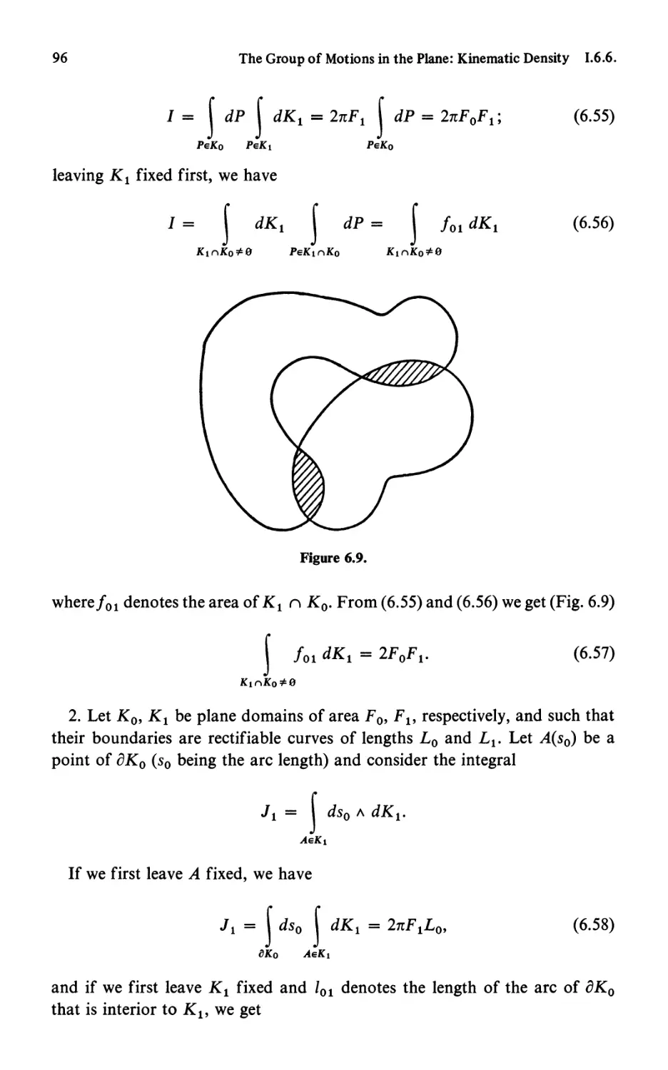
6. Some Integral Formulas . . . .. ....
7. A Mean Value; Coverage Problems . . . .
8. Notes and Exercises. . . . . . . . . . .
80
82
85
89
. . . . 93
. . . . 95
. . . . 98
. 100
Chapter 7. Fundamental Formulas of Poincare and Blaschke.
. . 109
1. A New Expression for the Kinematic Density. . . 109
2. Poincare's Formula . . . . . . . . . . . . . . 111
3. Total Curvature of a Closed Curve and of a Plane Domain 112
4. Fundamental Formula of Blaschke . . . . . . . . . . 113
5. The Isoperimetric Inequality . . . . . . . . . . . . . 119
6. Hadwiger's Conditions for a Domain to Be Able to Contain
Another . . .. ......... . 121
7 . Notes. . . . . . . . . . . . . . . 123
Chapter 8. Lattices of Figures.
. 128
1. Definitions and Fundamental Formula.
2. Lattices of Domains. . . . .
3. Lattices of Curves . . . .
4. Lattices of Points. . . . .
5. Notes and Exercise . . . . . . . . .
. 128
. . . . . . 131
. 134
. . 135
. . . . . . 138

Contents
VII
Part II. GENERAL INTEGRAL GEOMETRY
Chapter 9. Differential Forms and Lie Groups.
143
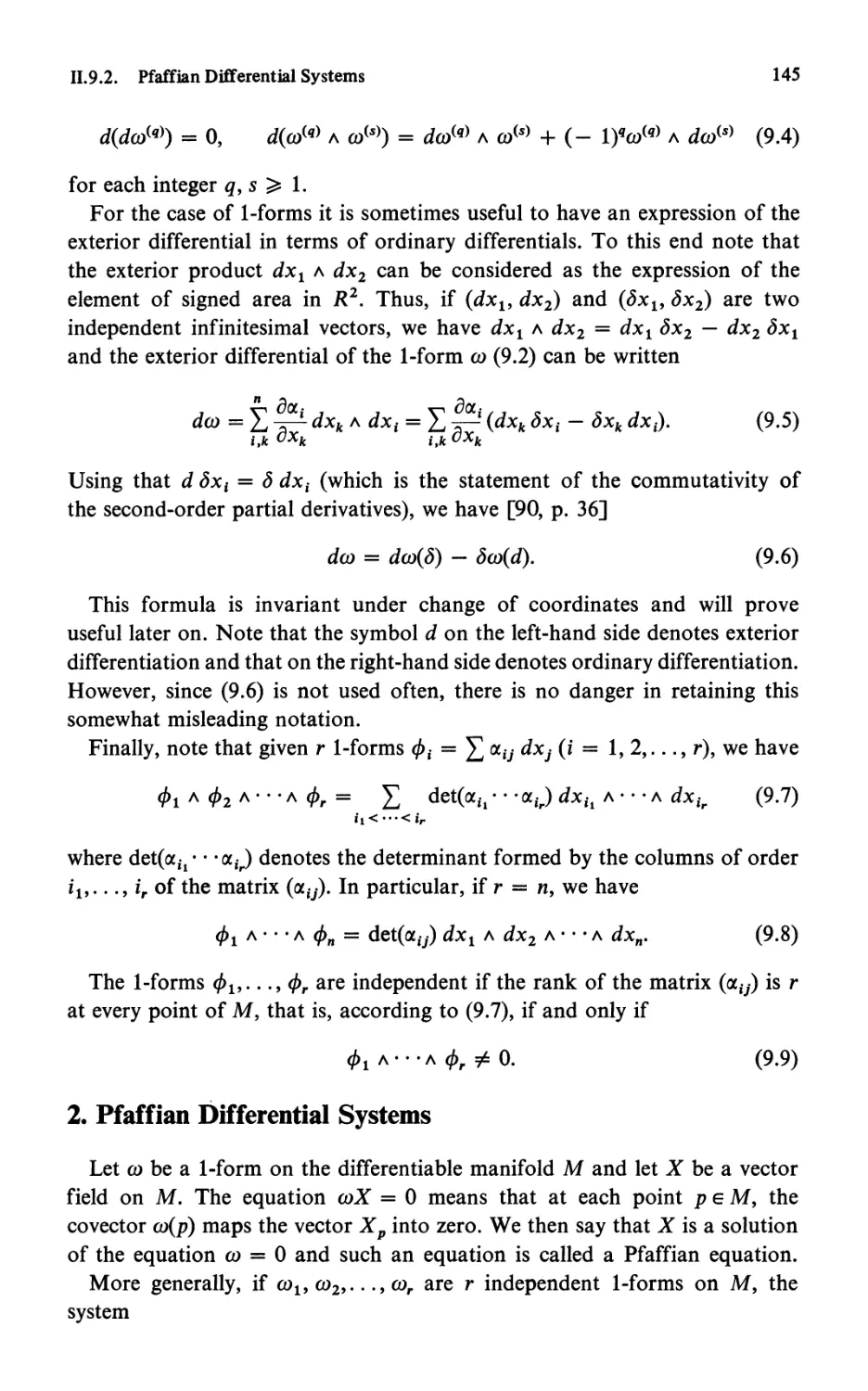
1. Differential Forms . . . . . .. ........ 143
2. Pfaffian Differential Systems . .. ........ 145
3. Mappings of Differentiable Manifolds. . . 148
4. Lie Groups; Left and Right Translations. . . .. . 149
5. Left-Invariant Differential Forms . . . . . . .. . 150
6. Maurer-Cartan Equations . . . . . . . . . . . 152
7. Invariant Volume Elements of a Group: Unimodular
Groups . . . . . . . . .. ....... . 156
8 . Notes and Exercises. . . . . . . . . . . 160
Chapter 10. Density and Measure in Homogeneous Spaces. .
165
1. Introduction. . . . . . . . . . . . . . .
2. Invariant Subgroups and Quotient Groups. . . . .
3. Other Conditions for the Existence of a Density on Homo-
geneous Spaces. . . . . . . 170
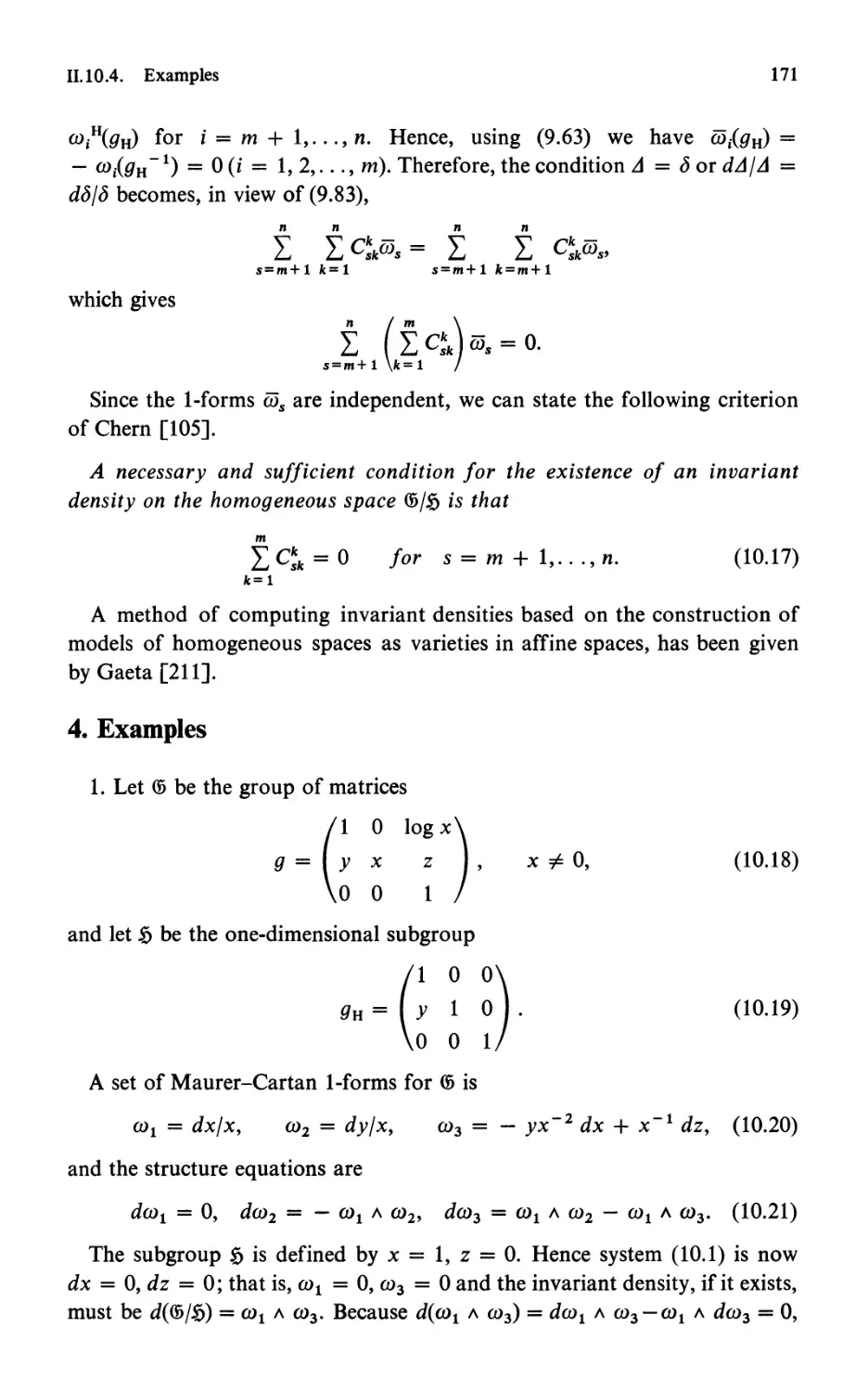
4. Examples . . . . . . . . . . . . . . . . . . 171
5. Lie Transformation Groups . . . . . . . 173
6. Notes and Exercises. . .. ........ . 175
. 165
169
Chapter 11. The Affine Groups
. 179
t. The Groups of Affine Transformations . . . . . . . . 179
2. Densities for Linear Spaces with Respect to Special Homo-
geneous Affinities. . . . . . . . . . . . . . . . . . 183
3. Densities for Linear Subspaces with Respect to the Special
Nonhomogeneous Affine Group . . . . . . . 187
4. Notes and Exercises. . . . . . .. ....... 189
Chapter 12. The Group of Motions in En
. 196
1. Introduction. . . . . . . . . . . .
2. Densities for Linear Spaces in E" . . . . .
3. A Differential Formula . . . . . . . . .
4. Density for r-Planes about a Fixed q-Plane.
5. Another Form of the Density for r-Planes in En .
6. Sets of Pairs of Linear Spaces . . .
7. Notes. . . . . . . . . . . . . . . . . . . .
. . 196
. . . . 199
. 200
. . 201
. . . . 204
. 205
. 207

VIII
Contents
Part III. INTEGRAL GEOMETR\ IN En
Chapter 13. Convex Sets in E". . . . . . . . .
. 215
I. Convex Sets and Quermassintegrale . ....... 215
2. Cauchy's Formula . . . . . . . . . . . 217
3. Parallel Convex Sets; Steiner's Formula . 220
4. Integral Formulas Relating to the Projections of a Convex
Set on Linear Subspaces. . . . . . . . . . . . . . . 221
5. Integrals of Mean Curvature . . . . . . . . . . . . . 222
6. Integrals of Mean Curvature and Quermassintegrale. . . 224
7. Integrals of Mean Curvature of a Flattened Convex Body 227
8. Notes. . . . . . . . . . . . . . . . . . . . . . . 229
Chapter 14. Linear Subspaces, Convex Sets, and Compact Manifolds . 233
I. Sets of r-Planes That Intersect a Convex Set . 233
2. Geometric Probabilities . . . . . . . . . . . . 235
3. Crofton's Formulas in Ell . . . . . . . . . . 237
4. Some Relations between Densities of Linear Subspaces . . 240
5. Linear Subspaces That Intersect a Manifold 243
6. Hypersurfaces and Linear Spaces . . . 247
7. Notes. . . . . . . . . . . . . . 248
Chapter 15. The Kinematic Density in Ell
. 256
1. Formulas on Densities. . . . . 256
2. Integral of the Volume (J,+q-n(M' n Mq) . ..... 258
3. A Differential Formula . . . . . . . . . . 260
4. The Kinematic Fundamental Formula. . . . . . . . . 262
5. Fundamental Formula for Convex Sets . . . . . 267
6. Mean Values for the Integrals of Mean Curvature. . . . 267
7. Fundamental Formula for Cylinders . . . . 270
8. Some Mean Values . . . . . 272
9. Lattices in En. . . . . . . . . . . 274
10. Notes and Exercise ............... 275
Chapter 16.
Geometric and Statistical Applications; Stereology
282
1. Size Distribution of Particles Derived from the Size
Distribution of Their Sections . . . 282
2. Intersection with Random Planes . . . 286
3. Intersection with Random Lines . . . . . . 289
4. Notes. . . . . . . . . . . . . . . . . . . . 290

Contents
IX
Part IV. INTEGRAL GEOMETRY IN SPACES OF
CONSTANT CURVATURE
Chapter 17.
1.
2.
3.
4.
5.
Noneuclidean Integral Geometry. . . . . . . . . . .
The n-Dimensional Noneuclidean Space . . . . . . .
The Gauss-Bonnet Formula for Noneuclidean Spaces .
Kinematic Density and Density for r-Planes . . . . .
Sets of r-Planes That Meet a Fixed Body. . . . . .
Notes . . . . . . . . . . . . . . . . . . . . . .
. 299
. 299
. 302
. 304
309
. 311
Chapter 18. Crofton's Formulas and the Kinematic Fundamental Formula
in Noneuclidean Spaces. . . .. ...... . 316
1. Crofton's Formulas . . . . . . . . .. ..... 316
2. Dual Formulas in Elliptic Space . . . . . . . .. 318
3. The Kinematic Fundamental Formula in Noneuclidean
Spaces. . . . . . . . . . . . . . . . . . . . . . . 320
4. Steiner's Formula in Noneuclidean Spaces . . . . . . . 321
5. An Integral Formula for Convex Bodies in Elliptic Space 322
6. Notes. . . . . . . . . . . . . . . . . . . . . . . 323
Chapter 19. Integral Geometry and Foliated Spaces; Trends in Integral
Geometry . . . . . . . . . . . . . .. .... 330
1. Foliated Spaces. . . . . . . . . . . . . . . . . . . 330
2. Sets of Geodesics in a Riemann Manifold . . .. . 331
3. Measure of Two- Dimensional Sets of Geodesics. . . . . 334
4. Measure of (2n - 2)- Dimensional Sets of Geodesics. . . 336
5. Sets of Geodesic Segments . . . . . .. ..... 338
6. Integral Geometry on Complex Spaces . . . . . . 338
7. Symplectic Integral Geometry . . . . . .. ... 344
8. The Integral Geometry of Gelfand . . . . . . . . . . 345
9. Notes. . . . . . . . . . . . . . . . . 349
Appendix. Differential Forms and Exterior Calculus . . .. .. 353
1. Differential Forms and Exterior Product. ..... 353
2. Two Applications of the Exterior Product . . .. . 357
3. Exterior Differentiation . . . . . . . . . . . . . . . 358
4. Stokes' Formula . . . . . . . . . .. ... 359
5. Comparison with Vector Calculus in Euclidean Three-
Dimensional Space . . . . . . . . . . . . .. . 360
6. Differential FornlS over Manifolds . . . . 361
Bibliography and References . . . . . 363
Author Index . . . . . . . . . . .. ...... ... 395
Su bject Index . . . . . . . . . . .. . 399

Editor's Statement
A large body of mathematics consists of facts that can be presented and
described much like any other natural phenomenon. These facts, at times
explicitly brought out as theorems, at other times concealed within a proof,
make up most of the applications of mathematics, and are the most likely
to survive changes of style and of interest.
This ENCYCLOPEDIA will attempt to present the factual body of all
mathematics. Clarity of exposition, accessibility to the non-specialist, and a
thorough bibliography are required of each author. Volumes will appear in
no particular order, but will be organized into sections, each one comprising
a recognizable branch of present-day mathematics. Numbers of volumes and
sections will be reconsidered as times and needs change.
I t is hoped that this enterprise will make mathematics more widely used
where it is needed, and more accessible in fields in which it can be applied but
where it has not yet penetrated because of insufficient information.
GIAN-CARLO ROTA
XI

Foreword
This monograph is the first in a projected series on Probability Theory.
Though its title "Integral Geometry" may appear somewhat unusual in this
context it is nevertheless quite appropriate, for Integral Geometry is an
outgrowth of what in the olden days was referred to as "geometric probabil-
ities. "
Originating, as legend has it, with the Buffon needle problem (which after
nearly two centuries has lost little of its elegance and appeal), geometric
probabilities have run into difficulties culminating in the paradoxes of
Bertrand which threatened the fledgling field with banishment from the home
of Mathematics. In rescuing it from this fate, Poincare made the suggestion
that the arbitrariness of definition underlying the paradoxes could be removed
by tying closer the definition of probability with a geometric group of which it
would have to be an invariant.
Thus a union of concepts was born that was to become Integral Geometry.
It is unfortunate that in the past forty or so years during which Probability
Theory experienced its most spectacular rise to mathematical prominence,
Integral Geometry has stayed on its fringes. Only quite recently has there been
a reawakening of interest among practitioners of Probability Theory in this
beautiful and fascinating branch of Mathematics, and thus the book by
Professor Santal6, for many years the undisputed leader in the field of Integral
Geometry, comes at a most appropriate time.
Complete and scholarly, the book also repeatedly belies the popular belief
that applicability and elegance are incompatible.
Above all the book should remind all of us that Probability Theory is
measure theory with a "soul" which in this case is provided not by Physics or by
games of chance or by Economics but by the most ancient and noble of all
of mathematical disciplines, namely Geometry.
MARK KAC
General Editor, Section on Probability
xiii

Preface
During the years 1935-1939, W. Blaschke and his school in the Mathematics
Seminar of the University of Hamburg initiated a series of papers under the
generic title "Integral Geometry." Most of the problems treated had their
roots in the classical theory of geometric probability and one of the project's
main purposes was to investigate whether these probabilistic ideas could be
fruitfully applied to obtain results of geometric interest, particularly in the
fields of convex bodies and differential geometry in the large. The contents
of this early work were included in Blaschke's book Vorlesungen iiber
lntegralgeometrie [51].
To apply the idea of probability to random elements that are geometric
objects (such as points, lines, geodesics, congruent sets, motions, or affinities),
it is necessary, first, to define a measure for such sets of elements. Then, the
evaluation of this measure for specific sets sometimes leads to remarkable
consequences of a purely geometric character, in which the idea of probability
turns out to be accidental. The definition of such a measure depends on the
geometry with which we are dealing. According to Klein's famous Erlangen
Program (1872), the criterion that distinguishes one geometry from another
is the group of transformations under which the propositions remain valid.
Thus, .for the purposes of integral geometry, it seems natural to choose the
measure in such a way that it remains invariant under the corresponding
group of transformations. This sequence of underlying mathematical concepts
- probability, measure, groups, and geometry - forms the basis of integral
geometry.
The original work was limited almost entirely to metric (euclidean and
noneuclidean) geometry and the probabilistic ideas were those of the classical
geometric probability initiated by Crofton [132, 133] and Czuber [134 J in
the last century. After 1940 the new methods of differential geometry and
group theory made it possible to unify and to generalize several questions in
integral geometry, which led to new problems and noteworthy progress in
this field. Consideration of a differentiable manifold (instead of euclidean
space) and of a transitive transformation group operating on it gave rise to
integral geometry in homogeneous spaces, and the whole theory was illuminated
by the ideas of the theory of locally compact groups and their invariant
measures. The inclusion of the methods of integral geometry within the
framework of the theory of homogeneous spaces was the work of A. Weil
xv

XVI
Preface
[710, 711] and S. S. Chern [105]. However, integral geometry generally has
been restricted to Lie's transformation groups - more precisely, to matrix
Lie groups - for two reasons. First, because they are the most important from
the point of view of their geometric applications, and second, because they
lead to more computable results. Further, the resulting simplification of the
presentation compensates for the loss of generality.
As main references on integral geometry, after the work of Blaschke [51],
we have our early introduction [568] and the books of M. I. Stoka [646, 647].
Also closely related are Hadwiger's books [270, 274]. With regard to the
theory of geometric probability there is the book of Deltheil [144] and
the nice brochure of M. G. Kendall and P. A. P. Moran [335], where a large
number of applications to different fields are brought together. The present
book intends to provide a synopsis of the main topics of integral geometry,
including their origins and their applications, with the aim of showing how
the interplay between geometry, group theory, and probability has become
fruitful for all of these fields.
In recent times, mainly due to the work of R. E. Miles [410, 411, 414, 418],
the field of integral geometry has been enriched by the introduction of the
ideas and tools of stochastic processes. In a symposium on integral geometry
and geometric probability held at Oberwolfach (Germany) in June 1969,
D. G. Kendall, K. Krickeberg, and R. E. Miles suggested the term "stochastic
geometry" to indicate precisely those contents of geometry and group theory
that are in a sense related to stochastic processes. This constitutes a promising
field, to which the present book may be considered an introduction, at least
from its geometric point of view (see [294] and G. Matheron's recent book
[401a], where the theory of random sets and applications to practical problems
are treated in great detail, using deep topological ideas).
The book presupposes only a basic course in advanced calculus, although
some elementary knowledge of differential geometry, group theory, and
probability is desirable. Publications in which prerequisite material can be
found are always indicated where apt.
Part I is concerned with integral geometry on the euclidean plane. It is
treated in an elementary way. Most of the problems are handled by specific
techniques and the main results are proved directly and independently in each
case. We consider this part fundamental in that it exhibits the power of the
methods and their usefulness in various fields. Chapters 1 to 4 are classical
in the theory of geometric probability. They are devoted to the current
notions on the measure of sets of points and lines in the plane, including some
fairly recent results, in order to illustrate the breadth of the field of applica-
tions. Chapter 5 deals with sets of strips as an immediate generalization of
sets of lines. In Chapters 6 and 7 the kinematic measure in the plane is treated
in detail in order to emphasize how the measure on groups can be applied

Preface
xvii
to strictly geometric problems. These chapters prepare the ground for the
general approach of Chapters 9 and 10. Chapter 8 deals with some discrete
subgroups of the motions group and their interpretation from the integral
geometric viewpoint.
Part II presents an account of the necessary elements of the theory of Lie
groups and homogeneous spaces in order to obtain the invariant measures
in these spaces and their properties. The general theQry is exemplified by the
groups of affine transformations (Chapter 11) and the group of motions in
euclidean space (Chapter 12). Several examples are discussed. For instance,
it is shown that the affine invariant measure of sets of planes with reference
to a fixed convex body permits a geometric interpretation of some inequalities
among various characteristics of the convex body - a typical result of integral
geometry (Sections 2 and 3 of Chapter 11).
Part III is concerned with integral geometry in euclidean n-dimensional
space. Chapter 13 contains a resume of the main results on convex sets in
n-dimensional space. Chapter 14 is devoted to the measure of linear spaces
that intersect a convex set or, more generally, a compact manifold embedded
in euclidean space. Several integral formulas are obtained and some applica-
tions to the theory of geometric probability are mentioned. Chapter 15 is
concerned with the so-called kinematic fundamental formula, which includes
most formulas in euclidean integral geometry as special or limiting cases.
In Chapter 16 the general theory is applied in detail to three-dimensional
euclidean space, especially to the question of the size distribution of particles
embedded in a convex body when only two-dimensional sections are available,
a problem that has several areas of application and has received considerable
attention in recent years, giving rise to so-called stereology [166].
Finally, Part IV deals with integral geometry in spaces of constant curvature
(noneuclidean integral geometry), in particular integral geometry on the
sphere, and some new trends in integral geometry (integral geometry and
foliated spaces, integral geometry in complex spaces, symplectic integral
geometry, and integral geometry in the sense of Gelfand and Helgason).
A survey of these new trends is given, entirely without proofs, but with detailed
references to the literature.
Each chapter ends with a section of notes or notes and exercises, including
a number of references and theorems without proof and emphasizing applica-
tions. These notes increase the amount of material covered and, with the
extensive bibliography, establish the book's encyclopedic character.
LUIS A. SANTALO

Integral Geometry
and
Geometric Probability

PART I
Integral Geometry in the Plane
CHAPTER 1
Convex Sets in the Plane
1. Introduction
Convex sets play an important role in integral geometry. For this reason
we will review here their principal properties, especially those which will
be needed in the following sections. In this chapter we consider convex sets
in the plane. For convex sets in n-dimensional euclidean space, see Chapter 13.
For a more complete treatment, refer to the classical books of Blaschke [50]
and Bonnesen and Fenchel [63], or to the more modern texts of Benson [27],
Eggleston [162], Griinbaum [247], Jaglom and Boltjanski [320], Hadwiger
[270], Hadwiger and coauthors [282], and Valentine [683].
A set of points K in the plane is called convex if for each pair of points
A E K, B E K it is true that AB c K, where AB is the line segment joining
A and B. For convenience we shall assume throughout that the convex sets
are bounded and closed.
A curve with end points P, Q is called convex if its point set, together with
the segment PQ, bounds a convex set. If the convex set K is bounded and
has interior points, then the boundary of K is called a closed convex curve.
Throughout, we will denote by oK the boundary of the set K. If all the points
of K belong to oK, then K is a line segment.
We can prove that (a) All convex curves are piecewise differentiable (i.e., they
are the unio n of a countable set of arcs with continuously turning tangent);
ENCYCLOPEDIA OF MATHEMATICS and Its Applications, Gian-Carlo Rota (ed.).
1, Luis A. Santal6, Integral Geometry and Geometric Probability
Copyright @ 1976 by Addison-Wesley Publishing Company, Inc., Advanced Book Program.
All rights reserved. No part of this publication may be reproduced, stored in a retrieval
system, or transmitted, in any form or by any means, electronic, mechanical photocopying,
recording, or otherwise, without the prior permission of the publisher.
1

2
Convex Sets in the Plane 1.1.2.
in other words, convex curves have at most a countable set of corners;
(b) All bounded convex curves are rectifiable. The length of the boundary oK of
a convex set K is called the perimeter of K.
2. Envelope of a Family of Lines
The envelope of a family of curves F(x, y, ;") = 0, depending on a parameter
;", is defined as that curve every point of which is a point of contact with a
curve of the family. As is well known, the equation of the envelope can be
obtained by eliminating the parameter ;" from the two equations F = 0,
iJF/o;" = O. We will apply this result to the case of a family of lines.
A line on the plane may be determined by its distance p from the origin
and the angle 4> of the normal with the x axis (Fig. 1.1). The equation of the
line is then
x cos 4> + Y sin 4> - p = o.
(1.1)
H
/
/
/
/
p//
/
/
/
/

o
x
Figure 1.1.
If p is a function p = p( 4», then (1.1) is the equation of a family of lines
and if we assume that p( 4» is differentiable, the envelope of the family is
obtained from (1.1) and the derivative

1.1.2. Envelope of a Family of Lines
3
- X sin cjJ + Y cos cjJ - p' = 0
(p' = dpjdcjJ).
(1.2)
From (1.1) and (1.2) we get the parametric representation of the envelope
of the lines (1.1),
X = p cos cjJ - p' sin cjJ,
y = p sin cjJ + p' cos cjJ.
(1.3)
These formulas give the X, y coordinates of the contact point P of the line
with the envelope (Fig. 1.1). Since the coordinates of the point H in which
the perpendicular through 0 intersects the line are p cos cjJ, p sin cjJ, it follows
that
HP = p'.
(1.4)
Assuming that the function p is of class e 2 (recall that class en means
n times continuously differentiable), from (1.3), it follows that dx =
- (p + p") sin cjJ dcjJ, dy = (p + p") cos cjJ dcjJ. Hence ds = Ip + p"l dcjJ and
the radius of curvature of the envelope becomes p = dsjdcjJ = Ip + p"l.
If the envelope is the boundary 8K of a convex set K and 0 is an interior
point of K, then p = p(cjJ) is called the support function of K or the support
function of the convex curve 8K with reference to the origin O. The lines (1.1)
are then the support lines of K. In this case we can prove that p + p" > 0
(see, e.g., [63, p. 18]), and the formulas in the preceding paragraph may be
written
ds = (p + p") dcjJ,
p = p + p".
( 1.5)
It can be proved that a necessary and sufficient condition that the periodic
function p be the support function of a convex set K is that p + p" > O.
From the first equation in (1.5) it follows that the length of a closed convex
curve that has support function p of class e 2 is given by
21t
L = J p dcjJ.
o
(1.6)
The assumption that p is of class e 2 C3!1 be removed. We can show that
formula (1.6) holds for any closed convex curve (see, e.g., [683, p. 161]).
The area of the convex set K can be also evaluated in terms of the support
function. Indeed, if we consider K decomposed into elementary triangles of
height p and base ds, with the point 0 as common vertex, we have
21t
F = t J P ds = t J p(p + p") dcjJ
oK 0
( 1.7)

4
Convex Sets in the Plane 1.1.3.
and by integration by parts
21t
F = ! j (p2 - p,2) d4J.
o
(1.8)
3. Mixed Areas of Minkowski
Let Kt, K 2 be two bounded convex sets on the plane whose support
functions with reference to 0 1 and O 2 are, respectively, PI and P2, assumed
of class C 2 . Consider the function p(cjJ) =-Pl(cjJ) + P2(cjJ). The envelope of
the lines x cos cjJ + y sin cjJ - P = 0 is a closed curve whose radius of
curvature is P = P + p" = (PI + PI") + (P2 + P2") = PI + P2. Since 8K 1
and oK 2 are convex curves, we have PI > 0, P2 > 0 and hence P > o.
Therefore the envelope above is the boundary of a convex set K 12 . If PI and
P2 are not of class C 2 the proof fails, but the result is still true: the function
P = PI + P2 is always the support function of a convex set K 12 called the
mixed convex set of K 1 and K 2 [63, p. 29].
The area of K 12 has the form
21t
F = ! j (p2 - p,2) d4J = F 1 + F 2 + 2F 12
o
( 1.9)
where F 1 , F 2 are the areas of K 1 , K 2 and
21t
F 12 = F 21 = ! j (P1P2 - P1'P/) d4J
o
(1.10)
is the so-called mixed area of Minkowski of K 1 and K 2 .
Integration by parts, using (1.5), gives
21t
F 12 = ! j P1(P2 + p/') d4J = t j P1 dS 2
o oK2
(1.11)
and similarly we have
F 21 = -! j P2 dS 1
oK!
(1.12)
where ds 1 , dS 2 are the arc elements of 8K 1 , 8K 2 at the contact points of the
support lines normal to the direction cjJ.

1.1.3. Mixed Areas of Minkowski
5
Note that the mixed area F 12 does not depend on the origins 0 1 , O 2 , In
fact, if 0 1 is replaced by 0 1 * such that 0 1 0 1 * = a and a is the angle of 0 1 0 1 *
with the x axis (Fig. 1.2), the support function relative to 0 1 * is PI * =
PI - a cos(cjJ - (X), and using (1.10) and integrating by parts we verify that
Fi2 = F 12. The same is clearly true if we change O 2 .
y
x
Figure 1.2.
Furthermore, the mixed area F 12 does not change by translations of K 1
and K 2 since PI and P2 remain unchanged. Assume now that one of the sets,
say K 1 , is rotated an angle e about a point o. Let 0 1 * be the image of 0 1 .
The rotation is equivalent to the rotation of angle e about 0 1 composed by
the translation defined by the vector 0 1 0 1 *. Thus, because of the invariance
of F 12 by translations, it remains for us to consider rotations about 0 1 . By
the rotation of angle e about 0 1 the new support function of K 1 is PI *( cjJ) =
Pl(cjJ - e) and the mixed area of K 2 and the rotated set K 1 * becomes
F 12(0) = ! J Pt(4J - 0) ds 2 .
OK2
Integrating with regard to e and using (1.6) we get
21t
J FdO) dO = !Lt L 2'
o
(1.13)
This formula will be useful later .

6
Convex Sets in the Plane 1.1.4.
Examples 1. If K 1 is a translate of K 2 , we may assume P1 = P2, dS 1 = ds 2 ,
and (1.12) gives F 12 = F 1 = F 2' That is, the mixed area of convex sets that
are translation congruent is equal to the common area of the sets.
2. If K 2 is a circle of radius r, we have dS 2 = r dcjJ and (1.11) gives
21t
F 12 = !r J Pt d4J = !rLt.
o
(1.14)
3. Let K 1 , K 2 be two line segments of lengths 2a, 2b, respectively, and let
(X be the angle between the lines which contain the segments. Using (1.10)
we get F 12 = 2ablsin (XI. Integrating with respect to (X over the range 0, 2n,
we get 8ab, in accordance,with (1.13). Note that a line segment is a convex set
whose perimeter is twice the length of the segment.
4. Some Special Convex Sets
A line h is said to be a support line of the convex set K at a point P E oK
if P E hand K is contained in the closure of one of the two open half planes
into which h cuts the plane. If oK possesses a tangent at P, then the support
line at P coincides with the tangent. Every point on the boundary of a convex
set lies on a support line and there are exactly two support lines perpendicular
to a given direction.
The breadth A( cjJ) of K in the direction cjJ is the distance between the two
parallel support lines to K that are perpendicular to the direction cjJ and that
contain K between them. If p(cjJ) is the support function of K, we have
A(cjJ) = p(cjJ) + p(cjJ + n) and according to (1.6) we have
1t
L = J A(4J) d4J.
o
( 1.15)
Therefore, the mean value or expected value of A is
E(A) = Lln
( 1.16)
where L is the perimeter of K. Note that the breadth A(cjJ) may be defined as
the length of the orthogonal projection of K on a line parallel to the direction
cjJ. Consequently, (1.16) gives: any closed convex curve oK of length L can
be projected on a line in such a way that the length of the projection is  Lln.
It can also be projected so that such a length is ::::;; Lln.
The least of the breadths of a convex set K is called the width of K. We
shall represent it by E. The diameter of K, represented by D, is the greatest
distance between two points of K. It can also be defined as the greatest

1.1.4. Some Special Convex Sets
7
breadth of K. Since we obviously have E  L1  D, from (1.15) it follows that
ltE  L  ltD.
( 1.17)
We now want to define some special convex sets that have particular
interest for our purposes.
Parallel convex sets. The parallel set Kr in the distance r of a convex set K
is the union of all closed circular disks of radius r the centers of which are
points of K. The boundary 8Kr is called the outer parallel curve of 8K in the
distance r. Figures 1.3, 1.4, and 1.5 show parallel sets of a segment, a triangle,
and an ellipse, respectively.
Figure 1.3.
Figure 1.4.
Figure 1.S.
If p( </» is the support function of K relative to 0, the support function of
Kr relative to the same point 0 is p(</» + r, and using (1.6) and (1.8) we have
that the perimeter and the area of Kr are, respectively,

8
Convex Sets in the Plane 1.1.4.
Lr = L + 2nr,
Fr = F + Lr + nr 2 .
(1.18)
If 8K is of class C 2 , the radius of curvature of 8Kr, by (1.5), is
Pr = p + r.
(1.19)
For values of r such that r ::::;; min p we can define the interior parallel set
K-r as the set whose support function is p(cjJ) - r. Then the length of 8K-r
and the area of K-r are given by the same formulas (1.18) after the substitution
r  - r.
Sets of constant breadth. If A( cjJ) = A = constant for all cjJ, the convex
set K is said to be of constant breadth. In this case we have E = A = D and
by (1.15) the perimeter of K is given by the simple formula
L = nA.
(1.20)
Furthermore, if 8K is of class C 2 , using (1.5) and the fact that A = p(cjJ) +
p(cjJ + n), we have
p( cjJ) + p( cjJ + n) = A.
(1.21)
Besides the circle, the simpler convex sets of constant breadth are the
so-called Reuleaux polygons. Given a linear regular polygon of 2n + 1 sides
(n = 1, 2,. . .), the corresponding Reuleaux polygon is formed by the circular
arcs that are subtended by the sides and whose centers are the opposite
vertices of the polygon. Figure 1.6 shows the Reuleaux triangle and Reuleaux
pentagon. Note that each set parallel to a convex set of constant breadth
is also of constant breadth.
c
A
8
Figure 1.6.
It can be shown that any set of diameter D  A is a subset of a convex
set of constant breadth A [63, p. 130].

1.1.5. Surface Area of the Unit Sphere and Volume of the Unit Ball
9
Triangular convex sets. Convex sets of constant breadth can rotate in the
interior of a square (i.e., all circumscribed rectangles are congruent squares;
Fig. 1.7). There are also convex sets that can rotate inside a fixed equilateral
triangle, which is equivalent to saying that all the equilateral triangles that
are circumscribed to the set are congruent triangles. These sets are called
triangular sets. For instance, the shaded spindle in Fig. 1.8 is a triangular
set. Each parallel set of a triangular set is also a triangular set.
Figure 1.7.
Figure 1.8.
Since the sum of the distances from an interior point of an equilateral
triangle to the sides is equal to the height h of the triangle, it follows that
the support function of a triangular set satisfies the condition p( cjJ) +
p(cjJ + 2n/3) + p(cjJ + 4n/3) = h. From this equality and (1.6) it follows that
the perimeter of the triangular sets inscribed in an equilateral triangle of
height h is L = (2n/3)h.
5. Surface Area of the Unit Sphere and Volume of the Unit Ball
Throughout this text we shall denote by On the surface area of the n-
dimensional unit sphere and by "n the volume of the n-dimensional unit ball
or solid sphere. Their values are
2n(n + 1 )/2
On = r«n + 1)/2) ·
°n-l
" =
n n
2n n / 2
(1.22)
nr( n/2)
where r denotes the gamma function, which satisfies the relations
r(n + 1) = nr(n),
r(n) = (n - 1)! (n integer), r(!) = .In. (1.23)
For instance,
0 0 = 2, 0 1 = 2n, O 2 = 4n, 0 3 = 2n 2 , "1 = 2, "2 = n, "3 = tn.

10
Convex Sets in the Plane 1.1.6.
6. Notes and Exercises
1. Minimum problems concerning convex sets. The area F, perimeter L,
diameter D, and width E of a convex set are related by certain inequalities,
some of which are the following.
L 2  4nF, .J3 F  E 2 , L  nE,
L  2(D 2 - E2)1/2 + 2E arc sin(E/D),
L ::::;; 2(D 2 - E2)1/2 + 2D arc sinCE/D),
2F ::::;; E(D 2 - E2)1/2 + D 2 arc sin(E/D),
2F  ED,
4F ::::;; 2EL - nE 2 .
A complete set of inequalities remains unknown. The determination in
each case of the set that satisfies the equality sign is in general a difficult
problem. For references and a systematic exposition, see the articles by
Kubota and Hemmi [349], Ohmann [462], Santal6 [576], and Sholander
[606]. Several results on convex sets can be found in the book Convexity
(V. Klee, ed.; Amer. Math. Soc., Providence, R.I., 1963).
2. Polar reciprocal convex sets. Let K be a bounded convex set in the plane.
Let 0 be an interior point of K and let P be the boundary point of K in the
direction cjJ from o. The function h*(cjJ) = IOPI-l is the support function of
a convex set K* called the polar reciprocal of K with respect to O. The polar
reciprocal convex sets have several applications to the geometry of numbers
(see the work of C. G. Lekkerkerker [361] and Cassels [92]). We state the
following properties:
(a) The mixed area F 12(K, K*) satisfies F 12(K, K*)  7r with equality if
and only if K is a circle of center 0 [192].
(b) If K has 0 as center of symmetry, then the areas F(K) and F(K*)
satisfy the inequalities
!n2 ::::;; F(K).F(K*) ::::;; n 2 .
( 1.24)
The affine invariant F(K). F(K*) has been studied for closed curves not
necessarily convex, for which the polar angle is a monotone functioh of the
arc length, and 'applied to inequalities related to periodic solutions of differen-
tial equations by Guggenheimer [255]. For convex curves in the plane, see
[296] and for applications to differential equations see [445-448].
The inequalities (1.24) may be extended to centrally symmetric convex sets
in n-dimensional euclidean space En. Calling V(K) and V(K*) the respective
volumes, we have
"n 2n -n12 ::::;; V(K). V(K*) ::::;; "n 2 (1.25)
where "n is the volume of the unit ball in En (1.22). Inequalities (1.25) have
their origin in the work of Mahler [387] and were improved by Bambah [19]
and Santal6 [556]. The right-hand inequality in (1.25) is the best possible
for all convex bodies, not necessarily centrally symmetric, and equality holds
for the n-dimensional ellipsoid centered at O. For centrally symmetric convex
bodies, the left-hand equality in (1.25) holds if and only if K is a parallelotope

1.1.6. Notes and Exercises
11
or a cross polytope. Mahler conjectured that if K ranges over all convex
bodies, then V(K). V(K*)  4 n n! (equality sign if and only if K is a simplex),
but this inequality has not been proved. Some improvements can be seen in
the work of Dvoretzky and Rogers [157] and Guggenheimer [258]. For
applications to the geometry of numbers see [361, pp. 104-110]. The affine
invariant V(K*) has a clear geometrical meaning in affine integral geom-
etry, as we shall see in Chapter 11, Sections 2 and 3.
EXERCISE 1. Let K be a convex set with boundary oK of class ct. Assuming
oK oriented, we consider for each point A of oK the chord AB such that the
angle between AB and the tangent at point A is a constant e. Assume that K
is such that IABI = A = constant. Show that the length of oK is then L =
nAlsin e. If K is of constant breadth and e = n12, then A is the breadth and
this formula coincides with (1.20).
EXERCISE 2. Let oK be a closed convex curve of class C 1 and assume that
through each point A E oK there passes a chord of given length IABI = A.
On every such a chord take the point X such that IAXI = a, IXBI = b
(a + b = A). Show that the area between oK and the curve described by X is
nab (independent of oK). This result is known as the Holditch theorem.
EXERCISE 3. If the support line perpendicular to the direction CPo contains
a line segment PIP 2 of oK (Fig. 1.9), prove that the support function p( cp)
Figure 1.9.
has no derivative at the point CPo, but there exist the right-hand derivative
p+'(CPo) and the left-hand derivative p-'(CPo) such that p+'(CPo) = HP 1 and
p _'( CPo) = H P 2 where H is the foot of the perpendicular to the support line
from o.

CHAPTER 2
Sets 01 Points and Poisson Processes
in the Plane
1. Density for Sets of Points
Let x, y denote rectangular Cartesian coordinates in the plane. In integral
geometry and in the theory of geometrical probability the measure of a set
of points X is defined as the integral over the set of a differential form OJ =
f(x, y) dx A dy (provided this integral exists, in the Lebesgue sense), where
the functionf(x, y) is chosen according to the following criterion: the measure
m(X) is to be invariant under the group of motions in the plane.
Throughout, we shall use the notation and rules of the exterior calculus,
which can be seen in any book of modern calculus or differential geometry
(e.g., in those of Fleming [204], Flanders [201, 202], Loomis and Sternberg
[368], and H. Cart an [91]).
Let 9Jl be the group of motions in the plane. With reference to a rectangular
Cartesian system of coordinates the equations of a motion u E 9Jl are
x' = x cos ex - y sin ex + a,
y' = x sin ex + y cos ex + b
(2.1)
where (a, b) are the components of the translation and ex is the rotation of u.
We want to find a function f(x, y) such that the measure m(X) =
Ix f(x, y) dx A dy is invariant under 9Jl for any set X. If X' = uX is the
transform of X by the motion u, using that dx A dy = dx' A dy', we have
m(X') = Jf(X" y') dx' A dy' = Jf(X', y') dx A dy (2.2)
x' x
ENCYCLOPEDIA OF MATHEMATICS and Its Applications, Gian-carlo Rota (ed.).
1, Luis A. SantalO, Integral Geometry and Geometric Probability
Copyright @ 1976 by Addison-Wesley Publishing Company, Inc., Advanced Book Program.
All rights reserved. No part of this publication may be reproduced, stored in a retrieval
system, or transmitted, in any form or b.y any means, electronic, mechanical photocopying,
reoording, or otherwise, without the prior permission of the publisher.
12

1.2.2. First Integral Formulas
13
and the condition m(X') = m(X) for any X gives f(x', y') = f(x, y) for all
pairs of corresponding points (x, y) -+ (x', y'). Since any point x, y can be
transformed into any other x', y' by a motion (i.e., the group of motions is
transitive for points), we have f(x, y) = constant. This justifies the following
definition.
The measure of a set of points P(x, y) in the plane is defined by the
integral over the set of the differential form
dP = dx A dy,
(2.3)
which is called the density for points.
Up to a constant factor this density is clearly the only one that is invariant
under motions. Similarly, for sets of n-tuples of points PI' P 2'. . ., Pn, assumed
independent, we state the following definition.
The density for sets of independent n-tuples ofpointsP;{x;,Yi)' i = 1,2,.. .,n
in the plane, is
dP A dP A... A dP
1 2 n
(2.4)
where dP i = dXi A dYi. This density is unique up to a constant factor.
Densities (2.3) and (2.4) are always taken in absolute value.
If the points P are given in a system of coordinates related to the Cartesian
coordinates x, y by the equations x = h(, '1), Y = g(, '1), the point density
takes the form dP = dx A dy = IJI d A d'1 where J is the Jacobian deter-
minant J = hg" - h"g.
Once we have defined the measure of sets of points and sets of n-tuples of
points, the probability that a "random" element (point or n-tuple of points)
is in the set Y when it is known to be in the set X (Y c X) is defined by the
quotient of measures
m(Y)
p = m(X) .
(2.5)
The elementary notions on geometrical probability that we shall need in
the sequel can be seen in the books of Deltheil [144], M. G. Kendall and
P. A. P. Moran [335], and M. I. Stoka and R. Theodorescu [654]. For an
axiomatic construction see the work of Hadwiger [275] or Renyi [501, 503].
2. First Integral Formulas
We will give an example in the style of Crofton [132, 133] and Lebesgue
[357] to show that the simple computation of the density dP = dx A dy in

14
Sets of Points and Poisson Processes in the Plane 1.2.2.
different coordinate systems gives some remarkabl integral formulas referring
to convex sets in the plane.
Let K 1 , K 2 be two bounded convex sets whose support functions relative
to the points 0 1 , O 2 are Pl(4)I)' P2(4)2). Assume that all the support lines have
only one point in common with the corresponding convex set. Let 1'i =
4>i + n/2 (i = 1, 2) be the directions of the support lines that are perpendicular
to the directions 4> i (Fig. 2.1). The equations of these support lines are
(x - Xi) sin 1'i - (y - Yi) COS 1'i - Pi = 0
(i = 1, 2)
(2.6)
where Xi' Yi are the coordinates of Oi'
K 2
Figure 2.1.
The coordinates of the point P in which the support lines (2.6) intersect
are the solutions of system (2.6). We want to express the density dP in terms
of 1'1 and 1'2' By differentiation of (2.6) we get
sin 1'. dx - COS 1'. d y = - t. dt.
I I I I
(2.7)
where t i denotes the length of the tangent PA i from P to the support point Ai'
Indeed, (x - X i) COS 1'i + (y - Y i) sin 1'i = HiP is the projection of 0 i P on
the support line, and according to (1.4) we have dpi/d1'j = HiA i .

1.2.2. First Integral FormuJas
15
Exterior multiplication of (2.7) for i = 1, 2 yields
t 1 t 2 sin(r2 - !1) dP.
dP = dx A dy = . ( ) d'l A d'2 or d'l A d'2 =
SIn ! 2 - ! 1 t 1 t 2
(2.8)
Let us integrate both terms of this equality over all values of ! 1 and ! 2.
The left-hand side gives 4n 2 . O the right-hand side we observe that through
each point P exterior to K 1 and K 2 there pass two support lines of K 1 and
two support lines of K 2 . Let t i , t 1 ' and t 2 , t 2 ' be the lengths of these lines from
P to the corresponding support points and let (t i , t j ) denote the angle between
t i and t j . To each point P there corresponds the sum
sin(t 1 , t 2 ) sin(t 1 , t 2 ') sin(t 1 ', t 2 ) sin(t 1 ', t 2 ') ( 2 .9)
+ , + , + "
t 1 t 2 t 1 t 2 t 1 t 2 t 1 t 2
and therefore we have the integral formula
J [ Sin(tl' t2) + sin(t l , 2') + sin(t', t 2 ) + sin(t', 2') ] dP = 4n 2 (2.10)
t 1 t 2 t 1 t 2 t 1 t 2 t 1 t 2
PKl UK2
where the integral is extended over all the points P exterior to K 1 , K 2 .
Formula (2.10) contains some particular cases:
(a) If K 1 = K 2 = K and we call t, t' the lengths PAl' PA 2 (Fig. 2.2), we
have t = t 1 = t 2 , t' = t 1 ' = t 2 ' and (t 1 , t 2 ) = (t 1 ', t 2 ') = 0, (t 1 , t 2 ') =
K
Figure 2.2.
(t 1 ', t 2 ) = (J) = angle A 1 PA 2 . Hence we have
J sin (J) dP = 2n 2 .
tt'
PK
(2.11 )
(b) If the boundary oK of the convex set K has continuous radius of
curvature P, calling Pi (i = 1, 2) the radius of curvature at the support points
Ai' we have Pi d!i = dS i where dS i is the arc element of the boundary of K

16
Sets of Points and Poisson Processes in the Plane 1.2.3.
at Ai. Then formula (2.8) can be written
SIn (J)
, PI dP = dS I A dt2
tt
or
SIn (J)
, PIP2 dP = dS I A ds 2 . (2.12)
tt
(c) Integrating over all points P outside K and taking into account that each
point P belongs to two support lines, we get
J SIn (J)
, (PI + P2) dP = 2nL,
tt
PK
J SIn (J) 2
, PIP2 dP = !L .
tt
PK
(2.13)
The factor ! in the last term arises from the fact that by interchanging 81
and 82 we get the same point P.

EXERCISE. Prove the more general formulas
J sinm (J) dP = 2r( m12) n 3 / 2
tt' r[(m + 1)/2] ,
PK
J sinm (J) 2r( m12) -
tt' (PI + P2) dP = r[(m + 1)/2] .jn L.
PK
(2.14)
Similar formulas have been gIven by Czuber [135], Masotti-Biggiogero
[393-395], and Stoka [647].
3. Sets of Triples of Points
Let PlXb Yi)' i = 1, 2, 3, be three independent points in the plane. Assuming
that they are not collinear, let Q(, 11) be the circumcenter of triangle P 1 P 2 P 3
and let (R, (Xi) be the polar coordinates of Pi with respect to Q (R being the
circumradius of triangle P 1 P 2 P 3 ). We have
Xi =  + R cos (X i,
Y i = 11 + R sin (Xi.
(2.15)
Putting dP i = dXi A dYb dQ = d, A dl1, we obtain by a straightforward
calculation the following density for triples of points in the plane.
dP 1 A dP 2 A dP 3 = R 3 1S1 dQ A dR A d(X1 A d(X2 A d(X3
(2.16)
where
S = sin«(X2 - (Xl) + sin«(X3 - (X2) + sin«(X1 - (X3)
4 . «(X2 - (Xl) . «(X3 - (X2) . «(Xl - (X3)
= - sIn sIn SIn ·
222
(2.17)

1.2.4. Homogeneous Planar Poisson Point Processes
17
Noting that lR2 S is the area T of triangle P t P 2P 3' we can write
dP t A dP 2 " dP 3 = 2RTdQ A dR A dcx t A dcx 2 A dcx 3
= 2(TjS) dQ A dT A dcx t A dcx 2 A dCX3.
(2.18)
Let C = C(P 1 , P 2 , P 3 ) denote the circumdisk of triangle P 1 P 2 P 3 . Consider
the set of all ordered triples PI' P 2' P 3 such that C is contained in a given
circle C p of radius p. According to (2.16), the measure of this set of triples,
calling r, l/J the polar coordinates of Q with respect to the center of C p' is
2 J 1t 1 J p 4 2 J 1t 2 J 1t 2 J " n3 p 6
m(P 1 ,P 2 ,P 3 ;CcC p )= dl/J 4 (p-r)rdr dcx 1 dCX 2 ISldcx3=S.
o 0 0 «1 «2
(2.19)
The measure of the set of all ordered triples PI' P 2, P 3 such that C c C p
and PIP 2 P 3 is an acute-angled triangle is
21t P 21t «1 + 1t «2 + 1t
J d4>  J (p - r)4r dr J drt 1 J drt2 J 151 drt3 = n66 ·
o 0 0 «1 «1 + 1t
Thus, the probability of an acute-angled triangle in the considered set of
triples such that C c C p is equal to 1. Taking the limit as p -+ 00, we get
that the probability of a random triangle in the plane (in the sense of density
(2.16)) being an acute-angled triangle is 1 (cf. the work of R. E. Miles [411]).
Richards [510] has shown that the probability density function for the
perimeter L of the triangle PIP 2P 3 whose vertices are three random points
in a domain D of area F is (4n 2 /21F2)L3 dL (asymptotically for large F).
4. Homogeneous Planar Poisson Point Processes
Let Do, D be two domains of the plane such that D c Do. Let F 0, F be the
areas of Do, D, respectively. According to the density dP = dx A dy, the
probability that a random point of Do lies in D is F j F o. If there are chosen
at random n points in Do, the probability that exactly m of them lie in D is
(binomial distribution)
_ ( n )( F ) m ( F ) n-m
p - - 1-- .
m m Fo Fo
(2.20)
If Do expands to the whole plane and both n, F 0 -+ 00 in such a way that
n/ F 0 -+ p, positive constant, we get

18
Sets of Points and Poisson Processes in the Plane 1.2.4.
lim Pm = (PFr e- pF .
m.
(2.21 )
The right-hand side of (2.21) is the probability function of the Poisson
distribution; it depends only on the product pF, which is called the parameter
of the distribution. This probability model for points in the plane is said to be
a homogeneous planar Poisson point process of intensity p. It is characterized
by the property that the number of points in each domain D is a random
variable that depends only on the area F (not on the shape nor the position
of D in the plane) and has the distribution (2.21). A systematic study of
stochastic point processes, in particular of Poisson processes, in n-dimensional
space can be seen in J. R. Goldman's article [232]. From the point of view of
integral geometry the most important applications are due to R. E. Miles.
We present some of his results given in [411].
1. Let r 8 (v, A) (0 > 0, A > 0, v > 0) denote the so-called gamma distribu-
tion, which has the probability density function
f( ) = O ,v18 v-I exp( - AX 8 )
X A X r( v j 0) ,
where r is the gamma function which satisfies relations (1.23). This means
that the probability that the random variable x lies between x and x + dx
is equal to f(x) dx and thus we have
x  0,
(2.22)
00
If(X) dx = 1.
o
(2.23)
The moments are
= { r[(v + k)jO] } A -k18
J.lk r(vjO) ,
k = 1, 2,. . . .
(2.24)
In particular, the expected value of x is
E( ) = = { r[(v + l)jO] } , -1/8
x J.ll r(vjO) A .
Let the points of a Poisson process be called particles and consider the set
C( m) of triangles whose vertices are particles and that contain exactly m
particles in its interior. Let PIP 2P 3 be one such triangle and let T be its area.
According to the pro bability identity pro b( area Tand m particles in its interior) =
prob(area T) x prob(m particles in its interior, assuming area T) and taking
(2.18) and (2.21) into account, we get that the probability density function
for the area T of the triangles PIP 2P 3 whose vertices are particles of a Poisson
process and that contain exactly m particles has the form
(2.25)

1.2.4. Homogeneous Planar Poisson Point Processes
19
I' ( T ) = K (pT)m e-pTT
Jm m, '
m.
m = 0, 1, 2,. . .,
(2.26)
where Km is a constant that we determine by condition (2.23). The result is
Km = p 2 /(m + 1) and hence we have
The distribution of the areas of triangles that contain exactly m particles
in a homogeneous planar Poisson point process of intensity p is r 1(m + 2, p).
In particular, the mean area of the empty triangles (m = 0) is E(To) = 21p.
2. Consider now the radius R of the circumdisk of triangle P 1 P 2 P 3. According
to (2.16) the probability density function of R is proportional to R 3 and hence
the probability density function of radii R of circumdisks that contain
exactly m particles (ignoring the particles P l' P 2, P 3 of its boundary) has the
form Km *(pnR 2 )m[exp( - pnR 2 )/m !]R 3 . Condition (2.23) gives Km * =
2( np 2)2/(m + 1) and we get
The distribution of radii Rm of circumdisks to triang les P 1 P 2 P 3 of a
homogeneous planar Poisson point process of intensity p that contain
exactly m particles is r 2(2m + 4, np).
The mean value of Ro is thus E(Ro) = 3/2) p. For details and more
complete results, see Miles's article [411].
Other point processes have been studied by Krickeberg, for instance, the so-
called Cox process or doubly stochastic Poisson process, which plays an
important role in the study of point processes that have invariance properties
under transformation groups arising in geometry (see the articles by Krickeberg
[345, 346]). Related questions are to be found in Matheron's book [401 a]'.
3. Random tessellations. A tessellation is an aggregate of cells (bounded
convex polygons) that fit together to cover E 2 without overlapping. Regular
tessellations in euclidean and hyperbolic planes have been well studied, for
instance by Coxeter [128, 130]. The problem arises of defining random
tessellations. We will consider some that are generated by homogeneous
planar Poisson point processes.
Write Plx) for the ith nearest particle to the point x and define the following
equivalence relation: x is equivalent to y if and only if Plx) = Ply) for
i = 1, 2,. . ., n. Apart from points for which the ith nearest particle is not
unique, this equivalence relation divides the plane into disjoint exhaustive
sets of equivalent points, which are almost surely bounded convex polygons.
These polygons constitute a random tessellation of the plane, which Miles
[411] represents by V n * .
For those points x for which it is unique, define the neighboring n-set of x
as the set of the n particles nearest x. The equivalence relation x is equivalent

20
Sets of Points and Poisson Processes in the Plane 1.2.5.
to y if and only if they have the same neighboring n-set generates the random
tessellation represented by V n . Clearly V n * is a refinement of V n in the sense
that each cell V n is the disjoint union of cells of V n *. If n = 1, then VI * = VI
and we have the so-called Voronoi tessellation, which generalizes to En (see
[704]).
For each cell of a tessellation we may define the area A, number of vertices
N, and perimeter L. Miles [4J 1] has given the following mean values of these
scalars for V n and V n * .
(a) For V n
E(A) = [(2n - 1)p]-t,
E(N) = 6,
E(L) _ (2n)! '" 4
n!(n - 1)!(2n - 1)2 2n - 3 p l/2 (nnp)I/2.
(b) For V n *
9n 2
E(A) = {n[2n - 1 + (64/9n 2 )(n - 1)(n - 2)]p} -I  ,
64n 3 p
E(N) = 54n 2 n + 256(n - l)(n - 2) '" 4,
9n 2 (2n - 1) + 64(n - 1)(n - 2)
E L _ 2L[(2m)!/m!(m - 1)!2 2m - 2 ] 3 ( it3 ) 1/2
( ) - n[2n - 1 + (64/9n 2 )(n - l)(n - 2)]pl/2 '" 4 n 3 p
where  refers to n -+ 00.
The higher-order moments are not known, except that E(A 2 ) = 1.280p-2
for V n *. If v denotes the number of members of V n * that contain a member
of V n , the foregoing results give
E(v) = n ( 1 + 64(n - 1)(n - 2) ) '" 32n 2 .
9n 2 (2n - 1) 9n 2
For Voronoi tessellations, Crain [130], by a Monte Carlo technique, has
estimated the expected values of N 2 , N 3 , N 4 , L 2 , L 3 , A 2 , A 3 . Interesting
theoretical and experimental results on random tessellations have been
reported by Matschinski ([403] and references therein); see also Ambarcumjan's
articles [8, 9]. For random tessellations in E3 see Chapter 16, Section 4,
Note 9.
5. Notes
1. Some classical integral formulas. (a) Let K be a bounded convex
set in the plane and consider two fixed support lines that form an agnle
,ex (0  ex  n) (Fig. 2.3). These support lines divide the plane into five regions

1.2.5. Notes
21
R4
Figure 2.3.
exterior to K, say Rt, R 2 ,. . ., Rs, as indicated in Fig. 2.3. If Ii represents the
integral of (sin wItt') dP extended over R i , where t, t' are the lengths of the
support lines from P to the support point, the following formulas can be
proved.
1 1. 2
t = 2 IX ,
1 2 = !( n - IX)2,
14 = !n2 + nIX.
I 3 = I s = !( n 2 - IX2),
These formulas are the work of Crofton [132, 133] and Czuber [134];
they hold good for any IX (0  IX  n). Note that It + 1 2 + . . · + Is = 2n 2 ,
as expected according to (2.11).
(b) Let K be a bounded convex set. The points of the plane such that
the angle w between the support lines through it is a constant, say w = wo,
form a closed convex curve C. Show that the integral of the differential form
(sin wItt') dP over the ring between C and K has the value 2n(w - wo) [135].
(c) Assuming that t, t', and w have the same meaning as in cases (a)
and (b), we can prove the following formulas [394]:
J w 2 (+ +  ) dP = 8nL log 2,
P,K
J sin 2 w (+ + :' )dP = 2nL.
P,K
2. The probability that a random triangle is obtuse. Let p(L) be the
probability that three points chosen at random in a rectangle with dimensions
1 x L form an obtuse triangle. Then according to Langford [355],
1 47 ( 2 1 ) n ( 3 1 ) log L ( 2 1 )
p(L) = 3 + 300 L + L2 + 80 L + L3 - 5 L - L2
if 1  L  2, and
1 1 ( n 47 10gL ) ( L2 3 ) L + (L 2 - 4)1/2
p(L) = 3" + £2 80L + 300 + 5 + 10 - 5£2 log L - (£2 - 4)1/2
L 3 . 2 L 2 10gL 47L 2 L(L 2 - 4)1/2 ( 63 64 )
+ 40 arc SIn L - 5 + 300 + 150 - 31 + L2 + L4

22
Sets of Points and Poisson Processes in the Plane 1.2.5.
if L  2. When the rectangle is a square, L = 1, we have p(1) = (97/150) +
(n/40) = 0.7252. Compare this result with those of Section 3. Are they con-
tradictory?
3. On the convex hull of n randomly given points. Let K be a bounded
convex set with boundary oK of class C 2 . Let K = K(S) be the curvature of
oK and assume that it satisfies the inequalities 0 < K < M where M is a
constant. Let Hn be the convex hull of n randomly given points in K. If Fn
is the area of Hn and Ln is the length of its boundary, Renyi and Sulanke [504]
have shown the following formulas for their expectations:
E ( F ) = F - r(8/3)(12F)2/3Ql/3 + 0 (  )
n 10n 2 / 3 n '
E(Ln) = L - r(2/3)(12F)2 / 3Q4/3 + 0 (  )
12n 2 / 3 n
where F and L are the area and perimeter, respectively, of K and
L
Qm = I "m ds.
o
For the number of vertices v of Hn we have
E(v) '" r( : )(i)1/3(F- 1 / 3 Ql/3)n 1 / 3 .
If oK is not of class C 2 , the computations are more involved. For a square
of side a the results are
E(Fn) = a 2 _ 8a 2 ;g n + 0 (  ),
E(Ln) = 4a - a(2 -n21t)1/2 + 0 (  )
where q is the constant
1
I [(1 + t 2 )1/2 - 1]
q = dt.
t 3 / 2
o
Consider now the case of a convex polygon K with r vertices. The expected
value of the number v of vertices of the convex hull Hn is
E(v) = 2; (log n + C) +  log (F-r(If;) + 0(1)
where C = 0.5772. .. is Euler's constant, F is the area of K, and fi denote
the area of the triangle A i - I A i A i + l' where AI' A 2 ,. . ., Ar are the ordered
vertices of K. For instance, if K is a triangle, we have E(v) = 2(log n + C) +
0(1), which is independent of the shape of the triangle. The product F- r [lfi
is an affine invariant of K that is maximal for regular polygons. AU these
results are the work of Renyi and Sulanke [504].

1.2.5. Notes
23
Some extensions to m-dimensional space have been given by H. Raynaud
[496]. For instance, if K is the unit m-ball and n points are chosen at random
in K, the expected value of the number of faces of its convex hull, as m  00,
has the infinity order
2 2 / ] [ ] (m2+1)/(m+l)
E(v) '" 2 "m- 2 1 r[(m + 1) ( + 1) (m + 1) "m n(m-l)/(m+1)
Km (m + 1). Km-l
where K i is the volume of the unit ball of dimension i (1.22).
Other results have been given by Efr9n [160] and Geffroy [220, 221].
These results refer to the uniform density (2.4) for sets of n-tuples of points.
The case of normally distributed points has been considered by Renyi and
Sulanke [504]. The more general case of points distributed according only
to the assumption of rotational symmetry has been considered by Carnal [84],
who gives the asymptotic behavior of the expectations E(v), E(L n ), E(Fn)
according to the behavior of the probability that the distance OP of a random
point P to the origin 0 be > x as x  1 (distribution on the unit disk) or
x  00 (distribution on the whole plane). See also [736]. The probabilities
that the polytopal convex hull of a set of random points in the interior of
the unit m-ball possesses a certain number of vertices have been investigated
by Miles [420]. For a different approach to the study of random convex
hulls see that of L. D. Fisher [196, 197].
4. Nearest neig hbors in a Poisson process. Lt Pn denote the probability
that a point of a Poisson process is the nearest neighbor of exactly n other
points. The maximum number of points that can have a given point P as
nearest neighbor equals 6. This occurs when P is the center of a regular
hexagon and each of the six points lies at a vertex. The probability that such
a configuration occurs in a Poisson process is zero; hence Pn = 0 if n  6.
The exact value of Pn is not known. Roberts [514], by Monte Carlo tech-
niques, has obtained these bounds:
Po < 0.3785,
P2 < Po,
Po 0.3785
Pn < 1 < 1
n- n-
(n = 2, 3, 4, 5).
A direct approach to evaluating Pn runs into combinatorial problems that
have thus far proved insurmountable.
Consider now a homogeneous Poisson point process of intensity p in the
plane. Assume that each point is an end point of a linear segment, the orienta-
tion of which is uniform over the unit two-dimensional sphere and the length
of which has the distribution dF(s) (0 :s:;; s < (0). Assume that the lengths
and orientations are mutually independent. Then the probability that the
distance from a point, chosen independently of the process of segments, to
the nearest end of a segment exceeds u is exp( - pB 2 (u)) (0 :s:;; u < (0), where
B2(U) = 2u 2 {n - Ju [arc cos(s/2u) - (s/2u)(1 - s2/4u 2 )1/2] dF(s)}. The re-
sult is due to Coleman [121]. The same problem in n-dimensional euclidean
space En has the probability exp( - pBn(u)), where
2u
Bn(u) = ( 2: n ) {On-l - 0n-2 J [n-ilX)
o

24
Sets of Points and Poisson Processes in the Plane 1.2.5.
- ( 2(n  l)J (l - 4: ZZ r- 1 )/Z] dF(S)}
where CPh(i/.,) = J sinh x dx, i/., = arc cos(sI2n), and Oh is the surface area of
the unit h-dimensional sphere. For related results see those of Holgate [311],
Eberhardt [158], and Coleman [120].
5. Coverage problems on the line. Suppose that we have n - 1 random
points PI' P 2 ,..., P n - l that are independently and uniformly distributed on
the interval 0, L of the real line. The density for (n - I)-tuples of points is
dX I /\ dX 2 /\ . . ./\ dx n - l , where Xi is the coordinate of Pi (0 :s:;; Xi :s:;; L). It can
be shown that the probability that exactly m of the n intervals determined
by the points 0, Xl' X 2 ,. . ., X n - l , L have length greater than.u (m.u :s:;; L, m :s:;; n)
IS
P{m) = (:){(1 - 7 )"-1 _ (n  m)[l _ (m  1)Jl r- 1
( n - m ) [ (m + 2).u ] n-l }
+ 1- -...
2 L
(2.27)
where the sum ends with the last term for which 1 - (m + h).uIL is positive
(see [335]).
In particular, for m = 0, we have that the probability that all intervals
have length equal to or less than .u (n.u  L) is
( n ) ( .u ) n-t ( n ) ( 2.u ) n-1
p{O} = 1 - 1 1 - L + 2 1 - T - . · .
+ (- 1)'(:)(1 - i )"-1
(2.28)
where r is the greatest integer such that r.u :s:;; L.
The probability that at least m of the intervals will exceed .u in length
(m.u :s:;; L, m < n) is
Pm= (:)(1- 7 )"-1 - (7)(m: 1)[1- (m  1)Jl r- 1
+ (m; l)(m : 2)[ 1 _ (m  2)Jl r- 1 -... (2.29)
the sum continuing as long as (m + h).u :s:;; L (h = 0, 1, 2,. . .).
These problems have been considered by a number of authors, among
them R. A. Fisher [198]; Garwood [214], who gives an application to
vehicular controlled traffic; Baticle [23]; and Levy [365]. See also Kendall
and Moran's book [335].
Consider now sets of intervals of length a on the line. Each such interval
may be determined by the coordinate of its midpoint (or by the coordinate
of any other fixed point in the interval) and the measure of a set of intervals

1.2.5. Notes
25
of constant length is defined to be the measure of the set of their midpoints.
Then, from (2.28) follows the solution of the following coverage problem
on the line:
Let So be a fixed interval of length L on the line. Suppose that we have
n random intervals of length a (na  L) that intersect So. Then the prob-
ability that they completely cover So is
( n + 1 ) ( a ) n ( n + 1 ) ( 2a ) n
p=l- 1- + 1-
1 L+a 2 L+a
( n + 1 ) ( ha ) n
+ . . . + (- l)h h 1 - L + a
(2.30)
where h is the greatest integer such that h :s:;; n + 1, ha :s:;; L + a.
The analogous problem on the circle may be stated as follows [630]:
For n arcs of length 4> chosen independently and at random on the circle
of unit radius, the probability that they completely cover the circle is 0 if
n4> :s:;; 2n and if n4>  2n has the value
P *-
o -
( n ) ( 4> ) n-l ( n ) ( 24» n-l
1- 1-- + 1--
1 2n 2 2n
( n )( h4» n-l
+ (- l)h h 1 - 2n
- . . .
(2.31 )
where h is the greatest integer such that h4> :s:;; 2n.
Coverage problems in spaces of dimension greater than 1 are much more
difficult and in general no exact solution is known (see Chapter 6, Section 7).
For other coverage problems see the articles by Robbins [512, 513], Takacs
[666], and Votaw [705].
6. The "parking" problem of Renyi [502]. Let us consider the interval
(0, x) with x > 1. An interval of unit length is chosen at random in it. After
that, a second interval of unit length is placed at random in the unfilled
intervals. This process continues until no additional interval of unit length
can be accommodated. Suppose that the number of unit intervals placed in
the given interval (0, x) is N. The problem consists in determining the mean
value of N as a function of the length x. The problem is clearly that of
parking at random cars of unit length on a street of length x. The main
result of Renyi is that the ratio of the mean value of the number N of unit
intervals parked at random in the interval of length x to the total length x,
as x  00, is C = 0.74759. . . .
The problem has been generalized by several authors. Ney [449] considers
the case in which the intervals for parking have their lengths given at random.
Dvoretzky and Robbins [156] give certain limit theorems for N(x). Mannion
[389] shows that the variance of the occupied portion of the interval as it
becomes infinite is proportional to c 1 x, where x is the length of the interval
and Cl = 0.035672. (See also [440].) Suggestions and bibliographical notes

26
Sets of Points and Poisson Processes in the Plane 1.2.5.
on the parking problem and its extensions to higher dimensions have been
given by H. Solomon [616, 618]. For two dimensions see the articles by
Palasti [467] and Gani [212]. The three dimensions several problems on
random space-filling or random parking have been considered, mainly in
connection with models of liquid structure, by Bernal [28], Bernal, Masson,
and Knight [29], and D. G. Scott [602].

CHAPTER 3
Sets of Lines in the Plane
1. Density for Sets of Lines
A straight line G in the plane is determined by the angle 4> that the direction
perpendicular to G makes with a fixed direction (0 :s:;; 4> :s:;; 2n) and by its
distance p from the origin 0 (0 :s:;; p). The coordinates p, 4> are the polar
coordinates of the foot of the perpendicular from the origin onto the line.
y
Figure 3.1.
ENCYCLOPEDIA OF MATHEMATICS and Its Applications, Gian-Carlo Rota (ed.).
1, Luis A. Santal6, Integral Geometry and Geometric Probability
Copyright @ 1976 by Addison-Wesley Publishing Company, Inc., Advanced Book Program.
All rights reserved. No part of this publication may be reproduced, stored in a retrieval
system, or transmitted, in any form or by any means, electronic, mechanical photocopying,
recording, or otherwise, without th prior permission of the publisher.
27

28
Sets of Lines in the Plane 1.3.1.
The equation of G is then (Fig. 3.1)
x cos l/J + y sin l/J - p = o.
(3.1 )
The measure of a set X of lilles can be defined by any integral of the form
m(X) = Jf(P' <P) dp A d<p
x
(3.2)
where the function f must be chosen according to certain criteria, depending
on the nature of the problem. In integral geometry and in the theory of
geometrical probability the chosen criterion establishes that the measure is
to be invariant under the group of motions IDl.
By a motion u (2.1) the line (3.1) transforms into
x cos(l/J - Ct) + y sin(l/J - Ct) - (p - a cos l/J - b sin l/J) = O.
Comparing with (3.1), we see that under the motion u(a, b, Ct) the coordinates
p, l/J of G transform according to
p' = p - a cos Ct - b sin Ct,
l/J' = l/J - Ct,
(3.3)
so that dp'/\ dl/J = dp' /\ dl/J'. The measure of the transformed set X' = uX is
m(X') = J f(p', <p') dp' A d<p' = J f(p - a cos <p - b sin <p, <p - a.) i p A d<p. (3.4)
x' x
If we want m(X) to equal m(X') for any set X, (3.2) and (3.4) lead to
f(p - a cos l/J - b sin l/J, l/J - Ct) = f(p, l/J) and since equality is to hold for
all motions u, we must have f(p, l/J) = constant. Choosing this constant
equal to unity we have
The measure of a set of lines G(p, l/J) is defined by the integral, over the
set, of the differential form
dG = dp /\ dl/J,
(3.5)
which is called the density for sets of lines.
Up to a constant factor, this density is the only one that is invariant under
motions. The density (3.5) will always be taken at absolute value.
We will give an immediate application of density (3.5). Let D be a domain
in the plane of area F and let G be a line that intersects D. Multiplying both
sides of (3.5) by the length (J of the chord G n D and integrating over all the
lines G, using the fact that (J dp is the area element of D, so that the integral
with reference to dp for any fixed l/J (0  l/J  n) is the area F, we have

1.3.1. Density for Sets of Lines
29
J U dG = nF.
GnD:I=9
(3.6)
Other forms of dG. If the line G is determined by other coordinates than
p, if>, the density dG takes different forms, which can be easily obtained by
simple changes of coordinates.
(a) If G is determined by the angle fJ that it makes with the x axis and the
abscissa x of the point at which it cuts the same axis (Fig. 3.2), we have
p = x sin fJ, if> = fJ - n12, and therefore
dG = sin fJ dx A dfJ.
(3.7)
y
x
Figure 3.2.
(b) If G is determined by its intercepts x, y on the coordinate axis, we have
p = xy(x 2 + y2)-1/2, if> = arc tan(xly), and therefore
dG = xy dx A dYe
(x2 + y2)3/2
(3.8)
(c) Let G be determined by the coefficients u, v of its equation written in
the form ux + vy + 1 = O. Then in (3.8) we have x = - 1/u, y = - 11v,
and thus
dG = dx A dv
(U 2 + V 2 )3/2
(3.9)

30
Sets of Lines in the Plane 1.3.2.
(d) If G is determined by the coordinates , 11 of the foot of the perpendicular
from the origin onto the line, we have  = p cos 4>, 11 = P sin 4>, and therefore
dG = d A d'1
(2 + 112)1/2
(e) Let P(x, y) be a point of G and let fJ be the angle that G makes with the
x axis. We have p = x sin 0 - y cos fJ, 4> = 0 - rc/2, and thus
(3.10)
dG = sin fJ dx A dO - cos fJ dy A dO.
(3.11 )
All these forms for dG must be taken up to the sign, because we consider
all densities to be positive.
2. Lines That Intersect a Convex Set or a Curve
We want to measure the set of lines that meet a fixed bounded convex set K.
Take as origin a point 0 E K and let p = p(4)) be the support function of K
with reference to o. Applying (3.5) and (1.6), we have
27t
m(G; G n K ,= 0) = J dp A dcfJ = J p dcfJ = L
GnK*9 0
(3.12)
where L is the length of oK (perimeter of K). Hence we have
The measure of the set of lines that intersect a bounded convex set K is
equal to the length of its boundary.
In terms of geometric probability, we can state
Let K 1 be a convex set contained in the bounded convex set K. The prob-
ability that a random line G intersects K 1 if it is known that it intersects K
is p = L 1 /L, where L 1 , L are the perimeters of K 1 and K, respectively.
From (3.12) and (3.6) we also deduce that the mean length of the chords
that random lines intercept in a convex set K is
E(O') = rcF/L
(3.13)
where F is the area and L the perimeter of K.
Let C be a piecewise differentiable curve in the plane that has a finite
length L. Assume that C is defined by the equations
x = x(s),
y = y(s)
(3.14)
where the parameter s is the arc length. Let G be a line that intersects C at
the point x, y and forms with the tangent at this point an angle fJ. The co-

1.3.2. Lines That Intersect a Convex Set or a Curve
31
ordinates s, 0 determine the line G and we want to express dG in terms of
s, O. We have
l/J = 0 + -r - (rc/2)
(3.15)
where -r is the angle between the tangent to C and the x axis.
Since x, y is a point of G, we have p = x cos l/J + y sin l/J and therefore
dp = cos l/J dx + sin l/J dy + (- x sin l/J + Y cos l/J) dl/J. Since dx = cos -r ds,
dy = sin -r ds, we get dp = cos(l/J - -r) ds + (- x sin l/J + Y cos 4» d4>. Exterior
multiplication by dl/J gives
dG = dp A dl/J = cos(l/J - -r) ds A dl/J
and according to (3.15), since dl/J = dO + -r' ds, we have
dG = /sin 0/ ds A dO
(3.16)
where we have written /sin 0/ because we consider all densities to be positive.
Now integrate both sides of (3.16) over all lines that intersect C. On the
right-hand side we have
L 7t
1 ds I lsin 01 dO = 2L
o 0
and on the left-hand side each line G has been counted as many times as it
has intersection points with C. Calling this number n, we obtain
1 n dG = 2L
(3.17)
where the integral is extended over all lines of the plane, n being 0 for the
lines G that do not intersect C. For n = 2 we again have the result (3.12).
We have proved (3.17) for piecewise differentiable curves, but it holds good
for any rectifiable curve [377, 51]. The left-hand side of (3.17) can be taken
as the definition of the length of a continuum of points; it is called the F avard
length of the continuum [172, 604]. On the importance that the integral
in (3.17) be in the Lebesgue sense instead of the Riemann sense, see [171].
Formula (3.17) can be applied for measuring the length of curves. Following
Steinhaus [625, 626], we proceed as follows. Take a transparent sheet with a
family of equidistant parallels G i (i = 1, 2,. . .). Assume that the arc C to be
measured cuts G i in ni points, so that So = L ni is the total number of inter-
sections. Turning the sheet through an angle (k/m)n (k = 0, 1,. . ., m - 1),
we get Sk intersections and the total amount is N = L-l Sk. Calling a the
distance between G i and G i + 1, we get the expression

32
Sets of Lines in the Plane 1.3.3.
Nrca
2m
(3.18)
as an approximation of the length of C (since it is an approximation of
! J n dG). The accuracy of(3.18) depends on a and m. For a -+ 0 and m -+ 00,
(3.18) tends to the length of C. Estimates of the errors involved in this method
are given by Moran [427].
3. Lines That Cut or Separate Two Convex Sets
Let K 1 , K 2 be two bounded convex sets in the plane and let L 1 , L 2 be the
lengths of the boundaries oK 1 , oK 2 .
We call external cover C e of K 1 and K 2 the boundary of the convex hull
of K 1 u K 2 (recall that the convex hull of a set of points is the intersection
of all the convex sets containing the set). The external cover may be intuitively
interpreted as a closed elastic string drawn about K 1 and K 2 (Fig. 3.3). Let
Le denote the length of Ceo If K 1 n K 2 #- 0, as in the case of Fig. 3.3, we
can also consider the internal cover C i realized by a closed elastic string
drawn about K 1 and K 2 and crossing over at a point 0 placed between K 1
and K 2 . Let L i denote the length of C i .
Figure 3.3.
Though they have arcs in common, we will consider oK 1 , oK 2 , C e , C i as
different curves. Except for lines of support that belong to a set of measure
zero, every line that meets K 1 and K 2 has two intersection points with each
of the curves oK 1 , oK 2 , and C e , and four intersection points with C j ; there are
in all ten points of intersection. Let m 1 0 be the measure of the set of such lines.
The lines that meet either K 1 or K 2 , but not both, have six common points
with the curves oK 1 , oK 2 , Cj, C e : let m6 be the measure of this set of lines.
The lines that separate K 1 and K 2 have four intersection points with the curves
above (two common points with C e and two common points with C j ): let
m4 denote the measure of this set of lines.
Since the measure of the set of lines that meet a convex set is equal to its
perimeter, the measures m6', m6" of the lines that meet K 1 without meeting

1.3.3. Lines That Cut or Separate Two Convex Sets
33
K 2 , or vice versa, are
m6' = L 1 - m 1 o,
" L
m6 = 2 - m10,
(3.19)
and therefore we have
m6 = m6' + m6" = L 1 + L 2 - 2m 1 o.
(3.20)
Since C e is a closed convex curve, we have
m4 + m6 + m10 = Le
(3.21)
and applying (3.17) to the set of the four curves oK 1 , oK 2 , Cj, C e , we obtain
4m4 + 6m6 + 10m 1o = 2(L 1 + L 2 + Le + L j ).
(3.22)
From (3.19)-(3.22) we get
m4 = L j - (L 1 + L 2 ),
m6' = L 1 - (L j - Le),
m6" = L 2 - (L i - L e ),
m10 = L i - Le.
(3.23)
In words,
(a) The measure of all lines that meet K 1 and K 2 is L j - Le.
(b) The measure of the set of lines that meet K 1 without meeting K 2 is
L 1 - (L j - Le) and the measure of the set of lines that meet K 2 without
meeting K 1 is L 2 - (L j - Le).
(c) The measure of the set of lines that separate K 1 and K 2 is L j - (L 1 + L 2 ).
We have assumed that K 1 n K 2 = e. If they overlap, it is easy to see that
results (a)-(c) hold good with the convention of putting L j = L 1 + L 2 .
In terms of geometrical probability these results can be stated as follows:
Let K 1 and K 2 be two bounded convex sets. If G is a line chosen at random
in the plane with the condition that it meets the convex hull of K 1 and K 2 ,
then:
(a) The probability that G meets K 1 and K 2 is
p(G n K 1 n K 2 :F e) = (L j - Le)/Le.
(b) The probability that G meets K 1 without meeting K 2 is
L i - L 1
p(GnK 1 :Fe,GnK 2 =e)=I- L
e
and similarly
L j - L 2
p(G n K 1 = e, G n K 2 :F e) = 1 - L ·
e

34
Sets of Lines in the Plane 1.3.4.
(c) The probability that G separates K 1 and K 2 is
L j - (L 1 + L 2 )
p(G n K 1 = e, G n K 2 = e, G n C e * e) = L .
e
If K 1 n K 2 * e in the preceding formulas, we must put L j = L 1 + L 2 .
If we consider only lines that meet K 1 , by applying the same type of argument
we obtain the following.
If K 1 and K 2 are two bounded convex sets in the plane (which mayor may
not overlap), the probability that a random chord of K 1 intersects K 2 is
P = (L j - Le)/Ll
where L j is the length of the internal cover if K 1 n K 2 = e and L j = L 1 + L 2
if K 1 and K 2 overlap.
The preceding results are the work of Sylvester [665a], who also considered
the case of more than two convex sets. About the distribution of the number
of intersections of a rectifiable curve C and a random line G (i.e., about the
probability Pk that G has k intersection points with C, for every k) very
little is known (see the articles by Sulanke [662] and Ambarcumjan [6]).
4. Geometric Applications
1. Let C be a plane closed curve of class C 2 , which is oriented, so that there
is a prescribed sense of rotation. Let s denote the arc length of C and let
-r(s) denote the angle of the tangent to C with a fixed direction, say the x axis.
The curvature of C is defined by K = d-r/ds and the total absolute curvature
is defined by the line integral
C a = f 1"1 ds = f Id-rl.
c c
(3.24)
Let v(-r) denote the number of unoriented tangents to C that are parallel
to the direction -r (e.g., in Fig. 3.4, v = 6). Since in the last integral (3.24) each
direction -r appears vCt) times, equation (3.24) can be written
1t
C a = f v( -r) Id-rl.
o
(3.25)
On the other hand, if a line G is parallel to the direction -r and meets C in
n points Pi' then there are at least n tangents to C that are parallel to G
(one for each of the arcs P 1 P 2 , P 2 P 3 ,..., P n - 1 P m P n P 1 ) and thus n(-r)  v(-r).
Using (3.17), we have

1.3.4. Geometric Applications
35
2L = 1 n dG :::;;
GnC*9
1t
1 V dG = 1 V dp A d-r :::;; Li m 1 V Id-rl = Limc a (3.26)
GnC*9 GnC*9 0
where L is the length of C and Am its maximal breadth.
Figure 3.4.
In particular, if C lies inside a circle of radius r, then Am  2r and we have
the following theorem of Fary [169]:
If a closed plane curve of length L and absolute total curvature C a can
be enclosed by a circle of radius r, then L  rc a .
2. Let K be a bounded convex set of area F and perimeter L. Let G, G'
be two lines that intersect oK at the points corresponding to the arc lengths
s, s'. Call 0, 0' the angles of G, G' with the support lines at their intersection
points with the boundary oK and let (J, (J' be the lengths of the chords inter-
cepted by G, G' in K. We consider the integral
I = 1 (0' sin (J' - 0" sin (J)2 ds A d(J A ds' A d(J'
(3.27)
extended over the ranges 0  s  L, 0  s'  L, 0  0, 0'  n. According to
(3.16) we have sin 0 ds A dO = dG, sin 0' ds' A dO' = dG'. Now

36
Sets of Lines in the Plane 1.3.4.
1t
J q2 dO = 2F,
o
1t
J sin 2 0 dO = n/2
o
(3.28)
where the first integral follows from the formula for area in polar coordinates.
An analogous formula holds for G'. Hence
I = 2nL 2 F - 2 J q dG J q'dG' = 2nF(L 2 - 4nF)
GnK=I=0 G'nK=I=0
where we have applied (3.6) and the fact that in integral (3.27) each line G, G'
is counted twice, once for each intersection with oK.
Figure 3.5.
Since clearly I  0, we have proved the classical isoperimetric inequality
L 2 - 4nF  o.
(3.29)
The equality sign holds if I = 0, so that (J /sin 8 = (J' /sin 8', which means
that K is a circle. This proof is due to Blaschke [38].
3. Let C be a curve of length L contained in a closed convex curve C 1 of
length L 1 . If we consider all lines G that intersect C l' the average of the
number of intersection points of these lines with C will be E(n) = 2L/L 1 .
Since there must be lines G the number of whose intersections with C is not

1.3.5. Notes and Exercises
37
less than E(n), we have: if a curve of length L lies inside of a closed convex
curve of length Lt, there exist lines that cut it in at least 2L/Lt points.
,.
5. Notes and Exercises
1. Again the isoperimetric inequality for convex curves. Let C be a closed
convex curve of class ct. Let At, A 2 be the points in which C is intersected
by the line G(p, 4» and let ds t , dS 2 be the arc length elements at At, A 2 and
0t, O 2 the angles of G with the tangents to C at At, A 2 . It is easy to see that
(J dG = sin 0t sin O 2 dS t A dS 2 (3.30)
where (J is the length of the chord AtA2' Integrating over all oriented lines
that meet C, we have
2nF = J dS 1 J sin 0 1 sin O 2 dS 2
L L
= t J dS 1 J [COS(01 - ( 2 ) - COS(01 + ( 2 )] ds 2 .
L L
The integral JL cos(Ot + ( 2 ) dS 2 is equal to the projection of C on the
tangent line at At and therefore is equal to zero. Thus we have
4nF = L 2 - 2 J dS 1 J sin 2 !(01 - ( 2 ) ds 2 , (3.31)
L L
which contains the isoperimetric inequality L 2 - 4nF  O. This proof is due
to Pleijel [479].
A more general result can be obtained from the formulas
J u" dG =  J J u n - 1 COS 0 1 COS O 2 dS 1 A ds 2 ,
GnC:#:0 LL
J Un dG =  J J u n - 1 sin 0 1 sin O 2 dS 1 A ds 2 ,
GnC:#: 0 L L
which yield the following formula of Ambarcumjan [7] (for any integer n > 0)
2(n + 1) J u" dG= n J J u n - 1 dS 1 A dS 2 - 2n J J U n - 1 sin 2 ( 0 1 ; O 2 )dS 1 A ds 2 .
GnC:#:0 LL LL
As a consequence we have the inequality
J u" dG ::::; 2(n: 1) J J u n - 1 dS 1 A dS 2
GnC:#: 0 L L
(3.32)
which for n = 1 gives the isoperimetric inequality.

38
Sets of Lines in the Plane 1.3.5.
Pleijel's proof has been generalized to nonsimple curves by Banchoff and
Pohl [20]. Then F is replaced by the sum of the areas into which the curve
divides the plane, each weighted with the square of the winding number,
that is,
L 2 - 4n f w 2 dP  0
where the integral is over the whole plane. The wInding number w(P) of P
with respect to the curve can be defined as the number of turns of the vector
PX when X goes around the curve. Equality holds if and only if the curve
is a circle or a circle traversed several times. Banchoff and Pohl have general-
ized this isoperimetric inequality to arbitrary dimension and codimension,
as we shall see in Chapter 14, Section 7, Note 8.
2. Distance of two curves. Let C t and C 2 be two curves in the plane and
let Nt(G), N 2 (G) be the numbers of points at which they are intersected by
a variable line G. Define the distance of C t, C 2 by the integral
(C t , C 2 ) = ! f INt(G) - N 2 (G)1 dG
(3.33)
extended over all lines of the plane.
If C 1 and C 2 are rectifiable curves, the distance (C t , C 2 ) is finite, since
(C 1 , C 2 )  L 1 + L 2 . Show that the distance so defined satisfies the condi-
tions (a) (C 1 , C t ) = 0; (b) (C t , C 2 ) = (C 2 , C t ); (c) (C t , C 2 ) + (C 2 , C 3 ) 
(C 1 , C 3 ).
If C 1 , C 2 are Jordan curves (i.e., homeomorphic images of a line segment
or of a circle), then (C t , C 2 ) = 0 implies C 1 = C 2 . With the definition
above, prove that:
(i) If C 1 and C 2 are closed convex curves such that C 1 lies inside C 2 ,
then (C 1 , C 2 ) = L 2 - L 1 ;
(ii) If C 1 , C 2 are closed curves such that C 1 lies outside C 2 , then (C 1 , C 2 ) =
L 1 + L 2 - 2(L i - L e ), where L i , Le are the lengths of the external and
internal covers of C t , C 2 (Section 3). (See [625].)
3. Asymmetry of convex curves. If C is a given curve of length L, its
asymmetry relative to a line Go may be defined as the distance (C, C*),
where C* denotes the reflection of C in Go. The line Go that minimizes the
asymmetry (C, C*) is called the axis of symmetry of C and the difference
1 - min(C, C*)j2L is called the index of symmetry of C. Compare this
definition of Steinhaus [625] with other definitions of symmetry for convex
curves (e.g., that of Griinbaum [246]).
4. Length of order m. Steinhaus [625J calls the length of order m of a set
of points C the integral
Lm = t f W m dG
GnC:;:0
(3.34)

1.3.5. Notes and Exercises
39
where W m = n is the number of points of the intersection G n C if n  m
and W m = m if n > m. Note that if C is a rectifiable closed curve, then L 2
is the length of the boundary of its convex hull and Loo is the ordinary length.
5. Systems of nonseparable convex sets. A system of n closed convex sets
K i (i = 1, 2,. . ., n) in the plane is called separable if there is a line G that
intersects no K i and that divides the plane into two half planes, each con-
taining at least one K i. In the contrary case, the system is said to be non-
separable. The following theorem can be proved: Let Ko denote the convex
hull of the nonseparable convex system K i (i = 1,2,..., n). Let Lj, D i , and
R i denote the perimeter, diameter, and radius, respectively, of the circum-
circle of the set K i' Then
n
Lo  L L i ,
1
n
Do  L D i ,
1
n
Ro  L R i .
1
(See the articles by Hadwiger [266] and A. W. Goodman and R. E. Goodman
[233].)
6. lnvariance of the line density by reflection and refraction. Assume
that the line G is the trajectory of a ray of light that is incident on a fixed
curve C and is reflected according to the law of reflection: the angle of
reflection is equal to the angle of incidence. Then if fJ is the angle between G
and the tangent to C, the angle of the tangent with the reflected line G* is
0* = - fJ (Fig. 3.6) and by making use of expression (3.16) for dG (at
absolute value), we have dG = dG*. Hence, the density dG is invariant
under reflections in curves.
c
G
Figure 3.6.
Suppose that the line G 1 is refracted at the curve C that separates two
mediums whose indices of refraction are nl and n2, respectively (Fig. 3.7).

40
Sets of Lines in the Plane I. 3.5.
If i 1 , i 2 are, respectively, the angles of incidence and refraction, the classical
Snell law of optics says that sin i 1 /sin i 2 = n2/nl. On the other hand, the
angle of the tangent with G 1 and the angle of the tangent with G 2 are
(Jl = n/2 - i 1 and (J2 = n/2 - i 2 , so that, using (3.16), we have dG 1 =
- cos i 1 ds A di 1 = - ds A d(sin i 1 ), dG 2 = - cos i 2 ds A di 2 = - ds A d(sin i 2 ) =
- (nl/n2) ds A d(sin i 1 ) = (n 1 /n2) dG 1 . Thus, when a ray is refracted from a
medium of index of refraction nl to a medium of index of refraction n2, the
density dG 1 is multiplied by the constant factor nl/n2.
,
,
,
,
,
,
,
, .
" 1 2
c
G 1
Figure 3.7.
Consider an optical instrument composed of several mediums of indices
of refraction n l' n2,. . ., n m such that the first medium, where the rays enter
the instrument, coincides with the last medium, where the rays emerge; that is,
n 1 = n m . WehavedG m = (nm-l/nm)dGm-l = (nm-lnm-2)/(nmnm-l)dGm-2 =
. .. = (n m - 1 · . . n 1 )/(n m n m - 1 . . . n2) dG 1 = dG t . Hence, line density is pre-
served during its propagation through optical instruments [40].
7. The convex billiard table of G. D. Birkhoff. Let C be a closed convex
curve in the plane. Suppose that a point P moves inside C and collides with
C according to the law "the angle of incidence is equal to the angle of
reflection." The path of P is determined by the length s of the arc OA (where
o is an arbitrary point on C) and the angle rx (0  rx  n) of the line G = AP
with the tangent to C at A (Fig. 3.8). According to (3.16) the line density
can be written dG = sin rx ds A drx and since this density is preserved under
reflection, we have that the differential form sin rx ds A drx is invariant under
the motion of point P (see the books by Birkhoff [31] and Arnold and
Avez [13]).

1.3.5. Notes and Exercises
41
B
A
Figure 3.8.
8. An inequality of Feller. Let D be a plane domain of area F contained
in the unit circle. Suppose that the intersection of D with any line has measure
not exceeding a fixed constant a < 1. Then necessarily F < 2a. This result
is the best possible in the sense that there exists a domain such that its inter-
section with any line has a total length not exceeding a, whereas for its area
F we have F > 2a(1 - n- 2 a 2 - e) where e > 0 is arbitrarily small (see [184]).
Generalization to the sphere and noneuclidean spaces has been done by Veno
and co-workers [682] and Santalo [563]. If D is convex, we have F  na 2 /4
where the equality sign holds if and only if D is a circle [30a].
Figure 3.9.

42
Sets of Lines in the Plane 1.3.5.
9. An integral formula. Let C be a closed convex curve of length L that
contains m line segments of length a l' a 2'. . ., am, respectively (Fig. 3.9). Let
A 1 , A 2 be the points at which a line G meets C and call u the length of the
chord A 1 A 2 and 0 1 , O 2 the angles that G makes with the support lines of C
at A 1 and A 2 . Then'the following formula holds.
J u 1 ( 2  2 )
dG = - L - L.- a. .
sin 0 1 sin O 2 2 l'
GnC:;:0
(3.35)
10. Integral geometry of plane linear graphs. Sulanke [622] has con-
sidered the following kind of problem. Recall that a linear graph is a finite
set of points (vertices) together with a finite number of arcs of curve (edges,
assumed rectifiable) joining two distinct vertices, such that no two of the
edges have an interior point in common and each vertex is the end of at
least one edge. To each graph Q is attached the set of real numbers plQ)
(i = 1, 2,. . .) that are equal to the probability that a random line intersects
Q exactly i times.
THEOREM. A necessary and sufficient condition for a linear graph to be
Eulerian (i.e., a graph such that it is possible to find a path that traverses
each arc exactly once, goes through all vertices, and ends at the starting
point) is that Pi = 0 for all i odd.
Linear graphs with the same set of natural numbers {i 1 , i 2 ,. . ., iN} such
that Pi > 0 are said to be of the same type. The problem arises of knowing
whether to each set of natural numbers i 1 < i 2 < · . · < iN there corresponds
a linear graph. Sulanke has solved the problem for iN  5 with the exceptions
{I, 2, 5}, {I, 4, 5}. Recently Hristov has shown that the type {I, 2, 5} cannot
exist (M R 50, # 8295).
Let c be the number of bounded regions into which Q partitions the plane
(faces of the graph) and let C G be the analogous number for the graph Q + SG,
where SG is the line segment of the random line G determined by the first
and the last point of the intersection G n Q. Then, if we assume Q to be
connected, the expected value of CG is E(c G ) = C - 1 + 2L(Q)jL(Q*) where
L(Q) is the total length of Q and L(Q*) is the length of the convex hull of Q.
If m(G; N G(Q) i= N G(Q')) denotes the measure of the line set G such that
the number of intersection points of G with Q is not equal to the number
of intersections ,of G with another linear graph Q', then p( Q, Q') =
m(G; NG(Q) i= NG(Q')) defines a metric in the space of graphs. Compare
with the distance of Note 2. For more details, see [662].
11. A mean free path. The mean free path through a plane that contains
laminae whose mean area is F 0 and mean perimeter Lo, with a density of
D laminae per unit area, is E(u) = (1 - F oD)jLoD. If the laminae are circular
of radius r, we have E(u) = (1 - nr 2 D)j2nrD and for r small, this value can
be approximated by 1j2nrD.
In the space E3 the analogous mean free path for a moving point through
particles of mean volume v and mean area f distributed uniformly at random
with a mean density of D particles per unit volume is E(u) = 4(1 - vD)jfD.
F or small particles we can take E( u) = 4(fD) - 1 .
Polya [486] interprets the plane mean free path as the mean visible distance
from a point inside a forest of trees of radius r distributed uniformly at

1.3.5. Notes and Exercises
43
random with a density of D trees per unit area and the mean free path in the
space as the mean visible distance inside a cloud of snow formed by flakes
distributed uniformly at random with mean density D. Santal6 [542] has
considered the case in which the trajectories are curves of a given shape.
EXERCISE 1. Let AB be a convex arc of length L. Let Lo be the length of
the line segment AB. Show that the probability that a random line that
intersects the convex set bounded by the arc AB and the chord AB meets
the chord AB is 2Lo/(L + Lo).
EXERCISE 2. If it is known that a random line meets a side of a given square,
show that the probability that it also meets the opposite side is p = .J 2 - 1.
EXERCISE 3. If it is known that a random line meets a diagonal of a given
square, the probability that it meets the other diagonal is p = 2 - .J 2.
EXERCISE 4. Let C i be m closed convex curves of lengths L i (i = 1, 2,. . ., m)
that are inside a closed convex curve C of length L. Show that there are lines
that meet a number of curves C i that is equal to or greater than the integral
part of (I Li)/L.
K
Figure 3.10.
EXERCISE 5. Let Ko, K 1 be two convex sets such that K 1 C Ko. The
probability that n random lines that intersect Ko do not have common point
with K 1 is equal to (1 - Ll/Lo)n, where Ll), L 1 are the perimeters of Ko, K 1 .

44
Sets of Lines in the Plane I. 3.5.
More difficult is the following question: assuming n random lines that
intersect Ko, find the probability that a convex set congruent to K 1 may
be placed inside Ko without meeting anyone of the given lines. Consider the
cases when K 1 is a line segment or a circle.

CHAPTER 4
Pairs of Points and Pairs of Lines
1. Density for Pairs of Points
A pair of points Pl(X l , Yl)' P 2 (X 2 , Y2) may be determined by the four
coordinates Xl' Yl, X2, Y2, as well as by the coordinates p, <p of the line G that
unites them, together with the distances t l' t 2 from P l' P 2 to the foot H of
,
,
,
,
P,'
,
,
,
,
cp
o
x
Figure 4.1.
ENCYCLOPEDIA OF MATHEMATICS and Its Applications, Gian-Carlo Rota (ed.).
1, Luis A. SantalO, Integral Geometry and Geometric Probability
Copyright @ 1976 by Addison-Wesley.Publishing Company, Inc., Advanced Book Program.
All rights reserved. No part of this publication may be reproduced, stored in a retrieval
system, or transmitted, in any form or by any means, electronic, mechanical photocopying,
recording, or otherwise, without the prior permission of the publisher.
45

46
Pairs of Points and Pairs of Lines 1.4.2.
the perpendicular from the origin 0 to G (Fig. 4.1 ). We want to express the
product dP l A dP 2 = dx. A dYl A dX2 A dY2 in terms of the coordinates
p, 4>, t 1 , t 2 . We have
Xi = pcos 4> - tisin 4>,
Y i = P sin 4> + t i COS 4>
(i = 1, 2).
(4.1 )
Hence
dXi = cos 4> dp - (p sin 4> + t i cos 4» d4> - sin 4> dt;,
dYi = sin 4> dp + (p cos 4> - t i sin 4» d4> + cos 4> dt;,
and by exterior multiplication we get
dP; = dXi A dy; = p dp A d4> + dp A dt; - t i d4> A dt;
(i = 1, 2)
and
dP l A dP 2 = (t 2 - t 1 ) dp A d4> A dt 1 A dt 2 .
Since dp A d4> = dG, we can write
dP l A dP 2 = It 2 - t 1 1 dG A dt 1 A dt 2
(4.2)
where we have put the absolute value of t 2 - t 1 because all densities are
assumed to be positive.
2. Integrals for the Power of the Chords of a Convex Set
Let K be a plane bounded convex set and let (] denote the length of the chord
determined by the line G on K. Consider the integrals
1" = J a" dG,
GnK::I=9
J" = J r" dPl A dP 2
Pl,P2 eK
(4.3)
where n is an integer and r means the distance between points PI and P 2 of K.
In order to relate the integrals In and J n we apply (4.2) and observe that
It 1 - t 2 1 = r. We have
J" = J It 2 - tll"+l dt 1 A dt 2 A dG
b 11
= J dG A dt 1 [ J (t 2 - t 1 )"+ 1 dt 2 + J (tl - t 2 )"+ 1 dt 2 ]
tl a

1.4.2. Integrals for the Power of the Chords of a Convex Set
47
b
- n  2 1 dG 1 [(b - t 1 )"+2 + (t 1 - a)"+2] dt.
a
- (n + 2:Cn + 3) 1 (b - a)"+3 dG
GnK::I=9
(4.4)
where a, b denote the values of t corresponding to the end points of (J, so
that b - a = (J. We conclude that
J = 2 I
n (n + 2)( n + 3) n + 3'
(4.5)
which holds for n = - 1, 0, 1, 2,. . . . Formula (4.5) can be written
n(n - 1)
In = 2 I n - 3 ,
(4.6)
which holds for n = 2, 3, 4,. . . . For the cases in which n = 0, 1, using (3.6)
and (3.12), we have
10 = L,
I 1 = nF
(4.7)
where L is the perimeter and F the area of K.
For n = 2, (4.3) and (4.6) become
1 2 = 1 (12 dG =
GnK::I=9
J dP.; dP 2 .
PI,P2 e K
( 4.8)
For n = 3, because J o = F 2 , (4.6) becomes
1 3 = J (13dG=3F2,
GnK::I=9
(4.9)
which is a remarkable integral formula due to Crofton [133].
For n = 4, denoting by E(r) the mean distance between two points of K,
that is,
1
E(r) = 2
F
1 r dP. dP 2,
PI,P2eK
(4.10)
we have, using (4.6),
14 = J (14 dG = 6F 2 E(r).
GnK::I=9
( 4.11 )

48
Pairs of Points and Pairs of Lines 1.4.2.
In the case of a circle of radius R, by direct computation we get
I = 2 · 4. ... . n 2n + I n R n + 1
n 3.5. ... .(n + 1)
for n even;
I = 1.3.. .. . n 2nn2 Rn+ 1
n 2.4.. .. .(n + 1)
for n odd.
(4.12)
The integrals In are not independent. They satisfy certain inequalities. For
instance, the inequality 10 2 - 41 1  0 is the isoperimetric inequality (3.29).
In connection with this point, Blaschke [51] proposed the problem offinding
necessary and sufficient conditions for a sequence of real numbers to be the
sequence In associated with a convex set and of determining, when those
conditions are satisfied, whether or not the corresponding convex set is unique.
In addition to the isoperimetric inequality, the following necessary conditions
are known:
I  2 · 4. ... · n 2 n + I n - n I (n + 1) / 2
n 3.5. ... .(n+ 1) 1
for n = 2,4, 6,. . . ;
1  1 · 3. ... · n 2nn - (n + 1)1 (n + 1)/2
n  2.4. ... .(n + 1) 1
for n = 3, 5, 7,. . . ;
( 4.13)
2 8 1 1 3  3 2n 4 I 2 2 ,
(4.14)
2 n I n _ ( k ) 2n + 1 I n + 1 + ( k ) 2n + 2 I n + 2 2n + k I
+ . . . + (_ 1)k n+k > 0,
Ion 1 Ion+l 2 Ion+2 Ion+k
( 4.15)
for any n, k = 0, 1, 2,. . . ;
1 2m ] 2n  I;'+m
] p-n] n-m  ] p-m
m p  n ,
(4.16)
for any integers m, n, p such that 0  m  n  p.
Inequalities (4.13) are due to Blaschke [35] and (4.14) is due to Carle man
[81]; in both cases the equality sign holds only for circles. Inequalities (4.15)
are related to the moment problem of Hausdorff (see the book by Shohat
and Tamarkin [605]) and were pointed out by Sulanke ([659]; see also
[339]). Inequalities (4.16) are easily deduced from classical inequalities of
Schwarz and Holder. About the distribution function of the lengths of chords
G n K, that is, the probability that the chord that a random line G determines
on a fixed convex set K has length  x, see the articles by Sulanke [659] and
Geciauskas [217, 218]. Mallows and Clark [388] have shown that this
distribution function does not characterize the convex set K. They give an
example of two noncongruent convex sets with the same distribution function
of the chord length. The problem of Blaschke is thus partially solved. The

1.4.3. Density for Pairs of Lines
49
question is related to some methods of pattern recognition (see [443a, 457,
627]).
Examples of mean distances. By direct computation, from definition (4.10),
using (4.11), we obtain the following mean distances between two points
of a con vex set.
For a circle of radius R: E(r) = (128/45n)R.
For an equilateral triangle of side a:
3a ( 1 1 . )
E(r) = - - + -log3 .
5 3 4
( 4.1 7)
For a rectangle of sides a, b (a  b):
1 [ a3 b 3 ( a2 b 2 )
E(r) = - - + - + d 3 - - - -
15 b 2 a 2 b 2 a 2
5 ( b2 I a + d a 2 I b + d )]
+ - - og + - og
2 a b b a
(4.18)
where d is the diagonal of the rectangle. In particular, for a square of side a
we have E(r) = (a/15)[J 2 + 2 + 510g(1 + J 2) ] = 0.521. The distribution
of random distances within a rectangle and between two rectangles has been
investigated by Ghosh [225]. Other results have been obtained by Fairthone
[167].
3. Density for Pairs of Lines
Let Gi(Pb 4>i)' i = 1, 2, be two lines that intersect at the point P(x, y) and
make angles (Xl' (X2 with the x axis. As a kind of "dual" problem of that
considered in Section 1, we are going to express the product dG l A dG 2 in
terms of the coordinates x, y, (Xl' (X2.
We have (Fig. 4.2) 4>i = (Xi - (n/2) and therefore Pi = x cos 4>i + Y sin 4>i =
x sin (Xi - Y COS (Xi (i = 1, 2). Hence, d4>i = d(Xi and dpi = sin (Xi dx -
COS (Xi dy + (x cos (Xi + y sin (Xi) d(Xi' and by exterior multiplication we have
dG i = dpi A d4>i = sin (Xi dx A d(Xi - COS (Xi dy A d(Xj. From this it follows
that
dG l A dG 2 = Isin«X2 - (Xl)1 dP A d(Xl A d(X2
( 4.19)
which is the formula "dual" to (4.2).
As a first application we are going to evaluate the integral of both sides
of(4.19) over all pairs of lines that meet a bounded convex set K. The left-hand
side, according to (3.12), is equal to L 2 where L is the perimeter of K. The

50
Pairs of Points and Pairs of Lines 1.4.3.
H2.1
,
.I
,
,
,
,
.I
.I
,
,
,
,
.I ,.
' </> ,"
2 ,.'
, ,.
,."
:' </>1
o
Figure 4.2.
right-hand side may be integrated first over the points P E K' and then over
the points outside K. For the points P E K we have
1t 1t
J dP J J Isin(oc 2 - ocl)1 dOCI A dOC2 = 2nF
PeK 0 0
( 4.20)
and for the points outside K, if rx and f3 are the angles formed with the x axis
by the support lines of K drawn from P, we have
p p
J J Isin( oc 2 - o( 1 )1 dOC2 A dOCI
a a
P a1 P
= J doc 1 (J sin(oc 1 - O(2) dOC2 + J sin( OC 2 - O( 1 ) doc 2 )
a a a1

1.4.4. Division of the Plane by Random Lines
51
p
= J [2 - COS(1X 1 - IX) - cos(P - 1(1)] dIX 1 = 2(P - IX) - 2 sin(p - IX).
IX
( 4.21)
If we call OJ = P - a the angle between the support lines of K through P,
we have
p p
J dP J J Isin(1X 2 - 1( 1 )1 dIX 1 A dIX2 = 2 J (w - sin w) dP
PK IX IX PK
( 4.22)
and since the sum of (4.20) and (4.22) must be equal to L 2 , we get the following
formula of Crofton
J (w - sinw) dP = iL2 - nF,
PK
( 4.23)
which holds for any bounded convex set K (Fig. 4.3). See [133, 144, 335].
Figure 4.3.
Note that (4.9) and (4.23) result when we try to compute, respectively, the
measure of the sets of pairs of points inside, K and that of the sets of pairs
of lines that meet K. Therefore, these formulas may be considered as cor-
responding formulas under a certain kind of "duality" in the plane. This
fact appears more clearly when we treat the same problem on the sphere
[539].
4. Division of the Plane by Random Lines
Let K be a bounded convex set of the plane with interior points. Let F be
its area and L its perimeter. Assume n random lines GlPi, 4>i) that intersect
K (Fig. 4.4). These lines will divide K into a number c of regions and will
determine a number v of interior vertices (intersection points of pairs of

52
Pairs of Points and Pairs of Lines 1.4.4.
lines that are interior to K) and a number e of edges. In Fig. 4.4, n = 5,
c = 11, v = 5, e = 25. We want to find the mean values of c, v, e.
G 3
G 2
G 4
G s
Figure 4.4.
Let us begin with the mean number of vertices v. By definition we have
1
E(v) = L n
) vdG 1 A dG 2 A"""A dG n "
GinK::I=9
(4.24)
Let Vhk (h '# k) denote the function of G h , G k that is equal to 1 if G h n G k E K
and to 0 otherwise (set Vii = 0 for completeness). We have v = L Vhk where
the number of summands is n(n - 1)/2. Calling (1h the length of the chord
G h n K, we have
) Vhk dG h A dG k = 2 ) Uh dG h = 2nF
( 4.25)
where the integrals are extended over all lines G h , G k that meet K. Therefore
we have

1.4.4. Division of the Plane by Random Lines
53
r V dG A dG A... A dG = n(n - 1) r dG dG
J 1 2 n 2 J V hk 1 A . . . A n
GjnK:#9 GjnK:#9
= n(n - l)nF L n - 2.
( 4.26)
Thus
For n lines chosen at random so as to meet a bounded convex set K, the
mean number of intersection points that are inside K is
E(v) = n(n - /)nF .
L
( 4.27)
We can also find E(v 2 ). Indeed, we have
L n E(v 2 ) =
J (v 12 + v 13 + · · . + V n - 1 .n)2 d G 1 A d G 2 A" . A d G n
GjnK:#9
J C/:j ) dG l A" · A dG n
GjnK:#9
+2 J
GjnK:#9
L VijVkhdGl A'.' A dG n
(i,j):#(k,h)
= 2n G) FL n - 2 + 2L n - 4 (:) 3 J VijV kh dG j A dG j A dG k A dG h
I
+ 2L n - 3 G) 3 J VijVjh dG j A dG J A dG h
II
( 4.28)
where in integral I we assume i < j < k < h and the factor 3 arises from
the possibilities VijVkh, VikVjh, VihVjk, and in integral II we assume i < j < h
and the factor 3 arises from the possibilities VijVih, VijVjh, VihVjh. Therefore
we have
LnE(v 2 ) = 2nG)FLn-2 + 24L n - 4 (:)n 2 F 2 + 24L n - 3 G) J q 2 dG.
GnK*9
(4.29)
Putting 1 2 = J GnK:# 9 q2 dG, as in (4.8), we get the following result.
2 ( n ) F 2 ( n ) F2 ( n ) 12
E( v ) = 2n 2 L 2 + 24n 4 L 4 + 24 3 L 3 .
( 4.30)

54
Pairs of Points and Pairs of Lines 1.4.4.
For instance, if K is a circle of radius R, we have 1 2 = (16/3)nR 3 (4.12) and
we get
E(v 2 ) =  (;) +  (:) + 16n- 2 (;).
(4.31 )
Consider the number c of regions into which the n random lines divide K.
The chords G i n K and the boundary oK form a graph with c regions and
v + 2n vertices (v interior vertices and 2n vertices on the boundary). Through
each interior vertex pass four edges and through each vertex of the boundary
pass three edges. Thus, since each edge unites two vertices, the number of
edges will be e = !(4v + 6n) = 2v + 3n and, applying the Euler formula
v - e + c = 1, we get
c = v + n + 1.
( 4.32)
Note that we have not considered the cases in which more than two lines
pass through a point or two of them intersect on the boundary, because these
cases have measure zero and do not affect the result. Taking expected values,
equality (4.32) yields
E(c) = n(n - 1)(nF/L 2 ) + n + 1.
( 4.33)
That is,
For n lines chosen at random so as to meet a bounded convex set K, the
mean value of the number of regions into which they divide K is given by
( 4.33).
We now consider the number of sides of each region. Let e i be the number
of sides of the region Ci (i = 1,2,. . ., c). The total number of edges is e = 2v + 3n
and since 2n of them belong to the boundary of K, we have that the number
of interior edges is 2v + n. Thus, since each interior edge is a side of two
regions and each edge of the boundary is a side of only one region, we have
c
e* = L el :;; 2(2v + n) + 2n = 4v + 4n
1
( 4.34)
and thus
4n(n - l)nF
E(e*) = E(Iei) = 4E(v) + 4n = L2 + 4n.
( 4.35)
Similarly, the sum of the perimeters of all regions is
c n
S = LSi = 2LO'i + L
1 1
( 4.36)

1.4.4. Division of the Plane by Random Lines
55
and then, since E(o-) = nFjL (3.13), we have
E(s) = 2nE(u) + L = 2nnFjL + L.
( 4.37)
For any set of lines G 1 , G 2 ,. . ., G n that intersect K, the mean value of the
number of sides of the regions into which K is partitioned is N = e*je.
This quotient N is a random variable the mean value of which probably has
a very involved expression. Instead of it we consider the following quotient
of mean values.
E*(N) = E(e*) = 4 _ 4L 2 . (4.38)
E(e) n(n - l)nF + (n + I)L 2
Similarly, instead of the mean value of the random variable S = sje
(difficult to calculate), we write the following quotient of mean values
E*(5) _ E(s) _ 2rrnFL +L 3
- E(e) - n(n - l)nF + (n + I)L2
( 4.39)
and instead of the mean value of the average A = Fje of the area of the
regions, we write the following quotient of mean values
E*(A) _  _ FL 2
- E(e) - n(n - l)nF + (n + I)L2 .
( 4.40)
EXERCISE. Show that for n = 2 we have
E( F ) = (2L 2 - nF)F
e 6L2'
so that E*(A)jE(A) = 6L 4 j(6L 4 + nFL 2 - 2n 2 F2). For instance, if K is a
circle, we have E*(A)jE(A) = 48j49. Compute the analogous ratios for N
and S.
Limit case: averages for polygons formed by random lines. Let K(t)
be a family of convex domains of area F(t) and perimeter L(t) depending
upon the parameter t. Assume that for any point P of the plane there is a
value t p of t such that, for all t > t p we have P E K(t). That means that K(t)
expands over the whole plane as t  00.
LEMMA. Independently of the shape of K(t) we have
. L( t)
11m F( ) = o.
t 00 t
( 4.41)
Proof. Let C(t) be the greatest circle contained in K(t) and let R(t) be its
radius. Let 0 be the center of C( t) and let ht = ht( <p) denote the support

56
Pairs of Points and Pairs of Lines 1.4.4.
function of K(t) with respect to o. We have F(t) = ! J ht(<!J) dS t where dS t
denotes the arc element of oK at the contact point of the support line per-
pendicular to the direction <!J and the integral is over oK. Since hl<!J)  R(t),
we get F(t)  lR(t)L(t) and because R(t)  00 as t  00, we get (4.41).
Consider a line segment Ko of length b contained in K(t). If n random
lines are assumed to intersect K(t), the probability that exactly m of them
meet K is (binomial distribution)
Pm = (:) ( r(l -  r-m
( 4.42)
where we have applied that the probability that a randon1 line intersecting
K(t) also intersects Ko is 2b/L (Chapter 3, Section 2). Assume that K(t)
expands to the whole plane and that n = n(t)  00 in such a way that
. n( t) A
}:rr;, L(t) = "2'
A = positive constant.
( 4.43)
-We say that there is generated in the plane a Poisson line system or that
we have a homogeneous planar Poisson line process [414]. The limit of
Pm is then
P * = lim P = (bA)m e- b1
m m ,
too m.
(4.44)
and the mean value of m is E(m) = L mpm * = bA; that is, the constant A
is equal to the mean value of the number of lines crossing any line segment
of unit length and A-I is the mean free length of a line.
From (4.27) and (4.30) we have
lim E(v/F) = (1tA 2 )/4,
lim E(v 2 /F2) = (n 2 A4)/16
too
(4.45)
too
and hence the variance var(v/F) = E(v 2 /F2) - (E(v/F»2  o.
According to probability theory, from this result we deduce that, with
probability 1,
. v 1tA 2
hm - = -.
too F 4
( 4.46)
This is the mean number of vertices per unit area.
According to (4.43) and (4.41) we have n/F = (n/L)(L/F)  0 as t  00
and using (4.32) we get that the mean area of the regions into which the plane
is partitioned by the random lines is
E(A) = lim £ = lim(v/F + n/F + 1/F)-1 = ;2 '
too C too 1tA
(4.47)

1.4.4. Division of the Plane by Random Lines
57
For the mean number of sides of each region, from (4.34) and (4.32) we have
E( N) = lim e* = lim 4v + 4n = 4
t-+oo C t-+oo V + n + 1
( 4.48)
and for the mean perimeter, using (4.36),
E(S) = lim  = lim 2(L l1i/n) + L/n = i (4.49)
t-+oo C t-+oo v/n + 1 + l/n A
where we have used that (2: (1i/n)  E«(1) = nF/L and vJn = (v/F)(FJL)(LJn).
All these equalities hold with probability 1 (almost surely). Hence we can
state
If a plane is partitioned into an infinite number of convex polygonal
regions by random lines of a homogeneous Poisson line process of parameter
l, then the mean values of the area A, perimeter S, and number of sides N
of each region are, respectively,
E(A) = 4Jnl 2 ,
E(S) = 4Jl,
E(N) = 4.
( 4.50)
Note that these mean values coincide with the limit of quotients (4.38)-
(4.40) as t  00. The parameter l is the mean number of lines intersecting
an arbitrary segment of unit length.
Richards [510] and Miles [407,418] by probabilistic methods have obtained
the mean values of several other measurements of these random polygons.
We state without proof the following results of Miles:
E(N 2 ) = (n 2 + 24)/2,
E(AN) = 2n/l2,
E(AS) = 4n/l 3 ,
E ( NA 2 ) = (81[2 - 21)16
211 4 '
E(SN) = (n 2 + 8)/l,
E(S2) = [2(n 2 + 4)]/l2,
E(A 2 ) = 8/l4,
E ( SA 2 ) = 256n 2
211 5 '
E ( A 3 ) = 256n .
7A 6
Among the results of Richards [510] are
00
EGf(r) dP l A dP 2 ) = (8/).2) J rf(r)e-A'dr,
o
00
E Gf(P) dP 1 A dP 2 A dP 3 ) = (8/21).2) J r 3 f(r) exp( - ).r/2) dr,
o
where p denotes the perimeter of the triangle PIP 2P 3 and the integral on the

58
Pairs of Points and Pairs of Lines 1.4.5
left-hand side is extended over a typical polygon (the choice of f = 1 yields
E(A 3 )), and
00
E (J f(r) dS 1 A dS 2 ) = (2/),) J (4 + 1[2 ).r)f(r)e- r dr
o
where ds 1 , dS 2 are the arc elements on the boundary of a typical region and
r is the distance between them.
The rigorous proofs of these results are not easy; they can be found in a
series of papers by Miles [414, 415, 418] and Matheron [399]. The origin
of the problem is an earlier result of Goudsmit [234]. The extension to the
hyperbolic plane has been carried out by Santal6 and Yanez [592]. For the
division of E3 by random planes see Chapter 16, Section 4, Note 8.
The Poisson line process is only one example, perhaps the most interesting
due to its simplicity, of different line processes that can be defined in the plane.
The study of these line processes and the random divisions of the plane into
regions originated by them seems to be a very promising field. We refer the
reader to the papers of Davidson [140] and Krickeberg [345, 346] and to
Stochastic Geometry, edited by E. F. Harding and D. G. Kendall [294]
(cf. Note 8, Section 5).
5. Notes
1. lntegral formulas for convex sets. Crofton's formulas (4.9) and (4.23)
are typical examples of a number of integral formulas referring to convex
sets in the plane that are obtained by calculating in different ways certain
sets of points and lines related to the convex set. We want to give some
other examples.
(a) Let K be a bounded convex set with boundary oK of class ct. Let P
be a point not in K and call t 1 and t 2 the lengths of the tangent lines through
P, from P to the contact point, and OJ the angle between these tangents.
Then if f is an integrable function over oK and 11' f2 are its values at the
contact points of the tangent lines through P, we have
2n
J (: +  ) sin 2 (  ) dP =  L J f d
K 0
(4.51 )
where 4> is the direction of the tangent line. Applying (4.51) for particular
values of I (f = constant, f = p2, f = p,. . .), we obtain several integral
formulas as particular cases (see the results of Lebesgue [357], Masotti-
Biggiogero [396], and Stoka [647]).
If AI' A 2 are the contact points of the tangent lines through P and D
denotes the diameter of the circle determined by At, A 2 , P, Masotti-
Biggiogero [392] proved that

1.4.5. Notes
59
J p1P2 dP = L
D3 '
J PIP2 sin 3 w dP = 3F 2 ,
J P1P2 sin 3 (J) dP = reF
2 '
U
J Pt + P2 dP = 4re
D3
where (J) is the angle AlP A 2 , u is the chord AtA2' and Pi are the radii of
curvature at Ai (i = 1, 2). The integrals are extended over the whole of the
plane outside K.
Integral formulas of an analogous kind may be obtained using the Fourier
series expansions of the functions p( <fJ) and p( <fJ), as was done by Hurwitz
[319]. For instance, if! denotes the angle of the tangent to oK with a fixed
direction (0  !  2re), putting
2n
a 2 =  J P COS 2T dT,
o
2n
a 2 ' =  J P sin 2T dT,
o
we have
J sin 3 w dP = (3j4)L 2 + (n 2 j4)(a/ + a2,2).
P,K
For any convex set K we can prove that
(J6 - n 2 )F  J (w 2 - sin 2 w) dP  (4jn)L 2 - n 2 F
P,K
where the equality sign holds on the left-hand side for circles and on the
right-hand side for sets of constant breadth [270, 396].
Let x = xes), y = yes) be the parametric equations of a closed convex
curve oK of length 2re and let am b n and C m d n be the coefficients of the
Fourier expansions for xes) and yes), respectively. Then the functionals
4>n(oK) = an 2 + b n 2 + C n 2 + d n 2 (n  1) satisfy noteworthy inequalities, for
instance, 4>t(oK)  (336j27n) - 3/2 = 1.282. .. and 4>n(oK)  8/ren 4 (n  2)
(see [145a]).
(b) Let G I , G 2 , G 3 be three lines that form the triangle of vertices Pt, P 2 , P 3 .
Let D be the diameter of the circle determined by these points. Then (according
to Blaschke [51])
dP I A dP 2 A dP 3 = D 3 dG I A dG 2 A dG 3 .
( 4.52)
More generally, consider the ordered set of n points Pi (i = 1, 2,. . ., n)
and denote by G i the line PiP i + t (i = 1, 2,. . ., n - 1), G n = Pn P l' by L i
the length of PiP i + I' and by a i the angle of G i-I and G i. Then we can prove
that [418]
/\ L i dpi A d<fJi = /\ Isin ail dPj.
( 4.53)

60
Pairs of Points and Pairs of Lines 1.4.5.
(c) Let D be a plane domain with smooth boundary aD. Let dS l and dS 2
denote the arc elements at points PI and P 2 of aD and call (1 the distance
between PI and P 2. Then the area of D is given by
F 2 = - 1 J (12 COS '" dS l A dS 2
aD x aD
( 4.54)
where t/J is the angle between the outward normals at PI and P 2. This formula
is the work of Redei and Nagy [497] and has been extended to domains
of n-dimensional euclidean space by Hadwiger [267] and Ruben [518].
2. Functions and their integrals over straight iines. Note that if f(x, y) =
1/(1 - x 2 - y2)1/2 for x 2 + y2 < 1, then J f(x, y) ds = 11: when the integral
is extended over any chord of the unit circle. Renyi raised the question:
does there exist a convex curve oK other than the circle and an integrable
function f defined on the interior of oK and not identically zero such that
J f ds = constant over all chords of K?
The solution was given by J. W. Green [235], who proved the following
theorem.
Let oK be a convex curve and f a summable function over its interior,
with J f ds = k over all chords of K. Then either f = 0 almost everywhere
or else K is a circle and f = kn -1(1 - x 2 _ y2) -1/ 2 .
If k = 0, we get the theorem: If f(x, y) is a continuous and summable func-
tion over the plane and the line integral J f ds is zero when extended over
any infinite straight line, then f = o.
The generalization to higher dimensions has been considered by Darling
[139].
3. Density for points and lines that are incident. Let P(x, y) be a point
of a line G(p, <p). If t denotes the length of the segment H P from the foot
of the perpendicular to G from the origin to P and 0 is the angle of G with
the x axis, we have t = x cos 0 + y sin O. Thus dt = cos 0 dx + sin 0 dy +
(- x sin 0 + Y cos 0) dO. Exterior multiplication with expression (3.11) for
dG gives, up to the sign, dG A dt = dP A dO, where dP = dx A dYe This
formula assumes 0  0  1t. If G is an oriented line, we can set
dG* A dt = dP A dO
( 4.55)
and then 0 varies in the interval 0  0  2n. Equation (4.55) is the density
for sets of pairs (P, G*) of points P and oriented lines G* such that P belongs
to G*.
4. On the mean length of the chords of a convex set. There are different
ways of defining the mean value of the length of random chords of a bounded
convex set K. They depend on what is meant by a chord given at random.
We give some examples.
(i) If we assume that the line G that contains the chord is chosen at random
in the sense of integral geometry, we know that the mean length of the chord
has the value £((1) = nFIL (3.13).

1.4.5. Notes
61
(ii) Suppose that oK is a perfectly reflecting wall and that a particle is
projected from a point P of K into the direction 0 (Fig. 4.5). When the
particle arrives at oK, say at point At, it is reflected and describes the chord
A 1 A 2 ; then it is reflected again and successively describes the polygonal line
A 1 A 2 .... Our aim is to find the mean value of the length of the chords A 1 A 2 ,
A 2 A 3 ,. .. when P is chosen at random in K and 0 is chosen at random
A 2

A 1
Figure 4.5.
between 0 and 2n. Calling (J the length of the chord that contains PAt, we
define this mean value by
J (J dP A dO 1 J
Et«(J) = = 2F (JdPAdO
J dP A dO n
( 4.56)
where the integrals are extended over all P E K and to the range 0  0  2n.
According to (4.55) we have J(JdPAdO=J(JdG*Adt=2J(J2dG=212
where 1 2 is defined by (4.8). Consequently we have
E 1 «(J) = I 21nF.
( 4.57)
The invariant 1 2 depends on the shape of K and generally lacks a simple
expression. In order to compare E«(J) with E 1 «(J) we set E«(J - E«(J))2 =
E(u 2 ) - (E«(J))2 and therefore, putting var«(J) = E«(J - E(U))2, we can write
E«(J2) = (E«(J))2 + var«(J) and since 1 2 = E(u 2 )L, we have
L nF L
Et«(J) = E«(J) + nF var«(J) = L + nF var«(J).
As a consequence we have E«(J)  Et«(J).

62
Pairs of Points and Pairs of Lines 1.4.5.
For instance, for a circle of radius R we have
E(u) = (n/2)R,
E 1 (u) = (16/3n)R.
( 4.58)
For the square of unit side we have
E(u) = n/4 = 0.785...,
El(U) = (4/3n)(310g(1 + )2 ) - ) 2 + 1) = 0.546.
( 4.59)
This problem has applications in architectural acoustics. See [22, 335, 336].
(iii) Another possibility of defining the mean free path in convex domains
is the following. Assume a point P chosen at random on the boundary of K
and a direction P PI chosen at random about P (Fig. 4.6). Let u be the length
of the chord P P 1. The mean value of u is then
L 7t
£2(0") = 7r H 0" ds A dO
00
( 4.60)
where s is the arc of oK at P.
Figure 4.6.
For example, for a circle of radius R the result (given by Horowitz [315])
is E2(U) = 4R/n and for a rectangle of sides a, b

1.4.5. Notes
63
a b
E2(O) = b f(a, b) + b f(b, a)
a+ a+
where
a ( a 2 + b 2 b ) 2b [ a + (a 2 + b 2 )1/2 ]
f(a, b) = -log + - + -log b
n a a n
_  [ (a 2 + b 2 )1/2 _ 1 ] .
na b
(iv) Let P, Q be two points chosen at random on oK. The mean value of
the distances u = I PQ I is
Eiu) = L -2 J u ds. A dS 2
oK x oK
(4.61)
where dS I and dS 2 are the arc elements of oK at P and Q. For a given length
L, the mean value E3(U) attains its maximum only for circles. More generally,
if the function g(u) is increasing and concave, the mean value
E3(g) = L -2 J g(u) ds. A dS 2
oK x oK
attains its maximum, for L fixed, only for circles [375]. In particular, choosing
g(u) = u, we find that the mean length of chords of a closed curve of length
L does not exceed 2L/n 2 .
(v) Finally, if the random chord is defined by two points PI' P 2 chosen
independently at random inside K, we have
Eiu) = F- 2 J u dP. A dP 2 .
KxK
(4.62)
Using (4.2), (4.4), and (4.11), we have E4(U) = 2E(r), where E(r) denotes
the mean distance between two points of K.
Some details about the preceding results and their generalization to 3-space
have been given by Coleman ([119]; see also the articles by Geciauskas
[217, 218]).
5. Sylvester's problem. A classical problem of geometrical probability,
interesting in integral geometry, is that of Sylvester (see [144, 335]):
Find the probability that four points Po, PI' P 2 , P 3 chosen at random
inside a convex set K form a convex quadrilateral; that is, that none of
the points is inside the triangle formed by the other three.
Consider the complementary probability that the quadrilateral is not
convex. This can occur in four different ways, according to which of the

64
Pairs of Points and Pairs of Lines 1.4.5.
points Pi occurs inside the triangle formed by the other three. The measure
of the set of quadrilaterals such that P 3 lies inside the triangle PoP 1 P 2 is
T 2 = J T 012 dPo A dP l A dP 2
PjeK
where T 012 denotes the area of the triangle with vertices Po, PI' P 2 . The
other three cases have the same measure, so that the total measure of cases
in which the quadrilateral is not convex is 4T 2 . The corresponding prob-
ability will be 4T 2 /p4 (where P is the area of K) and the probability of a
convex quadrilateral is
p = 1 - (4T 2 /p4).
Since T 2 contains only areas and area elements, and thus is invariant
under unimodular affinities, in order to compute the probability p it suffices
to take a simpler figure equivalent to K under affinities. For instance, p has
the same value for all ellipses, the same value for all triangles, and the same
value for all parallelograms. A direct computation gives these results:
ellipse, T 2 = 35P4( 48n 2 ) - 1 ;
parallelogram, T 2 = Ilp4/144;
T = 9 cos 2 rx + 52 cos rx + 44 p4.
2 36n 2 sin 2 rx '
triangle, T 2 = P4/12;
regular n-sided polygon,
where rx = 2n/n. The last result is due to Alikoski [3]. From these results
we can write the corresponding probabilities.
Blaschke [33] has shown the inequalities
35 T 2 1
---,
48n 2 p4 12
( 4.63)
which say that the probability of Sylvester's problem has the greatest value
for ellipses and the smallest value for triangles.
In n-dimensional euclidean space Sylvester's problem leads to the integral
Tn = J T 012 ... n dPo A dP 1 A . · · A dPn where TOl...n means the volume of the
simplex with vertices Po, PI'. . ., P n and the integral is extended over all
(n + I)-tuples of points of a convex body K. For the n-dimensional unit ball,
direct computation gives, up to the factor pn + 2,
( n + 1 ) n+ 1 ( (n + 1)2 ) -1
Tn (unit ball) = t(n + 1) t(n + 1)2 Tn
(4.64)
where if n + 1 is odd we must put
( n + 1 ) 22n+4 ( n + 2 ) -1
!(n + 1) = (n + 2)n !(n + 2) ·

1.4.5. Notes
65
For example
1
Tl = 3"'
35
T 2 = 48n 2 '
9
T3 = - ·
715
The value above for Tn(unit ball) is due to J. F. C. Kingman [337]. The
first inequality of Blaschke generalizes to n-dimensional euclidean space;
that is, the ellipsoid has the greatest value of the probability of Sylvester's
problem. The result is due to Groemer [244, 245]. For historical remarks
concerning this problem see [338]; see also [498]. Miles [420] has generalized
Sylvester's problem in the sense of finding the probabilities pen, m) that the
polygonal convex hull of n + 3 random points of the unit n-ball possesses
m vertices. Values of special interest are
p(2, 3) = 15/16n 2 = 0.0949. . .,
p(2,4) = 65/12n 2 = 0.5488. . .,
p(2,5) = 1 - 305/48n 2 = 0.35619. . ., p(3,4) = 9/200n 2 = 0.004559. . .,
p(3,5) = (1) - ( 17t2 ) = 0.17969...,
p(3,6) = G) + ( 27t2 ) = 0.81575. . · ·
Other particular cases have been computed by Miles [420] but the general
value of pen, m) is not known.
6. Lines that intersect a convex set. Let G i , i = 1, 2,. . ., n, be n random
lines that intersect a convex set K. We know that the mean number of inter-
section points of the lines G i that are interior to K is E(v) = n(n - 1)nF/L 2
(4.27). More difficult is the problem of finding the probability Ph' for
h = 0, 1, 2,. . ., n(n - 1)/2, that exactly h intersection points lie inside K.
The expression of these probabilities requires new invariants of K besides
the area F, the perimeter L, and the invariants In of Section 2. For instance,
for n = 3 there appears the integral
u = J u(G 1 , G 2 ) dG 1 A dG 2
GI nG2eK
where u(6 1 , 6 2 ) denotes the length of the convex quadrilateral whose vertices
are the intersections of 6 1 and G 2 with iJK. Applying the results of Chapter 3.
Section 3, we can prove that for n = 3
1 3
Po = L3 (U + 1 2 + L - 6nFL),
3
PI = L3 (2nFL - U),
3
P2 = L3 (U - 1 2 ),
1
P3 = L3 (21 2 - U).

66
Pairs of Points and Pairs of Lines 1.4.5.
If oK is of class C 2 , the probability Pn(n _ 1 )/2 that all the intersection points
lie inside K satisfies the inequality
n! ( bL ) n
Pn(n-l)/2 < (2n)! 2
where b is the maximal value of the curvature of oK. These results are due
to Sulanke [660].
7. Random polygons in a ring domain. Let Ko be a bounded convex
domain of the plane containing in its interior another convex domain K 1.
Let G i (i = 1, 2,. . ., n) be n independent lines, drawn at random, meeting
Ko but not K 1. Let Hi be the closed half plane that is bounded by G i and
contains K 1 . Let Kn be the intersection of all the Hi. Then Renyi and Sulanke
[505] have proved:
(i) The probability that Kn is an open set is of the order of yn as n -+ 00,
where y is a constant, 0 < y < 1, that depends on Ko and K 1. We will write
p(K n open) = O(yn). In particular, if Ko and K 1 are parallel convex sets,
then p(K n open) = nj2 n - 1 .
(ii) If K 1 reduces to a point, the expected value of the number of vertices
V n of Kn is E(V n ) = n 2 j2 + O(yn) (0 < y < 1). Thus, E(V n ) -+ n 2 j2 as n -+ 00.
(iii) If oK I has bounded continuous curvature K > 0, then
[( ) 1/3 ( ) J L1 ]
_ 2 5 2/3 1/3
E(Vn) - 3(Lo _ L 1 ) r 3 K ds n + 0(1)
o
where Lo and L 1 are the perimeters of Ko and K 1 , respectively.
(iv) If K 1 is a convex r-gon, then E(V n ) = ir log n + 0(1).
For partial generalization to more dimensions see the work of W. M.
Schmidt [598] and Sulanke and Wintgen [665]. The same problem with a
general distribution function for lines on the plane has been treated by
Ziezold [736], who by "duality" relates this problem to that of the expected
number of vertices of the convex hull of n random points in a convex
domain (see Chapter 2, Section 5, Note 3).
'8. Stochastic processes of lines. An oriented line G in the plane E 2 can be
regarded as a point (p, </J) in the cylinder C(p, </J; - 00 < p < 00, 0 < </J < 2n).
Let 9Jl be the group of motions on C induced by the group of motions (transla-
tions and rotations) on E 2 . Let Bq be the ball Bq = {(p, </J); Ipl < q}. A line
process in E 2 can be considered as a point process on C, that is, a non-
negative integer-valued random Borel measure Z on C such that (a) for all
q  0, Z(B q ) is almost surely finite ; (b) Z has almost surely no atoms of
mass greater than 1. Davidson [140] considers line processes, denoted by
LP4, satisfying the further conditions: (c) for all q  0, E(Z2(B q » < 00 and
for all TE9Jl, E(Z(A» = E(Z(T A» (first-order stationarity), E(Z(T A I)Z(T A 2 » =
E(Z(A 1 )Z(A 2 » (second-order stationarity), provided there is a q such that
At u A 2 C Bq; (d) Z has almost surely no parallel (or anti parallel) lines.
Those members of LP4 that also satisfy the condition that (e) the finite-
dimensional distributions of Z are stationary under 9Jl, that is,

1.4.5. Notes
67
Prob (0 (Z(A i ) = n i )) = Prob (0 (Z(TA i ) = n i ))
for all k, nt, n2"'.' nk, At,..., A k , and TE 9)1, form the class LP5.
Davidson [140] and Krickeberg [345] have shown that every Z E LP4 is
second-order stationary under reflections of E 2 (equivalently, under transla-
tions of C). For Z satisfying (a), (b), and (c), define the intensity A of Z as
the mean number of points of Z in any set of measure unity. Davidson
shows that given Z E LP4, a second process Z* E LP4 can be constructed
such that Z* is doubly stochastic Poisson (dsP) with the same intensity and
covariant measure as Z. Although Davidson obtained an element of LP4
that is not dsP, all processes constructed by him to satisfy the restrictions
on LP5 are dsP and he conjectures that dsP does exhaust LP5. If this is so,
we can use Miles' results [407, 410, 414] on distributions associated with
the Poisson process to get expressions for the same distributions associated
with any Z E LP5.
Davidson [140] has discussed the applications of line processes to the
structure of paper and to road networks. Paper may be regarded as a (closely
packed) random process of long fibers. The strength of paper surely lies in
the matting density of its fibers; it is thus of interest to find what line proc-
esses have the greatest specific density of intersections per unit area. This
specific density is defined as the ratio of the mean number of intersections
per unit area to the mean number of pairs of distinct lines per unit area and
is invariant under changes in the thickness of the paper. Davidson shows
that the strongest paper will be produced by the so-called mixed Poisson
process, which is just the ordinary homogeneous Poisson process with a
random change of global density. Other results on random fibrous networks
have been obtained by Dodson [147, 148] and Corte [124].
With reference to road networks, the problem is to put a network of
(conceptually) infinite straight roads in the plane so as to make the average
road journey as short as possible. Let A be a random point on the network
and consider all the points B on the network at a distance d from A. Let
r(d, A) denote the mean distance of the points B from A via the roads of the
network. The coefficient of inefficiency m(d) of the network is defined as
the mean value, over A, of r(d, A) divided by d. For the rectangular grid,
it can be shown that m(d)  (2 + n)J4 and approaches this limit as d  00.
For a Poisson line process, m(d) is finite for all d, and m(d)  1 as d  00.
In this sense, a Poisson process is the most efficient for long journeys.
The expected number of intersections per unit area between two sets of
random parallel lines in the plane has applications in problems of road
traffic theory [213]. Other results on points and lines processes are to be
found in the work of Papangelou [469] and Daley [136]. For the general
theory see the book of G. Matheron [401a].

CHAPTER 5
Sets of Strips in the Plane
1. Density for Sets of Strips
By a strip of breadth a we mean the closed part of the plane consisting of
all points that lie between two parallel lines at a distance a from each other.
We will represent the strips by the letter B. The position of a strip B can
be determined by the position of its midparallel. Calling p, </J the coordinates
of such a line, the density for sets of strips of fixed breadth will be (Fig. 5.1)
dB = dp A d</J.
(5.1)
Clearly this density is unique, up to a constant factor, if it is to be invariant
under the group of motions of the plane.
Let K be a bounded convex set. If B n K ¥= 9, the mid parallel of B inter-
sects the parallel set K a / 2 of K in the distance a/2. Conversely, if the mid parallel
of B intersects K a / 2 , then B intersects K. Therefore, using (1.18) and (3.12),
we have that the measure of the set of strips of breadth a that intersect a
convex set K is
m(B; BilK =F 9) = J dB = L + na
BnK*0
(5.2)
where L is the perimeter of K. In particular, we have
(i) The measure of all strips of breadth a that contain a fixed point P is
meR; P E B) = na.
(5.3)
(ii) The measure of all strips of breadth a that meet a line segment S of
length s is
ENCYCLOPEDIA OF MATHEMATICS and Its Applications, Gian-Carlo Rota (ed.).
1, Luis A. Santalo, Integral Geometry and Geometric Probability
Copyright @ 1976 by Addison-Wesley Publishing Company, Inc., Advanced Book Program.
All rights reserved. No part of this publication may be reproduced, stored in a retrieval
system, or transmitted, in any form or by any means, electronic, mechanical photocopying,
recording, or otherwise, without the prior permission of the publisher.
68

1.5.1. Density for Sets of Strips
69
m(B; B () S ¥= 9) = 28 + 1ta.
(5.4)
(iii) The measure of all strips of breadth a that meet a connected domain,
not necessarily convex, is given by the same formula (5.2), where L denotes
in this case the perimeter of the convex hull of the domain.
Iy
A
1'\0..
& ,
& ....
....
,
,. ....
"
'"
'L
. I
,
....
/

p//

,
,/cp
o
....
....
" ,. ......
,
"- 'I. X
"-
"-
'" "-

Figure 5.1.
More involved is the measure of the set of strips that contain a given set.
However, the result is simple if the set is a convex set of diameter D  a.
In this case the measure is the difference between measure (5.2) and the
measure of all strips whose boundary meets K, which is equal to 2L. Thus
m(B; K c: B) = 1ta - L.
(5.5)
Note that this measure is not negative because L  1tD and D  a.
The preceding results may be stated in terms of geometrical probability
as follows.
(a) Let K 1 be a convex set contained in a bounded convex set K. The
probability that a random strip of breadth a that meets K intersects K 1 is

70
Sets of Strips in the Plane 1.5.1.
L 1 + na
P = L + na
(5.6)
where L 1 and L are the perimeters of K 1 and K, respectively.
If the diameter of K 1 is less than or equal to a, then the probability that
the strip B contains K 1 is
na - L 1
P = na + L .
(5.7)
If K 1 reduces to a point, then (5.7) applies with L 1 = o.
(b) Consider N convex sets K i (i = 1, 2,. . ., N) contained in a bounded
convex set K (Fig. 5.2). Let L be the perimeter of K and L i the perimeter of K j .
o
Figure 5.2.
If n denotes the number of sets K i that are intersected by the strip B (in
Fig. 5.2, n = 3), we have
J N N
n dB = L m(B; B () K i ¥= e) = L L j + nNa.
1 1
BnK#=0
(5.8)
If the diameters of all K i are equal to or less than a, and ni denotes the
number of sets K i that are covered by the strip B, from (5.5) we deduce
J n i dB = nN a -  L;.
BnK#=0
(5.9)

1.5.2. ButTon's Needle Problem
71
From (5.5), (5.8), and (5.9) we have
Let K i (i = 1, 2,. . ., N) be N convex sets that are contained in a bounded
convex set K. The mean number of sets K i that are met by a strip of breadth
a that intersects K at random is
E(n) = L L i + nNa .
L + na
If the diameters of the sets K i are all less than or equal to a, then the
mean number of sets K i that are covered by the strip is
(5.10)
E(n.) = nNa - L L i .
I na + L
(5.11)
2. Bufron's Needle Problem
Let us go back to the problem (a) of the preceding section. Assume that K
is a convex set of constant breadth D and K 1 is any convex set contained in K.
Recall that any convex set of diameter D 1  D can be contained in K (Chapter 1,
Section 4). The probability that a strip B of breadth a that intersects K will
meet Kl is given by (5.6). Instead of assuming that K is fixed and the strip
, ,
0: :' Q \1K
I ' K '
\ I

Figure 5.3.
B is given at random, we can consider that the set K, together with the set
K 1 , is placed at random on a plane on which are ruled parallel strips B at a
distance D from each other (Fig. 5.3). Then it is sure that K will meet one
and only one strip (except for tangent positions of measure zero) and the
probability that Kl will meet a strip will be given by (5.6); that is, using that
L = 1tD, we have

72 Sets of Strips in the Plane 1.5.3.
L 1 + na
p = n(a + D) · (5.12)
Clearly, the existence of the set K is not necessary and we may state that
if a convex set K 1 of diameter D 1  D and perimeter L 1 is placed at random
on the plane, the probability that it intersects a strip is given by (5.12).
If a = 0 and K 1 reduces to a line segment of length 1, we have L 1 = 21
and (5.12) gives the solution of the classical Buffon needle problem:
The probability that a needle of length 1 placed at random on a plane
on which are ruled parallel lines at a distance D  I apart will intersect
one of these lines has the value p = 21/nD.
Note. The Buffon needle problem was stated and solved by Buffon in his
Essai d'Arithmetique Morale (1777) and is considered the first problem in
the theory of geometric probability. The formula p = 21/nD gives the possibility
of estimating 1t by the random process of throwing a needle N times on the
plane where the parallel lines are drawn. If in n of these throws the needle
intersects one parallel line, then p* = n/N is an estimate of p and n* =
21/p*D is the corresponding estimate for 1t. From the theory of probabilities
it is known that the standard error of p in N falls is [p/(1 - p)/N]1/2. Since
n* = (21/p2 D) p, it follows that by N large the standard error of n* is
n[( 1tD - 21)/21N] 1/2 and this formula indicates that the more precise estimate
of n corresponds to the greatest possible value of I, that is, 1 = D.
The experiment has been carried out several times and the results are
quoted in the literature (e.g., by Kendall and Moran [335]). However, all the
published results are better than should be expected, as has been pointed
out by Gridgeman [238]. This author shows that in order to get the value of
1t with d exact decimal figures, with a probability of 95%, it is necessary that
N I'OtJ 90.10 2d (assuming D = 1), a value much greater than that announced
by experimenters (see also the results of Mantel [390]). For applications of
the needle problem and other integral geometric results to the construction
of pattern recognition devices, see the work of Novikoff [457]. For applica-
tions to estimate the length of curves see [205]. The assumptions that underlie
the treatment of Buffon's problem have been analyzed by Kac, Van Kampen,
and Wintner [328]; see also [318] and [601].
3. Sets of Points, Lines, and Strips
Let D be a domain in the plane, not necessarily convex, of area F. The
density for sets of pairs of points and strips (P, B), assuming the independence
of P and B, is dP A dB. The measure of the set of pairs (P, B) such that
P E B () D will thus be

1.5.3. Sets of Points, Lines, and Strips
73
m(P, B; P E B n D) = J dP A dB.
PeB" D
(5.13)
To calculate this integral we fix P and apply (5.3). The result is
m(P, B; P E B n D) = na J dP = naF
PeD
(5.14)
where a is the breadth of B. On the other hand, if we first fix B and call f
Figure 5.4.
the area of B r) D (Fig. 5.4), we get
m(P, B; P E B n D) = J f dB
B"D::I=0
( 5 .15)
and thus
J f dB = naF.
B"D::I=9
(5.16)
Let L be the perimeter of the convex hull of D. Then m(P; P e D) = F and
m(B; B r) D :F 9) = L + na and we can state

74
Sets of Strips in the Plane 1.5.3.
If P and B are chosen at random such that P e D and B (') D :j:. 9, the
probability that P belongs to B (') D is
na
p = L + na
(5.17)
and the mean value of the area f of the intersection B (') D is
E(f) = naF .
L + na
(5.18)
Let K be a convex set and consider the sets of pairs G, B (line and strip) such
that G (') B (') K :j:. 9. The measure of this set is the integral of the form
dG A dB over the set G (') B (') K :j:. 9. The integration can be accomplished
either by first fixing G and then integrating over the strips B or by first fixing
B and then integrating over the lines G. The first way gives, using (5.4),
m(G, B; G n B n K "# e) = J (20" + na) dG = 2nF + naL (5.19)
GnK=I=9
where (1 is the length of the chord G (') K. The second way gives
m(G, B; G n B n K "# e) = J u dB
BnK=I=9
( 5.20)
where u denotes the perimeter of B (') K (Fig. 5.5). From (5.19) and (5.20)
Figure 5.5.

1.5.4. Some Mean Values
75
we deduce
J U dB = 2nF + nL.
BnK=I=9
(5.21)
These results can be stated as follows.
Let G and B be a line and a strip of breadth a chosen at random such
that G n K # e and B n K # e. The probability that G n B n K # e is
2reF + reaL
p = L(L + rea) .
( 5.22)
If a = 0, we get the probability that two random chords of K will intersect
inside K, that is, p = 2reFjL 2 .
The mean length of the boundary of B n K is
E(u) = 2reF + reaL .
L + rea
(5.23)
The density for pairs of independent strips Bt, B 2 is dBt " dB 2 and thus the
measure of the set of pairs of strips Bl' B 2 such that B l n B 2 n K # e is
m(B 1 , B 2 ; B 1 n B 2 n K =1= e) = J dB 1 A dB 2 =
Bl nB2nK =1= 9
J (Ul + na2) dB 1
BlnK=I=9
= 2reF + realL + rea2(L + real)
(5.24)
where we have applied (5.2) and (5.21) and at, a2 are the breadths of strips B l
and B2' respectively.
Therefore we have
If Bl' B 2 are two random strips intersecting the convex set K, the prob-
ability that B 1 n B 2 n K # e is
2reF + reL(al + a 2 ) + re 2 a l a 2
p = (L + rea 1 )(L + rea2) .
(5.25)
For strips whose breadth is random variable, see [216].
4. Some Mean ValDes
Let B j (i = 1, 2,. . ., n) be n random strips of breadth a that intersect a
convex set K. We want to find the mean value of the area fr of the part of K

76
Sets of Strips in the Plane 1.5.4.
that is covered by exactly r strips. Consider the integral
I = r dP A dB A dB A... A dB
r J t 2 n
(5.26)
extended over the set of strips B i that intersect K and over the points P that
are covered exactly by r strips. We have
I = ( n ) r dP A dB A... A dB r dB A.. · A dB
r r J t r J r+ 1 n
PeBi P,Bh
(5.27)
where i = 1, 2,. . ., rand h = r + 1,. . ., n. Since the measure of the strips
that contain P is equal to rea and the measure of the strips that do not contain
P is (L + rea) - rea = L, we have
Ir = (:) (na)'Ln-rF.
(5.28)
On the other hand, if in order to calculate I r we first keep fixed the strips
Bt, B2'. . ., Bn' we have
Ir = J f, dB 1 A dB 2 A.. · A dBm
the integral being extended over all strips that meet K. From (5.28) and (5.29)
we have
(5.29)
J fr dB 1 A dB 2 A.. · A dBn = (:) (na)' Ln-rF.
(5.30)
Since the measure of the set of n-tuples of strips that intersect K is equal to
(L + rea)n, we can state
The mean value of the areafr that is covered exactly r timesfor n randomly
given strips of breadth a that intersect a convex set K is
() (na)'U-rF
EUr) = (L + nat '
r = 0, 1, 2,. . ., n.
(5.31)
If n --+ 00 and simultaneously a -+ 0 according to the law na = cx =
constant (Le., the total breadth of the n strips remains constant and equal
to cx), we get
( ) r ( )
1 recx recx
E(j; ) -+ - - F exp - - ·
r r! L L
(5.32)

1.5.5. Notes
77
For instance, the mean value of the area that is not covered by any strip
(r = 0), in the limit, becomes E(fo) = F exp( - rcrxJL).
In other words these results may be stated as follows.
If it is assumed that n strips of breadth a cross at random a convex set K,
the probability that a given point of K belongs exactly to r strips is equal to
( n ) (rea)r L n - r
Pr = r (L + rea)n '
r = 0, 1,. . ., n.
(5.33)
If n -+ 00, a -+ 0 in such a manner that na = rx (constant), then
( ) r ( )
1 rerx rcrx
Pr -+ r! L exp - L ·
5. Notes
1. Generalization of the Buffon needle problem. Assume that the needle
has a length L greater than the distance D between parallels. Then the prob-
ability that it will cross at least one parallel line is
2 D 2
p = -arccos - + - [L - (L 2 - D2)1/2].
re L rcD
( 5.34)
More precisely, if we assume that D = 1 and L = n + L' (0  L'  1),
the probability that the needle will cross exactly h parallel lines (1  h  n + 1)
IS
2
Ph = - [(h + 1)rx h + 1 - 2hrih + (h - 1)ri h -- 1 ]
rc
2L
+ - (cos rx h + 1 - 2 cos rxh + cos rih-l)
re
(5.35)
where rx i is the angle such that L sin rx i = i for i = 1, 2,. . ., n, and rxn+ 1 = reJ2.
For h = n + 1, Pn+ 1 = 2Lrc- 1 cos rx n + 2nre- 1 (rx n - rcJ2). See [335].
2. Buffon's problem with a broken line. Assume the plane ruled with
equidistant parallel lines a distance D apart. A broken line y = BAC com-
posed of two sides AB, AC of lengths IABI = a and IACI = b is dropped
at random on the plane. Assuming that the greatest side of the triangle ABC
is less than D, prove as an exercise that the probabilities that y has zero,
one, or two intersection points with the parallel lines are, respectively,
1 a+b+c
Po = - rcD
2c
PI = -,
reD
a+b-c
P2 = rcD
where c = IBCI (Fig. 5.6).

78
Sets of Strips in the Plane 1.5.5.
B
C , /
B;\C Y
B
C
Figure 5.6.
3. White and black random strips. Let K be a convex set of area F and
perimeter L that we suppose to be white. Assume that K is crossed at random
by a black strip B 1 of breadth a. After that, K is crossed at random by a
white strip B 2 of the same breadth a, which erases the part of B 1 that it meets.
The process continues, drawing at random alternately black and white strips
of the same breadth a (Fig. 5.7). After n + 1 black strips and n white strips
have been drawn, the mean value of the black area of K is
8 3
8 2
8 4
Figure 5.7.

1.5.5. Notes
79
reaF [ ( L ) 2 ( L ) 4 ( L ) 2n ]
E(!2n+ 1) = L + rea 1 + L + rea + L + rea +... + L + rea
(5.36)
and after n + 1 black and n + 1 white strips have been drawn, the mean
black area becomes
reaF L [ ( L ) 2 ( L ) 4 ( L ) 2n ]
E{f2n+2) = (L + na)2 1 + L + na + L + no + . . . + L + na ·
For n -+ 00 we get
(See [534].)
(5.37)
E F(L + rea)
(!2n+ 1) -+ 2L + rea '
FL
E(!2n+2) -+ 2L + rea .
(5.38)

CHAPTER 6
The Group 01 Motions in the Plane:
Kinematic Density
1. The Group of Motions in the Plane
We have imposed on the densities for points and lines in the plane the
condition of being invariant under the group of motions. We shall now
consider in detail this group of motions, which we will represent by 9Jl, as
an introduction to the general study of groups of matrices that appears in
Chapter 9.
Assume the euclidean plane referred to a rectangular system of Cartesian
coordinates. A motion is defined as a transformation u: P(x, y) -+ P'(x', y')
represented by the equations
x' = x cos 4> - y sin 4> + a,
y' = x sin 4> + Y cos 4> + b (6.1)
where a, b, 4> are parameters that have the following respective ranges:
- 00 < a < 00,
- 00 < b < 00,
o  4>  21t.
(6.2)
If K is a set of points and K' = uK is the image of K under the motion
u, we say that K and K' are congruent.
It is easy to give a geometric interpretation of parameters a, b, 4>. Let
(0; x, y) denote the rectangular frame of origin 0 and x, y axes (Fig. 6.1).
Assume that by the motion u the frame (0; x, y) is mapped onto the frame
(0'; x', y'); then a, b are the coordinates of 0' and 4> is the angle between the
x axis and the x' axis.
The unit element of the group is the identity a = 0, b = 0, 4> = O. Instead
of equations (6.1), it is sometimes useful to represent the motion u by the
ENCYCLOPEDIA OF MATHEMATICS and Its Applications, Gian-Carlo Rota (ed.).
1, Luis A. SantalO, Integral Geometry and Geometric Probability
Copyright @ 1976 by Addison-Wesley Publishing Company, Inc., Advanced Book Program.
All rights reserved. No part of this publication may be reproduced, stored in a retrieval
system, or transmitted, in any form or by any means, electronic, mechanical photocopying,
reoording, or otherwise, without the prior permission of the publisher.
80

1.6.1. The Group of Motions in the Plane
81
matrix
( COS 4J
u = Si 4J
- sin 4J a )
co  4J  ·
(6.3)
y
0' -
I
I
P b:
t I
Y' I
I I
0 x A a A 1 X
Figure 6.1.
Then the motion U2Ul is represented by the product matrix U2Ul and the
inverse motion U - 1 is represented by the inverse matrix
( cos 4J sin 4J
U - 1 = - sin 4J cos 4J
o 0
- a cos 4J - b sin 4J )
a sin 4J - b cos 4J .
1
(6.4)
Hence the group of motions IDl can be defined as the group of matrices of
the form (6.3) with the ordinary matrix product as composition law. We will
use the same symbol to represent a motion and the corresponding matrix.
Each motion is determined by a point of the 3-space (a, b, 4J). This space,
with the equivalence relation (a, b, 4J) '" (a, b, 4J + 2kn) (k any integer) is the
space of the group IDl and it will be represented by the same letter IDl.
Each motion SEIDl defines two endomorphisms of IDl: the left translation
Ls: u -+ su;
(6.5)
and the right translation

82
The Group of Motions in the Plane: Kinematic Density 1.6.2.
Rs: u -+ us.
(6.6)
For instance, if
( COS 4>0
S = Sin/ o
- sin 4>0
cos 4>0
o
a o )
o ,
(6.7)
we have
( COS 4>
L. : Si cP
- sin 4> a )
cos 4> b
o 1
( COS( 4> + 4>0) - sine 4> + 4>0)
--+ sin( 4> ; cPo) cos( 4>0 + 4>0)
a cos 4>0 - b sin 4>0 + a o )
a sin 4>0 + b i cos 4>0 + b o , (6.8)
which can be written
{ a -+ a cos 4>0 - b sin 4>0 + ao,
Ls b -+ a sin 4>0 + b cos 4>0 + b o ,
4> -+ 4> + 4>0.
( 6.9)
Analogously we have
{ a -+ ao cos 4> - b o sin 4> + a,
Rs b -+ ao sin 4> + b o cos 4> + b,
4> -+ 4>0 + 4>.
(6.10)
2. The Differential Forms on 9R
A differential form of order 1 or a 1-form on IDl (also called a Pfaffian form)
is any expression of this type
W(u) = (X(u) da + P(u) db + y(u) d4>
(6.11)
where (X(u), P(u), y(u) are functions of class Coo defined on the space IDl, that
is, infinitely differentiable functions of the coordinates a, b, 4> of the point
u E IDl.
All differential 1-forms on IDl at the point u with the addition and product
by a scalar defined in the natural way (wt(u) + w 2 (u) = ((Xt + (X2) da +
(Pt + P2) db + (Yt + Y2) d4>, AW = A(x da + AP db + AY d4» constitute a
vector space of dimension 3, called the vector space of the 1-forms at u (or
the cotangent space to IDl at the point u) and represented by T" *. The 1-forms

1.6.2. The Differential Forms on 9.Jl
83
da, db, dl/J and any set of three independent linear combinations of them
constitute a basis for Tu *. The left and right translations Ls and Rs induce
on Tu * the maps
Ls *: ro(u) -+ ro(su),
Rs *: ro(u) -+ ro(us)
(6.12)
where in order to write ro(su) and ro(us) in explicit form the following equations,
consequences of (6.9) and (6.10), must be used.
I da -+ cos l/Jo da - sin l/Jo db,
Ls * db -+ sin l/Jo da + cos l/Jo db,
dl/J -+ dl/J;
(6.13)
I da -+ - (ao sin l/Jo + b o cos l/J) dl/J + da,
Rs * db -+ (a o cos l/J - b o sin l/J) dl/J + db,
dl/J -+ dl/J.
(6.14 )
An important problem is that of finding the I-forms on 9Jl that are invariant
under Ls * and those that are invariant under Rs *. They are called left-invariant
and right-invariant I-forms, respectively. To this end, note that the matrix
D L = u- 1 du
( 6.15)
is invariant under left translations, because
Ls*D L = (SU)-1 d(su) = U- 1 S- 1 S du = u- 1 du = D L
( 6.16)
and therefore the elements of D L are left-invariant 1-forms. From (6.3) and
(6.4) we deduce
( 0 - dl/J cos l/J da + sin l/J db )
D L =u- 1 du= </>  -Sin</>dao+COS</>db.
( 6.1 7)
Hence the 1-forms
ro 1 = cos l/J da + sin l/J db,
ro2 = - sin l/J da + cos l/J db,
ro3 = dl/J
(6.18)
are left-invariant I-forms.
On the other hand, ro1, ro2, ro 3 are independent forms (since the determinant
of the coefficients of da, db, dl/J is not zero) and thus any linear combination
of them with constant coefficients is also an invariant 1-form under Ls *.
We will prove that the converse is also true, that is, any 1-form on 9Jl that
is left invariant is a linear combination with constant coefficients of the
1-forms (6.18).

84
The Group of Motions in the Plane: Kinematic Density 1.6.2.
For a proof, we observe that since rol, ro2, ro 3 are independent, they form
a basis for Tu * and therefore each I-form ro(u) may be written as ro(u) =
ex(u)ro 1 + {3(U)ro2 + y(u)ro 3 . If ro is invariant under L s *' we have
ro(su) = ex(su)ro 1 (su) + {3(su)ro 2 (su) + y(su)ro 3 (su) = ro(u)
and since rolsu) = roi(u) (i = 1, 2, 3), we have
(ex(su) - ex(u))ro 1 (u) + ({3(su) - {3(u))ro 2 (u) + (y(su) - Y(U))ro3(U) = o.
Because of the independence of ro 1 , ro 2 , ro3 it follows that ex(su) = ex(u),
{3(su) = {3(u), y(su) = y(su), which implies (since s is any point of IDl) that
ex, {3, yare constants. Thus, we have solved the problem of finding all left-
invariant 1-forms on rol.
To find the right-invariant 1-forms we consider the matrix
DR = du u- 1
(6.19)
which is right invariant, because
Rs*DR = d(us)(US)-1 = du SS-I U -l = du u- 1 = DR.
According to (6.3) and (6.4) we have
( 0 d4J
DR = d4J 0
o 0
b d4J + da )
- a dt + db
(6.20) .
and therefore we have the following set of right-invariant 1-forms.
ro 1 = b d4J + da,
ro 2 = - a d4J + db,
ro 3 = d4J.
(6.21)
Any linear combination with constant coefficients of ro 1 , ro 2 , ro 3 will be a
right-invariant 1-form and the same proof as above shows that, conversely,
any right-invariant 1-form on WI is a linear combination with constant
coefficients of the forms (6.21).
Finally, observe that by differentiating the identity uu - 1 = e = unit matrix,
we get du · u - 1 + u. du - 1 = 0 and therefore
du - 1 = - U - 1 du u - 1.
( 6.22)
From this equality and (6.15), (6.19) we get
D L (u- 1 ) = - DR(u),
( 6.23)
which is an important relation that will be useful later.

1.6.3. The Kinematic Density
85
3. The Kinematic Density
Since WI' W2, W3 are left-invariant I-forms, the exterior product
dK = W 1 A W2 A W3 = da A db A dl/J
( 6.24)
is a left-invariant 3-form. Furthermore, up to a constant factor, dK is the
unique left-invariant 3-form in 9)1. Indeed, if t/J = f(a, b, l/J) da A db A dl/J =
f(u)W 1 A W 2 A w 3 is a left-invariant 3-form, we have f(su)w 1 (su) A W2(SU) A
w 3 (su) = f(u)w 1 (u) A w 2 (u) A w 3 (u) and since wlsu) = wlu) (i = 1,2,3),
it follows thatf(su) = feu). Since any u may be sent into any su by a suitable
left translation s, the function f must have the same value for all points of IDl;
thus, it is a constant.
From (6.21) it follows that
w 1 A w 2 A w 3 = da A db A dl/J = dK
(6.25)
that is, the differential form dK is also right invariant. The same argument
as above shows that, up to a constant factor, it is the unique 3-form that is
invariant under right translations. Finally, from (6.22) we deduce
dK(u- 1 ) = - dK(u);
(6.26)
that is, up to the sign, dK is also invariant under inversion of the motion.
Since we will always take the densities in absolute value, the change of sign
in (6.26) is immaterial and we can state that the 3-form (6.24) is invariant
under left and right translations and under inversion of the motion. It is
called the kinematic density for the group of motions in the plane.
The kinematic density dK is the invariant volume element of the space
of the group of motions IDl. By integrating dK over a domain on IDl, we get
the measure of the corresponding set of motions (kinematic measure). We
now consider some examples in order to see the geometrical meaning of the
kinematic measure and its invariance properties.
Consider a rectangle K = OABC and a fixed domain Ko, as shown in
Fig. 6.2. We ask for the measure of the set of motions u such that uK (') Ko =1= 9,
that is, the set of motions that carry K into a position in which it intersects Ko.
This measure is the integral of dK = da A db A dl/J over the points O'ea, b)
and the angles l/J such that uK (') Ko =1= l/J. The left invariance of this measure
means that instead of Ko we could take the domain sKo, the image of Ko by
the motion s, the measure being the same in both cases. In other words, the
measure of motions such that uK (') Ko '# 9 is equal to the measure of
motions such that uK (') sKo '# 9, for any fixed s.
The right in variance means that instead of K we could take sK and the
measure of the motions such that u(sK) (') Ko =1= 9 is also the same as before.

86
The Group of Motions in the Plane: Kinematic Density 1.6.3.
It follows that the kinematic measure does not depend on the initial position
of K or Ko, so that instead of the measure of a set of motions we can say that
the problem is that of finding "the measure of the set of rectangles congruent
to K that have common point with the domain Ko." This terminology, based
on "sets of congruent figures," is sometimes more intuitive than that based
on "sets of motions," though they are obviously equivalent.
y
c
K
o
B

A
a..
x
Figure 6.2.
The invariance of dK by inversion of the motion means that the measure
of the set of motions such that uK n Ko i= e is equal to the measure of the
set of motions u' = u -1 such that K n u' Ko i= e. For instance, if K reduces
to a single point Po(O, 0) and we put uPo = P(a, b), we have
m(u;uPoEKo)= J daAdbAdljJ=2n J daAdb= 2nF o (6.27)
uPoeKo uPoeKo
where F 0 is the area of Ko. If we c<;>nsider the set of inverse motions u' such
that Po E u'K o , the result should be the same and we have

1.6.3. The Kinematic Density
87
m(u'; Po E u'K o ) = J dKo = 2nFo
Poeu'Ko
( 6.28)
where we have used dKo in order to indicate that the moving figure is now
the domain Ko. Equation (6.28) is a simple but useful integral formula.
Remark. From the preceding paragraphs it follows that to compute the
measure of a set of congruent figures, or a set of positions of a figure K, we
must choose a frame (0'; x', y') fixed in K (moving frame) and then compute
the integral of dK = da A db A dl/J over the set, where a, b are the coordinates
of 0' with respect to the fixed frame (0; x, y) and l/J is the angle between the
x axis and x' axis.
v
Y'
I
I
I
.
I
I
I
I b 1
I
I
a a a 1 x
Figure 6.3.
The choice of the moving frame is arbitrary. Indeed, if instead of (0'; x', y')
we choose the frame (0 1 '; Xl" Yl') such that (Fig. 6.3)
a 1 = a + ao cos l/J - b o sin l/J,
b 1 = b + a o sin l/J + b o cos l/J,
l/J 1 = l/J + l/Jo,
( 6.29)

88
The Group of Motions in the Plane: Kinematic Density 1.6.3.
where ao, b o are the coordinates of 0 I' relative to the frame (0'; x', y') and
l/Jo is the angle between O'x' and 01'XI', we note that (6.29) are the equations
of a right translation (6.10) and therefore the kinematic density remains
unchanged. In other words, the right invariance of dK is equivalent to the
invariance by a change of moving frame. This property allows the choice
of the more suitable moving frame for each particular case.
Other expressions for the kinematic density. Let (P; x', y') be a moving
frame defined by the point Pea, b) and the angle l/J that the line Px' makes
with the x axis. If we define this moving frame by new coordinates, we will
have new expressions for dK. For instance, let (P; x', y') be determined by the
y
x
Figure 6.4.
line Px', which we will denote by G(p, e) and the distance t = PH from P
to the foot of the perpendicular drawn from 0 to G (Fig. 6.4). The transforma-
tion formulas are
a = p cos e + t sin e,
b = p sin e - t cos e,
l/J = e - n/2.
Hence dK = da A db A dl/J = dp A de A dt, or
dK = dG* A dt
(6.30)

1.6.4. Sets of Segments
89
where we write G* in order to indicate that G must be considered oriented,
because a change of orientation does not superpose the frame (P; x', y') onto
itself. Each un oriented line is the support of two oriented lines.
If we set dP = da A db, (6.30) can be written
dP A dl/J = dG* A dl.
(6.31)
Another expression for dK is the following. Except for translations, which
depend on two parameters (a, b) and therefore belong to a set of measure
zero, each motion u is a rotation about an invariant point called the center
of rotation of u. Let Q(, 17) be the center of rotation of the motion that
maps (0; x, y) onto (0'; x', y') and let l/J be the angle of this rotation. The
coordinates a, b, l/J and , 17, l/J are related by the equations
a = (1 - cos q,) + sine l/J )17,
b = - sine l/J) + (1 - cos l/J)17
as follows putting x = x' = , y = y' = 17 into equations (6.1). From these
transformation formulas it follows easily that
dK = 4 sin 2 ( l/J/2) d A d17 A dq,.
( 6.32)
This expression is not applicable to translations, since then Q is a point
at infinity.
4. Sets of Segments
Let Ko be a fixed convex set of area F 0 and perimeter Lo. Consider an
oriented segment K of length I. We want to calculate the measure of the set
of segments congruent to K that meet Ko (Fig. 6.5). Choosing expression
(6.30) for the kinematic density, letting G be the line that contains segment
Figure 6.5.

90
The Group of Motions in the Plane: Kinematic Density 1.6.4.
K, and calling (j the length of the chord G n Ko, we have (using (3.6) and
(3.12) ),
m(K; K (') Ko =F e) = f dG* A dt = f (0" + l) dG* = 2nFo + 21Lo.
K()Ko =1= {}
G()Ko =1= {}
(6.33)
Thus, the measure of all oriented segments of length I having a point
in common with a convex set of area F 0 and perimeter Lo is equal to
2rcF 0 + 21Lo.
The problem of finding the measure of the segments of a constant length
that are contained in Ko has no simple solution and depends largely on the
shape of Ko. For a circle C of diameter D  I, a direct computation gives
m(K; K c C) = (rc/2)[rcD 2 - 2D 2 arc sin(I/D) - 21(D 2 - 12)1/2] (6.34)
and for a rectangle R of sides a, b (I  a, I  b) we have
m(K; K c R) = 2(rcab - 2(a + b)1 + 12).
(6.35)
For a convex polygon, under certain conditions for I, this measure will be
computed in (6.44) below.
Figure 6.6.
If Ko reduces to a segment of length 10 the measure (6.33) reduces to 411 0 .
If Ko is a polygonal line of total length Lo, writing this measure for each side
of Ko and summing over all sides, we get
f n dK = 41Lo
K()Ko =1= {}
(6.36)

1.6.4. Sets of Segments
91
where n denotes the number of sides of Ko that are intersected by K for each
position of this segment (Fig. 6.6).
We now evaluate the measure of the set of oriented segments K of length I
that intersect both sides of a given angle A (Fig. 6. 7). Vie denote by A indis-
A
,
,
,
G:
,
,
,
,
,
,
M:
c
B
.
,
,
,
,
........-.
...... ....
.
E
Figure 6.7.
tinctly the vertex of the angle and its measure. Denoting by (J the chord cut
by the angle A from the line G that contains K, we have
m(K; K () AB #- e, K () AC #- e) = J dG* A dt = 2 J (l - u) dG. (6.37)
al
Further
7t - A
J I dG = I j dp A dt/J = I J IAEI dt/J = 2 J T dt/J
a<l a<l 0
(6.38)
where T is the area of the triangle AH M defined by a chord H M of length I
perpendicular to the direction l/J.
On the other hand, we have
7t-A
J u dG = J u d p A dt/J = J T dt/J.
al al 0
(6.39)

92
The Group of Motions in the Plane: Kinematic Density 1.6.4.
Therefore
x-A
m(K; K (') AB #- e, K (') AC #- e) = 2 J T dljJ.
o
( 6.40)
In order to evaluate this integral we observe that
2T = ([2/ s in A) sin l/J sin(A + l/J)
(6.41)
and consequently
x-A
[2 J 12
m = sin A sin l/J sin(A + l/J) dl/J = 2 [1 + (n - A) cot A].
o
( 6.42)
Thus, the measure of the set of oriented segments of length [ that intersect
both sides of an angle A is given by (6.42).
Sets of segments interior to a given convex polygon. Let Ko be a convex
polygon and K an oriented segment of length I such that it cannot intersect
two nonconsecutive sides of Ko.
Let mi (i = 0, 1, 2) be the measure of the set of positions of K in which
it has exactly i points in common with the boundary of Ko (mo is the measure
of the set of segments K that are interior to Ko). Formulas (6.33), (6.36), and
(6.42) can be written
mo + m 1 + m 2 = 2nFo + 21Lo,
m 1 + 2m 2 = 41Lo,
m2 = (/ 2 /2) L [1 + (n - Ai) cot Aa,
Ai
(6.43 )
respectively, and therefore
1 2
mo = 2nFo - 21Lo + 2 L [1 + (n - Ai) cot A;],
Ai
m 1 = 41Lo - 1 2 L [1 + (n - Ai) cot Aa,
Ai
1 2
m2 = "2 L [1 + (n - Ai) cotAa.
Ai
(6.44)
For unoriented segments these formulas should be divided by 2.

1.6.5. Convex Sets That Intersect Another Convex Set
93
5. Convex Sets That Intersect Another Convex Set
Let K 1 be a convex set of area F 1 and perimeter L 1 and let Ko be a convex
set of area F 0 and perimeter Lo. We want to calculate the measure of the set
of convex sets congruent to K 1 that have some common point with Ko. In
other words, we wish the measure of the set of positions of K 1 in which it
intersects Ko. The position of K 1 is defined by the coordinates x l' Y 1 of a
point P 1 E K 1 and the angle cP that a direction P 1 A fixed in K 1 makes with
a direction Pox fixed in the plane (Fig. 6.8).
Ko
Figure 6.8.
The kinematic density is dK 1 = dX 1 A dY1 A dcP where we put dK 1 (instead
of dK) to indicate that it refers to the moving set K 1. We want to calculate
m(K 1 ; Kl (') Ko =F e) = J dK 1 = J dP 1 A d</J.
( 6.45)
K1n K o*9
K1nKo*9
Let po(a) and pl(a) be the support functions of Ko and K 1 with respect to
the origins Po(x o , Yo) E Ko, P1(X 1 , Y1) E K 1 and the parallel reference lines
Pox, P 1 x', respectively. If we keep cP fixed and translate K 1 so that it is in
contact with Ko externally (Fig. 6.8), then the locus of the translated point

94
The Group of Motions in the Plane: Kinematic Density 1.6.5.
P 1 traces a new curve, which is the boundary of the convex set defined by
the support function
p(a) = PO(a) + P1 (a + n).
( 6.46)
Since P 1 (a + n) is the support function of the set K 1 * 0 btained by reflecting
K 1 in P l' according to Chapter 1, Section 3, the area of the set whose support
function is p(a) is Fo + F 1 + 2F;1 where F;1 is the mixed area of Ko and
K 1 *. Thus, the measure of the set of translates of K 1 such that Ko n K 1 #- e
is F 0 + F 1 + 2F;1. This is the result of integrating (6.45) with respect to dP 1.
Further integration with respect to dcP gives
27t
m(K l ; Kl ('\ Ko #- e) = 1 (Fo + Fl + 2F;l) dljJ = 2n(F o + F l ) + LoLl
o
( 6.47)
where we have applied (1.13). Note that K 1 and K 1 * have the same perimeter.
We have proved
The measure of all positions of a convex set K 1 in which it intersects
another fixed convex set Ko is
m(K l ; Kl ('\ Ko #- e) = 1 dK l = 2n(Fo + F l ) + LoLl' (6.48)
K tf....Ko * 9
Particular cases. 1. If K 1 is a segment of length 1, then F 1 = 0, L 1 = 21,
and (6.48) yields (6.33).
2. If K 1 is a circle of radius R, we can choose for the point P 1 the center
of K 1 and then J dK 1 = 2n J dP 1 . Formula (6.48) becomes
1 dP l = Fo + LoR + nR 2 ,
KonK1 *9
( 6.49)
which is the second of formulas (1.18), as it should be.
Convex sets contained in another convex set. In general, there is no simple
expression for the measure of the positions of a convex set K 1 in which it is
contained in a fixed convex set Ko. However, the solution is simple under the
hypothesis that oK 1 and oK o have continuous radii of curvature and the
greatest radius of curvature of oK 1 is less than or equal to the least radius
of curvature of oKo. Indeed, with the same notation as above, if K 1 is trans-
lated to all positions in which it is interior to Ko, then the locus of the point
P 1 is the convex set whose support function is
p(a) = po(a) + P1 (a).
(6.50)

1.6.6. Some Integral Formulas
95
Note that p(rx) is the support function of a convex set because p + p" =
(Po + Po") - (PI + PI") > 0 (see Chapter 1, Section 2). By (1.8) the area
of this convex set is
27t
t J (p2 - p,2) dcfJ = Fo + F 1 - 2F o1 '
o
(6.51)
Integrating over all rotations of KI and taking (1.13) into account, we get
m(K I ; KI c: Ko) = 2n(Fo + F I ) - LoLl.
(6.52)
We can state
If Ko and KI are bounded convex sets whose boundaries oK o and oK I
have continuous radii of curvature and the greatest radius of curvature of
oK I is less than or equal to the least radius of curvature of oKo, then the
measure of all convex sets congruent to KI that are contained in Ko is
given by (6.52). If we consider only translations of K I , then such a measure
is given by (6.51).
If Pm is the least radius of curvature of oKo and K I is a circle of radius
R  Pm' choosing for the point PI the center of K I' from (6.52) it follows
that the area filled by the centers of the circles K I that are contained in Ko,
that is, the area of the convex set interior parallel to Ko in the distance R,
is (see Chapter 1, Section 4)
(2n)-lm(K I ;K I c: Ko) = F - LR + nR 2 .
( 6.53)
If PM is the greatest radius of curvature of oKo and K I is a circle of radius
R  PM' then (6.53) gives the area filled by the centers of the circles KI that
completely cover Ko.
6. Some Integral Formulas
1. Let Ko, K I be two plane domains, not necessarily convex, of area F 0
and F I' respectively. Assume that Ko is fixed and K I is moving. Let dK I be
the kinematic density for KI. If P(x, y) is a point in the plane and dP =
dx A d y its density, we consider the integral
I=m(P,K 1 ;PeK o nK 1 )= J dPAdK 1
PeKonK1
( 6.54)
over all positions of P and KI in which P belongs to Ko n KI. If first we leave
P fixed, using (6.28), we have

96
The Group of Motions in the Plane: Kinematic Density 1.6.6.
I = J dP J dK I = 27tF I J dP = 27tF o F 1 ;
PeKo PeKI PeKo
( 6.55)
leaving K 1 fixed first, we have
I = J dK 1
Kl nKo * {}
J
PeKI nKo
dP = J JOI dK I
Kln K o*{}
( 6.56)
Figure 6.9.
wherefol denotes the area of K 1 n Ko. From (6.55) and (6.56) we get (Fig. 6.9)
J JOI dK I = 2FoFl'
Kl nKo * {}
( 6.57)
2. Let Ko, K 1 be plane domains of area F 0' F l' respectively, and such that
their boundaries are rectifiable curves of lengths Lo and L 1 . Let A(so) be a
point of oK o (so being the arc length) and consider the integral
J 1 = J ds o A dK I'
AeKI
If we first leave A fixed, we have
J 1 = J ds o J dK I = 27tFI L O'
aKo AeKI
(6.58)
and if we first leave K 1 fixed and 1 01 denotes the length of the arc of aK o
that is interior to K 1 , we get

1.6.6. Some Integral Formulas
97
J 1 = J dK 1 J ds o = J 1 01 dK 1 ,
KlnKo*9 AeKl KlnKo*9
(6.59)
From (6.58) and (6.59) we deduce (Fig. 6.10),
J 1 01 dK 1 = 2nF1 L O'
KonKl *9
(6.60)
K 1
Ko
Figure 6.10.
By the invariance property of the kinematic measure under inversion of
the motion, if 1 10 denotes the length of the arc of oK I that is interior to Ko,
we have the analogue of (6.60), namely
J 110 dK 1 = 2nFoL1'
KonKl *9
(6.61)
Adding (6.60) and (6.61), we get
J L 01 dK 1 = 2n(F1 L O + FoL1)
KonKl * 9
( 6.62)
where L 01 is the length of the boundary of Ko n K 1 .
3. Let Ko, K 1 , K 2 be three bounded convex sets in the plane. Assume that
Ko is fixed and K 1 , K 2 are moving with the kinematic densities dK I and dK 2 ,
respectively. By successive application of (6.48) we have
m(K 1 . K 2 ; Ko ('\ K 1 ('\ K 2 #- e) = J dK 1 A dK 2
KonKl nK2 * 9

98
The Group of Motions in the Plane: Kinematic Density 1.6.7.
J [2(F 2 +/01) + L 2 L 01 ]dK 1
Kor.Kl -:1=9
= (2n)2(Ft F 2 + FOFt + FoF2) + 2n(FOLt L 2 + Ft L O L 2 + F2 L OLt) (6.63)
where we have applied formulas (6.56) and (6.62). The generalization of
(6.63) to n moving convex domains is straightforward [523]. Related results
have been obtained by Stoka [648, 650, 651] and Filipescu [190]. For the
extension to En of (6.57) and to Lebesgue measurable sets, see [17, 18].
7. A Mean Value; Coverage Problems
LetK o be a fixed convex set of area F 0 and perimeter Lo and let Kt, K 2 ,. . ., Kn
be n congruent convex sets of area F and perimeter L. Assume that the sets
K i are dropped at random on the plane in such a way that they intersect Ko.
1<0
K 2
K3
Figure 6.11.
We seek the mean value of the area fr filled by those points of Ko that are
covered exactly by r sets K i (r = 0, 1,2,..., n). In Fig. 6.11 the shaded area
corresponds to r = 2, n = 4. To this end let us consider the integral
I = J dP A dK A dK A". A dK
r t 2 n
( 6.64)
over all points P of Ko that are covered exactly by r sets K i and to all positions

1.6.7. A Mean Value; Coverage Problems
99
of K j such that K j n Ko ¥= e. If we leave P fixed, we have
Ir = (:) J (2nF)'(2nF o + LoL)"-r dP = (:)(2nF)r(2nF o + LoL)"-rFo.
PeKo
( 6.65)
On the other hand, if we first leave Kt, K 2 ,. . ., Kn fixed, we have
Ir = J fr dK. A dK 2 A" · A dKft'
KinKo * 9
( 6.66)
Thus the required mean value is
()(2nF)r(2nFo + LoL)"-rFo
EUr) = [2n(F + F 0) + LLo]ft ·
( 6.67)
Consider the limit case in which n  00, leaving constant the total area
of the sets Kb that is, nF = ex = constant. Putting F = ex/n and taking the
limit as n  00, we get
(a) If the sets K i tend to line segments of length s, then L  2s and we have
EUr)   f ( mx :asLJ r exp ( - nF 0 : SLJ .
(b) If the perimeter of the sets K j tends to zero as F  0, then
( 6.68)
E(fr) Fo (  ) r exp ( -  ) .
r! Fo Fo
( 6.69)
For r = 0 these formulas give the mean value of the area of the part of Ko
that remains uncovered by the sets K i.
From (6.65) it follows that if a point P and n congruent convex sets K j are
chosen at random so as to meet a boundej convex set Ko, the probability
that P is covered exactly by r sets K j (r = 0, 1, 2,. . ., n) is
()(2nF)r(2nF 0 + LoL)"-r
Pr = [2n(F + F 0) + LLo]n .
(6.70)
More difficult and not yet solved is the problem of finding the probability
that every point of Ko is covered exactly by r sets K i . The so-called coverage
problems are of the following form. Let S be a fixed set and Ai a sequence of
random sets in the same space thtlt contains S. Then, for fixed N we want
to find the probability that S c: U Ai (coverage probability). Cooke [122,

100
The Group of Motions in the Plane: Kinematic Density 1.6.8.
123] has given general upper and lower bounds for coverage probabilities.
These probabilities are in general difficult to calculate exactly and we seek
asymptotic results. We shall give an example.
Let D be a domain contained in the convex set Ko. The probability that
a random point in D is covered exactly by r convex sets K i is given by (6.70).
Assume that Ko expands to the whole plane in such a way that n/ F 0 -+ p
(positive constant). Then, independently of the shape of Ko, we have Lo/F 0 -+ 0
(Chapter 4, Section 4) and (6.70) becomes
lim Pr = (pY e- pF .
r.
(6.71)
The countable set of convex sets K i of area F generated by this process
constitutes a field of convex sets of density p. According to (6.71) the number
of them that cover a point of the plane is a Poisson random variable with
parameter pF. As before, the probability that every point of D is covered
exactly by r sets K i is not known. For the limiting case area of D -+ 00,
Miles [412] has given the following asymptotic results.
The probability that every point of D is covered by at least r plates K i is
 exp{ - rpF* exp( - pF)[1 + . . . + «pF)r/r I)]},
r = 0,1,2,..., (6.72)
and the probability that every point of D is covered by at most r plates K i
is (asymptotically as F* -+ (0)
 exp [ _ (r + l)pF* exp( _ pF) ( PF)r + (pF)r+ 1 +.. . )]
r! (r + I)! '
r = 0, 1,. . .,
(6.73)
where F* is the area of D.
For a review of the literature on a class of coverage problems see that of
W. C. Guenther and P. J. Terragno [251]. For covering problems on the sphere,
see Chapter 18, Section 6, Note 4.
8. Notes and Exercises
1. Two mean values. Let Ko be a fixed convex set of area F 0 and perimeter
Lo and let K 1, K 2 ,. . ., Kn be n congruent convex sets of area F and perimeter
L. Assume that the sets K i are dropped at random on the plane with the
condition of intersecting Ko. Let U r be the length of the boundary of the part
of Ko that is covered exactly by r sets K i . This boundary may be composed
of several closed curves. Then the mean value of U r is the ratio of
J U r dK l A dK 2 A' . · A dKn = G) (2nF)'( 2nF o + LLo)"-rLo

1.6.8. Notes and Exercises
101
+ n [( = ) (21tF)'-1(21tF 0 + LLo)n-r21tF oL
+ (n  1) (21tF)'(21tF o + LLot-r-121tFOL]
(6.74)
to
1 dK 1 A dK 2 A" 'A dKn = [21t(F + Fo) + LLO]n,
Kir.Ko * {}
(6.75)
The mean value of the nUlnber N r of separate domains that are covered
exactly r times (in Fig. 6.11, No = 2, N 1 = 4, N 2 = 4, N 3 = 1) is equal to
the ratio of
1 NrdKl A dK 2 A" 'A dKn
= n(21tFy-l(21tF o + LLo)n-r- 121tF o [(n  1)21tF + (= )(21tFo+LLo)]
+ (:)(21tF)'(21tF O + LLot- r + G) 21tL 2 F o (21tF)'-2(21tF o + LLo)n-r-2
, [( = ) (21tF 0 + LLo)2 + ( = :) 41tF(21tF 0 + LLo) + (n  2) (21tF)2]
+ LL o n(21tF)'-1(21tF 0 + LLot- r - 1 [C = :)(21tF 0 + LLo) + (n  1 )21tF ]
(6.76)
to (6.75). In (6.74) and (6.76) when the binomial coefficients make no sense,
they should be replaced by -zeros [560]. For related mean values and their
generalization to three-dimensional space see [658].
2. Number of clumps in a random distribution of convex sets. Let N small
convex laminae be placed at random on an area A. A clump of laminae is
defined as a set of laminae each of which overlaps or is overlapped by at
least one other member of the set. For convenience, a single lamina (i.e.,
nonoverlapped) will also be considered as a clump. Armitage [12] and
Mack [385] have considered the problem of finding approximate formulas
for the expected number of clumps, a problem that has importance in certain
techniques of particle counting on a sample plate, where overlapping particles
are difficult to distinguish from single particles, owing to their small size.
We will consider the simple case in which all N laminae K l' K 2 ,. . ., KN are
congruent and have area f and perimeter u.
Let P b cP i be the point and the direction that define the position of K b so
that the kinematic density for K i is dK i = dP i A dcp i' Let ex be a domain

102
The Group of Motions in the Plane: Kinematic Density 1.6.8.
contained in the area A such that every K i that intersects et has the point
Pi in A. Given at random a lamina Kr, the probability that Pr E et is et/A and
therefore the mean number of laminae with this property is Net/A. On the
other hand, if Kr is fixed, the probability that Kin Kr = e for a random
K i is 1 - (4nf + u 2 )/2nA (using (6.48) and the probability that K i n Kr = e
for all i =1= r) is [1 - (4nf + u 2 )/2nA]N-l. Therefore the mean number of
laminae Kr that do not overlap (mean number C 1 of clumps with a single
lamina) is
E(Cl) = Net [ 1 _ 4nf + U 2 ] N-l .
A 2nA
(6.77)
To find the mean number of clumps (including clumps with a single lamina),
we note that each clump can be determined by the lamina Kr for which the
point Pr has the greatest abscissa Xr. Then, with Kr fixed, the probability
that K i (i =1= r) intersects Kr is (4nf + u 2 )/2nA and by symmetry, the prob-
ability that K i intersects Kr and the abscissas of Pi satisfy x i  X r is
(4nf + u 2 )/4nA and the probability that none of the K i (i =1= r) intersects
Kr and has Xi  X r will be [1 - (4nf + u 2 )/4nA]N-l. Thus the mean number
of Kr with such a property (i.e., the mean number of clumps c, including
those composed of a single lamina) is
[ 2 ] N - 1
E(c) = Net 1 _ 4nf + u .
A 4nA
(6.78)
Assuming that N -+ 00, A -+ 00 in such a way that N / A -+ A (mean number
of laminae per unit area), we have
E(c 1 ) -+ Aet exp[ - A(2f + u 2 /2n)],
E(c) -+ Aet exp[ - A(f + u 2 /4n)].
(6.79)
(6.80)
These formulas are due to Mack [385], who also considers the case of
noncongruent laminae. For details and numerous examples of the theory
of random clumping, see Roach's book [511].
3. Expected number of aggregates in a random distribution of points.
Suppose that n points are independently and uniformly distributed over
a domain of the plane. A k-aggregate with respect to a given domain D is
defined as a set of k points that can be covered by such a domain D without
covering any other point. An interesting problem is that of finding the mean
value of the number of such aggregates for domains D of different size and
shape. The problem has been considered by Mack [382, 383].
Ambarcumjan [10] uses the term "cluster" for the finite set of n points and
assuming that it is contained in a basic circle of radius R centered at the
origin, determines the probability P k( r) of finding k points of the cluster in
a random circle C(r) of constant radius r with center distributed uniformly
in the interior of the basic circle. If the cluster M is centrally symmetric, with
o as the center of symmetry, and the number of points n tends to infinity,
then the mean length h m of the perimeter of the convex hull of a randomly
chosen m-subset of the cluster satisfies the inequaJity hm+2  4p(1 - 2-m-l),

1.6.8. Notes and Exercises
103
where p denotes the mean distance of the points of M from O. Another
asymptotic result given by Ambarcumjan is p* 1 H  1, where p* denotes the
mean distance between the pairs of points in M and H denotes the perimeter
of the convex hull of M.
4. Probability of detecting a convex domain by a linear search. Let Ko
be a convex domain within which lies another convex domain K. The process
of making a linear random cut of length s in Ko is called a linear search. The
problem arises of detecting K, that is, of the cut of length s intersecting the

Ko
Figure 6.12.
domain K (Fig. 6.12). Assume that all the segments S of length s that cut
K are contained in Ko. According to (6.33) the probability of detecting K is
m(S; S n K # e) 2nF + 2sL
p = m(S c Ko) = m(S c Ko)
(6.81)
where F and L are, respectively, the area and the perimeter of K. If Ko is a
circle of radius R > s/2, according to (6.34) we have
p(S n K # e) = 4nF + 4sL .
n[4nR 2 - 8R 2 arc sin(s/2R) - 2s(4R 2 - S2)1/2]
(6.82)
If Ko is a rectangle of sides a, b (a > s, b > s), according to (6.35) we have
nF + sL
p(S n K =fi e) = b 2( b) 2 ·
na - a + s + s
(6.83)
(See [260].) Vinogradov and Zaragradsi [703] discussed the search for
random objects uniformly positioned in a convex domain Ko, where the
search is conducted by tracing a curve C of fixed length L, contained in
Ko, with constant velocity. See also [468]; on search by networks, see [80].
For applications in ecology, see [404]; other results are given in [219].

104
The Group of Motions in the Plane: Kinematic Density 1.6.8.
5. Self-intersections in continuous random wa lk. An n-step random walk
(n  3) is a sequence of n straight segments, called steps, in the plane, such
that each step is of length 1, the first step starts at the origin, and each successive
step starts at the end of the previous one. Every step is in a random direction
with a uniform distribution angle. Neglecting certain events of probability 0,
a self intersection is defined as the event when for some i and j, with 1 
i < j  nand j - 1 > 1, the ith step and the jth step have in common
exactly one point interior to each step.
Let E(n) be the expected number of self-intersections. Then, for large n,
the following asymptotic result is known.
E(n) '" (2/n 2 )n log n.
See the article by Melzak [406], which also gives the exact value of E(n)
(rather involved).
6. A new proof of the isoperimetric inequality. Assume that Ko and K 1
are two congruent convex sets. Then (6.47) gives m(K 1 ; K 1 n Ko # e) =
4nFo + L02. Using expression (6.32) for dK 1 , we easily obtain
m(K. ; K. n Ko =F e) = 4nF 0 + 4 J ( - sin  ) dP
P,Ko
where l/J is the angle that Ko can rotate with center P f# Ko without being
exterior to its initial position. Therefore we have
J (  - sin  ) dP = L; 2 ·
P,Ko
Comparison with Crofton's formula (4.23) gives the isoperimetric inequality
Lo 2 - 4nF 0  0 [531].
7. Random figures not uniformly distributed. The kinematic measure gives
equal weight to all points P and all orientations l/J of geometrical figures. This
is a consequence of the assumed invariance under translation and rotation.
If we assume only invariance under translation, we have a density of the form
dK* = F( l/J) dP A dl/J and can calculate integral formulas and probabilities
for random figures whose orientations are not uniformly distributed. This
nonisotropic case has been investigated by S. W. Dufour [155].
EXERCISE 1. Some integral formulas on the intersection of convex sets.
Let Ko and K 1 be two bounded convex sets in the plane, of area F 0' F 1 and
perimeter Lo, L 1 respectively. We denote by F i the area of Ko n K 1 ; Foe the
area of Ko - Ko n K 1 ; FIe the area of K 1 - Ko n K 1 ; Lli the length of
the arc of oK 1 that is interior to Ko; L Oi the length of the arc of oK o that is
interior to K 1 ; LIe the length of the arc of oK 1 that is exterior to Ko; Loe the
length of the arc of oK o that is exterior to K 1. Prove as an exercise the follow-
ing integral formulas:
J Lo; dK. = 2nF .Lo,
J Lli dK. = 2nF oL.,

1.6.8. Notes and Exercises
105
J Lie dK i = 2nL i F i + LoL12,
J (Lie L Oe - LliL oi ) dK 1 = LO 2 L/,
J LOe dK i = 2nLOFO + Li L 02,
J (F1e F Oe - Fj2) dK i = FOFi L OLt
where the integrals are taken over all positions of K 1 in which K 1 n Ko # e.
EXERCISE 2. Problems in geometric probability. We shall give some
examples of problems in geometric probability that can be solved using the
results of this chapter. Throughout these problems, we denote by F i, L i the
area and the perimeter, respectively, of the bounded convex set K i .
(a) Let Ko, K 1 be two convex sets in the plane such that K 1 C Ko. The
convex set K 2 is placed at random in the plane so as to meet Ko. Find the
probability that it intersects K 1 .
Solution. From (6.48) we deduce
2n(F 1 + F 2) + L 1 L 2
p= .
2n(F 0 + F 2) + LoL2
(b) A point P and a convex set K 1 are chosen at random such that P E Ko
and Ko n K 1 # e. Find the probability that P E K 1 n Ko.
Solution.
2nF 1
p= .
2n(F 0 + F 1) + LoLl
(c) A line G and a convex set K 1 are placed at random in the plane; both
intersect Ko. Find the probability that G n K 1 n Ko =1= e.
Solution.
2n(FoLl + FI L O)
p= .
Lo[2n(F 0 + F 1) + L o L 1 J
In particular, if K 1 is a line segment of length s we have F 1 = 0, L 1 = 2s
and the required probability becomes
- 2nF oS
p = Lo(nFo + Los) .
For s -+ 00 we get that the probability that two random chords of a convex
set Ko will intersect inside Ko is p = 2nF 0/ Lo 2 .
(d) Let K 1 and K 2 be two random convex sets that intersect a fixed convex
set Ko. Find the probability that Ko n K 1 n K 2 # e.
Solution. The solution is the ratio of (6.63) to the product [2n(F 1 + F 0) +
LI L oJ[2n(F2 + Fo) + L2 L OJ. In particular, if K 1 and K 2 are two segments
of length Sl, S2, respectively, we have

106
The Group of Motions in the Plane: Kinematic Density 1.6.8.
2ns t s 2 F 0
p= .
(nF 0 + Lost)(nF 0 + LOs 2 )
(e) Assume n random congruent convex sets K i that intersect a fixed
convex set Ko. Show that the probability that all K i have a point in common
interior to Ko is
(2n)"(F ft + nF or-i) + (2n)"- i (nLLor-i + (;)F oLr- 2)
P = [27r(F + F 0) + LLo]n
(6.84)
The proof follows by straightforward induction from Problem (d), F and
L denoting, respectively, the area and the perimeter of the congruent sets K i .
(f) Assume that n points are chosen at random inside a circle K of radius
R. Find the probability that they may be enclosed in a circle of radius r
(r  R) contained in K.
Solution. The problem is equivalent to that of finding the probability that
n circles of radius r whose centers are chosen in K have a nonvoid intersection
with the circle of radius R - r concentric with K. Thus, the solution is given
by (6.84) with F = nr 2 , L = 27rr, F 0 = n(R - r)2, Lo = 2n(R - r). The
result is
r 2n - 3 [ ( n ) ]
p = nr 3 + nnr(R - r)2 + 2nnr 2 (R - r) + (R - r)2 .
nR 2n 2
(g) Let Ko be a fixed convex polygon. An oriented segment S* such that
it cannot intersect two nonconsecutive sides of Ko is placed at random with
the condition of intersecting Ko. Find (i) the probability Po that S* is
interior to Ko; (ii) the probability Pt that S* has one and only one point
in common with oK o ; (iii) the probability that S* has two intersection points
with oKo.
The solutions are Pi = md2(nF 0 + LoS) where s is the length of Sand
mi are the measures (6.44).
We shall give an application of this result. Assume a rectangle R of sides
a, vb divided in v partial rectangles R i by parallel lines to the base a at a
distance b apart (Fig. 6.13). The measure of the set of segments S* of length
s  b that are contained in R is, according to (6.35),
m(S*; S* c R) = 2nvab - 4s(a + vb) + 2S2
( 6.85)
and the sum of the measures of the sets of those segments that are contained
in the rectangles R i (i = 1, 2,. . .) is
vm(S*; S* c R i ) = [27rab - 4s(a + b) + 2s 2 ]v.
( 6.86)
Consequently, we can state that if a rectangle R of sides a, vb (a > b) is
ruled with equidistant lines parallel to the base a at a distance b apart, then
the probability that a needle of length s (s < b) chosen at random in the
interior of R will not cross one of the parallel lines is

1.6.8. Notes and Exercises
107
(nab - 2s(a + b) + S2)V
P = nvab - 2s(a + vb) + S2 .
(6.87)
If a -+ 00, V -+ 00 so that the entire plane is ruled by parallel lines a distance
b apart, we again obtain the result of the Buffon needle problem (Chapter 5,
Section 2).
/'S
b
a
Figure 6.13.
(h) Let Ko be a convex polygon and let h be the maximal length of a
segment which cannot intersect two nonconsecutive sides of Ko. Let PI' P 2
be two random points chosen in the interior of Ko. Find the probability
that the distance IP 1 P 21 is equal to or less than h.
Solution. Let IP IP21 = r. From the expression of the area element in polar
coordinates we have dP 1 A dP 2 = r dP 1 A dr A d4J where 4J is the angle
between the line P IP2 and a reference direction in the plane. If we leave r
fixed, then dP 1 A d4J is the kinematic density for the segment PIP 2 of length
r, and using (6.44) we have
h
m(Pl' P 2 ; IP 1 P 2 1 < h) = J dP l A dP 2 = J mor dr
rh 0
= nF oh2 - iL o h 3 + Ih 4 L [1 + (n - Ai) cot A;]
Ai
and the desired probability is
1 { 2 1 }
p(r  h) = F 2 nFoh2 - J"L o h 3 + gh 4 L[1 + (7r - Ai)cotAJ .
o Ai
(i) Let PI' P 2 be two points chosen at random in the interior of a circle
of diameter D. Find the probability that the distance IP 1 P 21 is equal to or
less than h  D.

108
The Group of Motions in the Plane: Kinematic Density 1.6.8.
Solution.
P(!PI P 21  h) = n2 [nh 2 + rx(D 2 j4 - h 2 ) - (D 2 j4 + h 2 j2) sin rx]
where rx = 2 arc sin(hjD).
Analogous results when PI' P 2 are random points in the interior of triangles,
squares, and polygons in general have been computed by E. Borel [64].
In general the distribution function prob(r  x) of the distance r between
two points of a convex set K is given by the integral with respect to r, from
o to x, of rm(r)jF 2 , where F is the area of K and m(r) denotes the measure
of all oriented segments of length r that lie inside K. This follows immediately
from the equality dP 1 A dP 2 = r dr A d4J A dP 2. For the generalization to En'
see [217].

CHAPTER 7
Fundamental Formulas of Poincare and
Blaschke
1. A New Expression for the Kinematic Density
Let (0; x, y) be a fixed frame and let r 0 denote a fixed rectifiable curve
composed of a finite number of arcs with continuous turning tangent at
y
.0
I 1
I
:b
I
I
I
I
0 a x
Figure 7.1.
ENCYCLOPEDIA OF MATHEMATICS and Its Applications, Gian-Carlo Rota (ed.).
1, Luis A. Santal6, Integral Geometry and Geometric Probability
Copyright @ 1976 by Addison-Wesley Publishing Company, Inc., Advanced Book Program.
All rights reserved. No part of this publication may be reproduced, stored in a retrieval
system, or transmitted, in any form or by any means, electronic, mechanical photocopying,
recording, or otherwise, without the prior permission of the publisher.
109

110
Fundamental Formulas of Poincare and Blaschke I. 7.1.
every point. Let
x = x(so),
y = y(so)
(7.1 )
be the equations of r 0 referred to the arc length So as parameter and to the
coordinate system (0; x, y) (Fig. 7.1).
Let (0 1 ; X, Y) be a moving frame and ria moving curve, also piecewise
smooth, whose equations with respect to the frame (0 1 ; X, Y) are
X = X(SI)'
Y = Y(SI)
(7.2)
where s 1 denotes the arc length of r l' With respect to the coordinate system
(0; x, y) the equations of r 1 become
x = a + X cos l/J - Y sin l/J,
y = b + X sin l/J + Y cos l/J (7.3)
where a, b are the coordinates of 0 1 and l/J is the angle between Ox and 01X,
The intersection points of r 0 and r 1 are given by the system
x(so) = a + X(SI) cos l/J - Y(SI) sin l/J,
y(so) = b + X(SI) sin l/J + Y(Sl) cos l/J
(7.4)
with the unknowns So, Sl' From (7.4) we deduce
da = x'ds o - (X' cos l/J - Y ' sin l/J) ds 1 + (X sin l/J + Y cos l/J) dl/J
db = y' ds o - (X' sin l/J + Y ' cos l/J) dS I - (X cos l/J - Y sin l/J) dl/J (7.5)
where the prime symbols denote derivatives. By exterior multiplication we get
da A db A dl/J = [(X' y' - x' Y') cos l/J - (Y' y' + X' x') sin l/J] ds o A ds 1 A dl/J.
(7.6)
If CXo denotes the angle between the tangent to r 0 at the point PEron r 1
and the x axis, and CX 1 denotes the angle between the tangent to r 1 at
the same point and the X axis, we have
,
x = cos cxo,
, .
y = SIn cxo,
X' = COSCXl,
Y ' .
= sIn CXl,
(7.7)
and the kinematic density can be written dK I = da A db A dl/J =
sine CXo - CXl - l/J) ds o A ds 1 A dl/J. If 8 is the angle between r 0 and r 1 at
P, then 181 = Icx o - CXl - l/JI and since CXo and CXl are functions only of So
and Sl, we conclude that
dK l = Isin 81 ds o A dS I A d8.
(7.8)

1.7.2. Poincare's Formula
111
This is a very useful expression for dK l' It says that the probability that
the angle between r 0 and a random curve r 1 at any intersection point lies
between fJ and fJ + dfJ for 0  fJ  n is ! sin fJ dfJ. The expected value of fJ
is thus
E(fJ) = n/2.
(7.9)
2. Poincare's Formula
Suppose that we want to calculate the measure of the set of curves congruent
to r 1 that have common point with the fixed curve r 0 or, in other words,
the measure of the set of locations of r 1 in which it intersects r o. This measure
is equal to the integral of dK lover all values of the parameters a, b, l/J for
which r 0 n r 1 =1= e and in general it lacks a simple form, depending on the
shape of the curves r 0' r l' However, if we integrate both sides of expression
(7.8) over all values of So, Sb fJ (assuming 101  n), we get, on the right-hand
side,
Lo L 1 1t
J ds o J dS 1 J Isin 91 d9 = 4LoL1'
o 0 -1t
(7.10)
On the left-hand side of (7.8) each position of r 1 has been counted as many
times as it has intersection points with r 0' so that we can write
J n dK 1 = 4LoL1
TonTI :1:9
(7.11 )
where n is the number of intersection points of r 0 and r 1 and Lo, Ll are the
lengths of r 0 and r 1 .
Formula (7.11) is known in integral geometry as Poincare's formula.
To be precise, Poincare only considered formula (7.11) on the phere as the
mean value of the number of intersection points between spherical curves
of given length [484, p. 143]. In such a form it was also known by Barbier [21].
The foregoing proof assumes that the curves are piecewise smooth [523].
However, the formula holds for the case in which the curves are only assumed
rectifiable [377, 378, 455]. For a different approach, see [351].
If A denotes the area of the region covered, by the points 0 1 (origin of the
frame attached to r 1) for all positions of r 1 such that r 0 n r 1 =1= e, then
Poincare's formula says that the expected number of intersections of r 1 and
r 0 is 2LoLI/nA. Obviously each curve can be composed by a separate set of
curves of total length Lo or Ll (see [434]).

112
Fundamental Formulas of Poincare and Blaschke 1.7.3.
Note that multiplying both sides of (7.8) by 101 and performing the integra-
tion over all values of So, SI, 0 (- n  0  n), we obtain
J
n
L 10il dK I = 2nLoLI
1
(7.12)
ronrl :1:9
where Oi are the values of 0 at the intersection points r 0 n r 1.
A particular case. If r t is a circle of radius r, we may choose the expression
dK t = dP A dc/J, P being the center of the circle. Then for each position
of P the angle c/J can vary from 0 to 2n without the change of n and Poincare's
formula gives
J n dP = 4rLo,
the integral being extended over the whole plane. From (7.13) we have
Lo = (1/4r) J n dP, which may be taken as the definition of the length of a
continuum of points r o. This definition may be extended to curves in n-
dimensional euclidean space (as has been done by Santal6 [535]).
(7.13)
3. Total Curvature of a Closed Curve and of a Plane Domain
Let r be a closed oriented curve in the plane with continuous curvature K.
The total curvature of r is defined as the integral
c(r) = J K ds
r
(7.14)
where s is the arc length of r. Since K = d1:/ds, where 1: is the angle of the
oriented tangent to r with the x axis, it follows that c can be defined as
c(r) = J d1:,
r
(7.15)
that is, the total curvature is equal to the total variation of 1: when the tangent
describes r in the sense given by the orientation of r.
If r is the union of a finite number of arcs at = A 1 A 2 , a2 = A 2 A 3 ,. . .,
am = AmAt of class C 2 and we denote by O(A i ) the exterior angles at the
corners (Le., O(A i ) is the angle of the tangent to ai-t and the tangent to ai
at the point Ai' - n  0  n), the total curvature is defined by
c( 1:) = Jl J d1: +; O(A;).
Qj
(7.16)

1.7.4. Fundamental Formula of Blaschke
113
A closed curve is called simple if it has no double points. Then the so-called
theorem of turning tangents asserts that the total curvature of a simple closed
curve is + 2n where the sign depends on the orientation of the curve [113].
The definition of total curvature can also be applied to plane domains. Let
D be a domain of the plane bounded by a finite number of closed piecewise
smooth curves without double points. We suppose these closed curves
oriented so that the domain lies on the left over each contour. Then the
total curvature of D is the total curvature of its boundary aD. For instance,
assuming the positive orientation to be counterclockwise, the total curvature
of the shaded domain in Fig. 7.2a is - 2n and the total curvature of the
shaded domain in Fig. 7.2b is 2n.
a
Figure 7.2.
Note that the total curvature of a domain D is always an integer multiple
of 2n. Therefore we can write
c(D) = 2nX(D)
(7.17)
where XeD) is an integer called the Euler characteristic of D. The Euler char-
acteristic of a domain bounded by a single simple curve is + 1. In general, if
D can be decomposed into f faces or cells (sets homeomorphic to a disk) with
a edges and v vertices, it is well known that (see, e.g., the results of Coxeter
[128])
xeD) = v - a + f.
(7.18)
4. Fundamental Formula of Blaschke
Assume a domain Do bounded by a finite number of oriented closed
piecewise smooth curves without double points. Let Co be the total curvature,

114
Fundamental Formulas of Poincare and Blaschke 1.7.4.
F 0 the area, and Lo the perimeter of Do. Let D 1 be another domain of the same
kind of total curvature c 1 , area F 1 , and perimeter L 1 . We assume D 1 moving
in the plane with kinematic density dK 1. Calling Co 1 the total curvature of
the domain Do n D 1 , we wish to prove the following fundamental kinematic
formula of Blaschke
J COl dK l = 2n(Foc l + Flc o + LoLl)'
DonDI #: 9
(7.19)
Proof. Denote by a/ (j = 0, 1) the arcs with continuous tangent of aD j
and by A/ the corner points. According to (7.16) the total curvature of Dj
is (Fig. 7.3)
Cj =  r dT +  O(A/),
J J J
at J
j = 0, 1.
(7.20)
Do
0,
Figure 7.3.
If peso) denotes a point of aDo and Q(SI) denotes a point of aD I (so, SI
being the respective arc lengths), the total curvature of Don D 1 is
COI = J d(so) + J d(SI) + L 9(A i O ) + L 9(A/) + L9 h (7.21)
AjOeD. Aj1eDo h
PeDI QeDo

I. 7 .4. Fundamental Formula of Blaschke
115
where (}h are the angles between aDo and aD l at their intersection points,
assuming these boundaries oriented so that Do, D l , and thus Do n D 1 , lie
on the left; then, except for positions of D 1 that belong to a set of measure
zero, we have 0  (}h  n, so that I(}hl = (}h' Let us consider
1 1 = j d'T:(so) A dK 1
PeDt
(7.22)
where dK 1 is the kinematic density referring to D 1 as a moving set. We have
1 1 = j d'T:(so) j dK 1 = 2nF 1 j d'T:(so) = 2nF 1 t j d'T:(so) (7.23)
oDo PeD! oDo ai O
and also
1 1 = j dK 1 J d'T:(so) = j (j d'T:(So») dK 1 .
DonDt #:9 PeDt DonD! #:9 PeDt
(7.24)
Consequently we have
j (J d'T:(So») dK 1 = 2nF 1  j d'T:(so).
DonD! #: 9 PeD! ai o
(7.25)
On the other hand, we have
J
DonD! #:9
( L (}(A j O » ) dKl = L J (}(AjO) dK l = 2nF l L (}(Ajo).
AiOeDt j j
A iOeD!
(7.26)
From (7.25) and (7.26), using that we may set dK l = dKo (invariance of
kinematic density under inversion of the motion), it follows that
j (j d'T:(S1»)dK 1 = 2nFo t j d'T:(S1)
DonDt #: 9 QeDo ait
(7.27)
and
j (j 9(A/») dK 1 = 2nFo  (A/)
DonD! #:9 Ai!eDo
(7.28)
and by virtue of (7.12), since 0  (}h  n, we also have
j (t 9;) dK 1 = 2nLoL1'
DonD! #:9
(7.29)

116
Fundamental Formulas of Poincare and Blaschke I. 7.4.
Summing the last five equalities and applying (7.21) and (7.20), we get the
stated formula (7.19).
Particular cases. 1. If Do and D 1 are convex domains, we have Co = C 1 =
C01 = 2n and formula (7.19) reduces to (6.48), as expected.
2. If each domain Do, D 1 is bounded by a single simple curve, then Co =
C1 = 2n and Do n D 1 is composed of a certain number v of separate domains,
°1
Figure 7.4.
each of total curvature 2n; hence C0 1 = 2nv. For instance, for the case in
Fig. 7.4 we have v = 2. The fundamental formula (7.19) then takes the form
1 V dK 1 = 2n(Fo + F 1 ) + LoLl'
DonD1 :1:9
(7.30)
3. If Do is the union of a finite number m of separate convex sets Do i
(i = 1, 2,. . ., m) of total area F 0 and total perimeter Lo, we have Co = 2nm
and assuming that D 1 is bounded by a single simple curve, so that Cl = 2n,
we have
J V dK 1 = 2n(Fo + mF 1 ) + LoLl
DonD1 *9
(7.31)
where v is the number of sets Doi that are met by D 1 (e.g., in Fig. 7.5 v = 5,
m = 7).

,7.4. Fundamental Formula of Blaschke
117
o
o
Figure 7.5.
o
o
o
o
0 1
o
Figure 7.6.
In particular, if Do reduces to m points, we get
J V dK 1 = 2nmF 1 (7.32)
where v is the number of points that belong to D 1 for each position of this
domain (in Fig. 7.6 m = 9, v = 3) and the integral is extended over the whole
of plane.
4. Assume that D 1 is a rectangle of sides a, b (a > b). We have F 1 = ab,
L 1 = 2(a + b), Cl = 2n. For the kinematic density we may take the form
dK 1 = dG 1 * A dt (6.30), where G 1 * is the line through the center of the
rectangle that is parallel to the sides of length a. Then, for each position of

118
Fundamental Formulas of Poincare and Blaschke 1.7.4.
G l' the integral on the left-hand side of (7.19) can be divided into two parts:
part I, corresponding to values of t for which the sides of length b do not
intersect Do; and part II, corresponding to values of t for which one or both
sides of length b meet Do. For the positions of part I, Co 1 does not depend on
t and the integral of dt gives a factor of the form a - hI' where hI is less
than or equal to the diameter of Do. If a  00 and b remains fixed, then for
any G t the positions of part II have finite measure, so that by dividing both
sides of (7.19) by a and taking the limit as a  00, we have
j C0 1 dG 1 * = 2n(bc o + 2Lo)
Bn Do :# {)
(7.33)
where B denotes the strip of breadth b that has G 1 as its midparallel. Ifweput
dG 1 *=2dB, where dB denotes the density for nonoriented strips (Chapter 5,
Section 1) we get
j Co 1 dB = n( bco + 2L o ),
BnDo :# {)
(7.34)
which is the fundamental formula for strips of breadth b. For instance, in
Fig. 7.7 Co = - 21t, COt = 61t.
B
Figure 7.7.
The fundamental formula (7.19) may be extended to more general domains
than those considered here: see the work of Blaschke [51] and Nobeling
[454]; for another kind of proof, see that of Hadwiger [270, 274].

1.7.5. The Isoperimetric Inequality
119
5. The Isoperimetric Inequality
Let K i (i = 0, 1) be two bounded congruent convex sets of area F and
perimeter L. Blaschke's and Poincare's formulas applied to Ko, K 1 , and
their boundaries give, respectively,
J dK 1 = 4nF + L 2 ,
KonKt *0
J n dK 1 = 4L 2 ·
KonKt *0
(7.35)
Denoting by m i the measure of the set of positions of K 1 in which oK 1 has
i points in common with oKo, (7.35) can be written (since each position of
K 1 with i odd belongs to a set of measure zero)
m2 + m4 + · · · = 4nF + L 2 ,
2m2 + 4m4 + 6m6 +...= 4L 2 .
From these equations it follows that
L 2 - 4nF = m4 + 2m6 + 3ms + · · .
(7.36)
and since the measures m i are always  0, we get the classical isoperimetric
inequality
L 2 - 4nF  O.
(7.37)
Note that (7.36) gives a geometrical interpretation of the isoperimetric
deficit L1 = L 2 - 4nF of a convex set. If K = Ko = K 1 is not convex, we
consider the convex hull K*. Between the areas F, F* of K and K* and the
lengths L, L * of oK and oK* there exist the relations F  F*, L *  L, so
that L 2 - 4nF  L *2 - 4nF*  O. Therefore the isoperimetric inequaHty
holds good for any domain of the plane, not necessarily convex.
Stronger isoperimetric inequalities. Let K be a bounded convex set.
Consider the maximal circle that can be contained in K (let r i be its radius)
and the minimal circle that can contain K (let re be its radius). Obviously
r i  r e' r i being equal to r e if and only if K is a circle. Let K 1 be a circle of
radius r satisfying the condition
ri  r  reo
(7.38)
As before, let mi be the measure of positions of K 1 in which its boundary
has exactly i points in common with the boundary of K. In the same way
as above, we have
m2 + m4 + · · · = 2nF + 2n 2 r 2 + 2nrL,
2m2 + 4m4 + · · · = 8nrL,
and thus m4 + 2m6 + · · · = 2n(rL - F - r 2 ). Since m i  0, we obtain

120
Fundamental Formulas of Poincare and Blaschke 1.7 .5.
Bonnesen's inequality [62]
r L - F - nr 2  0,
(7.39)
which holds for any r within the limits of (7.38).
If we consider the identity
L 2 ( L ) 2
Lr - F - nr 2 = - - F - n - - r
4n 2n
(7.40)
and call Si and Se to the expressions (m 4 + 2m6 +. · · )/2n corresponding to
the circles of radius r i and r e' respectively, we have
L 2 -F=n ( - r. ) 2 +s.
4n 2n 1 l'
L 2 ( L ) 2
4n - F = n 2n - r e + See
Consequently
L 2 1 [ ( L ) 2 ( L ) 2 1
- - F = - n - - r. + n - - r + S. + s
4n 2 2n 1 2n e 1 e
and therefore
L 2 - 4nF  ![(L - 2nr i )2 + ( 2nr e - L)2].
(7.41)
This inequality is stronger than (7.37) and shows that the equality L 2 -
4nF = 0 holds only when ri = r e = L/2n, that is, when K is a circle. In
other words, circles are the only sets that enclose the maximum area for a
specified perimeter. This result and (7.36) give the following theorem (due to
Fujiwara [206] and Bol [61]).
If a bounded convex set K is not a circle, then there are positions of
kinematic measure> 0 in which the boundary of K has at least four points
in common with the boundary of another convex set congruent to K.
Taking the general inequality 2(x 2 + y2)  (x + y)2 into account, we
find that from (7.41) it follows that
L 2 - 4nF  n2(re - r i )2,
(7.42)
which is another isoperimetric inequality due to Bonnesen [62].
An upper limitfor the isoperimetric deficit. Assume now that the boundary
oK of the convex set K has a continuous radius of curvature p. Let Pm and
PM be the smallest and the greatest values, respectively, of p. Let K 1 be a
circle of radius r such that either r  Pm or r  PM. According to (6.53), the
measure of the set of circles K 1 that are contained in K or that contain K
satisfies

1.7.6. Had wiger's Conditions for a Domain to Be Able to Contain Another
121
( ) 2 ( 2 )
mo 2 L L
2n = F + nr - Lr = n 2n - r - 4n - F .
(7.43)
Since mo  0 and (7.43) holds for r = Pm and r = PM' we have
L 2 ( L ) 2
--Fn --P ,
4n 2n m
L 2 ( L ) 2
- - F  n PM - - .
4n 2n
(7.44)
Using that 2nPm  L  2nPM, we can multiply these inequalities and we
obtain
L 2 -Fn ( -p )( PM- ) '
4n 2n m 2n
(7.45)
The general inequality 4xy  (x + y)2 then gives
L 2 - 4nF  n 2 (PM - Pm)2,
(7.46)
which is an upper limit for the isoperimetric deficit due to Bottema [66].
The equality sign holds if and only if Pm = PM' that is, if K is a circle.
Pleijel [480] has shown that L 2 - 4nF  n(4 - n)(PM - Pm)2, which is
an improvement of (7.46).
6. Hadwiger's Conditions for a Domain to Be Able to Contain
Another
Following Hadwiger [263, 264], we wish to obtain some sufficient condi-
tions in order that a given domain K 1 of area F 1 bounded by a simple closed
curve of length Ll can be contained in another domain Ko of area F 0 bounded
by a simple closed curve of length Lo. Since we will apply the formulas of
Poincare (7.11) and Blaschke (7.19), we first assume that the boundaries
aKo and aK 1 are piecewise smooth, but then we shall see that the result
remains valid under more general conditions.
Assume Ko fixed and K 1 moving in the plane. Let n be the number of
points of aKo n oK 1 and let v be the number of pieces of which the inter-
section Ko n K 1 is composed. If mo denotes the measure of all positions
of K 1 in which either K 1 c Ko or K 1 :::> Ko, formula (7.30) can be written
mo + J v dK 1 = 2n(Fo + F 1 ) + LoLl'
oKonoKI :1:9
(7.47)
Each piece of Ko t1 Kt, when oKo n OKl :F 9, is bounded at least by an
arc of aKo and an arc of OKl' Thus v  n/2 and (7.11) and (7.47) give
mo  2n(Fo + Ft) - LoLt.
(7.48)

122
Fundamental Formulas of Poincare and Blaschke 1.7.6.
Hence, if the right-hand side exceeds zero, then it is sure that there are
positions of K 1 in which either it contains Ko or it is contained in Ko. To
remove the condition that aKo and aK l are piecewise smooth it is enough
to consider domains Ko (m), K 1 (m) whose boundaries are polygonal lines
inscribed in aKo and aK l' If we have 2n(F 0 + F 1) - LoLl > 0 and Ko, K 1
are rectifiable curves, we can take Ko (m), K 1 (m) such that 2(F 0 (m) + F 1 (m») -
Lo (m) L 1 (m) > 0 for any m > Jl. This means that for any m > Jl one of the
domains Ko (m), K 1 (m) can be contained in the other. In the limit the same
property will be true for Ko and K 1 . Observe that we say that Ko is contained
in K 1 when no point of Ko is outside of K 1 (the boundary curves may have
a common point). Therefore we have the following theorem:
In order that a domain K 1 bounded by a simple closed rectifiable curve
can be contained in, or contain, a domain Ko of the same kind, it is sufficient
that
2n(Fo + F 1 ) - LoLl> O.
(7.49)
This condition does not really distinguish between the cases Ko c K 1 and
K 1 c Ko. To make this point clear, let us consider the inequality
LoLl - 4nF l > (L02L12 - 16n2FoFl)1/2
(7.50)
where the expression under the root is always nonnegative, in accordance
with the isoperimetric inequality (7.37), which holds for Ko and K 1 . If (7.50)
holds, then (7.49) is also true and thus either Ko can be contained in K 1 or
K 1 can be contained in Ko. Furthermore, if(7.50) holds, then LoLl - 4nF 1 > 0,
and by adding this inequality to (7.49) we get 2n( F 0 - F 1) > 0, that is,
Fo > Fl' This means that the case in which Ko c K 1 must be excluded and
Ko must be capable of containing K 1 .
If instead of (7.50) we consider the inequality
4nFo - LoLl> (L02L12 - 16n2FoFl)1/2,
(7.51)
we note that if it is satisfied, then (7.49) is also satisfied; furthermore, the
inequality 4nF 0 - LoLl > 0 or 16n 2 F 0 2 - Lo 2 L 1 2 > 0, which follows from
(7.51), together with Lo 2 L 1 2 - 16n 2 F of 1 > 0, gives F 0 > F l' that is, if
(7.51) holds, then K 1 c Ko. Thus we can state:
In order that a domain K 1 bounded by a simple closed rectifiable curve
can be contained in another domain Ko of the same kind, it is sufficient
that either condition (7.50) or condition (7.51) be satisfied.
Of course, these sufficient conditions are not necessary. (They were
obtained by Hadwiger [263, 264].)

1.7.7. Notes
123
A particular case. Suppose that K 1 is a circle of radius r. From (7.50) we
deduce the following result: in order that a circle of radius r can be contained
in a domain Ko of area F 0 bounded by a simple closed curve of length Lo it
is sufficient that
Lo - (Lo 2 - 4nF 0)1/2
r < 2n = roo
(7.52)
Similarly, from (7.51) we have that in order for a circle of radius R to be
able to contain a domain Ko of area F 0 bounded by a simple curve of length
Lo, it is sufficient that
R Lo + (L02 - 4nFo)1/2 - R
> 2n - o.
(7.53)
These inequalities show that for any 8 there are circles of radius ro - 8
(Ro + B) that are contained in Ko (that contain Ko) and thus taking the limit
as 8 -+ 0 we get the theorem:
For a domain Ko of area Fo bounded by a simple curve of length Lo
there exists a circle of radius
Lo - (L02 - 4nFo)I/2
r
2n
(7.54)
contained in Ko and a circle of radius
L + ( L 2 - 4nF ) 1/2
R  0 0
 2n
(7.55)
that contains Ko.
Since Lo - (Lo 2 - 4nF)1/2  2n(F 0/ L o ), the right-hand side of (7.54) may
be replaced by F o/Lo. This result is the work of Grunwald and Turan [249].
7. Notes
1. More isoperimetric inequalities. If Ko and K 1 are domains bounded
by a single simple curve of finite length such that neither of them can be
contained in the other, then conditions (7.50) and (7.51) cannot hold and
we have
(Lo 2 L 1 2 - 16n 2 F of 1)1/2  LoLl - 4nF l'
(Lo 2 L 1 2 - 16n 2 F of 1)1/2  4nF 0 - LoLl
(7.56)
(7.57)
and by permuting Ko and K 1 , we obtain

124
Fundamental Formulas of Poincare and Blaschke 1.7.7.
(L02L12 - 16n2FoFI)I/2  LoLl - 4nFo,
(L02L12 - 16n2FoFI)I/2  4nF I - LoLl.
(7.58)
(7.59)
If rj is the radius of the largest circle K I that is contained in Ko, the measure
of the positions in which KI c Ko is zero. Thus (7.56) and (7.57) hold and
we have
2 ( 2Fo )
Lo - 41tF 0   _ Lo 2.
Similarly, if r e is the radius of the smallest circle that contains Ko, we have
Lo 2 - 4nF 0  (Lo - 2nr j )2,
(7.60)
2 ( 2Fo ) 2
Lo - 4nF 0  Lo - -----r: '
From these inequalities, using that x 2 + y2  !(x + y)2, we find that
L02 - 4nFo  (2nre - Lo)2. (7.61)
Lo 2 - 4nF 0  r i - 2( F 0 - nr j 2)2 ,
) 2
2 2 1 1
Lo - 4nF 0  F 0 ( - - - .
r j re
(7.62)
Inequalities of this kind were givn by Bonnesen [62] and Hadwiger [264].
Other sharpened forms of the isoperimetric inequality have been given by
D. C. Benson [26].
2. Minkowski's inequality for convex sets. Let Ko, KI be two convex sets
with support functions Po, PI' respectively. Assuming Ko fixed, we know that
the measure of the set of translates of K I that meet Ko is F 0 + F I + 2F ril
where F ril is the mixed area of Ko and the set K I * obtaind by reflecting K I
in a point (Chapter 6, Section 5). That is, if PI is a point attached to K I' we
have
J
*
dPI = Fo + F l + 2Fol.
(7.63)
KonK1 *9
Consider now the convex curves oKo, oK I . We want to find an analogue
of Poincare's formula (7.11) for oKo, oK I when only translations are taken
into account. Let so, SI denote the arc lengths of the boundaries oKo, oK I
and let PI be a point of oK o n oK 1. Since the corner points of oK o and oK 1
form a countable set (Chapter 1, Section 1), we may assume that both curves
are differentiable at P I and thus the area element at P I can be written dP I =
Isin 01 ds o A dS I where 0 is the angle between oK o and oK I at PI. If So is
fixed, integration of Isin 01 dS I gives the projection of oK I on the line per-
pendicular to the tangent to oKo, which is equal to 2[Pl(l!» + PI(l!> + n)]
where <p denotes the angle that makes the normal of oK o at PI with a reference
direction. Therefore, if n is the number of intersections of oK I and oKo,
taking into account (1.12), we can write
J n dPl = 2 J [Pl(cP) + Pl(cP + 1t)] ds o = 4(F o1 + Fril) (7.64)
oKonoK1 * 9 oKo

1.7.7. Notes
125
where F 01 is the mixed area of Ko and K I. From this equality and from
(7.63) we get the average of n,
*
E(n) = 4( F Ot + Fot) * .
F 0 + F I + 2F 0 I
Assuming that oK o and oK I always intersect, we have E(n)  2. Then
(7.65) gives
(7.65)
2F 0 I  F 0 + F I
and since (Fo + FI)2  4FoFI' we have
(7.66)
2
FOl  FoFI
(7.67)
It can be proved that this Minkowski inequality holds good for any pair
of convex sets. Note that if KI is the unit circle, we have F 1 = n, F 01 =
t J1t Po dl!> = Lo/2 and (7.67) specializes to Lo 2 - 4nF 0  0, which is the
isoperimetric inequality.
A stronger form of (7.67) is the following. The inradius of Ko relative to
KI is the largest real number ro such that a translate of rOK1 is in Ko (rOK1
denotes the transform of K I by a homothety of ratio ro) and the circumradius
of Ko relative to K 1 is the smallest real number Ro such that a translate of
RoKI contains Ko. Obviously, Ro  ro with equality if and only if KI and
Ko are similar and similarly placed. Note that if K I is the unit circle, then
ro and Ro are the radii rj and re of Section 5. With these definitions the
strongest inequality
F1 - FoFI  (FI2/4)(Ro - ro)2
(7.68)
can be proved. This inequality is due to Bonnesen [62]. For a proof in the
style of Section 5, see that of Blaschke [51]; an elementary and detailed proof
has been given by Flanders [201].
3. Difference set and bisected chords of a convex set. Following Chakerian
and Stein [101], we are going to give an application of (7.64). Let oK o be a
convex curve and let oK o * be the reflection of oK o in the point Q E Ko
(Fig. 7.8). The curve oK o *, up to a translation, is independent of Q. If P 1
is the image of a fixed point Po E Ko by the reflection in Q, then P 1 is fixed
in Ko * and formula (7.64) applies. Noting that dP I = 4dQ, we have
J n(Q)dQ = Frio + Foo (7.69)
QeKo
where F 00 = F 0 (mixed area of Ko and Ko) and F;o denotes the mixed
area of Ko and its reflection Ko *; n(Q) is the number of intersection points
of oK o and oK o *.
Let us consider the so-called difference set DKo, which has the support
function pel!» = Po(l!» + Po(l!> + n). According to (1.9) the area of DKo is
F(DKo) = 2F 0 + 2F rio and Minkowski's inequality (7.66) applied to Ko
and Ko * gives F(DKo)  4F 0 where equality holds if and only if Ko is

126
Fundamental Formulas of Poincare and Blaschke I. 7.7.
I
I
I
R
1

Figure 7.8.
centrally symmetric. Furthermore, it can be shown (as has been done by
Bonnesen and Fenchel [63, p. 105]) that F(DKo)  6F 0 (with equality if
and only if Ko is a triangle), so that we have
*
F 0  F 00  2F 0
(7.70)
where equality holds on the left for centrally symmetric sets and on the right
for triangles.
Let v(Q) denote the number of chords of Ko bisected by Q. Clearly 2v(Q) =
n( Q) and (7.69) and (7.70) give
Fo  1 v(Q) dQ  iFo (7.71)
QeKo
with equality holding for the same cases as in (7.70). Since v(Q)  1, (7.71)
implies that Ko is centrally symmetric if and only if the set of points of Ko
bisecting more than one chord has measure zero. This generalizes a result
of Viet [701].
Put M k = {Q E Ko; v(Q) = k} and call F(M k ) = area of M k . Then, from
the foregoing formulas, Chakerian and Stein [101] have deduced the following
results:
(a) If k is even, F(M k ) = 0;
(b) 3Fo  4F(M 1 )  4Fo;
(c) If Ko is of constant breadth, then 1  F(M 1)/F 0  F(M 1(R)/F(R) fOOt.;
0.943, where R is the Reuleaux triangle (Chapter 1, Section 4). Equality holds
on the right if and only if Ko is a Reuleaux triangle and on the left if and only
if Ko is a circle.
4. Close packing of segments. Let n(Q) convex plates be placed at random
inside a square Q of area A(Q) in such a way that the distance between two
of them is at least 2r. Let F(Q), L(Q) denote the average area and the average

I. 7.7. Notes
127
perimeter of these plates. Assume that Q increases infinitely in such a way
that F( Q), L( Q), and n( Q)/ A( Q) tend to the limits F, L, N, respectively. Then
it is easy to prove that N  (F + Lr + nr 2 ) -1. If the plates reduce to line
segments with an average length a, this result can be improved to N 
(2ar + 2J3 r 2 )-1 [181].

CHAPTER 8
Lattices of Figures
1. Definitions and Fundamental Formula
A set of points in the plane is called a domain if it is open and connected.
A set of points is called a reg ion if it is the union of a domain with some,
none, or all its boundary points.
By a lattice of fundamental regions in the plane we understand a sequence
of congruent regions aI' a2,. .. that satisfies the following conditions:
(i) Every point P of the plane belongs to one and only one region ai;
(ii) Every ai can be superposed on ao by a motion t i that superposes on
every ah an as, that is, by a motion that takes the whole lattice onto itself.
The set of motions {t i} such that ao = t ifli is a discrete subgroup of the
group of motions. Such groups are called crystallographic groups. There
are seventeen classes of nonisomorphic crystallographic groups, but for any
given group there are infinitely many possible fundamental regions. It is not our
purpose to present details on these groups, which are explored, for instance,
in the books of Coxeter [127] and Guggenheimer [254]. Figures 8.1 to
8.5 are examples of lattices whose fundamental regions are squares, par-
allelograms, hexagons, or figures of more complicated shape.
Let Do be a figure in the plane, that is, a set of points, which can be a region
bounded by a finite number of closed curves without double points, a set
of rectifiable curves, a finite number of points, etc. Suppose that Do is con-
tained in the fundamental region fl m of a given lattice. Let D I be another
figure without the condition of being contained in a fundamental region.
We assume Do fixed and DI moving with kinematic density dK I = dP A d4>,
where P is a point of DI and 4> denotes the angle that a fixed direction attached
ENCYCLOPEDIA OF MATHEMATICS and Its Applications, Gian-carlo Rota (ed.).
1, Luis A. Santalo, Integral Geometry and Geometric Probability
Copyright @ 1976 by Addison-Wesley Publishing Company, Inc., Advanced Book Program.
All rights reserved. No part of this publication may be reproduced, stored in a retrieval
system, or transmitted, in any form or by any means, electronic, mechanical photocopying,
recording, or otherwise, without the prior permission of the publisher.
128

1.8.1. Definitio ns and Fundamental Formula
129
[J
Figure 8.1.
-------7
I
I
I
I
I
Figure 8.2.
to D 1 makes with a reference direction. Consider the integral
I = J f(Do () D 1 ) dK 1
DonDi :1= 9
(8.1)
where I denotes a real-valued function of the intersection Do n D 1 such that
1(9) = O. We can write
I = t I f (D o () D 1 ) dK 1
CI,
(8.2)

130
Lattices of Figures 1.8.1.
r - - ""'\
I \
U
Figure 8.3.
Figure 8.4.
where the sum is extended over all fundamental regions, and for each i the
integral is extended over all P E (Xi and 0  4>  2n.
By the motion tithe fundamental region (Xi is carried over into (xo, that is,
ti(Xi = (Xo. Consequently, by the change of variables K 1 -+ tiKI (Le., the
moving frame P, 4> is translated by ti)' taking the in variance of the kinematic
density into account (i.e., dK I = d(t i K 1 )), we have
I = t Jf(D o (') t;Dl) dK 1
«0
(8.3)

1.8.2. Lattices of Domains
131

,.--
, ....
"
"
,
"
,-----
Figure 8.5.
and since the intersection Do n t i D 1 is congruent with t i -1 Do n D 1 , we can
write
I = J (f(ti-IDo n D I ») dKlo
«0
(8.4 )
Therefore, if we draw on the plane the set of all sets t i -1 Do (i = 0, 1, 2,. . .)
and for each position of D 1 with P E Clo, 0  4>  2n, we carry out the sum
LiJ(t i -1 Do n D 1 ), the value of integral (8.4) coincides with the value of
integral (8.1).
2. Lattices of Domains
Suppose that Do and D 1 are closed domains bounded by a finite number
of simple, piecewise smooth closed curves. Let F b L i , C i be the area, perimeter,
and total curvature, respectively, of D i (i :::::: 0, 1). Assuming Do contained in
the fundamental region Clo, we consider the lattice of all translates t i -1 Do
(i = 0, 1, 2,. . .). Then, taking J(Do n D 1 ) = total curvature of Do n D 1 ,
from the fundamental formula (7.19) and from (8.4) we deduce
J COI dK I = 2n(F o C I + FIco) + LoLl
«0
(8.5)
where COI means now the total curvature of the intersection of D 1 with all
figures t i - 1 Do, that is, with the lattice of figures generated by the reproduction
in each Cli of Do. The integration in (8.5) is over the field P E Clo, 0  4>  2n.

132
Lattices of Figures 1.8.2.
For instance, if Do and Dt are both bounded by a single closed curve, we
have Co = Ct = 2n, COt = 2nv, where v denotes the number of pieces of the
intersection Li (t i -1 Do) n D 1 and we have '
J V dK 1 = 2n(Fo + F 1 ) + LoLl'
ClO
(8.6)
For the case in Fig. 8.6 we have v = 8.
[f1][f1][JlJ
Figure 8.6.
The case in which Do coincides with the fundamental region CXo together
with the necessary boundary points in order that Do be a closed set is of
special interest. Then, formula (8.6) holds and v means the number of pieces
into which D 1 is divided by the lattice. For instance, in the case of Fig. 8.7,
v = 8.
Since the volume of the field of integration is 2ncx o , where CXo also denotes
the area of the fundamental region CXo, from (8.6) we deduce
The mean value of the number of pieces into which a closed domain D 1
of area F 1 bounded by a single curve of length L 1 is divided when it is put
at random on a lattice whose fundamental regions have area CXo and contour
of length Lo is
E(v) = 2n(cx o + F 1 ) + LoLl .
2ncxo
(8.7)

1.8.2. Lattices of Domains
133
The number N of fundamental regions that have a common point with D 1
is always N  v (e.g., in the case of Fig. 8.7 we have N = 6, v = 8). Con-
sequently, E(N)  E(v) and we get
Any closed domain D 1 of area F 1 bounded by a single curve of length L 1
can be covered by a number J1 of fundamental regions, of area CXo and
contour Lo, that satisfies the inequality J1  E(v) where E(v) has the value
(8.7) .
Figure 8.7.
Application of this result to the case of the lattice of squares of side a
(cxo = a 2 , Lo = 4a) gives the result that every domain D 1 bounded by a
single curve can be covered by a number of squares that is less than or equal to
2L 1 F 1
J1 =1+-+-.
s na a 2
(8.8)
If the lattice is that of regular hexagons of side a (Fig. 8.3), we find that
D 1 can be covered by a number of hexagons not exceeding
2L 1 2F 1
J1h=1+ - + - .
3 na 33 a 2
(8.9)
If we consider the circles circumscribed about the regular hexagons of
side a, we get the result that D 1 can be covered by a number of circles of

134
Lattices of Figures 1.8.3.
radius a that is less than or equal to the same value as Ph. These results are
due to Hadwiger [263]. For the generalization to n dimensions, see Chapter 15,
Section 9. Problems on lattices in Riemannian two-dimensional space and'
in three-dimensional euclidean space have been considered by Trandafir
[675, 677, 677a]; see also [464, 465].
3. Lattices of Curves
Let Do and D 1 be piecewise smooth curves of lengths Lo and L 1 , respec-
tively. From (7.11) and (8.4), taking f(Do n D 1 ) = number of points of the
intersection Do n D l' it follows that
j n dK I = 4LoLI
ao
(8.10)
where n means the number of intersection points of D 1 with the lattice of
curves t i -1 Do (i = 0, 1, 2,. . .). In Fig. 8.8 we have n = 4. Consequently, we
have
r----T----..,.----.
I I I I
I I I I
I I : I
I I I 1
I I 0 1 I 00 1
t------i- ---t-----i
I I I
, I 1
I I I
I I : 1
1 I I I
r- - - -----------1
- I I
I I I I
I I r I
I I I I
I I I I
I I I I
L..--__L____I____ .J
Figure 8.8.
If the fundamental regions of a given lattice have area CXo and each
contains a curve of length Lo, then the mean value of the number of inter-
section points of these curves with a curve D 1 of length L 1 placed at random
on the plane is
E(n) = 2LoLI .
1tCX o
(8.11)

1.8.4. Lattices of Points
135
For instance, consider the lattice of rectangles of sides a, b and let Do be
composed of two consecutive sides of these rectangles (Fig. 8.9). We have
CX o = ab, Lo = a + b, and thus
E(n) = 2(a + b)L 1 .
nab
(8.12)
If a  00, the lattice becomes the lattice of parallel lines a distance b apart
and we get E(n) = 2L 1 /nb. In particular, if D 1 is a line segment of length
0 1
b
a
-------..,
I
I
I
I
J. o
Figure 8.9.
L 1  b, then n can take only the values 0, 1 and E(n) is the probability that
a random segment of length L 1 will cross one of the parallel lines. We again
have the result of Buffon (Chapter 5, Section 2).
4. Lattices of Points
Let Do be composed ofafinite number, say m, of points. Takingf(Do n D 1 ) =
number of points of Do that are contained in D 1 , from (7.32) and (8.4) we
find that
f n dK 1 = 2nmF 1
ao
(8.13)
where n is the number of points of the lattice that belong to D 1. For instance,
in the case of Fig. 8.10 we have m = 3, n = 4 and in Fig. 8.11 m = 1, n = 2.
The result may be stated as follows.

136
Lattices of Figures 1.8.4.
r----I----..,----,
10 10 10 I
I I I I
I 0 I 0 I 0 I
I I I I
I 0 0 I 0 I
I - - : __I- 
I I I
I 0 0 I 0 I
I I I D
I 0 I 1 I
I 0 I 0 I I
I I
...--_-_ _ _ _ _ ...J
I I
I 0 I
I 0 I 0 , 0 I
I I 1
I 0 I 0 I 01
L________L___ .J
Figure 8.10.
Figure 8.11.
If each fundamental region contains m points, the mean number of
points contained in a domain D 1 of area F 1 placed at random in the plane is
mF l
E(n) =-.
CX o
(8.14)
We will give three applications of this mean value.
1. Consider the lattice of points formed by the vertices of a lattice of
equilateral triangles of side a. The fundamental regions are parallelograms
fi7
Figure 8.12.

1.8.4. Lattices of Points
137
formed by two triangles and we have CXo = (.J 3/ 2)a 2 , m = 1 (Fig. 8.12). Thus
we have E(n) = 2F 1 (.J3 a 2 )-1 and we get the theorem:
It is always possible to put n points inside a given domain of area F 1 so
that the minimal distance a between two of them satisfies the condition
a 2  2F 1 (.J3 n)-1 [179].
2. If only translations of D 1 are taken into account, formula (7.32) holds
good without the factor 21t. on the right-hand side, so that the mean value
(8.14) holds good without change. We will prove that if D 1 is bounded and
closed, there are positions of D 1 in which it contains at least EmF 1/CXO] + 1
lattice points, where [ ] means "integral part." Indeed, if there exists a set of
positions of positive measure for which n < EmF 1/CXO]' to compensate it
there will be a set of positions of positive measure for which n > EmF 1/CXO]
and therefore for some positions n will be equal to EmF 1/CX O ] + 1. Suppose
that, except for locations of D 1 that belong to a set of measure zero, we have
n = [mF1/cxo]. Take a position of D 1 in which some of these points are in
the boundary aD 1 . Let 8 be the minimal distance to D 1 from the lattice points
that do not belong to D 1 ; since D 1 is bounded and closed, we have 8 > O.
By translations of length < 8 we can ascertain that some of the lattice points
that belong to aD 1 are left out of D 1 and thus we will have a set of positions
of positive measure for which n < EmF 1/CXO]' contrary to the hypothesis.
Consequently we have proved Blichfeldt's theorem [53]:
If D 1 is a bounded, closed domain of area F 1 in the plane of a lattice
of points that has m points in each fundamental region, assumed of area CXo,
there are always translates of D 1 that contain at least EmF 1/CX O ] + 1 points
of the lattice.
3. Given a lattice of points, a difficult problem is that of finding the shape
of the domain of minimal area such that it contains at least a given number
of lattice points for any position of it in the plane.
Consider, for instance, the lattice of points of integral coordinates with
reference to a pair of rectangular axes, and ask for the closed convex set of
minimal area such that, however it is displaced in the plane, a point of the
integral lattice is covered. In this case, from (8.14) it follows that E(n) = F 1
and the required condition implies E(n)  1, so that we have F 1  1. If we
consider translations only, the solution is given obviously by the unit square,
with F 1 = 1. When all motions are taken into account, the area F 1 = 1 is
not enough. D. B. Sawyer ([593], for the case of convex sets having a center)
and J. J. Schaffer ([594], for the general case) have shown that the solution
is given by the domain consisting of a unit square and two parabolic segments,
the angle formed by the tangents to the parabola and the side of the square
being 1t/4 (Fig. 8.13). The area of this minimal set is F 1 = 4/3. (See also [332].)

138
Lattices of Figures 1.8.5.
A similar problem is the following (devised by Scott [603]). Let K be a
bounded convex set in the euclidean plane. Let c5(K) be the width of K. If
c5(K)  i(2 + .J 3) , then K contains a point of the integral lattice. Equality -
is necessary when and only when K is the equilateral triangle of side length
(2 + .J 3) /.J 3.
Figure 8.13.
A domain D not necessarily convex is said to be admissible relative to the
lattice of points in the plane with integer coordinates if no points of the lattice
are interior to D. Then, Bender [25] proved that 2F  L, where F is the
area and L the perimeter of D. See also the results of Silver [612], Hadwiger
[277, 278], and Wills [726, 727]. The following general result was obtained
by Bokowski, Hadwiger, and Wills [60]: let K be a convex body in euclidean
n-space with volume Vand surface area F, and let N be the number of lattice
points (points with integer coordinates) interior to K. Then N > V - F/2
and the factor! cannot be replaced by a smaller number. (See also [598a].)
The problem of finding in the plane the convex region of smallest area that,
after suitable translations and rotations, will cover any given arc of length L
has been considered by Poole and Gerriets [491], who assert that a closed
rhombus R with diagonals Land 3- 1 / 2 L will cover every such arc. They also
mention that R may be "truncated" to obtain an even smaller region of area
less than .0.2861L 2 with the required property. Related problems have been
considered by Chakerian and Klamkin [100] and Wetzel [714a].
The problem of determining the variance of the number of lattice points
covered by a random region is in general difficult. Kendall and Rankin [334]
have treated the case of lattice points inside a random sphere in En. (For re-
lated results see [335].)
5. Notes and Exercise
1. Probabilities on lattices. Consider a lattice whose fundamental regions
are convex polygons of area CX o . The boundaries of the fundamental regions
form a linear lattice (or infinite graph) generated by the transforms by t i of
a certain arc of the boundary of CX o . Let U o denote the length of this arc. For
instance, for the lattice of parallelograms of sides a, b and angle (J in Fig. 8.2,

1.8.5. Notes and Exercise
139
we have eto = ab sin 0, U o = a + b; for the lattice of regular hexagons in
Fig. 8.3, we have et o = (3 3/ 2)a2, Uo = 3a. In this section, the term lattice
will indicate the lattice of the boundaries of the fundamental regions.
Let S* be an oriented segment of length r such that it cannot have more
than two points in common with the lattice. The measure mo of the set of
locations of S* in which it is contained in a fundamental domain is given
by (6.44). On the other hand, calling m i (i = 0, 1, 2) the measure of the loca-
tions of S* in which it has i points in common with the lattice, according to
(8.10) we have m l + 2m2 = 4ruo and the measure of all locations of S*
that are not equivalent under the group of motions {tJ is mo + m l + m2 =
2net o . If mo is known, these formulas give m l and m 2 and we have solved
the problem of finding the probability that S* has 0, 1, or 2 common points
with the lattice.
Examples. (i) Consider the lattice of parallelograms in Fig. 8.2. According
to (6.44) we have
mo = 2nab sin 0 - 4r(a + b) + r 2 [2 + (n - 20) cot OJ, (8.15)
and making use of the results above we obtain
m l = 4r(a + b) - 2r 2 [2 + (n - 20) cot OJ,
m 2 = r 2 [2 + (n - 20) cot OJ.
(8.16)
Consequently, we can state
A needle of length r is thrown at random on the plane containing a lattice
of congruent parallelograms of sides a, b and angle O. We assume that
the needle cannot intersect the lattice in more than two points. Then the
probabilities of 0, 1, or 2 intersection points are
2r(a + b) r 2
Po = 1 - b. 0 + 2 b. 0 [2 + (n - 20) cot OJ,
na SIn na sIn
2r(a + b) r 2 (2 + (n - 20) cot 0
PI = nab sin 0 - nab sin 0 '
r 2 [2 + (n - 20) cot OJ
P2 = 2nab sin 0
(ii) For a lattice of regular hexagons of side a and a needle of length r  a,
the probabilities are
Po = 1 _ 4.J3 r + ( 3 _  ) r2 ,
3na 3n 9 a 2
_ 43r ( 23 2 ) r2
PI - 3na - 31t - 9 a 2 '
P2 = ( 3 _  ) r2 .
3n  a 2

140
Lattices of Figures 1.8.5.
These problems have been considered by Santal6 [532].
2. Lattices of convex sets. Suppose that each fundamental region contains
a single convex set Do of area F 0 and perimeter Lo. Let D 1 be another convex,
set of area F 1 and perimeter L 1 such that it cannot intersect more than one
v  \A
V V V
Figure 8.14.
of the sets Do (Fig. 8.14). Then, accordingto(7.19)wehavem(D 1 ;Do nD 1 =F e)
= 2n(F 1 + Fo) + LoLl and since the measure of all positions of D 1 (up to
a motion t i ) is equal to 2ncx o , we have
The probability that a convex set D 1 placed at random on the plane of a
lattice of convex sets Do will intersect one of them (under the hypothesis that
D 1 can meet only one of the sets Do) is
2n(F 0 + F 1) + LoLl
p= 2ncx o ·
EXERCISE. Let D 1 be a segment of length r, greater than or equal to the
diameter of Do and such that it cannot intersect more than one of the convex
sets Do of the lattice. Show that the probabilities of cutting the boundaries
aDo in 0, 1, or 2 points are
For Lo
Po = 1 - - - -,
CX o ncx o
2Fo
Pl = -,
CXo
r Lo F 0
P2 = - - -.
ncxo CXo
3. Lattices of equilateral triang lese Consider the lattice of equilateral
triangles of side a (Fig. 8.12). A segment of length r  ( 3/ 2)a placed at
random on the lattice can cut the lattice in 0, 1, 2, or 3 points. The respective
probabilities are [532]
Po = 1 _ 4-J3r + 2 ( 3 +  ) r2 ,
na 2n 3 a 2
P1 = 4-J3r _ ( 3 +  ) r2 ,
na n 3 a 2

1.8.5. Notes and Exercise
141
P2 = ( i _ J3 ) r2 ,
3 n a 2
P3 = ( J3 _  ) r2 .
n 3 a 2
4. Convex sets of particular shape and lattices. (a) Consider a lattice of
rectangles of sides a, b (a  b) (Fig. 8.15) and let K 1 be a convex set of
o
Figure 8.15.
constant breadth h  b. Assuming K 1 placed at random on the plane, the
probabilities that it meets 0, 1, or 2 lines of the lattice are
Po = 1 _ (a + b)h + h 2 J
ab ab
(a + b)h 2h 2
P1 = ab - ab '
h 2
P2 = - .
ab
(b) Consider the lattice of equilateral triangles of side a (Fig. 8.16) and a
triangular convex set Kt whose circumscribed equilateral triangles have side
Figure 8.16.
at  a (Chapter 1, Section 4). If we assume that Kt is placed at random in
the plane, the probability that it intersects the lattice is P = 2a l la - (alla)2
and the probability that K I falls entirely inside a triangle of the lattice is
Po = 1 - (2alla) + (alla)2 [551].
( c) Consider the lattice of squares of side a and with center at each vertex
of the lattice draw a circle of radius al4 (Fig. 8.17). Show, as an exercise,
that (i) the mean number of intersections of the circles of the lattice with a
random curve of length L is E(n) = Lla. (ii) If a lamina K of arbitrary
shape with 16 small holes in it is dropped at random on the plane, the mean
number of holes that fall inside a circle of the lattice is equal to n.

142
Lattices of Figures 1.8.5.
Figure 8.17.
5. Measuring the length of a curve. Applying formula (8.12) to a lattice
of squares of side a, we obtain L 1 = (n/4}aE(n). This result can be used to
provide a practical method of measuring the length of curves. Suppose that
we cover the curve with a transparent grid of squares of side a. If we count
the number of intersections of the curve with the lines of the grid and take
the average by rotating the grid through successive multiples of n/n, then
(n/4)a times this average is an estimate for Lt. Estimates of the errors involved
in this method have been analyzed by Moran [427J.

PART II
General Integral Geometry
CHAPTER 9
Differential Forms and Lie Groups
1. Differential Forms
In Part I we treated integral geometry in the plane from an elementary
point of view. The densities for sets of points and sets of lines and the
kinematic density were obtained by particular devices and their invariance
properties were proved directly and independently in each case.
We want to include the foregoing results and ideas in a general context.
In order to do this we need (i) a base space M that contains certain geometric
objects (in the preceding part, M was the euclidean plane and the objects
were points, lines, or congruent figures); (ii) a group of transformations (fj
operating on M (in the preceding part (fj was the group of motions in the plane).
Once we have the space M and the group (fj, the next step is to define a
measure for sets of geometric objects invariant under (fj and then to compute
this measure for some specific sets in order to obtain some results of geometric
interest.
We will assume known the usual definitions and fundamental theorems
about differentiable manifolds and Lie groups, as contained for instance in
the books of Sterneberg [628], Kobayashi and Nomizu [341a], or Bishop
and Goldberg [32]. In this chapter we will give only a resume of the principal
properties of differential systems and invariant n1easures on Lie groups and
homogeneou s spaces.
ENCYCLOPEDIA OF MATHEMATICS and Its Applications, Gian-Carlo Rota (00.).
1, Luis A. Santalo, Integral Geometry and Geometric Probability
Copyright @ 1976 by Addison-Wesley Publishing Company, Inc., Advanced Book Program.
All rights reserved. No part of this publication may be reproduced, stored in a retrieval
system, or transmitted, in any form or by any means, electronic, mechanical photooopying,
recording, or otherwise, without the prior permission of the publisher.
143

144
Differential Forms and Lie Groups 11.9.1.
Let M be a differentiable manifold of class Coo and dimension n. Let Tp
denote the tangent vector space at the point p and let T(M) denote the union
of all tangent spaces Tp. A vector field X is a function X: M  T(M) that
assigns to each point p E M a vector X p E Tp. If X is a vector field and f
belongs to the ring of functions of class Coo defined on M, then Xf is the
function p  Xp(f) or Xf(p) = Xpf. If Xi is a local coordinate system, a
vector field is given by the expression
n. a
X = Lal(x)-
1 aXi
(9.1)
where we will always assume that the functions ai(x) are of class Coo.
If Tp * denotes the dual vector space of Tp (called the cotangent space of
M at p) and T*(M) is the union of all spaces Tp *, a I-form on M is a function
M  T*(M) that assigns to each point p E M a covector w p E Tp *. The
expression of a I-form in a local coordinate system is
n
W = L C(lx) dXi
1
(9.2)
where C(lx) are functions of class Coo. If 1\ Tp *(M) denotes the exterior
algebra over Tp *(M), a q-form w(q) is an assignment of an element of degree
q in 1\ Tp *(M) to each point p E M. In terms of a local coordinate systeJ;11 Xi'
w(q) can be expressed uniquely as
w(q) = L C(it...i q dX it A dX h A.. · A dX iq
it < ...< iq
where C(it...i q are functions on M of class Coo. There are no q-forms :F 0 when
q > n. The q-forms are called differential forms of degree q and we adopt
the convention that functions are differential forms of degree O. Clearly the
set of all q-forms on M is a module on the ring of functions of class Coo
defined on M. A basis for this module is the set of exterior products dx it A . · . A
dX iq (i 1 < . . · < i q ). More generally, if w 1 , W2,. . ., W n is a basis for the I-forms,
then the set of exterior products Wit A.. · A W iq (i 1 <... < i q ) is a basis for
the q-forms.
The exterior derivative or exterior differential of w(q) is defined by
dw(q) = "dC(. . dx. A... A dx.
i..J It...lq It Iq
i
aCt . .
L It...lq d d d
= X A X. A...A X.
aX k It Iq
i,k k
(9.3)
where the sums are extended over all permutations of the indices i h such that
i 1 <. · · < iq and 1  k  n. Note the properties

11.9.2. Pfaffian Differential Systems
145
d( dro(q» = 0,
d( ro(q) " roes» = dro(q) " roes) + (- 1 )qro(q) "dro(s) (9.4)
for each integer q, s  1.
For the case of I-forms it is sometimes useful to have an expression of the
exterior differential in terms of ordinary differentials. To this end note that
the exterior product dX 1 " dX2 can be considered as the expression of the
element of signed area in R 2 . Thus, if (dx 1 , dx 2 ) and (£5x 1 , £5X2) are two
independent infinitesimal vectors, we have dX1 " dX2 = dX1 £5X2 - dX2 £5x 1
and the exterior differential of the I-form ro (9.2) can be written
 8(X.  8(X.
dro = '-'  dXk " dXi = '-'  (dXk £5Xi - £5Xk dx i ).
i,k 8Xk i,k 8Xk
(9.5)
Using that d £5Xi = £5 dX i (which is the statement of the commutativity of
the second-order partial derivatives), we have [90, p. 36]
dro = dro(£5) - £5ro(d).
(9.6)
This formula is invariant under change of coordinates and will prove
useful later on. Note that the symbol d on the left-hand side denotes exterior
differentiation and that on the right-hand side denotes ordinary differentiation.
However, since (9.6) is not used often, there is no danger in retaining this
somewhat misleading notation.
Finally, note that given r I-forms <Pi = L (Xij dXj (i = 1, 2,. . ., r), we have
<P1" <P2"..." <Pr = L det«(Xit.. . (Xi r ) dXi1"..." dXi r (9.7)
i 1 < . . . < i r
where det( (Xi! · · · (Xi r ) denotes the determinant formed by the columns of order
i 1 ,. . ., i r of the matrix «(Xij). In particular, if r = n, we have
<P1 " · · ." <Pn = det«(Xij) dX 1 " dX2 " · · ." dXn.
(9.8)
The I-forms <P1'. . ., <Pr are independent if the rank of the matrix «(Xij) is r
at every point of M, that is, according to (9.7), if and only if
<P 1 " · · ." <Pr #= o.
(9.9)
2. Pfaffian Differential Systems
Let ro be a 1-form on the differentiable manifold M and let X be a vector
field on M. The equation roX = 0 means that at each point p E M, the
covector ro(p) maps the vector X p into zero. We then say that X is a solution
of the equation ro = 0 and such an equation is called a Pfaffian equation.
More generally, if ro 1 , ro2,. . ., ror are r independent I-forms on M, the
system

146
Differential Forms and Lie Groups 11.9.2.
W 1 = 0, W2 = 0, ... , w, = 0
(9.10)
is called a Pfaffian system on M. Two Pfaffian systems Wi = 0 (i = 1, 2,. . ., r) I
and c/Jj = 0 (j = 1,2,. . ., m) are called equivalent on M (or on an open set
of M) if there exist functions Aij, Jlij of class Coo such that
m
w. = " A. ,,I...
I i..J IJo/ J'
j=1
,
c/J j = L JlijWi'
i= 1
(9.11 )
It is clear that if the I-forms Wi are independent and the I-forms c/Jj are
independent, conditions (9.11) can only be verified if m = r and the matrix
(Jlij) is the inverse of the matrix (A ji)' If we assume that Wi = L (Xik dx k , then
a vector field X = L aj(ojoxj) is a solution of system (9.10) if and only if
n
L (Xik ak = 0,
k=1
i = 1, 2,. . ., r.
(9.12)
If the I-forms Wi are assumed independent, the rank of the matrix ((Xik) is
equal to r and then at each point p E M the vectors X p whose components
ak(p) satisfy linear equations (9.12) form a linear subspace of dimension
n - r, or an (n - r)-plane, of the tangent space Tp. Thus, with each Pfaffian
system (9.10) there is associated a field of (n - r)-planes, that is, a function
that assigns to each p E M an (n - r)-plane of Tp. Such a function is called
an r-dimensional distribution on M. We say that this field of (n - r)-planes
is the annihilator or the solution of system (9.10). A submanifold M' of lVf
is called an integral manifold of system (9.10) if for every p E M' the tangent
space Tp' of M' at p is contained in the annihilator of (9.10). Conversely, if
we have a field of (n - r)-planes on M, spanned by n - r independent
vector fields X/ = L a/(ojox k ) (i = 1,..., n - r; k = 1,2,..., n), the
system ,of linear equations
n
L (Xhai h = 0
h=1
(i = 1, 2,. . ., n - r)
(9.13)
defines an r-plane of the cotangent space Tp * at each point p E M. That is,
to each field of (n - r )-planes there is associated a function (called an r-
dimensional codistribution) that assigns to each p E M an r-plane of Tp *,
that is, a set of r independent I-forms defined up to a linear combination.
A Pfaffian system (9.10) is called completely integrable on M (or on an
open set of M) if there exists a set ofr functions y;(x 1 , X2,. . ., x n ) (i = 1,2,. . ., r)
such that system (9.10) is equivalent to the system
dY1 = 0, dY2 = 0, ..., dy, = O.
(9.14)

11.9.2. Pfaffian Differential Systems
147
In other words, system (9.10) IS completely integrable if there exist r
functions y;(x 1 ,. . ., x n ) such that
r
Wi = L aih dYh
h=1
(9.15)
where (a ih) is an invertible matrix whose elements a ij are of class Coo. If
system (9.10) is completely integrable, then there is an integral submanifold
of dimension n - r through each point p E M. In fact, in the neighborhood
of each point p, the equations y;(x) = y;(p) define a submanifold of dimension
n - r that obviously is an integral submanifold (since (9.14) is equivalent
to (9.10». Conversely, given a family of (n - r)-dimensional differentiable
submanifolds with the property that through each point of M there passes
one and only one submanifold, then they are integral submanifolds of a
completely integrable Pfaffian system. Indeed, in a local coordinate system,
the given manifolds are represented by
F i( x 1, X 2'. . ., X n;  l'  2,. . . , ,.) = 0,
i = 1, 2,. . ., r,
(9.16)
where each point p determines one and only one set of parameters  1" . . , r.
The stated Pfaffian system is
n of.
L  dx j = 0,
j= 1 uXj
i = 1, 2,. . . , r
(9.1 7)
where the parameters i are replaced by functions of Xi deduced from (9.16).
Finally, note that if system (9.10) is completely integrable, that is, the
I-forms Wi can be written in the form of (9.15), then we have
n r 
" "ua ih
dWi = l.J l.J - dXj A dYh,
j=1 h=1 OXj
i = 1, 2,. . . , r,
(9.18)
and using equations (9.14), we get dW i = O. We can therefore state
A necessary condition for system (9.10} to be completely integrable is
that the exterior differentials dWi be zero when the equati,on$ .of the system
are taken into account.
In other words, in order that system (9.10) be completely integrable,
it is necessary that the conditions
dW i A W1 A W2 A.. · A W r = 0
(i = 1, 2,. . ., r)
(9.19)
hold.
The preceding conditions are also sufficient (theorem of Frobenius) but
we shall need them only 'as necessary conditions. For a proof of Frobenius'
theorem see the work of Flanders [201], Sternberg [628], or H. Cartan [91].

148
Differential Forms and Lie Groups 11.9.3.
3. Mappings of Differentiable Manifolds
Before beginning the study of Lie groups, we need to recall some definitions,
about mappings of differentiable manifolds. Let «P: M -+ M' be a mapping
of the differentiable manifold M of dimension n into the differentiable
manifold M' of dimension m. The mapping 4> is called differentiable if for
any I E COO defined on M', it is I 0 4> E COO. If 4> is differentiable, then there
is an induced linear mapping d«P: T(M) -+ T(M'), called the differential of 4>,
defined by d«P(X p)1 = X p(1 0 «P) for any vctor X p E Tp and any function
I E COO defined in a neighborhood of p' = «P(p). In terms of local coordinates,
if «P has the expression xa.' = xa.'(x l' X2,. . . , x n ), CX = 1, 2,. . ., m, and X p =
L ai(ajaxi)p, then
(df/J)X p = Lai ( aXa.' ) (  )
i,a. ax i p axa. p'
(9.20)
where the ranges of indices are i = 1, 2,. . ., n; cx = 1, 2,. . ., m.
From this expression follows this chain rule: if 4>: M -+ M' and tp: M' -+ M",
then
d('P 0 4» = d'P 0 d4>.
(9.21)
The differentiable mapping 4>: M -+ M' also induces a mapping «P* : T*(M') -+
T*(M), called the dual of d4>, defined as follows:
4>*( ro')X p = ro' X p'
(9.22)
where X p' = (d4»X p and ro' denotes a 1-form of T;. If ro' = L cxa.' dxa.',
the expression of 4>*( ro') is
( m ) a '
* ,,_ , Xa.
«P L CXa. dxa. - L CXa. _ a dx i.
1 i ,a. Xi
(9.23)
Note that the matrices of dt/> and 4>* are transposed matrices.
The mapping 4>* may be extended to a mapping ro,(q) -+ ro(q) of q-forms
as follows.
cP* (  1X;''''''.''4 dx, A" · A dX;"')
L I aX1 ax d d
= cx -... --.!.. x. A...A x..
a.1...a. q ax. ax. 11 Iq
a.,i '1 Iq
(9.24)
In particular, if m = nand ro' is an n-form on M', we have
4>*ro n ' = IJfro n = (det d4»ro n
(9.25)

11.9.4. Lie Groups; Left and Right Translations
149
where IJI denotes the determinant of the Jacobian matrix J = (oxa' jox i )
(i = 1, 2,. . ., n; ex = 1, 2,. . ., m).
From (9.24) it is easy to deduce the following formulas.
(tJI 0 4»* = 4>* 0 tJI*, 4>*(w" cp) = 4>*(w) " 4>*(cp), 4>*(dw) = d(4)*(w)).
(9.26)
4. Lie Groups; Left and Right Translations
A Lie group ffi is a group whose elements are points of a differentiable
manifold, which we shall represent by the same letter ffi, such that the group
operation (a, b)  ab- 1 (a, b E ffi) is a differentiable mapping of ffi x ffi
into ffi. If e E ffi is the identity, the mapping x  x- 1 can be written (e, x) 
ex - 1, so that it is also a differentiable mapping ffi -+ ffi.
The general linear group GL(n) (group of all n x n invertible real matrices)
is a Lie group. The map aij = X n (i-1)+ j (i, j = 1, 2,. . ., n) represents each
matrix (aij) into a point of R n2 . The group manifold of GL(n) is then the
n 2 -dimensional affine space with the points det(aij) = F(x 1 ,. . ., X n 2) = 0
excluded. Integral geometry deals mainly with Lie groups of matrices, that is,
subgroups of GL(n) that are differentiable manifolds, for instance, the special
linear group SL(n) (group of all n x n real matrices of determinant equal to 1)
and the orthogonal group O(n) (group of all n x n real matrices such that
oot = I, where ot means the transpose of 0 and I denotes the n x n unit
matrix). Since oot = I implies n(n + 1)j2 conditions, the dimension of
O(n) is n(n - 1)j2.
For each fixed go E ffi we have two differentiable mappings ffi -+ ffi:
(a) the left translations Lgo: g -+ gog; and (b) the right translations Rgo:
g  ggo.
A vector field X on ffi is said to be left invariant if for every g, go E ffi, we
hav
(dLgo)Xg = X90g.
(9.27)
By the substitution go  g, g  e, we get
Xg = (dLg)X e .
(9.28)
Hence, any left-invariant vector field can be generated by left translations
from a tangent vector at the identity e.
Similarly, a vector field X on G is called right invariant if for every g, go E ffi
we have (dRgo)X{I = Xg90' and therefore, setting go -+ g, g -+ e, we have
Xg = (dRg)Xe, which proves that any right-invariant vector field can be
generated by right translations of a tangent vector at the identity.

150
Differential Forms and Lie Groups 1I.9.S.
For all go, g 1 E  we have LgORgt = Lgo(gg 1) = gogg l' RglLgog = R g1 (gog) =
gogg l' so that
LgORgt = R g1 Lgo.
(9.29)
On the other hand, according to (9.21) we have d(LgO 0 R g1 ) = dLgO 0 dR gl
and thus we have the commutative property
dLgO 0 dR gl = dR gl 0 dLgo.
(9.30)
We now note that L g190 : g  (g1g0)g = g1(gOg), R g1go : g  g(g1g0) =
(gg1)gO and consequently
L g190 = L g1 0 LgO'
R g190 = RgO 0 R g1 .
(9.31)
Hence, by (9.21),
dL g190 = dL gl 0 dLgO'
dR g190 = dRgO 0 dR gl .
(9.32)
From (9.31) it follows that LgO-l 0 LgO = RgO 0 RgO-l = identity and there-
fore
dLgO - 1 = (dLgo) - 1 ,
dRgO-l = (dRgo)-1.
(9.33)
Adjoint representation. Let Te denote the tangent space of 63 at the identity
e. Each go E  induces a linear transformation of Te into itself defined by
ad(go): Xe  (dRgO-l 0 dLgo)Xe.
(9.34)
This transformation is called the adjoint transformation of go and it is
linear because dLgO and dRgO-l are linear transformations. The mapping
g  ad(g) is called the adjoint representation of  and it is a homomorphism
of ffi into the group of automorphisms of Te (i.e., into GL(n». In fact, using
(9.30) and (9.32), we can easily prove that ad(g1go): Xe  ad(g1) 0 ad(go)X e
and ad(go -1) = (ad(go»-1.
5. Left-Invariant Differential Forms
Any left translation LgO induces the dual mapping (9.22)
L*.T*T*
gO · gog 9
(9.35)
of the cotangent space Tg:g onto Tg *. A I-form w E T*( G) is called left
invariant if
Lg:w(gog) = w(g)
(9.36)

11.9.5. Left-Invariant Differential Forms
151
for all g, go E (fj. In terms of local coordinates, denoting by Xi' X i O , and
Yi = yiCx i ; x i O ) the coordinates of g, go, and gog, respectively, we can write
in variance condition (9.36) as
n a n
L ai(Y) dYi = L aly(x» Yi dXh = L alx) dXi
1 i,h U X h 1
(9.37)
and this expression justifies the symbolic notation
w(g og) = w(g)
(9.38)
sometimes used for indicating the left invariance of w. For instance, w = X-l dx
is a left-invariant form for the multiplicative group of real numbers because
w(xox) = (XOX)-l d(xox) = X-l dx = w(x) for any constant Xo.
If W l and W 2 are left-invariant 1-forms, so are aWl + bW2 for any constants
a, b, so that the left-invariant 1-forms are the elements of a vector space on
the field of real numbers. From (9.36) it follows that Lg*_tw(e) = w(g). Hence,
all left-invariant 1-forms on (fj can be generated from the 1-forms at the
identity and therefore the vector space of the left-invariant 1-forms has the
dimension of Te *, that is, the dimension n of (fj. The 1-forms w l , w 2 ,. . . , W n
of any basis for this space are called M aurer-Cartan forms for (fj. In other
words, a set of Maurer-Cartan 1-forms for (fj is any set ofn linearly independent
left-invariant 1-forms on (fj. Each left-invariant 1-form can then be written
n
W = " a.w.
i...J  
1
(9.39)
where a i are constants. For a direct proof of this fact, note that if w is a left-
invariant 1-form, we have
n n
L g: w(g og) = L a iCg og )w iCg og) = w(g) = L a iCg )w iCg )
1 1
and since wiCgog) = wiCg), we get Li (aiCgog) - ai(g»wiCg) = O. Since the
1-forms Wi are assumed independent, the last equation proves that aiCgog) =
ai(g) and thus ai = constant (i = 1, 2,. . ., n).
In general we have the following important theorem:
Any left-invariant h-form can be written
W(h) = L aith...ih wit"..." W ih
it,...,ih
(9.40)
where the 1-forms Wi s belong to a set of Maurer-Cartan forms and the
coefficients a it... ih are constants.
The proofis the same as above, using that the () products Wit" W h " · · ." W ih
form a basis for the module of the h-forms.

152
Differential Forms and Lie Groups 11.9.6.
COROLLARY. If  is of dimension n, all left-invariant n-forms are equal,
except for a constant factor.
6. Maurer-Cartan Equations
Let {Wi} (i = 1, 2,. . ., n) be a set of Maurer-Cartan I-forms, that is, a
basis for the vector space of the left-invariant I-forms on the group . Because
of the last of equations (9.26), we have Lg * dw = d(Lg *w). Thus the exterior
derivatives dWi are left-invariant 2-forms, and according to the last theorem
in the preceding section we can write
n
dW i = L Cjk W j A Wk
j ,k = 1
(9.41)
where Ck are constants. Setting C)k - Cj = C; and agaIn writing Ck
instead of C, we can write equations (9.41) as
n
dW i = ! L Ck Wj A W k
j ,k = 1
(9.42)
where Cjk are constants such that
Ck + Cj = o.
(9.43)
Equations (9.42) are known as the Maurer-Cartan equations or structure
equationsfor the group. The constants Cjk are called the structure constants
for  with respect to the basis {Wi}.
Sometimes it is useful to have structure equations (9.42) in terms of ordinary
differential calculus. Taking (9.6) into account, we can write equations
(9.42) as
dwl) - wi(d) = ! L Cjk(wj(d)Wk() - Wj()wk(d»
j,k
= L C;k Wj(d)Wk()'
j,k
(9.44)
where on the right-hand side we have an ordinary product of differential forms.
Pro perties of the structure constants. The structure constants satisfy the
conditions of skew symmetry (9.43). Moreover, exterior differentiation of
the Maurer-Cartan equations, using that d(dwi) = 0, gives
o = ! L C)k(Cq W p A W q A W k - C: q Wj A W p A W q )
= ! L CjkCq W p A W q A Wk
= L L (C;kCq + C;qCl p + CpCk)Wp A W q A Wk.
j p<q<k

11.9.6. Maurer-Cartan Equations
153
Since the products {W p A W q A Wk} (p < q < k) form a basis for the vector
space of left-invariant 3-forms and are independent, we have
n
L (CJkCq + CjqCp + CJpCk) = 0
j=l
(9.45)
for all values of i, p, q, k  n.
The structure constants defined by equations (9.41) depend on the basis
{Wi}. If we replace this basis with another {i} such that
n
i = L UihWh,
h=l
n
Wi = L Uihh
h=l
(9.46)
where u ih, U ih are constants such that
n
L UihU hj = ij'
h= 1
(9.47)
we have the following new set of structure constants.
C;l = L ChUmSUhkUji.
i,m,h
(9.48 )
These equations show that:
(a) The conditions Ch = 0 are independent of the basis. They give an
intrinsic property of m. We can prove that they are the necessary and sufficient
conditions that m be commutative.
(b) From (9.47) and (9.48) it follows that
n
L C; = L CiUms
j = 1 i ,m
and hence
n
L Ci = 0,
i= 1
m = 1, 2,. . ., n,
(9.49)
is a set of equations that is independent of the basis and thus it gives another
intrinsic property of m . We shall see later that system (9.49) characterizes the
so-called unimodular groups.
Construction of the Maurer-Cartan forms for matrix groups. Let m be
a group of matrices g = (g ij). Consider the matrix
Q = g - 1 dg
(9.50)
whose elements are the I-forms

154
Differential Forms and Lie Groups 11.9.6.
n
(J)ij = L Y ih dg hj
h= 1
(9.51)
where Yih denote the elements of the inverse matrix g-1. The matrix Q is
left invariant, that is, the forms (J)ij are left invariant. Indeed, we have
Lg:Q(gog) = (gog)-1 d(gog) = g-1go -1go dg = g-1 dg = Q(g), (9.52)
which is the condition (9.36) of left invariance.
If the matrices g E  are r x r matrices and  is of dimension n, we want
to show that among the r 2 I-forms (J)ij there exist exactly n that are linearly
independent. In fact, at the identity we have Q(e) = (dg)e = (dgij(e» and
because dg ij(e) form a basis for the cotangent space to GL(r) at the identity,
they contain a basis for the cotangent space to  at e and the covectors that
form this basis generate n linearly independent I-forms. Hence, from the
forms (9.51) we can select a basis for the left-invariant I-forms, that is, a set
of Maurer-Cartan forms for .
Exterior differentiation of(9.50) gives dQ = dg -1 A dg = - g -1 dg g -1 A dg;
tha tis,
dQ = - Q A Q.
(9.53)
Among the r 2 equations contained in this matrix equation are the Maurer-
Cartan equations for .
Example. Consider the three-dimensional matrix group
( X 0 Y )
g = x log x x z ,
o 0 1
x "# o.
(9.54)
The group manifold is R 3 except for the plane x = o. We have
( dX/X 0
Q = g-1 dg = dx/x dx/x
o 0
dy/x )
-x-lI0gdY+dZ/X .
(9.55)
Thus a set of Maurer-Cartan forms is
dx
(J)1 = -,
x
dy
(J)2 = - ,
x
(03 =
log x d dz
y +-.
x x
(9.56)
Since
Q A Q = (  WI A :2 1 ; :: A W3 ) ,

11.9.6. Maurer-Cartan Equations
155
the structure equations for  are
dro 1 = 0,
dW2 = - ro 1 A ro2,
dW3 = - ro 1 A ro2 - rol A ro3 (9.57)
and the structure constants that are not zero are
C2 = - Cl = - 1,
C 3 - C 3 - 1
12 - - 21 - - ,
C 3 - C 3 - 1
13 - - 31 - - ·
(9.58)
Right-invariant I-forms. All that we have said about left-invariant I-forms
can be repeated almost without change for right-invariant I-forms. A I-form
w is called rig ht invariant if
Rg: w (ggo) = w (g)
for all g, go E . Briefly we shall write this condition
(9.59)
R * w = ro
g
or
ro (ggo) = w (g),
(9.60)
understanding that the true meaning of (9.60) is the relation (9.59), since
strictly speaking w (ggo) is an element of the cotangent space Tg:o and w (g)
is an element of Tg * .
As in the case of left-invariant forms, the right-invariant I-forms are
elements of a vector space of dimension n over the real field. For matrix
groups, the right-invariant I-forms are given by the matrix
Q =dgg- 1 ,
(9.61)
which is right invariant since Rg: Q = d(ggo)(ggO)-1 = Q . A basis for the
vector space of the right-invariant I-forms is obtained by choosing n linearly
independent elements of the matrix Q . From (9.61) and (9.50) we get
Q(g-l) = g dg- 1 = _ dg g-1 = _ Q (g).
(9.62)
Therefore it is always possible to choose basis {roJ, { W i} such that
ro lg) = - rolg -1),
i = 1, 2,. . ., n.
(9.63)
In a manner like that by which we obtained (9.42) we arrive at
n
d - - 1 '" c i - -
roj - "2 i..J jk W j A rok
j ,k = 1
(9.64 )
where Cjk are constants. Applying (9.64) to g -1 and taking (9.63) into account,
we get
n
- droj = ! L Cjk ro j A ro k
j ,k = 1
(9.65)

156
Differential Forms and Lie Groups 11.9.7.
and comparison with (9.42) yields CJk = - CJk. Thus, the structure equations
for right-invariant 1-forms can be written
n
d W i = - ! L CJk Wj A Wk .
j ,k = 1
(9.66)
For commutative groups, left- and right-invariant forms are the same and
(9.66) and (9.42) give CJk = O. That is, commutative groups have structure
constants equal to zero. We can prove that this condition is also sufficient
for the commutativity of ffi.
As for (9.44), structure equations (9.66) C'"an be written
d w l) -  w ld) = - L C;k Wj (d) Wk ().
j,k
(9.67)
Example. Consider the group of matrices (9.54). We have
( X-I dx 0
Q =dgg- 1 = x- I dx x- I dx
o 0
- yx- I dx + dy )
- yx- 1 dx - ozx- 1 dx + dz ,
so that a system of right-invariant I-forms is
_ dx
W1 = - ,
x
w 2=-dx+dy,
x
y+z
W 3 = - dx + dz. (9.68)
x
The structure equations are
d W I = 0,
d W 2 = W I A W 2,
d W 3 = W I A W 2 + W I A W 3. (9.69)
The structure constants are the same as (9.58) with opposite sign.
7. Invariant Volume Elements of a Group: Unimodular Groups
Let {coJ be a set of Maurer-Cartan I-forms of the group ffi. The exterior
product
dI.;ffi = WI A CO2 A.. · A COn
(9.70)
is a left-invariant n-form that, according to the corollary in Section 5, is
unique up to a constant factor. We shall write the left in variance of d L ffi
symbolically as follows.
dL(goffi) = dLffi,
go E ffi.
(9.71)
The n-form dLffi is called the left-invariant volume element of ffi. In integral
geometry it is also known as the kinematic density of ffi. The kinematic

11.9.7. Invariant Volume Elements of a Group: Unimodular Groups
157
density considered in Chapter 6 is the left-invariant volume element of the
group of motions on the plane.
In like manner, the right-invariant volume element of ffi is defined as
d R ffi = W 1 A W 2 A . · . A W n
(9.72)
where { w } is a basis for the space of the right-invariant i-forms. The right
invariance of dRffi can be written symbolically as
dR(ffig o ) = dRffi,
go E ffi.
(9.73)
By integration of the left-invariant (right-invariant) volume element we
have a left-invariant (right-invariant) measure on ffi. This invariant measure
exists on any locally compact group and is called the left (right) Haar measure
on the group. Most of the properties of the left-invariant (right-invariant)
measure that we shall prove for Lie groups are valid for the more general case
of locally compact groups (see [443, 500, 710]).
A Lie group is called unimodular if its left-invariant volume element is
also right invariant. In this case dLffi and dRffi coincide except for a constant
factor and we can choose bases {wJ, { w J such that dLffi = dRffi. If ffi is
unimodular, from (9.63) it follows that (up to the sign)
d L ffi(g) = d L ffi(g - 1) ;
(9.74)
that is, for unimodular groups, the invariant volume element is also invariant
under the mapping g  g':- 1. This invariance corresponds to the so-called
invariance under inversion of the motion (see Chapter 6, Section 3).
We shall now give some conditions for a group ffi to be unimodular. Since
the n i-forms W i are independent and the module of i-forms on ffi is of
dimension n, we can write
n
Wi = L aik wk
k=1
(9.75)
where a ik are functions on ffi. If we consider the structure equations in the
form (9.67) and assume that  denotes an elementary left translation and d
an elementary right translation, using the right invariance of W i' we have
d w l) = 0 and (9.67) becomes
n
 w ld) = L elk Wj (d) rok ().
j ,k = 1
(9.76)
On the other hand, by the left in variance of rold) we have rold) = 0 and
from (9.75) we get
n
L (aik wk (d) + aik  wk (d» = o.
k=1
(9.77)

158
Differential Forms and Lie Groups 11.9.7.
From (9.76) and (9.77) we find that
ktl (t5a ik - m.l Cjaim Wi t5») wk (d) = 0
(9.78)
and since the 1-forms wk (d) are independent, using d instead of , we have /
n
d a . k - " C'? k a. OJ . = o.
I  J 1m J
j ,m = 1
(9.79)
On the other hand, calling J the determinant laikl of system (9.75), up to
the sign, we have
d L (f) = J(g) dR(f).
(9.80)
The derivative of a determinant is given by
n
dJ = L rl ik daik
i ,k = 1
(9.81)
where rlik are defined by
n
L rlikaih = Jkh.
i= 1
(9.82)
Multiplying both sides of (9.79) by rl ik and summing for i, k, we have
dA =  Ck W j'
A j ,k = 1
(9.83)
If (f) is unimodular, then A is a constant and dA = O. Conversely, if A is
constant, then the volume elements can be normalized so that A = 1 and
from (9.80) it follows that (f) is unimodular. Hence we have that in order for
(f) to be unimodular it is necessary and sufficient that
n
L Ck = 0
k=l
for j = 1, 2,. . ., n.
(9.84)
Properties of A(g). The determinant A(g) defined by (9.80) has important
properties, which we shall now investigate. Applying the right translation
RgO to both sides of (9.80) and using the right invariance of dR(f), we get
* * A(ggo) d
RgO dL(f) = A(ggo) RgO dR(f) = A(ggo) dR(f) = A(g) L(f).
(9.85)
According to (9.29), Rg: commutes with any left-invariant n-form and hence
Rg: d L (f) is again left invariant. Thus, from the Corollary in Section 5, it

11.9.7. Invariant Volume Elements of a Group: Unimodular Groups
159
follows that Rg: dL<fJ and dL<fJ differ by a constant factor, and using (9.85) we
have
A(ggo)
A(g) = C
(9.86)
where c is constant with respect to g, but can depend on go. To find the value
of c we consider the case in which g = e. Then, using (9.63) we have ro le) =
- role) and hence, up to the sign, (dL<fJ)e = (dR<fJ)e' that is, A(e) = 1. Thus
c = A(go) and we can write
A(ggo) = A(g) A(go),
( - 1 ) 1
A g = A(g)
(9.87)
for all g, go E <fJ. These equalities show that A(g) is a homomorphism of <fJ into
the multiplicative group of positive real numbers.
From (9.85) and (9.87) we deduce Rg: dL<fJ = A(go) dL<fJ, which can be
written
dL(<fJg O ) = A(go) d L <fJ.
(9.88)
If <fJ has a finite volume, the integral of dL(<fJg O ) and the integral of dL<fJ
over the whole group have the same value and thus A(go) = 1 for all go E <fJ.
Hence, the groups of finite volume are unimodular. The converse is not
true. For instance, although GL(n) is not of finite volume, it is unimodular,
as we shall see later.
A Lie group is said to be compact if the underlying differentiable manifold
is compact. Since any compact group has finite volume, compact groups are
unimodular.
Another condition for <fJ to be unimodular can be found in terms of the
adjoint representation. Indeed, ad(g 0) induces on Te * the linear transformation
(ad(go»*: w(e)  (RgO-l 0 Lgo)*w(e) = Lg: 0 R g :- 1 w(e)
(9.89)
for alII-forms w(e) E Te *. Note that the matrix of this linear transformation
is the transpose of the matrix of (9.34); in consequence, they have the same
determinant, which we will indicate by det ad(go). Applying transformation
(9.89) to both sides of (9.80) and using that Rg:-l dR<fJ = dR<fJ, we obtain
Lg: 0 Rg:-l dL<fJ = A(goggo -1)Lg: dR<fJ = A(goggo -1) dR(go<fJ). (9.90)
Using (9.26) we have
L 0 Rg:-l dL<fJ = Lg: 0 R g :- 1 (J)1 A.. · A Lg: 0 R g :- 1 W n = det ad(go) dL<fJ
and consequently

160
Differential Forms and Lie Groups 11.9.8.
detad(go) dL<fi = ,1(goggo -1) dR(go<fi) = ,1((::;;1) dL<fi. (9.91)
Putting g = e we have
A(e)
det ad(go) = ,1(go) ·
(9.92)
If ffi is unimodular, then A = constant and from (9.92) it follows that
det ad(go) = 1. Conversely, if det ad(go) = 1, we have A(go) = A(e) =
constant, and ffi is unimodular. Hence we have
A necessary and sufficient condition that the group ffi be unintodular
is that
det ad(go) = 1
(9.93)
for all g, go E ffi.
8. Notes and Exercises
1. The group of motions and the group of similitudes in the plane. The
group of motions in the plane was considered in detail in Chapter 6. It is
isomorphic to the group of matrices
( COS 4>
g = Si tP
- sin 4>
cos 4>
o
) .
(9.94)
A system of Maurer-Cartan forms is C0 1 = COS 4> da + sin 4> db, CO2 =
- sin 4> da + cos 4> db, C03 = d4>. The structure equations are dco 1 = co 3 A CO2'
dC0 2 = C0 1 A C03, dW 3 = 0 and the nonzero structure constants are C!3 =
- e1 2 = - 1, ef3 = - e1 = 1. Hence, conditions (9.84) are satisfied and
we have that the group of motions in the plane is unimodular. The invariant
volume element is dLffi = dRffi = da A db A d4>. These results agree with those
of Chapter 6.
The group of similitudes in the plane is the four-dimensional transformation
group
x' = p( x cos 4> + y sin 4» + a,
y' = p( - x sin 4> + y cos 4» + b.
(9.95)
The parameters are p, a, b, 4>, with p =1= O. This group is isomorphic to the
group of matrices
( p cos 4>
g= -pintP
p sin 4> a )
p CS tP  '
p =1= O.
(9.96)

11.9.8. Notes and Exercises
161
Using (9.50) we get the set of Maurer-Cartan 1-forms:
C0 1 = dp/p, CO 2 = d4>, C03 = p-1 cos 4> da - p-1 sin 4> db,
C04 = p-1 sin 4> da + p-1 cos 4> db.
(9.97)
The structure equations are
dW I = 0,
dco 2 = 0,
dW3 = - C01 A C03 - CO 2 A C04,
dC0 4 = CO 2 A C03 - C0 1 A C0 4 ,
and the nonzero structure constants are
C3 = - C1 = - 1,
C 3 - C 3 - 1
24 - - 42 - - ,
C13 = - C2 = 1,
Ct4 = - C: 1 = - 1.
Conditions (9.84) are not satisfied; hence, the group of similitudes is
not unimodular. The left-invariant volume element is
dp A d4> A da A db
d L  = C0 1 A CO 2 A C03 A W4 = 3 ·
P
Similarly, the right-invariant volume element is
dRID = dp A dcf> A da A db .
p
For instance, a set C of circles defined by the center (a, b) and the radius
p has the following left- and right-invariant measures under the group of
similitudes.
(C) - 2 J da A db A dp
m L - 'It 3 '
P
c
(C) - 2 J da A db A dp
m R - 'It ·
P
c
These measures are defined up to a constant factor (see [647]).
2. Direct product of groups. A group  is said to be the direct product
1 x 2 of its subgroups ffi 1 and ffi 2 if it is the set of all pairs (g1' g2), where
g1 E 1' g2 E 2 with the multiplication law (g1' g2Xg1', g2') = (g1g1', g2g2').
If d L ffi 1 and dL2 are the left-invariant volume elements of ffi 1 and ffi 2 , the
left-invariant volume element of  is dLffi = d L ffi 1 A d L ffi 2 and similarly,
dRffi = d R ffi 1 A d R ffi 2 . Consequently, we have that if ffi 1 and ffi 2 are unimodular,
then ffi is also unimodular.
EXERCISE 1. Prove the relations
dL(ffig o ) = det ad(go -1) dLffi, dR(goffi) = det ad(go) dRffi,
dL(g-1) = detad(g)dL. (9.98)

162
Differential Forms and Lie Groups 11.9.8.
EXERCISE 2. If elk are the structure constants and aij are defined by equa-
tions (9.75), establish the identities
n n
L CqaqkapS = L ekair
p,q = 1 r = 1
(9.99)
for any i" s, k  n.
Example 1. Consider the matrix group
g = ( ),
a "# O.
Using (9.50) and (9.61), we get
C0 1 = da/ a,
(J)2 = db/a,
(O t = da/a,
(02 = - (b/a) da + db
(9.100)
and therefore
d GJ = da A db
L 2'
a
dR(f) = da A db ,
a
1
A=-.
a
(9.101)
The following mappings are easily obtained:
Lgo: a  aao, b  aob + b o ;
Rgo: a  aao, b  ab o + b;
RgO-l 0 Lgo: a  a, b  - ab o + bao + b o ;
iJ iJ iJ iJ iJ
ad(go): iJa  iJa - b o iJb ' iJb  ao iJb ;
so that det ad(g 0) = a 0' in accordance with (9 .92) We can easily check
relations (9.98).
Example 2. Consider the group ffi of matrices (9.54). From (9.56) and
(9.68) it follows that
dLGJ = x- 3 dx A dy Adz,
dRGJ = X-I dx A dy Adz. (9.102)
The group is not unimodular. Comparing with (9.80), we get A(g) = x- 2 ,
dA/A = - (2/x) ,dx.' Using (9.58) it is easy to verify that relation (9.83)
holds. 'The group element g' = ggo is the matrix of the form (9.54) whose
elements are x' = xXo, y' = XYo -t- y, z' = XYo log x + xZo + z, "so that
wehaveA(ggo) = (X 2 X 0 2 )-1 = A(g)A(go)anddL(GJg o ) = X,-3 4x' A dy' A-dz' =
(xxo)-3xo dx A dy A dz = A(go) dLGJ, as it should be according to (9.88).
The mapping g  goggo -1 is
x' = x
,
y' = - Yox + xoY + Yo,
z' = - xyo log x + xoY log Xo - zoX + Xoz + Zo,

11.9.8. Notes and Exercises
163
and therefore the 1-form w' = a' dx' + b' d y' + c' dz' goes to
W = [(a' - yob' - (Yo log x + Yo + zo)c'] dx
+ [b'xo + Xo log xoc'] dy + c'x o dz.
The identity e corresponds to x = 1, y = 0, z = 0; hence, the transforma-
tion (ad(go))* can be written
a = a' - yob' - (Yo + zo)c',
b = xob' + Xo log xoc',
,
c = xoc ,
and we have det ad(go) = Xo 2 . With this value we can easily verify equation
(9.92) and identities (9.98).
Example 3. Consider the group GL(2), that is, the four-dimensional group
of 2 x 2 invertible matrices
g = (; ),
xt - yz = D -# O.
(9.103)
The matrix Q = g - t dg has the elements
1
'w t = V(tdx - ydz),
1
w 2 = V (t dy - y dt),
1
w 3 = v(- zdx + xdz),
1
W 4 = V (- z dy + x dt).
The structure equations, deduced from (9.53), are
dW t = - W 2 A W 3 ,
dW 2 = - W t A W 2 - W2 A W 4 ,
dW 3 = W t A W 3 + W 3 A W 4 ,
dW 4 = W 2 A W3,
so that the structure constants that are not zero are
C3 = - C2 = - 1,
C3 = - Cl = 1,
CI2 = - Cl = - 1,
C4 = - C3 = 1,
C4 = -. C2 = - 1,
Ci3 = - Cj2 = 1.
Therefore conditions (9.84) are verified and we can state that the group
GL(2) is unimodular. We shall see later that the same is true for GL(n). The
invariant volume element is
dx A dy A dz A dt
dL(fj = dR(fj = W t A W 2 A W3 A W 4 = D2 .
(9.104)
Example 4. Let (fj be the group of matrices
g = ( ) ,
x -# O.
It is a commutative group, so that it is unimodular. The general method gives

164
Differential Forms and Lie Groups 11.9.8.
W 1 = W l = dx/x,
W 2 = W 2 = dy/x - (y/x 2 ) dx.
The structure equations are dW 1 = 0, dW 2 = 0 and the invariant volume
element is dL(f) = dR(f) = x- 2 dx A dYe
Example 5. Let (f) be the matrix group
g = ( lX) ,
x -# o.
By the general method we have
WI = dx/x, W 2 = dy/x + (y/x 2 ) dx, W I = dx/x, W2 = - Y dx + x dYe
The structure equations are dW l = 0, dW 2 = - 2W 1 A w 2 and the structure
constants that are not zero are Ci2 = - Cl = - 2. The group is not
unimodular. The volume elements are dL(f) = x- 2 dx A dy and dR(f) =
dx A dYe Hence we have A = 1/x 2 and dA/A = - 2(dx/x), in accordance
with (9.83). The adjoint mapping is A dx + B dy  (A - 2xoYoB) dx +
Bx o 2 d y. Hence, det ad(g 0) = Xo 2 .

CHAPTER 10
Density and Measure in Homogeneous
Spaces
1. Introduction
In this chapter we shall use only left invariance, so that, for simplicity, we
shall say invariance instead of left invariance. The left-invariant volume
element dLGJ will be represented simply by dGJ.
Let GJ be a Lie group of dimension n and let  be a closed subgroup of GJ
of dimension n - m (a subgroup  is called closed if the set of points  is
closed in the underlying differentiable manifold of GJ). The set of left co sets
g, g E GJ, is the homogeneous space GJ/, which, as is known, admits a
differentiable manifold structure of dimension m (see, e.g., [628, p. 230]).
We want to find the conditions for the existence of a nonzero m-form on
GJ/ invariant under GJ. Such an m-form is called a density on GJ/ and it
gives rise, by integration, to an invariant measure on GJ/. Since GJ acts tran-
sitively on GJ/, the invariant density, ifit exists, is unique up to a constant factor.
Note that  and its left cosets g (g E GJ) are differentiable submanifolds
of the differentiable manifold GJ, in such a way that through each point of GJ
there passes one and only one submanifold g. Hence, according to Section 2
of Chapter 9, they are integral manifolds of a completely integrable Pfaffian
system
WI = 0, W 2 = 0, ... , rom = 0
(10.1)
where Wi are I-forms on GJ.
Because  and its left co sets as a whole are invariant under GJ, the left-hand
members of (10.1) can be chosen to be invariant I-forms and therefore to be
ENCYCLOPEDIA OF MATHEMATICS and Its Applications, Gian-Carlo Rota (ed.).
1, Luis A. SantalO, Integral Geometry and Geometric Probability
Copyright @ 1976 by Addison-Wesley Publishing Company, Inc., Advanced Book Program.
All rights reserved. No part of this publication may be reproduced, stored in a retrieval
system, or transmitted, in any form or by any means, electronic, mechanical photocopying,
recording, or otherwise, without the prior permission of the publisher.
165

166
Density and Measure in Homogeneous Spaces 11.10.1.
linear combinations with constant coefficients of a system of Maurer-Cartan
forms for GJ (Chapter 9, Section 5). Because these forms are defined up to a
linear combination with constant coefficients, we may assume that I-forms
(10.1) are the m first forms of a Maurer-Cartan system for GJ. The differential
m-form
d(GJ/f:» = ro 1 A (J)2 A . · · A rom
(10.2)
is then invariant under GJ and, up to a constant factor, it is the unique m-form
with this property. Indeed, any other invariant m-form can be written )
f(g) d(ffi/f:» and by the property of invariance we have f(gog) d(GJ/fJ) =
f(g) d(GJ/f:»; hence, f(gog) = f(g) for any go and since GJ is transitive on
GJ/f:>, it follows that f(g) = constant. However, d(GJ/f:» is not always a density
for GJ/fJ because its value can change when the points g E ffi displace on the
submanifold gfJ. We shall prove the following theorem.
A necessary and sufficient condition for the m-form d(GJ/fJ) to be a density
for GJ/fJ is that its exterior differential vanish, that is,
d(d(GJ/f:») = o.
( 10.3)
Proof. Let x i be the coordinates of the point g E GJ in a local coordinate
system. We CC;ln make a change of coordinates (Xl' X2'...' x n )  (l' 2'...'
m' Ym+ 1'. . ., Yn) such that the submanifolds gf:> be represented by equations
 i = constant (i = 1, 2,. . ., m) and Y j (j = m + 1,. . ., n) be local co-
ordinates on gf:>. Then system (10.1) is equivalent to d I = 0, d2 = 0,. . .,
dm = 0 and we have
d(GJ/f:» = F(l'...' m' Ym+b...' Yn) d1 A...A dm.
(10.4)
Under a variation b on gf:>, the coordinates  i remain constant and we have
n of
(d(ffi/fJ)) = L a dYj A d I A . . . A dm.
j=m+l Yj
( 10.5)
On the other hand, by exterior differentiation of (10.4) we get
m of
d(d(ffijfJ)) = jl aj dj A dl A.. · A dm
n aF
+ L a - dYj A dl A...A dm = (d(ffi/fJ)) (10.6)
j=m+ 1 Yj
because the first sum vanishes. Consequently, in order that b(d(GJ/fJ)) = 0,
that is, for d(GJ/fJ) to be invariant under displacements on the manifolds gfJ,
it is necessary and sufficient that d(d(GJ/f:») = O. This proves the theorem.

11.10.1. Introduction
167
Alternative approach. We shall give other forms for the conditions of
existence of an invariant density on (fj/$j (we always refer to "nonzero"
invariant densities). Let  1, 2'. . ., m' Ym+ 1'. . ., Yn be the local coordinates
introduced above. The elements of , which we will indicate by gH, have
coordinates (el' e2'...' em, Ym+b...' Yn) where (e 1 , e2'...' en) are the co-
ordinates of the identity. Each element of (fj belongs to a coset g$j and we may
take as representative of the coset the element h of coordinates (b 2'. . ., m'
e m + l' e m +2,. . ., en). Since the forms (10.1) are the first m forms of a Maurer-
Cartan system of (fj and they are equivalent to d 1 = 0, d2 = 0,. . ., dm = 0,
it follows that they have the form wl, Y, d) = 0 (i = 1, 2,. . ., m), that is,
they do not involve the differentials dYm+ 1'. . ., dYne Moreover, if in the
remaining forms of the Maurer-Cartan system of(fj we set 1 = e 1 , 2 = e2,. . .,
m = em, the resulting forms will be invariant under $j and therefore they
constitute a Maurer-Cartan system of . Hence we have
The Maurer-Cartan forms of (fj can be written
Wi = wl, Y, d),
(J)s = ws*(g, Y, d) + wsH(y, dy),
i = 1, 2,. . ., m,
s = m + 1,..., n
(10.7)
where the I-forms wsH(y, dy) are a set of Maurer-Cartan forms for the
group $j.
By exterior multiplication of the forms (10.7) we get
d(fj(g) = d«(fj/$j)(h) A d(gH)
(10.8)
where d$j(gH) = W+ 1 A.. · A W n H is the invariant volume element of $j at the
element gH and g = hg H .
In order that d«(fj/)(h) be a density it must be invariant under displacements
on the cosets g$j; that is, it does not change under h  hg H . Hence we must
have
d«(fj/)(hgH) = d«(fj/)(h)
for all gH E $j.
(10.9)
Recall equation (9.88), which we can now write d«(fjgH) = A(gH) d(fj and
the corresponding equation d(gH) = £5(gH) d$j for the group . By the
translation g  ggH, (10.8) gives d«(fjgH) = d«(fj/)(hgH) A d(gH)' which can
be written
A(gH) d(fj = d«(fj/)(hgH) A <5(gH) d$j.
(10.10)
From this equation and (10.8) it follows that
A(gH)
<5(g H)
d( (fj /  )( h g H)
d«(f>/)(h)
(10.11)

168
Density and Measure in Homogeneous Spaces 11.10.1.
for each gH E. Thus, in order that condition (10.9) be satisfied we must
have A(gH) = £5(gH). Since we are always considering densities in absolute
value, we can state the following condition of Weil [710]:
A necessary and sufficient condition for the existence of an invariant
density on the homogeneous space ffi/ is that
IA(gH)1 = 1£5(gH)1
(10.12)
for all gH E .
According to (9.92), condition (10.12) implies that
Idet adG(gH) I = Idet adH(gH)I.
(10.13)
Consequences. (a) If ffi is unimodular, we have det adG(g) = 1 for all
g E ffi and from (10.13) it follows that if ffi/fJ has an invariant density and ffi
is unimodular, then  is also unimodular.
(b) If (10.13) holds, then by (9.92) we have IA(gH)/£5(gH)1 = I A (e)/£5(e) I =
constant, and since dffi and dfJ are defined up to a constant factor, they can
be normalized so that IA(gH)1 = 1£5(gH)I. Then we have that condition (10.13)
is a necessary and sufficient condition for the existence of an invariant
density on ffi/.
(c) If ffi and fJ are unimodular, then condition (10.12) holds and we have
if ffi and  are unimodular, then ffi/ has an invariant density.
(d) Recall that as a consequence of (9.87) the map g  A(g) is a homo-
morphism of ffi into the multiplicative group of positive real numbers. If
 is compact, then its image under A or £5 is a compact subgroup of the
multiplicative group of positive real numbers and therefore it must reduce
to unity, that is, A(gH) = £5(gH) = 1. Hence we have if a closed subgroup
 of ffi is compact, then there is an invariant measure on ffi/fJ.
That a compact subgroup of the multiplicative group of positive real
numbers consists only of the unity element can be proved as follows: if it
contains any real number a #- 1, then it will contain am for any m, and this
is not possible since am  00 or am  0 as m  00; both cases are impossible
since am must remain in a bounded closed interval not including O.
Note that Idet adG(gH) I = 1 does not imply that Idet adG(g)1 = 1 for any
g E ffi. Therefore it is possible that  be unimodular and ffi/fJ have an invariant
density without ffi being unimodular. For instance, let ffi be the group of
ma trices
g = ( ),
a#-O
and  be the subgroup of matrices

11.10.2. Invariant Subgroups and Quotient Groups
169
gH = ( ).
Then  is unimodular because it is commutative. The Maurer-Cartan forms
for GJ are WI = da/a, W2 = db/a, so that the co sets g are defined by WI = 0
and since dW I = 0, it follows that by criterion (10.3), GJ/ has an invariant
density. However, GJ is not unimodular, since W I = da/a, W 2 = - (b/a) da + db
and therefore
dLGJ = a- 2 da A db,
dRGJ = a- 1 da A db.
The linear transformation adG(go) is A' = A, B' = - boA + aoB, so that
det adG(go) = ao. We have det adG(go) = 1 if go = gH E  and det adG(go) =F 1
otherwise.
2. Invariant Subgroups and Quotient Groups
A subgroup  of a Lie group is called invariant or normal if for all gH E 
and all 9 E GJ the relation ggHg -1 E  holds. Then, if  is closed, it is well
known that with the definition of the product (x)(y) = xy, the homogeneous
space GJ/ becomes a Lie group, called the quotient group, which is also
denoted by GJ/.
Let dL(GJ/) denote the left-invariant density of this group GJ/. If h E GJ is
a representative of the coset g, from the relation hgHh - 1 E  it follows that
hg H = gH*h, where gH* E and we can write symbolically (GJ/)gH = gH*(GJ/).
Therefore the left invariance dL(GJ/) = dL(gH*(GJ/)) implies that dL(GJ/) =
dL«(fj/)gH)' and then from (10.9) it follows that dL«fj/) is an invariant
density for the homogeneous space (fj/. Hence we have
If  is a closed invariant subgroup of GJ, the homogeneous space (fj/ has
an invariant density under GJ that is equal to the left-invariant density for
the quotient group GJ/.
From this theorem and consequence (a) of the preceding section we deduce
that if GJ is unimodular and  is a closed invariant subgroup of (fj, then 
is unimodular.
The condition of  being an invariant subgroup cannot be dropped. For
instance, GL(2) is unimodular and its closed subgroup of matrices
( )
with xz = 1 is not unimodular. The converse is not always true. For instance,
the group of matrices

170
Density and Measure in Homogeneous Spaces 11.10.3.
gH = ( )
is a closed unimodular invariant subgroup of the group of matrices
( ),
x =F 0;
this group, however, is not unimodular. Of course, if  is unimodular and
ffi/ is compact, then ffi is unimodular.
3. Other Conditions for the Existence of a Density on
Homogeneous Spaces
Applying transformation (9.89) to both sides of (10.8), we obtain
Lg: 0 Rg:-1 dffi(e) = Lg: 0 Rg:-1 d((ffi/)(e)) A Lg: 0 R: H - 1 dfJ(e). (10.14)
The diffeomorphism -r(gH): gfJ  gHg of ffi/fJ onto itself is equivalent
to g  gHgi)gH -1 (since gH E); thus the first factor on the right-hand
side in (10.14) is the mapping -r*(gH)e. Equating the determinants of the matrices
of linear transformation (10.14) and using that the matrices of -r* and d-r are
transposed matrices, we have
det adG(gH) = det adH(gH). det(d-r(gH))e.
(10.15)
The linear group of transformations (d-r(gH))e, which acts on the tangent
space to (fj/ at e (i.e., the point represented by the coset ), is called the
linear isotropy group of ffi. From (10.13) and (10.15) we have the theorem
(see [353]):
A necessary and sufficient condition for the existence of an invariant
densit.y on the homogeneous space ffi/ is
Idet d-r(gH)el = 1,'
(10.16)
that is, that the linear isotropy group have determinant equal to unity.
Finally, we shall give a last condition for the existence of invariant density
on ffi/i). From (10.7), writing the structure equations dOJ s = ! L Ck OJ i A OJ k
(s = m + 1,..., n) and equating the terms that do not involve the differentials
di' we get dOJ s H = ! L Ck OJ i H A rok H (i, k, s = m + 1,. . ., n). Thus, the
structure constants Ck for i, k, s = m + 1,..., n are the same for the group
(fj a,s for the -subgroup i). On the other hand, according to (10.7), for the
points gH (i = constant) we have OJi(gH) = 0 (i = 1,2,..., m) and OJlg H ) =

11.10.4. Examples
171
WiH(gH) for i = m + 1,. . ., n. Hence, using (9.63) we have w lgH) =
- wlg H -1) = 0 (i = 1, 2,. . ., m). Therefore, the condition A = J or dA/A =
dJ/J becomes, in view of (9.83),
n n n n
L L C:k U) s = L L C:k w s ,
s=m+ 1 k= 1 s=m+ 1 k=m+ 1
which gives
f ( f Ck ) Ws = o.
s=m+l k=1
Since the 1-forms W s are independent, we can state the following criterion
of Chern [105].
A necessary and sufficient condition for the existence of an invariant
density on the homogeneous space (fj/Sj is that
m
L C: k = 0
k=l
for s = m + 1,. . ., n.
( 1 0.1 7)
A method of computing invariant densities based on the construction of
models of homogeneous spaces as varieties in affine spaces, has been given
by Gaeta [211].
4. Examples
1. Let (fj be the group of matrices
( 1 o log X )
g= y x z ,
o 0 1
x #- 0,
(10.18)
and let Sj be the one-dimensional subgroup
gH = ( r ).
(10.19)
A set of Maurer-Cartan I-forms for (fj is
W 1 = dx/x,
W 2 = dy/x,
W3 = - yx- 2 dx + X-I dz, (10.20)
and the structure equations are
dW 1 = 0, dW2 = - WI A W2, dW 3 = W 1 A W2 - WI A W 3 . (10.21)
The subgroup  is defined by x = 1, z = O. Hence system (10.1) is now
dx = 0, dz = 0; that is, W 1 = 0, W 3 = 0 and the invariant density, if it exists,
must be d«(fj/Sj) = Wl A W 3 . Because d(w 1 A (3) = dW 1 A W 3 -WI A dW3 = 0,

172
Density and Measure in Homogeneous Spaces 11.10.4.
condition (10.3) is fulfilled and hence the space ffi/Sj has the invariant density
d(ffi/Sj) = WI A (03. The co sets gSj (points of ffi/Sj) are determined by the
x, z coordinates (1' 2 coordinates of Section 1) and in terms of these co-
ordinates the invariant density becomes
d(ffi/Sj) = x- 2 dx Adz.
(10.22)
We want to verify, as an exercise, that the other conditions for the existence
of an invariant density on ffi/Sj are satisfied. Indeed, from (10.21) it follows
that the nonzero structure constants are Ci2 = - Cl = - 1, C2 =
- Cl = 1, C3 = - Cl = - 1 and therefore conditions (10.17) are
fulfilled. The mapping g  goggo -1 is x' =-x, y' = - Yox + xoY + Yo,
z' = (Yo log Xo - zo) x + Yo log x - XoY log Xo + Xoz - Yo log Xo + Zo and
Idet adG(go)1 = X02. If go E Sj, we have Xo = 1 and Idet adG(gH)1 = 1. The
mapping gH  gHogHgii o l can be written y' = y and therefore Idet adH(gH)1 = 1.
Hence, condition (10.13) is fulfilled. The coset gSj is the set of matrices
( 1 0 log X )
Y + xyo x z
o 0 1
for all Yo E R 1 . Thus, if gH l is the element x = 1, y = Yl, X = 0, the mapping
-r(gH 1 ) is x' = x, y' = y + Yl, Z' = Yl log x + z, so that the mapping
(d-r(gH 1 ))e may be written x' = x, y' = y, z' = Yl + z. Thus Idet(d-r(gH 1 ))el = 1,
according to (10.16).
2. Consider the matrix groups
( X 0 0 )
ffi: g = 0 Y z , xy -# 0;
001
( 1 0 0 )
Sj: gH = 0 yO, Y -# 0,
001
(10.23)
such that Sj c: ffi. A system of Maurer-Cartan forms for ffi is WI = dx/x,
W2 = dy/y, W 3 = dz/y, and the structure equations are dW l = 0, dW2 = 0'
dW 3 = - W2 A W3. The co sets gSj are defined by x = constant, z = constant,
so that system (10.1) becomes WI = 0, W3 = O. We must see whether d(ffi/Sj) =
WI A w 3 is or is not an invariant density for ffi/Sj. We have d(d(ffi/Sj)) =
dW l A W3 - WI A dW 3 = WI A W2 A W 3 -# O. Hence, the homogeneous space
m/Sj does not have an invariant density under m. The same result yields the
other criteria of Sections 2 and 3. For instance, from the structure equations
it follows that Cl + C2 + C3 = - 1, and hence condition (10.17) is not
fulfilled. A set of right-invariant I-forms is W I = dx/x, W 2 = dy/y, (0 3 =
- (z/y) dy + dz = - ZW 2 + yw 3 , so that according to the definition of
A(g) (9.80), we have A(g) = l/y. Thus the group ffi is not unimodular. For the
group Sj we have WI H = (0 1 H = dy/y, c5(g.J = 1 and hence Sj is unimodular.

11.10.5. Lie Transformation Groups
173
Condition (10.12) is not fulfilled. The reader can easily compute Idetad G (g1)1 =
Y1, Idet ad H (g1)1 = 1, I det(dt(gH1))el = Y1.
5. Lie Transformation Groups
Let ffi be a Lie group and let M be a differentiable manifold. The group ffi
is called a Lie transformation group of M if to each x E ffi there is associated
a homeomorphism p -+ xp (p E M) of M onto itself, such that (a) (X 1 X 2 )P =
X 1 (X 2 P) for X b X 2 E ffi, P E M; (b) the mapping (x, p) -+ xp is a differentiable
mapping of ffi x M onto M. It follows that for each x E ffi the mapping
p -+ xp is a diffeomorphism of M onto itself. We call xp the transform of p
by x. The group of motions on the plane is an example of a Lie transformation
group.
A Lie transformation group is called transitive if for every pair of points
P1, P2 E M there is at least one x E ffi such that XP1 = P2. If for every pair
of points P1, P2 E M there is one unique x such that XP1 = P2, then ffi is
called simply transitive. If the identity e is the only element in ffi that leaves
all of M fixed, then ffi is called effective.
Assume that ffi acts transitively on M. The elements s offfi such that spo = Po
for a given point Po E M form a subgroup ffio of ffi called the isotropy grou P
at Po (or the stability subgroup of ffi at Po). This group ffio is closed in ffi. If
(fj is effective, the homogeneous space ffi/ffio is mapped in a continuous
one-to-one way onto M by the map t/J: xffio -+ xPo; that is, to the coset xffio
(an element of ffi/ffio) there corresponds the point XPo of M and, conversely,
to the point p E M such that p = XPo corresponds the coset xffio. Let {y} be a
set of representatives of ffi/ffio, that is, a set of elements y E ffi such that
yffi o (y E {y}) are all cosets of ffi/ffio and if Y1 # Y2, then Y1 ffi O # Y2ffiO. We
call {y} a set of translations of the group ffi. By the mapping t/J above, the
set {y} is mapped in a continuous one-to-one way onto the points of M.
If ffi/ffio has an invariant density under ffi, the mapping t/J gives rise to an
invariant density for points of M, the invariant measure of a point set X c: M
being
m(X) = 1 tjJ(y) d(<D/<Do)
(f)j(f)o
(10.24)
where 4J(y) = 1 if YPo E X and 4J(y) = 0 otherwise. The density d(ffi/ffio) is
called the density for points in M that is invariant under ffi and we set
dP = d(ffi/ffio).
(10.25)
From (9.74) and (10.8) it follows that if ffio and ffi are unimodular, then
dP = d(ffi/ffio) is invariant under the mapping Y -+ y-1 and (10.24) can be

174
Density and Measure in Homogeneous Spaces 11.10.5.
written
m(X) = 1 tjJ(y-l) dP
(f)j(f)o
where 4J(y-1) = 1 if Po E yX and 4J(y-1) = 0 otherwise.
We give two applications of these forn1ulas.
1. Let Ko be a set of N fixed points P1, P2,. . ., PN in M. Writing (10.26)
for each point Pi and summing, we get
(10.26)
1 v(Ko n yX) dP = Nm(X)
(f)j(f)o
(10.27)
where v(Ko n yX) denotes the number of points of Ko that belong to yX.
If m(M) = m(ffijffi o ) denotes the volume of M, it follows tl:tat the mean value
of the number of points of Ko covered by the set yX, for all y, is
m(X)
E(v) = m(M) N.
(10.28)
Since the mean value E( v) lies between the greatest and the smallest values
of v, we can state the following theorem.
Let M be a differentiable manifold on which the group ffi acts transitively.
Assume that the homogeneous space (fj/(fjo has an invariant density «(fjo
being the isotropy group at Po E M) and that (fj and (fjo are unimodular.
Let X be a given point set in M of volume m(X) and assume that M has a
finite volume m(M) (both m(X) and m(M) measured with the point density
d«(fj/(fjo) = dP). Then, given N points Pi E M (i = 1, 2,. . ., N), there exists
a translation y E ffi such that yX contains at least (at most) Nm(X)jm(M)
of the given points. It certainly contains a number greater (less) than
Nm(X)jm(M) if X is closed in M and m(X) < m(M).
The proof of the last part of the theorem is the same as that in Chapter 8,
Section 4.
2. Consider the complex variable z =  + il1. The group SL(2) (group of
all 2 x 2 matrices of determinant equal to 1) acts on the upper half plane
11 > 0 as the transformation group
, az + b
z = --,
pz + q
where a, b, p, q are real numbers. The Maurer-Cartan forms for SL(2) are
aq - bp = 1,
(10.29)
00 1 = q da - b dp,
00 2 = q db - b dq,
00 3 = - p da + a dp,
(10.30)

11.10.6. Notes and Exercises
175
and using that d(aq - bp) = 0, we have
da = aco 1 + bco 3 ,
db = - bco 1 + aco 2 ,
dp = pco 1 + qco 3 ,
dq = - qco 1 + pco 2 .
(10.31)
The structure equations are
dWl = - 00 2 A co 3 ,
dW 2 = - 2001 A 00 2 ,
dW3 = - 200 3 AW l . (10.32)
The isotropy group ffio at z = i is characterized by the conditions b = - p,
a = q, which according to (10.31) are equivalent to 00 1 = 0, CO 2 + 00 3 = o.
Since d(co 1 A (CO 2 + (03)) = 0, it follows from criterion (10.3) that ffijffi o has
the invariant density d(ffijffi o ) = dP = 00 1 A (co 2 + (0 3 ). Noting that dz =
(00 2 + co 3 + 2i( 1 )/(p + iq)2, Z - Z = 2i(p2 + q2)-1, we get
dP = i dz A dz = _ d A d17
(z - Z)2 217 2 .
(10.33)
Consider now the subgroup ffi 1 of the elements of ffi = SL(2) that preserves
the half circle Izl = 1 (17 > 0). They are characterized by the condition
1 = (a 2 + 2ab + b 2 )(p2 + 2pq + q2)-1 for any . Thus we have the
conditions a 2 + b 2 = p2 + q2, ab = pq, from which we deduce a = q,
b = p, or a = - q, b = - p. These conditions are equivalent to 00 1 = 0,
CO 2 - 003 = o. Since d( co 1 A (002 - (0 3 )) = 0, it follows that the homogeneous
space ffijffi 1 has the invariant density d(ffijffi 1 ) = co 1 A (CO 2 - co 3 ). Element
(10.29) of ffi transforms the half circle Izl = 1 (17 > 0) onto the half circle with
center (, 0) and radius r given by
 = (bq - ap)(q2 _ p2)-1,
r=(q2_p2)-1.
(10.34)
Using (10.30), we find by an easy computation that
d(ffijffi 1 ) = co 1 A (CO 2 - co 3 ) = - (d A dr)j2r 2 .
(10.35)
This is the invariant density under the group (10.29) for half circles whose
centers are on the  axis.
The upper half plane 11 > 0 with the transformation group (10.29) is the
classical Poincare model for noneuclidean hyperbolic geometry. The density
for points (10.33) is then, up to a constant factor, the noneuclidean area
element and (10.35) is the invariant density for sets of lines (geodesics) in the
hyperbolic plane (see, e.g., [360]).
6. Notes and Exercises
1. An analogue to Blichfeldt's and Minkowski's theorems. Let M be a
differentiable manifold on which a Lie transformation group ffi acts transitively.

176
Density and Measure in Homogeneous Spaces 11.10.6.
Assume that the homogeneous space ffi/ffio «fjo being the isotropy group
at Po) has an invariant density d(ffi/ffio) and that there exists a partition of
M into fundamental regions Dh (h = 0, 1,. . .), Dh n Dm = e if h ¥= m, and
a discrete subgroup tj of ffi such that (a) each Dh is the transform of Do by the
transformation Xh E tj (xo = identity of tj), that is, Dh = XhDO (Xh E tj,
h = 0, 1, 2,. . .) ; (b) each Xh transforms a fundamental region D j into a
fundamental region Dm withj ¥= m if h ¥= 0; (c) the fundamental regions have
a finite volume 0 < m(Do) = m(D h ). Then we can prove the following
theorem:
Let Pi be N points contained in the fundamental region Do. We consider
the lattice of all points XhPi (Xh E tj) and a function f(Pi) defined on the
points Pi and their translates, such that f(Pi) = f(xhPi). Then, for every
point set X of M there are translates yX ({y} = set of representatives of
ffi/(fjo) for which the sum If(Pi) extended over the lattice points contained
in yX is not less than
m(X) N
m(Do)  !(Pi)
(10.36)
and there are translates yX for which that sum is not greater than (10.36).
If X is closed in M, then there are translates for which the sum If(Pi) is
certainly less and translates for which it is certainly greater than (10.36).
If f(Pi) = 1, we get the mean value of the number v of lattice points that
are covered by yX, namely, E(v) = Nm(X)/m(Do), and the theorem gives
bounds for the number of lattice points contained in suitable translates
of X. If M is the euclidean n-dimensional space Em (fj is the group of motions
in it, and tj the subgroup of translations that leaves unchanged the lattice
of points with integral coordinates, then ffi/ffio is the group of translations in
En and the theorem coincides with the classical Blichfeldt theorem:
Consider in En the lattice of points with integral coordinates; let X be a
measurable closed set such that m(X)  k; then there are translations y
such that yX contains at least k lattice points. For n = 2, see Chapter 8,
Section 5.
If M is the unit disk I z I  1 of the complex plane, (fj is the group of linear
transformations that maps M onto itself, and tj is a real discontinuous
subgroup of (fj (Fuchsian group), the theorem gives some results of Tsuji [680].
Consider the case in which N = 1. Given a domain X that contains Po, we
shall say that the domain X* contained in X is an m-domain of X with
respect to the group (fj if for each pair x, y E (fj the following conditions are
satisfied: (a) if XPoEX*, then X-1PoEX*; (b) if XPoEX* and YPoEX*,
then xYPo E X. With these conditions, we can prove that if the domain X
that contains the point Po possesses an m-domain X* such that m(X*) >
m(Do), then X contains at least one lattice point distinct from Po.
If M is En and (fj, tj are the group of translations and the subgroup that
preserves the points with integral coordinates, this theorem is a classical
Minkowski theorem [361]. For applications to the unit disk of the complex
plane and to Fuchsian groups, see the work of Tsuji [679] and Santal6 [571].

11.10.6. Notes and Exercises
177
2. Measurable groups according to M. I. Stoka. Let ffi be a Lie group that
acts transitively as a transformation group of a differentiable manifold M.
Let ffio be the isotropy group at Po E M. If the homogeneous space ffi/ffio
has an invariant density d(ffi/ffio) (density for points in M), then ffi is said to be
a measurable group in the sense of Stoka [646]. In other words, a transitive
group (fj is called measurable if there exists an invariant density under ffi for
sets of points. The following theorems can be proved:
(i) All simply transitive groups on M are measurable (since d(ffi/ffio) is
then the invariant density of ffi).
(ii) If M has dimension n, any group of dimension n + 1 acting on M
is either measurable or has a measurable subgroup of dimension n.
(iii) If ffi has a transitive subgroup ffi 1 c ffi that is not measurable, then
ffi is not measurable.
(iv) If ffi possesses two simply transitive subgroups ffit, ffi 2 , a necessary and
sufficient condition for ffi to be measurable is that (fjt and ffi 2 have the same
invariant density. For instance, the affine group ffi: x' = ax + b (a i= 0) that
acts on the real line has the subgroup ffi 1 : x' = x + b, which is measurable
with invariant density equal to dx, and the subgroup of homotheties x' = ax,
a i= 0, which is also measurable with dx/x as invariant density. Hence, since
the two densities are different, it follows that the group ffi is not measurable;
that is, the sets of points on the real line do not have an invariant density
under the affine group ffi. A fortiori, the projective group x' = (ax + b )/( cx + d),
ad - be i= 0, is not measurable, that is, it lacks an invariant density for
sets of points, as can also be seen by direct computation.
Other properties of measurable groups and the necessary and sufficient
conditions for a group to be measurable in terms of the infinitesimal operators
and the structure constants of the group were given by Stoka [646]; see also
the work of Chebotarev [102], Drinfel'd [152, 153], and Vranceanu [706].
3. The chain rule. (a) Let 6 c tj be closed subgroups of the Lie group (fj.
If we assume that the homogeneous spaces ffi/tj and ffi/6 have nonzero
invariant densities d(ffi/tj) and d(ffi/6), respectively, then tj/6 also has an
invariant density, which with a suitable normalization can be written
d(ffi/6) = d(ffi/tj) A d(tj/6).
(10.37)
See [298, p. 449]; on homogeneous spaces with finite invariant measure, see
[ 436].
(b) Let ,  be closed subgroups of the Lie group (fj. Assume that (fj/Sj
and ffi/ have invariant density under ffi. Then a necessary and sufficient
condition for / n  and /Sj n  to have an invariant density is that
ffi/ n  have invariant density [661].
4. Relative invariant density in homogeneous spaces. Let ffi be a Lie group.
We know that a differential form Q defined on ffi is called invariant under ffi
(recall that in this chapter invariance means "left invariance") if Q(gog) = Q(g)
for all g, go E ffi. More generally, the form Q is called relatively invariant
under ffi if there exists a positive real-valued function cP: ffi  R + (called the
multiplier of Q) such that Q(gog) = cP(go)Q(g), g, go E ffi.

178
Density and Measure in Homogeneous Spaces 11.10.6.
Let  be a closed subgroup of ffi and consider the homogeneous space
ffi/f:>. Assume that ffi/f:> is of dimension m and let Q be an m-form on <f>. Then
Q will be an m-form on ffi/f:> if it remains invariant under translations on the
cosets g, that is, if Q(ggH) = Q(g) for g E ffi, gH E. We have seen criteria
for finding the m-forms on ffi/f:> that are invariant under ffi. We shall now
give a criterion for finding the m-forms on ffi/f:> that are relatively invariant
under ffi.
Let W 1 = 0, W 2 = 0,. . ., W m = 0 be the Pfaffian system that determines
the cosets gf:> of ffi/. Put W = W t A W2 A . . . A Wm. As a generalization of
criterion (10.3) it can be shown that a necessary and sufficient condition for
the existence of a relatively invariant density for ffi / of multiplier 4> is d( 4>w) = 0,
provided that 4>(gog) = 4>(go)4>(g). Then, the desired relatively invariant
m-form is Q = 4>w. Moreover, the multiplier 4> restricted to  satisfies the
equation 4>(gH) = det adH(gH)/det adG(gH)' with the same notation as in
(10.13). See [521]. From 4>(gtgo) = 4>(gt)4>(go) it follows that, up to a
constant factor, 4>(gH) = b(gH)/A(gH). Any strictly positive function 4> on
ffi satisfying these conditions gives rise to a relatively invariant positive
density on ffi/. More general results are discussed by Bourbaki [69] and
Reiter [500].
EXERCISE 1. Triangular groups. Let ST(n), n  2, be the group ofaJI n x n
matrices g with determinant equal to unity and such that g ij = 0 (1  j < i  n)
and g ii > 0 (1  i  n), called the special triangular group. Show that it
is not unimodular. The group STt(n) of all n x n matrices such that gij = 0
(1  j < i  n) and g ii = 1 (1  i  n) is a closed invariant subgroup of
ST(n). Show that it is unimodular (see [500]).

CHAPTER 11
The Affine Groups
1. The Groups of Affine Transformations
Let R n denote the space of n-tuples of real numbers (Xl' X2,. . ., x n ) with
the usual topology . We shall call it Cartesian n-dimensional space. The
r-dimensional linear spaces of R n will be called r-planes (for r = 1, lines;
for r = 2, planes; and for r = n - 1 , hyperplanes).
The results of the preceding chapters will now be applied to the case of the
affine groups of R n . We shall represent by X the point of coordinates
(Xl' X 2 ,. . ., x n ) as well as the n x 1 matrix whose elements these coordinates
are. An affinity or an affine transformation is a transformation of Rn onto
itself, represented by a matrix equation of the form
X' = ax + b,
det a # 0,
(11.1)
where a = (a ij) and b = (b i) are n x nand n x 1 matrices, respectively.
A group of affinities is a group of transformations of the form (11.1). These
groups are isomorphic to the corresponding groups of (n + 1) x (n + 1)
matrices
g = ( )
( 11.2)
with the customary rules
( a 2 a l
g2g1 = 0
a2 b l + b 2 )
1 '
_ I _ ( a - I - a - I b )
g - .
o 1
(11.3)
ENCYCLOPEDIA OF MATHEMATICS and Its Applications, Gian-Carlo Rota (ed.).
1, Luis A. Santalo, Integral Geometry and Geometric Probability
Copyright @ 1976 by Addison-Wesley Publishing Company, Inc., Advanced Book Program.
All rights reserved. No part of this publication may be reproduced, stored in a retrieval
system, or transmitted, in any form or by any means, electronic, mechanical photocopying,
recording, or otherwise, without the prior permission of the publisher.
179

180
The Affine Gro ups 11.11.1.
The Maurer-Cartan forms for a group of affinities are those of the cor-
responding group of matrices, that is, a set of independent I-forms of the
matrix g - 1 dg, which in this case splits up into the matrices
Q1 = a- 1 da,
Q2 = a- 1 db.
(11.4)
By exterior differentiation and using the fact that da - 1 = - a - 1 da a - 1 ,
we get the following structure equations.
dQ1 = - Q1 A Q1'
dQ2 = - Q1 A Q2'
( 11.5)
In explicit form, if we set
a = ( a .. )
J} ,
b = (b i ),
a - 1 = ( (X .. )
J} ,
Q 1 = (w ij ),
Q2 = (Wi), (11.6)
equations (11.4) can be written in the form
n
W.. = " (X° h da h .
J) i..J J }'
h=1
n
Wi = I (Xih db h ,
h=1
( 11.7)
and the structure equations become
n
dw.. = - " W. h A W h .
J} i..J J }'
h=1
n
dWi = - L W ih A W h .
h=1
(11.8)
If the group of affinities has dimension r, among the n 2 + n 1-forms
W ij , Wi there are exactly r of them that are linearly indepelJ.dent and they form
a system of Maurer-Cartan forms for the group. For instance, for the general
affine group (n) (a is any n x n nonsingular matrix and b any n x 1 matrix)
we have r = n 2 + n and the Maurer-Cartan forms are all the forms Wij, Wi'
For the special affine group s(n) (det a = 1) we have r = n 2 + n - 1 and
therefore there is a relation between the I-forms w ij , Wi' Indeed, developing
the equation d(det a) = 0, we get \
I (Xhi daih = 0
i,h
or
W 11 + W 22 +. · . + W nn = 0
(11.9)
and the Maurer-Cartan forms ofs(n) are all the forms W ij , Wi except one of the
forms Wii.
The moving frames of E. Cartan. In order to give a geometric meaning to the
Pfaffian forms w ij , W h , let us consider in R n a fixed frame (Po; e 1 0, e 2 0 ,. . ., en 0),
composed of a point Po and n independent vectors e i o , and a moving frame
(p; e 1 , e 2 ,. . ., en), which results from the fixed frame by the affinity represented
by (11.1). Let us assume that Po is the origin (0, 0,. . ., 0) and that ei o are the
coordinate vectors
e 1 0 (1, 0,. . . , 0), e 2 0 (0, 1, 0,. . ., 0), ..., en 0 (0,. . ., 0, 1). ( 11.10)

11.11.1. The Groups of Affine Transformations
181
If we introduce the vector matrices
eO = ( e ° eO. . · e 0 )
1 2 n ,
e = ( e e... e )
1 2 n ,
(11.11)
we can write
P - Po = eO b,
e = eOa,
(11.12)
and therefore
dp = eO db = ea- 1 db = eD 2 ,
de = eO da = ea- 1 da = eD 1 ,
(11.13)
which are the so-called moving frame equations for affine groups. They can
be written
n
d p = '" w.e.
i..J 1 I'
i= 1
n
de. = '" w..e.
1 i..J JI r
j=1
(11.14)
Note that from the equation e = eOa it follows that the components of the
vectors e i of the moving frame with respect to the fixed frame are the columns
a1i, a2i'...' ani of the matrix a. Thus, det a can be written leI e 2 ... en I where
each vector e i must be replaced by the column of its components with respect
to the fixed frame. With this notation, the special affinities are those such
that leI e 2 · .. en I = 1, and using (11.14) we have
Wi = lei e 2. · · e i-I d p e i + 1 · · · e n I , W j i = lei · · . e j - 1 de i e j + 1 · · · en I. ( 11.15)
Invariant volume of affine groups. We have seen that the left-invariant
I-forms for affine groups are given by the matrices D 1 , D 2 of (11.4). The
right-invariant I-forms are given by the matrix dg g -1, which now splits up
into
- -1
D 1 = da a ,
D 2 = - da a- 1 b + db.
( 11.16)
In order to obtain the explicit form for the invariant volume elements of
affine groups, we shall consider separately the cases in which b = 0 and b ¥= O.
When the column matrix b is the zero matrix, we have the so-called homoge-
neous affinities (or central affinities)
X' = ax,
det a ¥= o.
(11.1 7)
This group, which we shall represent by O( n), is isomorphic to G L( n).
According to (11.7), the left-invariant volume element is dLo(n) = dLGL(n) =
/\k (det a)n da lk A da 2k A.. · A dank where Cl = a-I. The right-invariant 1-
forms are W ih = L daikClkh, as follows from (11.16), and thus dRO(n) =
dRGL(n) = /\i (det Cl)n dail A dai2 A.. · A dain. Since det Cl = (det a)-I, we
can state

182
The Affine Gro ups 11.11.1
The group o(n) (or the group GL(n» is unimodular. The left- and right-
invariant volume element can be written
° 1 /\
dl!1 (n) = dGL(n) = (d )n daik'
et a i,k
( 11.18)
The special homogeneous affine group in R n is the group, which we shall
represent by sO(n),
x' = ax,
det a = 1,
(11.19)
that is isomorphic to SL(n). This group is a closed invariant subgroup of
GL(n). For if g E GL(n), gH E SL(n), we have det(ggHg- 1 ) = 1 and hence
ggHg- 1 E SL(n). Consequently, since GL(n) is unimodular, from Chapter 10,
Section 3, it follows that SL(n) is also unimodular. Its left- and right-invariant
volume element is (recall that we always consider densities in absolute value)
n
ds O( n) = d S L( n) = L (- l)n + i a in /\ da hk( d a in)
i = 1 h ,k
(11.20)
where (dain) indicates that the factor dain is to be omitted. For instance, for
n = 2, we have
dl!1 s 0(2) = dSL(2) = da 11 A da 12 A da 2 1 .
a 11
For the general affine group (11.1), according to (11.7) we have
dL{(n) = (det a)-1 dLGL(n) /\ db h .
h
(11.21)
The right-invariant volume element is the exterior product of all elements
of the matrices (11.16) and it has the value
dRn) = dRGL(n) /\ db h .
h
(11.22)
Hence we have that the general affine group is not unimodular. According
to (9.80), we have A(g) = (det a)-I.
The nonhomogeneous special affine group s(n): x' = ax + b, det a = 1,
is unimodular and its invariant volume element is
ds(n) = dSL(n) /\ db h
h
(11.23)
where dSL(n) is given by (11.20).

11.11.2. Densities for Linear Spaces with Respect to Special Homogeneous Affinities 183
2. Densities for Linear Spaces with Respect to Special
Homogeneous Affinities
Consider the group s o( n), or simply s 0 , (11.19) of special homogeneous
affinities acting on the n-dimensional space R n . This group is transitive and
effective on R n - O. Let L, be a fixed r-plane that does not go through the origin
and let , denote the subgroup of s 0 consisting of the elements that leave
L, fixed. It is clear that , is closed in s 0 and that there is a one-to-one
correspondence between the set of r-planes and the points of the homogeneous
space s 0 /,. The invariant density for s 0 /, under s 0 , if it exists, is called
the invariant density for r-planes. In order to see whether such an invariant
density exists or not, we assume that L, is the r-plane that goes through the
end point of e 1 and is parallel to the r-plane spanned by e 2 , e 3 ,. · ., e, + l'
where (e 1 , e 2 ,. . ., en) is a moving frame of origin 0 that satisfies the condition
le 1 e 2 . · . enl = 1. The elements of s 0 that leave L, fixed are those for which
de i (i = 1, 2,. . ., r + 1) are linear combinations of e 2 , e 3 ,. . ., e,+ l' Thus,
according to the second set of equations (11.14), they are characterized by
the conditions
W 1 i = 0
for i = 1, 2,. . ., r + 1;
W.. = 0
)J
for j = r + 2,. . ., n, i = 1, 2,. . ., r + 1.
( 11.24)
This is system (10.1) of the general theory. From (10.3) it follows that a
necessary and sufficient condition for the sets of L, to have an invariant
density under s 0 is that
d(/\ W 1 i /\ w ji ) = 0
(11.25)
where the exterior products have the range of indices of (11.24). The structure
equations of s 0 are the first set of equations (11.8) with condition (11.9).
When these equations are taken into account, (10.25) becomes
( '+ 1 )
/\ W 1 i /\ W ji /\ L W hh = 0,
h=l
i = 1,...,r + 1,
j = r + 2,. . ., n.
(11.26)
This condition is satisfied if and only if
W 11 /\ (W 22 +... + W,+l,,+l) = 0
(11.27)
and since (11.9) is the only relation between the Maurer-Cartan I-forms, it
follows that either r = 0 or r = n - 1.
For r = 0 the density for points becomes dLo = W 11 /\ W 21 /\. · ./\ W n1 =
da 11 /\ da21 /\ · · ./\ da n l and since all' a 21'. . ., a n1 are the coordinates of

184
The Affine Groups 11.11.2.
the end point of e l , we have that the density for points is equal, up to a
constant factor, to the volume element of the space, which is an obvious
result, since the special affinities are volume preserving. For r = n - 1, the
density for hyperplanes becomes
dLn-1 = WI I " W l2 " · · ." WIn.
(11.28)
This expression corresponds to the hyperplane that goes through the end
point of e l and is parallel to e 2 , e3,. . ., en. In order to give a metric interpreta-
tion of this density, we proceed as follows. Let b be the unit normal vector to
Ln-l through the origin 0 and let b 2 , b 3 ,. . ., b n be n - 1 orthonormal unit
vectors of origin 0 that are contained in the hyperplane (0, e 2 ,. . ., en)
parallel to Ln-l. The scalar product b. db i is equal to the arc element on the
(n - 1 )-dimensional unit sphere Un _ 1 at the end point of b in the direction
of bi' so that, denoting by dU n - 1 the (n - l)-dimensional volume element
of U n - l at the end point of b, we have
dU n - 1 = /\ (b. db i ),
i = 2, 3,. . ., n.
(11.29)
On the other hand, since vectors b i and e i belong to the same hyperplane,
we may write
n
ei = }: Aikbk'
k=2
i = 2, 3,. . ., n,
(11.30)
and therefore
/\ (b. de i ) = det(Aik) /\ (b. db i ) = det(Aik) dUn-I.
(11.31)
Since b . e i = 0 (i = 2,. . ., n), from (11.14) we have (b. de i ) = wllb . e l ) =
WliPI cos (J (i = 1, 2,. . ., n) where PI is the length of el and (J is the angle
between e l and b. That is, if P denotes the distance from 0 to Ln- b we have
P = PI cos (J and from (11.31) we deduce
( .A W li ) pn-l = det(A ik ) du n - l .
1=2
(11.32)
Moreover, from (b. del) = Wll(b .e l ) = WIIP and (b. del) = dp - (el.db),
using that (el.db)" dUn-1 = 0, which is a consequence of (11.29) and the
relations b . b i = 0, b 2 = 1, b. db = 0, we get
(W ll " dun-l)p = dp" dUn-I.
(11.33)
On the other hand, since the parallelepiped spanned by e l , e 2 ,. . ., en has
volume 1, according to the condition leI e 2 . · · enl = 1, and the parallelepiped

11.11.2. Densities for Linear Spaces with Respect to Special Homogeneous Mfinities 185
spanned by e2, e3,' . ., en has its volume equal to det(Aik)' we have det(A ik ). p = 1
and thus we finally get
dL = dp 1\ dU n - 1
n-l n+l'
p
(11.34)
which is the wanted metric interpretation for dL n - l . We may summarize
the foregoing results in the following theorem.
The points and the hyperplanes that do not pass through the origin are
the only linear subspaces that have an invariant density under the special
homogeneous affine group so. The density for points equals the volume
element. The density for hyperplanes may be written in the metric form
(11.34) where p is the distance from the origin to the hyperplane and dU n -l
denotes the volume element of the (n - I)-dimensional unit sphere cor-
responding to the direction of the normal to the hyperplane (i.e., the solid
angle element corresponding to the unit normal vector to the hyperplane).
An application to convex bodies. Let p = P(U n -l) denote the support
function of the convex body K in En with respect to the origin 0 contained in
K. That is, p is equal to the distance from 0 to the support hyperplane of K
that is normal to the direction Un _ 1. According to (11.34) the measure of the
set of hyperplanes exterior to K, which is invariant under s 0 , is
I(K,O) = m(Ln-l; Ln-l n K = 0) =  i dU nn - 1
n J p
U n -l
(11.35)
where the integral is extended over the whole (n - 1 )-dimensional unit
sphere Un _ 1. This integral I(K, 0) is an affine invariant that depends on K
and on the point 0 E K. There exists a unique point OM E K such that
I(K, OM) = min I(K, 0) (0 E K). Consequences of this fact have been given
by Petty [476]. Note that I(K, 0) is the volume of K*, the polar reciprocal
body of K with respect to 0 (defined by the vector radius 1/ p). Properties of
this invariant were reported in Chapter 1, Section 6, Note 2.
Linear subspaces through the origin. The group so leaves invariant the
origin 0 and hence it maps linear subspaces through the origin into linear
subspaces through the origin. We shall now see if the r-planes Lr[o] through
the origin have an invariant density under s 0 (0 < r < n).
Assume Lr[o] determined by the vectors e 1 , e 2 ,. . ., ere Then, in order that
Lr[o] remain fixed under the mapping (11.19) the differentials del' de 2 ,. . ., de r
must be linear combinations of e 1 , e2"'" e r and (11.14) gives
OJ.. = 0
JI
for i = 1, 2,. . ., r;
j = r + 1,. . . , n.
(11.36)

186
The Affine Groups 11.11.2.
According to the general theory, in order that the sets of r-planes have an
invariant density it is necessary and sufficient that d(f\ (J)ji) = 0 where the
exterior product refers to the range of indices in (11.36). Taking (11.8) and
(11.9) into account, we have
d(f\ (J)ji) = f\ (J)ji 1\ ( t w jj - t W ii ) = - 2 f\ (J)ji 1\ ( f Wii ) . (11.37)
r+ 1 1 1
Since (11.9) is the only relation between the I-forms (J)ji and r < n, dif-
ferential form (11.37) cannot be zero. Thus we have that the linear subspaces
through the origin do not have an invariant density under s o.
Let us now consider as elements sets of m-tuples of linear subspaces
(Lrt[o], L r2 [o],. . ., Lrm[O]) of dimensions r 1 , r 2 ,. . ., r m passing through the
origin and having no other common point. Assume that these m-tuples
transform transitively under s o . We take the moving frame so that Lrh[o] is
determined by the vectors ert+...+rh-t+1, ert+...+rh-t+2,..., ert+...+rh-1+rh
(h = 1, 2,. . ., m). The elements of s ° that leave the m-tuple fixed form a
closed subgroup (r1'. . ., r m) characterized by the conditions that the dif-
ferentials de i (r 1 +... + r h - 1 + 1  i  r 1 +... + r h ) are linear combina-
tion of e s for r 1 +... + r h - 1 + 1  s  r 1 +... + rho Consequently,
according to (11.14) we have (J)ji = 0 for all pairs i, j between the ranges
r 1 +... + r h -1 + 1  i  r 1 +... + r h , 1  j  r 1 +... + r h -1,
r 1 +... + rh + 1  j  n,
for h = 1, 2,. . ., m (with r ° = 0).
By exterior multiplication of all (J)ij corresponding to these ranges of
indices we get a differential form ll> which will be an invariant density for the
homogeneous space so/(r1 + · .. + r m ) and consequently for m-tuples
(Lrt[O]'. . ., Lrm[O]) if and only if dll> = 0 (according to condition (10.3».
Using structure equations (11.8), we see by an easy calculation that dll> =
ll> 1\ L (J)hh (h = 1, 2,. . ., r 1 + r 2 +. · · + r m). Since (11.9) is the only relation
between the forms (J)ij, the condition dll> = 0 holds if and only if
r 1 + r 2 + . . · + r m = n
(11.38)
and we have the theorem
The m-tuples (Lrt[O]'. . ., Lrm[O]) of linear spaces of dimensions r 1 , r 2 ,. . ., r m
passing through the origin and having no other common point have an
invariant density under so if and only if condition (11.38) holds.
In this case, the density for m-tuples (Lrt[O]'. . ., Lrm[O]) is the differential
form ll> of degree (n - r 1)r 1 +... + (n - r m)r m. For example, on the plane,

11.11.3. Densities for Linear Subspaces
187
n = 2, no invariant density exists under s 0(2) for sets of lines through the
origin; such a density does exist, however, for pairs of lines (L I , L I '). If
the lines are determined by the angles 4>, 4>' that they form with the x axis
(assuming an orthogonal Cartesian system), the invariant density takes the
form
d(L, L') = sin - 2( 4> - 4>') d4> 1\ d4>'.
3. Densities for Linear Subspaces with Respect to the Special
Nonhomogeneous Affine Group
We now consider the group s or s(n)
x' = ax + b,
det a = 1.
(11.39)
Each element ofs is defined by the position of an n-frame (p; e I , e2,. . ., en)
such that leI e 2 . · .enl = 1 and the Maurer-Cartan forms are given by (11.4).
The structure equations are (11.8) with condition (11.9). Let Lr be the r-plane
defined by the point p and the vectors e I ,. . ., e r (0  r < n). From (11.13) it
follows that the subgroup r of the affinities that leave Lr fixed is characterized
by the conditions
(J). = 0
J
for i = r + 1,..., n;
(J)jh = 0
for h = 1,. . ., r; j = r + 1,. . ., n.
(11.40)
This is system (10.1) of the general theory. The homogeneous space s/r
will have an invariant density under s if and only if d(/\ (J)i /\ (J)jh) = 0
where the indices have the ranges indicated in (11.40). Making use of structure
equations (11.8) we easily get, up to the sign,
d(/\ (J)i /\ (J)jh) = /\ (J)i /\ (J)jh 1\ (2«(J)r+ I,r+ 1 +... + (J)nn)). (11.41)
Since the forms (J)i, (J)jh are only related by equation (11.9), the right-hand
side of(11.41) is zero if and only ifr = O. Hence we have that exceptfor points,
the linear subspaces Lr have no invariant density under s. For points, r = 0,
the invariant density is dLo = (J)I 1\ · . · 1\ (J)n = db i 1\ db 2 1\ . · · 1\ db n , which
is equal to the volume element of the space.
For sets of m-tuples of linear spaces (L r1 ,. . ., Lr m ) without common point,
proceeding as in the case of the homogeneous group s 0 , we prove the following
theorem.
The sets of m-tuples of linear subspaces (L r1 ,. . ., Lr m ) without common
point, whose dimensions r i satisfy the condition r1 + r2 +. . . + r m + m 
n + 1 and transform transitively under s(n), have an invariant density

188
The Affine Groups 11.11.3.
under s(n) if and only if either all r i are equal to zero or the condition
r 1 + r 2 +... + r m + m = n + 1
(11.42)
holds.
For instance, the sets of (point Lo, hyperplane L n - 1 ) such that Lo is not in
Ln-1 have an invariant density whose metric expression is d(Lo, L n - I ) =
p-(n+ 1) dLo A dU n -1 A dp, where dLo is the volume element at the point
Lo, dUn - 1 is the solid angle element corresponding t the direction perpendic-
ular to Ln _ 1, and p is the distance from the point to the hyperplane.
Density for sets of parallel hyperplanes. We will prove that sets of parallel
hyperplanes have an invariant density under s. Since pairs of parallel hyper-
planes transform transitively under s' we can take the hyperplane determined
by the point p and the vectors e I , e 2 ,. . ., e n - I and its parallel through the
end point of en. According to (11.14), the system whose integral varieties
correspond to these parallel hyperplanes is
W n = 0,
Wnh = 0
for h = 1, 2,. . ., n.
(11.43)
In view of (10.3), the condition that the exterior product df!IJ =
W n A W ni A.. . A w nn be a density is that d(df!JJ) = o. Taking the structure
equations into account we have, up to the sign,
d(dfJl» = dfJl A ( W ii ) = O.
Therefore we have
The sets of parallel hyperplanes have an invariant density with respect
to the group s(n) that is given by
df!IJ = W n A W ni A . . · A W nn .
(11.44)
It is not difficult to obtain a metric expression for df!IJ. If P1, P2 denote
the distances from the origin to the ,hyperplanes and dUn _ 1 denotes the volume
element on the (n - I)-dimensional unit sphere corresponding to the direction
perpendicular to the hyperplanes, we can prove that [577]
df!IJ = dU n - I A dpi A dp2
Ipi - P21 n + 2 .
(11.45)
Application to convex bodies. Let K be a given convex body in the euclidean
space En and let A = L1(u n - I ) be the breadth of K corresponding to the
direction Un _ 1. The measure of all pairs of parallel hyperplanes that contain
K has the value

11.11.4. Notes and Exercises
189
J dUn-I A dpi A dp2 = 1 J dUn-I .
Ip2 - PIl n + 2 n(n + 1) An
U n -1/2
( 11.46)
This measure gives rise to the affine invariant of K
J=
J dUn - 1
An
U n -1/2
(11.47)
where the integral is extended over half of the (n - 1 )-dimensional unit
sphere.
If K possesses a center of symmetry, then J is related to the affine invariant
I(K, 0) (11.35) by the obvious relation nI(K, 0) = 2n+ 1 J. If K does not have
a center of symmetry, J and I are not trivially related. Using the inequalities
x- n + y-n  2(xy)-nI2, (xy)nI2  [(x + y)/2Jn, x- n + y-n  2n+I(x + y)-n,
valid for x > 0, y > 0 and where equality occurs only for x = y, and denoting
by PI' P2 the values of the support function P (with respect to a point 0 inside
K) at opposite points, we have
2J = J dUn-I = J dUn-I   J ( dUn-I + dUn-I ) =  I(K,O)
An (PI + P2)n 2n+ 1 PI n P2 n 2 n
U n -l U n -l U n -l
and therefore we have
n
J  -I(K, 0)
2n+ 1
(11.48)
valid for any point 0 E K, with equality if and only if K is centrally symmetric
about o. We can prove the inequalities
2 n - I 4n n
<JV
n !(n - 1)! 2n+ l(r(n/2))2n
(11.49)
where V is the volume of K [577J. The upper bound is attained if and only
if K is an ellipsoid. The lower bound is not the best possible and its best value
is not known for n > 2. For n = 2, Eggleston [161J established that JV  3/2
and that equality characterizes triangles.
4. Notes and Exercises
1. Sets of lattices. Let e I , e 2 ,. . ., en be linearly independent vectors in
R n . The set of all points x = u i e i +... + une n with integral U I , U2,' . ., Un
is called the lattice with basis e I , e 2 ,. . ., en. The half-open parallelepiped
defined by x = x i e i +.. . + xne n where Xi are real numbers such that

190
The Affine Groups 11.11.4.
o  Xi < 1 is a fundamental region of the lattice (in the sense of Section 1
of Chapter 8) and the volume of this fundamental region is the value of the
determinant let e 2 . . . enl, called the determinant of the lattice. Consider the
lattice 2 () of all points with basis e ;(0,. . ., 0, 1, 0,. . ., 0), where 1 is the ith
component, and the group sO(n) of special homogeneous affine transforma-
tions. The lattices 2 = a20 (a E s 0) have determinant 1 and conversely
any lattice with determinant 1 is the transform of 20 by a suitable a E s o .
Let 2 denote the set of all lattices with determinant 1. If r denotes the sub-
group of s 0 whose elements leave 20 invariant, the set 2 can be identified
with the homogeneous space s 0 / r. Since r is a discrete group, the invariant
density dIe for lattices of determinant 1 coincides with the density ds 0 =
dSL(n) given by (11.20). We shall set d2 = dso.
With this density we can prove that the total measure of 2 is m(2) =
'(2)'(3)'. .'(n), where '(n) = 1 + 2- n + 3- n +... . Moreover, given a fixed
domain D of volume v(D) in R n and denoting by N the number of lattice
points of 2 that belong to D and have coordinates prime to each other
(called primitive lattice points) and by Nt the total number of lattice points
of 2 that are contained in D, we have
J N d5i' = v(D)(2)(3)' . · (n - 1),
L
J Nt d5i' = v(D)(2)' · · (n - 1)(n).
L
Therefore we have
(a) The mean value of the number of primitive lattice points contained in
a fixed domain D of volume v(D) is E(N) = v(D)/'(n).
(b) The mean value of the number of lattice points contained in D is
E(N t ) = v(D).
These mean values are taken over the set of all lattices with determinant 1.
As a consequence we have the following theorem of Minkowski and Hlawka:
If D is an n-dimensional domain in R n that is star-shaped relative to the
origin (i.e., a domain that contains with any point X the whole segment AX,
o  A  1) of volume v(D) < '(n), then there exists a lattice with determinant
1 such that D does not contain any lattice point other than the origin.
This theorem was conjectured by Minkowski and first proved by Hlawka
in 1944. The proof based on the mean values E(N) and E(N t ) is due to Siegel
[610a] and Weil [712]. A simplified proof and more general results have been
given by Macbeath and Rogers [381]. Other kinds of proofs and interesting
related results are quoted in the books of Cassels [92] and Lekkerkerker
[361]; see also [557].
2. Sets of parallel subspaces in affine space. The result of Section 3 about
sets of parallel hyperplanes is a particular case of the following theorem (due
to Santal6 [578]):
In order that the sets of q-tuples H(L h1 ,. . ., Lh q ) of parallel linear sub-
spaces of dimensions ht,. . ., hq that transform transitively under the special
affine group in) have an invariant density with respect to s' it is necessary
and sufficient that the dimensions hi all be equal, ht = h 2 =. . . = hq = h,
and that q = n + 1 - h.

11.11.4. Notes and Exercises
191
The case of two parallel hyperplanes corresponds to the case in which
h = n - 1, q = 2.
For n = 3 we have the case of two parallel planes and the case of sets of
three parallel lines (noncoplanar). In this case, if dU2 denotes the area element
of the unit sphere corresponding to the direction of the lines and dP 0' dP l' dP 2
denote the area elements on a plane perpendicular to the lines at the cor-
responding intersection points, the measure of the set of three parallel lines
whose convex hull contains a convex set K gives the following affine invariant
of K:
(K) =  r d J dP 0 A dP 1 A dP 2
m 1 64 J u 2 T6
U n /2
(11.50)
where T denotes the area of the triangle PoP 1 P 2. The first integral is extended
over all triangles POP 1 P 2 that contain the projection of K on the plane
perpendicular to the direction u 2 and the second integral is extended over
half of the unit sphere. It should be interesting to find inequalities between
the invariant (11.50) and other affine invariants of K.
3. Sets of parabolas, ellipses, and hyperbolas. Consider the affine plane.
The parabolas transform transitively under the special affine group s(2).
Therefore, it makes sense to seek a density for sets of parabolas invariant
under s(2). Assuming the parabolas given by the equation
x 2 + 2bxy + b 2 y2 + px + qy + r = 0,
we can show that the invariant density is [104]
dP = db A dp A dq A dr
(q _ bp)8/3 .
Similarly, assuming the ellipses given by the equation
x 2 + 2axy + (a 2 + b 2 )y2 + 2px + 2qy + r = 0,
we have, as the invariant density for sets of ellipses under the group (2),
1 a p
L1 = a a 2 + b 2 q .
b
dE = L12 da A db A dp A dq A dr,
p
q
r
For hyperbolas given by the equation
x 2 + 2axy + (a 2 - b 2 )y2 + 2px + 2qy + r = 0
the invariant density under (2) is
b
dH = L12 da A db A dp A dq A dr,
1 a p
L1 = a a 2 - b 2 q .
p
q
r
These densities are the work of Stoka [634, 647].

192
The Affine Groups 11.11.4.
4. The real projective group. Let V n + 1 be an (n + l)-dimensional vector
space over the real numbers. Let V* n+ 1 = v n + 1 - {O} denote the set of all
nonzero vectors in v n + 1. Two vectors x, y of V * n + 1 are said to be in the
relation p: x '" y if they are linearly dependent, that is, if there exists a real
number c "# 0 such that y = cx. This relation is an equivalence relation
(proportionality relation). The quotient V* n+ 1/ p, the set of all equivalence
classes, is called the projective n-dimensional space Pn' If L,*+ 1 is an (r + 1)-
dimensional subspace of V n + 1 (r = 0,1,..., n), then (L'*+1 - {O}/p is a real
projective r-dimensional space contained in P n that is called an r-plane of P n.
If x is a vector of V * n + 1, then all vectors of the form cx (c "# 0) are rep-
resentatives of the same point x. If the nonzero vectors x O , X l ,. . ., x' define
an (r + l)-dimensional subspace in V* n+ 1, the corresponding points define
an r-plane in P n.
Let Ao, A 1 ,. . ., An be a basis for v n + 1. Then every vector x can be rep-
resented in the form x = xoAo + Xl A 1 + . . . + xnAn. The numbers Xo, Xl'. . ., X n
are called the homogeneous coordinates of the point x corresponding to the
class cx (c "# 0). Two points are coincident if their homogeneous coordinates
are proportional. If Xo "# 0, the ratios Xl/XO' X2/XO'. . ., xn/XO are the non-
homogeneous coordinates of the point x. The vector space v n + 1 is called the
vector space associated with Pn and the bases Ao, AI'. . ., An constitute a
system of homogeneous coordinates.
Let x denote the point x E Pn and the column matrix (n + 1) x 1 whose
elements are the homogeneous coordinates of x. A projective transformation
or a collineation of P n into itself is a transformation defined by the matrix
equation x' = Ax, det A "# 0, where A = (aij) is an (n + 1) x (n + 1)
nonsingular matrix. Since x and cx represent the same point, we can always
assume that det A = 1. The collineations of P n into itself form the projective
group n' A system of Maurer-Cartan forms of n is a set of independent
elements of the matrix Q = A - 1 dA and the structure equations are dQ =
- Q A Q. In explicit form, if A = (aij), A -1 = (ij)' Q = (wij), we have
n n
(J)ij = L ih dahj = - L ahj dih'
h=O h=O
n
dWij = - L W ih A Whj,
h=O
and differentiating det A = 1, we get Woo + W 11 +... + Wnn = O.
Calling Ai the vectors of v*n+l whose components are (aOi, a 1 i'...' ani),
i = 0, 1,. . ., n, we can write the equation dA = AQ as
n
dA. = " w.. A.
l i..J Jl J
j=O
(11.51)
and hence we have
Wji = IAo'. 'A j - 1 dA i Aj+1.. .Anl.
(11.52)
The kinematic density for n has the following metric form. A collineation
in Pn is determined by the n + 2 points Qo, Q1,. . ., Qn+ l' which are the
transforms of the points (1, 0,. . ., 0), (0, 1, 0,. . ., 0),. . ., (0, 0,. . ., 0, 1),
(1, 1,. . ., 1). Let Sh denote the volume of the simplex whose vertices are the

11.11.4. Notes and Exercises
193
points Qo, Ql'. . ., Qn+ 1 (Qh excluded) and let dQi denote the volume element
at Qi. Then the invariant volume element of n (kinematic density of n) can
be written [370]
dlJl n = dQo A dQl A"'A dQn+l .
So Sl" 'Sn+l
(11.53)
The problem of determining whether sets of m-tuples of linear spaces have
an invariant measure under n can be solved in like manner as for the affine
group [557]. The result is the following theorem:
In order that the sets of m-tuples (L h1 ,..., Lh m ) of linear subspaces
without common point, whose dimensions hi satisfy the condition hI +
h 2 + . . · + h m + m  n + 1, have an invariant density with respect to the
projective group, it is necessary and sufficient that
hI + h 2 + · · · + h m + m = n + 1.
(11.54)
In this case the invariant density is given by the exterior product /\ (J)i)
where the forms are given by (11.52) and the indices have the ranges
o  i  hI'
hI + 1  j  n,
hI + 1  i  hI + h 2 + 1,
o  j  hI'
hI + h 2 + 2  j  n,
hI +... + h m - 1 + m - 1  i  hI + h 2 + . . . + h m + m - 1,
o  j  hI +... + h m - 1 + m - 2,
hI +... + h m + m  j  n.
For m = 2 this result is due to Varga [686].
Example 1. For the projective line (n = 1) the only possible case is that
in which hI = h 2 = 0, that is, pairs of points. The invariant density for
the points (Ao, AI) is d(Ao, AI) = (J)01 A (J)10 = a OO a 11 da 10 A da O l -
a OO a Ol da 10 A da 11 - a 10 a 11 da oo A da Ol + a 10 a Ol da oo A da 11 . On the other
hand, the nonhomogeneous coordinates of Ao and Al are  = a 10 /a OO '
'1 = a 11 /a O l, so that an easy calculation gives d A d'1 = (a OO a 01 )-2(J)10 A (J)01
and ('1 - )2 = (a 01 a Oo )-2. Hence we have: The projective invariant density
for pairs of points on the line is d(Ao,Al)=(-'1)-2 d A d'1 where , '1 are
the nonhomogeneous coordinates of the points. For instance, the measure
of the set of pairs of points (Ao, AI) such that Ao lies in the interval (o,  1)
and Al lies in the interval ('10' "1)' assuming that both intervals do not
intersect, is m(, '1; o    1' '10  '1  '11) = log('12, '11' 2' 1)' where
('12' '11' 2' 1) denotes the cross ratio of the four points '12' '11' 2' l.
Example 2. For the projective plane (n = 2) the cases in which condition
(11.54) holds are (a) h l = h 2 = h) = 0, m = 3 (triples of noncollinear
points); (b) h l = 0, h 2 = 1, m = 2 (point and line that are not incident).
(a) In order that the points Ao, AI' A 2 be fixed, using (11.51) we have the
conditions (J)10 = (J)20 = 0, (J)01 = (J)21 = 0, (J)02 = (J)12 = 0, and the
invariant density becomes d(Ao, A l , A 2 ) = (J)10 A (J)20 A (J)01 A (J)2l A (J)02 A (J)12.

194
The Affine Groups 11.11.4.
The nonhomogeneous coordinates of Ao, AI' A 2 are Ao(o = aIO/aOO, rJo =
a 20 /a OO )' Al( = all/a Ol ' rJl = a 21 /a Ol )' A2(2 = a 12 /a 0 2, rJ2 = a 22 /a 02 )' and
with the aid of (11.52) we get d(Ao, AI' A 2 ) = aOala2 do /\ drJo /\ dl /\
drJl /\ d2 /\ drJ2. Taking into account that the area of the triangle AoAlA2
is T = !(aOOaOla02)-I, we get, up to a constant factor,
d(Ao, AI' A 2 ) = T- 3 dAo /\ dA I /\ dA 2
where dA i = di /\ drJi is the area element at the point Ai.
(b) For the point Ao and the line G = AIA2 the invariant density is d(Ao, G) =
(010 /\ (020 /\ (001 /\ (002. The metric form of this density is d(Ao, G) =
£5- 3 dAo /\ dG, where dAo and dG are the metric densities for A and G and
£5 is the distance from Ao to G.
Sets of hyperquadrics. A nonsingular hyperquadric C in Pn has a matrix
equation of the form xtQx = 0, where Q is a nonsingular (n + 1) x (n + 1)
symmetric matrix (q ij) and x is the (n + 1) x 1 matrix whose elements are
the homogeneous coordinates of the point x. Then the density for sets of
nonsingular hyperquadrics invariant under n can be written dC =
(qnn)-l dqoo /\ dqol /\.../\ dqn-l,n, where qnn is the element (n, n) of the
inverse matrix Q - I and we have assumed Q normalized in such a way that
det Q = 1.
If the equation of the hyperquadric is normalized so that it has the form
'L q XiXj = 0 with qn = 1 (i, j = 0, 1,. . ., n), then we have
* * *
dC = dqoo /\ dqol /\... /\ dqn-l,n
(n + 1)L1(n+2)/2
*
where L1 = det(q ij).
For instance, the invariant density for sets of conics written in the fornl
qoox02 + 2qOlX O X l + 2q02XOX2 + q ll X l 2 + 2q12XIX2 + X 2 2 = Ois (see [646,
647, 577])
dC = dqoo /\ dqOl /\ dq02 /\ dqll /\ dq12 .
3L12
The case of singular hyperquadrics has been considered by Luccioni [371].
The integral geometry of the group of collineations in P 2n+ I that leave
invariant two planes has been investigated by Stanilow [622].
EXERCISE 1. With respect to the general affine group (2), parallelograms
transform transitively and have the invariant density F- 3 dPo /\ dP l /\ dP 2 ,
where Po, PI' P 2 are three vertices of the parallelogram and F denotes its
area.
EXERCISE 2. Under the special affine group s(2) the pairs of lines (G l , G 2 )
have an invariant density given by d(G o , G t ) = sin- 3 () dGo /\ dG l , where
dGo, dG l denote the metric density for lines and () is the angle between
Go and G I .
EXERCISE 3. With respect to the group of similitudes (9.95), the pairs of
points (Po, PI) have the density d(Po, PI) = £5- 4 dPo /\ dP l where £5 is the

11.11.4 . Notes and Exercises
195
distance between the points. The pairs of parallel lines (Go, G 1 ) have the
density d(G o , G 1 ) = A- 2 dGo A dp1 where A is the distance between the two
lines and P 1 is the distance from the origin to G 1.
Other examples are given by Stoka [634] and Santal6 [581]. The inverse
problem of finding the groups when the density of point pairs or pairs of
lines is given has been considered by Lucenko and Jurtova [374].
EXERCISE 4. Check the following densities for points and lines in the
plane, under the indicated subgroup of the projective group 2. Where the
densities are missing, it means that they do not exist.
(a) x' = ax, y' = by; dP = (xy)-1 dx A dy, dG = (psin4>cos4»-1 dpA d4>.
(b) x' = ax, y' = y + h; dP = x- 1 dx A dy, dG = (sin 2 4> cos 4»-1 dp A d4>.
(c)x'=x+e, y'=ex+y+h; dP=dxAdy, dG=sin- 3 4>dpAd4>.
(d) x' = ax, y'=ay+h; dP=x- 2 dxAdy.
(e) x' = x + log a, y' = ay + h; dP = e-xdx A dy, dG = (cos 2 4>sin4»-1.
dp A d4>.
(f) x' = x, y' = ay + b; dG = (cos 2 4>sin4»-1 dpA d4>.
(g) x' = (ax + b)(ex + h)-1, y' = (ex + h)-1y, ah - be = 1; dP = y-3.
dx A dy, dG = sin- 3 4> dp A d4>.
(h) x' = ax + b, y' = ex + a 1 / 2 y + h, dG = sin 3 4> dp A d4>.
The projective groups in the plane for which there exists a measure for
n-tuples of points have been considered by Lucenko [372].

CHAPTER 12
The Group of Motions in En
1. Introduction
Let X(Xl'...'X n ) and Y(Yl,...,Yn) be two points of R n . If the distance
between x and Y is defined by d(x, y) = [(Xl - Yt)2 + · · · + (xn - Yn)2]1/2,
then R n is a metric space called euclidean n-dimensional space and denoted
by En. An affine transformation of En onto itself that preserves distance is
called a motion. The motions form a subgroup IDl of the affine group, defined
by the equations
x' = ax + b,
aa t = e
(12.1)
where at denotes the transpose of the n x n matrix a and e is the unit n x n
matrix. The condition aa t = e says that a is an orthogonal matrix. If det a =
+ 1, we have a subgroup of IDl, called the group of special motions.
The study of IDl can be easily done by the method of moving frames (Chapter
11, Section 1). Let (Po; e t 0,. . ., en 0) = (Po; e i o) be an orthonormal fixed
frame (e i O .ejo = ij). To each motion g E IDl corresponds a moving frame
(p; ei) = g(po; ei 0), the transform of (Po; e i 0) by g, and conversely, to each
orthonormal frame (p; ei) corresponds the motion g such that (p; ei) =
g(po; e i o). From equations (11.14)
n
d p = " oo.e.
f..J 1 I'
i= 1
n
de. = " oo..e.
1 f..J JI)
j=l
(12.2)
using the relations e i . e j = ij' de i . ej + ei . dej = 0, we have
00. = d p . e.
1 I'
00 .. = de. . e .
JI 1 J'
00.. + 00.. = O.
) 1 I)
(12.3)
ENCYCLOPEDIA OF MATHEMATICS and Its Applications, Gian-Carlo Rota (ed.).
1, Luis A. Santal6, Integral Geometry and Geometric Probability
Copyright @ 1976 by Addison-Wesley Publishing Company, Inc., Advanced Book Program.
All rights reserved. No part of this publication may be reproduced, stored in a retrieval
system, or transmitted, in any form or by any means, electronic, mechanical photocopying,
recording, or otherwise, without the prior permission of the publisher.
196

11.12.1. Introduction
197
In terms of the matrices a, b these I-forms are given by (11.7), which can
now be written (since rLih = ahi for orthogonal matrices)
n
(J)ij = L ahi dahj,
h=l
n
(J)i = L ahi db h .
h=l
(12.4)
The structure equations are
n
d(J).. = - " (J) . h A (J) h .
IJ i..J I J'
h=l
n
d(J)i = L (J)h A (J)ih.
h=l
(12.5)
We proceed to find the invariant volume elements of IDl and some of its
subgroups.
The group of translations. Is the subgroup  c: IDl defined by x' = x + b.
The dimension of  is n and the I-forms db i form a set of Maurer-Cartan
forms. Since  is commutative, it is unimodular and its invariant volume
element is
d = db lAd b 2 A.. · A db n.
(12.6)
The integral geometry of the group of translations has been investigated by
Berwald and Varga [30], Blaschke [44] and Miles [422].
Rotations about a point. The group IDl[o] of rotations about the origin is
defined by x' = ax (a orthogonal). It is isomorphic to the orthogonal group
O(n). From the condition aa t = e it follows that afh  1 for all i, h and thus
the group manifold of IDl[o] is bounded (and closed). Therefore IDl[o] is a
compact group and we have, according to Section 6 of Chapter 9, that the
group IDl[o] of rotations about a point in En (orthogonal group O(n)) is
unimodular. The invariant volume element is given by
dIDl[o] = /\ (J)ij.
i<j
(12.7)
As a consequence of (9.63) we have dIDl[o](a) = dIDl[o](a -1), that is, the
invariant volume element dIDl[o] is not changed by replacement of the rotation
by its inverse.
We shall compute the total volume of IDl[o]. By rotation about the origin 0,
the end points of the vectors e i move on the unit sphere U n - l centered at O.
The scalar product dei . e j = (J)ji is equal to the arc element on U n - l at the end
point of e i in the direction of ej, so that, denoting by dU n -1 the (n - 1)-
dimensional volume element of U n - 1 at the end point of e1, we have
dUn-l = (J)2l A (J)3l A...A (J)nl.
(12.8)

198
The Group of Motions in En 11.12.1.
By similar reasoning, if Un _ 2 is the (n - 2)-dimensional unit sphere
contained in the (n - I)-plane orthogonal to e l , its (n - 2)-dimensional
volume element at the end point of e 2 is
dU n -2 = (032 A (042 A.. · A (On2
(12.9)
and by induction we get
d 9Jl[ 0] = dUn - I A dUn - 2 A.. · A du I .
(12.10)
Note that the last vector en has two possible senses, en and - em both giving
rise to an orthonormal n-frame (0; e i ). The group 9Jl[O] includes both possibil-
ities, so that integration of (12.10) over the whole group gives
m(9Jl[O]) = 20 n - 1 On- 2. . · 0 1
(12.11)
where 0 i denotes the surface area of the i-dimensional unit sphere (1.22).
If only special rotations are considered, then the measure (12.11) should be
divided by 2.
For n = 3, the kinematic density about the origin 0 takes the form d9Jl[o] =
du 2 A du 1 = sin 0 dO A d4> A drx, where 0, 4> are the spherical coordinates on
the unit sphere U 2' of the end point of e3 and rx denotes the rotation about
this vector (0  0  11:, 0  4>  211:, 0  rx  211:). If the rotation is defined
by the axis of rotation with spherical coordinates 0 1 , 4>1 and the rotation rx l
about it, then a change of coordinates gives d9Jl[o] = 2 sin 2 (rx l /2) sin 0 1 dOl A
d4>l A drx 1 . This shows that the guess of choosing uniformly at random both
the axis of rotation and the angle of rotation is wrong. (See [144, 335, 408,
670].)
The group of motions. Since 9Jl[O] and  are unimodular, the group of
motions 9Jl is also unimodular and its invariant volume element can be written
d9Jl = d9Jl[o] Adz'.
(12.12)
Assuming the motion defined by the frame (p; e i ), taking into account
(12.6) and (12.10), and noting that the volume element of En at p is dP =
db 1 A db 2 A . . . A db m we can write the invariant volume element (12.12) as
d9Jl = dP A d9Jl[o] = dP A dU n - 1 A dU n -2 A. · · A dUI.
(12.13)
Rotations about a q-plane. The motions in En that leave invariant all
points of a fixed q-plane Lq form the group 9Jl[q] of rotations about Lq. If
we cut Lq by an orthogonal (n - q)-plane Ln-q, the group 9Jl[q] is clearly
isomorphic to the group 9Jl]q) of rotations about 0 = Lq n Ln-q in the
euclidean space Ln-q. Thus 9Jl[q] is unimodular and its total volume, according

11.12.2. Densities for Linear Spaces in En
199
to (12.11), has the value
m(931[q]) = 20n-Q-l0n-q-2.. .01.
(12.14)
In all the cases above, if the moving frame (p; e i ) has the same orientation
as the original frame (Po; e i o ), then det a = 1 and we have the groups of
"special" rotations or "special" motions. The total measures (12.11) or
(12.14) are twice the total measures of the corresponding special groups.
2. Densities for Linear Spaces in En
We want to define a density for r-planes Lr in Em invariant under the group
of motions. Let r denote the group of all motions that leave invariant a fixed
Lr o . Clearly, r is closed in 931. If g E 931, to each coset gr there corresponds
the r-plane gL r 0 and, conversely, to each Lr there corresponds a coset gr'
where g is a motion such that Lr = gL r o . That is, there is a one-to-one
correspondence between the r-planes of En and the elements of the homogeneous
space 931/r. The problem of finding an invariant density for sets of r-planes
is equivalent to that of finding an invariant density on 931/r. We will apply
the general methods of Chapter 10.
The group r is the direct product of the group of rotations about Lr 0 , say
931[r]' and the group of motions in Lr 0 , say 931(r). Since 931[r] and 931(r) are
unimodular groups, the product r = 931[r] x 931(r) is also unimodular. Thus,
by consequence (c) of Section 1, Chapter 10, we have that the homogeneous
space 931/r (r = 0, 1,. . ., n - 1) has an invariant density. This invariant
density is called the density for r-planes and it will be indicated by dLr. We
shall compute the explicit form of dLr. Let (p; e i ) be a moving frame in En.
Assume that Lr 0 is the r-plane spanned by the point p and the r unit vectors
e 1 , e 2 ,. . ., ere If Lr 0 is kept fixed, then p and the vectors e 1 ,. . ., e r can vary
only on Lr 0 and therefore we have dp. e(Z = 0 (cx = r + 1,.. ., n) and
de( efJ = 0 (P = r + 1,..., n; i = 1, 2,. . ., r). Consequently, by (12.3) we
have
W(Z = 0,
W ifJ = 0,
(12.15)
with the range of indices
cx, P = r + 1, r + 2,. . ., n,
i = 1, 2,. . ., r.
(12.16)
System (12.15) is Pfaffian system (10.1) of the general theory. The invariant
density for 931/r becomes
d(931/r) = /\ WifJ /\ W(Z
(12.17)
with the range of indices in (12.16). Though we know that this differential

200
The Group of Motions in En 11.12.3.
form is an invariant density for 9Jl/fJ r , we can verify as an exercise, using
structure equations (12.5), that condition (10.3) is fulfilled. Thus we can state
There exists a density for sets of r-planes in En that is given by
dLr = /\ W ifJ /\ W(l
i ,fJ (l
(12.18)
where W(l' WifJ are the forms in (12.3) and the range of indices is given by
(12.16).
The density dLr is defined up to a constant factor and it is a form of degree
(n - r)(r + 1), as expected, since the space of r-planes of En has dimension
(n - r)(r + 1). For a direct proof of the invariance properties of form (12.18)
see [36, 664, 274].
Example. Consider the case in which n = 2, r = 1. We have dL I =
W l2 A W2 = (del .e 2 )A (dp.e 2 ).Ifx,yarethecoordinatesofpandel(cosO,sinO),
e2( - sin 0, cos 0), we have W l2 = dO, W2 = - sin 0 dx + cos 0 dy and
dL I = - sin 0 dO A dx + cos 0 dO A dy, which is form (3.11) of the density
for lines in the plane.
3. A Differential Formula
Let P, PI'. . ., Pr be r + 1 points in Lr. Assuming that P is the origin of
the moving frame (p; e i ) and that Lr is the r-plane spanned by (p; e l , e 2 ,. . ., e r ),
we can write
r
P . - P = " A..e.
I f..J "J J'
j=l
r r
d p . - d p = " dA..e. + " A.. de.
I f..J IJ J f..J "J J
j=l j=l
(i = 1,..., r).
Multiplying by e(l (ex = r + 1,..., n), we have
r
dpi" e(l - dp. e(l = L Aije(l. de}
}=1
or
r
dpi.e(l = W(l + LAijW(lj
j=l
(ex = r + 1,. . ., n).
Exterior multiplication of these equalities for i = 1, 2,. . ., r and by
d p . e(l = W(l gives
(dp.e(l) /\ (dpi"e(l) = r!Sw(l/\ w(lj
i j
(i,j = 1,2,...,r) (12.19)
where

11.12.4. Density for ,-Planes about a Fixed q-Plane
1 0 0 0
r!S = 1 All A l2 AIr
1 Arl A r 2 A"
201
(12.20)
that is, S is equal to the volume of the simplex of vertices P, PI'. . . , Pr contained
in Lr. Exterior multiplication of equalities (12.19) for ex = r + 1,.. ., n gives
!\ (dp. e(Z) !\ (dpi" e(Z) = (r !s)n-r dLr.
(Z i ,(Z
(12.21)
The volume element of En at Pi can be written dPi(E n ) = !\h (dpi"eh)
(h = 1, 2,. . ., n) and the volume element of Lr at Pi is dPlLr) = !\j (dpi" ej)
(j = 1,2,. . ., r). Thus, by exterior multiplication of(12.21) by !\h (dp. eh) !\i,j.
(dpi. ej) (h, i, j = 1, 2,. . ., r) we get
dP(En) /\ dP 1 (En) /\ · · · /\ dPr(En) = (r !s)n-r dP(Lr) dP 1 (Lr) A.. · /\ dPr(Lr) /\ dLr.
(12.22)
This is a very useful formula due to Blaschke [37]. Similar formulas have
been obtained by Petkantschin [471] and Kingman [337]. Miles [420]
applies (12.22) to problems in random geometry, for instance, to determine
all the moments of the random volume of various isotropic random r-
dimensional simplexes in En (r = 1, 2,. . ., n).
As particular cases of (12.22) we have:
(a) r = 1. Let P, PI be two points of the line L 1 of En. If t, t 1 are their co-
ordinates on L 1 , we have dP(L I ) = dt, dP 1 (L 1 ) = dt l' S = t 1 - t, and (12.22)
becomes (taking the absolute value of S)
dP(En) /\ dP 1 (E n ) = It 1 - tl n - 1 dt /\ dt 1 /\ dL 1 ,
(12.23)
which for n = 2 is formula (4.2).
(b) r = n - 1. If P, Pl,. . ., Pn-l are n independent points of the hyperplane
L n - 1 , we have
dP( En) /\ dP 1 (En) /\ · · · /\ dP n - 1 (En)
= (n - 1)!S dP(L n - 1 ) /\ dP 1 (L n - 1 ) /\.../\ dP n - 1 (L n - 1 ) /\ dL n - l . (12.24)
4. Density for r-Planes about a Fixed q-Plane
Assume a q-plane Lq ° fixed in En. We seek a density for r-planes Lr (r > q)
that contain Lq o. Let Lq ° be determined by the point P and the unit vectors
e 1 , e 2 ,. . ., e q and consider the r-plane Lr o determined by Lq ° and the unit

202
The Group of Motions in En 11.12.4.
vectors e q + 1,. . ., ere The group r[q] of all motions that kept Lr 0 fixed, con-
sidered as a subgroup of the group q of all motions that kept Lq 0 fixed, is
defined by
(J) h O = 0
J ,
i = q + 1,. . ., r, h = r + 1,. . ., n,
(12.25)
for e q + 1'. . ., e r can only vary in Lr o . Consequently the invariant volume
element of q/r[q], which is equal to the density for r-planes about Lq 0 , reads
dLr[q] = /\ (J)h i
h, i
(i = q + 1,..., r; h = r + 1,..., n). (12.26)
From the structure equations (12.5) for IDl, it follows that d( dLr[q]) = O.
Hence, according to (10.3) the space q/r[q] has the invariant density (12.26)
and we can state
The r-planes about a q-plane in En (q < r  n - 1) have an invariant
density given by (12.26).
For q = 0 we get the density for r-planes about a fixed point
dLr[o] = /\ Whi
i,h
(i = 1, 2,. . ., r; h = r + 1,..., n),
(12.27)
which is the invariant volume element of the Grassmann manifold Gr,n-r.
Recall that the Grassmann manifold Gn,p is the set of n-planes through the
origin of Rn+ p with a suitable differentiable manifold structure (see, e.g.,
[341a]).
Between the r-planes Lr[o] and their orthogonal complement Ln-r[O] we
have the duality
dLr[o] = dLn - r[O]'
(12.28)
as follows immediately from (12.27) and (12.3).
The set of all Lr about Lq 0 has a finite measure. In order to compute this
measure we consider first the case in which q = O. Let L n - 1 [0] be the (n - 1)-
plane perpendicular to e 1 through the origin p of the moving frame (p; ei).
Calling L r - 1 [0] to the (r - 1)-plane Lr[o] n L n - 1 [0], we have that the density
for L r - 1 [0] in Ln- 1[0] is
dL (n- 1) - /\
r-l[O] - (J)hi
h, i
(i = 2,. . ., r; h = r + 1,. . ., n).
(12.29)
From (12.27) and (12.29), using that the volume element on U n - 1 at the
end point of e 1 is dU n -l = (J)21 A (J)31 A.. · A (J)nl, we get
dLr[o] A (J)21 A (J)31 A.. · A (J)rl = dL': 6] A dUn - 1.
(12.30)

11.12.4. Density for r-Planes about a Fixed q-Plane
203
If dU r -1 denotes the volume element of the unit (r - l)-sphere in Lr[o],
(12.30) can be written
dLr[o] A dU r -1 = dL"--16] A du n - 1 .
(12.31)
Exterior multiplication by dU r -2 using (12.31) gives (up to the sign)
dLr[o] A dU r -1 A dU r -2 = dL"--16] A dU r -2 A dU n -1
- dL (n-2) d d
- r-2[0] A U n - 1 A U n -2.
(12.32)
Successive exterior multiplication by du r - 3'. . ., du r - q , taking (12.31) into
account each time, gives
dLr[o] A dU r -l A. · · A dU r - q = dL"-t6] A dU n -1 A.. · A du n - q . (12.33)
F 1 . dL (n - r + 1) d h
or q = r - , sInce 1[0] = U n - r ' we ave
dL r [ 0] A d U r - 1 A.. . A d U 1 = dUn - 1 A.. · A dUn - r.
(12.34)
Integrating over the hemispheres of the unit spheres Un - 1 , Un - 2'. . ., U 1 and
dividing by 0 0 = 2, since we consider unoriented Lr[o], we get
The total measure of the unoriented r-planes of En through a fixed point
(i.e., the volume of the Grassmann manifold Gr,n-r) is
(G ) (G ) J dL On - 1 O n - 2 · · . On - r
m r,n-r = m n-r,r = r[O] = 0 0 . . . 0 0
r-1 r- 2 1 0
Gr,n - r
(12.35)
where OJ is the surface area of the i-dimensional unit sphere (1.22).
The measure of all Lr[q], that is, the measure of all r-planes of En that
contain a given L q O , can be deduced from (12.35). Let Ln-q[o] bean(n - q)-plane
perpendicular to Lq 0 and let 0 be the intersection point. Each Lr[q] can be
defined by the intersection Lr[q] n Ln-q[o], which is an (r - q)-plane through
0, and consequently the measure of all Lr[q] in En is equal to the measure of all
Lr-q[o] in Ln-q[o]. Formula (12.35) then gives
J dL = °n-q-l °n-q-2. . .On-r .
r[q] 0 0 . . . 0 0
r-q-l r-q-2 1 0
Total
(12.36)
Example 1. The measure of all the lines through a point in E3 corresponds
to n = 3, r = 1, q = 0 and (12.36) gives the value 2n.
Example 2. The measure of all the planes through a line in E3 corresponds
to n = 3, r = 2, q = 1 and (12.36) gives the value n.

204
The Group of Motions in En 11.12.5.
Note that we have considered unoriented r-planes. If they were considered
oriented, the measures above would be multiplied by 2.
5. Another Form of the Density for r-Planes in En
Formula (12.18) gives dLr in terms of a point p and r orthonormal vectors
e i contained in Lr. It is sometimes useful to introduce the elements of the
(n - r)-plane perpendicular to Lr through a fixed point O. To this end, let
Ln-r[O] be the (n - r)-plane perpendicular to Lr through 0 and let p be the
point Lr n Ln-r[O]' Let p be the distance Ope Choose the orthonormal frame
(p; e i ) in such a way that p, e 1 ,. . ., e r are in Lr and e,.+ 1 have the direction of
Ope The I-form Wr+h = dp.e r + h is the arc element of Ln-r[O] at p in the
direction e r + h . Thus w r + 1 A W r +2 A.. . A W n is the volume element of Ln-r[O]
at p, which we will denote by dO' n - r , so that
dO' n - r = W r + 1 A W r +2 A'. · AWn'
(12.37)
From (12.27) and (12.28) it follows that the product A Whj (h = r + 1,. . ., n;
j = 1, 2,. . ., r) is equal to dLn-r[O] and hence we have
dLr = dO' n - r A dLn-r[O].
(12.38)
Exam pIe 1. n = 2, r = 1. This corresponds to lines on the plane. In this
case L 1 [0] is the line perpendicular to L 1 through 0 and dO'I is the arc length
on L 1 [0]. On the other hand, dL 1 [0] is the density for lines about 0, that is,
dL 1 [0] = d4>, where 4> is the angle of L 1 [0] with a fixed reference direction.
With these notations, (12.38) gives (3.5).
Example 2. r = 1. A line L 1 in En may be determined by its direction and
its intersection point p with the hyperplane L n - 1 [0] perpendicular to L 1
through O. The density dL n - 1 [0] is the volume element dU n - 1 of the unit
sphere U n - 1 at the end point of the vector el parallel to L 1 and dO' n -l is the
volume element of L n - 1 [0] at p. We have
dL I = dO' n -l A dUn-I.
(12.39)
Example 3. r = n - 1. Let p be the distance from the origin 0 to the
hyperplane L n - 1 ; then dO' I = dp. The density dL 1 [0] is the volume element
dUn - 1 of the unit sphere Un - 1 at the end point of the vector en perpendicular
to Ln _ 1 through O. Thus we have
dL n - 1 = dp A dUn-I'
(12.40)
For n = 2 we again have the density for lines in the plane in the form of
(3.5).

11.12.6. Sets of Pairs of Linear Spaces
205
6. Sets of Pairs of Linear Spaces
1. Let Ln-l and L n *-1 be two hyperplanes of En. We want to express
dLn - 1 A dL n *_ 1 in terms of the density dLn - 2 of the intersection Ln - 2 =
Ln -1 n L n *- 1 and the densities d4> l' d4>2 of the angles of Ln - 1 and L n *- 1 about
Ln - 2.
For this purpose let us consider the orthonormal frames (p; e 1 ,. . ., en),
(p;e 1 ,e2,.. .,e n -2,e n *_I,e n *),and(p;e 1 ,.. .,e n _2,a,b)suchthat(a)p,el'.. .,e n -2
define Ln _ 2 ; (b) en - 1 is contained in Ln - 1 and en is the unit normal vector to
Ln - 1 ; (c) e n *- 1 is contained in L n *- 1 and en * is the unit normal vector to
L n *-1 ; (d) a and b are constant unit vectors. By (12.18) and (12.3) we have
dL n - 1 = 1\ (de( en) A (dp. en),
i = 1, 2,. . ., n - 1,
dL * = 1\ ( de.. e * ) A ( de * . e * ) A ( d p . e * )
n-l I n n-l n n ,
i = 1, 2,. . ., n - 2,
dL n - 2 = 1\ (de(a)(de(b)(dp.a)(dp.b),
i = 1,2,..., n - 2. (12.41)
Calling 4>1 and 4>2 the angles of Ln-l and Ln*-l about Ln-2 that are equal
to the angles of en and en * with b, we have
e n -l = cos 4>1 a + sin 4>1 b,
en = - sin 4>l a + cos 4>lb,
e n *-1 = cos 4>2a + sin 4>2b,
en * = - sin 4>2 a + cos 4>2 b ,
and therefore
(de(e n ) A (de(e n *) = sin(4)2 - 4>1)(de(a) A (de(b)
(de n - 1 · en) = d4>I'
(de n *_ 1 · en *) = d4>2,
(dp. en) A (dp. en *) = sin( 4>2 - 4>1)(dp. a) A (dp. b).
(12.42)
From (12.41) and (12.42) it follows, up to the sign, that
dL n - 1 A dL n *-1 = sin n - 1 (4)2 - 4>1) d4>2 A d4>1 A dL n - 2 .
(12.43)
This is the formula that we want to obtain. For n = 2 we have (4.19).
2. We can extend (12.43) to the case of two subspaces Lr, Ls such that
r + s - n  O. To this end let L r + s - n = Lr n Ls and consider the following
sets of unit orthogonal vectors through p E L r + s - n :
(a) e 1 , e2,. · ., e r ts-m which span L r + s - n ;
(b) b 1 , b 2 ,. . ., b 2n - r - s , which span the (2n - r - s)-plane L 2n - r - s per-
pendicular to Lr+s-n through p;

206
The Group of Motions in En 11.12.6.
(c) f 1 , f 2 ,. . ., f n - s , perpendicular to Lr+s-n and contained in Lr;
(d) f 1 ', f 2 ',. . ., f-r' perpendicular to L r + s - n and normal to Lr;
(e) gl, g2,. . ., gn-r' perpendicular to L r + s - n and contained in Ls;
(f) gl', g2',. · ., g-s' perpendicular to Lr+s-n and normal to Ls.
Set
2n-r-s
f. = '" (X ..b .
I l.J I))'
j=l
2n - r - s
fh' = L (Xjb j,
j=l
2n - r - s
gh = L phjb j ,
j=l
2n - r - s
g/ = L P;jb j ,
j=l
(12.44)
where the ranges of indices are
i = 1,2,. . ., n - s;
h = 1,2,. . ., n - r; j = 1,2,. . ., 2n - r - s. (12.45)
According to (12.18) and (12.3) we have
dLr+s-n = /\ (dp. b j ) /\ (de m . bj),
j m,j
m = 1, 2,. . ., r + s - n,
dLr[r+s-n] = /\ (df( f h '),
i,h
dLs[r+s-n] = /\ (dg h . g/),
h, i
dLr = /\ (d p · f h ') /\ (de m · f h ') /\ (df;. f h '),
h m,h i,h
dLs = /\ (dp. g/) /\ (de m . g/) /\ (dg h . g/).
i m,i h,i
Substituting the values in (12.44) into the foregoing expreSSIons and
introducing the determinant
f t' . b t f l' . b 2 fl'.b2n-r-s
f 2 ' . b t f 2 ' . b 2 f 2 '. b 2n - r - s
L1 - f-r.bl f-r. b 2 f-r. b 2n - r - s ( 12.46)
gt' . b 1 gl' · b 2 gt'.b 2n - r - s
g-s. b t g-s. b 2 g-s. b 2n - r - s
we easily get the desired formula
dLr A dLs = A r + s - n + 1 dLr[r+s-n] A dLs[r+s-n] A dLr+s-n. (12.47)
3. Finally we want to consider sets of pairs of linear spaces (Lr, Lr 1) such
that L11 C Lr (i + 1  r). Choose the moving frame (p; e 1 , e2,. . ., en) so

11.12.7. Notes
207
that p, el,. . ., ei+ 1 belong to L11 and p, el,. . ., e r belong to Lr. The density
for the (i + 1)-planes L11 in Lr is, according to (12.18),
dL11 = /\ OJjp /\ OJ a
j,fJ a
(12.48)
where
j = 1, 2,. . ., i + 1;
tx, P = i + 2,. . ., r.
( 12.49)
On the other hand, the density dLr[i+ 1] of Lr about Lr21 is, according to
(12.26),
dLr[i+ 1] = /\ OJha,
h,a
h = r + 1,..., n; tx = i + 2,. . ., r. (12.50)
Furthermore, (12.18) gives
dL i + 1 = /\ OJ jm /\ OJ h ,
j,m h
m, h = i + 2,. . ., n; j = 1, 2,. . ., i + 1.
(12.51)
From these results we get
dL11 A dLr * = dLr[i+ 1] A dL i + 1
(12.52)
where on the left-hand side the r-planes Lr are oriented because each un oriented
Lr that contains L11 is the support of two Lr[i+ 1] about L11 that differ in
orientation.
If we consider only linear spaces through a fixed point 0 of Em (12.52) still
holds and may be written
dL11[0] A dLro] = dLr[i+ 1] A dL i + 1[0].
(12.53)
Formulas in the style of (12.52) and (12.53) and more general ones have
been given by Petkantschin [471].
Example. Let n = 3, r = 2, i = O. Let dG be the density for lines in E 3 , dE
the density for planes, dE(G) the density for planes about G, and dG(E) the
density for lines in E. Then (12.52) becomes
dG(E) A dE* = dE(G) A dG.
(12.54)
7. Notes
1. Stiefel manifolds. Consider the set of all orthonormal frames (e 1 , e2,. . ., e r )
through the origin 0 in Er+n. This set can be made, in a natural manner, into
a differentiable manifold called the Stiefel manifold Sr,n' If the components

208
The Group of Motions in En 11.12.7.
of the vectors ei with respect to a fixed orthonormal (n + r)-frame are taken
as columns of a matrix, the result is an (r + n) x r matrix A such that
At A = e (unit r x r matrix). The Stiefel manifold Sr,n can be considered as
the set of such matrices. For instance, Sr,O is the set of r x r orthogonal
matrices and can be identified with the orthogonal group O(r). More generally,
Sr,n can be identified with the homogeneous space O(r + n)jO(n). The density
for sets of r-frames invariant under the group of rotations about 0 is obtained
as follows. Let (el"..' en) be the orthonormal frame complementary to
(e 1 ,. . ., e r ). The Pfaffian system (10.1) that determines the r-frame(e 1 , e2,. . ., e r )
is (J)ih = e(deh = 0, 4>ah = ea.deh = 0 (1  i, h  r; 1  r:J.  n). Therefore
the volume element of the Stiefel manifold is
dSr,n = A (J)ih A 4>ak
i < h a,k
(1  i, h, k  r, 1  r:J.  n).
(12.55)
By reasoning similar to that in Section 1 for the orthogonal group, we
prove that (12.55) can be written dSr,n = dU r + n -l A dU r + n -2 A . · · A dUn and
the total volume of the Stiefel manifold Sr,n is
m(Sr,n} = J dSr,n = 0r+n-1 0r+n-2' · · On.
Sr,n
(12.56)
In particular, for n = 0 we get the volume of O(r) = M[o].
2. Some differential formulas. (a) Let Lr[O] and Ls[o] be two orthogonal
subspaces in En through O. Assume r + s  n. It can be shown that
dLr[o] A dLs[n - r] = dLs[O] A dLr[n - s]
(12.57)
where dLs[n-r] denotes the density of Ls about the (n - r)-plane perpendicular
to Lr and similarly dLr[n-s]'
(b) Let L_p be a fixed (n - p)-plane. Let L i O be the orthogonal projection
of a given L i on L_p (assuming i < n - p) and let L i + P be the (i + p)-plane
perpendicular to L_p that contains L i and L j o. Then it can be proved that
dL;(E n ) = dLjO(L_p) A dL;{L i + p ) (12.58)
where dLh(L) denotes the density of Lh in L.
(c) Let Lr and Ls be two linear subspaces of En with r + s  n. If Lr+s-n =
Lr n Ls, consider a (2n - r - s)-plane, say L 2n - r - s , perpendicular to Lr+s-n,
and let 0 be the intersection point L 2n - r - s n Lr+s-n. Put Ln*-s = L 2n - r - s n Lr,
Ln*-r = L 2n - r - s n Ls, and consider the (2n - r - s - I)-dimensional unit
sphere U 2n-r-s-1 of L 2n - r - s with center O. The intersections U 2n-r-s-1 n
* d * * *
Ln-s an U 2n-r-s-1 n Ln-r are great spheres U n - s - 1 and U n-r-1 of U 2n-r-s'
Consider the great circles meeting both U n*-s-1 and U n*-r-1 at right angles
and let ° 1 , ° 2 " . ., be the spherical distances between the intersection points.
These distances 0t, ° 2 ,. . . are called the angles between Lr and Ls.
Consider now a fixed Ls, say Lso, and a variable Lr. We want to express
the density dLr in terms of the density dLss_n of Lr+s-n = Lr n Lso as an
(r + s - n)-plane of Lso and the density dLr[r+s-n] of Lr about Lr+s-n. The

11.12.7. Notes
209
result is
dL ( . f) . f) ) r+s-n+ 1 dL (s) dL
r = sIn 1 sIn 2... r+s-n A r[r+s-n].
( 12.59)
Example 1. r = 1, s = 1, n = 2. Then (12.59) coincides with (3.7).
Example 2. r = 1, s = 2, n = 3. Then we have
dL l = sin f) dP A dU2
(12.60)
where t!P = dLo (2) is the area element of the plane L 2 0 at the intersection
point P = L 1 n L 2 0 , dU2 is the density for lines about P, and f) is the angle
between L 1 and L 2 o.
These results are the work of Petkantschin [471].
3. Volume in terms of concurrent cross sections. Let PI' P 2 ,. . ., P;.-1 be
points in En and call T(P 1 , P 2 ,..., P n - 1 , 0) the volume of the simplex with
vertices PI'. . ., P n - l' 0 (0 being a fixed point taken as origin). Then from
(12.22) it follows easily that
dP 1 (E n ) A dP 2 (E n ) A...A dP n - 1 (E n )
= (n - 1)!T(P 1 ,..., P n - 1 , 0) dP 1 (L n - 1 ) A...A dP n - t (L n - 1 ) A dU n -l
(12.61)
where Ln-l is the (n - I)-plane spanned by PI' P 2 ,..., P n - 1 , 0 and dU n -l =
dLn - 1 denotes the area element of the (n - 1 )-unit sphere Un _ 1 at the end
point of the unit normal vector to L n - 1 .
IfKi(i = 1,2,.. .,n - 1) are convex bodies in En(n  3)andKlL n - 1 ) = K i *
denotes the cross sections K i n Ln-t' by integrating (12.61) over all points
PiE K i we get
V t V 2 ... V n - t = (n  1)! J (J.., J T(Pt,.. " P n - t , 0)
U n -l Kl* K .
n-l
'dP t(L n - t ) A ' , 'A dPn-t(L n - t ») dU n - t (12.62)
where Vi is the volume of K i and the factor ! arises after observing that by
integration over U n - 1 every K i (L n - 1 ) is counted twice.
If we replace the sets Kn-h+ 1" . ., Kn-l by the unit ball Sn with center 0,
after some computation (12.62) yields expressions for VI V 2 . · · V n - h in terms
of the volume T(P 1'. . ., P n - h , 0). For instance, for h = n - 1, (12.62) yields
the well-known formula
V t =  J r"du n - t
U n -l
(12.63)
where r is the distance from 0 to the point of oK I in the direction Un-I' The
computations can be seen in Busemann's article [75]. If V i * = VlL n - 1 )

210
The Group of Motions in En 11.12.7.
denote the (n - I)-dimensional volume of the cross section K i *, Busemann
has also proved the inequality
1 n-2 J
. . . "n * *... * n/(n - I)
VI V 2 V n - l  - n (VI V 2 V n - l ) dU n - t (12.64)
n "n-l
U n -l
where "i denotes the volume of the i-dimensional unit ball (1.22), and the
equality sign holds only when K i are homothetic ellipsoids with center o.
In particular, for a convex body K, assuming n  3, we have
1 n-2 J
V n - 1  _ "nn - (v*)ndu n _ t
n "n - I
U n -l
( 12.65)
with equality, if V > 0, only for ellipsoids with center O.
For a reinterpretation of these results and other relations of the same type,
see that of Petty [473].
4. Mean density in En. Let 4>(P) be a function with which a finite mass is
distributed throughout Em that is, a real-valued, nonnegative, measurable
function on En that is bounded over any bounded subset of En (n  2). The
mean density £5(4)) of 4> is defined (provided the limit exists) as
b(ljJ) = i ( J ljJ(P) dP) "n -l(R)
SR
where "n(R) means the volume of the n-ball SR of radius R. Let H = Ln-l be
a hyperplane through 0 and let 4>H be the restriction of 4> to H. If the mean
density £5(4)H) exists for every H through 0, then £5(4))  inf £5(4)H) and if,
in addition, £5(4)) is bounded, then £5(4))  sUP.£5(4)H)' where inf and sup refer
to the set of hyperplanes through o. The result is due to Groemer [241].
Analyze the situation when instead of hyperplanes we consider the set of all
r-planes through 0 (r = 1, 2,. . ., n - 2).
5. Densities for planes and lines in E3. We wish to describe different forms
of the densities for planes and lines in E 3 , which are easily obtained from the
general expressions (12.18) and (12.38) by the rule for change of variables in
a differential form. For simplicity we shall represent the planes by E and the
lines by G, instead of the general notations L 2 and Lt used earlier.
According to (12.40), the density for planes is dE = dp A dU2, where p is
the distance from the origin to E and dU2 = sin 0 d4> A dO is the area element
of the unit sphere U 2 at the end point of the unit vector perpendicular to
E (0, 4> are the polar coordinates on U 2).
(i) IfEisgiven by the equation ax + {3y + yz = 1, we have a = p-l cos4> sinO,
{3 = p-l sin 4> sin 0, y = p-l cos 0, and da A df3 A dy = p-4 sin 0 dp A d4> A dO,
so that the density for planes becomes
dE = da A d{3 A dy
(a 2 + f32 + y2)2 .
( 12.66)

11.12.7. Notes
211
(ii) If a, b, c are the abscissas of the intersection points of E with the
coordinate axis of a rectangular system, we have a = l/rx, b = 1 I {3, c = 11"1
and thus
a 2 b 2 c 2 da A db A dc
dE =
(b 2 c 2 + a 2 c 2 + a 2 b 2 )2.
(iii) Let Eo be a fixed plane in E3. A plane E can be determined by the line
G = E n Eo and the angle t/1 between E and Eo. Then
( 12.67)
dE = sin 2 t/1 dG(E o ) A dtjJ
( 12.68)
where dG(Eo) denotes the density for lines in Eo. This formula has been
applied to obtain the angular distribution of planes in space from observations
of the angular distribution of their traces on one or more section planes
(see [435]).
According to (12.39), the density for lines G is dG = dO'2 A dU2, where
dO' 2 is the area element on a plane perpendicular to G at the intersection point
and dU 2 is the area element on V 2 at the end point of the unit vector parallel
to G.
(i) If G is determined by its direction and its intersection point (x, y) with
a fixed plane, denoting by "I the angle between G and the direction perpendicular
to the fixed plane, we have
dG = Icos "II dx A dy A du 2 .
( 12.69)
(ii) If VI' V 2 , V3 are the direction cosines of G, we havedu 2 = (dv 1 A dV2)/v3
and V3 = COS "I, so that (12.69) can be written
dG = dV I A dV 2 A dx A dYe
(12.70)
(iii) If G is defined by the equations x = az + m, y = bz + q with respect
to a rectangular coordinate system, the direction cosines are V I =
a(1 + a 2 + b 2 )-1/2, V2 = b(1 + a 2 + b 2 )-1/2, V 3 = c(1 + a 2 + b 2 )-1/2,
and using that the coordinates of the intersection point of G with the (x, y)-
plane are x = m, y = q, we find that (12.70) becomes
dG = (1 + a 2 + b 2 )-2 da A db A dm A dq.
(12.71)
Two parameter families of lines (called congruences of lines) have two
invariant densities. The first is the area element of the spherical image of
the lines. The second density is more important; it can be written
dG* = - sin rxl dx A drx l - sin rx 2 dy A drx2
(12.72)
where rx I' rx 2 , rx 3 are the angles of G with the coordinate axis of a rectangular
coordinate system (x, y, z) and x, yare the coordinates of the intersection
point of G with the (x, y)-plane. This density was introduced by E. Cartan [85J.
See also the work of Vidal Abascal [695] and Pohl [481]. Sulanke [663] has
studied in detail the integral geometry of such congruences of lines in E 3.
For the generalization to Em see the work of Stanilov and Sulanke [623].
Relations between the densities of lines and planes in E3 were given by
Blaschke [51'] and Varga [685]. For applications to mineralogy, see [54-56].

212
The Group of Motions in En 11.12.7.
6. Distribution of distances in an n-ball. The probability distribution of
the distance r between two points P, Q taken at random inside an n-dimen-
sional ball of radius R has been considered by Deltheil [143], Hammersley
[288], Lord [369], and Miles [420]; see also [335]. If fn(x) dx denotes the
probability that the distance r will assume a value in the interval x, x + dx and
we put r = 2RA, we prove that
fn(A) = 2 n nA n - l / t _;'2[(n + 1)/2, I]
(12.73)
where / x(p, q) is the complete beta function, defined by
x
1 ( ) - F( p + q) r P - I ( 1 _ ) 4 - 1 d
x p, q - T(p)r(q) J t t t.
o
For n = 1, 2, 3 we get
fleA) = 2(1 - ),,), f2(A) = 16A7r- I [arc cos A - A(1 - A2)1/2],
f3(A) = 12A2(1 - A)2(2 + A),
which correspond to the cases of a segment, a disk, and a three-dimensional
ball, respectively.
From (12.73) we can obtain the kth moments of r,
( n ) 2 r(n + k + 1)r(n/2) k
Ilk(n) = n + k r(n + t + k/2)r«n + k)/2) R ·
( 12.74)
In particular, the first moment or mean value of the distance PQ in an
n-dimensional ball of radius R becomes
( n ) 2 F(n + 2)F(n/2)
J11(n) = n + 1 r(n + 3/2)r«n + 1)/2) R.
When n becomes large it can be shown that the distribution tends to the
normal distribution with mean J2 R and variance (2n) - t R 2 . I t follows that
for n large, the distance is almost always nearly equal to J2 R, the distance
between the extremities of two orthogonal radii.
A more general result has been given by Miles [420]. Let Pl,P 2 ,...,Pi
be independent random points in the interior of the unit n-ball and let
Ql'. . ., Qj be independent random points on its bounding (n - I)-sphere.
Consider the case in which 2  i + j  n + 1; in it, the convex hull of the
i + j points is almost surely an r-simplex (r = i + j - 1) having the points
as vertices. Then, the r-dimensional volume T of this random r-simplex has
moments
1 \ .
E( Tk ) = .. T k d P A... A d p. A d Q A... A d Q .
I O J 1 I 1 J
Kn n - 1 .
( 1 ) k ( n ) i r[!( r + 1)( n + k) - j + i]
= r! n + k r[!(rn + n + rk) - j + 1]

11.12.7. Notes
213
{ r(n/2) } r r-l r[(n - r + k + 11)/2]
. r[(n + k)f2] JI r[(n - r + h)f2]
(12.75)
where dP 1'. . . , dP i denote the volume elements in En and dQ 1'. . . , dQj
the volume elements on the unit (n - 1 )-sphere; Kn and 0n-l are given
by (1.22).
7. Random clusters. Consider points scattered at random in E3 in such
a way that the probability of a volume V containing exactly s points is
Ps(J.., V) = e- AY(J.. V)s/s! (Poisson process of intensity J..). Two points are
said to be connected if they lie within a distance 2R of each other. A cluster
of size n is a set of n points, each of which is connected to at least one other
point in the set but none of which are connected to points not contained in
the set. Although the distribution of the number of points in a cluster and the
expected cluster size depend on the two parameters J.. and R, dimensional
analysis suggests that they are functions of the one composite parameter
t = J..R 3 . Let Pn(t) be the probability distribution of cluster sizes and E(t)
the expected cluster size. Roberts and Storey [515] consider the problem
of finding the critical value t = t c at which E( t) becomes infinite and that for
values of t > t c infinite clusters occur. They gave the lower bound t c  0.0434
and the Monte Carlo estimate t c = 0.0889. Holcomb, Iwasawa, and Roberts
[310] estimate t c to be 0.070 and Domb [149], by series expansions, suggests
the value t c = 0.081.
Tate [668] has also considered clusters of random points in E3. Let B be
the boundary of a right-circular cylinder of length T and cross-sectional area
A in such units that T  1 and A  1. Let Z, Z' be unit cylinders, right-
ircular cylinders of unit length and unit cross-sectional area, with axes
parallel to the axis of B. Let t/I n(A, A, T) be the probability that no unit
cylinder contains n or more points. A set of k points falling within a unit
cylinder is called an aggregate of degree k or k-aggregate. Then, the prob-
ability for no aggregates of degree n or higher can be written
00 (J.. V)S
t/ln(J.., A, T) = L e- AV , fn(s, A, T)
s= 0 s.
where V = AT and fn(s, A, T) is the probability for no aggregate of degree
n or higher when B contains exactly s randomly placed points. Analytical
expressions for fn(s, A, T) can be obtained easily only if A = 1, n = 2,
namely, f2(S, 1, T) = (1 - (s - l)/T)s. In general, fn(s, 1, T) is a polynome
of degree s in T- 1 . For n > 2 the analytical calculation of t/ln(J.., A, T) is
impracticable and Tate [668] reported some results based on Monte Carlo
method.

PART III
Integral Geometry
.
In
En
CHAPTER 13
Convex Sets in En
1. Convex Sets and Quermassintegrale
A set of En is called convex if and only if it contains, with each pair of its
points, the entire line segment joining them. We shall restrict our attention
throughout to convex sets that are bounded and closed. A convex set with
non empty interior is called a convex body. The boundary oK of a convex body
is called a convex surf.ace.
We can prove the following properties: (a) A convex surface is almost
everywhere differentiable; that is, it has almost everywhere a tangent plane
[74, p. 13]. (b) Any convex surface can be approximated by a sequence of
analytic convex surfaces and by a sequence of convex polyhedral surfaces
[63, p. 36; 195].
A support hyperplane of a convex set K (or a support hyperplane of the
convex surface oK) is a hyperplane that contains points of K but does not
separate any two points of K. If K has interior points, then the support
hyperplanes may be defined as those hyperplanes which contain points of
oK but no interior points of K. Through each boundary point of a convex
set there passes at least one support hyperplane. If a boundary point admits
only one support hyperplane, it is called a regular point.
Let K be a convex set and let 0 be a fixed point in En. Consider all the
(n - r)-plan es Ln-r[o] through 0 and let K-r be the orthogonal projection
ENCYCLOPEDIA OF MATHEMATICS and Its Applications, Gian-Carlo Rota (ed.).
1, Luis A. Santal6, Integral Geometry and Geometric Probability
Copyright @ 1976 by Addison-Wesley Publishing Company, Inc., Advanced Book Program.
All rights reserved. No part of this publication may be reproduced, stored in a retrieval
system, or transmitted, in any form or by any means, electronic, mechanical photocopying,
recording, or otherwise, without the prior permission of the publisher.
215

216
Convex Sets in En 111.13.1.
of K into Ln-r[o]. That is, K-r denotes the convex set of all intersection points
of Ln-r[O] with the r-planes perpendicular to Ln-r[O] through each point of K.
We want to define the mean value of the volume V(K_r) of these projected
sets.
Equation (12.27) gives the densities dLn-r[O] for (n - r)-planes about a
fixed point 0, that is, the invariant volume element of the Grassmann manifold
Gn-r,r. Then the mean value of the projected volumes V(K_r) is
E(V(K_r» = IlK) = Or-I" '0 1 0 0 Ir(K)
m(Gn-r,r) On-I. · · On-r
where m(Gn-r,r) denotes the volume of the Grassmann manifold Gn-r,r given
by (12.35) and
Ir(K) = J V(K_r) dLn-r[O] = J V(K_r) dLr[o] (13.2)
Gn-r,r Gr,n-r
(13.1 )
is an important characteristic of the convex set K, which we proceed to
investigate. Equation (13.2) defines Ir(K) for r = 1, 2,. . ., n - 1. For
completeness we define
Io(K) = V(K) = volume of K.
(13.3)
Formula (12.53) for r = n - 1 and i + 1 = r becomes
dL:[o A dL n *-I[O] = dL n - 1 [r] A dLr[O]
(13.4)
and the same formula (12.53) for n  n - 1, i + 1  r - 1 becomes
dL r dL *n-l dL n-l dL n-l
r- 1[0] A r[O] = r[r-l] A r-l[O)"
( 13.5)
Multiplying both sides of (13.4) by dL-I[O] and taking (13.5) into account,
we have (up to the sign and noting that an oriented plane is equivalent to two
unoriented planes)
dL n - 1 [0] A dL:= :[0] A dL:[ 1] = dLr[O] A dL-l[O] A dL n - 1 [r]. (13.6)
Let us multiply by V(K-r) and perform the integration over all pairs
Lr[o], L-I[O]. Since K-r is also the orthogonal projection onto Ln-r[O] of
the convex set K-I' orthogonal projection of K onto L n - 1 [0], and dL n - 1 [0] =
dU n - 1 is the area element of the unit sphere Un-I' on the left-hand side we get
!On-r-l J I;-I(K-I) dUn-I' where we have applied that the measure of all
L:[ 1] is lOn-r-l (12.36) and I;-I(K-I) refers to K-1 as a convex set of
L n - 1 [0]. On the right-hand side we get Ir(K) times the measure of all L-I[O]
(which is equal to lOr-I) and the measure of all L n - 1 [r] (which is equal to
!On-r-l). Therefore, we have the recursion formula

111.13.2. Cauchy's Formula
217
IlK) = 0 2 J I;-t(K-t) dUn-to
r-t
!U n -l
( 13.7)
Note that the unit hemisphere lUn is precisely G t ,n-t, that is, the manifold
of all unoriented lines through the origin o.
Instead of the integrals Ir(K), which are related by (13.2) to the expected
values of the projected volumes V(K-r)' it is usual to introduce the so-called
quermass integ ra Ie, or mean cross-sectional measures, introduced by Minkowski
and defined by
W,(K) = (n - r)On-1 E( V(K_,)) = (n - r)O'-l · · . 0 0 IlK).
nOn-r-t nOn- 2 . . . On-r- t
(13.8)
Then (13.7) becomes
W,(K)= 2(-1) J W;-l(K-l)dun-l'
n n-2
!U n -l
(13.9)
which is known as Kubota's formula ([348]; see also the work of Bonnesen
and Fenchel [63, p. 49], and of Hadwiger [274, p. 209]). For completeness,
we put
Wo(K) = Io(K) = V(K),
Wn(K) = On-tIn,
(13.10)
where the last formula comes from (13.9) if we assume that W n is a constant
that depends only on n.
It is worth observing that from (13.8) it follows that the mean breadth
of K is
E(V(K 1 '» = (2nIO n - t )W n - t (K).
(13.11)
It is easy to show that the quermassintegrale are continuous functionals
over the space of convex sets ([274, p. 211]; see also [243]). For the generaliza-
tion of the quermassintegrale to any measurable set, see [460, 461].
2. Cauchy's Formula
Suppose first that K is a convex polyhedral region. Let fi be the area of a
face of oK and let f/ be the area of its orthogonal projection onto L n - 1 [o].
Then we have f/ = Icos (Jilfi' where (Ji is the angle between the direction
U n - t normal to L n - 1 [o] and the outer normal to oK. Since the sum of all
projections is twice the area V(K-l) of the projection of K, we have

218 Convex Sets in En 111.13.2.
m
2 V(K_l) = L Icos Oilfi (13.12)
1
where m is the number of faces of oK.
Multiplying by dU n - 1 and integrating over the unit hemisphere we get
2 J V(K-l)dun-l = :21 F
!U n -l
(13.13)
where F denotes the (n - I)-dimensional surface area of oK and we have
applied that J Icos Oil dUn-lOVer lU n - 1 is equal to the projection of !U n - 1
onto a diametral hyperplane, that is, the volume of the (n - I)-dimensional
unit ball "n-l = On- 2/(n - 1).
Equation (13.13) can be written
F= 2n21) J V(K-l)dun-l=nWl'
!Un-t
(13.14)
which is the so-called Cauchy formula for convex polyhedrons. Since any
convex set can be expressed as the limit of a sequence of convex polyhedral
regions, it follows that the formula also holds for arbitrary convex sets
[93, 63, 274]. For a generalization to subsets of the unit n-sphere, see [188].
The case in which n = 3. For n = 3, if Fu denotes the area of the orthogonal
projection of K on a plane perpendicular to the direction U 2' Cauchy's formula
can be written
F =  J Fu dU 2
U2
(13.15)
where F is the surface area of oK. The expected value of Fu is
E(Fu) = F14.
(13.16)
This provides a practical method for measuring the surface area of small
convex bodies. If E 12 and E 20 denote the means of the projections of K on
the faces of a dodecahedron and an icosahedron, respectively, then Moran
[424] has shown that 0.2294  E 12 1F  0.2696 and 0.2390  E 20 lF  0.2618.
A similar result can be proven for curves. If r is a curve of length L, the expected
value of the length of the projections on a plane is E(Lu) = (nI4)L and the
mean values of the projections on the faces of a dodecahedron or icosahedron
give approximate values of L. If these mean values are L 12 and L 20 , we have
0.229  L12/nL  0.269 and 0.244  L 20 lnL  0.252.
The probability density function f(Fu) (Le., the function such that the
probability that F u lies in the interval from a to b is given by integrating

111.13.2. Cauchy's Formula
219
f(F u) between these limits) has, in general, an involved expression depending
on the shape of K. In some particular cases, however, it can be computed.
Let, for instance, K be a right-circular cylinder of height h and radius r.
The area of the orthogonal projection onto a plane normal to the direction


,




,
,
,
,
,
,

h
-----
, ...,




,


,
,
,
,

Figure 13.1.
that makes an angle (J with the axis of the cylinder is (Fig. 13.1)
F8 = nr 2 cos (J + 2rh sin (J.
( 13.1 7)
The maximum area corresponds to (J = arc tan(2h/nr) and has the value
F M = n 2 r 4 + 4h 2 r 2 . The resulting distribution function is
f(F =  [ 2rhFu + nr 2 ]
u) FM 2 (FM 2 - F /)1/2 -
for min(nr 2 , 2rh) < Fu < max(nr 2 , 2rh), and
F ) _ 1 4rhFu
f( u - FM 2 (FM 2 _ F/)3/2
for max(nr 2 , 2rh) < Fu < F M .
(13.18)
(13.19)

220
Convex Sets in En 111.13.3.
The positive sign in (13.18) is used when nr 2 > 2rh and the negative sign
when nr 2 < 2rh. Assuming, for instance, nr 2 < 2rh, we have
FM
j f(F")dF,, = 1,
nr 2
FM
r nr 2 nrh
E(F,,) = J F.J(F,,) dF" = 2 + 2' (13.20)
nr 2
which is in accord with the result above. The second moment is
FM
r 4rh n 2 r 4
J F,,2f(F,,) dF" = T(2rh + 1[r 2 ) + 3 '
nr 2
(13.21)
These formulas, as well as those for rectangular parallelepipeds, are due to
A. G. Walters [707].
3. Parallel Convex Sets; Steiner's Formula
The parallel body Kp in the distance p of a convex set K is the union of all
solid spheres of radius p the centers of which are points of K. The boundary
oK p is called the parallel surface of oK in the distance p.
We want to prove the following expression for the volume of Kp
V(K p ) =  G) W;(K)pi,
( 13.22)
which is valid for any p  0 and is called Steiner's formula for parallel
convex sets.
We proceed by induction. For n = 1, (13.22) becomes V(K p ) = V(K) + 2p;
this is true because K is a line segment of length V(K) and Kp is a line segment
of length V(K) + 2p. Assume that (13.22) holds for convex sets of En-t.
Applying it to the convex set K', which is the orthogonal projection of K onto
L n - 1 , we have
n - 1 ( n - 1 )
V'(Kp') =  i W/(K')pi.
( 13.23)
Multiplying both sides of this equality by dUn-I' the area element of the
unit sphere Un - 1 at the end point of the unit vector perpendicular to Ln - t,
and integrating over the whole Un-t, using the formulas of Kubota and
Cauchy, we get
n-l ( n - 1 )
F(K p ) = t n i W i + l(K)pi,
( 13.24)

111.13.4. Integral Formulas Relating to the Projections of a Convex Set
221
On the other hand, we have
p
V(K p ) = V(K) + J F(K p ) dp
o
and thus
n-l ( n )
V(K p ) = V(K) +  i + 1 W i + 1 (K)pi+1,
By virtue of (13.10) we can put Wo(K) = V(K) and then the change of
indices i + 1 --+ i gives the desired formula.
A more general formula can be obtained by simply writing that the parallel
body Kp+ coincides with the parallel body (Kp) of Kp in the distance a.
Indeed, we have
 (;) W;{Kp)Cl i = t (:) Wh(K)(p + Clt
( 13.25)
or
f (  ) Wi(Kp)Cli = f (h n ) Wh(K)..i (  ) ph-iai.
o I h=O .=0 I
(13.26)
Since this equality holds for any a  0, we can identify the coefficients
of a i (i = 0,1,..., n) and we get, after substituting h - i --+ j,
n - i ( n - i )
W;(K p ) = L . W i + j(K)pj,
j=O )
(13.27)
which holds for i = 0, 1,. . ., n.
4. Integral Formulas Relating to the Projections of a Convex Set
on Linear Subspaces
Let K be a convex set and let K-r be its orthogonal projection onto the
(n - r)-plane Ln-r[O] that passes through the origin o. Formula (13.8) gives
the mean volume of K-r in terms of Wr(K). We want to find the mean value
of the invariants W/(K-r).
To this end we apply (13.8) to the body Kp. We have
( ) (n - r)O r - 1 . · · 0 0 J V( ' ) d
W r K p = 0 . . . 0 K p n - r Lr[o].
n n-2 n-r-l
G,.,n -,.
(13.28)

222
Convex Sets in En 111.13.5.
According to (13.27) we have
n - r ( n - r )
Wr(K p ) = L . Wr+j(K)pj
j=O J
( 13.29)
and, applying Steiner's formula to (Kp')n-r and using that (Kp')n-r = (K-r)p,
we get
n - r ( n - r )
V(Kp')n-r = L . W/(K-r)pj.
j=O J
(13.30)
Putting (13.30) and (13.29) into (13.28) and equating the coefficients of
pj, we have
J W ' (K ' )dL nOn-2...0n-r-l W (K)
j n-r r[O] = (n - r)Or-l.. .0 0 r+j ,
G rt " - r
(13.31)
which holds for 0  j  n - r  n - 1. Consider the cases in whichj = 0, 1.
If j = 0, then W o ' = V(K-r) is the volume of the projection K-r and
(13.31) coincides with (13.8); that is,
J V(K' )dL = nOn-2...0n-r-l W(K)
n - r r[ 0] (n - r) ° r _ 1 . . . ° 0 r .
G r t" - r
( 13.32)
For j = 1, according to (13.9) and (13.14) we have Wl'(K-r) =
F(K_r)/(n - r), where F(K-r) denotes the area of oK-r. Then (13.31)
becomes
J F(K ' )dL °n-2...0n-r-t W (K)
n - r r[ 0] = ° . . . O n r + 1 .
r-l 0
G r t" - r
(13.33)
5. Integrals of Mean Curvature
If the boundary oK of a convex set K is a hypersurface of class C 2 , the
quermassintegrale W r can be expressed by means of the integrals of mean
curvature of oK. It is known that at each point of a hypersurface I there are
n - 1 principal directions and n - 1 principal curvatures K l' K 2,. . ., Kn - 1.
If da denotes the area element of I, then the rth integral of mean curvature
Mr(I) is defined by
M .( E) = (n  I r 1 J {" iI' "i 2'. . ., /(;) d a
I
( 13.34)
where {K i1 , Kiz'. . ., Ki r } denotes the rth elementary symmetric function of the

111.13.5. Integrals of Mean Curvature
223
principal curvatures. The product K 1 K2. · · K n - 1 is called the Gauss-Kronecker
curvature and is related to the area element dUn _ 1 of the spherical image of
I by the equation
K 1 K2. · . K n - 1 du = dUn-I.
(13.35)
Recall that the spherical image of I is the mapping I --+ Un-I' which maps
a point P of I to the end point of the unit vector through the origin 0 parallel
to the normal vector to I at P.
If R i = 11Ki (i = 1, 2,. . ., n - 1) are the principal radii of curvature, then
(13.34) can be written
M.(I) = e  1 r 1 J {R;., R i2 ,. .., Ri n - r _.} dU n - 1
Un-t
(13.36)
where the integration is over the unit sphere Un - 1.
If I is a compact, orientable hypersurface of class C 2 and n - 1 is even,
then M n - 1 (I) is equal to the total volume of the spherical image of I and
is a topological invariant of I that is related to the Euler-Poincare char-
acteristic x( I) by
M n - 1 (I) = !On-IX(I)
(n - 1 even).
(13.37)
If I is the boundary of a domain D, for every n we have
M n - 1 (oD) = On-lX(D).
(13.38)
For instance, if D is a topological ball, in particular if D is a convex body,
it is known that X(D) = 1 and we have
Mn-l(oD) = On-I.
(13.39)
Finally, recall that if a compact differentiable manifold Im of dimension
m has a finite simplicial decomposition and lJ,i denotes the number of simplexes
of dimension i, then
X(Im) = lJ,o - lJ,1 + lJ,2 - . . · + (- 1)mlJ,m.
(13.40)
Applying this formula to a simplex of dimension n, we easily get that for
any topological ball D in En we have
X(D) = 1,
X(oD) = 1 - (- 1)n.
(13.41)
For an axiomatic definition of the Euler-Poincare characteristic see the
work of Hadwiger [272, 274], Groemer [243], and Lenz [363].

224
Convex Sets in En 111.13.6.
6. Integrals of Mean Curvature and Quermassintegrale
Let K be a convex set and assume that oK is a hypersurface of class C 2 .
If R i are the principal radii of curvature of oK, then the principal radii of
curvature of oK p are R i + p and the area element du p of oK p becomes
(using (13.35»
du p = (R 1 + p)(R 2 + p).. .(Rn-l + p) dUn-I.
(13.42)
Hence, the area of oK p is
F(K p ) = j (R 1 + p)"'(Rn-l + p)du n - 1
U n -l
n-I j n-l ( n - 1 )
= L {Rit'...' R in _ 1 _ r }pr dU n - 1 = L Mr(oK)pr.
r=O r=O r
(13.43)
For the volume of Kp we have
V(K p ) = V(K) + (F(K p ) dp = V(K) + nf pr+; ( n - 1 ) MloK). (13.44)
J r=O r+ r
o
Comparison of this expression with Steiner's formula (13.22) gives
Mr(oK) = nWr+I(K).
(13.45)
Note that W r + l(K) is well defined for any convex set, whereas the definition
(13.34) of Mr(oK) makes sense only if oK is of class C 2 . However, we can
define Mr(oK) by equality (13.45), as we shall do from now on, so that we
willhaveawell-definedintegralofmeancurvatureMr(oK),r = 0,1,2,.. .,n -1,
for any convex set K. Conversely, equality (13.45) can be used for computing
W r + I (K). Indeed, the parallel convex body Kp has a smooth boundary oK p
and Mr(oK p ) can often be computed directly from (13.34), in which case the
limit of Mr(oK p ) as p -+ 0 yields nW r + 1 (K). We collect some values of
Wr(K) for some particular convex sets of En.
(a) Ball of radius R
Wr(ball) = (On_l/n)Rn-r,
r=0,1,...,n.
(13.46)
(b) Right parallelepiped of edges ai (i = 1,2,..., n)
W.(right parallelepiped) = (:) {ait,..., ain-J
( 13.47)

111.13.6. Integrals of Mean Curvature and Quermassintegrale
225
where {ail' ail'. . ., ai n - r } is the (n - r)th elementary symmetric function
of the ai. For instance, for a cube of edge a we have
W r ( cube) = (Or_t/r)an-r.
(13.48)
(c) Line segment of length s. For n  2 we have
W; = 0 (i = 0, 1,. . . , n - 2),
W °n-2
n - 1 - n( n _ 1) s,
w= On-l .
n n
(13.49)
For n = 1 we have
W o = s,
W t = 2.
(13.50)
(d) Convex cylinders. Let Ap, Bn-p be convex domains contained respec-
tively in two orthogonal planes Lp, Ln- p of En. If X E Ap and y E Bn- p' the
set of all points of the form x + y constitutes the convex set Ap x Bn- p'
called the Minkowski sum of Ap and B,,_p. Then we have
W;(A p x B n - p )
= °1-1 If v(i - v) ( P )(  - P ) Wy(P)(Ap)W':P)(Bn_p)
i () v= 1 °.- 1 ° 1 -.- 1 V I - V
+  [( n - P ) w: (p) ( A ) w.(n - P) ( B ) + ( P ) W.(P) ( A ) w: (n - p) ( B )]
() i 0 P I n- P i I P 0 n- P
(13.51)
where Wy(p)(A p ) denotes the vth quermassintegral of Ap as a convex set of
Lp and similarly Wp)(Bn-p) denotes the (i - v)th quermassintegral of
Bn - p as a convex set of Ln _ p.
In particular, if p = 1 and A 1 is a line segment of length hand Bn _ 1 is an
(n - I)-dimensional ball of radius a, then (13.51) are the quermassintegrale
of the cylinder of revolution of radius a and height h; that is,
W;(cylinder) = °n-2 [ (i - 1)0 1 - 1 a n - I + (n - i)a n - I - 1 h ] (13.52)
n(n - 1) 0;-2
for i  2 and
W - °n-2 n-t h
o - l a,
n-
W t = °n-2 (2a n - t + (n - 1)a n - 2 h). (13.53)
n( n - 1)

226
Convex Sets in En 111.13.6.
(e) Ellipsoid of revolution. If K is an ellipsoid of revolution of semiaxis a
and Aa (a = radius of the equator), we have
W = (On_1/n)Ar+1a n - r F[(n + 1)/2, r/2, n/2; 1 - A2]
(13.54)
where F is the hypergeometric function. The preceding values are from
Hadwiger's book [274, pp. 220-221].
(f) It is worth noting that using (13.45) and (13.27), we obtain, as the integrals
of mean curvature of the parallel surface oK p to oK in the distance p,
n- i-1 ( n - i-I )
MloK p ) = L . Mi+j(oK)pj,
j=O J
j = i = 0, 1,. . ., n - 1.
(13.55)
(g) The case in which n = 3. For convex bodies K in E 3 , the integrals of
mean curvature are Mo = F (area of oK); M 1 = M (integral of mean
curvature of oK); M 2 = 4n. Then, using (13.45), (13.11), and (13.33), we
easily get
M = 2 J Lu dU 2 =  J A dU 2
U2 U2
(13.56)
where Lu denotes the perimeter of the orthogonal projection of K onto a plane
perpendicular to the direction u 2 and L1 is the breadth of K in the direction u 2'
that is, the distance between the two support planes of K that are perpendicular
to U2 and that contain K between them. Thus we have the mean values
E(Lu) = M/2,
E(L1) = M/2rc.
(13.57)
It follows from the last equation that M is equal, up to the factor 2n, to the
mean distance between parallel support planes and in technical books is also
referred to as "the mean caliper diameter" [166].
The method of computing M(K) by first computing M(K p ) and then
taking the limit as p -+ 0 easily yields the following results.
(a) For a convex polyhedron the edges of which have lengths ai with
corresponding dihedral angles (Xi' we have
M = ! L (n - (Xi)a i
(13.58)
where the sum is extended over all edges of oK.
(b) For a right cylinder of revolution of height h and radius r we have
M = nh + n 2 r.
(13.59)
In particular, for a line segment of length h (r = 0) we have M = nh.

111.13.7. Integrals of Mean Curvature of a Flattened Convex Body
227
(c) For a plane convex set, considered as a flattened convex body of £3'
we have
M = (n/2)L
(13.60)
where L is the perimeter of the convex set.
The method of computing M for the parallel surface in the distance p
and then taking the limit as p  0 can also be applied to the boundary of
nonconvex sets. or instance, for a right cylinder Z of height h that has a
I
I
,
I
I
I
I I I I
I I _- --I- -..L.
,. i' I I ,
)" I I I'
#I' I I I ,-
 I ,.- '- "
/ I /, V 
I I I '-.. - '
I t 
I '- #I'
Figure 13.2.
cross section of perimeter L and total curvature c (in Fig. 13.2, c(Z) = - 2n),
we have
M(Z) = !(nL + ch).
(13.61)
7. Integrals of Mean Curvature of a Flattened Convex Body
Let K r be a convex body in the r-plane Lr c: En. The boundary aK r , as a
set of Lr, is an (r - I)-dimensional manifold of Lr that we assume twic(;
differentiable. Let Mq (r)(aK r ) (q = 0, 1,. . ., r - 1) be the mean curvature
integrals of aK r as a convex surface of Lr. If we consider K r as a flattened
convex body of En (n > r), the integrals of mean curvature Mq(n)(aK r ) can
be evaluated by considering first the mean curvatures of the convex body

228
Convex Sets in En 111.13.7.
K/ parallel to K' in a distance 8 (as a convex set of En) and then taking the
limit as 8 -+ O. We state without proof the following result, which is not
difficult to obtain (see [574, 274]).
(i) If q  n - r, then
( r-1 )
M (n) ( oK' ) = q - n + r Oq M(') ( oK' )
q ( n - 1 ) ' 0 q-n+"
q-n+r
q
(ii) If q = n - r - 1, then
q  n - r. (13.62)
( 1 ) - 1
Mn'_l(oK') = n - 1 0n-,-l V,(K')
n-r-
( 13.63)
where V,(K') denotes the r-dimensional volume of K'.
(i ii) If q < n - r - 1, then
Mq(n)(oK') = 0,
q < n - r - 1.
(13.64)
From these mean curvature integrals we pass to the quermassintegrale by
(13.45).
Example 1. For the ordinary space E3 we have the following possibilities.
(a) r = 1. K 1 reduces to a line segment of length s. The mean curvature
integrals are
M (3) - 0
o - ,
M t (3) = ns,
M 2 (3) = 4n.
(13.65)
(b) r = 2. K 2 is a plane convex domain. Let u be its perimeter and 1 its
area. We get
M O (3) = 2/,
M t (3) = (n/2)M 0 (2) = (n/2)u,
M 2 (3) = 2M 1 (2) = 41t.
(13.66)
Example 2. For a ball of radius R and dimension r, considered as a convex
body of Em we have
( r-1 )
M(n)= q-n+r Oq 0'-1 R n -q-l
q (n q 1) Oq-n+r r
( 13.67)
for q = n - r, n - r - 1,. . ., n - 1 and

111.13.8. Notes
229
<n> 1
Mq = r(n q 1) °n-r-l0r-l
For q < n - r - 1 we have Mq<n) = o.
Example 3. For an r-dimensional cube of edges a, as a convex set of En'
we have
for q = n - r - 1.
(13.68)
( r-1 )
M (n) = r q - n + r Oq
q (n ; 1) q - n + r + 1
n-q-t
a
for q = n - r,. . . , n - 1,
( 13.69)
and
( 1) -1
<n> n - r
M n - r - 1 = r °n-r-l a .
(13.70)
Forq < n - r - 1 we have Mq<n) = o.
Example 4. For a line segment of length s in En we have Mn 1 = On- l'
M q <n> = 0 for q = 0, 1,. . ., n - 3, and
M <n> _ °n-2
n-2 - I s.
n-
(13.71)
8. Notes
1. Volume, surface area, and integral of mean curvature for convex
bodies of various shapes in E3. (a) For regular polyhedrons whose circum-
sphere has the radius R, we have the following values volume V, surface
area F, and mean curvature integral M, for the [270].
Tetrahedron
V = (8J 3/ 27)R3,
Cube
F = (8J3/3)R2,
M = 2J6 R arc cos( - 1/3).
V = (8 3/ 9)R3,
F = 8R 2
,
M = 2J3 nR.
Octahedron
V = (4/3)R 3 ,
F = 4,,/3 R 2 ,
M = 6J 2 R arc cos(1/3).
Dodeca hedrol1
V = (2/9)J 1S( J5 + 1)R 3 ,
F = (200 - 40J 5) 1/2R2,

230
Convex Sets in En 111.13.8.
M = 5J 3( JS- - l)R arc tan 2.
1 cosahedron
v = (40 + 8J 5) 1/2R3f3,
F = J 3( 10 - 2J5)R2,
M = (450 - 90,,/ 5) 1/2 R arc sin(2f3).
(b) For the rectangular parallelepiped whose concurrent edges have
lengths at, a 2, a 3' we have
v = a 1 a 2 a3,
F = 2(a 1 a2 + a2 a 3 + a 1 a3)'
M = n( a 1 + a 2 + a 3).
(c) For the cone of revolution having height h and radius R we have
v = (lf3)nR 2 h,
F = nR 2 + nR(h 2 + R 2 )t / 2,
M = n 2 R + nh - nR arc tan(hf R).
(d) For the cylinder of height h and radius R,
v = nR 2 h,
F = 2nR(h + R),
M = n(h + nR).
(e) For the hemisphere of radius R,
v = (2f3)nR 3 ,
F = 2nR 2 ,
M = 2nR( 1 + nf4).
(f) For the ellipsoid of revolution with semiaxes a, a, Aa, we have, for
o < A < I,
V = (4f3)nAa 3 , F = 2n[1 + A 2 (1 - A 2 )-1/2I og {[1 + (I - A2)1/2]A-l}]a 2 ,
M = 2n[) + (1 - A2)-1/2arccosA]a,
and for 1 < A < C/J
v = (4f3)nAa 3 , F = 2n[1 + A2()w 2 - 1)-1 / 2 arc cos(lfA)]a 2 ,
M = 2n{A + (A 2 - 1)-t/2Iog[A + (A 2 - l)1/2]}a.
(g) The values of some other geometric quantities relating to convex
bodies in E3 and upper and lower estimates for them may be found in [490].
2. Integral formulas for convex bodies in E3. Let K be a convex body in E3.
Denote by G s the secant lines of K and by G e the lines that are exterior to
K. Let du 1 , dU2 denote the area elements of oK at the intersection points
Pt and P2 of G s with K. Let s denote the length of the chord G s n K, w the
angle between the support planes of K through G e , and C(t, C(2 the angles
between G s and the outer normals of oK at PI' P 2' respectively. Finally,
let t t, t 2 denote the distances from PI' P 2 to G e and k t, k 2 the Gaussian
curvature of oK at PI' P 2. Then the following relations hold.
dG - cos at cos C(2 d d
s- 2 UI A U2,
S
k 1 k 2 t 1 t 2
dG e = . 2 dUI A dU2'
sIn w

111.13.8. Notes
dG = k 1 k 2 t 1 t 2 dG
e COS (Xl COS (X2 sin 2 (JJ s'
231
dG = kk2S4 dG .
e sln4 (JJ S
From these expressions the following integral formulas can be proved,
where the integrals are taken over all G e exterior to K and all G s that meet K:
J sinm (JJ rCm/2)
dG = 4n 5 / 2 ,
t 1 t 2 e rCCm + 1)/2)
J C 2(JJ - sin2(JJ) (  +  ) dGe = 16nM,
t 1 t 2
J sin2 (JJ dG = ( !!..- ) F2
k 1 k 2 t 1 t 2 e 2 '
J sin4 (JJ
k 1 k 2 s 3 dGe = 2n V,
J klk2S2 dG = 8n 2
cos (Xl COS (X2 s ,
J :: dGe = (  )F,
J sin4 (JJ dG = 6 V 2
k 1 k 2 e ,
J S2 F 2
dG = - ,
COS (Xl COS (X2 s 2
J (k1 + k 2 )S2 dG = 4nF,
cos (Xl COS (X2 s
J ( 11 + 12 ) dG = 2n J I du,
COS (Xl COS (X2 s
oK
J( 11 + 12 ) S3 dG = 3V J l dU,
cos (X 1 COS (X2 s
oK
where 11,12 are the values of the function I, defined on oK, at PI' P2' See
[395, 397, 546].
3. An inequality 01 Ambarcumjan. Let G be a line that intersects the convex
body K. Let s be the length of the chord G n K and let du 1 , dU2 denote the
area elements of oK at the intersection points G n oK. Then Ambarcumjan
[7] has proved the following inequality (for any integer n > 0)
J sn dG  n(n: 2) J sn-2 dU 1 A dU2'
G('\K0 oKxoK
For n = 2 we get 1 2  F 2 /2n.
4. Support Ilats to convex bodies. Imagine a family of q-planes in En
constructed in the following way: to each q-plane Lq tangent to the unit
sphere Un-I' centered at the origin 0, we make correspond a translate Lq'
in the Lq + 1 containing Lq and o. What conditions are necessary and sufficient
for the family {Lq'} to be the full set of support q-planes to some convex
body K? We sa that Lq' supports K if Lq' n K is a nonempty subset of oK.
The cases in which q = 0, q = n - 1 are classical [63, p. 26]. Firey [194]

232
Convex Sets in En 111.13.8.
has given the answer as a set of conditions on the distance r of Lq' from o.
Calling rj(n - q)I/2 = hq the q-support function of K, Firey has also given
formulas for the quermassintegrale of K in terms of hq.
5. I soperimetric inequalities of Chakerian. (a) Let K be a convex body
in En and let L1(u) be the breadth of K in the direction u. Let u 1 ,. . ., up (p  1)
be fixed unit vectors that form a p-frame, not necessarily orthogonal, which
we assume moving about the origin 0 with the kinematic density d9R[o]
(12.7). Consider the average of the product of the breadths L1(u i ), J p =
(20 1 . . . On - 1) -1 J L1(u 1 ). · . A(u p ) d9R[o]' where the integration is extended over
all of the group 9JI[O] (Chapter 12, Section 1). Chakerian [98] has proved
the following inequalities: (i) J p  2 P n W n _ p O;_11 (1  p  n); (ii) J p 
()2Pnlp_nO;_11 (p  n), where W n - p is the (n - p)th quermassintegral of
K and Ih is defined by JK r h dP, where r is the distance from the point P E K
to oK. For p > 1, equality holds in (i) and (ii) if and only if K is an n-dimen-
sional sphere.
(b) Let K be a convex body in En' with volume V, surface area F, and ith
quermassintegral Wi- Let Ku be the projection of K onto a hyperplane Ln-l
perpendicular to the direction u. Let (J u be the (n - I)-dimensional volume
of Ku and let Au be one half the mean breadth of Ku relative to Ln - 1. Chakerian
[99] has established the inequalities
2W n - 1  Wn_2Au-1 + n-tOnAu,
[ ] -I/(n-l) [ ]
F ;?; (n - 1) (n - 1)O'u V + (n - 1)On O'u.
0n-l nOn-l
Additional inequalities can be derived by integration over the unit sphere.
For n = 2 the inequalities are due to D. C. Benson [26].

CHAPTER 14
Linear Subspaces, Convex Sets, and
Compact Manifolds
1. Sets of r-Planes That Intersect a Convex Set
Let K be a convex set in En. We want to find the measure of all r-planes Lr
that intersect K. Using expression (12.38) for dLr and taking (13.2) into
account, we see that this measure is equal to Ir(K) or, in terms of the quermass-
integrate (13.8),
m(L r ; Lr n K ¥= e) =
J dLr = nOn- 2 0 n- 3' · · °n-r-l W,(K).
(n - r)Or- 1 · . .0 1 0 0
L,.f"IK *- e
(14.1 )
Thus we can state
The measure of all r-planes that intersect a convex set in En is given by
(14.1) for r = 1,2,..., n - 1.
For r = 0, the measure of points of K is equal to the volume V(K).
Using relation (13.45) we can also write
m(Lr; Lr (") K # 0) = (On-\'On-r- M r - 1 (oK).
n-r r-l... 0
( 14.2)
If K is a convex body contained in an Lq, then in (14.1) and (14.2) the
terms W r and M r - 1 must be replaced by the values given in Section 7 of
Chapter 13.
For n = 3, we have the cases in which m(L 1 ; L 1 n K ¥= e) = (nj2)F,
m(L 2 ; L 2 n K ¥= e) = M l' which are the measures of lines and planes that
meet a convex set in E3' For a direct proof see [586, 335, 144].
ENCYCLOPEDIA OF MATHEMATICS and Its Applications, Gian-Carlo Rota (ed.).
1, Luis A. Santalo, Integral Geometry and Geometric Probability
Copyright @ 1976 by Addison-Wesley Publishing Company, Inc., Advanced Book Program.
All rights reserved. No part of this publication may be reproduced, stored in a retrieval
system, or transmitted, in any form or by any means, electronic, mechanical photocopying,
recording, or otherwise, without the prior permission of the publisher.
233

234
Linear Subspaces, Convex Sets, and Compact Manifolds 111.14.1.
Next we want to compute the integrals of the quermassintegrale W/r)(K n Lr)
over all Lr that intersect K. To this end we shall use formula (12.52), that is,
dL11 A dLr * = dLr[i+ 1] A dL i + l'
i + 1  r.
(14.3)
Consider the integral
I = j dLnl A dL,*.
(r)
L i + 1 r.K=#=e
(14.4)
Keeping Lr fixed and integrating dL11' we get, using (14.1),
I = rOr-2.. .Or-i-2 j W (r) (K L ) dL *
( 0 i+ 1 n r r.
r - i-I) i... 0 1 0 0
L,.r.K =#= e
( 14.5)
On the other hand, by (14.3) and (12.36) we have
1 =
dL j dL - 20n-i-2...0n-r
i + 1 r[ i + 1] - 0 . . . 0
r-i-2 0
L i + 1 r. K =#= e To ta 1 L i + 1 r. K =#= e
j
j
dL i + 1
(14.6)
where the factor 2 arises from the fact that Lr is assumed oriented. Thus, by
(14.1) and (14.5), assuming Lr unoriented, we have
j . Wr) ( K L ) dL = (r - i - l)On- i-2 0 n-2. . .On-r n w. ( K )
1 + 1 n r r ( . 1 )0 0 0 0 1 + 1 ,
n - 1- r-i-2 r-2... 1 or
L,.r.K =#= e
(14.7)
or, according to the identity
2nO i - 2 = (i - 1)0 i,
( 14.8)
we can write
j W r) (K L)dL = °n-2.. .0n-rOn-i  W . (K)
1+1 n r r 0 .. . 0 0 1+1.
r-2 0 r-i r
L,.r.K =#= e
(14.9)
Note that for i = r - 1, according to (13.10) we have W/ r ) = 0r-l!r
and (14.9) coincides with (14.1).
In terms of the integrals of mean curvature, taking (13.45) into account,
we can write (14.9) in the form
r M t)(iJ(K n Lr}} dLr = 0,,- 2' . · O,,-r 0,,- i M liJK}. (14.10)
J 0r-2... 0 0 0r-i
L,.r.K =#=.e

111.14.2. Geometric Probabilities
235
The formulas in this section were given by Santal6 [565, 572] and Hadwiger
[274].
2. Geometric Probabilities
The preceding formulas give the solution of the following typical problems
in geometrical probability.
1. Let Ko, K 1 be convex sets in En such that K 1 c Ko. The probability
that a randomly chosen r-plane Lr (r = 1, 2,. . ., n - 1) that meets Ko also
meets K 1 is
(L K 01 ) _ W r (K 1 ) _ M r - 1 (oK 1 )
P n 1 #u - - .
r Wr(Ko) M r - 1 (oK O )
(14. 11 )
The result is an immediate consequence of (14.1) and (14.2).
2. Let K be a convex set in En. Assume that p + q  n, and let Lp and Lq
be two independent random subspaces both intersecting K. Find the prob-
ability that Lp n Lq intersects K.
Solution. We need the value of the integral
m(L p , Lq; Lp n Lq n K # e) =
J
dL p A dLq.
(14.12)
LpnLqnK *-.e
Fixing Lq and integrating over all Lp that meet Lq n K, we have
°n-2.' 'On-p-l J
m = (n - P)Op-l . . .0 0
LqnK*e
M p - 1 (L q n oK)dL q .
(14.13)
In order to compute the last integral we distinguish two cases:
(i) p + q  n + 1. According to (13.62) we have
( q-l )
Mp-t= P+(-)-l o°P-t
n - p+q-n-l
p-l
M (q)
p+q-n-l
(14.14)
and by (14.10)
J
Lqn K *- e
(q) _ °n-2...0n-q02n-p-q+l
Mp+q_n_l(LqnoK)dLq- ° ...0 ° M p + q - n - 1 (oK).
q-2 0 n-p+l
(14.15)

236
Linear Subspaces, Convex Sets, and Compact Manifolds 111.14.2.
Substituting (14.14) and (14.15) in (14.13), we get the measure of all pairs
Lp, Lq such that Lp n Lq n K # e. The measure of all pairs Lp, Lq that
intersect K is equal to the product of measures m(L p ; Lp n K # e) and
m(L q ; Lq n K # e) given by (14.2). By division we get the desired probability
p(L p n Lq n K # e when p + q > n)
2(p - l)!(q - 1)!Op-tOq-l02n-p-q+l M p + q - n - 1 (iJK)
-
(p + q - n - 1)!( n - 1) ! On - p + 1 On - q + 1 ° p + q - n - 1 M p - 1 (iJ K)M q - 1 (iJ K)
(14.16)
(ii) p + q = n. In this case, (13.63) gives
( 1 ) -1
M p-t = ; = 1 On-q-t(1q(Lq n K)
( 14. 17)
where uq(Lq n K) indicates the q-dimensional volume of Lq n K. Moreover,
using expression (12.38) for dLq and since the integral of uq(Lq n K) dU n - q
over the projection K_q of K onto Ln-q[o] is the volume V(K) of K, we have
J j . On-I.. .On-q
uq(L q n K) dLq = V(K) dLn-q[o] = 0 . . .0 V(K).
q-l 0
Lq()K*e G n - q . q
(14.18)
Therefore in this case we have
m(L p , Lq; Lp n Lq n K =1= e)
0n-2... 0 n-p-l °n-q-l 0 n-l... 0 n-q
V(K)
(n - p)O p _ 1 . . . ° 0 ( n - l ) ° q - 1 . . . ° 0
p-t
(14.19)
and the desired probability becomes
(L K 01 h p!q!On-lV(K)
p p n Lq n ¥' u w en p + q = n) = (n _ 1)!M p _ t (oK)M q _ t (oK) '
( 14.20)
Examples. (a) For p = 1, q = n - 1, we have
0n-l V(K)
p=
F(iJK)M n _ 2 (iJK)
(14.21)
where F(oK) denotes !he surface area of oK.
(b) If K is a ball, (14.21) gives p = Iln and we can state that the probability
of a hyperplane and a line that intersect a ball having an intersection inside
the ball is l/n.

111.14.3. Crofton's Formulas in En
237
3. The method above gives the solution of the following general problem:
Given h randomly chosen subspaces L ri (i = 1, 2,. . . , h), such that r 1 +
r 2 + . . . + r h  (h - 1)n, that intersect a convex set K, find the probability
that L r1 n L r2 n. . . n Lrh n K ¥= e.
The general formula is involved, but the method above easily gives the
solution for each particular case. For instance, the probability that three
planes in E3 intersecting K have their common point inside K is n 4 VI M 3 .
3. Crofton's Formulas in En
We want to extend to En two classical formulas of Crofton that were given
for E 2 in Chapter 4.
Chord formula. Let PI' P 2 be two points in En and let G be the line deter-
mined by them. Let t l' t 2 be the abscissas of PI' P 2 on G. If dUn _ 1 denotes the
volume element on the hyperplane perpendicular to G at PI' the volume
element of En at PI can be written dP 1 = dUn - 1 A dt l' On the other hand,
the volume element at P 2 can be written dP 2 = t n - 1 dU n - 1 A dt 2 where
t = / t 2 - t 1/ and dUn - 1 denotes the solid angle element corresponding to
the direction of G. Thus we again have formula (12.23),
d PIA d P 2 = t n - 1 d GAd t 1 A d t 2.
( 14.22)
Integrating over all pairs of points PI' P 2 inside the convex body K and
using the relation
a a
f f I I n-l d d 2 n+ 1
J J t 1 - t 2 t 1 A t 2 = n( n + t) U
00
( 14.23)
where U denotes the length of the chord intercepted by G, we have
J qn+1 dG = n(nt 1) V 2
GnK*e
(14.24)
where V is the volume of K.
This generalization of Crofton's formula for chords to En is due to Hadwiger
([269]; see also [337]). Since the measure of lines that intersect K is
[On- 2/2(n - 1)]F (according to (14.2», it follows that the mean value of
u n + 1 is given by
£(u"+ I) = n(n 2 - 1) V 2 .
0n-2 F

238
Linear Subspaces, Convex Sets, and Compact Manifolds 111.14.3.
More generally, multiplying both sides of (14.22) by a power of t and
integrating as before, we get the relation
21m = m(m - I)J m - n - 1
( 14.25)
where
1m = J u'" dG,
GnK*e
r
J m = J
t m dPI A dP 2 .
(14.26)
Pl,P2eK
Between 1m and J m there are inequalities similar to those given in Chapter 4
for E 2 . Hadwiger [269] has proved that F 2  2(n - 1)(n - 2)J -2, where
the equality sign holds only for the ball.
From (14.25) and (14.26) it follows that the mean distance between two
points of a convex set is given by
E( ) 21n+2
r = (n + l)(n + 2)V 2 .
For the three-dimensional ball of radius R a direct computation gIves
2m+2
1 = n 2 R m + 2 .
m m +2
Some known inequalities between the integrals 1m for n = 3 are the following
81 0 3 - 9n 2 I 1 2  0,
41 0 3 - 3n 4 1 4  0,
3 4 I 1 4 - 2 6 n 2 I 2 3  0,
3 5 1 1 5 - 5 3 n 4 13 3  0,
73n81s3 - 3 7 1 1 7  0,
in all of which the equality sign holds if and only if the convex set is a ball
(see [35, 81]).
Angle formula. Next we want to extend to En Crofton's formula (4.26).
Let Ln- 1 and L n *-l be two hyperplanes that intersect a convex set K. The
total measure of such pairs of hyperplanes is
J dL n - 1 A dL n *-l = M;_kJK).
Ln - 1 n K * e
L_lnK*e
( 14.27)
We compute the measure of the pairs of hyperplanes whose intersection
Ln-l n L n *-1 intersects K. Using (14.13), (14.14), and (14.15) for p = n - 1,
q = n - 1, we get (assuming n > 2)
* n - 2 0 n 2 - 2 1T: (
M(Ln-l n Ln-l n K i= e) = _ 1 0 _ 4 Mn-3 oK).
n n-3
( 14.28)

111.14.3. Crofton's Formulas in En
239
On the other hand, in order to compute the measure of all pairs of hyper-
planes that intersect K but whose intersection does not intersect K, we apply
formula (12.43). Denoting by l/J the angle between the two supporting hyper-
planes of K through Ln-2 and putting
q,t!J
<Pn-1 (cP) = J J Isin n - 1 ( cP2 - cP1)1 dcP1 A dcP2,
o 0
(14.29)
we find that the desired measure is equal to J 4>n-l(l/J) dLn-2 extended over all
Ln-2 exterior to K. Since the sum of this measure and (14.28) must be equal
to (14.27), we get
f ,I.. d 2 (  n - 2 0;-2 1t 
J <P n - 1 ('I') Ln-2 = M n - 2 uK) - n _ 1 0n-3 "4 M n - 3 (uK). (14.30)
Ln - 2"K = e
This is the generalization of Crofton's formula (4.26) to En for n > 2. The
case in which n = 2 has been considered directly in Chapter 4. The explicit
value of 4>n-l(l/J) is as follows.
(a) For n - 1 even
<P n - 1 ( cP) = - 2 1 [ 1 1 si n n - 1 cP
n - n-
(n - 3)/ 2 ( 2) ( 2 . ) ]
" n - . .. n - z . n-I-2i At.
+ L. . sIn 'V
i=1 (n-3)...(n-1-21)
( n - 2 ) . ... · 3 . 1
+ 4>2
(n - 1). ... .4.2
(b) For n - 1 odd
<P n - 1 ( cP) = - 2 1 [ 1 1 si n n - 1 cP
n - n-
n/l (n - 2).. .(n - 2i) . n-I-2i,l..
+ L. . SIn 0/
i=1 (n-3)...(n-1-2z)
(n - 2). ... .4.2 ]
- l/J.
(n - 3). ... . 3 · 1
Formula (14.30) was given by Santal6 [565]. For n = 3 we have
J (cP 2 - sin 2 cP) dL l = 2M 2 - (n 3 J2)F,
LI "K:I: e
which was established by Herglotz [51, 306].
(14.31)
(14.32)
(14.33)

240
Linear Subs paces, Convex Sets, and Compact Manifolds 111.14.4.
4. Some Relations between Densities of Linear Subspaces
Let 0 be a fixed point (origin) and let Lq[o] be a fixed q-plane through O.
Let Lr[o] be a moving r-plane through 0 and assume q + r > n, so that
Lq[o] n Lr[o] is, in general, an (r + q - n )-plane through 0, which we
represent by Lr+q-n[O]' We want to express dLr[o] as a product of dLr[r+q-n]
(density of Lr about Lr+q-n[O]) and dLq-n[o] (density of Lr+q-n[O] as subspace
of the fixed Lq[o]). To this end we consider the following two orthonormal
moving frames:
Moving frame I
(a) e 1 , e 2 ,. . ., e r + q - n span Lq[o] n Lr[o].
(b) er+q-n+b..., e r lie on Lr[o]'
(c) e r + 1'. . ., en are arbitrary unit vectors that complete orthonormal
frame I.
Moving frame II
(a) e 1 , e 2 ,. . ., e r + q - n span Lq[o] n Lr[o].
(b) b r + q - n + 1'. . ., b r are constant unit vectors in the (n - q)-plane Ln-q[o]
perpendicular to Lq[o]'
(c) b r + 1'. . ., b n are contained in Lq[o] and such that together with
e 1 ,. . ., e r + q - n they form an orthonormal frame in Lq[o].
With these notations, according to (12.27) and (12.3) we have
dLr[o] = /\ (e r + a , de;) /\ (e r + a , deh)
a,; a,h
(14.34)
with the following ranges of indices, which will be used throughout the rest
of this section.
lJ. = 1, 2,. . . , n  r;
i = 1, 2,. . ., r + q - n;
h=r+q-n+ 1,...,r.
(14.35)
According to (12.26) we have
dLr[r+q-n] = /\ (e r + a , deh)'
a,h
(14.36)
dLfl)q-n[O] = /\ (b r + a , de;).
a, ;
( 14.37)
Put
e r + a = I Ur+a,hbh + I Ur+a,kbk
h k
(14.38)
where the range of h is given by (14.35) and k = r + 1, r + 2,. . ., n.

111.14.4. Some Relations between Densities of Linear Subspaces
241
Since b h are constant vectors, we have (b h . de i ) = - (e( db h ) = 0 and thus
(er+a.de i ) = L ur+a,k(bk.de i ).
k
(14.39)
From (14.34) and (14.39) we get the desired formula
dL - Ar+q-n dL dL (q)
r[O] - LJ r[r+q-n] A r+q-n[O]
(14.40)
where
A = det( e r + a . b k ).
(14.41)
Integrating (14.40) over all Lr[o], we obtain on the left-hand side the known
value (12.35) and on the right-hand side we can integrate dLq-n[O]' applying
the same formula (12.35) for n --+ q, r --+ r + q - n, since A depends only
on Lr[r+q-n]. The result is
J On - 1 O n - 2 . . . 0 q
r+q-n _
A dLr[r+q-n] - 0 0 . . .0
r- 1 r- 2 r+q-n
( 14.42)
where the integral is extended over all Lr[q + r - n].
We can give this formula another useful form. Recall that dLr[q] = dLr6]
(Chapter 12, Section 4), which can be written
dL - dL (2n-r- q )
r[r+q-n] - n-q[O]
(14.43)
and therefore (14.42) becomes
J 0 ...0
Ar+q-n dL(2n-r- q ) _ n-l q
n-q[O] - 0 0
r-1. .. r+q-n
G n - q ,n - ,.
(14.44)
Making the change of notation r + q - n = N,2n - r - q = v, n - q = p,
we have for this equation
J 0 ...0
AN dL(\I = N+\I-1 N+\I-p .
p[ ] 0 . . . 0
N+p-l N
Gp,v-p
( 14.45)
Recall the meaning of the determinant A : through the origin 0 there are p
fixed orthonormal vectors e 1 0, e 2 0 ,. . ., e p ° and a moving Lp[o] spanned by
the orthonormal vectors e 1 , e 2 ,. . ., e p . Then Lt = det(ei o . e j ) where 1  i,
j  p.
We consider further consequences of (14.40). Consider the fixed Lq[o] and
a moving Lr, r + q > n. Let x be a point of the intersection Lr n Lq[o] and
consider moving frames I and II above with reference to point x. In order
to apply (14.40) we observe that dLn-r[o] = dLr[o] = dLr[x] and dU n - r =
(dx. e r + 1) A.. . A (dx. en). Hence we have

242
Linear Subspaces, Convex Sets, and Compact Manifolds 111.14.4.
dLr = dLr[x] /\ (dx. e r + a ),
a
lJ. = 1, 2,. . ., n - r.
(14.46)
Since the vectors b h (h = r + q - n + 1,. . ., r) are perpendicular to
Lr (\ Lq[o] and x E Lr (\ Lq[o], we have dx. b h = 0 and thus (14.38) gives
dx. e r + a = L ur+a,k(dx. b k ).
k
(14.47)
It follows that
/\ (dx. e r + a ) = A /\ (dx. b k ),
a k
k = r + 1,..., n.
(14.48)
Since dLt1)q-n = dLq-n[O] /\k (dx. b k ), from the last relations and (14.39)
it follows that
dL - ..4r+q-n+ 1 dL dL (q)
r - LJ r[r+q -n] A r+q -n°
(14.49)
Let F(Lr) be an integrable function that depends only on Lq-n = Lr (\ Lq[o].
We get
1 F(Lr) dLr = 1 Ar+q-n+ 1 dLr[r+q-n] 1 F(LilJq-n) dLilJq-n (14.50)
where the integrals are extended over all possible values of the integrands.
According to (14.43), we have
r Ltr+q-n+ 1 dL = r Ar+q-n+ 1 dL(2n-r-q)
J r[r+q-n] J n-q[O]
(14.51)
and applying (14.45) to the case in which N = r + q - n + 1, p = n - q,
and v = 2n - r - q, we obtain
1 00 ...0
Ar+q-n+ 1 dL = n n-1 q+ 1
r[r+q-n] 0 0 0
r r-l... r+q-n+l
(14.52)
and finally
1 - °n O n-1.. .Oq+1 1 (q) (q)
F(Lr) dLr - 0 0 . . .0 F(Lr+q-n) dL r + q - w
r r-1 r+q-n+1
(14.53)
Formulas (14.44) and (14.53) are the work of Chern [112].
As an application of (14.53), let Kq be a convex set contained in Lq[o] and
let F be the function that is equal to 1 if Lr (\ Kq ¥= e and to 0 otherwise.
Then, the left-hand side of (14.53) is the measure of all Lr that intersect Kq.
Thus, by (14.2) we have

111.14.5. Linear Subspaces That Intersect a Manifold
243
J
dL = °n-2. . .On-,-1 M (n)
, ( ) ,-1
n - r 0'-1 . . .° 1 ° 0
( 14.54)
L r f"'\K q :1: 0
where M".! 1 denotes the (r - 1 )th integral of mean curvature of Kq as a
convex body of En. The integral on the right-hand side in (14.53) is the measure
of all Lil).q-n of Lq[o] that intersect Kq. Therefore, according to the same
formula (14.2) we have
J
(q) _ Oq-2...0n-,-1 (q)
dL r + q - n - ( _ )0 . . .0 M r + q - n - 1 (14.55)
n r '+q-n-l 0
(q) K f>.
Lr + q - n f"'\ q :1: 11(}
where Mil).q-n-1 is the (r + q - n - l)th integral of mean curvature of
Kq as a convex set of Lq[o]. Thus, (14.53) gives
(n) O,+q-nOnOn-1 (q)
M'-1 = ° ° ° M,+q-n-t.
, q q-t
(14.56)
This formula must coincide with (13.62). To verify this coincidence it
suffices to take into account the value (1.22) of ° i and the following well-known
properties of the gamma function.
r(z) = (z - I)!,
r(z)r(z + !) = 21-2znt/2r(2z).
(14.57)
5. Linear Subspaces That Intersect a Manifold
Let (x; e i ) be a moving orthonormal frame and consider the r-plane L,
determined by x, e t , e 2 ,. . ., e,. The density for L, is, by (12.18),
dL, = 1\ Wi 1\ Whj, ;, h = r + 1,. . ., n, j = 1, 2,. . ., r. (14.58)
h,j
The exterior product 1\ Wi = 1\ (dx. e i ) (i = r + 1,. . ., n) is equal to the
volume element dun-,(x) of the (n - r)-plane Ln-,[x] orthogonal to L, at x.
The exterior product 1\ Whj = 1\ (e j. de h ) is the density dL,[x] of the r-planes
about x. Hence we have (compare with (12.38)),
dL, = dun-,(X) A dL,[x].
(14.59)
Let Mq be a compact differentiable manifold of dimension q embedded in
Em assumed piecewise smooth. Assume r + q  n and consider the set of
r-planes that have common point with Mq. The intersection L, n Mq is in
general a manifold of dimension r + q - n. Take the frame (x; ei) such that
x E L, n Mq and e t , e 2 ,. . ., e,+q-n are orthonormal tangent vectors to L, n Mq.
Let b,+ l' b,+2,. . ., b n be a set of orthonormal vectors such that the tangent

244
Linear Subspaces, Convex Sets, and Compact Manifolds 111.14.5.
space to Mq at x is spanned by e 1 ,. . ., e r + q - m b r + 1'. . ., b n . Since we consider
only r-planes that intersect Mq, we may assume that point x in (14.59) is such
that
r+q-n n
dx = L Aie i + L Pkbk
;=1 k=r+l
( 14.60)
where Ai and Pk are differential I-forms. We have
n
W r + a = dx. e r + a = L Pk(b k . e r + a ),
k=r+ 1
C( = 1, 2,. . . , n - r, (14.61)
and thus
Il-r
dun-r(x) = /\ W r + a = L1 /\ Pk'
a= 1 k
k = r + 1,. . ., n,
(14.62)
where L1 = det(b k . e r + a ) = det(cos <Pk,r+a), <Pk,r+a being the angle between b k
and e r + a .
If dur+q-n(x) denotes the volume element of Lr n Mq and duq(x) the
volume element of Mq at x, since /\ Pk is the (n - r)-dimensional volume
element of Mq orthogonal to Lr n Mq, we have
n
/\ Pk A dur+q-n(x) = duq(x)
k=r+1
(14.63)
and from (14.59), (14.62), and (14.63) we obtain
dur+q-n(x) A dLr = L1 duq(x) A dLr[x].
( 14.64)
Note that (a) L1 depends on the position of Lr with respect to the tangent
q-plane to Mq at x, but is independent of x.
(b) If r + q - n = 0, formula (14.64) remains true and becomes
dLr = L1 duq(x) A dLr[x],
r + q = n.
( 14.65)
Let u(Mq) denote the q-dimensional volume of Mq. Integrating both sides
of (14.64) over all r-planes that intersect Mq, we get
j ur+q-n(Mq n Lr) dLr = cuq(Mq)
(14.66)
Lrf"'\MQ:l: 0
where c = S L1 dLr[x] is a constant that we want to calculate. To this end we
shall calculate directly the left-hand side of (14.66) for the q-dimensional unit
sphere U q in En- Let Lm (q + 1), m  q, denote the m-planes of the (q + 1 )-plane

111.14.5. Linear S ubspaces That Intersect a Manifold
245
that contains U q. Consider first the integral
J (J ( u n L (q + 1 » dL (q + 1)
m-l q m m
( 14.67)
over all Lm (q + 1) that intersect U q. If 0 is the center of U q and p denotes the
distance from 0 to Lm (q + 1), then U q n Lm (q + 1) is a sphere of dimension m - t
and radius (1 - p2)1/2, whence (Jm_l(U q nL m (q+l» = (1 - p2)(m-l)/20 m _ 1 .
On the other hand, since the volume element of the (q + 1 - m)-plane
perpendicular to Lm (q+ 1) through 0 at its intersection point with Lm (q+ 1) is
e q ual to P q-m du A d p we have dL (q+ 1) = P q-m du A d p A dL(q+ 1)
q-m' m q-m q+ I-m[O]"
Taking into account that S pq-m(1 - p2)(m-l)/2 dp = Oq+ I(Oq-m O m) -1 and
using (12.35) applied to the Grassmann manifold G q + I-m,m' we have
J
00...00
(U L (q+ 1» dL (q+ 1) = q+ 1 q m+ 1 m-l .
(Jm-l q n m m 0 0 0
q-m q-m-l... 0
(t 4.68)
L + 1) (") U q * e
Now return to the case of a general Lm of En. We apply formula (14.54) to
the case in which F is the volume of U q n Lm. Replacing q + 1 by q, since
Uqiscontained in a fixed (q + 1)-plane,and using(14.68) for m  r + q + 1 - n,
we obtain
J
0n O n-l. . . Or+ 1 0 r+q-n
(J r + q - n( U q n Lr) d Lr = 0 . . . 0 0 .
n-r-l 10
Uq(")L r * e
Comparing with (14.66) we get the value of the constant c and substituting
in (14.66) we have the final result
J
On. . .0n-rOr+q-n
(Jr+q-n(Mq n Lr) dLr = 0 . . .0 0 (Jq(Mq).
r 0 q
(t 4.69)
MqnLr*e
It is noteworthy that this formula holds without change for any space of
constant curvature, that is, for euclidean and non-euclidean geometry (see
[561, 565]). For r + q = n, (14.69) becomes
J N(Mn-r n Lr) dLr = On. . . °n-r+ 1 (J (M n - r )
o ,..0 q
r 1
M" - r (") Lr * e
(14.70)
where N(M n - r n Lr) denotes the number of points of the intersection M n - r n Lr.
Formula (14.69) includes a great number of special cases. We state the
following:

246
Linear Subspaces, Convex Sets, and Compact Manifolds 111.14.5.
Example 1. For the plane, n = 2, we have two possibilities:
(a) r = 1, q = 1. Then M 1 is a curve, 0'1(M 1 ) is its length, and O'o(M I n L 1 )
is the number of intersection points of M 1 with the line L 1 . Formula (14.69)
reduces to (3.17).
(b) r = 1, q = 2. Then M 2 is a plane domain of area 0'2(M 2 ). The integrand
0'1(M 2 n L 1 ) is the length of the chord M 2 n L 1 and (14.69) coincides with
(3.6).
Example 2. For the space n = 3, we have the following cases:
(a) r = 1, q = 2. L 1 are lines that intersect a fixed surface M 2 of area F
and (14.69) becomes
1 N dL I = 1tF
Lt f"'\M2 :I: e
(14.71)
where N is the number of intersection points of L 1 and M 2 .
(b) r = 1, q = 3. L 1 are lines that intersect a fixed domain D. If 0'1 denotes
the length of the chord L 1 n D, we get
1 (11 dL I = 21tV,
Ltf"'\D:l:e
v = volume of D.
(14.72)
(c) r = 2, q = 1. L 2 are planes that intersect a curve C of length L. We get
J N dL 2 = 1tL
L2f"'\C:I: e
(14.73)
where N is the number of intersection points of L 2 and C. This formula
(14.73), which we have proved for piecewise smooth curves, holds good for
any rectifiable curve.
(d) r = 2, q = 2. L 2 are planes that intersect a fixed surface M 2 . Then
(14.69) gives
1 A. dL 2 = (1t 2 /2)F
L2f"'\M2:1: e
(14.74)
where A is the length of L 2 n M 2 and F the surface area of M 2 .
White [721] has given integral formulas relating the length and the total
curvature of curves cut from M 2 by planes passing through a fixed point to
invariants of the surface.
( e) r = 2, q = 3. L 2 are planes that intersect a fixed domain D of volume V.
Then (14.69) becomes

111.14.6. Hypersurfaces and Linear Spaces
247
J (J'2 dL 2 = 2n V
L2r.D:I: 0
(14.75)
where U 2 is the area of the intersection L 2 n D.
From (14.74) and (14.75), using the fact that m(L 2 ; L 2 n K i= e) = M,
we get the following mean values (for convex bodies K).
E(A) = n 2 F/2M,
E(U2) = 2n VIM.
(14.76)
Example 3. Let ro(n-,) be an (n - r)-form defined on M n -,. Then (14.70)
may be generalized to an integral formula of the form
J ( w<n-r)(P i )) dLr = c J w<n-r)
L,.r.Mn-r:l:e Mn-r
where Pi are the intersection points M n -, n L, and c is a constant. Formulas
of this kind have been applied to the proof of the Stokes formula JOMn-r ro =
SMn-r dro (by, e.g., Maak [379] and Horneffer [312, 313]).
6. Hypersurfaces and Linear Spaces
We want to extend formula (14.10) to the case of a body Q, not necessarily
convex, intersected by moving r-planes. We assume that oQ is a hypersurface
of class C 2 . Let L, be an r-plane that intersects Q and let x E L, n oQ. For
q = n - 1, formula (14.64) becomes
dU'-I(X) A dL, = L1 dUn-leX) A dL,[x].
(14.77)
Let PI'. . ., P,-l be the principal radii of curvature of the (r - 1)-dimen-
sional manifold oQ n L, at x. Multiplying both sides of (14.77) by
{11 Ph.'. · ., 1/ PhJ and integrating over all values of the variables, we get, on
the left-hand side, the integral ('i 1) J M/') dL, over all L, such that L, n oQ i= e.
In order to calculate the integral on the right-hand side, we observe that the
curvatures 1/Ph (h = 1, 2,. . ., r - 1) can be expressed in terms of the principal
curvatures 1/Rs (s = 1, 2,. . ., n - 1) of oQ at x and the angles 4>h,s of the
vectors e h and b s of Section 5 (because the classical theorems of Euler and
Meusnier hold for hypersurfaces in a way analogous to that for surfaces of
E 3 ,see [165]). In consequence of this, putting {1/PhJ" .., 1/PhJL1 = F(1/R b 4>h,s),
we have that the integral J F dL,[x] extended over all L, through x depends only
on R 1 , R 2 ,. . ., Rn-l. A direct evaluation of this integral seems to be difficult.
However, since we know that for the case of convex bodies it is equal to the
symmetric function {1/Rhl'. . ., 1/Rh) (up to a constant factor, formula (14.10))
and this "local" result cannot be influenced by the properties in the large

248
Linear Subspaces, Convex Sets, and Compact Manifolds 111.14.7.
of oQ, we deduce that (14.10) holds in general. That is, we can state the
formula
f MtJ(oQ n L,) dL, = °n-2" .On-,On-i M;(oQ)
J 0,- 2 . . .0 0 0,- i
Q(")L r :1: 0
(14.78)
for any body whose boundary is of class C 2 .
If Q is a convex body and we take i = r - 1, we have M':21 = 0'-1 and
(14.78) coincides with (14.2). For any body, not necessarily convex, using
(13.38) we have
f X(Q n L,) dL, = °n-2' , · On-.on-,+ 1 M'-I(OQ)
J 0,-2.. .00010,-1
Q(")L r :1: °
= °n-2" 'On-,-1 M'-I(OQ).
(n - r)O,-1 . . .0 0
(14.79)
If we replace M,( OQ) = n W, + 1 (Q), (14.79) can be taken as the definition
of W,+I(Q) for nonconvex bodies [274, p. 240].
7. Notes
1. Favard measure and dimension. If A is a subset of En and k is a positive
integer less than n, then the k-dimensional Favard measure of A is defined by
mpk(A) = 0n-k. . .° 1
°n...Ok+l
J
N(A n L n - k ) dLn-k
L n -k(")A#=0
where N(A n L n - k ) denotes the number (possibly infinite) of points of
A n Ln-k. If sand n are integers, n > 0, 0  s  n, and mpS(A) = 0, then
dim A  s - 1.
The following formula (compare with (14.69)) can be proved.
mpk(A) = 0n-k+h. . .OOOk
0".. .0k-hOh
L n -k+h(")A:1:0
J
mph(A n L n - k + h ) dL n - k + h .
The properties of the Favard measure, its comparison with other measures
(Caratheodory, Hausdorff), and its relation to dimension have been treated
in important papers by Federer [174, 175].
2. Sets of r-planes that support a convex body. Let w be a set of points on
the unit sphere U of all directions in En. Let S(K; w) denote the (n - 1)-
dimensional area of the set of all those points in the boundary of the convex
body K in En that lie in at least one supporting hyperplane whose outer
normal falls in OJ. If B is the unit ball and A  0, then S(K + AB; OJ) is a

111.14.7. Notes
249
polynomial in A whose coefficients define the so-called area functions
Sn-q-t (K; w) for K (q = 0, 1,. . ., n - 1). For each U E U there is a unique
hyperplane that supports K + AB and has outer normal u. In this hyperplane,
let Cq(u, A) be the set of all q-planes that have points in common with K + AB.
For each set wand for each YJ > 0 let Fq(K; w, YJ) = U Cq(u, A) (u E W,
o < A < YJ). Let J1 q (K; w, YJ) be the invariant measure of Fq(K; w, YJ) as a set
of q-planes in En. Firey [193] proves that lim,,-.o +(F(K; w, YJ)/YJ) = Sn-q-t (K; w).
If w = U, then Sn-q-l(K; U) = nWq+t(K) where Wq+t(K) is the (q + 1)-
quermassintegral of K. Consequently, W q + t(K), which is known to be the
measure of the set of(q + I)-planes that meet K up to a constant factor (14.1),
can also be considered as the measure of the q-planes that "support" K.
3. An integral geometric formula for n-dimensional ellipsoids. Let K be
an n-dimensional ellipsoid centered at the origin and let G"n-, denote the
Grassmann manifold of r-planes through the origin in En. Furstenberg and
Tzkoni [209a] have given the formula
cn.rm(Gr.n-r}(uiK})' = j [u.(K n Lr[o])]n dLr[o]
G r ,n - r
where m( G"n-,) is the measure (12.35) of the Grassmann manifold G"n-"
(Jh denotes h-dimensional measure, and c n " = [r(n/2)(n/2)]'[r(r/2)(r/2)]n.
This formula can be iterated to the case of flag manifolds consisting of all
m-tuples of planes L S1 c L S2 C . . . c LSnt. For related results see those of
Miles [421] and Guggenheimer [259].
4. Sets of strips. By a strip of breadth a in En we mean the part of the space
between two parallel hyperplanes at a distance a from each other. The position
of a strip B can be determined by the position of its midhyperplane and the
density for strips is the same as for hyperplanes, dB = dp 1\ dU n - 1 (12.40).
Let K be a convex set in En. Since the integral of mean curvature of the
convex body K a / 2 parallel to K in a distance a/2 is M n - 2 (iJK) + (On-l/2)a
(13.55), we have
m(B; B n K "# e) = M n - 2 (iJK) + (On-t/2)a.
(14.79a)
I f a is less than the diameter of K we also have
m(B; B ::) K) = (On-l/2)a - M n - 2 (iJK).
Let Ko be a convex set of constant breadth Do, so that M n - 2 (iJK o ) =
(On-t/ 2 )Do. Let K 1 be a convex set such that K 1 c Ko. Instead of assuming
B moving, we can assume a fixed sequence of parallel strips B a distance Do
apart (Fig. 5.3) and then Ko placed at random in space, together with K 1
in its interior. Since Ko will always meet one and only one of the strips B,
and it is known that every convex set of diameter Do is a subset of a set of
constant breadth Do [63, p. 130], we can state
Consider a set of parallel strips of breadth a in the space En at a distance
Do apart and let a convex set K 1 of diameter D 1  Do be placed at random
in the space. The probability that K 1 will intersect one of the strips is

250
Linear Subspaces, Convex Sets, and Compact Manifolds 111.14.7.
2M n - 2 (oK t ) + °n-ta
p= .
On-t(Do + a)
In particular, if a = 0, we have
2M n - 2 (oK t )
p=
On-t Do
and if Kt reduces to a line segment of length b,
20 n - 2 b
p= .
(n - l)On-tDO
These formulas generalize to En the classical needle problem of Buffon
(Chapter 5, Section 2). For another approach see that of Stoka [649] and
Ambarcumjan [11].
5. Mean values for convex polyhedrons. 1. From (14.1) and (14.73) it
follows that the mean number of vertices of the polygonal section of a given
convex polyhedron by a random plane is E(v) = nL/M, where M is the integral
of mean curvature and L is the total length of the edges of the polyhedron.
2. Let Q be a convex polyhedron and let Ai (i = 1,. . ., N) be its vertices.
Let 4>i denote the interior solid angle of Q at Ai. A line through Ai is called
exterior to Q if Ai is the only point that it has in common with Q. Clearly the
probability that a random line through Ai is exterior to Q is Pi = 1 - 4>d2n.
The number of vertices of the orthogonal projection of Q onto a plane E is
equal to the number of lines through the vertices Ai that are perpendicular
to E and are exterior to Q. Thus, the expected value of the number of vertices
of the polygonal projection of Q onto a random plane is E(v t ) = N -
(1/2n) L 4>i. This result generalizes to En (see [412]).
6. Integral formulas for space curves. We state some results about curves
in E3 that were obtained by [481].
Let r be a closed curve in E3 that is differentiable of class C 3 and has
no cusps or double points. For each line G let A( G) denote the linking number
of G with r (the algebraic number of times that r twists around G) and for
each plane E let Pt, P 2 ,... denote the points of E n r. Call r(Pi' pj).the
distance from Pi to Pj and let i p . denote the intersection number of E and r
at Pj (+ 1 or - 1, according to J the orientation of the frame formed by the
tangent to the curve at P j and two ordered vectors of E, assumed oriented).
Then Pohl proves the integral formula
1t j A.2 dG = - j (f.; r(P i , P)iP1i PJ ) dE
( 14.80)
where the first integral is extended over all lines and the second over all
planes of E3.
The right-hand side of (14.80) may be put in a different form in the following
way. To each ordered pair of points P, Q of r associate the unit vector
e = e(P, Q) directed from P to Q and the distance r(P, Q). Let t(P), t(Q)

111.14.7. Notes
251
denote the tangent vectors to r at P and Q and let (J p and (J Q be the angles
(t(P), e) and (t(Q), e), respectively. Let T(P, Q) denote the angle between the
oriented planes spanned by (t(P), e) and (t( Q), e). Let ds denote the arc
element and let
dI = - r- 1 cos T sin (Jp sin (JQ ds{P) A ds(Q)
(14.81)
for (P, Q) at which the quantities involved are defined and dI = 0 otherwise.
Then
- j (t; r(Pj, P)ipJpi) dE = (nj2) j r dl.
rxr
(14.82)
Another integral formula of Pohl is
2L = j dl
rxr
(14.83)
where L is the length of r.
For plane curves, (14.81) and (14.82) give
2n 1 W Z dP = j r dl
E2 r x r
( 14.84)
where dP is the area element in E 2 and w is the winding number of P with
respect to r (algebraic number of times the curve winds around the point P).
These formulas generalize to En [481].
Prove, as an exercise, that dI = d G* (12.72).
7. Linking numbers for space curves. Let r, r' be two closed, disjoint,
oriented curves in E3 of class C 1 . We assume that r is the boundary of a
disk D, assumed oriented compatibly with r. The linking number L(r, r')
is defined to be the intersection number of D and r'; hence, it is an integer.
In order to give an integral formula for the linking number, we assign to each
pair of points PEr, Q E r' the unit vector e from P to Q and denote by
du 2 the area element on the unit sphere U 2 corresponding to the direction
of the vector e. Then it can be shown that L is given by the Gauss integral
L(r, r') = (lj4n) j du z .
rx r'
(14.85)
Let t 1 = t 1 (P), t 2 = t 2 (Q) denote the tangent unit vectors to r, r' at
P, Q, respectively. Then an easy calculation shows that the right-hand side
of (14.85) can be written
L(r,r') = (lj4n) j r-Z(et1tz)ds 1 A ds z
rx r'
(14.8())

252
Linear Subspaces, Convex Sets, and Compact Manifolds 111.14.7.
where ds t , dS 2 denote the arc elements of r, r' at P and Q, respectively, and
(et t t 2 ) is the scalar triple product of the vectors e, t t, t 2 .
Calugareanu [77-79] raised the question of the significance of L(r, r')
if r = r'. By considering a parallel curve to r in a distance e (suitably
defined) and letting e  0, he found that if r is of class C 3 and has non-
vanishing curvature, then
(1/41t) j dU2 + (l/21t) J T ds = SL(r)
rxr r
(14.87)
is an integer, where T is the torsion of r. This integer SL(r) is called the
self-linking number of r.
A simplified proof of this formula of Calugareanu, together with topological
questions related to it, has been given by Pohl [483]. The generalization to
submanifolds of a differentiable manifold of higher dimensions has been
carried out by White [720].
8. The isoperimetric inequality of Ranchoff and Pohl. The isoperimetric
inequality of Banchoff and Pohl (of Chapter 3, Section 5, 1) may be generalized
to arbitrary dimension and codimension. Let M be a compact oriented
manifold of dimension m in En. Let P t, P 2 be two points of M and let r =
r(Pt, P 2 ) denote the chord length from Pt to P 2 . Let dP t , dP 2 denote the
volume elements on M at Pt, P 2 , respectively. Then Banchoff and Pohl [20]
have obtained the inequality
j r- m + 1 dP l A dP 2 - (1 + m)OmCm.n j A,2 dLn-m-l  0
MxM
where A, is the linking number of Ln-m-t with M and cm,n is a constant
(cm,n = km,m+ 2km,m+ 3 . . . km,n where km,j = n- (m+ t)/2 r«j + 1)/2)/r«j - m)j2)).
The second integral is extended over all (n - m - 1)-planes in En. Equality
holds only for one or several coincident spheres with coincident orientations,
or (n = 1) one or several coincident circles all traversed in the same direction,
each a number of times.
The last integral A(M) = cm,n S A,2 dLn-m-t has the following properties:
(a) A(M) is just the volume bounded by M if n = m + t. (b) If M c En C EN'
then A(M) in the sense of submanifolds of EN is the same as A(M) in the sense
of submanifoJds of En. (c) A(M) has the so-called reproductive property
S A(M n Lq) dLq = bm,n,qA(M) where bm,n,q is a constant. For details and
other similar results see [20].
9. Mean values and curvatures. Let M n be a compact n-dimensional
differentiable manifold (without boundary) in En+N. To each point P E M n
we attach the qth tangent fiber over P, that is, the plane spanned by the vectors
o/OXt,...,%xn; 02/0Xt 2 , 82joXt 8x 2 ,..., 82/8xn2;...; 8 q /8x t q ,..., 8 q /8x n Q
where Xi are local coordinates in a neighborhood of P whose dimension is
q ( n + i - 1 )
pen, q) = il i .

111.14.7. Notes
253
Assuming 1  r  n + N - 1, p  n + N - 1, we define the rth total
absolute curvature of order q of M n as follows.
(a) Case in which 1  r  p. Let 0 be a fixed point of En+N and consider
an (n + N - 1)-plane Ln+N-r[O] through O. Let rr denote the set of r-planes
Lr of En + N that are contained in some of the fibers, pass through the cor-
responding base point P of the fiber, and are orthogonal to Ln+N-r[O]. The
intersection r r n Ln + N - r[O] will be a compact variety in Ln + N - r[O] whose
dimension is b = rp + n - r(n + N). Let J1(rr n Ln+N-r[O]) be the n1easure
of this variety as subvariety of the euclidean space Ln + N _ r[O]; if b = 0, then
J1 means the number of intersection points of rr and Ln+N-r[O]; if b < 0,
we put J1 = O. Then we define the rth total absolute curvature of order q of
M n c En + N as the mean value of the measures J1 for all Ln + N - r[O]; that is,
making use of (12.35), we have
K(q) ( M n ) = 0 1 . . . °n+N-r- I
r,N 0 0
r... n+N-t
1 J1(rr n Ln+N-r[o]) dLn+N-r[o].
Gn+N-r,r
Note that the coefficient of the right-hand side may be replaced by
0 1 . . . 0r-I/On+N-r. . .0n+N-I and that it differs by a factor of 2 from
(12.35) because we now consider unoriented (n + N - r)-planes.
(b) Case in which p  r  n + N - 1. Instead of the set of Lr that are
contained in some qth tangent fiber, we consider the set of Lr that contain
some of them and are orthogonal to Ln + N _ r[O]. As before, we represent this
set by rr and the rth total absolute curvature of order q of M n is defined by
the same mean value as earlier. The dimension of Tr n Ln+N-r[O] is now
b = rp + n - r(n + N).
We want to consider some particular cases.
1. The case in which n = N, r = 1, q = 1 has the following geometric
interpretation. Let U 2n _ I denote the unit (2n - 1 )-sphere centered at O. Let
Ln[o] be the n-plane through 0 parallel to the tangent space T p at P E M n .
The intersection U 2n _ I n Ln[o] is an (n - 1 )-dimensional great circle of
U 2n - I. If we assume identified the pairs of antipodal points in U 2n - I' we
have the (2n - 1 )-dimensional .elliptic space P 2n _ I and the intersections
U 2n - I n Ln[o] define an n-parameter family of (n - 1 )-planes in P 2n - I' say
C n - t . Let vn-I(Y) be the number of (n - 1)-planes of C n - I that contain the
point Y E P 2n - 1 and let V2n-I(17) denote the number of (n - 1)-planes of
C n - I that are contained in the hyperplane 17 of P 2n - l . Let dU2n-I(Y) denote
the volume element in P 2n - 1 at Y and let dL 2n - 1 (r,) denote the density for
hyperplanes of P 2n - 1 at 17 (see Chapter 17, Section 3). Then the curvatures
above are clearly equal to
K 1 ( M n ) = 2
l,n 0
2n-t
1 V n - 1 (y) du 2n-l (Y)'.
P2n - 1
1 2
K 2n - 1 ,n = 0
2n-l
1 V2n-l(") dL 2n - 1 (,,).
L2n-1 cP2n-1

254
Linear Subspaces, Convex Sets, and Compact Manifolds 111.14.7.
For n = 2, N = 2, r = 1, we have a congruence of lines C 1 in P3 and,
in a certain sense, the foregoing curvatures are the mean "order" and the
mean "class" of the congruence C 1.
2. The case in which r = n + N - 1 gives rise to the curvature defined by
Chern and Lashof [116].
3. The case o.f curves, n = 1. For curves, n = 1, we have the two possibil-
ities p = N, r = 1 and p = 1, r = N. For p = N, r = 1 the corresponding
curvature is
(N) ( 1 ) 1 J d
K 1 ,N M = ON VI LN[o]
GNti
where VI is the number of lines in En+N that are orthogonal to LN[o] and are
contained in some Nth tangent fiber of the curve MI. Note that G N ,l is the
unit sphere UN and dLN[o] is the area element of this sphere. If e 1 ,. . . , eN + 1
are the principal normals of M 1 , it is not hard to see that the right-hand side
of the last equation is equal to the length of the spherical curve e N + I(S)
(s = arc length of M 1 ) up to the factor 1/n. That is, if KN is the Nth curvature
of M 1 (see [165, p. 107]), we have
KN1 =  J IKNI ds.
, n
M1
For curves in E 3 , KN is the torsion of the curve.
For the case in which p = 1, r = N we have the curvature
(1) 1 [
KN,N = ON J V N dL 1 [o]
G1,N
where VN is the number of hyperplanes LN of EN+ 1 that are orthogonal to
L 1 [0] and contain some tangent line to MI. The right-hand side of the last
equation is equal to the length of the curve e 1 (s) (spherical image of M 1 ), up
to the factor 1 In. Therefore if K 1 denotes the first curvature of M 1, we have
KI(Ml) =  J IKll ds.
, n
M1
Noting that for each direction L 1 [0] there are at least two hyperplanes
orthogonal to L 1 [0] that contain a tangent line to M 1 , we see that the mean
value KI, is  2 and hence SM1 IK 1 1 ds  2n, which is a classical inequality
of Fenchel [187]. If the curve M 1 has at least four hyperplanes orthogonal
to an arbitrary direction L 1 [0] that contain a tangent line to M 1 (as happens
for knotted curves in E 3 ), the mean value of KI, is  4 and we have the
inequality S IK 1 1 ds  4n, which is due to Fary [168]. For details and com-
plements see [588, 590, 591]. Related results have been obtained by Slavskii
[614].

111.14.7. Notes
255
Let M h be a compact differentiable manifold of dimension h enclosed by
a sphere of radius r in En. The problem arises of finding inequalities connecting
the area and the total absolute curvatures of M h . For instance, for n = 3,
h = 2 we have F  (4jn)r 2 K where F is the area and K the total absolute
curvature (Gaussian curvature) of M 2 . This inequality is due to Fary [169].
In this connection, see [96, 97].

CHAPTER 15
The Kinematic Density in En
1. Formulas on Densities
In Section 1 of Chapter 12 we defined the volume element of the group
of motions in En. Now we shall investigate in detail the group of special
motions, that is, the transformation group x' = ax + b, where a is an
orthogonal matrix and det a = + 1. As is usual, the kinematic density for
this group will be represented by dK and is given by
dK = /\ Wi /\ Wjh
j<h
(15.1)
where Wi = dx'e i , W jh = ej'de h = - eh.de j (i,j, h = 1,2,..., n) (12.3).
Denoting by dP = /\ Wi (i = 1, 2,. . ., n) the volume element of En at
point x and by dK[x] the kinematic density of the group of special rotations
about x (isomorphic to SO(n)), we have (12.13)
dK = dP A dK[x].
(15.2)
Note that dK[x] and dM[x] (12.7) are the same differential form. The only
difference is that the total measure of M [x] is twice the total measure of the
group of special rotations.
Let Mq be a fixed q-dimensional manifold and M r a moving one of dimension
r, both assumed piecewise smooth of class C 1 , having finite volumes uq(Mq)
and ur(M r ), respectively. Let q + r  n and consider positions of M r such
that Mq ('\ M r =F e. Let x E Mq ('\ M r and choose the orthonormal vectors
e 1 , e2,' . ., en such that el, e 2 ,. . ., e r + q - n are tangent to Mq ('\ M r and
e r + q - n + 1" . ., e r are tangent to Mr. Let b 1 ,. . ., b n - r be orthonormal vectors
such that e 1 , e 2 ,. . ., e r + q - n , b 1 ,. . ., b n - r span the tangent q-plane to Mq at x.
ENCYCLOPEDIA OF MATHEMATICS and Its Applications, Gian-Carlo Rota (ed.).
1, Luis A. Santalo, Integral Geometry and Geometric Probability
Copyright @ 1976 by Addison-Wesley Publishing Company, Inc., Advanced Book Program.
All rights reserved. No part of this publication may be reproduced, stored in a retrieval
system, or transmitted, in any form or by any means, electronic, mechanical photocopying,
recording, or otherwise, without the prior permission of the publisher.
256

111.15.1. Formulas on Densities
257
Since x E Mq, we have
r+q-n n-r
dx = L ahe h + L /3jb j
h=1 j=1
(15.3)
where (Xh and /3j are 1-forms. Thus
n-r
Wr+h = dx. e r + h = L /3j(b j · e r + h ),
j=1
h = 1, 2,. . ., n - r, (15.4)
and
n-r n-r
/\ Wr+h = A /\ /3j
h=1 j=1
(15.5)
where A isthe(n - r) x (n - r)determinant
A = I (b j . e r + h) I (j, h = 1, 2,. . ., n - r).
( 15.6)
The exterior product /\ f3j (j = 1, 2,. . ., n - r) is the (n - r)-dimensional
volume element on Mq in the direction of the tangent (n - r)-plane orthogonal
to Mq n Mr. Therefore, denoting by duq+r-n(x) the volume element of
Mq n M r at x, we can write
n-r
duq+r-n(x) /\ f3j = duq(x)
j=1
( 15 .7)
where duq(x) is the q-dimensional volume element of Mq at x.
On the other hand, the exterior product w 1 A W2 A'. · A W r is equal to the
volume element dur(x) of M r at x. Thus, multiplying (15.5) by dur+q-n(x) A
W 1 A.. · A W r and taking (15.7) into account, we get
n
dur+q-n(x) /\ Wj = A duq(x) A dur(x).
i= 1
(15.8)
Multiplying by dK[x] = /\ W jh (j < h; j, h = 1, 2,. . ., n) we get
dur+q-n(x) A dK = A duq(x) A dur(x) A dK[x],
(15.9)
which is a very useful differential formula, similar to (14.64). For r + q - n = 0,
we have
dK = A duq(x) A dur(x) A dK[x]'
(15.10)
Note that A depends only on the angles between the unit vectors er+h and
b j (h,j = 1,2,..., n - r), not on the point x.
Another important differential formula is the following. Let Lh be the
h-plane through x spanned by e 1 ,. . ., e h . We have
dL h = /\ Wj /\ Wjk
j j,k
(j = 1,2,..., h; i, k = h + 1,..., n). (15.11)

258
The Kinematic Density in En 111.15.2.
Let dK h denote the kinematic density in L h , that is,
dK h = /\ OJ j /\ OJ sm ,
j s<m
j, s, m = 1, 2,. . ., h,
(15.12)
and let dK'[;j h denote the kinematic density about x in the (n - h)-plane
orthogonal to Lh (density for rotations about L h , given by (12.7». Then
dK'[;jh = /\ OJik,
i<k
i, k = h + 1,..., n.
(15.13)
From (15.1), (15.11), (15.12), and (15.13) it follows that
dK - dL * A dK h A dKn-h
-- h [x] ,
(15.14)
which holds good for h = 1, 2,. . ., n -- 1. We have used Lh * in order to
indicate that Lh must be supposed "oriented," so that the factor 2 arises
when the right-hand side of (15.14) is integrated.
We leave to the reader the proof of the following analogue of (15.14). Let
Lh[o] be the h-plane through 0 that is parallel to the h-plane determined by
(x, e t ,. . ., e h ) and let Ln-h[o] be the (n - h)-plane orthogonal to Lh[o] through
O. Then
dK = dLhO] A dK h A dK n - h
(15.15)
where dK h and dK n - h denote the kinematic density on Lh[o] and Ln-h[o],
respectively.
2. Integral of the Volume (Jr+q_n(M r r\Mq)
Integrating (15.9) over all positions of M r we have
j ur+q-n(Mq n M r ) dK = cuq(Mq)ur(M r )
Mqr\Mr=t:=.e
(15.16)
where c is a constant (independent of x and independent of the manifolds
Mq, M r ) that depends on the dimensions q and r and is given by the integral
c = j ..1 dK[x]
taken over all positions of M r about x. In order to calculate c, let us consider
the case when M r is a finite domain of an r-plane Lr. Expression (15.14) for
dK (for h = r) leads to
j ur+q-n(Mq n M r ) dL.* A dK r A dK'[;]r = cuq(Mq)ur(M r ) (15.17)
Mqr\Mr=t:=.e

111.15.2. Integral of the Volume or+q-n(M n M'l)
259
where we can set dK r = dpr 1\ dK[x]' dpr being the volume element in Lr at x.
Keeping Lr and x fixed and applying (12.10), recalling that the right-hand side
must be divided by 2, we have
j dK[x] = 0r-1 . . · 0 1 ,
j dK'[;jr = 0n-r-1 . . .0]
(15.18)
where the integrals are taken over all positions of Mr about x. Furthermore,
the integral of d pr (by fixed Lr) gives the volume ur(M r ), so that (15.17)
becomes
°r-t...OtOn-r-t...Ot
j ur+q-n(Mq (") M r ) dL,* = cuiMq). (15.19)
Mqr\Mr =I=.e
Thus, applying (14.69), we get c = On. . .0 1 Or+q_n(OrOq)-t and the final
result is
j U ( M' n Mq ) dK = l?n. . . °t O,+q-n U ( Mq ) u ( M' )
'+q-n 0 0 q r .
q ,
Mqr\Mr =1= e
( 15.20)
For I" + q - n = 0, ur+q-n(Mq n M r ) denotes the number of points of
the intersection Mq n M r , so that (15.20) can be written
.\ N(M r (") M n - r ) d K = On1rOO u r ( Mr)u n _ r ( M n - r ). (15.21)
Mrr\Mn-r=l=.e
The case of several moving Inanifolds. Let Mq be a fixed q-din1ensional
manifold in En and consider h moving manifolds Mrl,. . ., Mrh of dimensions
r 1 ,. . ., r h , respectively. Assuming q + r 1 +... + rh - nh  0 and calling
d K; the kinematic density for Mri, we find by induction that
j u q + r , +...+rh-nh(Mq (") M r ! ("). . . (") Mrh) dK] A. . . A dK h
_ n._ . .0t)hOq+rl+...+rh-hn (M q ) (M 'l ) ... (M rh )
o 0 ...0 U q U rl U rh
q rl rh
( 15.22)
where the integral is taken over all positions of M i for which Mq n M r ! n. . . n
M'h =I O.
It is interesting to consider the case of moving hyperspheres. Let rl =
1"2 = . . . = rh = n - 1 and let each Mri be a hypersphere Ii of radius R i .
We may take the origin of moving frames to be the center of the respective
hypersphere. Then from dK i = dP i 1\ dK i[x]' using the fact that the integral
of dK;[x] is equal to On-I. . .0 1 (12.10), we get

260
The Kinematic Density in En 111.15.3.
J OnhOq_h
U ( Mq n En. . . n E ) dP A d P A... A dP = R(n - 1)h u ( Mq )
q-h 1 h 1 2 h 0 q.
q
(15.23)
This formula holds for h = 1, 2,. . ., q. For It = q, the integrand
uo(Mq n 17 1 n' . . n 17q) is the number of points of the intersection Mq n
17 1 n. . . n 17q, say N 12...q' and (15.23) becomes
r N dP A... A dP = ( 20 q j O ) Rq(n-l)u ( Mq ) (15.24 )
J 12...q 1 q n q q
where the integral is extended over the whole space En X En X . . . X En
(q times), N 12...q being zero when Mq n 17 1 n. . . n 17q = e. Some simple
special cases are the following:
(a) n = 2, q = 1. Then M 1 is a curve of the plane and (15.24) becomes
S N 1 dP 1 = 4LR where L denotes the length of MI.
(b) n = 3, q = 1. Then M 1 is a curve of 3-space and (15.24) becomes
S N 1 dP I = 2rcR 2 L.
We have assumed that Mq is a piecewise smooth manifold of class C 1 .
Conversely, (15.24) conduces to define the q-dimensional measure of a
continuum of points in En by the formula
Oq J
uq(Mq) = 20 n q RQ(n- 1) N 12.. q dP I A. . . A dPq
(15.25)
provided the integral on the right-hand side exists. Integral geometry has
been applied to the definition of q-dimensional measure for continua of points
by Federer [174, 175], Hadwiger [274], Nobeling [452, 453], Santal6 [559],
and Maak [380]. (See Federer's book [178].)
If M r is a line segment of unit length (r = 1) and M n - 1 is contained in a
domain of volume V in En' the expected number N of intersection points
M 1 n M n - 1 , according to (15.21), is E(N) = (OnjrcOn_l)Un_l(Mn-l)/ V. This
formula has been used to define the surface area of a given hypersurface by
Kulle and Reich [350].
3. A Differential Formula
One of the most important results in integral geometry is the so-called
fundamental formula, which we saw for the case of the plane in Chapter 7.
Our purpose here is to extend this formula to n-dimensional euclidean space.
The proof we shall give in the next section is due to Chern [108] and is a
generalization of Blaschke's proof for n = 3 in [42] (see also [586]). First,
however, we shall prove an interesting differential formula.

111.15.3. A Differential Formula
261
Let So and S 1 be two piecewise smooth hypersurfaces in En of class C 2 .
We assume So fixed and SI moving with the kinematic density dK I . Consider
a generic position of S 1 in which the intersection So n S 1 is a manifold of
dimension n - 2. Let x E So n SI and consider the orthonormal frame
(x; e l , . . ., en) such that e l , e2,. . ., en - 2 span the tangent (n - 2)-plane to
So n S 1 and elJ - l' en are, respectively, tangent and normal unit vectors to
Slat x. Let e,; _ b en' be the unit vectors that are, respectively, tangent and
normal to So at x, so that (x; e l ,. . ., en _ 2' e - l' en') is a second orthonormal
frame of origin x. The kinematic density is
dK I = 1\ (dx.e i )1\ (deh.e j ),
h<j
i, j, h = 1, 2,. . ., n.
( 15.26)
Since the densities are always considered in absolute value, there is no
question of sign. We define the kinematic density dT I on S 1 (i.e., the density
for sets of frames (x; e l ,. . ., en-I' en) such that en is the unit normal to SI) by
dT I = 1\ (dx. e i ) 1\ (e h . de j ),
h<j
i, h, j = 1, 2,. . ., n - 1, (15.27)
so that
d K 1 = d T 1 A (d x . en) A (del · en) A . . . A (den - 1 . en).
(15.28)
Similarly, the kinematic density on So (density for frames (x; e l ,. . ., e n -2,
e-I' en') tangent to So) is defined by
dTo = 1\ (dx. e i ) 1\ (e h . de j ) A (dx. e-l) A (del . e-l) A . . . A (de n - 2. e-I)
i h<j
( 15.29)
where the range of indices is i, h, j = 1, 2,. . ., n - 2.
The kinematic density on So n Sl (Le., density for frames (x; e l ,..., e n - 2 )
attached to So n S 1) is
dT ol = 1\ (dx.e i ) 1\ (eh.de j ),
i h<j
i,h,j = 1,2,...,n - 2. (15.30)
Thus dTo can be written
dTo = dT ol A (dx.e_l) A (del.e_l) A...A (den-2.e-1). (15.31)
Let cP be the angle between en' and en. On the plane normal to So n S l'
determined by en and en', we have
en = sin cP e-1 + cos cP en',
e n - 1 = cos cP e-l - sin cP e,/ (15.32)
and hence

262
The Kinematic Density in En 111.15.4.
dx. en = sin l/J (dx. e-l) + cos l/J (dx. en')
de( en = sin l/J (de( e-l) + cos l/J (de( en'),
i = 1, 2,. . . , n - 2,
den - 1 . en = - dl/J - e - 1 . den' .
(15.33)
Since en' is normal to So, we have dx. en' = 0 and since So is a fixed hyper-
surface, the unit vector en' does not depend on the position of S l' so that
de i . en' = - ei . den' = 0 and de_l . en' = O. Hence, (15.28) and (15.33) give,
up to the sign,
dK 1 = sinn-ll/J dl/J A dT l A (dx. e-l) A (del . e-l) J\ . . . A (de n - 2 . e-l). (15.34)
Multiplying both sides of this formula by dT ol and using (15.31), we get
dT ol A dK l = sin n - l l/J dl/J A dT 1 A dTo,
(15.35)
which is the desired formula. Note that by integrating over all locations of
51 such that So n Sl =I e we obtain (15.20) for the case in which r = q =
n - 1.
4. The Kinematic Fundamental Formula
We are now in a position to prove the kinematic fundamental formula
following Chern [108]. Let Do and D l be two domains in En bounded by the
hypersurfaces aDo and aD l , which we assume to be of class C 2 . Moreover, we
assume that Do and D l are such that for all positions of Dl the intersection
Do n D l has a finite number of components. Suppose Do fixed and D l moving.
Then, if dK l denotes the kinematic density for D l and M i o , Mil are the ith
integrals of mean curvature of aDo and aD l , respectively, the kinematic
fundamental formula in En is
J X(Do n D 1 ) dK 1 = ° 1 .. .0.-2 [On-1X(D o )V1 + 0.-lX(D 1 )V O
DonD1 * 9
1 n-2 ( n ) ]
+-L h 1 MhoM_h_2
n h={) +
(15.36)
where X denotes the Euler-Poincare characteristic anq V o and V l are the
volumes of Do and Db respectively.
To prove (15.36) we use (13.38), that is,
X(Do n D l ) = (lj O n-l)M n - l (a(D o n D l ))
(15.37)
where M n - l (a(D o n D l )) is the volume of the spherical image of a(D o n D l ).
The boundary a(D o n D l ) consists of a finite number of hypersurfaces
aDo n D l and Do n aD l that intersect in aDo n aD l , the (n - 2)-dimensional

111.15.4. The Kinematic Fundamental Formula
263
edges of the intersection. We have
Mn-t(a(Do n Dt)) = Mn-t(aDo n Dt) + Mn-t(Do n aD t ) + Mn-t(aDo n aD t ).
(15.38)
The last term on the right-hand side corresponds to the spherical image
of the normals belonging to the angle subtended by the outward normals
to aDo and aD t at the points of aDo n aDt. In order to calculate the volume
of this spherical image, we use the notation of the last section and proceed
as follows. Let en and en' be the unit normal vectors to aDo and aD t , respec-
tively, and denote by v, w two unit vectors in the directions of the angle
bisectors of en, en'. Let c/J be the angle between en and en'. We have
en = (cos ; ) V - (sin ; ) w,
en' = (cos ; ) v + (sin ; )w (15.39)
and therefore
v = [2 cos( c/Jj2)] - t( en + en'),
w = [2 sin(c/Jj2)]-t(e n ' - en)' (15.40)
Let  be a variable unit vector between en and en'. Let rx denote the angle
between  and v and define the unit vector 11 by
 = cos rxv + sin rxw,
11 = - sin rx v + cos rx w
(15.41)
for - c/Jj2  rx  c/Jj2. The volume element on the unit sphere U n - t cor-
responding to the direction  is
dUn-t = (d'e!) A (d'e2) A..'A (d.en-2) A drx
n-2
= /\ [cos rx(dv.e i ) + sin rx(dw.e i )] A drx.
i= t
(15.42)
By (15.40) we have
. sin( c/Jj2 - rx) sin( c/Jj2 + rx) ,
cos rx(dv'ei) + sm rx(dw'e i ) = sin(q,) (den 'e j ) + sin(q,) (den .e j )
(15.43)
and therefore
- 1 n-2 [ . ( c/J ) . ( c/J ) , 1
dU n - 1 - sinn-2(q,) /:J sm "2 - rx (den'e j ) + sm "2 + rx (den .e;) A drx.
( 15.44)
Let us introduce the unit tangent vectors V t ,. . ., V n - t to aD! in the principal
directions and the unit tangent vectors v t ',. . ., V-t to aDo in the principal

264
The Kinematic Density in En 111.15.4.
directions at point x. We have
n-l n-l
e i = L CihV h = L ChVh'
h=1 h=1
(i = 1, 2,. . ., n - 2),
n-l
e n - 1 = L C n - 1 ,hVh,
h=1
n-l
, ' ,
e n - 1 = cn-l,hvh.
h=1
(15.45)
Since the vector sets {ei' e-I}' {v h }, {v h '} are orthonormal systems, the
matrices (C ih ) and (Ch) are orthogonal matrices, and therefore we have
n-l
V h = L Cihei,
i= 1
n-2
, ' , ,
Vh =  cihe i + C n - 1 ,h e n-l.
i= 1
(15.46)
The equations of Rodrigues for hypersurfaces in En give V h . den =
- Kh(dx. v h ), where Kh denotes the principal curvature of aD I in the V h direc-
tion. Therefore we have (i = 1, 2,. . ., n - 2)
n-l n-l
den' e i = L Cih(de n ' v h ) = - L CihKh(dx'v h )
h=1 h=1
n-l
= - L CihKhCjh(dx'e j ).
h ,j = 1
(15.47)
Similarly, for aDo we have
n - 1 ( n - 2 )
den"e i = L ChKh' L c;h(dx.e j ) + C:'-I,h(dx.e-I) .
h=1 j=1
(15.48)
In order to compute dU n - 1 by (15.44) we use that x displaces on aDo n aD 1
so that dx' e n - 1 = 0, dx' e-1 = 0, and thus
sin ( i - OC)<den.e;) + sin( i + OC)<den'.e i )
n-2 [ ( c/J ) n-l ( c/J ) n-l ]
- -.L sin _ 2 - rL L CihCjhKh + sin _ 2 + rL L ClhCJhKh' (dx.e j ).
)=1 h=1 h=1
(15.49)
Substituting in (15.44) and using the fact that the product (dx.e t )(dx.e2)'..
(dx'e n - 2 ) is the volume element dU n -2 of aDo n aD t , we get
H
dU n - t = dU n -2 A drL
sinn - 2( c/J)
( 15.50)
where H is the determinant of type (n - 2) x (n - 2) whose elements are
( c/J ) n-t ( c/J ) n-t
H ij = - sin T - oc h"f. CihCjhKh - sin T + oc h"f. ClhCJhKh'.
(15.51)

111.15.4. The Kinematic Fundamental Formula
265
Therefore H has the form
H = ni,2 H p sin n - 2 - p ( !t - ex ) sinP ( !t + ex )
p=o 2 2
( 15.52)
where
L ' ,
H - A K ... " " ... "
- ..... .. .
P 1.l... 1. qJl...Jp 1.1 1. q Jl Jp
ih ,jm
(15.53)
where p + q = n - 2.
The coefficients Ait...iqi!...jp are functions of Cih, C;h and the sum is extended
over all combinations (i 1'. . ., i q ) and (j 1'. . ., j p). That is, the only terms in H
that depend on aDo, aD 1 are the products Kil. . . K iq ";1 . . . ";p; the remaining
coefficients depend only on the position of aD 1 about x, and they are the same
for every pair of hypersurfaces aDo, aD 1 .
Since M n - 1 (aD o (\ aD 1 ) is equal to the volume of the spherical image
corresponding to the (n - 2)-dimensional edges aDo (\ aD 1 of the hyper-
surface a(D o (\ D 1 ), by (15.50) we have
MII-t(aD o (\ aD 1 ) = J H da n -2 A dex
sin n - 2 (4))
( 15.54)
where the integral is extended over - 4>/2  ex  4>/2 with respect to ex and
over aDo (\ aD 1 with respect to the remaining variables. Using (15.35) and
noting that the density (15.30) can bewrittendTo1 = da n -2 A dU n -3 A...A du 1 ,
we have
J Mn-l(aDo"aDl)dKl=(On-3"'Ol)-l J Hsincpdcp
oDof"'toDI * 9
oDof"'toDI * 9
A dex A dT 1 A dT 2 .
(15.55)
The densities dTo and dT 1 on aDo and aD 1 are dTo = da_1 A dU n -2 A. · · A
dU 1 and dT 1 = da_1 A dU n -2 A . . . A du 1 , respectively. First keeping x fixed
and integrating (15.55) over all positions of aD 1 about x and then moving x
over aDo, with the aid of (15.52) and (15.53) we obtain
r n-2
J Mn-l(aD o " aD l ) dK l p  cpMpoM_2_P
oDof"'toDt * 9 -
(15.56)
where c p are constants and M p o , M-2-p are the integrals of mean curvature
of aDo and aD 1 , respectively.
It remains to calculate the integrals of the first and second terms on the
right-hand side in (15.38). To this end, let P be a point of aDo (\ D 1 and let

266
The Kinematic Density in En 111.15.4.
du n - 1 (P) denote the volume element of the spherical image of P. Fixing DI
and then letting P vary on aDo (') D 1 , we get
j du n - 1 (P) A dK I = j M n - 1 (oDo n D 1 ) dK j
( 15.57)
Pee Do f"'\ D 1
Dof"'\Dl * 9
and fixing P and then rotating D 1 about this point and letting it vary over
D 1 and aDo, we have
j dU n -l A dK I = On-I' · .0 1 V1M-1
PeeDof"'\Dl
(15.58)
where M-l = M n - 1 (aD o ). Thus, from (15.57) and (15.58) we have
j Mn-l(oDonDl)dKI = On-l"'0IV1M-1
DOf"'\Dl #: 9
(15.59)
where V 1 denotes the volume of D 1 .
Similarly, by the invariance of the kinematic measure under inversion of
the motion,
j Mn-l(DonoDl)dKI =On-j"'OIVoM_1
Do f"'\Dl * 9
(15.60)
where V o denotes the volume of Do and we have put M-l = Mn-l(aD I ).
From (15.37), (15.38), (15.56), (15.59), and (15.60) it follows that
j
n-2
X(Do n D I ) dK I = On-I.. .01(V 1 XO + VOXI) + L cpMpoM_2_P.
p=O
Do f"'\Dl * 9
(15.61)
It remains to determine the constants Cpo This can be done by taking Do
to be a convex body and DI a hypersphere of radius p. Then X(DI n Do) = 1,
Xo = Xl = 1, and (15.61) gives
n-2
V lp O n - 1 . . .° 1 = 0n-l · . · 01(V 1 + yO) + L cpM p 0 M-2-P (15.62)
p=O
where VIP denotes the volume of the parallel body of Do in the distance p.
Comparing with (13.44) we get
c = On-2'''01 ( n -1 )
p r + 1 r
and the proof of (15.36) is complete.

111.15.6. Mean Values for the Integrals of Mean Curvature
267
5. Fundamental Formula for Convex Sets
1. If Do and D 1 are convex bodies, we have X(Do) = X(Dt) = X(Do (\ Dt) = 1
and the fundamental formula becomes
J dK I = °n-2" '° 1 [On-l(V o + VI) +  :t: (h : 1)MhOM-2-h]'
Do,...D. * 9
(15.63)
Introducing the quermassintegrale W h , we can write
J dK I = °n-2" 'Ol h t nG) WhOW_h'
Do,...D. * 9
( 15.64)
Though we have proved (15.63) for bodies Do, D 1 whose boundaries were
assumed of class C 2 , since any convex body can be approximated by smooth
convex bodies (actually, by convex bodies whose boundaries are analytic
manifolds [63]) and the quermassintegrale are continuous functionals, it
follows that (15.64) holds for any pair of convex sets in En.
From the point of view of the theory of geometric probability, formula
(15.64) may be interpreted as follows: If D, Do are convex bodies such that
D c: Do, the probability that a random convex body D 1 intersecting Do also
intersects D is
ht (:)WhW-h
P = n ( n )
hO h WhOW_h
(15.65)
where Wi' W i o , W/ are the quermassintegrale of D, Do, and Dt, respectively.
2. If Do is composed of m congruent nonintersecting convex bodies Ko and
D 1 is a convex body K 1 , then X(Do (\ D 1 ) = N, the number of convex bodies
Ko that are met by Kt, and the fundamental formula becomes
J N dK I = °n-2" 'Ol m [On-l(V o + VI) +  :t: (h : 1)MhOM-2-h]'
( 15.66)
6. Mean Values for the Integrals of Mean Curvature
We will pursue the situation studied in the preceding sections. We want
to evaluate the integral

268
The Kinematic Density in En 111.15.6.
J M q _ 1 (i)(Do (') D I » dK I ,
Do ,...Dl * 9
q = 1,2,..., n - 1. (15.67)
Consider first the case in which Do and D 1 are convex bodies. The funda-
mental kinematic formula is (15.63). If Do is a q-dimensional convex set Doq
contained in a q-plane Lq, formula (15.63) is still valid, but the integrals of
mean curvature Mh o have the limit values given in Section 7 of Chapter 13.
Therefore we have
J dK I = °n-2" '° 1
Doq,...Dl * 9
(n  q) q 1
On-I VI + n(nl)On-q-l(1iDo)Mq-1
( q-l )
1 n 2 ( n ) h + q - n Oh O(q) 1
+ -  h 1 ( - 1) 0 Mh+q-nMn-2-h
n h=n-q + n h+q-n
h
( 15.68)
where uq(Doq) denotes the q-dimensional volume of Doq and Mq-n denotes
the (h + q - n)th integral of mean curvature of the boundary of Doq as a
convex body of Lq. In order to calculate (15.67) we use the following device.
Let Do, D 1 be two convex bodies. Let Do be fixed and D 1 moving with kinematic
density dK 1. Let Lq be a moving q-plane and consider the integral
I = J dK I A dL q ,
Do,...D. ,...Lq * 9
(15.69)
First keeping D 1 fixed, according to (14.2) we have
I = °n-2'" °n-q-I [M q - 1 (O(D o n D 1 ) dK 1 ,
(n - q)O q - 1 . . . 0 0 J
Do,...D. * 9
(15.70)
and then keeping Lq fixed and integrating dK 1 , by (15.68) we have
1= 0 ... 0 r
n-2 1 J
(n  q) I
On-I VI + n(n  1) 0n-q-l(1q(D o (') Lq)M q-I

111.15.6. Mean Values for the Integrals of Mean Curvature
269
( q - 1 )
1 n2 ( n ) h+q-n 0h t
+ -- i.J h 1 ( _ 1) ° Mh+q-n(o(Do n Lq))M n-2-h dLq.
n h=n-q + n h+q-n
h
(15.71)
The last integrals can be evaluated by (14.69) and (14.10) and the obtained
value, when compared with (15.70), gives the final result
J M q - 1 (o(D o (") D 1 » dK I
Dof"'tD. * 9
= 0n-2" '01 [On-l(VIM-1 + VOM-I)
( )0 n-2 ( q h t ) 02n-h-qOh ]
n - q q-1 L q + - n M 1 M O (15.72)
+ 0n-q-t h=n-q (h + 1)On-h O h+q-n n-2-h h+q-n '
which holds for q = 1, 2,. . ., n - 1. For q = n it must be replaced by
(15.36). Division of (15.72) by (15.63) gives the expected value of
Mq-t(o(Do n D 1 )).
Formula (15.72) can be generalized to m convex bodies Dt, D 2 ,. . ., Dm
intersecting a fixed convex body Do. The result is the expected value of
Mq-t(o(Do n. . · n Din)) (see [657]). Applications to geometric probabilities
have been made by Stoka [648].
Generalization to nonconvex domains. Formula (15.72) holds for bounded
domains Do, D 1 , not necessarily convex, provided the mean curvatures
Mh(oD o ), M h (oD 1 ), and Mh(o(Do n Dt)) exist in the sense of Section 6 of
Chapter 13. In order to show this, consider the identity
M q - 1 (o(D o n D 1 )) = M q _ 1 (oDo n Dt) + Mq-t(Do n oD 1 ) + M q - 1 (oD o n aD t ).
(15.73)
An argument similar to that used in proving (15.59) and (15.60) gives
J M q _ 1 (Do (") oD 1 ) dK 1 = On-I' , ,OI M :-l V o ,
J M q _ 1 (oDo (") D 1 ) dK I = On-I" 'OIM-1 VI'
(15.74)

270
The Kinematic Density in En 111.15.7.
For the integral of the last term of (15.73) the same method that yields
(15.56) gives an expression of the form
J M q - 1 (oD o n oD 1 ) dK 1 = L cnqhM-2-hM2+q-n
(h = n - q, n - q + 1,. . ., n - 2)
(15.75)
whose coefficients Cnqh do not depend on the shape of Do, D 1 (they are "local"
coefficients). Consequently, they must be the same as in (15.72) and thus
formula (15.72) holds for any pair of domains Do, D 1 provided that the
integrals of mean curvature MhO, M h 1 , and Mh(o(Do n D 1 » exist (h = n - q,
n - q + 1,..., n - 2).
7. Fundamental Formula for Cylinders
Let 0 be a fixed point in En and let Ln _ p[O] be an (n - p )-plane through o.
Let Dn-p be a bounded domain in Ln-p[o] whose boundary oD n - p c Ln-p[o]
is smooth of class C 2 . For each point x E Dn-p we consider the p-plane Lp
orthogonal to Ln _ p[O]. The set of all such Lp constitutes a cylinder Zp. The
p-planes Lp are the generators of Zp and Dn- p is a normal cross section. The
density for congruent cylinders in En is
dZ p = dL:_p[o] A dKn-p
(15.76)
where dK n - p denotes the kinematic density on Ln _ p[O] and the asterisk means
that Ln-p[o] must be considered as oriented. From (15.76) and (15.14) it
follows that the kinematic density in Em which we will now denote by dK n ,
can be written
dK n = dZ A dKP
p
( 15.77)
where dKP is the kinematic density on Lp.
Since dK n can also be written dK n = dL p * A dK[p] A dKP, we have
dZ p = dL p * A dK[p]
(15.78)
where dK[p] denotes the density for rotations about Lp (Chapter 12, Section 1).
A cylinder Zp is determined, up to a motion, by its cross section Dn- p and thus
we may define the integrals of mean curvature of Zp as those of oD n - p con-
sidered as an (n - p - 1 )-dimensional manifold in Ln _ p. That is, we shall
define
M;(Zp) = Mt-P(oD n - p ), i = 0,1,..., n - p - 1, (15.79)
and Mi(Zp) = 0 for i = n - p, n - p + 1,..., n. We represent by V(Zp)
the (n - p)-dimensional volume of Dn- p.

111.15.7. Fundamental Formula for Cylinders
271
We want to extend the fundamental formula (15.36) to the case in which
D 1 is a cylinder Zp. In order to do this, we first consider the bounded body
of all p-dimensional balls U p(p) of radius p whose centers are the points of
the cross section Dn _ p and are contained in the corresponding generator Lp
orthogonal to Ln-p[o]. Let Zp(p) denote this body (so that Zp = Zp( 00 )). To
find the integrals of mean curvature of Zp(p), consider its parallel body in
the distance 8 and then let 8 -.. O. We easily obtain
MlZp(p)) = hi
n-p-1
for i > n - p - 1,
for 0  i  n - p - 1,
(15.80)
where hi is the part of the integral of mean curvature corresponding to the
locus of the boundaries of the balls U p(p), so that hdp P --+ 0 as p --+ 00. Note
that (Op-l/P)pP is the volume of the p-dimensional ball of radius p. We write
the fundamental formula (15.36) for Do and Zp(p), using expression (15.77)
for dK 1. On the left, when the boundaries of the balls U p(p) do not intersect
Do, the integral of dKP yields 0 1 ... Op-l(Op-l/P)pP (asymptotically for
large p). On the other hand, the measure of Zp(p) such that the boundaries
of U p(p) intersect Do is bounded above by an expression of the form pp-l x
constant. Therefore, dividing both sides of the fundamental formula by
0 1 . . · Op-l(Op-l/P)pP and letting p --+ 00, taking (15.80) into account, we
get the fundamental kinematic formula for cylinders
J X(Do ('\ Zp) dZ p
Dof"'\Zp * 9
= 0n-l · · . OpX(D o ) V(Zp)
n-2 1 ( n - p )
+ 0n-2.. .Op L 1 Mv(Do)Mn-v-2(Zp).
v=p-tn-p v-p+
(15.81)
Particular cases. 1. When Dn- p reduces to a single point, then Zp reduces
to an "oriented" Lp. In this case, using (15.78) and (12.14), formula (15.81)
reduces to (14.79).
2. When Do reduces to a point P, we have
J dZ p = °n-l" 'OpV(Zp).
PeZp
(15.82)

272
The Kinematic Density in En 111.15.8.
3. If Zp is a convex cylinder and Do is a convex set, (15.81) becomes
J dZ p = °n-l' . 'OpV(Zp)
Dof"'\Zp:# {}
o . . .0 n- 2 ( n - p )
+ n-2 p L 1 Mv(Do)Mn-v-2(Zp)
n - p v=p-l V - P +
(15.83)
or, in terms of the quermassintegrale Wi'
J n-l ( n-p )
dZ p = nOn-2.. .Op L 1 Wv+l(Do)Wn-l-v(Zp) (15.84)
p- 1 v - p +
Dof"'\Zp:# {}
where we have put W n - 1 - v (Zp) = W:f-v(aDn-p).
This result may be stated as follows: If Do and D 1 are convex sets such that
Do c: D 1 , the probability that a random cylinder Zp intersecting D 1 also
intersects Do is m(Zp; Zp n Do # e)/m(Zp; Zp n D 1 # e) where the numerator
and denominator are given by (15.84) applied to Do and D 1 , respectively.
4. In euclidean space E3 we have the cases in which p = 1, 2. If p = 1, the
cross section of Z 1 is a plane domain D 2; let f Z be the area, U Z the perimeter,
and Cz the total curvature of this domain (Chapter 7, Section 3). Then we
have Mo(Zt) = Uz, M l(Zl) = Cz = 2nX(Zl)' V(Zt) = fz, and (15.81) becomes
J X(Do (") Zl) dZ 1 = 8n2X(Do)fz + nFcz + 2nM 1 u Z (15.85)
Dof"'\Z 1:# {}
where F and M 1 are the' area and mean curvature integral of aDo, respectively.
If p = 2, then .Z2 is a strip or a set of parallel strips in E3. Assuming that
Z2 is a strip of breadth a, we have M t (Z2) = 0, M O(Z2) = 2, V(Z2) = a, and
(15.81) becomes (compare with (14.79a»,
J X(Do (") Z2) dZ 2 = 4nax(Do) + 2M l(aD o )'
(15.86)
DOf"'\ Z 2:# {}
8. Some Mean Values
1. Let K = K i (i = 1, 2,. . ., m) be m fixed congruent convex sets. Let n
be the number of K i intersected by a moving convex cylinder Zp. Applying
the fundamental formula (15.81) for Do as the union of all sets Kb we have
J n-l ( n - p )
n dZ p = nmO n - 2 .. .Op L 1 Wv+t(K)Wn-t-v(Zp). (15.87)
v=p-l v - p +

111.15.8. Some Mean Values
273
Hence we have if m congruent convex bodies K i = K are interior to a
convex body Ko, the expected number of them intersected by a random
convex cylinder intersecting Ko is
n-l ( n - p )
m L _ 1 W.+1(K)W n - 1 -.(Zp)
E( ) _ ,, = p - 1 V P +
n - -1 ( n _ p ) .
L 1 W,,+ 1 (Ko) W n - 1 -,,(Zp)
,,=p-l v-p+
(15.88)
2. Now consider m congruent cylinders Zpi (i = 1, 2,. . ., m) that meet
at random a fixed convex set Ko. We wish to find the mean value of the
fraction of volume of Ko that is covered exactly by r cylinders (r  m). To
this end, consider the integral J dP A dZ p 1 A.. · A dZ p m taken over all cylinders
Zpi that intersect Ko and over all points P E Ko that are covered exactly by r
cylinders. Fixing either first the cylinders and integrating dP or first P and
integrating dZ p i and equating the results, we obtain
J V dZ 1 A . . . A dZ m
r p p
= () (On-2' . 'Op)m(On_l V(Zp»'
l n - 1 ( n - p ) ] m - r
. n L _ 1 W,,+l(Ko)Wn-l-\,(Zp) - 0n-l V (Zp) V(K o ).
v=p-l V P +
(15.89a)
As a consequence of (15.84) and (15.89a) we have
Consider m random congruent cylinders intersecting a fixed convex set
Ko. The mean value of the fraction of volume of Ko covered exactly by
r  m cylinders is
( m ) O r I n nf (  - P 1 ) W,,+l(Ko)Wn-l-,,(Zp)-On-l V(Zp) ] m-r
E( V) = n - 1 P - 1 V P + .
r r n m I n-l ( n _ p ) ] m
L _ 1 W,,+ l(K o ) W n - i-"(Zp)
p- 1 V P +
(15.89b)
This formula holds for r = 0, 1,. . ., m.
EXERCISE. Assuming that m -+ 00 in such a way that the total volume of
the cross sections remains constant, that is, m V(Zp) = S (constant), show
that, as m -+ 00,

274
The Kinematic Density in En 111.15.9.
[ ] r ( )
E( V) --+ V(Ko) (n - p) 0n-l S exp _ j n - p)On-1 S .
r r! nOn-p-1Wp(Ko) nOn-p-1Wp(Ko)
9. Lattices in En
The extension to En of the results of Chapter 8 is straightforward. Assume
En divided by a lattice of fundamental regions ai = Tiao where T i (i = 0, 1,. . .)
are the elements of a discrete subgroup of the group of motions in En that
leaves invariant the lattice. We assume that each point of En belongs to one
and only one ai. Let Do be a set of points contained in ao and consider the
set TiDO (i = 0, 1, 2,. . .). Applying (15.36) and using the same method as in
Chapter 8 for the plane, we obtain
j x(TPo(\D)dK = 0n-l... 0 l(VXO + VoX)
Peao
1 n- 2 ( n )
+ 0n-2.. .01 - L h 1 MhoMn-2-h
n h=O +
( 15.90)
where the integral on the left-hand side is taken over all locations of the
moving set D for which the origin P of the moving frame is contained in a o .
We shall consider two consequences of (15.90).
1. Assume En partitioned by the lattice of cubes of edges parallel to the
coordinate axis and length a. Assume that ao is the cube 0  Xi < 1
(i = 1, 2,. . ., n) and that Do is the closure of ao. Let D be a topological ball,
so that X = X(D) = 1, Xo = X(Do) = 1, and Li X(TiDO (\ D) is equal to the
number of pieces, say v, into which D is divided by the lattice of cubes. Hence,
applying (15.90) and using the values (13.48) of the mean curvature integrals
of a cube of edge a, we have
V 1 n- 2 ( 11 ) 0h
E(v) = 1 + Ii + ° L M n - 2 - h .
a n - 1 h = 0 h + 1 (1 + h )a h + 1
(15.91)
Since the number of fundamental regions that have common point with D,
say N, is always equal to or less than v, we have E(N)  E(v) and hence we can
state
Every body D that is a topological ball can be covered by cubes of edge a
so that their num,ber is not greater than the quantity (15.91).
By considering the n-dimensional balls of radius r = (.J n/ 2)a circumscribed
to the cubes a i we can also state
Every body D that is a topological ball can be covered by n-dimensional
balls of radius r so that their number is not greater than the quantity

111.15.10. Notes and Exercise
275
V 1 n-2 ( n ) 0 n(h+ 1)/2
1 + nn/2 + h
2 n r n On-I hO h + 1 (h + 1)2h+lrh+1 M n - 2 - h .
For n = 2 these inequalities are due to Hadwiger [263] and their extension
to En was obtained by Santal6 [543]. See also the work of Hadwiger [278]
and Trandafir [677a].
2. Assume that Do is a convex body and D is a line segment of length s.
Moreover, assume that D cannot meet more than one of the bodies TiDo.
Then, using (15.90) and the values (13.49) for the mean curvature integrals
of a line segment of length s, we have the following result.
Consider a lattice of convex bodies formed by Do and its translates
TiDo (i = 0, 1,. . .). Given a randomly chosen line segment of length s,
such that it can intersect at most one of the bodies TiDo, the probability
that it intersects one of them is
1 ( On- 2 )
P = 1(101 V o + (n - 1)0"-1 sFo
where 1(101 denotes the volume of (10 and V o , F 0 are the volume and surface
area, respectilJely, of Do.
10. Notes and Exercise
1. Problems on random sets. Let A be a right parallelepiped in En con-
sisting of the points x(x 1'. . . , x n ) such that 0  x i  a i (i = t,. . . , n). The
volume of A is VA = a 1 a 2 . · . an' Let Y 1 ,..., Y m be m congruent right
parallelepipeds whose edges have the lengths b 1'. . ., b n , so that their volumes
are all V y = b 1 . . . bno Let Pi be the center of Y i and let dP i be the volume
element of En at Pi. Assume that the Y i have all their edges parallel to the
coordinate axis and that they are moving by translations (not by rotations).
The measure of a set of translates of Y i is the volume covered by their centers
Pi. Put X = (Y i U Y 2 u. . . u Y m ) u A and consider the integral I =
J dP A dP 1 A . . . A dP m taken over the set of points PI'... , Pm such that
PEA, Y i (\ A -# e, and P f/: Y i (i = 1,. . ., m). In order to calculate I, note
that Y i (\ A -# e is satisfied if Pi belongs to the right parallelepiped that has
the same center as A and has edges a i + b i . Note also that J dP i = V y (the
integral taken over P E Y i ). Keeping P fixed first, we have I = (V o - Vy)m VA
where we have put V o = (a 1 + b 1 ). . . (an + b n ). On the other hand, integrat-
ing P while keeping the parallelepipeds V y fixed, we obtain I = J (VA - X).
dP I A...A dPm. HencewehaveJ X dP I A...A dPm = VA[V O m - (V O - Vy)m].
Dividing by V o m, we get the expected value of the volume X:
E(X) = VA [1 - ( 1 - : r] .
(15.92)

276
The Kinematic Density in En 111.15.10.
The expression for the higher-order moments turns out to be more com-
plicated. For these and related problelTIs see the articles by Robbins [512],
Votaw [705], and Bronowski and Neyman [71]. For n = 2 we can consider
the case where the random rectangles also have random orientation [552].
Instead of parallelepipeds Y i we can consider random congruent spheres
(see [512, 213, 335]). For a general approach see [2]. If the random sets are
not uniformly distributed, the results are more involved (see [432, 616, 617]).
2. A general kinematic formula of Chern and Federer. Let M be a
compact Riemann manifold of dimension k. Suppose M embedded in En and
suppose that Tp is the set of all points a distance p from M. Then for p suf-
ficiently small, Weyl [716] proved that the volume of Tp is given by the
formula
(e - 1)( e - 3). . . 1 m + e
V(T p ) = Om-I L ()( 2) p.iM)p
e m+e m+e- ...m
( 15.93)
(e even, 0  e  k, m = n - k) where J-le(M) are integral invariants of M
that can be computed from the components of the curvature tensor of M.
In particular, J-lo(M) is the total volume of M and if k is even,
(2n)k/2
J-lk(M) = - (k - l)(k - 3). . .1 X(M)
( 15.94)
where X( M) is the Euler-Poincare characteristic of M.
Let MP and Mq be two compact submanifolds (without boundary) of
dimensions p and q in Ell. Let MP be fixed and Mq moving with kinematic
density dK. Then
J
Mpf"'IMq*0
J-le(MP n Mq) dK = L CiJ-li(MP)J-le- i(Mq)
o  ie
ieven
( 15.95a)
where Ci are constants, rather involved, depending on n, p, q, e.
If dLq means the density for q-planes in En' we have
J
p.iMP n Lq) dLq = On. . . On-qO p+q-n+1 0 p+q-n O p+ I -e p.iMP).
Oq...Ol0p+l0pOp+q-n+l-e
Mp f"'ILq * 0
(15.95b)
For e = 0, (15.95a) coincides with (15.20); for p = n - 1, (15.95b)
coincides with (14.78). General formulas (15.95a) and (15.95b) were given
by Chern [112] and are similar to those given earlier by Federer [177].
Flaherty [200] has extended the curvature measures J-lk to bounded Borel
sets is En (see also the book by Sulanke and Wintgen [664]). Nijenhuis [451]
pointed out that there exists a normalization of the J-l'S and a kinematic
density, so that the curvature polynomials defined by J-l(X, l) = Le J-le(X)le
satisfy J J-l(MP n Mq) dK = J-l(MP, l)J-l(Mq, l)(mod lP+q-n+ 1).
Chen [103] has given some kinematic formulas that involve extrinsic
invariants of MP, Mq, and MP n Mq. For instance, let -r(C) denote the total
square curvature of a curve C in E3 and for a surface M 2 with mean curvature

111.15.10. Notes and Exercise
277
H and Gaussian curvature K let H*(M 2 ) = J H 2 du, K*(M 2 ) = J K du,
u(M 2 ) = surface area of M 2 . Chen proves that
J 'C(M02 n M 2 ) dK = 2n 3 (3H*(M o 2 ) - K*(M o 2 »uo(M 2 )
+ 2n 3 (3H*(M 2 ) - K*(M 2 »uo(M o 2 ). (15.96)
For surfaces in E3 see also [687].
General formula (15.95a) can be extended to moving cylinders. Let M h be
an orientable, compact, differentiable manifold (without boundary) con-
tained in an (n - m)-plane of En (h + m < n). Through each point of Mil
we consider the m-plane Lm perpendicular to Ln-m. The set of all these Lm
is a cylinder Zh,m of dimension h + m, whose generators are the m-planes
Lm and cross section M h . The density for Zh,m is dZh,m = dLn-m[O] A dK n - m ,
where dK n - m is the kinematic density on Ln-m[O]. The kinematic formula
(15.95a) becomes
e-h Ie I m-l + m
Mp "Zh,m * e .
e-l
( 15.97)
(e even, 0  e  p + h + m - n, i  0, i even).
3. Extensions of Poincare's formulas. Formulas such as (15.95a) con-
cerning the integral of the intersection of a fixed manifold MP with a moving
manifold Mq are usually known in integral geometry as Poincare's formulas.
Formulas (7.11) and (15.20) are particular cases. This kind of formula has
been generalized to homogeneous spaces by Kurita [351], Federer [177], and
Brothers [73]. The following are examples of the type of formula given by
Brothers.
Let M be an n-dimensional Riemann manifold with a transitive group of
isometries ffi. Let MP, Mq be proper p-, q-dimensional submanifolds of class
C l of M, and let A c MP, B c Mq be Borel sets. Assume that ffi acts tran-
sitively on the set of tangent spaces of MP and of Mq, respectively. Let dg be
the left-invariant measure on ffi and suppose p + q  n. Then there exists
a constant ct depending only on MP, Mq, and ffi such that
J meA n gB) dg = ocm(A) 1 LI dUB
ffi B
(15.98)
where m(A n gB) is the (p + q - n)-dimensional measure (Hausdorff
measure) of A n gB, dUB is the element of q-dimensional measure on Mq,
and L1 is a positive function that depends on M and ffi. The constant ct is
-# 0 if and only if for some g E ffi there exists a point a E MP n gMq for which
the union of the tangent space Ta(MP) with Ta(gMq) spans Ta(M).

278
The Kinematic Density in En 111.15.10.
Formula (15.98) may be generalized in the following way. Let C be a set
of closed q-dimensional submanifolds of M such that ffi acts transitively
on C and if E E C, then ffi n {g; gE = E} is transitive on C. Also assume that
C has a ffi-invariant density dE. Then we have
J m(A n E) dE = pa.m(A)
8
( 15.99)
where m(A n E) is the (p + q - n)-dimensional measure of A n E and fJ
is a positive constant depending on the density dE (which, in general, is not
unique).
4. Fields of convex sets and fields of cylinders. Consider a countable set
of congruent convex sets K = K 1 = K 2 = . . . in En' not necessarily disjoint
and such that if m(r) denotes the number of convex sets intersecting an n-ball
Sr whose center is the point P and that has radius r, the asymptotic relation
In(r) = PKn rn + o(r n ),
K n = nn/2(r(1 + n/2» - 1
(15.100)
holds for r  00; that is, the limit
I . m( r)
1m ----n = P
r 00 Kn r
(15.101)
exists and is independent of the center P. We \X/ill say that we have in En a
field of convex sets K of density p. Assuming that a convex set Ko is placed
at random in En' what is the probability that it meets exactly s sets of the field?
To solve the problem we proceed as follows. Suppose that we place the
convex set Ko at random inside the ball Sr. Then, the probability that a
random convex set K intersecting Sr also intersects Ko is given by (15.65),
which can be written, denoting by W h 1 the quermassintegrale of sr (13.46),
p = : , B i = Kn -1 Jo G) WhiW n _ h (i = 0,1).
(15.102)
If we consider m random convex sets congruent to K that intersect Sr, the
probability that exactly s of them meet Ko will be
ps(r) = (7) pS(1 - p)m-s.
Allowing both m, r  00 in such a way that relation (15.101) holds, we
find, by a simple calculation, that
. (pBo)S
Ps = hm pir) = , exp( - pBo).
r 00 s.
(15.103)
That is, the number of convex sets K of a field of density p that are inter-
sected by a convex set Ko placed at random in En (a "probe") is a Poisson
random variable with parameter pBo (see [228]).

111.15.10. Notes and Exercise
279
Now consider a countable set of congruent convex cylinders Zp, not
necessarily disjoint, such that if m(r) denotes the number of cylinders inter-
secting a ball Sr of radius r, the asymptotic relation
1 . m(r)
1m = p
r-+oo K r n - p
n
holds, independently of the center of Sr. We shall say that we have in En a field
of cylinders Zp of density p. By considerations similar to those above, if a
probe convex set Ko is placed at random in En' the number of cylinders that
are intersected by it is a Poisson random variable with parameter pBo *, where
n-l ( n - p )
Bo * = K;_lp L. 1 Wi+ 1 (Ko) W n - 1 - i(Zp).
i= p-l I - P +
(See Exercise 1.)
5. Agglomerations o.f convex sets. Imagine a fixed convex set Ko in E3 and
n convex sets K l' K 2'. . . , Kn that intersect Ko. Let Ko 1...n = Ko (") K 1 (") . . . (") Kn
and call V o 1...n the volume, F 0 1...n the surface area, and M 0 1...n the integral
of mean curvature of KOl...n. We can prove that
1 V 0 1...n dK I A dK 2 A" · A dKn = (8n2)nv o VI · · · V n .
1 F01...n dK I A dK 2 A"'A dKn = (8n2)n  V o '" Vi-IFiVi+I'" V n .
J M OL . n dK I A dK 2 A' . . A dKn
- In 4 ( Sn 2 ) n-l  V.. · V F V . · . V F V.. · V
- "2 f..J 0 i-I i i+l j-l j j+l n
i ,j
+ (Sn 2 )n I V o . . . V i - 1 M i V i + 1 . · . V n ,
r dK A dK A'" A dK
J 1 2 n
= ( Sn 2 ) n  V.. . V. V. · . . V
f..J 0 .-1 .+1 n
+ 2n(Sn 2 )n-l L V o '.. Vi-IFiVi+l'" Vj-lMjVj+l'.' V n
i ,j
+ n 5 (Sn 2 )n-2 L V o '.. Vi-IFiVi+l.'. Vj-lFjVj+l'.' Vk-lFkVk+l". V n
; ,j ,k
where the integrals are taken over the locations of K i such that Ko (") K 1 (") . . . (")
Kn -# O. Note that the least integral divided by the product of measures
m(K;; K i (") Ko -# 0) gives the probability that the common intersection of

280
The Kinematic Density in En 111.15.10.
the n convex sets K i hitting Ko and Ko itself is not empty. See [524] and,
for the generalization to Em [657]; see also [190, 191].
Let Pi be n random points inside a convex set K. What is the probability
that they may be enclosed by a ball of radius r? Assume that each point is the
center of a ball of radius r. The required probability is equal to the probability
that all such balls have a nonvoid intersection. Let K -r denote the interior
parallel set of K in the distance r and let V -r' F -r' and M -r be its volume,
area, and integral of mean curvature, respectively. Applying the last result,
we get the following value for the required probability.
p(r) = (4n/3)n-l r 3n- 3 v- n [(4n/3)r 3 + n(M _rr 2 + F -rr + V- r )
+ 3n(n - 1)«n 2 /32)F_ r r + V- r ) + (3n 2 /32)n(n - 1)(n - 2)V_ r ].
Hadwiger and Streit [281] extended this result to the case of cylinders or
strips intersecting a fixed convex set Ko and then used it to solve the problem
of finding the probability that n random lines (or random planes) that
intersect a convex set Ko form an "almost bundle," that is, there exists a ball
of radius r that has common point with all the lines (or planes). Note that
the problem requires only that such a ball exist, without prescribing its
position within Ko.
6. Cylinders in E3. Let Z be a right cylinder in E3 whose cross section is a
plane domain of area f and perimeter u. The density for Z, according to
(15.78), can be written dZ = dG* A dcp where G* is an oriented line parallel
to the generators of the cylinder and cp denotes a rotation about G*. We quote
the following results.
(a) If K is a fixed convex body of area F and integral of mean curvature M,
fundamental formula (15.85) becomes, assuming C z = 2n,
J dZ = 2n(nF + 4nf + Mu).
K"Z:l:e
(b) If r is a rectifiable curve of length Land n denotes the number of
intersection points with az, then
J n dZ = 4n 2 uL.
r "oz:I: e
(c) If I is a surface of area F and A denotes the length of the curve I n az,
J A. dZ = 2n 3 uF.
I"oZ:l:e
(d) Assume a fixed plane E divided into fundamental domains of area ll,
each domain containing a convex set K E of area f and perimeter u. Assume
that each K E is the cross section of a right cylinder Z, so that they define a
lattice of convex cylinders in E3 (Fig. 15.1). Let K be a convex set of area F
and integral of mean curvature M that cannot meet more than one cylinder

111.15.10. Notes and Exercise
281
of the lattice. Then, the probability that K, placed at random in space, meets
a cylinder of the lattice is
p = (nF + 4nf + Mu)/4nrx.
In particular, if K is a line segment of length b, we have F = 0, M = nb,
and the probabiJity becomes p = (4f + bu)/4rx. If the cylinders reduce to
lines (f = u = 0), we have p = F/4rx. These are new generaJizations of
Buffon's problem. For other related results see [51].
/
/

/
/
/
,
,
/
/
,
Figure 15.1.
EXERCISE 1. Apply the last result in Note 4 to the case of fields of lines or
planes of density p, considered as cylinders whose cross sections reduce to a
single point.

CHAPTER 16
Geometric and Statistical Applications;
Stereology
1. Size Distribution of Particles Derived from the Size
Distribution of Their Sections
Let us consider convex particles distributed at random in E3. The determina-
tion of the size distribution of these particles from the size distribution of
their sections with random figures of known shape (e.g., a convex body,
a cylinder, a plane, a strip, or a line) is one of the basic problems of so-called
stereo logy , which is an interdisciplinary field relating such seemingly disparate
disciplines as biology, mineralogy, metallurgy, and geometry. Elias [166] has
proposed the following definition: Stereology deals with a body of methods
for the exploration of three-dimensional space when only two-dimensional
sections through solid bodies or their projections are available. The chief
methods of stereo logy are closely related to integral geometry, as we shall
show in this chapter with some typical examples. As a main reference see
[166]; for a discussion of the fundamental equations, see [226, 227].
We first state some formulas from the preceding chapter for the case in
which n = 3. Let K be a fixed convex body in E3 and Kl a moving one with
kinematic density dK l . The kinematic fundamental formula (15.63) becomes
J dK 1 = 8n 2 (V + VI) + 2n(FM I + FIM)
Kf'\K1 * e
(16.1 )
where V, F, M denote the volume, surface area, and integral of mean curvature,
respectively.
ENCYCLOPEDIA OF MATHEMATICS and Its Applications, Gian-Gulo Rota (ed.).
1, Luis A. Santalo, Integral Geometry and Geometric Probability
Copyright @ 1976 by Addison-Wesley Publishing Company, Inc., Advanced Book Program.
All rights reserved. No part of this publication may be reproduced, stored in a retrieval
system, or transmitted, in any form or by any means, electronic, mechanical photocopying,
recording, or otherwise, without the prior permission of the publisher.
282

111.16.1. Size Distribution of Particles
283
Formula (15.20) for n = 3, q = r = 3 and formula (15.72) for n = 3,
q = 1 and n = 3, q = 2 give
j VOl dK I = 8n 2 VV I ,
Kn K l=#=e
j FOI dK I = 8n 2 (FV I + VF I ),
Kn K l=#=e
j MOl dK I = 8n 2 (V I M + M I V) + (n 4 /2)FFI
KnKl =#=e
(16.2)
where VOl is the volume of K (') K 1 and F 01 , MOl are the surface area and
the mean curvature integral, respectively, of iJ(K (') K 1 ).
If the moving figure is a convex cylinder Z1 and u, f denote the perimeter
and the area of its normal cross section, the preceding formulas become
j dZ I = 2n(nF + 4nf + Mu),
(16.3)
KnZl =#=e
j VOl dZ I = 8n 2 Vf,
j FOI dZ I = 8n 2 (Ff + Vu), (16.4)
Kn Z l=#=e
KnZI =#= e
j MOl dZ I = 2n 2 (4Mf + 4nV + !n 2 Fu)
KnZI =#=e
(16.5)
where (16.3) is a particular case of (15.83) and the remaining formulas follow
easily from (16.2) by reasoning similar to that in Section 7 of Chapter 15.
If the moving figure is a strip B consisting of two parallel planes in distance
A, we have
j dB = M + 2nA,
KnB=#=e
j VOl dB = 2nVA,
(16.6)
KnB=#=e
j FOI dB = 2n(2V + FA),
KnB=#=e
j MOl dB = (n 3 /4)F + 2nMA
KnB=#=e
(16.7)
where the density dB for strips is equal to the density for the midplane of the
stri p.
We next assume congruent convex particles K distributed at random in E3
and consider the problem of determining the particle quantities p (number
of particles per unit volume), V (volume), F (surface area), M (integral of
mean curvature) from the quantities V 1 , F 1, M 1 of a moving convex body
K 1 (the probe) and the total number of particles N*, total volume V*, total
surface area F*, and total integral of mean curvature M* of the intersection
of K 1 with the particles, averaged over all positions of K 1.

284
Geometric and Statistical Applications; Stereology 111.16.1.
Assuming the particles inside a ball of radius R and letting R --+- 00, using
(16.1) and (16.2), we have V* = pVV 1 , F* = (F 1 V + V1F)p, and thus
V*
V=-,
pV t
F= F*V 1 -V*F t .
pV t 2
( 16.8)
Analogously we get
M= P13 [V/M* - 7 FIVIF* +( 7 F12 - M 1 V 1 )V*J (16.9)
and using (15.66) for n = 3, we obtain
N* FtM* ( n 2 VIM 1 ) F*
P= V t - 4nV I 2 + 32 Ft - 2n 2V t 3
( VtFtMt _ V 2 _ F 3 ) V* .
+ 2 n t 64 1 V t 4
( 16.10)
These formulas permit an estimation of p, V, F, M from N*, V*, F*, M*,
using the known quantities Vt, F 1 , Mt of the probe Kt.
If the moving figure is a cylinder Zt, from (16.3)-(16.5) we easily get
V* = p V,
F* = pF + p V(uff),
M* = pM + pn(Vff) + pn 2 Fuf16f,
N* = p(Ff4f + Muf4nf + 1)
(16.11 )
where N*, V*, F*, M* are, respectively, the number of particles, volume,
surface area, and mean curvature integral of the intersection of Z 1 with the
particles (averaged over all positions of Z 1) per unit volume of Z 1.
From (16.11) we deduce
V*
V= -,
P
F*f - V*u
F = ------,
pf
M* n V* n 2 u
M = P - pf - 16pJ2 (Pf - V*u),
uM* ( nu 2 ) F* ( nU2 ) u V *
P = N* - 4nf + 16f - 1 4f + 1 - 32f 2f2 .
(16.12)
If the moving figure is a strip B of breadth A, from (16.6) and (16.7) it is
easy to deduce that
V*=pVA,
P = p(FA + 2V), M* = P(MA + 2 F)'
N* = P(A +  ) (16.13)
and hence

111.16.1. Size Distribution of Particles
285
V*
v=-,
pA
F*A - 2V*
F = pA2 '
8M* A 2 - n 2 F* A + 2n 2 V*
M = 8pA3 '
N* 8M* A 2 - n 2 F* A + 2n 2 V*
P = Lf - 16nA4
(16.14)
where N*, V*, F*, M* refer to the hits per unit area of the strip.
If the particles are not congruent, then V, F, M denote the averaged
quantities over all particles. We can derive the values of p and M by using
Figure 16.1.
K
Figure 16.2.

286
Geometric and Statistical Applications; Stereology 111.16.2.
measurements of N* in at least two strips of different breadth. For details
and complements see the paper of G. Bach in Elias' book [166]. Usually
the moving figure is a random plane E (strip with L1 = 0) (Fig. 16.1) or a
random line G (cylinder with f = 0, u = 0) (Fig. 16.2). We are going to
consider these cases separately.
2. Intersection with Random Planes
Consider a convex body Q that contains a certain number of convex
nonoverlapping particles distributed at random. Suppose that all particles
are similar to a convex body K and let A be the ratio of similitude: we shall
denote by K). the convex body similar to K with ratio A, so that K 1 = K.
Let R(A) dA be the number of particles per unit volume in Q whose ratio lies
in the range A, A + dA.
We intersect Q by a random plane E and let h(u) du be the number of
sections per unit area in Q (') E that have area between u and u + du. The
problem that we shall now consider is that of finding R(A) from h( u), a
problem that has applications in several fields (see [335, p. 86] and references
therein).
Let <p( u) be the probability distribution of the area u of E (') K, so that
<p(u) du is the probability of a plane chosen at random having an intersection
of area in the range u, u + du. Denoting by U m the maximal value of u, we
have
am
j4J( u) du = 1,
o
am
j u4J(u) du = 2n VIM,
o
(16.15)
where the second equality is equivalent to the second formula (14.76). If
<p(u, A) denotes the probability distribution of the areas of E (') K;., so that
<p(a, 1) = <p(a), we have <p(u, A) d(A 2 U) = <p(U/A 2 ) du, or
4J(u, A) = A 12 4J ( ; ).
(16.16)
The function <p(u) is in general not simple. It should be interesting to have
it for simple bodies, such as a simplex or a cube. We win give it for the unit
sphere. In this case, putting x 2 = 1 - r 2 , we find that the probability of a
plane section chosen at random having a radius in the range r, r + dr is
Idxl = r(1 - r 2 ) -1/2 dr. Since u = nr 2 , du = 2nr dr, the probability of
having an area in the range u, u + du is 2[n(n - u)] - 1/2 du and thus
<p( u) = 1/2 n (n - U)1/2.
(16.17)

111.16.2. Intersection with Random Planes
287
For the sphere of radius A, according to (16.16), we have
<p(u, A) = 1/2 n A(nA 2 - U)1/2
(16.18)
. '] 2
or, sInce u m = nil, ,
<p(U,A) = 1/2 n A(Um - U)1/2.
(16.19)
Let M;. and M Q denote the integrals of mean curvature of K;. and Q,
respectively. The total number of particles whose ratio A lies in the range
A, A + dA is VH(;") dA, where V denotes the volume of Q, and the mean value
of the number of particles that are intersected by a random plane E that cuts
Q is (M;./MQ)VH(A) dA. Multiplying by the probability distribution <p(u, A),
we obtain the mean value of plane sections E (') K;. with A in the range
A, A + dA and u in the range u, u + duo By integration over A, from A =
(U/U m )1/2 to A = 00, we get the mean value of intersections K;. (') E whose area
lies between u and u + du, namely
00
du J (M;./MQ)VH()')cp(u,).) d)..
o
(16.20)
Since the number of intersected particles per unit area in Q (') E whose area
lies between u and u + du is h(u) du and the mean area of the intersections
Q (') Eis 2n V/M Q , it follows that mean value (16.20) is equal to (2n V/MQ)h(u) duo
Taking (16.16) into account, we obtain the equation
00
J ;'-1cp(U/).2)H()') d)' = (2n/M)h(u)
(alam)1/2
(16.21)
where we have appiied the relation M;. = AMI and have put M = MI.
Equation (16.21) is the integral equation that relates H(;") and h(u). Using
measurements of the intersection of Q by random planes, we can estimate
h(u) and then calculate H(A) from (16.21). This integral equation contains
the function <p(u), which depends on the shape of the particles K and is in
general difficult to calculate. We will consider some particular cases.
(a) Spherical particles. If K are spheres, we can take A = r (radius of the
spheres). Then we have M = 4n, U m = n, and using (16.17), equation (16.21)
becomes
00
J H(;") dA
(n).2 _ u)1/2 = In h(u).
(aln)I/2
( 16.22)

288
Geometric and Statistical Applications; Stereo logy 111.16.2.
Putting 1tA 2 = sand H 1 (s) = H«S/1t)1/2)/ S, h 1 (u) = 2nh(u), we find that
(16.20) becomes
00
r H 1(S) ds = h 1 (q),
J (s - U)1/2
(16.23)
tT
which is an integral equation of Abel's type. The solution IS (see, e.g.,
[125, p. 158]),
00
H 1(S) = - ! r h 1 '(q) dq
n J (u - S)1/2
s
(16.24)
where the prime denotes derivative. In terms of H(A) and h( u) this solution
can be written
00
H(A) = - 2n!12 A J h'(u) du.
(u - 1tA 2)1/2
1tA. 2
( 16.25)
If we introduce the distribution function g(r) of the radii (g(r) dr =
h( u) du = number of intersected spheres per unit area in Q (') E whose inter-
sections have radii in the range r, r + dr), we have u = nr 2 , h(u) = g(r)/2nr,
h'(u) = (g(r)/r)' /4n 2 r, and (16.25) becomes
00
H(A) = _  r ( g(r) ) ' dr
1t J r (r 2 - A 2) 1 1 2 '
A.
( 16.26)
which is a formula due to Wicksell [724].
(b) Nearly spherical particles. An analogous formula holds for particles
whose function <p(u) may be assumed of the form
<p( u) = a( U m - u) - #l
( 16.27)
for 0  u  U m and <p(u) = 0 for u > u m , where a and Jl are constants. The
sphere corresponds to Jl = !, a = 1/2 n. From (16.15) we have
a 1-#l- 1
1 Um -,
-Jl
a 2 - #l 2n V
u =-,
(1 - Ii )(2 - Ii) m M
(16.28)
from which we get
- -p
a - pu m ,
Jl = 1 - p,
p = (Mu m /21tV) - 1.
(16.29)

111.16.3. Intersection with Random Lines
289
Since for any convex body we have the known inequalities U m  F/4 and
MF  12nV, it follows that p  MF(8nV)-1 - 1  land henceJl !. From
(16.27) and (16.21) we have
aM
00
J A 2/l-1 H(A)
(U m A2 _ u)" dA = 21th(u).
(O'O'm) 1 12
(16.30)
This is a generalized Abel's type equation whose solution is (see [125,
p. 159])
00
4u A 2 (1 - /l) sin J.11t J h ' ( u)
H(A) = - m du.
aM (u - U m A2)1-/l
O'mA,2
(16.31)
(c) Particles of the same shape and size. If all particles embedded in Q are
congruent and there are N of them per unit volume, we can consider H(A)
as N times a Dirac delta function, more precisely, N times the translated
function <5(A) such that <5(A) = 0 if A # 1 and J <5(A) dA = 1 when the region
of integration includes the point A = 1. Then, for an arbitrary function g(A)
that is continuous at A = 1, the equation J g(A) <5(A) dA = g(l) is valid, where
again the integration includes the point A = 1. Then (16.21) gives N =
2nh(u)/Mc/>(u). The case of ellipsoidal particles has been considered by
De Hoff [142, a, b]
3. Intersection with Random Lines
With the same notation as above, we shall now consider the intersections
of Q by random lines G. Let h(u) du be the number of intersected particles
per unit length of Q n G whose chords have their length in the range u, u + du.
The problem is to relate H(A) and h(u).
Since the mean length of the chords that G determines in Q is 4 VQ/F Q'
where V Q is the volume of Q and F Q is the surface area of Q, the mean number
of particles intersecting G in chords whose length lies in the range u, u + du
is (4V Q /F Q)h(u) du. On the other hand, the mean number of particles inter-
secting G and having a similitude ratio in the range A, A + dA is (F A,/F Q) VH(A) dA
where FA, denotes the surface area of KA,. Let K 1 be a particle that corresponds
to A = 1 and let c/>(u) du be the probability that the length of the chord
G n K 1 lies between u and u + du. The same probability for a particle KA,
is c/>(u, A) = A -1c/>(U/A) du and the number of chords whose lengths lie in the
range u, u + du becomes
00
du J (F ;.IF Q) VH(A)4J(U, A) dA
O'/O'm
(16.32)

290
Geometric and Statistical Applications; Stereo logy 111.16.4.
where Urn denotes the greatest chord cut from G by Kt. By equating this value
with (4V Q /F Q )h(u)du and using that F;., = A 2 F, where F = Ft is the area
of Kt, we get the integral equation
00
j Acp«(j/A)H(A) dA = (4/F)h«(j).
a/am
(16.33)
The solution of this equation depends on l/J(u). For spherical particles we
have l/J(u) du = (uI2) du, Urn = 2, F = 41t, and (16.33) becomes
00
J H(A) dA = (2/(j1t)h«(j),
a/2
(16.34)
which has the immediate solution
H(A) = - (1/n)(h(2A)/A)'.
(16.35)
For the case in which all particles have the same shape and size, assuming
that there are N particles per unit volume, we can consider H(A) to be N times
a Dirac delta function and (16.33) gives N = 4h(u)/Fl/J(u).
4. Notes
1. Further results. For details and bibliography relating to the topics in
this chapter, see the pertinent works by Duffin [154], Kendall and Moran
[335], Moran [430], De Hoff and Rhines [142], Bodzioni [54, 55], Matheron
[400], and Santal6 [573]. See also a number of related investigations in [166].
Nicholson [450] considers in detail the case of cylindrical particles. Watson
[708] warns on the bad statistical properties of some of the often-used
estimators. Miles [416] has generalized many stereological results to higher-
dimensional spaces. See also [321, 322].
Marriot [391] considers rods of fixed length whose centers are uniformly
distributed in a planar domain. If the rods make a random angle l/J with some
fixed direction, where l/J has density function f( l/J) = 2( 1 + k cos 2l/J )/n
(- 1  k  1), k an unspecified parameter, we can derive the probability
that the rod is intersected by a. system of parallel lines making an angle rJ.
with the reference direction. The number of intersections of the rods with
two systems of parallel lines with different rJ. enables us to estimate the total
rod length per unit area and the parameter k.
Sidak [609] considers an aggregate of spheres and a slice section of breadth
A through the aggregate. Let Y be the maximum diameter of that portion
of the sphere falling in the section and let X be the diameter of the original
sphere. If two sections of different thickness At, L1 2 are taken, then E(X) can
be expressed in terms of Et(Y), E 2 (Y), At, and A 2 .

111.16.4. Notes
291
Tallis [667] considers planar sectioning of aggregates of ellipsoids whose
principal axes have fixed directions. The case of spherical particles whose
diameters follow a normal distribution is considered by Giger and Riedwyl
[229]. Computational methods for some stereological problems are reported
by Jakeman and Anderssen [321, 322].
Duffin, Meussner, and Rhin [154a] (see also [154]) consider the problem
of determining the true size distribution of spherical particles from the
observation of linear or planar samples. They define the following distribu-
tion functions: ( a) the sphere distribution function G 3( s) is the average
number of spheres per cubic centimeter having diameter greater than s ; (b) the
circle distribution function G 2 (s) is the average number of circles per square
centimeter having diameter greater than s (the circles are the intersection
of a plane with the spherical particles); (c) the segment distribution Gt(s)
is the average number of segments per centimeter having length greater
than s (the segments are the intersection of a line with the spherical particles).
Then, the cumulative distribution functions are related by the following
Stieltjes integrals:
00 00
(i) G 2 (s) = -1 (u 2 - S2)1/2 dG 3 (u), Gis) = -  1 (u 2 - S2) - 1/2 dG 2 (u),
s s
00
(ii) G 1 (s) = - ( : ) 1 (U 2 -S 2 ) dGiu),
s
G 3 (s) =
2 dG 1
---,
ns ds
00 00
(iii) G 1 (s) = -1 (U 2 _S 2 )1/2 dG 2 (u), Gis) = -  1 (U 2 _S 2 )-1/2 dG 1 (u).
s s
A distribution function is termed Gaussian if it has the form G(s) =
A exp( - ks 2 ) where A and k are constants. Then the following theorem holds:
If any two oftheaistributionfunctions G 1 , G 2 , G 3 are proportional, then they
are all Gaussian. If anyone of them is Gaussian, a II are Gaussian.
2. Moments of the distributions of sizes of particles. Instead of the func-
tions H(A) and g(r) in (16.26), it is sometimes best to introduce the probability
density function of the diameters D of the spherical particles embedded in an
opaque medium, say G(D), and the probability density of the diameters of
the circles of intersection with a random plane, say l/J(D). If v denotes the
mean number of spheres in a unit volume and Do is the mean diameter of
a sphere chosen at random, we have F(D/2) = 2vG(D), g(D/2) = 2vD o l/J(D).
Thus, (16.22) and (16.26) become
00
,I,. ( D ) - D r G(t) d
'I' - Do J (t2 _ D2)1/2 t,
D
00
H(D) = - 2D: o 1 (t 2 - D2)-1/2 ( <Pt» )' dt.
r

292
Geometric and Statistical Applications; Stereology 111.16.4.
Following Kendall and Moran [335], we can express the moments of one
distribution in terms of those of the other. Putting
00
M h = J thG(t) dt,
o
we obtain the result
m h = J h + 1 D o -lM h + 1
where
00
m h = J thtjJ(t) dt,
o
for h = - 1, 0, 1, 2,. . .
nl2
J h = J sinh () d() =
o
2.4. ... . (h - 1)
1.3. ....h
1.3. ... .(h -1) n
2.4. ....h 2
For Do we have the value
if h is odd,
if h is even.
Do = ( ; ) [r tjJt) dt r 1 ·
o
If Vo denotes the mean number of circles per unit area, we have Vo = vD o
and thus v can be estimated by
00
v = ( 2v o/n) J (tjJ(t)/t) dt.
o
We can also introduce in (16.35) the probability density function G(D)
and the probability density function s(u) of the lengths of the chords. Then
we have h(u) = s(u)vnD 2 /4, where D 2 is the mean value of D 2 and (16.35)
becomes G(D) = - (D 2 /2)(s(D)/D)' [335], [309c].
3. Nearly spherical particles. When the particles embedded in a medium
are not spherical, the results of this chapter are less satisfactory. Wicksell
[724] considers the case of ellipsoidal particles and further references can be
seen in [335].
A formula analogous to (16.35) may be applied for particles that do not
depart very far from sphericity in the sense that the probability density <fJ( u)
may be assumed of the form 4>(u) = (au}J\ where a, J.1 are constants determined
by the conditions
00
J tjJ( u) du = 1,
o
00
J utjJ(u) du = 4V/F
o

111.16.4. Notes
293
where V is the volume and F the surface area of the particle corresponding
to A = 1 . We get
u m F-8V
J1 = 4V - umF'
a = [(J1 + l)u m -(+ 1)]1/.
Then (16.33) takes the form
00
j ).l-"H().) d)' = (QU:)"F h(u)
a/am
and thus
H()') = _ 4).,.-1 ( h(UmA) ) ,
(aUm) F A
which generalizes (16.35).
4. Size distribution of cubic particles. If the number of particles per unit
volume is N v, then the number of particle intersections N A per unit area of
a sectioning plane is given by N A = N v M /2n « 16.13) for L1 = 0). Where the
particles are congruent cubes randomly oriented, we have M = 3na, where
a is the cube edge, and thus N A = (3/2)N va. The possible sections observed
have three, four, five, or six sides, with four sides comprising, on the average,
48.7% of the total. Since some sections will be nearly square, a can be
estimated closely and the equations above used to determine N v.
Such a dispersion of cubic particles may also be analyzed by lineal traverses.
Then, the number of particle intersections N L per unit length of the sectioning
line is N L = (f/4)N v, where f is the area of the particles. For cubes, we have
f = 6a 2 , N L = (3/2)N v a2 . Combining these equations, we have N v =
2N A 2 /3N L and a = NL/N A (see [442]).
5. Sectioning by random spheres. Consider the case of spherical particles
whose centers form a Poisson field with a mean of A centers per unit volume.
We may intersect by a random sphere SR of radius R greater than the radii
of the particles and then study how the size distribution of the particles can
be estimated from the distribution of the sizes of their intersection circles with
SR. If a sphere Sr of radius r does intersect S R, under the assumption that
R > r, the probability that the radius p of the intersection circle lies in the
interval p, p + dp is
3(R 2 + 3r 2 - 4p2)p
dp.
r(3R 2 + r2)(r2 _ p2)1/2
(16.36)
Let F(r) dr be the probability of a random particle's having a radius
between rand r + dr. The expected number of particles whose radii lie in
the range r, r + dr and that' intersect an arbitrary sphere of radius R in a
unit area of the latter is (2/3)A(3r + r 3 / R 2 )F(r) dr; hence, the probability
density of the distribution of radii of spheres that intersect S R is

294
Geometric and Statistical Applications; Stereology 111.16.4.
f(r) = (r + r 3 f3R2)F(r)
J (r + r 3 /3R2)F(r) dr .
Hence, writing r 1 , r3 for the moments of order 1, 3 and using (16.36), we
get that the probability distribution of the observed radii, that is, of the radii
of the intersection circles of the particles with S R, is
R
4J(p) = 3p r (R 2 + 3r 2 - 4p2)(1 + r 2 f3R2)F(r) dr.
r 1 + r 3 /3R 2 J (3R 2 + r 2 )(r 2 _ p2)1/2
p
This is the integral equation that relates lj>(p) with F(r). The radius p is
related to the spherical radius r:t.. of the intersection S R n S" considered as
a circle of SR' by p = R sin r:t...
Consider now the space divided at random into convex polyhedra by a
Poisson field of infinite random planes. If the resulting density of polyhedra
is A per unit volume, the density of the resulting convex areas on a random
intersecting plane is (977:/16) 1 13 A 2/3 [430]. The density of the resulting convex
spherical areas on a random intersecting sphere of radius R such that
(4/3)nRA > 1 is As = (9n/16)1 / 3 A 2/3 - «6n 2 )1/3 /16R)A 1/ 3 . This would give
a means of estimating A from cross sections by a random sphere of radius R.
6. Pattern analysis. Integral geometry is related to some problems in
pattern recognition, that -is, the study of how to restore pure geometric
objects when we can observe only deformed or partial versions of them.
Typical problems are those of restoring a pattern in a certain n-dimensional
domain A from a sample in the euclidean space that contains A, or of rec-
ognizing a set of pure images given a set of deformed images. See [15, 16, 237]
and references therein; see also [199, 457], [206a].
7. Division of a body by random planes. Let D be a domain in E3 topolog-
ically equivalent to a ball, but not necessarily convex. Let V, F, M denote,
respectively, the volume, surface area, and integral of mean curvature of D.
Let Do be the convex hull of D. Consider n independently random planes
E 1 , E 2 ,. . ., En intersecting D. Then we have the following integral formulas
(from Santal6 [544, 553]):
(i) If N i denotes the number of intersection points of three planes that
belong to D, then
r N. dE A dE A'" A dE = n 4 ( n ) M n - 3 V
J 1 1 2 n 3 0
( 16.37)
where M 0 denotes the mean curvature integral of aDo and the integral is
taken over all n-tuples of planes meeting D.
(ii) If N s denotes the number of points in which the intersection line of
two planes meets aD, then
J N s dEl A' . · A dEn = (n 3 f2) (;) Mon-2F.
(16.38)

111.16.4. Notes
295
(iii) If R denotes the number of regions into which the planes divide D, then
J R dE A... A dE = n 4 ( n ) M n - 3 V + n 3 ( n ) M n - 2 F + nM n - 1 M + M n
1 n 3 0 42 0 0 o.
(16.39)
From these formulas we deduce the following mean values.
E ( N . ) = n 4 ( n ) 
· 3 M 0 3'
( n ) V ( n 3 ) ( n ) F M
E(R) = n 4 - + - - + n - + 1.
3 M 0 3 4 2 Mo2 Mo
E ( N ) _ ( n 3 ) ( n ) F
s - 2 2 Mo2 '
(16.40)
Consider a convex body K in E3. Consider the regions into which K is
divided by n planes E 1 ,. . ., En intersecting K. Noting that each interior vertex
belongs to eight regions and each vertex on oK belongs to four regions, we
have that the mean number of vertices of each region is (8N i + 4N s )jR.
Hence, if the variable N R denotes the number of vertices of each region, we
can define the following quotient of mean values.
E ( 8N. 4N ) 32 ( ; ) n4V+8 (  ) n3MF
E*(N R ) = .+ s =
E(R) 4(;)n 4 V + (;)n 3 MF + 4(n + 1)M3
(16.41)
Similarly, as the mean number of edges of each region we can take E*(A R ) =
E(4A i + 2A s )jE(R), where Ai is the number of interior edges and As the
number of edges on oK. Since 6N i + N s = 2A i , 4N s = 2As, it follows that
E*(A) = 12E(N j ) + 6E(N s ) = 48 (;)n 4 v + 12 (;)n: 3 FM
r E(R) 4(;)n: 4 V+ (;)n: 3 MF +4(n+l)M 3
( 16.42)
The mean number of faces, say C R, of each region follows from the last
mean values and the Euler relation N R - A R + C R = 2. The result is
24 ( n ) n 4 V + 6 ( n ) n 3 FM + 8(n + I)M 3
E*( C ) = 3 2
R 4(;)n: 4 V + (;)n: 3 FM + 4(n + 1)M 3
( 16.43)
To calculate the mean area of each region, note that if we call (1 i the area
of E; n K, we have

296
Geometric and Statistical Applications; Stereology 111.16.4.
  (J. dE A... A dE = 2nn VMn - 1
i..J I 1 n ,
1
E (Ui) = 2nn(VjM), (16.44)
and since the interior faces belong to two regions and the faces on oK have
their total area equal to F, the mean area of each region can be defined as the
quotient
* _ 1 ( 4nn V )
E (SR) - E(R) M + F
(16.45)
and for the mean volume of each region we have
E*(V R ) = VjE(R)
where E(R) is given by (16.40).
8. Averages for polyhedrons formed by random planes. We know that
if Ko is a line segment of length s contained in the convex set K, the prob-
ability that a random plane intersecting K also intersects Ko is nsjM. Hence,
if there are n random planes intersecting K, the probability that exactly m
of them intersect Ko is
( 16.46)
Pm = (:) (nsjM)m(1 - nsjM)n-m.
Assuming that K expands to the whole space and the number of random
planes grows in such a way that
n A
---+-,
M n
A a positive constant,
(16.47)
it follows easily that Pm tends to the Poisson law
Pm * = lim Pm = «AS)mjm !)e- As .
(16.48)
Such a distribution of planes in space is called a Poisson field or a homoge-
neous Poisson system of parameter A. The mean value of m is E(m) = AS, so
that A is equal to the mean number of planes crossing any line segment of
unit length. Noting that for any convex body K that expands to the whole
space we have F j V --+ 0, M j F --+ 0, M j V --+ 0, independently of its shape,
from (16.41)-(16.46) we deduce the following mean values E* for the poly-
hedrons into which the space is partitioned by planes of a homogeneous
Poisson system of parameter A:
E*(N R) --+ 8, E*(A R ) --+ 12, E*(C R ) --+ 6, E*(SR) --+ ;2 ' E*(V R ) --+ n3 '
For the true mean values E of the quantities N R, SR' etc. (suitably defined)
and their second moments, Miles [418] found the following values.
E(N R ) = 8,
E(SR) = 24jnA 2 ,
E(V R ) = 6jnA 3 ,
E(C R ) = 6,

111.16.4. Notes
297
E(N R2) = (13n 2 + 96)/3,
E(N R V R ) = 8n/A3,
E(N RSR) = 28n/A 2 ,
E(SRV R ) = 96/A5,
E(SR 2 ) = 240/A 4 ,
E(V R 2 ) = 48/A6,
E(V R 3 ) = 1344n/A 9 ,
E (C V ) _ 4(n 2 + 3)
R R - nA 3 '
E(CRS R ) = 2(71[2 + 24) .
nA 2
Furthermore, if L R denotes the total edge length and M R the mean curvature
integral of a polyhedron, Miles showed that
E(L R ) = 12/A, E(M R ) = 3/2A, E(NRL R ) = 2(5n 2 + 12)/A,
E(L R 2 ) = (24n 2 + 24)/A 2 , E(NRM R ) = (13n 2 + 48)/12A
E(LRM R ) = (5n 2 + 12)/2A 2 , E(M R 2 ) = (13n 2 + 48)/48A 2 ,
E(CRL R ) = (51[2 + 36) ,
A
2 3 13n 2 + 120
E(MRS R ) = (7n + 12)/1tA, E(CRM R ) = 12A '
E(LRS R ) = 72n/A3,
/ 4 ( 2 )/ 4 ( 2 13n 2 + 336
E(L R V R )=247rA, EM R V R )=2(n +3 nA, EC R )= 12 ·
If the random planes that divide the space into polyhedrons are assumed
perpendicular to three orthogonal axes and are uniformly distributed on each
of these three directions, then it is easy to show that E( V R 2) = 288/n 2 A 6 .
Interesting and promising results on random sets, with applications to
random polyhedral regions defined by Poisson fields of hyperplanes in En
(n = 2, 3,. . .), are to be found in [399-401]; see also [333].
9. Random division of space into cells. The random tessellations described
in Section 4 of Chapter 2 generalize easily to En. We will consider the case in
which n = 3 for simplicity. The following models are of interest [405, 230].
Let Pi (i = 1, 2,. . .) be a countable set of points uniformly distributed in
E3 with a density of p points per unit volume. Next, subdivide the space into
regions or cells by the following rule: the cell C i contains all points in space
closer to Pi than to any Pj (j # i). Then C i is a convex polyhedron, because it
is the intersection of several half spaces. Pi is called the center of C i. Figure
16.3 shows an example for the plane. The model is of interest in mineralogy.
The centers Pi represent the location of the original nucleus or seed crystals
from which C i grow . We assume that the sets for all crystals start growing
at the same instant and that they grow at the same rate in all directions,
staying fixed in space without pushing apart as they grow into contact. Call
S R the surface area of a cell, L R the total length of the edges of a cell; N R, A R, C R
the number of vertices, number of edges, and number of faces of a cell; and
v the number of crystal sections per unit area cut by a plane. Then Meijering
[405] derived the following mean values.
E(SR) = 5.821p-2/3, E(L R ) = 17.50p-l/3,
E(A R ) = 40.61, E(C R ) = 15.54,
E(N R) = 27.07,
E(v) = 1.458 p 2/3.

298
Geometric and Statistical Applications; Stereology 111.16.4.
The mean number of sides of a face is 3E(N R )/E(C R ) = 5.23. Comparing
with the values for polyhedrons obtained by random planes in the last section,
we note that E(N R)' E(A R ), E(C R ) differ by a factor of 3. It should be interest-
ing to compare this factor for dimensions n > 3.
Figure 16.3.
Johnson and Mehl [325] considered more complicated random tessellations,
assuming that seeds appear at a constant rate of a seeds per second per unit
volume, starting at an initial time t = O. In this model the cells do not have
plane faces and they need not be convex. With the notation used above,
Meijering obtained the following mean values for the Johnson-Mehl model:
E(S R) = 5.143p - 2/3,
E(A R ) > 33.84,
E(L R ) = 14.71p-l/3,
E(C R ) > 13.28,
E(N R) = 22.56,
E(v) = 1.225 p 2/3,
where p = 0.8960( a/v )3/4 and v denotes the growth rate of the cells. Other
mean values and variances for these models have been computed by Gilbert
[230]. For instance, the volume variance of a cell for the first model is
0.180p-2 and for the Johnson-Mehl model it is 1.136p-2. These values are
much less than the values corresponding to the division of the space by
random planes, as was to be expected. For details, complements, and further
references, see the important paper of Miles [418].

PART IV
Integral Geometry in Spaces of
Constant Curvature
CHAPTER 17
Noneuclidean Integral Geometry
1. The n-Dimensional Noneuclidean Space
Let P n be the real n-dimensional projective space. Let Xo, Xl' . . . , X n be the
homogeneous coordinates of a point x and consider the quadric
4> = X 2 + x 2 + · . . + X2 + ex 2 = 0
- 0 1 n-l n
(17.1)
where e can take the value + 1 or - 1.
We assume the homogeneous coordinates of the points x that do not belong
to 4> normalized so that
4>(x) = 1jeK
(17.2)
where K is a positive constant. For e = - 1 the points such that <I>(x) > 0
have complex coordinates and are called ideal or imaginary points.
The real n-dimensional noneuclidean space (or n.e. space) is the set of all
points of Pn if e = + 1, and the set of all poivts of Pn such that <I>(x) < 0 if
e = - 1, with the group of motions and the metric we shall define below.
The r-planes of Pn are also the r-planes of the n.e. space (r = 0, 1,. . ., n - 1).
The quadric <I> is called the fundamental or absolute quadric; for e = + 1,
ENCYCLOPEDIA OF MATHEMATICS and Its Applications, Gian-Carlo Rota (ed.).
1, Luis A. SantalO, Integral Geometry and Geometric Probability
Copyright @ 1976 by Addison-Wesley Publishing Company, Inc., Advanced Book Program.
All rights reserved. No part of this publication may be reproduced, stored in a retrieval
system, or transmitted, in any form or by any means, electronic, mechanical photocopying,
recording, or otherwise, without the prior permission of the publisher.
299

300
Noneuclidean Integral Geometry IV.17.1.
4> has no real points and the space is called the elliptic n.e. space, and for
e = - 1, <P is a real quadric and the set of points interior to 4> (i.e., the points
such that 4>(x) < 0) constitute the hyperbolic n.e. space. In both cases eK
is called the curvature of the space. The elliptic space can be identified with
the n-dimensional hemisphere with the points of its boundary antipodally
identified. For details see, for instance, the book by Busemann and Kelly
[76] .
The inner product of two points a( ao, al,. . ., an) and b( b o , b 1'. . ., b n ) is
defined by
n-l
(a, b) = (b, a) = L aibi + eanb m
i=O
(a, a) = 1jeK.
(17.3)
In matrix notation, quadric (17.1) can be written
1 0
CP(x) = xtQx = 0, Q= 0 1
0 0
o
o
(17.4)
B
where x is now an n x 1 matrix whose elements are the homogeneous
coordinates of point x and x t is its transpose. By means of Q the inner product
can be written (a, b) = atQb = btQa.
The collineations of P n that carry 4> into itself are called noneuclidean
motions (n.e. motions) and they form a group that we will represent by m*.
A necessary and sufficient condition that a collineation x' = Ax be an
n.e. motion is that 4>(X') = xtAtQAx = xtQx = 4>(x) for all points x, and
hence AtQA = Q.
Note that the inner product is invariant under n.e. motions, namely,
(ai, b ' ) = atAtQAb = atQb = (a, b). Two points such that (a, b) = 0 are
called conjugate points. In the hyperbolic space (e = - 1) the conjugate
points of a real point are ideal points.
Let aO, a 1 ,. . ., an be n + 1 points that are vertices of a self-conjugate
simplex, that is, such that (ai, a j ) = bijjeK, where bij is the Kronecker
symbol. Assume that aO is a real point and consider the matrix
A = «eK)1/2 a l, (eK)1/2 a 2,..., (eK)1/2 a n, K 1 / 2 aO)
(1 7.5)
whose columns are the coordinates of the points (eK)1/2 a l,. . ., K 1 / 2 aO. We
have AtQA = Q and thus x' = Ax is an n.e. motion. According to the method
of moving frames, the Maurer-Cartan forms for the n.e. motions group m*
are defined by
n
d«eK)1/2 a i) = L wji(eK)1/2 a j + wOiKl/2aO
j=l
(17.6)

IV.17.1. The n-Dimensional Noneuclidean Space
301
for i = 1, 2,. . ., nand
n
d(K 1 / 2 aO) = L w jo (eK)I/2 a j .
j=1
( 17. 7)
Multiplying (17.6) by a j and by aO we get
W.. = eK ( a j dai ) = - w..
) 1 , I)
(i, j = 1, 2,. . ., n),
W Oi = .J e eK(ao, da i ) = - .JeK(ai, daD).
(17.8)
Multiplying (17.7) by a j we have WjO = .J K(a j , daD) = - .J K(ao, da j )
and thus we have the relations
WjO + eWOj = 0,
WOj + ero jO = o.
(17.9)
Differentiating (17.6), we get the structure equations
n
dw.. = " W. h A W h .
)1 i..J 1 )'
h=O
n
dWOi = e L W ih A WhO.
h=1
(17.10)
We shall give the definition of the n.e. distance between two points a, b.
The distance s between a and b is defined by
cos(eK)I/2 s
(a, b) = eK .
(17.11)
If a and b are real points, the distance s is a real number. In the case in which
e = - 1 we can put
cos .J - K s = cosh .J K s.
(17.12)
The distance between two conjugate points satisfies the condition
cos(eK)I/2s 1 = 0 and thus SI = n/2(eK)I/2, which is real for e = + 1 and
complex for e = - 1. Since SI and - SI correspond to the same point (the
conjugate point of aD), it follows that the lines of the elliptic space of curvature
K are closed lines of length n/.J K.
Let a = aO and assume that b lies in the line joining the pair of conjugate
points aD, a i . Then b = (Xao + pa i , (b, aO) = (X(eK)-1 and (17.11) gives (X =
cos(eK)I/2 s . On the other hand, the relation (b, b) = (eK)-1 gives(X2 + p2 = 1.
Therefore, denoting by Si the distance from b to aD, we have
b = cos«eK)I/2si)aO + sin«eK)I/2 si )a i .
(17.13)
Assuming aD, a i fixed and b moving on the line aOa i , we have
db = (eK)I/2( - sin«eK)I/2 si )aO + cos«eK)I/2si)a i ) ds i .
(17.14)

302
Noneuclidean Integral Geometry IV.17.2.
In particular, for Si = 0, we have daD = (eK)I/2 a i ds i . From this relation
and (17.9) we obtain
d K -l/2 K -l/2
S i = OJiO = - e OJo i .
( 17.15)
The volume element at point aO is the product dS I A dS 2 A . . · A ds n ; that is,
d v = K - n/ 2 OJ A OJ A . . . A OJ = ( - e ) n K - n/ 2 OJ A . . . A OJ
10 20 nO 01 On'
( 1 7.16)
The angle between two lines through point aO that lie in the plane aOaia j
is defined by
cos 4J = eK(a', b')
(1 7.1 7)
where a', b' are any pair of conjugate points to aO that lie respectively in the
given lines. In particular, if a' = ai, we have cos 4J = eK(a i , b'). Assuming
h' moving on the line aia j (i.e., assuming that the line aOb' rotates about aO
in the plane aOaia j ), we get - sin 4J d4J = eK(a i , db'). If b' = a j , we have
4J = n/2 and the angle element on the plane aOaia j about aD, corresponding
to the direction aOa j in the sense from a j to ai, takes the form
d,l.... = eK ( a i daj ) = OJ..
'PrJ ' rr
(17.18)
Therefore the solid angle element corresponding to the direction aOa j
through aO is given by
dU n - 1 (ao a j ) = OJ 1j A OJ 2j A . · . A OJj_ i,j A OJj+ l,j A . · . A OJ nj . (17.19)
2. The Gauss-Bonnet Formula for Noneuclidean Spaces
We need the so-called Gauss-Bonnet formula for compact, orientable
hypersurfaces of the n-dimensional n.e. space. This formula is a particular
case of the generalized Gauss-Bonnet formula of Allendoerfer and Weil [5]
and Chern [106]. For the special case of hypersurfaces of the n.e. space, the
formula was given independently by Herglotz [307].
Let Q be a connected domain in the n.e. space that is bounded by a compact
hypersurface oQ of class C 3 . At each point aO of oQ we attach the self-
conjugate simplex aO a 1 . . . an such that the points aO, a 1 ,. . ., an - 1 define the
tangent hyperplane and aOa n is the normal of oQ at aD. Assuming that aOa i
(i = 1, 2,. . ., n - 1) are the principal directions at aO, the principal radii of
curvature R i are defined by the Rodrigues formulas OJ in = d4Jin = - dsdRi
and the ith integral of mean curvature is defined by
M j = (n  1) J{ Rl ... ;J df
. oQ
I
(17.20)

IV.!7.2. The Gauss-Bonnet Formula for Noneuclidean Spaces
303
where { } denotes the elementary symmetric function of degree i of the
curvatures 1/ Rh and df denotes the area element of oQ. Then the Gauss-
Bonnet formula for the boundary oQ of a domain Q states that
cn-lM n - l + Cn-3Mn-3 +... + clM l + (BK)n/2V = !OnX(Q) (17.21)
for n even, and
cn-lM n - l + c n - 3 M n - 3 +...+ C2 M 2 + coF = !OnX(Q) (17.22)
for n odd. In these formulas M i are the mean curvature integrals and
c h = ( n - 1 ) On (BK)(n-l-h)/2.
h 0hOn-l-h
(17.23)
If n is odd, we can use the equality
x( Q) = !X( oQ),
n odd.
(17.24)
If oQ is only piecewise of class C 2 , the Gauss-Bonnet formula holds in all
cases where the boundary of the parallel set Q£ of Q in the distance B is of
class C 2 . Then the integrals M i are defined to be the mean curvature integrals
of oQ£ as B --+ O. Federer [177, 178] extended the Gauss-Bonnet formula to
sets with positive reach (the reach of a subset A of the n.e. space is the largest
B such that if the distance from point x to A is smaller than B, then A contains
a unique point nearest to x) and Hadwiger [274, 276] to sets of the convex
ring (sets representable as the finite union of convex sets). All formulas in
this chapter hold for these kinds of sets.
Examples. For n = 2 (17.21) becomes
J K ds + 8KF = 2nX(Q)
oQ
where K is the curvature (geodesic curvature) of oQ and F is the area of Q.
On the unit sphere we have B = + 1, K = 1 and on the hyperbolic plane
B = - 1, K = 1.
For n = 3, (17.22) becomes
M 2 + BKF = 4nX(Q).
(17.25)
Dual formulas in elliptic space. Consider the elliptic case B = + 1. For
simplicity, without loss of generality, we can take K = 1. Then the hyper-
surface parallel to oQ in a distance n/2 is called the hypersurface "dual" or
"polar" of oQ. This hypersurface is the boundary of a domain QP (which
does not contain Q). It can be proved that the mean curvature integrals of

304
Noneuclidean Integral Geometry IV.17.3.
oQ and those of its polar oQP satisfy the equations
Mi(oQP) = Mn-l-i(OQ),
i = 0, 1,. . ., n - 1
(17.26)
(for a proof see [558, 580]). Writing (17.21) for QP and using that X(Q) =
X(QP), we get (putting Mo = F, MoP = F P )
cn-lF + c n - 3 M 2 +. . . + c l M n - 2 + v P = !OnX(Q)
(n even)
(17.27a)
and
cn-lF P + c n - 3 M n - 3 +... + clM l + V = !OnX(Q)
(n even). (17.27b)
Similarly, from (17.22) it follows that
cn-lF + C n -3 M 2 +...+ C2 M n-3 + coF P = lOnX(oQ)
(n odd) (17.28)
where we have applied that X(Q) = !X(oQ).
For n odd the volume v P of QP can be evaluated as the difference between
twice the volume of the elliptic space (which is equal to On) and the volume
of the body parallel to Q in the distance n/2. The result is [4]
C n -2 M n-2 +... + clM l + V + v P = (1 - !X(Q»On
(n odd). (17.29)
Example 1. n = 2. Calling L the length of the closed curve oQ and F the
area of Q, we have
L + F P = 2nX(Q),
L P + F = 2nX(Q).
(17.30)
Example 2. For n = 3, we have
F + F P = 4nX(Q),
M 1 + V + v P = 2n 2 - n2X(Q). (17.31)
3. Kinematic Density and Density for r-Planes
- According to the general theory, the kinematic density of the group 9)1* of
n.e. motions is equal to the exterior product of the 1-forms of a set of Maurer-
Cartan forms. Since the kinematic density is defined up to a constant factor,
using (17.16) and (17.19) we can take the normalized form
( 1 ) n/2
dK = K 1\ OJ h 1\ OJij = dv A dUn - 1 A . . . A du 1 ;
h i<j
i, j, h = 0, 1,. . ., n,
(17.32)
where dv denotes the volume element corresponding to the point aO and dUh
is the area element of the h-dimensional unit sphere in the linear space defined
by aO, a l ,. . ., a h + 1 (h = 1, 2,. . ., n - 1). Note that (17.32) has the same

IV.17.3. Kinematic Density and Density for r-Planes
305
form as in the euclidean case (15.1). Similarly, as in the euclidean case, the
kinematic density about a fixed q-plane Lq can be written
dK[q] = dU n - q - 1 A. . . A dU 1
(q = 1, 2,. . ., n - 2).
(17.33)
Consider now the r-plane Lr defined by the set of conjugate points
a O , a 1,. . ., are The n.e. motions that leave Lr invariant are characterized
(according to (17.6) and (17.7» by
OJOi = 0
for
i = r + 1,. . ., n;
OJjh = 0
for
j = r + 1,..., n, h = 1,. . ., r.
(17.34)
Therefore, the density for r-planes can be taken as
( 1 ) (n-r)/2
dLr = K /\ OJ Oi /\ OJ jh
(17.35)
where the indices of the exterior products run over the ranges
;, j = r + 1, r + 2,. . ., n,
h = 1, 2, . . ., r.
(17.36)
The constant factor (1/K)(n-r)/2 is not essential, but it is useful in order to
simplify some formulas in the sequel. The density for r-planes that contain
a fixed q-plane (q < r) is given by the same formula (12.26) as in the euclidean

Figure 17.1.

306
Noneuclidean Integral Geometry IV.17.3.
case. The duality (12.28) and the total measure of r-planes through a fixed
q-plane (12.36) also hold without change.
It is useful to express the density dLr in terms of the distance p from Lr to
a fixed point 0, the density dLn-r[O] of the (n - r)-plane perpendicular to Lr
through 0, and the volume element d(Jn-r of Ln-r[O] at the intersection point
Lr n Ln-r[O]. To do this we proceed as follows.
Let p be the distance from ° to the point aO (Fig. 17.1). If a h is the conjugate
point of aO on the line Oao and a j is a conjugate point of aO and a h , by (17.8)
we have
OJ jh = BK(a j , da h ) = - BK(a\ da j ).
(17.37)
By (17.18) we know that OJ jh denotes an elementary rotation about aO in
the plane aO a j a h corresponding to the direction aO a". If ° 1 is the conjugate
point of ° on the line Oao, using (17.13) and the fact that the distance ahaO is
equal to nj2(BK)1/2, we have a h = cos(BK)1/2(p + nj2(BK)1/2)0 + sin(BK)1/2.
(p + nj2(BK)1/2)01 = - sin«BK)1/2 p )0 + cos«BK)1/2p)01. Therefore, between
the elementary rotation OJ jh about aO and the elementary rotation OJj =
BK(a j , dOl) = - BK(Ol' da j ) about 0, using that (a j , 0) = (a j , ° 1 ) = 0
and that dO = 0, we have the equation
« ) 1 /2 *
W jh =- cos BK p)W jh .
(17.38)
Let aO be the foot of the perpendicular drawn from ° to Lr, the r-plane
defined by aO, a 1 ,. . ., are Take, moreover, a r + 1 on the line Oao. The elementary
rotations OJj (j = 1,2,..., r; h = r + 2,..., n) are contained in planes
orthogonal to Oao and thus they have the same value at the point aO as at
the point 0; that is, we have
*
OJ jh = OJ jh
for j = 1, 2,. . ., r, h = r + 2,. . ., n;
(17.39)
while according to (17.38) we have
OJj,r+ 1 = wtr+ 1 cos«BK)1/2 p ),
j = 1, 2,. . ., r.
( 1 7.40)
Substituting (17.39) and (17.40) into (17.35) and using that the product
(I/K)(n-r)/2/\ W o ; (i = r + 1,..., n) is the volume element d(Jn-r of Ln-r[O]
at point aO, we get
dLr = cosr«BK)1/2p) d(Jn-r A dLn-r[O]
(r = 1, 2,. . ., n - 1) (17.41)
where dLn-r[O] = /\ OJj (j = r + 1,. . ., n; h = 1, 2,. . ., r) is the density for
(n - r)-planes through 0. This formula (17.41), which generalizes (12.38) of
euclidean space, is the desired expression for dLr. Another expression for dLr
in terms of matrices has been given by Muller [437].

IV.l? .3. Kinematic Density and Density for r-Planes
307
Let us consider the case in which r = 1. In it, dLn-l[o] = dLI[o] is the
solid angle element of vertex ° corresponding to the normal of the (n - 1)-
plane perpendicular to L 1 through 0. In order to replace this solid angle
element dLI[o] by the analogous element dL1[aO] of vertex aO, since Ll is
defined by aO and aI, using (17.19), (17.39), and (17.40), we have
dL l = d(Jn-1 A dU n - 1
(17.42)
where dU n - t is the solid angle element corresponding to the direction of Ll
at point aO and d(Jn- I is the volume element of the (n - I)-plane perpendicular
to Ll through aO. If ds denotes the arc element on L 1 at aO, we have d(Jn-t A
ds = dv, volume element of the space at aO, and (17.42) gives
dL l A ds = dv A dUn-I.
(17.43)
Consider, for instance, a domain Q of the n.e. space and integrate both
sides of (17.43) over all points aO E Q. The right-hand member gives i VO n - 1
(where the factor i arises from the fact that the lines L 1 are considered
unoriented) and on the left-hand side the integral of ds gives the length A of
the chord Q n Lt. The result is the integral formula
f ). d L 1 = to. - 1 V.
( 1 7.44)
LtnQ::f:O
Note that (17.43) and (17.44) are independent of the curvature of the space.
Actually, they hold for any Riemann space.
Formula (17.41) fails for r = O. In this case, dL o is the density for points
and the formula that corresponds to (17.41) is the expression of the volume
element in polar coordinates. In order to find it, note that with the same
notation as above we have aO = cos((BK)I/2p)0 + sin«(BK)I/2 p )01 and
therefore (sin,ce ° is fixed and thus (0, da i ) = - (ai, dO) = 0) we have
W iO = - (BK)I/2(aO, da i ) = - (BK)1/2 sin«BK)I/2 p )(01' da i ). (17.45)
On the other hand, considering the self-conjugate simplex 0, ° I' a 2 ,. . ., an,
the solid angle element of vertex ° corresponding to the direction Oao,
according to (17.19), is du n - 1 = W; I A W; I A . . . A Wl' where Wl =
BK(a i , dOl) = - BK(OI' da i ) = /-; w i o/sin(BK)I/2 p (i = 2,3,. . ., n). There-
fore, applying (17.16) we have
dv = (..J B/ (BK)n/2)sin n - 1 (BK)I/2 p ) W 10 A dUn-to
According to (17.15) we have dp = dS I = (1/..JK)w IO and hence
dL = dv = - 1 sin,,-t«BK)t/2 p ) dp A du _ .
° (BK)(n-l)/2 n t
( 17.46)

308
Noneuclidean Integral Geometry IV.17.3.
This expression for the volume element of the n.e. space in polar coordinates
immediately gives the volume of the n.e. sphere of radius p, namely
p
V(p) = °n-l r sin n - 1 «BK)I/2 p )dp,
n (BK)(n-l)/2 J
o
( 17.47)
and the area An(P) = d Vn(p)/dp of the n.e. sphere of radius p,
A (p) = °n-l sin n - 1 «BK)1/2 p ).
n (BK)(n-l)/2
(t 7.48)
For completeness we are going to compute the mean curvature integrals
Mr(p) of the n.e. sphere of radius p. We need only recall that if R i is the
principal radius of curvature of a hypersurface at the point P corresponding
to the line of curvature C i, and Pi denotes the distance from P to the contact
point of the normal to the hypersurface at P with the envelope of the normals
along C i, we have the relation (see, e.g., [165, p. 2 t 4]),
R i = (BK)-1/2 tan«BK)1/2 pi ).
(17.49)
Thus, for an n.e. sphere of radius p, according to definition (17.20), we have
°
M (p) = ,,-1 sin n - r - l «BK)1/2 p ) cosr«BK)1/2 p ).
r (BK)(n-l-r)/2
(t 7.50)
Measure of the r-planes that meet an n.e. sphere. As an application of
(17.41) we want to compute the measure of the r-planes that intersect a fixed
n.e. sphere Lp of radius p. We can take the center of Lp as a fixed point 0.
Then we have
dU n - r = An-r-1(p) dp = (BK)-(n-r-l)/2 sin n - r - 1 «BK)1/2 p)On-r- 1 dp; (17.5 t)
hence, applying (t 7.48) and (12.35), which holds without change for n.e.
spaces, we obtain
r dL = O,,-l.'.Or
J r (BK)(n-r-l)/20,,_r_2. . '0100
LrnIp * e
p
, j' cos'«BK)1 /2 p) sinn -,- I«BK) I /2 p) dp.
o
(17.52)
For the elliptic case, B = + 1, the space is finite and the measure of all
Lr is also finite. Its value follows from (17.52) for p = n/2(eK)1/2. Since

IV.17.4. Sets of r-Planes That Meet a Fixed Body
309
n/2
r cosr(a) sin.-r-I(a) da = O. ,
J OrOn -r- 1
o
(17.53a)
it follows that
J dLr = °nOn-I.. .0r+1
K (n-r)/2 0 .. . 0
n-r-l 0
Tota 1
(e = + t).
(t7.53b)
Note. It is sometimes advantageous to write (17.52) and (17.53b) in the
equivalent forms
p
r d Lr = O. - I .. · O.-r- I f cosr«BK) 1/2 p) sin.- r - 1«BK)1/2 p) dp
J (eK)(n-r-I)/20 r _ 1 . . .0 0 J
Lr('\I p *- e 0
(17.52)*
J dL = °nOn-I.. .On-r
r K(n-r)/20...0.
r 0
Tota 1
(17.53b)*
For instance, for r = n - 1, (17.52) is not directly applicable, but (17.52)*
gIves
p
J dL._ I = 0.- 1 J coS.- 1 «BK)1/2 p) dp.
Lr - 1 ('\I p *- e 0
(17.54)
4. Sets of r-Planes That Meet a Fixed Body
Since dLr and dLr[o] have the same form, up to a constant factor, in the
euclidean as in the n.e. case, it follows that formula (14.77) holds good in both
cases. Then since the theorems on local differential geometry that are used
in proving (14.78) are also valid in n.e. differential geometry, it follows that
(14.78) is also valid for any n.e. space of curvature eKe In like manner, (14.69)
holds without change in n.e. geometry. In particular, for q = n we have
J (Q L)dL °n-l...0n-r (Q)
a r n r r = 0 .. . 0 an
r-I 0
Q('\L r =1= e
(17.55)
where an(Q) denotes the volume of the domain Q and ar(Q n Lr) is the
r-dimensional volume of Q n Lr. For r = 1 we again get (17.44).
Consider Q n Lr as a body of Lr and let M /r) (i = 0, 1,. . ., r - 1) be the
mean curvature integrals of a(Q n Lr). The generalized Gauss-Bonnet formula
gives, for r = 2r' (r even)

310
Noneuclidean Integral Geometry IV.17.4.
1 __ r'
2 0 nX(Q n Lr} -- (BK) (Jr(Q n Lr)
r' ( r -- 1 ) °
+ L. r (BKY'-;Ml-l
;=1 21 -- 1 02;-1 0 r-2;
(17.56)
and for r = 2r' + 1 (r odd),
r' ( r -- 1 ) °
O"X(Q n Lr) =.L 2' 0.0 r . - (BK(-iMl,
1=0 1 2, r-2,-1
( 17.57)
Multiplying both sides of these equations by dLr and integrating over all
Lr that intersect Q, we have, for r = 2r',
j . Q L ) d L 0" - 2 . . . On - r [ ( K ) r ' ° ( Q )
x( n r r = 0. :--:0- B n - 1 (J
r 1
QnL r *" e
r' ( r -- 1 ) ° ° ° ]
L r r-l ,,-2;+1 (Ky'-;M.
+ i= 1 2; -- 1 02i-l Or- 2i O r- 2i+ 1 B 21-1
(17.58)
and for r = 2r' + 1,
r X( Q n Lr) dLr = 0,,- 2 ' " ,'"-r .£ ( r --: ' ) °r-\ 0,,_ 2i (BK( - i M 2i'
J Or - . ° 1 1 = 0 21 ° 2 i O r - 2 i-I Or - 2 i
QnL r *" 0
( 17.59)
For r = 0, dLo is the volume element and X(Q n Lo} = 1, so that integral
(17.59) is the volume of Q.
Note that for r = 1 (r' = 0) (17.59) is not directly applicable. However,
using the identity
0,,- 2 . . .O,,-r
°r-l...0.
Oil - 2 . . . Or
0n-r-l.. '01
( I 7.60)
we get
J X(Q n L\) dL\ = (0,,/4n)F.
QnLt *" 0
(17.61)
If Q is a convex set, then X( Q n Lr) = 1 and we can state
The lneasure of all Lr intersecting a convex set Q in the n.e. space of
constant curvature BK is given by the right-hand side of (17.58) or (17.59),
according to the parity of r.

IV.I7.5. Notes
311
For instance, for n = 3, assuming Q convex, we have
j dL I = (n/2)F,
QnLl =1= 0
j dL 2 = M 1 + BK V.
QnL2 =1= 0
(17.62)
For the elliptic integral geometry, see the work of Blaschke [43] and
T. J. Wu [73 t, 732, 732a].
5. Notes
1. An inequality for tetrahedrons in n.e. geol11etry. Let T be a tetrahedron
in three-dimensional n.e. space of curvature eKe The mean curvature integral
M 1 of T can be computed by the same method as in the euclidean case, and
we get the same result (13.58). Therefore we have
.\
6 6
d L 2 =  7r L a i - 1 L a i a i + e K V,
i=1 ;=1
.\
6
NdL 2 =7rLa;
i = 1
L2n T =1= e
L2 n T =1= e
where a; are the lengths of the edges, a; are the corresponding dihedral angles,
V is the volume, and N denotes the number of edges that are intersected by L 2 .
Therefore either N = 3 or N = 4, except for locations of L 2 that belong to
a set of measure zero.
Calling n1; the measure of planes that intersect i edges, from the last
formulas we deduce
6 6
1113 = lrIa i - 2Ia i a i + 4eKV,
i=1 i=1
6 6
m 4 = tIaiai - 7rIai - 3eKV.
;=1 i=1
Since these measures are nonnegative, we have the inequalities
6 6
7rLa; + 4eKV 2La;a;,
;=1 ;=1
6 6
3 L aia i  7r La; + 6eK V.
;=1 ;=1
These inequalities generalize to n.e. space those given by P61ya and Szego
[489] for Euclidean space. They may be of some interest because, as is well
known, V cannot be expressed in terms of elementary functions of a; and
a;. The volume of a tetrahedron in n.e. geometry has been studied by several
authors (including Coxeter [J 28] and Bohm [57-59]).
2. An integral fornlula. Let Q be a connected domain in the elliptic 11-
dimensional space and assume that the boundary oQ is of class C 3 . For each
point P of the elliptic space we draw the normals P A; (i = 1, 2,. . .) to oQ
and let C ih (h = t, 2,. . ., n - t) be the n - 1 lines of curvature of oQ at
A;o Set e;h = - t if P A; is a relative maximum of the distances from P to
C ih and e;h = + t if P A i is a relative minimum of these distances; set e ih = 0

312
Noneuclidean Integral Geometry IV .17.5.
otherwise. Putting Vi = Bit B i2 . . . B i,n - t and N = LVi where the sum is over
all normals from P to Q, we find that the following integral formulas hold
f N dP = OnX(Q)
.
(n odd),
J N dP = OnX(Q) - 2V P (n even)
where dP is the volume element and the integrals are extended over the whole
elliptic space. For n = 2, 3 these formulas are the work of Blaschke [45]
(see [570]).
3. Geometric probability in n.e. spaces. From the results of this chapter,
we can easily obtain the solution of typical problems on geometric probability
in n.e. spaces. We state some of them, leaving the proofs to the reader.
1. If Kt is a convex set contained in a convex set Ko in n-din1ensional
n.e. space of curvature BK, the probability that a random secant of Ko
also intersects K 1 is FI/Fo, where Ft and Fo are the surface areas of oK 1
and oKo, respectively.
2. The mean length of a secant of a convex body K in n.e. n-dimensional
space is E(O') = 2nO n - 1 V/OnF.
3. If K 1 is a convex set interior to a convex set Ko in n.e. space o.f three
dimensions, the probability that a random plane intersecting Ko also
intersects K 1 is
M1+BKV t
p=
Mo + BKV o
where M i and Vi are, respectively, the mean curvature integrals and the
volumes of Ki(i = 0, t).
4. Let K be a convex body in three-dimensional n.e. space and let Lt
and L 2 be a line and a plane that meet K independently and at randol1l.
Then the probability that they meet inside K is
4nV
p = (M + BKV)F.
5. Let K be a convex body in three-dimensional n.e. space and let L 2 , L 2 *
be two independently random planes, both intersecting K. The probability
that their line of intersection intersects K is
n 3 F
p = 4(M + BK V)2 .
4. Geometric probability on the sphere. We state some problems con-
cerning the theory of geometric probabilities on the two-dimensional sphere U.
They are easily solved using the results of this chapter, taking into account
that the geometry on U is locally the geometry on the elliptic plane, the lines
being the great circles on the sphere.
t. The probability that two random great circles intersect inside a convex
set K of area F is p = F/2n. If the great circles are assumed secant to K,
then the probability that they intersect inside K is p = 2nF/L2.

IV.I? .5. Notes
313
By duality we have
2. The probability that the circle defined by two random points on the
unit sphere does not intersect a fixed convex set K of perimeter L is p =
(2n - F)/ L.
3. The probability that the arc of great circle P 1 P 2  n joining two
random points PI' P 2 cuts a fixed convex set K is p = (L + 2F)/8n.
4. The mean distance between two random points on the unit sphere is n/2.
5. Let PI' P 2 , P 3 be three points chosen at random on the unit sphere.
The mean perimeter of the triangle P 1 P 2 P 3 is 3n/2 and the mean area is n/2.
6. Let HI' H 2 be the two hemispheres defined by a given great circle Go
on the unit sphere. The mean distance between two points PI' P 2 chosen at
random on H I and H 2' respectively, is E(O) = n - 4/n.
Consider the hemisphere H of unit radius. Because of the lack of symmetry,
mean value problems on the hemisphere are in general more involved than
those on the whole sphere. We consider some examples:
7. The mean distance between two points on the unit hemisphere is 4/n.
8. The mean perimeter of a triangle defined by three random points
PI' Pz, P 3 on the hemisphere is 12/n, and the mean area is (12/n) - n. If
the triangle is defined by three random great circles, the mean perimeter
is E*(L) = 3n - 12/n and the mean area E*(F) = 2n - 12/n.
9. The probability that four random points on the unit hemisphere form
a convex spherical quadrilateral is p = 3 - 24/n 2 = 0.569. .. (Sylvester's
problem on the hemisphere).
Second-order moments. Let f H(L) denote the probability density function
of the perimeter L of the triangle PIP zP 3 generated by three independent
random points PI' P 2, P 3 on a hemisphere H of the unit sphere U and let
f(L) be the probability density function of L when P 1, P 2' P 3 are chosen
randomly on the unit sphere U. Then, given at random three points PI' P 2, P 3
and a great circle G, we have p(P l' P 2 , P 3 E H) .fH(L) = f(L). p(G n P IP2P3 = e),
where p(P 1 , Pz, P 3 E H), the probability that PI' P 2 , P 3 all lie in some single
hemisphere of those into which G partitions U is equal to 1, and
p(G n P 1 P 2 P 3 = e), the probability that the great circle G does not intersect
the triangle PIP 2P 3 is 1 - L/2n. Hence we have
fH(L) = 4f(L) - (2/n)Lf(L).
Multiplying both sides by L and integrating from 0 to 2n, we get
EH(L) = 4E(L) - (2/n)E(L 2 )
and since EII(L) = 12/n and E(L) = 3n/2, we get E(L 2 ) = 3n 2 - 6. By
duality, if E* denotes the mean value when the spherical triangles are generated
by three random great circles, we have E*(F) = E«2n - L)2) = n 2 - 6.
These and other second-order moments of certain quantities of random
spherical figures have been given by Miles [413]. In this paper, Miles gives
a complete survey of geometrical probability on the sphere, including the
tessellation determined by n uniform random great circles and the first and
second moments of the area, perimeter, and number of angles of the polygons
I of the tessellation.

314
Noneuclidean Integral Geometry IV.I? .5.
5. Integra 1 formu Las with tangents. Let K be a convex set on the unit
two-dimensional sphere U. Let t l' t z be the lengths of the arcs of great
circles tangent to oK through the point P measured from P to the contact
Figure 17.2.
point (t i  n) and let (JJ be the angle between these tangent great circles
(Fig. 17.2). Then the integral formula
J . sin 0: dP = 1(2n - F)z
sIn t 1 sIn t z 2
P,K
holds, where the points situated at the extremities of a diameter are considered
as a single point. By duality we get
J . sin dG=1L z
sIn a 1 sIn az 2
Gr.K::I=e
where ljJ is the length of the chord G (') K and a 1 , a z are the angles that G
makes with the great circles tangent to oK at the intersection points G (') K
[539].
6. Density for horocycles. When the center of a circle in a hyperbolic plane
moves off to infinity, stiIl requiring the circle to pass through a fixed point,
then the circle becomes a circle of infinite radius, which is called a horocycle.
Assuming a system of polar coordinates (r, a) with origin at 0, the density
for horocycles is dH + = e' dr 1\ da if the horocycle has its convexity toward
the origin 0 and dH _ = e-' dr 1\ da if the convexity of the horocycle is
turned a way from the origin. We shall write dH for the density of horocycles,
with the convention of taking dH + or dH _, according to the case. It is easy
to see that two points A, B determine two horocycles joining them. A set

IV.I?5. Notes
315
of points K is said to be h-convex (horocycle convex) if for each pair of points
A, B E K the entire horocycle segments joining A and B are contained in K.
Then, if (J denotes the length of the chord H (') K, we can prove that
j (J dH = 2nF,
HnK=I=e
j (J3 dH = 6F 2
HnK=I=e
where F is the area of K.
Let K be an h-convex set with smooth boundary. Let h(O) be the distance
from a fixed point 0 E K to the horocycle that is tangent to K and is per-
pendicular to the line emanating from 0 and making the angle 0 with a
reference direction through 0, K being on the convex side of H. The function
h(O) is called the support function with respect to horocycles that have K
on the convex side. Then the length of 8K is given by
27t
L ""  j (e h - e- h + e- h h,2) dO.
o
( 17.63)
If h* is the support function for K constructed as was h but with K on the
concave side of the horocycle, (17.63) becomes
27t
L = ! j (e- h * + e- h * - e- h *h*,2) dO.
o
( 1 7.64)
If h - 11* = B is a constant, K is said to be of constant breadth with respect
to horocycles, and then
27t
L = !(I - e- B ) 1 e h dO.
o
(17.65)
Formulas (17.63), (17.64), and (17.65) are the work of J. P. Fillmore [189J.
Any convex set of constant breadth with respect to horocycles is also of
constant breadth with respect to its tangent lines and then the perimeter L
and area F are related to the constant breadth B by the formula L =
(2IT + F) tanh(B/2) [548, 589J. For applications of integral geometry to the
theory of curves in three-dimensional hyperbolic space, see the work of
D. Jusupov [326J.

CHAPTER 18
Crofton's Formulas and the Kinematic
Fundamental Formula in Noneuclidean
Spaces
1. Crofton's Formulas
We want to generalize formula (14.24) to convex bodies of the n.e. space
of curvature eK. Let P l' P 2 be two points and let L 1 denote the line P 1 P 2.
Let t 1 and t 2 denote the coordinates of P l' P 2 on L 1 . Assuming that P 1 is the
origin of a polar coordinate system, the volume element at P 2' according to
(17.46), may be written
dP = sin n - 1 «eK)1/2It 2 - t 1 1) dt "du _ .
2 (eK)(n-t)/2 2 n 1
( 18.1 )
Exterior multiplication by the volume element d PI' using (17.43) (where
dv is now denoted by dP 2)' gives [283]
d P "d P = .si n n - 1 ( ( e K) 1 /21 t 2 - t 11) d t "d t "d L .
1 2 (eK)(n-t)/2 1 2 1
( 18.2)
Let Q be a convex body and integrate (18.2) over all pairs of points PI' P 2 E Q.
On the right-hand side we have the integral
(1(1
4J _ (a, eK) = J J sinn- 1«eK)I/2It 2 - t II) dt A dt ,
n 1 (eK)(n-t)/2 2 1
00
( 18.3)
which has the value
ENCYCLOPEDIA OF MATHEMATICS and Its Applications, Gian-Carlo Rota (ed.).
1, Luis A. Santalo, Integral Geometry and Geometric Probability
Copyright @ 1976 by Addison-Wesley Publishing Company, Inc., Advanced Book Program.
All rights reserved. No part of this publication may be reproduced, stored in a retrieval
system, or transmitted, in any form or by any means, electronic, mechanical photocopying,
recording, or otherwise, without the prior permission of the publisher.
316

IV.IB.I. Crofton's Formulas
317
4J _ (a, eK) = _ 2 [ 1 sin n - 1 «eK)1/2 a )
n 1 (n _ 1)(eK)(n+ 1 )/2 n - 1
(n-3)/2 ( 2 ) ( 2. ) ]
+ L n - . .. n - I. sinn-1-2i«eK)1/2a)
i=1 (n - 3)...(n - 1 -21)2
+ (n - 2). . .1 (eK)-(n-1)/2 a 2
(n - 1)...2
(18.4)
for n odd, and
4J n - 1 (a, eK) = _ 2 [ 1 sinn-1«eK)1/2a)
(n - 1 )(eK)(n+ 1)/2 n - 1
(n-2)/2 ( 2) ( 2")
+ L n - . .. n - 1 . Sinn-1-2i«eK)1/2a)
i=1 (n - 3)...(n - 1 -21)
_ (n - 2).. .2 (eK)1/2 a ]
(n - 3)...1
(18.5)
for n even and n > 2. For n = 2 we have
cP 1 (a, eK) = 2«eK)1/2 a - sin«eK)1/2 a »(eK)-3/2. (18.6)
Therefore, integrating both sides of (18.2), we have
f <Pn-t(U' eK) dLt = V 2 ,
Ll r'lQ::I= 9
( 18.7)
which is the desired generalization. For instance, for n = 2, we have
1 r ( _ Sin«eK)1/2 a » ) dL =  F 2
eK J a (eK)1/2 1 2
Ltr'lQ::I=9
(18.8)
and for n = 3
r ( a 2 - Sin2«eK)1/2a» ) dL = 2V 2 . (18.9)
eK J eK 1
Llr'1Q::I=9
From (18.8) with the help of (17.44) it follows that, for e = + 1 (elliptic
plane) we have
J U dLt = nF,
Qr'lLl ::1= 9
J sin u dLt = nF - tF 2
Qr'lLl ::1= {}
(18.10)
and for e = - 1 (hyperbolic plane)

318
Crofton's Formulas and the Kinematic Fundamental Formula IV.18.2.
1 (J dL j = nF,
Qf1L. * e
1 sinh (J dL j = nF + tF 2 . (18.11)
Qf1L. * e
Prove, as an exercise, that passing to the limit as K -+ 0, (18.8) and (18.9)
become (4.9) and (14.24) (for n = 3), respectively.
2. Dual Formulas in Elliptic Space
In the elliptic space, B = 1, the so-called principle of duality holds, which
affirms that every theorem remains true when we interchange "point" and
"hyperplane" and make the consequent alterations in wording (e.g., "contains"
is interchanged with "is contained in," "dimension r" is interchanged with
"dimension n - r - I"). As we saw in Section 2 of Chapter 17, to each Lr
there corresponds by duality an L-r-l' called the dual of Lr. We want to
translate by duality some of the formulas of the preceding section.
Consider first formula (17.44). Assume Q convex. The dual of a line Ll is
an L-2' and to the length A of the chord Q (') L 1 there corresponds the angle
n: - ljJP, where ljJP is the angle between the tangent hyperplanes to the convex
body QP, dual ofQ, through L:- 2 . Thus, (17.44) gives
1
(n: - ljJP) dL_2 = !On-l V.
(18.12)
P
QPf"\L n -2=e
The measure of all L-2 that do not meet QP is equal to the measure of all
L 1 that meet Q; hence, by (17.61) it is equal to (On/4n:)F. Consequently (18.12)
yields
1
ljJP dL_2 = (On/4)F - (On-l/ 2 )V
(18.13)
P
Q Pf1L n - 2 = e
or, interchanging Q and QP, we have
1
ljJ dL n - 2 = (On/ 4 )F P - (On-l/ 2 )V P
(18.14)
Qf1L n - 2 * e
where F P and v P are the area and volume of QP, whose values can be deduced
from the formulas in Section 2 of Chapter 17.
For instance, for n = 2, (18.14) becomes
) cP dP = n(L - F)
P,Q
(18.15)

IV.18.2. Dual Formulas in Elliptic Space
319
where ljJ is the angle between the tangents to Q from the exterior point Q.
For n = 3 we get
1 cjJ dL I = 2n(M I + V) - in 2 F
Qf"ILt = e
(18.16)
where we have applied (17.31).
We want to translate by duality formula (18.7). Note that for n even,
according to (18.5) we have (n > 2)
2(n - 2). . .2 4(n - 2). . .2
4>n-t(n - ljJ, 1) = 4>n-l(ljJ, 1) + (n _ 1).. .1 11: - (n _ 1).. .1 ljJ. (18.17)
Therefore, using (18.12) and (18.7), we get
r (n - 2).. .2
J CP,,-I (cjJ, 1) dL,,_ 2 = (V P )2 + 2(n _ 1)' . . 1 (O"F P - 40"-1 V P )
Q n Ln - 2 = e
(18.18)
where ljJ is the angle between the tangent hyperplanes to Q through Ln - 2
and CPIJ - 1 (ljJ, 1) is given by (18.5).
Similarly, for n odd we have
r (n - 2)...1 11:
J CP,,-I(cjJ, 1) dL n - 2 = (V P )2 + (n _ 1)" .2 4 (O"F P - 40"-1 V P ).
Qf"ILn - 2 = e
(18.19)
Examples. For n = 2, (18.6) yields (/)1(11: - ljJ, 1) = l/J 1 (ljJ, 1) + 2(11: - 2ljJ)
and (18.18) becomes
1 (cjJ - sin cjJ) dP = iL2 - nF
PQ
which is the classical result of Crofton (4.24) extended to the elliptic plane.
From (18.20) and (18.14) it follows that
( 18.20)
1 sin cjJ dP = nL - iL2.
PQ
(18.21)
For n = 3, using (17.31), we obtain from (18.19)
1
2
 2 . 2  d 2 11: 3
J' ( 'I' - Sin 'I' ) L I = (M 1 + V) - 4 F,
Lt f"IQ = e
(18.22)
which is the generalization to elliptic three-dimensional space of the formula
of Herglotz (14.33).

320
Crofton's Formulas and the Kinematic Fundamental Formula IV.18.3.
3. The Kinematic Fundamental Formula in Noneuclidean Spaces
Formula (15.72) of the euclidean n-dimensional space is also valid for
domains with sufficiently smooth boundary of the n-dimensional n.e. space
of curvature eK. In fact, all the steps of the proof are based on formulas of the
local differential geometry of hypersurfaces, which have the same form for
euclidean and n.e. spaces (namely, the Meusnier, Euler, and Rodrigues
formulas). Formula (15.72) is valid for q = 1,2,..., n - 1. For q = n it
must be replaced by (15.36), taking (15.37) into account. That is, as a com-
plement of (t 5.72) we have (for q = n)
1 M" - I (i3( Don D 1 ) d K I = 0" - I . . . 0 I [M - I V I + M  - I V 0
no f"I D 1 * 9
I 11-2 ( n ) J
+ -- L I 1 MhOM_2_h ' (18.23)
n h= 0 1 +
which is valid for any pair of domains Do, Dt with sufficiently smooth
boundaries of the n.e. space of curvature eKe
With these preliminaries, it is easy to obtain the fundamental kinematic
formula for n.e. spaces. We consider separately the cases of n even and n odd.
1. n even. We apply the Gauss-Bonnet formula (17.21) to the intersection
Do (') Dl and integrate over all positions of D 1 . The integral of the volume
V(Do (') Dt) is immediate.
j V(DonDI)dK I = O,,-I"'OIVOVI'
Do f"I D 1 *- e
(18.24 )
Then, (15.72) and (18.23), after some rearrangements, give
1 X(D o n DI)dK t
Do f"I D 1 *- 9
_ 20,,_. . . 0 1 (eK)"/2 V o VI
II
1 n-2 ( n )
+ 011-1.. .01(V t XO + VoXt) + 0,,-2.. .Ot - I h 1 MhOM_2_h
11 h=O +
{ n 1 2 - 2 ( n - t ) - 2' - 2 2
° ... 0  n I ( K) (n-2i-2)/2
+ n-2 1 i..J . ---- e
i=O 21 + 1 0n-2i-3 0n-2i-2

IV.18.4. Steiner's Formula in Noneuclidean Spaces
321
n-2
I
h=n-2i-2
( 2i + 1 )
h 1 °2n-h-2i-2 0 }
n- - h 1 0
( h 1 )0 0 M n - 2 - h M h + 2 i + 2 - n .
+ n-h 2i+h-n+2
( 18.25)
2. n odd. Applying (17.22) to Do n Dl and integrating both sides over all
positions of D 1 , using (15.72), after some rearrangements, we get
J X(D o () Dt) dK 1
Dor.Dl * e
1 n-2 ( n )
= 0n-t.. .0t(VtXo + VoX.) + 0n-2.. .Ot - L h 1 MhOM_2_h
n h=O +
{ (n-3)/2 ( n - I ) 2 - 2 . - 1
O .. . 0 )' n I ( K ) (n-t-2i)/2
+ n-2 t  2 . 0 0 B
i=O I ,,-2i-l n-2i-2
n- 2 ( 2; ) 0 0 }
 h 2n-h-2i-l M 1 M o
i..J 1 0 . (h 1)0 n-2-h h+2i+l-n.
h=n-2i-l n - h - 2,+h-n+ 1 + n-h
( 18.26)
For n = 2 formula (18.25) must be written as
J X(Do () Dt) dKt = - (eK)FoFt + 2n(FtXo + FOXt) + LoLt (18.27)
Dor.Dl *- e
and for n = 3
J X(Do () Dt) dKt = 8n 2 (V t xo + VoXt) + 2n(FOMt + FtMo). (18.28)
Dor.Dl *- e
Note that according to (18.25) and (18.26), n = 3 is the only case such that
the kinematic fundamental formula is independent of the curvature of the
space. For the "dual" fundamental formula in the elliptic case, see [732].
4. Steiner's Formula in Noneuclidean Spaces
Consider the special case when Dl is a ball of radius p and Do is a convex
set Q. Then X(Q n D 1 ) = 1 if Q n Dl =ft e and X(Q n D 1 ) = 0 otherwise.
Using expression (17.32) for dK 1 and choosing the center of the ball D 1 as
the origin of the moving frame, for each position of D 1 we can integrate
dUn _ 1 1\. . . 1\ du 1 and the kinematic fundamental formula gives the volume

322
Crofton's Formulas and the Kinematic Fundamental Formula IV.18.5.
of the convex body Qp parallel to Q in the distance p (i.e., the generalized
Steiner formula for n.e. spaces). The resulting formula is rather complicated,
so we will write it only for the particular cases in which n = 2, 3. For a
different approach, see that of Allendoerfer [4].
(a) n = 2. With the natural change of notation V o -+ F 0, VI -+ F l' Mo 0 -+ Lo,
MOl -+ L 1 where Lo, F 0 are the perimeter and area of Q and L 1 , F 1 the perimeter
and area of the disk of radius p, that is,
L 1 = (2n/(eK)1/2) sin«eK)l/2 p ),
F 1 = (2n/eK)[1 - cos«eK)I/2 p )],
( 18.29)
we get the following expression for the area of Qp [690]
Fp = F 0 cos«BK)1/2 p) + (B)1/2 sin«BK)1/2 p) + :: [1 - cos«BK)1/2 p )].
( 18.30)
The perimeter of Qp can be calculated by the formula Lp = dFp/dp.
(b) n = 3. For the ball of radius p, by (17.47), (17.48), and (17.50), we have
V = 2n [(eK)I/2 p _ sin«eK)I/2p)cos«eK)1/2 p )],
1 (eK)3/2
Fl = Mol = :; sin 2 «BK)1/2 p ),
M = M 1 = 4n sin«eK ) l/2 p ) cos«eK)1/2 p),
1 1 (eK)1/2
Substituting into (18.26) and dividing by 8n 2 , we get
F sin 2 «eK)l/2 p )
V = V + 0 sin«eK)l/2 p ) cos«eK)1/2 p ) + M
p 0 (eK)1/2 1 eK
Xl = 1. (18.31)
+ 2n [(eK)l/2 p _ sin«eK)l/2p)cos«eK)1/2 p )].
(eK)3/2
(18.32)
The surface area Fp of Qp can be calculated by the formula Fp = dVp/dp.
5. An Integral Formula for Convex Bodies in Elliptic Space
Consider the elliptic n-dimensional space (e = 1, K = 1). We know that the
lines L 1 are closed and have the length n. Let L 1 be such a line. We can consider
L 1 as a degenerate body for which

IV.18.6. Notes
323
Xl = 0, VI = 0, Mo = M 1 =...= M n - 3 = M n - l = 0,
M n - 2 = en/en - l)]On-Z
(18.33)
and then apply fundamental formula (18.25) or (18.26) to the case in which
D 1 = L 1 and Do = Qo, a fixed convex body. We have X(Qo n L l ) = 1. Let
P be a point of L 1 and take the kinematic density (17.32) with P as origin of
the moving frame. The integral on the left-hand side is equal to
0n-t"'OtVO + 20 n - 2 ...O t 1 QdP
PQo
( 18.34 )
where Q is the solid angle under which Qo is seen from the point P (exterior
to Qo). The factor 2 before the second summand arises from the fact that each
point P is the common vertex of two angles Q that subtend Qo (because L 1
is closed). The integral on the left-hand side, in view of (18.33), reduces to
0IJ-z.. .010n-Z(n/(n - 1»J\tl 0 1 . Therefore, denoting by Fo = MOl the area
of aQo, we have the formula
[ n 1
J QdP= 2(n_I) On-2Fo-20n-tVo.
PQo
(18.35)
For n = 2 we again have (18.15).
6. Notes
1. Integral forl11ulas relating to the intersection of lnanifolds in n.e. space.
Formula (15.20), which was proved for euclidean space, is valid without
change for noneuclidean space. That is, we may state
Let Mq be a fixed q-dimensional compact Inanifold in n-din1ensiona I
noneuclidean space and let M r be an r-din1ensional compact manifold,
rtloving with kinel11atic density dK. Assun1e r + q - n  0 and let
ar+q_IJ(Mq n M r ) denote the (r + q - n)-din1ensionul volun1e of the inter-
section Mq n Mr. Then we have
1
0IJ O IJ-l. . .° 1 °r+q-n
ar+q-n(Mq n M r ) dK = ° ° aq(Mq)a,(M r ) (18.36)
q r
MqnMr=l:-e
where aq(Mq) and ar(M r ) are the volulnes of Mq and M'., respectively.
If r + q - n = 0, then ar+q-n(Mq n M r ) denotes the number of intersection
points of Mq and Mr. For instance, if r 0' r I are two curves of the n.e. plane,
we have
1 ndKt=4LoLt
TonTI =I:- e
(18.37)

324
Crofton's Formulas and the Kinematic Fundamental Formula IV.18.6.
where Lo, Ll are the lengths of the curves and n is the number of intersections.
This shows that Poincare's formula (7.11) is independent of the curvature of
the space.
2. The isoperin1etric inequality. Let Do, D] be two congruent domains
in the n.e. plane, of area F and bounded by a single curve of length L. Assuming
Do fixed and Dl moving with kinematic density dK t , we have X(Do n D]) =
v = the number of pieces of the intersection Do n D., and using that X(D o ) =
X(D]) = 1, we can write the fundamental formula (18.27) as
.\ v dK 1 = 47rF + L 2 - (eK)F 2 .
(18.38)
DonDt * e
Since v  n/2, from (18.37) and (18.38) it follows that
L 2 + eKF 2 - 4n:F  0,
(18.39)
which is the isoperimetric inequality for the n.e. plane of curvature eK.
Proceeding as in Section 5 of Chapter 7, we can prove the following stronger
inequalities (for convex domains).
(a) For the elliptic plane (e = I, K = 1), putting L1 = L 2 + F 2 - 4n:F,
we have
( r - r )
L1  4n: 2 sin 2 M 2 m ,
( r - r )
L1  4n: 2 tan 2 M 2 m
[62J,
L1  [F cot(r m/2) - LJ2, L1  [L - F cot(r M /2)J 2 .
(b) For the hyperbolic plane (e = 1, K = I), putting L1 = L 2 - F 2 - 4n:F,
we have
L1  [L - F coth(r m /2)J2, L1  [F coth(r M /2) - LJ2.
In both cases r M is the radius of the smallest circle that contains the convex
domain D and rill is the radius of the greatest circle that is contained in D
[539, 541J. For isoperimetric inequalities in the elliptic plane, see [34IJ; for
the hyperbolic plane, see [458J.
3. The theoren1 ql H ad\viger }'or the n.e. plane. The same argument that
produced Hadwiger's theorem in Section 4 of Chapter 7 now gives
(a) For the elliptic plane (e = I, K = I): Do and D. being two domains
bounded by simple closed piecewise smooth curves, the inequalities
Lo L . - F. ( 4 n: - F 0)  [Lo 2 L t 2 - F 0 F . ( 4 n: - F 0)( 4 n - F.) J · / 2
and
F o (4n: - F.) - LoL.  [L02L.2 - FOF](4n - F o )(4n - Ft)Jl/2
are two sufficient (but not necessary) conditions in order that D. can be
contained in Do.

IV.18.6. Notes
325
(b) For the hyperbolic plane (e = - 1, K = 1) the analogous conditions
are
LoLl - F I (4n + Fo)  [L0 2L 12 - F o F I (4n + Fo)(4n + F 1 )]1/2,
Fo(4n + F I ) - LoLl  [L02L12 - FoFI(4n + F o )(4n + F 1 )]1 / 2.
In particular, if Dl is a circle of radius r on the unit sphere, we have Ll -
2n sin r, F 1 = 2n( 1 - cos r) and recalling that the elliptic plane is locally
the unit sphere, we can state
In order that a domain Do on the unit sphere, bounded by a simple closed
curve, contain a circular cap of angular radius r, it is sufficient that one
of the inequalities
( r ) Lo - A 0 I 1 2
tan 2 < 4n - F 0 '
co t (  ) > Lo + A__ 
2 f'o
hold, where Ao = L02 - 4Fo + F02. In like manner, either of the conditions
( R ) Lo - A 0 1 1 2
cot 2 < F 0 '
( R ) Lo + Ao 1/2
tan 2 > 4n - F 0
is a sufficient condition for Do to be conta ined in a ca P o.f angula r rad ius R.
Another result of the same kind is the following: let D be a domain, not
necessarily convex, of area F and perimeter L, bounded by a single simple
closed curve contained in a hemisphere of the unit two-dimensional sphere.
Then there exists a spherical cap of angular radius p contained in D such that
tan p  F / L. The ineq uality is the best possible in the sense that it cannot be
replaced by tan p  c(F/ L) with a constant c > 1. If D is convex, then the
angular radius of the largest cap in D satisfies the ineq uality p  F /4. This
inequality is due to D. J. White [719] and can be extended to convex domains
of the n-dimensional unit sphere. Its form is then F  (p/n)O", where On is
the area of the n-dimensional unit sphere. This inequality is the best possible,
as we see by taking D to be the intersection of two closed hemispheres.
4. Sonte covering problems. The geometry of elliptic space is locally the
geometry of the sphere. The fundamental formula of Section 3 for e = 1,
K = 1 gives the kinematic fundamental formula of the n-dimensional unit
sphere. We will apply it to some covering problems on the unit two-dimen-
sional sphere.
Let Ko be a fixed convex domain, of area F 0 and perimeter Lo, on the
two-dimensional unit sphere U. Let K l' K 2'. . ., K'J be n congruent convex
domains that are moving on U and have area F and perimeter L; let dK;
denote the corresponding kinematic density. Let F 0 1...n denote the area and
Lo 1.. n the perimeter of the intersection Ko n KIn. . . n Kw Then in a way
analogous to that in Section 7 of Chapter 6 we can prove that
j FOI...n dK 1 A dK 2 A' . . A dKn = (2rr)nrFo.
( 18.40)

326
Crofton's Formulas and the Kinematic Fundamental Formula IV.18.6.
1 L 0 1...n dK I A dKz A" 'A dKn = (2nt rL o + n(2ntFn- IF oL, (18.41)
where the integrals are extended over all locations of K i (i = 1, 2,. . ., n).
Hence we have the following mean values.
E(F Ot...n) = FnF o( 4n) -n,
E(LOl...n) = (FnL o + nF n - 1 F o L)(4n)-n. (18.42)
Furthermore, by successive application of (18.27) for e = K = 1, we get
I!2'''n = 1 dK I A dKz A" 'A dKn = (2nt(Fn + nFoFn-l)
+ (2nt- 1 [nr-ILoL + G) FoLzr-z - nFor] (18.43)
where the integration is extended over all locations of K 1" . ., Kn such that
Ko n K 1 . . . n Kn =I e.
This result may be stated as follows.
Given a fixed convex set Ko on the two-dimensional unit sphere, the
probability that n random congruent convex sets K l' K 2 ,. . ., Kn have a
nonvoid intersection interior to Ko is
p = (8n 2 )-nl 12 ... n
where 1 12 ... n is given by (18.43).
Assume n + 1 points chosen at random on the unit sphere. We want the
probability that they may be covered by a circular cap of radius r. If we
consider each point as the center of a spherical cap of radius r, then the
desired probability is equal to the probability that n circular caps of radius r
have a nonvoid intersection with a fixed cap of radius r. The probability is
given by (18.44) with the values Lo = L = 2n sin r, F 0 = F = 2n(t - cos r).
In particular, for r = n/2 we have
( 18.44)
The probability that n + 1 randon1 points on the unit two-dimensional
sphere belong to the same hemisphere is
p* = ;n [(n + 1) + n(n;- 1) ], (18.45)
By duality we have that the probability that n + 1 random hemispheres
will have a nonv.QiQ.i intersection is given by the same formula (18.45). If the
n + 1 hemispheres have a common point P, then the opposite point p*
will not belong to any hemisphere and therefore the n + 1 random hemispheres
will not cover the unit sphere U. Hence, the probability of covering the whole
unit sphere U by n + 1 random hemispheres is 1 - p*.
Wendel [714] has proved the more general result that the probability
that 11 random points on the surface of the unit sphere in euclidean 111-dimen-
sional space belong to the same hemisphere is
m - 1 ( n - 1 )
Pn,m = 2-(n-1) hO h
( 18.46)

IV.18.6. Notes
327
for n > 111 and p",,,, = 1 for n  111. The probability of covering the whole
(111 - 1 )-sphere by n random hemispheres is 1 - Pn,Iw
More difficult and not yet solved is the problem of finding the probability
of covering the unit sphere U with N circular caps of angular radius r < n/2
given at random on U. An approximate solution is given by Moran and
Fazekas de St. Groth [431J, and some bounds for the probability have been
given by Gilbert [231 J.
Miles [412] has considered the following general problem. Consider 11
arbitrary subsets of a set X. Suppose that the point x E X lies in H(x) of these
subsets and define H * = min H(x), H* = max H(x) for x E X. That is, the
least and most covered regions of X are, respectively, H *-covered and H*-
covered, with 0  H *  H*  n. Each subset is taken to be the uniform
randolTI image of a fixed subset of X; that is, they are n different positions of
a fixed subset of X, the n positions assumed to be given independently. Find
the asymptotic values, as 11  rfJ, of the probabilities p(H *  111) and
p( H*  n - 111). Assume that X is the surface U of the unit sphere in E 3
and let Y be a spherical polygon, that is, a subset of U bounded by a simple
closed curve consisting of great circle arcs. Write F and L for the area and
perimeter of Y. Let Y 1 ,..., Y" be a set of independent random positions
of Y. Then Miles proves that as n  00
P (VI Y i #- X) - n(n - l)L 2 (4rr - Ft- 2 (4rr)-II,
P(OI Y i #- 0) - n(n - I)L 2 F"-2(4rr)-II.
Both p(H *  111) and
p(H * = 111) '" ( n 2) (111 + 1 )(111 + 2)L 2 F m (4n - F)n-m- 2(4n) -no
111 +
Both p(H*  n - 111) and
p(H* = 11 - 111) '" ( 11 2) (111 + 1)(111 + 2)L 2 F,,-m-2(4n - F)m(4n)-".
111 +
The last results generalize to the case in which Y c X is bounded by a
simple closed curve with bounded (spherical) curvature. They also generalize
to the 111-dimensional unit sphere [412J.
5. Tessellations 011 the sphere. A set of n great circles in general position
on the unit two-dimensional sphere U partitions U into a" = n(n - 1) + 2
convex spherical polygons. This aggregate of polygons is called a tessellation
on the sphere and it has v" = n(11 - 1) vertices and ell = 211(n - 1) edges.
If the 11 great circles are given independently at random, Miles [413J has
considered the problem of finding the moments E,,* of the area F, perimeter L,
and number of vertices N of the resulting polygons (faces of the tessellation).
The first-order moments are immediate:
£ *- 4/
" - n ",
E,,*(L) = 4nn/a",
£n*(N) = 4n(n - 1)/a" (18.47)

328
Crofton's Formulas and the Kinematic Fundamental Formula IV.18.6.
for all n  2. The second-order moments are
E,,*(F 2 ) = 8n 2 Yn/lJ.n (n  1),
E,,*(L 2 ) = 2n 2 (4 + P",2)/lJ." (n  2),
E,,*(N 2 ) = (1211(n - 1) + P",4/2)/" (11  4),
E,,*(LN) = n(8n + P",3)/lJ. n (n  3),
E,,*(N F) = 2np",2/" (n  2),
En*(LF) = 4n 2 P",1/lJ. n (n  1),
where
lJ. n = n( n - 1) + 2,
Pn, i = n( 11 - 1).'. (n - i + 1 )Yn - i,
1 _ j(j - 1) + j(j - 1 )(j - 2)(j - 3) _ . . .
Y j = n2 n 4
J(-I)j/22(j!)n- j , jeven,
+ 1(- I)U-l)/2(j!)n- j , j odd.
For instance, when n = 3 (triangles given by three random great circles),
E 3 *(F 2 ) = n 2 - 6, E 3 *(L 2 ) = (5/2)n 2 , E 3 *(FL) = (3/2)n 2 - 6.
If the triangles are generated by three random points instead of random great
circles, by duality we have
E 3 (F 2 ) = n 2 /2,
E 3 (L 2) = 3n 2 - 6,
E 3 (LF) = E 3 *(LF).
These and si milar results are the work of Miles [413J.
6. Randol11 polyhedral convex cones. If N hyperplanes in En are so placed
that every n but no n + 1 have a common point, the number of regions into
which they decompose the space is
f(N, n) = (:) + () +... + (:).
( 18.48)
If the given N hyperplanes go through the origin 0 and are in Iologeneral
position," then they decompose the space into
[( N - 1 ) ( N - 1 ) ( N - 1 )]
C( N, n) = 2 0 + 1 + . . . + n - 1
( 18.49)
polyhedral convex cones. A set of N vectors in En is said to be in Iologeneral
position" if every n-element subset is linearly independent, and a set of N
hyperplanes through the origin is said to be in general position if the cor-
responding set of normal vectors is in general position.
Formulas (18.48) and (18.49) are due to SchHifli [597J. Using (18.49),
Cover and Efron [126J have established the following results:
(a) Let W be a random polyhedral convex cone spanned by N random
half lines through the origin. Then, the expected number of r-faces of W,

IV.18.6. Notes
329
conditioned on W being a proper cone (i.e., given that the N half lines all
lie in some single half space), is given by
E{Rr{ W» = 2 r ( N ) C(N - r, n - r)
r C(N, n)
( 18.50)
and
( n - 1 )
lim E(Rl W)) = 2 r .
Noo r
(18.51)
(b) Let W* be the random polyhedral convex cone resulting from the inter-
section of N random half spaces in En through the origin. Then the expected
number of r-faces Rl W*) of W*, conditioned on W* i= e, is given by
(r = 1, 2,. . ., n - 1)
E(R r (W*))=2n-r ( N ) C(N-n+r,r)
n - r C(N, n)
( 18.52)
and we have
( n - 1 )
lim E(Rr( W*)) = 2 n - r .
Noo n - r
(18.53)
If the random half lines of (a) or the random half spaces of (b) are inter-
sected by the unit (n - 1 )-dimensional sphere Un _ l' theorems (a) and (b)
give theorems on the expected values of random polyhedral regions on U,,-t.
In particular, theorem (a) affirms that for N random points in Un-I' given
that they all lie in some single hemisphere, the mean number of vertices of
their convex hull (taken with great (n - 2)-dimensional spheres), is
E(R1(W)) = 2NC(N - 1, n - l)jC(N, n)
and hence
limE(R1(W)) = 2(n - 1).
Noo
(18.54 )
Cover and Efron [126] note that for N points chosen at random on the unit
sphere in E 3 , so that they all lie in some single hemisphere, the mean number
of extreme points of their convex hull does not grow without bound as N
increases, but rather approaches the limit 4. In the case of the plane, however,
this limit goes to infinity (Chapter 2, Section 5, Note 3). On the other hand,
from (18.54) we deduce, for N great circles chosen at random on the unit
two-dimensional sphere, that they decompose the sphere into regions having
an expected number of sides 4 as N goes to infinity (as follows also from the
last formula in (18.47)). This agrees with the case of polygons formed by
random lines in the plane (4.50) and of polygons formed by random lines
in the hyperbolic plane [592].

CHAPTER 19
Integral Geometry in Foliated Spaces;
T rends in Integral Geometry
1. Foliated Spaces
In the preceding chapters we have considered integral geometry from the
point of view of homogeneous spaces, that is, spaces with a transitive trans-
formation group ffi. The measure for sets of geometric objects embedded in
such space has been defined by the condition of being invariant under ffi, a
condition that determines the measure up to a constant factor. Integral
geometry in Riemann spaces of nonconstant curvature cannot be based on
the same principle because in general such spaces do not admit a transitive
transformation group that preserves the metric nor a transitive transformation
group that maps geodesics into geodesics. Thus, the density for sets of geodesics
cannot be defined by the property of being invariant under a certain group
of transformations.
Nevertheless, it is possible to start from another point of view and to
define a measure for sets of geodesics and sets of points which, though it is
not invariant under any group, has some invariance properties that make it a
measure of geometric interest. The method is based on the theory of foliated
spaces and was developed by Hermann [308] and Vidal Abascal [696-699].
We want to give a resume of the method and apply it to the integral geometry
of Riemann manifolds.
Let X be a differentiable manifold of dimension m + n. Let F be a field
of tangent linear subspaces F x of dimension m, that is, a map F: x  F x c Tx
(Tx = tangent space to X at the point x). Assume that F is completely
integrable. That means that about every point x E X there is a local coordinate
ENCYCLOPEDIA OF MATHEMATICS and Its Applications, Gian-Carlo Rota (ed.).
1, Luis A. Santalo, Integral Geometry and Geometric Probability
Copyright @ 1976 by Addison-Wesley Publishing Company, Inc., Advanced Book Program.
All rights reserved. No part of this publication may be reproduced, stored in a retrieval
system, or transmitted, in any form or by any means, electronic, mechanical photocopying,
recording, or otherwise, without the prior permission of the publisher.
330

IV.19.2. Sets of Geodesics in a Riemann Manifold
331
system (Xl' X 2 ,. . ., x n + m ) such that the system X m + 1 = constant,. . ., Xm+n =
constant, represents locally differentiable submanifolds L of X whose tangent
spaces are the subspaces Fx. Then F is called a foliation on X and the sub-
manifolds L are called the leaves of the foliation (of dimension m). The set
of leaves of the foliation F on X is represented by X/F. The global study
of this set is in general not easy (see the work ofPalais [466]). For our purposes
we shall assume that X / F is a differentiable manifold of dimension nand
that there exists a map fJ: U  X / F of every open subset U of X into X / F
such that it is constant along the leaves; that is, for all points X E U that belong
to the leaf, fJ(x) is the same point of X/F.
A differential form OJ on X is said to be an invariant form of the foliation
F providing that (a) it is invariant under changes of local coordinates on
X ; (b) it is invariant by displacements on the leaves of the foliation. This last
property means that OJ reduces to a form on X/F or, more precisely, that for
any map fJ: U  X / F there exists a differential form OJ o on X / F such that
O*(OJ o ) = OJ (recall Chapter 9, Section 3).
Every nonzero invariant form OJ of the foliation gives rise, by integration
of OJo over X/F, to a measure for sets of leaves. We are going to apply these
definitions to the case of geodesics of an n-dimensional Riemann manifold.
2. Sets of Geodesics in a Riemann Manifold
Let M be a Riemann manifold of dimension n endowed with the fundamental
quadratic form (in a local coordinate system)
n
ds 2 = " g ..dx.dx.
'-' IJ I J.
i ,j= 1
(19.1)
Putting
( n ) 1/2
r = .  gijXiX j
I ,J = 1
ar
Pi = _ a . ,
Xi
i = 1, 2, . . ., n,
(19.2)
we have
n
" p .x. = r
 I I ,
i= 1
II
L gijPiPj = 1
i ,j = 1
(19.3)
where gij are the elements of the inverse matrix (g ij) -1 and x i is the derivative
with respect to a parameter t. Since g ij is a covariant tensor and x i is a
tangent vector, it follows from (19.2) that r is a scalar invariant and equations
(19.3) say that Pi is a unit co vector of M.
Take as manifold X the bundle of all unit covectors of M. A local coordinate
system for X is (x 1'. . ., X n , PI'. . ., Pn) where the coordinates Pi satisfy the

332 Integral Geometry in Foliated Spaces; Trends in Integral Geometry IV.19.2.
second of conditions (19.3). Hence, the dimension of X is 2n - 1. The
geodesic curves of M are, by definition, the integral curves of the Euler
eq uations
 ( or ) _ or =0
dt ox i ax i '
I = t, 2,. . . , n.
( t 9.4)
Any integral curve of these second-order differential equations is defined
by a point (x I'. . . , x n ) and a direction (PI'. . ., Pn); that is, through each
point of X goes one and only one integral curve. It follows that the geodesics
of M define a foliation F G on X. The geodesics G are the leaves of the foliation
and, since dim G = 1, it follows that dim X / F G = 2n - 2.
Consider the 2-form on X
"
dG l = I dpi A dx i .
i = I
(19.5)
,We want to prove that dG l is an invariant form of the foliation F G. To
this end we have to prove the following invariance properties.
1. lnvariance with respect to a change oj' coordinates. Let Xl". . ., x n ' be
a second coordinate system, given by Xi = Xi(XI',...,x n ') (i = 1,2,...,n)
where the functions x;(x I',. . . , xn') and the inverse X ;'(x I'. . ., x n ) are dif-
ferentiable functions with a nonvanishing Jacobian. Since Ph is a covector, we
have
 ox.
Ph' =   Pi'
i= I uX h
n  "2
I , "uX i d "u Xi d '
(Ph =  -,- Pi +  0 ' a , Pi X k
i = I u X h i ,k = I X h X k
( t 9.6)
and conseq4ently
" " , 
" d ' I ' "ux h uX i d I
'- Ph A(X h =  _ 8 --  Xh ' PiA(Xj
h = 1 h, i ,j = 1 X j u
+
" 2
" u Xi d ' d '
 , Pi X k A X h .
i,k,h= I uX h uX k
( t 9.7)
Using the fact that dx k ' A dx h ' = - dXh' A dx k ' and that
 Oh'_  = ?i = <5.i
'- rl ,  J '
h= 1 GX j uX h uX j
we get
" "
" d p .' A dx.' = " d p . A dx.
'- I I  I J'
;=1 ;=1
(19.8)
which proves the first invariance property.

IV.19.2. Sets of Geodesics in a Riemann Manifold
333
2. Invariance by displacements on the leaves. We must prove that the
integral of dG l over any two-dimensional set of geodesics is invariant under
displacements on the geodesics. The following proof is due to Firey.
Let S be a family of geodesics depending on two parameters. The equation
of the geodesics will have the form Xi = xlC(, {3; t) (i = 1,2,.. ., n) where
c(, {3 define the geodesic among the elements of S, and t is the parameter on
the geodesic. According to (19.2), we have Pi(C(' {3; t) = or(xi(C(, {3; t),
Xi(C(, {3; t»/ox i . Let R be the set of values (C(, {3) corresponding to the geodesics
of the family S. We want to prove that
m(S) = r dG I = r t dpi A dx; = rt O ( Pi'  ) ;) dC( A d{3
J J , = 1 J , = 1 U C(, P
S S R
( 19.9)
is independent of t for all R.
By Stokes' theorem we have
J  0 X .( a; t)
rn(S) = - i.J p;( a; 1) '0 -- da
i=1 a
c
(19.10)
where C: C( = C(a), {3 = {3(a) is the boundary of R, and we have set PiCa; t) =
p;(C(a), {3(a); t), xi(a; t) = x;(C(a), {3(a); t). Then
d_1!!i S = _ J f ( op; OX; + Pi 0 2 Xi ) da.
dt ;= 1 ot oa oa ot
c
Making use of (19.2) and (19.4), we obtain
dm(S) = - J f ( or OX; + o:oXi ) d(T = - r dr = o.
dt i=1 ax; oa ax; oa J
c c
(19.11)
Since this holds for any set S of geodesics, dG 1 is independent of t.
Note that we have taken dG l with its sign in order that Stokes' theorem
could be applied. If we take the absolute value IdG 1 1, as is usual in integral
geometry, the independence with respect to t is still true. To prove this we
decompose R into R + and R - such that the sum L o(p;, x i)/O( c(, {3) is  0
over R + and < 0 over R - at t, and suppose that these sets are bounded by a
finite number of simple closed curves that are piecewise smooth. Then we
have JR IdG 1 1 = JR+ dG l - JR- dG l . The last two measures are invariant
separately under a change in the choice of t and so this is true for the left-hand
member.
Thus we have proved invariance properties 1 and 2. Since dG 1 is an invariant
form of the foliation F G, the exterior powers

334 Integral Geometry in Foliated Spaces; Trends in Integral Geometry IV.19.3.
dG h = (dG1)h =
'" d p . Adx. A...Ad p . Adx.
 '1'1 'h'h
(il,...,ih)
(19.12)
are also invariant forms (h = 1, 2,. . ., n - 1). They define a measure for
2h-dimensional sets of geodesics. The most interesting cases, which we will
study separately, are h = 1 and h = n - 1.
3. Measure of Two-Dimensional Sets of Geodesics
Let M be a Riemann manifold of dimension n > 2. Consider a two-
dimensional family of geodesics on it, such that there is a transversal surface
B that cuts each geodesic in one and only one point. Such a set is called a
congruence of geodesics. If we choose a rectangular coordinate system so
that the equations of B are (locally) X3 = 0, X4 = 0,. . ., X n = 0, then
n
ds 2 = '" g OO dX.2
 " I'
i= 1
dx.
I
Pi = g ii ds .
(19.13)
The angle ai of the geodesic G with the Xi curve is given by cos ai =
(gii)1/2(dxdds) and therefore we have
P . = (g . . ) 1 /2 cos a .
L I' "
n  ( ) 1 /2
d ( ) 1/2. d "u gii d
Pi = - g ii sin ai ai +  0 cos a; X".
h = 1 X h
(19.14)
Making use of the second in variance property, we may determine G by its
intersection point P with B, that is, by the point (x l' x 2 , 0,. . ., 0). Then we get
dG l = dpl A dX 1 + dp2 A dX 2
- ( ) 1/2' d d ( ) 1/2' d d
- - gll Sinal a 1 A Xl - g22 slna2 a 2 A X 2
( O(g 22) 1/ 2 o(g 11 ) 1/ 2 )
+ OX 1 cosa2 - OX 2 cosa 1 dX 1 A dx 2 .
(19.15)
Let us consider a pencil of geodesics whose intersection with B is a domain
R bounded by a closed piecewise smooth curve oR. Contrary to the general
convention of taking the densities in absolute value, we define as measure
of this pencil of geodesics the integral of dG l with the corresponding sign,
so that we can apply the Stokes formula; we get
ml(G) = J dG 1 = J (gll)I/2 COS (XI dX 1 + (g22)1/2 COS (X2 dx 2 . (19.16)
R oR
If 4> denotes the angle of G with the tangent to oR at its intersection point,
we have

IV .19.3. Measure of Two-Dimensional Sets of Geodesics
335
,k 1/2 dX 1 1/2 dX 2
COS'f' = (g11) COS (Xl ds + (g22) COS(X2dS
( 19.17)
where we have applied that the unit tangent vector to G has the components
(cos (Xi)/(g i)1/2 and the unit tangent vector to oR has the components dx;/ds.
Therefore we have
m1(G) = J dG 1 = J cos cjJ ds.
R oR
(19.18)
This integral, which was discovered by E. Cartan [85J, has interesting
properties. Note that cos 4> ds is the projection of ds onto the corresponding
geodesic. Hence, if we consider a tube made up ()f the geodesic lines going
through a closed contour and AEA' is an orthogonal trajectory of the geodesics
around the tube, then m 1 (G) is equal to the arc AA' (Fig. 19.1).
Figure 19.1.
Consider the case in which n = 3. Then, if all geodesics of the congruence
are orthogonal to a surface B, the congruence is said to be a normal con-
gruence. In this case A = A' and ml(G) = O. Conversely, if ml(G) = 0 for
any set of geodesics of a given congruence, then all normal trajectories from
a point A will generate a surface B to which the geodesics are normal (locally
about A). Therefore, the congruence is a normal congruence and we have
a necessary and sufficient condition that a congruence of geodesics of a
three-dimensional Riemann space be a normal congruence is that ml(G) = 0
for any set of geodesics; that is, that dG 1 = o.

336 Integral Geometry in Foliated Spaces; Trends in Integral Geometry IV.19.4.
Another property of the measure m 1 (G) is its behavior under refraction
by a surface B. Indeed, if a geodesic passes through a surface B according
to the refraction law of physics sin i = n sin i' (where n is the refraction
index, Fig. 19.2), since i = nl2 - 4> and i' = nl2 - 4>', we have cos 4> =
n cos 4>' and therefore m l (G) = nml(G'), where G' denotes the refracted
geodesic. Hence, when a congruence of geodesics is refracted by a medium
of index of refraction n, the measure m l (G) goes into nnl l (G'). In particular,
the property of being a normal congruence is conserved by refraction.
Figure 19.2.
Case of the lines of E3. If the Riemann manifold M is the euclidean space
E 3 , then the geodesics are the straight lines and the density dG l coincides
with the density dG* (12.72). Indeed, if the transversal surface B is a plane E,
then ds 2 = dx 2 + dy2, gll = g22 = 1, and (19.15) reduces to dG l =
- sin C(l dC(l 1\ dx - sin C(2 dC(2 1\ dYe All properties given here for congruences
of geodesics obviously hold for congruences of lines in E3. In particular,
dG* = 0 is a necessary and sufficient condition that a congruence of lines
be a congruence of normal lines to a surface.
4. Measure of (2n - 2)-Dimensional Sets of Geodesics
Sets of geodesics depending on 2h parameters can be measured by means
of the density dG h (19.12). We have considered the case in which h = 1 and
we now want to consider the case in which h = n - 1. The intermediate
cases h = 2, 3,. . ., n - 2 are little known.

IV.19.4. Measure of (2n - 2 )-Dimensional Sets of Geodesics
337
For h = n - 1 the density becomes
'1
d Gn - 1 = L d PI /\ d x 1 1\ · · · /\ d P ; - 1 /\ d X; - I /\ d p ; + 1 /\ d X; + 1 /\ · · · /\ d p n /\ d x n.
i = 1
(19.19)
In order to give a geometric interpretation to this density, consider a
hypersurface Sn _ 1 that intersects all the geodesics of the given (2n - 2)-
dimensional set. Let G be a geodesic and let P be its intersection point with
Sn-l. In a neighborhood of P we may assume that Sn-l is defined by the
equation X n = 0 and that the coordinate system is orthogonal, so that equations
(19.13) and (19.14) hold good. In order to define G, we may choose the point
P so that we have x n = 0, dXn = 0 and hence (19.19) becomes
dG n - 1 = dp1 /\ dX 1 /\ . . ./\ dPn-l /\ dXn-1
(19.20)
or, according to (19.14), up to the sign,
d Gn - 1 = (g 11 . . . g n _ 1 ,n _ 1) 1 1 2 sin a 1 . · . sin an - I d X 1 /\ . · . /\ d X n - 1
/\ da 1 /\. . ./\ dan-I.
(19.21)
If da denotes the (n - 1)-dimensional area element on Sn-1' we have
da = (gll.. .gn_l,n_l)1/2 dX 1 /\.../\ dX n - 1 and the area element on the unit
(n - I)-dimensional sphere of center P corresponding to the direction of the
line tangent to G at P has the value
. .
sin a 1 . . . sin an - 1
d U'I - 1 = d a 1 /\ . . . /\ d an - 1.
CoS an
Hence, (19.21) can be written (in absolute value)
dG n - 1 = Icos ani da /\ dU n - 1
(19.22)
where an is the angle between the geodesic and the normal to Sn-1 at inter-
section point P.
This expression (19.22) immediately gives a very general integral formula.
Let/(a, an) be an integrable function defined on Sn-l, depending on the point
pea) and on the direction an at P. Multiplying both sides of (19.22) by I and
performing the integration over Sn _ I and half of the (n - 1 )-dimensional
unit sphere (in order to consider un oriented geodesics), on the left-hand side
each geodesic appears as common factor of the sum LI(a;, an,;) of the
values of I( a, an) at the N intersection points of G with Sn-l. Hence we have
1 J/{a i. an,i) dG n - 1 = J 1 f{a. an)lcos ani da A du n - l' (19.23)
sn- 1 U n -1/2

338 Integral Geometry in Foliated Spaces; Trends in Integral Geometry IV.19.6.
For instance, iff = 1, the integral of Icos C<nl dU n - 1 is half of the projection
of the unit (n - I)-dimensional sphere onto a diametral plane and we get
J N dG n - 1 = [On-2/(n - l)]F
( 19.24)
where N is the number of intersection points of G with Sn- 1 and F is the
surface area of Sn - 1.
5. Sets of Geodesic Segments
Let t denote the arc length on the geodesic G. From (19.22) it follows that
dG n - 1 1\ dt = Icos C<n' da A du n - 1 A dt.
(19.25)
The product Icos C<nl dt equals the projection of the arc element dt on the
normal to the hypersurface Sn-l at P. Consequently, Icos C<1I1 dt A da represents
the volume element dP of the given Riemann manifold at P. Hence, (19.25)
can be written
dG n - 1 1\ dt = dP 1\ du n - 1 .
(19.26)
An oriented geodesic segment S can be determined either by G and t
(where G is the geodesic that contains Sand t is the coordinate of the origin
of S on G) or by P, U n -l (where P is the origin of the segment and U n - 1 denotes
the point on the unit (n - I)-dimensional sphere giving the direction of S).
Either of the two equivalent forms in (19.26) can be taken as the density for
geodesic segments. Consider, for example, the measure of the set of "oriented"
segments S* that have their origin inside a fixed domain D. The integral
on the left-hand side of (19.26) gives 2,1 dG n - 1 where A denotes the length
of the arc of G that lies in D (the factor 2 appears because dG n - 1 is the density
for unoriented geodesics). The integral on the right-hand side in (19.26) is
equal to 0n-l V where V is the volume of D. Thus we have the integral formula
J AdG=On-1V,
Dr'lG =1= °
(19.27)
which generalizes (17.44) to Riemann manifolds. Other applications are
given in [567].
6. Integral Geometry on Complex Spaces
IGtegral geometry on complex spaces has not been sufficiently developed
and probably deserves further study. We shall give a resume of the densities

IV.19.6. Integral Geometry on Complex Spaces
339
and some formulas relating to the n-dimensional complex projective space
Pn( C) and the unitary group U acting on it.
Let Z i (i = 0, 1,. . ., n) be the homogeneous coordinates of a point Z E P n( C),
so that Z = (zo,. . ., zn) and ,1Z = (,1z o ,. . . , ,1Z n ) define the same point (A i= 0).
Let Z i denote the complex conjugate of Z i. We define the hermitian inner
product
n
(z, Y) = L Z iY i
i=O
( 19.28)
and assume the homogeneous coordinates Z i normalized so that
n
(z,z) = LZiZi = 1.
i=O
(19.29)
This condition determines the coordinates Z i up to a factor of the form
exp(iex) (i = .J - 1, ex real). We consider the group U(n + 1), called the
unitary group, of all linear transformations z' = Az that leave invariant
the form (19.29). Then the (n + 1) x (n + 1) complex matrix A satisfies
AA t = E
,
A - 1 = At
,
At A = E
(19.30)
where E is the (n + 1) x (n + 1) unit matrix. These relations show that
U(n + 1) depends on (n + 1)2 real parameters. Because Z and z exp(iex)
denote the same point, matrix A and matrix A exp( iex) define the same linear
transformation z' = Az; hence A can be normalized so that det A is a rea I
number and then equations (19.30) give det A = 1.
If 9t E U(n + 1) denotes the group of matrices exp(iex)E, then the factor
group U(n + 1)/9t is called the hermitian elliptic group (n + 1) and it defines
in Pn the so-called hermitian elliptic geometry (see [89J). The elements A of
(n + 1) satisfy (19.30) and det A = 1; hence the dimension of (n + 1) IS
n(n + 2). It is easy to show that U(n + 1) and (n + 1) are compact groups.
The Maurer-Cartan forms of U(n + 1) are given by the matrix
Q = A - 1 dA = At dA
such that Q + Q t = o.
(19.31)
A system of Maurer-Cartan forms is then
n
OJjk = L ahj dahk = (a j , dak)'
h=O
OJ jk + W kj = 0
(19.32)
where ahk are the elements of the matrix A.
The kinematic density of U(n + 1) is equal to the exterior product of all
independent I-forms OJ jk , Wj k, that is, up to a constant factor,
dU = 1\ (OJ jk 1\ W j k) 1\ ()Jhh,
j < k, 0  j, k, h  n.
(19.33)

340 Integral Geometry in Foliated Spaces; Trends in Integral Geometry IV.19.6.
Since U(n + 1) is compact and hence unimodular, this density is left and
right invariant (Chapter 9, Section 7). The structure equations are
n
dW. k = - " W.. 1\ W' k
J i..J Jf, f, ·
i=O
(19.34)
The group .D(n + 1) has the same invariant forms (19.32) and the same
structure equations (19.34). The only difference is that now the relation
Woo + W 11 +... + W nn = 0 holds, as follows by differentiating the relation
det A = 1. Hence the kinematic density for .D( n + 1) is the exterior product
of all the wij except one of the forms, W ii . Calling w ii the exterior product
(19.33) from which the W ii form has been omitted, we can take for dfJ(n + 1)
the symmetric expression [47]
d.D(n + 1) = woo + W 11 +... + w nn .
(19.35)
Densities for linear subspaces and normal chains. We want to give the
invariant densities with respect to .D(n + 1) for linear subspaces and normal
chains in Pn(C). They are the same, up to a constant factor, as the invariant
densities under U(n + 1).
Let Lr 0 be a fixed r-plane of P n( C) and let Qr denote the su bgrou p of fJ( n + 1)
that leaves Lr 0 invariant. The invariant density for r-planes is the invariant
volume element of the homogeneous space .D(n + 1)/Qr. Since Qr is a closed
subgroup of the compact group .D(n + 1), it is also compact and fJ(n + 1)/Qr
has an invariant volume element. In order to find it, we will follow the general
method of Chapter 10. Let ak denote the point whose coordinates are the
columns of matrix A. Conditions (19.30) give (aj, Qk) = b jk and from (19.32)
it follows that dak = L W jka j. It follows that, assuming Lr 0 defined by the
points ao, a 1 ,. . ., a r , we have w jk = 0 for 0  k  rand r + 1  j  n.
Since w jk are complex forms, from w jk = 0 it follows that Wj k = 0; hence, the
density for r-planes invariant under fJ(n + 1) is
dLr = A (W jk 1\ W jk)
(0  k  r, r + 1  j  n)
(19.36)
which is defined up to a constant factor. Note that dLr is a differential form
of degree 2(r + 1)(n - r), as expected, since the r-planes in Pn(C) depend on
2( r + 1)( n - r) real parameters.
For r = 0 we get the density for points, that is, the volume element of
Pn(C) with respect to the hermitian (elliptic) geometry, which coincides with
the volume element deduced from the so-called hermitian metric
ds 2 = (dz, dz) - (z, dz)(z, dz)
(19.37)
where z is normalized according to (19.29). Indeed, applying (19.37) to the

IV .19.6. Integral Geometry on Complex Spaces
341
point ao, we have ds 2 = (dao, dao) - (ao, dao)(ao, dao) = L WjO Wj O and
the volume element is A W jO 1\ Wj O (j = 1, 2,. . ., n), which coincides with dLo.
In the complex space Pn(C) there are, besides the linear subspaces, the so-
called normal chains. A normal chain Kn of dimension n is the set of points
that may be expressed parametrically by
n
Z =  A.a.
L.. I I
i=O
(19.38)
where Ai are real parameters such that L ,1/ = 1. A normal chain depends
on (n + 1)(n + 2)/2 real parameters. In order to find the density for normal
chains, we put W rs = rx rs + iPrs where rx rs and Prs are real forms that satisfy,
according to (19.32), the relations rx rs + rx sr = 0, Prs - Psr = o. We have
n n n
dz = L Ah da h = L Ahrxjha j + i L AhPjhaj
h = 0 j ,h = 0 j ,h = 0
(19.39)
and therefore, in order that Kn remain fixed, we have Pjh = Oforj, h = 0, 1,. . ., n,
that is, the density for normal chains with respect to the group .D(n + 1) is
the exterior product of all the P jh, with one of the P ii forms omitted because
he relation Woo + · . . + W nn = 0 implies that Pll +... + Pnn = O. Denoting
by pH the exterior product of all the P jh with P ii omitted, the density for
normal chains becomes [47]
d K n = p l1 + p2 2 + . . . + pnn.
(19.40)
The density for normal chains Kr (r < n) is equal to the exterior product
of the density for Kr, as a normal chain of the subspace Lr that contains Kr,
times the density dLr.
Integral formulas. We shall present, without proof, some results of
integral geometry on hermitian spaces. (For details, see Santal6's article [564]).
Each of the groups U(n + 1) and .D(n + 1) has a finite volume; according to
(19.33) and (19.35), these volumes are
n + 1 ( 2 . ) h
m(U(n + 1» = ;(n+1)(n+2)/2 TI 7r1
h=l(h -I)!
(19.41)
and
n + 1 ( 2 . ) h
m(Sj(n + 1) = i n (n+3)/2 TI 7r1 ,
h=2 (h - I)!
( 19.42)
respectively, where the powers of i have been added as a factor in order to get
a real-valued measure.

342 Integral Geometry in Foliated Spaces; Trends in Integral Geometry IV.19.6.
The measure of all r-planes of the hermitian n-dimensional space is also
finite and has the value
m(L) = (2n)(n-,)(,+1)1 12!" 'r! .
r n!(n -l)!...(n - r)!
(19.43)
For r = 0 we get the volume of the n-dimensional hermitian (elliptic) space,
(L ) _ (2n)n
m 0 - .
n!
( 19.44 )
Let C h be an analytic manifold of complex dimension h contained in
P n( C), that is, a manifold piecewise defined by a set of n + 1 analytic functions
z i = Z i( t 1'. . ., t h ) (i = 0, 1,. . ., n) of r complex variables t 1'. . ., t r in a
domain D. Assuming Zi normalized according to (19.29), let us consider the
following differential form of degree 2h :
Qh =
, dz. 1\ dz. 1\... 1\ dz. 1\ dz.
 , 1 , 1 'h'h
(il,oo.,ih)
(19.45)
where the sum is over all combinations of iI' i 2 ,. . ., i h = 0, 1,. . ., n. This
form is invariant under U( n + 1 ) (actually it is the only differential form of
degree 2h that is invariant under U(n + 1); see [86]) and the integral of Qh
over an h-plane is
r Q = (2ni)h .
J h h!
Lh
(19.46)
For an analytic manifold C h of complex dimension h, we define
h! J
Jh(C h ) = Qh,
(2ni)h
Ch
(19.47)
which has the property of being equal to the order of C h if it is an algebraic
manifold.
Assume that C h is fixed and let Lr be an r-plane moving with density dLr.
Then the following integral formula holds (assuming h + r - n  0).
J Jh+,-iC h (') L,) dL, = m(L,)Jh(C h )
Ch nLr =1= e
(19.48)
where m(Lr) is given by (19.43). In particular, if r + h - n = 0, JO(C h n Lr)
denotes the number of intersection points of C h and Lr.
For algebraic manifolds (compact manifolds) J o( C h n L,,-h) is a constant,
equal to the order J h( C h ) of the manifold. For noncompact manifolds the
difference between J h( C h ) and the number of points of intersection of a

IV.19.6. Integral Geometry on Complex Spaces
343
generic (n - h)-plane and C h , each counted with its proper multiplicity, can
be expressed as an integral over the boundary of C h [364, 109].
If C r is another analytic manifold of dimension r such that r + h - n  0
and uC r denotes the transform of C r by u E U(n + 1), we have
j Jr+h-n(C h (\ uC r ) dU(n + 1) = m(U(n + 1»J h (C h )Jr(C r ), (19.49)
U(n + 1)
The same formula holds for (n + 1) by replacing m(U(n + 1» by
m((n + 1». For the proof of (19.48) and (19.49) see [564]. A generalization
and a different proof using techniques of currents has been given by Schiffman
[596].
Formulas (19.48) and (19.49) relate to the invariants (19.47). If instead of
Jh(C h ) we consider the volume of C h induced by the hermitian metric (19.37),
the resulting formulas are not so simple. They give rise to interesting inequal-
ities, related to those of Wirtinger [728], which are not yet completely known.
For n = 2 see the work of Rohde [516] and Varga [688] (see also that of
De Rahm [145]).
For algebraic manifolds Jr+h-n(C h n uC r ) is independent of u and (19.49)
is Bezout's theorem. For noncompact manifolds (19.49) may be considered
an average Bezout theorem. The idea of extending Bezout's theorem to
noncompact manifolds has given rise to important publications. We set
Ch(p) = C h n S(p), where S(p) = {z; Izi  p} and N(C h , p) = Sg Jh(Ch(t»(dt/t).
The Bezout problem is then to find estimates of N(C h n C r , p) in terms of
p, N(C h , p), and N(C r , p). See the articles by Carlson [82], Stoll [655, 656],
Griffiths [239], and Carlson and Griffiths [83], in several points of which
integral geometry plays an important role.
Integral geometry has been applied to the geometry of submanifolds in a
complex projective space by Chern [110] (see also Pohl [482]). For applications
to complex analytic mappings in several complex variables, see [114].
Holomorphic curves. The tools of complex integral geometry have been
successfully applied to the theory of mercmorphic or holomorphic curves
in complex projective space in the sense of H. Weyl [717], H. Weyl and
J. Weyl [718], and L. Ahlfors [1]. Consider a holomorphic curve C 1 : Y = yet)
in the complex projective space P n( C) defined by n + 1 holomorphic functions
yi = yi(t) (i = 0, 1,. . ., n) of the complex variable t ranging on a given
Riemann surface. We can associate to C 1 the manifolds C r (r = 1, 2,. . ., n)
generated by the (r - 1) osculating linear spaces of C 1. Let Y r (r = 0, 1,. . ., n)
denote the multivector YAY' A y" A . . . A y(r- 1), that is, the multivector whose
components are the determinants of order r of the r x (n + 1) matrix
(yk(i» where i denotes derivatives (i = 0, 1,. . ., r) and k = 0, 1,. . ., n. Then
the invariants Jr(C r ) can be written

344 Integral Geometry in Foliated Spaces; Trends in Integral Geometry IV .19.7.
J ( C ) =  ( I Y r_11 2 I Y r+d 2 d d-
r r 27r i J t Y r 14 tAt
Cl
(19.50)
where I Yl2 denotes the scalar product y. 1': For instance, for r = 1, we have
1 J Iy A y'1 2 -
J 1(C 1 ) = 2ni IYl4 dt A dt
Cl
(19.51)
where YAY' denotes the bivector whose components are yiy'h _ yhyfi.
For a plane algebraic curve C 1 : yO = yO(t), yl = yl(t), y2 = y2(t), J 2 (C 1 )
is the class of C 1 (up to the sign)
J ( c ) =  ( IY121yy'y"12 dt A dl
2 1 2niJ IYAy'12
Cl
(19.52)
where Iyy' y"l denotes the absolute value of the determinant whose elements
are the components of y, y', y".
The classical Plucker formulas for algebraic curves are linear relations
among the invariants J h , namely, s + J r - 1 - 2J r + J r + 1 = - X where s
is the so-called stationary index (depending on the critical points of C 1) and
X is the Euler-Poincare characteristic of the Riemann surface on which C 1
is defined. Integral formulas (19.48), (19.49) give a geometric interpretation
of the classes in terms of the average number of points of intersection of the
loci of osculating h-planes and random (n - h)-planes or random (n - h)-
dimensional analytic manifolds. On holomorphic curves, see the earlier work
of Weyl [717] and Ahlfors [1] and the more recent contributions of Hung-Hsi
Wu [730], Chern [115], and Griffiths [240].
7. Symplectic Integral Geometry
Let Z = (Zhk) be a symmetric n x n matrix with complex elements and let
Z = (Zhk) denote the conjugate complex matrix of Z. Put Z = X + i Y, where
X = !(Z + Z ) and Y = (lj2i)(Z - Z ), and let H be the domain defined by
the inequality Y > O. The real dimension of H is n(n + 1). The homogeneous
symplectic group 60 is the group of all real 2n x 2n matrices
M = ( )
(19.53)
where A, B, C, Dare n x n real matrices such that
MtJM = J,
J = (_0 E )
(19.54)

IV.19.8. The Integral Geometry of Gelfand
345
where E is the unit n x n matrix and 0 denotes the null matrix. Since M t J M
is skew-symmetric, it follows that the dimension of So is 2n 2 + n.
I t is easily proved that the transformations
Z' = (AZ + B)(CZ + D)-l
(19.55)
map the domain H onto itself. They form the symplectic group S, which acts
transitively on H and is obtained from So by identifying M and - M. The
group S defines on H the so-called symplectic geometry. The quadratic
differential form
ds 2 = Tr(y-1 dZ y- 1 dZ) = Tr(y- 1 dX y- 1 dX + y-1 dY y- 1 dY)
(19.56)
is invariant under S and defines a Riemannian metric on H. The volume
element defined by this metric is the density for points in symplectic
geometry. Up to a constant factor this density can be written
dP = [Tr( y-l dZ A y-l d z )]n(n+ 1)/2
(19.57)
where the power is to be understood as an exterior product.
With reference to geodesics, it can be proved that the symplectic metric
(19.56) exactly defines one geodesic connecting two arbitrary points of Hand
that all geodesics are symplectic images of the curves represented by Z =
i exp(sG), where s is the arc length and G is the diagonal matrix (b jkgk) in
which 0 < g 1  g2  . . .  gn are arbitrary constants such that L g / = 1.
This proves that the set of all geodesics of H splits into an (n -I)-dimensional
bundle of symplectic equivalent classes, each class determined by the real
numbers (g1' g2,..., gn) satisfying the condition L g/ = 1. The geodesics
of each class and the geodesics that go through a fixed point have a density.
These densities and applications to a kind of Crofton's formula for sets of
geodesics that intersect a fixed hypersurface have been studied by Legrady
[358] .
It seems that symplectic integral geometry deserves much further study.
For the necessary concepts in symplectic geometry see the fundamental paper
of Siegel [610].
8. The Integral Geometry of Gelfand
The term integral geometry has been used in a sense different from that
of the present book by Gelfand, Helgason, and others. They consider the
following general problem.
Let X be a differentiable manifold in which certain submanifolds M(u) =
M( u 1 , U 2,. . ., Uk)' depending analytically on the parameters u 1'. . ., Uk' are

346 Integral Geometry in Foliated Spaces; Trends in Integral Geometry IV.19.8.
given. Given a function f(x) on X, we associate its integrals over each M(u):
J(u) = J f(x) du(u)
M(u)
(19.58)
where du is a suitable differential form on M(u). This gives a new function
leu) defined on the set of submanifolds. The problem is to invert the "Radon
transform" f --+ l, that is, to determine f(x) in terms of leu). For a systematic
exposition of the results on this subject obtained before 1966, see the book
of Gelfand, Graev, and Vilenkin [224].
The classical case is when X is R n and the manifolds M(u) the hyperplanes
in R n . The problem was solved by Radon in 1917 [493] for n = 2 and n = 3
and generalized to any n by John [324].
John's result may be stated as follows. With the hyperplane (u, x) =
U 1 X 1 +. . . + unx n = p, determined by the unit normal vector u and the real
number p, we shall associate the differential form
d u = (- l)h - 1 U h :- 1 d x 1 A . . . A d x h _ lAd x h + 1 A . . . A d x n
(oriented area element on the hyperplane), which is independent of h. Then,
for any f(x), infinitely differentiable and rapidly decreasing (criteria that
can be weakened), we consider the Radon transform
J(u, p) = J f(x) duo
(u,x)=p
(19.59)
The formula expressing f(x) in terms of leu, p) depends on whether the
space has odd or even dimensions. If the dimension n is odd, the inverse
Radon transform is
( 1 ) (II-l)/2 J
f(x) = - J (lI-l)(U, (u, x» du
2( 2 IT )n - 1 P 1
I
( I 9.60)
where dU1 = L (- 1)h- 1 U h dU l A. . . A dUh-l A dUh+ 1 A. . . A dUll is the surface
element on the unit sphere sn - 1, and Jp (n - l) denotes the (n - 1 )th derivative
of leu, p) with respect to p. The integral is over any hypersurface  that
encloses the origin in u-space.
If n is even, the inverse Radon transform is
00
(- 1 )n/ 2( n - I)' r ( r A )
f(x) = (2n:t - . J Jf(U, p)[p - (u, x)r" dp du 1
I -00
(19.61)
where the integral over p is understood in terms of its regularization. For
details see [224], which includes a table of Radon transforms of some functions.

IV .19.8. The Integral Geometry of Gelfand
347
The general question of determining a function .f on a space from the
knowledge of the integrals of f over certain subsets of the space was initiated
by Funk [210], who proved that a function f on the two-dimensional sphere
symmetric with respect to the center can be determined by means of the
integrals of f over the great circles (for an application to convex bodies, see
[50, p. 154]). Radon [493] treated the problem of determining a function on
the noneuclidean plane from the integrals of the function over all geodesics.
For related results see those of Blaschke [39] and J. W. Green [235].
Radon's and John's formulas (19.60), (19.61) were generalized to hyperbolic
spaces by Helgason [297], who associated with every f(x) of bounded support
its integrals over all possible hyperplanes (geodesic submanifolds). In a different
direction, Gelfand, Graev, and Vilenkin [224] treated the same problem,
associating with every such function its integrals over horospheres, since
the intrinsic geometry of the horospheres in hyperbolic space is euclidean
and thus they form one of the analogues of hyperplanes of a euclidean space.
The result was extended by Gelfand and Graev [222] to noncompact sym-
metric spaces with a complex isometry group, and Helgason [299, 301]
extended Radon's formula to all noncompact symmetric spaces.
Helgason [300, 301] noted that formula (19.60), when (19.59) is taken into
account, contains two integrations, dual to each other: first, we integrate
over the set of points in a given hyperplane through x, then this integral is
integrated over the set of hyperplanes through x. Guided by this duality,
Helgason [301] adopted the following very general setup.
Let G be a locally compact topological group. Let H x' HE be two closed
subgroups of G and consider the left coset spaces X = G/Hx, 3 = G/H E .
Assume that (i) G, Hx, HE' Hx n HE are unimodular; (ii) if hx E H x'
hxHE C HEHx, then hx E HE; if hE E HE' hEHx C HXHE' then hE E Hx.
Two elements in X and 3, respectively, are called incident if as cosets in
G they have a point in common. Then, for x E X put x = {E E; x,  incident}
and for  E B, put  = {x EX; x,  incident}. These sets can be identified with
coset spaces of certain subgroups of G and they have invariant densities, say
dJl and dm, respectively. Then, iff and 4> are suitable restricted functions on X
and 3, respectively, we define
J() = j f(x) dm(x),
"

(fi(x) = J cpW dp.W
x
(19.62)
and Helgason [301] has stated the following general problems:
(A) Relate function spaces on X and 3 by means of integral transforms
f -+ 1 and 4> -+ (fi;
(B) Relate directly the functions f and (1)'" on x, 4> and «(fi)" on 8.

348 Integral Geometry in Foliated Spaces; Trends in Integral Geometry IV.19.8.
Helgason [301] proved that for suitable normalized invariant measures
dx and d on X and E, respectively, the formula
j f(x)4)(x) dx = j JWrP() d
x
(19.63)
holds for all continuous f and 4> of compact support.
As an example, let G be the group of all rigid motions of R n . Let Hx be
the subgroup of G leaving a given h-plane Lh fixed and let HE be the subgroup
of G that leaves an r-plane Lr containing Lh invariant (h < r, Lh C Lr). Then
X = GfHx is the set of h-planes and 3 = GfH E is the set of r-planes in R n .
The density dJ1() = dLr[h] is the invariant density for r-planes through Lh
and dm(x) = dL h (r) is the invariant density for h-planes in Lr. Formula
(19.63) is then a consequence of (12.52).
Formulas (19.60) and (19.61) show that for R n there is a remarkable
contrast between the inversion formulas in cases in which n is odd and those
in which n is even. In the first case, (19.59) is inverted in terms of a differential
operator; in the second case, by an integral operator. This contrast persists
for the case of a symmetric space, but then the decisive feature is not the
parity of the dimension, but whether the group of isometries has all Cartan
subgroups conjugate or not [301].
Applications of the Radon transform on R n to constant coefficient differential
equations in R n are given by John [324a] and Borovikov [65] (cf. also Rhee's
article [509]). Applications of the Radon transform on symmetric spaces to the
solving of differential equations on these spaces are given by Helgason
[299, 303, 305].
Several examples and applications to group representations are given by
Gelfand and Graev [222], Gelfand, Graev, and Vilenkin [224], and Helgason
[300, 304].
Further work on the Radon transform on symmetric spaces has been done
by Helgason ([302] ; compact symmetric spaces of rank one and Grassmannians),
Petrov and Sibasov ([472, 607]; Grassmannians), and Morimoto [433] and
Kelly [331] (on lower-dimensional horocycles). A general group-theoretic
approach is described in [301] and a related differential form generalization
by Gelfand, Graev, and Shapiro [223], Kelly [331], Morimoto [433], and
Petrov [472].
Some uniqueness theorems for various integral geometric problems have
been given by Romanov [517]. For instance, Romanov considers the problem
of determining a function from its integrals over a family of ellipsoids of
revolution with one focus fixed and the other running over a point set of a
fixed hyperplane passing through the fixed focus. The problem has applications
to the study of the earth's internal structure from seismological data.

IV.19.9. Notes
349
9. Notes
1. Two formulas of Hermann [308]. (a) Let X be a differentiable manifold
of dimension m + n with a foliation F. Let n be the dimension of the leaves
and let X j F be the set of leaves. Suppose that Y is an (In + p )-dimensional
manifold and lI.: Y --+ X a differentiable map. Let ()(P) be a p-form on Yand
let w(m) be an invariant m-form of the foliation on X. Suppose that for each
L E XjF, except perhaps for a set of w(m)-measure zero, lI.-1(L) is a p-dimen-
sional submanifold of Y. Define the function N almost everywhere on XjF as
N(L) = J O(P),
-l(L)
( 19.64a)
Then
J a*( w(m» A O(P) = J N W(m).
Y X/F
( 19.64 b )
As an application of this formula, suppose that q: X --+ Z is a mapping
of X onto a manifold Z and S c Z is a submanifold of Z with dim S =
dim Z - dim F. Let Y = q -1(S) and lI.: Y --+ X be the inclusion map. Then,
in formula (19.64a), N(L), for L E XjF, becomes the number of times the
projection of L in Z intersects S and the right-hand side of (19.64a) is the
measure of all leaves of F that intersect S, counted according to multiplicity.
(b) Let (fj be a connected Lie group and  a closed subgroup. Let (fjj be
the space of left co sets of  and p: (fj --+ (fj I  the projection g --+ g. Let
K, Ko be submanifolds of (fjj with dim K + dim Ko = dim (fjj. Let gK
denote the transform of K by g E (fj and let N(g) be the number of points
of gK n Ko. Suppose that there are cross sections (): K --+ (fj and t/J: Ko --+ (fj
and define the map lI.: K 0 x  x K --+ (fj as
lI.(y, s, x) = t/J(y)S()(X)-l
for y E Ko, s E £, x E K. Then
J N dg = .\ a*(dg)
(f) Ko x  x K
where dg denotes the left-invariant measure on (fj. The evaluation of lI.*{dg)
depends on the structure of (fj as a Lie group.
2. Sets of geodesics of din1ension 2h. Consider the formula dG h =
(dG l)h (19.12). Assume two h-dimensional differentiable submanifolds of the
Riemann manifold M, say M 1 and M 2' such that any pair of points PIE M l'
P2 E M 2 determines one and only one geodesic G. Call dUi the volume element
of M i at Pi' r the length of the geodesic arc PIP 2' lI.i the angle that G makes
with the tangent space T i of M i at Pi and () the angle between the geodesic
(h + I)-dimensional manifolds containing T i and G (i = 1, 2). Then, up to

350 Integral Geometry in Foliated Spaces; Trends in Integral Geometry IV.19.9.
a constant factor, we have dG h = r- h cos () sin at sin a2 dU l A du z . For lines
in En' see Pohl [481].
3. Vector integral geon1etry. Let Hr denote the rth elementary symmetric
function of the n - 1 principal curvatures of the boundary oK of a convex
body K of En- The vectorial quermassintegrale of K are defined by
q;(K) =(nC ll)fl jXH;_ldU (i = 1,2,...,n); qo(K) = jXdV
oK K
where dv is the volume element of En' du is the area element of oK, and x
denotes the radius vector from the origin to the point. From these, we deduce
the so-called curvature centroids Pi = q;/ Wi (i = 0, 1,. . ., n), where Wi are
the ordinary q uermassintegrale (13.8) and (13.45). I n particular, Pn is the
Steiner point s( K) of K, which has important properties (for references and
an account of the history, see [247, 248]). Hadwiger and Schneider [280]
extended the definitions of q;, Pi to sets D of the convex ring, that is, sets
representable as finite unions of convex bodies, and proved that many integral
formulas of ordinary integral geometry have their analogues by replacing
the scalar q uermassintegrale W; with q ;. For instance, if d K 1 is the kinematic
density of the domain Dt and Do is a fixed domain, Dt and Do being elements
of the convex ring, we have S qh(D o n D l ) dK l = L CnhiWh-;(Do)q;(Dt) for
certain constants Cnh;. This is the analogue of (15.72) in vector integral geom-
etry. Details and extensions can be seen in the work of Hadwiger and
Schneider [280], Schneider [599, 600], Hadwiger and Meier [279], and
H. R. Muller [438,439].
4. Integral geometry 011 surf'aces. Let ds z = e du 2 + g dv z be the first
fundamental form of a surface E in terms of local rectangular coordinates.
If ljJ denotes the angle between the geodesic G and the u-curve at the point
(u, v), the density (19.15) for geodesics takes the form
dG = - ,,/ e sin ljJ dljJ A du + J g cos ljJ dljJ A dv
+ [(o,,/glou)sinljJ - (oJ e/ ov)cosljJ]du A dv. (19.65)
In particular, if (u, v) is a geodesic coordinate system (i.e., the curves
v = constant are geodesics and u is the arc length parameter along each of
these geodesics), we have e = 1 and (19.65) becomes
dG = (o,,/glou) sin ljJ du A dv - sin ljJ dljJ A du + ,,/g cos ljJ dljJ A dv. (19.66)
I f each geodesic of the set is perpendicular to a u-curve, according to the
second invariance property (Section 2) we can choose on each geodesic the
point at which ljJ = nl2 and the density dG takes the simple fornl
dG = (o,,/glou) du A dv.
(19.67)
For geodesic polar coordinates, u denotes the distance from the origin 0
to the geodesic G and v is the angle that the geodesic perpendicular to G from
o makes with a fixed direction at O.

IV.19.9. Notes
351
Let r be a curve of length L on the surface L. Formula (19.24) is then
1 N dG = 2L
Gnr=:l=e
(19.68)
and for a geodesic segment S* of length Lo, denoting by N the number of
intersection points S* n r, we have
1 N dS* = 4LLo
r nS* =:1= e
( 19.69)
where dS* = dP A dO = dG* A ds is the kinematic density on L (dP is the
area element at the origin P of the segment S* and 0 is the angle of S* with
a reference direction at P (19.26».
Let us give an application of these formulas. Let E be a convex surface in
E3 all of whose geodesics are closed curves. Then it can easily be shown that
all the geodesics have the same length, say L, and that each pair of geodesics
intersects at N  2 points. If G 1 is a fixed geodesic and G is a moving one, con-
sidered as a geodesic segment of length L, according to (16.69) we have
4L 2 = 1 N dP 1\ dO ;.: 21 dP 1\ dO = 411:£
where F is the surface area of L. If 1/ Ro 2 is the greatest value of the Gaussian
curvature K of E, we have F = S K - 1 du 2  4nRo 2 and from (19.70) it
follows that L  2nRo, which is an inequality due to Zoll [735].
Let A be the length of the greatest geodesic segment that cannot intersect
a geodesic of E in more than one point. Then, from (19.69) it follows that
( 19.70)
4AL = 1 N dP 1\ dO  1 dP 1\ dO = 211:£
and since )  L/2, we have 4A 2  nF. If f(P, 0) denotes the distance from
the point P to its first conjugate point P' along the geodesic determined by
the angle f) at P and call a = inf f(P, 0) for PEE and 0  0  2n, then
a  ).. and the last inequality gives 4a 2  nF. For compact orientable
surfaces of Euler-Poincare characteristic X, this inequality (which is due to
Berger: see L. W. Green [236]) generalizes to 2a2X  nF.
For the integral geometry on surfaces and on Finsler spaces, see [39, 95,
463, 555, 621, 646]; for other points of view, see [253, 254].
(19.71)

APPENDIX
Differential Forms and Exterior
Calculus
1. Differential Forms and Exterior Product
The object of this Appendix is to give a rather informal approach to
differential forms, mainly as they relate to the applications that have been
made in the text. The so-called exterior differential forms, or simply dif-
ferential forms, were used by Poincare in his "new methods" on celestial
mechanics and by E. Cartan in his work on continuous groups and Pfaffian
systems at the end of the last century. A systematic treatment of these forms
was presented by E. Cartan [87] in his theory of integral invariants (1922).
Later on, mainly through the 1946 work on Lie groups of Chevalley [118],
differential forms were incorporated into the domains of algebra and since
that time they have been widely and successfully used in differential geometry
and mathematical physics (see the works of Sternberg [628, (\29] and H. Cartan
[91]). In this Appendix, however, since our purpose is only to compile some
definitions and some results that have been used in the text, we will follow a
more classical and intuitive exposition, giving more emphasis to the practical
handling of differential forms and their geometric meaning than to their
rigorous and precise formulation. This geometric approach can be seen in
the work of E. Cartan [90] and Flanders [201, 202].
A differential form of degree 1, or I-form (also called a Pfaffian form),
in R n is the expression
ro(1) = a l dX I + a2 dX2 +. · . + an dXn, (1)
which occurs under the integral sign in line integrals. That means that (1)
can be integrated over oriented curves, the result being independent of the
parametrization of the curve.
The coefficients a i are real-valued functions of the variables Xl' X2,. . ., X n ,
which for simplicity are assumed of class Coo. By a change of coordinates
Xi  X;' the I-form (1) may be written
ENCYCLOPEDIA OF MATHEMATICS and Its Applications, Gian-carlo Rota (ed.).
1, Luis A. Santalo, Integral Geometry and Geometric Probability
Copyright @ 1976 by Addison-Wesley Publishing Company, Inc., Advanced Book Program.
All rights reserved. No part of this publication may be reproduced, stored in a retrieval
system, or transmitted, in any form or by any means, electronic, mechanical photocopying,
reoording, or otherwise, without the prior permission of the publisher.
353

354
Differential Forms and Exterior Calculus A.l.
W (l) =  ax; d '  ah ' dXh '
L..J a i a ---, x h = L..J
i= 1 Xh h= 1
(2)
and thus the transition law relating the coefficients a; to the a / is given by
the equation
,  aX i
ah = L..J _ a ' ai'
i= 1 Xh
(3)
which is known to define the transformation law for covectors in R n .
An example of a i-form is the differential of a function f,
n af
df = L _ a dx i.
i= I x;
(4)
Not all I-forms, however, can be obtained in this manner. By a well-known
theorem of calculus, the necessary and sufficient conditions for a differential
form (1) to be the differential of a function is that aa;/ax h = aah/oxi'
The product of a I-form w(1) and a scalar A is defined by }(I) = Ii )..ai dXi
and the sum and difference of I-forms w(l) = Li ai dXi, </J(I) = Li b i dXi is
defined by W(l) + </J(I) = Li (a; + b i ) dx i . With these operations the I-forms
constitute a module on the ring of differentiable functions on R n . The I-forms
dx l , dX2,. . ., dXn are a basis for the module. Any set of independent I-forms,
that is, any set of i-forms W h (I) = Li a hi dx i (11 = 1, 2,. . ., n) such that
det lahi I -# 0, also constitute a basis of the module.
To define the differential forms of degree two, or 2-forms, we consider first
the case of the plane R 2 . The expressions under the integral sign in double
integrals on R 2 contain the product dx 1 dX2, which according to the change
of variables formula, by the change Xi -+ X;' becomes
( aX I aX2 aX I aX2 ) , ,
dX I dX2 = _ a '- a ' - _ a '- a ' dX I dX2.
XI X2 X2 XI
(5)
This shows that the "'product" dx I dx 2 that appears under the double
integral sign is not the ordinary product of the differentials dX i = (ox;/axl')dx l '
+ (aX;/aX2') dX2' (i = 1,2) but another kind of product, which is called the
exterior product of dx I and dX 2 and is denoted by /\ (usually read "'wedge
product"). The fundamental property of the exterior product is that it is
skew-symmetric, or alternating; that is,
dX I A dX 2 = - dX2 A dx l ,
dx i A dx i = o.
(6)
Using this skew symmetry, by the change of coordinates Xi -+ X;' we have
d d ( ax I d ' ox I d ' ) ( OX 2 d ' ax 2 d ' )
Xl A X2 = aX I' Xl + ax 2 ' X2 A aX I' Xl + aX2' X 2
_ ( ax I aX2 _ ax! aX 2 )d ' d '
- a ' a ' a ' a ' Xl A X 2 ,
XI X2 X2 XI
which agrees with the classical rule (5).

A.l. Differential Forms and Exterior Product
355
If x.' X 2 denote rectangular coordinates, then the exterior product dx. 1\ dx 2
denotes the element of the signed area on the plane. Thus, considering an
oriented parallelogram whose sides are the infinitesimal vectors of com-
ponents (dx., dx 2 ) and (£5x., £5x 2 ), respectively, we have
I dX 1
dx 1 1\ dx 2 = I 
uX.
dX 2 I
£5X2 = dx( £5x 2 - dX 2 £5x t o
(7)
For instance, taking two displacements, respectively parallel to the co-
ordinate axes, we have (dx. = dx., dX 2 = 0), (£5x 1 = 0, £5x 2 = dx 2 ) and the
area element takes the usual form dx 1 dx 2. Taking the first displacement in
the direction of the radius vector of a polar coordinate system (p, 0) and
the second in the perpendicular direction, we have dx 1 = cos 0 dp, dx 2 =
sin 0 dp, £5x. = - p sin 0 dO, £5x 2 = P cos 0 dO and (7) gives £Ix. 1\ dX 2 =
p dp 1\ dO, which is the area element in polar coordinates.
From the representation (7) of the exterior product, which could be taken
as a definition in any affine coordinate system, not necessarily rectangular,
the following distributive laws follow easily.
dX 1 1\ (dx 2 + dX3) = dx. 1\ dX 2 + dX 1 1\ dX3' dX 1 1\ (x 3 dx 2 ) = X3 dx. 1\ dx 2 .
(8)
After these preliminaries we can define the 2-forms in R n as the expressions
that occur under the integral sign in double integrals, that is, the expressions
n
W(2) = " a.. dx. 1\ dx.
'- 'J I J'
i ,j = 1
(9)
which can be integrated over oriented two-dimensional manifolds, the result
being independent of the parametrization of the manifold.
The functions a ij are assumed of class Ceo. If we again call a ij the difference
!(aij - a j;), it is clear that it is always possible to assume that the coefficients
of the 2-forms are skew-symmetric, that is, a ij = - a ji. The condition that
the 2-form (9) remains invariant under the change of coordinates Xi --+ x;'
conduces to the transformation law
,  iJx h iJx k '
aij = '- - iJ -, _ a ' ahk'
h ,k = 1 X i X j
(10)
which proves that a ij are components of a skew-symmetric covariant double
tensor.
A way of generating 2-forms is the exterior product of two I-forms w( 1) =
. a. dx. (1) = . b. dx. defined b y
'-" " 0/ '-'"
n a.
w( 1) 1\ (1) =  a.b. dx. 1\ dx. =  '
0/ '- IJ I J '- b
i ,j = 1 i < j i
aj
b. dx i 1\ dx j'
J
(11)
which according to (7) can be written

356
Differential Forms and Exterior Calculus A.l.
n
w( 1) 1\ 4> (1) = L a i b j( d x 1 b x j - b x; d x j )
i ,j = 1
( 12)
or, putting w(l)(d) = Li Q; dXi' w(1)(b) = Li ai bX i and introducing the
analogous expressions for 4>( 1),
w(1) 1\ 4>(1) = w(1)(d)4>(l)(b) - w(l)(b)4>(l)(d),
( 13)
which is the expression of the exterior product in terms of ordinary products
of differential forms.
Obviously not all 2-forms are the product of two I-forms. When this is the
case, the 2-form is said to be decomposable. For instance, if n > 3, and
co 1 , W2, co 3 , W4 are independent i-forms in R n , the 2-form (WI 1\ ( 2 ) + (w 3 1\ ( 4 )
is not decomposable.
The definition of r-forms (differential forms of degree r) follows the same
lines as above. They are the expressions
w(r) = " a. . dx. 1\..' 1\ dx.
 'I...'r II Ir'
( 14)
it ,...,;r
which occur under the integral sign in r-fold integrals over r-dimensional
manifolds of R n . If r > n, then the only r-form is the null form.
According to the skew symmetry of the wedge product, we can always
assume that the coefficients a ;I...;r are skew symmetric. They are the components
of a covariant skew-symmetric tensor of order r.
The exterior product of the r-form (14) and the q-form
w(q) = " b. . dx. 1\... 1\ dx.
 JI...Jq JI Jq
is the (r + q)-form defined by
w(r) 1\ w(q) = " a. . b . . dx. 1\... 1\ dx. 1\ dx. 1\". 1\ dx.. ( 15)
 ll...lr JI...Jq'l Ir JI Jq
i ,j
Note that by r interchanges we may bring dXjt to the left past dX;I'. . ., dXir
and similarly, r interchanges bring each dx j2 ,. . ., dX jq in turn past dX;I'. . ., dXir.
Thus w(q) 1\ w(r) is obtained from w(r) 1\ w(q) by rq interchanges. Hence, the
exterior product, which is associative and distributive with respect to addition,
has the property
w(r) 1\ w(q) = (- I yqw(q) 1\ w(r).
( 16)
In particular, the product of I-forms does not change if we perform an
even permutation of the factors and is changed into its negative if we perform
an odd permutation of the factors.
It is clear that under conventional addition and scalar multiplication the
r-forms constitute a module on the ring of differentiable functions on R n and
that a basis for this mod ule is the set of r-forms dx i I 1\ . . . 1\ dX;r with i 1 <
i 2 <. . . < ire Hence, the dimension of the module of r-forms in R n is ().
If WI' W2'. . ., W r is a set of independent I-forms, the set of r-forms

A.2. Two Applications of the Exterior Product
357
Wi l /\ w i2 /\ . . ./\ W ir
(i t < i 2 < . . . < i r )
is also a basis for the module of r-forms.
2. Two Applications of the Exterior Product
1. If Wi = Lh aih dX h (i = 1,2,.. ., r) are r 1-forms in R n , they may be
considered as linear forms in the indeterminates dx i and then from linear
algebra we know that they are linearly independent if and only if the rank of
the matrix (aih) is r. On the other hand, as a generalization of (11), we have
Q t i I at i r
W t /\. . . /\ W r = L
it < . . . < i r
dX il /\.../\ dXi r .
(17)
Qri I
Qri r
Hence we have
The 1-forms WI' W2,. . ., W r are linearly independent if and only if
WI /\ W 2 /\ . . . /\ W r "# O.
Note that for r = n we have
W t /\.../\ W n = detlaihl dXl /\ dX2 /\.../\ dXn.
(18)
2. Let WI'. . ., W r be I-forms in R n that are linearly independent and assume
that there exist other I-forms 4> t,. . ., 4>r such that
W t /\ 4> t + W 2 /\ 4>2 + . . . + W r /\ 4>r = O.
(19)
Then
r
4>i = L AihW h ,
h=1
Aih = Ahi
(i = 1, 2,. . ., r).
(20)
This is a useful property known as E. Cartan's lemma. For a proof choose
w r + 1,. . ., W n so that W t ,. . ., W r , W r + 1'. . ., W n is a basis of the I-forms in R n .
Then we can write
r
n
4>i = L AihW h + L BihW h
h=1 h=r+l
and substituting this expression into (19), we have
L
r n
( A.. - A. . ) w. /\ w. +" "B . h W, /\ W h = 0
IJ J I I J   I I .
i=1 h=r+l
li<jr
Since the set of exterior products Wi /\ w j is a basis for the 2-forms in R n ,
we deduce A ij = Aj;, Bih = 0, and this proves (20).

358
Differential Forms and Exterior Calculus A.3.
3. Exterior Differentiation
The exterior differential or exterior derivative of an r-form
w(r) = " a. . dx. 1\... 1\ dx.
 1....lr I. Ir
it,...,i r
(21)
is defined as the (r + i)-form
dw(r) =
L
da. . 1\ dx. 1\... 1\ dx.
1....lr I. Ir
it, . . . , i r
oa. .
'" '....'r d d d
  X h 1\ X i. 1\ . . . 1\ X i r
h,i.,'..,i r uX h
(22)
where the sums are extended over all permutations of the indices.
For instance, if w = Li ai dXi' we have
  oa. ,, ( oa. oah )
dw =  dai 1\ dXi ==  oh ' dXh 1\ dXi =  _ 0 I - _ 0 dXh 1\ dXj.
i = 1 i ,h = 1 h i < h Xh Xi
(23)
Since a it... i r may be assumed components of a skew-symmetric covariant
tensor of order r, the coefficients of dw(r) are also the components of a skew-
symmetric covariant tensor of order r + 1 (the so-called rotor, or curl, of
a i .... ir ), so that definition (22) is independent of the coordinate system. To
complete the definition, we agree that the exterior differential of a function f
(considered as a differential form of degree 0) coincides with its ordinary
differential (4).
The exterior differential has the following properties:
(a) If w(r) and w(s) are forms of degrees r, s, respectively, then
d( w(r) 1\ w(s») = dw(r) 1\ w(s) + (- l)r w(r) 1\ dw(S).
(24)
The proof is an easy consequence of definition (22).
(b) For any w,
d(dw) = O.
(25)
Proof. Assuming w = w(r), we have
02a. .
d(dw) = L a 1..lr dX k A dX h A dx it A . · . A dXir
h,k,it ,"',ir X h X k
( 0 2 a .. 0 2 a . . )
1....lr 't...'r
= L a a - a a dX k A dXh A dXi, A" . A dXi r
h < k, i. , . .. , i r X h X k X k X h
=0
,
proving (25).
We can prove that the exterior differential operator d is uniquely determined
by the condition of linearity d( w + l/J) = dw + dl/J and properties (24), (25),
and (4). This proves again that the exterior differential does not depend on
the coordinate system (see, e.g., [628]).

A.4. Stokes' Formula
359
A differential form w is called closed if dw = O. It is called exact if w = d4>
for some differential form 4>.
According to (25), every exact differential form is closed. The converse
is true only locally. For instance, the form w = (X 1 2 + X 2 2)-1(X 1 dX 2 - X2 dx 1 )
in R 2 - {O} satisfies dw = 0 but w = d4> only locally. In general we have
the following result, which is called Poincare's lemma:
Let w be an r-form (1  r  n) defined on a star-shaped open set of
R n with dw = O. Then there exists an (r - I)-form 4> such that w = d4>.
For a proof see Sternberg [628] or H. Cartan [91].
Recall that a set U is called star-shaped if there is a point x E U such that
for every Y E U the line segment joining x and y is contained in U. The star-
shapedness is only a sufficient condition on U that every closed form be exact.
A necessary and sufficient condition has been given by Whitney [723].
4. Stokes' Formula
Let w be an (r - I)-form of compact support on an oriented r-dimensional
manifold V r in R n and let a V r denote the boundary of V r considered as an
oriented (r - I)-dimensional manifold with the orientation induced by that
of V r . Then
J w = J dw.
(26)
oV r V r
This is the so-called Stokes formula. For a proof see, for instance, [628,
201, 723]. Note that for r = 1 it isjust the fundamental theorem of the calculus.
Particular cases. 1. The case in which r = 2, n = 2. In this case V 2 is a
closed region in R 2 bounded by a smooth simple closed curve a V 2 . Let
w = a 1 .dx 1 + a2 dx 2 . Then formula (26) becomes
J J ( aa 2 a a 1 )
a l dX l + a 2 dX 2 = oX l - OX2 dX l A dx 2 ,
OV2 V2
(27)
which is the classical Green theorem.
2. The case in which r = 2, n = 3. In this case V 2 is a smooth oriented
surface in R 3 whose boundary iJ V 2 is a smooth simple closed curve directed
in accordance with the given orientation in V 2 . Let w = a 1 dX 1 + a2 dX2 +
a3 dX3. Then
J a l dX l + a2 dx 2 + a 3 dx 3
OV2
J ( aa 3 aa2 ) ( aal iJa3 ) ( aa2 aa1 )
= OX2 - OX3 dX2 A dX 3 + OX3 - oX l dX 3 A dX l + oX l - OX2 dX l A dx 2 ,
V2
which is often called Ostrogradsky's theorem, or the curl theorem.

360
Differential Forms and Exterior Calculus A.5.
3. The case in which r = 3, n = 3. Let V 3 be a closed region in R 3 bounded
by a smooth surface a V 3 . Let w = at dX2 " dX 3 + a2 dX3 " dXt + a 3 dXt " dX2'
Then
J a l dX2 A dX3 + a2 dX3 A dX l + a 3 dXl A dX 2
OV3
r ( aa t aa2 aa 3 )
= J OX l + OX2 + OX3 dX l A dX 2 A dX3'
V3
which is the so-called Gauss theorem.
4. Integration by parts. If V r is a compact manifold without boundary
(a V r = 0) and w = w(p) " w(q) (p + q = r - 1), then from (24) and (26) we
have
J dw(p) A w(q) = (- 1)p+ 1 J w(p) A dw(q),
V r V r
which is a generalization of integration by parts.
5. Comparison with Vector Calculus in Euclidean
Three-Dimensional Space
Consider euclidean three-dimensional space and the standard orthonormal
frame e t , e2, e 3 such that e(e j = b ij . Each I-form w(1) = at dXt + a2 dX2 +
a3 dX 3 defines a field of vectors A = atel + a 2 e 2 + a 3 e 3 and each 2-form
W(2) = a l 2 dXt " dX 2 + a23 dX2 " dX 3 + a 31 dX 3 "dx l , with au = - aji,
defines a field of skew-symmetric covariant tensors of second order a ij'
or a field of axial or relative vectors  = a23 e l + a31e2 + a12e3. Remember
that axial vectors or relative vectors are geometric objects that transform like
vectors except that they change direction when the "handedness" of the
original frame is changed. For instance, the vector product A x B of two
vectors is an axial vector. Analogously, a 3-form W(3) = a dx I " dX 2 " dX3
defines a relative invariant a = a.
Consider the differential forms
w(1) = at dX I + a2 dX2 + a3 dX3'
4>(1) = b l dX I + b 2 dX 2 + b 3 dx 3 ,
W(2) = C t dX2" dX 3 + C2 dx 3 " dX I + C 3 dX I "dX2' W(3) = a dX I "dX2" dX3'
and let tfJ denote the operator that associates to each differential form the
corresponding vector element, that is,
tfJ( w( I») = A,
tfJ( w( 2 ») = <£,
tfJ( W(3») = a,
tfJ( w( 1) " 4>(1») = A x B,
tfJ( w( I) " W(2») = A. <£.

A.6. Differential Forms over Manifolds
361
According to the definitions
af af af
gradf = _ a el + _ a e2 + _ a e3,
Xl X2 X3
( aa 3 aa2 ) ( aa1 aa3 ) ( aa2 aa1 )
curl A = - - - e 1 + - - - e2 + - - - e3,
aX2 iJx 3 aX 3 aX 1 aX 1 aX 2
d . A aal aa2 iJa3
IV = - + - + -,
aX 1 aX 2 aX 3
we have
t/J(df) = grad f,
t/J(da/ 1 » = curl A,
t/J( dW(2» = div <t.
Applying these relations, we obtain the following correspondence between
identities of exterior calculus and identities of vector calculus:
d(df) = 0 --+ curl grad f = 0,
d( dw( 1» = 0 --+ div curl A = 0,
d(fg) = df. g + f dg --+ grad(fg) = g grad f + f grad g,
d(fw(1) = df 1\ w(1) + f dW(l) --+ curl(f A) = (grad f) x A + f curl A,
d(fw(2» = df 1\ W(2) + f dW(2) --+ div(f<t) = grad f. <t + f div <t,
d(w(1) 1\ fjJ(l» = dw(1) 1\ fjJ(1) - w(1) 1\ dfjJ(l)
--+ div(A x B) = (curl A). B - A. curl B.
Poincare's lemma translates into the following theorems of vector calculus.
(a) For w = w(1) we have the condition curl A = 0 is the necessary and
sufficient condition for the existence of a function f such that A = grad f
(assuming that the region for which curl A = 0 is star shaped).
(b) For w = W(2) we have if is a field of axial vectors, then the condition
div  = 0 is the necessary and sufficient condition for the existence of a
vector field B such that  = curl B (assuming that the region for which
div  = 0 is star shaped).
Thus, we see that the exterior calculus can serve to represent and to unify
the basic operations of classical vector calculus in euclidean three-dimensional
space.
6. Differential Forms over Manifolds
We have seen how differential forms transform under the change of co-
ordinates Xi --+ x/. It suffices to replace each coefficient ait...ir(x) by the
composite function ait...ir(x(x'» and replace each dXi by the differential dX i =
Lh (aXdaXh') dx h ', then use the exterior product of these I-forms. Because of

362
Differential Forms and Exterior Calculus A.6.
this simple transformation rule under mappings, the differential forms work
on spaces that are defined by means of local coordinate systems, for instance,
on differentiable manifolds.
On such a manifold M, local charts (U i, h i) exist such that the open sets
U i cover the whole manifold and the hi are one-to-one maps of each U i onto
open sets of R n . Differential forms over U i are then trivial transforms of
differential forms over the corresponding open sets of R n . Moreover, it is
possible to consider a form w as existing over the whole manifold if its
representations over U i and U j in the intersection U i n U j are related by
the change of coordinates hi 0 h j -1.
The integration of differential forms on manifolds has the conventional
meaning if the domain of integration is contained in some U i. Otherwise,
it is necessary to use the so-called "partition of unity" (see, e.g., the work of
Sternberg [628] and Fleming [204]). With this device, all exterior calculus,
including Stokes' formula, translates without change from R n to any dif-
ferentiable manifold M.
We conclude this Appendix with the definition of the rank of a differential
form and the statement, without proof, of some theorems related to the
problem of finding a normal form for linear differential forms.
An r-form w over an n-dimensional manifold is called of rank p (r  p  n)
if there exist p and no less than pI-forms 4>h such that
w = "',h. "...",h.
 Il Ir
(1  i l <... < i r  p).
If r = p, then w = 4>1 " · · ." 4>r and the form is said to be decomposable.
We mention the following results:
1. The rank of a 2-form W(2) is an even integer p = 2s where s is the greatest
integer such that W(2) " W(2) " . . ." W(2) "# 0 (s factors).
2. If W(2) is a closed 2-form of rank p = 2s on an n-dimensional manifold
M, then about every point of M we can introduce coordinates x I' X2,. . ., Xs,
Yl,. . ., Ys such that in terms of these coordinates W(2) = dx 1 " dYl +
dX2 1\ dY2 + . . · + dxs " dys.
3. Let w be a I-form such that dw has rank p on M. If w "# 0 and w "
dw " . . ." dw = 0 (with s factors dw), then about every point of M we can
find coordinates Xl' X2'...' Xs, Yl,..., Ys such that w = Xl dYl +... + Xs dys.
If w " dw " . . ." dw "# 0 (with s factors dw) everywhere, about every point
of M we can introduce coordinates Xl'...' XS' X s + l , YI'...' ys so that w =
Xl dYl +... + Xs dys + dXs+l. This property is known as Oarboux's
theorem [628].

Bibliography and References
This section lists books and articles on topics closely related to the content of the book.
An extensive list of related publications may also be found in each of the following
references: [51, 63,152,271,274,335,367,392,428,429,647].
1. L. Ahlfors, "The theory of meronlorphic curves," Acta Soc. Sci. Fenn. A3 (1941),
1-31.
2. G. Ailam, "Moments of coverage and coverage spaces," J. Appl. Probability 3
(1966), 550-555.
3. H. A. Alikoski, "Uber das Sylvestersche Vierpunktproblem," Ann. A cad. Sci.
Fenn. SI (1939), no. 7, 1-10.
4. C. B. Allendoerfer, "Steiner's formulae on a general Sn," Bull. Al11er. Math. Soc.
S4 (1948), 128-135.
5. C. B. Allendoerfer and A. Weil, "The Gauss-Bonnet theorem for Riemannian
polyhedra," Trans. A/ner. Math. Soc. S3 (1943),101-129.
6. R. V. Ambarcumjan, "Intersections of complex curves and random straight lines,"
Soviet Math. Dokl. 10 (1969), 865-868. (Translated from Dokl. Akad. Nauk SSSR
187 (1969), no. 3, 487-489.)
7. R. V. Ambarcumjan, "Invariant imbedding in the theory of random lines,"
Izv. Akad. Nauk Armjan. SSR 5 (1970), 167-206.
8. R. V. Ambarcumjan, "On random plane mosaics," Soviet Math. Dokl. 12 (Pt. 2)
(1971), 1349-1353.
9. R. V. Ambarcumjan, "Convex polygons and random tessellations," in Stochastic
Geometry (E. F. Harding and D. G. Kendall, eds.), pp. 176-191. Wiley, New York,
1974.
10. R. V. Ambarcumjan, "Probability distributions in the geometry of clusters,"
Studia Sci. Math. Hungar. 6 (1971), 235-241.
11. R. V. Ambarcumjan, "On the solution of the Buffon-Sylvester problem in R3,"
Dokl. Akad. Nauk SSSR 210 (1973), 1257-1260.
12. P. Armitage, "An overlap problem arising in particle counting," Biol11etrika 36
(1949), 257-266.
13. V. I. Arnold and A. A vez, Problenles ergodiques de la nlecanique classique. Gauthier-
Villars, Paris, 1967.
14. L. Auslander, Differential Geometry. Harper & Row, New York, 1966.
15. F. Azorin, "Reconstruccion de patrones por muestreo sistematico espacial,"
Estadist. Espanola S7 (1971), 5-43.
16. F. Azorin, "Comparacion de supuestos y disenos en la estimacion de patrones por
muestreo sistematico pluridimensional," Trabajos Estadist. 21 (1970), 3-23.
17. M. Balanzat, "Generalisation de quelques formules de geometrie integrale,"
c. R. A cad. Sci. Paris 210 (1940), 596-598.
18. M. Balanzat, "Sur quelques formules de la geometrie integrale des ensembles dans
un espace it n dimensions, Portugal. Math. 3 (1940), 87-94.
19. R. P. Bambah, "Polar reciprocal convex bodies," Proc. Call1bridge Phil. Soc. SI
(1954),377-378.
20. T. F. Banchoffand W. F. Pohl, "On a generalization of the isoperimetric inequality,"
363

364
Bibliography and References
J. Dif/. Geometry 6 (1971), 175-192.
21. E. Barbier, "Note sur Ie probleme de l'aiguille et Ie jeu du joint couvert," J. Math.
Pures Appl. (2) 5 (1860), 273-286.
22. A. E. Bates and M. E. Pillow, "Mean free path of sound in auditorium," Proc.
Phys. Soc. 59 (1957), 535-541.
23. M. Baticle, "Le probleme des repartitions," C. R. A cad. Sci. Paris 201 (1935),
862-864.
24. G. Baxter, "A combinatorial lemma for convex numbers," Ann. Math. Statist. 32
(1961),901-904.
25. E. A. Bender, "Area-perimeter relations for two-dimensional lattices," Anler.
Math. Monthly 69 (1962), 742-744.
26. D. C. Benson, "Sharpened form of the plane isoperimetric inequality," Anler. Math.
Monthly 77 (1970), 29-34.
27. R. V. Benson, Euclidean Geometry and Convexity. McGraw-Hill, New York, 1966.
28. J. D. Bernal, "A geometrical approach to the structure of liquids," Nature 183
(1959),141-147; 185 (1960),68-70.
29. J. D. Bernal, J. Masson, and K. F. Knight, "Radial distribution of the random
close packing of spheres," Nature 189 (1962), 956-958.
30. L. Berwald and o. Varga, [I] Uber die Schiebung im Raum, Math. Z. 42 (1937),
710-736.
30a. L. Bieberbach, "Uber eine Extremaleigenschaft des Kreises," Jber. Deutsch. "'lath.
Verein 24 (1915), 247-250.
31. G. D. Birkhoff, Dynamical Systems. Amer. Math. Soc., Providence, R.I., 1927.
32. R. L. Bishop and S. I. Goldberg, Tensor Analysis on Manifolds. Macrnillan, New
York, 1968.
32a. B. E. Blaisdell and H. Solomon, "On random sequential packing in the plane and
a conjecture of Palasti," J. Appl. Probability 7 (1970), 667-698.
33. W. Blaschke, Vorlesungen uber Differentialgeonletrie, Vol 2 (Affine Differential-
geometrie). Springer, Berlin, 1923.
34. W. Blaschke, "Einige Bemerkungen uber Kurven und Flachen konstanter Breite,"
Ber. Verh. Sachs. Akad. Wiss. Leipzig. Math. Natur. Kl. 67 (1915), 290-297.
35. W. Blaschke, "Eine isoperimetrische Eigenschaft des Kreises," Math. Z. 1 (1918),
52-57.
36. W. Blaschke, "Integralgeometrie I : Ernlittlung der Dichten fur lineare Unterraume
im En'" Actualites Sci. Indust. 252 (1935).
37. W. Blaschke, "Integralgeometrie 2: Zu Ergebnissen von M. W. Crofton," Bull.
Math. Soc. Roumaine Sci. 37 (1935), 3-11.
38. W. Blaschke, "Integralgeometrie 10: Eine isoperimetrische Eigenschaft der Kugel,"
Bull. Math. Soc. Roumaine Sci. 37 (2) (1936), 3-7.
39. W. Blaschke, "Integralgeometrie 11: Zur Variationsrechnung," Abh. Math. Senl.
Univ. Hamburg 11 (1936), 359-366.
40. W. Blaschke, "Integralgeometrie 12: Vollkommene optische Instrumente," Abh.
Math. Sem. Univ. Hamburg 11 (1936),409-412.
41. W. Blaschke, "Integralgeometrie 13: Zur Kinematik," Math. Z. 41 (1936),465-478.
42. W. Blaschke, "Integralgeometrie 17: Uber Kinematik," Deltion (Athens) 1936,
3-14.
43. W. Blaschke, "Integralgeometrie 20: Zur elliptischen Geometrie," Math. Z. 41
(1936), 785-786.
44. W. Blaschke, "Integralgeometrie 21: Uber Schiebungen," Math. Z. 42 (1937),1-12.
45. W. Blaschke, "Integralgeometrie 22: Geschlossene Kurven und Flachen in der

Bibliography and References
365
elliptischen Geometrie," Abh. Math. Sem. Univ. Hamburg 12 (1937), 111-113.
46. W. Blaschke, "Sulla proprieta isoperimetrica del cerchio," Rend. Sem. Mat. Uni".
Roma IV 1 (1937), 233-234.
47. W. Blaschke, "Densita negli spazi di Hermite," Atti Accad. Naz. Lincei Rend. CI. Sci.
Fis. Mat. Natur. Sere VI 29 (1939), 105-108.
48. W. Blaschke, "Uber Integrale in der Kinematik," Arch. Math. (Basel) 1 (1948),
18-22.
49. W. Blaschke, "Zur Integralgeometrie," Rend. Circ. Mat. Palermo II 1 (1952),
108-110.
50. W. Blaschke, Kreis und Kugel, 2nd ed. W. de Gruyter, Berlin, 1956.
51. W. Blaschke, Vorlesungen uber Integra/geometrie, 3rd ed. Deutsch. Verlag Wiss.,
Berlin, 1955.
52. W. Blaschke and o. Varga, "Integralgeometrie 9: Uber Mittelwerte an Eikorpern,"
Mathematica (Cluj) 12 (1936), 65-80.
53. H. F. Blichfeldt, "A new principle in the geometry of numbers with some applica-
tions," Trans. A mer. Math. Soc. 15 (1914), 227-235.
54. J. Bodziony, "On the probability of application of integral geometry methods in
certain problems of liberation of mineral grains," Bull. Acad. P%n. Sci. Sere Sc.
Techniques, 13 (1965),459-467.
55. J. Bodziony, "On certain indices characterizing the geometric structure of rocks,"
Bull. A cad. P%n. Sci. Sere Sc. Techniques, 13 (1965), 469-475.
56. J. Bodziony, "On the liberation of mineral grains," Bull. A cad. P%n. Sci. Sere
Sc. Techniques, 13 (1965),513-518.
57. J. Bohm, "Untersuchung des Simplex-Inhaltes im Raum konstanter Krummung
beliebiger Dimensionen," J. Reine Angew. Math. (Crelle) 202 (1959), 16-51.
58. J. Bohm, "Uber Inhaltsmessung im Raum konstanter Krummung," Wiss. Z.
Friedrich-Schiller-Univ. Jena/Thuringen 10 (1960-1961), 29-32.
59. J. Bohm, "Inhaltsmessung im Rs konstanter Krummung," Arch. Math. (Basel)
11 (1960), 298-309.
60. J. Bokowski, H. Hadwiger, and J. M. Wills, "Eine Ungleichung zwischen Volumen,
OberfUiche und Gitterpunktzahl konvexer Korper im n-dimensionalen euklidischen
Raum," Math. Z. 127 (1972), 363-364.
61. G. Bol, "Zur kinematischen Ordnung ebener Jordan-Kurven," Abh. Math. Sem.
Univ. Hamburg 11 (1936), 394-408.
62. T. Bonnesel1, Les problemes des isoperimetres et des isepiphanes. Gauthier-Villars,
Paris, 1920.
63. T. Bonnesen and W. Fenchel, Theorie der konvexen Korper. Ergeb. Math., Springer,
Berlin, 1934.
64. E. Borel, Principes et formu/es c/assiques du ca/cul des probabilites. Gauthier-Villars,
Paris, 1925.
65. V. A. Borovikov, "Fundamental solutions of partial differential equationt with
constant coefficients," Trans. Moscow Math. Soc. 8 (1959), 199-257.
66. O. Bottema, "Eine obere Grenze fur das isoperimetrische Defizit ebener Kurven,"
Nederl. Akad. Wetensch. Proc. A36 (1933), 442-446.
67. J. L. Boursin, "Sur quelques problemes de geometrie aleatoire," Ann. Fac. Sci.
Univ. Toulouse (4),28 (1965),9-99.
68. N. Bourbaki, General Topology, Pt. I. Addison-Wesley, Reading, Mass., 1966.
69. N. Bourbaki, Elements de Mathematiques, Livre VI (Integration), Chap. 7. Hermann,
Paris, 1963.
70. L. G. Briarty, "Stereology methods for quantitative light and electron microscopy,"

366
Bibliography and References
Sci. Progr. 62 (1975), 1-32.
71. J. Bronowski and J. Neyman, "The variance of the measure of a two-dimensional
random set," Ann. Math. Statist. 16 (1945), 330-341.
72. B. Brosowski, "Uber die konvexe Hulle von zunilligen Pfaden," Z. Angew. Math.
Mech. 43 (1963), Supplement, T. 40, T. 41.
73. J. E. Brothers, "Integral geometry in homogeneous spaces," Trans. Amer. Math.
Soc. 124 (1966),480-517.
74. H. Busemann, Convex Surfaces. Wiley (Interscience), New York, 1958.
75. H. Busemann, "Volume in terms of concurrent cross-sections," Pacific J. Math.
3 (1953), 1-12.
76. H. Busemann and P. J. Kelly, Projective Geometry and Projective Metrics. Academic
Press, New York, 1953.
76a. J. W. Cahn, "The generation and characterization of shape," Advances in Appl.
Probability, Spec. Suppl. (Proc. Symp. Statist. Probabilistic Problems in Metallurgy,
Seattle, 1971) (1972), 221-242.
77. G. Calugareanu, "L'integrale de Gauss et l'analyse des noeuds tridimensionnels,"
Rev. Roumaine Math. Pures Appl. 4 (1959), 5-20.
78. G. Calugareanu, "Sur les classes d'isotopie des noeuds tridimensionnels et leurs
invariants," Czechoslovak Math. J. 11 (1961), 588-624.
79. G. Calugareann, 'Sur les enlacements tridimensionnels des courbes," Comm. Acad.
R. P. Roumaine 11 (1961), 829-832.
80. I. P. Caregradskii, "A certain problem of search by networks," Teor. Verojatnost.
i Primenen. 15 (1970), 326-330. (English transl: Theor. Probability Appl. 15 (1970),
315-319.)
81. T. Carleman, "Uber eine isoperimetrische Aufgabe und ihre physikalischen An-
wendungen," Math. Z. 3 (1916), 1-7.
82. J. A. Carlson, "A remark on the transcendental Bezout problem," in Value
Distribution Theory (R. O. Kujala and A. L. Willer III, eds.), Pt. A, pp. 133-143.
Dekker, New York, 1974.
83. J. A. Carlson and P. A. Griffiths, "The order function for entire holomorphic
mappings," in Value Distribution Theory (R. O. Kujala and A. L. Willer III,
eds.), Pt. A, pp. 225-248. Dekker, New York, 1974.
84. H. Carnal, "Die konvexe Hiille von n rotationssymmetrisch verteilten Punkten,"
Z. Wahrscheinlichkeits. 15 (1970), 168-176.
85. E. Cartan, "Le principe de dualite et certaines integrales multiples de l'espace
tangentiel et de l'espace regIe," Bull. Soc. Math. France 24 (1896), 140-177.
(Oeuvres Completes, Pt. II, Vol. 1, pp. 265-302.) Gauthier-Villars, Paris, 1952.
86. E. Cartan, "Sur les invariants integraux de certains espaces homogenes clos et
les proprietes topologiques de ces espaces," Ann. Soc. Polon. Math. 8 (1929),
181-225. (Oeuvres Completes, Pt. II, Vol. 1, pp. 265-302.) Gauthier-Villars, Paris,
1952.
87. E. Cartan, Leons sur les invariants integraux. Hermann, Paris, 1922.
88. E. Cartan, La theorie des groupes finis et continus et la geometrie differentiel/e
traites par la methode du repere mobile. Gauthier-Villars, Paris, 1937.
89. E. Cartan, Leons sur la Geometrie Projective Complexe. Gauthier-Villars, Paris,
1931.
90. E. Cartan, Les systemes differentiels exterieurs et leurs applications geometriques,
Actualites Sci. Indust. 994 (1945).
91. H. Cartan, Formes differentielles. Hermann, Paris, 1967.
92. J. W. S. Cassels, An Introduction to the Geometry of Numbers. Springer, Berlin, 1959.

Bibliography and References
367
93. A. Cauchy, "Memoire sur la rectification des courbes et la quadrature des surfaces
courbes," Mem. A cad. Sci. Paris 22 (1850), 3-15.
94. C. B. S. Ca vallin, "Question 6571," Educational Times 34 (1881), 23.
95. G. D. Chakerian, "Integral geometry in the Minkowski plane," Duke Math. J.
29 (1962), 375-381.
96. G. D. Chakerian, "An inequality for closed space curves," Pacific J. Math. 12
(1962), 53-57.
97. G. D. Chakerian, "On some geometric inequalities," Proc. Amer. Math. Soc. 15
(1964), 886-888.
98. G. D. Chakerian, "Isoperimetric inequalities for the mean width of a convex
body," Geometria Dedicata 1 (1973), 356-362.
99. G. D. Chakerian, "Higher-dimensional analogues of an isoperimetric inequality
of Benson," Math. Nachr. 48 (1971), 33-41.
100. G. D. Chakerian and M. S. Klamkin, "Minimal covers for closed curves," Math.
Mag. 46 (1973), 55-61.
101. G. D. Chakerian and S. K. Stein, "Bisected chords of a convex body," Arch.
Math. (Basel) 17 (1966), 561-565.
\02. N. G. Chebotarev, "The determination of volume in Lie groups," Zap. Mat.
Otdel. Fiz.-Mat. Fak. Kharkov Mat. Obsc. 14 (1937), 3-20.
103. C.-S. Chen, "On the kinematic formula of square of mean curvature," Indiana
Univ. Math. J. 22 (1972-1973),1163-1169.
104. S. S. Chern, "Sur les invariants integraux en geometrie," Sci. Repts. Natl. Tsing-
Hua Univ. A4 (1940), 85-95.
105. S. S. Chern, "On integral geometry in Klein spaces," Ann. of Math. (2) 43 (1942),
178-189.
106. S. S. Chern, "A simple intrinsic proof of the Gauss-Bonnet theorem for closed
riemannian manifolds," Ann. of Math. (2) 45 (1944), 747-752.
107. S. S. Chern, "On the curvature integral of a riemannian manifold," Ann. of Math.
(2) 46 (1945), 674-684.
108. S. S. Chern, "On the kinematic formula in the euclidean space of n dimensions,"
Amer. J. Math. 74 (1952), 227-236.
109. S. S. Chern, "Differential geometry and integral geometry," Proc. Internal. Congr.
Math., Edinburgh, 1958 pp. 441-449. Cambridge Univ. Press, New York, 1960.
110. S. S. Chern, "Geometry of submanifolds in a complex projective space," Symp.
Internat. Top. Alg., Mexico, 1958 pp. 87-96.
111. S. S. Chern, "Holomorphic mappings of complex manifolds," Enseignement Math.
7 (1961),179-187.
112. S. S. Chern, "On the kinematic formula in integral geometry," J. Math. and Mech.
16 (1966), 101-118.
113. S. S. Chern, "Curves and surfaces in euclidean space," in Studies in Global Geometry
and Analysis, pp. 17-56. The Mathematical Association of America, 1967.
114. S. S. Chern, "The integrated form of the first main theorem for complex analytic
mappings in several complex variables," Ann. of Math. (2) 71 (1960), 536-551.
115. S. S. Chern, "Holomorphic curves in the plane," in Differential Geometry in
Honour of K. Yano, pp. 13-94. Kinokuniya, Tokyo, 1972.
116. S. S. Chern and R. K. Lashof, "On the total curvature of immersed manifolds, I,"
Anler. J. Math. 79 (1957), 306-318; II, Michigan Math. J. 5 (1958), 5-12.
] ] 7. S. S. Chern and C. T. Yien, "Sulla formula principale cinematica dello spazio
ad n dimensioni," Boll. Un. Mat. Ita I. (2) 2 (1940), 434-437.
118. C. Chevalley, Theory of Lie Groups. Princeton Univ. Press, Princeton, N.J., 1946.

368
Bibliography and References
119. R. Coleman, "Random paths through convex bodies," J. Appl. Probability 6 (1969),
430-441.
120. R. Coleman, "Sampling procedures for the lengths of random straight lines,"
Biometrika 59 (1972), 415-426.
121. R. Coleman, "The distance from a given point to the nearest end of one member
of a random process of linear segments," in Stochastic Geometry (E. F. Harding
and D. G. Kendall, eds.), pp. 192-201. Wiley, New York, 1974.
122. P. J. Cooke, Sequential Coverage in Geometrical Probability, Ph.D. dissertation,
Dept. of Statist., Stanford Univ., 1971.
123. P. J. Cooke, "Bounds for coverage probabilities with applications to sequential
coverage problems," J. Appl. Probability 11 (1974),281-293.
124. H. Corte, "On the distribution of mean density in paper, I, II," Papier 23 (1969),
381-393; 24 (1970), 261-271.
125. R. Courant and D. Hilbert, Methods of Mathematical Physics, Vol. 1. Wiley
(Interscience), New York, 1953.
126. T. Cover and B. Efron, "Geometrical probability and random points in a hyper-
sphere," Ann. Math. Statist. 38 (1967), 213-220.
127. H. S. M. Coxeter, Introduction to Geometry. Wiley, New York, 1961.
128. H. S. M. Coxeter, Non-Euclidean Geometry, 3rd ed. Univ. Toronto Press, Toronto,
1957.
129. H. S. M. Coxeter, "Regular compound tessellations of the hyperbolic plane,"
Proc. Roy. A cad. A278 (1964), 147-167.
130. I. K. Crain, "Monte Carlo simulation of random V oronoi polygons; preliminary
results," Search 3 (1972),220-221.
131. A. Creanga-Samboan, "Random sets, random coverings," Stud. Cerc. Mat. 23
(1971),845-851.
132. M. W. Crofton, "On the theory of local probability," Phil. Trans. Roy. Soc. London
158 (1868), 181-199.
133. M. W. Crofton, "Probability," in Encyclopaedia Britannica, 9th ed., Vol. 19
(1885), pp. 768-788.
134. E. Czuber, Geometrische Wahrschein/ichkeiten und Mittelwerte. Teubner, Leipzig,
1884. (French transl. Hermann, Paris, 1902.)
135. T. Dalenius, J. Hajek, and S. Zubrizcki, "On plane sampling and related geometrical
problems," Proc. 4th Berkeley Symp. Math. Statist. and Probability, 1961 Vol. I,
pp. 125-150.
136. D. J. Daley, "Various concepts of orderliness for point processes," in Stochastic
Geometry (E. F. Harding and D. G. Kendall, eds.), pp. 148-161. Wiley, New York,
1974.
137. H. E. Daniels, "The covering circle of a sample from a circular distribution,"
Biometrika 39 (1952), 137-143.
138. L. Danzer, B. Grunbaum, and V. Klee, "Helly's theorem and its relatives,"
in Convexity (Proc. Symp. Pure Math., 7, Seattle, 1961), pp. 101-180. Amer. Math.
Soc., Providence, R.I., 1963.
139. D. A. Darling, "On a problem of Renyi," Period. Math. Hungar. 3 (1973), 5-7.
140. R. Davidson, "Construction of line processes: second-order properties," in
Stochastic Geometry (E. F. Harding and D. G. Kenda,l, eds.), pp. 55-75. Wiley
New York, 1974. (This book contains all of Davidson's published and a great part
of his unpublished work on stochastic line processes.)
141. N. G. De Bruin, "Asym.>totic distribution of lattice points in a rectangle," SIAM
Rev. 7 (1965), 274-275.

Bibliography and References
369
141a. R. T. De Hoff, "The determination of the size distribution of ellipsoidal particles
from measurements made in random plane sections," Trans. Met. Soc. A/ME
224 (1962), 474.
141 b. R. T. De Hoff, "The estimation of particle size distribution from simple counting
measurements made on random plane sections," Trans. Met. Soc. AIME 233
(1965), 25-29.
141c. R. T. De Hoff, "The quantitative estimation of mean surface curvature," Trans.
Met. Soc. AIME239 (1967),617-621.
141d. R. T. De Hoff, "The evolution of particulate structures," Spec. Suppl. (Proc.
Symp. Statist. Probabilistic Problems in Metallurgy, Seattle, 1971), Advances in
Appl. Probability (1972), 188-198.
141e. R. T. De Hoff and P. Bousquet, "Estimation of the size distribution of triaxial
ellipsoidal particles from the distribution of linear intercepts," J. Microscopy 92
(1970), 119-135.
142. R. T. De Hoff and F. N. Rhines, "Determination of number of particles per unit
volume," Trans. Met. Soc. AIME 221 (1961), 975-982.
143. R. Deltheil, "Sur la theorie des probabilites geometriques," Ann. Fac. Sci. Univ.
Toulouse (3) 11 (1919), 1-65.
144. R. Deltheil, Probabilites geometriques. Gauthier-Villars, Paris, 1926.
145. G. De Rahm, "Sur un procede de formation d'invariants integraux," Jber. Deutsch.
Math. Verein 49 (1939), 156-161.
145a. H. L. De Vries, "Uber Koeffizientenprobleme bei Eilinien und iiber die Heinzsche
Konstanz," Math. Z. 112 (1969), 101-106.
146. D. Z. Djorovic, "A problem in geometrical probability," Publ. Fac. Electrotec.
Univ. Belgrade, Sere Mat.-Fis. 175-179 (1967), 26-33.
147. C. T. J. Dodson, "Statistical analysis of patterns of deformation in flat bounded
fibrous networks," J. Phys. D3 (1970), 269-276.
148. C. T. J. Dodson, "Spatial variability and the theory of sampling in random fibrous
networks," J. Roy. Statist. Soc. 833 (1971), 88-94.
149. C. Domb, "The problem of random intervals on a line," Proc. Cambridge Phil.
Soc. 43 (1947), 329-341.
150. C. Domb, "A note on the series expansion method for clustering problems,"
Biometrika 59 (1972), 209-211.
151. R. Dontot, "Sur les invariants integraux et quelques points d'optique geometrique,"
Bull. Soc. Math. France 42 (1914), 53-91.
152. G. I. Drinfel'd, "Integral geometry," Progr. Math. 12 (Algebra and Geometry,
R. V. Gamkreilidze, ed.; English transl.: N. H. Choksy), pp. 173-215. Plenum
Press, New York and London, 1972.
153. G. I. Drinfel'd, "On measure in Lie groups," Kharkov Gos. Univ. Ucen. Zap.
29 (1949); Zap. Mat. Otdel. Fiz.-Mat. Fak. Kharkov Mat. Obsc. 21 (1949),47-57.
154. R. J. Duffin, "Some problems of mathematics and science," Bull. Amer. Math.
Soc. 80 (1974), 1053-1070.
154a. R. J. Duffin, R. A. Meussner, and F. N. Rhines, "Statistics of particle measure-
ment and of particle growth," Carnegie-Mellon Univ., Technical Report 32, April
1953.
155. S. W. Dufour, Intersections of Random Convex Regions, Ph.D. dissertation, Dept.
of Statist., Stanford Univ., 1972.
156. A. Dvoretzky and H. Robbins, "On the parking problem," Publ. Math. Inst.
Hungar. Akad. Sci. A9 (1964),209-226.
157. A. Dvoretzky and C. A. Rogers, "Absolute and conditional convergence in normed

370
Bibliography and References
linear spaces," Proc. Natl. A cad. Sci. USA 36 (1950), 192-197.
158. L. L. Eberhardt, "Some developments in distance sampling," Biometrics 23 (1967),
207-216.
159. J. Echarte Reula, "Medidas en espacios foliados y en espacios homogeneos,"
Publ. Rev. A cad. Ci. Zaragoza Sere 2 21 (1966).
160. B. Efron, "The convex hull of a random set of points," Biol11etrika 52 (1965),
331-344.
161. H. G. Eggleston, "Note on a conjecture of L. A. Santalo," Mathel11atika 8 (1961),
63-65.
162. H. G. Eggleston, Convexity. Cambridge Univ. Press, Cambridge, England, 1958.
163. H. G. Eggleston, Problenls in Euclidean Space: Application of Convexity. Pergamon
Press, London, 1957.
164. P. Eggleston and W. o. Kermack, "A problem in the random distribution of
particles," Proc. Roy. Soc. Edinburgh 62 (1944),103-115.
165. L. P. Eisenhart, Riemannian Geometry. Princeton Univ. Press, Princeton, N.J., 1949.
166. H. Elias (ed.), Stereo logy (Proc. 2nd Internat. Congr. Stereo logy). Springer, Berlin,
1967.
167. D. Fairthone, "The distance between random points in two concentric circles,"
Bio/netrika 51 (1964), 275-277.
168. I. Fary, "Sur la courbure totale d'une courbe gauche faisant un noeud," Bull. Soc.
Math. France 77 (1949), 128-138.
169. I. Fary, "Sur certaines inegalites geometriques," Acta Sci. Math. (Szeged) 12
(1950), 117-124.
170. I. Fary, "Functionals related to mixed volumes," Illinois l. Math. 5 (1961),425-430.
171. H. Fast and A. Gotz, "Sur l'integrabilite riemannienne de la fonction de Crofton,"
Ann. Soc. Polon. Math. 25 (1952), 301-322.
172. J. Favard, "Definition de la longueur et de l'aire," C. R. A cad. Sci. Paris 194
(1932),344-346.
173. H. Federer, "Coincidence functions and their integrals," Trans. Amer. Math. Soc.
59 (1946), 441-466.
174. H. Federer, "The (ifJ, k)-rectifiable subsets on n space," Trails. Anler. Math. Soc.
62 (1947), 114-192.
175. H. Federer, "Dimension and measure," Trans. Anler. Math. Soc. 62 (1947),
536-547.
176. H. Federer, "Some integral geometric theorems," Trans. Anler. Math. Soc. 77
(1954), 238-261.
177. H. Federer, "Curvature measures," Trails. A/ller. Math. Soc. 93 (1959),418-191.
178. H. Federer, Geonletric Measure Theory. Springer, Berlin, 1969.
179. L. Fejes Toth, "Uber einen geometrischen Satz," Math. Z. 46 (1940), 83-85.
180. L. Fejes Toth, Lagerung in der Ebene, auf der Kugel und im RaUI11. Springer, Berlin,
1953.
181. L. Fejes Toth, "Close packing of segments," Anll. Univ. Sci. Budapest. Eotvos Sect.
Math. 10 (1967), 57-60.
182. L. Fejes Toth and H. Hadwiger, "Mittlere Trefferzahlen und geometrische Wahr-
scheinlichkeiten," Experientia 3 (1947), 366-369.
183. L. Fejes Toth and H. Hadwiger, "Uber Mittelwerte in einem Eibereichsystem,"
Bull. Inst. Poly tech. lassy 1948, 29-35.
184. W. Feller, "Some geometric inequalities," Duke Math. J. 9 (1942), 885-892.
185. W. Feller, An Introduction to Probability Theory and Its Applications. Wiley, New
York, 1950.

Bibliography and References
371
186. W. Fenchel, "On the differential geonletry of closed curves," Bull. A 111er. Math.
Soc. 57 (1951), 44-54.
187. W. Fenchel, "Uber Kriimmung und Windung geschlossener Raumkurven," Math.
Annal. 101 (1929), 238-252.
188. T. Figiel, "Some remarks on Dvoretzky.s theorem on almost spherical sections
of convex bodies," Colloq. Math. 24 (1971-1972), 241-252.
189. J. P. Fillmore, "Barbier's theorem in the Lobatchewski plane," Proc. Al11er. Math.
Soc. 24 (1970), 705-709.
190. D. Filipescu, "On some integral formulae for convex bodies," Stud. Cere. Mat.
22 (1970), 1013-1031.
191. D. Filipecu, "Integral formulae for systenls of random convex figures in Euclidean
space," Bull. Illst. Politechn. Bucuresti 34 (1972), 21-36.
191 a. D. Filipescu, "Integral formulas relative to convex figures in the euclidean space
E 2 ," Stud. Cere. Mat. 23 (1971),693-709.
191 b. D. Filipescu, "On some integral formulas relative to convex curves in a riemannian
space V 2 of constant curvature," Stud. Cere. Mat. 23 (1971), 561-578.
192. W. J. Firey, "The mixed area of a convex body and its polar reciprocal," Israel
J. Math. 1 (1963), 201-202.
193. W. J. Firey, "An integral-geometric meaning for lower order area functions of
convex bodies," Mathe111atika 19 (1972), 205-212.
194. W. J. Firey, "Support flats to convex bodies," Geonletria Dedicata 2 (1973)
225-248.
195. W. J. Firey, "Approximating convex bodies by algebraic ones," Arch. Math. 25
(1974), 424-425.
196. L. D. Fisher, "The convex hull of a sample," Bull. A/ner. Math. Soc. 72 (1966),
555-558.
197. L. D. Fisher, "Limiting convex hulls of samples; theory and function space
examples," Z. Wahrscheinlichkeits. 18 (1971), 281-297.
198. R. A. Fisher, "On the similarity of the distributions found for the test of significance
in harmonic analysis and in Steven's problem in geometrical probability," Ann.
Eugenics 10 (1940),14-17.
199. R. A. Fisher and R. E. Miles, "The role of the spatial patterns in the competition
between crop plants and weeds: A theoretical analysis," Math. Biosci. 18 (1973),
335-350.
200. F. J. Flaherty, "Curvature measures for piecewise linear manifolds," Bull. Amer.
Math. Soc. 79 (1973), 100-102.
201. H. Flanders, Differential Forms with Applications to the Physical Sciences. Academic
Press, New York, 1963.
202. H. Flanders, "Differential forms," in Studies in Global Geometry and Analysis
(S. S. Chern, ed.) pp. 57-95. Prentice-Hall, Englewood Cliffs, N.J., 1967.
203. H. Flanders, "A proof of Minkowski's inequality for convex curves," Amer. Math.
Monthly 75 (1968), 581-593.
204. W. H. Fleming, Functions of Several Variables. Addison-Wesley, Reading, Mass.,
1965.
205. E. Fratila, "Une methode statistique d'evaluer la longueur d'un arc de courbe
spatial," Rev. Roumaine Math. Pures Appl. 16 (1971), 493-498.
206. M. Fujiwara, "Ein Satz uber konvexe geschlossene Kurven," Sci. Repts. Tohoku
Univ. 9 (1920), 289-294.
207. K. Fukunaga, Introduction to Statistical Pattern Recognition. Academic Press,
New York, 1972.

372
Bibliography and References
208. R. L. Fullman, "Measurement of particle sizes in opaque bodies," J. Metals
5 (1953), 447-452.
209. R. L. Fullman, "Measurement of approximately cylindrical particles in opaque
samples," J. Metals 5 (1953), 1267-1268.
209a. H. Furstenberg and I. Tzkoni, "Spherical functions and integral geometry," Israel
J. Math. 10 (1971), 327-338.
210. P. Funk, "Uber eine geometrische Anwendung der Abelschen Integralgleichung,"
Math. Ann. 77 (1916), 129-135.
211. F. Gaeta, "Sobre la subordinacion de la geometria integral a la teoria de la
representacion de grupos mediante transformaciones lineales," Contrib. Ci. Univ.
Buenos Aires, Fac. Ci. Ex. Nat. Sere Mat. 2 (1960), 31-87.
212. J. Gani, "A car parking problem," Period. Math. Hungar. 2 (1972), 61-72.
213. F. Garwood, "The variance of the overlap of geometrical figures with reference to
a bombing problem," Bio111etrika 34 (1947),1-17.
214. F. Garwood, "An application of the theory of probability to vehicular controlled
traffic," J. Roy. Statist. Soc. Suppl. 7 (1960), 65-67.
215. F. Garwood, "The vectorial representation of the frequency of encounters of
freely flowing vehicles," J. Appl. Probability 11 (1974), 797-808.
216. E. Gaspar, "Formulas integrales referentes a la interseccion de una figura plana
con bandas paralelas variables," Pub I. Inst. Mat. Univ. Litoral, Rosario, Argentina
2 (1940), 113-118.
217. E. P. Geciauskas, "Distribution of the distance between two points in an ovaloid,"
Litovsk. Mat. Sh. 7 (1967), 35-36.
218. E. P. Geciauskas, "The method of integral geometry for finding the distribution
of distances in an ovaloid," Litovsk. Mat. Sb. 9 (1969), 481-482.
219. E. P. Geciauskas, "Search by an oval," Theor. Probability Appl. 9 (1965),635-637
(translation).
220. J. Geffroy, "Contribution a la theorie des valeurs extremes," Publ. Inst. Statist.
Univ. Paris 8 (1959), 123-185.
221. J. Geffroy, "Localisation asymptotique du lophy polyhedre d'appui d'un echantillon
laplacien en k dimensions," Publ. Inst. Statist. Univ. Paris 10 (1961), 3, 212-228.
222. I. M. Gelfand and M. I. Graev, "The geometry of homogeneous spaces, group
representations in homogeneous spaces and questions in integral geometry related
to them, I," Trans. Moscow. Math. Soc. 8 (1959), 321-390.
223. I. M. Gelfand, M. I. Graev, and Z. Va. Shapiro, "Differential forms and integral
geometry," Functional Anal. Appl. 3 (1969),101-114 (translation).
224. I. M. Gelfand, M. I. Graev, and N. Va. Vilenkin, Generalized Functions, Vol. 5:
Integral Geometry and Representation Theory. Academic Press, New York, 1966.
224a. J. Gerriets and F. Poole, "Convex regions which cover arcs of constant length,"
Amer. Math. Monthly 81 (1974), 36-41.
225. B. Ghosh, "Random distances within a rectangle and between two rectangles,"
Bull. Calcutta Math. Soc. 43 (1951), 17-24.
226. H. Giger, "Zufallsmoires," Optica Acta 15 (1968), 511-519.
227. H. Giger, "Fundamental equations in stereology, I," Metrika 16 (1970), 43-57;
II, 18 (1972), 84-93.
228. H. Giger and H. Hadwiger, "U ber Treffzahlwahrscheinlichkeiten im Eikorperfeld,"
Z. Wahrscheinlichkeits. 10 (1968), 329-334.
229. H. Giger and H. Riedwyl, "Bestimmung der Grof3enverteilung von Kugeln aus
Schnittkreisradien," Biometrische Z. 12 (1970), 156-162.
230. E. N. Gilbert, "Random subdivisions of space into crystals," Ann. Math. Statist.

Bibliography and References
373
33 (1962), 958-972.
231. E. N. Gilbert, "The probability of covering a sphere with n circular caps,"
Biometrika 52 (1965), 323-330.
232. J. R. Goldman, "Stochastic point processes: limit theorems," Ann. Math. Statist.
38 (1967), 323-330.
233. A. W. Goodman and R. E. Goodman, "A circle covering problem," Amer. Math.
Monthly 52 (1945), 494-498.
234. S. Goudsmidt, "Random distributions of lines in a plane," Rev. Modern Phys.
17 (1945),321-322.
235. J. W. Green, "On the determination of a function in the plane by its integrals
over straight lines," Proc. Amer. Math. Soc. 9 (1958), 758-762.
236. L. W. Green, "Auf WiedersehenfUichen," Ann. of Math. (2) 78 (1963), 289-299.
237. U. Grenander, "Statistical geometry: a tool for pattern analysis," Bull. Amer.
Math. Soc. 79 (1973), 829-856.
238. N. T. Gridgeman, "Geometric probability and the number n," Scripta Math. 25
(1960), 183-195.
239. P. A. Griffiths, "On the Bezout problem for entire analytic sets," Ann. of Math. (2)
100 (1974), 533-552.
240. P. A. Griffiths, "On Cartan's method of Lie groups and moving frames as applied
to uniqueness and existence questions in differential geometry," Duke Math. J. 41
(1974), 775-814.
241. H. Groemer, "Uber die mittlere Dichte von Massenverteilungen," Monatsh. Math.
70 (1966), 437-443.
242. H. Groemer, "On plane sections and projection of convex sets," Canad. J. Math.
21 (1969), 1331-1337.
243. H. Groemer, "Eulersche Charakteristik, Projektionen und Quermassintegrale,"
Math. Annal. 198 (1972), 23-56.
244. H. Groemer, "On some mean values associated with a randomly selected simplex
in a convex set," Pactfic J. Math. 45 (1973), 525-533.
245. H. Groemer, "On the mean value of the volume of a random polytope in a convex
set," Arch. Math. (Basel) 25 (1974), 86-90.
246. B. Grunbaum, "Measures of symmetry for convex sets," in Convexity (Proc.
Symp. Pure Math. 7th Seattle, 1961), pp. 233-270. Amer. Math. Soc., Providence,
R.I., 1963.
247. B. Grunbaum, Convex Polytopes. Wiley, New York, 1967.
248. B. Grunbaum, "Polytopes, graphs and complexes", Bull. Amer. Math. Soc. 76 (1970),
1131-1201.
249. G. Grunwald and P. Turan, "Uber den Blochschen Satz," Acta Lift. Sci. R. Univ.
Hungar. 8 (1936), 238.
250. W. C. Guenther, "Circular probability problems," Amer. Math. Monthly 68
(1961), 541-544.
251. W. C. Guenther and P. J. Terragno, "A review of the literature on a class of
coverage problems," Ann. Math. Statist. 35 (1964), 232-260.
252. H. Guggenheimer, Differential Geometry. McGraw-Hill, New York, 1963.
253. H. Guggenheimer, "Pseudo-Minkowski differential geometry," Ann. Mat. Pura
Appl. (4) 70 (1965), 305-370.
254. H. Guggenheimer, Plane Geometry and Its Groups. Holden-Day, San Francisco, 1967.
255. H. Guggenheimer, "Integral geometry in the Laguerre group," Afti Congr.
Internaz. Geom. Diff. (Bologna) 1967, 1-3.
256. H. Guggenheimer, "Hill equations with coexisting periodic solutions," J. Diff.

374
Bibliography and References
Equations 5 (1969), 159-166.
257. H. Guggenheimer, "Bemerkung zur Aufgabe 493," Elem. Math. 24 (1969), No.1.
258. H. Guggenheimer, "Polar reciprocal convex bodies," Israel J. Math. 14 (1973),
309-316.
259. H. Guggenheimer, "A formula of Furstenberg- Tzkonis type," Israel J. Math. 14
(1973),281-282.
260. R. S. Guter, "On the probability of detecting a region by a linear search," Theor.
Probability Appl. 9 (1964), 331-333.
261. H. Hadwiger, "Uber Mittelwerte im Figurengitter," Comment. Math. Helv. 11
(1939), 221-233.
262. H. Hadwiger, "Uber statistische FHichen- und Langenmessung," Mitt. Naturforsch.
Gesellsch. Bern 53-58 (1939).
263. H. Hadwiger, "Uberdeckung ebener Bereiche durch Kreise und Quadrate,"
Comnlent. Math. Helv. 13 (1941), 195-200.
264. H. Hadwiger, "Gegenseitige Bedeckbarkeit zweier Eibereiche und Isoperimetrie,"
Vierteljschr. Naturforsch. Gesellsch. Ziirich 86 (1941), 152-156.
265. H. Hadwiger, "Die erweiterten Steinerschen Formeln fur ebene und spharische
Bereiche," Comment. Math. Helv. 18 (1945), 59-72.
266. H. Hadwiger, "Nonseparable convex systems," Amer. Math. Month/y 54 (1947),
583-585.
266a. H. Hadwiger, "Un valor medio integral de la caracteristica de Euler para ovalos
moviles," Rev. Un. Mat. Argentina 13 (1948),66-72.
267. H. Hadwiger, "Neue Integralrelationen fur Eikorperpaare," Acta Sci. Math.
(Szeged) 13 (1950), 252-257.
268. H. Hadwiger, "Einige Anwendungen eines Funktionalsatzes fur konvexe Korper
in der raumlichen I ntegralgeometrie," Monatsh. Math. 54 (1950), 345-353.
269. H. Hadwiger, "Uber zwei quadratische Distanzintegrale fur Eikorper," Arch.
Math. (Basel) 3 (1952), 142-144.
270. H. Hadwiger, Altes llnd Neues iiber konvexe Korper. Birkhauser, Basel and Stuttgart,
1955.
271. H. Hadwiger, "Uber Gitter und Polyeder," Monatsh. Math. 57 (1953), 246-254.
272. H. Hadwiger, "Eulers Charakteristik und kombinatorische Geometrie," J. Reine
Angew. Math. (Crelle) 194 (1955),101-110.
273. H. Hadwiger, "Integralsatze im Konvexring," Abh. Math. Sem. Univ. Hamburg
20 (1956), 136-154.
274. H. Hadwiger, Vor/esungen iiber Inhalt, Oberf/ache und lsoperimetrie. Springer,
Berlin, 1957.
275. H. Hadwiger, "Zur Axiomatik der innermathematischen Wahrscheinlichkeits-
theorie," Mitt. Verein. Schweiz. Versich.-Math. 58 (1958), 151-165.
276. H. Hadwiger, "Normale Korper im euklidischen Raum und ihre topologischen
und metrischen Eigenschaften," Math. Z. 71 (1959), 124-140.
277. H. Hadwiger, "Volumen und Oberflache eines Eikorpers der keine Gitterpunkte
uberdeckt," Math. Z. 116 (1970), 191-196.
278. H. Hadwiger, "Gitterperiodische Punktmengen und Isoperimetrie," Monatsh.
Math. 76 (1972), 410-418.
279. H. Hadwiger and C. Meier, "Studien zur vektoriellen Integralgeometrie," Math.
Nachr. 56 (1973), 261-268.
280. H. Hadwiger and R. Schneider, "Vektorielle lntegralgeometrie," E/em. Math.
26 (1971),49-52.
281. H. Hadwiger and F. Streit, "Uber Wahrscheinlichkeiten raumlicher Bundelungs-

Bibliography and References
375
erscheinungen," Monatsh. Math. 74 (1970), 30-40.
282. H. Hadwiger, H. Debrunner, and V. Klee, Combinatorial Geometry in the Plane.
Holt, New York, 1964.
283. M. Haimovici, "Geometrie integrale sur les surfaces courbes," C. R. A cad. Sci.
Paris 203 (1936), 230-232.
284. M. Haimovici, "Geometrie integrale sur les surfaces courbes," Ann. Sci. Univ.
Jassy 23 (1937), 57-74.
285. M. Haimovici, "Generalisation d'une formule de Crofton dans un espace de
Riemann a n dimensions," C. R. A cad. Sci. Roumaine 1 (1936), 291-196.
286. M. Halperin, "Some asymptotic results for a coverage problem," Ann. Math.
Statist. 31 (1960), 1063-1076.
287. J. Hammer, "On a general area-perimeter relation for two-dimensional lattices,"
Amer. Math. Monthly 71 (1964), 534-537.
288. J. M. Hammersley, "The distribution of distances in a hypersphere," Ann. Math.
Statist. 21 (1950), 447-452.
289. J. M. Hammersley, "On counters with random head time, I," Proc. Cambridge
Phil. Soc. 49 (1953),623-637.
290. J. M. Hammersley and K. W. Morton, "A new Monte-Carlo tecnnique: antithetic
variates," Proc. Cambridge Phil. Soc. 52 (1956),449-475.
291. H. Hancock, Developnlent of the Minkowski Geometry of Numbers, Vol. I. Dover,
New York, 1939.
292. D. C. Handscomb, "On the random disorientation of two cubes," Canad. J. Math.
10 (1958), 85-88.
293. H. Happel, "Einige Probleme uber geometrische Wahrscheinlichkeiten," Z. Math.
Phys. 61 (1912), 43-56.
294. E. F. Harding and D. G. Kendall (eds.), Stochastic Geometry. Wiley, New York,
1974.
295. P. Hartman and A. Wintner, "On the needle problem of Laplace and its generaliza-
tions," Bol. Mat. 14 (1941), 260-263.
296. E. Heil, "Abschatzung fur einige Affininvarianten konvexer Kurven," Monatsh.
Math. 71 (1967), 405-423.
296a. E. Heil, Zur affinen Differentialgeometrie der Eilinien, Ph.D. dissertation, Darm-
stadt, 1965.
297. S. Helgason, "Differential operators on homogeneous spaces," Acta Math. 102
(1959), 239-299.
298. S. Helgason, Differential Geonletry and Symmetric Spaces. Academic Press, New
York, 1962.
299. S. Helgason, "Duality and Radon transform for symmetric spaces," Amer. J.
Math. 85 (1963),667-692.
300. S. Helgason, "A duality in integral geometry: some generalizations of the Radon
transform," Bull. Al11er. Math. Soc. 70 (1964),435-446.
301. S. Helgason, "A duality in integral geometry on symmetric spaces," U.S.-Japan
Sem. Diff Geonletry (Kyoto, /965), pp. 37-56, Nippon Hyoronsha, Tokyo, 1966.
302. S. Helgason, "The Radon transform on Euclidean spaces, compact two-point
homogeneous spaces and Grassmann manifolds," Acta Math. 113 (1965), 153-180.
303. S. Helgason, "Fundamental solutions of invariant differential operators on
symmetric spaces," Al11er. J. Math. 86 (1964), 565-601.
304. S. Helgason, "A duality for symmetric spaces with applications to group rep-
resentations," Adrances ill Math. 5 (1970), 1-154.
305. S. Helgason, "The surjectivity of invariant differential operators on symmetric

376
Bibliography and References
spaces, I," Ann. of Math. (2) 98 (1973), 451-479.
305a. J. M. Hemmersley, "Stochastic models for the distribution of particles in space,"
Advances in Appl. Probability Spec. Suppl. (Proc. Symp. Statist. Probabilistic
Problems in Metallurgy, Seattle, 1971) (1972), 47-68.
306. G. Herglotz, Lectures on Geometrical Probability (mimeographed notes), Gottingen,
1933.
307. G. Herglotz, "Uber die Steinersche Formel fur ParallelfUiche," Abh. Math. Sem.
Univ. Hamburg 15 (1943),165-177.
308. R. Hermann, "Remarks on the foundations of integral geometry," Rend. Circ.
Mat. Palermo, 119 (1960),91-96.
309. J. E. Hilliard, "Determination of structural anisotropy," in Stere%gy (Proc.
2nd Internat. Congr. Stere%gy), pp. 219-227. Springer, Berlin, 1967.
309a. J. E. Hilliard, "Stereology: an experimental viewpoint," Advances in Appl. Prob-
ability Spec. Suppl. (Proc. Symp. Statist. Probabilistic ProblenlS in Metallurgy,
Seattle, 197/) (1972), 92-111.
309b. J. E. Hilliard, "Direct determination of the moments of the size distribution of
particles in an opaque sample," Trans. Met. Soc. Al ME 242 (1968), 1373-1380.
310. D. F. Holcomb, M. Iwasawa, and F. D. K. Roberts, "Clustering of randomly
placed spheres," Bionletrika 59 (1972), 207-209.
311. P. Holgate, "The distance from a random point to the nearest point of a closely
packed lattice," Biometrika 52 (1965), 261-263. '
312. K. Horneffer, "Eine Crofton-Formel und der Satz von Stokes," Izv. Akad. Nauk
Armjan SSR Sere Mat. 5 (1970), 235-250.
313. K. Horneffer, "Uber die Integration von Differentialformen mittels integral-
geometrischer Masse," J. Difl Geometry 5 (1971), 451-466.
314. H. Hornich, "Eine allgemeine Ungleichung fur Kurven," Monatsh. Math. Phys.
47 (1939), 432-438.
315. M. Horowitz, "Probability of random paths across elementary geometrical shapes,"
J. Appl. Probability 2 (1965), 169-177.
316. B. Hostinsky, "Sur les probabilites geometriques," Publ. Fac. Sci. Univ. Masaryk,
Brno 50 (1925).
317. B. Hostinsky, "Probabilites relatives a la position d'une sphere a centre fixe,"
J. Math. Pures Appl. (Liouville) (9) 8 (1929), 35-43.
318. B. Hostinsky, "Sur une nouvelle sol ution du probleme de l'aiguille," Bull. Sci. Math.
44 (1920), 126-136.
319. A. Hurwitz, "Sur quelques applications geometriques des series de Fourier,"
Ann. Ecole Normale Sup. (3) 19 (1902), 357-408.
320. I. M. Jaglom and W. G. Boltjanski, J(vnt:exe Figuren. Deutsch. Verlag Wiss.,
Berlin, 1956.
321. A. J. Jakeman and R. S. Anderssen, "A note on nurnerical methods for the thin
section model," Proc. 8th Internat. Congr. Electron Microscopy (Canberra, 1974)
Vol. 2, pp. 4-5.
322. J. Jakeman and R. S. Anderssen, "On computational stereology, Proc. 6th Austra/.
Computer Con/. (Sydney, 1974) Vol. 2, pp. 353-362.
323. A. T. James, "Normal multivariate analysis and the orthogonal group," Ann.
Math. Statist. 25 (1954), 40-75.
324. F. John, "Bestimmung einer Funktion aus ihren Integralen uber gewisse Mannig-
faltigkeiten," Math. Ann. 100 (1934), 488-520.
324a. F. John, Plane Waves and Spherical Means Applied to Partial Differential Equations.
Wiley (Interscience), New York, 1955.

Bibliography and References
377
325. W. A. Johnson and R. F. Mehl, "Reaction kinetics in processes of nucleation and
growth," Trans. Amer. Ins/. Min. Met. Eng. 135 (1939), 416-458.
326. D. Jusupov, "On the integral geometry method in the theory of nonregular curves,"
Izv. Vyss. Ucebn. Zaved. Matematika 119 (4) (1972), 120-122.
327. M. Kac, "Toeplitz matrices, transformation kernels and a related problem in
probability theory," Duke Math. J. 21 (1954), 501-509.
328. M. Kac, E. R. van Kampen, and A. Wintner, "On Buffon's problem and its gen-
eralizations," Amer. J. Math. 61 (1939), 672-676.
329. B. C. Kahan, "A practical demonstration of a needle experiment to give a number
of concurrent estimates of n," J. Roy. Statist. Soc. A124 (1961), 227-239.
330. J. Karamata, "On the distribution of intersections of diagonals in regular polygons,"
Univ. of Wisconsin Research Center Tech. Rept. 281 (Dec. 1961).
331. E. Kelly, "Lower-dimensional horocycles and the Radon transforms on symmetric
spaces," Trans. Amer. Math. Soc. (to appear).
332. D. G. Kendall, "On the number of lattice points inside a random oval," Quart.
J. Math. (2) 19 (1948), 1-26.
333. D. G. Kendall, "Foundations of a theory of random sets," in Stochastic Geometry
(E. F. Harding and D. G. Kendall, eds.), pp. 322-356. Wiley, New York, 1974.
334. D. G. Kendall and R. A. Rankin, "On the number of points of a given lattice in a
random hypersphere," Quart. J. Math. (2) 4 (1953),178-189.
335. M. G. Kendall and P. A. P. Moran, Geometrical Probability. Griffin, London, 1963.
336. J. F. C. Kingman, "Mean free paths in a convex reflecting region," J. Appl. Prob-
ability 2 (1965), 162-268.
337. J. F. C. Kingman, "Random secants of a convex body," J. Appl. Probability
6 (1969), 660-672.
338. V. Klee, "What is the expected volume of a simplex whose vertices are chosen at
random from a given convex body?" A mer. Math. Monthly 76 (1969), 186-188.
339. E. Knothe, "Uber Ungleichungen bei Sehnenpotenzintegralen," Deutsche Math.
2 (1937), 544-551.
340. E. Knothe, "Konjugierte Normalensystcme und Stacheln von EifUichen," Arch.
Math. (Basel) 19 (1968),214-224.
341. E. Knothe, "Bemerkungen zur Isoperimetrie des Kreises auf der Kugel," Arch.
Math. (Basel) 22 (1971), 325-327.
341 a. S. Kobayashi and K. Nomizu, Foundations of Differential Geometry, Interscience
Publ., New York, vol. I, 1963; vol. II, 1969.
342. A. Kolmogoroff, Grundbegriffe der Wahrscheinlichkeitsrechnung (Ergeb. Math. 2,
1933). English transl. Chelsea, New York, 1950.
343. C. W. Kosten, "The mean free path in room acoustics," Acustica 10 (1960),
245-250.
344. G. Kowalewski, Einfuhrung in die Determinantentheorie. Berlin, 1942.
345. K. Krickeberg, "Invariance properties of the correlation measure of line processes,
Izv. Akad. Nauk Armjan. SSR Sere Mat. 5 (1970),251-262. Reproduced in Stochastic
Geometry (E. F. Harding and D. G. Kendall, eds.), pp. 76-88. Wiley, New York,
1974.
346. K. Krickeberg, "Moments of point processes," in Stochastic Geometry (E. F.
Harding and D. G. Kendall, eds.), pp. 89-113. Wiley, New York, 1974.
346a. K. Krickeberg, "The Cox process," Symposia Matematica (Convegno di calcolo
delle probabilita, INDAM, Roma, 1971), pp. 151-167. Academic Press, London,
1972.
347. J. P. V. Krishma, "The theory of probability distributions of points on a lattice,"

378
Bibliography and References
Ann. Math. Statist. 21 (1950), 198-217.
348. T. Kubota, "Uber konvex geschlossene Mannigfaltigkeiten im n-dimensionalen
Raum," Sci. Repts. T6hoku Univ. 14 (1925), 85-99.
349. T. Kubota and D. Hemmi, "Some problems of minima concerning the oval,"
J. Math. Soc. Japan 5 (1953), 372-389.
349a. R. D. Kulle, "Messung des sezifischen FHicheninhaltes," Nachr. Akad. Wiss.
Gottingell II, Math. Phys. KI. 1971, No. 10, 209-215.
350. R. D. Kulle and A. Reich, FHichenmessung mit gleichverteilten Folgen, Nachr.
Akad. Wiss. Gottingen II, Math.-Phys. KI. 1973, Heft 12.
351. M. Kurita, "An extension of Poincare's formula in integral geometry," Nagoya
Math. J. 2 (1951), 55-61.
352. M. Kurita, Integral Geol11etry. Nagoya Univ., 1956 (japanese).
353. M. Kurita, "On the volume in homogeneous spaces," Nagoya Math. J. 15 (1959),
201-217.
354. M. Kurita, "On the vector in homogeneous spaces," Nagoya Math. J. 5 (1953),
1-33.
355. E. Langford, "Probability that a random triangle is obtuse," Bio111etrika 56 (1969),
689-690.
356. E. La:1gford, "A problem in geometrical probability," Math. Mag. 43 (1970),
237-244.
356a. M. M. Lavrentev and A. G. Buhgeim, "A certain class of problems of integral
geometry," Dokl. Akad. Nauk SSSR 211 (1973), 38-39; English transl.: Sot:iet
Math. Dokl. 14 (1973), 957-959.
357. H. Lebesgue, "Exposition d'une memoire de M. W. Crofton," NOlil'. Ann. Math.
(4) 12 (1912), 481-502.
358. K. Legrady, "Symplektische Integralgeometrie," Ann. Mat. Pura Appl. (4) 41
(1956), 139-159.
359. K. Legrady, "Sobre la deternlinacion de functionales en geometria integral,"
Rev. Un. Mat. Argentina 19 (1960), 175-178.
360. J. Lehner, A Short Course in Auto1110rphic Functions. Holt, New York, 1966.
361. C. G. Lekkerkerker, Geo111etry of NUl11bers. North-Holland, Amsterdam, 1969.
362. J. Lengauer, "Geometrische Wahrscheinlichkeitsprobleme," Progr. Gyn111.
(Wiirzburg) 1899.
363. H. Lenz, "Mengenalgebra und Eulersche Charakteristik," Abh. Math. Sen1.
Univ. Halnburg 34 (1969-1970), 135-147.
364. H. Levine, "A theorem on holomorphic mappings into complex projective space,"
Ann. of Math. (2) 71 (1960), 529-535.
365. P. Levy, "Sur la division d'un segment par des points choisis au hasard," C. R.
A cad. Sci. Paris 208 (1939), 147.
366. G. van der Lijn, "Sur la mesure d'un ensemble autre qu'un ensemble de points et
son application au probleme du Buffon," Bull. Soc. Roy. Sci. Liege 2 (1933),
1 04-11 3.
367. D. V. Little, "A third note on recent research in geonletrical probability,'. Adrances
in Appl. Probability 6 (1974), 103-130.
368. L. H. Loomis and S. Sternberg, Adl'anced Calcu/us. Addison-Wesley, Reading,
Mass., 1968.
369. R. D. Lord, "The distribution of distances in a hypersphere," Ann. Math. Statist. 25
(1954), 794-798.
370. R. Luccioni, "Geometria integral en espacios proyectivos," Rel'. A1at. Fis. Tear.
Unit.. Tucun1Gn 15 (1964), 53-80.

Bibliography and References
379
371. R. Luccioni, "Sobre la existencia de medida para hipercuadricas singulares en
espacios proyectivos," Rel'. Mat. Fis. Teor. Unit.. Tucul1uln 14 (1962), 269-276.
372. A. V. Lucenko, "Measurability of n-point sets with respect to projective groups
in the plane," Ukraine GeOllletr. Sb. 11 (1971), 53-63.
373. A. V. Lucenko, "The measure of sets of geometric elements and their subsets,"
Uk rain. Ge0l11etr. Sb. 1 (1965), 39-57.
374. A. V. Lucenko and L. M. Jurtova, "Measures of sets of pairs on the plane that
are invariant under projective transformation groups," Ukrain. Ge0l11etr. Sb.
5-6 (1968), 99-102.
375. G. Luko, "On the mean length of the chords of a closed curve," Israel J. Math.
4 (1966), 23-32.
375a. E. Lutwak, UA general Bieberbach inequality," Proc. Call1bridge Phil. Soc. 78
(1975), 493-495.
376. W. Maak, "Integralgeometrie 18: Grundlagen der ebenen Integralgeometrie,"
Abh. Math. Se111. Unit'. Hal11burg 12 (1938), 83-110.
377. W. Maak, "Integralgeometrie 27: Uber stetige Kurven," Abh. Math. Se111. Unil'.
Hal"burg 12 (1938), 163-178.
378. W. Maak, "Schnittpunktzahl rektifizierbarer und nicht rektifizierbarer Kurven,"
A-lath. Ann. 118 (1942), 229-304.
379. W. Maak, "OberfUichenintegral und Stokes-Formel im gewohnlichen Raum
(Integralgeometrie 29)," Math. Anll. 116 (1939), 574-597.
380. W. Maak, "Uber Langen- und Inhaltsmessung," Nachr. Akad. Wiss. Gottillgen II,
Math. Phys. KI. 1970, 57-66.
381. A. M. Macbeath and C. A. Rogers, "Siegel's mean value theorenl in the geometry
of numbers," Proc. Call1bridge Phil. Soc. 54 (1958), 139-151; 51 (1955), 567-576;
54 (1958), 322-326.
382. C. Mack, "An exact formula for Qk(n), the probable number of k-aggregates in a
random distribution of n points," Phil. Mag. (7) 39 (1948), 778-790.
383. C. Mack, "The expected number of aggregates in a random distribution of points,"
Proc. Call1bridge Phil. Soc. 45 (1949), 285-292.
384. C. Mack, "The effect of overlapping in bacterial counts of incubated colonies,"
Bionletrika 40 (1953), 220-222.
385. C. Mack, "The expected number of clumps when convex laminae are placed at
random and with random orientation on a plaQe area," Proc. Call1bridge Phi/.
Soc. 50 (1954), 581-585.
386. J. K. Mackenzie, "Sequential filling of a line by intervals placed at random and
its application to linear adsorption," J. Chenl. Phys. 37 (1962), 723.
387. K. Mahler, "Ein Ubertragungsprinzip fur k.onvexe Korper," Casopis Pest. Mat.
Fys. 68 (1939), 93-102.
388. C. L. Mallows and J. M. Clark, "Linear intercept distributions do not characterize
plane sets," J. Appl. Probability 7 (1970), 240-244.
389. D. Mannion, "Random space-filling in one dimension," Publ. J\1ath. Illst. HUllgar.
A cad. Sci. A9 (1964), 143-154.
390. L. Mantel, "An extension of the Buffon needle problem," Ann. Math. Statist. 2
(1951),314-315; 24 (1953), 674-677.
391. F. H. Marriot, "Buffon's needle problem for non-random directions," Bionletrics
27 (1971), 233-235.
392. G. Masotti-Biggiogero, "La geometria integrale," Relld. Senl. Mat. Fis. Milano
25 (1953-1954), 3-70.
393. G. Masotti-Biggiogero, "Su alcune formule di geometria integrale," Rend. Mat.

380
Bibliography and References
(5) 14 (1955), 280-288.
394. G. Masotti-Biggiogero, "Sulla geolnetria integra Ie: generalizzazione di formule
di Crofton, Lebesgue e Santalo," Rev. Un. Mat. Argentina 17 (1955), 125-134.
395. G. Masotti-Biggiogero, "Sulla geometria integrale: nuove formule relative agli
ovaloidi, in Scritti Math. in Onore di Filippo Sib irani, pp. 173-179. Cesari Zuffi,
Bologna, 1957.
396. G. Masotti-Biggiogero, "Nuove formule di geometria integrale relative agli
ovali," Ann. Mat. Pura Appl. (4) 58 (1962), 85-108.
397. G. Masotti-Biggiogero, "Nuove formule di geometria integrale relative agli
ovaloide," Rend. Se. 1st. Lonlbardo A96 (1962), 666-685.
398. M. Masuyama, "On a fundamental formula in bulk sampling from the viewpoint
of integral geometry," Rept. Statist. Appl. Res. Un. Japan. Sci. Engrs. 4 (1956), 85-89.
399. G. Matheron, "Ensembles fermes aleatoires, ensembles semi-markoviens et
polyedres poissoniens," Advances in Appl. Probability 4 (1972), 508-543.
400. G. Matheron, "Random sets theory and its applications to stereology," J. Micro-
scopy 95 (1972), 15-25.
401. G. Matheron, "Hyperplanes poissoniens et compacts de Steiner," Advances in
Appl. Probability 6 (1974), 563-579.
401 a. G. Matheron, Random Sets and Integral Geonletry. Wiley, New York, 1975.
402. M. Matschinski, "Considerations statistiques sur les polygones et les polyedres,"
Publ. Inst. Statist. Univ. Paris 3 (1954), 179-201.
403. M. Matschinski, "Determination experimentale des probabilites du nombre des
cotes des polygones couvrant chaotiquement un plan sans lacunes," Pub I. Inst.
Statist. Univ. Paris 18 (1969), 246-265.
404. G. A. McIntyre, "Estimation of plant density using line transects," Ecology 41
(1955),90-96.
405. J. L. Meijering, "Interface area, edge length and number of vertices in crystal
aggregates with random nucleation," Philips Research Rept. 8 (1953), 270-290.
406. Z. A. Melzak, "Self-intersections in continuous random walk," Bull. Amer. Math.
Soc. 70 (1970), 1251-1252.
407. R. E. Miles, "Random polygons determined by random lines in a plane, I, II,"
Proc. Natl. A cad. Sci. USA 52 (1964),901-907,1157-1160.
408. R. E. Miles, "On random rotations in R3," Biometrika 52 (1965), 636-639.
409. R. E. Miles, "Probability distribution of a network of triangles (a solution to
problem 67-15)," SIAM Rev. 11 (1969), 399-402.
410. R. E. Miles, "Poisson flats in Euclidean space, Pt. I: A finite number of random
uniform flats," Advances in Appl. Probability 1 (1969), 211-237.
411. R. E. Miles, "On the homogeneous planar Poisson point process," Math. Biosci.
6 (1970), 85-127.
412. R. E. Miles, "The asymptotic values of certain coverage probabilities,'" Biollletrika
56 (1969), 661-680.
413. R. E. Miles, "Random points, sets and tessellations on the surface of a sphere,"
Sank hyti A33 (1971), 145-174.
414. R. E. Miles, "Poisson flats in Euclidean spaces, Pt. II: Homogeneous Poisson
flats and the complementary theorem, Advances in Appl. Probability 3 (1971), 1-43.
415. R. E. Miles, "A synopsis of Poisson flats in Euclidean spaces," Izv. Akad. Nauk
Arm. SS R Sere Mat. 5 (1970), 263-285. Reprinted in Stochastic Geonletry (E. F.
Harding and D. G. Kendall, eds.), pp. 202-227. Wiley, New York, 1974.
416. R. E. Miles, "Multidimensional perspectives on stereology," J. Microscopy 95
(1972), 181-195.

Bibliography and References
381
417. R. E. Miles, "On the elimination of edge effects in planar sampling," in Stochastic
Geometry (E. F. Harding and D. G. KendalJ, eds.), pp. 229-247. Wiley, New York,
1974.
418. R. E. Miles, "The various aggregates of random polygons determined by random
lines in a plane," Advances ill Math. 10 (1973), 256-290.
419. R. E. Miles, "The random division of space," Advances in Appl. Probability Suppl.
(1972), 243-266.
420. R. E. Miles, "Isotropic random simplices," Advances in Appl. Probability 3 (1971),
353-382.
421. R. E. Miles, "A simple derivation of a formula of Furstenberg and Tzkoni,"
Israel J. Math. 14 (1973), 278-280.
421 a. R. E. Miles, "The fundamental formula of Blaschke in integral geometry and
geometrical probability and its iteration, for domains with fixed orientations,"
Austral. J. Statist. 16(2) (1974), 111-118.
421 b. R. E. Miles, "Direct derivation of certain surface integral formulae for the mean
projection of a convex set," Advances in Appl. Probability 7 (1975), 818-829.
422. E. Mohr, "Bemerkung zu Mises' Behandlungen des Nadelproblems von Buffon,"
Deutsche Math. 6 (1941),108-113.
423. P. G. Moore, "Spacing in plant populations," Ecology 35 (1954), 222-227.
424. P. A. P. Moran, "Measuring the surface area of a convex body," Ann. of Math.
4S (1944),783-789.
425. P. A. P. Moran, "The random division of an interval, I," J. Roy. Statist. Soc. Supple
9 (1947),92-98; II, B13 (1951),147-150; III, B15 (1953),77-80.
426. P. A. P. Moran, "Numerical integration by systematic sampling," Proc. Cambridge
Phil. Soc. 46 (1950), 111-115.
427. P. A. P. Moran, "Measuring the length of a curve," Biometrika 53 (1966), 359-364.
428. P. A. P. Moran, "A note on recent research in geometrical probability," J. Appl.
Probability 3 (1966), 453-463.
429. P. A. P. Moran, "A second note on recent research in geometrical probability,"
Advances in Appl. Probability 1 (1969), 73-89.
430. P. A. P. Moran, "The probabilistic basis of stereo logy," Advances in Appl. Probability
Spec. Suppl. (Proc. Symp. Probabilistic Problems in Metallurgy, Seattle, J97 J)
(1972), 69-91.
431. P. A. P. Moran and S. Fazekas de St. Groth, "Random circles on a sphere,"
Biometrika 49 (1962), 289-396.
432. G. W. .Morgenthaler, "Some circular coverage problems," Biometrika 48 (1961),
313-324.
433. M. Morimoto, "Sur les transformations horospheriques generalisees dans les espaces
homogenes," J. Fac. Sci. Univ. Tokyo Sect. fA 13 (1966), 65-83.
434. R. R. A. Morton, "The expected number and angle of intersections between
random curves in a plane," J. Appl. Probability 3 (1966), 559-562.
435. V. M. Morton, "The determination of angular distribution of planes in space,"
Proc. Roy. Soc. A302 (1967),51-68.
436. G. D. Mostow, "Homogeneous spaces with finite invariant measure," Ann. of
Math. (2) 7S (1962), 17-37..
437. A. Muller, "Integralgeometrie 16: Dichten linearer Mannigfaltigkeiten im euklidi-
schen und nichteuklidischen Rn'" Math. Z. 42 (1936), 101-124.
438. H. R. Muller, "Uber lineare und quadratische Momente konvexer Bereiche,"
Nachr. Osterr. Math. Ges. 21-22 (1952), 47.
439. H. R. Muller, "Ober Momente ersten und zweiten Grades in der Integralgeometrie,"

382
Bibliography and References
Rend. Circ. Mat. Palermo II 2 (1953), 119-140.
440. J. P. Mullooly, "A one-dimensional random space-filling problem," J. Appl.
Probability 5 (1968), 427-435.
441. M. E. Munroe, A Modern Multidimensional Calculus. Addison-Wesley, Reading,
Mass., 1963.
442. E. J. Myers, "Size distribution of cubic particles," in Stereo logy (Proc. 2nd Internat.
Congr. Stereology), pp. 187-188. Springer, Berlin, 1967.
443. L. Nachbin, The Haar Integral. Van Nostrand, Princeton, N.J., 1965.
443a. G. Nagy, "State of the art in pattern recognition," Proc. IEEE 56 (1968), 836-862.
444. J. I. Naus, "Clustering of random points in two dimensions," Biometrika 52
(1965), 263-267.
445. F. Neumann, "Center affine invariants of plane curves in conl1ection with the
theory of the second-order linear differential equations," Arch. Math. Brno 4
(1968),201-216.
446. F. Neuman, "A note on Santalo's isoperimetric problem," Rev. Mat. Fis. Teor.
Univ. Tucuman 20 (1970), 204-206.
447. F. Neuman, "Closed plane curves and differential equations," Rend. Mat. 3 ,1970),
423-433.
448. F. Neuman, "Linear differential equations of the second order and their applic(l-
tions," Rend. Mat. (6) 4 (1971),559-617.
449. P. E. Ney, "A random space-filling problem," Ann. Math. Statist. 33 (1962),
702-718.
449a. W. L. Nicholson and K. R. Merckx, "Unfolding particle size distribution,"
Technometrics 11 (1970), 707-723.
450. W. L. Nicholson, "Estimation and linear properties of particle size distributions,"
Biometrika 57 (1970), 273-297.
451. A. Nijenhuis, "On Chern's kinematic formula in integral geometry," J. Difl
Geometry 9 (1974),475-482.
452. G. Nobeling, "Uber die FUichenmaBe im Euklidischen Raum," Math. Ann. 118
(1943), 687-701.
453. G. Nobeling, "Uber die FUicheninhalte dehnungsbeschrankter Flachen," Math. Z.
48 (1943), 747-771.
454. G. Nobeling, "Uber die Hauptformel der ebenen Kinematik von L. A. Santalo
und W. Blaschke, I, II," Math. Ann. 120 (1949), 585-614, 615-633.
455. G. Nobeling, "Die Formel von Poincare fur beliebige Kontinuen," Abh. Math.
Sem. Univ. Hamburg 15 (1943), 120-126.
456. G. Nobeling, "Verallgemeinerung eines Satzes von Herrn W. Maak," Abh. Math.
Sem. Univ. Hamburg 17 (1951),95-97.
457. A. B. J. Novikoff, "Integral geometry as a tool in pattern perception," in Principles
of Self-Organization (H. von Foerster and G. W. Zopf, Jr., eds.), pp. 347-368.
Pergamon Press, London, 1962.
458. N. Obrechkoff, "On hyperbolic integral geometry," C. R. Acad. Bulgare Sci. Math.
Nat. 2 (1949), 1-4.
459. A. M. Odlyzko, "On lattice points inside convex bodies," A mer. Math. Monthly
80 (1973),915-918.
460. D. Ohmann, "Ungleichungen zwischen den Quermassintegralen beschrankter
Punktmengen, I," Math. Ann. 124 (1952), 265-276; II, 127 (1954), 1-7; III, 130
(1956), 386-393.
461. D. Ohmann, "Eine Verallgemeinerung der Steinerschen Formel," Math. Ann.
129 (1955), 209-212.

Bibliography and References
383
462. D. Ohmann, "Extremalprobleme fur konvexe Bereiche der euklidischen Ebene,"
Math. Z. SS (1952), 347-352.
463. o. G. Owens, "The integral geometric definition of arc length for two-dimensional
Finsler spaces," Trans. Amer. Math. Soc. 73 (1952), 198-210.
464. S. Oshio, "On mean values and geometrical probabilities in E3'" Sci. Rept.
Kanazawa Univ. 3 (1955), 35-43.
465. S. Oshio, "On mean values and geometrical probabilities in En'" Sci. Rept.
Kanazawa Univ. 3 (1955), 199-207.
466. R. S. Palais, "A global formulation of the Lie theory of transformation groups,"
Amer. Math. Soc. Memoirs No. 22 (1957).
467. I. Palasti, "On some random space-filling problems," Pub I. Math. Inst. Hung.
A cad. Sci. S (1960), 353-360.
468. J. E. Paloheimo, "On a theory of search," Biometrika S8 (1971),61-75.
469. F. Papangelou, "On the Palm probabilities of processes of points and processes
of lines," in Stochastic Geometry (E. F. Harding and D. K. Kendall, eds.), pp. 114-147.
Wiley, New York, 1974.
470. B. Parzen, [1] Modern Probability Theory and Its Applications. Wiley, New York,
1960.
471. B. Petkantschin, "Zusammenhange zwischen den Dichten der linearen Unterraume
im n-dimensionalen Raume," Abh. Math. Sem. Univ. Hamburg 11 (1936), 249-310.
472. E. E. Petrov, "The Radon transform in matrix spaces and in Grassmann manifolds,"
Soviet Math. Dokl. 8 (1967), 1504-1507.
473. C. M. Petty, "Centroid surfaces," Pacific J. Math. 11 (1961), 1535-1547.
474. C. M. Petty, "Projection bodies," Proc. Colloq. on Convexity, Copenhagen, 1965,
pp. 234-241. Copenhagen Univ. Math. Inst., 1967.
475. C. M. Petty, "Isoperimetric problems," Proc. Con! on Convexity and Combinatorial
Geometry pp. 26-41. Univ. of Oklahoma Press, Norman, Okla., 1972.
476. C. M. Petty, "Geominimal surface area," Geometria Dedicata 3 (1974), 77-97.
477. J. R. Philip, "Some integral equations in geometrical probability," Biometrika S3
(1966), 365-374.
478. E. M. Philofsky and J. E. Hilliard, "The measurement of the orientation distribution
and arear arrays," Quart. Appl. Math. 27 (1969), 79-86.
479. A. Pleijel, "Zwei kurze Beweise der isoperimetrischen Ungleichung," Arch. Math.
(Basel) 7 (1956),317-319.
480. A. Pleijel, "On konvexa kurvor," Nordisk Math. Tidskr. 3 (1955), 57-64.
481. W. -F. Pohl, "On some integral formulas for space curves and their generalization,"
A mer. J. Math. 90 (1968), 1321-1345.
482. W. F. Pohl, "Extrinsic complex projective geometry," Proc. Con! Complex
Analysis, Minneapolis, 1964 pp. 18-29.
483. W. F. Pohl, "The self-linking number of a closed space curve," J. Math. Mech. 17
(1968), 975-986.
484. H. Poincare, Calcul des probabilites, 2nd ed. Gauthier-Vi liars, Paris, 1912.
485. H. Poincare, "Theorie des groupes fuchsiens," Acta Math. 1 (1882), 1-62.
486. G. Polya, "Zahlentheoretisches und Wahrscheinlichkeitstheoretisches uber die
Sichtweite im Walde," Arch. Math. Phys. 27 (1918), 135-142.
487. G. Polya, "Ober geometrische Wahrscheinlichkeiten," Sitze Akad. Wiss. Wien 124
(1917),319-328.
488. G. Polya, "Ober geometrische Wahrscheinlichkeiten in konvexen Korpern," Ber.
Verh. Sachs. Ges. Wiss. Leipzig 69 (1917), 457-458.
489. G. Polya and G. Szego, Aufgaben und Lehrsiitze aus der Analysis, Vols. 1 and 2.

384
Bibliography and References
Springer, Berlin, 1925.
490. G. Polya and G. Szego, Isoperimetric Inequalities in Mathematical Physics (Ann.
of Math. Studies No. 27). Princeton Univ. Press, Princeton, N.J., 1951.
491. G. Poole and J. Gerriets, "Minimum covers for arcs of constant length," Bull.
Amer. Math. Soc. 79 (1973), 462-463.
492. A. Prekopa, "On the number of vertices of random convex polyhedra," Period.
Math. Hungar. 2 (1 72), 259-282.
493. J. Radon, "Uber die Bestimmung von Funktionen durch ihre Integralwerte langs
gewisser Mannigfaltigkeiten," Ber. Verh. Sachs. Akad. Wiss. Leipzig. Math. Natur.
KI. 69 (1917), 262-277.
494. E. Raimondi, "Sobre un problema de probabilidades geometricas," Rev. Un. Mat.
Argentina 7 (1940-1941), 106-109.
495. E. Raimondi, "Sobre los pares de secantes de un poligono," Rev. Un. Mat. Argentina
7 (1940-1941), 133-134.
496. H. Raynaud, "Sur I'enveloppe convexe des nuages des points aleatoires dans Rn' I,"
J. Appl. Probability 7 (1970), 35-48.
497. L. Redei and B. v. Sz. Nagy, "Eine Verallgemeinerung der Inhaltsformel von
Heron," Publ. Math. Debrecen 1 (1949), 42-50.
498. W. J. Reed, "Random points in a simplex," Pacific J. Math. 54 (1974), 183-198.
499. W. P. Reid, "Distribution of sizes of spheres in a solid from a study of slices of the
solid," J. Math. Phys. 35 (1955),95-102.
500. H. Reiter, Classical Harmonic Analysis and Locally Compact Groups (Oxford Math.
Monographs). Oxford Univ. Press, London and New York, 1968.
501. A. Renyi, "On a new axiomatic theory of probability," Acta Math. A cad. Sci.
Hungar. 6 (1955), 285-335.
502. A. Renyi, "On a one-dimensional problem concerning random place filling,"
Magyar Tud. Akad. Mat. Intezet Kozi. 3 (1958), 109-127 (in Hungarian).
503. A. Renyi, Wahrscheinlichkeitsrechnung. Deutsch. Verlag Wiss., Berlin, 1962.
504. A. Renyi and R. Sulanke, "Uber die konvexe Hulle von n zufallig gewahlten
Punkten, I," Z. Wahrscheinlichkeits. 2 (1963),75-84; 11,3 (1964), 138-147.
505. A. Renyi and R. Sulanke, "Zufallige konvexe Polygone in einem Ringgebiet,"
Z. Wahrscheinlichkeits. 9 (1968), 146-157.
506. Y. G. Reshetnyak, "Integral geometric methods in the theory of curves," Proc.
3rd All-Union Math. Congr. Vol. 1, p. 164. Akad. Nauk SSSR, Moscow, 1956
(in Russian).
507. J. Rey Pastor and L. A. Santalo, Geometria Integral. Espasa-Calpe, Buenos Aires,
Argentina, 1951.
508. J. Rezek, "A contribution to embracing the basic concepts of the integral geometry
within the scope of ideas of Lie's group theory," Casopis Pest. Mat. Fys. 75 (1950),
17-26.
509. H. Rhee, "A representation of the solutions of the Darboux equation in odd-
dimensional spaces," Trans. Amer. Math. Soc. 150 (1970), 491-498.
510. P. I. Richards, "Averages for polygons formed by random lines," Proc. Natl. Acad.
Sci. USA 52 (1964), 1160-1164.
511. S. A. Roach, The Theory of Random Clumping. Methuen, London, 1968.
512. H. E. Robbins, "On the measure of a random set, I," Ann. Math. Statist. 15 (1944),
70-74; II, 16 (1945), 342-347.
513. H. E. Robbins, "Acknowledgement of priority," Ann. Math. Statist. 18 (1947),297.
514. F. D. K. Roberts, "Nearest neighbours in a Poisson ensemble," Biometrika 56
(1969),401-406.

Bibliography and References
385
515. F. D. K. Roberts and S. H. Storey, "A three-dimensional cluster problem,"
Biometrika SS (1968), 258-260.
516. H. Rohde, "Integralgeometrie 33: UniHire Integralgeometrie," Abh. Math. Sem.
Univ. Hamburg 13 (1940), 295-318.
517. V. G. Romanov, Integral Geometry and Inverse Problems for Hyperbolic Equations
(Springer Tracts in Natural Philosophy, Vol. 26). Springer, Berlin, 1974.
518. H. Ruben, "An intrinsic formula for volume," J. Reine Angew. Math. (Crelle)
226 (1967),116-119.
519. A. M. Russell and N. S. Josephson, "Measurement of area by counting," J. Appl.
Probability 2 (1965), 339-351.
520. H. Sachs, "Ungleichungen fur Umfang, FUicheninhalt und Tdigheitsmoment
konvexer Kurven," Acta Math. A cad. Sci. Hungar. 11 (1960), 103-115.
521. J. Sancho San Roman, "Sobre la existencia de medidas relativamente invariantes
en un espacio de Klein," Actas 2nd Coloq. Geometria Dif., Santiago de Compostela,
1967 pp. 39-44.
522. L. A. Santalo, "Algunas propiedades de las curvas esfericas y una caracteristica
de la esfera," Rev. Mat. Hispano-Amer. 10 (1935), 1-4.
523. L. A. Santalo, "Geometria integral 4: Sobre la medida cinematica en el pIano,"
Abh. Math. Sem. Univ. Hamburg 11 (1936), 222-236.
524. L. A. Santalo, "Integralgeometrie 5: Uber das kinematische MaB im Raum,"
Actualites Sci. Indust. 3S7 (1936).
525. L. A. Santalo, "Geometria integral 7: Nuevas aplicaciones de la medida cinematica
en el pIano y en el espacio," Rev. A cad. Ci. Madrid 33 (1936), 451-477, 481-504.
526. L. A. Santalo, "Unos problemas referentes a probabilidades geometricas," Rev.
Mat. Hisp.-Amer. (2) 11 (1936), 87-97.
527. L. A. Santalo, "Geometria integral 15: Formula fundamental de la medida
cinematica para cilindros y pIanos paralelos moviles," Abh. Math. Sem. Univ.
Hamburg 12 (1938), 38-41.
528. L. A. Santalo, "Geometria integral de figuras ilimitadas," Publ. Inst. Mat. Univ.
Litoral, Rosario, Argentina 1, No.2 (1939).
529. L. A. Santalo, "Geometria integral 31: Sobre valores medios y probabilidades
geometricas," Abh. Math. Sem. Univ. Hamburg 13 (1940), 284-294.
530. L. A. Santalo, "Geometrie integrale 32: Quelques formules integrales dans Ie plan
et dans I'espace," Abh. Math. Sem. Univ. Hamburg 13 (1940), 344-356.
531. L. A. Santalo, "Una demonstracion de la propiedad isoperimetrica del circulo,"
Publ. Inst. Mat. Univ. Litoral, Rosario, Argentina 2, No.3 (1940).
532. L. A. Santalo, "Sur quelques problemes de probabilites geometriques," Tohoku
Math. J. 47 (1940),159-171.
533. L. A. Santalo, "Beweise eines Satzes von Bottema uber Eilinien," T6hoku Math. J.
48 (1941), 221-224.
534. L. A. Santalo, "Un esquema de valores medios en la teoria de probabilidades
geometricas," Rev. Ci. (Lima) 43 (1941), 147-154.
535. L. A. Santalo, "A theorem and an inequality referring to rectifiable curves," Amer.
J. Math. S3 (1941), 635-644.
536. L. A. Santalo, "Generalizacion de un problema de probabilidades geometricas,"
Rev. Un. Mat. Argentina 7 (1941), 129-132.
537. L. A. Santalo, "Algunos valores medios y desigualdades referentes a curvas
situadas sobre la superficie esferica," Rev. Un. Mat. Argentina 8 (1942), 113-125.
538. L. A. Santalo, "La desigualdad isoperimetrica sobre superficies de curvatura
constante negativa," Rev. Mat. Fis. Teor. Univ. Tucuman 3 (1942), 243-259.

386
Bibliography and References
539. L. A. Santalo, "Integral formulas in Crofton's style on the sphere and some
inequalities referring to spherical curves," Duke Math. J. 9 (1942), 707-722.
540. L. A. Santalo, "Una formula integral referente a figuras convexas," Rev. Un. Mat.
Argentina 8 (1942), 165-169.
541. L. A. Santalo, "Integral geometry on surfaces of constant negative curvature,"
Duke Math. J. 10 (1943), 687-704.
542. "Sobre la distribucion probable de corpusculos en un cuerpo deducida de la
distribucion en sus secciones," Rev. Un. Mat. Argentina 9 (1943), 145-164.
543. L. A. Santalo, "Acotaciones sobre la longitud de una curva 0 para el numero de
puntos necesarios para cubrir aproximadamente un domino," An. A cad. Brasil.
Ci. 16 (1944),112-121.
544. L. A. Santalo, "Valor medio del numero de regiones en que un cuerpo del espacio
es dividido por n pIanos arbitrarios," Rev. Un. Mat. Argentina 10 (1945), 111-108.
545. L. A. Santalo, "Note on convex curves on the sphere," Bull. Amer. Math. Soc.
50 (1944), 528-534.
546. L. A. Santalo, "Unas formulas integrales referentes a cuerpos convexos," Rev. Un.
Mat. Argentina 12 (1946-1947), 78-87.
547. L. A. Santalo, "Sobre el circulo de radio maximo contenido en un recinto," Rev.
Un. Mat. Argentina 10 (1945), 155-162.
548. L. A. Santalo, "Note on convex curves on the hyperbolic plane," Bull. Amer.
Math. Soc. 51 (1945), 405-412.
549. L. A. Santalo, "Sobre la longitud de una curva del espacio como valor medio de
las longitudes de sus proyecciones ortogonales," Math. Notae 6 (1946), 158-166.
550. L. A. Santalo, "Sobre figuras planas hiperconvexas," Summa Brasil. Math. 1
(1946), fasc. 11.
551. L. A. Santalo, "Sobre la medida de figuras convexas congruentes contenidas en
el interior de un rectangulo 0 de un triangulo," Actas A cad. Ci. Lima 10 (1947),
103-116.
552. L. A. Santalo, "On the first two moments of the measure of a random set," Ann.
Math. Statist. 18 (1947), 37-49.
553. L. A. Santalo, "Sobre la distribucion de pIanos en el espacio," Rev. Un. Mat.
Argentina 13 (1948), 120-124.
554. L. A. Santalo, "Geometria integral en los espacios tridimensionales de curvatura
constante," Math. Notae 9 (1949), 10-28.
555. L. A. Santalo, "Integral geometry on surfaces," Duke Math. J. 16 (1949), 361-375.
556. L. A. Santalo, "Un invariante afin para los cuerpos convexos del espacio de n
dimensiones," Portugal. Math. 8 (1949), 155-161.
557. L. A. Santalo, "Integral geometry in projective and affine spaces," Ann. of Math.
(2) 51 (1950), 739-755.
558. L. A. Santalo, "On parallel hypersurfaces in the elliptic and hyperbolic n-dimen-
sional space," Proc. Amer. Math. Soc. 1 (1950), 325-330.
559. L. A. Santalo, "Unas formulas integrales y una definicion de area q-dimensional
de un conjunto de puntos," Rev. Mat. Fis. Teor. Univ. Tucuman 7 (1950), 271-282.
560. L. A. Santalo, "Sobre unas formulas integrales y valores medios referentes a
figuras convexas moviles en el pIano," Publ. Fac. Ci. Univ. Buenos Aires, Sere Mat.
No.2 (1950).
561. L. A. Santalo, "Integral geometry in general spaces," Proc. Internat. Congr. Math.,
Cambridge, Mass., 1950 Vol. 1, pp. 483-489. The American Math. Soc., Providence,
R.I., 1952.
562. L. A. Santalo, "Problemas de geometria integral," UNESCO Symp. sobre Algunos

Bibliography and References
387
problemas Inatem. que se estan estudiando en America Latina, Montevideo, 1952
pp. 23-40.
563. L. A. Santalo, "Generalizacion de una desigualdad isoperimetrica de Feller,"
Rev. Un. Mat. Argentina 16 (1954), 78-81.
564. L. A. Santalo, "Integral geometry in Hermitian spaces," Amer. J. Math. 74 (1952),
423-434.
565. L. A. Santalo, "Geometria integral en espacios de curvatura constante," Pub/.
Com. Nac. Energia Atomica, Sere Mat. 1 (1952), fasc. I.
566. L. A. Santalo, "Algunos valores medios sobre la semiesfera," Math. Notae 12
(1952),32-37.
567. L. A. Santalo, "Measure of sets of geodesics in a riemannian space and applications
to integral formulas in elliptic and hyperbolic spaces," Summa Brasil. Math. 13
(1952), fasc. I.
568. L. A. Santalo, Introduction to integral geometry, Actualites Sci. Indust. 1198 (1952).
569. L. A. Santalo, "On the kinematic formula in spaces of constant curvature," Proc.
Internat. Congr. Math., Amsterdam, /954 Vol. 2, pp. 251-252. North-Holland
Publ. Co. Amsterdam, 1957.
570. L. A. Santalo, "Cuestiones sobre geometria diferencial e integral en espacios de
curvatura constante," Rend. Sem. Mat. Torino 14 (1955), 277-295.
571. L. A. Santalo, "On geometry of numbers," Japan. J. Math. 7 (1955), 208-213.
572. L. A. Santalo, "Sur la mesure des espaces lineaires qui coupent un corps convexe
et problemes qui s'y rattachent," Colloq. sur /es questions de realite en geometrie
Liege, 1955 pp. 177--190. Masson, Paris, 1956.
573. L. A. Santalo, "Sobre la distribucion de los tamanos de los corpusculos contenidos
en un cuerpo a partir de la distribucion en sus secciones," Trabajos Estadist.
6 (1955), 181-196.
574. L. A. Santalo, "On the mean curvatures of a flattened convex body," Rev. Fac.
Sci. Univ. Istanbul 21 (1956), 189-194.
575. L. A. Santalo, "Un nuevo invariante afin para cuerpos convexos del piano y del
espacio," Math. Notae 16 (1958), 78-91.
576. L. A. Santalo, "Sobre los sistemas completos de desigualdades entre los elementos
de una figura convexa del pIano," Math. Notae 17 (1958), 82-104.
577. L. A. Santalo, "Two applications of the integral geometry in affine and projective
spaces," Publ. Math. Debrecen 7 (1960), 226-237.
578. L. A. Santalo, "On the measure of sets of parallel linear subspaces in affine space,"
Canad. J. Math. 14 (1962), 313-319.
579. L. A. Santalo, "Sobre la formula fundamental cinematica de la geometria integral
en espacios de curvatura constante," Math. Notae 18 (1963), 79-94.
580. L. A. Santalo, "Una relacion entre las curvaturas medias de cuerpos convexos
paralelos en espacios de curvatura constante," Rev. Un. Mat. Argentina 21 (1963),
131-137.
581. L. A. Santalo, "Integral geometry on the projective groups of the plane depending
on more than three parameters," An. Sti. Univ. "AI. I. Cuza" Iasi, Sect. Ia Mat.
(N.S.) lIB (1965), 307-335.
582. L: A. Santalo, "Valores medios para poligonos formados por rectas al azar en el
piano hiperbolico," Rev. Mat. Fis. Teor. Univ. Tucuman 16 (1966), 29-44.
583. L. A. Santalo, "Horocycles and convex sets in the hyperbolic plane," Arch. Math.
(Basel) 28 (1967), 529-533.
584. L. A. Santalo, "Horospheres and convex bodies in hyperbolic space," Proc. Amer.
Math. Soc. 19 (1968), 390-395.

388
Bibliography and References
585. L. A. Santalo, "Grupos del piano respecto de los cuales, los conjuntos de puntos
y de rectas admiten una medida invariante," Rev. Un. Mat. Argentina 23 (1967),
119-148.
586. L. A. Santalo, "Integral geometry," in Studies in Global Geometry and Analysis
(S. S. Chern, ed.), pp. 147-195. Math. Assoc. Amer., Washington, D.C., 1967.
587. L. A. Santalo, "On some geometric inequalities in the style of Fary," Amer. J. Math.
91 (1969), 25-41.
588. L. A. Santalo, "Curvaturas absolutas y totales de variedades contenidas en un
espacio euclidiano," Acta Ci. Compostelana 5 (1969), 149-158.
589. L. A. Santalo, "Convexidad en el pIano hiperbolico," Rev. Mat. Fis. Teor. Univ.
Tucumdn 19 (1969),174-183.
590. L. A. Santalo, "Mean values and curvatures," Izv. Akad. Nauk Armjan. SSR Sere
Mat. 5 (1970), 286-195. Reprinted in Stochastic Geometry (E. F. Harding and
D. G. Kendall, eds.), pp. 165-175. Wiley, New York, 1974.
591. L. A. Santalo, "Total curvatures of compact manifolds immersed in euclidean
space," Symp. Mat. 1st. Naz. Alta Mat. Roma 14 (1974), 364-390.
592. L. A. Santalo and I. Yanez, "Averages for polygons formed by random lines in
euclidean and hyperbolic planes," J. Appl. Probability 9 (1972), 140-157.
593. D. B. Sawyer, "On the covering of lattice points by convex regions," Quart. J.
Math. Oxford Sere 2, 4 (1953), 284-292.
594. J. J. Schaffer, "Smallest lattice-point covering convex set," Math. Ann. 129 (1955),
265-273.
595. E. Scheil, "Die Berechnung der Anzahl und GroBenverteilung kugelformiger
Korper mit Hilfe der durch ebene Schnitte erhaltenen Schnittkreise," Z. Anorg.
Allgem. Chem. 201 (1931), 259-264.
596. B. Schiffman, "Applications of geometric measure theory to value distribution
theory of meromorphic maps," in Value Distribution Theory (R. O. Kujala and
A. L. Willer III, eds.), Pt. A, pp. 63-95. Dekker, New York, 1974.
597. L. Schlafli, Gesammelte mathematische Abhandlungen, Vol. 1. Birkhauser, Basel,
1950.
598. W. M. Schmidt, "Some results in probabilistic geometry," Z. Wahrscheinichkeits.
9 (1968), 158-162.
598a. W. M. Schmidt, "Volume, surface area and the number of integer points covered
by a convex set," Arch. Math. (Basel) 23 (1972), 537-543.
599. R. Schneider, "On Steiner points of convex bodies," Israel J. Math. 9 (1971),
241-249.
600. R. Schneider, "Kriimmungsschwerpunkte konvexer Korper, I, II," Abh. Math. Sem.
Univ. Hamburg 37 (1972), 112-132, 204-217.
601. E. F. Schuster, "Buffon's needle experiment," Amer. Math. Monthly 81 (1974),
26-29.
602. D. G. Scott, "Packing of spheres," Nature 188 (1961),908-909; 194 (1962),956-957.
603. P. R. Scott, "A lattice problem in the plane," Mathematika 20 (1973), 247-252.
604. S. Sherman, "A comparison of linear measures in the plane," Duke Math. J. 9
(1942), 1-9.
605. J. A. Shohat and J. D. Tamarkin, The Problem of Moments. Amer. Math. Soc.,
Providence, R.I., 1943.
606. M. Sholander, "On certain minimum problems in the theory of convex curves,"
Trans. Amer. Math. Soc. 23 (1952), 139-173.
607. L. P. Sibasov, "Integral geometry in Grassmann manifolds," Moskov. Oblast.
Pede Inst. Ucen. Zap. 262 (1969), 256-270.

Bibliography and References
389
608. F. Sibirani, "Alcune probabilita geometriche," Mem. Accad. Sci. 1st. Bologna,
Cl. Sci. Fis. (10), 1, (1944), 113-123.
609. Z. A. Sidak, "On the mean number and size of opaque particles in transparent
bodies," in Studies in Mathematical Statistics: Theory and Applications (K. Sarkadi
and I. Vincze, eds.), Acad. Kiadr., Budapest, 1968.
610. C. L. Siegel, "Symplectic geometry," Amer. J. Math. 65 (1943), 1-86.
610a. C. L. Siegel, "A mean value theorem in geometry of numbers," Ann. of Math. (2)
46 (1945),340-347.
611. L. Silberstein, "Aggregates in random distribution of points," Phil. Mag. (7)
36 (1945),319-336.
612. M. Silver, "On extremal figures admissible relative to rectangular lattices," Pacific
J. Math. 40 (1972), 451-457.
613. J. G. Skellam, "The mathematical foundations underlying the use of line transects
in animal ecology," Biometrics 14 (1958), 385-400.
614. V. V. Slavskii, "A certain integral geometry relation in surface theory," Sibirsk. Mat.
Z. 13 (1972), 645-658.
615. C. S. Smith and L. Gutman, "Measurement of internal boundaries in three-
dimensional structure of random sectioning," J. Metals 5 (1953), 81-87.
616. H. Solomon, "A coverage distribution," Ann. Math. Statist. 21 (1950), 139-140.
617. H. Solomon, "Distribution of the measure of a random two-dimensional set,"
Ann. Math. Statist. 24 (1953), 650-656.
618. H. Solomon, "Random packing density," Proc. 5th Berkeley Symp. Math. Statist.
and Probability pp. 119-154. Univ. of Calif. Press, Berkeley, 1966.
619. H. Solomon and P. C. C. Wang, "Non-homogeneous Poisson fields of random
lines with applications to traffic flow," Stanford Univ. Statist. Dept. Tech. Rept.
No. 22 (1971).
620. F. Spiter and H. Widom, "The circumference of a convex polygon," Proc. Amer.
Math. Soc. 12 (1961), 506-509.
621. G. Stanilow, "Zur Integralgeometrie im euklidischen Raum E 3 ," Math. Nachr.
43 (1970), 181-183.
622. G. Stanilow, "The integral geometry of generalized biaxial spaces," Bulgar. Akad.
Nauk. Otdel. Mat. Fiz. Nauk. Izv. Mat. Inst. 11 (1970), 39-53.
623. G. Stanilow and R. Sulanke, "Crofton type integral formulae in the theory of line
congruences in the euclidean space En'" Bulgar. Akad. Nauk. Otdel. Mat. Fiz. Nauk.
Izv. Mat. Inst. 11 (1970), 27-37.
624. S. K. Stein, "Averages over a pair of convex surfaces," Michigan Math. J. 15
(1968), 377-380.
625. H. Steinhaus, "Sur la portee pratique et theorique de quelques theorcmes sur la
mesure des ensembles de droites," C. R. ler Congr. Mathematiciens des Pays
Slaves, Warszawa, 1929 pp. 348-354.
626. H. Steinhaus, "Length, shape and area," Colloq. Math. 3 (1954), 1-13.
627. J. A. Steppe and E. Wong, "Invariant recognition of geometric shapes," Internal.
Con/. Method. Pattern Recognition, Hawaii, 1968.
628. S. Sternberg, Lectures on Differential Geometry. Prentice-Hall, Englewood Cliffs,
N.J., 1964.
629. S. Sternberg, Advanced Calculus (with L. H. Loomis). Addison-Wesley, Reading,
Mass., 1968.
630. W. L. Stevens, "Solution to a geometrical problem in probability," Ann. Eugenics
9 (1939), 315-320.
631. M. I. Stoka, "Masura unei multimi da varietati dintr-un spati Rn," Bull. Stint.

390
Bibliography and References
Aead. R. P. Romine 7 (1955), 903-937.
632. M. I. Stoka, "Asupra masurii multimii cerculiror din plan," Gaz. Mat. Fiz. AI0
(1955), 556-559.
633. M. I. Stoka, "Invariantii integrali ai unui grup Lie de transformari," An. Univ.
Buearesti Mat.-Mee. 20 (1958), 33-35.
634. M. I. Stoka, "Geometria integrale in uno spazio euclideo En'" Boll. Un. Mat.
Ital. 13 (1958), 470-485.
635. M. I. Stoka, "Masura familitor de varietati dintr-un spatiu En'" Stud. Cere. Mat.
(2) 9 (1958), 547-558.
636. M. I. Stoka, "Asupra grupurilor G r masurabili dintr-un spatiu En'" Comm. Acead.
R. P. Romina 9, 1 (1959), 5-10.
637. M. I. Stoka, "Geometrie integrale dans un espace En'" Rev. Roumaine Math.
Pures Appl. 4 (1959), 123-156.
638. M.1. Stoka, "Congruence de varietes mesurables dans un espace En'" Rev. Roumaine
Math. Pures Appl. 4 (1959), 431-449.
639. M. I. Stoka, "Famiglie de varieta misurabili in un spazio En'" Rend. Cire. Mat.
Palermo 8 (1959), 192-205.
640. M. I. Stoka, "Sulla misura cinematica in un spazio euclideo En'" Boll. Un. Mat.
Ita/. 14 (1959), 467-476.
641. M. I. Stoka, "Asupra grupurilor de miscare ale spatilor riemanniene V 2 cu curbura
constanta," Stud. Cere. Mat. 11 (1960), 207-228.
642. M. I. Stoka, "Geometrie integrala intr-un spatiu riemannian V n ," Stud. Cere.
Mat. 11 (1960), 381-395.
643. M. I. Stoka, "Das MaG der Untersysteme von Mannigfaltigkeiten in einem Raum
Xn," Rev. Roumaine Math. Pures Appl. (2) 5 (1960), 275-286.
644. M. I. Stoka, "Geometrie integrale dans un espace E 3 ," Rev. Mat. Fis. Teor. Univ.
Tueuman 14 (1962), 25-59.
645. M. I. Stoka, "Familii de varietati mesurabili intr-un spatiu riemannian V 3 cu
curbura constanta," Stud. Cere. Mat. 12 (1963), 365-376.
646. M.1. Stoka, Geometrie Integrale (Memorial des Sciences Mathematiques, Fasc. 165).
Gauthier-Villars, Paris, 1968.
647. M. I. Stoka, Geometria Integrala. Ed. Acad. R. S. Romania, 1967.
648. M. I. Stoka, "Alcune formule integrali concernenti i corpi convessi dello spazio
euclideo E 3 ," Rend. Sem. Mat. Torino 28 (1969), 95-105.
649. M. I. Stoka, "Une extension du probleme de ]'aiguille de Buffon dans l'espace
euclidien Rn'" Boll. Un. Mat. Ital. (4) 10 (1974), 386-389.
650. M. I. Stoka, "Alcune formule integrali concernenti Ie curve convesse di uno spazio
riemanniano V 2 dalla curvatura constanta," Rend. Sem. Mat. Messina 12
(1968-1970), 63-78.
651. M. I. Stoka, "La variance d'une variable aleatoire associe a une famille des ovales
du plan euclidien," Aead. Roy. Belg. Bull. CI. Sei. (5) 59 (1973),178-184.
652. M. I. Stoka, "Geometrie integrale dans Ie plan projectif," Rev. Roumaine Math.
Pures Appl. 19 (1974), 79-96.
653. M. I. Stoka, "Sur quelques probabilites geometriques Iiees aux systemes de corps
convexes dans un espace eucIidien En'" Boll. Un. Mat. Ital. (4) 11 (1975), 22-29.
654. M. I. Stoka and R. Theodorescu, Probabilitate si geolnetrie. Bucaresti, 1966.
655. W. Stoll, "A Bezout estimate for complete intersections," Ann. of Math. (2) 96
(1972), 361-401.
656. W. Stoll, "Deficit and Bezout estimates," in Value Distribution Theory (R. o. Kujala
and A. L. Willer III, eds.), Pt. B, pp. 1-272, Dekker, New York, 1973.

Bibliography and References
391
657. F. Streit, "On multiple integral geometric integrals and their applications to
probability theory," Canad. J. Math. 22 (1970), 151-163.
658. F. Streit, "Mean value formulae for a class of random sets," J. Roy. Statist. Soc.
3S (1973), 437-444.
659. R. Sulanke, "Die Verteilung der SehnenHingen an ebenen und raumlichen Figuren,"
Math. Nachr. 23 (1961), 51-74.
660. R. Sulanke, "Schnittpunkte zufalliger Geraden," Arch. Math. 16 (1965), 320-324.
661. R. Sulanke, "Croftonsche Formeln in Kleinschen Raumen," Math. Nachr. 32
(1966),218-224.
662. R. Sulanke, "Integralgeometrie ebener Kurvennetze," Acta Math. A cad. Sci.
Hungar. 17 (1966), 233-261.
663. R. Sulanke, "Croftonsche Formeln fur Strahlensysteme des euklidischen Raumes,"
Math. Nachr. 38 (1968), 299-307.
664. R. Sulanke and P. Wintgen, Differentialgeometrie und Faserbunde. Birkhauser,
Basel, 1972.
665. R. Sulanke and P. Wintgen, "Zufalliger konvexer Polyeder im N-dimensionalen
euklidischen Raum," Period. Math. Hungar. 2 (1972), 215-221.
665a. J. J. Sylvester, "On a funicular solution of Buffon's needle problem," Acta Math.
14 (1890), 185- 205.
666. L. Takacs, "On the probability distribution of the measure of the union of random
sets placed in a Euclidean space," Ann. Univ. Sci. Budapest, Eotvos Sect. Mat. 1
(1958), 89-95.
667. G. M. Tallis, "Estimating the distribution of spherical and elliptical bodies in
conglomerates from plane sections," Biometrics 26 (1970), 87-103.
668. C. Tate, "Aggregates in a random distribution of points in a cylinder," SIAM J.
Appl. Math. 17 (1969), 1177-1189.
669. H. R. Thomson, "Distribution of distance to nth neighbour in a population of
randomly distributed individuals," Ecology 37 (1956), 391-394.
670. H. Tietze, "Wurfelspiel und Integralgeometrie," S.-B. Mat. Kl. Bayer. Akad.
Munchen 1945/46 (1947), 131-158.
671. R. Trandafir, "Families de courbes mesurables d u plan euclidien, I," Rev. Roumaine
Math. Pures Appl. (2) 11 (1966),1009-1013; 11,12 (1967).
672. R. Trandafir, "Familii de varietati cu unu, doi, si trei parametri masurabili din
spatiul euclidean E 3 ," Stud. Cerc. Mat. 19 (1967),619-634.
673. R. Trandafir, "Probleme de acoperiri in spatiul euclidean E 3 ," Stud. Cerc. Mat.
19 (1967),1105-1111.
674. R. Trandafir, "Probleme de acoperiri in spatii riemannien V 2 cu curbure constante,"
Stud. Cerc. Mat. 19 (1967).
675. R. Trandafir; "Problems of integral geometry of lattices in an euclidean space E 3 ,"
Boll. Un. Mat. Ita I. (3) 22 (1967), 228-235.
676. R. Trandafir, "Problems of integral geometry of lattices in a riemannian space V 2
with constant curvature," Boll. Un. Mat. Ital. (3) 23 (1968), 244-248.
677. R. Trandafir, "Problemi di geometria della reti di un spazio omogeneo," Rend.
Senl. Mat. Messina 12 (1971), 3-25.
677a. R. Trandafir, "Probleme de geometrie integrala de retelelor dintr-un spatiu omogen,"
Stud. Cerc. Mat. 23 (1971), 425-466.
678, F. Tricomi, "Densita di un continuo di punti 0 di rette e densita di una corres-
pondenza," Rend. A cad. Naz. Lincei (6) 23 (1936), 313-316.
679. M. Tsuji, "Theorems in the geometry of numbers for Fuchsian groups," J. Math.
Soc. Japan 4 (1952), 189-193.

392
Bibliography and References
680. M. Tsuji, "Analogue of Blichfeldt's theorem for Fuchsian groups," Comment.
Math. Univ. St. Paul 5 (1956), 17-24.
681. S. Ueno, "On the densities in a two-dimensional generalized space," Mem. Fac.
Sci. Kyusyu Univ. A9 (1955), 65-77.
682. S. Ueno, H. Hombu, and J. Naito, "Some integral geometric inequalities," Mem.
Fac. Sci. Kyusyu Univ. A6 (1951), 97-106.
682a. E. E. Underwood, Quantitative Stere%gy. Addison-Wesley, Reading, Mass., 1970.
683. F. Valentine, Convex Sets. McGraw-Hili, New York, 1964.
684. K. Valsala, "Zur Theorie der geometrischen Wahrscheinlichkeiten," Ann. A cad.
Sci. Fenn. A51 (1938), No.6, 1-22.
685. O. Varga, "Integralgeometrie 3: Croftons Formeln fur den Raum," Math. Z. 40
(1935), 387-405.
686. O. Varga, "Integralgeometrie 8: Ober die Masse von linearen Mannigfaltigkeiten
im projektiven Raum Pn," Rev. Mat. Hisp. Amer. (2) 10 (1935),241-264; 11 (1936),
1-14.
687. O. Varga, "Integralgeometrie 19: Ober Mittelwerte an dem Durchschnitt bewegter
FUichen, Math. Z. 41 (1936), 768-784.
688. O. Varga, "Ober die Integralinvarianten, die zu einer Kurve in der Hermiteschen
Geometrie gehoren," Acta Lift. Sci. Szeged 9 (1939), 88-102.
689. G. P. Ventikos, "On the mean value of a straight segment in a plane convex
region," Bull. Soc. Math. Grece 22 (1946), 195-197.
690. E. Vidal Abascal, "A generalization of Steiner's formula," Bull. Amer. Math. Soc.
53 (1947), 841-844.
691. E. Vidal Abascal, "Geometria integral sobre superficies curvas," Publ. Observe
Astron. Santiago de Compostela 7 (1950).
692. E. Vidal Abascal, "Sobre los fundamentos de la geometria integral," Rev. Mat.
Hisp.-Amer. (4) 12 (1952), 290-310.
693. E. Vidal Abascal, "Sobre los fundamentos de la geometria integral," Mem. A cad.
Ci. Madrid 4 (1953), 1-29.
694. E. Vidal Abascal, "A generalization of integral invariants," Proc. Amer. Math. Soc.
10 (1959),721-727.
695. E. Vidal Abascal, "Generalizacion de los invariantes integrales y aplicacion a la
geometria integral en los espacios de Klein y de Riemann," Collect. Math. 12
(1960), 71-102.
696. E. Vidal Abascal, "Sobre algunos problemas en relacion con la medida en espacios
foliados," Acta 1 er Coloq. Geometria Dif., Santiago de Compostela, /963 pp. 63-82.
697. E. Vidal Abascal, "Mesures definies sur les espaces des feuilles d'un feuilletage,"
Rend. Circ. Mat. Palermo (2) 15 (1966), 247-256.
698. E. Vidal Abascal, "Sur les feuilletages reguliers et les problemes qui s'y reportent,"
Acta Ci. Composte/ana 3 (1966), 3-12.
699. E. Vidal Abascal, "On regular foliations," Ann. Ins!. Fourier (Grenoble) 17 (1967),
129-133.
700. E. Vidal Abascal, "Cuestiones en relacion con las medidas en espacios foliados,"
Acta 2nd Coloq. Geometria Dif., Santiago de Compostela, 1967 pp. 59-63.
701. U. Viet, "Umkehrung eines Satzes von H. Brunn uber Mittelpunktbereiche,"
Math.-Phys. Semesterber. 5 (1956), 141-142.
702. P. Vincensini, Corps convexes series lineaires, domaines vectoriels (Memorial des
Sciences Mathematiques, Fasc. 94). Gauthier-Villars, Paris, 1938.
703. O. P. Vinogradov and I. P. Zaregradski, "Geometrical probabilities in the theory
of optimal search," Izv. Akad. Nauk Armjan. SSR Sere Mat. 5 (1970), 207-218.

Bibliography and References
393
704. G. Voronoi, "Nouvelles applications des parametres continus it la theorie des
formes quadratiques, J. Reine Angew. Math. 134 (1908), 198-287.
705. D. F. Votaw, "The probability distribution of the measure of a random linear set,"
Ann. Math. Statist. 17 (1946), 240-244.
706. G. Vranceanu, "The measurability of Lie groups," Ann. Polon. Math. (2) 15
(1964), 179-188.
707. A. G. Walters, "The distribution of projected areas of fragments," Proc. Cambridge
Phil. Soc. 43 (1947), 342-347.
708. G. S. Watson, "Estimating functionals of particle size distributions," Biometrika
58 (1971), 483-490.
709. G. S. Watson, "Orientation statistics in the earth sciences," Bull. Geol. Insl. Univ.
Uppsala (2) 9 (1970), 73-89.
710. A. Weil, "L'integration dans les groupes topologiques et ses applications," Actualites
Sci. Indust. 869 1938.
711. A. Weil, "Review of Chern's article [105], Math. Reviews 3 (1942), 253.
712. A. Weil, "Sur quelques resultats de Siegel," Summa Brasil. Math. 1 (1946), 21-39.
713. J. L. Weiner, "A generalization of the isoperimetric inequality on the 2-sphere,"
Indiana Univ. Math. J. 24 (1974), 243-248.
714. J. G. Wendel, "A problem in geometric probability," Math. Scand. 11 (1962),
109-111.
715. J. E. Wetzel, "Covering balls for curves of constant length," Enseignement Math.
(2) 17 (1971), 275-277.
716. H. Weyl, "On the volume of tubes," Amer. J. Math. 61 (1939), 461-472.
717. H. Weyl, Meromorphic Functions and Analytic Curves (Ann. of Math. Studies
No. 12). Princeton Univ. Press, Princeton, N.J., 1943.
718. H. Weyl and J. Weyl, "Meromorphic curves," Ann. of Math. 39 (1938), 516-538.
719. D. J. White, "On the largest cap in a convex set of a sphere," Proc. London Math.
Soc. (3) 17 (1967), 157-162.
720. J. H. White, "Self-linking and the Gauss integral in higher dimensions," Amer.
J. Math. 91 (1969), 693-728.
721. J. H. White, "Geometric inequalities for surfaces in euclidean three-space," Rev.
Roumaine Math. Pures Appl. 17 (1972), 1487-1494.
722. J. H. White, "Some differential invariants of submanifolds of euclidean space,"
J. Diff. Geometry 5 (1971), 357-369.
723. H. Whitney, Geometric Integration Theory. Princeton Univ. Press, Princeton, N.J.,
1957.
724. S. D. Wicksell, "The corpuscle problem, Pt. I: A mathematical study of a biometric
problem," Biometrika 17 (1925), 84-99; Pt. II, 18 (1926), 151-172.
725. T. J. Willmore, An Introduction to Differential Geometry. Oxford Univ. Press,
London and New York, 1959.
726. J. M. Wills, "Ein Satz uber konvexe Mengeu und Gitterpunkte," Monatsh. Math.
72 (1968), 451-463.
727. J. M. Wills, "Gitterpunkte und Volumen-OberfUiche-Verhaltnis konvexer Mengen,"
Arch. Math. (Basel) 22 (1971), 445-448.
728. W. Wirtinger, "Eine Determinantenidentitat und ihre Anwendungen auf analytische
Gebilde in Euklidischer und Hermitescher MaBbestimmung," Monatsh. Math.
Phys. 44 (1936), 343-365.
729. J. Wolfowitz, "The distribution of plane angles of contact," Quart. J. Appl. Math. 7
(1949), 117-120.
730. H. H. Wu, The equidistribution theory of holomorphic curves (Ann. of Math.

394
Bibliography and References
Studies, No. 64). Princeton Univ. Press, Princeton, N.J., 1970.
731. T. J. Wu, "Integralgeometrie 26: Uber die kinematische Hauptformel," Math.
z. 43 (1937), 212-227.
732. T. J. Wu, "Integralgeometrie 28: Ober elliptische Geometrie," Math. Z. 43
(1938), 495-521.
732a. T. J. Wu, "Der Dual der Grundformel in der Integralgeometrie," J. Chinese
Math. Soc. 2 (1940), 199-204.
733. I. M. Yaglom, "Integral geometry in the set of line elements," Appendix to the
Russian translation ofL. A. Santalo's Introduction to Integral Geometry, pp.153-169,
Moscow, 1956.
734. L. M. Yurtova and A. V. Lutsenko, "Measures of sets of pairs," Ukraine Geometr.
Sh. 1968.
735. O. Zoll, "Ober FUichen mit Scharen geschlossener geodetischer Linien," Math.
Ann. 57 (1903), 108-133.
736. H. Ziezold, "Uber die Eckenzahl zufalliger konvexer Polygone," Izv. Akad. Nauk
Armjan. SSR. Sere Mat. 5 (1970), 296-312.

Author Index

Author Index
Ahlfors, L., 343, 344
Ailan, G., 276(2)
Alikoski, A. A., 64
Allendoerfer, C. B., 302, 304(4), 322
Ambarcumjan, R. V., 20, 34, 37, 102, 231,
250
Anderssen, R. S., 290(321, 322), 291
Armitage, P., 101
Arnold, V. I., 40
A vez, A., 40
Azorin, F., 294(15, 16)
Bach, G., 286
Balanzat, M., 98(17, 18)
Bambah, R. P., 10
Banchoff, T. F., 38, 252
Barbier, E., 111
Bate, A. E., 62(22)
Baticle, M., 24
Bender, E. A., 138
Benson, D. C., 124, 232
Benson, R. V., 1
Berger, M., 351
Bernal, J. D., 26
Berwald, L., 197
Bieberbach, L., 41 (30a)
Birkhoff, G. D., 40
Bishop, R. L., 143
Blaschke, W., 1, 31 (50), 36, 40(40), 48, 59,
64,113,114,118,121,125,197,
200(30),201,211,238(35),260,
281(51), 311, 312, 340(47), 341(47),
347, 351 (39)
Blichfeldt, H. F., 137, 175, 176
Bodzioni, J., 211 (54-56), 290
Bohm, J., 311
Bokowski,J.,138
Bol, G., 120
Boltjanski, V. G., 1
Bonnesen, T., 1, 3(63), 4(63), 8(63), 120,
124, 125, 126, 215(63), 217, 231(63),
249(63), 267(63), 324(62)
Borel, E., 108
Borovikov, V. A., 348
Bottema, 0., 121
Bourbaki, N., 1 78
Briarty, L. G., 282(70)
Bronowski, J., 276
Brothers, J. E., 277
Busemann, H., 209, 215(74), 300
Calugareanu, G., 252
Caregradskii, I. P., (see Zaregradski) 103(80)
Carle man, T., 48, 238(81)
CarlsonJ. A., 343
Carnal, H., 23,147
Cartan, E., 145(85), 151, 152, 153, 154,
180, 211, 331, 339(89), 342(86), 353
Cartan, H., 12, 353, 359
Cassels, J. W. S., 10, 190
Cauchy, A., 218
Chakerian, G. D., 125, 126, 138, 232,
255(96,97), 351(95)
Chebotarev, N. G., 177
Chen, Chang-shing, 276, 277
Chern, S. S., 113(111), 171, 242, 254, 260,
262,276,302,343,344
Chevalley, C., 353
Clark, J. M., 48
Coleman, R., 23, 24, 63
Cooke, P. J., 99
Corte, H., 67
Cover, T., 328, 329
Courant, R., 288(125)
Coxeter, H. S. M., 19, 113, 128, 311
Crain, I. K., 20
Crofton, M. W., 13, 21, 47, 51, 58
Czuber, E., 16, 21
Daley, D. J., 67
Darling, D. A., 60
Davidson, R., 58, 66, 67
De Hoff, R. T., 289, 290
Deltheil, R., 13, 51 (143), 63( 143),
198(144), 212, 233(144)
De Rahm, G., 343
De Vries, H. L., 59(145a)
Dodson, C. T. J., 67
Domb, C., 213
Drinfel'd, G. I., 177
Duffin, R., J., 290, 291
Dufour, S. W., 104
Dvoretzky, A., 11, 25
Eberhardt, L. L., 24
Efron, B., 23, 328, 329
Eggleston, H. G., 1, 189
Eisenhart, L. P., 247(165), 254(165),
308(165)
Elias, H., 226(166), 282, 286, 290(166)
395

396
Fairthone, D., 49
Fary, I., 35, 254, 255
Fast, H., 31(171)
Favard, J., 31, 248
Fazekas de St. Groth, S., 327
Federer, H., 248, 260, 276, 277, 303
Fejes Toth, L., 127(181), 137(179)
Feller, W., 41
Fenchel, W., 1, 3(63),4(63),8(63), 126,
215(63), 217, 231(63), 249(63), 254,
267(63)
Figiel, T., 218(188)
Fillmore, J. P., 315
Filipescu, D., 98, 280( 190, 191)
Firey, W.J., 10(192),215(195),231,249,
333
Fisher, L. D., 23
Fisher, R. A., 24, 294(199)
Flaherty, F. J., 276
Flanders, H., 12, 125, 147, 353
Fleming, W. H., 12, 362
Fratila, E., 72(205)
Fujiwara, M., 120
Fukunaga, K., 294(206a)
Funk, P., 347
Furstenberg, H., 249
Gaeta, F., 1 71 (211 )
Gani, J., 26
Garwood, F., 24, 67(213)
Gaspar, E., 75(216)
Geciauskas, E. P., 48, 63, 103(219),
108(21 7)
Geffroy,J.,23
Gelfand, I. M., 345, 346, 347, 348
Gerriets, J., 138
Ghosh, B., 49
Giger, H., 278(228), 282(226), 291
Gilbert, E. N., 297(230), 327
Goldberg, S. I., 143
Goldman, J. R., 18
Goodman, A. W., 39
Goodman, R. E., 39
Gotz, A., 31 (70)
Goudsmit, S., 58
Graev, M. I., 346, 347, 348
Green, J. W., 60, 347
Green, L. W., 351
Grenander, U., 294(237)
Gridgeman, N. T., 72
Griffiths, P. A., 343, 344
Groemer, H., 65, 210, 217(243), 223
GrUnbaum, B., 1, 38, 350(247, 248)
Author Index
Grunwald, G., 123
Guenther, W. C., 100
Guggenheimer, H., 10, 11, 128, 249,
351(253, 254)
Guter, R. S., 103(260)
Hadwiger, H., 1, 13, 39, 59(270), 60, 118,
121,122,124,134,138,200(274),217,
218(274), 223, 226, 229(271), 235,
237, 238, 248(274),260,275, 278(274),
280,303,324,350
Hammersley, J. M., 212
Harding, E. F., 58
Heil, E., 10(296)
Helgason, S., 177(298), 345, 347, 348
Hemmi, D., 10
Herglotz, G., 239, 302, 319
Hermann, R., 330, 349
Hilliard, J. E., 292(309c)
Hilbert, D., 288( 125)
Holcomb, D. F., 213
Holgate, P., 24
Hombu, H., 41(682)
Horneffer, K., 247
Horowitz, M., 62
Hostinsky, B., 72(318)
Hurwitz, A., 59
Iwasawa, M., 213
J aglom, I. M., 1
Jakeman, A. J., 290(321, 322)
John, F., 346, 348
Johnson, W. A., 298
Jurtova, L. M., 195
Jusupov, D.t 315
Kac, M., 72
Kelly, E., 348
Kelly, P. J., 300
Kendall, D. G., 58,137(332),138,297(333)
Kendall, M. G., 13, 24, 51 (335), 58,
62(335),63(335), 72, 77(335),
138(335), 198(335), 212(335),
233(335), 276(335), 286(335),
290,292
Kingman, J. F. C., 62(336), 65, 201,
237(337)
Klamkin, M. S., 138
Klee, V., 10, 65(338)
Knight, K. F., 26
Knothe, E., 324(341)
Kobayashi, S., 143, 202(341a)

Author Index
Krickeberg, K., 19, 58, 67
Kubota, T., 10, 217
Kulle, R. D., 260
Kurita, M., 111(351), 170(353), 277
Langford, E., 21
Lashof, R. K., 254
Lebesgue, H., 13, 58
Legrady, K., 345
Lehner, J., 175(360)
Lekkerkerker, C. G., 10, 11(361), 176(361),
190
Lenz, H., 223
Levy, P., 24
Loomis, L. H., 12
Lord, R. D., 212
Luccioni, R., 193(370), 194
Lucenko, A. V., 195
Liiko, G., 63(375)
Maak, W., 31 ( 377), 111 ( 3 77, 378), 247,
260
Macbeath, A. M., 190
McIntire, G. A., 103(104)
Mack, C., 101, 102
Mahler, K., 10, 11
Mallows, C. L., 48
Mannion, D., 25
Mantt;l, L., 72
Marriot, F. H., 290
Masotti Biggiogero, G., 16, 21(394), 58,
59(396), 231 (395, 397)
Masson, J., 26
Matheron, G., 19, 67,290, 297(399-401)
Matschinski, M., 20
Mehl, R. F., 298
Meijering, J. L., 297
Melzak, Z. A., 104
Miles, R. E., 17, 18, 19, 20, 23, 56(414),
57,58,59(418),65,67, 100, 197,
198(408), 201, 212, 249, 250(412),
290, 294(199), 296, 297, 298, 313,
327,328
Moran, P. A. P., 13, 24, 32,51(335),
62(335),63(335), 72, 77(335),
138(335), 142, 198(335), 212(335),
218,233(335),276(335), 286(335),
290, 292, 294(335), 327
Morgenthaler, G. W., 276(432)
Morimoto, M., 348
Morton, R. R. A., 111(434)
Morton, V. M., 211
Mostow, G. D., 177(436)
397
MUller, H. R., 350
Mullooly, J. P., 25(440)
Myers, E. J., 293(442)
Nachbin, L., 157(443)
Neuman, F., 10(445-448)
Ney, P. E., 25
Neyman, J., 276
Nicholson, W. L., 290
Nijenhuis, A., 276
Nobeling, G., 111(455),118,260
Nomizu, K., 143, 202(341a)
Novikoff, A. B.J., 49(457),72,294(457)
Obrechkoff, N., 324(458)
Ohmann, D., 10, 217(460, 461)
Owens, O. G., 351
Oshio, S., 134(464, 465)
Palais, R. S., 331
Palasti, I., 26
Paloheimo,J. E., 103(468)
Papangelou, F., 67
Petkantschin, B., 201, 207, 209
Petrov, E. E., 348
Petty, C. M., 185, 210
Pillow, M. E., 62(22)
Pleijel, A., 37, 38, 121
Pohl, W. F., 38, 211,250,251(481),252,
343,350
Poincar, H., 111, 121
Polya, G., 42, 230(490), 311
Poole, G., 138
Radon, J., 346, 347
Rankin, R. A., 138
Reed, W. J., 65(498)
Raynaud, H., 23
Redei, L., 60
Reiter, H., 157, (500), 178
Renyi, A., 13, 22, 23, 25, 60, 66
Rhee, H., 348
Rhin, G., 291
Rhines, F. N., 290
Richards, P. I., 1 7, 57
Riedwyl, H., 291
Roach, S. A., 102
Robbins, H. E., 25, 276
Roberts, F. D. K., 23,213
Rogers, C. A., 11, 190
Rohde, H., 343
R.omanov, V. G., 348
Ruben, H., 60

398
Sancho San Roman,J., 178(521)
Santal6, L. A., 10, 41, 43, 51(539), 58,
79(534),98(523), 101(560), 104(531),
111(523),112,140,141(551),176,
188(577), 190(557), 194(577), 195,
228(574), 231(546), 260, 275, 290,
294, 324(539, 541), 329(592),
338(567), 341
Sawyer, D. B., 137
Schaffer, J. J., 137
Schiffman, B., 343
SchIafli, L., 328
Schmidt, W. M., 66, 138
Schuster, E. F., 72(601)
Scott, D. G., 26
Scott, P. R., 138
Sherman, S., 31 ( 604 )
Shohat, J. A., 48
Sholander, M.. 10
Sibasov, L. P., 348
Sidak, Z. A., 290
Siegel, C. L. 190, 345
Silver, M., 138
Slavskii, V. V., 254
Solomon, H., 26, 276(616, 617)
Stanilov, G., 194,211,351(621)
Stein, S. K., 125, 126
Steinhaus, H., 31, 38
Steppe, 49(627)
Sternberg, S., 12, 143, 147, 165, 353,
358(628), 359, 362(628)
Stevens, W. L., 25(630)
Stoka, M. I., 13, 16, 58, 98, 161, 177, 191,
194(646, 647), 195, 250, 269,
351 (646)
Stoll, W., 343
Storey, S. H., 213
Streit, F., 101(658), 269(657), 280
Sulanke, R., 22, 23, 34, 42, 48, 66,
177(661), 200(664), 211, 276
Sylvester, J. J., 34, 63, 64
Szego, G., 230(490), 311
Takacs, L., 25
Tallis, G. M., 291
Author Index
Tamarkin,J. D., 48
Tate, C., 213
Terragno, P. J., 100
Theodorescu, R., 13
Tietze, H., 198(670)
Trandafir, R., 134, 275
Tsuji, M., 1 76
Turan, P., 123
Ueno, S., 41
Valentine, F., 1, 3(683)
Van Kampen, E. R., 72
Varga, 0., 193, 197, 211, 277(687),
343
Vidal Abascal, E., 211, 322(690), 330
Viet, U., 126
Vilenkin, N. Ya., 346, 347, 348
Vinogradov, O. P., 103
Voronoi, G., 20
Votaw, D. F., 25, 276
V ranceanu, G., 1 77
Walters, A. G., 220
Watson, G. S., 290
Weil, A., 157(710), 168, 190, 302
Wendel, J. G., 326
Weyl, H., 276, 343
Weyt,J.,343
White, J. H., 246, 252, 325
Whitney, H., 359
Wicksell, S. D., 288, 292
Wills, J. M., 138
Wintgen, P., 66, 200(664), 276
Wintner, A., 72
Wirtinger, W., 343
Wong, E., 49(627)
Wu, H. H., 344
Wu, T. J., 311
Yanez, 58, 329(592)
Zaregradski, I. P., 103
Ziezold, H., 23(736), 66
Zoll, 0., 351

Subject Index

Subject Index
Abel's integral equation, 288, 289
Adjoint representation, 150, 159, 160
Admissible domains, 138
Affine groups, 179-182
homogeneous, 181
special, 180, 187
special homogeneous, 183
special nonhomogeneous, 182, 187
Affinity, 179
Agglomerations of convex sets, 279
Aggregates
of ellipsoids, 291
of points, 102
of spheres, 290
Algebraic manifolds, 343
Almost bundle, 280
Ambarcumjan inequality, 37, 231
Angle formula, 238
Angle in n.e. geometry, 302
Annihilator, 146
Area of convex set, 3, 60
Asymmetry, 38
Averages,
for curves, 111
for polygons, 55
for polyhedrons, 296
Axial vectors, 360
Bezout theorem, 343
Blaschke's fundamental formula, 113-116
Blichfeldt's theorem, 137
generalized, 176
Bonnesen's inequality, 120
Breadth, 6
of stri p, 68
Buffon's needle problem, 71, 107, 135
generalized, 77, 250, 281
with broken line, 77
Cartan's lemma, 357
Cartesian space R n , 179
Cauchy's formula, 217
Chain rule, 177
Class C n , 3
Class of curve, 344
Closed differential forms, 359
Closed geodesics, 351
Closed subgroups, 165
Close packing of segments, 126
Clumps of convex sets, 101
CI usters, 102, 213
Coefficient of inefficiency, 67
Commutative groups, 156
Compact groups, 159
Completely integrable, 146
Complete set of inequalities, 10
Complex analytic mappings, 343
Complex spaces, 338
Concurrent cross sections, 209
Congruences, of lines, 211, 254
of geodesics, 334, 335
Conjugate points, 300
Constant breadth, 8
Convex billiard, 40
Convex body, 215
in elliptic space, 322
of various shapes, 229
Convex curves, 1
Convex hull, 32
of n random points, 22
Convex ring, 350
Convex sets, 1, 215
at random in E 3 , 283
contained in another, 94, 95
in En' 215
intersecting another, 93, 94
Convex surface, 215
Cotangent space, 82, 144
Coverage problems,
on circle, 25
on line, 24, 25
on plane, 98
on sphere, 325-327
Covectors in R n , 354
Crofton's formulas,
in En' 237-239
in n.e. spaces, 316
in plane, 47, 51
Crystallographic groups, 128
Cube, 229
Cubic particles, 293
Curvature of Chern-Lashof, 254
399

400
Curvature of space, 300
Cylinders,
in E 3 , 280
in En' 270
intersecting convex sets, 273
intersecting ball, 279
Darboux's theorem, 362
Density
for cylinders, 270, 280
for horocycles, 314
for hyperplanes, 184, 185
for linear spaces in En' 199
for linear spaces in Pn< C), 340
for lines, 27, 28
for m-tuples of linear spaces, 186, 193
for normal chains, 341
for pairs of lines, 49, 194
for pairs of linear spaces, 205
for pairs of points, 45
for parallel hyperplanes, 188
for parallel subspaces, 190
for parallelograms, 194
for planes and lines in E 3 , 210
for points, 13, 173
for points and lines, 195
for r-planes, 183, 187, 204, 305
for r-planes about a q-plane, 202
for strips, 68
for triples of points, 16
Density function,
for area, 18
for orthogonal projection, 218
for perimeter, 17
for radii of circumdisk, 19
Diameter, 6
Difference set, 125
Differential forms, 82, 353
closed, 359
decomposable, 356
exact, 359
over manifolds, 361
over the group of motions, 82
Differential of a mapping, 148
dual, 148
Direct product of groups, 161
Distances
in n-ball, 212
non-euclidean, 301
of two curves, 38
in the space of graphs, 42
Distribution,
of areas of triangles, 19
of distances in n-ball, 212
of lengths of chords, 48
of particles, 282
S ubj ect Index
of radii of circumdisks, 19
of sizes of particles, 291
Division
of a body by random planes, 294
of a convex set by random lines, 54
of plane by random lines, 51-58
Dodecahedron, 229
Domain, 128
Dual formulas, 303
in elliptic space, 318
Effective Lie transformation group, 173
Ellipsoid, 249, 291
Elliptic n.e. space, 300
Envelope, 2
Equations of Rodrigues, 264, 302, 320
Euclidean space En' 196
Euler characteristic, 113
Eulerian graph, 42
Euler-Poincare characteristic, 223
Exact differential form, 359
Exterior derivative, 144, 358
Exterior differential, 358
Exterior product, 353-357
External cover, 32
Favard length, 31
Favard measure, 248
Fields
of convex sets, 100, 278
of cylinders, 278
Fixed frame, 87
Flattened convex body, 227
Foliated spaces, 330
Foliation, 331
Forms linearly independent, 357
Forms of degree r, 356
Functions over straight lines, 60
Fundamental kinematic formula, 113-115,
262-266
for convex sets, 267
for cylinders, 270, 271
for strips, 118
in n.e. spaces, 320, 321
Fundamental quadric, 299
Fundamental region, 128
Gamma distribution, 18
Gaussian distribution, 291
Gauss-Bonnet formula, 302
Gelfand's integral geometry, 345
General affine group, 180, 182
General linear group GL(n), 149
Geodesics, 331
Geodesic curvature, 303
Geodesic segments, 338

Subject Index
Geometric probability, 105, 235
in n.e. spaces, 312
on the hemisphere, 313
on the sphere, 312
problems, 43, 105-108, 138-142, 235,
267,312
Grassmann manifolds, 202
volume of, 203
Great circles at random, 329
Group of affine transformations, 179
Group of motions, 12, 160, 198
in En' 196-199
in n.e. spaces, 300
in the plane, 12, 80--82
Growth rate, 298
Haar measure, 157
Hadwiger's condition, 121-122
for n.e. plane, 324
Herglotz formula, 239
in elliptic space, 319
Hermann's formulas, 349
Hermitian elliptic geometry, 339
Hermitian group, 339
Hermitian inner product, 339
Hermitian metric, 340
Holditch theorem, 11
Holomorphic curves, 343
Homogeneous affinities, 181
Homogeneous spaces, 165
density in, 165, 169, 170
invariant measure in, 165
Homogeneous symplectic group, 344
Horocycles, 314
Horocycle convex sets, 315
Horospheres, 347
Hyperbolic n.e. space, 300
Hyperplanes in general position, 328
Hypersurface polar, 303
Hypersurfaces and linear spaces, 247
Icosahedron, 230
Ideal points, 299
Independent differential forms, 145, 354
Inequalities for tetrahedrons, 311
Inequality
of Ambarcumjan, 37, 231
of Fary, 254, 255
of Feller, 41
of Fenchel, 254
Integral formulas, 13, 16,21,42, 58, 59,
95, 221, 230
in elliptic space, 314, 322
in Hermitian space, 341-343
Integral formulas and Fourier series, 59
Integral geometry,
401
on surfaces, 350
in complex spaces, 338
in Riemann manifolds, 330- 338
Integral manifold, 146
Integral of volume, 258
Integrals of mean curvature, 222, 223
for cylinders, 271
and quermassintegrale, 224-227
of a flattened convex body, 227-229,
243
of n.e. sphere, 308
I ntegral of the power of chords, 46,
237
Interior parallel set, 8
Intersection of manifolds, 258-260
in n.e. spaces, 323
Intersection, with random planes, 286
with random lines, 289
with random spheres, 293
Internal cover, 32
Invariant densities in homogeneous spaces,
165-169
Invariant subgroups, 169
Invariant volume element, 156
of affine groups, 181
Inverse Radon transform, 346
Isoperimetric deficit, 119
Isoperimetric inequality, 36, 37, 104, 119,
123
of Banchoff and Pohl, 252
of Chakerian', 232
in n.e. plane, 324
Isotropic random simplexes, 201
Isotropy group, 170, 173
Jacobian matrix, 149
Kinematic density
for projective group, 192
in E 2 , 85, 109-110
in En' 256
in n.e. spaces, 304
other expressions, 88
Kinematic fundamental formula
for convex sets, 267, 282
for cylinders, 270, 277, 283
for strips, 118, 283
in E 2 , 113-116
in En' 262
in n.e. spaces, 320
of Chern-Federer, 276
Kubota's formula, 217
Lattice points, covered by a region, 137,
138
Lattices in E 2 , 128

402
Lattices in En' 274
Lattices,
of balls, 274
of cubes, 274
of convex sets, 140, 275
of curves, 134
of domains, 131
of equilateral triangles, 140
of figures, 128
of fundamental regions, 128
of points, 135
of regular hexagons, 133, 139
of squares, 133
Leaves, 331
Left-invariant differential forms, 83, 150
Left translations, 81, 149
Length of continuum of points, 112
Length of curve, 31, 142
Length of order m, 38
Lie group, 149
Lie transformation group, 173
Linear graphs, 42
Linear isotropy group, 170
Linear search, 103
Linear subspaces
in En' 199
intersecting a manifold, 243-247
through origin, 185, 186
Line density, in E2' 28-30
in E 3 , 211
invariance by reflection, 39
invariance by refraction, 39
Lines intersecting a convex set, 30, 65
Lines intersecting curve, 30
Lines that cut two convex sets, 32-34
Lines that separate two convex sets, 32-34
Linking numbers, 251, 252
Mappings of differentiable manifolds, 148
Maurer-Cartan equations, 152
Maurer-Cartan forms, 151
for affinities, 180
for matrix groups, 153-154
Mean breadth, 217
Mean cross-sectional measures, 217
Mean density in En' 210
Mean distances
in circle, 49
in equilateral triangle, 49
in n-ball, 212
in rectangle, 49
Mean free path, 42
Mean length of chords, 30, 60-63
Mean number
of faces, 295
of regions, 295
Subject Index
of vertices, 295
Mean values and curvatures, 252
Mean values for convex polyhedrons, 250
Mean values for integrals of mean cur-
vature, 267-269
Mean values of domains covered r times,
101
Mean values of projected volumes, 216
Measurable groups, 177
Measure of continuum of points, 260
Minkowski and Hlawka theorem, 190
Minkowski's inequality, 124-125
Minkowski's theorem, 176
Mixed convex set, 4
Mixed area of Minkowski, 4
Moments of sizes of particles, 291
Moments of gamma function, 18
Motions in En' 196
Motions in plane, 80-82
Moving frames, 180
n-dimensional euclidean space, 196
n-dimensional noneuclidean space, 299
Il-dimensional projective space, 192, 299
Nearly spherical particles, 288, 292
Noneuclidean elliptic geometry, 300
Noneuclidean hyperbolic geometry, 175,
300
Noneuclidean integral geometry, 299
Noneuclidean motions, 300
Nonseparable convex sets, 39
Normal chains, 340
Normal congruence, 335, 336
Octahedron, 229
Orthogonal group, 149, 197
Orthonormal frame, 196
Osculating linear spaces, 343
Packing of segments, 126
Pairs of linear spaces, 205
Pairs of lines, 49
Pairs of points, 44, 237
Parallel convex sets, 7, 220
Parallel hyperplanes, 188
Parking problem, 25
Particles inside ball, 284
Partition of unity, 362
Pa ttern analysis, 294
Perimeter, 2
Pfaffian differential systems, 145
completely integrable, 146, 147
Plane linear graphs, 42
Plucker formulas, 344
Poincare's formula, 109, III
generalized, 277
Poincare's lemma, 359, 361

Subject Index
Poisson field of planes, 296
Poisson line system, 56
Poisson point processes, 17
nearest neighbors in, 23
Polar reciprocal convex sets, 10, 185
Polygons formed by random lines, 55
Power of the chords, 46, 238
Probabilities on lattices, 138
Probability of acute angled triangle, 17
Probability of obtuse angled triangle, 21
Projections of convex sets, 221
Proper cone, 329
q-dimensional measure, 260
Quermassintegrale, 217
of ball, 224
of convex cylinder, 225
of ellipsoid of revolution, 226
of line segment, 225
of right parallelepiped, 224
Quermassintegrale and integrals of mean
curvature, 224
Quotient group, 169
Radius of curvature, 3
Radon transform, 346, 348
Random clusters, 213
Random chords, 60-63
Random division of space, 297
Random elements, 13
Random figures, 104
Random great circles, 329
Random lines, 289
Random planes, 294, 286
Random points,
inside of convex set, 280
in unit ball, 23, 65, 212
on unit sphere, 326
Random polygons, 66
Random polyhedral cones, 328
Random rectangles, 276
Random regions on sphere, 329
Random sets, 275
Random spheres, 293
Random spherical figures, 313
Random strips, 68
Random tesselations, 19, 298
Random triangles, 21
Rank of a differential form, 362
Real projective group, 192
Reflection of lines, 39
Refraction of lines, 39
of geodesics, 336
Region, 128
Relation between densities, 240
Relative invariant density, 177, 360
403
Relative vectors, 360
Reproductive property, 252
Reuleaux polygons, 8
Right invariant differential forms, 84, 155
Right translations, 81, 149, 183
Rodrigues' formulas, 264, 302, 320
Rods of fixed length, 290
Rotations
about a point, 197
about a q-plane, 198
r-planes,
intersecting a convex set, 233
intersecting a manifold, 243
in n.e. spaces, 309
that support a convex body, 248
rth total absolute curvature, 253
Second order moments, 313
Sections,
by random lines, 289
by random planes, 286
by random spheres, 293
Self intersections, 104
Self-linking number, 252
Sets,
of circles, 161
of congruent figures, 86
of constant breadth, 9
of ellipses, 191
of geodesics, 331
2h-dimensional, 334, 349
(2n - 2)-dimensional, 336
of geodesic segments, 338
of hyperbolas, 191
of hyperquadrics, 194
of intervals on the line, 24
of lattices, 189
of lines, 27
of n-tuples of points, 13
of pairs of spaces, 205
of parabolas, 191
of parallel hyperplanes, 188
of parallel subspaces, 190
of points, 12
of points, lines and strips, 72-75
of r-planes, 233, 309
of segments
on plane, 89
interior to a polygon, 92
intersecting an angle, 92
of strips, 68, 249
that are met by a strip, 71
with positive reach, 303
Several moving manifolds, 259
Similitudes in the plane, 160
Skew symmetric covariant tensor, 355

404
Solid angle element, 185, 302
Space curves, 250
Special affine groups, 180
Special linear group, 149
Special motions, 196
Special nonhomogeneous affine groups,
187
Spherical image, 263
Spherical particles, 287, 291
Stability subgroup, 173
Steiner's formula, 220
in n.e. spaces, 321
Stereology, 282
Stiefeld manifold, 207
Stochastic processes of lines, 66
Strips, 68
Strips that contain a set, 69
Strips that meet a domain, 69
Stoke's formula, 267, 333, 359
Stronger isoperimetric inequalities, 119
Structure constants, 152
Structure equations, 152
Subspaces through origin, 185
Support flats, 231
Support hyperplane, 215
Support function, 3, II
Support line, 3, 6
Surface area of the n.e. sphere, 308
Sylvester's problem, 63-65
in n-dimensional euclidean space, 64
on the hemisphere, 313
Symplectic group, 345
Symplectic integral geometry, 344, 345
Tangent vector space, 144
Tessellations,
in En' 297
on the plane, 19
on the sphere, 327
Tetrahedron, 229
Tetrahedron in n.e. geometry, 311
Subject Index
Theorem of Frobenius, 147
Torsion of curve, 254
Total absolute curvature, 34, 253, 255
Total curvature, 112
of a closed curve, 112
of a plane domain, 112
Total square curvature, 276
Transitive Lie transformation group, 173
Translations, 197
Triangular convex sets, 9
Triangular groups, 178
Triples of points, 16
Tubes of geodesics, 335
Unimodular groups, 156
Unitary group, 339
Unit ball.
random points in the, 23, 65, 212
vol ume of, 9
U nit sphere,
random points on the, 326
surface area of, 9
Upper limit for isoperimetric deficit, 120
Vector integral geometry, 350
Volume element in polar coordinates, 307,
308
Volume element in Ell' 256
Volume
of Grassmann manifold, 203
of Hermitian elliptic space, 342
of n.e. sphere, 308
of parallel convex sets, 220, 321-322
of unit ball, 9
V oronoi tessellations, 20
Wedge product, 354
Weil's condition, 168
White and black random strips, 78
Width, 6
Winding number, 38, 251