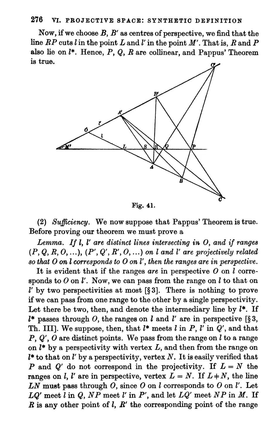
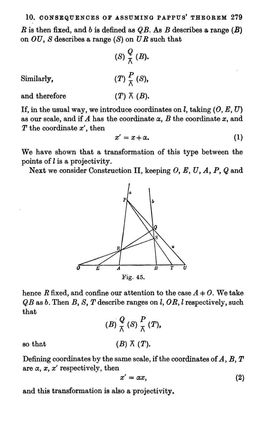
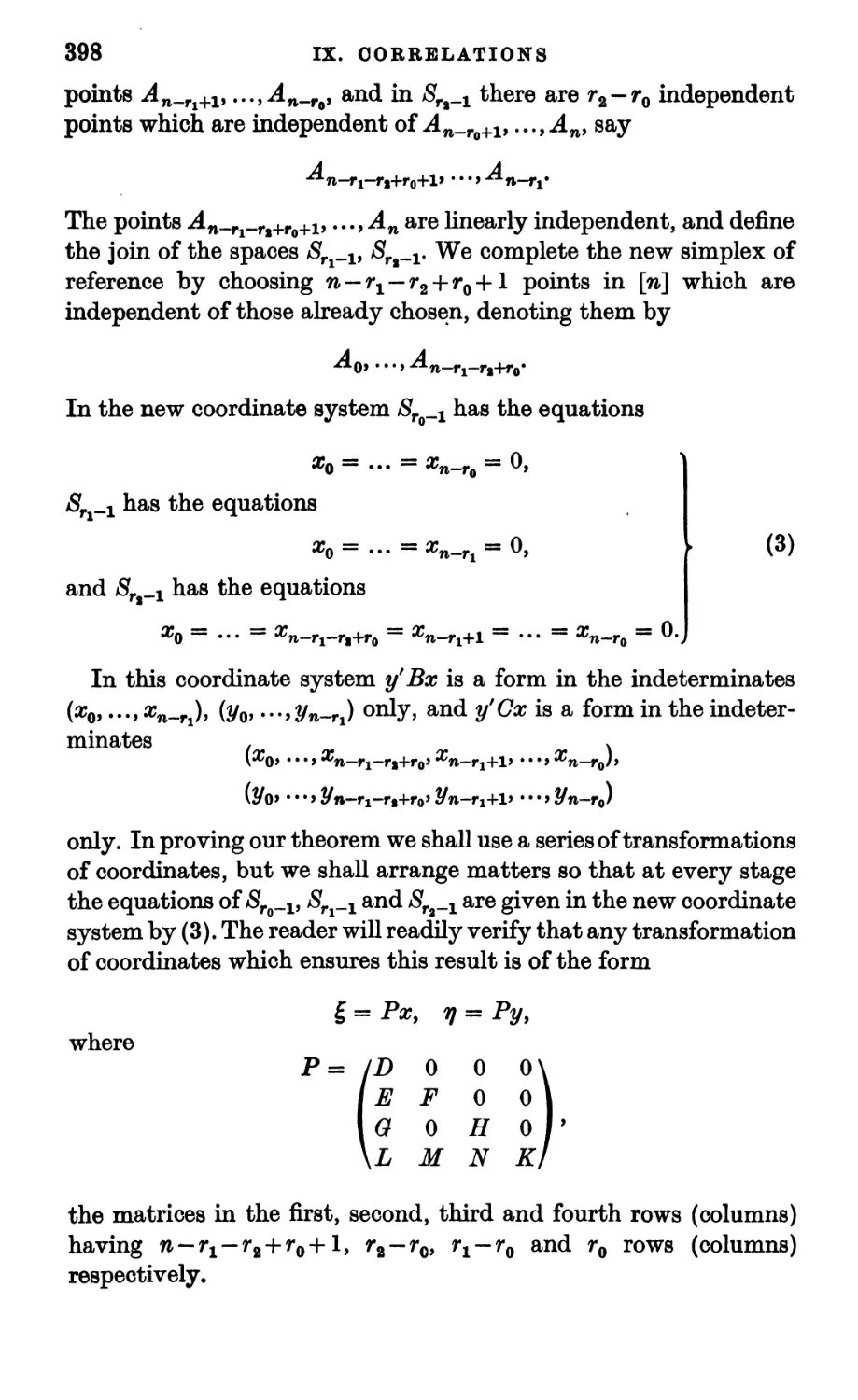
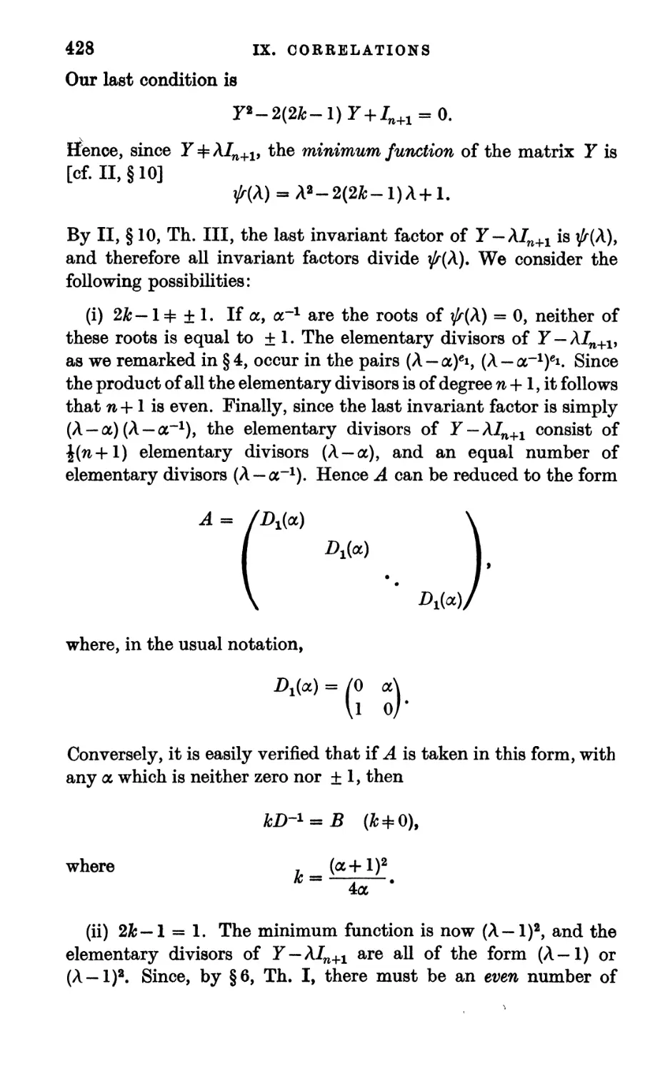
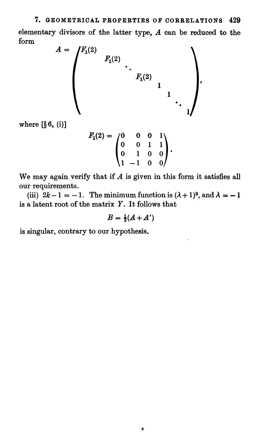
/


Текст
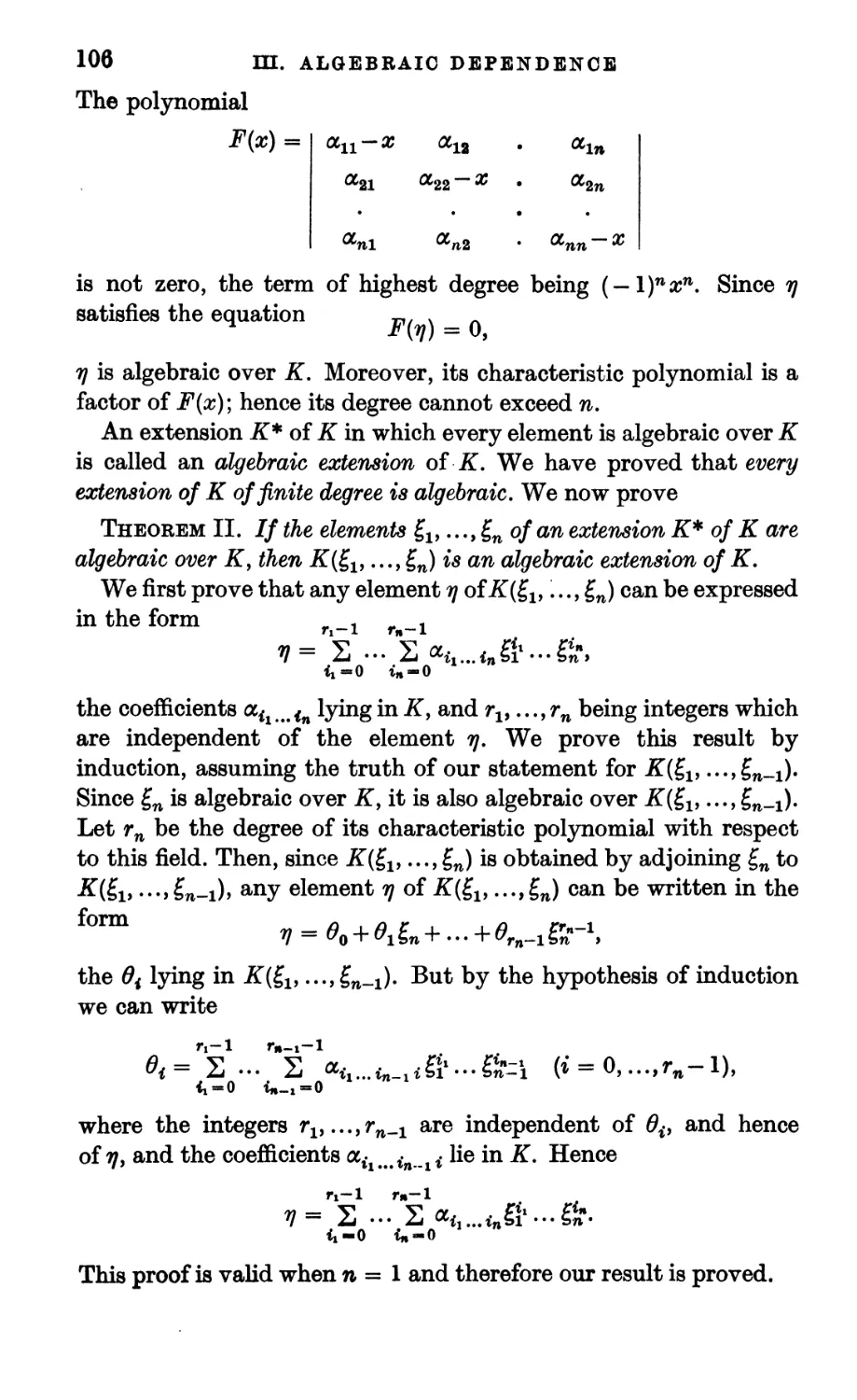
METHODS
OF
ALGEBRAIC GEOMETRY
by
W. V. D. HODGE, Sc.D., F.R.S.
Lowndean Professor of Astronomy and Geometry, and
Fellow of Pembroke College, Cambridge
and
D. PEDOE, B.Sc. (Lond.), Ph.D. (Cantab.)
Sometime Charles Kingsley Bye-Fellow
of Magdalene College, Cambridge
VOLUME I
BOOK I: ALGEBRAIC PRELIMINARIES
BOOKII: PROJECTIVE SPACE
CAMBRIDGE
AT THE UNIVERSITY PRESS
1953
*
*
PUBLISHED BY
THE SYNDICS OF THE CAMBRIDGE UNIVERSITY PRESS
London Office: Bentley House, n.w. i
American Branch: New York
Agents for Canada, India, and Pakistan: Macmillan
Printed in Great Britain at the University Press, Cambridge
(Brooke Crutchley, University Printer)
*
CONTENTS
PREFACE
page vu
BOOK I
ALGEBRAIC PRELIMINARIES
Chapter I: RINGS AND FIELDS
1. Groups
2. Rings
3. Classification of rings
4. The quotient field of an
integral domain
5. Polynomial rings
PAGE PAGE
2 6. The division algorithm 24
6 7. Factorisation in an integral
12 domain 27
8. Factorisation in polynomial
15 rings 33
19 9. Examples of fields 37
Chapter II: LINEAR ALGEBRA, MATRICES,
DETERMINANTS
1. Linear dependence 41
2. Matrices 49
3. Square matrices 54
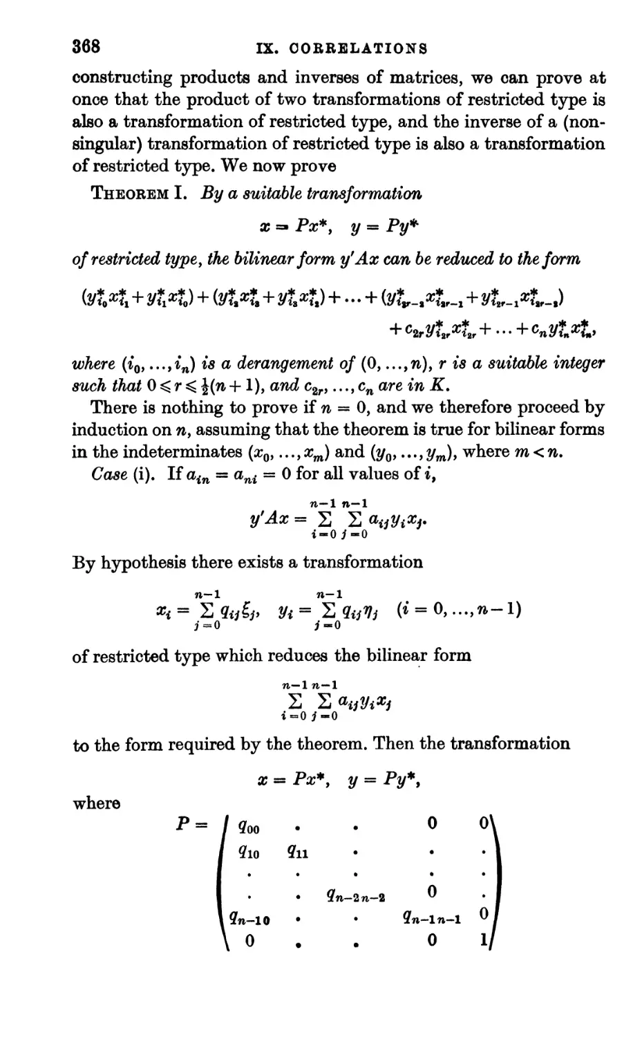
4. Transformations of a matrix 58
5. The rank of a matrix 65
6. Homogeneous linear equations 68
7. Matrices over a commutative
field 71
8. Determinants 73
9. A-matrices 86
10. Miscellaneous theorems 95
Chapter III: ALGEBRAIC DEPENDENCE
1. Simple algebraic extensions
2. Extensions of a commutative
field
3. Extensions of finite degree
4. Factorisation of polynomials
5. Differentiation of polynomials
99 6. Primitive elements of
algebraic extensions 126
. Differentiation of algebraic
functions 128
. Some useful theorems 136
101
105
111
119
Chapter IV: ALGEBRAIC EQUATIONS
1. Introduction 139
2. Hilbert's basis theorem 142
3. The resultant of two binary
forms 146
4. Some properties of the
resultant 152
5. The resultant of a system of
binary equations 156
6. The resultant system for a set
of homogeneous equations
in several unknowns 159
7. Non-homogeneous equations
in several unknowns 162
8. Hilbert's zero-theorem 165
9. The resultant ideal 166
10. The w-resultant of a system of
equations 171
vi
CONTENTS
BOOK II
PROJECTIVE SPACE
Chapter V: PROJECTIVE SPACE: ALGEBRAIC DEFINITION
1. Introduction
2. Projective number space
3. Projective space of n
dimensions
4. Linear dependence in PJ,(i£)
5. Equations of linear spaces.
Duality
PAGE
175
176
178
180
6. Desargues' Theorem
7. Some fundamental
constructions
8. The condition for a
commutative field; Pappus' Theorem
9. Some finite geometries
186 10. r-way spaces
PAGE
191
196
202
205
206
Chapter VI: PROJECTIVE SPACE: SYNTHETIC DEFINITION
253
1. Propositions of incidence 208
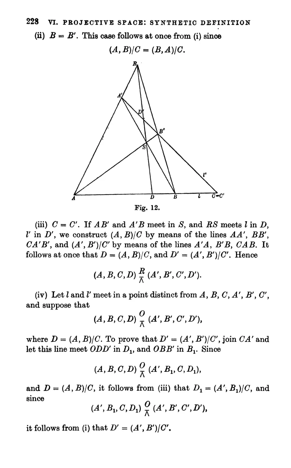
2. Desargues' Theorem 213
3. Related ranges 216
4. Harmonic conjugates 224
5. Two projectively invariant
constructions 231
6. Reference systems 246
7. The algebra of points on a line
8. The representation of the
incidence space as a P^K)
9. Restrictions on the geometry
10. Consequences of assuming
Pappus' Theorem
Chapter VII: GRASSMANN COORDINATES
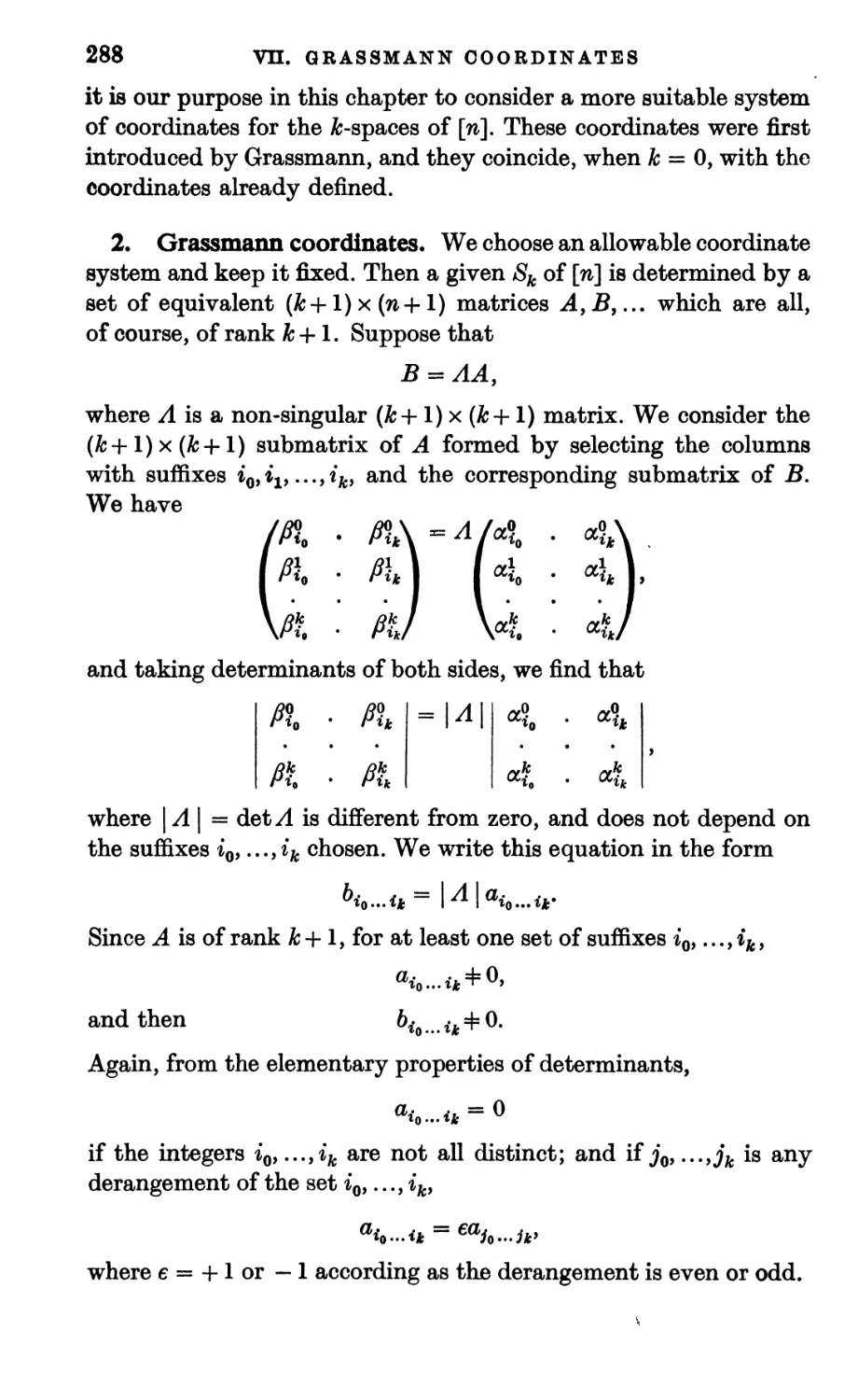
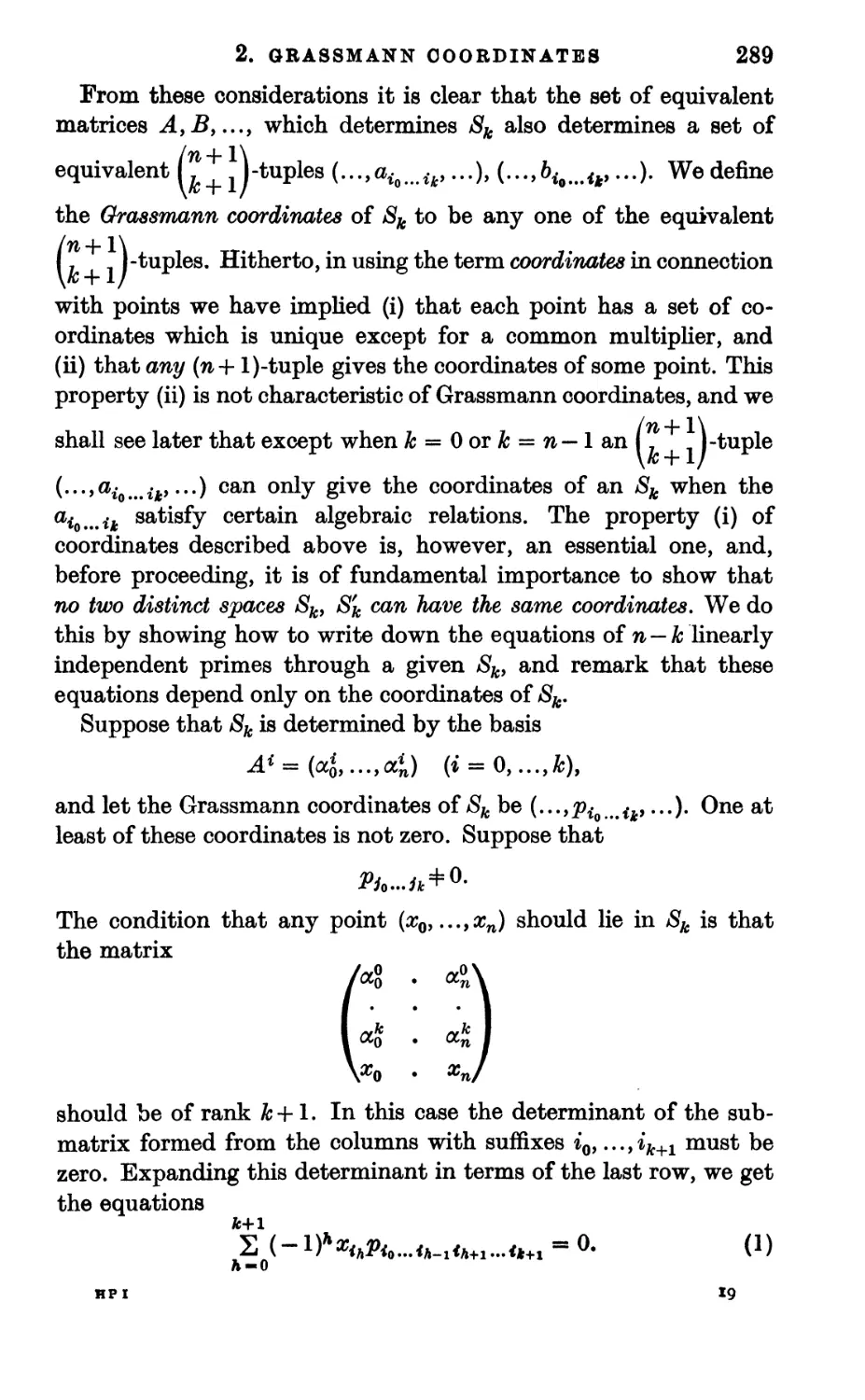
5
1. Linear spaces 286
2. Grassmann coordinates 288
3. Dual Grassmann coordinates 292
4. Elementary properties of
Grassmann coordinates 297
Some results on intersections
and joins
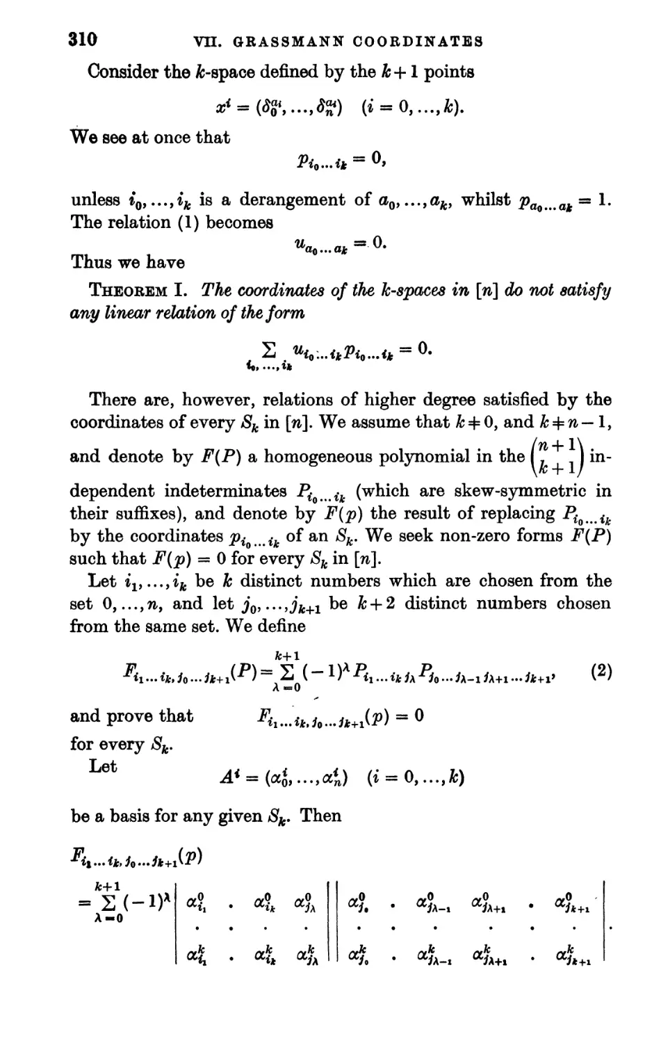
Quadratic p -relations
The basis theorem
259
272
274
304
309
315
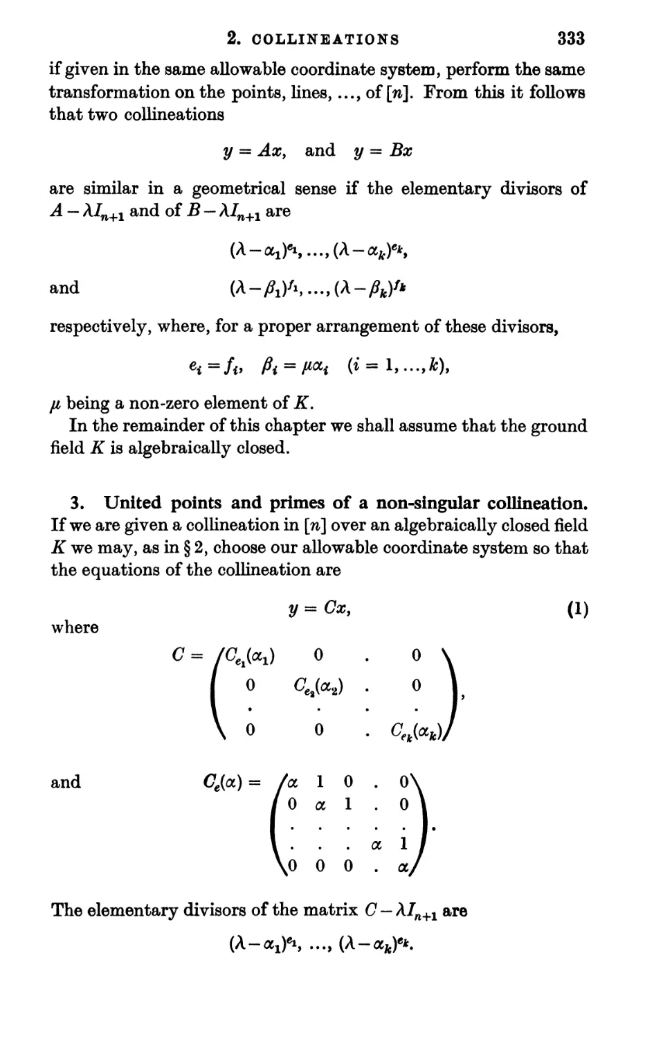
Chapter VIII: COLLINEATIONS
Projective transformations 322
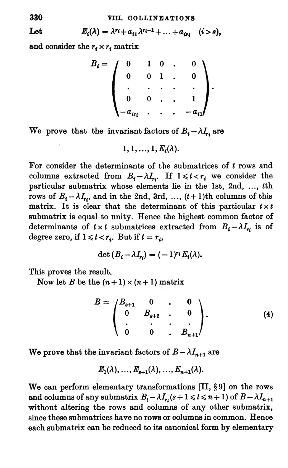
Collineations 327
United points and primes of a
non-singular collineation 333
4. The united fc-spaces of a non-
singular collineation
5. Cyclic collineations
6. Some particular collineations
7. Singular collineations
Chapter IX: CORRELATIONS
1. Correlations 362
2. Polarities 367
3. Null-polarities 378
4. Simple correlations 390
5. Transformation of the general
correlation 395
Bibliographical Notes
Bibliography
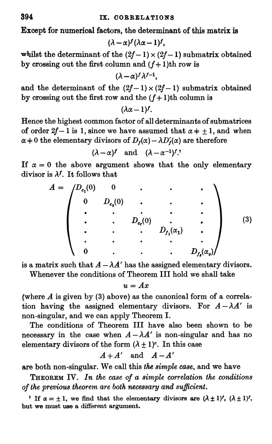
6. Canonical forms for
correlations
7. Some geometrical properties
of correlations
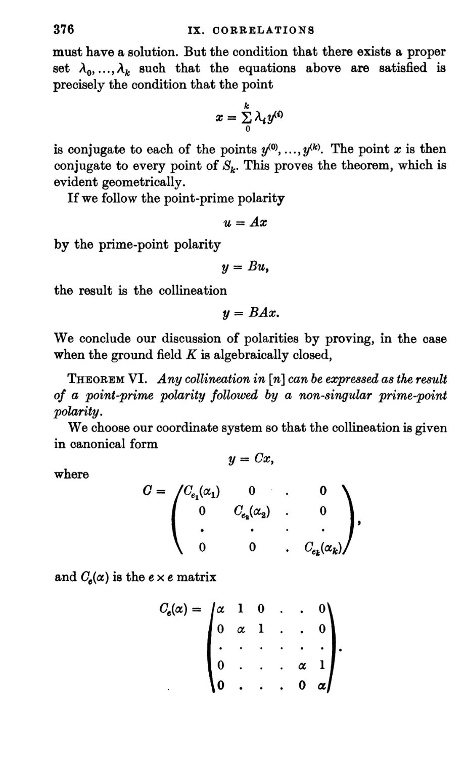
344
352
354
358
411
419
430
431
Index
433
*
PREFACE
This volume is the first part of a work designed to provide a
convenient account of the foundations and methods of modern
algebraic geometry. Since nearly every topic of algebraic geometry
has some claim for inclusion it has been necessary, in order to keep
the size of this volume within reasonable limits, to confine ourselves
strictly to general methods, and to stop short of any detailed
development of geometrical properties.
We have thought it desirable to begin with a section devoted to
pure algebra, since the necessary algebraic topics are not easily
accessible in English texts. After a preliminary chapter on the basic
notions of algebra, we develop the theory of matrices. Some novelty
has been given to this work by the fact that the ground field is not
assumed to be commutative. The more general results obtained are
used in Chapters V and VI to analyse the concepts on which
projective geometry is based. Chapters III and IV, which will be
required in a later volume, are devoted to a study of algebraic
equations.
Book II is concerned with the definition and basic properties of
projective space of n dimensions. Both the algebraic and the
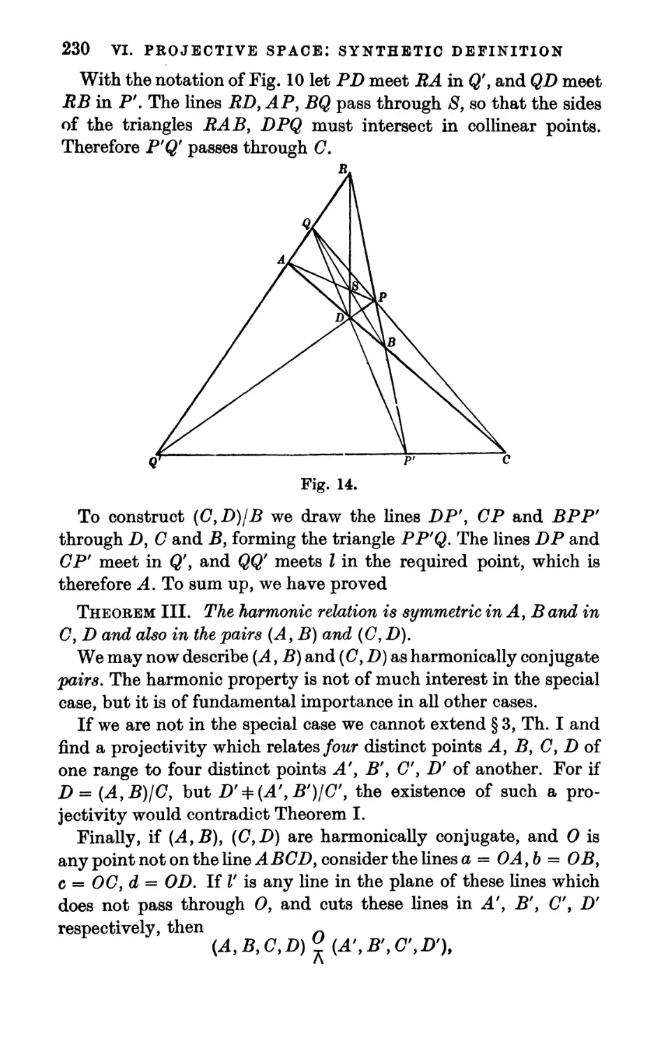
synthetic definitions are discussed, and the theory of matrices over
a non-commutative field is used to show that a space based on the
propositions of incidence can be represented by coordinates,
without the introduction of any assumption equivalent to Pappus'
theorem. The necessity of considering a large number of special
cases has made Chapter VI rather long, but some space has been
saved in the later parts of the chapter by merely mentioning the
special cases and leaving the proofs to the reader, when they
are sufficiently simple. It is hoped that this will not cause any
difficulty. This Book concludes with a purely algebraic account of
collineations and correlations. Certain elementary geometrical
consequences are indicated, but a complete study of the geometrical
problems involved would have taken us beyond our present
objective.
It is hoped that Volume II will appear shortly. This will be
devoted to the theory of algebraic varieties, and to the study of
certain loci which arise in many geometrical problems.
Viii PREFACE
We wish to express our thanks to ProfessorT. A. A. Broadbent
of the Royal Naval College, Greenwich, who has read this volume
in manuscript and in proof, and to Mr D. B. Scott of the University
of Aberdeen, who has read it in proof. We must also thank the
staff of the University Press for the care they have taken in the
production of this book, and for their ready courtesy in meeting
our wishes.
Note. The reference [II, §4, Th. II] is to Theorem II in §4 of
Chapter II. If the reference is to the same chapter or section, the
corresponding numeral or numerals will be omitted.
w.v. D.H*
D.P.
CAMBRIDGE
November 1946
*
*
BOOK I
ALGEBRAIC PRELIMINARIES
CHAPTER I
RINGS AND FIELDS
The reader is assumed to be familiar with the use of
homogeneous and non-homogeneous coordinates in geometry, when the
coordinates are real or complex numbers. When geometry is
developed with the help of these coordinates, results are obtained
by methods which belong to algebra, the differential calculus, and
so on. Those results which can be obtained by purely algebraic
processes (and they include many which are usually obtained by
the methods of the calculus) make up the subject with which we
are concerned in this work.
The operations of algebra we shall study are those of addition,
subtraction, multiplication, division, and the solution of algebraic
equations. While ordinary complex numbers are the most familiar
elements for which these operations are defined, there are more
general sets of elements for which it is possible to define them. By
allowing our coordinates to belong to these sets, a more general
geometry is obtained. We thus arrive at the definition of a more
general space than that considered in elementary geometry, and
the study of this space is the purpose of this work.
In this and succeeding chapters we consider sets of elements for
which some or all of the algebraic operations cited above are defined,
and step by step we arrive at a characterisation of the sets of elements
from which our coordinates may be chosen. These sets are known in
algebra as fields. In order, however, that the geometry which we
derive may conform to the general pattern which appears when the
field is that of the complex numbers, we shall find it desirable to
impose certain restrictions on the fields considered. These
restrictions are not all imposed simultaneously, but in succession; and
only when we have proceeded under the Umitations already adopted
as far as our subject demands do we impose a new condition. The
mathematical advantages of such a method are evident.
HPI
i
2
I. RINGS AND FIELDS
1. Groups. Consider a set S of elements, which we denote by
a,6,c,.... A law by which, given any ordered pair of elements a
and 6 of /S, possibly not distinct, we can derive a unique element c
of S, is called a law of composition for S. A non-vacuous set S of
elements with a law of composition which satisfies certain
conditions, explained below, is called a group.
We denote the element resulting from the combination of a and
b (in the given order) by ab; if the resulting element of 8 is c, we write
ab = c.
ab is a uniquely defined element of S, but may be different from ba.
The law of composition is said to be associative if, given any three
elements a, 6, c of S, we have the equation
(ab) c = a(bc).
We then write this element as abc.
The conditions that a set S, with a given law of composition,
should form a group are that
(i) the law of composition is associative;
(ii) given any two elements a, 6 of S, there exist elements x, y
such that
ax = b and ya = 6.
As an example of a group, consider the possible derangements of
the integers 1, 2, 3. If a, /?, y is any derangement of these integers,
we denote the operation of replacing 1, 2, 3 by a, /?, y by the symbol
/1 2 3\
[a /? Y)'
The successive application of any two of the six possible operations
is equivalent to some single operation of the set, and hence a law
of comppsition for the set of operations is defined. If we denote
the six operations
/1 2 3\ /12 3\ /1 2 3\
\1 2 3/' \2 3 1/' \3 1 2J'
/1 2 3\ /12 3\ /1 2 3\
\1 3 2/' \3 2 l/' \2 1 3/
by a, 6, c, d, e, f respectively, and denote the result of performing
1. GROUPS
3
first the substitution x and then the substitution y by xy, the
complete law of composition is given by the table of double entry:
a
b
c
d
e
f
a
a
b
c
d
e
f
b
~b~
c
a
f
d
e
c
c
a
b
e
/
d
d
~T
e
/
a
b
c
e
e
/
d
c
a
b
f
f
d
e
b
c
a
where the entry in the row containing x and the column containing
y is xy. From the table, or directly from the definition, it is at once
seen that the law of composition is associative. Again, since each
row contains all six elements, the equation
px = q
always has a solution; the corresponding result for the equation
yp = q
follows from the fact that each column contains all six elements.
Hence the six elements, with the law of composition, form a group.
We notice in this group that bd = e, but db = /. Hence the
equation xy = yx does not hold for all pairs of elements in the group.
Such a group is called non-commutative. If, in a given group, the
equation xy = yx is always true, we say the group is commutative,
or Abelian. A very simple example of such a group is provided by
the natural integers (positive, zero and negative), the law of
composition being ordinary addition of integers.
It is often convenient, when dealing with commutative groups,
to use the symbol of addition for the law of composition, writing
a + b instead of ab. We then call the group an additive group. It is
important to remember that this notation is never used for a
non-commutative group.
We now obtain certain properties common to all groups. From
condition (ii) we know that, given any element a, there exist elements
e and/such that
ae = a, fa = a.
Let 6 be any element of S. Then there exist elements c, d such that
ac = 6, da =* b.
4 I. RINGS AND FIELDS
From condition (i) we have
be = (da) e = d(ae) = da = 6,
fb = f(ac) = (/a)c = ac = 6.
In particular, in the first of these equations put 6=/, and in the
second put 6 = e. Then / = /e, and fe = e. Hence e = /. If there is
another element e' with the properties of e,
e'e = e', and e'e = e,
and therefore e is unique. We have thus established the existence
of a unique element e of the group such that
ae = a = ea
for every element of the group. This element e is called the unity
of the group. In the case of an additive group it is usually called
the zero of the group, and denoted by 0.
Now consider the equation
ax = e,
where a is any element of the group, e being the unity. By (ii) this
has a solution x. Then
xax =— xe -5 Xy
and therefore the element / = xa has the property fx = x, for the
x considered. But, by an argument used above, fb = b for any b in
the group. In fact, let c be an element satisfying the equation
xc = 6. Then
fb =fxc = xc = b.
It follows, taking 6 = 6, that / = e. Therefore xa = e. If y is any
element such that
ay = e = ya9
then 2/ = 2/^ = i/aa; = ea; = #.
Hence a; is uniquely defined by the equations
ax = e = xa.
This element is called the inverse of a, and is denoted by a"1. (In
the case of an additive group it is called the negative of a, and
denoted by — a. We then write 6 - a for 6 + (- a).)
1. GROUPS 5
We now show that the equations
ax = 6, ya = b,
where a, b are any elements of the group, serve to define x and y
uniquely. For
x = ex = a~lax = a~16,
and i/ = ye = j/oa^1 = 6a""1.
Hence # and y are determined explicitly. In particular the equation
a~xx = e
has a unique solution. But
a^a = e.
The solution is therefore x = a. Therefore
(a-*)-* = a.
In the case of an additive group this becomes
— ( — a) = a.
A non-vacuous subset s of S may, with the law of composition
assumed for the elements of S, also form a group. This is called a
subgroup of the given group. The following conditions are evidently
necessary and sufficient for the elements of s to form a subgroup:
(i) if 8 contains elements a, 6, it contains ab;
(ii) if 8 contains an element a, it also contains a*1.
We conclude this section with a brief reference to an evident
generalisation of the example of a group described above, namely,
the symmetric group whose elements are the permutations of the
numbers 1,2,3,...,n. The law of composition is defined as in the
example. An important subgroup of this group is the alternating
group. To define the alternating group we assume the definition of
polynomials in the n indeterminates xv ...9xn which will be given
in § 5. Consider the polynomial
A = II (*<-**) (*'»*= 1,2,...,n).
i<k
If the suffixes 1,2,...,n are permuted, it is easily seen that the
polynomial A is either unchanged (except for the order of the
factors) or becomes — A. Permutations which leave A invariant are
called even permutations, the others are called odd permutations.
6 I. RINGS AND FIELDS
A transposition, that is, a permutation which interchanges two
suffixes only, is seen to be an odd permutation. Any permutation
can be regarded as the product of transpositions. Such a
decomposition of a permutation into transpositions is not unique, but the
parity of the number of transpositions for a given permutation is
independent of the method of decomposition. The product of two
even or two odd permutations is even; the product of an even and
an odd permutation is an odd permutation. Hence the set of even
permutations of the symmetric group forms a subgroup, which is
called the alternating group, and the number of even permutations
in the symmetric group is equal to the number of odd
permutations.
2. Rings. A set of elements may have more than one law of
composition. We shall be particularly concerned with sets having
two laws of composition, under one of which the set forms a
commutative group. We write this group as an additive group, and
refer to the corresponding law as the addition law of the set. The
zero of the group is called the zero of the set.
The second law of composition is called the multiplication law,
and the result of combining elements a, b of the set by this law is
denoted by the product ab. Multiplication need not be commutative,
but we shall require it to be associative. It is said to be distributive
over addition if
a(b + c) = ab + ae, and (b + c)a = ba + ca9
for all a, b, c in the set.
A ring, then, is a set of elements with two laws of composition,
addition and multiplication, with the properties:
(i) the set is an additive group with respect to addition;
(ii) multiplication is associative, and distributive over addition.
The following examples will illustrate the various possibilities
which may arise in the study of rings. In the first four cases the
laws of composition for the elements involved are addition and
multiplication as usually defined:
I. The set of all complex numbers.
II. The set of all integers, positive, zero, and negative.
III. The set of all even integers.
IV. The set of all integers, reduced modulo the integer m.
2. RINGS 7
V. The set of all matrices of q rows and columns whose elements
are complex numbers. A matrix of this type is the array
fan a12 . alq\
^21 ^22 • &2q
• • • •
^aql ag2 • aqq/
where each a{j is a complex number. Addition is defined by the rule
/an a12 • ala\ /fin fi12
a21 a22 . <z2q I I /?21 /?22
\&ql <%q2 • &qq/ \Pql Hq2 • A«
A*U + All «13 + As • "lq + Plq\
a21 + Al a22 + ^22 • a2q + 02q
• • • .
^Pql+Pql <*q2 + fiq2 • <*qq +fiqq/
and multiplication by the rule
/Ai As •
Ai A2
a«i ag2 • aw/ \Ai A* • Aa/ v«i ^«2
where r«sS^«.
fc-i
The reader may easily verify that these sets, with the prescribed
laws of addition and multiplication, form rings. Further study
reveals certain features common to some of the rings, but not
necessarily to all.
(i) In the cases I, II, III and IV the zero of the ring is the number 0.
In case V the zero is the zero matrix
In all five cases
for all elements a
0 =
1
!
a.
of the ring
(°
(o
ii
0 =
,•
0
0
•
0
= 0 =
•
•
1
•
= 0
0
0
0,
.a
8 I. RINGS AND FIELDS
(ii) In cases I, II and IV let e be the integer 1, and in case V let
^0 0 . 1;
in each of these cases e has the property given by the equations
ae = a = ea
for every element a of the ring. When such an element e exists, it
will be shown to be unique. It is called the unity of the ring. In
case III there is no element of the ring with this property.
(iii) In all but the last case multiplication is commutative. In
case V it is non-commutative, since, if q > 1,
. 0
and
0
0
0
(iv) In cases I, II and III, if a and b are two elements of the ring
such that , ~
ab = 0,
then either a = 0 or b = 0.
This property holds for the ring IV if and only if m is a prime
number. If m = pq, where neither p nor q is 1, then p and q are two
non-zero elements of the ring such that pq = 0. On the other hand,
if m is prime and ab = 0, so that
ab = cm,
it follows, by the unique factorisation properties of ordinary integers,
that either a or 6 is divisible by m.
The property we are discussing does not hold in case V if q > 1.
For „ A A, #A Q t ox = 0>
1
^0 0 , 0/ \0 0 , 0j
and neither factor is the zero of the ring.
2. RINGS 9
(v) In case I there is associated with every element a of the ring,
other than the zero, a unique inverse ar1 such that
aa*1 = arxa = e.
The rings II and V do not have this property, and it can be shown
quite simply that the ring IV has the property only when m is a
prime number. The property is meaningless in case III since the
ring has not unity,
(vi) If we write
a + a = 2a, a + 2a = 3a, etc.,
the elements a, 2a, 3a,... (a + O) are all distinct, except in case IV,
when
ma = 0
for all elements a in the ring.
It will be observed that only in (i) did we have a property common
to the five rings, namely, the zero has the property aO = 0 = Oa.
We now show that this property holds for all rings, and deduce
other elementary results true for any ring.
Let a, b be any two elements of a ring i2, and let 0 be the zero
of R. Then
a + 0 = a,
and therefore ba = 6 (a + 0) = ba + 60,
and also ab = (a + 0) b = ab + 06.
From the uniqueness of the zero of a ring it follows that
60 = 0 = 06,
these equations holding for any element 6 in R.
Again, we know that any equation
a + x = 6
has a unique solution
x = 6 + (-a) = 6 —a
in R. Now
a(6-c) + ac = a(b-c + c)
= a6.
Hence a(6 — c) = a6 — ac,
and similarly (6 - c) a = 6a - ca.
10
I. RINGS AND FIELDS
Therefore, taking 6 = 0, we obtain the equations
a( — c) = —acf { — c)a = —ca
for all a, c in B. Again,
(-a)(-6)-a& = (-a)(-6) + (-a)6
= (-a)(-6 + &)
= (-a)0 = 0,
and therefore (— a) (— b) = aft.
We have thus shown that the usual multiplicative properties of
the minus sign hold in any ring.
We now define the relationship between two rings known as
isomorphism. Let B and i2* be two rings such that to each element
a of B there corresponds a unique element a* of i2*, and such that
any element a* of B* arises from exactly one element a of B. Such
a correspondence is said to be one-to-one. Now suppose, in addition,
that the correspondence is such that if a, 6 correspond respectively
to a*, &*, then a + b and ab correspond respectively to a*+ 6* and
to a*6*. The correspondence is then called an isomorphism.
Isomorphism between rings is a relation of the class known as
equivalence relations. Consider any set 8 of elements a, yff, y,..., and
let there be a relation, which we denote by ~, between the elements
of S, so that, given any two elements a, ft, we know whether a~ p
is true or false. If the relation ~ is:
(i) reflexive, that is, a ~a for all a in 8;
(ii) symmetric, that is, a ~ ft implies f}~ a;
(iii) transitive, that is, if a ~ /? and /? ~ y, then a ~ y\
we say it is an equivalence relation.
An equivalence relation between the elements of a set 8 divides
8 into subsets, no two of which have any elements in common. If
a, fi are in the same subset, <z~fi. Every element of 8 lies in one of
these subsets.
It is clear that if S is the set of all rings, and if a ~/? means that
the ring a is isomorphic with the ring /?, the relation is an equivalence
relation. We shall often speak of two isomorphic rings as being
equivalent, implying that if in our discussion we replace one ring
by the other (making any necessary consequential substitutions)
nothing in our conclusions is altered.
2. RINGS
11
A subset S of the elements of a ring R is said to form a subring
of R if the elements of S form a ring under the addition and
multiplication laws of B. For this to be so it is necessary and sufficient
that if a and b are any two elements of S, then a — 6 and ab belong
to £.
If S is a subring of 22, B is said to be an extension of 8. The
following theorem is frequently used:
Theorem I. If A and JB* are two rings, and A is isomorphic with
a subring B of J5*, there exists an extension A* of A which is
isomorphic with J5*, this isomorphism including that between A and B.
Let C be a set of elements in a one-to-one correspondence jTwith
those elements of J3* which are not in B, and let A* consist of the
elements of A and C. We have merely to define addition and
multiplication in A* so that A* becomes a ring with the required
properties. Let al9a2,... be elements of A*. To each at there
corresponds a unique element bt in J3*. If at is in A, bt is the element of
B corresponding to ai in the isomorphism between A and B. If
ai is in C, bt is that element of the set of elements of J5* not in B
which corresponds to ai in the correspondence T. Conversely, to
any element bi of J5* there corresponds a unique element ai of A*.
Now, ifal9 a2 are any two elements of A*, we define ax + a2 and axa2
as follows. To ax and a2 there correspond bx and b2 in J5*. Let
bx + b2 = 68, bxb2 = 64,
and let a3 and a4 be the elements of A* which correspond to 63
and 64. We then define
ax + a2 = a3, axa2 == a4.
Clearly A * is a ring isomorphic with B*. Moreover, the construction
shows that A is a subring of -4*. Hence A* has all the required
properties.
We conclude this section by describing a particular type of sub-
ring which we shall meet in later chapters. Let R be any ring, I a
subset of R with the following properties:
(i) if a, b are in I, then a — b is in I;
(ii) if a is in /, r in R, then ra is in I.
We call I a left-hand ideal in i2; a right-hand ideal is defined by
reading ar instead of ra in (ii). The two ideals coincide when
multiplication in jR is commutative.
12
I. RINGS AND FIELDS
To show that if I is not vacuous it is a subring of R we remark
that if r is in I conditions (i) and (ii) coincide with the conditions
stated above for a subring. On the other hand, not all subrings are
ideals, since the condition (ii) need not hold.
R itself is an ideal in R, and is called the unit ideal. The subset
of R which consists only of the zero of R is also an ideal. These two
ideals are usually called the improper ideals of R. A ring containing
a proper ideal is the ring of integers (Example II, above). If m is
any integer greater than 1, the set I of all integers of the form + ma,
where a is an integer, clearly forms a proper ideal in this ring.
The existence of an ideal I in R enables us to define an
equivalence relation in R. If a, 6 are two elements of R, we write
a = 6 (I)
if a —6 is in I. The reader may easily verify that this is an
equivalence relation. It is a type of equivalence which will often appear
subsequently.
3. Classification of rings. Rings which are subject to no other
conditions than those imposed by the definition given in §2 are
too general to be of much interest in algebraic geometry. We limit
the rings with which we deal by imposing fresh conditions which
are, in fact, equivalent to requiring the rings to possess one or more
of the properties noted in the remarks (ii), ..., (vi) on the examples
of rings given in § 2. Different restrictions lead to rings with quite
different properties. We now consider some of the more important
types of rings.
We saw that a ring R may or may not possess an element c with
the property
r r j ea = a = ae
for every element a in R. We now show that R cannot have two
distinct elements e,/ with this property. For, if
ea = a, bf = 6,
for all elements a, b in R, we may take a = /, b = e, and obtain
the equations , _ «
If this unique element e exists in R, it is called the unity of jB.
All the rings we shall consider will be rings with unity, unless the
contrary is stated explicitly. For the present we continue to denote
the unity by e.
3. CLASSIFICATION OF RINGS
13
If a is any element of a ring J2 with unity, there may or there may
not exist an element a*1 of R such that
aa*1 = e = a^a.
There cannot be two such inverse elements, for if
ax = e,
then a~"xax = a^e,
that is, x = a"1.
When such an inverse element a""1 exists, a is said to be regular, or
to be a unit of R. Clearly e and — e are units of R. On the other
hand, the zero 0 is not a unit, since for every element a of R
a0 = 0.
Again, we have seen [§ 2, (iv)] that there are rings R in which
there exist pairs of elements a, b, neither of which is zero, such that
ab = 0.
We call a a left-hand divisor of zero, b a right-hand divisor of zero.
The divisor of zero a cannot be regular. For, if a has an inverse a-1,
6 = a~xab = a~x0 = 0,
contradicting our assumption that 6 is not zero. Similarly, 6 cannot
be regular.
The two types of ring with which we shall be particularly
concerned are the integral domain and the field. An integral domain is
defined as a ring with unity, in which multiplication is commutative,
and which has no divisors of zero. Examples I, II, and IV (in the
case m prime) of § 2 are integral domains.
A field is defined as a ring with unity in which every non-zero
element is regular. The ring of all complex numbers is clearly a
field. By the result proved above a field cannot contain any divisors
of zero. A commutative field—that is, a field in which multiplication
is commutative—is an integral domain.
We shall eventually be able to confine our attention to
commutative rings, but it is convenient to obtain certain results which
are valid for non-commutative rings, as these will be used in an
analysis of the postulates on which projective geometry is usually
based. Therefore, except when we say so expUcitly, we shall not
assume our rings to be commutative.
14
I, RINGS AND FIELDS
In a ring R consider any element a. Write
a + a = 2a, a + 2a = 3a, ...,
noting that na is not a product, but the sum of n elements each
equal to a. We have seen by an example that there exists a ring R
for which we can find an integer m such that
ma = 0
for all elements a in R.
Now, let R be a ring with unity e, and suppose that for some
positive integer n, __ 0
Let m be the smallest positive integer satisfying this condition.
Then, first of all, if a is any element of R,
ma = a + a+ ...+a
= ea + ea + ... + ea
= (e + e+...+e)a
= (me) a
= 0.
If m is not prime, and m = pq, then
#e=#0, je + O,
but peqe = pqee
= me = 0,
and R has divisors of zero. The number m is called the characteristic
of the ring R. We have proved that the characteristic (if there is
one) of an integral domain or a field is a prime number.
If, for all non-zero integers n,
ne + O,
the ring is without characteristic. (It is then often said to be of
characteristic zero, but this terminology is not strictly correct.)
If a ring R with unity has characteristic m, the subset
0, e, 2e, ..., (m —l)e
forms a subring. For
ae — be = (a — 6) e
= ce,
where c = a — b (modulo m\
and (ae) (be) = de,
where d = ab (modulo m).
3. CLASSIFICATION OF RINGS
15
Thus R contains a subring isomorphic with the ring of integers
reduced modulo m. By Th. I, § 2, there is an extension of this ring
isomorphic with R.
Similarly, if R is without characteristic, it is isomorphic with an
extension of the ring of natural integers. It follows that a ring
without characteristic contains an infinite number of elements.
In each case we identify R with its isomorph, and so in future we
shall write the unity of the integral domain or field we are
considering as 1.
Later on we shall confine ourselves to integral domains and fields
without characteristic, but at present we do not make this restriction.
4. The quotient field of an integral domain. It is a familiar
result that the integral domain of the natural integers is embedded
in a field, namely, the field of rational numbers. This is a special case
of a general theorem which we shall frequently use.
Theorem I. Given an integral domain I, there exists a
commutative field K which, regarded as a ring, contains I as a subring.
The construction which we give for K gives the minimum field
having the required property. This minimum field is defined
uniquely, to within isomorphism.
The elements of I are denoted by a, 6, c,..., the zero and unity by
0 and 1. Consider the set of all ordered pairs (a, 6) in which 6#0,
and the relation denoted by ~ between pairs where
(a,b)~(c,d)
stands for the equation
ad — bc = 0.
Since multiplication is commutative, it follows at once that this
relation is reflexive and symmetric. It is also transitive. For, if
(a,b)~(c,d) and (c,d)~(e,/),
ad = be and c/ = de.
Therefore adf = bef = bde,
and so # d(af— be) = 0.
From our definition of an ordered pair, d is not zero. Since an
integral domain contains no divisors of zero it follows that
af = be,
that is, (a>yb)~(e,f).
16 I. RINGS AND FIELDS
The relation is therefore an equivalence relation, and divides all
pairs under consideration into classes. The class to which (a, 6)
belongs will be denoted indifferently by [a, 6] or [c, d], where
(a,6)~(c,d).
We define the sum of a pair {a, b) and a pair (c, d) by the equation
{a, b) + (c, d) = {ad + be, bd).
By hypothesis, b and d are not zero, and therefore bd =f= 0. The pair
denoted as the sum is therefore admissible. It is evident that
addition of pairs is commutative. Now let
{a, 6) -(a', 6'), {c,d)~{cf ,d').
Then (a', 6') + (c', d') = (a'd' + 6V, 6'd') - {ad + be, bd),
since {ad + 6c) 6'd' - {a'd1 + 6'c') 6d
= {aV - a'6) dtf' + (cd' - c'd) 66'
= 0.
Hence we may define the addition of classes by the equation
[a, 6] + [c, d] = [ad + be, bd].
Since
{[a, b] + [c, d]) + [e, /] - [adf+ bcf+ bde, bdf]
= [a,b] + {[c,d] + [e,f]),
addition is associative. Also, the equation
[a,b] + z= [c,d]
has the solution
x = [6c — ad,bd].
Hence the classes form a commutative group under addition. The
zero of the additive group is [0,1] = [0, a], where a is any non-zero
element of I.
We now define multiplication of pairs by the equation
{a,b){c,d) = {ac,bd).
Multiplication is clearly commutative. Also, if
(a, 6) ~{a', V), {c,d)~{c',d')y
then {a'c', b'd') ~ (ac, bd),
since a'c'bd — ac6'd'
- {a'b-ab')c'd + {c'd-cd')ab'
»0.
4. THE QUOTIENT FIELD OF AN INTEGRAL DOMAIN 17
Thus we can define multiplication of classes by the equation
[a, 6] [c, d] = [ac, bd].
Multiphcation can immediately be proved to be associative. Again,
[a, b] ([c, d] + [e, /]) = [a, 6] [cf+ de, df]
= [acf+ade,bdf]
= [abcf+abde,b2df]
= [ac, bd\ + [ae, 6/]
= [a,b][c,d] + [a,b][e,f].
Hence multiphcation is distributive over addition. The set of
classes of equivalent pairs, with addition and multiphcation defined
as above, therefore forms a commutative ring If*. If a is any
non-zero element of /,
(a,a)~(l,l),
and so [«,«] = [1,1].
Since [a, b] [1,1] = [a, 6],
[1,1] is the unity of K*. Finally, if [a, 6] is any non-zero element
of K*, both a and b are non-zero. Therefore [6, a] is in K*. But
[6,a][a,6] = [o6,a6] = [l,l].
Therefore every non-zero element of K* has an inverse. Thus K*
is a commutative field.
Now consider the elements of K* which can be written as [a, 1],
and let them form the subset 8. Since
[a,l]-[6,l] = [a-6,l],
and [a, 1] [6,1] = [ab, 1],
S forms a subring of K* isomorphic with I. By § 2, Th. I, there
is an extension K of I which is isomorphic with If*, and which is
therefore a field. The element of K corresponding to [a, b] of If* is
usually written a/b. If
a _ c
6~^
then orf = 6c.
We also have a
— = a.
1
HP I 2
18 I. RINGS AND FIELDS
The field K is the one required. It is usually called the quotient field
of I. To complete the proof of our theorem we now show that any
commutative field K' which contains I as a subring contains a
subfield isomorphic with K.
We first observe that, by the definition of a field, the non-zero
elements of Kf form a group under multiplication. Hence the
equation
bx = a (6 # 0),
where a, 6 are in K'y has a unique solution in K'. We now show
that the equations
bx = a, dx = c,
where a, 6, c, d are in I, and 6 and d are not zero, have the same
solution in K' if and only if
ad = be.
First, if this condition is satisfied, and # is a solution of the first
equation, we have
bdx = ad = be.
Therefore b(dx — e) = 0,
that is, dx = c.
Secondly, if the two equations have the same solution x, then
ad = bdx = be.
Thus to every element x of K' which satisfies an equation
bx = a,
where a, b are in /, and b # 0, there corresponds a unique element
afb of If, and conversely. Moreover, if x, y correspond to a/6, c/d
respectively, then
bx = a, dt/ = e.
and therefore d6(a; + y) = od + 6c,
and 6d#2/ = a6.
Hence a? + y and o^/ correspond to r + i and y-z respectively. The
field K' therefore contains a subfield isomorphic with K.
4. THE QUOTIENT FIELD OF AN INTEGRAL DOMAIN 19
From this theorem we deduce that K is the smallest field which
contains I as a subring.
Finally, we note that if I is of characteristic p, the sum to p terms
1 + 1 + ... + 1 = 0.
Hence [1,1] + [1, l]+... + [l, 1] = 0,
and it follows that K is of characteristic p. On the other hand, if
I is without characteristic,
[l,l] + [l,l]+... + [l,l] = [l + l + ... + l,l]#[0,l],
and hence K is without characteristic.
5. Polynomial rings. We now discuss a method of extending
a ring by the adjunction of an element x, called an indeterminate.
The only case of any importance which we shall meet in this book
is that in which the ring is an integral domain, and it will make for
simplicity if we assume throughout this section that the basic ring
from which we start is an integral domain 7.
Let us consider the ordered sets
(aQ,av...,ar)
which consist of a finite number of elements ai of I. Two sets
{aQ,al9...,ar)9 (b0,bv ...,b8)
are said to be equivalent if
«*< = &< (i== l,2,...,min(r,a)),
a. = 0 (i = 5+1,...,r) when r>8>
bt = 0 (i = r+1, ...,5) when s>r.
This relation is evidently reflexive, symmetric and transitive, and
is therefore an equivalence relation. We define the addition of two
sets by the equation
(a0,av ...,ar) + (60, bl9..., b8) = (c0, cv ..., ct),
where t = max (r, s), and ct = at + 6i5 defining a{ = 0 for i > r and
6i = 0 for i > 8. It is easily seen that if either of the two sets is
2-2
20 I. RINGS AND FIELDS
replaced by an equivalent set, the sum is replaced by an equivalent
set. Multiplication of two sets is defined by the equation
(a0, av..., ar) (60, bl9..., b8) = (d0,dl9..., dr+8),
where d< = a<60 + a<_161+...+^6^ (i = 0, ...,r + s),
and, as above, we define at = 0 for i > r, and bi = 0 for i > s. Again,
the replacement of either set by an equivalent set converts the
product set into an equivalent set. If we now consider the classes of
ordered sets defined by the equivalence relation, we see that they
form an additive group with respect to addition, the zero of the
group being all sets equivalent to the set (0); also, multiplication is
associative, and distributive over addition. Hence our classes of
equivalent sets, with the two laws of composition we have defined,
form a ring R, and it is easily seen that (1) is the unity of R. This
ring R contains a subring which is isomorphic to I. The elements
of this subring are (a). For
(a) + (6) = (a + 6),
and (a) (b) = (ab).
Hence an isomorphism is set up if (a) is mapped on the element
a of I.
Let us now consider the set (0,1). We see that
(0,1)2 =(0,1)(0,1) = (0,0,1),
(0,1)3 =(0,1)2 (0,1) = (0,0,0,1),
• •••••
(0,1)^=(0,1)^(0,1) = (0,0,0,...,1),
where in the last set written the unity is preceded by n zeros. Since
(a) (0,1)» = (0,0,0,..., a),
we may express the set (a0,av ...,ar) as follows:
(a0,^,...,af) = (a0) + ^
Now let us denote by I[x] the ring which is an extension of I and
which is isomorphic with R [§2, Th. I], x being the element of the
extension which is mapped on the set (0,1) of J?. Then, from the
above reasoning, the set (a0,al9...,ar) of R is mapped on the
element a0 -+-axx + a2x2 + ... -+-arxr of I[x\. These elements are called
polynomials, with coefficients a0,av ...,ar. If ar#= 0, the polynomial
a0 + aix + • • • + ar& iQ sai(* to ^6 °f degree r.
6. POLYNOMIAL RINGS 21
We note that the zero (0) of R is mapped on the zero of 7, and
therefore the equation
a^ + axx+...+arsif = 0 (1)
is satisfied if and only if
a0 = a± = ... = ar = 0.
Because of this property of the element x, it is said to be an
indeterminate over I.
In the representation of a polynomial we usually omit any term
a^1 in which at = 0, whether i exceeds or is less than the degree of
the polynomial. In this sense anxn is a polynomial whose complete
representation is 0 + Ox + ... + Ox11*1 + anxn. Furthermore,
a0 + a1x1+... +arof
can be regarded as the sum of the r + 1 polynomials
o> 0/]X) ..., a^x .
Since also a^ is the product of at and xi9 and since for the
polynomials x,x2}... we have the multiplication law
xi>xv = xp+<*,
the ring I\x] is obtained by introducing a new element x among the
elements of I which can be multipUed commutatively by any
element of I. We say that I[x] is obtained from I by adjoining the
indeterminate x to I. I[x] is also called the ring of polynomials in
x over I.
These results apply when I is any commutative ring with unity.
We now proceed to draw conclusions concerning the ring I[x] from
the fact that I is an integral domain.
Theorem I. If I is an integral domain, so is I[x\.
We have already seen that I[x] is a commutative ring with
unity. We must now show that I[x] has no divisors of zero. If
f=a0 + a1x+...+amxm9
and g = b0 + b±x+ ... +bnxn
are two non-zero polynomials, we may assume am #= 0, bn # 0. Then
fg = c0 + cxx+ ...+cm+nx™+n,
where cm+n = am6n=i=0, since I has no divisors of zero. Hence
/gr#=0. In other words, if fg = 0, and /#0, we must have g = 0.
Therefore I[x] has no divisors of zero.
22
I. RINGS AND FIELDS
The process of adjoining an indeterminate to an integral domain
to obtain another, more extensive, integral domain may be repeated.
If J = I[xx], J[x2] is an integral domain. Its elements are
polynomials , , , n
where a€ = ai0 + aaxx+...+ aimx^
is in I\x^\y and m is the maximum of the degrees of a0,..., an. The
elements a{i lie in I. Hence, the elements of J[x2] can be written
in the form n m
in which each term a{jxlx{ is the commutative product of aij9 x\, x{.
If J' is the integral domain I[x2], the elements of Jf[x^\ are of the
form m n
and the integral domains J[x2] and /'[a;!] are easily proved to be
equivalent. We denote this integral domain by I[xvx2].
Proceeding in this way, we can adjoin indeterminates xl9x2, ...,xt
in turn to I. The resulting ring I[xv ...,xr] is independent of the
order in which the indeterminates are adjoined. For the elements
of this ring are of the form
r
fh
s
<!-<)
nr
... S aiit
ir-0
,..<,*ll-
the term written explicitly being the commutative product of
aii...ir> xi> •••> x%- Also, I[xv ...,xr] is an integral domain. We have
already proved this result when one indeterminate is adjoined to I.
We assume it is true when r— 1 indeterminates are adjoined. The
result is assumed true for J = I[xv ...,av_J, and by Th. I is
therefore true for J[xr]. But J[xr] = I[xv ...,&r]. Hence we have
Theorem II. If I is an integral domain, so is I[xv ...,xr].
We conclude this section by introducing an important operation
on polynomials in I[xv ...,xr] known as specialisation. Let
be any polynomial in our integral domain. We select any number
j (0^j<r) of the indeterminates xly...,xry say, for example,
6. POLYNOMIAL RINGS 23
xv ..., Xj. Let a19..., o^ be any elements of I. Then if in / we replace
xly..., Xj by ax,..., a^ respectively, / becomes
/•- "£' ...S6i( ^{...^,
where . 5» ** i i
is in /. (a* is, of course, the product of i factors each equal to a.)
Then / is said to specialise to a polynomial /* in I\xi+V ...,xr].
We use the notation
to describe the specialisation.
By using the fact that equations such as
f+9 = h9 fg = k
express relations between the coefl&cients of/, gy h and k which do
not involve the ^determinates xv ..., #r, we see at once that if,
for any specialisation of the indeterminates,
/->/*> g->g*> h->h*y k->k*,
then /* + gr* = A*, /*gr* = &*.
The converse of this result is not, of course, true.
Note. While we do not have to consider polynomials whose
coefl&cients are in a non-commutative ring, it should be pointed out
that a theory of such polynomials exists. The only result of this
theory which we shall use is the following. Let
f=a0xm + a^™-1 +... + am,
where at is in a non-commutative ring K, x is indeterminate and is
assumed to commute with every element of K. Then if a is any
element of K, there exist polynomials
p = box™"1 +...+ bm_l9 q = c^-1 +...+ cm_x,
and elements 6m, cm of K such that
/= (:^)(60^-1+...+6^^
= (Co*™-1 +...+ cm_x) (x - a) + cm.
Indeed, we need only take
b{ = a<a0 + a'-S +...+ ai9\
24 I. RINGS AND FIELDS
6. The division algorithm. In this section I denotes an integral
domain, K a commutative field, and I[x]9 K[x] the rings obtained
by adjoining the indeterminate x to Iy K respectively.
Let / = a0 + a±x+ ...+amxmy
g = 60 +&!#+...+ 6n#n (n^m)
be two polynomials in I[x] of degrees my n respectively, and let us
suppose, in the first place, that bn = 1. Then, clearly,
is a polynomial in I[x] of degree m1<m. If n ^ mly and if
then A=A-a'mlxmi-n9
= f-{amx™-n + a'mx™>-")g
is a polynomial of degree m2<mv Proceeding in this way we arrive,
in all cases, at a polynomial q of degree m — n such that
is a polynomial of degree less than n, the degree of g.
This result can be generalised to include the case in which bn is
a regular element of I. For, if b~1bn = 1,
9' = b^g
is a polynomial of degree n in which the term in xn has coefl&cient
unity. Then there exists a polynomial q' such that
r=/-jV=/-(jV)»
is of degree less than n.
We now show that the polynomials qy r obtained in this way are
unique. For if q'y r' are any two polynomials such that r' —f—q'g
is of degree less than n, we have the equation
r~-/ = (q'-q)g.
But the degree of r — r' is less than ny and the degree of (q' — q)g is
at least ny unless q9 = q. Hence, unless q' = qy we have a polynomial
of degree less than n equal to a polynomial of degree at least n.
This is impossible, and therefore q = q\ and consequently r = r'.
6. THE DIVISION ALGORITHM
25
The process given above for determining q and r is called the
division algorithm.
A special case of the result just proved is the Remainder Theorem.
If c is any element of I, take g = x — c. Then there exists a
polynomial a such that * , x
f-q{x-c) = r
is in I. This equation remains true when we make the specialisation
x->c. Hence £l x
where/(c) is the result of replacing x by c in/.
Returning to the division algorithm, it may happen that r = 0.
We then have three non-zero polynomials/, g9 q in I[x] such that
<7 and g are said to be divisors of/, and / is a multiple of ^ and of g.
If the degrees of both g and q are greater than zero, both g and g
are said to be proper divisors of/.
We now suppose that I is a field K. Since every non-zero element
of K is regular, the division algorithm can be applied to any pair of
polynomials/0,/i of K[x], By repeated applications of the division
algorithm we shall construct a sequence of polynomials/2,/3, ....
We shall denote the degree of/^ by miy and suppose that m0^mv Our
purpose is to obtain information on the common divisors of/0 a,nd/1.
Applying the algorithm to /0,/1, we get the equation
/0 = ^1/1+/2^
where m2<mv If/2 is not zero we apply the algorithm to /x,/a,
obtaining the equation
/1 = ¢2/2 +/3»
and proceed thus until we have
J8-1 = ?*/s+/*+i>
where /8+1 is zero. We reach this stage after at most mx +1
applications of the algorithm.
Now, let g be a divisor of/0 and of fv Then, if
/0 = ho9>
and /x = hxgf
we have /2 = h2g,
where h2 = h0 — gx Ax.
26 I. RINGS AND FIELDS
Hence /3 = hzg,
where hz = h± — q2h2,
aM so on. Finally . ,
fa = M>
where h8 = *^a - ga-1 h8_v
Thus any common divisor of/0 and/^ is a divisor of the set of
polynomials/2, ..., /8. Conversely, let g be a divisor of/8. Then since
/• = hs9>
we have f8„x = qsf8 = q8h8g = h^g, say,
/8_2 = (?mjm + *«)? = V2^ say,
and so on, until finally we obtain
/1 = *ift
and /0 = ^0gr.
Thus any divisor of/8 is a common divisor of/0 and/^
Since any common divisor of/0 and/x is a divisor of/8, the degree
of such a divisor g cannot exceed ra8, the degree of/8. On the other
hand, f8 is itself a divisor of/8, and therefore of/0 and fv These
polynomials therefore have a common divisor of degree ra8, and
have no common divisor of higher degree. We call /8, or a/8, where a
is any non-zero element of K, the highest common divisor of/0 and/^
The division algorithm enables us to express f8 in terms of/0, fx
as follows. We have the equations
/2 =/o"~3i/i>
/3 = /1"~ #2/2
= -Qjo + (l+9i9*)fi>
and by a simple induction we find that
fe = *fo + bfi,
where a, b are polynomials in K[x].
If/0, fx have no divisors of degree greater than zero, /0, f± are said
to be relatively prime elements of K[x], Then ms = 0, and fs is a
non-zero element of K. Let its inverse be g. Then
1 = f*g = <*9fo + bgfv
that is, l**Af0 + Bfv
where A, B are polynomials in K[x].
6. THE DIVISION ALGORITHM
27
A non-zero element of K[x] which has no proper divisors is called
a prime element of K[x], or an irreducible polynomial. Our work
above now enables us to prove
Theorem I. Iff is an irreducible polynomial in K[x], and g, h are
polynomials in K[x] such that f is not a divisor of g, butf is a divisor
of gh, then f must be a divisor of h.
Since/ is not a divisor of g, the degree of any common divisor of
these two polynomials is less than the degree of/. But/is irreducible.
Therefore the only divisors of/have degree zero. Hence/ and g are
relatively prime, and so we can find polynomials a, 6 such that
1 =af+bg.
Therefore h = afh + bgh.
But/divides gh. Therefore, for some polynomial k9
gh=fk.
Hence h = (ah + bk)f,
showing that/ is a divisor of h.
We note here that the term factor is often used in the same sense
as divisor, so that we may refer to the highest common factor of two
polynomials instead of to their highest common divisor.
We conclude this section with a theorem of frequent application.
Let K* be an extension of the field K, and suppose that /, g are
polynomials in K[x], and therefore in K*[x]. If/, g are regarded
as polynomials in K*[x], the process of the division algorithm, when
applied to/and g, is carried out entirely in the subring K[x]. Hence
the process of finding the highest common factor of / and g in
K*[x] can be carried out entirely in K[x]. Thus the highest common
factor of/ and g in K[x] is the highest common factor in K*[x], and,
conversely, the highest common factor of/ and g in K*[x], when
multiplied by a suitable element of jBl*, is in K[x], and is the highest
common factor of/and g in this ring. Hence, in particular, we obtain
Theorem II. If K* is an extension field of the field K, and iff, g
are two polynomials in K[x] which are relatively prime, then f, g are
still relatively prime when regarded as polynomials in K *[#].
7. Factorisation in an integral domain. We have defined a
unit or regular element of an integral domain I to be an element a
which has an inverse a"1 in I, so that
aa*1 = 1.
We saw that the inverse is necessarily unique.
28
I. RINGS AND FIELDS
Clearly, 1 and — 1 are always units of I. There exist integral
domains, such as the ring of natural integers, with no other units.
If, however, the integral domain is a field, every non-zero element
m it is a unit. We shall make use of the following results in the
sequel:
Theorem I. The product of any finite number of units is a unit.
If the product of any finite number of elements of I is a unit, each
element in the product is a unit.
Let ev ..., er be units, ef \ ..., e~x their respective inverses. Then
ci ... c*.cJ ... cy. == ti c^ Co So ... Sr Sj, == A •
Hence e±... er is a unit.
If a±... ar = e
is a unit, then a± ...ars-x = 1.
That is, ai(a1... ^-1^^+1... ar) = 1.
Therefore ai is a unit.
We now define the term factor. If any non-zero element a of an
integral domain I can be written as
a = 6c, (1)
where 6, c are in 7, these elements are said to be factors of a, and a
is said to be a multiple of b and c. When a is written in the form (1)
it is said to be decomposed into the factors b and c. If one of the
factors is a unit, the decomposition is said to be trivial. Since every
I has at least one unit ev every element of I has at least one trivial
decomposition a = e^e^a).
An element of I which is not a unit may or may not have a non-
trivial decomposition. If it has only trivial decompositions it is
called a prime element of I. (If I is the polynomial ring K[x], the
prime elements are the irreducible polynomials of degree greater
than zero.) We prove that if any product a1...arof elements in I is
a prime, then one of the factors is a prime, and the rest are units.
Forif 6 = ^...^,
and each ai is a unit, so is b [Th. I]. This is contrary to the definition
of a prime. Hence one ai at least, suppose it is av cannot be a unit.
Then since b is prime, b = a^ _aj
can only be a trivial decomposition. But ax is not a unit. It follows
that a2...ar is a unit, and therefore, by Th. I, that a2,az,...,ar are
all units.
7. FACTORISATION IN AN INTEGRAL DOMAIN 29
An element a of I is said to be completely factorised if it is expressed
as the finite product
a = ax... ar,
where each ai is either a unit or a prime. By Th. I we can combine all
the factors which are units into a single one. We then write this
first, using a Greek letter to denote it, so that
a — ouax ...ar
implies that a is a unit, av ...,ar are primes. In particular cases, of
course, a may be unity.
Two complete factorisations of the same element
a = ouax ... ar, a = ^bx ...b8
are said to be equivalent if r = s, and for a suitable reordering of
the factors , /., x
bi^e^t (i = 1,..., r),
where ev ...,er are units. We now give the following definition:
If an integral domain is such that every non-zero element can
be completely factorised, and all complete factorisations of a given
element are equivalent, it is called a unique factorisation domain.
We shall abbreviate this to u.f.d.
The ring of the ordinary integers is a well-known example of a
u.f.d. But we now give an example of a ring, in which not all
elements are units, which is not a u.f.d. Consider the set S of complex
numbers which can be written in the form
where a and /? are integers. It is immediately verified that this set
is closed under the operations of addition and multiplication, and
it is easily shown that it forms an integral domain. This integral
domain is, of course, a subring of the ring of complex numbers.
We define the norm N(a) of a by the rule
N(a) is always a non-negative integer. The following properties are
rapidly verifiable:
(i) N(a) = 0 if and only if a = 0;
N(a) = 1 if and only if a = ± 1;
N(a) #= 2 for any a in 8;
N(a) = 3 if and only if a = ±V-3;
N(a) = 4 if and only ifa = ±2, ora = ±l± ^- 3.
30 I. RINGS AND FIELDS
(ii) N(a)N(b) = N(ab).
Since JV(1) == 1, we deduce that if aft = 1,
N(a)N(b) = 1.
Hence N(a) = N(b) = 1,
that is, by (i), a = ± 1, 6 = +1.
Therefore the only units of the ring are + 1 and — 1.
Again, if
° a = a1...ar
is a factorisation of a in which no factor is a unit, it follows from the
fact that Tij/ \ vr/ \ tit/ x
N{a) = NiaJ.^Nia,.)
that r cannot exceed the number of prime factors of N(a). It
follows from this that a can be completely factorised.
(iii) The numbers ±2, ± 1 ± ^/- 3 are all primes. For if any one
of them could be written as be, where neither b nor c is a unit, we
should have ,T/LX ,T/ x
N(b)N(c) = 4,
while N(b)>l and N(c)>h
Therefore N(b) = N(c) = 2,
and we saw in (i) that there are no elements in the ring with norm
equal to 2. The elements in question are therefore all primes. Now,
since the only units are + 1 and — 1, we cannot have the equation
l ± V-3 = e2>
where e is a unit. Therefore the factorisations
(2)(2) = 4 = (l + V-3)(l-V-3)
are not equivalent factorisations of 4. The ring 8 is therefore not
a u.f.d.
We now return to the integral domain I, and assume that it is
a u.f.d. We prove that any two elements a, 6 of I have a unique
highest common factor. First of all let us call two primes p, q
equivalent if there exists a unit e such that
p = eq.
Now let us examine the consequences of assuming that an element c
is a factor of an element d, so that
d = ce.
7. FACTORISATION IN AN INTEGRAL DOMAIN 31
Let c=*yc1...cri
d = Sd1 ...d8,
e = ee1... et x
be complete factorisations of c, d, e in which, as we agreed, 7, 8, e
denote units, all the remaining factors being primes. Then from
the equation *, ,
^ od1...d8 = 76¾...^¾ ...¾
we deduce that r +1 = 5, and that the primes cl9..., cr are equivalent
to r distinct primes of the set dl9..., d8.
Now let , ou ,
be the complete factorisations of two elements a, 6 of I, and suppose
that, by suitably choosing the arrangement of the factors, and the
unit multipliers of the primes, we can say that
a< = 6i (*'= 1, ...,*),
but ty and bk are not equivalent for any j and k greater than t. By
what has been proved above, any factor of a is the product of a
unit and a certain number of the aif and similarly, any factor of b
is the product of a unit and a certain number of the b{. From the
fact that I is a u.f.d. it follows that if d is a factor of both a and 6,
d can be written , *
a = oaix...aiv
where 1 ^ ix < i2... < ii < t. Hence d is a factor of
D = ax... ai9
which is itself a factor of a and b. This element D is called the
highest common factor of a and 6, and is uniquely defined, save for
a unit factor. We now prove
Theorem II. Ifav...,an are any n elements of I, there is an element
d, determined to within a unit factor, which is a factor of each ai9 and
is such that any factor common to all the ai is a factor of d.
We shall call d the highest common factor of av...9an. The
theorem has already been proved when n = 2. Let us suppose that
it is true for 71— 1 elements of 2", av ...,an-1, and let dn be their
highest common factor. Let d be the highest common factor of
dn and an. Then d is a factor of an, and of dny which is itself a factor
of al9...,an_v Hence d is a factor of al9 ...yan_van. Conversely,
if c is any factor of al9 ...yan_van, it is a factor of dn and an9 and
32
I. RINGS AND FIELDS
hence of d. It only remains to prove that d is unique. Now, if d'
is another element of I with the properties of dy df is a factor of
a-i^..., an, and therefore of d. Therefore
d = ad',
where a is in I. Similarly ,, _ .,
where 6 is in 7, and hence , ,*
d = abdf
giving ab = 1,
so that a and b are units.
We conclude this section with the important
Theorem III. If K is any commutative field, K[x] is a u.f.d.
We first prove that any polynomial in K[x] of degree n > 0 can
be written as the product of a finite number of prime factors. We
proceed by induction on n.
If n = 1 there is nothing to prove, since, if/is of degree 1, and
where gy h are of degrees ly m respectively,
l + m = 1.
Hence either g or h is of degree zero, and is therefore a unit, and the
decomposition is a trivial one; that is,/is prime.
We therefore suppose the result true for polynomials of degree
less than n. Now let / be of degree n. If it is irreducible, then it is
already expressed as a product of prime factors. If it is reducible,
where gy h are of degrees ly m, say, and
I + m = n (l<ny m<n).
By hypothesis g and h can be expressed as products of a finite
number of prime factors. Hence/ can be so expressed.
We now prove that all factorisations of/ are equivalent. That is,
if/ is a polynomial of degree n which can be expressed in two ways
as the product of prime factors
/s«/i4 / = ^i-..^ (^/?in K)y
we prove that r = sy and after a rearrangement of the factors,
9i = 7ifi (*= 1,...,r).
7. FACTORISATION IN AN INTEGRAL DOMAIN 33
We again proceed by induction on n. For n = 1 the result is trivial,
since all polynomials of degree 1 are irreducible. Assume that the
result is true for polynomials of degree less than n. Since
<tfi-/r = £& - 0..
fx is a factor of gx or of fig2... g8 [§ 6, Th. I], If it is a factor of the
second polynomial, the same theorem tells us that it is a factor of
g2 or of fig3...g8. Continuing thus, f± is either a factor of some gi
or of/?. This last conclusion is untenable, since/x has degree greater
than zero, while/? is of degree zero. Hence, byre-ordering the factors
gi9 if necessary, we can say that
9i = Yifv
Since gx (as well as fx) is irreducible, yx must be a unit. K[x] is an
integral domain, and so we can cancel the factor/1? obtaining the
equation - £ 0
between two polynomials of degree less than n. By our induction
hypothesis , , ,, , .
Jr r—1=5—1, that is r = s,
and, after a suitable arrangement of the factors,
9i = 7ifi (i = 2,...,r),
where the yi are units. This proves the theorem.
8. Factorisation in polynomial rings. The main theorem of
this section, which we shall prove with the help of three lemmas, is
Theorem I. If I is a u.f.d., so is I[x],
Let/ be any non-zero polynomial in I[x], and suppose that d is
the highest common factor of the coefficients of/. We can write
f=*dg9
where g is a polynomial in I[x] whose coefficients have a unit as
their highest common factor. Such a polynomial is called a primitive
polynomial. It is clear that both g and d are uniquely determined,
save for unit factors. The importance of primitive polynomials is
brought out by the following lemma.
Lemma 1. The product of two primitive polynomials is a primitive
polynomial.
HP I
3
34
I. RINGS AND FIELDS
Let / = a0 + axx + ...+anxnt
and g = 60+6!»+ ... + bmxm
be two primitive polynomials, and suppose that the product fg is
not primitive. Then the coefl&cients of this polynomial have a
common factor d which is not a unit. If p is a prime factor of d,
p must divide all the coefl&cients of fg. Now, / is primitive, and so
not all the coefl&cients of/ can be divisible by p. Let ar be the first
coefficient which does not have p as a factor. Similarly, let b8 be
the first coefficient of g not divisible by p. Consider the coefficient
of af+* in the product/</. It is
cr+8 = arb8 + ar-A+l + ar+l V-l + -- + «06r+« + ar+$bQ
= arb8+pc,
where c is in I. By hypothesis cr+8 has p as a factor, and therefore
the product arb8 must be divisible by p. The prime factors of arb8,
since I is a u.f.d., are the prime factors of ar and of bs. Therefore
either ar or b8 is divisible by p, contrary to hypothesis. Our
assumption that fg is not primitive is therefore false.
Let K be the quotient field of /. By § 7, Th. Ill, we know that
K[x] is a u.f.d. We use this theorem, together with properties of
primitive polynomials, to establish our theorem. Let <p be any
polynomial in K[x]9 and suppose that
0 = a0 + a1x+..t+anxnf
wnere a€ = ai\bi (ai9 bt in I).
We now write the coefl&cients in 0 with a common denominator
6 = b0...bn.
If Ci = V--6*-iaA+i--A>
and /= ¢0 + ^3+. ..+cnxnf
then $ = //6,
the polynomial/lying in I[x], If now
/ = <*g,
where g is primitive, we have expressed cf> in the form
* = b9-
8. FACTORISATION IN POLYNOMIAL RINGS 35
Lemma 2. The primitive polynomial g is uniquely determined by
the non-zero polynomial <j>> save for a factor which is a unit of I.
CI c
Suppose that $ = j-g and also 0 = jh, where g and h are both
primitive in I[x]. Then
adg = bch,
and therefore ad is a factor of the coefficient of every term in bch.
But since h is primitive, the highest common factor of the
coefficients is be. Hence , ,
be = eaa,
where e is in I. Similarly, since be is a factor of adf
ad = e'fcc,
where e' is in I. Therefore
bead = (eer)bcad.
Since <f> is not zero, and I is an integral domain,
ee' = 1,
and therefore e is a unit. Hence
and the lemma is proved.
If now the polynomial \Jr in K[x] determines the primitive poly-
/*
nomial h, and \lr = -h, then
a
By Lemma 1, gh is primitive. Hence, by Lemma 2, the primitive
polynomial determined by ¢^ is gh. We therefore obtain
Lemma 3. If <f> is an irreducible polynomial in K[x], the
corresponding primitive polynomial in I[x] is irreducible, and conversely.
With these preparations we now come to the proof of our theorem.
Let / be any polynomial in I[x], and let d be the highest common
factor of the coefficients. Write
f=dF,
and consider F as a polynomial in K[x], which is a u.f.d. Let the
prime factors of F in K[x] be 0X,..., 0r. These are uniquely
determined, save for units of K. If
V
3-2
*<-?**
36 I. RINGS AND FIELDS
where Fi is the corresponding primitive polynomial in I[x], then,
by the above lemma, Fi is irreducible in I[x]. We have
o1...or
that is, bx ...brF = ax... arFx ...Fr.
Since F,FX, ...,Fr are primitive polynomials, 6x...6f is a factor of
ax... ar, and conversely. Hence
ax...ar — ebx... brf
where e is a unit of J, and therefore
Writing ed = 8dx... d8>
where dv ...,d8 are primes, the equation
f=8d1... d8F1...Fr (8 a unit)
expresses/ as a product of prime factors. Now let
/ = eex... es> Ox... 0^ (ea unit)
be another representation of / as a product of irreducible factors
in I[x\. By Lemma 3 the Fi9 Gj are irreducible in K[x], and therefore,
since K[x] is a u.f.d., we must have r = r', and
(JL = a^Ft (a^ a unit of K),
when the factors have been suitably arranged. By Lemma 2
a* = ^,
where ei is a unit of I. Hence, finally,
8dx... ds = ecx... e^^ ... er,
where # and eex ... er are units, whilst the d{, e^ are not units. But
I is a u.f.d. Therefore s = 5', and after a suitable rearrangement
of the factors, , a m -± r T\
dt = 0iei (^ a unit of I).
This proves that I[x] is a u.f.d.
By a simple process of induction we then deduce
Theorem II. If K[xv ..., xr] is the ring obtairied by adjoining the
r indeterminate^ xl9..., xr to the commutative field K, then K[xl9..., xr]
is a u.f.d.
9. EXAMPLES OP FIELDS
37
9. Examples of fields. In constructing the spaces whose
geometry we propose to discuss, the first step is always the selection
of a field K. It is therefore appropriate to end this chapter with a
few examples of fields.
I. We have already noted that the complex numbers form a
commutative field under the usual laws of addition and
multiplication.
II. We know that the natural integers form an integral domain 7.
By § 4, this integral domain can be embedded in the quotient field
of 2", which is just the field of rational numbers.
Both these fields are commutative and without characteristic.
We now give an example of a field with finite characteristic.
III. Let p be any prime integer. We saw in § 2 that the ordinary
integers, reduced modulo p9 form a commutative ring with unity.
The zero 0 represents the set of integers which are multiples of py
and the unity 1 the set of integers equal to 1 (modulo p). We now
show that every non-zero element of this ring has an inverse. If
a is any integer not a multiple of p, a and p are mutually prime.
Hence we can find integers 6, c such that
ab—pc = 1.
If now a' — a (modulop), b' = 6 (modulop),
it follows that a'b' = 1 (modulop).
The set of integers modulop therefore form a field. This field is
clearly of characteristic p. This example also illustrates the case of
a field with a finite number of elements.
IV. Let I be any integral domain with elements a,6,.... The
quotient field K consists of elements ajb (b #= 0). The polynomial
ring I[x], consisting of polynomials
aQ + axx+ ...+anxn,
is an integral domain. There is also an integral domain K[x],
consisting of polynomials
£+£*+•...+£*» (6....6, + 0).
We show that the quotient fields of I[x] and K[x] are
isomorphic.
38
I. RINGS AND FIELDS
To each element
g b(> + b1x+...+bmxm
of the quotient field of I[x] there corresponds the unique element
of the quotient field of K[x] similarly represented. Iff'jg' is another
representation of this element in the quotient field of I[x]y so that
fgf = f'g, the elements//</ and f'jg' are equal in both quotient fields.
Conversely, any polynomial in K[x]
j aa °h tin M
b0 bl bn
can be written . _ c0 + c1x+... +cnxn _/
T c c
where ct = bQ... b^a^^... bn9 c = b0... bn.
If, similarly, . _ d0 + dxx+ ...+dmxm __ g
*~ d ~d'
we have, in the quotient ring of K[x],
0 _ d(cQ + cxx+... + cnxn)
f ~~ c{d0 + dxx+...+dmxmY
so that <f>/r/r determines an element of the quotient field of I[x].
If, similarly,
and , _ g[
V " d"
and <j>yjf' = <f>'ifrf
then c'dfgf = cd'f'g,
and therefore the element of the quotient field of I[x] corresponding
to <f>jrjr is the same as that corresponding to $'/&'. I'he correspondence
between the two fields is therefore one-to-one. It can be immediately
verified that it is an isomorphism.
The quotient field of K[x] is denoted by K(x). It is called the
field of rational functions, over K, of the indeterminate x. By the
above argument, the field of rational functions of x2 over the field
9. EXAMPLES OF FIELDS
39
K(xx) is isomorphic with (and can be identified with) the quotient
field of K[xl9 x2]. It is denoted by K(xv x2). Proceeding, we see that
K(xl9...9xr_1){xr) = K(xly...9xr)
is isomorphic with the quotient field of K[xv ...,xr]. It is called
the field of rational functions of xv ..., xr over K. It is evident that
the characteristic of this field is equal to that of K.
V. Finally, we give an example of a non-commutative field.
Let K be the field of the real numbers. Defining matrices as in
§ 2, Example V, consider the set Q of matrices which are of the form
oc 8 -/? -y\
-8 a y -0
f$ -y a -8
y /? 8 a
where a, fiy yy 8 are in K. Clearly, the sum of two matrices of Q is
a matrix of Q, and if a, b are matrices of Q, the equation
a + x = b
has the solution x = b — a
in Q. Thus the set Q forms a group under the addition law. Next, if
a= /a 8 —8 — y\ a* =
the product
F* =
aa* = / t> s
P
—r
q
where p = aa* - /?/?* — 77* — 88*,
q = /?a* + a/?*- *7* + 7(J*,
r = ya* + fy?* + a7* -/?£*,
5= (Ja*-7/?* + /?7* + aeJ*,
and therefore aa* is in Q.
Since multiplication of matrices is associative, and distributive
over addition, the set Q forms a subring of the ring of matrices. The
40 I. RINGS AND FIELDS
zero of Q is the matrix with a = /? = y = eJ = 0, and the unity of
Q is the matrix with a = 1, /? = y = 8 = 0. If, now, a#0, and a*
is given by
a*= a(a2+ ^ + 72 + ^)^,
^ = -/^2 + ^2 + ,),2 + ^)-^
7* = _r (a2 + /?2 + y2+ ^2)-1^
^ = -^2 + /^2 + ^ + ^2)-1^
we find that
aa* = 1 = a*a.
Therefore every non-zero element of the set Q is regular: Q is a field.
Let us write 1, i,j, k for the matrices corresponding to
<x=l, /? = y=(J=0; /?=1, y=£ = a = 0;
y=l, (J = a = /? = 0; 8=1, a =/? = y = 0,
respectively. Then the element a of Q written above is expressible
in the form
a = a + fii + yj + 8k,
and the product
(a + j3i + yj + 8k)(a* + 0*i + y*j + 8*k)
can be evaluated by multiplying out and using the relations
i2=j2 = p = -1>
jk = -kj = i,
ki = — ik = j,
y = - j* = &.
In particular, since ij and ji are unequal, the field Q is not
commutative. This field is usually called the field of quaternions.
*
CHAPTER n
LINEAR ALGEBRA, MATRICES,
DETERMINANTS
I n this chapter we investigate properties of a set of elements which
can be combined according to certain rules to form elements of the
same set. These rules involve the use of the elements of a field. In
the applications which have to be made in later chapters we shall
usually assume that the field used is commutative, and without
characteristic. But the main results of this chapter are independent
of any such assumption, and, unless an explicit statement is made
to the contrary, our results will be true for any field whatsoever.
We begin our investigation by selecting a field, which we denote
throughout by K. We shall often refer to K as the ground field.
1. Linear dependence. Having selected a ground field K, let
L be a set of elements (not necessarily belonging to K) which have
the following properties:
(i) there is a law of composition in L, denoted by +, under which
the elements form an additive group; the zero of the group is
denoted by 0;,
(ii) corresponding to each element of K there is an operation
which transforms any element of L into an element of L. If a is the
element of K9 u the element of L, the result of operating on u with
a is an element of L which is written au;
(iii) the operations described above obey the following laws:
(a) \u = u,
(b) a(u +v) = au + av,
(c) (a + b)u = au + bu,
(d) a(bu) = (ab) u.
A set Shaving these properties is called a left-hand linear set over K.
From the definition, certain properties of linear sets can be
immediately deduced. First,
u + Ou = lu + Ou = (1 + 0)m = lu = tc,
for all u in L. Hence, for all u in L,
0w = 0.
42 H. LINEAR ALGEBRA, MATRICES, DETERMINANTS
Corollary. m+(-1)m= 1w+(-1)w = Om = 0.
Hence (— 1) u is the negative of u as defined in the additive group.
Secondly, if a is a non-zero element of K,
u + aO = aa_1ii + a0
= a(a~1M + 0)
= a(a-hi)
Hence aO = 0.
This result is also true if a = 0, by the first result.
The converse of these results is immediate. If
au = 0,
and a 4= 0, we have the equations
u = lw = (0-½) m = cr^at*) = a-H) = 0.
Hence, the equation au _ q
implies either a = 0 or ti = 0.
Corollary. If aw = 6w and w + 0,
then a = 6;
and if au = at? and a 4= 0,
then u = v.
A right-hand linear set can be defined as above, except that all
operations are performed on the right. We can deduce similar
results to those proved above for left-hand Unear sets. In the case
of a commutative field K we shall not distinguish between right-
hand and left-hand Unear sets, and we shall write
au = ua,
and talk simply of linear sets. But in the foUowing work we shaU not
assume that K is commutative. However, it will be sufficient to
confine our attention to left-hand Unear sets, since from each
property of these sets a corresponding property of right-hand Unear
sets will be immediately deducible. Whenever there is no risk of
confusion we shall simply call the left-hand Unear set L a linear set.
1. LINEAR DEPENDENCE 43
Any r members uv ..., ur of L are said to be linearly dependent
over K if there exist elements av ..., ar of K, not all zero, such that
a^ + .^+a^ = 0;
otherwise they are linearly independent.
We note that no finite set of elements of L which includes 0 can
be linearly independent, since, if the other members of the set be
uv ...,ur, we always have the equation
a0 + 0ut + ... + 0ur = 0 (a + 0).
If uv ..., ur are linearly independent, then any subset u^,..., Ujs
consists of linearly independent elements. For the linear dependence
of the subset would involve the linear dependence of the whole set.
Any element v of L which can be expressed in the form
v = a{ut + ...+arur (at in K)
is said to be linearly dependent on uv ..., ur. We shall denote the
set of elements of L which are linearly dependent on ut,..., ur by
the symbol L(uv ...,ur). The zero 0 is always in the set. We now
prove
Theorem I. L(uv ..., ur) is a linear set.
If u, v are in the set,
u = axux +...+ arurf
and v == bxut + ...+ brur.
Then u+v = (^ + 6^^ + ... + (^ + 6,.)11,..
Hence u+v is in the set. Also
au = aaxux +... +aarury
and therefore au lies in the set. Since the negative of u in the
additive group is equal to (— 1) u, we see that the set L(ut,..., ur) is
an additive group and is closed under multiplication by elements
of K. It is therefore a linear set.
Theorem II. Ifuv...,ur are linearly independent, the expression
v = axut + ...+arur
for any element of L{ut,..., ur) is unique. Conversely, if the expression
is unique, uv...,ur are linearly independent.
44 II. LINEAR ALGEBRA, MATRICES, DETERMINANTS
If any element v of L(uv ..., ur) can be written in two ways as
v = axut + ...+arur,
and v = bxut + ... + brur,
we see that 0 = (¾ - bx) ut +... + (ar - br) ur.
Since uv ...,wr are linearly independent, it follows that
«i = ^ (»= 1,...,^).
Conversely, suppose that the representation is unique, but that
axux + ...+arur = 0.
Then v = b±ut + ...+ brur
can also be written as
v = (^+^)^ + ... + (6,. + ^)11^.
From fy + a, = 6^ (i = 1,...,r),
we deduce that a* = 0 (i = 1,...,r).
This proves that tf|,...,ur are Unearly independent.
Theorem III. Ifvv...9va lie in L(uv...,ur)9 and wv...,wt
lie in L(vv ...,vs), ihenwv ...,wt lie in L(ut, ...,nr).
For, from the equations
v{ = o^M, + ... +airur (i = 1,.
and W{ = bnvt + ... + biavs (i = 1,.
we deduce that
W| = caMi + -- + cirMr (*=!»•
Whefe , V- A „
..,*),
..,0.
..,<).
Theorem IV. /w any finite set uv...,ur, not all 0, we can find a
subset tc^, ...,1¾ , which is linearly independent, and such that
L{uv ...,ur) = £(wtV ...,Mtg.
We prove this by induction on r. The theorem is evident if r = 1,
since, by hypothesis, ut =# 0, and is therefore linearly independent.
Suppose now that the theorem is true for r — 1 elements, and
consider the set uv ...,ur. If these elements are linearly independent
1. LINEAR DEPENDENCE 45
we choose them as the subset, and there is nothing to prove. Assume
then that they are dependent, and that
a1ut+. ..+arur = 0,
where at least one ai 4= 0. If ak =f= 0, we see that
uk = - ak ^i^i -...- afcW-i^-i - aklak+iuk+i -...- a>k 1a>rur.
Not all the elements uv ..., uk_v uk+v ...,ur can be 0, otherwise
Uk = 0 also. We can therefore apply the induction hypothesis to
L(uv ...,ti£_j, Uk+V ...,wr), and we deduce that there exists a set
of linearly independent elements u^9..., u^ such that
L(uv...,uk_v uk+v...yur) = L(u{l>...9uis).
Clearly L(U£V ...,u^ is contained in L(uv ...,ur). Conversely, any
element v of L(uv ..., ur) can be written in the form
v = 6^ + ...+6^+...+6,.11,.
= (h ~ M*1^) ui + ••• + (bk -bkVk1® k) ^+... + {br-bka^ar)ur,
and is therefore in
L(uv ...,uk_vuk+v ...,ur) = L(uii9...,uis).
Hence L(uv ..., ur) = L(u^f..., w^),
and the theorem is proved.
The elements vv ..., vs, whether linearly independent or not,
are said to form a basis for the linear set L(uv ...,ur) if
L(vv...,va) = L{uv...,ur).
If the elements are linearly independent the basis is described as
a minimal basis. We shall prove that the number of elements in a
minimal basis for L(uv ...,ur) is the same for all minimal bases,
and this number will be called the dimension of L(uv ...,ur).
The principal step in proving that the number of elements in a
minimal basis is always the same is the result known as theExchange
Theorem. This has many applications in algebra.
Theorem V. If vu ...,vs are s linearly independent elements of
L(uv ...,ur)> there is a subset Ujt,...,Ujs of the basis uu ...,ur, such
that if we exchange this subset for vt,...,vs the new set of r elements
is a basis for L(uv ..., ur).
46 H. LINEAR ALGEBRA, MATRICES, DETERMINANTS
We prove this theorem by induction on 8. Assume that the
theorem is true for vv ...,vs_v and suppose that these elements
have been exchanged with ^,...,11^^, where ily ..., v^,...,ir is
a derangement of 1,...,r. Then, by hypothesis,
L(uu ...,ur) = L{vt9 ...,tV-n uia> .--.^),
and contains v8. Hence
vs = a1vt +...+ eVxtVi + a8uis +...+ aruir. (1)
Not all the elements as,...,ar of K can be zero, since this equation
would then imply the linear dependence of vv ...,vs. We may,
without loss of generality, assume that the derangement iv ...,ir
has been chosen so that a8 ^ 0. We can then write
uia = -07^1^1-----^^-1^-1 + ^1^
-^^+1^.+1- - -a7larUir. (2)
Now, ^1,...,1^,1^,11^,...,1¾. lie in L{vt,..., vs_u uis,... ,1¾).
and therefore, by Th. Ill,
L(vly...9vs_vvs,uia+iy...9uir)^L(vly...yvs^u uis,...,uir).
But conversely, equation (2) shows that 1¾ lies in
L(vv ...,vs_uvsy uis+l>...,uir),
and therefore
L(vt9 ...9vs_l9 uia, ...,uir)^L{vly ...yvs_ly vs, uia+i>...,uir).
Hence
L(uv ...,ur) = L(vt9...,vs_t9 uisy...,uir)
= L(vly...yvs_vvsy uis+l> ...yuir).
The same reasoning can be applied to the case 5=1, when there
has been no exchange. Hence the theorem is proved.
Corollaries
(1) Ifuv ...,ur is a minimal basis for L(uly ...,tir), and vv ...,vr
are r linearly independent elements of this sety then
L(uv...,ur) = L(vv...,vr).
(2) Ifvv ...,t?r+| are any r+1 elements of L(uv ...,ur)y they are
linearly dependent.
L LINEAR DEPENDENCE 47
If any r of the elements Vf are linearly dependent, the corollary
needs no proof. Suppose, then, that vx,..., vr are linearly independent.
Then vr+l is in L(ul9 ...,ur)9 which, by the Exchange Theorem, is
the same as L(vv...9vr). Therefore
vr+i =ai»i + ...+arVr>
and therefore vv .. .,tv+i are Unearly dependent.
Note that this proof does not assume that ul9...9ur form a
minimal basis for L(uv ...,ur).
Theorem VI. The number of dements in a minimal basis for
L(ul9..., ur) is the same for all bases.
Let vt,..., vn> and wt,..., wm be two minimal bases. Then
L(uv ...9ur) = L{vv ...yvn) = L(wv ...,wm).
If n>my Corollary (2) states thati?j, ...,t?n are linearly dependent,
and similarly, if m > ny wv ..., wrn are linearly dependent. But, by
definition, the elements of a minimal basis are linearly independent.
Therefore m = n.
As stated above, this number is called the dimension of the linear
set. As an evident corollary to the above theorem we have
(1) If Ly M are linear sets of finite dimensions Z, m respectively,
and L^M, then l^m. If L^M and I = m, then L = M.
We now give an important example of a left-hand linear set over
a field K.
We consider the set of n-tuples
(av ...,an)
consisting of n elements ai oiK. Two n-tuples
(av...,an) and (blf...,6n)
are equal if and only if
«< = &< (i = l,...,tt). *
If u = (al9...,an)9 and v = {bl9 ...,bn)
are two n-tuples, we define u + v by the equation
u + v= (a1 + bv...9an + bn)f
and au (a in K) by the equation
au = (aal9..., aan).
48 II. LINEAR ALGEBJtA, MATRICES, DETERMINANTS
With these definitions it is evident that n-tuples form a left-hand
linear set. If
^ = (1,0,0,...,0),
^2 = (0,1,0,...,0),
• • •
^=(0,0,0,...,1),
then uv...,un are linearly independent, and any n-tuple
u = (al9..., an) is given by the equation
u = axux+...+anun.
Hence the set of n-tuples forms a linear set of finite dimension n,
for which uv ..., un are a minimal basis.
The elements of this linear set are usually called left-hand vectors,
or left-hand n-vectors when we wish to emphasise the dimension of
the set. We say that the set of vectors forms a left-hand vector
manifold. In the same way we can define right-hand vectors, and,
when the ground-field K is commutative, simply vectors.
Theorem VII. Any left-hand linear set L(uv...yun) of finite
dimension n is isomorphic with the set of left-hand n-vectors.
Since the linear set is of dimension ny uly...yun are linearly
independent. Hence [Th. II] any element u of the set can be written
in a unique way as
tc = a1ul+...-\-anun. (3)
There corresponds to u, therefore, the unique vector
(aly...9an).
Conversely, the w-vector above determines the unique element
of the linear set given by (3). The proof that this one-to-one
correspondence is an isomorphism is trivial.
It will be noted that the correspondence between the linear set
and the set of n-vectors depends on the choice of a minimal basis
in the linear set.
In the remainder of this chapter, and in the applications to be
made later, we shall have to consider simultaneously the properties
of a finite number of subsets, each of finite dimension, belonging to
some linear set L. Now, if we choose a minimal basis for each of
these subsets, we have an aggregate which consists of a finite number
of elements of L. These elements define a subset U of L, of finite
1. LINEAR DEPENDENCE
49
dimension, which contains each of the given subsets. All our
operations will take place in L'. We may always assume, therefore,
that we are dealing with a linear set U of finite dimension. By
Th. VII, U is isomorphic with a vector manifold. For this reason we
shall usually speak of the elements of U as vectors, and in this sense
the discussion in the following paragraphs is related to vectors.
We shall not state the dimension of the manifold of vectors explicitly,
since our results will not depend on it; but on occasion it may be
necessary to assume that the dimension is 'sufficiently high'.
2. Matrices. A matrix of p rows and q columns over a field K
(called, for brevity, &pxq matrix) is an array
A = /au a12 . alq\ = (ar8)
I «21 a22 • a2q 1
\ ' ' I
\Ct>pl dp2 - apq/
ofpq elements of K, arranged in rectangular form. In § 2 of Chapter I
we met, by way of example, the special case in which K is the field
of complex numbers, and p = q.
The theory of matrices is closely related to the theory of vectors,
and we shall use the results of the preceding section to develop
properties of matrices. The connection with vectors is established
in this way. We consider in some vector manifold of finite but
sufficiently high dimension, which need not be specified, a set of q
left-hand vectors ul9...,uq. By means of the matrix A we can
determine from these q vectors p vectors vl9...9vp where
^ = %i% + ...+Va (*' = 1,...,!>). (1)
Then L(vl9 ...9vp)^L(ul9 ...9uQ). (2)
The individual vectors vi are uniquely determined from the vectors
ut by means of the matrix A. The set vv ..., vp is called the transform
of the set ul9..., uQ by A. We notice, on the other hand, that if we
are given condition (2) the matrix A is uniquely determined if and
only if uv ...,uq are linearly independent. This is an immediate
consequence of § 1, Th. II.
Sets of equations such as (1) will occur very often in this book,
and it is convenient to have an abbreviated notation for them. If
we generalise the notion of a matrix so that the elements may be
50 H. LINEAR ALGEBRA, MATRICES, DETERMINANTS
vectors instead of elements of K, and let U, V be respectively the
qx 1 andpxl matrices
we write (1) in the form
V = AU. (3)
We shall see later that in writing A U for the p x 1 matrix
^11^1+... + ¾^
V«pi% +...+apquq/
we are using a special case of the law of multiplication of matrices.
Finally, in writing ajxl matrix, such as ?7, in full, it is sometimes
typographically convenient to write
U = [uv ...,uq],
the square brackets indicating that the elements enclosed should
be read as a matrix of one column.
Now let B be any otherpxq matrix over K, and use it to define
p vectors wl9 ...,wp, where
[101,...,1¾] = BU.
Then
Vi + w^ (aa + ba)u1 + ... + (a{q + b{q)ua (i = 1,...,^).
These equations can be abbreviated to the equation
V+W = (A + B)U,
if the sum of two pxq matrices is defined by the equation
(
an «12 • «iA + Ai &ia • blQy
«21 «22 • a2q I I ^21 ^22 • ^2q
«pl «j>2 • apq/ \>pl bp2 . bpq/
= /aii + fcn «12 + ^12 • «1<? + 61(?>
«21 + ^21 «22 + ^22 • a2q^~^2q
• • • •
*pl + &pl «i>2 + 6p2 • «Pfl + 'W
2. MATRICES
61
With this definition of addition for p x q matrices, we see that
p x q matrices over K form an additive group. The zero of the group
which, without risk of confusion, may be denoted by 0, is the zero
p x q matrix, that is, the p x q matrix whose elements are all zero.
Now let A be a p x q matrix over K, and let B be a q x r matrix
over K. Let ul9 ...,ur be r vectors and vv...,vq the vectors defined
by the equation v — FiTT
where now U = [ul9 ...yur] and V = [vl9 ...,t?J.
Similarly, consider the set of vectors
W = [wl9...9wp]
defined by the equation
W = AV.
Then L(wl9 ...,wp)cL(vl9 ...9vq)c L(ul9 ...9ur)9
and hence there must be a p x r matrix G such that
W=CU.
As in § 1, Th. Ill, we may take
G = (c„),
Q
where ctj = ^aikbki (i = l,...,p;j= 1,..., r). (4)
If we formally eliminate V from the equations
W = AV9 V=BU
by writing W = 4(£t7) = 4J3C7,
this suggests that we define the product AB of A and B to be the
p x r matrix (7, whose elements are given by means of (4). We see
that the product of a p x q matrix and an r x s matrix is only defined
when q = r9 and that the result is &p x s matrix. If AB and BA are
both defined they are not necessarily equal.
We note here that AB is said to be obtained from A by post-
multiplication by B9 and that AB is obtained from B by pre-
multiplication by A.
Matrices do not form a ring, since the sum of two matrices is
only defined when each is a p x q matrix, and the product is only
defined when the number of columns in the first matrix is equal to
the number of rows in the second matrix. If we restrict ourselves to
52 H. LINEAR ALGEBRA, MATRICES, DETERMINANTS
square nxn matrices we do obtain a ring, as we shall see in the
next section; but certain associative, distributive and commutative
properties also hold for all rectangular matrices.
Let 4, Av 42 denote pxq matrices, let B, Bv B2 denote qxr
matrices, and let C denote anrxs matrix. If
BC = D, AD = E,
r
then d<,= :¾¾ (i= l,...,ff;j= 1,...,*),
and therefore
Q
q r
= 2 S aiu^utCtj
r
= S factj>
where F = (/^) = 42?. Hence
and the product can be written as ABC without ambiguity. This
is the associative law for the multiplication of matrices.
By direct calculation we may easily prove that
4(^ + 52) = 4^ + 4^,
and (4x + 42) B = AXB + A2B.
These are the distributive laws for matrices.
If 4 is a pxq matrix, and il9...,ip,, jv ...,jq, are any integers
satisfying the relations
l^i1<i2...<ip><:p,
we can obtain from 4 a new matrix of type p' x q' by striking out
all the elements which do not lie in the
i^th, i2 th, ..., or ip.th rows,
and in the ^th, j2th, ..., or j^th columns.
The matrix we obtain is called a submatrix of 4.
2. MATRICES 53
Now let pv ..., p8, ql9..., qt be s +1 positive integers such that
8 t
1 1
Let the submatrix of A whose elements are in the
( S Pk + 1W, ( S Pk +2W, ..., ( S ^W rows,
and the ( 2 #fc + l)th, ( 20* + 2)th, ..., ( £ g^lth columns
U-i 1 U-i / U-i /
be denoted by 4^. The submatrix Ay is a ^ x ¢^ matrix, and in
an obvious notation we can write
A = /An . Alt\
181 ' 4/
The matrix A may then be described as divided into blocks,
corresponding to the numbers pv...,p8,ql9...,q(.
If B is a q x r matrix, let r1? ...,rw be a set of positive integers
u
such that 2 ri = r. We may then divide B into blocks corresponding
l
to the numbers qv ...,qt\ rv ...,ru, and write
1? = /-Bn • -Bi
5a • Btu
Now, ^4lA. is a Pi*qk matrix, and Bkj is a (foxr, matrix. Hence
AikBki is defined, and is a pi x r, matrix. We can therefore define
aPi^Tj matrix Gij9 given by the equation
(7,,= 2 4¾. (5)
Consider the element in the Ith row and mth column of Ctj. It is
2 ahnbnk>
n-l
where & = Z#a + ^ *= 2 ^a + w*
Thus /Cn
is simply the division of (7 = -45 into blocks corresponding to the
54 H. LINEAR ALGEBRA, MATRICES, DETERMINANTS
numbers pv ..., pa, rv ...,ru. We may therefore regard A and B as
8xt and txu matrices whose elements are matrices, and their
product is defined by (5). This is a definition similar to that given in
(4). But it must be remembered that (5) is only possible when the
submatrices of A and of B are chosen in the way we have indicated.
Similar, but simpler, reasoning shows that if A and B are two
p x q matrices divided into blocks corresponding to the same set of
numbers, thus
A=/An . Au\, B=/Bn . Blt\
\A8l . AJ \Bs1 . BJ
then A + B = /An + Bn . Alt + Blt\
W + -B.1 • A*+BJ
The device of considering matrices divided into blocks is often used.
The operations discussed above are the only ones which will be
employed, and the matrices concerned will always be matrices with
elements in a field.
3, Square matrices. A matrix in which the number of rows
is equal to the number of columns is said to be a square matrix. If
we consider only nxn matrices, we see that two such matrices can
always be added or multiplied, and the result is an n x n matrix.
The properties demonstrated in §2 enable us to say that nxn
matrices over Kform a ring. If we refer to I, § 2, Example V we see
that the ring is non-commutative, and has divisors of zero. But it
has unity, namely, the unit matrix
. o
^0 0 . 1/
where <*« = 0 (**.?")>
and <*«=! (•-1,..., *)•
The symbol Sy defined in this way is frequently used in algebra.
It is called the Kronecker delta.
3. SQUARE MATRICES 55
In accordance with the terminology of I, § 3, an n x n matrix A
is said to be regular if it has an inverse A~l such that
AA-1 = A~*A = In.
From the theory of rings developed in the previous chapter, we
know that a matrix cannot have two distinct inverses. We also
see that if both A and B are regular, having inverses A*1, B"1
respectively, then AB is regular, with inverse B^A"1. For
{AB) {B^A-1) = ABB-tA-1 = AInA~* = AA'1 = /n,
by the associative law. Similarly,
(B-iA-i)(AB) = In.
We now obtain two theorems giving necessary and sufficient
conditions for anwxw matrix A to be regular.
Theorem I. An nxn matrix is regular if and only if it transforms
a set of n linearly independent left-hand vectors into a set of n linearly
independent vectors.
(1) Let uv ..., un be a set of n linearly independent vectors.
Suppose that the n vectors
vi = ailu1 + ...+ainun (i= l,...,n)
are linearly independent. By § 1, Th. V, Cor. (1)
L(vv...,vn) = L(uv...,un).
Hence ^ = 6,^ + ...+6<nt;n (i = l,...,n),
where by is in K. Then
n n
Vi = S ^,6,^ +... + 2 aqbjnvn9
n n
and ^ = 2 &#%^i f...+ 2 &«a* A-
Since both the sets u1?..., wn and ^,..., t;n are sets of linearly
independent vectors, each of the two equations above must be an
identity. Therefore
n n
2 a>ijbjk = #iA;, and 2 &#%* = #**•
In matrix notation this is simply
AB = /n = £A
Therefore ^4 = (a{j) has an inverse 5, and is regular.
56 n. LINEAR ALGEBRA, MATRICES, DETERMINANTS
(2) Now suppose that A is regular, and B is its inverse. Let
uv...,unbesb set of independent vectors, and let
vi^ailu1 + ...-^ainun (i= 1,...,»);
then L(vl9...9vn)sL(uv...9un).
Now 6^+...+ binvn
n n
= S b{ianul +... + S 6«aM«H
Hence
and therefore
-*<i«i + ... + *<»t«n
-««.
L(uv...,un)^L(vv...,vn),
L(u1}...,un) = L(vu...,vn).
Since uv...,un are linearly independent, it follows from § 1, Th. VI,
Cor. 1, that vv ...,vn are linearly independent. This completes the
proof of the theorem.
If G is any pxq matrix n . x
we may regard the p rows of C
(civ ...,c^a)
as £) left-hand g-vectors. We speak of these as the q-vectors given by
the rows of C, and we shall always regard them as left-hand vectors.
Our second criterion for a regular matrix is given by
Theorem II. An nxn matrix A is regular if and only if the
n-veetors given by the rows are linearly independent.
As in the previous theorem we denote n linearly independent
vectors by uv ..., un, and the transforms of these by A by vv ..., vn.
(1) Suppose that the n-vectors (aiv...,ain) are linearly
independent. Then if
n
i —1
we must have bi = 0 (i = 1,...,n).
Now if vl9..., vn satisfy a relation
&!*>!+... +bnvn = 0 (bi in K)y
this implies that
n n
E 6^1^1+ -. + S biainun = °-
i-1 i-1
3. SQUARE MATRICES 67
Since uv ..., un are linearly independent,
n
26<atf = 0 0'= It ...tn)f
<-i
and therefore, by the above,
bi = 0 (i = l,...,n).
Therefore t^,..., tfn are hnearly independent, and, by Th. I, A is
regular.
(2) Suppose that A is regular. Then vv ..., vn are linearly
independent. Now, if the n- vectors (aiv ..., ain) are linearly dependent,
there exist elements bv..., bn of K, not all zero, such that
n
2^a =0 (j= 1,..., rc).
Then 6i^i+... + 6nvn
= 2 Mii^i + ... + 2 biainun
= 0.
This implies the linear dependence of t^,..., vn. From this
contradiction we deduce that the n-vectors given by the rows of A are
linearly independent.
The methods used above also give us
Theorem III. If A is a pxn matrix, and the left-hand n-vectors
determined by the rows of A determine a vector manifold of dimension r,
the manifold L(vv ..., vp), where
vi = aixux+...+ainiin
is also of dimension r, provided that uv ...,un are linearly independent.
If the vectors defined by the rows of A be
then ai9...,aig, the vectors of any subset of the vectors av ...,ap
are hnearly dependent or independent according as the
corresponding vectors vix,..., vig are linearly dependent or independent,
and conversely. For
iif...,ii Uf..,U i-l
if and only if _ , ^ / • , \
since wx,..., wn are linearly independent.
58 H. LINEAR ALGEBRA, MATRICES, DETERMINANTS
It follows that if the maximum number of independent vectors
in the set av...,ap is r, the maximum number of independent
vectors in the set vv ..., vp is also r. This proves the theorem.
Theorem IV. If A is a pxn matrix, and the p left-hand vectors
determined by the rows of A are linearly independent, then p^n, and
there exists an (n—p)xn matrix B such that thenxn matrix
@
is regular.
We have seen that a minimal basis for the manifold of n-vectors
is given by the n vectors
(ta>->*<n) (»-l,...,n).
It follows that the maximum number of hnearly independent
n-vectors is n. Therefore p^n. Now let uv...,un be n linearly
independent vectors and let
Then, as in the above theorem, vv...,vp are hnearly independent.
Applying the Exchange Theorem [§ 1, Th. V], we deduce that there
is a derangement il9..., in of the numbers 1,..., n such that if
then vv...,vn form a basis for L(ulf..., un). This basis is necessarily
minimal. Hence, by Th. I,
*>i = cilul+ -~+Cinun (i = !f —»*)»
where C = (ctj) is regular. But
where B is the (n—p)xn matrix whose ^th row is
This establishes the theorem.
4. Transformations of a matrix. Now let A be a p x q matrix.
If uv ...,uq are q linearly independent vectors, A transforms them
into p vectors, vv ..., vp9 say, and
L(vv ...,vp)^L(uly ...yuq).
If we are concerned with the vector manifolds L(vv...fvp) and
4. TRANSFORMATIONS OF A MATRIX 59
L(uv ..., uq), we are at liberty to change the bases in these manifolds
without altering the manifolds themselves. Since uv...,uq are
assumed to be linearly independent, a new set of vectors uf,..., u*
forms a minimal basis for L(ul9..., uq) if and only if
U=QU*, (1)
where, in the notation of § 1, U = [uv ...,uq], ?7* = [uf,..., w*],
and Q is a regular g x # matrix [§ 3, Th. I].
Ifvv ...,vp are linearly independent, a similar argument applies
to L(vv ...,vp). The set v$,..., v* is then a minimal basis for
L^i,..., vp) if and only if ym = p^
where P is a regular pxp matrix. This result requires modification
if vv ..., vp are not linearly independent. But in the case we are
considering P is a regular pxp matrix, and if
F* = PF, then V = P^F*,
and therefore
L(vf,...,v*)g:L(vv...,vp)^L(vf,...,v*),
so that Zr(t?f, ...,**) = £K, ...,¾).
Hence, in order that the equation (2) should represent a change of
basis in L{vl9..., vp), it is a sufficient condition that P should be
regular. Simple examples show that it is not a necessary condition
when vv ..., vp are not linearly independent.
Equations such as (1) or (2), where Q and P are regular matrices,
are said to define allowable transformations of the bases uv ...,uq
and vv...,vp of L(uv...,uq) and L(vv...,vp) respectively. These
allowable transformations replace the matrix equation
V = AU
(which connects vl9...,vp with uv ..., uq) by
V* = A*U*>
where A* = PAQ.
We note that
(i) A = IpAIq,
(ii) if 4* = PAQ (P and £ regular),
then A = P-M*^1;
(hi) if 4* = P-4Q and A** = PM*#*,
then 4** = (P*PM(#Q*).
60 H. LINEAR ALGEBRA, MATRICES, DETERMINANTS
Thus the relation between A and A* is reflexive, symmetric and
transitive. It is therefore an equivalence relation [I, § 2]. Our object
in this section is to determine a set of canonical forms for p x q
matrices. In other words, we shall obtain a set of p x q matrices
with the properties
(1) No two matrices of the set are equivalent, in the above
sense.
(2) There is a matrix of the set equivalent to any pxq matrix.
We first establish the existence of a numerical character which is
invariant under our equivalence relation.
Let rA denote the maximum number of q-vectors given by the
rows of A which are linearly independent. If these j-vectors are
all zero, rA = 0. By § 3, Th. Ill, we see that rA is also the maximum
number of linearly independent vectors of V. That is, the dimension
of L(vv ..., vp) is rA. But since
L(vv...,vp) = L(v*,...,vl),
it follows that rA is also the number of linearly independent vectors
in the set v*,..., v*. Therefore rA =, rA*. We notice that the equations
V* = PAU, V* = PAQU*
determine the same vectors of
L{uv...,uQ) = !«...,<).
Therefore the number of independent rows of PA is equal to the
number of independent rows of A * = PAQ, and both these are
equal to the number of independent vectors in the set v*,..., v*,
which is rA. Hence, calling the number rA the row-rank of A, we
have
Theorem I. The row-rank of a matrix A is equal to the row-rank
of PAQ, where P and Q are regular matrices.
This includes the cases in which Q = Iq, P = Ip, when we have,
respectively, the matrices PA, and AQ. Pre-multiplication or post-
multiplication of A by a regular matrix does not alter its row-rank.
Now, the replacement of the vectors vv...yvp by the same vectors
vixy..., v* in a different order is a transformation
Vx = W
where Px is a regular matrix. For, since every permutation of the
numbers !,...,# has an inverse permutation, Px must have an inverse.
4. TRANSFORMATIONS OF A MATRIX 61
We choose Px so that the first rA permuted vectors are linearly
independent. Let us denote the permuted vectors by
VU 0'= !> •••>?).
Then since the vectors
vi,i (.7 = ^+1,...,^)
are linearly dependent on the first rA, we have the equations
Let
Vitf = It *>jkvltk
Zc-l
^= /KA+11
\*,x
U
m
•
•
= ^+1,.
bU+lrA
hrA J
..,p)
|
1'
and let P2 = I Ir
Since
IPJ[-B IpJ
the matrix P2 is regular. If we now put
H = AK>
calling the transformed vectors v2l9 ...9v2p9 then of these, the
Hi (* = 1,...,^)
are linearly independent, but the rest are zero; that is,
v2j = ° U = rA+ly...,p).
Since V2 = P2K = P2PX V = P^^tf
= ^2^,
say, and uv...yuq are linearly independent, the last p — rA rows of
A2 must be zero. We therefore write
0'
where C is a r^ x q matrix.
62 II. LINEAR ALGEBRA, MATRICES, DETERMINANTS
By the Exchange Theorem we can replace rA of the vectors
uly...yuq by the linearly independent vectors v21, ...9v2rA, and thus
obtain a new basis for L(ul9 ...,uq). Before doing this we make a
transformation tt — n tt
which merely permutes the vectors ul9 ...yuq, so that those to be
replaced are the first rA vectors. The exchange is then represented
by another transformation
where Q2 is regular. Hence, finally, we have
V2 = A2U = A2Q1QiU2
ICQiQ*\
that is, V2 = (D\ U2>
"■©■
say, where D = (d{j) = CQ1Q2. Now consider the first rA of the
p equations given by this last matrix equation. Since
Q
we have u2i = ^d^u^ (i = 1, ...,rA).
Since u21> ...yu2q are linearly independent, we must have
dij = 8a (i = 1,...,^)-
Hence /D\ = /IrA 0\
U/ \0 0/'
That is, P^AQ^^ /IrA 0\
Since Pv P2, Ql9 Q2 are regular matrices,
P = P2P± and Q = QXQ2
are regular. We have therefore proved
Theorem II. IfAisapxq matrix of row-rank rA> A is equivalent
to the matrix
PAQ = (IrA 0\
U oj-
4. TRANSFORMATIONS OF A MATRIX 63
It is sometimes convenient to effect the transformation (or
reduction) of A to this canonical form by a series of elementary
steps, or elementary transformations. We define these as the following
transformations of the basis wly..., wr (not assumed to be minimal)
of a vector manifold L(wv ..., wr):
(i) the interchange of two elements wi9 w^
(ii) the multiplication of an element wi of the basis by a non-zero
element of K;
(iii) the addition to any element of the basis of any vector linearly
dependent on the remaining r — 1 elements of the basis. Each of
these transformations of the basis is called an elementary
transformation, and is represented by the equation
W* = RW.
The matrix R is regular, for the inverse of an elementary
transformation is easily constructed, and is itself an elementary
transformation. It follows that the result of any number of elementary
changes of basis replaces the basis by an equivalent basis, and is
reversible.
We now consider the equation
V = AU,
Q
that is, vi = yElaijuj (i = 1,...,p).
j —l
Unless rA = 0, there is at least one element of A, say aijf which is
not zero. By performing an elementary change of basis of type (i)
on the bases uv ..., uq and vl9..., vp, we obtain new bases, which we
denote by ,
ultl,...,ultQ and v1>v ...,vltP,
and a relation Vx = A^ (A± = (ahij))9
where ain = <%4=0. By a transformation of type (ii) applied to
uhl we may arrange that altll = 1. We then perform the
transformation of type (iii) on ulv ..., ulq which is given by the equations
Q
i-2
so that we now have the matrix equation
Vi — A^U^y
64 H. LINEAR ALGEBRA, MATRICES, DETERMINANTS
where A2 = IIX 0 \
[c b}>
Bind C is a (p — 1) x 1 matrix,
<7=(cw) (1 = 2,...,^=1).
Now perform the transformation
on vltl,..., vliP. This is a series of transformations of type (iii). We
obtain the equation
V2 = A3U2,
where Az = /Jx 0^
(o' i)-
Since the number of independent rows of A3 is still rAi it follows at
once that B is of row-rank rA — 1.
We now show by induction that the matrix A can be reduced to
canonical form by elementary transformations on the bases of
L(vv ..., vp) and L(ul9..., uq). There is nothing to prove when rA = 0,
since A must then be a zero matrix. Let us suppose that the theorem
is true for any matrix whose row-rank is less than rA. By what has
been proved above we can reduce A, by elementary transformations,
to the form .j Q.
(o B)>
where B is of rank rA—\. By the induction hypothesis we can reduce
B to canonical form by elementary transformations applied to
v2 a> • • • > v2,p an(l u2,2> • • • > u2t <r But these transformations can also be
regarded as elementary transformations applied to v2Vv229..., v2p
and w2,i> u2t 2,..., u2q. This proves the theorem.
As a corollary we have
Theorem III. Any allowable transformation
of the basis of a vector manifold L(uv ...,uq) of dimension q is the
result of a finite succession of elementary transformations.
For we can apply the result proved above to the set of vectors
t*f,...,u* and to the set uv...,uq, and reduce the matrix P to
canonical form. Suppose that a succession of elementary
transformations, corresponding to matrices Qv ..., Qa, on the vectors
4. TRANSFORMATIONS OF A MATRIX 65
uf,...,u*, together with a set of elementary transformations,
corresponding to matrices Rv...,Rb, on the vectors ul9...9uq9
transforms the first set of vectors into vf,..., v*9 and the second set into
vl9..., vq. Then if the matrix expressing the relation between the
vf and the Vj is in canonical form, we have the equations
v* = v{ (i= l,...,rP),
But since P is regular, rP = q. Therefore the transform of
U* = PU
is V* = IQV.
But V* = QaQa_1...Q1U*9
and 7 = ¾¾^...¾^.
Hence QaQa^... ^P^1... ^1 = Iq>
that is, P = Qr1... Qa1 Rb ... Rv
Since (¾ is the matrix corresponding to an elementary
transformation, so is Qj1. This proves the theorem.
5. The rank of a matrix. Until now, our theory of matrices
has been based on the consideration of left-hand vectors, and in
particular we have been led to consider the rows of a p x q matrix
as left-hand ^-vectors. We now consider how our results would be
affected if we based our investigation on right-hand vectors.
The theory of right-hand vectors is immediately deducible from
the results of § 1. If xl9..., xp are p such vectors, they are said to be
linearly independent over K if the equation
x1a1 + ...+xpap = 0 (fyin K)
implies the equations
^ = 0 (i = 1,...,p).
Also, if
y is said to be linearly dependent on xl9..., xp. We then prove the
analogues of § 1, Th. I-VII, noting in Th. VII that a set of right-hand
vectors of dimension p is isomorphic with the set of right-hand
^-tuples
in which multiplication on the right is the only kind admitted.
66 H. LINEAR ALGEBRA, MATRICES, DETERMINANTS
A p x q matrix A transforms the p right-hand vectors xv ..., xp
into theq vectorsyl9...,yqy where
p
Proceeding from this equation we can deduce results similar to those
obtained in §§ 2-4. The most important one from our point of view
is that if x-±,..., Xp are linearly independent, the number of linearly
independent vectors in the set yly...,yq is the number of linearly
independent columns of A, regarded as right-hand vectors. We call
this the column-rank of A. Just as in §4 we show that if A is of
column rank sA, there exist regular matrices P and Q such that
But we saw in § 4 that the row-rank of A is equal to the row-rank
of PAQ, which in this case is clearly sA. Hence we have
Theorem I. In any pxq matrix A the number of linearly
independent rows, regarded as left-hand vectors, is equal to the number of
linearly independent columns, regarded as right-hand vectors.
This number we now call the rank of A. We recall that by §3,
Th. II, an n x n matrix is regular if and only if its rank is n.
The rows of A may be considered as right-hand vectors, and the
columns as left-hand vectors if we interchange rows and columns.
We define the transpose A' of A as the qxp matrix
where a^ = ajt {i = 1,...,g; j= 1,...,#).
Clearly, the number of linearly independent rows of A1, regarded as
left-hand vectors, is equal to the number of linearly independent
columns of A, regarded as left-hand vectors. The number of linearly
independent columns of A', regarded as right-hand vectors, is
equal to the number of linearly independent rows of A, regarded as
right-hand vectors. By the theorem above these numbers are equal,
and give the rank of A1. The consideration of the case when K is
commutative, and left-hand and right-hand vectors are identical,
gives us
Theorem II. If the ground field K is commutative, the rank of a
matrix A is equal to the rank of its transpose A'.
5. THE RANK OF A MATRIX 67
On the other hand, if K is not commutative, this theorem is not
necessarily true. For K contains at least two elements a, b such that
ab + ba.
Neither a nor b is zero. Consider the 2x2 matrix
A = /l a\
\b ab)'
If P(l,a) + q(b9ab) = 0,
then p + qb = Qf
and pa + qab = 0.
Hence — qba + qab = 0,
that is, q(ab - 6a) = 0.
Since K is a field, and ab # ba, we deduce that ¢ = 0. Therefore
p = — qb = 0.
Hence the number of independent rows of A is 2, and its rank is 2.
On the other hand, the equation
{l,a)p + (byab)q = 0
is satisfied by p = 6, q = — 1, and so the rank of A' is 1.
Our final theorem in this section is often useful:
Theorem III. If A is a pxq matrix of rank r, A contains a sub-
matrix of type rxr which is of rank r. No submatrix of A is of rank
greater than r.
If A is of rank r it has r linearly independent rows. Every other
row of A is linearly dependent on these. If the submatrix defined
by the r independent rows be denoted by J5, B is an r x q matrix
of rank r. Recalling the proof of § 3, Th. IV, we see that there exists
&> (q-r)xq matrix C such that the matrix
is regular, where the hth row of G is
(h> ---jiq) being a derangement of (1,...,q). Since D is regular, its
rank is ¢, and hence its columns are linearly independent, regarded
as right-hand vectors. In particular, the ixth,...,irth columns are
68 H. LINEAR ALGEBRA, MATRICES, DETERMINANTS
linearly independent. These columns contain only zeros in the last
(q — r) rows of D. It follows that the columns of the rxr submatrix
E, which consists of the ^th,..., irth columns of B, are independent.
That is, E is of rank r. Hence the first part of the theorem is proved.
If J?7 is a submatrix of rank s > r, it contains s independent rows.
Let these lie in the jxth, ..., ^th rows of A. Since 8>r, there exist
elements bi of K> not all zero, such that
2¾¾. = 0 (i = jv ...,j8; j = 1, ...,g).
But since this summation includes values of j corresponding to the
columns of F, it follows that the rows of F assumed to be
independent are linearly dependent. From this contradiction we deduce
the second part of our theorem.
6. Homogeneous linear equations. Let i beayxg matrix
over the field K. Consider the j-tuples (xv ...9xq) which satisfy the
equa ions ailx1+...+aiqxq^ 0 (i = 1,...,p). (1)
If y = (Vv •••></(?)> and z = (Zi, ...,¾) are two ^-tuples satisfying (1),
then . , . , v
yb + zc = (y1b + z1c,...,yqb + zQc)
also satisfies (1), for any b and c in K. It follows that the g-tuples
(xv ...9xQ) which satisfy (1) form a right-hand vector manifold. Any
vector of this manifold is called a solution of the left-hand linear
homogeneous equations (1), in which (xv...9 xq) is called the unknown.
We write the equations (1) in matrix notation as
Ax = 0, (2)
where x = [xv ..., xJ.
If A is of rank r there exist regular matrices P and Q such that
PAQ=lIr 0\
\o or
Let y — \yv ...,yq] be a solution of (2), and let
z = Q~xy.
Then 0 = PAy
= PAQz
= 1^,...,^,0,...,0].
Hence zf = 0 (* = 1, ...,r).
6. HOMOGENEOUS LINEAR EQUATIONS 69
On the other hand, let zr+1,..., zq be any elements in any extension
of K, and let rA 1
z= [0,...,0, zr+1,...,zj,
and let y = Qz.
Then Ay = P^PAQz
= P^(Ir 0\z
\0 0)
= 0.
Hence we obtain any solution of (2) as follows: let
z = [0,..., 0,zr+1,...,za],
where zr+1,..., zQ are indeterminate over K. Any solution y of (2)
is obtained by a suitable speciahsation of the indeterminates in Qz.
A basis for the manifold of solutions is obtained by taking
z = [0,..., 0, 8hr+1,..., Shq] (h = r+ 1,...,q).
Hence the manifold of solutions has dimension q — r.
Let us call this manifold, which consists of right-hand vectors,
R, and let L denote the manifold of left-hand vectors defined by the
rows of the matrix A. If
a = (av...9aq)
is any vector of L, we can write
p
If y is any vector of J?,
axyx +...+aqyQ
p p
The two vectors a and y are said to be apolar.
The theory of right-hand linear homogeneous equations
£*A7 = ° 0' =1,...,3) (3)
can be developed as above, and we can prove that if the matrix
B = (b„)
70 n. LINEAR ALGEBRA, MATRICES, DETERMINANTS
is of rank t, the solutions form a left-hand vector manifold of
dimension q — t. In particular, consider the case when the columns of B
are right-hand (/-vectors forming a basis for the manifold R of
Solutions of (2). Then
and the solutions of (3) form a left-hand vector manifold of dimension
q — t = r.
But any vector of L is then a solution of (3), and it therefore follows
that L is the manifold of solutions of (3).
Hence the manifold L and the manifold R are in a dual
relationship, each defining the other uniquely.
We conclude this section by using the foregoing results to prove
Theorem I. If A is a pxq matrix of rank rA, B a qxr matrix of
rank rB, then C = AB is apxr matrix of rank rc, where
rA + rB-q^rc^mm(rA,rB).
(i) Since B is of rank rB there exist regular matrices Q (of type
q x q) and R (of type r x r) such that
B = QIITB 0\R. (4)
U 0/
Also, by §4, Th. I,
C* = GBr\ A* = AQ (6)
are of ranks rc, rA respectively. We write
A* = {Af Af),
where A* is a p x rB matrix, and A% a p x (q — rB) matrix. Now A*
has rA linearly independent columns, regarded as right-hand
vectors. It follows that Af has at least
linearly independent columns, since any set of rA columns of A
contains at least this number of columns of A%. Hence, the rank
of the matrix
M?0)
is at least
rA + rB-q'
6. HOMOGENEOUS LINEAR EQUATIONS 71
But (Af 0) = (Af A!)/Irs 0\
-t :°) °
= ABR~\ from (4),
= CR~l
= C*, from (5).
Since C* is of rank ra, it follows that
rA + rB-q^ra.
(ii) The solutions of the equations
Gx = 0, (6)
form a right-hand vector manifold R of dimension r — rc. If y is
any solution of the equations
Bx = 0, (7)
we have Gy = A By = 0.
Hence, any solution of (7) is a solution of (6). But the solutions of
(7) form a vector manifold S of dimension r — rB. Since
it follows that r—rB < r — r0;
that is ra ^ rB.
If instead of considering equations (6) and (7) we considered
the equations
xC = 0, and xA = 0,
we should obtain the relation
Finally, then rc < min (rA, rB),
and the proof is completed.
1. Matrices over a commutative field. The remainder of this
chapter is devoted to the case in which the ground field K is
commutative. Most of the results we shall obtain will be independent of
the characteristic of the field, but some will be proved only in the
case of a field without characteristic. Unless the contrary is stated,
72 H. LINEAR ALGEBRA, MATRICES, DETERMINANTS
K is assumed to be commutative, and no restriction is imposed on
its characteristic.
The rank of a matrix A is now equal to the rank of its transpose
*A' [§5, Th. II]. Hence, in particular, if A is a regular nxn matrix,
A' is also a regular nxn matrix. An nxn matrix of rank less than
n is said to be singulary and the terms 'non-singular' and 'regular'
are synonymous.
We consider how to obtain the transpose of the product AB of a
pxq matrix A and a,qxr matrix B. Let
AB=C,
where
IfC'is
the
transpose
aikbkj
ofC,
<
(i= 1,. ..,p
1 = cii
Q
= li^jkhi
fc-i
Q
«= S akjKk
= S bikakj,
k~\
since iT is commutative. Hence
C" = B'A'.
Now let .4 be a non-singular nxn matrix. A' is also non-singular,
and therefore has an inverse
B = {A')-1-
We then have A'B = In = 54',
and hence (4'-B)' = i; = In = (54')'.
But (A')' = A,
and therefore B'A = In = AB',
that is ^ = 4-1. or B = (A~1)'.
Hence, for any non-singular matrix A,
(A')-1 = (4-1)'.
We shall usually write this matrix as A, and call it the complement
of A.
7. MATRICES OVER A COMMUTATIVE FIELD 73
We now have three methods for obtaining nxn matrices from a
non-singular nxn matrix A. These are: forming the inverse, the
transpose, and the complement. If we denote by 8 the operation of
forming the inverse, T that of forming the transpose, and U that
of forming the complement, we have
TV = 8 = UTy
US = T = SU,
ST=U = TS,
and S2 = 272 = *72 = I,
where I is the identity operation which leaves A unaltered. The four
operations I, S, T, U form an Abelian group.
Other properties of these operations which can be verified
immediately are:
(A + B)' = A' + B',
(AB)-1 = B-*A-\
(AB) = IB,
where A, B are nxn matrices, which need not be regular for the
first property to hold. It is only in the last case that K must be taken
as commutative. The first two properties hold in any field.
8. Determinants. When the ground field K is commutative
we are able to define determinants exactly as in the case in which K
is the field of complex numbers. Determinants over a commutative
field K have many properties which are similar to those of
determinants defined over the field of complex numbers. It will therefore
be sufl&cient to give a brief outline of the main results which we
shall need in the sequel.
We begin by defining certain symbols which are frequently used.
(i) The symbol
eH-in (OT€ilmmmin)
is zero unless il9...9ini& some derangement of the first n natural
numbers. If the derangement is an even permutation [I, § 1],
^-^ = ^...^=1.
If the derangement is an odd permutation,
eh-tn = e^ t_ = — 1.
74 n. LINEAR ALGEBRA, MATRICES, DETERMINANTS
Both notations will be used as may be convenient. In tensor theory
there is an important difference to be observed in the uses of the
tjro symbols, but this difference does not concern us.
(ii) The symbol
(n)
is zero unless il9..., ip and jx,..., jp are derangements of the same
set of p distinct integers, each one of which lies between 1 and n
(inclusive). When the derangements are of like parity,
<n)
and when they are of unlike parity,
Evidently
**:::fc--i.
(n)
(n)
The (n) beneath the ^-symbol is usually omitted when there is no
doubt about the value intended.
Now let A = (dy) be an n x n matrix. We define its determinant
to be
det^ =
«12
a22
nl U/n2
n n
-in
aln
a2n
«v.i -"Obi
From this definition it follows at once that if B = (btj) is a p x q
matrix, and A is the nxn submatrix whose elements are in the
ixth,..., inth rows and jjth,...,jnth columns of B, then
detA=i i ftr.th^-b^.
Theorem I. If A is an nxn matrix, A' its transpose,
det4 =detu4'.
In the expression for det.4 consider any term
^M,i"flW'V
8. DETERMINANTS
75
in which e*!—*» is not zero. Then il9...,in is a derangement of
1,...,7i, defining a substitution [I, § 1]
(1 2 • n\.
Let the inverse substitution be
/1 2 . n\
Then these substitutions have the same parity, and therefore
If we rearrange the factors of ailX... ainn, we obtain the equation
ahl---ainn =zalj1---anjn>
and eh-in a{il...ainTt = eh-Ualh...anJn.
Conversely, any term
eh-lnalh...anjn
in which the e-symbol is not zero determines uniquely a term
Therefore
eH-Haiil...ainn.
det^4= S ... iev»W.1(„fl{
= S ... S^-^aiii...alin
= S ••• £ ^.-^^^...^^ = det^'.
Theorem II (Laplace's expansion):
an al2
^21 ^22
anl an2
a
In
a
2n
a,
iih
a
a,
iph
hJp
lipjp
a,
ip+iip+i
inJp+i
a
i>p+1 in
linin
where jl9..., jn is any fixed derangement of I,...,n, and the summation
is over all possible divisions of 1,..., n into two sets
ix < i2... < ip and ip+l <... <in
76 n. LINEAR ALGEBRA, MATRICES, DETERMINANTS
(so that there are (%) terms) and pi = +1 or — 1 according as iv ...,in
and jl9 ..., jn are like or unlike derangements of 1,..., n.
By rearranging the factors ati in the expression for det^4 we
find that
n n
&QtA = 2 ... 2 6{l-{nail...ainn
Since
n n
det^l = e'i-..*n S ... S e*i-*»flfeft...aWll.
In the summation on the right consider the p\ x (n —p)\ terms in
which kl9...9kp are derangements of il9...9ip9 and A?p+1, ...,A;n are
derangements of ip+l9...,in. These terms sum to
ull...tn
**!*!
%il
^
*ii*
a,
and hence
detii = £p<
a
nil
ipip
a,
a,
ip+lfp+l
a
a,
inip+i
a
iph
hip
aiPip
a
ip+i1p+i
ain1p+i
ip+lfn
ainin
ainin
This result is usually referred to as the Laplace expansion in terms
of the determinants of the jrfh,... 9jp th columns.
Using Th. I we obtain a similar expression for det^4 in terms of
determinants in p selected rows.
Theorem III. If two columns (rows) of a determinant are the same9
the determinant is zero.
We first prove the theorem for the case n = 2. By direct
evaluation
a a
b b
== ab — ab = 0.
8. DETERMINANTS
77
Now suppose that in a determinant of n rows and columns the
Ath and &th columns are identical. Expanding the determinant in
terms of these two columns we have
*ii
a
In
a
nl
a,
= 2±
ahh aixk
aizh aizk
ahU
a<
ahin
a*
where h, k, jz,,
jn is a derangement of 1,..., n. Since
ai2h ai2k
= 0
for all values of iv i2, the theorem, as applied to columns, follows.
The result for rows follows from Th. I.
If we expand det A in terms of the ^th column,
det^ = 2(-l)m^
a
li
nh-i
a
lh+l
a
a,
<-ii
a
a,
a
i+n
*nl
i~l h-1 "i-1 h+1
ai+l h-1 ai+l h+1
an h-1 an h+1
In
H-ln
a
i+ln
a*
If we write the coefficient of aih in this expression as Ahi, we have
n
S%iw = deti.
i-l
On the other hand, if h 4= &,
n
Sa^w = det5,
i=i
where B is the matrix obtained from A by replacing the hth column
by the kth column. By Th. Ill, det B = 0, if h*k. Hence
n
£^*4w = <^detA
i-i
Expanding in terms of rows we get, similarly, the equation
n
<-i
We call A^ the signed minor or cofactor of a^ in det A.
78 H. LINEAR ALGEBRA, MATRICES, DETERMINANTS
We now prove
Theorem IV. If A, B, C are nxn matrices, and C = AB, then
detC = detAdetB.
If G Hc,) = (s^O,
detC= £ ... S^-^^i-V
= £•••£ S-.^'-Sa^"'^.^
= S-. S^-^ndet^^!...^)
= det^4detJ5.
Theorem V. // J. is any matrix with n columns, B any matrix
with n rows, any t-rowed determinant of the matrix AB is equal to a
sum of terms, each of which is the product of a t-rowed determinant
of A by a t-rowed determinant of B.
Let A = (a^) be a p x n matrix, B = (by) smnxq matrix, so that
0 = (ci}) = AB is a p x q matrix.
Any Crowed determinant D extracted from G is of the form
/) =
Chkx
•
%kt
'
•
•
Ciikt
•
citkt 1
that is
= £ ... £ £ - £ WKi.-^)^-6*^
s... s
ii-i ii-i
a,
hh
a
Uh
aixU
(bh*i"'bit*)*
8. DETERMINANTS
79
Now
a.
hh
"hit
a,
ith
a,
Uh
2«'
a
"HOI
aUax
a
hot
a,
itOt
where the summation 2 is over the I J sets of distinct gv ...,gt
which can be chosen from the set (1,...,n). Hence
Z> = 2 2 -. S
a.
not
aitoi
a,
hot
a
U at
*to?<W»W
0
a.
hOi
a
hat
a,
itOi
a,
itOt
Jgxki
JOikt
"ffikt
. k
Otkt
We have proved then that
bhh
Ciikt
Hxkt
%kt
a
HQ\
a.
ilOt
a>
HQ\
a
not
^ifci
Jatki
J0ikt
Jotkt
and this is the form in which we shall subsequently use this theorem.
The values of certain determinants will be needed in the next
section, and we state these values here. They can be obtained at
once, expanding the determinants by rows or columns.
(i)
ax 0
0 a2
• •
0 0
0
0
*1«>2 '
This determinant has non-zero elements only along the principal
diagonal {au = at, atj = 0 (*#.?))•
(ii)
«1
0
0
0
0
0
Oa
•
•
0
. ah
• •
a
. ak ,
•
•
•
• an
= ajflg...^.
80 H. LINEAR ALGEBRA, MATRICES, DETERMINANTS
Non-zero elements occur only along the principal diagonal and in
one other place {au = ai9 ahk = a for a particular hy k).
(iii) If A = (a^), where
then detu4 = e*i •••*».
With these preliminaries, we consider certain operations on a
matrix A which correspond to the elementary transformations
discussed in § 4. The operations are:
(a) interchanging two rows of A, say the hth and kth rows;
(6) multiplying the elements of the hth row by an element a of K\
(c) adding to the elements of the hth row a linear combination
of the corresponding elements of the other rows.
The operation (a) is equivalent to premultiplying A by the matrix
B=(Shij) (»,j=l,...,n),
where (hv ...,hn) = (1, ...,^- 1,k,h+ 1,...,k— l,h9k + 1,...,n).
That is, B is the unit matrix with the hth and &th rows interchanged.
By (iii) above, detU = -1, and therefore
If the two rows of a determinant are interchanged the sign of the
determinant is changed.
Operation (b) is equivalent to premultiplying A by
JB= A 0 . . 0
/ 0 b2 . . 0
\ 0 . . 6^ 0
\0 . . . bn
where bi = 1 if i + h, bh = a. By (i), det B = a, and therefore
If the elements of a row of a determinant are multiplied by a
constant a, the determinant is multiplied by a.
Operation (c) can be split up into a set of operations, each of
which consists of adding to the hth row a multiple bk of the
corresponding element of the kth row, k taking the values (1,...,h— 1,
h +1,...,n). For a given k each operation is equivalent to
premultiplying A by a matrix B of the type considered in (ii) above.
B has 1 in each place on the principal diagonal, bk in the ^th row
and fcth column, and zeros in all other places. But det -5=1, and so
8. DETERMINANTS 81
Adding to the dements of any row of A a linear combination of the
corresponding elements of the remaining rows does not alter the value
of det A.
All these operations may be performed on columns instead of
rows. If a given operation on rows is carried out by premultiplying
A by a matrix B, postmultiplying A by B' gives the corresponding
operation for columns. Since
deti5 = detJB',
the results stated above remain true when 'column' is read for
'row'.
We now discuss some properties of the cofactors Ait of the
elements a{j of a determinant. If
A = (atj)9
the matrix A* = (Atj)
is called the adjugate of A. We saw that
n n
i-l i-l
Hence AA* = (det A) In = A*A.
If, therefore, det A 4= 0, the matrix
\detii/
is the inverse A"1 of A. The determinant of this matrix must be
(det A )-1, for if A is regular, so that
A{A~i) = /n,
then det A det (A'1) = det 4 = 1,
and therefore det (A-1) = (det ^4)-1.
On the other hand, if A has an inverse U, we have
det A det J5 = 1, and hence det A =f= 0.
We have thus proved
Theorem VI. An nxn matrix A is non-singular if and only if
det A is not zero.
Let us now examine the case in which detu4 = 0. Then
n
S%\ = 0 (h,P= 1,...,n).
82 n. LINEAR ALGEBRA, MATRICES, DETERMINANTS
Now the cofactor Aiq is itself a determinant, and contains all the
rows and columns of A except the qth row and the jth column.
If we multiply the above equation by the cofactor of a^ in Ajq,
and sum over the following values of h:
h= 1, ...,0-1,0+1, ...,n,
we obtain the equation
iAj§ 4.-0.
where AjA, I denotes the determinant obtained from Ajq by
replacing the element a^ by %, for each value of I. Since
AjQ\k) " A*9
and otherwise
the equation
Ai<Kk) """^,
a4)=u>
reduces to the equation
Hence any two rows (or columns) of the adjugate matrix A* are
proportional, and we have
Theorem VII. If detA = 0, and p>l, the determinant of any
pxp 8ubmatrix of A* is zero.
We now prove
Theorem VIII (JacobVs Theorem):
• • •
a
jp+iip+i
a
'jp+ltn
a
inip+l
a
'in in
(det^)*-1,
where iv...,in and j1}... fjn are any derangements of the set {!,... ,n).
8. DETERMINANTS
83
Let B be the matrix obtained from A by interchanging the ith
and jth rows of A. If, with the usual notation, the elements of the
adjugate matrix jB* are represented by Br8, it is easily seen that
and
Brj = — Ar{.
Assuming Jacobi's Theorem to be true for the matrix B, we readily
prove its truth for the matrix A, and conversely. A similar result
is obtained by interchanging any two columns of A. Hence, if we
prove the theorem when
the theorem as stated above follows.
If p = l the theorem is true, by definition of Aiih. If p > 1 and
det A = 0, it follows from Theorem VII. Assume that det ^4 + 0.
Then
An .
Apl ,
0
0
^ip
A
pp
0
0
•
1
0
A
•"nn
A
-^pn
0
l
a
li
«n\
det A
0
0
det A
0
a,
'p+ii
Ln\
det A
a.
and therefore
p+ip
anp
a
m
a.
nn
0
a
p+ln
Lll
1P1
LlP
''PP
det A =
a
p+ip+i
a
a
np+1
p+ln
(det4)*
Since det A + 0, the theorem follows. As a special case we have the
result det;l*-(det4)»-*.
We have already shown [Th. VI] that emnxn matrix A is non-
singular, and therefore of rank n, if and only if det A is different
84 II. LINEAR ALGEBRA, MATRICES, DETERMINANTS
from zero. We now obtain further results connecting determinants
with the rank of any matrix. If A is a p x q matrix of rank r, there
exists at least one rxr submatrix of A which is of rank r, and any
8X8 submatrix of A (s> r) is of rank not greater than r, and
therefore less than 8 [§5, Th. III]. It follows from Th. VI that the
determinant of any 8X8 submatrix must be zero. Hence we have
Theorem IX. A pxq matrix A is of rank r if there exists in it an
rxr submatrix with determinant different from zero, and if every 8X8
submatrix (s > r) has zero determinant.
If A = (a^.), and
the matrix
a
Hh
*<rh
a.
Hil • "ixq
h1r
%ir
a*
*0,
\a,
a.
is of rank r. Hence the vectors given by the ixth,...,irth rows of
A are linearly independent. But since A is of rank r, the vectors
determined by the rows of A form a manifold of dimension r, and
therefore any row is linearly dependent on the ixth,...,irth rows.
It follows from this reasoning that to solve the equations
ailx1+...+aiqxq^ 0 (i = 1,...,^), (1)
we have only to solve the equations for i = iv ...,ir. To simplify
the notation let us write
and consider the solution of the equations
&ti*i+- ^ + biqxq = 0 (i= 1,..., r).
(2)
Then
Jih
9rh
JUr
*0.
By renaming the xi we may suppose that jp = p (p = 1,..., r). Now
fb€j
6 = 16,
let Bji be the cofactor of btj in
^n
"n
8. DETERMINANTS
85
If (xv ..., xq) is any solution of the set of equations
bax1+...+biqxq = 0 (i= 1,..., r), (3)
then 2 £ BnbyXi = 0 {h = 1, ...,r),
that is,
3
^u • ^1/1-1 ^ii blh+1 . 6lr
^ = 0. (4)
br\ - Kh-i bri brhJrl . br
Conversely, let xr+1, ...,xq be any q — r elements of K, and let
xl9...,xr be defined by the above equations (4). By direct
substitution we see that (xv ...,¾) is then a solution of (3). Thus we
see how to construct explicitly all the solutions of (1).
Theorem X. A necessary and sufficient condition that the non-
homogeneous equations
Q
2 ai]xj^ci (i= 1,...,11)
have a solution is that the matrices
. alq\ and /an . alq
\apl • apq/ \apl • apq
have the same rank.
Let us refer to the two matrices in question as the matrix of
coefficients and the augmented matrix. The rank of the augmented
matrix cannot be less than that of the matrix of coefficients. If
the equations have a solution, the last column of the augmented
matrix is a linear combination of the remaining columns of the
matrix. The rank of the augmented matrix is therefore equal to
the rank of the matrix of coefficients. On the other hand, if we are
given the equality of the ranks, we deduce that the last column of
the augmented matrix is linearly dependent on the first q columns,
and if the equations
9
c<= 2¾¾ (* = !> •••»!>)
express this linear dependence, (£x,..., £q) is a solution of the given
equations.
None of the results proved so far in this section requires any
restriction on the characteristic of K. We conclude with a theorem
86 II. LINEAR ALGEBRA, MATRICES, DETERMINANTS
which is only true if K is not of characteristic 2. First of all, an
nxn matrix A is said to be symmetric if
A = A',
skew-symmetric if A — —A'.
If A is skew-symmetric,
detA = det(-A)'
= det(-/Jdet.4'
= (-l)~detA
Hence, if n is odd, 2det4 = 0,
and therefore, if K is not o/ characteristic 2,
detA = 0.
On the other hand, a , x \
A= a h g\
[h b f)
\g f c/
is skew if K is of characteristic 2, since any element I of K satisfies
the relation ? — _ 7
But det A = abc + a/2 + bg2 + ch2,
which is not zero for all a, 6, c,/, gr, ^ in jfiT. In fact, if
a = 6 = c= 1; /=gr = & = 0,
det^l = 1.
This brief account of determinantal theory establishes the main
results which we shall use in later chapters., We have shown that
nearly all the results proved in textbooks for determinants whose
elements are real or complex numbers extend to determinants over
any commutative field. The many theorems on special methods of
expansion, and on the value of determinants of special type (e.g.
Vandermonde's determinant) which can be found in textbooks can
easily be deduced from the above theorems for determinants over
any commutative field. When necessary, such special results will
be assumed in the sequel.
9. A-matrices. Let K be a commutative field, and let A be
an indeterminate over K. In the following chapters we shall often
have to consider matrices whose elements are polynomials in A, and
it is convenient to obtain here a number of results which will
frequently be used.
9. A-MATRICES 87
Strictly speaking, we have so far only defined matrices over a
field. We can, however, deduce the basic properties of matrices
whose elements are in an integral domain /, say K[X]y simply by
regarding these matrices as forming a subset of the set of matrices
whose elements are in the quotient field of the integral domain.
Addition and multiplication of matrices of the subset give further
matrices of the subset.
A matrix whose elements are in the integral domain K[X] is
called a \-matrix. An nxn A-matrix which has an inverse which is
also a A-matrix is called a regular A-matrix, of order n.
Theorem I. A necessary and sufficient condition for the nxn
X-matrix M to be a regular \-matrix is that det M is a non-zero
element of K.
(i) Suppose that M is regular, and let N be its inverse. Since
the elements of M and N are polynomials in A, the determinants of
these matrices are polynomials in A. Let
det M = /(A), det N = g(\),
where/(A) is of degree r, g(X) of degree s. Then since
MN = /n,
detM det# = 1,
that is, /(A)flr(A) = 1.
But one side of this equation is a polynomial of degree r + s, while
the other side is a polynomial of degree 0. Hence
r = s = 0,
and/(A), g( A) are non-zero elements of K. The condition is therefore
necessary.
(ii) Suppose that detM = m, where m is a non-zero element
of K. Let M = (m^), and write
n^. = (-)^01-1
m
ii
mn-i
m
li+l
%-n
m>j-u-i mj-n+i
m
i+n
m
'i+i i-i mj+i i+i
• • • •
mn\ • mni-\ mni+l
Then N = (n{j) is a A-matrix, and [§ 8, Th. VI]
m
m
m,
j-m
m
i+ln
MN = In.
88 H. LINEAR ALGEBRA, MATRICES, DETERMINANTS
We now define equivalent A-matrices. Two p x q A-matrices A
and B are said to be equivalent if there exist regular A-matrices M
$nd JV, of orders p and q respectively, such that
A = M BN. (1)
This relation is reflexive, since
A = IpAIr
From (1) we have B = M-1AN^
and Jkf~\ N'1 are regular A-matrices, since M, iV are regular. The
relation is therefore symmetric. Again, if besides (1) we also have
B = PCQ,
where P and Q are regular, then
A = (MP)0(QN)9
where MP, QN are regular A-matrices. The relation is therefore
transitive, and it is thus an equivalence relation.
We wish to find a set of canonical forms for all p x q A-matrices.
As in § 4 we say that a set of p x q A-matrices is a set of canonical
forms for the set of allpxq A-matrices if
(a) no two matrices of the set are equivalent;
(b) there is a matrix of the set equivalent to any given p x q
A-matrix.
Clearly, if we can construct such a canonical set, and also find
a method for determining the canonical form equivalent to any
pxq A-matrix, we shall have a method for determining whether
two given A-matrices are equivalent.
Our first step is to consider certain simple operations on a A-
matrix A. These are known as elementary transformations [cf. §4],
and produce a A-matrix B equivalent to A.
(i) Let kl9..., kp be any derangement of the integers 1,...,#, and
let P be thepxp matrix
Then detP = ± 1, and the matrix B = PA is the matrix obtained
from A by performing the permutation
II 2 . p\
on the rows. Hence, the elementary transformation of A which
9. A-MATRICES
89
consists of a permutation of the rows of A transforms A into an
equivalent matrix.
(ii) A permutation of the columns of A transforms A into an
equivalent matrix. The proof is similar to that in (i), the new matrix
being of the form AQ.
(iii) Let R be the pxp matrix (r^) where
Ui = $a (***)•
rhj=fj&) (j= 1>- • •> *- 1.A+ !>•• •> P)f
where/^(A) is a polynomial in K[X], and
rhh — fhft) = a (a^n K> and not zero).
Then det R = a, and R is therefore a regular A-matrix. We obtain
a matrix B = RA equivalent to A by multiplying the ^th row by
a and adding to it/^A) times the first row, /2(A) times the second
row,..., A-i(A) times the (h— l)th row, fh+1(h) times the (h+l)th
row, ..., /P(A) times the pth row.
(iv) If a column of A is multiplied by a non-zero element of Ky
and to it we add a multiple (by a polynomial) of any other column,
we obtain a matrix, equivalent to A, of the form AS. The proof is
similar to that in (iii).
We now show how a matrix can be simplified by a series of
elementary transformations until it is reduced to a canonical form.
Let A be a p x q A-matrix. If it is the zero matrix, any matrix
equivalent to it is clearly zero, and no reduction is possible. We
therefore assume that at least one element of A is not zero, and by
a permutation of rows and columns we bring a non-zero element of
A to the top left-hand corner. Let this element an be of degree p
in A. We show that unless aiv regarded as a polynomial in A, is a
factor of every element ai;j of A, we can transform A into an
equivalent matrix C, where cn is not zero and is of lower degree than au.
Our transformation will be a series of elementary transformations.
(i) If, for some j, an is not a factor of aip then
aii = an6(A) + c(A),
by the division algorithm, where c(A) is not zero, and is of lower
degree than alv From the jth column we subtract 6(A) times the
first column, and then interchange the first and jth columns. The
resulting matrix is equivalent to Ay and has c(A) in the top left-hand
corner.
90 H. LINEAR ALGEBRA, MATRICES, DETERMINANTS
(ii) If, for some i, an is xiot a factor of ail9 we operate on rows
instead of columns.
(iii) Suppose that an is a factor of all non-zero elements in the
first row and column, but is not a factor of ahk (h,k>l). Let
aix = 6ia11, and axi — fy^n- Then if we subtract from the ith row
bi times the first row, for each i> 1, and then subtract from the
jth column c^ times the first column, for each j>l, we obtain a
matrix B equivalent to A in which
611 = «n> bu = 0 (j> 1), ba = 0 (i > 1),
while bhk is still not divisible by blv Now add the hth row of B to
the first row, and apply method (i). We obtain a matrix C equivalent
to A9 with cn # 0, and of lower degree than alv
Since there is a finite upper bound to the degree in A of the
elements of the matrix A, the processes described above cannot be
repeated more than a finite number of times. We eventually obtain
a matrix J5, say, equivalent to ^4, in which 6n is a factor of every
element by. By (iii) we can arrange that
6n = 0 (»>1), 6y = 0 (i>l).
Thus a series of elementary transformations has produced from A
the equivalent matrix
PAQ= /bn 0 0
0 622 .
0 . .
0
0 bp2 .
where 6n is a factor of all the elements 6
If the submatrix D ,,
^1 = /&22 •
\bpz .
is not zero, we can repeat the process given above, until we obtain
an equivalent matrix
\o 0J9
each element of Gt containing c22 as a factor. Then
/1 0\PAQ(1 0\=/6n 0 0\
[0 pj [0 Qj 0 c22 0 ,
\o 0 cj
9. A-MATRIOES
01
so that the elementary transformations on the submatrix Bx can
be considered as elementary transformations on A. Proceeding in
this way we can transform A into an equivalent matrix in which
the only non-zero elements are on the principal diagonal, and each
element on the diagonal is a factor of all those following it. Finally,
multiplying each row of this matrix by a non-zero constant, A is
equivalent to the matrix
MAN =
'^(A) 0
0 ES{A)
0
0
EM)
01
0
Oj
(2)
where each 2^(A) is a polynomial in A with + 1 as the coefficient of
the highest power of A, and 2^(A) is a factor of 2?m(A). Since
equivalent A-matrices have the same rank, and the rank of the matrix
MAN is evidently r, it follows that r is the rank of A.
Again, writing MAN = E = (Cy)>
an evident extension of § 8, Th. V gives us the theorem
*iih
*<th
= 22
A /*
m.
ix\x
m
it Ai
™*iA*
mU*t
a*i
Pi
a
AtPi
aAx^
a\tHt
n
>i/i
n
nit
n
Hh
n
Mt it
It follows that if Dt(\) is the highest common factor of the
determinants of order t formed from A,Dt(\) is also a factor of each
determinant of order t extracted from E. But since if, N are regular,
the equation
can be written as
MAN = E
A = M^EN-\
and therefore the highest common factor of determinants of order
t formed from E divides each determinant of order t formed from A.
Hence, save for a factor in K, this highest common factor is Dt(A).
But from the properties of the polynomials 2^(A),
Dt\)-E1(A)E%(\)...EA\)9
|j8 H. LINEAR ALGEBRA, MATRICES, DETERMINANTS
provided that the coefficient of the highest power of A in Dt(X) is
taken to be +1. Therefore
Et{X) = DtMID^iX) (i =l,...,r),
defining D0(X) = 1.
This last result shows us that the JE?i( A) are uniquely defined by means
of the highest common factors of the determinants of different
orders extracted from A. Calling the E{( A) the invariant factors of A
we have now proved
Theorem II. If Aisapxq X-matrix of rank r, and E^X)*..., Er(X)
are its invariant factors, there exist regular X-matrices M, N such that
MAN = /J^(A) 0 . 0
^»(A)
0
EM)
°i
Since the inverse of a regular A-matrix is a regular A-matrix we
also have
Theorem III. Two pxq X-matrices A and B are equivalent if and
only if they have the same invariant factors.
Hence the set of matrices (2) is a set of canonical forms for
pxq A-matrices.
If the field K is such that every polynomial /(A) in K[X] can be
written as a product of linear factors, it is sometimes convenient
to use elementary divisors in place of invariant factors. We define
these as follows. Let
E^X) = (A-aiMA--a2)«i2... (A-a8)«u,
E2(X) = (A - a^i (A - a2)***... (A - as)*«,
Er(X) = (A - o^fn (A - a,)*.... (A - a,)*«,
where each etj^0, and A — ax,...,X — a8 are the distinct linear
factors of Er(X)> that *s> erj > ® (J = 1> •••>*)• Then those factors
(A-a^i, (A-a^i, ..., (A-a2)«u, ..., (A-asK
for which the indices etj are greater than zero are called the
elementary divisors of A. By definition, these are determined by
the invariant factors.
9. A-MATRIOES 93
Suppose, conversely, that we are given the elementary divisors
of A, which is known to be of rank r. Let them be
(A-a)0!, (A-a)°2, ..., (A-a)°< K^a2^ ... >af),
(A-*)*, (A-*)*, ..., (rf^rf2^...).
Each invariant factor JE^(A) must be a product of these factors.
Since Er(\) contains 2^(A) as a factor (i < r), Er(\) must contain the
highest power of A — a, the highest power of A — /?, etc. Hence
^(A) = (A - a)«i (A - /?)*i... (A - S)dK
Similarly, since -6^( A) is divisible by E^X) (i < r — 1),
^U(A) = (A-a)«2 (A-/?)**... (A-eJ)d»,
and so on. Once all the elementary divisors which are powers of
A —a are used up, the remaining E^X) do not contain A —a as a
factor. Similarly for A—/?,.... When all the elementary divisors
have been used up, the remaining invariant factors (if any) are
Et(X) = 1. An equivalent form of Th. Ill, is therefore
Theorem IV. A necessary and sufficient condition that two pxq
X-matrices be equivalent is that they have the same rank and the same
elementary divisors.
Our next theorem is often useful in subsequent chapters.
Theorem V. IfA, B are two nxn X-matrices which can be written
A = A^-A^ B = BXX-B2,
where Av A2, Bv B2 are nxn matrices over K, and Bx is non-singular,
then the equivalence of A and B implies the existence of non-singular
matrices P, Q over K such that
PAQ = B.
Since A and B are equivalent, there exist regular A-matrices
M, N such that MAJjf = A
Let X = B2Bi\
Then if M = JMi + JMiA+...+JH;Ar,
where the Mt are matrices over K, and if
p = MrX~i + {Mr_1 + XMr)\'-*+. .. + (M1 + XMz+... + X'~1Mr),
94 II. LINEAR ALGEBRA, MATRICES, DETERMINANTS
and P = M0 + XM1+...+X'M„
then M = (A7n - X)p + P = (A/n - B^r1) B1 B^p + P,
that is M=BP1 + P,
where Px = B^p.
Similarly, let 7 = B^B2,
and write
q = N8M-i+{Ns_1 + Ns Y)\'-*+... + (Nt + Nt Y+... +N8 7-»),
Q = N0+N1Y+...+NaY:
Then we have
N = q(\In-Y) + Q
= Q1B+Q,
where Qt = qB^1.
Now PAQ-B = (M-BP1)A(N-Q1B)-B
= MAN-MAQXB- BPXAN+BP^AQ^- B
= BPXAQXB- BN-^ B - BPX M~XB
(since MAN = B). Thus PAQ-B = BRB, where
22 = P^Q^N-^-P^M-1,
and since M and jV are regular A-matrices, R is a A-matrix. Suppose
that R is not zero, say
R = RQ + R1X+...+R(\t (Rt*0,t>0).
Then, from the above,
PAQ-B = BRB,
where the left-hand side is of degree 1 at most in A, whilst the right-
hand side is of degree
This contradiction shows that R = 0, and therefore
PAQ = B.
Since P, Q are independent of A,
PA1Q = BV PAiQ = Bt.
Since Bt is not singular, P, Q are not singular, and the theorem is
proved.
10. MISCELLANEOUS THEOREMS 95
10. Miscellaneous theorems. We conclude this chapter with
a number of results which will be needed later. Some of them
require the use of theorems which are more appropriately dealt
with in later chapters, and it will avoid repetition if we borrow
these theorems without proof at the present stage.
If A is any nxn matrix over K, the A-matrix
A-Mn
is called the characteristic matrix of A, and its determinant
/(A) = det(,4-A4)
is called the characteristic function of A. The roots of the character-
istic equation -,. x A
/ (A) = u
are called the latent roots of A. Let us write
/(A) = a0 + a±\+ ...+anAn.
Form the adjugate matrix of A — Mn. It is a A-matrix whose elements
are at most of degree n — 1. We may therefore write it as
B0 + B1A+... + Bn_1 A"-1,
where the Bi are nxn matrices over K. Remembering that
{A - A/n) adjugate (4 - AIJ = det (A - AJJ Jn,
we have the equation
(A-Mj(B0 + B1\+... + Bn_1A«-i)=f(A)In.
Equating like powers of A on both sides of this equation, we have
AB0 = a0In,
4^-^0 = ^4,
AB2 — B1 = a2In,
Premultiply these equations by Jn, A, A2,..., An respectively, and
add. We obtain the matrix equation
0 = a0In + a1A+azA2+...+anAn.
This result is usually stated in the form
Theorem I. A square matrix satisfies its own characteristic
equation.
96 H. LINEAR ALGEBRA, MATRICES, DETERMINANTS
We note that since the characteristic function
/(A) = a0 + at A +... + an Xn = det (A - A/n),
/(0) = a0 = det A.
Hence A = 0 is a root of the characteristic equation if and only if
A is singular.
We next introduce the idea of the square root of a matrix.
Assuming the ground field K to be not only commutative but
algebraically closed, so that every polynomial <j>(x) in K[x] is
expressible as the product of linear factors, we shall prove the
following theorem in the next chapter [III, § 8, Th. II]:
If(j){x) is any polynomial in K[x] such that <f>(0) ^10, then there exists
a polynomial g(x) such that [g(x)]r — xis divisible by <p(x), r being any
given positive integer.
We use the case r = 2 of this theorem and take $(x) to be the
characteristic function f(x) of a non-singular matrix A. Then we
can find g(x) such that
\g(x)]*-x=f(x)h(x).
Since f(A) = 0,
\g(A)]*-A = 0,
that is, [g{A)f = A.
Hence we have
Theorem II. If A is a non-singular matrix over an algebraically
closed field K, there exists a matrix X such that
X* = A.
Finally, we introduce the idea of the minimum function of a
matrix A. If
^(A) = A"»+«4 A"*-1 +...+am
is the polynomial of least degree for which
f{A) = 0,
we call ^(A) the minimum function of the matrix A. Let the
invariant factors of A — XIn which are of degree > 0 be
E8+lW> •••> EnW-
10. MISCELLANEOUS THEOREMS
We shall see in VIII, § 2, that there exists a matrix B, where
97
IB.
8+1
0
0
B
S+2
0 . . Bn,
such that
(a) B = P-XAP for some non-singular P over K9
(6) det(J3<-A2) = ±^(A) (i = $+1,...,n).
In fact, we need only take
3,=
0
1
where Et( A) = Ar< + an A'*-1 +,
By Theorem I, ^^ = 0
We observe that 2^(A) is the minimum function for the matrix Bt.
To see this, we first note that when r < ri the rth power of Bi has
the form (BJ = (A In.r\
\B C )'
where A is the zero (^ — ^xr matrix, Ir._r is the unit matrix of
ri — r rows and columns, and B and C are, respectively, rxr and
rx{ri — r) matrices whose elements are polynomials in the a{j.
Now let /(A) = &0 + M+-+M8 (&s*0)
be a polynomial of degree s over K, where s < r{. Then it follows that
f{Bt) is a ri x ri matrix having the (s + l)th element in the first row
equal to bs. Hence/(2¾ cannot be zero.
Again, if g(X) is any polynomial over K such that g(B{) = 0,
we can write ,^ /-*\ rw>\ , t/*\
gr(A) = a(A)i^(A) + 6(A),
where 6(A) is of degree less than rv Then
6(5,)-^)-^)^(¾)
= 0,
and by the result just proved it follows that 6(A) » 0. Thus g(X)
must have Et(\) as a factor.
HP I
7
98 II. LINEAR ALGEBRA, MATRICES, DETERMINANTS
Now suppose that F{\) is any polynomial over K such that
F(A) = 0. We have
F(B) = /F(Ba+1) 0 . 0
0 F(Ba+2) . 0
• • • •
o . . F(Bn)/
= FiP-iAP) = P-*F{A) P = 0,
and hence 1^(1^) = 0 {i = s+ 1, ...,7&).
Thus i*\A) must have ^s+i(A),^+2(A), ...,JSJn(A) as factors, and
conversely, if J7(A) contains these polynomials as factors, F(B) = 0.
Since E^A) is a factor of Ej(\) for i <j we obtain
Theorem III. If A is an nxn matrix over K, and A — XIn has
the invariant factors ^(A),..., En(\), En(X) is the minimum function
of A, and a necessary and sufficient condition that a polynomial f'(A)
over K be such that f {A) is zero is thatf{\) has En(\) as a factor.
*
*
CHAPTER HI
ALGEBRAIC DEPENDENCE
In this chapter it is assumed that all fields are commutative.
1 • Simple algebraic extensions. In I, § 9, we discussed a method
of extending a commutative field K by the adjunction of an
indeterminate x. We now describe another method by which we can
extend a commutative field K.
Let f(x) be an irreducible polynomial of degree n in K[x]. We use
f(x) to define an equivalence relation in K[x].
Two polynomials a(x) and b(x) of K[x] are to be equivalent if
a{x)-b{x) = c(x)f{x),
where c(x) is in K[x]. This relation is clearly reflexive, symmetric,
and transitive, and it is therefore a proper equivalence relation
[I, §2]. The polynomials of K[x] are divided into classes by this
relation. We denote a class of equivalent polynomials by {a(x)}9
where a(x) is any member of the class.
If a(x), a'(x) are equivalent polynomials, and b(x), b'(x) are also
equivalent,
a'{x) = a(x) + c(x)f(x)y
and b'(x) = b{x) + d(x)f(x).
Hence a'(x) + b'{x) = a(x) + b(x) + [c{x) + d(x)] f(x),
and a'{x)b\x) = a(x)b(x) + g(x)f(x),
where g{x) = a(x)d(x) + b(x)c(x) + c(x)d(x)f(x).
Hence we may define addition of classes of equivalent polynomials
unambiguously by the equation
{a(x)} + {b(x)} = {a(x) + b(x)}y
and multiplication by the equation
{a(x)}{b(x)} = {a(x)b(x)}.
It may be verified without difficulty that the classes form an Abelian
group under addition, and that multiplication is associative,
commutative, and distributive over addition. Hence the classes form
a commutative ring with the given laws of composition. The zero
7-2
100
m. ALGEBRAIC DEPENDENCE
of the ring is the class {0}, that is, the class of polynomials divisible
by/(#). There is also a unity, represented by {1}.
Now let {g(x)} be any non-zero class. Then g(x) is not divisible by
f(x). Since f(x) is irreducible it follows that the highest common
factor of f(x) and g(x) lies in if, and therefore polynomials a(x),
b(x) can be found so that
a{x)g{x) + b{x)f(x) = 1.
We deduce that
Wx)}{g{z)} = {l}.
Thus every non-zero element of the ring of equivalent classes of
polynomials has an inverse. That is, the ring is a field, which we
denote by if'.
If a, J3 are any elements of K,
{«} = w
if and only if a —ft is divisible by f(x); that is, if and only if a = /?.
Hence the classes {a} form a subfield of K' isomorphic with K. By
I, § 2, Th. I, we deduce the existence of an extension if* of K which
is isomorphic with if'. The field if* is uniquely defined to within
an isomorphism in which the elements of K are self-corresponding.
Let £ denote the element of if* which corresponds to {x} in if'.
Then, if g(x) is any polynomial of K[x], g(£) corresponds to {g(x)}.
By the division algorithm we can write
g{x) = h(x)f(x) + gx(x)y
where gx{x) is a polynomial of degree less than n. If g(x) itself is of
degree less than n9 we take h(x) = 0, g(x) = gx{x). Since
{g(v)} = {0i(z)}>
we have g(£) = ^(g).
It follows that any element tj of K * can be written in the form
V = <*0 + axi + ... + ctn^-1 (¾ inK)y (1)
and, of course, the right-hand side of this equation, for any
<*o> •jtfn-i in K» represents an element of if*. Now the element
/(g) of if* corresponds to the element {/(#)} of if'. Since
M) = o.
1. SIMPLE ALGEBRAIC EXTENSIONS 101
Let F(x) be any polynomial over K such that
m = o.
Then {F(x)} = {0},
and hence F(x) is divisible by f(x). F(x) is therefore zero or of
degree n at least, and it follows that the representation (1) of the
elements of K* is unique. Equation (1) thus gives a very convenient
means of representing the elements of If*. Using this representation
we have
(*0 + x1£+... + 0^^) + (^ + ^+. -+/^-1^-1)
==(^0+^0) + (^1 + ^1)^+... + (^-1+^1)^^-
To construct the product we have
(^+^5+... + ^.^^)(^0+^+...+^1^-1)
= cc0J30 + KA + ccj0) I +... + an_Jn^ £2""2,
and we then use the relations
0 = ?M) = y0£r+yi£r+1+...+7n£n+r (r = n-2,^-3,...,0)
to express £2n~2 in terms of £n~2,..., £2n-3, and then £2n-3 in terms
of £n~3,..., Pn_4, and finally to eliminate powers of £ of degree higher
than n—l from the product.
A simple example will serve to show that for some fields K a
true extension is constructed in this way. If K is the field of rational
numbers, and /(0:) = ^-2,
K* is the field of numbers
where a and b are rational. K* is not equal to K. If, on the other
hand, K is the field of complex numbers, every polynomial of degree
greater than one is reducible, and no proper extension of K can be
constructed.
The method of extension described above is called simple algebraic
extension.
2. Extensions of a commutative field. We now consider some
general properties of extensions of a commutative field Ky first
defining equivalent extensions. Extensions Kl9 K2,... of K are said to
be equivalent if they are isomorphic in such a way that those elements
of Kv K2,... which lie in K are self-corresponding.
102 m. ALGEBRAIC DEPENDENCE
Let K* be any extension of K, and let £ be any element of K*.
We say that £ is algebraic over K if there exists a non-zero
polynomial f(x) in K[x] such that
M) = o.
If £ is not algebraic, it is transcendental over K.
Clearly, any element a of K is algebraic over K; for we merely
have to take £l x
f(x) = x~a.
Theorem I. If £ is algebraic over K> there exists an irreducible
polynomial f(x) in K[x], unique save for a non-zero factor in K>
such that j>/r. -
/(§) = o.
Since £ is algebraic over K there exists a non-zero polynomial
g(x) in K[x] such that .*. _ 0
Let g(x) = gi(x)g*(x)---9^)
represent the factorisation of g(x) into irreducible factors. Then
g^(£) is in Z*, and
^)^).-^) = ^) = 0.
Since K* is a field, and therefore has no divisors of zero, for some
integer i (1 < i < r) we have
9M) = o.
Take f(x) = ?,(*).
If h(x) is any irreducible polynomial such that
*(£) = o,
then either ^(#) = a/(#) (a in i£),
or ^(#) and f(x) are relatively prime. In the latter case there exist
polynomials a(x) and b(x) such that
a(x)f(x) + b(x)h(x) = 1.
But this gives us the equation
a(i)f{g) + b(i)h{g) = l,
which, since the left-hand side is zero, is a contradiction. Hence
f(x) is uniquely defined, save for a non-zero factor in K. It is called
the characteristic polynomial of £ with respect to K.
2. EXTENSIONS OF A COMMUTATIVE FIELD 103
Now let £ denote any element of an extension K * of K. We
consider all the elements of Z* which can be obtained by performing
the operations of addition, subtraction and multiplication (a finite
number of times) on £ and the elements of K. Such elements can
be written - «., , . ,rx ,, v
<*o + ai£+---+^ (otiinK). (1)
Clearly these elements form a commutative ring with unity, the
unity being that of K. If ?/, £ are two elements of this ring, the
product ?/£ is equal to the product of these elements regarded as
elements of K*y and therefore t/£ = 0 only if either r\ or £ is zero.
The ring is therefore an integral domain. We denote it by K[g],
noting that K[g] = K if and only if £ is in K. Since K[£] is an
integral domain, it can be embedded in a field [I, §4]. We denote
this quotient field by K(£)y and refer to it as the field obtained by
adjoining £to K.
Case (i). Let £ be algebraic over K, and let/(#) be its characteristic
polynomial, of degree n. If
9(£) = ^ + ^^+...+^^,
we can wri ^ = ^ ^ + ^^
where gx{x) is of degree less than n. Then
and hence every element of K[£] can be expressed in the form (1),
where r <n — 1. This expression is unique, for if any element could
be so expressed in two ways, there would exist a non-zero
polynomial g(x) of degree less than n such that
QiZ) = 0,
and this would contradict Th. I.
It follows that the integral domain K[£] is equivalent to the
simple algebraic extension of K defined, as in § 1, byf(x). Hence,
in particular, K[£] is a field, and
As an important corollary we have
Theorem II. If £x and £2 are two elements of an extension of K
which are algebraic over K and have the same characteristic
polynomial, then If (£x) and K(£2) are equivalent extensions of K.
104
in. ALGEBRAIC DEPENDENCE
Case (ii). Now suppose that £ is transcendental over K. Then
^ + ^+...+^ = /?0+A£+."+A£* (<*r>A*0),
if and only if r = s and at = fi{ (i = 0,..., r). It follows that Z[£] is
equivalent to the integral domain K[x], and therefore that K(£) is
equivalent to the field of rational functions of the indeterminate x
over K. The field J5T (£) is called a transcendental extension of K.
In either case it is clear that K(E) is the smallest extension of K
which contains £. There may, of course, be extensions of K which
are proper subfields of !£(£), but these will not contain £. For
instance, if £ is transcendental over K,
Ze*(g») <=*(£).
The ideas introduced above can be extended by considering the
smallest extension of K which contains a finite set £x, ...,£n of
elements of K*. The elements of this extension are those elements
of K* which are obtained by applying the operations of addition,
subtraction, multiplication and division (except by zero) to £lf..., £n
and to the elements of K. The resulting field is denoted by
K{£v •••y£n)> an(i evidently does not depend on the order of the
elements £x, ..., £n. We can define the field K(£l9..., £n) inductively
as follows: K(£v...,izr) is the field obtained by adjoining £r to
#(£i,. -, £^)(^ = 2,...,^).
Some of the £t- may be algebraic over K, and we shall usually
find it convenient to order the £^ in the set gv ..., £n to satisfy
certain conditions. If each §rf is algebraic, there is no restriction on
the order. If some of the £^ are transcendental over K, we take one
of them as £r If £if, ...,£*, are transcendental over K(£x) (and hence
transcendental over K), we take one as £2, and continue thus.
Eventually we can say that in K(£v ..., £n) the element £x is
transcendental over K, the element £s is transcendental over K(£lf..., £a_j)
(s = 2, ...,r), and £r+1,...,£n are algebraic over Jf(glf ...,£r).
With this arrangement, #(£^...,£r) is equivalent to the field of
rational functions ofxv...,xr with coefficients in K [I, § 9]. We have
proved this result when r = 1, and we now assume it is true for
r = s — 1. Then #(^,..., £*-i) is equivalent to the field of rational
functions K(xv .-.,¾^). Now
-KX£i> • • • > £*-i> £5) = ^(£i>..., £^) (£J,
and since £s is transcendental over #(£^..., £^), #(£^..., £^) (£J
is equivalent to #(£^ ...,^) (#s), and hence to
^(^1,...,^-1)(^) = ^(^,...,¾).
2. EXTENSIONS OF A COMMUTATIVE FIELD 105
The elements £v ..., £f are said to be independent indeterminates
over K.
In this book we shall only be concerned with the extensions of a
field K obtained by adjoining a finite number of elements £x,..., £n
toK.
3. Extensions of finite degree. An extension K* of K is said
to be of finite degree if there exists a finite number of elements
£i> •••> £n °f ^* such *ha* any element r\ of K* is expressible in the
form r y
^ = <*l£l+...+an£n>
the av ..., an lying in if. The elements £x,..., £n are said to form
a basis for K* over K. This basis is a minimal basis if the equation
0^+...+0^ = 0 (¾ in if)
implies that o^ = 0 (i = 1,..., w).
The elements of if* clearly form a linear set
£(ii,...,fj
over K [II, § 1], and therefore if K* is of finite degree over K we
deduce the existence of a minimal basis, the number of elements
in the basis being the same for all minimal bases [II, § 1, Th. VI].
This number is called the degree of the extension K* of K.
Theorem I. If if* is an extension of K of finite degree n, every
element of K* is algebraic over K, and has a characteristic polynomial
of degree not greater than n.
Let £l9..., £n be a minimal basis for if* over if. Then, if tj is any
element of if*, rj^ is an element of if* and
Vii = <*ii£i+--- + ^-^ (*' = !> —>n).
The linear equations
Ki-7/)^+...+alnzn = 0,
otnlx1+... + (ctnn-ri)xn = 09
have a solution in if*, namely, (£x, ...,£n), which is not trivial.
Hence
= 0.
«11-
a21
<*nl
7
«12
<*n-V
«n2
•
•
.
am
a2»t
«nn-7 i
106 m. ALGEBRAIC DEPENDENCE
The polynomial
F(x) =
CC-t i *™~ X ^12
a
In
^21 ^22 ^ • ^2
a,
nl
a
/i2
a„
is not zero, the term of highest degree being ( — l)nxn. Since tj
satisfies the equation ^,,
H F{rj) = 0,
tj is algebraic over jRl. Moreover, its characteristic polynomial is a
factor of F(x); hence its degree cannot exceed n.
An extension K* of K in which every element is algebraic over K
is called an algebraic extension of K. We have proved that every
extension of K of finite degree is algebraic. We now prove
Theorem II. If the elements £l9 ...y£nofan extension K* of K are
algebraic over K, then K(£l9..., £n) is an algebraic extension of K.
We first prove that any element rj ofK(£l9..., £n) can be expressed
in the form r_1 x
the coefficients aix #An lying in 1£, and rl9..., rn being integers which
are independent of the element tj. We prove this result by
induction, assuming the truth of our statement for K(£l9..., £n_i).
Since £n is algebraic over K, it is also algebraic over K(£v ..., £n_i).
Let rn be the degree of its characteristic polynomial with respect
to this field. Then, since K(£l9 ..., £n) is obtained by adjoining £n to
K(E,l9..., £n_i), any element tj of K(£v ...,£n) can be written in the
form 3-00 + 01^+- + ^-1^-1.
the 0^ lying in K(£l9..., ^n_i). But by the hypothesis of induction
we can write
0i=rii-..'*?: ^...in-^i1-"fir-i (* = o,...frm-i),
where the integers r1?..., rn_i are independent of 0i9 and hence
of r/, and the coefficients <x,il%inli lie in Z. Hence
This proof is valid when n = 1 and therefore our result is proved.
3. EXTENSIONS OF FINITE DEGREE 107
It follows that the r1r2...rn elements
&...& (^ = 0,...,/1-^ ...;»tt = 0,...,rn-l)
form a basis for K(£l9..., £n). Hence, by Th. I, any element of
^£(£i> • • • > £n) iQ algebraic over If. By definition, therefore, K(£l9..., £n)
is an algebraic extension of if, and the theorem is proved.
Suppose now that of the elements £x,..., £n the first r, £x,..., £r,
are independent indeterminates over K, but that £r+1,..., £n are
algebraically dependent on^K(^v ..., £r). Then K (£1?..., £n) is an algebraic
extension of If (£x, ..., £r). It is called an algebraic function field, and
its elements are algebraic functions of the indeterminates £x,..., £r.
Theorem III. If K* is any extension of K, the elements of K*
which are algebraic over Kform afield K'y where
If £ and r\ are elements of If* which are algebraic over K so is
every element of If (£,?/), by the previous theorem. Hence, the
elements £ —?/ and £?/, lying in If (£,?/), are algebraic over K. It
follows that the elements of If* which are algebraic over K form
an integral domain which contains K as a subring. Further, if £
is algebraic over K, but not zero, £-1 lies in if (£) and is therefore
algebraic over K. Hence the set of algebraic elements of K* form
a field K!. Clearly if c if'c if*.
Theorem IV. If if* is any extension of K, and if' a subfield of K*
whose elements are algebraic over if, then any dement of K* which is
algebraic over if' is also algebraic over K.
We do not assume that K' contains K. Let £ be any element of
if* which is algebraic over if', and let
xn + 7\xxn~x +...+i]n (^in if')
be its characteristic polynomial with respect to if'. Consider the
field K(rjv ...,?/„,£). Any element can be written as
S6g<-* (^mK(Vl,...yVn)).
But for each i we can write
£<= £ .../£ 4...^^-1...^1 «...in inif),
and therefore K(7/l9 ...,?/„,£) has a finite basis over if, and hence,
by Th. I, it is algebraic. It follows that £ is algebraic over K.
108
III. ALGEBRAIC DEPENDENCE
We now introduce the notion of algebraic dependence. A set of
elements gx,..., £r of an extension K* of K is said to be algebraically
dependent over K if there exists a non-zero polynomial f(xv ...,xr)
in K[xl9 ...,xr] such that
/(^,...,^) = 0.
If not dependent the elements are algebraically independent over K.
In the case r = 1, £2 is algebraically dependent over K if and
only if it is algebraic over K. A proof similar to that of § 2, Th. I,
enables us to show that if £x,..., £r are algebraically dependent over
K there exists an irreducible polynomial f(xv ..., xr) such that
/(£1(...,U = 0.
If £x,..., £r are algebraically independent, §i> •••>§r are independent
indeterminates over K, and therefore if(£x, ...,£r) is the field of
rational functions of the indeterminates £l9..., £r.
We have already remarked that there exists in K(£l9..., £n) a set
of indeterminates, which we may take as ^,...,^,., which are
algebraically independent over if, and which are such that any
element of K(£l9...,£n) is algebraic over K(£l9 ...,£r). More
generally, there may exist in any extension if* of if a finite set of elements
£i> • • • > £r which are algebraically independent over If, and such that
any element r/ of K* is algebraic over K(£ly...9£r). When this is
the case we say that K* has & finite algebraic basis with respect to
if, and since gx,...,£r are algebraically independent over if, these
elements are said to form a minimal algebraic basis.
Certain properties of extensions K* of K with finite algebraic
bases are similar to properties of linear sets of finite dimension
[II, § 1]. We now prove the generalised form of the Exchange
Theorem.
Theorem V. If 0/i,....,%,) is any algebraic basis for an extension
K* of K9 and £l9..., (^ are t algebraically independent elements of
if*, then JO, and for a suitable rearrangement of ?/i,...,%, the set
(£i> •••>£/, Vt+i> • • > Vs) w a basis for if*.
We consider the case £ = 1 first of all. Since £x is in if*, it is
algebraically dependent over K(t/19...,%). Therefore there exists
a non-zero polynomial/^,...,x8+1) such that
/(?/i,...,^,£i) = 0.
If s = 0, this implies that £x is algebraic over K9 which is contrary
to hypothesis. Hence s ^ 1.
3. EXTENSIONS OF FINITE DEGREE 109
Again, and for the same reason, one at least of the indeterminates
xv ..., x8 must be present inf(xv ..., x8+1). We may suppose that the
rji are rearranged so that xx is present. Then it follows that ijx is
algebraically dependent over K(£l9ijZ9...,¾). By hypothesis, any
element £ of K* is algebraically dependent over K(ijlf7i2f ...,¾).
But we now know that ijv tj2, ..., rj8 are algebraic over K(£l91/2,---, Vs)-
Hence, by Th. IV, we deduce that £ is algebraically dependent over
#(£1,^2,...,¾). This proves the theorem when ¢=1. We now
proceed by induction on t.
It is clear from the definition of algebraic dependence that if
£i> •••,£< are algebraically independent over K, any subset is also
algebraically independent. In particular, £^..., £^ are independent.
Hence, if we assume that our theorem is true for t — 1 elements £,,
we have the relation A _ ^
t-1^8,
and we may suppose that the ijv ..., rj8 are arranged so that the set
(£1,...,^-1,^,...,¾)
is an algebraic basis for K* over K. Since £, is in K*> it is algebraic
over J^(£i, ...,£/_i,%, ...,¾). That is, there exists a non-zero
polynomial/^, ...,x8+1) such that
/(£i,...,^-i,^,...,^a,£/) = 0.
If t — 1 = s, it would follow that £!,...,£* are algebraically dependent,
contrary to hypothesis. Hence
t—1<5, that is t^8.
Again, one at least of the indeterminates xt, ...,xs must be present
hi f(xi,.-., xa+i)> otherwise £x,..., £, would be algebraically dependent
over K. We may suppose that the rii are rearranged so that xt is
present. Then it follows that ijt is algebraically dependent over
#(£1, -..,£<-i,£/,Vt+i> ..-,^).
By hypothesis, any element £ of K* is algebraically dependent over
#(£1, • • •, £<-i, Vt> • • •, Vs)- But we now know that £1» • • •, &-i. Vt>—>V*
are algebraic over #(£1,...,^,^+1,...,¾). Hence, by Th. IV, we
deduce that £ is algebraically dependent over K(£x,..., £„ ^/+1, ...,¾).
Hence (£1,...,^,^+1,...,¾) is an algebraic basis for if*, and the
theorem is proved.
We deduce from the first part of this theorem that any set of
t elements, where t>8, must be algebraically dependent. Now
110 HI. ALGEBRAIC DEPENDENCE
suppose that the set (ijl9 ..., rj8) is a minimal basis for K*9 and let
(£i> •••>£«') be another minimal basis. Then
s' ^ s and s < a',
and therefore 5 = 5'.
Therefore the number of elements in a minimal algebraic basis for
K* with respect to K is independent of the minimal basis chosen.
We call this number the dimension of K* with respect to K.
Theorem VI. If £v ...,£r is a minimal algebraic basis for an
extension K* of K9 and £ is any element of K*, there exists a non-zero
irreducible polynomial f(xl9..., xr+1) ^n K[xi> •••j^r+i] suc^ $**&
/(^,...,^,0 = 0.
If 9(xi> • • • 9 xr+i) i8 any other polynomial such that
(7(^,...,^,0 = 0,
then g(xl9..., xr+1) = f(xl9..., xr+1) h(xl9..., xr+1)9
where h(xl9...9xr+1) ^s ^n K[xi> •••j^r+J-
Since £ is algebraic over K(£l9...9£r) there exists a non-zero
irreducible polynomial/^,...,#r+1) in K[xv ...,#r+1] such that
/&,...,&,£) = <>.
Now let g(xv ...,xr+1) be any polynomial such that
<7(£i,...X,0 = o.
Since f(xl9...,#r+1), regarded as a polynomial in K(xl9 ...,xr) [#r+i]>
is irreducible, g(xl9 ..., #r+1), likewise regarded as a polynomial in
K(xl9...,xr)[xr+1]9 either contains/(^,..., xr+1) as a factor, or the
two polynomials are relatively prime.
Case (i). Suppose that
y v /./ \^\xl9 •••*Xr+l)
g(xl9...,xr+1) —j[xl9...,xr+1) -^- ^ .
Then h(xl9 ...,xr)g(xl9 ...,zr+i) =f(xl9 ...,xr+i)Hxi> — »av+i).
Since K[xl9...,xr+1] is a unique factorisation domain, and
f(xv ...,#r+1) is irreducible, and contains terms in &r+1, the
polynomial k(xl9...,xr) must be a factor of h(xl9 ..., #r+1). Hence, after
division by k(xv ..., xr)9
g(xl9...,xr+1) = f(xl9...,xr+1)h'(xl9...,xr+t).
3. EXTENSIONS OP FINITE DEGREE 111
Case (ii). Iff(xl9 ..., #r+1) and g(xv ..., #r+1) are relatively prime
as polynomials in K(xv • ..,&,.) frr+iL there exist elements
a(xv ...,xr+1) and b(xlf...,xr+1) of K(xl9 ...,xr) [xr+1] such that
a(xl9 ...9xrJhl)f(xl9 ...,xr+1) + b(xl9 ...,xr+1)g(xx, ..., zr+1) = 1.
Let ^-^1)-1¾^¾
«d 6<* *»>- fe^y-
where -4(&i, ...,&r+i) an(i ^(#i> •--^+1) lie ^11 ^T#i>---^r+iL and
41(a;1,..., xr) and .6^:½..., xr) lie in K[xv ..., xr]. Then
^ll^l* • • • y xr) A (Xl9 ..., #,.+1)/(^1, •.., #r+l)
+ 41(iC1,..., xr) B(xl9..., xr+1) g(xl9..., #r+i)
= A^x^y..., #r) ^o1(ic1,..., xr)9
and therefore
4^,...,^)1^,...,^)
-54»,&)i(Si,..X0/(Si,»X0
+ A1(Zv...9£,)B(Zv...9L9Qg(tv...9£„Q
= 0.
Hence §!,...,§,. are algebraically dependent over K9 contrary to
hypothesis. The only possible case is therefore the first, and the
theorem is therefore established.
4. Factorisation of polynomials. Let f(x) be any irreducible
polynomial in K[x], and let us use it, as in § 1, to construct an
algebraic extension K(£) of K. Now consider f(x) as a polynomial in
K(£) [x]. By the Remainder Theorem [I, § 6],
/(*)M*-£)A(*),
since /(£) = 0, f^x) lying in K{£) [x]. Thus, when we extend K to
K(£)9 f(x) becomes reducible. More generally, let F(x) be any
polynomial of degree n in K[x], and suppose that
F(x) = Fl(x)F2(x)...Fk(x)9
where the factor Ft(x) is irreducible and of degree n{ > 0. Then
k
1
112
m. ALGEBRAIC DEPENDENCE
If, for some i, n< > 1, we can construct an algebraic extension of K
in which F^x) is reducible; that is, we can find an algebraic extension
R' of K over which F(x) has at least k+l factors. Proceeding in
this way, we reach a field K*, which is an algebraic extension of K,
over which F(x) is equal to the product of n factors, each of the first
degree. When a polynomial with coefficients in a given field can be
expressed as the product of linear factors, it is said to be completely
reducible over the field. Hence we have
Theorem I. Given any polynomial f(x) in K[x], there exists an
algebraic extension of K over which f(x) is completely reducible.
This theorem takes the place in our present work of the '
Fundamental Theorem of Algebra', which asserts that when K is the field
of complex numbers every polynomial in K[x] is completely
reducible over K.
A field K which is such that every polynomial in K[x] is
completely reducible over K is said to be algebraically closed. The field
of complex numbers is one example of such a field. In later chapters
we shall often begin by considering a field K which is algebraically
closed. But we cannot restrict ourselves to such fields, for the
adjunction of an indeterminate to K gives a field which is not
algebraically closed. For instance, if K is the field of complex
numbers, and x, y are indeterminates, x2 + y2—l9 regarded as a
polynomial in y, is irreducible over K(x). We shall therefore
investigate fields which are not algebraically closed, merely stating
the important
Theorem II. Given any field K there exists an algebraic extension
K* of K which is algebraically closed. K* is uniquely defined by K to
within equivalent extensions.
This field K* is called the algebraic closure ofK. We shall not use
this theorem, and therefore omit the proof, which is difficult.
Let us return to the commutative field K in which the polynomial
F(z) = Fx(x)...Fk(z)
is of degree n, the F^x) being irreducible polynomials in K[x], Let
K% and JfiT* he any extensions of K over each of which F(x) is
completely reducible. If
F(x) = al\ (a-£<), and F(x) = a U {x - Vi)
are the respective factorisations of F(x) in Kf, K%, we examine the
4. FACTORISATION OF POLYNOMIALS 113
relation between the extensions K(l;l9...9£n) and K(ijl9..., rjn).
These fields are subfields of Kf and K£ respectively. Since we shall
not go outside these subfields, we may suppose that
Z* = Z(^,...,U and K* = K(Vv...iVn).
Then Kf and K$ are both algebraic extensions of K [§3, Th. II].
We prove that they are equivalent extensions of K.
The proof is by induction on n. If n = 1 there is nothing to prove,
since K% = K = K%. We therefore assume that the theorem is true
for polynomials F(x) of degree less than n. If the polynomial we
are considering has a linear factor x — a in K[x],
K(a, £2,..., £n) = K(£2,..., £n),
and the theorem follows by the induction hypothesis. We now assume
that no irreducible factor F^x) of F(x) is of degree 1, so that none of
§!,..., £n and ^,..., r/n is in J5T. Since Kf is a field, Kf [a;] is a unique
factorisation domain, and hence the factors of F±(x) are certain of
the factors x — gi# By renaming the factors, if necessary, we may
assume that x — £± is a factor of jFi(#), so that 2^(^) = 0. Similarly,
we may suppose that J^O/x) = 0. By § 2, Th. II, the fields if (£x) and
#(^) are equivalent. It follows that the rings K(^) [x] and K(^) [#]
are equivalent, so that if
is the factorisation of F{x) in 1^(^) [x], the polynomials Ff'^x)
being irreducible polynomials with coefficients in K^), then also
^)=:^(^)...^(0:)
is an equivalent factorisation of F(x) in K(^) [a], the polynomial
F^x)(x) being the isomorph of Ffl)(x). But i^(o;) has now a linear
factor # -^ in 1^(^)[&], ora;-^ in #(^)[#], so that, by the
induction hypothesis, we may assume that the extension obtained by
adjoining £2,..., £n to K{ix) is isomorphic with the extension obtained
by adjoining 9/2,..., ?/n to lf(?/i), the isomorphism being such that
any element of K(£±) is the isomorph of the corresponding element
of the equivalent field K(rj^). Hence, K(£v ..., £J and K(tjv ...,7jn)
are equivalent extensions of K.
If ^(#) is any polynomial of degree n in !£"[#], and, if over some
extension of K n
W-«11 (*-&),
HPI 8
114
HI. ALGEBRAIC DEPENDENCE
the field K(£v ..., £n) is called a root field of F(x). We have therefore
proved
Theorem III. The root field of a polynomial F(x) in K[x] is
uniquely defined to within equivalence over K.
We may use these theorems to illustrate an important
observation, namely that, given two extensions Kx and K2 of a field K,
there may be no extension K* of K which contains Kx and K2 as
subfields. To see this, let F(x) be an irreducible polynomial over
K, of degree n(n> 1), and take Kx and K2 to be equivalent, but
not identical, root fields of F(x) such that Kx and K2 intersect
only in K. Suppose that gx,...,£n are the roots of F(x) in Kl9 and
that r/l9...,r/n are its roots in K2. Then ^4=^ for any choice of
i> j. If J5T* were a field containing both Kx and K2i we should
have, over X*, n
F(x) = aU (*-&),
and J^(^) = 0.
Hence II (^-^) = 0,
and therefore r\i = gA for some choice of k, contrary to hypothesis.
If F(x) is any non-zero polynomial in K[x]9 any element £ in K,
or in an extension of Ky such that F{E) = 0, is called a root or zero
of -F(#). We now prove
Theorem IV. A necessary and sufficient condition that two poly-
nomials in K[x] should have a common root is that their highest common
factor should be of degree greater than zero.
Let F(x) and G(x) be the polynomials, d(x) their highest common
factor. Then there exist polynomials a(x), b(x),f(x), g{x)y all in K[x],
such that ^x) F^ + b(x) Q(x) = d^ (1)
and F(x) = d(x)f(x), 0(x) = d(x) g(x). (2)
Let If* be an extension of K such that F(x) and G(x) are completely
reducible in K*[x], Then d(x) is also completely reducible. If £ is
a common root of F(x) and 0(x) then, from (1), £ is a root of d(x),
and if £ is a root of d(x) we see, from (2), that £ is a root both of F(x)
and 0(x). This proves the theorem.
We note that the highest common factor of F(x) and 0(x) can be
found by operations in K[x] [I, § 6], but the common root of F(x)
4. FACTORISATION OP POLYNOMIALS 115
and 0(x), if there is one, may lie in some algebraic extension of K,
defined by d(x).
The theory of root fields is a large one, but most of it lies outside
the scope of this book. We conclude this section with an account of
the symmetric functions of the roots of a polynomial.
Let xl9...yxn be n independent indeterminates over K9 and let
c1 = x1+...+xn,
C2 = #i#2 + #13¾ + • • • + ^n~l^n>
• • • • •
Cn ~ Xl • • • Xn'
We call cvc2, ...,cn the elementary symmetric functions of xl9 ..., xn.
They are evidently unchanged by the n! permutations of the
indeterminates xv ...,xn. Any polynomial in K[xl9 ...9xn] is said to
be a symmetric integral function ofxv ..., xn if it is unaltered by the
n\ permutations of xl9 ...,xn. We prove that such a polynomial is
expressible in terms of the elementary symmetric functions, or,
more precisely, we prove
Theorem V. If f(xv...,xn) is a symmetric integral function of
xv ...,xn, it lies in K[cv ...,cJ.
n
We define the total degree of an expression x^xl*... xr* to be 2 ri9
i = l
and the total degree oif(xv ...,xn) to be the maximum of the total
degrees of its terms xrfxr2% ...xr£ for which the coefficient aTi fa... fn 4s 0.
We prove the theorem by induction, first on n, then on the total
degree of f{xv...f x J.
In the case n = 1, c± = xv and hence K[x^\ == K[c±], and the
theorem is trivial. On the other hand, if f(xv ..., xn) is of total
degree 1, £l K ,, ,,
Interchange xi and x^ Since f(xly..., xn) is symmetric, we must
have ai = a^ We deduce that
/(*!>•.M*n) =«(*!+-+^) + 6
= ac± + b.
It therefore lies in K[cv ..., cn]. Having established our theorem
when n = 1, we assume that it is true for symmetric integral
functions of xl9...,xn_v It is true for symmetric integral functions of
xl9..., xn of total degree 1; and so we assume it is true when the total
8-2
116 III. ALGEBRAIC DEPENDENCE
degree is k-~ 1, and prove it is true for the symmetric polynomial
f(xv..., xn) of total degree k.
n 6 /(*i, ..., Xn) ==/o+/A+... +fkxt
where/0, ...,/^ are in K[xv ..., #n_i]. If we consider the permutations
of
xv*>xn which leave xn unchanged, f(xv ...,¾) is unchanged,
and therefore /0,...,fk are unchanged by the permutations of
%v • • • 9 xn-v I* follows that/0,... ,/j. are symmetric integral functions
of xv ...9xn_v By the induction hypothesis each of these
polynomials, and in particular/^ is expressible in terms of the elementary
symmetric functions of xv ..., xn_v Writing
d0= 1,
d1 = x1 + ... + %n-v
#2 = X± #2 "I" %i %3 ~^" • • • "I" xn—2 Xn—1>
we have /0 = ^(d^,..., dn^)9
and we note that
ct = di + Xnd^ (i = 1,...,n). (3)
Now /(»!,..., xn) = /0 + zn i^,..., xn),
and, by (3),
<f>o(Cl> • • • > <V-l) = <f>0(dl> • • • > dn-l) + *n&o(Xl> • • • > *n)-
Therefore
/(¾ ...,^)-^(¾ -»Vl) = ^[%. ...,^)-¾¾ -^n)]- (4)
The total degree of <fi0(cv ...,cn-i)> regarded as polynomial in
#i> • • • > ^n* iQ equal to that of$Q(dl9..., dn_1), which is that of/0. Hence,
since this cannot exceed k, the total degree of the right-hand side
of (4) cannot exceed k. Since the left-hand side of (4) is a symmetric
integral function of xv...,xn9 the right-hand side must contain,
besides xn9 the factor We can therefore write
f(xv ...,xn)-fo(cv ...,cn_x) = x1...xnO(xv ...,xn)
= cnO(xv...,xn),
4. FACTORISATION OF POLYNOMIALS 117
where 0(xv ...,xn) must be symmetric in xv ..., xn9 and is of total
degree < k — n. By hypothesis, we can write
and finally
and thus/(^,... ,#n) lies in #[/^,...,cn]. This proves the theorem.
This theorem is mainly used to connect the coefficients of a
polynomial with the roots of the polynomial. We adjoin cv...,cn
to K9 obtaining a field K* which is a subfield of K(xl9...,xn). We
consider the polynomial in K*[x],
f(x) = xn-c1xn-1 + c2xtl-2 -... + (- l)ncn.
In an extension of K*[x] this equation can be written as
f(x) = (x-xt) (x-x2)... (x-xn),
and Th. V can be regarded as a property of the root field of/(#).
Again, consider the polynomial
F(x) = ocP-v1xn-1+... + (-l)nvn
in K[x], and let §i> •••> §n be its roots, in some extension K* of K.
Any element of the root field K(£v...9jzn) can be written as a
polynomial in E,l9...9£,n with coefficients in K [§3, Th. II]. Let
a(£v ...,£n) denote such a polynomial. It is said to be a symmetric
function of the roots gv ...,£n if a^,..., #n) is a symmetric integral
function of the indeterminates xv ...9xn. By Th. V,
a(xl9...,xn) = b(cv...,cn)9
where b(cl9...9cn) is a polynomial with coefficients in K. Hence,
by specialising xi-^^i (i = 1,..., n)9 we find that
and we have proved
Theorem VI. // jP(o;) ia any polynomial in K[x]9 any symmetric
function of the roots of F(x) lies in K.
On the other hand, it may happen that a{E,v ..., £n) is in K9
although a(xl9...,xn) is not symmetric.
Theorem VII. If rj is any element in the root field of F(x)9 the
characteristic polynomial of ij over K is completely reducible in the
root field.
118 m. ALGEBRAIC DEPENDENCE
As above, let £v ..., £n be the roots of F(x), and let us write
wEere a(xl9..., xn) lies in K[xv ..., xn]. Now let
a*{xv...9xn) (i = 1,...,n,!)
denote the result of performing a permutation on the indeterminates
xv...,xn in a(a;1,...,xn). Consider the polynomial
n!
11^-^1,...,^)3 = ^^61^^+... + 6,,,.
The coefl&cients bi are clearly symmetric integral functions of
#1, • • •, #n> and therefore if
¢(#) lies in J5l[#]. But (j>{rj) = 0, and therefore the characteristic
polynomial of tj is a factor of <f>(x). Since ¢(#) is completely reducible
in the root field, so is the characteristic polynomial.
We conclude this section with
Theorem VIII. The elementary symmetric functions cl9...9cn of
n independent indeterminates over K are themselves algebraically
independent over K.
Let the indeterminates be xv ...,xn. If n = 1, cx = xl9 and the
result is evident. We prove the theorem by induction on n9 using
the notation of Th. V. By hypothesis, then, dl9..., dn_± are
algebraically independent over K. Now, if cv..., cn are algebraically
dependent, there is a relation
#a>...>0 = 0o + 0icn + -..+&<4 = 0,
where the fa lie in K[cv ...,cn_1], and are not all zero. Putting
xn = 0 in this identity, we find that
<f>(dv ...,dn„v0) = 0o(clf ...,Cn-l)«^0 = 0o(^l> — i^n-i)
= 0.
By hypothesis, $0(dv ..., dn_1) = 0 implies that <fi0 is identically zero.
Hence, if <j>{cl9 ...,cj = 0, we have
#a>...,O = cnfr(cl9 ..., cj = 0,
and therefore tlr{cly..., cn) = ^ +... + <ptcf~x = 0.
The theorem now follows. For we prove, in succession, that
0i,02> •*•>& are aU identically zero.
5. DIFFERENTIATION OF POLYNOMIALS 119
5. Differentiation of polynomials. Let x be an indeterminate
over Ky and let
f(x) = a0 + axx + oc2x2 + ... + ocnxn
be any polynomial in K[x]. Then, if h is any new indeterminate,
f(x + h)-f(x) = a0-a0 + a1[(x + h)-x] + ...+aJ{x + h)n-xn]
= ^1 + a2[x + h + x] + ...+01^ + 11,^-1
+ x(x + h)n~2 +...+ a;71-1]},
and therefore
f(x + h)—f(x) -„ v 7 , 7V
- ^-^ =f'{x) + 1ig{x9h)9
where g(x, h) is a polynomial in K[x, h], and
f'(x) = ax + 2oc2x + 3a3a;2 + ...+ na^"1.
The polynomial/'(#) is called the derivative off(x) with respect to x,
J 7/»
and is often written -?-/(#) or -p.
Let us consider in what circumstances f'(x) = 0. We must have
0^ = 0, 2a2 = 0, ..., nocn = 0.
If K is without characteristic, this implies that
ax = a2= ... = an = 0,
and therefore f(x) = a0, and so lies in K. Conversely, if f(x) is in K
we find that f'(x) = 0.
If K has characteristic p, the equation f'(x) = 0 implies that the
coefficient at = 0 only when i is not a multiple of p. In this case, then,
f(x) lies in K[xp], Conversely, if f(x) is in K[xp], the derivative is
zero. This difference between fields with and without characteristic
has many important consequences, and will shortly lead us to
impose the restriction that K be without characteristic.
Let us first note some formal consequences of the law of
differentiation. If / V /> /> . O ™
we see at once that
U(*) +9(*)Y = («i + A) + 2(Oi+A)* + ...
120 HI. ALGEBRAIC DEPENDENCE
and that
= [<*0 A) + («1A + a0 fil) * + • • • + (<*r#> + a,-i A + • • • + ao A) *"
+ ...+ anfim**+»]'
= (a^0 + a0ft) + ...+ r(ary?0 +...+ a0&) x'-1
+ ... + (m + n) anpmxm+n-x
= {ax + 2a2a; + ...+ wa^-1) (/?0 + /?xa; + ... + /?mz"»)
+ (a0 + a^ + ... + anxn) {fit + 2fi2x +...+ mpmxm-x)
= f'(x)g(x)+f(x)g'(x).
As an immediate corollary, we have, for any positive integer r,
{U(x)ry = rfr(x)[f(x)Y-\
We extend the definition of a derivative to rational functions of
x as follows.
so that yg(x)=f(x),
we define t/', formally, by the equation
f'(x) = y'g(x) + yg'(x),
and therefore we have the equation
„' = IM JMIW = f'(*)9(x)-f(x)g'(x)
y g(x) [g(x)f [g{x)f
In the particular case in which g(x) is a factor off(x), y is a
polynomial ^(#), and we can verify that y' = h'{x).
The operation of differentiation may be repeated any finite
number of times. If f(8)(x) denotes the 5th derivative of f(x), the
following results are immediate:
(i) [fW(x)r=f(r+s)(x);
(ii) [xn]W = n(n- 1)... (n-r + l)xn~r (r^n);
(Hi) /W(») = 0
if/(#) is a polynomial of degree less than r;
(iv) if K is of characteristic p, and r ^ #,
/(r)(*) = 0.
This follows from (ii), since, if r^p, one at least of the integers
n,n— 1,...,n — r+1 is a multiple of p.
5. DIFFERENTIATION OF POLYNOMIALS 121
(v) if J5T* is an extension of K, and f(x) is in K[x], the derivative
oif(x) in K*[x] is equal to its derivative in K[x],
Iff(xv ...,xn) is a polynomial in K[xl9..., xn], we may consider it
as a polynomial in K[xv ...,xr_vxr+l9...,xn] [xr], and so define its
derivative with respect to xr. We call this the partial derivative with
respect to xri and write it
^-f(xv...9xr).
When r=l,
Now
=— (oafl... a;^... »J») = mrax^... ^¾^-½¾^... x%»,
and therefore, if r # 5,
32
3¾. 9¾
- (Mft... xrnn) = ^_ j~JL (<l ... aj.) J
= mrm8ax?1... x^l^x?'"1 ... xfi^x^'"1... #™*
and this relation is obviously true when r = s. Similarly, we show
that
3_
dxm
ki^1"*'"^)= ^.(4^-^)»
and we can write either of these expressions as
33
dxrdx8dxt
[axp...x%*].
Since the polynomial/^,...,xn) is a sum of terms like ax?l... x%»,
we obtain the commutative and associative laws
32 32
and 4(^^- -^) = 3^(^/(^ -^)
122 HI. ALGEBRAIC DEPENDENCE
Our next result is valid without restriction only when the field
K is without characteristic. As a preUminary we note that the usual
elementary proof of the multinomial theorem
(^+...+3^ = 27 ' tag...aff,
' 1 • • • •' n •
where the summation is over all ordered partitions (rv ...,rn) of r,
is valid over any field K without characteristic.
Now let
We can write this symbolically as
^5»/(«i.-.*») = (^9^+--+^^-) f(x»->xn)>
We prove
Taylor's Theorem. If f(xv...,xn) is any polynomial in
K[xv...,xn] of total degree N, then
N I
f(x1 + y1,...,xn + yn)= S ^|^J»/(*i.—.*»).
Let us first establish this theorem when n = 1. If
/(«) = a0 + a1a;+... + aJva^r,
then f{x+y) = 0^ + 0^(3:+2/) + ...+0^(3:+2/)^
= a0+ <*!«+...+ (½^
+ y[ax + 2a2 a; + ... + NctN x"-1]
+ ^-[2.1a2 + 3.2a3x+...+N(N-l)aNxN-i]
+W\NlaN
.. , 1 df(x) 1 232/(a:) 1 „dNf(x)
= §o^*/(*).
6. DIFFERENTIATION OF POLYNOMIALS 123
We now proceed by the method of induction, assuming that the
result is true for any polynomial in less than n indeterminates. If
^-(^+--+^5¾^
we verify by direct calculation that
=AC) ^¾¾ [Dv*sf{xi> --^-
Now, by the induction hypothesis,
N I
f(xl + Vl> • • • i *n-l + Vn-V xn + 2/n) = S 77 Dyx/fal* • •> ^n-l> ^n + 2/n)>
and, applying Taylor's Theorem for the case w = 1, we have
N-a l yt
^yxJ\xV • "9Xn-Vxn + Vn) = 2j 7i 2/n ^Zd •^yxJ\xH '">xn)'
Therefore
tf 1 ^-« 1 d*
The summations on the right are over a lattice of points on the
boundary of and within an isosceles right-angled triangle of side N.
We may exhaust all the points of the lattice by considering those
on lines parallel to the hypotenuse. In other words, put
s + t = r (0^<r),
and let r vary from 0 to N. Then
'khMyk^'^ *->
N l
r = 0' l
by the result stated above. This proves the theorem.
We now consider certain applications of the process of
differentiation to the theory of the roots of a polynomial.
124 m. ALGEBRAIC DEPENDENCE
Theorem I. Iff{x) is any polynomial in K[x] of degree n greater
than zero, a necessary and sufficient condition that (in an extension K*
of K in which it is completely reducible) f(x) should have less than n
distinct roots is that the highest common factor of f(x) and f'(x) be of
degree greater than zero, or else thatfr(x) = 0.
The latter case only arises in the case of a field of finite
characteristic.
(i) The condition is necessary. Suppose that f(x) is completely
reducible in K*[x] and that
f(x) = a(x - gj-t...(»- £r)"r (m< > 0),
where £x,..., £r are distinct. Then
f'{x) = a £ m<(* - ^)-4...(«- UY*-1 •••(*- &)"*•
If%, ...,m5> 1, ms+1, ...,mr = 1, then
or else (x - £)1¾-1...(#- Q™*""1
is a common factor in !£*[&] oif(x) and /'(#). Since/(#) and/'(a;)
are not relatively prime in !£*[#], they cannot be relatively prime
in#[>][I,§6,Th. II].
(ii) The condition is sufficient. Consider, first, the case in which
f'(x) is zero. Then, as we saw above, p. 119, K must be of finite
characteristic, say py and/(#) is in K[xp]. Let
where <f>(y) is in K\y\. There exists an extension K' of K such that
<f>(y) is completely reducible in K'[y]\
r
<f>(y) = aU(y + Vi) (rp = n).
There also exists an extension K* of K' containing elements
£,...,5, such that
# = V< (i=l,...,r).
Now, since jfif* is of characteristic p, a simple application of the
binomial theorem shows that
(x + £i)p = xp + £f = xp + V+
5. DIFFERENTIATION OF POLYNOMIALS 125
Hence in K*[x], r
f(x) = all(xP + Vi)
t-1
= a (ft (* + &)}*.
Hence f(x) is completely reducible in K*[x] and has only r distinct
roots, £x,...,£r.
Next, suppose that f'{x) is not zero, and that f(x) and f\x) have a
common factor g(x) of degree greater than zero. Since f'(x) is of
degree n — 1, g(x) is of degree m<n. We have
/(a) = 0r(a;)A(aO,
and hence f'(x) = gr(a:) A'(oj) + g'{x) h(x).
Since (/(a:) is a factor of /'(#) it is a factor of !/'(#) ^(#), or elge this
product is zero. Since h(x) is not zero, the product can only vanish
if g'(x) is zero. The proof given above shows that g(x) is then the pth
power of a polynomial in some extension K'[x] of K[x], and hence
in this extension f(x) has a multiple factor. On the other hand, if
g'(x) is not zero and g(x) is a factor of gf(x)h(x)i g(x) and h(x) must
have a common factor, since g'(x) is of lower degree than g(x).
Hence once again f(x) contains a multiple factor. Hence in both
cases we have, for a suitable extension K',
/(*) = n[/i(*)n
where some mi > 1. Making a further extension K* of K' so that
each/i(a;) is completely reducible in K*[x], we obtain the required
theorem.
We conclude this section with
Theorem II. If K is without characteristic, the roots of an
irreducible polynomial f(x) are all distinct.
In the root field we may write
f(x) = aU(x-U
1-1
and we must prove that E,v ..., £n are all distinct. If they are not,
the previous theorem tells us that f(x) and f'{x) have a common
factor. Since/'(#) is of lower degree than/(#), and f(x) is irreducible,
there is no coitnmon factor. K being without characteristic, we have
excluded the possibility oif'{x) being identically zero.
126
in. ALGEBRAIC DEPENDENCE
6. Primitive elements of algebraic extensions. In § 3, Th. I,
we saw that any extension of K of finite degree was an algebraic
extension of K. On the other hand, we saw in § 1 that a simple
algebraic extension of K is an extension of finite degree. We now
strengthen this relationship between extensions of finite degree and
simple algebraic extensions by proving
Theorem I. If K is a commutative field without characteristic,
any extension J5l* of K which is of finite degree is a simple algebraic
extension.
Since K* is an extension of finite degree we can write
K* = K(Tl9...,Tn)9
where rl9...9Tn are algebraic over K. We prove the theorem by
induction on n. When n = 1, K{r^) is the algebraic extension of K
defined by the characteristic polynomial of r± [§2, Th. I]. We
therefore assume that the theorem is true for K(rl9 ...,rn_^). By
hypothesis, there exists an element £ of K(t19 ..., 7,^) such that
K(Q = 1^,...,7^).
We must show that !£*(£, 7n) is a simple algebraic extension of K.
Thus we need only consider the case n = 2; that is, we need only
prove the theorem for the field K(^9r/)9 and the theorem will then
be proved by induction.
Let f(x) and g(x) be the characteristic polynomials of £ and y with
respect to K9 and suppose that in the extension K' of K
f(x) = (s-gi)... (z-£J, g{x) = (a-flx)... (x-yj,
where we may suppose that £ = £x and r/ = ijv The result we are
trying to prove is trivial if either n or m is equal to 1, so we assume
that n > 1, and m > 1.
Since K is without characteristic and f(x)9 g(x) are both
irreducible, the roots £v ..., gn are distinct, and so are the roots Vv^Vm
[§ 5, Th. II]. If k 4= 1, then rjk =J= r)9 and therefore the equation
£* + *% = £ + *?/ (1)
has, for all values of i9 a unique solution x = cik in K'. The field K
is without characteristic, and therefore contains an infinite number
6. PRIMITIVE ELEMENTS OF ALGEBRAIC EXTENSIONS 127
of distinct elements. We can therefore find in K an element c
different from any of the solutions
cik (i= l,...,n; k = 2,...,m)
of the equation (1) which happen to be in K. For this value of c,
£i + cVk * £ + cV (i = !> •••>**; & = 2> ...,^).
Let 0 be the element in K(£, 9/) defined by
0 = £ + q/.
Since 0 is in 2£(£, ?/), !£(#) lies in lf(£, rj). We prove, conversely, that
K(£, ?/) lies in if(0), and therefore that the two fields are the same.
We know that , x
9(V) = 0,
and /(^)=/(0-^) = 0.
Writing f(6-cx) = h{x),
the polynomial ^(#) Ues in K{6) [x]. Also, the polynomials h(x) and
</(#) have the common factor x — i) in -£'[&]. This is also the highest
common factor, for if x — rjk (k > 1) were a common factor,
%*)=/(0-<%) = o,
and for some value of i we should have
0-cyk = £i>
and therefore 0 = ^ + cr/k,
contrary to the definition of c. The polynomials g(x), h(x) oiK(6) [x]
therefore have x — rj as their highest common factor in K'[x].
Their highest common factor in K(6) [x] is therefore
ax + b = a(x — r/) (a and b in K(6)).
It follows that rj is in K(0). But
£ = 0-<"/>
and therefore £ is also in K(6). Hence K(^r/) is in K(6), and the
theorem follows.
An element £ of an extension K* of If is called a primitive element
of K if 2£* = If (£). Any extension of finite degree of a field without
characteristic therefore contains primitive elements.
128 HI. ALGEBRAIC DEPENDENCE
7. Differentiation of algebraic functions. In § 5 we defined the
partial derivatives of a polynomial in K[xv ...yxn] with respect to
xl9 .♦.,xn. Assuming that the ground field K is without characteristic
we now show how to extend the definition so that we can define the
partial derivatives of an algebraic function rj of xl9...,xn. We shall
then obtain an important criterion for the algebraic independence
of a given set of elements of a given function field.
Let JSl* be an algebraic extension of K[xl9...,xn], and let rj be
any element of it. As in § 3, r/ is said to be an algebraic function of the
indeterminates xv...9xn. By § 3, Th. VI, there exists an irreducible
polynomialf(xv...,xn,y), unique save for a non-zero factor in K,
such that », x
/(^,...,^,^) = 0.
Any polynomial g(xv ..., xn, y) such that
g(xl9...9xn,ri)=rO
contains/(&!,..., xn,y) as a factor. Now, xl9 ...,xn are algebraically
independent over K. The polynomial f(xl9..., xn,y) therefore
contains y, and, since K is without characteristic,
We write 3 *, v
for the result of replacing y by i) in w-f(xl9...,xn,y). This latter
polynomial cannot contain f(xl9..., xn, y) as a factor, and therefore
With these prehminaries, we define the partial derivatives drijdxi
by means of the equations
^-/(^,...,^,7/)^ + ^-/(^,...,^,^) = 0 (» = 1,...,n).
We note that if F(xv ...,xn,y) is any polynomial such that
F(xl}...,xn,V) = 0,
then F{xv ...,xn,y) = 0(xv ...,xn,y)f(x1,...,xn,y),
7. DIFFERENTIATION OF ALGEBRAIC FUNCTIONS 129
and therefore
= /(*!> -,xn,y) |^0{xlt...,xn,y)^ + ^- G(xv ...,xn,y)\
+ 0{x1,...,xn,y)^d-f(xl,...,xn,y)^ + ^f(x1,...,xn,y)].
It follows that
^¾....¾^)^¾¾....¾^^.
In the particular case in which 7] lies in #(^,..., xn), our definition
of 3^//3¾ coincides with that given in § 5. For if
g(Sl,-.-,*n)
h(xlf...,zn)'
where both g(xv ...,a?n) and /1(0^,...,a?n) are polynomials without
common factor, the characteristic polynomial of rj is
f(x1,...,xn,y) = h(x1,...,xn)y-g(xl9...,xn),
and our present definition leads to
g|- = I^,...,0^—0(0;^
Since the dimension of i£* is n, a minimal basis is formed by any
n algebraically independent elements of K*. Let £lf...,£n be 7&
such elements. Then, by § 3, Th. VI, there exists a unique irreducible
polynomial F(xl9...,xn,y) such that
^,...,^) = 0.
As above, we show that
^(^,...,^) + 0,
and define 3?//3£t- by the equations
We wish to estabhsh a relation between the partial derivatives
dr/jdxi and 3^//3^, but we must first prove a lemma.
130 m. ALGEBRAIC DEPENDENCE
Let £l9..., £r be r elements of an algebraic extension of a field K
without characteristic, and letf^x) be the characteristic polynomial
of & with respect to K. We prove that
If F(xv ...,xr)is any polynomial in K[xv ...yxr] such that
2^,...,^) = 0,
then there exist polynomials A(xly..., xr), B^x^ ...yxr) in K[xly...,xr],
where A(£ly..., £r) 4= 0, such that
r
A(xly ...,xr)F(xv ...,o;r) = S B^x^ ...,zr)/t(^).
i-i
This result has been proved already when r = 1, being implicit in
§2, Th. I, and we proceed by induction, assuming its truth when
r = s — 1. In place of K, we consider the field K(£,8), which is a simple
algebraic extension of K. Over this new field the characteristic
polynomials f^x) (i = 1,...,s— 1) of £lf...,g9_x may be reducible.
But since 2£(£8), with K, is without characteristic, only one
irreducible factor of each characteristic polynomial f^x) can become
zero for the specialisation o;->^. We write
where <f>i(x8,x) and ^(o;8,o;) are polynomials in K[x8,x], <f>i(£,8,x) is
irreducible in K(g8) [x]y and
&(£*>£*) = o, Mk£<)*o (i-i,...,*-i).
By hypothesis, there exist polynomials
a(xv ..., x8_ly £8) and 6^, ..., x8_ly £8)
in K{Q [xly..., z8_i] such that a(£l9..., £8_x, £J 4= 0, and
8-1
^i,...,Vi)W%-»vi»y = SM«i.•••>xs-i>£8)$i(£8>xi)- (i)
^=i
Since K(£8) is a simple algebraic extension of K we may assume
[§ 1, (1)] that a(xv ...yx8) and b^x^ ...yx8) are in K[xly ...yx8]. Now
multiply (1) by appropriate factors, so that each term &(£8,#t) is
replaced by/^). Then (1) becomes
{ II lM£* *<)l a(xi> • • • > *s-i> &) ^(*i> • •>*#-i. £.)
= S%,..,Vi,Q/i(4 (2)
where i-1
Bi(xly..., a^, £,) = bi{xl9..., ^, £8) n frj(£8> xj)
i
(j = 1,..., i-i.i + i, ...y8-l).
7. DIFFERENTIATION OF ALGEBRAIC FUNCTIONS 131
If we write 8-i
A(xly...,x8) = a(xl9 ., x8) n ifa(x8>xi)>
we have = nV«(k&) + 0.
Now, the polynomial
8-1
.4(^,...,^)^(^,... S^<(*i,...,*•)/<(*<) (3)
vanishes (by (2)) for the specialisation
This must be true for the coefficient of each power-product in
xl9 ...yx8__v Hence, the coefficient of each power-product must be
of the form 0(x8) f8(x8). Therefore the polynomial (3) must be
equal to B8(xv ...9x8)f8{x8)9 where B8(xv ...9x8) lies in K[xv ...,aj.
Therefore
a
A(xv...,x8)F(xv...,x8) = %Bi(xl9...9x8)fi(xi)9
*=i
and our lemma is proved.
Now let rfv...,?inbe n elements of an algebraic extension K* of
K(xv ...,xn) which are algebraically independent over K, and let
£ be any other element of K*. By §3, Th. VI, there exist unique
irreducible polynomials/^, ...,xn,z), g(yv ...,yn,z) such that
/(^1,...,^0 = 0 and ^i,...,^n,0 = 0,
and also unique irreducible polynomials fi(xl9 ...,#n,2/J such that
fi(*i> ~-,xn>Vi) = 0 (» = 1, ...,n).
In the lemma proved above, take the field K(xv ..., xn) in place of K,
and the field K* in place of the extension field of K. Then we can
find polynomials
A(x,y,z) = A(xl9 ...9xn9 yv ...,yn, z),
Bi(x,y9z) = Bfa, ...,xn, yv ...,«/n, z),
C(x,y,z) = G{xv ...,xn, yv ...,«/n, z)
such that
A(x,y,z)g(yv...,yn,z)
n
= S -B«fo«/,2;)Uxv ...,xn,yt) + C(x,y,z) f(xv ...,xn,z),
<-i
where A(x,ri,£)^0.
9.2
132 m. ALGEBRAIC DEPENDENCE
Differentiating this equation with respect to xi9 y^ z, and substituting
?fy for yp £ for z, we obtain the equations
0 = £ Bfa v, Q £-ft{xy Vt) + 0(x9 7/, £) £-f(z9 a W
*-i
-^./1^.71/ ■ ^X-'V.W^
1
4(x, i/, £) g- 0fo, 0 = Bj(x, V, £) g-/,(«, V,), (5)
A(x,V,Q^g(V,Q = C(x,V,Q^f(x,Q. (6)
Since -4(#,?/,£)4:0 and ^(/(^,0 + 0, it follows that C(x, 7}, £) 4= 0.
We know already that ^/(^, £) 4= 0. Now, since f(x, £) = 0,
» 3/3
^5[¾W¾*,•0][¾/^/¾/^,J]■
using (4), (6), and (5) respectively. But this last expression is
t-id7itdx{'
Hence we have proved
Theorem I. If yv ..., r/n is any minimal basis for an algebraic
extension K* of K(xl9..., xn), and £ is any element of K*, then
^ »9£9%
Since the particular basis xv...,xn for K* has no special
significance, this theorem gives a rule for determining the partial
7. DIFFERENTIATION OF ALGEBRAIC FUNCTIONS 133
derivatives of £ with respect to any base ijv ..., tyn when they are
known for any other base xl9...,xn. In particular
Hence we have a
Corollary. The matrices
are inverses of one another.
The partial derivatives~(i = 1,...,n) are defined only when
the minimal basis ijv ...>rjn is given. If r/v-'-yVr are anV elements
of K* and £ is any other element of K* algebraically dependent
on them, the irreducible polynomial/(^,...,«/r,z) such that
may not be unique. If ^ = ~~f(y,z) \yimmVi is not zero, and if we
define ^- formally by the equation
the proof of Th. I, which does not make use of the fact that
Vi> "-yVn are algebraically independent, shows that
dx{ j-idrijdx^
This result has some importance in practical problems.
Now let xl9...fxn be any minimal basis for an algebraic function
field, and let r/v ..., rjr be r elements of the function field. The rxn
matrix
is called the Jacobian matrix of the functions /rjly...yrjr with respect
to xv ...,xn. When r = n the determinant of the Jacobian matrix
is called, simply, the Jacobian of ^, ...,7jn with respect to xv ...,xn,
and is denoted by
d(9l>->9n)
d(xv...9xn)m
134 HI. ALGEBRAIC DEPENDENCE
Theorem II. If (xv ...,xn) is a minimal basis for an algebraic
function field If*, and ?li,...,Vn are n efewewte of K*, a necessary and
sufficient condition for ?/i,...,?/n to be algebraically independent is
d(xv...,xn)
(i) Suppose that yi,...,yn are algebraically dependent. Let
f(yv ..., yn) be a non-zero polynomial such that
f(Vi> -»7«) = 0.
At least one of the rjly...yrjn is algebraically dependent on the rest.
After rearrangement, let this be ijn. Then we may assume that
f{Vi> •••> Vn-v Vn) ^8 a non-zero irreducible polynomial in
and since K(tjv ...,rjn^ is without characteristic,
Also, f(r/v ..., Vn-v Vn) ^8 *^e zero °^ ^*> and therefore
^-/(^1, • • •» Vn) = ° (» - 1, • •., »)•
But • VdJk_dl_
and, since not all 3//3^. are zero, it follows that
det (^ = ^^ = 0.
\dXfJ d(xu...,xn)
(ii) Now suppose that riv ..., rfn are algebraically independent.
Then we may take them to be a minimal basis for K*, and dxJdTfj
is uniquely defined. By the corollary to Th. I,
d(Vl>-,Vn) d(Xy.:,Xn) = j
d{x1,...,xn)d{tIl,...,r}n)
and therefore d(V»->Vn) + 0
d{xl,...,xn)
7. DIFFERENTIATION OF ALGEBRAIC FUNCTIONS 135
More generally, we can prove
Theorem III. If (xl9...,xn) is a minimal basis for an algebraic
function field K*> and 7jv ..., rjr are r elements of K*> a necessary and
sufficient condition that yi,...,yr be algebraically independent is that
the Jacobian matrix ofr/l9...9 rjr with respect to xl9..., xn be of rank r.
Suppose that the Jacobian matrix is of rank r. By II, § 3, Th. IV,
this matrix can be augmented to a regular nxn matrix, the elements
in the part added being
8ipi (/> = ^+1,...,7^ = 1,...,^),
where (ir+1,...,in) is a derangement of the set (r+1,...,n). Hence,
by the above theorem, the elements
Vl9--->Vr9 xir+x>'->xin
are algebraically independent. Therefore the subset yi,...,yr ^8 a
set of algebraically independent elements.
To prove that the condition is necessary, we assume that ^,..., %■
are algebraically independent. Then r^n, and by the Exchange
Theorem for algebraic dependence [§ 3, Th. V], we can find n — r of
the x's, say , , x
Vp = xiP (p = r+l,...,n),
such that the set (ijl9...,rjn) is a minimal basis for K*. Then
9(^1,...,^) '
and the rows of the matrix
must be linearly independent. In particular, the first r rows are
linearly independent, and the rank of the Jacobian matrix of
Vi>--->Vr wi*h respect to xv ...,xn is r. This completes the proof.
Finally, we note the following theorem, which is an immediate
consequence of the results proved in Th. I:
Theorem IV. If (zv...9zn), (yl9...,yn)9 («i,...,««) are three
minimal bases of an algebraic function field K*, the Jacobians satisfy
the relations
dfci* — >gn) = d(si>—>sn) d(yi>—>yn)
d(xv...,xn) d(yl9...,yn) d(xl9...9xn)9
9(Zl,...,Zn)%l>--->2/n)
-1.
136 HI. ALGEBRAIC DEPENDENCE
8. Some useful theorems. We conclude this chapter with the
proof of some theorems which are of use in later chapters.
Theorem I. If K is any commutative field containing an infinite
number of elements, and if
4>i(xl9...,zn) (t = 1,..., r)
are r non-zero polynomials in K[xv ...9xn], there exist elements
cl9..., cn in K such that
0<(ci»—»Cfi)*° (* = !> •••>*•).
We need only consider the case r = 1, for if
r
#(x19...,xn) = n&(si,...,*«)t
then ^1,...,0 + 0
implies &(Ci,...,cn)*0 (* = ^---^)-
We prove the theorem for a single polynomial ${xl9...9xn) by
induction onw. If n = 1, let <f>(xx) be of degree m (m > 0), that is,
<f>(x1) = d0x? + d1x?~1+...+dm (d0#=0).
By § 4, there is an extension K* of K in which ^{xx) is completely
reducible That is,
0(#l) = d0(*l-£i) — (*l-£m)>
where £1? ...,£m are uniquely determined elements in K*. Since
K^K*, and If contains an infinite number of elements, there is an
element c± in K not equal to any one of the set £1?..., £m. Hence
since cx # £*, and there are no divisors of zero.
We now assume that the theorem is true when n — 1 indeterminates
are adjoined to K. Let
be a non-zero polynomial in K[xv ...,xn]. We may suppose that
^0(^1^---^71-1) + 0. By hypothesis we can therefore find elements
cv ..., cn_! of if such that <f>0(cl9 ...,^^)4=0. Now apply the proof
for the case n = 1 to the polynomial <f>(cv ...,cn_vxn), and the
result follows.
8. SOME USEFUL THEOREMS 137
Corollary. The theorem is true if K is any commutative field
without characteristic. For K then contains the field of rational
numbers, and therefore has an infinite number of elements.
Theorem II. If K is a commutative field without characteristic
which is algebraically closed, <j){x) any polynomial in K[x] such that
¢(0) + 0, and if r is a given positive integer, then there exists a
polynomial f(x) such that [f(x)]r — x is divisible by <f>(x).
Since K is algebraically closed we can write
0(z) = an (*-&)•< (£,inZ),
where ^,...,^ are assumed to be distinct. Let polynomials
g^x),...,gk(x) be defined by the equations
(l-r)(l-ar)...(l-ylfr) 1
^sr'K-i)! ( w J'
where f */r denotes an element of K such that (£J/r)r = ^. Such
elements exist, since K is algebraically closed. By direct calculation
it may be seen that [gt(x)]r—x is divisible by (x—E^fK Now write
(j>{x) = (x-Qoifaix),
so that <pi(x) does not contain x — E,t as a factor. By the division
algorithm, there exists a pair of polynomials a^x), b^x) such that
Then, using this identity,
gjps) _ &(*K(«0&(*) , giWbjWix-gjY*
■ + ■
(j){x) 4>{x) 4>{x)
We may write
ft(«0«i(«0 9i(x)bj(x)
gi(x)ai(x) = h(x)+Ai(x)
{x-itfi tv ' {x-Zi)'*'
Ai(x) being a polynomial of degree less than s€, and then
9i{*)b{(x) _ h Bi(x)
138 m. ALGEBRAIC DEPENDENCE
Hence g{(x) = A4(x) fa{x) + Bt{x) (x - £<)%
and since [gi{x)]r — x contains (x — gj)8* as a factor, it follows that
[Ai(x)(f>i(x)]r — x contains (& — §<)** as a factor. Now let
/(*)-2U<(*)&(*).
Since Afflcfr^x) contains (x — £J8* as a factor for all J=H, and
[Ai(x)<j!>i(x)]r — x contains (x — ^)s* as a factor, it follows that
[f(x)]r — x contains (x — ^)s* as a factor. By symmetry, this holds
for all values of i from 1 to ky and therefore [f(x)]r — x contains
k
n(#--£i)8' as a factor. But a is in K, and not zero. Therefore
l
[f(x)]r — x contains (j){x) as a factor. This proves the theorem.
It will be noted that the degree off(x) is less than that of ¢(#).
But f(x) is not uniquely defined by the requirements of the theorem.
We could, for instance, take
f(x) = 2^4^)^) + ^)^),
where el9...,ek are k elements of K such that €5=1, and r/r(x) is
any polynomial. ..
*
*
CHAPTER IV
ALGEBRAIC EQUATIONS
1. Introduction. In this chapter we shall be dealing with
polynomials in several indeterminates, with coefficients in a field
K. This field will be assumed to be commutative, and to contain
an infinite number of elements.
Let f(xl9..., xn), g(xv...,xn),... be a set of polynomials in
K[xv ..., xn]. A set of elements (£x,..., £n) of an extension If* of the
ground field K is called a solution of the equations
f(xv...,xn) = 0,\
0(^,...,^) = o,r (1)
if M»-,£n) = 0,
It will be observed that xl9..., xn in (1) are not indeterminates, but
unknowns, otherwise (1) would imply that f(xv..., xn),... were zero
polynomials. Strictly speaking, we should use a different symbol
for an unknown, but it will save a multiplication of our symbols if
we use the same letters for unknowns and indeterminates. There
will be no confusion provided that we observe the following
conventions: if f(xl9...,xn) is written alone, it is a polynomial in the
indeterminates xl9..., xn; if we write
/(^...,^) = 0
the x ^,..., xn are unknowns; and if we wish to express the fact that
the polynomial f(xl9...,xn) is the zero polynomial, that is, that
f(xl9...,xn) is identically zero, we shall write
/(*!>• •., *J=0.
The main purpose of this chapter is to find criteria for the
existence of a solution of a given set of equations. While we shall often
discover solutions in a field JST* which is a transcendental extension
140 IV. ALGEBRAIC EQUATIONS
of K9 our reasoning will show that if a set of equations with
coefficients in a field K has a solution, the set necessarily has a solution
in an algebraic extension of K.
We shall be much concerned with homogeneous equations. The
equations (1) are homogeneous equations if all the polynomials
f{xl9...9xn)9 g(xl9 ..., xn)9 ... appearing in the equations are
homogeneous. The polynomial f(xl9...,xn) is homogeneous of degree r
if, for an indeterminate A,
f(Axl9...,AzJ = fcf(xl9...,xn).
All terms in f(xl9...,xn) then have the same total degree r. A
homogeneous polynomial is usually called a, form.
If (£1?..., £n) is any solution of a set of homogeneous equations,
so is (A£1?..., A£n), where A lies in any extension of K. Thus (0,..., 0)
is always a solution, but we shall regard this as the trivial solution.
We shall find it convenient to consider two solutions (^,...,^),
(Vi> • • • i Vn) which are non-trivial as equivalent solutions if there exists
a a such that ,. /., x
U = Mi (*=l,...,n).
Any non-trivial solution of a set of homogeneous equations will be
identified with all equivalent solutions.
So far we have said nothing about the number of equations in a
given set, and have not even assumed the set to be enumerable.
We shall be concerned with the number of equations in our next
section. We remark here that there are two ideals associated with
a given set of equations. First, in the non-homogeneous case, let
h(xl9..., xn)9 k(xl9..., xn) be two polynomials which vanish for every
solution (glf..., £J of (1). Then
^,...,^) = ^,...,^) = 0.
But if a(xv ..., xn) is any polynomial in K[xv ..., xn], the equations
h(xlf ...,xn)-k(xl9 ...,xn) = 0 and a(xl9...9xn)h(xl9...9xn) = 0
are satisfied by (£l9..., £n), since
*(gi,...,gj-*(gi,-,fn) = <>i and ^,...,^)^,...,^) = 0.
Therefore the polynomials h(xl9...,xn), k(xv ...,xJ,... form an
ideal [I, § 2]. Now consider the case in which the equations (1) are
homogeneous. Let us write
1. INTRODUCTION 141
where hi(xv ...,xn) is homogeneous of degree i in xl9...,xn. Since
the set (1) is a set of homogeneous equations, if (£lf...,£n) satisfies
Hxi> -..»»tt) = °> so does (*£i> •••» Agtt). That is,
MSi.---.^) + AAi(gi,...,^) + ...+A^(g1,...f^)-0.
Since A may be taken as an indeterminate over K(£lt...,£n) it
follows that
*o(£i> '-U = *i(fi,..,£J = -. = M£i» ...>L) = o.
Therefore every polynomial of the ideal is a sum of homogeneous
polynomials, each of which belongs to the ideal.
Again, suppose that we may write the equations (1) in the form
A(xv->xn) = °>
Mxl9...,xn) = 09
• • •
Consider the polynomials
2 a{\xi> • • • j xn)fi\xly ...»xn)>
i
where the a^x^ ...,¾) are in K[xv ...,a;J, and the various
summations are all over a finite number of values of i. It is clear that
these polynomials form an ideal. Also, every polynomial of this
ideal vanishes for every solution of the equations (1), and therefore
belongs to the first ideal. In the case in which (1) consists of
homogeneous equations we may write
ai(xv...}xn) = aoi(xv...9xn) + ...+ar%i(xv...9xn)}
where aji(xv ..., #n) is homogeneous of degree j, and hence
S ai(xv ' • • > Xn)fi(xV ..-, Xn) =5 2 S aji\xV .-., Xn)fi\xV • • •, Xn)>
3 i
where each term in the summation is homogeneous and belongs
to the ideal.
The two ideals we have associated with the set of equations (1)
do not necessarily coincide. To take a very simple example, let
the set (1) be simply 2 n
X-± = u.
Then the polynomial xx lies in the first ideal, but not in the
second.
142
IV. ALGEBRAIC EQUATIONS
2. Hilbert's basis theorem. We now show that in considering
sets of equations, homogeneous or not, it is suflficient to confine
ourselves to sets containing a finite number of equations. We first
consider non-homogeneous equations, and then deduce the result
for homogeneous equations.
Theorem I. In any non-vacuous ideal i in K[xl9...,xn] there
exists a finite number of polynomials g${xl9..., xn) (j = 1,..., r) such
that any polynomial F(xl9 ..., xn) in i can be written in the form
r
F(xl9...9xn) = ^lai(xv...9xn)gi(xv...9xn)9
where the ai(xv ..., xn) are in K[xv ..., xn].
Such a set of polynomials gi(xv ..., xn) is said to form a basis for
the ideal i. It is evident, conversely, that if the gi{xl9 ..., xn) are in i,
and the ai(xl9 ..., xn) in K[xv ..., xn], then F(xl9..., xn) is in i.
We prove the theoreip. by induction on n. If n = 0, the result is
trivial. In this case K[xv ...,xn] = K. If i contains only the zero
of K there is nothing to prove. If i contains a non-zero element a
of K it contains any other element /? of K, since /3 = (/¾¾-1) a.
Hence, to prove the theorem, we need only take g± = a.
Now suppose that the theorem has been proved for ideals in
K[xv ...9xn_1], We write the elements of i in K[xv ...,xn] as
polynomials in xn, with coefficients in K[xv ...,xnrm{\. We consider the
coefficients of the highest powers of xn in the various polynomials,
that is, the leading terms of each polynomial. We write
F(Xl9 ..., Xn) =f1(Xv ..., Xn_1) X% +/2(^1, • • •, #n-l) xnT + • • • >
and prove that the polynomials f1(xv ...,xn_1) form an ideal in
K[xv ...,#n_i]- To prove this, let
0(xv...9xj^g1(xv...9xn^1)x^ + g2(xv...9xn_1)x^1 + ...
be another polynomial in i, and suppose that a ^ /#. Then
F(xv...9xn)-**-fiG(xlf...9xn)
s lfl\xV • • • 9 xn-l) — ^1(^1» • • • > xn-l)J xn + • • •
is a polynomial in i with leading coefficient
fl(xl> • • • > #n-l) "" ^lv^l* • • • > ^n-l)*
2. hilbert's basis theorem 143
Also, if a(xv ..., #n_i) is any element of K[xv ...,a?n.J, then
a(xv ...,xn_1)F{x1, ...,xn) = a(xv ...,^-1)/1(¾ ...,vK + -
is a polynomial in i whose leading coefficient is
a(xv ...,xn_1)f1 (xv ...,xn_1).
Hence, from the definition of an ideal, we deduce that the leading
coefficients of polynomials in i, together with zero, form an ideal in
K[xv ...,xn__1]. By hypothesis, there exists in this ideal J a finite
set of polynomials
such that any element of J can be written as the sum
S«<(*1, ••• . *n-l)&(*l> — »*n-l)>
i = l
where the ty(&i, ...,&n_i) are elements of K[xv ...,xn_1]. Since
^(^, ..., &n_i) is in j, there is a polynomial gi(xv ...,xn) of i which,
considered as a polynomial in xn, has ¢^(¾...,xn_±) for its leading
coefficient. Select polynomials gi(xv ...,xn) corresponding to the
r0 values of i considered, and let Nt be the degree of g^x^ ..., xn)
in*-Let N-max{Nv...9N,J.
Then if F(xv ...,xn) =/(¾ ...,xn_x)»« + ...
is any element of i, of degree oc^N,we can write
To
i-i
and JFfci, ...,^)-1^(¾ ^^n-i)xn~Ni9i(^v ...>*n)
i-i
is a polynomial in i of degree less than a. Repeating this argument
at most a — N further times, we show that there exist polynomials
6^(¾ ...,xn) such that
F(x1,...,xn)-^lbi(xv...,xn)gi{x1,...,xn)^h(xl9...fxn)
i»i
is a polynomial in i of degree less than N.
We therefore consider the polynomials in i of degree less than N
144 IV. ALGEBRAIC EQUATIONS
in xn. We show that the coefficients of x*-1 in these polynomials
form an ideal jt in K[xl9 ...,av-il- Let
and fc(»lf ...,^) = ^(^, ...,^1)^ + -
Then
h(xl9...,xn)-k(xv...,xn)
= [h1(xl9 ---yXn_1) — k1(xl9 ---9xn__1)]xn" + ...,
and
a(*i,...,*tt-i)£(^1,...,¾)
= a(xl9 ...,^-1)/^1(^, '",xn_1)xn"~ + ...
are polynomials in i of degree less than N9 and their leading
coefficients are
^1\XV ...,^71-1)^^1(^1, .--,^n-l), a(xv ...,^71-1)^1(^1, ••., #n-i),
where a(#i, ...,#n_i) is an element of K[xl9 ...9xn_1\. The leading
coefficients therefore form an ideal jv which, by hypothesis, has
a oasis j 1 v jl t \
Yr0+l\XV ---,^71-1), ••-, Yn\XV ---J^n-l)-
If the polynomials of degree N - 1 whose leading coefficients are
these <f>ro+i(xl9..., #n_i) are
flVo+i^l' • • •, ^n) — Pro+i^l' '"> Xn-l) Xn~ + • • •,
we can write any element of i of degree iV -1 in the form
^1,---,^) = ^1(^1,---,^-1)^^+---
ri~r0
= 2 ^0+^(^1^---^71-1)^0+1(^1^---^71-1)¾- +•••,
i=»l
and therefore
n-r0
"(^1» • • •, xn) ~~ S ^ro+A^l' • • • * Xn-l) 9r0+i(XV • • •, Xn)
i = l
is an element of i of degree N — 2 at most. Repeating this process
JV — 2 times at most, we obtain a finite number of polynomials
gi(xl9 ...,¾) (i = 1, ...,5) in i such that for suitable a{(xl9 ...,¾) in
JT[#i,..., xn] we find that
^(*li ...,*n)-2M*1> —,*n)0<(*i, --,¾)
i«l
is a polynomial of degree zero, and a further application of the
hypothesis of induction shows that
r
F(xlf...fxn)sJ^ai(xl9...9xn)gi{xv...9xn).
i«i
This proves Hilbert's basis theorem.
2. hilbert's basis theorem 145
Now suppose that we are given an enumerable sequence of
equations ^ ^ _ 0 y_ ^ } (1)
We have seen that the polynomials
Saj{xl9...,xn)fj{xl9...,xn)9
where the summation is over a finite number of values of j, form
an ideal i. This has a finite basis consisting, say, of polynomials
9k(xv~,*n) (k = !> •••>*•).
Since each of these polynomials lies in i,
9k\XV -)^)=¾¾ ---yxn)fj\xV •••j^n)?
where the summation is over a finite number of values of j. There
exists, therefore, a finite number s such that
8
9k\xV • • • > xn) = 2 akj\xV • • • 9 xn)fj\XV • • ■ ? xn) {* = 1, • • •, ?*)•
i=l
Now, any polynomial of the sequence (1), say ft(xv ..., a?n), is
expressible in terms of the gk(xv ..., xn); that is,
r
ft(xl9 ...9xn) = ^btk(xv ...9xn)gk(xv ...}xn)
k=l
8
== £%(#1> • • • 9 xn)fj(xl> "'9 xn)> (2)
i-1
r
where c(j{xl9 ...,xn) = £ btk(xv ...,xn)akj(xv ...,a;J.
From (2) we see that in the sequence of equations (1) we may
consider only the first s of them, the remaining polynomials fj(xl9..., xn)
belonging to the ideal defined by the first s9 and vanishing at all
common zeros of these s polynomials.
The argument given above holds whether the set (1) is
homogeneous or non-homogeneous.
Another application of the basis theorem is to the ideal defined
by polynomials which vanish for every solution of a given set of
equations. Let 9j(xl9...9xn) (i=l,...,r) ,
be a basis for this ideal. Then
(7^,...,^) = 0 (j =1,...,/-) (3)
is satisfied by all the solutions of the given set of equations. If
/(*l,".,*n) = <>
HP I 10
146 IV. ALGEBRAIC EQUATIONS
is any equation of the set, f(xv ...,xn) is in the ideal we are
considering, and therefore
r
f(xV • • • > xn) ~ S aj(xi> • • • , xn) 9j(xv • • •, xn)>
Hence every solution of the set (3) is a solution of the set of equations
considered. The two sets of solutions therefore coincide, and we may
replace the set of equations by the finite set (3).
If the given set of equations is homogeneous we can replace it
by a finite set of homogeneous equations. For we saw in § 1 that if
we write
where g^(xv ..., xn) is homogeneous and of degree i, the homogeneous
polynomials (orforms) g^x^ ...,xn) belong to the ideal. Hence, the
set of homogeneous equations can be replaced by the finite set of
homogeneous equations
9{j(xi>~>>Xn) = ° (* = 1,...,ft,;.? = 1,..., r).
3. The resultant of two binary forms. The results of the
previous section enable us to confine our study of systems of
algebraic equations to finite systems. We proceed to investigate the
conditions that a system of equations may have a solution.
While we are ultimately concerned with equations whose
coefficients he in the given ground field K, it is essential to consider,
as part of our method, equations with coefficients which may belong
to an extension K' (possibly transcendental) of K. If the coefficients
of the various equations in the system are a,/?, ...,8, the elements
of K' obtained by applying the operations of addition and
multiplication to a,/#, ...,8 and to the elements of K lie in an integral
domain which is a subring of K'. We call this subring of Kf the ring
of the coefficients, and its quotient field is the field of the coefficients.
An extreme case is that in which the coefficients are all
independent indeterminates over K. The ring of the coefficients is then
K[a,fi,..., 8], while the field of the coefficients is K(a,fi, ...,8), the
field of rational functions of these indeterminates. The system of
equations will be called a system with indeterminate coefficients in
this case.
The idea of the specialisation of polynomials has been described
in I, §5. Let ^ ^ _ Q {i = lf_s) (1)
be a set of equations with indeterminate coefficients. We obtain a
3. THE RESULTANT OF TWO BINARY FORMS 147
set of polynomials in the coefficients (that is, elements in the ring
of coefficients) which has the following property: a necessary and
sufficient condition that the set of 8 equations
ft{*i,-,*n) = 0 (t=l,...,«) (2)
obtained from (1) by the specialisations
fi(xV •••fXn) -*fi (XV " • > xn)
should have a solution is that the corresponding specialisations of
the set of polynomials all vanish.
As a first step in our reasoning, and as an illustration of the
method, we consider the case of a pair of homogeneous equations
in two unknowns,
/(*o>*i) = °» 0(*o»*i) = °-
In the case of a single non-homogeneous equation
f(x) = 0
it has already been shown [III, §4] that there is an algebraic
extension of the field of coefficients in which f(x) is completely
reducible, so that
f(x) = a{x-a1)...{x-am).
UK* is any other extension of the field of coefficients in which f(x)
is completely reducible, and if
/(aOsa(*-£i)...(*--£m)>
we know that K(£lf...,£m) and K(av ...,am) are equivalent
extensions of K, in which ^ and at correspond if the factors are suitably
arranged. For our present purpose we need not distinguish between
^ and 0¾. Hence we can say that the only solutions off(x) = 0 are
al> "'fam'
Iff(x0, x±) is a form, that is, a homogeneous polynomial of degree
m, we can write
f{x09x±) = a{/31x1 -a^o) ...{fimx1-amx0)
in some algebraic extension of the field of coefficients, and the only
solutions, in the homogeneous sense, oif(xQ9 xx) = 0 are
(/?!,<*!), ..., (#n,aj.
IO-2
148
IV. ALGEBRAIC EQUATIONS
Now consider a pair of forms in x0, x^ (usually called binary
forms) in which all the coefficients are indeterminates over K:
Then
f{x0, xj)=a0x?+axx? -i«0 + ... + amx%,\
9(x0>xi) = Mi + hxi~lxo +...+bnx%. J
(3)
a0x^+n~1+... +amxl-^xf
a0af+n~2x0 +...+ am^-2<+1
= Xi f{x0, Xj),
=a?i~ x0f{x0, Xy),
a0xfx^ +...+ am<+«-1 = x$-if(x0, xj,
b^m+n-i + _ + 6na^-1«J s zT-igiXo, xx),
b0x?+n~*x0 +... + bnxf-*xZ+i = x?-2x0g(x0, xx),
b0xfx?-1+...+bnxF+«-1 Ejfi^*,).
If J? is the determinant of the square matrix
a„
0 a0 «!
a.,
n rows
a„
60 6X
0 bn
&i
h
(4)
}* m rows
the multiplication of these m + n equations in order by the
corresponding cofactors of the successive elements in a column of the
matrix (4) gives us the identity
itejzg = An(x0, xx)f(x^ xx) + Brs(x0, xx) g(x0, xx),
(5)
where Ar8(x0, xx) and Br8(x0, x±) are forms of degrees n — 1 and m — 1
respectively whose coefficients are in the ring K[a0,..., am9 60,..., 6n].
There is one such equation for each pair of values of r, s such that
r + 8 = m + n— 1. In particular,
jfcm+n-i = A(x09 xx)f{xQ9 xx) + B(x0, xx) g(x0, xx)9 (6)
when r = 0, * = m + n— 1.
3. THE RESULTANT OF TWQ BINARY FORMS 149
Now consider any specialisation in K'[x0, zj of the forms (3),
where K' is any extension of K. If, for this specialisation, R is not
zero, the specialised equations
f(xo>*i) = °> 9(xo>xi) = °
can have no solution. Suppose, indeed, that they have the solution
(co> <a), in which c0, say, is not zero. From (6) we have the equation
= 0,
which is a contradiction.
Suppose, on the other hand, that for some specialisation of the
forms (3) the determinant R is zero. The rows of the matrix (4),
considered as vectors, are then linearly dependent. Hence we can
find elements ,, ,
a0f aj,..., an_j, c0, cl9..., cm_i
in K'y not all zero, such that
d0 u0 + d1u1+... +dn^1un_1-c0v0-c1v1-...-cm_1vm_1 = 0,
where the vectors u0,..., un_v v0,..., vm_1 are the row-vectors of the
matrix (4). We therefore have the set of equations
dQa0-c0bQ = 0/|
doai + diao-co6i_-ci6o = o I pj
dn-lam-cm~lh = °J
If d(x0, xx) = d0*?-i +...+ dn^x^\
and c(a;0, a^) = c0xf -1 + ...+ c^ag1"1,
the equations (7) express the fact that
d(xo> xi)f(xo> xi) = c(Xo> xi) 9(xo> *i)> (8)
being merely the equations which express the equality on both sides
of (8) of the coefficients of a;f+"-1,..., ag^-i.
Now resolve both sides of (8) into irreducible factors in K'[x0, &J.
By the unique factorisation theorem [I, § 7], any irreducible factor
on one side must also appear on the other. Since d(x0, x±) is of degree
n — 1, at most, one of the factors of gix^Xj) must be a factor of
f(xQ9 Xy). Hence if R = 0,f(x0, x±) and g(x0, xx) have a common factor
160 IV. ALGEBRAIC EQUATIONS
of degree greater than zero. Any solution of the equation obtained
by equating this common factor to zero is a solution of the equations
/(^0^1) = 0, 00^1) = 0.
The common factor can be found in K'[x0,x^\ by the division
algorithm. The common solution of the two equations is in an
algebraic extension of K'.
Calling R the resultant of the two binary forms (or equations),
we have proved
Theorem I. A necessary and sufficient condition that two
homogeneous equations with coefficients in afield K' have a common solution
is that their resultant vanishes. The common solution, when it exists,
lies in an algebraic extension of K\
We may use this result to obtain a theorem for two polynomials
in K'[x]. Let £l .
L J f(x) = a0xm+...+am9
g(x) = b0x"+... + bn.
Make these polynomials homogeneous by introducing a new
indeterminate y\ we obtain the forms
/(*, V) = a0x™+... + amy™f
g(x,y) = b0xn+... + bnyn.
Let R be the resultant of these two forms. If J?#= 0, the equations
/(*) = 0, 0(*)-O (9)
cannot have a solution. For if they had a solution x = c, the
homogeneous equations
f(x,y) = 0, g(x,y) = 0
would have the solution (c, 1).
If R = 0, the homogeneous equations have a solution. Let this
be (c, d). If d # 0, this solution is equivalent to (cd*1,1), and x = cd~x
is a solution of (9). But this reasoning fails if d = 0. In this case
substitution in f(x, y) and g(x, y) shows that aQ = 0, bQ = 0. The
determinantal expression for R makes it evident that if a0 = b0 = 0,
then R = 0. Hence we have
Theorem II. A necessary condition for the existence of a solution
of two non-homogeneous equations is R = 0. It is not a sufficient
condition unless we impose the additional condition that the leading
coefficients of the equations are not both zero.
3. THE RESULTANT OF TWO BINARY FORMS
151
We deduce from (6) that the resultant of two polynomials f(x)
and g(x) can always be expressed in the form
B = A{x)f(x) + B(x)g(x)9 (10)
where both A (x) and B(x) are polynomials in x with coefficients in
the ring of coefficients of/(#) and g(x).
We conclude this section by indicating how an alternative
approach to the foregoing argument can be extended to give a set
of conditions to be satisfied when the binary forms f(x0, x±) and
9(xo> xi) i*1 (3) have a common factor which is at least of degree t.
If this is the case,
f(x0, x±) =Mx09 xx) d(x0, xx)9
and g(x09 xx) == gx{x^ xt) d(x0, xj,
where ft(x09 xx) == d0x? ~l +...+ d^aft-*,
gi\XQ9x1)^cQx1 +...+ cn_iX0 .
Since gx(x0f xx)f(x09 x±) =fx{x09 x±) g(x0, x±),
we have the equations
c0aQ-d0b0 = 0,^
c0a1 + c1a0 — d0b1 — d1b0 = 0,|
(ii)
cn-tam~~ dm_tbn — O.J
Hence the rows of the (m + n — 2t + 2) x (ra + n —1+1) matrix
(12)
m — t+1
rows
are Unearly dependent. Its rank is therefore not greater than
m + 7i — 2t+ 1. Conversely, if the rank of this matrix is less than
m + n — 2t + 29 the rows are Unearly dependent, and we can find
elements d09 ...9dm__49 c0,..., cn_j, not all zero, in the field of the
152 IV. ALGEBRAIC EQUATIONS
coefl&cients such that (11) is true. Defining fx{xQ9 x±) and g^x^x^
as above, it follows that
9i(Xo> xi)f(xo> xi) =/i(*o> xi) 9(xo> xi)>
and from the unique factorisation theorem we deduce that /(#<>> #1)
and g\x0, x±) have a common factor which is of degree t at least.
Hence
Theorem III. A necessary and sufficient condition that f(x0, x±)
and g(x0, xx) have in common a factor of degree t at least is that all the
determinants ofm + n — 2t+2 rows and columns in (12) should be zero.
4. Some properties of the resultant. Let ocl9..., ocm, fiv ..., fin
he m + n indeterminates over the ground field K, and let cl9...,cm,
dlf..., dn be the elementary symmetric functions of these two sets.
That is, let
c1 = a1+... + aw, <*i = A+ — +Ap
c2 = aia2+ ... +am^am, d2 = AA+-+LX
<>m = axa2... am, dn = fi±fi% ...fin.
Let a0, bQ be two further indeterminates, and write
«i = (-1)^0¾ (•= *>—>™)»
&<=(-l)'M< (*=l,...,n).
If f(x) s a0#m + 0^-1 + ... + am,
and gr(a;) = b0xn + 6^-1 + ... + bn9
then f(x) = a0(xm-c1xm-1 + c2xm-2+... + (- l)mcm)
^olK^-a,.),
n
and 0(aOs&oII(3-A)-
Let i? be the resultant of/(#) and gr(a:). Then i? is an element of
K[a0,...,am, 60,...,6J, and we express this by writing
R = R(a0,...,am, 60,...,&n).
The determinantal expression for the resultant shows that it is
homogeneous, of degree n, in a0,..., am, and homogeneous, of degree
4. SOME PROPERTIES OF THE RESULTANT 153
ra, in 60,..., bn. For every term in R contains one and only one element
from every row, and one and only one element from every column
of the determinant. The principal diagonal of the determinant gives
the term aj b% as one term in B. We may write, by the above remark,
R(a09...9am9b09...9bn) = anb$R(l9-cl9...9±cm9 l,-dv ...,±dn).
Now, R(l9 — cl9..., ±cm, 1, —dlf ...,±dn) is an element of
K[ocv. ..,¾^ jJJ,
and may therefore be regarded as a polynomial in ai9 with coefficients
in K[av ...,0^, oci+l9..., ocm9 fil9...9 fin]. This polynomial vanishes
for each of the specialisations
since /(a;) and gr(a;) then have a common factor. Hence, since the
fiv •••> fin are aU distinct, a factor of the polynomial is
(*i-p1)...{*i-fin).
This is true for each value of i9 and therefore
B(l,-cl9...,±cm, l9-dl9...9±dn)9
regarded as a polynomial in K[al9..., am, /?x,...,/?n], contains
as a factor; or JK(a
as a factor. But
and therefore
that is,
Similarly
m n
i «* 1 j -«1
'o> • • • i am> fy» • • • >6n) contains
m m n
n »(«<) = 6? n n(««-A),
(1)
(2)
(3)
since /(») = a0 n (*-a») = (- l)ma0 II («*-*)•
154 IV. ALGEBRAIC EQUATIONS
Now (2) can be expanded as a homogeneous polynomial of degree
m in the coefl&cients 60,..., bn ofg(x). The coefficient of each term is
Oq x (a symmetric function of al9...,am). Hence [III, §4, Th. V]
S is a form of degree m in bQ9...,bn, with coefl&cients which are
polynomials in a09cl9 ...,cm. We deduce from (3) that S can also be
expressed as a form of degree n in a0,..., am with coefficients which
are polynomials in b09dl9...,dn. Comparing these two results, we
see that S is an element of K[a0,...,am9 60,...,6J which is
homogeneous of degree n in a0,...,am9 and homogeneous of degree m in
60,..., bn. It also follows from (2) that one term in S is a%b%.
We have already noted that
R(<*o>-a0cl9...9±a0cm9b09-b0dv...9±b0dn)9
regarded as a polynomial in a0, b09 al9...,am, fil9 ...,/?n, contains S
as a factor. That is,
B(a09-a0cl9...9±a0cm9b09-b0dl9...9±b0dn) = ST9
where T is a polynomial in a0, 60, alf..., am, fil9...90n which must be
symmetric in al9..., am and in /?1?..., /?n. Hence T can be expressed
as a polynomial in a0, 60, cl9..., cm, ^,..., dn. By comparing degrees
on each side and remembering [III, §4, Th. VIII] that a0i bQ9
cl9..., cm, dl9...9dn are algebraically independent over K9 we see
that T is in K. Hence, expressing S as a polynomial in aQ9...,am,
&o> --^^, we have a relation
B(a09al9 ...9am9b09 ...9bn) = ST
between the at and bi which must be an identity. By considering
the coefficient of a % b% on each side we find that T = 1. Hence
m n m n
i-l i=l i —1 i—1
Now consider any speciahsation
of the coefl&cients off(x) and gr(#), and let the roots of the specialised
polynomials be £x,..., £m, ^, ...9rjn. Then, since the speciahsations
<*<-*£;> A->%» ^o-^Aq, 60-^/^0
imply the speciahsations
<*>i->hi9 bj'+fip
we obtain the equation
m n
-R(A0, ...,^, /*0,...,ftn) = a?/*? n n (&-**)•
4. SOME PROPERTIES OF THE RESULTANT 155
We show next that R is isobaric in the a, and bj9 of weight mn.
In other words, if cafyal1 ...alfibl9... bft is any term of
m n
then 2 nr + S SJ8 = mn-
0 0
To prove this, consider the expressions for R given in (4). If in
these we substitute ol\ = Aa,, fij = A/?^, where A is an indeterminate,
we obtain
a = ajfty n n k-#) = a-x&s* n n (««-#),
that is, R = Amni?,
where 5 is the resultant of the polynomials
f(x) = a0 n (*-oJ) = a0 II («- Aa<),
i i
^) = 60n(*-^) = 60n(*-w.
i i
But these polynomials may also be written in the form
f(x) = a0xm + Aa^™'1 + \2a2xm-2 +...+ Amam,
g(x) = b0xn +\b1xn~x +A2b2xn~2 +... + An6n,
R = R(a0, \al9..., Amam, 60, Aft^ ..., Xnbn)
= A^i?(a0,...,am,60,...,6J.
This proves the theorem.
In later applications we shall need to consider the case in which
the coefficients a^bj are forms in an integral domain K[£l9 ..., £8],
obtained by adjoining the indeterminates £l9..., £8 to K. We suppose
that the degree of at ish + i, where h is constant, and that the degree
of bj isk+j, where k is constant. Since R is homogeneous, of degree
7i, in the ai, and homogeneous, of degree m, in the 6^, the degree
of a term u ,, u v%
m n
in 22 is Ti(h + t)it+^(k + t)jt
m n m n
^h^it + kZJt+Xtit+ZtJt
= hn + km + mn>
R being isobaric, of weight mn. Hence R is a form in K[£l9...,§J
of degree nh + mk + mn.
156 IV. ALGEBRAIC EQUATIONS
5. The resultant of a system of binary equations. We consider
the system of r homogeneous equations
/i(Vi) = 0 (i-=l,...,r), (1)
and suppose, in the first place, that the coefficients are independent
indeterminates over K. Let /^(¾ #i) be of degree mi, and let
m = max [mv ...,mr]. Then if
'} (i=l,...,r),
, (i= 1,...,r),
<l>r+i (*0. xi) = 6< xi-mifi(x0> xi)J
where the ai9 b{ are new indeterminates, we consider the auxiliary
system of equations
&G*o>*i) = 0 (* = 1 2r). (2)
Clearly if, for any specialisation of the coefficients in an extension
K' of K, the system (1) has a solution, so has the system (2).
Conversely, if the system (2) has the solution (c,d), so that
Mm"m\AM) == 0 j
then, since aiy bt are not zero, and c, d! are not both zero, it follows that
fi(c,d) = 0 (i=l,...,r),
and therefore the system (1) has a solution. Thus, in order to find
conditions for a solution of (1) when the coefficients are specialised
in K', we merely need to find the conditions for a solution of (2)
under the same specialisations. We do this by combining the system
(2) into two equations.
Let ul9..., u2r, vv ..., v2r be 4r further indeterminates, and let
2r
%«i)sS«#o.*i))
1
2r
i
If R(u, v) is the resultant of this pair of binary forms <P(x0, xx) and
^(#0,2^), we first note that R(u, v) is a polynomial in ul9...,u2r,
vv ..., v2r. The coefficient of
is evidently of the form
D8 = daa\^ ... 4'+j' 6j'+»+*'+i... 6J»h-^,
where d, is a polynomial in the coefficients of the original forms
5. RESULTANT OF A SYSTEM OF BINARY EQUATIONS 157
fi(xo>xi)- These polynomials dl9..., dN constitute a resultant system
of the set of homogeneous equations (1).
If, for any specialisation of the coefficients, the system (1) has a
solution, so has the system (2), and hence also the pair of equations
¢(^0,^) = 0, !P(»0,»i) = 0.
Then B(u, v) = 0. This implies that every coefficient D8 vanishes,
and therefore, since the ai9 bi are indeterminates,
. dx = 0, ..., dN = 0.
Conversely, if each d8 vanishes, the forms
0(xo,x1)f W(x09xx)
have a common factor. This can be determined by the division
algorithm [I, § 6], and it is therefore an element of
K'ia^bpU^ix^x^.
We may assume that the common factor is in K'[aiy bp u8, vt] [xQ, xx]
and is not divisible by an element of K'[ai9 bp u8, vt]. Now, 0(xo, xx)
does not contain vl9...9v2r, so that this common factor does not
contain any Vp and W{x^ xx) does not contain ul9...9 u2r, and so the
common factor is independent of the ut. Hence every common
factor of 0(xo, xx) and ^(Xq, xx) is independent of ui9 Vp and must
therefore be a common factor of the forms
$<(*•> *i) (*' = 1,..., 2r).
The system (2), and hence the system (1), therefore has a solution.
From § 3, (5), we may write
B(u, v)xr0x{ = ar8(xQ, xx)0(xO9 xx) + br8(x0, x±) W{xQ9 xx), (3)
where r + s = 2m—1, and ar8(x0,xx), br8(xQ,xx) are forms in x0, xx
whose coefficients are polynomials in the coefficients of 0(xo, xx)
and tPfa^Xi). Remembering that 0(xO9x1) and W(xQ,xx) are hnear
expressions in the ^(x^x^ and how these are obtained from the
original forms fi(x0,xx), we obtain, on equating like powers of
ui> vp as> fy on both sides of (3),
r
diXf0x{= 2 bf8tij(xQ9 xdfs{xi>9 xx). (4)
As in the case of two forms, we can deduce from these results
others applicable to a system of r equations in one unknown. As
158 IV. ALGEBRAIC EQUATIONS
before, we make the equations homogeneous, and construct the
resultant system. Then we show that for specialised coefficients
the members of the resultant system vanish if the given equations
have a common solution, but that if the resultant system vanishes
the equations either have a common solution, or the leading
coefficient in each of the equations vanishes. We have proved the
following result:
Given r polynomials fx(x),...,fr(x) in one indeterminate with
indeterminate coefficients there exists a set dv ..., dN of polynomials
in the coefficients with the property that for specialisations of
the coefficients the conditions dx = 0,..., dN = 0 are necessary and
sufficient to ensure that (i) the equations fx(x) = 0,...,fr(x) = 0 are
soluble in some extension field; or (ii) the leading coefficients infx{x),...,
fr(x) all vanish. Moreover, if the equations have a solution, they have
a solution in an algebraic extension of the field of coefficients.
From (4) above we derive important expressions for dv ...,dN.
Putting s = 0, we find that
i<=SMW (6)
Finally, we extend the result proved at the end of § 4 for two
forms /(#<),#!), g(x0i xx) whose coefficients are themselves forms in
K[£i> • ••>£«]• We consider r forms
/<(*o>*i) (*= 1.-»*0»
and suppose that the coefficient of x\xjQ in fk{x^xx) is a form in
^[£o> •••>£«] °f degree hk+j. If h = max[^,..., Ar], then in the
preparatory stage of finding a resultant system for the fi(x0, xx) we
choose ai9 bi to be forms in £v ..., £8, with indeterminate coefficients,
of degrees h — hi + m — mi and h — hi respectively. At this stage our
orms are ^^ ^ _ a^-^f^, xx),
The coefficient of x[+m"m^xjQ in <f>k(x0, xx) is a form of degree h +j in
£1?..., £8. Hence we may apply the result of § 4 to
i
2r
and W(x09 xx) = £ vk$k(x09 xx).
l
5. RESULTANT OF A SYSTEM OP BINARY EQUATIONS 159
The coefficient of u{1... vig v{1... vfc; in B(u, v), which is
Dt = dtO%+h ... 0,*'+*' 6jr+t+^+l ... 6*"+J"
is therefore a form of degree 2mh + m2 in £lf..., £8. Since the a^, fy
are forms in §lf..., £8, it follows that the dt are forms in ^,..., £,.
6. The resultant system for a set of homogeneous equations in
several unknowns. We now consider r homogeneous equations in
n+1 unknowns », \ a /• i \ /i\
/^0.-.^) = 0 (* = 1,...,r), (1)
again beginning with the case in which all the coefficients are in-
determinates. Let £0, §x be two further indeterminates, and write
( (» = 0,...,71-1).
xn =3 bl
We then obtain from (1) a set of equations, homogeneous in £0, glf
/<(£o*o. -.£0<-i.£i) = ° (» = !> -.r). (2)
The coefficient of £\ £{ in fM0xf09..., g0«n-i> £i)is a form in #o> • • •.xn-i
of degree j. If we construct the resultant system of the equations
(2), using the result of the preceding section, we obtain a set of
forms in x'Qy ...,x'n_l9
di(x'09...X-i) (% = i,...,jy),
whose coefficients are in the ring of coefficients of (1), with the
following properties:
(i) <W = 5X,(£o> §i)/j(£o*o. •••> £o^4-1. £i)
3
for a suitable integer pi9 where the a#(£0> £i) are forms in £0, £x
with coefficients in the ring which contains x'Q, ...yx'n_l9 K9 and the
coefficients of the equations (1);
(ii) if for the specialisations (x0y..., ^n-1) of (x'09..., x^),
di(xQ,..., 2n_i) = 0 (* = 1, ...,#),
the speciahsed equations (2) have a solution, and conversely. This
result remains true for any specialisation of the coefficients of (1),
the coefficients of the forms di(x'09...9xfn_ml) being speciahsed to
correspond to the specialisation of (1).
Now, if the equations (2) have the solutions (c, d) for the
specialisations (x0y...,^i) of (x'0,...,<_!), evidently (cx0y ...ycxn__l9d) is
a solution of the set (1). Conversely, suppose that the set (1) has
160 IV. ALGEBRAIC EQUATIONS
the solution (x0>...,xn). If xQ,...,xn_x are not all zero, the set (2)
has the solution (l,Sn) for the speciahsation (xQ9 ..., xn_^) of
(x'0,...,x'n_x). If, on the other hand, x0 = ... = xn_x = 0, #n4=0, the
equations (2) have the solution (0,xn) for any speciahsation of
#o> -y^n-v Hence, in this case,
^(^,...,0:^) = 0 (i =1,...,#).
We see then that a necessary and sufficient condition that the
equations (1) have a solution is that the equations
^K,...,<_i) = 0 (i=l,...9N)
have a solution. Since these are homogeneous equations, and
xi = £0x'i9 this is simply the condition that the equations
di(x0f...9xn^) = 0 («= 1,..., N) (3)
have a solution. We see that if the equations (3) have a solution
which is algebraic over the field of coefficients, so has the system (1).
As a final preparatory step towards our first theorem, consider
the reverse transformation connecting xt with x\y
xi = xd«\\ (i = 0 n-l),
£l = xn I
and its effect on the identity
ditft = S %(&» £i)M£ox'o> • > £o<-i> §i)-
This becomes
»*(#<) bo J--->^n-lb0 )bSl—S r^/ fj\x0> --">Xn)>
J bO
where biJ(x09...9xn) is a form in .r0,..., #n; the coefficients are
polynomials in £0. On multiplying by a suitable power of £0 we
obtain the equation
di\xQ,..., #n_i) £01 = 2boiybij(xQ9...,xn)fj(x09 ...,#„),
and on equating like powers of £0 we have, finally,
di\X0, ..., #n_i) = 2 Gij\XQ, ..., %n)fj\%o> • • •, #n)' W
We are now in a position to prove
Theorem I. Let
/,.(^,...,^) = 0 (t = l,...,r) (1)
be a set of homogeneous equations with indeterminate coefficients,
and let f<{x0,...,xa) = 0 (t = l,...,r) (5)
6. EQUATIONS IN SEVERAL UNKNOWNS 161
be the equations obtained from (I) by a given specialisation of the
coefficients in (1). Then there exists a finite set of polynomials in the
coefficients of (1), dv ...,^, with the properties
r
(i) ^^ = 2^(¾ -,^)/^(¾ — >*n)
for some value of m, the coefficients of a#(#0> • • • > xn) being in the ring
of coefficients of (I); and
(ii) a necessary and sufficient condition that the equations (5) liave
a solution in an algebraic extension of the ring of coefficients is that the
specialisations of the polynomials di arising from the given
specialisations of the coefficients should be zero.
We have proved this theorem when n = 1 [§ 5] and we now proceed
by induction. Beginning with the set of equations (1), we construct
the set of forms d{(xQ9..., aV-i) which satisfy (4) and have the
property that the equations (3) have a solution if and only if the
equations (1) have a solution. This property remains true for any
specialisation of the coefficients.
Now consider a set of N homogeneous equations
%-,Vi) = 0 (i=l,...,iV) (6)
with indeterminate coefficients, Dt(x09 ...,xn_x) being of the same
degree as d^x^ ..., #n_i). Applying the hypothesis of induction to
(6), we construct the set Et(i = 1, ...,&), of polynomials in the
coefficients which are such that
E^^^A^Xq, ...,^^)2)^0,...,^^) (i = 1,...,¾
and which also have the property that a necessary and sufficient
condition that any specialisation of (6) should have a solution is
that the corresponding specialisations of the Ei should vanish.
We can specialise the coefficients of (6) in two stages. First we
specialise the coefficients of (6) so that Di(xQ9...9xn_1) becomes
di(xQ9..., xn__t)9 and then we specialise the coefficients of d^(#0,... #n_i)
by the specialisation which leads from (1) to (5). The first
specialisation induces a specialisation
Ei-^di (i =l,...,fc)
of Ei9 and we have
diX0 = 2j*%(#o> • • • > xn-l) dj\%Q, • • •, %n-i)
= SS^^/ftKr'^J (7)
by (4), where 2a^fyfc is a form in x09...,xn9 with coefficients in the
ring of coefficients of (1).
HP I
II
162 IV. ALGEBRAIC EQUATIONS
When we make the further specialisation which leads from (1)
to (5) we induce a further specialisation of the d€. The vanishing of
these is a necessary and sufficient condition for the existence of a
solution of the specialised forms of (3) in an algebraic extension of
the field of coefficients; that is, in an algebraic extension of the field
of coefficients of (5). This, in turn, is a necessary and sufficient
condition for the existence of a solution of (5) in an algebraic
extension of the field of coefficients. Our result is therefore proved.
Moreover, if the set (5) has any solution, it follows from (7) that
the di are all zero, and hence that the set (5) has a solution in an
algebraic extension of the field of coefficients of (5).
7. Non-homogeneous equations in several unknowns. We
now consider how we may apply a process similar to that of § 6 to
test for the existence of a solution of a set of non-homogeneous
equation* ^,...,^),0 « _ 1 ,), (1)
having coefficients in the ground field K. It will be recalled that the
condition given in § 5 for the case n = 1 was necessary, but was only
sufficient if we imposed the restriction that the actual degrees of
the equations were equal to the assigned degrees. We make a similar
restriction in the present case, but even when this is made we may
not be able to proceed in the obvious manner. For, let the
polynomial gi(xv ..., xn) be of degree mi9 and let it be of degree m^ when
regarded as a polynomial in xn with coefficients in K[xl9..., #n_i].
Write
9i(Xl>»->Xn)=*i(xl>"->*n-l)^ (2)
at(xl9...,xn_^) is a polynomial in K[xl9...,&n_i] of degree mi — mfi.
Our restriction implies that it is not zero. When we apply the results
of § 5 to (1), regarded as equations in xn> we obtain a set of
polynomials , x ) (i-1 s)
having the properties
r
(i) hi(xu...,xn_1) = ^a{j(x1,...,xn)gj(a1,...,xn) (i = 1,...,a);
(ii) necessary conditions that the equations
ftfa.--,^-1.¾) = 0 (i = 1,..., r) (3)
(where xt is a specialisation of xt) have a solution are
7. NON-HOMOGENEOUS EQUATI0N8 163
(iii) if K0V ...,Sn-i) = ° (*' = !> •••>«),
then, either the equations (3) have a solution, or else
a*(£i>...>£n-i) = 0 (»= l,...,r).
In order to remove this last possibihty we proceed as follows.
Let ul9...9 un_x be n — 1 independent indeterminates, and write
yi^Xi-UiXn (i= 1,...,71-1),
Vn = **•
Then we have gt(xl9..., xn) e= (2,(^,..., yn),
where Oi(yl9 ..., yn) is a polynomial with coefficients in ^[t^,..., un^\
of degree mi in yx,..., ?/n. In this polynomial y™» appears with
coefficient ¢£(^,...,un_l91), where (/*(#!,...,xn) is the set of terms
in gi(xv ..., #n) which are of degree m^ We apply the results of § 5 to
the equations %.^j = 0 (i-I,...,,), (4)
regarded as equations in yn. We then obtain polynomials
#i(2/l>..->2/n-l)
with coefficients in K[ul9 ..., Mn_J, such ^18^
r
(i) Hi{yl9...9y^ = j:Aii{yl9...9yjai{yu...9yn) (i = 1,...,a);
i-i
(ii) necessary and sufficient conditions for the existence of a
solution of the equations
flWyi.—>yn-i.yJ = o (»= i,...,r),
are Ht{yl9 ...9yn^) = 0 (i = 1,..., a).
In this case the possibility (iii) does not arise since
which is a non-zero element of K[ul9...,un^\.
There exist [III, §8, Th. I] specialisations ul9...9un^1 of
fl#(Si,...,un_l9 1) + 0 (i = 1,...,r),
and the results just stated hold when ul9..., wn_i are specialised to
%> •••>un-v In what follows we assume that these specialisations
have been made.
II-2
164 IV. ALGEBRAIC EQUATIONS
Any solution (x'v ..., aQ °f *^e equations (1) leads to a solution
(x'x — uxx'n9..., x'n) of (4) and hence to a solution
(x1 — uxxn,..., xn_1 — un_1 xn)
of fii(2/i>...,2/n-i) = 0 (i = 1,...,^). (5)
Conversely, any solution {y'l9...,y^-i) of (5) implies the existence
of a solution y'n of the equations (4) obtained by specialising
Vi> -~>yn-ito Vv --->y'n-i> and the solution (y'v ...,^) of (4) implies
the solution (y[ + u1y/n9 ...,^n-i + *V-i2/n>2/n) of (1).
Thus we have shown how to find a set of equations (4) in n — 1
unknowns, the existence of a solution of which is a necessary and
sufficient condition for the existence of a solution of the equation
(1) in 7i unknowns. Repeating this process n times we can determine
whether a given set of equations (1) has a solution.
Theorem I. If the equations
9i(xi>—>Xn) = ° (i =l,...,r) (1)
have no common solution, there exist polynomials At(xl9...,xn) such
that r
H^i(xV -->xn)9i(xl9 '->xn)== !•
We have already [§ 5, (5)] proved this result in the case n = 1, so
we proceed by induction. To this end, we assume the truth of the
result for equations in n — 1 unknowns, in particular for the equations
(5) above. Since equations (1) have no solution, neither have (5)
and therefore there exist polynomials B^y^ ...,yn^) such that
8
i = IiBi(yi,---,yn-i)Hi(yi>-~>yn-i)-
Using the property found above of the polynomials Hi(yl9...,yn_i)
we have 8 r
l^TlBi{yl9...9yn__1)"ElAij{yl9...9yn)Oj(yl9...9yn)
i~i i=i
r
= 1,0^,...9yn) 0^...^,
j-1
8
where C$(yl9..., yn) = S ^(2/i> • • • > 2/n-i) ^;(</i> • • •. ifo)-
i«i
Replacing yi by ^-¾¾¾ (i = 1, ...,n- 1) and yw by xn we have
r
l - s ^(^, ...,«„) ^(xl ..., xn),
i-l
where 4^,...,xn) = (¾^-uxxn,...,xn).
7. NON-HOMOGENEOUS EQUATIONS 165
This important result will be used in the next section. Apart from
this application we shall not have occasion to consider other
properties of non-homogeneous equations, and we do not pursue the
topic further.
8. Hilbert's zero-theorem. Let
/<fa, •••,**) = 0 (»'=!,-,') (1)
be any set of non-homogeneous equations with coefficients in K,
and let g(xv ..., xn) be a non-zero polynomial which is such that
(7(^,...,^) = 0
for every solution £l9..., £n of (1) which is algebraic over the ground
field. We prove Hilbert's zero-theorem:
Theorem I. There exist polynomials ai(xv ...,xn) and an integer
s such that
T
Let z be any new indeterminate. Consider the equations (1)
together with the additional equation
2g(*i,...,*n)-l=0 (2)
as equations in K[xl9 ...9xn9z], This new set of equations has no
solution in any algebraic extension of K9 since for any such solution
the left-hand side of (2) is — 1. There can be no solution in any
extension of K9 since this would involve the vanishing of the
resultant system, and hence lead to a solution in an algebraic
extension of K. Hence [§7, Th. I] there exist polynomials
^■i\xV • • • > xw> z)> "\xv • • • > xn> z)
in K[xv ..., xn9 z] such that
r
1 = 2^t(#l> '••9Xn>z)fi\xl> "'fxn)
itml +B(xl9...,xn,z)[zg{xv...,xn)-1].
This identity remains true when we replace z by [g(xl9 ...,¾)]-1.
Hence r
l = 2-4^(#i, ...9xn9g~~ )fi(xv ...9xn)9
i=i
and multiplying both sides by a suitable power of g(xv ...,xn) we
have the required result:
r
[g(xv ...,«n)]8 = Sai(»i» •■.,*«)/<(*!, • ••»*»). (3)
i = l
the 0,(¾....,xn) lying in K[zv ...,xn].
166 IV. ALGEBRAIC EQUATIONS
From this we deduce immediately that if (1) is a system of
homogeneous equations, and g(xl9 ...9xn) is a form of degree m which is
satisfied by all non-trivial solutions of (1) in an algebraic extension
of K, then a relation (3) holds, the a^x^ ...,xn) being homogeneous
and of degree ms — mi9 where mi is the degree offt(xly..., xn).
9. The resultant ideal. The procedure we followed in obtaining
the resultant system of a set of homogeneous equations was not
symmetric in the indeterminates x0,...,xn. We eliminated these in
a definite order, and a different order of elimination may well lead
to a different resultant system. Also, the number of forms which
appear in the resultant system has not been indicated. We show
here that a single resultant suffices for n +1 forms in n +1 variables,
whereas for any number of forms less than n + 1 no condition for
solubility in a suitable extension of the ground field is necessary.
The method is based on the consideration of resultant-forms.
Let the set of homogeneous equations considered be
fi(x09...9xn) = 0 (* = 1,..., r),
where ft(x09 ...9xn) sa^+ ...+(0^ (% = 1,..., r),
all coefficients being indeterminates. In §6 we have already
encountered polynomials dl9..., dN in the coefficients of the forms f{
with the properties expressed by the identities
r
diXl. = ^Aj(xQ, ...,#n)/j(#o, •••9%n)
j =1
for a suitable r and a suitable fc, the Aj being polynomials in xQ9..., xn-
with coefficients in the ring of coefficients. We use this property to
define resultant-forms.
Any polynomial T(av ..., ar9..., oj19 ..., cor) in K[al9..., cor] for
which there is a relation
r
TxI^^A^Xq, ...,^n)/j(^o» •••J^n) (1)
for a suitable r and a suitable k9 the Aj being polynomials in
x09...,#n with coefficients in K[al9...,a)r]9 is called a resultant-form.
The polynomials dl9...9dN of §6 are all resultant-forms. We may
give another definition of resultant-forms. Write
fi = aixfi+... +<*)iX%i=ft +w,a#<.
9. THE RESULTANT IDEAL
167
Then if we substitute ^ = _/?/<< (2)
in (1), theft all vanish, and therefore
xlT{ax,...,ar,...,-^,..., -^)-0. (3)
Conversely, if for any polynomial T(av ...,ar, ...9a)v ...,a)r) the
relation (3) holds, we have
T(av...,ar,...,a)v...,(or)
(f* f* /»* /* \
al9...,ar,..., - ±±- +0), + ^-,..., - *£- +a)r+ i{-\
on expanding the polynomial T(al9..., ar,..., o)v ..., o)r) in ascending
powers of wi + (/*/#™*)• Multiplying this last equation by a suitable
power of xn, and using (3), we find
r
x°T(av ...,<tfr)s2 jfyfro, ...,^)/^0, ...,¾).
l
Hence T is a resultant-form. From (1) we can deduce (3), and from
(3) arrive back at (1), but with xn instead of xk. Since the suffix n
plays no special part in this process, we see that from (3) we may
deduce (1), k being any one of the numbers 0,1,..., n.
The resultant-forms can be used as a resultant system for the set
of homogeneous equations
fi(x0,...,xn) = 0 (i = 1,..., r). (4)
For if, after specialisation of the coefficients, there is a non-trivial
solution, and we substitute this in (1), the right-hand side vanishes,
and since not all xi are zero, T == 0, T being any resultant-form. On
the other hand, if all resultant-forms vanish for a given specialisation
of the coefficients of (4), those resultant-forms dv...,dN which belong
to the resultant system of (4) also vanish, and the set of equations
has a non-trivial solution. As we shall see immediately, the resultant-
forms constitute an ideal in the ring of polynomials K[av ...,o)r].
If we can find a basis for this ideal [cf. § 2], this same basis will serve
as a resultant system for the equations (4).
168 IV. ALGEBRAIC EQUATIONS
If S(av...,G)r) and T(av ..., o)r) are two resultant-forms, and
JR(av ...,G)r) is any element of K[av ...,a)r], then since
4 -£M- -§H
4- -£)4--fH
it follows that
8{al9 ...9a)r)-T(alf...,o)r) and JB(alf ...,a)r) S(av ..., <*)r)
are resultant-forms. Hence resultant-forms constitute an ideal in
K[al9...,cor]. We call this the resultant ideal.
If the product of two elements of K[av ...,o)r] lies in this ideal,
one of the elements must lie in the ideal. For if R(av ...yo)r)9
U(av ..., cor) are the elements, we have
4 -£)4---fH-
One of the factors on the left must vanish, and therefore one of the
polynomials must be a resultant-form. An ideal with this property
is called a prime ideal. We now prove
Theorem I. If the number r of forms fi is less than n+1, there
are no resultant-forms different from zero.
If T is a non-zero resultant-form,
4,.^---,-!>•••>-f>o,
(5)
but T{alt...,0,,.,...,0)^...,0),)^0. (6)
We show that a relation of this type continues to hold even when
the coefficients av ...,ar,... are no longer indeterminates, but
specialisations av ...,ar,... in K. Consider, first of all, the
specialisation ¢4^%. It may happen that
T{av ...,ar,...,o)v ...,(or) = 0.
If this is so,
T(av..., (1,,...,^,..., o)r) = {a1-a1)9 T*(au...,o)r)
for some integer s, where
T*(av ...,ar, ...,o)lt ...,0),)^0.
9. THE RESULTANT IDEAL
169
Since
it follows that
(0,-0,)-^(0,,...,0,,...,-^ -|)S»,
and so T*(av ...,ar,o)v...,o)r) is a non-zero resultant-form.
Specialising each of the indeterminates present in turn, we find at each stage
a non-zero polynomial which vanishes when the substitution (2) is
made; that is, a resultant-form. Hence, finally, we obtain a non-zero
resultant-form when
a1->av ..., ar->ar,...,
provided that we began with a non-zero resultant-form before any
indeterminates were specialised.
Now, since r <n + 1, we may specialise av ...,ar... so thatft->fi9
where
fi^xTii + UiX™* (i = l,...,r).
The existence of a non-zero resultant-form before the specialisation
involves the existence of a non-zero polynomial
T{(DV ...,0),)
such that
But x0,..., #r_i, xn are independent indeterminates, and we are
therefore led to a contradiction. This proves the theorem.
It follows that the resultant system of r(r < n+ 1) homogeneous
equations in n 4-1 unknowns vanishes identically, and therefore
that the equations always have a solution in some algebraic
extension of the ground field.
Theorem II. There is a non-zero resultant-form for n 4-1 equations
inn+1 unknowns.
There must be one, at least. For if not, n 4-1 homogeneous
equations always have a solution, for any specialisation of the
coefficients. But there is an evident specialisation for which the
equations become
xfi = 0 (* = 0,...,n),
and these equations have no non-trivial solution. Our assumption
is therefore false, and there is at least one non-zero resultant-form!
170
IV. ALGEBRAIC EQUATIONS
The argument of the previous theorem shows us that when
r = n + 1 there can be no non-zero resultant-form which is
independent of o)n+1. Assumption of the contrary hypothesis leads to an
algebraic equation connecting xQ,...,xn.
Hence if we choose, from the ideal of all resultant-forms in
K[av ...,a)n+1], a polynomial whose degree in o)n+1 is the least
possible, this degree is not zero. If this polynomial is reducible, one
of its irreducible factors must belong to the ideal, which is prime,
and this factor must also be of the minimum possible degree in
o>n+1. We call this resultant-form R, and prove
Theorem III. Every resultant-form is divisible by R.
R = Aa)*+1+...9
when arranged in descending powers of (c>n+1, and let
be any member of the ideal, similarly arranged. Since /i > A,
AS-Bo)f^l\R=T
is another member of the ideal, with a lower degree in o)n+1 than 8.
Repeating this process, using T instead of S for the next stage, we
finally arrive at a polynomial
T* = AkS-QR
in the ideal which is of lower degree than R. This must be a zero
polynomial, and therefore
AkS = QR,
showing that AkS is divisible by R. Since R is irreducible and
cannot divide A, which is independent of con+v R divides S. This
proves the theorem.
This resultant-form R is therefore a basis for the ideal of resultant-
forms in K[al9 ...,o>n+1]. A necessary and sufficient condition for
the 7i+l homogeneous equations
fi(x0,...yxn) = 0 (i= 1,...,71+1)
to have a non-trivial solution is given by the vanishing of R. We
call R the resultant of the system.
10. THE ^-RESULTANT OF A SYSTEM OF EQUATIONS 171
10. The n-resultant of a system of equations. Suppose that
we know that a system of homogeneous equations over K
fi(z09...,xn) = 0 (»'=l,...,r) (1)
has a finite number of solutions. Let these be
in some extension of K.
To the equations (1) we add the equation with indeterminate
coefficients „
fr+1 = U0X0+...+UnXn = 0. (2)
Since the ui are indeterminates,
StfigP + 0 (j =1,...,^),
t = 0
and therefore the resultant-forms of equations (1), (2), of which (1)
are specialised, do not all vanish. These resultant-forms are
polynomials in u0,..., un. If one such is T(u),
r+l
T(u)xrn = ^Ai(x0y...,xn,u) fi(xQy...9xn). (3)
Now the fi} if they contain u0,...,un, are homogeneous in these
indeterminates. If we equate sums of terms of equal degree in the
u'a on each side of (3), we obtain equations similar to (3), but the
T(u) are now homogeneous in u0,...,un. These T(u) are still
resultant-forms, satisfying equations of type (3), and we therefore
need only consider resultant-forms which are homogeneous in
^0> •••> unm
Let 6^),...,6^) (4)
be a basis for the resultant-forms of equations (1), (2). We may
assume that each b^u) is homogeneous in the w's, and is also of
degree greater than zero, since all resultant-forms of the set (1)
vanish. The set of forms (4) serves as a resultant system for the r+l
equations given by (1) and (2).
This resultant system vanishes for the specialisations
^-+¾ (i = 0,...,n),
if and only if a solution of the equations (1) satisfies (2); that is, if
and only if f^u0^+... + ujf = 0,
for some value of j. In other words, the common zeros of the
172 IV. ALGEBRAIC EQUATIONS
forms (4), considered as forms in the set uQy...,un> are precisely the
zeros of the product
Q(u)=lJf<fi=m»o6P+-.-+Un8&
i-1 1
in a suitable extension ring of K[u].
It follows by Hilbert's zero-theorem that on the one hand
[W^i^SW (i =1,...,0, (5)
and on the other that t
[GMY^OiMbiiu). (6)
Now, the fa are linear forms in uQ,..., un, and therefore irreducible.
From (5) the b^u), and therefore their highest common factor D(u),
can be divided by the linear factors/^). But (6) can also be written
[G(u)Y = B{u)D(u)9
from which it follows that D(u) contains no other linear factors but
these/(i). We deduce therefore that
D(u) = n(u08P+...+ungfri (cr,>l).
Since D(u) is the highest common factor of the forms (4) which
are a basis for the resultant-forms of equations (1), (2), D(u) divides
all resultant-forms, and, in particular, D(u) divides every member
of any resultant system of the r+1 equations (1) and (2). We
have proved
Theorem I. The linear forms fa which determine the solutions
of equations (1) are found by the resolution into factors, in a suitable
extension field, of the form D(u). This form D(u) is the highest common
factor of the resultant-forms offv... ,/r, /r+1, and is called the u-resultant
of
A,-.,frit the set of equations (1) has an infinite number of solutions,
we may extend the notion of the ^-resultant. We consider the
equations (1) together with the set of linear equations with
indeterminate coefficients
n
/r+i=£ Vj = 0 (* = 1,...,5). (7)
i-o
If s is large enough, the sets of equations (1) and (7) have no common
solutions. For if we take s = n+ 1, the set (7) taken by itself has
no solution.
10. THE tt-RESULTANT OP A SYSTEM OF EQUATIONS 173
Choose s to be the smallest integer such that (1) and (7) have no
common solution. Consider the resultant-forms of these equations.
Generalising our previous argument, we see that the only resultant-
forms we need consider are those homogeneous in each set of
indeterminates
ui = (ui0>-~yuin) (* = 1, •••>*)•
If for the specialisations
usj-+u8j U = 0,...,71)
the equations (1) and (7) have a solution (£0,..., £n), all resultant-
forms T(uv ..., u8) vanish for this specialisation. That is,
r(t*i Vi»5i)s0«
Reasoning as above, we see that
n
is a factor of T(uv ...,u8). If D(ul9...,us) is the highest common
factor of all resultant-forms, the factor (7) divides D(uv ..., us).
But since this highest common factor, regarded as a form in
w«o> --->u8n has only a finite number of linear factors in any
extension field, the equations
/, = 0 (i = l,...,r + *-l) (8)
have only a finite number of solutions.
The ^-resultant of (8) is D(uv ...,us). It may also be called the
^-resultant of equations (1). In a case which will be considered in
vol. H, in which the equations (1) define an irreducible variety, this
generalised ^-resultant is of considerable importance.
*
*
BOOK II
PROJECTIVE SPACE
CHAPTER V
PROJECTIVE SPACE: ALGEBRAIC
DEFINITION
1. Introduction. It has been customary to follow two distinct
and alternative lines of approach in defining a projective space of
n dimensions. One is purely algebraic, and the other is based on the
so-called 'propositions of incidence'. We propose to consider both
methods of approach, devoting this chapter to the algebraic
approach, and the next to the synthetic method. One of our main
objects will be to compare the two methods in considerable detail.
For this reason we shall begin by defining a more general space than
that with which we shall ultimately be concerned. We shall impose
new conditions only when we have examined their significance in
some detail.
Our first action in defining a projective space algebraically is to
select the ground field K. Initially we shall impose no restrictions
on K. It may be non-commutative, and of finite characteristic.
When K is non-commutative we shall be led to consider another
field K, which bears to K a relation similar to isomorphism, but
differing in one respect. To define this relation, which we call skew-
isomorphism, in general terms, let 8 denote a set of elements in
one-to-one correspondence with the elements of K, a and a denoting
corresponding elements of if and 8 respectively. We define addition
and multiplication in the set by the rules
a + b = a + b, ab = (ba).
It is easily proved that the elements of S, with these laws of
composition, form a field, which we denote by K. This field K is
isomorphic with K, the reversal of the order of the factors in the product
being, simply, a change of notation for the product of two elements
a and b in K. But we shall find it convenient to distinguish between
176 v. projective space: algebraic definition
an isomorphism between two fields K and K in which ab corresponds
to a&, and one in which ab corresponds to ba. We shall refer to the
first case simply as isomorphism, and to the second as
skew-isomorphism.* In the case of a commutative field, of course, there is
no difference between isomorphism and skew-isomorphism.
2. Projective number space. A set (a0,..., an) of n + 1 elements
of the ground field K will be called an (n+ l)-tuple if not all the
elements a0,..., an are zero. Two (n+ 1 )-tuples (a0,..., an), (/?0,..., /?n)
are said to be right-hand equivalent if there exists an element A of
K such that 0 ^ ,. - x
<Zi = fliA (i = 0,...,n),
and left-hand equivalent if there exists an element /i of K such that
ai = M (i = 0,...,n).
Clearly, when the two (n+ l)-tuples are right-hand equivalent, A
cannot be zero, since, otherwise, each ai would be zero. Similarly,
if they are left-hand equivalent, /i cannot be zero. Right-hand
(left-hand) equivalence is clearly reflexive, symmetric and transitive.
A set of right-hand equivalent (n+ l)-tuples is called a point of
right-hand projective number space of dimension n over K. The
aggregate of such points is called a projective number space of
dimension n over K. This is denoted by PNrn(K). If left-hand equivalence
is used in place of right-hand equivalence we obtain a left-hand
projective number space of dimension n over K, denoted by PNln(K).
If K is commutative, pN^K) _ P^;(Z)#
If K is not commutative, and K is skew-isomorphic to K, two
(w+l)-tuples (a0, ...,an), (/?0,...,/?n) over K are right-hand (left-
hand) equivalent if and only if the corresponding (n+ 1)-tuples
(a0,..., an), (/?0,..., /?n) are left-hand (right-hand) equivalent.
Hence, in an obvious sense, PNln(K) and PNrn(K) are similar spaces,
and PNln(K) and PNrn(K) are also similar. For this reason it will
be sufficient to develop the properties of PNrn(K), those of PNln(K)
being read off from those of PNrn(K).
Let A = (a{j) be any regular (n+1) x (n+1) matrix whose
elements are in K, and consider the equations
n
yi = Ti*ijXj (i = 0,...,71), (l)
j-0
* van der Waerden uses the term inverse-isomorphism.
2. PROJECTIVE NUMBER.SPACE 177
and also the equivalent equations
Xi^itPiiVi (i = 0,...,71), (2)
where B = (/¾) is the inverse of A. If (#0 A,:.., xn A) is a set of right-
hand equivalent (w+ l)-tuples, the equations (1) transform these
(n + 1 )-tuples into the set (*/0^> • • • > 2/n^) °f equivalent (n + 1 )-tuples;
that is, the equations (1) transform a point of right-hand projective
number space into a point of right-hand projective number space.
By virtue of (2) this correspondence is one-to-one.
A set of equations (1), which we shall usually write in matrix
form as y = Ax, (3)
determines a projective transformation of PNrn(K) into itself.
To each regular (n+ 1) x (n+ 1) matrix A over K there
corresponds a proj ective transformation (1). Let A x and A 2 be two regular
matrices, defining the transformations
V = Axx, (lx)
V = A2x. (12)
We operate on a point x with (1^, and follow with (12). The point x
becomes y = Atx, and y is transformed into z = A2y = ^^a;;
and so the relation between x and z is
z = A2Axx.
Since [II, §3] A2AX is regular, the product of the two projective
transformations of PNrn(K) given by (lx) and (12) is a projective
transformation of PNrn(K), and hence we have
Theorem I. The projective transformations of PNrn(K) into
itself form a group.
Projective transformations of PNln(K) can be defined in a similar
way. It should be noted that the equation of the transformation
corresponding to the matrix A is now
y = xA9 (4)
where x and y are now 1 x {n+ 1) matrices.
Let K* be an extension of K. The points of PNrn(K) are a subset
of the points of PNrn(K*). The projective transformations of
PNrn(K*) correspond to the regular (n+ 1) x (n-h 1) matrices over
HPI
12
178 V. projective space: algebraic definition
K*, and a subset of these are matrices over K. The projective
transformations corresponding to the matrices of this subset form a
subgroup of the group of projective transformations of PNrn{K*),
and under the transformations of this subgroup the points of
PNrn(K) are transformed into points of PNrn(K). We say that
PNrn{K*) is the extension of PNrn(K) corresponding to the extension
K* of K. Similarly, the group of projective transformations of
PNrn(K*) is an extension of the group of projective transformations
oEPN*n(K).
3. Projective space of n dimensions. Let S be a set of elements
which can be put in one-to-one correspondence with the points of
PNrn(K), and let T denote a correspondence such that if A is any
element of 8, and B any point of PNrn(K), there corresponds to A
a unique point T(A) of PNrn(K), and to B a unique element T-X{B)
of S. Then to each element A of S there corresponds a set of
equivalent (n+ l)-tuples (a0A,...,anA), where T(A) is (a0, ...,an).
Any (n + 1)-tuple of this set is called a set of coordinates of A.
Now consider a projective transformation in PNrn(K). If this takes
the point T(A) of PNrn(K), which corresponds to the element A of
S, into T'(A), the correspondence between the elements A of #and
the points T'{A) of PNrn(K) is one-to-one, and thus a new coordinate
system is defined in S. Indeed, a coordinate system is defined for
each projective transformation of PNrn(K). The various coordinate
systems obtained in this way will be called allowable coordinate
systems in S. From the group properties of projective
transformations, discussed in § 2, it is clear that the same set of allowable
coordinate systems in S is defined if the initial correspondence T
between S and PNrn(K) is replaced by any other correspondence T'
which gives an allowable coordinate system.
The set S, with the set of allowable coordinate systems, is called
a right-hand projective space ofn dimensions over K, and the elements
of S are called the points of this space. The space may be denoted by
P^K), but various other notations will be used. In the case in which
K is commutative, and there is no doubt about the ground field, the
symbols [n]9 Sni S'n will be used to denote a projective space of n
dimensions, the notation Sn being particularly useful when a number
of projective spaces have to be considered simultaneously.
If (x0i...,xn) is a set of coordinates of a point P in P^iK) in a
given allowable coordinate system, the coordinates (y09...9yn) of
3. PROJECTIVE SPACE OP U DIMENSIONS 179
this point in another allowable coordinate system are given by the
equations n
Vi = Ti^iM (i = 0,...,^),
where A = (a#) is a regular (n+ 1) x (n+ 1) matrix over K. The
equations for transformation of coordinates in Prn(K) can therefore
be written, in matrix notation, as
y = Axy
and there is one such transformation for each regular (n + 1) x (n + 1)
matrix over K.
We consider how P^iK) can be extended when the field K is
replaced by an extension K*. In § 2 we saw how to extend PNrn(K).
We now embed the set S in a set #* which can be put in one-to-one
correspondence with the points of PNrn(K*) in such a way that the
elements of $* which lie in S correspond to points of PNrn(K*)
which are in PNrn(K). This is clearly possible; a set such as S* can
be formed by the elements of S and the points of PNrn(K*) which
are not in PNrn(K). Using the given correspondence between 8*
and PNrn(K*), and the projective transformations of PNrn(K*)> we
construct a projective space of n dimensions P^K*) whose points
are the elements of $* in which P^iK) is embedded. Amongst the
allowable coordinate systems of P^(iC*) there is a subset which
induces the allowable coordinate systems of Prn(K).
In later chapters we often have to replace a field K by an
extension K*. When this is done we shall assume that P^K) has been
extended to P^(Z*), as above. The effect of this is to add new points
to P^(iT), and to exteijd the group of allowable transformations.
Let us suppose that we have a coordinate system in P^(Jf*) in
which the points of Prn{K) can be given coordinates in K. Consider
the coordinates (aj,..., a*) of a point R in P^(iC*).
(i) If, for some A* in J5T*,
a* A* (i = 0,...,71)
is in K, the point R is in PTn{K), and is sometimes called a rational
point of Prn(K).
(ii) If, for some value of A*, each ocf A* is algebraic over K, R is
called an algebraic point of P^iK).
(iii) If, however, for all A* in K*f at least one a? A* is
transcendental over K, R is said to be a transcendental point of P^K).
12-2
180 v. projective space: algebraic definition
This completes our description of a right-hand projective space
P^(JSl). The method of construction of a left-hand projective
space Pln{K) is now evident, and the reader can immediately read
off the relations between Pln(K) and P^(J?), where K is skew-
isomorphic to K.
4. Linear dependence in P&K). Consider k +1 points
A\...,Ak
in«(*),andlet {< ^ (. _ „ k)
be their coordinates in an allowable coordinate system. We say that
the points A0,..., Ak are linearly dependent in P^K) if there exist
elements A0,..., Xk of K, not all zero, such that
S^ = o (i = 0,...,^). (l)
In order that linear dependence may be considered as a property of
the points A0,..., Aky it must be shown to be independent of the
coordinates selected for A0,..., Ak in the chosen coordinate system,
and also to be independent of the allowable coordinate system.
To prove the first result, let (/?j, ...,/¾) be other coordinates for
A1 in the given allowable coordinate system. Then
where /i€ is some non-zero element of K. From (1) we deduce that
2/^(/^) = 0 (i = 0,...,^).
Hence, if a relation of type (1) holds for one choice of the coordinates
in a given allowable coordinate system, a relation of this type also
holds for any other choice in the given coordinate system.
Now consider any allowable transformation of coordinates
Siven ^ y = Cx, (2)
where C = {ytj) is a regular (n+ 1) x (n+ 1) matrix over K. In the
new coordinate system the coordinates of A1 can be taken as
(/&...>An), where
# = 27*,«,-
Then 2$A< = S Sr^-0,
i«0 1-0 />«0
from (1). Hence, again, if a condition such as (1) holds in one
4. LINEAR DEPENDENCE IN P^(k) 181
allowable coordinate system, a similar condition holds in any other
allowable coordinate system. Thus the linear dependence of points
in F^K) is a property of the points, and does not depend on the
allowable coordinate system.
Recalling the properties of the linear dependence of vectors
derived in Chapter II, we have the following alternative statements
of the conditions for the linear dependence of the points ^4°,..., Ak.
(i) If (al,...,ai) (i = 0,..., k) are the coordinates of A0,..., Ak in
a given allowable coordinate system, a necessary and sufficient condition
that A0,..., Ak be linearly dependent is that thek+1 right-hand vectors
(aj, ...,<) (i = 0, ...,&)
be linearly dependent.
(ii) A necessary and sufficient condition that A0,..., Ah be linearly
independent is that the matrix
'oc°o
a?
K
aj
*\
•
*l
m
•
•
.
a?
<x\
«5.
be of rank k+1.
An immediate corollary is
Theorem I. Any mpoints of Prn(K), where m>n+l, are linearly
dependent.
We can introduce a useful symbolic notation if we assume that
the symbol A1 for a point represents a particular (n 4-1)-tuple in the
class of equivalent (n+ l)-tuples which give the coordinates of Ai
in a given allowable system. The transformation (2) then defines
a particular set of coordinates for each A1 in the new coordinate
system, and this set will also be denoted by A1. When we use the
symbol A1 for a point in this way, we extend our notation by
multiplying A*, on the right, by a non-zero element of K, so that if
Ai = (a0,...,an), then AlX = (a0A,...,anA), and the symbols Ai
and u4*A represent the same point. The equation (1) can then be
written as k
£4^ = 0,
<-o
and this relation does not depend on the allowable coordinate system
used.
182 V. PROJECTIVE space: algebraic definition
Any point A such that k
A/i^^A^
for some non-zero /i in K, is said to be linearly dependent onA°9...9Ak.
If lc = n9 and in a given allowable system of coordinates we take
A* = {*{qA» •••>*«, -..,*<tt) (*' = °> •••»*)
= (0, 0,...,1,...,0),
we obtain n+1 linearly independent points. Since any point
A = (a0, ...,an)
can be written as n
A = ZA%9
every point in Prn(K) is linearly dependent on these n+\ points.
They are said to form the simplex of reference for the given coordinate
system.
The properties of the linear dependence of points can now be
read off from the properties of the linear dependence of vectors
[II, § 1]. It will not be necessary to give proofs in detail, since these
can be deduced at once from the corresponding proofs for vectors.
The main results are as follows. In the first, A1 has the symbolic
meaning just defined.
Theorem II. If A°9 ..., Ak are linearly independent, and if
k
A\^J^A%
is linearly dependent on them, the (Jc+ \)4uple (A0,..., A^) is uniquely
determined to within the class of equivalent (&+ \)-tuples.
Theorem III. If B°, ...9Bh are linearly dependent on A°9..., Ak9
and P is linearly dependent on B°,..., Bh9 then P is linearly dependent
onA°9...9Ak.
Theorem IV. In any finite set of points A0, ...9Ak we can find a
linearly independent subset A^,.:., A** such that any point linearly
dependent on A0,..., Ak is linearly dependent on A{o,..., A**.
Theorem V. If B°9 ..., Bh are h+\ linearly independent points,
each of which is linearly dependent on A0,..., Ak, then h^k, and we
can find k — h points A**+i,..., A1* in the latter set such that every point
linearly dependent on A0,..., Ak is linearly dependent on B°,..., Bh,
4^+1,...,21^. (Exchange Theorem.)
4. LINEAR DEPENDENCE IN ^(k) 183
If u4°,..., Ak are k +1 Unearly independent points of P^iK), the
aggregate of points of Prn(K) which are linearly dependent on them
constitute a linear space of k dimensions. We shall call a linear space
of 1 dimension a line, and a linear space of 2 dimensions a plane.
From the first part of the Exchange Theorem we deduce that any
h+l points of a linear space of k dimensions, where h>k, are
necessarily linearly dependent. On the other hand, there exists at
least one set of k+1 independent points, A0,..., Ak. If B°,...,Bk
is any other set of k+ 1 Unearly independent points of the space,
the second part of the Exchange Theorem tells us that the linear
space determined by B°,..., Bk is the same as that determined by
A»,...,Ak.
Any set of k + 1 Unearly independent points of a linear space of
k dimensions is called a basis for that space.
We use the above results to show that a linear space of k dimensions
is a Prk(K). Let A°,..., Ak be any basis for the Unear space. Then
any point Q of the space is given by an equation
where the (&+l)-tuple (A0,..., A^.) is uniquely determined by the
point Q, to within right-hand equivalence. This estabUshes a one-to-
one correspondence between the points of the linear space and those
of PNrk(K). Now consider what happens if B°,..., Bk is any other
basis for the linear space. We have
k k
Bi^^iA^ji, and 4* = 2#a«.
k k
Hence Ai: = 2 2 ^Vw^.
But this must be an identity, since ^4°,..., Ak are Unearly
independent. The matrices n , n . A , x
J? = (/y, A = (0¾)
are therefore inverse matrices. It follows that A and B are both
regular.
k
Now, if Q = 2 4*Af, we also have
o
0 0 0
ft
where ^ = 2½^ (3)
o
184 v. projective space: algebraic definition
and therefore the change of basis from A0,...,Ak to B°,...,Bk
results in the projective transformation (3) in PNrk(K). Conversely,
any projective transformation in PNrk(K) corresponds to a change
of basis in the linear space. Thus a linear space of k dimensions is a
PkiK), each allowable coordinate system corresponding to a choice
of basis in the linear space.
From Th. Ill we deduce at once that if Sh is a linear space of h
dimensions determined by a basis B°,..., Bh, and if each Bl lies in
a linear space Sk, then every point of Sh lies in Sk. That is, Sh lies
in Sk. We write this 0 0
It is evident that if Sa^8b9 and Sb^Sc, then Sa^Sc. Also, if
Sa^Sb and Sbs Sa, then Sa = Sb.
From Th. IV we deduce that any k + 1 points lie in an Sh (h < k)
and that h < k if and only if the points are linearly dependent.
Again, let Sp and Sq be two linear spaces in P^iK), and suppose
that P°,..., P* is a basis for Sp, and Q°,..., 0* a basis for Sq. If the
p + q + 2 points P°,..., Pp, Q°,..., Q1, are linearly dependent, so that
SP^ + SQ^O,
o o
we deduce that Sp and Sq have a point in common. For neither
P Q
2 P*A^ = 0, nor 2 QlH = 0, since P°,..., Pv are linearly indepen-
oo p
dent, and so are Q°,..., Qq. Hence 2 J0*^ ig a point in /S^ which,
Q o
since it can be written as — 2 Q1/^, is linearly dependent on Q°,..., QQ,
and therefore lies in Sq. °
Finally, we note the trivial fact that if P and Q are distinct
(that is, linearly independent) points of P^iK) the point which is
represented symbolically by P + Q is necessarily distinct from both
P and Q; hence, since any St contains at least two points, any S±
contains at least three points, and we may sum up the results
established in this section as follows:
In P'niK) there are linear spaces of dimensions 0,1,2,...,n, a
space of 0 dimensions being a point. Between any two such spaces
8h and Sk there may exist a relation of one ' lying in' the other, say
Sh £ Sk. This relation satisfies the conditions
I. If 8h s Sk, and Sk c Sh then Sk = 8h.
II. IfiSf^s^and^c^then^s^
4. LINEAR DEPENDENCE IN Prn{K) 185
A set of p + 1 points is linearly dependent if there exists a linear
space Sq containing them, where q <p.
III. Every S± contains at least three distinct points.
IV. Given p + 1 linearly independent points there exists at least
one Sp containing them.
V. In any Sp there exists at least one set of p+1 linearly
independent points.
VI. If P°,..., Pp are p + 1 linearly independent points which lie
in an Sq, any Sp containing them lies in Sq.
VII. If Sp and Sq are any two linear spaces of dimension p and q,
and P°,...,Pp are p+1 independent points of Sp and Q°, ...,0^
are q + 1 independent points of Sq, then if the p + q + 2 points
P°,..., Pp, Q°,..., Qq are linearly dependent there exists at least one
point R which lies in 8p and in 8q.
VIII. There exists at least one set of n+ 1 linearly independent
points, but any set of m points, where m > n + 1, is linearly dependent.
We have, indeed, proved a great deal more, but it is desirable at
this stage to emphasise that a right-hand projective space satisfies
these propositions, which we call the Propositions of Incidence. In
the next chapter we shall begin by taking an aggregate of undefined
elements, which we shall call linear spaces of dimensions 0,1,2,....
We shall postulate the existence of a relation <= between certain of
these spaces, and assume that this relation satisfies I and II above.
The statement which follows II is then taken as a definition of linear
dependence. We shall then impose the further conditions III-VIII,
noting that it is only in VIII that the number n appears. It will be
our main object in Chapter VI to show that these linear spaces of
dimensions 0,1,2,... can necessarily be represented as the linear
spaces of a P^(if), for a suitably chosen K. This will follow directly
from the above postulates if w > 2. If w = 2 a further postulate will
be necessary. The case n = 1 is without interest.
For a left-hand space Pln(K) a theory of linear dependence,
similar to that developed for P^if), may be stated. If
4* = («$,..., 4) (» = 0,...,¾)
are & + 1 points, the points linearly dependent on them are the points
k I k k \
0 \ 0 0 /
and the theorems proved earlier in this section can be proved for
186 V. projective space: algebraic definition
Pln(K), with the necessary formal alterations. In particular, we
arrive at the same propositions of incidence, and we shall therefore
be able to prove that, with the necessary reservations if n ^ 2,
these propositions serve to define a left-hand projective space. This
implies that a left-hand projective space may be regarded as a
right-hand projective space, and conversely.
The explanation of this fact will be found in our method of
constructing a projective space from the propositions of incidence.
We shall have to construct a field, and we shall see that there are
two ways of doing this, leading to two fields which are skew-
isomorphic. Now, if K is skew-isomorphic to K, there is a one-
to-one correspondence between the points of P^K) and those of
Pln(K), and a one-to-one correspondence between their allowable
coordinate systems. Choosing corresponding allowable coordinate
systems in Pln(K) and P^iK), the points
(aj,..., a*n) and (3j,...,a£)
correspond. The point
(27^,...,27¼¾)
of Pln(K) corresponds to the point
(27^,...,27¾¼)
of P'niK). Hence, the points of Pln(K) which are linearly dependent
on a given set of m points of Pln(K) correspond to the points of
P^K) linearly dependent on the m corresponding points. Indeed,
corresponding to any property of spaces 8a, #6,... in Pln{K) which
remains unchanged under any allowable projective transformation
in Pln(K) there is a property of spaces 8ai Sbi... in Prn(K) which
remains unchanged under any allowable projective transformation
in P^(JSl ). We say that the two spaces are projectively identical.
5. Equations of linear spaces. Duality. We consider a right-
hand projective space P^(K), and a left-hand projective space
Pln(K). In each of these we fix, quite arbitrarily, an allowable
coordinate system, but, having done this, we regard the two as
associated. We now show how we can proceed to associate with each
allowable coordinate system in P^(K) a unique allowable coordinate
system in Pln{K).
5. EQUATIONS OP LINEAR SPACES. DUALITY 187
If the transformation from the selected coordinate system in
P^K) to the new coordinate system is
y = Axy
the transformation from the selected coordinate system in Pln(K)
to the coordinate system which we associate with the new system in
F'niK) is taken to be , , A _x
y — x j±
(where xf and y' are, of course, 1 x (n + 1) matrices).
It can be verified at once that this association of allowable
coordinate systems in the two spaces is one-to-one, and is determined
by the above rule when the selected coordinate systems are any pair
of associated systems.
Now consider a linear space 8k in P^K). Let A0,..., Ak be a
basis for this space, where
A* = (aj, ...,<)
are the coordinates of A1 in a given allowable system. Consider the
equations n
S^j = o (; = o,...,&). (1)
Since the (w+ 1) x (fc+ 1) matrix (of) is of rank k+1 [§4, (ii)], the
solutions of the homogeneous equations (1) form a left-hand vector
manifold of dimension n — k [II, §6]. Let the non-zero vectors of
this manifold be taken as the coordinates of the points of a linear
space in the associated coordinate system in Pln(K). Its dimension
will be n — k - 1. We denote the space by En_k_1. If
«...,<) (l = 1,...,71-¾)
is a basis for Zn_k_v the (n — k) x (n + 1) matrix (uj) is of rank n — k,
and from (1),
StijaJ = 0 (i = l,...,?i-&; A = 0, ...,&). (2)
But, since (wj) is of rank n — k, the equations
5>fo = 0 (i = l,...,n-&) (3)
are satisfied by vectors of a right-hand vector manifold of dimension
k+ 1. The non-zero vectors of this manifold are the coordinates of
points of a linear space of dimension k in P^iK). By (2) above, this
space contains A0,..., Aky and therefore coincides with 8k. Thus
Sk determines -Tn_fc-i> and conversely 2?n_fc_i determines Sk.
188 v. projective space: algebraic definition
We now show that this association does not depend on the
particular associated pair of coordinate systems in P^iK) and
Pln(K) of which we have made use.
To see this, we first note that the relation between Sk and -£n_fc_i
can be expressed as follows: the equation
n
i = 0
is satisfied for every point (u0,...,un) of Zn^k-V for all choices of
(xo>'"9xn) *n &k> and conversely. Now, if we perform the
transformation of coordinates A
y = Ax
in jP^(jfiT), and the associated transformation
v = uA"1
in Pln{K), then (noting that u, v are both lx(n+l) matrices)
n n
2 viVi = VV = uA"xAx = UX = 2 1^0¾ = 0.
0 0
Hence the property characterising the relation between Sk and
2?n_fc_i remains unchanged in the new associated pair of coordinate
systems.
The spaces Sk and Zn-k-i are said to be dual spaces.
If we take any n — k points of £n-k-i which form a basis for this
space, and which have the coordinates
«...,<) (» = 1,...,^-¾)
in an allowable coordinate system in Pln(K), then the points of Sk
in P'niK) satisfy the equations
Sttfo = 0 (* = l,...,n-fc) (3)
j = 0
in the associated coordinate system. We may call (3) the equations
ofSk.
Given any set of equations
2^==0 (i = 1,2,...), (4)
o
we may consider the space in Pln(K) linearly dependent on
«...,<) (< = 1,2,...).
If this is a Zn_k_ly the solutions of (4) are the points of the dual
Sk, and the equations therefore determine this Sk. In algebraic
5. EQUATIONS OF LINEAR SPACES. DUALITY 189
language, if the matrix of coefficients of a set of linear homogeneous
equations (4) is of rank n — lc, these equations determine a unique Sk.
Now consider two linear spaces 8p and Sq in P^iK) with
respective equations n
3>ja;,= 0 (i = l,...,n-2>),
o
n
and y£lvjxj = 0 (i = 1, ...,n —g).
o
Suppose that the (2n—p -q) x (n+ 1) matrix
/u\ (u = (tty), v = (t^)) (5)
is of rank n — h. Then the two sets of equations, taken together,
determine an Sk. Each point of Sk lies in Sp and in Sq, and each
point common to Sp and Sq must lie in Sk. We call Sk the intersection
of #p and #¢, and have proved
Theorem I. The intersection of two linear spaces is a linear space.
If the matrix (5) is of rank n - fc, the 2n — p — q points
«...,<) (* = l,..-,n-p),J
« •••><) (*'= l,...,n-g) j
in Pln(K) are Unearly dependent on n — fc of them, and therefore the
duals En_p_1 and En_q_1 of #p and Sq lie in a En_k_1, which is the
dual of Sk. Moreover, there is no smaller space containing both
Zn-p-x and En_q_1. For any space containing both of these spaces
must contain the 2n—p — q points (6), of which n — k are linearly
independent. Calling the smallest linear space which contains two
linear spaces their join, we have
Theorem II. The dual of the intersection of two linear spaces is
the join of their duals (and conversely).
As a corollary we deduce that
If Sp 2 Sq, then E^_x <= Zn_q_v
We now find a relation between the dimensions of the intersection
8k and the join Sr of two linear spaces Sp and Sq. Let A0,..., Ak
be a basis for the intersection. By the Exchange Theorem we can
find bases P°,..., P» for Sp, and Q°,..., Q<* for 8q such that
pi = A< = Qt (i = 0,...,¾).
Then clearly, any space containing P°,..., Pv, Qk+1, ...,01 contains
Sp and Sq, and therefore Sr, their join. Therefore
r^p + q-k.
190 v. projective space: algebraic definition
A similar argument applies to the duals £n„p_v En-q-i and their
join, which, by Th. II is Sn_k^1. Hence
n — k— 1 ^(n-p — l) + (n — q—l) — (n — r—l),
that is, r^p+q— k.
It follows that k + r = p + q.
Hence we have
Theorem III. If Sp and SQ meet in Sk, their join is a linear space
of dimension p + q — k.
This theorem remains true when Sp and Sq have no intersection,
provided that we then put k = — 1.
We have established a correspondence between P^K) and
Pln{K) in which an Sk of the former corresponds to a Sn_kr_1 of the
latter, and intersections and joins correspond to joins and
intersections respectively. If we establish any theorem for P^K)
which is based only on properties of linear spaces, their intersections
and joins, this correspondence enables us to state forthwith a
theorem for Pln{K)> without further proof. For historical reasons
this relation between theorems for P^iK) and for Pln(K) is called
the Principle of Duality for projective space.
If if is a field skew-isomorphic to K, there is a correspondence
between Pln(K) and Prn(K) in which a linear space of k dimensions
corresponds to a linear space of k dimensions, and intersections and
joins correspond to intersections and joins respectively. Hence, by
the Principle of Duality, if we have any theorem in P^iK) which
concerns linear spaces Sa,Sb,..., their intersections and joins, we
obtain a corresponding theorem in P^iK) concerning linear spaces
Sn_a_l9Sn^b_1,..., their joins and intersections. If K is a
commutative field we can take K = K, and the dual theorem is therefore
true in P^K). Again, if the original theorem is true for all ground
fields K, it is true in particular for Prn(K), and therefore the dual
theorem is true in P^iK).
This last case is the most usual one. The theorems we shall prove
will be either
(i) true for all ground fields Ky
or (ii) true for commutative ground fields K,
or (iii) true for all ground fields with a given characteristic,
5. EQUATIONS OF LINEAR SPACES. DUALITY 191
It will be noted that if K belongs to one of these classes, the skew-
isomorphic field K belongs to the same class. Hence, every theorem
which we shall prove in P^iK) will have a dual in P^K).
6. Desargues' Theorem. In this section we consider the
celebrated Theorem of Desargues which deals with two triangles in
perspective in P^K). In order to avoid needless repetition in the
next chapter, we shall prove the theorem and its converse as
consequences of the propositions of incidence [§4]. We notice here
some immediate deductions from the propositions of incidence,
which we shall use in this section. A more complete treatment will
be found at the beginning of the next chapter.
Every Sx (or line) contains at least three distinct points. Two
distinct points determine one line. Any S2 (or plane) contains three
linearly independent points. If a line I is determined by the points
P°, P1, and a line m is determined by the points Q°, Q1, and the
points P°, P1, Q°, Q1 are linearly dependent, that is, the lines are
coplanar, there is at least one point R on both lines. If P is any
point in a plane n, at least three distinct lines can be drawn through
P; for if P, Q, R is a set of linearly independent points in n, the line
QR contains at least one point different from Q and R. Let this be
S. Then PQ, PR, PS are three distinct lines through P. To complete
the deductions from the propositions of incidence for a plane we
show that if A, B, U are three distinct collinear points in n, we can
draw lines a, b, u through A, B, U respectively which lie in n, are
distinct from the line A U, and do not all pass through one point.
For there is at least one point X in n such that X, A, U are linearly
independent. The line XU contains a point Y distinct from X and U.
The lines a = AX, b = BY,u = TJX satisfy the conditions.
The theorems we shall use in #3 are: a line meets a plane in one
point, or it lies in the plane; two planes in Sz meet in a line; at least
three distinct planes pass through a given line.
We now return to the consideration of Desargues* Theorem.
In order that we may avoid the consideration of a large number
of special cases it will be useful to use the terms collinear and
concurrent in the following sense: three points are collinear if there
is at least one line containing them (if the points coincide there may
be more than one line); three lines are concurrent if there is at least
one point lying on all three of them. We shall use the word triangle,
or the term proper triangle, to denote a triad of points which are
not collinear.
192 v. projective space: algebraic definition
Two triangles ABC, A'B'C are said to be in perspective from 0
if there exists a point 0 such that OAA', OBB' and OCC are each
collinear triads. We note that 0 need not be unique as, for example,
when A = A'y and B = B'. With these definitions Desargues*
Theorem is
Theorem I. If two triangles ABC, A'B'C are in perspective
there exists a line I passing through a point common to BC and B'C,
a point common to CA and CfA', and a point common toAB and A'B'.
The converse theorem is
Theorem II. If ABC, A'B'C' are two triangles such that there is
a line I passing through a point common to BC and B'C, a point
common to CA and CA', and a point common to AB and A'B', then
the triangles are in perspective.
We remark that in both theorems the whole configuration lies
in a linear space of either two or three dimensions. (Since A, B, C,
are not collinear the space cannot be of less than two dimensions.)
For in Theorem I there must be three lines a, b, c through O
containing, respectively, AA1, BB', CC. On these lines take three
points P, Q, R different from O. Then the set O, P, Q, R determines
an Sr (r<3) which contains O, P, Q, R and therefore 0, A, A',
B, B', C,C, and hence the whole configuration. The line I of the
theorem lies in this Sr. We also note that if r = 3 the two planes
determined by A, B, C and A', B', C are necessarily distinct,
except in the trivial case A = A', B = B', C = C.
In Theorem II the triangles A BC, A 'B'C each determine a plane.
Let these be n and n'. The fine I of the theorem meets BC, CA and
AB, and, since A, B, C are not collinear, at least two of these
intersections are distinct. Hence I has at least two points in n, and
therefore lies in n. Similarly I lies in n'. The planes n, n' having at least
a line in common, their join is an Sr (r ^ 3). The point O must lie
in this Sr, except in the trivial case A = A', B = B', C = C.
We may therefore confine ourselves to the two cases (i) r = 3 and
(ii) r = 2. In case (i) the planes n and n' determined by A, B, C
and A', B', C are distinct, in case (ii) they are not.
Theorem I, Case (i). The lines a, b, c containing OAA', OBB', OCC
are distinct, otherwise they would all he in a plane. Hence any two
of them determine a plane. The points B, C, B', C all lie in the plane
determined by b and c. Therefore BC and B'C have at least one
point P in common. Similarly there is a point Q common to CA
6. DESARGUES' THEOREM
193
and CA'f and a point R common to AB and A'B'. These three
points P, Q, R all lie in n and n'. Now, n and n', being planes in S9i
meet in a line, and this is a line I satisfying the theorem. This line
I is unique. Indeed, if there existed a line V different from I satisfying
the conditions of the theorem, V could not lie both in n and in n'.
Suppose it did not lie in n. Then it would meet n in a point common
to BC, CA, AB, which is impossible, since A, B,C are not collinear.
Theorem II, Case (i). The line I must be the intersection of n
and n'. Since BG and B'C' have a point in common, B, B', C, C
are linearly dependent, and hence BBf and CC have at least one
point in common. If they have more than one point in common the
four points are collinear, and must therefore lie on the intersection
I of 77 and n'. In this latter case A and A' cannot lie on I. Since AB
and A'B' meet, we must have B = B'. Similarly G = C, and
therefore the triangles have two pairs of corresponding vertices coinciding.
When two pairs of corresponding vertices of the triangles ABC,
A'B'C coincide, the triangles are clearly in perspective from any
point on the join of the other two vertices.
The case in which just one pair of corresponding vertices, say
A and A', coincide is also easily disposed of. Then BB' and CC
meet, but do not coincide, and their intersection O is a point from
which the two triangles are in perspective.
Finally, we have the case where no two corresponding vertices
coincide, and therefore the lines AA', BB', CC are each uniquely
defined, and each has a single point in common with each of the
other two. Let 0 be the point common to BB' and CC. If O does
not lie on A A'', the points 0, A, A' determine a plane containing
A A', BB' and CC, and therefore n = n', contrary to hypothesis.
Therefore A A' passes through O, and the triangles ABC, A'B'C
are in perspective from O.
We now turn to Case (ii), when the two triangles lie in a plane. It
is desirable to deal, first of all, with certain special cases which may
arise.
Theorem I. If all three pairs, A and A', B and B', C and C
coincide, the theorem is trivial. If two coincide, say B = B' and
C = C, the line BC satisfies the theorem. If only one pair coincide,
say A = A', the line joining this to any point common to BC and
B'C (there is at least one) satisfies the theorem. Again, if the lines
BC, B'C coincide without any pairs of corresponding vertices
coinciding, BC and B'C are the only pair of corresponding sides
HP I 13
194 V. PROJECTIVE space: algebraic definition
which coincide. Hence AB intersects AfBf in just one point R, CA
intersects C'A' in just one point Q, and the line QR satisfies the
theorem.
Next, suppose that the corresponding vertices A, A'; B, B';
C, C are distinct, but that O coincides with at least one of the
vertices, say A. Then B'C satisfies all the requirements of the
theorem. This is also true if a non-corresponding vertex, B' say,
coincides with A and with O.
Finally, if two vertices, say B and C, coincide, but not in 0,
the lines BG, B'C must coincide, and we are back at a case already
examined.
There only remains the case in which the seven points A, B, C,
A', B', C, O are all distinct, and corresponding sides, such as BC,
B'C' are also distinct. We call this the general case. We now consider
the various special cases which may arise in proving Theorem II.
Theorem II. We consider the possibility of the pairs A, A';
B, B'\ C, G' coinciding. If all three pairs coincide, the theorem is
trivial. If two pairs coincide, say B = B', C = C, A^A', the
triangles are in perspective from any point on AA'. If only one pair
coincide, say A = A', 2? =j= 2?', C =j= C", the triangles are in perspective
from the point (any point) common to BB' and (7(7'. Again, if
two corresponding sides coincide, say BG = B'C, the triangles are
in perspective from a point on this line collinear with A and A'.
Next, suppose that I coincides with BG. Then C'A' must pass
through (7, and B'A' must pass through B. The triangles are
therefore in perspective from A'. Finally, if two non-corresponding
sides coincide, say BG = C'A', but not in I, we must have G = C,
and we return to a case considered above.
The only remaining case to be considered in proving this theorem
is therefore the general case in which the seven lines BC, CA, AB,
B'C', C'A', A'B', I are all distinct, and the pairs of points A, A';
B, B'; C, C' are also distinct.
We note that all the special cases considered above illustrate the
two theorems, the proofs following directly from the propositions
of incidence. We now prove the two theorems in the general case
on the assumption that n>2, that is, that there exists a point not in
the plane n = n'.
Theorem I {general case). Since there exists a point not in n, there
exists a line A through 0 which is not in n. Take two distinct points
V and V on A, distinct from 0. The lines VV, A A' meet in 0, and
6. DESARGUES' THEOREM
195
therefore lie in a plane. They do not coincide, because VV = A
does not lie in n. Hence VA, V A' have a unique point A * in common.
Since A ^A' (for we are in the general case) and VA is not in tt,
A * is not in n. Nor is it on A, since this would imply A = 0 or A' = O.
Similarly VB, VB' have a unique point B* in common, and VC,
VC' have a unique point (7* in common. The points A*, B*, (7* do
not lie in n, and they are distinct from V and V. If A*9 jB*, C* were
linearly dependent, the points V, A*, U*, C* would lie in a plane
which would be distinct from n. But this plane would contain
A, B, C, and these would therefore be collinear points, contrary to
hypothesis.
Hence ABO, A*B*C* are two triangles in perspective from V.
Therefore BG passes through the point P common to U*<7* and n,
GA passes through the point Q common to C*A* and n, and AB
passes through the point R common to A*B* and n.
Similarly A'B'C and A*B*C* are in perspective from V, and
we deduce in the same way that B'C, C'A' and A'B' pass through
P, Q, B respectively. But P, Q, R are on the intersection I of n
with the plane of A*B*C*. This line I therefore satisfies the
requirements of the theorem.
Theorem II (general case). Through I draw a plane n' distinct from n.
P, Q, R are the intersections of BG, GA, AB respectively with I.
If Q = R, then we must have A = Af, which is not the case (since
we are dealing with the general case). Hence P, Q, R are all different,
and we can draw through them three lines in nf to form a triangle
A*B*(7*. By the converse of the three-dimensional Desargues'
Theorem, ABG and ^4*iJ*C* are in perspective from some point V,
and similarly A'B'C' and A*B*C* are in perspective from some
point V. If V = V we should also have V = V = A* = 5*= C*9
whereas the points A*, J5*, 0* are constructed so as to be distinct.
Again, neither V nor V lies in n, for if either did, we should have
n' = n. The line VV is therefore uniquely determined, and meets
it in one point 0. Since VA and VA' meet in A*, VV and AA'
meet in 0. Similarly BB' and CG' pass through 0.
Thus we have proved Desargues' Theorem and its converse, using
only the propositions of incidence, except in the general case in two
dimensions. We then had to make the additional assumption that
the plane is contained in a space of higher dimension. This additional
assumption can easily be justified for a space defined over a field K
by the method of § 2, and we shall give a simple algebraic proof of
13-2
196 v. projective space: algebraic definition
Desargues' Theorem in this case. But we first remark that assuming
Desargues' Theorem in the plane, the converse follows without any
additional assumption. We need only consider the general case.
Let BC, B'C meet in P, CA, CA' in Q, and AB, A'B' in R.
In the general case neither BBfR nor CCQ can be collinear triads.
We consider the two triangles BB'R, CC'Q, and we see that they
are in perspective from P. Now, B'R and C'Q meet only in A', and
RB and QC meet only in A. Hence, by Desargues' Theorem in the
plane, BBf and CC meet on A A'. That is, the triangles ABC,
A'B'C are in perspective.
We conclude this section with a simple algebraic proof of Theorem
I which is valid as long as 0 is distinct from the vertices of at least
one of the triangles. Let this triangle be ABC. We use the symbolic
notation introduced in § 4.
Since A' is on OA, and is assumed to be distinct from A, we may
choose the multipliers of A', B', C so that
A' = 0 + Aa,
and similarly B' = 0 + Bfi,
and C = 0 + Cy,
where a, ft, y are in K. Then
P = B'-C = B/3-Cy
is a point on B'C and on BC.
Similarly, Q = C'-A'= Cy-Ax
is on CA1 and on CA, and
R = A'-B' = Aol-B/3
is on A'Bf and on AB. But
P + Q+R = 0.
Therefore P, Q, R are collinear. This proves the theorem.
7. Some fundamental constructions. We now discuss some
constructions which are of fundamental importance in the next
chapter. They are valid in any Prn(K) for which n ^ 2.
Let 0 and U be any two distinct points in P^(K). We suppose
that the multipliers of these points are fixed, and we define a point
E> which is distinct from 0 and U, by the equation E = O+U.
7. SOME FUNDAMENTAL CONSTRUCTIONS 197
Let A, B be two points of OU which are both distinct from U. We
may suppose that their multipliers are chosen so that
A = O+Ua, 5= O+U/3.
We propose to show how to obtain the points
0+U(ot + J3), O+Uccfi
by geometrical construction. In each case the construction will
be given in italics, and the justification for the construction will
follow.
I. A construction for 0+ U(a + fi). In any plane through the line
OU draw three lines a, b, u through A, B, U, respectively. These lines
are distinct from OU and do not all pass through one point. Let M be
the intersection of u and a, B' the intersection of u and b, A' the
intersection of OB' and a, and L the intersection of UA' and b. The
intersection P of LM and OU is the point 0+ £7(a + /?). [See Plate I.]
By Proposition of Incidence V, if n is any plane through the line
OU there exists a point X in n which is independent of 0 and U.
The point Y = U + X is different from X, and does not he on OU
or on AX. Hence the lines AX, BY, UX are three lines through
A, B, U in n which are each distinct from OU, and do not all pass
through one point. Hence the first part of the construction, the
selection of the lines a, b, u, is possible.* The points M, B' are
uniquely defined. So also is the point A'. For if OB' intersected a
in more than one point, we should have OB' = AM = a. Then
A,M,0,B' would be collinear, that is, MB' would contain 0, and we
should have u = OU, contrary to hypothesis. Similarly, the point L
is uniquely defined. The points L, M can only coincide if both are at
the intersection of a and b. But M is on u, and u does not pass
through the intersection of a and b. Hence the fine LM is uniquely
defined. This line cannot coincide with OU, for M would then
coincide with A, and we should have u = OU. The intersection P
of LM and OU is therefore a unique point. We now show that
P = 0+U{a + fi).
This is evident when one or both of the points A, B coincides
with O, and we may therefore confine our attention to the case
represented by the first two figures. In these cases A' is easily
* This was proved in § 6, using only the propositions of incidence. Here
we merely select the point Y on UX.
PLATE 1
0=A=A' B=L=P
0=B A=P
0-A=B=A=L~P
*
7. SOME FUNDAMENTAL CONSTRUCTIONS 199
shown to be distinct from A and M. Hence, in writing the
equation
M\ + A'/i+Av = 0
which expresses the collinearity of M, A', A, the multipliers A and
v are different from zero, and we may choose the multipliers of A
and M so that
M = A+A'/i= O+Ua + A'/i.
Hence M — Ucl = O + A'/i is on MU and on OAf, and is therefore
the point B'. We define the symbol for Bf by the equation
jB' = O + A'/i.
Now B'-B= 0 + A'/i-0-Uj3 = A'fi-Up, and therefore the
point L, which is on A 'U and B'B has the symbol
A'/i-Up=B'-B
ETftnce
M-L = A+A'p-A'p+Up = A + Ufi = 0+U(a + P)
is the symbol of a point on LM and on OJ7. This point is P, and we
have therefore proved that P = 0+ U(oc + P).
II. ^L construction for O+Uap. In any plane through the line
OEU draw three lines a, 6, u through A, B, U, respectively. These lines
are distinct from OU and do not all pass through one point. Let P be
the intersection of u and a, Y the intersection of u and b, X the
intersection of EY and a, Q the intersection of OX and b. Then PQ meets
OU in the point R = 0+ Ua,p.
By definition E = 0+U, and it is therefore different from 0 and
U. As above, the selection of the lines a, 6, u is possible. The points
P, Y are distinct, and neither lies on OU. The intersection X of EY
and a is unique. For otherwise EY = a, and Y would coincide with
the intersection of a and 6. But Y is on u, and a, 6, u are not
concurrent. Again, X is distinct from 0, since X is on EY, which does
not coincide with OU, Y not lying on OU. Hence OX is defined.
The point Q, the intersection of OX and 6, is unique. For otherwise
OX = 6 and we should have, in the first place, B = 0. If B =j= 0, we
have a contradiction. If 5 = 0, and OX = 6, we can still obtain
a contradiction. For X and Y would lie on 6, and since XY cuts
OU in E, and 6 is distinct from OU, we should have E = B = 0,
contrary to hypothesis. Hence Q is unique. If P coincides with Q,
it can only be at the intersection of a and 6. Since P is on u, this
200 v. projective space: algebraic definition
would contradict the fact that a, 6, u are not concurrent. Hence the
line PQ is defined, and since P is not on OU the line PQ meets OU
in a unique point R. We now prove that R = O + Uafi.
[Plate II shows the possible special cases.]
The proof is again trivial in the cases in which A or B coincides
with 0 or E, and it will simplify matters if we confine ourselves to
the cases in which A and B are different from O or E. When A is not
at E the points P, A and X are all different. In the first place P is
on u and not at U, hence it is not on OU, and therefore cannot
coincide with A. If P = X, then E, P, Y are collinear. But PY is u
which does not contain E, and we have a contradiction. Finally,
since X is on a and on EY, it can only coincide with A when A = E,
which is contrary to our hypothesis. Hence in the relation
P\ + A/i + Xv = 0
which expresses the colhnearity of P, A, X, the multipliers A, /i, v
are all different from zero.
Now if B is not at O, ft is not zero, and it follows that we can
choose the multipliers of P and X so that
P = Afi + X.
Then P+ U{l-ot)j3 = (0+ Ua)/3+ U(l-oc)]3 + X
= (0+U)/2+X
= EJ3+X;
it follows that this is the symbol of a point on PU and on EX.
Hence we may write
Y=(0+U)]3 + X.
PLATE II
O-A-R
U <J>
u o
E-A-X B-Q-R U 0 E-B A=R
U O-B-Q-R
O E
A-B
R V
t
202 v. projective s£ace: algebraic definition
Then Y-B = (0+U)/$+X-0-U/3
= X+0(/?-l);
we have a point on YB and on XO which is therefore Q. Finally,
P-<2 = Afi+X-X-0(fi-l)
that is, the intersection of PQ and OU, namely B, is represented
by the symbol 0 + Uafi.
8. The condition for a commutative field; Pappus* Theorem.
The construction given in the last section for the point B = 0 + Uafi
is not symmetric in A and B, and if the roles of these two points
are interchanged, the point B' = 0 + Ufa is obtained. This is
distinct from JS, unless fa = a/?. In all the various cases considered
in the last section, except in the first or 'general9 case, the
condition aft = /?a is satisfied; for either a = ft, or one or both of a, /3
is zero or unity. We therefore confine ourselves to the first case.
Fig. 2.
With the same figure as for Fig. 1, let 07 meet a in P', and let
XU meet b in Q'. Then P'Q' meets OU in B' = 0 + Ufa. Hence the
condition that a/? = fa is the condition that the two collinear triads
P'PX and QQ'Y are such that the intersection 0 of P'Y, QX and
the intersection U of XQ', YP should be collinear with the
intersection of PQ and P'Q'. We can express this more briefly by saying
that the intersections of the cross-joins of the two triads PP'X and
p p* x
V Q Y
Q'Q Y are collinear.
8. THE CONDITION FOR A COMMUTATIVE FIELD 203
We consider this theorem by itself, altering the notation. Let
Z, V be two coplanar lines, and let ABC and A'B'C be two triads
of points on I, V respectively. Let P, Q, R denote the intersections
of their cross-joins BC, B'C; CA', C'A; AB', A'B.
It can at once be verified that if the three points of either triad
are not distinct the points P, Q, R, as long as they are determinate,
are collinear. On the other hand, if one or more of the points P, Q, R
is indeterminate, there is at least one line containing a point P
common to BC and B'C, a point Q common to CA' and C'A, and
a point R common to AB' and A'B. The theorem can also be proved
at once when any one of the six points A,B,G,A',B',C coincides
with 0, the intersection of Z and V. We notice further that if P, Q, R
are not distinct, A9 B, C, A\ B', C cannot all be distinct and
distinct from 0. If, for instance, Q = R, and A ^ A', we must have
B = C, B' = C, in which case P is indeterminate, or A = B= C,
withP = Q = R = A.
If ABC, A'B'C are two triads of points on two coplanar lines
Z and V and the intersections of the cross-joins are collinear, we say
that Pappus9 Theorem is satisfied. We have seen that Pappus'
Theorem is always satisfied in the case when either triad contains
a pair of coincident points, or a point coinciding with the
intersection O of I and V, and we need only consider the theorem when
none of these special cases arises.
We can prove Pappus' Theorem for the case in which the lines
AA', BB', CC have a point in common. We apply Desargues'
Theorem to the triangles A'BC, A B'C. We deduce that the points
0, Q, R are collinear. Similarly, by considering the triangles AB'C
and A'BC we deduce that P, O, R are collinear. By hypothesis
these are triads of distinct points. It follows that P, Q, R, 0 are
collinear.
On the other hand, if the ground field K is not commutative
Pappus' Theorem cannot be true for all pairs of triads. For there
must exist a pair of elements a, ft in K such that a/?=#/?a. We
perform the construction (Fig. 2) given above for R = 0+ Uafi and
R' = 0+ Ufia. As we saw above, if Pappus' Theorem is true for
the triads PP'X, Q'QY, then R = R' and therefore a/? = /?a,
contrary to hypothesis. We conclude that if Pappus' Theorem is
universally true in Prn(K), then K is a commutative field.
We now show, conversely, that if the ground field K is
commutative, Pappus' Theorem is universally true in Prn(K). This
204 V. projective space: algebraic definition
can be done by showing that any two triads can be taken as PP'X,
Q'QY for a suitable Fig. 2, but the following proof is simpler. As
explained above, we need only consider the case in which A, B, C,
A'y B'y C are all distinct, and distinct from the intersection O of
I and V. We denote the intersections of the cross-joins by P, Q, R.
Fig. 3.
Then, since the special cases are excluded, P, Q, R are all distinct.
If QR passes through 0, the converse of Desargues' Theorem shows
that the triads A'BC, AB'C are in perspective. Hence, as above,
Pappus' Theorem holds for the triads ABC, A'B'C. We assume
then that QR does not pass through 0, and cuts I in X, V in Y'. It
can be immediately verified that since A, B, C are distinct, and
since also A\ B', C" are distinct, the point X is distinct from points
of the first triad, and Y' is distinct from points of the second triad.
We may therefore choose the multipliers of 0, X, Y' so that
A = 0 + X9 £' = 0+r.
Since R is on AB' and on IF,
R = A-B' = X-Y'.
Now, if B = 0 + X/$, A'^O+Y'ol',
A'B meets XYf in Xfi— Y'a'. Since this is the point R, we must
have a' = /?.
8. THE CONDITION FOR A COMMUTATIVE FIELD 205
Again, if C=0 + Xy, C' = 0+Y'y',
CA' meets XY' in Q = Xy- 7'a'. But CA meets X 7' inX- Y'y\
Since this is the point Q, we must have y'y = a'.
Now consider the intersection P of 5(7' and B'G. The line J5C
meets X Yf in the point Xa' - 7'y', and U'C meets X Y' in the point
Xy - 7'. The point P is on X 7', that is, Pappus' Theorem is true,
if and only if X«'-Yy = (X7-Y')y',
that is, if and only if , , ,
J yy' = a = y y.
But this is always the case, since K is commutative. Hence we have
proved
Theorem I. A necessary and sufficient condition that Pappus'
Theorem be universally true in P^(K) is that K be commutative.
There are, of course, other geometrical theorems equivalent to
the condition that K be commutative. But since Pappus' Theorem
is one of the simplest of these, and since it is traditionally taken as
the geometric equivalent of the assumption of commutativity, we
take it as our geometric criterion.
9. Some finite geometries. The constructions given in §7
were possible because we were able to draw a sufl&cient number of
distinct lines through a given point to make the various
intersections determinate. If the ground field K contains an infinite
number of elements, we can draw as many distinct fines through a
given point O as we please. For in any plane through O there exist
two points, X, 7 such that 0, X, 7 are linearly independent. The
lines joining 0 to X + 7a, where a ranges over K, are infinite in
number, and we can always select from these a finite number which
satisfy our requirements.
If K is a finite field containing k elements (including 0 and 1)
the fine XY contains the k points X+Yot (a in K) and also the
point 7. Through 0 we can therefore draw exactly k+1 lines
(k > 2); that is we can draw at least three distinct fines through O in
the given plane. As we saw in § 7 this is a sufficient number to make
the constructions given there determinate.
The plane through 0 contains at least seven points, namely
0, X, 7, 0 + X, 0+7, X+7, 0 + X+Y.
If K is the field of integers reduced modulo 2, in which case K
206 v. projective space: algebraic definition
contains only the elements 0, 1, these seven points are the only
points in the plane. Then, since
o+x+x+y+o+y = 2(o+x+y) = o,
the three points 0 + X, X + Y, 0 + Y are collinear. We shall return
to this finite geometry of seven points in the next chapter.
x x+y y
Fig. 4.
The number of points in P^K), where K is the field containing
only the elements 0,1, is 2n+1 — 1. For in a given allowable coordinate
system these are the points (a0,..., an), where each at takes the
values 0, 1 independently, only the case in which every a{ is zero
being excluded. The number of points in Pln(K) is the same, since
Prn(K) = P'n(K).
In the same way we can show that if K is the field of integers
reduced modulo p, so that K contains only the elements
0, 1, ..., p-l9
the number of points in P^iK) = Pln(K) is
p"*1 -1
10. r-way spaces. Many generalisations of P^iK) are possible.
Only one will be used in this work. The ground field K is here taken
to be commutative.
We consider r projective number spaces
PNJK) (i=l,...,r),
and suppose that
(4,...,4.) (»=l,...,r)
10. r-WAY SPACES
207
are the coordinates in allowable coordinate systems of points in
these r spaces. Now consider an ordered association of these points
These are called the points of the r-way projective number space
An allowable transformation of PNni nr{K) is defined to
correspond to a projective transformation of PNni(K), a projective
transformation of PNni(K),..., a projective transformation of PNnr(K).
We consider a set # of elements which can be put in one-to-one
correspondence with the points of PNni # ^(K). This correspondence
establishes a coordinate system in 8. The allowable transformations
of PNni nr(K) lead to new correspondences, and hence to new
coordinate systems in S. The elements of S, taken together with
these allowable coordinate systems, constitute the points of r-way
projective space Pni _ nr{K). In fact Pni _ nr(K) is simply an aggregate
in one-to-one correspondence with all the sets of points (Av ..., Ar)f
where Al9...,Ar are arbitrary points of P7ll(K),...,P^K), the
coordinate systems being obtained by associating allowable
coordinate systems in each of these spaces.
*
*
CHAPTER VI*
PROJECTIVE SPACE: SYNTHETIC
DEFINITION
1. Propositions of incidence. In Chapter V we defined a
projective-space of n dimensions over a field K, and derived [V, § 4]
certain theorems which we called the Propositions of Incidence.
The object of this chapter is to consider to what extent these
propositions characterise a projective space.
We begin by postulating the existence of certain objects which
we call linear spaces of 0,1,2,... dimensions (or points, lines,
planes, ...) and a relation which may exist between a linear space
Sp of p dimensions and a linear space Sq of q dimensions. If this
relation connects Sp and Sq, we say that Sp lies in Sq, and write
Sp c Sq.
This relation is also written
Sq^Spy
and is then read 'Sq contains Sp\
If P0,...,Pp are any p+ 1 points we say that they are linearly
dependent if there is a Unear space Sq of q dimensions such that
PiS8q (i = 0,...,^),
where q <p. Otherwise the points are said to be linearly independent.
We now postulate the following properties for the incidence
relation c [cf. V, §4].
I. If Sh s Sk and Sk c Sh then Sk = Sh.
II. If Sp S Sq and Sq c Sr, then Sp s Sr.
III. Every line contains at least three distinct points.
IV. Given any p + 1 linearly independent points, there is at
least one linear space of p dimensions which contains them.
V. Any linear space of p dimensions contains at least one set of
p + 1 linearly independent points.
VI. If P0,...,Pp are p+1 linearly independent points which lie
in an 8q, any Sp containing them is contained in Sq.
* This chapter is almost completely independent of the rest of the book,
and may be omitted at a first reading.
1. PROPOSITIONS OP INCIDENCE
209
VII. If P0,..., Pp are p + 1 hnearly independent points of an Sp,
and Q0,..., Qq are q +1 hnearly independent points of an Sq, and if
the p + q + 2 points P0,..., Pp, Q0> •.•,#$ are -inearly dependent,
there exists at least one point R which lies both in Sp and
mSr
VIII. There exists a finite integer n > 1 such that there is at
least one set of n + 1 hnearly independent points, but any set of m
points, where m > n+ 1, is linearly dependent.
That these are a set of consistent postulates is proved by the
example of a projective space, defined in the previous chapter.
We now draw certain conclusions about the relation ^, about
linear dependence, and, later on, about the intersections of linear
spaces.
(1) Each linear space Sh lies in itself. For by V, Sh contains ^+1
hnearly independent points. By VI, any S'h containing these points
lies in Sh. Choose S'h = Sh, and the result follows.
(2) If Sp £ Sq, then p ^ q. For by V there is a set of p + 1 hnearly
independent points lying in Sp. By II these he in Sq. If q<p,
these points would be linearly dependent. Hence p ^ q.
(3) If Sp^S'p, then Sp = Sp. For if P0,...,Pp are p+1 linearly
independent points of Sp, by II they are p + 1 hnearly independent
points of Sp. Hence, by VI, Sp £ Sp, and therefore, by I, 8p = Sp.
Corollary. The Sp containing p + 1 linearly independent points
is unique, and any set of p + 1 independent points of an Sp serves
to determine it.
We shall call any set of p + 1 linearly independent points in an
Sp a basis for the Sp.
(4) Let P0,..., Pp be p+ 1 independent points, and suppose that
P0,...,Ps is a linearly dependent subset. Then P0,...,P8 lie in some
8i9 where t<s. Let Q0,..., Q( be a basis for S(, and consider the
q+1 =p-s + t+l points Q0,...,Qt, P8+v,Pp- If these are
hnearly independent they determine an Sq. In any case, they he
in an Sr, where r^q<p. Now, 8r contains Q0>..., Qt and hence, by
VI, St. Therefore, by II, Sr contains P0, ...9P8. Also, Sr contains
Ps+i>->Pp- Hence P0, ...9Pp are contained in Sr (r<p) and are
therefore hnearly dependent. From this contradiction we deduce
that any subset of a linearly independent set of points is necessarily a
linearly independent set.
Corollary. The points of a hnearly independent set are all
distinct.
HP I
*4
210 VI. projective space: synthetic definition
(5) Let P0, ...fPp be a basis for Sp; Q0, ...>Qq a basis for Sq. If
Sp and Sq have no common point it follows from VII that P0,...,Pp,
Q0,..., Qq are linearly independent. Suppose that Sp and Sq have
at least one point in common. Considering the set of common points
there exists an integer r (0 < r < n) such that there is at least one
set A0,..., Ar of r + 1 linearly independent points common to Sp
and Sq, but any set of m points (m>r+ 1) common to Sp and Sq
must be linearly dependent. Now, A0,..., Ar determine an Sr.
Since Ai(^Sp (i = 0,...,r), it follows from VI that 8r^Sp.
Similarly Sr^Sq. Hence r^min(p,q). Also, if the point R lies in Sr,
R^Sr^ Sp, and therefore, by II, R c ^. Similarly P c ^. On the
other hand, if the point B lies in Sp and in Sq, the points -40,..., Ar,
B are linearly dependent, and therefore lie in an St (t^r). Since
Ai^Si (i = 0,...,r), Sr^St and therefore r^t. Hence r = t and
Sr = St. Therefore the points common to Sp and Sq are all the points
of a linear space Sr. If now St is any space lying both in 8p and in
Sq, and C0,..., Ct is a basis for St, then the points of this basis lie in
8p and in Sq and therefore in Sr. Hence St lies in Sr.
(6) With the notation of (5) we prove the converse of VII, that
if 8p and Sq have at least one point (and therefore all the points of
an #r) in common, the p + q + 2 points P0,...,Pp, Q0,...,Qq are
linearly dependent. If p > r there exists a point in Sp which is not
in 8r. Otherwise Sp ^ Sr, and hencep^r. Let Br+1 be a point which
is in Sp but not in 8r. Then A0,..., Ar, Br+1 must be linearly
independent. Otherwise we could show, as above, that Pr+1 is in Sr.
Hence A0,..., Ar, Br+1 determine an Sr+1 in Sp. If p>r+ 1 we can,
similarly, find another point in Sp, Br+2, say, such that A0,..., Ar,
Br+1, Br+2 are linearly independent. If we continue in this way we
obtain a basis A0,..., Ar, Br+1,..., Bp for Sp whose first r-h 1 points
are a basis for Sr. In the same way we can construct a basis A0,..., Ar,
Cr+i> •••>£* for Sr If the Points Ao> —>Ar, Br+1,...,Bp, Cr+1, ...iCq
are linearly independent, they determine a linear space of p + q — r
dimensions. In any case they determine an St (t^p + q — r). Since
St contains A0,...,Ar, Br+x,...,Bp, it contains Sp, and therefore,
by II, P0,...,Pp. Similarly it contains Q0,..., Qq. Hence the set
P0,..., PP,Q0, ...,QQ lies in St(t^p + q-r <p + ¢+1) and is therefore
linearly dependent.
(7) We now prove that in fact the points A0,..., Ar, Br+1,..., Bp,
Cr+1,..., Gq are linearly independent. For, let us suppose that they
are linearly dependent. By construction, AQ,..., Ar, Br+1,..., Bp
1. PROPOSITIONS OF INCIDENCE
211
are linearly independent and determine 8p. Also, Cr+1, ...,Ca is a
subset of a linearly independent set. By (4) above this subset is a
linearly independent set, and it therefore determines an Sq_+_1.
By VII, Sp and 8q^r_1 have a point, R, say, in common. Since
Ct ^Sq (i = r + 1,..., q), Sq_r_1^Sq, and therefore jR lies in Sq and
in Sp. Hence, by (5) above, it is in Sr. Since Sr and Sq^r^1 have the
point R in common, the points A0,..., Ar, Cr+1,...,Gq must be
linearly dependent, by (6) above. This contradiction proves that
A0,..., Ar, Br+1,..., Bp, Cr+1,...,Cq are linearly independent. These
points therefore determine an Sp+q_r, the result still holding, as at
the beginning of (5) above, if 8p and Sq have no point in common,
provided that we put r = - 1. Clearly Sp c Sp+q_r, and Sq £ Sp+q_r.
On the other hand, if Sk is any linear space such that Sp £ Sk, and
also Sq^Sk, then .40,..., Ar, Br+1,..., Bp, Gr+1,...,Gq are all in /¾.
Therefore Sp+q__r^Sk. Finally then, /Sp+a_r is contained in every
linear space which contains both Sp and Sq. If we call this space the
join of Sp and SQ, the space Sr being called the intersection of #p
and $g, we have proved
Theorem I. The dimension r of the intersection of two linear
spaces Sp and SQ is connected with the dimension t of their join by the
relation .
r + t = p + q.
We know, by VIII, that there exists a set of n+ 1 linearly
independent points. Let these be A0,..., An. They define an Sn.
If R is any other point, then, again by VIII, A0,..., An, R are linearly
dependent, and therefore lie in an Sm (m^n). Since Ai^Sm
(i = 0,...,n), it follows that Sn^Sm and therefore, by (1) above,
n^m. Hence Sm = Sn, and all points (and similarly all lines,
planes, ...) lie in Sn. The complete configuration of points, lines,
planes,... lying in Sn is said to form an incidence space of n
dimensions.
A set of n +1 linearly independent points in Sn is called a simplex.
Let A0,..., An be a simplex. The points ^0,...,^4^, Ai+1,..., An
are linearly independent, and determine an Sn_1 (or prime) Zi,
which we call a face of the simplex.
For the sake of later applications [§ 6] we now prove that there is
a point E which does not lie in any face of the simplex A0,..., An.
We prove this by induction on n. If n = 1, the result is simply
Postulate III. We therefore suppose that we have proved the
theorem for a space of n — 1 dimensions, in particular for 27°, the
14-2
212 VI. PROJECTIVE space: synthetic definition
face of the simplex which does not contain AQ. Let E12 n be a
point of Z° which does not he in any face of the simplex Al9..., An
of that space. Since any point common to Z° and Zi (i > 0) lies in
a face of this simplex, E12 n does not he in any Zl (i > 0). Since
A0 is not in 27°, the points A0 and E12 n must be linearly
independent. They determine, in consequence, a line l0. This line cannot
lie in 27°, since A0 is not in Z°; nor in Zl (i = 1,...,n), since E12 n
does not Ue in Zl. The line meets Zl (i = 0,..., n) in unique points,
namely, in the points E12 n, A0,..., A0. Now, Z0 contains at least
one point E distinct from A0 and E12 n, and this point satisfies
our requirements.
Now let i0,...>in be any derangement of the integers 0,..., n, and
consider the points Aik , ---,Ain (k^O). These are linearly
independent. If, therefore, the set Aik ,..., Ain, E was linearly
dependent, E would lie in the space determined by Aik+i,..., Ain,
and therefore in ZV This is contrary to hypothesis. The n — k + 1
points considered therefore determine an Sn_k. Now, Aio, ..., Aik
determine an Sk, and since the join of Sk and Sn_k is the whole
space Sn, the spaces Sk and Sn_k have just one point in common.
We denote this by Eio_ik. The points Eu_ih, Aik+l, ...,Ain are
linearly independent.
If Eio ik lay in any of the faces of the simplex Aio,..., Aik of Sk,
say in that face determined by Ait,..., Aik, Sn_k would lie in the
space determined by Ah, ...,Aik, Aijc+i,...,Ain, that is, in ZV
Hence Z{<> would contain E, and this contradiction proves that
EiQtik does not he in any of the (k— l)-spaces determined by the
points Aio,..., A^, Aij+1,..., Aik.
We obtain in this way 2n+1— 1 points Eio t ik, including Ei = At
and EQ n = E. It should be noted that any incidence space of n
dimensions contains such a set of points, at least, and that they
are all distinct.
Let us now consider the space Sk determined by Aio,..., Aik. In
this space let us use the point Eio^ik, which does not lie in any of
the faces of the simplex Aio...,Aik, to construct points E'JoJ8,
where j&...>j8 is a subset of i0,...,ik. Arrange i0,...,ik so that
(Jo> • • • >Js) = (h> • • • >h)' Then 2¾ . js is the intersection of the space
determined by Aio,..., Aia with that determined by Eio _ik, Ais^,..., Ai]c.
But this last space is the intersection of the space determined by
Aio,...,Aik, or Sk, and the space determined by E, Ais+l, ...,Ain.
It follows that E'JQ u = EJo u, so that no new points are obtained
in t.hifl Txrfl.v
1. PROPOSITIONS OF INCIDENCE
213
We shall always assume that n > 1 in subsequent sections, the
case n = 1 being of little interest. Indeed all that we can deduce
from the propositions of incidence when n = 1 is that there are at
least three points, and that two points are linearly independent if
and only if they are distinct.
2. Desargues* Theorem, This theorem is fundamental for
the development of this chapter. Since the proof of both Theorem
and converse given in V, § 6 was based only on the propositions of
incidence, except in the case n = 2, we may state the theorems
without further proof for the case n > 2.
Theorem I. If ABC and A'B'C are two triangles in perspective
there exists a line I passing through a point common to BG and B'C,
a point common to CA and C'A' and a point common to AB andA'B'.
Theorem II. If ABC and A'B'C' are two triangles such that there
is a line I passing through a point common to BC and B'C, a point
common to CA and C'A' and a point common to AB and A'B\ the
triangles are in perspective.
We shall refer to these theorems as Desargues' Theorem and its
converse.
The theorems were only proved from the propositions of
incidence in the case n = 2 for a number of special cases. The
connection between the algebraic proof given in V, § 6 and the
propositions of incidence is necessarily not very clear at present. But
we have no a priori reasons for thinking that the case n = 2 is not
a consequence of the propositions of incidence. However, we now
show, by means of a counter-example, that when n = 2 the theorems
cannot be deduced from the propositions of incidence. In fact, we
construct an aggregate of points and lines which satisfy the
propositions of incidence in the case n = 2, but for which Desargues'
Theorem is not true. This construction is due to F. R. Moulton.
As a preliminary, we consider a Euclidean plane referred to
rectangular Cartesian coordinates (x, y), and in it a certain set of
loci, which we call L-loci. An L-locus is defined by the equation
y = mf(y,m)(x-a)f
where m, a are real numbers, and/(i/, m) is defined as follows:
(i) ifm^O, /(2/, m) = 1;
(ii) if m > 0, f(y, m) = 1, when y < 0,
f(y>™) = h when«/>0.
214 VI. projective space: synthetic definition
We also include the case m = oo, the line x = a being an -L-locus,
and m = 0, a = oo, the line y = b being an L-locus.
It is clear that an -L-locus is completely determined by that part
of it which lies in the region y ^ 0, or by that part which lies in y ^ 0.
Moreover, if an Zrlocus has m > 0 (and is therefore not a line), the
line joining any two points of it has positive slope. Bearing these
facts in mind, it is easily seen that there is an L-locus joining any two
points A, B, of the plane, and that it is uniquely determined by
these points. In fact, if A and B both lie in y > 0 the upper half of
the L-locus is the upper half-line through A and B\ and this
determines the Z-locus uniquely. A similar result holds if A and B both
he in y < 0. Suppose now that A lies in the region y > 0, and B in
y<0. If the line AB has negative slope, the unique L-locus
containing A and B is the line AB. If, finally, AB has positive slope,
let A be (xl9y^j9 and let A' be the point (#1,2^). Let A'B meet
y = 0 in M. Then the L-locus containing A and B is necessarily
that determined by the half-line MA.
We show now that any two distinct -L-loci
y = rnf(y,m)(x-a)y y = nf(y,n)(x-b)
(m + n) have a unique point in common. This is evident if both
m, n are negative, or, by the above remarks, if one of m, n is negative.
If both m, n are positive, and we solve the equations
y = m(x — a), y = n(x — 6),
we find that y = mn(b — a)/(n — m);
and solving the equations
y' = \m(x' - a), y' = \n(x' - 6),
we find that y' = |mn(6 — a)/{n — w).
Thus «/ gives the intersection of the L-loci if (b — a)/(n — m) is
negative, and y' if this ratio is positive. This proves the result, and we
deduce again that one and only one L-locus joins any two points.
If m = n the -L-loci do not meet, unless they coincide. They are
then said to be parallel.
The process by which we pass from a Euclidean plane to a
projective plane by the introduction of elements at infinity is well
known. In this projective plane Desargues' Theorem is, of course,
true. We can now follow a similar process to arrive at a set of
2. debauches' theorem
215
elements for which our postulates (with n = 2) are satisfied, but
Desargues' Theorem is not true. To distinguish the points and lines
of this space from those of the original Euclidean plane, we shall
call them Points and Lines. The points of the Euclidean plane are
Points. Corresponding to each set of parallel Z-loci we postulate a
further Point (at infinity) which is regarded as a Point of each locus
of the set. The Lines are the L-loci of the Euclidean plane together
with one other element, the Line at infinity, which contains all the
Points at infinity. It is now a simple exercise to verify that the
Plane which contains these Points and Lines, and the Points and
Lines themselves satisfy the Propositions of Incidence of p. 208.
In this Plane we now construct a configuration which violates
Desargues' Theorem. The construction involves certain points and
lines in the Euclidean plane which are treated as Points and Lines.
It is important to observe the difference between points and lines
on the one hand, and Points and Lines on the other. The justification
of the assertions concerning the elementary geometry involved may
be left to the reader.
Fig. 5.
We construct two triads ABC, A'B'C for which the lines AA',
BB\ CC are all parallel to 0 Y, G and C lying on 0 7, for simplicity,
A on OX, and the intersections of corresponding sides lying on a
216N VI. projective space: synthetic definition
line WW parallel to OX in the upper half of the plane. We also
suppose that the slopes of BC, B'C, CA', CA are negative, while
those of AB, A'B' are positive. Then the Lines AA', BB', CC are
parallel, and therefore concurrent, the Lines BC, B'C1 intersect
in U, the Lines CA, CA' in V. The Line AB is the same as the
half-line AB (since A is on OX), and passes through W, whereas if
A' is on the opposite side of OX to Bf, as in the diagram, the line
A'B' passes through W, and therefore the Line A'B' cannot pass
through W. Hence ABC, A'B'C are two triads in perspective
whose corresponding sides do not intersect in the points of a Line,
and Desargues' Theorem does not follow from the Propositions of
Incidence when n = 2. An even simpler example than the above
shows (as we should expect) that the converse of Desargues'
Theorem is also not necessarily true in an incidence S2.
Geometries in which Desargues' Theorem is not true have been
the subject of numerous researches, but since they cannot be
identified with the geometry of Chapter V we are not concerned with
them here. We add to our postulates
Villa. If n = 2, Desargues' Theorem is true.
We only need to postulate Theorem I of the present section, and
not the converse, Theorem II, since, as we saw in V, § 6, the latter
can be deduced from the former.
3. Related ranges. A set of points P, Q, R, ... on a line I is
called a range of points on I. A set of coplanar lines p,q,r,... through
a point L is called a pencil of lines through L. From the Propositions
of Incidence it follows that if 0 is any point not on I, and I' is any
line in the plane joining 0 and I which does not pass through 0,
V will intersect any line of the pencil 0(P,Q,R,...) in a point,
giving a range of points P', Q', R', ... on V. The ranges on I and V
are said to be in perspective from 0, and we write
(P,Q,R,...)°(P',Q',R',...).
Such a perspectivity establishes a one-to-one correspondence
between the points on I and those on V.
If I contains only k points, V contains only k points, and every line
in the plane contains exactly k points. Through 0 there pass exactly
k lines, and through every point in the plane there pass exactly k
lines lying in the plane. By Postulate III, k ^ 3. We shall see that
3. BELATED RANGES
217
there are geometries in which a plane contains only a finite number
of points, and our methods must be devised to take account of these
finite geometries, especially when k = 3. The Propositions of
Incidence assure us of the existence of 7 points in a plane in this case,
and there are finite geometries in which a plane contains exactly
7 points [V, §9].
Returning to our perspectivities, suppose that another per-
spectivity has been established between the points of V and those of
a fine Z", the vertex being 0'. The fine V must cut Z', but need not
he in the plane joining 0 to Z, which we write 0(1). We describe the
perspectivities thus:
(P,Q,*,...) °(P',Q',R',...) V(P»,Q»,£",...).
A one-to-one correspondence, which is not necessarily a perspec-
tivity, is set up between the ranges on Z and Z", and we say that these
ranges are protectively, or homographically, related, or simply that
they are related ranges. We write
(PyQ,R,...)K(P",Q"9R\...)
in this case.
The process may be continued, and we say that two ranges are
related if they can be put into a one-to-one correspondence by means
of a finite chain of perspectivities. It is clear that in a perspectivity
distinct points are projected into distinct points. Hence, if two
ranges are related, distinct points in one range correspond to
distinct points in the other range.
An important problem in the theory of related ranges is to
determine when two given ranges, which are in a one-to-one
correspondence, are related by a series of perspectivities. The following
theorem is a first step towards an answer. We shall use the term
projectivity for series of perspectivities.
Theorem I. Given two triplets of distinct points Pl9 Qv Rx and
P& Q& ^3 tying9 respectively, on two distinct lines l± and Z3, there is a
projectivity which assigns Pv Qv Rx to P3, Q3, j?3 respectively.
Since Pl9 Qv Rt are distinct, and lx is distinct from Z3, at most one
of these points lies on Z3. Similarly, at most one of the points P3, Qz,
Rs lies on lv Hence we can always choose one pair of points which
are not required to correspond in the projectivity, say Px and Qz,
neither of which lies on both lx and Z3. Let PXQ3 be the fine Z2.
218 VI. PROJECTIVE SPACE: SYNTHETIC DEFINITION
The join Qi#s is distinct from lx and Z2. On it take a point Ot
which is not on either of these lines, and let 01R1 meet Z2 in R2
(Ox and Rx lie in the plane Ox(Z2)). Since Z3 and Z2 meet, PXPZ and
jR2J?3 meet. Indeed, their intersection is unique, since P8#=J?3, and
PXP3 has a single point in common with Z3. Let this intersection be
02. (It is not necessarily distinct from Ov) Then
(Pl9Ql9B1)(^(Pl9 Q^R^iP^RJ.
Pt R* it Qs
Fig. 6.
An immediate corollary is that a projectivity which is the result
of three perspectivities, at most, can be set up between two ranges
on the same line, so that three distinct, arbitrarily chosen points
correspond to three distinct, arbitrarily chosen points.
It may be thought that the projectivity established between Zx
and Z3 is a special one, because it is the result of only two
perspectivities. This is not the case, for we now prove
Theorem II. If a range of points on a line lx is related by a chain
of m perspectivities to a range of points on a line Zm+1 #= lv this
projectivity is equivalent to at most two perspectivities.
Two preliminary theorems are necessary. Consider a sequence
of two perspectivities between the lines lx and Z2, and l2 and Z8. We
shall call l2 the intermediary line for the projectivity between lx
and lz. lt and l2 must intersect: let them meet in the point L12,
and let Z2, Z8 intersect in the point L2Z; the points L12 and L2Z may
or may not coincide. If they do, we have
Theorem III. If lv Z2, Z8 are concurrent and lx 4= Z3 the sequence
of two perspectivities between the points of lx and Z3 is equivalent to a
single perspectivity.
3. RELATED RANGES 219
Let (^01,¾...)^¾¾.¾...).
and (P2><?2^2,...)^23(A><?3>^3>...).
There is nothing to prove if 012 = 023, so we may suppose that
0124=6)23. We consider the triads P1P2PZ> QXQ2Q& and we see that
these are in perspective from L12 = L23. If both triads are proper
triangles we are necessarily in the general case of Desargues' Theorem,
and the sides P1P3, Qx Qz intersect on the j oin 012 02Z of the two centres
of perspective at a point 0, say. Thus QXQZ, and similarly RXRZ,
passes through 0, the intersection of 01202S with PXPZ. Thus
If the points Pv P2, P3 are collinear, which is the case when Pt lies
on 01202a> the point 0 may be taken at the intersection of QXQZ
with 0l2 02Z = PXP2PZ. If both sets of points Pv P2> P3 and Qv Q2, Qz
are collinear then we must have 012 = 02Z.
If, on the other hand, L12 =(= jL23, we have
Theorem IV. In the sequence of two perspectivities between the
points of lx and Z3, the intermediary line may be replaced by any other
220 VI. PROJECTIVE SPACED SYNTHETIC DEFINITION
line ZJ which joins a pair of points on lx and l3 which are neither
corresponding nor coincident.
Fig. 8.
We apply the previous theorem twice. Let 1$ be the line joining
Xx of lx to Yz of Z3. By hypothesis, Xx and Yz are distinct, and do
not correspond in the projectivity between lx and ls. Let us suppose,
in the first place, that Xx does not correspond to L2Zi the
intersection of l2 and l3. Since L2Z is self-corresponding in the
perspectivity, centre 023, between l2 and l3, we deduce that Xx L2S does not
pass through 012. We take the line X1L2S as l2. It satisfies the
requirements of our theorem, since Xx and L2S are not
corresponding points.
We can project the range (P2,...) on l2 from 012 into the range
(P2,...) on V2. For l2 Ues in the plane ^23(^1) = 012(lx). By a sequence
of two perspectivities, vertices 012 and 023, we have set up a
projectivity between the ranges (P2,...) on V2 and (P3,...) on Z3, and the
lines, V2y l2, l3 are concurrent. By the previous theorem there is a
point 023 on 012 023 such that
0 Of
(Pv...) _ (P2,...) _ (-Fa,...)*
Similarly, since X± and F3 are not corresponding points, and Xx is
self-corresponding in the perspectivity, centre 012, between lx and
V2y the line XXY3 = Z£ does not pass through 023. If we now project
3. BELATED RANGES
221
the range (P2,...) on l2 into the range (P*,...) on If from the point
023, then again, by the previous theorem, since 1$, l2i lx are concurrent,
there exists a point 0'12 on 012 023 and therefore on 012 023, such that
The line I* therefore satisfies the requirements of our theorem, and
may be used instead of l2 as an intermediary line.
If Xx corresponds to L2S, the argument fails. If L12 does not
correspond to F8 we can prove the theorem, as above, by taking
L12YZ in place of V2 as the first intermediary line used in our
argument. There remains the case in which X± corresponds to L23, and
L12 corresponds to F3. We consider this case.
On lx there exists at least one other point besides L12 and Xv Let
Tt be such a point. If ls meets lv and Tx is the point of intersection,
the point Tz of ls which corresponds to Tx is different from Tv unless
the join 01202Z of the centres of perspective passes through Tv
Suppose that 0120^ passes through Tl9 and that Tx = Tz. There are
two possibilities:
(i) There is a point Z3 on lz distinct from T3, L2Z, F3. We can pass
from the intermediary line l2 to the intermediary line If by taking
as intermediary lines, in order
-^12^23) L12ZZy Z3Xly X± I3,
none of which joins corresponding points, or passes through the
intersection of lx and l3.
(ii) Every line contains only three points. Then the ranges on
lx and lz are in perspective from the intersection of X1X23 and
YZL12, and this point is 012 = 028. The case in which 012 = 023 is,
of course, trivial.
Finally, if l± and lz meet, and Tz and Tx are diflFerent, or if lx and
Z3 do not meet, and Tz corresponds to Tv we replace Z3 by T3 in the
proof of (i), above. This concludes the proof of Theorem IV.
We are now in a position to complete the proof of Theorem II.
In order to do this we first consider the case of four lines lv l2, Z3, Z4,
with ranges (Pl9...), (P2,...), (P3, ...)> (P4,...) on them, and suppose
that
(pv...)°£(p2,...), (p2,...)^8(p3,...), ^...)^(¾...).
222 VI. projective space: synthetic definition
By the definition of perspective, lx and l2 are distinct intersecting
lines, and similarly for l2 and Z3, and for l3 and Z4; but other
coincidences of the lines lv l2, Z3, Z4 consistent with these restrictions are
permissible, and must be taken into account.
Fig. 9.
We first prove that if lx and Z4 are distinct lines we can pass from
the range (Pl9...) to the range (P4,...) by two perspectivities. We
first observe that in the case in which each line of the configuration
contains only three points the result follows by the argument used
to prove Theorem I. Indeed, the ranges on lx and Z4 each consist of
three points and are in one-to-one correspondence. Using the
argument adopted to prove Theorem I it follows at once that we can
pass from the range on lx to the range on Z4 by two perspectivities.
In proving the result generally we may now confine ourselves to
the case in which each line of the configuration contains at least
four distinct points. We first consider the cases which arise
when the lines ll9l2, Z3, \ have certain special mutual relationships.
(i) lv l2, l3 distinct but concurrent. By Theorem III, we can pass
from (Pv ...) to (P3,...) by one perspectivity, and the result follows
at once.
(ii) l2, lz, Z4 distinct but concurrent. This case follows in exactly
the same way as (i).
(iii) lx = Z3, Z4 not through L12 = L2Z. Then there is a line 1$
through L12, different from Z3, which meets Z4 in a point different
from a possible intersection of l2 and Z4 and from the point of Z4
which corresponds to L12 on l2. By Theorem IV we may replace
lz by 1% and then apply (ii).
(iv) l2 = Z4, lx not through L2S = L34. This case follows as in (iii).
(v) lx = Z3, l2 = H4. Let m be any line through L12 = L2Z = L34
different from lx = Z3 and from l2 = Z4. From a point Vx in the plane
3. BELATED RANGES
223
of lx and m we project the range (Pl9...) on lt into the range (P,...)
on m. Then
(p,...)^(pv...)°^(p^...)0»(pu...)°^(p1f...).
Using Theorem III, we obtain, in turn,
(/>,...)£* (P„...) (^ = 1,2,3,4)
for suitably chosen points V2, Vz, Vt. Hence we have
{Pv...)%(P,...)%(P4f...),
and indeed, by another application of Theorem III, we see that
the ranges on lx and Z4 are in perspective in this case.
The cases considered above deal with all the cases in which lv Z2, Z3
are concurrent, or Z2, Z3, Z4 are concurrent. The remaining cases are
first, the general case illustrated in Fig. 9, and the cases in which
lv Z2, Z4 are concurrent (but all different) or lv Z3, Z4 are concurrent (but
all different). These last possibilities cannot occur simultaneously,
otherwise we should be in a case already considered. We need only
consider the case in which lv Z2, Z4 are not concurrent (whether
lv Z3, Z4 are concurrent or not), since the case in which lv Z2, Z4 are
concurrent and ll9 Z3, Z4 are not concurrent is obtained by
interchanging the roles of Z2 and Z3. Our argument, of course, includes
the general case.
Since lv Z2, Z4 are not concurrent we may replace Z3 by a line ZJ
joining L12 to a point of Z4 not on Z2, nor corresponding, in the range
on Z4, to L12 regarded as a point of Z2. We then have lv Z2, Z£
concurrent, and may apply (i). This completes our proof of Theorem II
in the case m = 3.
Now consider m perspectivities, that is, the general case of
Theorem II. The case in which each line has only three points can
be dealt with as when m = 3, and may be omitted. If, in the sequence
of lines 777 7 / o\
we can find a line Zi which is different from Zi+3 we can apply the case
m = 3 to reduce the number of perspectivities. We proceed in this
way until either we reach the case of two perspectivities, or else
k = k+s (* = l,...,m-2).
224 VI. PROJECTIVE SPACE: 8YNTHETIC DEFINITION
In this case m > 3 since we have assumed lx + lm+v Then lv l29 ls are
distinct lines. We can, by Theorem IV, replace l2 by a different line
ZJ without altering any other l{. Then, since 1$ #= l5 we can apply
the result for m = 3 to shorten the sequence of perspectivities. Thus
in all cases we can reduce the number of perspectivities to two and
our theorem is proved.
Corollary. A one-to-one projective correspondence between two
ranges on the same straight line can be obtained as the result of
at most three perspectivities.
4. Harmonic conjugates. On a line I take two distinct points
A and B. If C is any point of I we construct a new point D on I
as follows. n. r*
Fig. 10.
In a plane n through I take three lines a, 6, c passing respectively
through A, B, C, each distinct from I and not all meeting in one
4. HARMONIC CONJUGATES 225
point. Since at least three distinct lines pass through every point in
n, it is possible to choose a, b> c to satisfy these conditions. Let b and
c meet in P, c and a in Q, and let a meet b in the point P. Then A
cannot coincide with P, nor P with ¢. Since A, B, P9Q are coplanar
points, and not collinear, AP and BQ meet in a point. Let this be 8.
Then 8 must be distinct from P, since J? is distinct from A. The line
RS has a unique intersection D with Z. This is the point we seek.
It is immediately verified that if C = B then D = P, and if
C = ^4, then D = A. In these cases the construction of D does not
depend on the particular set of lines a, 6, c chosen. We prove now
that if C is distinct from A and B the point D is independent of the
coplanar set of lines a, 6, c chosen: in other words, D is determined
only by the ordered triad A, B, C.
We first examine the case in which there are only three points
A, P, C on I. Then D must coincide with one of these points. If
D = A, then P, 8, Q, A must be collinear, and hence Q = S or Q = A.
If Q = $, then R = P, and a, 6, c are concurrent, contrary to
hypothesis; if Q = A, then C = A9 which is again contrary to hypothesis.
Similarly we cannot have D = P, and so the only remaining
possibility is D = C. Hence in this case too, the position of D does not
depend on the particular choice of A, P, C.
We may now confine ourselves to the case in which I (and hence
every line) contains at least four points, and through any point
there pass at least four lines which lie in any given plane through
the point. We consider any plane n' (not necessarily distinct from n)
through I, and in it we draw three lines a', 6', c' through A, P, C
respectively, these lines being distinct from I and not concurrent.
We repeat the construction given above, denoting the points
corresponding to P, Q, P, 8 by P', Q'9 P', S'. Let R'S' meet
ImD'.
Consider, first of all, the case in which the lines a, a'; 6, 6'; c, c' are
all distinct. Corresponding sides of the triangles PQR, P'Q'R'
intersect in ^4, P, C, which are collinear. Hence, by the converse of
Desargues' Theorem, these triangles are in perspective. If P = P',
then b = 6', and c = c', contrary to hypothesis; for similar reasons
Q*Q\ P4=P'. Thus the lines PP', QQ\ RR' are determinate, and
they have a point 0 in common. If two of these lines coincide, say
QQ' = RR\ then QR = Q'R', that is, a = a', which is contrary to
hypothesis. Therefore O is determined by any two of the three
lines.
HPI
15
226 VI. projective space: synthetic definition
Again, corresponding sides of the triangles PQS, P'Q'S' intersect
in 5, A, C, and therefore these triangles are in perspective. Hence
$, S' and 0, the intersection of PP' and QQ'y are collinear. The
triangles QRS, Q'R'S' are therefore in perspective from 0. Let us
assume, first of all, that SQ=^S'Q'. Since SQ meets S'Q' in B, and
QR.meets Q'R' in A, Desargues' Theorem shows that RS and
R'S' have a point in common on BA = I. Since RS meets I only in
D, and R'S' meets it only in D' it follows that D = D'.
If SQ = #V, but SP^S'P' we may use the triangles PRSy
P'R'S' in place ofQRS,Q'R'S' and prove that Z> = 2)'. IfSQ =£'0'
and SP = S'P' then 5=5' and QQ'y PP' meet in S. Since PQ£,
P'Q'R' are in perspective, .RjR' goes through S = #'. Hence
jR$ = R'S' meets I in the same point Z>.
This proof may break down if the lines a, a'; 6, 6'; and c, c' are not
all distinct. For instance, if c = c', the triangles PQRy P'Q'R' are
in perspective from the intersection of RR' with c, and PQS,
P'tyS' are in perspective from the intersection of SS' with c,
but since PP' = QQ' we cannot deduce from these facts that
QRS, Q'R'S' are in perspective. We must therefore modify our
proof.
We note that if c = c' the planes n, n' coincide. We show that if
the lines a, a'; 6, b'\ c, c' are not all distinct there exists at least one
other set of lines a*, 6*, c* through A, B, C satisfying the
requirements of the construction, such that a, a*; 6, 6*; c, c*, and a', a*;
6', 6*; c', c* are distinct sets of lines. The case in which c = c' is
typical. Since through each point of I there pass at least four
distinct lines of n we can find lines a* and 6* through A and B
respectively distinct from I, a, a' and I, b, b' respectively. Let 6*
meet a* in i2*. Since c = c', there is at least one line c* in n which
passes through C and is distinct from c = c', I and Oi?*. The lines
a*, 6*, c* satisfy our requirements. We use them to construct a
point D*. By the proof given above D = D* and similarly D' = D*.
It follows once more that D = D'.
This unique point Z) is called the harmonic conjugate of C with
respect to A and B, and is denoted by
D = (A,B)/C.
It is clear from the construction that
D = (ByA)/C.
4. HARMONIC CONJUGATES
227
We now prove that
C = (A,B)ID = (B,A)ID.
To construct the harmonic conjugate of D with respect to A and B
we draw three lines AQR, BSQ, DSR through A, B,D respectively
to form a triangle QSR. Then BR and AS intersect in P, and QP
meets I in the harmonic conjugate of D with respect to A and B
(or B and A). This is the point Gy so that the result is proved.
We saw in § 3, Th. I, that a projectivity can be established between
the points A, J5, C, and the points A\ B\ C, these being two
triplets of distinct collinear points. We now prove that such a
projectivity makes (A, B)fC correspond to (A', J3')/C".
If in fact C = A or C = B then we must have C = A' or C = 2?',
and in these cases the result is evident. We therefore suppose that
Ay By C (and therefore A', B', C") are distinct. Since a projectivity
is the result of a finite number of perspectivities, we need only
consider ranges A, J5, C, A'y B\ C on distinct lines I, I', which are
in perspective.
(i) A = A'. Let the ranges be in perspective from R. To construct
D = (A, B)/C we draw the lines ARy BB\ CB' through Ay B, C,
respectively, to form the triangle B'QR. Since AB'y BQ meet in S9
RS meets I in the required point D. To construct D' = (A\ jB'J/C,
we draw through A', B\ C" the lines A'QR, B'QG and C'CR
respectively to form the triangle CRQ. Since A'C and B'R meet
in B, BQ meets V in D'. Therefore D' = S. Hence (A, J5, C,D) and
(A',B',C'yD') are in perspective from R.
15-2
228 VI. projective space: synthetic definition
(ii) B — B'. This case follows at once from (i) since
(A,B)IC = (B,A)IC.
(iii) C = C. If AB' and A'B meet in S, and RS meets I in D,
V in D', we construct (A, B)jG by means of the lines AA', BB',
CA'B', and (A', B')jC' by means of the lines A'A, B'B, CAB. It
follows at once that D = {A, B)jC, and D' = (A', B')IC Hence
(A,B,C,D)R(A',B',G',D').
(iv) Let I and V meet in a point distinct from A,B,C,A',B',G',
and suppose that
(A,B,C,D)^{A',B',G',D'),
where D = {A, B)/G. To prove that D' = (4', #')/£', join GA' and
let this line meet ODD' in Dx, and OBB' in -Br Since
(,4,5,(7,2))^(^,^,0,2^),
and D = (A,B)IC, it follows from (iii) that 2¾ = (A^BJ/C, and
since
(i'.^C.D^^'.F.CD'),
it follows from (i) that D' = {A', B')\G'.
4. HARMONIC CONJUGATES 229
Fig. 13.
These results are usually stated in the following form:
Theorem I. Harmonic conjugacy is protectively invariant.
An important corollary is
Theorem II. If there exist three distinct points A> B> C such that
G = (Ay B)jC, then, given any three points A\ B'y C> with A'' 4= J3',
wehaveC = {A'yB')jC'.
This is evident if C" = A' or C" = B'. If C is distinct from A'
and B'y there is a projectivity which takes A\ B', C into A, J5, C.
By Theorem I this takes (A'> B')IC into (A, B)jG. Since, by
hypothesis, this last point coincides with (7, we must have
G' = (,4',£')/C".
When this happens we shall say that we are in the special case.
For the purpose of completing the relationship between the pairs
Ay B and Gy Dy we find it convenient to define (A, B)jG when A = B.
The definition varies with the circumstances. If we are in the
special case we allow any point of the line to be D = (AyA)/C. If
we are not in the special case we define (AyA)/G to be A when
G^Ay and to be any point of the line when C = A.
We now prove that if D = (Ay B)jCy then A = (GyD)jB. It may
be seen at once that this follows from the definition of harmonic
conjugacy, with the above convention, if the points Ay By CyD are
not all distinct. We need only consider the case, therefore, in which
Ay By Gy D me four distinct points on I.
230 VI. PROJECTIVE space: synthetic definition
With the notation of Fig. 10 let PD meet RA in Q\ and QD meet
RB in P'. The lines RD, APy BQ pass through S, so that the sides
of the triangles RABy DPQ must intersect in collinear points.
Therefore P'Q' passes through C.
Fig. 14.
To construct (C,D)/B we draw the lines DP\ CP and BPP'
through D, C and B, forming the triangle PP'Q. The lines DP and
CP' meet in Q', and QQ' meets I in the required point, which is
therefore A. To sum up, we have proved
Theorem III. The harmonic relation is symmetric inA9Band in
C, D and also in the pairs {A, B) and (C, D).
We may now describe (A, B) and (C, D) as harmonically conjugate
pairs. The harmonic property is not of much interest in the special
case, but it is of fundamental importance in all other cases.
If we are not in the special case we cannot extend § 3, Th. I and
find a projectivity which relates four distinct points A, JS, C, D of
one range to four distinct points A', B\ C", D' of another. For if
D= {A,B)/Cy but D'*(A',B')IC'9 the existence of such a
projectivity would contradict Theorem I.
Finally, if (A, B), (C,D) are harmonically conjugate, and 0 is
any point not on the line A BCD, consider the lines a = OAy b = OB,
c = OCyd— OD. If V is any line in the plane of these lines which
does not pass through 0, and cuts these lines in A\ B\ C", D'
respectively, then n
(A,B,CyD)°(A'yB'yC'9D'),
4. HARMONIC CONJUGATES
231
and so (A\ J5') are harmonically conjugate with respect to (C\D').
We express this property of the pencil of lines a, 6, c, d by saying
that (a, 6) are harmonically conjugate with respect to (c9d).
5. Two projectively invariant constructions. We re-examine
the constructions already given in V, §7, and prove that they are
projectively invariant. Their importance lies in the fact that they
can be used to construct a field by which we shall introduce
coordinates into the incidence space [§§ 7,8].
On a line I take three distinct points 0, Ey U. Let A9 B be two
points of ly each distinct from U.
Construction I. In a plane n through I draw three lines a, 6, u
through Ay J5, Uy respectively. These lines are to be distinct from I and
must not all pass through one point. Let P be the intersection of u and ay
Q the intersection of u and 6, R the intersection of OQ and a9 S the
intersection of UR and b. Then PS intersects I in a definite point T.
After justifying this construction we shall show that T depends
on Oy Uy Ay B only, and not on the construction lines a, 6, u. The
first part of the construction, the selection of the three lines a, 6, u9
is possible because, as we have already seen [§3], at least three
distinct lines pass through every point in n. The point Q cannot
coincide with 0, and so the line OQ is defined. The point R is unique,
since even when A = 0, P 4= Q. Since R is on a, R 4= £7, and therefore
UR is determined. The points P and S are distinct, and their join
is distinct from Z, since u does not go through the intersection of a
and by and does not coincide with I. Hence PS meets I in a definite
point Ty and since PS is distinct from u> T^U.
The 'general' case is illustrated by Plate III, (i). We first
show, however, that T is independent of the construction lines
a, by u in the following special cases, in which the points 0, Ay B
are not all distinct (the numbering refers to the diagrams in
Plate III):
(ii) A = 2? + 0. We see that T = (Ay U)/09 performing the usual
construction for the harmonic con j ugate, using only lines of the figure.
(iii) 0 = A. Evidently T = B.
(iv) 0 = B. Here T = A.
(v) A = B = 0. We see that T = 0.
If in a projectivity the points 0, Ay By U become the points
0', A\ B'y U'y the point T becomes the point Tf in the above special
cases, since coincident points become coincident points, and
232 VI. PROJECTIVE space: synthetic definition
harmonic conjugates become harmonic conjugates. In these cases,
then, the constructions are projectively invariant.
We now suppose that 0, A, B, U are distinct. We prove that
P, Qy By S are distinct points, no three of which are collinear. By
construction, P and Q are distinct points. Also OQ=^b9 and Q does
not lie on a. Hence B is not on 6, and, in particular, B 4= Q. If B = P
then we should have QB = QP; but QB meets Z in 0, and QP meets
Z in U. Since 0^U> it follows that jR+P. Again, since ?7#=-4,
f7P#= UBy and since ¢7 + 5 the points Qy S are distinct. Finally,
B is not on 6, and therefore S^B. We conclude that P, Q, 5, S are
distinct points, no three of which are collinear.
If B were on Z, B would be A> and OQ would be Z; that is, Q would
lie on Z, contrary to our construction. Similarly, if S were on Z, S
would be By and B would lie on Z, which we have seen is not the case.
Hence none of the points P, Qy By 8 lies on Z. These facts will help
to clarify certain points in subsequent proofs.
We must show that if n' is any plane through Z (which may
coincide with n) and a', &', u' are lines of n' through A, By U
respectively, all distinct from Z and not concurrent, then the construction
given above, with a, 6, u replaced by a', 6', v! respectively, leads to
a point Tf which coincides with T.
Case (i). n^n'. By the converse of Desargues' Theorem the
triangles PQB9 P'Q'B' are in perspective, corresponding sides
intersecting at the collinear points 0, Ay U. Similarly, the triangles
SQBy S'Q'B' are in perspective. Hence there is a point common to
the lines PP\ QQ\ BB'> SS', so that the triangles SPQ> S'P'Q'
are in perspective. Hence SP meets S'P' on the line UB; that is,
T= T.
Case (ii). n = n'. If the configuration lies in a space of dimension
n > 2, then the uniqueness of the point T is at once established by a
double application of (i); the two constructions in n = n' are
compared with a construction in a plane through I distinct from n = n'.
But if n = 2, we must proceed differently. We first establish the
uniqueness of T for the cases, three in number, in which two and
only two of the coincidences a = a', b = 6', u = u' occur. Having
done this, we observe that there are at least three lines in n distinct
from Z through each of the points Ay By Uy for Z has been assumed to
contain at least four distinct points 0, Ay By U. The reader may now
easily verify that we can pass from construction lines a, 6, u to
construction lines a', 6', u' by a series of steps in each of which only
PLATE III
0 A
0)
o~A=n
B~S~ T
(iii)
0=B
A = T
Ov)
0~A~B~R-S~T
(T)
*
234 VI. projective space: synthetic definition
one of these lines is altered. Thus we have only to consider the three
following special cases (iia), (ii&), (iic).
(iia). a = a', b = &', u*u'. Let PS meet QR in Y. Clearly XY is
the harmonic conjugate of XU with respect to the distinct lines
XAy XB. Similarly, XY' is the harmonic conjugate of XU with
respect to XA, XB. Hence Xy 7, Y' are collinear points. The
triangles PQYy P'Q'Y' are therefore in perspective from X. Since
PQ meets P'Q' only in U, and QY meets Q'Y' only in 0, it follows
from Desargues' Theorem that PY meets P'Y' in a point of OU;
that is, T = T.
(iifc). a = a', 6 + 6', ti = i^'. Consider the triangles QRS, Q'R'S'.
Corresponding sides meet in the points U, B9 0 respectively. Hence
Fig. 16.
the triangles are in perspective. But QQ' meets RR' in the one
point P. Therefore P, S, S' are collinear, and hence T = T'.
5. TWO PROJBCTIVELY INVARIANT CONSTRUCTIONS 235
(iic). a*a', b = 6', u = u'. The triangles PMS, P'R'S' are in
perspective from Q. Since PR meets P'R' only at -4, and RS meets
j?'£' only at U (if S = S', R = #', since 0* 17, and then a = a'),
it follows from Desargues' Theorem that PS meets P'S'onAU.
That is, T = T'.
The three special cases having been examined, the uniqueness of
T is now completely established.
We now proceed to establish the projective invariance of the point
T\ that is, we shall prove that if there is a projective correspondence
between I and V such that
(A9B,U909...)7i(A'9B'iU\0'9...)9
and if T' is the point obtained by applying Construction I to
A\ B\ U\ 0', then
(A9B9U909T9...)7l{A\B\U\0'9T'9...).
We need only prove the invariance of the construction in question
under a perspectivity.
If n ^ 3, and the ranges on I and V are in perspective from V9 there
are planes n9 n' through Z, V respectively which do not contain V.
We perform Construction I on I in n9 and project the configuration
in n from V on to n'. The projected figure gives Construction I on
V', and therefore the projective invariance of T is proved.
If n = 2 we must use other arguments. As we have already noted,
we need only consider the case in which A9 B9 09 U are all distinct.
236 VI. projective space: synthetic definition
We suppose that AyByOyU and A', B', 0', U' are two ranges on
lines I, V respectively, which are in perspective from 7.
Case (i). 0 = 0'. To construct T we use the lines A Vy BVy UB'
for a, 6, u. Then, in the notation of the figure, PQ meets I in T. To
construct T we use the Unes AVy BV, U'B through A', B'y U'
respectively. Then SR meets V in T'. Let PB'Uy SBU' meet in X.
Evidently OX is the harmonic conjugate of OF with respect to I
and V. Similarly, if A'U meets A U' in 7, OF is the harmonic con-
Pig. 18.
jugate of OF with respect to I and V. Hence, 0, Xy Y are collinear
points, and XY meets BB' in (5, B')jV. Projecting from X, we see
that -XT meets AAf in (P, #)/7, and, projecting from F, it meets
BB1 in (Q, 12)/7. Hence, the intersection Z of PQ, £P is on IF.
Now, the corresponding sides of the triangles T'U'R, TUQ meet
at F, Z, 0 respectively, and therefore, by the converse of Desargues'
Theorem TT' passes through 7, the intersection of UU\ QR.
Case (ii). U = U'. To construct T we use the lines AVy BVy V
for a, by u respectively. If OB1 meets AV in R and UR meets BV in
Sy then -4'$ meets I in T. To construct T' we use the Unes A Vy BVy I.
If O'B meets 47 in R'y and £772' meets 57 in S'y then 4£' meets
V in T'. Let £'12 meet A'S in X, and BR' meet 4S' in X\ Then
VX is the harmonic conjugate of VU with respect to VA, VB, and
so is VX'. Hence 7, JC, X' are collinear. Similarly, if BR' meets
P'J? at L, and AS' meets A'S at M, we see that E7X and J7Jlf are
5. TWO PROJECTIVELY INVARIANT CONSTRUCTIONS 237
both harmonic conjugates of UV with respect to UO> UO'. Hence
(7, L, M are collinear. Now consider the triangles OXT, O'X'T.
Corresponding sides intersect at the collinear points M, U, L. The
triangles are therefore in perspective. But 00' and XX' meet
only in V. Therefore T, T', V are collinear.
Case (iii). The intersection of I and I' is distinct from 0 and U.
Join O'U, and let this line cut VA, VB in 4*, B*. Using 0\ A*, £*,
U, we construct T*. By Case (ii) above TT* passes through F,
and by Case (i) above T*T' passes through V. Hence TT' passes
through Vy and the proof of the projective invariance of
Construction I is complete.
We shall return to a study of this construction later. We note
here that given 0 and U the point T is determined by A and B
independently of the order in which they are taken; that is, T is symmetric
238 VI. projective space: synthetic definition
in A and B. For, having already shown that T is invariant, we may
use the line TJ8R as uy and although this interchanges the parts
played by A and 5, we evidently obtain the same point T in the
only case we need examine, namely A + 0> B^O.
Construction II. In a plane n through I draw three lines a, 6, u
through A, J5, U respectively. These lines are to be distinct from I and
must not pass through one point. Let P be the intersection of u and a,
Q the intersection of u and 6, R the intersection of EQ and a, S the
intersection of OR and b. Then PS intersects I in a definite point T.
Fig. 21.
After justifying this construction we shall show that T depends
on the points A, B, U, 0, E, but not on the construction lines a, 6, u.
As in Construction I, we can select three lines a, 6, u to satisfy the
given conditions. The points P, Q are distinct, and neither lies on I.
The intersection R of EQ and a is unique. For otherwise EQ = a,
and Q would coincide with the intersection of a and 6, so that a, 6, u
would be concurrent, which is not the case. Again R is distinct from
0, since R is on EQ, which does not coincide with Z, Q not lying on I.
Hence OR is defined. The intersection 8 of OR and b is unique. For
if not, we should have OR = 6, so that B = 0, and since Q lies on 6,
we should also have QR = 6, so that E = B. But we cannot have
E = B = 0, for E is distinct from 0. Hence 8 is unique, and it
does not coincide with P, because P does not he on 6. The line PS is
therefore determinate, and since P does not lie on Z, PS has a unique
intersection T with I. Finally, T=# U. For if T = U, S = Q, and
QR = SRy and therefore 0 = E> which is contrary to hypothesis.
To show that T is independent of the plane n and of the
construction lines a, 6, u, we first consider a number of cases in which
A, B,U, 0> E are not all distinct. These are illustrated in Plate IV.
PLATE IV
*
240 VI. projective space: synthetic definition
(i) If A = 0, or B — 0, the construction shows that T = 0.
(ii) If A = Ey we see that T = B.
(iii) If B = Ey we find that T = A.
(iv) Suppose that A = J?, but that -4 and J5 are different from 0
and JS7. Let 0' = E, U' = A = B, A' = 0, J3' = C7. Taking 0', £/',
-4', B' in place of the four points 0, U, A, B of Construction I, we
draw 0i2£, UQP, BSQ through 4', 5', U' respectively. Using
these lines as the lines a', b'y u' of Construction I it is clear that PS
meets I in the invariant point T' of that construction. Hence T = T'
does not depend on the choice of lines through A, B, U, and is
projectively invariant with regard to the points 0, E, A = J5, 17.
Hence, to prove the uniqueness of T and its projective in variance,
we may confine ourselves to the case in which 0, Ey U, Ay B
are all distinct, and therefore every line contains at least five
points. Then T is distinct from 0, A, B and U.
As in Construction I, we show that in this case P, Q, R, S are
all distinct points, no three are collinear, and none lies on I. Now let
tt' be any plane through Z, and draw Unes a', 6', u' through A, J5, U
respectively which are not concurrent, and do not coincide with I.
Complete the construction for T'. We show that T = T'.
Case (i). tt^tt'. The triangles PQR, P'Q'R' are in perspective,
since corresponding sides meet at the collinear points E9 A, U.
Similarly, the triangles QRS, Q'R'S' are in perspective,
corresponding sides meeting at the points 0, J5, E. Hence the triangles
PQS, P'Q'S' are in perspective, and therefore PS meets P'S' on
the line UB. Therefore T = T.
Case (ii). n = n'. If the configuration lies in a space of n>2
dimensions, we can establish the uniqueness of T by comparing
the constructions with a third construction in a plane through I
distinct from n = n'y using the result of Case (i). If, however, n = 2,
we must proceed differently. We consider three special cases.
(iia). a 4= a', b = 6', u = u'. We use the notation of the previous
figure. The triangles PRSy P'R'S' are in perspective from Q. Now
PR and P'R' are distinct, and meet only in A. Also RS^R'S'.
For if R = R', R = R' = A> and then E = A, contrary to hypothesis.
Similarly, if 8 = 8\ OS = OS' = OR = 0£', and therefore RR'
contains 0, so that 0 — E, which is also contrary to hypothesis.
Hence if RS = JB'/S' we must have RR' = SS', which implies
E = J5, which is also not the case. Hence RS meets R'S' in the one
point 0. Applying Desargues' Theorem to the triangles PRSy
5. TWO PROJEOTIVELY INVARIANT CONSTRUCTIONS 241
P'R'S', we see then that PS meets P'S' on OA. That is,
T = T'.
(iift). a = a'y 6 + 6', u = u'. Since 6 #= 6', ##=#', and therefore
iSJ+i?'. Also, RR' = a*n = ##'. Now, g# meets #'i?' at Ey RS
LP-F
Fig. 23.
meets R'S' at 0, and QS meets #'#' only at B. Hence the triangles
QRSy Q'R'S' are in perspective. But QQ'&nd RR' meet only in P.
Therefore P, $, S' are collinear points, and so T = T7'.
16
HPI
242 VI. PROJECTIVE space: synthetic definition
(iic). a = a', b = 6', u^u'. Let a, 6 meet in X, let PS, RQ meet
in 7, and P'S', £'Q' meet in Y'. Let i?£ meet u in F, and let R'S'
meet tt' in F'. The triangles RQV, R'Q'V are in perspective, since
corresponding sides meet at U, 0, E respectively. Since RR' and
Fig. 24.
QQ' meet only in X> it follows that W passes through X. Now,
XY is the harmonic conjugate of XV with respect to XA, XB, and
X Y' is the harmonic conj ugate of X V with respect to the same pair of
lines. Since XV = XV, X, Y, Y' are collinear points. Now consider
the triangles PYQ, P'Y'Q'. By what we have just proved, these
triangles are in perspective from X. Since PQ meets P'Q' only at
U, and YQ meets Y'Q' only at Ey it follows that PY meets P'Y'
on Z. Hence T = T\
Having proved that T = T' in these special cases, we can proceed,
as in the case of Construction I, to prove that T = T' for any two
constructions in the one plane which use the same distinct points
0, Ey U,A, B. Since at least four lines distinct from I pass through
each of the points A, J5, U we can pass from the first construction
to the second by a series of alterations of one of the lines a, 6, u.
At each change T remains invariant, since we have one of the three
special cases considered above, and finally we reach the lines
a', 6', uf of the second construction.
We now prove that if there is a projective correspondence such
that (Q,E,UyA,By...) A {0',E',U',A',B'f...)
5. TWO PROJEOTIVBLY INVARIANT CONSTRUCTIONS 243
and if T' is the point obtained by applying Construction II to the
points 0', E'y U'y A'y B'y then
(0, Ey Uy A, By T) A (0'y E'y U'yA'y B'y T).
We need only consider the case when the two ranges are in
perspective from a vertex V. We may suppose that 0, E, UyAyB are
all distinct, the cases in which Ay B coincide with 0 or Ey or A = B
having already been considered. We suppose in the first instance
that
(i) 0 = 0'. To construct Tand T we use the lines VAA'y VBB'
first as a, 6, then as a', 6'. Let EA' meet VB in P. We take UP as uy
meeting a in Qy and QBf then meets I in T. Let 22'.4 meet 75 in
P'. We take EPP' as < meeting a' in Q\ and then Q'J5 meets VmT.
Let ^, meet J5'^ in Xy BT meet 5'T in F, and let PQ meet
P'Q' in Z. Finally, denote the intersections of PQ and Vy and of
P'Q' and ly by #' and H respectively.
Consider the triangles A'PH'y AP'H. Since corresponding sides
intersect at Z, 0, X respectively we can deduce that HH' passes
through V if we prove that Zy 0, X are colhnear. But this follows
at once from the fact that the triangles EPUy E'P'TJ' are in
perspective from Vy since corresponding sides of these triangles
intersect at Zy Oy X respectively. The triangles R'QB'y HQ'B are now
seen to be in perspective, vertex V. Since corresponding sides
intersect at F, 0, Z it follows that 0, X, F, Z are colhnear. It is
clear that OX is the harmonic conjugate of OF with respect to I
and V. If TT' meets BB' in K, the harmonic conjugate of OK with
16-2
244 VI. projective space: synthetic definition
respect to I and V is 0 Y, which coincides with OX. Hence OK = 0V>
and therefore TT' passes through V.
(ii) Now let U = V. This case can be deduced from the one just
proved by observing that if we rename the points 0, E9UyA, B by
^1118 (0,*,l7,Jf5)-(l7,tf,0,B,4),
and construct T from the points 0, Ey U9 A, B, we have T = T.
Thus the projective invariance of T when £7 = CT is covered by the
previous case.
Finally, let the lines I, V meet in a point distinct from 0 and U.
If Z* is the line O'TJ we proceed in two stages, first considering the
ranges on I and Z*, and then the ranges on I* and l\ and the proof
of the projective invariance of T is completed as in the case of
Construction I.
The preceding proofs of the invariance of the points T obtained
by the two constructions can be greatly simplified when n = 2 if
we may assume that every line contains an unlimited number of
points. It is then possible to ensure that all the required inter-
gections in the uniqueness proofs are determinate. Alternatively,
the assumption that we are not in the special case mentioned
In §4 leads to simplifications. Our purpose has been to provide
proofs which are valid when n = 2 without the use of these
assumptions.
We conclude this section with some remarks on the various
constructions we have discussed. It will be observed that in the
'general' cases of Constructions I and II a set of four coplanar
points P, Qy R9 S enters, with the property that no three of the
points are collinear. These points form a quadrangle with three pairs
of opposite sides: PQ, BS; PS, QB\ PB, Q8. The respective
intersections Z9 X, Y of these pairs of opposite sides are the diagonal
points of the quadrangle, and the joins of the diagonal points are
the diagonals.
If we apply the usual construction for (B> S)/Z we see that this
point is the intersection of B8 and X Y. Hence X, F, Z are collinear
if and only if we are in the special case.
Let I be any line in the plane which is distinct from the sides of
the quadrangle. It meets the sides in six points which form three
paira, each pair corresponding to a pair of opposite sides. We can
select a set of three points from the six, one belonging to each pair,
in eight possible ways. These triads fall into pairs, two paired triads
5. TWO PROJECTIVELY INVARIANT CONSTRUCTIONS 245
making up the whole set of six points. The sides of the quadrangle
to which a given triad belongs either form a triangle or are
concurrent. In the first case we say the triad is a triangle triad; in the
second case we say it is a point triad. Thus, in the figure, A> J5, G is
a triangle triad, A', B'y C a point triad. If a given triad is a triangle
triad (point triad) the triad with which it is paired is a point triad
(triangle triad). If two triads have one point in common they are
of like type; if they have two points in common they are of opposite
type.
n s z v
Fig. 26.
It may, of course, happen that the pairs are not all distinct.
Suppose, for instance, that C = C" (= Z). Then A, B, C may
be regarded as both a triangle and a point-triad, and so may
A', B\ G\ but A, A\ C and JS, B\ C, which also have one
point in common, may be regarded as each consisting of two
triangle triads.
Our Constructions I and II are, essentially, constructions for
completing our quadrangular set of six points, given five of them.
In I, one pair consists of the point U counted twice, and another is
the pair A, B. The construction is then simply a method for
determining the third pair of the quadrangular set, given one of its
points, namely 0. The fact that triangle triads are point triads,
and conversely, explains why the construction for the point T is
symmetric in A and B. In II, the given points are paired as (0, U)
and (A, B), and we are given one member E of the third pair.
The problem is then to construct T so that E, JS, U is a point-
triad.
246 VI. projective space: synthetic definition
If we denote the quadrangular set of points which occurs in II by
Q(OEA9 UTB),
where OEA is a point triad, UTB a triangle triad, and 0 and U>
E and T, A and B are respectively the intersections with the line
of the set of the pairs of opposite sides of the quadrangle PQRS,
we have proved that
The property of being a quadrangular set Q(OEAy UTB) is
invariant under any projectivity.
6. Reference systems. In an incidence space of n dimensions
there exists at least one set of n + 1 Unearly independent points. We
call such a set a simplex. We saw in § 1 that there is a point E which
is not in any face of the simplex A0>..., An> and we found 2n+1— 1
points Eio ik which are the unique intersection of the Sn_k
determined by the points Aik ,..., Ain, E with the Sk determined by the
points Aio,..., Aik. The point Eio ik does not lie in any face of the
simplex Aio,..., Aik ofSk. Also, 2¾ = Aiy and EQ n = E.
We now construct a further set of \n(n+\) points Fy
(iy j = 0,..., n\ i 4=j). Since Ai and Ai are distinct, and Ey is distinct
from each of these points, the harmonic conjugate of Etj with respect
to Ax and A^ is uniquely determined. It is always different from Ai
6. REFERENCE SYSTEMS
247
and Ajy and coincides with Etj if and only if we are in the special case
mentioned in § 4. We denote this harmonic conjugate by Fy = Fjt.
To construct F{j consider the plane AiAiAk through AtAp
and in this draw AtEjky AjAky EijAk through Aiy Ajy Etj
respectively. These lines form the triangle AkEmEjk. Since AtAk and
AjEijk meet in Eiky it follows that EikEjk passes through (AtA^/Ey,
that is, through Fy. This is true for all values of k.
Suppose, first, that we are not in the special case. Then Eip Ejky
Eki are not collinear. The triangles AiAjA^ EjkEkiEi:j are in
perspective from Eijk. Hence the intersections of corresponding sides
are collinear; that is, Fjk9 Fki9 Ftj are collinear. If we are in the special
case, Eijy Ejk, Eki are collinear, and so Fy = Eijy Fik = Ejk and
Fki = Eki are again collinear.
We now prove that the %n(n+ 1) points F{j all lie in an Sn__v
This result has just been proved when n = 2, and we prove the
theorem by induction on n. We suppose that the theorem is true for
the configuration in 27°, the face opposite the vertex A0. That is,
we assume that the points Ftj (t, j = 1,..., n) lie in an #n_2- If a^
the points F^ he in this Sn_2 the result is evident. Suppose that
F01 is not in this #n_2. Then F01 and Sn__2 determine a prime, £^
say. Consider the point Foi. Since the p6ints Foi, Fov Fu are collinear,
and Fov Fu are in Sn-1 and are distinct, the point Foi lies in Sn__x
also, and the theorem is proved.
It is easily seen that the points Ftj cannot all lie in an Sk (k < n — 1).
For if they do, and A0 is a vertex of the simplex which does not lie
248 VI. projective space: synthetic definition
in this Sk, the vertex A0 and Sk determine an Sk+V This Sk+t contains
A0 and Foi, which is distinct from A0. Hence Sk+1 contains the line
A0Ai9 and in particular it contains At. Therefore Sk+1 (k+l<n)
contains the set A0i..., An, contradicting our assumption that
these points are linearly independent. The above results still hold
in the special case.
The points Eio ik were constructed by means of the vertices
A0,..., A n and the point E. We now prove, as a converse to the above
result, that if we are given any Sn_1 not containing any vertices Ai9
we can find a point E such that all the F{j constructed from E he'
in this Sn_v Let AtAj meet this Sn_1 in the point Ftj. If
we show that the primes
A0, ..., Aim_l9 Ai+li ..., Aj_v Aj+l9 ..., Ani Ey
all meet in a unique point E. (In the special case we define Etj as the
point where A^^ meets Sn_v)
First consider the case n = 2. If we are in the special case, for
which Etj = (AtAfilFy = Fy, we construct Ey by drawing A^^
AjAk, FtjFjkFki through Ai9 Ajf F{j respectively to form the triangle
AkFkiFjk. lfAiFkj, AjFki meet in Eijk then AkEijk passes through
(AtAJIFy = Etj. Since Fki = Eki, Fkj = Ekji Eijk clearly satisfies
the requirements of our theorem. If we are not in the special case,
Ei^Fii, and we have
Ak = (44)/4 Ak = (EikFih)IAs.
Hence it follows that the lines A^p EikEjk) FikFjk are concurrent,
that is, EikEjk passes through Fy. Consider the triangles A^jA^
EikEkiEijt Corresponding sides meet in the collinear points Fjki
Fki, Ftj. Hence, by the converse of Desargues' Theorem the
triangles are in perspective from a point Eiik, and this point satisfies
the requirements of the theorem. It is easily verified that if Eijk
lay on any side of the triangle A^A^ the line F^F^F^ would
contain a vertex of the triangle, contrary to hypothesis.
We now suppose that the theorem is true for each face Sl and
construct the points ^0...i-n+i...rr If * *■?"> *^e ^nes AjE0 A_1M n
and ^A.-j-ii+i..." have the Point ^o...<-i«+i...j-u+i...n in com"
mon. Hence the lines AiEQ *_n+1... n and Aj -¾¾... j-u+i... n intersect.
This is true for all values of i and j. Since all these lines cannot Ue
in a plane they must all pass through a point E. This point does not
6. REFERENCE SYSTEMS
249
lie in any of the Eiy and from E and the vertices A0,..., An we
return to the points Fij9 if we carry out the constructions given at
the beginning of the section.
The configuration discussed above will be called a system of
reference in the space.
We have seen [§ 3, Th. I] that a projectivity can be established
between two ranges on lines I, V so that three distinct assigned
points on I correspond to three distinct assigned points on V. We
also saw, later on, that this theorem cannot be extended to any four
pairs of corresponding points. But we do not know, as yet, whether
the projectivity is uniquely determined by the assignment of three
pairs of corresponding points.
We may therefore establish a correspondence between ranges on
any two fines AiAi and AhAk of our reference system so that
Ai9 Ap Etj correspond to Ahi Ak) Ehk respectively. We wish to do
this, however, in such a way that if AtAjt AhAk and AxAm are three
lines between which such correspondences are established, and Py
corresponds to Phki and also Phk corresponds to Plm) then Ptj also
corresponds to Plm (Pijy Phk, Plm being, of course, points on A{Ajy
AhAk and AxAm respectively). We do this as follows.
Let T\k denote the operation of projecting AiAi into AiAk from
the vertex Fjki which is Ejk in the special case. The result of following
the projection T)k by the projection 7¾ or by the projection T\ will
be denoted by T^T^, or by T\kT\h respectively. We note that
T\k T%c is not defined unless
(i, k) = (a, b) or (i, k) = (6, a).
Since the operation T\kTlki consists of projecting A{Aj into AiAk
and back again, we write TjkT^ = 1, where, as is usual, 1 denotes
the identical transformation.
Now, we can pass from the points (A^ApE^) to the points
(Ah) Ak) Ehk) by a series of projections Tgc, and we wish to show that
the correspondence between the ranges does not depend on the series of
projections chosen. We first consider the transformation between
points on AtAj given by
(i) TfaTfyTh^Hy. Let P{j be any point on AtAp and let
FjkP{j meet AiAk in Pki\ let FiiPki meet AjAk in Pjk; and let
FikPjk meet A^^ in P'tj. H{j is a transformation of the points of
AiAi into points of AtAj9 and we see at once that RiiAi = Ap and
HyAj = Ai; also H^E^ = Etj and H^F^ = F{j. We now consider
250 VI. projective space: synthetic definition
the case of any other point P{j of At Ay It is verified at once that
PijfPkiiPjktP'a are ^611 aH distinct.
Fig. 29.
Let PjciPy meet P^Py in K. We first prove that AkK passes
through E{j. We may construct the harmonic conjugate of F{j
with respect to Ai)Aj by taking the Unes AtAk) A^A^ F^P^P^
through Ait Ajt Ftj. It follows that AiPjk and A^PU meet on the
line joining Ak to (Ai9 A^/F^, that is, to E{j. Now consider the
triangles AiAjAk and PjkPkiK (which are proper triangles, even
in the special case). Corresponding sides meet in Fjk> Fki9 Fijf and
hence, by the converse of Desargues' Theorem, ^2¾ and A^Pki
meet on AkK, which is therefore the same as AkEij.
The triangles EikEjkAk and P'yPyK are in perspective, since
corresponding sides intersect in the collinear points Fjki Fkii 2¾.
Hence EikPq and EjkP{j meet on KAk = E{jAk. Also, the triangles
EikEjkAk and PyP'yK are in perspective, since corresponding sides
meet in Pjki Pki) Fip and hence E^Py meets EjkP'{j on KAk = EtjAk.
From these results we deduce a simple construction for the
transformation Hy: let the join of Ptj to Ejk meet AkEij in Q; then EikQ
meets A{j in P^. We also deduce the following properties of Hti\
(a) H{j = Hn\
(b) (/¾)2 =1.
Further, we have
mi tj — mi tj —mi mk mi mi _ 17 77¾
•* jfc^tfc — i iknki — 2 jk1 ijIki1 jk — nij x iky
that is, (c) ^ = ¾¾.
6. REFERENCE SYSTEMS
251
Finally, if Ah is any other vertex distinct from ^, Aj9 Aky and
the plane AiAiAk is projected from the point Fhk on to the plane
AiA)A> the points Ai9 Ajy Aki Pip Fjk) Fip Fik project, respectively,
into the points, Ai9 Ap Ahi Pip Fjhi Fip Fih. Hence the
configuration of lines in AiAjAk which determines the transformation Hy
is projected into the configuration of lines in A^^A^ which
determines the transformation in that plane. Since P^ is projected
into P^, the transformation Hi:f is independent of the third vertex
Ak by which it is defined.
We may note, in passing, that if we are not in the special case,
so that E{j 4= Fij9 P^ can also be defined as (Eij9 F^jPy.
A second type of transformation is T)k Tkh. We prove that
(ii) T\kT\n=T)h. Let Tk(P<,) = Ptt, and T{h{Pik) = Pih. We
wish to prove that T^P^) = Pih. We assume that P{j #= Eijf since
in that case the result is trivial. Now, the triangles P^P^P^ and
E^EikEiU are in perspective from A{. Hence corresponding sides
meet in collinear points. Two of these points are Fjki Fkh. Hence
FjkFkh passes through the intersection of PijPih and Ei;jEih. But
E{jEih and FjkFkh meet only in Fjh. Therefore PijPih passes through
Fjh. That is
Fig. 30.
Finally, if i, j> h, k are all different, we prove that
(iii) T)kT^h^ T{hT^k. Both transformations in question take
ranges on A{Aj into ranges on AhAk so that the points Ai9 Eijy A^
252 VI. PROJECTIVE space: synthetic definition
are transformed into the points Ah, Ehk9 Ak respectively. Let
Py be any other point of A^p and let
Tjk(Pij) = Poc> Tih(Pik) = Phk.
If T\K(Py) = Pih9 we wish to prove that T%(Pjh) = Phk.
Now, P{jPjh passes through Fih, and PikPhk passes through Fih.
Hence these two lines (which are distinct if P{j^Aiy as we have
supposed) lie in a plane. Therefore -¾¾ and P^hk m&&t. Since
one of these lines lies in the plane A^jA^ and the other in AhAjAk,
they can only meet on the line of intersection, which is given by
AjAk. But since P^^Aj the line /¾¾ meets AiAk only in Fjk.
Hence PjhPhk passes through Fjk. That is, T%{Pjh) = Phk.
We use these three types of transformation to prove the main
theorem of this section. Consider two series of T\k transformations
which transform a range on ApAq into a range on ArA8 so that
Apy Epv Aq transform into Ar, Er8, A8 respectively. We wish to
prove that the resultant projectivities are identical. Let one series
of transformations be mp ml
■*■ ql-L mn ■ • •
and the other T\v Tl^n
Since m>TlM,n....)-* = (... T^Tfq)
it is sufficient to prove
Theorem I. The resultant of any series of T)k transformations
which transforms the line AaAb into itself in such a way that Aa9 Ah
{and therefore E^) correspond to themselves must be the identity
transformation.
If there are only two transformations in the series, they must be
either T%CT% or TbacTbca in order that Aa and Ab should be self-
corresponding. As we have seen, each of these transformations is
the identity transformation.
If there are more than two transformations in the series, consider
any sequence of three transformations. If two consecutive
transformations in the selected three involve the same upper index we
can substitute one transformation for the pair, using the result of
(ii) above. Hence we need only consider a sequence such as
mi rpk ml
x jk x ilx km>
and consider the various possibilities.
(a) I = j, m = i. By (i) above the sequence can be replaced by
H{i. If this is preceded by any transformation of the series, this
6. REFERENCE SYSTEMS 253
transformation must be either Tf, or 7¾. In either case we may use
the result of (i) (c) to move the Hy transformation towards the head
of the series of transformations. When it reaches this position it
must be an Hab transformation.
(6) l=j,m* i. Then
T\k T% T{m = T)k T\m T% (by (iii))
= T^T?, (by (ii)).
(c) If 14= j, we have, similarly,
Tjk n nm=n i% nM (by m
= T^T)m, (by (ii)).
Hence, in all three cases, we can reduce the number of
transformations in the sequence. Finally, the whole series of transformations
must be reducible to one of the following forms:
(H^r, (H^rTZ,, {H^YT^Tlb (<r = 0orl).
Only the first of these transformations transforms Aa into Aa and
Ab into Ab, and then only when a = 0. Hence we can reduce the
series of transformations to the identity transformation, and the
theorem is proved.
This theorem enables us to establish a unique projectivity between
ranges on any two lines AaAb and AtAj9 in which Aa, E^, Ab
correspond respectively to Ait Eii9 A,. Such a projectivity will be
used later and we shall denote it by T%. Then Tfb = 1, and Tfa = H^.
7. The algebra of points on a line. In § 5 we discussed two
projectively invariant constructions. We now use these to construct
a field, which will be used in a later section to introduce coordinates
into our space.
The constructions depend on the choice of three distinct points
0, E, U on a line I. We call the process of choosing these points the
establishing of a scale on I. Our constructions determine points on I
from any two points Ay J5, neither of which coincides with U. The
points determined are always distinct from U. We have, therefore,
two laws of composition for the points of I other than U. We
consider these laws of composition separately.
Construction I is symmetric in A and JS, and we denote the
derived point T by A + B. We show that this law of addition is
associative.
254 VI. PROJECTIVE space: synthetic definition
Let A, B, Cbe three points on I. The result is evident if any one
of these points is at 0, so we confine ourselves to the case in which
they are all distinct from 0. Perform the usual construction for
o A B TG FT u
Fig. 81.
T = A + B, using the notation of § 5. To construct T+C we draw
TSP through T and let OS meet UQ in Q\ which is necessarily
distinct from S. If OQ' meets US in S', then PS' meets I in T,
Using the same figure, QS' meets I in Tf = B+C. We construct
A + T' by means of the KnesARP, T'S'Q, and Oii!g. Then PS'
meets i in A + T'. But this is T. Hence
A + (B+C) = (A + B) + C.
We have already seen that if A is any point on I distinct from U,
A + 0 = A.
We show now that given any two points A.BoU (distinct from U),
there is a point X of I, also distinct from £7, such that
A + X = B.
It is sufficient to show that there is a point Y such that
A+Y = 0.
For if Y has this property, the point
Z= Y + B
satisfies our requirements. Let A' be the point (0, U)/A. Then, in
the usual construction for harmonic conjugate, as in Fig. 32, the
lines ARS9 A'PQ are drawn through A and A', and ORQ meets
7. THE ALGEBRA OF POINTS ON A LINE
255
them in i?, Q respectively. Also, UQ9 UB meet them in 8, P
respectively, and PS meets I in A + A'. Hence
A+A' = 0,
and A' is the required point F. Since A + T = 0, we shall usually
denote the point F by —A, and write B — A for JB + { — A). We
have proved
Theorem I. The points of the line I other than U form a com-
mutative group under the addition law.
We now consider Construction II of § 5, which also gives us a
law of composition for the points of I other than U. We regard this
256 VI. projective space: synthetic definition
as a multiplication, and write T = A-B. Let us prove that
multiplication is associative. It is easily verified that
if any one of the points A, J3, C coincides with 0 or E9 and we
therefore suppose that none of the points A, B, C coincides with 0
or with E. Now, draw two lines OU' > UU' through 0 and U,
intersecting in U'. Through A draw ARPy meeting OU' > UU' in R
and P respectively, and let ER meet UU' in Q, QB meet OU' in S9
ES meet UU' in Q'y and CQ' meet OU'in S'. Let PS meet I in T,
QS' meet Z in T'y and let PS' meet I in T.
Considering the quadrangle PQSR, we see that T = ^4 • J5, and
from the quadrangle PQ'S'S that T = T-C. On the other hand,
the quadrangle QQ'S'S shows that T' = J5* C, and the quadrangle
PgS'jR that T = ^4 • T'. Hence
Multiplication is also distributive over addition. We prove that
C-(A + B) = C-A + C-B.
Fig. 34.
In a plane through I take a point Z, and then a point Y on the
line ZU. Join YB, YA and ZC. Let YE meet ZC in C", and let
OC meet 75 and YA respectively in P' and P. Let ZP' and ZP
respectively meet OU in B' and .4', and let UP and £/P' meet
ZP' and ZP respectively in R' and R, these same lines meeting
YP' and FP respectively in Q' and Q.
7. THE ALGEBRA OP POINTS ON A LINE 257
Since corresponding sides of the triangles PQRy P'Q'R' meet in
the collinear points U, Z, Y, the converse of Desargues' Theorem
shows that QQ' passes through the intersection F of PP' and RR'.
Also, if CT, C'Z meet QQ' and RR' respectively in H and K, then
since corresponding sides of the triangles YHQ' and ZKR' meet in
the collinear points F> P'y C, it follows that KH passes through
the intersection U of YZ and Q'R'.
We can now prove our theorem. Denoting the intersections of
QQ' and RR' respectively with I by S and My the quadrangle
QPQ'P' shows that S = A + B, and the quadrangle G'FHK that
M = C-jS = C-(A + B). On the other hand, consideration of the
quadrangles C'PYZy C'P'YZ and P'RPR' respectively tells us
that A' = C-Ay B' = C-B and Jf = ^' + B' respectively. We have
therefore shown that
C-(A + B) = C-A + C-B.
In a similar fashion it may be proved that
(A + B)-C = A-C + B-C.
We have already noted in § 5 that
AE = A = E-A.
Hence the point E acts as unity under multiplication. Finally, if
A is any point on I distinct from 0 (and U) we can construct an
inverse A * such that
The construction of A* is evident from the diagram, as is the proof
of the properties of j4*.
HP I
17
258 VI, PROJECTIVE space: synthetic definition
These results show that the set of points on Z, excluding U> can
have two laws of composition associated with them, one a law of
addition, the other a multiplication law, and that under these laws
the points form afield. In this field 0 is the zero, E the unity. We
sum these results in
Theorem II. Under the two laws of composition defined by
Constructions I and II the points of the line I other than U form afield.
Before passing on it is convenient to prove here a result, which
we shall use later, concerning the construction of the inverse A*
of A.
Let RS and QP meet in Z, QS and RP in X, and let ZX meet Z
in F. Since ZE is the harmonic conjugate of ZX with respect to
ZP and ZRy F = (0, U)/E. Again, XS, XR are harmonically
conjugate with respect to XE, XZ. Hence A* and A are harmonically
conjugate with respect to E and F. In other words, we have (if we
are not in the special case)
Theorem III. If F is the harmonic conjugate of E with respect to
0 and U> the inverse of A may be defined as the harmonic conjugate
of A with respect to E and F.
Returning now to the consideration of the field we have
constructed, we note that it has been defined by selecting on a line I
an ordered set of three points 0, E, U. Let us denote the field which
is then defined by K(0, E, U). If 0\ E\ U' be any other ordered
set of points on a line Z', we may similarly construct a field
K(0\ E\ U'). Now, there is a projectivity which relates a range on
7. THE ALGEBRA OF POINTS ON A LINE 259
I to a range on l\ 0, E, U corresponding to 0', E', W respectively.
If points P, Q, ... of the first range (other than U) correspond to
points P', Q', ... of the second range, then P + Q corresponds to
P' + Q', and P* Q corresponds to P' • Q''. For we have proved that
Constructions I and II yield projectively invariant points. Hence,
there is a one-to-one correspondence between the elements of the
fields K(0, E, U) and K{0\ E\ U') which is, in fact, an
isomorphism.
In particular, there is a projectivity which transforms I into
itself, 0, E9 U being self-corresponding points. This defines an
automorphism ofK(0, Ey U) which is the identical correspondence
only if the projectivity is the identical projectivity.
Since all the fields we can construct by establishing a scale on
any line I in Sn are isomorphic, we can call any field isomorphic
with them the field of the geometry. There is, of course, another field,
for which addition is defined, as above, by Construction I, and
multiplication by interchanging the roles of A and B in
Construction II. This second field is the skew-isomorph [V, § 1] of the field of
the geometry.
8. The representation of the incidence space as a Pn(K). We
are now in a position to introduce coordinate systems into our space
Sn. We first choose a reference system [§6], and use the notation
already introduced. On any line AiAi there are three points Aif
Aiy Ey. We choose these as 0, U, E, and define, as in the preceding
section, a field by means of these points. All the fields obtained in
this way are isomorphic, and the transformations T*\ defined in
§ 6 estabUsh, in a unique fashion, an isomorphism between the fields
K(Aa, E^ Ab) and K(AC, Ecd, Ad).
This means that if K denotes the field of our geometry, we have
established without ambiguity, for every choice of a, 6, a
correspondence between the points of AaAh (other than Ab) and the
elements of K in which Aa corresponds to zero. The element of if
which corresponds to the point P on AaAb will be called the
coordinate of P in the scale (Aa, 2^,, Ab); or more briefly, when there is
no risk of ambiguity, the coordinate of P. The coordinate of E^
is always 1.
If P is distinct from both Aa and Ab, and a is the coordinate of
P in the scale (Aa, Eab, Ab), the coordinate a* of P in the scale
(Ab, Eba, Aa) is found as follows, when we are not in the special case.
17-2
260 VI. projective space: synthetic definition
The transformation T%\ takes P into P*, where P and P* are
harmonically conjugate with respect to Eab and F& [§6], and of
course this transformation takes P* into P. But [§ 7, Th. Ill], if
P and P* are harmonically conjugate with respect to E^ and P^,
the corresponding elements of K are inverses. Since the coordinate
of P* in the scale (Aai E^, Ab) is the coordinate of P in the scale
(Ab9 Eba> Aa), the coordinate of P in this last scale is a* = a"1.
Hence
Theorem I. If P is any point of AaAb distinct from Aa and Ab,
and a> a* are its coordinates in the respective scales (Aa, 25^, Ab) and
(Ab9Eba9Aa)9 then act* = 1.
This theorem is also true in the special case, which has been
excepted from the foregoing proof. To see this we first note that in
the special case the configuration of Fig. 36 has the following
properties: P, E, S are collinear points, and lie on the sides of the
triangle OZU, therefore OP, ZE, US are concurrent. Let the point
of concurrence be T. Also, Z, Ey X are collinear. Now identify this
configuration with that of Fig. 29, identifying 0, U, Z> T with
Ai9 Ap Ak, Eijk respectively. Then E, P, S are identified with Eijy
Ejk, Eki respectively. We saw in § 6 that if Py is any point on AtAp
the point P^ which corresponds to P{j in the transformation Hy
which makes Ai9 Eij9 Aj correspond to Ap Ej{, Ai respectively is
obtained thus: E^P^ meets EikP'{j on AkEtp Now, returning to
Fig. 36, with the above identification, the point Af corresponding
to A is constructed as follows: let AP meet ZE in X> then XS
meets I in A'. But this shows that A* = A'. Hence it follows that
Theorem I remains true in the special case.
We now consider any point P of the given space, and we suppose,
in the first instance, that P is not in any face of the simplex A0,..., A n.
If we use P as we used E in the constructions of § 6 we obtain a
series of points
P P P
where Pio„.ik lies in the space of k dimensions determined by
Ai9...,Aik> but not in any face of the simplex formed by these k + 1
points. Since P^ = P^ is on AiAj and distinct from both Ai and Ap
it has a coordinate in each of the scales (Aiy Ey, Aj) and (Ap Ejiy A^.
Let these coordinates be^ andj?# respectively. Then, by the above
theorem,
ViiVa = 1.
8. THE INCIDENCE SPACE AS A P^(x) 261
Theorem II.* If i, j, k are all distinct,
PikPkjPji = !•
Aj RH /Ejle Qij ?jk Ak
Fig. 37.
Let FjkPki meet A{Aj in Qkii and let FkiQki meet A,Ak in Rki.
Clearly T$Pki = 2¾.^ and therefore the coordinate of Rki in the
scale {ApEjk,Ak) is pik. Similarly, if P{jFki meets A^ in Q^,
then TfyPij = Q#, and the coordinate of Q{j in the scale (Ap Ejk> Ak)
is Pa-
With these prehminary remarks we prove the
Lemma. Qki Ejk intersects P{j Pjk on Ai Ak.
The harmonic conjugate Ejk oiFik with respect to Ai and Ak can
be constructed by drawing the lines AjAi9 AkAi and FjkQkiPki.
Hence AjPki and AkQki intersect in a point X of AiEik.
Now consider the triangles EjkPjkAi and Q^P^A^
Corresponding sides intersect at the points Pijk) X, A^ These points are
collinear, and the triangles are therefore in perspective. The vertex
of perspective Y lies on Ai Ak> and is the intersection of QkiEjk
and Pi j Pjk- This proves the lemma.
We now take (Ajy Ejk, Ak) as our scale on AjAk, and construct the
product Rki*Pjk> as in Construction II. We use the quadrangle
Fki YQkiPi:f. The line AjAk meets the pairs of opposite sides of this
* We are indebted to Mr G. Kreisel of Trinity College, Cambridge, for
assistance with the proofs of Theorems II and III, which do not involve
the assumption of Pappus' Theorem.
262 VI. PROJECTIVE space: synthetic definition
quadrangle in the pairs of points Ajy Ak; Rki> Pik\ and Eik, Q^\
and we find that consequently
Therefore pikPkj = pij9
or, by Th. I,
PikPkjPji x PijPji = 1.
This proves the theorem.
Now, if x0 is any non-zero element of Ky let
^i^Pioxo (i = !>•••> n)> («**0).
PijPjoPoi = l>
Pij = PioiPjo)-1*
Pa = w1-
The set of right-hand equivalent (n+ l)-tuples
(x0,xv ...,xn)
determined by different x0's are the coordinates of P with regard to
the given reference system.
We now suppose that P lies in the space defined by Aio,..., Aiv
but does not lie in any face of the ^-simplex defined by these points.
If we complete the reference system in this space by means of the
point E^ Aky we obtain, as above, a set of equivalent (k+ l)-tuples
{xioy ...9xik) as coordinates of P with respect to the system of
reference in the fc-space. The coordinates (y0i..., yn) of P with regard
to the system of reference in 8n are defined as follows:
yi = xi (i = i0,...,ik),
We see that this definition is consistent with our definition of the
coordinates of P when P does not he in any face of the simplex
AQy..., An. In fact, if the coordinates of any point P are (yQy..., yn)>
a necessary and sufficient condition that y{ = 0 is that, for each
j #= i, the space defined by the set of points
Aq, ..., A^i, Ai+ly ..., Aj_i> Aj+1> ..., An> r
intersects the line AtAj at the point Ajy or that this set is linearly
Then, since
that is,
we see that
8. THE INCIDENCE SPACE AS A P^k) 263
dependent. For the intersebtion is the point Pijy and in the scale
(Ajy Eijy AJ the coordinate of P{j is p{j = y^J1. If Pti = AJy
Pij = ViVT1 = °>
and therefore yi = 0. Also, a necessary and sufficient condition that
P lies in the space defined by Aio,..., Aiv and not in any face of this
simplex, is that the points
AQy ..., A^ly Ai+i> ..., Aj_ly Aj+i> ..., An> P (^4=*o> •••>*&)
are linearly independent and determine a space which intersects
A{Aj in Ap where j takes the values (i0,...,ik). Also, if P is not in
the space Aik^...Ain the space Aik+i ...AinP meets the space
Aio...Aik in a point /^..,^ whose coordinates are (z0,..., zn)y
W ^6 % = Vij U = 0,...,^), z^ = 0 0' = fc+l,...,n).
We leave the proofs of these last results to the reader.
We show now that any set of right-hand equivalent (n+l)4uples
corresponds to one and only one point P of the space.
Let (xQy..., xn) be any (n + 1 )-tuple of the set. If
Xik+i = ••• = Xin = °>
P must lie in the fe-space defined by Aio,..., Aik. We may therefore
suppose that no xi = 0.
On A^sAi take the scale (A^E^A^, and let Pi be the point on
this Une which has the coordinate xtx^x in this scale. Then, by
hypothesis, Pi^Ai (i = 0,...,n). The n primes defined by the points
Av ...,^<-i>^i+i> ...yAn,Pi have a single point P in common. We
prove this by induction on n.
When n = 2, the result is trivial, since two lines intersect in a
point. We assume that the theorem is true for an 8n_v in particular
for that defined by AQy ...,An__v Then the n— 1 spaces S^^x defined
Aly ..., A{_i, Ai+V ..., An> Pi (¾ = 1,...,tt—1)
intersect in a space 8r which, by hypothesis, meets the 8n_x defined
by A0y..., An_x in a single point R; for Si^x meets the Sn_x defined
by^0,..., An_x in the £n_2 defined by Aly...yA^vAi+ly ...yAn_vPi.
This point R does not lie in any face of the simplex AQy ...yAn_v
Again, AnR does not lie in the S^t defined by Al9 ...yAn_lyPn. It
therefore meets it in a single point, and this is the required
point P. It is evident that the coordinates of P are (xQy ...yxn).
264 VI. projective space: synthetic definition
The condition for the collinearity of three points is our next
subject. We prove
Theorem III. A necessary and sufficient condition that the points
P = (x0,...,xn), Q = (y0> ...,yn) and R = (z0, ...,¾) be collinear is
that the rank of the matrix
(*o 2/o *o\
*i Vi %| (1)
be less than three.
If the rank is one, the three (n+1)-tuples given by the columns
of this matrix are necessarily equivalent, and the three points
P, Qy R coincide. If, conversely, they coincide, the rank is clearly
one. We may therefore omit this case.
Similarly, in proving the necessity of the condition, we may omit
the case when two of the points coincide.
Since the rank of the matrix is now two, at least, there are at
least two linearly independent rows. Without loss of generality we
may assume that the first two rows are linearly independent. A
necessary and sufficient condition that the matrix is of rank two is that
every other row of the matrix is linearly dependent on the first
two rows.
(1) We first prove that the condition in the enunciation of
Theorem III is necessary. By what we have just said, it is enough
to prove that if P, Q, R are distinct collinear points such that the
left-hand vectors {x0,y0,z0), (xvyvz1) are linearly independent,
then any other row of the matrix (1), regarded as a left-hand vector,
is linearly dependent on these two. The first step is to show that
this simplified form of the hypothesis implies that the line PQR
does not meet the space determined by A2,...,Ai__1,AM>...yAn
(i > 2). If P, Qy R all lie in this space, then
*o = xi = xi = °; Vo = Vi = Vi = °; zo = *i = ** = o,
and therefore the first two rows of the matrix (1) consist of zeros,
which is contrary to hypothesis. Next, suppose that the line PQR
meets the space determined by A2i ...,ili-i>2i<+i» ...9An in a single
point. Then the Sn_2 containing this space and the line PQR meets
the plane A0A1Ai in a single point, S, say. If P lies in the space
A2... Ai_1 AM... An,
X(i = X\ ^ x^ = u,
8. THE INCIDENCE SPACE AS A^) 265
and if it does not, P01i is determinate, and equal to 8. A similar
argument can be applied to Q and to JR. Hence in all cases we have
where 8 is (t0, tly 0,..., 0, tit 0,..., 0). Therefore
/*o
V*<
and is therefore a matrix of rank one. We conclude that the first
two rows of the matrix (1) are linearly dependent, which is contrary
to hypothesis.
Since the linear independence of (x0)yQ)zQ) and (xvyvz1) has
been shown to imply that PQR does not meet the space determined
by A2,A39 ...,^4i_1,^4i+1,..., Ani it follows that the collinear points
P01i, Qm, R01i are distinct. To simplify the notation we denote these
points by P', Q\ R'. We have now to show that the collinearity of
these three points implies that the ith row of the matrix (1) is
linearly dependent on the first two rows.
If the line P'Q'R' lies on a side of the triangle A^A^A^
*l = Vj = ^= 0 (j = 0, or j = 1, or j = i),
and the matrix
/xo Vis zo\
(2)
is of rank two. If this is not the case, but P'Q'R' passes through one
vertex only of the simplex A^A^^A^ say the vertex Ap let us first
suppose that P', Q\ R' are all different from Aj. Then
Wit1 = VhVk1 = ZftZfc *>
where (j9hyk) is some derangement of (0, l,i); for we obtain the
same point on the side AkAh if we project P', Q' or R' from Ay
Thus the matrix
XjVk1 VjVk1 Zjtk1^
Wk1 VhVk1 ^1
'**
xx
Pi
Vo
Vi
Vi
*o
«1
%ii
has two rows which are linearly dependent, as left-hand vectors;
266 VI. projective space: synthetic definition
its rank is therefore less than three. But this matrix is the
product
'*i
*h
<xk
Vi
Vn
Vk
zi\
zh\
ZJ
fa1
P
\o
0
Vk1
0
0'
0
zfc*
that is, the product of the matrix (2), with its rows possibly
deranged, by a regular matrix. Hence the rank of the matrix (2)
must be less than three.
If, on the other hand, P' = Aj9
%
*h
1¾
Vi
Vh
Vk
z\
Zh\
zj
VhVk1
= /1
°
\o
= zhzk
Vi
Vh
Vk
1
>
2A
«»1»
**/
where
and we prove as before that the matrix (2) is of rank two.
We are therefore left with the case in which the line P'Q'R' does
not pass through a vertex of A^AxAi9 Let V = P'Q'R meet the
sides of A^AxAi in the points UQy Uv Uiy and let X be any point on V.
In the first instance let X be distinct from UQi Ux and 17+. Let AQX
Fig. 38.
meet A1Ai in Xxi9 and AtX meet AQAX in X01. Let XliU1 meet
A0At in N, EnUi meet A0AX in L, and FoiL meet AxAi in M.
Then, in this construction, the points UQ, Uly Ui9 L> M depend only
on V, and not on the point X chosen on it.
8. THE INCIDENCE SPACE AS A P^K) 267
Taking the scale (Av EU,A^ on A1Ai we construct the product
Xu as follows. Through M, Xu, Eu we draw the lines MF^,
XliU1 and EliU1 respectively. Then, by the usual construction,
F^N meets Ax At in the required point S = M #XU. If we denote
the elements of the ground field K corresponding to the points Y
of A1Ai by y we have _
Passing from AXAX to AXA0 by the transformation T{q> it follows
that in the scale (AVE109A0) the product L*X'U = N. If, in the
same scale, we construct N + X01, using the quadrangle Xf71u4iXli,
we see that JV + X01 = Ut. That is
It follows, that if X is the point (£0,..., £n),
wg< + £0 = *<£i- (3)
We note that this formula holds when X is at Z70, C^ or C^. For, if
X — U0) N = U{ and £#X^ = Ui9 so that m^ = u^l9 and £0 = 0.
If X = Uiy £< = 0, and ut = x01. Finally, if X = Ul9 let ^¾ meet
AqAx in £7^. Then L and U'x are harmonically conjugate with
respect to AQ and Av But the elements of K which correspond to
L and to U[ in the scale (Al9 E1Q, AQ) are m and wx = xoi respectively.
Hence m = — a^, and £x = 0, so that once again the formula is
satisfied.
Since the formula (3) is true for all points on Z', it is true, in
particular, when X coincides with P', Q' and R' respectively. The
rows of the matrix (2) are therefore linearly dependent, and so
once again it is of rank two.
Applying this result for i = 2,..., n we deduce that if P, Q9 R are
collinear the rows of the matrix
(*o Vo *o\
«i Vi *i I
*n Vn Zn/
are all linearly dependent on the first two rows. The rank of this
matrix is therefore two. We have proved the necessity of our
theorem, and we now prove its sufficiency.
(2) Let us suppose then that the rank of the matrix is less than
three. We must show that P, Q, R are collinear. If the (n -f l)-tuple
defined by any column is equivalent to that defined by any other
268 VI. projective space: synthetic definition
column the points P, Q, R are not distinct, and the theorem is
trivial. We need only consider, therefore, the cases in which P, Q, R
are distinct.
The point P = (x0,..., xn) cannot lie in every face of the simplex.
Suppose, for instance, that it does not lie in the face A1...An.
Then x04=0. A necessary and sufficient condition that P, Q9 R are
collinear is that PQ and PR meet the face At... An in the same
point. If PQ, PR meet this face in Q'y R', then by the first part of
the theorem, proved above, Qf is linearly dependent on P, Q and
satisfies the equation y'0 = 0, if we suppose that Q' = (y'0,...,y'n).
Hence, by (1) above,
Q' = (0,2/i, ..-,2/^) = (Ofy1-x1x^1y09...fyn-xnx^1y0).
Similarly,
R = (0,2^...,2^) = (0,z1 — x1x0 z0> ...,zn — xnx0 z0).
Now, the matrix
0 0\ = /x0 yQ z0\ /1 -Xoly0 -x^z,
Vi
V'n
0\
1 0
0 1
is the product of the original matrix by a non-singular matrix, and
therefore its rank is equal to that of the original matrix. By
hypothesis, this rank is less than three. The columns of the first matrix
are therefore linearly dependent. Since x0 4= 0 this can only be the
case if the submatrix
is of rank one, that is, if Q' = R'. Therefore P, Qy R are collinear,
and both parts of Theorem III are proved.
Theorem IV. A necessary and sufficient condition that the points
Pi = (*o**i* •••fSn*) (* = 0,...,r)
be linearly dependent is that the rank of the matrix
(4)
I * f
\xn0 . xnr/
be less than r+1.
xoo
#10
iXn0
•
•
•
•
#0r
x1r
•
xnrt
8. THE INCIDENCE SPACE AS A i^(Jl) 269
We have proved this theorem when r = 2, and we therefore
assume that it is true for r points, and use the principle of induction.
(1) Necessity. Suppose that the r+ 1 points are linearly
dependent. If any set of r of these points is also linearly dependent
then, by the hypothesis of induction, the corresponding columns
of the matrix (4) are linearly dependent. The rank of this matrix
must then be less than r+ 1.
If no set of r points is linearly dependent, the first r points of the
set of r + 1 points determine a space Sr_x which contains the
remaining point Pr. In this #,._! the points Pv ...,Pr_x define an #r_a
which is met by the line P0Pr in a point jB, say. By the induction
hypothesis we may write, with the usual symbolic notation [V, § 4],
£=¾^
and also R = — P0 A0 — Pr A,.
r
Hence, 2 JFJ A^ = 0, and this means that the columns of the matrix
o
(4) are linearly dependent, and therefore the rank of (4) is less than
r+l.
(2) Sufficiency. Let the symbolic relation 2^^- = 0 express
o
the linear dependence of the columns of the matrix (4). There must
be at least two A^ which are not zero. If there are only two, the
corresponding Pt coincide. The theorem is evident if any of the
Pi coincide. If more than two Xi are not zero, say A0, A1? A2 are not
r
zero, then the points P^k^PxXXy — S^A^ are coincident. Hence
2
the points P0, Px and P2, ..., Pr define intersecting spaces, and
therefore by § 1, (6), p. 210, the pointsP0,Pl9 ...,Pr, are linearly dependent.
Just as in Chapter V we deduce that the points of a A;-space Sk
are precisely those which satisfy n — k linearly independent left-
hand linear equations.
We have now proved that an incidence space Sn has the property
that its points can be put in one-to-one correspondence with the
points of a projective number space PNrn(K) in such a way that the
points of Sn lying in an Sa correspond to the points of PNrn(K)
which satisfy n — a linearly independent left-hand linear equations.
Nowlet y = Ax, x = By (AB = /w+1)
be a projective transformation of PNrn(K). This gives us a new
270 VI. projective space: synthetic definition
correspondence between the points of Sn and the points (y0>...,yn)
of PNrn(K). A necessary and sufi&cient condition for the collinearity
of three points of Zn is still that the corresponding matrix of the y
coordinates be of rank less than three, for the rank of a matrix is
invariant under a non-singular transformation.
Now let A\ (i = 0,...,n) be the points of Sn corresponding to
those of PNrn(K) with coordinates (8i0,..., Sin), and let E' be the
point in En which corresponds to (1,1,..., 1) in PN?(K). Then we
can construct a new reference system in En, using A'0>..., A'n, Ef in
place of A0i..., An> E. Let P' be any point of Sn which is not in
any face of the new simplex, and let the corresponding point in
PNrn(K) (more briefly, its y-coordinates) be (y0,...,yn). We show
that we can oonstruct a coordinate system for Zni using the methods
described above, in which the coordinates of P' are also (y0,..., yn).
First of all it is evident that if the prime
A' A* A* A' A' A' P'
meets the line A \ A J in P'ijy then the y-coordinates of Py are
(0,...,0,^,0,...,^,0,...,0) = (0,...,0,^^0,...,1,0,...,0).
There is, indeed, a one-to-one correspondence between the points
of A'iA'j (other than A^) and the field Ky given by the y-coordinates
of the points, in which A\ corresponds to 0, and Ey corresponds to 1.
Let us now consider the efifect of the fundamental constructions on
the points of A^A'p choosing (A'i9 E'ij9 Aj) as the scale. By V, §7,
we see that if the points Q> R of the line correspond respectively to
the elements q> r of K, the points Q + R and Q • R correspond to the
elements q + r and qr of K. Hence we can set up an isomorphism
between the field determined by choosing the scale (A'i9 Ey, Aj)
on A\AJ and the field K.
Now, if the y-coordinates of any point Q' on A\A^ are
(0,...,0,^,0,...,1, 0, ..., 0),
let R' be the point on A\A'k with ^-coordinates
(0,...,0,^, 0,...,0,..., 1,...,0).
Then Q'R' meets A\A'k in the point F'ik with coordinates
(0,...,0,0,..., 1,...,-1,...,0)#.
From these results it follows that if we choose the scale (A'0, E'01i A[)
8. THE INCIDENCE SPACE AS A ^(k) 271
on one line, A'0A[ say, and construct our field as in §7, the
isomorphism between the field so constructed and the field K of the
geometry can be set up so that the constructed coordinates of P'ol
are the same as its ^-coordinates. We may then use the
transformations T\k to assign coordinates to points on any edge A\A'm
of the simplex of reference, and the constructed coordinates of these
points are also the same as their y-coordinates. Hence the
constructed coordinates of P' are the y-coordinates of P' for all
points P'.
Our method of introducing coordinate systems into Sn allows us
to establish a one-to-one correspondence between the points of En
and those of a right-hand projective number space PNrn(K)> and,
furthermore, as we have just seen, we can construct a new coordinate
system corresponding to each projective transformation in PNrn(K).
But we cannot say, conversely, that every coordinate system
obtained by the methods of this section necessarily arises from the
original one by means of a projective transformation of PNrn(K).
In fact, let us consider the coordinate system (xQ)..., #n)
constructed at the beginning of this section. This gives, of course, an
isomorphism between the points P of AQAX other than Ax and the
elements p of the field of the geometry, in which AQ and EQl
correspond to 0 and 1 respectively. There may, however, exist other
isomorphisms between the points of AQAX other than Ax and the
elements of K satisfying the same conditions, in which the point P
corresponds to the element p of K, where p is not always the same
as p. This isomorphism maps AQ on the element 0, EQ1 on the element
1, the point P + Q on p + q, and P-Q onpq. If we now construct a
coordinate system as above, using the T)k transformations, we may
obtain a coordinate system for the incidence space which is not
obtainable from PNrn(K) by a projective transformation. For
example, if K is the field of complex numbers, and p denotes the
conjugate complex of p> the coordinates of a point (xQi...,xn) are
(xQ,...,xn) in the new coordinate system. This transformation is
not a projectivity, since it transforms the line x2 = xz =... = xn = 0
into itself and every real point of this line is a united point, whereas
a projectivity on a line has only a finite number of united points.
Thus the space Zn can be represented as a projective space
PJ^(X), and our method of establishing coordinates in Zn yields all
the allowable coordinate systems of P^iK), but, possibly, other
coordinate systems as well.
272 VI. projective space: synthetic definition
The reader may ask how, starting from the Propositions of
Incidence, in which there is no mention of right or left, we arrive
at a right-hand projective space, rather than a left-hand space. In
particular, how is it that a left-hand projective space Pln(K), which
satisfies the Propositions of Incidence, can be represented as a
right-hand projective space? The answer lies in our choice of the
definition of A-B in §7. We might have interchanged the parts
played by A and B in the construction, and so arrived at the skew-
isomorph of the field of the geometry. Using this field, we should
have obtained a representation of En as a Ze/f-hand projective
space.
9. Restrictions on the geometry. We have shown that a
space defined by the Propositions of Incidence can be represented as
a projective space, as defined in Chapter V, and have, in fact, shown
that the definitions of that chapter are identical with those of our
present chapter. For the further development of the properties of
a projective space it is now convenient to impose certain further
conditions on the space. The imposition of these conditions is
equivalent to restrictions being imposed on the field of the
geometry.
A. The field K is to be commutative. There are several ways in
which this condition can be expressed. By V, § 8, we see that an
equivalent form of the restriction is to require that Pappus'
Theorem is true in the geometry. In our next section we shall discuss
alternative forms of the same restriction. In the meantime we
prove
Theorem I. If Pappus' Theorem holds in an incidence space
of two dimensions, then Desargues9 Theorem is a true theorem in that
space.
After the discussion in V, § 6, it is sufficient to consider the' general'
case, in which the vertices of the two triangles ABC, A'B'C and
the centre of perspective 0 are all distinct points. Let the
intersection of corresponding sides of ABC and A'B'C be P, Q, B.
Let QR cut OB in P', and let AP' meet A'C in L and OC in M.
Also, let LB' cut AB in N. Now consider the two triads of colHnear
points OAA' and LB'N. By Pappus' Theorem ON and A'L
intersect on P'R = QR. Hence 0, Q, N are collinear. Next,
consider the triads OMC, ABN. By Pappus' Theorem MN and BC
meet on QR. Finally, consider the triads OMC, LB'N. By Pappus'
9. RESTRICTIONS ON THE GEOMETRY 273
Theorem B'C and MN meet on QR. Therefore BG and B'C pass
through the point common to MN and QR. That is, Desargues'
Fig. 39.
Theorem is true. In place of VIII (a) (p. 216), which postulates the
truth of Desargues' Theorem forn = 2 (in the plane), we substitute
a new postulate:
IX. Pappus' Theorem is true.
B. The field K is to be without characteristic. Let (0, E, U) be a
scale on a line I, and define the set of points El9 E2,... (Fig. 40) by
the relations ^ = E^± + E^ Ei = Em
Fig. 40.
If the field is of characteristic p, the points 0,EV ...,Ep_x are all
distinct, but Ep = 0.
HP I 18
274 VI. projective space: synthetic definition
In particular, if p = 2, E% = 0, and therefore -E ~ E.
That is,
E = -E = (09U)IE, (1)
and we have the special case discussed in § 4, in which the diagonal
points of a complete quadrilateral are collinear.
Conversely, if we are in the special case the relation (1) holds,
and E2 = 0, so that the field K is of characteristic 2. We now add
the postulate
X. The points Ey E2iEz>... are all distinct.
Finally, we sometimes wish to impose the condition that the
field K be algebraically closed. The incidence space Zn can be
represented as a projective space Pn(K). We know [III, §4, Th. II]
that there is a unique field K which is the intersection of all
algebraically closed fields containing K. We can embed Pn(K)
in Pn(K) [V, §3]. Hence En can be embedded in an essentially
unique space En whose field is K. We call Tn the algebraic
closure of En. Our final postulate may then be stated as: The
space Zn coincides with its algebraic closure. More simply we shall
usually say
XI. The field of the geometry (or ground field) is algebraically
closed.
In the rest of this work we shall always assume Postulates I-X.
We shall state at the beginning of each chapter whether Postulate XI
is to be assumed.
10. Consequences of assuming Pappus5 Theorem. It has
already been remarked that there are several geometrical
assumptions which are equivalent to the assumption that the field of the
geometry is commutative. Our choice fell on Pappus' Theorem
because it is possible to state it without a considerable amount of
preliminary explanation.
A more fundamental result, which is equivalent to the condition
that the field is commutative (and hence to Pappus' Theorem),
concerns projectivities between ranges. We have seen [§ 3] that it
is possible to establish a projectivity between two ranges so that
three distinct points of the one range correspond to three distinct
points of the other. On the other hand, if we are given four points
Ay By Cy D Of 0^ TBJigOy SiTid fOXXT pOUltS A'y B'y C'y D' Of tlte Otl^,
10. CONSEQUENCES OF ASSUMING PAPPUS* THEOREM 275
there may be no projectivity in which A, B, 0, D correspond,
respectively, to A', B', C, D'. We now prove
Theorem I. A necessary and sufficient condition that a
projectivity between two ranges be uniquely determined by the assignment
of three pairs of corresponding points is that Pappus' Theorem be true.
(1) Necessity. Suppose that a projectivity is uniquely
determined when three pairs of corresponding points are given.
Let ABC, A'BfC be two triads of points on two lines I, V which
intersect at 0. Let B'C, BC meet in P, CA', G'A meet in Q, and
A'B, AB' meet in R.
(a) If the triads are in perspective from a point V then clearly
the lines OP, OQ, OR all coincide with the harmonic conjugate of
OV with respect to I and V. Then P, Q, R are collinear, and Pappus'
Theorem is true without any further condition.
Suppose, next, that the line joining two of the points P, Q, R,
say Q and R, passes through 0. Then if BB' meets A A' in V3, OV3
is the harmonic conjugate of OR with respect to I and V. If CC
meets AAf in V2, OV2 is the harmonic conjugate of OQ with respect
to I and I'. Hence OVz = OV2, and therefore Vz = V2, the triads are
in perspective, and P lies on QR.
(b) If the triads are not in perspective, we use the hypothesis
that a projectivity is determined by the assignment of three
corresponding pairs of points to deduce Pappus' Theorem. Let QR
meet I in L, and V in M'. Then the points L, Mf, 0 are all distinct,
by what we have just proved. Let A A' meet QR in S. We denote
the line LM'QR by I*.
By hypothesis there is a unique projectivity between the ranges
on I and V in which A, B,G correspond, respectively, to A', B', C.
This projectivity may therefore be defined by the perspectivities
(A,B,C,...)^(S,R,Q,...)^(A',B',C,...).
Now, regarding 0 as a point of I, there is a unique point of V
corresponding to it in the range on V. Passing from I to V via I* by the
above perspectivities, 0 becomes M', then M'. Similarly, the point
L of I corresponds to 0 of V. Since, by hypothesis, the projectivity
is uniquely determined by the pairs A, A'; B,B' and C,C, the
points L, Mf are uniquely determined by the projectivity. The line
Z* is therefore uniquely determined by the projectivity, and this
line contains the points Q, R.
18-3
276 VI. projective space: synthetic definition
Now, if we choose B> B' as centres of perspective, we find that the
line RP cuts Z in the point L and V in the point M'. That is, R and P
also lie on Z*. Hence, P, Q, R are collinear, and Pappus' Theorem
is true.
Fig. 41.
(2) Sufficiency. We now suppose that Pappus' Theorem is true.
Before proving our theorem we must prove a
Lemma. If Z, V are distinct lines intersecting in O, and if ranges
(P, Q, R, 0,...), (P', Q', R',0,...) on I and V are protectively related
so that 0 on I corresponds to 0 onl', then the ranges are in perspective.
It is evident that if the ranges are in perspective 0 on Z
corresponds to 0 on V. Now, we can pass from the range on Z to that on
V by two perspectivities at most [§3]. There is nothing to prove
if we can pass from one range to the other by a single perspectivity.
Let there be two, then, and denote the intermediary line by Z*. If
Z* passes through 0, the ranges on Z and V are in perspective [§ 3,
Th. III]. We suppose, then, that Z* meets Z in P, V in Q\ and that
P, Q', 0 are distinct points. We pass from the range on Z to a range
on Z* by a perspectivity with vertex L, and then from the range on
Z* to that on V by a perspectivity, vertex N. It is easily verified that
P and Q' do not correspond in the projectivity. If L = N the
ranges on Z, V are in perspective, vertex L = N. If L #= N, the line
LN must pass through 0, since 0 on Z corresponds to 0 on V. Let
LQ9 meet lmQyNP meet V in P\ and let LQ' meet NP in M. If
R is any other point of Z, Rf the corresponding point of the range
10. CONSEQUENCES OF ASSUMING PAPPUS* THEOREM 277
on V, LR and NR' must meet in a point JS* of Z*. Now, applying
Pappus' Theorem to the triads LON, PR*Q', we see that RR'
Fig. 42.
passes through M. Since R, R' is any pair of corresponding points,
it follows that the ranges are in perspective from My and the lemma
is proved.
We now return to our main theorem. Let (P,Q,R,...),
(P', Q'y R',...) be ranges on two distinct lines ly V, and suppose that
there are two projectivities 77! and 772 between the ranges which
Fig. 43.
make P, Q, R correspond to P', Q', R' respectively. If a pair of
corresponding points, say P and P', coincide at the intersection oi
I and l\ then, by the lemma, 77! and 772 are both perspectives with
the intersection of QQ' and RR' as vertex of perspective. In thig
case nx = 772. Since the three pairs of corresponding points are
278 VI. projective space: synthetic definition
assumed to be distinct pairs we can select points on I and V, say Q
and P', which are both distinct from the possible intersection of I
and Vy and do not correspond. We can now pass from the range
on I to the range on V by two perspectivities in which QR' is the
intermediary line I* for both projectivities II1 and 772 [§ 3, Th. IV].
Let the vertices of perspective for TI1 be 0 and 0'. If X is any other
point of I, X' the point on V corresponding to X in IIl9 then
(P, Q, P, X) ° (P*, Q\ B\ X*) ^ (P\ Q\ R\ X'),
where #* = Q and R* = R'.
Now let -X" be the point of V corresponding to X in 772, and let
O'X meet Z* in Z*. Then
(P*, Q*f i2*, X*) ^ (P', Q', P', X) A (P, Q, B, X) (in 772).
Since Q* = Q, the ranges (P*, Q*,P*,X*), (P,Q,P,X), by the
lemma, must be in perspective. The vertex must be 0. Hence
0, X, X* are collinear points. That is, X* = X*, therefore X' = X,
and hence nx = 772.
If the ranges (P, Q, P,...), (P', Q', P',...) are on the same line
lf we project the second range on to a line V, obtaining a range
(PvQvRl9...). If there were two distinct projectivities from
(P, Q, P,...) to (P', Q\ R\ ...) there would be two distinct
projectivities from (P, Q, P,...) to (Px, QVRV ...)> and we have just
shown that this is not so. This concludes the proof of Theorem I.
We now consider certain particular projectivities on a line I.
In Construction I of § 5 for A + B let us keep A, 0, U fixed, and
also the lines a, u. This fixes P, and we suppose that Q is also fixed.
10. CONSEQUENCES OF ASSUMING PAPPUS' THEOREM 279
R is then fixed, and b is defined as QB. As B describes a range (B)
on OU, S describes a range (S) on UR such that
(S) % (B).
Similarly, (T) £ {S)f
and therefore (T) A (J3).
If, in the usual way, we introduce coordinates on Z, taking (0, E, U)
as our scale, and if A has the coordinate a, B the coordinate #, and
T the coordinate a?', then
x' = x + a. (1)
We have shown that a transformation of this type between the
points of I is a projectivity.
Next we consider Construction II, keeping 0, E,U,A,P,Q and
0 E A B T U
Fig. 45.
hence R fixed, and confine our attention to the case A #= 0. We take
QB as 6. Then J5, S> T describe ranges on l> OR, I respectively, such
that
(B) % (S) * (T),
so that (B) A (37).
Defining coordinates by the same scale, if the coordinates of A, B, T
are a, x, xf respectively, then
x' = ocxy (2)
and this transformation is also a projectivity.
280 VI. PROJECTIVE space: synthetic definition
Finally, in the construction [§7], p. 257, for the inverse A* of A,
Fig. 46.
we keep 0, E, U, Q> R fixed. Then A*, S, P, A describe ranges
on I, OR, UQy I, so that
(A*) % (S) * (P) * (A),
and (A*) A (A).
If the coordinates of A, A* are x, x' respectively, then
xx' = 1, (3)
and this transformation is a projectivity.
These three projectivities are of fundamental importance. If we
consider the transform of U under the projectivities, given
respectively by (1), (2), (3), we see that under (1) U is transformed into
itself; under (2) U is transformed into itself when a #=0, and under
(3) U is transformed into 0. There is no element of K corresponding
to U> but it is convenient to attach the symbol oo to U. The
properties of this symbol are
(i) oo + a = oo,
(ii) aoo = oo (a 4=0),
(iii) l/oo = 0,
1/0 = oo.
These are the usual properties of ' infinity' assumed in elementary
algebra.
We consider now, with reference to the coordinate system set up
on I, the bilinear transformation
x' ~ ^^ (4)
10. CONSEQUENCES OP ASSUMING PAPPUS' THEOREM 281
where a, 6, c, d are in K, and are not all zero. If ad = be this
transformation reduces to x' = constant, where the constant is in K, or
is oo. Then x' does not depend on x> and we exclude this case. We
now consider two cases.
(i) c = 0. Neither a nor d can be zero, and
, a b
X — ~z X + -3«
d d
Writing xx = axjd, this becomes
x' = xt + bjdy xt = oaj/dL
We can therefore pass from x to x' by a transformation of type (2),
which takes x into xv followed by a transformation of type (1),
which takes xx into x'. Since both transformations define pro-
jectivities, it is clear that (4) defines a projectivity when c = 0,
ad + 0.
(ii) c=#0, ad 4= be. We can pass from x to x' by the series of
transformations
_ _ ,7 __ * __ fa —ad) , __ a
X\ == eXy Xc% — X-t ~t~ Cv, Xo z=z y X^ — ^a* •*> == ^4 n— •
Xo c e
These are of types (2), (1), (3), (2), (1) respectively. Since each
transformation represents a projectivity it follows that (4)
represents a projectivity. Hence we have
Theorem II. A transformation given in a coordinate system on a
line I by the equation
ax + b
x =
cx + d9
where a, 6, c, d are in K and ad #= 6c, is a projectivity.
We now show that every projectivity on I can indeed be
represented by an equation of the form given in the above theorem. We
first see what happens to the point x = oo under the five projecti-
vities into which x' = (ax + b)/(cx + d) has been resolved. The first
two leave it invariant, the third transforms it into 0, the fourth
leaves 0 invariant, and the fifth transforms it into aje. The point
oo is therefore transformed into the point x' = a/c. Hence we
derive a further property of the symbol oo:
ax + b a .
= = -, when x =; oo.
cx + d c
282 VI. projective space: synthetic definition
Now let us suppose that a given projectivity transforms the points
0, 1, oo into the points p, q, r respectively. The transformation
*> = «*-*)*+&-*) (5)
(V-p)*+(r-q)
clearly transforms 0 into p, 1 into q> and, by virtue of the relation
above, it also transforms oo into r. This transformation is also, by
Theorem I, a projectivity, since
ad-bc = (q-p)(r-q)(r-p),
which is not zero if p, q, r are all distinct. But a projectivity is
uniquely defined if we are given three pairs of corresponding points.
The transformation (5) therefore represents the given projectivity,
and we have proved
Theorem III. Any projectivity on I is given by an equation
, ax + b
cx + d
where a, 6, c, d are in K, and ad 4= be.
As an immediate corollary to this theorem we see that the
projectivity in which (xvx[)9 (x2> x'2)y (x3> x'3) are corresponding pairs
is given by
\X — Xi) (#2 -" 3¾) __ (# -"*^l) (^2 ~" ^3/
{x-x^){x2-xx) ~ (a'-a^Mai-ai)'
Let us now consider a change of coordinate system on I. Let x
be the coordinate of a variable point in the original coordinate
system for which (0, E, U) is a scale, so that these points are given
by x = 0, l,oo respectively. Let (0'y E'y U') be a new scale on I.
This does not of itself fix a new coordinate system, since we still
have to set up an isomorphism between the points on I other than
TJ' and the elements of the ground field K so that 0', E' correspond
to 0, 1 respectively. There may be several ways of doing this. For
example, if K is the field of complex numbers and we replace every
element of K by the conjugate complex element we satisfy all the
conditions and obtain a new coordinate system. But we can
determine a particular isomorphism as follows. There exists a unique
projectivity operating on the points of I which takes 0, E, U into
0', E'y V respectively. If this takes P into P' we associate with P'
the element x which is the coordinate of P in the original coordinate
10. CONSEQUENCES OF ASSUMING PAPPUS* THEOREM 283
system. This correspondence between the points of I and the
elements of K is clearly an isomorphism, and the coordinates 0, 1
are associated with 0'9 W respectively.
We now find the coordinate y of a point X in the new coordinate
system in terms of its coordinate x in the original system. If Y is
the unique point of I such that
(09E9U9Y)7{(0'9E'9U'9X)9
then y is the coordinate of Y in the original coordinate system.
Since the correspondence between X and Y is a projectivity,
ax + b
y ** cx + d'
by Theorem III, where a, 6, c, d are in Ky and ad #= be.
Next, consider a projectivity between two distinct lines I and V,
such that
(O,#,tf,P,...)fi(0',#',t7',P',...).
If a coordinate system exists on I for which (0, E9 U) is a scale, then
the projectivity between I and V sets up a coordinate system for
which (0', W 9 Uf) is a scale, corresponding points of the two ranges
having equal coordinates. The projectivity is given by
x' = x
in the two coordinate systems chosen.
We have stressed the point that the selection of a scale (0, E9 U)
on a line does not, of itself, fix the coordinate system. But, having
determined a coordinate system on any line I with respect to the
scale (09 E9 U)9 we can determine a unique coordinate system on
any line V with respect to any given scale (0\ E'9 U') on that line,
by using the unique projectivity which makes (0, E9 U) correspond
to (0\ E\ V) respectively, as above. The coordinate systems on I
and V related in this way may be described as related coordinate
systems.
Let us fix, once and for all, a coordinate system on a definite fine
I of the given space. For brevity we shall call any coordinate system
related to this chosen one on I a related system. If AQ) ...9Ani E is
a reference system, and we use the related coordinate system on
A^ for which the scale is (Ai9 Eij9 Aj)9 we can introduce coordinates
into the space as in §8. We call this coordinate system a scale
coordinate system of the space.
284 VI. PROJECTIVE space: synthetic definition
Now let m be any line of the space. It cannot meet all the $n_2
spaces A^ Ain%y spanned by vertices of the simplex of reference,
and we may suppose that it does not meet that determined by
A2,..., An. Then if it meets x0 = 0 in P, xx = 0 in Q> the points
P, Q are distinct. By suitably choosing the multipliers, we may take
P =(0,1, ^)2,...,pn),
and Q = (l,0,ga,...,gn).
Let R = (1, l,p2 + q2, ...,2>n + ?n).
This point is on PQ and in the Sn_1 determined by A2,..., An> E.
Now let „ , x
X = {x0,...,zn)
be any point of m other than P. Then xQ =f= 0, and we can write
X^Q + Px^^Q + PZ.
We now have a one-to-one correspondence between the points X
of PQ other than P and the elements £ of K. We show that this
correspondence is that determined by the related coordinate system on
m with scale (Q, M, P).
Project the range on m from the Sn_2 formed by A2,..., An on
to the line AQAV The points Q, P, P project, respectively, into
AQ9 EQli Av and X projects into the point (1, £, 0,..., 0), which has
£ as its scale coordinate. This proves the result.
Now let Ly My N be any three distinct points on m, and choose
the multipliers of their coordinates so that
M = L + N.
Then, if Q = La + Ny
and P = L/3+NS,
then <x8-fiy*0y
since P, Q are distinct. Also, the point X onm can be represented
by the symbol X = L + NV,
where rj
a+M'
Since this last relation is of type (4), it follows that the correspondence
between the points Xofm and the elements rj of K (and oo) is that defined
by the related coordinate system on mfor which the scale is (L, M, N).
10. CONSEQUENCES OF ASSUMING PAPPUS* THEOREM 285
Now carry out an allowable transformation of coordinates
x' = Ax {A = (a#)).
If, in the original coordinate system,
L = (l0y...,ln)y
N = (n0,...,nn),
and Z = (x0,...9zn),
where xi — li + ntf (i = 0,...,n),
the new coordinates of Ly N9 X are
L = (l'0> ...,l'n),
N = (n'Q,...,n'n),
X == \XQ> •••yXn),
n
where l\ = J^aylp
n
and therefore
Xi — Yt&ijXj,
^i = Zi + ^i^ (i = 0,...,n).
Hence, the correspondence between the points X of m and the
elements 7/ of if (and oo) is unaltered by an allowable transformation
of coordinates. Since this result is true for every line of the space, it
follows that an allowable transformation of the coordinate system
merely changes the simplex of reference used to construct the scale
coordinate system. Finally, since a scale coordinate system is
uniquely defined when we are given the reference system AQ,...,An,E,
and an allowable transformation is uniquely defined (save for
a common multiplier) when the points with new coordinates
(1,0,...,0), (0,1,...,0), ..., (0,0,...,1), (1,1,...,1) are given, it
follows that the set of transformations of coordinate systems from one
related system to another coincides with the set of allowable
transformations of coordinates.
*
*
CHAPTER VII
GRASSMANN COORDINATES
We now return to the algebraic methods used in Chapter V. From
now on we shall assume that the ground field K is commutative, and
without characteristic. Indeed, the main reason for considering
more general fields in Chapter V was that this cleared the way for
the detailed analysis of the Propositions of Incidence which was
made in Chapter VI. It is not necessary to assume in this chapter
that K is algebraically closed, since all the algebraic operations
which we shall use are rational.
1. Linear spaces. In V, § 4, we defined a linear space of k
dimensions in P'niK), and in the subsequent sections we obtained certain
elementary properties of linear spaces. We indicated how similar
definitions and properties could be obtained for Pln(K)9 and it was
clear that the two sets of definitions and properties coincide when
K is commutative. In this chapter it will not be necessary to
indicate the ground field explicitly. We shall denote the space with
which we are concerned by [n]. Linear spaces in it will be denoted
by Sa,Sb>..., the suffix denoting the dimension.
We recall that if
4< = («$,...,a£) (* = 0,...,fc)
in a given allowable coordinate system, the points A0,..., Ak are
linearly dependent if and only if the matrix
is of rank less than k + 1. By definition, any point (a0,...,an) is
linearly dependent on A0,..., Ak if and only if there exist elements
^o> • • • > ^k °f K such *hat
k
<*>i = S^al (i = 0,...,7i).
We saw also that in a linear space of k dimensions there exist sets
of k + 1 independent points, but no set of h independent points if
h>k+l.
1. LINEAR SPACES 287
Now let 4°,..., Ak be a basis for Sk. The points 5°,..., Bk of Sk
can be expressed in the form
# = EALi' (i = 0,...,¾).
As we saw, the set of points JS°,..., Bk forms a basis for Sk if and
only if the matrix A , w.
J A = (Aj)
is non-singular. If 2^(^,...,^),
and £ = (/?}),
the space $fc spanned by ^4 °,...,-4 fc is determined, in an obvious
sense, by the matrix Ay or, when A is non-singular, by the matrix
B = AA.
Thus Sk is determined by a set of equivalent (¾ + 1) x (n 4- 1) matrices
Ay By..., equivalent matrices being such that we can pass from any
one to any other by premultiplication by a non-singular square
matrix.
Let us consider an allowable transformation of the coordinate
system n
#* = 2^¾ (t = 0,..., n),
i-o
or x* = Px,
in matrix notation. If, in the new coordinate system,
^• = (a*%...,a**),
n
then af = 2 riA.a|.,
and hence in the new coordinate system Sk is determined by the
set of matrices equivalent to
A* = {af*) = AP'. (1)
Thus in [n] a linear space 8k is determined by a set of
(k 4-1) x (n -f 1) matrices which are equivalent (in the sense described)
in a given allowable coordinate system. The law of transformation
for allowable transformations of coordinates is given by (1).
However, for many purposes the identification of a space by means of
a set of equivalent matrices is not the most convenient method, and
288
VH. GRASSMANN COORDINATES
it is our purpose in this chapter to consider a more suitable system
of coordinates for the ^-spaces of [n]. These coordinates were first
introduced by Grassmann, and they coincide, when k = 0, with the
coordinates already defined.
2. Grassmann coordinates. We choose an allowable coordinate
system and keep it fixed. Then a given Sk of [n] is determined by a
set of equivalent (k+ 1) x (n-f 1) matrices A9B>... which are all,
of course, of rank k+l. Suppose that
B = AA,
where A is a non-singular (k+ 1) x (k+1) matrix. We consider the
(k+ l)x (fc-f 1) submatrix of A formed by selecting the columns
with suffixes i0>iv ...,^, and the corresponding submatrix of B.
We have
and taking determinants of both sides, we find that
fil
fit
• n>
■ fit
-Ml
a?
"■to
where | A \ = detA is different from zero, and does not depend on
the suffixes i0,...,ik chosen. We write this equation in the form
&*o...^ = MK0...*r
Since A is of rank k + 1, for at least one set of suffixes i0,..., ik,
«<•...<* *0,
and then
J<o».ik
4=0.
Again, from the elementary properties of determinants,
^0...^ = 0
if the integers i0, ...,¾ are not all distinct; and if j0,...,jk is any
derangement of the set i0>..., ik>
a
io.>.ik
ea.
U-.iv
where e = + 1 or — 1 according as the derangement is even or odd.
2. ORASSMANN COORDINATES
289
From these considerations it is clear that the set of equivalent
matrices A,B9...y which determines Sk also determines a set of
equivalent / *+ x j-tuples (...,¾...¾....), (..,^0...^, ...)• We define
the Orassmann coordinates of Sk to be any one of the equivalent
I, I-tuples. Hitherto, in using the term coordinates in connection
with points we have implied (i) that each point has a set of
coordinates which is unique except for a common multiplier, and
(ii) that any (n + l)-tuple gives the coordinates of some point. This
property (ii) is not characteristic of Grassmann coordinates, and we
shall see later that except when & = 0or& = w — Ian 1-tuple
(...,¾...^ ...) can only give the coordinates of an Sk when the
ai0...ik sa*isfy certain algebraic relations. The property (i) of
coordinates described above is, however, an essential one, and,
before proceeding, it is of fundamental importance to show that
no two distinct spaces Sk, S'k can have the same coordinates. We do
this by showing how to write down the equations of n — k linearly
independent primes through a given Sk> and remark that these
equations depend only on the coordinates of Sk.
Suppose that Sk is determined by the basis
4* = (aJ,...,o£) (* = 0,...,^),
and let the Grassmann coordinates of Sk be (...,^,...^, •••)• One at
least of these coordinates is not zero. Suppose that
The condition that any point (x0,...,xn) should lie in Sk is that
the matrix
'«?
<4
<xo
•
.
•
•
<
CCn
xn.t
should be of rank k+ 1. In this case the determinant of the sub-
matrix formed from the columns with suffixes i0, ...,ifc+1 must be
zero. Expanding this determinant in terms of the last row, we get
the equations
ft+i
RPI 19
290
VH. GRASSMANN COORDINATES
These equations, for all possible choices of i0,...,H+i> are either
identically true, or define primes which contain all points of Sk.
Jlence the aggregate of these L I equations defines a linear
space which contains Sk. In order to show that these equations
actually define Sk itself it is therefore sufficient to show that
amongst them there is a set of n — k linearly independent equations.
We consider the equation of the set for which
where j is any integer 0 ^ j ^ n distinct from j0,..., jk. This equation is
/1 = 0
Since each Grassmann coordinate is skew-symmetric in its suffixes
we may write the equation in the form
2(-1^,(-1^...^^..1,+(-1^%...¾ = o,
k
/1=0
If 0'o> -~>jk>jk+i>-~>jn) is a derangement of (0,...,n), we consider
the equations (2) for the values of j given by
The matrix of coefficients of these equations is an (n — k) x (n+1)
matrix. It is of rank n — k> for the determinant of the submatrix
corresponding to the columns with suffixes jk+l,..., jn is equal to
(Pj ...ta)n~"&> anc* *k*s *s n0* zero- I* follows that the set of equations
(2) defines n — k linearly independent primes, and therefore
defines Sk.
The equations of Sk are therefore determined by the Grassmann
coordinates of Sk, and it follows that no two distinct ^-spaces can
have the same coordinates.
We conclude this section by considering the effect of an allowable
transformation of coordinates in [n] on the Grassmann coordinates
of Sk. We saw in § 1 that the transformation
x* = Px (3)
transforms the matrix A which defines 8k into the matrix
A* = AP'.
2. GRASSMANN COORDINATES
291
Hence
Pt...ik
oc
*0
a*o
a;
*fc
a
ft
h
= s
11*0 fy>
Ti0hk
Tikho
'ikhic
<
<
rtk
by II, § 8, Th. V, and this is equal to
S
r<o**
rikho
rikhk
Ph0...hk-
(4)
Hence an allowable transformation of coordinates in [n] induces
a linear transformation of the Grassmann coordinates of a &-space.
The matrix of this transformation has as its elements the minors
of order k +1 which can be extracted from P. Let all minors which
come from the same set of Jc +1 rows (or columns) of P be placed in
the same row (or column), and let the priority of elements in rows
or columns be decided on the principle by which words are ordered
in a dictionary; that is, let the order be lexicographical order. The
resulting I. I x J. J matrix is called the (Jc + l)th compound
of P, and it is denoted by pcfc+i). From the reasoning given above
it follows easily that
(PQ)(fc+l) = pifc+«QC*+l># (5)
IfP
= A+i (*ke un^ matrix), evidently
1**+» = Ln+1)
Hence, taking Q = P-1, we see from (5) that
i(n+1) = (/n+1yfc+« = **"■»#*+»,
and therefore the matrix
is the inverse of P^+U.
(p-l)(fc+D
19-2
292
VH. GRASSMANN COORDINATES
These compound matrices are of importance later on, when we
consider them as defining a particular type of allowable
transformation in an associated JV-space, where ^+1 = 1, I.
3. Dual Grassmann coordinates. An Sk may be defined not
only by Jc +1 linearly independent points which lie in it, but also
by means of n — Jc linearly independent primes which pass through it.
In a given allowable coordinate system let Sk have Grassmann
coordinates
and let 2^ = 0 (i = 1,...,n-&) (1)
be the equations of n — Jc linearly independent primes which contain
** If U = («$),
the equations (1) may be written in matrix form as
Ux - 0. (1)'
These equations are the equations of Sk, and the (n — Jc) x (n+1)
matrix U is of rank n — Jc, since the primes are linearly independent.
Any prime through Sk has for its equation a linear combination of
the equations (1), and n — k such primes, given by the matrix
equation yx = ^
are linearly independent primes through Sk if and only if there
exists a non-singular (n — Jc) x (n — Jc) matrix M such that
that is, in the terminology of § 2, if and only if U and V are equivalent
matrices. Thus Sk can also be determined by a set of equivalent
(n — Jc) x (n +1) matrices.
If, as in § 2, we consider the transformation of coordinates
x* = Px, (2)
the equations of Sk become
UP-ix* = 0,
and the set of equivalent matrices U> V, ... becomes the set of
equivalent matrices UP"1, FP"1, ....
3. DUAL GRASSMANN COORDINATES
293
Again, the determinants of the (n — k)x(n — k) submatrices of
the set of equivalent matrices U> V, ... determine a class of
equivalent I , J-tuples. A representative member of the class can be
determined from the matrix U. We write
P
{ii»»in-k
<
U
in-h
U
n—k
U
n—k
in-k
(3)
Then Sk is determined by the set of I ,) -tuples
(...,^1-^,...).
We call these dual Orassmann coordinates.
It is easy to show that no two distinct spaces Sk, Sk give rise to
the same set of dual coordinates. If (x0,...,#n) is any point of
Sk, then
n—k n
i-li~0
where Ax,..., An_& are any elements of K. Now choose
A< = (-1)'
<
<-'
<+1
1 ul~«
' <-*-!
ui"1
vn-k
and we obtain the equation
J^ph-ln-k-ilzj^ 0.
j-0
(4)
If we give jx, ...,jn-k-ia^ possible values, (4) gives us a set of
equations defining a linear space which contains 8k. As in the previous
section we now show that there are n — k linearly independent
equations in the set, and deduce that the linear space coincides
with Sk.
294 Vn. ORASSMANN COORDINATES
Since U is of rank n — k, there is at least one non-zero dual
coordinate. Suppose that
-pOi...«n-*4=o,
and consider then —A; equations obtained from (4)whenj1, ...,in-*-i
are selected from the set ax,..., an_k. If ai is the element omitted in
the selection, (4) becomes
n
2 pai — ai-\ai+i — an-k1x4 = 0,
that is,
^ai—^-1^+1-an-fcai# 4- 2 pa\ — at-i<H+x — an-k1xA = 0,
i*«i On-*
Or pai"a*-*Zai+ S ^1-^-1^+1-^-^ = 0.
i+cH a»_*
If we take i = 1,..., n — k, we obtain n — k linearly independent
equations, since the determinant of the submatrix of the (n — k) x (n + 1)
matrix of coefficients which corresponds to the columns av ..., an_k
is evidently
and this is not zero. The dual coordinates of ^¾ therefore determine
it uniquely.
These dual coordinates are closely related to the ordinary Grass-
mann coordinates defined in § 2. We now prove
Theorem I. Let (i0,..., in) be any derangement of (0,..., n). Then
if Sk has Orassmanncoordinates (..., #t-0...i*> •••)> anddval Grassmann
coordinates (...,p<*+i,,,<»,...), there exists a non-zero element p in K
such that
This equation defines q^mmmir The proof is in two stages. We show,
first of all, that the transformation (2) of coordinates in [n] induces
a non-singular linear transformation in the coordinates &0...^, of
the same kind as that induced in the coordinates pi9_ik [cf. §2].
We then show that P can be chosen so that in the new coordinate
system it is evident that
for some p. The theorem then follows from the fact that the co-
3. DUAL GRASSMANN OOORDINATES
205
ordinates (...,!>*,...<*>•••) and (...,#*...**>•••) ar© transformed in the
same way for each allowable transformation in [ri\.
Since the transformation (2) transforms the equations of Sk into
if
then
UP-W = 0,
P -(t,,), and P-i-(crtf)f
2>
*ii —in-*
3
. 2^:
n-fc,
rtfn-»
== s
/ll ...,irt-Jfc
W
u:
'Jl
W:
7*-*
7/n-fc
= £ ph-U-k
°Viil • ^1 in-*
• • •
• • •
°Vn-*il * °"in-*in-*
Hence
= e.-...
= ¾.
.in S P**+t-f-
/* + i,...,Jn
,.<n 2^0...^/1^0-..^
°V*+i<*+i
1 ^Vnfc+i
°V* + X<*+1
°Vni*+i
•
•
•
•
•
°V*+i*» '
^inin
Vfr+iin
Vjnin 1
= Z#:::fcffj....*i
°V*+ii*+i ' °V*n<»
°Vni*+i * °Vn<ii
the summation being over all the 1, 1 distinct partitions
(Jo> ~->Jk)Uk+v->Jn) of Oot—Jn). The sets (i0>...>%J> Oo»—»j»)
are, of course, derangements of (0,...,?&).
296
VH. GRASSMANN OOOEDINATBS
But [II, § 8, Th. VIII],
^t+l^+l
^inU+l
•
•
Jk+xin
^inin
-^:::^1^1-1
TUh
Tiote
' Tikh
Tikik
where I PI = det P. Hence
Ttoh
TUii
Tiih
Tik1k
¢/0.../4-
(6)
Comparing this with the result of § 2, (4) we see that the allowable
transformation of coordinates in [n] given by (2) induces the same
linear transformation on the coordinates (...,¾...^ ...) as it does
on the coordinates (...,^...^,...), save for a common non-zero
factor.
Now, by V, § 4, Th. V, there is an allowable coordinate system
in [n] in which the points A0,..., Ak, which form a basis for Sk>
coincide with vertices X*°,..., X*k of the simplex of reference of an
allowable coordinate system. Let us suppose that the
transformation (2) is to this coordinate system. Then Sk is now given by the
(k + 1) x (n +1) matrix
1 0 . . . 0>
0 1...0
<0 0
0>
and therefore p$m k = 1, but p*mmmik = 0, unless the set (i0, ...,ik) is
a derangement of (0, ...,&). Also, Sk is given by the equations
xi = 0 (i = k + l,...,7i),
that is, by the (n — k) x (n + 1) matrix
. 1 0 .
. 0 1 .
. 0 . .
and therefore #*...& = p*k+1-n = 1, but qf0_ik = ±p*i*+vi* = 0 if
(*o» •••»**) *s no* a derangement of (0, ...,&). In this special system
of coordinates * ^
&o...** — Pio...ik>
3. DUAL GRASSMANN COORDINATES 297
and therefore, as explained above, we conclude that in any
allowable coordinate system the relations (5) hold for a suitable p.
The Principle of Duality [V, §5] throws further light on the
relation between the Grassmann coordinates of an Sk and its dual
Grassmann coordinates. If the points
Ai^((49...9ain) (i = 0,...,A?)
form a basis for Sk, the equations
n
^ajxi = 0 (i = 0,...,fc)
define the dual space SnmmkmmV Hence, if
(-~>Pi0...ik>---) and (...,^1-*»-*,...)
are the Grassmann and dual Grassmann coordinates respectively
of 8k> and
(--1¾...¾.^...) and (...,s^-*'**+i, —)
are the Grassmann and dual Grassmann coordinates of 2^.^,
then evidently . ,
J ql*'~lk = PPi0 ...ik>
and therefore, by our theorem,
Using these results it is possible to read off a property of Grassmann
coordinates dual to any known property. For instance, it follows
at once from the fact that the equations of Sk are [§ 3, (4)]
n
2 p*v1n-k-i1 Xj = 0,
i-0
that if the vector
is not zero, it gives us the coordinates of a point in the Sn_k_x
whose Grassmann coordinates are (...,¾...^.^ ...)• By giving the
set of integers (jv ...,jn_&_i) a^ possible values we obtain a set oi
points in #n_fc_i which contains a basis for this space.
4. Elementary properties of Grassmann coordinates. The
condition -
Pa0...ak = °>
for a given set of suffixes (a0,...,a&), is easily interpreted as a
298 VH. GRASSMANN COORDINATES
geometric property of the 8k which has the Grassmann coordinates
(-.^...^,...). For if
Ai = (al...,ocin) (» = 0 k)
is a basis for Sk, the condition is
< • < I - o.
• • •
From this statement of the condition we deduce the existence of
elements \$,..., Afc of K, not all zero, such that
k
£A^ = 0 (j = a0,...,a&).
i-0
k
It follows that S \Ai is a point in 8k whose coordinates satisfy
i-0
the conditions _ _ _ _
These last equations define an Sn_k_ly a basis for which consists
of n — k vertices of the simplex of references. The condition we are
examining is a sufficient condition for Sk to meet this Sn_k_v
Conversely, if Sk meets this Sn_k_ly one of the points, say Ak> of a basis
for Sk can be chosen in Sn_k_v and then
< = ... = <x£k = o,
and therefore pao„,ak = 0.
This result can be generalised:
Theorem I. Let a0, ...,a8 be s+1 distinct integers (s+l^k+1)
chosen from the set 0,...,n; and let #n_8_i be the linear space whose
equations are
xao == • • • == xas = 0.
The necessary and sufficient conditions that Sk should meet Sn^8^
in a space of dimension at least k — s are
Pao...asis+i...ik == ®
for all possible choices of i8+v ..., ik.
Clearly we need only consider sets (i8+v ••.,*&) which consist of
distinct numbers, none of which is equal to any member of the set
(a0,...,as). After what has been proved above we may also suppose
that 8 < k.
4. PROPERTIES OF GRASSMANN COORDINATES 299
Now let us assume that Sk and Snr_8_1 have a linear space of at
least k — 8 dimensions in common. Then we can find k — 8+1
linearly independent points of Sk in Sn_8„v and we may include
these in a basis for Sk, say as the points A8, A8+1> ..., Ak. Then
0
(i = sy...yk)j = a0, ...,¾).
It follows that in the matrix A = (aj) which defines Sk the columns
corresponding to the suffixes a0,...,a5 have non-zero elements only
in the first s rows. The rank of the submatrix formed by these
columns is therefore not greater than s> and hence these columns,
considered as vectors, are linearly dependent. Therefore the
columns corresponding to suffixes (a0,...,ad, i8+1> ...,½) are also
linearly dependent, and finally
This proves the necessity of the condition. To prove its sufficiency
we recall that any Sk intersects an Sn_8_1 in a linear space of at least
k — 8—l dimensions. Hence we can choose the points A8+1, ...,Ak
to lie in Sn_8_l9 so that
a) = 0 (i = 8 +1,..., k;j = a0, ...,aj.
Then evidently
Pao...as{8+i...tk
a
«0
a
a*
a
a0
a:
as
a:
a:
k
a:
I*
a:
t*
using elementary properties of determinants.
Not all the determinants
a8-*1
a*
a
'it+t
<
can be zero. If they were, the last k — s rows of A would be linearly
dependent. Since k — s>0, this would imply that the rank of A
was less than k+ 1, contrary to hypothesis. Hence the equations
imply that
Pao...asis+i...ik """
a"
a!
'««
= 0.
o£
a
^
300 VH. GRASSMANN COORDINATES
It follows that there exist elements A0,..., A& of K> which are not
8
all zero, such that the point 2 Ai-4i, which is a point of Sk linearly
independent of A8+1y...yAk9 lies in Snr^9mmV Hence 8k and Snr_a_1
have at least k — s + 1 linearly independent points in common, and
therefore intersect in a space of at least k — s dimensions. This
completes the proof of the theorem.
We now show how to determine a basis for an Sk when we are
given its Grassmann coordinates (...,2>t-0...**> •••)• Let ^..,^ be a
non-zero coordinate, and define
ri __
>n).
(1)
x) =2>a0...ai-i^+1...a* (» = °> —>*J 3 = °>
Since < =Pa....a**0,
the (Ti+1 )-tuple Bi = (aj,..., x*n)
represents a point, which we denote by Bl. Since
«} = 0 (j = a0, ...,flM,aw, ...,^),
the point Bl lies in the #„__£ whose equations are
We show that J3* is the unique point of intersection of Sk with this
Sn_k. Since
(2)
**; =
a
a!
a
a
A;
a
ai-i
ay a
A;
a
a*
A:
= 2(-
l)h+i
cc
cc
cc
«0
ft-1
a.
a
«0
a,
o
'tzi-i
a
a
a
'«*
a
a;
a»-i
a
a!
ft+i
A;
a
a!
a
a*
a*
a*
a:
a*
/vfc
-SAfo*,
fc=»0
it follows that J3* = 2 Aj[-4* is a point of /¾. If Sk meets the j8fn_fc
ft = 0
given by (2) in more than the point Biy it has at least a line in
common with it, and this line, lying in #n_fc, must meet the Sn^k^1
4. PROPERTIES OF GRASSMANN COORDINATES 301
This S^^i would then meet Sk, and by Theorem I we should have
Pa0...ak = Vy
contrary to hypothesis. It follows that Bl is the unique point
common to Sk and the Sn_k given by (2).
We now show that the points B°,..., Bk defined in this way form
a basis for Sk. Since each J3* lies in Sk it is sufficient to prove that the
k + 1 points are linearly independent; that is, that the matrix
2L = /Xq • xn
xn
is of rank k +1. The submatrix of X whose columns correspond to
the suffixes a0,..., ak is
fPa0...ak
0
0
Pa0...ak
0
0
0
Pa0...
a>ki
(since #at-= jPa0...a*)> an(* **ris submatrix is non-singular, since
Pa0...a**0- Hence X is of rank fc+1, and the points B°,...9Bk
form a basis for Sk.
An immediate consequence of this result is the fact that there
exists a non-zero element p in K such that
PPi0...ik =
x\
lo
X)
%l
Ik
for all choices of (i0, ...,¾). If we take
ij = aj U = °>
this equation becomes
PPao...ak=(P
a0...ak
,k),
and therefore
P = (Pa*...ak)k-
Again, suppose that ij = aj9 except when j = t, u> v>..
being 8 elements in this last set. Then
PPi0...i*
x)
a.
*4
x\
lu
*l
Xak
}wy there
<
x\
<
<
"at
302
VII. GRASSMANN COORDINATES
In any column corresponding to the suffix a{ every element other
than xj^ is zero. Since a determinant can be expanded in terms of
the elements of such a column, and since x^ = pao_ak is on the
principal diagonal,
PPu-i* = (2V..a*)fc~8+1
that is,
a&
vlw
a£
(a
Oo».a*
)^^0...^ =
XI
*z
(3)
If we dualise these results we can obtain a basis for the primes
which pass through Sk. But we may also use the results of § 2. If
(a0,..., an) is an even derangement of (0,..., n)y
by hypothesis. By § 2, (2) the equations
k
Pa0...akXi~~ 2 Pa0...ah-1iah+1...akXah = 0 (l = ak+l> •••» an)
h = 0
are the Equations of a dual basis for Sk. Since for the given values
of i we may write
» = 0j 0' = &+l,...,n),
and then
the equations become
k
pak+l...OnXam+ 2 pak+i-aj-iah*j+i-<*nxah = 0 (j = fc+l,...,w),
j fc-0
or, more simply,
n
2 p«*+i-^-1^+1-^¾ = 0 (j = fc+1,...,n),
<-0
on inserting terms with zero coefficients. We write
ulj = pak+i'"aj-iiaj^van9
and the equations of Sk are then
(4)
S «***« = 0 (j = k+1, ...,n).
<-o
4. PROPERTIES OF GRASSMANN COORDINATES 303
The matrix
K+1 • «fc+i\
defines Sk, and
pph+i'^in =
<4*-tt • 4+i
<*+i . ttJr
•
Since uf = jp«*+i-«» (j = k +1,...,w),
ppak+i»*On =
^a/,+1...an 0 . .
0 p^+i-an 0
0
• •
pak+1...an
and therefore we may write our previous result in the form
(pak+i — <*>n)n-k-l pik+1 •••*»! =
<4*tt
Mfc-i
<*+l • «*•
If i^ = ¢^, except when j = t,u,v,...,w, we find, as before, there
being s elements in the set (t, u, v,..., w), that
(pak+l — Ony-ipik+i — in =
U}'
U
W
U,
iu,
(5)
Finally, we note the following relations between the uj defined
in (4) and the x\ defined in (1) above,
(i) If j > k, and i ^ k,
(ii) if i>j >kyi 4=j, and Z, m ^ k, I #= m,
«? = o = <*;
(iii) ifi>fc,j<&,
-rao...Gy-i<2ia/+i...<2n #i-
We now use these results to obtain necessary and sufficient
conditions for a given Sh to meet a given Sk in a space of at least t
dimensions.
304 VII. GRASSMANN COORDINATES
5. Some results on intersections and joins. Let the coordinates
of Sh be (.-.,jP<0...to> •••) and let the dual coordinates of Sk be
(..., g^+i — S ...). We prove
Theorem I. Necessary and sufficient conditions that Sh and Sk
have a linear space of dimension not less than t in common are
2 ^•••""-'^••^...A.yv..^-, = © (1)
for all choices of <xk+1,...,ocn_3; /?0,...,/3h__s, where s = h — t+l.
A sufficient set of conditions is obtained from (1) if we restrict our
choices of a&+1,..., an_8 to all possible selections from ak+v ..., an, and
Ao> --->Ph-8 t° aM possible selections from 60, ...,6^, where afc+1,...,an
and b0, ...>bh are sets of n — k and h+1 numbers respectively chosen
from the set 0,...,n such that
^+1--^...6, + 0. (2)
Clearly if
^--^0...^ = °
for all sets (an_a+1,..., a J, (&A_a+1,... A), condition (1) is satisfied.
We need only consider sets ak+v ...yan\ 60, ...,6^, therefore, for
which (2) is true.
If we now write
and xi = Pb,...bi-libi+l...bh>
the equations of Sk can be written
n
S 1^ = 0 (j = *+l,...,n),
and the points
^ = (4,...,4) (*' = 0,...,¾)
form a basis for Sh. Any point of Sh can be written in the form
h
2 Aaa^, and lies in 8k if and only if
o
S 2*4*?Aa = 0 (j = ^+l,...,?i). (3)
These equations in (A0,..., A^) determine the (h + l)-tuples such that
h
2Aaa^ lies in Sk. Hence a necessary and sufficient condition that
o
6. SOME RESULTS ON INTERSECTIONS AND JOINS 305
Sh and 8k meet in an St (at least) is that the equations (3) should
have at least t + 1 independent solutions. The rank of the matrix
{zM
must therefore be h — t, at most [II, § 6]. For this to be the case it
is necessary and sufficient that every determinant of 8 = h — t + 1
rows and columns extracted from this matrix should be zero. A set
of necessary and sufficient conditions is therefore given by the
equations
2 uXiA • S <*£
A-0 A-0
2 mW1
A-0
2 <4'
A«0
= o,
(4)
for all possible selections of iv...,i8 from (&+1,...,n) and of
ji> '-->j8 from (0, ...,¾). The above determinant, by II, §8, Th. V,
Ai,...,A*
<*
«2?
<*
tt:
*«
a&
a*
Ai
^A,
Now, by equation (5) of the preceding section,
u'l
u
u
*1
u
= e(qafc+i••• ^)8^1 ga*+i ••• an-« *i — **f
where afc+1,...,ocn_8 is a selection of n — k — s numbers of the set
a&+1,..., an which is uniquely determined by the set ^,..., i8, no two
distinct sets iv ...,i8 giving the same selection ak+1, ..., a„_s, and e
is +1 or —1 and is uniquely determined by iv...,i8. Similarly,
using equation (3) of the last section,
*%
a*
Ai
- e'{Pbo...bh)* 1P*i...XMfio-fih-i>
where /?0> •••>/?&-* is a selection from the set b0)...,bh which is
uniquely determined by jl9..., jg, and e' = ± 1 is also uniquely
determined by jl9...,j8. We can therefore write, instead of (4),
Alt..., Aj
where the factor ee', being independent of \lf..., As, may be ignored.
HPI
20
306
VH. GRASSMANN COORDINATES
Using (2) it follows that the necessary and sufficient conditions (5)
are equivalent to equations (1) for all choices of a&+1,..., an_8
from a^+1,..., an, and of /?0, ...,fih-a from 60,..., bh. This proves
the theorem.
We now obtain some formulae connected with the joins and
intersections of linear spaces. Let Sh have the coordinates
(•••>Pi0...ih> •••)> sk the coordinates (...,&0...iife,...), and, as usual,
denote the dual coordinates of Sh by (...,p*A+i•••*»,...) and those of
flffc by (...,^+1-^,...). Let
a** = (4>---^1) (i =-= 0,...,¾)
be a basis for aS^, and
y* = (yj,••.,!*) (^ = 0,...,¾)
be a basis for #&. A necessary and sufficient condition that Sh and
Sk meet is that there exist elements Aq,...,\h and /i0, ...,/£&, not all
zero, such that h k
0 0
A necessary and sufficient condit:
\y\
on, therefore, is that the matrix
xn\
W
y"
2/n/
should be of rank h + k +1 at most, since the rows are to be linearly
dependent. Hence all determinants of h + k + 2 rows and columns
extracted from this (h + k + 2) x {n+ 1) matrix must vanish. If we
consider the determinant which corresponds to the columns with
suffix i0,---,ih+k+v an<i expand it by Laplace's formula [II, §8,
Th. II], we have
n* ...»ja+*+i
It can be verified that these conditions are equivalent to those
given by Theorem I.
If 8h and Sk do not meet, the points x°>..., xh, y°,...,yk are linearly
independent [V, § 4], and determine the join of the two spaces.
5. SOME RESULTS ON INTERSECTIONS AND JOINS 307
Hence the determinants of h + k + 2 rows and columns extracted
from the matrix (6) are the Grassmann coordinates of the join of
the two spaces. We may write these coordinates as (..., rio ### ih+k+l,... )>
where
U* -»>lh+k+i
Ignoring a common factor, we may also write these equations as
r<0...ih+k+i = ? ±Pio...ihQih+i...ih+k+i> (8)
where the summation is over all derangements Jo>--->ifc+*+i °^
i0, ...,*A+fc+i> the positive sign being taken with even, and the
negative sign with odd derangements.
Introducing the dual coordinates, we have
where (j0, ...,jh+k+1, ih+k+2,...,»») is an even derangement of
(to,...,tN). Hence
i
= ( _ 1 )(^+1)(15+1) 2 jp. j qlo-hh+k+i-in.
Ignoring the common factor + 1, we may write this as
i
An alternative form is
This follows from equation (8), the proof being left to the reader.
By duality, or by an exactly similar argument, we show that if
h + k > n, and
th — iw-h-k = ^8U'--j™-h-*ph"-1n-hqin-h+i-"hn-h-k9
then fa- im-h-k = 0 (all iv ..., i2n-h-k)
is the condition that 8h and 8k meet in a space of more than h + k — n
dimensions, but if these spaces meet in a space of dimension
h + k — n, the coordinates of their intersection are (...,**!••• *»-*-*,...).
Equivalent formulae can also be found for tio_ih+k_n.
MOM
308
VH. GRASSMANN COORDINATES
We now obtain the coordinates of the projection, from a vertex
Sh, of a space 8k on to a space $n_a_i. We assume that Sh does not
meet Sk. The projection is then the intersection of the join of Sh
and Sk with Sn_h_v The coordinates of the join of Sh and 8k are
given by
and if the coordinates of Sn_h_1 are (..., s1*--\ ...), the coordinates
(--->hQ...iv •••) of the intersection of this join with #„_&_! are given
by the equations
j i m
In the case h = 0 the coordinates of the projection of Sk from the
n
point 6 = (60,...,bn) on to the prime 2 -¾¾ = 0 can be obtained
more simply. Let °
zi = (xl...yxin) (1 = 0,...,¾)
be a basis for Sk. Since b does not lie in Sk, the points 6, x°, ..., xk
are linearly independent. Hence the points t/°,...,yfc, where
y* = ^-(s^)& (^= 60^0+.. . + 6n^n*0)
are linearly independent. But since
i i \ 3 1
the points y°,...,yk lie in the prime 2 -6* xt = 0. Hence these points,
i
which lie in the projection of Sk on to the prime, may be taken as a
basis for the projection. Therefore
U
.**
y\.
yt
y\
yl
*<-*%„
M-^K
where
A* = S Brf.
5. SOME RESULTS ON INTERSECTIONS AND JOINS 309
Expanding this determinant we obtain
£
V..**
= Ak+1
4
4
• 4
• A
-Ak^b
v
Xi,
4
• 4-.
• 4-.
a° 4+.
** 4+.
x*- 1
• A\
and substituting for A* we find that
i /
We have therefore proved
Theorem III. The coordinates (..., tft- ...^,...) o/ ^ projection of
the k-space (...,2^...^,...) from the point (60,..., bn) onto the prime
B0x0 + ... + Bnxn = 0
are given by the equations
where
k*...ik = ^0...^-22(-1)^¾¼...^^...^
i i
A = B0b0 + ... +Bnbn.
6. Quadratic /j-relations. We have shown that any &-space
Sk has a set of coordinates (...,^ ...**>•••) in a given allowable
coordinate system, but it does not follow that a set of I, J elements
Pi0...ik which are skew-symmetric in their sufi&xes, and are not all
zero, are necessarily the coordinates of an Sk. Indeed, this is not
the case, except when & = 0 or Ic = n—l. We must therefore
consider what algebraic relations, if any, connect the coordinates
of an Sk.
We first show that there can be no linear relation. Suppose that
2 u,
io...ikPi0...ik
is a homogeneous linear form in the I, J independent indeter-
minates i* .¾ (which are skew-symmetric in their sufi&xes) such
m S.^...i*2V..i* = 0, (1)
U ik
whenever P{ ik is replaced by the coordinates pio _ ik of any fc-space.
We show that each coefficient uio„tik must be zero. Let us show that
ua*...av f°r instance, is zero.
310 Vn. GRASSMANN COORDINATES
Consider the &-space defined by the k+1 points
^ = (^,...,¾4) {i = 0,...,¾).
We see at once that
unless i0>..., i& is a derangement of a0, ...,&*, whilst #ao...ait = 1.
The relation (1) becomes
<V..a* = 0.
Thus we have
Theorem I. The coordinates of the k-spaces in [n] do not satisfy
any linear relation of the form
2 . ^i0:..ikPi0...ik = 0.
There are, however, relations of higher degree satisfied by the
coordinates of every Sk in [n]. We assume that k 4= 0, and k 4= n — 1,
and denote by jP(P) a homogeneous polynomial in the I, , I
independent indeterminates Pi(i_ik (which are skew-symmetric in
their suffixes), and denote by F(p) the result of replacing Pi0_ik
by the coordinates Pi0.,.ik of an Sk. We seek non-zero forms F(P)
such that F(p) = 0 for every Sk in [n].
Let iv...,ik be k distinct numbers which are chosen from the
set 0,..., n, and let j0>--->jft+i be k + 2 distinct numbers chosen
from the same set. We define
fc+i
^1...^0...^+1^)== S (- !) Pii...ikhP1o...h-ih+i...ik+i> (2)
and prove that Fix„Akth...iit+1(p) = 0
for every Sk.
Let 4< = (a*,...,a£) (1 = 0,...,¾)
be a basis for any given Sk. Then
fc+i
= 2(-l)x
A-0
/y9 /v° /y°
4 • < 4*
aJ. • ajA-! ajA+i * aJ*+i
^o * aJA-i aJA+i • aJ*+i
6. QUADRATICS-RELATIONS
311
If A* is the cofactor of afA in the determinant
<
a:
t*
<4
we may write
k fc+1
,,-OA-O '
«<,
«4 <*h
a:
'*.
4.
a:
ix-
oc.
■h+i
a!
ato-, %+t
i*+i
ay*+i
= S A"
/.-0
<4
a.
*A
4
a',
JA
4*+l
Since every determinant in the above sum has two rows equal,
every term in the sum vanishes, and therefore
^...^....^) = 0- (3)
This relation simplifies when the numbers iv ...,ik include some
«fi»»..jw If ir=jr (f-1,...,A),
all other terms vanishing. Since the indeterminates are assumed to
be skew-symmetric in the suffixes we have
■^ii...ik>Jo>~Jk+i("' = -^1...^0^1-^^+1^^1-^0^1-^^+1 =
In this case there is no relation. We obtain non-trivial relations
containing three terms if
respectively. Writing ik = h, we find that
and therefore
Pii...ik-ihlPi1...ik-1mn+Pii...ik-ihmP{1...iit-1nl
+ Pi1...ik-1hnPi1...ii-1hn = 0.
312 VH. GRASSMANN COORDINATES
We now obtain an alternative form for the relations (3). If we
write . . ...
h> •••> V-i> Vn> • • • y H> h^Joy •••>,?&
in place of il9..., i8, is+1,..., ik,j0Ji>..., ju+i
for any 0 < s ^ k, the relation (3) becomes
^o.»<i-i<i+i«.<b<.fc...fc^)
A esa 1
or
(-i)fc-iV.<A.../*
using the skew-symmetric property of the coordinates with respect
to the interchange of suffixes. Hence (3) may always be written
in the form
k
The relations (3), or (4), will be referred to as the quadratic p-relations.
We now prove
Theorem II. If (...,P*0...<fc>...) be I, J elements of K which
are not all zero, which are skew-symmetric in the suffixes and which
satisfy the quadratic p-relations, then there is a k-space which has
coordinates (...,2V..fc>—)•
If there is such a &-space it is, of course, unique. Since not all
the coordinates are zero we may suppose that
IV.. «*
flit will simplify our notation if we assume that
ai==i (i = 0, ...,&).
It will be evident that the method of proof can be extended to any
set a0,...,ak. We have, then,
2>o...**0,
6. QUADRATIC ^-RELATIONS 313
and since we are dealing with homogeneous coordinates we may
assume thatp0##Jfc = 1. If
b] = 2>o...i-i><-n...* (i = <>,...,&; j = 0,..., n),
we shall prove that the k +1 points
#-(¾....¼) (* = 0,...,fc)
determine a fc-space with the prescribed coordinates.
Since b\ = p0tk = 1 (i = 0, ...,&), the submatrix formed by the
first k+ 1 columns of the matrix (6^) is the unit matrix. Hence this
matrix has rank k + 1, and the points B°f..., Bk determine a &-space,
which we call Sk. If
&o...** -
6?.
bl
bi
ut
.), and all that
the Grassmann coordinates of 8k are (...,0*o...<*> «
we must prove is that
Since the Pi0...ik are skew-symmetric in the suffixes, this result is
independent of the order of the suffixes. Let the set iQ,..., ik contain
the integers lv l2,...,l8 which are greater than &, and write the set
Since
&H*f 0'<*)>
the determinant which gives #^...¾ can be simplified by expanding
it in terms of the elements of any column whose suffix is in the
natural order of the integers. This column contains only one
nonzero term, and this is on the principal diagonal, and is unity. Hence,
noting which row and column are removed by this simplification
from the determinant we are considering, we eventually find that
Qi<,...ii =
H' • 6fc
(6)
Our theorem is now proved by induction on a.
*o> •••> *ft — ^> •••> ^» •
and
&<,...<* = 1 =^0..^-
314 VH. GRASSMANN COORDINATES
If * = 1, ft0...<* = b1l\ = ft...fc-lMi+l...*»
so that the theorem is also true when $=1. We therefore assume
that if s < t, jp^...fc = &0...i*; that is,
I * * *
Now suppose that * = t. Since the pio.„ik satisfy the quadratic
^-relations we have, from (4),
where r is at our disposal (0 ^ r ^ k). Choose r so that ir = Z,. Then
Pi0...ir-1Hr+i...ik = °>
unless j = jl9..., j/, these being the only missing integers of the set
0,...,¾. If now j = jA, say, ^...^.^^...¾ has only <-l suffixes
wof chosen from (0,..., &), and hence, by the hypothesis of induction
Pio...ir-ihir+i'»it ~~
b\\
k
6JL, 6k C
«U 6¾ &L.
'fc-i
6¾
&?>-• 6¾..
^-
*'-
HA-+.1 fy+1
*t
*
6¾
6£*
6¾
«-,
to
to
6¾
6*
*t • to
on expanding by the last column, the only non-zero element in
6. QUADRATIC ^RELATIONS 315
which is 6¾ = 1. Now jfy...* = l> an(l, since j = jx and ir = lt, we
have 2>o...j-itri+i...& = HA> an(i so ^e quadratic p-relation gives us
Pi0...ik
t
A-l
1)H-A6£
Mi -
&£-.
&£+» .
*£
*L
• bfcl
• 6fc?
i 6*J
6¾ • 6JL 6fc
a*
H-
n
thus proving the theorem for s = t. This completes our proof of
Theorem II.
We have thus obtained certain necessary and sufficient conditions
to be satisfied in order that a set of elements (...,2V..**>...) of J?
may be the coordinates of a &-space. In the course of doing this we
have found certain conditions—the ^-relations—satisfied by the
coordinates of a fc-space. This raises the question of other relations
satisfied by the coordinates of a fc-space, and the complete answer
to this question is the subject of the next section.
7. The basis theorem. This section is devoted to the following
theorem:
Theorem I. If F(P) is any homogeneous polynomial in P^.,,^
such that
F(p)-0
for all Sk, then
F(P)= 2-^...^,...^(^)¾...¾¾...¾^^). (1)
is i
where -^...^,^...^(^) is ^e quadratic form defined in §6, (2), and
Aix tik Jo ...jk+l{P) is a homogeneous polynomial in Pio.,.ik-
For the purpose of this proof we define a generic fc-space in [n
to be the fc-space defined by k + 1 points
(½....¾) (i = 0,...,^),
316
Vn. GRASSMANN COORDINATES
where the bj are (n+ 1) (k+1) independent indeterminates over the
ground field K. Clearly, if F( P) is any form such that
'<
bl • b%
6^ 6*
r
this relation remains true when the bj are specialised in any way;
in particular, when the points (&£,..., bln) are specialised so that they
become 1c +1 independent points of any assigned fc-space. Hence
F(p) = 0
for every Sk. Conversely, if
F(p) = 0
for every 8k9
F{
\
bl • 6?J
• • •
bl . bl
)
vanishes for all specialisations of the b]. Hence, regarding this last
expression as a polynomial in the (n+l)(fc-f 1) indeterminates
bj> since it vanishes for all specialisations of these indeterminates,
it vanishes identically [III, §8, Th. I]. Thus in order that F(P)
should satisfy the conditions of the theorem, it is necessary and
sufficient that F(p) = 0, where (...,piot ik,...) are the coordinates
of a generic fc-space.
Now let F(P) be a form satisfying the conditions of the theorem.
We group together all the power products in F(P) which are isobaric
in each of the suffixes 0,...,n; that is, we consider all the power
products in which the suffix 0 appears A0 times, the suffix 1 appears
Ax times, and so on. If the sum of such a set of terms is denoted
by/Ao...AnCP),
Now let bj (i = 0, ...,Jc;j = 0,...,n) be (n+l)(k+l)
indeterminates, /90,...,/?n n+1 additional indeterminates, and let
%...ik
Piobl • Pikbl
Piobl • PM
= Pi*Pi1-PikPi*...ir
7. THE BASIS THEOREM
317
Then (...,2^...<*»•••) and (...,&0...^,...) are coordinates of generic
^-spaces. Hence
0 = F(q) = S/ao...a„(?) = Xpk-Pkf^.xnip)-
A
Since p0,..., pn are independent indeterminates over K(b)), it follows
/A0...Anb) = 0
for each set A0,..., An. Hence
Theorem II. Any form F(P) which satisfies the conditions of
Theorem I is the sum of forms isobaric in each of the suffixes 0,..., n
which satisfy the conditions of Theorem I.
In proving our first theorem we may therefore confine ourselves
to forms F(P) which are isobaric in each of the suffixes. We now
proceed by double induction. First, we assume that k is fixed, and
let n vary. If n = &4- 1, an Sk is a prime, given by a single linear
equation , , n
and its coordinates are
Po...i-u+i...k+i = (-l)fc"i+1^ = (-l)k~i+1at.
Since the ai can take arbitrary values independently, there is no
non-zero form F(P) such that
F(p) = 0
for every 8k in [k+ 1].
We may therefore assume, as hypothesis of induction, that
Theorem I is true for the coordinates of fc-spaces in [n— 1]. Equi-
valently, we may assume that the theorem is true for forms F(P)
in which none of the Pio_ik actually present has n as a suffix.
We now suppose that F{P)y which is isobaric in each suffix, is
isobaric of weight r in the suffix n, and is of degree t in Pi0,„{k. By
the hypothesis of induction made above, Theorem I is true if r = 0.
We therefore make the further hypothesis of induction that the
theorem is true for forms F(P) which are isobaric of weight less
than r in the suffix n.
We write dF(p)
dPio~.tk
to denote the result of replacing P{0.„ik by the coordinates pio„tik
of an Sk in dF(P)
318 Vn. GRASSMANN COORDINATES
Let bj (i = 0,...,k; j = 0,...,n) be independent indeterminates,
and let
.¾
bl
b°- 1
uik
6*
Then if O(P) is any form in Pio.„ik, {0(p) does not necessarily
vanish), we write
9(b) = Q(P),
and we find that
where
Mb) v w 8C(j))
36j
^....^ = (-1)^
Hence
Since
*L.
&L
/(6) = *•(*) = 0,
(2)
and the 6- are independent indeterminates, /(6) is identically zero,
and therefore & a/7A\
i=0
S6*
By (2) we can write this in the form
dF(p)
Hence the n forms
(¾ = 0,...,n—1)
Lz0. ..^-1^
satisfy the conditions of our theorem. Since each of them is isobaric
in the suffix n of weight r—l, we may write, by the hypothesis
of induction,
dF{P)
l ujrlo...lk-\n
where h = 0,...,?&—1.
= 2^L.**.*o...i*+,(p)^...^o...*+1(n (3)
7. THE BASIS THEOREM 319
We propose to deduce (1) from (3) by operating on each side of
(3) with • d
-^h == 2j *mo...mk-in 3p » \ )
and then summing with respect to h from h = 0 to h = n—1. We
first consider the effect of this operation on the left-hand side of (3).
+nYYYP P d°F(P)
A-OmJ °-rmo...mt_1At;-f7o — '*-i»
d*F(P)
"• 2j 2j 2j^m0...m;fe_in^/0.../^_1A ;
_vyP' P *FW
Z-» ^-4 mo...mi-!n-4/0.../|:-in op op
m Z cy^wio...mjt_1nu^/0.../*-in
= [nr-t(t-1)] jP(P)
+ .^ S S-^...mij-in-no...'*-i*ap jap > ( )
fc=0 m / Vjrm0...mjc^1hCI^l{i..Jic-in
using the isobaric property of F(P), and Euler's theorem on
homogeneous polynomials.
Now let a0,..., afc be a set of numbers chosen from (0,...,n), and
consider the terms of the summation in (5) corresponding to
h = at%
Then the corresponding terms in the summation in (5) are
d*F(P)
iZPa0...ak*Pi0
I v P P
...h-in Li=0 J
v M(P) p p
_ __J^(P)__
^*2P r)P ^/0.../^-1,^00...^^/)
/ Ujrao...a*Ujt/o...^-in
by §6, (2).
320 VH. GRASSMASTN COORDINATES
Hence,
= T(n-T+l)F(P) + WPa<t...akPl0...li-1n?p ^P
d*F(P)
a I °<ra0...akCjrl0...lk-in
^r(n-r+l)F(P) + TlPl^lk_l d (SP ff<£)
I C'rl0...lk-in\a °^ra0...ak/
_vp dF^
92i^(P)
~*2-i 2-i ;fp op -*V../*-i,nao...a*' "/
= T{7l-T+l)F(P)+TtF(P)
-TF(P)
v v WF(P) F (p,
^^7\p 2P jr/0.../Ar-i,na0...aifcVjr/
a Z ^-^0...^^-^0.../1.-^
= T(n + t-T)F{P)
""2 S ^p sp -^...fc-i.wao...a*(-P)- (6)
Since f ^ r, and we are assuming that r > 0, the coefficient of F(P)
in (6) is not zero.
We now consider the effect of operating on the right-hand side
of (3). We have
(P)l
From this equation, and equations (3) and (6), we derive (1) if we
can finally prove that
7. THE BASIS THEOREM 321
is expressible as a linear combination of forms ^...^,60...6^(^)
for all choices of ix,..., ik> j0,..., jk+1 and h.
(i) If h is different from ^,..., ik and from j0>... ,jk+v clearly
(ii) If h = il9 say, but h^jQ,..., jk+v it is easily seen that
(iii) If h = j0, say, but h * tlf..., ^,
^i...<fcfc.../*+i(f)] = ^1...^^^...^+1(^)-
(iv) Finally, if ft = i2 = j0, say,
^[^...^^0-..^+1(^ = ^^...^,^...^+1(^) + ^1...^^^...^+^^)-
This completes the proof of Theorem I.
*
*
CHAPTER VIII
COLLINEATIONS
In this chapter the ground field K is again assumed to be
commutative and without characteristic. It will not be necessary at first to
assume that it is algebraically closed but, later, results will be
obtained on the explicit assumption that K is algebraically closed.
1. Projective transformations. Let 8m, Sn be two distinct
projective spaces over the field K, of dimensions ra, n respectively.
Fix an allowable coordinate system x in 8n and y in Sm. Then
consider the set of equations
n
Vi = E*«j*j (i = 0, ...,m; atj in K),
which we usually write in matrix form as
V = Ax. (1)
We may assume that the (ra+ 1) x (n+1) matrix A is not the zero
matrix. The equations (1) associate a point (y0>...,ym) of 8m with
any point (x0,..., xn) of Sn which does not satisfy the equations
n
2 ayZj^O (i = 0, ...,m).
These points, which we call the exceptional points of Sn, fill a linear
space of dimension n — r, where r is the rank of A.
If r = n+ 1 there are no exceptional points, and (1) is said to
define a non-singular projective transformation of Sn on 8m. In order
that such a transformation should be possible, we must have
If r<n, the equations (1) are said to define a singular projective
transformation of 8n on Sm.
Now let x = px. (2)
define an allowable transformation of coordinates in 8n, and let
y = Qy* (3)
define an allowable transformation of coordinates in Sm. In
1. PROJECTIVE TRANSFORMATIONS 323
the new coordinate systems the projective transformation (1)
becomes _ A _
Qy* = APx*,
that is y* = Q~lAPx*.
By II, § 4, Th. II, we can find P and Q so that
(o o)'
where r is the rank of A. Calling r the rank of the transformation,
we have proved
Theorem I. By a suitable choice of coordinate systems in Sn and
in 8m any projective transformation of rank r from Sn to Sm can be
taken in the form
yi^xi (i = 0,...,r~l), Ui = 0 (i^r).
We call this form of the equations (1) the canonical formy and in
discussing the geometry of a projective transformation it is usually
convenient to use the canonical form of the equations of the
transformation. Before doing this, we consider the points of Sm
which lie in the prime m
2^ = 0.
o
In the projective transformation (1) these are just the points which
arise from the points of 8n lying in
n
^UjXj = 0,
0
m
where ut = £ v^ (j = 0,...,n).
We write these last equations in matrix form as
u = A'v, (4)
where A' is the transpose of the matrix A. These equations define
a projective transformation of the primes of Sm on the primes of Sn.
We call this transformation the dual of the projective
transformation (1). The transformations of coordinates (2) and (3) induce
the dual transformations
u* = P'u, v* = Q'vy
21-2
324 VIII. OOLLINBATIONS
respectively. Therefore the dual transformation (4) becomes, in
the new coordinate systems,
u* = P'u = P'A'v = P'A'iQ'^v*
^(Q-iAPyv*.
The relation between a projective transformation and its dual is
therefore preserved under transformations of coordinates. This
result is otherwise evident from the geometrical definition.
If the point transformation is in canonical form, the dual
transformation is in the canonical form
ui = vi (i = 0, ...,r~l), ut = 0 (i^r).
Before discussing the geometry of projective transformations
for arbitrary m, n, r, we consider the simple case in which
m = n = r—1.
The canonical forms are then
Vi = Xi {i = 0,...,n), ui^vi {i = 0,..., n).
To each point of Sn (prime of Sm) there corresponds a point of 8m
(prime of 8n), and conversely. The inverse correspondence is also
a projective transformation of Sm on Sn. Linearly independent
points or primes correspond to linearly independent points or
primes, and, similarly, linearly dependent points or primes
correspond to linearly dependent points or primes. Hence, any Sk of
8n corresponds to a unique fc-space S'k of Sm, and any S'k of Sm
arises from a unique Sk of Sn. If Sk is determined by the points
(bl..., b\) (i = 0,...,&)
of Sny and has Grassmann coordinates (...,2¾ mmik,...), Sk is
determined by the points
(¾....½) (* = 0,...,¾)
in Sm. Hence its Grassmann coordinates are (...,(7^...^,...), where
Qi0...ik
bi • %
bl • bl
= Pi0...iy
It follows that the projective transformation carries the Sk with
coordinates (--->jft0 ...<*>•••)> into the Sk of Sm with coordinates
1. PROJECTIVE TRANSFORMATIONS 325
(...,pio_<t,...), for any value of k. In particular, if fc = ra—1,
n~x {^,..., un)
of Sn is transformed into the S^^
(u0,...,un)
of #m, and this transformation of the primes of Sn into the primes
of 8m is the inverse of the dual projective transformation of the
primes defined above.
We now return to the study of the projective transformation of
rank r of Sn on Sm, where m, n are arbitrary, and r > 0. We choose
coordinate systems in both spaces so that the projective
transformation is given in canonical form by the equations
yi = xi (i = 0,...,7--1),
(5)
2/i = 0 (%>r). \ v '
The dual transformation is then given by the equations
ui = vi (i = 0,...,r~l),
(6)
Ui = 0 (i^r). \ v '
The exceptional points of Sn, that is, those which have no
transforms, are the points of the $„_,.
xt = 0 (i = 0,...,7--1).
We call this the singular space of Sn. The locus of points in Sm
which are transforms of points of Sn is given by the equations
7/,. = 0 (i>r),
and is therefore a linear space of r — 1 dimensions, 2Jr_x say. This we
call the vertex of the transformation.
Now consider the dual transformation (6). It is also of rank r:
and the primes of Sm which have no transforms are given by
Vi = 0 (i = 0,...,7--1).
These primes intersect in the vertex 2Jr_v Similarly, the primes oi
Sn which are transforms of primes in Sm are the primes which pass
through the singular space 8n_r.
The equations (5) define a non-singular projective transformation
T* of the space 5fr_x of Sn, given by the equations
xi = 0 (i > r),
326
VIII. COLLINEATIONS
on SrmmV and the equations (6), for i = 0,...,r— 1, define the dual
of T*. The properties of this non-singular transformation from
#,_! to Er_t follow at once from our previous discussion of the non-
singular case of projective transformations.
We now consider how the properties of the transformation (5)
follow from a knowledge of the properties of T*. Two points
(x0,..., xn) and (x'0>...,x'n) of Sn, which are not in the singular locus
/Sn_r, are transformed by (5) into the same point of 8m if and only if
xi = Xx'{ (i = 0,...,r—1).
Geometrically this condition indicates that the points have the
same projection from the singular locus Sn_r on Sr__v this projection
being (x0, ...9xr_l9 0, ...,0). Now, each point P of Sn which is not
in Sn_r is joined to #„_,. by a space Sn_r+1. It follows that a point Q
of 8n which is not in 8n^ has the same transform as P in 8m if and
only if Q lies in the #n_r+1 defined by P. Thus, to any #n_r+1 in Sn
wh^ch passes through the singular space 8n_r there corresponds a
unique point in 27,.^, and conversely. We may call this
correspondence between the #„_,.+! through Sn_r and the points of i7r_1 a
projective correspondence. It is easily seen that in this
correspondence the (n — r+1) -spaces of Sn which pass through the singular
locus Sn_r and lie in an (t& —r + &+ l)-space through the same 8n_r
correspond to the points of a i-space in Zr_v In particular, primes
of 8n through the singular locus correspond to (r — 2)-spaces in Zr_v
The properties of the dual transformation (6) from 8m to 8n are
obtained in a similar manner. If 77 is any prime in Sm which does
not contain the vertex Sr_ly and if II' is the corresponding prime
in Sn, which passes through the singular locus Sn_r, a necessary and
sufficient condition that another prime nx of Sm should have the
same transform IT' as 77, is that 77 and 77x meet the vertex Er_x in the
same (r— 2)-space. To each Sr_2 in Er_x there corresponds a unique
prime in 8n through the singular space Sn_r. This correspondence
between the (r — 2)-spaces in 27r_x, and the primes of Sn through the
singular space 8n^r is precisely that obtained above by the direct
transformation.
Now let us consider what happens when 8n and Sm, instead of
being distinct spaces, are the same space, which we denote by [ri].
Then the transformation (1) takes a point P of [n] into another
point P* of [ri], and, more generally, an 8k of [ri] which does not meet
the singular #n_r is transformed into another Sk of [ri].
1. PROJECTIVE TRANSFORMATIONS 327
It is important not to confuse this type of transformation in [ri]
with a transformation of coordinates. A transformation of
coordinates is a relation between two sets of coordinates for the same
point. The present correspondence is a relation between the sets
of coordinates of two different points.
A transformation of type y = Ax which transforms [ri] into itself
is called a collineation in [ri]. Projective geometry is the study of
the properties of configurations which are invariant under collinea-
tions. In the study of collineations we can deduce, by what has been
said above, properties of the transform of* any configuration, but
we have a new problem to consider, that of the relation of a
configuration to its transform. The remainder of this chapter is devoted
to a study of collineations.
2. Collineations. In the space [ri] over K we choose an
allowable coordinate system and consider the collineation given by
the equations n
yi= Ii<t>ijZj (i = 0,...,n),
or, in matrix notation,
y = Ax. (1)
Let a transformation of coordinates in [ri] be given by
x = Px*.
The coordinates of the points x> y are transformed into x*, y*y where
x = Px*, y = Py*y
and therefore in the new coordinate system the collineation has
the equations „ = p-iAPx+%
The collineation dual to (1) is (cf. § 1)
u = A'v, (2)
u = (uQ,...yun) being the prime which contains every point x whose
transform y by (1) lies in v = (vQ,..., vn). If A is non-singular, (2)
can be written as r /0v
v = Auy (3)
where A = (A')*1 is the matrix complementary to A. The
collineation (3) transforms a prime u into the prime v which contains the
transforms y of all the points x of u, and no other points.
328
VIH. OOLLINBATIONS
The transformation of coordinates
x = Px*
changes (2) into w* = (P-^Pj't;*,
and (3) into v* = (f^AP)u*.
Having seen the effect of a transformation of coordinates on
equations (1), (2) and (3) we now define similar coUineations of [n].
Two coUineations
y = Ax, and y = Bx
are similar if there exists a non-singular matrix P with elements
in K such that D Dnn
B = P-*AP.
This relation is clearly reflexive and symmetric, and if
C = Q-XBQ (Q non-singular),
then C = (PQ)^A(PQ),
and hence the relation is also transitive. It is therefore an
equivalence relation. The relation between similar coUineations is simply
that there exists a non-singular projective transformation
x = Px*
of [n] into itself which transforms one collineation into the other.
Our main problems here are
(i) to determine necessary and sufficient conditions that two
coUineations be similar, and
(ii) to find a set of canonical forms for coUineations in [ri], that
is, a set of coUineations with the properties: (a) no two coUineations
of the set are equivalent; (b) every coUineation is equivalent to one
member of the set.
The canonical forms are chosen so that it is a simple matter to
read off from them the geometrical properties of the coUineations.
We now prove
Theorem I. A necessary and sufficient condition that the
coUineations A D
y = Axy y = Bx
should be similar is that the \-matrices A — \In+1 and B — \In+1
should have the same invariant factors (or, in the case in which K is
algebraically closed, the same elementary divisors).
2. OOLLINBATIONS 329
By II, § 9, Th. Ill, a necessary and sufficient condition that the
A-matrices A— AJn+1 and J3 —A/n+1 should be equivalent, in the
sense of that section, is that they have the same invariant factors.
When this is the case,
B-\In+1 = M(A-AIn+1)N.
But by II, § 9, Th. V, this equation implies the existence of non-
singular matrices P, Q over K such that
It follows that
and
Hence
and therefore
B-
-Mn+1 = P(A-Mn+X)Q.
B = PAQ,
4+x = PQ-
p = g-1,
B = Q-iAQ.
Now let K be algebraically closed. We note first of all that
det {A - A/n+1) and det (B - AJn+1)
are each polynomials of degree n +1 containing the term
(_ 1)^+1 An+1.
These polynomials are therefore not zero polynomials, and
rank (A — A/n+1) = rank (J3 —A/n+1) = n+ 1.
Hence the form of Theorem I which is applicable when K is
algebraically closed follows from II, §9, Th. IV.
Now let E±{\)9 ...9En+1(\) be the invariant factors of A—\In+ly
and let 2^(A) be of degree rt. Since
(_l)n+innW) = det(A-Mn+l),
it follows that »+*
1
and since E{(\) is a factor of Ei+1(A)9
We suppose that _ _ A
and that r8+1 > 0.
330
VHI. OOLLINBATIONS
Let E^X) = Ar*+aa A'*-1 + ...+airi (i > «),
and consider the rt x rt matrix
St-
0
0
0
ain
1
0
0
.
0
1
•
•
0 '
0
-ailt
We prove that the invariant factors of Bi — XIri are
1,1,..., 1,2^(A).
For consider the determinants of the submatrices of t rows and
columns extracted from Bt — Mr{. If 1 < t < ri we consider the
particular submatrix whose elements lie in the 1st, 2nd, ..., tth
rows of Bi — \Ir.) and in the 2nd, 3rd, ..., (t + l)th columns of this
matrix. It is clear that the determinant of this particular t x t
submatrix is equal to unity. Hence the highest common factor of
determinants of t x t submatrices extracted from Bi — XIri is of
degree zero, if 1 ^ t < r^ But if t = riy
det(5,-A^)-(-l)^^(A).
This proves the result.
Now let B be the (n + 1) x (n + 1) matrix
B = /B
8+1
0 B
0
8+2
0
0
0
(4)
We prove that the invariant factors of B — A/n+1 are
^(A),..., ^+1(A),..., En+X(\).
We can perform elementary transformations [II, § 9] on the rows
and columns of any submatrix Bt — \Irt (s+l^t^n+l)of B — XIn+1
without altering the rows and columns of any other submatrix,
since these submatrices have no rows or columns in common. Hence
each submatrix can be reduced to its canonical form by elementary
2. COLLINEATIONS
331
transformations on B — XIn+v By another elementary
transformation this matrix can be reduced to the matrix
(/,0.0
0 EM(X) . 0
• • • •
0 . . En+X(\)
Since E{(A) is a factor of i^+1(A), the highest common factor
property of invariant factors makes it evident that the invariant
factors of this last matrix are
1, 1, ..., 1, E8+1(X), ..., i£n+i(A),
that is, ^(A), ..., E§(\), EM(\), ..., En+1(\).
Thus B — AJn+1 is equivalent to the matrix A—\In+1, since it has
the same invariant factors [II, §9, Th. III].
We shall take the canonical form for collineations similar to (1) as
y = Bxy
where B is given by (4). Hence we have
Theorem II. If the matrix A — A/n+1 has the invariant factors
-E^A), ...,-E?n+1(A),
and if the matrix B is defined as in (4) above, the collineation
y = Ax (1)
is similar to the collineation y = Bx, and this latter form of the
equations may be taken as the canonical form for collineations similar to (1).
When the ground field K is algebraically closed, and we use
elementary divisors in place of invariant factors, it is usually more
convenient to use another set of canonical forms for collineations.
Let A — A/n+1 have the elementary divisors
(A-a!)V..,(A-a&)S
where, for the moment, it is not necessary to distinguish the a^
which are equal from those which are unequal. By the properties
of elementary divisors obtained in II, § 9,
ei>0 (i = !,...,&),
and
^+...+ek = n+1.
332 vni. OOLLINEATIONS
Now let Ce(a) be the e x e matrix
Ce(a)= /a 1 0 .
0 a 1 .
• 4 • •
0 . . a 1
^0 . . 0 a)
Then the matrix Ce(ot) — XIe has the one elementary divisor (A — a)e.
For det (Ce(a) - AJe) = (a - A)e,
whilst the determinant of the (e— 1) x (e— 1) submatrix obtained by
omitting the last row and the first column of the matrix under
consideration is equal to unity.
Now let C be the (n + 1) x (n + 1) matrix
C= /CeiK) 0 . 0 \
0 G€2(a2) 0 J. (6)
0 . . Cek(aJ
By methods exactly similar to those used in the proof of Theorem II
we can show that C — A/n+1 has the elementary divisors
(A~a1)S...,(A~a&)cA;.
This gives us
Theorem III. If A — A7n+1 has the elementary divisors
(A~a1)%...,(A-afc)S
the collineation (l)is similar to the collineation
t/= Cxy
where the matrix C is constructed as in (5) with the given elementary
divisors. This collineation serves as a canonical form for collineations
similar to (I).
It should be noted, however, that geometrically the two
collineations A
y = Ax,
and py = Ax (p4=0),
2. COLLINEATIONS 333
if given in the same allowable coordinate system, perform the same
transformation on the points, lines,..., of [ri]. From this it follows
that two collineations
y = Ax> and y = Bx
are similar in a geometrical sense if the elementary divisors of
A — A/n+1 and of B — \In+1 are
(A -^)^,..., (A -otk)%
and (A~^)/i,...,(A~^)/*
respectively, where, for a proper arrangement of these divisors,
ei=U fii = P*i (i= 1,. ..,&),
[i being a non-zero element of K.
In the remainder of this chapter we shall assume that the ground
field K is algebraically closed.
3. United points and primes of a non-singular colUneation.
If we are given a colUneation in [n] over an algebraically closed field
K we may, as in § 2, choose our allowable coordinate system so that
the equations of the colUneation are
where
y = Gxy (1)
c = /cClK) o . o
0 CCa(a2) . 0
0 0 . Cek(ak)j
and Ce{a) = /a 1 0 .
0 a 1 .
. . a 1
v0 0 0 . a>
The elementary divisors of the matrix C — A Jn+1 are
(A-a^, ..., (A-a^*.
334 vm. OOLLINEATIONS
It is usual to call them the elementary divisors of the collineatioi
(1). We note that if the original collineation is
there exists a non-singular matrix P such that
C = P~*AP.
Hence C- A/n+1 = P~\A - A/n+1) P,
and therefore
det(C-A/n+1) = det(^-A4+1)
= (-l)n+1Il(A-a^.
1
Hence, putting A = 0,
det G = det^4 = af1... af.*.
We shall assume in this section that the collineation is non-singular,
that is, that , , A , -
' det A 4=0.
It follows that each latent root OLi is different from zero.
In the canonical form (1) the submatrices C^OLj) may be arranged
in any order along the principal diagonal of C, but it will be
convenient to order them so that
(i) those submatrices (7^(0¾) which correspond to equal latent
roots at come together, and
(ii) if <xt = a,] and ei < ej then C^fa) precedes GAolj).
We shall assume that the submatrices are arranged in this way
in all future applications.
A point (z0,..., zn) of [n] is called a united point of the collineation
(1) if it is transformed into itself by the collineation. The condition
for this is ^
Cz = pz>
where p is a non-zero element of K. The equations
(C-pIn+1)z = 0
have a solution (z0,..., zn) if and only if [II, § 8]
det(C-/>4+1) = 0.
Hence p must be a latent root of the collineation. Let us take p = av
and suppose that
at = a2 = ... = cciy
fci + ty (i>t).
3. UNITED POINTS AND PRIMES 335
The equations to determine the united points arising from /) = 0¾ are
axz0 = cciZ0 + zly\
0^1 = 0^ + 32,1 (2-1)
alz«j,-l = alzcx-l> J
alzcx — a2zC! + ze!+l>
alze1+c8-l ~ a2zC!+c8-l> J
(2-2)
al2«i+...+e»-i ~ a/2e1+...+«i-1 + 2ei+...+«-i+l>
alzei+...+e*-l ~ a/2ei+...+«r-l>
al ^+...+^ = ^+1^+...+^ +^+...+^+1 >
• ••••••
alzn = a*zn-
From equations (2-1) we have, successively,
Zi = 0, z2 = 0, ..., zei_i = 0;
from (2-2) we have, successively, since ax = a2,
*«i+i
— 0, ..., zc .c j — 0;
from (2-1) we find that
% + ...+<*_!+!
-o,
•> ^+...+^-1
-1 = 0;
(2-0
if, finally, we consider the last equation and work backwards we
find that
%+...+«*+!
= 0, ..., zn = 0.
Hence a united point (z0, ...,zn) arising from the latent root ax
necessarily has all its coordinates zero except
Conversely, we can verify at once that if (z0,...,zn) has all its
coordinates zero except those named above, it satisfies the equations
(2), and is therefore a united point.
336
VIII. COLLINBATIONS
If A0,..., An are the vertices of the simplex of reference of our
coordinate system we deduce from these results that the united
points corresponding to the latent root ax of G form the linear
space of t—l dimensions spanned by the points A0,Aei,Aei+e%,...,
-4^+.,.+^-1- ^e ca^ ^k*8 sPace the fundamental space of the collinea-
tion corresponding to the latent root av
The united points corresponding to any other latent root of C
are found in a similar way. The following rule is immediately
obtained:
Theorem I. Let a{ be any latent root of C, and let
Ceq(*Q)> Ceg+1K+l)> •••> ^+,(««+•)
be the submatrices of C which correspond to latent roots equal to 0¾.
Then the united points corresponding to 0¾ form the fundamental
space spanned by the points
A A A
and therefore lie in a space of dimension s.
Since each fundamental space is determined by a set of vertices
of the simplex of reference, and since also no two sets corresponding
to distinct latent roots have any vertices in common we deduce
Theorem II. The fundamental spaces defined by distinct latent
roots have no points in common. Indeed, they are linearly independent;
that is, if their dimensions are m1,...,mr their join is a space of
r
r — 1 + 2 mi dimensions.
1
Again, we see from Theorem I that the join of all the
fundamental spaces is the space spanned by the vertices
AAA A
^■O* X1c1> ^0i+ei> •••> •••> ^Lc1+c1+...+Cjt-1>
and is therefore a space of k — 1 dimensions. Therefore
r
r-l + 2%= fc —1.
1
The join is the whole of [n] if and only if Jc = n + 1, that is, if and
only if ______ 1
This case, in which all the elementary divisors are linear, will
sometimes be referred to as the non-special case; the special case
being that in which at least one of the elementary divisors is of
degree greater than one.
3. UNITED POINTS AND PRIMES
337
The collineation (1) transforms any &-space Sk into another
&-space S'k, this space consisting of all points y which are transforms
of the points x of Sk. The reasoning is exactly that used in the case
of a non-singular projective correspondence between two distinct
n-spaces. In particular, when Jc = n— 1, if Sk is
u = (u0,...yun),
and S'kia v = (v0,...,vn),
the correspondence is given by the equations
v = On. (3)
The self-corresponding primes of this collineation are obtained by
finding primes w = (wQ,...,wn) such that
pw = Cw (/>4=0).
We are thus led to consider the elementary divisors of the matrix
C-XL
Since
0= /Cja,)
and since
0e(a) =
ar
•a
ar
0
0
-2
n+V
0
0*(«1>
0
0
a-1
— a-
0
0«(«*V
0
0
ar
A-lf-^a-'
-2//-«+l
(_l)e-2a-
it is easily calculated that the elementary divisors ofC — A/n+1 are
(A-ar1)*, ..., (A-a»*)*.
However, it will simplify our notation if we observe that a necessary
and sufficient condition that Cw = pw (for some p =t= 0) is that
C'w = <rw (for some <r=|= 0). Hence we need only consider the united
primes of the dual transformation
u = G'v (4]
HP I 22
338
VIII. 00LLINBATI0NS
to obtain the united primes of the collineation (3). The elementary
divisors of <7' — AJn+1 are evidently the same as those of C —AJn+1,
that is /\ x^ /> w
(A-a^i, ..., {X-OLk)eK
Hence the following equations determine the united prime
(w0,..., wn) corresponding to the latent root ax:
octw0 = axw09
a1w1 = wQ+ 0,^^
«i*V-i = ^-2 + ^1^-1 J
a±wei = a2wCi,
• •••••
alwe,+e,-l = ^+^^ +a2Wei+ei_v
(5-1)
(5-2)
ai ^6,+...+6,-, = a/^«1+...+«_,»
al ^+...+^-1 = ^+...+^-2 + ^^+...+^-1^
ai ^+... + 61 — ^+1^+...+^
ai^n = ^n-l + ^'^n-
From (5-1) we find, successively, that
and then, from (5-2), ..., (5-£), we find that, since ax= ... = <xt,
w,
^,-2 = 0, ...,11^ = 0,
a == 0, ..., w(
and finally that
^+...+^-2
^+...+^.
. = °.
wf = 0 (i>c1+... + e<).
(5-0
Hence the united prime necessarily contains the points
A A A A
>4 /4 /1 A
■/:le1+...+c<-1> • • • 9 ^ei+...+e*-2> -^^+...+^ • • • > ^n>
and, conversely, any prime which contains these points satisfies (4).
3. UNITED POINTS AND PRIMES
339
These points determine a linear space 8n_ly and the primes through
it form a star with vertex Sn_t. This star of primes is the dual of the
set of united points in the space S(^ly and the properties of the star
may be determined by duality from the properties of the set of
united points corresponding to the latent root olx.
Corresponding to each distinct latent root of C there is a star of
united primes, and we see that there is a rule, similar to Theorem I,
for determining the star of united primes corresponding to a given
latent root.
Theorem III. If at is any latent root of C (or C) and
are the submatrices of G which correspond to the latent root a^ of C,
then the united primes corresponding to 0¾ form the star whose vertex
is the join of the points
A A A A
A A A A
-^+... +eq+8-\> ' -^-^+...+^+,-2^ -^+...+eg+*> "-><n-n*
We have agreed to place 0^(^) before Ce (a^) in C if at = a^ and
ei<ej; suppose that
eq = • • • = eq+t = 1 > eq+t+l> • • • > ^q+s > 1 •
Then, by Theorems I and III we see that the space S8 of united
points corresponding to the latent root at and the vertex Sn_8_t of
the star of united primes arising from the same latent root intersect
in the space S^^ defined by the points
A A
-^-Ci+.-.+e^+p •••» -rie1+...+c?+,_1*
Similarly we observe that the space of united points arising from
any latent root a^ (a^ 4= aj lies in the vertex of the star corresponding
to the latent root at. Hence we have
Theorem IV. The fundamental space of united points arising
from any given latent root a lies in the vertex of the fundamental star
corresponding to any other latent root, and meets the vertex of the star
corresponding to the same latent root a in a space of p — 1 dimensions,
where p is the number of non-linear elementary divisors of the type
(A-a)€(e>l).
As an immediate corollary, we deduce that if a collineation is non-
special the vertex of the fundamental star corresponding to any given
latent root is the join of the fundamental spaces corresponding to the
other latent roots.
22-2
340
VHI. OOLLINBATIONS
Now let Si^1 and Sn„( denote the fundamental space and the
vertex of the fundamental star, respectively, corresponding to the
latent root ax of C, and suppose that
1 = ex = ... = e8<e8+1^e8+2^...^et. (6)
Let x be any point of [n], let y = Cx, and
z = y-axx = (C-a^+Jx. (7)
Evidently z is collinear with x and y, and from (7) it is the
transform of x under the collineation with matrix C —#1^+1- Since
det (C — axIn+1) = 0, this collineation is a singular collineation.
The point z is uniquely defined by (7) unless
Cx = axxy
that is, unless x lies in St_v If x is not in 8t_x then we see from (7)
that the coordinates of z satisfy the equations
z0 = zl = ••• == z8-l = zs+e,.n-l = ••• = z8+c,+1...+er-i = 0.
That is, z lies in Sn_(.
It is also easily seen that if x* is any point of the space S( which
joins x to S(_x> the transform of x* by (7) is also z, and the
correspondence between the ^-spaces through St_x and the points z of
Sn_t is a projective one. We prove this result, which should be
compared with a similar result in § 1, using the symbolic notation
for points. If the points
Pq>Pv --^^-1
form a basis for St_v then
0(Pi)^<t1Pi (*' = 0,...,*-l).
Let P be any point not in St_v Then any point x* in the 8t joining
P to #{_! is given by
0
for suitable A^, /1 in K. Now
Cz* =^0^)+/10^)
0
0
and therefore
z = Or* - a^* = /*[C(P) - ax P], (8)
3. UNITED POINTS AND PRIMES
341
which is independent of the particular #* chosen in the #,. If P is
chosen in an S'n_( which does not meet St_v then P determines and
is uniquely determined by S(. Since 8(_x is the join of the points
A0,A19 ...,A8_V A„A8+es¥i, ...,4^+,,^,, we may take P to lie
in the S'n_t spanned by the remaining vertices of the simplex of
reference. The equations (8) determine a unique point z in 8n_^ if
P is taken anywhere in S'n_t. Conversely, if we write down these
equations, assuming that z is in Sn__(, we see that we can solve for
the coordinates of P, and that the solution is unique if we assume
that P lies in S'n_t. Hence the correspondence between f-spaces
through 8(_1 and the points z ofSn_( may be described as a projective
correspondence.
Now let us consider the effect of the original collineation (1),
y = Cx, on the 8t determined by P and the space of united points
S(_v Since t~i
y=Cx* = 0^2^+/iC(P),
o
the points of St are transformed into the points of the S't determined
by the transform of P under (1) and S(_v Since
z = y-^x* = [i[C(P)-axP]
gives a point in Sn_t which is independent of the point x* chosen in
St, it follows that the correspondence between S( and S't is a per-
spectivity, vertex z.
Now let us assume that in (6) we have s < t, so that the collineation
(1) has non-linear elementary divisors corresponding to the latent
root <xv Then St_t and Sn_( have a space of t — 5—1 dimensions,
S(-8-v say> in common. If z is in St_8_v and Stis the unique f-space
through St_t which corresponds to z in the projective transformation
described above, the transform of St under (1) is in perspective
with St, vertex z. Since this transform contains S(_v and z lies in
St_v the transform must coincide with St. Algebraically, if
2 z=z Vz0» •••» Zn)>
each zt except
is zero, and if we solve (8) for the coordinates (#0,...,xn) of P, not
restricting P this time, we find that
r = (Xq, X^y..., x8_i, x8i Z8, 0,..., U, #8+e#+1>
z«+e,+1> 0, ..., 0, ..., %8+e8+1+...+et-i> zs+es+1+...+et-i> ®> " *" > ®/>
342
Vni. COLLINEATIONS
where each xi can be chosen arbitrarily. These points P fill the space
St which corresponds to z. This expression for the coordinates of P
makes it evident that the collineation (1) transforms P into a point
with coordinates of the same form. Hence, again, St is transformed
into itself by (1).
If we anticipate Theorem VI, we can say that the collineation (1)
induces a collineation in St. This induced collineation is such that
/¾ contains an S(_t of united points corresponding to the latent root
ax. The number of elementary divisors (A — at)fi must therefore be t.
t
Since also J/* = t+1, there being no united points of (1) in St
l
outside St_19 it follows that the elementary divisors of the induced
collineation consist of £—1 elementary divisors (A — ax), and one
quadratic elementary divisor (A — ax)2.
We return now to the consideration of (7), x being any point of
[n] which is not in a fundamental space. Its transform by (1), that
is, the point y = Cx, is distinct from x. We consider the p points
y-*iX {i= 1,. ..,/>),
where p is the number of distinct latent roots of C. These are the
points in which the line xy meets the vertices of the fundamental
stars corresponding, respectively, to the latent roots ocv ...,ap.
This range of points, together with the points x and y, is projectively
related to any other range of p + 2 points constructed from the
collineation (1) in the same way [VI, § 10]. We remark that if the
line xy lies in a vertex of a fundamental star, the points x and y = Cx
must he in the vertex. Conversely, if x lies in a vertex of a
fundamental star, say in that corresponding to the latent root otly so that
x0 = xl = ••• = ^8-1 = X8+es+1-l = ••• = #8+e,+1+...+e*-l = 0,
then
Vo = V\ " ••• = 2/a-i == 2/s+e,+1-i =...= ys+e5+1+...+ct_i = 0,
so that y also lies in the vertex. The vertices, in fact, are all united
spaces under the collineation (1). This is also evident from the fact
that any prime through a vertex is a united prime, and the
intersection of any number of united primes is necessarily a united
space. Returning to the ranges of points discussed above, we have
Theorem V. If any point x of [n] is transformed by the collineation
y=Cx into a point y=M, the line xy meets the vertex of each of the
3. UNITED POINTS AND PRIMES
343
fundamental stars of the collineation. If x does not lie in a vertex, let
Aly...,Apbe the unique points of intersection of xy with the vertices.
Then if y* is the transform by y = Cx of any other point x* which
does not lie in a vertex, and y* #= x*, and ifx*y* meets the fundamental
vertices in Af9..., A*, respectively, the ranges x, y,Aly...,Apy and
x*yy*,Afy..., A*9 are related.
We conclude this section by noting two simple results which will
frequently be used in the sequel.
Theorem VI. If a space 8k is transformed into itself by a
collineation, the points of Sk may be regarded as transformed by a collineation
in 8k.
The property of a space 8k being transformed into itself under
the collineation (1) is invariant under any allowable change of
coordinates. For let one of the linear equations satisfied by Sk be,
in matrix notation, , _ /rkX
ux = 0. (9)
Then since the point y = Cx continues to lie in Sk,
u'Cx = 0. (10)
The allowable transformation of coordinates x = Px* transforms
(9) into , * A /m,
x ' v x* = 0, (9)
where v = P'uy and transforms (10) into
v'P-WPx* = 0, (10)'
which is just the condition that the prime given by (9)' should pass
not only through #*, but through
y* = P-WPx*.
But this is the transform of (1) under the transformation of
coordinates x = Px*. Our initial result is therefore proved.
We may therefore choose the coordinate system so that the
equations of Sk are _ __ n
xk+l ~ U> ..., £n — U.
Then if the collineation in this coordinate system is
n
!fc = Ii<*<ijXj (» = 0,...,^),
we have the equations
n
J^a^Xj = 0 (i = fc+1, ...,n)
344
VIII. OOLLINEATIONS
for every point (x0>...,xk, 0, ...,0) of Sk\ that is, for all choices of
x0,..., xk. This implies that
*<j = ° (* > h j < &)•
The transformation in Sk is given by the equations
k
Vi = liUijXj {i = 0,. ..,&)>
j-o
which is a collineation in Sk.
The only united points possessed by this induced collineation
are the united points of the given collineation which lie in Sk.
Theorem VII. In any collineation there is at least one united
point and one united prime.
We need only prove the result for a united point, the result for
a united prime following at once by duality. Since any collineation
has at least one latent root, and since to each latent root there
corresponds at least one united point, the theorem is evident.
There are collineations with exactly one united point. As an
example, consider the collineation
y = ^n+i(a)«-
The elementary divisors are (A —a)n+1, and the only united point is
(1,0,...,0).
4. The united ^-spaces of a non-singular collineation. A col-
lineation' y-Ax (1)
induces a transformation, given by VII, § 2, (4),
a,
ioh
a
hik
a
ikh
a
ikik
Pjo...1k
(2)
on the Grassmann coordinates of the ^-spaces of [n], and we could
find the united ^-spaces of the collineation (1) by considering the
^-spaces which satisfy the equations
s
1*,...,ik
as a
a,
a,
ikh
ioJk
aikik
^0-..¾ = <r^o ...*»'
4. UNITED fc-SPACES OF NON-SINGULAR COLLINEATION 345
remembering that the coordinates pio,„{k satisfy the quadratic
2>-relations[VII,§6, (4)]
k
Pio...ikPlo — Jk = Z*Pio:.i9-ihU+i»* ikPfo — h+iiah+i — Jk'
A-0
This method of procedure is not, however, very convenient. One
difficulty is that a qualitative description of the united points of
the collineation (1) in [n] is not, in itself, sufficient to allow us to
determine qualitatively the united points of (2), regarded as a
collineation in a space of I, I — 1 dimensions. For example, if
n = 3, and Vfc+1/
A= /a 0 0 0\
o y? o o
0 0 y 0
\0 0 0 8)
where a, /?, y, 8 are all distinct, we have a complete qualitative
description of the united points of (1) in the statement that there
are four united points, at the vertices of a simplex. But if k = 1, we
obtain equations (2) in the form
? = Bp9
where B is the second compound A<2) of the matrix A, and may be
written, [VII, §2],
= /<*/?
/ °
1 °
1 °
\ °
\o
0
ay
0
0
0
0
0
0
<x8
0
0
0
0
0
0
Py
0
0
0
0
0
0
/tt
0
0'
0
0
0
0
y8{
The collineation in [5] has six united points at the vertices of a
simplex, if the elements which appear on the principal diagonal of
B are all distinct. But if, say, ay? = y8, the collineation has an
infinite number of united points. These do not all satisfy the
quadratic ^-relations, and therefore do not all represent united
lines in [3].
We therefore use a different method to find the united ^-spaces of
a collineation. We begin with the facts [§ 3, Ths. VI, VII] that if an
346
Vm. OOLLINEATIONS
8k is transformed into itself a collineation is induced in Sk, and this
has at least one united point, which is a united point of the original
collineation. Thus we need only consider those ^-spaces which meet
a fundamental space of the given collineation.
Let P be any point of the fundamental space corresponding to
the latent root av We seek the ^-spaces through P which are united
in the collineation. Our search will be greatly simplified by the
following theorem:
Theorem I. If P is any united point of the collineation (1) an
allowable coordinate system can be found in which the collineation is
given in canonical form by the equations
V = Cx, (3)
where
0= /Oei(«i) o o
0 C^o.) . 0
0 0 . Gek(cck)/
and P is a vertex of the simplex of reference.
As in § 3 we assume that
ctx = ct2= ... = ^4=^. (i>t)y
and that ei^ejifi<j^t. By the results of § 2, an allowable system
of coordinates can be found in which the collineation is given in
the canonical form (3). The fundamental space of united points
corresponding to the latent root ax is defined by the vertices
of the simplex of reference. Let P lie in this fundamental space,
so that
P = A0A0 + A1Aei + ... + A/_1-4ei+...+ct-1.
Let us suppose that . n / • * \
*^ A$ = 0 (i<ra-l),
but Am_x 4= 0.
We find a transformation of coordinates which leaves (3) unchanged,
and transforms P to the vertex Af1+t+em_l of the new simplex of
reference.
4. UNITED ^-SPACES OF NON-SINGULAR COLLINEATION 347
The equations of the collineation (3) have been written out in
detail in § 3, (2). We are now concerned only with the particular set
2/^1+...+em-i """ <xmxt1+...+em-iJt~ xex+...+em_l+l>
^1+...+^-1 ~ (Xmxe1+...+tm-l>
Vei+.^+em = ^+1^61+...+6^+ X6i+...+6m+l>
^/ci+.-.+em+i-l == am+la'e1+...+em+1-l>
(4*m)
(4-m+l)
^+...+6^-1 — ^^61+...+^-1+^+...+6^-1+1)
2/ei+...+6^-1 ~ a*x6i+...+6^-1-
(**)
We perform a transformation of coordinates which affects only the
coordinates involved in the above equations. We write
XI
^61+...+6t-i+i
= ViV-^-1+rVi^+...Hn-i+i 0 = o,...,em— l),
and #*+...+e;_i+j = ^771-1^61+...+61-1+^ U = em> •••>£* — 1)>
for each value of i from i = m + 1 to i = £. We perform the same
transformation on the y's.
The equations of the collineation in this new allowable coordinate
system are obtained by multiplying the equations (4-i) by Am_x and
subtracting from each of the first em of them A^ times the
corresponding equation of the set (4-ra). The other equations of the
collineation are unaltered. It follows at once that the new equations
of the collineation are just the original equations with x*, y*
written for x, y, that is,
y* = Cx*.
It is immediately verified that in the new coordinate system P is
the vertex ^?1+...+«TO_1 of the new simplex of reference. Thus our
theorem is proved.
We now assume that the united point P of the collineation (3) is
the vertex A^+tmt+em of the simplex of reference. Consider the line
joining P to any point x of [ri]. The collineation (3) transforms this
line into the line joining P to the transform y = Cx of x by (3),
348
VHI. OOLLIKBATIONS
since P is a united point. The two lines we are considering meet the
face of the simplex of reference
in the points (x0, ...9xei^+^^l90,xei^+e^_^v ...yxn)9 and
(yo> --^+...+^-1. 0, ^+...+^.,+1, ..., yn). If (x0> — »*n-i) and
(j/0,..., t/n_i) denote the coordinates of these points in the coordinate
system whose simplex of reference contains the vertices which lie
in the face xei+_+emi = 0, namely
-^■o> • • • 9 -^+...+^-^-1) -^+..>+6wi_1+1,..., -4n,
the relation between x and i/ is
V = 05, (5)
where C is the n x n matrix obtained from C as follows:
(i) if em = 1 we obtain C from C by omitting the one row and
column of GJ.aJ;
(ii) if em > 1 we obtain C from (7 by replacing CeJam) by Cem-i(am)>
that is by omitting the (e± + ... + em-1 + 1 )th row and column of C.
It is clear that a united line through P is the join of P to a united
point of the collineation (5) in the prime
xe1+...+em_1 = °>
and conversely. More generally, any united &-space through P is
the join of P to a united (k— l)-space of the collineation (5) in the
face of the simplex of reference opposite P, and conversely. We thus
have a means of constructing a theory of the united ^-spaces of a
non-singular collineation, by induction on k.
A formal statement, in all generality, of the theory of united
fc-spaces is somewhat complicated, although it does not involve
any serious difficulties, either of an algebraic or of a geometrical
nature. It is usually simple enough to obtain the desired results in
any particular case. We shall confine ourselves here to a description
of the properties of the united lines of [n]. This involves a study of
the united points of the collineation (5).
We have seen that in the collineation (3) each submatrix C^a^)
corresponds to a vertex -4^+...+^ of the simplex of reference which
is a united point, and the fundamental space of united points
corresponding to a latent root <Xj is the join of the vertices corresponding
to submatrices (¾^) for which ^ = ^. All these corresponding
4. UNITED AJ-SPACES OF NON-SINGULAR OOLLINEATION 349
vertices except P = Atl¥mmm+em_1 lie in #^+...+^.^ = 0. It is at once
seen that if Ah is the vertex associated with the submatrix GAa^)
of C, where j 4= m> then Ah is also the vertex associated with the
submatrix GAoLj) of C. When we consider the vertex associated with
CCm(am) (remembering that ax = ... = am = ... = at) there are two
cases:
(i) if em = 1 the matrix Cem(am) is simply struck out of G to form
C> and there is no associated vertex for the collineation (5).
(ii) if em > 1 we form C from C by replacing CeJ<xm) by C^^ctJ,
and the vertex associated with this latter matrix is the point
A
-^ei+.-.+em-i+l-
In case (i) the united points of (5) are just the united points of (3)
which lie in ^+...+^^ = 0, and a point associated with any latent
root a of C is also associated with the latent root a of C. In case (ii)
the united points associated with the latent roots of C different
from olx are the same as those associated with the corresponding
latent roots of C. But the united points of (5) associated with ax
form the (t— l)-space defined by the vertices
Hence, recalling our original reason for investigating the united
points of the collineation (5), we have
Theorem II. 7/ the vertex Aei+_+eml of the simplex of reference
is associated with the submatrix Cr6m(am) of C, the united lines of (3)
which pass through Ae+mmm+em_t either join the point to another united
point of (3) or, in the case in which em > 1, they lie in the tspace which
joins the fundamental space S(_x of united points of (3), which passes
through ^+...+^, to the vertex ^+...+^+1-
If we consider the implications of this theorem for the case
em> 1, we see that the £-space joining the fundamental S^
corresponding to the latent root ax to the vertex Aei+mmm+em +1 must be
united. This is immediately verifiable from the equations of the
collineation. Since in connection with this new result the vertex
Aei+...+em-1+i plays no special part, we evidently obtain a more
general theorem thus: Let
1 = e-± = ... = e8 < e8+i ^ e8+2 ^ • • • ^ et»
Then the 8( which joins S(_1 to any point in the space defined by
the vertices
Aei+...+es+l> ^rK..+e,-i-i+l> • • • > -^+...+^^+1
350
VTII. COLLINEATIONS
is united. This result should be compared with that in § 3,
p. 341, which gave the coordinates of a point P in a united 8t
through S(__t as
xs-fe,+1+...+e<-!> 2*+€,+1+...+c<_!> 0, ..., 0).
The two results are the same.
An immediate deduction from the above is
Theorem III. If a collineation is non-special the only united
Jc-spaces are those determined by k 4- 1 united points.
Finally, we remark that if a collineation has a non-linear elementary
divisor, then there is a united line which contains only one united point.
With the notation used above, if s < t the line
is united, and contains the one united point Ae+mmm+e§. This result
will be found useful on later occasions.
Our discussion of the geometry of the united points and spaces
of a non-singular collineation has made use of the indices ely..., e&,
and of the equalities between the latent roots; the actual values of
the latent roots do not enter into our results. The geometrical
properties of the collineation are therefore sufficiently indicated if
we give the numbers ev ...,e& (whose sum is n+l) and indicate
which of them refer to equal latent roots. We do this by writing the
Segre symbol for the collineation. This consists of the ev...,ek
written inside square brackets in any order, subject only to the
condition that indices which refer to equal latent roots are put
together, and enclosed in round brackets. Thus in [3] there are
the following types of non-singular collineation:
[1,1,1,1] [(1,1),1,1] [(1,1),(1,1)] [(1,1,1),1] [(1,1,1,1)],
[1,1,2] [(1,2),1] [(1,1),2] [(1,1,2)],
[2,2], [(2,2)],
[1,3] [(1,3)],
Writing (x, y, 2, t) instead of (xQ, xv x2, x3), and denoting the vertices
of the simplex of reference by X, Y, Z9 T, the canonical forms of
these collineations are, respectively, as follows:
4. UNITED ^-SPACES OF NON-SINGULAR COLLINEATION 351
(i) x' = ax, y' = fly, z' = yz, t' = St.
The vertices X, Y, Z, T are the only united points, their joins the
only united lines, and the faces of the simplex are the only united
planes.
(ii) x' = ax, y' = ay, z' = yz, t' = St.
The united points are the points of XY, and the points Z, T. A
united line joins any two united points, and a united plane is a plane
containing three independent united points. In particular, there is
a pencil of united planes through ZT.
(iii) x1 = ax, y' = ay, z' = yz, t' = yt.
The united points lie on the lines XY and ZT, and the united lines
and planes are obtained as in (ii). In particular, there are pencils
of united planes through XY and ZT.
(iv) x1 = ax, y' = ay, z' = az, t' = St.
The united points fill the plane X YZ, and the point T is also united.
United lines and planes are found as in (ii). In particular, any plane
through T is united.
(v) x' = ax, y' = ay, z' = az, t' = at.
This is the identity transformation.
(vi) x' = ocx, y' = fly, z' = yz +1, t' = yt.
The united points are X, Y, Z\ the united lines are YZ, ZX, X Y and
also ZT. The united planes are YZT, XZT,XYZ.
(vii) x' = ax, y' = ay + z, z'= az, t' = St.
The fundamental spaces are XY and T. United lines either join
two united points, or join a point of ZX to Y. The planes of the
star with vertex YT are all united, and the plane X YZ is also united.
(viii) x1 = ax, yf = ay, zf = yz + t, t' = yt.
The united points are Z and the points of XY; united lines either
join two united points, or coincide with ZT. The united planes are
the planes through ZT, and the plane X YZ.
(ix) x'= ax, y' — ay, z' = az + t, t'' = at.
United points fill the plane XYZ; the united lines either lie in this
plane or pass through Z. Any plane through Z is united.
(x) x1 = ax + y, y' = ay, z' = flz + t, t' = flt.
The united points are X, Z; the united lines are XY, XZ, ZT, and
the united planes are XZT, XYZ.
352
VIH. COLLINEATIONS
(xi) x' = ax + y> y' = ay, z' = az + t, t' = at.
The united points form the fundamental space XZ\ the united
lines join the points (a,0,c,0) and (0,a,0,c). The united planes all
pass through XZ.
(xii) x' = ax> yf = /?y + z, z' = /?z +J, «' = fit.
The united points are X, F; the united lines XY and FZ, and the
united planes YZT and XFZ.
(xiii) x' = a#, y' = ay + z, z' = <xz +t, t' = at.
The united points form the fundamental space XY; the united lines
lie in XYZ and pass through F. The united planes form a star
having YZ as vertex.
(xiv) x' = ocx + y, y'^ay + z, z'= az + t, t' = at.
X is the only united point, XY the only united line, and XYZ the
only united plane.
5. Cyclic collineations. As in V, § 2, Th. I, we see that the non-
singular collineations in [n] form a group. We now ask: what
elements, if any, of this group are of finite order? That is, we seek
to determine the non-singular collineations
y = Ax (1)
which are such that for some integral value of m, y = Amx is the
identity transformation. This is equivalent to the condition
A™ = kl (&*0).
When this condition is satisfied, (1) is said to be cyclic, of order m.
The successive transforms Ply P2,... of any point P of [n] form a
finite set containing at most m points, since Pm = P. When m = 2
the collineation (1) is often called an involutory transformation of
the points of [n], and in the case n = 1 the pairs of points P, Pt are
said to be in involution on the line.
We show that if (1) is cyclic the elementary divisors of A must be
linear. We saw at the end of § 4 that if A has a non-linear elementary
divisor there exists a united line which contains only one united
point. The collineation induced on a united line must also be cyclic,
and its order must be a factor of m. If we choose the coordinate
system so that the line is given by the equations
#2 = 0,...,xn = 0,
we can also assume that the induced collineation is in canonical
5. CYCLIC 0OLLINBATIONS 353
form. Since there is only one united point on the line the canonical
form must be
y0 = otx0 + xv
yx = <xxl9
corresponding to a non-linear elementary divisor. If we apply this
collineation m times to (x0, xx) we obtain the collineation
y0 = ccmx0 + moLm-xxXy
yx = ocmXv
This is the identical transformation if and only if
mam-i = o.
Since the ground field K is without characteristic, and a=#0, this
cannot happen. Therefore, if (1) is cyclic its elementary divisors are
necessarily linear.
We now write the collineation (1) in canonical form, which is
y = /ax 0 0 .
0 a9 0 .
k0 0 0 .
since the elementary divisors are all linear. The condition that (1)
be cyclic of order m is now easily seen to be
af = k (i= l,...,n+l)
for some non-zero k. This result may be stated as
Theorem I. A necessary and sufficient condition that the collineation
y = Ax
be cyclic of order m is that the elementary divisors of A — A/n+1 be linear,
and the latent roots of A satisfy the equation
xm = ky
where k is a non-zero element of the ground field.
The condition can also be expressed in terms of invariant factors:
Theorem II. A necessary and sufficient condition that the
collineation A
y = Ax
be cyclic of order m is that the invariant factors of A— AJn+1 have no
repeated factors and that each invariant factor be a factor of the
polynomial Xm — k, where k is some non-zero element of the ground field.
HP! 23
354
VIH. COLLINEATIONS
This last theorem also holds when the ground field K is not
algebraically closed. Indeed, let A be a non-singular matrix over
any field K without characteristic, and let us suppose that the
collineation (1) is cyclic of order m. Then
Am = fc/n+1 {k in K).
Now let K' be an algebraic extension of K over which the
characteristic polynomial of A is completely reducible. Each invariant factor
of A — AJn+1 is then completely reducible. The reasoning used in
proving § 2, Th. Ill, shows that over K' the collineation can be
reduced to the canonical form used in the case of algebraically
closed fields. The reasoning given above then shows that the
conditions given in Theorem II are necessary and sufficient for
the equality ,m _
k being in K.
6. Some particular collineations. In this section we consider
some particular collineations which are of geometrical interest,
confining ourselves to the case in which the ground field K is
algebraically closed. Some of the results we shall obtain are
particular cases of theorems proved in § 3, in particular of Theorem V
of that section.
We first consider the non-special collineation with only two
fundamental spaces 8a and Sb of united points. Since the collineation
is non-special, we have [§ 3, Th. II]
a + b+1 = n.
The Segre symbol for the collineation is
[(1,1,...,1), (1,1,..., 1)],
with a+1 units in one bracket, b +1 in the other. The collineation
can be written, in canonical form, as
Vo = ccx09
Vi = ccxv
• • .
Vn = fan.
6. SOME PARTICULAR OOLLINBATIONS 355
where a=k/3. The line joining any point x which is not in Sa or Sb
to its transform y meets 8a in the point z = y — fix, and 8b in the
point t = y — ocx. If #* is any other point of [n] not in a united space,
and y*, z*, t* are constructed as above, we see that the ranges
(x, y, z, t) and (#*, y*, z*91*) are related.
We can construct this collineation geometrically, as follows. We
assume that we are given the fundamental spaces 8a and Sb, that
these do not meet, and that we are also given one pair P, Q of
corresponding points which are not united points. Let PQ meet 8a in
R and Sb in 8. We find the point B corresponding to a given point A
as follows. If A is in either united space, B = A. If this is not the
case the join of A to 8a is a space of a+ 1 dimensions, £a+v say.
Since a+1 = n — b, Za+1 meets Sb in a point, at least. If 27a+1
met Sb in a space Se (c > 0), then Sc, lying in 27a+1, would meet #a,
which also lies in 2*a+1. Hence Sa would meet Sb> contrary to
hypothesis. Hence £a+1 and Sb have only one point in common. Let this
be D. Then AD, being a line in 2*a+1, meets Sa> in C> say. Hence A CD
is a line through A which meets both Sa and Sb. It is the only line
of this kind. For if AC'D' is another, C in Sa, and 2)' in Sb> it
contains two points A and 0' of £a+v and therefore lies in Ea+1. Hence
D' is common to Ta+1 and £6. Therefore D' = J9, and AGD = 4C'Z>\
On ^4 CD there is a unique point B such that
(J[,B,C,2))A(P,g,^,5).
This is the required point B.
Since the collineation is non-special, the united ^-spaces of the
correspondence are the spaces determined by k+ 1 united points.
There are no others [§4, Th. III]. Hence they join an Sa> in Sa to
an Sb> in Sb> where
a' + ft' + l = & (a'^0,6'^0),
or they he in $a or in Sb. In particular, any prime through Sb (Sa)
joins 8b (Sa) to an /Sa_x (S^) in #a (/¾) and is therefore united. The
spaces Sb and 8a are the vertices of the stars of united primes, as
is evident from the dual transformation.
A particular case is that in which ot+fi = 0. The collineation is
then cyclic, of order 2. If P is transformed into Q, Q is transformed
into P, and, with the notation used above, (P, Q9 R9 S) is a harmonic
range. This is the involutory case.
Another special case of interest is that in which a = 0, 6 = 71— 1.
Our construction for the point corresponding to a given point
23-3
356
VIII. COLLINEATIONS
becomes very simple. The collineation in this case is called an
homology, and the special case of homology, when a+fi = 0, is
called involutory homology.
We now turn to certain collineations in which there is only one
fundamental space of united points, confining ourselves to those
whose Segre symbol is [(1,1,..., 1,2)]. We first consider the case in
which n = 1. The equations are
y0 = ccz0 + xv
yx = ocxv
This is the same collineation, from the projective point of view, as
and since the elementary divisor of this last collineation is (A— 1)2
it follows that any collineation on a line with Segre symbol [2] can be
written in the form _
Vo -~ ^o + ^u
Vi = *i>
by a suitable choice of coordinate system. Hence these collineations
are all projectively equivalent.
Conversely, if we are given a collineation on a line with one united
point, Xy say, and a pair of corresponding points P, Q, a
transformation of the above type is determined. We assume that X, P, Q
are distinct. There exists a transformation of coordinates such that
in the new coordinate system X = (1,0), P = (1,1) and Q = (2,1).
Let the collineation be given in this coordinate system by the
equations y0 = ax0 + /3xv yi = yx0 + 8xv
Then, since (1,0) is a united point, y = 0. Since also it is the only
united point, there is only one elementary divisor, of degree two.
Therefore 8 = a. Finally, since (1,1) is transformed into (2,1), we
have a + P = 25, and therefore
a = /3 = 8.
The collineation is therefore projectively equivalent to
Vx = *i-
Such a collineation is sometimes called a displacement on the line,
its equation in non-homogeneous coordinates being
y = 3+1.
6. SOME PARTICULAR OOLLINBATIONS 357
The collineation in [n] of type [(1,1,..., 1,2)] has the equations
2/o
Pi
n-2
n-1
Vn
=
=
=
=
=
ax0,
axv
axn.
<xxn-
axn.
"V
>
-2>
-l + ^n*
J
The united points form the fundamental space
*n = 0.
If the equations of any united ^¾ are
n
S toifii = 0 (i = 0, ...,n — fc — 1),
the equations (1) show that
n
a2a^+-¾^¾ = 0 (i = 0, ...,n-fc-l)
for every point (x0,..., xn) of 5¾. If xn = 0 for every point of Sk then
Sk lies in the fundamental space of (1). If xn is not zero for every
point of 8k we must have
ain-l = ° (* = 0, ...,n-fc-l),
if #fc is united. Hence Sk passes through the point
4 = (0,0,...,0,1,0).
Conversely, the equations show that if Sk passes through this point
it is united [cf. §4].
From the equations (1) it is evident that if P is transformed by
the collineation into Q>
Q = aP + xnA,
so that Ay P, Q are collinear. If P is not a united point, so that
Ay P, Q are distinct, there is a collineation induced on the line. This
has only one united point, the point A. Hence it is the displacement
having A as united point which transforms P into Q. The
displacement is thereby defined.
Now consider any Sn_2 which lies in the fundamental space, but
does not pass through A. Any prime through Sn_2 is transformed into
358
VIH. COLLINEATIONS
another prime through $n_a. In particular, the join of P and Sn„%
is transformed into the join of Q and Sn_2. Let any line through A
meet the first prime in P' and the second in Q'. The collineation (1)
transforms P' into the point on A P' which lies in the second prime,
that is, into Q'. Thus, having chosen an Sn__2 in the united space, and
being given one pair of corresponding points P, Q, we can find a
pair of corresponding points P', Q' on each line through A> and
these determine the displacement on the line. The transformation (1)
then transforms any point R into the point S into which R is
transformed by the displacement on AR.
7. Singular collineations. We conclude this chapter with a
brief account of the singular collineations in [n]. The reasoning of
§ 2 shows that, if the ground field K be algebraically closed, the
coordinate system can be chosen so that the coUineation may be
written in the canonical form
y = /ceiK) o . o \ x, (l)
\ 0 0 . Gek(ock)/
where at + 0 (i ^ h),
and ^ = 0 (i > A),
so that the submatrices corresponding to zero latent roots are
together at the end.
The discussion of united points given in § 3 is valid, subject only
to the modification that the fundamental space S^^i
corresponding to the latent root zero is now the space of points which have
no transform; but the geometrical relation of this to the other
fundamental spaces is as before.
Again, it is clear from (1) that the points of [n] which have a
transform are all transformed into points in the space Sn„k+h
whose equations are
^+...+^+1-1 = 0, #Ci+mmm+eh+2~i = 0, ..., xn = 0. (2)
In the case in which
e*+i = ^+2= ••• = Cfc= 1>
the spaces /¾^^ and Sn_k+h have no points in common, and their
join is [»]. The description of the collineation is particularly simple
7. SINGULAR COLLINEATIONS 359
in this case. Just as in § 3 we see that there is a projective
correspondence between the (k - A)-spaces through 8hmmh_1 and the
points of Sn_k+h. The collineation (1) may then be described as
follows:
A point x in Sk_h_x has no transform. If x does not lie in Sk_h_x
it is projected from Sk_h_1 into the point
z = \x0> • • • > xn-k+h> 0, ..., 0)
-k+h- In &n-k+h we consider the non-singular collineation
y* = /OeMi) ° • o \ «*,
0 Cet(a2) . 0
• • • •
where y* = (2/0> — !&»-*+*)> and z* = (*<» — >aW-JH-»)- The Point
y = (y*, 0,. ..,0)
of #„_&+& obtained from the transform of 2* is evidently the
transform of # under the collineation (1).
If the indices eh+v ..., ek are not all equal to unity, the
construction of (1) by a series of non-singular collineations and projections
is not quite so simple, because #£_&_! and Sn_k+h have points in
common. We may, however, proceed thus:
Let En_k+h be the space given by
This has no points in common with the space Sk_h__v which is
spanned by the vertices
A A A
^¢1+...+W ^¢1+...+ca+i> • • • 9 -^ei+.-.+e*-!*
We project any point x not in Sk_h_1 from Sk^.h_1 into a point x^) of
ZnM. Then
, * —>
%) == (X0> • • • > a?Ci+...+CA-l> "> XCi+...+ca+1> • • • > ^Ci+.^+CA+i-lJ 0,
xe1+...+^+1+l> •••)>
the zeros corresponding to the first rows of the submatrices
¢^0),...,^(0) (3)
in (1). Since we wish to consider a collineation in Zn_k+h, we omit
the zero coordinates in X(1)9 and write
#(1) = \x0> •••J^ei+.-.+eft-l'#«!+...+ca+1> •••)•
360 VIIL OOLLINEATIONS
We now perform the non-singular collineation in 2?n_&.+A,
X(2) -
0
Att+1-1
x\
U)>
R
ek-U
where 76i,...,Ieh are each unity matrices, and De is the (cyclic) exe
matrix, 2), = /0 1 0 . 0\
0 0 1
0 . .
,1 0 .
The effect of the matrices De is to displace the first to the last
coordinate in each batch of coordinates in xfX) which corresponds to
a submatrix (3), so that
x(2) - \x0> •••>xei+...+eh-l>Xei+.»+eh+2> '">xe1+...+eh+i~l>Xe1+...+eh+l> "')'
Now consider the (k — h— l)-space i^-^-i whose equations are
Xn — X-t —
= ¾
ei+...+e/r-l
X,
'«Ji+...+e/k+l
Xt
^+...+^+1-2
X.
'«Ji+...+ca+1+1
= ... = Xt
^+...+^^+2-2
o,
-2 = 0,
-2 = 0,
as,
xn-l
, + X.
= o,
i-i = °>
ei+...+e/i ^ ^ei+...+eA+
^+...+^+1 +^ei+...+^+1-l = °>
a:.
= 0.
This space evidently does not meet the Sn_k+h given by (2). If we
project the point xf2) in Zn_k+h from 2^.,^ on to Sn_k+h (noting that
£n-k+h does not meet Ek_h_^) we obtain the point
r K s
X(S) = (^0» • "9Xei+... +eh-l> X6i+...+eA+l> •-^^+...+eA+i-l> ^, ...)>
+ If z is the point in 2?*_A_i which is collinear with x$y in £„-*+* and
<r(8) in Sn_te+h9 we see that z = #<8)-#$).
7. SINGULAR COLLINEATIONS
361
where in each batch of coordinates corresponding to a submatrix (3)
the order is standard. Since'%) is in Sn_k+h, the coordinate
corresponding to the last row of each submatrix is absent. Hence, if
we omit the zero coordinates in #(3), and write
x\
'(3)
— (Xq9 •••>^c1+...+CA-l>a?e1+...+CA+l> •••>a:c1+...+eA+1-l> •••)>
the non-singular collineation in Sn_k+h given by
TyH^ V ^=
0 ¢,(0,) 0
0
0
Geh{ah)
^+1-1
X'
**
transforms x*3f into the transform of x by the collineation (1).
It will be noticed that in each of the various projections and
collineations we have used above, a united point of (1) remains a
united point. For the coordinates of a united point are of the form
(x0, xly..., #ei+###+6^_i, 0,0,.. •, 0),
and are therefore unaffected.
Finally, the Segre symbol can be extended to denote singular
collineations. This is usually done by drawing a line above the
indices et in the symbol which correspond to a zero latent root. It
should be noted that there is only one line, and this covers a single
index, or a single set of indices in a round bracket. Thus the singular
collineations in [3] are, apart from the improper one with zero
matrix, y = 0,
[1,1,1,1] [(1,1),1,1] [(1,1),1,1] [(1,1)(1,1)] [(1,1,1),1] [(1,1,1),!],
[1,1,2] [1,1,2] [(M), 2] [(1,1), 2],
[1,(1,2)] [1,(1,2)] [(1,1,2)],
[2,2] [(2¾
[3,1] [3,1] [(M)],
[*]•
*
CHAPTER IX
CORRELATIONS
Ik this chapter we assume once more that the ground field K is
commutative and without characteristic. We shall indicate in the
various sections whether K is also assumed to be algebraically closed.
1. Correlations. Let Sm, Sn be two projective spaces of
dimensions m and n respectively over K. In each of them choose an
allowable coordinate system. Then, if
A = (a{j)
is an (m+ 1) x (n+ 1) matrix over K, the equations
n
*>i = 2i<t>ijZj (i = 0,...,m),
that is, in matrix notation,
v = Ax, (1)
determine a prime v, of equation
in Sm corresponding to any point x of Sn which does not satisfy the
equations ^ = Q
If A is of rank r, the exceptional points in Sn> that is, those with no
transform under (1), form a space of n — r dimensions. The primes
in Sm corresponding to non-exceptional points of Sn form a star of
dimension r — 1, and hence all pass through a space of m — r
dimensions in Sm. We denote these spaces of n — r dimensions in Sn and
m — r dimensions in Sm by the symbols Sn_r, Sm_r respectively.
If P and Q are any non-singular matrices, of orders1 n -f 1 and
m + 1 respectively, over K, the equations
x = Px*, y = Qy*
determine allowable transformations of coordinates in Sn, Sm. The
f An (n+1) x (n+1) matrix is sometimes said to be of order n+1.
1. CORRELATIONS 363
corresponding transformations of the prime coordinates in these
spaces are given by the equations
w* = P'u, and v* = Q'v,
and (1) becomes ^ = qAp%%
in the new coordinate systems.
Since A is assumed to be of rank r, we can determine P, Q so that
Q'AP=tIr 0\
[o or
The relation (1) now becomes
v* = z* (i = 0,...,r-l),
v* = 0 (i > r)
in the new coordinate systems. The space #„_, is given by
x0 = ... = #r_i = 0,
andS^by - „* - 0
By an argument similar to that used in VIII, § 1, we can show that
the points of any (n — r + l)-space through $n_r all correspond to
the same prime through Sm_r, and there is a one-to-one
correspondence between these (n — r+ 1)-spaces through #„_, and the
primes through Sm_r.
Now choose two (r — l)-spaces, /Sr_x in Sn and S^ in Sm, which
have no intersection with Sn_r and Sm_r respectively. Then there is
clearly a correspondence between the points of S,.^ and the primes
((r — 2)-spaces) of S^, in which a point P of S,.^ corresponds to the
intersection of S^ with that prime of Sm through Sm__r which
corresponds to P and to the join of P to Sn_r.
The properties of the correspondence (1) can evidently be
obtained at once from the properties of the point-prime
correspondence between Sr_t and S'r_t. Hence we need only consider
that case of (1) in which r = ra+ 1 = n+ 1.
We then have a non-singular correlative correspondence between
two distinct spaces of equal dimension, Sn and Sm. If the allowable
coordinate systems in the two spaces are suitably chosen, the
correspondence is given by the equations
v* = xi (t = 0,..., m = n).
364 IX. CORRELATIONS
Linearly independent (dependent) points of Sn give rise to linearly
independent (dependent) primes of 8m. Hence the points of 8n
which lie in a linear space Sk are transformed into the primes of Sm
which pass through an 8m_k_v If (..., j?io ^,...) are the Grassmann
coordinates of 8k it is evident that the coordinates of £m_fc_i are
(...,gv-H,...), where
Indeed we can pass from 8n to 8m by the projective transformation
yi = xi (i = 0,...,m),
followed by the dual transformation in Sm itself. The enumeration
of the properties of this correspondence is a simple matter, and
need not detain us here.
In this chapter we are more concerned with the case in which the
two spaces Sm and Sn coincide in a single space, which we denote
by [n]. We choose an allowable coordinate system in [n], and
consider the equations
n
u>i = IiCiijXj (* = 0,..., n), (2)
that is, u = Ax,
in matrix notation. These equations relate a point x of [n], which
does not lie in the space whose equations are
Ax = 0,
to a prime u whose equation is
u0x0 + ...+unxn = 0.
Such a relation is called a correlation in [n]. If
x = Py
is an allowable transformation in [n], the induced transformation
of the prime coordinates is
u = Pvy
where P is the complement of P. Equations (2) then become
v = P'u
= P'Ax
= P'APy.
1. CORRELATIONS
365
One of the main objects of this chapter is to obtain canonical
forms for sets of equivalent matrices A>B>..., equivalent under
the relationship __ w AT>
where P is non-singular. This will enable us to write the equations
of any given correlation in canonical form, so that we can examine
its properties. But before doing this we examine certain preliminary
notions concerning correlations which, besides being of interest in
themselves, will be useful in our discussion of equivalent
correlations.
The correlation (2) sets up a correspondence between points x
and y of [n] in which there corresponds to any point x all the points
y of the prime u. The point y corresponds to # if and only if y'u = 0,
that is, if and only if , A
9 J y Ax = 0. (3)
The equation (3) is said to determine a bilinear correspondence
between x and y, and the form y'Ax> which is linear in the inde-
terminates x and y, is called a bilinear form. From (3) we can
always obtain (2). Since we can also write (3) as
x'A'y = 0,
we see that if y corresponds to # in the bilinear correspondence
arising from (2), then x corresponds to y in the dual correlation
v = A'y. (4)
Hence the points x whose associated primes under (2) contain a
given point y lie in the prime v given by (4).
The correlation (2) and the dual correlation (4) suggest another
correspondence, between points which give the same prime in
(2) and (4), A>y _ ^ (g)
This correspondence can be interpreted geometrically as follows:
if z is any point corresponding to x in the bilinear correspondence
(3), then z'Ax = 0. Using (5), this becomes
z'A'y = 0, or y'Az = 0,
which shows that y corresponds to z in (3). In the case of a non-
singular correlation, that is, when A is non-singular, (5) is the
collineation r A //JX
y = AAx; (6)
we call this the associated collineation.
366
IX. CORRELATIONS
If we transform the coordinates by the equations
x = Px*,
writing B = P'AP,
(2), (3), (4) and (5) become, respectively,
u* = 2to*,
2/*'J3z* = 0,
v* = J3'y*>
•and B'y* = Bx*.
Hence the bilinear correspondence, dual correlation and, when defined,
the associated collineation are invariantly related to the given correlation.
The study of the correlation (2) will be greatly simplified if, at
the same time, we consider the associated correspondences given
by (3), (4) and (5). We begin by considering the special case in which
the correlation (2) is identical with the dual correlation (4); that is
A'x = pAx
for all points x in [n], p being some non-zero element of K. Then
A' = pA.
Forming the transpose of these equations, we obtain
A = pA'.
Hence A = p2A.
Therefore p = ± 1.
When p = 1, so that A' = A, the matrix A is a symmetric matrix.
The correlation (2) is then called a polarity. When p = — 1, so that
A' = —A, and A is skew-symmetric, (2) is called a null-polarity.
We shall find it convenient to consider the properties of polarities
and null-polarities in some detail before considering the properties
of correlations in general.
We conclude this introductory section by remarking that we
may consider, if we wish, a correspondence between two (possibly
identical) spaces Sn and #m in which primes in Sn determine points
in Sm by means of the equations
n
Vi = Hb^ (»« 0,...,fn),
or y = Bu. (7)
1. CORRELATIONS
367
It is clear that the properties of such a prime-point transformation
can be obtained from the properties of the point-prime
transformation we are discussing, and it is not necessary to discuss
prime-point transformations separately. We note, however, that
when m = n and both A and B are non-singular, the point-prime
transformation (1) determines the prime-point transformation
x = A -*v
from 8m to Sn, and the prime-point transformation (7) determines
a point-prime transformation
u = B-hf
from Sm to Sn.
2. Polarities. Let u = Ax (1)
be the equations of a polarity in an allowable coordinate system
in [ri\. The bilinear correspondence which arises from (1) is
y' Ax = x' Ay = 0.
Any two points £, t\ which are specialisations of x, y such that
y'AZ = g'Ar, = 0
are said to be conjugate points in the polarity (1); if a point is
conjugate to itself, it is self-conjugate in the polarity. If £, y\ are
conjugate points, the prime A£ corresponding to £ contains 1/, and
the prime Ai\ corresponding to rj contains £.
We begin our study of the polarity (1) by obtaining an allowable
coordinate system in [n] in which the equations of the polarity can
be written in a standard form. There are several methods by which
we may proceed. The one we shall follow is one which will prove
useful later in this chapter. Our method involves the bilinear form
n n
y'Ax = ^ YA^iiVi^i (2)
in the two sets of indeterminates (#0,..., xn) and (y0,..., yn), and only
uses transformations of coordinates of a very restricted type. We
shall, for the purpose of the present reduction, say that an allowable
transformation of coordinates in [n] given by
is of restricted type if the elements of the matrix P above the
principal diagonal are all zero. Using the rules given in Chapter II for
368 IX. CORRELATIONS
constructing products and inverses of matrices, we can prove at
once that the product of two transformations of restricted type is
also a transformation of restricted type, and the inverse of a (non-
singular) transformation of restricted type is also a transformation
of restricted type. We now prove
Theorem I. By a suitable transformation
x =» Px*, y = Py*
of restricted type, the bilinear form y'Ax can be reduced to the form
+<>2rytxt+ --+cnytxh
where (iQy...,in) is a derangement of (0,..., n), r is a suitable integer
such that 0 ^ r < \{n + 1), and c2r,..., cn are in K.
There is nothing to prove if n = 0, and we therefore proceed by
induction on n, assuming that the theorem is true for bilinear forms
in the indeterminates (x0,..., xm) and (yQ,..., ym)> where m < n.
Case (i). If ain = ani = 0 for all values of i9
tt—l n—1
y'Ax = S S <W*j.
By hypothesis there exists a transformation
n—1 n—1
xi = S <lij£p Vi = S &^; (*' = °> ...,n-l)
of restricted type which reduces the bilinear form
71— 1 71—1
i =0?-0
to the form required by the theorem. Then the transformation
x = Px*, y = Py*,
where
P = I ¢00 • 0
«10 ¢11
• • • •
9V-271-2 0
?n-10 • • ?n-ln-l 0,
0.. 0 l/
2. POLARITIES 369
is of restricted type, and reduces y'Ax to the required form, with
in = n, and cn = 0.
Case (ii). ann4=0. We may write
y'Ax =
=
Since a
where
n
s
i=0
n
/ n
\i=0
in =
= an<>
ain^j
Wo
anixi\
n-1
i-0
the transformations
i
X =
p
W
Q-H,
0
l
•
0
»1»
2/ =
•
• a
n-1
j=0
0-Y
1
n,—In
0 1
0
0
annl
are of restricted type, and reduce y1 Ax to
n—l n—l
CnVnL+ S S M«6»
i=0i-0
where cn = a"n, and bit = «„,*(«„«.<%-«<«.«»>)• BY the hypothesis
of induction we can perform a restricted transformation on
(lo. •••» £n-l) and (%. •••>Vn-l) s0 that
n—l n—l
i=Oi»o
is a form of the kind required by the theorem and then, just as in
Case (i), we deduce a transformation of restricted type which reduces
n—l n—l
2 S buViZj + CnVnZn
to the required form. Since the product of two transformations
of restricted type is also of restricted type, the form y'Ax is
reduced to the required form by a transformation of restricted
type.
370 IX. CORRELATIONS
Case (iii). ann = 0, ain = ani + 0 for some values of i. Let k be
the largest value of i for which ain 4= 0. Then
(k \ / k \ n~l n"x
i«0 / \i-0 / i-0i-0
n—1 n-1
= Vn£k + *nVk+ 2 2 <%2/i^>
i-0 i-0
where _ *
From this last equation, we have
fc-i
#* = ~ 2 <*>nkanixi + ank£k-
i-0
Replacing x& by this expression in the indeterminates #0,..., xk_v £k,
and making a similar substitution for yk, we find that
n— 1 n—1
i-0 i-0
w—1 n—1
= yn£k + XnVk+ 2' <%2/fc^ + E' «iA:2/^A;
?=0 i-0
w—1 n—1
+***#***+ 2' 2'^*W
i-0 i-0
= ( 2' &<& + yn) £fc + 7* ( E' Mi + *n ) + afcfcanf ZkVk
\i-0 / \i-0 /
+ 2' S'^i^ (&<* = M>
i^O ;-0
where the 6^, 6^ are elements of K easily determined by direct
substitution. Now, the transformation
k
£& = E flni^i*
i-0
n-1 fc
£n = 2' ^1 + ^ +\akkank S «ni*i>
i-0 i-0
£, = 3¾ (i = 0,. ..,fc-l,fc+1,..., n-1),
n-1
+ In the summations E' the value i = A; is omitted.
i-0
2. POLARITIES 371
is of restricted type, and therefore its inverse is of restricted type.
The form above becomes
under the inverse transformation. We now apply our hypothesis
n— 1 n— 1
of induction to 2' 2' ^nVi^i- This is reduced to the form required
i =0:/=0
in the theorem by a transformation of restricted type on
(b0> • • • > bfc-l> bfc+l> • • • > bn-l)*
If the new indeterminates are
(b0> • •' 9 bfc-l> bk+V • • • y bn-l)>
and we add to the equations of transformation the two equations
ik = bft>
bn = Sn
in their correct position, the new matrix is still of restricted type, and
we have reduced y'Ax by a sequence of restricted transformations
to the required form. Thus our theorem is proved.
The use of transformations of restricted type is of purely auxiliary
importance, and when we are concerned with only one symmetric
bilinear form y'Ax we can obtain a simpler standard form by using
allowable transformations which are not of the restricted type.
We first carry out the transformation
< = ££+£&
*i\ — bi0 bi!>
• • •
x* = £* _ £*
on the standard form obtained in Theorem I. It becomes
n
where
and
c2i = 2 (» = 0,...,r-l),
Cai+i = -2 (» = 0,...,r-l).
24-4
372
IX. CORRELATIONS
Remembering that (iQ,...,in) is a permutation of (0,..., n), we
finally use a transformation which merely amounts to a permutation
of the indeterminates and we have
y'Ax^ZdJtXt,
where dQ,..., d8 are not zero. If the resultant of all the
transformations used is the transformation
then
x=RX, y = RY,
R'AR =
i0
0
0
•
0
di
•
•
ds
•
0 .
0'
0
. 0
0
0
and therefore the rank of A is s +1. Hence we have
Theorem II. (a) By a suitable choice of the allowable coordinate
system any symmetric bilinear form y'Ax can be reduced to
8
where s +1 is the rank of A.
(b) By a suitable choice of an allowable coordinate system the
polarity u = Ax can be reduced to the equations
U^d^ (i = 0,...,^),
where dQ,...,d8 are not zero, but ds+1 = ... = dn = 0, the rank of A
being s+l.
When the ground field K is algebraically closed we may use
a further transformation
ZJ-djZ, (i = 0,...,5), X? = X, (i = 8+1,. ..,n).
The effect of this is to replace each di (i ^ s) in the above Theorem
by 1. Hence we have
Theorem III. If the ground field K is algebraically closed, the
only projective invariant of a polarity is its rank. By a suitable choice
of the allowable coordinate system the equations of a polarity of rank
5+1 may be taken as
ui^xi (i = 0,...,5), 1^ = 0 (i = 5+1,..., n).
2. POLARITIES 373
The system of allowable coordinates which reduces a polarity to
the form given in Theorem III is not uniquely determined, as the
following discussion will show. We assume that the matrix A in (1)
is of rank s + 1, and that O 0. Let
be any point which is not self-oonjugate with respect to the polarity
(1). Then a-W^a^ + 0. (3)
The equation ^Ax = 0 (4)
determines a prime. This prime contains the #n_8_i given by
Ax = 0,
coinciding with it if s = 0. By virtue of (3) the point P®> does not
lie in the prime (4). We may therefore choose n independent points
in this prime, say,
P<*> =(4,...,4) = ^) (i=l,...,n),
which, together with P®\ form a simplex. We take this simplex as
a simplex of reference for a new coordinate system, noting, first of
all, that dWAiP = 0 (i = 1, ...9n).
Let the equation of the bilinear correspondence determined by (1)
in the hew coordinate system be
y*'Bx* = 0 (B = (bti)).
Then if x*(i) is the transform of x®,
xWBx*® = 0 (i = 1,..., n).
But xW=(8i0,...,8in) (i = 0,..., n).
Hence boi = 0 (i = 1,...,»).
Since x*«»'J3a;*«»4=0,
it follows that 600 =|= 0.
n n
Hence y*'Bx* = b00y0x0+^l S 6^?*?,
and the matrix
• • •
374
IX. CORRELATIONS
must be of rank 8. Repeating the process just described for the
bilinear form n n
we arrive at the following result:
Theorem IV. If a polarity is of rank s +1 we can construct a
simplex of reference, referred to which the polarity has its equation in
canonical form, as follows:
(i) there exists a point P0) which is not self-conjugate with regard
to the polarity;
(ii) there exists a point P® which is not self-conjugate with regard
to the polarity and is conjugate to P0);
• *.*••••
(i +1) there exists a point Pl) which is not self-conjugate with regard
to the polarity, and is conjugate to P°\ ..., P^-D;
• **•*••
{s+l) there exists a point P8) which is not self-conjugate with regard
to the polarity, and is conjugate to P(0),..., P8-V;
(s + 2) now let i*8+1),..., Pn) ben — s independent points of the space
Sn-8-i whose points have no corresponding prime in the polarity.
Then we can take P°\ ..., Pn) as simplex of reference, and, choosing
the multipliers suitably, the equations of the polarity become
u^Xt {i = 0,...,5), ^ = 0 (i = s+l,...,n).
The properties of a polarity are easily read off from the canonical
form found above. In particular we observe that the properties of
the polarity we have been considering,
ui = xi (i = 0,...,5), \
^. = 0 {i = s+l,...,n),f K '
can be deduced immediately from those of the non-singular polarity
Ui = x{ (i = 0,...,5) (6)
in the space S8 whose equations are
xs+l = ••• = xn == 0.
The space Sn_8_v whose equations are now
x0 = ... = x8 = U,
is called the vertex of the polarity. No point in this space has a
corresponding prime in the polarity (5). Since the prime
corresponding to any point not in Sn^8^,1 passes through Sn_s_ly it follows
2. POLARITIES
375
that a point of Sn_8_x is conjugate to any point of [n] not in Sn_8„v
It also follows immediately, from the equations, that two points P
and Q of [n] which are not in #„_,_! are conjugate with regard to (5)
if and only if their projections from Sn_8_x on to S8 are conjugate
with regard to (6).
The geometrical meaning of polarities will become clearer when
we discuss conjugate points in the chapter on Quadrics in vol. n.
We need only remark here that points which are conjugate with
regard to the polarity _ .
are also conjugate with regard to the quadrio
x'Ax = 0,
and conversely, the relation between the points being the same in
each case.
The non-singular polarity (6) transforms the points of an Sk
whose Grassmann coordinates are (...,2^...^,...) into the primes
through an S8^k^x whose dual coordinates are (...,gv-u,...), where
&"'* = Pu...iv
This is evident from the equations (6). Conversely, the transform
of the points of Sg^^ is the set of primes through 8k. The spaces
Sk and S8_k_t are said to be conjugate in the polarity. Every point
in the one space is conjugate to every point in the other space. We
now prove
Theorem V. If Sk and #s_fc_i are conjugate in a non-singular
polarity, a necessary and sufficient condition that they should meet is
that 8k should contain a point P which is conjugate with regard to
every point of Sk.
Let lP=tol-,yi) (» = 0, ...,*)
be k+1 independent points of Sk. The equations of ^-^-1 are given
by the equations 8
2yfo = o (i = 0,...,¾).
If Ss_k^ contains a point of Sk> say the point
the equations in A0,..., Afc,
a-0i-0
376
IX. CORRELATIONS
must have a solution. But the condition that there exists a proper
set A0,..., Afc such that the equations above are satisfied is
precisely the condition that the point
x
SA,0»
is conjugate to each of the points «/<0), ...,t/fc). The point x is then
conjugate to every point of Sk. This proves the theorem, which is
evident geometrically.
If we follow the point-prime polarity
u = Ax
by the prime-point polarity
y = Buf
the result is the collineation
y = BAx.
We conclude our discussion of polarities by proving, in the case
when the ground field K is algebraically closed,
Theorem VI. Any collineation in [n] can be expressed as the result
of a point-prime polarity followed by a non-singular prime-point
polarity.
We choose our coordinate system so that the collineation is given
in canonical form
y = Cx,
where
0= /0^((¾) 0 . 0
o cjog . o
0
and Ge(a) is the exe matrix
0
CM)J
OJLa) =
la,
/o
10
\o
1 0
a 1
. .
• •
• °\
°
a 11
. 0 a/
2. POLARITIES
Now let
£ = /Bei 0
0 0
where B, is the exe matrix
0 0
0 0
0 1
1 0
0
1
0
0
1\
01
Of
o/
Then
A = BG= /B&fa) 0
0 £eaCe,(a2)
But BeGe(a) is the exe matrix
fo
0
0
[0C
0
0
a
1
0
a
0
0
a
1
0
0
0
0
BekCek(*kh
which is symmetric. Hence A is symmetric. Now B is not
symmetric, but also non-singular, and, indeed,
B = B-1.
The collineation y = Cx is the result of the polarity
u = Ax
followed by the non-singular prime-point polarity
y = Bu.
378 IX. CORRELATIONS
3. Null-polarities. The properties of null-polarities may be
discussed along lines similar to those followed in § 2 in the discussion
of polarities. We first consider the reduction, by means of a suitable
choice of allowable coordinate system, of the equations of a null-
polarity to a standard form. We prove the analogue of § 2, Th. I,
using the same restricted type of transformation.
Theorem I. By means of a transformation
x = Px*, y = Py*
of restricted type, a skew-symmetric bilinear form y'Ax can be reduced
to the form
(*/<*** - vZK)+(y%xt - vtxt)+• • •+(yt-,xt-i - »t-i*t-.)>
where (i0>--->^2r) are %r distinct numbers chosen from the set
(0,..., n).
y'Ax = a01(y0x1-y1x0).
When a0l = 0 there is nothing to prove. If a01#= 0, we take
P=/l 0\
and «01(2/0*1 - yixo) = 2/o xi - Vix*•
This proves the theorem when n = 1, and we now proceed by
induction. There are only two cases to consider in this theorem, since
ann = 0, the matrix A being skew-symmetric.
Case (i) If ain = 0 for all i, the theorem follows immediately
from the hypothesis of induction (cf. § 2, Th. I).
Case (ii). If not all ain are zero, let k < n be the largest value of i
such that ain 4=0. Then
(k \ / k \ n-1 w-1
S 0>nixi + 2 G*n2/* )xn + S S <fy*/i^-
Now let
k
£* = ** (* = 0,...,*-l,*+l,...,n).
3. NULL-POLARITIES 379
This is a restricted transformation. Its inverse is
fc-i
0
*i = ii {i = 0,...,fc-l,fc+l,...,tt)>
which is also of restricted type. Since we can write
(k \ I k \ n-l n-l
i«0 / \i=0 / <«0 i«0
n-l n-l
we have, after transformation,
n—1 n-l
\ i=0 / \ i-0 / i-0 i=0
where the bit bti are easily calculated elements of K. We now use
the restricted transformation
St = it (i = 0,...,n-l),
n-l
and 2/\4z = ,,*£*-,,*£* + 2' S'M?#. '
The rest of the argument follows from the hypothesis of induction,
and is exactly as in § 2, Th. I. The theorem is then proved.
Since the rank of PAP is equal to the rank of A, and the rank of
the bilinear form described in the theorem is 2r, it follows that the
rank of A is 2r.
+ In the summations 2', the value i = Jc is omitted.
i
380 IX. CORRELATIONS
By a further transformation, not of restricted type, which merely
rearranges the indeterminates, the bilinear form y'Ax can finally
be reduced to the form
r-l
S (52i-^2i+l""^2i+1^2i)*
When we state this result in terms of null-polarities we have
Theorem II. A null-polarity has only one projective invariant,
its rank, which must be even. If the rank is 2r the coordinate system can
be chosen so that the equations of the null-polarity are
U2i == X2i+1>
U2i+1 = ~~X2i>
^ = 0 0>2r).
It is easy to show that the reduction to this form is not unique,
but we do not stop to prove this explicitly.
An essential difference between the null-polarity and the polarity
is that every point x is conjugate to itself in a null-polarity. For, if
A is skew-symmetric,
x'Ax = (x'Ax)' = x'A'x = —x'Ax,
and therefore x'Ax = 0.
In other words the prime u = Ax always contains the point x.
If two points x, y are conjugate, so that
y'Ax = — x'Ay = 0,
then any two points Xx+fiy and px + cry on their join are also
conjugate. For
(Ax' +/iy')A(px+ay)
= Apx'Ax + Acrx'Ay+fipy'Ax+iicry'Ay = 0.
Hence every line in [n], joining a pair of points which are conjugate
in the null-polarity, contains an infinite number of pairs of
conjugate points. We also have
n n
0 = y'Ax = 2 2 aaViXj = 2 a^a;,-^)
-SaoPw. (2)
where (..., Py, •••) are the Grassmann coordinates of the line joining
} (» = 0,...,r-l),
(1)
3. NULL-POLARITIES 381
the two conjugate points x, y. Conversely, ifx and y are two points
of a line whose coordinates (...,##,...) satisfy a relation
2^, = 0,
i<j
then we may write this as
where bij = -bji (i>j),
and bu = 0.
Hence a null-polarity is associated with a system of lines (called a
linear complex) whose Grassmann coordinates satisfy the relation (2),
and conversely any linear complex is associated with a unique
null-polarity. The geometry of a null-polarity is, essentially, the
geometry of a linear complex and, as such, belongs to Line
Geometry.
A null-polarity can only be non-singular when n is odd, and then
r = \(n +1). Let us briefly consider this case. We take the equations
in canonical form.
U2i — X2t+1>
(» = 0,...,r-l).
U2i+1 — ~~~X2i>)
if j^ = (y&...,!£) (i = 0,...,&),
are k +1 independent points of [n] which determine an 8ki the
equations of the conjugate #„_£_! common to the transforms of all
the points of Sk are
S (yh+iZ2j-yijx2j+i) = 0 (i = 0,..., k).
This Sn_k_x meets Sk if these equations are satisfied by
0
that is, if the equations
S sWiA-^+i)A» = 0 (1 = 0,...,¾) (3)
have a proper solution (A0,..., Afc). The (&+ 1) x (k+1) matrix
(aa) = ( 2 (yv+i!&-!&y&+i))
382
IX. CORRELATIONS
is skew-symmetric, and is therefore singular if k 4- 1 is odd. Thus
there is always a proper solution of (3), and therefore 8k meets
#n-ft-i> when k is even. On the other hand, if k is odd the matrix
(aih) may be non-singular, and then ^¾ does not meet Sn_k_v This
may be seen by taking
that is, by considering an Sk determined by the first k +1 vertices
of the simplex of reference. In fact the equations of Sn_k_x are then
x1 = Xq = 0, 0¾ = x2 = 0, ..., 0¾. = %k-l =s 0>
and this does not meet the Sk we have selected.
An 8k is called self-conjugate if it coincides with its conjugate
Sn-k-v This can only occur iffc = n — fe—1. We then have k = r — 1.
If this condition is satisfied there are ^-spaces which are self-
conjugate. For instance, the fc-space determined by the first, third,
fifth, ..., nth vertices of the simplex of reference is self-conjugate.
In fact, the equations of the conjugate Sk are
Let us find the condition that the space Sk whose coordinates are
(...,Pi0.„ik,...) is self-conjugate. Since the method does not use the
canonical form of the null-polarity, we assume that the null-polarity
is given by the equations
u = Ax. (4)
Clearly, a necessary and sufficient condition that 8k be
self-conjugate is that any two points in Sk should be conjugate. Hence, any
fine in 8k must belong to the linear complex
2 auPij = 0.
Now any line in Sk is the intersection of Sk and an Sn_k+1. Let
(...,<fo — l'*-2,...) be the dual coordinates of an Sn_k+V If this
$n_fc+1 meets Sk in a space of more than one dimension we have
U,...,tt-i
for all values of i, j, but if the intersection is a line, its coordinates
are (...,rij9...), where [VII, §5]
3. NULL-POLARITIES 383
It follows that a necessary and sufficient condition that 8k be
self-conjugate is that
i<i to i*-i
for all choices of elements <jf*§ •••**-« which are coordinates of an
Sn-k+v But we can always find an Sn_k+1 for which every Grass-
mann coordinate except an assigned one is zero. We can therefore
write the necessary and sufficient conditions that Sk be
self-conjugate as
2jaijPiji0...ik-% — u>
i<i
for all choices of i0>...,tfc_2.
A point-prime null-polarity
followed by a prime-point null-polarity
t/ = ifa
leads to the collineation y = iLlz.
If n is even, both A and 2? are singular, and the collineation is also
singular. Hence we cannot expect to represent a non-singular
collineation in this way. We may ask whether the representation is
possible when n is odd. Similarly, we may enquire whether any
collineation can be represented as the resultant of a point-prime
null-polarity (polarity) followed by a prime-point polarity (null-
polarity). In each case it is seen that certain conditions must be
satisfied by the elementary divisors of the collineation, and that
these are necessary and sufficient for the desired representation.
Since the method of investigating the problems is the same in each
case, we only consider one of them in detail, merely stating the
results in the other cases.
Theorem III. If n is odd and the ground field K is algebraically
closed, a necessary and sufficient condition that a collineation in [»],
y = Cx,
can be represented as the result of a point-prime null-polarity
u = Ax
followed by a non-singular prime-point null-polarity
y = Bu
384
IX. CORRELATIONS
is that the elementary divisors of C — A/n+1 can be arranged in equal
pairs: (A-0¾)% (A-(¾)^ (A-a2)c2, (A-a2)ca; ....
We take C in the canonical form
0= /C^K) 0 . 0
0 Cet(oc2) . 0
. ...
0 0 . <yafc),
and find the conditions that there exist skew-symmetric matrices
A, B such that „ D A ,s.
9 C = BA. (5)
An elementary argument shows that a necessary condition on C is
that there is another elementary divisor (\ — ot)f corresponding to
any elementary divisor (A —a)e of C — A/n+1. Let P = B~x. Then
the elementary divisors of C — AIn+1 are also the elementary
divisors of PC-\PIn+1 = A-\P,
which is a skew-symmetric matrix. Hence, if A = a is a latent root
of C> the rank of A — aP, and hence the rank of C — aIn+v is
n+1 — 2p, where p is an integer [Th. II]. There must therefore be
2p elementary divisors of the form
(A--^, ...,(A-a)c2p.
This does not prove, however, that the numbers ev ...,e2p can be
arranged in equal pairs, as is required by our theorem, and a more
detailed argument is required to prove this.
We divide A and P = J5_1 into blocks of a size suggested by the
canonical form of C. We write
and
where Aij and P# are ei x e^ matrices. Since A and P are skew-
symmetric,
(AVy^-iAH), and (P«)' =-(**)• (6)
3. NULL-POLARITIES 385
Since PG = A, multiplication of the appropriate matrices shows
that we must have ^^ ; , AU
Using (6), we find that
iA**y = (P%(o,))' = (%,(*,) (p«y = -c^p*.
But (4«)' = ~ Aji = - i*Q»(«*)
for all values of i, j. Hence
(^.(0,)^ = ^(0,). (7)
We use this result to determine the form of the submatrices P11.
Write
-°"=/*ll • Vle^
\Pe,l • *W
and define
Poh = ° (* = 1,...,^), ^o = ° (^= 1>--.,4)-
Equating elements in the hth row and &th column on both sides of
(7) we have
<*jPhk + Ph-lk = *<Phk + Phk-l (*= l,...,c/, fc= 1,...,¾). (8)
Suppose, first of all, that 0¾ 4=^-. Then, if A = k — 1 in (8), we get
(^-^)^11 = 0,
and therefore pn = 0.
Next, if h = 1, & = 2, (8) becomes
(a*-aj)Pi2 + 2>u = 0,
and so ^12 = 0.
Proceeding along the first row of Pji, then along the second row,
and so on, we find that
Pi* = 0,
if 0Lt 4= 0¾.
On the other hand, if aa- = aiy (8) becomes
Ph-ik = Phk-i (h = l,...,e/, &= 1,...,4).
1! P I 25
386 IX. CORRELATIONS
If ei < ejf all elements on lines parallel to the line joining plei to pHX
are equal, and if ei > e^ all elements on lines parallel to the line
joining p^ top^ are equal. Since also, if ei ^ ejy
and if e€ ^eiy - ,, , 7 ^ .
we obtain two forms for the submatrix PH:
pn =
(9)
e,>e,;
pn =
•
•
•
•
•
• •
. 0
0
a
0
a
b
a
b
c
(9)
[0 . 0 a b c
Thus the matrix P is divided into diagonal blocks of square matrices
P= /P1 0 .
0 P2 .
• • •
0 0 . P*J
corresponding to sets of equal latent roots
(av ..., akl) (afcl+1,..., ak%)... (a^1+1>..., a^),
where kr = fc. It is easily seen that the matrix A is similarly divided
into diagonal blocks since
PC = A
3. NULL-POLARITIES 387
Writing
A = /A1 0 .
0 48 .
• • • •
0 0 . Ar>
we may write the relation between the three matrices A, P, C as
p7<V1+IK-l+i) o . o \-a*. (10)
• • • •
0 0 . Ceki(ccki)j
In order that P be non-singular, each submatrix P1 must be non-
singular. We therefore consider whether there exists a non-singular
matrix Pi made up of matrices of the form (9), such that both Pi
and A1 are skew-symmetric. The latent roots which occur in the
set (ockil+v . ..,¾) are all equal, and our concern is with the suffixes
{ekix+1, ...,6^). To simplify the notation we omit the indices and
sub-suffixes in (10), and write the relation as
= A,
where 0^ = ^2=...=^, and we assume that c1^e2^ ••• ^cfc-
We have
P = /P11 . Plk\
• •
[Pki .
where the elements P*1 are e^ x et matrices given by (9). Since P is
to be skew, it follows from (9) that
pn = 0 (»'=1,...,^)-
Again, as in (6), P« + (P*)' = 0.
If e4 = et, we see from (9) that
pa = (pay, (H)
and therefore pv = - P**.
«5-3
388 IX. CORRELATIONS i
We now form a new matrix
Q = (g«)
from P, by picking out the element q{j at the bottom left-hand
corner of Pl\ Then Q is a k x k matrix, and from (9) we see that
^ = 0 (if e^e,),
but, if ei = ej, &* = -?#>
from (11). Now, if
e± = ... = eai<eax+i — ••• = ^+08^ ...= 6ai+...+a, =5 eJfe»
so that the indices el9...,eki which are assumed to be arranged in
ascending order of magnitude, fall into s sets of equal indices,
¢= /Qn o . 0
/ . Q22 . 0
■ • • • •
\ . • . Q88
where Qu is an at x a{ matrix, and all the submatrices above the
principal diagonal are zero matrices. Since
detg= ndetg**,
l
Q is singular unless all the matrices Qu are non-singular. Since Qu
is a skew-symmetric matrix, it is only non-singular when at is even.
We now show that Q cannot be singular unless P is singular. For if
Q is singular, its columns are linearly dependent. But if we replace
the elements of Q in their original positions in P, we see that the
remaining elements of the column of P which contains q{j are all
zero. Hence if the columns of Q are linearly dependent the columns
of P which contain elements qtj are also linearly dependent.
Therefore if Q is singular, P is singular. Since we assumed P to be non-
singular it follows that the at are even, and we have proved the
necessity of the conditions of the theorem, that the elementary
divisors of C — A/n+1 can be arranged in equal pairs:
(A-a^i, (A-a^i; (A-a2)c», (A-a2)««; ....
3. NULL-POLARITIES
380
The sufficiency of the conditions is proved more easily. Assuming
that k = 2h, and that
e1 = e2y e% = c4, ..., e2ft-i = e2h>
we write, in equation (10),
1* =
0 Eei
-Kx o
0 0
0 0
• •
0
0
x i matrix
Ei = ,
\
0
0
0
-Ee
•
•
•
(0 0
0 .
a o
0
0 ,
4, -
0
•
•
•
. 0
. 1
• •
1
0
0
0
2h
It is clear that Pi is non-singular and skew-symmetric, and by
elementary calculation we see that the matrix Al defined by (10)
is also skew-symmetric. We have therefore constructed the matrices
A and B = P_1 required, and have proved our theorem.
Other results, involving a combination of a null-polarity and a
polarity, are most easily stated in terms of the properties of matrices.
Theorem IV. Given a matrix C, necessary and sufficient
conditions that there exist matrices Ay B (where A is skew-symmetric, and
B is non-singular and symmetric), such that
C = BA
are that the elementary divisors of C — A/n+1 corresponding to non-zero
latent roots can be arranged in pairs (A — a)e, (A + a)e, and the
elementary divisors A.f corresponding to a zero latent root are even in number
for any given even value off.
Theorem V. Given a matrix (7, necessary and sufficient conditions
that there exist matrices A, B (where A is symmetric and B is non-
singular and skew-symmetric)y such that
C = BA
390
IX. CORRELATIONS
are that the elementary divisors of C—AJn+1 corresponding to a
nonzero latent root of G can be arranged in pairs (A—a)e, (A+a)e, and the
elementary divisors Xf corresponding to a zero latent root are even in
number for any given odd value off.
4. Simple correlations. We now consider correlations in [n]
which are neither polarities nor null-polarities. We assume that the
ground field K is algebraically closed, and investigate the conditions
in which the correlation _ * n.
can be transformed to „
v = By
by a non-singular transformation
x = Py, or equivalently u = Pv>
of point or prime-coordinates respectively. We may regard the
transformation as a collineation in [n] instead of a transformation
of coordinates, if we wish to do so.
Algebraically, this is the problem of determining when a non-
singular matrix P can be found such that
B = P'AP. (2)
If (2) holds, B, = p>A,p
and therefore, if A is an indeterminate,
B-XB' = P\A-\A')P9
so that the matrices A — XAf and J3 —AJ3' have the same rank and
elementary divisors. This gives a necessary condition for the
existence of a matrix P satisfying (2). We now show that it is also
a sufficient condition when the matrices A—XA' and B — \Bf are
non-singular.
We can choose an element d (not ± 1) in K such that
C = A-dA' and D = B-dB'
are non-singular. If A—XA' and 5 — AJ5' (which are both of rank
n+1) have the same elementary divisors, so have
C-fiC' and D-/iD't
/i being an indeterminate over K related to A by the equation
(l+d/i)\ = d+/i.
4. SIMPLE CORRELATIONS 391
If there exists a non-singular matrix P such that
D = P'GP,
then 5-(1- d2)-i [D+dD']
= (l-d*)-1P'[C+dG']P
- P'AP.
Now let us suppose that C—fiC' and D—pD' have the same
elementary divisors. Sinoe C and D' are non-singular, there exist
[II, § 9, Th. V] non-singular matrices R and S such that
D = RCS, and D' = RC'8.
From the second equation we have
D = S'CR',
and therefore RGB = S'CR';
that is, XG = OX',
where X = #i?.
From XC = GX'
we derive X2C = XCX' = C(X')2,
and X*C = XC{X'Y = C(X'f,
and finally XnC = C7(Z')re.
Hence, if /(A) is any polynomial in -K"[A],
/(Z) (7 = Cf(X').
But [II, § 10, Th. II] there exists a polynomial/(A) such that if
7»/(Z), and therefore YC = CY't
then 72 = X
Now, D = iS'Cir
= S'CX'S
= S'C(Y')*S
■ S'GY'Y'S
= (S'Y)C(Y'S).
Defining P = F'/S,
we have proved that D = P'GP.
392
IX. CORRELATIONS
Hence we have
Theorem I. If A and B are two (n+ 1) x (h+1) matrices which
wre such that A — XA' and B — XB' are non-singular, A being an
indeterminate, then a necessary and sufficient condition that there should
exist a non-singular matrix P such that
B = P'AP
is that A — XA' and B — KB' have the same elementary divisors.
In the case in which A (and therefore J5) is non-singular, we
deduce as an immediate corollary
Theorem II. A necessary and sufficient condition that the two
non-singular correlations
u = Ax, u = Bx
should be equivalent is that the associated collineations
y = AAx, y = J5Bx
should be similar collineations.
The next question which suggests itself is: can we find an
(n +1) x (n + 1) matrix A such that A—XA' has assigned elementary
divisors? It is easily seen that this is not always possible. Let the
elementary divisors of A — XA' be
(X-cc1)%...,(X-akYK
If a^ + O, and (A — atf* is a factor of each determinant of A — XA'
of order j, then (A —a^"1)^ is a factor of each determinant of A' — XA
of order j, and the converse of this statement is also true. Now, the
transpose of A — XA' is A' — XA, and the transpose of a A-matrix
has the same elementary divisors as the original matrix. Hence it
follows that if (A — atf* is an elementary divisor of A — XA' (a( 4= 0),
so is (X — oti1)6*.
Again, if ax = a2 = ... = ar = 0, so that X\ ..., Ac' are the
elementary divisors of A — XA' corresponding to a zero latent
root, we deduce from the fact that
det (A - XA') = det (A' - XA)
that the characteristic polynomial of A — XA' is of degree
r
n+l-S^.
It therefore follows that l
k r
2 ef = ^+1-2¾.
l l
4. SIMPLE CORRELATIONS
393
We have thus found some necessary conditions to be satisfied by
the elementary divisors of A — XA\ If a€+ ± 1, the elementary
divisors (other than Ac<) can be arranged in pairs, a typical pair
being (A — 0¾)% (A — 0¾-1)% but when at = ± 1 the elementary divisor
(A — OLifi may, possibly, be paired with itself. We now prove
Theorem III. Sufficient conditions that there exists a matrix A
such that A — \A' has assigned elementary divisors are
(i) the elementary divisors other than those of type Xe can be arranged
in pairs (A-a^, (A-a^1)^ (a^4= ± 1);
(ii) if the elementary divisors are
AV..,A% (A-a^A, (A-afi)A, ..., (A-a8)A, (A-O'*,
then
r
l
^ + 2^ = fl
l
Let Df(a) be the 2/x 2/matrix
Df(a)= /0
|
0
1 °
v
\l<
ThenDf(a)-AD'f{a)
= /0 . .
I •
■
1 °
1 °
I
\ *
\l-Aa -
A
, ]
» •
i •
t •
. 1
) .
0
•
•
•
0
l-Aa
-A
•
•
0 0
0 a
1 0
0 0
. 0
0
•
•
•
a—A
0
0
•
0
-+1.
• •
1
•
•
•
•
•
•
•
1
0
•
•
•
. a\
a l\
1 o\
..01
. . 0 1
. . 0 1
. . 0/
• •
. a —A
1
. •
•
a—A
1
0
•
•
0
0
•
0 i
394
IX. CORRELATIONS
Except for numerical factors, the determinant of this matrix is
(A-a)'(Aa-l)',
whilst the determinant of the (2/-1) x (2/-1) submatrix obtained
by crossing out the first column and (/+ l)th row is
(A-a)* A'-1,
and the determinant of the (2/-1) x (2/-1) submatrix obtained
by crossing out the first row and the (/+ l)th column is
(Aa-1)A
Hence the highest common factor of all determinants of submatrices
of order 2/- 1 is 1, since we have assumed that a 4= + 1, and when
a 4= 0 the elementary divisors of Df(<x) — XD'f(a) are therefore
(A-a)' and (A-a-1)'.'
If a = 0 the above argument shows that the only elementary
divisor is A'. It follows that
A =
D.
(0)
DfM
(3)
Df.(cCsV
is a matrix such that A —\A' has the assigned elementary divisors.
Whenever the conditions of Theorem III hold we shall take
u = Ax
(where A is given by (3) above) as the canonical form of a
correlation having the assigned elementary divisors. For A— \A' is
non-singular, and we can apply Theorem I.
The conditions of Theorem III have also been shown to be
necessary in the case when A — XAf is non-singular and has no
elementary divisors of the form (A + l)c. In this case
A + A' and A -A1
are both non-singular. We call this the simple case, and we have
Theorem IV. In the case of a simple correlation the conditions
of the previous theorem are both necessary and sufficient.
+ If a = ± 1, we find that the elementary divisors axe (A± l)f, (A± 1)',
but we must use a different argument.
4, SIMPLE CORRELATIONS
395
We observe that if n is even, A—A\ being skew, is necessarily
singular, and the simple case does not arise. We could extend the
notion of a simple correlation to include the case in which A — \Af
has elementary divisors (A + l)e, provided that these can be arranged
in pairs, but it turns out to be more convenient to proceed with the
transformation of the most general type of correlation in [n] to
canonical form.
5. Transformation of the general correlation. In this section
we show how to obtain a canonical form for any correlation in [n]
which does not fall into the categories already considered. Such &>
correlation, which is not necessarily a polarity, a null-polarity, or
a simple correlation will be called a general correlation. We treat
the problem of transforming (or reducing)
u = Ax
to a canonical form as a purely algebraic one, working with the
bilinear form y'Ax associated with the correlation.
Let B and C be, respectively, the symmetric and skew-symmetric
parts of A: that is, let
B = HA+A')> C = \(A-A').
When A is transformed to P'AP, B is transformed to
\(P'AP + P'A'P) = P'BP,
and C is transformed to
\(PAP-P'A'P) = P'CP.
Hence our problem may be regarded as that of the determination of
canonical forms for the simultaneous reduction of the symmetric
and skew-symmetric forms
y'Bx> y'Cx.
If B and G are both non-singular, we are in the simple case
considered in § 4, and we may use the canonical form given there for
A = B + C. When, in the notation of § 4,
A= De(a),
y'Bx = i(cL+l)[(y0x2e_1 + y2e-1x0) + ... + (ye-iXe + yexe„1)]
+ £[(2/1^-1 + y*-l*l) + • • • + (ye-l*e+l + ye+l*«-l)]f
and
y'Cx = J(a-l)[(y0*8e-l-yto-i«b) + ... + (y«-l*e-ye*e-l)]
+tf(yi**-i - y*-i*i)+• • • + (&-!*«+! - ye+i*«-i)]-
396 IX. CORRELATIONS
We shall denote these expressions by
y?(a, e) and y(a, e)
respectively. When A is in the canonical form
(Dei{ax) 0 . 0
0 Zy<x2) . 0
• • • •
0 0 . Dek(ak)j
the form y'Bx is equal to a sum of forms such as /?(a, c), differing
only in the a, e and in the indeterminates (y0,..., 026-i)> (#o> • • •» #2e-i)
involved. Similarly, i/'Cto is equal to a sum of forms such as y(ay e).
We shall write
y'Bx = 2 ^(a*, et.), y'Cx = 2 y(aiy e{)
i i
to express these facts. When we use this notation it is to be
understood that each fi{ai9 et) is paired with a y(oci9 e{) having the same
<xiyeiy and involving the same indeterminates, in the same order,
and that two terms fi(aiy et) and fi(ajy e^) have no indeterminates
in common. Similarly, y(oc{y et) and y(ocjy e^) have no indeterminates
in common. The results of § 4 can now be stated as
Theorem I. If B and C are each non-singulary the symmetric and
skew-symmetric forms y'Bx and y'Cx can be simultaneously reduced
to the canonical forms 2 /?(<**> ^) ^nd 2 y(ociy e{).
i i
We must now extend this theorem to the case in which B or C
is singular. We introduce five different pairs of forms
(l) PM = (00*26-1 + 026-1¾) + (01*26-2 + 026-2¾) + • • •
+ (06-1¾+ 0e*6-l)>
7i(e) = (0^-1-026-1¾)+ (02*26-2-026-2^ + -
+ (0e-l*6+l"~ 0e+l*e-l)>
where 7i(l) = 0;
(ii) y?2(e) = {y1x2e^1 + y2e_1x1) + (y2x^2 + y2e^2x2) + ...
+ (06-1*6+1+ 06+l*6-l)f
72(^) = (00*26-1-026-1¾)+ (01*26-2 ~ 026-2¾) +—
+ (06-1¾-06«6-l).
where fi%{!) = 0;
5. TRANSFORMATION OF THE GENERAL CORRELATION 397
(iii) /?8(e) = (2/oSfc-a+2/2e-2*o) + (2/1*26-3+2/2«-3*i) + —
+ (2/6-2*6 + y*Xe-t) + 2/6-1*6-1»
y3(«) = (2/1^-2-2/26-2^1)+(2/2^-3-2/26-3^2)+...
+ (2/e-i*e-2/«^-i)»
where #,(1) = y0*o» and y3(l) = 0;
(iv) &(e) = (&«„_!+y^e-iVi) + (2/2*26-2+2/26-2*2) + —
+ (2/6-1*6+1 + 2/e+l*6-l) + 2/e*6>
74(e) = (t/„*26-l - 2/2e-l»o) + (2/l*26-2~ 2/26-2*l) + —
+ (2/6-1^-2/6^-1),
where ytf4(l) = y^;
(v) #>(«) = (2/0*26 + 2/2e*o) + (2/1*26-1 + 2/26-1 *i) + • • •
+ (2/e-i «e+i + 2/6+1*6-1).
7e(«) = (2/1^26-2/26^1) + (2/2^26-1-2/26-1^2) + ...
+ (2/6^6+1-2/6+1^).
Our object is to obtain the following generalisation of Theorem I:
Theorem II. If B, G are, respectively, symmetric and skew-
symmetric (n+l)x(w+l) matrices, the bilinear forms y'Bx, y'Cx
can be simultaneously transformed to
S^a^e^ + SA^ + SA^ + S^W + E^O + S^K).
i j k I m h
and
2 y(<z*, *i) + 2 ri(^) + 2 yjfih) + 2 yM) + 2 y4(«J + 2 y5(«*)
t i A; J m ft
respectively, with the conventions previously introduced for the pairing
of the terms and for the indeterminates involved in the two expressions.
We consider the equations
Bx = 0, (1)
Gx = 0. (2)
Let these define, respectively, linear spaces 8rirl9 S,^ of dimensions
rx— 1, r2— 1, and let these spaces intersect in a space Sro-1 of r0— 1
dimensions. We transform our coordinates, choosing a new simplex
of reference in the following way. In 5ffo-1 take r0 independent
points <4n_fp+1,..., An. In Srx_x there exist rx - r0 further independent
398 IX. CORRELATIONS
points -4n_fl+1, ...,^4n-fo, and in S,^ there are r2 — r0 independent
points which are independent of An_ro+ly..., An, say
A A
The points ^4n_ri_r8+ro+1,..., An are linearly independent, and define
the join of the spaces Sr v Sr^v We complete the new simplex of
reference by choosing n —^-r2 + r0+l points in [n] which are
independent of those already chosen, denoting them by
A A
In the new coordinate system Sro__x has the equations
xQ = ... = %n-r0 = 0,
^-1 kas *ke equations
x0 = ... = xn_ri = 0,
and Sr x has the equations
xQ = ... = #n_ri_ri+ro = xn_ri+1 =...= xn_ro = 0.
(3)
In this coordinate system y'Bx is a form in the indeterminates
(x0,...,#n_fi), (y0, ...,2/n-rx) only> and y'Ck is a f°rm in tlie
^determinates , V
(#0,..., a?n_ri_f8+ro, #n_ri+1,..., xn_ro)y
only. In proving our theorem we shall use a series of transformations
of coordinates, but we shall arrange matters so that at every stage
the equations of Sy^, Sri_x and S,^ are given in the new coordinate
system by (3). The reader will readily verify that any transformation
of coordinates which ensures this result is of the form
£ = PXy ri = Py9
where
P =
D
E
G
L
0
F
0
M
0
0
H
N
0
0
0
K
the matrices in the first, second, third and fourth rows (columns)
having n —rx —ra + r0+l, r2 — rQy rx — r0 and r0 rows (columns)
respectively.
5. TRANSFORMATION OF THE GENERAL CORRELATION 399
Our proof of Theorem II will be by induction on the number of
indeterminates xiy y^ involved, and for the purpose of the induction
it is found convenient to impose a further restriction on P by
requiring that the elements of F and H above the principal diagonal
are zero, and that K = I . The transformation is then called a
permissible transformation.
We shall prove that y'Bxy y'Gx can be reduced to the forms given
in the enunciation of Theorem II by a permissible transformation,
after the preliminary transformation has been made.
We commence our induction proof by considering the case n = 1.
y' Bx = ay0x0 + b{y0x1 + ytx0) + cyxxx,
y'Cx^kiyoXy^-y^o),
before any preliminary transformation is carried out. We have
three cases to consider:
(i) If B and C are non-singular, r0 = rx = r2 = 0. No preliminary
transformation is required, and any non-singular transformation is
a permissible one. The result follows from the consideration of the
simple case treated in § 4.
(ii) If B = 0, C 4= 0, rx = 2, r0 = r2 = 0, and y'Cx is not essentially
altered by the preliminary transformation. The permissible
transformation
£=/1 0\x
[0 Jc)
transforms y'Cx to 72(1), an(i y'Bx to /?2(1).
If C = 0, J5 + 0, r2 == 2, r0 = rx = 1 or r0 = fi = 0. If rx = 1, a
preliminary transformation reduces y'Bx to the form ay0x0, and
the permissible transformation
completes the reduction to fiB(l). We take y'Cx in its transformed
form as y3(l). If rx= 0 we need no preliminary transformation,
and the restricted transformation of § 2, Th. I, which is permissible
in this case, transforms y'Bx to the form x0yt + xty0 (which is /^(1),
and can be paired with y^l)), or to the form ay0x0 + cyxxv This last
form can be reduced by a permissible transformation to the form
Voxo + Vl xi - Thus we have the reduction y'Bx = /ff3( 1)+^3( 1),
^ = 73(1) + 7^(1).
400
IX. CORRELATIONS
(iii) The only remaining case is that in which G is not singular,
and therefore k is not zero, and B is singular, but not zero, so that
ac = 62. Then rQ = ra = 0, rx = 1, and the preliminary
transformation reduces the forms y' Bx> y'Gx to forms of the type
%o*o P(y 0*1-yi*o)>
where d and p are not zero. The transformation
£= l-d* 0 \x
/-d* 0 \;
\ 0 pd-i)
is permissible, and reduces the two bilinear forms to
£o?7o> ?i£o-?7o£i>
which are yff4(l), y4(l) respectively.
We may therefore assume as hypothesis of induction that
Theorem II holds for a pair of forms y'Bx, y'Gx which can be
expressed in terms of the indeterminates (y0,..., ym), (%...,«J,
where m < n.
Now, our preliminary transformation expresses y'Bx, y'Gx in
terms of the indeterminates (y& .-.,yn-r^, (%0> ~->xn-ro)> anc* n°t
in terms of fewer indeterminates. By the hypothesis of induction
we can reduce these forms to canonical forms, as required by
Theorem II, by a permissible transformation if (i) r0 > 0, and (ii) the
indeterminates (y0, ...,2/n-r0)> (xo>"->xn-r0) are subjected to a
preliminary transformation. But no preliminary transformation
is necessary since, in the new coordinate system r'0 = 0, r[ = r1 — rQi
r'% = r2-r0, and, if n' = n — rQi the equations of S^^ are
#0 = ••• = Xn' = ^>
those of ^, are _ _
and those of /Sy^ are
#0 = ... = a?n'-r'i-r'i = xn'-r\+l = ••• = #n' = ^>
in accordance with (3). Hence the permissible transformation
transforms the bilinear forms in the indeterminates (y0, ...,2/n-r0)>
5. TRANSFORMATION OF THE GENERAL CORRELATION 401
(x0, ...,#n-r0) into *he required forms. Since we obtain from this
the permissible transformation
£ = ID 0 0 0 \ x
D
E
G
,0
0
F
0
0
0
0
H
0
0
0
0
**
on the indeterminates (y0i ...yyn)y (x0i..., xn), which also reduces
y'Bx, y'Cx to canonical form, our theorem is proved if r0>0. We
may therefore now confine ourselves to the case r0 = 0.
Now suppose that rx > 0. A preliminary transformation gives us
n—rx
y'Bx = 2 byytz,,
o
n
y'Cx = YloaVi^
o
n
where 2' denotes summation over the values
o
0, ...,^-^-^5 71-/^+1,...,71, (4)
of the suffixes i, j. In order to avoid the inconvenience of having to
introduce new symbols for the indeterminates with each successive
transformation, we shall start each step of the argument afresh
with the indeterminates (x0,..., xn), (y0,..., j/n), except in cases
where this would cause misunderstanding.
Using the transformation of §3 applied to y'Cx, we have to
consider only Case (ii), in which not all cin = 0, since, if cin = 0 for
all values of i, r0>0, contrary to hypothesis. The restricted
transformations of that section are permissible, because of the absence
of terms c{i in y'Cx in which either i or j lies between n — rt — r2 + 1
and 7i — rv both values inclusive. Hence, using the same symbols
as above, a permissible transformation reduces our bilinear forms to
n—rx
y'Bx = 2 byytx,,
o
n-l
y'Cz= 2' 0^^ +(ynxk-ykxn)y
0
• n-l
where k is one of the suffixes given by (4), and 2' omits the suffixes
o
n and fc, besides those already mentioned. We now have two cases:
HP I 26
402 IX. CORRELATIONS
Case (i). k > n — rv The forms
n—rx n— 1
0 0
are forms in the indeterminates
(XQ, ..., Xk_v #&+i> ..., #n-l)> \2/o> • • • y Vk-1> Vk+V • • • > 2/n-l)
for which r£ = 0, r^ = r2 — 2, rj = r2, n' = w—2,
and we see that these forms require no further preliminary
transformation. By the hypothesis of induction, they can be reduced to
canonical forms by a permissible transformation, and it is easily
seen that a permissible transformation on the indeterminates
(xQy...,xk_v xk+1>...,#n_!) is still permissible when we add to the
equations of transformation the further equations
bfc = xk> bn = xn>
in their proper place. Since
the theorem is proved in the case k > n — rv
Case (ii). k^n — rv Since cknykxn was a term in the prepared
form y'Cx, we must have k^n — rx — r2. Since a transformation of
coordinates which permutes x0, ...,#n_ri_ra, but does not affect the
remaining xi9 is permissible we may, after a suitable permissible
transformation, take k = 0. We now write
n-rx
y'Bx = y0£+vxo + S hVixP
n-l
y'Cx = ynx^y^xn+ 2' c^y^
n-l
where the summation £' is over the values
l
1,...,71,-^-7-2,71-^+1,...,71-1
of the suffixes i> j, and
n-n n-n
0 0
where 260 = 600, and 6^ = 6i.
(6)
5. TRANSFORMATION OF THE GENERAL CORRELATION 403
Now, by hypothesis, the matrix
(6)
is of rank n — rx+l. We first prove that this implies that the
submatrix
(7)
260
W
•
Pn-n
bi
&u
•
^n-rx 1
h
&12
•
•
•
•
•
•
®n—ri
^ln-n
^i—f^n-iY
)
\®n-ri 1 • On—rx n—rv
is of rank n — rx or n—rx — 1. For, suppose that the rank of (7) were
less than n — rx—l. Then there would exist at least two distinct
relations n_ri
2^6^ = 0 (j= 1,...,71-^),
i = l
n—rx
2 /^ = 0 (j= 1,...,^-^),
connecting the rows of (7). If p, or are chosen so that
n-rx n—rx
p S A^ + cr S /*<&< = <>,
l l
then the multiples
0, pXx + <r/il9..., pAn_ri + cr/in„ri
of the first, second, ..., (n —rx+l)th rows respectively of (6) are
linearly dependent, and (6) is singular, contrary to hypothesis.
Case (iia). Suppose that the matrix (7) is of rank n — rl9 and
consider the forms
n— rt n—1
l l
For these forms in the indeterminates (xv ..., #n_i), {yl9 .-,2/11-1)we
have n' = n-2, ^ = ^-1, r'2 = r2.
Hence no preliminary transformation is necessary, and by
hypothesis there is a permissible transformation which reduces these to
canonical form. The equations of transformation, together with the
equations r _ » __
26-2
404 IX. CORRELATIONS
are seen to define a permissible transformation of the indeter-
minates (#0, ...,¾). Before making this transformation, however,
we make the permissible transformation
Xq = Xq,
xi ==^.-¾¾ (* = 1,...,^-7^),
Xi^Xi (i = 71-7^+1,...,71)
on the original forms (5), our object being to simplify the term
y0£, + rfx0 before carrying out the final permissible transformation
described above. We find that
n—rx n — i\
y'Bx = y0{b„x0+ 2 Mi ~ »o S ^cf)
l l
+ *o(&o£o + ZbiVi-yo 1,'biCA
n—rx
+ 2 M%-^)(^-¾¾)
= 2b0xQyQ + yQ£ + i)xQ+ 2 b^y^
(n-r, n-r, \
2 ftyCi^-2 2 Vd^O,
and
_ n-n-r, _ _ _ _
y'Ck = yn*o - 0o*n +- 2 fy(y< - c<y0) (¾ - Ci*o)
+ 2 ^¾¾
n-ri+l
n—1 n — r^ — ri n—ri — rt
+ 2' ^¾¾ - y0 2 ^¾¾ - £0 2 tyCjy<,
n-fi-r,
since x0i/0 2 cijcicj = 0. In the first expression we have written
n—n n—rx
1=2 &<»<. ^=2 &<y<.
i i
5. TRANSFORMATION OF THE GENERAL CORRELATION 405
Now, since the matrix (7) is non-singular, we can choose the
constants cv ...,cn_fl so that
This simplifies the expression for y'Bx to
_ __ n-rt /n-rt \
%boxoy0+ S b^y^-l £ 6<c,ls0y0
say. Now make the further permissible transformation
xf = ¾ (i = 0, ...,n-l),
xn=zXn+ £ cijcixj*
We then have
y'Bx = py$x$ + 2 b^tjfxf,
.71-1
y'Cfc = ^4-*/*** + £' c«y*«*.
Now p cannot be zero, otherwise J? would be of rank n — rv instead
of n — rA + 1. Hence, by another permissible transformation which
consists of replacing p*x$ by a?}, we may take p = 1. iVow apply
the hypothesis of induction to the forms
n—n n—1
and, as explained above, we deduce a permissible transformation of
the indeterminates (xj,..., x*), (y*,...,yt) which gives us
y'Bx = ^^ + SP(ai,ei) + ZZpi(ei)1
y'Gx = ^atf-^xS + iTyfo, ^) + 2727^(¾).
Since these forms may finally be written
y'Bx = faW + Zftat^ + ZZfifa),
y'Cx = 7,(1)+2:7(^, «<) + 2727y,(e,),
this completes the proof of Case (iia).
406 IX. CORRELATIONS
Case (ii&). Suppose that the matrix (7) is of rank n — rx— 1. Then
the equations n_ri
2 6^ = 0 (i = 1,...,71-^)
have just one solution. Apply the methods of § 2 to reduce
2 bijViZj to canonical form. The restricted transformation of that
section can evidently be amplified to a permissible transformation
of the indeterminates (x0, ...,xn), (y0,..., yn). Now consider the
canonical (n — rx) x {n — r^ matrix corresponding to the reduced
n—ri
form 2 bijijiXj. Since this matrix is of rank n — rx — 1, it is clear that
one row consists entirely of zeros. That is, preserving the same
notation, , - ,. , v
t>ih = 0 (»= l,...,n-f!),
for some value of & (1 ^h^n — rx)9 so that the one solution of the
equations above is now / .A *Av
We have two cases to consider\h^n — r1 — r2,h>n — r1 — r2.
Case (iiftx). h > n — rt — r2. We have, with the previous notation,
n—rx
y'JSa = y0£+?Fo+ 2* &<iy<*/f
y'c* = ynxo-yoxn+ 2'w*v>
where the summation Z* omits the value fe. We now proceed as in
Case (iia), making the substitution
xo = xo>
xi = Xi-CiXo (i = 1,...^-1,^+1,...,71-^),
Xi = ¾ (i = n-rx+1,...,^).
This is a permissible transformation, and gives us
y'Bx = ^0[-2S* 6,0,+ S* W>]+2* &ii^^
+M^o^+^^o)+yo 2* Mi+^o 2* M*
0 0
n—n n-n
5. TRANSFORMATION OF THE GENERAL CORRELATION 407
We can choose c^,...,ch_l9 ch+1>...,cn-- so that
n—rx
the matrix of coefficients having rank n — rx — 1, and then
y'Bx = y0(i>*o+2%) + (m + ^A)*o + 2*Mi*i-
Since I? is of rank n—rx+l, j cannot be zero. At this stage
we have
y'Cx = ynx0-y0xn
since n — rx — ra < & ^ w — rv The permissible transformation
x* = #* (* = 0, ...,?&—1),
_ n-n-r, _
^==^71 + S cijcixj
leaves y'JSx unaltered, and transforms y'Cx into
n-l
y'Cx = yM-^o^ + S'^***-
As a final transformation on
we write
& = «? (i = 0,...,*-l,A+l,...,n),
S* = ^4 + 83¾.
This is a permissible transformation, and gives us
n—rx
y'Bx = Vo£h+Vh£o+ S* 6<i^^,
n-l
y'Cx = yn£0-VoL+ S' %7i^-
We now make use of the hypothesis of induction to reduce
Z*Mi& and ^'ct)Vd)
408 IX. CORRELATIONS
to canonical forms by a permissible transformation on the
indeterminates^, ...,^-i,^+i,..., L-i), (Vv •••> Vh-v Vh+v ...> Vn-i)>noting
that no preliminary transformation is necessary. For this set of
indeterminates,
n' = n-3, rjssfj-l, r'2 = r2-l,
and the transformation induces a permissible one of (£0, ...,£„),
(Vo> •••>?»)• We have, finally,
that is,
y'Jfcc = y?6(l) + 27y?(ai,e,) + 2Ty?,(ei),
y'C* = 76(l) + rr(ai, eJ + ZZyfa).
Case (iife2). /^^-7^-^. By means of a permissible
transformation, which interchanges the suffixes 1 and h, we have,
preserving the notation,
y'Bx = y0£ + ^o+ 2 b^y^,
2
n-l
y'Cfc = ynxo-yoXn+ 2' ^¾.
1
In considering Cases (iia) and (ii6x) we left the forms
unaltered until the end, and then reduced them to canonical form.
In this case it is necessary to reduce the forms
n—ri n— 1
2 b^y^j and £' c^a,
2 1
to canonical form at this stage. In applying the hypothesis of
induction to the two forms, we take the indeterminates in the order
#2, • • •, #n_ri_ra, #n_ri_r2+i, .... ^n-rjj #i> #n_ri+1> • • • > ^n-1*
We see that for these indeterminates,
ri = n-2, r[ = rv *a = r2,
and no preliminary transformation is necessary. Furthermore, a
permissible transformation in these indeterminates induces a
permissible transformation in (x0,...,xn), (y0,...,yn). For the sub-
matrix H which appears in the matrix of a permissible trans-
5. TRANSFORMATION OF THE GENERAL CORRELATION 409
formation has only zeros above its principal diagonal, and therefore
the equations of such a transformation are, as far as the displaced
indeterminate xx is concerned,
£1= S aixi + bxv
2
Hence, when xx is replaced, and the additional equations
£0 = xo>
are added, we have a permissible transformation of {xQ,..., xn),
(2/o> '">Vn)' At this stage we have
y'Cx = ynx0-y0xn + Zy(aiiei)^Ui:yi{ej)i
where £, y involve the same set of indeterminates as before the
transformation, with different coefficients. For simplicity we
preserve our previous notation, and write
n—ri
y'Bx = y0£+i}x0 + 2 btjytxit
2
n-1
y'Cx = ynx0-y0xn + 2' cyy^,
n—r! n—1
w/&ere 2 ^iiVi^j and 2' cijVixj are ^n canonical form. We now
2 1
proceed as in Case (ii6x), this time taking h = 1, and obtain
n—ri
2
n-1
y'Cx = y„x0-t/0xn+ 2' CuV&y
l
w^ere tAe coefficients bti, cti are unchanged by these final
transformations. Hence we have
y'Bx = y0x1 + y1x0 + Zfi{at, et) + EZfifo),
y'Cx = yn*o - y0xn+Zy(*i> «<)+zzyfa)-
The indeterminates xlt yx occur in
<£y(««.«i)+££y«(«j).
but not in Zft^tt + ZEMt,).
410 IX. CORRELATIONS
It follows that xv yx appear in some term y^). On the other hand,
#o> y& xn> Vn do not appear in either of these two expressions.
Suppose that xly yx appear in
The corresponding
^) = (^^0,+2/0,^) + -^
where d\ j c^oy • • • are different from 0,1, n. Now, we may write
(2/0*1 + 2/1*0) + (Va^ar + Va^a) + • • • = fifa + *)»
{yn^o-y^n) + {yiXai-yaix1) +... = y<(e,+1),
the terms in /?<(fy +1), y^+l) being taken in the order
•^n* x0> xl> ^oi* xo,> ••••
This completes the proof of Theorem II when rt > 0.
We suppose now that r0 = rx = 0, r2 > 0. The analysis in this
case is similar to that followed when r1>0, and it will only be
necessary to indicate the changes. After our preliminary
transformation we have
n n—rt
y'Bx = E&a&fy jfOx = 2 c^y^.
0 0
We may assume that not all bin = 0, for in that case the hypothesis
of induction would apply immediately. Hence the permissible
transformations of § 2 give us either
n-l
y'Bx = 2 byytXj + kynxn (k * 0),
o
and ,n n~r«
o
n-l
or y'Bx = 2' b^y^ + (ynxk + ykxn)9
o
and ,n n"r*
y Cx = 2 %*/<*;•
o
In the former case the permissible transformation
xi^xi (i = 0,..., n-l), xn = k*xn
5. TRANSFORMATION OF THE GENERAL CORRELATION 411
enables us to take k = 1, and by applying the hypothesis of induc-
n—1 n—rt
tion to 2 bijVixiy 2 cijl/ixj> we finally obtain
0 0
y'Bx = Z£(0,,6,) + ZZfifaHMl),
y'Cx = 2:7(0,,6,) + 2:2:7,(6^) + 73(1).
We now consider the second alternative:
Case (i). k>n — r2. This is dealt with in exactly the same way as
Case (i) above, interchanging the roles of B and C. We find that
y'Bx = 27/?(o„ 6,) + 2^,(6,)+^(1),
y'ttr = 2:7(0,,6,) + 2:2:7,(6^) + 7^1).
Case (ii). If k^n — r2, the interchange of suffixes 0 and k is a
permissible transformation, and we may write
n-l
y'Bx = 2 &<#<**+ (yn*o + yo*n)>
n—rt
0
The methods followed above, for rx > 0, still apply, interchanging
the roles of B and C, but since G is skew-symmetric and therefore
always of even rank, only Case (iife) appears. Case (ii6x) gives us
y'Bx = 27y?(o,,e,) + r2;/?,(6i)+y?6(l),
y'Cx = 2:7(0,, 6,) + 2:2:7,(6,) + 75(1)-
Case (ii&2) leads to a result exactly similar to Case (ii&2) above.
Finally, if r0 = rt = r2 = 0, we are in the simple case, and the
reduction of § 4 applies.
6. Canonical forms for correlations. Having completed the
reduction of the forms y'Bx, y'Cx to the canonical forms
y'#r=£/?(o,,6,)+£ SA(eJ),
2,'C* = 27(o,, 6,)+s Sy«(«J),
1 i=i j-i
we arrange the indeterminates involved more conveniently so that
the 26, indeterminates involved in y#(a,, 6,) and 7(0,, 6,) are
a:2(c1+...+ci-1)> •••> ^2^+...+e,)-l>
412
IX. CORRELATIONS
We then order those in ^(e^), y*(fy) so that their suffixes exceed the
suffixes of the indeterminates in fia(eb), ya{eb) if a < i, or if 6 < j
vhen a = i. We now consider the matrix of A = B+G. We have
at once
A = ID^cc,)
DM
\
M
*iK)
*i(ej)
(1)
F,{<)
J
the diagonal submatrices being defined as follows:
De(a) is defined in the proof of Th. Ill, § 4. It is a 2e x 2e matrix,
and De(a) — AZ)g(a) has the elementary divisors (A — ot)e9 (A — a-1)6
if a 4= 0, and Ae if a = 0.
J^(e) (i = 1,..., 5) is the matrix of the bilinear form
fii(e) + 7iie).
It is a simple matter to verify that these matrices are:
(i) FM =
1
1 -1
I
ll -1
1 1
The methods already used for determining elementary divisors
show that J?i(e) - XF[{e) has (A-l)«, (A-l)6 as its elementary
divisors.
6. CANONICAL FORMS FOE CORRELATIONS 413
(ii) *,(«)-
I
1 1 \
i l l
L -::
-1 \
-1 1 !
/
and Ft(e)—&F'2(e) has the elementary divisors (A+ l)e, (A+ l)c.
(iii) F,(e) =
1
1 1
1 1 -1
1 -1 1
1 1
1 -1 1
1
1 1
1 1
• •
1 1
1
and F3(e) — AF'3(e) has the one elementary divisor (A— l)2*-1.
(iv) FA(e) =
-1
-1 1
• •
-1 1
-1 1
1 1 I
1 1
1
/
and Ft(e) — \Fi(e) has the elementary divisor (A+ 1)26. Finally,
414 IX. CORRELATIONS
o '• 1
11 -l
l ~i I
and the (2c + 1) x (2c + 1) matrix Fb{e) - \F'b(e) (A indeterminate) is
of rank 2c.
Now, if A — \A' is non-singular for indeterminate A, there are no
zero matrices on the diagonal of (1), nor are there any F5(e) matrices.
We can now give Th. Ill, § 4 in its complete form as
Theorem I. Necessary and sufficient conditions that there exists a
matrix A such that A — \A' is non-singular and has assigned
elementary divisors are:
(i) the elementary divisors, other than those of type Ae, (A— 1)^,
(A+ I)*7 can be arranged in pairs (A — a^, (A —a^1)^;
(ii) the elementary divisors (A— 1)^, for a given even integer /, are
even in number;
(iii) the elementary divisors (A +1)^, for a given odd integer g> are
even in number;
(iv) if the elementary divisors are Aci,..., A6*, (A— 1)A,..., (A— 1)A,
(A+ 1)*,...,(A+ 1)^, (A-a1)\(A«ar1)\...,(A-ad)^, (A-aj1)^,
then
2Se< + S/* + ifc + 2 2A< = n+l.
iii l
The necessity of these conditions is an immediate consequence
of the reduction to a canonical form and of the results given above,
which give the elementary divisors of the various submatrices in
the canonical matrix (1). The sufficiency of the conditions is evident,
because we can construct a matrix A as given by (1), after grouping
the elementary divisors into suitable pairs.
6. CANONICAL FORMS FOR CORRELATIONS 415
The canonical form (1) may be simplified to some extent. We
observe that Fx(e) — XF[(e) has the same elementary divisors
(A- l)c, (A- l)e as De(l). Hence, by§ 4, Th. I, there exists a non-
singular matrix P such that
P^(e)P = De(l).
For similar reasons we can find non-singular matrices Q, R, 8
SUch that r\>vii \n t\ i i\
B'W.e) 0 \R = D2e_1(l),
\ 0 Fz(e))
and S'(FA(e) 0 \ S = 2)to(-l).
Hence, by a further transformation of coordinates, we can assume
that (1) contains no submatrices Fx(e) or F%(e), and that for given
fif gi there is at most one ^(e), and one -F4(e). In future we shall
suppose that this has been done.
We now consider the case in which A—XA' is singular, for
indeterminate A. In the canonical form of A the number of zero rows
(and columns) is r0, where n — rQ 4- 1 is the rank of the matrix
a
and therefore n — r0 4-1 is also the rank of the matrix
(})■
This rank is invariant under transformations of coordinates, since
I P'AP \ = (P'AP\ = P'IA\P.
\(P'AP)') \P'A'P] \A'J
If the canonical matrix A contains k matrices F5(e), we see that the
rank of A — \A' is n — r0 +1 — k. Hence k is also an invariant of A.
We now prove that the ef which appear in the submatrices -F5(e$),
and which determine the number of terms in y'Ax corresponding
to each submatrix -F6(ef), are also invariants of A. We assume
that k > 0.
416 IX. CORRELATIONS
We consider the linearly dependent rows of the matrix
(A-AA')x,
writing _- nz,r» . v ,.
%i = 2 (^-Aa^)^ (% = 0,...,n-r0).
These linear forms have k independent relations connecting them,
say n_r
¢= S^(A)Ii = 0, (2)
where we may assume that the d^(A) are polynomials in A. Amongst
all possible relations of the form (2) we consider those in which the
maximum of the degrees in A of the polynomials d0,..., dn_ro is least.
Let this smallest maximum be mv and suppose that there are qx
relations (2) of this degree, say
We now consider all relations (2) which are not of the form
l
and amongst these we again consider those of lowest degree, which
degree we denote by m2. If
is a basis for this set of polynomials, we then consider those relations
(2) of lowest degree which are not expressible in the form
and so on. We obtain a set of polynomials
which form a basis for the relations (2). We prove that the integers
#i> •••>?,» mv -~>mP are invariants under allowable transformations
of coordinates. If ^-
x = Px
is such a transformation, the relation
becomes Zd^q^Xj = 0,
where Q = (q^) = P.
6. CANONICAL FORMS FOR CORRELATIONS 417
Since q{j is in K, the degree of any relation is unaltered by an
allowable transformation. This proves the invariance of qv ...,qp,
mv ...,mp. We now associate these integers with the e\.
In the canonical form (1) the only submatrices 0 such that
G — XG' is singular are the k matrices Fb(e\). Since all the sub-
matrices are on the principal diagonal of A, we obtain relations (2)
only from the Fb(e\) matrices, and there is one relation corresponding
to each matrix. Let Fb(e)) have rows and columns corresponding
to the indeterminates
xm> • • • 9 xm+2e (e = ej)*
Then Xm = (1 - A) xm+2e,
Xm+1 = (1 - A) aW2*-l +(!+*) Xm+2e>
-^■m+2 = (1 ~~ *) xm+2e-2 + (1 + A) #m+2e-l>
• ••••••
-^-m+e-1 = (1 "" A) #m+e+l + (1 + A) #m+e+2>
Xm+e = (l+A)^m+e+i,
Xm+C+1 = (1 ~ A) #m+e-l - (! + ^) xm+e,
• •••••»
Xm+2e= (1 -^)^-(1 + ^)^+1-
The relation of least degree connecting Xm,..., Xm+2e is
^s(l + A)«Zm-(l + A)-Ml-A)Xm+1
_(l+A)e-2(i_A)2Zm+a...±(l-A)«Xm+e = 0,
and ^lf..., ^fc form a basis for the relations (2). We deduce that if
ef<e|<...<ejj, then
and therefore the integers ef,...,e\ are invariants of .4 under
allowable transformations of coordinates.
We sum up our results in
Theorem II. Let A be any (n+ 1) x (n+ 1) matrix, let (A, A') be
ofrankn — r+l, let A — AA' be of rank n — r -f 1 — k, and let
HPI *7
418 IX. CORRELATIONS
be a basis of polynomials of minimum degree for the relations
connecting the rows of (A-XA')x. Let the degree of fa be mit and
suppose that
mj = ... = mQl - %<mft+1 = ... = mq% = n2< ...
Let the elementary divisors of A—XA' be
A%...,AS (A-l)Vi-i,...,(A-l)»»-i, (A +1)^,..., (A + 1)«*,
(A —0¾)¾. (A —of1)*!,.... (A — ad)h*, (A — aj 1)/><*, where a{ may be ±1,
andf1<f3<... <fb, gt<g2<... <ge.
Then
2Ze + E(2f-l) + 2Zg + 2Zh = n-r+\-ki
and there exists a non-singular matrix P such that the correlation
« = Ax is transformed into the correlation v = By by the
transformation x = Py, where
B = P'AP
= K(o)
Ft(gc)
FMi)
K(mqp)
0/
q =» k, and the zero matrix has r rows and columns.
7. GEOMETRICAL PROPERTIES OF CORRELATIONS 419
7. Some geometrical properties of correlations. We begin
with a simple correlation [§4],
u as Ax,
(1)
this having been defined as one for which A +A' and A—A1 are
both non-singular. The canonical form is given by (1), where
A= /Dei(0)
JUO)
A,(0)
A point x has no transform if it lies in the space given by
Ax = 0.
Remembering that De(oc) is the 2e x 2e matrix
DJL*) =
a 1
a 1
(2)
a 1
1 0
1 0
I1 °
it is easily seen that the space given by (2) is of r — 1 dimensions,
being spanned by the vertices
-^•Ci> ^tex+Ct* •••» -^2(^+...+^.J+er>
of the simplex of reference. This space may be called the
fundamental space of the correlation corresponding to the zero latent root
of A — XA\ Similar working shows us that the transform of any
point which has a transform is a prime which always passes through
the space spanned by
-^0» -^2^ X^+ej, ..., -^2(^+...+^-^
«7-2
420
IX. CORRELATIONS
This is also a space of r— 1 dimensions which, we see at once, is
the space defined by the equations
A'x = 0. (3)
We may regard this as the fundamental space corresponding to the
infinite latent root of A — XA\ We note that the spaces defined by
(2) and (3) do not meet.
The space given by
(A-atA^x** 0,
where cct is a latent root of A — XA\ is called the fundamental space
of the correlation corresponding to olv Recalling that the dual
correlation is
v = A% (4)
we see that a necessary and sufficient condition that a point x
should have the same transform under (1) and (4) is that it should
lie in a fundamental space corresponding to a latent root of A — /L4\
Let us consider the space defined by
(A-^A^x^ °>
and assume that
04=^ = ^= ... =a,,
and a*4=ai (i>t).
We see that this space is an 8(__v defined by the vertices
The correlation (1) transforms the points of this St_x into the primes
which pass through the Sn_t given by the equations
#22^+^-1 = 0> X2£e+2fx+f%-l = 0> •••» ^22^+2(^+...+/^)+/^-1 = 0.
This Sn_t contains the St_v and also contains every fundamental
space corresponding to a latent root of A — XAf distinct from af1.
The fundamental space corresponding to af * is seen to be an Sf^
spanned by the vertices
22Te> A2re+2/!> -*2re+2(/!+/2)> •"> -A2Te+2(/1+...+/i-|)'
7. GEOMETRICAL PROPERTIES OF CORRELATIONS 421
Hence 8n^ and #jLx meet in a space which is spanned by the
vertices
^2re+2(A+...+/i)> ^2^+2(^+...+/<+1)> •••» -^2^6+^+...+/1-^
where we have assumed that/1}/2, ...,/^ are so arranged that
and fi+vfi+2> ...,/<>L
We now turn to the general correlation discussed in § 6. In the
simple case discussed above, the possibility of latent roots equal to
± 1 was excluded. Such latent roots arise here. Before finding the
fundamental space corresponding to A = 1 we remark that in
discussing the geometrical properties of any correlation we are led
to consider certain loci:
(i) the locus of points which lie in their transforms under (1).
These are the points whose coordinates x = (x0, ...9xn) satisfy the
equation ^ _ %lA% = Q
This equation may also be written
(x'Ax)'=x'A'x = 0,
or x'Bx = 0, (5)
where B = \(A + A') is the symmetric part of A.
(ii) the locus of points which have the same transform under
(1) and (4). These points satisfy the equations
(A-aA')x = 0, (6)
where a is any latent root of A — AA', and were considered in the
simple case. If x is any solution of (6),
xrAx = aux'A'x = olx'Ax.
Hence, if a 4=1, x<Ax = 0,
and therefore every point which lies in a fundamental space
corresponding to a latent root a 4= 1 satisfies equation (5).
We assume that A is in the canonical form described in § 6, and
suppose that a = 1 in equations (6). These become
Cx = 0, (7)
where C is the skew-symmetric part of A. In solving these equations
422 IX. CORRELATIONS
we observe that the only submatrices of A which yield any non-zero
coordinates are those submatrices 0, say, such that Q—G' is a
singular matrix. These are the submatrices
2),(1), Fz(e), FB(e).
It is therefore sufficient to consider the case in which
■4- IDJI)
r
By direct calculation we find that a basis for the solutions of (7)
is given by the set of vertices
Xo> Xex> ^2e^ -^2ex+ei» •••> ^2(^+...+^-^+¾ (2a points),
^r2e> -^r2e+2/x-l> •••> ^26+2(^+...+/^)-(6-1) (& points),
-^2Te+2r/-6> ^-2re+2r/-6+2(7i+l> •••> ^2^+22:/-6+2(^+...+0^)+(0-1)
(c points),
Xm,Xm+1, ...,1, (m = 2re + 2r/+2rgr~6 + c).
The point P = S^X^ where the summation is over the suffixes
contained in the above table, lies on the locus
x* Ax = EdyXiXj = 0
if and only if
d'-l
2(A0A!+ ... + A2d_2^2d-l) + 2 ^1^+...+^)+^ = 0,
where i""°
«i = ••• =«*= If Cd+i^f and/!= ... =/<*'= l,/d'+i>l.
A correlation may be singular for several reasons. If we consider
the canonical form, we see that A is singular if
(i) there are zero matrices on the principal diagonal;
(ii) there are submatrices De(0) on the principal diagonal;
(iii) there are submatrices F5(e) present; and
(iv) if there is a combination of (i), (ii) and (iii).
7. GEOMETRICAL PROPERTIES OF CORRELATIONS 423
If a correlation is singular because of (i) only, we shall say that
it is of the first kind. If it is singular because of (ii) and (ill) only,
we shall say that it is of the second kind.
If a correlation is singular on account of (i), by itself, or on account
of (iv), the canonical form is
(t !)•
where Ax is an (m +1) x (m +1) matrix such that the correlation
u = Axx (8)
in the 8m whose equations are
^m+l = ••• — xn = 0
is either non-singular, or singular only because of (ii) and (iii)
above. If Sn_m_x is the space
Xq = ... = xm = 0,
no point of this space has a transform under the given correlation
in [ri], but the transform of any other point, if it exists, passes
through Sn_m_v We thus obtain the following construction for the
given correlation in [n]; if P is any point not in Sn_m^ly project P
from Sn_m_1 into the point P' of 8m. Let /7' be the transform of
P' by the correlation (8) in Sm, and let 77 be the prime joining 77' to
Sn_m_v Then 77 is the transform of P by the given correlation
in [n].
From this result it follows that the geometry of any correlation
in [n] can be deduced from the geometry of a correlation of the
second kind. The properties.of a singular correlation of the second
kind are most easily discussed by showing that such a correlation
can be represented as the product of a non-singular collineation
(of a kind which is, geometrically, particularly simple) and a
correlation (in the same space) of the first kind. We do this below.
Ultimately, therefore, the properties of singular correlations can be
made to depend on those of non-singular correlations in a subspace.
Let u — Ax
be a correlation of the second kind, where we suppose that A is
in canonical form and, to simplify our notation, we omit the
submatrices 2)e(a)(a*0), P3(e), P4(e). Let 2)^(0),...,2)^(0) be the
4Z4
IX. CORRELATIONS
diagonal submatrices corresponding to the latent root A = 0, and
Iftt
Be the diagonal submatrices of type F5(e). The space of points having
no transform in the correlation is defined by the equations
Ax = 0.
By direct calculation this space is seen to be the Si+C_^1 spanned
by the t points
and the c points whose coordinates are of the form
(0,0,...,0, 1,1,...,1,0,...,0).
01+1
Each one of these c points arises from a submatrix -F^(^), and the
non-zero coordinates are gt+l in number, their position
corresponding to that of the first ^+1 rows of FB(g€) in the matrix A.
Again, the primes which correspond to points in [ri] with a
transform all pass through the space $/+<._! spanned by the t points
and the c points
(0,0,...,0, 1,-1,1,-1,..., ±1, 0,...,0).
v „ '
0i+l
Here also, each one of these c points arises from a submatrix F^g^,
and the non-zero coordinates, which alternate in sign, are gi + 1 in
number, their position corresponding to that of the first gi + 1 rows
of F^) in the matrix A. This space ^+c_x is evidently defined by
the equations A, A
It is immediately verified that #/+<._! and #/+<._! do not meet. This
may also be seen from the fact that if the equations
Ax = 0 and A'x = 0
have a common solution, the integer r0 introduced into our
discussion, p. 415, of the canonical form is not zero, and therefore zero
matrices appear on the principal diagonal of A, contradicting our
hypothesis that the correlation is of the second kind.
7. GEOMETRICAL PROPERTIES OF CORRELATIONS 425
When we consider the points which have the same transform
in the dual correlation as in the given one, we have only to
concern ourselves with the submatrices ^5(^1),...,^5(^), since
De(0) - AZ>e(0) is non-singular if A 4= 0. Now
has a solution for each value of A. We see that all such solutions lie
in the space _ __ _ _
#0 ~ xl — ••• — x2(ex+... +ei)-l — 0,
X2Ze+gi+l =...= x2Ee+2g{ = 0, (10)
• ••••••
x2Ze+2(gi+...+gc-i)+(c-l)+gc+l = ••• = x2 Ze+2 Zg+c-1 = 0,
where 2Ze + 2Zg + c- 1 = n+1.
Now consider the collineation
y«!+i
%"M ¢ = 0,...,^-1), (1M)
+i = ^ J
— ^9.0. JL-e^JL-i, I
^2e1+i " *2e1+e,+< (< = 0, ...,e,-1), (11-2)
2/2(^+...+^)+^ = Z^+.-.+e^+eH-tj ^ = Q> _^_ ^ (n.^
2/2^+...+^-1)+^ ~ ^(cx+.-.+ci-^+i i
2/2^+...+e*)+2i = X2(c1+...+^)+2i> 1 (lht')
2/2^+...+^)+21+1 = "" ^2(^+...+^)+21+^)
where in (1W) the suffix i varies so that the equations range over
all the remaining coordinates. This collineation is evidently an
involutory collineation. If we write it in matrix form as
y = Cx9 (ii)
then C2 = In+V
It transforms 8e+i^t into #c+/_i, and leaves the space defined in
(10) invariant. Now consider the correlation
u = ACy. (12)
Since u = (AC) (Cx) = ACy = Ax,
our given correlation of the second kind is now expressed as the
426
IX. CORRELATIONS
product of the non-singular collineation (11) and the correlation (12).
We show that the correlation (12) is of the first kind. In fact, actual
multiplication of the matrices involved shows that the matrix AG
is symmetric, and therefore the correlation (12) is necessarily of the
first kind. The vertex of the primes u in the correlation (12) is
$c+j-i> since the solutions of
(AC)'y = 0
are the solutions of A, -
A 'y = 0,
the matrix G being non-singular.
We conclude with some remarks on non-singular correlations.
These are most easily discussed by means of the associated
collineation r a ,m\
y = AAx. (13)
The points, lines, etc., which have the same transform under (1)
and the dual correlation are precisely the united points, lines, etc.,
of (13), and we have discussed the methods of obtaining these in
Chapter VIII. We recall the theorem established in § 4, that the
elementary divisors of AA—\In+ly which are those of A — XA\
cannot be chosen arbitrarily, but if A = a (a #= ± 1) is a latent root,
so is A = a-1. Applying VIII, § 3, Th. V, gives us an interesting
geometrical result. Let x be any point of [n] which is not a united
point, and y its transform under (13). The line xy meets all the
fundamental spaces of the collineation (13), the point of intersection
with the fundamental space corresponding to the latent root a being
Aa = y-ax.
We see that the points
Aa> ^«-1
are in involution, and if A = ± 1 are latent roots of the collineation,
the points Av A_x are the united points of the involution.
As we have already seen, the correlation u = Ax, when A is
non-singular, gives a prime-point transformation
y = Av. (14)
For if x lies in the prime v, u passes through the point y, where
u'y = x'Afy = x'v.
We can develop a similar theory for this prime-point correlation,
7. GEOMETRICAL PROPERTIES OF CORRELATIONS 427
which is, indeed, the same correlation as u = Ax. In particular,
the correlation associated with (14) is
w = AAv,
and since {AA) = AA,
this is the dual form of (13).
Finally, some aspects of the elementary theory of quadrics are
of interest in connection with the theory of correlations. If the
prime u which is the transform of the point x contains the point x>
this point satisfies the equation
' x'u = x'Ax = 0,
or, equivalent^, ^ = Q> (16)
where B = \(A + A').
We call the locus of points given by (16) the incidence quadric
associated with the correlation u = Ax. Similarly, the primes v
which contain their transforms under (14) satisfy the equation
v'Dv = 0, (16)
where D = \{A + A~l).
We see that B = A'DA.
Let us assume that the correlation u = Ax, besides being non-
singular, is such that B and D are non-singular. The point-equation
of the locus (16) is x'lrhi = 0.
For this to coincide with the incidence quadric (15) we must have
kD-1 = B
for some k in K. We determine the simple non-singular correlations
for which the 'envelope' incidence quadric (16) is the dual of the
incidence quadric (15).
The above condition is
4Mn+1 = (A-l+l)(A+A')
= 2ln+1 + lA+A-iAf,
or AA + (lA)~i = 2(2¾ -1) /„+!.
Let Y = AA.
428
IX. CORRELATIONS
Our last condition is
7*-2(2fc-l)r + 4+1 = 0.
Hence, since Y 4= A/n+1, the minimum function of the matrix Y is
[cf.II,§10]
^(A) = A2-2(2fc-l)A+l.
By II, § 10, Th. Ill, the last invariant factor of 7- \In+l is ^(A),
and therefore all invariant factors divide ^(A). We consider the
following possibilities:
(i) 2& — 1 #= ± 1. If a, a"1 are the roots of ^(A) = 0, neither of
these roots is equal to ± 1. The elementary divisors of 7 —AJTn+1,
as we remarked in §4, occur in the pairs (A —a)ei, (A —a_1)ei. Since
the product of all the elementary divisors is of degree n + 1, it follows
that n+ 1 is even. Finally, since the last invariant factor is simply
(A — a) (A— a""1), the elementary divisors of 7 —A/n+1 consist of
|(n+l) elementary divisors (A— a), and an equal number of
elementary divisors (A— a-1). Hence A can be reduced to the form
A = /Dx{a)
DM)
where, in the usual notation,
D^oc) = /0 a]
(-)■
Conversely, it is easily verified that if A is taken in this form, with
any a which is neither zero nor ± 1, then
JcD-i^B (fc*0)f
where , _ (a+1)2
4a
(ii) 2Jfc—1 = 1. The minimum function is now (A—l)2, and the
elementary divisors of Y — \In+1 are all of the form (A—l) or
(A—l)2. Since, by §6, Th. I, there must be an even number of
7. GEOMETRICAL PROPERTIES OP CORRELATIONS 429
elementary divisors of the latter type, A can be reduced to the
form
A= /Fx(2)
Ji(2)
*1(2)
1
where [§6, (i)]
>i(2) =
0
0
0
1
0
0
1
-1
0
1
0
0
1
1
0
o,
We may again verify that if A is given in this form it satisfies all
our requirements.
(iii) 2k — 1 = — 1. The minimum function is (A +1)2, and A = — 1
is a latent root of the matrix F. It follows that
B = \{A + A')
is singular, contrary to our hypothesis.
*
*
BIBLIOGRAPHICAL NOTES
Book I
A considerable part of the material of Chapters i-iv will be found in
works on Modern Algebra, such as Albert (1), Dickson (5), Macaulay (9) and
van der Waerden (10). As far as we know, the development of the theory
of linear dependence over a non-commutative field, given in Chapter n, is
new, and the algebraic theory of Jacobians given in § 7 of Chapter in has
not previously been published. In Chapter rv we have preferred to use the
term resultant-forme instead of the literal translation inertia-forms of the
Tragheitsformen introduced by Hurwitz.
Book II
Chapter v. The method given here for defining a projective space has
been used by Lefschetz (8) for the case of a commutative field, and is
derived from Veblen and Whitehead (11). The development for a non-
commutative field given here has not previously been published.
Chapter vi. Much has been written on the axiomatic foundations of
projective geometry. For a full account of these writings, the reader is
referred to the article by Enriques (6) and to Baker (2). The method followed
here bears most resemblance to that adopted by Veblen and Young (12),
but differs from their treatment in the choice of the initial axioms, and in
the introduction of coordinate systems before the imposition of limitations
which effectively restrict the field from which the coordinates are taken.
The development in Chapter n of the theory of linear dependence over a
non-commutative field was designed to make this treatment possible.
Chapter vn. The use of coordinates to distinguish linear spaces originated
with Grassmann and was developed into line-geometry by Plucker.
References will be found in the article by Segre (7), and an account is given in
Bertini (3). Properties of determinants which are in effect Grassmann
coordinates play an important part in the algebraic theory of invariants.
The basis theorem of § 7 was first proved by Mertens. Our proof is similar
to that given by Weitzenbock [Proc. K. Akad. Wetensch. Amsterdam,
vol. xxxix, p. 503 (1936)].
Chapter viii. The geometrical theory of collineations has been fully
discussed by Segre. For references see Segre (7). An account is given in
Bertini (3). The treatment given here is more algebraic than either of these.
Chapter ix. The account of correlations given here is based on the
simultaneous consideration of symmetric and skew-symmetric bilinear
forms, which derives from the treatment of two quadratic forms given in
Bromwich (4), who bases his work on that of Kronecker. For the geometrical
aspects reference should be made to Segre (7).
*
431
BIBLIOGRAPHY
(1) Albert, A. A. Modern Higher Algebra (Cambridge, 1938).
(2) Baker, H. F. Principles of Geometry, vol. i (Cambridge, 1922).
(3) Bertini, E. Geometria Proiettiva degli Iperspazi (Messina, 1923).
(4) Bromwich, T. J. FA. Quadratic Forms and their Classification by
means of Invariant Factors (Cambridge, 1906).
(5) Dickson, L. E. Modern Algebraic Theories (Chicago, 1926).
(6) Ency. der Math. Wissenschaften, in, A, B 1, F. Enriques.
(7) Ency. der Math. Wissenschaften, in, C 7, C. Segre.
(8) Lefschetz, S. Lectures on Algebraic Geometry (Princeton, 1937).
(9) Macaulay, F. S. Algebraic Theory of Modular Systems (Cambridge,
1916).
(10) van der Waerden, B. L. Moderne Algebra (Berlin, 1930).
(11) Veblen, O. and Whitehead, J. H. C. The Foundations of Differential
Geometry (Cambridge, 1932).
(12) Veblen, O. and Young, J. W. Projective Geometry, vol. i (Boston,
1910).
*
*
INDEX
(The numbers refer to the page where the term occurs for the first time in the
book or is defined)
Abelian or commutative group, 3
of operations on a matrix, 73
Addition of points on a line, 253
Additive group, 3
Adjugate matrix, 81
Adjunction of algebraic element, 103
of indeterminate, 19
Algebra of points on a line, 253
Algebraic closure of a field, 96, 112
dependence, 108
element of extension field, 102
Algebraic extension over a field, 106
primitive element of, 126
simple, 101
Algebraic functions, 107
differentiation of, 128
Algebraic function field, 107
independence, 108
point of projective space, 179
Algebraically closed field, 96, 112
Allowable coordinate systems, 178
Allowable transformations, 59
of restricted type, 367
Alternating group, 5
Apolar vectors, 69
Associated collineation, 365
Associated coordinate systems, 186
Associative law of composition, 2
for multiplication of matrices, 52
Basis, finite algebraic, 108 •
for extensions of finite degree, 105
for ideal, 142
for linear set, 45
Basis for linear space, 183
derived from Grassmann coordinates,
300
in incidence space, 209
Basis, minimal algebraic, 108
Basis theorem for Grassmann
coordinates, 315
theorem, Hilbert's, 142
Bilinear correspondence, 365
form, 365
Binary form, 148
forms, resultant of two, 150
Block matrices, 53
Canonical form for
collineations, 331
correlations, 411
A-matrices, 88, 92
matrices, 60, 62
null-polarity, 380
polarity, 372
projective transformation, 323
skew-symmetric bilinear form, 378,
380
symmetric bilinear form, 368, 372
Chain of perspectivities or projectivity,
217
Characteristic equation of matrix, 95
Characteristic function of matrix, 95
Characteristic of ring, 14
Characteristic matrix, 95
polynomial of algebraic element,
102
Coefficients of polynomial, 20
Cofactor of element in determinant, 77
Collinear points, 191
Collineations, 327
as product of null-polarities, 383
as product of null-polarity and
polarity, 389
as product of polarities, 376
associated with correlation, 365
canonical form, 331, 332
cyclic, 352
fundamental space corresponding to
latent root, 336
in [3], 350
induced in linear space, 342, 343
non-special, 336
particular, with only one fundamental
space, 356
Segre symbol for, 350
similar, 328
singular, 358
special case, 336
united points of, 334
with only one united point, 344
Column of matrix as right-hand vector,
66
matrix printed as row matrix, 50
rank of matrix, 66
HPI
28
434
INDEX
Commutative or Abelian group, 3
Complement of matrix, 72
Complete factorisation of element in
integral domain, 29
^Completely reducible polynomial, 112
Compound matrix, 291
Concurrent lines, 191
Condition for commutative field, 202
Conjugate points in polarity, 367
spaces in polarity, 375
Consequences of assuming Pappus*
Theorem, 274
Construction for 0+ U(a+/5), 197
for O+Uafi, 199
Coordinate of point in a scale, 259
Coordinate systems, allowable, 178
associated, 186
related, 283
scale, 283
Coordinates, Grassmann, of linear space,
289
of a projected space, 308
Coordinates of point in a reference
system, 262
set of, for point in projective space,
178
Correlation between distinct spaces, 362
Correlation, canonical forms for
general correlation, 418
null-polarity, 380
polarity, 372
simple correlation, 394
Correlation,
exceptional points, 362
geometrical loci connected with, 421
in [n], 364
non-singular, 426
permissible transformations for
reduction of, 399
simple, geometrical properties of, 419
singular, 422
singular of first and second kind, 423
Cyclio collineations, 352
Decomposition of element into factors,
28
Degree of extension of finite degree, 105
of a polynomial, 20
Delta symbols used in determinant
theory, 74
Dependence, algebraic, 108
linear, 43
Derivative of a polynomial, 119
of a rational function, 120
Desargues* Theorem, 191
assuming Pappus' Theorem, 272
converse, assuming the theorem, 196
general case, 194
in an incidence space, 213
Determinant,
cofactor of element in, 77
effect of interchange of rows, 80
Laplace's expansion of, 75
of matrix product, 78
of skew matrix, 86
Determinants, 73
value of certain, 79
Diagonal points of a quadrangle, 244
Diagonals of a quadrangle, 244
Differentiation of algebraic functions,
128
of polynomials, 119
Dimension of extension over a field,
110
of a linear set, 45
Displacement on a line, 356
Distributive law for elements in a ring, 6
for multiplication of matrices, 52
Division algorithm, 24
Divisor of a polynomial, 25
of zero, right-hand, left-hand, 13
Dual correlation, 365
Grassmann coordinates, 292
projective transformation, 323
relationship between solutions of
linear equations, 70
spaces, 188
theorems, 190
Duality, Principle of, 190
Elementary divisors of A-matrix, 92
Elementary transformations, 63
on A-matrices, 88
Envelope incidence-quadric, 427
Epsilon symbols used in determinant
theory, 73
Equation of projectivity on a line, 281
Equations, homogeneous linear, 68
solution by determinants, 84
Equations in several unknowns, 159
non-homogeneous linear, 85
of a linear space, 188
Equivalence relation, 10
Equivalent extensions of a
commutative field, 101
factorisations, 29
A-matrices, 88
(n+l)-tuples, 176
primes in a u.f.d., 30
rings, 10
solutions of homogeneous
equations, 140
INDEX
435
Even permutation, 5
Exceptional points of a oorrelation, 362
of a singular projective
transformation, 322
Exchange theorem
for linear sets, 45
generalised form, 108
in projective space, 182
Extensions, equivalent, of a
commutative field, 101
Extensions of a commutative field, 101
of finite degree, 105
of projective number space, 178
of projective space, 179
Factor of element in integral domain, 28
Factorisation, complete, 29
in an integral domain, 27
in polynomial rings, 33
of polynomials, 111
Factorisations, equivalent, 29
Field, 13
algebraic closure, 96, 112
algebraically closed, 96, 112
commutative, 13
example of non-commutative, 39
formed by points on a line, 258
ground, 41
Field obtained by adjunction of
algebraic element, 103
of transcendental element, 104
Field of characteristic p, 37
of coefficients of set of equations, 146
Field of geometry algebraically closed,
274
commutative, 272
in an incidence space, 259
without characteristic, 273
Field of rational functions of #, 38
of*! xry 39
Field, root, of a polynomial, 114
Fields, examples of, 37
Finite algebraic basis, 108
Finite geometries, 205
Form, 140
binary, 148
Forms, canonical, see Canonical form
Fundamental projectivities on a line,
278
Fundamental space corresponding to
latent root of collineation, 336
to infinite latent root of correlation,
420
to zero latent root of correlation, 419
Fundamental space, rule for its
determination, 336
spaces, their join, 336
theorem of algebra, 112
General correlation, 395
Generic linear space, 315
Geometrical loci connected with
correlations, 421
properties of a simple correlation,
419
Grassmann coordinates, 288
basis theorem, 315
determine basis for linear space, 300
dual, 293
elementary properties, 297
intersections and joins, 304
linear space with given, 312
of linear space, 289
of projected space, 308
quadratic ^-relations, 309
relation between, and dual, 294
three-term p-relations, 311
Ground field, 41
Group, 2
additive, 3
alternating, 5
commutative or Abelian, 3
inverse of element in, 4
non-commutative, 3
of operations on a matrix, 73
of projective transformations, 177
subgroup, 5
symmetric, 5
unity of, 4
zero of, 4
Harmonic conjugates, 224
special case, 229
Harmonically conjugate pairs, 230
Highest common divisor of two
polynomials, 26
factor of elements of integral
domain, 31
Hilbert's basis theorem, 142
zero-theorem, 165
Homogeneous equations, 140
linear equations, 68
Homographic ranges, 217
Homology, 356
involutory, 356
Ideal, 11
basis for, 142
defines equivalence relation in rings,
12
improper, 12
prime, 168
436
INDEX
Ideal (cont.)
resultant, 166
right-hand, left-hand, 11
unit, 12
Ideals associated with sets of equations,
140
Improper ideal, 12
Incidence, Propositions of, 185, 208
Incidence quadric of correlation, 427
Incidence space of n dimensions, 211
as a Pln(K), 272
as a Prn(K), 259
Independence, algebraic, 108
linear, 43
Independent indeterminates over a
field, 105
Indeterminate, adjunction of, 19
Indeterminate coefficients, system of
equations with, 146
Indeterminates, independent over a
field, 105
Infinity, properties of, 280
Integral domain, 13
indeterminate over, 21
quotient field of, 15
Intermediary line in projectivity, 218
Intersection of linear spaces, 189
in an incidence space, 211
in Grassmann coordinates, 304
Invariant factors of A-matrix, 92
Invariant of null-polarity, 380
of polarity, 372
Inverse matrix, 55, 81
of element in a group, 4
Involution on a line, 352
Involutory homology, 356
particular collineation, 355
transformation, 352
Irreducible polynomial, 27
Isobaric, 155
Isomorphism between rings, 10
Isomorphism, skew, 175
Jacob ian, 133
matrix, 133
Jaoobi's theorem on determinant of
submatrix of ad jugate matrix,
82
Join of fundamental spaces in a
collineation, 336
Join of linear spaces, 189
in an incidence space, 211
in Grassmann coordinates, 306
Kronecker delta, 54
A-matrices, canonical forms for, 88, 92
elementary transformations on, 88
equivalence of, 88
A-matrix, 86
elementary divisors of, 92
invariant factors of, 92
Laplace's expansion of determinant, 75
Latent roots of a matrix, 95
Law of composition, 2
Leading term of polynomial, 142
Left-hand projective space or Pln(K),
185
Left-hand vector, 48
row of matrix as, 56
Line, united, containing only one
united point, 350
meeting vertices of fundamental
stars, 342
Linear complex, 381
dependence, 43
independence, 43
Linear dependence, in Prn(K)y 180
of one point on others in projective
space, 182
of points in an incidence space, 208,
268
Linear homogeneous equations, 68
manifold of solutions, 69
right-hand, 69
solution by determinants, 84
Linear non-homogeneous equations, 85
Linear set, 41
basis for, 45
dimension of, 45
left-hand, 41
minimal basis for, 45
right-hand, 42
Linear space, 183, 208
basis for, 183
equations of, 188
generic, 315
with given Grassmann coordinates,
312
Linear spaces, intersection of, 189, 211
join of, 189, 211
Lying in, relation between linear spaces,
184
Manifold of solutions of linear
homogeneous equations, 69
Matrices, 49
over a commutative field, 71
postmultiplication of, 51
premultiplication of, 51
product of, 51
ring of square, 7, 54
INDEX
437
Matrices (corU.)
square, 54
sum of, 50
Matrix,
adjugate, 81
characteristic, 95
characteristic function of, 95
column printed as row, 50
complement of, 72
compound, 291
determinant of, 74
determinant of product, 78
division into blocks, 53
Jacobian, 133
product, 51
rank, 65
regular, 55
ring, 54
rows as vectors, 60
singular, 72
skew-symmetric, 86
square root of, 96
submatrix, 52
symmetric, 86
transformations of, 58
transpose of, 66
transpose of product, 72
zero, 51
Minimal algebraic basis, 108
basis of linear set, 45
Minimum function of matrix, 96
Minus sign, multiplicative property, 10
Multiplication of matrices, associative
law, 52
distributive law, 52
Multiplication of points on a line, 256
(n+ l)-tuple, 176
(n-f 1)-tuples, equivalent, 176
Negative of element in additive group, 4
Non-commutative field, 39
group, 3
Non-Desarguesian geometry, 213
Non-homogeneous equations, 162
linear equations, 85
Non-singular correlations, 426
projective transformations, 322
Non-special collineation, 336
Null-polarity, 366, 378
canonical form for, 380
invariant of, 380
Odd permutation, 5
One-to-one correspondence, 10
denned by perspectivity, 216
Order of square matrix, 362
Pn(K) or left-hand projective space of
dimension n over K, 185
Prn(K) or right-hand projective space of
dimension n over K, 178
Pappus' theorem, 203
consequences of, 274
Partial derivatives, 121
Particular collineations, 354
with only one fundamental space,
356
Particular involutory collineation, 355
Pencil of lines, 216
Permissible transformations for
reduction of correlation, 399
Permutation, even, odd, 5
Perspective ranges, 216
Perspective, triangles in, 192
PNln(K) or left-hand projective number
space of dimension n over K,
176
PN^iK) or right-hand projective
number space of dimension n over K,
176
Point in projective space, 178
algebraic, 179
rational, 179
symbolic notation for, 181
transcendental, 179
Point triad, 245
Polarities, 367
Polarity, 366
canonical form, 368, 372
conjugate points in, 367
conjugate spaces in, 375
invariant of, 372
vertex of, 374
Polynomial, 20
characteristic, of algebraic element,
102
coefficients of, 20
completely reducible, 112
degree of, 20
derivative of, 119
divisor of, 25
irreducible, 27
leading term of, 142
primitive, 33
Polynomial rings, 19
Polynomial, root of, 114
root field of, 114
symmetric functions of roots of, 115
total degree of, 115
zero of, 114
Polynomials, in a non-commutative
ring, 23
438
INDEX
Polynomials (cont.)
relatively prime, 26
specialisation of, 22
Taylor's theorem for, 122
Postmultiplication of matrices, 51
Premultiplication of matrices, 51
Prime or Sn_x, 211
Prime ideal, 168
element of integral domain, 28
Primes, equivalent, in integral domain,
30
star of, in projective space, 339
Primitive element of algebraic
extension, 126
polynomial, 33
Principle of duality, 190
Product of matrices, 51
of projective transformations, 177
Projective correspondence between
points and spaces, 326
Projective number space, 176
extension of, 178
Projective ranges, 217
Projective space of n dimensions, 178
point in, 178
Projective transformation, 322
canonical form, 323
dual, 323
exceptional points of, 322
non-singular, 322
rank of, 323
singular, 322
singular space of, 325
vertex of, 325
Projective transformations, 177, 322
group of, 177
Projectively identical linear spaces,
186
invariant constructions, 231, 238
Projectivities, fundamental, on a line,
278
Projectivity or chain of perspectivities,
217
equation of, on a line, 281
Proper divisor of a polynomial, 25
Properties of infinity, 280
Propositions of incidence, 185, 208
Quadrangle, 244
Quadrangular set of points, 245
Quadratic ^-relations for Grassmann
coordinates, 309
alternative form, 312
Quadric, 375
envelope incidence, 427
incidence, of correlation, 427
Quaternions, 40
Quotient field of integral domain, 15
r-way spaces, 206
Range of points, 216
Ranges, homographically related, 217
in perspective, 216
projectively related, 217
Rank of a matrix, 65
column-rank, 66
connection with determinants in
commutative case, 84
row-rank, 60
Rank of projective transformation, 323
Rational point of projective space, 179
Reference system in incidence space,
249
Regular element, or unit, of ring, 13
matrix, 55
Related coordinate systems, 283
ranges, 216
Relation of one linear space lying in
another, 184
Relatively prime polynomials, 26
Remainder theorem, 25
Representation of incidence space as a
Prn(K), 259
Restricted type of allowable
transformation, 367
Restrictions on the geometry in an
incidence space, 272
Resultant-forms, 166
Resultant ideal, 166
for set of binary equations, 156
of (n-f 1) homogeneous equations in
(n+1) unknowns, 170
of two binary forms, 150
system for equations in several
unknowns, 159
Resultant, properties of, 152
Right-hand linear homogeneous
equations, 69
Right-hand vectors, 48, 65
columns of matrix as, 66
Ring, 6
characteristic of, 14
condition for field, 13
condition for integral domain, 13
not a u.f.d., 29
of coefficients of set of equations, 146
of square matrices, 54
polynomial, 19
regular element, or unit, of, 13
unit, or regular element of, 13
unity of, 12
without characteristic, 14
INDEX
439
Rings, 6
classification of, 12
equivalence between, 10
extension of, 11
isomorphic, 10 '
subrings, 11
Root of polynomial, 114
field of a polynomial, 114
Roots, latent, of a matrix, 95
Row-rank of a matrix, 60
Rows of matrix as vectors, 66
Rule for determining fundamental
space of collineation, 336
vertex of united primes of dual
collineation, 339
Scale coordinate systems, 283
Scale on a line, 253
Segre symbol for collineations, 350
for singular collineations, 361
Self-conjugate points in a polarity,
367
Sk in a null-polarity, 382
Set, linear, 41
Set of coordinates of point in projective
space, 178
Signed minor or cofactor, 77
Similar collineations, 328
Simple algebraic extensions, 99
Simple correlations, 390
geometrical properties, 419
Simplex in an incidence space, 211
of reference in projective space,
182
Singular collineations, 358
Segre symbol, 361
Singular collineations in [3], 361
Segre symbol, 361
Singular correlations, 422
of first and second kind, 423
Singular matrix, 72
projective transformation, 322
space of a projective
transformation, 325
Skew-isomorphism, 175
Skew-symmetric bilinear form, 366
canonical form, 378, 380
Skew-symmetric matrix, 86
Solution of linear homogeneous
equations, 68
by determinants in the commutative
case, 84
"Solutions of a set of equations, 139
Space, incidence, 211
linear, 183, 208
of points with no transform, 358 '
projective, 178
. projective number, 176
Special case of collineation, 336
of harmonic conjugacy, 229
Specialisation of polynomials, 22
Square matrices, 54
root of a matrix, 96
Star of primes, 339
vertex of, 339
Subgroup, 5
Submatrix, 52
Subring, 11
Symbolic notation for points in
projective space, 181
Symmetric bilinear form, 366
canonical form, 368, 372
Symmetric functions of roots of a
polynomial, 115
group, 5
integral function, 115
Symmetric matrix, 86
Symmetric matrix, lemma on rank, 403
System of equations with
indeterminate coefficients, 146
System of reference in incidence space,
249
Taylor's theorem for polynomials, 122
Three-term relation for Grassmann
coordinates, 311
Total degree of a polynomial, 115
Transcendental element of extension
field, 102
extension of a field, 104
point of projective space, 179
Transform of set of vectors, 49
Transformations, allowable, 59
elementary, 63
of general correlation, 395
of matrix, 58
projective, 177, 322
Transpose of matrix, 66
determinant of, 74
Transpose of matrix product, 72
Transposition permutation, 6
Triangle, 191
Triangle triad, 245
Triangles in perspective, 192
Trivial decomposition into factors, 28
U.f.d. or unique factorisation domain, 29
Unit or regular element of ring, 13
Unit ideal, 12
United k-spaces of a collineation, 344
lines of [n], 348
points of a collineation, 334
440
INDEX
Unity of a group, 4
of a matrix ring, 8, 64
of a ring, 12
Unknowns, 139
pf linear homogeneous equations, 68
u-resultant of system of equations,
171
Vectors, apolar, 69
given by columns of matrix, 66
given by rows of matrix, 66
right-hand, left-hand, 48
Vertex of a polarity, 374
of a projective transformation, 326
of a star of primes, 339
Weight of isobaric polynomial, 155
Zero, divisor of, 13
matrix, 51
of a group, 4
of a matrix ring, 7
of a polynomial, 114
-theorem, Hilbert's, 165
*