/


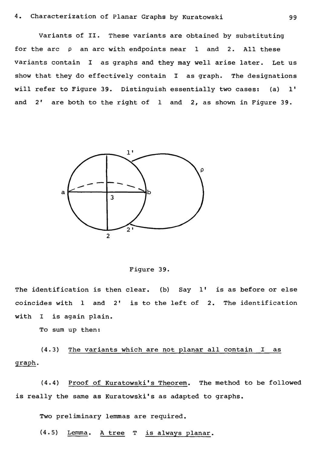
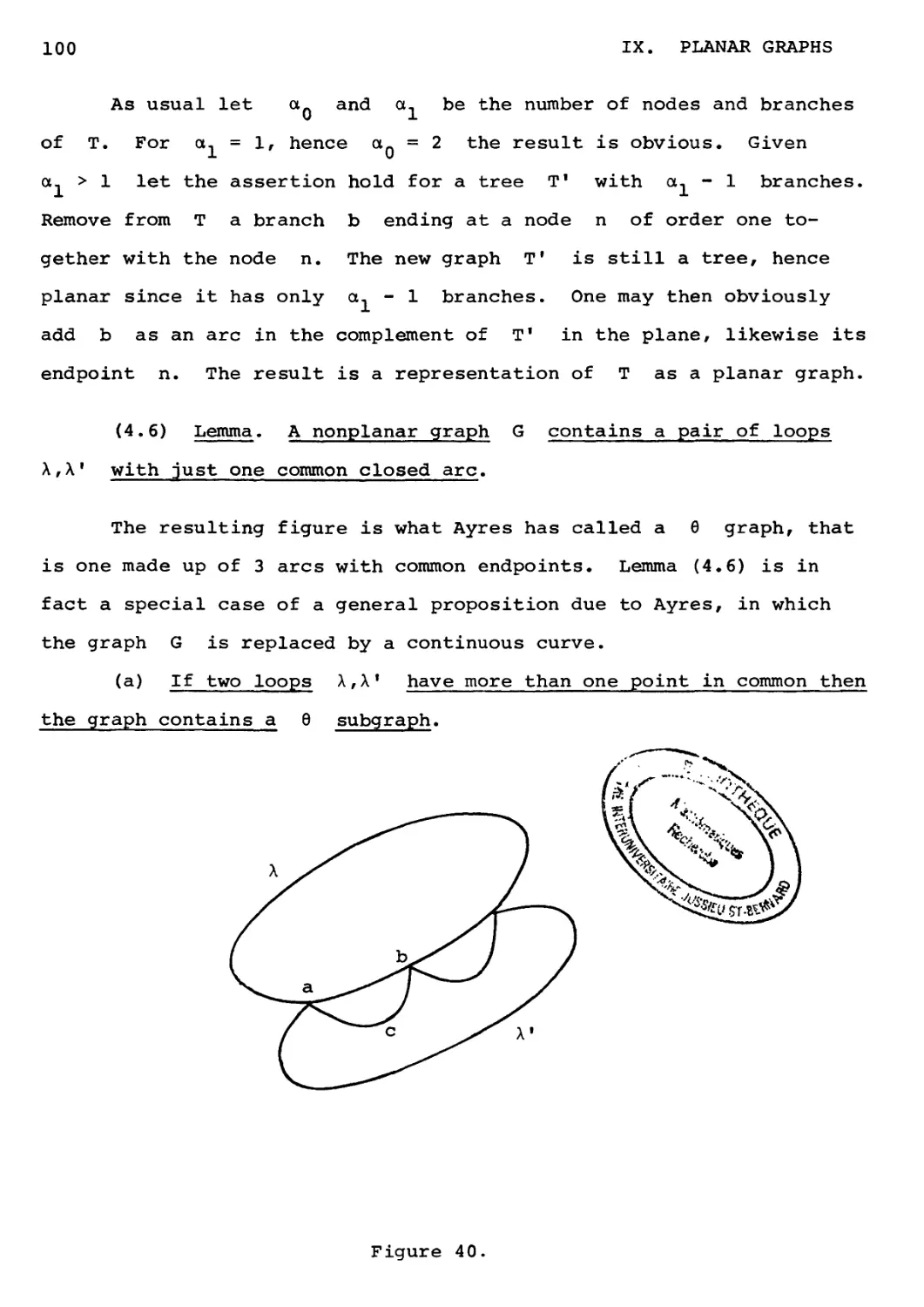


Текст
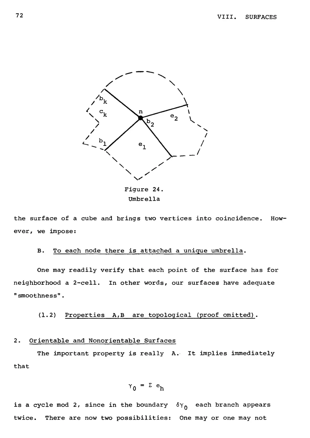
S. Lefschetz
Applications
of Algebraic
Topology
Applied
Mathematical
Sciences
16
Springer-Verlag
New York Heidelberg Berlin
Applied Mathematical Sciences Volume 16
S. Lefschetz
Applications
of Algebraic
Topology
Graphs and Networks
The Picard-Lefschetz Theory
and Feynman Integrals
With 52 Illustrations
1
Springer-Verlag New York • Heidelberg • Berlin
1975
S. Lefschetz
Formerly of Princeton University
AMS Classifications: 55-01,55A15,81A15
Library of Congress Cataloging in Publication Data
Lefschetz, Solomon, 1884-1972.
Applications of algebraic topology.
(Applied mathematical sciences; v. 16)
Bibliography: p.
Includes index.
1. Algebraic topology. 2. Graph theory. 3.
Electric networks. 4. Feynman integrals. I. Title.
II. Series.
QA1.A647 vol.16 [QA611] 510'.8 [514'.2] 75-6924
ISBN 0-387-90137-X
All rights reserved.
No part of this book may be translated or reproduced in any form
without written permission from Springer-Verlag.
© 1975 by Springer-Verlag New York Inc.
Printed in the United States of America.
ISBN 0-387-90137-X Springer-Verlag New York • Heidelberg • Berlin
ISBN 0-540-90137-X Springer-Verlag Berlin • Heidelberg • New York
V
Solomon Lefschetz (1884-1972) was one of the great mathematicians
of his generation. This volume published posthumously and completed
shortly before his death is in his own unique and vigorous style.
Were he alive there are many people whom he would thank. Among them
are Sandra Spinacci for the careful typing of his manuscript,
Mauricio Peixoto for his constant encouragement, and John Mallet-Paret
for his careful reading of the manuscript.
January 1975
J. P. LaSalle
vi
TABLE OF CONTENTS
PART I
APPLICATION OF CLASSICAL TOPOLOGY
TO GRAPHS AND NETWORKS
Page
INTRODUCTION 4
CHAPTER I. A RESUME OF LINEAR ALGEBRA 5
1. Matrices 5
2. Vector and Vector Spaces 7
3. Column Vectors and Row Vectors 10
4. Application to Linear Equations 11
CHAPTER II. DUALITY IN VECTOR SPACES 13
1. General Remarks on Duality 13
2. Questions of Nomenclature 14
3. Linear Functions on Vector Spaces.
Multiplication 15
4. Linear Transformations. Duality 16
5. Vector Space Sequence of Walter Mayer 18
CHAPTER III. TOPOLOGICAL PRELIMINARIES 22
1. First Intuitive Notions of Topology 22
2. Affine and Euclidean Spaces 25
3. Continuity, Mapping, Homeomorphism 26
4. General Sets and Their Combinations 27
5. Some Important Subsets of a Space 28
6. Connectedness 29
7. Theorem of Jordan-Schoenflies 30
CHAPTER IV. GRAPHS. GEOMETRIC STRUCTURE 34
1. Structure of Graphs 34
2. Subdivision. Characteristic Betti Number 37
CHAPTER V. GRAPH ALGEBRA 43
1. Preliminaries 43
2. Dimensional Calculations 46
3. Space Duality. Co-theory 48
CHAPTER VI. ELECTRICAL NETWORKS 51
1. Kirchoff's Laws 51
2. Different Types of Elements in the Branches 53
3. A Structural Property 54
4. Differential Equations of an
Electrical Network 56
CHAPTER VII. COMPLEXES 61
1. Complexes 61
2. Subdivision 64
3. Complex Algebra 66
4. Subdivision Invariance 68
CHAPTER VIII. SURFACES 71
1. Definition of Surfaces 71
2. Orientable and Nonorientable Surfaces 72
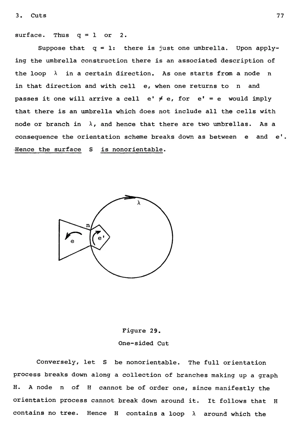
3. Cuts 7 6
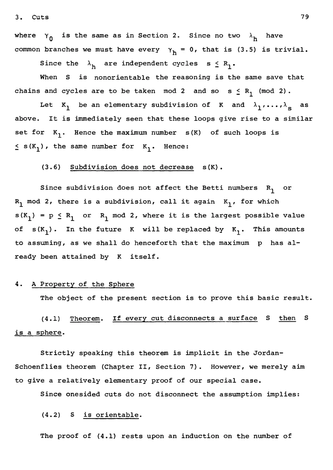
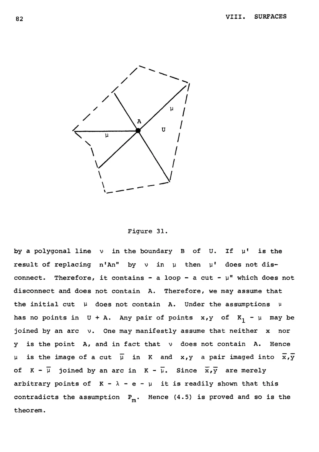
4. A Property of the Sphere 79
vii
Page
5. Reduction of Orientable Surfaces
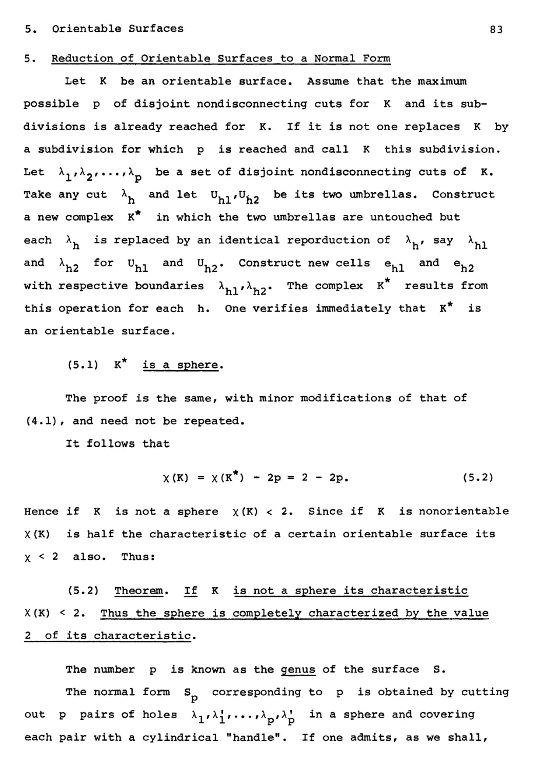
to a Normal Form 83
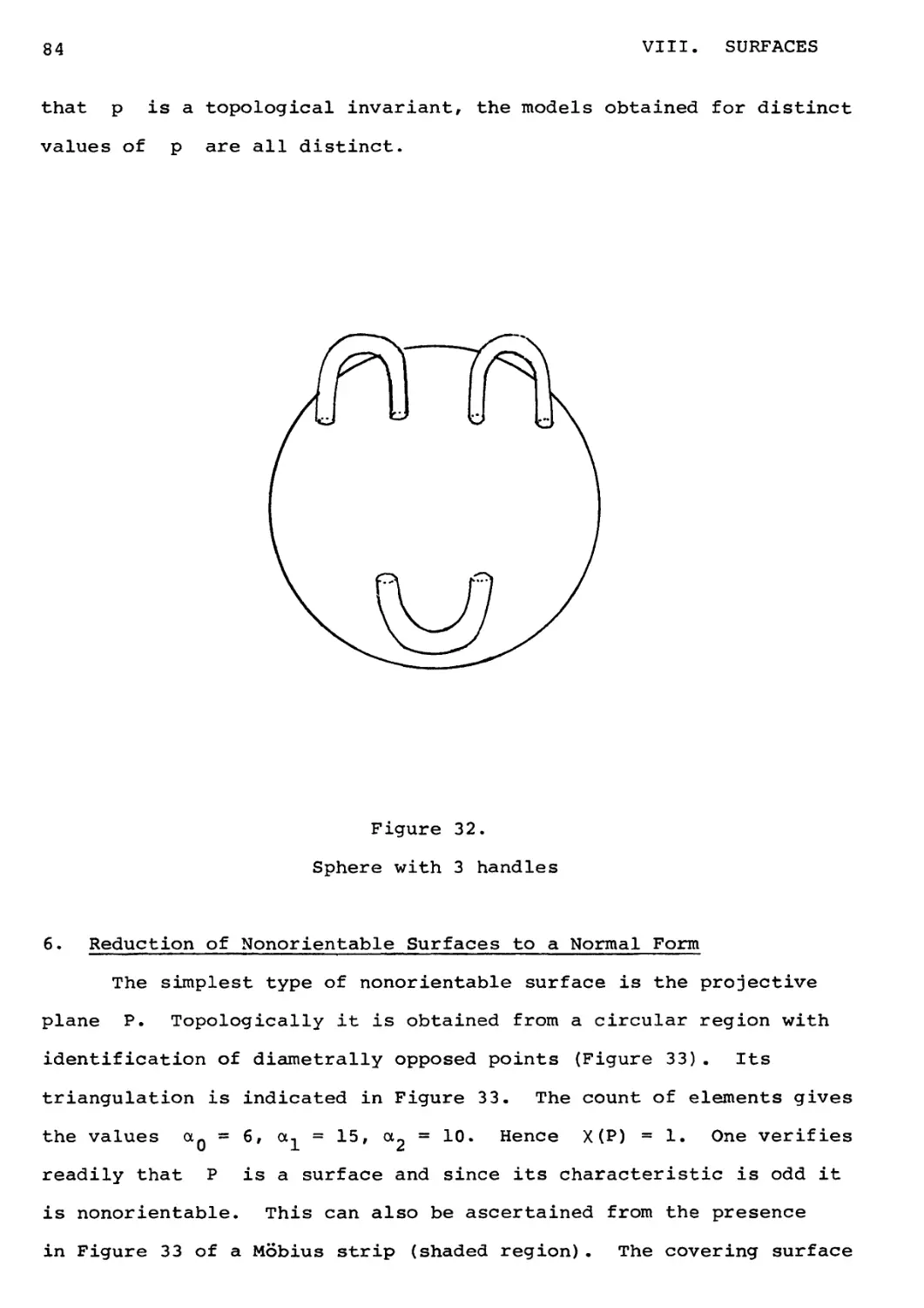
6. Reduction of Nonorientable Surfaces
to a Normal Form 84
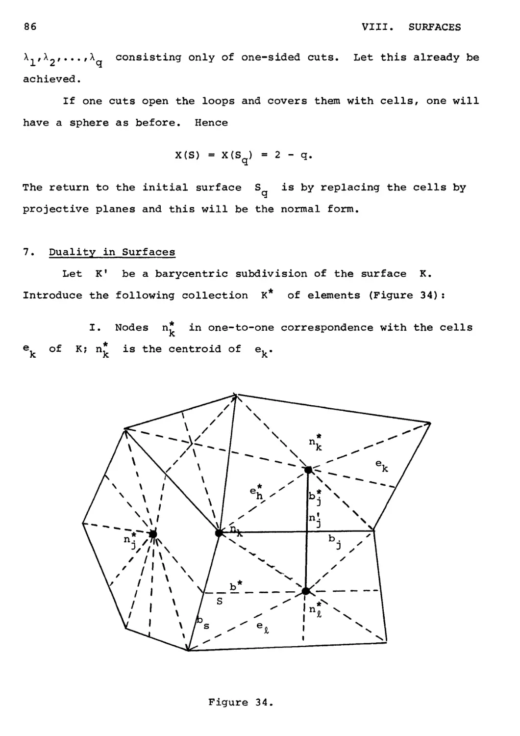
7. Duality in Surfaces 86
CHAPTER IX. PLANAR GRAPHS 89
1. Preliminaries 89
2. Statement and Solution of the
Spherical Graph Problem 90
3. Generalization 95
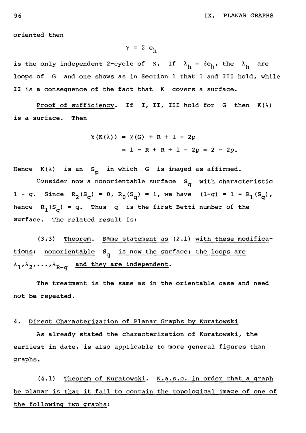
4. Direct Characterization of Planar
Graphs by Kuratowski 96
5. Reciprocal Networks 103
6. Duality of Electrical Networks 104
PART II
THE PICARD-LEFSCHETZ THEORY
AND FEYNMAN INTEGRALS
INTRODUCTION 113
CHAPTER I. TOPOLOGICAL AND ALGEBRAIC CONSIDERATIONS 119
1. Complex Analytic and Projective Spaces 119
2. Application to Complex Projective
n-space ^n 119
3. Algebraic Varieties 121
4. A Resume of Standard Notions of
Algebraic Topology 124
5. Homotopy. Simplicial Mappings 128
6. Singular Theory 129
7. The Poincare Group of Paths 130
8. Intersection Properties for Orientable
M Complex 131
9. Real Manifolds 133
CHAPTER II. THE PICARD-LEFSCHETZ THEORY 135
1. Genesis of the Problem 135
2. Method 136
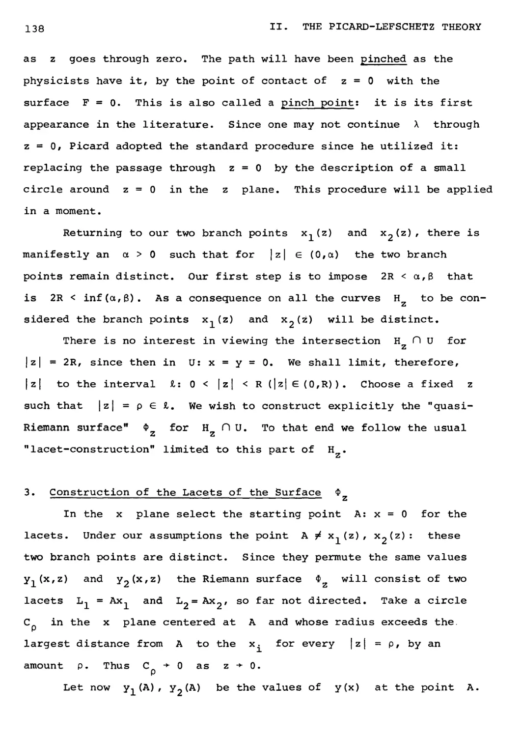
3. Construction of the Lacets of
Surface Ф 138
z
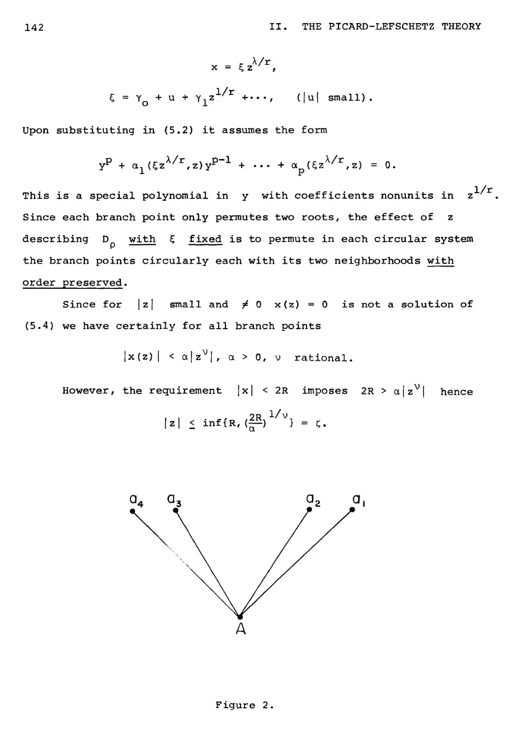
4. Cycles of Ф . Variations of Integrals
Taken On Ф 140
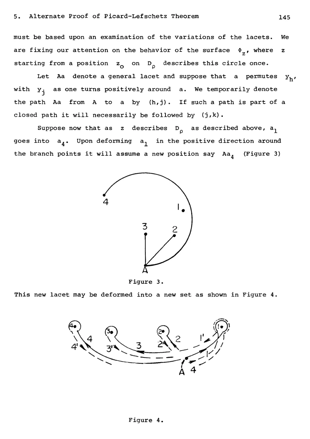
5. An Alternate Proof of the
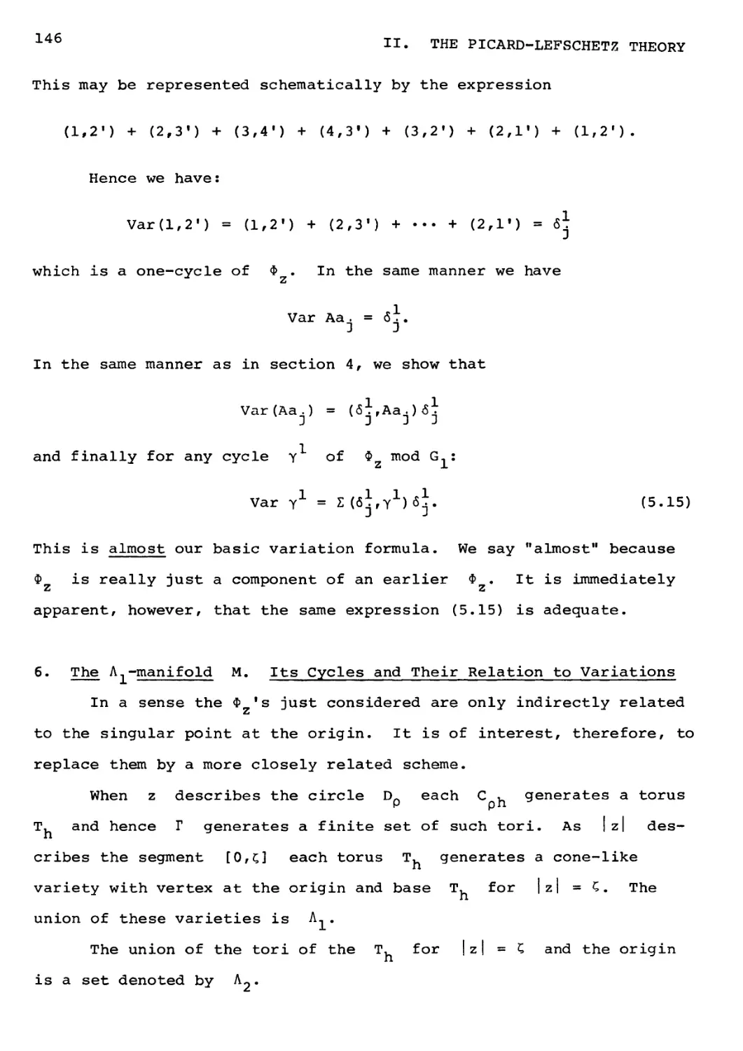
Picard-Lefschetz Theorem 140
6. The Л,-manifold M. Its Cycles and
Their Relation to Variations 146
CHAPTER III. EXTENSION TO HIGHER VARIETIES 149
1. Preliminary Remarks 149
2. First Application 150
3. Extension to Multiple Integrals 151
viii
Page
4. The 2-Cycles of an Algebraic Surface 152
CHAPTER IV. FEYNMAN INTEGRALS 154
1. On Graphs 154
2. Algebraic Properties 156
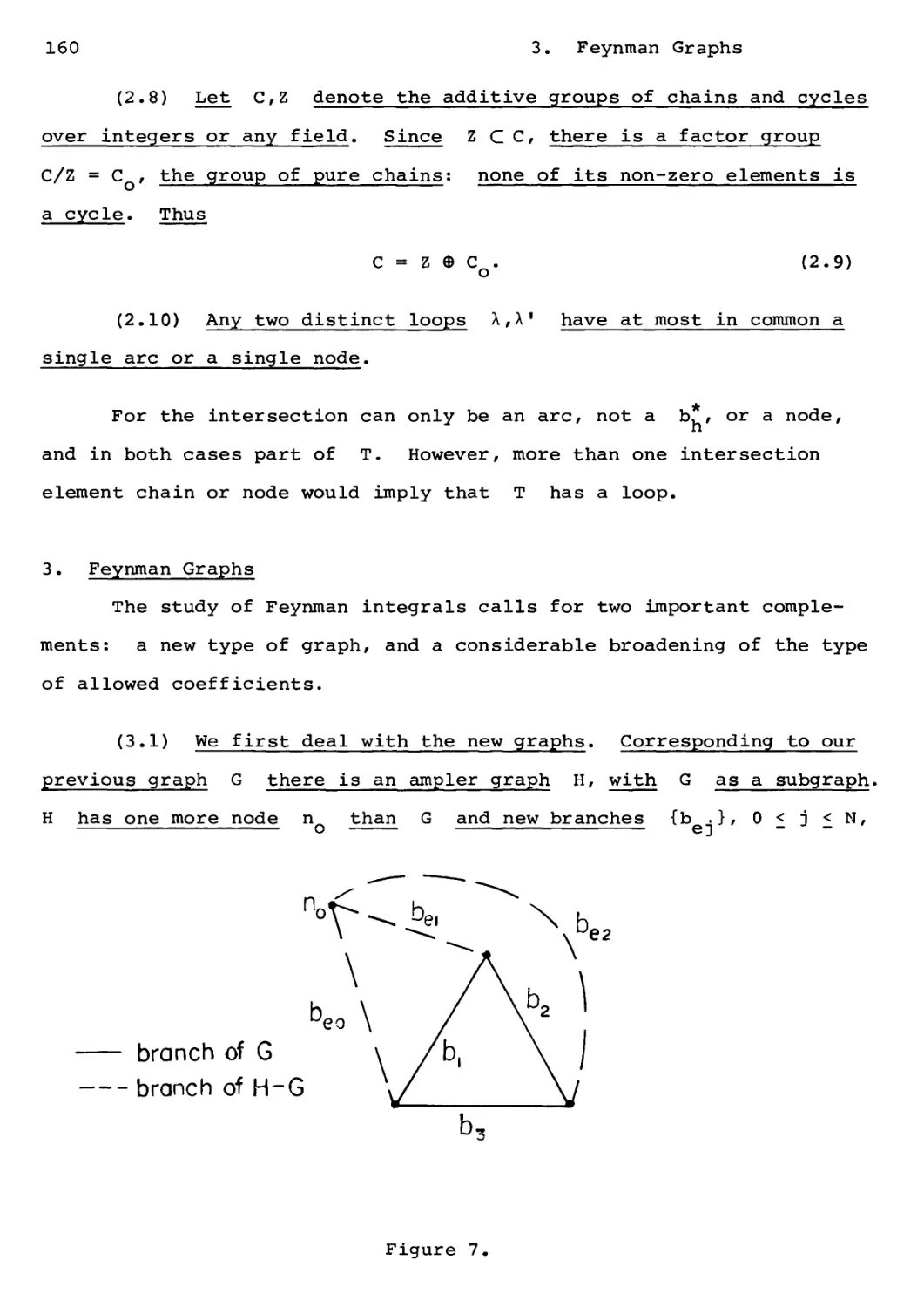
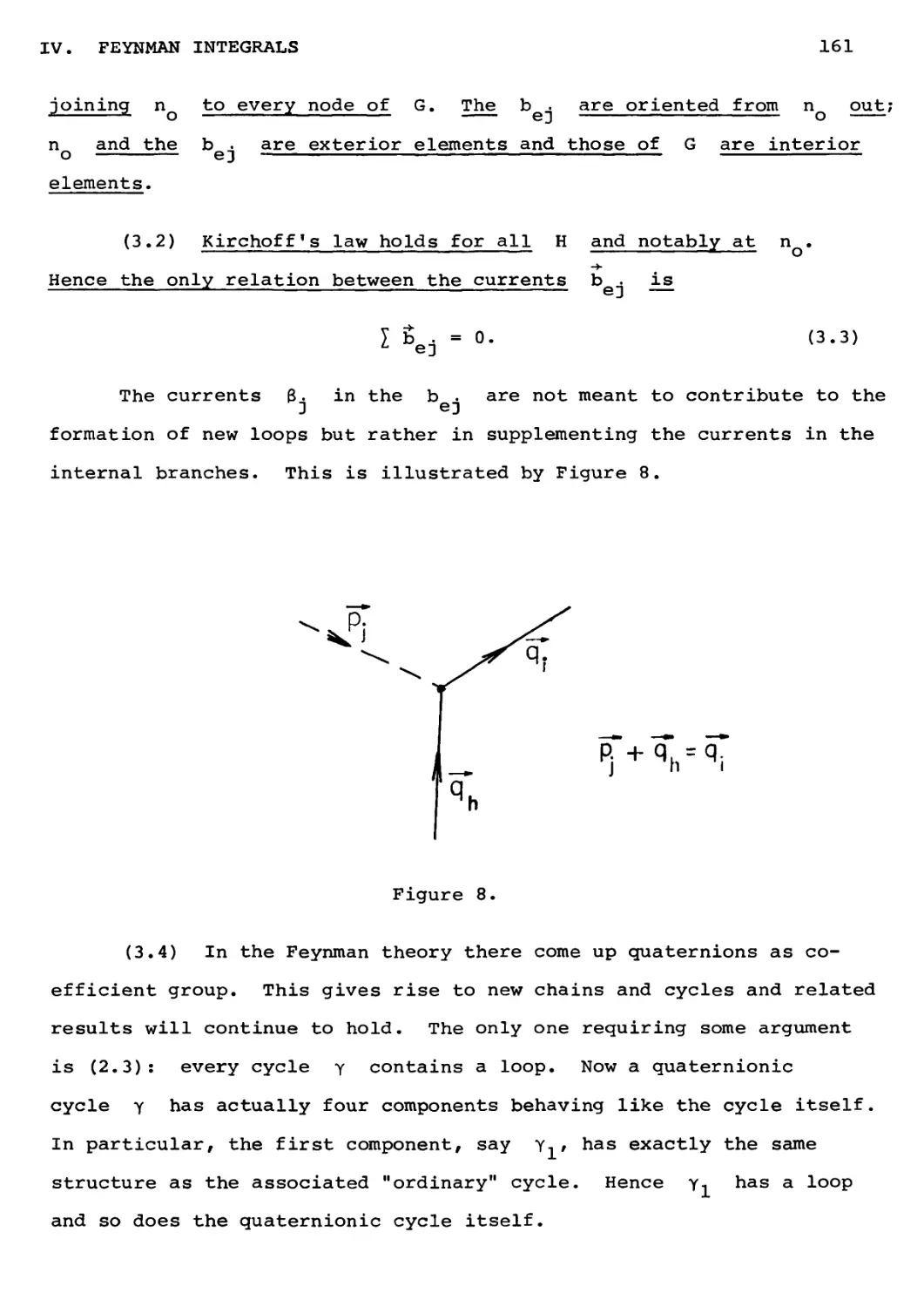
3. Feynman Graphs 160
4. Feynman Integrals 162
5. Singularities 163
6. Polar Loci 164
7. More General Singularities 168
8. On the Loop-Complex 170
9. Some Complements 170
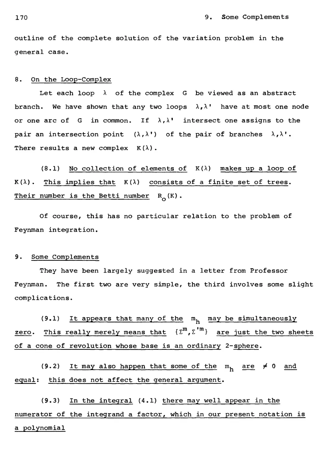
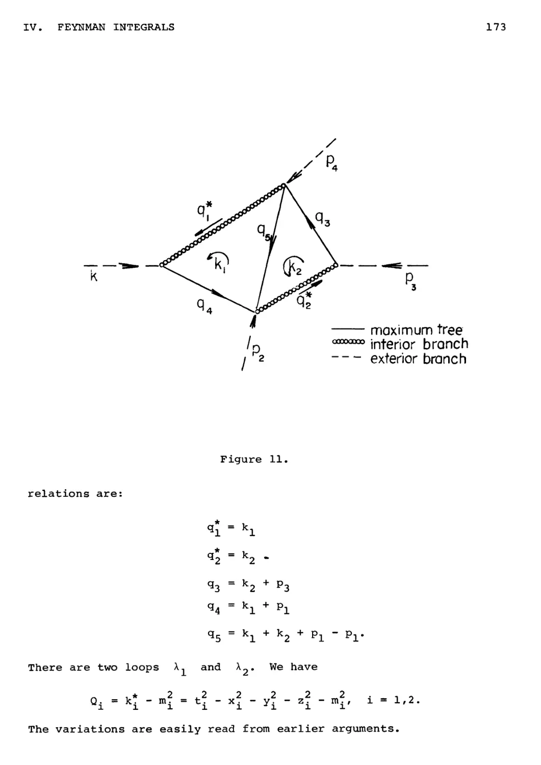
10. Examples 171
11. Calculation of an Integral 174
12. A Final Observation 175
CHAPTER V. FEYNMAN INTEGRALS. B. 177
1. Introduction 177
2. General Theory 177
3. Relative Theory 178
4. Application to Graphs 178
5. On Certain Transformations 180
BIBLIOGRAPHY 181
SUBJECT INDEX PART I 183
SUBJECT INDEX PART II 187
PART I
APPLICATION OF CLASSICAL TOPOLOGY
TO GRAPHS AND NETWORKS
PREFACE
This monograph is based, in part, upon lectures given in the
Princeton School of Engineering and Applied Science. It presupposes
mainly an elementary knowledge of linear algebra and of topology. In
topology the limit is dimension two mainly in the latter chapters
and questions of topological invariance are carefully avoided.
From the technical viewpoint graphs is our only requirement.
However, later, questions notably related to Kuratowski's classical
theorem have demanded an easily provided treatment of 2-complexes
and surfaces.
January 1972
Solomon Lefschetz
4
INTRODUCTION
The study of electrical networks rests upon preliminary theory
of graphs. In the literature this theory has always been dealt with
by special ad hoc methods. My purpose here is to show that actually
this theory is nothing else than the first chapter of classical
algebraic topology and may be very advantageously treated as such by
the well known methods of that science.
Part I of this volume covers the following ground: The first
two chapters present, mainly in outline, the needed basic elements of
linear algebra. In this part duality is dealt with somewhat more
extensively. In Chapter III the merest elements of general topology
are discussed. Graph theory proper is covered in Chapters IV and V,
first structurally and then as algebra. Chapter VI discusses the
applications to networks. In Chapters VII and VIII the elements of
the theory of 2-dimensional complexes and surfaces are presented.
They are applied in Chapter IX, the last of Part I, to the important
question of planar graphs, Kuratowski related theorem, and dual
networks.
It is to be noted that in the electrical part, linearity has
nowhere been assumed. In general as regards networks, I have been
considerably inspired by the splendid paper of Brayton and Moser: A
theory of nonlinear networks, Quaterly of Applied Mathematics, Vol. 29,
pp. 1-33, 81-104, 1964.
The exposition of the material is new in many parts; moreover
in certain parts the material is completely new. This is notably the
case in Chapter IX.
CHAPTER I
A resume" OF LINEAR ALGEBRA
Two elements dominate linear algebra: matrices and vectors.
One may identify vectors with certain matrices but not vice versa.
Thus matrices are the dominant feature. We shall, therefore, first
deal with matrices and then with vectors.
As appropriate for a resume, proofs will rarely be given and
for them the reader is referred to any standard text on the subject.
1. Matrices
A matrix is a rectangular array of elements
all a12 ••• aln
a21 a22 •'•
a t а л ... a
ml m2 mn
Such an array, known as m * n matrix is usually abridged as
[a., ] or even written a. The standard matrix operations are:
Addition: The sum of two m x n matrices, a as above and
b = [b.,] is the matrix
a + b = [ajk + bjk];
Product: With a as before and b an n x p matrix one
defines
a b =
[jai-b*]'
6 I. A RESUME OF LINEAR ALGEBRA
The implication is that in both addition and multiplication the
operations indicated have a meaning. This is usually clear from the
context but one must not be entirely careless about it.
The transpose a1 of the m x n matrix a is the n x m
matrix obtained by permuting the rows and columns of a. Note that
if ab has a meaning (ab) f = b'a1.
The derivative of a matrix a(t) = [a., (t)] of elements
differentiable functions of t is
a(t) = tajk(t)j.
Square matrices. These are the n x n matrices. The number
n is the order of the matrix.
A square numerical, n x n matrix has a determinant written
|a.,| or |a|. The matrix is singular if |a| = 0, nonsingular
otherwise.
The square matrix with diagonal a,,...fa and zeros outside
is frequently written diag(a,,...,a ) . The unit matrix of order n,
written E or E (when n is obvious) is diag(1,1,...,1) (n terms).
A nonsingular matrix a has an inverse a characterized by
aa"1 = a_1a =E. If |a|+0, |b|+0, then (ab)^ = b"1a~1.
Recall this important property: inversion and transposition
commute. That is (a" )! = (a')~ .
Evidently, sums and products of n x n matrices are n x n
matrices.
Rank of a matrix. The rank p of an m x n numerical matrix
a is the largest order of a nonzero determinant formed from the
elements of a.
(1.1) Theorem. Let a be an m x n matrix and b,c non-
singular square matrices of respective order m,n. Then
rank a = rank b a c.
2. Vectors and Vector Spaces 7
It is convenient to note that if a = [a.,] is m x n and
b = diagfb^ . . . ,bm) , с = diag (c.^, . . . ,cn) .
Then
ba = [b. ajk], ac = [ajk ck].
2. Vectors and Vector Spaces
Vectors are inextricably mixed with a collection of numbers,
the scalars, called a field. A field is simply any set of elements
obeying the ordinary rules of rational operations, for example all
real or all complex numbers. However an interesting field is made up
of just two elements 0 and 1 under these rules:
0.0 = 0.1 = 1.0 =1+1=0; 1.1 = 1.
In that field, called the field mod 2, x = -x, -■ = x, (x + 0)
hence subtraction and division may be forgotten. This is the ideal
field in geometric questions in which direction does not occur.
Take now a fixed field F and n elements A,,...,A which
obey no special relation (pure symbols). Form all the expressions
A = a. A- +• • •+ <x A
11 n n
with coefficients in F, the obvious rule for addition and the
conventions A = 0 if every a, = 0, likewise
aA = (aa^ A, +•••+ (aan) An
for every a in F. The collection of all expressions A is a
vector space V, the elements A are the vectors.
The vectors B,,B2,...,B are linearly dependent if there
exists a relation
31 Bl +,ee+ &r Br = °' 3h in F
8 I. A RESUME OF LINEAR ALGEBRA
with the 3, not all zero (non-trivial relation). If no such
relation exists the B, are linearly independent (the term "linearly"
is often omitted in such statements). The maximum number of linearly
independent vectors is the dimension of V
dim V = n. (2,1)
Bases. A base for the space V is a set B,,...,B of
independent vectors such that every vector С satisfies a relation
С = 31 Bx +...+ 6S Bg, 0h in F.
(2.2) A base consists exactly of n( = dim V) elements.
(2.3) Any n independent elements form a base. Hence
A-, , .. .,A is a base*
l n
Isomorphism. Two vector spaces V,W over the same field F
are isomorphic, written V ^ W, if there is a one-one correspondence
between their elements preserving the relations of dependence between
them. That is if В,#...,В are elements of V and C,
corresponds to B. then the relations
l eh Bh = o, I eh ch = 0
imply one another.
(2.4) N.a,s.c, to have V ъ W is that they have the same
dimension.
(2.5) If V ^ W one may select for them respective bases
{В,}, {C,} such that the isomorphism between them associates
I sh Bh with i eh ch.
Change of base. Let {Bv^f ^Ch^ ^e two bases ^or ^е same
vector space V. We have the relations
2. Vector and Vector Spaces y
ch = ^hj V Bh = i 6hJcj
with the 3/Y in the field F. As a consequence there follow
Bh - l 6hs Ysk Bk' h = X'2 n' (2-6)
s
However, since the B, are independent these relations must be
identically true, that is
I 3h Y , = <
Jhs 'sk
s
1 if h = к
0 otherwise
This means that the product
t*hj].[Yhj] =E (2.7)
and implies for the determinants
|ehjl-lYhjl -i.
Consequently, the matrices t3h-:l and £YhnJ are non-singular.
Conversely any relation
ch = l Yhj Bj' iYhjl * ° (2-8)
is a change of base from {B.} to {C,} for the space V.
Remark, The important properties of the space V are those
which are invariant with respect to changes of base. For the
present we only have the dimension, but other properties will appear
in the application to graphs.
Direct sum. Let V,,V2 be two vector subspaces of V
(vector spaces over the same field whose vectors are all in V). We
say that V is their direct sum and write
V = v± • v2
10 I. A RESUME OF LINEAR ALGEBRA
whenever the following two conditions hold:
(a) V, and V2 only have zero in common;
(b) if В is any vector of V then В = B1 + &2,
B0
where B,
is in V,
Then also
dim V = dim V\ + dim V2«
(2.9)
(2.10) If V, is a subspace of V, there is another subspace
V2 such that V = V, Ф V2. The subspace V2 need not be unique,
but all such subspaces are isomorphic. By identifying them in a
suitable manner there results a unique space V2 called the factor
space of V by_ V, and written V/V, .
3. Column Vectors and Row Vectors
Let the numbers x.,,x2,..., be elements of the scalar field F
and consider all the 1-column matrices
x =
under the addition rule for n x 1 matrices, the multiplication rule
ax = diag(a,...,a)-x, a in F, and the convention x = 0 if and
only if every x, = 0, then the collection of all matrices x makes
up a vector space V. Its dimension is n, hence it is isomorphic
with the vector space VQ of elements
xl Al +-"+ xn An
already defined in Section 2. We may think of VQ as a
representation of the space V. In this context one refers to x as a
column-vector, and to the x, as components of x. The transpose
h
4. Application to Linear Equations
matrix x1 = [x,,...,x ] is called a row-vector. The space V of
all the xf is again a representation of V. It is worth noting
that if one calls A the formal n x 1 matrix
11
A =
then one may write
xi Ai +-
■+ x A = x' A = A'x.
n n
These abridged designations will be found most convenient in later
chapters. Notice, also that if x and у are both column vectors
with n terms all taken from the field F then
xfy = y!x = I xh yh.
(3.1)
This is the well known direct product of the vectors x,y.
If the space of the x, is considered as Euclidean, with
coordinates x, then
n
x'x = ||x||-
(Euclidean length square)
4. Application to Linear Equations
Let
ajl xl +'
•+ а. хм = 0
jn n
(4.1)
(j = 1,2/... ,m)
be a system of linear equations with coefficients in a field F. If
a = [a-k] and
same as the equation
x denotes the column vector [x,] then (4.1) is the
ax = 0.
(4.2)
12 I. A RESUME OF LINEAR ALGEBRA
Let r be the rank of the matrix a. Then from the well known
elementary theory of equations we have:
(4.3) The solution vectors of the system (4.2) make up a
vector space of dimension n - r.
Consider also the system
y'a = 0 (4.4)
where у is an m-vector. Since this equation is equivalent to
a'у = 0/ and a,a' have the same rank, we have from (4.3)
(4.5) The solution vectors of (4.4) make up a vector space of
dimension m - r.
Exercises
1. Derive the proofs missing in 1, 2, 3, and 4.
2. Let P = [p..] be a real m x n matrix. The rank r of
P is the largest order of a determinant extracted from P. Prove
that if Q is m x mf R is n x n both nonsingular then
rank P = rank QPR.
3. Let P be real n x n and symmetric: Pf = P. If x is
any vector x'Px - Ф(x). Show that by a linear transformation of co-
2
ordinates x = Py one may reduce Ф in various ways to form Z а,у,
where the a. are all real. Show that in such a reduction:
n
(a) the number of a / 0 is fixed and equal to the
rank of P;
(b) the number of positive a. is likewise fixed.
This number is known as the index of inertia of P. (This last
result is due to Sylvester.)
13
CHAPTER II
DUALITY IN VECTOR SPACES
1. General Remarks on Duality
The idea of duality occurs in many parts of mathematics. Its
earliest appearance (some 125 years ago) was in projective geometry
where it permitted to halve the number of theorems to be proved. It
also played a most important role in analysis, for example in Banach
spaces. In topology, beginning with Poincare its role has been no
less important.
The central attack on duality in modern mathematics may be
described in these terms. If S is a space of any sort on which one
may specify linear functions, then their space Z is defined as the
dual space to S.
It is our purpose to develop duality for vector spaces from the
standpoint just described.
Observe that the relatively simple duality of projective
geometry fits in perfectly with the above general description. To be
precise consider the projective plane P with related projective
coordinates x,,x2,x-, under these conditions:
(a) the three coordinates are never simultaneously zero;
(b) the point (kx,,kx2,kx3), к ^ 0, is the same as
\X«i ,X« /X-5 ) •
A linear function of the point is an expression ф (x) = u-, x. +
u2 x2 + ul x3* ^ one exc^U(^es tne form ф = 0 and identifies ф
and кф, к ф 0/ then the points (u,,u2,u3) of the projective plane
P are in one-one correspondence with the linear forms ф. The
plane P is the dual of the plane P . Observe finally that the
14
II. DUALITY IN VECTOR SPACES
form ф is completely identified by the point (u,,u2,uO of the
plane P . Thus lines of P correspond to points of Pu and
points of Px to the lines of P . Thus the duality relation
P <—> P is entirely symmetrical.
2. Questions of Nomenclature
We shall generally accept the following standard designations:
I. Transformations; A transformation f from one
collection G or elements to another H is written f: G ■* H.
II. Kronecker deltas; These are the symbols б,^ = 0
for h ? k, =1 for h = k.
III. Dimension: This term is generally dropped and one
says "n-plane, space, sphere,... "for" n-dimensional plane, space,
sphere,...".
IV. n-yector stands for a vector in a vector n-space.
V. Vector spaces and their bases. The general
designation for these spaces is by Latin capitals A,B,C... . A
vector space, say A, will usually be referred explicitly or
implicitly to a definite base. Assume that dim A = n and that it
has the base e ,e , ...,e . An element of A will be an
expression a-,e/ ' +•••+ a e/n , where a, are its components. As a
result the space A is represented by the space of the column-
vector a = [a,]. That is there is a tacit identification of the
space A with the space of column vectors [a, ].
The preceding situation occurs frequently in geometry. For
instance in plane geometry referred to the axes x^,x2 one will
speak of "the point (x^x^) " meaning actually "the point presently
represented in this coordinate system by the members x1,x2".
Incidentally, if one thinks of the vectors of A as "points"
3. Linear Functions on Vector Spaces: Multiplication 15
the space A is also known as affine n-space-
3. Linear Functions on Vector Spaces. Multiplication
Let A be a vector space and let its base be
(e(1),e(2),...,e(n*}. A function f(a) on A to the reals is
linear whenever given any two elements a,a of A and any two
real scalars, a,$:
f ( a+ a1) = f (a) + f (a1) .
It follows that if
a = але(1) + ••• + a e(n)
— l— n—
then
f(a) = a1a1 + a2a2 + ... + anan (3.1)
a;=f(e(h)),
so that the a, are all real. Suppose that g(a) is another linear
function on A to the reals and let
g(a) = a1b1 + ••• + anbn .
If we define ctf + 3g by the relation
(af+Bg) (a) = ctf (a) + 3g (a)
for every a of Af then the linear functions f will become the
* *(1) *(n)
elements of a vector space A whose base is (e ч ,...,e ),
* (h)
where e y is the particular function defined by
*
e
(h) (к) = 5
(^ } 6hke
(The 6,, are the Kronecker deltas: 1 if h = к, 0 otherwise.)
The space A is the dual of the space A, and since the base
16 II. DUALITY IN VECTOR SPACES
of A consists of n terms dim A = dim A = n.
One may write (3.1) as
a*(a) = I a*ah . (3.2)
It is clear from (3.2) that A = A: duality of spaces is a
symmetrical relationship.
One may also aptly write (3.2) as a multiplication
a • a = [ ahah
and we recognize that this new product is commutative.
The new product has been extensively utilized in the literature.
In particular, in algebraic topology it has been referred to as
Kronecker index.
4. Linear Transformations. Duality
Let В be a second vector space. A transformation ф: A ■> В
is linear whenever given a, a1 of A and any two real scalars a,a*
we have
фСаа+а'а1) = аф(a) + а'ф(а').
Let {e^h*} and {f(k*} be bases for A and B. Then
<Ke(h)) =Inhkf(k).
Hence if a = £ an^ ' tnen
♦ (•)-! Vhk£(k)-
That is in the column-vector representation
Ф(а) = a'n. (4.1)
If n = dim A and m = dim В the matrix n is n x m.
4. Linear Transformations. Duality 17
The nucleus N(<j>) of ф consists of all the vectors a sent
by ф into zero. These vectors are characterized by
l Vhi£(k) - °- <4'2>
(k)
Since the f ' satisfy no relation from (4.2) follows that
h
that is in a vector notation
a'n = 0. (4.3)
This is the characteristic equation of the elements of the
nucleus Ы(ф) of ф.
Let В be the dual of B. We propose to define a dual linear
transformation ф : В -> A .
Observe first this general property:
(4.4) An identity in x,y
f<X,Z) = l ShkXhyk 5 0
where £ = [£hk] is a constant matrix, is equivalent to £ = 0.
It is clear that £ = 0 implies f = 0, Conversely f = 0
implies f(«hlr«h2r...,6hnr 5kl'6k2'-'-'6km) = Chk = ° that is
£ = 0.
We shall now prove:
(4.5) The relations £' = n and
ф*(Ь*)а = Ф(а)Ь* (4.6)
i *. u х*,**(к)ч г *(h)
are equivalent where Ф (f_ ) = I 5ku£
In fact
Ф (b )a = b ca
Ф(а)Ь* = a'nb* = b*,(a,n)' = b*'n'a.
18 II. DUALITY IN VECTOR SPACES
Hence (4.6) is equivalent to
b*'(C-n')a = 0
and therefore to £ = П1 by (4.4).
Whenever either (4.6) holds or equivalently с1 = Л we shall
say that ф is dual to ф. This implies
ф is dual to ф* (symmetry of duality). (4.7)
An important consequence of (4.5) is:
(4.8) A n.a.s.c. in order that a be in the nucleus 1Я(ф) of
ф is that ф*(Ь*)а = 0 for all b*. Similarly a n.a.s.c. to have
b* in the nucleus Л(ф*) is that ф(а)Ь* = 0 for all a.
It is sufficient to treat the first case. Necessity being
obvious let the condition hold. Then by (4.6), ф(a)b* = 0 for all
b . Hence all the coefficients of this linear form in the b. must
— n
vanish, and this implies that ф (a) =0: a is in 1Я(ф).
5. Vector Space Sequence of Walter Mayer
Consider a finite sequence of vector spaces 0,A ,A _,,...,A,,0
with linear transformations ф : A ■* А л .
P P p-1
The assumption, borrowed from topology, is made that
ФР-1ФР = °' a11 Pe (5Л)
These are the Walter Mayer sequences.
Special notation. Before proceeding let us introduce a
convenient notation. If spaces are such that P = Q Ф R, and R ^ S
we shall write P = Q Ф S. Since our main concern is to find certain
dimensional relations, we merely note that we continue to have
dim P = dim Q + dim S.
5. Vector Space Sequence of Walter Mayer 19
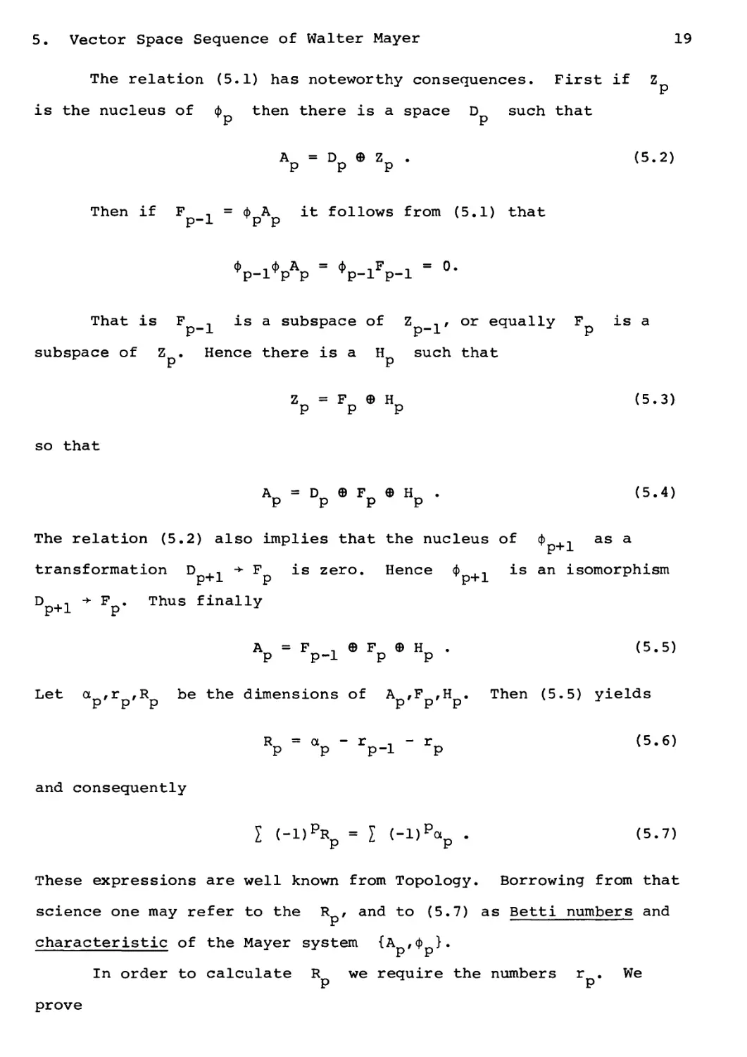
The relation (5.1) has noteworthy consequences. First if Z
is the nucleus of ф then there is a space D such that
r^ ir
Ap = Dp ф zp • (5-2)
Then if F n = ф A it follows from (5.1) that
p-1 Tp p
ф лф A = ф nF .. = 0.
p-1 P P P~l P"l
That is F _, is a subspace of Z _,, or equally F is a
subspace of Z . Hence there is a H such that
P P
Zp = Fp ф Hp (5.3)
so that
AP = DP e FP e HP • (5-4)
The relation (5.2) also implies that the nucleus of ф . as a
transformation D ,, + F is zero. Hence ф .. is an isomorphism
p+1 p Tp+1
D^.t -»■ Pn. Thus finally
p+1 p
A = F . Ф F Ф H . (5.5)
P P-1 P P
Let aD'r /R be the dimensions of A ,F ,H . Then (5.5) yields
RP = aP - rP-i - rP (5-6)
and consequently
I (-DPRp = I (-D% • (5.7)
These expressions are well known from Topology. Borrowing from that
science one may refer to the R , and to (5.7) as Betti numbers and
characteristic of the Mayer system {АП'ФП}«
ir IT
In order to calculate R we require the numbers r . We
P P
prove
20
II. DUALITY IN VECTOR SPACES
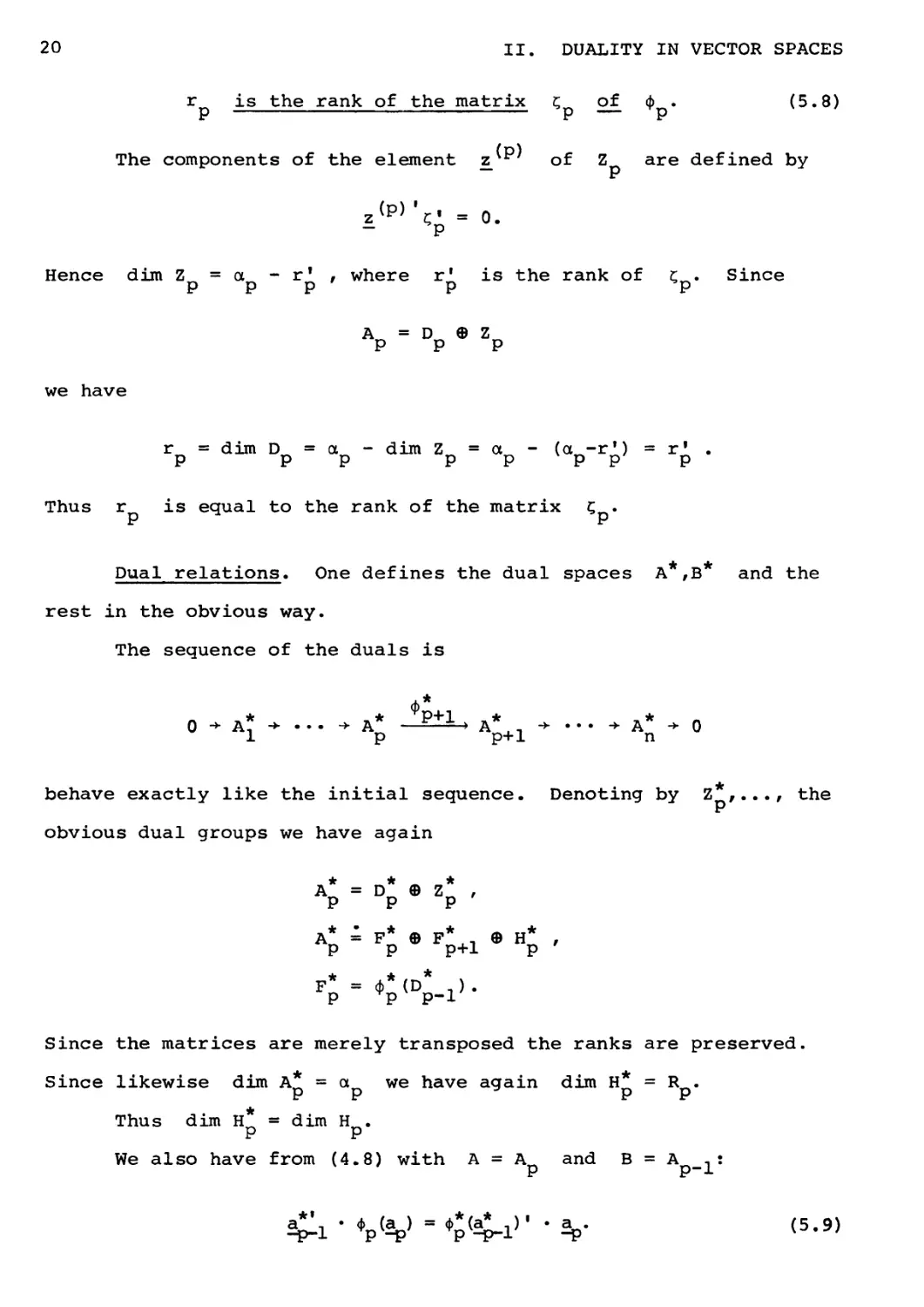
r is the rank of the matrix CD of ф . (5.8)
The components of the element z/ of Z are defined by
Hence dim Z = a - r1 , where r' is the rank of r« Since
P P P P P
A = D © Z^
P P P
we have
r = dim D = a - dim Zrt = ал - (a -r') = r' .
P PP PPPPP
Thus r is equal to the rank of the matrix с .
Dual relations. One defines the dual spaces A*,B* and the
rest in the obvious way.
The sequence of the duals is
■** »* P+l , * ■* * „
0 ■*■ A, -*- • • • -* A — > A , . ■*••.-► A ■> 0
1 p p+1 n
behave exactly like the initial sequence. Denoting by Z ,•.., the
obvious dual groups we have again
* * *
AP - DP • ZP *
Ap ; Fp e f;+i • нр '
Since the matrices are merely transposed the ranks are preserved.
Since likewise dim A* = a we have again dim H* = R .
P P P P
if
Thus dim H = dim H .
P P
We also have from (4.8) with A = A and В = A ,:
a
*i
&,> - ♦«{■JLi)' • a,- (5.9)
-p-1 yp4> Tpv-p-r -p
5. Vector Space Sequence of Walter Mayer
21
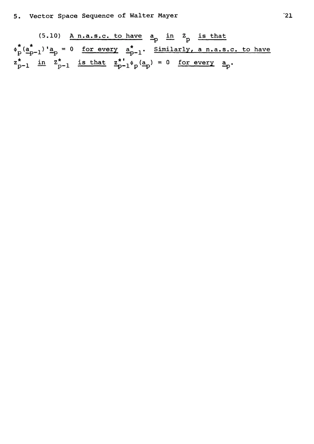
(5.10) A n.a.s.c. to have a in Z is that
-P — P
Ф (а л)1a =0 for every a* .. Similarly, a n.a.s.c. to have
p —p—± —p + —p-i ■*-■
z* л in Z* is that z*' Ф (a ) = 0 for every a .
p-l — P~i ——— -p-i p —p * —p
22
CHAPTER III
TOPOLOGICAL PRELIMINARIES
There are many approaches to topology. One of the most
accessible is by means of the notion of distance. Our purpose in the
present chapter is to sketch this approach and a few of the general
concepts derivable from it. It may be said that this material amply
covers our future needs.
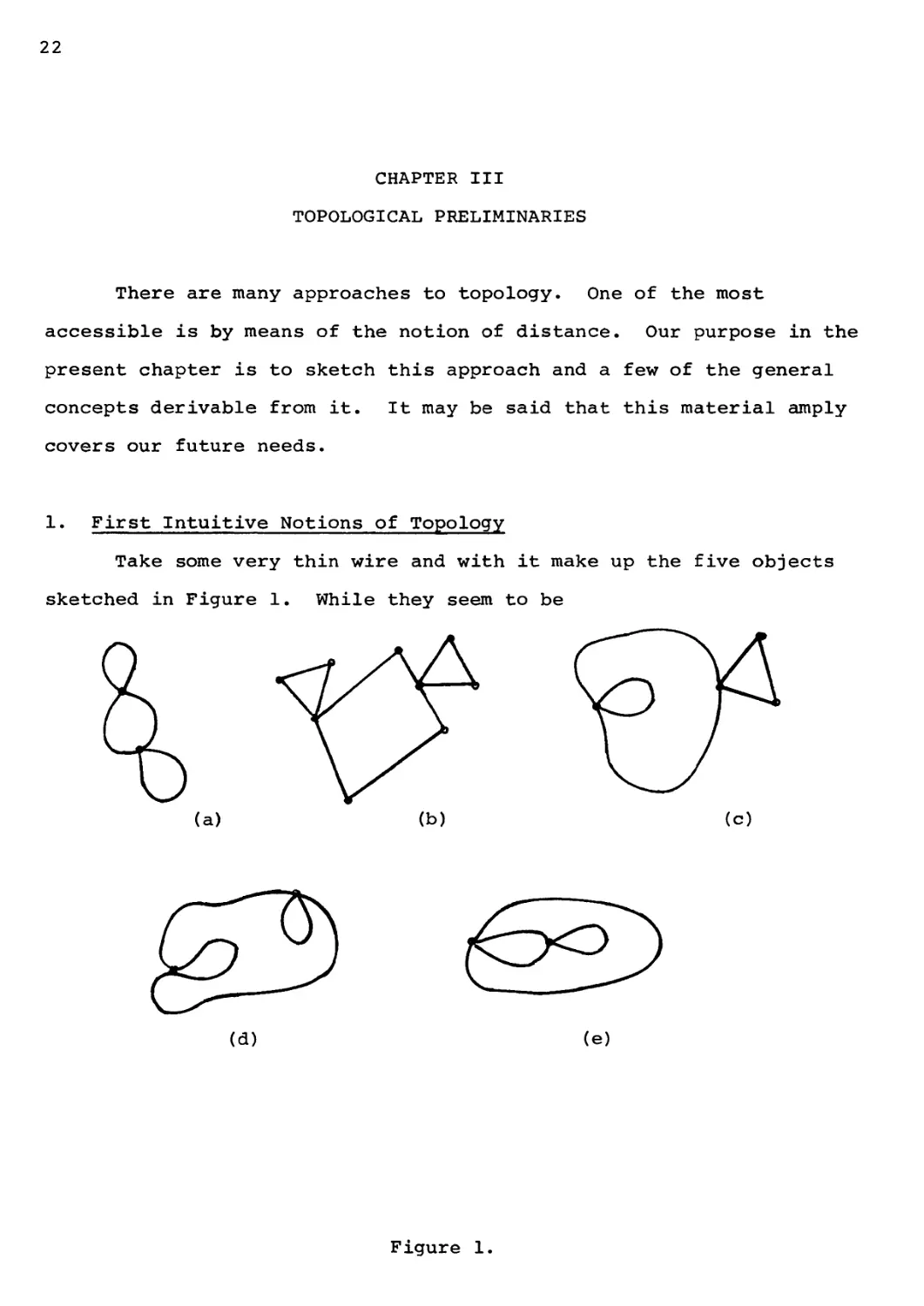
1. First Intuitive Notions of Topology
Take some very thin wire and with it make up the five objects
sketched in Figure 1. While they seem to be
(a) (b) (c)
(d) (e)
Figure 1.
III. TOPOLOGICAL PRELIMINARIES
23
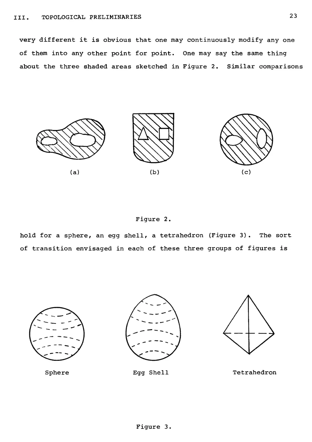
very different it is obvious that one may continuously modify any one
of them into any other point for point. One may say the same thing
about the three shaded areas sketched in Figure 2. Similar comparisons
(a) (b) (c)
Figure 2.
hold for a sphere, an egg shell, a tetrahedron (Figure 3). The sort
of transition envisaged in each of these three groups of figures is
Sphere Egg Shell Tetrahedron
Figure 3.
24 1. First Intuitive Notions of Topology
said to be topological or a homeomorphism (defined with precision in
Section 3). Topology is concerned with the properties common to all
the figures, for example in Groups 1, 2, 3. Are there any common
properties in each of our three groups of figures? Certainly, and,
some at least, are very simple.
Group 1. Figure 1: In each there are two and exactly two points
(the nodes) which may be approached from four directions.
Group 2. Figure 2: In each/ one may join by arcs the inner
boundaries to the outer boundaries.
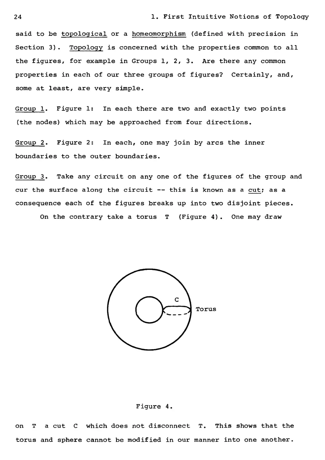
Group 3. Take any circuit on any one of the figures of the group and
cur the surface along the circuit — this is known as a cut; as a
consequence each of the figures breaks up into two disjoint pieces.
On the contrary take a torus T (Figure 4). One may draw
Figure 4.
on T a cut С which does not disconnect T. This shows that the
torus and sphere cannot be modified in our manner into one another.
III. TOPOLOGICAL PRELIMINARIES
25
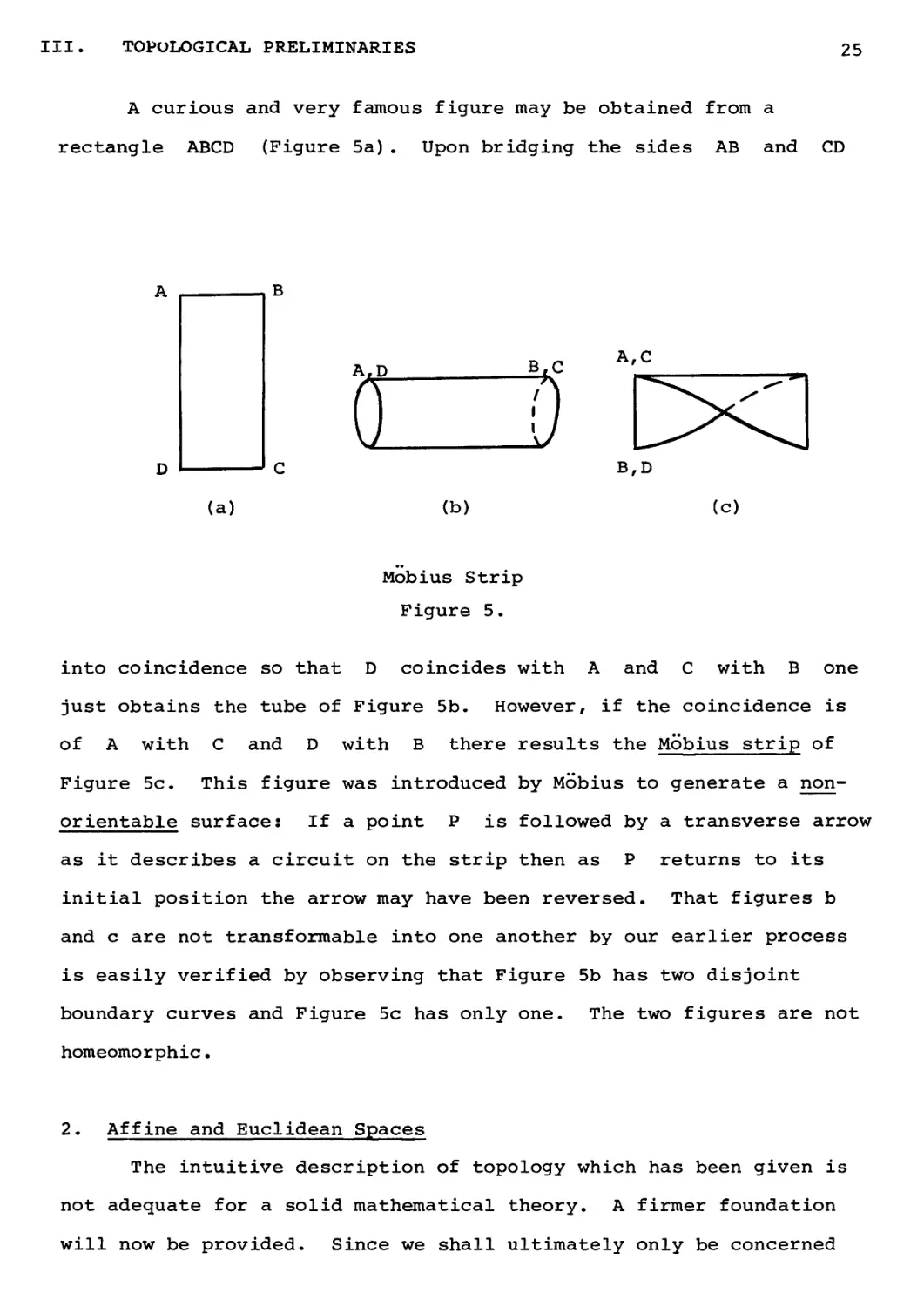
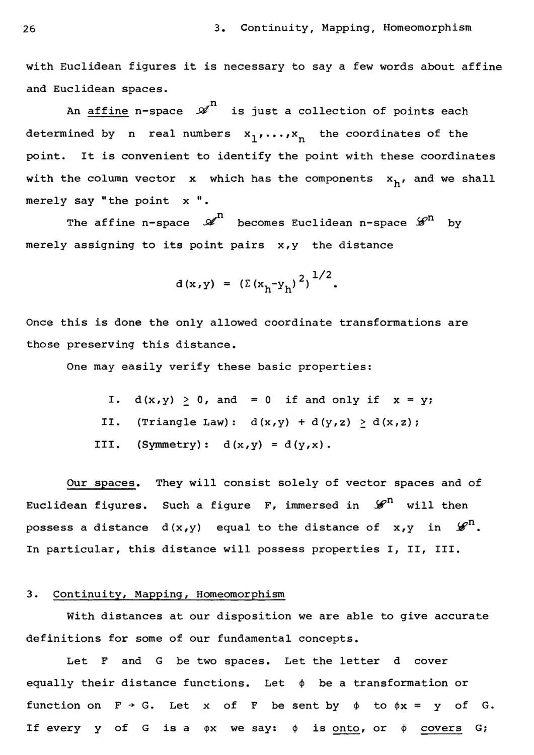
A curious and very famous figure may be obtained from a
rectangle ABCD (Figure 5a). Upon bridging the sides AB and CD
(a)
A,D
(b)
3
ArC
B,D
(c)
Mobius Strip
Figure 5.
into coincidence so that D coincides with A and С with В one
just obtains the tube of Figure 5b. However, if the coincidence is
of A with С and D with В there results the Mobius strip of
Figure 5c. This figure was introduced by Mobius to generate a non-
orientable surface: If a point P is followed by a transverse arrow
as it describes a circuit on the strip then as P returns to its
initial position the arrow may have been reversed. That figures b
and с are not transformable into one another by our earlier process
is easily verified by observing that Figure 5b has two disjoint
boundary curves and Figure 5c has only one. The two figures are not
homeomorphic.
2. Affine and Euclidean Spaces
The intuitive description of topology which has been given is
not adequate for a solid mathematical theory. A firmer foundation
will now be provided. Since we shall ultimately only be concerned
26
3. Continuity, Mapping, Homeomorphism
with Euclidean figures it is necessary to say a few words about affine
and Euclidean spaces.
An affine n-space S# is just a collection of points each
determined by n real numbers x,,...,x the coordinates of the
point. It is convenient to identify the point with these coordinates
with the column vector x which has the components x,, and we shall
merely say "the point x ".
The affine n-space srf becomes Euclidean n-space Sfn by
merely assigning to its point pairs x,y the distance
2 1/2
d(x,y) = <z<xh-yh) }
Once this is done the only allowed coordinate transformations are
those preserving this distance.
One may easily verify these basic properties:
I. d(x,y) > 0, and =0 if and only if x = y;
II. (Triangle Law): d(x,y) + d(y,z) > d(x,z);
III. (Symmetry): d(x,y) = d(y,x).
Our spaces. They will consist solely of vector spaces and of
Euclidean figures. Such a figure F, immersed in Sf will then
possess a distance d(x,y) equal to the distance of x,y in j^7 .
In particular, this distance will possess properties If II, III.
3. Continuity, Mapping, Homeomorphism
With distances at our disposition we are able to give accurate
definitions for some of our fundamental concepts.
Let F and G be two spaces. Let the letter d cover
equally their distance functions. Let ф be a transformation or
function on F ■+ G. Let x of F be sent by ф to фх = у of G.
If every у of G is а фх we say: ф is onto, or ф covers G;
III. TOPOLOGICAL PRELIMINARIES
27
otherwise that ф is into. We also describe ф as continuous at
the point x whenever given any positive number £ there is another
n such that if у1 = фх' then the requirement <^(У/У') < S is met
by imposing d(x,x') < n. Or in words, but less precisely: to have
y* near enough to у it is sufficient to take x1 near enough
to x. A transformation ф which is continuous at all points of the
space F is known as a mapping. Examples of mappings are folding of
a square F around a diagonal (ф: F ■+ F) , or projection of a
circular region F into a line G of its plane (ф: F -> G) .
Let again ф be merely a transformation F -* G. If every
point у of G comes from a unique x through ф then there is
defined a unique transformation ф: G ■* F written ф and called
inverse of ф. We say then that ф is 1-1. A topological
transformation or homeomorphism ф: F ■* G is a transformation which is
1-1 and bicontinuous: both ф and ф are continuous.
Tne topology of the space F is the study of all the properties
of F, which persist under a homeomorphism. These properties are
said to be topological.
4. General Sets and Their Combinations
Generally speaking a set is just any collection of objects,
called points for convenience, so that one speaks of a point-set.
We have also used the term figure for Euclidean sets. There are a
few standard combinations of sets and associated symbols that may be
utilized later. In describing them the letters A,B will refer to
general sets of elements:
ADB or ВСА: В is a subset of A;
A + B: union of A and В or set of elements in A or in B;
A • B: or AB: intersection of A and В or set of elements
in both A and B;
28 5. Some Important Subsets of a Space
A - B: if В С A it is the set of all points in A but not
in B, called, in general, complement of В in A;
A - В = A - AB: complement of AB in A.
5. Some Important Subsets of a Space
Let our space R be a definite subset of some Euclidean space.
All the subsets to be mentioned are to be subsets of R.
Spheroid J^(x,r) of center x and radius r: set of all
points nearer than r to x;
Open set U: any union of spheroids. One agrees also that
vacuum is (formally) an open set.
Neighborhood N(x) of a point x: any open set containing x.
Closed set F: complement R - U of an open set.
If А С R then аУ(х,г), is a spheroid in A of the point x
of A, and UA,FA are an open and a closed set of A.
2
Examples. Let R be a Euclidean plane & . Then the circular
or polygonal regions are open sets of R, while a line, an ellipse
are closed sets of R.
(5.1) Cells and spheres. These are two figures of frequent
occurrence later and contributing important topological types.
A zero-cell is just a point. For n > 0 we have: an open
n-cell is the homeomorph of the Euclidean set
x'x = x? + x? + ••• + x2 < 1.
L 2. П
Replacing < by < yields the closed n-cell.
The (n-1)-sphere is the homeomorph of the set of Sf
represented by x'x = 1. The zero-sphere consists of just two points.
A one-cell is called arc, a closed one-cell is called closed arc.
III. TOPOLOGICAL PRELIMINARIES 29
An interval is an open one-cell on a line. A segment is the
corresponding closed one-cell.
Standard designations are: (a,b) for the interval a < t < b
and [a,b] for the segment a 1 t < b (a<b throughout).
Let ф be a topological mapping [afb] ■+ F with x = фа,
у = фЬ and X = ф[а,Ь]. We say then that x,y are joined by the
arc X in F.
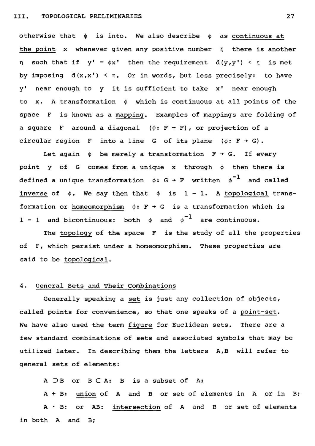
6. Connectedness
This is an important topological property of constant occurrence
later. The definition given presently is a restricted version of a
more general definition. It is, however, ample for our purpose.
Let F be a figure. Two points x,y of F are connected if
they may be joined by an arc in F. The set С(x) of all points у
of F which are connected with x is the component of x. Let у
of C(x) be connected with z so that z is in С(у). Denote by
Х/у arcs joining x to у and у to z. Let X followed from x
Figure 6.
30
7. Theorem of a Jordan-Schoenflies
to у first meet u at the point u. Let A' be the part of X
from x to u and у' the part of у from u to z (y followed
after u). Then A' + yf is an arc connecting x to z. Hence
C(y) С C(x) and vice versa, and so C(x) = C(y). That is the
component of every point of С(x) is C(x) itself. For this reason
we refer to C(x) as a component of the figure F itself. F is
said to be connected if it has just one component (namely itself):
any two points are connected by an arc.
Examples; n-cells and n-spheres n > 0, are connected. One
agrees also that a point is connected. The type of connectedness
here considered is sometimes designated as arcwise connectedness.
Under a homeomorphism connected sets go into connected sets.
Hence the number p(F) of components of F is a topological
invariant of F.
7. Theorem of Jordan-Schoenflies
This is a classical theorem of topology required repeatedly
later. As the proof is definitely arduous no attempt will be made to
give it here.
A Jordan curve is merely a 1-sphere, that is the homeomorph of
a circle.
(7.1) Theorem. A Jordan curve J situated on a 2-sphere S
divides S into two component regions U,V with the common boundary
Jr and U + J, V + J are both closed 2-cells. Equivalently: the
same property holds for a Jordan curve in a plane П save that only
one of the regions is a 2-cell and the other is infinite.
The assertion that S - J consists of two regions with the
common boundary J was first stated, but defectively proved by
Camille Jordan about a century ago — hence the name "Jordan curve".
III. TOPOLOGICAL PRELIMINARIES 31
This part of the theorem is often referred to as "Jordan curve
theorem". Its correct proof was first given by Oswald Veblen
(Chicago thesis 1904). The Schoenflies' part refers to the assertion
that U + J and V + J are 2-cells. A proof of the Jordan curve
theorem is given in the author's Introduction to Topology, p. 65.
It is evident that all these results are topological. We shall
accept them without proof.
The following, also given without proof is a reasonable
exercise.
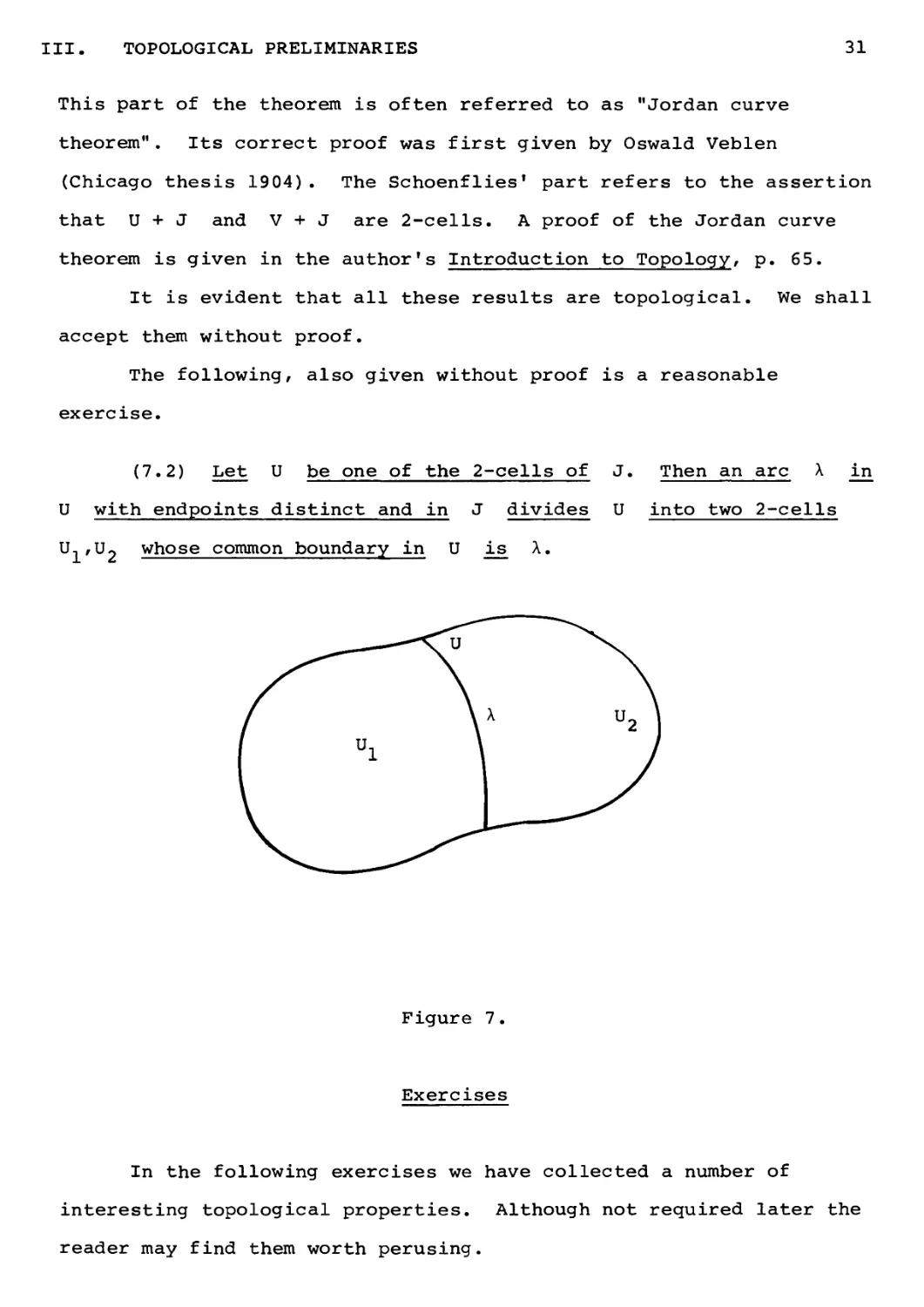
(7.2) Let U be one of the 2-cells of J. Then an arc X in
U with endpoints distinct and in J divides U into two 2-cells
U,,U2 whose common boundary in U is Л.
Figure 7.
Exercises
In the following exercises we have collected a number of
interesting topological properties. Although not required later the
reader may find them worth perusing.
32 Exercises
1. Let ф: F -* G be a transformation. Show that the
continuity of ф is equivalent to the following property: the points
of any open set V of G comes from an open set U of F.
Consequences: (a) a homeomorphism ф: F <—> G is
characterized by mere interchange of open sets: (b) open sets and closed
sets are topological invariants.
2. Prove that the union of any number and the intersection of
a finite number of open sets are open sets. Show also that the union
of a finite number and the intersection of any number of closed sets
are closed sets.
3. Let R be a space and А С R. A limit point of A is a
point x of R such that every j^(x,r) contains points of A - x.
Show that closed sets F of R are characterized by this
property: limit-points of any subset of F are points of F.
4. The closure A of a set A is the intersection of all
closed sets D A (least closed set over A). Show that A is the
set of all points at distance zero from A. Hence a closed set is
characterized by the property F = F.
5. Given a set of real numbers N let sup N denote the
least upper bound of all numbers > N and inf N =-sup(-N).
The distance d(x,A) from a point x to a set A is defined
as inf d(x,y) for all points у of A; the diameter d(A) of A
is sup d(x/y) for all x,y in A.
Show that A is the set of all points at zero distance from A.
6. Compactness. An open covering of R is any collection of
open sets containing R. The space R is compact if every open
covering has a finite subcovering. Show the equivalence of this
property: every non-empty subset of R has a limit point.
III. TOPOLOGICAL PRELIMINARIES 33
7. A compact set is bounded (containing in some spheroid) and
closed.
8. Let f(x) be a continuous real function of the point x of
a compact space R. Then f(x) attains both sup f(x) and inf f(x)
on R.
9. The compact subsets of En are exactly those which are
closed and bounded.
10. A union of connected sets with common point is connected.
11. A sequence of connected sets A,,A2,A3 ,.. ., such that
A,A,+, is never empty has a connected union.
12. Let F-,F2f... be bounded closed connected sets in E
such that F, DF. DF. ... . Then the intersection F^ F F ...
is closed non-empty connected (or a point) and bounded.
13. A more general definition of connectedness than the one
given in Section б is this: The set A is connected if it is
impossible to have A = В + С where В, С are disjoint, non-empty
and open in A (hence, also closed in A) . Prove that under this
definition
(a) a closed arc is connected.
(b) Show that the properties of 10, 11, 12 also hold under
this more general definition.
14. Prove the Jordan-Schoenflies theorem for a plane polygon.
34
CHAPTER IV
GRAPHS. GEOMETRIC STRUCTURE
The properties of a finite graph (only type considered) may be
divided into two distinct groups: geometric/ really topological
properties, and algebraic properties. In the present chapter, we
present the geometry of a graph and in the next its algebra.
1. Structure of Graphs
By definition a finite graph G consists of a finite collection
of points: its nodes П.. /П~, • • • fll and disjoint arcs bn,b0,•..,b
о 1
the branches of G. We assume that each branch has two distinct end
points which are nodes; and also that every node is an endpoint of
some branch: and that no two branches have the same endpoints.
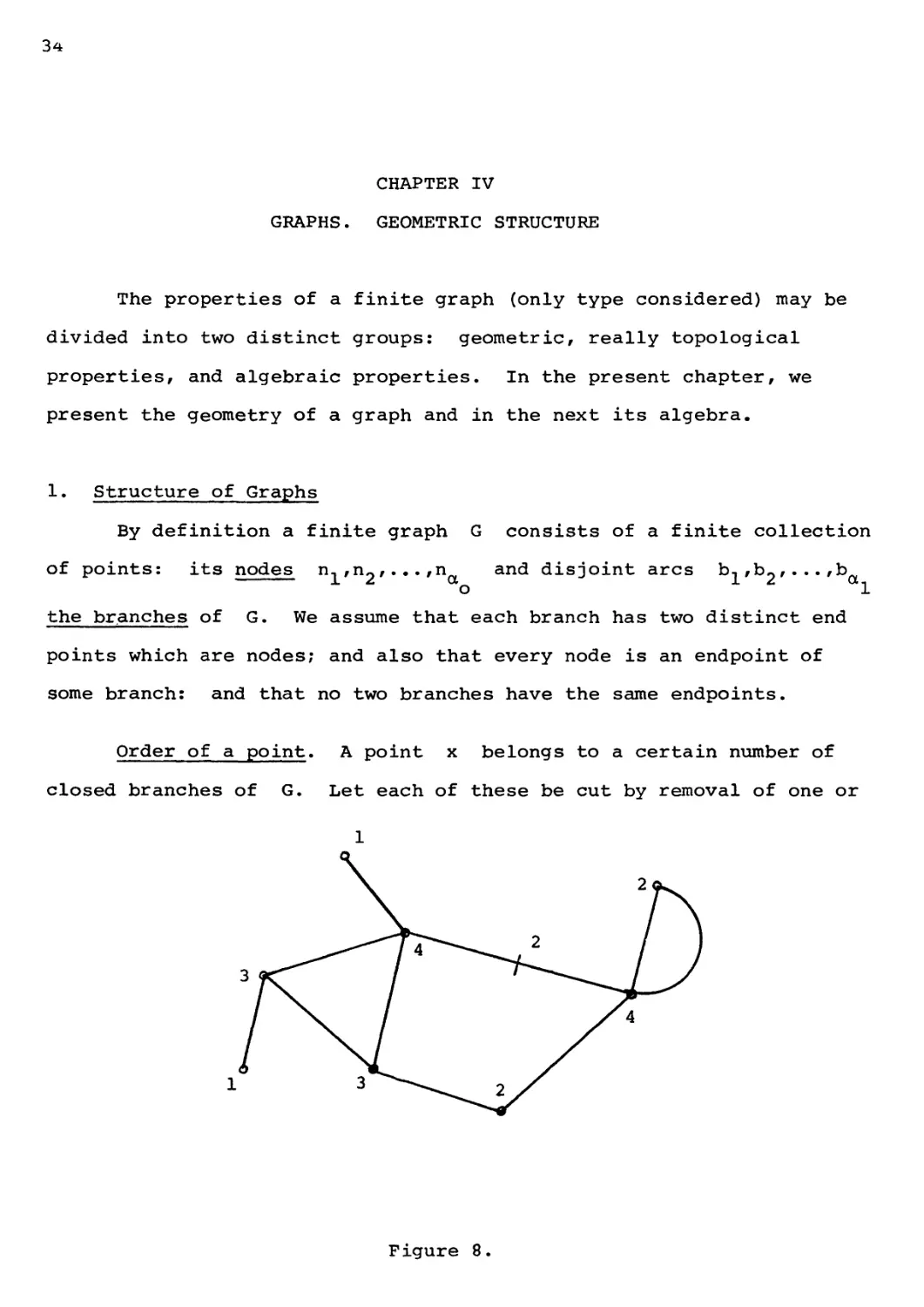
Order of a point. A point x belongs to a certain number of
closed branches of G. Let each of these be cut by removal of one or
Figure 8.
IV. GRAPHS. GEOMETRIC STRUCTURE
35
two nonend points other than x. The order to(x) of x is the
number of these "cut points". At a non-node the order is always 2.
The order is a topological invariant in this sense. If G,G' are
homeomorphic graphs and x of G, and x1 of G1 are corresponding
points under the homeomorphism then oj(x) in G = cu (x ■) in G1 .
Note this property: the number N, of points of G whose
order is к is a topological invariant of G.
In Figure 8, the numbers indicate orders of the points.
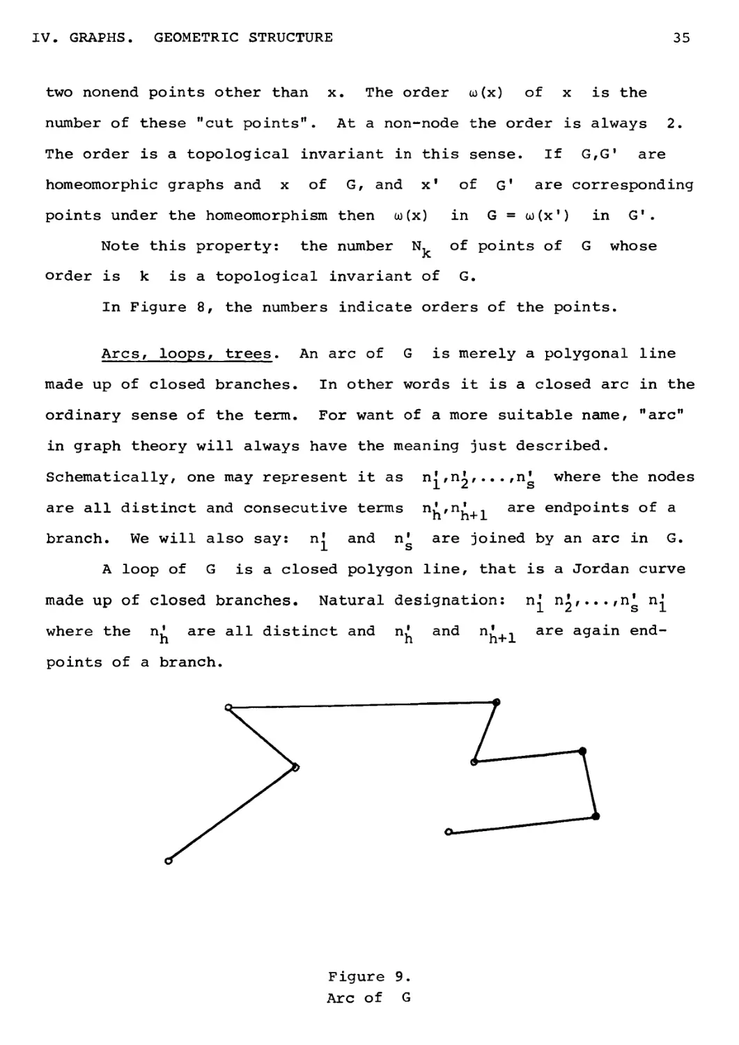
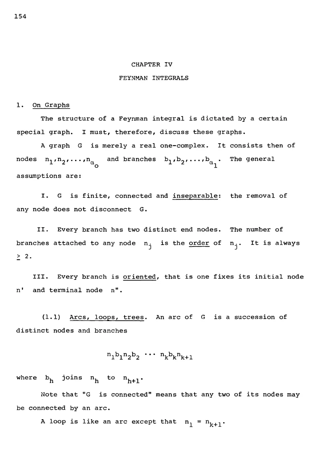
Arcs, loops, trees. An arc of G is merely a polygonal line
made up of closed branches. In other words it is a closed arc in the
ordinary sense of the term. For want of a more suitable name, "arc"
in graph theory will always have the meaning just described.
Schematically, one may represent it as n,f ,nl, .. . ,n' where the nodes
are all distinct and consecutive terms пь'пь+1 are endP°ints of a
branch. We will also say: n' and n1 are joined by an arc in G.
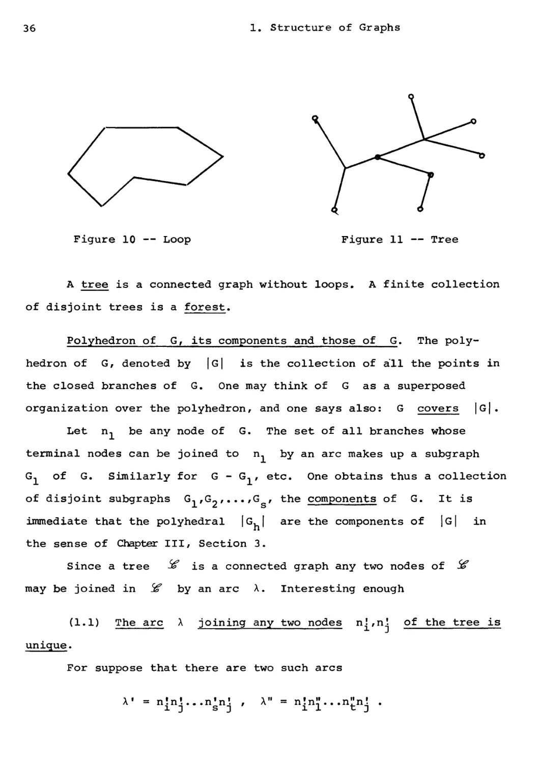
A loop of G is a closed polygon line, that is a Jordan curve
made up of closed branches. Natural designation: n^ nl,...,n' n£
where the n' are all distinct and n/ and nL+-\ are again end-
points of a branch.
Figure 9.
Arc of G
36
1. Structure of Graphs
Figure 10 — Loop Figure 11 — Tree
A tree is a connected graph without loops. A finite collection
of disjoint trees is a forest.
Polyhedron of G, its components and those of G. The
polyhedron of G, denoted by |g| is the collection of all the points in
the closed branches of G. One may think of G as a superposed
organization over the polyhedron, and one says also: G covers |g|.
Let n, be any node of G. The set of all branches whose
terminal nodes can be joined to n, by an arc makes up a subgraph
G, of G. Similarly for G - G,, etc. One obtains thus a collection
of disjoint subgraphs G,,G2,...,G , the components of G. It is
immediate that the polyhedral |G,| are the components of |g| in
the sense of Chapter III, Section 3.
Since a tree if is a connected graph any two nodes of 5*
may be joined in ^ by an arc X. Interesting enough
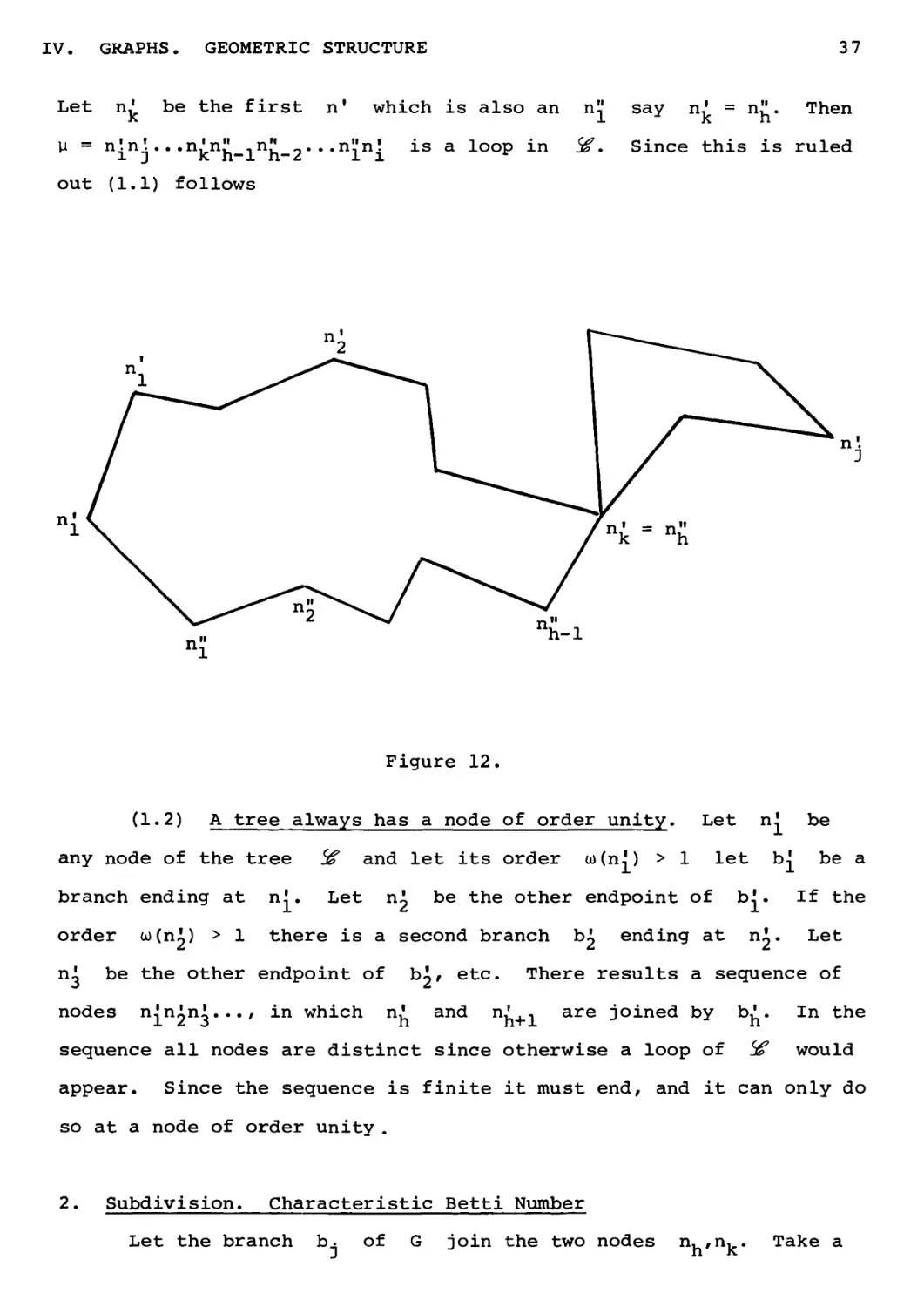
(1.1) The arc Л joining any two nodes п|'пч of the tree is
unique.
For suppose that there are two such arcs
A» = n!n'...n,n'. , A" = n!n" .n"n! .
1 J Sj 1 J- ^ J
IV. GRAPHS. GEOMETRIC STRUCTURE
37
Let n' be the first nf which is also an nV say n' = n". Then
U = nini•••ninh_inh_2#**nlni is a looP in ^' Since this is ruled
out (1.1) follows
Figure 12.
(1.2) A tree always has a node of order unity. Let n| be
any node of the tree 5f and let its order w(n') > 1 let b| be a
branch ending at n'. Let пЛ be the other endpoint of b*. If the
order ш(пЛ) > 1 there is a second branch hi ending at nl- Let
ni be the other endpoint of bi/ etc. There results a sequence of
nodes n^nlnl..., in which n^ and ni+n are joined by b/. In the
sequence all nodes are distinct since otherwise a loop of S£ would
appear. Since the sequence is finite it must end, and it can only do
so at a node of order unity .
2. Subdivision. Characteristic Betti Number
Let the branch b. of G join the two nodes п,,п,. Take a
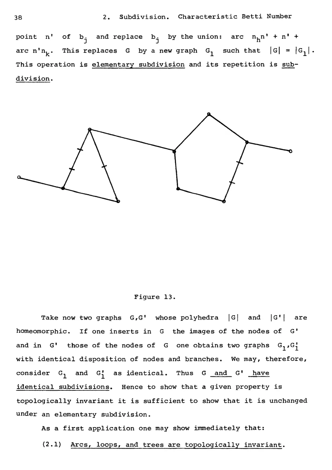
38 2. Subdivision. Characteristic Betti Number
point nf of b. and replace b. by the union: arc nun% + n' +
arc n'n, . This replaces G by a new graph G, such that |g| = |G,|.
This operation is elementary subdivision and its repetition is
subdivision.
Figure 13.
Take now two graphs G,G' whose polyhedra \G\ and |G'| are
homeomorphic. If one inserts in G the images of the nodes of G'
and in G' those of the nodes of G one obtains two graphs G\'Gi
with identical disposition of nodes and branches. We may, therefore,
consider G, and G' as identical. Thus G and G' have
identical subdivisions. Hence to show that a given property is
topologically invariant it is sufficient to show that it is unchanged
under an elementary subdivision.
As a first application one may show immediately that:
(2.1) Arcs, loops, and trees are topologically invariant.
IV. GRAPHS. GEOMETRIC STRUCTURE
39
(2.2) The number p of components of a graph is a topological
invariant.
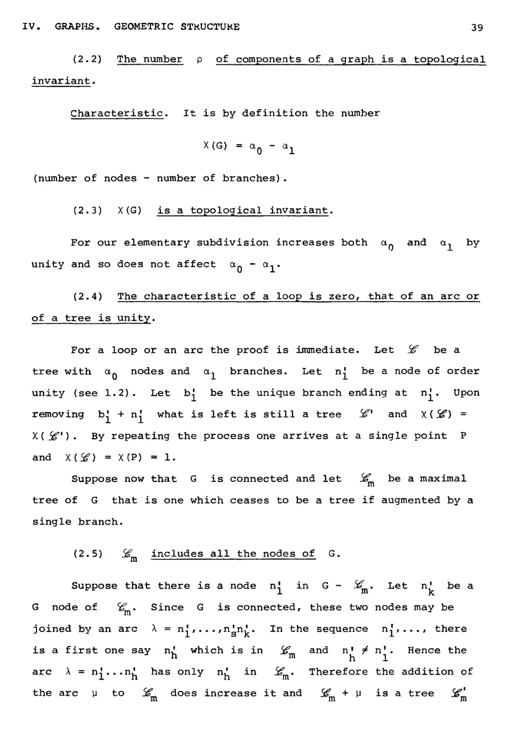
Characteristic. It is by definition the number
X(G) = aQ - ax
(number of nodes - number of branches).
(2.3) X(G) is a topological invariant.
For our elementary subdivision increases both a~ and a, by
unity and so does not affect otQ - a,.
(2.4) The characteristic of a loop is zero, that of an arc or
of a tree is unity.
For a loop or an arc the proof is immediate. Let % be a
tree with aQ nodes and a, branches. Let ni be a node of order
unity (see 1.2). Let Ы be the unique branch ending at n'. Upon
removing b' + ni what is left is still a tree & and X($£) =
X( SSX) • By repeating the process one arrives at a single point P
and X(5f) = X(P) = 1.
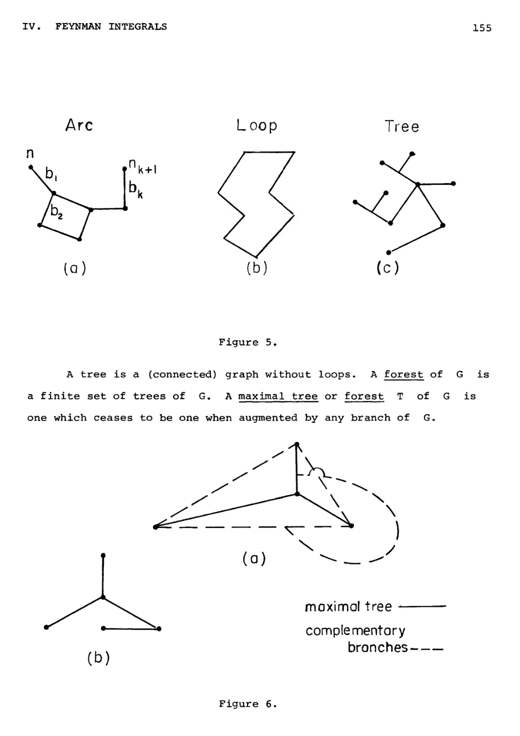
Suppose now that G is connected and let $£ be a maximal
tree of G that is one which ceases to be a tree if augmented by a
single branch.
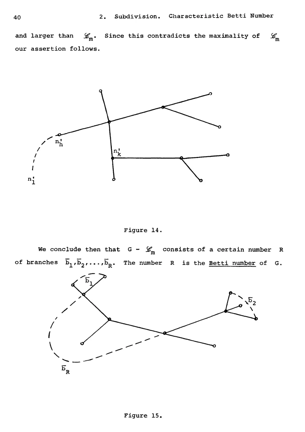
(2.5) &m includes all the nodes of G.
Suppose that there is a node n' in G - .Ц1. Let n' be a
G node of ЦL. Since G is connected, these two nodes may be
joined by an arc X = nj,. . . ,n'nJ* . In the sequence n{r.../ there
is a first one say nJ" which is in j£L and n» ^ nf . Hence the
h m hi
arc X = n-l ...пЛ has only n/ in &. Therefore the addition of
In -* n m
the arc у to S£ does increase it and & + У is a tree 5£l
m mm
40
2. Subdivision. Characteristic Betti Number
and larger than ^. Since this contradicts the maximality of 5f
m u m
our assertion follows.
/ К
Figure 14.
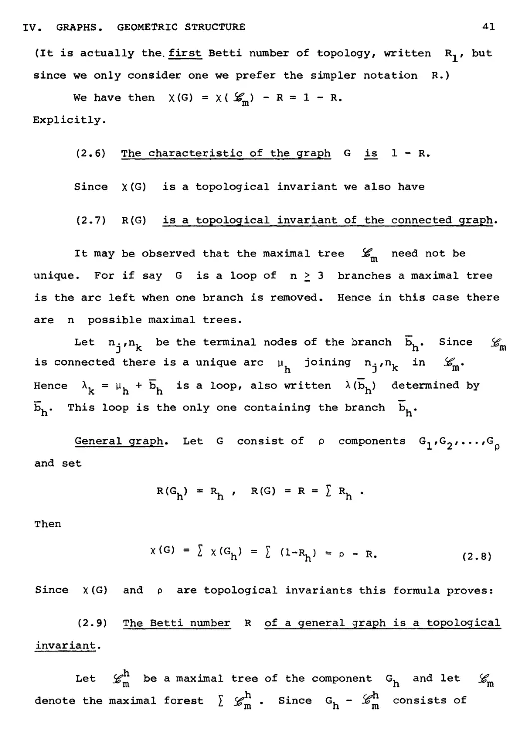
We conclude then that G
consists of a certain number R
Figure 15.
IV. GRAPHS. GEOMETRIC STRUCTURE 41
(It is actually the, first Betti number of topology, written R, / but
since we only consider one we prefer the simpler notation R.)
We have then X (G) = x( S?m) - R = 1 - R.
Explicitly.
(2.6) The characteristic of the graph G is 1 - R.
Since X(G) is a topological invariant we also have
(2.7) R(G) is a topological invariant of the connected graph.
It may be observed that the maximal tree 5f need not be
■* m
unique. For if say G is a loop of n > 3 branches a maximal tree
is the arc left when one branch is removed. Hence in this case there
are n possible maximal trees.
Let n.,n, be the terminal nodes of the branch b, . Since 5£L
j к h m
is connected there is a unique arc \x joining n. ,n, in b£ •
Hence Л = u + b, is a loop, also written Л (b.) determined by
b,. This loop is the only one containing the branch b,.
General graph. Let G consist of p components GlfG2/...,G
and set
Then
R(G. ) = R, , R(G) = R = I R,
X(G) =1 x(Gh) = I (1-Rh) « p - R. (2#8)
Since X(G) and p are topological invariants this formula proves:
(2.9) The Betti number R of a general graph is a topological
invariant.
Let & be a maximal tree of the component G, and let
denote the maximal forest У $g„ . Since G, - SS^ consists of
*■ -^m h m
^m
42 2. Subdivision. Characteristic Betti Number
branches joining pairs of nodes of % we have
(2.10) G - 5f consists of branches b.. ,.. . ,b .
43
CHAPTER V
GRAPH ALGEBRA
1. Preliminaries
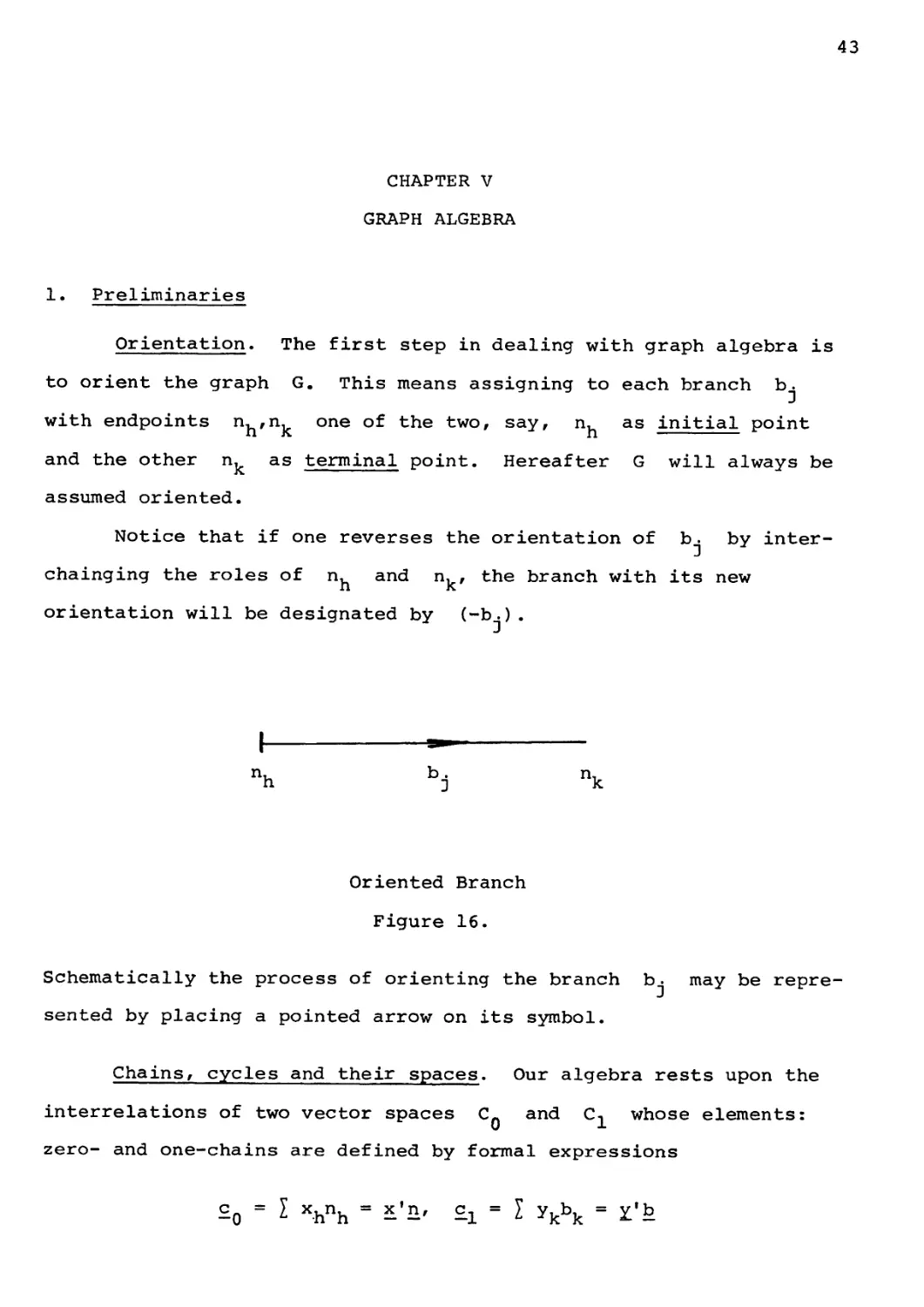
Orientation. The first step in dealing with graph algebra is
to orient the graph G. This means assigning to each branch b.
with endpoints nh'nk on^ of the two, say, n, as initial point
and the other nk as terminal point. Hereafter G will always be
assumed oriented.
Notice that if one reverses the orientation of b. by
interchanging the roles of nh and nRf the branch with its new
orientation will be designated by (-b.).
n, b. n,
h -} к
Oriented Branch
Figure 16.
Schematically the process of orienting the branch b. may be
represented by placing a pointed arrow on its symbol.
Chains, cycles and their spaces. Our algebra rests upon the
interrelations of two vector spaces Cn and C-, whose elements:
zero- and one-chains are defined by formal expressions
^o = l xhnh = £'£' £i " l Укьк ш *'ь
44
V. GRAPH ALGEBRA
where the coefficients хи'Уъ. are real. The convention is made that
ук(-ьк) = -укьк
Correspon<
a formal boundary relation
Corresponding to the orienting process described for b. write
fib. = n, — n, •
j к h
This relation is conveniently set in the general form
5bj = l ljsns
where n... = 1, r\.. = -1 and otherwise ц . =0. The number n-
jk jh js js
is the incidence number of the branch b. with the node n and
D s
Л = [n.0] is the incidence matrix of the graph.
Once <5 is defined for each branch, that is for the elements
of a base for the space C., one can extend it to all of C, as a
linear transformation 6: C, -*■ Cn by the relation
6£l = б l у.Ъ. = I y.Sbj = I yjnjknk
or in vector form
6v/b = y/ nn .
One may define a similar operation, still written 5: Cq ■* 0
(since there is no С-:,) . This means that zero-chains have no
boundary ^ 0.
Let Z, be the nucleus of the transformation 6: C-, -* CQ. Its
elements z are the one-chains without boundary that is such that
z/nn = o. Since the n, satisfy no relation, the equation just
written is equivalent
z'n = 0. (1.1)
This is the characteristic equation of one-cycles. Since 6C = 0
all zero-chains are cycles.
1. Preliminaries
45
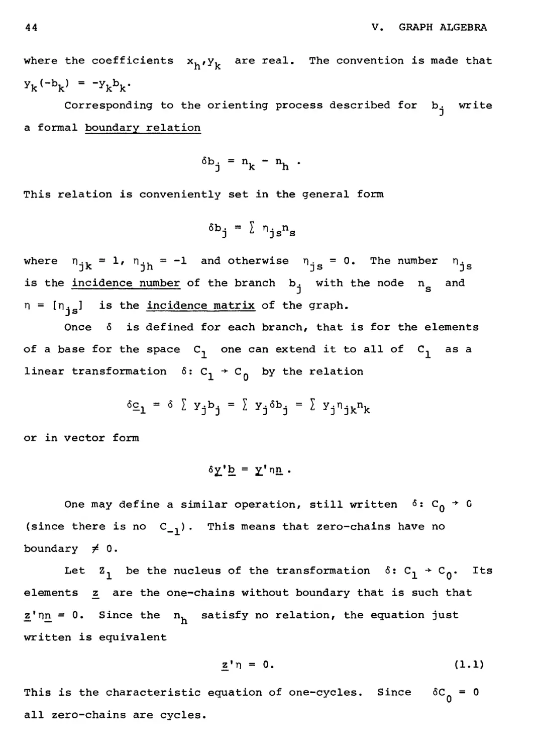
The simplest type of one-cycle is one attached to a loop X.
Let X = n|n',...,n'n| where the successive branches bibl,..., are
so oriented that 6b' = n' , - n' (n1.n = n'). Since б Z Ь/ = 0,
n h+1 h s+1 l n
lb' is a one-cycle and this is the one that we had in mind. For
convenience we keep the designation A for this cycle. Note that
the full orientation of X is determined by that of any b/. We
may also refer to the cycle as -X (-Ы) and we have X(b-j) =
X(b^) = ... = -X(-b|) = -X(-b£) = ... = n.
Figure 17.
Since Z, is the nucleus of 6: C, ■> CQ we have
Cl я Dl ® Zl
where D, is the space of the one-chains with non-zero boundary
(except d, = 0) .
Since CQ = ZQ/ the analogue of D, for the space Cfl is
DQ = 0.
Let 6D, = FQ. The space FQ consists of zero-chains which
are boundaries of one-chains. Since <5 has no nucleus as an
46 V. GRAPH ALGEBRA
operation D1 -* F , the two spaces D, and F are isomorphic. We
also have
co - zo = Fo ф Ho - Dl ф Ho (1-2)
where HQ = CQ/F (recall that according to Chapter II, Section 5
и . fi
signifies that subspaces have been replaced by isomorphs).
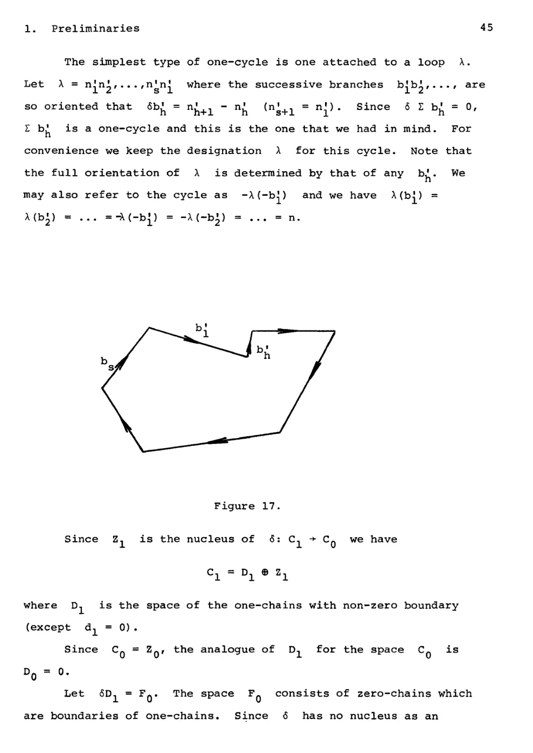
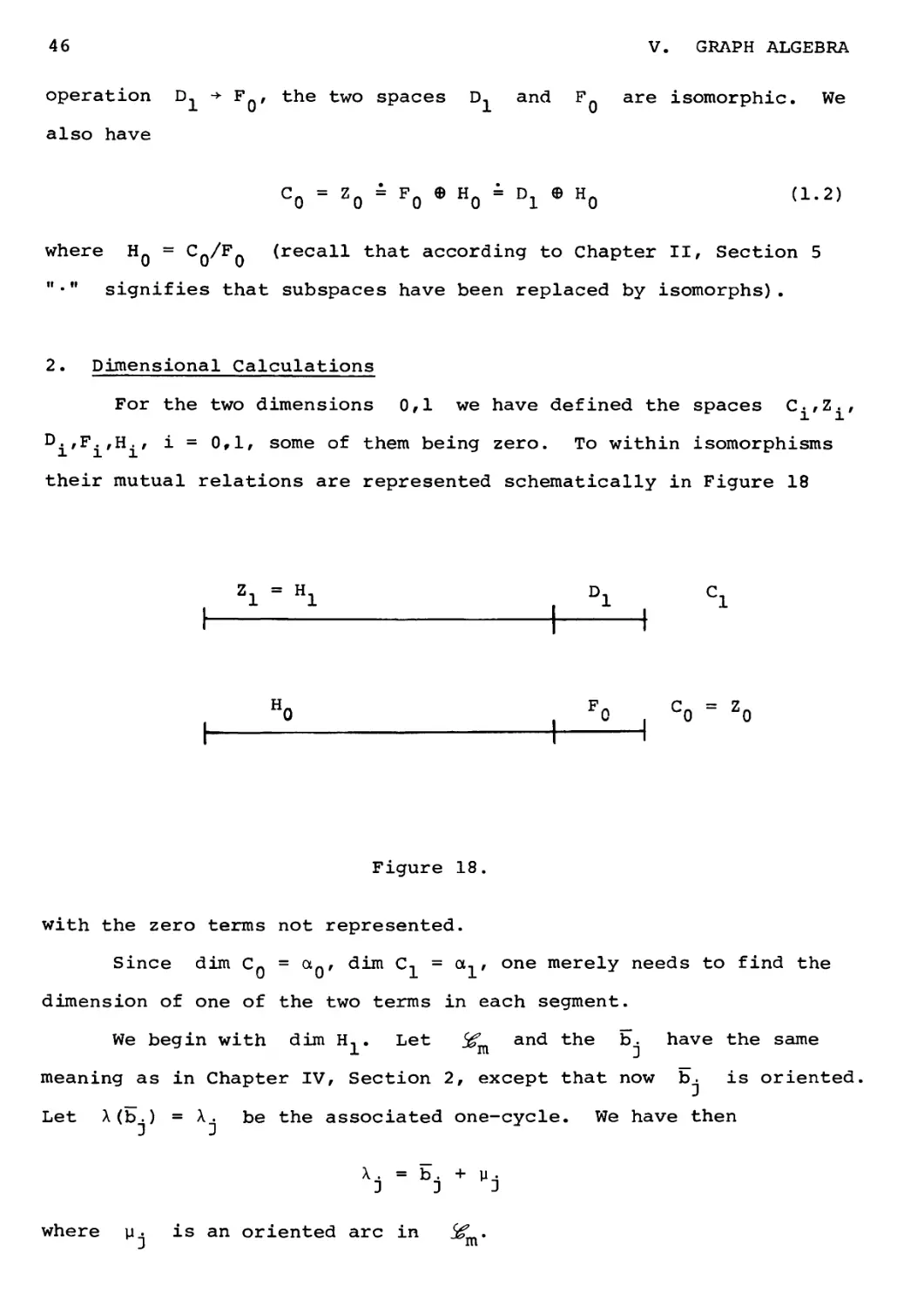
2. Dimensional Calculations
For the two dimensions 0,1 we have defined the spaces C,Z.,
Di/Fi/Hi' * = °'1' some of them being zero. To within isomorphisms
their mutual relations are represented schematically in Figure 18
zi - Hi . Di ci
Ho . Fo , co = zo
Figure 18.
with the zero terms not represented.
Since dim C0 = aQ, dim C-, = a, , one merely needs to find the
dimension of one of the two terms in each segment.
We begin with dim H,. Let Sf^ and tne b. have the same
^ 1 m j
meaning as in Chapter IV, Section 2, except that now b. is oriented.
Let A(b.) = X. be the associated one-cycle. We have then
X. = b. + Wj
where у. is an oriented arc in $g .
2. Dimensional Calculations 47
If c, is any one-chain let [c ] stand for the graph which
is the union of the closed branches actually present in the expression
Of £..
(2.1) The subgraph [z.,] of a cycle z, always contains
a loop.
Suppose that
zx = a^ + a2b2 + • • •
and suppose the b's so numbered that a, ^ 0. Let бЬ.^ = nl - n' .
Since 6z, = 0 the node nl appears in a branch, say b~ ^ b-, with
a coefficient a2 ^ 0, and in such manner that 6b2 = n' - nl, etc.
One obtains thus an arc nl nl •••nl °f [£il • Since the process
must end sometime n' = n' , h < t, so that n',...,n' is a loop
contained in [z,].
Since the forest if contains no loop, we also have
m c
(2.2) A forest contains no 1-cycle.
Denote in general by f any one-chain of & (maximal forest
of the graph G) . From (2.2) there follows:
(2.3) If f is a cycle then f = 0.
Write now
Ak = bk + f, zx = I 6kbk + f.
This implies that
*i ~ l Bkxk = £ = °
since the first term is a cycle. Thus every one-cycle depends upon
the cycles A..
48 V. GRAPH ALGEBRA
On the other hand the X. are independent. For a relation
l Vh = °
yields
l YjAi - f •
However, f includes no b, , and so this relation implies that every
Yk= 0.
Conclusion: {A,} is a base for the one-cycles. Hence
dim U1 = dim zx = Ri = R* (2.4)
From the sketch (Figure 18) one infers then that
dim D. = a, - R = dim Fq . (2.5)
Therefore/ from the sketch
dim HQ = aQ - dim FQ = aQ - a., + R = p. (2.6)
This completes the calculations of the space dimensions.
Remark. The preceding calculations rest directly upon the
geometric evaluation of the numbers R and p. One may, however,
calculate R immediately in terms of the matrix n. For if its
rank is r we have at once for (1.1):
dim Z1 = a1 - r = R. (2.7)
3. Space Duality. Co-theory
The spaces of chains С ,C, of a graph G and operator 6
are an obvious example of the situation cinsidered in Chapter II,
Sections 4, 5. There arises then an associated graph duality. The
only deviation is the reference to the various elements as cochains,
3. Space Duality. Co-theory 49
cocycles, etc., and so one speaks of the co-theory.
Corresponding to the nodes n, and branches b. of G
introduce new co-elements nu'b£ and their zero- and one-cochains
£o = * xhnh " * « ' £1 - l Укьк = 2 ь ,
generating spaces ct and C?.
Reversing the earlier boundary scheme we ask now what branches
b (same as b ) end at the node n£ (same as n, ). The resulting
coboundary is
6 nk = I nskbs '
and hence for a cochain Z y£n£
6 I Укпк " I vknskbs ' 6 * n = y_ n b
This shows that the matrix of б is n . Thus сл'сл'5 are related
to C*,C*,6* like А,В,ф to А*,В*,ф* in Chapter II, Section 5.
All that is required, therefore, is to adapt the notations to the
present situation. We shall not attempt to do so in full, but will
only obtain the explicit form of a property of importance later.
Referring then to Chapter II, (5.11) we find
(3.1) A n.a.s.c. in order that zjb be a one-cycle is that,
whatever the coboundary u, b we have
z^u* = 0. (3.2)
Let the spaces C-, and C, be referred to the same coordinates.
The preceding property affirms then
(3.3) The subspaces __Z, of the one-cycles and F* of the co-
boundaries are orthogonal and complementary, that is
C-i =Z-i © F, .
50 V. GRAPH ALGEBRA
(3.4) A direct proof of (3.3). A one-cycle is any one-chain
z/b such that <5z/b = z'nn = 0 which yields z*r\ = 0. The co-
boundary of a cochain £*'n* is y^'n'b* / that is it is a cochain
u* = nv*. Hence
z/u* = z'nv* = 0.
Property (3.3) has an important application to network theory.
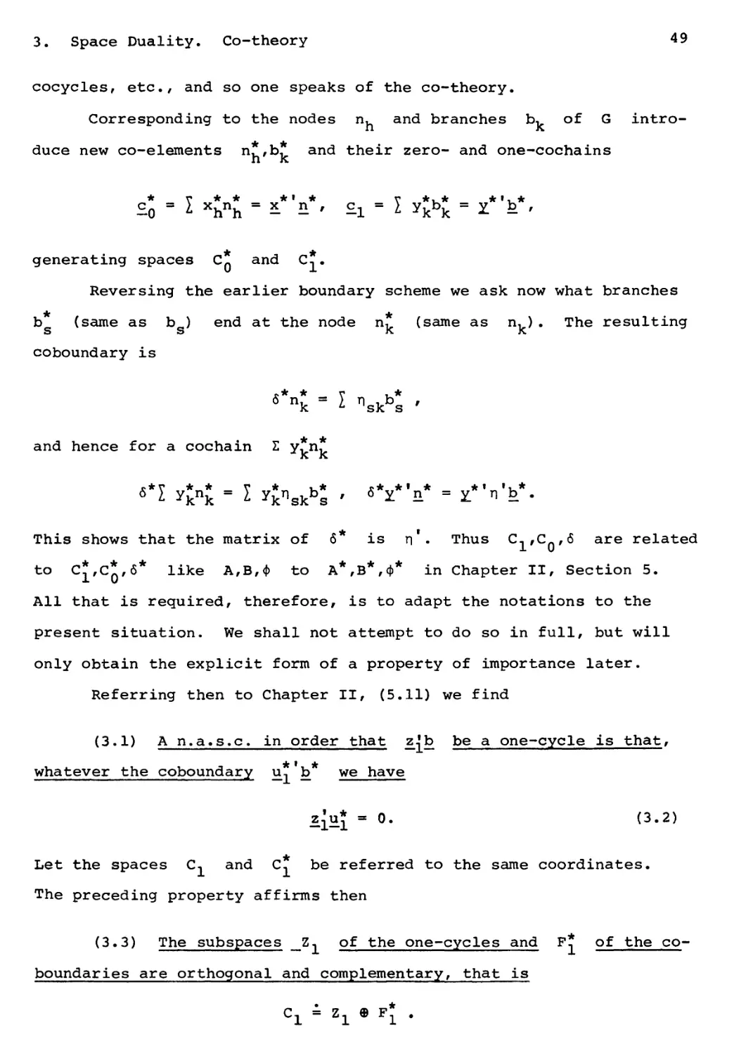
Dimensional calculations for the dual spaces. We first draw a
sketch analogous to Figure 18.
zo = *Z , Do , c;
h^H
Hi ,FI , cI = zi
ь^ч
It implies
Figure 19.
dim C* = aQ, dim C* = o^
Also from (3.3): dim F* = c^ - R = dim D,. Hence
dim H* = aQ - (o^-R) = p = dim HQ;
dim H* = ax - (c^-R) = R = dim H1#
That is:
(3.5) The cohomology spaces have the same dimension as the
corresponding homology spaces.
51
CHAPTER VI
ELECTRICAL NETWORKS
An electrical network is just a graph to whose branches there
are assigned two functions: a voltage distribution and a current
distribution, each subjected to classical laws due to Kirchoff. We
first discuss these laws and reformulate them in keeping with the
topological development of the preceding chapter.
1. Kirchoff s Laws
Let N be a network and G its graph. All notations of the
previous chapters will be applied to G.
To each (oriented) branch b, of G there are assigned a
voltage v. and a current i, positive in the same directions as
bh itself, and making up vectors у and i. For the present they
are merely subjected to Kirchofffs laws. We state them and
reformulate them.
(1.1) First Kirchoff law (current law). A current distribution
is any vector i'b, such that the algebraic sum of the currents
arriving at any node is zero.
The physical meaning of this law is that a node is neither a
source nor a sink of electrical fluid.
Let n, be an endpoint of b,. Then i, arrives at or leaves
n, accordingly as iunhk > ® or < ^.
The obvious conclusion is that the algebraic sum of the currents
arriving at the node n, is
I Vhk •
h
52 VI. ELECTRICAL NETWORKS
Hence Kirchoff's first law means that i'n = 0 or that the
chain i'b is a cycle. The reformulation of the law is therefore:
(1.2) A current distribution is any vector i'b which is a
cycle of the graph G.
(1.3) Second Kirchoff law (voltage law). A voltage distribution
is any cochain vector v'b such that the algebraic sum of the
voltages along any loop is zero.
Reformulation of the second law. One may state the second law
in this way. Let any loop be given by
A = I ekbk ' ek = ±3- or °'
Then
l ekvk = 0.
In particular let A, ,A~/••.,A„ be a maximal set of independent
loops and set
Л . = У e.,b, .
j L ]k к
If v is the same as above then
I ejkvk =0' J = 1,2,...,R.
Let i denote the current distribution represented by the cycle
a.A,, its value being a, in each branch of A. . We have then
*h2 ehkvk= °=i(h)'v.
Since every current distribution i depends upon the i we have
i'v = 0. d.4)
That is the vector v of the voltage distribution is orthogonal to
2. Different Types of Elements in the Branches 53
every current vector. Therefore v is a coboundary.
Conversely, if v is a coboundary it will be orthogonal to the
special current X and the second law will be obeyed. Hence this
reformulation of the second law:
A voltage distribution is any coboundary (of a zero-cochain).
That is v'b* = <5*w'n* = w'n'n* or finally vf = w'n', hence
у = nw. (1-5)
Thus if 6b. = n. - n. then v, = w, - w.. The w*s are the electro-
П к з n К j
static potentials and are arbitrary. We may therefore state:
(1.6) One may assign arbitrary electrostatic potentials w
and then determine the voltages v. of the branches, by the following
rule: If 6bu = n. - n. then v, = w, - w..
— n k j h к j
Returning to (1.4) notice that since v is a vector in a linear
subspace, the latter (that is V„ „) likewise contains dv. Hence
from (1.4)
i'dv = 0 = di'v (1.7)
a relation of much importance in the rest of the chapter.
2. Different Types of Elements in the Branches
One may envisage various types of electrical mechanisms in the
branches. Through the insertion of new nodes which does not modify
the situation in any manner one may always assume that each branch
contains a single mechanism such as we will now envisage.
We distinguish then the following typical branches:
I. Resistor. Basically this is the name given to any
branch b in which a current i and voltage v are related by a
single relation F(i,v) =0. We shall always assume that F is
54 VI. ELECTRICAL NETWORKS
defined for all real values of i and v, that it has continuous
first partials Fi'Fv throughout the plane i,v, and moreover that
F.,F never vanish simultaneously. Geometrically it means that the
curve F = 0 has a continuously turning well defined tangent and no
multiple points (or other singularities).
The simplest instance is the linear (ohmic) resistance v = Rif
(R a positive constant). Of interest also are a voltage or constant
current generator, when F = 0 is respectively a line parallel to the
i axis, and one parallel to the v axis. Still another noteworthy
case is the vacuum tube. Van der Pol had proposed the simple
characteristic
v = ai - bi ,
a and b > 0. A more realistic description is a characteristic
. 3 5
v = ai - bi + ci , a,b,c > 0.
II. Inductor. Here the relation between i and v is
L(i) U = v, L(i) > 0, (2.1)
where we accept for L(i) the same general type as for R(i). This
is the case of the potential induced in a solenoid or electromagnet
by a current i(t).
III. Capacitor. Same situation with i,v interchanged, the
relation now being
C(v) |£ = i, C(v) > 0.
3. A Structural Property
By means of a maximal forest btf of the graph G the
following property has been obtained: Let b,,b2/...rbR be the branches
3. A Structural Property
55
of G - $f. Let f designate any chain of &m* Then there exist R
linearly independent loops A,,..., A such that
Ah = bh + fh-
(3.1)
We propose to describe an algebraic method for arriving at the
same result. To that end let A,,A2,...,A be a base for cycles and
let
Yh = I e
hkV
Since the y's are independent the matrix tev,k^ ^"s °^ rank R- Let
the branches be so ordered that the matrix D = [ehjJ ; h,k = 1,2,...,I
is already nonsingular. Upon replacing the vector
Y =
by D у there will result a set of cycles, still called Y-,/.••/YR
such that the corresponding D = 1.
Now if a branch is in no Yh it will receive no current and
hence it is electrically inactive. We may then as well surpress it.
In other words we merely replace the graph G by the subgraph
[Y-j] + [Yo] + ••• + [YR] . To simplify matters assume that this graph
is G itself.
Let H be the subgraph composed of the closed branches
bR ,,...,b . There is no cycle in H, since such a cycle would
have to be independent of the Y,. Thus H is a forest.
Let now A, be a loop contained in [YiJ . Since A is not
a chain f we have (replacing perhaps A by *^n)
56 VI. ELECTRICAL NETWORKS
Xh = bh + f' Yh - bh + f' •
Hence Xh-Yh=f-fl =0f since f - f' is a cycle. Hence
Yh = X,. Thus we have reproduced by an algebraic attack the exact
situation announced at the beginning of the section.
Since X, are loops we have
Xh ■ bh + l £hsbR+s <3-2>
ehs - ±!L or °'
4. Differential Equations of an Electrical Network
We propose to assign a certain number p of independent
currents and q of independent voltages to express all currents and
voltages in terms of these and write the corresponding equations of
the network.
Since there are only R independent current distributions we
must have p < R.
With the same notations as in Section 3 choose then b.,,...fb
as inductor branches and let any one of these be designated by b
and their currents by i
Let the branches b .w--./b_ be resistors and let b denote
P'i к p
any one of these branches. The loop
X = b + У e b
p p L pv v
where b designates any branch of a chain X - b . The branches
v ^ 2 p p
* *
b are taken as capacitors and assigned voltages v ; their number
is q and their currents are i .
The remaining branches (if any): b_, ,.,...,b are denoted
K+q+i ot-i
by b and they are again resistors.
4. Differential Equations of an Electrical Network 57
(4.1) The current and voltage distribution i,v depend
entirely upon the independent variables i and v .
By the second law v is a sum of voltages v :
"VP = I epv< • <4'2>
Since b is a resistor
P
ip=gp(vp) (4.3)
and hence the current in every branch is determined by the currents
i and i (first law). Hence they are functions of the i^ and
v* . Thus in every branch b. either v. is given (one of the vv)
or else determined by the resistor relations, or else again if a b*
from the second law (in A ).
Our next step will result from the application of the relation
v'di = 0. (4.4)
Upon taking account of the relation
dKv = v*div+ 4dv*
we obtain
l \dil ' 2 Кй< + l vpdip + l "odi-o + I d^iv<) = °« <4'5)
We shall show that each of the last three sums is an exact
differential. Conventionally we shall write
f(i)di = dF(i)f g(v)dv = dG(v).
Now
vPdiP = fP(iP)diP = dFP(iP5 " dFp(gp(vpn = dHp(v*)-
Hence
58 VI. ELECTRICAL NETWORKS
I vpdip = dH(v*), H ■ I Hp . (4.6)
Next, since b is a branch of one or more A we have
\ - I Sa1! ' va = fa(V-
Hence
vadia " fa(ia)dic = dPa(V = ^a*1**
and/ therefore
Finally/
I vadi0 - dK(i*b К ■ I Ka . (4.7)
i = [ e i* + J e i
pv u «; pv p
- J e i*-[B g [У e v*l ,
J yv и £ pvyp (/ pvvvj
Hence
I V* я I SvW + L(v*>- (4-8)
Hence, if we set M = H + L then -P(i*/V*) = K(i*) + M(v*) + i*' ev*
we find from (4.5)
I v^dij - I ivdv* = dP(i\v*). (4.9)
Since i* / v* are independent variables upon equating the
coefficients of their differentials we obtain
^T* vu ' " M7= К ' (4-10)
4. Differential Equations of an Electrical Network
59
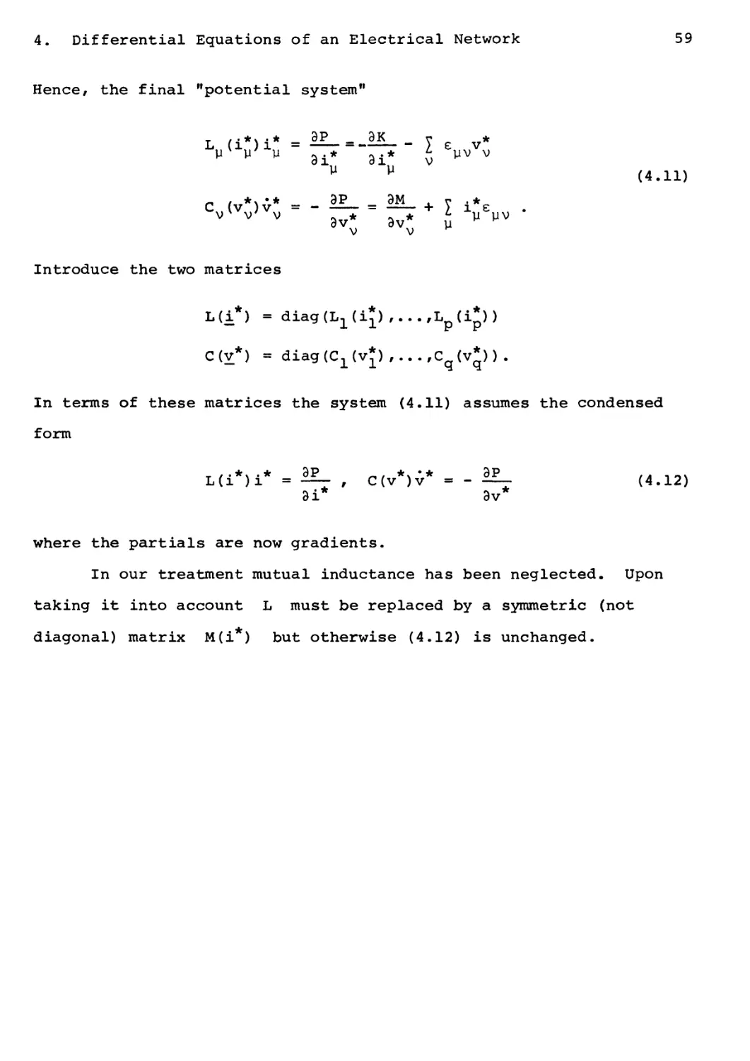
Hence, the final "potential system"
ЭР _ ЭК г. *
p p u 9i* 31* v yv v
(4.11)
*4•* ЭР _ ЭМ
С (v*)v* = - 2£L- = «S_ + у i*e
3v- 3v" p
Introduce the two matrices
L(i*) = diagd^d*) ,.. .,Lp(i*))
C(v*) = diagfC^v*) ,...,C (v*)) .
In terms of these matrices the system (4.11) assumes the condensed
form
_ z ■ ft » • ft oP ^^/<^\*ft oP / л i ^ \
L(i )i = —- , C(v )v * (4.12)
3i* 8v*
where the partials are now gradients.
In our treatment mutual inductance has been neglected. Upon
taking it into account L must be replaced by a symmetric (not
diagonal) matrix M(i ) but otherwise (4.12) is unchanged.
61
CHAPTER VII
COMPLEXES
Our further progress rests upon another excursion into topology:
theory of complexes and related polyhedra (only for dimension two),
with applications to surfaces in the next chapter. However, we do not
plan to pursue topology beyond "piecewise linear" arguments. This is
done in order to minimize recourse to more delicate arguments which
would be imposed by full fledged topology, and which we really do not
need.
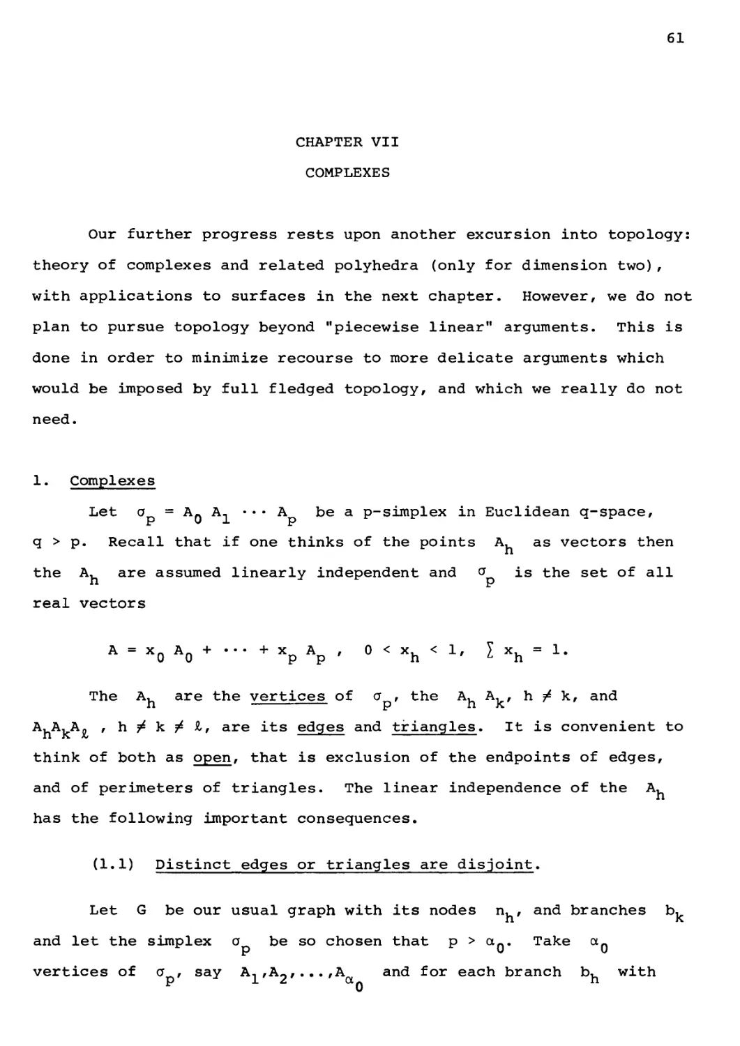
1. Complexes
Let a = AQ A. ••• A be a p-simplex in Euclidean q-space,
q > p. Recall that if one thinks of the points A, as vectors then
the A, are assumed linearly independent and <? is the set of all
real vectors
A = xQ AQ + ... + xp Ap , 0 < xh < 1, I xh = 1.
The A, are the vertices of a , the A, A, , h ф к, and
A,A, A* , h / к / l; are its edges and triangles. It is convenient to
think of both as open, that is exclusion of the endpoints of edges,
and of perimeters of triangles. The linear independence of the A,
has the following important consequences.
(1.1) Distinct edges or triangles are disjoint.
Let G be our usual graph with its nodes n,, and branches b,
and let the simplex о be so chosen that p > otQ. Take aQ
vertices of a , say A,,A2,...,A and for each branch bh with
"0
62 VII. COMPLEXES
terminal nodes n^'nv draw the edge A. A, . As a consequence these
edges and vertices make up a complete and faithful representation of
the graph G with rectilinear branches. In order not to diversify
notations to excess we may assume that this representation is G
itself. Thus the node n. is now also the vertex A. of ст and
h n p
the branch n. n, is the edge A. A, of the simplex.
Consider now any set of distinct loops A-/A2r.•., A of the
graph and suppose that p > aQ + s. To the loop A, assign the
vertex Ал ,, of о . The loop A, is now a polygon of о . Draw
oIq+п p n *■ p
in a a segment from A +, to every point of A, . Let
A, = nlnl • • • nini • Tne collection of all the segments to the
points of nnnh+i ^nr+l ~ n:P ^s a closed triangle with vertex at
A ,, . The collection of all these triangles has the same structure
as say the collection of triangles, with vertex at the center of a
regular r-gon and bases on its sides. This is manifestly the
topological image of a circle - that is a closed 2-cell and will be called
here "cell" for short. The open cell includes the point A +h but
not the base A. .
Upon applying the preceding construction to each of the loops
^. there result s new cells e.,,...,e all disjoint from one
another and from the graph G itself. The collection К of G
plus these s cells is known as a 2-complex, or simply complex for
short.
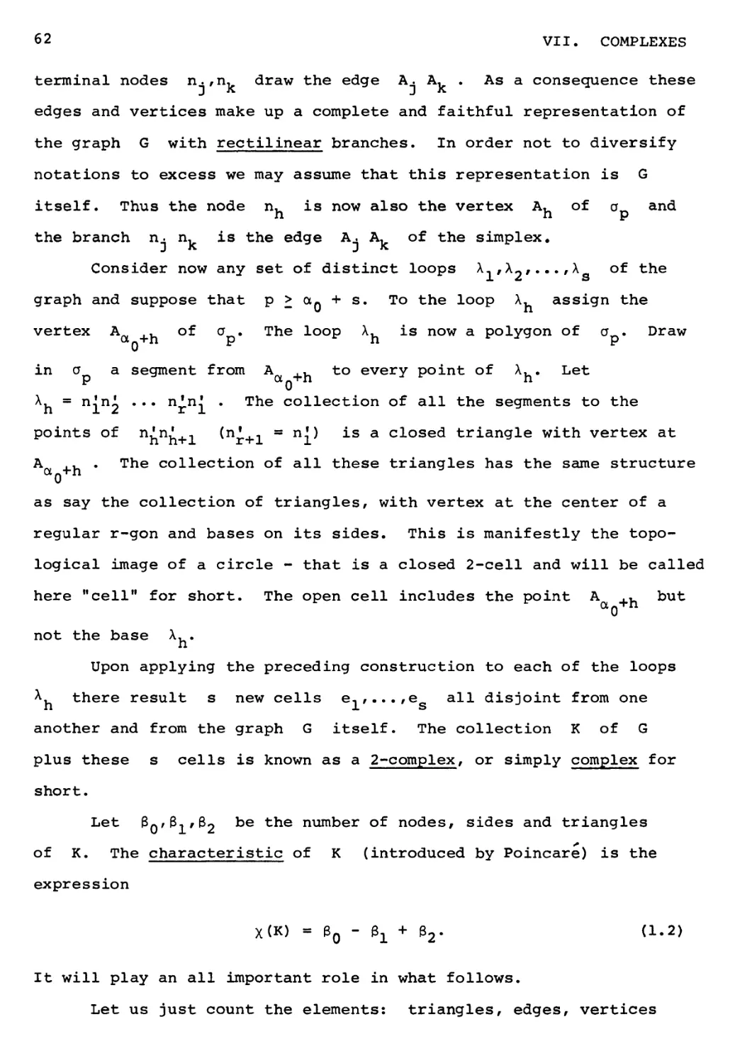
Let £o'^l'^2 ke tne num^er °f nodes, sides and triangles
of K. The characteristic of К (introduced by Poincare) is the
expression
X(K) = 30 - 3X + 02. (1.2)
It will play an all important role in what follows.
Let us just count the elements: triangles, edges, vertices
1. Complexes 63
which are in the cell e. , and let their numbers be ^o'Yi'Yo'
Since there is just the vertex A .- and equal numbers of sides and
a0+h
triangles we find at once
X<eb> - Yn " Y, + Yo - 1.
Hence, as far as x(K) itself is concerned we may merely count each
cell as unity. We then have
X(K) = X(G) + s = aQ - a± + s = p (G) - R + s.
In keeping with our earlier notations it is best to set
s = a2 = the number of cells of K. If we think of a0/ai as numbers
of "0-cells" and "1-cells" of К we have the consistent notation
X(K) = aQ - ax + a2 = p(G) - R + a2 , (1.3)
where a2 is now the number of loops X..
To sum up the characteristic may equally well be calculated
directly from the number of cells e, (that is from the number of
loops X.) .
Polyhedron. The set of all points in the elements: nodes,
branches, cells of К is called a polyhedron, and denoted by |к|
or also by П. The complex К is said to cover the polyhedron |к|.
The distinction between К and |к| is meant to emphasize the fact
that the complex is a geometric figure plus a definite structure:
decomposition into nodes, branches and cells.
Connectedness. Since every point of |K| is connected by an
arc to a point of the graph G the components П_ of |K| are
polyhedra each uniquely determined by a component G, of G and
there is a subcomplex K. of К which covers П., so that the latter
is merely a connected subpolyhedron of |к|. The Kh are the
64 VII. COMPLEXES
components of К and their number p is the same as the number of
components of the graph G. Evidently p is a topological
invariant of |K|.
2. Subdivision
It was shown in Chapter V, Section 2 that topologically
identical graphs have a common subdivision. As a consequence to prove
topological invariance for graph properties it was sufficient to
prove their invariance under subdivision. This agreeable situation
is much more difficult to establish for complexes. However, we do
not require the more stringent topological invariance and so we shall
merely consider subdivision invariance.
One must first define subdivision. This is done in two steps.
We first define elementary subdivision as consisting of one of the
following two operations:
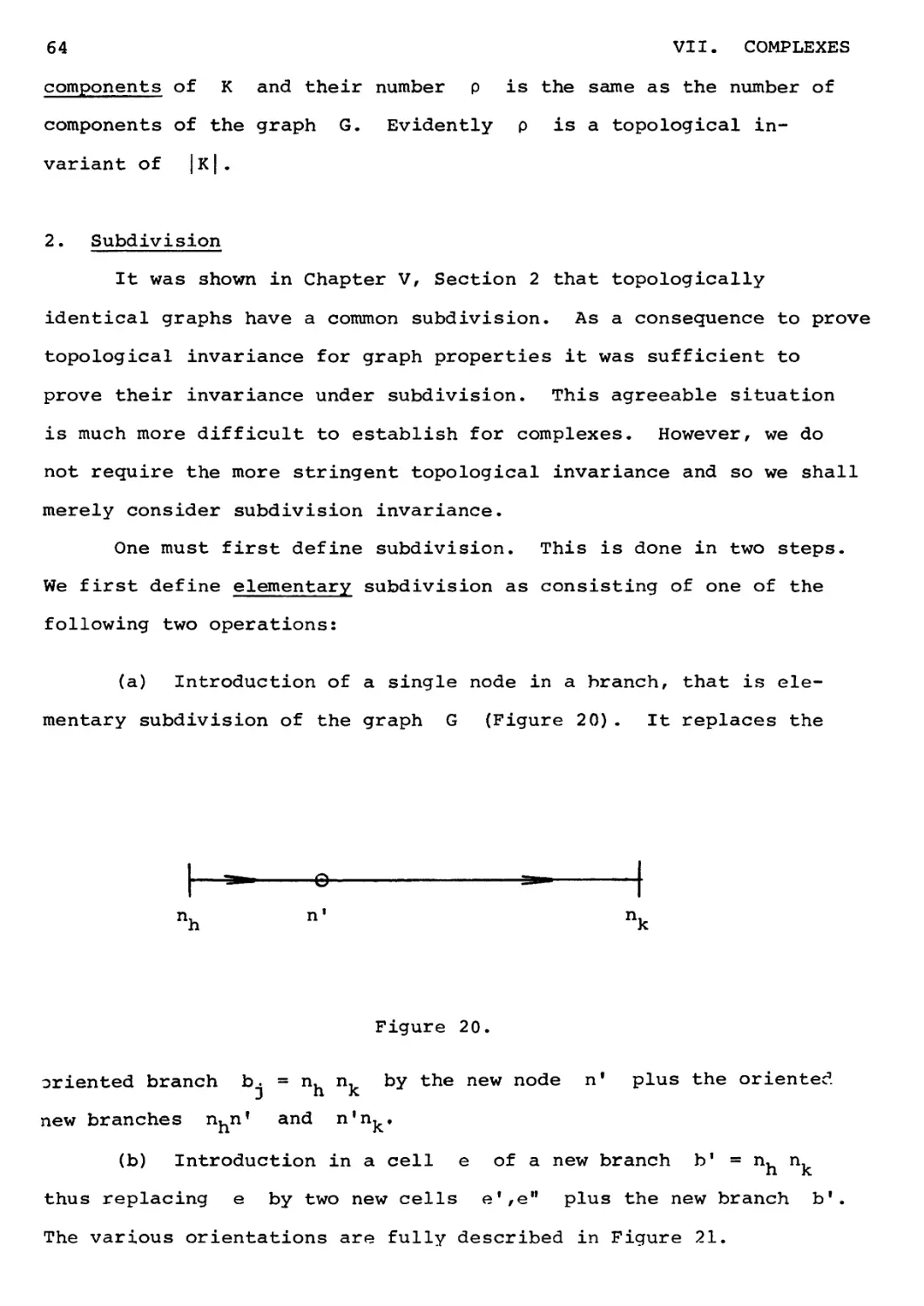
(a) Introduction of a single node in a branch, that is
elementary subdivision of the graph G (Figure 2 0). It replaces the
nh n' nk
Figure 20.
oriented branch b. = n. n, by the new node n' plus the oriented
new branches п^п? and n,nk'
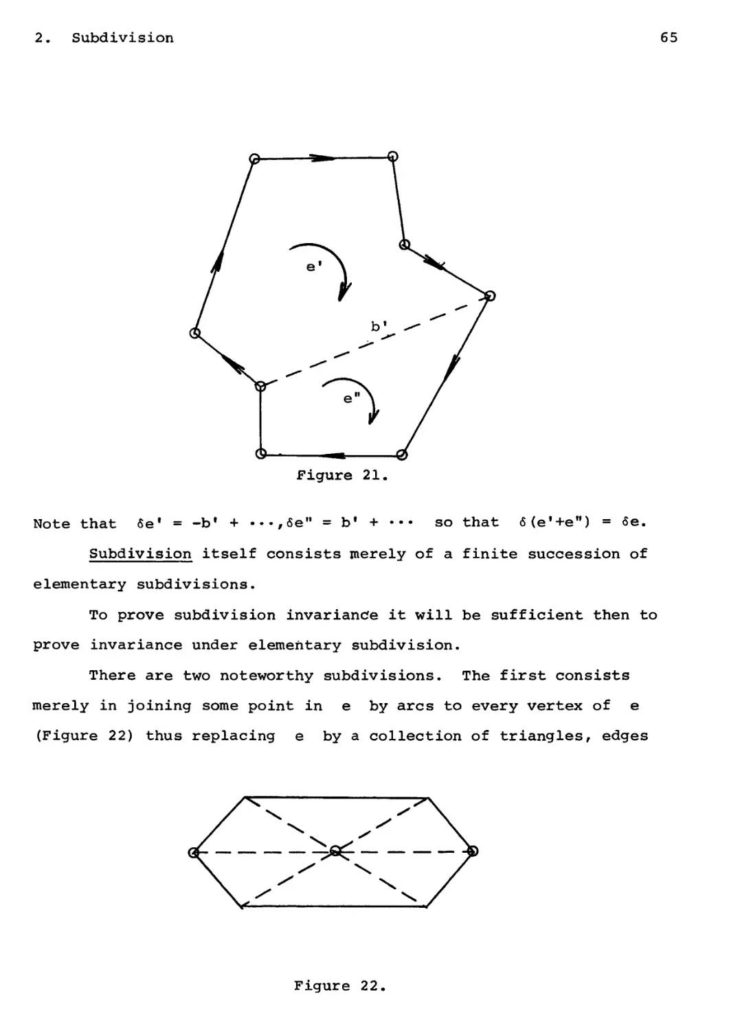
(b) Introduction in a cell e of a new branch b' = n, n,
thus replacing e by two new cells e'/e" plus the new branch b'
The various orientations are fully described in Figure 21.
2. Subdivision
65
Figure 21.
Note that бе1 = -Ь' + .-^бе" = b1 + ••• so that б(е'+е") = бе.
Subdivision itself consists merely of a finite succession of
elementary subdivisions.
To prove subdivision invariancfe it will be sufficient then to
prove invariance under elementary subdivision.
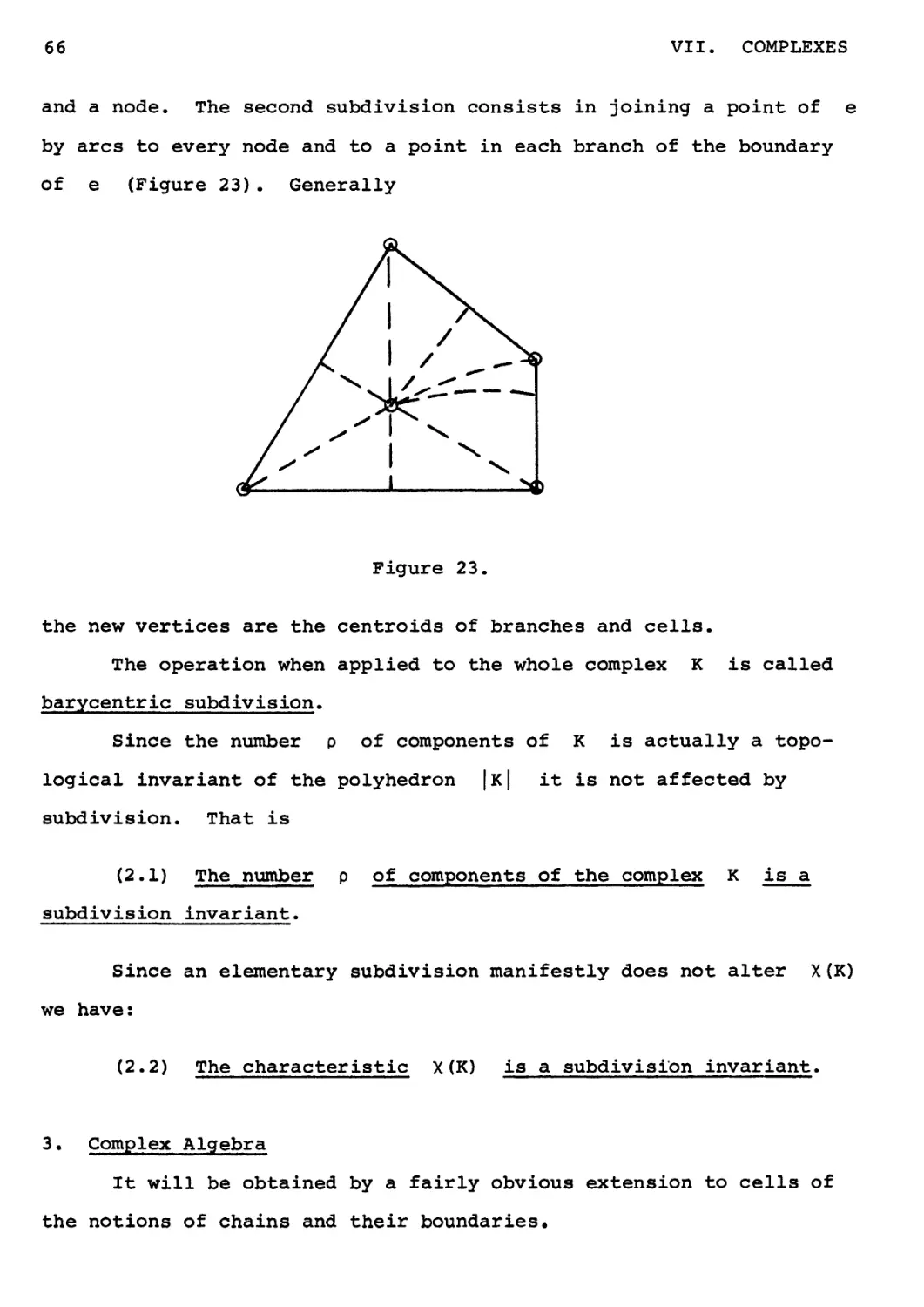
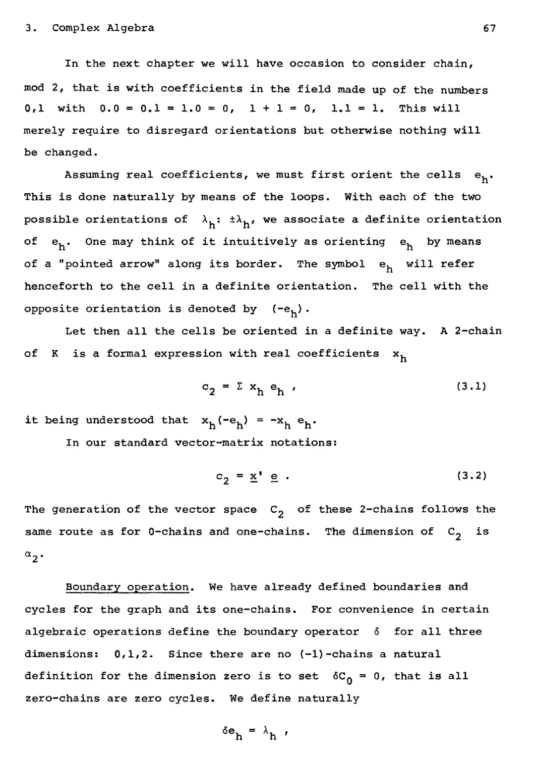
There are two noteworthy subdivisions. The first consists
merely in joining some point in e by arcs to every vertex of e
(Figure 22) thus replacing e by a collection of triangles, edges
Figure 22.
66
VII. COMPLEXES
and a node. The second subdivision consists in joining a point of e
by arcs to every node and to a point in each branch of the boundary
of e (Figure 23). Generally
Figure 23.
the new vertices are the centroids of branches and cells.
The operation when applied to the whole complex К is called
barycentric subdivision.
Since the number p of components of К is actually a
topological invariant of the polyhedron |к| it is not affected by
subdivision. That is
(2.1) The number p of components of the complex К is a
subdivision invariant.
Since an elementary subdivision manifestly does not alter X(K)
we have:
(2.2) The characteristic X(K) is a subdivision invariant.
3. Complex Algebra
It will be obtained by a fairly obvious extension to cells of
the notions of chains and their boundaries.
3. Complex Algebra
67
In the next chapter we will have occasion to consider chain,
mod 2, that is with coefficients in the field made up of the numbers
0,1 with 0.0 = 0.1 = 1.0 = 0, 1+1=0, 1.1 = 1. This will
merely require to disregard orientations but otherwise nothing will
be changed.
Assuming real coefficients, we must first orient the cells e,.
This is done naturally by means of the loops. With each of the two
possible orientations of Л,: ±A., we associate a definite orientation
of е.. One may think of it intuitively as orienting e. by means
of a "pointed arrow" along its border. The symbol e, will refer
henceforth to the cell in a definite orientation. The cell with the
opposite orientation is denoted by (~eO•
Let then all the cells be oriented in a definite way. A 2-chain
of К is a formal expression with real coefficients x,
c2 = Z xh eh ' (3>1)
it being understood that хи^""еь^ = ~xh eh"
In our standard vector-matrix notations:
c2 = x' e . (3.2)
The generation of the vector space C~ of these 2-chains follows the
same route as for 0-chains and one-chains. The dimension of C2 is
a2.
Boundary operation. We have already defined boundaries and
cycles for the graph and its one-chains. For convenience in certain
algebraic operations define the boundary operator 6 for all three
dimensions: 0,1,2. Since there are no (-1)-chains a natural
definition for the dimension zero is to set 6CQ = 0, that is all
zero-chains are zero cycles. We define naturally
6eh - xh '
68 VII. COMPLEXES
hence
6 z xh eh - E хь xh •
In terms of the branches bk we have
Ah = Z Chk bk
and hence
6 l xh eh = I xh Chk bk . (3.3)
The number (integer) £,, is the incidence number from the
cell e, to the branch b, - It is ±1 if b, is a branch of X,
and zero otherwise. The matrix £ = [£nkl is the incidence matrix
from cells to branches.
We have thus two incidence matrices: n from branches to nodes,
and £ from cells to branches. In our usual vector matrix notation
(3.3) reads
бх'е = x'Cb. (3.4)
In complete parallel to the branch case one defines as 2-cycles the
chains with boundary zero, that is xfe is a 2-cycle whenever
x'Cb = 0 that is whenever
x4 = 0. (3.5)
From Chapter II, Section 5 we have
X(K) = ci0 - ax + a2 = RQ - RL + R2 .
4. Subdivision Invariance
The importance of the homology groups H.7 i = 0,1,2 and of
their dimensions R. — Betti numbers — rests upon their being the
2
same for two homeomorphic figures, for example a sphere S and the
4. Subdivision Invariance 69
boundary of a 3-cell say. This points to a more "important" relation
between two figures. Actually it is that of topological identity.
However, its full treatment calls for a deeper theory than we wish to
utilize. We shall therefore confine our argument to "subdivision
invariance", that is to the identity of various properties upon mere
subdivision.
Now subdivision of a complex of dimension < 2 is merely
obtained by a repetition of simpler operations: elementary subdivisions.
Hence we shall only require the treatment of invariance under
elementary subdivision. For a graph G it merely consists of adding a
node. For a 2-complex it may consist either in adding a new node or
else just a new branch. I shall avoid a more extensive digression by
suggesting the solution of this easy
Problem. To prove that the homology groups H., i = 0,1,2 of
a 2-complex К (hence also their Betti numbers) are invariant under
elementary subdivisions, hence also under any subdivision.
General remark. In the whole theory of chains and cycles the
only properties of real numbers that have been utilized are those
appropriate to rational numbers: addition, subtraction, multiplication,
division. Therefore, one could as well consider coefficients from
any field F. Actually we will have occasion to use, in Chapter VIII
the field mod 2 made up of the symbols 0,1 under the rules:
0.0 = 0.1 = 1.0 =1+1; 0+1=1+0= 1.1 = 1. In this field
1 = -1 and so one may dispense with negatives. There are obtained
Betti numbers, written R.(2) or R. mod 2, but no changes otherwise.
71
CHAPTER VIII
SURFACES
Up to the present we have not seriously limited the type of
complex envisaged, that is the nature of the polyhedron П. The
class of particular interest for the application to networks, and
indeed the most noteworthy class from any viewpoint is the class of
surfaces.
1. Definition of Surfaces
Generally speaking a surface S is a connected figure with the
property that each point of S has for neighborhood a 2-cell. This
definition is however too general for our requirements/ and so we
shall restrict "surface" to the following:
(1.1) Definition. A surface is a connected polyhedron |к|
whose covering complex К has the following two properties;
A. Every branch b of К is adjacent to exactly two cells
e/e1 of K/ and their boundary loops have only b in common.
Let n be any node of К and b, a branch ending at n.
There is a cell e, adjacent to b-, and so there is a second
boundary branch b2 of e, ending at n. Hence there is a second
cell e2 adjacent to b2 and another branch b3 of e2 ending at
n, etc. There results a sequence bieib2e2 "## ekbk ' en(^n9 when
b^ occurs again, in which bn is adjacent to eu-± and
eh' ^ek+l = el^• Tn^s is a circular system of elements or umbrella
with the common node n. Now a priori there may be several such
systems attached to any node. For example, this happens if one takes
72
VIII. SURFACES
the surface of a cube and brings two vertices into coincidence.
However, we impose:
B. To each node there is attached a unique umbrella.
One may readily verify that each point of the surface has for
neighborhood a 2-cell. In other words, our surfaces have adequate
"smoothness".
(1.2) Properties А,В are topological (proof omitted).
2. Orientable and Nonorientable Surfaces
The important property is really A. It implies immediately
that
Y0 = Z eh
is a cycle mod 2, since in the boundary 6y0 each branch appears
twice. There are now two possibilities: One may or one may not
2. Orientable and Nonorientable Surfaces
73
orient all the cells e, so that yQ is actually a real cycle. In
the first case the surface is orientable, in the second nonorientable.
Strictly speaking the orientability process refers to the
covering complex К and not to the surface. However, the following
theorem, stated without proof, justifies its direct assignment to the
surface.
(2.1) Theorem. Orientability (hence also nonorientability) is
a topological property.
In other words, the two properties are independent of the
particular covering complex of the surface S.
Let the cell e, be oriented and let b, be a branch of the
loop Л (e1), boundary of e,. There is another cell e2 adjacent to
e,, and let it be oriented so that e, and e2 are oppositely
related to b, that is so that b1 does not appear in 6(e.,+e2).
Call this the "orientation process" (Figure 25). By this process if S
Figure 25.
is orientable one will obtain a unique orientation for all the cells.
74 VIII. SURFACES
That is any geometric chain such as Figure 26 will behave as
indicated: there will be no violation of the orientation process. On
Figure 26.
Orientable Geometric Chain
the contrary in a nonorientable surface there will always be some
geometric chain of the type of Figure 27.
Figure 27.
Nonorientable Geometric Chain
2. Orientable and Nonorientable Surfaces
75
In the orientable case all geometric chains drawn on the surface
behave like a cuff. In the nonorientable case there will be some
band of the type of Figure 28: the sides 1,2 are matched as
indicated:
Figure 28.
Mobius Strip
This is the classical Mobius strip, the first example (given by Mobius
over a century ago) of a nonorientable surface piece. (See also
Chapter III, Section 1.)
A noteworthy property is this:
(2.2) Theorem. All the 2-cycles of an orientable surface are
of the form xYq. The only 2-cycle mod 2 on a nonorientable surface
other than zero is
itself.
Suppose that S is orientable and let
Yl = xlel + x2e2 +
+ x
ct2 a2
be any 2-cycle. Suppose that x^ ф 0. Then between е.. and e one
may draw a geometric chain such as in Figure 26. Since y, is a
cycle 6y, will not contain b,. Since the coefficient of b1 in
6y1 is ±(x1-x2) we must have x2 = x^ and likewise x2 = x3
= ... = x . Hence y, = x, yQ.
76
VIII. SURFACES
The same proof holds for the nonorientable case, except that
every x, = 1.
Betti numbers. A noteworthy consequence of the above is this
distinction between orientable and nonorientable surfaces:
Orientable
surface R2 =
Nonorientable J ^ 0
That is, one may distinguish between the two by the value of R~.
Suppose that К is nonorientable. Take for each closed cell e
two copies e',e" oriented in opposite ways. Let eu'eic be adjacent
across the branch b. Unite say e/ with the one of the cells
е'еУ which is oppositely related to b. As a consequence/ and since
К is nonorientable there results a new complex К which is a
surface (proof elementary) and is orientable. The surface К is
said to be a doubly covering surface of K.
Note that the same procedure applied to an orientable surface К
results in two distinct orientable surfaces K* and K* with
corresponding cells oppositely oriented and both copies of K.
Returning again to the nonorientable surface K, since the
numbers of nodes, branches, cells in К are double the same for K:
X(K) = \ X(K*)
3. Cuts
Let X be a loop in the surface S. The umbrella construction
of Section 1 may be applied to the cells with a node or branch in X,
with X replacing the node n in the construction. The resulting
number q of umbrellas cannot exceed two. For if q > 2 some
branch of X would be adjacent to q cells, and S would not be a
3. Cuts
77
surface. Thus q = 1 or 2.
Suppose that q = 1: there is just one umbrella. Upon
applying the umbrella construction there is an associated description of
the loop X in a certain direction. As one starts from a node n
in that direction and with cell e, when one returns to n and
passes it one will arrive a cell e' ф e, for e' = e would imply
that there is an umbrella which does not include all the cells with
node or branch in \, and hence that there are two umbrellas. As a
consequence the orientation scheme breaks down as between e and e'.
Hence the surface S is nonorientable.
Figure 29.
One-sided Cut
Conversely, let S be nonorientable. The full orientation
process breaks down along a collection of branches making up a graph
H. A node n of H cannot be of order one, since manifestly the
orientation process cannot break down around it. It follows that H
contains no tree. Hence H contains a loop Л around which the
78 VIII. SURFACES
orientation scheme breaks down. However, this can only happen if Л
has a single umbrella. Thus
(3.1) Theorem, A n.a.s.c. in order that a surface be non-
orientable is that it possess a loop with a single umbrella.
(3.2) Corollary. A n.a.s.c. in order that a surface be orient-
able is that every loop possess two umbrellas.
A loop X is said to be a 2-sided [one-sided] cut whenever it
possesses two umbrellas [one umbrella]. The umbrellas are the sides
of the cut.
The remainder of our argument will rest heavily upon a set
X.T...,X of disjoint loops which do not disconnect the surface S.
x S
In this connection we prove the following basic property:
(3.3) Let p be a maximum number of disjoint nondisconnecting
cuts. Then for an orientable [nonorientable] surface P < R-,
[p < R, mod 2].
Let first S be orientable and let Л..,Л ,...,X be a set of
oriented disjoint nondisconnecting cuts of S. Designate also their
cycles by A,.
(3.4) The cycles A, are independent.
Assume a boundary relation
6 I 6heh=.E YkAk . (3.5)
Since К - Z A, is connected the reasoning of Section 2 will apply
here and we will find that with suitable orientation of the cells e^:
31 = 32 = ••• = 3- Hence
6 Z 3heh = 36 I eh = 3<$y0 = 0 = E YhAh ,
3. Cuts 79
where yQ is the same as in Section 2. Since no two A, have
common branches we must have every y, = 0, that is (3.5) is trivial.
Since the A, are independent cycles s < R, .
When S is nonorientable the reasoning is the same save that
chains and cycles are to be taken mod 2 and so s < R, (mod 2).
Let K, be an elementary subdivision of К and A,,...,A as
above. It is immediately seen that these loops give rise to a similar
set for K,. Hence the maximum number s(K) of such loops is
< s(K,), the same number for K,. Hence:
(3.6) Subdivision does not decrease s(K).
Since subdivision does not affect the Betti numbers R, or
R, mod 2, there is a subdivision, call it again K,, for which
s(K1) = p < R. or R mod 2, where it is the largest possible value
of s(K.). In the future К will be replaced by K_. This amounts
to assuming, as we shall do henceforth that the maximum p has
already been attained by К itself.
4. A Property of the Sphere
The object of the present section is to prove this basic result.
(4.1) Theorem. If every cut disconnects a surface S then S
is a sphere.
Strictly speaking this theorem is implicit in the Jordan-
Schoenflies theorem (Chapter II, Section 7). However, we merely aim
to give a relatively elementary proof of our special case.
Since onesided cuts do not disconnect the assumption implies:
(4.2) S is orientable.
The proof of (4.1) rests upon an induction on the number of
80 VIII. SURFACES
cells of the complex K. Let P represent (4.1) for a surface with
a number m of cells. To prove P we need to prove the following
properties:
(4.3) If m = 2, К is a sphere.
(4.4) pra-1 implies Pm«
Proof of (4.3). When m = 2 one may represent К as an
ordinary Euclidean sphere whose cells are the upper and lower (open)
hemispheres and common boundary the equator E divided into q > 3
arcs by 3 nodes. Thus К is a sphere.
Proof of (4.4) . Let К have m > 2 cells. Take one of these
e and replace it by a point A. This is done as follows. If A is
the boundary loop of e, it has an umbrella U not containing e.
Let K. be the complex consisting of A and the cells of К - e
plus their boundaries modified as follows: if e, is a cell of U
with a node or branch in Л then they are replaced by A.
In K, the umbrella U becomes the unique umbrella of A.
Since each branch of K.. is still adjacent to just two cells, and
K, is manifestly connected, it is a surface and has exactly m - 1
cells. If we can show that every loop of K.. disconnects K, then
by P , it will be a sphere. Hence P т - A is a cell
m-1 m-l
(proof immediate) and so is P - e - A. Hence by (4.3) P is a
^ m л m
sphere. Thus our final task is to prove:
(4.5) In K1 every cut u disconnects.
Before proceeding with the proof of (4.5) observe that
V = e + A + U is a cell. For it has exactly the structure of a
convex closed plane polygon plus an umbrella around it. Hence,
in particular, any two points of V may be joined by an arc in V.
4. A Property of the Sphere
81
Figure 30.
Proof of (4.5). Suppose first that K, - A - U is a point B.
Then, manifestly K, is a sphere. In that case again K, - A is a
cell. Hence К consists of two cells with common boundary Л and
so К is a sphere. Hereafter then we may suppose that K-, - A - U
is not a point. Under these conditions it will be shown that the
assumption that a cut у of K, does not disconnect K, leads to
a contradiction.
Suppose first that u passes through A (Figure 31). Then
contains two branches b = n'A, b1 = n"A where n1,n" are nodes
opposite A in U. Since U is an umbrella one may join nf to n"
82
VIII. SURFACES
Figure 31.
by a polygonal line v in the boundary В of U. If yf is the
result of replacing n'An" by v in у then y* does not
disconnect. Therefore, it contains - a loop - a cut - y" which does not
disconnect and does not contain A. Therefore, we may assume that
the initial cut У does not contain A. Under the assumptions у
has no points in U + A. Any pair of points x,y of К, - у may be
joined by an arc v. One may manifestly assume that neither x nor
у is the point A, and in fact that v does not contain A. Hence
у is the image of a cut у in К and x,y a pair imaged into x,y
of К - у" joined by an arc in К - у. Since x,y are merely
arbitrary points of К - Л - e - у it is readily shown that this
contradicts the assumption P . Hence (4.5) is proved and so is the
theorem.
5. Orientable Surfaces 83
5. Reduction of Orientable Surfaces to a Normal Form
Let К be an orientable surface. Assume that the maximum
possible p of disjoint nondisconnecting cuts for К and its
subdivisions is already reached for K. If it is not one replaces К by
a subdivision for which p is reached and call К this subdivision.
Let X-,X2,...,X be a set of disjoint nondisconnecting cuts of K.
Take any cut X and let U,wU,2 be its two umbrellas. Construct
a new complex K* in which the two umbrellas are untouched but
each X is replaced by an identical reporduction of X., say X, ,
and X.2 for U., and Uh2# Construct new cells e,n and e,2
with respective boundaries *hl'*h2# TJie comPlex K results from
this operation for each h. One verifies immediately that K* is
an orientable surface.
(5.1) K* is a sphere.
The proof is the same, with minor modifications of that of
(4.1), and need not be repeated.
It follows that
X(K) = X(K*) - 2p = 2 - 2p. (5.2)
Hence if К is not a sphere X (Ю < 2. Since if К is nonorientable
X(K) is half the characteristic of a certain orientable surface its
X < 2 also. Thus:
(5.2) Theorem. If К is not a sphere its characteristic
X(K) < 2. Thus the sphere is completely characterized by the value
2 of its characteristic.
The number p is known as the genus of the surface S.
The normal form S corresponding to p is obtained by cutting
out p pairs of holes XwX,' ,...,X ,X • in a sphere and covering
J. J. br br
each pair with a cylindrical "handle". If one admits, as we shall,
84
VIII. SURFACES
that p is a topological invariant, the models obtained for distinct
values of p are all distinct.
Figure 32.
Sphere with 3 handles
6. Reduction of Nonorientable Surfaces to a Normal Form
The simplest type of nonorientable surface is the projective
plane P. Topologically it is obtained from a circular region with
identification of diametrally opposed points (Figure 33). Its
triangulation is indicated in Figure 33. The count of elements gives
the values aQ = 6, a1 = 15, a2 = 10. Hence X(P) = 1. One verifies
readily that P is a surface and since its characteristic is odd it
is nonorientable. This can also be ascertained from the presence
in Figure 33 of a Mobius strip (shaded region). The covering surface
6. Nonorientable Surfaces
85
Figure 33,
Projective Plane
has characteristic 2 and so it is a sphere. Hence P is the
nonorientable surface with largest characteristic.
We have seen that a nonorientable surface S must have a
Mobius strip, through a one-sided cut. Let it be \^ and let
A,/A2f...fA be a maximal set of disjoint nondisconnecting cuts. As
before we may assume that q is the largest possible for all the
subdivisions of S.
Suppose now that Л2 is a two-sided cut. We replace it by a
cut A» such as outlined in Figure 33, and A' will be one-sided.
The set A,,\l,A-,...,A continues to be nondisconnecting. By this
process the initial set will be replaced by a set still called
86 VIII. SURFACES
A-,A2,...,A consisting only of one-sided cuts. Let this already be
achieved.
If one cuts open the loops and covers them with cells, one will
have a sphere as before. Hence
X(S) = X(S ) = 2 - q.
The return to the initial surface S is by replacing the cells by
projective planes and this will be the normal form.
7. Duality in Surfaces
Let Kf be a barycentric subdivision of the surface K.
Introduce the following collection K* of elements (Figure 34):
I. Nodes n* in one-to-one correspondence with the cells
e of K; n. is the centroid of е..
Figure 34.
7. Duality in Surfaces 87
II. Branches b^ defined as follows. The branch b. is
adjacent to two cells ev/eo of K« 0n b. there is a new node nt
of K1 and on еъ'ец new nodes n£,n£ of K*. The branch
bj - nknj + nj + nK-
III. Cell e* consisting of the node n. plus all the open
branches and triangles of K' ending at n,.
It is a simple matter to verify the following properties.
(a) The collection K* is a surface.
(b) K' is a barycentric-like subdivision of К the new
vertices are not necessarily "centroids", but the structure of K1
relative to K* is that of a barycentric subdivision.
It follows from (b) that
RX(K*) = R-^K') - R1(K) . (7.1)
Hence if К is orientable [nonorientable] so is K*.
Suppose that К is orientable. Then K1 is likewise
orientable. Hence the orientation of any triangle of K1 is
determined by that of any one triangle plus the orientation process.
One may then determine through the orientation process the orientations
of all the cells of К,К!,К*. Moreover, as a consequence the
analogues of the matrices n,c for K* are merely s'/n1* Hence
the one-one relation ni'bh'e£ <—> ei'bh'nJl determines a duality
relation К <■■: ■> К* relative to the operations 6,6* in the sense
of II.
89
CHAPTER IX
PLANAR GRAPHS
1. Preliminaries
A graph G is planar if one may sketch it on an Euclidean
plane, that is represent it faithfully (map it topologically) on the
plane: The problem of finding conditions under which G is planar
is of evident geometric interest, and also of interest for network
theory as we shall see. This is the main problem to be discussed in
the present chapter.
The first solution was given by Kuratowski who not only solved
the graph problem but found n.a.s.c. for a continuous curve Г: map
of an interval, to be planar. A more strictly "graph" solution was
first given by Hassler Whitney and was improved a few years later by
Saunders MacLane.
Now both Whitney's and MacLanefs solutions were strictly
"graphic" and of the type known as combinatorial - that is with
topological considerations dispensed with. I have shown that by a
judicious use of the theory of surfaces as developed in Chapter VIII,
one could obtain a far more rapid solution. This is the solution
that will be given here. Within the same order of ideas it has been
found possible to deal with a noteworthy extension of the graph
problem.
From many points of view the Euclidean plane is a rather
awkward and sometimes exasperating figure. This is due mainly to its
infinite extension. Now if a graph G may be sketched on a plane
it may likewise be sketched on a sphere and conversely. My deviation
from my predecessors is mainly due to having dealt with the
90
IX. PLANAR GRAPHS
graph-sphere problem: to find n.a.s.c. in order that a graph may be
sketched upon a sphere.
Relevant Bibliography
Kuratowski, Casimir
"Sur le probleme des courbes gauches en topologie" Fundamenta
Mathematicae, Vol. 15, 1930, pp. 271-283.
Whitney, Hassler
"A set of topological invariants for graphs" American Journal
of Mathematics, Vol. 55, 1933, pp. 231-235.
"On the classification of graphs" American Journal of
Mathematics, Vol. 55, 1933, pp. 236-244.
"Planar graphs" Fundamenta Mathematicae, Vol. 21, 1933, pp. 73-84.
MacLane, Saunders
"A structural characterization of planar combinatorial graphs"
Duke Mathematical Journal, Vol. 3, 1937, pp. 460-472.
Lefschetz, Solomon
"Planar graphs and related topics" Proceedings of the National
Academy of Sciences, Vol. 54, 1965, pp. 1763-1765.
2. Statement and Solution of the Spherical Graph Problem
Let G be our usual graph with its nodes n, and branches b,.
Suppose that G has a topological image G.. on a Euclidean sphere S.
It is an easy matter to show that S - G, ^ 0. Take then a point A
of S - G, and from A project G, on a plane П not passing
through A. The projection G2 is a topological image of G in П.
Conversely given a topological image G2 of G in П and a point A
of S not in the intersection S-П the projection G.. of G2 from
A onto S is a topological image of G, in S. Thus to find
conditions under which G is planar or spherical are equivalent problems.
2. Spherical Graph Problem
91
We shall deal directly with the spherical problem.
A natural restriction on G is to assume that it is connected.
A less evident restriction is the property of separability
introduced by Whitney. A connected graph is separable whenever the
removal of some node (not any node) disconnects it. It is not
difficult to show that if G is disconnected by the removal of a
node into G1 and G" and if the closures G' and G" are spherical
graphs so is G. Therefore we simplify matters by assuming definitely
that the graph under consideration is inseparable that is both
connected and inseparable.
The best planar graph theorem is due to Saunders MacLane, and
this is the proposition that we propose to prove. However, because
of our looking at it as a spherical theorem our phrasing differs
somewhat from MacLane1s original version.
(2.1) Theorem of Saunders MacLane. Let G be connected and
inseparable with Betti number R. N.a.s.c. in order that G may be
represented as a spherical graph is that it possess a set of R + 1
loops A, ,\~r •..i^p+1 such that
I. Every branch of G belongs to exactly two loops A, .
II. Let A, also designate the cycle of A,. Then with a
suitable orientation of the cycles A. the only independent relation
which they satisfy is
Z Ah = 0. (2.2)
Property II implies that any R of the A, form a base for
the cycles of G.
Proof of necessity. In order not to interrupt the main argument
we will prove first this elementary property:
92 IX. PLANAR GRAPHS
(2.3) A graph G has only a finite number of geometrically
distinct loops.
For the loops are in one-one correspondence with some of the
symbols (b,,b.,. .. ,b,) whose number is manifestly finite.
Suppose now that G connected and inseparable is spherical and
let it be identified with its image in an Euclidean sphere S. On
the strength of the Jordan Schoenflies theory (Chapter IIIf Section 7)
plus the connectedness and inseparability of G we find readily
enough that S - G consists of cells bounded by loops of G. Hence
the number 1 + R1 of the cells is finite. Designate them by
el'e2'* * *^l+R1 and let *h = 5еп* Thus G + Z e^ = K, a covering
complex К of the sphere S.
Recall now the following topological invariances:
(a) of properties А,В of the definition of surface
(Chapter VIII, Section 1);
(b) of the Betti numbers (Chapter VII, Section 4).
As a consequence К defines an orientable surface and R2(K) = 1.
Hence if the cells e, are properly oriented
YQ = Z eh (2.4)
is a 2-cycle of K. Moreover, any other 2-cycle у = oty*. Hence
first
6y0=S Xh = 0, 1 < h < 1 + R». (2.5)
Suppose that there is a relation
I ahXh = 0. (2.6)
This implies that
6 Z a,e, = 0,
n n
2. Spherical Graph Problem 93
or that E aheh ^"s а 2~cYcle» Hence
I aY\eh = a ^ eb' ai = a2 ~ ' * ' = a*
Hence (1.5) is a consequence of (1.4). Thus except for the value of
R* the X, already possess property II. Letf however, X be any
loop of G = S since R1(K) = 0 necessarily
X = 6 Z $heh = Z 3hXh,
hence Rf of the X, form a base for all the 1-cycles of G.
Therefore Rf = R. Thus the X, have property II.
Regarding property I let
H = S[Xh] ,
so that H consists of all closed branches in the X. . Assume that
L = G - H =f 0. Then some branch b, of L must have a node n, in
H, for otherwise L would be a subgraph of G disjoint from H, in
contradiction to the connectedness of G. Let n2 be the other node
of b, and suppose that it is in L. Then there is a second branch
b~ in L with a node n3 =f no' etc^ Thus there arises a sequence
n, b,, n« b9 ... b , n with n, and perhaps also n in H and
the rest of the terms in L. The process must end and can only do so
in one of these three ways:
(a) n is in H. This gives rise to a new loop u not
in H. This is excluded since H by construction contains all the
loops of G.
(b) n = n , s < r. Same objection.
(c) n is of order unity. This is excluded since G is
inseparable: it would break down through the removal of the node
nr i/ the other node of b ,.
The conclusion is that L = 0, G = H, that is every branch b
94
IX. PLANAR GRAPHS
of G is part of a loop of G. Because К defines a surface b is
part of exactly two loops of G. Thus property I is also satisfied.
This completes the proof of necessity.
Proof of sufficiency. Let {A. } be the collection of loops of
G fulfilling properties I and II of the theorem. Cover the A,
with cells e, so oriented that бе, = A and let К be the
resulting complex. К is clearly connected and has property A of
Chapter VIII, Section 1. Hence what may prevent К from being a
surface is the possible nonuniqueness of umbrellas at some of the
nodes. Suppose that there are p umbrellas (p > 1) U,,U2/.../U
at the node n. Construct a new complex K1 as follows. Outside of
the U. it coincides with K. The umbrella U. is reconstructed as
before save that its central node n is replaced by a new node n!.
This construction is repeated in succession for all the nodes with
multiple umbrellas. There results a new complex К which is
manifestly a surface. However, if e is the number of excessive
umbrellas in К (for the node n above it was p - 1) , then K*
has merely e more nodes than K. Hence
X(K) = X(K*) - e < 2,
if e + 0.
On the other hand since the number ou of cells of К is
R + 1 we have
X(K) = X(GR) +R+1=1-R+R+1=2.
Hence e = 0 and К is a surface. Since X(K) = 2, К covers a
sphere S. Hence G is spherical. This proves sufficiency and
hence also the theorem.
3. Generalization
95
3. Generalization
This generalization refers to the possible imaging of a given
graph G into a surface other than a sphere. However, since one will
cease to dispose of the simple property X(S) = 2, more strict
conditions will have to be imposed.
If К is any complex (not necessarily a surface) the graph
obtained by removing the cells of К is called the skeleton of K.
We shall only aim at the outset to image G as the skeleton of a
covering complex of a surface. Here one must distinguish between
orientable and nonorientable surfaces.
Take first an orientable surface S , of genus p > 0. Let
A-,...,A be a set of loops of G. As in Chapter VII, form a
complex К(Л) by introducing a set of disjoint cells e, , where
6e, = A,. We may then state:
(3.1) Theorem. In order that a connected inseparable graph G
may be imaged as a skeleton of a covering complex К of a surface
S п.а.з.с. are that it contain a set of R - 2p + 1 loops
А1,Л2*...'xr_2p+1 such that;
I. Every branch of G belongs to exactly two loops A, .
II. The loops with any single common node n, form a
"graph-umbrella": system b, A.., b2A2, .. ., b , (b = b,) where b^ is
adjacent to *u_i and ^ь+1*
III. The only independent relation satisfied by the cycles
Ah IS
Z Ah = 0. (3.2)
Proof of necessity. Identify G with its image as skeleton of
a covering complex K. As for the sphere this complex defines an
orientable surface and R2(K) =1. If e, are its cells properly
96
IX. PLANAR GRAPHS
oriented then
Y = I eh
is the only independent 2-cycle of K. If A, = <5e,, the A, are
loops of G and one shows as in Section 1 that I and III hold, while
II is a consequence of the fact that К covers a surface.
Proof of sufficiency. If I, II, III hold for G then К (A)
is a surface. Then
X(K(A)) = x(G) + R + 1 - 2p
=l-R+R+l-2p=2- 2p.
Hence К(A) is an S in which G is imaged as affirmed.
Consider now a nonorientable surface S with characteristic
1 - q. Since R2(S ) = 0, RQ(S ) = 1, we have (1-q) = 1 - R1(S ),
hence R-, (S ) = q. Thus q is the first Betti number of the
surface. The related result is:
(3.3) Theorem. Same statement as (2.1) with these
modifications: nonorientable S is now the surface; the loops are
A1,A2,...,A and they are independent.
The treatment is the same as in the orientable case and need
not be repeated.
4. Direct Characterization of Planar Graphs by Kuratowski
As already stated the characterization of Kuratowski, the
earliest in date, is also applicable to more general figures than
graphs.
(4.1) Theorem of Kuratowski. N.a.s.c. in order that a graph
be planar is that it fail to contain the topological image of one of
the following two graphs:
4. Characterization of Planar Graphs by Kuratowski 97
(a) graph made up of the edges of a tetrahedron plus a segment
joining two opposite edges (Figure 35);
(b) graph consisting of 5 nodes joined in pairs by branches in
all possible ways (10 branches) (Figure 36).
Figure 35.
Figure 36.
98 IX. PLANAR GRAPHS
We shall prove directly the following equivalent formulation of:
(4.2) N.a.s.c. for a graph to be planar is that it does not
contain topological images of the types I or II.
We shall actually obtain certain intermediary forms which arise
as variants of I or II. We examine them before taking up the proof
of the theorem.
Variants of I. They could come up by interchanging in 5 vertices
1 and 2, or 3 and 4 or making 1 = 2, or 3 = 4, or both. These
variants are readily drawn and verified to be planar. As we shall
see they will not arise in our argument. A very curious type arises
for 1=2, 3=4 and may be represented in Figure 37 by the
intersection of two circles plus a dotted arc. However, the equivalent
graph of Figure 38 is planar.
Figure 37.
Figure 38.
4. Characterization of Planar Graphs by Kuratowski 99
Variants of II. These variants are obtained by substituting
for the arc p an arc with endpoints near 1 and 2. All these
variants contain I as graphs and they may well arise later. Let us
show that they do effectively contain I as graph. The designations
will refer to Figure 39. Distinguish essentially two cases: (a) l1
and 2' are both to the right of 1 and 2, as shown in Figure 39.
Figure 39.
The identification is then clear. (b) Say l1 is as before or else
coincides with 1 and 2f is to the left of 2. The identification
with I is again plain.
To sum up then:
(4.3) The variants which are not planar all contain I as
graph.
(4.4) Proof of Kuratowski's Theorem. The method to be followed
is really the same as Kuratowski1s as adapted to graphs.
Two preliminary lemmas are required.
(4.5) Lemma. A tree T is always planar.
100 IX. PLANAR GRAPHS
As usual let a and a1 be the number of nodes and branches
of T. For a, = 1, hence aQ = 2 the result is obvious. Given
a.. > 1 let the assertion hold for a tree T1 with a, - 1 branches-
Remove from T a branch b ending at a node n of order one
together with the node n. The new graph T* is still a tree, hence
planar since it has only a, - 1 branches. One may then obviously
add b as an arc in the complement of T' in the plane, likewise its
endpoint n. The result is a representation of T as a planar graph.
(4.6) Lemma. A nonplanar graph G contains a pair of loops
A, A1 with just one common closed arc.
The resulting figure is what Ayres has called а б graph, that
is one made up of 3 arcs with common endpoints. Lemma (4.6) is in
fact a special case of a general proposition due to Ayres, in which
the graph G is replaced by a continuous curve.
(a) If two loops A,A1 have more than one point in common then
the graph contains a 6 subgraph.
Figure 40.
4. Characterization of Planar Graphs by Kuratowski
101
Figure 40 represents two loops A, A' with more than one common
point. Evidently X plus the loop а с b make up a figure 6.
(b) If any two loops of a graph G have at most one point in
common then G is planar.
We may evidently assume G connected.
Suppose first that G has a loop-cluster, that is a set of
loops A,,.../* with the following property:
(a) there is a point P such that either A, has the node P
or else is connected with it by an arc;
(b) the loop-cluster meets no other loop of G. Let G1 be
the graph G - cluster + P.
If we can show that G1 is planar, say in a plane П, then by
inserting the cluster in the obvious way in IT there will follow a
planar representation of G itself. We may, therefore, assume that
G contains no loop-cluster. As a consequence any loop A of G has
at least two nodes a,b each belonging to some other loop or attached
to it by an arc. Let all the loops be oriented in some manner. Take
some loop A1 and a node a of A, which is also a node of a loop
A2 or is attached to such a loop by an arc aia2# In tne f^rst case
we may consider that a.. = a2. Follow A2 positively until a new
node a~ is reached to which there is attached a loop A- either
directly or by means of an arc, etc. Suppose that the process either
forward or backward from A.. never leads back to some A., j > 1.
Since the number of loops is finite we thus obtain a finite loop
string. Let it consist of к loops and call it S,. If к = 1 the
string is planar. Assume that Sk_i nas been shown to be planar.
Then а к loop may be attached in the obvious way to S^-i i-n its
plane and produce S, as planar. Thus every S, is planar.
Suppose now that we do not have a string. Then the к loop,
102
IX. PLANAR GRAPHS
say forward is again A., j < к and we may as well take it to be
A.,, and к > 3. The successive arcs a-ja2' a2a~,..., give rise to a
new loop u. If the к step leads to the same initial point a, as
before then p has an arc in common with A2# If it leads to a node
a' 7* a, on A, then A, and у have the common arc aia_* Since
the case under present consideration corresponds to the only non-
planar possibility Lemma (3.5) is proved.
Proof of Kuratowski's Theorem (4.1). Let G be a nonplanar
graph. Suppose that G has a nonplanar subgraph G, whose Betti
number R(G..) < R(G). Let G, itself have a nonplanar subgraph G2
such that R(G2^ < r(gt)' etc- There is thus obtained a descending,
necessarily finite chain G,G-,, . . . ,G, of nonplanar graphs such that
G, 1 is a subgraph of G, (GQ = G) and that R(Gh_]_) < R^Gh^ ' The
graph G, will have the property that if H is any subgraph of G,
and R(H) < R(G,) then H is planar. It is therefore sufficient
to assume that already.
(4.7) The nonplanar graph G is such that if H is any
subgraph of G such that R(H) < R(G) then H is planar.
According to Lemma (4.6) G contains two loops A, A' with
exactly one common closed arc у . Hence X + A* - у (у is the
open arc) is a loop С of G. But if H = G - у then R(H) < R(G).
Hence H is planar and the Jordan curve С is a subgraph of H.
Assume already that H coincides with its representation in a
plane П. In Figure 41, С is the circle. Now no arc v in П - H
joins a to b of Figure 41. For if such a v existed H + v
would be a representation of G in II, and so G would be planar.
Let ft be the finite region of II (interior of C) .
We face now two distinct possibilities according to the presence
or absence in the graph H of an arc joining the two points a,b
in Q.
5. Reciprocal Networks
103
Figure 41.
These two situations must be examined separately.
I- The points a,b are not joined by any arc of the
graph H in Q. Since no arc may join a to b in П - H, H must
contain the only disposition corresponding to a nonplanar graph I
itself, or G contains a subgraph such as I.
II. The points a,b are joined by an arc of H in the
region ft. Since no arc may join a to b in П - H the only
possibility is the one corresponding to II. This completes the proof
of the theorem.
5. Reciprocal Networks
The general concept of reciprocal networks is this: two
networks N,N are reciprocal if it is possible to turn a current and
voltage distribution in N into a voltage and current distribution
in N* and conversely. It is evident that the graphs G and G*
of the two networks must be related in some special way. A more
precise definition of reciprocity is that the following conditions must
be fulfilled:
104
IX. PLANAR GRAPHS
(a) There is a one-one correspondence between their branches.
The branches may then be so numbered that this correspondence is
actually b, <—> b,.
(b) Let ih/vn and ^h/Vh be current and voltage distributions
in N and N*. Then v, is a distribution and ih is a v£, and
conversely from N* to N.
Let n, and n* denote the nodes of G and G*. Kirchofff s
h 3
current law for N must become his second law for N*. Hence there
must be a set of loops A*,...,A* in G in one-one correspondence
a0
with the nodes n, ,n~,...,n of G.. and likewise a set of loops
l z aQ ±
A.,...,A * in G in one-one correspondence with the nodes
nw.../П** of G . This suggests at once the passage to certain
complexes.
Let then К and K* be the complexes obtained from G by
means of cells e, bounded by the A., and similarly for К and
*
the A.. This strongly suggests a reversal of the incidence relations
between К and K*. That is if 6b, = n, - n. then in K* the
branch bj* is to be adjacent to the cells ewe* that is to exactly
two cells. Likewise if b* is on the boundary of e£ then n.
must be an endpoint of b,. Furthermore if <5e* = A* then n, must
possess exactly one umbrella. In other words, except for
connectedness К and K* have all the surface properties (А,В of Chapter VIII,
Section 1). We impose therefore the condition that К and K* are
a complex defining a surface S and the dual of that complex.
6. Duality of Electrical Networks
Let N and N, be two electrical networks and G and G,
their graphs. As network-graphs one may assume at all events that
both are connected.
Let the usual designation n, ,b. prevail for G and denote by
^ 3
6. Duality of Electrical Networks 105
nlk'bli those appropriate for G,. One would like to bring the
branches b.,b,. into a one-one relation such that the current
distributions in N become voltage distributions in N.. and conversely.
That is one would like to be able to interchange cycles and co-
boundaries in the two graphs G,G.. .
Let the branches be so numbered that their one-one correspondence
is expressed by b. < > Ъ1 .. The node conditions for a cycle at n,
become in G, loop conditions for a loop X,, of G, and there is
a one-one correspondence n, < > L, . Similarly there is a select
collection of loops X . of G with a one-one correspondence
n,, < > X.. This suggests immediately covering X-. and X. with
cells elk and e., yielding as in Chapter VII, two complexes K^
and К with G = К - £ e., G, = K1 - Z e.,,.
(6.1) Theorem. The complexes K,K., define two dual orientable
surfaces.
Since b. has two endpoints n,,n. the branch b,. belongs
to exactly two loops ^ти'^ть an<^ bence b. is adjacent to exactly
two cells eih'eik °^ Kl" TJlus the surface property A of
Chapter VII, Section 1 holds for K,, and similarly also for K. From
the fact that ^e,, consists of just one loop we also conclude that
nk Possesses the umbrella property В and similarly for K. Hence,
except for connectedness of К , К and К, are surfaces. However
К is connected. Hence any two nodes of К may be joined by an arc
of G. Hence any pair of cells of K-, may be joined by a geometric
chain in К • bl is connected. Thus К and K, are surfaces.
The nature of the correspondence between their elements shows that
they are duals.
Let now the branches and cells be oriented in К and let them
be oriented in K, so that if П is the incidence matrix b^ ■> nk
106 IX. PLANAR GRAPHS
in К then n* is the incidence matrix e.., -* b,, in K_. In any
row of n two elements are +1/-1 and the rest zero. Hence this
holds also in any column of n'. Therefore
6 Z elh = 0.
* = Z elh
is a 2-cycle of K... Hence K.. is orientable. From
R2(K) = К2(КХ) = 1
follows that К is likewise orientable» This completes the proof of
the theorem.
The problem of network duality is now easily solved. In fact:
(6.2) Theorem. N.a.s.c. in order that the two networks N
and N-, be dual is that their graphs G,G, be spherical (= planar) .
If say the complex К of G is taken as the sphere then G and G-,
are dual in the sphere.
For duality between the two networks implies that the cycles of
G represent the voltage of N... Moreover, "coboundary" now means
"boundary in the sphere". Hence the cycles of К all bound in К
and so R-. (K) = 0, that is (Section 1) К is a sphere. Then also
the cycles of K.. bound in K1 and hence they represent the voltages
of N. Since "cycle" and "current distribution" are interchangeable
terms the theorem is proved.
PART II
THE PICARD-LEFSCHETZ THEORY
AND FEYNMAN INTEGRALS
Ill
PREFACE
I learned very recently of an important mathematical connection
between old work of Picard and myself and the theory of Feynman
integrals. A central question in particle physics, mathematicians
seem to know very little about it. I believe that some elementary
mathematical analysis together with my early topological work, might
serve to attract the attention of some younger physicists and
mathematicians to this general problem. The following short monograph has
resulted from this conviction.
As my "topology" belongs to the first third of this Century it
has to be the basis of my work.
The monograph consists of the following main parts: I. Algebraic
and topological resume, with almost no proofs. II and III. The
Picard-Lefschetz theory and extensions. IV. Feynman integrals.
The profuse mathematical contributions in the physical
literature are based almost entirely upon very up to date differential
topology. Since the Feynman theory comprises only algebraic
structures, differential topology seemed really excessive. As I am an
old hand at algebraic geometry and topology, both together seemed to
be quite sufficient for early starters. I hope that the following
pages go some way toward proving these assertions.
I have derived much profit from reading Poincare's paper [8] on
residues, and its enormous extension by Leray [4]. Much profit was
derived from reading Hwa-Teplitz [1] and Pham [5]. It is also with
pleasure that I recall that Professors Regge and Wightman listened
with patience to long discourses of mine, and that both of them warmly
encouraged me to pursue my present task.
July 1971
Solomon Lefschetz
113
INTRODUCTION
Let the equation
F(x,y,z) = 0
represent a complex irreducible algebraic surface. It is assumed that
the surface has no other singularities than a general projection from
a complex projective 4-space. Moreover, although the representation
is cartesian, the surface is really assumed to be in a complex
projective 3-space with infinity taken care of by a projection of type
1 vV z1
x - 3F' y = p-' z = зр- •
However, from the point of view of the problem of interest, this is
not too important.
Let {H } denote the sections of the surface by the pencil of
planes z = const. Let the plane z = 0 be tangent to F at the
origin and this so that H has the origin as mere double point with
distinct tangents. Consider now an abelian integral
J(z) = R(x,y,z)dx
JY
taken along a path у in H . Suppose that while the integral is
well behaved away from z = 0 the path у tends to pass through the
origin as z -> 0. As part of his fundamental study of simple and
double integrals of rational functions taken on F, Picard determined
exactly the behavior of the integral J(z) near the origin by
studying the variation of у as z turned around z = 0. Some fifteen
years later I gave an exact topological determination for all possible
paths. I also dealt with relatively simple extensions. All told this
constitutes the theorem of Picard-Lefschetz.
114 INTRODUCTION
Coming now from a different order but related idea, some two
decades ago Feynman in the course of investigations on particle physics
introduced multiple integrals in whose description I shall utilize a
general notation repeatedly occurring throughout this paper. Let
(a,,...,a ) be a finite collection of symbols whose range is known
from the context» We shall use the quasi-vector designation a to
describe the collection.
Set then x = {x.,...,x }, у = {y,i...iy } where the x, are
real or complex coordinates and the y, likewise real or complex
parameters. Let Qh(x,y), 0 < h < s denote real quadratic polynomials
and let dx = dx, ••• dx be skew symmetric products. The Feynman
problem consists in the study of the analytical character as function
of y, of
dx
h
where Г is the whole admissible part of the x space. Admissible
since Г may not cross the sets Q. = 0. One must therefore deform Г
around the singular loci in the complex extension of the space x and
describe the consequences, The analogy with the Picard problem is
clear.
In essence the problem reduces to the topological study of the
various possibilities of by-passing the different types of
singularities that may well arise. That is, one must study the possible
topologies around each singularity. Since the simplest singularity
is an isolated point much space will first be devoted to this type
and various extensions will be dealt with later.
My purpose in the following pages is to present an introductory
treatment suggested by the general problem which combines the Picard
and Feynman problems.
The major part of the treatment must consist in the manner of
INTRODUCTION 115
bypassing all singularities, infinity included. This is a largely
topological question. The topological foundations have been completely
established in my book Topology [2]. I will present a resume of the
required material.
Some standard mathematical symbols. We admit acquaintance with
symbols U/ П,А-В, Э, C,e. Less well known are {x|•••} = all elements
with property ••• . Thus tx.|l < h < n} = the collection
(X^/Xpf.••/X)•
A matrix with terms a., (j for rows, к for columns) is
written [a ., ] .
P stands for Euclidean product.
К generally denotes a finite simplicial complex and a are
its simplexes.
M represents a real compact orientable n-manifold.
V stands for "complex algebraic d-dimensional variety".
9 represents a complex projective it-space. When referred to
complex projective coordinates x ,x,,...,x then &*} represents
the 2n cell x, 7* 0. In particular ^n has the projective
coordinates l,x..,...,x . We then (carelessly) consider the x, as the
complex coordinates of ^n.
о
Some useful designations related to analytic functions of
several complex variables. Let x,,x2,...,x be cartesian coordinates
for a complex n-space. Let 0 denote the origin. We are particularly
concerned with functions F(x) holomorphic at the origin. Let
F(0) = a. We refer to F as:
a nonunit when a = 0,
a unit when a И 0.
If F is a unit so is F (but with a possibly smaller
116 INTRODUCTION
convergence region). E(x) is the general designation for a unit.
Recall these basic theorems of Weierstrass.
Preparation theorem. Suppose that F (x^O, ..., 0) = х?П2(х,)
Then
E(x)F(x) = x^ + a1(x2f...,xn)x^" +•••+ a (x2#...,xn)
where the a, are nonunits.
The polynomial in x, is said to be special. The integer p,
the least degree of a term in x, alone, is the degree of F in x, .
A nonunit F(x) is irreducible when one may not write F = GH
where G and H are both nonunits.
Factorization theorem. Any nonunit may be decomposed into
nonunit factors
n n^ n
F = f^2 ... P/
where the F, are irreducible and unique (except for their order) to
within unit factors.
Topological concepts. All the spaces considered will be topo-
logically identical with Euclidean subsets. The standard concepts
related to such subsets are assumed familiar to the reader. We
emphasize particularly the fundamental notion of compactness and
recall that:
an n-cell En is the topological image of an open
spherical region of Euclidean n-space;
a topological (n-1)-sphere, n > 1, is the topological
image of the sphere of Euclidean n-space.
Recall also these designations: if a,b, a < b, are real numbers
then (a,b) denotes the interval (one-cell) a < x < b; [a,b]
INTRODUCTION 11'
denotes the segment a < x < b; [a,b) or (a,b] denote the sets
a < x < b or a < x < b.
If V denotes a real variety a simplicial covering complex — if
it has one — will be denoted by V*.
119
CHAPTER I
TOPOLOGICAL AND ALGEBRAIC CONSIDERATIONS
1. Complex Analytic and Projective Spaces
A complex analytic 2n-manifold M is a connected space defined
by the following properties:
(1.1) It has a finite covering by 2n-cells U,V,...,W each
parametrized by n complex coordinates respectively uh'vi/##e/Wk
with metrics defined by
du ш l uh"h
(1.2) At all points of overlap say of U,V, the vk are holo-
morphic in the u..
If A is a fixed point of U V and Q a variable point of
U V which ■* A then (1.2) implies that as one of the distances
d (A,Q) , d (A,Q) -* 0 so does the other. That is the various
distances are mutually coherent. Hence the set of all spherical
regions on every cell U,.#., is a suitable open set base for an open
set topology of our space and is the one adopted henceforth.
(1.3) Orientation. Let u, = u' + iuj*. Orient U by naming
the real coordinates in the order u',uj,u*,...,u". By standard
112' n 2
methods one may show that this provides an orientation for M n. It
is thus shown to be an orientable manifold.
2. Application to Complex Projective n-space j2*n
It is defined by the following properties:
I. To each point of i^n there corresponds an ordered
120 I. TOPOLOGICAL AND ALGEBRAIC CONSIDERATIONS
collection of n + 1 complex numbers x ,x1,...fx not all zero.
The collections {x.} and {kx.}, к ^ 0, and only these define
the same point.
The x are the projective coordinates of their point.
II. A complex transformation of coordinates
XI= 2 aijxj' Kji + °' (2-1}
merely sets up a new correspondence of 9 «-*■ {x.} but does not
change the space & .
(2.2) Theorem. One may assign to j^n an open set topology
under which it is a complex analytic M n. Moreover under this
topology the transformation (2.1) is topological.
On ^h^xh ^ ^ one mav take хь = ^' that is coordinates
X1'X2'•••'xh-i'1,xh+l'*•"fXn" uP°n assigning to &. a metric
defined by
dh = l Vj (j * h)
it becomes an analytic 2n-cell parametrized by the X,. Thus 9
has a finite covering by analytic 2n-cells. All that is needed,
therefore is to show that wherever cells overlap their parameters are
mutually holomorphic. This only needs to be done for any two of the
pairs of cells say & and i^n. Let their coordinates be X^
* J о 1 n
for ^£ and Y, for ^!?. Since projective coordinates are
proportional at a point Q of В * ^n П ^n we have
1 _ Xl _ Xh h > -
о h
Hence
1 Xh
Yo " x^ ' Yh = X^ ' h - 2-
3. Algebraic Varieties
121
Since on (2: X / 0, X, / 0, the Y are everywhere holomorphic in
the X,. The converse is obvious. As we have seen this suffices to
define an adequate open set topology for 9 .
Passing now to the topological nature of (2.1) if ^'n is the
set x' ^ 0 it is sufficient to show concordance of the topologies of
^, and -^y/1 whenever they overlap. This may be safely left to the
reader.
(2.3) Remark. It is easily shown that the adopted ^n topology
induces on a subspace x, = 0 the analogous & ~ topology.
To prove that &n is a complex analytic M n it suffices to
show that it has these two properties:
The space i^n is connected. The ^£ are cells hence
connected. Since they have the common point (1,1,...,1) & is also
connected.
(2.4) The space ^n is compact. This follows from the fact
that j^n may be covered by a finite simplicial complex.
For the proof see [10], p. 133.
3. Algebraic Varieties
Hereafter, all polynomials or forms (homogeneous polynomials)
are assumed with complex coefficients.
Let ^n and x = {x ,x,,...,x } be a complex projective n-
space and its coordinates. Let F(x) be a form. The set of points
of ^n defined by the relation
F(x) = 0 (3.1)
is an algebraic hypersurface of ^n. An algebraic variety V is
merely the intersection of a finite set of hypersurfaces, that is the
set of points satisfying a finite system
122 I. TOPOLOGICAL AND ALGEBRAIC CONSIDERATIONS
Fh(x) =0, 1 < h < s. (3.2)
The variety V is irreducible whenever if G,H are two forms and
GH = 0 at all points of V then one of the factors say G = 0 at
all points of V. For a hypersurface irreducibility in this sense is
the same as in the algebraic sense.
Let V be irreducible and agree to set GEO whenever it
vanishes at all points of V. Denote such forms by G*. Define a
pi
rational function R as the quotient ^ of two forms of equal
degree. Define now two rational functions
r = a R = Hi
R G ' Rl Сх
where G and G, are not a G , as identical
whenever
к*
R - Ri - щ '
Let R* denote a class of rational functions thus identified.
The collection {R*}, with elements combined like "natural" numbers
constitutes a field: the function field С(V) of the variety V.
The maximum number d of algebraically independent elements of С(V)
is the complex dimension of V. One refers to V as a d-variety and
often denotes it by V (2d = the classical Menger-Urysohn
dimension of V ).
(3.3) Algebraic varieties are compact. For they are closed in
a 9 which is compact.
(3.4) Generic points and varieties (van der Waerden). Let V
be an irreducible variety defined say by (3.2). A point £_ of V
is generic for V whenever it satisfies no other algebraic relations
than (3.2) or their consequences.
The term "generic" is also used in a (seemingly) wider sense
3. Algebraic Varieties 123
described in the following example. Let f (a,x fx,fx?) = 0 be the
equation of a family of conies depending upon a set of six homogeneous
coefficients a = ^^1° 1 k £ 5^ and satisfying an irreducible system
£(a) = 0. Thus every solution a of this system defines a unique
conic у of the family. We call у a generic curve of the family
{y} whenever a is a generic point of ф(a) = 0. The extension to
irreducible families of varieties is clear.
(3.5) Algebraic varieties in cartesian coordinates. Very
frequently, especially in analytic considerations we shall be mainly
interested in the part of varieties situated say in &\* that is in
the cell x ^ 0. We may then set x =1/ and utilize cartesian
coordinates {xh|! 1 h < n}. One may then consider the variety as
defined by a hypersurface
F(X) =0
where F is now a complex polynomial or more generally by the
intersection of a finite set of hypersurfaces:
Fh(X) = 0f 1 < h < s.
The previous definitions of irreducibility, etc., apply in toto save
that rational functions are now merely quotients of any polynomials
(denominators still ± 0 on V ).
(3.6) Singularities of varieties. Let V be the same
irreducible complex variety as before defined by
A point £ of V is nonsingular whenever the system in the
dx. at С
9F (£)
-з|— dxh = 0 (3.7)
124
I. TOPOLOGICAL AND ALGEBRAIC CONSIDERATIONS
has a Jacobian matrix
3Fk(£)
_8«h
of rank n - d at jj..
Let M(x) = {M (x) } be the set of minors of order n - d of
3F
the matrix [^77]. The system F(x) = 0, M(x) =0 is of rank n - d,
dX — — — —
while if it is of lower rank the point _£ is singular. The system
(3.7) defines the singular variety W of V . It is covered by a
complex W* of the one covering V . Since dim W < d - 1, V -W
is connected. Thus V - W is covered by a locally finite collection
of analytic 2d-cells [U ]. We call it an open analytic 2d-manifold
M2d.
(3.8) General remark. We shall repeatedly shift to the real
domain, but only in arguments applicable to both real and complex
domains.
4. A Resume of Standard Notions of Algebraic Topology
More detailed information may be found in my three books (two in
Colloquium Lectures, the earliest also reprinted by Chelsea).
(4.1) A p-simplex cr (dimension always upper index) is a
collection of Euclidean points or vectors given by
A = J0XhAh' 0 < xh < 1, J xh - 1.
Replacing p - q of the x, by zero yields a q-face a4 of aF;
jq of тР'
the union ag, (q < p) is the boundary Эар of ар; ap U Эар
= CI ap: closure of ap.
A p-complex Kp is a collection {a?| 0 < q < p;
1 1 J 5 aq} such that а e К => 9а 6 К; any two a's are disjoint.
4. Resume of Standard Notions of Algebraic Topology 125
One orients ag by naming its vertices A. in a
definite order modulo an even permutation. An odd permutation replaces
a^ by -a^. If q = 0: A. one merely writes +A. or -A.;
hereafter all simplexes are oriented.
A q-chain cg of К over & = a field or the set of
integers (or quaternions in IV) is a formal expression
cq = I x.c/jf, Xj e Sf.
If, say
oq = (AQ,...,Aq) e к
its chain boundary or merely boundary Эа^ is
3aq = I (-l)rAo...Ar_1Ar+1...Aq
and also if c^ is as above
3cq = I Xj304 .
If 9cg = 0 one calls cg = q-cycle of К over if (of К omitted
when clear from contex).
One verifies that ЭЭар = 0, hence also ЭЭср = 0: Эср is a
cycle. The collection {cp| cp = Эср } is denoted by Fp. We also
write cp ~ 0: read cp is a bounding cycle.
If Zp is the collection of all p-cycles over if then
Fp С ZP. Hence
HP = ZP/FP
(factor group) is an additive group: the p homology group over
(~ is the symbol of "homology"). The number RP = dim HP (over
integers or a field) is the p Betti number of К over if.
Let a be the number of a^ of K. Then the characteristic
126 I. TOPOLOGICAL AND ALGEBRAIC CONSIDERATIONS
X(K) = K-l)qRq = !(-!)%•
(4.2) Relative notions. A subcomplex L of К is a subset
{ag} of its simplexes which (a) is a complex; (b) if a € К has all
vertices in L then a e L. One calls L a closed subcomplex of K.
Then naturally, К - L = L, is called an open subcomplex of K.
Interesting exercise: Define "open" and "closed" complexes
without reference to K.
Actually only the notions of closed and open subcomplexes will
occur in the sequel.
Returning then to L = closed subcomplex of K, we define a
chain c^ of К with Эсд С L as a relative q-cycles of К or
cycle mod L of K. We call c^ - 0 mod L (= bounding mod L) whenever
cq = 9cq+1 + dq, dq С L.
To the cycles mod L one may extend all the properties of
ordinary cycles.
The star St a of a в К is the set of all a* € К with 3a
(including a) as a face.
(4.3) Still assume the simplexes of К rectilinear in some
Euclidean n-space $£n. The metric of the latter is extended to K.
In particular
Mesh К = sup diam o\a e K.
If £ = {a1} is any collection of simplexes of K, denote by
|E| the set of all points of the a'. In particular |к| is called
a polyhedron.
(4.4) Manifolds. The connected complex К is an absolute
n-manifold [n-manifold mod L] whenever |St a\, о e К, [a e К - L] is
an n-cell.
4. Resume of Standard Notions of Algebraic Topology 127
Let M be an absolute n-manifold. It has then an n-cycle —
the union of its a — which is an absolute n-cycle y11, or merely
one mod 2. In the first case M is orientable, in the second non-
orientable. If orientable, M may be oriented by у or ~Y
(two opposite orientations).
Same thing for the relative Mn.
(4.4a) Duality. According to Poincare for an absolute M :
RP = Rn"P.
I have also shown that for an Mn mod L
RP(Mn-L) =Rn"P(MnfL). (4.4b)
Moreover, if L-, ,L~ are two closed subcomplexes of an absolute
Mn then
RP(Mn-Lx/L2) = Rn"P(Mn-L2,L1). (4.4c)
(4.5) Subdivision. Denote by a the barycenter of a. Define
the subdivision operation D recursively as follows: Da = a = a .
If a? are the faces of ap define
Dap = LKS^Daf"1) U оар-1и oP.
In an obvious sense this expression may be formulated as
Dap = D3ap U (ap,D3ap).
Thus D is defined for all K. It results in a new complex K' = DK:
the derived of K. The successive derived are then
K(n) = DK(n-l)_
Any derived of К is called subdivision of K.
128
I. TOPOLOGICAL AND ALGEBRAIC CONSIDERATIONS
One proves readily that
acq+l = cq => 3Dcq+l = Dcq, all q#
Hence:
(4.6) Subdivision does not alter (a) the homology and Betti
numbers absolute or relative; (b) the manifold properties.
5. Homotopy. Simplicial Mappings
(5.1) As applied to Euclidean spaces homotopy means this:
Given two Euclidean sets X,Y and two mappings ф,ф: X -* Y, they are
homotopic whenever there is a third mapping u> of X * £ (£=[0,1])
into Y such that ф = o>| (X x 0) and ф = u>| (X * 1).
Necessary conditions for this homotopy: if x e X and
у* = ф(x), у" = ф(х) then a closed segment joins y' and y" in Y.
(5.2) Simplicial mappings. Let К = {a}, L= {£} be two
simplicial complexes (the c;' s are the simplexes of L). A mapping
u: L -* К is simplicial whenever every y^ is a simplex of K.
(5.3) Theorem. Every mapping u: L + К may be £-approximated
by a simplicial mapping of some subdivision of L into one of К
(Alexander) .
(5.4) A fundamental generalization. Let К be simplicial with
cells ef. Let u be a topological mapping of |к| into some
space X. The formal interrelations of the image cells yeP = gP
are identical with those between the eP. We consider {$?} as a
complex & and shall extend to it automatically all the terminology
utilized for K.
6. Singular Theory 129
6. Singular Theory
Let ap be a p-simplex, X a compact metric space, f a mapping
ap -»■ X. The pair (a ,f) is a singular p-simplex in X. If a p is
another p-simplex and ф is a linear homeomorphism a p -> ap we
agree that the two singular p-simplexes (a ,f) and (a,p,f^) are
identical. If a^ is an oriented q-face of ap then (a^,f) is а
singular q-simplex called a q-face of (ap,f).
Singular chains are defined in the obvious way as finite sums
cp = I mh(<jP,fh). (6.1)
If
then by definition
do
P = v ^ „P"1
I r.aV"
9(ap,f) = I r^cr*"1,*).
Hence, for the singular chain (6.1)
9cp = I mh3(ap,fh) ~ 0, 99 = 0,
and cp is a singular p-cycle if 9cp = 0. Also 9cp is defined as
a singular bounding (p-1)-cycle.
Let |ap,f| = fap. This is a compact set, the carrier of
(ap,f). For the chain (6.1) define its carrier |cp| as the union,
which is compact, of the carriers lah'fvJ' for a11 mh ^ 0# Clearly
|Эср| С |cP|.
Let A be a compact subset of X. If the singular chain cp
has its boundary Эср С A define it as a singular p-cycle mod A.
We also call cp "singular bounding" and write cp ~ 0 mod A
whenever there is a singular chain cp such that 9cp = cp + d ,
|dp| С A.
A singular cp is defined as in X - A if its carrier
■30 I. TOPOLOGICAL AND ALGEBRAIC CONSIDERATIONS
|c^| С X - A. This gives rise automatically to the boundary and
related relations for X - A.
(6.2) Theorem, Let К = {a}. If we consider the { (a,
identity)} as singular simplexes then the homology groups of the
singular simplexes of |к| are isomorphic with those obtained from
the singular cells (a, identity) that is from those of К itself.
Hence the homology groups of К are topological invariants. Similarly
if L is a closed subcomplex of К and the homology groups of
К mod L and of К - L,
(6.3) Applications» The Betti numbers of an n-sphere n > 0,
are R° = Rn = l, R = 0, k ^ 0, n. The Betti numbers of a p-cell,
p ^ 0/ are R° = 1, Rq = 0 for q > 0.
(6.4) Subdivision of a singular cell (cr,f) is defined by
reference to the antecedent a.
7. The Poincare Group of Paths
Let X be an arcwise connected space. Let A be a point of X
and consider the image у in X of an oriented segment & whose two
ends are imaged into A. Let y' be a similar image of an oriented
segment &'. Then у followed by y1 is again an image y" of a
similar segment £" with both end points imaged into Af and we
define y" = y'y. If у is homotopic to A in X we define у = 1.
Finally, the image of & inverted defines у . Under these
definitions there is obtained a group G(A). If A is replaced by
another point В one shows readily that G(B) ъ G(A)/ under the
operation у ■+ \~ уЛ where Л is a directed arc BA. The abstract
group thus defined, manifestly a topological invariant of X, is
known as group of the paths, or Poincare group of X, and designated
by 7T (X) .
8. Intersection Properties 131
(7.1) The group тг (К) of a simplicial complex К is a factor
group of a free group on a finite number of generators.
We may evidently suppose that К is connected. Let K2 be the
subcomplex of К consisting of all closed 2-simplexes (triangles) of
K. Let also Г be the graph consisting of the closed arcs of K.
Evidently, both K2 and Г are connected. And clearly тг (К) = тг(К2).
We may, therefore, assume that dim К = 2, that is that К = K2.
Let now {X.,...,XR} be a maximal set of independent loops of Г
as one-cycles of Г. Thus R = R1(T). Take a fixed vertex A of Г
and join it by an arc y, = AA, to a vertex A, of \y.. Thus
u^ ^ъМъ ~ *v is an operation of тт(Г) based on A and {*£} is
manifestly a set of independent generators for тг(Г). Now in К the
A* may be subject to a certain number of relations, resulting from the
possible Эс2 among the chains Z m, X*. These relations generate a
subgroup G of тг(Г) and тг (К) = ir(r)/G (factor group).
8. Intersection Properties for Orientable M n Complex
(8.1) Fundamental theorem. Let cp,cq,p + q > 2n, be chains of
К - L (orientable M n) whose boundaries 8cp,9cq are disjoint
(their carriers are disjoint). Then one may define their intersection
as a (p+g-2n)-chain of K* - L1, written cp*cq and it satisfies the
relation
3(cp-cq) = cp • 3cq + (-l)2n'q3cp • cq.
If cp and cq are disjoint cp-cq = 0. Hence if each chain is
disjoint from the boundary of the other their intersection is a
(p+q-2n)-cycle.
(8.2) Corollary. If say cp = y^, a cycle, then
3(YP-cq). = yP • 3cq. (8.3)
132 I. TOPOLOGICAL AND ALGEBRAIC CONSIDERATIONS
Hence if yp and yq are cycles of К - L their intersection
YP-Yq is a (p+q-2n)-cycle of K' - L'.
Finally let cp and cq be singular chains of К - L: their
boundary-carriers are disjoint from St L. Then by arbitrary
approximations by chains of K*m' - l one may show that the various singular
chains considered may be arbitrarily closely approximated by chains
of some К * - L* , and hence that the various intersections
considered have topological character. Explicitly:
(8.4) All the above properties continue to hold for singular
chains and cycles of К - L.
(8.5) Special case p + q = 2n. Then cp-c n~p with non-
intersecting boundaries is a cycle у and so it has a Kronecker
index also called intersection number which we denote more simply by
(cp,c n~p) and we have
(cP,c2n-P) = (_1)P(c2n-PfCPb
Finally from (8.2)
3(cp+1.Y2n_p) = (-l)pOcp+1.Y2n-p).
Hence if YP = 3cp+1, that is if YP ~ 0 then
(YP,Y2n-P) = 0
whatever у n p. Similarly with p and 2n-p interchanged. This
is also obvious from
(YPfY2n-P) = (_1)P(Y2n-P;YPb
All this applies likewise to appropriate singular chains. We note in
particular that if cp and с n"p are singular with disjoint
9. Real Manifolds 133
boundaries then the index (cp,c n p) is uniquely defined and the
properties just proved hold for it.
(8.6) Application. Let L,,L2 be normal subcomplexes of К
such that К - (L, U L2) is a 2n-manifold. It is easily seen that
everything just said holds if yp is a cycle of К - L, mod L2 and
6 n~p (in place of Y ~P) is a cycle of К - L2 mod 1^. Then one may
define the index (YP,62n~p) whatever yp and 62n"p and it
depends solely upon the appropriate homology classes: of yp as a
cycle of К - L, mod L2 and of 6 n p as a cycle of К - L2 mod L,.
Moreover, this index has topological character.
Remembering now that say the cycles of К - L. mod L2 depend
upon a finite number of independent relations between a finite set of
oriented simplexesf we may state:
(8.7) The homology groups Hp(K-L.,L.), i ^ j, i,j = 1,2 have
the same structure as those of a finite complex. In particular, the
associated Betti numbers are finite.
We also note this important property:
(8.8) N.a.s.c. in order that some multiple of у ~ 0 in
K-L, mod L2 is that
(YP,62n-P) = Q
for every б , and conversely. Hence if fY?} an(3 {6. } are
maximal independent sets of their types the determinant
n ,2n-p,
Ит£,б5п-*)| Ф 0.
Real Manifolds
For later purposes we shall have to consider real analogues of
the preceding situation. The only modifications required in the
134 I. TOPOLOGICAL AND ALGEBRAIC CONSIDERATIONS
statements (a) to replace everywhere "complex" by "real", and (b) to
suppose that whenever two neighborhoods U and UQ overlap the
related Jacobians
Эй
a
^№
> 0.
We note explicitly that the only intersection that we will
require are of type (H,c), where H is any hyperplane of Vn. Let
H* denote the M2n"2 part of H. Then: If yp is a cycle of
H* П M2n and y2n"p a cycle of M2n then:
(a) (Y2n"P,YP) 2n = ((H,Y2n-p),YP) , ;
Mzn H*
(b) the two homologies у n~p - 0 in M n and
(H,Y2n~P) - 0 in H* are equivalent.
For details on covering complexes of analytic manifolds the
reader may consult the paper of Lefschetz-Whitehead, Trans. Am. Math.
Soc. 35, 310-316, 1933.
135
CHAPTER II
THE PICARD-LEFSCHETZ THEORY
1. Genesis of the Problem
This problem arose in the study, first undertaken by Emile Picard
in the period 1880-1905, of the extension to algebraic surfaces of
the classical Riemann theory. The more remarkable part of this work
is that Picard carried it out with the scantiest aid of algebraic
topology, since indeed that chapter of mathematics was entirely in its
infancy.
We are particularly interested here in a special phase of
Picard*s program. Let
F(x,y,z) = 0 (1.1)
be a complex irreducible algebraic surface whose sections z = const,
are denoted by H . Suppose that A is an ordinary point of F with
tangent plane z = z at the point and such that Hz has A as
double point with distinct tangents. Then a suitable linear
transformation
z-*z + z,x + ax+3y, y-*-yx+6y, a6- $Y7*0
will reduce A to the origin 0 and the equation of the surface F
about 0 to the form
F ~ z + x2 + y2 + 2z(ax+by) + ••• = 0f
the dots indicating here and later neglected terms of higher degree.
Take now an abelian integral on H
e
u=R(x,y,z)dx, (1.2)
16Ь II. THE PICARD-LEFSCHETZ THEORY
where R € C(F), the function field of Ff is holomorphic at 0, and
the path of integration is in H .
(1.3) Picard's problem. To find the behavior of the periods of
u as functions of z in the vicinity of z = 0.
The solution to be given is essentially that of Picard [2], save
that his recourse to the classical Picard-Fuchs equation has been
replaced by an extensive application of the Weierstrass preparation
theorem plus topology. This is justified on the following basis. The
general Picard method is not only valid for absolute cycles as paths
of integration but also for paths which are relative cycles with
respect to boundaries "remote" from the singularities and this could
only be done by utilizing topology of the neighborhood of the
singularity. This will characterize all our later deviations from the
method of Picard.
2. Method
In substance it will consist in replacing the collection of
Riemann surfaces of the set H near the origin by a suitable
Riemann representation of the neighborhood with the origin excluded.
Remark. It is clear that a ruled surface F = 0 offers no
interest as regards to the Picard problem so that this special case
is entirely ruled out in what follows.
(2.1) At the outset it is desirable to limit the discourse to
analytic functions in a small neighborhood of the origin say
— — — 2
U:xx+yy+zz<R.
Consider now F = 0 as an equation in y. The preparation
theorem allows us to replace the equation of the surface in a suitable
2. Method
137
U by a special polynomial in у
2
w = у - 2<J>(xfz)y + ф(х,г) = 0
where
EF e w.
By identifying one obtains
ф = -b'z + •-., ф = z + x2 + 2a'xz + c!z +
Hence in U one has the two solutions:
-b'z + ... ±(b|2z2 + ... - (z+x^a'xz-to'z^.*.))1/2.
(2.2)
Let y.,(x,z), y2(xfz) designate these two roots. They become equal
when the radical is zero. Once more the preparation theorem shows
that this occurs when
x2 + 2(c"z+. •-)x + z + • • • = 0. (2.3)
The two x(z) roots of this equation are given by
x = -c"z + ••• ±(-z+«-.)1'2
= -c"z + •-• ±(-z)1/2(1-1/2 c2z+...) (2.4)
= z1/2(±i-cz1/2 +i c"z+...)
T2-
1/2
These two power series in z ' have a common radius of convergence
/3 (3 real and > 0). Hence for |z| < 3 they represent the branch
points x^z) and *2(z) of y(x,z) as a function of x for z
fixed, on the curve H . Of course both ■> 0 with z.
At this point an important observation must be made. If a path
of integration X for the integral passes on H between the two
branch points, it will not be possible to consider the behavior of
I Rdx
138 II- THE PICARD-LEFSCHETZ THEORY
as z goes through zero. The path will have been pinched as the
physicists have it, by the point of contact of z = 0 with the
surface F = 0. This is also called a pinch point: it is its first
appearance in the literature. Since one may not continue Л through
z = 0/ Picard adopted the standard procedure since he utilized it:
replacing the passage through z = 0 by the description of a small
circle around z = 0 in the z plane. This procedure will be applied
in a moment.
Returning to our two branch points x,(z) and x2(z), there is
manifestly an a > 0 such that for ]z| e (0,a) the two branch
points remain distinct. Our first step is to impose 2R < a,8 that
is 2R < inf(a,6). As a consequence on all the curves H to be
considered the branch points x,(z) and x2 (z) will be distinct.
There is no interest in viewing the intersection H П и for
|z| = 2R, since then in U: x = у = 0. We shall limit, therefore,
|z| to the interval £: 0< |z| <R(|z|e(0,R)). Choose a fixed z
such that |z| = p G Л. We wish to construct explicitly the "quasi-
Riemann surface" Ф for H Пи. To that end we follow the usual
z z
"lacet-construction" limited to this part of H .
z
3. Construction of the Lacets of the Surface Ф
z
In the x plane select the starting point A: x = 0 for the
lacets. Under our assumptions the point A / x.. (z) , x2(z): these
two branch points are distinct. Since they permute the same values
y,(x,z) and y2(x,z) the Riemann surface Ф will consist of two
lacets L, = Ax. and L2=Ax2, so far not directed. Take a circle
С in the x plane centered at A and whose radius exceeds the.
largest distance from A to the x. for every |z| = p, by an
amount p. Thus С ->■ 0 as z ■* 0.
Let now y, (A) , y2 (A) be the values of y(x) at the point A.
3. Construction of Lacets
139
Figure 1.
The values are uniquely determined for the whole of the interior of
С minus the lacets L... Continue to denote by L. the lacet L.
p l J l l
followed with the value y1 from A.. to x. and returning after a
positive rotation around x. back to A2 (dotted line in Figure 1.)
with the value y2- Let also L1. denote the lacet L. starting from
A2 with y2 (dotted line in Figure 1.) and after a positive rotation
around x. returning to A, with y,. The surface Ф is obtained
in the following manner. Let С . denote the image of С in the
sheet x. (z) corresponding to y.(x,z) (|z| = p) and let ft .
denote the image of |x| < p in the sheet y.(x,z) (|z| = p). The
surface Ф is now constructed by copying the ordinary construction
of a Riemann surface limited however to the closed regions ^D-/ thus
it is bounded by the circles С ..
2 pi
140 II. THE PICARD-LEFSCHETZ THEORY
4, Cyles of Ф . Variations of Integrals Taken on Ф
It is now evident that there exists in Ф a one-cycle б
z
which ■*■ 0 with z. Moreover, as z describes positively the circle
D : |z| = p in its plane the positive lacet L, augments by exactly
the one-cycle б .
In other words we have
Var Lx - б1 = (61fL1)61. (4.1)
Similarly
Var L2 = б1 = (61fL2)61.
Hence if с is any pinched chain we will have
Var с = (б1/с)б1. (4.2)
This is the basic formula that we had in view. It expresses the
Picard-Lefschetz theorem.
As regards its variations then defined by
** с
Var [ = (б^с) per б1,
•'с
5. An Alternate Proof of the Picard-Lefschetz Theorem
The proof just given for the theorem is adequate for the theorem
proper but not for others to follow. For the present, we confine our
attention to an isolated singularity for convenience located at the
origin.
Since F is a nonunit by the theorem of Weierstrass we may
write
EF = П Fhh (5.1)
where the F, are locally irreducible and relatively prime special
polynomials in y. Moreover since H for z small and ? 0
5. Alternate Proof of Picard-Lefschetz Theorem
141
has no singular points we may select R so small that in U any two
distinct factors Fy.'-^ ar^ only jointly zero at the origin. Hence
as far as the behavior in U is concerned we may merely consider one
of the factors F,. That is, we may merely discuss
F = yp + a1(xfz)yp"1 + ••• + a (x,z) = 0 (5.2)
where the right hand side is an irreducible special polynomial in y.
Our first task will be to reconstitute the topological features of M.
Evidently F = yp (y+a,) is without interest. Hence the
discriminant of F as to у is only of interest when it has a
special polynomial factor in x of positive degree. Let the product
of its simple roots in x (evidently a special polynomial in x) be
A(x,z) = xq + B1(z)xq"1 + ... + 8 (z). (5.3)
The equation Л = 0 represents the distinct branch curves of the
solutions of (5.2). What interests us, however, is primarily the
branch points of the solutions of (5.2) for z fixed and small. The
general Puiseux analysis is applicable here. We infer from it that
for |z| small enough these solutions are given by a finite set of
fractional power series in z. Let one of these be
x = zX/r(Y0+Y1z1/r+...) = zVrE(z1/r), yo 5* 0. (5.4)
r 1/r
In fact, if we set z = u , and consider z / as any one of the
solutions in u of this equation, x will represent a set of r
branch points of (5.2), which are circularly permuted as z describes
once the positive circle D of the z-plane given by |z| = p. We
shall limit p in a moment. Let the successive branch points just
considered be denoted by a,(z) , 0 < h < r.
We propose to examine the variation of the solutions of (5.2)
near these branch points as z describes D . To that end set
P
142
II. THE PICARD-LEFSCHETZ THEORY
x = £z ' ,
С = YQ + u + У^1 +•••/ (|u| small).
Upon substituting in (5.2) it assumes the form
yp + a1(CzX/r,z)yP'1 + ... + apUzA/r,z) = 0.
1/r
This is a special polynomial in у with coefficients nonunits in z ■
Since each branch point only permutes two roots, the effect of z
describing D with £ fixed is to permute in each circular system
the branch points circularly each with its two neighborhoods with
order preserved.
Since for |z| small and £ 0 x(z) =0 is not a solution of
(5.4) we have certainly for all branch points
|x(z)| < a|zv|, a > 0, v rational.
However, the requirement |x| < 2R imposes 2R > a|zv| hence
|z| < inf{Rr(|£) } = C-
Figure 2.
5. Alternate Proof of Picard-Lefschetz Theorem
143
On the complex x sphere S draw a positive circle С
x p
centered at the point A: x = 0 and of radius apv, for p e (0,c].
For |z| € (0,P] let a,(z) , 0 < h < q, be the critical points in S
(all solutions of (5.4)). In S draw the lacets Aau* Let ft be
the open region between the lacets and С . Thus H = St С Ulacets
In ft the values of the roots are uniquely determined by their values
on С . Hence one may imitate the construction of the standard
Riemann surface for the portion of H coresponding to x e ft. The
surface Ф may differ from a standard surface in that it has
boundaries. Call their union Г. We agree that the designation Ф
represents the open surface. Thus Ф* = Ф U Г.
We must also show that Ф is connected. In fact, in the
z —
contrary case let yh(x,z), 0 < h < s < p be the collection of the
related roots to one of its components. The symmetric functions of
these roots are manifestly nonunits. Hence they are the roots of a
special polynomial factor in у which is a factor of F of (5.1) —
contrary to the assumption that F is irreducible. Thus Ф
corresponds to F itself and is connected.
In Ф* the lacets, ft and С will be repeated r times for
y, and denoted by ft, for ft and с . for С . However, in ft.
n n pn p n
one may omit the lacets corresponding to any branch points which do
not permute y,. Let now Г designate the collection С . .
We note these properties:
(5.5) (а) Ф is a connected complex mod Г which is an orientable
2
analytic 2-manifold (surface) M . (b) Each ft. is homeomorphic to a
closed plane ring surface.
Let G be the graph composed of all the lacets. From (5.5) we
infer:
(5.6) The graph G is a deformation retract of Ф hence also
21 V
144 II. THE PICARD-LEFSCHETZ THEORY
Agree to denote the one-cycles of Ф by 6 with eventual
subscripts. Then (5.6) imples:
(5.7) Every 61 ~ in Ф to a cycle б"1 of G. If 61 ~ 0
in Ф2 then 6 - 0 in G and hence (since dim G = 1) б" = 0.
For a later purpose we need an extension of the preceding
properties. Let A, be the image of x = 0 (the point A of S )
and draw an arc AhBh in Г2 from A, to a point B, of С ,. Let
Gx = G U AhBh.
(5.8) ft, - AhBh j"s a 2-cell E,. The set of these 2-cells
plus their boundaries constitute a decomposition of Ф into a
cellular complex whose derived is simplicial.
(5.9) The graph G, is a deformation retract of T .
Since G, consists of G plus the lacets confined to Г along
the arcs AwBu' we infer from (5.9):
(5.10) Every cycle у of Ф mod Г is_ ~ in Ф to a
cycle of G, mod Г.
— 2
We point out finally these properties of Ф as an M bounded
by Г:
(5.11) Between the absolute cycles 6 of Ф and those у
of Ф mod Г there exist the Betti number relation;
R1^) = ^(«^Г) = r. (5.12)
(5.13) From (5.12) one infers that one may choose bases
{y | 0 < h < s}, s < r, and {6^| 0 < к < s} for their types such
that their intersection number matrix [(yhf<$,)] is nonsingular.
(5.14) We must now consider the variations of the cycles. This
5. Alternate Proof of Picard-Lefschetz Theorem
145
must be based upon an examination of the variations of the lacets. We
are fixing our attention on the behavior of the surface Ф , where z
starting from a position z on D describes this circle once.
Let Aa denote a general lacet and suppose that a permutes y,
with y. as one turns positively around a. We temporarily denote
the path Aa from A to a by (h,j). If such a path is part of a
closed path it will necessarily be followed by (jrk).
Suppose now that as z describes D as described above, a,
goes into a... Upon deforming a, in the positive direction around
the branch points it will assume a new position say Aa. (Figure 3)
Figure 3.
This new lacet may be deformed into a new set as shown in Figure 4.
Figure 4.
146 " • THE PICARD-LEFwSCHETZ THEORY
This may be represented schematically by the expression
(1,2») + (2,3») + (3,4») + (4,3') + (3,2») + (2,1') + (1,2').
Hence we have:
Var(l,2') = (1,2») + (2,3») + ••• + (2,1») = 6^
which is a one-cycle of Ф . In the same manner we have
Var Aa. = <S;j.
In the same manner as in section 4, we show that
Var(Aaj) = (б^Аа..) <5j
and finally for any cycle у of Ф mod G.. :
Var у1 = E (б^гУ1)^^. (5.15)
This is almost our basic variation formula. We say "almost" because
Ф is really just a component of an earlier Ф . It is immediately
apparent, however, that the same expression (5.15) is adequate.
6- The Л ..-manifold M. Its Cycles and Their Relation to Variations
In a sense the Ф-'s just considered are only indirectly related
to the singular point at the origin. It is of interest, therefore, to
replace them by a more closely related scheme.
When z describes the circle Dp each С h generates a torus
T, and hence Г generates a finite set of such tori. As |z|
describes the segment [0,Cl each torus T, generates a cone-like
variety with vertex at the origin and base T, for |z| = С The
union of these varieties is Л..
The union of the tori of the T, for |z| = С and the origin
is a set denoted by Л2.
6. Manifold Generation 147
When |z| describes the interval (0,c), Ф - Г generates an
orientable analytic 4-manifold M. Clearly
ЭМ = A U A .
One may cover M with a subcomplex of F, still written M, with F
so chosen that Л1'Л? are normal in M. From the fundamental duality
theorem (1.12.8) we have then
R1(M-A2fA1) = R3(M-AlfA2). (6.1)
(6.2) Lemma. Let 6 denote any 3-cycle of M - A1 mod A2
1 3
and let 6=6 '$-• Then there is equivalence between the homologies
(a) 61 ~ 0 in Ф2 - Г; (b) 53 ~ 0 in M - A1 mod A^
The second relation obviously implies the first. There remains
to prove (b) .
From (5.7) there follows that we may assume that 6 is a cycle
of the graph G. As such when z varies 6 generates a certain
—3 1 —
6 . Evidently if 6 is a cycle of Ф mod Г then
<Y1»«3)M = (Т1,«1)ф •
z
Hence
(y1,*3-!3) = 0; (Y1,«3)M = (Y1,63)M.
Now 6 ~ 0 in Ф Implies б =0, hence 6^0 and so
1 3
whatever у . Therefore 6 - 0 in M - A, mod A2- This proves the
lemma.
(6.3) Corollary. If {63| 0 < h < r} is a base for the б3
cycles then {6, = б,Ф | 0 < h < r} is a base for the one-cycles of
Ф . Hence a base {v. } for the cycles of Ф mod Г is likewise a
z ft z
148 II. THE PICARD-LEFSCHETZ THEORY
base for the one-cycles of M - Л~ mod Л-.
(6.4) Hence every one-cycle у of M - Л2 mod Л, depends
upon a one-cycle of Ф mod Г (whatever Ф , |z| € (0, £) ) .
Finally, if 6, is the 3-cycle of M - Л, mod Л2 such that
3 11
Ф 6, = 6, (6, vanishing cycle) then:
Va
r У1 - I(6h/yl)6h in M " Л1 mod Л2*
This is the "M variation expression" which we had in view.
14У
CHAPTER III
EXTENSION TO HIGHER VARIETIES
1. Preliminary Remarks
A problem entirely analogous to the extension of a one-dimensional
integral beyond an isolated singularity arises for higher dimensional
integrals. What is required is an analysis of the behavior of the
k+1
k-cycles of the sections H of a V around the isolated
singularity. (We write now у instead of the earlier z.) As it
happens the performance concerned with an irreducible algebraic
variety Ur in the space X * Y ("irreducible and "algebraic") have
their obvious meaning. However, the varieties y_ = const, will only
play a minor role. To simplify matters we assume that the generic
varieties (dimension p) have no singularities. Our purpose will be
precisely to study the effect on certain algebraic integrals
J(y_) = [ R(x,y_)dx
of the eventual singularities in the x varieties H . Their
singularities are characterized by a locus in the у space known as
the Landau variety whose definition is fairly clear and need not be
described explicitly. We designate it by the letter L. Historically,
L has been introduced by the distinguished Moscow theoretical
physicist Liov Davidovich Landau who died a couple of years ago, a
victim of an automobile accident.
It is evident that L is an algebraic variety of the space у
and we will continue to take full advantage of this fact.
We state explicitly that the points of Y - L correspond to the
nonsingular varieties H , while those of L correspond to the
150
III. EXTENSION TO HIGHER VARIETIES
singular varieties H •
2. First Application
In the preceding part we have dealt extensively with the cases
p = q = 1. The next most interesting case is p = 1 and q > 1. In
other words it is the first case when the Landau variety is not of
dimension zero. The varieties H continue to be algebraic curves
(nonsingular or general).
Let Y* denote a simplicial covering complex of the space Y.
Since L is algebraic one may cover it also by a simplicial normal
subcomplex L* of a suitable subcomplex of Y^. Take now St L^
(in Y#). If P is any point of St L* - L^ we have seen that there
is a unique segment QR with Q € L* and R St L# - St L*.
Let the ratio PQ/PR = к > 0. The locus of all the points P
for a fixed k, 0 < к < 1, is the S? of L. It is evidently a
polyhedral complex with the following properties:
(a) All the S?, are homeomorphic.
(b) Since Y is an M g all the s£ are absolute
orientable M g~ .
(c) S, is a deformation retract of both L and the
locus of the point R.
(d) Let Sk, kx < k, = {s£| 0 < h < k}. Since q > 2,
с ** о
dim S, > 3. Hence one may construct the Poincare group тг (Y - L-S,)
issued from a fixed point A, of s£ so that no two of its generators
(finite in number) meet at any other point than A,.
(2.1) Let now X* denote a simplicial complex covering X and
whose mesh < e (edges of length < e). Let S/ denote the set of
singular points of the curves H (they correspond to the points of
the Landau variety L in Y). Since <f is algebraic it has a
covering subcomplex У* of X* and we may assume that it is a
3. Extension to Multiple Integrals 151
normal subcomplex of Хл.
(2.2) Let now g, be an element of the Poincare group of
YA - St L issued from A, . It is now evident that there exists a
close parallel between the arguments of II, Sections 2 and 3.. to the
end of Chapter II. It is only necessary to point out the differences;
(a) the operation g, takes the place of С of
Section 1 and on;
(b) the number к takes the place of p;
(c) as к ■> 0 the vanishing one-cycles 6 are
replaced by the one-cycles of Sf",
(d) of course </ takes the place of the isolated
singularity of the surface F;
(e) h-cycles mod Л. are replaced by analogous cycles
easily defined;
(f) the variation formulas are also modified in an
obvious way.
3. Extension to Multiple Integrals
It is clear that what has been done so far for simple integrals
on H also may be dealt with for multiple integrals on H . However,
there arise new considerations which must be discussed separately. It
so happens that the key to the real questions will already occur for
double integrals and so we discuss them first.
(3.1) Topologically the new problem is actually how to continue
a real double field of integration across a complex isolated
singularity in the complex X-space. It is, therefore, necessary to
study the V case of X complex somewhat fully. This requires,
however, the study of the behavior of the 2-cycles of a surface around
3
a point of contact of an ordinary tangent plane of a surface in <? .
15 2 III. EXTENSION TO HIGHER VARIETIES
This as it happens has already been done by Picard. All that is
necessary, therefore/ is to give a reasonably extensive resume of his
results.
4. The 2-Cycles of an Algebraic Surface
For simplicity identify the surface F with the earlier surface
F(x,y,z) = 0/ F(0,0/0) = 0. We call again H the sections z = const,
and assume once more that for |x|, |z| both small enough there are
v distinct values, yh(x,z), 1 < h < , such that the planes у = у,
are tangent to F, with two distinct tangents to H .
Now in the plane of x draw v lacets from a fixed point A
to the points xft'Ah' an(* ^et ^h ^e tne vanisni-n9 cycle of H from
the contact B, of z = z, with F. Assume that |B-.-B2| -*• 0 with z.
11 2
This implies in H „ that the cycles 6, ~ 60 mod H . Call 6., the
c az -* 1 2 °° i
с ha
ins generated by у as it describes AB., i = 1,2. Denote by Нд
the section у = A. It is evident that 6, - 52 in [H ] (finite).
2 2 2 2
Hence 6 = A, - Л2 - [Нд] - 0 in Нд. Therefore, у is a vanishing
cycle of H as z -*■ 0. Hence when z turns positively around zero
in its plane,
2 2 2 2
Var A, = 6 = -Var A2. From this follows readily that if с
is a 2-chain in H , then under the same conditions
2 2 ? 2
Var с = ~{б',с*)6 .
Except for the sign this is the same result as already obtained for
one-chains.
More generally for V ~ , n > 2, one will obtain
Var cn = (-l)n"1(6n,cn)6n.
(all taken in any H ).
Hence finally for any n-chain near the singular variety ^,
4. The 2-Cycles of an Algebraic Surface
153
Var cn = I (-l)n-1(6n,cn)6n (4.1)
where the 6 tend to a specific n-cycle of S/. It is really not
necessary to go beyond.
154
CHAPTER IV
FEYNMAN INTEGRALS
1. On Graphs
The structure of a Feynman integral is dictated by a certain
special graph. I must, therefore, discuss these graphs.
A graph G is merely a real one-complex. It consists then of
nodes n.,,n0,...,n and branches b,,b0,...,b . The general
О 1
assumptions are:
I. G is finite, connected and inseparable: the removal of
any node does not disconnect G.
II. Every branch has two distinct end nodes. The number of
branches attached to any node n- is the order of п.. It is always
> 2.
III. Every branch is oriented, that is one fixes its initial node
n' and terminal node n".
(1.1) Arcs, loops, trees. An arc of G is a succession of
distinct nodes and branches
П1Ь1П2Ь2 •" nkbknk+l
where b, joins n, to n, Ll .
n n h+1
Note that "G is connected" means that any two of its nodes may
be connected by an arc.
A loop is like an arc except that n, = n.+,.
IV. FEYNMAN INTEGRALS
155
Arc
Loop
Tree
(a)
Figure 5.
A tree is a (connected) graph without loops. A forest of G is
a finite set of trees of G. A maximal tree or forest T of G is
one which ceases to be one when augmented by any branch of G.
maximal tree
(b)
complementary
branches-
Figure 6.
156 2. Algebraic Properties
(1.2) A maximal tree of G contains all the nodes of G.
(Proof elementary.)
The boundary of a triangle is a loop. The broken line between
two vertices is an arc.
(1.3) Remarks. A maximal tree of a graph G need not be unique.
Thus if G is a polygon the removal of any side leaves a maximal tree,
and is certainly not unique.
(1.4) Connectedness of G implies that the choice of T as
maximal tree is unique. For suppose that another tree Tf of G is
also maximal. By (1.2), and since G is connected T and Tf have
the same nodes. Since T1 ^ T some pair (n,n') of nodes of G must
be common end nodes for b e T and b' G T', b ф b1. But this
implies that b U b1 is a loop of T U b', and therefore, that T is
not maximal. Therefore, T1 does not exist and T is unique.
2. Algebraic Properties
They are, a combination of orientation and a basic abelian group
of coefficients &\ frequently the additive group of rational numbers,
most usual, and later that of quaternions.
Two linear collections of nodes and of branches will play an
important role. They are the zero-chains
с = У x .n .
о L 3 3
and one-chains
cl = I *kbk
x. and yk e У.
A branch b of G has assigned an initial node n1 and a
terminal node n". A definite selection is described by the symbol b
IV. FEYNMAN INTEGRALS 15 7
and its opposite may be denoted by b or -b. Define n" - n1 as
the boundary of b written
ЭЬ = 3(-(-b)) = n" - n'.
Hence by linear extension
3ci = * *k К = djnj-
Fixing the arrow in this conventional way is called orienting b.
Whenever 3c, = 0, that is every d. = 0f one refers to c, as
a one-cycle over G, or merely a cycle (understood with & the
rationale)• The maximum number R of linearly independent one-cycles
(usually over the rational numbers) is the first Betti number of G.
This is a very important number in all that follows.
(There is an analogue Betti number R , for zero cycles
(= zero-chains) but in a connected graph R = 1.)
(2.1) Characteristic. It is defined as
X(G) = aQ - ar
X(G) = 1 - R (Poincare).
Let b. be a branch and n, a node. Define an incidence
3 к
number r\., as +1,-1 or zero accordingly as n, is terminal,
initial, or not one of the two types. One refers to [n] as
incidence matrix of G.
(2.2) Kirchoff's current law (electric current). For every
node n, in a cycle у = Z y.b.
У у .n ., = 0.
That is: the numbers of arriving and departing currents to any node
are equal.
158 2. Algebraic Properties
For this reason a one-chain is sometimes referred to as current.
(2.3) Every cycle у contains a loop.
That is with some of the elements of у one may arrange a loop.
Let у = I у-b.. Suppose that y, 7* 0 so that b.. is a branch
of у and let n" be its terminal node. From Kirchofffs law there
follows that there is a b2 in у with the initial node n".
Similarly beyond b2, etc. That is there is obtained a succession of
elements of
nlbln2b2 •" nkVk+l
forming an arc с Y» However, since the construction must terminate
for some к: пк+т = nir resulting in a loop in y.
(2.4) Observe in passing that the arc above may have its
branches oriented so that
3bh = nh+i • nh
which produces for the total arc a the orientation
ЭЗ = nk+1 - nr
The result for the loop X is an orientation Л turning it into
a cycle. Then reversing all the orientations produces the cycle -X.
(2.5) With the same G,T, the difference G - T consists of a
set of distinct branches {b*| 1 < h < p} with their end nodes
(n',n") in T. Since T is connected n' may be joined by an arc
ть 2*L T to the node n". Let b, and т. be oriented from n'
to n" for bh and from n" to n' for т.. Hence
1, - 6? ♦ tu
IV. FEYNMAN INTEGRALS 159
is an oriented loop of G. We refer to т. as a junction of b,.
There is exactly one junction of each b,.
For if there were another say т/, т, - т. would be a loop of T.
(2.7) {A, } is an additive base for the cycles of G. Hence
the number of distinct A, jls R for all trees. In particular,
p = R.
This will follow from these two properties:
(a) Every cycle у is a linear combination of the A,.
(b) The cycles A, are independent.
Proof of (a). Since у is a cycle it cannot be in T. Thus
У = l иуРъ + Vf v С T, the u, not all zero.
Since
we have
Xh = S* + w, w С T
У = I uh^n + U' U С T.
However (by difference) у is a cycle and hence у = 0. This
proves (a).
Proof of (b). A relation
£ Vh - °
with the y, not all zero implies that, in fact
which is rules out since the bj are all distinct. Hence (b) holds.
160
3. Feynman Graphs
(2.8) Let C,Z denote the additive groups of chains and cycles
over integers or any field. Since Z С С, there is a factor group
C/Z = С , the group of pure chains: none of its non-zero elements is
a cycle. Thus
С = Z Ф С
(2.9)
(2.10) Any two distinct loops \,\* have at most in common a
single arc or a single node.
For the intersection can only be an arc, not a b,, or a node,
and in both cases part of T. However, more than one intersection
element chain or node would imply that T has a loop.
3. Feynman Graphs
The study of Feynman integrals calls for two important
complements: a new type of graph, and a considerable broadening of the type
of allowed coefficients.
(3.1) We first deal with the new graphs. Corresponding to our
previous graph G there is an ampler graph H, with G as a subgraph.
H has one more node n than G and new branches {b .}, 0 < j < N,
branch of G
branch of H-G
Figure 7.
IV. FEYNMAN INTEGRALS
161
joining n to every node of G. The b . are oriented from n out;
n and the b . are exterior elements and those of G are interior
о ej
elements.
(3.2) Kirchoff's law holds for all H and notably at n .
Hence the only relation between the currents b . is
i eej = o.
(3.3)
The currents 3. in the b . are not meant to contribute to the
formation of new loops but rather in supplementing the currents in the
internal branches. This is illustrated by Figure 8.
pj + Vqi
Figure 8.
(3.4) In the Feynman theory there come up quaternions as
coefficient group. This gives rise to new chains and cycles and related
results will continue to hold. The only one requiring some argument
is (2.3): every cycle у contains a loop. Now a quaternionic
cycle у has actually four components behaving like the cycle itself.
In particular, the first component, say y,, has exactly the same
structure as the associated "ordinary" cycle. Hence Yi has a loop
and so does the quaternionic cycle itself.
162
4. Feynman Integrals
As is well known quaternions lend themselves naturally to
defining zero, addition and subtraction. Difficulties occur however
with multiplication and division. Multiplication requires this
deviation. Suppose that we deal with a collection {Yh| 1 < h < r}
of quaternion cycles say relative to if:
The Yb are dependent or independent accordingly as there exist
rational elements n. such that
n
hI.nhxhjqj -= о
j = 1,2,3,4.
4. Feynman Integrals
They appear as the coefficients in a power series which occurs
in particle physics. Their number is, therefore, infinite but we
shall only treat a single integral.
The general form is:
'(£,m) = J
4
П d k,
h *
r« I0*
(4.1)
See, however, Section 9.
Here F is an analytic function of parameters p. and m,. The
m, are real masses and generally distinct.
The integral is taken over a real 4R-space. The integration may
have to omit certain singularities by passing to an appropriate complex
and merely local space. (For details see Section 10.)
The notation
a\ = dkhldkh2dkh3dkh4
(quaternionic components of k).
IV. FEYNMAN INTEGRALS
163
Q, is a quadratic polynomial in the components of q, (branch
b, of G) . Similarly p. corresponds to the exterior branch b . .
The exact expression is
Qi - Iqjl - *2
(quaternionic distance).
Restriction. Any two loops A,X' intersect in at most one node
or one arc.
(4.2) Currents in the branches b.. Actually this current
q, = k,. Hence
К
an important relation in a moment.
5. Singularities
The feature that will attract our attention is the variation of
the function F in a neighborhood of a singularity. We first discuss
the problem for a rather simple situation.
(5.1) The first observation is that the range R in the differ-
entials leaves one free to modify the order of the dku« We assume
that as the first move the first R Q, are in the same order as the
dk,, that these Q, for adjustable parameters m, are all distinct,
and the same Q, occur only once. Moreover, we assume that in (4.1)
and at least as regards our "singularity problem" one may integrate
successively with respect to dk1/dk2#.•.fdkR. That is one may
substitute for (4.1)
f R
= П
J h=l
d4
Qh
1 < h < R. (5.2)
164 6. Polar Loci
(5.2a) This implies that for the present we assume that every
Q . = 0.
Referring to (4.2) one may replace in the integral k, by q*.
That is
(5.3)
= | П
J h=l
Qh
the integral being taken in succession as to q, .
Take now a typical q* and Q, and call them q and Q. Thus
I will be formally replaced by the succession of integrals
(for 1 < h < R)
-i
H4rr
d_3
Q
Finally replace q and components by t,x,y,z. Thus
^2 2 2 2 2
Q = t -x - у - z -m
where t represents energy.
Note also that
л Л 2 2 2 2^_2^2
Q = t -r -m, r =x +y +z.
6. Polar Loci
The first step is to examine the effect of the single polar
locus Q = 0 on the integral I*. In terms of the new coordinate this
locus may be written
t2 - r2 = m2. (6.1)
One recognizes in it the 4-dimensional analogue of the 2-sheeted
hyperboloid of 3-space. Therefore (6.1) is seen to consist likewise of two
sheets £m,£ corresponding to t > m and < -m. Their joint
appearance is that of the hyperboloid and is well illustrated by
IV. FEYNMAN INTEGRALS
Figure 9.
I
m
t ^m
i'
m
t^-m
Figure 9.
For m = 0,£° and E ° are the two sheets of a cone of revolution.
Take now any point £(^0'хг,'У 'zn) on ^. We nave to calculate
the residues of
0(t,xo,yo,zo) ' Q(t0,x,y0,zj
, etc. relative to the
point £ in the complex planes тг гтт ,... parallel to the planes t
о xo
alone complex, x alone complex, etc., through £•
The first residue is the integral ;~-rr ——%- around £
J и^'х0'У0'2о'
in 7T , that is
J, Q(t,x .y .
o'Jo*zo)
around £ in тт . Now
0(t,xo,yo,Jo) ■ t2 - t2.
''"J
l
2t
t-t„
t+t„
166
6. Polar Locci
Hence the required residue is — • Similarly the other three residues
are
-7Г1 -TT1 -7Г1
x ' у ' z
о ^o о
Hence the total residue of our integrals taken in succession is
и
t x у z
о oJo о
= Var(Vxo,yo,Zo) {43
The total variation of the whole integral is then
Var
iE
J h=l
d4
^h
(-i)VR
П t ux , у , z ,
. oh ohJoh oh
(6.2) The residues and variations just calculated refer to
residue and variations just around a point of the polar locus. The
actual variation in the integral is to be obtained by integrating this
local residue over the whole connected part of the polar locus.
The justification of this computation is as follows: It results
from integrations in тг ,тт /..., along small circles 4YrYx/---/
centered at t ,x ,..., in тг.,тт .... . Take points £./?_./.../ on
w О t X U X
the complex arcs of Y^rY #•••* and join each to a fixed complex point
£ near £ by arcs Yt/Y /••• • The four closed paths
(-vVf (л>Ух
are basic paths of the Poincare group of paths relative to £ and
the local complex extensions of the spaces ir./ii ,... • This justifies
our calculation of the residues and variations.
(6.3) Polar locus Q. = 0, j < R, when some of the factors
Q-i r ^ 1 3 - R coinci
ide.
IV. FEYNMAN INTEGRALS
167
This may occur notably when some of the masses m. are equal.
Assume that for a certain collection {Q-, ,. .. ,Q ), s < R, the
l s -
exponents are always unity, but that for all other cases they are > 1-
We may then range the Q. in such an order that for 1 < j < s the
exponents, all distinct, are always unity, but for j > s they are
always > 1. Set
v = I1qv я = По,.
j>s J j<s J
One may deal with ft and its integration as before. One obtains
residues for each factor, and none for the factors of У. Further
details are obvious and need not be discussed.
(6.4) Returning to the integral (5.3) , in the ultimate
integration its limits must be -°°,+°°. Recall that in this integration the
complete polar locus Q = 0 of that integral must be avoided. This
means that we must avoid the pair (£,£') by going to the complex
domain. To that effect we take a sort of tubular neighborhood N of
the pair in their complex neighborhood, and replace integration
through Z and Z' by complex integration along the boundary В o£
v
(6.5) Return now to the complete integral, that is with
properly indexed variables th/Xh/^h'zh/ we merely have to replace
(Zm,Z ) by the cartesian product
m »m,
Ph(Z n,Z n)
together with
but without the neighborhoods N .
(6.6) We now proceed to put back — in their place — the Q. for
168
7. More General Singularities
j > h. These Q. consist of those corresponding to loop branches
other than the basic branches q. of the loops. In these branches
(through loop intersections) there may appear diverse q,. The all
important factf however, is the possible presence of elements p. of
the exterior branches. One of these branch currents already labelled
may be described as q« + p? where q° may depend on several q*
and p„ upon several initial p.. The actual current is actually a
parameter. We set then
1 о . о • r »2, «2
the combination referring to parameters, and outside the basic
integral.
To sum up then the full integral may now be described as
i f R
i - iHr j П
]i uii >4R h=l
я4 *
d qh
Qh
where the part outside the integral consists solely of parameters.
7. More General Singularities
We shall now attack the same problem, but with a much more
general point of view.
One must first ask what is a singularity? Since the question
bears upon the performance of the Feynman integral (4.1) a singularity
may be interpreted as referring to an integral for which there arises
a new infinity with a polar residue, or rather one beyond the "normal"
situation — that is the situation already dealt with. This means
really a situation depending upon special values of the parameters. We
confine the treatment to singularities at finite distance.
Let {ТъЛ be a complete family of independent quaternionic
cycles. Upon separating the four quaternionic components for each
IV. FEYNMAN INTEGRALS 169
cycle there will result a larger family tYh-| l<j<4;l<h<p}
of rational cycles: with real rational coefficients. Let the rank of
the matrix
U = [qhj]
for all variable parameters be p. The singular locations will arise
when the rank у is below p. Let {M } 1 < s < a be the collection
s - -
of the minors of u of rank p. The singular situations correspond to
the solutions of the algebraic system
M = Or 1 < s < a.
s — —
However, this system contains other variables than the parameters.
These extraneous variables may be eliminated by a standard algebraic
method. There results a strict algebraic system
^ = 0, 1 < u < c,
consisting of polynomials in the parameters alone. The solutions of
this system characterize a strict collection of singularities. Let V
denote its variety in the spaces of the parameters. The irreducible
subvarieties {V } of V characterize the collection of all narrower
singularities.
(7.1) Relation to the Landau variety. The Landau variety V
describes the projection of the real singular variety into the space
Y of the parameters. Recall that it operates as follows: Take a
point P in Y - proj. V = Y.. and let Г be the group of paths of
Y.. Let {a|l<ot<Q} be the fundamental operations of Г. To
each aa there will correspond a residue aa after the procedures
described above. If the residue is zero set о =1. To an operation
aaaa' "*" aR °^ ^ tnere corresponds the residue aR ••• опмОа °f
the integral (modulo a certain constant product). This gives an
170
9. Some Complements
outline of the complete solution of the variation problem in the
general case.
8. On the Loop-Complex
Let each loop Л of the complex G be viewed as an abstract
branch. We have shown that any two loops \,\* have at most one node
or one arc of G in common. If A, A' intersect one assigns to the
pair an intersection point (A,A') of the pair of branches A, A1.
There results a new complex К(A).
(8.1) No collection of elements of K(A) makes up a loop of
K(X). This implies that K(A) consists of a finite set of trees.
Their number is the Betti number R (K).
Of course, this has no particular relation to the problem of
Feynman integration.
9. Some Complements
They have been largely suggested in a letter from Professor
Feynman. The first two are very simple, the third involves some slight
complications.
(9.1) It appears that many of the m, may be simultaneously
zero. This really merely means that {Em,E m} are just the two sheets
of a cone of revolution whose base is an ordinary 2-sphere.
(9.2) It may also happen that some of the m, are ^ 0 and
equal: this does not affect the general argument.
(9.3) In the integral (4.1) there may well appear in the
numerator of the integrand a factor, which in our present notation is
a polynomial
IV. FEYNMAN INTEGRALS
171
G(t. , x. fy_ , z, r t . . f t-
••fZ-J
This requires a slight additional argument. Let G, denote what G
becomes when all the variables except t, ,
are set equal to zero.
Now the varieties G and Q =. 0 intersect in a surface Ф. Let
P be a point of Ф. In the neighborhood of P the variety G is a
power series in z the powers t - t , ...,z - z , where t , ...,z
are the coordinates of P. Hence G* (P) = 0. It follows that all the
residues as calculated earlier are multiplied by G (P) and hence
vanish at P. Therefore, along Ф there are no residues of the
integral, and the latter is meromorphic about P.
10. Examples
(10.1) The representative figure of the first is Figure 10.
} interior branches
exterior branches
Figure 10.
172 10. Examples
Referring to this figure we arrive at the basic relations expressing
all the q's in the terms of the k's and the p's:
qh = V h = Х'2'3
q4 = pl + k3 " kl
q5 = P2 + kl " k2
q6 = p3 + k2 - k3
Px + P2 + P3 + P4 = °-
There are three loops \.,\2,\~. We examine the relations for
Л., and deduce those for L,X3 by obvious permutations of indices.
In conformity with our general designations
2 2 2 2 2
Qi - fci " xi - *i " zi " mi-
For m. / 0 the locus Q, = 0 consists of a generalized hyperboloid
of two sheets separated by and symmetrical with respect to t-, = 0.
The separation is complete when m, ф 0 and the two sheets join when
m. = 0 at the unique coordinate origin t, = x1 = ••• = 0. The
coresponding variations are given earlier, and we need not repeat
them.
The permutations are given by
l-*2-*3, 4 + 5 + 6.
This gives a complete description of the situation.
(10.2) The second example is described by Figure 11. It is
shorter than the first but has no permutation symmetry. The basic
IV. FEYNMAN INTEGRALS
173
maximum tree
00000000 interior branch
exterior branch
relations are:
Figure 11.
ч = ki
q2 = k2 .
q3 = k2 + p3
q4 = kL + Pl
q. = kn + k, + p. - p.
There are two loops X, and X2> We have
Q. = k* - mj = tJ - 4 - 4 - г* - «J. i - 1,2.
The variations are easily read from earlier arguments.
174 11. Calculation of an Integral
11. Calculation of an Integral
We shall calculate the integral relative to the first example of
Section 10 with a linear factor
G = at + bx + cy + dz
in the numerator. The constant coefficients and the masses m will be
so chosen as to avoid a crossing of G = 0 and Z , Z , which may
manifestly be done. Note that since the Q's are quadratic in the
coordinates the integral -> 0 at ±«>, thus avoiding a well known
complication.
For t alone variable the partial integral corresponding to it
is
f dt(at+bx+cy+dz)
ХЬ I Jl 2 2 2 2
J t -x -y -z -m
The previous treatment of the "variation" applies also here. The
integral has to be taken along the whole real line t and its residues
calculated. Since x,y,z are arbitrary (but fixed) we have three
integrals:
t'-e' f-e" +«>
f •! ■(
t'+e t"+e"
where e' , e" are arbitrarily small and ultimately -> 0. The
quantities t' ± e', t" ± e" are on the circumferences utilized in
computing the residues. Between the first and second integral and the
second and third there appear ultimately the residues relative to Z
• m 7Г i
and Z , both equal to — • Hence the integral is in the limit
t'- t"- +°°
-co t'+ t" +
The same computation applies to the three integrals to x,y,z yielding
IV. FEYNMAN INTEGRALS
175
say for x
Xй- +00
+
f -j
2ttj
X
x' + x"+
and the same for y,z with obvious modification.
For the total integral one must introduce x and the product of
the residues. The required modifications are obvious.
12. A Final Observation
I return here to a relation between the complexes G and H to
clear up a moot point left pending (Theorem 11.2).
First some simplifying notations. Denote the branches b . by
® J
3./ 0 < j < N. Call T_ the earlier maximal tree T of G and T„
one of H. Complete TG with $Q and the exterior vertex n — this
will be TH- In fact
(12.1) This T__ is actually a maximal tree of H.
—_____ jj ________
Since T may only be augmented by a bj* or by a 3 • we must
prove that one or the other addition Tu ceases to be a tree.
H
At all events T„ is manifestly a tree. If augmented by b*
it acquires the loop Л of G С H. Take now 3 .. Let nQ'n^
designate the nodes of 3/3.: both in G С H. As nodes of TQ they
may be joined by an arc 9. of TG# Hence 3Q U 0• U 3- = У• is a
loop of H. Hence T has the maximal tree property for T and
(12.1) follows
Let ц. be the cycle of u.. ^h,ui are the cvcles of H
which complement (in H) the branches b* and 3^ (j > 0). Since no
h. contains a branch b, we may state:
3 h •*
(12.2) Theorem. No branch b* contains a p. or any other
element of а ц..
176 12. A Final Observation
For the p.'s and p. are entirely composed of elements of
T- - G U b ., while every b* is exterior to T^, and has nothing in
G ез n ь
common with the p.'s.
The above theorem was implicit in the earlier treatment and is
now proved explicitly.
177
CHAPTER V
FEYNMAN INTEGRALS. B.
1. Introduction
What follows is a continuation of the general theory developed
in Chapter IV. This prolongation was more or less inspired by the
excellent Paris These of Felix Pham. Briefly speaking it deals with
the subgraphs, open or closed, of the basic graph G. The geometric
methods of Chapter IV continue to prevail. For I continue to believe
that they are more suitable for an Introduction to our theory, more
so indeed than the very abstruse methods utilized by all previous
authors.
2. General Theory
(2.1) In this and the next section I dwell upon ideas mostly
developed between 1920 and 1930. For clarity it seems that it is best
to start not with a mere graph but with a general simplicial complex.
(2.2) Let then К = {a} be a finite connected simplicial
complex with the a's as its simplexes. Except for the points they are
all oriented and the dimension p is indicated by a*5. The star
St a of a is the collection of all ag (including a**) with ap
as face. The boundary Ba of a is the set of all its proper faces
and its closure CI a _is a U Ba.
All these elements are assumed geometric, К being in some
Euclidean space.
If Z = {cr} is any subset of simplexes of K, I denote by |Z|
the totality of points of the a's £ Z. In particular |к| is a
178 V. FEYNMAN INTEGRALS. В.
polyhedron with |St a| for a € К an open set of |к| and |ci o\
is a closed subset of the polyhedron |к|.
A closed subcomplex L of К is one such that a e L => CI a G L.
Thus |l| is a closed subset of the polyhedron |к|. It follows that
L, = К - L is such that (a) a € L. ==> St a 6 L. hence (b) |L. | is
an open subset of the polyhedron |к|.
Notice that the chain-cycle arrangements in L are the same as
in K. A difference is presented by L,.
3. Relative Theory
In L, we have to deal with a new facet of our theory. This
arises as follows. The chains of L., are really incomplete in that
their boundaries 3c may have parts in L. This gives rise to the
relative theory,
A chain c^ of L, with Эср С L is referred to as a p-cycle
mod L or a relative p-cycle of L, . We call cp = у bounding
cycle mod L whenever there is a cp such that
ЭсР+1 = YP + dp, dP С L.
The maximum number of linearly independent p-cycles of L, mod L is
the Betti number of L-, mod L. Actually we may neglect in the part
in L the chain in L* = L ^Cl L and this is assumed henceforth.
The relative cycles are easily seen to have all the usual cycle
properties.
4. Application to Graphs
Let now К = G be the same graph as before. Thus L is a
closed subcomplex of G and L.. is its open complement.
(4.1) In L then we are only concerned with chains of dimension
zero and one and for the present only real chains. The only dimensions
4. Application to Graphs 179
being 0 and 1, every с is a one-cycle and none of these are
bounding. Therefore the Betti number R (L) is merely the maximum
number of linearly independent one-cycles of L.
Regarding the zero-chains every c° is a zero-cycle. The Betti
number R°(L) is the maximum number of linearly independent zero-
chains mod (bounding one-chains). The related Betti number R°(L) is
here the number of components of L.
(4.2) To conform with our treatment of G itself write R for
R1(L). We have then all the elements for expressing the Feynman
integrals relative to L.
The quadratic polynomials Q. are attached to the branches b
of L. Since L С G their number is smaller than the earlier number
of Q's.
We may freely add to L the condition that it be connected.
Referring to Chapter IV.A., (1.4), L will have a unique maximal
tree T. Its complement in L consists of branches b, , 1 < h < R .
They have currents q*L flowing in loops yh, and we have all that
is required to write down the Feynman integral attached to L.
(4.3) It has been assumed throughout that G and all its sub-
complexes are closed. However, the literature repeatedly envisages
possible open subcomplexes. They dof in fact, open new perspectives.
Consider then the open complement L, of L in G. What is required
is to define an analogue T of a maximal tree. It would be a
connected graph deprived of an absolute or relative one-cycle. Now a
relative one-cycle у is a chain with boundary a zero-chain с in
L П CI L-l = L*. This last complex would have a homology group H°
with a finite number of base elements {c£| 1 < h < c}. Thus the
relative cycles have for base a collection {Yn} where
180 V. FEYNMAN INTEGRALS. В.
Necessary conditions are that T be a connected open subgraph of L,,
and contain no linear combination of the y., in particular it must
contain no absolute one-cycle. A maximal T is one which ceases to
be a T upon being augmented by a branch of L... The complement of
T in L, is again a finite collection of disjoint branches b, of
On Certain Transformations
(5.1) Mapping G -* L. From the inclusion i: L -> G = L U L-.
we may define
G = L U Lx -> L
identity L ■+ L; L-, ■> 0. This is in a sense an analytic mapping
G ■+■ L such that if t is its "vector-variable" then the mapping is
analytic with L as a singular locus. This may be compared with an
analytic mapping G ■* L which has L as singular position, and
considered by Speer [12, II]. Needless to say Speer's mapping is far
more sophisticated than the one just presented.
(5.2) Mapping L, ■> G. The result just given will help to
orient the reader and details may well be omittted.
181
BIBLIOGRAPHY
Hwa, R. C. and V. L. Teplitz
4 [1] Homology and Feynman Integrals, Benjamin, New York, 1966«
Lefschetz, Solomon
[2] Topology, Am. Math. Soc. Colloquium Publ. 12, 1930.
Reprinted by Chelsea, 2nd ed., 1953.
[3] L'Analysis Situs et la Geometrie Algébrique, Gauthier-
Villars, Paris, 1924.
Leray, Jean
[4] Le calcul differential et intégral sur une variété
analytique complexes, Bull. Soc. Mathématique de France,
87, 1959.
Pham, Frédéric
4- [5] Introduction à l'étude Topologique des Singularities de
Landau, Gauthier-Villars, Paris, 1967.
Picard, Emile
[6] Traite d'analyse, Vol. 2, Gauthier-Villars, Paris.
Picard, Emile and George Simart
[7] Théorie des Fonctions Algébriques de Deux Variables,
Vol. 2, Gauthier-Villars, Paris.
Poincaré, Henri
[8] Sur les residues des intégrales doubles, Acta Math. 9,
320-380, Stockholm, 1887.
182
Regge, Tullio
[9] Algebraic topology methods in the theory of Feynman
relativistic amplitudes, Battelle Memorial Institute,
Recontres, 1967,
van der Waerden, B. L.
[10] Einführung Über Algebraische Geometrie, Teubner,
Leipzig, 1939.
Streater, R. F. and A. S. Wightman
-V [11] Spin and Statistics and All That, Benjamin, New York, 1964
Speer, E. R.
[12] Generalized Feynman amplitudes, Annals of Math. Study
No. 62, Princeton University Press, Princeton, N. J.
PART I
SUBJECT INDEX
affine space 15 , 16
arc 28
of graph 35 - 36
Ayres 100
base
of one - cycles 48 , 55
of vector space 8
Betti numbers
of complex 68 - 69
of graph 40 - 41
of Mayer sequence 19
subdivision invariance 69
of surface 76
Boundary relation
for chains 44
for complex 67
branch 34
boundary relation of 44
incidence number 44
orientation of 43
Brayton 4
capacitor 51
cell 28
chain
boundary relation of 44
orientable 74 - 75
characteristic
of complex 62 , 66
of graph 39 , 41
of Mayer sequence 19
of projective plane 84
of sphere 83
183
subdivision invariance of 66
of surface 83
closed set 28
closure 32
coboundary 49
as voltage distribution 53
cochain 49
cocycle 4 9
Cohomology 50
compactness 32
complement 28
complex
Betti numbers of 68 - 69
boundary operator of 67
characteristic of 62 , 66
connectedness 63
Homology of 68 - 69
incidence matrix of 68
incidence numbers of 68
orientation of 67
polyhedron of 63
subdivision of 64 - 66 , 68
component 29
of graph 36
connectedness 29
of complex 63
continuity 27
current distribution 51 - 52 , 103 - 104
as cycle 52
cut 78
184
INDEX
cycle 44
base for 48 , 55
as current distribution 52
of forest 47
of loop 45 , 47
on surface 75
differential equation of
electrical network 56 - 59
dimension
of Cohomology 50
of Homology 4 6 - 48
of vector space 8
direct sum 9
double covering 76
duality 13 , 15 - 17
dual transformation 17
of electrical network 104 - 106
for graphs 48 - 50
of Mayer sequence 20
in surfaces 86 - 87
symmetry of 18
dual space 15
dual transformation 16
electrical network 51
differential equation of 56 - 59
duality in 104 - 106
reciprocal 103 - 104
electrostatic potential 53
Euclidean space 26
factor space 10
field 7 , 67 , 69
forest 36
cycles in 47
in electrical networks 54 - 55
genus 83
graph
arc of 35 - 36
Betti numbers of 40 - 41
branch of 34
chains of 43 - 50
characteristic of 39 , 41
component of 36
cotheory for 48 - 50
cycles of 44 - 50
forest 36
incidence matrix 44
loop in 34
maximal tree of 39 , 41
node of 34 , 36 - 37
order of a point of 34
orientation of 43
Planar 89
polyhedron of 36
separable 91
spherical 90
subdivision of 38
topological invariants 38 - 42
tree 36 - 37
homeomorphism 24 , 27
Homology
of complex 68 - 69
dimension of 46 - 48
subdivision invariance of 68 - 69
incidence matrix
of complex 68
of graph 44
incidence number
of complex 68
of graph 44
inductor 54
intersection 27
interval 29
INDEX PART I
185
into 27
invariants
subdivision 66 , 68 - 69
topological 30 , 38 - 42
73 , 83 - 84
inverse
of matrix 6
of transformation 27
isomorphism 8
Jordan 30
curve 30
Jordan - Schoenflies Theorem 30 , 79
Kirchoff 51
Kirchoff's Laws 51 - 52
Kronecker Delta 14
Kronecker Index 16
Kuratowski 89 , 96
limit point 32
linear function 15
linear independence 8
linear transformation 16
dual of 17
nucleus of 17
loop 35
cycles of 45 , 47
orientation of 45
MacLane 89 , 91
mapping 27
matrix 5 - 7
incidence matrix 44
Mayer sequence 18
Betti numbers of 19
characteristic 19
dual of 20
Mobius strip 25
in projective plane 84
Moser 3
neighborhood 28
node 34 , 36 - 37
boundary relation 44
incidence number 44
nucleus 17
onto 26
open set 28
order of a point 34
orientation 25
and Betti numbers 76
of branch 43
of complex 67
of graph 43
invariance of 73
of loop 45
of surface 72 - 78
Poincare 13
polyhedron
of complex 63
of graph 36
potential , electrostatic 53
projective plane 13
characteristic 84
covering surface 85
orientability 84
rank 6
resistor 53 - 54
Schoenflies 31
segment 29
set 27 - 28
simplex 61
186
INDEX
sphere 28
characteristic of 83
orientation 79
spheroid 28
subdivision
barycentric 66
elementary38 , 64 - 65 , 69
invariant 66 , 68 - 69
of surface 79
surface
Betti number of 76
characteristic of 83
cycles on 75
double covering 76
duality in 86 - 87
genus of 83
normal forms of 83 - 86
orientation of 72 - 75
subdivision of 79
Sylvester 12
topological invariants 30
of graph 38 - 42
of surface 73 , 83 - 84
Topology 24 , 27
transformation 14
dual 17
into 27
linear 16
onto 26
topological 27
transpose 6
tree 36 - 37
maximal 39 , 41
Triangle Law 26
umbrella 71
union 27
van der Pol 54
Veblen 31
vectors , vector spaces
base for 8
column vector 10
dimension 8
direct sum 9
dual space 15
factor space 10
isomorphism 8
linear function 15
linear independence 7
linear transformation 16
voltage distribution 52 - 53 , 103 - 104
as coboundary 53
Whitney 89
187
PART II
SUBJECT INDEX
Abelian integral 113 , 135
Alexander 128
algebraic
hypersurface 121
surface 113 , 152
variety 115 , 121 - 123 , 149
arc 154 , 158
Betti numbers 125 , 133
of graph 157
of Ф 144
z
subdivision 128
boundary 125
in graph 157 - 159
relative 126 , 177 - 180
singular 129
branch
curve 141
point 137 , 138
Carrier 129
chain 125
boundary of 125
in graph 156 - 160
intersection 131 - 134
singular 129
characteristic
of complex 125 - 126
of graph 157
complex 115 , 124
characteristic of 125 - 126
covering complex 117 , 121 , 150
Poincare group of 131
subcomplex 126 , 127
subdivision of 127 , 128
current 158 , 161 , 163
cycle 125
in graph 157 , 160
intersection of 131 - 134
in lacet graph 144
in M 147 - 148
of Ф 144
z
quaternion 161 , 168
relative 126 , 177 - 180
singular 129
dimension of variety 122
duality
Lefschetz 127
in M 147
Poincare 127
Feynman 114
Feynman integral 154 , 162 , 174 , 179
equal masses in 167
graph of 160 , 175 - 176
variation in 163 - 168
forest , see tree , maximal
form 121
Fuchs 136
function field 122
generic point 122
graph 154
characteristic of 157
Feynman 160
inseparable 154
orientation of 156
group , Poincare 130 - 131 , 151 , 166
188
INDEX
Homology 125 , 133
relative 126 , 177 - 180
singular 129 - 130
and subdivision 128
Homotору 128
hypersurface , algebraic 121
incidence
matrix 157
number 157
intersection
of chains 131 - 135
in M 147
number 132 , 144 , 147
in ф 144
z
junction 154
Kirchoff's Law 157 , 161
lacet
construction 138 - 139 ,
143 , 152
cycles on 144
graph of 143
Landau variety 148 , 169
Lefschetz , Picard - L. Theorem
113 , 140 , 148
loop 154 , 158 - 161
M (manifold generated by Ф )
146 - 148
manifold 115
absolute 126
duality in 127
generated by Ф 146 - 148
orientation of 119 , 127
projective space 119 - 121
masses , in Feynman integral 162
equal 167 , 170
zero 170
Menger - Urysohn dimension 122
mesh 126
orientation
of graph 156
of manifold 119
of simplex 125
Pham 177
Ф , see Riemann surface
z
Picard 113 , 114 , 135 - 136 , 152
Picard - Lefschetz Theorem 113 ,
140 , 148
pinch point 138
Poincare 127 , 130 , 150
group 130 - 131 , 151 , 166
polar locus 164 - 166
Puiseux 141
quaternion 161 , 162
cycle 161 , 168
relative homology 126 , 178 - 181
singular 129
residue 165 - 166 , 169
Riemann surface (Ф ) 138 - 139 , 143
z
Betti numbers of 144
branch curves in 141
cycles of 144
intersection numbers in 144
lacets in 138 - 139 , 143
manifold generated by 146 - 147
simplex 124
orientation of 125
singular 129 - 130
star of 126
simplicial complex , see complex
simplicial map 128
Singular Homology 129 - 130
INDEX PART II
singularity 113 - 114 , 123
159 , 163
polar locus 169 - 165
Speer 180
star 126 , 177
subdivision 127 - 128
surface , algebraic 113 , 152
tree 154 - 155
maximal 155 - 156 , 175 - 176
179 - 180
unit 115
irreducible non - unit 116
Urysohn , Menger - U. dimension 122
variation
of cycles 140 , 144 - 146
in Feynman integral 163 - 168
in higher dimensions 152 - 153
of integrals 140 , 144 - 146
of lacets 145 - 146
in M 150
variety
algebraic 115 , 121 - 122 , 149
covering complex of 117
dimension of 122
function field of 122
generic points of 122
irreducible 122
Landau 149 , 169
singularities of 123
Weierstrass 116
preparation theorem 116 , 136 - 137