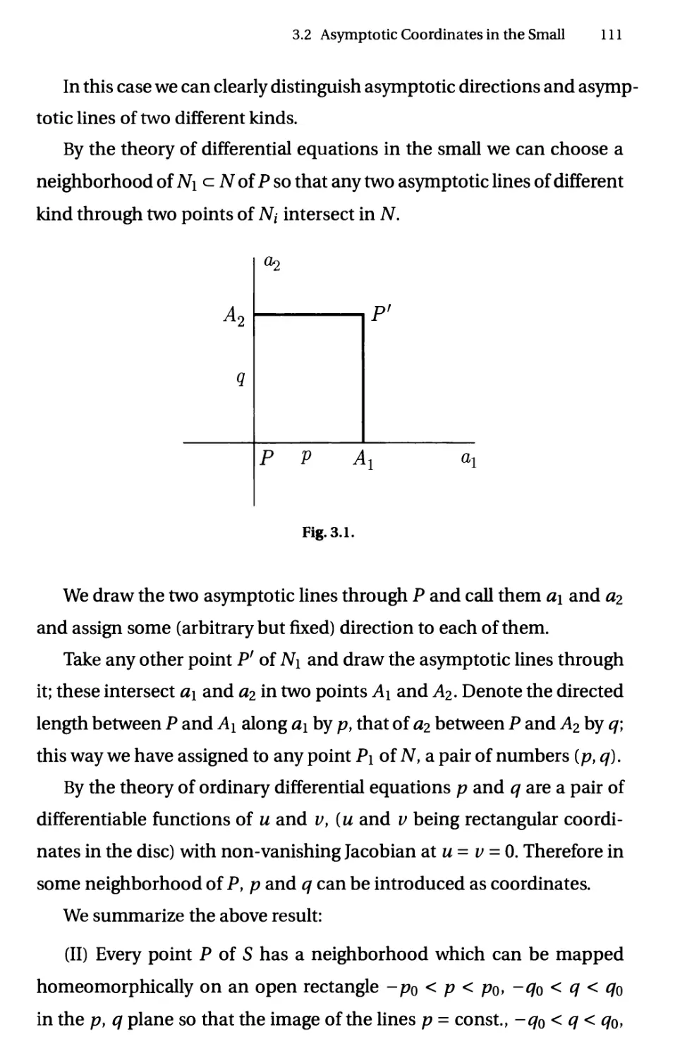
/


Автор: Nirenberg L.
Теги: mathematics differential geometry differential equations
ISBN: 978-7-04-050302-9
Год: 2018

Текст
CTM7
Louis Nirenberg
Lectures on Differential Equations
and Differential Geometry
тяшттш®
■^88^
HIGHER EDUCATION PRESS
Lectures on Differential Equations and Differential Geometry by Louis Nirenberg.
first published 2018 by Higher Education Press
Copyright © 2018 by Higher Education Press
4 Dewai Dajie, Beijing 100120, P.R. China
All rights reserved. No part of this book may be reproduced or transmitted in any
form or by any means, electronic or mechanical, including photocopying, recording
or by any information storage and retrieval system, without permission in writing
from the Publisher.
Cataloging in Publication Data
ffl#«№SSB (стр)ЯЖ
Ш6^^ТШ^Ш6^1ЬЩ = Lectures on Differential
Equations and Differential Geometry: $£3t/ (ЙП)
%Ш ' /ШШ(Ьош8 Nirenberg) Щ. - Ш:
S^ttWajJKtt, 2018.9
ISBN 978-7-04-050302-9
i. ф «■■■ п. ф i&- ш. ф тяш-ш®т/л
ЛЩ-^Х® IV. ® 0175© 0186.1
^тштшаршт^ (2ощ ш i68049 ч
Copy Editor: Liping Wang
Cover Design: Zhi Zhang
Print Editor: Yimin Zhao
787mmx 1092mm 1/16
11.75 Printed Sheets
Printed and Bound in P.R. China by Beijing Shengtong Printing Co., Ltd.
ISBN: 978-7-04-050302-9
1 2018
Classical Topics in Mathematics
Mathematics is the queen of sciences. She is pure, noble and attractive, and also
has a distinct character in comparison with subjects in sciences such as physics: its
permanent relevance and eternal validness of its theories and theorems. Whatever
was once proved will stay true forever.
Mathematics is a vast subject, and many new concepts, theories and results
spring up like mushrooms after spring rain. Similarly, there is also a large number
of new mathematics books appearing in libraries and on bookshelves. Probably
due to the usefulness of mathematics and its foundational nature, there seems to
be more books in mathematics than in other subjects. On the other hand, only a
limited number, or even a few, of them stand out and are appreciated and used
by many people. The best test on the quality of books is the test of time.
In this series of books Classical Topics in Mathematics, we have selected books
written by leading experts on topics which are well-tested by time. We believe
that in spite of the passage of time, their power and value have not diminished,
and hence they bear the trademark of the classical mathematics.
The first volumes of this series consist of an annotated version of Klein's
masterpiece Lectures on the icosahedron and the solution of equations of the fifth
degree, and the first English translation of Klein and Pricke's four big volumes on
modular functions and automorphic functions. For this series, we have tried to
pick books which share or reflect Klein's vision of the grand unity of mathematics.
The publication of this series of books is consistent with the motto of the
Higher Education Press: to provide high quality books on the essential
mathematics to the world mathematics community at an affordable price.
Classical Topics in Mathematics
(Series Editor: Lizhen Ji)
1. Lectures on the Theory of Elliptic Modular Functions, First Volume
Felix Klein, Robert Fricke (Authors), Arthur M. DuPre (Translator)
2. Lectures on the Theory of Elliptic Modular Functions, Second Volume
Felix Klein, Robert Fricke (Authors), Arthur M. DuPre (Translator)
3. Lectures on the Theory of Automorphic Functions, First Volume
Robert Fricke, Felix Klein (Authors), Arthur M. DuPre (Translator)
4. Lectures on the Theory of Automorphic Functions, Second Volume
Robert Fricke, Felix Klein (Authors), Arthur M. DuPre (Translator)
5. Lectures on the Icosahedron and the Solution of Equations of the Fifth Degree
(With a New Introduction and Commentary)
Felix Klein
6. The Bochner Technique in Differential Geometry
Hung-Hsi Wu
7. Lectures on Differential Equations and Differential Geometry
Louis Nirenberg
8. Notes on Jacquet-Langlands' Theory
Roger Godement
9. Kuga Varieties: Fiber Varieties over a Symmetric Space
Whose Fibers Are Abelian Varieties
Michio Kuga
Preface
There are long books and short books. It is hard to say which kind is more
valuable, or which kind one should read. When a short book contains all
essential things of a subject and arranges them in a clear and accessible
way, a short book is probably more preferable for some obvious reasons.
Additionally, if it is written by a leading expert on the subjects and a
master expositor, then the answer is a definite and clear yes.
The booklet "Existence Theorems in Partial Differential Equations" is
of this type. It was written by the world top expert on partial differential
equations, Louis Nirenberg, at one of the peaks of his long and
productive life. It covers existence and uniqueness of solutions of elliptic
differential equations. When one opens this booklet or rather lecture notes,
one can immediately see the flow of thoughts of a great mathematician: it
is direct to the point, everything moves smoothly and quickly, and there
is no unnecessary discussions or digressions. Elliptic differential
equations are central in partial differential equations and their applications
in differential geometry. Though many results have been obtained in the
past half century, the essential things are still the same. Furthermore,
though there have been many books on differential equations, the
freshness and the spirit of these lecture notes cannot be surpassed by later
more comprehensive ones.
vi Preface
Besides being a great analyst, Prof. Nirenberg is also a greater
differential geometer. Many beginning mathematics students have some
familiarity with the geometry of surfaces in the Euclidean space R3 and
may wonder what one wants know about surfaces besides the standard
topics in textbooks. But the global differential geometry of surfaces,
especially various rigidity results of convex surfaces, is highly nontrivial and
interesting. To be convinced by this claim, the quickest route is to open
the lecture notes tided "Seminar on Differential Geometry in the Large"
written by Prof. Nirenberg. Many topics there will be new and surprising
to many students, even to some experts in differential geometry. One
reason is that they are not in most standard books on differential geometry,
especially books on surfaces. Both the selection of topics and the
exposition are superb. Like the previous booklet on elliptic differential
equations, these seminar notes on differential geometry of surfaces are always
to the point, and they are also short when one thinks of the amount of
information contained in them. The detailed discussion of the case of
surfaces motivated the later analogues in the higher dimensions.
Therefore, in view of the above reasons, it makes perfect sense to
formally publish these classical lecture notes and make them available to
the mathematics community in the world. Given the importance of the
topics in this book and their classical nature, it fits particular well with
the philosophy behind the book series "Classical Topics in Mathematics".
This book will be a very valuable introduction to the topics under
discussion and complements well many existing books on partial
differential equations and differential geometry. We believe that hope that both
beginners and experts will welcome it and appreciate it.
Shiu-Yuen Cheng
Lizhen Ji
August 2016
Contents
Part I Existence Theorems in Partial Differential Equations
1 Preliminaries 3
1.1 Introduction 3
1.2 The Maximum Principle 8
1.3 Consequences of the Maximum Principle 12
2 The Potential Equation 17
2.1 Fundamental Solution 17
2.2 The Poisson Integral Formula 21
2.3 The Mean Value Property of Potential Functions 25
2.4 Estimates of Derivatives of Harmonic Functions and
Analyticity 26
2.5 The Theorems and Inequality of Harnack 29
2.6 Theorem on Removable Singularities 31
3 The Perron Method for Solving the Dirichlet Problem 33
3.1 The Perron Method 33
3.2 The Perron Method for More General Elliptic Equations .. 40
4 Schauder Estimates 43
4.1 Poisson's Equation 43
viii Contents
4.2 A Preliminary Estimate 48
4.3 Statement of Schauder's Estimates 50
4.4 Some Applications of the Interior Estimates 55
4.5 The Boundary Value Problem 63
4.6 Strong Barrier Functions, and the Boundary Value Problem 69
5 Derivation of the Schauder Estimates 75
5.1 A Preliminary Estimate 77
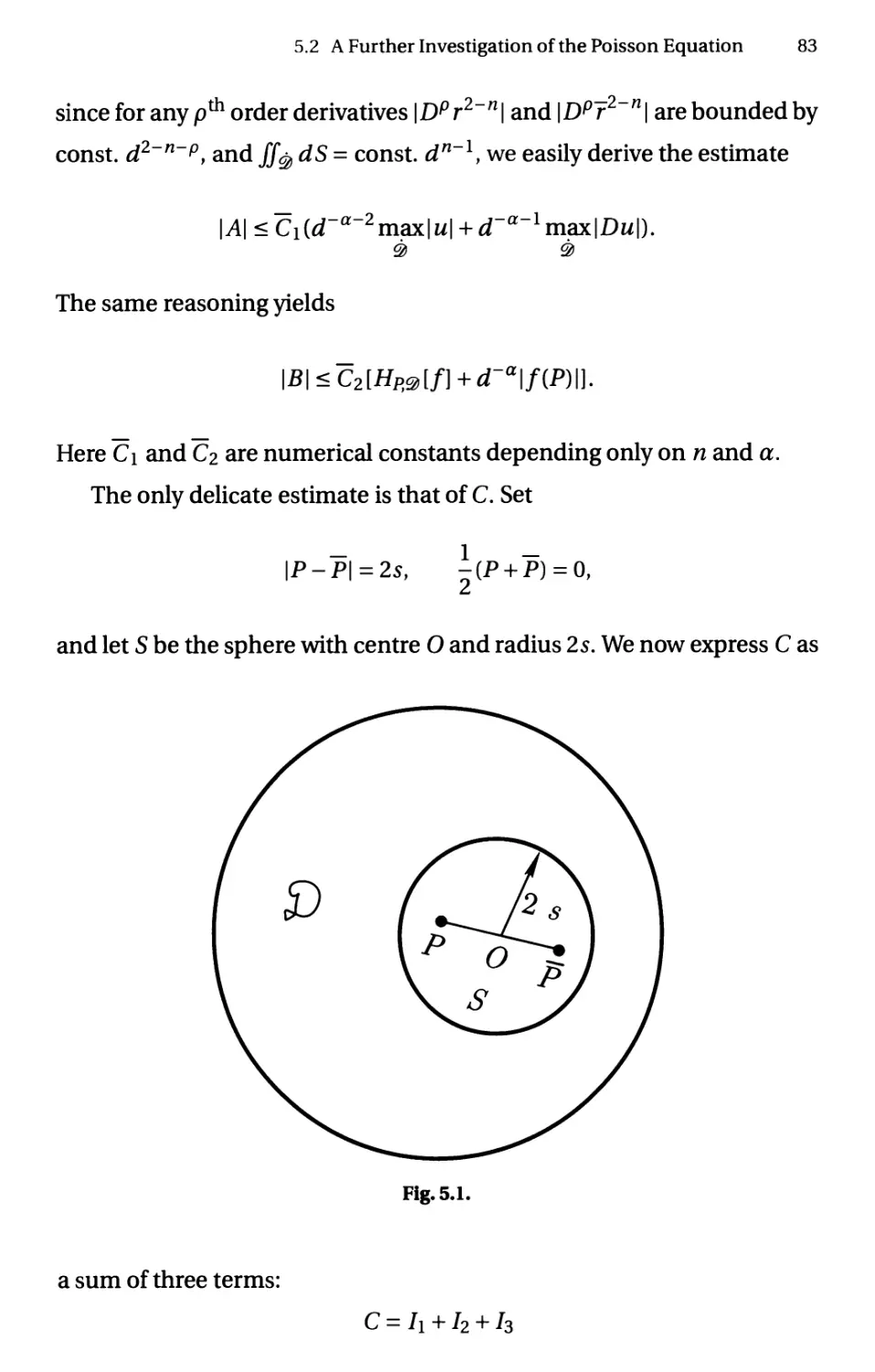
5.2 A Further Investigation of the Poisson Equation 81
5.3 Completion of the Interior Estimates 86
Part II Seminar on Differential Geometry
in the Large
1 Complete Surfaces 93
2 The Form of Complete Surfaces of Positive Gauss Curvature
in Three-dimensional Space 103
2.1 Hadamard's Principle 103
2.2 Completeness of a Surface 103
2.3 Examples Showing that the Properties V, V' and E are
Independent 104
2.4 Main Theorem 105
2.5 Consequence 105
2.6 Analogous Theorems for Plane Curves 106
2.7 Proof of Theorem 2.1 107
3 On Surfaces with Constant Negative Gauss Curvature 109
3.1 Hilbert's Theorem on Hyperbolic Surfaces 109
3.2 Asymptotic Coordinates in the Small 110
3.3 Considerations in the Large 115
3.4 Bounds on the Extended Angle Function 118
Contents ix
4 Isometric Deformations in the Small 123
5 Rigidity of Closed Convex Surfaces 133
6 Rigid Open Convex Surfaces 137
7 Rigidity of Sphere 143
8 Uniqueness of Closed Convex Surfaces with Prescribed Line
Element 147
9 A Theorem of Christoffel on Closed Surfaces 155
10 Minkowski's Problem 165
11 Existence of a Closed Convex Surface Solving Minkowski's
Problem 171
Parti Existence Theorems in
Partial Differential Equations
1
Preliminaries
1.1 Introduction
This course is concerned mainly with existence problems for partial
differential equation, i.e. with the problem of showing the existence and
uniqueness of solutions of such equations, which satisfy prescribed
boundary or initial conditions. Most of the time will be spent on elliptic
equations1; in particular, we shall study in great detail the second order elliptic
equation for a single unknown u(x\f • • •, xn):
" d2u " du
Q1Y Jdxtdxj £i dxt
Here the coefficients a\ \,...,/ are given real functions of (jci ,..., jc„) ; and
the ellipticity of the equation is expressed by the fact that the quadratic
form
Y, aijtitj (f ъ • • •»f л arbitrary real numbers)
is positive definite at every point.
We wish to define ellipticity for the most general systems of N
equations for N functions Mi,..., un of variables jci, ..., xn.
Only the material on elliptic equations will appear in these notes.
4 1 Preliminaries
dkuj
Fi{xi,...,xnfui,...fuN,...,—г tt,...) = 0, (1.1)
дх*---дх*п
i,j = lf...fN;l^ki + --- + kn^ rij.
For each function Uj there is a highest order rij derivative of it which
appears in the system. Consider first a system which (i.e. each F/) is linear
in the highest order derivative
Д ^ k k dnJuj I dkuj \
L L ai)—k ~ir+Fi\xl>...,xn>ul,...,uN>— i—r- = 0,
ytife+.-.^n; ; a**1-a**" I dx\l...dx*»)
(1.2)
i = 1,...,JV,
where the a*V"kn are functions of xi,...fxn alone and where the F/
involve derivatives of the uj only up to order rij-I. (Such a system is called
semilinear.) Let S be a sufficiently smooth (л - 1)-dimensional surface
through a point P in the (jq,..., jc„) space. We introduce the notion: S is
"free" or "non-characteristic" at P with respect to the semilinear system
(1.2). Suppose that the values of the functions uj and of their derivatives
up to order rij -1 are known on S in a neighborhood of P. S is said to be
"free" at P if, assuming that the functions Uj satisfy the semilinear system
at P, we may always calculate the луЛ order derivatives of Uj at P.
We may easily express this property of S at P in terms of a
condition on the coefficients a.)"' \ We note first that the и/А derivatives
of Uj obtained by differentiating those of order rij - 1 in directions
tangent to the surface are easily calculated; it remains only to calculate the
derivatives in the normal direction. This may be expressed as follows: Let
Zi (jcb..., xn) • • • £ л (*ъ. •., xn) be new coordinates in the neighborhood of
P such that the surface f i = 0 is simply S and such that the Jacobian
I |jk | Ф 0 in a neighborhood of P (such coordinates are easily introduced).
1.1 Introduction 5
On S we therefore know the derivatives of Uj up to order rij - 1 with
respect to the £jt; and by differentiation with respect to £2, • •., f я we can
calculate all the n /th order derivatives except for —wf- In order to calculate
these we must employ the equations (1.2). Applying the transformation
of coordinates we have, at P,
дп'Щ
axf'-dx*" д{"] \dxi
dxn
d^k°
+ •
where the remaining terms are expressed in terms of derivatives of the
Uj which have already been calculated. Inserting into (1.2) we have
N
L L *tJ
j=lki+--+kn=nj
k^k^Ujtd^
*i
»' [dxiJ '"{dxj
kn
= 0, {i = l,...,N)
where the neglected terms maybe calculated at P. In order that it be
possible to solve these equations for —wf- it is necessary and sufficient that
the determinant of order N
a
ki+-+kn=nj
ki...kn
4
dx\
Ь
dxn
kn
be different from zero at P. In the transformation of coordinates above,
since £i = 0 is the surface S, ^,..., g|*- at P are proportional to the
direction cosines ct\,..., an of the normal to S at P. Thus, the condition that S
be "free" at P is simply that the determinant
ki...knki
ki+---+kn=rij
aij
a
..a
kn
7*0
where a\,..., an are the direction cosines of the normal to S at P.
This determinant is called the characteristic determinant and the
equation, in parameters ct\,..., an, resulting from setting it equal to zero
6 1 Preliminaries
is called the characteristic equation of the system (1.2). If the
characteristic equation is satisfied by the normal (a\,..., an) to S at P, S is said to
be characteristic at P. S is said to be a characteristic surface if it is
characteristic at every point on it.
Ellipticity. The system of equations (1.2) is said to be elliptic at P (and
simply elliptic if elliptic at every point) if the characteristic equation
has no real solution {ct\,..., an) other than (0,..., 0), i.e., if every surface
through P is "free" at P.
For semilinear systems the property of ellipticity is simply a property
к к
of the coefficients a.1."' n. (Note that this definition of ellipticity agrees
with the one given earlier for the single second order equation.) For the
general nonlinear system (1.1) the notion of ellipticity depends on the
particular solutions Uj and their derivatives that are inserted into the
arguments of the F(. The characteristic equation is defined, in analogy, as
det
ki+-+kn=nj д{—л—V)
dFi Jti к
— a1 a n
dnJuj *1 "an
= 0.
A surface S is called characteristic at P (or simply characteristic, if it is so
for all points on it) for (1.1) and/or a given system of functions щ,..., u^ if
the normal {a\,..., an) to S at P satisfies the characteristic equation with
Mi,..., un and their derivatives inserted in the arguments of the Ft. The
nonlinear system is called elliptic with respect to a given system of
functions Mi,..., un if at every point the corresponding characteristic
equation has as the only solution (ct\,..., an) = (0,..., 0).
Throughout this course in proving the existence and uniqueness of
solutions of the equation we shall stress the use of a priori estimates for
these solutions. Thus much of the material is concerned with the
derivation of such estimates. Then a priori estimates assert that if a function
LI Introduction 7
is a solution of the given problem, then it is, with some of its derivatives
(or possibly square integrals of such derivatives) bounded by constants
which depend only on the given equation and the given boundary data
— but are otherwise independent of the particular solution itself. The
derivation of such estimates need not, in general, make use of explicit
representations of the solutions.
When not explicidy stipulated, all functions are assumed defined in
a bounded domain (open connected set) 0 in the n-dimensional space
(jci,...,jcw). The boundary and closure of @ are denoted by @ and @
respectively. We shall denote partial differentiation by subscripts, e.g.
fa.QX. - utj or uXiXj\ and shall use the summation convention over
repeated indices. Thus the general linear second order equation for a
function и will have the form
atjUtj + щщ + au = f (1.3)
where the coefficients atj, щ, a, f are functions of {x\}...}xn) (here the
subscripts on the coefficients atj, щ do not denote differentiation).
Our first large program is to study the boundary value problem, or
Dirichlet problem, for linear elliptic equation of the form (1.3). This is the
problem of finding a solution which takes on given boundary values on
@. If one wishes to attack nonlinear equations it is essential to have very
sharp results for linear ones. For this reason we shall present the theory
of J. Schauder2 for linear equations (1.3), which makes few assumptions
regarding the coefficients of the equations. Further on we shall present
another approach to these equations which extends also to equations of
2 J. Schauder (a) Ober lineare elliptische Differentialgleichungen zweiter Ordnung,
Math. Zeits. Vol. 38, No. 2, 1934, pp. 257-282. (b) Numerische Abschatzungen in el-
liptischen linearen Differentialgleichungen; Studia Math., Vol. 5, 1934, pp. 34-42.
8 1 Preliminaries
higher order and to elliptic systems which has been worked out recently
by M. I. Vishik, L. C&rding, F. E. Browder and К. О. Friedrichs3.
In Chapter 2 we begin the discussion of such equations by studying
the simplest — the Laplace equation. In the remainder of this chapter we
consider the uniqueness question for the B.V problem for elliptic
equations (1.3) and derive the first a priori estimates. The uniqueness and
estimates are consequences of the important maximum principle for elliptic
equations of the second order.
1.2 The Maximum Principle
Consider the second order differential operator in (1.3)
L[u] = atjUij + ciiUi + au
which is assumed to be elliptic (i.e., я/у£/£у is positive definite at every
point in @). We may write it in the form
L[u] = M[u] + au.
The assertion that the solution of the B.V problem for (1.3) is unique is
equivalent to the assertion that the only solution of L[u] - 0 which
vanishes on 0 is identically zero. If no restriction is placed on the coefficient
3 M. I. Vishik: (a) The method of orthogonal and direct decomposition in the theory of
elliptic RD.E. Mat. Sbornik, N.S. 25,1949, pp. 189-234. (b) On strongly elliptic systems
of D.E. Mat. Sbornik, 2 (1951), pp. 615-676.
L. Girding: Dirichlet's problem for linear elliptic P.D.E., Math. Scand. 1, 1953, pp. 55-
72.
E E. Browder: Strongly elliptic systems of D.E. in Annals of Studies, No. 33, Princeton
Univ. Press and 4 notes in the Proc. of Mat'l Acad, of Sci. (i) Vol. 38, No. 3, 1952, pp.
230-235, (ii) Vol. 38, No. 8,1952, pp. 741-747, (iii) and (iv) Vol. 39, No. 3, 1953, pp. 179-
184 and 185-190.
K. O. Friedrichs: On the differentiability of the solutions of linear elliptic RD.E. Comm.
on Pure and Appl. Math., Vol. 6,1953, pp. 299-325.
1.2 The Maximum Principle 9
a, this assertion is, in general, not true. (For example, и = cos x cos у is
such a solution of the equation uxx + uyy + 2w = 0 in \x\, \y\ < f.) If,
however, we restrict ourselves to operators with a < 0 then the assertion is
true. In the proof we shall assume that the coefficients of L are
continuous in Qf and that the function и is twice continuously differentiable in
@ and is continuous in @.
Maximum Principle4: If и satisfies M[u] > 0 a/irf /ш$ а/2 interior
maximum point in @> then и = constant.
It follows that the maximum of any function satisfying M[u] > 0 is
assumed on the boundary Qf (this is sometimes called the weak form of
the maximum principle.) Clearly an analogous minimum principle may
be formulated.
The uniqueness of the solution of (1.3) with a < 0 follows immediately
from the
Corollary 1.1. If и satisfies L[u] > 0 in 0 {a < 0) and u<0on2> then u<0
inQ).
The proof is simple: Suppose that и was positive somewhere so that
и has an interior positive maximum point P. By continuity, и > 0 in some
neighborhood of P; but there M[u]>-au> 0, since a < 0. By the
maximum principle it follows that и = const, in this neighborhood. Thus the
set of maximum points in @ is open. On the other hand, by continuity of
u, the set is closed in @> (i.e. a limit point in 0 of maximum points и is a
maximum point), and is therefore all of @; so by continuity и = positive
4 Our formulation of the maximum principle is due to E. Hopf, Elemenare Bemerkun-
gen uber die Losungen partieller Differentialgleichungen zweiter Ordnung vom el-
liptischen Typus, Sitzungsberichte. Berlin Akad. Wiss. Vol. 19 (1927), pp. 147-152. A
modification of his proof is presented here.
10 1 Preliminaries
const, in 0 — in contradiction to our original assumption that w<0on
Before proving the maximum principle, we observe that M[v] <0 at
an interior maximum point P of any sufficiently differentiable function
v. For at P the first derivatives of v vanish, and the matrix of second
derivatives (i/,-y) is that of a non-positive quadratic form. The value of
M[v] at P then equals atjVij, the trace of the product of matrices (a;;),
[Vij)9 which we may take as symmetric. Since the trace is invariant under
orthogonal transformations we may use such a transformation to reduce
the positive definite matrix (a,-y) to diagonal form (p,-), with p,- > 0. With
[Vij) transformed thereby to (1/,-y) the trace equals L/P/T^/. But (vtj)
is also the matrix of a non-positive quadratic form; hence Т)ц < 0, and
M[i/]< Oat P.
The proof of the maximum principle is based on the following
Lemma 1.2. 5 Let S be an open sphere, and Po a point on its boundary.
Assume that the coefficients ofM[ u] are bounded in S and that there exists
a positive constant m such that
aijtitjZmY,** (1.4)
holds throughout S for all real (ft,..., f „). Assume that и is continuous in
S + Po and is twice continuously differentiable in S, that M[u] > 0 in S,
and that и < u(Pq) in S. Then the exterior normal derivative ^ at Po,
understood as the Urn. inf. of^, is positive.
Proof. Let Si be a smaller sphere internally tangent to S at Po. Clearly the
only maximum point of и in Si (the closure of Si) is at Po. Choose the
center of Si as the origin and set r = (£ jc?)1/2. Denote by Sr the
intersection of Si with a fixed closed sphere S2 having P0 as center and radius less
5 E. Hopf: A remark on linear elliptic differential equations of 2nd order. Proc. A.M.S.,
Vol.3,1952, pp. 791-793.
1.2 The Maximum Principle 11
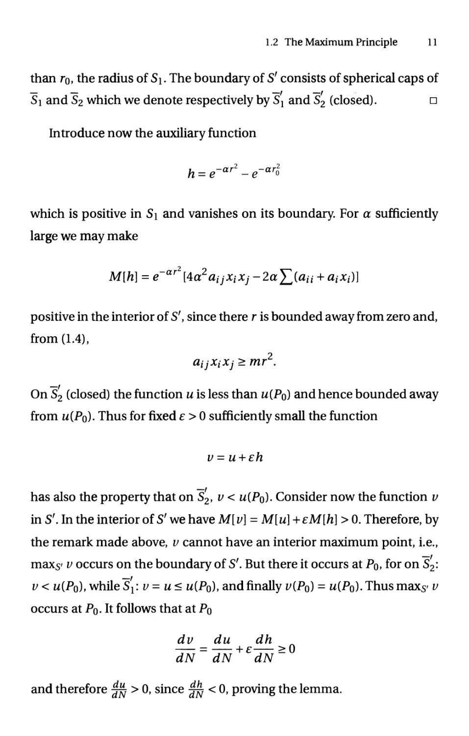
than ro, the radius of Si. The boundary of S' consists of spherical caps of
Si and S2 which we denote respectively by S2 and S2 (closed). □
Introduce now the auxiliary function
h = e-ar2-e~ar2o
which is positive in Si and vanishes on its boundary. For a sufficiently
large we may make
M[h] = e~ar [4a2aijXiXj-2aY,(an + aiXi)\
positive in the interior of S', since there r is bounded away from zero and,
from (1.4),
ciijXiXj >mr2.
On S2 (closed) the function и is less than u{Pq) and hence bounded away
from u(Po). Thus for fixed e > 0 sufficiently small the function
v-u+eh
has also the property that on S2, v < u{Po). Consider now the function и
in S'. In the interior of S' we have M[ v] = M[u]+ eM[h] > 0. Therefore, by
the remark made above, v cannot have an interior maximum point, i.e.,
maxy v occurs on the boundary of S'. But there it occurs at Po, for on S2:
v< u{Pq), whileSl:u=u< и{Р0),andfinally v{P0) = u{P0).Thusmaxs' v
occurs at Po. It follows that at Po
dv du dh
= +e >0
dN dN dN
and therefore ^ > 0, since ^ < 0, proving the lemma.
12 1 Preliminaries
The maximum principle now follows easily. Let и satisfy M[u] > 0 in
@. If и Ф const, and has an interior maximum then it is easy to find a
closed sphere lying in 0 having a maximum point of и on its
boundary but none in its interior. By the lemma we have ^ > 0 at this point,
contradicting the fact that the first derivatives of и vanish at an interior
maximum point.
1.3 Consequences of the Maximum Principle
In this section we consider only operators L [ u] with я < О unless otherwise
stated.
(a) We have already proved uniqueness for the B.V. problem of (1.3).
The maximum principle yields also a bound on the solution. Let и be
a solution which is continuous in 0 and equals 0, the given boundary
values, on @. Assume the coefficients of (1.3) are bounded in absolute
value
\atjl |a,-|, \a\<K, (1.5)
and that the equation is uniformly elliptic in 0, i.e. there exists a positive
constant m such that
aijZiZj>mY,Z2i (1.6)
throughout ®.
We assert that if g is a function satisfying the condition
-L[g] > max[/L g ^ max|0| on @,
then
M<g.
In order to prove this, it suffices to show that v = и - g is non-positive.
This follows from the Corollary to the maximum principle, since v satis-
1.3 Consequences of the Maximum Principle 13
fies the conditions
L[v]=L[u]-L[g]=f-L[g]>0,
v = (p- g<0 on @.
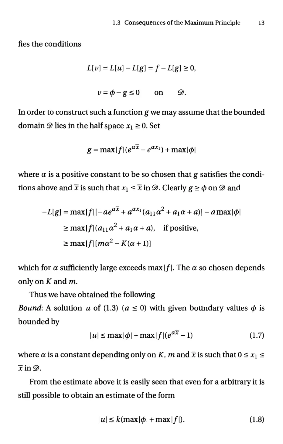
In order to construct such a function g we may assume that the bounded
domain @ lies in the half space jci > 0. Set
g = max |/| (ea* - eaXl) + max|0|
where a is a positive constant to be so chosen that g satisfies the
conditions above and ~x is such that x\ < ~x in ®. Clearly g > ф on ® and
-L[g] = max|/| [-aea* + aaXl (an a2 + a\a + a)]- amax|0|
> тах|/|(аца2 + а\а + a), if positive,
> max|/| [ma2 - K{a + 1)]
which for a sufficiendy large exceeds max|/|. The a so chosen depends
only on К and m.
Thus we have obtained the following
Bound: A solution и of (1.3) {a < 0) with given boundary values ф is
bounded by
|м|<тах|0| + тах|/|(ва*-1) (1.7)
where a is a constant depending only on K, m and x is such that 0 < jci <
jcin®.
From the estimate above it is easily seen that even for a arbitrary it is
still possible to obtain an estimate of the form
\u\ < fc(max|0| +max|/|).
(1.8)
14 1 Preliminaries
Provided the domain @ is sufficiently narrow in, say, the x\ direction; to
be precise, provided
maxa{ecx-l) < 1.
(The constant к then depends on K, m, max a and ~x.) For in this case we
write the equation as
M[u] + a~u = {a~ -a)u + f = f
where a~ = min(a, 0). Applying the estimate (1.7) to this equation we find
max|u| < max|0| + max|/|[eax -1)
< max|0| + {eax - l)(max|/| +max|w| maxa)
or
max |0| + max |/| {eax -1)
max|i/| < I ^-= .
1 -таха- (eax -1)
Note that (1.8) implies the uniqueness of the solution.
(b) The Neumann Problem: With the aid of the maximum principle
and the lemma which is used in its proof we may also show the
uniqueness of a solution for the second boundary problem, or Neumann
Problem. (We restrict ourselves here to the operator M[u] but the argument
given are easily extended to the more general operator L[u] with a < 0.)
This may best be formulated as follows. Given a continuous function ф
defined on the boundary @ which is assumed to possess a normal
direction at every point. It is required to find a solution и of M[u] = 0 such
that и and its first derivatives are continuous in @ and such that, on @,
the exterior normal derivative ^ equals ф within an additive constant
du
dN Y
finally и is required to have some fixed value at some fixed point P.
1.3 Consequences of the Maximum Principle 15
In order to prove uniqueness we assume that the coefficients of M
satisfy conditions (1.5) and (1.6) throughout @, and that @f is such that to
every point Po of @ we may find an open sphere S lying entirely in 0 and
having P0 °n its boundary.
By the maximum principle any solution и of M[u] = 0 achieves its
maximum and minimum at points on the boundary @. By the
requirement made above concerning the boundary, and by application of the
maximum principle and the lemma, it follows that ^ is respectively
positive and negative at these points if и is not identically constant. We
may therefore conclude that if и is a solution of M[u] = 0 which vanishes
at a point P and satisfies ^jjy = const, con®, then с = 0 and и = 0. But
this is just the uniqueness statement for the Neumann problem. (Note
that the constant с in the formulation of the problem is also uniquely
determined.)
It is worthwhile to remark that this uniqueness proof is valid even if
the equation ceases to be elliptic on the boundary (i.e. if (1.6) does not
hold) provided that the coefficients atj are continuous up to the
boundary and that the boundary is nowhere characteristic (see §1). This is so
because the proof of the lemma goes through provided that the
boundary of S is not characteristic at Po; for all that is required of the matrix atj
in the proof is that the quadratic form atjXtXj be bounded away from
zero near P0, which is equivalent to the non-characteristic requirement.
Thus, for example, any solution (for у > 0) of the equation
yuxx + uyy = 0
(which is elliptic for у > 0 but not for у = 0) which has a maximum
for у > 0 on the x-axis has uy < 0 at the maximum point — for the x-
axis is non-characteristic. If the boundary is characteristic at Po the
conclusion of the lemma need not hold, as is easily seen by the example:
16 1 Preliminaries
и = -у2 sin х, 0 < x < л, у > О, which solves the equation 2uxx+y2 uyy - 0,
has a maximum on у - 0, but has also uy = 0 on у = 0.
(с) The maximum principle yields also the uniqueness of solutions of
the B.Y problem for certain nonlinear elliptic equations of second order.
F{xi,...,xn,z,zXl,...,zXnXn) = 0.
Assume that the equation is elliptic for all (jci ,..., xn) in 0 and all values
of the other arguments in F, i.e. the quadratic form
dF
dZXiXj
Mi
is positive definite for all such arguments in F. Assume further that
dF
7Г-0
dz
for all such arguments6. Then the solution of the B.V. problem is unique.
For if z and z are two solutions of the equation their difference w = z - ~z
satisfies the equation
FzXtXJwXiXj+FZxiwXi+Fzw = 0
where in general ф represents
ф= I ф(Xl)...)xnJz+(l-t)zJzXl + (l-t)zXl)...JzXnXn + (l-t)zXnXn)dt.
Jo
(This is obtained by subtracting the equation for z from that of z and
expressing the resulting left hand side as an integral.) This equation is
of the form (1.3) L[u] = 0 with a = Fz < 0, to which the arguments of §2
apply.
The conclusion holds under slightly weaker conditions.
2
The Potential Equation
We review some well-known properties of the potential, or Laplace,
equation
n
Au=Y,Uu = 0, (2.1)
/=i
a solution of which is assumed to be twice continuously differentiable in
a domain @.
2.1 Fundamental Solution
In the next chapter we shall solve the boundary value, or Dirichlet
problem, for bounded domains @. For @ a sphere the problem is solved in
this chapter. The solution is found by means of the "fundamental", or
"singular" solution of the equation. By a fundamental solution we mean
a function w{P, Q) of a pair of points P{x\,..., xn), Q{x[,. ..,xfn) which for
P Ф Q is harmonic in each set of variables (х\,...,хп), {х[,...,хгп), has
an appropriate singularity for P = Q, and has the property that for any
twice continuously differentiable function и which together with its first
derivatives is continuous in @, the identity
С \ ди dw] ГГ
u{P) = j\w'm~u'dN\dSQ~jj w(p>®AuWdvQ (2-2>
18 2 The Potential Equation
holds for P in @. Here the first integration is performed on the boundary
0 of @, dSQ representing element of surface area, and the second, with
d Vq as volume element, is extended over @; both are integrated with
respect to the Q variable. Since w has a singularity at Q = P the second
integral is singular and is to understood as the limits as e — 0 of the
integral extended over the intersection of @ and the exterior of a sphere of
radius e about P. We shall use a single integral sign to represent n - 1
dimensional surface integrals, and a double integral sign for n dimensional
volume integrals, with dV as volume element. The operator -^
represents differentiation (with respect to Q variables) along the direction of
the exterior normal to @. In writing this identity and in the remainder
of this section we work completely formally, assuming that the domain
@ has a sufficiently "smooth" boundary and that the functions involved
are sufficiendy "smooth" so that all equations are meaningful and the
arguments justifiable. In application we shall employ the singular solution
only in case ® is a sphere.
A particular singular solution is given by
for n = 2,
(2.3)
for n > 2.
Here r = \P-Q\ = л/LiUi - *j.)2 and П is the surface area of the n
dimensional unit sphere £ jc? < 1. A more general singular solution is given
by
w(P,Q)=v{P,Q) + h{.P,Q)
where h(P, Q) is harmonic in the P and Q variables separately for all P,
Q in @ and, for P fixed, is continuous together with its first derivatives
with respect to (jcj x'n) in 9). Since v{P, Q) is harmonic in P and Q sep-
v(P,Q) =
-logr,
Jl-n
{n-2)Q'
2.1 Fundamental Solution 19
arately, for P Ф Q, it follows once (2.2) is verified that w{P, Q) is a singular
solution. Let C£ be a closed sphere of radius e > 0 about P. An application
of Green's theorem on the domain @ - Q yields the identity
/jf [w(£Q)Az/(Q)-uAQw(£Q)]dVQ
Г ( du dw\ jo
Г I du dw\ JO Г I du dw\ Jo
-/ \wTrr~uTrr\ds" I \w^—u—-\dS.
h\ dN dN) Jc£{ dr dr)
Неге Р is held fixed and the integration is with respect to Q; in the last
integral r = \P-Q\. Since AQ w(P, Q) = 0 for Q Ф P we have
Г ( du dw\ f f
\w— -u— \dS- w(P,Q)Au(Q)
h\ dN dN) h-Ce
Г ( du dw\ Jo
4c\wTr-u-d7)ds
JcA dr dr)
where dQ. represents the element of solid angle. In the last integral wen~l
0 and en~l Zff- — - ^ for e -> 0. It follows that as e -> 0 the right hand side
tends to u(P). Hence the double integral on the left converges and we
have the desired identity (2.2).
In case и is harmonic the double integral in (2.2) vanishes and (2.2)
yields a representation of и in terms of its values and those of its normal
derivative on the boundary. If in addition it were possible to select h{P, Q)
in such a way that w(P,Q) = 0 for Q on Э, the function w(P,Q) is then
called the Green's function G{P, Q) corresponding to the Dirichlet problem
for © and (2.2) yields a representation for и in terms of its boundary
values alone
u(P) = -[m u—G(P,Q)dS. (2.4)
J® dN
20 2 The Potential Equation
If, as in the Dirichlet problem, we were given a function defined on the
boundary and seek a harmonic function u(P) which equals this function
on @ we would expect the function u{P) to be given by this boundary
integral. That the function u{P) so defined is harmonic in 0 follows
immediately from the harmonicity of G(P, Q) with respect to the P variable.
It would remain only to show that this function does take on the required
boundary values. In the next section we construct G(Pt Q) for the sphere
and solve the Dirichlet problem for given continuous boundary values.
Before carrying this out, a remark about the Neumann problem. This
is the problem of finding a harmonic function in @ which is continuous
and has continuous first derivatives in @ and such that |^ equals a
prescribed function / on @. It was shown in Chapter 1 for a second order
elliptic equation that the function / could only be prescribed within an
additive constant. For the Laplace equation this constant is easily
determined. Setting v = 1 in Green's identity
В™ы-*,муш1('ш-ыШ'и!
yields,
for any harmonic function u. Thus the additive constant с determined
by the condition that the mean value of (/ + c) on the boundary be zero.
For the Neumann problem there is a formula analogous to (2.4). We
require that h{P,Q) be so chosen that j^w{PtQ) = const, for Q and @.
The constant is determined by the condition f@ jftdS = -1, which
follows from (2.2) by setting и = 1. The resulting w(P,Q) = N(P,Q), which
is usually fixed by the requirement /^ N{P, Q)dS = 0 for all P, is called
a Green's function for the Neumann problem, or Neumann function. The
solution и if it exists is represented by
2.2 The Poisson Integral Formula 21
u{P)= [mN{P,Q)-£(Q)-dS + const.
J® oN
2.2 The Poisson Integral Formula
To solve the Dirichlet problem for the sphere S, we may, without loss of
generality assume the radius to be 1. A suitable stretching of coordinates
will then give a solution for any sphere. We will construct the Green's
function G(P,Q) for S.
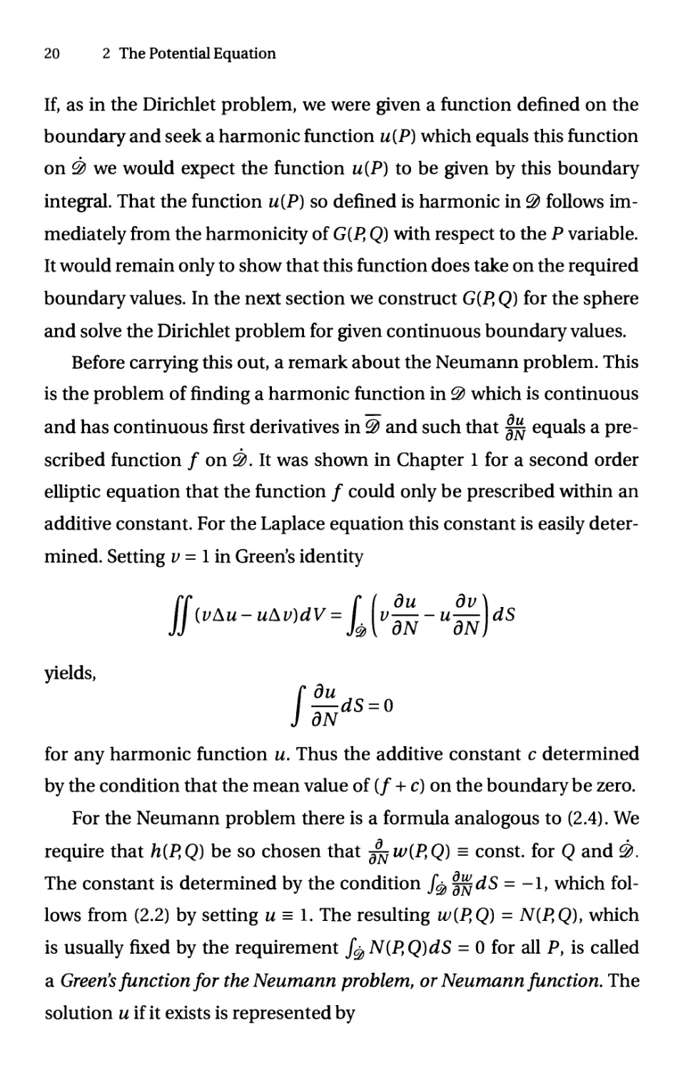
Fig. 2.1.
Let О be the center of S, P a point in S other than O, and Q any point in
S. Draw OP and let Pr be the point on OP (extended) such that ~OP'OPi =
1. We denote the lengths of PQ, OPt QPf by r, p, r\ respectively and the
angle POQ by 0. A simple geometrical argument shows that r = p r\ for Q
on the boundary of S. If we therefore set, forl n > 2,
1 For л = 2 set h{P,Q) = ^log(pn).
22 2 The Potential Equation
for P Ф 0 and h{P, Q) = П{„_2) for P = 0, we see that the function
G{P,Q) = v{P,Q) + h{P,Q)
is the Green's function. Evaluating the value of jfi on the boundary (we
omit the calculation) we obtain, from (2.4), the expression for a harmonic
function in terms of its boundary values /(Q).
:[ й
Js (p2 +1 -
П Js (p2 + l-2pcos0)"/2'
Thus is Poisson's integral formula. (The denominator in the integrand is
merely rn.) For spheres of arbitrary radius R this formula becomes
u{P)Jr2-p2U Щ№ (25')
nR Js(p2 + fi2-2fipcos0)"'2- ( ]
Thus any sufficiently regular solution of the Dirichlet problem for the
sphere, which equals /(Q) on the boundary is given by (2.5) or (2.5').
Next we wish to show that u{P) as defined by (2.5) is the solution of
the Dirichlet problem with given continuous boundary values.
Theorem 2.1. Let f bea continuous function defined over the surface of
the unit sphere S. Then the function u(P) given by (2.5) /5 a harmonic
function in S which may be extended as a continuous function in S equal
to f on the boundary.
Proof For P in the interior of S we may differentiate the integral (2.5)
under the integral sign with respect to the P variables. Since G(P,Q) is
harmonic in P for P ^ Q it follows u{P) has derivatives of all orders and
is harmonic in S.
To conclude the proof, it suffices to show that for Pq on S
2.2 The Poisson Integral Formula 23
lim u(P)=f{P0).
P^Po
PinS
Fig. 2.2.
To that effect, divide S into two spherical "caps" a\ (containing Po)
and a2 (the remainder of S) with cri so small that for Q on G\ we have
l/(Q)-/(Po)l<*.
Next, we observe that
1 =
1-P2
Js(p2 + 1-
dS
П Js (p2 + l-2pcos0)"/2'
This is seen by setting и = 1 in (2.5). It follows that
(2.6)
24 2 The Potential Equation
1-P2 Г [f(Q)-f(Po)]dS
|M(P)-/(P0)I =
:Jt
<£
П Js (p2 + l-2p cos 0)"/2
1-p2 f dS
\L (P2 + l-
П Jai (p2 + l-2pcos0)"/2
Vf l/(Q)
n Л, (p2 +1 -
+ 1^г |/tQ»-/wi &
a2(p2 + l-2pCOS0)"/2
Since the integrand in the first integral is positive we may extend the
integration over all of S instead of o\ and obtain, in virtue of (2.6),
1-P2 Г 1Л«-/(Ро)1 ds
M-w.ifLjjg
a2 (p2 + l-2pCOS0)
nil
For P in a sufficiently small neighborhood of Po> the integrand of the
latter integral is bounded, by a constant independent of P, for the
denominator = rn is bounded away from zero. Now by making P sufficiently
close to Po we can make p as close to 1 as desired. Hence we can make the
second term of the inequality above less than e. Thus for P sufficiently
close to Po, we have
\u{P)-f{P0)\<2e.
□
The remainder of this chapter is concerned with some properties of
harmonic functions, all of which are consequences of Poissoris integral
formula. One basic property is that a harmonic function possesses
continuous derivatives of all orders. This follows from the fact that the Poisson
integral formula (2.5') may be differentiated any number of times under
the integral sign to yield expressions for the derivatives of и at P in terms
of the values of и on the boundary S of any sphere containing P in its
interior. Differentiating Laplace's equation we find that all derivatives of
harmonic functions are also harmonic.
2.3 The Mean Value Property of Potential Functions 25
2.3 The Mean Value Property of Potential Functions
Let и be a function continuous in a domain 0. Then if и satisfies
uip)=nk^!suiQ)ds (2-7)
(P is center of S) for every sphere S contained in 0, we say that и has the
first mean value property in @. If, и is continuous in @ and satisfies2
u(P)=^!iu(Q)dv as)
for every sphere S in 0, we say that и has the second mean value property
in®.
The first and second mean value properties are equivalent, for (2.7)
and (2.8) and may be rewritten in the form
Rn-lu(P) = ^-[u(Q)dS
and
Rn 1 Г Г
— w(P) = -// u(Q)dV.
n Q.JJs
Integrating the first of these with respect to R yields (2.8), while
differentiating the second with respect to R yields (2.7). We therefore speak of the
mean value property.
It is remarkable that the mean value property of a function is
equivalent to the property that it be harmonic. Before proving this fact we show
that the mean value property of a function и implies that the function
satisfies the strong maximum principle, i.e. that if и has a maximum in
a domain @ (connected open set) then it is identically constant. For if и
has its maximum at a point P it follows from (2.8) that и = и{Р) in every
2 ^ is the volume of S.
26 2 The Potential Equation
sphere S with center P lying in @. Thus the set of points where u- u{P)
is open in @. By continuity it is closed in @, and hence all of @.
A continuous function и in @ /s harmonic if and only if it has the mean
value property.
Proof If и is harmonic we obtain (2.7) for any sphere S in 0 by setting
P = 0 (the center of the sphere S) in (2.5'). Conversely suppose и has
the mean value property; it suffices to show that и is harmonic in every
sphere S in @. Let i/ be the harmonic function in S which equals и on S.
v exists by virtue of the results of the previous section. Then w = и- и
has the mean value property in S since both и and v do. Then w and - w
satisfy the maximum principle in S, and since w = 0 on S, w = 0 in S.
Thus и = v in S or и is harmonic in S. □
2.4 Estimates of Derivatives of Harmonic Functions and
Analyticity
In this section we shall derive some a priori estimates of the derivatives of
a harmonic function и in a certain domain @ in terms of the least upper
bound of |u\ in®.
Consider again the Poisson integral formula (2.5') for a sphere S of
radius R.
R2-P2 ff(Q)dS
u{P) =
[ f(Q)c
Js rn
QR
where
r2 = (p2 + R2 - 2/?ocos0) = \P- Q|2, p = \OP\.
Let D denote differentiation with respect to any one of the independent
variables (x\, X2,..., xn). Differentiating under the integral sign, we obtain
the estimate
\Du(0)\< z-^, (2.9)
К
2.4 Estimates of Derivatives of Harmonic Functions and Analyticity 27
where К is understood to be a constant depending only on n. We may
derive (2.9) in another manner, as follows. The derivative of a harmonic
function has been shown to be harmonic. ^ = щ is harmonic, and
therefore has the mean value property, so that for any sphere S about
O,
|и,(0)|<
using the divergence theorem,
l«H0)l<
Ш&щШУ<>
^TsISsumidSQ
where f,- is the ith direction cosine of the vector OQ. Hence
Area S
|м/(0)|< const———-max | м|
Vol S 5
or
|W;(0)|<-l.U.b.|w|.
XI
We now proceed to obtain estimates for higher derivatives. Dm и
analogous to (2.9), where Dmu shall denote any mth order partial derivative
of u.
Let и be harmonic in the sphere S (with radius R), and continuous in
S. For P in any concentric sphere So with radius Ro<R
Kmem~lm]
\Dmu(P)\<max\u\-———-, (2.10)
where К is the constant occurring in (2.9) which depends on n only.
Proof. We use induction. By (2.9) the assertion holds for m - 1. Assume it
true for m; we wish to prove it for m + 1. Let P be any point in the sphere
So- Let Si be a concentric sphere with radius R\ = (1 - 6)R + 0/?o where в
is a number between 0 and 1 to be chosen later. Since R\ - Rq - (1 -в) (R -
28 2 The Potential Equation
До) the sphere of radius (1 - 0)(R - До) about P lies in Si. Applying (2.9)
to the harmonic function Dm и we find
\Dm+lu(P)\ < — max|Dmw|.
(1-0)(R-Ro) s,
By induction hypothesis however we may assert that
Kmem~lm\ Kmem~lm\
max|Dmw| < :max|w| = -max|w|.
5, {R-Ri)m s em{R-R0)m s
Inserting into the previous inequality we find
|""'"("|*«зз5)=яТ|"|-г=(Г^-
If we can now select в so that (1_i0m <(m+l)ewe have the desired result.
It suffices to take 0 = -^т. Then
m+l
1 (m + l)m+1 J l\m
- = {m + l) 1 + — <{m + l)e.
a-6)0m mr>
"(1+s) s'
From our estimates (2.10) for its derivatives we may easily prove the
analyticity of a harmonic function uy by showing that it equals its
Taylor series expansion. By Taylor's theorem we have for x = [xi,...fxn)f
h = {hi,...,hn),
u(x + h) =
^iv!V dxi dxn)
[if. a . д \т 1
[mil a^i a*j 1Х+0Л
for some 0, 0 < в < 1; here it is to be understood that the brackets are
to be evaluated at the respective points x, x + Oh. To prove analyticity it
suffices to show that for |ft|2 = £ h2. sufficiently small the last term tends
2.5 The Theorems and Inequality of Harnack 29
to zero for m ■— oo. If 2d is less than the distance from x to the boundary
@, and |/г| < d} then it follows from (2.10) (for S a sphere with center x
and radius R = 2d = 2R0) that
1 If, д , <5 Г I Mm m^m^m_1m!
- Й1Т- + - + ЙД— u\ <—-иш — max|w|
m\\\ dxi dxn) \x+eh m\ dm $
(u Ken\m . .
< \h-——J max|w|
which tends to zero for ft < j^ — giving the desired result. □
2.5 The Theorems and Inequality of Harnack
Harnack's first theorem states that a uniform limit of harmonic functions
is harmonic. This follows from the fact that the limit function satisfies the
mean value property, and is therefore harmonic. It may also be proved by
means of the estimates for derivatives of §2.4. If и is the uniform limit of
harmonic functions un then in every closed sphere lying in the domain
the derivatives of the un also converge uniformly, as follows from (2.10)
applied to [un - um). Thus и has continuous derivatives there, and \Au\ =
\&{un - u)\ ■— 0 in the sphere, or, и is harmonic.
As a corollary we have: a uniformly bounded (in absolute value)
sequence of harmonic functions in a domain has a subsequence which
converge uniformly in every closed subdomain to a harmonic function. By
(2.9) the first derivatives of the functions in the sequence are uniformly
bounded — so that the functions are equicontinuous — in every closed
subdomain. By Arzela's theorem we may choose a subsequence which
converges uniformly in every closed subdomain to a function which, by
virtue of the Harnack theorem, is harmonic.
It is also obvious (by the maximum principle) that if the boundary
values of a sequence of harmonic functions (continuous in the closure of a
30 2 The Potential Equation
bounded domain) converge uniformly then so do the harmonic functions,
and also their derivatives in every closed subdomain.
Another useful result is
Harnack's Inequality: If и is harmonic and non-negative in a sphere
with center О and radius R then
I R \n~2R-p I R \n~2R + p
d -^и(ОКи(РК T^uiO) (2.11)
\R + p) R + p \R-p) R-p
for any point P with \0-P\ = p < R. To prove this we observe that the
Poisson integral kernel of (2.5'), given by
R2-p2 1
QR {R2-2pRcose + p2)n/2'
lies between
д2-р2 = i д-р and i д+р
QR{R + p)n nR(R + p)n~2 R + p nR(R-p)n~2 R-p'
Since и > 0 Harnack's inequality now follows from the Poisson integral
formula applied to the sphere (to be perfectly rigorous this should first
be carried out for a sphere of radius R-e with e then going to zero).
As a consequence of Harnack's inequality we have the theorem: a
harmonic function defined for all space and bounded from below is
identically constant By adding a constant we may assume that the function is
positive; the result then follows by letting R — oo in (2.11).
Harnack's inequality may be extended to arbitrary bounded domains
@ as follows: Let @ be a closed subdomain of @. Then there exist positive
constants c\y C2 such that if и is harmonic and non-negative in @ and О
and P are points in @ i, then
ciu{0)< u{P)<c2u(0).
2.6 Theorem on Removable Singularities 31
This may be proved by covering @i by a finite number of (open) spheres
Si, S2,..., Sv each bounded away from @, and such that S\ has О as center
and Sjc+i has center in S^. Applying Harnack's inequality, in turn, to each
sphere, we get the result.
We can now prove Harnack's second theorem: Let un be a monotone
increasing sequence of harmonic functions bounded from above at a
point О in @. Then in each closed subdomain of @, wn converges
uniformly to a function (which is harmonic). Clearly the bounded mono-
tonic sequence un{0) converges. Then by our last result, for any closed
subdomain,
c\{um+p{0) - um{0)) < um+p{P) - um{P) < c2{um+p{0) - um{0)).
The theorem then follows immediately.
2.6 Theorem on Removable Singularities
If и is harmonic in a neighborhood of О with О deleted, and if3u =
o(r2~n) where r denotes the distance from O, then и can be defined at О
to be continuous and harmonic there.
To see this let S be a closed sphere with center О lying in the given
neighborhood. Let v be the harmonic function which equals и on S,
and set w = v - u. We wish to show that w = 0 in S. Let S£ denote a
smaller concentric sphere with radius e and denote by Me the maximum
of I w\ on its boundary. On the boundary of the domain between the two
spheres we clearly have \w\<M£ j^, for w = 0 on the outer boundary. By
the maximum principle this must hold for every point P, with \0-P\ = r,
is that domain. But because of the regularity of v near О and because of
the assumption on и we have
3 Here n > 2; for n - 2 this should read и = o(log j).
32 2 The Potential Equation
M£ = o(e2-n).
Thus keeping P fixed and letting £-0we obtain the desired result.
3
The Perron Method for Solving the
Dirichlet Problem
3.1 The Perron Method
The Perron method though not very constructive enables one to solve
the boundary value problem for arbitrary prescribed continuous
boundary values in the wide class of domains. It uses the concept of subhar-
monic and superharmonic functions. These are extensions to higher
dimensions of convex and concave functions of one variable, just as
harmonic functions are considered generalizations of linear functions of
one variable. In §3.2 we show how the method can be extended to solve
the boundary value problem for a general equation with variable
coefficients.
Definition 3.1. A continuous function и in @ is called subharmonic
(superharmonic) if for every sphere С contained in @
U<Uc [U>Uc)
where uq denotes the harmonic function in С equal to и on C.
Defining Mclu] as the function equalling u'mG-C and uq in C, the above
inequalities become
u<Mc[u] {u>Mc[u\).
34 3 The Perron Method for Solving the Dirichlet Problem
As an illustration, we note that if Д v > 0 in @ then by the maximum
principle of Chapter 1 v is subharmonic.
We state some obvious properties of subharmonic and
superharmonic functions. First, и > 0 implies Mq[u] > 0; for the minimum of
uc occurs on C. Hence if и - v > 0 then Mc[u] - Mq[v\ = Mc[u - v] >
0. Any linear combination of subharmonic (superharmonic) functions
with non-negative constant coefficients is also subharmonic
(superharmonic). If и is subharmonic (superharmonic) then - и is superharmonic
(subharmonic).
Next some less obvious properties which we state only for
subharmonic functions; analogues hold for superharmonic functions.
1) If и is subharmonic and has a maximum point in 0 then и =
constant; hence, the maximum of any subharmonic function continuous in
0 occurs on 0.
Proof. Suppose v = Mq[u] where С is a sphere in @, with the maximum
point P as center. Since max^ и < u{P) < v{P) it follows that v has a
maximum in C. But v is harmonic in С so that by the maximum principle v =
const, in C. Hence u = u(P) on C. Since this holds for any sphere С ^Q)
the set of maximum points of и is open in @; by continuity it is closed in
@, hence it is all of 0. □
Note: 1) may be proved more directly by the mean value property of
harmonic functions. Our proof has the advantage that it extends to any
elliptic equation for which the maximum principle holds.
2) lfu\tU2,...,um are subharmonic, then so is u = max{u\,..., um).
Proof. If С is any sphere in 0, then, by a previous remark,
щ<Мс[щ]<Мс[и\}
so that
3.1 The Perron Method 35
u = maxui <Mc[u].
i
□
3) If и is subharmonic, then so is v - Mc[u], where С is any sphere in
Fig. 3.1.
Proof. Let us consider С as fixed and С be any sphere in @. We wish to
show that v = Mc [ u] < Mc [ v]. This is clearly the case if Cf => С or С' с С.
Now suppose С and C' intersect. At any point P in C' - С we have
i; = Mc[w] = w<Mc[w] < Mc'[i/],
since и < v. Finally in the domain CnC',v and Mc[ v] are harmonic, and
on the boundary we have v - Mc [ v] < 0 by the result obtained for points
in C' - С By the maximum principle the last inequality holds in С n C,
and the proof is complete. □
We proceed with the Perron method. From now on ф is a given
continuous function defined on @. Our aim is to find a function harmonic in
@, continuous in @, and equal to ф on @.
36 3 The Perron Method for Solving the Dirichlet Problem
A function v continuous in @ is called a subfunction (superfunction)
if it is subharmonic (superharmonic) in @ and satisfies v < ф {v > ф) on
@.
We note that subfunctions (superfunctions) actually exist; for min0
(max0) is such a function. Clearly properties 1), 2) and 3) (and their
analogues) hold for subfunctions (and superfunctions).
The following remark will serve to motivate our construction of the
solution to our problem. First of all, every subfunction v < any super-
function w. This follows from 1) applied to the function v-w which is
subharmonic, and non-positive on 0. Secondly, if и is a solution to our
boundary value problem (i.e. и is continuous in @, harmonic in @, and
equals ф on 0) then и is both a sub- and superfunction, and hence:
any subfunction v<u< any superfunction w.
This suggests a method for constructing u. Since all subfunctions are
uniformly bounded from above by max</>, we define the function и at any
point P in@ as the l.u.b. of the values of all subfunctions at P. We will
show that и defined in this manner solves our boundary value problem
(provided we put certain restrictions on @). We break up the proof into
the following three lemmas:
(i) и is continuous in 0.
(ii) и is harmonic in 0.
(iii) и is continuous at, and equals 0(Q), at those boundary points Q for
which there exists a "barrier function" wq.
Definition 3.2. For any Q in @, wq is said to be a barrier function if wq
is superharmonic in 0, continuous in @, and satisfies
wq > 0 in 0 and wq = 0 only at Q.
3.1 The Perron Method 37
Proof of (i). It suffices to show that и is continuous in the set @^ of points
whose distance to @ is > d, for any d > 0. For any given e > 0 and point P
in 0^ there is, by the construction of u, a subfunction v such that u{P) <
v{P)+e. Since vi = max{min0, v] is also a subfunction by property 2), we
have
u(P)< vi{P)+e.
If С denotes a sphere with center P and radius d, then by property 3)
we see that vz = Mc[v\] is also a subfunction; and u{P) < vziP) + £. The
function i/2 is harmonic in С and bounded:
min0 < v\ < i/2 < max0.
Thus in the sphere centered at P with radius d/2 there exists an upper
bound (not depending on P) for the first partial derivatives of 1/2 (see
§2.4) and consequently a positive 6 <\d (independent of P but
depending on e) such that
\vi{P)-V2{Q)\<e
for \Q - P\ < 6. Since 1/2 is a subfunction it follows that
u(Q) > 1/2(Q) > v2(P)-£> u(P)-2e.
Similarly, since 6 is independent of P, u{P) > u{Q) - 2e. Thus \u{P) -
u{Q)\ < 2e, where P, Q are less than 6 apart, u is thus continuous in @^,
hence in @. n
Proof of (ii). It suffices to show that и is harmonic in any sphere К such
that AT с @. For any г > 0, and P in AT there is a subfunction v such that
и(Р)-с <i/(P)<m(P).
38 3 The Perron Method for Solving the Dirichlet Problem
Since и (by (i)) and v are continuous, we have
u-e<v<u
in some sphere centered at P. We cover AT by a finite number of such
spheres, say with centers Pb...,Pm, corresponding to which we have
subfunctions v\,..., vm. The function
~u = max{vi,..., vm)
is, by 2) also a subfunction and satisfies
и-£<~й< и
throughout K. By 3), М^ПТ], which is harmonic in K, is also a
subfunction, and in К satisfies и - e < D < Mr:[77] < u. Thus и can be uniformly
approximated in К by harmonic functions. But then, by Harnack's
theorem, §2.5, и itself is harmonic in K> hence in Q). □
Proof of (Hi). From the continuity of the function ф and the properties of
wq{P) it follows that for any e > 0 there is a positive constant к such that
и(Р) = ф((1)-е-к1ио(Р)
is a subfunction, and
M/(P) = 0(Q)+£ + fcH/Q(P)
is a superfunction. Hence u{P) lies between them, so that
\u{P)-u{Q)\<e + kwQ{P)t
3.1 The Perron Method 39
which, for \P - Q\ sufficiently small, and by continuity of wq{P), is less
than 2e. This is the desired continuity of и in @.
To complete the discussion of the boundary value problem we
indicate some conditions on @ which ensure the existence of a barrier
function wq for each point Q in @: wq will exist provided there is a closed
sphere S such that S n @ = Q; we merely take the harmonic function
il 1
T^> ~ ~^> > for n> 2,
Rn-2 rn-2
log- , forn = 2.
where R is the radius of S and г denotes the distance of P to its center. It
satisfies the required conditions.
For n = 2 we can do better: it suffices that @ be a simple closed Jordan
curve. Let Q be on @, which we may assume lies within the unit circle
\z\ < 1 with Q as center. In @ the complex analytic function logz is single-
valued and the function
f 1 | -logr
WQ = ~Re[bfzj=(\ogr)^e^
(where (г, в) are polar coordinates about Q) therefore satisfies all
requirements for a barrier function. We have thus proved □
Theorem 3.1. There exists a solution of Laplace's equation with prescribed
continuous values for bounded domains @ in the following cases
a) If to every boundary point Q there exists a closed sphere S such that
2>nS = Q.
b) n = 2 and Si is a simple closed Jordan curve.
Note: It is possible to give weaker conditions assuming the existence
of barrier functions for boundary points.
40 3 The Perron Method for Solving the Dirichlet Problem
3.2 The Perron Method for More General Elliptic Equations1
We now re-examine the Perron method with the intent of extending it to
solve the boundary value problem for homogeneous elliptic equations
with variable coefficients
L[u] = aijUij + ciiUi + au = Ot a<0. (3.1)
For this we have already proved in Chapter 1, §2, the uniqueness. We
assume the boundedness of all its coefficients and uniform ellipticity of the
equation (1.4)
aijtitjZmtf, m>0. (3.2)
The following aspects of the Perron method would need extension to the
more general equation:
(a) A generalization of the maximum principle for solutions of (3.1).
This is furnished by the corollary to the maximum principle of Chapter
1,§2.
(b) To be able to define analogous sub- and superharmonic functions,
we must solve the boundary value problem for (3.1) for spheres С (It
suffices to do this for sufficiently small spheres.) For any continuous и we
then define as before Mq[u\ as the function which agrees with uinQ)-C
and, in C, equals the solutions of (3.1) in С having the same values as и
on C. We then say that и is a generalized subharmonic (superharmonic)
function provided и < Mq[u\ {u > Mc\u\) for every C. Clearly properties
1) — 3) continue to hold for these generalized functions. We observe as
1 The argument given here is due to Peter Lax. See further G. Tautz, "Zur Theorie der
elliptischen Differentialgleichungen II". Math. Annalen 118, 1943, 733-770 and E. E
Beckenbach, L. K. Jackson, "Submnctions of several variables", Pacific J. Math. 3,291-
313 (1953). N. Simonoff, "Uber die erate Randewertaufgabe der Nichtlinearen
elliptischen Gleichung". Bull. Math. Univ. Moscou 2, No. 1, 1939 has also applied a
modification of the Perron method to solve the nonlinear elliptic equation of second order
under the assumption that a solution with prescribed continuous boundary values
may be found for small domains.
3.2 The Perron Method for More General Elliptic Equations 41
before (from the corollary to the maximum principle) that any function
v having continuous second derivatives and satisfying L[v] > 0 is a
generalized subharmonic function.
In the next chapter we show how to solve the boundary value problem
for small spheres, C, so that Mq[u] can be defined, under the condition
that the coefficients of L are Holder continuous.
Holder continuity. A function / defined on a point set in Euclidean space
is said to satisfy a Holder condition (or inequality) with constants (a, H)
— be Holder continuous — if there exist positive constants a, H, a< 1,
such that for every pair of points P, Q in the set
\f(P)-f(Q)\<H\P-Q\a. (3.3)
a and H are called the exponent and coefficient of the inequality.
(c) Our proof of the continuity in @ of the function и constructed
by the Perron method made use of estimates of the first derivatives of
a harmonic function defined in a sphere, inside a concentric sphere of
smaller radius. The bound of the derivatives depend only on the bound
of the function and on the magnitudes of the sphere we require then
similar estimates for solutions of (3.1). Such estimates for equations with
Holder continuous coefficients are part of Schauder's interior estimates
to be presented in the next chapter.
(d) In the proof of harmonicity of и we used the fact that a uniform
limit of harmonic functions is harmonic. Similarly, a uniform limit of
solutions of (3.1) will satisfy (3.1). This will follow again by Schauder's
interior estimates.
(e) Finally we show how to construct a "generalized barrier function"
wq for a point Q of © for which there exists a closed sphere S such that
Sn@ = Q. This function must have the properties of the barrier functions
42 3 The Perron Method for Solving the Dirichlet Problem
for Laplace's equation with "superfunction" replaced by "generalized
superfunction". We take
where R is the radius of S and г the distance from P to its center; here к
is a positive constant to be fixed. Clearly wq > 0 in @ and = 0 only at Q.
Taking the center of S as the origin we have, by direct calculation,
k(k + 2) к
к(к + 2) к „ .
by virtue of (3.2) and the fact that яи/q < 0 in ®. Since m > 0 and the
coefficients are bounded we may make this expression negative by choosing
к large enough. By virtue of a previous remark - wq is a generalized sub-
harmonic, or wq is generalized superharmonic and therefore satisfies all
the required conditions.
Thus with the aid of the Schauder estimates (of next chapter) which
are used in proving (c) and (d) and assuming that the boundary value
problem for (3.1) can be solved for small spheres we can carry over the
Perron method to the boundary value problem for (3.1) and obtain the
Theorem 3.2. Assume coefficients atj, at, a are bounded in absolute value
in @, satisfy (3.2), and satisfy a Holder condition in every closed subdo-
main of 9), (see (3.3)J. Assume that to every boundary point Q ofQ) there
exists a closed sphere having only the point Q in common with @. Then
there exists a unique solution of equation (3.1) which takes on prescribed
continuous boundary values on @. From the results of the next chapter
it will follow in addition that the second derivatives of the solution are
Holder continuous in every closed subdomain of '@.
4
Schauder Estimates
In this chapter we describe the estimates derived by Schauder (compare
footnote 2 of Chapter 1) for solutions of a second order elliptic
equation and shall give various applications. The derivation of the estimates
is given in the next chapter and is based on properties of solutions of the
Poisson equation. We begin by a preliminary study of the Dirichlet
problem for this equation.
4.1 Poisson's Equation
We seek a solution и of the inhomogeneous Laplace equation, or Poisson
equation
Дм = /(*!,...,*„) (4.1)
for the domain @, with prescribed и - ф on @. @ is assumed bounded
and sufficiently smooth so that Gauss' theorem holds. (We consider only
the case n > 2; an analogous treatment holds for n - 2.) It suffices to find
any twice continuously differentiable function v satisfying (4.1) in @ and
continuous in @. The desired function и is then given byu=v+w where
w is the harmonic function in @ which equals ф-vonQf.
In order to motivate our construction of the function v9 suppose there
is a solution и of (4.1) which is continuous together with its first deriva-
44 4 Schauder Estimates
tives in @. From (2.2) and (2.3) we have
where P - (jci,...,jcw), Q = (jc^...,^) and г = |P-Q|. Since, for P in@,
the integrand in the first integral is harmonic in P, so is the integral, and
it follows that the second integral, as a function of P, is also a solution of
(4.1).
We are thus led to define as trial solution
But we must verify that v has continuous second derivatives and
satisfies (4.1). We prove first that iff is continuous then v has continuous
first derivatives which may be obtained by differentiating formally under
the integral sign. We introduce the approximating but non-singular
kernel which is continuously differentiable and differs from rn~2 only in a
sphere Cg of radius 6 about P
K6(r) = <
for г > 5,
rn-2'
1/2 n-2tr\n\
and correspondingly
»6(P) = -f * [[ KsfdV.
{n-2)0.3 Jq,
Clearly
|i/-i/$|<const ff \f\(62-n + r2-n)dV<const. <52max|/|
4.1 Poisson's Equation 45
so that vg converges uniformly to v as 6 — 0. Since K$ is non-singular
and continuously differentiable the first derivatives of v$ are obtained by
formal differentiation under the integral sign. It follows therefore that
< const. max|/| if (6l~n+ rl~n)dV
< const. max|/|-<5.
Hence
dxt ~" (n- 2)Q J J dxt [ rn~2)fdV
uniformly as 8 — 0. It follows that v has continuous first derivatives and
that Vi equals the integral on the right.
Our main result is the
Theorem 4.1. v, given by (4.3), has continuous second derivatives in Q)
and satisfies (4.1) provided f is Holder continuous in @ (see §3.2).
We derive these properties for v assuming at first that / is once
continuously differentiable: We have already established that
(n-2)Qvi(P) = -ff(r2-n)Xif(Q)dVQ.
Since г = |P —Q| this equals
ff(r2-\fdV,
which upon integration by parts equals
fr^NifdS-ffr^f^dV
46 4 Schauder Estimates
where N/ is the Ith component of the exterior normal on the boundary.
The singularity in the volume integral is the same as that in (4.3) so that
by the argument above we may differentiate the integral to obtain an
expression for a second derivative of v
(n-2)nvij(P) = f(r2-n)XjfNidS- ff(r2-n)Xjfx>dVQ.
We observe now that the last term may be expressed as
ff(r2-n)Xj(f(Q)-f(P))x>dVQ (since (f(P))x> = 0)
which may be integrated by parts to yield the sum
J\r2-n)Xj(f(Q)- f(P))NidS- ff\r2-n)XjX'{f{Q)-f{P))dV
where the latter integral is absolutely convergent, (and the integration
by parts valid) because /(Q) - /(P) vanishes to first order at P. Inserting
this expression into the equation for vtj above, and noting some
cancellations, we find
(n-2)nvij{P)
=f(P) f(r2-n)XjNidS + ${r2-n)XjX,{f{Q)-f{P))dV
=f(P) J\r2-n)XjNtdS- fj\r2-n)XjXi(f(Q)- f{P))dVf (4.4)
again because r - \P - Q\. If we now set j - i and sum over i we find,
since r2~n is harmonic,
(n-2)nY.va = f^L iir2-n)XiNidS. (4.5)
i=\J
In order to evaluate the integral on the right it suffices to take / = 1.
и - j^ Y,*2 is then a solution of (4.1), and the corresponding v-~v given
4.1 Poisson's Equation 47
by (4.3) satisfies Av = 1. Inserting into (4.5) we obtain an evaluation for
the integral on the right.
(n-2)n = f(r2-n)XiNidS.
Thus, in general, from (4.5), we have
2>n=/(P).
Suppose now that / is merely Holder continuous with constants K,
a. The right hand side of (4.4) is still meaningful, for the integrand in the
volume integral is bounded in absolute value by const. К • ra~n, which is
integrable, so that the integral is absolutely convergent. We might hope
therefore that v of (4.3) still has continuous second derivatives given by
(4.4). That this is the case is easily shown: Approximate the given Holder
continuous function / uniformly by a sequence of continuously differ-
entiable functions fm satisfying the same Holder condition. (These are
furnished, for example, by the approximating polynomials of the Weier-
strass approximation theorem as constructed in §4.2 of Chapter 2, Vol. I
of Courant-Hilbert "Methods of Mathematical Physics" — as is seen by a
simple calculation.) Construct the corresponding functions vm by (4.3).
From (4.4) we have
(w-2)Q|i/^-R.H.S.of(4.4)|
<\fm(P)- f{P)\.\f {r2-n)XjNids\
+ ff\(r2~n)XjAfm(Q)- /(Q)- /W(P) + f{P))\dV.
For P constrained to a closed subdomain of @ the first expression on the
right can be made less than any positive e for m large. In estimating the
second term we divide © into two non-overlapping regions @ = @iU@2
48 4 Schauder Estimates
where @i is a sphere about P with radius R. By the uniform Holder
continuity of the functions /, fm the integrand is bounded by const. Kra~n so
that the integral over @i does not exceed const. Kray which can be made
< e for R small enough. With R fixed we have then in @2 the integrand <
const. iT"(|/w(Q) -/(Q)| + |/W(P) -f(P)\) < £ for m large enough. Thus
the right hand side of the inequality is less than 2e for m large enough. It
follows that v has continuous second derivatives given by (4.4) and that
these are uniformly continuous in every closed subdomain of @. Since
also A vm = fm it follows that A v = f.
It will be shown in Chapter 6 that the second derivatives are even
Holder continuous (exponent a) in every closed subdomain.
We have therefore established the
Theorem 4.2. If the boundary ofSf is sufficiently smooth (so that Gauss'
theorem holds) then for any Holder continuous function f in Q) Poissoris
equation
Au = /
has a unique solution taking on prescribed continuous boundary values ф
on<2).
4.2 A Preliminary Estimate
If we differentiate (4.2) and make use of (4.4) we obtain the following
expressions for the second derivatives of any solution и of (4.1)
(n-2)Qul7(P) =uij + f(P) [ (r2-n)XjNidS
+ ff {r2-n)x.x, (/(Q) - f(P))dV, (4.6)
where й is the harmonic function given by
4.2 A Preliminary Estimate 49
й=( k~nS-"^r2~">lds- w
J® [ dN dN \
From this we may easily derive an estimate for the w/y. In (4.6) the
domain @ is arbitrary provided it lies in the region where (4.1) is satisfied.
Take @ to be a sphere in this region with center P and radius d. For any
point P' in the sphere introduce
We now estimate the various terms on the right of (4.6). In й the factor
of и in the integrand is bounded by const. dl~n. Therefore on
differentiating we find that the factor of и in the integrand of u/; is bounded
by const. d~l~n. Similarly the fact of |^ in this integrand is bounded by
const. d~n. Since the surface area of Ф) is const. dn~l we obtain as an
estimate for the first term on the right of (4.6)
const. [d~2max|w| + d-1max|Dw|]
where max^ \Du\ represents the maximum in absolute value of all first
derivatives on @. A similar argument yields an estimate for the second
term on the right of (4.6): const. |/(P)|. Finally the last term is estimated
by
const. JJrn\f(Q)-f(P)\dV
< const. HP#[f\ ■ ff r~n+adV
const. da
HpMf].
a
Combining these estimates we obtain the estimate for a general
second derivative D2uofu
50 4 Schauder Estimates
C|D2w(P)|<d"2max|w| + d_1max|Dw| + |/(P)| + daHp^[/] (4.9)
where С is a positive numerical constant depending only on n and a, 0 is
a sphere about P with radius d, and Hp& [/] is defined by (4.8). (4.9) will
be of use in obtaining estimates for equations with variable coefficients.
4.3 Statement of Schauder's Estimates
These estimates for solutions of second order linear elliptic equations are
of two kinds: the "interior" estimates, valid for closed subdomains of 0;
and the estimates "up to the boundary" valid in all of 0. For the latter we
shall have to make some smoothness assumptions about the boundary
0. Namely, we shall assume that 0 is of class L2+a (defined below) for
some a, 0< a< 1.
Classes of Domains: 0 is said to be of class Lj {j a non-negative integer)
if 0 can be covered by a finite number of open spheres, in each of which
0 may be described by an equation of the form
X[ = g[X\,... ,Xi-i, Xi + it..., Xn)f
for some i, with g a continuous function possessing continuous
partial derivatives of order < j. In such a sphere all n coordinates except
xt serve as local coordinates for 0. The domain 0 is said to be of class
Lj+a (0 < a < 1) if, in addition to the above, in each sphere the jth partial
derivatives of the function у satisfy a Holder condition with exponent a1.
In order to be able to state the estimate in a more compact form, we
introduce certain function spaces which, when suitably normed, form
Banach space, i.e., complete normed vector spaces. Throughout, j will
See Section 3.2 for definition.
4.3 Statement of Schauder's Estimates 51
denote a non-negative integer, and a a real number 0 < a < 1. All
functions are to be real.
Spaces:
Cy. The space of functions which, together with all their first j partial
derivatives, are continuous in @. (Each derivative approaches a limit as a
boundary point is approached.)
Cj+a: The subspace of functions in Cj whose jth partial derivatives
are Holder continuous in @ with exponent a. In addition to these, we
shall need spaces of functions ф defined only on the boundary @, where
we have fixed local coordinate systems as described previously. For
domains Q) of class Lj we define.
C'.: The space of j times continuously differentiable functions (in
terms of local coordinates) defined in @. For @ of class Lj+a we define
C'.+a: The subspace of functions in C'. whose y'm order derivatives are
Holder continuous (with respect to local coordinates) with exponent a.
Norms: We have defined the function classes Ca and C'a for all a > 0, and
these are easily seen to be linear spaces. We now introduce norms into
the Ca. Letting Dl и be a generic symbol for an arbitrary Ith partial
derivative of w, we define for и in Cj
\u\j = m^|w| + max|Dw| + --- + max|D;w|,
where "max^|D' u\n is the maximum of the absolute value of all Ith
order partial derivatives of и over all points in @. In Cj+a we introduce the
norm
\u\j+a = \u\j+Ha[DJu]9
where
Ha[DJu] = l.u.tr
P,Qe® \P~Q\a
52 4 Schauder Estimates
Here the l.u.b. is also taken with respect to all 7th order derivatives DJ u.2
In Сa we have defined norms | u\a. In exact analogy we define norms
in C'a\ (These norms will be represented by the same symbol \ф\ау but it
will be clear whether the symbol refers to functions defined in 3) or on
0.)
|0|/ = max|0| + --- + max|£>70|
where the derivatives are calculated in the fixed local coordinate systems.
P,Qe2> \P-Qr
Clearly the norms | \a satisfy the usual requirements: (i) | u\a > 0 and
= 0 if and only if w = 0; (ii) for any real constant A, \Xu\a = \M'\u\a; (iii) the
triangle inequality \u+ v\a<\u\a + \v\a.ln addition it is easily seen with
the aid of Arzela's Theorem3 that the spaces Ca(C'a) are complete under
the respective norms | \a, so that they form real Banach spaces. We shall
later need the following which we leave as an
Exercises: If b > a > 0, the sphere \и\ь < 1 in Сь in compact in Ca\ that
is if {un} is a sequence of functions in Сь satisfying | ип\ъ < 1 then there
exists a subsequence {un.} and a function и in Ca such that | ищ - u\a — 0.
Furthermore, if b is not an integer then и is also in Сь and satisfies | и\ъ <
1.
In order to formulate the interior estimates of Schauder we introduce
still another norm. Denote the distance from a point P in @ to the
boundary by dpy and for any pair of points Py Q set dpq = min(dp, (Iq). We
define now for any j times continuously differentiable function и in @
2 The symbol "| |" without subscript means simply "absolute value".
3 See for example, Chapter 2, §2 of methods of Mathematical Physical, Vol. 1, by
Courant-Hilbert.
4.3 Statement of Schauder's Estimates 53
Mj[u]=lu.b. dJp\Dju(P)\, 7=0,1,...; (4.10)
here the l.u.b. is also taken with respect to all derivatives of 7 th order, and
introduce the new norm
\u\j = M0[u] +M\[u\ + --- + Mj[u\
which may be infinite. In addition we define
ал г i l KJ+aWb« (лллл
Mj+a[u] = l.u.b dJpo (4.11)
J P,QeQ> ^ \P-Q\a
and
\U\j+a = \U\j+Mj+a[u].
Clearly the values of the Mj[u] of a function и cannot be prescribed
arbitrarily. We give a concrete illustration of this fact by proving the
following simple lemma, which we shall have occasion to use later on. In
what follows Mj shall denote the same quantity as Mj [ u].
Lemma 4.3. Let и be twice continuously differentiable in a domain 9) and
letMj[u] be finite for j = 0,1,2. Then for any positive \i < 1 the following
inequality holds4
a-ij)2 /j
Proof From the definition of M\ we conclude that for any e > 0 there
exists some point Pin Of where
dp
du
OXi
>M\-£, for some i.
Consider a sphere with center P and radius fid p. Let Г/ represent the
diameter parallel to the xt axis and Pi and P2 its endpoints. By the theorem
4 This lemma may be clearly generalized to yield estimates for M\ + M2 + ■ • • + M/-i in
terms of Mq and Mj, for any positive integer j.
54 4 Schauder Estimates
of the mean applied on Г,- we see that there is some point Pf and Г,- where
du , u{P2)-u{Pi)
dxt 2fidp
so that
OXi
2M0 M0
2\idp \idp
We may therefore estimate §^{Pf) from the expression
t-(P) = t-(P,)+/ -z-^dxt.
dxt dxt Jp' dxf
Inside the sphere we have \D2u\< 22^2. It follows that
du
OXi
Mq M2
fidp (1-д)24
•\idp,
so that
M0 \iM2
M\-e< — +
V (l-/i)
-/Л2*
П
Since this holds for every e > 0 the desired inequiality follows.
Conditions on the coefficients: We consider now an elliptic equation
of the form
L[u] = aijUij + atUi + au- f (4.12)
and assume that for some a, 0 < a < 1, and positive constants К and m
the coefficients are in Ca and
\dij\aAcii\aAa\a<Kt
(4.13)
aijS&j >т^] (ellipticity). (4.14)
4.4 Some Applications of the Interior Estimates 55
/ is also assumed to be in Ca. Unless stated otherwise, the letters К\,К2,...,К(,
are used to denote positive constants which depend only on K, m, a and
the domain @.
We now state Schauder's estimates, with a more general formulation
of the interior estimates than Schauder's.
Interior estimates: Let и be a solution of (4.12) in @ which in every closed
subdomain lies in C2+a- Then there exists a constant K\ such that
|w|2+a<^l(Mo[w] + |/la). (4.15)
Estimates up to the boundary: Let и be a solution of (4.12) which is in
C2+a in @ of class L2+a and equals ф in the boundary. Then there exists a
constant K2 such that
Iu\2+a < K2(M0[U] + \f\a + \ф\2+а). (4.16)
These estimates are derived in the next chapter. First we study some
applications.
4.4 Some Applications of the Interior Estimates
In the next section — with the aid of the interior estimates and those up
to the boundary — we solve the boundary value problem for (4.12), with
a < 0 for domains of class L2+a> for arbitrary continuous boundary values
ф. The second derivatives of the solution so obtained are shown to be in
Са for every closed subdomain. In this section we assume this result and
derive some further applications of the interior estimates. It should be
remarked that for the purposes of this section it suffices to be able to
solve the Dirichlet problem with continuous boundary values ф in small
56 4 Schauder Estimates
spheres. 5 To carry this out one does not need the full estimates (4.16);
it may be shown that it suffices to have estimates of the form (4.16) for
equations with atj = 5,-y, ai = a- 0. Such estimates were first derived by
A. Korn (for the case n - 2) and were used to solve the Dirichlet problem
for small spheres. 6
We note that the interior estimates furnish a bound for the norm \ u\2+a
of и in every closed subdomain ofQ).
(a) A corollary of the priori estimates in case a < 0: Suppose that a < 0 in
(4.12) and that и is a solution which is continuous in ® and equals ф on
the boundary. Then by (1.7), which is a consequence of the maximum
principle, we have
\u\ <max|0| + Кзmax|/|.
The interior estimates may therefore be written in the form
|U|2+a^(|/|a+max|0|), (4.15')
and the estimates up to the boundary in the form
|ы|2+а<^(|/|а + |0|2+а|, (4.16')
(b) Differentiability of solutions of linear and nonlinear elliptic equations:
7 We consider first a solution и of the linear equation (4.12) having con-
5 This is all one needs also for step (b) in the Perron method of §3.2 for equations of the
form (3.1).
6 A. Korn derived the estimate for n = 2 in "Ober Minimal-flachen, deren Randkurven
wenig von ebenen Kurven abweichen" Abh. Kgl. Akad. Wiss. phys. -math. Kl. Berlin,
1909, and made the application in "Zwei Anwendungen der methode der sukzessiven
Annaherungen" Schwarz Festschrift, 1914, pp. 215 - 229.
See also С Mtintz, "Zum Randwertproblem der partiellen Differentialgleichung der
Minimalflachen", J. fur Math., 139,1911, pp. 52-79.
See also, for n > 2, "S. Simoda, Sur le theoreme de Mtintz dans la theorie du potentiel",
Osaka Math. Jour. 3,1,1951, pp. 65-75.
7 The results in this section are due to E. Hofp, "Ueber den funktionalen insbesondere
den analytischen Charakter der Losungen elliptischer Differentialgleichungen zweiter
4.4 Some Applications of the Interior Estimates 57
tinuous second derivatives in 0. The coefficients, together with /, are
assumed to be in Ca. Our first assertion is: the second derivatives of и are
also in Ca, that is, и is in Cz+a* in every closed subdomain of 9).
It suffices to prove this result for closed spheres in 0. Let s be a closed
sphere in @ and sf a larger concentric sphere in @. In sf write the equation
(4.12) in the form
atj uij + a(Ut + f -au- f.
Since и is continuously differentiable in @, /' is in Ca in sf. By the results
of the next section described at the beginning of this section there exists
a solution v of the equation
atj vtj + at vt = /72 = f + au
in sf which equals и on the boundary of sf. Furthermore v is in Сг+а in
every closed subdomain of s', in particular in s. w = и - v is then a
solution of the homogeneous equation atj wtj + a,- w\ - 0 which vanishes on
the boundary of sr. By uniqueness (§1.2) w is identically zero in s! and
the result follows.
From now on unless otherwise stated we may therefore assume that
any solution of (4.12) is in Cz+a in every closed subdomain of @. Our
main result which includes the one just obtained is
Theorem 4.4. Assume that f and the coefficients of (4.12) are in Cj+a (j
a nonnegative integer, 0 < a < I). Then any solution и with continuous
second derivatives is in Cj+2+a in every closed subdomain В ofQ).
Proof For j = 0 the proof was just given. We present the proof for j = 1;
for j > 1 the argument may simply be repeated. Consider closed sub-
domains B, B\ B" with Bn and Bf containing Bf and B, respectively, in
Ordnung", Math. Zeit, 34,2,1931, pp. 191-233. Our derivations are different. Since the
statements here are of a purely local character it is clear that the conditions on / and
the coefficients of (4.12) need only be required locally
58 4 Schauder Estimates
their interiors. Let h0 > 0 be so small that for h < ho and every point
P : (x\,...,xn) in Bf the point P^ : (jq + h,X2,...,xn) lies in £". For any
continuous function g in B" denote the difference quotient (h fixed)
h-\g{Ph)-g{P)) by g",
regarded as a function P in B'. Now subtract the equation (4.12) at P from
the equation at P& and divide by h. The resulting equation may be
written in the form
а17(Р)11?. + а/(Р)11? + а(Р)11Л
tatjUijiPh) + af и,(Рл) + а*1 и{Рп) + /л
=Рл, (4.17)
as is easily seen. Since / and the coefficients are in C\+a in B" their
difference quotients may be expressed as integrals
fh=il^dt
and it follows that these difference quotients are in Ca in B". Since in
addition, by what we have already proved, и is in Сг+а in B" it follows
that Fh is in Ca. Furthermore it follows from the form of F^ that in B'
\Fh\a ^ constant independent of h.
Applying the interior estimates (4.15) to the function uh regarded as a
solution of (4.17) in B' we obtain the estimate for its norm in a closed
subdomain В
I u h+a - constant independent of h.
4.4 Some Applications of the Interior Estimates 59
From this estimate it follows that the functions uh and their first and
second derivatives are uniformly bounded and equi-continuous in B. We
may therefore select a sequence {hn} — 0 for which uhn and their
derivatives up to second order converge to a function v and its corresponding
derivatives in B. v is also in Cz+a in В and satisfies the preceding
inequality. But for h — 0, uh converges simply to uXl. Therefore uXl - v is in C2+a
in R. Similarly it follows that uXl is in Cz+a in B, / = 1,..., w, or that и is in
Сз+а in B, and the theorem is proved. □
The technique used above may also be used to derive the
differentiability of solutions of nonlinear equations of second order, elliptic with
respect to these solutions and of the form
F(x\,..., xnt u, u\t..., unn) = 0. (4.18)
EUipticity is expressed by the condition that for the solution u, the quadratic
form
Fuij(x\> • • • >unn)tit j
is positive definite at each point in the domain. We consider a solution и
in Cz+a in@; the points x\}...} хП}и(х\}...} xn)}... }unn(x\,..., xn) forma
closed set A in the space in which F is defined.
Theorem 4.5. 8 Assume that in an open convex set containing A the
function F satisfies FUij^t(j > m£?. with m a positive constant, and that F has
continuous partial derivatives up to order j>\ and the derivatives ofor-
This result is contained in E. Hopf s paper of the footnote 7. Under the same
conditions on и he proved the analyticity of и in case F is analytic. The problem of analyt-
icity of solutions of analytic elliptic partial differential equations has been considered
by many authors. S. Bernstein was the first to prove analyticity of solutions of
nonlinear elliptic equations (4.18). He assumed и is in C3. "Sur la nature analytique des
solutions des equations aux derivees partielles du second ordre", Math. Ann. 59,1904,
pp. 20-76.
60 4 Schauder Estimates
der j satisfy a Holder condition with exponent j8. Then и is in Cj+2+p in
any closed subdomain of@.
Once the theorem has been proved for the case j = 1 the proof for
j > 1 follows from Theorem 4.4. To see this, consider for instance the
case j = 2. Since we assume the theorem to hold for j = 1, и is in C3+p in
any closed subdomain of®, and we may differentiate the equation with
respect to x\. The resulting equation
FUiJ u\ij + Рщ uu + Fu щ + FXl = 0
may be considered as a linear equation in щ in which, because of the
assumptions on j and on w, the coefficients and the inhomogeneous term
FXl are in C\+p in any closed subdomain. By Theorem 4.4, щ> and
similarly щ} are in C$+p in every closed subdomain, so that и is in C$+p in
every closed subdomain. The proof of the theorem for j > 2 is obtained
by differentiating further and repeating the argument.
Thus we need finally consider only the case j = I. The proof makes
use of difference quotients as in the proof of Theorem 4.4 and we use the
notation of that proof. Again В is any closed subdomain and we
consider B' and B" as before. We subtract the equation (4.18) at a point
P : {xi,...,xn) in B' from (4.18) at P^ and divide by h. The result may
be written in the form
Fuijutj + Furf + Fu^ + Fx^O
where in general
g= I g{PthAl-t)u{P) + tu{Ph),...^l-t)unn{P) + tunn{P))dt.
Jo
4.4 Some Applications of the Interior Estimates 61
We regard this as a linear equation in uh{P). If h is small enough then
Fuijtitj ^ (say) ra/2X£? everywhere in Bf. From the assumptions on F
and и it follows in addition that the coefficients of this equation, and the
inhomogeneous term are in Cap in B', and in fact that their | \ap norms
in B' are < constant independent of h. We may therefore conclude by the
interior estimates (4.15) that in the closed subdomain В of B'
| uh \2+ap ^ constant independent of h.
As in the proof of Theorem 4.4 we may therefore select a sequence /г„ — О
of values of h for which uhn and their derivatives up to second order
converge uniformly in В to a function v and its corresponding derivatives, v
is also in C2+ap *n В and satisfies the same inequality on the uhn. Since
uhn — J^-, and similarly |^, are in C2+ap> от и is in C3+a^, in B.
We are not through with the proof yet since we wish to conclude that
и is in C3+p in B. But we may infer this by going over the argument just
given and making use of the additional information just derived — that и
has continuous third derivatives. That is, we may assume the argument
that a = 1; we then obtain the desired result.
(c) Compactness of solutions: In this section we derive analogues of some
of the theorems for harmonic functions of §2.5. For later purposes we
formulate these results in a rather general way. Let
be a sequence of elliptic equations with coefficients and f{n) converging
uniformly to the coefficients and / of an equation L[ u] = f. Assume that
there are positive constants K, m and a(a < 1) such that the coefficients
62 4 Schauder Estimates
of each equation satisfy (4.13) and (4.14); and assume the \f{n) \a are
uniformly bounded.
In the following lemmas when a solution of an elliptic equation is
referred to it is to be understood that the solution is in C2+a in every closed
subdomain. In view of Theorem 4.4 (for j = 0) this stipulation is
unnecessary since it is a consequence of the continuity of the second derivative.
However the proof of Theorem 4.4 rests on the results of the next section
and these in turn rest on the succeeding lemmas.
Lemma 4.6. Iful,u2,..., is a uniformly bounded (in absolute value)
sequence of solutions of (4.12)(1), (4.12)(2), ..., then there is a subsequence
ищ converging to a solution и of the limit equation L[u] = f. Furthermore
in every closed subdomain ищ and derivatives up to second order converge
uniformly to и and its corresponding derivatives.
The proof follows from the equicontinuity of the un and their first
and second derivatives in every closed subdomain, which in turn follows
from the interior estimats.
As an immediate corollary we have the analogue of Harnack's firs
theorem of §2.5.
Lemma 4.7. If и is uniform limit of a sequence {un} of solutions of (4.12){n)
then и is a solution of the limit equation L[u] = f.
Consider finally equation (4.12) with a < 0. Solutions satisfy the
interior estimates (4.15') and as a consequence we have
Lemma 4.8. A sequence of solutions of (4.12) (with a<0) which are
continuous in @ and whose boundary values фп converge uniformly
converges also uniformly in @ to a solution with boundary values ф = lim фп.
This follows from (1.7) and (4.15') applied to the differences of
elements of the sequence of solutions un\
4.5 The Boundary Value Problem 63
\ип-ит\<тзх\фп-фт\^0,
|z7"^P^|2+a < K[ тах\фп-фт\ - О,
the last inequality implying that in any closed subdomain of @ \un -
um\2+a-0.
Note: Lemma 4.7 proves part (d) of the Perron method equation (3.1) as
described in §3.2, while (c) of that section follows from (4.15). Thus to
complete the Perron method described there we need only prove (b).
This result is contained in the next section.
4.5 The Boundary Value Problem
We present Schauder's method of solving the boundary value problem
for equation (4.12),
L[u] = atjUij + atUi + au- /, witha<0, (4.19)
in a bounded domain of class L2+a> 0 < a < 1. The coefficients are
assumed to satisfy conditions (4.13) and (4.14) and / is assumed to be in
Ca. Our object is to prove
Theorem 4.9. If ф is a function defined on @ which is in Cf2+a then there
exists a unique solution и of (4.19) which is continuous in @ and equals
фоп&Лп addition и is in Сг+а-
The uniqueness was proved in §1.2 via the maximum principle. Our
proof Theorem 4.9 is not completely self-contained in that it relies on a
theorem of O. D. Kellogg on harmonic functions — which we describe
below.
Once one has Theorem 4.9 one may solve (4.19) for merely
continuous boundary values ф by approximating ф uniformly by a sequence of
64 4 Schauder Estimates
three times continuously differentiable functions {фп}. By Theorem 4.9
there is for n = 1,2, a solution un of (4.19) equaling фп on @; applying
Lemma 4.8. We obtain the desired solution as a limit of the un. Thus we
have
Theorem 4.10. If ф is continuous then there exists a unique solution of
(4.19) in @ (of class L2+a) which is continuous in 0 and equals фоп&. In
addition и is in Сг+а in every closed subdomain.
In order to solve (4.19) for more general domains we may either
approximate a given domain from within by smooth domains of class L2+a
and attempt to carry out a limiting procedure with the aid of the interior
estimates, or we may try to extend the equation and the function / to a
larger smooth domain, subtract from и a particular solution of the inho-
mogeneous equation in the larger domain, and use the Perron method
of §3.2 to solve the resulting homogeneous equation in the original
domain. In the next section we carry out the first procedure and show how
to solve boundary value problem in a rather general class of domains.
Continuity method: The method of proof of Theorem 4.9 is the
"continuity method". Our aim is to solve L[u] = f for any given / in Ca, i.e.,
to "invert" the operator L. The continuity method consists of embedding
the operator L in a one parameter family of operators Lt, depending
continuously on r, 0 < t < 1, which for t = 1 reduces to the given L and for
t = 0 reduces to an operator Lo having an inverse. One has then to show
that the set T of values of t for which Lt is invertible is a closed set in the
unit interval, and finally that it is also an open set. Then, being not empty
(it contains t = 0), and both open and closed, T is the whole interval.
Before describing the operator Lt we remark that we may assume ф =
0. Because of our assumptions on @ and on ф there exists a function щ
in C2+a which equals ф on the boundary. Setting u=uq+v the boundary
4.5 The Boundary Value Problem 65
value problem for и reduces to the following problem for v
L[v] = f - L[uol = f, i/ = 0on@,
i.e., to a problem with 0 = 0.
Now to proceed with the proof of Theorem 4.9. For functions и in
C2+a we define the operators
Lt[u] = tL[u] + (1 - t)Hu, 0 < t < 1, (4.20)
which map the space of functions и in C2+a into the space of functions
Ca. We call Lt invertible if for every / in Ca there exists a function и in
C2+a which satisfies the conditions
Lt[u]=f, w = 0on@. (4.21)
(Since a < 0 any such function и is unique.) Let T be the set of values of
t for which Lt is invertible. Our aim is to prove
(i) f = 0isin7\
(ii) Г is a closed set, i.e. if {tn} is a sequence of numbers in T which
converge to t then t is in T.
(iii) T is an open set, i.e., if to e T then there is an e{to) > 0 such that all t
in the unit interval 0 < t < 1 which satisfy | Г - Го1 < г(Го) lie in Г.
From these it follows that T is the whole interval and, in particular, that
L\ = L is invertible, which is what we wish to prove.
We observe first that the coefficients of all the operators Lt satisfy
conditions (4.13) and (4.14) with К replaced by max{K, 1) and m replaced
by min(m, 1). In virtue of (4.16') we may conclude that if и in C2+a is a
solution of Lt [u] = f which vanishes on @ then
\u\2+a<K^\f\a
(4.22)
66 4 Schauder Estimates
where K2 is a constant independent of t.
Proof of (i). The proof of (i) relies on two results which we do not prove
here. One is theorem of Kellogg9 and the other is proved in §5.2. Kellogg's
theorem asserts that if the boundary values ф of a harmonic function и
which is continuous in the closure of a domain of class L2+a belong to
C'2+a then и belongs to C2+a-
To prove (i) we must show that there exists a solution и in C2+a, with
и = 0 on @, satisfying the equation А и = /, where / is any given function
in C2+a-
Let / be an extension of / to an open sphere S containing @ such that
/ is in Са in S. By the results of §4.1 the function (see (4.3))
where г = \P - Q\, is a solution of the equation Aw = / in S. We have
shown in §4.1 that v has continuous second derivatives in S. From the
results of the next chapter it will follow (this is the result proved in §5.2,
referred to above) that v is in C2+a in every closed subdomain of S, in
particular in 0. As a consequence the function v restricted to @ is in Cf2+a.
Now let w be the harmonic function in @ which equals v on @. By
Kellogg's theorem w is in C2+a. The function u-v-w satisfies therefore all
the conditions desired. □
Proof of (ii). Let {tn} be a sequence of numbers in T converging to t. We
wish to show that t lies in T, i.e., for every / in Ca there exists a function
и in C2+a satisfying (4.21). Let un be the solution of
Ltn[un]=f, un = 0 on Э.
9 O. D. Kellogg, "On the derivatives of harmonic functions on the boundary", Trans.
A.M.S. 33,1931, pp. 486-510.
4.5 The Boundary Value Problem 67
By (4.22) the norms \un\2+a are uniformly bounded. By the exercise of
§4.3 a subsequence of the un together with their derivatives to second
order converge uniformly to a function и in С2+a and its corresponding
derivatives. Going to the limit in the differential equations we see that и
satisfies (4.21). □
Proof of (Hi). Let f0 be in T and / be any function in Ca; we wish to solve
(4.21) for t close enough to to. (4.21) may be written in the form
Lto[u] = Lto[u]-Lt[u]+f
or
Lto[u] = {t-to){Au-L[u]) + f, u = 0 on @.
We shall solve this equation by an iteration scheme. For any function и in
C2+a the right hand side of (4.23) becomes a function F in Ca, and since
to is in T there is a function v in С2+а satisfying
Lto[v]=F, v = 0 on 9).
We consider v as defined by a transformation v = A[u] of Сг+а into Сг+а
and seek a "fixed point" of this transformation, i.e, a function и such that
u- A[u].u will then be the desired solution of (4.23).
A simple calculation shows that
\F\a<K3\t-to\-\u\2+a + \f\a.
By (4.22) applied to the equation above for v it follows that
\V\2+0C< K%K3\t- t0\-\u\2+a+ K^lfla,
so that
68 4 Schauder Estimates
\u\2+a < 2K%\f\a implies that \A[u]\2+a = \v\2+a < 2K^\f\a
provided 2КЦК3 \ t - t01 < 1.
In addition we note that if vl = A[ul], v2 = A[u2] then [vl - v2) is the
solution of
Lto[vl-v2] = (t-t0M-L)(ul-u2)> vi-v2 = $ on @.
Application of (4.22) again yields the estimate
\vl-v2\2+a<K^K3\t-t0\-\ul-u2\2+a
1 1 ?
<-\и1-иг\2+а
for2K^K3\t-t0\<l.
Thus for t satisfying IK^K^t - Го I ^ 1 the transformation A[u] maps
the set of function S satisfying | u\2+a < 2K%\f\a into itself and is
contracting. It follows from the following simple exercise that A[u] has a unique
"fixed point" in this set of functions. (Here we use the fact that the linear
space C2+a is complete.) This completes the proof of (iii) and of Theorem
4.9. □
Exercise. Let A[u] be a transformation of a closed sphere S in a Banach
space into itself and assume that A is contracting, i.e., that there is a
positive constant в < 1 such that for any element и1, и2 in S
Norm (A[ul] - A[u2]) < в • Norm (w1 - u2).
Then A has a unique fixed point и in S.
The proof of the exercise, which is easily carried out by iterations, is
left to the reader.
4.6 Strong Barrier Functions, and the Boundary Value Problem 69
4.6 Strong Barrier Functions, and the Boundary Value Problem
in Non-smooth Domains
Let @ be a bounded domain which is the union of a sequence 9)n of
domains of class L2+a with each Q)n contained in the following @w+i. We
shall solve the boundary value problem for (4.19) provided that to each
boundary point Q there exists a "strong barrier function" wq defined as
follows:
Strong barrier function: wq is a strong barrier function (corresponding
to the point Q on @) if wq is continuous and non-negative in Of,
vanishes only at Q, and in @ has continuous first and second derivatives and
satisfies
L[wQ]<-\.
Defining С а as the class of functions having finite norm \ й\ а we prove
the
Theorem 4.11. Let f be in Ca in 2f and let ф be a continuous function
defined in ®. There exists a unique solution и in C2+a of (4.19)
L[u]=f, a<0,
withu-фопФ).
Proof In ®„ consider the equation L[u] = f. There / belongs to Cat so
that, by Theorem 4.10, there exists a solution un which agrees with ф on
Q)n. By the interior estimate (4.15), and from the fact that the norm \f\a
of / in S>n is not greater than the value of the norm in @, it follows that
the norms \u^\2+a of the un in Q)n are uniformly bounded. It follows by
the (by now familiar) compactness arguments that a subsequence of the
functions un converges (uniformly in each Q}n) to a function и having
70 4 Schauder Estimates
finite norm \й\2+а in © and satisfying the differential equation Lu = f.
In order that и be the desired solution we have only to show that и is
continuous in @ and equals ф on the boundary.
Here the barrier functions enter. Let wq be the strong barrier function
associated with a boundary point Q. From the properties of wq it follows
that for every e > 0 there exists a constant к such that
\(p-(p{Q)\<e + kwQ in ®.
Set
W = e + k\ wq, k\ - max(fc,l.u.b.|/- a0(Q)|,
then also
\<p-<p{Q)\<:W in ®.
Furthermore
L[W] = ae + kiL[wQ]
<-Lu.b.|/-o0(Q)|,
anda<0andL[M/Q] < -1.
From our construction of W we have
W±(h„-0(Q))>O on ®я>
and
L[W±(MII-0(Q))] = L[lV]±(/-a0(Q))<O in ®я.
Applying the maximum principle to W ± (мл - 0(Q)) we conclude that
|^-(/>(Q)|<W in ©,,,
and, by going to the limit, that
4.6 Strong Barrier Functions, and the Boundary Value Problem 71
|M-0(Q)|<W in®.
Since wq is continuous we have W < 2e in some neighborhood of Q,
and we infer that и is continuous in @ + Q and equals 0 at Q. Since Q
was arbitrary it follows that и is continuous in @ and has the prescribed
boundary values, and the theorem is proved. □
We now show how to construct a strong barrier function in a bounded
domain @ for a boundary point Q for which there is a closed sphere S
which intersects @ only at Q. Let R be the radius of S and let r denote
distance from the origin which we take as the center of S. In constructing
wq we assume only that the operator L is uniformly elliptic, i.e. satisfies
aijSitj > m£<^, \aijl\atl\a\ < К (4.23)
for some positive constants m, AT, and that a < 0.
For fci and A positive constants set
wQ = kl(e-XR2-e-Xr2y,
clearly wq is non-negative in 0, vanishing only at Q. By direct calculation
L[wq] = k\e~Xr [-4X2ciijXiXj + 2А]Г(я// + щх{) + awQ
<k\e~Xr [-4A2mR2 + 2A£(a// + я/*/)1 since a<0
<-l
for A and then Ari chosen sufficiently large (depending only on m, K, R
and the diameter of®). With A and Ari thus fixed the function wq has the
desired properties of a barrier function.
72 4 Schauder Estimates
A useful lemma: With the aid of the barrier function just constructed we
may obtain a bound for the first derivatives — at all boundary points —
of solutions of Lи = f which vanish on the boundary.
Lemma 4.12. Let и be a solution of the equation
Lu = f, a<0
which is assumed to be uniformly elliptic, i.e. to satisfy conditions (4.23).
Assume that и and its first derivatives are continuous in 0 and that и
vanishes on @. Assume further that 0 is bounded, that its boundary has a
continuously turning tangent plane and that there exists a positive
number R such that to every boundary point Q there exists a closed Д-sphere
intersecting @ only at Q. Then at every boundary point
du
<k2 l.u.b.l/l, i = l,...,n (4.24)
I dxi I
where k2 is a constant depending only on m, К and 0.
Proof. Let wq be the strong barrier function constructed above
corresponding to any boundary point Q. From its construction it is clear that
the interior normal derivative of wq satisfies the inequality
dwQ
dn
< some constant k2
which depends only on m, К and @.
set v = Wq l.u.b.|/4; clearly
L[v±u]<0.
Since и vanishes on the boundary we find, as above, by applying the
maximum principle to v ± u, that
4.6 Strong Barrier Functions, and the Boundary Value Problem 73
\u\<v.
Since both и and v vanish at Q it follows that at Q
ди
дп
<
dv
дп
= k2 l.u.b.|/|.
The desired inequality (4.24) then follows from the inequality
du
dxi
<
du
дп
on the boundary
which is a consequence of the vanishing of и on the boundary
□
5
Derivation of the Schauder
Estimates
The derivation of these estimates for the general equation (4.12) is based
on the analogous estimates for a special equation: the Poisson equation
l. We have broken it up into a number of steps: §5.1 is concerned with a
preliminary interior estimate based on the estimate (4.9) for the second
derivatives of solutions of Poisson's equation. In §5.2 we derive an
estimate (given by (5.12)) for the Holder continuity of these second
derivatives, and obtain as a consequence the result that a solution of Aw = / in
a domain is in C2+a in every closed subdomain, provided / is in Ca. The
estimate (5.12) is then applied in §5.3 to complete the interior estimates.
In the remainder of the chapter, we consider, somewhat more briefly, the
derivation of the estimates up to the boundary, which, perhaps
surprisingly, differs little from that of the interior estimates.
The general scheme of obtaining the estimates is to apply what is
generally called a "boot strap". In general this means the following: assume
that l.u.b. of the quantity one wishes to estimate is M, then obtain, by
some devilish trick or other, a bound for M in terms of known quantities
and possibly M itself. If things have been arranged very clearly, the re-
The derivation presented here is a modification of Schauder's and is due to A. Douglis
and L. Nirenberg. It uses some ideas of the E. Hopf paper referred to on page 8, and
admits extension to a wide class of elliptic equations of higher order.
76 5 Derivation of the Schauder Estimates
suiting inequality M < const, (the constant depending on M) may yield,
after some manipulation, a bound for M itself, depending only on known
quantities. In our situation we proceed roughly as follows: If we wish to
estimate, say, the second derivatives (whose l.u.b. we shall denote by M)
of a solution of (4.12), we consider a point P where some second
derivative is at least \M. About P we make a linear transformation of
independent variables so that the equation (4.12) transforms into one which
at P has the Laplacian for its second order part. Writing the equation in
the form Aw = (A - differential operator) и + /, and considering the right
hand side as a known function F, we now apply the estimate for the
second derivatives of a solution of the Poisson equation А и = F. This will
give us an estimate for the second derivatives of и at P, and hence of
M, in terms of F. Since F itself involves the second derivatives of u, we
will have an estimate of M in terms of M. However, from our
construction, the coefficients in F of the second order terms of и vanish at P and
hence are small in a neighborhood of P, which might lead one to expect
an estimate of the form
M < small constant • M + constant
from which a bound for M follows. That such a scheme actually works
can, of course, be seen only on carrying out the details.
In the derivation of the interior estimates we assume that the norm
\it\2+a for the solution is finite. To be perfectly rigorous therefore we
should first derive the estimates for subdomains @e consisting of points
in @ whose distance to @ exceeds e — in which the appropriate norms
are of course finite — and then let e — 0, thus proving that the norm
is also finite in ®. However we don't bother with these details here.
Throughout we consider equation (4.12) and assume that the conditions
5.1 A Preliminary Estimate 77
above (5.12) are satisfied. We use the notation of §4.3 except that Mj[u]
is denoted simply by My.
We shall derive a form of the interior estimates which is even stronger
than that expressed by (4.15). Define
i/r=i.u.b. 4\f(P)\+i.u.b. ^'^;y
Our interior estimates will have the form
|Й|2+а<^1(М0(ы) + |/Г).
5.1 A Preliminary Estimate
As a first step we shall derive a preliminary estimate, using the estimate
(4.9). We prove that any solution of (4.12) satisfies the inequality
\u\2<K4(M0[u] + \f\*). (5.1)
Proof. We follow the recipe described above. By the definition (4.10) of
M2 there exists a point P in @ and a second derivative A.*x. such that
4
d2u
dxidxj
dx(dxj
> \m2. (5.2)
We now perform the appropriate linear transformation of the variables.
(For further uses we give the following paragraph a heading.) □
Transformation: Suppose we perform a linear transformation of the
independent variables (xi,...,xn) to (уъ...,ул); then @ goes over into a
domain g, and the equation (4.12) is transformed in a known way into
an equation btj U(j + b( щл-Ьи-g. We now choose the transformation so
that btj(P) = 8ij (this is easily done). The coefficients of the new equa-
78 5 Derivation of the Schauder Estimates
tion will satisfy conditions (4.13) and (4.14) with К and m replaced by
new constants K> In depending only on К and m. Denote by eQ the
distance from any point Q in 8 to the boundary of 8. Although the y-
derivatives of и will no longer satisfy conditions (4.10), it is clear that
there does exist a constant K$ (depending only on К and m) such that
distance are stretched (contracted) at most
by a factor K5{K$l) and such that in 8
|gr<^|/r,and
eQ\Du(Q)\ < K5Mi, e2Q\D2u(Q)\ < K5M2
(5.3)
for all first and second order y-derivative Duy D2uofu and all points Q
of 8.
It also follows from (5.2) that there is a constant Kq > 0 and a
particular second derivative of u, dyg , such that
d2u
■(P)
> KqM2.
I dyidye
Now write the differential equation in 8 in the form
(5.4)
Д и = {6ij - btj) utj - h\ щ -bu + g,
(5.5)
and denote the right hand side by F. Let S be a sphere with centre P and
radius d-Xep where A < \ is a positive constant to be fixed later. In S
with A sufficiendy small we shall apply the estimate (4.9) which holds for
solutions of Д и = F. According to (4.9) we have for every D2 uy
C\D2u(P)\<d-2max\u\ + d-lmax\Du\ + \F(P)\ + daHPS[F] (5.6)
s s
where С is a positive numerical constant, S is the boundary of S, and
where Hpts[F] is defined by (4.8). Since every point in S is at least a dis-
5.1 A Preliminary Estimate 79
tance (1 - Л) ер from the boundary of §, we have
HPiS[g]<\a-A)ep\-2-a\g\*. (5.7)
We may also infer from (5.3) that
d~2max\u\ + d~1max\Du\ + \F(P)\<—^r + —^- x
X2e2p XeP (l-A)ep
+ гакМ1, +^M0 + l.u.b. |/|
5(1 - A)ep
which, since 0, and hence 8> is bounded,
(with АГ7 a new constant).
Making use of the easily proved inequalities
HPtS[s• t] <max|s|• HPtS[t] + \t(P)\-HPtS[s],
and
HPts[s+t]<Hpts[s] + HptS[t]
for functions 5 and t> let us consider the last term on the right of (5.6).
The coefficients of the second derivative terms appearing in F vanish at
P and therefore the value of Hpts[D2u] does not enter into the estimate
for HP>S[F]. We find that
daHPSlF] < Xaep~K\max\D2u\ + max|Dw| + HPS[Du] +max|w|
r 1 s s ' s
+ HP>s[u]} + XaeapHp>s[gl
As in the derivation of (5.8) the terms max|D2 u\, max|Dw|, max| u\ on the
right are estimated in terms of M0, Mb M2 by means of (5.3) and (5.7).
80 5 Derivation oftheSchauder Estimates
The remaining terms on the right we then estimate using the theorem of
the mean. Combining these we find
daHP>s[F]<X epK\-—r^-T+n a. +~—7ZTl[Xep) +M°
41-A)2^ (l-A)ep {l-XYe^p
+ ^L-aep)1""} 4- A«(l - A)-2-^p2|g|*
<Аавр2^8{М24-М14-М04-|/Г} (5.9)
(with Kq some constant).
Inserting (5.8) and (5.9) into (5.6) we obtain the inequality
e2p\D2u(P)\<K9{XaM2 + X-lMl+X-2M0 + \f\*}.
In virtue of (5.4) we may infer that
M2<Kio{XaM2 + X~lMl + X-2M0 + \f\*}.
We now insert for M\ the bound given by Lemma 4.3 and find that
M2 < Kl0{XaM2 + A"Vm2(1 -[iY2 4- (A"V"1 + A"2)M0 4-1/|*).
Here \i < 1 and A < | are otherwise arbitrary positive numbers.
Setting \i - A1+a in the above, we find that
М2<^ц{АаМ2 4-А"2"аМо4-|/Г}.
By now choosing a fixed A so that \aK\\<\, say we obtain
M2<tfi2(Af0 + |/P).
Lemma 4.3 now yields a similar estimate for M\y
5.2 A Further Investigation of the Poisson Equation 81
М1<К{2(Мо + |/Г),
thus establishing (5.1).
5.2 A Further Investigation of the Poisson Equation
In order to derive the full interior estimate (5.1) we extend our
investigation of solutions of the equation Д и = f started in §4.1 and §4.2.
Consider a solution и of Д и = /, with continuous first and second
derivatives in the closure of a sphere @ of radius d. Assume / is in Ca in
@. According to (4.6) the second derivatives of и at any point P(x\,..., xn)
may be expressed by
(n-2)nuij(P)=Uij+f(P) [ (r2-n)XjNidS
JO)
(r2-n)x'.Af(Q)-f(P))dVy (5.10)
ii®
where й is the harmonic function given by (4.7):
, ди д
U=f^2~n^r-U^y~^dS' ^
Jg> dN dN
Here we follow the notation of §4.1: r denotes the distance from P to the
point of integration Q(x[,..., xfn), Nt represents the Ith component of the
exterior normal on the surface @, and -A? represents differentiation along
the exterior normal. (In the last integral of (4.6) ^ has been replace by
Our aim is to estimate the Holder continuity of utj at the centre of the
sphere, or, to be more precise, to estimate Яр^/4 [ щ]\, where P is the
centre of @ and @/4 is a concentric sphere of radius d/4. We shall establish
the following estimate:
82 5 Derivation oftheSchauder Estimates
-\Uij(P) иЧ{Р) <d-2-amaxM + d-l-amaxlDul
\p-p\a ® g>
+ d"a|/(P)| 4- Hp0lf] + Hpplf] (5.12)
for every point P within a distance d/4 of P; here С is a constant
depending only on n and a.
From (5.12) we infer immediately the result stated above, and used in
the proof of (i) in §4.5: the second derivatives of any solution ofAu = f
with f in Ca in some domain are in C2+a in any closed subdomain.
We proceed with the derivation of (5.12). It is a typical potential-
theoretic argument but somewhat tedious. Let 1 denote the distance
from the point of integration Q to P(3ti,...,jc„). The second derivatives
of и at P are given by a formula similar to (5.10), we infer that
{UidP)-Uij(P))
(w-2)Q— =r-i = A + B + C (5.13)
\p-p\a
where
A=\P-P\-a{uij{P)-uij(P))f
B=\P-P\~a[f(P) [ (r2-n)XjNidS-f(P) [ (r2-n)x.NidS]
J® J Jg> J
=\P-P\-a{if(P)-f(P))fm (F2-nhjNidS
-Л«/. Kr2-nhj-(r2-n)Xj]Nids},
C=\P-P\~a [[ [(r2-")^y(/(Q)-/(P))-(r2-")^(/(Q)-/(P)]rf^.
JJg> J l J l
We wish to obtain estimates for these terms. This is easily done for A and
B. Namely, since P and P are away from @, the second derivatives utj of
и are obtained by differentiation under the integral sign, and their
difference at P and P may be estimated by the theorem of the mean. Then,
5.2 A Further Investigation of the Poisson Equation 83
since for any рл order derivatives | Dpr2 "|and|Dpr2 n\ are bounded by
const. d2~n~p, and jfjf^ dS = const. dn~l, we easily derive the estimate
|A|<Ci(d"a"2max|w|4-d"a_1max|Dw|).
The same reasoning yields
\B\<C2[HP}oz[f] + d-a\f{P)W.
Here C\ and С2 are numerical constants depending only on n and a.
The only delicate estimate is that of С Set
|P-P| = 25, -(P + P) = 0,
and let S be the sphere with centre О and radius 25. We now express С as
Fig. 5.1.
a sum of three terms:
C = /i + /2 + /3
84 5 Derivation oftheSchauder Estimates
with
h=\P-P\-affij2-n)x'jX'i(f(Q)-f(P))dV
-\P-P\~a ff\r2-n)x>x>{f{Q)- f{P))dV,
I2=\P-P\~a(f(P)-f(P)) [[ (r2-n)x>x>dV,
JJ2>-S J l
I3=\P-P\~a [[ (/(Q)-/(P))(F2-"-r2-\7dV,
JJg>-s J l
and proceed to estimate these.
Ii is a sum of two integrals. Taking absolute values in each, and
extending them over spheres of radius 3s and centres P and P respectively,
we find that
\Ii\<C3s-a[Hp0[f] + Hp9[f]) [ *r-l+adr = C4(HPMf] + Hpg[f]).
Jo
To estimate h we observe that by an explicit integration
12 = \Р-РГЧ№- f(P))\fAr2-"^
so that, since the boundary integrals are bounded by constants, we have
|J2|< C5HP>®[fl
In the expression for /3 let p denote the distance from the point of
integration Q to O. We observe that
r = \Q-P\<\Q-0\ + \0-P\<2\Q-0\=2p,
so that if the point Q is in @ - S
\f(Q)-f(P)\<Hp^[f]'\P-Q\a<2aHp^[f]pa.
5.2 A Further Investigation of the Poisson Equation 85
Furthermore for any point P on the straight segment joining P and P,
\0-Q\<\0-P\ + \P-Q\<^\0-Q\ + \P-Q\,
so that
p = \0-Q\<2\P-Q\ = 27.
By the theorem of the mean the expression
(Jl-n -zil-n^
in the integrand of /3 equals
2sD{r2-n)x,x'
evaluated at some point P on the segment between P and P, where D
represents differentiation in the direction from P to P. Therefore in
absolute value this expression is not greater than
— --n-\
CQsr
<C6s2n+lp-n-\
by the above remark. Inserting this into the expression for /3 we obtain
the inequalities
|/3| < (2s)-a2aHpg[f}Ces2n+1JJ pap-"-ldV
Jroo
2s
= CsHpgl[f].
If we now combine these estimates for Jb I2 and /3 with those for A
and В we obtain the desired estimate (5.12).
86 5 Derivation oftheSchauder Estimates
5.3 Completion of the Interior Estimates
In view of the estimate (5.1) of §5.1 there remains only to estimate M2+a I u]
(to be denoted simply by M2+a) for any solution и of (4.12) in order to
have the complete interior estimates. The desired estimate is
M2+a<Kl2{M0 + \f\*)f (5.14)
and its derivation, which uses (5.1)', is similar to that of (5.1)'. We proceed
with the derivation which is based on (5.12), in the same way that of (5.1)
was based on (5.6).
By the definition of M2+a there exists two points P, P' and a particular
second derivative D2uofu for which
dlP\D2u{P)-D2u{Pf)\-\P-Pf\-a>^M2+a. (5.15)
Suppose dpp/ = dp. Now repeat the procedure described by the
paragraph entided Transformation of §5.1; in fact insert here that whole
paragraph verbatim. Then under this transformation P, P' go over into P, P.
In addition to the conditions (5.3), there is a constant to be denoted again
by К$, such that for all Q and Q, with eQQ = min(eQ, e^),
e2^\D2u{Q)-D2u(Q)\-\Q-Q\-a<K5M2+a (5.3')
holds for all second derivatives. It follows in addition from (5.15) that
there is a constant Kq > 0 and a particular derivative /? such that
e2p+a\^^(P)--^^(P)\^\P-P\-a>K^M2+a. (5.16)
дукдуе дукдуе
Furthermore we note that
ep>K^ldp>K^ldp>K^2eP. (5.17)
5.3 Completion of the Interior Estimates 87
Let e > 0 be a number to be chosen later. In estimating N2+a we have
to distinguish various cases depending on the positions of the points P
and P.
(a) Suppose \P-P\> e. Then the left hand side of (5.16) is majorized
by £"4+a(lS;l + llefel) which, by (5.3), is not greater than
*P "дукдуе^*дукдуе
e-ae2p+a(e-p2 + e^2)K5M2
<e~ae^K5M2(l + iC54) in virtue of (5.17)
<e~aK13M2, for some constant K13.
This with (5.16) tells us that KUM2 > ЦМ2+а. But by (5.1) we have that
M2<Ki(Mo + |/P). Hence
М2+а<^гИ(Мо + |/Г),
thus proving (5.14).
(b) Suppose |P - P\ > \ep. Then, as above, the left hand side of (5.16)
ae2(\£+
ep"dyi
not greater than
is majorized by 8a e2p (| ggg | +1 ggg |) which, again by (5.3) and (5.17) is
ЪаКЪМ2{\+К%)<КиМ2.
Again from (5.16) and (5.1) we would have the desired estimate for M2+a.
So we consider finally the nontrivial case:
(c) Suppose \P-P\<e, and |P-P| < \ep. In 8 we write the differential
equation in the form (5.5)
А и - (6tj - btj) utj -btUi-bu + g = E
88 5 Derivation oftheSchauder Estimates
Let £ be a sphere with centre P and radius d = \ ep. By assumption, \P -
P\<j. For P in £ we shall apply the estimate (5.12), according to which
for every second derivative D2 u,
C|D2w(P)-D2w(P)||P-Pra<d"2_amax|w| + d"1"amax|Dw|
I I
+ d-a\F{P)\ + HF.L[F] + HPtIi[F]. (5.18)
We shall estimate the right hand side of (5.18) as we did that of (5.6)
in §5.1. We observe that every point in £ is at least a distance \ep from
<?; thus, (as in (5.7))
HPtL[ghHpL[g]<22+ae-p2-a\g\\ (5.7')
The first four terms of the right of (5.18) are closely related to the right
side of (5.6) and indeed by setting A equal to \ in (5.8) and (5.9) (the
estimates for the r.h.s. of (5.6)) we find immediately the desired estimates:
d"2"amax|w| + d"1_amax|Dw| + d"a|F(P)|
1 X
<^>p2"a(M0 + Mi)+2aepal.u.b.|/|, (5.8')
HP>L[F] < e-p2-aK^M2 + Mi + M0 + l/l*). (5.9')
Finally, to estimate Щ у [F] we obtain, following the derivation of (5.9')
and suing (5.7'), an estimate that differs from that for Hp^ [F] only by the
additional term
Y,\8ij-bij{P)\-HpfLlUijl
Observing, from (5.3r), that
HTl[D2u] < 22+ae-p2-aK5M2+a,
5.3 Completion of the Interior Estimates 89
and that
\6и-Ьи(Р)\<К\Р-Р\а,
we find that
HpL[F]<ef-aK^2 + Ml + Mo + \fn + ef-aKl5\P-P\aM2+a. (5.19)
If we now insert the estimates (5.8')> (5.9') and (5.19) into (5.18) we
find
4+a|D2w(P)-D2w(P)HP^
It follows from (5.16) that
M2+a < KU{\P - P\aM2+a + M2 + Mi + M0 + |/|*);
or, and here we use the assumption that \P-P\<e,
M2+a<KlleaM2+a+Kll{M2 + Ml+M{) + \f\*).
Thus, if we now define £ by the equation
Kv£a = ~
2
we find
M2+a<2Kl7{M2 + Ml+M0 + \f\*).
In virtue of the results of §5.1 this yields the desired estimate (5.14)
for case (c), and thus concludes the derivation of the interior estimates.
Part II Seminar on
Differential Geometry
in the Large
1
Complete Surfaces1
1. Differential geometry in the large is concerned with properties of
non-contin- uable surfaces, that is, those which cannot be increased by
adding new points, (for example closed surfaces are non-continuable).
Non-continuability is however not the best property of surfaces to work
with for (as will be shown) the theorem that there exists a line of shortest
length lying on the surface joining any two points is not true in general
for non-continuable surfaces. A new concept, the "completeness" of a
surface will be introduced.
By a topological surface we mean a connected topological space in
the sense of Hausdorff2 consisting of points and neighborhoods such
that every point has neighborhoods which can be mapped homeomor-
phically onto the interior of a circle in the Euclidean plane. (If we can find
a finite chain of overlapping neighborhoods connecting any two points
the space is said to be connected.) The surface is a differential
geometric (or Riemann) surface, of class Ck, if every point has certain
distinguished neighborhoods homeomorphic to the unit circle, (so that
coordinates can be introduced on these neighborhoods) such that if two
Hausdorff, Grundziigo der Mengenlehre, Chapt. 7. sec. 1, Chapt 8, sec. 1-3.
2 H. Hopf and W. Rinow — "Uber der Begriff der vollstandigen differentialge-
ometrischen Flache", Commentarii. Math. Helvetia, p. 209-225, vol. 3, 1931.
94 1 Complete Surfaces
distinguished neighborhoods overlap then there is a common
neighborhood whose images in the circles under the two mappings can be
mapped onto each other by a one-to-one mapping with continuous
partial derivatives up to the fcth order, and non-zero Jacobian. In addition
in every distinguished neighborhood with coordinates jc1, jc2 a positive
definite line element
ds2 = Y,gijdxldxk
i,k
is defined with the condition that if jcT, jci be a different coordinate
system in the neighborhood with corresponding gTJt then
Y^Sikdxldxk = Ys^Zikdx* dxk identically.
This arrangement of overlapping coordinate systems is needed since it is
not always possible to introduce one coordinate system over the whole
surface without singularities; for instance more than one coordinate
system is needed on the sphere.
A surface S is said to be continuable if there exists a topological
mapping of S onto a proper subdomain of a surface Sf so that the line element
is preserved. Otherwise the surface is said to be non-continuable (e.g. a
closed surface). We denote the class of non-continuable surfaces by Fo.
2. We will give four different definitions of a complete surface (defining
four classes of surfaces Fi,..., F4); in the paper of Hopf and Rinow2 these
are shown to be equivalent. We define F\ to be the class of surfaces
having the property that every geodesic ray is infinitely long, i.e. on every
geodesic ray emanating from a point we may measure off any length. If
a surface S is continuable with an image S с S', we may join a boundary
point of S to some inner point of S by a geodesic. Clearly we cannot
measure off any length on this from the inner point and obtain a point on S.
1 Complete Surfaces 95
Hence
^o => Fi.
We define F2 to be the class of surfaces having the property that every
divergent line is infinitely long. A divergent line is the topological image
of the line 0 < x < 1, such that the images of a sequence of points jc/ — 1
do not converge. We will prove that
Fi=>F2.
It suffices to prove that a geodesic ray g on which it is not possible to
measure off any length is a divergent line. If s be the arc length from the
initial point у then the geodesic g may be represented as the image of
0 < s < a where a is the l.u.b of distances from points on g to the point
y. Our proof is indirect. We suppose we may pick out a sequence s,- — a
whose images X( on g converge to a point z. We may then pick out a
subsequence (again denoted by s{) for which the directions of g at the points
xt converge to some direction h at z. For all s,- > с < a we can measure off
a length с on g from jc,- toward у. The directions of g at the endpoints of
these lines of length с converge toward the direction e of g at the point
corresponding to S = a - c. Because of the regular dependence (for suffi-
ciendy high к in Ck) of geodesic lines on initial points and initial
directions these lines of length с converge to a line of length с emanating from
z with direction h having the point S = a - с as its endpoint with
direction e there. Hence z lies on the geodesic g and is at a distance a from
the initial point y. Since however there exist geodesic emanating from z
in any direction the length of the geodesic g can be increased — in
contradiction with the definition of a.
3. We now define a metric on the whole surface. The distance between
any two points is defined to be the g.l.b. of lengths of curves joining them.
96 1 Complete Surfaces
This distance function satisfies the axioms of a metric space3, and the
convergence of points toward a limiting point in terms of neighborhoods
is equivalent with the statement that the distances of these points from
the limiting point tend to zero. The distance between any two points xl,
xJ' will be denoted by
p{x\xh.
We now introduce two new classes surfaces. Let F3 denote by the class
of surfaces satisfying the Completeness Postulate, which states that given
any sequence of points x\ for which
p(xl,xJ)<£ if i,j>N(£),
there exists a point x toward which the jc/ converge. We denote by F4 the
class of surfaces satisfying the Compactness Postulate which states that
every bounded set is compact. A set is bounded if the distance between
any two of its points is bounded, and a set is compact if every infinite
sequence of points possesses a limit point. It is easy to see that
F2 ^ F3 ^ F4.
Hence
Fo=>Fi=>F2=>F3=>F4.
We will show that the classes F\, F2> ^3 and F4 are the same and shall
call the surfaces of that class 'complete surfaces'. We will further show
that the class Fo is larger than F\, that is, we will show that there
exist non-continuable surfaces which are not complete. The proof of the
equivalence of class F\ to F4 depends on the following important
theorem which is proved by Hopf and Rinow This states: On a surface of class
Hausdroff, Grundzuge der Mengenlehre, p. 290-.
1 Complete Surfaces 97
Fi there exists a line of shortest length joining any two points. Making use
of this theorem, (which we don't prove here) we will show that
FlczF4
proving the equivalence of the classes F\ to F4.
We wish then to show that if M is a bounded set on a surface S of
class F\ then M is compact. From the boundedness of M it follows that
p(a, x) < Кy where a is some point of S, for every point x e M. By the
theorem just stated we can connect a with each such x by a line of length
p{a>x). Denoting by N the set of points where distance from a is not
greater than К we see that M с N. It suffices to prove the compactness of
N. We can pick from every infinite subset Nr of N a sequence jc,- having
the property that the lengths and initial directions (at a) of the geodesies
gi, joining a and jc,-, converge to some limit length к < К and limit
direction. Since S belongs to class F\ we may find a point of distance к from
a on the geodesic emanating from a with this limit direction. Because
of the regular dependence of geodesies on initial points and initial
direction it follows that the point у so obtained is a limit point of the sequence
xt and hence of N'. This completes the proof.
4. To prove that Fo is larger than F\ we will construct a surface which
is not complete and at the same time non-continuable. Consider the
infinite sheeted Riemann surface S corresponding to the function logz
and take as the Riemannian metric simply the Euclidean distance. (The
origin is not on the surface.) The straight lines drawn from a point are
geodesies; on the line drawn toward the origin we cannot measure off
any length hence the surface S is not complete; on any other straight line
through the point it is possible to measure off any length. Let us suppose
that S is continuable so that there exists a surface Sf having a proper sub-
98 1 Complete Surfaces
domain S which is a homeomorphic, length preserving, image of S. Let
P g Sf be a boundary point of S (the image in S of the sequence of points
in S tending to P must have a limit point which cannot belong to S and
hence this must be the origin). There is a sufficiently small neighborhood
U с Sf about P in which any two points can be joined by one and only
one line of shortest length4. If x e S is in this neighborhood then of course
all the geodesies through x except one are infinitely long and lie in S. This
one geodesic must be the one joining x and P since P is not contained in
S. Thus if z is any point in U not lying on the geodesic xPy or its
extension, it follows, since x and z can be joined by a geodesic, that z e S. Any
such point z can also be joined to any point of the geodesic xP, and its
extension, by a geodesic and hence every point of xP except P belongs to
S. Thus the whole neighborhood U except for the point P belongs to S. If
we consider a positive number a so small that every point at a distance a
from P lies in U then those points trace out a simple closed curve. Their
images however in S trace out the circumference of the circle of radius a
about the origin infinitely many times and this curve is not closed. From
this contradiction we conclude that S is non-continuable.
Fig. 1.1.
4 Bolza, Vorlesungen tiber Variationsrechnung, sec. 33.
1 Complete Surfaces 99
This surface which was constructed has zero Gauss curvature; it is
possible however to construct similar open non-continuable surfaces
which are not complete with constant positive or negative curvature.
From the completeness of a surface we may draw several conclusions
(see paper of Hopf and Rino) in particular we will prove the following.
Theorem 1.1. Л complete surface with curvature greater than a positive
constant is closed.
Proof If we set up a system of geodetic (or Riemann) coordinates uy v
where и = 0 is a geodesic v as arc length and the lines v = const, are
normal geodesies arc length и as parameter then the line element takes
the form
ds2 = du2 + G(utv)dv2
where G{u> v) = 1 on и = 0. As we know, for a complete surface there
exists a unique line of shortest length, a geodesic, joining any two points.
If we compare the length L of the geodesic и = 0 between any two points
on it with the length of any other curve
u- st](v)
joining the two points whose length is
.= [\fdu2
i2 + Gdv2
- / y£2rif2 + G(£ri(v),v)dv,
we find one expansion in powers of £ that
Li = L+( ^W2 + 1lrGuu(0,v)\E2dv + -
Jo £ I ^
100 1 Complete Surfaces
and Gw(0, v) - 0 since the first variation of L must vanish. In general if the
coefficients of the first fundamental form are E, F and G and F = 0 then
Gauss Curvature
K= 1 ld(Ev\d(Gu\\Guu on u = Q
since GM(0, v) = 0.
Hence the second variation which must be non-negative is given by
62L = ]-[ [r),2-K{Qyv)T)2]dv. (1.1)
^ Jo
If now, as we assumed, К > ^ •
Then taking 77 = sin ^ we find
fL\n2 9nv 1 . 9nv] , L^2 1\
0 < I —ч cos^ r sur — \dv= -\ — —r,
Jo U2 La2 L\ 2U2 a2)
Hence L < na.
The surface is thus bounded in the sense used in defining class F4 and
since the surface is in class F4 it is compact and hence closed. In addition
we have found я a to be a bound for its diameter.
From this we may conclude that a complete surface whose curvature
is larger than a positive constant is either homeomorphic to the sphere
or to the projective half plane. Since the surface is closed, we have the
theorem on Curvatura Integra
I KdA = 2nx
where the Gauss curvature is integrated over the whole surface. It follows
that the Euler characteristic % is positive; the only surfaces with positive
characteristic are the two mentioned above. □
1 Complete Surfaces 101
5. These results have been extended to higher dimensional manifolds by
J. L. Synge5 who proved the following
Theorem 1.2. Let V be a complete Riemannian manifold of even
dimensionality N. If at every point every curvature is greater than or equal to ^
and ifV is orientable then the manifold is simply connected. (Definition of
curvature: If geodesies are drawn in two directions from a point these yield
a planar two dimensional element for which a curvature К is defined. For
every such plane element a curvature is defined.)
Proof. We will first prove that the manifold is closed. This follows, as in
the two dimensional case, by comparing the length of a geodesic with
that of a neighboring curve, only here we consider a special variation.
Consider a geodesic, of length L, joining two points; since the
manifold is complete this is the shortest curve joining the points. Through the
initial point we pick a direction orthogonal to the geodesic and continue
this by parallel transport along the curve, its direction at every point is
orthogonal to the curve (since the curve is a geodesic). Through these
directions we draw geodesies thus defining a two dimensional surface on
which the geodesic lies. Just as before, using the fact that on this surface
the curvature К is greater than \t we find that
L<na.
Thus the length of every geodesic is bounded and as in £ -4 it follows that
the manifold is closed.
We now suppose that the manifold were not simply connected, that
is, there is a closed curve which is not deformable into a point. Among all
curves homotopic to this one (i.e. which can be continuously deformed
into it) there is one of shortest length and it is a geodesic. The process
5 J. L. Synge, On the connectivity of spaces of positive curvature. Quart. J. Math. Oxford
Ser. 7, 316^320 (1936).
102 1 Complete Surfaces
of parallel transport around this curve, C, gives a linear transformation
of the N dimensional vector space at any point P on C. Since parallel
transport preserves the scalar product of two vectors this transformation
is orthogonal. The N-l dimensional space of vectors orthogonal to the
curve at P is thus transformed into itself by an orthogonal
transformation. Since an orthogonal transformation of odd dimension has one real
eigenvalue it follows one vector of this space goes into itself after parallel
transport around C. If this vector were to return in the opposite direction
then, since the tangent vector to the curve remains the same after parallel
transport, the orientation would be changed, contradicting the fact that
the surface is orientable. We now generate a two dimensional surface by
drawing geodesies through all the points of С in the direction indicated
by parallel transport of this 'invariant' vector. We consider neighboring
curves obtained by giving to each point of С a constant displacement 77
along the invariant geodesic through that point. These curves are homo-
topic to С and the variation of length is given by equation (1.1),
62L = -- [ Kt)2dS.
2Jc
Since the curvature К is bounded away from zero the second variation is
negative contradicting the fact that the geodesic С is the shortest curve in
its homotopy class. This completes the proof that the manifold is simply
connected. □
If the surface were not orientable then by parallel transport around
the curve taken twice there would again be an invariant vector; hence
twice every curve can be deformed into a point.
2
The Form of Complete Surfaces of
Positive Gauss Curvature in
Three-dimensional Space1
2.1 Hadamard's Principle2
A closed surface, free from singularities, in 3-dimensional space, whose
curvature is everywhere positive, is the topological image of a sphere.
Our aim is to prove a similar proposition for open surfaces. Let ф be
a given abstract topological surface, (every point has a neighborhood
which is homeomorphic to the interior of a circle in the (u, v) plane
belonging to the class C2. Let three functions, with continuous derivatives
up to the second order, be defined on </>. They can be considered as the
components of a vector X in R3 (three dimensional Euclidean space),
and we assume that Xu x Xv = 0. This vector X defines a "surface in
space" F = Х{ф);ф is the "parameter surface" of F.
2.2 Completeness of a Surface
P g R3 is a boundary point of F if there is on ф a diverging and bounded
point sequence a; such that limX(a;) = P. [A sequence is diverging
1 This is a synopsis of J. J. Stoker's paper: Uber die Gestalt der positiv gekrummten of-
fenen Flachen im dreidimensionalen scheme, Compositio Mathematica, 3, p. 55-89,
1936.
2 J. Hadamard: Sur certaines proprietes des trajectoires en dynamique, Journ. de Math.
(5)3, (1897), 331-387.
104 2 The form of complete surfaces of positive Gauss curvature
when it does not have any accumulation point.] From now on, we
assume that F has no boundary point. This will be assumption V. This
property is equivalent to the statement that ф is a complete surface for,
as we know, a surface ф with a Riemannian metric is complete if every
bounded point sequence in ф is compact in ф. (This being one of the
several equivalent definitions of completeness.)
A point P e R3 is an asymptotic point if there is a diverging
(unbounded) sequence a,- e ф such that
limX(a,-) = P.
The fact that a surface has no asymptotic point will be called property
V''. This is equivalent to the fact that to every diverging sequence a,- in ф
corresponds a diverging sequence X(a/) in R3. Property E will be that F
has no double point, i.e., the mapping of ф to F is one-to-one.
2.3 Examples Showing that the Properties V, V' and E are
Independent
(In this section if one of the three properties is written with a bar over it
we mean that this property is not satisfied; if without a bar it is satisfied.)
I. ф is closed, F has double points, then Vy Vf, E.
II. С is a plane curve going to infinity in two directions with a double
point, F is the right cylinder on C, then ф is homeomorphic to the plane,
and V, V, £.
III. С is the spiral r = ^ F is the right cylinder on C, then V, Vf, E.
IV. F is the surface z-\-ip (cylindrical coordinates), then V, V, E.
2.5 Consequence 105
2.4 Main Theorem
By limiting ourselves to surfaces of positive curvature, Vr and E follow
from V) or, a complete surface in R3, with curvature everywhere positive,
has no asymptotic point and no double points. The complete
formulation would be:
Theorem 2.1. Assumptions; 1) ф is a complete surface (this is
Assumption V; in other words, F has no boundary point); 2) the curvature ofF is
everywhere positive.
Conclusions: 1) ф is homeomorphic to the sphere or to the plane; 2)
the mapping of ф by X is one-to-one (Property E: F has no double point);
3) F has no asymptotic point (Property V').
2.5 Consequence
If F is an open, complete surface, of positive curvature, then
Theorem 2.2. F is the boundary of an unbounded convex set.
Theorem 2.3. For every surface F, we can find rectangular coordinate
system in space such thatF can be represented in the form z = /(jc, y), where
f{xt y) is a single-valued function defined in a convex domain of the xy-
plane, for this x у-plane, we can always take a proper tangent plane ofF.
Theorem 2.4. The spherical mapping ofF is one-to-one; the spherical
image lies entirely on an (open) half-sphere; it is spherically convex.
Theorem 2.5. F has no two parallel tangent planes.
Theorem 2.6. The curvatura integra of a surface F is always < 2n.
Theorem 2.7. For every surface F, there is at least one direction in space
which is not parallel to any tangent of F.
106 2 The form of complete surfaces of positive Gauss curvature
Theorem 2.8. Every plane E in space is either parallel to a tangent plane
ofF, or it contains a direction which is not parallel to any tangent.
2.6 Analogous Theorems for Plane Curves
А К curve will be a curve which satisfies: Property Vr [it has no boundary
or asymptotic points, or the curve is infinitely long in both directions],
Property E [no double points], and the curvature does not change sign.
(For plane curves the conditions V and positive curvature do not suffice
to eliminate double points.)
Theorem 2.9. The total curvature of а К curve is<n.
Theorem 2.10. А К curve has no two parallel tangents.
Theorem 2.11. For every К curve, we can find a rectangular coordinate
system such that К can be represented byy- f[x), where f[x) is a single-
valued function, with continuous derivative, defined for x~ < x < x+, the
values +oo being admitted for x+ and x~; f'{x) increases monotonically
with x, and y-f{x) tends to infinity asx-> xf and x — x+.
Theorem 2.12. 1) К is the boundary of a set M; 2) M is convex; 3) M is
identical to the set of all chords ofK.
Theorem 2.13. In the representation у = f{x) of a curve let C\ and C2 be
two arcs making up the curve then if у increases on each arc C\, and C2
monotonically to the same finite limit y*, and the curve С = C\ + C2 is free
from double points, then С has finite length.
Theorem 2.14. Let у increase on each arc C\ and C2 monotonically to the
same finite limit y*, where y* = 00 is permitted, and let С be infinitely
long and free from double points, then y* = 00.
Theorem 2.15. For a closed curve С (with curvature always of the zero
sign), having at least one double point, the total curvature is > An.
2.7 Proof of Theorem 2.1 107
2.7 Proof of Theorem 2.1
Let z be a function defined on </>, with continuous derivatives up to the
second order. A critical point is a point where zu - zv = 0. A point that is
not critical is an ordinary point.
Then, a level line, given by zudu + zvdv = 0, is either simple closed
curve or a simple open curve diverging in both directions in ф or it has
an accumulation point, which is a critical point, (by differential equation
theory). Through every ordinary point there passes a level line.
Let us assume that at the point a there is an extremum of z, say a
minimum. In the neighborhood of a, the level lines form a system of
simple closed curves homeomorphic to a family of concentric circles. Such
an (open) neighborhood consisting of a and of level lines z - const, for
0 < z < z\ is denoted by LUi) and z\ is said to be a regular value of z.
Lemma. If the boundary o/£(zi) is a closed level line free from critical
points, then there is a regular z2 > z\. This is proved by considering the
orthogonal trajectories of level lines.
By the "regular neighborhood" £ of a, we denote the sum of all LUi)
for regular z\. We have now 3 cases:
A) X is the whole surface ф;
B) £ is a proper part of </>, and the boundary of L contains a critical
point a' of z;
C) £ is a proper part of 0, and every boundary point of £ is an
ordinary point.
Case A: X = 0 is homeomorphic to the plane; z has no other critical
point than the minimum a.
Case В: ф is homeomorphic to the sphere; z has no other critical point
than its minimum in a and its maximum in af; then ^ = ф-а'.
108 2 The form of complete surfaces of positive Gauss curvature
Case C: It is necessary to prove that this case does not exist, and that
will complete the proof of the theorem.
It can be seen, first, that the boundary of £ consists, in this case, of
open, hence diverging, level lines.
On one hand, z is bounded in £, on the other, the lengths of the level
lines in £, measured with a "complete" metric - are bounded. These two
propositions are shown to be contradictory, excluding Case С In doing
this the theorems on plane curves are used.
3
On Surfaces with Constant Negative
Gauss Curvature
3.1 Hilbert's Theorem on Hyperbolic Surfaces
We shall give a proof of the following theorem of Hilbert:
Theorem (Hilbert). No complete surface with Gauss curvature = -1 can
be imbedded in three dimensional Euclidean space (R3).
Complete surfaces with constant negative Gauss curvature serve as
models for the Bolyai - Lobachefsky geometry; hence the significance of
the problem of imbedding such a surface in R3.
Hilbert's original proof of this theorem can be found in the earlier
editions of his book: "Grundlagen der Geometrie"l. The proof which will be
presented here is Holmgren's2; it can be found, stripped of all details, in
Blaschke's "Differential Geometrie", Vol. 1,96, or in the later edition of the
"Grundlagen der Geometrie".
There is a paper by L. Bieberbach, (Acta Math. Vol. 48, 1926) in which
he gives a proof of his own of this theorem, fashioned after but more
rigorous than Hilbert's, and in which he states that the much simpler proof
of Holmgren's is not correct. Bieberbach's objections, however, are not
valid.
1 See D. Hilbert, Trans. Amer. Math. Soc, V. 2,1901.
2 E. Holmgren, Comptes Rendus, V. 134, 740-743, 1902.
ПО 3 On Surfaces with Constant Negative Gauss Curvature
Holmgren's proof is indirect, i.e. we assume that there exists a
complete surface S with К = -1 imbedded in R3, and derive a contradiction
from this assumption. This derivation is done in three steps: first we
introduce, in a sufficiently small neighborhood of some point, asymptotic
coordinates p and qt and find that in term of those coordinates w{py q),
the angle between the asymptotic directions, satisfies a particularly
simple partial differential equation.
Next we show that — in a sense that will be made precise — the
asymptotic coordinate system can be extended to a sufficiently large part
of the surface, so that w{p, q) satisfies the partial differential equation in
the whole p> q plane. But in the next paragraph we show that this is
incompatible with the inequality 0 < w < л which w, the angle between
the two distinct asymptotic directions, naturally satisfies.
3.2 Asymptotic Coordinates in the Small
We assume that S is a complete surface with К = -1 imbedded in R3. At
each point of S we have then two distinct asymptotic directions.
At some point P on S we select any of the two asymtotic directions:
(I) There exists a curve called an asymptotic curve going through P,
tangent to a selected asymptotic direction at P, and at any other point
on it tangent to one of the asymptotic directions. The existence of such a
curve follows from existence theorems for solutions in the large of
ordinary of differential equations.
Let P be a point on the surface S; take a neighborhood TV of P so that
(i) N is homeomorphic to an open disc.
(ii) At any point of the disc the asymptotic directions are between
(w 1 - £, w 1 + e) and {1V2 - £, w2 + e) respectively, where w\, W2 are the
asymptotic directions at the image of P, and e < (w 1 - w2)/2.
3.2 Asymptotic Coordinates in the Small 111
In this case we can clearly distinguish asymptotic directions and
asymptotic lines of two different kinds.
By the theory of differential equations in the small we can choose a
neighborhood of N\ с N of P so that any two asymptotic lines of different
kind through two points of N,- intersect in N.
A2
q
<h
P P A
P'
li ai
Fig. 3.1.
We draw the two asymptotic lines through P and call them a\ and аг
and assign some (arbitrary but fixed) direction to each of them.
Take any other point P' of N\ and draw the asymptotic lines through
it; these intersect a\ and a2 in two points A\ and Az. Denote the directed
length between P and A\ along a\ by p, that of a2 between P and A2 by q;
this way we have assigned to any point Pi of N, a pair of numbers (p, q).
By the theory of ordinary differential equations p and q are a pair of
differentiable functions of и and vy (u and v being rectangular
coordinates in the disc) with non-vanishing Jacobian at и = v = 0. Therefore in
some neighborhood of P9 p and q can be introduced as coordinates.
We summarize the above result:
(II) Every point P of S has a neighborhood which can be mapped
homeomorphically on an open rectangle -po < p < po, -qo < q < qo
in the p, q plane so that the image of the lines p = const., -qo < q < q$y
112 3 On Surfaces with Constant Negative Gauss Curvature
and of q = const., -po< p< poaie asymptotic lines; furthermore if Ey F,
G denote the coefficients of the first fundamental form with respect to p
and qy we have
E(Py0) = ly G(Oyq) = ly
-po<P<Po> -qo<q<qo-
Theorem 3.1. For all values ofp and q in the rectangle
E{pyq) = G{pyq) = \. (3.1)
Proof. Let X{py q) be a vector representing the surface S with unit normal
given by X3{py q). We now derive an identity which yields the results of
(3.1). Consider the identity
%3qp ~ %3pq - 0
and take a vector product of X3 with both sides. We obtain
(X3 x X3q)p - (X3 x X3p)q = 2X3p x X3q = 2KAX3
where Д2 = EG - F2. This last equality follows from the well known fact
that the ratio of element of area on the surface to that of the spherical
representation is ^. Now
X3xX3p = ^(XpxXq)xX3p
= —[{Xp • X3p)Xq - {Xq - X3p)Xp]
= ^[MXp-LXq]
and, similarly,
X3xX3q = ^[NXp-MXq].
3.2 Asymptotic Coordinates in the Small 113
We have thus derived the following general identity which will also be of
further use in a later section:
Since we have chosen the asymptotic lines as parameter lines it
follows that if L, M, N are the coefficients of the second fundamental form
then
L = N = 0. (3.3)
Since Gauss Curvature
We must have
LN-M2
*"IC=F5—'• ,3'4)
M2 = EG-F2 = k2. (3.5)
Substituting equations (3.3), (3.4) and (3.5) into equation (3.2) it reduces
to
2MX3 = 2Xpq.
Hence Xp • Xpq = 0 and Xq • Xpq = 0, or
Eq = Gp = 0, (3.6)
for Xp and Xq are vectors tangent to the surface and so orthogonal to X$.
Equation (3.6) coupled with E{p,0) = G(0,q) = 1 implies that E(p,q) =
G{p,q) = l. n
Corollary. From the form of the line element it follows that the lines p =
const, a< q<b, and q = const, a<p<b, have lengths equal tob-a.
Let w{p,q) denote the angle between the positive direction of the two
asymptotic lines at [p, q)> w which is in general determined only mod 2л,
114 3 On Surfaces with Constant Negative Gauss Curvature
is chosen at p = q = 0 so that
0< н/(0,0)<л,
and at every other point of the neighborhood N by continuity; since the
two asymptotic directions are always distinct, we see that we have for all
values of p and q
0< w(p,q) < л.
Theorem 3.2. w {p, q) satisfies the differential equation
d2w .
dpdq
= sin w.
(3.7)
Proof.
F = cos w, Д = VEG-F2 =
sinw.
Substituting these together with E = G = 1 into the Gauss compation for
К we obtain:
K=-l = -
4Д4
h hp fcq
FFpFq
1 f д Eq-Fp д Fq-Gp
--Ч
2Д 1
d?
|G Gp Gq\
~ 2Д 1 dq Д + dp Д J
1 f д (-sinw \ д /-sinw \\
dp
w
d2
dpdq
I sinw
PI
which yields equation (3.7).
□
3.3 Considerations in the Large 115
3.3 Considerations in the Large
We select an arbitrary point P on S, draw an asymptotic line a\ issuing
from it and denote one direction arbitrarily as positive.
We consider now the (ст, т) plane and assign to each point of it a point
of S in the following manner: At P we draw the other asymptotic line
Я2 and call one of its rays, ray r\ positive. Then on a\ we measure the
distance a in the positive direction from P, at this point P1 we draw the
other asymptotic line and pick out that ray r[ which is oriented the same
way as ri as we go from P to Pf along a\ in the direction a.
We then measure the distance т along r[ from Pf, coming to a unique
point P". It is this point P" = P(cj,t) that we assign to (ст,т). This can be
done for every point of (ст, т) plane since the surface is complete.
Remark. There are two asymptotic lines through P", the positive rows on
these asymptotic lines are defined as the ones which, followed
continuously from P" to P along the path described above go into the positive
rays of a\ and Я2 respectively.
Definition. w{a, т) = angle between the positive rays of the asymptotic
lines at P(cj,t).
Theorem 3.3. The mapping of the (ст, т) plane into S is continuous.
Proof Let {ау т) and (а, т) be two points with \a - a\ < £, (т - т) < е\
construct as above the points P' and P ; their distance will be < ey since
solutions of differential equations depend continuously on their initial
values; therefore if we measure off on the corresponding rays from P1 and P
the respective distances т and т, the distance of the endpoints will be as
close as we wish if only the starting points P' and P were close enough
and (т - т) is small. □
Theorem 3.4. The mapping of a sufficiently small neighborhood in the
(ау т) plane is one-to-one.
116 3 On Surfaces with Constant Negative Gauss Curvature
Proof. This follows from the theory of differential equations. From
Theorems 3.3 and 3.4 it follows by elementary topology that every sufficiently
small rectangle R(8fao,To), сто - 8 < а < сто + 5, т0 - 8 < т < т0 + 8 is
mapped in a one-to-one way into an entire neighborhood N{8, сто, т0) of
P(CT0,T0). □
Theorem 3.5. The line t = ti, -oo < a < oo is an asymptotic line with a
as arclength.
Proof. Each point of the line a = a\, 0 < т < т\ has a rectangular
neighborhood (i.e. one of the shape aa < о < 0ь> та < т < ть) *n which
asymptotic coordinates can be introduced; by the Heine-Borel theorem a finite
number of such neighborhoods cover every point of the line.
Let these rectangles, denoted by Rt, be т1а < т < т1ь, а\ - ala < a <
0*1 +ab> * ~ l>2,...,/2. Let
6= min (alatalb)t
i=l,...,n
then any two rectangles which have a point in common have an interval
т = const, cti-5<ct<cti+5
in common.
Assume that for some то, т1а < то < т1ь, the line т = To, (J\ - 8 < a <
a i + 8 is an asymptotic line with a as arclength. We claim that then for all
т, т1а < т < rlb the line т = const, cti - 8 < a < a\ + 8 is an asymptotic line
with о as arclength.
To see this we observe that the line т = const., cti-5<ct<cti+5,
is obtained as the locus of the endpoints of asymptotic lines of length т
whose starting point is (at 0). This is the same as taking the locus of end-
points of asymptotic lines of length т - To whose starting point is the line
3.3 Considerations in the Large 117
(a, T0). But this line was assumed to be an asymptotic line with a as ar-
clength, and since the points (а, т), (a, To), o\ -8 < a < o\ +5 all belong to
a rectangle in which asymptotic coordinates can be introduced, it follows
from the corollary to Theorem 3.1 that the line т = const., т1а < т < т1ь,
ai-5<c7<c7i+5isan asymptotic line with a as arclcngth.
From these considerations it follows that if two rectangles have a
horizontal line segment т = const., cr\-8 <a <a\+8 in common, and the
lemma holds for one of the rectangles, then it also holds for the other.
But the lemma does hold for that particular rectangle which includes
the interval G\ - 8 < a < &\ + 5, т = 0, and any other rectangle can be
reached from this one by a finite chain of connected rectangles;
consequently the lemma holds for all rectangles, in particular for the last one.
Therefore the line
t = ti, G\ -8<a<(7\ +5
is an asymptotic line with a as arclength.
Since Ti and &\ were completely arbitrary in this proof, we have
proved Theorem 3.5. □
Let (a, t) be an arbitrary point and iVbe so small a neighborhood that
asymptotic coordinates p, q can be introduced in N. Then in N the lines
p - const, and q - const, are asymptotic lines with qy and p respectively
as arclengths. Similarly: the lines (a = const, and т = const, are
asymptotic lines with т and a respectively as arclength. But then (p, q) and (ст, т)
must be related by a linear transformation of one of the forms:
a-A = ±p or a-C = ±q,
(3.8)
a-B = ±q T-D = ±p,
where A, B,C, D are constants.
118 3 On Surfaces with Constant Negative Gauss Curvature
We saw that w as function of p and q satisfied the differential
equation
d2w
= sin w.
dpdq
From (3.8) it follows that as function of а, т it satisfies one of the two
differential equations
d2w
= ±sinw. (3.9)
дадт
Around a = т = 0, а, т and p, q coincided, i.e. at a = т = 0 equation (3.9)
holds with the plus sign. Since for all а, т
0< w{g,t) <n
the right side of (3.9) never vanishes, and is positive for a = т = 0. But
then it must be positive throughout.
We summarize our results: For every value of а, т we have a twice
continuously differentiable function w{afr) defined which satisfies the
partial differential equation
d2w
—— = smw (3.10)
дадт
and the inequality
0<w<n. (3.11)
In the following paragraph we shall show that no such function can exist,
i.e. our hypothesis that there exists surface with К = -1 which can be
imbedded in three dimensional space leads to a contradiction.
3.4 Bounds on the Extended Angle Function
From equations (3.10) and (3.11) we know that
3.4 Bounds on the Extended Angle Function 119
d2w
5*0,
дадт
i.e. |jjf is nowhere a constant function of т; therefore there exists a point
wheredwlda Ф 0. We can suppose, withoutlossof generalitythatdiWda >
0 since otherwise we can consider the function w' = w(-af-r) which
still satisfies (3.10) and (3.11) and for which dw'lda > 0.
A shifting of the coordinate axes enables us to take the point at which
divider > 0 as the origin.
Since the first partial derivatives are continuous, a sufficiently small
a2 can be found so that |^ will remain positive for 0 < a < ог> т = 0. This
means that w(ay 0) is an increasing function of a in the interval 0 < a <
a2.
We integrate both sides of equation (3.10) with respect to a and т
between the limits £o> £i and О, Т respectively. The left hand side can be
integrated explicitly.
и/ffi, T) - w(Zo, T) - m/(Ii,0) + w(Z0,0) = I / sin wdadr (3.12)
or
Since by (3.11), sin w is always positive, it follows from (3.12) that
и/ffi, Г) - m/(Io, Г) = ii;(Zi,0) - ii;(Zo,0) + / / sin wdadr. (3.12')
Jo Jin
ii/(Zb Л - ii/(Z0, Г) > ii/(Zb0) - ii/(Z0,0). (3.13)
We choose two values а о and a\ arbitrarily so that
0 < сто < a\ < a2
and put
120 3 On Surfaces with Constant Negative Gauss Curvature
б = min{w(cro) - w(Q), w(a2) - w{a\)}.
Since w is monotonically increasing in (0,a2), 5 is a positive constant.
We take now the rectangle
<70<<7<(7i, 0<Т<Г
where Г is a yet arbitrary constant. We claim that for T sufficiently large
there exists a point (а, т) in this rectangle for which:
either 0 < w(atf) < б (3.14)
or 7i-6 < w(a,T) <n.
For assume that / or all points of the rectangle neither inequality
holds, i.e. at all points of the rectangle
6<w{a,T)<n-8. (3.15)
Then at all points of the rectangle
sin5 < sin w(o> t). (3.16)
Applying (3.12) with £0 = a0) £i = G\ we find that
' / sin wdadr (3.17)
0 Ja0
substituting (3.16) into the right hand side of (3.17) we see that it is
greater than or equal to (a\ - ao)Tsin6; the left hand side is, by (3.11),
less than 2я, which yields the inequality
r(<7i-(7o)sin<5<27r.
3.4 Bounds on the Extended Angle Function 121
This shows that for T > 2л/(a i - Gq) sin<5 (3.15) cannot hold at all points
of the rectangle.
Let (cj,t) be the point where (3.14) holds, say 0 < w(a, т) < <5. We apply
(3.13) with Ii = a, lo = О, Г = т:
ьи(а,т) - м/(0,т) > w(a,Q) - w(Q,Q).
Since a > а о and w{a,0) is monotonically increasing, we have
w(a,0) - ш(0,0) > w(a0,0) - ш(0,0) > 6
where last inequality was obtained from the definition of 6, combining
this with the previous inequality we find that
w(a,T)- w{0,T) >5
or
h/(0,t) < w(a,r)-6.
But at (<7,т) we have w(atr) < <5, which would give
h/(0,t)<0,
a contradiction to (3.11).
If in (3.14) the inequality
71-5 < w(afT)
holds, we arrive at a contradiction by a similar analysis, applying (3.13)
to the case £i = #2, Li - <5> T = т.
4
Isometric Deformations in the
Small1
Definitions: 1) Two surfaces F and F are isometric if when referred to
the same (u-v) parameter plane they have the same line element ds2 =
Edu2 + 2Fdudv + Gdv2.
2) By a continuous isometric deformation of F into F we mean that
F and F are both members of a family of isometric surfaces F{u, v; t)
depending, with their second derivatives, continuously on a parameter
Г(0 < t < 1) and such that F(u9 v;0) = F, F(u, v\ 1) = F.
The paper of Schilt is concerned with continuous isometric
deformation of surfaces in the small, with emphasis on the construction of
isometric surfaces which cannot be isometrically deformed into one
another, even in the small. The paper consists of three parts. In Section I of
the first part some topological notions are developed concerning mainly
the nature of the level lines of a function z(jc, y) defined in a circular disc
of the (jc, y) plane, twice differentiable, and whose gradient is zero only
at the origin.
Schilt relies heavily on Bendixson in these considerations. Next, he
considers continuous mapping functions of the disc in the jc, y-plane on
to a region in an jc', /-plane, which have the property that their func-
1 Report on "Uber die isolierten Nullstellen der Flachenkriimmung und einige Verbieg-
barkeitssatze", by H. Schilt, Compos. Math., 5, p. 239, 1937.
124 4 Isometric Deformations in the Small
tional determinant D vanishes only at the origin. These considerations
are applied later to the mapping of a region on a surface on to its
spherical image. The functional determinant in that special case is the Gauss
curvature К and, as the title indicates, the isolated zeros of К are
precisely what interests Schilt. He deduces: If К > 0 in a neighborhood N(0)
of the point O, and if К = 0 at O, then the mapping of ЩО) on the sphere
is one-to-one. If, К < 0 in N(O), К = 0 at 0, then the surface has a saddle
of order 5, such that s = -g where g is the degree of the mapping. In other
words, the spherical image behaves like \g\\/z.
When К < 0 in ЩО), then there exist two distinct asymptotic
directions through each point of N{0). Denoting by j the multiple of я
through which one asymptotic field turns as we pass around О on a
closed curve, we have the relation: s = -g=l-j which yields a new
definition of saddle order in terms of the "index" of the field of asymptotic
lines. As corollary, we see that, if L2 + M2 + N2 Ф 0 at О then s = l because
7=0 since then asymptotic field is regular.
In the second section of the first part of the paper, Schilt proves the
following invariance theorem:
Let X(UyV\ t) be a family of twice differentiable surfaces depending,
with their second derivatives, continuously on the parameter t, 0 < t < 1.
If К < 0 at all points in N(O) and K = 0 atO, and if the sign of К remains
unchanged during the deformation for all values oft,0<t<l, then the
order s of the saddle is invariant in such a transformation.
Proof Since К < 0 in N(O) (except at O), and since Xuu> XUVy Xvv are
continuous in t, the asymptotic directions remain defined and vary
continuously with Г, so that no new singularity occurs. Since the index 7 of
that field is an integer, continuity of j implies invariance of 7, and hence
of s= 1-7. □
4 Isometric Deformations in the Small 125
In the third section of part I, Schilt discusses, analytic surfaces. He
constructs analytic surfaces with any preassigned saddle order 5 by merely
taking z(xt y) as either the real or the imaginary part of an analytic
function 8m = (jc + iy)m and thus obtaining 5 = m - 1 at the origin.
In this section, he also studies the homogeneous polynomials f (jc, y)
of degree i which are obtained in the expansion: z(x,y) = fm(xty) +
fm+i (*> y) + • • •. In part II, Schilt proves the following important theorems
for isometric surfaces F and F:
Theorem A. Let K>0 in a neighborhood N(0) of the point О on F. Then
F may be deformed continuously in the small into either F, or into the
mirror image ofF. (Known to E. E. Levi.)
Theorem B. Let К < 0 in N(0). Then F may be deformed into F in the
small (and no reflection is necessary). (Known to E. E. Levi.)
Theorem A'. Theorem A holds if we admit K = 0atO, but L, M, N and L,
M, N not all = 0. (Generalization due to Schilt.)
Theorem С There exist analytic surfaces, F and F, such that F and F are
isometric, but one cannot be deformed into the other.
We first prove Theorem С The proof consists of two step:
(a) We show that, if F(u, v) is any given surface, there exists in a
sufficiently small neighborhood of the point и = v = 0 another surface
F(uy v)y isometric with F and such that the coefficients L, M, N of the
second fundamental form of F do not vanish simultaneously at и = v = 0.
That is, F has a saddle point of order 1.
(b) Next, we use the invariance theorem of Part I of Schilt's paper
which asserts that 5 is invariant under continuous isometric
deformations. It was also demonstrated that surfaces with s> 1 exist. Therefore,
we choose F in (a) with 5 > 1, construct F with 5=1 and thus construct
isometric but non-deformable surfaces.
126 4 Isometric Deformations in the Small
Part (b) of proof is established (see Part I).
Proof of (a). We seek functions x(uy v)> y{uy v)y z{uy v) such that dx2 +
dy2 + dz2 = ds2 = Edu2 + 2Fdudv + Gdv2y where Ey Gy Fy are given
analytic functions of uy v.
Suppose we had such a function triple. We may then put the surface
determined by it into the following position:
(4.1) z(0,0)=0, (4.4) *(0,0) = 0, (4.6) jc„(0,0)>0,
(4.2) zM(0,0)=0, (4.5) y(0,0)=0, (4.7) ^(0,0) =0,
(4.3) z„(0,0)=0, (4.8) y„(0,0)>0.
Consider the expression: dx2 + dy2 = ds2 - dz2 = da2 = (E-zfydu2 +
2{F-zuzv)dudv + {G-z2v)dv2. da2(0,0) = ds2 by (4.2), (4.3); Hence it
is positive definite in a neighborhood of (0, 0). Consider da2 the line
element of a surface ф with the Euclidean metric dx2+dy2. Then it is known
that its Gauss curvature
К{ф) = 0. (4.9)
When expressed in terms of Ey Gy F by the Gauss theorem, (4.9) is a
second order partial differential equation in z.
Assume that z(uy v) is a solution of (4.9) satisfying (4.1), (4.2), (4.3).
Then, by a well known theorem of differential geometry nor proved here,
it is possible to introduce new coordinates x{u, v), y{uy v) such that щ^ Ф
0 and such that rfjc2 + dy2 - do2. By the proper rotations and reflections,
we can furthermore have (4.4), (4.5), (4.6), (4.7), (4.8) satisfied; so that
every solution z[u, v) of equation (4.9) determines a function triple xyyyz
which determines a surface with line element ds2 and satisfies
conditions (4.1) — (4.8).
Thus, it is sufficient for our purposes to solve equation (4.9). We
proceed with its solution by imposing the following Initial Values:
4 Isometric Deformations in the Small 127
(4.10) z(0, v) = (p(v), (4.12) z„(0, v) = if/(v),
(4.10') z(0,0) = <p(0) = 0, (4.12') z„(0,0) = ip(0) = 0,
(4.11) zv(0,0) = (pf(0) = 0, cp and 1//- are analytic functions.
(4.11') zvv{0,0)=(p"{0)*0,
In other words, z and zw are prescribed along the [/-axis in such a way
that z„^Oat (0,0).
We see that conditions (4.1), (4.2), (4.3) are automatically satisfied.
Equation (4.9), when written explicitly is:
2GFV-GGU-FGV EGv + FGu-2FFVi
Zuu\Zvv + Zu _2(EG_p2) +*v _2{EG_F2) J
= h{u, vy zw zvy zuvi zvv)y (4.9')
where h is some function. Initially, zu- zv- 0, but zvv Ф 0. Hence, we can
solve for zuu obtaining: zuu = H{uy v,zu,zv,zuv,zvv). Since H is an
analytic function, and since the initial conditions are analytic, the Cauchy-
Kowalewski theorem is applicable and yields a unique-function z(u,y)
(in power series form) satisfying (4.9) with the given initial conditions.
As indicated above, x(u, v)y y{uy v) can now be formed so that dx2 +
dy2 + dz2 = ds2 and (4.4), (4.5), (4.6), (4.7), (4.8) are satisfied. We show
next that, given any direction ty through 0, we can construct the new
surface F with given ds2 in such a way that t is not an asymptotic
direction at O; that is the same as saying that О is not a planar point, or
L2 + M2 + N2^0atO.
By a regular parameter transformation, we can make t coincide with
du = 0.
Contention: du = 0 is not an asymptotic direction because: L(^)2 +
2M^ + iV = iVfor du = 0.
128 4 Isometric Deformations in the Small
N - X3 • Xvv - —==XU x Xv • Xvv
Veg-f2
1
Veg-f2
xvv Уии zvv
xu Уи zu
%v Уи %v
VEG-F2
^ии^иУи r^ Vf
see (4.6), (4.8), (4.11*), here X{u, v) is a vector representing the surface
and Хз{и, v) is the surface normal. Hence, du = 0 is not an asymptotic
direction. That means 1 = 1 at О of F, by the way in which our
initial conditions were chosen. By choosing F in such a way that 5 > 1 at
O, the demonstration of the existence of isometric but non-deformable
surfaces is completed; the other isometric surface being F and having
s= 1. □
Next, Schilt proves the following three Theorems from which
Theorems A', A and В can readily be deduced:
Theorem D. Let F and F be two isometric surfaces whose second
fundamental forms are: 11 = Ldu2+2Mdudv+Ndv2 andll = Ldu2+2Mdudv+
Nd v2 respectively. If there exist a direction datO (and 0)for which Hand
II are of the same sign and different from O, then a neighborhood N{0) of
О is continuously deformable into a neighborhood N(O) ofO.
Theorem E. Let F and F be isometric and II and II both different from
0. Then N{0) can be continuously deformed into either N{0) or into the
mirror image ofN(O).
Theorem E Let К < 0 in N{0) (also К < 0 at O). Then N{0) may be
deformed into its own mirror image.
Theorems A' and A are consequences of Theorem E; for, if in Theorem
E, we impose К > 0 in N(0) except possibly at О itself, we obtain
Theorem A'; if in Theorem A' we impose К > 0 everywhere in N{0), even at О
itself, we obtain Theorem A. Theorem В is a corollary of Theorem F, for; if
4 Isometric Deformations in the Small 129
К < 0 everywhere in N[0) including the point O, we may apply Theorem
E, and if that leads us to the mirror image of the surface F we may apply
Theorem F to obtain the desired surface F.
Thus, Schilt proves Levi's theorems again by his method with the
generalization Theorem A' of Theorem A.
Proof of Theorem D. Letdu = 0 be the direction on which II, IIФ 0 and of
same sign. Put F and F in such a position that x(u, v), y(u, v), z{u, v) and
~x(u, v), ~y(u, v), ~z{u, v) satisfy conditions (4.1) — (4.8) in existence proof
Theorem С Consider the following Initial Conditions for equation (4.9):
z(0, i/;t) = cp{T)(v) = (1 -t)z(0, v) + rz(0, v), 0 < т < 1, (4.10)
zu{0, v;t) = y/{T)(v) = (1 -r)z„(0, v) + tz{0, v), (4.11)
ZwiO, v;0) = zvv(0, v) = (p"{v) Ф 0, (4.11*)
WO, v;l) = zuv(Ci/J^O,
and of the same sign as
zvv(0, v;0) since II and II
are of the same sign by assumption.
For each value of the parameter r, the method indicated, in the proof
of Theorem С yields an isometric surface, and it can be shown that this
family of surfaces depends continuously on т. Thus т = 0 yields F and
т = 1 yields F, and this is a continuous deformation. □
Proof of Theorem E. If II and II are not identically 0 at O, then there exists
a direction d which is non-asymptotic for both surfaces (since each has
at most two distinct asymptotic directions at О and O). Along d,
(a) either II and II have the sane sign
(b) or II and II are of opposite sign.
130 4 Isometric Deformations in the Small
Fig. 4.1.
Case (a): The assumptions of Theorem D are fulfilled and (b) is reduced
to Theorem D, which has already been proved.
Case (b): Perform a reflection of F about its tangent plane at O, thus
obtaining Fm. The sign of II is changed in this process so that IIm has the
sign now as II. Hence, we have again reduced the problem to Theorem D,
but now Theorem D is applied to F and to the mirror image Fm of F. □
Proof of Theorem F. Let Fm be the mirror image of F. Consider the
asymptotic direction t of F through 0, across which II changes sign. By Theorem
C, there exists a surface F on which t is not an asymptotic direction.
Assume II > 0 along t on F, then II > 0 in a whole sector £ including t. In
£, there are directions for which II > 0 on original surface F. Hence,
Theorem D is applicable, and F may be deformed into F. Also X contains
directions for which II < 0. Hence IIm > 0. Again, by Theorem D, Fm may
be deformed into Fm. Hence, F may be deformed in into Fm. In part III
of Schilt's paper he asks the following question: Given ds2 and a surface
F having that ds2 and a saddle of order s; then we know that there is a
surface F with that ds2 and with 5=1; hence if 5 > 1, then we have found
two isometric surfaces with different saddle orders; are there, perhaps,
other surfaces F^ with the same ds2 having s^ Ф 1 and sjc Ф s? Schilt is
4 Isometric Deformations in the Small 131
unable to answer this question in general but finds a whole class of
surfaces such that if 5 > 2 then there are only two types of isometric surfaces;
namely those with the same saddle order s, and those with saddle order
1.
He also shows that, given ds2, the order 5 of possible saddles is bounded
from above by intrinsic considerations; i.e. we cannot find surfaces with
arbitrarily high saddle orders if we prescribe their line element.
Schilt obtains these results taking the Taylor expansion f{x,y) - z-
fm (x, У) + /m+1 (x, y) + • • • and forming К = (1+^/2) where Hf = fxxfyy -
f2y = Hessian form, and proving many properties of Hessian forms.
These investigations have been continued in a later paper by H. Schilt
and Heinz Hopf in which the authors were able to obtain another
quantity which, in the case of certain classes or surfaces, is invariant under
continuous deformations, but not under isometric mappings. This new
invariant enables them to construct isometric surfaces with К > 0 in
N(O) and К = 0 at О which are non-deformable.
Questions.
1) In the proof of Theorem С presented here, the analyticity of
Theorem E, G, F of the given surface as well as the analyticity of the initial
values were used in order to apply the Cauchy-Kowalewski theorem. Since
for К < 0, equation (4.9) is of the hyperbolic type, and since we know
from the theory of partial differential equations, that we can get existence
and uniqueness a solution under less stringent conditions, we might
investigate just how these conditions can be weakened. On the other hand,
for those theorems which assume К > 0 or make no assumption on K, we
seem to be in the elliptic case for which not much weakening is possible.
2) Given F with s = A>l,F isometric with F, and 1 = A. It might be
interesting to investigate whether we can deform F into F in that case. This
132 4 Isometric Deformations in the Small
question corresponds to finding whole deformation classes for solutions
of partial differential equations. □
5
Rigidity of Closed Convex Surfaces1
We shall prove the following theorem: If a closed convex surface in three
dimensional space is deformed continuously and isometrically into
another closed convex surface the latter is the result of imposing a rigid
body motion on the initial surface. More precisely,
Theorem 5.1. Given a family of regular surfaces, denoted by the vector
X{u, v; t), depending on a parameter t so that X has continuous
derivatives of the second order with respect to t. If for every t the surface X{uf v; t)
is a regular closed surface with Gaussian Curvature K>0 (i.e. the surface
is convex) and if the line element is preserved for all t then the result of
varying t is a set of rigid body motions.
Proof. For any surface of the family the line element is given
ds2 = dX-dX
in which t is kept fixed. The condition that it remain constant in t is
expressed by
д 9 (дХ\
— (ds2)=2dX-d\ — \=0.
dt \dt)
1 W. Blaschke: Gott. Nachr. 1912, p. 607-610, Math. Z. vol 9, p. 142-146, 1921.
H. Weyl. Berliner Sitzungsberichte 1917, p. 250-266.
See W. Blaschke: Vorlesungen uber differentialgeometrie vol I, p. 199-202.
134 5 Rigidity of Closed Convex Surface
Writing Z{u, v; t) = ^ we have
dX-dZ = 0.
This equation may be solved for dZ, namely there exists a vector Y{u, v\ t),
as is easily shown, such that
dZ=YxdX. (5.1)
This vector Y is unique for if Yf were another vector with dZ =Yfx dX,
then
(Y-Y')xdX = 0
for a two-dimensional manifold of vectors dX and hence Y = Y'.
Since dZ = Y x dX = (У x Xu)du + (У х Xv)dv is an exact differential
it follows that
(YxXu)v = (YxXv)u or
(5.2)
*v x ^w — ^м x ^y*
If we consider the scalar products of this equation with Xu and Xv we see
that Yu and Yv lie in the plane of Xu and Xy. Therefore we may write
Yu = aXu + pxv,
(5.3)
Yv=yXu + 6XVt
where a, j8,7 and 5 are scalar functions of и and 1/. From (5.2) we see that
a + 6 = 0.
From (5.3) it follows that {aXu + fiXv)v - {jXu+8Xv)u = 0; taking a scalar
product of X3 (the unit surface normal) with this equation we obtain the
relation
5 Rigidity of Closed Convex Surface 135
jL-2aM-pN = 0,
where L, M, N are coefficients of the second fundamental form. This may
be written in the form
(y2L - 2ayM + a2N) - N(fiy + a2) = 0.
Since К > 0, i.e. LN - M2 > 0 it follows that y2L - 2ajM +a2N has the
same sign as N and therefore
£y + a2>0,
the equality holding only when a = () = у = 0.
We now make use of an identity
(X- Yu x Y)v ~(X-Yvx Y)u = 2X-YuxYv
which is a consequence of (5.2). By integrating both sides of the equation
over some closed domain on the surface and using Stokes' theorem we
obtain
&X-dYxY = 2ff(X-YuxYv)dudv.
Since the surface is closed and convex a simple closed curve on it divides
it into two regions, so that upon integration over both regions the left
hand side vanishes and to obtain the result
ff(X-YuxYv)dudv = 0 (5.4)
where the integral is taken over the whole surface; this is valid since the
expression [X • Yu x Yv)dudv is invariant under parameter
transformation. Substituting for Yu and Yv from (5.3) this becomes
136 5 Rigidity of Closed Convex Surface
ff(X-XuxXv)(ap-Pj)dudv.
Since the body is convex we may take the origin to be in the interior and
make X, Xu and Xv form a right handed system so that X • Xu x Xv is
positive. Then
ff(X-XuxXv)(a6-Pj)dudv = -ff(X-XuxXv)(a2 + Pr)dudv<0.
Since a2 + ySy > 0. Hence the integral vanishes only when a2 + /5y = 0
which implies a = /3 = у = б = 0, as we saw
Thus Yu = Yv = 0 and hence Y depends only on t. Therefore
dZ=Y*dX
may be integrated to yield
Z=YxX + Zq.
If Xi {u\> v\\ t) and X2(U2, Уъ t) are any two points on the surface X{u, v; t)
then we may write
— UXl-X2)-(Xl-X2)]=2(Zl-Z2)-(Xl-X2)
ot
= 2yx(Xi-X2)-(Xi-X2) = 0.
That is, the distance between any two points is unchanged as t varies so
that the deformation of the surface is equivalent to rigid body motion.
□
6
Rigid Open Convex Surfaces1
This Chapter is concerned with certain classes of open convex surfaces
which are shown to be rigid under isometric infinitesimal deformations.
It was shown in the paper discussed in Chapter 2 that any regular open
complete2 surface in three-dimensional space with positive Gauss
curvature has the following properties: (a) It is the boundary of an unbounded
convex point set. (b) Rectangular coordinates (jc, y, z) can be so chosen
that the surface possesses a representation in the form z = z{x, y) with z
a single-valued function in an open convex domain D of the x-y plane;
further, \z\ —• oo as (jc, y) tends to oo or to a boundary point of D.
We will deal with the open surfaces of the class just described and will
refer to them as surfaces S. Under the condition that the deformation
is required to be uniformly bounded Stoker suspects that the following
theorem is true: Every open convex surface is rigid. He has succeeded in
proving the theorem for two classes of surfaces S: 1) All surfaces S for
which the domain of definition of z[x,y) is the entire x-y plane. 2) All
surfaces which are surfaces of revolution.
1 J. J. Stoker: Open Convex Surfaces Which Are Rigid, Courant Anniversary Volume,
Pages 407-420, 1948.
2 Complete surfaces are defined in Chapter 1.
138 6 Rigid Open Convex Surfaces
We consider a surface S : X{u, v) = {x{u, v),y{u, v),z{u, v)) to be a
member of a family of surfaces Y{u} v; t) with Y{u, v;0) = X{u, v). For
small t we may write
Y{u, v; t) = X{u, v) + t6X{u, !/) + •••.
The condition that the line element be the same within second order of
t may be expressed by the condition
dX-d6X = 0, (6.1)
which is the same as the relation at the bottom of the first page in Chapter
5. A vector 6X satisfying (6.1) will be referred to as a deformation of X; a
surface is rigid if all deformations (having continuous third derivative)
are such that X + t6X differs from X only by a rigid body motion.
We assume that the open convex surface S is given by z = z[x, y)
defined over the whole x-y plane with x and у as surface parameters. We
write
X{x)y) = {x)y)z{xty)))
вХ{х9у) = $,Т1,0.
Equation (6.1) leads to the following differential equations for £, 77, (:
Sx + p(x = 0,
Sy + T]x + p(y + q(x = 0, (6.2)
T]y + q(y = 0,
where p = zX) q = zy. If the first of these relations is differentiated twice
with respect to y, the second with respect to x and y, and the third twice
with respect to x then <*; and 77 may be eliminated giving the following
6 Rigid Open Convex Surfaces 139
partial differential equation for (:
zyysxx ~ £-zxysxy + zxxsyy — 0» (6.3)
To prove the rigidity it is sufficient to show that the only solutions (
of (6.3) which arc bounded are given by ( = const. For if ( = const, the
equations (6.2) reduce to £ x = 0f^y + 7]x = 0, r\y - 0, so that £ = /(y), r\ =
g(x) and |£ + |f = 0, implying |£ = -|f = -a = const. Thus £ = -ay + b,
77 = ax+с with a, b, с all constants. The deformations <5X are seen to lead
to rigid body motion.
Using a theorem of Bernstein3 we find immediately that all bounded
solutions ( of (6.3) are constant. Berstein's theorem states that the
equation
А(хх-2В(ху + С(уу = 0
if it is elliptic, i.e. if AC - B2 > 0, has as the only solution, for which \(\ is
bounded for all x, y, the solution, f = constant. The equation (6.3) is
elliptic in our case since the condition zxxzyy - z2xy > 0 is satisfied as z(jc, y)
has positive Gauss curvature. Hence our statement that S is rigid when
z[x, y) is defined over the entire x-y plane is proved.
It was discovered, in the seminar that Bernstein's proof of the
theorem is incorrect. A reference to the paper by Hopf where he published a
correct proof will be presented in a later chapter.
We consider now surfaces of revolution Sr obtained by rotating a
curve z = z{r) about the z-axis, with z{r) defined in the interval
0 < a < r < b.
3 S. Bernstein: Ober ein geometrisches Theorem und seine Anwendung auf die par-
tiellen Differentialgleichungen vom Elliptischen Typus, Math. Zeit., vol. 26, pages 551-
558 (1927).
140 6 Rigid Open Convex Surfaces
The convexity is insured by requiring that zrr > 0. In addition we require
that, p = zr = 0 for r = a and limr^ z = +oo. If а Ф 0 such a surface has a
hole in it and is of course not complete.
We shall show first that if a - 0 (i.e. no hole) the surface Sr is rigid.
It is convenient to introduce cylindrical coordinates (r,0, z). In addition
we introduce the radial component р{г,в) and the tangent component
(р(Гув) of the deformation SX. In terms of these equations (6.2) take the
form
pr + p(r = 0f (6.4a)
r2 [-<P] +Po + p(o = 0> (6.4b)
p + cpe = 0, (6.4c)
where p = zr(r). By differentiation and elimination we can obtain the
following differential equations for ( and p:
(p(r)r + — (ee = 0, (6.5a)
r
r2(l
~\ZP
ГРг (1
L p \r )r\r p<- \r Jqq
Introducing a new variable 7 given by
- P
dr - —zdr}
equation (6.5b) takes on the form
4(£) +Щ-) -«•
+ -Ч- \-P\ =°- (6.5b)
(6.6)
It is easily seen that the variable 7 ranges from -oo to oo while r ranges
from 0 to b and since p is necessarily periodic in в it follows that we may
consider equation (6.6) to hold in the entire 7-0 plane. Equation (6.6)
6 Rigid Open Convex Surfaces 141
is elliptic and therefore again by Bernstein's theorem it follows that j is
constant if it is bounded for all 7, 0. By a simple discussion, using
equations (6.4), we may show that j is bounded if p is bounded. Thus p = cr,
с = const. But с = 0 since /02я pd6 - 0, as follows directly from (6.4c).
Hence we see from equations (6.4) that cp is independent of 0, and (
independent or r. It follows from (6.4b) that
— \-(p\ =-(o = const,
P \Г In
but ( being periodic in 0 implies
P lr )r
Thus С = const, and (p = wr,(o a constant, and p = 0 giving a rigid body
motion.
The rigidity of surfaces of revolution with a hole (a ^ 0) is proved
under the assumption that
г2л г2л
\ (p2rd6 and / p\dQ
are bounded for a < r < b. The procedure is to multiply. Equation (6.5a)
by (drd6 and integrate over a circular ring; then integration by parts
and making use of (6.4a), (6.4c) and the Schwartz inequality for integrals
yields the fact that ( = const, from which it follows, using equations (6.4)
that the surface is rigid.
7
Rigidity of Sphere
In 1909 Hilbert1 proved that the only closed surface in three space with
Gauss Curvature К identically a constant is the sphere; this result was
later generalized by Chern2 to special Weingarten surfaces.
We consider closed surfaces S, in three space, of class Cm{m > 3);
these are convex if К = k\ fc2 > 0 everywhere, where k\ and kz are the
principle curvatures. We define a Weingarten surface as one on which
dk\ and dkz satisfy a linear relation
Aidfci + A2dfc2 = 0. (7.1)
Chern considered Special Weingarten Surfaces for which the Ai and A2
are positive, and proved the following theorem, using a slight
modification of Hilbert's method.
Theorem 7.1. Л convex Special Weingarten Surface is a sphere.
Proof We choose k\ > k2. The linear relation (7.1) with positive Ai and
Xz implies that k\ is a monotonically decreasing function of fc2; thus
D. Hilbert: Grundlagen der Geometrie 3, Appendix 5, Leipzig and Berlin 1909, see
Blaschke: Vorlesungen tiber Differentialgeometrie, vol. 1, pages 195-198.
2 Chern, Duke Math. Journal 1935.
144 7 Rigidity of Sphere
where k\ has a maximum кг has a minimum. The proof is divided into
two parts, the first of which is very simple.
(a) Consider the umbilical points of the surface, i.e., where ^ = Ц- = ^ =
К so that кг = k\. It is well known that if every point of S is an umbilical
point then the surface is a sphere. For, representing the surface by X(u, v)
and the unit normal by X3{uf v) we see from Rodrigues formula that
X3u + klXu = 0,
X3v + kiXv = 0,
by differentiation
-Х3И1/ + k\vXu + k\Xuv = 0,
X3VU + k\uXv + k\Xuv = 0,
so that by subtraction k\vXu - k\uXv = 0. Hence k\u = кги = 0 and k\ is a
constant. It then follows again from Rodrigues formula
X^ + kiXf = 0
that
X3 + k\X = a,
where "a is a constant vector. Hence
X = (a-X3)/ki
and X is a sphere of radius j- and center ~a I k\.
(b) We now wish to prove that every point is an umbilical point.
Assume the contrary: that there exist non-umbilical points, then the point
P where k\ takes on its maximum value is not an umbilical point. For if it
7 Rigidity of Sphere 145
were we would have k\ = кг and maximum of k\ = the minimum of кг at
P. Then at a point P' which is not an umbilical point k[ < k\, k'2> кг so
that k[ < k!v which contradicts the assumption that k[ > k'2. и
Hence k\ Ф кг at P; by continuity there exists a neighborhood, N{P),
0 where к\^кг. We choose the lines of curvature as parameter curva-
ofP
ture in N(P) so that F = M = 0
^ L ^ N
fci = —, кг- —.
1 f z a
The Gauss equation becomes
1
K= —
д Ev | д ( Gu
^ д I Gu
and the Codazzi equations become:
(7.2)
Hence
fci„= £2 =^|(fc2-fci)> (7-3)
, GNU-GUN GUf. ил
fc2u= G2 =55 (*!-**)■
(7.4)
Differentiating (7.3) and (7.4) with respect to у and u respectively we find
K„ = -Л- (fc2 - *i) + terms in £„, (7.3')
Zh
k2uu = ^7г(^1 - k2) + terms in Gu. (7.4')
At the point P, fci is a maximum, fo a minimum. Therefore
146 7 Rigidity of Sphere
k\v = 0, so that Ev = 0 (from (7.3)),
k2u = 0, so that Gu = 0 (from (7.4)),
kivv < 0, so that Evv > 0 (from (7.3')),
k2uu > 0, so that Guu > 0 (from (7.4')).
If we expand the terms in the Gauss equation (7.2) we find
1
K=-
2y/EG
, -== + terms in Ev + t + terms in Gu
[y/EG \fEG
(7.2')
К > 0 by hypothesis, but at P the right hand side of this expression is
< 0. We have arrived at a contradiction, hence every point is an umbilical
point and the theorem is proved.
Corollary 7.2. Hilberfs theorem: a closed surface with К = constant is a
sphere.
Corollary 7.3. A closed convex surface with mean curvature H = constant
is a sphere.
Corollary 7.4. A closed convex surface with aK + 2bH + с = 0 where a, b,
с are constants such that b2 - ac> 0 is a sphere. For the relation may be
written as
ak\ k2 + b{k\ + k2) + с = 0, (7.5)
and when multiplied by a may be written as{aki+b){ak2+b) = b2-ac>0
by assumption. Hence (ak\ + b) and {ак2 + Ь) have the same sign and never
vanish; from (7.5)
{ak2 + b)dk\ + {ak\ + b)dk2 = 0.
Therefore the conditions of the theorem are satisfied.
8
Uniqueness of Closed Convex
Surfaces with Prescribed Line
Element1
We shall give a proof of the following
Theorem 8Л. If there exist an isometric correspondence of two closed an -
alytic convex surfaces S and S then one surface may be obtained by a rigid
body motion of the other.
This theorem was first proved by Cohn-Vossen1; a modification of his
proof, due to Zhitomirsky2, will be presented here.
We introduce parameters (uf v) on the two surfaces S and S; since they
are isometric the first fundamental form is the same for both surfaces.
Let L, M} N and L, M, N be the coefficients of the second fundamental
forms for the two surfaces. If we can prove that L-LyM-M and N = N
then the surfaces are the same and we will have proved the theorem. Let
L' = Z-L, M' = М- М, iV' = iV- iVand consider
L'du2 + 2M'dudv + N'dv2
at every point. Directions for which this quadratic form vanishes are
called congruent directions. Points where the L1\ M' and N' vanish are
1 Cohn-Vossen: Zwei Satze tiber die Starrheit der Eiflachen, Gottinger Nachrichten,
1927, pages 125-134.
2 O. K. Zhitomirsky: Sur la non-flexiabilite des ovaloides, C. R. (Doklady) Acad. Sci.
U.R.S.S. (N.S) 25, 347-349, (1939).
148 8 Uniqueness of Closed Convex Surfaces with Prescribed Line Element
called congruence points. We first show that through every non-congruent
point pass two congruent directions. Since the surfaces are isometric
their Gauss curvatures must be the same at corresponding points hence
LN-M2 = LN-M.It follows that the two ellipses
Ldu2 + 2Mdudv + Ndv2 = 1,
Id v2 + 2Mdud v + ~Nd v2 = 1,
have the same area. (Here L,..., N assume their values at the non-congruence
point under consideration.) Since these ellipses concentric but not
identical, (because the point is not a congruence point) they intersect in four
points; the ratios of the coordinates of these points furnish the two
distinct solutions du: dv of
L'du2 + 2M'dudv + N,dv2 = 0;
and thus yields two congruent directions.
There must be at least one congruence point) otherwise we may choose
at an arbitrary point of S one of the congruent directions and extend, by
continuity, this choice over S; we thus obtain a field of tangential
directions on S without singularities. This is impossible since S is topologically
a sphere. Consider now a neighborhood of a congruence point (which we
take as и = 0, v = 0). If Z/, M'9 N' vanish throughout the neighborhood,
they vanish over the whole surface, by analyticity. We take the differences
of the Gauss and Codazzi equations for the surfaces and obtain
NL' + LN' - 2MM' + L'N' - M'2 = 0,
ov du
^_^ + w>M.,N.,=o,
du ov
8 Uniqueness of Closed Convex Surfaces with Prescribed Line Element 149
where Г and Г' are functions which are linear in L1', M' and N.
Expanding L'', M' and N' in a Taylor's series in the parameters uy v
about the congruence point we obtain the relations
!/ = !;+■■■,
where n is the smallest order of the terms occurring in the expansions
and Un, M'ny N'n are homogeneous polynomials in и and v of degree ny
so that L'n2 + M'n2 + N'n2 ф 0. Taking /2th order terms in the equations (7.1)
we find
iV0L; + L0iV;-2MoM^O,
dL'n = dM'n
dv du
dN'n = dM'n
du dv
where Lo> M0, N0 are the values of L, M, N at the congruence point
и = v = 0. Since the second fundamental form is definite we may make
a linear transformation of the parameter plane so that L0 = No, Mo = 0.
The above equations then reduce to
dM'n = dL'n^
du dv '
dM'n _ dVn
dv du J
> the Cauchy-Riemann Equations.
The function W = M'n + il!n must therefore be an analytic function of the
complex variable z = и + i vy in fact, we must have W = czn. By a simple
transformation we may take
150 8 Uniqueness of Closed Convex Surfaces with Prescribed Line Element
W = zn.
Expanding
LfNf-M'2 = L'nNfn-M'n2 + -
/2,
= -\z\2n + ---,
we see that L'N' - M'2 vanishes in a neighborhood of и - v - 0 only at (0,
0); the congruence point is therefore isolated.
Consider the direction field determined by one of the directions of
Lfndu2 + 2M'ndudv + N'ndv2 = 0.
We wish to find its index about the singularity at (0,0). The equation may
be written in the form
J?(zndz2) = 0
or
zndz2-zndz2 = 0,
i.e.
zn,2dz±zn/2dz = 0.
We choose the direction field given by
znl2 dz
^r2=+Tz say'
Let amp z = в, amp dz=a then
1 dz 1 '~4"/2
a^amp^ = 2amPz =-T'
8 Uniqueness of Closed Convex Surfaces with Prescribed Line Element 151
so that when в increases by 2/2, a increases by -пя. The index of the
direction field therefore is -n.
The index about every congruence point is therefore negative; since
they are isolated there arc only a finite number of them. This contradicts
the theorem that a direction field with finitely many singularities on a
closed surface of genus zero has index sum equal to 4. This contradiction
proves the theorem for we must have every point a congruence point.
A proof of the uniqueness of closed convex surfaces with proscribed
line element without making use of analyticity was given by G. Herglotz3.
He proved the following
Theorem 8,2, If two closed convex surfaces S and S with positive
curvature, having continuous third derivatives, are isometric then one may be
obtained by a rigid body motion of the other.
Proof Let the surface S be represented by a vector X{u, v), denote the
coefficients of its first and second fundamental forms by Ey Fy G and L,
M, N; the unit inner normal will be represented by X${uf v). For the
surface S these will be written with a bar over them; Ey F and G are of course
the same for both surfaces. We introduce
„ L M N
к к к
where Д = VEG-F2f so the Gauss Curvature К = Xv-^i2 = A v-~j22y since
it is the same for both surfaces. The mean curvatures are given by
H= —(GX-2Fv + Ev), H= — (Gl-2FJi + Ev). (8.2)
We introduce further
/ = Av-2/i/I + vA. (8.3)
3 G. Herglotz: Uber die Starrheit der Eiffachen, Abh. Math. Sem. Hansischen Univ. 15,
127-129 (1943).
152 8 Uniqueness of Closed Convex Surfaces with Prescribed Line Element
The proof depends on the following vector identity which will prove:
A/X3 = — (vXu -JiXv)-— QiXu -XXV). (8.4)
ou ov
For X = X this identity becomes
2AKX3 = — {vXu - ^Xv) - — фХи - XXV)
du dv
for which a simple proof was given earlier. An analogously simple proof
for equation (8.4) is not known and to prove it we will have to make use of
the Codazzi equations. In terms of the A, [i> v these take the particularly
simple form
vu-Jiv + rlnv-2r\2Ji + rl22I = 0f
*v-Jiu + Г? i v - 2Г212Ц + Г222 А = 0,
as is easily shown. The Weingarten equations take the form
Xuu-FnXu-rnXv- AAX3 = 0,
Xuv — T12XW — r12Xj, — А^/Хз = О,
Xvv - T22XU - T22XV - АуХз = О
Here the Tljk are the well known Christoffel symbols.
If now we multiply the five equations in order by Xu, XV9 v, -2ju, A
and add, the Christoffel symbols cancel out, and obtain equation (8.4).
Having derived equation (8.4) we take the scalar product of with
Xdudv and integrate to obtain (after integration by parts)
8 Uniqueness of Closed Convex Surfaces with Prescribed Line Element 153
fl JX3XdA = - fl(yXl-2JiXu-Xv + Ixl)dudv
+ &X- (j2Xu-Jxv)du + X • (yXu-JiXv)dv
where dA is element of area on the X surface. Since the surface is ori-
entable we may divide the surface into two parts by curves so that upon
integration over the two parts the line integrals drop out. Hence we have
ff JX3XdA=- ff(yE-2JiF + lG)dudv
= -2 jjHdA from equation (2).
For X = X this becomes
2ffKX3XdA=-2ff
HdA.
Subtracting we obtain
JC
A-A ji-fi
Ji-/i v-v
X3XdA = 2 ((_HdA-2 (( HdA.
(8.5)
As in the proof of the preceding theorem the quadratic form (A - A) x2 +
2(Ц~1л)xy + (v-v)y2 has two distinct directions x: у for which it vanishes.
A-A Ji-щ
Hence, the determinant
< 0, the equality holding only if A, \iy
\\i-\i v-v
v = A, \iy v. If we peak the origin to be inside the surface S then Х'ъ • X < 0.
Hence
//
A-A \i-\i
Ji-/i v-v
Xs'XdA = 2ff_HdA-2ff HdA>0.
Upon reversing the roles of X and X we find
154 8 Uniqueness of Closed Convex Surfaces with Prescribed Line Element
ff HdA- [j_HdA>0.
Hence the difference must be zero and so
//
A-A \i-\i
Ji-\i v-v
X3XdA = 0
whence
identical.
A-A \i-\i
Ji-\i v-v
= 0 so that A, \iy v = A, \iy v. Thus the surfaces are
□
The proof bears some resemblance to that of Blaschke's in proving
the rigidity of closed convex surfaces. In fact if the surface X and X are
considered to belong to a family of surface X{uyv\ t) and we expand all
relations in powers of t we find that to second order in t the integral of the
left hand side of (8.5) is the same as the one used by Blaschke in proving
the uniqueness theorem (equation (8.4)).
9
A Theorem of Christoffel on Closed
Surfaces
1. Consider a twice continuously differentiable function R\ + R2 given as
a function of the cartesian coordinates £ь£г»£з of a point on the unit
sphere, and such that
f(Ri + RzHidco = 0, i = 1,2,3, (9.1)
where the integration is performed over the whole surface of the sphere
{da) being the element of area on the sphere). Christoffel1 prove that if
each of two closed convex surfaces has this function R\ + R2 (f 1,&>£3) as
the sum of its radii of principle curvature at the point where the inner
unit normal to the surface is (^1,^2^3) then these surfaces are identical
within a translation. He also attempted to show the existence of a closed
convex surface having R\+R2 (£1, £2* <Ы as the sum of its radii of principle
curvature at the point where the inner unit normal is (£1, £2» £3). Christof-
fel's proof was later modified by A. Hurwitz2.
E. B. Christoffel: Ober die Bestimmung der Gestalt einer krummen Flache durch lokale
Messungen auf derselben. Works I, pages 162-177. Leipzig and Berlin 1910.
A. Hurwitz: Sur quelques applications geometriques des series de Fourier. Ann. de
l'Ecole Normale (3) vol. 19, pages 357-408, 1902.
See W. Blaschke: Vorlesungen tiber Differentialgeometrie vol. I, pages 202-206.
156 9 A Theorem of Christoffel on Closed Surfaces
2. We first show that the integral condition (9.1) is not restrictive, but
rather that it holds for every closed convex surface. There are many
proofs of this; the one we present here is perhaps not the best, but it will
come out of a certain identity which will be used in giving a second proof
of the uniqueness theorem. Consider a closed convex surface, with
continuous second derivatives and positive Gauss curvature, represented by
the vector X(u, v) with inner unit normal X3(u, v); let E, F, G and L, M,
N be the coefficients of the first and second fundamental forms and H
and К be the mean Gaussian curvatures.
We introduce the line element of the spherical representation: e =
Хзи'Хзи, f = X3u-X3v, g = X3v-X3v, and write VEG-F2 = Д, yjeg-f2 =
S = КА Ф 0, (since the Gaussian curvature К is assumed to be positive).
To simplify the arithmetic we choose the coordinate system such that
/ = X3u - X3v - 0. We also introduce
„ L M N
Now take the vector product of X3 with the vector
(Xu)v-(Xv)u = 0,
this yields the identity
{X3 *XU)V- {X3 *XV)U = X3v xXu- X3u x Xv. (9.2)
Using the Weingarten equations we may express Xu and Xv in terms of
X3u and X3v (since К Ф 0); in fact X3, X3uf X3v at any point may be taken
as basis vectors. Equation (9.2) then takes the form,
(XX3v -/1X3u)v - (/1X31/ - vXsu)u = "(gA + ev)X3 = -2HAX3 = -2^8X3
9 A Theorem of Christoffel on Closed Surfaces 157
since К А - 5;
or
ax3v-pX3u)v-{iiX3v-vX3u)u = -{gX + ev)X3 = -{Ri+R2)6X3.
(9.3)
This is the identity which we use.
Multiplying equation (9.3) by dud v and integrating over surface, the
right hand side becomes
-JJ{Rl+R2)X3da),
integrated over the unit sphere, where da) = 6dudv is the element of area
on the unit sphere. Since the surface is orientable and because the left
hand side of (9.3) is a divergence expression it follows by the usual
argument, that its integral over the whole surface vanishes. Thus we have
proved
(Ri + R2)X3da) = 0.
For any component f,- the vector X3 this takes on the form of (9.1).
3. To proceed with Hurwitz's proof we introduce the so-called Minkowski
support function which is defined as follows. Consider at each point of a
surface (which is assumed not to have Gauss Curvature zero along any
line) the tangent plane to be drawn. Let р(£ь£2>£з) be the distance of
this tangent plane from the origin as a function of the inner unit normal
(£ъ ^2> <Ы- We may extend the function p to a function P of any number
triple (a\,a2yCi3) bymakingP(ai,a2,a3) homogeneous of the first order.
We set
//
158 9 A Theorem of Christoffel on Closed Surfaces
P(ai,a2,a3) =
\Ja\ + a\ + a\P
a\ a2 a3
I Ja\ + a\ + a\ Ja\ + a\ + a\ Ja\ + a\ + a\\
For positive /л: P{/iai,iia2,iia3) = /iP{ai,a2, a3), so that the Euler
relation applies:
aiPi + a2P2 + a3P3 = P (9.4)
where P,- = J^. The tangent plane at each point is given by
a\X\ + a2x2 + a3x3 = P(ai,a2, a3). (9.4')
Specifically this relation is true at the point of tangency on the surface. If
we consider this point of tangency (any point on the surface) as a
function of the a,- then this equation of the tangent plane may be
considered as an identity in the a\9 a2, a3. As such, we notice the resemblance
between it and the previously written Euler equation; indeed these two
identities are the same. For differentiating equation (9.4) with respect to,
say, a i we obtain
( дх\ дх2 дхз\
x\ + a l т— + a2 — + a3 — = Pi.
V oct\ oct\ oa\)
The term in the brackets is zero; for it is the inner product of the normal
vector (a\,a2, a3) to the surface and the tangent vector (^- + J^- + j^-)
at the same point. Hence we have jci = Pi and, similarly:
X( — г l у I — 1,Z,0.
We see, as one would expect, that the jc/ are homogeneous functions of
the a t of degree zero since they are the first partial derivatives of a homo-
9 A Theorem of Christoffel on Closed Surfaces 159
geneous function of degree one. Hence we might as well consider the jc/
as functions of the f,-.
Using Rodrigues formula we see that along a line of curvature
dxi + Rdti = 0, i = 1,2,3
holds where R is the principle curvature corresponding to this line; or,
since
з
dxt = dPt = £ Pikdtk,
fc=i
£p,-jfcdufc + fldfc = 0, i = l,2,3
k=l
where P^ - qi!qI • We have here three linear homogeneous
equations in the d$i which we know have a nontrivial solution; hence the
determinant of the coefficients must be zero:
P\\ + R P\2 Pis
Рг\ P22 + R P23
P31 Р32 P33 + R
= 0.
This cubic equation for R has only two meaningful solutions namely the
principle radii of curvature. The constant term of the equation is just the
determinant
Informed by setting R = 0 in the previous determinant. This determinant
vanishes, for we may differentiate the Euler relation for P with respect to
a\, ct2 and аз to obtain
Pi + aiPu + a2P2i + «3^31 = Pi
160 9 A Theorem of Christoffel on Closed Surfaces
or
a\P\i + a2P2i + OC3P31 =0, i- 1,2,3.
Since these three linear homogeneous equations in a,- have a non-vanishing
solution, the determinant must be zero as stated.
Dividing through by R the cubic reduces to
R2 + (Pn+P22 + P33)R + ('-) = 0.
The roots R\ and R2 of this equation are of course the principle radii of
curvature and we may write
P\i + P22 + P33 = -№1 +Я2); (9.5)
this may be looked upon as a differential equation for P on the unit
sphere, where the f ,• are the variables. We can extend this equation to one
in three dimensions by extending the function R\ + R2 (defined over the
unit spheres) to a homogeneous function of degree minus one in three
space (this will of course have a singularity at the origin). The equation
(9.5) then holds everywhere in three space except at the origin.
4. Suppose now there were two closed convex surfaces S and P, with
support functions P and P, having the same value for sums of the principle
radii of curvature at corresponding points where the inner normals are
the same. Then from equation (9.5) we see that Q = P-P would satisfy
the Laplace equation
Differentiating this equation with respect to a,- we see that Q,- also
satisfies the Laplace equation. Since P, P and hence Q are homogeneous of
the first order it follows that Q,- is homogeneous of order zero. Consider
now the values which Q,- assures on the unit sphere; of course Q,- must
9 A Theorem of Christoffel on Closed Surfaces 161
have a maximum somewhere on the unit sphere and since Qt is
homogeneous of degree zero then at this point on the sphere it must have a
maximum in the three dimensional space. But, as is well known a
solution of Laplace's equation in some domain cannot have a maximum in
the interior of the domain unless the solution is a constant. Hence Qt is
a constant for i - 1,2,3 and so P - P is a linear function of the a/; this
implies that the surface S may be obtained by a translation of the surface
S, thus the proof of the uniqueness is complete.
5. In order to prove the existence of a function P satisfying equation (9.5),
with i?i + i?2 a given function, we may imagine the function R\ + i?2
expanded in a series of spherical harmonies
oo
Ri + R2=Zuk(Sbt2,S3)
k=0
and attempt to find a series
k=0 r
to represent a solution P of equation (9.5). (In these equations к
represents the degree the terms Щ, Vjt.) Substituting into equation (9.5) and
equating terms of like degree we find
y*=o- nLo^b fc = 0,2,3,4,....
(fc-l)(fc + 2)
Thus P exists if the series of the Vjt converges, and is determined within
an additive linear combination of the a,-, that is, within a translation.
The existence of the function P does not imply the existence of a
closed convex surface having the required properties; for the envelope
given by the set of planes (9.4r) is not necessarily a regular surface.
162 9 A Theorem of Christoffel on Closed Surfaces
6. We present now another proof of the uniqueness theorem which does
not make use of the Minkowski support function but follows from the
identity (9.3), which we rewrite here
aX3v-nX3u)v-(nX3v-vX3u)u = -{gA + ev)X3 = -(Rl + R2)6X3.
This proof is of the same type as that given by Herglotz for the uniqueness
of a closed convex surface with given line element, see before, it makes
use of certain integral identities.
Suppose now there exist two surfaces X{u, v) and X{u, v) satisfying
the conditions of the theorem; the vector X3} then, and its derivatives
are the same for both surfaces. (Here as before we suppose и and v are
parameters on the unit sphere such that / = X3u • X3v = 0.) We take the
scalar product of X with equation (9.3), multiply by dud v and integrate
over the whole domain of the parameters and obtain
^[X\XX3v-^X3u)v-^^X3v-vX3u)u]dudv^ -^{Rl+R2)X3^X6dudv.
These represent integrals taken over the whole surface X. Integrating by
parts on the left hand side and using the fact that the surface is orientable
(so that the line integral obtained on integration by parts drops out) this
becomes
Using the definitions of the coefficients of the second fundamental form
this equation becomes
И (Av + vA-2Jin)6dudv = - \\ {Rx + R2)X3-X8dudv (9.
6)
9 A Theorem of Christoffel on Closed Surfaces 163
where 6A, SJl9 8v are the coefficients of the second fundamental form of
X.
Since the left hand side is symmetric with respect to X and X we see
that
II (Xv + vA-2Jin)6dudv = - 11 (Ri + R2)X3-'X8dudv
= - ff(R\ + ~R2)X3-X8dudv. (9.7)
Had we used X in place of X equation (9.7) would read
2Jj{Xv-^2)8dudv = -jj{Ri + R2)X3'X8dudv
= - ff(Ri + R2)X3-'X8dudv,
by (9.7) and since R\ + R2 = R\ + R2- Using X in place of X we have finally
2 и {Xv-ii2)8dudv = 2 \\(Xv-Ji2)8dudv
= - [[{R\ + R2)X3 ^8dudv
= - ff(R\+R2)X3X8dudv. (9.8)
If we subtract equation (9.7) from equation (9.8) we find that
ff[a-J){v-v)-{^-Ji)2]8dudv = 0f (9.9)
since
i?i + i?2=JRi+JR2 (9.10)
by assumption. Expressing (9.10) in terms of the A, /i, etc. this becomes
(as seen from (9.3))
164 9 A Theorem of Christoffel on Closed Surfaces
g\ + ev = g\ + ev, or
(9.11)
g(A-A) + e(v-v) = 0.
Since g and e are positive it follows from this last equation that (A - A)
and (v - v) are of opposite sign or are both zero. Hence
(A-A)(v-v)-(/i-/I)2<0
must hold, so equation (9.9) implies
(A-A)(v-v) = (ju-ju)2 = 0
Together with (9.11) this Implies
We have thus shown that the second fundamental form is the same for
both surfaces, hence К = К and since we assumed = = 4 it follows that
к *
H = H. Since the two surfaces X and X have the same third fundamental
form III (namely X^2) it follows, from the relation connecting the three
fundamental forms of a surface,
Ш-2Я11 + 1П = 0,
that the first fundamental form is the same for both surfaces. Hence the
surfaces are identical to within a translation (since the inner normals
correspond, a rotation is not needed).
10
Minkowski's Problem1
H. Minkowski proposed the problem: to determine a closed convex
surface with a given Gaussian Curvature K{n) > 0, assigned as a continuous
function of the direction of the interior normal n to the surface. We shall
present a uniqueness proof due to H. Lewy2. He proved the following
Theorem 10.1. Л closed convex surface S whose Gauss curvature K{n) >
0 is given as an analytic function of the inner directed normal n to S, if
it exists, is unique within a translation. The question of existence will be
treated in the next section.
The proof is based on the following
Lemma 10.2. Given a partial differential equation F{x, y, u} p} q} r, s, t) =
0 where F is analytic in a neighborhood о/(*о, Уо» Щ> Ро> Яо> fo> so> to) and
4(§?)(|?) ~ (|?)2 > °* tfu(x>y) and u'(x,y), with their first derivatives
p, q and pf, q' and second derivatives, r, s, t and r', s', t', are solutions
ofF = 0, analytic in a neighborhood of{xo,yo) and such that u{xo,yo) =
u'{xo}yo) - Щу-", t{x0fyo) = tf{xo,yo) = to, then the difference U = u-u'
represents a surface U{x, y) whose Gaussian curvature is negative in a
sufficiently small neighborhood of{x0t yo) with the exception o/Uo, Уо) itself
1 H. Minkowski, Werke, pages 231-276, Volumen und Oberflache.
2 H. Lewy: On Differential Geometry in the Large I, Trans. Amer. Math. Soc, Vol. 43, 2,
pages 258-270, March 1938.
166 10 Minkowski's Problem
and the index of either of its asymptotic directions is negative at (хо>Уо)
unless u{x>y) = u'{x>y).
The theorem can be stated, in the following way: Given two closed
convex analytic surfaces S and S' whose Gauss curvatures, at the points
where the inner directed normals are parallel and similarly directed, are
the same, then the surfaces are congruent.
Proof of Theorem 10.1 usingLemma 10.2. We first remark that S and Sf
may be divided by closed curves (images of the same curve on the sphere
under spherical image mappings) into two parts in each of which they
may be expressed in the form z{x,y) where jc, y, z are cortesian
coordinates. Upon introducing the transformation
dz dz
ox oy
(the vector (p, q, -1) is thus normal to the surface) we obtain
дН дН
x = —, у = —, z = -Щр} q) + px{p} q) + qy{p} q).
op oq
Now S and Sr satisfy the condition that their curvatures for
corresponding parallel normals, i.e. for the same {p> q) are the same positive
function K{p> q)y so S and Sr are solutions of
a2z d2z ( d2z л2
дх2ду2 vdxdy}
К —
и+Ф2+ф2)2
or
a + p2 + q>fK(P,q)Jip'q)
or, finally, of
d{xfy)'
HppHqq-H2pq = K-l(p,q)(l + p2 + q2r2.
10 Minkowski's Problem 167
This is a partial differential equation for H of the type discussed in the
lemma. The second fundamental form of the surface is given by
zxxdx2 + 2zxydxdy + zyydy2
(l + p2 + q2)112 '
in terms of H this takes on the form
Hppdp2 + 2Hpqdpdq + Hqqdq2
(l + p2 + q2)m '
Before proceeding, we must remark that if M(£, 77, () is the Minkowski
support function of the surface (so that it is homogeneous of degree one,
see Chapter 9) then the function H, for ( Ф 0, may be expressed as
H(p,q) = -±;M(S,T1,0
with
so that
Нр = М{, Hq = Hlf
Hpp = Mtf,..., Hqq = Мщ.
As was done by Cohn-Vossen (see Chapter 8) we consider the
congruence points of S and S' i.e. those points where their normals and
second fundamental forms coincide. Thus at a congruence point Hpp =
H'pp,..., Hqq = Hqq. It must be noted the congruence points are defined
over the whole sphere independent of the coordinate system for from
the remarks of the preceding paragraph we see that they are determined
from the support function M which is defined over the whole surface. If
all the points were congruence points then the theorem would be proved.
If there were no congruence points then neither direction field given by
168 10 Minkowski's Problem
(Hpp - H'pp)dp2 + 2{Hpq ~ H'pq)dpdq - [Hqq + H'qq)dq2 = 0
would have a singularity: (By the usual argument as in Chapter 8 we show
that this equation determines two directions at non-congruence points.)
We would then have a field of tangential directions on a surface of genus
zero with no singularities; this is impossible. Hence there must exist at
least one congruence point (po, qo) on S.
Adding if necessary a linear function to H'{p, q) we may assume that
at (po, qo)> H(p, q) and H\p> q) coincide together with their derivatives
up to second order. But now the lemma implies that unless H and Hf
are identical the congruence point {p0, qo) is isolated and has a negative
index. Summing over all indices of all singularities (there can only be a
finite number) we obtain a negative number in contradiction to the fact
that if a field of tangential directions on a surface of genus zero has a
finite number of singularities the sum of the indices of these singularities
equals 2. Hence every point of S must be a congruent point and S and S'
are congruent. □
Proof of Lemma 10.2. Let R, S, T be the second derivatives of U = и - и'.
We wish to prove that RT - S2 < 0 in a sufficiently small neighborhood of
Ub» Уо) except at (jco, Уо)> and that either of the direction fields given by
Rdx2 + ISdxdy + Tdy2 = 0
has a singularity at (Jto, Уо) of negative index.
We expand F(x9y, u{x>y),...) - F(x9y, u'(x9y),...) as a cover series in
x - xo, у - уо about the point (x0,yo). We А™* that the terms of lowest
order are given by
(Fr)oi? + (F5)oS + (Fr)0T.
10 Minkowski's Problem 169
where R, S, and T are the second derivatives of the non-vanishing terms
U of lowest degree, n > 2, in the development of f/(x,y) about (xo,yo).
Since 4(Fr)0(Ff)o - (Fs)l > 0 was assumed it follows that RT-S < 0 or
# = s=T=o.
The equation
(Fr)0R + (Fs)0S+(Ft)0T = 0
is an elliptic partial differential equation for U and can be transformed
by a suitable non-singular linear transformation of the coordinates into
Laplace's equation. U is therefore transformed into a harmonic
polynomial of degree n > 2 in x-Xo, y-yo and for such polynomials the
discriminant of the second derivatives vanishes only (0,0) (see Chapter 8). Hence
we conclude RT-S2 is negative for sufficiently small | x - xo I, I у - yo I and
vanishes only at x = xo, у = yo- Since the linear transformation does not
change the index of a field of directions we conclude, as in Chapter 8,
that the index of the field given by Rdx2 + 2Sdxdy + Tdy2 = 0 is negative.
Since, for sufficiently small values of |x - x0|, I y - yol the directions of this
field differ arbitrarily little from those of
Rdx2 + 2Sdxdy + Tdy2 = 0,
the index of this latter field is also negative at (xo, yo). This completes the
proof of the lemma. □
11
Existence of a Closed Convex Surface
Solving Minkowski's Problem
We shall present a brief outline of the method of proof used by Lewy1 to
prove the existence of a closed convex surface S having Gauss Curvature
K{n) > 0 given as an analytic function of the unit inner normal ~n to the
surface (with some conditions on K(n)).
The unit vector ~n can be considered as being the radius vector of the
spherical image, G, of S. Hence K{n) is a function of position on G. Then,
denoting by do) the element of surface area on В and by m an arbitrary
fixed vector,
JJgK
as is well-known for closed convex surfaces. Thus, the motivation for the
following
Definition 11.1. LetF(Tz) denote a function of position on G. Then F(n)
is called admissible if it depends analytically on the point of G and if
11 F{n)~n -mda) = Q.
H. Lewy, On Differential Geometry in the Large I; Trans. Amer. Math. Soc, vol 43, 2,
pages 258-270, Mach 1938.
172 11 Existence of a Closed Convex Surface Solving Minkowski's Problem
Before proving Minkowski's conjecture its validity in the small must
be first established. As a problem in the small the assertion can be
formulated as the following
Theorem 11.1. Assume that for small values of a parameterт an adimis-
sible positive function К~1(п,т) depends analytically on the point ofG
(or ~n) and r, and that for т = 0 there exists a surface S(0) with K{n}0)
as curvature function. Then there exists an analytic closed convex surface
S(t) withK{ntT) as curvature provided! is sufficiently small.
Lewy's proof of this theorem (essentially a perturbation scheme,
developing in powers of t), which we shall not consider, establishes the
existence of a function M = М(£,т],(;т) which is homogeneous of degree
one in the the cartesian coordinates (£, r/, () and analytic in (£, rj, (, т) for т
sufficiently small and (£,r],0 different from (0,0,0). However, the surface
S(t) is related to the function M by the equations:
S(t) : x - M^y у = Мцу z = M^t
where x, y, z are the cartesian coordinates of S(t). Furthermore, if the
transformation
p = -SI(, q = -TlK, (H=-M (11.1)
is made, then the parametric representation of the surface is:
S{r):x = Hp, y = Hqt z = -H+px + qy, (11.2)
where
HppHqq - H2pq = K-\l + p2 + q2y2. (11.3)
Further M is the support function of the surface (see the previous
Chapter 10).
11 Existence of a Closed Convex Surface Solving Minkowski's Problem 173
The demonstration of the conjecture will follow from the above cited
theorem and an important compactness theorem of Lewy relating to
analytic solutions of analytic elliptic Monge-Ampere equations. The details
of the proof will now be considered.
Embed the given positive admissible distribution X~lCn) of
reciprocal curvature on G in the following family of positive admissible
distributions:
K~lCntr) = a-T) + rK~1Cn)t
which for т = 0 reduces to the reciprocal curvature of G and for т = 1
to that of the surface to be determined. Let т' be the least upper bound
of values т, 0 < т < 1, such that for every positive e there exists an
analytic surface S(t) of curvature К(п,т) with т' - £ < т < т'. We shall show
that т' = 1. First of all т' > О, as the theorem holds in the small (by this
we mean for small values of т). Since for all values of т in 0 < т < 1 the
curvature K(n ,т) is bounded from below by a fixed positive number, a
theorem of Bonnet shows that all existing S(t) have a diameter which is
bounded from above. Now take an arbitrary normal of G and introduce
coordinates (£, 77, () such that its intersection with G becomes (0,0,1). Our
introduction of the (p, q) -system will give this point the coordinate (0,0).
-H(p, q){\ + p2 + q2)~112 is the distance of the tangent plane of S(t) from
a fixed point which we may take as the center of gravity of S(t). Then,
we have |H(p, д;т)| < IB where В is the upper bound of the diameter of
S(t) and (p, q) is restricted to the circle p2 + q2 < 1. Lewy's compactness
theorem as applied to the equation
Hpp Hqq - H2pq = K~la + p2 + q2)~2 (H = H{p, q; т)) (11.4)
states that from a one-parameter family of uniformly bounded analytic
solutions H(p,q)T), having a common region of definition, a
subsequence can be selected which converges uniformly to an analytic solu-
174 11 Existence of a Closed Convex Surface Solving Minkowski's Problem
tion Н(р,д;т') of (11.4) with т = т'. Since the origin of the (p,g)-system
corresponds to an arbitrary normal of G, the Heine-Borel Lemma shows
the existence of a closed analytic surface S(t') of curvature K(n, т'). Now
S(t') may be made the starting point for the construction of S(t) for
infinitely many values of т, greater than and close to т', with the aid of the
theorem in the small. Thus the assumption that т' be less than 1 and at
the same time the greatest value in every neighborhood of which there
are smaller values of т admitting a surface s(t) has led to a contradiction.
Hence т' = 1 and Sir1) = S(l) exists.
About the author
Louis Nirenberg is one of the leading analysts of the 20th century, and has
had a very long and productive research career. He is best known for his
work in partial differential equations, and is a master of the art and
science of obtaining and applying a priori estimates in all fields of analysis.
He has written many papers covering all major aspects of elliptic
differential equations and harmonic analysis. They include his joint work with
Agmon and Douglis on a priori estimates for general linear elliptic
systems, the Garliardo-Nirenberg inequalities, his fundamental work with
Fritz John on functions of bounded mean oscillation, and his work with
Kohn introducing the notion of pseudo-differential operators. His work
with his student Newlander on the integrability of almost complex
structures plays a foundational role in complex geometry
It is probably less known that he is also an accomplished differential
geometer. For example, one of his first major papers is his thesis, and
it solves Weyl's problem on realizing a given Riemannian metric on the
sphere S2 with positive curvature and Minkowski's problem on realizing
a given positive function on S2 as the Gauss curvature by convex surfaces
in the Euclidean space IR3. His problem on a high dimensional
generalization — prescribing the Gauss on the sphere Sn, n > 3 — has motivated
a lot of recent work in geometric analysis.
Nirenberg has written a highly cited book titled Topics in nonlinear
functional analysis. According to the review by Jerrold Marsden: "For
students and researchers in nonlinear analysis this volume of lecture notes
is the most useful introduction to the subject currently available. It is
short, concise and to the point, and the proofs are unusually elegant,
always with a geometric flavor and the best available."
Due to his many deep contributions to mathematics over an
extraordinarily long period of time, Nirenberg has won numerous prestigious
prizes including the Abel Prize, the Bocher Memorial Prize, the Chern
Medal for lifetime achievement, the Crafoord Prize, and the Steele Prize
for Lifetime Achievement. He is a member of the National Academy of
Sciences, the American Philosophical Society, the American Academy of
Arts and Sciences, the French Academie des Sciences etc.
Mathematics is one love of his life, and the two sets of lecture notes
in this book deals with two subjects he loves: differential equations and
differential geometry.