Large and Medium Power Synchronous Generators: Topologies and Steady State
4-37
(   ) = EI -  = no _load _ voltage -load _ voltage
h/cos<i>1 IIp EI no _load _ voltage
( 4.96)
Autonomous SGs are designed to provide operation at rated load current and rated voltage and a
minimum (lagging) power factor cos <Plmin = 0.6-0.8 (point N on Figure 4.26c). It should be evident that
I lr should be notably smaller than 13sc.
Consequently,
X dsat Z VN
-= Xdsat <1; n
Zn IN
( 4.97)
The airgap in SGs for autonomous operation has to be large to secure such a condition. Consequently,
notable field current mmf is required. Thus, the power loss in the field winding increases. This is one
reason to consider permanent magnet rotor SGs for autonomous operation for low to medium power
units, even though full-power electronics are needed.
Note that for calculations with errors (below 1 to 2 0 /0) when using Equation 4.92, careful consideration
of the magnetic saturation level that depends simultaneously on IF' I d , Iq must be considered. This subject
will be treated in more detail in Chapter 5.
4.10 Synchronous Generator Operation at Power Grid
(in Parallel)
SGs in parallel constitute the basis of a regional, national, or continental electric power system (grid).
SGs have to be connected to the power grid one by one.
For the time being, we will suppose that the power grid is of infinite power, that is, of fixed voltage,
frequency, and phase. In order to connect the SGs to the power grid without large current and power
transients, the amplitude, frequency, sequence, and phase of the SG no-load voltages have to coincide
with the same parameters of the power grid. As the power switch does not react instantaneously, some
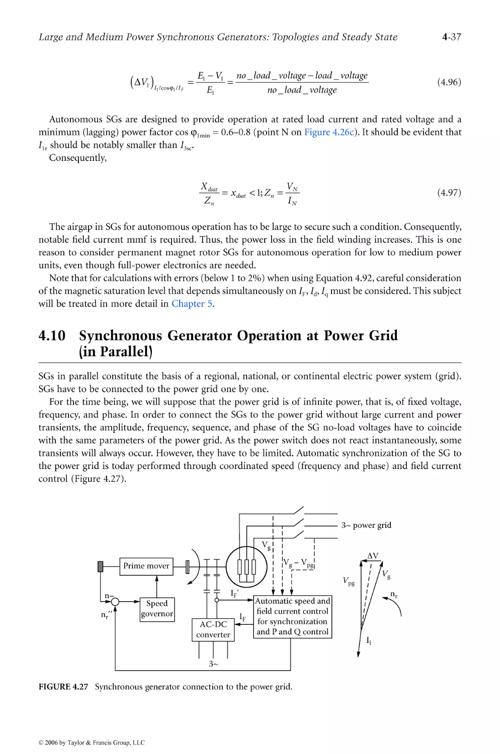
transients will always occur. However, they have to be limited. Automatic synchronization of the SG to
the power grid is today performed through coordinated speed (frequency and phase) and field current
control (Figure 4.27).
3", power grid
I
I
I
:V g - V pg :
I ,---
I I
I I
V
V pg

converter
Automatic speed and
field current control
for synchronization
and P and Q control
nil
r
Speed
governor
Il
3",
FIGURE 4.27 Synchronous generator connection to the power grid.
iD 2006 by Taylor & Francis Group, LLC

4-38
Synchronous Generators
El
-jXdld
-jXqlq
If
FIGURE 4.28 Synchronous generator phasor diagram (zero losses).
The active power transients during connection to the power grid may be positive (generating) or
negative (motoring) (Figure 4.27).
4.10.1 The Power/Angle Characteristic: Pe {8v}
The power (internal) angle b v is the angle between the terminal voltage VI and the field-current-produced
emf EI. This angle may be calculated for the autonomous and for the power-grid-connected generator.
Traditionally, the power/angle characteristic is calculated and widely used for power-grid-connected
generators, mainly because of stability computation opportunities. For a large power grid, the voltage
phasors in the phasor diagram are fixed in amplitude and phase. For clarity, we neglect the losses in the
SG. We repeat here the phasor diagram in Figure 4.17a but with RI = 0 (Figure 4.28).
The active and reactive powers P p QI from Equation 4.60 and Equation 4.61 with RI = 0 become
 = 3EIlq + 3(X dm - X q )Idlq
(4.98)
QI = - 3E Ild - 3XdI - 3XqI
(4.99)
From Figure 4.28,
I =  cos b v - EI . I
d X d ' q
 sin b v
X q
(4.100)
With Equation 4.100, Equation 4.98 and Equation 4.99 become the following:
n 3 EI  sin b v 3 1 T 2 ( 1 1 ) . <X
rl = +- Vl --- sln2u
I X 2 1 X X V
d q d
(4.101)
Q _ 3EI  cosby _ 1T2 ( COS2 b v sin 2 b v )
I - 3 VI +
X d X d X q
iD 2006 by Taylor & Francis Group, LLC

Large and Medium Power Synchronous Generators: Topologies and Steady State
4-39
PI
3V 1 E/X d
Leading
/
/
/
I
I
I
I
I
I
I
....-------
,
,
\
\
\
\
\
\
\ n/2
\
3V l E/X d
Motor
-n/2
2
3V l /X d
by
()y
Lagging /
I
I
I
I
/ ."
- ""- - - .,
\
\
---\------
\ 3V l 2 /X q
\
\
\ .
.....--_.4._ -
Generator 3V/ 1 2 ( 1- _1- )
2 X q X d
Motor
Generator
(a)
(b)
FIGURE 4.29 (a) Active PI and (b) reactive Ql powers vs. power angle b v .
The unity power factor is obtained with QI = 0, that is,
(  X d s in 2 8 v )
(E I )Ql=O =  cOS U v + 8
X q cos v
(4.102)
For the same power angle 8v and V p EI should be larger for the salient pole rotor SG, as X d > Xq. The
active power has two components: one due to the interaction of stator and rotor fields, and the second
one due to the rotor magnetic saliency (X d > X q ).
As in standard salient pole rotor SGs, Xd/X q < 1.7, the second term in Pe' called here saliency active
power, is relatively small unless the SG is severely underexcited: EI « VI. For given Ep V p the SG reactive
and active power delivery depend on the power (internal) angle 8v (Figure 4.29a and Figure 4.29b).
The graphs in Figure 4.29a and Figure 4.29b warrant the following remarks:
· The generating and motoring modes are characterized (for zero losses) by positive and, respec-
tively, negative power angles.
· As 8v increases up to the critical value 8 VK ' which corresponds to maximum active power delivery
P IK , the reactive power goes from leading to lagging for given emf Ep VI frequency (speed) COl.
· The reactive power is independent of the sign of the power angle 8v
· In salient pole rotor SGs, the maximum power P IK for given V p EI and speed, is obtained for a
power angle 8 VK < 90°, while for nonsalient pole rotor SGs, X d = (1 - 1.05 )X q , 8 VK  90°.
· The rated power angle 8vr is chosen around 22 to 30° for nonsalient pole rotor SGs and around
30 to 40° for salient pole rotor SGs. The lower speed, higher relative inertia, and stronger damper
cage of the latter might secure better stability, which justifies the lower power reserve (or ratio
PIK/P lr ).
4.10.2 The V-Shaped Curves: II{I F ), PI = ct., VI = ct., n = ct.
The V-shaped curves represent a family of II (IF) curves, drawn at constant V p speed (co l ), with active
power PI as a parameter. The computation of a V-shaped curve is straightforward once EI (IF) - the no-
load saturation curve - and X d and X q are known. Unfortunately, when IF varies from low to large
values, so does II (that is, I d , Iq); magnetic saturation varies, despite the fact that, basically, the total flux
linkage \}Is  V/co l remains constant. This is due to rotor magnetic saliency (X d "# X q ), where local
saturation conditions vary notably. However, to a first approximation, for constant VI and co l (that is
iD 2006 by Taylor & Francis Group, LLC

4-40
Synchronous Generators
Stator current limit
Il
P l
End-winding
core overheating
limit
COSCPl = 1
Field
current
limit
I I I I by
.III
b YK
(a)
Underexcited
Overexcited
IF
(b)
FIGURE 4.30 V-shaped curves: (a) P/b v assisting curves with IF as parameter and (b) the II (IF) curves for
constant PI.
'P I)' with EI calculated at a first fixed total flux, the value of MFA stays constant, and thus, EI  M pA . Ip
. cor  CPA. I p ; CPA  r . I FO is the field current value that produces EI = VIr at no load.
I po
For given IF' EI = CFAX IF and PI assigned a value from (4.101), we may compute by. Then, from
Equation 4.103, the corresponding stator current II can be found:
I[ =  I +I = (-E[ + idCOSOv J +( Ov J
(4.103)
As expected, for given active delivered power, the minimum value of stator current is obtained for a
field current IF corresponding to unity power factor (QI = 0). That is, (EI)Ilmin = (EI)QI=O may be
determined from Equation 4.103 with by already known from Equation 4.101. Then, Iff( = EI/ C FA . The
maximum power angle admitted for a given power PI limits the lowest field current admissible for
steady state.
Finally, graphs as shown in Figure 4.30a and Figure 4.30b are obtained.
Knowing the field current lower limit, for given active power, is paramount in avoiding an increase
in the power angle above b yK . In fact, b YK decreases with an increase in Pl.
4.10.3 The Reactive Power Capability Curves
The maximum limitation of IF is due to thermal reasons. However, the SG heating depends on both II
and IF' as both winding losses are very important. Also, 11' IF' and by determine the core losses in the
machine at a given speed.
When a reactive power request is increased, the increase in IF raises the field-winding losses and thus
the stator-winding losses (the active power PI) have to be limited.
The rationale for V-shaped curves may be continued to find the reactive power QI for the given PI
and IF. As shown in Figure 4.30, there are three distinct thermal limits: IF limit (vertical), II limit
(horizontal), and the end-winding overheating (inclined) limit at low values of field current. To explain
this latest, rather obscure, limitation, refer to Figure 4.31.
iD 2006 by Taylor & Francis Group, LLC

Large and Medium Power Synchronous Generators: Topologies and Steady State
4-41
Eddy currents
Stator
Retaining
solid/iron ring
Shaft
Rotor
FIGURE 4.31 End-region field path for the underexcited synchronous generator.
For the underexcited SG, the field-current- and armature-current-produced fields have angles smaller
than 90° (the angle between IF and II in the phasor diagram). Consequently, their end-winding fields
more or less add to each other. This resultant end-region field enters at 90° the end-region stator
laminations and produces severe eddy current losses that thermally limit the SG reactive power absorption
(QI < 0). This phenomenon is so strong because the retaining ring solid iron eddy currents (produced
solely by the stator end-windings currents) are small and thus incapable of attenuating severely the end-
region resultant field. This is because the solid iron retaining ring is not saturated magnetically, as the
field current is small. When the SG is overexcited, this phenomenon is not important, because the stator
and rotor fields are opposite (IF and II phase-angle shift is above 90°) and the retaining magnetic ring is
saturated by the large field current. Consequently, the stator end-windings-current-produced field in the
stator penetrates deeply into the retaining rings, producing large eddy currents that further attenuate
this resultant field in the end-region zone (the known short -circuit transformer effect on inductance).
The QI (PI) curves are shown in Figure 4.32.
1
0.95 pJ. lag
0.8
0.6
0.5
0.4
---
---
0.2
Armature current limit
--
15 PSIG
P l (P.U.)
-0.2
-0.4
-0.5
-0.6
A: - - - - 0.95 pJ.lead
-0.8
"
"
A '" \ "
\ "'-
\ ""
End-rgion heating lii
\ "
\ " 0.8 pJ. lead
\
\
\
-1
0.6 pJ. lead
FIGURE 4.32 Reactive power capability curves for a hydrogen-cooled synchronous generator.
iD 2006 by Taylor & Francis Group, LLC

4-42
Synchronous Generators
The reduction of hydrogen pressure leads to a reduction of reactive and active power capability of the
machine.
As expected, the machine reactive power absorption capability (QI < 0) is notably smaller than reactive
power capability. Both the end-region lamination loss limitation and the rise of the power angle closer
to its maximum limitation, seem to be responsible for such asymmetric behavior (Figure 4.32).
4.10.4 Defining Static and Dynamic Stability of Synchronous Generators
The fact that SGs require constant speed to deliver electric power at constant frequency introduces special
restrictions and precautionary measures to preserve SG stability, when tied to an electric power system
(grid). The problem of stability is complex. To preserve and extend it, active speed and voltage (active
and reactive power) closed -loop controls are provided. We will deal in some detail with stability and
control in Chapter 6. Here, we introduce the problem in a more phenomenological manner. Two main
concepts are standard in defining stability: static stability and dynamic stability.
The static stability is the property of an SG to remain in synchronism to the power grid in the presence
of slow variations in the shaft power (output active power, when losses are neglected). According to the
rising side of the PI (b v ) curve (Figure 4.28), when the mechanical (shaft) power increases, so does the
power angle b v , as the rotor slowly advances the phase of El' with the phase of VI fixed. When b v increases,
the active power delivered electrically, by the SG, increases.
In this way, the energy balance is kept, and no important energy increment is accumulated in the
inertia of the SG. The speed remains constant, but when PI increases, so does b v . The SG is statically
stable if ap/ab v > o.
We denote by PIs this power derivative with angle and call it synchronization power:
a  2 ( 1 1 ) 
s= -:\ =3EIcosuv-3 --- cos2uv
uUv X d X q
(4.104 )
PIS is maximum at b v = 0 and decreases to zero when b v increases toward b VK ' where PIS = o.
At the extent that the field current decreases, so does b VK ' and thus, the static stability region diminishes.
In reality, the SG is allowed to operate at values of b v , notably below b VK ' to preserve dynamic stability.
The dynamic stability is the property of the SG to remain in synchronism (with the power grid) in
the presence of quick variations of shaft power or of electric load short -circuit. As the combined inertia
of SGs and their prime movers is relatively large, the speed and power angle transients are much slower
than electrical (current and voltage) transients. So, for example, we can still consider the SG under
electromagnetic steady state when the shaft power (water admission in a hydraulic turbine) varies to
produce slow-speed and power-angle transients. The electromagnetic torque Te is thus, approximately,
T   . PI _ 3 PI [ EI  sin b v  2 ( 1 1 J .  ]
e  -- +- --- sln2uV
cor COr X d 2 X q X d
(4.105)
Consider a step variation of shaft power from P Shl to P Sh2 (Figure 4.33a and Figure 4.33b) in a lossless SG.
The SG power angle should vary slowly from b VI to b V2 . In reality, the power angle b v will overshoot
b V2 and, after a few attenuated oscillations, will settle at b V2 if the machine remains in synchronism.
Neglect the rotor damper cage effects that occur during transients. The motion equation is then written
as follows:
J dco r db v
-- = T shaft - Te;cor-co rO =-
PI dt dt
(4.106)
with co rO equal to the synchronous speed.
iD 2006 by Taylor & Francis Group, LLC

Large and Medium Power Synchronous Generators: Topologies and Steady State
4-43
Ptfb y
P lI <
Te
B' P 1I<
P Sh2
T a2
Deceleration energy
1
P Shl
1
Tal
Acceleration energy
b Yl b Y2
b YK
by
b Yl b y2 b Y3 b YK
by
----.-
(a)
(b)
FI GURE 4.33 Dynamic stability: (a) PI (b v ) and (b) the area criterion.
By multiplying Equation 4.106 by d8 v / dt, one obtains
d [ L ( d8v ) 2 ] = (haft - Te )d8 v = T. d8 v = dW
2 PI dt
(4.107)
Equation 4.107 illustrates the variation of kinetic energy of the prime-mover generator set translated
in an acceleration area AA'B and a deceleration area BB'C:
bY2
W AB = aTea_of _AA' B _ triangle = f (T'haft - 1;, ov
bYl
(4.108)
bY3
W AB , = aTea _ of _ BB' C _ tTiangle = f (T,haft - Te ov
bY2
(4.109)
Only when the two areas are equal to each other is there hope that the SG will come back from B' to
B after a few attenuated oscillations. Attenuation comes from the asynchronous torque of damper cage
currents, neglected so far. This is the so-called criterion of areas.
The maximum shaft torque or electric power step variation that can be accepted with the machine
still in synchronism is shown in Figure 4.34a and Figure 4.34b and corresponds to the case when point
C coincides with C'.
Let us illustrate the dynamic stability with the situation in which there is a loaded SG at power angle
8VI. A three-phase short-circuit occurs at 8 vp with its transients attenuated very quickly such that the
electromagnetic torque is zero (VI = 0, zero losses also). So, the SG starts accelerating until the short-
circuit is cleared at 8vse, which corresponds to a few tens of a second at most. Then, the electromagnetic
torque Te becomes larger than the shaft torque, and the SG decelerates. Only if
Area_of _ABCDArea_of _CB'B"
(4.110)
are there chances for the SG to remain in synchronism, that is, to be dynamically stable.
iD 2006 by Taylor & Francis Group, LLC

4-44
Synchronous Generators
Te
Te
Bl(
B'
A'
T shaft max
T shaft
T shaft = 0
A
by
b Yl
b ysc
by
(a)
(b)
FIGURE 4.34 Dynamic stability ideal limits: (a) maximum shaft torque step variation from zero and (b) maximum
short-circuit clearing time (angle: 8vsc - 8 V1 ) from load.
4.11 Unbalanced-Load Steady-State Operation
SGs connected to the power grid, but especially those in autonomous applications, often operate on
unbalanced three-phase loads. That is, the stator currents in the three phases have different amplitudes,
and their phasing differs from 120°:
I A (t) = II cos( colt- YI)
IBU) = 1 2 cas( (O\t- 2; -Yz )
Idt) = 13 cas( (O\t+ 2; - Y3 )
(4.111)
For balanced load, II = 1 2 = 13 and YI = Y2 = Y3. These phase currents may be decomposed in direct,
inverse, and homopolar sets according to Fortesque's transform (Figure 4.35).
1 .21t
lA+ = 3(lA +al B +azl e );a = e}3
1 .21t
_ ( 2 ) . 2 _ - J 3
IA- -3" LA +a IB+alc ,a -e
1
lAD = 3(lA + lB + le )
IB+ = a2IAI;
(4.112)
lc+ = alAI;
IB- = alA;
lc- = a 2 LA
iD 2006 by Taylor & Francis Group, LLC

Large and Medium Power Synchronous Generators: Topologies and Steady State
4-45
f B
+
f AO = f BO = fco
fA
+

fc-
FIGURE 4.35 The symmetrical component sets.
Unfortunately, the superposition of the flux linkages of the current sets is admissible only in the absence
of magnetic saturation. Suppose that the SG is nonsaturated and lossless (R I = 0). For the direct
components lAp IBl' lcp which produce a forward-traveling mmf at rotor speed, the theory unfolded so
far still holds. So, we will write the voltage equation for phase A and direct component of current lAI:
V A+ = E A+ - jX d LdA+ - jX q IqA+
(4.113)
The inverse (negative) components of stator currents lA-, IB-' and lc- produce an mmf that travels at
opposite rotor speed -cor.
The relative angular speed of the inverse mmf with respect to rotor speed is thus 2 cor. Consequently,
voltages and currents are induced in the rotor damper windings and in the field winding at 2co r frequency,
in general. The behavior is similar to an induction machine at slip S = 2, but which has nonsymmetrical
windings on the rotor and nonuniform airgap. We may approximate the SG behavior with respect to the
inverse component as follows:
LA . Z _ + U A- = E A-
(4.114)
Z_ = R_ + jX_
Unless the stator windings are not symmetric or some of the field coils have short -circuited turns _
= o. Z_ is the inverse impedance of the machine and represents a kind of multiple winding rotor induction
machine impedance at 2co r frequency.
The homopolar components of currents produce mmfs in the three phases that are phase shifted
spatially by 120 0 and have the same amplitude and time phasing. They produce a zero-traveling field in
the airgap and thus do not interact with the rotor in terms of the fundamental component. The corre-
sponding homopolar impedance is Zo  RI + jXo, and
Xo < Xl!
(4.115)
So,
X d > X q > X_ > Xl! > Xo
(4.116)
The stator equation for the homopolar set is as follows:
jlAoXo + V AO = 0
(4.117)
Finally,
V A = V A+ + V A- + V AO
(4.118)
iD 2006 by Taylor & Francis Group, LLC

4-46
Synchronous Generators
Similar equations are valid for the other two phases. We assimilated here the homopolar with the
stator leakage reactance (Xu  X o ). The truth is that this assertion is not valid if chorded coils are used,
when Xo < Xu. It seems that, due to the placement of stator winding in slots, the stator homopolar mmf
has a steplike distribution with 't/3 as half-period and does not rotate; it is an AC field. This third-space
harmonic-like mmf may be decomposed in a forward and backward wave and move both with respect
to rotor and induce eddy currents, at least in the damper cage. Additional losses occur in the rotor. As
we are not prepared by now theoretically to calculate Z_ and Xo, we refer to some experiments to measure
them so that we get some confidence in using the above theory of symmetrical components.
4.12 Measuring X d1 X q1 Z_1 Zo
We will treat here some basic measurement procedures for SG reactances: X d , Xq, Z-, ZOo For example, to
measureX d andXq, the open-field-winding SG, supplied with symmetric forward voltages (co rO ' frequency)
through a variable-ratio transformer, is driven at speed cor' which is very close to but different from the
stator frequency co rO (Figure 4.36a and Figure 4.36b):
COr = co rO . (1.01-1.02 )
(4.119)
We need not precisely measure this speed, but notice the slow pulsation in the stator current with
frequency cor - co rO  (0.01-0.02 )co rO .
Identifying the maxima and minima in the stator voltage VA(t) and current IA(t) leads to approximate
values of X d and X q :
X  V Amax . X
d , q
I Amin
YAmin
I Amax
(4.120)
The slip S = (COr - corO)/co rO has to be very small so that the currents induced in the rotor damper cage
may be neglected. If they are not negligible, X d and X q are smaller than in reality due to the damper eddy
current screening effect.
The saturation level will be medium if currents around or above the rated value are used.
Identifying the voltage and current maxima, even if the voltage and current are digitally acquired and
are off-line processed in a computer, is doable with practical precision.
The inverse (negative) sequence impedance Z_ may be measured by driving the rotor, with the field
winding short -circuited, at synchronous speed cor' while feeding the stator with a purely negative sequence
of low-level voltages (Figure 4.37). The power analyzer is used to produce the following:
1 Z 1 = V A - . R = (p_) phase
-- I ' - 1 2
-A- A-
(4.121)
x_ =  l z _I-(1C)2
(4.122)
Again, the frequency of currents induced in the rotor damper and field windings is 2co rO = 2co p and the
corresponding slip is S = 2.0. Alternatively, it is possible to AC supply the stator between two phases only:
Z 
U AB
2l A
(4.123)
iD 2006 by Taylor & Francis Group, LLC

Large and Medium Power Synchronous Generators: Topologies and Steady State
4-47
Prime
mover with variable
speed control and
low power rating
n
IF = 0
VA
I A
(OrO ;z!: (01
(3- ( ( WrO = 001
(a)
VAmax:
V Amix
I A
I Amax
(b)
FIGURE 4.36 Measuring Xci and X q : (a) the experimental arrangement and (b) the voltage and current waveforms.
This time the torque is zero and thus the SG stays at standstill, but the frequency of currents in the
rotor is only co rO = COl. (The negative sequence impedance will be addressed in detail in Chapter 8 of
Synchronous Generators on SG testing.) The homopolar impedance Zo may be measured by supplying
the stator phases connected in series from a single-phase AC source. The test may be made at zero speed
or at rated speed co rO (Figure 4.38). For the rated speed test, the SG has to be driven at shaft. The power
analyzer yields the following:
I z l =3V AO . =,x=  l z I 2_ 2
-0 3 I ' Ro 3 1 2 ' 0 -0 
AO AO
(4.124)
A good portion of Ro is the stator resistance RI so Ro  RI.
iD 2006 by Taylor & Francis Group, LLC

4-48
Prime
mover with low
power rating and
fixed speed
Synchronous Generators
VA
I A
Power
analyzer
( ( (
3",
FIGURE 4.37 Negative sequence testing for _.
Prime
mover with
fixed speed
FIGURE 4.38 Measuring homopolar o.
Power
3V AO analyzer
1",
The voltage in measurements for Z and Zo should be made low to avoid high currents.
4.13 The Phase-to-Phase Short-Circuit
The three-phase (balanced) short-circuit was already investigated in a previous paragraph with the
current 13se:
EI
1 3se =-
X d
(4.125)
The phase- to- phase short -circuit is a severe case of unbalanced load. When a short -circuit between two
phases occurs, with the third phase open, the currents are related to each other as follows (Figure 4.39a):
I B = -Ic = I se2 ; VB = VC;IA = 0
(4.126)
From Equation 4.109, the symmetrical components of lA are as follows:
1 ( 2 ) 1 ( 2 ) +j
I =- aI +a I =- a-a I =-1
-A+ 2 -B -c 3 -se2 J3 -se2
(4.127)
IA- = -IA+;IAo = 0
iD 2006 by Taylor & Francis Group, LLC

Large and Medium Power Synchronous Generators: Topologies and Steady State
4-49
Prime
mover (low
power rating)
SG
ABC
111
SG
I A
AC-DC converter
ABC
3
(b)
(a)
FIGURE 4.39 Unbalanced short-circuit: (a) phase-to-phase and (b) single-phase.
The star connection leads to the absence of zero-sequence current.
The terminal voltage of phase A, VA' for a non salient pole machine (X d = X q = X+) is obtained from
Equation 4.115 with Equation 4.112 and Equation 4.113:
V A = V A+ + V A- + V AO = E A+ - jX+ .IA+ - Z _IA_ =
= E A+ - .h Isc2 (jX+ - Z_ )
(4.128)
In a similar way,
2 2 j I se2 ( . 2 Z )
V B=a V A++a V A_=a E A +- J3 Ja X+-a__
(4.129)
2 j I se2 ( . 2 Z )
V c =a V A + +a V A _ =a E A + - J3 aJX+-a__
But, VB = Yc and thus
j I se2 ( . Z )
EA+ =- J3 JX+ + --
(4.130)
and
2j
V A = J3 I sc2 Z _=-2 V B
(4.131)
Finally,
.X +Z =-.J3 EA+(I p )
J + -- J I
-se2
(4.132)
iD 2006 by Taylor & Francis Group, LLC

4-50
Synchronous Generators
A few remarks are in order:
· Equation 4.132, with the known no-load magnetization curve, and the measured short-circuit
current I sc2 ' apparently allows for the computation of negative impedance if the positive one
jX+ = jX d , for nonsalient pole rotor SG, is given. Unfortunately, the phase shift between l and
Isc2 is hard to measure. Thus, if we only:
Z_ = -jX_
(4.133)
Equation 4.132 becomes usable as
X +x-= EA+oJ3
+
I se2
(4.134)
RMS values enter Equation 4.134.
· Apparently, Equation 4.131 provides a good way to compute the negative impedance Z_ directly,
with  and Isc2 measured. Their phase shift can be measured if the SG null point is used as
common point for  and 12sc measurements.
· During a short-circuit, even in phase to phase, the air gap magnetic flux density is small and
distorted. So, it is not easy to verify (Equation 4.131), unless the voltage VA and current I sc2 are
first filtered to extract the fundamental.
· Only Equation 4.132 is directly usable to approximate X_, with X+ unsaturated known. As X+»
X_ for strong damper cage rotors, the precision of computing X_ from the sum (X+ + X_) is not
so good
· In a similar way, as above for the single-phase short-circuit (Figure 4.39b),
X X X  3E A +(I p )
++ -+ o
Iscl
(4.135)
with X+ > X_ > Xo.
· To a first approximation,
Isc3 : I se2 : Iscl  3 : J3 : 1
(4.136)
for an SG with a strong damper cage rotor.
· EA+ should be calculated for the real field current IF' but, as during short-circuit the real distortion
level is low, the unsaturated value of X FA should be used: EA+ = IiX FA ) unsaturated.
· Small autonomous SGs may have the null available for single-phase loads; thus, the homopolar
component shows up.
· The negative sequence currents in the stator produce double-frequency-induced currents in the
rotor damper cage and in the field windings. If the field winding is supplied from a static power
converter, the latter prevents the occurrence of AC currents in the field winding. Consequently,
notable overvoltages may occur in the latter. They should be considered when designing the field-
winding power electronics supply. Also, the double-frequency currents in the damper cage, pro-
duced by the negative component set, have to be limited, as they affect the rotor overtemperature.
So, the ratio 1_/1+, that is the level of current unbalance, is limited by standards below 10 to 12 0 /0.
· A similar phenomenon occurs in autonomous SGs, where the acceptable level of current unbalance
1_/ If is given as a specification item and then considered in the thermal design. Finally, experiments
are needed to make sure that the SG can really stand the predicted current unbalance.
iD 2006 by Taylor & Francis Group, LLC

Large and Medium Power Synchronous Generators: Topologies and Steady State
4-51
· The phase-to-phase or single-phase short-circuits are extreme cases of unbalanced load. The
symmetrical components method presented here can be used for actual load unbalance situations
where the +, -, 0 current components sets may be calculated first. A numerical example follows.
Example 4.3
A three-phase lossless two-pole SG with Sn = 100 KVA, at V ll = 440 V and h = 50 Hz, has the
following parameters: X+ = X d = x q = 0.6 P.U., X_ = 0.2 P.U., Xo = 0.12 P.U. and supplies a single-
phase resistive load at rated current. Calculate the load resistance and the phase voltages VA' VB' V c
if the no-load voltage Ell = 500 V.
Solution
We start with the computation of symmetrical current components sets (with I B = Ic = 0):
IA+ = I A _ = I AO = IJ3
The rated current for star connection Ir is
I = Sn = 1 00000  131 A
r J3l J3.440
The nominal impedance Zn is
Zn == 440 =1.936 Q
J3I r J3.131
So,
X+ = Znx+ = 1.936 x 0.6 = 1.1616 Q
X_ = Znx_ = 1.936 x 0.2 = 0.5872 Q
Xo = ZnXO = 1.936 x 0.12 = 0.23232 Q
From Equation 4.112, the positive sequence voltage equation is as follows:
V A+ = E A+ - jX+ Ir / 3
From Equation 4.113,
V A- = - jX-Ir /3
Also, from Equation 4.116,
V AO = - jX o Ir / 3
The phase of voltage  is the summation of its components:
V A = E A+ - j(X+ +X_ +Xo)I r /3
iD 2006 by Taylor & Francis Group, LLC

4-52
Synchronous Generators
j(X+ + X_ + X O )I r /3
y = 0.333 rad
I A = Ir VA
FIGURE 4.40 Phase A phasor diagram.
As the single-phase load was declared as resistive, Ir is in phase with, and thus,
. ( ) Ir
E A+ = V A + + J X+ + X_ + Xo 3
A phasor diagram could be built as shown in Figure 4.40.
With EA+ = 500 V/sqrt(3) = 280 V and Ir = 131 A known, we may calculate the phase voltage of
loaded phase, VA:
VA =  El+ -[(x+ + X_ + Xo)Ir /3 J =  ( 289)2 -[(1.1616+0.3872+0.23232),13113 J
= 278.348 V
The voltages along phases Band Care
.21t I .21t I .21t I
V = E e -J 3 - J .X ---I-e -J 3 - J .X ---I-e +J 3 - J .X o ---I- =
-B -A+ + 3 - 3 3
.21t I .21t I .21t I
V - E + J 3 . x r J 3 . x r - J 3 . x r
- e - J -e - J -e - J e - 3
-c -A+ + 3 - 3
E A+ =EA+ .ejyo;yo =0.333 rad
The real axis falls along VA and I A , in the horizontal direction:
V B = -83.87 - j X 270[V]
V c = -188.65 + j213.85[V]
The phase voltages are no longer symmetric (VA = 278 V, VB = 282.67 V, V c = 285 V). The voltage
regulation is not very large, as x+ = 0.6, and the phase voltage unbalance is not large either, because
the homopolar reactance is usually small, xo = 0.12. Also small is X_ due to a strong damper cage
on the rotor. A small x+ presupposes a notably large airgap; thus, the field-winding mmf should be
large enough to produce acceptable values of flux density in the airgap on no load (B gFm = 0.7-0.75
T) in order to secure a reasonable volume SG.
iD 2006 by Taylor & Francis Group, LLC

Large and Medium Power Synchronous Generators: Topologies and Steady State
4-53
(OrO
1 - Resistive starting
2 - Self synchronization
SG
IF
3",
2
AC-DC
converter
Reactive power or
voltage controller
3",
V* or Ql*
FIGURE 4.41 Synchronous condenser.
ij = ( ;: ) ( Qj )
E I ql = 3V{
X d i1(P.U.)
-jXdId
1.0 ql (P.U.)
Vi 0.5
- jXdI d
E1/V 1
E I 0
IF II = Id II = Id -0.5
..
IF -1.0
VI < E I VI > E I
(a)
(b)
FIGURE 4.42 (a) Phasor diagrams and (b) reactive power of synchronous condenser.
4.14 The Synchronous Condenser
As already pointed out, the reactive power capability of a synchronous machine is basically the same for
motor or generating mode (Figure 4.28b). It is thus feasible to use a synchronous machine as a motor
without any mechanical load, connected to the local power grid (system), to "deliver" or "drain" reactive
power and thus contribute to overall power factor correction or (and) local voltage control. The reactive
power flow is controlled through field current control (Figure 4.41).
The phasor diagram (with zero losses) springs from voltage Equation 4.54 with Iq = 0 and RI = 0
(Figure 4.42a and Figure 4.42b):
V I = E I - jXdld;11 = ld
(4.137)
The reactive power QI (Equation 4.102), with b v = 0, is
iD 2006 by Taylor & Francis Group, LLC

4-54
Synchronous Generators
(EI - )
QI = 3 = -3Id
X d
(4.138)
_ 32 .X- X d
QI- X' - EI/-l
(4.139)
As expected, QI changes sign at EI = VI and so does the current:
_ ( ) . _ { > 0 for EI /  > 1
Id -  - EI / Xd,X -
< 0 for EI /  < 1
(4.140 )
Negative Id means demagnetizing Id or EI > VI. As magnetic saturation depends on the resultant magnetic
field, for constant voltage V p the saturation level stays about the same, irrespective of field current IF. So,
EI  COr ( M PA ) VI . I P
(4.141)
Also, X d should not vary notably for constant voltage VI. The maximum delivered reactive power depends
on I d , but the thermal design should account for both stator and rotor field-winding losses, together with
core losses located in the stator core.
It seems that the synchronous condenser should be designed at maximum delivered (positive) reactive
power Qlmax:
 [ ( ) ] Elmax - 
Qlmax = 3 X d E lmax I Fmax -  ; II = X d
(4.142)
To reduce the size of such a machine acting as a no-load motor, two pole rotor configurations seem to
be appropriate. The synchronous condenser is, in fact, a positive/negative reactance with continuous
control through field current via a low power rating AC-DC converter. It does not introduce significant
voltage or current harmonics in the power systems. However, it makes noise, has a sizeable volume, and
needs maintenance. These are a few reasons for the increase in use of pulse-width modulator (PWM)
converter controlled capacitors in parallel with inductors to control voltage in power systems. Existing
synchronous motors are also used whenever possible, to control reactive power and voltage locally while
driving their loads.
4.15 Summary
· Large and medium power SGs are built with DC excitation windings on the rotor with either
salient or nonsalient poles.
· Salient rotor poles are built for 2PI > 4 poles and nonsalient rotor poles for 2PI = 2, 4.
· The stator core of SGs is made of silicon-steel laminations (generally 0.5 mm thick), with uniform
slotting. The slots house the three-phase windings.
· The stator core is made of one piece only if the outer diameter is below 1 m; otherwise, it is made
of segments. Sectionable cores are wound section by section, and the wound sections are mounted
together at the user's site.
· The slots in SGs are generally open and provided with nonmagnetic or magnetic wedges (to reduce
emf harmonic content).
iD 2006 by Taylor & Francis Group, LLC

Large and Medium Power Synchronous Generators: Topologies and Steady State
4-55
· Stator windings are of single- and double-layer types and are made of lap (multiturn) coils or the
bar-wave (single-turn) coils (to reduce the lengthy connections between coils).
· Stator windings are generally built with integer slots/pole/phase q; only for a large number of poles
2PI > 16 to 20, q may be fractionary: 3.5, 4.5 (to reduce the emf harmonics content).
· The symmetric AC currents of stator windings produce a positive mmf wave that travels with the
coli PI angular speed (with respect to the stator) co l = 2nh, with h equal to the frequency of currents.
· The core of salient pole rotors is made of a solid iron pole wheel spider on top of which 2PI salient
poles usually made of laminations (1 mm thick in general) are placed. The poles are attached to
the pole wheel spider through hammer or dove-tail keybars or bolts and screws with end plates.
· Nonsalient pole rotors are made of solid iron with machined radial slots over two thirds of
periphery to house distributed field-winding coils. Constrained costs and higher peripheral speeds
have led to solid cores for nonsalient poles rotors with 2PI = 2, 4 poles.
· The rotor poles are provided with additional (smaller) slots filled with copper or brass bars short-
circuited by partial or total end rings. This is the damper winding.
· The airgap flux density produced by the rotor field windings has a fundamental and space har-
monics. They are to be limited in order to reduce the stator emf (no load voltage) harmonics. The
larger air gap under the salient poles is used for the scope. Uniform air gap is used for nonsalient
poles, because their distributed field coils produce lower harmonics in the air gap flux density. The
design airgap flux density flat top value is about 0.7 to 0.8 T in large and medium power SGs.
The emf harmonics may be further reduced by the type of stator winding (larger or fractionary
q, chorded coils).
· The airgap flux density of the rotor field winding currents is a traveling wave at rotor speed Or =
coJ Pl.
· When cor = COp the stator AC current and rotor DC current airgap fields are at standstill with each
other. These conditions lead to an interaction between the two fields, with nonzero average
electromagnetic torque. This is the speed of synchronism or the synchronous speed.
· When an SG is driven at speed cor (electrical rotor angular speed; Or = COJpI is the mechanical
rotor speed), the field rotor DC currents produce emfs in the stator windings with frequency co l
that is co l = cor. If a balanced three-phase load is connected to the stator terminals, the occuring
stator currents will naturally have the same frequency co l = cor; their mmf will, consequently,
produce an airgap traveling field at the speed co l = cor. Their phase shift with respect to phase emfs
depends on load character (inductive-resistive or capacitive-resistive) and on SG reactances (not
yet discussed). This is the principle of the SG.
· The air gap field of stator AC currents is called the armature reaction.
· The phase stator currents may be decomposed in two components (I d , Iq), one in phase with the
emf and the other at 90°. Thus, two mmfs are obtained, with airgap fields that are at standstill
with respect to the moving rotor. One along the d (rotor pole) axis, called longitudinal, and the
other one along the q axis, called transverse. This decomposition is the core of the two-reaction
theory of SGs.
· The two stator mmf fields are tied to rotor d and q axes; thus, their cyclic magnetization reactances
X dm and X qm may be easily calculated. Leakage reactances are added to get X d and Xq, the synchro-
nous reactances. With zero damper currents and DC field currents on the rotor, the steady-state
voltage equation is straightforward:
IIRI +  = E I - jXdl d - jXqlq;11 = ld + lq
· The SG "delivers" both active and reactive power, PI and QI. They both depend on X d , Xq, and RI
and on the power angle b v , which is the phase angle between the emf and the terminal voltage
(phase variables).
iD 2006 by Taylor & Francis Group, LLC

4-56
Synchronous Generators
· Core losses may be included in the SG equations at steady state as pure resistive short -circuited
stator fictitious windings with currents that are produced by the resultant airgap or stator phase
linkage.
· The SG loss components are stator winding losses, stator core losses, rotor field-winding losses,
additional losses (mainly in the rotor damper cage), and mechanical losses. The efficiency of large
SGs is very good (above 98 0 /0, total, including field-winding losses).
· The SGs may operate in stand-alone applications or may be connected to the local (or regional)
power system. No-load, short-circuit, zero-power factor saturation curves, together with the
output VI (II) curve, fully characterize stand-alone operation with balanced load. Voltage regulation
tends to be large with SGs as the synchronous reactances in P. U. (Xd or x q ) are larger than 0.5 to
0.6, to limit the rotor field-winding losses.
· Operation of SGs at the power system is characterized by the angular curve P I (8 v )' V-shaped
curves II (IF) for PI = ct., and the reactive power capability QI (PI).
· The PI (8 v ) curve shows a single maximum value at 8 VK ::;; 90°; this critical angle decreases when
the field current IF decreases for constant stator terminal voltage VI and speed.
· Static stability is defined as the property of SG to remain at synchronism for slow shaft torque
variations. Basically, up to 8v = 8 VK ' the SG is statically stable.
· The dynamic stability is defined as the property of the SG to remain in synchronism for fast shaft
torque or electric power (short -circuiting until clearing) transients. The area criterion is used to
forecast the reserve of dynamic stability for each transient. Dynamic stability limits the rated power
angle 22 to 40°, much less than its maximum value 8 VK ::;; 90°.
· The stand-alone SG may encounter unbalanced loads. The symmetrical components (Fortesque)
method may be applied to describe SG operation under such conditions, provided the saturation
level does not change (or is absent). Impedances for the negative and zero components of stator
currents, Z_ and Zo , are defined, and basic methods to measure them are described. In general,
I Z +1> I Z -I> I Z o 1 ' and thus, the stator phase voltage imbalance under unbalanced loads is not
very large. However, the negative sequence stator currents induce voltages and produce currents
of double stator frequency in the rotor damper cage and field winding. Additional losses are
present. They have to be limited to keep rotor temperature within reasonable limits. The maximum
1_/1+ ratio is standardized (for power system SGs) or specified (for stand-alone SGs).
· The synchronous machine acting as a motor with no shaft load is used for reactive power absorp-
tion (IF small) or delivery (IF large). This regime is called a synchronous condenser, as the machine
is seen by the local power system either as a capacitor (IF large, overexcited EI > VI) or as an
inductor (IF small, underexcited machine EI/V I < 1). Its role is to raise or control the local power
factor or voltage in the power system.
References
1. R. Richter, Electrical Machines, vol. 2, Synchronous Machines, Verlag Birkhauser, Basel, 1954 (in
German) .
2. J.H. Walker, Large Synchronous Machines, Clarendon Press, Oxford, 1981.
3. 1. Boldea, and S.A. Nasar, Induction Machine Handbook, CRC Press, Boca Raton, Florida, 2001.
4. IEEE Std. 115 - 1995, "Test Procedures for Synchronous Machines."
5. V. Ostovic, Dynamics of Saturated Electric Machines, Springer-Verlag, Heidelberg, 1989.
6. M. Kostenko, and L. Piotrovski, Electrical Machines, vol. 2, MIR Publishers, Moscow, 1974.
7. C. Concordia, Synchronous Machines, John Wiley & Sons, New York, 1951.
iD 2006 by Taylor & Francis Group, LLC

Synchronous
Generators: Modeling
for (and) Transients
5 .1 Introduction ........................................................................ 5 - 2
5.2 The Phase-Variable Model..................................................5-3
5 . 3 The d -q Model .................................................................... 5 - 8
5.4 The per Unit (EU.) d-q Model........................................5-15
5.5 The Steady State via the d-q Model ................................5-17
5.6 The General Equivalent Circuits ......................................5-21
5.7 Magnetic Saturation Inclusion in the d-q Model...........5-23
The Single d-q Magnetization Curves Model · The Multiple
d-q Magnetization Curves Model
5.8 The Operational Parameters ............................................5-28
5.9 Electromagnetic Transients.............................................. .5-30
5.10 The Sudden Three-Phase Short-Circuit from
No Load............................................................................ .5-32
5.11 Standstill Time Domain Response Provoked
Transients. . . . . . . . . . . . . . . . . . . . . . . . . . . . . . . . . . . . . . . . . . . . . . . . . . . . . . . . . . . . . . . . . . . . . . . . . . .5 - 3 6
5.12 Standstill Frequency Response........................................ .5-39
5.13 Asynchronous Running................................................... .5-40
5.14 Simplified Models for Power System Studies ..................5-46
Neglecting the Stator Flux Transients · Neglecting the Stator
Transients and the Rotor Damper Winding Effects · Neglecting
All Electrical Transients
5.15 Mechanical Transients....................................................... 5-48
Response to Step Shaft Torque Input · Forced Oscillations
5.16 Small Disturbance Electromechanical Transients ...........5-52
5.17 Large Disturbance Transients Modeling..........................5-56
Line-to-Line Fault · Line-to-Neutral Fault
5.18 Finite Element SG Modeling ............................................5-60
5.19 SG Transient Modeling for Control Design ....................5-61
5.20 Summary........................................................................... .5-65
Ref eren ce s ..................................................................................... 5 - 6 8
5-1
iD 2006 by Taylor & Francis Group, LLC

5-2 Synchronous Generators
5.1 Introduction
The previous chapter dealt with the principles of synchronous generators (SGs) and steady state based
on the two-reaction theory. In essence, the concept of traveling field (rotor) and stator magnetomotive
forces (mmfs) and airgap fields at standstill with each other has been used.
By decomposing each stator phase current under steady state into two components, one in phase with
the electromagnetic field (emf) and the other phase shifted by 90°, two stator mmfs, both traveling at
rotor speed, were identified. One produces an airgap field with its maximum aligned to the rotor poles
(d axis), while the other is aligned to the q axis (between poles).
The d and q axes magnetization inductances X dm and X qm are thus defined. The voltage equations with
balanced three-phase stator currents under steady state are then obtained.
Further on, this equation will be exploited to derive all performance aspects for steady state when
no currents are induced into the rotor damper winding, and the field-winding current is direct. Though
unbalanced load steady state was also investigated, the negative sequence impedance Z_ could not be
explained theoretically; thus, a basic experiment to measure it was described in the previous chapter.
Further on, during transients, when the stator current amplitude and frequency, rotor damper and
field currents, and speed vary, a more general (advanced) model is required to handle the machine
behavior properly.
Advanced models for transients include the following:
· Phase-variable model
· Orthogonal-axis (d-q) model
· Finite-element (FE)/circuit model
The first two are essentially lumped circuit models, while the third is a coupled, field (distributed
parameter) and circuit, model. Also, the first two are analytical models, while the third is a numerical
model. The presence of a solid iron rotor core, damper windings, and distributed field coils on the
rotor of nonsalient rotor pole SGs (turbogenerators, 2Pl = 2,4), further complicates the FE/circuit
model to account for the eddy currents in the solid iron rotor, so influenced by the local magnetic
saturation level.
In view of such a complex problem, in this chapter, we are going to start with the phase coordinate
model with inductances (some of them) that are dependent on rotor position, that is, on time. To
get rid of rotor position dependence on self and mutual (stator/rotor) inductances, the d-q model
is used. Its derivation is straightforward through the Park matrix transform. The d-q model is then
exploited to describe the steady state. Further on, the operational parameters are presented and
used to portray electromagnetic (constant speed) transients, such as the three-phase sudden short-
circui t.
An extended discussion on magnetic saturation inclusion into the d-q model is then housed and
illustrated for steady state and transients.
The electromechanical transients (speed varies also) are presented for both small perturbations
(through linearization) and for large perturbations, respectively. For the latter case, numerical solutions
of state-space equations are required and illustrated.
Mechanical ( or slow) transients such as SG free or forced "oscillations" are presented for electromag-
netic steady state.
Simplified d-q models, adequate for power system stability studies, are introduced and justified in
some detail. Illustrative examples are worked out. The asynchronous running is also presented, as it is
the regime that evidentiates the asynchronous (damping) torque that is so critical to SG stability and
control. Though the operational parameters with s = mj lead to various SG parameters and time constants,
their analytical expressions are given in the design chapter (Chapter 7), and their measurement is
presented as part of Chapter 8, on testing.
This chapter ends with some FE/coupled circuit models related to SG steady state and transients.
iD 2006 by Taylor & Francis Group, LLC

Synchronous Generators: Modeling for (and) Transients
5-3
/
/
Sink (motor) Source
a (generator)
  lfd  t la
.. E .. E
V fd Va
- ExH - ExH
p=- p=-
2 2
Ia
FIGURE 5.1 Phase-variable circuit model with single damper cage.
5.2 The Phase-Variable Model
The phase-variable model is a circuit model. Consequently, the SG is described by a set of three stator
circuits coupled through motion with two (or a multiple of two) orthogonally placed (d and q) damper
windings and a field winding (along axis d: of largest magnetic permeance; see Figure 5.1). The stator
and rotor circuits are magnetically coupled with each other. It should be noticed that the convention of
voltage-current signs (directions) is based on the respective circuit nature: source on the stator and sink
on the rotor. This is in agreement with Poynting vector direction, toward the circuit for the sink and
outward for the source (Figure 5.1).
The phase-voltage equations, in stator coordinates for the stator, and rotor coordinates for the rotor,
are simply missing any "apparent" motion-induced voltages:
. d'P A
lARs +V a =--
dt
. d'P B
lBRS+Vb =--
dt
. d'Pc
lcRs +V c =--
dt
. R - d'P D
lD D ---
dt
. d'P Q
lQRQ =--
dt
d'P f
If Rf - V f = ------;tt
(5.1)
The rotor quantities are not yet reduced to the stator. The essential parts missing in Equation 5.1 are the
flux linkage and current relationships, that is, self- and mutual inductances between the six coupled
circuits in Figure. 5.1. For example,
iD 2006 by Taylor & Francis Group, LLC

5-4
Synchronous Generators
'P A = LAAla + LABlb + LAC Ie + LAflf + LADI D + LAQIQ
(5.2)
Let us now define the stator phase self- and mutual inductances L AA , L BB , Leo LAB' LBO and LeA for a
salient - pole rotor SG. For the time being, consider the stator and rotor magnetic cores to have infinite
magnetic permeability. As already demonstrated in Chapter 4, the magnetic permeance of airgap along
axes d and q differ (Figure 5.2). The phase A mmf has a sinusoidal space distribution, because all space
harmonics are neglected. The magnetic permeance of the air gap is maximum in axis d, P d' and minimum
in axis q and may be approximated to the following:
Pd+Pq ( Pd- Pq )
P(8er) = Po + P 2 cos28 er = 2 + 2 cos28 er
(5.3)
So, the airgap self-inductance of phase A depends on that of a uniform airgap machine (single-phase
fed) and on the ratio of the permeance P(8 er )/(P O + P 2 ) (see Chapter 4):
L AAg = 4 2 (KW1)2 (po + Pz cas2e er )
1t
(5.4)
II T,Z II T,Z
n + P 1"""' 0 stack . n _ P _ 1"""' 0 stack . g < g
r 0 2 = , r 0 2 , ed eq
ged geq
(5.5)
Also,
L AAg = LO + L 2 cos28 er
(5.6)
To complete the definition of the self-inductance of phase A, the phase leakage inductance Lsl has to be
added (the same for all three phases if they are fully symmetric):
L AA = Lsl + Lo + L 2 cos28 er
(5.7)
Ideally, for a nonsalient pole rotor SG, L 2 = 0 but, in reality, a small saliency still exists due to a more
accentuated magnetic saturation level along axis q, where the distributed field coil slots are located.
I
I I
I 8er = P18r I
I I
I I
I I
I I
I I
-90° I 18er = 0 I 8er = 90° 18er = 180°
I I I I
I I I I (l k)
---------------------------------£
I I I I Ilo'tl stac k
I I I I P g(8 er ) =
I I I I ge(8 er )
I I I I
I I I
I I I
I I I
'T - Pole pitch
lstack- Stack length
ge(8 er ) - Variable equivalent airgap
FIGURE 5.2 The airgap permeance per pole versus rotor position.
iD 2006 by Taylor & Francis Group, LLC

Synchronous Generators: Modeling for (and) Transients
5-5
In a similar way,
L BB = L,/ + Lo + L 2 cas( 2e er + 2: )
(5.8)
Lee = Lsi + Lo + Lz cas( 2e er _ 2: )
(5.9)
The mutual inductance between phases is considered to be only in relation to airgap permeances. It
is evident that, with ideally (sinusoidally) distributed windings, LAB(Ser) varies with Ser as Lee and again
has two components (to a first approximation):
LAB = L BA = L ABO + L AB2 cas( 2e er _ 2: )
(5.10)
Now, as phases A and Bare 120 0 phase shifted, it follows that
2n Lo
L ABO  Lo cos- =--
3 2
(5.11)
The variable part of LAB is similar to that of Equation 5.9 and thus,
L AB2 = L 2
(5.12)
Relationships 5.11 and 5.12 are valid for ideal conditions. In reality, there are some small differences,
even for symmetric windings. Further,
Lo ( 2n )
LAC = LeA = -2+ L 2 cos 2S er +3
(5.13)
Lo
L BC = L CB = -- + L 2 cos2S er
2
(5.14)
FE analysis of field distribution with only one phase supplied with direct current (DC) could provide
ground for more exact approximations of self- and mutual stator inductance dependence on Sere Based
on this, additional terms in cos( 4S er ), even 6S er , may be added. For fractionary q windings, more intricate
Ser dependences may be developed.
The mutual inductances between stator phases and rotor circuits are straightforward, as they vary with
cos(Ser) and sin(Ser)'
L Af = M f cosS er
LBf = M f cas( eer _ 2: )
Lef = M f cas( eer + 2: )
(5.15)
iD 2006 by Taylor & Francis Group, LLC

5-6
Synchronous Generators
LAD = M D COsS er
L BD =MDCOs( eer _ 2: )
LeD =MDCOs( eer + 2: )
(5.15 cont.)
L AQ = -M Q sin Ser
LBQ =-MQSin( eer _ 2: )
L eQ =-MQSin( eer + 2: )
Notice that
( L dm + Lqm )
Lo =
2
( L dm - Lqm )
L 2 =
2
(5.16)
L dm and Lqm were defined in Chapter 4 with all stator phases on, and M f is the maximum of field/armature
inductance also derived in Chapter 4.
We may now define the SG phase-variable 6 x 6 matrix IL ABcjDQ (Ser )1 :
A f D Q
A Ll +  + M D cosetr -MQcos&r
 cos2& r
c
. ( 2IT ]
MQsm &r- 3
B
I L ABGDJ 8er )1 =
f
D
Q
o
o
o
LQI + rQm
(5.17)
A mutual coupling leakage inductance LjDl also occurs between the field winding f and the d-axis cage
winding D in salient-pole rotors. The zeroes in Equation 5.17 reflect the zero coupling between orthogonal
windings in the absence of magnetic saturation. Efm, E Dm , E Qm are typical main (airgap permeance) self-
inductances of rotor circuits. Eft, E Dl , EQl are the leakage inductances of rotor circuits in axes d and q.
The resistance matrix is of diagonal type:
iD 2006 by Taylor & Francis Group, LLC

Synchronous Generators: Modeling for (and) Transients
5-7
RABCfdq = Diag[ Rs, Rr' Rs, Rj, R;, RQ]
(5.18)
Provided core losses, space harmonics, magnetic saturation, and frequency (skin) effects in the rotor
core and damper cage are all neglected, the voltage/current matrix equation fully represents the SG at
constant speed:
[ J[ ] [ ] -d'P ABCjDQ
I ABCjDQ R ABcjDQ + V ABCjDQ = =
dt
[ ( ) ] d [ ] a [ L ABCjDQ ] dS er [ ]
- L ABCjDQ S er dt I ABCjDQ - as dt I ABCjDQ
er
(5.19)
with
[ J T dSff
V ABCjDQ = +VA,+VB,+VC,-Vf,O,O ;-=ill r
dt
(5.20)
\{J A BejDQ = [ \{J A' \{J B, \{J c> \{Jj , \{J  , \{J Q r
(5.21)
The minus sign for V f arises from the motor association of signs convention for rotor.
The first term on the right side of Equation 5.19 represents the transformer-induced voltages, and the
second term refers to the motion-induced voltages.
Multiplying Equation 5.19 by [IABCjDQ]T yields the following:
[ ] T [ ] 1 [ J T a [ L ABCjDQ ( S er ) ] [ ]
I ABCjDQ V ABCjDQ = -"2 I ABCjDQ as I ABCjDQ . ill r -
er
-  [  [IABCfDQ r . LABCjDQ (eer ). [I ABCjDQ ]]- [I ABejDQ r [IABejDQ][ R ABCjDQ ]
(5.22)
The instantaneous power balance equation (Equation 5.22) serves to identify the electromagnetic power
that is related to the motion-induced voltages:
P"bn = -  [I ABCfDQ r . a: [LABejDQ (eer ) J[ I ABCfDQ ]ror
er
(5.23)
P elm should be positive for the generator regime.
The electromagnetic torque Te opposes motion when positive (generator model) and is as follows:
_ + Pe _ _ Q [ J T a [ L ABCjDQ ( S er ) ] [ ]
Te - ( ) - I ABCjDQ I ABCjDQ
ill r / PI 2 bSer
(5.24)
The equation of motion is
L dill r = T _ T . dSer = ill
PI dt shaft e' dt r
(5.25)
iD 2006 by Taylor & Francis Group, LLC

5-8
Synchronous Generators
The phase-variable equations constitute an eighth-order model with time-variable coefficients (induc-
tances). Such a system may be solved as it is either with flux linkages vector as the variable or with the
current vector as the variable, together with speed ill r and rotor position S er as motion variables.
Numerical methods such as Runge-Kutta-Gill or predictor-corrector may be used to solve the system
for various transient or steady-state regimes, once the initial values of all variables are given. Also, the
time variations of voltages and of shaft torque have to be known. Inverting the matrix of time-dependent
inductances at every time integration step is, however, a tedious job. Moreover, as it is, the phase-
variable model offers little in terms of interpreting the various phenomena and operation modes in an
intuitive manner.
This is how the d-q model was born - out of the necessity to quickly solve various transient operation
modes of SGs connected to the power grid (or in parallel).
5.3 The d-q Model
The main aim of the d-q model is to eliminate the dependence of inductances on rotor position. To do
so, the system of coordinates should be attached to the machine part that has magnetic saliency - the
rotor for SGs.
The d-q model should express both stator and rotor equations in rotor coordinates, aligned to rotor
d and q axes because, at least in the absence of magnetic saturation, there is no coupling between the
two axes. The rotor windings f, D, Q are already aligned along d and q axes. The rotor circuit voltage
equations were written in rotor coordinates in Equation 5.1.
It is only the stator voltages, VA' VB' V c , currents lA' I B , Ie, and flux linkages 'P A' 'P B' 'Pc that have to
be transformed to rotor orthogonal coordinates. The transformation of coordinates ABC to d-qO, known
also as the Park transform, valid for voltages, currents, and flux linkages as well, is as follows:
cos( -Ser ) cas( -e + 211: ) cas( -e _ 211: )
er 3 er 3
[p(eer)J=  sin ( -Ser ) sin ( -e + 211: ) Sin(-e _ 211: ) (5.26)
er 3 er 3
1 1 1
- - -
2 2 2
So,
V d VA
V q = 1 p ( S er )1. VB
V o V c
(5.27)
Id I A
I q = 1 p ( S er )1. I B
10 Ie
(5.28)
'Pd 'P A
'P q = Ip( Ser )1. 'P B
'Po 'Pc
(5.29)
iD 2006 by Taylor & Francis Group, LLC

Synchronous Generators: Modeling for (and) Transients
5-9
The inverse transformation that conserves power is
[p(eer)T =  [p(eer)r
(5.30)
The expressions of 'P A' 'P B , 'Pc from the flux/current matrix are as follows:
I'P ABCjDQ 1 = 1 L ABCjDQ (S er )11 I ABCjDQ 1
(5.31)
The phase currents lA' I B , Ie are recovered from I d , Iq, 10 by
I A Id
l B =  [p( eer ) r . lq
Ie 10
(5.32)
An alternative Park transform uses H instead of 2/3 for direct and inverse transform. This one is fully
orthogonal (power direct conservation).
The rather short and elegant expressions of 'P d' 'P q' 'Po are obtained as follows:
\{J d = ( Lsi + Lo - L ABO +  Lz )rd + Mfl! + MDl
\{Jq =( Lsi +Lo-L ABO -  Lz)rq +MQl
'P 0 = ( Lsl + Lo + 2 L ABO ) 10 ; L ABO  - Lo / 2
(5.33)
From Equation 5.16,
3
L dm = - ( Lo + L 2 );
2
3
Lqm = - ( Lo - L 2 )
2
(5.34)
are exactly the "cyclic" magnetization inductances along axes d and q as defined in Chapter 4. So, Equation
5.33 becomes
'Pd = Ldld +Mflj +MDI;;
(5.35)
Ld = Lsl + L dm
'P q = Lqlq + MQI Q ;
(5.36)
Lq = Lsl + Lqm
'Po  Lsllo
(5.37)
iD 2006 by Taylor & Francis Group, LLC

5-10
Synchronous Generators

I
I
I
:j
I
V q
...
-- rfI
.
If
IQ
j V f
FIGURE 5.3 The d-q model of synchronous generators.
In a similar way for the rotor,
\J'j = (I'fl + Lfin )1; +  M f Id + MjDI
\J' = (I'DZ + L Dm )I +  M DId + MjDI!
(5.38)
Hir ( r ) r 3
T Q = LQl + L Qm IQ +"2 MQlq
As seen in Equation 5.37, the zero components of stator flux and current 'Po, 10 are related simply by the
stator phase leakage inductance L sl ; thus, they do not participate in the energy conversion through the
fundamental components of mmfs and fields in the SGs.
Thus, it is acceptable to consider it separately. Consequently, the d-q transformation may be visualized
as representing a fictitious SG with orthogonal stator axes fixed magnetically to the rotor d-q axes. The
magnetic field axes of the respective stator windings are fixed to the rotor d-q axes, but their conductors
(coils) are at standstill (Figure 5.3) - fixed to the stator. The d-q model equations may be derived directly
through the equivalent fictitious orthogonal axis machine (Figure 5.3):
d'P d
IdRs + V d =--+illr'Pq
dt
d'Pq
IqRs + V q =---illr'P d
dt
(5.39)
The rotor equations are then added:
iD 2006 by Taylor & Francis Group, LLC

Synchronous Generators: Modeling for (and) Transients
5-11
d'P f
IfRf - V f =--
dt
. d'P D
lDR D =--
dt
. d'P Q
lQRQ =--
dt
( 5.40 )
In Equation 5.39, we assumed that
d'P d __Hi
- T q
dSer
(5.41)
d'Pq
-='P d
dSer
The assumptions are true if the windings d-q are sinusoidally distributed and the airgap is constant but
with a radial flux barrier along axis d. Such a hypothesis is valid for distributed stator windings to a good
approximation if only the fundamental airgap flux density is considered. The null (zero) component
equation is simply as follows:
dio d'P 0
IoRs + V o =-L sl -=--;
dt dt
(IA+IB+lc)
10 =
3
(5.42)
The equivalence between the real three-phase SG and its d-q model in terms of instantaneous power,
losses, and torque is marked by the 2/3 coefficient in Park's transformation:
VAl A + VAI A + VAI A =  (Vala + Vqlq + 2V o l o)
(5.43)
Te =-  Pl(\{Jalq-\{Jqla)
Rs ( I l + I  + I  ) =  R, ( I + I + 2I 5 )
( 5 .44 )
The electromagnetic torque, Te' calculated in Equation 5.43, is considered positive when opposite to
motion. Note that for the Park transform with H coefficients, the power, torque, and loss equivalence
in Equation 5.43 and Equation 5.44 lack the 3/2 factor. Also, in this case, Equation 5.38 has JY instead
of 3/2 coefficients.
iD 2006 by Taylor & Francis Group, LLC

5-12
Synchronous Generators
d

I W r
I
FIGURE 5.4 Inductances of d-q model.
The motion equation is as follows:
J dill r 3 ( )
-- = T shaft + - PI 'P dlq - 'P dlq
PI dt 2
(5.45)
Reducing the rotor variables to stator variables is common in order to reduce the number of induc-
tances. But first, the d-q model flux/current relations derived directly from Figure 5.4, with rotor variables
reduced to stator, would be
'P d = Lsl I d + L dm ( I d + I D + If)
'P q = Lsl I q + Lqm ( I q + I Q )
'P f = L ft I q + L dm ( I d + I D + If)
'P D = L Dl I D + L dm ( I d + I D + If)
'P Q = LQl I Q + Lqm ( I q + I Q )
(5.46)
The mutual and self-inductances of air gap (main) flux linkage are identical to L dm and Lqm after rotor
to stator reduction. Comparing Equation 5.38 with Equation 5.46, the following definitions of current
reduction coefficients are valid:
If = If . K f
I D = I; . K D
IQ = IQ .K Q
(5.47)
M f
Kf=-
L dm
iD 2006 by Taylor & Francis Group, LLC

Synchronous Generators: Modeling for (and) Transients
5-13
M D
K D =-
L dm
(5.47 cont.)
M Q
K Q =-
L Qm
We may now use coefficients in Equation 5.38 to obtain the following:
Hir 2 L dm Hi ( )
Tf'--=Tf=Lftlf+Ldm If+ID+ld
3 M f
(5.48)
with
L -  E . Lm - E 
ft - 3 ft M 2 - ft 3K 2
f f
2 L dm
Lfm-l
3 M f
(5.49)
2 L dm  1
3 MfM D
Hi r 2 L dm Hi ( )
TD'--=TD=LDlID+Ldm If+ID+ld
3 M D
(5.50)
with
L -E Lm - E ..
Dl - 3 Dl M1 - Dl 3 K1
(5.51)
L .  L dm  1
Dm 3 M1
r 2 Lqm ( )
'PQ--='PQ=LQlIQ+Lqm Iq+IQ
3 M Q
(5.52)
with
( ) 2
2 r Lqm r 2 1
L Qz =3£Ql o M Q =£QZ3 K
(5.53)
L .  Lqm  1
Qm 3 M 2
Q
We still need to reduce the rotor circuit resistances Rf' R;, RQ and the field-winding voltage to stator
quantities. This may be done by power equivalence as follows:
iD 2006 by Taylor & Francis Group, LLC

5-14
Synchronous Generators
R ( I 2 ) -R r l r2
2 f f - f f
 RD(It )=R;I;2
(5.54)
R ( I 2 ) -R r l r2
2 Q Q - Q Q
3 r r (5.55)
- V f If = V f If
2
Finally,
R - R r 
f - f 3 K 2
f
r 2 1
R D =RD-
3 K D
(5.56)
r 2 1
RQ =RQ-
3 KQ
r 2 1
V f =V f --
3 Kf
Notice that resistances and leakage inductances are reduced by the same coefficients, as expected for
power balance.
A few remarks are in order:
· The "physical" d-q model in Figure 5.4 presupposes that there is a single common (main) flux
linkage along each of the two orthogonal axes that embraces all windings along those axes.
· The flux/current relationships (Equation 5.46) for the rotor make use of stator-reduced rotor
current, inductances, and flux linkage variables. In order to be valid, the following approximations
have to be accepted:
3 2
LfmLdm -Mf
2
3
M jDL dm  -MfM D
2
(5.57)
3 2
LDmL dm  - M D
2
3 2
LQmLqm  - M Q
2
· The validity of the approximations in Equation 5.57 is related to the condition that air gap field
distribution produced by stator and rotor currents, respectively, is the same. As far as the space
fundamental is concerned, this condition holds. Once heavy local magnetic saturation conditions
occur (Equation 5.57), there is a departure from reality.
iD 2006 by Taylor & Francis Group, LLC

Synchronous Generators: Modeling for (and) Transients
5-15
· No leakage flux coupling between the d axis damper cage and the field winding (LfDl = 0) was
considered so far, though in salient-pole rotors, LjDl "# 0 may be needed to properly assess the SG
transients, especially in the field winding.
· The coefficients Kf' K D , KQ used in the reduction of rotor voltage (V;), currents If' I;, IQ' leakage
inductances Eft, E Dl , E Ql , and resistances Rf' R;, RQ' to the stator may be calculated through ana-
lytical or numerical (field distribution) methods, and they may also be measured. Care must be
exercised, as Kf' K D , KQ depend slightly on the saturation level in the machine.
· The reduced number of inductances in Equation 5.46 should be instrumental in their estimation
(through experiments).
Note that when H is used in the Park transform (matrix), Kf' K D , KQ in Equation 5.47 all have to be
multiplied by H ' but the factor 2/3 (or 3/2) disappears completely from Equation 5.48 through
Equation 5.57 (see also Reference [1]).
5.4 The per Unit (P.U.) d-q Model
Once the rotor variables (V; , If' I;, IQ' Rf ' R;, RQ' Eft, E Dl , E Ql ) have been reduced to the stator, according
to relationships 5.47, 5.54, 5.55, and 5.56, the EU. d-q model requires base quantities only for the stator.
Though the selection of base quantities leaves room for choice, the following set is widely accepted:
Vb = V n fi - peak stator phase nominal voltage
(5.58a)
Ib = In fi - peak stator phase nominal current
(5.58b)
Sb = 3V n l n - nominal apparent power
(5.59)
ffib = ffi m - rated electrical angular speed (ffi m = PI Qm)
(5.60)
Based on this restricted set, additional base variables are derived:
T - Sb . PI
eb - - base torque
ffib
(5.61)
'P b = Vb - base flux linkage
ffib
(5.62)
Zb = Vb = V n - base impedance (valid also for resistances and reactances)
Ib In
(5.63)
Lb = Zb - base inductance
ffib
( 5.64)
iD 2006 by Taylor & Francis Group, LLC

5-16
Synchronous Generators
Inductances and reactances are the same in P. U, values. Though in some instances time is also provided
with a base quantity t b = l/ffi b , we chose here to leave time in seconds, as it seems more intuitive.
The inertia is, consequently,
Hb=J ( ffib ) 2
2 PI
1
Sb
(5.65)
It follows that the time derivative in P. U. terms becomes
dId s
-  - -; s  - (Laplace operator)
dt ffib dt ffib
(5.66)
The P. U. variables and coefficients (inductances, reactances, and resistances) are generally denoted by
lowercase letters.
Consequently, the P.U. d-q model equations, extracted from Equation 5.39 through Equation 5.41,
Equation 5.43, and Equation 5.46, become
1 d , 1 , 1 ( , , , )
--'Vd =ffir'V q -ldrs -Vd;'Vd = slId + dm Id +lD +If
ffib dt
1 d , 1 , 1 ( , , )
--'V q =-ffir'Vd -lqrs -Vd;'V q = slId + qm lq +lQ
ffib dt
1 d ,
--'Vo =-loro -v o
ffib dt
1 d, 1 , 1 ( , , , )
- - 'V f = -If r f + v f ; 'V f = ftl f + dm lQ + ID + IF
ffib dt
(5.67)
1 d , 1 , 1 ( , , , )
--'V D = -lDrD;'V D = DlID + dm Id + ID + IF
ffib dt
1 d , 1 , 1 ( , , )
- - 'V Q = -lQ r Q ; 'V Q = QlIQ + qm lq + lQ
ffib dt
d TSh* Te
2H dt ffir = t shaft - t e ; t shaft = - T ; t e T
eb eb
( , , ) 1 dSer S ' d '
te=-'Vd1q-'Vq1d ;--=ffi r ; er-lnralans
ffi b dt
with t e equal to the P. U. torque, which is positive when opposite to the direction of motion (generator
mode) .
The Park transformation (matrix) in P.U. variables basically retains its original form. Its usage is
essential in making the transition between the real machine and d-q model voltages (in general). Vd(t),
v/t), vft), and tshaft(t) are needed to investigate any transient or steady-state regime of the machine.
Finally, the stator currents of the d-q model (i d , i q ) are transformed back into i A , i B , ic so as to find the
real machine stator currents behavior for the case in point.
The field-winding current If and the damper cage currents I D , IQ are the same for the d-q model and
the original machine. Notice that all the quantities in Equation 5.67 are reduced to stator and are, thus,
directly related in P. U. quantities to stator base quantities.
In Equation 5.67, all quantities but time t and H are in P.U. measurements. (Time t and inertia Hare
given in seconds, and ffib is given in rad/sec.) Equation 5.67 represents the d-q model of a three-phase
iD 2006 by Taylor & Francis Group, LLC

Synchronous Generators: Modeling for (and) Transients
5-17
SG with single damper circuits along rotor orthogonal axes d and q. Also, the coupling of windings along
axes d and q, respectively, is taking place only through the main (airgap) flux linkage.
Magnetic saturation is not yet included, and only the fundamental of airgap flux distribution is
considered.
Instead of P. U. inductances Idm' lqm' 1£1, IDl' lQl' the corresponding reactances may be used: Xdm' x qm ' xft,
XDZ' xQz' as the two sets are identical (in numbers, in P.U.). Also, Id = Isz + Idm' Xd = XsZ + Xdm' lq = Isz + Idm' x q
= XsZ + Xqm'
5.5 The Steady State via the d-q Model
During steady state, the stator voltages and currents are sinusoidal, and the stator frequency ffi l is equal
to rotor electrical speed ffi r = ffi l = constant:
VA,B,e(t) = v.J2 cas[ (0\ -(i-I) 2: ]
IA,B,e(t) = I.J2 cos[ (01 -<PI -(i-I) 2: ]
(5.68)
Using the Park transformation with Ser = ffiIt+ So the d-q voltages are obtained:
V ao =  ( VA (t)cos( -eer) + VB (t) cas( -eer + 2: )+ Vdt) cas( -eer - 2: ))
V qO =  ( VA (t)sin( -eer) + VB(t)Sin( -eer + 2: )+ Vdt)cos( -eer - 2: ))
(5.69)
Making use of Equation 5.68 in Equation 5.69 yields the following:
V dO = v.J2 cosS o
V qO =-v.J2 sin So
(5.70)
In a similar way, we obtain the currents I do and Iqo:
I dO = I.J2 cos( So + <PI)
Iqo = -I.J2 sin (So +<PI)
(5.71)
Under steady state, the d-q model stator voltages and currents are DC quantities. Consequently, for
steady state, we should consider d/dt = 0 in Equation 5.67:
V dO = ffir'P qO - I dOrs; 'P qO = IszI qO + lqm I qO
V qO = -ffir'P dO - I qOrs; 'P dO = IszI dO + Idm ( I dO + I fO )
V fo = rfI fO; 'P fO = 1ft I fO + Idm (I do + I f O )
(5.72)
I DO = I QO = 0; 'P DO = Idm (I do + I fo);ld = Idm + Isz
t e = - ( 'P dol qO - 'P qOI dO ); 'P QO = lqm I qO; lq = lqm + Isz
iD 2006 by Taylor & Francis Group, LLC

5-18
Synchronous Generators
+ jq
I
roI=ror
-jror 'Vs O
_ (n _ 0.0] =)itive
(lsl + ldm) I dO
I ..
I __ __
: 1dm I £O
I
I
jI qO
j(lst + lqm)IqO
enerator
J G torque
- r sIso
FIGURE 5.5 The space-phasor (vector) diagram of synchronous generators,
We may now introduce space phasors for the stator quantities:
'P sO = 'P dO + j'P qO
Iso = I do + jl qo
(5.73)
O = V dO + jV qO
The stator equations in Equation 5.72 thus become
O = -rs Iso - jill r 'P sO
(5.74)
The space-phasor (or vector) diagram corresponding to Equation 5.73 is shown in Figure 5.5. With
<PI > 0, both the active and reactive power delivered by the SG are positive. This condition implies that
I do goes against 1£0 in the vector diagram; also, for generating, Iqo falls along the _negativdirection of axis
q. Notice that axis q is ahead of axis d in the direction of motion, and for <PI > 0, I sO and V sO are contained
in the th ird quadrant. Also, the positive direction of motion is the trigonometric one. The voltage
vector V sO will stay in the third quadrant (for generating), while Iso may be placed either in the third or
fourth quadrant. We may use Equation 5.71 to calculate the stator currents I do , Iqo provided that V dO ' V qO
are known.
The initial angle So of Park transformation represents, in fact, the angle between the rotor pole (d
axis) axis and the voltage vector angle. It may be seen from Figure 5.5 that axis d is behind V so , which
explains why
eo =-( 3; -b vo )
(5.75)
iD 2006 by Taylor & Francis Group, LLC

Synchronous Generators: Modeling for (and) Transients
5-19
Making use of Equation 5.74 in Equation 5.70, we obtain the following:
V dO = - V .fi sin 8vo < 0
V qO = - v.fi cos8 vo < 0
I do = -I.fi sin (8vo +<PI) <> 0
Iqo = - I.fi cos( 8vo + <PI) < 0 for generating
(5.76)
The active and reactive powers PI and QI are, as expected,
Il =  (Vdol do + Vqolqo) = 3VI cas <PI
(5.77)
Ql =  (Vdolqo - Vqoldo) = 3VI sin <PI
In P.U. quantities, VdO = -v X sin8vo, v qO = -vcos8 vo , i dO = -isin(8vo + <PI)' and i qo = -icos(8vo + <PI)'
The no-load regime is obtained with I do = Iqo = 0, and thus,
V dO = 0
V qO = -ffi r 'P dO = -ffirl dm I fO = - V /.fi
(5.78)
For no load in Equation 5.74, 8v = 0 and I = O. V o is the no-load phase voltage (RMS value).
For the steady-state short-circuit V dO = V qO = 0 in Equation 5.72. If, in addition, rs  0, then Iqs = 0, and
-ldm I fO
IdOse = Id
(5.79)
Isc3 = IdOse / .fi
where Isc3 is the phase short-circuit current (RMS value).
Example 5.1
A hydrogenerator with 200 MVA, 24 kV (star connection), 60 Hz, unity power factor, at 90 rpm
has the following P. U. parameters: Idm = 0.6, lqm = 0.4, lsl = 0.15, rs = 0.003, 1£1 = 0.165, and rf =
0.006. The field circuit is supplied at 800 Vdc' (V{ = 800 V).
When the generator works at rated MVA, COS<PI = 1 and rated terminal voltage, calculate the
following:
1. Internal angle 8vo
2. P.U. values of V dO , V qO ' I do , Iqo
3. Airgap torque in P.U. quantities and in Nm
4. P. U. field current 1£0 and its actual value in Amperes
Solution
1. The vector diagram is simplified as COS<PI = 1 (<PI = 0), but it is worth deriving a formula to directly
calculate the power angle 8 vo .
iD 2006 by Taylor & Francis Group, LLC

5-20
Synchronous Generators
Using Equation 5.70 and Equation 5.71 in Equation 5.72 yields the following:
<X -1 ( ffillqI COS <PI - rsI sin <PI )
UVO = tan
V + rsI COS<Pl + ffillqI sin <PI
with <PI = 0 and ffi 1 = 1, I = 1 P.U. (rated current), and V = 1 P.U. (rated voltage):
<X -1 1 x 0.45 x 1 x 1- 0.0 16 0
UVO = tan = 24.
1 + 0.003 x 1 x 1 x 0
2. The field current can be calculated from Equation 5.72:
, - V qO - Iqors - ffir1dldo 0.912 + 0.912 x 0.003 + 1, (0.6+ 0.15 )0.4093
If 0 = = = 2.036 P.U.
ffirl dm 1.0, 0.6
The base current is as follows:
10=1 fi,= Sn°fi, = 200 0 10 6o fi, =6792 A
n .J3 V nZ .J3 ' 24000
3. The field circuit P.U. resistance rf = 0.006, and thus, the P.U. field circuit voltage, reduced to the
stator is as follows:
V'fO =rf 'If 0 =2.036xO.006=12.216x10- 3 P.U.
Now with V; = 800 V, the reduction to stator coefficient Kf for field current is
2 VJ
Kf=
3 v fO ' Vb
-  800  2.224
312.216XlO-3 ° 2jlO ofi,
Consequently, the field current (in Amperes) If 0 is
I r = ifo'Ib = 2.036,6792 - 6218 A
fO K f 2.224
So, the excitation power: xc = VJolfo = 800x6218 = 4.9744 MW.
4. The P. U. electromagnetic torque is
t e  Pe + rsI2 = 1.0 + 0.003 ,1 2 = 1.003
The torque in Nm is (2Pl = 80 poles) as follows:
_ ,_ 200 x 10 6 _ 6,
 - t e b -1.003 x - 21.295 x 10 Nm(.)
2n ' 60 / 40
iD 2006 by Taylor & Francis Group, LLC

Synchronous Generators: Modeling for (and) Transients
5-21
5.6 The General Equivalent Circuits
Replace d/dt in the P.U. d-q model (Equation 5.67) by using the Laplace operator s/, which means that
the initial conditions are implicitly zero. If they are not, their values should be added.
The general equivalent circuits illustrate Equation 5.67, with d/dt replaced by s/ after separating the
main flux linkage components 'P dm' 'P qm:
'P d = Isl I d + 'P dm ; 'P q = Isl I q + 'P qm
'P dm = Idm ( I d + I D + If); 'P qm = lqm ( I q + I Q )
'P f = 1ft If + 'P dm ; 'P D = Isl I D + 'P dm
(TO + b 10}0 =-v o
(5.80)
with
( r f +lft ) If - V f =-'Pdm
ffib ffib
( r D +lDl ) ID =-'Pdm
ffi b ffi b
( r Q +lQl ) IQ = -'Pqm
ffi b ffi b
(5.81)
( rs +lsl ) Id + V d -ffir'P q =-'Pdm
ffib ffib
( rs +  Isl ) 1 q + V q + ffi r 'P d = -  'P qm
ffib ffib
Equation 5.81 evidentiates three circuits in parallel along axis d and two equivalent circuits along axis
q. It is also implicit that the coupling of the circuits along axis d and q is performed only through the
main flux components 'P dm and 'P qm' Magnetic saturation and frequency effects are not yet considered.
Based on Equation 5.81, the general equivalent circuits of SG are shown in Figure 5.6a and Figure
5.6b. A few remarks on Figure 5.6 are as follows:
· The magnetization current components I dm and Iqm are defined as the sum of the d-q model
currents:
I dm = Id +I D +If;
(5.82)
I qm = I q + I Q
· There is no magnetic coupling between the orthogonal axes d and q, because magnetic saturation
is either ignored or considered separately along each axis as follows:
Isl (is); lam (ram); q J, ),lqm (Iqm); Is =  I + I
iD 2006 by Taylor & Francis Group, LLC

5-22
i DI
rf
I I
I I
I I
I I
I I ...2.... I
I I Wb DB
I I
I I
t---1
I I
I I
I I
I I
I I
: : rDI
I I
I I
I I
L__.J_______
V f
...2....1
wb fDl
1
...2....1
wb sl
A
Synchronous Generators
rs
-W r '4J q
I dm = Id + If + I D
...2....1
Wb Dl
...2.... Id
Wb m
V d
s
-'4Jd
Wb
W r '4Jd ...2....1
Iq Wb sl IQ
C
......- ----,- -1- - - T - - 
I I I I
I I I I
Iqm = Iq + IQ I I
1...2.... 1 I I ...2.... 1
I I Wb qll I Wb q12
I I I I
I I I I
I I I I
V q b '4Jq I- --I 1--,
I I I I
I I I I
I I I I
I I I I
rQ I I I
I IrQI I IrQ2
I I I I
I I I I
I I I I
I
D
(b)
rD
FIGURE 5.6 General equivalent circuits of synchronous generators: (a) along axis d and (b) along axis q,
B
(a)
· Should the frequency (skin) effect be present in the rotor damper cage (or in the rotor pole
solid iron), additional rotor circuits are added in parallel. In general, one additional circuit
along axis d and two along axis q are sufficient even for solid rotor pole SGs (Figure 5.6a and
Figure 5.6b). In these cases, additional equations have to be added to Equation 5.81, but their
composure is straightforward.
· Figure 5.6a also exhibits the possibility of considering the additional, leakage type, flux linkage
(inductance, IfDl) between the field and damper cage windings, in salient pole rotors. This induc-
tance is considered instrumental when the field-winding parameter identification is checked after
the stator parameters were estimated in tests with measured stator variables. Sometimes, IfDl is
estimated as negative.
· For steady state, s = 0 in the equivalent circuits, and thus, the voltages V AB and V CD are zero.
Consequently, I DO = I QO = 0, V£O = -rf 1£0 and the steady state d-q model equations may be "read"
from Figure 5.6a and Figure 5.6b.
iD 2006 by Taylor & Francis Group, LLC

Synchronous Generators: Modeling for (and) Transients
5-23
· The null component voltage equation in Equation 5.80:
V o +(r o + b 10}0 =0
does not appear, as expected, in the general equivalent circuit because it does not interfere with
the main flux fundamental. In reality, the null component may produce some eddy currents in
the rotor cage through its third space-harmonic mmf.
5.7 Magnetic Saturation Inclusion in the d-q Model
The magnetic saturation level is, in general, different in various regions of an SG cross-section. Also, the
distribution of the flux density in the airgap is not quite sinusoidal. However, in the d-q model, only the
flux-density fundamental is considered. Further, the leakage flux path saturation is influenced by the main
flux path saturation. A realistic model of saturation would mean that all leakage and main inductances
depend on all currents in the d-q model. However, such a model would be too cumbersome to be practical.
Consequently, we will present here only two main approximations of magnetic saturation inclusion in
the d-q model from the many proposed so far [2-7]. These two appear to us to be representative. Both
include cross-coupling between the two orthogonal axes due to main flux path saturation. While the first
presupposes the e xistence o f a unique magnetization curve along axes d and q, respectively, in relation to
 2 2 ,* *
total mmf (1 m = I dm + Iqm ), the second curve fits the famIly of curves 'P dm (I dm ,Iqm)' 'P qm (I dm ,Iqm)' keep-
ing the dependence on both I dm and Iqm'
In both models, the leakage flux path saturation is considered separately by defining transient leakage
inductances l:l' Ibl' 1ft:
I t - 1 al sl ' < 1 . I -  I 2 1 2
sl - sl + ,Is - sl' s - d + q
al s
I t 1 al Dl , 1
Dl = Dl + -----:-lD < Dl
aID
t al ft '
1ft = 1ft + -----:-If < 1ft
alf
t al Ql '
lQl = lQl + ----=- lQ < lQl
al Q
(5.83)
Each of the transient inductances in Equation 5.83 is considered as being dependent on the respective
curren t.
5.7.1 The Single d-q Magnetization Curves Model
According to this model of main flux path saturation, the distinct magnetization curves along axes d and
q depend only on the total magnetization current 1m [2, 3].
\{J (1m) "" \{J;m (Im); 1m =  Im + Im
I dm = I d + I D + If
(5.84)
I qm = I q + I Q
iD 2006 by Taylor & Francis Group, LLC

5-24
Synchronous Generators
'V* dm(I m )
'V* dm
'V* qm(I m )
1m =  (Id + I D + If)2 + (I q + IQ)2
1m
FIGURE 5.7 The unique d-q magnetization curves,
Note that the two distinct, but unique, d and q axes magnetization curves shown in Figure 5.7 represent
a disputable approximation. It is only recently that finite element method (FEM) investigations showed
that the concept of unique magnetization curves does not hold with the SG for underexcited (draining
reactive power) conditions [4]: 1m < 0.7 P.U. For 1m > 0.7, the model apparently works well for a wide
range of active and reactive power load conditions. The magnetization inductances Idm and lqm are also
functions of 1m' only
'P dm = Idm ( 1m) , I dm
'P qm = lqm ( 1m) , I qm
(5.85)
with
( ) _ 'Pm ( 1m)
Idm 1m -
1m
( ) _ 'Pm(Im)
lqm 1m -
1m
(5.86)
Notice that the 'Pm (1 m ), 'Pm (1 m ) may be obtained through tests where either only one or both compo-
nents (I dm , Iqm) of magnetization current 1m are present. This detail should not be overlooked if coherent
results are to be expected. It is advisable to use a few combinations of I dm and Iqm for each axis and use
curve-fitting methods to derive the unique magnetization curves 'Pm (1 m ), 'Pm (1 m ), Based on Equation
5.85 and Equation 5.86, the main flux time derivatives are obtained:
d'P* * ( )
d'P dm = qm dIm , I dm + 'P dm I dI dm _ I dIm
dt dI dt I 1 2m dt dm dt
m m m
d'P qm = d'Pm dIm , Iqm + 'Pm ( I dlqm - I dIm )
dt dI dt I 1 2m dt qm dt
m m m
(5.87)
iD 2006 by Taylor & Francis Group, LLC

Synchronous Generators: Modeling for (and) Transients
5-25
with
dIm Iqm dlqm I dm dl dm
-=--+--
dt 1m dt 1m dt
(5.88)
Finally,
d'P dm -1 dl dm + 1 dlqm
dt - ddm dt qdm dt
d'P qm dI dm dI qm
=1 -+1 -
dt dqm dt qqm dt
(5.89)
2 1 2
1 1 I dm 1 qm
ddm = dmt+ dm
1m 1m
(5.90)
1 2 2
1 1 qm 1 I dm
qqm = qmt+ qm
1m 1m
( ) Iqm
Idqm = lqdm = Idmt -ldm I dm 
1m
(5.91)
Idmt -ldm = lqmt -lqm
*
1 - d'P dm
dmt - dI
m
(5.92)
*
d'P qm
1 =
qmt dI
m
The equality of coupling transient inductances Idqm = lqdm between the two axes is based on the
reciprocity theorem. Idmt and lqmt are the so-called differential d and q axes magnetization inductances,
while Iddm and lqqm are the transient magnetization self-inductances with saturation included. All of these
inductances depend on both I dm and Iqm' while Idm' Idmt' lqm' lqmt depend only on 1m'
For the situation when DC premagnetization occurs, the differential magnetization inductances Idmt
and lqmt should be replaced by the so-called incremental inductances lm' lm:
*
Ii _  'P dm
dm - M
m
(5.93)
*
i  'P qm
lqm =
M m
lm and lm are related to the incremental permeability in the iron core when a superposition of DC and
alternating current (A C) magnetization occurs (Figure 5.8).
The normal permeability of iron n = Bm/ Hm is used when calculating the magnetization inductances
Idm and lqm: d = dBm/dHm for lm and lm' and i = Bm/Hm (Figure 5.8) for the incremental magneti-
zation inductances ld and lq'
iD 2006 by Taylor & Francis Group, LLC

5-26
Bm
clBm
f.1t = - = tan at
clHm
Bm
f.1 = H = tan an
m
Hm
FIGURE 5.8 Iron permeabilities,
Synchronous Generators
B
Bm
f.1i = H = tan ai
m
H
a.
1
For the incremental inductances, the permeability i corresponds to a local small hysteresis cycle (in
Figure 5.8), and thus, i < d < n' For zero DC premagnetization and small AC voltages (currents) at
standstill, for example, i  (100 - 150) o' which explains why the magnetization inductances correspond
to ld and lq rather than to Idm and lqm and are much smaller than the latter (Figure 5.9).
Once Idm (1 m ), lqm (1 m ), lm (1 m ), lm (1 m ), lm (1 m ), lm (1 m ) are determined, either through field analysis or
through experiments, then Iddm(I dm , Iqm)' lqqm(I dm , Iqm) may be calculated with I dm and Iqm given. Interpo-
lation through tables or analytical curve fitting may be applied to produce easy-to-use expressions for
digital simulations.
The single unique d-q magnetization curves model included the cross-coupling implicitly in the
expressions of 'P dm and 'P qm' but it considers it explicitly in the d'P dm/ dt and d'P qm/dt expressions, that is,
in the transients. Either with currents Idm' Iqm' If' I D' IQ' ffi r , S er or with flux linkages 'P dm' 'P qm' 'Pf' 'P D'
'P Q' ffi r , S er (or with quite a few intermediary current, flux -linkage combinations) as variables, models
based on the same concepts may be developed and used rather handily for the study of both steady states
and transients [5]. The computation of 'Pm (1 m ), 'Pm (1 m ) functions or their measurement from standstill
tests is straightforward.
This tempting simplicity is payed for by the limitation that the unique d-q magnetization curves
concept does not seem to hold when the machine is notably underexcited, with the emf lower than the
terminal voltage, because the saturation level is smaller despite the fact that 1m is about the same as that
for the lagging power factor at constant voltage [4].
Relative permeability (PU)
\
\
,
f.1/ f.10 ' ,
L '
100 '
-----------------------
Bm(T)
1
2 2.2
FIGURE 5.9 Typical per unit (P,U,) normal, differential, and incremental permeabilities of silicon laminations,
iD 2006 by Taylor & Francis Group, LLC

Synchronous Generators: Modeling for (and) Transients
5-27
This limitation justifies the search for a more general model that is valid for the whole range of the
active (reactive) power capability envelope of the SG. We call this the multiple magnetization curve model.
5.7.2 The Multiple d-q Magnetization Curves Model
This kind of model presupposes that the d and q axes flux linkages 'P d and 'P q are explicit functions of
I d , Iq, Idm' Iqm:
'P d = IszId + Idq (Iq + IQ) + Idm (If + I D + I d ) = IszId + Idqlqm + Idmsldm = IszId + 'P dms
'P q = IszId + lqm (Iq + IQ) + Idq (Id + I D + If) = IszIq + lqmslqm + Idqldm = IszIq + 'P qms
'P f = 1ft If + Idm ( I f + I D + I d ) + Idq ( I q + I Q ) = 1 ftI f + Idms I dm + IdqI qm = 1ft If + 'P dms
'P D = IDzI D + Idm (If + I D + I d ) + Idq (Iq + IQ) = IDzI D + Idmsldm + Idqlqm = IDzI D + 'P dms'
'P Q = lQzI f + Idq (If + I D + I d )+ lqm (Iq + IQ) = lQzIQ + Idqldm + lqmslqm = lQzIQ + 'P qms
(5.94)
Now, Idms and lqms are functions of both I dm and Iqm. Conversely, 'P dms (I dm , Iqm) and 'P qms (I dm , Iqm) are two
families of magnetization curves that have to be found either by computation or by experiments.
For steady state, I D = IQ = 0, but otherwise, Equation 5.94 holds. Basically, the 'P dms and 'Pqms curves
look like as shown in Figure 5.10:
'P dms = Idms (I dm , Iqm )I dm
(5.95)
'P qms = lqms (I dm , Iqm )I qm
Once this family of curves is acquired (by FEM analysis or by experiments), various analytical approxi-
mations may be used to curve-fit them adequately.
Then, with 'P d' 'P q' 'Pf' 'P D' 'P Q' ffi r , and S er as variables and If' I D' IQ' I d , and Iq as dummy variables, the
'P dms (I dm , Iqm)' 'P qms (I dm , Iqm) functions are used in Equation 5.94 to calculate iteratively each time step,
the dummy variables.
When using flux linkages as variables, no additional inductances responsible for cross-coupling mag-
netic saturation need to be considered. As they are not constant, their introduction does not seem practical.
However, such attempts keep reoccurring [6, 7], as the problem seems far from a definitive solution.
'V dms
Iqm = 0
Iqm = Iqmmax
'V qms
I dm = 0
I dm = Idmmax
I dm
Iqm
FIGURE 5.10 Family of magnetization curves,
iD 2006 by Taylor & Francis Group, LLC

5-28
Synchronous Generators
Considering cross-coupling due to magnetic saturation seems to be necessary when calculating the
field current, stator current, and power angle, under steady state for given active and reactive power and
voltage, with an error less than 2% for the currents and around a 1 0 error for the power angle [4, 7].
Also, during large disturbance transients, where the main flux varies notably, the cross-coupling satura-
tion effect is to be considered.
Though magnetic saturation is very important for refined steady state and for transient investigations,
most of the theory of transients for the control of SGs is developed for constant parameter conditions
- operational parameters is such a case.
5.8 The Operational Parameters
In the absence of magnetic saturation variation, the general equivalent circuits of SG (Figure 5.6) lead
to the following generic expressions of operational parameters in the 'P d and 'P q operational expressions:
'P d (s ) = Id (s ) , I d (s ) + g( s )v ex (s) [P. U.]
'P q (s) = lq (s) , I q (s)
(5.96)
with
( 1 + sT ) ( 1 + sT' )
Id(s) = ( , )( " ) 'ld [P.U.]
1 + sT dO 1 + sT dO
( 1 + sT' )
lq(s) = ( " ) 'lq [P.U.]
1 + sT qo
( l+sT ) 1
g(s) = ,D " '[P.U.J
(1 +sT dO )( 1 +sT dO ) rf
(5.97)
Sparing the analytical derivations, the time constants T, T' , To' T'o' T, T have the following
expreSSIons:
, 1 ( Idm Isz )
Td  - 1ft + 1 jDZ + ; [s ]
ffi b r f 1 dm + 1 sZ
" 1 ( Idm 1 jDzl ft + Idm Iszl ft + Iszl jDzl ft )
Td - IDz+ ;[s]
ffibr D Idmlft + Iftlsz + IdmljDZ + IszljDz + IjDzlft + Idmlsz
To '" (ldm + IjDI + 1ft); [s]
ffibrf
(5.98)
" 1 ( Ift(ldm +ljDz) J .
TdO- IDz+ ,[s]
ffibrD 1ft + Idm + IjDz
" 1 ( 1 qm 1 sZ )
Tq  - lQZ + ;[s]
ffib r Q lqm + Isz
iD 2006 by Taylor & Francis Group, LLC

Synchronous Generators: Modeling for (and) Transients
5-29
" 1 ( )
Tqo  - lQZ + lqm ;[s]
ffibrQ
(5.98 cont.)
T D ;[s]
ffibr D
As already mentioned, with  measured in rad/ sec, the time constants are all in seconds, while all resistances
and inductances are in P.U. values. The time constants differ between each other up to more than 100-to-1
ratios. T dO ' is of the order of seconds in large SGs, while T/, T dO '" Tqo" are in the order of a few tenths of a
second, T/', Tq" in the order of a few tenths of milliseconds, and T D in the order of a few milliseconds.
Such a broad spectrum of time constants indicates that the SG equations for transients (Equation
5.81) represent a stiff system. Consequently, the solution through numerical methods needs time inte-
gration steps smaller than the lowest time constant in order to correctly portray all occurring transients.
The above time constants are catalog data for SGs:
· T dO ': d axis open circuit field winding (transient) time constant (I d = 0, I D = 0)
· T dO ": d axis open circuit damper winding (subtransient) time constant (I d = 0)
· Td: d axis transient time constant (I D = 0) - field-winding time constant with short-circuited
stator but with open damper winding
· T dO ': d axis subtransient time constant - damper winding time constant with short -circuited field
winding and stator
· Tqo": q axis open circuit damper winding (subtransient) time constant (I q = 0)
· Tq": q axis subtransient time constant (q axis damper winding time constant with short-circuited
stator)
· T D: d axis damper winding self-leakage time constant
In the industrial practice of SGs, the limit - initial and final - values of operational inductances
have become catalog data:
", TT'
Id = 11m Id (s ) = Id' , "
S---7 OO T T
(t---70) dO dO
" Jr
Id= 11m Id(s)=ld'
"S---7,<:" T dO
Td=TdO=O
1 d = lim 1 d ( S ) = 1 d
S---70
t ---7 00
(5.99)
", T'
lq = 11m lq (s) = lq -----;;-
S---7 OO T
t---70 qO
1 q = lim 1 q ( s ) = 1 q
S---70
t ---7 00
where
1/', 1/, Id = the d axis subtransient, transient, and synchronous inductances
lq", lq = the q axis subtransient and synchronous inductances
Ip = the Potier inductance in P. U. (lp  Isz)
Typical values of the time constants (in seconds) and subtransient and transient and synchronous
inductances (in P.U.) are shown in Table 5.1.
As Table 5.1 suggests, various inductances and time constants that characterize the SG are constants.
In reality, they depend on magnetic saturation and skin effects (in solid rotors), as suggested in previous
iD 2006 by Taylor & Francis Group, LLC

5-30 Synchronous Generators
TABLE 5.1 Typical Synchronous Generator Parameter Values
Parameter
Two- Pole Turbogenerator
Hydrogenerators
Id (ED,)
lq (ED,)
1/ (ED,)
l/, (ED,)
IfDl (ED,)
10 (ED,)
Ip (ED,)
rs (ED,)
T dO ' (sec)
T/ (sec)
T/' (sec)
T dO " (sec)
Tq" (sec)
Tqo" (sec)
lq" (ED,)
0,9-1.5
0,85-1.45
0,12-0,2
0,07-0,14
0,05-+0,05
0,02-0,08
0,07-0,14
0,0015-0,005
2,8-6,2
0,35-0,9
0,02-0,05
0,02-0,15
0,015-0,04
0,04-0,08
0,6-1.5
0.4-1.0
0,2-0,5
0,13-0,35
0,05-+0,05
0,02-0,2
0,15-0,2
0,002-0,02
1.5-9,5
0,5-3,3
0,01-0,05
0,01-0,15
0,02-0,06
0,05-0,09
0,2-0.45
Note: ED, stands for per unit; sec stands for second(s),
paragraphs. There are, however, transient regimes where the magnetic saturation stays practically the
same, as it corresponds to small disturbance transients. On the other hand, in high-frequency transients,
the Id and lq variation with magnetic saturation level is less important, while the leakage flux paths
saturation becomes notable for large values of stator and rotor current (the beginning of a sudden short-
circuit transient).
To make the treatment of transients easier to approach, we distinguish here a few types of transients:
· Fast (electromagnetic) transients: speed is constant
· Electromechanical transients: electromagnetic + mechanical transients (speed varies)
· Slow (mechanical) transients: electromagnetic steady state; speed varies
In what follows, we will treat each of these transients in some detail.
5.9 Electromagnetic Transients
In fast (electromagnetic) transients, the speed may be considered constant; thus, the equation of motion
is ignored. The stator voltage equations of Equation 5.81 in Laplace form with Equation 5.96 become
the following:
S S
-v d(S) = rsld + -ld(s )I d - ffirlq (s )I q + g(s )-v f (s)
ffib ffib
(5.100)
- v q ( S ) = rs I q +  lq ( S ) I q + ffi r [ld ( S ) I d + g( S )v f (s ) ]
ffib
Note that ffi r is in relative units, and for rated rotor speed, ffi r = 1.
If the initial values I do and Iqo of variables Id and Iq are known and the time variation of Vd(t), v/t),
and vlt) may be translated into Laplace forms of Vd(S), v/s), and vis), then Equation 5.100 may be solved
to obtain the id(s) and i/s):
sId (s) -ffirolq(s)
-Vd(S) S rs+- id ( s )
-g(s)-v f(s) ffib (5.101)
ffib iq ( s )
-vq(s) -ffirog(S)v f (s) ffirold(s) s
rs +-lq(s)
ffib
iD 2006 by Taylor & Francis Group, LLC

Synchronous Generators: Modeling for (and) Transients
5-31
Though Id(s) and I/s) may be directly derived from Equation 5.101, their expressions are hardly practical
in the general case.
However, there are a few particular operation modes where their pursuit is important. The sudden
three-phase short-circuit from no load and the step voltage or AC operation at standstill are considered
here. To start, the voltage buildup at no load, in the absence of a damper winding, is treated.
Example 5.2: The Voltage Buildup at No Load
Apply Equation 5.101 for the stator voltage buildup at no load in an SG without a damper cage on
the rotor when the 100 % step DC voltage is applied to the field winding.
Solution
With Id and Iq being zero, what remains from Equation 5.101 is as follows:
s
-v d(S) = g(s)-v f (s)
ffib
(5.102a)
-v q (s) = ffi r ' g( s)' v f (s)
The Laplace transform of a step function is applied to the field-winding terminals:
Vf
vf(s)=-ffi b
S
(5.102b)
The transfer function g(s) from Equation 5.97, with IDZ = IjDz = 0, V D = 0, and zero stator currents,
is as follows:
1 1
g( s ) = dm X ,
r f 1 + sT dO
(5.103)
, Idm + 1ft
T dO =
rf 'ffib
( 5 .104 )
Finally,
t
1 -----;-
vd(t)=-vf dm e TdO
(ldm + 1ft )
(5.105)
t
ffi 1 -
v (t) = -v r dm e TdO
q f r
f
(5.106)
with ffi r = 1 P.U., Idm = 1.2 P.U., 1ft = 0.2 P.U., rf = 0.003 P.U., vfO = 0.003 P.U., and ffib = 2 x 60 x n
= 377 rad/ see:
T' = 1.2+0.2 = 1.2378 sec
dO 0.003,377
iD 2006 by Taylor & Francis Group, LLC

5-32
Synchronous Generators
t
V d (t ) = -0.003 1.2 e - 1.2378 = -2.5714 X 10- 3 . e -t/1.2378 [P .U.]
1.2 + 0.2
v q (t) = -0.003 x 1 x 03 [1- e - 1.278 J = -1.2 (1- e- tl 1.2378) [PD.]
The phase voltage of phase A is (Equation 5.30)
V A (t) = v d(t )cosffibt - v q(t )sinffibt =
= -2.5714 X 10- 3 e-t11.2378 cos( ffibt + So) + 1.2 ( 1- e-t11.2378 )sin( ffibt + So) [P.U. ]
For no load, from Equation 5.75, with zero power angle (8 vo = 0),
S - _ 3n
0-
2
In a similar way, vB(t) and vc(t) are obtained using Park inverse transformation.
The stator symmetrical phase voltages may be expressed simply in volts by multiplying the voltages
in P. U. to the base voltage Vb = V n x .J2 ; V n is the base RMS phase voltage.
5.10 The Sudden Three-Phase Short-Circuit from No Load
The initial no-load conditions are characterized by I do = Iqo = O. Also, if the field-winding terminal voltage
is constant,
VfO=IfO'rf
(5.107)
From Equation 5.101, this time with S = 0 and I do = Iqo = 0, it follows that
( V dO ) =0
s=O
(5.108)
( ) Idm
V qO _ = -ffi rO -v fO
s-O r
f
So, already for the initial conditions, the voltage along axis d, VdO' is zero under no load. For axis q, the
no-load voltage occurs. To short -circuit the machine, we simply have to apply along axis q the opposite
voltage - v qO'
Notice that, as vf = vjD' vis) = 0, Equation 5.101 becomes as follows:
S -ffirol q (s)
0 rs + -ld(s) Id(s)
ffib (5.109)
v qO 'ffib -
-
s Iq(s)
s ffirold(s) ro +-lq(s)
ffib
The solution of Equation 5.110 is straighforward, with
iD 2006 by Taylor & Francis Group, LLC

Synchronous Generators: Modeling for (and) Transients
5-33
3
* ( ) -v qOffibffir
Id s = [ 2 2 2 ( 1 1 ) rs2ffi ]
sId (s) ffibffir + s + srsffib - + - +
Id (s ) lq (s ) Id (s ) 'lq (s )
(5.110)
As it is, Id(s) would be difficult to handle, so two approximations are made: the terms in r/ are neglected, and
rs ffi b ( 1 1 ) 1
2 Id(5) + lq(5) '" Ta = canst.
(5.111)
with
  rsffib (  +  )
Ta 2 l l
(5.112)
With Equation 5.111 and Equation 5.112, Equation 5.110' becomes
- Vqoffiffir
Id(s) ( )
5 52 + ;n 5+(o(o;
1
,-
Id (s )
(5.113)
- Vqoffiffir 1
Iq(s) ,-
( 2 ) lq (s)
52 + Tn 5 + (O(O;
(5.114)
Making use of Equation 5.96 and Equation 5.97, l/l d (s) and l/l/s) may be expressed as follows:
1 1 ( 11 ) s ( 11 ) S
Id (s) = 1; + 7; - 1; s + 1 / T + l -7; s + 1 / T'
(5.115)
1 1 ( 1 1 ) s
-=-+ ---
lq (s ) lq l l s + 1 / T'
(5.116)
With T/, Tq" larger than l/ffi b and ffi r = 1.0, after some analytical derivations with approximations, the
inverse Laplace transforms of Id(s) and Iq(s) are obtained:
I I ( 11 ) ' ( 11 ) " 1 l
I ( t )  -v - + - - - e- tlTd + - - - e- tlTd - _e- tITa cosffi t
d qO Id l Id l l l b
v qO -liT '
Iq (t)  -e a SIn ffibt;
lq
(5.117)
Id(t) = I do + Id(t)
Iq(t) = Iqo + Iq(t)
iD 2006 by Taylor & Francis Group, LLC

5-34
Synchronous Generators
The sudden phase short -circuit current from no load (I do = Iqo = 0) is obtained, making use of the
following:
I A (t) = [ I d (t) cos ( ffib t + YO) - I q (t ) sin ( ffib t + YO) ] =
j[ 1 ( 1 1 ) t IT ( 1 1 ) t IT ] ( )
-v qO -+ --;--- e- + --;-;----;- e- cos ffibt+yo
Id Id Id Id Id
(5.118)
1 ( 1 1 ) -tiT 1 ( 1 1 ) -tiT ( ))
- - --;-;- - --;-;- e a - - --;-;- - ---;-;- e a cos 2ffi b t + Yo
2 Id lq 2 Id lq
The relationship between lis) and Id(s) for the case in point (vis) = 0) is
If (s) = -g( s) Id(s)
ffib
(5.119)
Finally,
( ld -l ) l ' ( " ) " T 1
I ( t ) = I + I ' e- tlTd - 1- T / T e- tlTd - e-tITa cosffi t
f f 0 fOld D D T' b
(5.120)
Typical sudden short-circuit currents are shown in Figure 5.11 (parts a, b, c, and d).
Further, the flux linkages 'Pd(s), 'P/s) (with vis) = 0) are as follows:
3 2
-ffibffir v qO
'Pd(s) = Id(s)Id(s) = ( ) '-
2s s
S2 + - + ffiffi;
Ta
(5.121)
2 2
-ffib v qOffi r
'Pq(S) = lq(s)Iq(s) = ( 2s )
S2 + - + ffiffi;
Ta
With Ta » 1/, the total flux linkage components are approximately as follows:
'P d (t) = 'P dO + 'P d (t)  v qO x e -tlTa X COS ffib t
'P q(t) = 0 + 'P q(t)  -V qO x e- tlTa x sin ffibt
(5.122)
Note that due to various approximations, the final flux linkage in axes d and q are zero. In reality (with
rs "# 0), none of them is quite zero.
The electromagnetic torque t e (P.U.) is
te(t) = -('P d(t)Iq(t)- 'P q(t)Id(t))
(5.123)
iD 2006 by Taylor & Francis Group, LLC

Synchronous Generators: Modeling for (and) Transients
5-35
.-.
-1-1

.,
.-.
-1-1
'tr
.,
Wb t
Wb t
(a)
(b)
4-<
......
.-.
-1-1

......
Wb t
Wb t
(c)
(d)
FIGURE 5.11 Sudden short-circuit currents: (a) lci(t), (b) Iq(t), (c) If(t), and (d) IA(t),
The above approximations (r/  0, Ta » 1/, ffib = ct. T d ', T dO ' » T d ", T dO '" Ta' ra < Slq(S)/ffi b ) were
proven to yield correct results in stator current waveform during unsaturated short-circuit - with given
unsaturated values of inductance and time constant terms - within an error below 10%. It may be
argued that this is a notable error, but at the same time, we should notice that instrumentation errors
are within this range.
The use of Equation 5.118 and Equation 5.120 to estimate the various inductances and time constants,
based on measured stator and field current transients during a provoked short-circuit at lower than rated
no-load voltage, is included in the standards of both the American National Standards Institute (ANSI)
and International Electrotechnical Commission (IEC). Traditionally, grapho-analytical methods of curve
fitting were used to estimate the parameters from the sudden three-phase short-circuit. With today's
available computing power, various nonlinear programming approaches to SG parameter estimation
from short -circuit current versus time curve were proposed [8, 9].
Despite notable progress along this path, there are still uncertainties and notable errors, as both leakage
and main flux path magnetic saturation are present and vary during short -circuit transients. In many
cases, the speed also varies during short -circuit, while the model assumes it to be constant. To avoid the
zero-sequence currents due to nonsimultaneous phase short-circuit, an ungrounded three-phase short-
circuit should be performed. Moreover, additional damper cage circuits are to be added for solid rotor
pole SGs (turbogenerators) to account for frequency (skin) effects. Sub-subtransient circuits and param-
eters are introduced to model these effects.
For most large SGs, the sudden three-phase short-circuit test, be it at lower no-load voltage and speed,
may be performed only at the user's site, during comissioning, using the turbine as the controlled speed
prime mover. This way, the speed during the short -circuit can be kept constant.
iD 2006 by Taylor & Francis Group, LLC

5-36
Synchronous Generators
d
Power switch
V diode
V AB
DC
source
D 2
Power ( 
switch 
· V BC
(a)
(b)
FIGURE 5.12 Arrangement for standstill voltage response transients: (a) axis d and (b) axis q,
5.11 Standstill Time Domain Response Provoked Transients
Flux (current) raise or decay tests may be performed at standstill, with the rotor aligned to axes d and
q or for any given rotor position, in order to extract, by curve fitting, the stator current and field current
time response for the appropriate SG model. Any voltage-versus-time signal may be applied, but the
frequency response standstill tests have recently become accepted worldwide. All of these standstill tests
are purely electromagnetic tests, as the speed is kept constant (zero in this case).
The situation in Figure 5.12a corresponds to axis d, while Figure 5.12b refers to axis q.
For axis d,
I A +I B +Ic = 0; VB = VC;V A + VB + V c = 0
Id(t)=  rIA +IBcos 2: +Iecos( - 2: )l=IA(t)
Iq(t)=O
V d (t ) =  r VA + VB cas 2: + V e cos( - 2: ) 1 = VA (t)
Vq(t) = 0
( 5.124)
( VA ) 3 3
VA - VB = Vdiode = VA - -2 = 2 VA = 2 Vd(t)
3
VABC/IA=-Vd/ld
2
For axis q,
IA=O,IB=-I c
13 (5.125)
V = - r v sin ( O ) + V sin 2n + v: sin ( - 2n )1 =- ( V - v: ) ,=- ( V - v: ) /13
q 3 A B 3 c 3 3 B C 2 B C
iD 2006 by Taylor & Francis Group, LLC

Synchronous Generators: Modeling for (and) Transients
5-37
I =_I I sin(O)+I sin 211: +1 Sin ( - 2n )l =-I 13 =-21 /13
q 3l A B 3 C 3 3 B B
(5.125 cont.)
( ) \TBC
Vq/l q = VB-V C /2I B =-;I d =0
2I B
Now, for axis d, we simply apply Equation 5.101, with Vis) = 0, if the field winding is short-circuited,
and with Iq = 0, ffira = O. Also,
2
V d = +- V ABC
3
2 ffib ( S )
-V ABC '-= rs+-ld(s) Id(S);Id=IA
3 S ffib
(5.126)
If (s) = - g(s)Id(s)
ffib
For axis q, Id = 0, ffira = 0:
v = _ V BC
q 13
-  V BC . (Ob = ( rs +  lq ( S ) ) I q (s );
v 3 S ffib
I q =2I B /13
(5.127)
The standstill time-domain transients may be explored by investigating both the current rise for step
voltage application or current decay when the stator is short -circuited through the freewheeling diode,
after the stator was disconnected from the power source.
For current decay, the left-hand side of Equation 5.126 and Equation 5.127 should express only -2/3
Vdiode in axis d and 13 Vdiode in axis q. The diode voltage Vdiode(t) should be acquired through proper
instrumentation.
For the standard equivalent circuits with Id(s), lq(s) having Equation 5.96, from Equation 5.126 and
Equation 5.127,
2
+- V ABO (s )ffi b
3
Id(s)= [ ] =IA(S)
S ( 1 + sT ) ( 1 + sT' )
S rs +-ld
ffib (1 + sTo )( 1 + sT'o )
I ( ) - S Idm 1 + sT D I ( )
f s ---- , d S
ffib rf (1 + sTo )( 1 + sT'o )
(5.128)
V BC (s )
- ffib
Iq(s) = 13
[ s ( 1 + sT') ]
s rs +-lq
ffib ( 1 + sT )
2I B (s)
13
iD 2006 by Taylor & Francis Group, LLC

5-38
Synchronous Generators
With approximations similar to the case of sudden short-circuit transients, expressions of Id(t) and lit)
are obtained. They are simpler, as no interference from axis q occurs.
In a more general case, where additional damper circuits are included to account for skin effects in
solid - rotor SG, the identification process of parameters from step voltage responses becomes more
involved. Nonlinear programming methods such as the least squared error, maximum likelihood, and
the more recent evolutionary methods such as genetic algorithms could be used to identify separately
the d and q inductances and time constants from standstill time domain responses.
The starting point of all such "curve-fitting" methods is the fact that the stator current response
contains a constant component and a few aperiodic components with time constant close to T/', T/, Tad:
1 rs
-  ---;-;- ffi b
Tad 1 d
(5.129)
for axis d, and Tq" and Taq for axis q:
1 rs ffib
(5.130)
Taq l
When an additional damper circuit is added in axis d, a new time constant T/" occurs. Transient and
sub-subtransient time constants in axis q (Tq"', Tq') appear when three circuits are considered in axis q:
Id(t) = I do + Ie-t/T + Ie-tIT + Idae -t/Tad + I'e-tIT'
Iq (t) = Iqo + Ie -tIT + Ie -tIT' + Iqa e -tlTaq + I'e -tIT"
(5.131)
I (t) - I + i e -tIT + i' e -tIT + i" e -tIT' + I e -tlTad
f - fO f f f fO
Curve fitting the measured Id(t) and I/t), respectively, with the calculated ones based on Equation
5.131 yields the time constants and 1/", 1/', 1/, lq''', lq", lq'. The main problem with step voltage standstill
tests is that they do not properly excite all "frequencies" - time constants - of the machine.
A random cyclic pulse-width modulator (PWM) voltage excitation at standstill seems to be better for
parameter identification [11]. Also, for coherency, care must be exercised to set initial (unique) values
for stator leakage inductance Isz and for the rotor- to-stator reduction ratio K/
Kflf = If
(5.132)
In reality, I/(t) is acquired and processed, not 1ft). Finally, it is more often suggested, for practi-
cality, to excite (with a random cyclic PWM voltage) the field winding with short-circuited and
opened stator windings rather than the stator, at standstill, because higher saturation levels (up to
25 % ) may be obtained without overheating the machine. Evidently, such tests are feasible only on
axis d (Figure 5.13).
Again,Id = lA' V d = V q = 0, and Iq = O. So, from Equation 5.101, with Iq = 0 and Vd(s) = 0, V/s) = 0:
s
-g(s)- V f (s)
ffib
Id(s) =
s
rs + -ld(s)
ffib
(5.133)
iD 2006 by Taylor & Francis Group, LLC

Synchronous Generators: Modeling for (and) Transients
5-39
G
If(t)
FIGURE 5.13 Field-winding standstill time response test (SSTR) arrangement,
( ) l ( ) S 2 ( 1 sZ ) 1
Vf S 1- g S 2 1-
illb rs +Sld(S)/ill b
If (s) =
S
rf +-lft
illb
(5.133 cont.)
Again, the voltage and current rotor/stator reduction ratios, which are rather constant, are needed:
r 2 r 2 r
If =Kflf;V f =-Vf;rf =rf
3Kf 3Kf
(5.134)
To eliminate hysteresis effects (with VI t) made from constant height pulses with randomly large
timings and zeros) and reach pertinent frequencies, V It) may change polarity cyclically.
The main advantage of standstill time response (SSTR) tests is that the testing time is short.
5.12 Standstill Frequency Response
Another provoked electromagnetic phenomenon at zero speed that is being used to identify SG parameters
(inductances and time constants) is the standstill frequency response (SSFR). The SG is supplied in axes
d and q, respectively, through a single-phase AC voltage applied to the stator (with the field winding
short-circuited) or to the field winding (with the stator short-circuited). The frequency of the applied
voltage is varied, in general, from 0.001 Hz to more than 100 Hz, while the voltage is adapted to keep
the AC current small enough (below 5% of rated value) to avoid winding overheating. The whole process
of raising the frequency level may be mechanized, but considerable testing time is still required. The
arrangement is identical to that shown in Figure 5.12 and Figure 5.13, but now S = jill, with ill in rad/sec.
Equation 5.128 becomes
V ABC 3 [ ,ill 1 ( , )] 3 Z ( , )
= - rs + J - d Jill = - d Jill
LA 2 illb 2
(5.135)
If ( jill) = - j  g ( j ill) 'Ld ( jill )
illb
for axis d, and
iD 2006 by Taylor & Francis Group, LLC

5-40
Synchronous Generators
V Be = 2 [ rs + j  lq (jill ) ] = 2 Z q (jill )
I B illb
for axis q.
Complex number definitions can be used, as a single frequency voltage is applied at any time. The
frequency range is large enough to encompass the whole spectrum of electrical time constants that spreads
from a few milliseconds to a few seconds.
When the SSFR tests are performed on the field winding (with the stator short -circuited - Figure
5.13), the response in lA and If is adapted from Equation 5.133 with s = jill:
-g(jill) j V f (jill)
Id (j(O) = I A (j(O) = (O(Ob
rs + j-ld (jill)
illb
[ ill2 [ 1 J]
1 + g ( jill ) 2 1 - sZ
, , illb (rs + jilli d (jill ) / illb )
If (J(O) = -vf (J(O) (0
if + j-lsz
illb
(5.136)
The general equivalent circuits emanate Id(jill), lq(jill), and g(jill). For the standard case, equivalent circuits
of Figure 5.6 and Equation 5.96 and Equation 5.97 are used.
For a better representation of frequency (skin) effects, more damper circuits are added along axis d
(one, in general; Figure 5.14a) and along axis q (two, in general; Figure 5.14b).
The leakage coupling inductance IjDz between the field winding and the damper windings, called also
Canay's inductance [14], though generally small (less than stator leakage inductance), proved to be
necessary to simultaneously fit the stator current and the field current frequency responses on axis d.
Adding even one more such a leakage coupling inductance (say between the two damper circuits on the
d axis) failed, so far, to produce improved results but hampered the convergence of the nonlinear
programming estimation method used to identify the SG parameters [15].
The main argument in favor of IjDz#- 0 should be its real physical meaning (Figure 5.15a and Figure 5.15b).
A myriad of mathematical methods were recently proposed to identify the SG parameters from SSFR,
with mean squared error [16] and maximum likelihood [17] being some of the most frequently used. A
detailed description of such methods is presented in Chapter 8, dedicated to the testing of SGs.
5.13 Asynchronous Running
When the speed ill r #- ill rO = illp the stator mmf induces currents in the rotor windings, mainly at slip
frequency:
s = ill 1 - ill r
ill 1
(5.137)
with S the slip.
These currents interact with the stator field to produce an asynchronous torque t as ' as in an induction
machine. For S > 0, the torque is motoring; while for S < 0, it is generating. As the rotor magnetic and
iD 2006 by Taylor & Francis Group, LLC

Synchronous Generators: Modeling for (and) Transients
V d
V q
5-41
Id
s
(Db 1sl
S
(Db 1fDI
s
-1ft
(Db
(a)
Iq
rs
s
(Db 1sl
rQ
s
(Db 1 Ql2
s
-l Q l
(Db
(b)
FI GURE 5.14 Synchronous generator equivalent circuits with three rotor circuits: (a) axis d and (b) axis q,
electric circuits are not fully symmetric, there will also be asynchronous torque pulsations, even with ffi r
"# ffi l = const. Also, the average synchronous torque t eav is zero as long as ffi r "# ffi l .
The d-q model can be used directly to handle transients at a speed ffi r "# ffi l . Here we use the d-q model
to calculate the average asynchronous torque and currents, considering that the power source that supplies
the field winding has a zero internal impedance. That is, the field winding is short -circuited for asyn-
chronous (AC) currents.
The Park transform may be applied to the symmetrical stator voltages:
with
iD 2006 by Taylor & Francis Group, LLC
VA,B,e(t) = vcos( (Ol(Obt-(i-l) 2: } [P.U.]
V d = - V cos ( ffi l ffi b t - S e )
V q = + V sin (ffilffibt - Se)
(5.138)

5-42
Synchronous Generators
/
.....-"
Axis
d
,,-.....
/ "
/ "
/ Q9 Q9\
I \
,
\
\
\ .
\
Axis
d
,,_...../lfDl
/ "
@ \
I \
I \
, '
,
I
I
Q9 /
(a)
(b)
FIGURE 5.15 The leakage coupling inductance lfDZ: (a) salient-pole and (b) nonsalient-pole solid rotor,
1 dS e
-- = ffi r = ct.
ffi b dt
ee = f (Or (0 b dt + eo
with ffi l in P.U., ffib in rad/sec, t in seconds, and V in P.U.
We will now introduce complex number symbols:
V d =-V
(5.139)
V = J 'V
-q
As the speed is constant, d/ dt in the d-q model is replaced by the following:
1 d , ( ) ' s
-- d  J ffi l - ffi r = J ffi l
ffib t
( 5 .140 )
ffi r = ffi l (1- S)
As the field-winding circuit is short-circuited for the AC current, J:./JSffi l ) = O.
We will once more use Equation 5.101 in complex numbers and ffi r = ffi l (1 - S):
- V d (jSffi l ffib )
- V q (jSffi l ffib )
rs + jSffilld (jSffi l ffib )
ffi l ( 1- S) Id (jSffi l ffib )
-ffi l ( 1- S) lq (jSffi l ffib ) ld
rs + jSffill q (jSffi l ffib ) lq
(5.141)
Equation 5.141 may be solved for ld and lq with V d and V q from Equation 5.139. The average torque
t asav is
t asav = - Re [ \{J d (jS(O\ (0 b ) I: (js(O\ (0 b ) - \{J q (js(O\ (0 b ) l (js(O\ (0 b ) ]
(5.142)
iD 2006 by Taylor & Francis Group, LLC

Synchronous Generators: Modeling for (and) Transients
5-43
with
'P d (jSffi l ffib ) = ldld (jSffi l ffib );
'P q (jSffi l ffib ) = lqlq (jSffi l ffib )
(5.143)
The field-winding AC current If is obtained from Equation 5.135:
If (jSffi l ffib ) = - jSffilg (jSffi l ffib ) 'ld (jSffi l ffib )
( 5 .144 )
If the stator resistance is neglected in Equation 5.141,
I _ +V
-d - jffill d ( jSffi l ffi b )
(5.145)
-jV
I =
-q jffill q (jSffi l ffi b )
In such conditions, the average asynchronous torque is
v 2 [ 1 1 ]
t asav  - 2 Re * + * , [p . U. ]
ffi l jld (jSffi l ffib ) jlq (jSffi l ffib )
(5.146 )
The torque is positive when generating (opposite the direction of motion). This happens only for S < 0
(ffi r > ffi l ). There is a pulsation in the asynchronous torque due to magnetic anisotropy and rotor circuit
unsymmetry. Its frequency is (2Sffil) in rad/sec. The torque pulsations may be evidentiated by switching
back from Id' Iq, 'P d' 'P q' complex number form to their instantaneous values:
Id(t) = Re( Idej[(soo,00¥80 J)
Iq (t) = Re( Iqe{( SOOIOOb )'-8 0 J)
\{J d (t) = Re ( \{J de j[ ( 5001 OOb )'-8 0 ] )
\{J q (t) = Re ( \{J qe j[ (SOOI 00 b )'-8 0 ] )
I A (t) = Id (t) cos ( ffi l ffib (1- S) t + So ) - Iq (t) sin ( ffi l ffib (1- S) t + So )
(5.147)
Id(t), I/t), 'Pd(t), 'P/t) will exhibit components solely at slip frequency, while I A will show the funda-
mental frequency ffi l (P. U.) and the ffi l (1 - 2S) component when rs "# O.
The instantaneous torque at constant speed in asynchronous running is
t as ( t) = - ( 'P d ( t) I q ( t) - 'P q ( t) I d ( t) ); [p . U. ]
(5.148)
The 2Sffi l P.U. component (pulsation) in t as is thus physically evident from Equation 5.148. This
pulsation may run as high as 50% in P. U. The average torque t asav (P. U.) for an SG with the data V = 1,
iD 2006 by Taylor & Francis Group, LLC

5-44
Synchronous Generators
1
0.5
0.5
1
s
-0.5
rfl = 10rf
-1
FIGURE 5.16 Asynchronous running of a synchronous generator,
Isz = 0.15, Idm = 1.0, 1ft = 0.3, IDZ = 0.2, lqm = 0.6, lQZ = 0.12, rs = 0.012, r D = 0.03, r Q = 0.04, r f = 0.03, and
Vi = 0 is shown in Figure 5.16.
A few remarks are in order:
· The average asynchronous torque may equal or surpass the base torque. As the currents are very
large, the machine should not be allowed to work asynchronously for more than 2 min, in general,
in order to avoid severe overheating. Also, the SG draws reactive power from the power system
while it delivers active power.
· The torque shows a small inflexion around S = 1/ 2 when rs "# O. This is not present for rs  O.
· With no additional resistance in the field winding (r ft = r f ), no inflexion in the torque-speed curve
around S = 1/ 2 occurs. The average torque is smaller in comparison with the case of rft = 10 r f
(additional resistance in the field winding is included).
Example 5.3: Asynchronous Torque Pulsations
For the above data, but with rs = 0 and ffi l = 1 (rated frequency), derive the formula of instantaneous
asynchronous torque.
Solution
From Equation 5.145,
I _ V
-d - jld (jsffi b )
I = - jV
-q jlq (jSffi b )
(5.149)
'P d = Id ld = - jV
'P q = lq lq = - V
Also, let us define Id (jS) and lq (jS) as follows:
iD 2006 by Taylor & Francis Group, LLC

Synchronous Generators: Modeling for (and) Transients
5-45
jld (j5ffi b ) = rd + jldr = lId I e j<Pd
jlq (j5ffi b ) = rq + jlqr = Ilq 1 e j<Pq
(5.150)
According to Equation 5.147, with So = 0 (for simplicity), from Equation 5.149,
V
Ia = Valcos( S(Ob t - <l'a)
Iq = + II sin (S(Ob t - <l'q)
'Pd = V sin (5ffi b t)
'P q = - V cos( 5ffi b t)
(5.151)
( ) r V2 [ COS<Pd cos<Pq ] V2 ( )
ta.,(t)=- \{'alq -\{'qla = -2 Ilal + Ilql + 21lql COS 2S(Ob t -<I'q -
v 2 ]
- 21 l a I cos( 2S(Ob t - <l'a)
(5.152)
The first term in Equation 5.152 represents the average torque, while the last two refer to the
pulsating torque. As expected, for a completely symmetric rotor (as that of an induction machine)
the pulsating asynchronous torque is zero, because lId I = Ilql,l<pdl = l<pql for all slip (speed values).
For motoring (5 > 0), <Pd' <Pq < 90° and for generating (5 < 0), 90° < <Pd' <Pq < 180°. For small values
of slip, the asynchronous torque versus slip may be approximated to a straight line (see Figure 5.16):
t asav  - K as 5ffi l = + K as ( ffi r - ffi l )
(5.153)
Equation 5.152 may provide a good basis from which to calculate Kas for high-power SGs (r s  0).
Example 5.4: DC Field Current Produced Asynchronous Stator Losses
The DC current in the field winding, if any, produces additional losses in the stator windings through
currents at a frequency equal to speed ffi' = ffi l (1- 5) (P. U.). Calculate these losses and their torque.
Solution
In rotor coordinates, these stator d-q currents 1/, Iq' are DC, at constant speed. To calculate them
separately, only the motion-induced voltages are considered, with V/ = V q ' = 0 (the stator is short-
circuited, a sign that the power system has a zero internal impedance).
Also, I D ' = IQ' = 0, If = 110:
0= -( 1- 5 )ffillqI + rsI
0= +( 1- 5 )ffil (ldld + Idm I fO ) + rsI
(5.154)
iD 2006 by Taylor & Francis Group, LLC

5-46
Synchronous Generators
From Equation 5.154 and for ffi l = 1,
, _ -ldmI PO (1- 5 )21q
Id -
r/+(1-5) 21 d l q
(5.155)
, _ -ldmlpo(1-5)rs
Iq - 2
rs2+(1-5) Idlq
The stator losses po are as follows:
n' 3 (1 '2 1 '2 )
reo = 2 rs d + q
(5.156)
The corresponding braking torque tas' is
, Po
t as = ( » 0
ffi l 1 - 5
(5.157)
The maximum value of tas' occurs at a rather large slip SK':
21dlq - r/
5  1 -
21 + Idlq
(5.158)
The maximum torque t as 1c is as follows:
,k , (5 ' )
t as tas K
(5.159)
Close to the synchronous speed (5 = 0), this torque becomes negligible.
5.14 Simplified Models for Power System Studies
The P.U. system of SG equations (Equation 5.67) describes completely the standard machine for any
transients. The complexity of such a model makes it less practical for power system stability studies,
where tens or hundreds of SGs and consumers are involved and have to be modeled. Simplifications in
the SG model are required for such a purpose. Some of them are discussed below, while more information
is available in the literature on power system stability and control [1, 17].
5.14.1 Neglecting the Stator Flux Transients
When neglecting the stator transients in the d-q model, it means to make a\{'d = a\{'q = o. It was
at at
demonstrated that it is also necessary to simultaneously consider - only in the stator voltage equations
- constant (synchronous) speed:
iD 2006 by Taylor & Francis Group, LLC

Synchronous Generators: Modeling for (and) Transients
5-47
V d = - Idfs + 'P qffi rO
V q = - Iqfs - 'P dffirO
1 d'P f
--=-Iff f + V f
ffib dt
 d'P D -- I f
- DD
ffib dt
1 d'P Q
----I r.
ffi b dt - Q Q
'P d = Isz I d + Idm ( I d + If + I D )
'P q = 1 sZ I q + 1 qm ( I q + I Q )
'P f = 1ft If + Idm ( I d + If + I D ) + 1 jDZ ( If + I D )
'P D = 1ft I D + Idm ( I d + If + I D ) + 1 jDZ ( If + I D )
'P Q = lQZ I q + lqm ( I q + I Q )
dffi r d8v
2 H - = t shaft - t e ; t e = 'P d I q - 'P q I d ; ffi b - = ffi r - ffi 0
dt dt
(5.160)
V d Va
 deer = (Or; V q = Ip( eer )1 Vb
ffib dt
V o
V c
The flux and current relationships are the same as in Equation 5.67. The state variables may be I d , Iq,
'Pf' 'P D' 'P Q' ffi r , and Sere Id and Iq are calculated from the, now algebraic, equations of stator. The system
order was reduced by two units.
As expected, fast 50 (60) Hz frequency transients, occuring in I d , Iq, and t e , are eliminated. Only the
"average" transient torque is "visible." Allowing for constant (synchronous) speed in the stator equations
with a\{'d = a\{'q = 0 counteracts the effects of such an approximation, at least for small signal transients,
at at
in terms of speed and angle response [17]. By neglecting stator transients, we are led to steady-state stator
voltage equations. Consequently, if the power network transients are neglected, the connection of the
SG model to the power network model is rather simple, with steady state all over.
A drastic computation time saving is thus obtained in power system stability studies.
5.14.2 Neglecting the Stator Transients and the Rotor Damper
Winding Effects
This time, in addition, the damper winding currents are zero, I D = IQ = 0, and thus,
V d = - Idfs + 'P qffi rO
(5.161)
V q = - Iqfs - 'P dffirO
iD 2006 by Taylor & Francis Group, LLC

5-48
Synchronous Generators
1 d'P f
--=-Iff f + V f
ffi b dt
'P d = 1 sz I d + Idm ( I d + If)
'P q = IszIq + lqmlq
'P f = 1ft If + Idm ( I d + If)
dffi r d
2 H - = t shaft - t e ; t e = 'P d I q - 'P q I d ; ffi b - = ffi r - ffi r 0
dt dt
( 5 .161 con t. )
V d VA
 deer = (Or; V q = Ip( eer )1 VB
ffi b dt
V o V c
The order of the system was further reduced by two units. An additional computation time saving is
obtained, with only one electrical transient left - the one produced by the field winding. The model is
adequate for slow transients (seconds and more).
5.14.3 Neglecting All Electrical Transients
The field current is now considered constant. We are dealing with very slow (mechanical) transients:
V d = - Idfs + 'P qffi rO
V q = - Iqfs - 'P dffirO
If = V f / ff
dffi r d
2 H - = t shaft - t e ; t e = 'P d I q - 'P q I d ; ffi b - = ffi r - ffi r 0
dt dt
(5.162)
V d VA
(Ob d:;r = (Or; V q = Ip( eer )1 VB
V o V c
This time, we start again with initial values of variables: I do , Iqo, lfO' ffi r = ffi rO , 8 vo (SerO) and V dO ' V qO ' t eo
= tshaftO. So, the machine is under steady state electromagnetically, while making use of the motion equation
to handle mechanical transients. In very slow transients (tens of seconds), such a model is appropriate.
Note that a plethora of constant flux approximate models (with or without rotor damper cage) in use
for power system studies [1, 17] are not followed here [17]. Among the simplified models we illustrate
here, only the "mechanical" model is followed, as it helps in explaining SG self-synchronization, step
shaft torque response, and SG oscillations (free and forced).
5.15 Mechanical Transients
When the prime-mover torque varies in a nonperiodical or periodical fashion, the large inertia of the
SG leads to a rather slow speed (power angle 8v) response. To evidentiate such a response, the electro-
magnetic transients may be altogether neglected, as suggested by the "mechanical model" presented in
the previous paragraph.
iD 2006 by Taylor & Francis Group, LLC

Synchronous Generators: Modeling for (and) Transients
5-49
As the speed varies, an asynchronous torque t as occurs, besides the synchronous torque. The motion
equation becomes (in P. U.) as follows:
dffi r
2H - = t shaft - t e - t as
dt
(5.163)
with (r s = 0)
V sin 8v V 2 ( 1 1 ) ,
t e =ef +- --- sln28 v
Id 2 lq Id
( 5 .164 )
Kas d8 v
t =--
as ffib dt
(5.165)
1 d8 v
--=ffi -ffi l
ffib dt r
and ef = Idmlf represents the no-load voltage for a given field current.
Only the average asynchronous torque is considered here. The model in Equation 5.163 through
Equation 5.165 may be solved numerically for ffi r and 8v as variables once their initial values are given
together with the prime-mover torque t shaft versus time or versus speed, with or without a speed governor.
For small deviations, Equation 5.163 through Equation 5.165 become
2H d28v ( a te ) ,A Kas d8v _ A
2 + LlUv + - Llt shaft
ffib dt a8 v bV a ffi b dt
(5.166)
(t e )s: = tshaftO
uva
( at e )
a8 = t esO
v bva
(5.167)
Equality (Equation 5.167) reflects the starting steady-state conditions at initial power angle 8 vo . t eso is the
so-called synchronizing torque (as long as t eso > 0, static stability is secured).
5.15.1 Response to Step Shaft Torque Input
For step shaft torque input, Equation 5.166 allows for an analytical solution:
t shaft [ Y t Y t ]
8v(t) = + Re Ale- 1 + B l e- 2
t esO
(5.168)
-(K/(Ob)I ( : J
y =
-1,2 4( H / ffib )
8H 't esO
ffib
1 '
= - - I jffi
Tas
(5.169)
iD 2006 by Taylor & Francis Group, LLC

5-50
Synchronous Generators
 _ Kas .
,
Tas 4H
((Oft =-( s J +(O;
(5.170)
 t esO(Ob
ffiO=
2H
Finally,
( ) l1t shaft [ --f- sin ( ffit + 'P) ]
118v t = 1- e as
t esO sin 'P
The constant 'P is obtained by assuming initial steady-state conditions:
(118v)t=0 = 0,
(dO) to =0 (5.171)
Finally,
tan'P = ffi'T as (5.172)
The power angle and speed response for step shaft torque are shown qualitatively in Figure 5.17.
Note that ffio (Equation 5.170) is traditionally known as the proper mechanical frequency of the SG.
Unfortunately, ffio varies with power angle 8 y , field current 1£0' and with inertia. It decreases with increasing
8 y and increases with increasing 1£0'
In general, fo = ffi o /2n varies from less than or about 1 Hz to a few hertz for large and medium power
SGs, respectively.
Shaft torque
Wr
W rO
t
 t shaft
tshaft
8 yO
t
FIGURE 5.17 Power angle and speed responses to step shaft torque input,
iD 2006 by Taylor & Francis Group, LLC

Synchronous Generators: Modeling for (and) Transients
5-51
5.15.2 Forced Oscillations
Shaft torque oscillations may occur due to various reasons. The diesel engine prime movers are a typical
case, as their torque varies with rotor position. The shaft torque oscillations may be written as follows:
!it shaft = I. t,h'lJ cas ( Qv t - \{J v )
(5.173)
with Qy in rad/sec.
Consider first an autonomous SG without any asynchronous torque (K as = 0). This is the ideal case
of free oscillations.
From Equation 5.166,
2H d 2 L18v
- 2 ='LtshyCOs(Qyt-'Py)
ffi b dt
(5.174)
The steady-state solution of this equation is straightforward:
L18y = -L18 vum COS(Qyt - 'P y)
_ ffib t shy = L18 a
2HQ2 vYm
y
(5.175)
The amplitude of this free oscillation (for harmonic 1)) is thus inversely proportional to inertia and to
the frequency of oscillation squared.
For the SG with rotor damper cage and connected to the power system, both Kas and t eso (synchronizing
torque) are nonzero; thus, Equation 5.166 has to be solved as it is:
2H d 2 L18v Kas L18v  ( )
- 2 +-d-+tesoL1uv = 'LL1t shy COS Qyt- 'P y
ffib dt ffib dt
(5.176)
Again, the steady-state solution is sought:
L18VY = L18 vym sin (Qyt - 'P y - <py )
(5.177)
with
L18 vYm =
L1t shy
( : Q - t esO )2 +( :: Qv J
<py = tan- l
-1
( 2H 2 )
-Qv +t eso
Qy
Kas-
ffib
(5.178)
The ratio of the power angle amplitudes L18vvm and L18Ym of forced and free oscillations, respectively,
is called the modulus of mechanical resonance Kmy:
iD 2006 by Taylor & Francis Group, LLC

5-52
Synchronous Generators
5
4
S 3 K dv = 0.5

2
1
0.0
Qv
W o
0.8 1 0.8
..
..
0.0
(r
FIGURE 5.18 The modulus of mechanical resonance Km'
K = 8vvm
mv 8a
vvm
1
( 1- ffi ) 2 + ( Kas ) 2
Q 2HQv
(5.179)
The damping coefficient K dv is
K - Kas
dv - 2HQ
v
(5.180)
Typical variations of Kmv with the ffio/Qv ratio for various K dv values are given in Figure 5.17. The
resonance conditions for ffio = Qv are evident. To reduce the amplification effect, K dv is increased, but
this is feasible only up to a point by enforcing the damper cage (more copper). So, in general, for all
shaft torque frequencies, Qv' it is appropriate to fall outside the hatched region in Figure 5.18:
ffio
1.25> - > 0.8
Qv
(5.181)
As ffio - the proper mechanical frequency (Equation 5.170) - varies with load (8 v ) and with field
current for a given machine, the condition in Equation 5.181 is not so easy to fulfill for all shaft torque
pulsations. The elasticity of shafts and of mechanical couplings between them in an SG set is a source
of additional oscillations to be considered for the constraint in Equation 5.181. The case of the autono-
mous SG with damper cage rotor requires a separate treatment.
5.16 Small Disturbance Electromechanical Transients
After the investigation of fast (constant speed; electromagnetic) and slow (mechanical) transients, we
return to the general case when both electrical and mechanical transients are to be considered.
Electric power load variations typically cause such complex transients.
iD 2006 by Taylor & Francis Group, LLC

Synchronous Generators: Modeling for (and) Transients
5-53
For multiple SGs and loads, power systems, voltage, and frequency control system design are generally
based on small disturbance theories in order to capitalize on the theoretical heritage of linear control
systems and reduce digital simulation time.
In essence, the complete (or approximate) d-q model (Equation 5.67) of the SG is linearized about a
chosen initial steady-state point by using only the first Taylor's series component. The linearized system
is written in the state-space form:
.
x =ALli +BV
(5.182a)
Y=CLli+DV
where
Lli = the state variables vector
 V = the input vector
Y = the output vector
The voltage and speed controller systems may be included in Equation 5.182; thus, the small distur-
bance stability of the controlled generator is investigated by the eigenvalue method:
det(A-AI)=O
(5.182b)
with I being the unity diagonal matrix.
The eigenvalues A may be real or complex numbers. For system stability despite small disturbances,
all eigenvalues should have a negative real part.
The unsaturated d-q model (Equation 5.87) in P.U. may be linearized as follows:
1 ( 'Pd )
Vd =-Mdrs --d - +ffirO'Pq +ffir'PqO
ffi b dt
1 ( 'Pq )
Vq =-Mdrs --d - -ffirO'Pd -ffir'PdO
ffi b dt
1 ( 'Pf )
Vf = Mfrf +-d
ffi b dt
(5.183)
1 ( 'PD )
O=-MDr D --d
ffi b dt
1 ( 'PQ )
O=-Mr. --d
Q Q ffib dt
d
tshaft = te + 2H -( ffir )
dt
te = -('P dOMq + IqO'P dO - 'P qOMd - IdO'P q)
(5.184)
1 d8v = ffi
ffib dt r
iD 2006 by Taylor & Francis Group, LLC

5-54
Synchronous Generators
For the initial (steady-state) point,
V dO = - Ido's + 'P qOffi rO
V qO = - Iqo's - 'P dOffirO
'P dO = 1 sZ I dO + 1 dm ( I dO + I f 0 )
'P qO = (lsz + lqm ) Iqo
(5.185)
V fO = I fo'f; I DO = I QO = 0
t eo = -( 'P doldo - 'P qolqo ) = t shaft
v
8v =tan-l
V qO
V dO = -V o sin 8 0
V qO = - V o cos8 0
 V d  - V sin 8vo - V o cos8vo8v
 V q  - V cos8 vo + V o sin 8vo8v
(5.186)
'Pd = IszMd +ldmMdm;M dm = Md +M f +M D
'P q = IszMq + lqmMqm ;M qm = Mq + M Q
'P D = IDzM D + IdmMdm
'P Q = lQzM Q + lqmMqm
Eliminating the flux linkage disturbances in Equation 5.183 and Equation 5.184 by using Equation
5.186 leads to the definition of the following state-space variable vector X:
I  I = ( Mds , M f ' M dm , M qs , M qm , ffir , 8v ) t
(5.187)
The input vector is
I Vi = [ - V sin 80' V f ,O,- V cos80,0,tshaft'0 Jt
(5.188)
We may now put Equation 5.183 and Equation 5.184 with Equation 5.186 into matrix form as follows:
lvl=-ILId (AX) -IRIAX
ffi b dt
(5.189)
with
iD 2006 by Taylor & Francis Group, LLC

Synchronous Generators: Modeling for (and) Transients
5-55
1 2 3 4 5 6 7
1 Isz 0 Idm 0 0 0 0
2 0 1ft Idm 0 0 0 0
3 -lsz -lDz Idm + IDz 0 0 0 0
ILI=
4 0 0 0 Isz lqm 0 0
5 0 0 0 -lQZ lqm + lQZ 0 0
6 0 0 0 0 0 -1 0
7 0 0 0 0 0 0 -1
1 2 3 4 5 6 7
1 rs 0 0 -ffirol sz -ffirol qm -'P qO V o cos8 vo
2 0 rf 0 0 0 0 0
3 -r D -r D +rD 0 0 0 0
IRI=4 ffi rO Isz 0 ffirol dm rs 0 'P dO - V o sin 8v o
5 0 0 0 -rQ rQ 0 0
6 Isz Iqo - 'P qO 0 Idm Iqo 'P dO -lsz I do -ldm I do -1 0
2H ffib 2H ffib 2H ffib 2H ffib
7 0 0 0 0 0 1 0
Comparing Equation 5.182 with Equation 5.189,
A =-ILI- l 'IRI;
B = -[ L J- l I1,1,1,1,1,1,11
(5.190)
All that remains is calculation of the eigenvalues of matrix A, and thus establishing the small distur-
bance stability performance of a SG. The choice of I dm and Iqm as variables, instead of rotor damper cage
currents Id and Iq, makes [L] more sparse and leaves way to somehow consider magnetic saturation, at
least for steady state when the dependences of Idm and lqm on both I dm and Iqm (Figure 5.10) may be
established in advance by tests or by finite element calculations.
This is easy to apply, as values of I dmO and IqmO are straightforward:
I dmO = I do + If 0
(5.191)
IqmO = Iqo
and the level of saturation may be considered "frozen" at the initial conditions (not influenced by small
perturbations). Typical critical eigenvalue changes with active power for the Is, If' 1m model above are
shown in Figure 5.19 [18].
It is possible to choose the variable vector in different ways by combining various flux linkages and
current as variables [18]. There is not much to gain with such choices, unless magnetic saturation is not
rigorously considered. It was shown that care must be exerc ised in representing magnetic saturation by
single magnetization curves (dependent on 1m =  Im + Im ) in the underexcited regimes of SG when
large errors may occur. Using only complete I dm ('P dm , 'Pqm)' Iqm ('P dm , 'Pqm) families of saturation curves
will lead to good results throughout the whole active and reactive power capability region of the SG.
iD 2006 by Taylor & Francis Group, LLC

5-56
Synchronous Generators
-1-1 13.7

ro
0..
:>... Active

ro
s::: 13.6
......
OJ:)
ro
S
1--4
Real part
13.5
-1 -0.8 -0.5 0
FIGURE 5.19 Critical mode eigenvalues of unsaturated (Is' If' 1m) model when active power rises from 0,8 to 1.2
per unit (P,U,),
As during small perturbation transients the initial steady-state level is paramount, we leave out the
transient saturation influence here, to consider it in the study of large disturbance transients when the
latter matters notably.
5.17 Large Disturbance Transients Modeling
Large disturbance transients modeling of a single SG should take into account both magnetic saturation
and frequency (skin rotor) effects.
To complete a d-q model, with two d axis damper circuits and three q axis damper circuits, satisfies
such standards, if magnetic saturation is included, even if included separately along each axis (see Figure
5.20a for the d axis and Figure 5.20b for the q axis). For the sake of completion, all equations of such a
model are given in what follows:
'P d = 1 sZ I d + 'P dm
'P q = 1 sZ I q + 'P qm
'P f = 1ft If + 'P d m + 1 jDZ ( If + I D + I Dl )
'P D = IDz I D + 'P dm + IjDz ( If + I D + I Dl )
'P Dl =lDllIDl +'P dm +ljDz(I f +I D +I Dl )
(5.192)
'P Q = lQZ I Q + 'P qm
'P Ql = lQll I Ql + 'P qm
'P Q2 = lQ2z I Q2 + 'P qm
I dm = Id + I D + I Dl + If
Iqm = Iq + IQ + IQl + I Q2
'P dm = Idm (I dm , Iqm )I dm
(5.193)
'P qm = lqm (I dm , Iqm )I qm
The magnetization curve families in Equation 5.193 have to be obtained either through standstill time
response tests or through FEM magnetostatic calculations at standstill. Once analytical polynomial spline
iD 2006 by Taylor & Francis Group, LLC

Synchronous Generators: Modeling for (and) Transients
V d
V q
5-57
Id
(a)
Iq
2...1
wb Ql
(b)
FIGURE 5.20 Three-circuit synchronous generator model with some variable inductances: (a) axis d and (b) axis q,
approximation from Idm and lqm functions are obtained, the time derivatives of 'P dm and 'P qm may be
obtained as follows:
S d'P dm _ L  dl dm +L  dlqm
ffi b dt - ddm ffi b dt qdm ffi b dt
(5.194)
s d'P qm s dl dm S dlqm
- dt =Ldqm-- dt +Lqqm--
ffib ffib ffib dt
1 - 1 + a Idm I dm . 1 _ a Idm I dm
ddm - dm aI ' qdm - aI
dm qm
al qm Iqm al qm
Idqm = a ; lqqm = lqm + -;-- 1 Iqm
I dm U qm
The leakage saturation occurs only in the field winding and in the stator winding and is considered
to depend solely on the respective currents:
iD 2006 by Taylor & Francis Group, LLC

5-58
Synchronous Generators
V d
Id
l sit b
Iq
s
OJb 'V q
FIGURE 5.21 General three-circuit synchronous generator model with cross-coupling saturation,
s ( ( ) a 1 sZ ) S s
-lsz (Is) = Isz Is + - Is - = Iszt (Is)-
ffib al s ffib ffib
I(s)=  I+I
(5.195)
s ( ( ) alft ) s s
-1ft (If ) = 1ft If +- If - = Iftt(I f )-
ffib aI f ffib ffib
So, the leakage inductances of stator and field winding in the equivalent circuit are replaced by their
transient value Islt, Iftt. However, in the flux-current relationship, their steady-state values Isz, 1ft occur. They
are all functions of their respective currents. It should be mentioned that only for currents in excess of
2 P. U., is leakage saturation influence worth considering. A sudden short -circuit represents such a
transient process.
Equation 5.194 suggests that a cross-coupling between the equivalent circuits of axes d and q is required.
This is simple to operate (Figure 5.21). From the reciprocity condition, Idqm = lqdm' And the general
equivalent circuit may be identified:
· The magnetization curve family (Equation 5.193 and Equation 5.194) and leakage inductance
functions Isz(IJ, 1ft (If) are first determined from time domain standstill tests (or FEM).
· From frequency response at standstill or through FEM, all the other components are calculated.
The dependence of Idm and lqm on both I dm and Iqm should lead to model suitability in all magnetization
conditions, including the disputed case of underexcited SG when the concept of Idm(I m ), Idm(I m ) unique
functions or of total magnetization current (mmf) fails [4].
The machine equations are straightforward from the equivalent scheme and thus are not repeated
here. The choice of variables is as in the paragraph on small perturbations. Tedious FEM tests and their
processing are required before such a complete circuit model of the SG is established in all rigor.
That the d-q model may be used to investigate various symmetric transients is very clear. The same
model may be used in asymmetrical stator connections also, as long as the time functions of V d and V q
can be obtained. But, Vd(t) and v/t) may be defined only if VA(t), VB(t), Vc(t) functions are available.
Alternatively, the load-voltage-current relationships have to be amenable to the state-space form. Let us
illustrate this idea with a few examples.
5.17.1 Line-to-Line Fault
A typical line fault at machine terminals is shown in Figure 5.22.
iD 2006 by Taylor & Francis Group, LLC

Synchronous Generators: Modeling for (and) Transients
5-59
FIGURE 5.22 Line-to-line synchronous generator short-circuit,
FIGURE 5.23 Line-to-neutral fault,
The power source-generator voltage relationships after the short -circuit are as follows:
VB - V c = BB - Be
(5.196)
VA = VC;IA +I B +Ic =0, V o =0
Conseq uently,
1
Vc(t)=-(B c -BB)
3
VB(t) = -2V c (t)
VA (t) = Vc(t)
EA,B,e (t) = v.J2 cas( (01' - (i -1) 2: }i = 1,2,3
All stator voltages VA(t), VB(t), and Vc(t) may be defined right after the short-circuit.
5.17.2 Line-to-Neutral Fault
In this case, a phase of the synchronous machine is connected to the neutral power system (Figure 5.23),
which mayor may not be connected to the ground. According to Figure 5.23,
VB - V c = BB - Be
(5.197)
V c - VA = Be; VA + VB + V c = 0
iD 2006 by Taylor & Francis Group, LLC

5-60
Synchronous Generators
Conseq uently,
( Be + BB)
VA =-
3
VB = VA + BB
(5.198)
V c = VA + Be
So, again, provided that B A , BB' and Be are known, time functions VA(t), VB(t), and Vc(t) are also known.
5.18 Finite Element SG Modeling
The numerical methods for field distribution calculation in electric machines are by now an established
field with a rather long history, even before 1975 when finite difference methods prevailed. Since then,
the finite element (integral) methods (FEM) took over to produce revolutionary results.
For the basics of the FEM, see the literature [19]. In 1976, in Reference [20], SG time domain responses
at standstill were approached successfully by FEM, making use of the conductivity matrices concept. In
1980, the SG sudden three-phase short-circuit was calculated [21,22] by FEM.
The relative motion between stator and rotor during balanced and unbalanced short -circuit transients
was reported in 1987 [23].
In the 1990s, the time stepping and coupled-field and circuit concepts were successfully introduced
[24] to eliminate circuit simulation restrictions based in conductivity matrices representations. Typical
results related to no-load and steady-state short-circuit curves obtained through FEM for alSO MVA
13.8 kV SG are shown in Figure 5.24, modeled after Reference [4].
Also for steady state, FEMs were proved to predict correctly (within 1 to 2 % ) the field current required
for various active and reactive power loads over the whole p-q capability curve of the same SG [4].
Finally the rotor angle during steady state was predicted within 2 0 for the whole spectrum of active
and reactive power loads (Figure 5.25) [4].
18000
18000
6000
4000
2000
o Test point
-FE

-1-1
s:::
il)


;:j
u

o
-1-1
ro
-1-1
C/)

il)
s:::
......
........
il)
OJ:)
ro
-1-1
 8000
6000
4000
2000
600
Field current (A)
1200
FIGURE 5.24 Open and short-circuit curves of a 150 MVA, 13,8 kV, two-pole synchronous generator,
iD 2006 by Taylor & Francis Group, LLC

Synchronous Generators: Modeling for (and) Transients
5-61
100
90 0 Test
80 points
-FE
70
60 Power angle
(degrees)
50
40 10%
30
20
10
-80 -60 -40 -20 0 20 40 60 80
Power factor angle (<PI)
FIGURE 5.25 Power angle 8v vs, power factor angle <PI of a 150 MVA, 13,8 kV, two-pole synchronous generator,
The FEM has also been successful in calculating SG response to standstill time domain and frequency
responses, then used to identify the general equivalent circuit elements [25,26].
A complete picture of finite element (FE) flux paths during an ongoing sudden short-circuit process
is shown in Figure 5.26 [23]. The traveling field is visible. Also visible is the fact that quite a lot of flux
paths cross the slots, as expected.
Finally, FE simulation of a 120 MW, 13.8 kY, 50 Hz SG on load during and after a three-phase fault
was successfully conducted [28] (Figure 5.27a through Figure 5.27e).
This is a severe transient, as the power angle reaches over 90 0 during the transients when notable
active power is delivered, as the field current is also large. The plateau in the line voltage recovery from
0.4 to 0.5 sec (Figure 5.27d, Figure 5.27e and Figure 5.27c) is explainable in this way.
It is almost evident that FEM has reached the point of being able to simulate virtually any operation
mode in an SG. The only question is the amount of computation time required, not to mention the
extraordinary expertise involved in wisely using it. The FEM is the way of the future in SG, but there
may be two avenues to that future:
· Use FEM to calculate and store SG lumped parameters for an ever-wider saturation and frequency
effect and then use the general equivalent circuits for the study of various transients with the
machine alone or incorporated in a power system.
· Use FEM directly to calculate the electromagnetic and mechanical transients through coupled-
field circuit models or even through powers, torques, and motion equations.
While the first avenue looks more practical for power system studies, the second may be used for the
design refinements of a new SG.
The few existing dedicated FEM software packages are expected to improve further, at reduced addi-
tional computation time and costs.
5.19 SG Transient Modeling for Control Design
In Section 5.10, simplified models for power system studies were described. One specific approximation
has gained wide acceptance, especially for SG control design. It is related to the neglecting of stator
transients, neglecting the damper winding effects altogether (third-order model), or considering one
damper winding along axis q but no damper winding along axis d (fourth-order model).
iD 2006 by Taylor & Francis Group, LLC

5-62
Synchronous Generators
t = 0.0 s
t = 0.007 s
t = 0.001 s
t = 0.01 s
t = 0.002 s
t = 0.015 s
t = 0.003 s
t = 0.02 s
t = 0.005 s
t = 0.03 s
FIGURE 5.26 Flux distribution during a 0.5 per unit (P,U,) balanced short-circuit at a 660 MW synchronous
generator terminal (contour intervals are 0,016 Wb/m),
We start with Equation 5.161, the third-order model:
V d = - Idfs + 'P qffir
V q = - Iqfs - 'P dffir
'Pd
'Pf
Id
Idm
1 dm I d
;'Pq =lqlq
If If
1 ·
-'Pf =-Iff f +vf
ffib
(5.199)
t e = - ( 'P d I q - 'P q Id )
.
2H ffi r = t shaft - t e ;
.
ffib 8 = ffi r - ffi l
iD 2006 by Taylor & Francis Group, LLC

Synchronous Generators: Modeling for (and) Transients
14
12
---- 10
>
C 8
il)
OJ:)
ro 6
-1-1
........
 4
2
0
0.0 0.5 1.0
1.6
1.4
1.2
----
--< 1.0
C
-1-1 0.8
s:::
il)
 0.6

;:j
U
0.4
0.2
0.0
0.0 0.5 1.0
1 - Test results
5-63
25
20

 15
-1-1
s:::
il)
 10
;:j
U
5
o
0.0 0.5 1.0 1.5 2.0 2.5 3.0 3.5 4.0
Time (S)
1- Test results - Finite element calculation 1
1.5 2.0 2.5 3.0 3.5 4.0
Time (S)
1- Test results - Finite element calculation 1
(a)
(b)
30
20
S 10
0..

o
"'2 -10
il)
0..
C/) -20
-30
-40
1.5 2.0 2.5 3.0 3.5 4.0
Time (S)
- Finite element calculation 1
1- Test results - Finite element calculation 1
(c)
(d)
100
80
----
OJ:)
il)
::s 60
il)
........
OJ:)
s:::
--< 40
20
o I I I I I I I I I I I I I I I I I I I I I I I I I I I I I I I I I I I I I I I I
0.0 0.5 1.0 1.5 2.0 2.5 3.0 3.5 4.0
Time (S)
1- Test results - Finite element calculation 1
(e)
FIGURE 5.27 On-load three-phase fault and recovery transients by finite element and tests: (a) line voltage, (b)
line current, (c) field current, (d) rotor speed deviation, and (e) power angle,
Eliminate If from the flux-current relationships, and derive the transient emf e q ' as follows:
, Idm Hi
e q =+(J)r- T f
If
(5.200)
the q - axis stator equation becomes
iD 2006 by Taylor & Francis Group, LLC

5-64
Synchronous Generators
V q = -rslq -xId -e
(5.201)
where
x = (O{l r If; } If = 1ft + lam
(5.202)
We may now rearrange the field circuit equation in Equation 5.199 with e q ' and x/ to obtain the
following:
., vf-e+id(xd-X) , If
e q = T' ; T dO = -
dO rf
(5.203)
By considering a damper winding Q along axis q, an equation similar to Equation 5.200 is obtained,
with e/ as follows:
, lqm
ed = ffir-'P Q;
lQ
(5.204)
lQ = lQZ + 1 qm
· ' ( , ) ' 1 1 2
e' - -lq Xq-X q -ed . T' -. x' =1 _ qm
d - T' , qO - , q q 1
qO r Q Q
(5.205)
V d = -rsld - xIq - e
As expected, in the absence of the rotor q axis damping winding, e/ is taken as zero, and the third
order of the model is restored. x/ and Xq' are the transient reactances (in P.U.) as defined earlier in this
chapter. The two equations of motion in Equation 5.199 and Equation 5.203 and Equation 5.204 have
to be added to form the fourth order (transient model) of the SG.
As the transient emf e q ' differential equation includes the field-winding voltage vi' the application of
this model to control is greatly facilitated, as shown in Chapter 6, which is dedicated to the control of SG.
The initial values of transient emfs e/ and e q ' are calculated from stator equations in Equation 5.201
and Equation 5.204 for steady state:
(e; )'=0 = (Oro( 1 1 ; olf (If to + lam (Ia ),o )
(5.206)
1 2
( e' ) -ffi ' ( I )
d t=O - rO 1 q t=O
Q
In a similar way, a subtransient model may be defined for the first moments after a fast transient
process [2]. Such a model is not suitable for control design purposes, where the excitation current control
is rather slow anyway. Linearization of the transient model with the rotor speed ffi r as variable (even in
the stator equations) proves to be very useful in automatic voltage regulator (AVR) design, as shown in
Chapter 6.
iD 2006 by Taylor & Francis Group, LLC

Synchronous Generators: Modeling for (and) Transients
5-65
5.20 Summary
· SGs undergo transient operation modes when the currents, flux linkages, voltages, load, or speed
vary with time. Connection of the SGs to a power system can result in electrical load or shaft
torque variations that produce transients. The steady-state, two-reaction, model in Chapter 4,
based on traveling fields at standstill to each other, is valid only for steady-state operation.
· The main SG models for transients are as follows:
· The phase-variable circuit model is based on the SG structure, as multiple electric and magnetic
circuits are coupled together electrically and/or magnetically. The stator/rotor circuit mutual
inductances always depend on rotor position. In salient-pole rotors, the stator phase self-
inductances vary with rotor position, that is, with time. With one damper circuit along each
rotor axis, a field winding, and three stator phases, an eighth -order nonlinear system with
time-variable coefficients is obtained, when the two equations of motion are added. The basic
variables are lA' I B , 10 If' I D , IQ' ffi r , Sr.
· Solving a variable coefficient state-space system requires inversion of a time-variable sixth-
order matrix for each integration step time interval. Only numerical methods such as
Runge-Kutta-Gill and predictor-corrector can handle the solving of such a stiff state-
space high -order system. In addition, the computation time is prohibitive due to the time
dependence of inductances. Finally, the complexity of the model leaves little room for
intuitive interpretation of phenomena and trends for various transients. And, it is not
practical for control design. In conclusion, the phase-variable model should be used only
for special situations, such as for highly unbalanced transients or faults.
· Simpler models are needed to handle transients in a more practical manner.
· The orthogonal axis (d-q) model is characterized by inductances between windings which are
independent from rotor position. The d-q model may be derived from the phase-variable
model either through a mathematical change of variables (Park transform) or through a
physical orthogonal axis model.
· The Park transform is an orthogonal change of variables such that to conserve powers,
losses, and torque,
V d VA
V q = I p ( S er )1, VB
V o V c
1
2
cos ( -s + 2n )
er 3
sin ( -S + 2n )
er 3
1
2
cos ( -s _ 2n )
er 3
sin ( -s _ 2n )
er 3
1
2
(5.207)
cos( -Ser )
Ip( eer )1 =  sin (-eer )
I 1 -1 3 1 I T dS
P ( e er ) = "2 P ( e er) ; d; = (Or
· The physical d-q model consists of a fictitious machine with the same rotor f, D, Q
orthogonal rotor windings as in the actual machine and with two stator windings with
magnetic axes (mmfs) that are always fixed to the rotor d and q orthogonal axes. The fact
that the rotor d-q axes move at rotor speed and are always aligned with axes d and q secure
the independence of the d-q model inductances of rotor position.
iD 2006 by Taylor & Francis Group, LLC

5-66
Synchronous Generators
· Steady state means DC in the d-q model of SG.
· For complete equivalence of the d-q model with the real machine, a null component is added.
This component does not produce torque through the fundamental, and its current is determined
by the stator resistance and leakage inductance:
s dlo
V o = -rslo -lsz--
ffi b dt
(5.208)
· The dependence of the d-q model parameters on the real machine parameters is rather simple.
· To reduce the number of inductances in the d-q model, the rotor quantities are reduced to the
stator under the assumption that the air gap main magnetic field couples all windings along axes
d and q, respectively. Thus, the stator-rotor coupling inductances become equal to the stator
magnetization inductances Idm' lqm.
· An additional leakage coupling inductance IjDz between the field winding and the d axis damper
winding is also introduced, as it proves to be useful in providing good results both in the stator
and field current transient responses.
· The d-q model is generally used in the per unit (P. U.) form to reduce the range of variables during
transients from zero to, say, 20 for all transients and all power ranges. The base quantities, voltage,
current, and power are rated, in general, but other choices are possible. In this chapter, all variables
and parameters are in P. U., but time t and inertia H are in seconds. In this case, d/ dt  s/ ffib in
Laplace form (ffi b is equal to the base [rated] angular frequency in rad/sec).
· The rotor- to-stator reduction coefficients conserve losses and power, as expected.
· The d-q model equations writing assumes source circuits in the stator and sink circuits in the
rotor and the induced voltage e = -d'P / dt. Also, implicitly, the Poynting vector P = Ex H enters
2
the sink circuits and exits the source circuits. This way, all flux/current relations contain only
positive (+) signs. This choice leads to the fact that while power and torque are positive for
generating, the components V d , V q , and Iq are always negative for generating. But, Id can be either
negative or positive depending on the load power factor angle. This is valid for the trigonometric
positive motion direction.
· The space-vector diagram at steady-state evidentiates the power angle 8v between the voltage
vector and axis q in the third quadrant, with 8v > 0 for generating.
· Based on the d-q model, state-space equations in P.U. (Equation 5.81), two distinct general
equivalent circuits may be drawn (Figure 5.6). They are very intuitive in the sense that all d-q
model equations may be derived by inspection. The distinct d and q equivalent circuits for
transients indicate that there is no magnetic coupling between the two orthogonal axes.
· In reality, in heavily saturated SGs, there is a cross-coupling due to magnetic saturation between
the two orthogonal axes. Putting this phenomenon into the d-q model has received a lot of
attention lately, but here, only two representative solutions are described.
· One uses distinct but unique magnetization curves alon axes d and q: 'Pm (1 m ), 'P;m (1 m ), where
1m is the total magnetization current (or mmf): 1m = Im + Im . This approximation seems to
fail when the SG is "deep" in the leading power factor mode (underexcited, with 1m < 0.7 P.U.).
However, when 1m > 0.7 P. U., it has not yet been proven wrong.
· The second model for saturation presupposes a family of magnetization curves along axis d and,
respectively, q: 'Pm (I dm , Iqm)' 'P;m (I dm , Iqm). This model, after adequate analytical approximations
of these functions, should not fail over the entire active/reactive power envelope of an SG. But, it
requires more computation efforts.
· The magnetization curves along axes d and q may be obtained either from experiments or through
FEM field calculations.
iD 2006 by Taylor & Francis Group, LLC

Synchronous Generators: Modeling for (and) Transients
5-67
· The cross-coupling magnetic saturation may be handily included in the d-q general equivalent
circuit for both axes (Figure 5.21).
· The general equivalent circuits are based on the flux/stator current relationships without rotor
currents:
'P d (s) = Id(s)Id(s)+ g(s)v f (s)
'P q ( s ) = lq (s ) I q (s )
(5.209)
· Id(s), l/s) and g(s) are known as the operational parameters of the SG (s equals the Laplace
operator) .
· Operational parameters include the main inductances and time constants that are catalog data of
the SG: subtransient, transient, and synchronous inductances 1/', 1/, Id' along the d axis and lq",
lq' along the q axis. The corresponding time constants are T/', T/, T dO '" T dO " Tq", Tqo'. Additional
terms are added when frequency (skin) effect imposes additional fictitious rotor circuits: 1/", lq''',
l' T If' T If' T If' T If'
q' d , qO , q , qO .
· Though transients may be handled directly via the complete d-q model through its solving by
numerical methods, a few approximations have led to very practical solutions.
· Electromagnetic transients are those that occur at constant speed. The operational calculus may
be applied with some elegant analytical approximated solutions as a result. Sudden three-phase
short-circuit falls into this category. It is used for unsaturated parameter identification by com-
paring the measured and calculated current waveforms during a sudden short -circuit. Graphical
models (20 years ago) and advanced nonlinear programming methods have been used for curve
fitting the theory and tests, with parameter estimation as the main goal.
· Electromagnetic transients may also be provoked at zero speed with the applied voltage vector
along axis d or q with or without DC in the other axis. The applied voltage may be DC step voltage
or PWM cyclical voltage rich in frequency content. Alternatively, single-frequency voltages may
be applied one after the other and the impedance measured (amplitude and phase). Again, a way
to estimate the general equivalent circuit parameters was born through standstill electromagnetic
transient processing. Alternatively, FEM calculations may replace or accompany tests for the same
purpose: parameter estimation.
· For multimachine transient investigation, simpler lower-order d-q models have become standard.
One of them is based on neglecting the stator (fast) transients. In this model, the fast-decaying
AC components in stator currents and torque are missing. Further, it seems better that in this
case, the rotor speed in the stator equations be kept equal to the synchronous speed ffi r = ffi rO =
ffi l . The speed in the model varies as the equation of motion remains in place.
· Gradually, the damper circuit transients may also be neglected (I D = IQ = 0); thus, only one electrical
transient, determined by the field winding, remains. With the two motion equations, this one
makes for a third -order system. Finally, all electric transients may be neglected to be left only with
the motion equations, for very slow (mechanical) transients.
· Asynchronous running at constant speed may also be tackled as an electromagnetic transient, with
5  jSffi l ; 5 equals slip; and 5 = (ffi l - ffir)/ffi l . An inflexion in the asynchronous torque is detected
around 5 = 1/ 2 (ffi r = ffi/2). It tends to be small in large machines, as rs is very small in P. U.
· In close to synchronous speed, 151 < 0.05, the asynchronous torque is proportional to slip speed
5ffi l . Also, torque pulsations occur in the asynchronous torque that have to be accounted for during
transients, for better precision, as asynchronous torque t as is
t as = t asav + t asp cos( 25ffi l ffi b + 'P)
(5.210)
· Its pulsation frequency is small, because 5 gets smaller, as it is the case around synchronism
(151 < 0.05, ffi r  (0.95 -1.05 )ffi l ).
iD 2006 by Taylor & Francis Group, LLC

5-68
Synchronous Generators
· Mechanical (very small) transients may be treated easily with the SG at steady state electromag-
netically. Only speed ffi r and power angle 8v vary in the so-called rotor swing equation. Through
numerical methods, the nonlinear model may be solved, but for small perturbations, a simple
analytical solution for ffi,(t) and 8Jt) may be found for particular inputs, such as shaft torque step
or frequency response.
· For the SG in stand -alone operation without a damper cage, a proper mechanical frequency fa is
defined. It varies with field current If' power angle 8v, and inertia, but it is generally less than 2
to 3 Hz for large and medium power standard SGs. When an SG is connected to the power grid
and the shaft torque presents pulsations at Ow resonance conditions may occur. They are char-
acterized by severe oscillation amplifications (in 8v) that are tempered by a large inertia and a
strong damper cage. Torsional shaft frequencies by the prime-mover shaft and coupling to the SG
may also produce resonance mechanical conditions that have to be avoided.
· Electromechanical transients are characterized by both electrical and mechanical transients. For
small perturbations, the d-q model provides a very good way to investigate the SG stability -
without or with voltage and speed control- by the eigenvalue method, after linearization around
a steady-state given point.
· For large disturbance transients, the full d-q model with magnetic saturation and frequency effects
(Figure 5.21) is recommended. Numerical methods may solve the transients, but direct stability
methods typical to nonlinear systems may also be used.
· Finite element analysis is widely used to assess various SG steady state and transients through
coupled field/circuit models. The computation time is still prohibitive for use in design optimi-
zation or for controller design. With the computation power of microcomputers rising by the year,
the FEM will become the norm in analyzing the FEM steady-state and transient performance:
electromagnetic, thermal, or mechanical.
· Still, the circuit models, with the parameters calculated through FEM and then curve fitted by
analytical approximations, will eventually remain the norm for preliminary and optimization
design, particular transients, and SG control.
· The approximate (circuit) transient (fourth-order) model of SG is finally given, as it will be used
in Chapter 6, which is dedicated to the control of SGs.
References
1. J. Machowski, J.W. Bialek, and J.R. Bumby, Power System Dynamics and Stability, John Wiley &
Sons, New York, 1997.
2. M. Namba, J. Hosoda, S. Dri, and M. Udo, Development for measurement of operating parameters
of synchronous generator and control system, IEEE Trans., PAS-200, 2, 1981, pp. 618-628.
3. 1. Boldea, and S.A. Nasar, Unified treatment of core losses and saturation in orthogonal axis model
of electrical machines, lEE Proc., 134,6, 1987, pp. 355-363.
4. N.A. Arjona, and D.C. Macdonald, A new lumped steady-state synchronous machine model derived
from finite element analysis, IEEE Trans., EC-14, 1, 1999, pp. 1-7.
5. E. Levi, Saturation modeling in D-Q models of salient pole synchronous machines, IEEE Trans.,
EC-14, 1, 1999, pp. 44-50.
6. A.M. EI-Serafi, and J.Wu, Determination of parameter representing cross-coupling effect in satu-
rated synchronous machines, IEEE Trans., EC-8, 3, 1993, pp. 333-342.
7. K. Ide, S. Wakmi, K. Shima, K. Miyakawa, and Y. Yagi, Analysis of saturated synchronous reactances
of large turbine generator by considering cross-magnetizing reactances using finite elements, IEEE
Trans., EC-14, 1, 1999, pp. 66-71.
8. 1. Kamwa, P. Viarouge, and R. Mahfoudi, Phenomenological models of large synchronous machines
from short-circuit tests during commissioning - A classical modern approach, IEEE Trans., EC-
9,1, 1994,pp. 85-97.
iD 2006 by Taylor & Francis Group, LLC

Synchronous Generators: Modeling for (and) Transients
5-69
9. S.A. Soliman, M.E. El-Hawary, and A.M. AI- Kandari, Synchronous Machine Optimal Parameter
Estimation from Digitized Sudden Short -Circuit Armature Current, Record of I CEM - 2000, Espoo,
Finland.
10. A. Keyhani, H. Tsai, and T. Leksan, Maximum likelihood estimation of synchronous machine
parameters from standstill time response data, IEEE Trans., EC-9, 1, 1994, pp. 98-114.
11. 1. Kamwa, P. Viarouge, and J. Dickinson, Identification of generalized models of synchronous
machines from time domain tests, IEEE Proc., 138, 6, 1991, pp. 485-491.
12. S. Horning, A. Keyhani, and 1. Kamwa, On line evaluation of a round rotor synchronous machine
parameter set estimated from standstill time domain data, IEEE Trans., EC-12, 4,1997, pp. 289-296.
13. K. Beya, R. Pintelton, J. Schonkens, B. Mpanda-Maswe, P. Lataire, M. Dehhaye, and P. Guillaume,
Identification of synchronous machine parameter, using broadband excitation, IEEE Trans., EC-9,
2, 1994,pp.270-280.
14. LM. Canay, Causes of discrepancies in calculation of rotor quantities and exact equivalent diagrams
of the synchronous machine, IEEE Trans., PAS-88, 1969, pp. 1114-1120.
15. 1. Kamwa, and P. Viarouge, On equivalent circuit structures for empirical modeling of turbine-
generators, IEEE Trans., EC-9, 3, 1994, pp. 579-592.
16. P.L. Dandeno, and A. T. Poray, Development of detailed equivalent circuits from standstill frequency
response measurements, IEEE Trans., PAS-100, 4, 1981, pp. 1646-1655.
17. A. Keyhani, S. Hao, and R.P. Schultz, Maximum likelihood estimation of generator stability con-
stants using SSFR test data, IEEE Trans., EC-6, 1, 1991, pp. 140-154.
18. P. Kundur, Power System Stability and Control, McGraw-Hill, New York, 1993, pp. 169-191.
19. J.Y. Milanovic, F. AI- Jowder, and E. Levi, Small Disturbance Stability of Saturated Anisotropic
Synchronous Machine Models, Record of ICEM-2000, Espoo, Finland, vol. 2, pp. 898-902.
20. Y. Hanalla, and D.C. Macdonald, Numerical analysis of transient field in electrical machines, lEE
Proc., 123, 1976, pp. 183-186.
21. A.Y. Hanalla, and D.C. Macdonald, Sudden 3-phase shortcircuit characteristics of turbine gener-
ators from design data using electromagnetic field calculation, lEE Proc., 127, 1980, pp. 213-220.
22. S.C. Tandon, A.F. Armor, and M.Y.K. Chari, Nonlinear transient FE field computation for electrical
machines and devices, IEEE Trans., PAS-102, 1983, pp. 1089-1095.
23. P.J. Turner, FE simulation of turbine-generator terminal faults and application to machine param-
eter prediction, IEEE Trans., EC-2, 1, 1987, pp. 122-131.
24. S.L Nabita, A. Foggia, J.L. Coulomb, and G. Reyne, FE simulation of unbalanced faults in a
synchronous machine, IEEE Trans., MAG-32, 1996, pp. 1561-1564.
25. D.K. Sharma, D.H. Baker, J.W. Daugherty, M.D. Kankam, S.H. Miunich, and R.P. Shultz, Generator
simulation-model constants by FE comparison with test results, IEEE Trans., PAS-104, 1985, pp.
1812-1821.
26. M.A. Arjona, and D.C. Macdonald, Characterizing the D-axis machine model of a turbogenerator
using finite elements, IEEE Trans., EC-14, 3, 1999, pp. 340-346.
27. M.A. Arjona, and D.C. Macdonald, Lumped modeling of open circuit turbogenerator operational
parameters, IEEE Trans., EC-14, 3, 1999, pp. 347-353.
28. J. P. Sturgess, M. Zhu, and D.C. Macdonald, Finite element simulation of a generator on load
during and after a three phase fault, IEEE Trans., EC-7, 4, 1992, pp. 787-793.
29. T. Laible, Theory of Synchronous Machines in Transient Regimes, Springer-Verlag, Heidelberg, 1952.
iD 2006 by Taylor & Francis Group, LLC

Control of Synchronous
Generators in
Power Systems
6.1 Introduction....................................................................... .6-1
6.2 Speed Governing Basics.................................................... ..6-3
6.3 Time Response of Speed Governors ..................................6-7
6.4 Automatic Generation Control (AGC) ..............................6-9
6.5 Time Response of Speed (Frequency) and
Power Angle...................................................................... .6-11
6.6 Voltage and Reactive Power Control Basics ....................6-15
6.7 The Automatic Voltage Regulation (AVR) Concept .......6-16
6. 8 Exciters............................................................................... 6-16
AC Exciters · Static Exciters
6.9 Exciter's Modeling .............................................................6-19
New EU. System · The DC Exciter Model. The AC Exciter ·
The Static Exciter
6.10 Basic A VRs ........................................................................ .6- 27
6.11 Underexcitation Voltage.................................................. ..6-31
6.12 Power System Stabilizers (PSSs) .......................................6-33
6.13 Coordinated AVR-PSS and Speed Governor
Control. . . . . . . . . . . . . . . . . . . . . . . . . . . . . . . . . . . . . . . . . . . . . . . . . . . . . . . . . . . . . . . . . . . . . . . . . . . . . . .6- 37
6.14 FACTS-Added Control of SG ...........................................6-37
Series Compensators · Phase-Angle Regulation and Unified
Power Flow Control
6.15 Subsynchronous Oscillations........................................... .6-42
The Multimass Shaft Model · Torsional Natural Frequency
6.16 Subsynchronous Resonance............................................. .6-46
6.17 Summary........................................................................... .6-47
Ref eren ce s ..................................................................................... 6- 51
6.1 Introduction
Satisfactory alternating current (AC) power system operation is obtained when frequency and voltage
remain nearly constant or vary in a limited and controlled manner when active and reactive loads vary.
Active power flow is related to a prime mover's energy input and, thus, to the speed of the synchronous
generator (SG). On the other hand, reactive power control is related to terminal voltage. Too large an
electric active power load would lead to speed collapse, while too large a reactive power load would cause
voltage collapse.
6-1
iD 2006 by Taylor & Francis Group, LLC

6-2
Synchronous Generators
When a generator acts alone on a load, or it is by far the strongest in an area of a power system, its
frequency may be controlled via generator speed, to remain constant with load (isochronous control). On
the contrary, when the SG is part of a large power system, and electric generation is shared by two or more
SGs, the frequency (speed) cannot be controlled to remain constant because it would forbid generation
sharing between various SGs. Control with speed droop is the solution that allows for fair generation sharing.
Automatic generation control (AGC) distributes the generation task between SGs and, based on this
as input, the speed control system of each SG controls its speed (frequency) with an adequate speed
droop so that generation "desired" sharing is obtained.
By fair sharing, we mean either power delivery proportional to ratings of various SGs or based on
some cost function optimization, such as minimum cost of energy.
Speed (frequency) control quality depends on the speed control of the SG and on the other "induced"
influences, besides the load dependence on frequency. In addition, torsional shaft oscillations - due to
turbine shaft, couplings, generator shaft elasticity, and damping effects - and subsynchronous resonance
(due to transmission lines series capacitor compensation to increase transmission power capacity at long
distance) influence the quality of speed (active power) control. Measures to counteract such effects are
required. Some are presented in this chapter.
In principle, the reactive power flow of an SG may be controlled through SG output voltage control, which,
in turn, is performed through excitation (current or voltage) control. SG voltage control quality depends on
the SG parameters, excitation power source dynamics with its ceiling voltage, available to "force" the excitation
current when needed in order to obtain fast voltage recovery upon severe reactive power load variations. The
knowledge of load reactive power dependence on voltage is essential to voltage control system design.
Though active and reactive power control interactions are small in principle, they may influence each
other's control stability. To decouple them, power system stabilizers (PSSs) can be added to the automatic
voltage regulators (AVRs). PSSs have inputs such as speed or active power deviations and have lately
generated extraordinary interest. In addition, various limiters - such as overexcitation (OEL) and
underexcitation (UEL) - are required to ensure stability and avoid overheating of the SG. Load shedding
and generator tripping are also included to match power demand to offer.
In a phase of the utmost complexity of SG control, with power quality as a paramount objective, SG
models, speed governor models (Chapter 3), excitation systems and their control models, and PSSs, were
standardized through Institute of Electrical and Electronics Engineers (IEEE) recommendations.
The development of powerful digital signal processing (DSP) systems and of advanced power elec-
tronics converters with insulated gate bipolar transistors (IGBTs), gate turn-off or thyristors (GTIs), MOS
controlled thyristors (MCTs), together with new nonlinear control systems such as variable structure
systems, fuzzy logic neural networks, and self-learning systems, may lead in the near future to the
integration of active and reactive power control into unique digital multi-input self-learning control
systems. The few attempts made along this path so far are very encouraging.
In what follows, the basics of speed and voltage control are given, while ample reference to the newest
solutions is made, with some sample results. For more on power system stability and control see the
literature [1-3].
We distinguish in Figure 6.1 the following components:
· Automatic generation control (AGC)
· Automatic reactive power control (AQC)
· Speed/power and the voltage/reactive power droop curves
· Speed governor (Chapter 3) and the excitation system
· Prime mover/turbine (Chapter 3) and SG (Chapter 5)
· Speed, voltage, and current sensors
· Step-up transformer, transmission line (X T ), and the power system electromagnetic field (emf), Es
· PSS added to the voltage controller input
In the basic SG control system, the active and reactive power control subsystems are independent, with
only the PSS as a "weak link" between them.
iD 2006 by Taylor & Francis Group, LLC

Control of Synchronous Generators in Power Systems
6-3
Power
system
Es
Speed
governor
Turbine
Synchronous
generator
Exciter
Trans- Transmi-
former ssion line
I
a,b,c
V
a,b,c
(Or _
Speed
governor
controller r------------l r-------------1
I L.1(Or I I
---------------------:1 calculator r---j PSS :
r L_____________J L____________1
Voltage cont-
roller &
limiters
Voltage
compensator

LL
p*

L2:
Q*
From automatic
generation
control (AGC)
Communication link
From automatic
reactive power
control (AQC)
FIGURE 6.1 Generic synchronous generator control system.
The active power reference P* is obtained through AGC. A speed (frequency)/power curve (straight
line) leads to the speed reference cor *. The speed error cor * - COr then enters a speed governor control
system with output that drives the valves and, respectively, the gates of various types of turbine speed-
governor servomotors. AGC is part of the load-frequency control of the power system of which the SG
belongs. In the so-called supplementary control, AGC moves the co/ P curves for desired load sharing
between generators. On the other hand, AQC may provide the reactive power reference of the respective
generator Q* <> o.
A voltage/reactive power curve (straight line) will lead to voltage reference V c *. The measured voltage
V G is augmented by an impedance voltage drop IG(R c + jX c ) to obtain the compensated voltage Vc- The
voltage error V c * - V c enters the excitation voltage control (AVR) to control the excitation voltage V f in
such a manner that the reference voltage V c * is dynamically maintained.
The PSS adds to the input of AVR a signal that is meant to provide a positive damping effect of AVR
upon the speed (active power) low-frequency local pulsations.
The speed governor controller (SGC), the AVR, and the PSS may be implemented in various ways
from proportional integral (PI), proportional integral derivative (PID) to variable structure, fuzzy logic,
artificial neural networks (ANNs), J.loo' and so forth. There are also various built-in limiters and protection
measures.
In order to design SGC, AVR, PSS, proper turbine, speed governor, and SG simplified models are
required. As for large SGs in power systems, the speed and excitation voltage control takes place within
a bandwidth of only 3 Hz, and simplified models are feasible.
6.2 Speed Governing Basics
Speed governing is dedicated to generator response to load changes. An isolated SG with a rigid shaft
system and its load are considered to illustrate the speed governing concept (Figure 6.2, [1,2]).
The motion equation is as follows:
2H dcor =T -T
dt m e
(6.1 )
iD 2006 by Taylor & Francis Group, LLC

6-4
Synchronous Generators
Valve (gate)
system
Pm

Water or
steam (gas)
flow
Turbine
W r speed
Load
P L
Speed
governor
W r * speed
reference
FIGURE 6.2 Synchronous generator with its own load.
where
Tm = the turbine torque (per unit [EU.])
Te = the SG torque (EU.)
H (seconds) = inertia
We may use powers instead of torques in the equation of motion. For small deviations,
P=corT=Po+M
Tm = TmO + L1T m;Te = TeO + L1T e
(6.2 )
COr = COo + L1CO r
For steady state, TmO = Ten; thus, from Equation 6.1 and Equation 6.2,
M m - Me = COo ( L1T m - L1Te )
(6.3 )
For rated speed COo = 1 (EU.),
2H dL1ro r = ( L1Pm -  ) / roo; M = 2H roo
dt
(6.4 )
The transfer function in Equation 6.4 is illustrated in Figure 6.3.
The electromagnetic power Pe is delivered to composite loads. Some loads are frequency independent
(lighting and heating loads). In contrast, motor loads depend notably on frequency. Consequently,
Me = M L + DL1co r
(6.5)
where
M L = the load power change, which is independent of frequency
D = a load damping constant
Pm
1
Ms
Wr
Pe
FIGURE 6.3 Power/speed transfer function (in per unit [P.U.] terms).
iD 2006 by Taylor & Francis Group, LLC

Control of Synchronous Generators in Power Systems
6-5
Wr
Pm
+
1
Ms+D
Wr
PL
PL
D
Pe
t
FIGURE 6.4 Power/speed transfer function with load frequency dependence.
P m Wr
PL
t
Valve (gate)
system
Pm
-
Water or
steam
x
Turbine
Pe
x
l/s
-I(
Wo ref
speed
(a)
(b)
FIGURE 6.5 Isochronous (integral) speed governor: (a) schematics and (b) response to step load increase.
Introducing Equation 6.5 into Equation 6.4 leads to the following:
2HCO o d L1COr +DL1CO r =Mm -M L
dt
( 6.6)
The new speed/mechanical power transfer function is as shown in Figure 6.4. The steady-state speed
deviation L1CO r , when the load varies, depends on the load frequency sensitivity. For a step variation in
load power (L1PL)' the final speed deviation is L1CO r = L1P L /D (Figure 6.4). The simplest (primitive) speed
governor would be an integrator of speed error that will drive the speed to its reference value in the
presence of load torque variations. This is called the isochronous speed governor (Figure 6.5a and
Figure 6.5b).
The primitive (isochronous) speed governor cannot be used when more SGs are connected to a power
system because it will not allow for load sharing. Speed droop or speed regulation is required: in principle,
a steady-state feedback loop in parallel with the integrator (Figure 6.6a and Figure 6.6b) will do. It is
basically a proportional speed controller with R providing the steady-state speed vs. load power (Figure
6.6c ) straight-line dependence:
-L1f
R=-
M L
(6.7)
The time response of a primitive speed -droop governor to a step load increase is characterized now
by speed steady-state deviation (Figure 6.6d).
iD 2006 by Taylor & Francis Group, LLC

6-6
Synchronous Generators
Valve (gate)
system
Pm
-------.
Water or
steam
x
Turbine
P load
I(/s
Wo ref
speed
Wr I

-l/R
-II + :T GV
I x

T GV = l/I(R
x
(b)
R
P m wr
(a)
fo
3'
e

PL
t
x
Xo
Valve position (power)
1
f (P.U.) = wr (P.U.)
(c)
(d)
FIGURE6.6 The primitive speed-droop governor: (a) schematics, (b) reduced structural diagram, (c) frequency/
power droop, and (d) response to step load power.
With two (or more) generators in parallel, the frequency will be the same for all of them and, thus,
the load sharing depends on their speed -droop characteristics (Figure 6.7). As
-M1 R l = L1f;
-M 2 R 2 = L1f
(6.8 )
it follows that
M 2 Rl
M1 R 2
(6.9)
Only if the speed droop is the same (R 1 = R 2 ) are the two SGs loaded proportionally to their rating.
The speed/load characteristic may be moved up and down by the load reference set point (Figure 6.8).
By moving the straight line up and down, the power delivered by the SG for a given frequency goes
up and down (Figure 6.9). The example in Figure 6.9 is related to a 50 Hz power system. It is similar for
60 Hz power systems. In essence, the same SG may deliver at 50 Hz, zero power (point A), 50% power
(point B), and 100% power (point C). In strong power systems, the load reference signal changes the
power output and not its speed, as the latter is determined by the strong power system.
iD 2006 by Taylor & Francis Group, LLC

Control of Synchronous Generators in Power Systems
6-7
f (Hz)
fo
f
PI
P2
P (MW)
P (MW)
P lO
PI
P 20
P 2
SG I
SG 2
FIGURE 6.7 Load sharing between two synchronous generators with speed-droop governor.
O)r
l/R
1
1 + sT GV
x
+
Load reference
FIGURE 6.8 Speed-droop governor with load reference control.
52
51
50 C
.-.
N 49
6

48
0.5
Power (P. u.)
1
FIGURE 6.9 Moving the frequency (speed)/power characteristics up and down.
It should also be noted that, in reality, the frequency (speed) power characteristics depart from a
straight line but still have negative slopes, for stability reasons. This departure is due to valve (gate)
nonlinear characteristics; when the latter are linearized, the straight line f(P) is restored.
6.3 Time Response of Speed Governors
In Chapter 3, we introduced models that are typical for steam reheat or nonreheat turbines (Figure 3.9
and Figure 3.10) and hydraulic turbines (Figure 3.40 and Equation 3.42). Here we add them to the speed-
droop primitive governor with load reference, as discussed in the previous paragraph (Figure 6.10a and
Figure 6.10b):
iD 2006 by Taylor & Francis Group, LLC

6-8
Synchronous Generators
· T CH is the inlet and steam chest delay (typically: 0.3 sec)
· T RH is the reheater delay (typically: 6 sec)
· F HP is the high pressure (HP) flow fraction (typically: F HP = 0.3)
With nonreheater steam turbines: T RH = O.
For hydraulic turbines, the speed governor has to contain transient droop compensation. This is so
because a change in the position of the gate, at the foot of the penstock, first produces a short-term
turbine power change opposite to the expected one. For stable frequency response, long resetting times
are required in stand -alone operation.
A typical such system is shown in Figure 6.10b:
· T w is the water starting constant (typically: T w = 1 sec)
· Rp is the steady-state speed droop (typically: 0.05)
· T GV is the main gate servomotor time constant (typically: 0.2 sec)
· T R is the reset time (typically: 5 sec)
· R T is the transient speed droop (typically: 0.4)
· D is the load damping coefficient (typically: D = 2)
Typical responses of the systems in Figure 6.10a and Figure 6.10b to a step load (M L ) increase are
shown in Figure 6.11 for speed deviation L1CO r (in P. U.). As expected, the speed deviation response is
rather slow for hydraulic turbines, average with reheat steam turbine generators, and rather fast (but
oscillatory) for nonreheat steam turbine generators.
Turbine
Inertial load
Load
reference
+
1
1 + sT GV
x 1 + sFHpT RH p m
(1 + sT CH)(l + sT RH )
1
2Hwos + D
Wr
PL
(a)
------------------------------------,
+
I
I
I
I
I
I
I
I
1 - sT w I P m
1 + sT w/2 :
I
I
I
I
I
------------------------------------
Load
reference
Turbine
Inertial load
1
x
1 + sT R
Ry
1 + s - T R
Rp
1
2Hwos + D
wr
1 + sT GV
PL
(b)
FIGURE 6.10 (a) Basic speed governor and steam turbine generator; (b) basic speed governor and hydraulic turbine
generator.
iD 2006 by Taylor & Francis Group, LLC

Control of Synchronous Generators in Power Systems
6-9
0.00
Steam turbine
without reheat
-0.05
,
,
, \
, ,
, ,
, '....._-"'"
,
,
,
,
,
,
,
,
,
\
\
\
\
, /
, "'"
--
,."
,.
"'"
"'"
"'"
/
/
-0.10
-0.25
/
/
/
/
/
/
/
I
J----- Hydraulic turbine
I
I
Steam turbine
with reheat
3' -0.15
e
8;'" -0.20
<:]
-0.30
-0.35
-0.40
-0.45
5
10
15
Time (sec)
20
25
FIGURE 6.11 Speed deviation response of basic speed governor-turbine-generator systems to step load power
change.
The speed governor turbine models in Figure 6.10 are standard. More complete (nonlinear) models
are closer to reality. Also, nonlinear, more robust speed governor controllers are to be used to improve
speed (or power angle) deviation response to various load perturbations (L1PL).
6.4 Automatic Generation Control (AGC)
In a power system, when load changes, all SGs contribute to the change in power generation. The
restoration of power system frequency requires additional control action that adjusts the load reference
set points. Load reference set point modification leads to automatic change of power delivered by
each generator.
AGC has three main tasks:
· Regulate frequency to a specified value
· Maintain inter-tie power (exchange between control areas) at scheduled values
· Distribute the required change in power generation among SGs such that the operating costs are
minimized
The first two tasks are also called load-frequency control.
In an isolated power system, the function of AGC is to restore frequency, as inter-tie power exchange
is not present. This function is performed by adding an integral control on the load reference settings
of the speed governors for the SGs with AGC. This way, the steady-state frequency error becomes zero.
This integral action is slow and thus overrides the effects of the composite frequency regulation charac-
teristics of the isolated power system (made of all SGs in parallel). Thus, the generation share of SGs that
are not under the AGC is restored to scheduled values (Figure 6.12). For an interconnected power system,
AGC is accomplished through the so-called tie-line control. And, each subsystem (area) has its own
iD 2006 by Taylor & Francis Group, LLC

6-10
Synchronous Generators
SG1
l/R I
PL
Load +
ref. 1
Speed
governor 1
Turbine 1
1 O)
Ms+D
SG2
Composite
inertia and load
damping
------,
1
1
+1
Speed
governor 2
Turbine 2
Pm2
1(1
S
1/R 2
AGC
_____.J
FIGURE 6.12 Automatic generation control of one synchronous generator in a two-synchronous-generator isolated
power system.
central regulator (Figure 6.13a). The interconnected power system in Figure 6.13 is in equilibrium if, for
each area,
P Gen = P Zoad + P tie
(6.10)
The inter-tie power exchange reference (Ptie)rej is set at a higher level of power system control, based on
economical and safety reasons.
The central subsystem (area) regulator has to maintain frequency at tej and the net tie-line power (tie-
line control) from the subsystem area at a scheduled value Ptierej. In fact (Figure 6.13b), the tie-line control
changes the power output of the turbines by varying the load reference (Prej) in their speed governor
systems. The area control error (ACE) is as follows (Figure 6.13b):
ACE = -M tie - ARL1f
(6.11 )
ACE is aggregated from tie-line power error and frequency error. The frequency error component is
amplified by the so-called frequency bias factor A R . The frequency bias factor is not easy to adopt, as the
power unbalance is not entirely represented by load changes in power demand, but in the tie-line power
exchange as well.
A PI controller is applied on ACE to secure zero steady-state error. Other nonlinear (robust) regulators
may be used. The regulator output signal is Mref' which is distributed over participating generators with
participating factors a p ... an" Some participating factors may be zero. The control signal acts upon load
reference settings (Figure 6.12).
Inter- tie power exchange and participation factors are allocated based on security assessment and
economic dispatch via a central computer.
AGC may be treated as a multilevel control system (Figure 6.14). The primary control level is represented
by the speed governors, with their load reference points. Frequency and tie-line control represent secondary
control that forces the primary control to bring to zero the frequency and tie-line power deviations.
Economic dispatch with security assessment represents the tertiary control. Tertiary control is the
slowest (minutes) of all control stages, as expected.
iD 2006 by Taylor & Francis Group, LLC

Control of Synchronous Generators in Power Systems
6-11
(a)
f
A R
Pf
P refl
fref
+
P ref2
P tie
Area control
error
L::-
P ref
PI
(P tie)ref -
Ptie
+
--------....
--------....
P refn
(b)
FI GURE 6.13 Central subsystem (tie-line): (a) power balance and (b) structural diagram.
6.5 Time Response of Speed (Frequency) and Power Angle
So far, we described the AGC as containing three control levels in an interconnected power system. Based
on this, the response in frequency, power angle, and power of a power system to a power imbalance
situation may be approached. If a quantitative investigation is necessary, all the components have to be
introduced with their mathematical models. But, if a qualitative analysis is sought, then the automatic
voltage regulators are supposed to maintain constant voltage, while electromagnetic transients are
neglected. Basically, the power system moves from a steady state to another steady-state regime, while
the equation of motion applies to provide the response in speed and power angle.
Power system disturbances are numerous, but consumer load variation and disconnection or connec-
tion of an SG from (or to) the power system are representative examples. Four time stages in the response
to a power system imbalance may be distinguished:
· Rotor swings in the SGs (the first few seconds)
· Frequency drops (several seconds)
· Primary control by speed governors (several seconds)
· Secondary control by central subsystem (area) regulators (up to one minute)
iD 2006 by Taylor & Francis Group, LLC

6-12
Synchronous Generators
r-------------------------------------------
1
1
1
1
1
1
1
1
1
1
1 1
1 1
1_ _ _ _ _ _ _ _ _ _ _ _ _ _ _ _ _ _ _ _ _ _ _ _ _ _ _ _ _ _ _ _ _ _ _ _ _ _ _ _ _ _ _ _I Tertiary control
Economic dispatch
with security assessment
Power system data
f
---------------------------- --------------1
1 1
1
1
P ref 1
1
1
1
1
1 1 1 1 1
___________________________ _-----------J
r----------------------------I-rl-T---------
1 1 1 1
1 1 1 1 Other
1 1 1 1 units
1 1 1 1
, , , ,
ACE

Inter-communication
link
Secondary control
(frequency and tie-line
control)
Ptie
Primary
control
W r
Valve
SG
Primary control
(speed governor)
Steam (gas)
Step-up
transformer
Power
line
FIGURE 6.14 Automatic generation control as a multilevel control system.
During periodic rotor swings, the mechanical power of the remaining SGs may be considered constant.
So, if one generator, out of two, is shut off, the power system mechanical power is reduced twice. The
capacity of the remaining generators to deliver power to loads is reduced from the following:
P ( '>:., ) _ E'V s . '>:.'
_ Uo - , SIn Uo
X d + X y X
+ s
2
(6.12 )
to
P+ «» = E'V s sin() , (PD.)
X +X y +X s
(6.13 )
in the first moments after one generator is disconnected. Notice that Xy is the transmission line reactance
(there are two lines in parallel) and Xs is the power system reactance. X is the transient reactance of the
iD 2006 by Taylor & Francis Group, LLC

Control of Synchronous Generators in Power Systems
6-13
p
p -
PO Ad p+ PRI
Aa
8 ef 8 I
0
PSI(t)
P gen (t)
Ad - Deceleration area
Aa - Acceleration area
Ad;::::Aa
t
FIGURE 6.15 Rotor swings and power system contributing power change.
generator, E' is the generator transient emf, and V s is the power system voltage. The situation is illustrated
in Figure 6.15.
Notice that the load power has not been changed. Both the remaining generator (L1P R1 ) and the power
system have to cover for the deficit Mo:
MRJ = P+(8')- P m +
(6.14 )
M S1 =Mo-MRJ
While the motion equation leads to the rotor swings in Figure 6.15, the power system still has to cover
for the power L1Ps/t). So, the transient response to the power system imbalance (by disconnecting a
generator out of two) continues with stage two: frequency control.
Due to the additional power system contribution requirement during this second stage, the generators
in the power system slow, and the system frequency drops. During this stage, the share from L1P S1 is
determined by the inertia of the generator. The basic element is that the power angle of the studied
generator goes further down while the SG is still in synchronism. When this drop in power angle and
frequency occurs, we enter stage three, when primary (speed governors) control takes action, based on
the frequency/power characteristics.
The increase in mechanical power required from each turbine is, as known, inversely proportional to
the droop in the f(P) curve (straight line). When the disconnection of one of the two generators occurred,
the f(P) composite curve is changing from P T - to P T + (Figure 6.16).
f
f
PT PL
P
t
FIGURE 6.16 Frequency response for power imbalance.
iD 2006 by Taylor & Francis Group, LLC

6-14
Synchronous Generators
f
f
P L (load)
B \
\
,
,
,
"-
.....
,
....
.....
.....
,
,
P
t
Po (generation loss)
FIGURE 6.17 Extended f(P) curves with frequency collapse when large power imbalance occurs.
f
f
B
S2
D
P
t
FIGURE 6.18 Frequency restoration via two-stage load shedding.
The operating point moves from A to B as one generator was shut off. The load/frequency characteristic
is f(P L ) in Figure 6.16. Along the trajectory BC, the SG decelerates until it hits the load curve in C, then
accelerates up to D and so on, until it reaches the new stable point E.
The straight-line characteristics f(P) will remain valid - power increases with frequency (speed)
reduction - up to a certain power when frequency collapses. In general, if enough power (spinning)
reserve exists in the system, the straight -line characteristic holds. Spinning reserve is the difference
between rated power and load power in the system. Frequency collapse is illustrated in Figure 6.17.
Because of the small spinning reserve, the frequency decreases initially so much that it intercepts the
load curve in U, an unstable equilibrium point. So, the frequency decreases steadily and finally collapses.
To prevent frequency collapsing, load shedding is performed. At a given frequency level, underfrequency
relays in substations shut down scheduled loads in two to three steps in an attempt to restore frequency
(Figure 6.18).
When frequency reaches point C, the first stage of load (Pu) shedding is operated. The frequency still
decreases, but at a slower rate until it reaches level D, when the second load shedding is performed. This
time (as D is at the right side of 52)' the generator accelerates and restores frequency at 52.
In the last stage of response dynamics, frequency and the tie-line power flow control through the AGC
take action. In an islanded system, AGC actually moves up stepwise the f(P) characteristics of generators
iD 2006 by Taylor & Francis Group, LLC

Control of Synchronous Generators in Power Systems
6-15
such as to restore frequency to its initial value. Details on frequency dynamics in interconnected power
systems can be found in the literature [1, 2].
6.6 Voltage and Reactive Power Control Basics
Dynamically maintaining constant (or controlled) voltage in a power system is a fundamental require-
ment of power quality. Passive (resistive-inductive, resistive-capacitive) loads and active loads (motors)
require both active and reactive power flows in the power system.
While composite load power dependence on frequency is mild, the reactive load power dependency
on voltage is very important. Typical shapes of composite load (active and reactive power) dependence
on voltage are shown in Figure 6.19.
As loads "require" reactive power, the power system has to provide for it. In essence, reactive power
may be provided or absorbed by the following:
· Control of excitation voltage of SGs by automatic voltage regulation (AVR)
· Power-electronics-controlled capacitors and inductors by static voltage controllers (SVCs) placed
at various locations in a power system
As voltage control is related to reactive power balance in a power system, to reduce losses due to
increased power-line currents, it is appropriate to "produce" the reactive power as close as possible to
the place of its "utilization." Decentralized voltage (reactive power) control should thus be favored.
As the voltage variation changes, both the active and reactive power that can be transmitted over a
power network vary, and it follows that voltage control interferes with active power (speed) control.
The separate treatment of voltage and speed control is based on their weak coupling and on necessity.
One way to treat this coupling is to add to the AVR the so-called PSS, with input that is speed or active
power deviation.
P L  · QL
P L QL
P L
P L
QL
:; V
QL = QLr (J
V
V r
V r
P L QL
P L QL
QL = Qr (J
V
P L = p {J
QL = Qr (J
V
V r
V r
FIGURE 6.19 Typical Pi> QL load powers vs. voltage.
iD 2006 by Taylor & Francis Group, LLC

6-16
Synchronous Generators
3",
Step-up full power
transformer
Step-down
transformer
Auxiliary
services
Turbine
Synchronous
generator
+
V f
If
Ig V g
V ref
Exciter
AVR
1 1 1
1 1 1
1 1 1
1 1 1
: : 1_____________________
1 1________________________
1
L___________________________
FIGURE 6.20 Exciter with automatic voltage regulator (AVR).
6.7 The Automatic Voltage Regulation (A VR) Concept
AVR acts upon the DC voltage V f that supplies the excitation winding of SGs. The variation of field
current in the SG increases or decreases the emf (no load voltage); thus, finally, for a given load, the
generator voltage is controlled as required. The excitation system of an SG contains the exciter and the
AVR (Figure 6.20).
The exciter is, in fact, the power supply that delivers controlled power to SG excitation (field) winding.
As such, the exciters may be classified into the following:
· DC exciters
· AC exciters
· Static exciters (power electronics)
The DC and AC exciters contain an electric generator placed on the main (turbine-generator) shaft
and have low power electronics control of their excitation current. The static exciters take energy from
a separate AC source or from a step-down transformer (Figure 6.20) and convert it into DC-controlled
power transmitted to the field winding of the SG through slip-rings and brushes.
The AVR collects information on generator current and voltage (V g , Ig) and on field current, and,
based on the voltage error, controls the V f (the voltage of the field winding) through the control voltage
V con ' which acts on the controlled variable in the exciter.
6.8 Exciters
As already mentioned, exciters are of three types, each with numerous embodiments in industry.
iD 2006 by Taylor & Francis Group, LLC

Control of Synchronous Generators in Power Systems
6-17
Aux
source
3",
---------------------------
1
DC exciter 1
+
Turbine
V Power
con
electronics
(A VR) converter
1
1 Aux Main
1
1 exciter (AE) exciter (ME)
1
: Mechanical 3",
1 couplings
--------------------------
FIGURE 6.21 Typical direct current (DC) exciter.
The DC exciter (Figure 6.21), still in existence for many SGs below 100 MVA per unit, consists of two
DC commutator electric generators: the main exciter (ME) and the auxiliary exciter (AE). Both are placed
on the SG main shaft. The ME supplies the SG field winding (V f ), while the AE supplies the ME field
winding.
Only the field winding of the auxiliary exciter is supplied with the voltage V con controlled by the AVR.
The power electronics source required to supply the AE field winding is of very low power rating, as the
two DC commutator generators provide a total power amplification ratio around 600/1.
The advantage of a low power electronics external supply required for the scope is paid for by the
following:
· A rather slow time response due to the large field-winding time constants of the two excitation
circuits plus the moderate time constants of the two armature windings
· Problems with brush wearing in the ME and AE
· Transmission of all excitation power (the peak value may be 4 to 5% of rated SG power) of the
SG has to be through the slip-ring brush mechanism
· Flexibility of the exciter shafts and mechanical couplings adds at least one additional shaft torsional
frequency to the turbine-generator shaft
Though still present in industry, DC exciters were gradually replaced with AC exciters and static exciters.
6.8.1 AC Exciters
AC exciters basically make use of inside-out synchronous generators with diode rectifiers on their rotors.
As both the AC exciter and the SG use the same shaft, the full excitation power diode rectifier is connected
directly to the field winding of SG (Figure 6.22). The stator-based field winding of the AC exciter is
controlled from the AVR.
The static power converter now has a rating about 1/20(30) of the SG excitation winding power rating,
as only one step of power amplification is performed through the AC exciter.
The AC exciter in Figure 6.22 is characterized by the following:
· Absence of electric brushes in the exciter and in the SG
· Addition of a single machine on the main SG- turbine shaft
· Moderate time response in V f (SG field-winding voltage), as only one (transient) time constant
(T dO ') delays the response; the static power converter delay is small in comparison
· Addition of one torsional shaft frequency due to the flexibility of the AC exciter machine shaft
and mechanical coupling
· Small controlled power in the static power converter: (1/20[30] of the field-winding power rating)
iD 2006 by Taylor & Francis Group, LLC

6-18
Synchronous Generators
3",
3",
,--- --
---------------------1
1
1
1
1
1
1
1
Turbine
V con (A VR)
Static
power
converter
1
1
1
AC exciter 1
----------------------------
FIGURE 6.22 Alternating current (AC) exciter.
The brushless AC exciter (as in Figure 6.22) is used frequently in industry, even for new SGs, because
it does not need an additional sizable power source to supply the exciter's field winding.
6.8.2 Static Exciters
Modern electric power plants are provided with emergency power groups for auxiliary services that may
be used to start the former from blackout. So, an auxiliary power system is generally available.
This trend gave way to static exciters, mostly in the form of controlled rectifiers directly supplying the
field winding of the SG through slip-rings and brushes (Figure 6.23a and Figure 6.23b). The excitation
transformer is required to adapt the voltage from the auxiliary power source or from the SG terminals
(Figure 6.23a).
It is also feasible to supply the controlled rectifier from a combined voltage transformer (VT) and
current transformer (CT) connected in parallel and in series with the SG stator windings (Figure 6.23b).
This solution provides a kind of basic AC voltage stabilization at the rectifier input terminals. This way,
short-circuits or short voltage sags at SG terminals do not much influence the excitation voltage ceiling
produced by the controlled rectifier.
In order to cope with fast SG excitation current control, the latter has to be forced by an overvoltage
available to be applied to the field winding. The voltage ceiling ratio (Vfmax/Vfrated) characterizes the exciter.
Power electronics (static) exciters are characterized by fast voltage response, but still the T d ' time
constant of the SG delays the field current response. Consequently, a high-voltage ceiling is required for
all exciters.
To exploit with minimum losses the static exciters, two separate controlled rectifiers may be used, one
for "steady state" and one for field forcing (Figure 6.24). There is a switch that has to be kept open unless
the field-forcing (higher voltage) rectifier has to be put to work. When Vfmax/Vfrated is notably larger than
two, such a solution may be considered.
The development of IGBT pulse-width modulator (PWM) converters up to 3 MVA per unit (for electric
drives) at low voltages (690 VAC, line voltage) provides for new, efficient, lower-volume static exciters.
The controlled thyristor rectifiers in Figure 6.24 may be replaced by diode rectifiers plus DC-DC IGBT
converters (Figure 6.25).
A few such four-quadrant DC-DC converters may be paralleled to fulfill the power level required for
the excitation of SGs in the hundreds of MVAs per unit. The transmission of all excitation power through
slip-rings and brushes remains a problem. However, with today's doubly fed induction generators at 400
MVA/unit, 30 MVA is transmitted to the rotor through slip-rings and brushes. The solution is, thus, here
for the rather lower power ratings of exciters (less than 3 to 4% of SG rating).
The four-quadrant chopper static exciter has the following features:
iD 2006 by Taylor & Francis Group, LLC

Control of Synchronous Generators in Power Systems
6-19
Slip-rings and
brushes
Turbine
+
V con (A VR)
w
Excitation
From
3", == auxiliary
- source
From
- SG terminals
3",
(a)
SG
Voltage
transformer
(VT)
Current
transformer
(CT)
V con
(A VR)
V f
(b)
FIGURE 6.23 Static exciter: (a) voltage fed and (b) voltage and current fed.
· It produces fast current response with smaller ripple in the field-winding current of the SG.
· It can handle positive and negative field currents that may occur during transients as a result of
stator current transients.
· The AC input currents (in front of the diode rectifier) are almost sinusoidal (with proper filtering),
while the power factor is close to unity, irrespective of load (field) current.
· The current response is even faster than that with controlled rectifiers.
· Active front-end IGBT rectifiers may also be used for static exciters.
6.9 Exciter's Modeling
While it is possible to derive complete models for exciters - as they are interconnected electric generators
or static power converters - for power system stability studies, simplified models have to be used. The
IEEE standard 421.5 from 1992 contains "IEEE Recommended Practice for Excitation System Models for
Power Systems."
iD 2006 by Taylor & Francis Group, LLC

6-20
Synchronous Generators
Switch
Exciter
transformer
Field
forcing
rectifier
Excitation
rectifier
V f
to SG
excitation
*
*
3",
FIGURE 6.24 Dual rectifier static exciter.
J
V f
3",
*-
If
Power
filter
Diode
rectifier
FIGURE 6.25 Diode-rectifier and four-quadrant DC-DC converter as static exciter.
Moreover, "Computer Models for Representation of Digital-Based Excitation Systems" were also rec-
ommended by IEEE in 1996.
6.9.1 New P.U. System
The so-called reciprocal P.U. system used for the SG, where the base voltage for the field-winding voltage
V f is the SG terminal rated voltage V n x .J2 leads to a P. U. value of V f in the range of 0.003 or so. Such
values are too small to handle in designing the AVR.
A new, nonreciprocal, P. U. system is now widely used to handle this situation. Within this P. U. system,
the base voltage for V f is Vfb, the field-winding voltage required to produce the airgap line (nonsaturated)
no-load voltage at the generator terminals. For the SG in P. U., at no load,
V dO = +'P qO = +Lqlqo = 0
V qO =-'P dO =-Ldm1f
(6.15 )
IVqol = V o = Idm I f = 1.0
So,
iD 2006 by Taylor & Francis Group, LLC

Control of Synchronous Generators in Power Systems
6-21
If = 1/ Idm(P.U.)
( 6.16)
The field voltage V f corresponding to If is as follows:
rf
V f =rf .I f =-(P.U.)
ldm
( 6.17)
This is the reciprocal P. U. system.
In the nonreciprocal P. U. system, the corresponding field current Ijb = 1.0; thus,
I jb = ldmlf
(6.18a)
The exciter voltage in the new P. U. system is, thus,
V - ldm V
jb- f
rf
(6.18b)
Using Equation 6.16 in Equation 6.18, we evidently find Vjb = 1.0, as we are at no-load conditions
(Equation 6.15). In Chapter 5, the operational flux 'Pd at no load was defined as follows:
ldm (1 + sT D )L1 V f
L1'P d (s) = ( )( )
rf 1 +sTl o 1 +sTl
(6.19 )
in the reciprocal P. U. system.
In the new, nonreciprocal, P.U. system, by using Equation 6.18 in Equation 6.19, we obtain the
following:
(l+sT D )L1Vjb
L1'P db (S) = ( )( )
1 +sTl o 1 +sTl
(6.20 )
However, at no load,
L1 'P db = L1 V
(6.21 )
Consequently, with the damping winding eliminated (Tl, T D = 0),
L1 Vo(s) 1
L1 Vjb(s) 1 +sTl o
(6.22 )
The open-circuit transfer function of the generator has a gain equal to unity and the time constant Tlo:
, _ 1 (1 fl + ldm )
T dO --.
co base rf
(6.23 )
iD 2006 by Taylor & Francis Group, LLC

6-22
Synchronous Generators
Example 6.1
Consider an SG with the following P. U. parameters: Idm = lqm = 1.6, lsl = 0.12, 1£1 = 0.17, rf = 0.0064.
The rated voltage V o = 24/ J3 kY, h = 60 Hz. The field current and voltage required to produce
the rated generator voltage at no load on the air gap line are If = 1500 A, V f = 100 V.
Calculate the following:
1. The base values of V f and If in the reciprocal and nonreciprocal (V fb, Ifb) P. U. system
2. The open -circuit generator transfer function L1 Vol L1 V fb
Solution
1. Evidently, Vjb = 100 V, Ijb = 1500 A, by definition, in the nonreciprocal P. U. system.
For the reciprocal P. U. system, we make use of Equation 6.17 and Equation 6.18:
If = Idm I jb = 1.6.1500 = 2400 A
V = Idm V = ( 1.6 ) .100=250 kV
f rf jb 0.0064
2. In the absence of damper winding, only the time constant T'do remains to be determined
(Equation 6.23):
, 1 ( 0.17 + 1.6)
TdO=-. =7.34sec
2n60 0.0064
L1 Vo(s)
L1Vjb(s)
1
1+7.34xs
When temperature varies, r f varies, and thus, all base variables vary. The time constant T;o
also varies.
6.9.2 The DC Exciter Model
Consider the separately excited DC commutator generator exciter (Figure 6.7), with its no-load and on-
load saturation curves at constant speed.
Due to magnetic saturation, the relationship between DC exciter field current Ief and the output voltage
x is nonlinear (Figure 6.26). The airgap line slope in Figure 6.26 is Rg (as in a resistance). In the IEEE
standard 451.2, the magnetic saturation is defined by the saturation factor Se( x):
Vex AT
Ief = - + tilef
Rg
(6.24 )
M ef = Vex. Se (Vex)
The saturation factor is approximated by using an exponential function:
1
S ( V ) = _eBeVex
e ex R
g
(6.25 )
Other approximations are also feasible.
iD 2006 by Taylor & Francis Group, LLC

Control of Synchronous Generators in Power Systems
6-23
Vex
Ref
e
Q)
>
Airgap line
_ _ Open circuit
,.,.-
,.
"'"
"'"
Vex
Constant resistance
load curve
I efO I ef
FIGURE 6.26 DC exciter and load-saturation curve.
The no-load DC exciter voltage x is proportional to its excitation field 'Pef. For constant speed,
Vex = K e . 'P ef = K e . Lef .I ef
( 6.26)
d'P ef dI ef
Vef = Ref Ief + dt = Ref Ief + Lef ---:it
(6.27)
With Equation 6.24 through Equation 6.26, Equation 6.27 becomes
( Ref ( ) ) 1 dV ex
Vef = -+Ref 5 e Vex Vex +--
Rg Ke dt
(6.28 )
This is basically the voltage transfer function of the DC exciter on no load, considering magnetic
saturation.
Again, P.U. variables are used with base voltage equal to the SG base field voltage Vjb:
V exb = Vjb
(6.29 )
Iejb = Vjb / Rg; Rgb = Rg
In P. U., the saturation factor becomes
Se (Vex) = Rg5e (Vex)
(6.30 )
Finally, Equation 6.28 in P. U. is as follows:
Ref ( ( )) 1 dV ex
Vef =-V ex l+s e Vex +--
Rg K e dt
(6.31 )
It is obvious that l/K e has the dimension of a time constant:
1  Lef I ef 0 _ Lef _
- -- - T
 - - ex
Ke Rg V exO Rg
(6.32)
iD 2006 by Taylor & Francis Group, LLC

6-24
Synchronous Generators
+
Vef
1
sT E
Vex = V f
Vef +
1
](E + sT E
V f
FIGURE 6.27 DC exciter.
 V ef ..I
](
1 +sT
1 Vf

V f = Vex
FIGURE 6.28 Small-signal deviation of DC exciters with separate excitation.
The values IefO and xo in P. U., now correspond to a given operating point.
Finally, Equation 6.31 becomes
V ef =Vex(KE+SE(Vex))+TE dx
(6.33 )
with
Ref
K --.
E - R '
g
( 6.34)
SE(Vex)=Se(V ex ). Ref
Rg
This is the widely accepted DC exciter model used for AVR design and power system stability studies.
It may be expressed in a structural diagram as shown in Figure 6.27.
It is evident that for small-signal analysis, the structural diagram in Figure 6.27 may be simplified to
the following:
( 1 + sT)
L1 Vef = L1 V f
K
( 6.35)
1
K = ; T = KT E
SE(Vefo)+K E
The corresponding structural diagram is shown in Figure 6.28. As expected, in its most simplified
form, for small-signal deviations, the DC exciter is represented by a gain and a single time constant. Both
K and T, however, vary with the operating point (VjD). Note that the self-excited DC exciter model is
similar, but with K E = Rei Rg - 1 instead of K E = Rei Rg. Also, K E now varies with the operating point.
6.9.3 The AC Exciter
The AC exciter is, in general, a synchronous generator (inside-out for brushless excitation systems). Its
control is again through its excitation and, in a way, is similar to the DC exciter. If a diode rectifier is
used at the output of the AC exciter, the output DC current If is proportional to the armature current,
as almost unity power factor operation takes place with diode rectification. What is additional in the AC
iD 2006 by Taylor & Francis Group, LLC

Control of Synchronous Generators in Power Systems
6-25
Vex
V ef +
1
sT E
Vex
Airgap line
SE(VeJ
No load
saturation curve
K E
+
1
1 r------
1 - - - -  Kd :.... - - - - If
L______.J
I ef
SE(VeJ = (x - y)/y
FIGURE 6.29 AC exciter alternator.
---------------------I
1
1
Vex 1
 X ex :
+
If
V f
1
1
1
1
1
1
Alternator 1
---------------------
V ef
FIGURE 6.30 Diode rectifier plus alternator equals AC exciter.
exciter is a longitudinal demagnetizing armature reaction that tends to reduce the terminal voltage of
the AC exciter. Consequently, one more feedback is added to the DC exciter model (Figure 6.29) to obtain
the model of the AC exciter.
The saturation factor SE(V f ) should now be calculated from the no-load saturation curve and the
airgap line of the AC exciter. The armature reaction feedback coefficient Kd is related to the d axis coupling
inductance of the AC exciter (ldm' when the field winding of the AC exciter is reduced to its armature
winding). It is obvious that the influence of armature resistance and damper cage (if any) are neglected,
and speed is considered constant. It is x and not V f in Figure 6.29, because a rectifier is used between
the AC exciter and the SG field winding to change AC to DC. The uncontrolled rectifier that is part of
the AC exciter is shown in Figure 6.30.
The Vi If ) output curve of the diode rectifier is, in general, nonlinear and depends on the diode
commutation overlapping. The alternator reactance (inductance) X ex plays a key role in the commutation
process. Three main operation modes may be identified from no load to short -circuit [5]:
· Stage 1: two diodes conducting before commutation takes place (low load):
V f 1 If (  )
-=1-  -,forlf/Isc< 1-1/v3
Vex V 3 Isc
( 6.36)
I = vexJi
sc
X ex
(6.37)
iD 2006 by Taylor & Francis Group, LLC

6-26
Synchronous Generators
V f / vex
1.0
Vex
V f
0.8
0.6
v;
J (i f / isc)
ex
0.4
if
(i f / isc)
0.2
iff isc
0.2 0.4 0.6 0.8 1.0
FIGURE 6.31 Diode rectifier voltage/current characteristic and structural diagram.
· Stage 2: when each diode can conduct only when the counterconnected diode of the same phase
has ended its conduction interval:
V f
 - c: )2
(6.38 )
Vex
 If 3
1-1/'\13 <-<-
Isc 4
· Stage 3: four diodes conduct at the same time:
V f =J3 ( l- f ) ;
Vex lsc
(6.39 )
3 if
-<-<1
4 isc
The Vf/x (if/isJ functions in Equation 6.36, Equation 6.38, and Equation 6.39 are illustrated in
Figure 6.31. This is a steady-state characteristic. The response of the rectifier is so fast, in comparison
with the alternator or to the SG field current response, that the steady-state characteristic suffices to
model the rectifier.
6.9.4 The Static Exciter
Among the static exciter configurations, let us consider here the controlled three-phase rectifier
(Figure 6.32).
The average value (steady-state) characteristic represents the output voltage of the V f as a function of
input voltage x and the load (If) current [5,6]:
V f = 3J2 v ex J3 cosa- 2 xeJf
1t 1t
I = v ex J2
sc
x ex
(6.40 )
iD 2006 by Taylor & Francis Group, LLC

Control of Synchronous Generators in Power Systems
6-27
If
Vex X
ex
V f
From
AVR
a
a
u - Overlapping angle
a - Control angle
FIGURE 6.32 The controlled rectifier.
F (a, iff is c)
-fi/X ex
a
iff isc
Vex
AVR
FIGURE 6.33 The structure of a controlled rectifier.
In P. U. values,
V f 1 / ( . / . )
-=cosa- C lf Isc=F a, If Isc
Vex v3
(6.41 )
The characteristic in Equation 6.41 is similar to the first stage of the diode rectifier characteristic. The
structural diagram is also similar (Figure 6.33). For a = 0, it degenerates into stage 1 of the diode rectifier
case (Equation 6.36).
This time, the voltage V f applied to the field winding may be either positive or negative, while the field
current If is always positive. Faster response in If is expected, while the control is done through the firing
delay angle a.
The power source (a transformer in general) has a rather constant emf x and an internal reactance
X ex ' so cosa is input to the rectifier and is produced as the output of the AVR.
6.10 Basic AVRs
The basic AVR has to provide close-loop control of the SG terminal voltage by acting upon the exciter
input with a voltage, V con . It may have 1,2,3 stabilization loops and additional inputs, besides the reference
voltage V ref of SG and its measured value with load compensation V c :
V c = IV g +(rc + jX c )Igi. 1
1 + sTy
(6.42 )
The load compensator introduces the compensation of generator voltage variation due to load and
also the delay T y due to the voltage sensor. Other than that, a major field-winding voltage V f loop is
iD 2006 by Taylor & Francis Group, LLC

6-28
Synchronous Generators
V ref
V amax
V rmax
1 + sT c
1 + sT B
V f
V rmin
AC
brushless
exciter
model
S](F
1 + sT F
V'ef
If
(a)
V'ef
r - - - - - - - - - T - - - - - - - - - - - -I
V ef + -L r<:/\
sT E 1 \C;J 1
1 1
I 1
1 -III 1
1 Eqns l ( 6.36-6.39)
1 1
I 1
1
1
1
1
1
1 If
Typical values:
I(A = 300
T F = 1.0 S
I(E = 1.0
T B =0
Tc=O
T E = 0.8
I(d = 0.4
I(F = 0.03
V rmax = 7.0
V rmin = 6.5
V amax = 12.0
V amin = -12.0
X ex  0.2 = I(c
1
1
1
1
I
_ _ Alt e.:? at0 :j e ite r L _I Diod eE ifie r:... _ _ _ _ _ _ J
1
1
l - --[S]
(b)
FIGURE 6.34 (a) IEEE 1992 AC1A (brushless) excitation system and (b) AC exciter with diode rectifier.
introduced. The voltage regulator may be of many types (a lead-lag compensator, for example) with
various limiters. Figure 6.34a and Figure 6.34b show the IEEE 1992 AC1A excitation system (with
automatic voltage regulator).
A few remarks are in order:
· The feedback loop uses ; instead of x (exciter's excitation voltage) or SG field-winding V f .
· A windup limited single constant block with gain K A is imposed to limit the output variable VA"
· V UEL is the underexcitation limiter input.
· VOEL is the overexcitation limiter input.
· (1 + sT c )/(l + sT B ) is the voltage regulator implemented as a simple lead-lag compensator.
· A non -windup limiter  max'  min is applied to the exciter excitation supply voltage.
The IEEE 1992 type ST1A excitation system model is shown in Figure 6.35. It represents a potential
source-controlled rectifier. A transformer takes the power from the SG terminals and supplies the con-
trolled rectifier. The exciter ceiling voltage is thus proportional to SG terminal voltage Ee The rectifier
iD 2006 by Taylor & Francis Group, LLC

Control of Synchronous Generators in Power Systems
6-29
V 1max
V amax
(EtVrmin - I(CIF)
(1 + sT c )(l + sT CI )
(1 + sT B )(l + ST BI )
](A
1 + sT A
V FF
S](F
1 + sT E
Some sample typical values:
I(A = 200
T F = 1
I(F = 0.03
T A = 0.00
I(LR = 4.5
I(c = 0.04
I LR = 4.5
r---------,
+ If I
I(LR I
I I
I LR I
L I Field current limiter I
----------
FIGURE 6.35 IEEE 1992 type ST1A excitation system (with automatic voltage regulator [AVR]).
and voltage regulation is represented by Kc (K c = X ex in previous structural diagrams). The field current
IF is limited through gain K LR at the current limit I LR . Again, non-windup and windup limiters are
included, along with underexcitation (V UEL ) and overexcitation (V OEL ) limiters. The controlled rectifier
model is considered only through the non-windup limiter V Rmax ' V Rmin .
The IEEE 451.2 standard from 1992 contains a myriad of models for existing excitation systems. More
are added in Reference [4].
At the same time, more sophisticated and robust AVRs are presented, proposed, and tested. In what
follows, a case study of a digital AVR design is presented.
Example 6.2: Digital Excitation System Design
Let us consider here a PID AVR to be used with a IEEE-1992 standard 421.5, type AC5A alternator
and diode rectifier brushless exciter for turbine-SG sets of low to medium power (say up to 50 MW).
Provide a direct design method for the PID-type AVR.
Solution
The IEEE-1992, type AC5A analog excitation system model is modified to introduce the PID- type
AVR (Figure 6.36).
The diode rectifier voltage regulation (reduction) with load is neglected here for simplicity.
Although the AVR is to be implemented digitally, the design of the PID controller may be done as
if it were continuous, because the sampling frequency is more than 20 times the damped frequency
of the closed -loop system.
V f
FIGURE 6.36 Simplified AC5A excitation system with PID-type automatic voltage regulator (AVR).
iD 2006 by Taylor & Francis Group, LLC

6-30
Synchronous Generators
The transfer function of a PID controller is as follows:
K 1
Gc(s) = Kp +-+sK D
s
(6.43 )
where
Kp = the proportional gain
K 1 = the integral gain
K D = the derivative gain
Selecting Kp, K 1 , and K D is called controller tuning.
The AC exciter model in Figure 6.36 may be considered a first -order model, at least for small
deviations (Figure 6.29). The SG may also be modeled as a first-order system represented by the
excitation time constant Tlo at constant speed, in the absence of the damper windings. So, the AC
exciter plus the SG may be modeled through a second -order transfer function G( s):
1dm / (rf ( S E + K E ) )
G(s) =
( 1 + sTlo )( 1 + sTe )
( 6.44 )
1
T = ( ) . T E
e SE+KE
Tlo = (ldm + 1ft ) / ( cobrf )
(6.45 )
The closed -loop system characteristic is as follows:
G(s)Gc(s) + 1 = 0
( 6.46)
Consider, for simplicity,
1dm / (r f ( S E + K E ) ) = 1
With Equation 6.43 and Equation 6.44, Equation 6.46 becomes
K1s2 + Kps+ K 1 = -( 1 +sTl o )( 1 +sTe)s
(6.47)
It is desirable that the closed-loop system be almost of second order. To do so, select a real negative
pole S3 = c in the far left-half of the plane with the other two as complex conjugates Sl,2 = a 1: jb.
The peak overshoot and settling time represent the basis for the pole placement (a,b,c). In this pole
placement design method, from three equations, we find three unknowns: Kp, K 1 , K D . The controller
settings of Kp, K 1 , K D give rise to two zeros that might be real or complex conjugates. The zeros
affect the transient response; thus, some trial and error is required to complete the design. Over-
designing the specifications, such as choosing a smaller than desired value to overshoot leads
eventually to an adequate design.
For Tlo = 1.5 sec, Te = 0.3 sec, h = 60 Hz, settling time = 1.5 sec, peak overshoot = 10%, a good
analog PID controller gain set is Kp = 39.33, K 1 = 76.50, and K D = 5.4 [7].
iD 2006 by Taylor & Francis Group, LLC

Control of Synchronous Generators in Power Systems
6-31
The conversion of PID analog settings into discrete form is straightforward with the trapezoidal
integration method:
(1-z-1)
s .
T '
1 T (1+z-1)
--
S 2 1- Z-l
(6.48 )
with Z-1 representing the unit delay.
Consequently, Gc(t) is as follows:
[ KID ( -1 )] L1Vp(z)
Gc(z)= K pD + 1 +K DD 1-z .K AA =
1- z- L1 VI(z)
(6.49 )
with
K PD = K P - KIT / 2
KID = KIT
(6.50 )
K DD = K D / T
Again, K AA was added in Equation 6.49. For the case in point, T = 12.5 msec, K pD = 777, KID = 19,
K DD = 8640, and SE = 7, for a 75 kVA, 208 V, 0.8 PF lag generator [7].
Using the known property that Z-lX(K) = X(K -1), the expression of Gc(z) may be converted in
time discrete form as follows:
M(K) = M(K -l)+(K pD + KID + K DD )L1V I (K)-
-( K pD + 2K DD )L1 VI (K -1) + K DD L1 VI (K - 2)
(6.51 )
where L1 VI is the generator voltage error (Figure 6.36).
A 50 kVAR reactive load application and rejection response is shown in Figure 6.37a, while a step
change in voltage set point is presented in Figure 6.37b [7].
The settling time varies between 0.4 to 0.6 sec, while the voltage overshoot is below 1:10% (20 V) [7].
6.11 Underexcitation Voltage
The input V UEL in Figure 6.34a signals the presence of the UEL.
The UEL does not interfere with the AVR under normal transient or steady-state conditions, but takes
over the AVR control under severe conditions. When the excitation level is too low, UEL boosts excitation,
overriding or adding to the A VR.
UEL acts to prevent loss of SG synchronism due to insufficient excitation or to prevent loading to
overheating in the stator core end region of the SG, as defined in the leading reactive power zone of the
SG capability curve (Chapter 4).
There are many causes for excitation reduction, such as the following:
iD 2006 by Taylor & Francis Group, LLC

6-32
Synchronous Generators
Vg
Vg
20V
10V
2
6 8 10 12
t(s)
10V
20V
(b)
(a)
FIGURE 6.37 Generator voltage response: (a) 50 kVAR application and rejection and (b) step change in voltage set
point.
VARS Q(VARS) Q(VARS)
out VARS
Active power f U\. . f out
, tt \'\t\1b , VRS
ot \
VARS In
,
in
\J\.
\\\t\
Watts in
.......... ......
Watts out
FIGURE 6.38 Underexcitation limiters: circular, straight line, and multisegment.
· Increases in the power system voltage may lead to reduction of SG excitation to keep the voltage
at the SG terminals at a preset level by absorbing reactive power (underexcitation)
· Faults in the AVR
· Inadvertent reduction of AVR setting point ef
When underexcited, the SG absorbs more reactive power, even when the active (turbine) power is
maintained constant; thus, the machine stability limit in the P( b v ) curve (Chapter 4) is reached, or the
SG stator core end region gets overheated.
The UEL may input the AVR either at the generator voltage setting point ef or after the lead-lag
compensator (through a HV gate).
Three main types of UEL models were recommended by IEEE in 1995 (Figure 6.38) [8]:
· Circular type
· Straight-line type
· Multisegment type
A simple digital UEL is presented in Reference [9] and in Figure 6.39, where the limit reactive power
from the P-Q capability curves at various voltages is tabled as a function f (P,VJ:
Qlim = f(P, V c )
(6.52 )
iD 2006 by Taylor & Francis Group, LLC

Control of Synchronous Generators in Power Systems
6-33
UELL
MW(p.u.)
0.2 0.4 0.6 0.8 1
If)
..j..j
s:::
il)
S
il)

;:j
If)
ro
il)
S
S
o


Q
I(Q(l + sI Q )
s
UEL
output .-.
d
ci.



-0.2
-0.4
-0.6
-0.8
-1.0
UEL at 90% voltage
UEL at 100% voltage
UEL at 150% voltage
Qlimit
V c
p
f(P, V c )
---------------
FIGURE 6.39 Simplified underexcitation limiter.
Care must be exercised to prevent UEL side effects on other limiters, such as loss of excitation (LOE)
protection, PSSs, or the AVR, overexcitation limiter (OEL), volt/hertz limiters, and overvoltage limiters [10].
6.12 Power System Stabilizers (PSSs)
The field-winding current flux 'P f transients may be explored by using the third-order model (L1 'Pf' L18,
L1CO r ), where the damper cage is eliminated and so are the stator transients (Chapter 4).
After linearization [1],
L1Te = K1L18 + K 2 L1'P f
(6.53 )
110/ f = K3 (11 V f - K411b)
1 + ST3
( 6.54)
where
L1Te = the SG torque small deviation
L18 = the power angle small deviation
L1'Pf = the SG field-winding flux linkage small deviation
The change L1 'Pf in field flux linkage (Equation 6.54), even for constant field-winding voltage V f (L1 V f =
0), is explained by armature reaction contribution change when the power angle changes (L18"# 0).
Combining Equation 6.53 and Equation 6.54 yields the following:
L1T = K1L18+ K3 K 2 L1V - K2 K 3 K 4 L18
e 1 + ST3 f 1 + ST3
( 6.55)
The last term in Equation 6.55 represents the variation of 'Pf transients caused by the electromagnetic
torque, due to power angle variation. At steady state, or low oscillating frequency,
L1Te due to L1 'Pf is (-K2K3K4L18); CO < < 1/T 3
( 6.56)
So, the field flux variation produces a negative synchronizing torque component (Equation 6.56). If
K1 ::;; K2 K 3 K 4
( 6.57)
the system becomes monotonically unstable.
At higher oscillating frequencies (co > > 1/T 3 ) the last term of Equation 6.55 becomes
iD 2006 by Taylor & Francis Group, LLC

6-34
Synchronous Generators
L1T = -K2 K 3 K 4 L1b '" K2 K 3 K 4 (jL1b)
e 1 + jcoT 3 coT 3
(6.58 )
The air gap torque deviation caused by L1'¥f is now 90° ahead of power angle deviation and thus in
phase with speed deviation L1CO r . Consequently, the field-winding flux linkage deviation L1 '¥f produces a
positive damping torque component. At 1 Hz, L1 '¥f produces both a reduction in synchronizing torque
and an increase in damping torque of the SG. Moreover, as K 2 and K3 are positive, in general, K4 may be
positive or negative [1]. With K4 < 0, the synchronizing torque increase produced by L1 '¥f is accompanied
by a negative torque damping component. AVRs may introduce similar effects [1].
These two phenomena prompted the addition of PSSs as inputs to the AVRs. Damping the SG rotor
oscillations is the main role of PSSs. The most obvious input of PSSs should be the speed deviation L1CO r .
By adding motion Equation 6.1 to Equation 6.43 and Equation 6.44, a simplified model for an AVR-PSS
system can be derived, as shown in Figure 6.40. It is based on the small-signal third-order model of SG
(Equation 6.43 through Equation 6.45), with the damper windings present only in the motion equation
by the asynchronous (damping) torque K D L1co["
The transfer function of the PSS would be a simple gain if the exciter and generator transfer function
L1Te/L1 V f was a pure gain. In reality, this is not so, and the Gpss(s) has to contain some kind of phase
compensation (phase lead) to produce a pure damping torque contribution. A simple such PSS transfer
function is shown in Figure 6.41. The frequency range of interest is 1 to 2 Hz, in general. The washout
component is a high-pass filter. Without washout contribution, steady-state changes in speed would
modify the voltage V s (T w = 1 to 20 sec). Especially fast response static exciters need PSS contribution
to increase damping. A temporary increase of SG excitation current can significantly improve the transient
stability, because the synchronizing power (torque) is increased.
The ceiling excitation voltage is limited to 2.5 to 3.0 P.U. in thermal power units. But, fast voltage
variations lead to degraded damping as already pointed out. The PSS can improve damping if a terminal
voltage limiter is added. This is true for the first positive rotor swing. But, after the first peak of the local
swing, the excitation is allowed to decrease before the highest composite peak of the swing is passed by.
Keeping excitation at the ceiling value would be useful until this composite swing peak is reached.
1(1
SG
FIGURE 6.40 Automatic voltage regulator (AVR) with power system stabilizer (PSS): the small-signal model.
Phase
Gain Washout compensation
OJr I(pss sT w 1 + sT 1
I!I!I!I II1II 1 + sT w - 1 + st 2
To AVR
V s
FIGURE 6.41 Basic power system stabilizer (PSS) transfer function.
iD 2006 by Taylor & Francis Group, LLC

Control of Synchronous Generators in Power Systems
6-35
Pm
1
Ms
oor(speed)
Pe
M = 2HOJ o ;
OJo - average_speed[P.U.]
FIGURE 6.42 Accelerating power.
00
2Hs
+
+
G(s)
filter
fp acc dt
Pe
FIGURE 6.43 The integral of accelerating power as input to power system stabilizer (PSS).
Speed Ms Pace Pm + 1((1 + sT 1 )(1 + sT 3 ) V s
l+T f s (1 + sT 2 )(1 + sT 4 ) PSS
Washout output
filter 1 Pe
1 + sT p
FIGURE 6.44 Accelerating power or speed input power system stabilizer (PSS).
Discontinuous excitation control may be added to the PSS to keep the excitation voltage at its maximum
over the entire positive swing of the rotor (around 2 sec or so). This is called transient stability excitation
control (TSEC) and is applied, together or in place of other methods such as fast valving or generator
tripping, in order to improve power system stability. TSEC imposes smaller duty requirements on the
turbine shaft and on the steam supply of the unit.
As PSS should produce electromagnetic torque variations L1Te in phase with speed, the measured speed
is the obvious input to PSS. But what speed? It could be the turbine measured speed or the generator
speed. Both of them are, however, affected by noise. Moreover, the torsional shaft dynamics cause noise
that is very important and apparently difficult to filter out from the measured signal.
The search for other more adequate PSS inputs is based on the motion equation in power P. U. terms
(Figure 6.3), redrawn here in slightly new denominations (Figure 6.42). It should be noticed that as Pm
may not be measured, it could be estimated with cor (estimated) and Pe (measured). It is practical to
estimate cor as the frequency of the generator voltage behind the transient reactance, as it varies slowly
enough. This way, the speed sensor signal is not needed. Then, the structural diagram in Figure 6.42 can
be manipulated to estimate the mechanical power Pm' and then calculate the accelerating power (Figure
6.43). With a single structure, both speed input and accelerating power input PSS may be investigated
[11] (Figure 6.44).
The speed input of PSS may be obtained with Tp = 0 and M = Tf. For Tp "# 0 and M = 2H, the
accelerating power PSS is obtained. Accelerating power PSSs are claimed to perform better than speed
PSSs in damping local system oscillations in the interval from 0.2 to 5 Hz for 220 MVA turbogenerators
[11, 12]. Other inputs such as the electrical power variation, Me' or frequency may be used with good
results [13]. A great deal of attention has attracted the optimization of PSSs with solutions involving
fuzzy logic [13, 14], linear optimal PSSs [15], synthesis [16], variable structure control [17], and Hoc
[18]. Typical effects of PSSs are shown in Figure 6.45a and Figure 6.45b [12].
The damping of electric power and speed (frequency) oscillations is evident. The excitation system
design, including AVR and PSS, today in digital circuitry implementation is a complex enterprise that is
beyond our scope here. For details, see the literature [1, 10-18].
iD 2006 by Taylor & Francis Group, LLC

1.03
1.02
..j..j
> 1.01
1.00
0.99
0.96
0.94
0.92
il) 0.90

0.88
0.86
0.84
3.5
3.0
;E 2.5
 2.0
1.5
1.0
60.050
.-. 60.025
N
6 60.000
"'d
il) 59.975
il)
0.. 59.950
C/)
59.925
0 2 4 6 8 10
Time-seconds
(a)
1.025
1.020
1.015
..j..j
> 1.010
1.005
1. 000
0.995
0.93
0.92
il) 0.91
 0.90
0.89
0.88
3.5
3.0
;E 2.5
 2.0
1.5
1.0
60.050
.-. 60.025
N
6 60.000
"'d
il) 59.975
il)
0.. 59.950
C/)
59.925
0 2 4 6 8 10
Time-seconds
(b)
6-36
Synchronous Generators
FIGURE 6.45 Simulation response to =t2% step in terminal voltage: (a) no power system stabilizer (PSS) and (b)
integral of accelerating power PSS.
iD 2006 by Taylor & Francis Group, LLC

Control of Synchronous Generators in Power Systems
6-37
8
(gate)
V f
Washout
filter
Me
 Yvalve
FIGURE 6.46 Primitive coordinated synchronous generator control system.
6.13 Coordinated AVR-PSS and Speed Governor Control
Coordinated voltage and speed control of SGs requires methods of multivariable nonlinear control design.
Basically, the SG of interest may be modeled by a third-order model (L18, L1CO r , or L1<J, L1'¥f), while the
power system to which it is connected might be modeled by a dynamic equivalent in order to produce
a reduced -order system.
Optimization control methods are to be used to allocate proper weightings to various control variable
participation. A primitive such coordinated voltage and speed SG control system is shown in Figure 6.46
[19]. The weights K1 to K6 are constants in Figure 6.46, but they may be adaptable. The washout filter
also provides for zero steady-state error. A digital embodiment of coordinated exciter-speed-governor
control intended for a low-head Kaplan hydro turbine generator is introduced in the literature [20,21].
Given the complexity of coordinated control of SG, continual online trained ANN control systems
seem to be adequate [20-22] for the scope of this discussion. Coordinated control of SGs has a long way
to go.
6.14 FACTS-Added Control of SG
FACTS stands for flexible AC transmission systems. FACTS contribute voltage and frequency control for
enhancing power system stability. By doing so, FACTS intervene in active and reactive power flows in
power systems, that is, between SGs and various loads supplied through transmission lines.
Traditionally, only voltage control was available through changing transformer taps or by switching
current and adding fixed capacitors or inductors in parallel or in series.
Power electronics (PE) has changed the picture. In the early stages, PE has used back-to-back thyristors
in series, which, line commutated, provided for high-voltage and power devices capable of changing the
voltage amplitude. The thyristor turns off only when its current goes to zero. This is a great limitation.
The GTO (gate turn-off thyristor) overcame this drawback. MCTs (MOS-controlled thyristor) or
insulated-gate thyristors (IGCT) are today the power switches of preference due to a notably larger
switching frequency (kHz) for large voltage and power per unit. For the megawatt range, IGBTs are used.
FACTS use power electronics to increase the active and reactive power transmitted over power lines,
while maintaining stability. Integrated now in FACTS are the following:
· Static VAR compensators (SVCs)
· Static compensators (STATCOM)
· Thyristor-controlled resistors
· Power-electronics-controlled superconducting energy storage (SMES)
iD 2006 by Taylor & Francis Group, LLC

6-38
Synchronous Generators
A
B
c
FIGURE 6.47 Basic static VAR compensator (SVC).
Infinite
bus
a - Angle firing
circuit
FIGURE 6.48 Synchronous generator with static VAR compensation.
· Series compensators and subsynchronous resonance (SSR) dampers
· Phase-angle regulators
· Unified power flow controller
· High -voltage DC (HVDC) transmission lines
SVCs deliver or drain controlled reactive power according to power system (mainly local) needs. SVCs
use basic elements thyristor-controlled inductance or capacitor energy storage elements (Figure 6.47).
Adequate control of voltage amplitude on reactor SVCs and capacitor SVCs, connected in parallel to the
power system (in power substations), provides for positive or negative reactive power flow and contributes
to voltage control.
The presence of SVCs at SG terminals or close to SG influences the reactive power control of the
AVR-PSS system. So, a coordination between AVR-PSS and SVC is required [20, 21]. The SVC may
enhance the P/Q capability at SG terminals [22] (Figure 6.48). A simplified structure of such a coordinated
exciter SVC, based on multivariable control theory, is shown in Figure 6.49a and Figure 6.49b. It uses as
variables the speed variation 8, terminal voltage V p and active power Pe [23].
A standard solution is here considered in the form of a coordinated exciter-speed governer control
system.
The improvement in dynamic stability boundaries is notable (Figure 6.49b) as claimed in Reference
[23], with an optimal coordinated controller. STATCOM is an advanced SVC that uses a PWM converter
to supply a fixed capacitor. GTOs or MCTs are used, and multilevel configurations are proposed. A step-
down transformer is needed (Figure 6.50). The advanced SVC uses an advanced voltage source converter
instead of a VARIAC. It is power electronics intensive but more compact and better in power quality.
V 2 may be brought in phase with VI by adequate control. If V 2 is made larger than VI by larger PWM
modulation indexing (more apparent capacitor), the advanced SVC acts as a capacitor at SG terminals.
iD 2006 by Taylor & Francis Group, LLC

Control of Synchronous Generators in Power Systems
6-39
P(p.u.)
1.0
Node
admittance
,,"-
,/
""
,/
/\
/ Conventional
I
I
Firing
circuit
Power
network
(a)
-0.5 -0.4 -0.3 -0.2 -0.1
Q(p.u.)
(b)
FIGURE 6.49 Coordinated exciter static voltage controller (SVC) control: (a) structural diagram and (b) dynamic
stability boundary.
Step down
transformer
GTO
(MCT)
converter
FIGURE 6.50 Advanced static voltage controller (SVC) = STATCOM.
If V 2 < V p it acts as an inductor. For a transformer reactance of 0.1 P. U., a 1: 10°10 change in V 2 may
produce a 1: 100°10 P. U. change in the reactive power flow from and to SVC. A parallel-connected thyristor-
controlled resistor is used only for transient stability improvement, as it can absorb power from the
generator during positive swings, preventing the loss of synchronism.
Note that with SVCs used as reactive power compensators and power factor controllers, the interference
with the AVR-PSS controllers has to be carefully assessed, as adverse effects were reported by industry
[24]. In essence, the SG voltage-supporting capability may be reduced.
Superconducting magnetic energy storage (SMES) may also be used for energy storage and for damping
power system oscillations. The high-temperature superconductors seem to be a potential practical solu-
tion. They allow for current density in the superconducting coil wires of 100 A/mm 2 . Losses and volume
per MWh stored are reduced, as is the cost.
SMES may be controlled to provide both active and reactive power control, with adequate power
electronics. Four-quadrant P, Q operation is feasible (Figure 6.51), as demonstrated in the literature [25,26].
iD 2006 by Taylor & Francis Group, LLC

6-40
Synchronous Generators
P.S. bus
Transmission line
SG
ISM > 0
Forced (-)
Ps + jQs commutated
converter
PI +jQl V SM Superconducting
coil
Forced
commutated
converter
P 2 + jQ2 (+)
a l a 2
P SM
QSM
P,Q,I
controllers
aI' a 2
control angles
Measured
P*SM Q*SM
Ide
Errors
From voltage control
From speed control
SMES
modulation
control
FIGURE 6.51 SMES with double-forced commutated converter for four-quadrant P, Q operation.
To investigate the action of SMES, let us consider a single SG connected to the power system (PS) bus
by a transmission line. The dual converter impresses 1: V SM volts on the superconducting coil. On the AC
side of the converter, the phase angle between the voltage and current may vary from 90° when no energy
is transferred from the power system to SMES, to 0° when the SMES is fully charging, and to 180° for
maximum discharge of SMES energy into the power system.
The SMES current ISM is not reversible, but the voltage V SM is, and so is the converter output power P SM :
P SM = ISM V SM
V SM  KM V L cosa
V SM  Lds . S . ISM
(6.59 )
P SM = K M VLI sM cosa
QSM = K M VLI sM sin a
where
a = the converter commutation angle
KM = the modulation coefficient
V L = the line AC voltage of the converter
For given P SM * and QSM * demands, unique values of KM and a are obtained [27].
The DC voltage is controlled by changing the firing angle difference in the two converters: a 1 ,2. The
transfer function of the converter angle control loop may be written as follows:
Ko
L1 V SM = L1a
1 + sTa
(6.60 )
iD 2006 by Taylor & Francis Group, LLC

Control of Synchronous Generators in Power Systems
6-41
The SMES energy stored is
t
W SM =  LdIMo + f P SM ('t):t't
to
(6.61 )
The SMES power P SM intervenes in the SG motion equations:
MsL1CO r = M m - DL1co r - Me - M SM ;
(6.62 )
M=2H
sL18 = COb . L1CO r
(6.63 )
The power angle 8 is now considered as the angle between the no-load voltage of the SG and the
voltage V o of the PS bus. Essentially, the transmission line parameters r T and Xr are added to SG stator
parameters: D is the damping provided by load frequency dependence and by the SG damper winding;
M m is the turbine power variation; L1P e is the electric power variation; and L1P SM is the SMES power
variation, all in P.U. at (around) base speed (frequency) . The SMES may also influence the reactive
power balance by the phase shift between converter AC voltages and currents.
It was shown that optimal multivariable control, with minimum time transition of the whole system
from state A to B as the cost function, and lL1al < 1t / 2 as constraint, may produce speed and voltage
stabilization for large PS active power load perturbations or faults (short-circuit) [28]. However, using
speed variation L1CO r as input instead of optimal control to regulate the angle L1a loop does not provide
satisfactory results [28]. Notable SMES energy exchange within seconds is required for the scope [28].
Besides SG better control, the SMES was also proposed to assist automatic generation control, which
deals with inter-area power exchange control [29]. This time, the input of the SMES is proportional to
ACE (area control error, see Section 6.4) or is produced by a separate adaptive controller. In both cases,
the superconducting inductor current deviation (derivative) is used as negative feedback in order to
provide quick restoration of ISM to the set point, following a change in the load demand [30, 31].
The SMES appears to be a very promising emerging technology, but new performance improvements
and cost reductions are required before it will be common practice in power systems, together with other
forms of energy storage, such as pump storage, batteries, fuel cells, and so forth.
6.14.1 Series Compensators
A transmission line may be modeled as lumped capacitors in series. The line impedance may be varied
through thyristor-controlled series capacitors (Figure 6.52a and Figure 6.52b). The capacitor is varied by
Nonlinear
ZnO - oxide
resistive
protection
(b)
(a)
FIGURE 6.52 (a) Series compensator and (b) damper.
iD 2006 by Taylor & Francis Group, LLC

6-42
Synchronous Generators
FIGURE 6.53 (a) Phase-angle regulator and (b) unified power flow controller.
PWM short -circuiting it through antiparallel thyristors. Overvoltage protection of thyristors is impera-
tive. Nonlinear zinc-oxide resistors with a paralleled airgap is the standard protection for the scope.
When an additional resistance Rad is added (Figure 6.52b), an oscillation damper is built. Series
compensation of long heavily loaded transmission lines might produce oscillations that need attenuation.
6.14.2 Phase-Angle Regulation and Unified Power Flow Control
In-phase and quadrature voltage regulation done traditionally with tap changers in parallel-series trans-
formers may be accomplished by power electronics means (FACTS; see Figure 6.53). The thyristor AC
voltage tap changer (Figure 6.53a) performs the variation of L1 V through the ST, while the unified power
controller (Figure 6.53b) may vary both the amplitude and the phase of voltage variation L1 V':
The phase-angle regulator may transmit reactive power to increase voltage V 2 > V p while the unified
power flow controller allows for the flow of both active and reactive power, thus allowing for damping
electromechanical oscillations.
High voltage direct current (HVDC) transmission systems contain a high-voltage high-power rectifier
at the entry and a DC transmission line and an inverter at the end of it [1]. It is power electronics
intensive, but it really makes the power transmission system much more flexible. It also interferes with
other SG control systems.
As the power electronics SG control systems cost goes down, the few special (cable) or long power
transmission lines HVDC, now in existence, will be extended in the near future, as they can do the following:
· Increase transmitted power capability of the transmission lines
· Produce additional electromechanical oscillation damping in the AC system
· Improve the transient stability
· Isolate system disturbances
· Perform frequency control of small isolated systems (by the output inverter)
· Interconnect between power systems of different frequencies (50 Hz or 60 Hz)
· Provide for active power and voltage dynamic support
6.15 Subsynchronous Oscillations
In Chapter 3, dedicated to prime movers, we mentioned the complexity of mechanical shaft, couplings,
and mechanical gear in relation to wind turbine generators. In essence, the turbine-generator shaft system
consists of several masses (inertias): turbine sections, generator rotor, mechanical couplings, and exciter
iD 2006 by Taylor & Francis Group, LLC

Control of Synchronous Generators in Power Systems
6-43
0)0 0)0
8 1
Te
HI Dl
T 23
1(12 T 12
LP turbine
section
SG
FIGURE 6.54 The two-mass shaft model.
rotor. These masses are connected by shafts of finite rigidity (flexibility). A mechanical perturbation will
produce torsional oscillations between various sections of the shaft system that are above 5 to 6 Hz but,
in general, below base frequency 50( 60) Hz. Hence, the term "subsynchronous oscillations" is used.
The entire turbine-generator rotor oscillates with respect to other generators at a frequency in the
range of 0.2 to 2 Hz.
Torsional oscillations may cause the following:
· Torsional interaction with various power system (or SG) controls
· Subsynchronous resonance in series (capacitor) compensated power transmission lines
Torsional characteristics of hydrogenerators units do not pose such severe problems, as the generator
inertia is much larger than that in turbine-generator systems with shafts with total lengths up to 50 m.
6.15.1 The Multimass Shaft Model
The various gas or steam turbine sections, such as low pressure (LP), high pressure (HP), intermediate
pressure (IP), generator rotor, couplings, and exciter rotor (if any), are elements of a lumped mass model.
Let us consider, for a start, only a two-mass rotor (Figure 6.54).
The motion equation of the generator and LP turbine rotors is as follows:
d ( L1C0 1 )
2 HI = K 12 ( 8 2 - 8 1 ) - Te - Dl ( L1C0 1 )
dt
(6.64)
d8 1
- = L1C0 1 . COo
dt
d( L1(0 2 )
2 H 2 = T LP + K 23 ( 8 3 - 8 2 ) - K 12 ( 8 2 - 8 1 ) - D 2 ( L1C0 2 )
dt
(6.65 )
d8 2
- = L1C0 2 . COo
dt
COo is the rated electrical speed in rad/ see: 377 rad/ sec for 60 Hz and 314 rad/ sec for 50 Hz.
For more masses, more equations are added. For a coal-fired turbine generator with HP, IP, and LP
sections (and static exciter), two more equations are added:
d( L1(0 3 )
2H3 = TIP +K34(8 4 -( 3 )-K23(8 3 -( 2 )-D 3 (L1C0 3 )
dt
( 6.66)
d8 3
- = L1C0 3 . COo
dt
iD 2006 by Taylor & Francis Group, LLC

6-44
Synchronous Generators
d( L1(0 4 )
2H4 = T HP -K 34 (84 -( 3 )-D 4 (L1C0 4 )
dt
( 6.67)
d8 4
- = L1C0 4 . COo
dt
Two additional equations are needed for a nuclear power unit with LP p LP 2' IP, and HP sections with
static exciter.
Example 6.3
Consider a four-mass coal-fired steam turbine generator with HP, IP, and LP sections and a static
exciter with inertias: HI = 0.946 sec, H 2 = 3.68 sec, H3 = 0.337 sec, and H4 = 0.099 sec.
The generator is at nominal power and 0.9 PF (T e = 0.9). The stiffness coefficients K 12 , K 23 , and K34
are: K13 = 82.74 P.U. torque/rad, K23 = 81.91, and K34 = 37.95.
Calculate the steady-state torque and angle of each shaft section if the division of powers is 30 0 10
for HP, 40 0 10 for IP, and 30 0 10 for LP.
Solution
Notice that the damping coefficients (due to blades and shafts materials, hysteresis, friction, etc.)
are zero (D 1 = D 2 = D3 = D4 = 0). The angle by which the LP turbine section leads the generator
rotor is as follows (Equation 6.64):
8 2 - 8 1 = 2 / K 12
But, T 12 = Te = 0.9 (from power balance) and, thus,
8 2 - 8 1 = 0.9/82.74 = 0.010877 rad(electrical)
The torque between LP and IP shaft sections T23 at steady state is
T23 = 2 - T LP = 0.9(1- 0.3) = 0.54
From Equation 6.65,
8 3 - 8 2 = T23 / K23 = 0.54/81.91 = 6.5926 x 10- 3 rad(electrical)
Again,
T34 = T23 - TIP = 0.54 - 0.4.0.9 = 0.18
8 4 - 8 3 = T34 / K34 = 0.18 = 4.7431 x 10- 3 rad(electrical)
37.95
So, the HP turbine rotor section leads the generator rotor section by 8 4 - 8 1 :
iD 2006 by Taylor & Francis Group, LLC

Control of Synchronous Generators in Power Systems
6-45
8 4 - 8 1 = 0.010877 + 6.5926 x 10- 3 + 4.7431 x 10- 3
= 2.22057 X 10- 2 rad = 1.273deg
at steady state.
6.15.2 Torsional Natural Frequency
The natural frequencies and modal shapes are to be obtained by finding the eigenvalues and vectors of
the linearized free system equations from Equation 6.64 through Equation 6.67, with Te = KSL181:
.
L1X = AL1X
(6.68 )
and L1T HP = L1T LP = L1T 1P = o. With
L1X = [ L1C0 1 , L181 , L1C0 2 , L18 2 , L1CO 3' L18 3 , L1CO 4' L18 4 JT
001 81 002 82 003 83 004 84
1-
001 1 D 1 ( K 12 + K s ) K 12
--
2H 1 2H 1 2H 1
81 1 00 0
002 1 K 12 D 2 K 12 + K13 K13
--
IAI= 2H 2 2H 2 2H 2 2H 2
82 1 00 0
003 1 K13 D3 ( K 13 + K 34 ) K34
--
2H3 2H3 2H3 2H3
83 1 00 0
004 1 K34 -D 4 K34
--
2H4 2H4 2H4
84 1 00 0
The natural frequencies are the eigenvalues of IAI :
IAI- AlII = 0 (6.69 )
With zero damping coefficients (D i = 0), the eigenvalues are complex numbers jco i (i = 0,1,2,3). The
corresponding frequencies for the case in point are 22.4 Hz, 29.6 Hz, and 52.7 Hz. The first, low (system
mode) frequency is not included here, as it is the oscillation of the entire rotor against the power system:
fs = CO s = COo K s
2n 2n 2(Hl +H 2 +H3 +H4)
With Ks = 1.6 P. U. torque/rad,
iD 2006 by Taylor & Francis Group, LLC

6-46
Synchronous Generators
f 1.6
5 = 60 x = 1.23 Hz
2( 0.946 + 3.68 + 0.33 + 0.049) x 377
The torsional free frequencies are, in general, above 6 to 8 Hz, so they do not interfere, in this case,
with the excitation, speed-governor, or inter-tie control (below 3 to 5 Hz).
The PSS may interfere with the high (above 8 Hz) torsional frequencies, as it is designed to provide
pure damping (zero phase shift at system frequency is = 1.23 Hz in our case). At 22.4 Hz, PSS may
produce a large phase lag (well above 20°) and notable negative damping, hence, instability.
To eliminate such a problem, the speed sensor should be placed between LP and IP sections to reduce
the torsional mode influence on speed feedback. Another possibility would be a filter with a notch at 22.4
Hz. The terminal voltage limiter may also produce torsional instability. Adequate filter is required here also.
HVDC systems may, in turn, cause torsional instabilities. But, it is the series capacitor compensation
of power transmission lines that most probably interacts with the torsional dynamics.
6.16 Subsynchronous Resonance
In a typical (noncompensated) transmission system, transients (or faults) produce DC attenuated 60
(50) Hz and 120 (100) Hz torque components (the latter, for unbalanced loads and faults). Consequently,
the torsional frequencies always originate from these two frequencies.
Series compensation is used to bring long power line capacity closer to the thermal rating. In essence,
the transmission line total reactance is partially compensated by series capacitors. Consider a simple
radial system (Figure 6.55).
The presence of the capacitor eliminates the DC stator current transients, but it introduces offset AC
currents at natural frequency of the linductance capacitance (LC) series circuits:
1 
con LC =COoV -X:
(6.70 )
with
XL (X"+XT+XE)COO; Xc =l/co o C
(6.71 )
X" = (X + X) / 2 is the subtransient reactance of the SG. The fn frequency offset stator currents produce
rotor currents at slip frequency: 60 (50) - fn. The subsynchronous resonance frequency fn may depend
solely on the degree of compensation XC/XL (Table 6.1).
Shunt compensation (SVC) tends to produce oversynchronous natural frequencies unless the degree
of SVC is high and the transmission line is long. There are two situations when series compensation may
cause undamped subsynchronous oscillations:
· Self-excitation due to induction generator effect
· Interaction with torsional oscillations
 Infinite
bus
Transmission
line
FIGURE 6.55 Radial system with series capacitor compensation.
iD 2006 by Taylor & Francis Group, LLC

Control of Synchronous Generators in Power Systems
6-47
TABLE 6.1 Subsynchronous Resonance Frequency
Compensation Ratio in
0/0 (XC/XL)
Natural Frequency
fn (Hz)
Slip Frequency
60-fn (Hz)
10
20
30
40
50
18
26.83
32.86
37.94
42.46
42
33.17
27.14
22.06
17.54
As fn < fa, the slip S in the SG is negative. Consequently, with respect to stator currents at frequency
fn' the SG behaves like an induction generator connected to the power system.
The effective synchronous resistance of the SG at S = (fn - fa)/fa < 0, Ras' is negative. As such, it may
surpass the positive resistance of the transmission line. The latter becomes an LC circuit with negative
resistance. Electrical oscillations will self-excite at large levels. A strong damper winding in the SG or an
additional resistance in the power line would solve the problem. The phenomenon is independent of
torsional dynamics, being purely electromechanical.
If the series compensation slip frequency 60 (50) Hz - fn is close to one of the torsional- free frequencies
of the turbine-generator unit, torsional oscillations are initiated. This is the subsynchronous resonance
(SSR). Torsional oscillations buildup may cause shaft fatigue or turbine-generator shaft breaking. In fact,
the SSR was "discovered" after two such disastrous events took place in 1970 to 1971.
Some countermeasures to SSR are as follows:
· Damping circuits in parallel with the series compensation capacitors (Figure 6.52b)
· Dynamic filters: the unified power flow controller may be considered for the scope (Figure 6.53b),
as it can provide an additional voltage L1 V of such a phase as to compensate the SSR voltage [32]
· Thyristor-controlled shunt reactors or capacitors (SVCs)
· Selected frequency damping in the exciter control [33]
· Superconducting magnetic storage systems: the ability of the SMES to quickly inject or extract
from the system active or reactive power by request makes it a very strong candidate to SSR
attenuation (about 1 sec attenuation time is claimed in Reference [34])
· Protective relays that trip the unit when SSR is detected in speed by generator current feedback sensors
6.17 Summary
· Control of SGs means basically active power (or speed) and reactive power (or voltage) control.
· Active power (or speed) control of SGs is performed through turbine close-loop speed governing.
· Reactive power (or voltage) control is done through field-winding voltage (current If) close-loop
control (AVR).
· Though, in principle, weakly coupled, the two controls interact with each other. The main decou-
piing means used so far is the so-called power system stabilizer (PSS). The PSS input is active
power (or speed) deviation. Its output enters the AVR control system with the purpose of increasing
the damping torque component.
· When the SG operates in connection with a power system, two more control levels are required
besides primary control (speed governing and AVR-PSS). They are automatic generation control
(AGC) and economic dispatch with security assessment generation allocation control.
· AGC refers to frequency-load control and inter-tie control.
· Frequency-load control means to allocate frequency (speed)/power characteristics for each SG and
move them up and down through area control error (ACE) to determine how much power
contribution is asked from each SG.
iD 2006 by Taylor & Francis Group, LLC

6-48
Synchronous Generators
· ACE is formed by frequency error multiplied by a frequency bias factor A R added to inter-tie power
error Mtie" ACE is then PI controlled to produce load-frequency set points for each SG by allocating
pertinent participation factors a i (some of them may be zero).
· The amount of inter-tie power exchange between different areas of a power system and the
participation factors of all SGs are determined in the control computer by the economic dispatch
with security assessment, based on lowest operation costs per kilowatt-hour or on other cost
functions.
· Primary (speed and voltage) control is the fastest (seconds), while economic dispatch is the slowest
(minutes).
· Active and reactive power flow in a power system may be augmented by flexible AC transmission
systems (FACTS) that make use of power electronics and of various energy storage elements.
· Primary (speed and voltage) control is slow enough that third- and fourth-order simplified SG
models suffice for its investigation.
· Constant speed (frequency) closed loop is feasible only in isolated SGs.
· SGs operating in a power system have speed -droop controllers to allow for power sharing between
various units.
· Speed droop is typically 4 to 5010.
· Speed governors require at least second -order models, while for hydraulic turbines, transient
speed-droop compensation is required to compensate for the water starting time effect. Speed
governors for hydraulic turbines are the slowest in response (up to 20 sec and more for settling
time), while steam turbines are faster (especially in fast valving mode), but they show an oscillatory
response (settling time is generally less than 10 sec).
· In an isolated power system with a few SGs, automatic generation control means, in fact, adding
an integrator to the load-frequency set point of the frequency/power control to keep the frequency
constant for that generator.
· AGC in interconnected power systems means introducing the inter-tie power exchange error M tie
with frequency error weighted by the frequency bias factor to form the area control error (ACE).
ACE contains PI filters to produce M ref that provides the set point level of various generators in
each area. Consequently, not only the frequency is controlled but also the inter-tie power exchange,
all according to, say, minimum operation costs with security assessment.
· The time response of SG in speed and power angle for various power perturbations is qualitatively
divided into four stages: rotor swings, frequency drops, primary control (speed and voltage
control), and secondary control (inter-tie control and economic dispatch). The frequency band
of speed-governor control in power systems is generally less than 2 Hz.
· Spinning reserve is defined as rated power of all SGs in a system minus the actual power needed
in certain conditions.
· If spinning reserve is not large enough, frequency does not recover; it keeps decreasing. To avoid
frequency collapse, load is shedded in designated substations in one to three stages until frequency
recovers. Underfrequency relays trigger load shedding in substations.
· Active and reactive powers of various loads depend on voltage and frequency to a larger or smaller
degree.
· Equilibrium of frequency (speed) is reached for active power balance between offer (SG) and
demand (loads).
· Similarly, equilibrium in voltage is reached for balance in reactive power between offer and
demand. Again, if not enough reactive power reserve exists, voltage collapse takes place. To avoid
voltage collapse, either important reactive loads are shedded or additional reactive power injection
from energy storage elements (capacitors) is performed.
· The SG contribution to reactive power (voltage) control is paramount.
· Voltage control at SG terminal AVR is done through field-winding (excitation) voltage V f ,
(current If) control. The frequency band of automatic voltage regulators (AVR) is within 2 to 3
Hz, in general.
iD 2006 by Taylor & Francis Group, LLC

Control of Synchronous Generators in Power Systems
6-49
· The DC excitation power for SGs is provided by exciters.
· Exciters may be of three main types: DC exciters, AC exciters, and static exciters.
· DC exciters contain two DC commutator generators mounted on the SG shaft: the auxiliary exciter
(AE) and the main exciter (ME). The ME armature supplies the SG excitation through brushes
and slip-rings at a full excitation power rating. The AE armature excites the ME. The AE excitation
is power electronics controlled at the command (output) of AVR. DC exciters are in existence for
SGs up to 100 MW, despite their slow response - due to large time constants of AE and ME -
and commutator wear - due to the low control power of AE.
· AC exciters contain an inside-out synchronous generator (ME) with output that is diode-rectified
and connected to the SG excitation winding. It is a brushless system, as the ME DC excitation
circuit is placed on the stator and is controlled by power electronics at the command (output) of
AVR. With only one machine on the SG shaft, the brushless AC exciter is more rugged and almost
maintenance free. The control power is 1/20 (1/30) of the SG excitation power rating, but the
control is faster, as now only one machine (ME) time constant delay exists.
· Static exciters are placed away from the SG and are connected to the excitation winding of SG
through brushes and slip-rings. They are power electronics (static) AC-DC converters with very
fast response. Controlled rectifiers are typical, but diode rectifiers with capacitor filters and four-
quadrant choppers are also feasible. Static exciters are the way of the future now that slip-
ring-brush energy transmission at 30 MW was demonstrated in 400 MVA doubly fed induction
generator pump-storage power plants. Also, converters up to this rating are already feasible.
· Exciter modeling requires, for AVR design, a new, nonreciprocal, P.U. system where the base
excitation voltage is that which produces no load rated voltage at SG terminals at no load. The
corresponding P. U. field current is also unity in this case:
I jb = ldmlf = 1; V f = Ifrf
ldm
V jb = - V f = 1
rf
This way, working with P. U. voltages in the range of 10- 3 is avoided.
· The simplest model of SG excitation is a first -order delay with the transient open -circuit time
constant:
, _ (l dm + lif) 1
T dO - .- (seconds)
rf COo
and a unity P.U. gain (Equation 6.22).
· The DC exciter model (one level; ME or AE), accounting for magnetic saturation, is a nonlinear
model that contains a first -order delay and a nonlinear saturation -driven feedback. For small-
signal analysis, a first-order model with saturation-variable gain and a time constant is obtained.
· For the AC exciter, the same model may be adopted but with one more feedback proportional to
field SG current, to account for a d-axis demagnetizing armature reaction in the ME (alternator).
· The diode rectifier may be represented by its steady-state voltage/current output characteristics.
Three diode commutation modes are present from no load to short -circuit. In essence, the diode
rectifier characteristic shows a voltage regulation dependent on ME commutation (subtransient)
inductance.
· The controlled rectifier may also be modeled by its steady-state voltage/current characteristic with
the delay angle a as parameter and control variable.
· The basic AVR acts upon the exciter input and may have one to three stabilizing loops and,
eventually, additional inputs. The sensed voltage is corrected by a load compensator.
iD 2006 by Taylor & Francis Group, LLC

6-50
Synchronous Generators
· A lead-lag compensator constitutes the typical AVR stabilizing loop.
· Various exciters and AVRs are classified in IEEE standard 512.2 of 1992.
· Alternative AVR stabilizer loops such as PID are also practical.
· All AVR systems are provided with underexcitation (UEL) and overexcitation (OEL) limiters.
· Exciter dynamics and AVRs may introduce negative damping generator torques. To counteract
such a secondary effect, power system stabilizers (PSSs) were introduced.
· PSSs have speed deviation or accelerating power deviation as input and act as an additional input
to A VR.
· The basic PSS contains a gain, a washout (high-pass) filter, and a phase compensator in order to
produce torque in phase with speed deviation (positive damping). The role of the washout filter
is to avoid PSS output voltage modification due to steady-state changes in speed.
· Accelerating-power-integral input PSSs were proven better than speed or frequency or electric
power deviation input PSSs.
· Besides independent speed-governing and AVR-PSS control of SGs, coordinated speed and voltage
SG control were introduced through multivariable optimal control methods.
· Advanced nonlinear digital control methods, such as fuzzy logic, ANN, J.l synthesis, Hoc, and
sliding-mode, were proposed for integrated SG generator control.
· Power-electronics-driven active/reactive power flow in power systems may be defined as FACTS
(flexible AC transmission systems). FACTS may make use of external energy storage elements such
as capacitors, resistors, and inductors (normal or of superconductors material). They also assist
in voltage support and regulation.
· FACTS may enhance the dynamic stability limits of SGs but interfere with their speed governing
and AVR.
· The steam (or gas) turbines have long multimass shafts of finite rigidity. Their characterization
by lumped 4,5 masses is typical.
· Such flexible shaft systems are characterized by torsional natural frequencies above 6 to 8 Hz, in
general, for large turbine generators.
· Series compensation by capacitors to increase the transport capacity of long power lines leads to
the occurrence of offset AC currents at natural frequency fn solely dependent on the degree of
transmission-line reactance compensation by series capacitors (XC/XL < 0.5).
· It is the difference fa - fn' the slip (rotor) frequency of rotor currents due to this phenomenon that
may fall over a torsional free frequency to cause subsynchronous resonance (SSR).
· Subsynchronous resonance may cause shafts to break or, at least, cause their premature wearing.
· The slip frequency currents of frequency fa - fn produced by the series compensation effect, manifest
themselves as if the SG were an induction generator connected at the power grid. As slip is negative
(fn < fa), an equivalent negative resistance is seen by the power grid. This negative resistance may
overcompensate for the transmission line resistance. With negative overall resistance, the trans-
mission -line reactance plus series compensation capacitor circuit may ignite dangerous torque
pulsations. This phenomenon is called induction generator self-excitation and has to be avoided.
A way to do it is to use a strong (low resistance) damper cage in SGs.
· Various measures to counteract SSR were proposed. Included among them are the following:
damping circuit in parallel with the series capacitor, thyristor-controlled shunt reactors or capac-
itors, selected frequency damping in AVR, superconducting magnetic energy storage, and protec-
tive relays to trip the unit when SSR is detected through generator speed or by current feedback
sensors oscillations.
· Coordinated digital control of both active and reactive power with various limiters, by multivari-
able optimal theory methods with self-learning algorithms, seems to be the way of the future, and
much progress in this direction is expected in the near future.
· Emerging silicon-carbide power devices [34] may enable revolutionary changes in high-voltage
static power converters for frequency and voltage control in power systems.
iD 2006 by Taylor & Francis Group, LLC

Control of Synchronous Generators in Power Systems
6-51
References
1. P. Kundur, Power System Stability and Control, McGraw-Hill, New York, 1994.
2. J. Machowski, J.W. Bialek, and J.R. Bumby, Power Systems Dynamics and Stability, John Wiley &
Sons, New York, 1997.
3. L.L. Grigsby, Ed., Electric Power Engineering Handbook, CRC Press, Boca Raton, FL, 1998.
4. Task Force, Computer models for representation of digital-based excitation systems, IEEE Trans.,
EC-11, 3, 1996, pp. 607-615.
5. N. Mohan, T. Undeland, and R. Williams, Power Electronics, 3rd ed., John Wiley & Sons, New York, 2002.
6. 1. Boldea, and S.A. Nasar, Electric Drives, CRC Press, Boca Raton, FL, 1998, chap. 5, pp. 90-91.
7. A. Godhwani, and M.J. Basler, A digital excitation control system for use on brushless excited
synchronous generators, IEEE Trans., EC-11, 3, 1996, pp. 616-620.
8. Task Force, Underexcitation limiter models for power system stability studies, IEEE Trans., EC-1 0,
3, 1995,pp. 524-531.
9. G. Roger Berube, Les.M. Hayados, and R.E. Beaulien, A utility perspective on underexcitation
limiters, IEEE Trans., EC-10, 3, 1995, pp. 532-537.
10. G.K Girgis, and H.D. Vu, Verification of limiter performance in modern excitation control systems,
IEEE Trans., EC-10, 3, 1995, pp. 538-542.
11. H. Vu, and J.C. Agee, Comparison of power system stabilizers for damping local mode oscillations,
IEEE Trans., EC-8, 3, 1993, pp. 533-538.
12. A. Murdoch, S. Venkataraman, R.A. Lawson, and W.R. Pearson, Integral of accelerating power type
PSS, Part I and II, IEEE Trans., EC-14, 4, 1999, pp. 1658-1672.
13. T. Hiyama, K. Miyazaki, and H. Satoh, A fuzzy logic excitation system for stability enhancement
of power systems with multimode oscillations, IEEE Trans., EC-11, 2, 1996, pp. 449-454.
14. P. Hoang, and K. Tomsovic, Design and analysis of an adaptive fuzzy power system stabilizer, IEEE
Trans., EC-11, 2, 1996, pp. 455-461.
15. G.P. Chen, O.P. Malik, H.Y. Qim, and G.Y. Xu, Optimization technique for the design of linear
optimal power system stabilizer, IEEE Trans., EC-7, 3, 1992, pp. 453-459.
16. S. Chen, and O.P. Malik, Power system stabilizer design using synthesis, IEEE Trans., EC-10, 1,
1995, pp. 175-181.
17. Y. Caoi, L. Jiang, S. Cheng, D. Chen, O.P. Malik, and G.S. Hope, A nonlinear variable structure
stabilizer for power system stability, IEEE Trans., EC-9, 3, 1994, pp. 488-495.
18. R. Asgharian, and S.A Tavakoli, A schematic approach to performance weight selection in design
of robust H PSS using genetic algorithms, IEEE Trans., EC-11, 1, 1996, pp. 111-117.
19. W.J. Wilson, and J.D. Applevich, Co-ordinated governor exciter stabilizer design in multimachine
power systems, IEEE Trans., EC-1, 3, 1986, pp. 61-67.
20. M. Djukanovic, M. Novicevic, D. Dobrojevic, B. Babic, D. Babic, and Y. Pao, Neural-net based
coordinated stabilizing control for exciter and governor loops of low head hydroelectric power
plants, IEEE Trans., EC-10, 4, 1995, pp. 760-767.
21. M.B. Djukanovic, M.S Calovic, B.V. Vesovic, and D.J. Sobajic, Neuro-fuzzy controller of low head
hydropower plants using adaptive-network based fuzzy inference system, IEEE Trans., EC-12, 4,
1997, pp. 375-381.
22. G.K. Venayagamoorthy, and R.G. Herley, A continually online trained neurocontroller for excita-
tion and turbine control of a turbogenerator, IEEE Trans., EC-16, 3, 2001, pp. 261-269.
23. A.R. Mahran, B.W. Hegg, and M.L. El-Sayed, Co-ordinated control of synchronous generator
excitation and static VAR compensator, IEEE Trans., EC-7, 2, 1992, pp. 615-622.
24. J.D. Hurley, L.M. Bize, and C.R. Mummart, The adverse effects of excitation system VAR and power
factor controllers, IEEE Trans., EC-14, 4, 1999, pp. 1636-1641.
25. T. Ise, Y. Murakami, and K. Tsuji, Simultaneous active and reactive power control of SMES using
GTO converters, IEEE Trans., PWRD-1, 1, 1986, pp. 143-150.
iD 2006 by Taylor & Francis Group, LLC

6-52 Synchronous Generators
26. E. Handschim, and T. Stephanblome, New SMES Strategies as a Link Between Network and Power
Plant Control, paper presented at the International IFAC Symposium on Power Plants and Power
System Control, Munich, Germany, March 9-11, 1992.
27. Q. Jiang, and M.P. Coulon, The power regulation of a PWM type superconducting magnetic energy
storage unit, IEEE Trans., EC-11, 1, 1996, pp. 168-174.
28. A.H.M. Rahim, and A.M. Mohammad, Improvement of synchronous generator damping through
superconducting magnetic energy storage systems, IEEE Trans., EC-9, 4, 1996, pp. 736-742.
29. S.C. Tripathy, R. Balasubramanian, and P.S. Nair, Adaptive automatic generation control with
superconducting magnetic energy storage in power systems, IEEE Trans., EC-7, 3, 1992, pp.
439-441.
30. S.C. Tripathy, and K.P. Juengst, Sample data automatic generation control with superconducting
magnetic energy storage in power systems, IEEE Trans., EC-12, 2, 1997, pp. 187-192.
31. J. Chatelain, and B. Kawkabani, Subsynchronous resonance (SSR) countermeasures applied to the
second benchmark model, EPCS J., 21, 1993, pp. 729-739.
32. L. Wang, Damping of torsional oscillations using excitation control of synchronous generator: the
IEEE second benchmark model investigation, IEEE Trans., EC-6, 1, 1991, pp. 47-54
33. A.H.M.A. Rahim, A.M. Mohammad, and M.R. Khan, Control of subsynchronous resonant modes
in a series compensated system through superconducting magnetic energy storage units, IEEE
Trans., EC-11, 1, 1996, pp. 175-180.
34. A. Hefner, R. Singh, and J. Lai, Emerging silicon -carbide power switches enable revolutionary
changes in high voltage power conversion, IEEE Power Electron. Soc. Newsl., 16,4,2004, pp. 10-13.
iD 2006 by Taylor & Francis Group, LLC